Online Fresh Grocery Retail: A La Carte or Buffet? - INSEAD
45
Working Paper Series 2015/06/TOM A Working Paper is the author’s intellectual property. It is intended as a means to promote research to interested readers. Its content should not be copied or hosted on any server without written permission from [email protected] Find more INSEAD papers at http://www.insead.edu/facultyresearch/research/search_papers.cfm Online Fresh Grocery Retail: A La Carte or Buffet? Elena Belavina The University of Chicago Booth School of Business, [email protected] Karan Girotra INSEAD, [email protected] Ashish Kabra INSEAD, [email protected] This paper identifies the best revenue models for firms aspiring to capture the untapped trillion-dollar opportunity in online retail of fresh groceries. We compare the financial and environmental performance of two revenue models: the per-order model, where customers pay for each delivery; and subscription, where customers pay a subscription fee and receive free deliveries. We build a stylized model that incorporates customers with ongoing uncertain grocery needs who choose between shopping offline or online and an online retailer that makes deliveries through a proprietary distribution network. In contrast with practitioners’ widely-held views, we find that subscription incentivizes a customer order pattern that reduces total grocery sales on account of lower food waste. Subscription also has higher delivery costs, but these disadvantages are countered by delivery scale economies, lower grocery acquisition costs and potentially higher adoption of the online channel. From an environmental perspective, the per-order model has higher food waste related emissions, while subscription leads to higher travel. Ceteris paribus, the per-order model is both financially and environmentally preferable for retailers with higher margin and higher consumption product assortments, sold in sparsely populated markets spread over large elongated areas with high delivery costs. Based on geographic and demographic data, we find that for typical products subscription yields higher profits in small, dense, circular markets (Paris, Beijing) whereas per-order performs better in elongated or sparse and large markets (Manhattan, Los Angeles). Subscription is always environmentally superior because lower emissions from food waste dominate higher travel-related emissions. Electronic copy available at: http://ssrn.com/abstract=2520529 All rights reserved. Short sections of text, not to exceed two paragraphs. May be quoted without Explicit permission, provided that full credit including © notice is given to the source.
-
Upload
khangminh22 -
Category
Documents
-
view
3 -
download
0
Transcript of Online Fresh Grocery Retail: A La Carte or Buffet? - INSEAD
Working Paper Series 2015/06/TOM
A Working Paper is the author’s intellectual property. It is intended as a means to promote research to interested readers. Its content should not be copied or hosted on any server without written permission from [email protected] Find more INSEAD papers at http://www.insead.edu/facultyresearch/research/search_papers.cfm
Online Fresh Grocery Retail: A La Carte or Buffet?
Elena Belavina
The University of Chicago Booth School of Business, [email protected]
Karan Girotra
INSEAD, [email protected]
Ashish Kabra INSEAD, [email protected]
This paper identifies the best revenue models for firms aspiring to capture the untapped trillion-dollar opportunity in online retail of fresh groceries. We compare the financial and environmental performance of two revenue models: the per-order model, where customers pay for each delivery; and subscription, where customers pay a subscription fee and receive free deliveries. We build a stylized model that incorporates customers with ongoing uncertain grocery needs who choose between shopping offline or online and an online retailer that makes deliveries through a proprietary distribution network. In contrast with practitioners’ widely-held views, we find that subscription incentivizes a customer order pattern that reduces total grocery sales on account of lower food waste. Subscription also has higher delivery costs, but these disadvantages are countered by delivery scale economies, lower grocery acquisition costs and potentially higher adoption of the online channel. From an environmental perspective, the per-order model has higher food waste related emissions, while subscription leads to higher travel. Ceteris paribus, the per-order model is both financially and environmentally preferable for retailers with higher margin and higher consumption product assortments, sold in sparsely populated markets spread over large elongated areas with high delivery costs. Based on geographic and demographic data, we find that for typical products subscription yields higher profits in small, dense, circular markets (Paris, Beijing) whereas per-order performs better in elongated or sparse and large markets (Manhattan, Los Angeles). Subscription is always environmentally superior because lower emissions from food waste dominate higher travel-related emissions.
Electronic copy available at: http://ssrn.com/abstract=2520529
All rights reserved. Short sections of text, not to exceed two paragraphs. May be quoted without Explicit permission, provided that full credit including © notice is given to the source.
Electronic copy available at: http://ssrn.com/abstract=2520529
ONLINE FRESH GROCERY RETAIL: A LA CARTE OR BUFFET?
Abstract. This paper identifies the best revenue models for firms aspiring to capture the un-
tapped trillion-dollar opportunity in online retail of fresh groceries. We compare the financial and
environmental performance of two revenue models: the per-order model, where customers pay for
each delivery; and subscription, where customers pay a subscription fee and receive free deliveries.
We build a stylized model that incorporates customers with ongoing uncertain grocery needs who
choose between shopping offline or online and an online retailer that makes deliveries through a
proprietary distribution network. In contrast with practitioners’ widely-held views, we find that
subscription incentivizes a customer order pattern that reduces total grocery sales on account of
lower food waste. Subscription also has higher delivery costs, but these disadvantages are coun-
tered by delivery scale economies, lower grocery acquisition costs and potentially higher adoption
of the online channel. From an environmental perspective, the per-order model has higher food
waste related emissions, while subscription leads to higher travel. Ceteris paribus, the per-order
model is both financially and environmentally preferable for retailers with higher margin and higher
consumption product assortments, sold in sparsely populated markets spread over large elongated
areas with high delivery costs. Based on geographic and demographic data, we find that for typ-
ical products subscription yields higher profits in small, dense, circular markets (Paris, Beijing)
whereas per-order performs better in elongated or sparse and large markets (Manhattan, Los An-
geles). Subscription is always environmentally superior because lower emissions from food waste
dominate higher travel-related emissions.
1. Introduction
More than a decade has passed since the spectacular failure of Webvan, the heavily funded on-
line grocery retailer. Today, retail-savvy tech companies, ambitious startups, and deep-pocketed
investors are again betting on the online grocery opportunity.1 Just within the last year, Amazon—
the world’s most successful online retailer—has invested heavily in order to expand its fresh grocery
offering Amazon Fresh to San Francisco and Los Angeles,2 Peapod has invested $65 Million in new
1“The Next Big Thing You Missed: Online Grocery Shopping Is Back, and This Time It’ll Work”, Wired Magazine,4 February 2014, http://bit.ly/wiredOnlineBack“Next Up For Disruption: The Grocery Business”, Fortune, 4 April 2014, http://bit.ly/GroceryDisruption2“Amazon Fresh Launches in San Francisco with $299/year ‘Prime Fresh’ Membership”, Geekwire, December 12, 2013,http://bit.ly/FreshLaunch
1

2 ONLINE FRESH GROCERY RETAIL: A LA CARTE OR BUFFET?
warehouses while expecting to double its current revenues,3 Fresh Direct has expanded its services,
Google is developing its rival Google Shopping Express, and the startup Instacart expanded from
one city to 16 cities in just 18 months while raising more than $50 million (US) from investors at
valuations rumored to exceed $400 million.4
Online grocery retailing has several attractive features: the potential market is estimated to be
over $550 billion in the United States alone, groceries are the second biggest consumer expense
(after housing), demand is more stable and consumers are more loyal than in most other retail
categories, and online shopping has the potential to significantly improve on the offline experience.5
Further, unlike many other recent innovations from the tech world, the transfer of grocery buying
and delivery tasks from consumers to firms can create many new employment opportunities.
How customer’s buy groceries is also intimately tied to two major contributors to greenhouse gas
emissions and climate change. First, driving to buy groceries is the second biggest reason for use of
passenger vehicles (after driving to work); online grocery shopping has the potential to reduce some
of this driving by replacing individual trips to grocery stores with a more efficient delivery truck
route. Second, the mode of buying fresh groceries also drives food waste by consumers. About 30 to
50% of food production is lost/wasted.6 In contrast with a popular myth, waste of fresh groceries at
the consumer end is more important than those in the supply chain.7 In the developed world (North
America, Oceania, Europe, and industrialized Asia) retail and distribution stage waste accounts for
between 7%-11% of the total food loss, while waste at the consumption stage accounts for 46-61% of
the total food loss (Lipinski et al., 2013). American families throw out approximately 25 percent of
the food and beverages they buy, two-thirds of which is due to food spoilage (Gunders, 2012). The
environmental impact of this food waste is very harsh. UK analysts estimate that if food scraps were
removed from landfills, the level of greenhouse gas abatement would be equivalent to removing one-
fifth of all the cars from the roads (Gunders, 2012). By making grocery shopping more convenient,
3“In New Jersey, Launching Pads for Same-Day Shipments” New York Times, 5 August 2014,http://bit.ly/PeapodExpands4“On-Demand Grocery Startup Instacart Raises $44 Million from Andreessen Horowitz”, TechCrunch, 16 June 2014,http://bit.ly/InstaFunds5“Why Groceries Could Be Amazon’s Next Big Loyalty Play”, PandoDaily, 11 April 2014, http://bit.ly/GroceryPando6"Food Wastage Footprint: Impacts on Natural Resources", Food and Agriculture Organization, 2013,http://bit.ly/FAO-Waste. In recognition of the crucial role of food waste, the European Parliament pronouncedyear 2014 as the Year against Food Waste, proposing a 50% prevention target on avoidable food waste by 2025,http://bit.ly/1u9Mvj87“Budget buster: Food waste a disgrace”, 20 July 2014, http://bit.ly/1tmgK2P
ONLINE FRESH GROCERY RETAIL: A LA CARTE OR BUFFET? 3
online grocery retail has the potential to change customer buying patterns to reduce food waste and
its environmental consequences.
Despite the financial and environmental promise of online grocery retailing, most early attempts
failed. The failure in 2001 of Webvan/HomeGrocer is the subject of numerous case studies and
anecdotal analyses (see, e.g., Himelstein and Khermouch (2001)). The main reasons cited for that
failure are customer unfamiliarity with online shopping and payments, attempt to grow too big too
fast, and the fact that they did not generate enough revenues to cover the operational costs.8
Since the failure of Webvan, customers have become more accustomed to online shopping and
contemporary retailers are more cautious in designing their expansion strategies.Yet, almost 15 year
later, there is still only a limited understanding of appropriate revenue models their operational
consequences. The current generation of online grocery retailers are experimenting with different
revenue models. For example, Amazon charges a $7.99 per-order delivery fee in the Seattle area,
whereas a subscription model, Amazon Prime Fresh, is offered in the Los Angeles and San Francisco
areas. Customers pay $299/year and have access to unlimited free deliveries.9 It is worth noting
that all three cities share similar geography and demographics. Anecdotal accounts of Amazon’s
strategy suggest that the experiment is motivated by the lack of clarity about the right revenue
model.
Online retail of fresh grocery has some special features that make this revenue model choice more
involved than the relatively straightforward trade-offs (between sales and margins) that dictate
the pricing of generic products. First, an online grocery retailer sells two bundled products, the
groceries themselves and the accompanying delivery service. How a firm charges the customer for
the delivery affects the sales of groceries. Second, the revenue model regulates how customers batch
their ongoing grocery needs into a pattern of online/offline orders. This pattern affects delivery
costs and revenues. Finally, on the supply side, offering a fresh grocery delivery service requires the
retailer to build its own logistics and delivery network. Hence costs depend on the scale and scope
of operations—in particular, the number of deliveries, delivery mode, delivery area geography, and
demographics. Therefore, a detailed operational analysis that explicitly considers customer’s choice
of ordering pattern and the delivery network is necessary in order to identify preferred revenue
8“Where Webvan Failed and How Home Delivery 2.0 Could Succeed”, TechCrunch, 27 September 2013,http://bit.ly/WebVanTechCrunch9“Amazon Fresh: Big Radish or Bad Kiwi?”, AmazonStrategies.com, 8 May 2014, http://bit.ly/AmazonPricing
4 ONLINE FRESH GROCERY RETAIL: A LA CARTE OR BUFFET?
models and to avoid the mistakes that doomed the first generation of grocery startups and realize
the environmental and financial potential of online grocery retail.
This study presents the first stylized model that compares the two revenue models most commonly
used by online fresh grocery retailers: the per-order model, where customers pay for each delivery;
and the subscription model, where customers pay once each year and subsequently receive unlimited
free deliveries. On the customer side, our analysis includes a stochastic process that models their
ongoing grocery needs, the evolution of a customer’s perishable grocery inventory, and her choice of
offline/online channel, basket size, and order frequency in response to the proposed revenue model.
We develop a detailed delivery cost model for the retailer that is based on identifying the cost-
minimizing delivery routing that meets all delivery promises and allows us to relate customer order
streams to the driving costs, the delivery area geography, and demographics. We use this setup
to identify the revenue model that leads to higher profits and the one that results in lower carbon
emissions.
We find that differences in financial and environmental performance are driven by the same
three substantive distinctions between the two models. First, even though the subscription model
lowers the costs of placing an additional order, customers actually order fewer fresh groceries with
subscriptions than when paying per order. In deciding the amount of groceries to buy in one order
(the basket size), customers trade off the risk of having to place additional orders with the risk of
buying more groceries than can be consumed within their shelf life. The former risk is associated
with higher cost in the per-order model, leading to larger grocery sales. Even more surprising is that
this extra grocery volume does not translate into extra revenue for the retailer. Because customers
can shop offline, both the subscription and per-order model are limited in terms of the gain they
can extract from the customer; and since additional groceries in the per-order model do not deliver
customers additional value (on average, these groceries perish before use), the subscription model
can make up any revenue loss due to lower grocery volume by increasing the subscription fees. So
the per-order model leads to more grocery sales, but the extra grocery volume does not generate
additional revenue; instead it leads only to higher grocery acquisition costs for the retailer and more
emissions stemming from food waste. Thus, financially and environmentally, the per-order model
is at a food waste disadvantage to the subscription model.
The second substantive distinction is the more frequent orders in the subscription model. The
lower cost of ordering in this model drives customers to order more often, which has the effect
ONLINE FRESH GROCERY RETAIL: A LA CARTE OR BUFFET? 5
of increasing delivery costs. That increase is sub-linear due to volume economies in the delivery
process (i.e., the marginal distance traveled to deliver additional orders is decreasing in the number
of orders delivered). The delivery area’s specific geography and demographics moderate the extent
to which these economies play out. Overall, the subscription model leads to more frequent orders
and to higher delivery costs and emissions, although the difference (in comparison with the per-
order model) is diminishing in the adoption rate and certain delivery area characteristics. Thus, the
per-order model has a financial and environmental order-frequency advantage over the subscription
model.
The final important distinction is the difference in adoption of online grocery retailing with the
two models, an adoption effect. The previous two effects lead to different cost structures, and the
applicable profit-maximizing prices entail different market coverage. In particular, the model with
lower costs (as determined by the trade-off between the first two effects) also exhibits a higher
adoption. Because delivery involves economies of scale, the respective financial and environmental
advantages of the model that achieves higher adoption are in fact further enhanced by the adoption
effect. In short, adoption magnifies the first two effects and so increases the preferred model’s
advantage.
Note that these three effects play out in the same way from both a financial and an environ-
mental standpoint. In other words, greater food waste and higher order frequencies are each bad
both financially and environmentally. Furthermore, increased adoption accentuates the financial or
environmental advantage of the preferred model.
This analysis allows us to characterize the financially and environmentally preferred revenue
model given the retailer’s product assortment (the average margin and consumption rate), the de-
livery area’s characteristics (size, shape, and per-mile driving costs), the delivery area’s population
demographics (population density, distribution of store visit costs, and comfort with ordering on-
line), and the economics of a firm’s delivery operations (per-mile driving costs and number of orders
a delivery vehicle can carry). We find that, all else being equal, online retailers should choose the
per-order model over the subscription model for selling products with higher margins or higher con-
sumption rates and in markets that are spread over a large area, have a relatively more elongated
shape, necessitate higher per-mile delivery costs, are sparsely populated, or are served with faster
delivery promises (that require delivery vehicles to carry only a few deliveries at a time). The same
criteria apply from an environmental perspective.
6 ONLINE FRESH GROCERY RETAIL: A LA CARTE OR BUFFET?
Finally, we calibrate the models with real demographic and geographic data from major cities
around the world. We find that for reasonable estimates of input parameters and for a wide range
of cities and product categories, the financial consequences of the food waste disadvantage and
the order frequency advantage are comparable in magnitude and the trade-off at the heart of our
analysis has practical relevance. Moreover, which model earns greater revenues depends strongly
on product margins and city characteristics. For a city like Los Angeles and a retailer selling fresh
product assortments with average gross margins below ∼25%, the subscription model is preferred;
the per-order model is preferred for higher margins. The critical gross margin is much higher for
denser delivery regions (e.g., Manhattan), for more circular cities (e.g., Paris), and for cities with
lower per-mile delivery costs (e.g., Beijing).
As regards the environment, results from using our calibrated estimates are even more interest-
ing. The model predicts a trade-off between the two models, yet our estimates suggest that—for
almost all realistic delivery geographies, product assortments, and customer characteristics—the
subscription model is environmentally preferable even though it entails more driving. Essentially,
environmental costs associated with the food waste of the per-order model are much greater than
the environmental costs of extra driving; thus a trade-off that is financially relevant has no practical
relevance when the environment is considered.
This paper makes three contributions. First, our analysis provides important insights and pre-
scriptions for the design of viable revenue models for the online retailing of fresh groceries, which is
arguably the most lucrative and exciting open opportunity in online retail. Second, our analysis and
calibrated numerical study of the grocery value chain’s environmental impact show that food waste,
a previously overlooked contributor to emissions, is more important than the emissions associated
with transportation—the main focus of past work (e.g., Cachon, 2014). This suggests that future
work on the environmental impact of grocery supply chains should include a consumer inventory
model that accurately accounts for consumer food waste. Third, our detailed operational model of
an online grocery retailer value chain leads to predictions that are more precise (and sometimes con-
tradict) those derived from abstract economic models; it also provides a template for the operational
analysis of business models.

ONLINE FRESH GROCERY RETAIL: A LA CARTE OR BUFFET? 7
2. Related Literature
Our paper is related to past work on subscription versus usage-based pricing models, inventory
planning for perishables, and delivery networks. We also contribute to the active literature on the
environmental impact of operational choices.
Subscription versus Per-Order Revenue Models. These models were first studied as the
“theory of clubs”. Buchanan (1965) advocates a subscription (membership) model, whereas Berglas’s
(1976) extension, which incorporates consumer usage choices, argues for the per-order (visit) model.
Barro and Romer (1987) build on this approach by including congestion, and they establish that
the two models are equivalent. More recent work considers the choice between subscription and per-
order models in the context of cellphone access (Danaher, 2002), information goods (Sundararajan,
2004), and Netflix-like DVD rental services (Randhawa and Kumar, 2008; Cachon and Feldman,
2011). Our paper extends this literature by examining the revenue model choice in the rich new
context of fresh grocery delivery that involves two bundled products. We compare the models not
just from a financial but also an environmental point of view. The subsequent analysis will show
that our model exhibits positive consumption externalities (scale economies) as opposed to the
congestion effects found in existing work.
Inventory Management of Perishable Products. Consumers in our model make ordering
decisions to ensure that they have adequate inventories of groceries. This aspect of consumer
decision making builds directly on the vast operations management literature addressing firm-level
inventory choice models. In contrast to our setting, most inventory management theory focuses
either on single-period decision making or on nonperishable products. The literature analyzing
perishable products is less extensive (for an up-to-date review see (Nahmias, 2011)).
The perishable nature of products can be captured with a discrete lifetime (known (Fries, 1975)
or random (Kalpakam and Sapna, 1994)), or a continuous exponential decay (Kalpakam and Ari-
varignan, 1988). While exponential decay is more tractable, it turns out to be a poor approximation
(Nahmias, 1975) and very few real systems are captured by this models (Nahmias, 2011). As in
traditional inventory management, there can be continuous and periodic review models for perish-
able inventory. Continuous review models are typically easier to analyze, despite that there are
only a few continuous review perishable inventory models with fixed lifetime (Weiss, 1980; Liu and
Lian, 1999). For tractability, all fixed-life perishable inventory models assume Poisson demand and
8 ONLINE FRESH GROCERY RETAIL: A LA CARTE OR BUFFET?
negligible lead times. We follow the literature and use the same well-validated assumptions. How-
ever, most studies further assume zero ordering costs and that demand can be backlogged. Both
these assumptions are unreasonable in our context and we extend the literature on these two minor
dimensions. In sum, our perishable inventory consumer model shares the continuous review, fixed
lifetime, Poisson demand, and zero ordering time features with existing models, but in addition
considers lost sales and strictly positive ordering costs. Note that our model focuses on consumer
inventories, not on the firm inventories that are traditionally studied.
Delivery Networks. Our model includes the firm’s optimal choice of delivery routing choice. This
involves (i) an optimal division of the delivery area into sectors assigned to different delivery vehicles
and (ii) devising the shortest round-trip for each vehicle. The latter task is the well-known traveling
salesman problem (TSP), for which an extensive literature provides heuristics and solutions (see,
e.g., Lawler et al., 1985; Bramel and Simchi-Levi, 1997). The former task is studied in Daganzo
(1984a,b). More recently, (Cho et al., 2014) and (Cachon, 2014) have advanced this literature by
using its results to address highly influential operational system design questions such as location
of trauma centers (Cho et al., 2014) and in evaluating the environmental impact of retail store
location choices (Cachon, 2014). Our work takes inspiration from these recent developments; we
draw extensively on the classical results from the delivery networks and vehicle routing literature
to address revenue model design.
Environmental Impact of Operational Decisions. A recent high-impact body of literature has
studied the environmental impact of operational decisions. Among others, Agrawal et al. (2012)
compare the revenue models of leasing and selling, Lim et al. (2014) consider the leasing/selling
choice for batteries in electric vehicles, and Daniels and Lobel (2014) study the role of contracts in
green energy. Cachon (2014) compares the environmental performance of different supply chains
in offline retailing. That work is probably the closest to ours, although we consider online grocery
retail as well as the choice of revenue model and incorporate the role of consumer food waste.
Like this study, recent operations models include increasingly advanced models of customer be-
havior: consumer inventory buildup (Su, 2010), conspicuous consumption (Tereyağoğlu and Veer-
araghavan, 2012), and social comparisons (Roels and Su, 2013).

ONLINE FRESH GROCERY RETAIL: A LA CARTE OR BUFFET? 9
Customer∼ Poisson (µ)
Grocery Consumption ∼ Poisson (µ)
Grocery Shelf Life, T
Firm
cost of store visit α =
delivery charge plus a frictional cost of ordering, θ
Offline or Online (w)?
Order Timing?
Basket Size (Q
Subscription/Per-order (χ)?S O
Avg distance per order, D
Per-mile delivery cost, ϕ
Population density, ρ
Market area , size A
)?w
α + exp (λ )
Grocery Margins, 1 – η
A
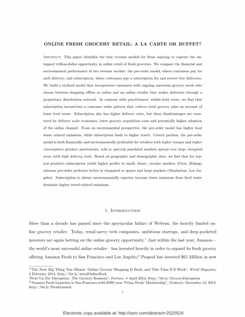
Figure 3.1. The Grocery Delivery Business Model
3. Model Setup
3.1. The Fresh Grocery Market. Consider an online fresh grocery retailer that serves a market of
area A with size A (see Figure 3.1). Potential customers are distributed over area A with uniform
density ρ. Fresh groceries purchased by the customer have a limited shelf life; a representative
basket expires T days after purchase. The grocery consumption of customers is random owing to
unpredictable demand shocks (e.g., unexpected guests, last-minute plans to dine out). Formally,
each customer’s consumption is generated according to a Poisson process with rate µ monetary
units.10
Customers choose to buy groceries either offline (by visiting a grocery store) or from an online
retailer that offers home delivery. A customer who buys offline incurs a cost α for each visit to the
store. Customers are heterogeneous in this cost because of their idiosyncratic marginal costs of time,
distances from the grocery store, travel patterns, utility from shopping, and so forth. Accordingly,
the per-visit cost α is a random variable observed only by each customer before making her choices.
We assume that the store visit cost follows a tractable exponentially distributed form; that is, we
assume α = α + x with x ∼ exp(λ).11 G (α) denotes its cumulative distribution function, g (α)
the density function and G (α) ≡ 1 − G (α) is the survival function. Extensive numerical analysis
reveals that our qualitative results remain unchanged by using either the uniform or the truncated
normal distributions.10For tractability, all fixed-life perishable inventory models assume Poisson demand (Fries, 1975; Nahmias, 1977;Weiss, 1980; Liu and Lian, 1999).11Brown and Borisova (2007) provide empirical support for this assumption, finding that the major component ofthe store visit cost is time. The value of time can be approximated by income, the distribution of which is known tobe roughly exponential (Wikipedia entry on “Household income in the United States”, http://bit.ly/HHIncome).
10 ONLINE FRESH GROCERY RETAIL: A LA CARTE OR BUFFET?
If instead the customer uses the online retailer, she incurs—in addition to the delivery charges—
a small frictional ordering cost θ. This term captures the inconvenience of going to the website,
selecting groceries, and placing the order. We assume that groceries ordered online are delivered
almost instantly (same-day delivery is typically offered by prominent online grocery retailers). Of
course, the cost of visiting the store is higher than the frictional cost of ordering online: α > θ.
Customers choose not only the timing of orders; each time they order, they also choose whether
to buy offline or online as well as the amount of groceries to buy (the basket size).
3.2. The Online Fresh Grocery Retailer. The online retailer of fresh groceries builds a Web-
based storefront, and a proprietary distribution network to make deliveries.12 This network consists
of a warehouse centrally located in area A along with a fleet of vehicles, each of which can make
as many as K deliveries per run.13
Revenues. In addition to generating revenue from the sale of groceries, the firm also charges for de-
livery. The retailer can choose between two revenue models for its delivery service: the subscription
model (S) or the per-order model (O). In the subscription model, customers pay a subscription fee
s each year and enjoy free delivery for all orders placed during that year; in the per-order model,
the customer pays delivery fee o for each delivery order.
Costs. The firm has two main variable cost heads: the cost of procuring groceries and the cost
of delivering them. The firm procures groceries at a cost of η times the sale price, where η < 1
and 1 − η captures the firm’s gross margins. For every order delivered, the firm incurs an average
direct delivery cost of ϕ · D. Here D is the average distance traveled to deliver an order under an
optimal routing scheme and ϕ is the per-mile delivery cost (which subsumes the costs of fuel, labor,
truck purchase, licensing, depreciation, etc.). The average distance traveled (D) arises from the
lowest-cost feasible routing scheme that can fulfill all delivery commitments. Section 5.1 derives the
expression for this distance.
In addition to the direct delivery costs, an online firm also incurs other costs associated with
delivery; these include picking costs as well as the costs of building a warehouse, buying vehicles,
12The use of third-party logistics providers is seldom viable in this context because of the short delivery times, specialtransit requirements, and perishable nature of the products.13The number of deliveries K is determined by the delivery offer. In particular, K is smaller for faster delivery,for a smaller delivery time windows, for a longer time to reach customers, and for smaller delivery vehicles—fasterdelivery implies that the provider has less time to wait for orders that can be batched; smaller delivery windowsrequire reduced uncertainty which is achieved by carrying fewer orders.
ONLINE FRESH GROCERY RETAIL: A LA CARTE OR BUFFET? 11
Customer’s storevisit cost α is drawn
Customers decide to shop online or offline: w
Customer buys units ofgroceries
Groceries areconsumed, leftovers expire at time T
Visit Costs Revenue Model
The firm choosesits revenue model relevant prices s/oχ∈ {S, O}
Shopping Mode
∈ {off, χ}
Replenishment Consumption
Qw
Order-Consumption Cycle
Re-
orde
r Poi
nts{Ti}
and
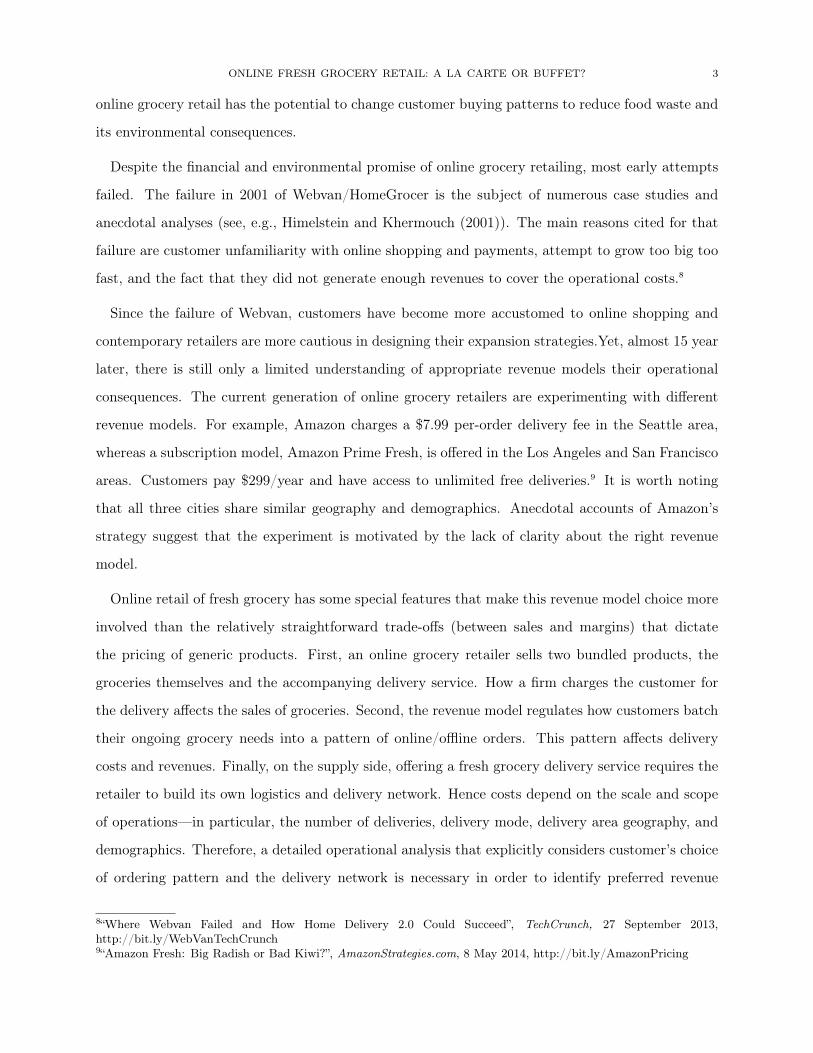
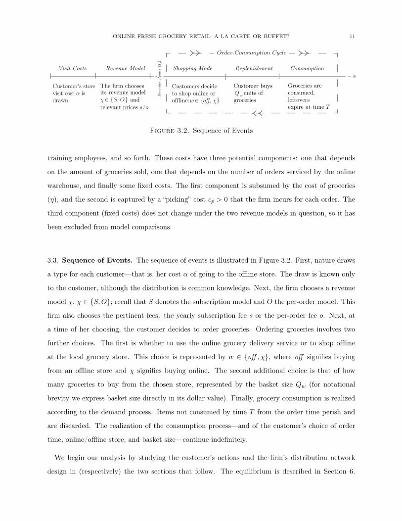
Figure 3.2. Sequence of Events
training employees, and so forth. These costs have three potential components: one that depends
on the amount of groceries sold, one that depends on the number of orders serviced by the online
warehouse, and finally some fixed costs. The first component is subsumed by the cost of groceries
(η), and the second is captured by a “picking” cost cp > 0 that the firm incurs for each order. The
third component (fixed costs) does not change under the two revenue models in question, so it has
been excluded from model comparisons.
3.3. Sequence of Events. The sequence of events is illustrated in Figure 3.2. First, nature draws
a type for each customer—that is, her cost α of going to the offline store. The draw is known only
to the customer, although the distribution is common knowledge. Next, the firm chooses a revenue
model χ, χ ∈ {S,O}; recall that S denotes the subscription model and O the per-order model. This
firm also chooses the pertinent fees: the yearly subscription fee s or the per-order fee o. Next, at
a time of her choosing, the customer decides to order groceries. Ordering groceries involves two
further choices. The first is whether to use the online grocery delivery service or to shop offline
at the local grocery store. This choice is represented by w ∈ {off , χ}, where off signifies buying
from an offline store and χ signifies buying online. The second additional choice is that of how
many groceries to buy from the chosen store, represented by the basket size Qw (for notational
brevity we express basket size directly in its dollar value). Finally, grocery consumption is realized
according to the demand process. Items not consumed by time T from the order time perish and
are discarded. The realization of the consumption process—and of the customer’s choice of order
time, online/offline store, and basket size—continue indefinitely.
We begin our analysis by studying the customer’s actions and the firm’s distribution network
design in (respectively) the two sections that follow. The equilibrium is described in Section 6.

12 ONLINE FRESH GROCERY RETAIL: A LA CARTE OR BUFFET?
t
T
T1 T2 T3 T4 T5
Q QQQQ Q
CT1 = T CT2 = T CT4 = TCT3 < T CT5 < T
Gro
cery
Inv
ento
ry
0R
e-or
der
FoodWasted
FoodWasted
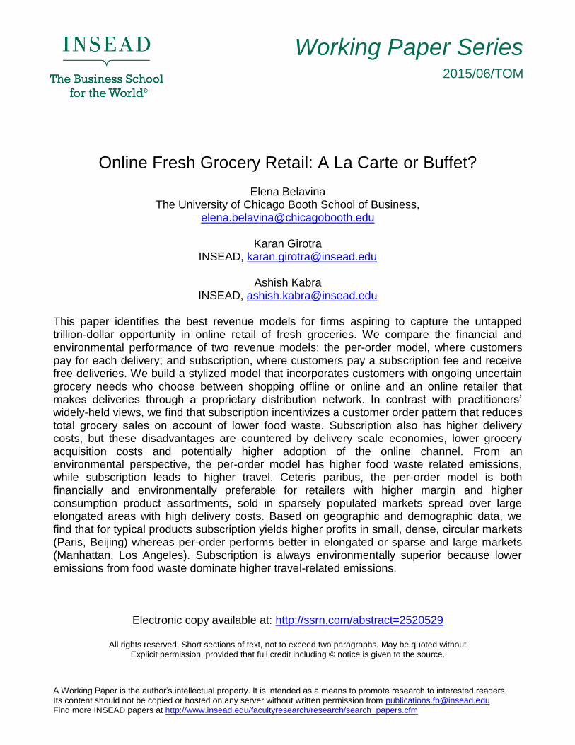
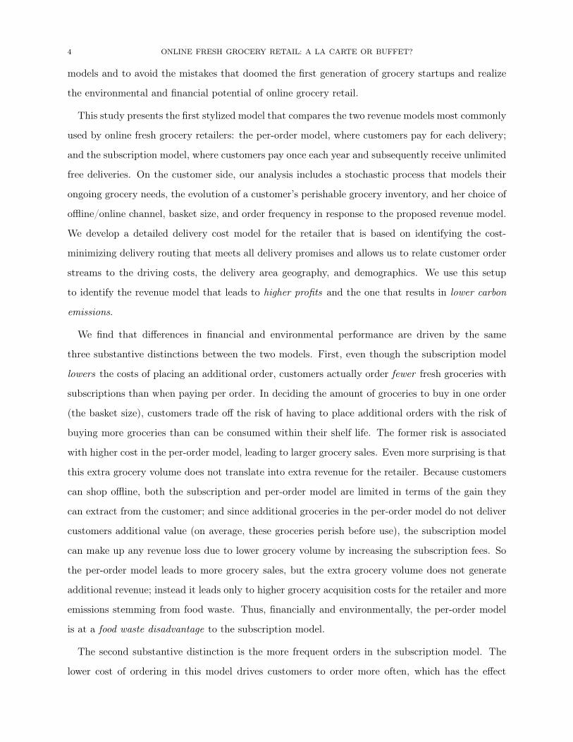
Figure 4.1. The Consumer Inventory Process: Possible Realizations of the Con-sumption Cycle
The choice of revenue model, which is the main focus of our analysis, is discussed in Section 7.
Implications for managers and some final remarks are presented in Sections 8 and 9, respectively.
4. Customer Behavior
The customer continuously reviews her inventory level and decides whether or not to place a new
order—bearing in mind the cost of ordering and the constraint that all grocery demand must be
met. Thus the customer decisions are: the timing {Ti} of orders and, at each order time, the choice
between offline versus online purchase (wTi ∈ {off , χ}) and the choice of basket size (QwTi ).
The ordering cost a depends on the preceding online/offline choice and the firm’s revenue model
choice. It is simply the cost of going to the store a = α if the customer chooses an offline store.
Suppose the customer decides to shop online. Then, for the per-order model, the ordering cost
is a = θ + o, or the sum of the frictional cost of placing the order and the per-order delivery fee
charged by the firm. For the subscription model, the ordering cost is just a = θ, the frictional cost
of ordering.
Our analysis establishes that the customer’s optimal “continuous review” inventory re-order policy
is to place an order when she runs out of groceries or when the leftover groceries expire, whichever
happens earlier (Lemma 5 in the Appendix). The customer must meet all demand and thus can
order no later than the point when she is out of fresh groceries. On the other hand, with positive
ordering costs, no lead time in delivery, and the perishable nature of groceries, the customer prefers
to delay ordering, i.e. order as rarely as possible and no earlier than absolutely necessary. This
re-order policy also implies that, at each re-order point, the system returns to the same state.
Hence the offline/online choice and the basket size are the same for every order point wTi = w and
QwTi = Q.

ONLINE FRESH GROCERY RETAIL: A LA CARTE OR BUFFET? 13
Figure 4.1 illustrates the customer’s grocery inventory process (under the optimal policy just
described) for a particular sample path of grocery consumption realizations. The inventory level is
reduced by grocery consumption and by the discarding of expired items. In ordering cycles 1, 3,
and 5, the consumption rate is high enough that all groceries are consumed; in cycles 2 and 4, the
consumption rate is low and some groceries expire before they are used (i.e., there is food waste).
The optimal re-order basket size Q must be such that it appropriately trades off ordering costs
against food waste. If the customer orders too few groceries, then all items will be consumed before
expiration and that would lead to an extra ordering cost. Yet if she orders too many then some of
the items will be wasted, leading to unnecessary grocery expenses.
Formally, the customer chooses her basket size to minimize her expected long-term average cost
rate of groceries. Since the customer re-orders the same quantity each time, successive cycles are
independent and identical. The expected long-term average cost rate is equal to the expected
average cost per ordering cycle divided by the expected length of one cycle (follows from standard
renewal theory arguments; see (Ross, 1970)).
For basket size Q, the expected average cost per ordering cycle is a+Q: the sum of the customer’s
ordering costs a and the direct costs of purchasing groceries Q Length of ith cycle CTi depends on
basket size Q. The expected length of the cycle is (Lemma 6):
E[CTi(Q)] =1
µ
Q− Q∑j=0
(Q− j) · pj (µT )
, pj (µT ) =e−µT (µT )j
j!
The denominator µ is the average consumption rate, and the “numerator” (in large parentheses) is
the expected consumption per cycle. Out of Q units ordered, in expectation,∑Q
j=0(Q− j) · pj (µT )
will be wasted. The probability that consumption during the shelf-life T equals toj is given by pj .
To accurately incorporate annual subscription costs, we consider all costs on an annual basis.
Toward this end, define n(Q) = min{n : CT1(Q) + CT2(Q) + · · ·+ CTn(Q) ≥ 1 year}. Since n is
independent of CTn+1, CTn+2, . . . for all n = 1, 2, . . ., it follows that n(Q) is a stopping time. We
can use Wald’s equation to express the expected number of orders in a year induced by ordering
Q units at a time: N(Q) = E[n(Q)] = 1 yearE[CTi(Q)] . Using expressions for the expected length of the
cycle, E[CTi(Q)], we obtain
(4.1) N(Q) =1
1µ
(Q−∑Q
j=0 (Q− j) · pj (µT )) .

14 ONLINE FRESH GROCERY RETAIL: A LA CARTE OR BUFFET?
Then the customer’s expected long-run average cost rate is (a + Q)N(Q) and the optimal basket
size is given by
(4.2) Q∗ (a) ≡ arg minQ
(a+Q) ·N (Q) .
Lemma 1. Customer Basket Size, Order Frequency, and Annual Volume of Groceries Purchased
i. The customer’s optimal basket size Q∗ (a) is a solution to
Q−Q∑j=0
(Q− j)pj (µT ) ≈ (a+Q) (1− Pj (Q,µT )) ,(4.3)
Pj (Q,µT ) =
Q∑j=0
pj (µT ) .
ii. Higher ordering costs lead to larger basket sizes, fewer annual orders, and a higher annual
volume of groceries purchased.
∂Q∗
∂a> 0,
∂N (Q∗)
∂a< 0,
∂ (N (Q∗) ·Q∗)∂a
> 0.
iii. A customer’s optimal grocery cost, (a+Q∗) ·N(Q∗), is increasing in a.
Proofs for all results are given in the Appendix.
The optimal grocery basket size trades off the risk of ordering too many groceries (which leads to
waste) against the risk of ordering too few groceries (which would trigger additional orders and
increase ordering costs). A marginal increase in the basket size affects per-cycle costs in two ways.
First, the procurement costs are simply higher by one unit: Q → Q + 1, which increases the cost
rate. Second, the extra unit increases the expected cycle time. If the extra unit was consumed for
sure then it would extend the cycle length by 1/µ time units, however the extra unit might end up
unconsumed, since there is some likelihood that the last unit would be wasted. In fact the cycle
time is actually increased by (1− Pj (Q,µT ))µ−1, where the additional factor captures the increase
in waste. This dynamic reduces the cost rate. The optimal quantity Q∗ is such that the increase
and decrease in cost rate are balanced:
a+Q+ 1
1µ
(Q+ 1−∑Q+1
j=0 (Q+ 1− j)pj (µT )) − a+Q
1µ
(Q−∑Q
j=0(Q− j)pj (µT )) ≈ 0.
Rearranging terms gives us the expression in Equation 4.3.

ONLINE FRESH GROCERY RETAIL: A LA CARTE OR BUFFET? 15
A higher ordering cost a incentivizes customers to order larger basket sizes less frequently. Larger
basket sizes increase the likelihood that some of the groceries expire before they are consumed,
which in turn increases the average waste. Given that annual grocery consumption does not depend
on ordering costs, higher waste implies that the customer purchases a higher annual quantity of
groceries N(Q∗) ·Q∗. Finally, the “larger basket size” effect dominates the “less frequent ordering”
effect and so the customer’s grocery costs are increasing in a.
Given this optimal order quantity choice, the customer’s optimal annual costs of buying offline
are
Coff = Cα ≡ (α+Q∗ (α)) ·N (Q∗ (α)) .(4.4)
The optimal costs of buying online depend on the online retailer’s choice of revenue model χ (which
can be subscription S or per-order O) and the corresponding prices, s and o:
(4.5) Cχ =
(o+ θ +Q∗ (o+ θ)) ·N (Q∗ (o+ θ)) ifχ = O,
s+ (θ +Q∗ (θ)) ·N (Q∗ (θ)) ifχ = S.
Finally, a customer’s choice between the offline store (off ) and the online store (χ) simply boils
down to minimizing the yearly cost: w∗ = arg minw∈{off ,χ}Cw.
We simplify notation for the optimal order size by putting Qα ≡ Q∗ (α) as the optimal offline
order size, Qo ≡ Q∗ (o+ θ) as the optimal online order size with per-order pricing, and Qs ≡ Q∗ (θ)
as the optimal online order size with subscription pricing. Similarly, for the number of orders per
year we set Nα ≡ N(Qα), No ≡ N(Qo), and Ns ≡ N(Qs).
5. Firm Decisions
The online grocery firm builds a distribution network to deliver groceries, chooses either the sub-
scription or the per-order revenue model, and determines the relevant price. We start by analyzing
the design of the distribution network that meets the delivery requirements at the lowest cost.
5.1. The Proprietary Distribution Network. This section adapts the analysis of Daganzo
(1984a,b) and Cachon (2014) to determine the direct delivery costs, which are proportional to
the distance traveled when making deliveries.

16 ONLINE FRESH GROCERY RETAIL: A LA CARTE OR BUFFET?
Kdi
LL
l
L/2
TSPi(K, L, l)
iLine haul, -di L/2
Si
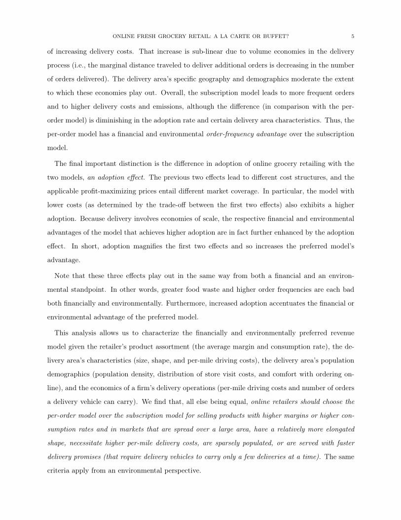
Figure 5.1. Distance Traveled to Deliver an Order in Sector i
A distribution network consists of a warehouse centrally located in area A and a fleet of vehicles,
each of which carries K delivery orders. We assume that the number of orders delivered by one
vehicle in one delivery period K is significantly smaller than the number to be delivered in the entire
market at the same time, K � A · ρd. Here ρd = ρNδ−1, ρ is the density of the population that
adopts the online service (we will define it explicitly as a function of the firm’s pricing in Section
5.2), N is the annual number of orders per customer, and δ is a coefficient that converts the annual
number of orders into the number of orders per delivery period. For example, if the retailer delivers
once per day then δ is 365.
Based on the specific orders to be delivered in a period, the firm devises the following distribution
plan. First, it optimally partitions area A into sectors Si, i ∈ {1, ..., I}, so that each sector has
K customers. Each sector is then assigned a vehicle that visits K customers following an optimal
route.
The distance traveled to deliver K orders in sector Si has two components: the distance between
the warehouse and the boundary of the sector, or the “line haul” distance, and the optimal traveling
salesman tour within the sector itself (see Figure 5.1). Minor variations in the specific shape of the
sectors do not greatly affect either the line-haul distance or the lengths of the traveling salesman
tours. We can therefore consider dividing area A into equal rectangular sectors of length L and
height l (L > l) and “slenderness factor” β = lL (Daganzo, 1984a). The distance traveled per order
delivered in sector Si can then be expressed as
(5.1) Di ≈2
K
(di −
L
2
)+ TSP ∗(K,L, l),
where di is the distance traveled in getting to sector Si’s center of gravity and L/2 is the approximate
distance from the sector’s center of gravity to the edge of the sector where the traveling salesman
tour starts. Together these two components constitute the line-haul distance, which must be covered

ONLINE FRESH GROCERY RETAIL: A LA CARTE OR BUFFET? 17
twice (to get to the sector and back) and is distributed over the K deliveries. We use TSP ∗(K,L, l)
to denote the per-order average length of the optimal traveling salesman tour within the sector.
Our quantity of interest, the average distance traveled per order, obtained by averaging over all
sectors Si, i ∈ {1, ..., I}, is D(ρ, N,A ,K) = 1I
∑Ii=1Di. Of Di’s three components, L and TSP ∗
depend on the area’s partition into sectors whereas di does not. We will first analyze di and then
the optimal partition of our market area into sectors; this will be followed by deriving the latter
two components as well as the optimal total distance.
Average Distance from the Warehouse to the Center of Gravity of Sectors d. (Daganzo, 1984a)
shows that d = 1I
∑di can also be interpreted as the average distance from the warehouse to a
point in market area A . Lemma 7 in the Appendix derives this distance for different shapes of the
market area. In general, d can be expressed as d = ζ√A, where the coefficient ζ is determined by
the region’s shape. We have d© ≈ 0.37√A for “circular” cities or markets and d ≈ 0.76
√A for
“square” ones. For a rectangular area with length-to-height ratio γ ≥ 1, we have d =√A ·ζ and
∂γζ > 0; that is, the higher the ratio γ, the longer the distance traveled. The distance traveled is
greater for sector shapes that are more irregular or elongated: ζ© < ζ ≤ ζ .
Partition of Market into Sectors. The area of individual sectors is predetermined by the per-delivery
period order volume ρd: L · l = Kρ−1d . Although the area is fixed, we can still choose the shape of
its sectors—that is, the slenderness factor β. As we elongate the rectangle toward the warehouse,
the distance from the center of the sector to the start of the tour increases (L is increasing); this
has the effect of lowering the distance traveled, di − L/2, yet increasing the length of the traveling
salesman tour. The proof of Lemma 2 identifies the optimal sector shape β∗.
Average Distance Traveled to Deliver an Order.
Lemma 2. (i) When K orders are delivered by one vehicle, the average distance traveled to de-
liver an order in an area A with uniform customer population density ρ and customer yearly order
frequency N is
(5.2) D(ρ, N,A,K) ∼= 2ζ√A
K+ λ(K)
√δ
ρN, with ∂Kλ(K) < 0.
(ii) The per-order average distance is decreasing in the number of orders (∂ND < 0) and in the
adopting density (∂ρD < 0), but it is increasing in the order costs (∂aD > 0). The total annual

18 ONLINE FRESH GROCERY RETAIL: A LA CARTE OR BUFFET?
distance traveled per customer, ND, is increasing in the number of orders (∂NND > 0) but it is
decreasing in the order costs (∂aND < 0).
Part (i) of this lemma is obtained by aggregating Equation 5.1 over different sectors while taking
in account the optimal slenderness factor and expression for d. The proof of Lemma 2 identifies
an expression for the coefficient λ(K). The economies of scale in the traveling salesman tour are
captured by λ(K): the per-order average length of the optimal traveling salesman tour decreases as
we add more points (orders) to the tour.
Part (ii) of the lemma shows that there are economies of scale in delivery. If there are more
customers (ρ ↑) and/or if customers order more often (N ↑), then the per-order delivery distance
decreases. Along the same lines, a higher ordering cost a will lead both to fewer orders and to fewer
customers and thus to a higher average distance traveled. Finally, with respect to total annual
distance traveled per customer, the order frequency effect dominates the average delivery distance
effect; hence a higher frequency leads to more annual travel.
5.2. Choice of Revenue Model. Suppose the firm chooses the per-order pricing model. Then
the customers whose store visit costs are above a certain threshold will choose the online retailer
(Lemma 8). In that case, the firm’s profits (at the profit-maximizing per-order price) can be written
as
πo = maxo
((o+Qo)No −
{ϕ · D
(ρG(α), No,A ,K
)+ ηQo + cp
}·No
)·AρG (αo) ,(5.3)
where αo = min{α ∈ [α, α s.t. Coff ≥ Co}. The first term in this profit formulation is the per-
customer delivery and grocery revenues. The second term includes the two variable cost components,
the per-customer costs of delivery and the per-customer costs of sourcing groceries. Finally, the
multiplicative term represents the number of customers buying from the online grocery retailer, i.e.
G(α) captures the fraction of customers that buy online.
If instead the firm chooses the subscription model, then again the customer’s online/offline choice
is a threshold choice in the store visit cost. Analogously, the maximum expected profit under
subscription pricing is
πs = maxs
({s+QsNs} −
{ϕ · D
(ρG(αs), Ns,A ,K
)+ ηQs + cp
}·Ns
)·AρG (αs) ,(5.4)

ONLINE FRESH GROCERY RETAIL: A LA CARTE OR BUFFET? 19
where αs = min{α ∈ [α, α s.t. Coff ≥ Cs}. As before, the first terms are the per-customer delivery
and grocery revenues, the next terms include the delivery and procurement costs, and the multi-
plicative term captures the fraction of customers that buy online. Finally, the firm will choose the
pricing scheme that maximizes its profit:
χ = arg maxχ∈{o,s}
πχ.
6. Equilibrium Outcomes
We can now combine the analysis of the distribution network from Section 5.1, which gives us the
relation between direct delivery costs and consumer order frequency (Equation 5.2), with the firm’s
best response (Equations 5.3 and 5.4) and the consumer’s best response (Equation 4.3) to determine
the equilibrium outcomes under each choice of revenue model.
6.1. Per-Order Revenue Model.
Lemma 3. Equilibrium Outcome under the Per-Order Revenue Model
i. The online retailer charges a per-order delivery fee o = α∗o − θ, where the optimal market
coverage α∗o is a unique solution to (Nα − ∂αho(α)) · G(α) = (Cα − ho(α)) · g(α); here
ho(α) = (θ + ϕ · D(ρG(α), Nα,A ,K) + ηQα + cp)Nα.
ii. Customers with store visit costs α > α∗o choose the online firm. These customers all order
the same basket size Q∗(α∗o) from the firm on an ongoing basis, re-ordering every time their
inventory runs out or expires. Customers with store visit costs α < α∗o purchase groceries
offline. Each such customer’s idiosyncratic basket size is Q∗(α), where α is her individual
store visit cost. These customers also re-order when their inventory runs out or expires.
The equilibrium is best understood by examining the effect of a price change on each term in the
firm’s profits (Equation 5.3) while keeping in mind customer response to this price (i.e., the customer
ordering costs; see Lemma 1), delivery costs (Lemma 2) and the adoption.
Recall that an increase in ordering costs increases the customer’s basket size, reduces the annual
number of orders per customer, and increases the amount of groceries purchased by each customer
(since there is more waste); see parts (ii) and (iii) of Lemma 1. Thus an increase in the per-order
price increases the direct grocery profits (1− η)QoNo but also increases a customer’s cost of using
the online channel—both directly (owing to higher annual delivery costs oNo) and indirectly (owing
20 ONLINE FRESH GROCERY RETAIL: A LA CARTE OR BUFFET?
to higher grocery expenses QoNo). As a result, customer adoption G (αo) declines. With regard
to delivery, an increase in the per-order price increases per-order delivery costs ϕD because of a
lower order frequency and lower adoption rate; yet the annual per-customer delivery costs DNo
actually decrease because the order frequency effect dominates (Lemma 2(ii)). Hence the delivery
profits (o−ϕD) ·No are increasing in o. Altogether, the delivery and grocery profits increase when
the firm sets higher per-order prices, though doing so reduces adoption. A per-order delivery price
of o = α∗o − θ (with α∗o defined above) optimally trades-off the per-customer profit effect with the
adoption or market size effect.
Given an optimal delivery fee, customers with α ≥ α∗o use the online store while all other customers
prefer the offline channel. All customers who use the online channel have the same basket size
because their ordering costs are now the same; in contrast, customers using the offline channel
choose different quantities based on their individual store visit costs (α). Hence the resulting yearly
per-customer delivery and grocery purchase cost is captured by ho(α∗o).
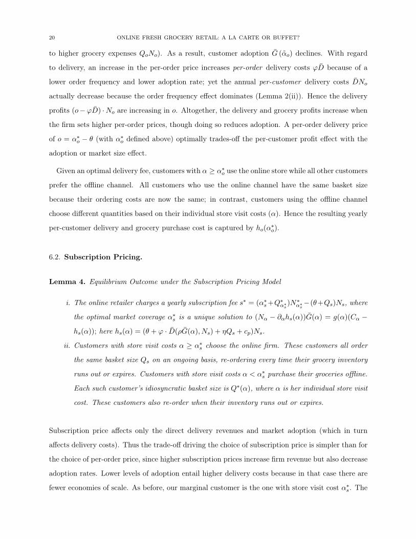
6.2. Subscription Pricing.
Lemma 4. Equilibrium Outcome under the Subscription Pricing Model
i. The online retailer charges a yearly subscription fee s∗ = (α∗s+Q∗α∗s )N∗α∗s−(θ+Qs)Ns, where
the optimal market coverage α∗s is a unique solution to (Nα − ∂αhs(α))G(α) = g(α)(Cα −hs(α)); here hs(α) = (θ + ϕ · D(ρG(α), Ns) + ηQs + cp)Ns.
ii. Customers with store visit costs α ≥ α∗s choose the online firm. These customers all order
the same basket size Qs on an ongoing basis, re-ordering every time their grocery inventory
runs out or expires. Customers with store visit costs α < α∗s purchase their groceries offline.
Each such customer’s idiosyncratic basket size is Q∗(α), where α is her individual store visit
cost. These customers also re-order when their inventory runs out or expires.
Subscription price affects only the direct delivery revenues and market adoption (which in turn
affects delivery costs). Thus the trade-off driving the choice of subscription price is simpler than for
the choice of per-order price, since higher subscription prices increase firm revenue but also decrease
adoption rates. Lower levels of adoption entail higher delivery costs because in that case there are
fewer economies of scale. As before, our marginal customer is the one with store visit cost α∗s. The
ONLINE FRESH GROCERY RETAIL: A LA CARTE OR BUFFET? 21
resulting yearly per-customer delivery and grocery purchase cost for online customers is captured
by hs(α∗s).
The equilibrium profits of online retailers depend in a predictable way on the setting. Irrespective
of the revenue model employed, online retailing is financially the most rewarding in dense, circular-
shaped cities with premium consumers (high consumption rate and high margins), low per-mile
delivery costs, and high consumer store visit costs. Each of these factors either decreases costs or
increases revenues, lowering the equilibrium price, leading to higher adoption and more economies of
scale, which further reinforce the effects. The role played by delivery area is more complex. Larger
areas tend to contain more customers but also involve greater travel distances, and generally the
former effect dominates.
7. Comparing Revenue Models: Subscription versus Per-Order
7.1. Comparison of Equilibrium Customer Behavior.
Theorem 1. Customers order larger basket sizes and order less frequently in the per-order model
than in the subscription model. Overall, annually more groceries are purchased in the per-order
model (larger basket size dominates the lower frequency) and greater delivery distances are traveled
in the subscription model.
Corollary. The amount of groceries that perish before use (food waste) is higher in the per-order
model.
At equilibrium prices, the ordering costs are higher in the per-order model. It directly follows from
Lemma 1 that the per-order model is characterized by larger basket sizes, fewer orders, and more
grocery purchased annually. Expected grocery consumption is simply the mean demand rate, which
is the same for these two revenue models. Since more groceries are purchased in the per-order
model, waste is higher.
Interestingly, in our model the total annual grocery purchases are increasing in the per-order
prices. This finding runs counter to results derived from abstract economic models, which almost
always ignore demand uncertainty and consumer inventories while simply assuming that demand
declines in response to higher prices. Note also that this result contrasts with the anecdotal wisdom
that subscription models lead to higher sales because they remove barriers to purchasing. While,

22 ONLINE FRESH GROCERY RETAIL: A LA CARTE OR BUFFET?
this may be true in settings that involve durable products, this commonly stated observation might
not hold in the case of fresh grocery.
A higher annual grocery volume with fewer orders suggests that the per-order firm sells more
while spending less money delivering the groceries; hence the per-order model should dominate.
But this analysis is incomplete. Besides these effects, there are two others that arise from the
customer’s adoption decisions. First the two models differ in how much total value they create and
how much of this total value is claimed by the firm. In turn, this implies that the two models
will have different adoption and consequently different levels of the economies of scale in delivery.
Together these effects lead to a drastic departure from the above suggestion.
In terms of environmental impact, the results of Theorem 1 suggest a trade-off between the two
models. While the per-order model’s higher levels of food waste makes it less eco-friendly, the
subscription model’s greater driving distances render it less desirable. Yet the subsequent analysis
establishes that, in practice, there is no trade-off: one of these two models always dominates.
7.2. Comparing Equilibrium Outcomes. The equilibrium profits can be rewritten as maxi-
mization problems in which the firm rather than choosing delivery price—which in turn determines
market adoption— it directly chooses an optimal adoption level (via the critical store visit costs
α∗):
πs = maxα≤α≤α
πs(α) ≡ maxα≤α≤α
((α+Qα)Nα − hs(α))A · ρG(α);
πo = maxα≤α≤α
πo(α) ≡ maxα≤α≤α
((α+Qα)Nα − ho(α))A · ρG(α).
This formulation subsumes customer behavior and allows for an intuitive decomposition of model
differences into (a) per-customer revenues and costs and (b) market adoption.
Both models have the same first term: the online retailer’s per-customer delivery and grocery
revenue, R ≡ (α + Qα)Nα. In equilibrium, an online retailer sets its price to make its revenues
from each customer equivalent to the offline grocery purchasing costs of the marginal customer,
thus leaving the marginal customer with no surplus. If the two models had the same equilibrium
adoption (same marginal customer), then their grocery and delivery revenues would be the same.
Note that the revenues are the same even though more groceries are sold in the per-order model.
The extra groceries are bought only to avoid placing another expensive order; in expectation the
customer derives no consumption value from them and so there is no extra value to extract. The
ONLINE FRESH GROCERY RETAIL: A LA CARTE OR BUFFET? 23
T
G
roce
ry C
ost
α − αAdoption, α − αAdoption, α − αAdoption, P
er-O
rder
& T
SP C
ost
Pro
fits
πs(α
),πo(α
)S
S
O
O S
Food Waste Disadvantage
Order Frequency Advantage
O
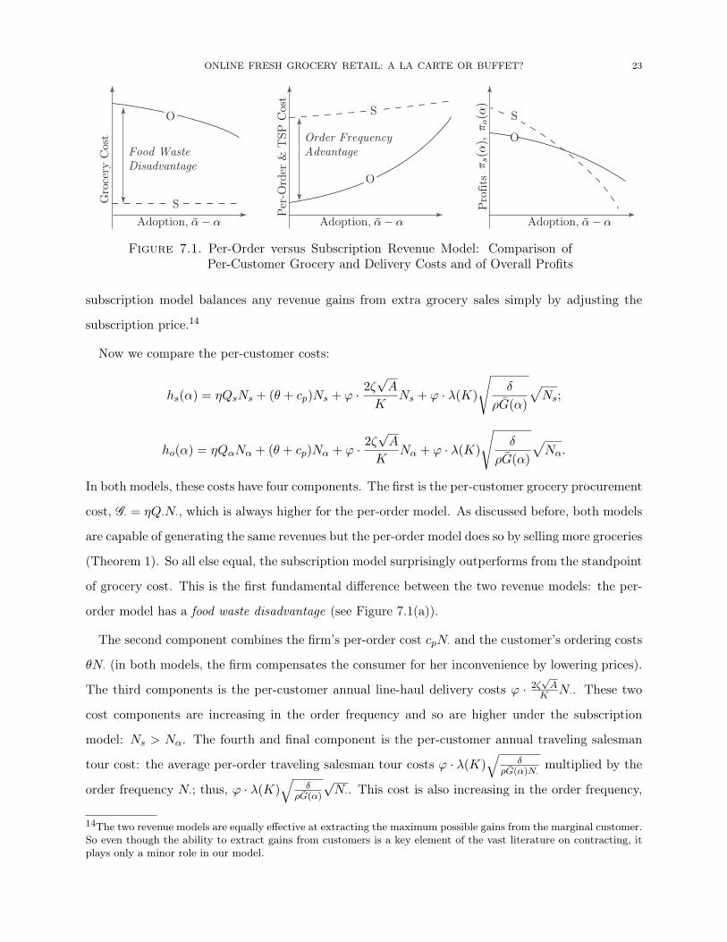
Figure 7.1. Per-Order versus Subscription Revenue Model: Comparison ofPer-Customer Grocery and Delivery Costs and of Overall Profits
subscription model balances any revenue gains from extra grocery sales simply by adjusting the
subscription price.14
Now we compare the per-customer costs:
hs(α) = ηQsNs + (θ + cp)Ns + ϕ · 2ζ√A
KNs + ϕ · λ(K)
√δ
ρG(α)
√Ns;
ho(α) = ηQαNα + (θ + cp)Nα + ϕ · 2ζ√A
KNα + ϕ · λ(K)
√δ
ρG(α)
√Nα.
In both models, these costs have four components. The first is the per-customer grocery procurement
cost, G· = ηQ·N·, which is always higher for the per-order model. As discussed before, both models
are capable of generating the same revenues but the per-order model does so by selling more groceries
(Theorem 1). So all else equal, the subscription model surprisingly outperforms from the standpoint
of grocery cost. This is the first fundamental difference between the two revenue models: the per-
order model has a food waste disadvantage (see Figure 7.1(a)).
The second component combines the firm’s per-order cost cpN· and the customer’s ordering costs
θN· (in both models, the firm compensates the consumer for her inconvenience by lowering prices).
The third components is the per-customer annual line-haul delivery costs ϕ · 2ζ√A
K N·. These two
cost components are increasing in the order frequency and so are higher under the subscription
model: Ns > Nα. The fourth and final component is the per-customer annual traveling salesman
tour cost: the average per-order traveling salesman tour costs ϕ · λ(K)√
δρG(α)N·
multiplied by the
order frequency N·; thus, ϕ · λ(K)√
δρG(α)
√N·. This cost is also increasing in the order frequency,
14The two revenue models are equally effective at extracting the maximum possible gains from the marginal customer.So even though the ability to extract gains from customers is a key element of the vast literature on contracting, itplays only a minor role in our model.
24 ONLINE FRESH GROCERY RETAIL: A LA CARTE OR BUFFET?
but at a slower than linear rate as there are two kinds of scale economies: the order frequency
itself (√N·) and the adoption level G−1/2(α). For the same level of adoption, the traveling salesman
tour costs will be higher in the subscription model. Although different equilibrium adoptions might
change this, they are usually higher in the subscription model. We refer to the combined effect of
these delivery costs (sum of second, third and fourth components) as the per-order model’s order
frequency advantage (Figure 7.1(b)).
In sum, per-order model enjoys the order frequency advantage but suffers from food waste disad-
vantage. These two effects are on a per-customer basis. Hence, the third and final effect concerns
optimal adoption levels. Because adoption scales up the magnitude of both the food waste disad-
vantage and the order frequency advantage, it determines which of these opposing effects dominates.
Both of them are decreasing in the adoption level (see panels (a) and (b) of Figure 7.1). Figure 7.1(c)
depicts the firm’s profit curves (as a function of adoption level α− α) under the two revenue mod-
els. We can show that if in both models the adoption levels are above (resp., below) intersection
point of the two profit curves then the financial impact of the order frequency advantage dominates
(resp., is dominated by) the food waste disadvantage. The likelihood of adoption level being above
the intersection point is increasing with area size and transportation cost and is decreasing with
population density. Thus, the per-order model is preferable for cities that are large, not densely
populated, and characterized by expensive transportation. We refer to the role of adoption as the
adoption effect.
The foregoing discussion illustrates that there are multiple competing effects that interact in a
nonlinear fashion and also that it is difficult to obtain intuitive and easy-to-use criteria for de-
termining which model is preferable from a financial and environmental point of view. However,
further analysis shows that an overall comparison of the two revenue models can be expressed using
a single metric—that allows us to relate the preferred revenue model to the market area’s spatial
and demographic properties, the product’s characteristics, and the economics of delivery.
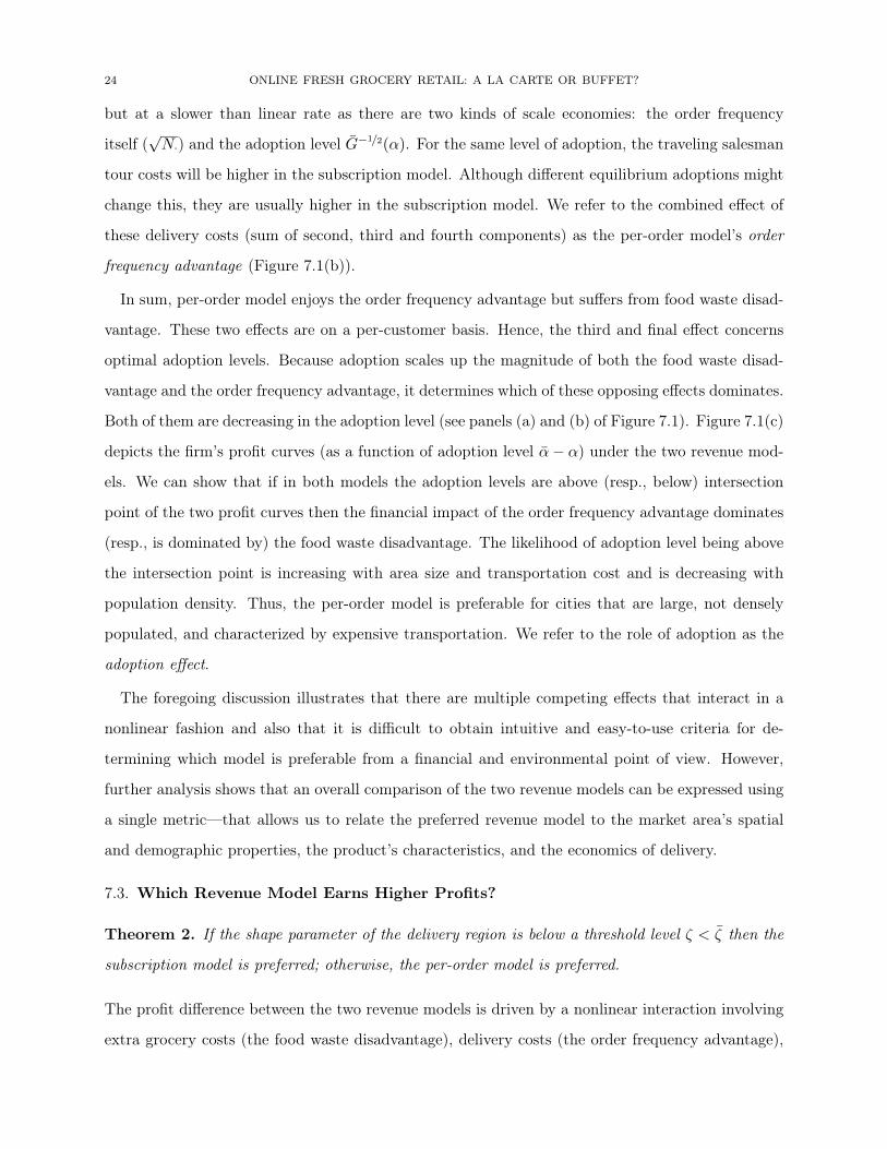
7.3. Which Revenue Model Earns Higher Profits?
Theorem 2. If the shape parameter of the delivery region is below a threshold level ζ < ζ then the
subscription model is preferred; otherwise, the per-order model is preferred.
The profit difference between the two revenue models is driven by a nonlinear interaction involving
extra grocery costs (the food waste disadvantage), delivery costs (the order frequency advantage),

ONLINE FRESH GROCERY RETAIL: A LA CARTE OR BUFFET? 25
TP
rofit
Diff
eren
ce,π
s−
πo
ζζ
Order Frequency Advangage (OFA)Food Waste Disadvangage (FWD)
Equilibrium Adoption (faster for subscription)
OFA > FWD
Delivery Costs
As ζ
As ζ
Figure 7.2. Retailer Profit: Subscription Model versus Per-Order Model
and the adoption effect. This comparison is involved and hard to characterize, but analysis of the
constituent marginals allows us to demonstrate a single-crossing property in the shape parameter.15
In particular, the difference takes the form shown in Figure 7.2. As the shape parameter ζ increases
(delivery region becomes more elongated), two things change: delivery costs increase (because of
longer line-haul distances) and adoption declines (in response to higher prices–higher costs make
higher prices optimal). The former effect increases the relative value of the order frequency ad-
vantage, since each trip becomes more costly; this is the main effect that progressively favors the
per-order model. Higher delivery costs mean that the optimal adoption decreases in both models;
however, in the subscription model this decline is more rapid because there are more deliveries to
make. As a consequence we observe second-order effects: lower adoption rates for the subscription
model imply a scaling down of its advantages. This dynamic also favors the per-order model. How-
ever, reduced adoption further implies increases in both the order frequency advantage and the food
waste disadvantage. This increase in order frequency advantage combined with the direct first-order
effect through increase in ζ outpace the increase in the food waste disadvantage (second-order effect)
once again favoring the per-order model. Eventually, in both models the adoption level becomes
low, reducing not only absolute profits but also the difference between the models’ respective profits.
Hence the profit lines cross only once, which allows us to characterize the preferred revenue model
in terms of the threshold shape parameter alone.
One advantage of an intuitive statement of Theorem 2 is that it allows one to characterize the
area, product, and operational characteristics that are best suited for each model.
15The single-crossing property that drives Theorem 2 also holds for the market area size A, density ρ, per-mile deliverycost ϕ, and number K of deliveries per truck. The intuition is the same as that for shape parameter (explained next),and both Theorem 2 and the financially preferred model could be equivalently characterized using any of theseparameters.

26 ONLINE FRESH GROCERY RETAIL: A LA CARTE OR BUFFET?
Theorem 3. Ceteris paribus, the per-order model is preferred over the subscription model if the
population is sparse, the delivery area is either large or elongated, and/or retailer delivery commit-
ments require that delivery vehicles carry fewer orders. Formally: the threshold shape parameter ζ
is decreasing in the city’s area A and in the per-mile delivery costs ϕ, but it is increasing in the
population density ρ and in the number K of deliveries per truck.
Theorem 3 follows from our previous discussion about the effect of increasing per-mile distances. A
sparsely populated area (ρ ↓), a large delivery area (A ↑), and high per-mile delivery costs (ϕ ↑) leadto the same main and second-order effects as an increase in the shape parameter—in particular, an
increase in the order frequency advantage, a lower optimal adoption rate, and a consequent increase
in both the food waste effect and the order frequency effect. The one difference is that the order
frequency–related phenomena in the main and second-order effect appear through the traveling
salesman component of the delivery distance for population density (and not through the line-haul
component, as in the case of the shape parameter); for the per-mile cost ϕ, they appear through
both the line-haul and traveling salesman components. Finally, less batching of deliveries (K ↓)induces the same operating phenomena and, like the per-mile delivery cost, operates through both
the line-haul and traveling salesman distances. Lower K implies that more trips are needed to the
sectors and that the tours within a sector are longer on a per-order basis, which increases the order
frequency advantage and lowers the adoption rate.
The preceding comparison of equilibrium profits in the two revenue models does more than tell us
which model will help the online retailer earn higher profits; it also provides important guidance
on which model gives a retailer the best shot at establishing a financially viable venture. In the
interest of brevity, our model does not directly include the fixed costs of setting up the business
and the associated costs of capital. Recall, however, that such setup costs are likely to be the same
irrespective of the revenue model. Thus, the preferred revenue model (according to the analysis
here) is also the one with the best chance for financial viability for a given city, set of product
characteristics, and so forth. Another challenge in startup ventures concerns the speed of product
diffusion. In other words, even some customers who (as rational agents in equilibrium) should adopt
the online delivery service nonetheless fail to do so. Often only a small fraction of customers will
know about the product and adopt it. The longer the diffusion process, the more “runway” or equity
funding a startup venture might need before it can take off and become independently viable. Again,

ONLINE FRESH GROCERY RETAIL: A LA CARTE OR BUFFET? 27
the diffusion process is likely to be independent of the revenue model; hence the above prescriptions
will serve also to identify which revenue model is right for a new venture in the fresh grocery space
that might be more interested in the length of the gestation period.
7.4. Environmental Impact of Revenue Models. In this section we compare the consumer
carbon emissions that arise from the online firm’s use of subscription versus per-order pricing. We
include the emissions that arise from delivery (travel from store/warehouse to home) and those that
arise from food waste. To ensure a fair comparison, we include the full population of customers—
that is, both online and offline customers. We do not include the differences in travel or food
waste in the supply chains from the producer to the store/warehouse, as these can be added with
predictable effects.16
Before comparing the two online revenue models, it is useful to compare offline and online cus-
tomers. Emissions differ for the online and offline customers, since in each channel the customers
have different basket sizes, order frequencies, and modes of transport. Regardless of the revenue
model, customers that adopt the online channel do so in order to reduce their grocery ordering
costs; this means that for those customers the online channel is associated with less food waste
and its related emissions. Furthermore, orders are now pooled in delivery and so per-order travel
is reduced. But online customers will shop more frequently and thus induce more trips (especially
in the subscription model), which could cancel out the benefits from their lower food waste and
per-order travel. Yet this rarely occurs for reasonable parameter values, and—in accordance with
anecdotal beliefs—an online customer typically causes fewer carbon emissions than does an offline
customer.
As discussed in Section 7.2, the key differences between the equilibrium outcomes of the two
revenue models are in the order frequency, levels of food waste, and rate of adoption. Each of these
factors has a direct effect on the carbon emissions associated with each model. The order frequency
determines the amount of driving that must be done to make grocery deliveries, and the volume of
groceries is directly related to the amount of food waste. Finally, adoption controls the number of
customers who actually use the online channel.
16Cachon (2014) examines the travel-related component of emissions for offline customers and different supply chains.However, that model does not incorporate online customers, delivery-related travel, or food waste—factors that turnout to be critical in our analysis.

28 ONLINE FRESH GROCERY RETAIL: A LA CARTE OR BUFFET?
The total emissions for the entire population of the delivery area in the two revenue models are
as follows:
Es = Aρ{(ed · D
(ρG(α∗s), Ns, A , K
)Ns + efQsNs
)· G (α∗s) +
α∗s∫α
(epdαNα + efNαQα) g(α)dα− efµ};
Eo = Aρ{(ed · D
(ρG(α∗o), Nα∗o ,A ,K
)Nα∗o + efQα∗oNα∗o
)· G (α∗o) +
α∗o∫α
(epdαNα + efNαQα) g(α)dα− efµ}.
Here ed and ep are the CO2-equivalent per-mile emissions for (respectively) a delivery truck and a
passenger vehicle, ef signifies the CO2-equivalent emissions for every dollar’s worth of food wasted,
and Es and Eo denote the total emissions in the subscription and per-order models, respectively.
The first (resp., second) part of each displayed expression captures the emissions due to online
(resp., offline) customers. Each part has two components, emissions from driving and emissions
from food waste. The food waste emissions are calculated as the carbon load of all food purchased
minus the carbon load of the food consumed (efµ). Finally, dα denotes distance to the store for
consumers whose cost of going to the store is α.
Comparing the two models in terms of their environmental impact is analogous to comparing them
in terms of profits. The per-order model leads to more food waste which has a high environmental
cost and therefore per-order model suffers from a food waste disadvantage. On the other hand, it
requires less deliveries and hence less driving and less carbon emissions. Because adoption differs
across the two models, there is also an adoption effect. Although the preferred model is determined
by a nonlinear interaction of these effects, we can more easily characterize the preferred model using
a single metric: a threshold level of food waste emissions.
Theorem 4. The per-order model is more eco-friendly than the subscription model if and only if
the emissions ef for every dollar of food wasted are less than a threshold level ef .
This threshold result is easier to establish than is the threshold result for our profit comparisons. An
increase in emissions from a dollar of wasted food increases the relative environmental consequences
of the food waste disadvantage while having no influence on the other effects. Increasing unit
emissions from food waste render the per-order model progressively less “green”, so at some point
the subscription model becomes relatively more green despite involving more travel. The result
now follows. This analysis suggests that either revenue model could be greener, depending on the

ONLINE FRESH GROCERY RETAIL: A LA CARTE OR BUFFET? 29
parameters. However, in the next section we calibrate our model using realistic parameters and find
that subscription revenue model always dominates.
8. Managerial Implications: Cities, Product Categories, and Revenue Models
The foregoing analysis can be used by an online grocery provider to choose the revenue model that
yields the highest profits and the best chance of financial viability. We now illustrate such use by
calibrating our model using indicative values of the input parameters.
8.1. Financial Considerations. We proceed by analyzing four different delivery areas: Manhat-
tan, Los Angeles, Paris, and Beijing (old city). Table 1 lists our parameter estimates for these
cities, which vary widely in terms of geography. Paris, Beijing, and Manhattan are relatively small
in area; Los Angeles is about 10 times their size. Paris and Beijing are roughly circular/oval cities,
whereas Los Angeles and Manhattan are rectangular. Note that Manhattan is extremely elongated,
so it has a much higher shape parameter. The cities also vary widely with respect to household
density, ranging from fewer than 3,000 households per square mile in Los Angeles to about 8 times
that density in Manhattan. Finally, the cities have different labor markets. The per-mile delivery
costs in China are estimated to be less than a third of those costs in Western cities. In addition
Parameter Manhat. L.A. Paris Beijing Sources
Area, A
(sq. mi)23 500 40 33.63 Wikipedia entries.
Density, ρ
(households
per sq. mi)
24,137 2,836 18,930 22,168
Population density is divided by an average household size of 2.9
(Consumer Expenditure Survey of the Bureau of Labor Statistics,
Table 1500: Composition of consumer units, 2012Q3–2013Q2).
Shape
parameter,
ζ
1.16 0.8 0.4 0.61
Computed based on the following assumptions: Manhattan can
be represented by a rectangle whose sides are proportioned as 1:5;
Los Angeles, a rectangle of proportion 2:3; Paris, approximately
a circle; and Beijing, an oval whose minor and major axes are
proportioned as 5:6.
Deliverycost, ϕ
($/mi)1.5 1.5 1.5 0.413
Computed as the cost of operating a truck, including labor and
delivery costs. For Western cities, the operating cost is $1.38/mi
(“The Real Cost of Trucking”, http://bit.ly/1ojPJaF) plus about
$0.12/mi for other items; for Beijing, costs are estimated to
be about 27% of Western costs (“China’s E-Commerce Secret
Weapon, the Delivery Guy”, http://bit.ly/reutersdelguy).
Note: Unless stated otherwise, each city’s geographic and demographic data are obtained from its Wikipedia entry.
Table 1. City Characteristics
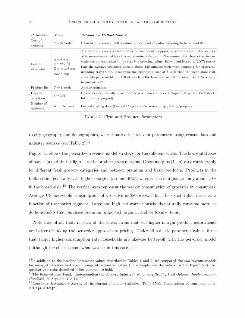
30 ONLINE FRESH GROCERY RETAIL: A LA CARTE OR BUFFET?
Parameter Value Estimation Method/Source
Cost of
orderingθ = 5$/order Hann and Terwiesch (2003) estimate mean cost of online ordering to be around $5.
Cost of
store visit
α = θ + x,x ∼ exp(λ)
E [α]= 35$ per
round-trip
The cost of a store visit is the value of time spent shopping for groceries plus other sources
of inconvenience (making choices, planning a list, etc.). We assume that these other incon-
veniences are equivalent to the cost θ of ordering online. Brown and Borisova (2007) report
that the average consumer spends about 140 minutes each week shopping for groceries,
including travel time. If we value the customer’s time at $13/hr then the mean store visit
costs $35 per round-trip—$30 of which is the time cost and $5 of which is the “selection
inconvenience”.
Product life T = 1 week Author estimates.
Days in
operationδ = 365
Customers can usually place orders seven days a week (Peapod Corporate Fact-sheet,
http://bit.ly/peepod).
Number of
deliveriesK = 15/truck Peapod routing data (Peapod Corporate Fact-sheet, http://bit.ly/peepod).
Table 2. Firm and Product Parameters
to city geography and demographics, we estimate other relevant parameters using census data and
industry sources (see Table 2).17
Figure 8.1 shows the prescribed revenue model strategy for the different cities. The horizontal axes
of panels (a)–(d) in the figure are the product gross margins. Gross margins (1−η) vary considerably
for different fresh grocery categories and between premium and basic products. Products in the
bulk section generally earn higher margins (around 40%); whereas the margins are only about 20%
in the bread aisle.18 The vertical axes represent the weekly consumption of groceries by consumers.
Average US household consumption of groceries is $86/week,19 but the exact value varies as a
function of the market segment. Large and high–net worth households naturally consume more, as
do households that purchase premium, imported, organic, and/or luxury items.
Note first of all that, in each of the cities, firms that sell higher-margin product assortments
are better-off taking the per-order approach to pricing. Under all realistic parameter values, firms
that target higher–consumption rate households are likewise better-off with the per-order model
(although the effect is somewhat weaker in this case).
17In addition to the baseline parameter values described in Tables 1 and 2, we compared the two revenue modelsfor many other cities and a wide range of parameter values (for example, see the values used in Figure 8.2). Allqualitative results described below continue to hold.18The Reinvestment Fund, “Understanding the Grocery Industry”, Financing Healthy Food Options: ImplementationHandbook, 30 September 2011.19Consumer Expenditure Survey of the Bureau of Labor Statistics, Table 1500: Composition of consumer units,2012Q3–2013Q2.

ONLINE FRESH GROCERY RETAIL: A LA CARTE OR BUFFET? 31
20% 0.25 0.3 0.35 40%50
1252
75
1752
100
1- η
μ20% 0.25 0.3 0.35 40%
50
1252
75
1752
100
1- η
μ
20% 0.25 0.3 0.35 40%50
1252
75
1752
100
1- η
O
S
Gross Margins, 1-η 20% 0.25 0.3 0.35 40%50
1252
75
1752
100
1- η
μ
Gross Margins, 1-η
O S
(a) Manhattan (b) Los Angeles
O
S
Gross Margins, 1-η Gross Margins, 1-η
O
S
(c) Paris (d) Beijing
Mea
n D
eman
d
Rat
e, µ
(in
$/w
k)
Mea
n D
eman
d
Rat
e, µ
(in
$/w
k)
Mea
n D
eman
d
Rat
e, µ
(in
$/w
k)
Mea
n D
eman
d
Rat
e, µ
(in
$/w
k)
Note: The per-order revenue model is preferred in the regions marked O, the subscription model in regions marked S.
Figure 8.1. Product Characteristics and Revenue Models by City
The differences between cities are more interesting. Manhattan, Paris, and Beijing (panels (a),
(c), and (d) in Figure 8.1) are small and densely populated delivery areas. Of these three, Beijing
and Manhattan are the most densely populated; however, Beijing has two advantages vis-à-vis
Manhattan. First, in contrast to Manhattan’s highly skewed rectangle, Beijing has an oval shape;
this difference in shape reduces travel distances. Second, because of Beijing’s lower labor costs,
its per-mile delivery costs are only about 30% of those in Manhattan. Beijing is therefore the city
where deliveries are the easiest to make, so the subscription model—with its frequent deliveries and
low levels of wasted food—is preferred for most margins and consumption rates.
Comparing Paris and Manhattan, we see that Manhattan’s density is higher but that Paris has
a more favorable shape. The shape effect is more significant, so for Paris the subscription model is
also preferred for the vast majority of items. The choice is a bit more subtle in Manhattan, where
there is a significant trade-off between the two models. When choosing a revenue model, firms that
operate in Manhattan must carefully examine their product margins as well as the consumption
rates of their targeted customers. Finally, Los Angeles (panel (b) in the figure) has a much lower
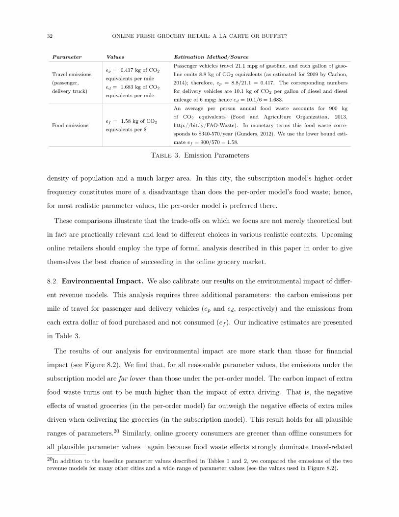
32 ONLINE FRESH GROCERY RETAIL: A LA CARTE OR BUFFET?
Parameter Values Estimation Method/Source
Travel emissions
(passenger,
delivery truck)
ep = 0.417 kg of CO2
equivalents per mile
ed = 1.683 kg of CO2
equivalents per mile
Passenger vehicles travel 21.1 mpg of gasoline, and each gallon of gaso-
line emits 8.8 kg of CO2 equivalents (as estimated for 2009 by Cachon,
2014); therefore, ep = 8.8/21.1 = 0.417. The corresponding numbers
for delivery vehicles are 10.1 kg of CO2 per gallon of diesel and diesel
mileage of 6 mpg; hence ed = 10.1/6 = 1.683.
Food emissionsef = 1.58 kg of CO2
equivalents per $
An average per person annual food waste accounts for 900 kg
of CO2 equivalents (Food and Agriculture Organization, 2013,
http://bit.ly/FAO-Waste). In monetary terms this food waste corre-
sponds to $340-570/year (Gunders, 2012). We use the lower bound esti-
mate ef = 900/570 = 1.58.
Table 3. Emission Parameters
density of population and a much larger area. In this city, the subscription model’s higher order
frequency constitutes more of a disadvantage than does the per-order model’s food waste; hence,
for most realistic parameter values, the per-order model is preferred there.
These comparisons illustrate that the trade-offs on which we focus are not merely theoretical but
in fact are practically relevant and lead to different choices in various realistic contexts. Upcoming
online retailers should employ the type of formal analysis described in this paper in order to give
themselves the best chance of succeeding in the online grocery market.
8.2. Environmental Impact. We also calibrate our results on the environmental impact of differ-
ent revenue models. This analysis requires three additional parameters: the carbon emissions per
mile of travel for passenger and delivery vehicles (ep and ed, respectively) and the emissions from
each extra dollar of food purchased and not consumed (ef ). Our indicative estimates are presented
in Table 3.
The results of our analysis for environmental impact are more stark than those for financial
impact (see Figure 8.2). We find that, for all reasonable parameter values, the emissions under the
subscription model are far lower than those under the per-order model. The carbon impact of extra
food waste turns out to be much higher than the impact of extra driving. That is, the negative
effects of wasted groceries (in the per-order model) far outweigh the negative effects of extra miles
driven when delivering the groceries (in the subscription model). This result holds for all plausible
ranges of parameters.20 Similarly, online grocery consumers are greener than offline consumers for
all plausible parameter values—again because food waste effects strongly dominate travel-related
20In addition to the baseline parameter values described in Tables 1 and 2, we compared the emissions of the tworevenue models for many other cities and a wide range of parameter values (see the values used in Figure 8.2).

ONLINE FRESH GROCERY RETAIL: A LA CARTE OR BUFFET? 33
City Area, A (sq. mi.) Gross Margins, 1 − η
(b) (c) (a)
Delivery Cost, ϕ ($/mi.)
Mean Demand Rate, µ ($/wk) Cost of Ordering, θ ($) Cost of Store Visit, 1/λ ($)
(e) (f) (d)
`
∆ E
mis
sions
(kg o
f C
O2
eq.)
∆ E
mis
sions
(kg
of C
O2
eq.)
∆ E
mis
sions
(kg o
f C
O2 e
q.)
0.5 20%
80 10
50
∆ E
mis
sion
s
(k
g o
f C
O2
eq.)
∆ E
mis
sion
s
(k
g o
f C
O2 e
q.)
∆ E
mis
sions
(kg
of C
O2 e
q.)
40%
Figure 8.2. Annual Per Capita Reduction in Emissions under Subscription PricingNote: Unless stated otherwise, ρ = 12, 500 hh/sq. mi, A = 150 sq. mi, ϕ = 1.5 $/mi, η = .75, ζ = 0.76, K = 15, 1/λ = 30$,
θ = 5$, T = 1 wk, µ = 90 $/wk, and δ = 365.
effects. Importantly, these results stand even if we use very conservative estimates of unit emissions
from food waste (that derive from 100% vegetarian diets), values that are as little as one-third of
the typical US estimate.
In practical terms, the subscription model’s emissions advantage over the per-order model amounts
to between 5% and 15% of the food waste emissions created by an average citizen of the Western
world. This means that the combination of subscription pricing and online grocery retailing can
significantly reduce emissions from the food supply chain. Finally, our findings indicate that food
waste plays a much more important role in the emissions impact of grocery retail than do the travel-
related emissions upon which previous studies focused (Cachon, 2014); hence a reexamination of
those results might be warranted.
Further inspection of Figure 8.2 reveals that the emissions advantage of the subscription model
is the most pronounced: for small cities, where the driving disadvantage is small; for low margins,
high delivery costs, and high store visit costs (all of which lead to waste increases due to lower
adoption rates); for high mean demand, which reduces the waste difference; and for moderate costs
of ordering (in the subscription model, waste is increasing in θ; eventually, this increase approaches
and exceeds the relatively modest effect of θ under the per-order model).
34 ONLINE FRESH GROCERY RETAIL: A LA CARTE OR BUFFET?
9. Discussion
Much as we do in this paper, the existing literature that compares subscription and per-order
pricing considers the two offerings in isolation yet does not consider their combination in a two-
part tariff; see, for example, Barro and Romer (1987); Danaher (2002); Randhawa and Kumar
(2008); Cachon and Feldman (2011). As this literature highlights, two-part tariffs are rarely used
in consumer settings because customers dislike paying twice and a two-part tariff removes the
behavioral incentive of “unlimited free usage”. These considerations apply also in the case of online
grocery delivery. Yet a firm could offer—at least theoretically—a two-part tariff and arguably do
no worse than implementing either subscription or per-order pricing in isolation. This statement is
almost true in our setup, but with one major caveat. We can show that a two-part tariff capable of
outperforming the two revenue models considered in this paper will likely need to charge negative
subscription fees or per-order prices. It is safe to say that a two-part tariff with negative tariffs is
even less practical and would rarely be feasible. Therefore, the firm will resort to choosing either
the subscription model or the per-order model, and all of our preceding analysis can be applied
directly to help it identify which revenue model is preferable.
Our model considers a fresh-grocery retailer and customers who only order fresh groceries. Cus-
tomers may prefer to order perishable and durable items in one order and thus even fresh grocery
retailers will often stock both. If customers purchase a mix of perishable and durable grocery prod-
ucts from our focal retailer, the relevant customer ordering behavior (frequency and size of orders)
is driven only by the consumption dynamics of the perishable products; the durable products are
simply batched with the time-dependent perishable orders. Non-perishable products can thus be
included in the analysis with minor modifications; the durable items are added to the order streams
in both pricing models and the comparison of different revenue models in unaffected.
In our model, the firm has a warehouse whose location is perfectly centered in the delivery area.
A centrally located warehouse is ideal, of course, but this is not always possible owing to real
estate costs, geographic factors, and so forth. When the warehouse is not centrally located, delivery
distances are longer and so the order frequency advantage of the per-order model is enhanced. Our
model can also be easily extended to the case where the firm divides the catchment area into multiple
zones and builds different warehouses in each of them. Delivery distances are now lower and the
order frequency advantage is diminished.
ONLINE FRESH GROCERY RETAIL: A LA CARTE OR BUFFET? 35
In our model there is no lead time between ordering and receiving the order. Positive lead times
will result in more waste, thus increasing the food waste disadvantage of the per-order model. A
random shelf life of the grocery basket has a similar effect, it also increases food waste, increasing
the food waste disadvantage of the per-order model and, thus, making subscription model more
desirable.
We do not explicitly consider issues arising from the retailer’s inventory and fleet size manage-
ment. The pricing model may influence the day-to-day variability in orders to be delivered which
affects inventory management related costs. Further, the model that induces lower inter-temporal
variability at the warehouse will require less vehicles to provide the same service level for on-time
order deliveries. In addition to other factors, the basket size itself might impact the number of
orders delivered by one vehicle. The per-order model has larger orders, this might lead to lower
number of orders delivered by one delivery vehicle making the order frequency advantage of the
per-order model less than estimated by our model.
We have assumed that the fixed costs of building and servicing the per-order and subscription
models are the same—that is, costs that depend neither on the volume of groceries sold nor on the
number of orders serviced are the same in each model. That being said, incorporating such costs
differences would be but a minor extension.
In addition to effects captured in this paper the online grocery retailers might need to consider
other advantages of subscription pricing. Cachon and Feldman (2011) and Gilbert et al. (2014)
describe a second-order revenue-extracting benefit of subscription pricing that operates in addition
to the lower ordering costs already captured in our analysis. Under subscription pricing consumers
purchase in advance of the service and, thus, are willing to pay their expected value for the service.
In contrast, when consumers spot purchase, i.e., when they know their value for the service, they
are naturally willing to pay only their realized value. It might be better to sell in advance to every
customer at their expected value than to sell in the spot market to a portion of consumers (i.e.,
those consumers with a high realized value). In our model this effect would operate when each
customer’s cost of going to the offline store is randomly drawn every period, in addition to the
long-term heterogeneity already captured in our model.
Behavioral phenomena can also alter customer preferences for different pricing schemes. Empirical
analysis by Danaher (2002) shows that customers have different sensitivity to subscription and
per-order fees. There might be other behavioral differences between the two models–such as the

36 ONLINE FRESH GROCERY RETAIL: A LA CARTE OR BUFFET?
ability to pick groceries, the physical exercise benefits of grocery shopping, etc.; these can be easily
incorporated through the adjustment of the store visit costs.
Another simplifying assumption was that the per-unit prices of grocery are the same in both
revenue models and also in the offline store. Obviously, that may not be the case. Lower prices can
increase adoption, thereby enhancing the relevant model’s effect and vice versa. It is also worth
mentioning that customers may have different grocery demand rates. Yet because the firm cannot
ex ante discriminate among different customers and so must offer different market segments the
same pricing model, our analysis provides a close first-order approximation. If there are indeed
widely different customer segments, then offering a menu of contracts might help the retailer select
which segments to serve and, as needed, help it steer different segments toward different revenue
models. Further analysis of this remains an open question and a promising avenue for future work.
Further, we considered an online retailer that competes with offline stores. While this is the case
in almost all major markets an extended model might consider the competition between different
online retailers. Our model captures competitive aspects through the customer’s outside option–
cost of buying offline. Under online competition this cost could be substituted by the customers
outside online option. This analysis is another interesting prospect for future work.
An interesting recent development in the online retailing space is the use of logistics structures
other than the traditional warehouse–delivery vehicle model considered in this paper. Pioneering
firms are now experimenting with crowd-sourced distribution schemes (e.g., Instacart) and the use
of autonomous flying vehicles or drones (Amazon). These developments highlight the increasing
importance of the grocery retail sector and the need to find viable business models in this large
but hitherto untapped category. These new delivery models are certain to have different economic
characteristics than the logistics model considered in this paper, and they are intriguing prospects
for future study.
References
V. V. Agrawal, M. Ferguson, L. B. Toktay, and V. M. Thomas. Is leasing greener than selling?.
Management Science, 58(3):523 – 533, 2012. ISSN 00251909.
R. J. Barro and P. M. Romer. Ski-lift pricing, with applications to labor and other markets. The
American Economic Review, 77(5):pp. 875–890, 1987.
E. Berglas. On the theory of clubs. The American Economic Review, 66(2):pp. 116–121, 1976.
ONLINE FRESH GROCERY RETAIL: A LA CARTE OR BUFFET? 37
J. Bramel and D. Simchi-Levi. The Logic of Logistics: Theory, Algorithms, and Applications for Lo-
gistics Management. Springer Series in Operations Research. P. Glynn S. Robinson, eds. Springer.
New York, 1997.
C. Brown and T. Borisova. Understanding commuting and grocery shopping using the american
time use survey. 2007.
J. M. Buchanan. An economic theory of clubs. Economica, 32(125):pp. 1–14, 1965.
G. P. Cachon. Retail store density and the cost of greenhouse gas emissions. Management Science,
2014.
G. P. Cachon and P. Feldman. Pricing services subject to congestion: Charge per-use fees or sell
subscriptions? Manufacturing & Service Operations Management, 13(2):244–260, 2011.
S.-H. Cho, H. Jang, T. Lee, and J. Turner. Simultaneous location of trauma centers and helicopters
for emergency medical service planning. Operations Research, 62(4):751–771, 2014.
C. F. Daganzo. The distance traveled to visit n points with a maximum of c stops per vehicle: An
analytic model and an application. Transportation Science, 18(4):331–350, 1984a.
C. F. Daganzo. The length of tours in zones of different shapes. Transportation Research Part B:
Methodological, 18(2):135 – 145, 1984b.
P. J. Danaher. Optimal pricing of new subscription services: Analysis of a market experiment.
Marketing Science, 21(2):119–138, 2002.
K. Daniels and R. Lobel. Demand response in energy markets: Voluntary and involuntary load
curtailment contracts. Wharton Working Paper, 2014.
B. E. Fries. Optimal ordering policy for a perishable commodity with fixed lifetime. Operations
Research, 23(1):46–61, 1975.
S. M. Gilbert, R. S. Randhawa, and H. Sun. Optimal per-use rentals and sales of durable products
and their distinct roles in price discrimination. Production and Operations Management, 23(3):
393–404, 2014.
D. Gunders. Wasted: How America Is losing Up to 40 Percent of Its Food from Farm to Fork to
Landfill. A Report of the National Resources Defense Council, 2012.
I.-H. Hann and C. Terwiesch. Measuring the frictional costs of online transactions: The case of a
name-your-own-price channel. Management Science, 49(11):1563–1579, 2003.
L. Himelstein and G. Khermouch. Webvan left the basics on the shelf. Business Week, 3742:43,
2001.
38 ONLINE FRESH GROCERY RETAIL: A LA CARTE OR BUFFET?
S. Kalpakam and G. Arivarignan. A continuous review perishable inventory model. Statistics, 19
(3):389–398, 1988.
S. Kalpakam and K. Sapna. Continuous review (s, s) inventory system with random lifetimes and
positive leadtimes. Operations Research Letters, 16:115 – 119, 1994.
E. Lawler, J. Lenestra, A. Rinnooy Kan, and D. Shmoys. The Traveling Salesman Problem: A
Guided Tour of Combinatorial Optimization. John Wiley & Sons Ltd. New York, 1985.
M. K. Lim, H.-Y. Mak, and Y. Rong. Toward mass adoption of electric vehicles: Impacts of the
range and resale anxieties. Available at SSRN 2236560, 2014.
B. Lipinski, C. Hanson, J. Lomax, L. Kitinoja, R. Waite, and T. Searchinger. Reducing Food Loss
and Waste. World Resources Institute, 2013.
L. Liu and Z. Lian. (s, s) continuous review models for products with fixed lifetimes. Operations
Research, 47(1):pp. 150–158, 1999.
S. Nahmias. On ordering perishable inventory under erlang demand. Naval Research Logistics
Quarterly, 22(3):415–425, 1975. ISSN 1931-9193.
S. Nahmias. Comparison between two dynamic perishable inventory models. Operations Research,
25(1):168 – 172, 1977.
S. Nahmias. Perishable inventory systems. volume 160. 2011.
R. S. Randhawa and S. Kumar. Usage restriction and subscription services: Operational benefits
with rational users. Manufacturing & Service Operations Management, 10(3):429–447, 2008.
G. Roels and X. Su. Optimal design of social comparison effects: Setting reference groups and
reference points. Available at SSRN 2246838, 2013.
S. Ross. Applied Probability Models with Optimization Applications. Holden Day, San Francisco,
1970.
X. Su. Intertemporal pricing and consumer stockpiling. Operations research, 58(4-Part-2):1133–
1147, 2010.
A. Sundararajan. Nonlinear pricing of information goods. Management Science, 50(12):1660–1673,
2004.
N. Tereyağoğlu and S. Veeraraghavan. Selling to conspicuous consumers: Pricing, production, and
sourcing decisions. Management Science, 58(12):2168–2189, 2012.
H. J. Weiss. Optimal ordering policies for continuous review perishable inventory models. Operations
Research, 28(2):365–374, 1980.
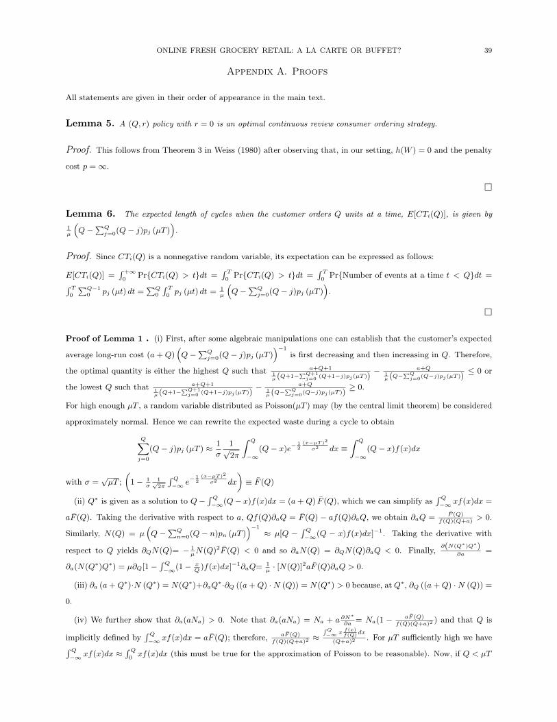
ONLINE FRESH GROCERY RETAIL: A LA CARTE OR BUFFET? 39
Appendix A. Proofs
All statements are given in their order of appearance in the main text.
Lemma 5. A (Q, r) policy with r = 0 is an optimal continuous review consumer ordering strategy.
Proof. This follows from Theorem 3 in Weiss (1980) after observing that, in our setting, h(W ) = 0 and the penalty
cost p =∞.
�
Lemma 6. The expected length of cycles when the customer orders Q units at a time, E[CTi(Q)], is given by
1µ
(Q−
∑Qj=0(Q− j)pj (µT )
).
Proof. Since CTi(Q) is a nonnegative random variable, its expectation can be expressed as follows:
E[CTi(Q)] =∫ +∞
0Pr{CTi(Q) > t}dt =
∫ T0
Pr{CTi(Q) > t}dt =∫ T
0Pr{Number of events at a time t < Q}dt =∫ T
0
∑Q−10 pj (µt) dt =
∑Q0
∫ T0pj (µt) dt = 1
µ
(Q−
∑Qj=0(Q− j)pj (µT )
).
�
Proof of Lemma 1 . (i) First, after some algebraic manipulations one can establish that the customer’s expected
average long-run cost (a+Q)(Q−
∑Qj=0(Q− j)pj (µT )
)−1
is first decreasing and then increasing in Q. Therefore,
the optimal quantity is either the highest Q such that a+Q+11µ (Q+1−
∑Q+1j=0 (Q+1−j)pj(µT ))
− a+Q1µ (Q−
∑Qj=0(Q−j)pj(µT ))
≤ 0 or
the lowest Q such that a+Q+11µ (Q+1−
∑Q+1j=0 (Q+1−j)pj(µT ))
− a+Q1µ (Q−
∑Qj=0(Q−j)pj(µT ))
≥ 0.
For high enough µT , a random variable distributed as Poisson(µT ) may (by the central limit theorem) be considered
approximately normal. Hence we can rewrite the expected waste during a cycle to obtain
Q∑j=0
(Q− j)pj (µT ) ≈ 1
σ
1√2π
∫ Q
−∞(Q− x)e
− 12
(x−µT )2
σ2 dx ≡∫ Q
−∞(Q− x)f(x)dx
with σ =√µT ;
(1− 1
σ1√2π
∫ Q−∞ e
− 12
(x−µT )2
σ2 dx
)≡ F (Q)
(ii) Q∗ is given as a solution to Q−∫ Q−∞(Q− x)f(x)dx = (a+Q) F (Q), which we can simplify as
∫ Q−∞ xf(x)dx =
aF (Q). Taking the derivative with respect to a, Qf(Q)∂aQ = F (Q) − af(Q)∂aQ, we obtain ∂aQ = F (Q)f(Q)(Q+a)
> 0.
Similarly, N(Q) = µ(Q−
∑Qn=0(Q− n)pn (µT )
)−1
≈ µ[Q −∫ Q−∞(Q − x)f(x)dx]−1. Taking the derivative with
respect to Q yields ∂QN(Q)= − 1µN(Q)2F (Q) < 0 and so ∂aN(Q) = ∂QN(Q)∂aQ < 0. Finally,
∂(N(Q∗)Q∗)∂a
=
∂a(N(Q∗)Q∗) = µ∂Q[1−∫ Q−∞(1− x
Q)f(x)dx]−1∂aQ= 1
µ· [N(Q)]2aF (Q)∂aQ > 0.
(iii) ∂a (a+Q∗)·N (Q∗) = N(Q∗)+∂aQ∗·∂Q ((a+Q) ·N (Q)) = N(Q∗) > 0 because, atQ∗, ∂Q ((a+Q) ·N (Q)) =
0.
(iv) We further show that ∂a(aNa) > 0. Note that ∂a(aNa) = Na + a ∂N∗
∂a= Na(1 − aF (Q)
f(Q)(Q+a)2) and that Q is
implicitly defined by∫ Q−∞ xf(x)dx = aF (Q); therefore, aF (Q)
f(Q)(Q+a)2≈
∫Q−∞ x
f(x)f(Q)
dx
(Q+a)2. For µT sufficiently high we have∫ Q
−∞ xf(x)dx ≈∫ Q
0xf(x)dx (this must be true for the approximation of Poisson to be reasonable). Now, if Q < µT

40 ONLINE FRESH GROCERY RETAIL: A LA CARTE OR BUFFET?
x
y
θθl
L
L/2
l/2
(1)
(2)
Figure A.1. Partitioning of a Rectangle
then∫ Q−∞ x
f(x)f(Q)
dx ≈∫ Q
0x f(x)f(Q)
dx ≤∫ Q
0xdx = 1
2Q2. Thus we obtain aF (Q)
f(Q)(Q+a)2≤
12Q2
(Q+a)2< 1. Furthermore, if
Q > µT then it follows (from IFR property of normal distribution) that f(Q)
F (Q)> f(µT )
F (µT )= 2√
2πµT. That is, we need
to show 1√π2µT
> a(Q+a)
1(Q+a)
or 1 > a(Q+a)
√π2µT
(Q+a). These inequalities hold if π
2< µT , and that expression is true by
our assumption µT � 0.
Lemma 7. The average distance from the warehouse to a point in the market area is given by Equation A.1 for a
regular m-gon and by Equation A.2 for a rectangle with length-to-height ratio of γ ≥ 1. Formally,
(A.1) d♦ =√Aζ♦; ζ♦ =
2
3
√1
m · tan Φ
(√1 + tan2 Φ + ln(tan Φ +
√1 + tan2 Φ) · tan−1 Φ
), Φ = πm−1;
(A.2) d =√Aζ ; ζ =
1
3
√1
γ
√γ2 + 1 +1
2
γ2 ln
(√γ2 + 1 + 1
γ
)+
ln(√
γ2 + 1 + γ)
γ
.
Proof. Cachon (2014) gives an expression for a regular m-gon. We can derive an expression for a circle and a square
by using Equation A.1 and setting (respectively) m =∞ and m = 4.
For a rectangle, the average round-trip distance from the warehouse to a point in market area 1 (see Figure A.1), d1,
and one in area 2, d2, can be calculated as follows:
d1 = 2 ·∫ l
20
∫ y tan θ
0
√x2 + y2dxdy
12( l
2)2 tan θ
and d2 = 2 ·∫ L
20
∫ x tan θ
0
√x2 + y2dydx
12(L
2)2 tan θ
.
We have tan θ = Ll
= γ and tan θ = lL
= 1γ; moreover, l =
√Aγand L =
√Aγ. Hence d1 = 1
3
√Aγ
(√
1 + γ2 + 1γ
ln[γ+√1 + γ2]) and d2 = 1
3
√γA(
√1+γ2
γ+ γ ln[ 1
γ+
√1+γ2
γ]) . Finally, there are an equal number of square miles in area 1
and area 2. This means that d = 12(d1 + d2) and so Equation A.2 follows.
�
Proof of Lemma 2. (i) We are looking to find D(ρ, N,A ,K) = 1I
∑Ii=1 Di = 2
K1I
∑Ii=1 di −
LK
+ TSP ∗(K,L, l)
(since all sectors are partitioned in the same fashion and contain K points). Daganzo (1984b) offers the following

ONLINE FRESH GROCERY RETAIL: A LA CARTE OR BUFFET? 41
approximation of the salesman tour:
(A.3) TSP ∗(K,L, l) =φ(βK)√ρd
, where φ(x) =
0.9, x ≥ 12;
√x
6+ 2√
x2
(x/4)2[(1 + x
4) log(1 + x
4)− x
4], x < 12.
Using Lemma 7 and Equation A.3 yields D(ρ, N,A ,K) = 2Kd− L
K+ φ(βK)√
ρd; furthermore, L · l = Kρ−1
d and β = lL,
which means that L =√
Kβρd
and so D(ρ, N,A ,K) = 2Kd− ρ−
12
d ((βK)−12 + φ(βK)). Optimizing with respect to β,
we obtain the optimal “slenderness factor”:
(A.4) β∗ =
1, K ∈ [1, 7];
6.7K, K ≥ 7.
Finally, for K ≤ 4 the approximation displayed as Equation 5.1 is not very accurate; Daganzo (1984a) provides the
more accurate expression D(ρ, N,A ,K) = 2Kd− ρ−
12
d ( (K−2)+
K+1(βK)−
12 + K−1
Kφ(βK)). Combining this equality with
the results from Equations A.1, A.2, and A.4 establishes the congruence displayed as Equation 5.2, where the factor
λ(K) is given as follows:
(A.5) λ(K) =
(K−2)+
K+11√β∗K
+ K−1K
φ(β∗K), K ≤ 4;
φ(β∗K)− 1√β∗K
, K > 4.
(ii) We have ∂N D = −λ(K) 12N
√δρN
< 0 and ∂ρD = −λ(K) 12ρ
√δρN
< 0. Now ∂aD = (∂N D)∂aN > 0, since
∂aN < 0 (by Lemma 1); therefore,∂NND = 2ζ√A
K+ λ(K) 1
2
√δρN
> 0 and ∂aND = (∂NND)∂aN < 0.
Lemma 8. Iff the customer with store visit cost α chooses the online retailer then customers with store visit costs
α ≥ α will also choose to shop online.
Proof. Since Coff = Cα is an increasing function of α, it follows that all customers for whom α ≥ α will purchase
online and the rest will purchase offline.
�
Proof of Lemma 3. The firm seeks to maximize its profit:
πo = maxo
((o+Qo)No − ho(o)) · G (α) ; α = min {α ∈ [α, α] s.t.Coff ≥ Co}(A.6)
Next we show that the constraint Coff = Cα ≥ Co is always binding. When it is binding the firm will charge
o+ θ = α and we can reformulate the problem as
(A.7) maxα≤α≤α
(Cα − ho(α)) G(α).
Otherwise, the firm is solving max0≤o≤α−θ((o+ θ +Qo)No − (y + ηQo + cp + θ)No − z
√No). Recall that Qo =
Q∗o+θ. First observe that (o+ θ +Qo)No is an increasing concave function because ∂o (o+ θ +Qo)No = No > 0 and

42 ONLINE FRESH GROCERY RETAIL: A LA CARTE OR BUFFET?
∂2o (o+ θ +Qo)No = ∂oNo < 0. Now, for o ≤ α − θ both (y + ηQo + cp + θ)No and ϕz
√No are decreasing convex
functions (since ∂o√No = 1
2N−1/2o ∂oNo < 0 and ∂2
o
√No = − 1
4N−3/2o ∂oNo + 1
2N−1/2o ∂2
oNo > 0. We can therefore
conclude that the objective function is an increasing concave function and so its maximum is achieved at o = α− θ,
which is covered in A.7 formulation.
Since Coff = Cα is an increasing function of α, it follows that all customers for whom α > α∗o will purchase online
and the rest will purchase offline. The equation for determining the optimal solution follows from taking the derivative
of A.7, and that solution’s uniqueness follows from the concavity of A.7. Note that the solution might sometimes be
a corner solution—that is,
α∗o =
α, if (Nα − ∂αho(α)) · G(α)− g(α) · (Cα − ho(α)) > 0 for all α;
α, if (Nα − ∂αho(α)) · G(α)− g(α) · (Cα − ho(α)) < 0 for all α.
Proof of Lemma 4. The proof follows along the lines of that for Lemma 3. As in that case, the solution may turn
out to be a corner solution:
α∗s =
α, if (Nα − ∂αhs(α))G(α)− g(α)(Cα − hs(α)) > 0 for all α;
α, if (Nα − ∂αhs(α))G(α)− g(α)(Cα − hs(α)) < 0 for all α.
Proof of Theorem 1. The theorem’s statements follow from Lemmas 1, 3, and 4 combined with the higher cost of
ordering under the per-order model, θ < α ≤ α∗o.
Proof of Corollary to Theorem 1. The yearly expected amount of groceries that is spoiled and wasted can be
expressed as (Q·) ·N·−µ. Theorem 1 establishes that (Q·) ·N· is higher in the per-order model, so the annual amount
of wasted groceries is higher in that model.
Lemma 9. Market coverage under both pricing schemes is decreasing with ζ; that is, α∗s and α∗o are increasing in
ζ, i.e. ∂α∗s∂ζ,∂α∗o∂ζ
> 0.
Proof. We first establish that α∗s is increasing in ζ, i.e. ∂α∗s∂ζ
> 0. To find the optimal α∗s , the firm solves
maxα≤α≤α (Cα − hs(α)) G(α). Since the firm can guarantee a zero profit by choosing α = α, it follows for any
α∗s < α that
(A.8) Cα∗s − hs(α∗s) > 0.
By Lemma 4, α∗s is implicitly defined by
(A.9) Nα∗s − ∂α∗shs(α∗s) =
g(α∗s)
G(α∗s)(Cα∗s − hs(α
∗s)).

ONLINE FRESH GROCERY RETAIL: A LA CARTE OR BUFFET? 43
The next is determining the behavior of α∗s with ζ. We can use the implicit function theorem and our optimality
condition to obtain
∂α∗s∂ζ
=
g(α∗s)
G(α∗s)12ϕ · 2
√A
KNs
(∂α∗sg(α∗s)
G(α∗s))(Cα∗s − hs(α∗s)) +
g(α∗s)
G(α∗s)
g(α∗s)
G(α∗s)(Cα∗s − hs(α∗s))− ∂α∗sNα∗s + ∂2
α∗shs(α∗s)
.
The numerator is positive because g(α)
G(α)= λ > 0, so it remains only to establish that the denominator is positive.
In the proof of Lemma 1 we showed that ∂Nα∂α
< 0; note also that the first and second summands are positive
because g(α)
G(α)= λ > 0 and Cα∗s − hs(α
∗s) > 0 (see A.8). Finally, the last summand is positive because ∂α(∂αhs) |α∗s=
∂α(
12g(α)
G(α)ϕz√
NsG(α)
|α∗s)
= 14g(α)
G(α)
g(α)
G(α)ϕz√
NsG(α)
+ 12
∂g(α)
G(α)
∂α|α∗s ϕz
√NsG(α)
> 0.
Similarly, α∗o is increasing in ζ, i.e. ∂α∗o∂ζ
> 0 and
∂α∗o∂ζ
=
g(α∗o)
G(α∗o)12ϕ · 2
√A
KNα∗o
(∂α∗og(α∗o)
G(α∗o))(Cα∗o − ho(α∗o)) +
g(α∗o)
G(α∗0)
g(α∗o)
G(α∗o)(Cα∗o − ho(α∗o))− ∂α∗oNα∗o + ∂2
α∗oho(α∗o)
.
�
Proof of Theorem 2. First, ∂∂ζ
(π∗o − π∗s ) = ϕ · 2√A
K{NsG(α∗s) − Nα∗o G(α∗o)}. Next we show that if NsG(α∗s) =
Nα∗o G(α∗o) for some ζ (which entails that α∗s > α∗o) and if π∗o > π∗s , then NsG(α∗s) < Nα∗o G(α∗o) for all ζ > ζ. To
establish these conditions we need only show that ∂α∗s∂ζ
>∂α∗o∂ζ
for ζ > ζ. Now, for the exponential distributiong(α)
G(α)= λ, thus ∂α∗o
g(α∗o)
G(α∗o)= 0; hence we can rewrite expressions for ∂α∗s
∂ζ,∂α∗o∂ζ
(derived in Lemma 9) and obtain
∂α∗s∂ζ
=λ 1
2ϕ · 2
√A
KNs
λ2(Cα∗s − hs(α∗s))− ∂α∗sNα∗s + ∂2α∗shs(α∗s)
;∂α∗o∂ζ
=1NsNα∗o
λ 12ϕ · 2
√A
KNs
λ2(Cα∗o − ho(α∗o))− ∂α∗oNα∗o + ∂2α∗oho(α∗o)
.
The two numerators are equal and we denote the respective denominators dens and deno.
Next we show that deno > dens for ζ > ζ:
deno−dens = λ2{ NsNα∗o
Cα∗o−NsNα∗o
ho(α∗o)−(Cα∗s −hs(α
∗s))}+{∂α∗sNα∗s −
NsNα∗o
∂α∗oNα∗o}+{ NsNα∗o
∂2α∗oho(α
∗o)−∂2
α∗shs(α
∗s)}.
We start by showing that the second summand is positive. We have already established that ∂αNα = −Nα 1(α+Qα)2
F (Qα)f(Qα)
,
so ∂α∗sNα∗s −NsNα∗o
∂α∗oNα∗o = Ns(α∗o+Qα∗o
)2
F (Qα∗o)
f(Qα∗o)−
Nα∗s(α∗s+Qα∗s
)2
F (Qα∗s)
f(Qα∗s)> 0. The third summand is also positive,
∂2α∗oho(α
∗o) −
Nα∗oNs
∂2α∗shs(α
∗s) > 0, as
Nα∗oNs
∂2α∗shs(α
∗s) = z
4λ2Nα∗o
√1
NsG(α∗s)and ∂2
α∗oho(α
∗o) ≥ z
4λ2
√Nα∗oG(α∗o)
; therefore,
∂2α∗oho(α
∗o) −
Nα∗oNs
∂2α∗shs(α
∗s) ≥ ϕ z
4λ2Nα∗o (
√1
Nα∗oG(α∗o)
−√
1NsG(α∗s)
) > 0. Finally, the first summand is also positive,NsNα∗o
(Cα∗o − ho(α∗o))− (Cα∗s − hs(α
∗s)) > 0, and we can rewrite it as follows: (α∗o + (1− η)Qα∗o )Ns − (α∗s +Qα∗s )Nα∗s +
NsηQs + zNs(√
1NsG(α∗s)
−√
1Nα∗o
G(α∗o)). We can now show that (α∗o + (1− η)Qα∗o )Ns − (α∗s +Qα∗s )Nα∗s +NsηQs is
increasing in ζ: ∂ζ(α∗o + (1−η)Qα∗o )Ns− (α∗s +Qα∗s )Nα∗s =(∂ζα∗o + (1−η)∂ζQα∗o )Ns−∂ζNα∗s∂ζα
∗s > 0. Furthermore,
at ζ NsNα∗o
(Cα∗o − ho(α∗o)) − (Cα∗s − hs(α
∗s)) > 0 if π∗o > π∗s ; hence Ns
Nα∗o(Cα∗o − ho(α
∗o)) − (Cα∗s − hs(α
∗s)) > 0 for all
ζ > ζ. This means that, for all ζ > ζ, we have ∂ζα∗s > ∂ζα∗s and so α∗s > α∗o. That is, ∂
∂ζ(π∗o − π∗s ) < 0 for ζ > ζ.
Proof of Theorem 3. By definition, ζ is such that π∗s = π∗o ; that is,(µ
F (Qα∗s )− hs(α∗s)
)G(α∗s)− z
√Ns
√G(α∗s) =
((
µ
F (Qα∗o )− ho(α∗o)
)G(α∗o) · z
√Nα∗o
√G(α∗o)

44 ONLINE FRESH GROCERY RETAIL: A LA CARTE OR BUFFET?
where hs(α) = (θ + cp)Ns + ζyNs + ηQsNs; ho(α) = (θ + cp)Nα + ζyNα + ηQαNα, z = ϕλ(K)√
δρ, and y =
2ϕ√A
K. Using the implicit function theorem yields ∂ζ
∂A= −ζ · ∂y
∂A
(G(α∗o)Nα−NsG(α∗s))y(G(α∗o)·Nα−G(α∗s)Ns)
< 0, since ∂y∂A
> 0; also,
∂ζ∂ϕ
= −ζ · ∂y∂ϕ
y(G(α∗o)·Nα−G(α∗s)Ns)+z(√
Nα∗oG(α∗o)−
√NsG(α∗s)
)y(G(α∗o)·Nα−G(α∗s)Ns)
< 0 because ∂y∂ζ
> 0 and(G(α∗o)Nα −NsG(α∗s)
)and(√
Nα∗o G(α∗o)−√NsG(α∗s)
)always have the same sign. Moreover, ∂ζ
∂ρ= −ζ · ∂z
∂ρ
(√Nα∗o
G(α∗o)−√NsG(α∗s)
)y(G(α∗o)·Nα−G(α∗s)Ns)
> 0 because
∂z∂ρ< 0. Finally, ∂ζ
∂K= −ζ ·
∂z∂K
(√Nα∗o
G(α∗o)−√NsG(α∗s)
)+ ∂y∂K (G(α∗o)Nα−NsG(α∗s))
y(G(α∗o)·Nα−G(α∗s)Ns)> 0 because ∂z
∂K, ∂y∂K
< 0.
Proof of Theorem 4. We can express the emission difference as follows:
Es − Eo = ed ·(G(α∗s)yNs + z
√G(α∗s)Ns − G(α∗o)yNα∗o − z
√G(α∗o)Nα∗o
)+∫ α∗sα∗o
(epdαNα) g(α)dα+
+ef{G(α∗s)QsNs−G(α∗o)Qα∗oNα∗o +∫ α∗sα∗o
NαQαg(α)dα}. If we set e = ep/ed then we can write Es−Eo = ed(†)+ef (∗)
for (†) ≡(G(α∗s)yNs + z
√G(α∗s)Ns − G(α∗o)yNα∗o − z
√G(α∗o)Nα∗o
)+∫ α∗sα∗o
(edαNα) g(α)dα; (∗) ≡ G(α∗s)QsNs −
G(α∗o)Qα∗oNα∗o +∫ α∗sα∗o
NαQαg(α)dα. We remark that both (†) and (∗) are independent of ef and ed. There are four
possible combinations: (i) (∗), (†) > 0, in which case ef =∞; (ii) (∗), (†) < 0, in which case ef = 0; (iii) (∗) < 0, (†) >
0, in which case ef = −ed (†)(∗) ; (iv) (∗) > 0, (†) < 0. Combinations (i)–(iii) are directly covered by the theorem, so we
need only rule out combination (iv).
We first consider α∗o ≥ α∗s which implies G(α∗s) ≥ G(α∗o). We will show that (∗) = G(α∗s)QsNs − G(α∗o)Qα∗oNα∗o +∫ α∗sα∗o
NαQαg(α)dα < 0. We have G(α∗o)(QsNs − Qα∗oNα∗o ) ≤ 0 since QsNs < Qα∗oNα∗o (by Theorem 1). Thus,
it only remains to show that (∗∗) ≡ (G(α∗s) − G(α∗o))QsNs −∫ α∗oα∗s
NαQαg(α)dα < 0. Since∫ α∗oα∗s
NαQαg(α)dα >
Nα∗sQα∗s∫ α∗oα∗s
g(α)dα = Nα∗sQα∗s (G(α∗o)−G(α∗s)), it follows that (∗∗) < (G(α∗s)− G(α∗o))(QsNs−Nα∗sQα∗s ) < 0. This
inequality allows us to obtain the desired result (∗) < 0, which rules out the possibility of combination (iv).
Next consider α∗o < α∗s , from which it follows that G(α∗o) ≥ G(α∗s). This means that, under the subscription
revenue model, the retailer’s coverage will be smaller and so more customers will end up traveling to the (offline)
store directly. As self-travel entails higher travel distances (†) > 0, which rules out (iv).