Online Appendix

Wealth Heterogeneity and the Income Elasticity of Migration

Samuel Bazzi

Contents

A Theoretical Results 2

B Econometric Procedures 4B.1 Parametric . . . . . . . . . . . . . . . . . . . . . . . . . . . . . . . . . . . . . . . . . . . . . . . . . . . . 4B.2 Semiparametric . . . . . . . . . . . . . . . . . . . . . . . . . . . . . . . . . . . . . . . . . . . . . . . . . 4B.3 Inference . . . . . . . . . . . . . . . . . . . . . . . . . . . . . . . . . . . . . . . . . . . . . . . . . . . . . 4

C Data Description 6

D Theory and Estimation with the Pareto Distribution 7Figures . . . . . . . . . . . . . . . . . . . . . . . . . . . . . . . . . . . . . . . . . . . . . . . . . . . . . . . . . 8

E Further Details on Agricultural Income Shocks 10E.1 Spatial Variation in the Rice Price Shock: Theory and a Simple Test . . . . . . . . . . . . . . . . . . . 10E.2 On Measuring Rice Prices . . . . . . . . . . . . . . . . . . . . . . . . . . . . . . . . . . . . . . . . . . . 11E.3 Spatial and Time Series Properties of Rainfall and Rice Prices . . . . . . . . . . . . . . . . . . . . . . . 12E.4 Exogeneity of Price Shocks with Respect to Landholdings Distribution . . . . . . . . . . . . . . . . . 12E.5 Effect of Rainfall and Rice Price Shocks on GDP, Wages, and Profits . . . . . . . . . . . . . . . . . . . 12Figures . . . . . . . . . . . . . . . . . . . . . . . . . . . . . . . . . . . . . . . . . . . . . . . . . . . . . . . . . 14Tables . . . . . . . . . . . . . . . . . . . . . . . . . . . . . . . . . . . . . . . . . . . . . . . . . . . . . . . . . . 17

F Further Empirical Results 20F.1 Heterogeneity in Land Quality . . . . . . . . . . . . . . . . . . . . . . . . . . . . . . . . . . . . . . . . 20F.2 Controlling for Agricultural Wage Shocks . . . . . . . . . . . . . . . . . . . . . . . . . . . . . . . . . . 20F.3 Assessing Exclusion Restrictions . . . . . . . . . . . . . . . . . . . . . . . . . . . . . . . . . . . . . . . 20F.4 Alternative Specifications of Rainfall and Rice Price Shocks . . . . . . . . . . . . . . . . . . . . . . . . 21F.5 Alternative Choices of the Pareto Lower Bound . . . . . . . . . . . . . . . . . . . . . . . . . . . . . . . 21F.6 Accounting for Village Demographic Structure and Past Internal Migration . . . . . . . . . . . . . . 22F.7 On the (Non-)Effect of Measurement and Reporting Outliers . . . . . . . . . . . . . . . . . . . . . . . 22F.8 Rainfall Shocks and Internal Migration . . . . . . . . . . . . . . . . . . . . . . . . . . . . . . . . . . . . 22F.9 Further Background on the Validation Exercise Using Micro Data . . . . . . . . . . . . . . . . . . . . 23F.10 Further Background on the Estimation of Village-Specific Migration Costs . . . . . . . . . . . . . . . 24F.11 What Role for Policy, Recruiters, and Networks? . . . . . . . . . . . . . . . . . . . . . . . . . . . . . . 25Tables . . . . . . . . . . . . . . . . . . . . . . . . . . . . . . . . . . . . . . . . . . . . . . . . . . . . . . . . . . 26

G Zeros, Balls, Bins, and Traveling Salesman 37G.1 Ruling out a Balls-and-Bins Interpretation of the Extensive Margin . . . . . . . . . . . . . . . . . . . 37G.2 A Heuristic Framework for Recruiter Location Choice . . . . . . . . . . . . . . . . . . . . . . . . . . . 37Tables . . . . . . . . . . . . . . . . . . . . . . . . . . . . . . . . . . . . . . . . . . . . . . . . . . . . . . . . . . 40

H Panel Data Construction 41

References 45

2

A Theoretical Results

This section provides proofs for the results in Section 2. Equations (3) and (4) can be obtained by integrating overlandholdings Riv in inequality (2) with (i) τvj > 0 and RL ≥ R or (ii) RL < R (⇐= τvj = 0). First, consider thefollowing expressions for the thresholds within which migration is both feasible and profitable in period t (from theperspective of t− 1 decision-makers required to pay fixed upfront costs in that period)

RL,t−1 =

(τvjCvjt

pv,t−1(σv + av,t−1)Kθv

)1/β

; RU,t−1 =

(Wvjt − Cvjt

αvpv,t−1σvχKθv

)1/β

, (A.1)

where Et−1[pvtσvt] = αvpv,t−1σv , which hinges on covt−1(pvt, σvt) = 0, i.e. households cannot forecast therelationship between rainfall and prices next period. This does not imply that past rainfall has no effect oncontemporaneous prices. Rather, av,t−k for k > 0 are elements of the error term

∑qs=0 υsev,t−s in the ARMA(1, Q)

expression for rice prices. Thus, past output has a direct effect on current prices.1

If CIA constraints are binding, then the stock migration rate in period t is derived by integrating over all land-holdings Riv ∈ [RL,t−1, RU,t−1] in village v (maintaining the innocuous normalization R = 1 ha)

P(RL,t−1 ≤ Riv ≤ RU,t−1) =Mvt

Nvt=

∫ RU,t−1

RL,t−1

λvR−λv−1iv dRiv = R−λvL,t−1 −R

−λvU,t−1. (A.2)

Replacing the expressions for RL and RU with those in equation (A.1) and taking the difference in logs betweent+ 1 and t, we obtain equation (3).

On the other hand, if CIA constraints are not binding and RL < R (⇐= τvj = 0), then

P(1 ≤ Riv ≤ RU,t−1) =Mvt

Nvt=

∫ RU,t−1

1

λvR−λv−1iv dRiv = 1−R−λvU,t−1. (A.3)

Similarly substituting for RU,t−1 and taking differences in logs implies equation (4). Recall that, by definition, theexpressions for the intensive margin in (A.2) and (A.3) must be greater than zero.

Proposition 1The proofs in the presence of CIA constraints follow immediately from differentiation of equation (3). Letting∆ ln(Mv,t+1/Nv,t+1) ≡ ∆Mv,t+1,

∂∆Mv,t+1

∂∆ ln pvt=λvβ> 0;

∂∆Mv,t+1

∂avt=

λvβ (σv + avt)

λv/β−1(τvjCvj,t+1)−λv/β(σv+avt

τvjCvj,t+1

)λv/β−(

αvσvWvj,t+1−Cvj,t+1

)λv/β > 0. (A.4)

The derivative with respect to rainfall last period, av,t−1, is identical to ∂∆Mv,t+1/∂avt with a leading negativesign and shifting all t subscripts back to t − 1. The proof that rainfall shocks have no effect in the absence of CIAconstraints is trivial since avt and av,t−1 do not enter equation (4). The positive effect of price shocks on Mv,t+1 inthe presence of CIA constraints follows immediately from the fact that λv/β > 0. The proof that price shocks havea negative effect on the change in migration rates in the absence of CIA constraints proceeds by checking that the

1The expressions are more complicated if prices (i) follow a higher-order autoregressive process or (ii) have a forecastable nonzero drift term,and/or (iii) households do not have rational expectations over the high frequency seasonality in prices. Nevertheless, the assumptions here arelargely consistent with the time series properties of rainfall and rice prices in Indonesia (and presumably elsewhere). Moreover, the first-orderprice formulation is sufficiently general to comprise more higher-order Markov processes (see Chambers and Bailey, 1996).

3

following expression satisfies increasing differences (over time) in (Hvs, pvs),

ln[1− (Hvspvs)

λvβ

],

where Hvs = αvσvχKθv/(Wvj,t+1 − Cvj,t+1). This condition holds so long as migration costs are non-increasing,

Cvj,t+1 ≤ Cvjt, which seems plausible in most settings. Of course, taking the derivative with respect to the pricelevel, we find

∂∆Mv,t+1

∂pvt=−λvβ p

λv/β−1vt

(αvσvχK

θv

Wvj,t+1−Cvj,t+1

)λv/β1−

(αvpvtσvχKθ

v

Wvj,t+1−Cvj,t+1

)λv/β < 0. (A.5)

Proposition 2The fact that λv has an ambiguous effect on the intensive margin follows immediately from differentiating equations(3) or (4) and recognizing that the terms inside brackets [·] within the logarithm are less than one. That ∂∆Mv,t+1

∂∆ ln pvt∂λv=

1/β > 0 in the presence of CIA constraints is immediate from equation (3). To show that ∂2∆Mv,t+1/∂avt∂λv > 0,simply rearrange and differentiate equation (A.4) with respect to λv

∂2∆Mv,t+1

∂avt∂λv=

1β (σv + avt)

−1

1−(

αvσvτvjCvj,t+1

(σv+avt)(Wvj,t+1−Cvj,t+1)

)λvβ

+

λvβ2 (σv + avt)

−1(

αvσvτvjCvj,t+1

(σv+avt)(Wvj,t+1−Cvj,t+1)

)λvβ

ln(

αvσvτvjCvj,t+1

(σv+avt)(Wvj,t+1−Cvj,t+1)

)(

1−(

αvσvτvjCvj,t+1

(σv+avt)(Wvj,t+1−Cvj,t+1)

)λvβ

)2 .

(A.6)Letting xv := αvσvτvjCvj,t+1 and yv := (σv + avt)(Wvj,t+1 −Cvj,t+1), recognizing that xv < yv (for those migrating,i.e. Riv ∈ [RL, RU ]), and noting that (yv/xv)

λv/β + (λv/β) ln(xv/yv) > 1, it can be shown that equation (A.6) is pos-itive. In the absence of CIA constraints, a similar calculation on equation (A.5) shows that ∂2∆Mv,t+1/∂pvt∂λv < 0.

Multiple Labor Units. There are two ways to think about the household income maximization problem above inthe context of allocating multiple units of household labor. In either approach, there is no tradeoff between holdingon to one’s land and migrating as in Jayachandran (2006). Moreover, the key insight in inequality (2) remainsunchanged. In case one, define Siv ≡ sivLiv where s is the share of household i’s total labor L working at home.The collective household objective is then

maxsiv

Et[pv,t+1σv,t+1]Kθv (sivLiv)

φRβiv + Liv(1− siv)(Wvj,t+1 − Cvj,t+1),

subject to Yivt ≥ τvjCvj,t+1, with the solution s∗iv implying that household i finds migration profitable ifs∗ivLiv(Wvj,t+1 − Cvj,t+1) > Et[pv,t+1σv,t+1]φKθ

vSφ−1iv Rβiv , which holds under equation (1). In case two, we appeal

to the fact that Yivt =∑L` y`ivt, where y`ivt is output per capita. Hence, household i has at least one migrant abroad

in t + 1 whenever Et[pv,t+1σv,t+1]y`iv,t+1 ≤ (Wvj,t+1 − Cvj,t+1). Because labor is perfectly substitutable within thehousehold and the technology is constant returns, this condition also holds under equation (1).

Extensive Margin. As discussed in Section 5, λv has an ambiguous effect on the extensive margin regardlessof the formulation of the extreme landholding statistics. Under the finite sample formulation, the proof followsimmediately from the derivative of the first equation in the footnote on page 15 with respect to λv ,NvR−λvNvU lnRU−Nv(1 − RλvL )NvR−λvL lnRL, the sign of which cannot be determined without imposing ad hoc bounds on parametervalues. The ambiguity similarly holds for the population-based order statistic approach. Meanwhile, the positiveeffect of population size Nv on the extensive margin follows from straightforward differentiation.

4

B Econometric Procedures

This section details the two-step estimating framework introduced in equations (8) in Section 5.

B.1 Parametric

The parametric approach due to Poirier (1980) presumes that (uvt, uv,t+1,∆εv,t+1) in equation (8) followa trivariate normal distribution with mean zero, variances (1, 1,var(∆ε)), and pairwise correlation terms(ρutut+1 , ρut∆ε, ρut+1∆ε). These assumptions imply that

E[∆εv,t+1

∣∣∣Z′v,t−1φt−1 > −uvt,Z′vtφt > −uv,t+1

]= ρut∆εκvt + ρut+1∆εκv,t+1,

where κvt and κv,+1 are bivariate Mills ratio terms. Implementation proceeds in two steps. First, I estimate abivariate probit model for the extensive margins in t and t + 1. Since prices, rainfall and population size varyover time, the bivariate first stage has several sequential exclusion restrictions. Second, I augment an empiricalspecification for the change in the log migration rate with the estimated correction terms κvt and κv,t+1, whichenter with population coefficients equal to ρut∆ε and ρut+1∆ε respectively. Straightforward OLS then delivers aconsistent estimate of second stage parameters. See Rochina-Barrachina (1999) for further theroetical background onthe relationship between Poirier’s original cross-sectional bivariate probit and the two-period panel implementationas described here.

B.2 Semiparametric

This section sketches a practical semiparametric procedure based on Das et al. (2003) for estimating the system ofequations in (8) that is arguably more robust to distributional misspecification than the parametric Poirier approach.Rather than closed-form correction terms, the semiparametric approach relies on a double-index in the propensityscores g(Z′v,t−1φt−1,Z

′vtφt), where g is an unknown function of the latent variable indices.

Implementation proceeds as follows. First, rather than assuming bivariate normality of (uvt, uv,t+1), I use aseemingly unrelated linear probability models (SU-LPM) making no assumptions on the joint distribution of uvtand uv,t+1 (Zellner and Lee, 1965).1

Second, I use the estimates of φt and φt+1 to approximate g(·). In practice, I employ an Lth-degree power seriesexpansion in the propensity scores Ps = Z′sφs—linear predictions recovered from the bivariate SU-LPM estimator—for village v to have at least one migrant in period s.2 Lastly, consistent second-stage estimates of Θ can be obtainedfrom an OLS regression conditioning on the power series g(·) function so long as at least two variables in Zt−1 ∪Ztdo not also appear in Xt.

B.3 Inference

In both the parametric and semiparametric framework outlined above, the correction terms introduce added sam-pling variation into the second-stage.3 Taking a conservative and unbiased approach to inference, I implement

1Results are similar albeit computationally costly using a semi-nonparametric pseudo-maximum likelihood (SNP-ML) procedure based on anapproximation to the unknown latent error densities (Gallant and Nychka, 1987).

2This is essentially the approach suggested by Das et al. (2003) who recommend using a fully nonparametric estimator to estimate the propensityscore. Newey (1988) argues that a first stage linear probability model provides consistent estimates in two-step selection models, though asemiparametric first stage estimator provides more efficient (second-stage) estimates (Newey, 2009). An important difference with Das et al.,however, is that they assume uvt⊥uv,t+1 whereas the estimates of φ obtained using bivariate SU-LPM explicitly allow for corr(uvt, uv,t+1) 6=0. Results are robust to estimating two distinct LPMs with corr(uvt, uv,t+1) = 0.

3Although the Pareto parameters λv are generated regressors, these fitted distributional terms are obtained from more than 55,000 regressionscomprising the universe of agricultural households in Indonesia. Similar to other studies employing population measures of inequality, I treatthe added sampling variation from these terms as negligible. This is reasonable here given that the Agricultural Census of 2003 purports tocapture the full agricultural population of every village. Moreover, even if these distributional parameters are estimated with error, these errors

5

a bootstrap−t procedure (also known as percentile−t) with clustering at the district level. All tables report theuncorrected standard errors, but the significance levels are computed based on the cluster bootstrap−t proceduredescribed in detail in Cameron et al. (2008).4 Each second-step significance level is based on 999 bootstrap iterations,where I cluster the standard errors at each iteration and construct the iteration-specific Wald test statistic (t-stat) re-centered on the original point estimate. Using these 999 Wald statistics, I then compute the (possibly asymmetric)90th, 95th, and 99th% confidence intervals in reporting the significance level α ∈ {0.1, 0.05, 0.01} associated witheach point estimate.

The simulation results in Cameron et al. (2008) suggest that the empirical setup in this paper is well suited tothe cluster bootstrap−t procedure. In particular, the data comprise a large number of districts (> 200 in all specifi-cations) with an unbalanced number of villages, several observable variables are relatively constant within district,and several binary regressors. Moreover, Yamagata (2006) finds that the bootstrap−t procedure outperforms theconventional bootstrap−se procedure in the context of estimating Heckman (1976)-type selection models similar tothose in this paper.5

should not affect the standard errors on the first- and second-step coefficients in the model in equation (8) because (i) the moment conditions inthe two village-level equations in (8) are orthogonal to the moment condition in the auxiliary OLS household-level regressions used to estimateλv for each village, and (ii) the λv terms enter linearly, and hence the added sampling variation can be ignored (see Newey and McFadden,1994, pp. 2182-2183).

4In applications of the bootstrap−t procedure, authors sometimes report p-values. While retaining the original biased standard errors, I reportthe unbiased significance levels when those p-values fall below 0.1. The underlying p-values are available upon request.

5The cluster bootstrap−t procedure that I employ yields confidence intervals with correct coverage in addition to asymptotic refinement. Inunreported results similar to Yamagata (2006), I also find that the 95% confidence intervals generated by a conventional cluster bootstrap−seprocedure fail to cover the original point estimate in more than 5% of iterations, suggesting important finite-sample shortcomings of theconventional bootstrap.

6

C Data Description

Variable Source Definitionpopulation Podes 2005/8 all people registered as residents for at least six months or less than six months with the intention

of staying

migrants Podes 2005/8 all people working abroad on a fixed wage for a fixed time period

λv Agricultural Census 2003 estimate of the Pareto exponent λv for village v based on OLS estimation (Gabaix and Ibragimov,2011); see Appendix D for details

share households above R Agricultural Census 2003 share of all households in village v reporting landholdings less than R where R = 0.1 hectares inthe baseline case

λ63v Agricultural Census 1963 estimate of the Pareto exponent λv for district d based on maximum likelihood estimation given

the reporting of landholdings frequencies in 8 bins

rice prices Wimanda (2009) via BPS see Appendix E for details

rainfall in year t NOAA/GPCP total amount of rainfall during the given growing/harvest season where (1) seasons are 12 monthintervals beginning with the first month of the province-specific wet season in a given year (Mac-cini and Yang, 2009), and (2) rainfall at the village level is based on rainfall levels recorded inter-polated down to 0.5 degree (latitude/longitude) pixels between rainfall stations

plurality destination fixed effect Podes 2005 indicators for whether a plurality of migrants from village v were working in Malaysia, HongKong, Singapore, Taiwan, Japan, South Korea, UAE, Saudi Arabia, Jordan, Kuwait, USA andOther

no motorized land travel to district capital Podes 2002 equals one if there is no direct travel to the district capital using motorized land-based vehicles

reporting frequency Podes 2005 one of five ordered levels: no formal population register, non-routine reporting, annual reporting,quarterly reporting, monthly reporting

distance to nearest district capital Podes 2005/8 the minimum of the travel distance in kilometers to the given district capital or the nearest capitalin a neighboring district

distance to subdistrict capital Podes 2005/8 travel distance in kilometers to the capital of the village’s subdistrict

distance to nearest emigration center great circle distance from the centroid of the district in which village is located to the centroidof the nearest of 17 cities capable of processing legal international contract migration; cities in-clude Aceh, Medan, Pekanbaru, Palembang, Jakarta, Bandung, Semarang, Yogyakarta, Surabaya,Pontianak, Banjarbaru, Nunukan, Makassar, Mataram, Kupang, Tanjung Pinang, and Bali

urban Podes 2005/8 a government-constructed indicator which equals one if the village has a population densitygreater than 5000 per square kilometer, a majority of the population recorded as non-farminghouseholds, and any number of public institutions which I do not observe directly in Podes

distance to Ho Chi Minh City/Bangkok (port) great circle distance from the centroid of the village is located to the nearest Indonesian port plusthe shipping distance abroad; geocoordinates of Indonesian port cities obtained from AtoBviaCand shipping distances from e-ships

Arab (Chinese) population share Population Census 2000 the number of individuals claiming Arab (Chinese) descent as a share of village population

Muslim population share Podes 2005/8 the number of individuals claiming adherence to Islamic faith as share of village population

post-primary education share Population Census 2000 share of the population aged 5 and above that has completed junior secondary (SLTP/setara), se-nior secondary (SLTA/setara), or post-secondary (Diploma/DIII/Akedemi/DII/DIV)

share population aged 15-29 Population Census 2000 age range is chosen to correspond to the majority migration age of 18-34 in later years as reportedin the Bank Indonesia (2009) survey

estimated mean household expenditure/capita Suryahadi et al. (2005) estimate of the average household expenditures per month, obtained from the poverty mappingexercise based on the 2000 Census

total rice output in tons per Ha Podes 2002 total rice output recorded in village in 2001 divided by total area harvested

bank presence Podes 2002/5 all formal banking institutions including rural people’s banks (BPR) and commercial microfinance(BRI)

village land area Podes 2005/8 total land area in hectares

wetland/total farmland Podes 2005/8 the ratio of sawah or wetland to the total agricultural land available in the village; wetland is mostsuitable for rice production though it can be used to grow other crops such as tobacco and sugaras well

agricultural GDP/capita Central Statistics Bureau district-level nominal GDP

7

D Theory and Estimation with the Pareto Distribution

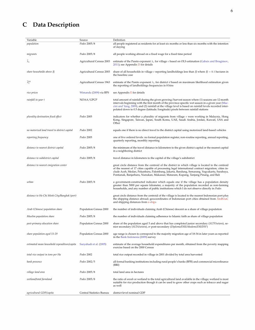
In this section, I provide additional background on the assumed Pareto distribution for land-holdings as well asdetails on the empirical content of the estimated Pareto shape parameters λv . Figure D.1 shows the familiar powerlaw linearity in plots of the log complementary CDF against log wetland holding size for 16 randomly chosendistricts. A more systematic analysis of Paretian properties at the village level requires estimating distributionalparameters using the universal microdata from the the Agricultural Census.

I obtain estimates of λv for every village in Indonesia using the Gabaix and Ibragimov (2011) estimator. Thatis, for each village I regress the log rank minus 1/2 on the log of the given land-holding size. Given that somehouseholds within each village report the same land-holding size, ties are broken by taking the average rank.1

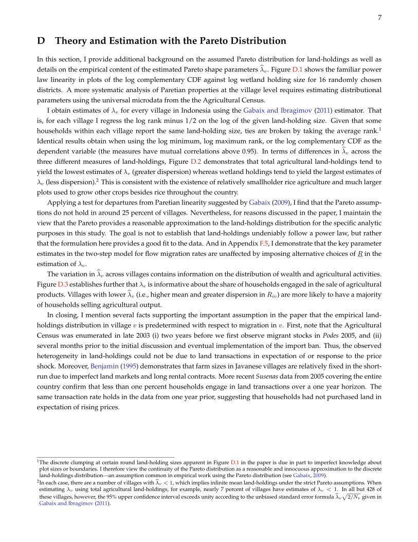
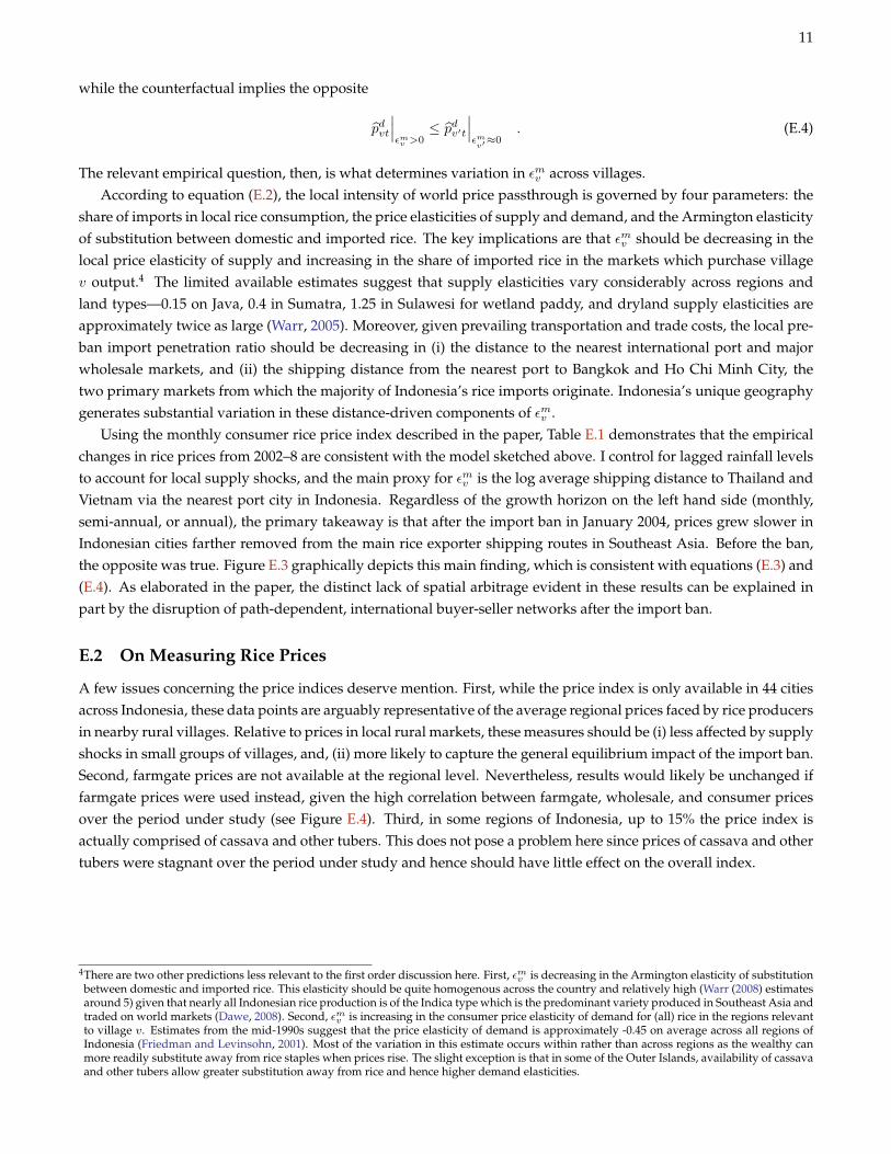
Identical results obtain when using the log minimum, log maximum rank, or the log complementary CDF as thedependent variable (the measures have mutual correlations above 0.95). In terms of differences in λv across thethree different measures of land-holdings, Figure D.2 demonstrates that total agricultural land-holdings tend toyield the lowest estimates of λv (greater dispersion) whereas wetland holdings tend to yield the largest estimates ofλv (less dispersion).2 This is consistent with the existence of relatively smallholder rice agriculture and much largerplots used to grow other crops besides rice throughout the country.

Applying a test for departures from Paretian linearity suggested by Gabaix (2009), I find that the Pareto assump-tions do not hold in around 25 percent of villages. Nevertheless, for reasons discussed in the paper, I maintain theview that the Pareto provides a reasonable approximation to the land-holdings distribution for the specific analyticpurposes in this study. The goal is not to establish that land-holdings undeniably follow a power law, but ratherthat the formulation here provides a good fit to the data. And in Appendix F.5, I demonstrate that the key parameterestimates in the two-step model for flow migration rates are unaffected by imposing alternative choices of R in theestimation of λv .

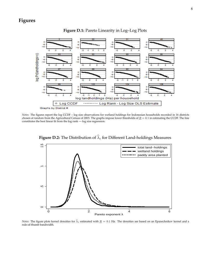
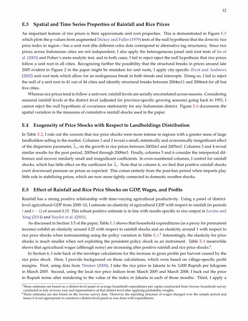
The variation in λv across villages contains information on the distribution of wealth and agricultural activities.Figure D.3 establishes further that λv is informative about the share of households engaged in the sale of agriculturalproducts. Villages with lower λv (i.e., higher mean and greater dispersion in Riv) are more likely to have a majorityof households selling agricultural output.

In closing, I mention several facts supporting the important assumption in the paper that the empirical land-holdings distribution in village v is predetermined with respect to migration in v. First, note that the AgriculturalCensus was enumerated in late 2003 (i) two years before we first observe migrant stocks in Podes 2005, and (ii)several months prior to the initial discussion and eventual implementation of the import ban. Thus, the observedheterogeneity in land-holdings could not be due to land transactions in expectation of or response to the priceshock. Moreover, Benjamin (1995) demonstrates that farm sizes in Javanese villages are relatively fixed in the short-run due to imperfect land markets and long rental contracts. More recent Susenas data from 2005 covering the entirecountry confirm that less than one percent households engage in land transactions over a one year horizon. Thesame transaction rate holds in the data from one year prior, suggesting that households had not purchased land inexpectation of rising prices.

1The discrete clumping at certain round land-holding sizes apparent in Figure D.1 in the paper is due in part to imperfect knowledge aboutplot sizes or boundaries. I therefore view the continuity of the Pareto distribution as a reasonable and innocuous approximation to the discreteland-holdings distribution—an assumption common in empirical work using the Pareto distribution (see Gabaix, 2009).

2In each case, there are a number of villages with λv < 1, which implies infinite mean land-holdings under the strict Pareto assumptions. Whenestimating λv using total agricultural land-holdings, for example, nearly 7 percent of villages have estimates of λv < 1. In all but 428 ofthese villages, however, the 95% upper confidence interval exceeds unity according to the unbiased standard error formula λv

√2/Nv given in

Gabaix and Ibragimov (2011).

8

Figures

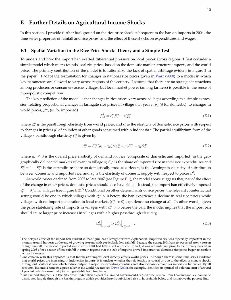
Figure D.1: Pareto Linearity in Log–Log Plots

Notes: The figures report the log CCDF – log size observations for wetland holdings for Indonesian households recorded in 16 districtschosen at random from the Agricultural Census of 2003. The graphs impose lower thresholds of R = 0.1 in estimating the CCDF. The lineconstitutes the best linear fit from the log rank — log size regression.

Figure D.2: The Distribution of λv for Different Land-holdings Measures

0.5

11.

5

0 2 4 6Pareto exponent λ

total land−holdingswetland holdingspaddy area planted

Notes: The figure plots kernel densities for λv estimated with R = 0.1 Ha. The densities are based on an Epanechnikov kernel and arule-of-thumb bandwidth.

9

Figure D.3: Probability Majority of Households in Village v Are Net Producers

0.5

11.

5ke

rnel

den

sity

1 2 3 4Pareto exponent λ

majority HH sell agri outputmajority HH consume agri outputmajority HH sell and consume

Notes: The curves are kernel densities of λv broken down by village depending depending on whether the village head reports in Podes2005 that a majority of (agricultural) households in the village sell, subsist, or both conditional on that village reporting agriculture beingthe most prominent source of employment. The densities employ an Epanechnikov kernel, a rule-of-thumb bandwidth, and trimming ofthe top and bottom 1 percent of λv .

10

E Further Details on Agricultural Income Shocks

In this section, I provide further background on the rice price shock subsequent to the ban on imports in 2004, thetime series properties of rainfall and rice prices, and the effect of these shocks on expenditures and wages.

E.1 Spatial Variation in the Rice Price Shock: Theory and a Simple Test

To understand how the import ban exerted differential pressure on local prices across regions, I first consider asimple model which micro-founds local rice prices based on the domestic market structure, imports, and the worldprice. The primary contribution of the model is to rationalize the lack of spatial arbitrage evident in Figure 2 inthe paper.1 I adapt the formulation for changes in national rice prices given in Warr (2008) to a model in whichkey parameters are allowed to vary across regions of the country. I assume that there are no strategic interactionsamong producers or consumers across villages, but local market power (among farmers) is possible in the sense ofmonopolistic competition.

The key prediction of the model is that changes in rice prices vary across villages according to a simple expres-sion relating proportional changes in farmgate rice prices in village v in year t, pdv (d for domestic), to changes inworld prices, pm, (m for imported)

pdvt = εmv pmt + εovp

ot (E.1)

where εmv is the passthrough elasticity from world prices, and εov is the elasticity of domestic rice prices with respectto changes in prices po of an index of other goods consumed within Indonesia.2 The partial equilibrium form of thevillage v passthrough elasticity εmv is given by

εmv = Smv (ρv + ηv)/(χdv + ρvS

mv − ηvSdv ), (E.2)

where ηv ≤ 0 is the overall price elasticity of demand for rice (composite of domestic and imported) in the geo-graphically delineated markets relevant to village v; Smv is the share of imported rice in total rice expenditures andSdv = 1− Smv is the expenditure share on domestically-produced rice; ρv is the Armington elasticity of substitutionbetween domestic and imported rice; and χdv is the elasticity of domestic supply with respect to prices pd.

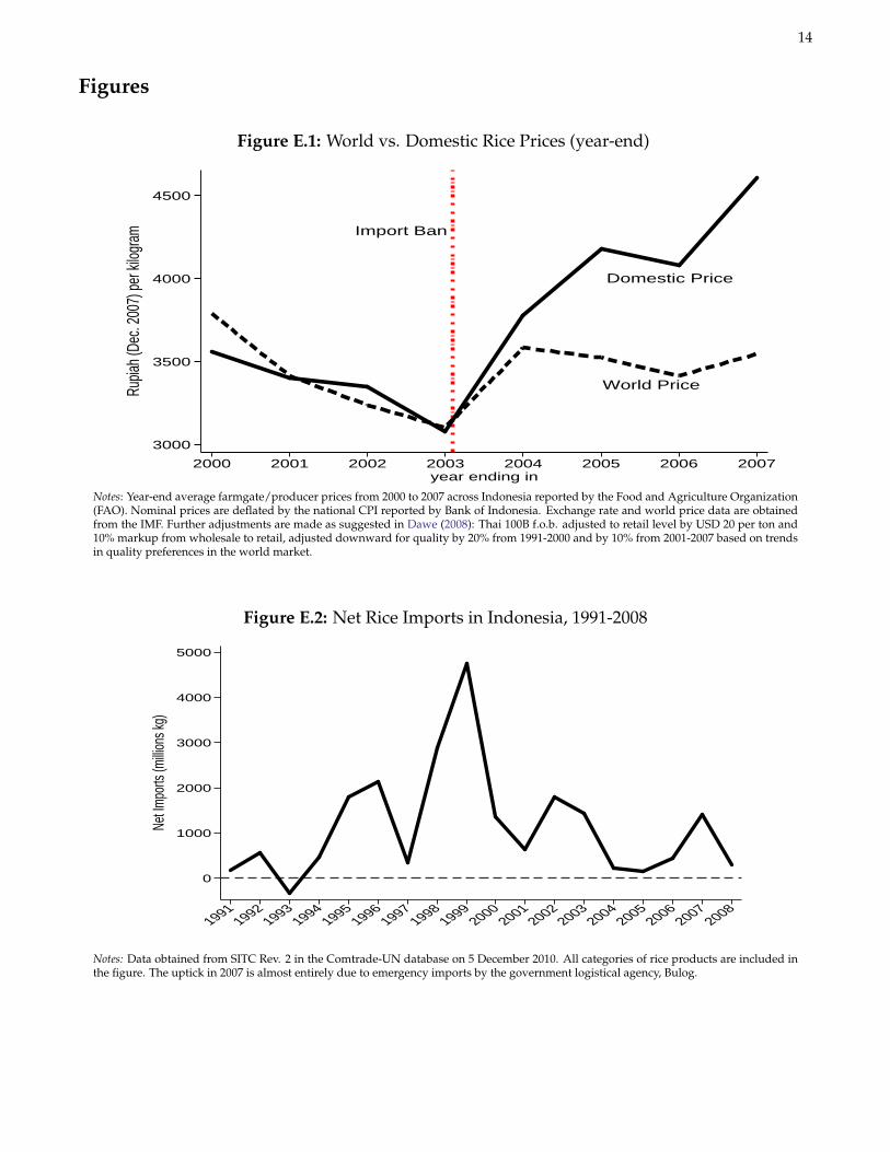
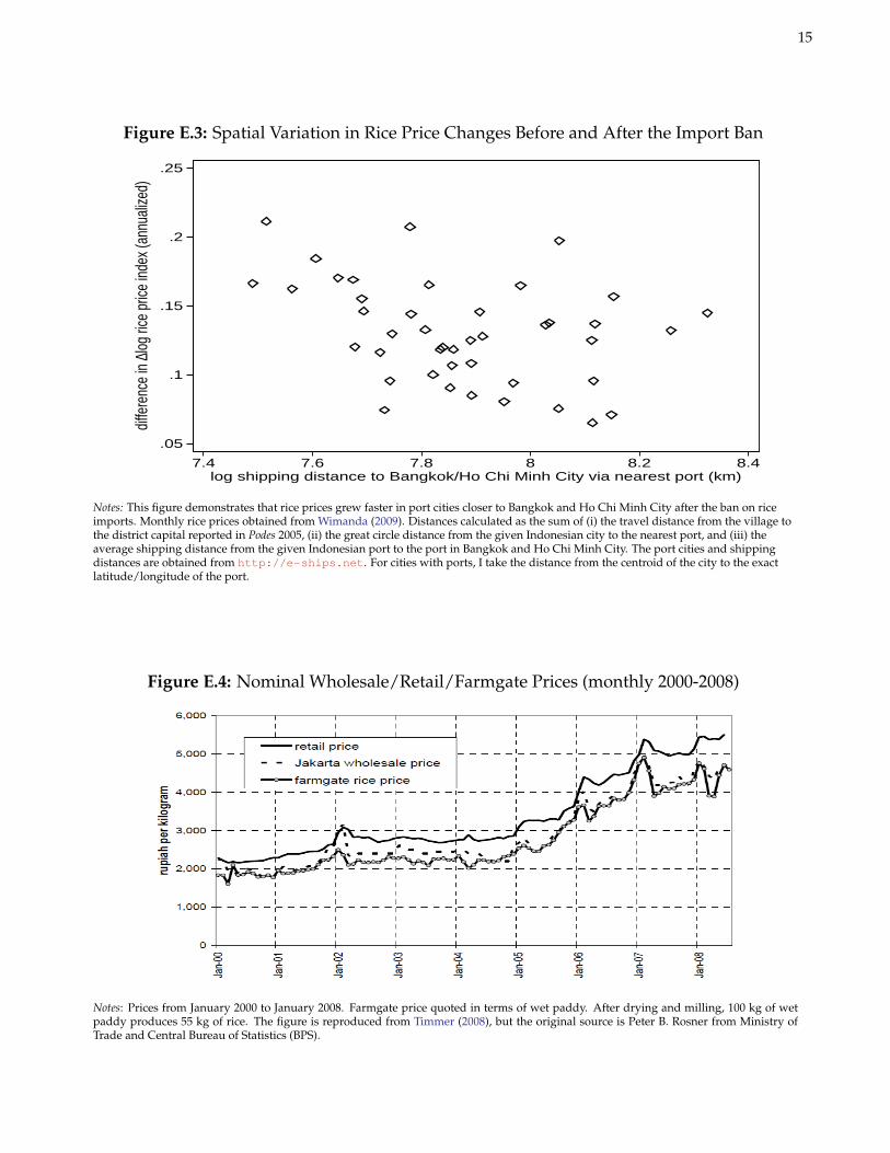
As world prices declined from 2005 to late 2007 (see Figure E.1), the model above suggests that, net of the effectof the change in other prices, domestic prices should also have fallen. Instead, the import ban effectively imposedεmv = 0 for all villages (see Figure E.2).3 Conditional on other determinants of rice prices, the relevant counterfactualsetting would be one in which villages with εmv > 0 before the ban experience a decline in real rice prices whilevillages with no import penetration in local markets (εmv ≈ 0) experience no change at all. In other words, giventhe price stabilizing role of imports in villages with εmv > 0 before the ban, the model implies that the import banshould cause larger price increases in villages with a higher passthrough elasticity,

pdvt

∣∣∣εmv >0

> pdv′t

∣∣∣εmv′≈0

, (E.3)

1The delayed effect of the import ban evident in that figure has a straightforward explanation. Imported rice was especially important in themonths around harvests at the end of growing seasons with particularly low rainfall. Because the spring 2004 harvest occurred after a seasonof high rainfall, the lack of imported rice in early 2004 had little effect on prices. In fact, it was not until just prior to the primary harvest inspring 2005 after a season of low rainfall in certain regions that the lack of imports proved important as domestic rice prices began to escalateacross Indonesia.

2One concern with this approach is that Indonesia’s import level directly affects world prices. Although there is some time series evidencethat world prices are increasing in Indonesian imports, it is unclear whether the relationship is causal or due to the effect of climate shocksthroughout Southeast Asia which reduce output in major rice-exporting countries and also increase demand for imports in Indonesia. By allaccounts, Indonesia remains a price-taker in the world rice market. Dawe (2008), for example, identifies an optimal ad valorem tariff of around4 percent, which is essentially indistinguishable from free trade.

3Small import shipments in late 2007 were undertaken as part of a limited government-licensed procurement from Thailand and Vietnam to bedistributed largely through the Raskin program which provides heavily subsidized rice to households below and just above the poverty line.

11

while the counterfactual implies the opposite

pdvt

∣∣∣εmv >0

≤ pdv′t∣∣∣εmv′≈0

. (E.4)

The relevant empirical question, then, is what determines variation in εmv across villages.According to equation (E.2), the local intensity of world price passthrough is governed by four parameters: the

share of imports in local rice consumption, the price elasticities of supply and demand, and the Armington elasticityof substitution between domestic and imported rice. The key implications are that εmv should be decreasing in thelocal price elasticity of supply and increasing in the share of imported rice in the markets which purchase villagev output.4 The limited available estimates suggest that supply elasticities vary considerably across regions andland types—0.15 on Java, 0.4 in Sumatra, 1.25 in Sulawesi for wetland paddy, and dryland supply elasticities areapproximately twice as large (Warr, 2005). Moreover, given prevailing transportation and trade costs, the local pre-ban import penetration ratio should be decreasing in (i) the distance to the nearest international port and majorwholesale markets, and (ii) the shipping distance from the nearest port to Bangkok and Ho Chi Minh City, thetwo primary markets from which the majority of Indonesia’s rice imports originate. Indonesia’s unique geographygenerates substantial variation in these distance-driven components of εmv .

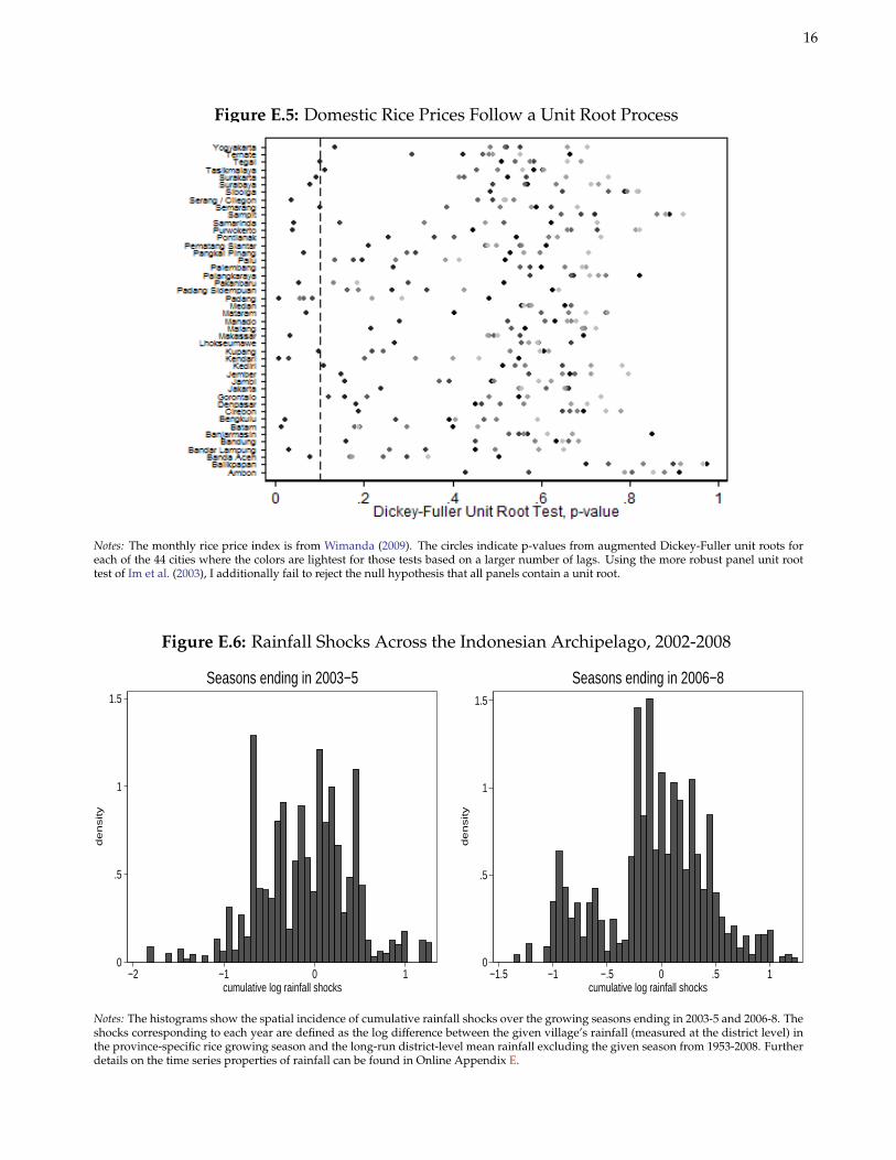
Using the monthly consumer rice price index described in the paper, Table E.1 demonstrates that the empiricalchanges in rice prices from 2002–8 are consistent with the model sketched above. I control for lagged rainfall levelsto account for local supply shocks, and the main proxy for εmv is the log average shipping distance to Thailand andVietnam via the nearest port city in Indonesia. Regardless of the growth horizon on the left hand side (monthly,semi-annual, or annual), the primary takeaway is that after the import ban in January 2004, prices grew slower inIndonesian cities farther removed from the main rice exporter shipping routes in Southeast Asia. Before the ban,the opposite was true. Figure E.3 graphically depicts this main finding, which is consistent with equations (E.3) and(E.4). As elaborated in the paper, the distinct lack of spatial arbitrage evident in these results can be explained inpart by the disruption of path-dependent, international buyer-seller networks after the import ban.

E.2 On Measuring Rice Prices

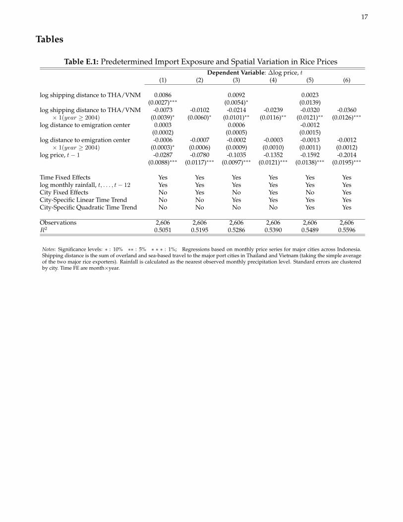
A few issues concerning the price indices deserve mention. First, while the price index is only available in 44 citiesacross Indonesia, these data points are arguably representative of the average regional prices faced by rice producersin nearby rural villages. Relative to prices in local rural markets, these measures should be (i) less affected by supplyshocks in small groups of villages, and, (ii) more likely to capture the general equilibrium impact of the import ban.Second, farmgate prices are not available at the regional level. Nevertheless, results would likely be unchanged iffarmgate prices were used instead, given the high correlation between farmgate, wholesale, and consumer pricesover the period under study (see Figure E.4). Third, in some regions of Indonesia, up to 15% the price index isactually comprised of cassava and other tubers. This does not pose a problem here since prices of cassava and othertubers were stagnant over the period under study and hence should have little effect on the overall index.

4There are two other predictions less relevant to the first order discussion here. First, εmv is decreasing in the Armington elasticity of substitutionbetween domestic and imported rice. This elasticity should be quite homogenous across the country and relatively high (Warr (2008) estimatesaround 5) given that nearly all Indonesian rice production is of the Indica type which is the predominant variety produced in Southeast Asia andtraded on world markets (Dawe, 2008). Second, εmv is increasing in the consumer price elasticity of demand for (all) rice in the regions relevantto village v. Estimates from the mid-1990s suggest that the price elasticity of demand is approximately -0.45 on average across all regions ofIndonesia (Friedman and Levinsohn, 2001). Most of the variation in this estimate occurs within rather than across regions as the wealthy canmore readily substitute away from rice staples when prices rise. The slight exception is that in some of the Outer Islands, availability of cassavaand other tubers allow greater substitution away from rice and hence higher demand elasticities.

12

E.3 Spatial and Time Series Properties of Rainfall and Rice Prices

An important feature of rice prices is their approximate unit root properties. This is demonstrated in Figure E.5which plots the p-values from augmented Dickey and Fuller (1979) tests of the null hypothesis that the domestic riceprice index in region c has a unit root (the different color dots correspond to alternative lag structures). Since riceprices across Indonesian cities are not independent, I also apply the heterogeneous panel unit root tests of Im etal. (2003) and Fisher’s meta-analytic test, and in both cases, I fail to reject reject the null hypothesis that rice pricesfollow a unit root in all cities. Recognizing further the possibility that the structural breaks in prices around late2005 evident in Figure 2 in the paper might be mistaken for unit roots, I apply city-specific Zivot and Andrews(2002) unit root tests which allow for an endogenous break in both trends and intercepts. Doing so, I fail to rejectthe null of a unit root in 41 out of 44 cities and identify structural breaks between 2004m11 and 2006m4 for all butfive cities.

Whereas rice prices tend to follow a unit root, rainfall levels are serially uncorrelated across seasons. Consideringseasonal rainfall levels at the district level (adjusted for province-specific growing seasons) going back to 1953, Icannot reject the null hypothesis of covariance stationarity for any Indonesian district. Figure E.6 documents thespatial variation in the measures of cumulative rainfall shocks used in the paper.

E.4 Exogeneity of Price Shocks with Respect to Landholdings Distribution

In Table E.2, I rule out the concern that rice price shocks were more intense in regions with a greater mass of largelandholders selling to the market. Columns 1 and 2 reveal a small, statistically and economically insignificant effectof the dispersion parameter, λv , on the growth in rice prices between 2002m1 and 2005m3. Columns 3 and 4 revealsimilar results for the post period, 2005m4 through 2008m3. Finally, columns 5 and 6 consider the interperiod dif-ference and recover similarly small and insignificant coefficients. In even-numbered columns, I control for rainfallshocks, which has little effect on the coefficient for λv . Note that in column 6, we find that positive rainfall shocksexert downward pressure on prices as expected. This comes entirely from the post-ban period when imports playlittle role in stabilizing prices, which are now more tightly connected to domestic weather shocks.

E.5 Effect of Rainfall and Rice Price Shocks on GDP, Wages, and Profits

Rainfall has a strong positive relationship with time-varying agricultural productivity. Using a panel of district-level agricultural GDP from 2000–10, I estimate an elasticity of agricultural GDP with respect to rainfall (in periodst and t− 1) of around 0.15. This robust positive estimate is in line with results specific to rice output in Levine andYang (2014) and Naylor et al. (2001).

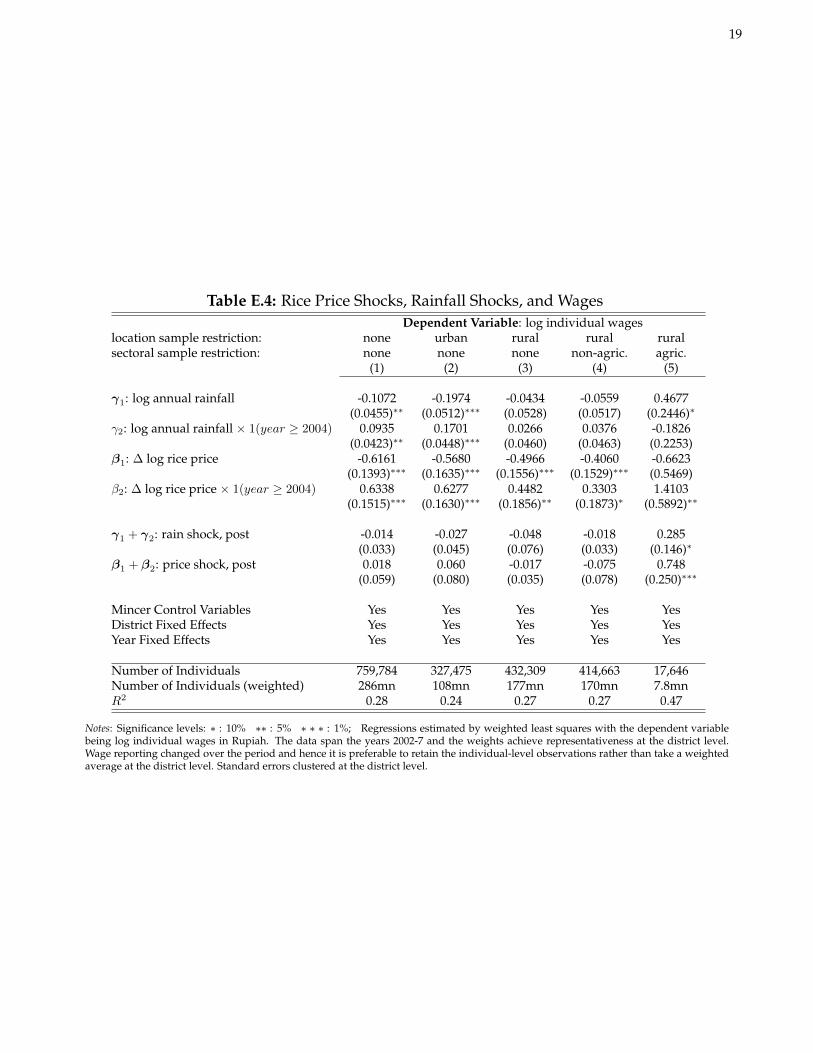
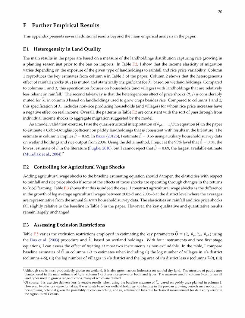
As discussed in Section 3.5 of the paper, Table E.3 shows that household expenditures (as a proxy for permanentincome) exhibit an elasticity around 0.25 with respect to rainfall shocks and an elasticity around 1 with respect torice price shocks when instrumenting using the policy variation in Table E.1.5 Interestingly, the elasticity for priceshocks is much smaller when not exploiting the persistent policy shock as an instrument. Table E.4 meanwhileshows that agricultural wages (although noisy) are increasing after positive rainfall and rice price shocks.6

In Section 6, I note back of the envelope calculations for the increase in gross profits per harvest caused by therice price shock. Here, I provide background on those calculations, which were based on village-specific profitmargins. First, using data from Timmer (2008), I take the rice price in Jakarta to be 3,000 Rupiah per kilogramin March 2005. Second, using the local rice price indices from March 2005 and March 2008, I back out the pricein Rupiah terms after reindexing to the value of the index in Jakarta in each of those months. Third, I apply a

5These estimates are based on a district-level panel of average household expenditures per capita constructed from Susenas household surveyconducted in July of every year and representative at that district level after applying probability weights.

6These estimates are also based on the Susenas survey data. However, the reporting structure of wages changed over the sample period andhence it is not appropriate to construct a district-level panel as was done with expenditures.

13

measure of village-specific total paddy output (in kilograms) per hectare in 2001 (see Appendix C) to all potentialfarmers in the village. Although unit-level productivity varies varies across households, the bulk of this variation isacross rather than within villages and hence little information is lost in focusing on productivity differences arisingpurely from land area planted (see Bazzi, 2012b). Fourth, I convert wet paddy output to marketable rice outputusing a standard conversion factor of 0.55. Fifth, I convert Rupiah to USD at an exchange rate prevailing in late2005 of 10,000 Rupiah to 1 USD. Finally, when accounting for own consumption, I assume that the household hastwo harvests per year and subtract 520 kilograms of rice (the recommended intake for a family of four) valued atthe market price. Although I only reported the income boost for farmers with 0.25 and 0.75 Ha of landholdings,estimates for other landholding sizes are available upon request.

14

Figures

Figure E.1: World vs. Domestic Rice Prices (year-end)

Import Ban

World Price

Domestic Price

3000

3500

4000

4500

Rupia

h (De

c. 20

07) p

er ki

logra

m

2000 2001 2002 2003 2004 2005 2006 2007year ending in

Notes: Year-end average farmgate/producer prices from 2000 to 2007 across Indonesia reported by the Food and Agriculture Organization(FAO). Nominal prices are deflated by the national CPI reported by Bank of Indonesia. Exchange rate and world price data are obtainedfrom the IMF. Further adjustments are made as suggested in Dawe (2008): Thai 100B f.o.b. adjusted to retail level by USD 20 per ton and10% markup from wholesale to retail, adjusted downward for quality by 20% from 1991-2000 and by 10% from 2001-2007 based on trendsin quality preferences in the world market.

Figure E.2: Net Rice Imports in Indonesia, 1991-2008

0

1000

2000

3000

4000

5000

Net Im

ports

(milli

ons k

g)

19911992

19931994

19951996

19971998

19992000

20012002

20032004

20052006

20072008

Notes: Data obtained from SITC Rev. 2 in the Comtrade-UN database on 5 December 2010. All categories of rice products are included inthe figure. The uptick in 2007 is almost entirely due to emergency imports by the government logistical agency, Bulog.

15

Figure E.3: Spatial Variation in Rice Price Changes Before and After the Import Ban

.05

.1

.15

.2

.25

diffe

renc

e in

∆log

rice

price

inde

x (an

nuali

zed)

7.4 7.6 7.8 8 8.2 8.4log shipping distance to Bangkok/Ho Chi Minh City via nearest port (km)

Notes: This figure demonstrates that rice prices grew faster in port cities closer to Bangkok and Ho Chi Minh City after the ban on riceimports. Monthly rice prices obtained from Wimanda (2009). Distances calculated as the sum of (i) the travel distance from the village tothe district capital reported in Podes 2005, (ii) the great circle distance from the given Indonesian city to the nearest port, and (iii) theaverage shipping distance from the given Indonesian port to the port in Bangkok and Ho Chi Minh City. The port cities and shippingdistances are obtained from http://e-ships.net. For cities with ports, I take the distance from the centroid of the city to the exactlatitude/longitude of the port.

Figure E.4: Nominal Wholesale/Retail/Farmgate Prices (monthly 2000-2008)

Notes: Prices from January 2000 to January 2008. Farmgate price quoted in terms of wet paddy. After drying and milling, 100 kg of wetpaddy produces 55 kg of rice. The figure is reproduced from Timmer (2008), but the original source is Peter B. Rosner from Ministry ofTrade and Central Bureau of Statistics (BPS).

16

Figure E.5: Domestic Rice Prices Follow a Unit Root Process

Notes: The monthly rice price index is from Wimanda (2009). The circles indicate p-values from augmented Dickey-Fuller unit roots foreach of the 44 cities where the colors are lightest for those tests based on a larger number of lags. Using the more robust panel unit roottest of Im et al. (2003), I additionally fail to reject the null hypothesis that all panels contain a unit root.

Figure E.6: Rainfall Shocks Across the Indonesian Archipelago, 2002-2008

0

.5

1

1.5

de

nsity

−2 −1 0 1cumulative log rainfall shocks

Seasons ending in 2003−5

0

.5

1

1.5

de

nsity

−1.5 −1 −.5 0 .5 1cumulative log rainfall shocks

Seasons ending in 2006−8

Notes: The histograms show the spatial incidence of cumulative rainfall shocks over the growing seasons ending in 2003-5 and 2006-8. Theshocks corresponding to each year are defined as the log difference between the given village’s rainfall (measured at the district level) inthe province-specific rice growing season and the long-run district-level mean rainfall excluding the given season from 1953-2008. Furtherdetails on the time series properties of rainfall can be found in Online Appendix E.

17

Tables

Table E.1: Predetermined Import Exposure and Spatial Variation in Rice PricesDependent Variable: ∆log price, t

(1) (2) (3) (4) (5) (6)

log shipping distance to THA/VNM 0.0086 0.0092 0.0023(0.0027)∗∗∗ (0.0054)∗ (0.0139)

log shipping distance to THA/VNM -0.0073 -0.0102 -0.0214 -0.0239 -0.0320 -0.0360× 1(year ≥ 2004) (0.0039)∗ (0.0060)∗ (0.0101)∗∗ (0.0116)∗∗ (0.0121)∗∗ (0.0126)∗∗∗

log distance to emigration center 0.0003 0.0006 -0.0012(0.0002) (0.0005) (0.0015)

log distance to emigration center -0.0006 -0.0007 -0.0002 -0.0003 -0.0013 -0.0012× 1(year ≥ 2004) (0.0003)∗ (0.0006) (0.0009) (0.0010) (0.0011) (0.0012)

log price, t− 1 -0.0287 -0.0780 -0.1035 -0.1352 -0.1592 -0.2014(0.0088)∗∗∗ (0.0117)∗∗∗ (0.0097)∗∗∗ (0.0121)∗∗∗ (0.0138)∗∗∗ (0.0195)∗∗∗

Time Fixed Effects Yes Yes Yes Yes Yes Yeslog monthly rainfall, t, . . . , t− 12 Yes Yes Yes Yes Yes YesCity Fixed Effects No Yes No Yes No YesCity-Specific Linear Time Trend No No Yes Yes Yes YesCity-Specific Quadratic Time Trend No No No No Yes Yes

Observations 2,606 2,606 2,606 2,606 2,606 2,606R2 0.5051 0.5195 0.5286 0.5390 0.5489 0.5596

Notes: Significance levels: ∗ : 10% ∗∗ : 5% ∗ ∗ ∗ : 1%; Regressions based on monthly price series for major cities across Indonesia.Shipping distance is the sum of overland and sea-based travel to the major port cities in Thailand and Vietnam (taking the simple averageof the two major rice exporters). Rainfall is calculated as the nearest observed monthly precipitation level. Standard errors are clusteredby city. Time FE are month×year.

18

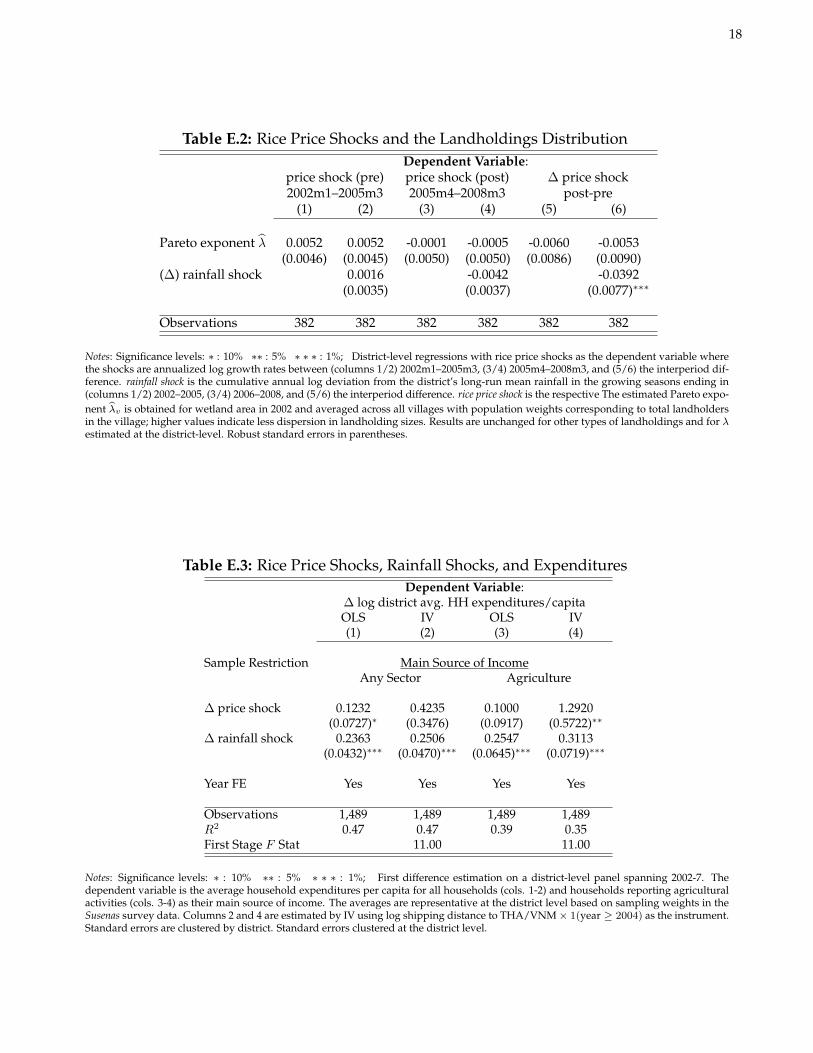
Table E.2: Rice Price Shocks and the Landholdings DistributionDependent Variable:

price shock (pre) price shock (post) ∆ price shock2002m1–2005m3 2005m4–2008m3 post-pre

(1) (2) (3) (4) (5) (6)

Pareto exponent λ 0.0052 0.0052 -0.0001 -0.0005 -0.0060 -0.0053(0.0046) (0.0045) (0.0050) (0.0050) (0.0086) (0.0090)

(∆) rainfall shock 0.0016 -0.0042 -0.0392(0.0035) (0.0037) (0.0077)∗∗∗

Observations 382 382 382 382 382 382

Notes: Significance levels: ∗ : 10% ∗∗ : 5% ∗ ∗ ∗ : 1%; District-level regressions with rice price shocks as the dependent variable wherethe shocks are annualized log growth rates between (columns 1/2) 2002m1–2005m3, (3/4) 2005m4–2008m3, and (5/6) the interperiod dif-ference. rainfall shock is the cumulative annual log deviation from the district’s long-run mean rainfall in the growing seasons ending in(columns 1/2) 2002–2005, (3/4) 2006–2008, and (5/6) the interperiod difference. rice price shock is the respective The estimated Pareto expo-nent λv is obtained for wetland area in 2002 and averaged across all villages with population weights corresponding to total landholdersin the village; higher values indicate less dispersion in landholding sizes. Results are unchanged for other types of landholdings and for λestimated at the district-level. Robust standard errors in parentheses.

Table E.3: Rice Price Shocks, Rainfall Shocks, and ExpendituresDependent Variable:

∆ log district avg. HH expenditures/capitaOLS IV OLS IV(1) (2) (3) (4)

Sample Restriction Main Source of IncomeAny Sector Agriculture

∆ price shock 0.1232 0.4235 0.1000 1.2920(0.0727)∗ (0.3476) (0.0917) (0.5722)∗∗

∆ rainfall shock 0.2363 0.2506 0.2547 0.3113(0.0432)∗∗∗ (0.0470)∗∗∗ (0.0645)∗∗∗ (0.0719)∗∗∗

Year FE Yes Yes Yes Yes

Observations 1,489 1,489 1,489 1,489R2 0.47 0.47 0.39 0.35First Stage F Stat 11.00 11.00

Notes: Significance levels: ∗ : 10% ∗∗ : 5% ∗ ∗ ∗ : 1%; First difference estimation on a district-level panel spanning 2002-7. Thedependent variable is the average household expenditures per capita for all households (cols. 1-2) and households reporting agriculturalactivities (cols. 3-4) as their main source of income. The averages are representative at the district level based on sampling weights in theSusenas survey data. Columns 2 and 4 are estimated by IV using log shipping distance to THA/VNM× 1(year ≥ 2004) as the instrument.Standard errors are clustered by district. Standard errors clustered at the district level.

19

Table E.4: Rice Price Shocks, Rainfall Shocks, and WagesDependent Variable: log individual wages

location sample restriction: none urban rural rural ruralsectoral sample restriction: none none none non-agric. agric.

(1) (2) (3) (4) (5)

γ1: log annual rainfall -0.1072 -0.1974 -0.0434 -0.0559 0.4677(0.0455)∗∗ (0.0512)∗∗∗ (0.0528) (0.0517) (0.2446)∗

γ2: log annual rainfall × 1(year ≥ 2004) 0.0935 0.1701 0.0266 0.0376 -0.1826(0.0423)∗∗ (0.0448)∗∗∗ (0.0460) (0.0463) (0.2253)

β1: ∆ log rice price -0.6161 -0.5680 -0.4966 -0.4060 -0.6623(0.1393)∗∗∗ (0.1635)∗∗∗ (0.1556)∗∗∗ (0.1529)∗∗∗ (0.5469)

β2: ∆ log rice price × 1(year ≥ 2004) 0.6338 0.6277 0.4482 0.3303 1.4103(0.1515)∗∗∗ (0.1630)∗∗∗ (0.1856)∗∗ (0.1873)∗ (0.5892)∗∗

γ1 + γ2: rain shock, post -0.014 -0.027 -0.048 -0.018 0.285(0.033) (0.045) (0.076) (0.033) (0.146)∗

β1 + β2: price shock, post 0.018 0.060 -0.017 -0.075 0.748(0.059) (0.080) (0.035) (0.078) (0.250)∗∗∗

Mincer Control Variables Yes Yes Yes Yes YesDistrict Fixed Effects Yes Yes Yes Yes YesYear Fixed Effects Yes Yes Yes Yes Yes

Number of Individuals 759,784 327,475 432,309 414,663 17,646Number of Individuals (weighted) 286mn 108mn 177mn 170mn 7.8mnR2 0.28 0.24 0.27 0.27 0.47

Notes: Significance levels: ∗ : 10% ∗∗ : 5% ∗ ∗ ∗ : 1%; Regressions estimated by weighted least squares with the dependent variablebeing log individual wages in Rupiah. The data span the years 2002-7 and the weights achieve representativeness at the district level.Wage reporting changed over the period and hence it is preferable to retain the individual-level observations rather than take a weightedaverage at the district level. Standard errors clustered at the district level.

20

F Further Empirical Results

This appendix presents several additional results beyond the main empirical analysis in the paper.

F.1 Heterogeneity in Land Quality

The main results in the paper are based on a measure of the landholdings distribution capturing rice growing ina planting season just prior to the ban on imports. In Table F.2, I show that the income elasticity of migrationvaries depending on the exposure of the given type of landholdings to rainfall and rice price variability. Column1 reproduces the key estimates from column 4 in Table 5 of the paper. Column 2 shows that the heterogeneouseffect of rainfall shocks (θaλ) is muted and statistically insignificant for λv based on wetland holdings. Comparedto columns 1 and 3, this specification focuses on households (and villages) with landholdings that are relativelyless reliant on rainfall.1 The second takeaway is that the heterogeneous effect of price shocks (θpλ) is considerablymuted for λv in column 3 based on landholdings used to grow crops besides rice. Compared to columns 1 and 2,this specification of λv includes non-rice producing households (and villages) for whom rice price increases havea negative effect on real income. Overall, the patterns in Table F.2 are consistent with the sort of passthrough fromindividual income shocks to aggregate migration suggested by the model.

As a model validation exercise, I use the quasi-structural interpretation of θpλ = 1/β in equation (4) in the paperto estimate a Cobb-Douglas coefficient on paddy landholdings that is consistent with results in the literature. Theestimate in column 2 implies β = 0.52. In Bazzi (2012b), I estimate β = 0.55 using auxiliary household survey dataon wetland holdings and rice output from 2004. Using the delta method, I reject at the 95% level that β = 0.34, thelowest estimate of β in the literature (Fuglie, 2010), but I cannot reject that β = 0.69, the largest available estimate(Mundlak et al., 2004).2

F.2 Controlling for Agricultural Wage Shocks

Adding agricultural wage shocks to the baseline estimating equation should dampen the elasticities with respectto rainfall and rice price shocks if some of the effects of those shocks are operating through changes in the returnsto (rice) farming. Table F.3 shows that this is indeed the case. I construct agricultural wage shocks as the differencein the growth of log average agricultural wages between 2002–5 and 2006–8 at the district level where the averagesare representative from the annual Susenas household survey data. The elasticities on rainfall and rice price shocksfall slightly relative to the baseline in Table 5 in the paper. However, the key qualitative and quantitative resultsremain largely unchanged.

F.3 Assessing Exclusion Restrictions

Table F.5 varies the exclusion restrictions employed in estimating the key parameters Θ ≡ (θa, θp, θaλ, θpλ) usingthe Das et al. (2003) procedure and λv based on wetland holdings. With four instruments and two first stageequations, I can assess the effect of treating at most two instruments as non-excludable. In the table, I comparebaseline estimates of Θ in columns 1-3 to estimates when including (i) the log number of villages in v’s district(columns 4-6), (ii) the log number of villages in v’s district and the log area of v’s district less v (columns 7-9), (iii)

1Although rice is most productively grown on wetland, it is also grown across Indonesia on rainfed dry land. The measure of paddy areaplanted used in the main estimate of λv in column 1 captures rice grown on both land types. The measure used in column 3 comprises allland types used to grow a range of crops, many of which are rainfed.

2Of course, this exercise delivers less favorable results when using the baseline measure of λv based on paddy area planted in column 1.However, two factors argue for taking the estimate based on wetland holdings: (i) planting in the pre-ban growing periods may not capturerice-growing potential given the possibility of crop switching, and (ii) attenuation bias due to classical measurement (or data entry) error inthe Agricultural Census.

21

the log population of v (columns 10-12), (iv) the log population of v and area in v’s district less v (columns 13-15),and (v) the log population of v and v’s district less v (columns 16-18). Except for a few insignificant differences, Ifind no systematic departures from the baseline results in Table 5.

F.4 Alternative Specifications of Rainfall and Rice Price Shocks

Table F.6 shows that the primary conclusions regarding the effects of rainfall shocks are robust to the inclusion ofperiod-specific shocks rather than the difference in shocks between t and t − 1. Furthermore, I fail to reject thatthe coefficient on the rainfall shock in t equals the absolute value of the coefficient on the rainfall shock in t− 1.

Table F.7 considers an alternative specification for rainfall shocks in which the annual shocks are fully elab-orated from 2002–8 (i.e., the rainfall shock in each season s is assigned its own elasticity parameter θas for200s = 3, . . . , 8 and θasλ for the interactions with λv). At the bottom of the table, I report the sum of coeffi-cients for period t (s = 3, 4, 5), period t− 1 (s = 6, 7, 8), and both t and t− 1 (s = 3, . . . , 8) as well as the associatedp-value for the null hypothesis that the given sum equals zero. In columns 1-3, we draw the same conclusions asin Table F.6: (i) the sum of period t (t − 1) rainfall shocks is positive (negative) and statistically significant, and(ii) the null hypothesis that θa3 + θa4 + θa5 = −(θa6 + θa7 + θa8) cannot be rejected. Furthermore, in columns 4-6,we similarly rule out the possibility that the baseline specification of rainfall shocks leads to spurious conclusionsregarding the key elasticity parameter θaλ. That is, the sum of period t (t − 1) coefficients on the interaction ofrainfall shocks and λv are positive (negative) and statistically significant.3 In unreported results, I also show thatthe main results are robust to allowing negative rainfall shocks to have a different effect than positive rainfallshocks (i.e., rather than using a single continuous measure crossing zero).

Table F.8 presents alternative approaches to measuring the rice price shock. Columns 1-4 report estimates ofθp and θpλ using λv for wetland holdings. In columns 5-8, I specify the price “shock” as a difference in log averageprices over 2005m4-2008m3 and 2002m2-2005m3 rather than a difference in annualized log growth rates betweenthose two periods. This specification yields similar results. In columns 9-12, I adopt insights from the model forrice prices developed in Appendix E.1. Because the model predicts that the price shock should be decreasing indistance from port cities in Indonesia and the shipping routes to Thailand and Vietnam, a negative coefficienton the two distance terms would be consistent with a positive elasticity of migration flows with respect to riceprice shocks. Columns 9-10 are consistent with this hypothesized relationship as are the negative coefficients onthe interaction terms with λv in columns 11-12. These results are effectively the reduced form of the IV results inTable F.4.

F.5 Alternative Choices of the Pareto Lower Bound

Although the λv parameters should be unaffected by the location of R, in practice, the Pareto distribution is onlyan approximation, which works better in some villages than others (see Appendix D). In Table F.9, I show that theestimates of the key elasticity parameters generally do not change when imposing alternative R ∈ {0.15, 0.2, 0.25}in the estimation of λv (and the share of households above R) for wetland holdings. The results are similar for λvestimated using total agricultural landholdings or paddy area planted in 2002.4

3An interesting feature of the fully elaborated specification is that the s and s − 1 coefficients alternative in sign, with the period s contem-poraneous with the Podes enumeration dates in 2005 and 2008 being positive. Two factors might explain this pattern: (i) the mean revertingproperties of rainfall (see Appendix E.5), and/or (ii) a particular spatial distribution of two-year migration contract cycles. Nevertheless, thecumulative migration flows are what we observe in the data and hence the sum is what matters, not the individual years per se.

4Note that the sample sizes differ across columns because consistent (i.e., usable) estimates of λv require at least 3 distinct size measures aboveR∗. Some villages do not satisfy this criteria for a given minimum threshold value and landholding type.

22

F.6 Accounting for Village Demographic Structure and Past Internal Migration

Table F.10 demonstrates that the main results are robust to controlling for (i) the share of the population that livedoutside the village in 1995, (ii) the share of population aged 15-29, and (iii) the average household size in thevillage—each drawn from the 2000 Population Census. Variable (i) proxies for potential prior experience in andnetwork connections to domestic labor markets outside the village. Variable (ii) captures to some extent labormarket pressures induced by Indonesia’s relatively recent demographic transition. Moreover, individuals withinthat given cohort are the most likely to have been potential migrants beginning 3-7 years later and hence recordedin 2005 and 2008 migrant stocks.5 Although highly correlated with mean village income, mean household sizealso picks up variation in household labor supply, which may in turn affect the robustness of agricultural labormarkets (i.e., off own-farm) and the capacity of households to diversify labor allocation across borders—both ofwhich could have direct effects on flow migration rates.

F.7 On the (Non-)Effect of Measurement and Reporting Outliers

Tables F.11 and F.12 demonstrate that the key estimates of Θ ≡ (θa, θp, θaλ, θpλ) in the paper are robust to andarguably strengthened by accounting for outliers in the data along a few important dimensions. Column 2 controlsfor the frequency with which the village updates its population register (see Appendix C). This helps account forsome of the measurement error in migration rates as well as potential misclassification bias arising from villagesreporting no migrants when in fact there is at least one migrant from the village. Column 3 trims the bottom andtop 1 percent of λv . Column 4 removes villages subject to censoring in reported migrant stocks in 2005 and/or2008.6 In column 5, I retain only those villages for which I did not have to rely on any fuzzy matching algorithmsfor merging villages across the 2005 and 2008 waves of Podes (see Section H). Although I have confidence in thematching algorithms, they may contribute to measurement error on both sides of the estimating equation. Last,column 6 simultaneously implements the prior four restrictions. In all cases, the main qualitative and quantitativeinterpretation of Θ remains unchanged.

In column 7 of Tables F.11 and F.12, I drop provinces identified in Bank Indonesia (2009) as having a largenumber of undocumented international migrants (primarily going to Malaysia). The Village Potential data, recallfrom Section 3.2, define international labor migrants as those working abroad for a fixed wage and time period.It is possible therefore that this count includes some undocumented migrants for which the determinants of mi-gration choice and the nature of liquidity constraints may be somewhat different than for legal migrants. Whendropping these provinces—which, keep in mind, still have a large number of legal international migrants—a fewdifferences emerge with respect to the full sample results. First, in Table F.11, the elasticity parameters for rainfalland price shocks slightly increase. However, the estimates of θaλ and θpλ in column 7 fall in magnitude. The large,precisely estimated θpλ for λv based on wetland holdings disappears entirely. It seems, then, that undocumentedmigrants may explain some of the stronger response of migration flows to price shocks in villages with a greatermass of small landholders.

F.8 Rainfall Shocks and Internal Migration

Here, I briefly discuss the effect of rainfall shocks on internal migration flows. Using weighted samples fromIndonesian Population Censuses in 2000 and 2010 as well as Intercensal Population Surveys in 1985, 1995, and5However, inclusion of this variable might introduce a source of bias in that villages with a large share of aged 15-29 in 2000 may be preciselythose villages for which (i) the Asian financial crisis of 1997-8 led to a large return migration from urban areas, and/or (ii) the local economywas (expected to be) thriving as global agricultural commodity prices remained high through the early 2000s.

6The 2005 survey records separately the total number of male migrants and the total number of female migrants whereas the 2008 surveysimply records the total number of migrants. Whether the different format of the question across years biases reporting is an open question.However, top coding poses a challenge in the following sense. In 2005, the separate reporting for male and female migrants allowed totalmigrant stocks to exceed 998 persons for 40 villages while villages could only record a maximum of 998 persons abroad in the 2008 survey.

23

2005, I am able to construct a bilateral district-level migration matrix in which each observation comprises thestock of individuals hailing from origin district o in year t − 5 and currently residing in destination district d inyear t.7 I estimate the following quasi-gravity model for internal (h for home) migration flows as a function oforigin and destination rainfall shocks:

lnmigrantshodt = αrainfall shockot + βrainfall shockdt + υo + υd + υt + εodt. (F.1)

where, for j = o, d, rainfall shockjt captures (in logarithmic form) the cumulative annual rainfall shocks over thefour years prior to t,8 υj are geographic fixed effects, υt is a year fixed effect, εodt is an idiosyncratic error term.9

Estimating equation (F.1) by OLS for the entire period 1985-2010, I find α ≈ −0.056 (std. error of 0.022), whichsuggests that origin rainfall shocks reduce internal out-migration. Restricting to the period 2005-2010—roughly,the period over which I observe international migrants in the Village Potential data used in the paper—I obtainα ≈ −0.452 (std. error of 0.071).10 (In both cases, I also find that β > 0 and statistically significant, which is con-sistent with migration being responsive to destination wage shocks.) Taken together, the negative estimates of αsupport the claim that positive rainfall shocks increase district population size and hence are likely also to increasevillage population size, presuming (i) inter-district migration is a lower bound for overall internal out-migrationobserved at the village level, and (ii) intra-district migration outside the home village follows similar processes.Such upward pressure on village population size in the denominator of the dependent variable in the paper (∆logmigrants/population) implies that the positive relationship between changes in international migration rates andrainfall cannot be explained by the unobservable internal migration flows at the village level.

F.9 Further Background on the Validation Exercise Using Micro Data

In the paper, I discuss results from estimating a migration choice model and using the implied marginal effects torecover an alternative measure of the village-level elasticity of flow migration rates with respect to income shocks.In this brief subsection, I provide a few additional details on the analysis therein.

First, note that in columns 3-4 of Table 2 in the paper, I report coefficient estimates from the following equation

migrateiv,t+1 = α+ β rainfall shockvt + γ price shockvt + rainfall shockvt × (landiζa1 + land2

i ζa2 )

+ price shockvt × (landiζp1 + land2

i ζp2 ) + ψi + ψt + eiv,t+1,

which, recall, I estimate using a conditional fixed effects (CFE) logit estimator, and where (i) landi comprisesall landholdings owned, under rental, or rented out and used to grow rice, and (ii) column 3 imposes ζa2 = 0

and ζp2 = 0. Using these estimates, I then recover average marginal effects (AMEs) at each value of landi ∈{0.1, 0.2, . . . , 2.5}Ha, where (i) 2.5 Ha is the maximum in the sample, and (ii) and the calculation of AMEs requiresimposing ηi = 0 ∀i. Thus, we obtain AMEs for both rainfall and rice price shocks at each landholding size (at 0.1Ha increments).11

I use these individual-level AMEs to construct implied aggregate village-level elasticities of migration rates

7The data were downloaded from the Integrated Public Use Microdata Series, International in August 2012. The district-level total migrantand population counts are based on summing the person-specific population weights provided by IPUMS-International and representativeat the district-level. Details on the (Inter-)Census specific samples can be obtained on the IPUMS website for Indonesia. Further details onthe panel construction are available upon request.

8For example, the shock in for origin district k in 2005 is simply the sum of the annual log deviations in 2001-2004 from the long-run district-level mean calculated over all years from 1948-2010 excluding 2001-2004.

9I use the log number of migrants rather than the migrant share or the odds of migration quite simply because the goal is to characterizechanges in district population levels arising from internal migration (i.e., the denominator in the dependent variable in the paper).

10I cluster standard errors by origin×destination district pair. Standard errors increase slightly when using two-way clustering (Cameron etal., 2011) on both origin and destination district.

11Recall that the estimates are quantitatively similar when using the less-biased LPM approach to estimating AMEs with household fixedeffects.

24

with respect to income shocks. I do so by applying the population shares to each landholding size-specific AMEas implied by the village-level Pareto distribution. Consider, for example, the AMEs for rainfall shocks at land-holding sizes 0.3 and 0.4 Ha. For each village v, I reweight the average of these two AMEs by the share of thepopulation with landholding sizes∈ [0.3, 0.4] Ha as implied by the Pareto exponent λv .12 I repeat this over allincrements of landholding sizes in the village, apply the AME at 2.5 Ha to all households above 2.5 Ha (as im-plied by λv), and then sum the reweighted AMEs to recover an aggregate village-level elasticity. In Table 8, I thencompared these implied elasticities to those from the actual village-level regressions in Table 5, which allowed theeffect of income shocks on flow migration rates to vary with λv .

In recovering the elasticities of flow migration rates with respect to price and rainfall shocks, I take the baselinecoefficient estimates of Θ ≡ (θa, θp, θaλ, θpλ) in column 2 of Table F.2 for λv based on wetland holdings. I thenassign to village v the average marginal effects of the price shock for all villages with λv in the same percentile.That is, I calculate the average marginal effects of income shocks at each percentile of the distribution of λv in thesecond-step sample of villages. Following this procedure makes it possible to compare the village-level elasticitieswith analogous elasticities recovered from an underlying migration choice model.

F.10 Further Background on the Estimation of Village-Specific Migration Costs

Having found strong empirical evidence of financial constraints to migration in testing the theory, I used thefollowing structural equation (4) for the log flow migration rate to back out estimates of the migration costs:

∆ ln

(Mv,t+1

Nv,t+1

)=

λvβ

∆ ln pvt + ∆ ln

[(σv + avtτvjCvj,t+1

)λvβ

−(

σvαvχ

Wvj,t+1 − Cvj,t+1

)λvβ

].

Here, I provide a few additional details on the calculation of these village-specific migration costs not mentionedin the paper.

First, I plug in the empirical analogues for rice prices and rainfall. I specify ∆ ln pvt in the above equationas the log difference in the local rice price index over the entire period, 2002m1-2008m3. I set the rainfall level,σvt ≡ σv + avt, equal to the average of the annual seasonal rainfall levels (in centimeters) over the three seasonsprior to mid-2008 (mid-2005 for σv,t−1). I set σv equal to the average annual seasonal rainfall levels (in centimeters)over the 55 year period 1953-2008. The rainfall shocks avt capture the empirical difference between σvt and σv .

Second, the prevailing wage offers Wvjt are calculated as follows. For villages with any migrants in 2005,Wvjt equals the two-year wage offered to Indonesians around 2005 in the plurality destination of migrants fromthat village. The wage in t + 1 equals the two-year gross wage in 2008 in that same destination. For villageswith no migrants in 2005, Wvjt equals the average among villages with any migrants in their district. BankIndonesia (2009) and other available sources report the monthly wages for low-skill Indonesian workers in eachof the destination countries as stipulated in bilateral Memoranda of Understanding and reported by recruiters.These typical wages fall between the very narrow range of actual wages received as reported by migrants in theBank Indonesia (2009) survey. Wages increased in early 2007 for most of the plurality destinations in the VillagePotential 2005 data, and for those that do not, I nevertheless increase the wages by 10 percent. The results arerobust to other choices.

Plugging in the relevant empirical data into the above equation, I then solve for the fixed migration costsCvjt. Obtaining an analytic solution, however, requires a few additional simplifications. First, I assume thatmigration costs are constant across periods. This assumption is conservative insomuch as migration costs likely

12One could also imagine reweighting nonparametrically by applying the observed shares in the Agricultural Census. The approach based onλv is more consistent with the testable implications of the theoretical model and is moreover necessary for the purposes of comparison withthe village-level elasticities of income shocks that vary with λv .

25

fell in response to (i) competitive pressures in the recruitment industry and (ii) improvements in transportationinfrastructure including the addition of new legal emigrant processing centers in a few provinces. Second, Iimpose Wvjt = Wvj,t+1 = Wvj , and I set Wvj to be the average of the empirical wages across both periods.

F.11 What Role for Policy, Recruiters, and Networks?

Reductions in (upfront) costs can make it easier for poorer households and regions to access international labormarkets even in the absence of large increases in own ability to finance. I use the estimated migration coststo provide two suggestive pieces of evidence on how intermediaries can reduce costs and dampen the incomeelasticity of migration.

Ethnic Networks. Several studies have shown how diaspora networks facilitate migration in low-income set-tings. In Indonesia, there are several ethnic groups that have longstanding religious ties to the Middle East ora migratory legacy across the Southeast Asia region. For example, the religiously conservative Sundanese havestrong ties to Saudi Arabia (de Jonge and Kaptein, 2002). Although their homeland lies in West Java, Sundanesecan be found in villages across the Indonesian archipelago as a result of several decades of inter-island populationresettlement beginning in the 1950s (see Bazzi et al., forthcoming). The Buginese meanwhile hail from South Su-lawesi but have a long seafaring history that led to a number of Buginese communities across Indonesia but alsoin Malaysia and Singapore (Lineton, 1975).

Here, I show that these longstanding Sundanese and Buginese networks may have reduced the fixed costsof international migration from rural areas of Indonesia. Although these ethnic communities may be isolatedfrom native ethnic populations when residing outside their historical homelands, they still have strong ties to thebroader Sundanese and Buginese networks with the potential for connections to international labor markets. Iexploit this identifying variation by regressing the estimated migration cost (in USD) for village v on (i) indicatorsfor whether the village has an ethnic Bugis or ethnic Sunda majority, and (ii) origin region and destination countryfixed effects. The results succinctly summarized in the following equation,

cost = 2390(28)∗∗∗

other ethnic majority − 419(133)∗∗∗

Bugis majority − 167(49)∗∗∗

Sunda majority,

suggest that informal network intermediaries may have reduced the costs of migration over time.

Recruiters. The second way in which the poor are able to access costly migration opportunities is throughrecruiters, and in Indonesia these recruiters typically target female migrants. Hence, costs should be lower invillages where female migrants are the dominant participants in international labor markets. A simple regressionanalogous to the previous one and summarized as follows

cost = 2331(31)∗∗∗

only female migrants + 269(88)∗∗∗

only male migrants − 29(28)

female and male migrants,

suggests that migration costs are around 10 percent higher in villages with only male migrants compared tovillages with only female migrants at baseline.

Although merely suggestive correlations, these results show that similar to other important migration channelstoday such as contemporary Mexico to the U.S. (McKenzie and Rapoport, 2007; Munshi, 2003) and historicalNorway to the U.S. (Abramitzky et al., 2013), migrant networks and intermediaries may play a crucial role inshaping the income elasticity of migration.

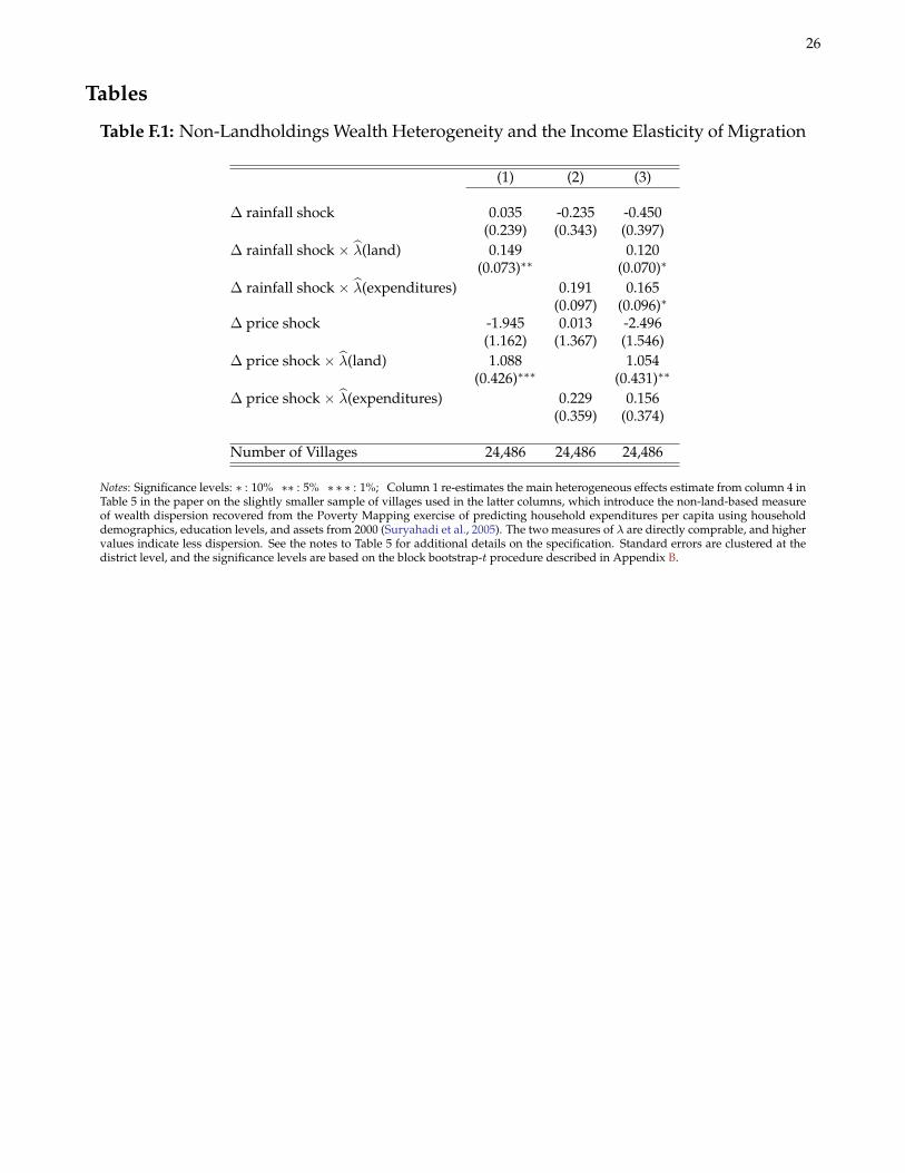
26

Tables

Table F.1: Non-Landholdings Wealth Heterogeneity and the Income Elasticity of Migration

(1) (2) (3)

∆ rainfall shock 0.035 -0.235 -0.450(0.239) (0.343) (0.397)

∆ rainfall shock × λ(land) 0.149 0.120(0.073)∗∗ (0.070)∗

∆ rainfall shock × λ(expenditures) 0.191 0.165(0.097) (0.096)∗

∆ price shock -1.945 0.013 -2.496(1.162) (1.367) (1.546)

∆ price shock × λ(land) 1.088 1.054(0.426)∗∗∗ (0.431)∗∗

∆ price shock × λ(expenditures) 0.229 0.156(0.359) (0.374)

Number of Villages 24,486 24,486 24,486

Notes: Significance levels: ∗ : 10% ∗∗ : 5% ∗ ∗ ∗ : 1%; Column 1 re-estimates the main heterogeneous effects estimate from column 4 inTable 5 in the paper on the slightly smaller sample of villages used in the latter columns, which introduce the non-land-based measureof wealth dispersion recovered from the Poverty Mapping exercise of predicting household expenditures per capita using householddemographics, education levels, and assets from 2000 (Suryahadi et al., 2005). The two measures of λ are directly comprable, and highervalues indicate less dispersion. See the notes to Table 5 for additional details on the specification. Standard errors are clustered at thedistrict level, and the significance levels are based on the block bootstrap-t procedure described in Appendix B.

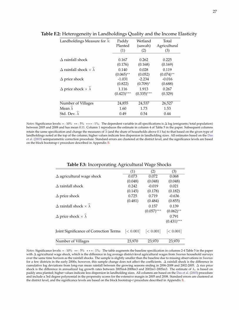
27

Table F.2: Heterogeneity in Landholdings Quality and the Income ElasticityLandholdings Measure for λ: Paddy Wetland Total

Planted (sawah) Agricultural(1) (2) (3)

∆ rainfall shock 0.167 0.262 0.225(0.176) (0.168) (0.169)

∆ rainfall shock × λ 0.140 0.028 0.119(0.065)∗∗ (0.052) (0.074)∗∗

∆ price shock -1.031 -2.234 -0.016(0.822) (0.709)∗ (0.688)

∆ price shock × λ 1.116 1.913 0.267(0.423)∗∗∗ (0.335)∗∗∗ (0.329)

Number of Villages 24,855 24,537 26,527Mean λ 1.60 1.73 1.53Std. Dev. λ 0.49 0.54 0.44

Notes: Significance levels: ∗ : 10% ∗∗ : 5% ∗∗∗ : 1%; The dependent variable in all specifications is ∆ log (emigrants/total population)between 2005 and 2008 and has mean 0.11. Column 1 reproduces the estimate in column 4 of Table 5 in the paper. Subsequent columnsretain the same specification and change the measures of λ (and the share of households above 0.1 ha) to that based on the given type oflandholdings noted at the top of the column; higher values indicate less dispersion in landholding sizes. All estimates based on the Daset al. (2003) semiparametric correction procedure. Standard errors are clustered at the district level, and the significance levels are basedon the block bootstrap-t procedure described in Appendix B.

Table F.3: Incorporating Agricultural Wage Shocks(1) (2) (3)

∆ agricultural wage shock 0.073 0.072 0.068(0.048) (0.048) (0.048)

∆ rainfall shock 0.242 -0.019 0.021(0.145) (0.178) (0.182)

∆ price shock 0.725 0.719 -0.636(0.481) (0.484) (0.855)

∆ rainfall shock × λ 0.157 0.139(0.057)∗∗∗ (0.062)∗∗

∆ price shock × λ 0.791(0.431)∗∗∗

Joint Significance of Correction Terms [< 0.001] [< 0.001] [< 0.001]

Number of Villages 23,970 23,970 23,970

Notes: Significance levels: ∗ : 10% ∗∗ : 5% ∗ ∗ ∗ : 1%; The table augments the baseline specification in columns 2-4 Table 5 in the paperwith ∆ agricultural wage shock, which is the difference in log average district-level agricultural wages from Susenas household surveysover the same time horizon as the rainfall shocks. The sample is slightly smaller than the baseline due to missing observations in Susenasfor a few districts in the early 2000s; however, this sample change does not affect the coefficients. ∆ rainfall shock is the difference incumulative log deviations from long-run mean rainfall between the growing seasons ending in 2006-2008 and 2002-2005. ∆ rice priceshock is the difference in annualized log growth rates between 2005m4-2008m3 and 2002m1-2005m3. The estimate of λv is based onpaddy area planted; higher values indicate less dispersion in landholding sizes. All columns are based on the Das et al. (2003) procedureand include a 3rd degree polynomial in the propensity scores for the extensive margin in 2005 and 2008. Standard errors are clustered atthe district level, and the significance levels are based on the block bootstrap-t procedure described in Appendix B.

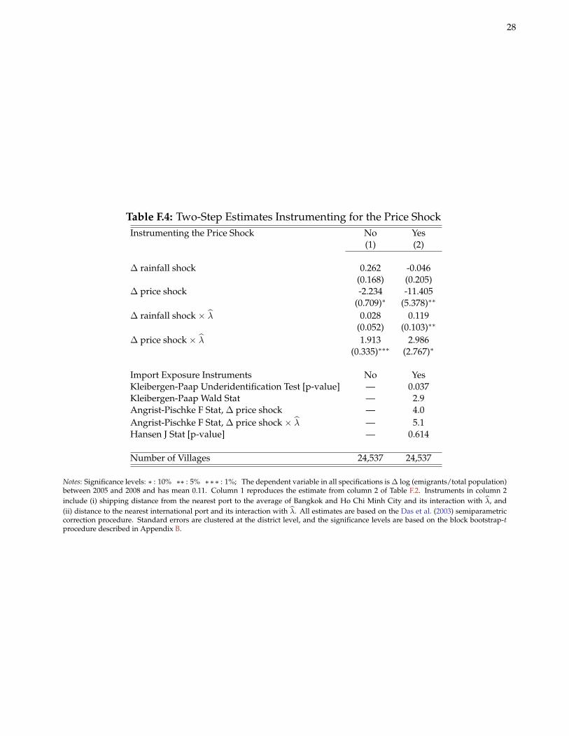
28

Table F.4: Two-Step Estimates Instrumenting for the Price ShockInstrumenting the Price Shock No Yes

(1) (2)

∆ rainfall shock 0.262 -0.046(0.168) (0.205)

∆ price shock -2.234 -11.405(0.709)∗ (5.378)∗∗

∆ rainfall shock × λ 0.028 0.119(0.052) (0.103)∗∗

∆ price shock × λ 1.913 2.986(0.335)∗∗∗ (2.767)∗

Import Exposure Instruments No YesKleibergen-Paap Underidentification Test [p-value] — 0.037Kleibergen-Paap Wald Stat — 2.9Angrist-Pischke F Stat, ∆ price shock — 4.0Angrist-Pischke F Stat, ∆ price shock × λ — 5.1Hansen J Stat [p-value] — 0.614

Number of Villages 24,537 24,537

Notes: Significance levels: ∗ : 10% ∗∗ : 5% ∗∗∗ : 1%; The dependent variable in all specifications is ∆ log (emigrants/total population)between 2005 and 2008 and has mean 0.11. Column 1 reproduces the estimate from column 2 of Table F.2. Instruments in column 2include (i) shipping distance from the nearest port to the average of Bangkok and Ho Chi Minh City and its interaction with λ, and(ii) distance to the nearest international port and its interaction with λ. All estimates are based on the Das et al. (2003) semiparametriccorrection procedure. Standard errors are clustered at the district level, and the significance levels are based on the block bootstrap-tprocedure described in Appendix B.

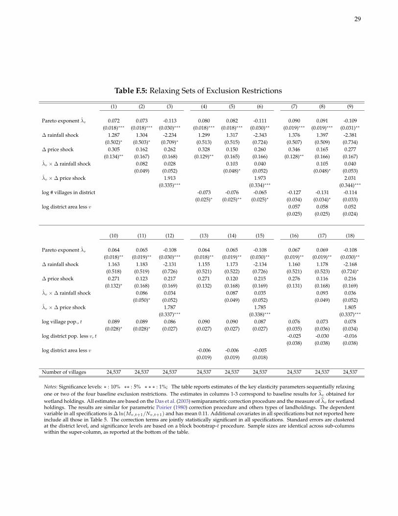
29

Table F.5: Relaxing Sets of Exclusion Restrictions

(1) (2) (3) (4) (5) (6) (7) (8) (9)

Pareto exponent λv 0.072 0.073 -0.113 0.080 0.082 -0.111 0.090 0.091 -0.109(0.018)∗∗∗ (0.018)∗∗∗ (0.030)∗∗∗ (0.018)∗∗∗ (0.018)∗∗∗ (0.030)∗∗ (0.019)∗∗∗ (0.019)∗∗∗ (0.031)∗∗

∆ rainfall shock 1.287 1.304 -2.234 1.299 1.317 -2.343 1.376 1.397 -2.381(0.502)∗ (0.503)∗ (0.709)∗ (0.513) (0.515) (0.724) (0.507) (0.509) (0.734)

∆ price shock 0.305 0.162 0.262 0.328 0.150 0.260 0.346 0.165 0.277(0.134)∗∗ (0.167) (0.168) (0.129)∗∗ (0.165) (0.166) (0.128)∗∗ (0.166) (0.167)

λv × ∆ rainfall shock 0.082 0.028 0.103 0.040 0.105 0.040(0.049) (0.052) (0.048)∗ (0.052) (0.048)∗ (0.053)

λv × ∆ price shock 1.913 1.973 2.031(0.335)∗∗∗ (0.334)∗∗∗ (0.344)∗∗∗

log # villages in district -0.073 -0.076 -0.065 -0.127 -0.131 -0.114(0.025)∗ (0.025)∗∗ (0.025)∗ (0.034) (0.034)∗ (0.033)

log district area less v 0.057 0.058 0.052(0.025) (0.025) (0.024)

(10) (11) (12) (13) (14) (15) (16) (17) (18)

Pareto exponent λv 0.064 0.065 -0.108 0.064 0.065 -0.108 0.067 0.069 -0.108(0.018)∗∗ (0.019)∗∗ (0.030)∗∗∗ (0.018)∗∗ (0.019)∗∗ (0.030)∗∗ (0.019)∗∗ (0.019)∗∗ (0.030)∗∗

∆ rainfall shock 1.163 1.183 -2.131 1.155 1.173 -2.134 1.160 1.178 -2.168(0.518) (0.519) (0.726) (0.521) (0.522) (0.726) (0.521) (0.523) (0.724)∗

∆ price shock 0.271 0.123 0.217 0.271 0.120 0.215 0.276 0.116 0.216(0.132)∗ (0.168) (0.169) (0.132) (0.168) (0.169) (0.131) (0.168) (0.169)

λv × ∆ rainfall shock 0.086 0.034 0.087 0.035 0.093 0.036(0.050)∗ (0.052) (0.049) (0.052) (0.049) (0.052)

λv × ∆ price shock 1.787 1.785 1.805(0.337)∗∗∗ (0.338)∗∗∗ (0.337)∗∗∗

log village pop., t 0.089 0.089 0.086 0.090 0.090 0.087 0.076 0.073 0.078(0.028)∗ (0.028)∗ (0.027) (0.027) (0.027) (0.027) (0.035) (0.036) (0.034)

log district pop. less v, t -0.025 -0.030 -0.016(0.038) (0.038) (0.038)

log district area less v -0.006 -0.006 -0.005(0.019) (0.019) (0.018)

Number of villages 24,537 24,537 24,537 24,537 24,537 24,537 24,537 24,537 24,537

Notes: Significance levels: ∗ : 10% ∗∗ : 5% ∗ ∗ ∗ : 1%; The table reports estimates of the key elasticity parameters sequentially relaxingone or two of the four baseline exclusion restrictions. The estimates in columns 1-3 correspond to baseline results for λv obtained forwetland holdings. All estimates are based on the Das et al. (2003) semiparametric correction procedure and the measure of λv for wetlandholdings. The results are similar for parametric Poirier (1980) correction procedure and others types of landholdings. The dependentvariable in all specifications is ∆ ln(Mv,t+1/Nv,t+1) and has mean 0.11. Additional covariates in all specifications but not reported hereinclude all those in Table 5. The correction terms are jointly statistically significant in all specifications. Standard errors are clusteredat the district level, and significance levels are based on a block bootstrap-t procedure. Sample sizes are identical across sub-columnswithin the super-column, as reported at the bottom of the table.

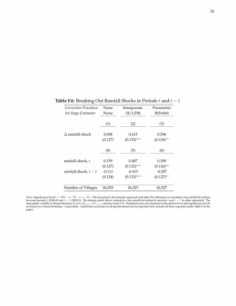
30

Table F.6: Breaking Out Rainfall Shocks in Periods t and t− 1

Correction Procedure None Semiparam. Parametric1st Stage Estimator None SU-LPM BiProbit

(1) (2) (3)

∆ rainfall shock 0.098 0.415 0.296(0.127) (0.133)∗∗∗ (0.128)∗∗

(4) (5) (6)

rainfall shock, t 0.159 0.407 0.309(0.127) (0.132)∗∗∗ (0.126)∗∗

rainfall shock, t− 1 -0.111 -0.415 -0.297(0.124) (0.133)∗∗∗ (0.127)∗∗

Number of Villages 26,529 26,527 26,527

Notes: Significance levels: ∗ : 10% ∗∗ : 5% ∗ ∗ ∗ : 1%; The top panel is the baseline approach and takes the difference in cumulative log rainfall deviationsbetween periods t (2006-8) and t − 1 (2003-5). The bottom panel allows cumulative log rainfall deviations in periods t and t − 1 to enter separately. Thedependent variable in all specifications is ∆ lnMv,t+1/Nv,t+1 and has mean 0.11. Standard errors are clustered at the district level and significance levelsare based on a block bootstrap−t procedure. Additional covariates in all specifications but not reported here include all those reported under Table 5 in thepaper.

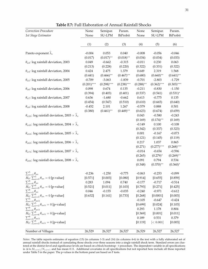
31

Table F.7: Full Elaboration of Annual Rainfall ShocksCorrection Procedure None Semipar. Param. None Semipar. Param.1st Stage Estimator None SU-LPM BiProbit None SU-LPM BiProbit

(1) (2) (3) (4) (5) (6)

Pareto exponent λv -0.004 0.053 0.040 -0.008 -0.056 -0.046(0.017) (0.017)∗∗ (0.018)∗∗ (0.034) (0.034) (0.033)

θa3: log rainfall deviation, 2003 0.049 -0.662 -0.315 -0.011 0.230 0.063(0.213) (0.228) (0.220) (0.322) (0.331) (0.322)

θa4: log rainfall deviation, 2004 0.424 2.475 1.379 0.649 2.319 1.568(0.441) (0.466)∗∗ (0.467)∗∗ (0.680) (0.660)∗∗ (0.641)∗∗

θa5: log rainfall deviation, 2005 -0.709 -3.063 -1.839 -0.701 -2.803 -1.729(0.201)∗∗∗ (0.298)∗∗∗ (0.238)∗∗∗ (0.288)∗∗ (0.362)∗∗∗ (0.303)∗∗∗

θa6: log rainfall deviation, 2006 0.098 0.674 0.135 -0.211 -0.830 -1.150(0.394) (0.403) (0.401) (0.537) (0.541) (0.531)∗

θa7: log rainfall deviation, 2007 0.636 -1.680 -0.662 0.613 -0.775 0.135(0.454) (0.547) (0.510) (0.610) (0.665) (0.640)

θa8: log rainfall deviation, 2008 -0.452 2.101 1.267 -0.579 0.888 0.501(0.380) (0.461)∗∗ (0.449)∗∗ (0.623) (0.674) (0.659)

θa3λ: log rainfall deviation, 2003 × λv 0.043 -0.580 -0.243(0.169) (0.174)∗∗ (0.169)

θa4λ: log rainfall deviation, 2004 × λv -0.149 0.100 -0.108(0.342) (0.337) (0.323)

θa5λ: log rainfall deviation, 2005 × λv 0.001 -0.167 -0.073(0.121) (0.145) (0.119)

θa6λ: log rainfall deviation, 2006 × λv 0.217 1.037 0.865(0.271) (0.277)∗∗∗ (0.268)∗∗∗

θa7λ: log rainfall deviation, 2007 × λv -0.014 -0.654 -0.596(0.265) (0.279)∗ (0.269)∗∗

θa8λ: log rainfall deviation, 2008 × λv 0.091 0.794 0.534(0.348) (0.370)∗∗ (0.360)∗

∑5s=3 θas -0.236 -1.250 -0.775 -0.063 -0.253 -0.099

H0:∑5s=3 θas = 0 [p-value] [0.571] [0.003] [0.080] [0.914] [0.655] [0.859]∑8

s=6 θas 0.283 1.094 0.740 -0.177 -0.717 -0.514H0:

∑8s=6 θas = 0 [p-value] [0.521] [0.011] [0.103] [0.793] [0.271] [0.425]∑8

s=3 θas 0.046 -0.155 -0.035 -0.240 -0.971 -0.612H0:

∑8s=3 θas = 0 [p-value] [0.632] [0.141] [0.733] [0.268] [0.0001] [0.003]∑5

s=3 θasλ -0.105 -0.647 -0.424H0:

∑5s=3 θasλ = 0 [p-value] [0.699] [0.024] [0.103]∑8

s=6 θasλ 0.293 1.178 0.804H0:

∑8s=6 θasλ = 0 [p-value] [0.369] [0.001] [0.011]∑8

s=3 θasλ 0.189 0.531 0.379H0:

∑8s=3 θasλ = 0 [p-value] [0.119] [< 0.001] [0.003]

Number of Villages 26,529 26,527 26,527 26,529 26,527 26,527

Notes: The table reports estimates of equation (13) (in columns 1-3) and (14) (in columns 4-6) in the text with a fully elaborated set ofannual rainfall shocks instead of cumulating those shocks over three seasons into a single rainfall shock term. Standard errors are clus-tered at the district level and significance levels are based on a block bootstrap−t procedure. The dependent variable in all specificationsis ∆ lnMv,t+1/Nv,t+1 and has mean 0.11. Additional covariates in all specifications but not reported here include all those reportedunder Table 5 in the paper. The p-values in the bottom panel are based on F tests.

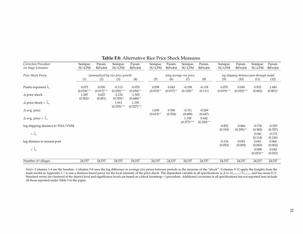
32

Table F.8: Alternative Rice Price Shock MeasuresCorrection Procedure Semipar. Param. Semipar. Param. Semipar. Param. Semipar. Param. Semipar. Param. Semipar. Param.1st Stage Estimator SU-LPM BiProbit SU-LPM BiProbit SU-LPM BiProbit SU-LPM BiProbit SU-LPM BiProbit SU-LPM BiProbit

Price Shock Proxy ∆annualized log rice price growth ∆log average rice price log shipping distance pass-through model(1) (2) (3) (4) (5) (6) (7) (8) (9) (10) (11) (12)

Pareto exponent λv 0.072 0.050 -0.113 -0.070 0.058 0.043 -0.338 -0.118 0.070 0.049 0.933 1.640(0.018)∗∗∗ (0.017)∗∗∗ (0.030)∗∗∗ (0.030)∗∗ (0.019)∗∗ (0.017)∗∗ (0.128)∗∗ (0.111) (0.019)∗∗∗ (0.018)∗∗∗ (0.842) (0.801)∗

∆ price shock 1.287 0.625 -2.234 -1.503(0.502)∗ (0.451) (0.709)∗ (0.688)∗∗

∆ price shock × λv 1.913 1.155(0.335)∗∗∗ (0.327)∗∗∗

∆ avg. price 1.630 0.396 -0.311 -0.269(0.613)∗∗ (0.524) (0.688) (0.647)

∆ avg. price × λv 1.158 0.442(0.377)∗∗∗ (0.320)∗∗

log shipping distance to THA/VNM -0.852 -0.866 -0.718 -0.529(0.319) (0.295)∗∗ (0.383) (0.357)

× λv -0.041 -0.172(0.114) (0.106)

log distance to nearest port -0.116 -0.001 0.041 0.064(0.053) (0.050) (0.065) (0.062)

× λv -0.098 -0.042(0.023)∗∗ (0.022)

Number of villages 24,537 24,537 24,537 24,537 24,537 24,537 24,537 24,537 24,537 24,537 24,537 24,537

Notes: Columns 1-4 are the baseline. Columns 5-8 uses the log difference in average rice prices between periods as the measure of the “shock”. Columns 9-12 apply the insights from thetrade model in Appendix E.1 to use a distance-based proxy for the local intensity of the price shock. The dependent variable in all specifications is ∆ lnMv,t+1/Nv,t+1 and has mean 0.11.Standard errors are clustered at the district level and significance levels are based on a block bootstrap−t procedure. Additional covariates in all specifications but not reported here includeall those reported under Table 5 in the paper.

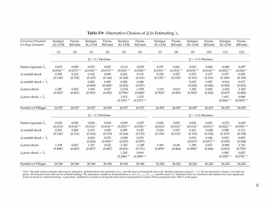
33

Table F.9: Alternative Choices of R in Estimating λv

Correction Procedure Semipar. Param. Semipar. Param. Semipar. Param. Semipar. Param. Semipar. Param. Semipar. Param.1st Stage Estimator SU-LPM BiProbit SU-LPM BiProbit SU-LPM BiProbit SU-LPM BiProbit SU-LPM BiProbit SU-LPM BiProbit

(1) (2) (3) (4) (5) (6) (7) (8) (9) (10) (11) (12)

R = 0.1 Hectares R = 0.15 Hectares

Pareto exponent λv 0.072 0.050 0.073 0.052 -0.113 -0.070 0.057 0.041 0.053 0.040 -0.090 -0.057(0.018)∗∗∗ (0.017)∗∗∗ (0.018)∗∗∗ (0.017)∗∗∗ (0.030)∗∗∗ (0.030)∗∗ (0.015)∗∗∗ (0.014)∗∗∗ (0.015)∗∗∗ (0.014)∗∗∗ (0.023)∗∗∗ (0.026)∗∗

∆ rainfall shock 0.305 0.212 0.162 0.069 0.262 0.135 0.320 0.227 0.270 0.137 0.357 0.200(0.134)∗ (0.130) (0.167) (0.166) (0.168) (0.161) (0.135)∗∗ (0.130)∗ (0.167) (0.161) (0.168)∗ (0.159)

∆ rainfall shock × λv 0.082 0.085 0.028 0.048 0.025 0.047 -0.014 0.017(0.049) (0.058)∗ (0.052) (0.051) (0.042) (0.046) (0.045) (0.043)

∆ price shock 1.287 0.625 1.304 0.627 -2.234 -1.503 1.319 0.615 1.326 0.609 -1.654 -1.265(0.502)∗ (0.451) (0.503)∗ (0.452) (0.709)∗ (0.688)∗ (0.503)∗ (0.453) (0.503)∗ (0.452) (0.657) (0.682)

∆ price shock × λv 1.913 1.155 1.451 0.908(0.335)∗∗∗ (0.327)∗∗∗ (0.266)∗∗∗ (0.285)∗∗∗

Number of Villages 26,527 26,527 26,527 26,529 26,527 26,527 26,435 26,435 26,435 26,435 26,435 26,435

R = 0.2 Hectares R = 0.25 Hectares

Pareto exponent λv 0.034 0.036 0.030 0.034 -0.093 -0.057 0.026 0.025 0.024 0.027 -0.072 -0.065(0.013)∗ (0.014)∗∗∗ (0.012)∗∗ (0.014)∗∗∗ (0.023)∗∗∗ (0.030)∗∗ (0.012)∗ (0.012)∗∗ (0.012)∗∗ (0.011)∗∗ (0.022)∗∗∗ (0.029)∗∗∗

∆ rainfall shock 0.291 0.204 0.219 0.056 0.299 0.145 0.326 0.225 0.161 -0.000 0.288 0.116(0.136)∗ (0.131) (0.162) (0.153) (0.164) (0.153) (0.136)∗ (0.131)∗ (0.165) (0.154) (0.167)∗ (0.158)

∆ rainfall shock × λv 0.034 0.072 -0.000 0.033 0.074 0.106 0.023 0.055(0.036) (0.039)∗∗ (0.037) (0.037) (0.037)∗ (0.037)∗∗∗ (0.039) (0.038)

∆ price shock 1.338 0.627 1.331 0.622 -1.361 -1.188 1.369 0.638 1.358 0.637 -0.998 -1.331(0.498)∗ (0.447) (0.497)∗ (0.447) (0.661) (0.731) (0.499)∗ (0.444) (0.498)∗∗ (0.444) (0.651) (0.735)∗

∆ price shock × λv 1.235 0.819 0.985 0.825(0.248)∗∗∗ (0.289)∗∗∗ (0.229)∗∗∗ (0.274)∗∗∗

Number of Villages 26,346 26,346 26,346 26,346 26,346 26,346 26,242 26,242 26,242 26,242 26,242 26,242

Notes: The table reports estimates allowing for alternative R thresholds in the estimation of λv (and the share of households above R). Baseline estimates using R = 0.1 Ha are reported in columns 1-6 of the toppanel. All estimates in the table are for wetland holdings. The dependent variable in all specifications is ∆ lnMv,t+1/Nv,t+1 and has mean 0.11. Standard errors are clustered at the district level, and significancelevels are based on a block bootstrap−t procedure. Additional covariates in all specifications but not reported here include all those reported under Table 5 in the paper.

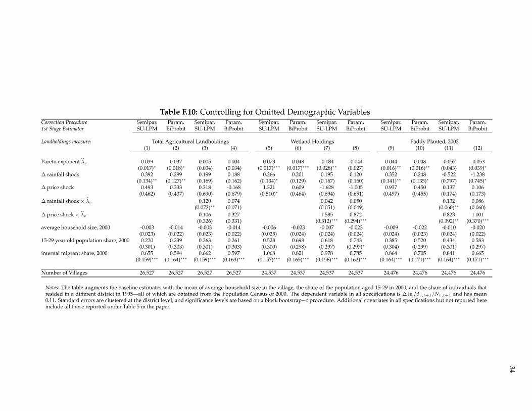
34

Table F.10: Controlling for Omitted Demographic VariablesCorrection Procedure Semipar. Param. Semipar. Param. Semipar. Param. Semipar. Param. Semipar. Param. Semipar. Param.1st Stage Estimator SU-LPM BiProbit SU-LPM BiProbit SU-LPM BiProbit SU-LPM BiProbit SU-LPM BiProbit SU-LPM BiProbit

Landholdings measure: Total Agricultural Landholdings Wetland Holdings Paddy Planted, 2002(1) (2) (3) (4) (5) (6) (7) (8) (9) (10) (11) (12)

Pareto exponent λv 0.039 0.037 0.005 0.004 0.073 0.048 -0.084 -0.044 0.044 0.048 -0.057 -0.053(0.017)∗ (0.018)∗ (0.034) (0.034) (0.017)∗∗∗ (0.017)∗∗∗ (0.028)∗∗ (0.027) (0.016)∗∗ (0.016)∗∗ (0.043) (0.039)∗

∆ rainfall shock 0.392 0.299 0.199 0.188 0.266 0.201 0.195 0.120 0.352 0.248 -0.522 -1.238(0.134)∗∗ (0.127)∗∗ (0.169) (0.162) (0.134)∗ (0.129) (0.167) (0.160) (0.141)∗∗ (0.135)∗ (0.797) (0.745)∗

∆ price shock 0.493 0.333 0.318 -0.168 1.321 0.609 -1.628 -1.005 0.937 0.450 0.137 0.106(0.462) (0.437) (0.690) (0.679) (0.510)∗ (0.464) (0.694) (0.651) (0.497) (0.455) (0.174) (0.173)

∆ rainfall shock × λv 0.120 0.074 0.042 0.050 0.132 0.086(0.072)∗∗ (0.071) (0.051) (0.049) (0.060)∗∗ (0.060)

∆ price shock × λv 0.106 0.327 1.585 0.872 0.823 1.001(0.326) (0.331) (0.312)∗∗∗ (0.294)∗∗∗ (0.392)∗∗ (0.370)∗∗∗

average household size, 2000 -0.003 -0.014 -0.003 -0.014 -0.006 -0.023 -0.007 -0.023 -0.009 -0.022 -0.010 -0.020(0.023) (0.022) (0.023) (0.022) (0.025) (0.024) (0.024) (0.024) (0.024) (0.023) (0.024) (0.022)

15-29 year old population share, 2000 0.220 0.239 0.263 0.261 0.528 0.698 0.618 0.743 0.385 0.520 0.434 0.583(0.301) (0.303) (0.301) (0.303) (0.300) (0.298) (0.297) (0.297)∗ (0.304) (0.299) (0.301) (0.297)

internal migrant share, 2000 0.655 0.594 0.662 0.597 1.068 0.821 0.978 0.785 0.864 0.705 0.841 0.665(0.159)∗∗∗ (0.164)∗∗∗ (0.159)∗∗∗ (0.163)∗∗∗ (0.157)∗∗∗ (0.165)∗∗∗ (0.156)∗∗∗ (0.162)∗∗∗ (0.164)∗∗∗ (0.171)∗∗∗ (0.164)∗∗∗ (0.171)∗∗∗

Number of Villages 26,527 26,527 26,527 26,527 24,537 24,537 24,537 24,537 24,476 24,476 24,476 24,476

Notes: The table augments the baseline estimates with the mean of average household size in the village, the share of the population aged 15-29 in 2000, and the share of individuals thatresided in a different district in 1995—all of which are obtained from the Population Census of 2000. The dependent variable in all specifications is ∆ lnMv,t+1/Nv,t+1 and has mean0.11. Standard errors are clustered at the district level, and significance levels are based on a block bootstrap−t procedure. Additional covariates in all specifications but not reported hereinclude all those reported under Table 5 in the paper.

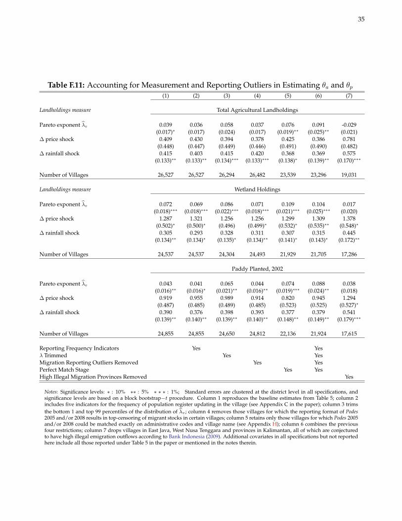
35

Table F.11: Accounting for Measurement and Reporting Outliers in Estimating θa and θp(1) (2) (3) (4) (5) (6) (7)

Landholdings measure Total Agricultural Landholdings

Pareto exponent λv 0.039 0.036 0.058 0.037 0.076 0.091 -0.029(0.017)∗ (0.017) (0.024) (0.017) (0.019)∗∗ (0.025)∗∗ (0.021)

∆ price shock 0.409 0.430 0.394 0.378 0.425 0.386 0.781(0.448) (0.447) (0.449) (0.446) (0.491) (0.490) (0.482)

∆ rainfall shock 0.415 0.403 0.415 0.420 0.368 0.369 0.575(0.133)∗∗ (0.133)∗∗ (0.134)∗∗∗ (0.133)∗∗∗ (0.138)∗ (0.139)∗∗ (0.170)∗∗∗

Number of Villages 26,527 26,527 26,294 26,482 23,539 23,296 19,031

Landholdings measure Wetland Holdings

Pareto exponent λv 0.072 0.069 0.086 0.071 0.109 0.104 0.017(0.018)∗∗∗ (0.018)∗∗∗ (0.022)∗∗∗ (0.018)∗∗∗ (0.021)∗∗∗ (0.025)∗∗∗ (0.020)

∆ price shock 1.287 1.321 1.256 1.256 1.299 1.309 1.378(0.502)∗ (0.500)∗ (0.496) (0.499)∗ (0.532)∗ (0.535)∗∗ (0.548)∗

∆ rainfall shock 0.305 0.293 0.328 0.311 0.307 0.315 0.445(0.134)∗∗ (0.134)∗ (0.135)∗ (0.134)∗∗ (0.141)∗ (0.143)∗ (0.172)∗∗

Number of Villages 24,537 24,537 24,304 24,493 21,929 21,705 17,286

Paddy Planted, 2002

Pareto exponent λv 0.043 0.041 0.065 0.044 0.074 0.088 0.038(0.016)∗∗ (0.016)∗ (0.021)∗∗ (0.016)∗∗ (0.019)∗∗∗ (0.024)∗∗ (0.018)

∆ price shock 0.919 0.955 0.989 0.914 0.820 0.945 1.294(0.487) (0.485) (0.489) (0.485) (0.523) (0.525) (0.527)∗

∆ rainfall shock 0.390 0.376 0.398 0.393 0.377 0.379 0.541(0.139)∗∗ (0.140)∗∗ (0.139)∗∗ (0.140)∗∗ (0.148)∗∗ (0.149)∗∗ (0.179)∗∗∗

Number of Villages 24,855 24,855 24,650 24,812 22,136 21,924 17,615

Reporting Frequency Indicators Yes Yesλ Trimmed Yes YesMigration Reporting Outliers Removed Yes YesPerfect Match Stage Yes YesHigh Illegal Migration Provinces Removed Yes

Notes: Significance levels: ∗ : 10% ∗∗ : 5% ∗ ∗ ∗ : 1%; Standard errors are clustered at the district level in all specifications, andsignificance levels are based on a block bootstrap−t procedure. Column 1 reproduces the baseline estimates from Table 5; column 2includes five indicators for the frequency of population register updating in the village (see Appendix C in the paper); column 3 trimsthe bottom 1 and top 99 percentiles of the distribution of λv ; column 4 removes those villages for which the reporting format of Podes2005 and/or 2008 results in top-censoring of migrant stocks in certain villages; column 5 retains only those villages for which Podes 2005and/or 2008 could be matched exactly on administrative codes and village name (see Appendix H); column 6 combines the previousfour restrictions; column 7 drops villages in East Java, West Nusa Tenggara and provinces in Kalimantan, all of which are conjecturedto have high illegal emigration outflows according to Bank Indonesia (2009). Additional covariates in all specifications but not reportedhere include all those reported under Table 5 in the paper or mentioned in the notes therein.

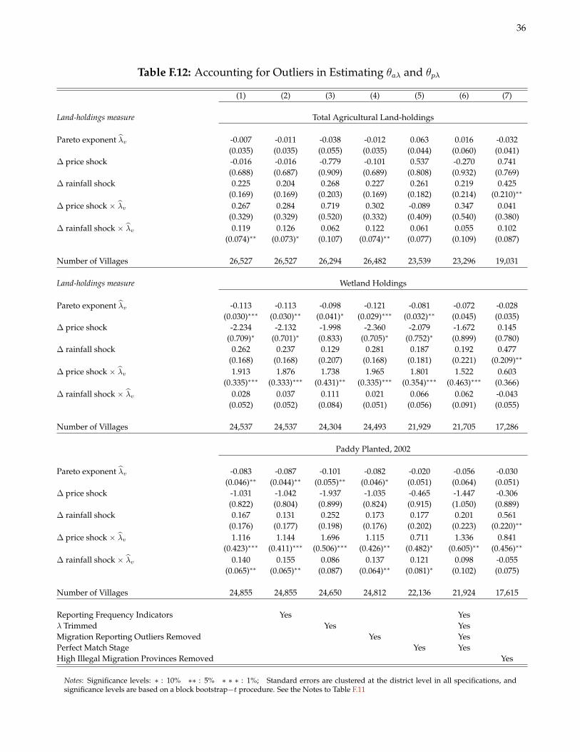
36

Table F.12: Accounting for Outliers in Estimating θaλ and θpλ

(1) (2) (3) (4) (5) (6) (7)

Land-holdings measure Total Agricultural Land-holdings

Pareto exponent λv -0.007 -0.011 -0.038 -0.012 0.063 0.016 -0.032(0.035) (0.035) (0.055) (0.035) (0.044) (0.060) (0.041)

∆ price shock -0.016 -0.016 -0.779 -0.101 0.537 -0.270 0.741(0.688) (0.687) (0.909) (0.689) (0.808) (0.932) (0.769)

∆ rainfall shock 0.225 0.204 0.268 0.227 0.261 0.219 0.425(0.169) (0.169) (0.203) (0.169) (0.182) (0.214) (0.210)∗∗

∆ price shock × λv 0.267 0.284 0.719 0.302 -0.089 0.347 0.041(0.329) (0.329) (0.520) (0.332) (0.409) (0.540) (0.380)

∆ rainfall shock × λv 0.119 0.126 0.062 0.122 0.061 0.055 0.102(0.074)∗∗ (0.073)∗ (0.107) (0.074)∗∗ (0.077) (0.109) (0.087)

Number of Villages 26,527 26,527 26,294 26,482 23,539 23,296 19,031

Land-holdings measure Wetland Holdings

Pareto exponent λv -0.113 -0.113 -0.098 -0.121 -0.081 -0.072 -0.028(0.030)∗∗∗ (0.030)∗∗ (0.041)∗ (0.029)∗∗∗ (0.032)∗∗ (0.045) (0.035)

∆ price shock -2.234 -2.132 -1.998 -2.360 -2.079 -1.672 0.145(0.709)∗ (0.701)∗ (0.833) (0.705)∗ (0.752)∗ (0.899) (0.780)

∆ rainfall shock 0.262 0.237 0.129 0.281 0.187 0.192 0.477(0.168) (0.168) (0.207) (0.168) (0.181) (0.221) (0.209)∗∗

∆ price shock × λv 1.913 1.876 1.738 1.965 1.801 1.522 0.603(0.335)∗∗∗ (0.333)∗∗∗ (0.431)∗∗ (0.335)∗∗∗ (0.354)∗∗∗ (0.463)∗∗∗ (0.366)

∆ rainfall shock × λv 0.028 0.037 0.111 0.021 0.066 0.062 -0.043(0.052) (0.052) (0.084) (0.051) (0.056) (0.091) (0.055)

Number of Villages 24,537 24,537 24,304 24,493 21,929 21,705 17,286

Paddy Planted, 2002

Pareto exponent λv -0.083 -0.087 -0.101 -0.082 -0.020 -0.056 -0.030(0.046)∗∗ (0.044)∗∗ (0.055)∗∗ (0.046)∗ (0.051) (0.064) (0.051)

∆ price shock -1.031 -1.042 -1.937 -1.035 -0.465 -1.447 -0.306(0.822) (0.804) (0.899) (0.824) (0.915) (1.050) (0.889)

∆ rainfall shock 0.167 0.131 0.252 0.173 0.177 0.201 0.561(0.176) (0.177) (0.198) (0.176) (0.202) (0.223) (0.220)∗∗

∆ price shock × λv 1.116 1.144 1.696 1.115 0.711 1.336 0.841(0.423)∗∗∗ (0.411)∗∗∗ (0.506)∗∗∗ (0.426)∗∗ (0.482)∗ (0.605)∗∗ (0.456)∗∗

∆ rainfall shock × λv 0.140 0.155 0.086 0.137 0.121 0.098 -0.055(0.065)∗∗ (0.065)∗∗ (0.087) (0.064)∗∗ (0.081)∗ (0.102) (0.075)

Number of Villages 24,855 24,855 24,650 24,812 22,136 21,924 17,615

Reporting Frequency Indicators Yes Yesλ Trimmed Yes YesMigration Reporting Outliers Removed Yes YesPerfect Match Stage Yes YesHigh Illegal Migration Provinces Removed Yes

Notes: Significance levels: ∗ : 10% ∗∗ : 5% ∗ ∗ ∗ : 1%; Standard errors are clustered at the district level in all specifications, andsignificance levels are based on a block bootstrap−t procedure. See the Notes to Table F.11

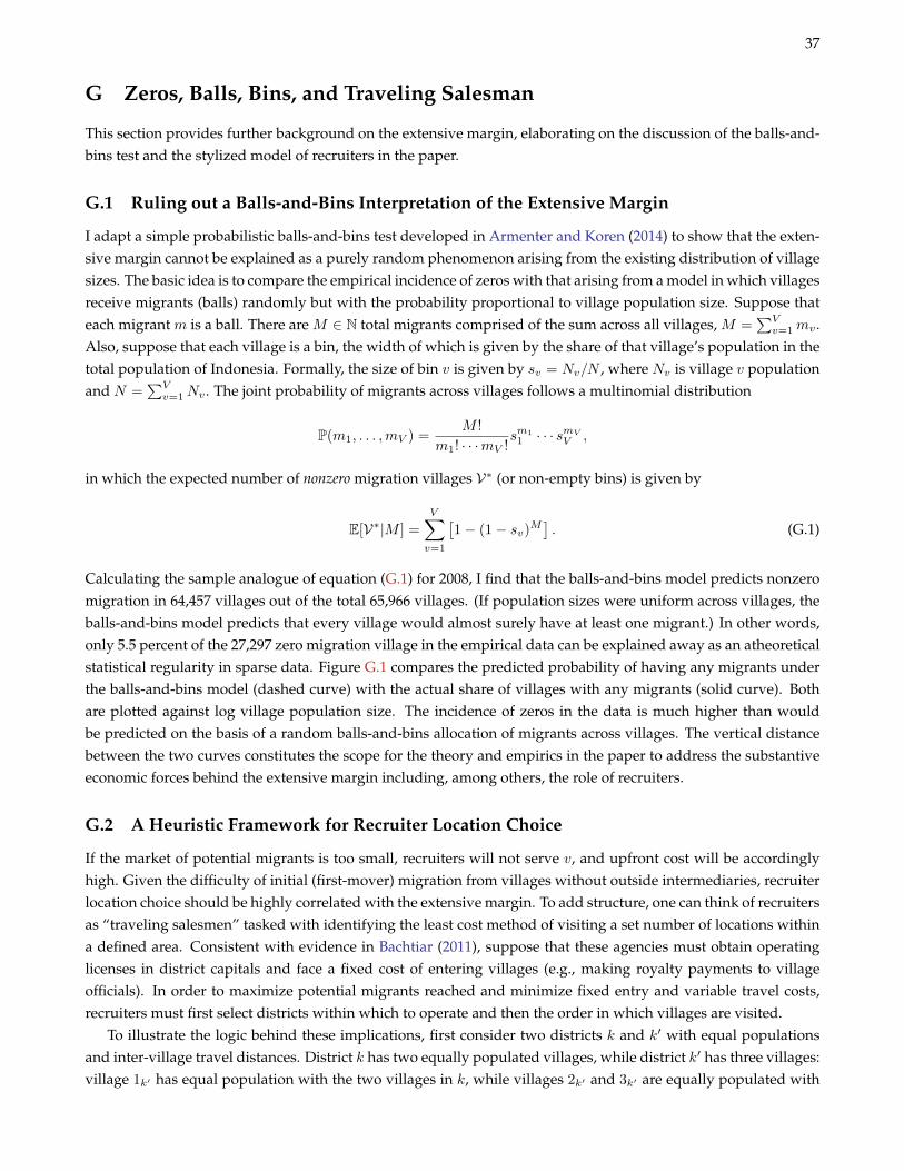
37

G Zeros, Balls, Bins, and Traveling Salesman

This section provides further background on the extensive margin, elaborating on the discussion of the balls-and-bins test and the stylized model of recruiters in the paper.

G.1 Ruling out a Balls-and-Bins Interpretation of the Extensive Margin

I adapt a simple probabilistic balls-and-bins test developed in Armenter and Koren (2014) to show that the exten-sive margin cannot be explained as a purely random phenomenon arising from the existing distribution of villagesizes. The basic idea is to compare the empirical incidence of zeros with that arising from a model in which villagesreceive migrants (balls) randomly but with the probability proportional to village population size. Suppose thateach migrant m is a ball. There are M ∈ N total migrants comprised of the sum across all villages, M =

∑Vv=1mv .

Also, suppose that each village is a bin, the width of which is given by the share of that village’s population in thetotal population of Indonesia. Formally, the size of bin v is given by sv = Nv/N , where Nv is village v populationand N =

∑Vv=1Nv . The joint probability of migrants across villages follows a multinomial distribution

P(m1, . . . ,mV ) =M !

m1! · · ·mV !sm1

1 · · · smVV ,

in which the expected number of nonzero migration villages V∗ (or non-empty bins) is given by

E[V∗|M ] =

V∑v=1

[1− (1− sv)M

]. (G.1)

Calculating the sample analogue of equation (G.1) for 2008, I find that the balls-and-bins model predicts nonzeromigration in 64,457 villages out of the total 65,966 villages. (If population sizes were uniform across villages, theballs-and-bins model predicts that every village would almost surely have at least one migrant.) In other words,only 5.5 percent of the 27,297 zero migration village in the empirical data can be explained away as an atheoreticalstatistical regularity in sparse data. Figure G.1 compares the predicted probability of having any migrants underthe balls-and-bins model (dashed curve) with the actual share of villages with any migrants (solid curve). Bothare plotted against log village population size. The incidence of zeros in the data is much higher than wouldbe predicted on the basis of a random balls-and-bins allocation of migrants across villages. The vertical distancebetween the two curves constitutes the scope for the theory and empirics in the paper to address the substantiveeconomic forces behind the extensive margin including, among others, the role of recruiters.

G.2 A Heuristic Framework for Recruiter Location Choice

If the market of potential migrants is too small, recruiters will not serve v, and upfront cost will be accordinglyhigh. Given the difficulty of initial (first-mover) migration from villages without outside intermediaries, recruiterlocation choice should be highly correlated with the extensive margin. To add structure, one can think of recruitersas “traveling salesmen” tasked with identifying the least cost method of visiting a set number of locations withina defined area. Consistent with evidence in Bachtiar (2011), suppose that these agencies must obtain operatinglicenses in district capitals and face a fixed cost of entering villages (e.g., making royalty payments to villageofficials). In order to maximize potential migrants reached and minimize fixed entry and variable travel costs,recruiters must first select districts within which to operate and then the order in which villages are visited.

To illustrate the logic behind these implications, first consider two districts k and k′ with equal populationsand inter-village travel distances. District k has two equally populated villages, while district k′ has three villages:village 1k′ has equal population with the two villages in k, while villages 2k′ and 3k′ are equally populated with

38

the total equal to the population of 1k′ . Assuming (i) constant fixed costs of establishing agency presence inequally sized districts and (ii) constant fixed costs of entering villages, a given recruiter would be more likely toenter district k than k′. If, however, recruiters choose to visit district k′ for other (unobserved) reasons, then village1k′ would be more likely visited than 2k′ or 3k′ . Now, add one identical village to each district with populationgreater than all existing villages in each district. Assuming recruitment agencies are subject to budget constraintspreventing visits to all villages within k, it is straightforward to show within this framework that recruiters wouldonly visit the newly added village in k.

I now provide a sketch of the general traveling salesman model underlying the proposed instruments for theextensive margin. Begin by considering the problem of recruiters selecting a district within which to operate,retaining the assumption that licensing and other fees are paid to district government officials.1 Let the cost oftraveling between villages v and v′ within district k be denoted by dkvv′ > 0. Suppose further that there are Vk

villages in district k and that the population of the district less village v is given by Nk−v . For empirical tractability,

additionally assume that the least-cost path of visiting every village within a district is approximately proportionalto the area of the district less village v, Ak−v .2 Now suppose that the fixed cost of entering a village, f , is identicalacross all villages and that the ex ante probability of successfully recruiting any individual potentials migrantis identical across villages. The optimization problem for the recruitment agency is to maximize the number ofpotential migrants, Mv , reached (with advertisements and contract offers) and to minimize the costs (and hencemaximize expected revenue). The objective is then

maxk

Vk∑v=1

Mv s.t. fVk +Ak−v ≤ B, Mv ≤ Nv ∀v

where B is the exogenously given budget of the recruitment agency. The (heuristic) solution function (i.e., theoptimal district) should be increasing in Nk

−v and decreasing in Ak−v and Vk. Once inside a given district k, all elseequal, budget-constrained recruiters are relatively more likely to visit villages with larger populations since theunconditional probability of successfully recruiting a single migrant is higher.

In Table G.1, I test the above hypotheses using the only available proxy for recruiter visits at the village level—ameasure in Podes indicating whether any recruiters targeting female migrants are based in the village. Conditionalon the presence of any migrants in the prior period (i.e., as recorded mid-2005), the likelihood that village v has arecruiter in period t + 1 (i.e., prior to mid-2008) is (i) increasing in the population of village v and the populationof v’s district less v, and (ii) decreasing in the number of village in v’s district. These findings are consistentwith the predictions of the traveling salesman framework sketched above. The positive albeit statistically nullcorrelation with the area of v’s district is not. However, that the probability is decreasing in the distance fromthe subdistrict capital (albeit not the district capital) suggests that some of the distance components of the modelhold. A more rigorous test would require computing the actual distances between villages and using some of theavailable methods for solving the traveling salesman problem. This is beyond the scope of the present study asthe patterns observed in Table G.1 bear out indications that recruiter decisions follow some approximation to themodel described above. Other important results in Table G.1 include (i) the positive correlation with the share ofethnic Arabs in the total population of v in 2000 and (ii) the statistically null correlation with agricultural incomeshocks. Finding (i) is consistent with the role of local ethnic intermediaries in facilitating migration to Middle

1This assumption follows from evidence on the procedures through which recruitment agencies engage with government institutions in theprocess of authorizing legal contract emigrants (Bank Indonesia, 2009). The engagement with local government officials has been increasingin recent years as decentralization has resulted in a devolution of authorities and regulatory power to the regions (see Bachtiar, 2011). UnderLaw 39/2004, recruitment agencies are only permitted to recruit and place prospective labor migrants who are registered at the local Ministryof Manpower and Transmigration. Of course agency field workers often bypass local governments and enter villages directly, but the agenciesmust still liaise with officials in the district capital for the purposes of document preparation and other predeparture certification processes.

2That is,∑Vk

v′ 6=v

∑Vkv 6=v′ d

kvv′ ∝ A

k−v .

39

Eastern destinations. Finding (ii) suggests that recruiters do not respond to income shocks in deciding where totarget their contract offers.

Figure G.1: Comparing the Actual Incidence of Zeros with the Balls-and-Bins Prediction

0

.2

.4

.6

.8

1

shar

e of

villa

ges w

ith m

igran

ts >

0

2 4 6 8 10log population

balls−and−bins prediction

actual data

density, log population

Notes: The “actual data” estimate is based on a local linear probability regression of an indicator for any migrants in village v on logpopulation, using an Epanechnikov kernel and trimming the top 1 percent of villages for presentational purposes. The “balls-and-bins”prediction is based on the model described in Section G.1.

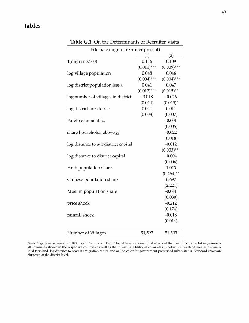
40

Tables

Table G.1: On the Determinants of Recruiter Visits

P(female migrant recruiter present)(1) (2)

1(migrants> 0) 0.116 0.109(0.011)∗∗∗ (0.009)∗∗∗

log village population 0.048 0.046(0.004)∗∗∗ (0.004)∗∗∗

log district population less v 0.041 0.047(0.013)∗∗∗ (0.015)∗∗∗

log number of villages in district -0.018 -0.026(0.014) (0.015)∗

log district area less v 0.011 0.011(0.008) (0.007)

Pareto exponent λv -0.001(0.005)

share households above R -0.022(0.018)

log distance to subdistrict capital -0.012(0.003)∗∗∗

log distance to district capital -0.004(0.006)

Arab population share 1.023(0.464)∗∗

Chinese population share 0.697(2.221)

Muslim population share -0.041(0.030)

price shock -0.212(0.174)

rainfall shock -0.018(0.014)

Number of Villages 51,593 51,593

Notes: Significance levels: ∗ : 10% ∗∗ : 5% ∗ ∗ ∗ : 1%; The table reports marginal effects at the mean from a probit regression ofall covariates shown in the respective columns as well as the following additional covariates in column 2: wetland area as a share oftotal farmland, log distance to nearest emigration center, and an indicator for government-prescribed urban status. Standard errors areclustered at the district level.

41

H Panel Data Construction

In this subsection, I describe the process of constructing a panel dataset of Indonesian villages comprised of datacollected in 2000, 2002, 2003, 2005, and 2008. Starting from the baseline 65,966 villages in Table 1 in the paper,the final sample of villages is reduced further by two factors. First, because this paper focuses on heterogeneousincome shocks in agricultural areas, I exclude urban villages without land-holdings entries in the AgriculturalCensus. There are other practical reasons for doing so as well. In Indonesia, agricultural commodity price in-creases generally have homogeneous, negative effects on real income in urban areas, and rainfall shocks tend tohave no effect on rice production in nominally urban areas (Levine and Yang, 2014). Second, changes in adminis-trative boundaries over the period 2000-2008 required dropping a small number of villages with missing data fromone or more of the additional sources, including the Population Census of 2000. I ultimately treat these villages asmissing at random. In the late 1990s and early 2000s, responding to a range of political and economic incentives inthe wake of decentralization, government officials set about proliferating administrative units across the countryand at varying levels of government (see Fitrani et al., 2005). The proliferation was relatively more common inthe Outer Islands than on Java. This process has created difficulties for researchers attempting to link adminis-trative units over time in the Podes and other surveys. Most researchers work with district-level aggregates andtake districts in some base year and aggregate backwards to achieve minimum comparative areas (MCA) (e.g.,Vothknecht and Sumarto, 2009). For studies such as the present one, however, it is crucial to retain the village asthe unit of analysis.

The remainder of this appendix details the matching of villages across multiple waves of Podes (2002, 2005 and2008), the 2003 Agricultural Census, and the 2000 Population Census. Prior to beginning, I exclude villages fromthe islands of Papua in Eastern Indonesia and Nias off the West coast of Sumatra. I exclude Papua because thedata quality is questionable and moreover the social and economic conditions do not lend themselves to the issuesaddressed in this study. I exclude Nias since the special post-Indian Ocean tsunami Podes survey administered inthis region in mid-2005 did not include questions on migration.

Panel construction proceeds with the merging of villages recorded in Podes 2005 and 2008. The Central Statis-tics Bureua (BPS) does not provide exact concordances between villages across these two survey rounds. As such,I manually construct a mapping between these two data sources, which contain the main dependent variables ofinterest, using a combination of exact and fuzzy merge-matching algorithms combining information on provinceID, district ID, subdistrict ID, village ID, village name, and village land area. In the initial step, I combine 2008villages with identical 2007 village IDs as made available in Podes 2008. I also remove all non-diacritic charactersfrom village names prior to implementing the algorithm. The resulting panel is comprised of 65,966 MCAs. Adetailed breakdown by province of the number of villages matched at each stage of the algorithm can be seenin Table H.1. Around 700 villages could not be merged into a reliable MCA across years.1 Nevertheless, I viewthese villages as missing at random insomuch as the timing of elections resulting in the splitting of districts andsubsequently villages has been shown elsewhere to be orthogonal to baseline observables of interest (Skoufias etal., 2010).

At the next stage of matching, I incorporate data from the 2000 Population Census using the unique adminis-trative IDs available in Podes 2005. The merge-matching algorithm proceeds analogously to that described above.Given the relatively longer period of possible administrative proliferation between 2000 and 2005, the resultingsuccess rate in matching villages was lower than that obatined for Podes 2005 and 2008. I then repeat the matchingprocedure for villages recorded in Podes 2002, which contains the requisite information to construct the commod-ity price index (sans rice) and the measure of overall village-level rice productivity. The resulting match rate isagain less favorable than that obtained for Podes 2005 and 2008. Table H.2 shows the match rates by source and

1These villages account for 4,570 migrants in 2005 and 12,746 migrants in 2008.

42

province.Lastly, I perform a similar matching procedure for the Agricultural Census conducted in August 2003. In rural

areas, all agricultural households were enumerated in every village. In urban areas as defined by the government,households in a sample of villages among those with any agricultural activities received enumerators. Addition-ally, due to security concerns at the time, only a subsample of all households in a few villages were enumeratedin Aceh Province in May 2004. Due to a lack of village names for certain areas in a few provinces in the raw dataprovided by BPS, I was unable to merge a number of villages in the Agricultural Census using the Podes 2005 IDs(or in unreported results, the Podes 2002 IDs). Ultimately, however, the resulting panel consisting of data from2000, 2002, 2003, 2005, 2008 comprises the overwhelming majority of Indonesian villages and particularly those inrural areas where international migration constitutes an important labor market opportunity.

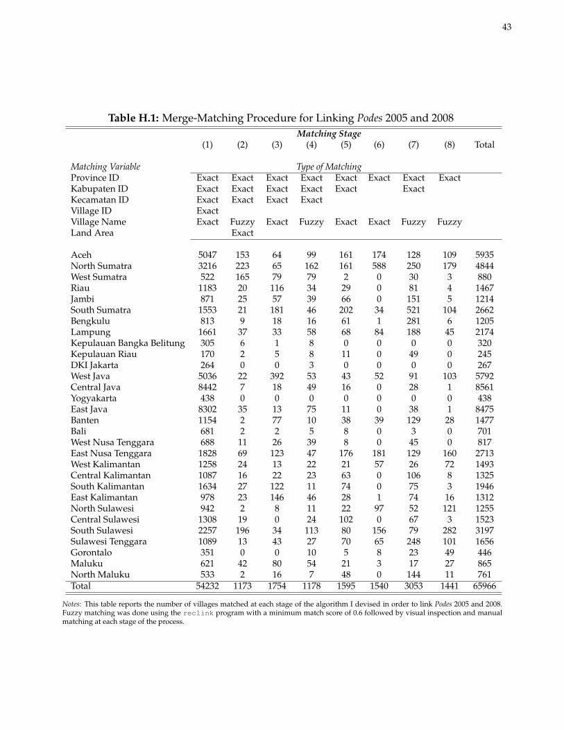
43

Table H.1: Merge-Matching Procedure for Linking Podes 2005 and 2008Matching Stage

(1) (2) (3) (4) (5) (6) (7) (8) Total

Matching Variable Type of MatchingProvince ID Exact Exact Exact Exact Exact Exact Exact ExactKabupaten ID Exact Exact Exact Exact Exact ExactKecamatan ID Exact Exact Exact ExactVillage ID ExactVillage Name Exact Fuzzy Exact Fuzzy Exact Exact Fuzzy FuzzyLand Area Exact

Aceh 5047 153 64 99 161 174 128 109 5935North Sumatra 3216 223 65 162 161 588 250 179 4844West Sumatra 522 165 79 79 2 0 30 3 880Riau 1183 20 116 34 29 0 81 4 1467Jambi 871 25 57 39 66 0 151 5 1214South Sumatra 1553 21 181 46 202 34 521 104 2662Bengkulu 813 9 18 16 61 1 281 6 1205Lampung 1661 37 33 58 68 84 188 45 2174Kepulauan Bangka Belitung 305 6 1 8 0 0 0 0 320Kepulauan Riau 170 2 5 8 11 0 49 0 245DKI Jakarta 264 0 0 3 0 0 0 0 267West Java 5036 22 392 53 43 52 91 103 5792Central Java 8442 7 18 49 16 0 28 1 8561Yogyakarta 438 0 0 0 0 0 0 0 438East Java 8302 35 13 75 11 0 38 1 8475Banten 1154 2 77 10 38 39 129 28 1477Bali 681 2 2 5 8 0 3 0 701West Nusa Tenggara 688 11 26 39 8 0 45 0 817East Nusa Tenggara 1828 69 123 47 176 181 129 160 2713West Kalimantan 1258 24 13 22 21 57 26 72 1493Central Kalimantan 1087 16 22 23 63 0 106 8 1325South Kalimantan 1634 27 122 11 74 0 75 3 1946East Kalimantan 978 23 146 46 28 1 74 16 1312North Sulawesi 942 2 8 11 22 97 52 121 1255Central Sulawesi 1308 19 0 24 102 0 67 3 1523South Sulawesi 2257 196 34 113 80 156 79 282 3197Sulawesi Tenggara 1089 13 43 27 70 65 248 101 1656Gorontalo 351 0 0 10 5 8 23 49 446Maluku 621 42 80 54 21 3 17 27 865North Maluku 533 2 16 7 48 0 144 11 761Total 54232 1173 1754 1178 1595 1540 3053 1441 65966

Notes: This table reports the number of villages matched at each stage of the algorithm I devised in order to link Podes 2005 and 2008.Fuzzy matching was done using the reclink program with a minimum match score of 0.6 followed by visual inspection and manualmatching at each stage of the process.

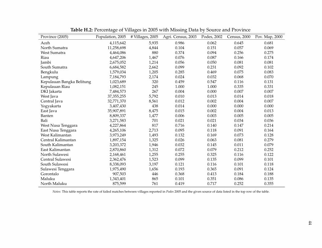
44

Table H.2: Percentage of Villages in 2005 with Missing Data by Source and ProvinceProvince (2005) Population, 2005 # Villages, 2005 Agri. Census, 2003 Podes, 2002 Census, 2000 Pov. Map, 2000

Aceh 4,115,642 5,935 0.986 0.062 0.645 0.681North Sumatra 11,258,698 4,844 0.104 0.151 0.057 0.069West Sumatra 4,464,086 880 0.374 0.094 0.256 0.275Riau 4,647,206 1,467 0.076 0.087 0.166 0.174Jambi 2,675,052 1,214 0.056 0.050 0.081 0.081South Sumatra 6,684,582 2,662 0.099 0.231 0.092 0.102Bengkulu 1,579,034 1,205 0.285 0.469 0.075 0.083Lampung 7,184,793 2,174 0.024 0.032 0.068 0.070Kepulauan Bangka Belitung 1,023,689 320 0.459 0.547 0.116 0.131Kepulauan Riau 1,082,151 245 1.000 1.000 0.335 0.331DKI Jakarta 7,484,573 267 0.004 0.000 0.007 0.007West Java 37,355,255 5,792 0.010 0.013 0.014 0.018Central Java 32,771,370 8,561 0.012 0.002 0.004 0.007Yogyakarta 3,407,430 438 0.014 0.000 0.000 0.000East Java 35,907,891 8,475 0.015 0.002 0.004 0.013Banten 8,809,337 1,477 0.006 0.003 0.005 0.005Bali 3,271,583 701 0.021 0.021 0.034 0.036West Nusa Tenggara 4,227,864 817 0.716 0.140 0.147 0.214East Nusa Tenggara 4,265,106 2,713 0.095 0.118 0.091 0.164West Kalimantan 3,973,249 1,493 0.132 0.169 0.073 0.128Central Kalimantan 1,897,154 1,325 0.026 0.063 0.081 0.279South Kalimantan 3,203,372 1,946 0.032 0.145 0.011 0.079East Kalimantan 2,870,860 1,312 0.072 0.079 0.212 0.252North Sulawesi 2,168,461 1,255 0.255 0.325 0.116 0.122Central Sulawesi 2,362,476 1,523 0.099 0.135 0.099 0.101South Sulawesi 8,338,093 3,197 0.121 0.116 0.101 0.118Sulawesi Tenggara 1,975,490 1,656 0.193 0.365 0.091 0.124Gorontalo 907,503 446 0.368 0.413 0.184 0.188Maluku 1,343,401 865 0.101 0.351 0.086 0.135North Maluku 875,599 761 0.419 0.717 0.252 0.355

Notes: This table reports the rate of failed matches between villages reported in Podes 2005 and the given source of data listed in the top row of the table.

45

ReferencesAbramitzky, R., L.P. Boustan, and K. Eriksson, “Have the poor always been less likely to migrate? Evidence from

inheritance practices during the Age of Mass Migration,” Journal of Development Economics, 2013, 102, 2–14.

Armenter, R. and M. Koren, “A Balls-and-Bins Model of Trade,” American Economic Review, 2014, 104 (7), 2127–2151.

Bachtiar, P. B., “The Governance of Indonesian Overseas Employment in the Context of Decentralization,” SMERUResearch Institute Working Paper, 2011.

Bank Indonesia, “Survei Nasional Pola Remitansi TKI,” Special Report, 2009.

Bazzi, S., “A Note on Heterogeneity and Aggregation Using Data on Agricultural Productivity,” Unpublished note,2012b.

, A. Gaduh, A. Rothenberg, and M. Wong, “Skill Transferability, Migration, and Development: Evidence fromPopulation Resettlement in Indonesia,” American Economic Review, forthcoming.

Benjamin, D., “Can unobserved land quality explain the inverse productivity relationship?,” Journal of DevelopmentEconomics, 1995, 46, 51–84.

Cameron, A. C., J. B. Gelbach, and D. L. Miller, “Bootstrap-based Improvements for Inference with Clustered Er-rors,” Review of Economics and Statistics, 2008, 90 (3), 414–427.

, , and , “Robust inference with multi-way clustering,” Journal of Business and Economic Statistics, 2011, 28,238–249.

Chambers, M.J. and R.E. Bailey, “A theory of commodity price fluctuations,” Journal of Political Economy, 1996,pp. 924–957.

Das, M., W.K. Newey, and F. Vella, “Nonparametric estimation of sample selection models,” Review of EconomicStudies, 2003, 70 (1), 33–58.

Dawe, D., “Can Indonesia Trust the World Rice Market?,” Bulletin of Indonesian Economic Studies, 2008, 44 (1), 115–132.

de Jonge, H.M.C. and N.J.G. Kaptein, Transcending borders: Arabs, politics, trade and Islam in Southeast Asia, Leiden:KITLV Press, 2002.

Dickey, D. A. and W. A. Fuller, “Distribution of the estimators for autoregressive time series with a unit root,” Journalof the American Statistical Association, 1979, 74, 427–431.

Fitrani, F., B. Hofman, and K. Kaiser, “Unity in Diversity? The Creation of New Local Governments in a Decentral-izing Indonesia,” Bulletin of Indonesian Economic Studies, 2005, 41, 57–79.

Friedman, J. and J. A. Levinsohn, “The Distributional Impacts of Indonesia’s Financial Crisis on Household Welfare:A “Rapid Response” Methodology,” NBER Working Paper No. 8564, 2001.

Fuglie, K. O., “Productivity growth in Indonesian agriculture, 1961-2000,” Bulletin of Indonesian Economic Studies,2010, 40, 209–225.

Gabaix, X., “Power Laws in Economics and Finance,” Annual Review of Economics, 2009, 1, 255–293.

and R. Ibragimov, “Rank-1/2: A Simple Way to Improve the Estimation of Tail Exponents,” Journal of Business andEconomic Statistics, 2011, 29 (1), 24–39.

Gallant, A. R. and D. W. Nychka, “Semi-nonparametric maximum likelihood estimation,” Econometrica, 1987, 55 (2),363–390.

Heckman, J. J., “The common structure of statistical models of truncation, sample selection and limited dependentvariables and a simple estimator for such models,” NBER Chapters, 1976, pp. 120–137.

Im, K.S., M.H. Pesaran, and Y. Shin, “Testing for unit roots in heterogeneous panels,” Journal of Econometrics, 2003,115, 53–74.

Jayachandran, S., “Selling labor low: Wage responses to productivity shocks in developing countries,” Journal ofPolitical Economy, 2006, 114 (3), 538–575.

Levine, D. and D. Yang, “The Impact of Rainfall on Rice Output in Indonesia,” NBER Working Paper No. 20302, 2014.

Lineton, Jacqueline, “Pasompe’Ugi’: Bugis migrants and wanderers,” Archipel, 1975, 10 (1), 173–201.

Maccini, S. and D. Yang, “Under the Weather: Health, Schooling, and Economic Consequences of Early-Life Rain-fall,” American Economic Review, 2009, 99 (3), 1006–1026.

McKenzie, D. and H. Rapoport, “Network effects and dynamics of migration and inequality: Theory and evidencefrom Mexico,” Journal of Development Economics, 2007, 84 (1), 1–24.

Mundlak, Y., D. Larson, and R. Butzer, “Agricultural dynamics in Thailand, Indonesia and the Philippines,” Aus-

46

tralian Journal of Agricultural and Resource Economics, 2004, 48 (1), 95–126.

Munshi, K., “Networks in the Modern Economy: Mexican Migrants in the U.S. Labor Market,” Quarterly Journal ofEconomics, 2003, 118 (2), 549–599.

Naylor, R. L., W. P. Falcon, D. Rochberg, and N. Wada, “Using El Nino/Southern Oscillation climate data to predictrice production in Indonesia,” Climatic Change, 2001, 50, 255–265.

Newey, W. K., “Two-step series estimation of sample selection models,” Unpublished manuscript, 1988.

, “Two-step series estimation of sample selection models,” The Econometrics Journal, 2009, 12, S217–S229.

and D. McFadden, “Large sample estimation and hypothesis testing,” Handbook of Econometrics, 1994, 4, 2111–2245.

Poirier, D., “Partial Observability in Bivariate Probit Models,” Journal of Econometrics, 1980, 12 (2), 209–217.

Rochina-Barrachina, M. E., “A new estimator for panel data sample selection models,” Annales d’Economie et deStatistique, 1999, 55-56, 153–181.

Skoufias, E., A. Narayan, K. Kaiser, and B. Dasgupta, “Electoral Accountability, Fiscal Decentralization and ServiceDelivery in Indonesia,” World Bank Policy Research Working Paper, 2010.

Suryahadi, A., W. Widyanti, R. Prama Artha, D. Perwira, and S. Sumarto, “Developing a Poverty Poverty Map forIndonesia: A Tool for Better Targeting in Poverty Reduction and Social Protection Programs, Book 1: TechnicalReport,” SMERU Research Report, 2005.

Timmer, C. P., “Causes of High Food Prices,” Asian Development Bank Working Paper, 2008, 128.

Vothknecht, M. and S. Sumarto, “Violent Conflict and Economic Growth: Evidence from Indonesian Villages,”Unpublished manuscript, 2009.

Warr, P., “Food policy and poverty in Indonesia: a general equilibrium analysis,” Australian Journal of Agriculturaland Resource Economics, 2005, 49 (4), 429–451.

, “The transmission of import prices to domestic prices: an application to Indonesia,” Applied Economics Letters,2008, 15, 499–503.

Wimanda, R. E., “Price variability and price convergence: Evidence from Indonesia,” Journal of Asian Economics, 2009,20 (4), 427–442.

Yamagata, T., “The small sample performance of the Wald test in the sample selection model under the multi-collinearity problem,” Economics Letters, 2006, 93 (1), 75–81.

Zellner, A. and T. H. Lee, “Joint estimation of relationships involving discrete random variables,” Econometrica, 1965,33 (2), 382–394.

Zivot, E. and D. W. K. Andrews, “Further evidence on the great crash, the oil-price shock, and the unit-root hypoth-esis,” Journal of Business and Economic Statistics, 2002, 20, 25–44.