JYRI SAARIKOSKI

On Text Document Classification and Retrieval Using Self-Organising Maps

ACADEMIC DISSERTATIONTo be presented, with the permission of

the Board of the School of Information Sciences of the University of Tampere,for public discussion in the Paavo Koli Auditorium, Kanslerinrinne 1,

Tampere, on November 17th, 2014, at 12 o’clock.

UNIVERSITY OF TAMPERE

JYRI SAARIKOSKI

On Text Document Classification and Retrieval Using Self-Organising Maps

Acta Universi tati s Tamperensi s 1993Tampere Universi ty Pres s

Tampere 2014

ACADEMIC DISSERTATIONUniversity of TampereSchool of Information Sciences Finland

Copyright ©2014 Tampere University Press and the author

Cover design byMikko Reinikka

Acta Universitatis Tamperensis 1993 Acta Electronica Universitatis Tamperensis 1480ISBN 978-951-44-9626-4 (print) ISBN 978-951-44-9627-1 (pdf )ISSN-L 1455-1616 ISSN 1456-954XISSN 1455-1616 http://tampub.uta.fi

Suomen Yliopistopaino Oy – Juvenes PrintTampere 2014 441 729

Painotuote

Distributor:kirjamyynti@juvenes.fihttp://granum.uta.fi

The originality of this thesis has been checked using the Turnitin OriginalityCheck service in accordance with the quality management system of the University of Tampere.

i

Abstract

Information retrieval (IR) focuses on providing means to find relevant information according to users' information needs. The most common task in IR is to automatically find relevant text documents from a data collection based on a user-generated search query. The search engines are the solution to this task. The IR research also deals with other information-related tasks, like text document classification and filtering. Machine learning methods, like unsupervised self-organising maps (SOMs), are able to automatically classify data. This thesis explores the possibilities to use SOMs in information retrieval tasks. The main focus was on classification of news document collections, but document retrieval was also considered. First, a SOM-based search engine prototype was developed with encouraging results. Then, extensive text document classification experiments with SOMs were carried out using four different data collections including English, German and Spanish news articles. The classification performance was compared against eight established machine learning methods. During this research the novel set of SOMs approach was introduced as an improvement to the original SOM classification. The SOM classification performed mostly very well with over 90% classification accuracies being the best of tested unsupervised methods, and, in some cases, comparable against some supervised methods. The set of 10 SOMs approach improved the SOM classification clearly and performed comparably against the best supervised methods. Moreover, the visual map generated by the SOM method proved to be a useful asset in IR tasks. The results strongly state that self-organising maps are an effective means in information retrieval. Additionally, the recently introduced scatter method was evaluated in dimensionality reduction of text data and it proved to be viable. The effects of training data quality on document classification of machine learning methods were also researched the main outcome being that low quality, noisy, data should be added into training set only if there is very much of it.

Keywords: Information retrieval, Text Classification, Data mining, Machine learning, Neural networks, Self-organising maps, Data collections, Text documents

ii

iii

Acknowledgements

First of all, I wish to warmly thank my supervisors, Professor Martti Juhola, Ph.D., Professor Kalervo Järvelin, Ph.D., and Docent Jorma Laurikkala, Ph.D, for all the invaluable guidance and support during this thesis project. The vast expertise in this team of supervisors has surely been much more than I would have ever deserved. Secondly, I also wish to thank the other co-writers of my publications, Henry Joutsijoki, Ph.D., who helped me with the support vector machines, and Markku Siermala, Ph.D., who supported with the scatter method.

I have had great time working with the inspiring people of the School of Information Sciences. Especially, I am very grateful to Kirsi Varpa, M.Sc., and Henry Joutsijoki for friendship and the almost daily discussions about varying topics of life and computer science. I would also like to thank all the members of our Data Analysis Research Group (DARG). More specifically, Jyrki Rasku, Ph.D., Kati Iltanen, Ph.D., Mika Rantanen, Ph.D., Yevhen Zolotavkin, Ph.D., Youming Zhang, Ph.D., and Xingan Li, Ph.D., have been there for me whenever I have needed help. The former DARG members Tuomas Talvensaari, Ph.D., Pekka Niemenlehto, Ph.D., and Antti Järvelin, Ph.D., helped me a lot in the early years of my thesis project. I also wish to thank the helpful administration staff of the school.

Special thanks go to the floorball teams of both the University, Yliopiston Sammakot, and our school. The weekly floorball games at Atalpa have been most relaxing and sometimes, if not always, much more important to me than the research and work. I would like to thank Jorma Laurikkala for his important work as the captain of our school’s floorball team, and Erkki Mäkinen for his excellent passes throughout these years.

This thesis was funded by Tampere Doctoral Programme in Information Science and Engineering (TISE), Alfred Kordelin Trust Fund, Emil Aaltonen Foundation, The Finnish Cultural Foundation, Oskar Öflund Foundation and the City of Tampere Science Fund. Supercomputer resources of the Finnish IT Center for Science (CSC) were also used. I am very grateful for this invaluable support.

I would also like to thank the members of my family. First of all, I wish to thank my brothers, Joni and Juha, for all the activities, usually dealing with long

iv

distance running and floorball, which have been able to keep my thoughts as far away as possible from my work topics. Secondly, I want to thank my parents, Sinikka and Olavi, and my in-laws, Tuula and Jouko, for those numerous extra hours of babysitting because of my work deadlines. Finally, I wish to thank my lovely sons, Eetu and Osku, the true researchers of life, and my dear wife Anne for all the love and the seemingly endless patience and belief during this long project.

Tampere, September 2014 Jyri Saarikoski

v

Contents

1 Introduction ....................................................................................................................... 1

2 Information Retrieval ....................................................................................................... 5

2.1 Text Retrieval ............................................................................................................ 5

2.2 Vector Space Model ................................................................................................. 7

2.3 Text Classification .................................................................................................. 10

2.4 Relevance ................................................................................................................. 12

2.5 Other Research Areas ............................................................................................ 14

3 Machine Learning ............................................................................................................ 15

3.1 Classification ........................................................................................................... 15

3.2 Learning Paradigms ............................................................................................... 17

3.3 Methods Applied .................................................................................................... 17

4 Self-Organising Maps ..................................................................................................... 21

4.1 SOM Algorithm ...................................................................................................... 21

4.2 Classification using SOMs .................................................................................... 24

4.3 Set of SOMs ............................................................................................................ 25

4.4 Related work ........................................................................................................... 26

vi

5 Evaluation......................................................................................................................... 27

5.1 Text Retrieval Evaluation ..................................................................................... 27

5.2 Text Classification Evaluation ............................................................................. 28

5.2.1 Training and Test Sets ...................................................................................... 28

5.2.2 Evaluation Measures ......................................................................................... 29

6 Results ............................................................................................................................... 33

6.1 Publication I: Text Retrieval with SOMs ........................................................... 33

6.2 Publication II: Text Classification with SOMs .................................................. 35

6.3 Publication III: Text Classification with SOMs ................................................ 36

6.4 Publication IV: Dimensionality Reduction in Text Classification .................. 37

6.5 Publication V: Training Data Quality and the Set of SOMs ........................... 39

7 Discussion and Conclusions .......................................................................................... 43

8 Personal Contributions................................................................................................... 49

Bibliography

Publications I - V

vii

List of Abbreviations

Abbreviation SOM

Description Self-organising map

BMU Best matching unit CLEF Conference and Labs of the Evaluation Forum CLIR Cross-language information retrieval FN False negative FP False positive HTML HyperText Markup Language IR Information retrieval IS Information seeking k-NN k nearest neighbour searching LDA Linear discriminant analysis LVQ Learning vector quantization SGML Standard Generalized Markup Language SVM Support vector machine TN True negative TNR True negative rate TP True positive TPR True positive rate TREC Text REtrieval Conference

viii

ix

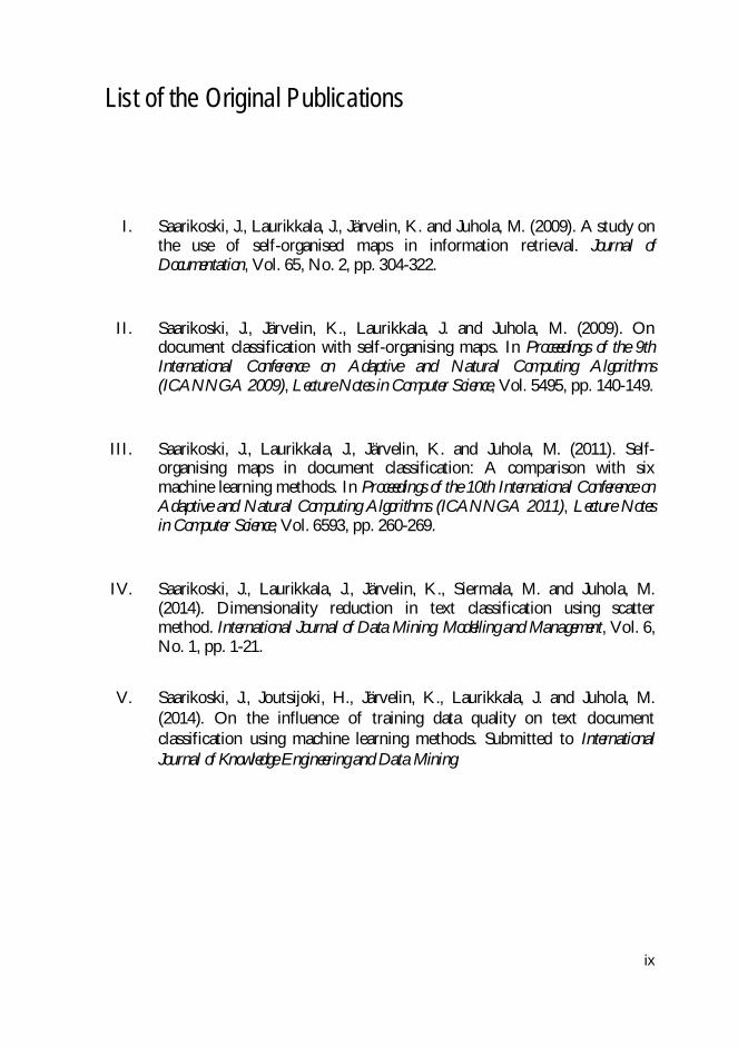
List of the Original Publications

I. Saarikoski, J., Laurikkala, J., Järvelin, K. and Juhola, M. (2009). A study on the use of self-organised maps in information retrieval. Journal of Documentation, Vol. 65, No. 2, pp. 304-322.

II. Saarikoski, J., Järvelin, K., Laurikkala, J. and Juhola, M. (2009). On document classification with self-organising maps. In Proceedings of the 9th International Conference on Adaptive and Natural Computing Algorithms (ICANNGA 2009), Lecture Notes in Computer Science, Vol. 5495, pp. 140-149.

III. Saarikoski, J., Laurikkala, J., Järvelin, K. and Juhola, M. (2011). Self-organising maps in document classification: A comparison with six machine learning methods. In Proceedings of the 10th International Conference on Adaptive and Natural Computing Algorithms (ICANNGA 2011), Lecture Notes in Computer Science, Vol. 6593, pp. 260-269.

IV. Saarikoski, J., Laurikkala, J., Järvelin, K., Siermala, M. and Juhola, M. (2014). Dimensionality reduction in text classification using scatter method. International Journal of Data Mining, Modelling and Management, Vol. 6, No. 1, pp. 1-21.

V. Saarikoski, J., Joutsijoki, H., Järvelin, K., Laurikkala, J. and Juhola, M.

(2014). On the influence of training data quality on text document classification using machine learning methods. Submitted to International Journal of Knowledge Engineering and Data Mining.

x

1

1 Introduction

The internet has become a major source of information in the Western world during the last 20 years. If one needs to find information about something, one usually makes a web search about it. The search engine needs just a few words related to the topic of interest and it is able to find relevant information quickly and accurately. At least, this is how the user expects the search engine to work. The research of information retrieval (IR) focuses on providing the means to meet these user expectations. Although there are multiple research areas in IR, in practice the main focus is on the development and evaluation of search engines. In the 1990's the desktop computer was by far the main machine capable of accessing the internet, but nowadays there are also laptops and a large variety of hand-held mobile devices with constant wireless internet connections, which enables users to browse and search the internet for any information virtually anywhere and at any time. The majority of us are using search engines every day both at work and home, even outdoors. Obviously, this development has made IR even more important field of study than it was earlier.

Although the internet is full of data in different formats (image, audio, video, multimedia), the majority of data, and searching, is still textual. The amount of online text data is so massive, that it is practically impossible to find the relevant data samples needed just by browsing through it. This is where sophisticated IR systems are needed. The systems are able to find highly relevant information or to categorize data under topical labels (like “sports”, “politics” or “science”). The former is what search engines do and the latter is called text classification. Searching aims to find the information needed while classification groups the data meaningfully in order to make the browsing, or searching, easier.

Data mining deals with automatic analysis and modelling of large data repositories. Machine learning algorithms are widely used in the data mining tasks. From the data mining point of view, text classification is predictive modelling of text document data, which makes machine learning methods, like self-organising maps (SOMs), a natural solution to the classification problem.

The self-organising maps method caught our interest in the first place for its aesthetic and intuitive visualisation abilities: SOMs are able to cluster high-

2

dimensional data to a low-dimensional map surface preserving the relations of the data samples as distances on the map. In our preliminary studies the SOM clustering of text documents seemed to be, at least visually, meaningful, which raised the question if the maps could also perform well in text document retrieval (ad hoc searching), as a search engine. At least, it seemed to be very promising candidate for text classification. Another interesting possibility was the visual output of SOMs itself. Although the devices are using more and more visual interfaces, the most popular web search engines, such as Google, Bing and Yahoo, are all still strongly text-based: the search results are shown as lists of links. However, SOMs are able to give intuitive visual representation of results with their map interface and the map view could also be useful in visualisation of classification results [68, 74, 75, 115]. Our literature search revealed that SOMs were used in classification tasks of text documents, but the text retrieval was researched in just a few brief studies [34, 69]. There were not much comparison results or testing with multiple data collections available, even considering the SOM classification. This was the motivation for this thesis, and therefore, the main research problem at the starting point of this thesis was simply:

- Are self-organising maps an effective method in information retrieval tasks?

This basic problem led quickly to many other questions, such as:

- How does one build a search engine based on SOMs? - How well does such search engine retrieve relevant documents? - Are SOMs effective in text classification? - Is the unsupervised learning of SOMs able to compete against well-known

supervised machine learning methods in text classification? How well do SOMs perform when compared to other unsupervised methods?

- Is it possible to develop the SOM method further to achieve better results in IR tasks?

- Is the map view generated by the method useful in IR? To sum up, the usage of SOMs in information retrieval seemed to be full of interesting questions and possibilities. Our main target was to generate actual numerical results about the SOM performance in information retrieval and provide comparison against other widely used machine learning methods in text classification. From that point of view, the “effectiveness” mentioned above could

3

be seen as ability to perform equally, or better, than the well-known baseline methods, such as k nearest neighbour searching or Naïve Bayes in text classification.

We started our research by studying the text document retrieval capabilities of SOMs. The Publication I introduced our search engine prototype based on self-organising maps. The outcome of this early research shifted our main focus from text searching towards text classification, while it became very clear that the topical grouping of documents was the key to successful information retrieval with SOMs. In Publications II and III, we classified text documents automatically using slightly modified self-organising maps performing classification instead of clustering. The SOM classification experiments of Publication II were carried out using one data set and two baseline methods for comparison. In Publication III, we used three data sets and six baseline machine learning methods in order to get a more complete evaluation of the SOM performance. After these experiments, we still continued the study of text classification and SOMs, but tackled some more general topics at the same time. Publication IV was about dimensionality reduction methods in text classification. We used SOMs in this paper, but the main focus was on the recently introduced scatter method, which we evaluated as a promising candidate for dimensionality reduction of text document data. Finally, in Publication V, we studied the effects of training data quality on document classification of machine learning methods. We included the self-organising maps again among the tested methods. The secondary goal of this final paper was to develop the SOM classification procedure further to achieve better results. This research was successful and we introduced the novel set of SOMs classification approach. Overall, these five publications provide an extensive evaluation of SOMs as a text classification method and gave some idea and evaluation of the possibilities to use SOMs in document retrieval. We also introduced some improvements to SOM classification and studied more general ideas about the dimensionality reduction of text data and training data quality of machine learning methods.

The rest of the introductory part of this thesis provides the background information needed to read and understand the attached Publications I-V. First, the basics of information retrieval and machine learning are introduced in Chapters 2 and 3. In Chapter 4, we are focusing on the self-organising maps. Then, in Chapter 5, the evaluation methods of text retrieval and classification are described. The Chapter 6 introduces the results of the individual publications. In Chapter 7

4

we discuss and sum up the outcome of the thesis. Finally, the last chapter is clarifying the personal contributions of the author.

5

2 Information Retrieval

Information retrieval deals with the representation, storage, organization of, and access to information items. [8]

The definition of information retrieval (IR) is relatively broad. First of all, "information item" is very general concept including, for example, text, speech, music, image and video. Still, the focus of IR research is heavily on text documents and the retrieval of other media types is usually text-based as well [25]. Secondly, representation, storage, organisation and access include a large variety of information-related tasks. Thus, it is nearly impossible to list all the possible tasks related to IR explicitly. However, the most common IR tasks are searching and classification with their many variations. This thesis deals with text classification (Publications II-V) and text retrieval (Publication I). Next, the basics of IR are introduced briefly. For more complete presentation, see [8]. More classical readings about IR can be found in [99, 111].

2.1 Text Retrieval

Text retrieval (ad hoc searching) is the main area of interest in IR. The aim is to develop effective search engines capable of finding relevant text documents according to user's information needs. In the usual search scenario the user has an information need, which he represents as a search query. After this, the search engine searches from its data collection text documents relevant to the query and ranks them as a list in decreasing order of relevance. This process seems simple, but poses multiple interesting problems.

Traditionally IR research has two different approaches: system-oriented and user-oriented. The system-oriented research deals with retrieval systems, which in practice means development of retrieval algorithms and models. In the user-oriented, or cognitive, approach, the focus is more on the user and user’s information needs. One of the main differences in these approaches is the interpretation of relevance: straightforward topical relevance versus more complex user relevance. In some contexts the user-oriented branch is called “Information

6

seeking” (IS), while the system-oriented is referred to as IR. The research of this thesis is system-oriented. More information about the system-oriented approach of IR can be found in [8, 25, 36], while [10, 50] discuss the IR from more user-oriented point of view.

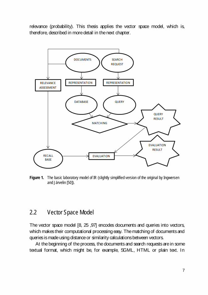
The theoretical framework of the system-oriented research, the basic laboratory model of IR, or the Cranfield model, is described in Figure 1. This classic evaluation model is all about documents, search requests, their matching and evaluation. Documents and search requests are processed resulting in document database and search queries. After this, a matching algorithm creates the retrieval results for the queries. The results are then compared to the recall base, which consists of the documents assessed relevant to each topic. This way the IR system performance can be systematically evaluated and further developed. In the Figure 1, the centremost parts (representation, database, query, matching and query results) belong to a working IR system, and the rest are parts of an evaluation system. The laboratory model is often criticised, for example, for the absence of user and for the technical system-oriented relevance approach (see, for example, [50]), but it is, however, widely used basis in system-oriented IR.

The retrieval model specifies the representations for documents and search requests, and also the matching of these two representations. There are plenty of retrieval models available [8, 25], but three of them are usually considered classical: Boolean model, vector space model and probabilistic model. Boolean model is an exact match model meaning that it retrieves only documents matching the query exactly, thus partially matching documents are ignored completely. In this model, a document is a set of index terms and a query is a set of index terms combined with Boolean operators. The matching algorithm finds all the documents fulfilling the requirements of the query, which is actually a Boolean expression. There is no ranking for the retrieved documents, thus they are all considered equally good, which is slightly problematic, at least, if the result set is large. Also, some important documents may only partially match the query, and, therefore, be completely ignored in this model. This problem can be solved using best match retrieval models, such as vector space model or probabilistic model. The vector space model treats documents and queries as vectors and the matching is done using proximity (similarity or distance) metrics. The probabilistic models rely on the so called Probabilistic Ranking Principle, which in brief is as follows: For a given query, estimate the probability for each document that the document belongs to the set of relevant documents and return the documents in ranked order of

7

relevance (probability). This thesis applies the vector space model, which is, therefore, described in more detail in the next chapter.

Figure 1. The basic laboratory model of IR (slightly simplified version of the original by Ingwersen and Järvelin [50]).

2.2 Vector Space Model

The vector space model [8, 25 ,97] encodes documents and queries into vectors, which makes their computational processing easy. The matching of documents and queries is made using distance or similarity calculations between vectors.

At the beginning of the process, the documents and search requests are in some textual format, which might be, for example, SGML, HTML or plain text. In

8

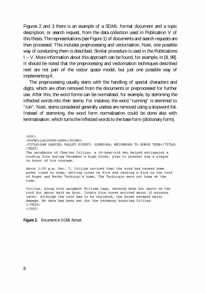
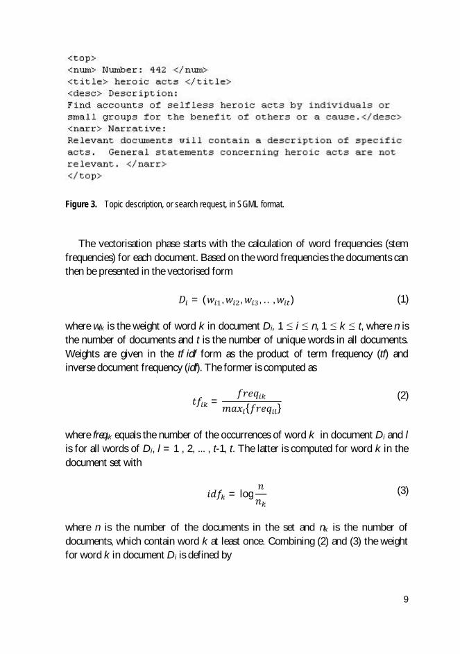
Figures 2 and 3 there is an example of a SGML format document and a topic description, or search request, from the data collection used in Publication V of this thesis. The representations (see Figure 1) of documents and search requests are then processed. This includes preprocessing and vectorisation. Next, one possible way of conducting them is described. Similar procedure is used in the Publications I – V. More information about this approach can be found, for example, in [8, 99]. It should be noted that the preprocessing and vectorisation techniques described next are not part of the vector space model, but just one possible way of implementing it.

The preprocessing usually starts with the handling of special characters and digits, which are often removed from the documents or preprocessed for further use. After this, the word forms can be normalised, for example, by stemming the inflected words into their stems. For instance, the word “running” is stemmed to “run”. Next, stems considered generally useless are removed using a stopword list. Instead of stemming, the word form normalisation could be done also with lemmatisation, which turns the inflected words to the base form (dictionary form).

Figure 2. Document in SGML format.

9

Figure 3. Topic description, or search request, in SGML format.

The vectorisation phase starts with the calculation of word frequencies (stem

frequencies) for each document. Based on the word frequencies the documents can then be presented in the vectorised form

= ( , , , … , ) (1)

where wik is the weight of word k in document Di, 1 i n, 1 k t, where n is the number of documents and t is the number of unique words in all documents. Weights are given in the tf·idf form as the product of term frequency (tf) and inverse document frequency (idf). The former is computed as

= { } (2)

where freqik equals the number of the occurrences of word k in document Di and l is for all words of Di, l = 1 , 2, ... , t-1, t. The latter is computed for word k in the document set with

= log (3)

where n is the number of the documents in the set and nk is the number of documents, which contain word k at least once. Combining (2) and (3) the weight for word k in document Di is defined by

10

= (4)

There are multiple versions of tf·idf weighting and other weighting schemes available (see, for example, [81, 98]). After these actions each document is represented by a document vector. The whole document collection can be seen as a matrix, where rows represent documents and columns represent all the words of the collection, the vocabulary. At this point the dimensionality of document vectors can be reduced in order to reduce the computational costs, if necessary. A comprehensive summary of dimensionality reduction methods is given in [102]. Similar vectorisation is also done for the search request. In the case of the search request in Figure 3, the query vector is usually constructed using the words of the title and description parts. The matching of query and document vectors is often calculated using cosine similarity. After matching of a query and all the documents in the collection, a ranked list of documents in decreasing order of estimated relevance, the query result, is constructed. The result can then be evaluated using relevance information of recall base (see Figure 1). The evaluation is discussed in Chapter 5.

2.3 Text Classification

Text classification, or text categorisation, is the process of automatically assigning labels (or classes) from a predefined set to documents. Text classification is an independent field of IR, but it can be also used as a way to improve the search engines [25, 102], for example using a classifier to group the search results meaningfully.

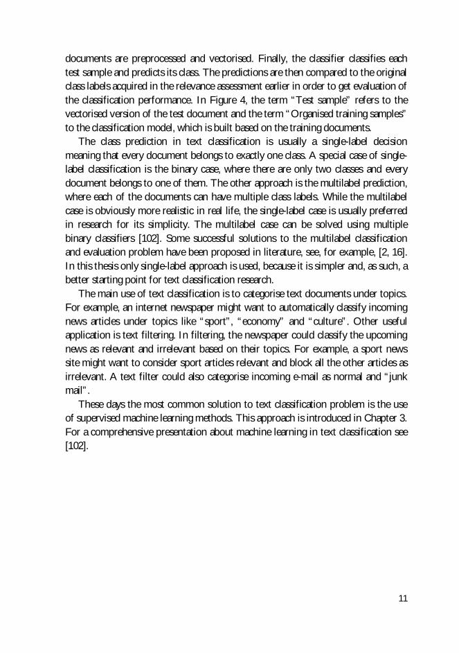
The basics of text classification research are mostly the same as in text retrieval, however the evaluation model (Figure 1) is slightly modified, see Figure 4. The preprocessing and the vector space model can be used similarly to vectorise the documents. However, the aim of the classification model is to predict the correct classes for previously unknown documents. Thus, the documents are initially divided into training and test sets for evaluation purposes. The relevance assessment for the documents, both training and test documents, is done basically in the same way as in searching, but the question is slightly different: “Does this document belong to the class X?” As the result of the assessment the documents are categorised, labelled, to predefined classes. First, the system acquires only the training documents and it builds the classifier based on them. Then, the test

11

documents are preprocessed and vectorised. Finally, the classifier classifies each test sample and predicts its class. The predictions are then compared to the original class labels acquired in the relevance assessment earlier in order to get evaluation of the classification performance. In Figure 4, the term “Test sample” refers to the vectorised version of the test document and the term “Organised training samples” to the classification model, which is built based on the training documents.

The class prediction in text classification is usually a single-label decision meaning that every document belongs to exactly one class. A special case of single-label classification is the binary case, where there are only two classes and every document belongs to one of them. The other approach is the multilabel prediction, where each of the documents can have multiple class labels. While the multilabel case is obviously more realistic in real life, the single-label case is usually preferred in research for its simplicity. The multilabel case can be solved using multiple binary classifiers [102]. Some successful solutions to the multilabel classification and evaluation problem have been proposed in literature, see, for example, [2, 16]. In this thesis only single-label approach is used, because it is simpler and, as such, a better starting point for text classification research.

The main use of text classification is to categorise text documents under topics. For example, an internet newspaper might want to automatically classify incoming news articles under topics like “sport”, “economy” and “culture”. Other useful application is text filtering. In filtering, the newspaper could classify the upcoming news as relevant and irrelevant based on their topics. For example, a sport news site might want to consider sport articles relevant and block all the other articles as irrelevant. A text filter could also categorise incoming e-mail as normal and “junk mail”.

These days the most common solution to text classification problem is the use of supervised machine learning methods. This approach is introduced in Chapter 3. For a comprehensive presentation about machine learning in text classification see [102].

12

Figure 4. System-oriented model for text classification. The model is based on the basic laboratory model of IR (Figure 1).

2.4 Relevance

The most fundamental concept in IR is relevance [12, 24, 45, 50, 100]. The basic idea of relevance is very simple: a relevant document contains the information that user is looking for. Yet, there are multiple types of relevance, which makes the concept more complex. The classical types are topical relevance and user relevance. Simply put, a document is topically relevant to a query, if it is on the same topic, and relevant to a user, if the user considers it to be relevant. It is easy to understand that these relevance types are very different from each other. For example, if a user makes a search with the query “Lasse Virén Montreal Olympic marathon”, which is very precisely formulated, he might not consider some of the retrieved documents relevant, even if they are about both the distance runner

13

called Lasse Virén and the Olympic marathon of Montreal, because he might have already read the documents earlier, or the documents are written in French, which he does not understand. Still, all these documents are topically highly relevant. Another point of view to relevance is algorithmic relevance, which is the relevance level determined by the retrieval model of a retrieval algorithm. In other words, it is the degree of match between a document and a search query. The discussion, and the criticism, about the relevance types used in IR research is, at the same time, discussion about the evaluation of IR, because the evaluation is fully based on the relevance assessment of documents. This means that if inappropriate relevance type is used the evaluation is failing to measure the intended retrieval performance. A more detailed discussion about the many dimensions of relevance is well beyond the scope of this thesis.

In IR research the evaluation of relevance is traditionally considered to be binary, meaning that a document is either relevant or irrelevant to a query. In practice, however, there is relevance of many levels. For example, a newspaper article titled “Mo Farah finishes eighth on full London Marathon debut”, which is a sports article about London marathon 2014, is likely to be highly relevant to queries like “Mo Farah marathon” and “London Marathon 2014”, but only marginally relevant to the query “London city”. If only binary relevance scale is used, the article must be considered equally relevant to these three queries or irrelevant to the last one. Either way, some information about the relevance is lost. In order to better measure the relevance, graded relevance scales are suggested. One of them is the four-level scale introduced in [106]:

1. Irrelevant: The document does not contain any information about the

topic. 2. Marginally relevant: The document only points to the topic. It does not

contain more or other information than the topic description. Typical extent: one sentence or fact.

3. Fairly relevant: The document contains more information than the topic description, but the presentation is not exhaustive. In case of a multifaceted topic, only some of the subthemes or viewpoints are covered. Typical extent: one text paragraph, two or three sentences or facts.

4. Highly relevant: The document discusses the themes of the topic exhaustively. In case of a multifaceted topic, all or most subthemes or viewpoints are covered. Typical extent: several text paragraphs, at least 4 sentences or facts.

14

The evaluation of IR is still done based on binary relevance, even if the use of graded relevance assessments has been considered in many studies, see, for example, [56, 95, 96, 114].

In this thesis only topical relevance is considered as the approach is purely system and algorithm-oriented. Also, the evaluation (see Chapter 5) is done using only binary relevance based measures. In Publication V graded relevance assessment are used as a measure of data quality in text classification using machine learning methods.

2.5 Other Research Areas

First of all, it should be noted that there exist more advanced approaches to text retrieval than the basic model introduced here. For instance, interactive approaches, like user relevance feedback, have been conducted in order to achieve better results in search tasks. An overview of these approaches is available, for example in [8]. In addition to text document retrieval, classification and clustering, there are also many other interesting research areas in modern IR, for example: web searching, retrieval of different media types and cross-language IR (see, for instance, [25]). Although web searching is basically using the same principles and techniques as the “normal” text retrieval, there are some additional aspects in it. For example, the contents of the document are only one factor when considering the relevance and importance of the document in web environment, the other factor is the links from and to other documents. Also, the clear document boundaries might be very hard to determine in hypertext context. There are also other types of search environments, like desktop and enterprise searching, which need special solutions. The retrieval of non-textual media types, like image, audio, video and multimedia, is still often based on textual descriptors, but development of techniques based on other modalities is made as well, especially in image retrieval. Cross-language IR (CLIR) is aiming to break the language barriers in IR. CLIR focuses on finding relevant information in situation where the documents and the query are in different languages. As mentioned earlier, the scope of IR is very wide.

15

3 Machine Learning

Machine learning research aims to develop computer algorithms capable of automatically learning from experience [85]. The basics of the field are based on, for example, statistics, artificial intelligence, biology and information theory.

3.1 Classification

Data mining is “the analysis of (often large) observational data sets to find unsuspected relationships and to summarize the data in novel ways that are both understandable and useful to the data owner” [43]. The data mining objectives can be categorized to five different types (according to [43]):

1. Exploratory Data Analysis: Visual exploration of data without any clear

initial targets, For example: a coxcomb plot visualisation. 2. Descriptive Modelling: Description of the data. For example: clustering

and variable relationship modelling. 3. Predictive Modelling: Prediction of unknown variable based on the

known variables. For example: classification and regression. 4. Discovering Pattern and Rules: Aims to find patterns and rules in

databases. For example: association rule based techniques. 5. Retrieval by Content: Finding similar samples based on an example. For

example: image search action “find similar images”. The machine learning methods can be applied in all of the above mentioned data mining tasks, but classification, which is predictive modelling, is the most interesting from the viewpoint of the present thesis.

16

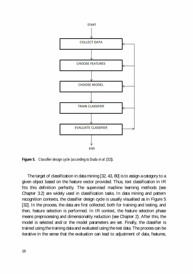
Figure 5. Classifier design cycle (according to Duda et al. [32]).

The target of classification in data mining [32, 43, 80] is to assign a category to a

given object based on the feature vector provided. Thus, text classification in IR fits this definition perfectly. The supervised machine learning methods (see Chapter 3.2) are widely used in classification tasks. In data mining and pattern recognition contexts, the classifier design cycle is usually visualised as in Figure 5 [32]. In the process, the data are first collected, both for training and testing, and then, feature selection is performed. In IR context, the feature selection phase means preprocessing and dimensionality reduction (see Chapter 2). After this, the model is selected and/or the model parameters are set. Finally, the classifier is trained using the training data and evaluated using the test data. The process can be iterative in the sense that the evaluation can lead to adjustment of data, features,

17

model parameters or training in order to achieve better performance. This approach is frequently used also in IR-related classification studies.

3.2 Learning Paradigms

The learning paradigms are the basis of machine learning. The paradigms are divided into supervised and unsupervised and reinforcement learning [44]. The division is made based on the availability of the external teacher during the learning process. In supervised learning, the external teacher is available. In classification context, this means that the classifier uses the class label information of training samples in classifier training. The situation in unsupervised learning is the opposite: the external teacher is not available. Unsupervised machine learning methods do not use the class label information of training data, and therefore, the methods are usually clustering methods. However, clustering methods can be used also in classification tasks with minor modifications (for example, see Chapter 4). In this case, the classification is of course also unsupervised. The reinforcement learning is theoretically positioned between supervised and unsupervised learning. This thesis, however, focuses only on supervised and unsupervised methods. More information about reinforcement learning can be found, for instance, in [85].

3.3 Methods Applied

In this chapter the machine learning methods applied in this thesis are introduced briefly. The unsupervised methods used were: self-organising maps, set of SOMs, k-means clustering and Ward’s clustering. The supervised methods used were: k nearest neighbour searching, linear discriminant analysis, decision tree classification, Naïve Bayes classifier, learning vector quantization and support vectors machines. The selected methods were all well-known and widely used machine learning methods. We wanted to select both supervised and unsupervised methods to get more complete comparison for SOMs. Most of the selected methods were supervised as they were expected to achieve better results.

Self-organising maps (SOMs) and its novel modification called the set of SOMs are artificial neural networks based on unsupervised learning. As SOMs are the main focus of this thesis, the method is introduced in detail in the next chapter.

18

Unsupervised k-means clustering is a simple clustering method. The algorithm creates k clusters and assigns data samples to the clusters with the nearest mean vector. After assignment the mean vectors are recalculated based on the samples in the cluster. This is iterated until the cluster means no longer change.

Ward’s clustering is an unsupervised hierarchical clustering method. At the beginning the method creates a cluster for each of the data samples. The method starts to join cluster pairs a pair at a time. At each stage the cluster pair whose merging minimizes the increase in the total within-group error sum of squares is joined.

The classic k nearest neighbours searching (k-NN) is a supervised classifier conducting instance-based learning. The class prediction is simply calculated based on the majority of class labels of the k nearest training samples in the training collection.

Linear discriminant analysis (LDA) is using supervised learning to find a linear combination of features which is able to separate the classes in the training data.

Decision tree classification is a supervised learner. The idea of the tree algorithm is to split the training set into subsets based on attribute values. The selection of these splitting attributes is based on (mathematical) information theory. This splitting is done recursively until conditions to stop the splitting are met.

Naïve Bayes classifier is a supervised probabilistic classifier, which is based on the Bayes' theorem including strong assumptions of feature independence. These assumptions are considered naive, which is the reason for the name of the classifier.

Learning vector quantization (LVQ) is yet another supervised classifier. The algorithm is prototype and winner-takes-all Hebbian learning-based. LVQ is related to self-organising maps and k nearest neighbour searching. The idea of LVQ is as follows. At the beginning, some number of prototype vectors is generated for each class in the training set. Then, the closest prototype vector is calculated for each training sample and the prototype is then either moved closer to the sample, if the classification was correct, or away from the sample, if the classification was incorrect.

Support vector machines (SVMs) use supervised means to construct a hyperplane, or multiple hyperplanes, in high-dimensional space to separate the classes from each other with maximum margin.

19

More information about the methods introduced here can be found in numerous text books of data mining, pattern recognition and machine learning, for example in [32, 43, 44, 63, 85].

20

21

4 Self-Organising Maps

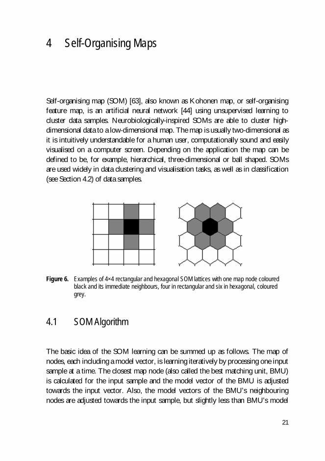
Self-organising map (SOM) [63], also known as Kohonen map, or self-organising feature map, is an artificial neural network [44] using unsupervised learning to cluster data samples. Neurobiologically-inspired SOMs are able to cluster high-dimensional data to a low-dimensional map. The map is usually two-dimensional as it is intuitively understandable for a human user, computationally sound and easily visualised on a computer screen. Depending on the application the map can be defined to be, for example, hierarchical, three-dimensional or ball shaped. SOMs are used widely in data clustering and visualisation tasks, as well as in classification (see Section 4.2) of data samples.

Figure 6. Examples of 4×4 rectangular and hexagonal SOM lattices with one map node coloured black and its immediate neighbours, four in rectangular and six in hexagonal, coloured grey.

4.1 SOM Algorithm

The basic idea of the SOM learning can be summed up as follows. The map of nodes, each including a model vector, is learning iteratively by processing one input sample at a time. The closest map node (also called the best matching unit, BMU) is calculated for the input sample and the model vector of the BMU is adjusted towards the input vector. Also, the model vectors of the BMU’s neighbouring nodes are adjusted towards the input sample, but slightly less than BMU’s model

22

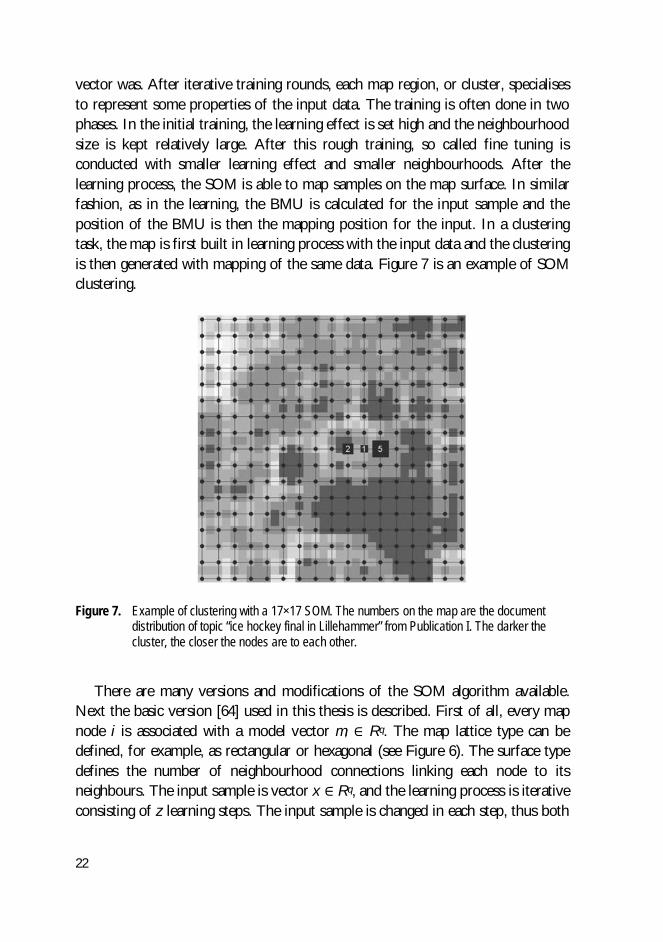
vector was. After iterative training rounds, each map region, or cluster, specialises to represent some properties of the input data. The training is often done in two phases. In the initial training, the learning effect is set high and the neighbourhood size is kept relatively large. After this rough training, so called fine tuning is conducted with smaller learning effect and smaller neighbourhoods. After the learning process, the SOM is able to map samples on the map surface. In similar fashion, as in the learning, the BMU is calculated for the input sample and the position of the BMU is then the mapping position for the input. In a clustering task, the map is first built in learning process with the input data and the clustering is then generated with mapping of the same data. Figure 7 is an example of SOM clustering.

Figure 7. Example of clustering with a 17×17 SOM. The numbers on the map are the document distribution of topic “ice hockey final in Lillehammer” from Publication I. The darker the cluster, the closer the nodes are to each other.

There are many versions and modifications of the SOM algorithm available.

Next the basic version [64] used in this thesis is described. First of all, every map node i is associated with a model vector mi Rq. The map lattice type can be defined, for example, as rectangular or hexagonal (see Figure 6). The surface type defines the number of neighbourhood connections linking each node to its neighbours. The input sample is vector x Rq, and the learning process is iterative consisting of z learning steps. The input sample is changed in each step, thus both

23

the map model vectors for each node i and the input vector are defined as a function of time: mi = mi(v) , x = x(v), where v = 0, 1,…, z - 1, and z is the total number of learning steps. The number of learning steps needed depends heavily on the data. Usually, it is advisable to go through the training data multiple times, for example ten times, but in some cases less is enough. Some practical suggestions are discussed in [63].

The basic SOM learning process can be described with the following algorithm:

1. Set v = 0 and initialise the map nodes mi(0) with small random values.

2. Find the best matching (closest) map node mc(v) for input x(v) based on the Euclidean distance:

( ) ( ) = min{ ( ) ( ) } (5)

3. Update the map nodes according to

( + 1) = ( ) + ( )[ ( ) ( )] (6)

where hci(v) is the neighbourhood kernel described below.

4. Set v = v + 1 and return to phase 2 if v <= z

The neighbourhood kernel controls the learning effect on the map surface. Often

( ) = ( , ) (7) where zc and zi are the position vectors of nodes c and i on the map. The learning effect is usually set to be higher near the node c and decreasing when moving away from it on map. The learning effect and the size of the effect area are also decreased over time (learning steps). For example, the so called “bubble” neighbourhood kernel is defined as follows:

( ) =( ) , ( )0 , ( ) (8)

24

where (v) is some monotonically decreasing function and 0 < (v) < 1, and Nc(v) consists of the node c, the BMU, and some set of the nearest neighbouring nodes around c. The neighbourhood is also getting smaller over time. It should be mentioned that, as well as there are multiple versions of SOM algorithm, there are also multiple neighbourhood kernel and distance metric options.

For more information and background of SOMs, see [63]. A recent overview of the SOM method and research can be found in [61].

4.2 Classification using SOMs

SOMs are using unsupervised learning and are, therefore, widely used in clustering tasks. However, SOM algorithm, and most of the other clustering algorithms as well, can be easily modified to perform also classification tasks.

First, the map needs to be labelled with the class labels of the training data set in some meaningful way. The labelled nodes then represent the classes and the map is able to classify unknown test samples by mapping them. The following simple algorithm can be implemented in order to use the self-organising maps in classification:

1. Create a self-organising map using a training data set.

2. Map each training set sample to the map by finding the BMU according to Euclidean distance.

3. Determine a class label for each node of the map according to the number

of training samples of different classes mapped on that node. The majority class determines the class of the node. In a tie case, label the node according to the class of the sample (from the tied classes) closest to the model vector of the node.

4. Map each of the test set samples to the labelled map by finding the BMU according to Euclidean distance. The class label of the map node is the class prediction for the test sample.

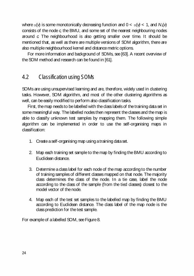
For example of a labelled SOM, see Figure 8.

25

Figure 8. Class labelled SOM from Publication III. Labels are #1 earn, #2 acq, #3 crude, #4 trade, #5 money-fx, #6 interest, #7 money-supply, #8 ship, #9 sugar and #10 coffee.

4.3 Set of SOMs

In Publication V, a novel set of SOMs method for SOM classification was introduced. The simple idea in this approach is to use multiple SOMs in class prediction of data samples. First, each map predicts the class for the unknown sample individually and the final class prediction is calculated based on the majority of the individual predictions. This approach is possible, because there is some randomness in the SOM algorithm, which leads to different predictions on different SOM runs. Using multiple maps and predictions seems to enhance the prediction performance by eliminating the random poor decisions (see the results section of Publication V).

26

4.4 Related work

The scope of SOMs is reasonably broad. The bibliography of SOM research papers [11] suggests that the most popular recent application fields of SOM method are clustering, visualisation and image-related tasks. From the point of view of this thesis, the most interesting application areas are information retrieval, especially text retrieval and text classification, and the visualisation and mining of text collections.

SOMs have been applied to many interesting IR and text mining tasks in the past two decades. Perhaps the most well-known example is the WEBSOM [46], which is designed for the data mining of large text collections. Also, some experiments of using SOMs in text retrieval have been made [31, 34, 69]. Text classification has been studied more frequently, for instance [14, 18, 28, 33, 40, 84], as well as text clustering, for example [4, 15, 21, 29]. Visualisation possibilities of SOM in IR context have been considered in [68, 74, 75, 115]. Mayer and Rauber [83] used SOMs in content analysis of WikiLeaks documents, Honkela et al. [47] introduced a multilingual document map based on SOMs and Kohonen and Xing [60] clustered Chinese words. Other SOM research in the IR field has included topics like web search personalisation [27], word sense discovery and disambiguation [76] and three-dimensional music archives [7]. Supervised SOM algorithms have been proposed in [13, 42, 63, 90, 116]. Multiple maps in SOM retrieval and classification have been suggested by [13, 34, 94]. In other research areas SOMs have been applied to, for instance, intrusion detection in computer systems [94], identifying user profiles based on mobile call habits [38], automatic classification of households using energy consumption data [9] and self-organising financial stability map [101].

27

5 Evaluation

Evaluation of IR systems is vital, because it makes the development of the systems possible. In this chapter the basic evaluation measures are introduced for both text retrieval and classification. The IR evaluation is based on the concept of relevance. In text retrieval the aim is to find relevant documents. In text classification the goal is to assign the unknown document to the correct, relevant, class. The means described here measure the effectiveness of the system.

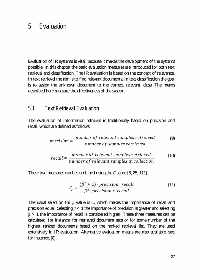
5.1 Text Retrieval Evaluation

The evaluation of information retrieval is traditionally based on precision and recall, which are defined as follows:

= (9)

= (10)

These two measures can be combined using the F score [8, 25, 111]:

=( + 1)

+ (11)

The usual selection for value is 1, which makes the importance of recall and precision equal. Selecting < 1 the importance of precision is greater and selecting > 1 the importance of recall is considered higher. These three measures can be

calculated, for instance, for retrieved document sets or for some number of the highest ranked documents based on the ranked retrieval list. They are used extensively in IR evaluation. Alternative evaluation means are also available, see, for instance, [8].

28

5.2 Text Classification Evaluation

5.2.1 Training and Test Sets

The evaluation of a text classifier is based on the usage of training and test sets [102]. The document collection available for classifier construction is split in two separate sets: training set and test set. The former is used for the training of the classifier and the latter for the evaluation of classifier performance. The idea is that when the original class labels (the information about the categories of the documents) of the test set documents are known, they can be compared to the class predictions given by the classifier. This way the classifier’s ability to give correct predictions can be evaluated.

One way to construct the training and test sets is using u-fold cross-validation [85]. In this approach, u disjoint sets are constructed randomly from the original collection. The size of each constructed set is p / u, where p is the size of the original collection. The testing is conducted iteratively in u rounds using one of the sets as the test set and the union of the rest u-1 sets as the training set. Each set is used in testing only once meaning that every document is in one of the u test sets and in u-1 training sets. In performance evaluation, the results obtained from these u separate test sets are averaged to get the overall measure of classification performance. This procedure is especially suitable when the aim is to achieve as reliable evaluation as possible with only a smallish data collection.

Some classifiers, for instance SOM classifier, are stochastic in the sense that there are some random factors in the learning phase. This leads to the situation where the class prediction of such classifier might be different if a new classifier instance is built with exactly the same training data. For stochastic classifiers it is advisable to run the classification test sets multiple times, for example ten times, and average the evaluation results. This way the results better reflect the expected average performance.

Finally, it should be strongly emphasised that to ensure as realistic evaluation results as possible, no information about the test set should be given to the classifier beforehand. It is obvious that none of the documents in the test set should be included in the corresponding training set. Moreover, the test set documents should not even take part in the vectorisation of the training documents in the preprocessing phase as the vocabulary of test documents is there

29

revealed to the classifier. The classifier should be built on the training set vocabulary only.

5.2.2 Evaluation Measures In evaluation of classification one of the most commonly used measures is classification accuracy. It can be calculated both based on individual decisions or class-wise [102]. Classification accuracy is called micro-averaged if the calculation is done summing over all individual decisions. When done class-wise, the accuracy is first calculated for each class and then averaged over the results of different classes. The latter approach is called macro-averaged classification accuracy. More specifically, the classification accuracy can be defined as follows:

= (12)

where cj is the number of correctly classified documents in test set j and nj is the number of all documents in that test set. The macro-averaged accuracy for test set j is computed with

=

(13)

where ncj is the number of classes in the test set j and the djk (k = 1, ... , ncj) is of form

= (14)

where cjk is the number of correctly classified documents in class k of test set j and njk is the number of documents in class k of test set j. The micro-averaged accuracy measures how well the whole test set was classified as it tells the proportion of correctly classified documents in percentage. The main advantage of micro-averaging is the intuitive nature of the measure. However, micro-averaging is very much influenced by the success or failure of the largest classes in the collection. For example, if there are two large classes forming a dominant majority, such as

30

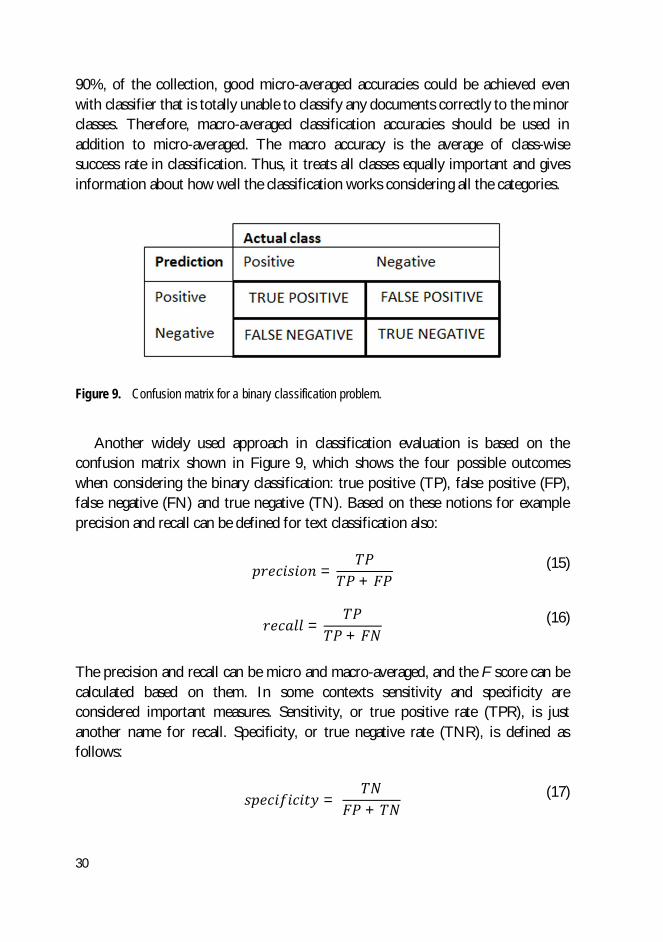
90%, of the collection, good micro-averaged accuracies could be achieved even with classifier that is totally unable to classify any documents correctly to the minor classes. Therefore, macro-averaged classification accuracies should be used in addition to micro-averaged. The macro accuracy is the average of class-wise success rate in classification. Thus, it treats all classes equally important and gives information about how well the classification works considering all the categories.

Figure 9. Confusion matrix for a binary classification problem.

Another widely used approach in classification evaluation is based on the

confusion matrix shown in Figure 9, which shows the four possible outcomes when considering the binary classification: true positive (TP), false positive (FP), false negative (FN) and true negative (TN). Based on these notions for example precision and recall can be defined for text classification also:

= + (15)

= + (16)

The precision and recall can be micro and macro-averaged, and the F score can be calculated based on them. In some contexts sensitivity and specificity are considered important measures. Sensitivity, or true positive rate (TPR), is just another name for recall. Specificity, or true negative rate (TNR), is defined as follows:

= + (17)

31

Often the choice of evaluation measures in classification depends on the application area and the point of view of the research. For further information about text classification evaluation, see [102].

32

33

6 Results

This chapter introduces briefly the research targets and the main results of the attached Publications I-V.

6.1 Publication I: Text Retrieval with SOMs

The aim of this publication was to explore the possibility of using unsupervised self-organising maps in text document retrieval. There were only a few examples available of using SOMs in text retrieval [34, 69]. The focus of the earlier IR-related SOM research had been mainly on clustering and classification of text documents. Our purpose was to measure the performance of SOMs in terms of traditional IR measures (precision and recall) to get a better idea of the effectiveness of the method in text searching. Therefore, we constructed a search engine prototype based on SOMs.

We used a German text document collection from CLEF 2003 [22]. The original collection had 294809 articles published in German newspapers. There were a total of 60 test topics (for instance “EU and Baltic countries”, “Olympic games and peace”) available with a pool of relevant documents associated with each of them. We selected 20 topics randomly and from the relevant documents associated with them we formed a collection of 580 documents. Finally, we added another 580 non-relevant (no relevance to the selected 20 topics) documents to the collection to achieve our final collection of 1160 text documents. Each topic had a topic title and a short textual description from which we formed the search queries for testing. The document data were first preprocessed, using stemming and removal of short words, and then transformed into document vectors.

In order to use SOMs in searching, we designed a search engine system which finds the best matching node (best matching unit, BMU) on the map surface for each search query and then retrieves the contents (text documents) of that node as a search result. We also retrieved documents from the neighbourhood areas of the BMU to get a better idea of the search performance. The neighbourhoods were defined by the link distances between the BMU and its neighbouring nodes (see

34

Figure 10). For example, in neighbourhood2 there are the map nodes that are two links away or closer to the BMU. We tested searching in the SOM using different map parameters to find the best settings. The results proved that SOM was able to retrieve relevant documents. The best SOM settings gave average precision of 50% and average recall of 26% in neighborhood1 for the 20 queries (topics). In neighbourhood2 the performance was precision 43% and recall 40%. Closer inspection revealed that about half of the topics were retrieved with precisions of 79-100% in neighbourhood1, but the rest of the topics scored very poorly or were even totally lost on the map. The majority of these difficult topics had only a small number of relevant documents on the map, which probably resulted in poor performance. It was still encouraging that the successful searches were retrieved with high precisions and the relevant documents were clustered near each other on the maps surface.

Figure 10. The neighbourhoods of the best matching unit on rectangular SOM surface. Neighbourhood0 (coloured black) contains BMU only, neighbourhood1 (dark grey) BMU and the four closest nodes, and neighbourhood2 (light grey) BMU and 12 nodes.

For comparison, we constructed similar search engines also with k-means and

Ward's clustering methods. The self-organising maps seemed to perform slightly better than the others in neighbourhood0. In neighbourhood1 k-means and Ward were quite evenly matched, but SOMs were struggling with low number of nodes and performing better than the others with high number of nodes. In neighbourhood2 SOMs were clearly behind and k-means was performing the best. Statistical testing found no significant differences in the smallest neighbourhoods, but in neighbourhood2 k-means was significantly better than Ward's clustering and SOMs.

The results suggested that SOMs are able to group topically relevant text documents near each other on the map. The comparison also proved that SOMs

35

achieve as good results as the two traditional clustering methods when using tight neighbourhoods (neighbourhood0 and neighbourhood1). Overall, the results were somewhat modest, but the successful searches were achieving high precision and recall values, which was an encouraging proof of the possibilities of the self-organising maps in text document retrieval. In this study, we did not compare performance to traditional text search engines.

6.2 Publication II: Text Classification with SOMs

The first publication had clearly revealed that self-organising maps are able to retrieve relevant documents if the documents are successfully grouped in compact clusters on the map surface. We wanted to research the clustering ability of SOMs further. Therefore, we studied the use of self-organising maps in text document classification.

The data set used was the same German collection as in Publication I. We selected the 10 largest topics from the 20 topics used earlier. The final collection included 425 documents. Each topic formed one class in the classification task. First, the preprocessing and vectorisation was done as usual, and then 10-fold cross-validation was used to construct 10 test sets.

The original self-organising map is a clustering method. Therefore, we needed to modify the procedure to be able to use it in classification. The simple idea was to find map positions, i.e. BMU, for all the training samples (documents) and then, based on the class labels of them, give class labels also for the map nodes (majority voting principle). After this the labelled map is able to predict the class of any unknown test sample simply by finding the BMU for it: the class label of the BMU is then the prediction. We constructed SOM classifiers and compared their (micro-averaged) classification accuracies against supervised k nearest neighbour searching and unsupervised k-means classifier. The k-means clustering was transformed to work as a classifier in the exactly same manner as the SOM classifier.

The testing was performed with several parameters to find the optimal settings. We tested the methods in classification tasks of 2, 5 and 10 classes. In the binary case of two classes k nearest neighbours searching was the best with classification accuracy of 99.3%, while k-means scored 97.9% and SOMs 93.2%. Interestingly, the self-organising maps were superior classifying the more complex, more realistic, cases of 5 and 10 classes. SOMs yielded accuracies of 89.0% and 89.2% with 5 and 10 classes, while k-NN got 83.4% and 83.3% and k-means 78.5% and

36

73.6%. The statistical testing proved that SOMs were performing significantly better than the other methods in 5 and 10 class cases, while k-NN and k-means (only with vector dimension 500) were significantly better than SOMs in the binary case.

The results strongly suggested that self-organising maps are able to group text documents in compact clusters according to their topical relevance, which means that SOMs can be used successfully in document classification tasks.

6.3 Publication III: Text Classification with SOMs

To get more knowledge about the classification effectiveness of self-organising maps, we made an extended comparison with six well-known machine learning methods using three data collections. The methods used were the unsupervised k-means clustering and Ward's clustering and the supervised k nearest neighbours searching, linear discriminant analysis, Naïve Bayes classifier and classification tree. The data collections were Reuters-21578, 20 Newsgroups collection and the Spanish CLEF 2003 collection.

The first data set used was a subset of Reuters-21578 collection [93] which originally included 21578 English news documents. We selected the 10 largest classes and only the single-labelled documents from the widely used Mod Apte split with 10789 documents and 90 classes (for example “coffee”, “trade”, “ship”). Our selection had 8008 documents, 5754 for training and 2254 for testing. The second data set was 20 newsgroups collection [1] and the Matlab/Octave version of it. It contains 18774 English documents, 12690 for training and 7505 for testing, in 20 newsgroup classes (for example “rec.sport.hockey”, “soc.religion.christian”). The third data set was a subset of Spanish CLEF 2003 collection [22]. The original collection has 454045 news documents. We selected the 20 largest topics (i.e. “Los Juegos Olímpicos y la paz”, “El Shoemaker-Levy y Júpiter”) to form the classes, which resulted in a collection of 1901 documents. For this data set we constructed the test sets using 10-fold cross-validation because there was no widely used existing test split available. For all the three data sets the preprocessing with stemming, stopword removal and vectorisation with tf·idf weights was done.

The self-organising maps performed well with Reuters and CLEF data sets achieving micro-averaged classification accuracies of 92.3% and 95.6%. The newsgroups data set was more difficult with more modest accuracy of 42.3%. The Naïve Bayes classifier performed the best classifying Reuters with 95.2%, CLEF

37

with 98.1% and newsgroups with 62.0% accuracy. The newsgroups collection turned out to be the most challenging with most of the methods scoring accuracies of only 30-46%. Overall, SOMs were performing the best in its own category of unsupervised methods, but was a bit behind of the best supervised methods, Naïve Bayes and discriminant analysis. When compared to the supervised k nearest neighbour searching and classification tree, SOMs were at least comparable and even superior in some cases. The statistical testing revealed that SOMs were statistically better than k-means clustering in the second and the third data set, and better than Ward clustering in the first data set. On the other hand, Naïve Bayes classifier was significantly better than self-organising maps in every data set, and discriminant analysis was better than SOMs in the second and the third data set.

The results of this study gave more insight about the performance of the self-organising maps compared to other methods. It was very interesting that SOMs were, in some cases, equal to some of the supervised methods in classification performance, although the training phase of the maps is unsupervised. This outcome and the fact that the (micro-averaged) classification accuracies with the two easier data sets were 92.3% and 95.6% strongly suggest that self-organising maps can be used effectively in text classification.

6.4 Publication IV: Dimensionality Reduction in Text Classification

After two studies of classifier comparisons with multiple data collections, we wanted to focus more on the preprocessing phase of text classification. At the same time we learned about the recently introduced scatter method [55], which evaluates the importance of each variable in the data set. It seemed to be a very suitable candidate for the dimensionality reduction task. Thus, we focused on the effects of dimensionality reduction in classification performance of machine learning methods. For comparison, we used two reduction methods based on document frequency and mutual information value. Although the main focus of this study was on dimensionality reduction in general, we were also keenly interested in the effects it has on self-organising maps classification performance.

We prepared two data sets for the testing. The data sets were the same subsets of Reuters-21578 and the Spanish CLEF 2003 which were used in Publication III. The preprocessing and test set splitting was also conducted in the similar way as earlier. After preprocessing the dimensionality of the data was reduced using the

38

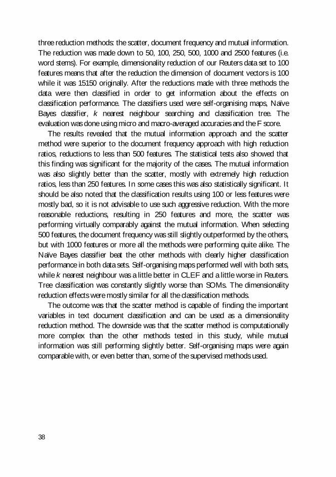
three reduction methods: the scatter, document frequency and mutual information. The reduction was made down to 50, 100, 250, 500, 1000 and 2500 features (i.e. word stems). For example, dimensionality reduction of our Reuters data set to 100 features means that after the reduction the dimension of document vectors is 100 while it was 15150 originally. After the reductions made with three methods the data were then classified in order to get information about the effects on classification performance. The classifiers used were self-organising maps, Naïve Bayes classifier, k nearest neighbour searching and classification tree. The evaluation was done using micro and macro-averaged accuracies and the F score.

The results revealed that the mutual information approach and the scatter method were superior to the document frequency approach with high reduction ratios, reductions to less than 500 features. The statistical tests also showed that this finding was significant for the majority of the cases. The mutual information was also slightly better than the scatter, mostly with extremely high reduction ratios, less than 250 features. In some cases this was also statistically significant. It should be also noted that the classification results using 100 or less features were mostly bad, so it is not advisable to use such aggressive reduction. With the more reasonable reductions, resulting in 250 features and more, the scatter was performing virtually comparably against the mutual information. When selecting 500 features, the document frequency was still slightly outperformed by the others, but with 1000 features or more all the methods were performing quite alike. The Naïve Bayes classifier beat the other methods with clearly higher classification performance in both data sets. Self-organising maps performed well with both sets, while k nearest neighbour was a little better in CLEF and a little worse in Reuters. Tree classification was constantly slightly worse than SOMs. The dimensionality reduction effects were mostly similar for all the classification methods.

The outcome was that the scatter method is capable of finding the important variables in text document classification and can be used as a dimensionality reduction method. The downside was that the scatter method is computationally more complex than the other methods tested in this study, while mutual information was still performing slightly better. Self-organising maps were again comparable with, or even better than, some of the supervised methods used.

39

6.5 Publication V: Training Data Quality and the Set of SOMs

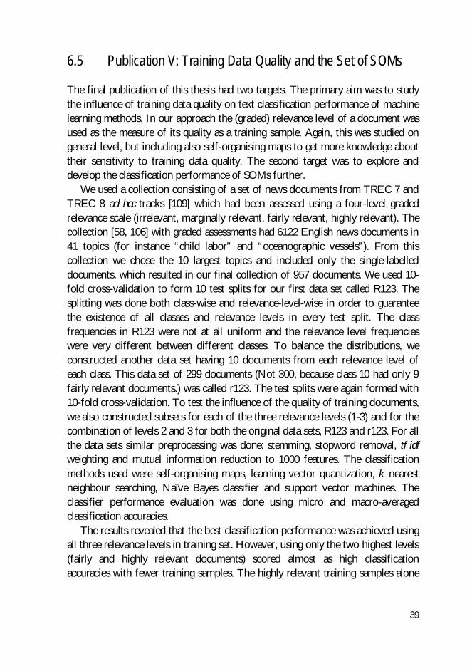
The final publication of this thesis had two targets. The primary aim was to study the influence of training data quality on text classification performance of machine learning methods. In our approach the (graded) relevance level of a document was used as the measure of its quality as a training sample. Again, this was studied on general level, but including also self-organising maps to get more knowledge about their sensitivity to training data quality. The second target was to explore and develop the classification performance of SOMs further.

We used a collection consisting of a set of news documents from TREC 7 and TREC 8 ad hoc tracks [109] which had been assessed using a four-level graded relevance scale (irrelevant, marginally relevant, fairly relevant, highly relevant). The collection [58, 106] with graded assessments had 6122 English news documents in 41 topics (for instance “child labor” and “oceanographic vessels”). From this collection we chose the 10 largest topics and included only the single-labelled documents, which resulted in our final collection of 957 documents. We used 10-fold cross-validation to form 10 test splits for our first data set called R123. The splitting was done both class-wise and relevance-level-wise in order to guarantee the existence of all classes and relevance levels in every test split. The class frequencies in R123 were not at all uniform and the relevance level frequencies were very different between different classes. To balance the distributions, we constructed another data set having 10 documents from each relevance level of each class. This data set of 299 documents (Not 300, because class 10 had only 9 fairly relevant documents.) was called r123. The test splits were again formed with 10-fold cross-validation. To test the influence of the quality of training documents, we also constructed subsets for each of the three relevance levels (1-3) and for the combination of levels 2 and 3 for both the original data sets, R123 and r123. For all the data sets similar preprocessing was done: stemming, stopword removal, tf·idf weighting and mutual information reduction to 1000 features. The classification methods used were self-organising maps, learning vector quantization, k nearest neighbour searching, Naïve Bayes classifier and support vector machines. The classifier performance evaluation was done using micro and macro-averaged classification accuracies.

The results revealed that the best classification performance was achieved using all three relevance levels in training set. However, using only the two highest levels (fairly and highly relevant documents) scored almost as high classification accuracies with fewer training samples. The highly relevant training samples alone

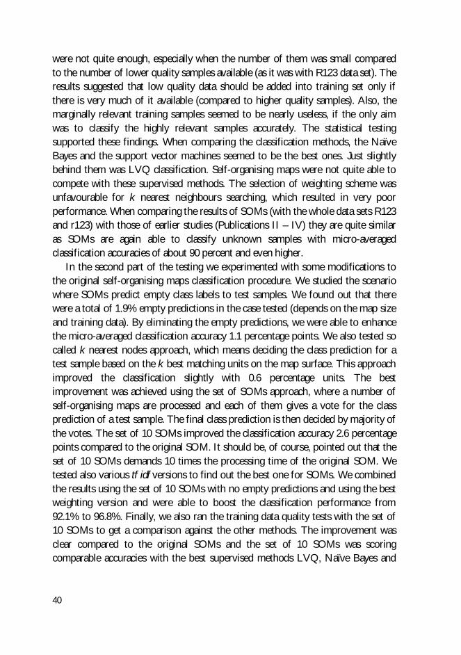
40

were not quite enough, especially when the number of them was small compared to the number of lower quality samples available (as it was with R123 data set). The results suggested that low quality data should be added into training set only if there is very much of it available (compared to higher quality samples). Also, the marginally relevant training samples seemed to be nearly useless, if the only aim was to classify the highly relevant samples accurately. The statistical testing supported these findings. When comparing the classification methods, the Naïve Bayes and the support vector machines seemed to be the best ones. Just slightly behind them was LVQ classification. Self-organising maps were not quite able to compete with these supervised methods. The selection of weighting scheme was unfavourable for k nearest neighbours searching, which resulted in very poor performance. When comparing the results of SOMs (with the whole data sets R123 and r123) with those of earlier studies (Publications II – IV) they are quite similar as SOMs are again able to classify unknown samples with micro-averaged classification accuracies of about 90 percent and even higher.

In the second part of the testing we experimented with some modifications to the original self-organising maps classification procedure. We studied the scenario where SOMs predict empty class labels to test samples. We found out that there were a total of 1.9% empty predictions in the case tested (depends on the map size and training data). By eliminating the empty predictions, we were able to enhance the micro-averaged classification accuracy 1.1 percentage points. We also tested so called k nearest nodes approach, which means deciding the class prediction for a test sample based on the k best matching units on the map surface. This approach improved the classification slightly with 0.6 percentage units. The best improvement was achieved using the set of SOMs approach, where a number of self-organising maps are processed and each of them gives a vote for the class prediction of a test sample. The final class prediction is then decided by majority of the votes. The set of 10 SOMs improved the classification accuracy 2.6 percentage points compared to the original SOM. It should be, of course, pointed out that the set of 10 SOMs demands 10 times the processing time of the original SOM. We tested also various tf·idf versions to find out the best one for SOMs. We combined the results using the set of 10 SOMs with no empty predictions and using the best weighting version and were able to boost the classification performance from 92.1% to 96.8%. Finally, we also ran the training data quality tests with the set of 10 SOMs to get a comparison against the other methods. The improvement was clear compared to the original SOMs and the set of 10 SOMs was scoring comparable accuracies with the best supervised methods LVQ, Naïve Bayes and

41

SVMs, even beating the LVQ in R123. This outcome was somewhat surprising, but proved again that SOMs can be used effectively in text classification tasks.

42

43

7 Discussion and Conclusions

This thesis studied the possibilities of using self-organising maps in information retrieval tasks. The main focus was on the text classification performance of SOMs, which was explored in Publications II-V, but text retrieval was also considered in Publication I. While SOMs were the main research interest, other topics were also covered: the dimensionality reduction of text data and the effects of training data quality on document classification of machine learning methods. Next, the main results of the thesis are discussed and some conclusions and future considerations made.

At the beginning of this thesis the main research problem was: - Are self-organising maps an effective method in information retrieval tasks?

The main problem led quickly to other problems, such as: - How does one build a search engine based on SOMs? - How well does such search engine retrieve relevant documents? - Are SOMs effective in text classification? - Is the unsupervised learning of SOMs able to compete against well-known

supervised machine learning methods in text classification? How well do SOMs perform when compared to other unsupervised methods?

- Is it possible to develop the SOM method further to achieve better results in IR tasks?

- Is the map view generated by the method useful in IR?

The thesis has answered some of these questions, fully or partially, but as usual raised a bunch of new ones.

First of all, the search engine prototype was successfully built in Publication I, and it was able to find relevant data samples from the test collection. The performance level, in terms of precision and recall measures, was slightly disappointing, somewhat lower than expected. This might be because of difficult data, which needs to be verified using other data sets in the future. However, the

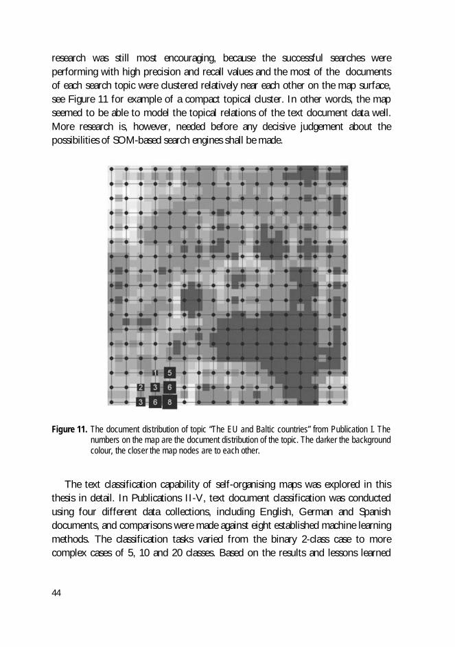
44

research was still most encouraging, because the successful searches were performing with high precision and recall values and the most of the documents of each search topic were clustered relatively near each other on the map surface, see Figure 11 for example of a compact topical cluster. In other words, the map seemed to be able to model the topical relations of the text document data well. More research is, however, needed before any decisive judgement about the possibilities of SOM-based search engines shall be made.

Figure 11. The document distribution of topic “The EU and Baltic countries” from Publication I. The numbers on the map are the document distribution of the topic. The darker the background colour, the closer the map nodes are to each other.

The text classification capability of self-organising maps was explored in this

thesis in detail. In Publications II-V, text document classification was conducted using four different data collections, including English, German and Spanish documents, and comparisons were made against eight established machine learning methods. The classification tasks varied from the binary 2-class case to more complex cases of 5, 10 and 20 classes. Based on the results and lessons learned

45

from this research it is fair to state that self-organising maps are able to perform well in text classification. SOMs were almost constantly beating the other unsupervised methods in evaluations. Moreover, SOMs achieved comparable results with some of the supervised machine learning methods, even beating some of them in some test cases. Still, the best supervised learners, like Naïve Bayes classifier and support vector machines, were performing constantly better than SOMs. In Publication V, the performance of the introduced set of 10 SOMs classifier was virtually equal to all the best supervised classifiers tested. This should be researched further, as well as the possibilities of the set of SOMs approach itself, but this result is still very interesting, while it was achieved using only unsupervised learning. The usage of multiple self-organising maps in classification seems to give some improvement in performance. Multiple SOMs have also earlier been used successfully in, for example, text retrieval [34], intrusion detection [94], and classification of sonar signals [13]. The good classification results achieved by SOMs are a convincing proof of the unsupervised clustering ability of the method.

When considering the self-organising maps in information retrieval in general, there are two important factors: visualisation power and computational complexity. On one hand, the visual map generated by the SOM method is useful and intuitive by-product of the processing, on the other hand the processing time of SOMs is usually higher than processing time of the most other machine learning methods. Thus, one needs to know when to use SOMs and when not.

The visual map is very useful in some applications. For example, the results of a search query could be given as a traditional ranked list of retrieved documents, but also the system could provide a browsable map interface, where the hit position (BMU) of given query is highlighted as the starting point for further browsing. In classification, the map interface is able to give more knowledge about the class prediction as user is able to see the neighbouring map clusters and their class labels and content, which provide hints about closely related, or the most distant, topical areas. Of course, in plain clustering the map interface is also much more informative than just separate groups as the map includes information about the cluster relations. Figures 12 and 13 illustrate a section of a class-labelled SOM. The visualisation is taken from our simple prototype of an internet browser based map viewer. In Figure 12, there is a high level representation showing only class labels of the focused map nodes. Figure 13 is a zoomed view of the centremost node, where the document titles and their class labels are also included. Based on the map, it seems to be that “sugar” (class 9) and “coffee” (class 10) are closely related classes, as they naturally should be. As mentioned earlier, after searching for

46

information, it would be very intuitive and easy for the user to browse through the data collection (or the set of retrieved documents) with this kind of visual browser, which is generated by the SOM method almost automatically: the map can be easily, with only relatively minor programming efforts, transformed into an easy-to-understand browsing tool. Similar, yet more advanced, SOM-based browsers for information retrieval are proposed by several studies, for example [68, 74, 75, 115]. As the computer technology, and the world as a whole, is getting more and more visual, the visualisation power is clearly one of the main reasons to use the self-organising maps in IR. The leading web search engines are still mostly text and list-based, excluding the image search services, which makes these visual possibilities of SOMs a very interesting prospect. It should be strongly emphasized that no user-oriented testing using SOM search engine were carried out in this thesis, which means that the real usefulness of the map view as a searching tool was not evaluated.

The downside of using self-organising maps is the computational complexity. Usually the other methods used are faster to process. This not always that straightforward though. For example, k nearest neighbours searching classifier is very much faster to build, but the prediction phase is usually even ten times slower than SOM prediction. The k-NN has to compare the test sample with all training samples to get the prediction while SOM only compares the unknown sample with the map nodes. The usual average number of training samples per map node in SOM classifier is around 10 in IR tasks. So, it depends heavily on the situation if the SOMs are a good choice or not. In Publication V, an 8x8 map with 846 documents was processed in 10 seconds using a conventional desktop computer (AMD Athlon 64 X2 4400+, 2.30 GHz dual core processor). In practice 10 seconds of processing might be tolerable or far too much depending on the usage scenario. In most practical use cases the classifier is built just once and then used in prediction for a long time. However, it is more than fair to state that SOMs are computationally heavy to use in general. This is even more the case with the set of SOMs approach, where multiple SOMs are processed. The set of SOMs should be considered only when the higher performance is very important and the processing time is not a crucial factor.

To sum up, the self-organising map is a strong tool when additional visualisation is needed in IR task, but the usage of self-organising maps is usually more preferable when the collection is somewhat static, in the sense that new classifier is processed quite rarely, and the size of the collection is reasonable, because the learning process of SOM is the most time consuming part of the

47

method. However, if the longer learning time is acceptable or the visual output is of highest importance, even larger collections can be processed with SOMs.

Figure 12. Section of a class-labelled SOM including 9 nodes visualised by a browsing tool. Class 9 is “sugar” and class 10 is “coffee”.

Figure 13. Zoomed view of the centremost node of Figure 12.

48

There were some research limitations in this thesis that should be mentioned. Only single-label classification was considered in this thesis in order to tackle the basic problems of classification first. The much more complex multi-label classification can only be solved after mastering the basic single-label case. The other limitation of this thesis was the relatively small size of the data collections: the largest collection used included 18774 documents and 20 classes (topics). It is clear, that the data collections should be larger in the future studies.

After this thesis there are multiple promising research lines concerning self-organising maps in information retrieval available. First of all, it would be most interesting to continue the research, started in Publication I, about SOM-based search engines after some lessons learned in Publications II-V. The usage of ranked retrieval lists and more advanced way of selecting the retrieved documents from the map surface, and perhaps the usage of multiple SOMs, could enhance the performance a great deal. The visual way of presenting the search results could also be developed further based on the browsable map view. There is also a need to evaluate the search engine with larger data sets.

In text classification there are multiple new areas of interest as well. The usage of multiple maps could be studied more deeply using, for example, different kinds of maps instead of just multiple copies of one type. Also, the single-label classification task could be extended to multi-label classification using multiple SOMs or the class prediction could be given on graded scale (irrelevant, marginally relevant, fairly relevant and highly relevant) instead of binary (irrelevant, relevant). One possible direction could be adding at least some supervised aspects to the learning phase of self-organising map in order to achieve even better performance in IR. There are some successful supervised versions of SOMs described in the literature, see for [13, 42, 63, 90, 116]. The ideas researched in the final publication of this thesis, the training data quality in machine learning, could be also studied further with a larger data collection.

49

8 Personal Contributions

The thesis consists of five publications (Publications I-V) on which the author (hereafter referred to as JS) has worked closely together with Martti Juhola (MJ), Kalervo Järvelin (KJ) and Jorma Laurikkala (JL). The original idea of using self-organising maps in information retrieval tasks came from MJ, who has also been the main supervisor for the research. All three collaborators (MJ, KJ and JL) have given guidance and support throughout the research. In the following the personal contributions of JS are described in detail.

Publication I: “A study on the use of self-organised maps in information retrieval”: JS programmed the software tools needed for the research, preprocessed the data, designed the test setup and performed the testing. MJ proposed the map neighbourhood approach and wrote the paper. KJ suggested the data set used and provided invaluable theoretical and practical IR expertise. JL performed the statistical testing.

Publication II: “On document classification with self-organising maps”: JS performed programming, preprocessing of the data, the test setup design and testing. MJ wrote the paper, KJ provided IR expertise on text classification and JL performed the statistical testing.

Publication III: “Self-organising maps in document classification: A comparison with six machine learning methods”: JS performed programming, preprocessing of the data, the test setup design, the testing and wrote the paper. MJ and JL gave support with the selection and processing of the baseline machine learning methods. JL also conducted the statistical testing. KJ suggested suitable data collections for the tests and provided IR expertise.

Publication IV: “Dimensionality reduction in text classification using scatter method”: JS performed programming, preprocessing of the data, the test setup design, the testing wrote the paper (except the section about the scatter method). The idea of using the scatter method in dimensionality reduction of text

50

data was by MJ, who also wrote the section about the scatter method. The scatter method was developed in an earlier research by MJ and Markku Siermala. JL conducted the statistical testing for the paper. KJ provided IR expertise.

Publication V: “On the influence of training data quality on text document classification using machine learning methods”: JS performed programming, preprocessing of the data, the testing (except SVMs) and wrote the paper (except the section about SVMs). The section about modifications to the original self-organising maps classification and the idea of the novel set of SOMs approach was by JS. Henry Joutsijoki wrote the section about the support vector machines and processed the SVM testing. KJ came up with the approach of measuring the data quality using relevance graded data and proposed the suitable data collection and the original idea of the test setting. JL conducted the statistical testing. MJ supervised the research and provided machine learning knowledge.

51

Bibliography

[1] The 20 newsgroups document collection. Available at: http://people.csail.mit.edu/jrennie/20Newsgroups/, accessed 15th of May 2014.

[2] Aiolli, F., Cardin, R., Sebastiani, F. and Sperduti, A. (2009). Preferential text classification: Learning algorithms and evaluation measures. Information Retrieval, Vol. 12, No. 5, pp. 559-580.

[3] Airio, E. (2006). Word normalization and decompounding in mono- and bilingual IR. Information Retrieval, Vol. 9, No. 3, pp. 249-271.

[4] Ai-Xiang, S. (2010). Improved SOM algorithm-HDSOM applied in text clustering.

In Proceedings of the International Conference on Multimedia Information Networking and Security (MINES 2010), IEEE, pp. 306-309.

[5] Apte, C., Damerau, F.J. and Weiss, S.M. (1994). Automated learning of decision

rules for text categorization. ACM Transactions on Information Systems, Vol. 12, No. 3, pp. 233-251.

[6] Asy'arie, A.D. and Pribadi, A.W. (2009). Automatic news articles classification in

Indonesian language by using Naive Bayes classifier method. In Proceedings of the 11th International Conference on Information Integration and Web-based Applications & Services (iiWAS 2009), ACM, New York, NY, USA, pp. 658-662.

[7] Azcarraga, A. and Manalili, S. (2011). Design of a structured 3D SOM as a music

archive. Advances in Self-Organizing Maps, Lecture Notes in Computer Science, Vol. 6731, pp. 188-197.

[8] Baeza-Yates, R. and Ribeiro-Neto, B. (2011). Modern Information Retrieval.

Second edition, Addison-Wesley, New York, NY, USA.

[9] Beckel, C., Sadamori, L. and Santini, S. (2012). Towards automatic classification of private households using electricity consumption data. In Proceedings of the ACM Workshop on Embedded Sensing Systems for Energy Efficiency in Buildings (BuildSys 2012), ACM, New York, NY, USA, pp. 169-176.

[10] Belew, R.K. (2000). Finding Out About, A Cognitive Pespective on Search Engine

Technology and WWW. Cambridge University Press, Cambridge, UK.

[11] Bibliography of SOM papers. Available at: http://www.cis.hut.fi/research/som-bibl/, accessed 15th of May 2014.

52

[12] Borlund, P. (2003). The concept of relevance in IR. Journal of the American Society for Information Science and Technology, Vol. 54, No. 10, pp. 913-925.

[13] Cervera, E. and del Pobil, A.P. (1997). Multiple self-organizing maps: A hybrid

learning scheme. Neurocomputing, Vol. 16, No. 4, pp. 309-318.

[14] ChandraShekar, B.H. and Shoba, G. (2009). Classification of documents using Kohonen’s self-organizing map. International Journal of Computer Theory and Engineering, Vol. 1, No. 5, pp. 610-613.

[15] Chen, Y., Qin, B., Liu, T., Liu, Y. and Li, S. (2010). The comparison of SOM and

k-means for text clustering. Computer and Information Science, Vol. 3, No. 2, pp. 268-274.

[16] Cheng, W., Dembczynski, K. and Hüllermeier, E. (2010). Graded multilabel

classification: The ordinal case. In Proceedings of the 27th International Conference on Machine Learning (ICML 2010), Omnipress, pp. 223-230.

[17] Cho, S. and Won, H. (2003). Machine learning in DNA microarray analysis for

cancer classification. In Proceedings of the First Asia-Pacific Bioinformatics Conference (APBC 2003), Conferences in Research and Practice in Information Technology, Vol. 19, pp. 189-198.

[18] Chowdhury, N. and Saha, D. (2005). Unsupervised text classification using

Kohonen’s self-organizing network. In Proceedings of the Sixth International Conference on Intelligent Text Processing and Computational Linguistics (CICLing 2005), Lecture Notes in Computer Science, Vol. 3406, pp. 715-718.

[19] Christianini, N. and ShaweTaylor, J. (2000). An Introduction to Support Vector

Machines and Other Kernel-based Learning Methods. Cambridge University Press, Cambridge, UK.

[20] Chrysostomou, K., Chen, S.Y. and Liu, X. (2008). Combining multiple classifiers

for wrapper feature selection. International Journal of Data Mining, Modelling and Management, Vol. 1, No. 1, pp. 91-102.

[21] Chumwatana, T., Wong, K. and Xie, H. (2010). A SOM-based document

clustering using frequent max substring for non-segmented texts. Journal of Intelligent Learning Systems &Applications, Vol. 2, No. 3, pp. 117-125.

[22] CLEF: Conference and Labs of the Evaluation Forum. Available at:

http://www.clef-initiative.eu/, accessed 15th of May 2014.

[23] Conover, W.J. (1999). Practical Nonparametric Statistics. John Wiley & Sons, New York, NY, USA.

[24] Cosijn, E. and Ingwersen, P. (2000). Dimensions of relevance. Information Processing

and Management, Vol. 36, No. 4, pp. 533-550.

53

[25] Croft, W.B., Metzler, D. and Strohman, T. (2010). Search Engines: Information Retrieval in Practice. Addison-Wesley, Boston, MA, USA.

[26] Deerwester, S., Dumais, S.T., Furnas, G.W., Landaer, T.K. and Harshman, R.

(1990). Indexing by latent semantic indexing. Journal of the American Society for Information Science and Technology, Vol. 41, No. 6, pp. 391-407.

[27] Ding, C. and Patra, J.C. (2007). User modeling for personalized web search with

self-organizing map. Journal of American Society for Information Science and Technology, Vol. 58, No. 4, pp. 494-507.

[28] Dittenbach, M., Merkl, D. and Rauber, A. (2000). Using growing hierarchical self-

organizing maps for document classification. In Proceedings of the Eighth European Symposium on Artificial Neural Networks (ESANN 2000), pp. 7-12.

[29] Dittenbach, M., Rauber, A. and Merkl, D. (2002). Uncovering hierarchical

structure in data using the growing hierarchical self-organizing map. Neurocomputing, Vol 48, No 1-4, pp. 199-216.

[30] Doan, A., Domingos, P. and Halevy, A. (2003). Learning to match the schemas of

data sources: a multistrategy approach. Machine Learning, Vol 50, No. 3, pp. 279-301.

[31] Drigas, A.S. and Vrettaros, J. (2008). Using the self-organizing map (SOM)

algorithm, as a prototype e-content retrieval tool. In Proceedings of the Eighth International Conference on Computer Science and Applications (ICCSA 2008), Lecture Notes in Computer Science, Vol. 5073, pp. 14-23.

[32] Duda, R.O., Hart, P.E. and Stork, D.G. (2001). Pattern Classification. Second

edition, John Wiley & Sons, New York, NY, USA.

[33] Eyassu, S. and Gambäck, B. (2005). Classifying amharic news text using self-organizing maps. In Proceedings of the ACL Workshop on Computational Approaches to Semitic Languages, pp. 71-78.

[34] Fernandez, J., Mones, R., Diaz, I., Ranilla, J. and Combarro, E.F. (2004).

Experiments with self organizing maps in CLEF 2003. CLEF 2003, Lecture Notes in Computer Science, Vol. 3237, pp. 358-366.

[35] Flach, P.A. and Lachiche, N. (2004). Naïve Bayesian classification of structured

data. Machine Learning, Vol. 57, No. 3, pp. 233-269.

[36] Frakes, W.B. and Baeza-Yates, R. (1992). Information Retrieval: Data Structures & Algorithms. Prentice Hall, Englewood Cliffs, NJ, USA.

54

[37] Frank, E. and Bouckaert, R.R. (2006). Naïve Bayes for text classification with unbalanced classes. In Proceedings of the 10th European Conference on Principles and Practice of Knowledge Discovery in Databases (PKDD 2006), Lecture Notes in Computer Science, Vol. 4213, pp. 503-510.

[38] Furletti, B., Gabrielli, L., Renso, C. and Rinzivillo, S. (2012). Identifying users

profiles from mobile calls habits. In Proceedings of the ACM SIGKDD International Workshop on Urban Computing (UrbComp 2012), pp. 17-24.

[39] Garg, V.K. and Murty, M.N. (2009). Feature subspace SVMs (FS-SVMs) for high

dimensional handwritten digit recognition. International Journal of Data Mining, Modelling and Management, Vol. 1, No. 4, pp. 411-436.

[40] Guerrero-Bote, V.P., Moya-Anegon, F. and Herrero-Solana, V. (2002). Document

organization using Kohonen’s algorithm. Information Processing and Management, Vol. 38, pp. 79-89.

[41] Guyon, I. and Elisseef, A. (2003). An introduction to variable and feature

selection. Journal of Machine Learning Research, Vol. 3, No. 3/1/2003, pp. 1157-1182.

[42] Hagenbuchner, M. and Tsoi, A.C. (2005). A supervised training algorithm for selforganizing maps for structures. Pattern Recognition Letters, Vol. 26, No. 12, pp. 1874-1884.

[43] Hand, D., Mannila, H. and Smyth, P. (2001). Principles of Data Mining. MIT

Press, Cambridge, MA, USA.

[44] Haykin, S. (1999). Neural Networks: A Comprehensive Foundation. Second edition, Prentice-Hall, Upper Saddle River, NJ, USA.

[45] Hjørland, B. (2010). The foundation for the concept of relevance. Journal of the

American Society for Information Science and Technology, Vol. 61, No. 2, pp. 217-237.

[46] Honkela, T. (1997). Self-organizing maps in natural language processing. Academic dissertation, Helsinki University of Technology, Finland.

[47] Honkela T., Laaksonen, J., Törrö, H. and Tenhunen, J. (2011). Media map: A

multilingual document map with a desing interface. Advances in Self-Organizing Maps, Lecture Notes in Computer Science, Vol. 6731, pp. 247-256.

[48] Hsu, C., Chang, C. and Lin, C. (2010). A practical guide to support vector

classification. Technical report, available at: http://www.csie.ntu.edu.tw/~cjlin/papers/guide/guide.pdf, accessed 15th of May 2014.

[49] Hsu, C. and Lin, C. (2002). A comparison of methods for multiclass support

vectors machines. IEEE Transactions of Neural Networks, Vol. 13, No. 2, pp. 415-425.

55

[50] Ingwersen, P. and Järvelin, K. (2005). The Turn: Integration of Information Seeking and Retrieval in Context. Springer, Dordrecht, Netherlands.

[51] Jain, A. and Dubes, R. (1988). Algorithms for Clustering Data. Prentice Hall,

Englewood Cliffs, NJ, USA.

[52] Joutsijoki, H. and Juhola, M. (2011). Kernel selection in multi-class support vector machines and its consequence to the number of ties in majority voting method. Artificial Intelligence Review, Vol. 40, No. 3, pp. 213-230.

[53] Joutsijoki, H. and Juhola, M. (2011). Comparing the one-vs-one and one-vs-all

methods in benthic macroinvertebrate image classification. In Proceedings of the Seventh International Conference on Machine Learning and Data Mining in Pattern Recognition (MLDM 2011), Lecture Notes in Computer Science, Vol. 6871, pp. 399-413.

[54] Juhola, M. and Siermala, M. (2005). Assessment methods of neural network

classification applied to otoneurological. European Notes in Medical Informatics, Vol. 1, No. 1, pp. 1092-1097.

[55] Juhola, M. and Siermala, M. (2012). A scatter method for data and variable

importance evaluation. Integrated Computer-Aided Engineering, Vol 19, No. 2, pp. 137-149.

[56] Järvelin, K. and Kekäläinen J. (2002). Cumulated gain-based evaluation of IR

tecniques. ACM Transactions on Information Systems, Vol. 20, No. 4, pp. 422-446.

[57] Kaski, S. (1998). Dimensionality reduction by random mapping: fast similarity computation for clustering. In Proceedings of IEEE International Joint Conference on Neural Networks (IJCNN 1998), IEEE, Vol. 1, pp. 413-418.

[58] Kekäläinen, J. (2005). Binary and graded relevance in IR evaluations comparison

of the effects on ranking of IR systems. Information Processing and Management: an International Journal, Vol. 31, No. 5, pp. 1019-1033.

[59] Kline, D.M. and Galbraith, G.S. (2009). Performance analysis of the Bayesian data

reduction algorithm. International Journal of Data Mining, Modelling and Management, Vol. 1, No. 3, pp. 223-236.

[60] Kohonen, T. and Xing, H. (2011). Contextually self-organized maps of Chinese

words. Advances in Self-Organizing Maps, Lecture Notes in Computer Science, Vol. 6731, pp. 16-29.

[61] Kohonen, T. (2013). Essentials of the self-organizing map. Neural Networks, Vol.

37, pp. 52-65.

[62] Kohonen, T. (1986). Learning Vector Quantization for Pattern Recognition. Helsinki University of Technology, Espoo, Finland.

56

[63] Kohonen, T. (2001). Self-Organizing Maps. Third edition, Springer, Berlin, Germany.

[64] Kohonen, T., Hynninen, J., Kangas, J. and Laaksonen, J. (1996). SOM_PAK: The

self-organizing map program package. Technical Report A31, Helsinki University of Technology, Espoo, Finland, available at: http://www.cis.hut.fi/research/papers/som_tr96.ps.Z, accessed 15th of May 2014.

[65] Kohonen, T., Kangas, J., Laaksonen, J. and Torkkola, K. (1996). LVQ_PAK: The

learning vector quantization program package. Technical Report A30, Helsinki University of Technology, Espoo, Finland, available at: http://www.cis.hut.fi/research/papers/lvq_tr96.ps.Z, accessed 15th of May 2014.

[66] Kohonen, T., Kaski, S., Lagus, K., Salojärvi, J., Honkela, J., Paatero, V. and

Saarela, A. (2000). Self organization of a massive document collection. IEEE Transactions on Neural Networks, Vol. 11, No. 3, pp. 574-585.

[67] Korenius, T., Laurikkala, J., Juhola, M. and Järvelin, K. (2006). Hierarchical

clustering of a Finnish newspaper article collection with graded relevance assessments. Information Retrieval, Vol. 9, No. 1, pp. 33-53.

[68] Lagus, K. (2000). Text mining with the WEBSOM. Academic Dissertation,

Helsinki University of Technology, Finland.

[69] Lagus, K. (2002). Text retrieval using self-organized document maps. Neural Processing Letters, Vol. 15, No. 1, pp.21-29.

[70] Lagus, K., Kaski, S. and Kohonen, T. (2004). Mining massive document

collections by the WEBSOM method. Information Sciences, Vol. 163, No. 1-3, pp. 135-156.

[71] Lee, C.-H. and Yang, H.-C. (1999). A web text mining approach based on self-

organizing map. In Proceedings of 2nd International Workshop on Web Information and Data Management, ACM, New York, NY, USA, pp. 59-62.

[72] Li, Y. and Bontcheva, K. (2008). Adapting support vector machines for F-term-

based classification of patents. ACM Transactions on Asian Language Information Processing, Vol. 7, No. 2, Article 7.

[73] Li, Y.H. and Jain, A.K. (1998). Classification of text documents. The Computer

Journal, Vol. 41, No. 8, pp. 537-546.

[74] Lin, X. (1997). Map displays for information retrieval. Journal of the American Society for Information Science, Vol. 48, No. 1, pp. 40-54.

57

[75] Lin, X., Soergel, D. and Marchionini, G. (1991). A self-organizing semantic map

for information retrieval. In Proceedings of 14th Annual International ACM SIGIR Conference on Research and Development in Information Retrieval (SIGIR 1991), pp. 262-269.

[76] Linden, K. (2005). Word sense discovery and disambiguation. Academic

dissertation, University of Helsinki, Finland.

[77] Liu, Y. and Takatsuka, M. (2009). Interactive hierarchical SOM for image retrieval. Lecture Notes in Computer Science, Vol. 5864, pp. 845-885.

[78] LVQ_PAK: The learning vector quantization program package. Available at:

http://www.cis.hut.fi/research/som-research/nnrc-programs.shtml, accessed 15th of May 2014.

[79] Maheswari, P.U. and Rajaram, M. (2009). Principal component analysis-based

frequent pattern evaluation on the object-relational data model of a cricket match database. International Journal of Data Analysis Techniques and Strategies, Vol. 1, No. 4, pp. 364-384.

[80] Maimon, O. and Rokach, L. (2010). Data Mining and Knowledge Discovery

Handbook. Second edition, Springer, New York, NY, USA.

[81] Manning, C.D., Raghavan, P. and Schutze, H. (2009). An Introduction to Information Retrieval. Cambridge University Press, UK..

[82] Manning, C.D. and Schutze, H. (2003). Foundations of Statistical Natural

Language Processing. The MIT Press, Cambridge, MA, USA.

[83] Mayer, R. and Rauber, A. (2011). On wires and cables: Content analysis of WikiLeaks using self-organising maps. Advances in Self-Organizing Maps, Lecture Notes in Computer Science, Vol. 6731, pp. 238-246.

[84] Merkl, D. (1998). Text classification with self-organizing maps: Some lessons

learned. Neurocomputing, Vol. 21, No. 1-3, pp. 61-77.

[85] Mitchell, T.M. (1997). Machine Learning. McGraw-Hill, New York, NY, USA.

[86] Moya-Anegon, F., Herrero-Solana, V. and Jimenez-Contreras, E. (2006). A connectionist and multivariate approach to science maps: the SOM, clustering and MDS applied to library and information science research. Journal of Information Science, Vol. 32, No. 1, pp. 63-77.

[87] Naoum, R.S. and Al-Sultani, Z.N. (2012). Learning vector quantization (LVQ) and

k-nearest neighbor for intrusion classification. World of Computer Science and Information Technology Journal, Vol. 2, No. 3, pp. 105-109.

58

[88] Papoulis, A. (1987). Probability, Random Variables, and Stochastic Processes. McGraw-Hill, Auckland, New Zealand.

[89] Patra, J.C., Abraham, J., Meher, P.K. and Chakraborty, G. (2010). An improved

SOM-based visualization technique for DNA microarray data analysis. In Proceedings of the International Joint Conference on Neural Networks (IJCNN 2010), IEEE, pp. 1-7.

[90] Plonski, P. and Zaremba, K. (2012). Self-organising maps for classification with

Metropolis-Hastings algorithm for supervision. In Proceedings of the 19th International Conference on Neural Information Processing (ICONIP 2012), Lecture Notes in Computer Science, Vol. 7665, pp. 149-156.

[91] Porter, M. (2001). Snowball: a language for stemming algorithms. Available at:

http://snowball.tartarus.org/texts/introduction.html, accessed 15th of May 2014.

[92] Redi, M. and Merialdo, B. (2012). A multimedia retrieval framework based on automatic graded relevance judgments. Advances in Multimedia Modeling, Lecture Notes in Computer Science, Vol. 7131, pp. 300-311.

[93] Reuters-21578 Text Categorization Collection. Available at:

http://kdd.ics.uci.edu/databases/reuters21578/reuters21578.html, accessed 15th of May 2014.

[94] Rhodes, B.C., Mahaffey, J.A. and Cannady, J.D. (2000). Multiple self-organizing

maps for intrusion detection. In Proceedings of the 23rd National Information Systems Security Conference (NISSC 2000), available at: http://csrc.nist.gov/nissc/2000/proceedings/papers/045.pdf, accessed 15th of May 2014.

[95] Robertson, S.E., Kanoulas, E. and Yilmaz, E. (2010). Extending average precision

to graded relevance judgments. In Proceedings of the 33rd International ACM SIGIR Conference on Research and Development in Information Retrieval (SIGIR 2010), ACM, New York, USA, pp. 603-610.

[96] Sakai, T. (2007). On the reliability of information retrieval metrics based on

graded relevance. Information Processing and Management: an International Journal, Vol. 43, No. 2, pp. 531-548.

[97] Salton, G. (1989). Automatic Text Processing: The Transformation, Analysis and

Retrieval of Information by Computer. Addison-Wesley, Boston, MA, USA.

[98] Salton, G. and Buckley, C. (1988). Term weighting approaches in automated text retrieval. Information Processing and Management: an International Journal, Vol. 24, No. 5, pp. 513-523.

[99] Salton, G. and McGill, M.J. (1983). Introduction to Modern Information

Retrieval. McGraw-Hill, Auckland, New Zealand.

59

[100] Saracevic, T. (2007). Relevance: A review of the literature and a framework for

thinking on the notion in information science. Part II: Nature and manifestations of relevance. Journal of the American Society for Information Science and Technology, Vol. 58, No. 13, pp. 1915-1933.

[101] Sarlin, P. (2013). Mapping financial stability. Academic Dissertation, Åbo

Akademi University, Turku, Finland.

[102] Sebastiani, F. (2002). Machine learning in automated text categorization. ACM Computing Surveys, Vol. 34, No. 1, pp. 1-47.

[103] Serrano, J.I., del Castillo, M.D. (2007). Evolutionary learning of document

categories. Information Retrieval, Vol 10, No. 1, pp. 69-83.

[104] SOM_PAK: the self-organising map program package. Available at: http://www.cis.hut.fi/research/som-research/nnrc-programs.shtml, accessed 15th of May 2014.

[105] Sormunen, E. (2000). A method for measuring wide range performance of

Boolean queries in full-text databases. Academic Dissertation, Tampere University Press, Tampere, Finland.

[106] Sormunen, E. (2002). Liberal relevance criteria of TREC counting on negligible

documents? In Proceedings of the 25th Annual International ACM SIGIR Conference on Research and Development in Information Retrieval (SIGIR 2012), ACM, New York, USA, pp. 324-330.

[107] Suykens, J.A.K. and Vandewalle, J. (1999). Least squares support vector machine

classifiers. Neural Processing Letters, Vol. 9, No. 3, pp. 293-300.

[108] Suykens, J.A.K., Van Gestel, T., De Brabanter, J., De Moor, B and Vandewalle, J. (2002). Least Squares Support Vector Machines. World Scientific, New Jersey, USA.

[109] TREC: Text REtrieval Conference. Available at: http://trec.nist.gov/, accessed

15th of May 2014.

[110] Vakkari, P. and Sormunen, E. (2004). The influence of relevance levels on the effectiveness of interactive information retrieval. Journal of the American Society for Information Science and Technology, Vol. 55, No. 11, pp. 963-969.

[111] Van Rijsbergen, C.J. (1980). Information Retrieval. Butterworths, Sydney,

Australia.

60

[112] Varpa, K., Joutsijoki, H., Iltanen, K. and Juhola, M. (2011). Applying one-vs-one and one-vs-all classifiers in k-nearest neighbour method and support vector machines to an otoneurological multi-class problem. In Proceedings of the 23rd International Conference of the European Federation for Medical Informatics (MIE 2011), Studies in Health Technology and Informatics, Vol. 169, IOSPress, pp. 579-583.

[113] Vesanto, J., Himberg, J., Alhoniemi, E. and Parhankangas, J. (2000). SOM

Toolbox for Matlab 5. Technical Report, available at: www.cis.hut.fi/projects/somtoolbox/package/papers/techrep.pdf, accessed 15th of May 2014.

[114] Voorhees, E.N. (2001). Evaluation by highly relevant documents. In Proceedings of

the 24th Annual International ACM SIGIR Conference on Research and Development in Information Retrieval (SIGIR 2001), ACM, New York, NY, USA, pp. 74-82.

[115] Yang, C.C., Chen, H. and Hong, K.K. (1999). Visualization tools for self-

organizing maps. In Proceedings of the fourth ACM conference on Digital libraries, ACM, pp. 258-259.

[116] Yu, D., Hu, J., Song, X., Qi, Y. and Tang, Z. (2013). Intelligent Science and Intelligent

Data Engineering, Lecture Notes in Computer Science, Vol. 7751, pp. 246-253.

[117] Zellhöfer, D. (2012). An extensible personal photograph collection for graded relevance assessments and user simulation. In Proceedings of the 2nd ACM International Conference on Multimedia Retrieval (ICMR 2012), ACM, New York, NY, USA, Article 29.

[118] Zhang, C., Xue, G., Yu, Y. and Zha, H. (2009). Web-scale classification with

Naive Bayes. In Proceedings of the 18th International Conference on World Wide Web (WWW 2009), ACM, New York, NY, USA, pp. 1083-1084.

Publication I

A study on the use of self-organised maps in information retrieval

Jyri Saarikoski, Jorma Laurikkala, Kalervo Järvelin and Martti Juhola

Copyright © 2009 Emerald Group Publishing Limited. Reprinted, with permission,

from Saarikoski, J., Laurikkala, J., Järvelin, K. and Juhola, M. (2009). A study on the

use of self-organised maps in information retrieval. Journal of Documentation, Vol. 65,

No. 2, pp. 304-322.

Available at:

http://dx.doi.org/10.1108/00220410910937633

A study of the use ofself-organising maps ininformation retrieval

Jyri Saarikoski and Jorma LaurikkalaDepartment of Computer Sciences, University of Tampere, Tampere, Finland

Kalervo JarvelinDepartment of Information Studies, University of Tampere, Tampere, Finland,

and

Martti JuholaDepartment of Computer Sciences, University of Tampere, Tampere, Finland

Abstract

Purpose – The aim of this paper is to explore the possibility of retrieving information with Kohonenself-organising maps, which are known to be effective to group objects according to their similarity ordissimilarity.

Design/methodology/approach – After conventional preprocessing, such as transforming intovector space, documents from a German document collection were trained for a neural network ofKohonen self-organising map type. Such an unsupervised network forms a document map from whichrelevant objects can be found according to queries.

Findings – Self-organising maps ordered documents to groups from which it was possible to findrelevant targets.

Research limitations/implications – The number of documents used was moderate due to thelimited number of documents associated to test topics. The training of self-organising maps entailsrather long running times, which is their practical limitation. In future, the aim will be to build largernetworks by compressing document matrices, and to develop document searching in them.

Practical implications – With self-organising maps the distribution of documents can bevisualised and relevant documents found in document collections of limited size.

Originality/value – The paper reports on an approach that can be especially used to groupdocuments and also for information search. So far self-organising maps have rarely been studied forinformation retrieval. Instead, they have been applied to document grouping tasks.

Keywords Information retrieval, Neural nets, Statistical analysis, Control system characteristics,Pattern recognition

Paper type Research paper

1. IntroductionIn information retrieval tasks, documents may be represented in a vector form, whichcan be considered in many ways to execute search or grouping tasks. One possibility isto apply machine-learning methods which utilise similarity values or distancesbetween documents. These methods include the traditional nearest neighbour

The current issue and full text archive of this journal is available at

www.emeraldinsight.com/0022-0418.htm

This research was funded, in part, by the Academy of Finland, Project Nos. 120996, 200844,202185, 204970 and 206568. The SNOWBALL stemmer by Martin Porter.

JDOC65,2

304

Received 4 November 2007Revised 23 June 2008Accepted 27 June 2008

Journal of DocumentationVol. 65 No. 2, 2009pp. 304-322q Emerald Group Publishing Limited0022-0418DOI 10.1108/00220410910937633

searching as well as more sophisticated methods, such as neural networks. Ourresearch objective was to explore the possibility of retrieving information withKohonen self-organising maps, which are known to be effective to group objectsaccording to their similarity or dissimilarity. The aim was interesting since they haveseldom appeared in information retrieval literature and the articles encountered seemto consider rather organisation of documents, not their retrieval.

Perhaps the most important application of self-organising maps (Kohonen, 1995)connected to electronic documents is WEBSOM by Honkela (1997) and Lagus et al.(2004), who used them to organise large document collections. A user of WEBSOM cansearch for documents from a collection by exploring a self-organising map given as atwo-dimensional representation. Words (concepts) describing different areas wereinserted in such a map to aid exploration. Additionally, colours were used to emphasizethe similarity of documents in adjacent map areas. WEBSOM was used to explore themap representation and supported access of browsing type. However, it was not usedfor an actual information retrieval evaluation as usually understood – applying a testcollection of topics and relevant documents. They treated very large collections, evenas large as approximately 6,840,000 English patent abstracts (Kohonen et al., 2000) forwhich a map of over one million nodes was built. Such a huge number inevitablyrequired a compression of document vectors, which was performed by a randommatrix projection (Kaski, 1998) to reduce a vector length of over 43,000 down to 500words. Despite this, the computation took seven weeks.

There are only a few applications of self-organising maps in information retrieval.Lin et al. (1991) introduced an information retrieval system, which utilisedself-organising maps for placing 150 documents on a map for browsing. Later, itwas extended as a general information representation tool (Lin, 1997). Proper nounsand other words were used to form two maps for retrieval from a Spanish collection of454,042 documents (Fernandez et al., 2004). Two maps were used for the classificationsof both words and documents (Lee and Yang, 1999). Moreover, Chowdhury and Saha(2005) classified 400, 500 and 600 sports articles, while Guerrero-Bote et al. (2002)classified 202 documents. Moya-Anegon et al. (2006) clustered scientific documents onthe basis of self-organising maps.

Altogether, the preceding articles can be chiefly seen to consider documentgrouping. The reports found that those slightly closer to information retrieval were thework of Fernandez et al. (2004) and that of Lagus (2002) in which a collection of 1,460documents was explored by searches based on self-organising maps. Nevertheless, theaverage length of its documents was short, merely 115 words, but queries wererelatively long, even a half of document lengths. Thus, its approach did not follow anordinary information retrieval situation. In spite of the shortage of actually comparablestudies, the former articles encouraged us that self-organising maps would bepromising for information retrieval. On the other hand, they seemed to be a fairlyunexplored area as to information retrieval.

The rest of this paper is arranged in the following way. Section 2 presents the testdata used in this study. Section 3 presents the creation of self-organising maps in thecurrent context. Sections 4 and 5 describe results obtained. Section 6 discusses theoutcomes and compares them to results computed with two clustering techniques.Section 7 concludes the research.

A study of theuse of self-

organising maps

305

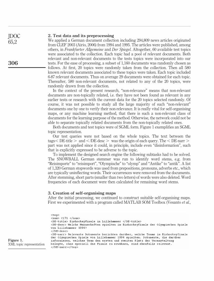
2. Test data and its preprocessingWe applied a German document collection including 294,809 news articles originatedfrom CLEF 2003 (Airio, 2006) from 1994 and 1995. The articles were published, amongothers, in Frankfurter Allgemeine and Der Spiegel. Altogether, 60 available test topicswere associated to the collection. Each topic had a pool of relevant documents. Bothrelevant and non-relevant documents to the tests topics were incorporated into ourtests. For the ease of processing, a subset of 1,160 documents was randomly chosen asfollows. At first, 20 topics were randomly taken from the collection. Then all 580known relevant documents associated to these topics were taken. Each topic included6-87 relevant documents. Thus on average 29 documents were obtained for each topic.Thereafter, 580 non-relevant documents, not related to any of the 20 topics, wererandomly drawn from the collection.

In the context of the present research, “non-relevance” means that non-relevantdocuments are non-topically related, i.e. they have not been found as relevant in anyearlier tests or research with the current data for the 20 topics selected randomly. Ofcourse, it was not possible to study all the large majority of such “non-relevant”documents one by one to verify their non-relevance. It is really vital for self-organisingmaps, or any machine learning method, that there is such a non-relevant class ofdocuments for the learning purpose of the method. Otherwise, the network could not beable to separate topically related documents from the non-topically related ones.

Both documents and test topics were of SGML form. Figure 1 exemplifies an SGMLtopic representation.

Our test queries were not based on the whole topics. The text between thetags, DE-title . and , /DE-desc . was the origin of each query. The , DE-narr .part was not applied since it could, in principle, include even “disinformation”, suchthat is explicitly expressed to be adverse to the topic.

To implement the designed search engine the following subtasks had to be solved.The SNOWBALL German stemmer was run to identify word stems, e.g. from“Reisimporte” to “reisimport”, “Olympische” to “olymp” and “Antike” to “antik”. A listof 1,320 German stopwords was used from prepositions, pronouns, adverbs etc., whichare typically uninflecting words. Their occurrences were removed from the documents.After stemming, short parts (smaller than two letters) of words were also deleted. Wordfrequencies of each document were then calculated for remaining word stems.

3. Creation of self-organising mapsAfter the initial processing, we continued to construct suitable self-organising maps.First we experimented with a program called MATLAB SOM Toolbox (Vesanto et al.,

Figure 1.XML topic representation

JDOC65,2

306

2000). However, the Matlab environment was inappropriate since our matrices were toolarge to be run with it. Therefore, we chose another program, SOM_PAK (Kohonenet al., 1996), which has been written in C and which allows larger data quantities and isfar faster compared to MATLAB. It supports the basic operations for a self-organisingmap like initialisation, learning and evaluation.

Our objective was to design a fairly straightforward search engine prototype inorder to form two-dimensional search networks on the basis of self-organising maps asfollows. First, text documents are input to the system in the SGML form. Second, aself-organising map is built after the preceding preprocessing subtasks. Third, abest-fit match (node) is searched for from the map and documents contained by such anode and by nodes in the close neighbourhood are retrieved. This means that the bestfit node is searched for a given query from the map and the documents of the best fitnode and possibly those of its close neighbourhood are produced as the outcome for thequery. Last, topics could be marked as words on a map. A user could browse acollection included in the map and also search by words.

After pre-processing of the data chosen, the frequency calculation of the remainingwords was accomplished. The following procedure was used to remove very frequentand rare words:

(1) Frequency information was computed for all words of the document set in howmany documents each word occurred.

(2) The words were sorted to the list of descending order along with theirfrequencies.

(3) An appropriate quantity of words, e.g. 1,000, was selected from the centre of thelist.

Our aim was to exclude such words that occur in all or most documents or only in fewdocuments.

Next, document vectors were created. Note that document lengths naturally varied.We employed document vectors from 500 to 5,000 words, which were shorter than theoriginal documents. Main results to be described were obtained with the vectors of1,000 words, but according to our preliminary experiments results did not essentiallydepend on this choice.

The document vectors were encoded with binary, frequency and tf.idf weights(Baeza-Yates and Ribeiro-Neto, 1999), but we shall only show main results for the lastone since these were slightly better than those of the others. To compute tf.idf weights,the frequencies of words (terms) were calculated according to:

tf ik ¼freqik

max j freqij� �

where freqik is the number of occurrences of word k in document Di and freqij is for allwords of Di. The whole document collection is dealt in this way. The inverse documentfrequency is obtained by:

idf k ¼ logN

nk

A study of theuse of self-

organising maps

307

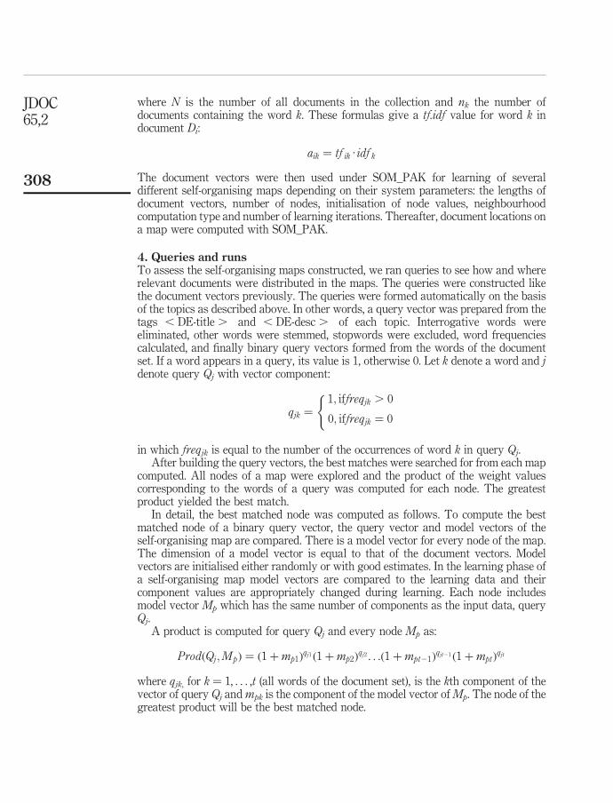
where N is the number of all documents in the collection and nk the number ofdocuments containing the word k. These formulas give a tf.idf value for word k indocument Di:

aik ¼ tf ik · idf k

The document vectors were then used under SOM_PAK for learning of severaldifferent self-organising maps depending on their system parameters: the lengths ofdocument vectors, number of nodes, initialisation of node values, neighbourhoodcomputation type and number of learning iterations. Thereafter, document locations ona map were computed with SOM_PAK.

4. Queries and runsTo assess the self-organising maps constructed, we ran queries to see how and whererelevant documents were distributed in the maps. The queries were constructed likethe document vectors previously. The queries were formed automatically on the basisof the topics as described above. In other words, a query vector was prepared from thetags , DE-title . and , DE-desc . of each topic. Interrogative words wereeliminated, other words were stemmed, stopwords were excluded, word frequenciescalculated, and finally binary query vectors formed from the words of the documentset. If a word appears in a query, its value is 1, otherwise 0. Let k denote a word and jdenote query Qj with vector component:

qjk ¼1; iffreqjk . 0

0; iffreqjk ¼ 0

(

in which freqjk is equal to the number of the occurrences of word k in query Qj.After building the query vectors, the best matches were searched for from each map

computed. All nodes of a map were explored and the product of the weight valuescorresponding to the words of a query was computed for each node. The greatestproduct yielded the best match.

In detail, the best matched node was computed as follows. To compute the bestmatched node of a binary query vector, the query vector and model vectors of theself-organising map are compared. There is a model vector for every node of the map.The dimension of a model vector is equal to that of the document vectors. Modelvectors are initialised either randomly or with good estimates. In the learning phase ofa self-organising map model vectors are compared to the learning data and theircomponent values are appropriately changed during learning. Each node includesmodel vector Mp which has the same number of components as the input data, queryQj.

A product is computed for query Qj and every node Mp as:

ProdðQj;MpÞ ¼ ð1 þmp1Þqj1 ð1 þmp2Þ

qj2 . . .ð1 þmpt21Þqjt21 ð1 þmptÞ

qjt

where qjk, for k ¼ 1, . . . ,t (all words of the document set), is the kth component of thevector of query Qj and mpk is the component of the model vector of Mp. The node of thegreatest product will be the best matched node.

JDOC65,2

308

Random or linear initialisation was used for model vectors. In the former way,model vector components are set to random values uniformly distributed. In the latter,model vectors are initialised along with a two-dimensional subspace spanned by thetwo principal eigenvectors of the learning data vectors. Learning, in other wordschanging model vector components after the initialisation, followed the generalprinciple of self-organising maps to modify model vectors so that a group of nodesclose to each other gradually begins to represent some type of input vectors (documentvectors) and finally groups or areas of nodes on a map correspond to certain documentvector types, i.e. documents that are somewhat similar to each other. An individuallearning iteration was as follows:

(1) An input vector was selected randomly.

(2) It was compared to the model vectors of a map using Euclidean distance.

(3) The best matching node (model vector) was taken.

(4) The components of the taken node (model vector) and its closest neighbourhoodnodes were modified toward the input vector given.

We applied bubble and Gaussian neighbourhood weighting types (Kohonen et al.,1996). In the former, the closest nodes, next closest nodes etc. of the best matching node(Figure 2) are taken and changes of their model vectors are multiplied by weightsdepending on their closeness to the best matching node. Straightforwardly a stepfunction was used here: the weight is equal to 1 if a node is within the bubble, otherwise0. In the latter type, weighting is given by a normal (Gaussian) distribution centred inthe best matching node.

Our goal was to pursue a situation on a map that most documents relevant for atopic would be fairly closely located around some node. To evaluate typicalperformance of self-organising maps we computed five different versions for each map

Figure 2.Neighbourhood is definedas link distance from the

best matching node inthe centre

A study of theuse of self-

organising maps

309

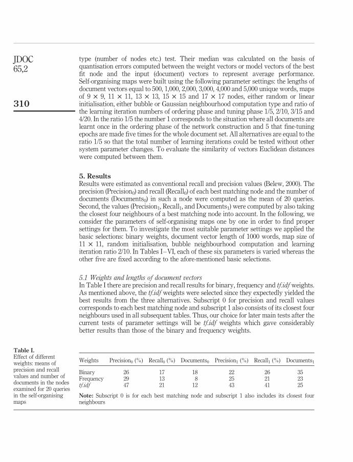
type (number of nodes etc.) test. Their median was calculated on the basis ofquantisation errors computed between the weight vectors or model vectors of the bestfit node and the input (document) vectors to represent average performance.Self-organising maps were built using the following parameter settings: the lengths ofdocument vectors equal to 500, 1,000, 2,000, 3,000, 4,000 and 5,000 unique words, mapsof 9 £ 9, 11 £ 11, 13 £ 13, 15 £ 15 and 17 £ 17 nodes, either random or linearinitialisation, either bubble or Gaussian neighbourhood computation type and ratio ofthe learning iteration numbers of ordering phase and tuning phase 1/5, 2/10, 3/15 and4/20. In the ratio 1/5 the number 1 corresponds to the situation where all documents arelearnt once in the ordering phase of the network construction and 5 that fine-tuningepochs are made five times for the whole document set. All alternatives are equal to theratio 1/5 so that the total number of learning iterations could be tested without othersystem parameter changes. To evaluate the similarity of vectors Euclidean distanceswere computed between them.

5. ResultsResults were estimated as conventional recall and precision values (Belew, 2000). Theprecision (Precision0) and recall (Recall0) of each best matching node and the number ofdocuments (Documents0) in such a node were computed as the mean of 20 queries.Second, the values (Precision1, Recall1, and Documents1) were computed by also takingthe closest four neighbours of a best matching node into account. In the following, weconsider the parameters of self-organising maps one by one in order to find propersettings for them. To investigate the most suitable parameter settings we applied thebasic selections: binary weights, document vector length of 1000 words, map size of11 £ 11, random initialisation, bubble neighbourhood computation and learningiteration ratio 2/10. In Tables I–VI, each of these six parameters is varied whereas theother five are fixed according to the afore-mentioned basic selections.

5.1 Weights and lengths of document vectorsIn Table I there are precision and recall results for binary, frequency and tf.idf weights.As mentioned above, the tf.idf weights were selected since they expectedly yielded thebest results from the three alternatives. Subscript 0 for precision and recall valuescorresponds to each best matching node and subscript 1 also consists of its closest fourneighbours used in all subsequent tables. Thus, our choice for later main tests after thecurrent tests of parameter settings will be tf.idf weights which gave considerablybetter results than those of the binary and frequency weights.

Weights Precision0 (%) Recall0 (%) Documents0 Precision1 (%) Recall1 (%) Documents1

Binary 26 17 18 22 26 35Frequency 29 13 8 25 21 23tf.idf 47 21 12 43 41 25

Note: Subscript 0 is for each best matching node and subscript 1 also includes its closest fourneighbours

Table I.Effect of differentweights: means ofprecision and recallvalues and number ofdocuments in the nodesexamined for 20 queriesin the self-organisingmaps

JDOC65,2

310

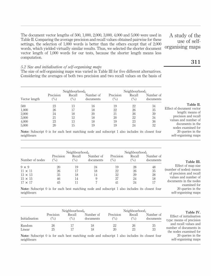
The document vector lengths of 500, 1,000, 2,000, 3,000, 4,000 and 5,000 were used inTable II. Comparing the average precision and recall values obtained pairwise for thesesettings, the selection of 1,000 words is better than the others except that of 2,000words, which yielded virtually similar results. Thus, we selected the shorter documentvector length of 1,000 words for our tests, because the shorter length means lesscomputation.

5.2 Size and initialisation of self-organising mapsThe size of self-organising maps was varied in Table III for five different alternatives.Considering the averages of both two precision and two recall values on the basis of

Neighbourhood0 Neighbourhood1

Vector lengthPrecision

(%)Recall

(%)Number ofdocuments

Precision(%)

Recall(%)

Number ofdocuments

500 23 13 16 19 22 341,000 26 17 18 22 26 352,000 24 18 20 21 26 393,000 21 12 18 20 22 344,000 23 13 18 19 23 365,000 20 15 19 19 24 32

Note: Subscript 0 is for each best matching node and subscript 1 also includes its closest fourneighbours

Table II.Effect of document vector

length: means ofprecision and recall

values and number ofdocuments in the

nodes examined for20 queries in the

self-organising maps

Neighbourhood0 Neighbourhood1

Number of nodesPrecision(%)

Recall(%)

Number ofdocuments

Precision(%)

Recall(%)

Number ofdocuments

9 £ 9 20 19 24 19 28 4811 £ 11 26 17 18 22 26 3513 £ 13 35 18 14 32 29 2815 £ 15 46 14 9 37 24 1817 £ 17 45 11 7 41 24 17

Note: Subscript 0 is for each best matching node and subscript 1 also includes its closest fourneighbours

Table III.Effect of map size

(number of nodes): meansof precision and recallvalues and number of

documents in the nodesexamined for

20 queries in theself-organising maps

Neighbourhood0 Neighbourhood1

InitialisationPrecision

(%)Recall

(%)Number ofdocuments

Precision(%)

Recall(%)

Number ofdocuments

Random 26 17 18 22 26 35Linear 25 17 18 20 23 33

Note: Subscript 0 is for each best matching node and subscript 1 also includes its closest fourneighbours

Table IV.Effect of initialisation

type: means of precisionand recall values and

number of documents inthe nodes examined for

20 queries in theself-organising maps

A study of theuse of self-

organising maps

311

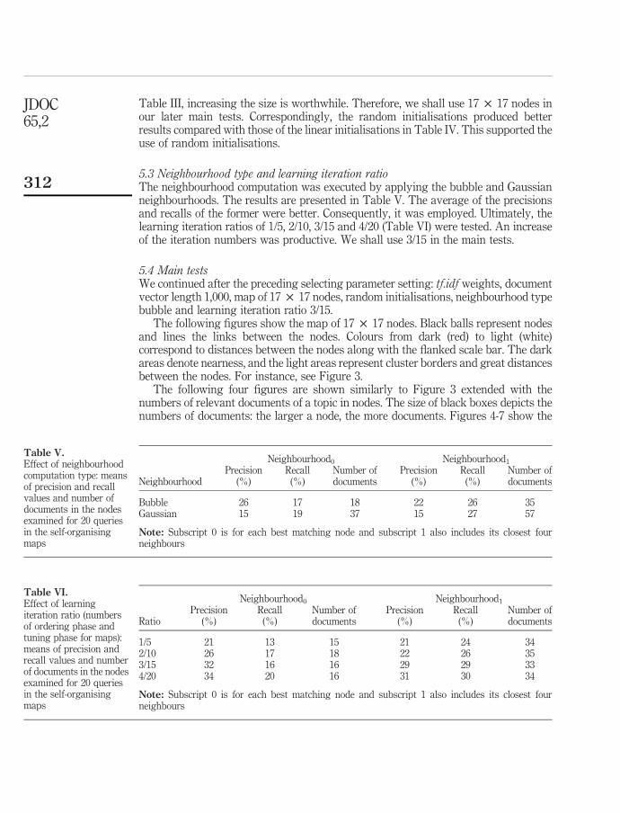
Table III, increasing the size is worthwhile. Therefore, we shall use 17 £ 17 nodes inour later main tests. Correspondingly, the random initialisations produced betterresults compared with those of the linear initialisations in Table IV. This supported theuse of random initialisations.

5.3 Neighbourhood type and learning iteration ratioThe neighbourhood computation was executed by applying the bubble and Gaussianneighbourhoods. The results are presented in Table V. The average of the precisionsand recalls of the former were better. Consequently, it was employed. Ultimately, thelearning iteration ratios of 1/5, 2/10, 3/15 and 4/20 (Table VI) were tested. An increaseof the iteration numbers was productive. We shall use 3/15 in the main tests.

5.4 Main testsWe continued after the preceding selecting parameter setting: tf.idf weights, documentvector length 1,000, map of 17 £ 17 nodes, random initialisations, neighbourhood typebubble and learning iteration ratio 3/15.

The following figures show the map of 17 £ 17 nodes. Black balls represent nodesand lines the links between the nodes. Colours from dark (red) to light (white)correspond to distances between the nodes along with the flanked scale bar. The darkareas denote nearness, and the light areas represent cluster borders and great distancesbetween the nodes. For instance, see Figure 3.

The following four figures are shown similarly to Figure 3 extended with thenumbers of relevant documents of a topic in nodes. The size of black boxes depicts thenumbers of documents: the larger a node, the more documents. Figures 4-7 show the

Neighbourhood0 Neighbourhood1

RatioPrecision

(%)Recall

(%)Number ofdocuments

Precision(%)

Recall(%)

Number ofdocuments

1/5 21 13 15 21 24 342/10 26 17 18 22 26 353/15 32 16 16 29 29 334/20 34 20 16 31 30 34

Note: Subscript 0 is for each best matching node and subscript 1 also includes its closest fourneighbours

Table VI.Effect of learningiteration ratio (numbersof ordering phase andtuning phase for maps):means of precision andrecall values and numberof documents in the nodesexamined for 20 queriesin the self-organisingmaps

Neighbourhood0 Neighbourhood1

NeighbourhoodPrecision

(%)Recall

(%)Number ofdocuments

Precision(%)

Recall(%)

Number ofdocuments

Bubble 26 17 18 22 26 35Gaussian 15 19 37 15 27 57

Note: Subscript 0 is for each best matching node and subscript 1 also includes its closest fourneighbours

Table V.Effect of neighbourhoodcomputation type: meansof precision and recallvalues and number ofdocuments in the nodesexamined for 20 queriesin the self-organisingmaps

JDOC65,2

312

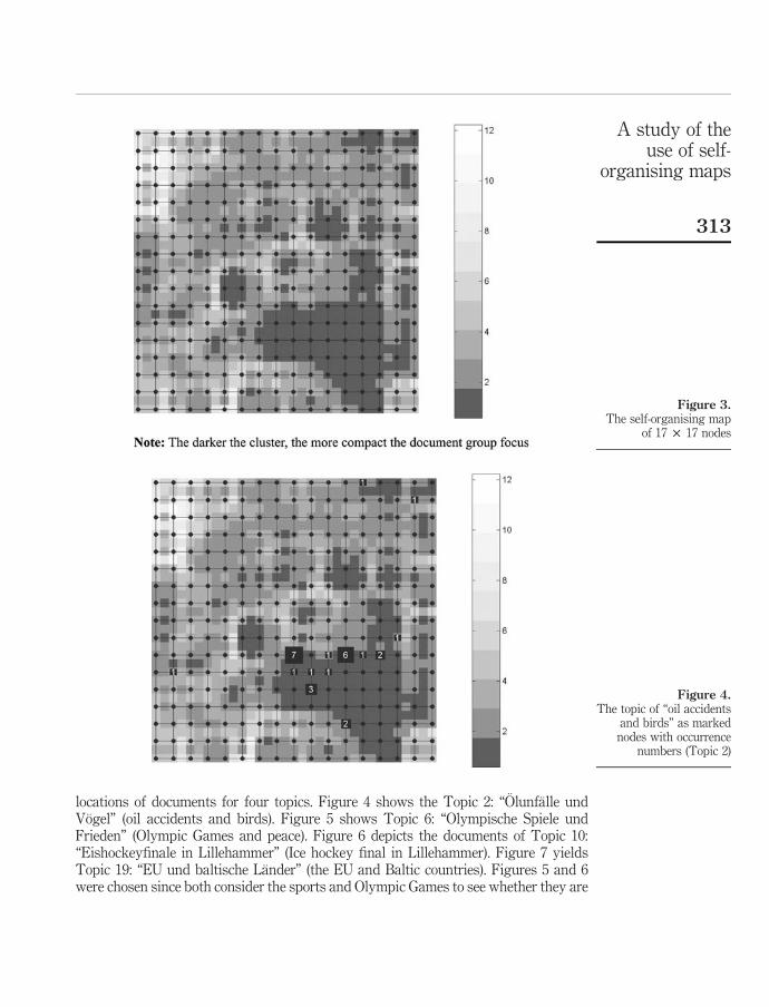
locations of documents for four topics. Figure 4 shows the Topic 2: “Olunfalle undVogel” (oil accidents and birds). Figure 5 shows Topic 6: “Olympische Spiele undFrieden” (Olympic Games and peace). Figure 6 depicts the documents of Topic 10:“Eishockeyfinale in Lillehammer” (Ice hockey final in Lillehammer). Figure 7 yieldsTopic 19: “EU und baltische Lander” (the EU and Baltic countries). Figures 5 and 6were chosen since both consider the sports and Olympic Games to see whether they are

Figure 3.The self-organising map

of 17 £ 17 nodes

Figure 4.The topic of “oil accidents

and birds” as markednodes with occurrence

numbers (Topic 2)

A study of theuse of self-

organising maps

313

close to each other. The other two topics, which do not represent sports, were taken tosee whether they are further away from the sports nodes. Indeed, the sports topics arenear each other, but especially the topic on the EU and Baltic countries are apart fromthe preceding two.

Since the retrieval results clearly depended on a topic, detailed precision and recallvalues associated to the topic numbers are shown in Table VII. The results of theclosest two neighbourhoods according to the linked distance (Figure 2) are presented.The results indicate how the documents of some topics are well found and those of the

Figure 5.The topic of “Olympicgames and peace” asmarked nodes withoccurrence numbers(Topic 6)

Figure 6.The topic of “ice hockeyfinal in Lillehammer” asmarked nodes withoccurrence numbers(Topic 10)

JDOC65,2

314

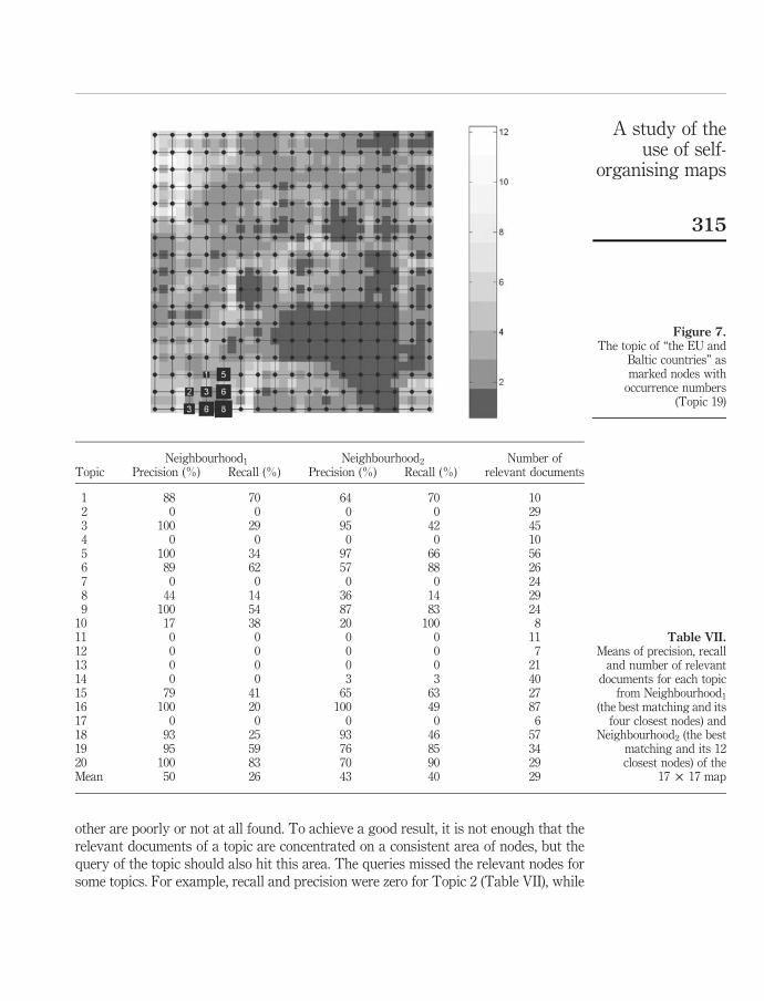
other are poorly or not at all found. To achieve a good result, it is not enough that therelevant documents of a topic are concentrated on a consistent area of nodes, but thequery of the topic should also hit this area. The queries missed the relevant nodes forsome topics. For example, recall and precision were zero for Topic 2 (Table VII), while

Figure 7.The topic of “the EU and

Baltic countries” asmarked nodes with

occurrence numbers(Topic 19)

Neighbourhood1 Neighbourhood2 Number ofTopic Precision (%) Recall (%) Precision (%) Recall (%) relevant documents

1 88 70 64 70 102 0 0 0 0 293 100 29 95 42 454 0 0 0 0 105 100 34 97 66 566 89 62 57 88 267 0 0 0 0 248 44 14 36 14 299 100 54 87 83 24

10 17 38 20 100 811 0 0 0 0 1112 0 0 0 0 713 0 0 0 0 2114 0 0 3 3 4015 79 41 65 63 2716 100 20 100 49 8717 0 0 0 0 618 93 25 93 46 5719 95 59 76 85 3420 100 83 70 90 29Mean 50 26 43 40 29

Table VII.Means of precision, recall

and number of relevantdocuments for each topic

from Neighbourhood1

(the best matching and itsfour closest nodes) and

Neighbourhood2 (the bestmatching and its 12closest nodes) of the

17 £ 17 map

A study of theuse of self-

organising maps

315

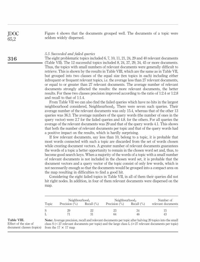
Figure 4 shows that the documents grouped well. The documents of a topic wereseldom widely dispersed.

5.5 Succeeded and failed queriesThe eight problematic topics included 6, 7, 10, 11, 21, 24, 29 and 40 relevant documents(Table VII). The 12 successful topics included 8, 24, 27, 29, 34, 45 or more documents.Thus, the topics with small numbers of relevant documents were generally difficult toretrieve. This is shown by the results in Table VIII, which are the same as in Table VII,but grouped into two classes of the equal size (ten topics in each) including eitherinfrequent or frequent relevant topics, i.e. the average less than 27 relevant documents,or equal to or greater than 27 relevant documents. The average number of relevantdocuments strongly affected the results: the more relevant documents, the betterresults. For these two classes precision improved according to the ratio of 1:2.4 or 1:2.8and recall to that of 1:1.4.

From Table VII we can also find the failed queries which have no hits in the largestneighbourhood considered, Neighbourhood2. There were seven such queries. Theiraverage number of the relevant documents was only 15.4, whereas that of the other 13queries was 36.3. The average numbers of the query words (the number of ones in thequery vector) were 2.7 for the failed queries and 4.8. for the others. For all queries theaverage of the relevant documents was 29 and that of the query words 4.1. This showsthat both the number of relevant documents per topic and that of the query words hada positive impact on the results, which is hardly surprising.

If few relevant documents, say less than 10, belong to a topic, it is probable thatmost words connected with such a topic are discarded from the set of words chosenwhile creating document vectors. A greater number of relevant documents guaranteesthe words of a topic a better opportunity to remain in the chosen word set and, thus, tobecome good search keys. When a majority of the words of a topic with a small numberof relevant documents is not included in the chosen word set, it is probable that thedocument vectors and a query vector of the topic consist of only few words, which isnot necessarily enough so that the documents would be grouped into a compact area onthe map resulting in difficulties to find a good hit.

Considering the eight failed topics in Table VII, in all of them their queries did nothit right nodes. In addition, in four of them relevant documents were dispersed on themap.

Neighbourhood1 Neighbourhood2 Number ofTopic Precision (%) Recall (%) Precision (%) Recall (%) relevant documents

S 29 22 23 34 15L 71 31 64 46 43

Note: Average precision, recall and relevant documents per topic after halving 20 topics into the smallclass S (,27 relevant documents per topic) and the large class L ($27 relevant documents per topic)from the 17 £ 17 map

Table VIII.Effect of the size ofdocument classes (topics)

JDOC65,2

316

6. Discussion and comparison with clustering experimentsThe results showed that it is possible to concentrate relevant documents on compactareas on a self-organising map. For instance, in Figure 5 most of the documentsrelevant to the Topic 6 were in four adjacent nodes. The means of the precision andrecall values in the best matched node and its closest four neighbour nodes weresatisfactory, 26-50 per cent. The majority of the documents of each topic were insidenearby area demonstrated by Figures 4-7. When on average there were 29 relevantdocuments per query, approximately the quantity of 1/40 of all documents wasrelevant for each topic. If we took 30 documents fully randomly from the 1160documents and compared them to a given query, the expectation of relevant documentswould be 0.75. This means that the self-organising maps giving expectations 7.5 – 14.5were able to produce an outcome better than ten times a random search.

The results indicated that it was not easy to find the documents of the current 20topics applied. Moreover, the detailed results in Table VII revealed how strongly thisoutcome depended on a topic. This may denote such a feature that it was not possibleto separate the “lost” topics from other documents on the basis of the used variables,i.e. the chosen words. However, our technique to choose words could possibly bedeveloped. At the moment, we discarded, after stemming, words shorter than twoletters. Perhaps by eliminating words shorter than three or four letters would be moreeffective. On the other hand, even after stemming most German words are longer thanthree letters.

In order to compare the results obtained with the self-organising maps, we clusteredour test data using k-means and hierarchical Ward’s algorithms with the Euclideanmeasure. Along with the tests of the preceding section, we used the same 20 topics andcomputed average results for 10 runs. We computed these results for cluster numbers kof 20, 30, 40,..., 290 and 300. In addition, we computed results for quadraticself-organising maps of sizes 4 £ 4 ¼ 16, 5 £ 5 ¼ 25, 6 £ 6 ¼ 36, . . . ,16 £ 16 ¼ 256 and 17 £ 17 ¼ 289. Cluster numbers that were closest to the nodenumbers of the self-organising maps were selected and their results were compared tothose of the maps. Regarding the two clustering techniques, we selected such clustersto a neighbourhood set whose centroids were closest to the query vector as measuredwith the Euclidean distance. Since the neighbourhoods of the self-organising mapsconsisted of 1, 5 and 13 nodes, the closest cluster, five closest clusters and 13 closestclusters were selected.

To condense results we combined precision P and recall R according to F value byManning and Schutze (2003):

F ¼2PR

P þ R100%:

In the following figures subscript 0 is for each best matching node, and subscripts 1and 2 include its two closest afore-said neighbourhoods. Figure 8 consists of the resultsof Neighbourhood0, Figure 9 those of Neighbourhood1 and Figure 10 those ofNeighbourhood2. The average results of the self-organising maps withNeighbourhood0 are superior to those of k-means and Ward’s clustering techniques.The best average results of k-means and Ward’s clustering with Neighbourhood1 inFigure 9 (between 81 and 144 nodes) and with Neighbourhood2 in Figure 10 (over 196nodes) are approximately 2-5 per cent higher than the best of the self-organising maps.

A study of theuse of self-

organising maps

317

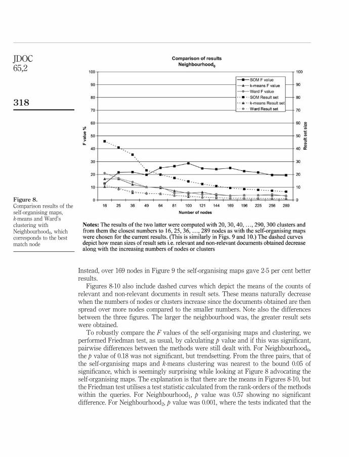
Instead, over 169 nodes in Figure 9 the self-organising maps gave 2-5 per cent betterresults.

Figures 8-10 also include dashed curves which depict the means of the counts ofrelevant and non-relevant documents in result sets. These means naturally decreasewhen the numbers of nodes or clusters increase since the documents obtained are thenspread over more nodes compared to the smaller numbers. Note also the differencesbetween the three figures. The larger the neighbourhood was, the greater result setswere obtained.

To robustly compare the F values of the self-organising maps and clustering, weperformed Friedman test, as usual, by calculating p value and if this was significant,pairwise differences between the methods were still dealt with. For Neighbourhood0,the p value of 0.18 was not significant, but trendsetting. From the three pairs, that ofthe self-organising maps and k-means clustering was nearest to the bound 0.05 ofsignificance, which is seemingly surprising while looking at Figure 8 advocating theself-organising maps. The explanation is that there are the means in Figures 8-10, butthe Friedman test utilises a test statistic calculated from the rank-orders of the methodswithin the queries. For Neighbourhood1, p value was 0.57 showing no significantdifference. For Neighbourhood2, p value was 0.001, where the tests indicated that the

Figure 8.Comparison results of theself-organising maps,k-means and Ward’sclustering withNeighbourhood0, whichcorresponds to the bestmatch node

JDOC65,2

318

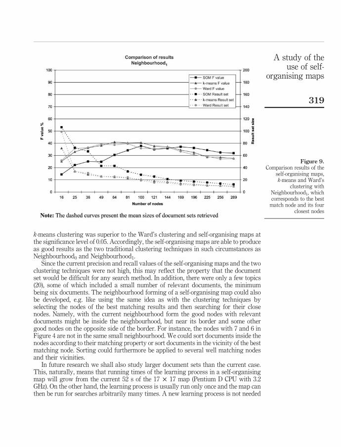
k-means clustering was superior to the Ward’s clustering and self-organising maps atthe significance level of 0.05. Accordingly, the self-organising maps are able to produceas good results as the two traditional clustering techniques in such circumstances asNeighbourhood0 and Neighbourhood1.

Since the current precision and recall values of the self-organising maps and the twoclustering techniques were not high, this may reflect the property that the documentset would be difficult for any search method. In addition, there were only a few topics(20), some of which included a small number of relevant documents, the minimumbeing six documents. The neighbourhood forming of a self-organising map could alsobe developed, e.g. like using the same idea as with the clustering techniques byselecting the nodes of the best matching results and then searching for their closenodes. Namely, with the current neighbourhood form the good nodes with relevantdocuments might be inside the neighbourhood, but near its border and some othergood nodes on the opposite side of the border. For instance, the nodes with 7 and 6 inFigure 4 are not in the same small neighbourhood. We could sort documents inside thenodes according to their matching property or sort documents in the vicinity of the bestmatching node. Sorting could furthermore be applied to several well matching nodesand their vicinities.

In future research we shall also study larger document sets than the current case.This, naturally, means that running times of the learning process in a self-organisingmap will grow from the current 52 s of the 17 £ 17 map (Pentium D CPU with 3.2GHz). On the other hand, the learning process is usually run only once and the map canthen be run for searches arbitrarily many times. A new learning process is not needed

Figure 9.Comparison results of the

self-organising maps,k-means and Ward’s

clustering withNeighbourhood1, whichcorresponds to the best

match node and its fourclosest nodes

A study of theuse of self-

organising maps

319

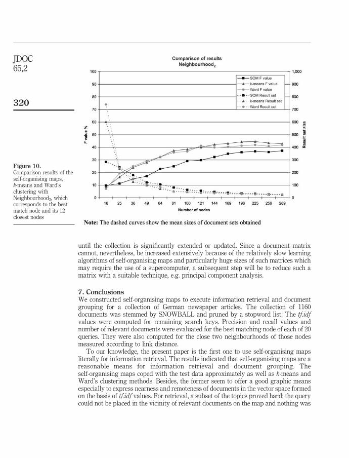
until the collection is significantly extended or updated. Since a document matrixcannot, nevertheless, be increased extensively because of the relatively slow learningalgorithms of self-organising maps and particularly huge sizes of such matrices whichmay require the use of a supercomputer, a subsequent step will be to reduce such amatrix with a suitable technique, e.g. principal component analysis.

7. ConclusionsWe constructed self-organising maps to execute information retrieval and documentgrouping for a collection of German newspaper articles. The collection of 1160documents was stemmed by SNOWBALL and pruned by a stopword list. The tf.idfvalues were computed for remaining search keys. Precision and recall values andnumber of relevant documents were evaluated for the best matching node of each of 20queries. They were also computed for the close two neighbourhoods of those nodesmeasured according to link distance.

To our knowledge, the present paper is the first one to use self-organising mapsliterally for information retrieval. The results indicated that self-organising maps are areasonable means for information retrieval and document grouping. Theself-organising maps coped with the test data approximately as well as k-means andWard’s clustering methods. Besides, the former seem to offer a good graphic meansespecially to express nearness and remoteness of documents in the vector space formedon the basis of tf.idf values. For retrieval, a subset of the topics proved hard: the querycould not be placed in the vicinity of relevant documents on the map and nothing was

Figure 10.Comparison results of theself-organising maps,k-means and Ward’sclustering withNeighbourhood2, whichcorresponds to the bestmatch node and its 12closest nodes

JDOC65,2

320

found. These topics were those of the small numbers of relevant documents. For a fewtopics the scarce relevant documents were dispersed across the map, unsuccessfullyfrom the viewpoint of the retrievals. This can also reflect the property of neuralnetworks that they may not learn efficiently such occurrences (documents) that areinfrequent in the data. For the majority of the topics, the queries gave satisfactoryresults.

References

Airio, E. (2006), “Word normalization and decompounding in mono- and bilingual IR”,Information Retrieval, Vol. 9 No. 3, pp. 249-71.

Baeza-Yates, R. and Ribeiro-Neto, B. (1999), Modern Information Retrieval, ACM Press andAddison-Wesley, New York, NY.

Belew, R.K. (2000), Finding out about, A Cognitive Pespective on Search Engine Technology andWWW, Cambridge University Press, Cambridge, UK.

Chowdhury, N. and Saha, D. (2005), “Unsupervised text classification using Kohonen’s selforganizing network”, Lecture Notes in Computer Science, Computational Linguistics andIntelligent Text Processing, 3406, Springer-Verlag, Heidelberg, pp. 715-718.

Fernandez, J., Mones, R., Dıaz, I., Ranilla, J. and Combarro, E.F. (2004), “Experiments with selforganizing maps in CLEF 2003”, Lecture Notes in Computer Science, ComparativeEvaluation of Multilingual Information Access Systems, 3237, Springer-Verlag,Heidelberg, pp. 358-366.

Guerrero-Bote, V.P., Moya-Anegon, F. and Herrero-Solana, V. (2002), “Document organizationusing Kohonen’s algorithm”, Information Processing and Management, Vol. 38, pp. 79-89.

Honkela, T. (1997), “Self-organizing maps in natural language processing”, academicdissertation, Helsinki University of Technology, Espoo.

Kaski, S. (1998), “Dimensionality reduction by random mapping: fast similarity computation forclustering”, Proceedings of IEEE International Joint Conference on Neural NetworksIJCNN’98, IEEE, Vol. 1, pp. 413-418.

Kohonen, T. (1995), Self-organizing Maps, Springer-Verlag, Berlin.

Kohonen, T., Hynninen, J., Kangas, J. and Laaksonen, J. (1996), “SOM_PAK: the self-organizingmap program package”, Helsinki University of Technology, Espoo, available at: www.cis.hut.fi/research/papers/som_tr96.ps.Z

Kohonen, T., Kaski, S., Lagus, K., Salojarvi, J., Honkela, J., Paatero, V. and Saarela, A. (2000), “Selforganization of a massive document collection”, IEEE Transactions on Neural Networks,Vol. 11 No. 3, pp. 574-85.

Lagus, K. (2002), “Text mining with WEBSOM”, academic dissertation, Helsinki University ofTechnology, Espoo.

Lagus, K., Kaski, S. and Kohonen, T. (2004), “Mining massive document collections by theWEBSOM method”, Information Sciences, Vol. 163 Nos 1-3, pp. 135-56.

Lee, C.-H. and Yang, H.-C. (1999), “A web text mining approach based on self-organizing map”,Proceedings of 2nd International Workshop on Web Information and Data Management,ACM, New York, NY, pp. 59-62.

Lin, X. (1997), “Map displays for information retrieval”, Journal of the American Society forInformation Science, Vol. 48 No. 1, pp. 40-54.

Lin, X., Soergel, D. and Marchionini, G. (1991), “A self-organizing semantic map for informationretrieval”, Proceedings of 14th Annual International ACM SIGIR Conference on Research

A study of theuse of self-

organising maps

321

and Development in Information Retrieval SIGIR’91, 13-16 October, Chicago, IL,pp. 262-269.

Manning, C.D. and Schutze, H. (2003), Foundations of Statistical Natural Language Processing,The MIT Press, Cambridge, MA.

Moya-Anegon, F., Herrero-Solana, V. and Jimenez-Contreras, E. (2006), “A connectionist andmultivariate approach to science maps: the SOM, clustering and MDS applied to libraryand information science research”, Journal of Information Science, Vol. 32 No. 1, pp. 63-77.

Vesanto, J., Himberg, J., Alhoniemi, E. and Parhankangas, J. (2000), “SOM Toolbox for Matlab 5”,Libella Oy, Espoo, available at: www.cis.hut.fi/projects/somtoolbox/package/papers/techrep.pdf

Corresponding authorMartti Juhola can be contacted at: Martti.Juhola@cs.uta.fi

JDOC65,2

322

To purchase reprints of this article please e-mail: reprints@emeraldinsight.comOr visit our web site for further details: www.emeraldinsight.com/reprints

Publication II

On document classification with self-organising maps

Jyri Saarikoski, Kalervo Järvelin, Jorma Laurikkala and Martti Juhola

Copyright © 2009 Springer-Verlag GmbH Berlin Heidelberg. Reprinted, with

permission, from Saarikoski, J., Järvelin, K., Laurikkala, J. and Juhola, M. (2009).

On document classification with self-organising maps. In Proceedings of the 9th

International Conference on Adaptive and Natural Computing Algorithms (ICANNGA

2009), Lecture Notes in Computer Science, Vol. 5495, pp. 140-149.

Available at:

http://dx.doi.org/10.1007/978-3-642-04921-7_15

M. Kolehmainen et al. (Eds.): ICANNGA 2009, LNCS 5495, pp. 140–149, 2009. © Springer-Verlag Berlin Heidelberg 2009

On Document Classification with Self-Organising Maps

Jyri Saarikoski1, Kalervo Järvelin2, Jorma Laurikkala1, and Martti Juhola1

1 Department of Computer Sciences, 33014 University of Tampere, Finland 2 Department of Information Studies,

33014 University of Tampere, Finland {Jyri.Saarikoski,Kalervo.Jarvelin,Jorma.Laurikkala,

Martti.Juhola}@uta.fi

Abstract. This research deals with the use of self-organising maps for the clas-sification of text documents. The aim was to classify documents to separate classes according to their topics. We therefore constructed self-organising maps that were effective for this task and tested them with German newspaper docu-ments. We compared the results gained to those of k nearest neighbour search-ing and k-means clustering. For five and ten classes, the self-organising maps were better yielding as high average classification accuracies as 88-89%, whereas nearest neighbour searching gave 74-83% and k-means clustering 72-79% as their highest accuracies.

1 Introduction

The growth of digital documents and information stored as text in the Internet has been rapid in the recent years. Searching and grouping such documents in various ways have become an important and challenging function. A myriad of documents are daily accessed in the Internet to find interesting and applicable information. Distin-guishing in some way interesting documents from the uninteresting ones is, even if a self-evident goal, crucial. For this purpose, computational methods are of paramount importance. We are interested in researching the classification of text documents, also those written in languages other than English.

There are known methods for constructing groups, clusters or models of documents, see for instance [4], [12] and [13]. These machine learning methods have included k nearest neighbour searching, probabilistic methods such as Naïve Bayesian classifiers [5] and evolutionary learning with genetic algorithms [13]. The methods were of the supervised category. We investigated the use of unsupervised Kohonen self-organising maps [8] that seemed to be seldom used in this field. They have been, however, applied to constructing visual maps of text document clusters, in which documents were clus-tered based on the features they contain. WEBSOM [7] [9] was employed to organize large document collections, but it did not include document classification in the sense to be compared with the current research. Chowdhury and Saha [2] classified 400, 500 and 600 sport articles, whereas Guerro-Bote et al. [6] employed 202 documents from a bibliographic database. Moya-Anegón et al. [10] made domain analysis of documents with self-organising maps, clustering and multidimensional scaling. Instead of

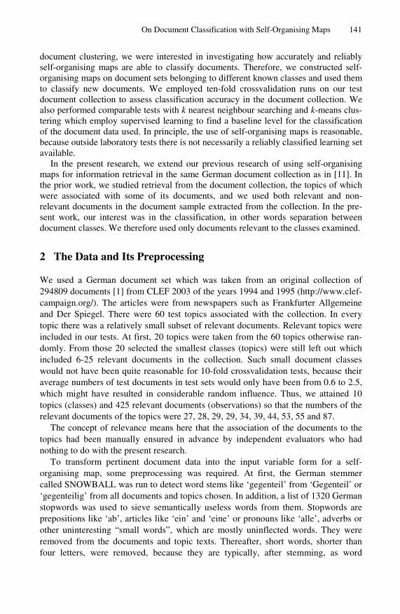
On Document Classification with Self-Organising Maps 141

document clustering, we were interested in investigating how accurately and reliably self-organising maps are able to classify documents. Therefore, we constructed self-organising maps on document sets belonging to different known classes and used them to classify new documents. We employed ten-fold crossvalidation runs on our test document collection to assess classification accuracy in the document collection. We also performed comparable tests with k nearest neighbour searching and k-means clus-tering which employ supervised learning to find a baseline level for the classification of the document data used. In principle, the use of self-organising maps is reasonable, because outside laboratory tests there is not necessarily a reliably classified learning set available.

In the present research, we extend our previous research of using self-organising maps for information retrieval in the same German document collection as in [11]. In the prior work, we studied retrieval from the document collection, the topics of which were associated with some of its documents, and we used both relevant and non-relevant documents in the document sample extracted from the collection. In the pre-sent work, our interest was in the classification, in other words separation between document classes. We therefore used only documents relevant to the classes examined.

2 The Data and Its Preprocessing

We used a German document set which was taken from an original collection of 294809 documents [1] from CLEF 2003 of the years 1994 and 1995 (http://www.clef-campaign.org/). The articles were from newspapers such as Frankfurter Allgemeine and Der Spiegel. There were 60 test topics associated with the collection. In every topic there was a relatively small subset of relevant documents. Relevant topics were included in our tests. At first, 20 topics were taken from the 60 topics otherwise ran-domly. From those 20 selected the smallest classes (topics) were still left out which included 6-25 relevant documents in the collection. Such small document classes would not have been quite reasonable for 10-fold crossvalidation tests, because their average numbers of test documents in test sets would only have been from 0.6 to 2.5, which might have resulted in considerable random influence. Thus, we attained 10 topics (classes) and 425 relevant documents (observations) so that the numbers of the relevant documents of the topics were 27, 28, 29, 29, 34, 39, 44, 53, 55 and 87.

The concept of relevance means here that the association of the documents to the topics had been manually ensured in advance by independent evaluators who had nothing to do with the present research.

To transform pertinent document data into the input variable form for a self-organising map, some preprocessing was required. At first, the German stemmer called SNOWBALL was run to detect word stems like ‘gegenteil’ from ‘Gegenteil’ or ‘gegenteilig’ from all documents and topics chosen. In addition, a list of 1320 German stopwords was used to sieve semantically useless words from them. Stopwords are prepositions like ‘ab’, articles like ‘ein’ and ‘eine’ or pronouns like ‘alle’, adverbs or other uninteresting “small words”, which are mostly uninflected words. They were removed from the documents and topic texts. Thereafter, short words, shorter than four letters, were removed, because they are typically, after stemming, as word

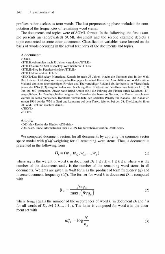
142 J. Saarikoski et al.

prefices rather useless as term words. The last preprocessing phase included the com-putation of the frequencies of remaining word stems.

The documents and topics were of SGML format. In the following, the first exam-ple presents an (abbreviated) SGML document and the second example depicts a topic connected to some other documents. Classification variables were formed on the basis of words occurring in the actual text parts of the documents and topics.

A document: <DOC> <TITLE>Ahornblatt nach 33 Jahren vergoldet</TITLE> <TITLE>Zum 20. Mal Eishockey-Weltmeister</TITLE> <TITLE>Sieg im Penaltyschießen</TITLE> <TITLE>Finnland </TITLE> <TEXT>Das Eishockey-Mutterland Kanada ist nach 33 Jahren wieder die Nummer eins in der Welt. Durch einen 3:2-Erfolg im Penaltyschießen gegen Finnland lösten die Ahornblätter im WM-Finale in Mailand den einst übermächtigen Rivalen und Titelverteidiger Rußland ab, der bereits im Viertelfinale gegen die USA (1:3) ausgeschieden war. Nach regulärer Spielzeit und Verlängerung hatte es 1:1 (0:0, 0:0, 1:1, 0:0) gestanden. Zuvor hatte Brind'Amour (56.) die Führung der Finnen durch Keskinen (47.) ausgeglichen. Im Penaltyschießen zeigten die Kanadier die besseren Nerven, die Finnen verschossen viermal in sechs Versuchen. Robitaille verwandelte den sechsten Penalty für Kanada. Die Kanadier, zuletzt 1961 bei der WM in Genf und Lausanne auf dem Thron, feierten bei den 58. Titelkämpfen ihren 20. WM-Titel und machten damit... </TEXT> </DOC> A topic: <DE-title> Rechte des Kindes </DE-title> <DE-desc> Finde Informationen über die UN-Kinderrechtskonvention. </DE-desc> We computed document vectors for all documents by applying the common vector

space model with tf·idf weighting for all remaining word stems. Thus, a document is presented in the following form

),...,,,( 321 itiiii wwwwD = (1)

where wik is the weight of word k in document Di, 1 ≤ i ≤ n, 1 ≤ k ≤ t, where n is the number of the documents and t is the number of the remaining word stems in all documents. Weights are given in tf·idf form as the product of term frequency (tf) and inverse document frequency (idf). The former for word k in document Di is computed with

{ }ill

ikik freq

freqtf

max= (2)

where freqik equals the number of the occurrences of word k in document Di and l is for all words of Di, l=1,2,3,..., t-1, t. The latter is computed for word k in the docu-ment set with

kk n

Nidf log= (3)

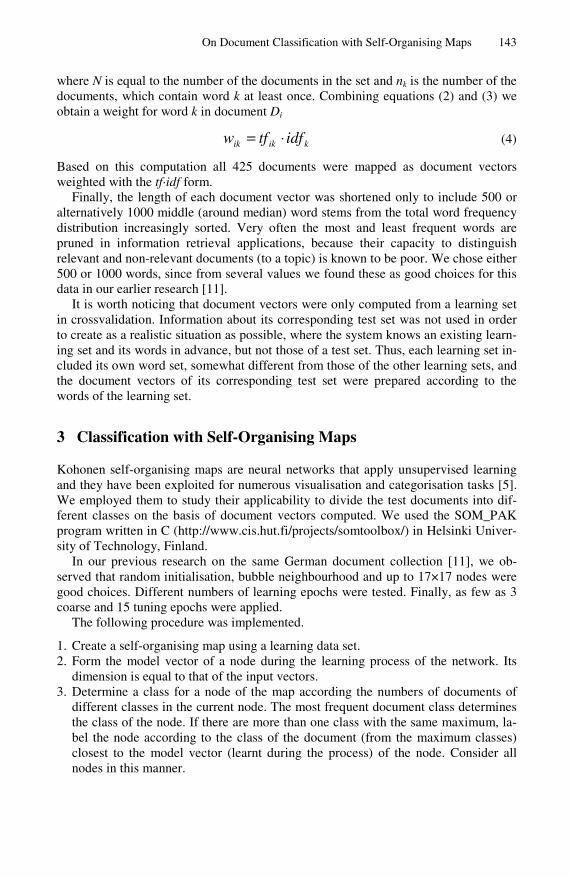
On Document Classification with Self-Organising Maps 143

where N is equal to the number of the documents in the set and nk is the number of the documents, which contain word k at least once. Combining equations (2) and (3) we obtain a weight for word k in document Di

kikik idftfw ⋅= (4)

Based on this computation all 425 documents were mapped as document vectors weighted with the tf·idf form.

Finally, the length of each document vector was shortened only to include 500 or alternatively 1000 middle (around median) word stems from the total word frequency distribution increasingly sorted. Very often the most and least frequent words are pruned in information retrieval applications, because their capacity to distinguish relevant and non-relevant documents (to a topic) is known to be poor. We chose either 500 or 1000 words, since from several values we found these as good choices for this data in our earlier research [11].

It is worth noticing that document vectors were only computed from a learning set in crossvalidation. Information about its corresponding test set was not used in order to create as a realistic situation as possible, where the system knows an existing learn-ing set and its words in advance, but not those of a test set. Thus, each learning set in-cluded its own word set, somewhat different from those of the other learning sets, and the document vectors of its corresponding test set were prepared according to the words of the learning set.

3 Classification with Self-Organising Maps

Kohonen self-organising maps are neural networks that apply unsupervised learning and they have been exploited for numerous visualisation and categorisation tasks [5]. We employed them to study their applicability to divide the test documents into dif-ferent classes on the basis of document vectors computed. We used the SOM_PAK program written in C (http://www.cis.hut.fi/projects/somtoolbox/) in Helsinki Univer-sity of Technology, Finland.

In our previous research on the same German document collection [11], we ob-served that random initialisation, bubble neighbourhood and up to 17×17 nodes were good choices. Different numbers of learning epochs were tested. Finally, as few as 3 coarse and 15 tuning epochs were applied.

The following procedure was implemented.

1. Create a self-organising map using a learning data set. 2. Form the model vector of a node during the learning process of the network. Its

dimension is equal to that of the input vectors. 3. Determine a class for a node of the map according the numbers of documents of

different classes in the current node. The most frequent document class determines the class of the node. If there are more than one class with the same maximum, la-bel the node according to the class of the document (from the maximum classes) closest to the model vector (learnt during the process) of the node. Consider all nodes in this manner.

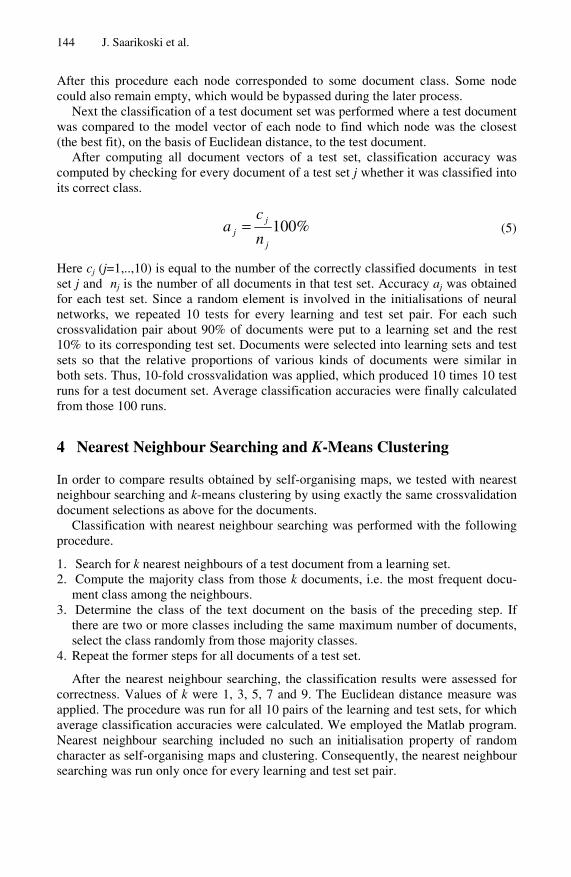
144 J. Saarikoski et al.

After this procedure each node corresponded to some document class. Some node could also remain empty, which would be bypassed during the later process.

Next the classification of a test document set was performed where a test document was compared to the model vector of each node to find which node was the closest (the best fit), on the basis of Euclidean distance, to the test document.

After computing all document vectors of a test set, classification accuracy was computed by checking for every document of a test set j whether it was classified into its correct class.

%100j

jj n

ca = (5)

Here cj (j=1,..,10) is equal to the number of the correctly classified documents in test set j and nj is the number of all documents in that test set. Accuracy aj was obtained for each test set. Since a random element is involved in the initialisations of neural networks, we repeated 10 tests for every learning and test set pair. For each such crossvalidation pair about 90% of documents were put to a learning set and the rest 10% to its corresponding test set. Documents were selected into learning sets and test sets so that the relative proportions of various kinds of documents were similar in both sets. Thus, 10-fold crossvalidation was applied, which produced 10 times 10 test runs for a test document set. Average classification accuracies were finally calculated from those 100 runs.

4 Nearest Neighbour Searching and K-Means Clustering

In order to compare results obtained by self-organising maps, we tested with nearest neighbour searching and k-means clustering by using exactly the same crossvalidation document selections as above for the documents.

Classification with nearest neighbour searching was performed with the following procedure.

1. Search for k nearest neighbours of a test document from a learning set. 2. Compute the majority class from those k documents, i.e. the most frequent docu-

ment class among the neighbours. 3. Determine the class of the text document on the basis of the preceding step. If

there are two or more classes including the same maximum number of documents, select the class randomly from those majority classes.

4. Repeat the former steps for all documents of a test set.

After the nearest neighbour searching, the classification results were assessed for correctness. Values of k were 1, 3, 5, 7 and 9. The Euclidean distance measure was applied. The procedure was run for all 10 pairs of the learning and test sets, for which average classification accuracies were calculated. We employed the Matlab program. Nearest neighbour searching included no such an initialisation property of random character as self-organising maps and clustering. Consequently, the nearest neighbour searching was run only once for every learning and test set pair.

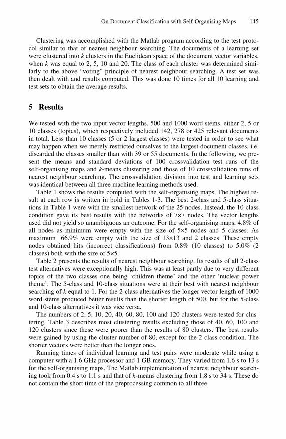
On Document Classification with Self-Organising Maps 145

Clustering was accomplished with the Matlab program according to the test proto-col similar to that of nearest neighbour searching. The documents of a learning set were clustered into k clusters in the Euclidean space of the document vector variables, when k was equal to 2, 5, 10 and 20. The class of each cluster was determined simi-larly to the above “voting” principle of nearest neighbour searching. A test set was then dealt with and results computed. This was done 10 times for all 10 learning and test sets to obtain the average results.

5 Results

We tested with the two input vector lengths, 500 and 1000 word stems, either 2, 5 or 10 classes (topics), which respectively included 142, 278 or 425 relevant documents in total. Less than 10 classes (5 or 2 largest classes) were tested in order to see what may happen when we merely restricted ourselves to the largest document classes, i.e. discarded the classes smaller than with 39 or 55 documents. In the following, we pre-sent the means and standard deviations of 100 crossvalidation test runs of the self-organising maps and k-means clustering and those of 10 crossvalidation runs of nearest neighbour searching. The crossvalidation division into test and learning sets was identical between all three machine learning methods used.

Table 1 shows the results computed with the self-organising maps. The highest re-sult at each row is written in bold in Tables 1-3. The best 2-class and 5-class situa-tions in Table 1 were with the smallest network of the 25 nodes. Instead, the 10-class condition gave its best results with the networks of 7×7 nodes. The vector lengths used did not yield so unambiguous an outcome. For the self-organising maps, 4.8% of all nodes as minimum were empty with the size of 5×5 nodes and 5 classes. As maximum 66.9% were empty with the size of 13×13 and 2 classes. These empty nodes obtained hits (incorrect classifications) from 0.8% (10 classes) to 5.0% (2 classes) both with the size of 5×5.

Table 2 presents the results of nearest neighbour searching. Its results of all 2-class test alternatives were exceptionally high. This was at least partly due to very different topics of the two classes one being ‘children theme’ and the other ‘nuclear power theme’. The 5-class and 10-class situations were at their best with nearest neighbour searching of k equal to 1. For the 2-class alternatives the longer vector length of 1000 word stems produced better results than the shorter length of 500, but for the 5-class and 10-class alternatives it was vice versa.

The numbers of 2, 5, 10, 20, 40, 60, 80, 100 and 120 clusters were tested for clus-tering. Table 3 describes most clustering results excluding those of 40, 60, 100 and 120 clusters since these were poorer than the results of 80 clusters. The best results were gained by using the cluster number of 80, except for the 2-class condition. The shorter vectors were better than the longer ones.

Running times of individual learning and test pairs were moderate while using a computer with a 1.6 GHz processor and 1 GB memory. They varied from 1.6 s to 13 s for the self-organising maps. The Matlab implementation of nearest neighbour search-ing took from 0.4 s to 1.1 s and that of k-means clustering from 1.8 s to 34 s. These do not contain the short time of the preprocessing common to all three.

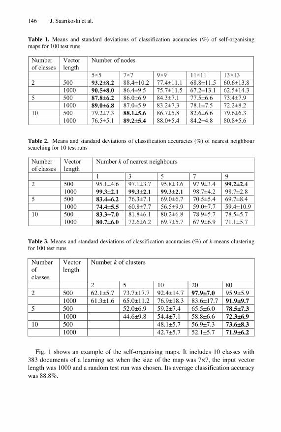
146 J. Saarikoski et al.

Table 1. Means and standard deviations of classification accuracies (%) of self-organising maps for 100 test runs

Numberof classes

Vectorlength

Number of nodes

5×5 7×7 9×9 11×11 13×132 500 93.2±8.2 88.4±10.2 77.4±11.1 68.8±11.5 60.6±13.8

1000 90.5±8.0 86.4±9.5 75.7±11.5 67.2±13.1 62.5±14.35 500 87.8±6.2 86.0±6.9 84.3±7.1 77.5±6.6 73.4±7.9

1000 89.0±6.8 87.0±5.9 83.2±7.3 78.1±7.5 72.2±8.210 500 79.2±7.3 88.1±5.6 86.7±5.8 82.6±6.6 79.6±6.3

1000 76.5±5.1 89.2±5.4 88.0±5.4 84.2±4.8 80.8±5.6

Table 2. Means and standard deviations of classification accuracies (%) of nearest neighbour searching for 10 test runs

Numberof classes

Vectorlength

Number k of nearest neighbours

1 3 5 7 92 500 95.1±4.6 97.1±3.7 95.8±3.6 97.9±3.4 99.2±2.4

1000 99.3±2.1 99.3±2.1 99.3±2.1 98.7±4.2 98.7±2.85 500 83.4±6.2 76.3±7.1 69.0±6.7 70.5±5.4 69.7±8.4

1000 74.4±5.5 60.8±7.7 56.5±9.9 59.0±7.7 59.4±10.910 500 83.3±7.0 81.8±6.1 80.2±6.8 78.9±5.7 78.5±5.7

1000 80.7±6.0 72.6±6.2 69.7±5.7 67.9±6.9 71.1±5.7

Table 3. Means and standard deviations of classification accuracies (%) of k-means clustering for 100 test runs

Number of classes

Vector length

Number k of clusters

2 5 10 20 80 2 500 62.1±5.7 73.7±17.7 92.4±14.7 97.9±7.0 95.9±5.9 1000 61.3±1.6 65.0±11.2 76.9±18.3 83.6±17.7 91.9±9.7 5 500 52.0±6.9 59.2±7.4 65.5±6.0 78.5±7.3 1000 44.6±9.8 54.4±7.1 58.8±6.6 72.3±6.9 10 500 48.1±5.7 56.9±7.3 73.6±8.3 1000 42.7±5.7 52.1±5.7 71.9±6.2

Fig. 1 shows an example of the self-organising maps. It includes 10 classes with 383 documents of a learning set when the size of the map was 7×7, the input vector length was 1000 and a random test run was chosen. Its average classification accuracy was 88.8%.

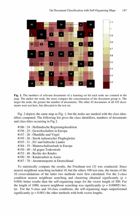
On Document Classification with Self-Organising Maps 147

Fig. 1. The numbers of relevant documents of a learning set hit each node are counted in the map. The darker the node, the more compact the concentration of the document group is. The larger the node, the greater the number of documents. The other 42 documents of all 425 docu-ments were not here, but allocated to the test set.

Fig. 2 depicts the same map as Fig. 1, but the nodes are marked with the class iden-tifiers computed. The following list gives the class identifiers, numbers of documents and class titles occurring in Fig 2.

#186 : 24 : Holländische Regierungskoalition #156 : 25 : Gewerkschaften in Europa #147 : 26 : Ölunfälle und Vögel #195 : 26 : Streik italienischer Flugbegleiter #193 : 31 : EU und baltische Länder #184 : 35 : Mutterschaftsurlaub in Europa #150 : 40 : AI gegen Todesstrafe #152 : 48 : Rechte des Kindes #190 : 50 : Kinderarbeit in Asien #187 : 78 : Atomtransporte in Deutschland

To statistically compare the results, the Friedman test [3] was conducted. Since nearest neighbour searching included 10, but the others 100 test runs, the means of the 10 crossvalidations of the latter two methods were first calculated. For the 2-class condition nearest neighbour searching and clustering obtained significantly (p = 0.004) better results than the self-organising maps for the vector length of 500. For the length of 1000, nearest neighbour searching was significantly (p = 0.00005) bet-ter. For the 5-class and 10-class conditions, the self-organising maps outperformed significantly (p < 0.001) the other methods with both vector lengths.

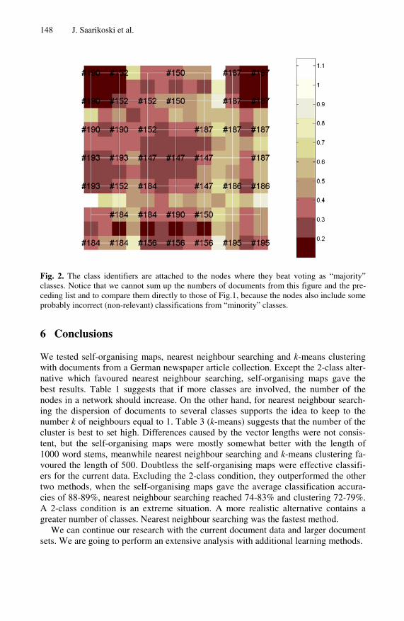
148 J. Saarikoski et al.

Fig. 2. The class identifiers are attached to the nodes where they beat voting as “majority” classes. Notice that we cannot sum up the numbers of documents from this figure and the pre-ceding list and to compare them directly to those of Fig.1, because the nodes also include some probably incorrect (non-relevant) classifications from “minority” classes.

6 Conclusions

We tested self-organising maps, nearest neighbour searching and k-means clustering with documents from a German newspaper article collection. Except the 2-class alter-native which favoured nearest neighbour searching, self-organising maps gave the best results. Table 1 suggests that if more classes are involved, the number of the nodes in a network should increase. On the other hand, for nearest neighbour search-ing the dispersion of documents to several classes supports the idea to keep to the number k of neighbours equal to 1. Table 3 (k-means) suggests that the number of the cluster is best to set high. Differences caused by the vector lengths were not consis-tent, but the self-organising maps were mostly somewhat better with the length of 1000 word stems, meanwhile nearest neighbour searching and k-means clustering fa-voured the length of 500. Doubtless the self-organising maps were effective classifi-ers for the current data. Excluding the 2-class condition, they outperformed the other two methods, when the self-organising maps gave the average classification accura-cies of 88-89%, nearest neighbour searching reached 74-83% and clustering 72-79%. A 2-class condition is an extreme situation. A more realistic alternative contains a greater number of classes. Nearest neighbour searching was the fastest method.

We can continue our research with the current document data and larger document sets. We are going to perform an extensive analysis with additional learning methods.

On Document Classification with Self-Organising Maps 149

Acknowledgements

The research was partially funded by Alfred Kordelin Fund and Academy of Finland, projects 120264, 115609 and 124131. SNOWBALL stemmer was by Martin Porter.

References

1. Airio, E.: Word normalization and decompounding in mono- and bilingual IR. Information Retrieval 9(3), 249–271 (2006)

2. Chowdhury, N., Saha, D.: Unsupervised text classification using Kohonen’s self organiz-ing network. In: Gelbukh, A. (ed.) CICLing 2005. LNCS, vol. 3406, pp. 715–718. Springer, Heidelberg (2005)

3. Conover, W.J.: Practical Nonparametric Statistics. John Wiley & Sons, New York (1999) 4. Doan, A., Domingos, P., Halevy, A.: Learning to match the schemas of data sources: a

multistrategy approach. Machine Learning 50, 279–301 (2003) 5. Duda, R.O., Hart, P.E., Stork, D.G.: Pattern Classification, 2nd edn. John Wiley & Sons,

New York (2001) 6. Guerro-Bote, V.P., Moya-Anegón, F., Herrero-Solana, V.: Document organization using

Kohonen’s algorithm. Information Processing and Management 38, 79–89 (2002) 7. Honkela, T.: Self-Organizing Maps in Natural Language Processing, Academic Disserta-

tion. Helsinki University of Technology, Finland (1997) 8. Kohonen, T.: Self-Organizing Maps. Springer, Berlin (1995) 9. Lagus, K., Kaski, S., Kohonen, T.: Mining massive document collections by the

WEBSOM method. Information Sciences 163(1-3), 135–156 (2004) 10. Moya-Anegón, F., Herrero-Solana, V., Jiménez-Contreras, E.: A connectionist and multi-

variate approach to science maps: the SOM, clustering and MDS applied to library and in-formation science research. Journal of Information Science 32(1), 63–77 (2006)

11. Saarikoski, J., Laurikkala, J., Järvelin, K., Juhola, M.: A study on the use of self-organising maps in information retrieval. To appear in Journal of Documentation (2008)

12. Sebastiani, F.: Machine learning in automated text categorization. ACM Computing Sur-veys 34(1), 1–47 (2002)

13. Serrano, J.I., del Castillo, M.D.: Evolutionary learning of document categories. Informa-tion Retrieval 10, 69–83 (2007)

Publication III

Self-organising maps in document classification: A comparison with six machine learning methods

Jyri Saarikoski, Jorma Laurikkala, Kalervo Järvelin, and Martti Juhola

Copyright © 2011 Springer-Verlag GmbH Berlin Heidelberg. Reprinted, with

permission, from Saarikoski, J., Laurikkala, J., Järvelin, K. and Juhola, M. (2011).

Self-organising maps in document classification: A comparison with six machine

learning methods. In Proceedings of the 10th International Conference on Adaptive and

Natural Computing Algorithms (ICANNGA 2011), Lecture Notes in Computer Science,

Vol. 6593, pp. 260-269.

Available at: http://dx.doi.org/10.1007/978-3-642-20282-7_27

A. Dobnikar, U. Lotrič, and B. Šter (Eds.): ICANNGA 2011, Part I, LNCS 6593, pp. 260–269, 2011. © Springer-Verlag Berlin Heidelberg 2011

Self-Organising Maps in Document Classification: A Comparison with Six Machine Learning Methods

Jyri Saarikoski1, Jorma Laurikkala1, Kalervo Järvelin2, and Martti Juhola1

1 Department of Computer Sciences 2 Department of Information Studies and Interactive Media,

33014 University of Tampere, Finland {Jyri.Saarikoski,Jorma.Laurikkala,

Kalervo.Jarvelin,Martti.Juhola}@uta.fi

Abstract. This paper focuses on the use of self-organising maps, also known as Kohonen maps, for the classification task of text documents. The aim is to ef-fectively and automatically classify documents to separate classes based on their topics. The classification with self-organising map was tested with three data sets and the results were then compared to those of six well known base-line methods: k-means clustering, Ward’s clustering, k nearest neighbour searching, discriminant analysis, Naïve Bayes classifier and classification tree. The self-organising map proved to be yielding the highest accuracies of tested unsupervised methods in classification of the Reuters news collection and the Spanish CLEF 2003 news collection, and comparable accuracies against some of the supervised methods in all three data sets.

Keywords: machine learning, neural networks, self-organising map, document classification.

1 Introduction

Finding relevant information about something is of highest importance, particularly in electronic documents. We need to seek information in our everyday lives, both at home and work while the amount of information available is getting enormous. The Internet is full of digital documents covering almost every topic one can imagine. How can one find relevant information in this massive collection of documents? One cannot really do it manually, so one needs some automatic methods. These methods can help in the search for useful information by clustering, classifying and labelling the documents. When the documents are ordered and preclassified, one can effec-tively browse through them. This is why we need document classification methods.

The machine learning solutions [21] for the text document classification task mostly use the supervised learning procedure. These include, for example, classic methods such as k nearest neighbour searching and Naïve Bayes classifier [8]. How-ever, we are interested in the unsupervised self-organising map method [13], also known as Kohonen map or SOM. It is an artificial neural network originally designed for the clustering of high-dimensional data samples to a low-dimensional map. It is widely used in the clustering and classification of text documents. WEBSOM [12, 15]

Self-Organising Maps in Document Classification 261

is a self-organising map based method for effective text mining and clustering of mas-sive document collections. However, it is not really designed for the classification of documents. ChandraShekar and Shoba [2] classified 7000 documents with self-organising maps and Chowdhury and Saha [4], Eyassu and Gambäck [9] and Guerro-Bote et al. [11] used smaller collections of a few hundred documents. Recently, Chumwatana et al. [5] used maps in clustering task of news collection of 50 Thai news and Chen et al. [3] compared self-organising maps and k-means clustering method in clustering of 420 documents collection. The method has also been used in information retrieval, see for instance [10] and [14].

We have used self-organising maps earlier in information retrieval [18] and docu-ment classification [19] tasks of a German news document collection. In classification self-organising map showed some potential by beating k nearest neighbour searching and k-means clustering in the five (278 documents) and ten class (425 documents) cases with accuracies as high as 88-89%. Encouraged by that performance, we de-cided to test its classification ability in this research with multiple reasonably large data sets and against well known baseline methods, something that is seldom seen in research papers of this field. We were also interested in testing the self-organising map classification method with documents of different languages. Therefore, one of our present data sets is in Spanish.

The research proved us that self-organising map is an effective method in docu-ment classification even when there are thousands of documents in the data set. Self-organising map yielded over 90% micro-averaged accuracy in Data Sets 1 (Reuters, Mod Apte Split collection) and 3 (Spanish CLEF 2003 collection) and competed very well against unsupervised methods and comparably against some of the supervised methods.

2 The Data Sets

2.1 Data Set 1: Reuters-21578, Mod Apte Split

The first data set is a subset of the well known Reuters-21578 collection [17, 21]. The complete collection includes 21578 English Reuters news documents from the year 1987. We chose the widely used Mod Apte split [1, 21] subset, which contains 10789 documents and 90 classes. Some of these documents have multiple class labels. To make things simpler, we discarded those and took only the documents with one label. Then, we selected 10 largest classes and finally obtained our collection of 8008 documents, consisting of 5754 training samples and 2254 test samples. The class la-bels are words, for example 'earn', 'coffee' and 'ship'.

2.2 Data Set 2: 20 Newsgroups, Matlab/Octave

The second data set is also a widely used collection of 20 Internet newsgroups [21, 23]. We selected its Matlab/Octave version, which provides 18774 English docu-ments, 12690 in the training set and 7505 in the test set. The class labels are names of newsgroups, for instance 'rec.sport.hockey', 'soc.religion.christian' and 'sci.space', and each document has only one class label.

262 J. Saarikoski et al.

2.3 Data Set 3: Spanish CLEF 2003

The third data set is the Spanish collection of CLEF 2003 news documents [6]. The collection contains news articles from the years 1994 and 1995. There are 454045 documents in the complete collection. Here test topics form the classes, and the rele-vant documents for each topic the class members. From the 60 available classes we selected 20 largest classes. There were, in all, 1901 documents for the top-20 classes. Finally, we constructed 10 test sets using a 10-fold cross-validation procedure. In this data set each document has only one class label. The labels are news topics, such as 'Epidemia de ébola en Zaire', 'Los Juegos Olímpicos y la paz', 'El Shoemaker-Levy y Júpiter'.

3 Preprocessing

Conventional preprocessing was performed to all three data sets. Firstly, the SNOW-BALL stemmer was used to transform words to their stems, for instance word 'con-tinued' became 'continu'. Then, stopwords, useless “little” words, such as 'a', 'about' and 'are', were removed. At this point also words shorter than three letters, numbers and special characters were discarded. This is because short words generally have little information value for the classification of documents.

Next, we calculated the frequencies of remaining words (word stems). Then we computed document vectors for all documents by applying the common vector space model [20] with tf·idf weighting for all remaining word stems. Thus, a document was presented in the following form

),...,,,( 321 itiiii wwwwD = (1)

where wik is the weight of word k in document Di, 1 ≤ i ≤ n, 1 ≤ k ≤, t, where n is the number of documents and t is the number of word stems in all documents. Weights are given in tf·idf form as the product of term frequency (tf) and inverse document frequency (idf). The former for word k in document Di is computed with

{ }ill

ikik freq

freqtf

max= (2)

where freqik equals to the number of the occurrences of word k in document Di and l is for all words of Di, l=1,2,..., t-1, t. The latter is computed for word k in the docu-ment set with

kk n

Nidf log= (3)

where N is the number of the documents in the set and nk is the number of docu-ments, which contain word k at least once. Combining equations (2) and (3) we obtain a weight for word k in document Di

Self-Organising Maps in Document Classification 263

kikik idftfw ⋅= (4)

After this procedure every document has its own document vector. Finally, the length of each document vector was shortened only to 1000 of middle frequency (around median) word stems from the total word frequency distribution sorted in ascending order. Very often the most and least frequent words are pruned in information re-trieval applications, because their capacity to distinguish relevant and non-relevant documents (to a topic) is known to be poor. Only 1000 stems were chosen to ease the computational burden and based on the fact that it had proven quite effective choice in a previous study [19]. The same vectors were then used for all of the methods used, except for the Naïve Bayes method, which needed frequency weighted vectors.

It should also be noted that document vectors were only computed from training sets. Information about its corresponding test set was not used in order to create as a realistic classification situation as possible, where the system knows an existing train-ing set and its words in advance, but not those of test set. Thus, each training set in-cluded its own word set, somewhat different from those of the other training sets, and the document vectors of its corresponding test set were prepared according to the words of the training set.

4 Document Classification with Self-Organising Map

In order to use a self-organising map in the document classification task we needed to label the map nodes with class labels of the training data set in some meaningful way. The labelled nodes then represent the document classes and the map is able to classify new documents (test set samples) by mapping them. The following simple procedure was implemented to label the self-organising map with class labels:

• Create a self-organising map using a training data set. • Map each training set sample to the map. • Determine a class for each node of the map according to the numbers of

training documents of different classes mapped on that node. The most fre-quent document class determines the class of the node. If there are more than one class with the same maximum, label the node according to the class of the document (from the maximum classes) closest to the model vector of the node.

After this procedure the map is labelled with class labels. Fig. 1 shows an example of a labelled map. The data on the map is the training set of Data Set 1 and the labels are: #1 earn, #2 acq, #3 crude, #4 trade, #5 money-fx, #6 interest, #7 money-supply, #8 ship, #9 sugar and #10 coffee. Most of the classes seem to form one or two clusters on the map.

After giving the labels to the map nodes, the classification of the test set was done by mapping each test sample and comparing the classification result given by the map with the known class label of the sample.

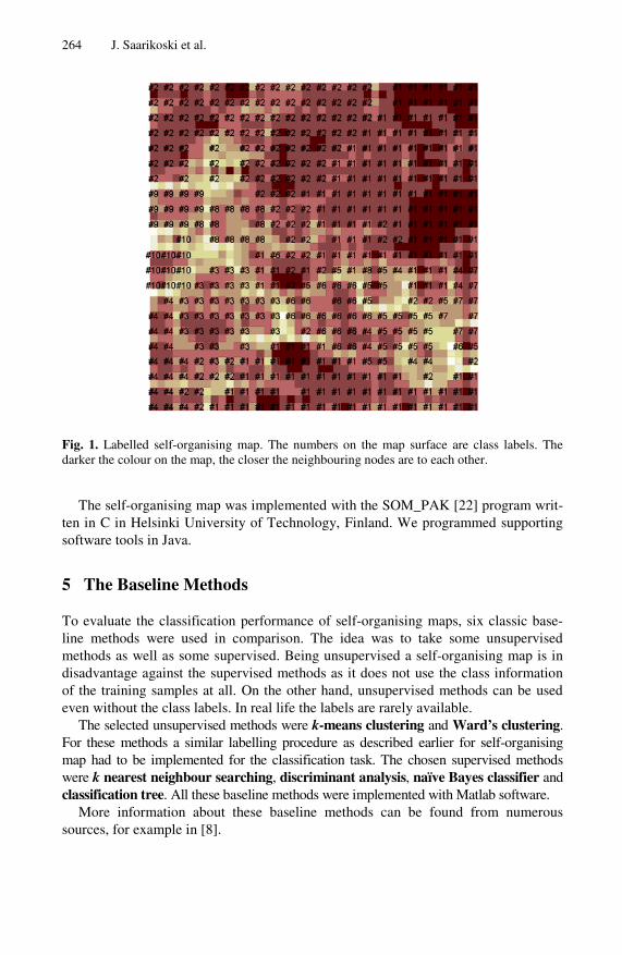
264 J. Saarikoski et al.

Fig. 1. Labelled self-organising map. The numbers on the map surface are class labels. The darker the colour on the map, the closer the neighbouring nodes are to each other.

The self-organising map was implemented with the SOM_PAK [22] program writ-ten in C in Helsinki University of Technology, Finland. We programmed supporting software tools in Java.

5 The Baseline Methods

To evaluate the classification performance of self-organising maps, six classic base-line methods were used in comparison. The idea was to take some unsupervised methods as well as some supervised. Being unsupervised a self-organising map is in disadvantage against the supervised methods as it does not use the class information of the training samples at all. On the other hand, unsupervised methods can be used even without the class labels. In real life the labels are rarely available.

The selected unsupervised methods were k-means clustering and Ward’s clustering. For these methods a similar labelling procedure as described earlier for self-organising map had to be implemented for the classification task. The chosen supervised methods were k nearest neighbour searching, discriminant analysis, naïve Bayes classifier and classification tree. All these baseline methods were implemented with Matlab software.

More information about these baseline methods can be found from numerous sources, for example in [8].

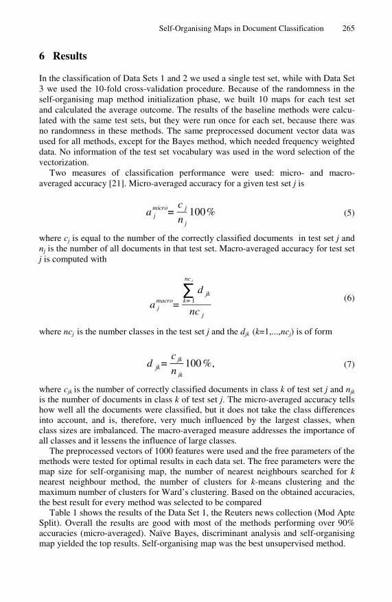
Self-Organising Maps in Document Classification 265

6 Results

In the classification of Data Sets 1 and 2 we used a single test set, while with Data Set 3 we used the 10-fold cross-validation procedure. Because of the randomness in the self-organising map method initialization phase, we built 10 maps for each test set and calculated the average outcome. The results of the baseline methods were calcu-lated with the same test sets, but they were run once for each set, because there was no randomness in these methods. The same preprocessed document vector data was used for all methods, except for the Bayes method, which needed frequency weighted data. No information of the test set vocabulary was used in the word selection of the vectorization.

Two measures of classification performance were used: micro- and macro-averaged accuracy [21]. Micro-averaged accuracy for a given test set j is

a jmicro=

c j

n j

100% (5)

where cj is equal to the number of the correctly classified documents in test set j and nj is the number of all documents in that test set. Macro-averaged accuracy for test set j is computed with

a jmacro=

∑k= 1

nc j

d jk

nc j

(6)

where ncj is the number classes in the test set j and the djk (k=1,...,ncj) is of form

d jk=c jk

n jk

100 %, (7)

where cjk is the number of correctly classified documents in class k of test set j and njk

is the number of documents in class k of test set j. The micro-averaged accuracy tells how well all the documents were classified, but it does not take the class differences into account, and is, therefore, very much influenced by the largest classes, when class sizes are imbalanced. The macro-averaged measure addresses the importance of all classes and it lessens the influence of large classes.

The preprocessed vectors of 1000 features were used and the free parameters of the methods were tested for optimal results in each data set. The free parameters were the map size for self-organising map, the number of nearest neighbours searched for k nearest neighbour method, the number of clusters for k-means clustering and the maximum number of clusters for Ward’s clustering. Based on the obtained accuracies, the best result for every method was selected to be compared

Table 1 shows the results of the Data Set 1, the Reuters news collection (Mod Apte Split). Overall the results are good with most of the methods performing over 90% accuracies (micro-averaged). Naïve Bayes, discriminant analysis and self-organising map yielded the top results. Self-organising map was the best unsupervised method.

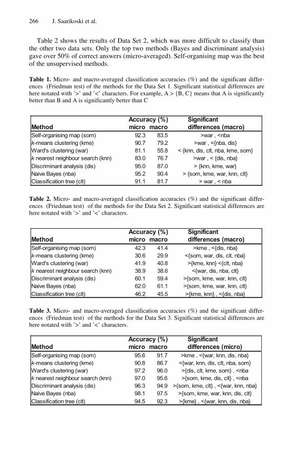
266 J. Saarikoski et al.

Table 2 shows the results of Data Set 2, which was more difficult to classify than the other two data sets. Only the top two methods (Bayes and discriminant analysis) gave over 50% of correct answers (micro-averaged). Self-organising map was the best of the unsupervised methods.

Table 1. Micro- and macro-averaged classification accuracies (%) and the significant differ-ences (Friedman test) of the methods for the Data Set 1. Significant statistical differences are here notated with ’>’ and ’<’ characters. For example, A > {B, C} means that A is significantly better than B and A is significantly better than C

Accuracy (%) SignificantMethod micro macro differences (macro)Self-organising map (som) 92.3 83.5 >war , <nba

90.7 79.2 >war , <{nba, dis}Ward's clustering (war) 81.1 55.8 < {knn, dis, clt, nba, kme, som}

83.0 76.7 >war , < {dis, nba}Discriminant analysis (dis) 95.0 87.0 > {knn, kme, war}Naive Bayes (nba) 95.2 90.4 > {som, kme, war, knn, clt}Classification tree (clt) 91.1 81.7 > war , < nba

k-means clustering (kme)

k nearest neighbour search (knn)

Table 2. Micro- and macro-averaged classification accuracies (%) and the significant differ-ences (Friedman test) of the methods for the Data Set 2. Significant statistical differences are here notated with ’>’ and ’<’ characters.

Accuracy (%)Method micro macro differences (macro)Self-organising map (som) 42.3 41.4 >kme , <{dis, nba}

30.6 29.9 <{som, war, dis, clt, nba}Ward's clustering (war) 41.9 40.8 >{kme, knn} <{clt, nba}

38.9 38.6 <{war, dis, nba, clt}Discriminant analysis (dis) 60.1 59.4 >{som, kme, war, knn, clt}Naive Bayes (nba) 62.0 61.1 >{som, kme, war, knn, clt}Classification tree (clt) 46.2 45.5 >{kme, knn} , <{dis, nba}

Significant

k-means clustering (kme)

k nearest neighbour search (knn)

Table 3. Micro- and macro-averaged classification accuracies (%) and the significant differ-ences (Friedman test) of the methods for the Data Set 3. Significant statistical differences are here notated with ’>’ and ’<’ characters.

Accuracy (%)Method micro macro differences (micro)Self-organising map (som) 95.6 91.7 >kme , <{war, knn, dis, nba}

90.8 86.7 <{war, knn, dis, clt, nba, som}Ward's clustering (war) 97.2 96.0 >{dis, clt, kme, som} , <nba

97.0 95.6 >{som, kme, dis, clt} , <nbaDiscriminant analysis (dis) 96.3 94.9 >{som, kme, clt} , <{war, knn, nba}Naive Bayes (nba) 98.1 97.5 >{som, kme, war, knn, dis, clt}Classification tree (clt) 94.5 92.3 >{kme} , <{war, knn, dis, nba}

Significant

k-means clustering (kme)

k nearest neighbour search (knn)

Self-Organising Maps in Document Classification 267

The results of Data Set 3, the Spanish CLEF news collection, are in Table 3. It turned out to be the easiest case of the three data sets. All methods gave over 90% accuracies (micro-averaged) and Naïve Bayes outperformed the others with very good 98.1% result. Self-organising map performed well with 95.6% and were the second best of the unsupervised methods. In this set also the macro-averaged accuracies were also reasonably high.

Naïve Bayes proved to be the most effective in all cases and discriminant analysis performed almost at the same level. Self-organising maps were at least average com-pared to others in all cases, and among the unsupervised methods it was the most con-sistent. Another interesting outcome was that in k nearest neighbour classification the best results was always, with all three data sets, obtained with k=1, although we tried with k values up to 20.

We conducted the Friedman test [7] to compare the results. For the Data Set 3 we used the micro-averaged accuracies of 10 test sets. For Data Sets 1 and 2 we had to use the macro-averaged accuracies to get enough data, because there was only one test set in these data sets. All the significant differences (p < 0.05) between methods are shown in the Tables 1-3. For example, self-organising map was significantly bet-ter than k-means clustering in Data Sets 2 and 3, and also significantly better than Ward’s clustering in Data Set 1. On the other hand, Naïve Bayes was significantly better than self-organising map in all three data sets.

7 Conclusions and Discussion

We tested self-organising map in text document classification task with three different kinds of collections and compared the results to those of the standard text classifica-tion methods. Naïve Bayes turned out to be the most effective of all, but self-organising map performed well in its own category of the unsupervised methods. Overall, the results of self-organising maps were encouraging with over 90% classifi-cation accuracy (micro-averaged) in Data Sets 1 and 3. This suggests that it is an ef-fective method for the document classification tasks. Futhermore, self-organising maps performed comparably against some of the supervised classification methods tested. The intuitive visual map (see Fig. 1) and the unsupervised learning phase are also a benefit of using self-organising map in document classification, because the map enables data visualization, and in some applications browsing. Additionally, la-belled data is rarely available.

Even the costly learning procedure has its benefits. If we compare self-organising map with k nearest neighbour, it is easy to see that the learning phase of the map takes much more time than the learning of k nearest neighbour. In actual classification it is quite the opposite. The map has usually by an order of magnitude less nodes than there are documents in the training set and this actually leads to 10 times faster classi-fication compared to k nearest neighbour with the same data. One does not have to construct a new map every time when a new document is added to the collection, one can just map it and do the learning later when there is more new data available. The slow learning is done rarely and the fast classification often.

The self-organising map method could give even better results, if some more ad-vanced features would be implemented. For example, it is possible to calculate

268 J. Saarikoski et al.

classification based on multiple class hits on the map, for instance using three nearest could be classes. Another approach is the use of multiple maps. In the future, we con-sider these options and focus on the dimensionality reduction and feature selection problem associated with document vectors.

Acknowledgements

Jyri Saarikoski was supported by the Tampere Graduate Programme in Information Science and Engineering (TISE). SNOWBALL stemmer was by Martin Porter.

References

1. Apte, C., Damerau, F.J., Weiss, S.M.: Automated learning of decision rules for text cate-gorization. ACM Transactions on Information Systems 12, 233–251 (1994)

2. ChandraShekar, B.H., Shobha, G.: Classification of Documents Using Kohonen’s Self-Organizing Map. International Journal of Computer Theory and Engineering 5(1), 610–613 (2009)

3. Chen, Y., Qin, B., Liu, T., Liu, Y., Li, S.: The Comparison of SOM and K-means for Text Clustering. Computer and Information Science 2(3), 268–274 (2010)

4. Chowdhury, N., Saha, D.: Unsupervised text classification using kohonen’s self organizing network. In: Gelbukh, A. (ed.) CICLing 2005. LNCS, vol. 3406, pp. 715–718. Springer, Heidelberg (2005)

5. Chumwatana, T., Wong, K., Xie, H.: A SOM-Based Document Clustering Using Frequent Max Substring for Non-Segmented Texts. Journal of Intelligent Learning Systems & Ap-plications 2, 117–125 (2010)

6. CLEF: The Cross-Language Evaluation Forum, http://www.clef-campaign.org/

7. Conover, W.J.: Practical Nonparametric Statistics. John Wiley & Sons, New York (1999) 8. Duda, R.O., Hart, P.E., Stork, D.G.: Pattern Classification, 2nd edn. John Wiley & Sons,

New York (2001) 9. Eyassu, S., Gambäck, B.: Classifying Amharic News Text Using Self-Organizing Maps.

Proceeding of the ACL Workshop on Computational Approaches to Semitic Languages, Ann Arbor, Michigan, USA, pp. 71–78 (2005)

10. Fernández, J., Mones, R., Díaz, I., Ranilla, J., Combarro, E.F.: Experiments with Self Or-ganizing Maps in CLEF 2003. In: Peters, C., Gonzalo, J., Braschler, M., Kluck, M. (eds.) CLEF 2003. LNCS, vol. 3237, pp. 358–366. Springer, Heidelberg (2004)

11. Guerro-Bote, V.P., Moya-Anegón, F., Herrero-Solana, V.: Document organization using Kohonen’s algorithm. Information Processing and Management 38, 79–89 (2002)

12. Honkela, T.: Self-Organizing Maps in Natural Language Processing, Academic Disserta-tion. Helsinki University of Technology, Finland (1997)

13. Kohonen, T.: Self-Organizing Maps. Springer, Berlin (1995) 14. Lagus, K.: Text retrieval using self-organized document maps. Neural Processing Let-

ters 15, 21–29 (2002) 15. Lagus, K., Kaski, S., Kohonen, T.: Mining massive document collections by the WEB-

SOM method. Information Sciences 163(1-3), 135–156 (2004)

Self-Organising Maps in Document Classification 269

16. Moya-Anegón, F., Herrero-Solana, V., Jiménez-Contreras, E.: A connectionist and multi-variate approach to science maps: the SOM, clustering and MDS applied to library and in-formation science research. Journal of Information Science 32(1), 63–77 (2006)

17. Reuters-21578 collection, http://kdd.ics.uci.edu/databases/reuters21578/ reuters21578.html

18. Saarikoski, J., Laurikkala, J., Järvelin, K., Juhola, M.: A study of the use of self-organising maps in information retrieval. Journal of Documentation 65(2), 304–322 (2009)

19. Saarikoski, J., Järvelin, K., Laurikkala, J., Juhola, M.: On Document Classification with Self-Organising Maps. In: Kolehmainen, M., Toivanen, P., Beliczynski, B. (eds.) ICANNGA 2009. LNCS, vol. 5495, pp. 140–149. Springer, Heidelberg (2009)

20. Salton, G.: Automatic Text Processing: The Transformation, Analysis and Retrieval of In-formation by Computer. Addison-Wesley, Reading (1989)

21. Sebastiani, F.: Machine learning in automated text categorization. ACM Computing Sur-veys 34(1), 1–47 (2002)

22. SOM_PAK, http://www.cis.hut.fi/research/som-research/ nnrc-programs.shtml

23. 20 newsgroups collection, http://people.csail.mit.edu/jrennie/20Newsgroups/

Publication IV

Dimensionality reduction in text classification using scatter method

Jyri Saarikoski, Jorma Laurikkala, Kalervo Järvelin, Markku Siermala and Martti Juhola

Copyright © 2014 Inderscience Publishers. Reprinted, with permission, from

Saarikoski, J., Laurikkala, J., Järvelin, K., Siermala, M. and Juhola, M. (2014).

Dimensionality reduction in text classification using scatter method. International

Journal of Data Mining, Modelling and Management, Vol. 6, No. 1, pp. 1-21.

Available at: http://dx.doi.org/10.1504/IJDMMM.2014.059978

Int. J. Data Mining, Modelling and Management, Vol. 6, No. 1, 2014 1

Copyright © 2014 Inderscience Enterprises Ltd.

Dimensionality reduction in text classification using scatter method

Jyri Saarikoski, Jorma Laurikkala, Kalervo Järvelin, Markku Siermala and Martti Juhola* School of Information Sciences, 33014 University of Tampere, Finland E-mail: jyri.saarikoski@uta.fi E-mail: jorma.laurikkala@uta.fi E-mail: kalervo.jarvelin@uta.fi E-mail: markku.siermala@gmail.com E-mail: martti.juhola@uta.fi *Corresponding author

Abstract: Preprocessing of data is a vital part of any task involving machine learning. In the classification of text documents, the most important aspect of preprocessing is usually the dimensionality reduction of data vectors. This paper focuses on the use of a recent scatter method in the dimensionality reduction of text documents. The effectiveness of the method was tested with the classification of two datasets, the Reuters news collection and the Spanish CLEF 2003 news collection. The classification methods used were self-organising maps, Naïve Bayes method, k nearest neighbour searching and classification tree. For comparison, we also conducted the dimensionality reduction of the data with document frequency and mutual information approaches. The scatter method proved to be an effective dimensionality reduction method for text document data. The suggested approach outperformed the document frequency reduction and scored comparably against the mutual information method, except when only very small set of features was selected where mutual information was better, especially in the CLEF collection.

Keywords: text documents; dimensionality reduction; classification; mutual information; self-organising maps; Naïve Bayes method; k nearest neighbour method; classification tree.

Reference to this paper should be made as follows: Saarikoski, J., Laurikkala, J., Järvelin, K., Siermala, K. and Juhola, M. (2014) ‘Dimensionality reduction in text classification using scatter method’, Int. J. Data Mining, Modelling and Management, Vol. 6, No. 1, pp.1–21.

Biographical notes: Jyri Saarikoski received his MSc in Computer Science in 2007 at the University of Tampere, Finland. At present, he is a researcher and postgraduate. His research focuses on information retrieval and document classification.

Jorma Laurikkala received his MSc and PhLic in Computer Science from the University of Kuopio (UKU), Finland, in 1995 and 1997, respectively, and his PhD in Computer Science from the University of Tampere (UTA), Finland in 2001. He has worked as an assistant, researcher and lecturer at UKU and UTA.

2 J. Saarikoski et al.

Currently, he is a Lecturer of Computer Science at UTA. His research interests include machine learning, information retrieval, genetic algorithms and medical expert systems.

Kalervo Järvelin is a Professor and Vice Chair at the School of Information Sciences, University of Tampere, Finland. He holds a PhD in Information Studies (1987) from the same university. He was an Academy Professor, Academy of Finland, in 2004–2009 (http://www.uta.fi/~likaja). His research covers information seeking and retrieval, linguistic and conceptual methods in IR, IR evaluation, and database management. He has co-authored over 260 scholarly publications and supervised 17 dissertations. He received the Tony Kent Strix Award 2008 in recognition of contributions to the field of information retrieval.

Markku Siermala received his MSc in 1999 and PhD in 2002 in Computer Science at the University of Tampere, Finland. His research interests include topics in bioinformatics and data analysis. He has worked for several years in IT companies in Tampere.

Martti Juhola received his PhD in 1987 in Computer Science at the University of Turku where he worked in 1980–1992. He was a Professor at the University of Kuopio from 1992 to 1997. Since 1997, he is a Professor at the University of Tampere, Finland. His research consists of topics in biomedical signal analysis, pattern recognition, data analysis and mining.

1 Introduction

Machine learning methods are very useful in many information related tasks, such as automatic clustering, filtering, classification and information retrieval. The preprocessing of data is an essential part of machine learning task. The data is usually transformed into numerical form and a part of the data is discarded to reduce computational costs. It is essential that valuable information is not lost during preprocessing.

We are interested in the dimensionality reduction of text document data, because it is an important phase of preprocessing of textual data and has a decisive effect, for example, on the classification performance. There are many techniques to reduce the number of terms (variables) in text document data (Sebastiani, 2002). In term selection approach, the aim is to select a set of the best terms from the original ones, while in term extraction a new set of artificial terms is created by combining or transforming the original terms. The dimension reduction techniques studied in this paper fall into the former category. Techniques of the latter category include latent semantic indexing (Deerwester et al., 1990), principal component analysis (Sharma, 1996; Maheswari and Rajaram, 2009) and term clustering (Jain and Dubes, 1988), where clusters of original terms are created and used as new terms. Random mapping (Kaski, 1998) technique is also suggested for high-dimensional data. Several other techniques were proposed in various areas (Chrysostomou et al., 2008; Garg and Murty, 2009; Kline and Galbraith, 2009; Xu and Wang, 2011).

This paper explores the use of the recently introduced scatter method (Juhola and Siermala, 2005; Siermala and Juhola, 2006; Siermala et al., 2007; Scatter Software, 2011)

Dimensionality reduction in text classification using scatter method 3

in the dimensionality reduction of text document data. The scatter algorithm evaluates the importance of each variable in a dataset. It is also able to evaluate the learnability value for an entire dataset or a single class. Earlier the method has been used very successfully to generate learnability information for datasets and for variable evaluation, therefore it would be exciting to see whether it is able to perform well in the dimensionality reduction task, in which it has not been used before. The method has also never before been used with text document data.

To evaluate dimensionality reduction, we conducted classification of text document data using four classification methods: self-organising maps, Naïve Bayes method, k nearest neighbour searching and classification tree. The latter three methods are all well-known baseline methods in classification field (Duda et al., 2001). Naïve Bayes has been applied, for example, to text classification with unbalanced classes (Frank and Bouckaert, 2006) and in classification of structured data (Flach and Lachiche, 2004). Li and Jain (1998) studied Bayes, k nearest neighbour and decision trees in text document classification.

Self-organising map (Lagus, 2002), also known as Kohonen (1995) map or SOM, is an artificial neural network. As an unsupervised learner, it is mainly used to cluster high-dimensional data samples to a low-dimensional map. Usually a two-dimensional map is preferred, because it gives an easy-to-understand visualisation of the clustering results and is computationally sound. More complex maps can be created, if needed. WEBSOM (Honkela, 1997; Lagus et al., 2004) is a well-known self-organising map-based method for effective text mining, browsing, and clustering of massive document collections. The studies by Chumwatana et al. (2010) and Ai-Xiang (2010) are recent examples of the use of self-organising maps in clustering. Besides clustering, the self-organising map can be applied to classify data (Chowdhury and Saha, 2005). The method has also been used in information retrieval (Fernandez et al., 2004; Lagus, 2002), but not as much as in clustering and classification. Liu and Takatsuka (2009) have applied hierarchical maps in image retrieval visualisation.

We have used self-organising maps successfully both in information retrieval (Saarikoski et al., 2009a) and classification (Saarikoski et al., 2009b) tasks of text documents. Furthermore, our recent study (Saarikoski et al., 2011) showed that self-organising maps perform well against some well-known methods in the classification of text documents. Unfortunately, self-organising maps have longer learning phases than simpler methods, and therefore, a substantial reduction of data has been necessary to limit computation time. In this context, it is very interesting to study the possibility to reduce dimensionality of data with the scatter method.

The results of this study suggest that the scatter method is a useful alternative in dimensionality reduction of text document data.

2 The datasets

In this study, we conducted classification of two datasets in order to evaluate the dimensionality reduction capability of the tested reduction methods. Both datasets are text document collections of news documents and labelled with class labels.

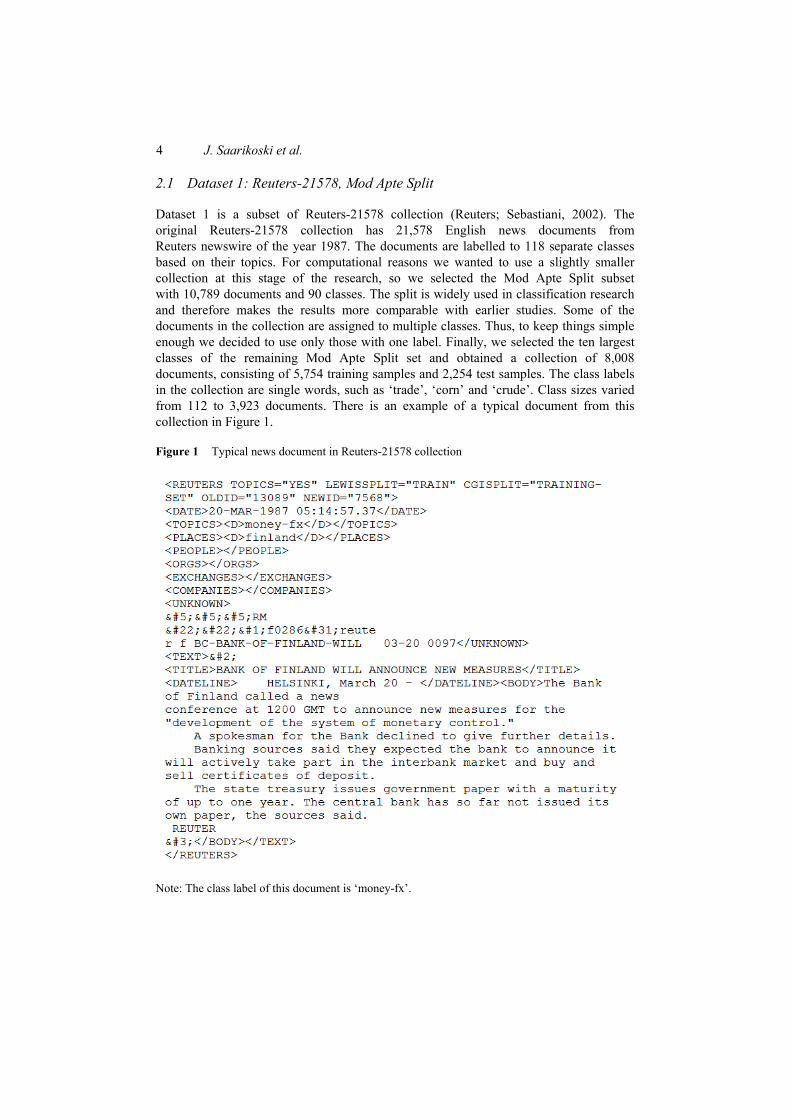
4 J. Saarikoski et al.

2.1 Dataset 1: Reuters-21578, Mod Apte Split

Dataset 1 is a subset of Reuters-21578 collection (Reuters; Sebastiani, 2002). The original Reuters-21578 collection has 21,578 English news documents from Reuters newswire of the year 1987. The documents are labelled to 118 separate classes based on their topics. For computational reasons we wanted to use a slightly smaller collection at this stage of the research, so we selected the Mod Apte Split subset with 10,789 documents and 90 classes. The split is widely used in classification research and therefore makes the results more comparable with earlier studies. Some of the documents in the collection are assigned to multiple classes. Thus, to keep things simple enough we decided to use only those with one label. Finally, we selected the ten largest classes of the remaining Mod Apte Split set and obtained a collection of 8,008 documents, consisting of 5,754 training samples and 2,254 test samples. The class labels in the collection are single words, such as ‘trade’, ‘corn’ and ‘crude’. Class sizes varied from 112 to 3,923 documents. There is an example of a typical document from this collection in Figure 1.

Figure 1 Typical news document in Reuters-21578 collection

Note: The class label of this document is ‘money-fx’.

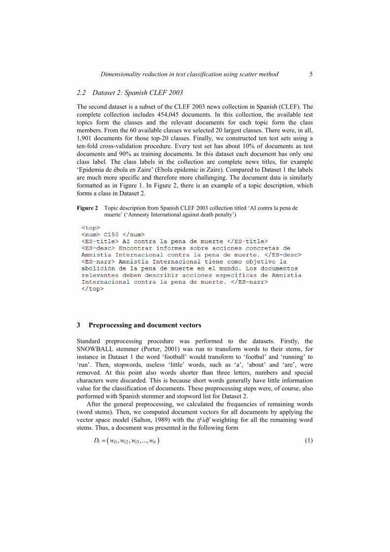
Dimensionality reduction in text classification using scatter method 5

2.2 Dataset 2: Spanish CLEF 2003

The second dataset is a subset of the CLEF 2003 news collection in Spanish (CLEF). The complete collection includes 454,045 documents. In this collection, the available test topics form the classes and the relevant documents for each topic form the class members. From the 60 available classes we selected 20 largest classes. There were, in all, 1,901 documents for those top-20 classes. Finally, we constructed ten test sets using a ten-fold cross-validation procedure. Every test set has about 10% of documents as test documents and 90% as training documents. In this dataset each document has only one class label. The class labels in the collection are complete news titles, for example ‘Epidemia de ébola en Zaire’ (Ebola epidemic in Zaire). Compared to Dataset 1 the labels are much more specific and therefore more challenging. The document data is similarly formatted as in Figure 1. In Figure 2, there is an example of a topic description, which forms a class in Dataset 2.

Figure 2 Topic description from Spanish CLEF 2003 collection titled ‘AI contra la pena de muerte’ (‘Amnesty International against death penalty’)

3 Preprocessing and document vectors

Standard preprocessing procedure was performed to the datasets. Firstly, the SNOWBALL stemmer (Porter, 2001) was run to transform words to their stems, for instance in Dataset 1 the word ‘football’ would transform to ‘footbal’ and ‘running’ to ‘run’. Then, stopwords, useless ‘little’ words, such as ‘a’, ‘about’ and ‘are’, were removed. At this point also words shorter than three letters, numbers and special characters were discarded. This is because short words generally have little information value for the classification of documents. These preprocessing steps were, of course, also performed with Spanish stemmer and stopword list for Dataset 2.

After the general preprocessing, we calculated the frequencies of remaining words (word stems). Then, we computed document vectors for all documents by applying the vector space model (Salton, 1989) with the tf·idf weighting for all the remaining word stems. Thus, a document was presented in the following form

( )1 2 3, , ,...,i i i i itD w w w w= (1)

6 J. Saarikoski et al.

where wik is the weight of word k in document Di, 1 ≤ i ≤ n, 1 ≤ k ≤ t, where n is the number of documents and t is the number of unique word stems in all documents. Weights are given in the tf·idf form as the product of term frequency (tf) and inverse document frequency (idf). The former for word k in document Di is computed with

{ }maxik

ikl il

freqtffreq

= (2)

where freqik equals to the number of the occurrences of word k in document Di and l is for all words of Di, l=1,2,..., t–1, t. The latter is computed for word k in the document set with

logkk

nidfn

= (3)

where n is the number of the documents in the set and nk is the number of documents, which contain word k at least once. Combining equations (2) and (3) we obtain a weight for word k in document Di

ik ik kw tf idf= ⋅ (4)

After this procedure every document has its own document vector. At this point the length of the vector can be reduced by dimensionality reduction methods. For example, if the length of a document vector would be 20,000 words (word stems) after vectorisation, one might want to select only the 1,000 most useful words to the final vector and leave the remaining 19,000 less effective words out to ease the computational burden and memory consumption. Unfortunately, it is not simple to identify the best words. This is why we need dimensionality reduction methods.

4 The scatter algorithm

The scatter algorithm (Juhola and Siermala, 2005; Siermala and Juhola, 2006; Siermala et al., 2007; Scatter Software, 2011) is designed for the evaluation of learnability of datasets. In this context, the concept of learnability is a measure of how well a dataset can be separated more or less successfully into different classes. In particular, it evaluates whether the given data are possible to learn with machine learning methods. The algorithm is able to measure the learnability of the whole dataset or a single class. It can also be used to evaluate the importance of each variable in the whole dataset or a single class. This output is useful in variable evaluation and weighting.

The basic idea of the method is to go through the dataset case by case moving always to the nearest unvisited neighbour of the current case as measured with the Euclidean distance. The starting point of this procedure is selected randomly. The class labels of the cases are stored to an ordered list and after the dataset has been traversed, the list is analysed and the learnability is evaluated. The decision of learnability is based on the changes of labels in the list. The less the classes change in the list order, the closer the class members are grouped to each other in the dataset, and the more accurately the data can be classified. Scatter value is small, being close to 0, if class changes in the list are rare. A high scatter value close to 1 means poor learnability.

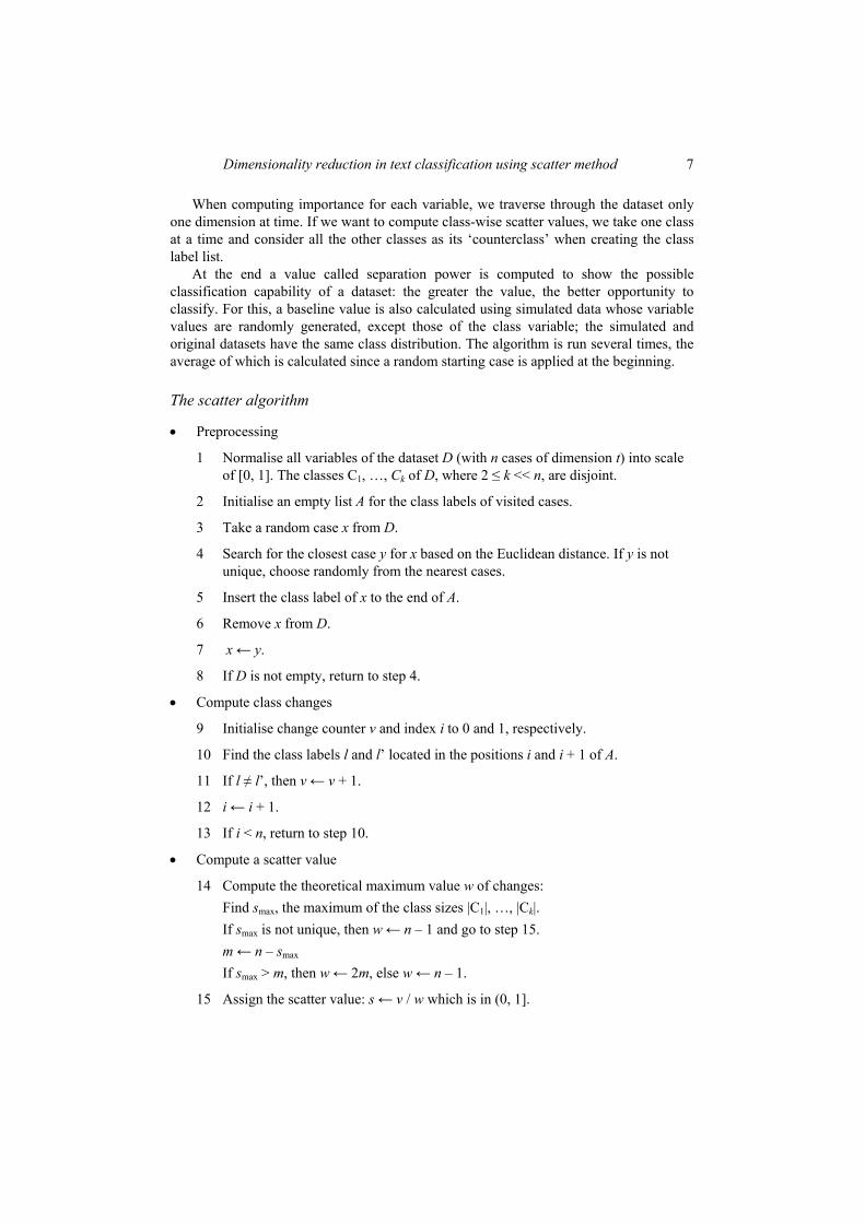
Dimensionality reduction in text classification using scatter method 7

When computing importance for each variable, we traverse through the dataset only one dimension at time. If we want to compute class-wise scatter values, we take one class at a time and consider all the other classes as its ‘counterclass’ when creating the class label list.

At the end a value called separation power is computed to show the possible classification capability of a dataset: the greater the value, the better opportunity to classify. For this, a baseline value is also calculated using simulated data whose variable values are randomly generated, except those of the class variable; the simulated and original datasets have the same class distribution. The algorithm is run several times, the average of which is calculated since a random starting case is applied at the beginning.

The scatter algorithm

• Preprocessing

1 Normalise all variables of the dataset D (with n cases of dimension t) into scale of [0, 1]. The classes C1, …, Ck of D, where 2 ≤ k << n, are disjoint.

2 Initialise an empty list A for the class labels of visited cases.

3 Take a random case x from D.

4 Search for the closest case y for x based on the Euclidean distance. If y is not unique, choose randomly from the nearest cases.

5 Insert the class label of x to the end of A.

6 Remove x from D.

7 x ← y.

8 If D is not empty, return to step 4.

• Compute class changes

9 Initialise change counter v and index i to 0 and 1, respectively.

10 Find the class labels l and l’ located in the positions i and i + 1 of A.

11 If l ≠ l’, then v ← v + 1.

12 i ← i + 1.

13 If i < n, return to step 10.

• Compute a scatter value

14 Compute the theoretical maximum value w of changes: Find smax, the maximum of the class sizes |C1|, …, |Ck|. If smax is not unique, then w ← n – 1 and go to step 15. m ← n – smax If smax > m, then w ← 2m, else w ← n – 1.

15 Assign the scatter value: s ← v / w which is in (0, 1].

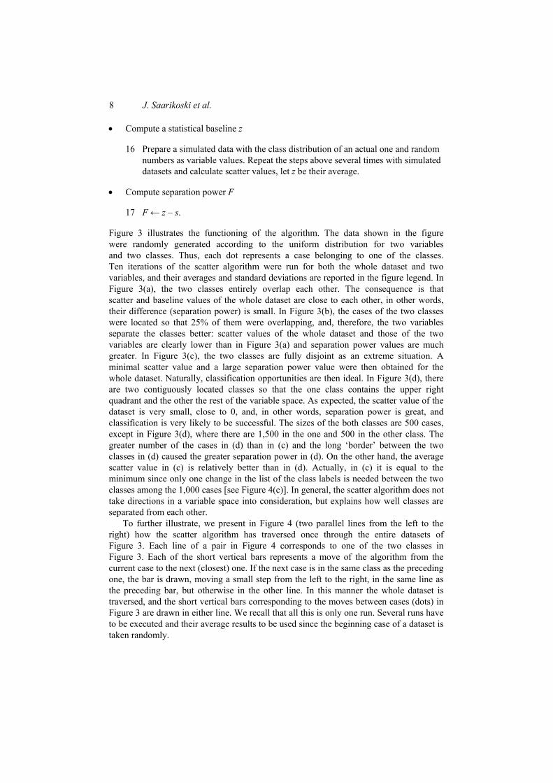
8 J. Saarikoski et al.

• Compute a statistical baseline z

16 Prepare a simulated data with the class distribution of an actual one and random numbers as variable values. Repeat the steps above several times with simulated datasets and calculate scatter values, let z be their average.

• Compute separation power F

17 F ← z – s.

Figure 3 illustrates the functioning of the algorithm. The data shown in the figure were randomly generated according to the uniform distribution for two variables and two classes. Thus, each dot represents a case belonging to one of the classes. Ten iterations of the scatter algorithm were run for both the whole dataset and two variables, and their averages and standard deviations are reported in the figure legend. In Figure 3(a), the two classes entirely overlap each other. The consequence is that scatter and baseline values of the whole dataset are close to each other, in other words, their difference (separation power) is small. In Figure 3(b), the cases of the two classes were located so that 25% of them were overlapping, and, therefore, the two variables separate the classes better: scatter values of the whole dataset and those of the two variables are clearly lower than in Figure 3(a) and separation power values are much greater. In Figure 3(c), the two classes are fully disjoint as an extreme situation. A minimal scatter value and a large separation power value were then obtained for the whole dataset. Naturally, classification opportunities are then ideal. In Figure 3(d), there are two contiguously located classes so that the one class contains the upper right quadrant and the other the rest of the variable space. As expected, the scatter value of the dataset is very small, close to 0, and, in other words, separation power is great, and classification is very likely to be successful. The sizes of the both classes are 500 cases, except in Figure 3(d), where there are 1,500 in the one and 500 in the other class. The greater number of the cases in (d) than in (c) and the long ‘border’ between the two classes in (d) caused the greater separation power in (d). On the other hand, the average scatter value in (c) is relatively better than in (d). Actually, in (c) it is equal to the minimum since only one change in the list of the class labels is needed between the two classes among the 1,000 cases [see Figure 4(c)]. In general, the scatter algorithm does not take directions in a variable space into consideration, but explains how well classes are separated from each other.

To further illustrate, we present in Figure 4 (two parallel lines from the left to the right) how the scatter algorithm has traversed once through the entire datasets of Figure 3. Each line of a pair in Figure 4 corresponds to one of the two classes in Figure 3. Each of the short vertical bars represents a move of the algorithm from the current case to the next (closest) one. If the next case is in the same class as the preceding one, the bar is drawn, moving a small step from the left to the right, in the same line as the preceding bar, but otherwise in the other line. In this manner the whole dataset is traversed, and the short vertical bars corresponding to the moves between cases (dots) in Figure 3 are drawn in either line. We recall that all this is only one run. Several runs have to be executed and their average results to be used since the beginning case of a dataset is taken randomly.

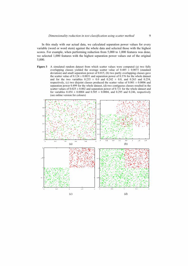
Dimensionality reduction in text classification using scatter method 9

In this study with our actual data, we calculated separation power values for every variable (word or word stem) against the whole data and selected those with the highest scores. For example, when performing reduction from 5,000 to 1,000 features was done, we selected 1,000 features with the highest separation power values out of the original 5,000.

Figure 3 A simulated random dataset from which scatter values were computed (a) two fully overlapping classes yielded the average scatter value of 0.485 ± 0.0073 (standard deviation) and small separation power of 0.015, (b) two partly overlapping classes gave the scatter value of 0.124 ± 0.0031 and separation power of 0.376 for the whole dataset and for the two variables 0.235 ± 0.0 and 0.242 ± 0.0, and 0.263 and 0.254, respectively, (c) two disjoint classes produced the scatter value of 0.001 ± 0.0006 and separation power 0.499 for the whole dataset, (d) two contiguous classes resulted in the scatter values of 0.025 ± 0.002 and separation power of 0.721 for the whole dataset and for variables 0.454 ± 0.0004 and 0.505 ± 0.0004, and 0.295 and 0.246, respectively (see online version for colours)

(a) (b)

(c) (d)

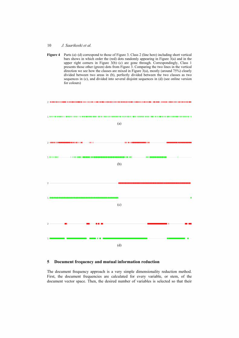
10 J. Saarikoski et al.

Figure 4 Parts (a)–(d) correspond to those of Figure 3. Class 2 (line here) including short vertical bars shows in which order the (red) dots randomly appearing in Figure 3(a) and in the upper right corners in Figure 3(b)–(c) are gone through. Correspondingly, Class 1 presents those other (green) dots from Figure 3. Comparing the two lines in the vertical direction we see how the classes are mixed in Figure 3(a), mostly (around 75%) clearly divided between two areas in (b), perfectly divided between the two classes as two sequences in (c), and divided into several disjoint sequences in (d) (see online version for colours)

(a)

(b)

(c)

(d)

5 Document frequency and mutual information reduction

The document frequency approach is a very simple dimensionality reduction method. First, the document frequencies are calculated for every variable, or stem, of the document vector space. Then, the desired number of variables is selected so that their

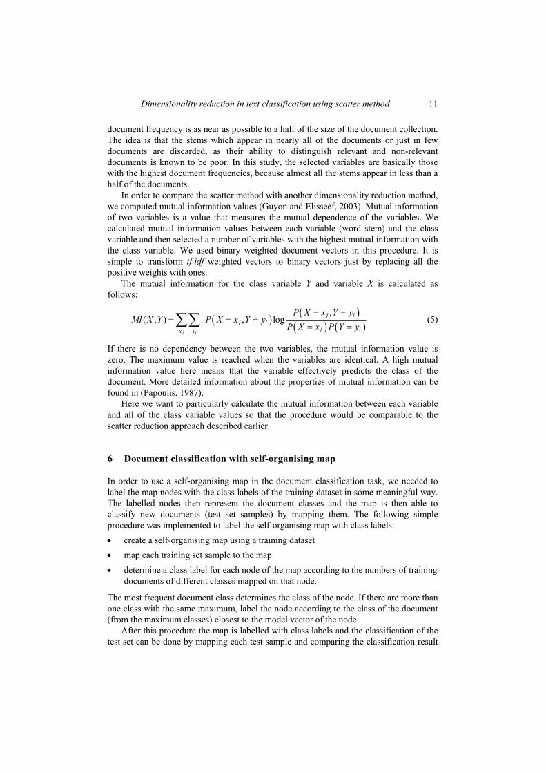
Dimensionality reduction in text classification using scatter method 11

document frequency is as near as possible to a half of the size of the document collection. The idea is that the stems which appear in nearly all of the documents or just in few documents are discarded, as their ability to distinguish relevant and non-relevant documents is known to be poor. In this study, the selected variables are basically those with the highest document frequencies, because almost all the stems appear in less than a half of the documents.

In order to compare the scatter method with another dimensionality reduction method, we computed mutual information values (Guyon and Elisseef, 2003). Mutual information of two variables is a value that measures the mutual dependence of the variables. We calculated mutual information values between each variable (word stem) and the class variable and then selected a number of variables with the highest mutual information with the class variable. We used binary weighted document vectors in this procedure. It is simple to transform tf·idf weighted vectors to binary vectors just by replacing all the positive weights with ones.

The mutual information for the class variable Y and variable X is calculated as follows:

( ) ( )( ) ( )

,( , ) , log

j i

j ij i

j ix y

P X x Y yMI X Y P X x Y y

P X x P Y y= =

= = == =∑∑ (5)

If there is no dependency between the two variables, the mutual information value is zero. The maximum value is reached when the variables are identical. A high mutual information value here means that the variable effectively predicts the class of the document. More detailed information about the properties of mutual information can be found in (Papoulis, 1987).

Here we want to particularly calculate the mutual information between each variable and all of the class variable values so that the procedure would be comparable to the scatter reduction approach described earlier.

6 Document classification with self-organising map

In order to use a self-organising map in the document classification task, we needed to label the map nodes with the class labels of the training dataset in some meaningful way. The labelled nodes then represent the document classes and the map is then able to classify new documents (test set samples) by mapping them. The following simple procedure was implemented to label the self-organising map with class labels: • create a self-organising map using a training dataset • map each training set sample to the map • determine a class label for each node of the map according to the numbers of training

documents of different classes mapped on that node.

The most frequent document class determines the class of the node. If there are more than one class with the same maximum, label the node according to the class of the document (from the maximum classes) closest to the model vector of the node.

After this procedure the map is labelled with class labels and the classification of the test set can be done by mapping each test sample and comparing the classification result

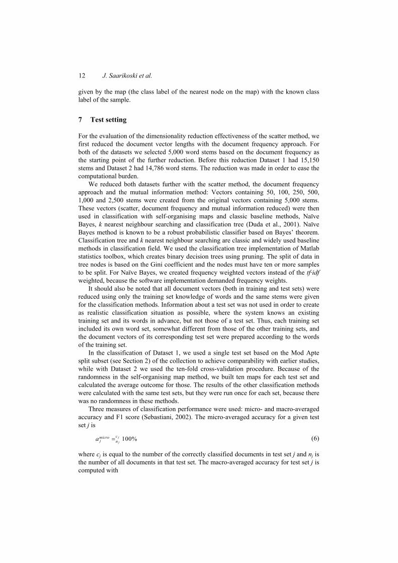
12 J. Saarikoski et al.

given by the map (the class label of the nearest node on the map) with the known class label of the sample.

7 Test setting

For the evaluation of the dimensionality reduction effectiveness of the scatter method, we first reduced the document vector lengths with the document frequency approach. For both of the datasets we selected 5,000 word stems based on the document frequency as the starting point of the further reduction. Before this reduction Dataset 1 had 15,150 stems and Dataset 2 had 14,786 word stems. The reduction was made in order to ease the computational burden.

We reduced both datasets further with the scatter method, the document frequency approach and the mutual information method: Vectors containing 50, 100, 250, 500, 1,000 and 2,500 stems were created from the original vectors containing 5,000 stems. These vectors (scatter, document frequency and mutual information reduced) were then used in classification with self-organising maps and classic baseline methods, Naïve Bayes, k nearest neighbour searching and classification tree (Duda et al., 2001). Naïve Bayes method is known to be a robust probabilistic classifier based on Bayes’ theorem. Classification tree and k nearest neighbour searching are classic and widely used baseline methods in classification field. We used the classification tree implementation of Matlab statistics toolbox, which creates binary decision trees using pruning. The split of data in tree nodes is based on the Gini coefficient and the nodes must have ten or more samples to be split. For Naïve Bayes, we created frequency weighted vectors instead of the tf·idf weighted, because the software implementation demanded frequency weights.

It should also be noted that all document vectors (both in training and test sets) were reduced using only the training set knowledge of words and the same stems were given for the classification methods. Information about a test set was not used in order to create as realistic classification situation as possible, where the system knows an existing training set and its words in advance, but not those of a test set. Thus, each training set included its own word set, somewhat different from those of the other training sets, and the document vectors of its corresponding test set were prepared according to the words of the training set.

In the classification of Dataset 1, we used a single test set based on the Mod Apte split subset (see Section 2) of the collection to achieve comparability with earlier studies, while with Dataset 2 we used the ten-fold cross-validation procedure. Because of the randomness in the self-organising map method, we built ten maps for each test set and calculated the average outcome for those. The results of the other classification methods were calculated with the same test sets, but they were run once for each set, because there was no randomness in these methods.

Three measures of classification performance were used: micro- and macro-averaged accuracy and F1 score (Sebastiani, 2002). The micro-averaged accuracy for a given test set j is

100%jj

cmicroj na = (6)

where cj is equal to the number of the correctly classified documents in test set j and nj is the number of all documents in that test set. The macro-averaged accuracy for test set j is computed with

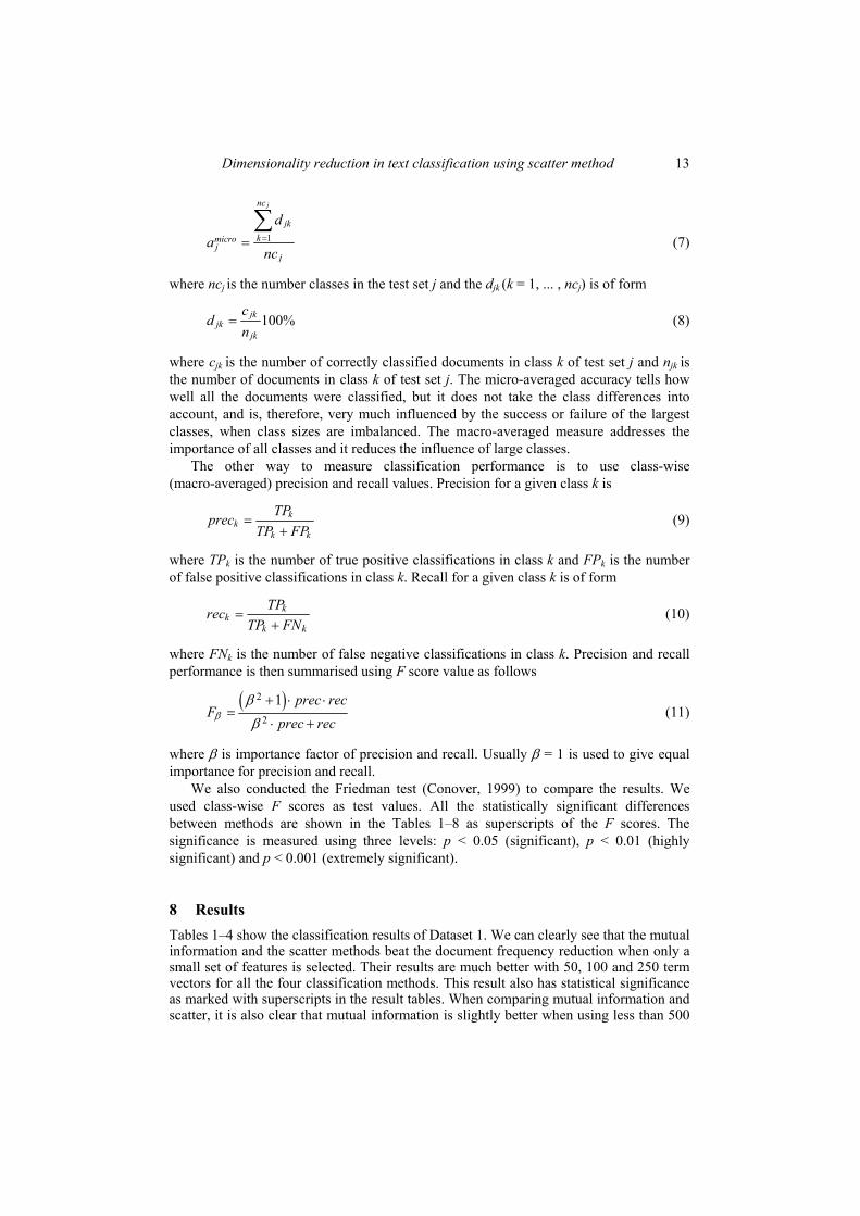
Dimensionality reduction in text classification using scatter method 13

1

jnc

jkkmicro

jj

da

nc==∑

(7)

where ncj is the number classes in the test set j and the djk (k = 1, ... , ncj) is of form

100%jkjk

jk

cd

n= (8)

where cjk is the number of correctly classified documents in class k of test set j and njk is

the number of documents in class k of test set j. The micro-averaged accuracy tells how well all the documents were classified, but it does not take the class differences into account, and is, therefore, very much influenced by the success or failure of the largest classes, when class sizes are imbalanced. The macro-averaged measure addresses the importance of all classes and it reduces the influence of large classes.

The other way to measure classification performance is to use class-wise (macro-averaged) precision and recall values. Precision for a given class k is

kk

k k

TPprecTP FP

=+

(9)

where TPk is the number of true positive classifications in class k and FPk is the number of false positive classifications in class k. Recall for a given class k is of form

kk

k k

TPrecTP FN

=+

(10)

where FNk is the number of false negative classifications in class k. Precision and recall performance is then summarised using F score value as follows

( )2

2

1 prec recF

prec recββ

β

+ ⋅ ⋅=

⋅ + (11)

where β is importance factor of precision and recall. Usually β = 1 is used to give equal importance for precision and recall.

We also conducted the Friedman test (Conover, 1999) to compare the results. We used class-wise F scores as test values. All the statistically significant differences between methods are shown in the Tables 1–8 as superscripts of the F scores. The significance is measured using three levels: p < 0.05 (significant), p < 0.01 (highly significant) and p < 0.001 (extremely significant).

8 Results Tables 1–4 show the classification results of Dataset 1. We can clearly see that the mutual information and the scatter methods beat the document frequency reduction when only a small set of features is selected. Their results are much better with 50, 100 and 250 term vectors for all the four classification methods. This result also has statistical significance as marked with superscripts in the result tables. When comparing mutual information and scatter, it is also clear that mutual information is slightly better when using less than 500

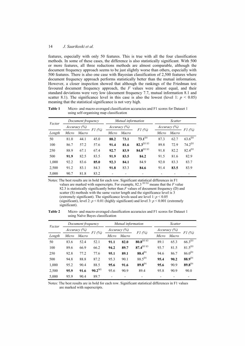
14 J. Saarikoski et al.

features, especially with only 50 features. This is true with all the four classification methods. In some of these cases, the difference is also statistically significant. With 500 or more features, all three reductions methods are almost comparable, although the document frequency approach seems to be just slightly worse than others, especially with 500 features. There is also one case with Bayesian classification of 2,500 features where document frequency approach performs statistically better than the mutual information. However, a closer inspection showed that although the rankings of the Friedman test favoured document frequency approach, the F values were almost equal, and their standard deviations were very low (document frequency 7.7, mutual information 8.1 and scatter 8.1). The significance level in this case is also the lowest (level 1: p < 0.05) meaning that the statistical significance is not very high. Table 1 Micro- and macro-averaged classification accuracies and F1 scores for Dataset 1

using self-organising map classification

Document frequency Mutual information Scatter Vector

Accuracy (%) Accuracy (%) Accuracy (%) Length

Micro Macro F1 (%)

Micro MacroF1 (%)

Micro Macro F1 (%)

50 81.0 44.1 45.0 88.2 73.1 73.1D3 87.3 62.7 63.6D3 100 86.7 57.2 57.6 91.4 81.6 82.3D3 S3 89.8 72.9 74.2D3 250 88.9 67.1 67.4 92.7 83.9 84.8D3 S3 91.8 82.2 82.4D3 500 91.9 82.5 83.5 91.9 83.5 84.2 91.5 81.6 82.9 1,000 92.2 83.6 85.0 92.3 84.1 84.9 92.0 83.3 83.7 2,500 91.2 83.1 84.3 91.8 83.3 84.6 91.4 83.5 83.9 5,000 90.7 81.8 83.2 - - - - - -

Notes: The best results are in bold for each row. Significant statistical differences in F1 values are marked with superscripts. For example, 82.3 D3 S3 means that the F value 82.3 is statistically significantly better than F values of document frequency (D) and scatter (S) methods with the same vector length and the significance level is 3 (extremely significant). The significance levels used are level 1: p < 0.05 (significant), level 2: p < 0.01 (highly significant) and level 3: p < 0.001 (extremely significant).

Table 2 Micro- and macro-averaged classification accuracies and F1 scores for Dataset 1 using Naïve Bayes classification

Document frequency Mutual information Scatter Vector

Accuracy (%) Accuracy (%) Accuracy (%)

Length

Micro Macro F1 (%)

Micro MacroF1 (%)

Micro Macro F1 (%)

50 83.6 52.4 52.1 91.1 82.0 80.8D3 S3 89.1 65.3 66.3D3 100 89.6 66.9 66.2 94.2 89.7 87.4D3 S3 93.7 81.5 81.5D3 250 92.8 77.2 77.6 95.1 89.1 88.4D1 94.6 86.7 86.0D1 500 94.8 88.8 87.2 95.3 90.1 88.5D1 95.4 90.2 88.9D1 1,000 95.2 90.4 88.5 95.6 91.6 89.8D1 95.6 90.9 89.8D1 2,500 95.9 91.6 90.2M1 95.6 90.9 89.4 95.8 90.9 90.0 5,000 95.9 90.4 89.7 - - - - - -

Notes: The best results are in bold for each row. Significant statistical differences in F1 values are marked with superscripts.

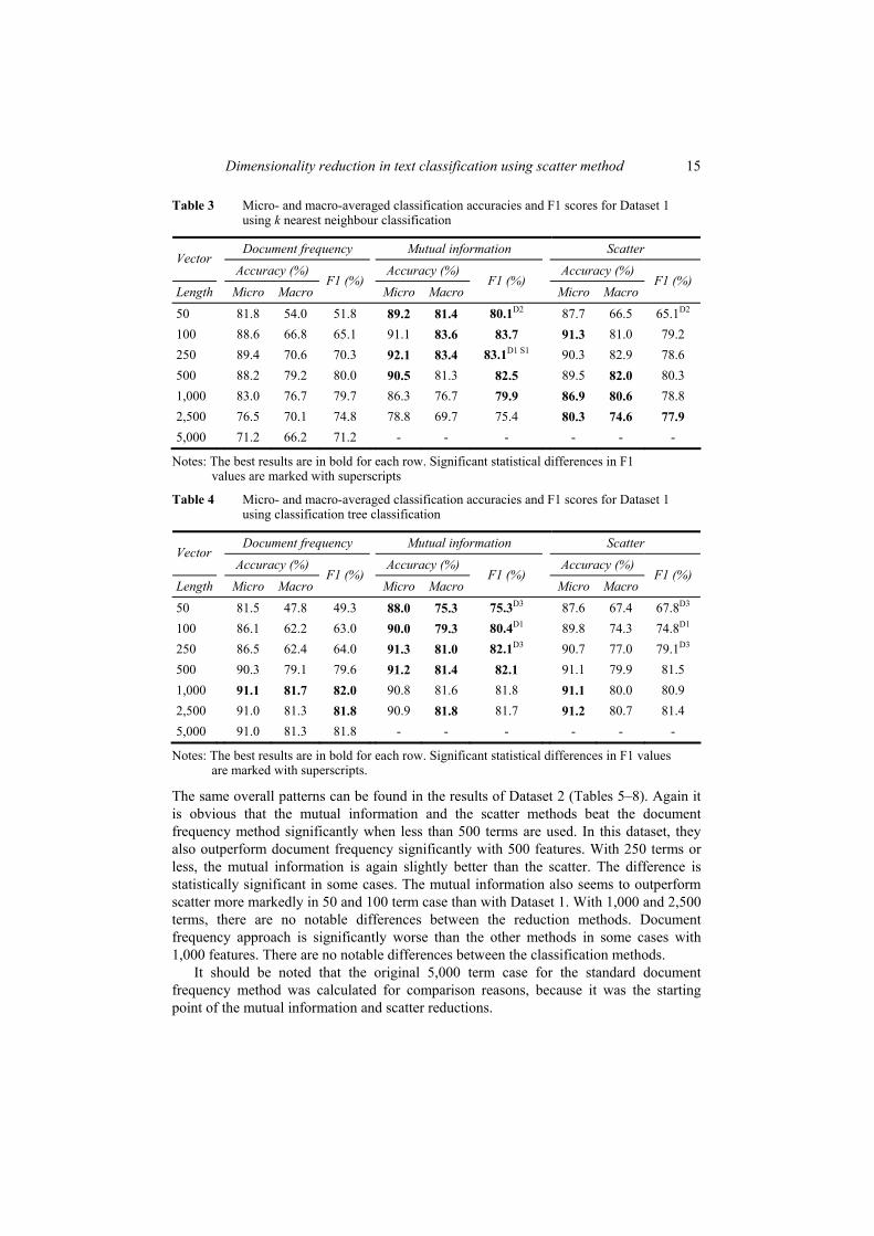
Dimensionality reduction in text classification using scatter method 15

Table 3 Micro- and macro-averaged classification accuracies and F1 scores for Dataset 1 using k nearest neighbour classification

Document frequency Mutual information Scatter Vector

Accuracy (%) Accuracy (%) Accuracy (%) Length

Micro Macro F1 (%)

Micro MacroF1 (%)

Micro Macro F1 (%)

50 81.8 54.0 51.8 89.2 81.4 80.1D2 87.7 66.5 65.1D2 100 88.6 66.8 65.1 91.1 83.6 83.7 91.3 81.0 79.2 250 89.4 70.6 70.3 92.1 83.4 83.1D1 S1 90.3 82.9 78.6 500 88.2 79.2 80.0 90.5 81.3 82.5 89.5 82.0 80.3 1,000 83.0 76.7 79.7 86.3 76.7 79.9 86.9 80.6 78.8 2,500 76.5 70.1 74.8 78.8 69.7 75.4 80.3 74.6 77.9 5,000 71.2 66.2 71.2 - - - - - -

Notes: The best results are in bold for each row. Significant statistical differences in F1 values are marked with superscripts

Table 4 Micro- and macro-averaged classification accuracies and F1 scores for Dataset 1 using classification tree classification

Document frequency Mutual information Scatter Vector

Accuracy (%) Accuracy (%) Accuracy (%) Length

Micro Macro F1 (%)

Micro MacroF1 (%)

Micro Macro F1 (%)

50 81.5 47.8 49.3 88.0 75.3 75.3D3 87.6 67.4 67.8D3 100 86.1 62.2 63.0 90.0 79.3 80.4D1 89.8 74.3 74.8D1 250 86.5 62.4 64.0 91.3 81.0 82.1D3 90.7 77.0 79.1D3 500 90.3 79.1 79.6 91.2 81.4 82.1 91.1 79.9 81.5 1,000 91.1 81.7 82.0 90.8 81.6 81.8 91.1 80.0 80.9 2,500 91.0 81.3 81.8 90.9 81.8 81.7 91.2 80.7 81.4 5,000 91.0 81.3 81.8 - - - - - -

Notes: The best results are in bold for each row. Significant statistical differences in F1 values are marked with superscripts.

The same overall patterns can be found in the results of Dataset 2 (Tables 5–8). Again it is obvious that the mutual information and the scatter methods beat the document frequency method significantly when less than 500 terms are used. In this dataset, they also outperform document frequency significantly with 500 features. With 250 terms or less, the mutual information is again slightly better than the scatter. The difference is statistically significant in some cases. The mutual information also seems to outperform scatter more markedly in 50 and 100 term case than with Dataset 1. With 1,000 and 2,500 terms, there are no notable differences between the reduction methods. Document frequency approach is significantly worse than the other methods in some cases with 1,000 features. There are no notable differences between the classification methods.

It should be noted that the original 5,000 term case for the standard document frequency method was calculated for comparison reasons, because it was the starting point of the mutual information and scatter reductions.

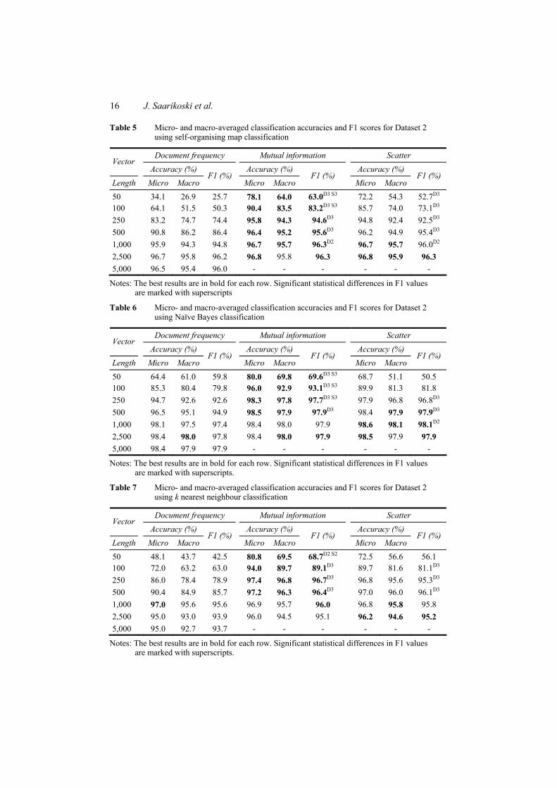
16 J. Saarikoski et al.

Table 5 Micro- and macro-averaged classification accuracies and F1 scores for Dataset 2 using self-organising map classification

Document frequency Mutual information Scatter Vector

Accuracy (%) Accuracy (%) Accuracy (%) Length

Micro Macro F1 (%)

Micro MacroF1 (%)

Micro Macro F1 (%)

50 34.1 26.9 25.7 78.1 64.0 63.0D3 S3 72.2 54.3 52.7D3 100 64.1 51.5 50.3 90.4 83.5 83.2D3 S3 85.7 74.0 73.1D3 250 83.2 74.7 74.4 95.8 94.3 94.6D3 94.8 92.4 92.5D3 500 90.8 86.2 86.4 96.4 95.2 95.6D3 96.2 94.9 95.4D3 1,000 95.9 94.3 94.8 96.7 95.7 96.3D2 96.7 95.7 96.0D2 2,500 96.7 95.8 96.2 96.8 95.8 96.3 96.8 95.9 96.3 5,000 96.5 95.4 96.0 - - - - - -

Notes: The best results are in bold for each row. Significant statistical differences in F1 values are marked with superscripts

Table 6 Micro- and macro-averaged classification accuracies and F1 scores for Dataset 2 using Naïve Bayes classification

Document frequency Mutual information Scatter Vector

Accuracy (%) Accuracy (%) Accuracy (%) Length

Micro Macro F1 (%)

Micro MacroF1 (%)

Micro Macro F1 (%)

50 64.4 61.0 59.8 80.0 69.8 69.6D3 S3 68.7 51.1 50.5 100 85.3 80.4 79.8 96.0 92.9 93.1D3 S3 89.9 81.3 81.8 250 94.7 92.6 92.6 98.3 97.8 97.7D3 S3 97.9 96.8 96.8D3 500 96.5 95.1 94.9 98.5 97.9 97.9D3 98.4 97.9 97.9D3 1,000 98.1 97.5 97.4 98.4 98.0 97.9 98.6 98.1 98.1D2 2,500 98.4 98.0 97.8 98.4 98.0 97.9 98.5 97.9 97.9 5,000 98.4 97.9 97.9 - - - - - -

Notes: The best results are in bold for each row. Significant statistical differences in F1 values are marked with superscripts.

Table 7 Micro- and macro-averaged classification accuracies and F1 scores for Dataset 2 using k nearest neighbour classification

Document frequency Mutual information Scatter Vector

Accuracy (%) Accuracy (%) Accuracy (%) Length

Micro Macro F1 (%)

Micro MacroF1 (%)

Micro Macro F1 (%)

50 48.1 43.7 42.5 80.8 69.5 68.7D2 S2 72.5 56.6 56.1 100 72.0 63.2 63.0 94.0 89.7 89.1D3 89.7 81.6 81.1D3 250 86.0 78.4 78.9 97.4 96.8 96.7D3 96.8 95.6 95.3D3 500 90.4 84.9 85.7 97.2 96.3 96.4D3 97.0 96.0 96.1D3 1,000 97.0 95.6 95.6 96.9 95.7 96.0 96.8 95.8 95.8 2,500 95.0 93.0 93.9 96.0 94.5 95.1 96.2 94.6 95.2 5,000 95.0 92.7 93.7 - - - - - -

Notes: The best results are in bold for each row. Significant statistical differences in F1 values are marked with superscripts.

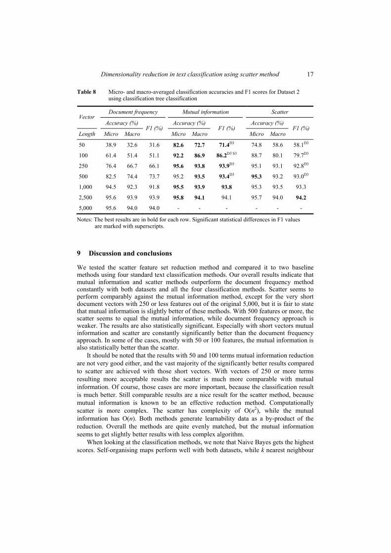
Dimensionality reduction in text classification using scatter method 17

Table 8 Micro- and macro-averaged classification accuracies and F1 scores for Dataset 2 using classification tree classification

Document frequency Mutual information Scatter Vector

Accuracy (%) Accuracy (%) Accuracy (%)

Length

Micro Macro F1 (%)

Micro MacroF1 (%)

Micro Macro F1 (%)

50 38.9 32.6 31.6 82.6 72.7 71.4D3 74.8 58.6 58.1D3

100 61.4 51.4 51.1 92.2 86.9 86.2D3 S3 88.7 80.1 79.7D3

250 76.4 66.7 66.1 95.6 93.8 93.9D3 95.1 93.1 92.8D3

500 82.5 74.4 73.7 95.2 93.5 93.4D3 95.3 93.2 93.0D3

1,000 94.5 92.3 91.8 95.5 93.9 93.8 95.3 93.5 93.3

2,500 95.6 93.9 93.9 95.8 94.1 94.1 95.7 94.0 94.2

5,000 95.6 94.0 94.0 - - - - - -

Notes: The best results are in bold for each row. Significant statistical differences in F1 values are marked with superscripts.

9 Discussion and conclusions

We tested the scatter feature set reduction method and compared it to two baseline methods using four standard text classification methods. Our overall results indicate that mutual information and scatter methods outperform the document frequency method constantly with both datasets and all the four classification methods. Scatter seems to perform comparably against the mutual information method, except for the very short document vectors with 250 or less features out of the original 5,000, but it is fair to state that mutual information is slightly better of these methods. With 500 features or more, the scatter seems to equal the mutual information, while document frequency approach is weaker. The results are also statistically significant. Especially with short vectors mutual information and scatter are constantly significantly better than the document frequency approach. In some of the cases, mostly with 50 or 100 features, the mutual information is also statistically better than the scatter.

It should be noted that the results with 50 and 100 terms mutual information reduction are not very good either, and the vast majority of the significantly better results compared to scatter are achieved with those short vectors. With vectors of 250 or more terms resulting more acceptable results the scatter is much more comparable with mutual information. Of course, those cases are more important, because the classification result is much better. Still comparable results are a nice result for the scatter method, because mutual information is known to be an effective reduction method. Computationally scatter is more complex. The scatter has complexity of O(n2), while the mutual information has O(n). Both methods generate learnability data as a by-product of the reduction. Overall the methods are quite evenly matched, but the mutual information seems to get slightly better results with less complex algorithm.

When looking at the classification methods, we note that Naive Bayes gets the highest scores. Self-organising maps perform well with both datasets, while k nearest neighbour

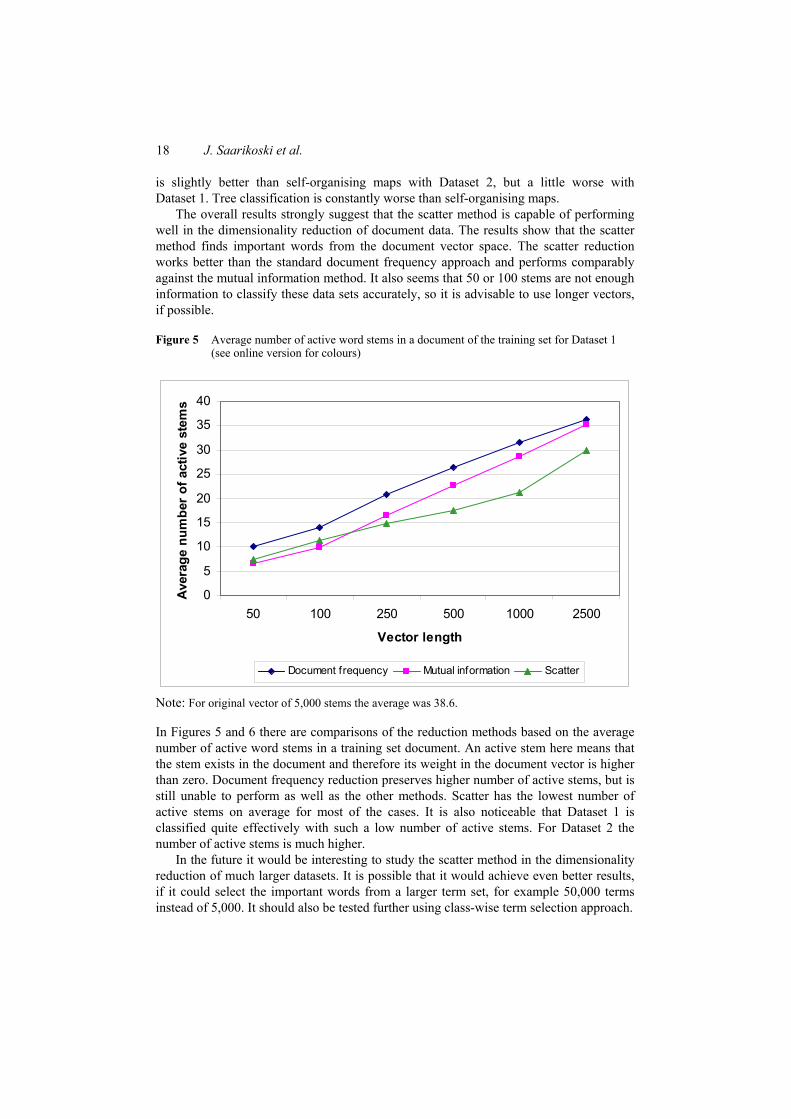
18 J. Saarikoski et al.

is slightly better than self-organising maps with Dataset 2, but a little worse with Dataset 1. Tree classification is constantly worse than self-organising maps.

The overall results strongly suggest that the scatter method is capable of performing well in the dimensionality reduction of document data. The results show that the scatter method finds important words from the document vector space. The scatter reduction works better than the standard document frequency approach and performs comparably against the mutual information method. It also seems that 50 or 100 stems are not enough information to classify these data sets accurately, so it is advisable to use longer vectors, if possible.

Figure 5 Average number of active word stems in a document of the training set for Dataset 1 (see online version for colours)

0

5

10

15

20

25

30

35

40

50 100 250 500 1000 2500

Vector length

Aver

age

num

ber

of a

ctiv

e st

ems

Document frequency Mutual information Scatter

Note: For original vector of 5,000 stems the average was 38.6.

In Figures 5 and 6 there are comparisons of the reduction methods based on the average number of active word stems in a training set document. An active stem here means that the stem exists in the document and therefore its weight in the document vector is higher than zero. Document frequency reduction preserves higher number of active stems, but is still unable to perform as well as the other methods. Scatter has the lowest number of active stems on average for most of the cases. It is also noticeable that Dataset 1 is classified quite effectively with such a low number of active stems. For Dataset 2 the number of active stems is much higher.

In the future it would be interesting to study the scatter method in the dimensionality reduction of much larger datasets. It is possible that it would achieve even better results, if it could select the important words from a larger term set, for example 50,000 terms instead of 5,000. It should also be tested further using class-wise term selection approach.

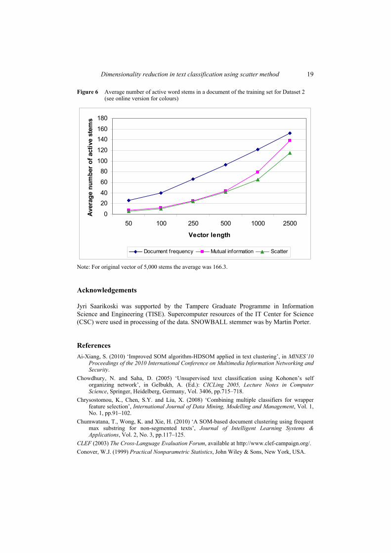
Dimensionality reduction in text classification using scatter method 19

Figure 6 Average number of active word stems in a document of the training set for Dataset 2 (see online version for colours)

0

2040

60

80100

120

140160

180

50 100 250 500 1000 2500

Vector length

Aver

age

num

ber

of a

ctiv

e st

ems

Document frequency Mutual information Scatter

Note: For original vector of 5,000 stems the average was 166.3.

Acknowledgements

Jyri Saarikoski was supported by the Tampere Graduate Programme in Information Science and Engineering (TISE). Supercomputer resources of the IT Center for Science (CSC) were used in processing of the data. SNOWBALL stemmer was by Martin Porter.

References Ai-Xiang, S. (2010) ‘Improved SOM algorithm-HDSOM applied in text clustering’, in MINES’10

Proceedings of the 2010 International Conference on Multimedia Information Networking and Security.

Chowdhury, N. and Saha, D. (2005) ‘Unsupervised text classification using Kohonen’s self organizing network’, in Gelbukh, A. (Ed.): CICLing 2005, Lecture Notes in Computer Science, Springer, Heidelberg, Germany, Vol. 3406, pp.715–718.

Chrysostomou, K., Chen, S.Y. and Liu, X. (2008) ‘Combining multiple classifiers for wrapper feature selection’, International Journal of Data Mining, Modelling and Management, Vol. 1, No. 1, pp.91–102.

Chumwatana, T., Wong, K. and Xie, H. (2010) ‘A SOM-based document clustering using frequent max substring for non-segmented texts’, Journal of Intelligent Learning Systems & Applications, Vol. 2, No. 3, pp.117–125.

CLEF (2003) The Cross-Language Evaluation Forum, available at http://www.clef-campaign.org/. Conover, W.J. (1999) Practical Nonparametric Statistics, John Wiley & Sons, New York, USA.

20 J. Saarikoski et al.

Deerwester, S., Dumais, S.T., Furnas, G.W., Landaer, T.K. and Harshman, R. (1990) ‘Indexing by latent semantic indexing’, Journal of the American Society for Information Science and Technology, Vol. 41, No. 6, pp.391–407.

Duda, R.O., Hart, P.E. and Stork, D.G. (2001) Pattern Classification, 2nd ed., John Wiley & Sons, New York, USA.

Fernandez, J., Mones, R., Diaz, I., Ranilla, J. and Combarro, E.F. (2004) ‘Experiments with self organizing maps in CLEF 2003’, in CLEF 2003, Lecture Notes in Computer Science, Springer, Heidelberg, Germany, Vol. 3237, pp.358–366.

Flach, P.A. and Lachiche, N. (2004) ‘Naïve Bayesian classification of structured data’, Machine Learning, Vol. 57, No. 3, pp.233–269.

Frank, E. and Bouckaert, R.R. (2006) ‘Naïve Bayes for text classification with unbalanced classes’, Knowledge Discovery in Databases: PKDD 2006, Lecture Notes in Computer Science, Vol. 4213, pp.503–510.

Garg, V.K. and Murty, M.N. (2009) ‘Feature subspace SVMs (FS-SVMs) for high dimensional handwritten digit recogntion’, International Journal of Data Mining, Modelling and Management, Vol. 1, No. 4, pp.411–436.

Guyon, I. and Elisseef, A. (2003) ‘An introduction to variable and feature selection’, Journal of Machine Learning Research, Vol. 3, No. 3/1/2003, pp.1157–1182.

Honkela, T. (1997) ‘Self-organizing maps in natural language processing’, Academic dissertation, Helsinki University of Technology, Finland.

Jain, A. and Dubes, R. (1988) Algorithms for Clustering Data, Prentice Hall, Englewood Cliffs, New Jersey, USA.

Juhola, M. and Siermala, M. (2005) ‘Assessment methods of neural network classification applied to otoneurological data’, in European Notes in Medical Informatics, Medical Informatics Europe, Geneve, Switzerland, European Federal for Medical Informatics, 2005, Vol. 1, No. 1, pp.1092–1097.

Kaski, S. (1998) ‘Dimensionality reduction by random mapping: fast similarity computation for clustering’, Proceedings of IJCNN’98, Vol. 1, pp.413–418.

Kline, D.M. and Galbraith, G.S. (2009) ‘Performance analysis of the Bayesian data reduction algorithm’, International Journal of Data Mining, Modelling and Management, Vol. 1, No. 3, pp.223–236.

Kohonen, T. (1995) Self-Organizing Maps, Springer, Berlin, Germany. Lagus, K. (2002) ‘Text retrieval using self-organized document maps’, Neural Processing Letters,

Vol. 15, No. 1, pp.21–29. Lagus, K., Kaski, S. and Kohonen, T. (2004) ‘Mining massive document collections by the

WEBSOM method’, Information Sciences, Vol. 163, Nos. 1–3, pp.135–156. Li, Y.H. and Jain, A.K. (1998) ‘Classification of text documents’, The Computer Journal, Vol. 41,

No. 8, pp.537–546. Liu, Y. and Takatsuka, M. (2009) ‘Interactive hierarchical SOM for image retrieval’, Lecture Notes

in Computer Science, Vol. 5864, pp.845–885. Maheswari, P.U. and Rajaram, M. (2009) ‘Principal component analysis-based frequent pattern

evaluation on the object-relational data model of a cricket match database’, International Journal of Data Analysis Techniques and Strategies, Vol. 1, No. 4, pp.364–384.

Papoulis, A. (1987) Probability, Random Variables, and Stochastic Processes, McGraw-Hill, Auckland, New Zealand.

Porter, M. (2001) Snowball: a Language for Stemming Algorithms’, available at http://snowball.tartarus.org/texts/introduction.html (accessed on 5 March 2012).

Reuters-21578, available at http://kdd.ics.uci.edu/databases/reuters21578/reuters21578.html (accessed on 5 March 2012).

Dimensionality reduction in text classification using scatter method 21

Saarikoski, J., Laurikkala, J., Järvelin, K. and Juhola, M. (2009a) ‘A study of the use of self-organising maps in information retrieval’, Journal of Documentation, Vol. 65, No. 2, pp.304–322.

Saarikoski, J., Järvelin, K., Laurikkala, J. and Juhola, M. (2009b) ‘On document classification with self-organising maps’, ICANNGA’09, Lecture Notes in Computer Science, Vol. 5495, pp.140–149.

Saarikoski, J., Laurikkala, J., Järvelin, K. and Juhola, M. (2011) ‘Self-organising maps in document classification: a comparison with six machine learning methods’, ICANNGA’11, Lecture Notes in Computer Science, Vol. 6593, pp.260–269.

Salton, G. (1989) Automatic Text Processing: The Transformation, Analysis and Retrieval of Information by Computer, Addison-Wesley, USA.

Scatter Software, available at http://www.cs.uta.fi/~mj/DARG/Scatter/ScatterCounter.exe (accessed on 5 March 2012).

Sebastiani, F. (2002) ‘Machine learning in automated text categorization’, ACM Computing Surveys, Vol. 34, No. 1, pp.1–47.

Sharma, S. (1996) Applied Multivariate Techniques, Wiley, New York, USA. Siermala, M. and Juhola, M. (2006) ‘Techniques for biased distributions and variable classification

with neural networks applied to otoneurological data’, Computer Methods and Programs in Biomedicine, Vol. 81, No. 2, pp.128–136.

Siermala, M., Juhola, M., Laurikkala, J., Iltanen, K., Kentala, E. and Pyykkö, I. (2007) ‘Evaluation and classification of otoneurological data with new data analysis methods based on machine learning’, Information Sciences, Vol. 177, No. 9, pp.1963–1976.

Xu, Y. and Wang, H. (2011) ‘A new feature selection method based on support vector machine for text categorization’, International Journal of Data Mining, Modelling and Management, Vol. 3, No. 1, pp.1–20.

Publication V

On the influence of training data quality on text document classification using machine learning methods

Jyri Saarikoski, Henry Joutsijoki, Kalervo Järvelin, Jorma Laurikkala and Martti Juhola

Submitted to International Journal of Knowledge Engineering and Data Mining.

Int. J. , Vol. x, No. x, xxxx 1

Copyright © 200x Inderscience Enterprises Ltd.

On the influence of training data quality on text document classification using machine learning methods

Jyri Saarikoski, Henry Joutsijoki, Kalervo Järvelin, Jorma Laurikkala and Martti Juhola jyri.saarikoski@uta.fi, henry.joutsijoki@uta.fi, kalervo.jarvelin@uta.fi,

jorma.laurikkala@uta.fi, martti.juhola@uta.fi

School of Information Sciences, 33014 University of Tampere, Finland

Abstract The main target of this paper was to study the influence of training data quality on the text document classification performance of machine learning methods. A graded relevance corpus of 10 classes and 957 text documents was classified with self-organising maps, learning vector quantization, k nearest neighbours searching, Naïve Bayes and support vector machines. The relevance level of a document (irrelevant, marginally, fairly or highly relevant) was used as a measure of the quality of the document as a training example, which is a new approach. The classifiers were evaluated with micro- and macro-averaged classification accuracies. The results suggest that training data of higher quality should be preferred, but even low quality data can improve a classifier, if there is plenty of it. In addition, further means to facilitate classification by the self-organising maps (SOMs) were explored. The novel set of SOMs approach performed clearly better than the original SOM and comparably against supervised classification methods. Keywords: data mining; document collections; graded relevance; relevance assessment; data quality; text classification; machine learning; self-organising maps; SOM; set of SOMs. 1. Introduction The concept of relevance (Borlund, 2003; Cosijn and Ingwersen, 2000; Hjørland 2010; Saracevic, 2007) is highly important in modern information retrieval (IR) research. Sophisticated IR systems are built to find relevant information automatically and as effectively as possible. In order to develop these systems further, evaluation of their effectiveness is required. The evaluation metrics, for example precision, recall and F-measure (Sebastiani, 2002), are based on the relevance of the information items retrieved by the system. Traditionally, relevance is considered to be binary, thus a retrieved item is either relevant or irrelevant. Unfortunately, there are many levels of relevance in the real world. For example, one newspaper article may be highly relevant to a given topic, while another may be only marginally relevant to the same topic. In this case, the binary relevance assessment forces us to decide whether we want to consider both of the articles equally relevant or the latter completely irrelevant. Either way, we lose some information about

2 J. Saarikoski et al.

their relevance. Moreover, we need to especially identify highly relevant items, because nowadays real-world collections are huge and we are very likely to find far too many relevant items to browse through in a reasonable time. Thus, we need systems that are able to retrieve such information effectively. Although different relevance levels have been studied extensively, IR evaluation has often been done with metrics dealing only with binary relevance. Search engine development has pushed IR evaluation towards metrics based on graded relevance (see, for example, Järvelin and Kekäläinen, 2002; Robertson et al., 2010; Voorhees, 2001; Sakai, 2007; Kekäläinen, 2005). Vakkari and Sormunen (2004) have applied graded relevance in interactive information retrieval and Korenius et al. (2006) clustered a Finnish newspaper article collection with graded relevance assessment. More recently, Cheng et al. (2010) proposed a solution for graded multi-label classification, Zellhöfer (2012) used graded relevance assessment in photograph collection and a content-based multimedia retrieval system supporting graded relevance was introduced by Redi and Merialdo (2012). We studied the influence of training data quality, as measured with the relevance level of the documents, on the classification effectiveness of five machine learning methods. We used a news document collection of 10 classes and 957 documents graded on a four-level relevance scale. The data samples were first preprocessed and transformed into tf·idf weighted document vectors. Then, classifiers were trained for the classification task using training document sets of different relevance levels. The evaluation was based on binary relevance for the whole test data set and for different relevance levels of the test set individually in order to learn about the influence of training document relevance level. We also continued our earlier research (Saarikoski et al. 2009, 2011 and 2014) of self-organising maps (SOM) method (Kohonen, 2001) and introduce the set of SOMs method, a multi-map voting approach of SOM. SOM is a machine learning method (Mitchell, 1997), i.e., a computer algorithm capable of learning from data automatically. SOM belongs to artificial neural networks whose learning mechanism resembles superficially the functioning of biological neural networks, such as the brain. Classification of data samples is one of the most common tasks in machine learning, and there are multiple solutions available (Sebastiani, 2002). The machine learning procedure is either supervised or unsupervised depending on the use of class information in the training process. Most classifiers use supervised learning, where learning examples have class labels. The present paper employs four supervised methods: learning vector quantization (LVQ), k nearest neighbours searching (k-NN), Naïve Bayes classifier and support vector machines (SVM). These learners have been used extensively in classification of different types of data (Naoum and Al-Sultani, 2012; Asy'arie and Pribadi, 2009; Zhang et al., 2009; Li and Bontcheva, 2008; Cho and Won, 2003). Being an unsupervised learner in its basic form, the SOM method is inherently at a disadvantage when pitted against the supervised learners in a classification task. The main advantage of the SOM method over many of the supervised learners is a visual data map, which is automatically created in the learning process. The method has been used mostly in data visualisation and clustering (Lagus, 2000; Patra et al., 2010; Chumwatana et al., 2010; Ai-Xiang 2010) of high-dimensional data samples to a low-dimensional map. Often a two-dimensional map is preferred for its simplicity. The map method can be easily modified to perform even more demanding tasks, like information retrieval (Fernandez et. al., 2004; Lagus, 2002) and classification (Beckel et al., 2012; Furletti et al., 2012). Supervised versions of SOM have also been proposed, see for example in Plonski and Zaremba (2012) and Hagenbuchner and Tsoi (2005).

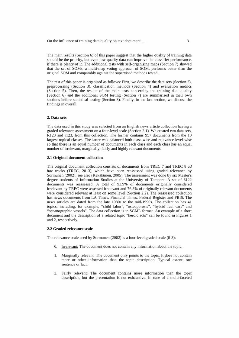
On the influence of training data quality on text document … 3

The main results (Section 6) of this paper suggest that the higher quality of training data should be the priority, but even low quality data can improve the classifier performance, if there is plenty of it. The additional tests with self-organising maps (Section 7) showed that the set of SOMs, a multi-map voting approach of SOM, performs better than the original SOM and comparably against the supervised methods tested. The rest of this paper is organised as follows: First, we describe the data sets (Section 2), preprocessing (Section 3), classification methods (Section 4) and evaluation metrics (Section 5). Then, the results of the main tests concerning the training data quality (Section 6) and the additional SOM testing (Section 7) are summarised in their own sections before statistical testing (Section 8). Finally, in the last section, we discuss the findings in overall. 2. Data sets The data used in this study was selected from an English news article collection having a graded relevance assessment on a four-level scale (Section 2.1). We created two data sets, R123 and r123, from this collection. The former contains 957 documents from the 10 largest topical classes. The latter was balanced both class-wise and relevance-level-wise so that there is an equal number of documents in each class and each class has an equal number of irrelevant, marginally, fairly and highly relevant documents. 2.1 Original document collection The original document collection consists of documents from TREC 7 and TREC 8 ad hoc tracks (TREC, 2013), which have been reassessed using graded relevance by Sormunen (2002), see also (Kekäläinen, 2005). The assessment was done by six Master's degree students of Information Studies at the University of Tampere. A set of 6122 documents was reassessed. A total of 93.9% of documents originally considered irrelevant by TREC were assessed irrelevant and 76.3% of originally relevant documents were considered relevant at least on some level (Section 2.2). The reassessed collection has news documents from LA Times, Financial Times, Federal Register and FBIS. The news articles are dated from the late 1980s to the mid-1990s. The collection has 41 topics, including, for example, “child labor”, “osteoporosis”, “hybrid fuel cars” and “oceanographic vessels”. The data collection is in SGML format. An example of a short document and the description of a related topic “heroic acts” can be found in Figures 1 and 2, respectively. 2.2 Graded relevance scale The relevance scale used by Sormunen (2002) is a four-level graded scale (0-3):

0. Irrelevant: The document does not contain any information about the topic.

1. Marginally relevant: The document only points to the topic. It does not contain more or other information than the topic description. Typical extent: one sentence or fact.

2. Fairly relevant: The document contains more information than the topic

description, but the presentation is not exhaustive. In case of a multi-faceted

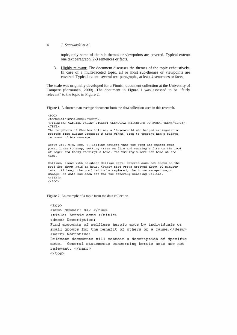
4 J. Saarikoski et al.

topic, only some of the sub-themes or viewpoints are covered. Typical extent: one text paragraph, 2-3 sentences or facts.

3. Highly relevant: The document discusses the themes of the topic exhaustively.

In case of a multi-faceted topic, all or most sub-themes or viewpoints are covered. Typical extent: several text paragraphs, at least 4 sentences or facts.

The scale was originally developed for a Finnish document collection at the University of Tampere (Sormunen, 2000). The document in Figure 1 was assessed to be “fairly relevant” to the topic in Figure 2.

Figure 1. A shorter than average document from the data collection used in this research.

Figure 2. An example of a topic from the data collection.

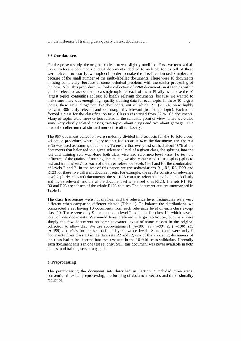
On the influence of training data quality on text document … 5

2.3 Our data sets For the present study, the original collection was slightly modified. First, we removed all 3722 irrelevant documents and 61 documents labelled to multiple topics (all of these were relevant to exactly two topics) in order to make the classification task simpler and because of the small number of the multi-labelled documents. There were 10 documents missing completely, because of some technical problems with the earlier processing of the data. After this procedure, we had a collection of 2268 documents in 41 topics with a graded relevance assessment to a single topic for each of them. Finally, we chose the 10 largest topics containing at least 10 highly relevant documents, because we wanted to make sure there was enough high quality training data for each topic. In these 10 largest topics, there were altogether 957 documents, out of which 197 (20.6%) were highly relevant, 386 fairly relevant and 374 marginally relevant (to a single topic). Each topic formed a class for the classification task. Class sizes varied from 52 to 163 documents. Many of topics were more or less related in the semantic point of view. There were also some very closely related classes, two topics about drugs and two about garbage. This made the collection realistic and more difficult to classify. The 957 document collection were randomly divided into test sets for the 10-fold cross-validation procedure, where every test set had about 10% of the documents and the rest 90% was used as training documents. To ensure that every test set had about 10% of the documents that belonged to a given relevance level of a given class, the splitting into the test and training sets was done both class-wise and relevance-level-wise. To test the influence of the quality of training documents, we also constructed 10 test splits (splits to test and training sets) for each of the three relevance levels (1-3) and for the combination of levels 2 and 3. In the rest of this paper, we use abbreviations R1, R2, R3, R23 and R123 for these five different document sets. For example, the set R2 consists of relevance level 2 (fairly relevant) documents, the set R23 contains relevance levels 2 and 3 (fairly and highly relevant) and the whole document set is referred to as R123. The sets R1, R2, R3 and R23 are subsets of the whole R123 data set. The document sets are summarised in Table 1. The class frequencies were not uniform and the relevance level frequencies were very different when comparing different classes (Table 1). To balance the distributions, we constructed a set having 10 documents from each relevance level of each class except class 10. There were only 9 documents on level 2 available for class 10, which gave a total of 299 documents. We would have preferred a larger collection, but there were simply too few documents on some relevance levels of some classes in the original collection to allow that. We use abbreviations r1 (n=100), r2 (n=99), r3 (n=100), r23 (n=199) and r123 for the sets defined by relevance levels. Since there were only 9 documents from class 10 in the data sets R2 and r2, one of the 9 existing documents of the class had to be inserted into two test sets in the 10-fold cross-validation. Normally each document exists in one test set only. Still, this document was never available in both the test and training sets of any split. 3. Preprocessing The preprocessing the document sets described in Section 2 included three steps: conventional lexical preprocessing, the forming of document vectors and dimensionality reduction.

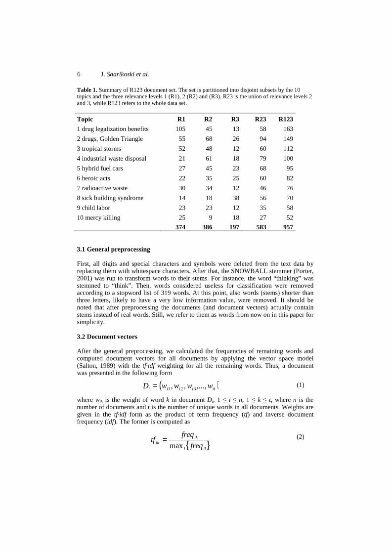
6 J. Saarikoski et al.

Table 1. Summary of R123 document set. The set is partitioned into disjoint subsets by the 10 topics and the three relevance levels 1 (R1), 2 (R2) and (R3). R23 is the union of relevance levels 2 and 3, while R123 refers to the whole data set.

3.1 General preprocessing First, all digits and special characters and symbols were deleted from the text data by replacing them with whitespace characters. After that, the SNOWBALL stemmer (Porter, 2001) was run to transform words to their stems. For instance, the word “thinking” was stemmed to “think”. Then, words considered useless for classification were removed according to a stopword list of 319 words. At this point, also words (stems) shorter than three letters, likely to have a very low information value, were removed. It should be noted that after preprocessing the documents (and document vectors) actually contain stems instead of real words. Still, we refer to them as words from now on in this paper for simplicity. 3.2 Document vectors After the general preprocessing, we calculated the frequencies of remaining words and computed document vectors for all documents by applying the vector space model (Salton, 1989) with the tf·idf weighting for all the remaining words. Thus, a document was presented in the following form

( )itiiii wwwwD ,...,,, 321= (1)

where wik is the weight of word k in document Di, 1 ≤ i ≤ n, 1 ≤ k ≤ t, where n is the number of documents and t is the number of unique words in all documents. Weights are given in the tf·idf form as the product of term frequency (tf) and inverse document frequency (idf). The former is computed as

{ }ill

ikik freq

freqtf

max=

(2)

Topic R1 R2 R3 R23 R123

1 drug legalization benefits 105 45 13 58 163

2 drugs, Golden Triangle 55 68 26 94 149

3 tropical storms 52 48 12 60 112

4 industrial waste disposal 21 61 18 79 100

5 hybrid fuel cars 27 45 23 68 95

6 heroic acts 22 35 25 60 82

7 radioactive waste 30 34 12 46 76

8 sick building syndrome 14 18 38 56 70

9 child labor 23 23 12 35 58

10 mercy killing 25 9 18 27 52

374 386 197 583 957

On the influence of training data quality on text document … 7

where freqik equals the number of the occurrences of word k in document Di and l is for all words of Di, l=1,2,..., t-1, t. The latter is computed for word k in the document set with

kk n

nidf log=

(3)

where n is the number of the documents in the set and nk is the number of documents, which contain word k at least once. Combining (2) and (3) we obtain a weight for word k in document Di

kikik idftfw ⋅= (4)

We used this version of tf·idf weighting for the main tests in this study, because it has proven reliable and effective in our earlier studies. We also tested some other tf·idf variations (Salton and Buckley, 1988) with self-organising maps classification. In those tests, we modified the tf term, defined in (2), by using the versions described in (5) - (8). We also tested the effect of cosine normalisation on the document vectors (9).

ikik freqtf = (5)

ikik freqtf log1+= (6)

)1log( ikik freqtf += (7)

{ }ill

ikik freq

freqtf

max

5.05.0

⋅+=

(8)

∑=

=t

iikw

factornorm

1

2

1_cos_

(9)

For all the versions of tf described here (2) and (5) - (8), we have followed:

=≠⋅

=0if,0

0if,

ik

ikkikik tf

tfidftfw

(10)

Additionally, we used binary and frequency weighting to have baseline for the weighting test result comparisons. In binary weighting the weight term wik equals 1, if the word k exists in the document Di, and 0, if the word does not exist in the document. In frequency weighting, weight wik equals the number of occurrences of word k in the document Di. All the document vectors were computed using only the training sets. Information about the corresponding test set was not used in order to create an as realistic as possible classification situation, where the system knows the training set and its words in advance, but not those of the test set. Thus, each training set included its own word set, somewhat different from those of the other training sets, and the document vectors of its corresponding test set were prepared according to the words of the training set only.

8 J. Saarikoski et al.

3.3 Dimensionality reduction The number of words used in vectors, i.e., the dimensionality of the vector space is usually reduced to ease the computational processing and to enhance the data quality. We used mutual information, a measure of the dependence between variables, for this task. The mutual information for the variables Y and X is calculated as follows:

∑∑ ====

===j ix ij

ijij

y yYPxXP

yYxXPyYxXPYXMI

)()(

),(log),(),(

(11)

If there is no dependency between the two variables, the mutual information value is zero. The maximum value is reached when the variables are identical. A high mutual information value here means that the variable effectively predicts the class of the document. Mutual information reduction is discussed by Guyon and Elisseef (2003) and Papoulis (1987), among others. We calculated mutual information values between each word (X) and the class label (Y) and selected 1000 words with the highest mutual information. This reduction is actually vital, because it is likely to improve the quality of the data in terms of learnability. For example, the 10th training set of R123 data set had altogether 17868 different words in its 875 document vectors after preprocessing and the number was then reduced by selecting the 1000 highest scoring words according to mutual information measure. The original data with 17868 words was classified with (micro-averaged) classification accuracy of 87.8% (see Section 5) by self-organising maps classification, while the 1000 word version scored 91.4%. One reason for this might be the huge sparsity of the data. In original data there was on average 98.8% of zero-valued term weights in the document vectors, while in the reduced data the amount was 91.4% 4. Classification methods We applied five well-known machine learning methods in classification of the data: self-organising maps, learning vector quantization, k nearest neighbours, Naïve Bayes classifier and support vector machines. The self-organising maps are unsupervised methods, while the remaining four are supervised. 4.1 Self-organising maps classification Self-organising maps (SOM) (Kohonen, 2001) is a clustering algorithm, but it can also be easily modified to perform classification tasks. First, we need to label the map nodes with the class labels of the training data set in some meaningful way. The labelled nodes then represent the classes and the map is able to classify unknown test samples by mapping them. The following simple procedure is usually implemented in order to use the self-organising maps in classification:

1. Create a self-organising map using a training data set.

2. Map each training set sample to the map by finding the closest map node according to Euclidean distance. This node is called the best matching unit (BMU).

On the influence of training data quality on text document … 9

3. Determine a class label for each node of the map according to the number of training samples of different classes mapped on that node. The majority class determines the class of the node. In a tie case, label the node according to the class of the sample (from the tied classes) closest to the model vector of the node.

4. Map each of the test set samples to the labelled map by finding the closest map

node according to Euclidean distance (BMU). The class label of the map node is the class prediction for the test sample.

There is one major issue in the classification when done as described above. Some of the test samples may not get any class prediction, because there may be nodes that are not labelled at all in the third step of the algorithm described above, but the node might still be a BMU for some test sample. We improved the SOM classification procedure by changing the mapping of the test samples so that a test sample mapped to unlabelled node is remapped (ignoring the earlier unlabelled BMUs) until a labelled node is found. This slightly improved version of SOM was used in the main tests (Section 6). More information about the empty node problem can be found in Section 7, where we also introduce and test some other improvements to the original SOM classification. The self-organising maps were implemented using SOM_PAK program package (Kohonen et al., 1996a) programmed in C. We programmed the supporting software, for example the set of SOMs implementation and some other tools, using Java. We used the random initialisation process, rectangular topology and bubble neighbourhood for the maps. The training was divided into two phases: a shorter rough training and a longer fine tuning phase both run with the same training samples. The maps trained were only square-shaped in order to keep the size of the map as the only factor changing with different map sizes. Map sizes varied from 16 to 8100 nodes. Larger maps were considered too impractical to be included in testing. The map sizes yielding the best results were selected for the final classification. 4.2 Supervised methods Learning vector quantization (LVQ) (Kohonen, 1986) is an artificial neural network. The training phase of LVQ is based on winner-takes-all approach. We used a C-coded LVQ_PAK program package (Kohonen et al., 1996b) to implement the classification. We experimented with several combinations of LVQ training and the best choice turned out to be the use of training procedures as a four round training phase in following order: ”eveninit”, ”balance”, ”olvq1”, ”lvq2”. This means that we first initialise the classifier with the same number of codebook vectors allocated to each class. Secondly, we balance the number of codebook vectors. Then, we conduct a round with the optimized-learning-rate LVQ version 1 and a round with LVQ version 2. For details and more information, see the report by Kohonen et al. (1996b). The number of codebook vectors at the initialisation was varied from 16 to 8100 and the number giving the best result was used. It should be noted that the “balance” procedure might change the number of codebook vectors during the process. The k nearest neighbours searching (k-NN) (Duda et al., 2001) is a classic and simple classification method used extensively in all types of classification tasks. The idea is to predict the class based on the class labels of the k closest training set samples. We used a Matlab implementation of the method. The variable k was tested with values from 1 to 15

10 J. Saarikoski et al.

and the distance measure used was Euclidean. The k value giving the best results was selected to the final tests. Naïve Bayes classifier (Duda et al., 2001) is a probabilistic classifier based on Bayes' theorem. The Matlab Statistics Toolbox implementation was used. Since the software accepted only frequency weighted data, the classification was done with frequency weighted vectors instead of tf·idf vectors. We used multinominal distribution parameter for the classifier process. Support vector machines (SVMs) (Christianini and Shawe-Taylor, 2000) are so-called maximum margin classifiers. SVM tries to construct a separating hyperplane between classes with maximum margin. Originally it was developed for binary classification tasks, but it can be extended to multi-class problems also. We used a Matlab implementation of the method and tested three kernel functions: linear, quadratic and radial basis function (RBF). In the training phase, we used the Least Squares method introduced by Suykens and Vandewalle (1999) and Suykens et al. (2002). In this paper, we used the One-vs-One (OVO) method (Joutsijoki and Juhola, 2011a; Joutsijoki and Juhola, 2011b; Varpa et al., 2011) to implement multi-class classification. In OVO method altogether M(M-1)/2 classifiers are constructed (the set of class labels is {1,2,...,M}); one for each class pair (i, j) where i<j. Each one of the classifiers is trained only with the training data from classes i and j. Every classifier was trained with the same parameter value which is proposed in (Hsu and Lin, 2002). When a test sample is classified, majority voting method is used where each one of the trained classifiers assigns a class label for the sample. Class label having the most votes is the final class prediction. Majority voting method can produce sometimes ties which need special attention. Here 1-NN method was used to resolve the ties. If a tie situation occurs, a 1-NN classifier is trained with the training data of tied classes. The classifier solves the final class label for the problematic test sample (Joutsijoki and Juhola, 2011a; Joutsijoki and Juhola, 2011b; Varpa et al., 2011). The search of optimal parameter value for SVM was made by applying 5-fold cross-validation for the training set (Hsu et al., 2010). This procedure was made for all the training sets. Since the linear and quadratic kernel functions have only one parameter to be optimised (box constraint), we set the parameter value space for it to be {0.5, 1.0,...,10.0}. Thus, 20 parameter values were tested. For the RBF kernel we used the same parameter value space for box constraint as before and assigned the parameter space to be same also for the RBF specific parameter σ. Hence, 400 parameter value combinations were tested with RBF kernel. For each parameter value combination the same cross-validation splits were used. The micro-averaged classification accuracy (Section 5.3) of the 5-fold cross-validation was done for every parameter combination. The best parameter value was selected by choosing that parameter combination which obtained the highest accuracy. When the optimal parameter combination was found, SVMs were trained again with the best parameter values and by using the full training data and they were tested with the test set. 5. Evaluation Two measures of classification performance were used: micro- and macro-averaged accuracy. The micro-averaged accuracy for a given test set j is

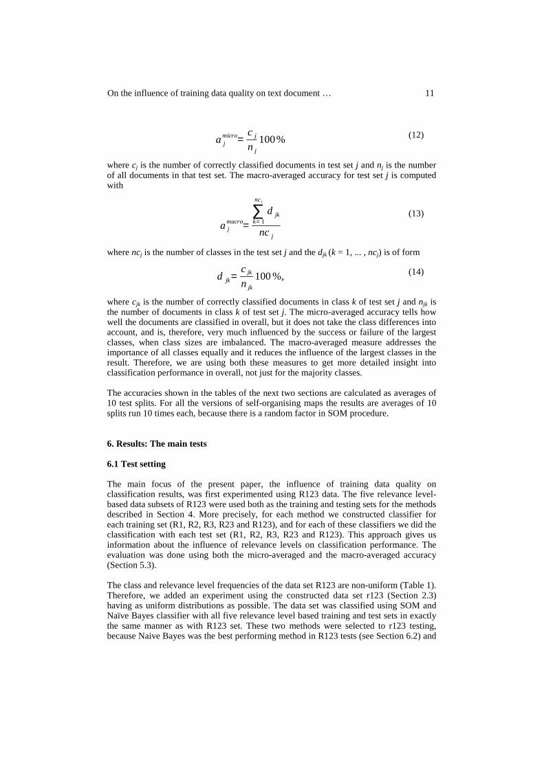
On the influence of training data quality on text document … 11

a jmicro=

c j

n j

100% (12)

where cj is the number of correctly classified documents in test set j and nj is the number of all documents in that test set. The macro-averaged accuracy for test set j is computed with

a jmacro=

∑k= 1

ncj

d jk

nc j

(13)

where ncj is the number of classes in the test set j and the djk (k = 1, ... , ncj) is of form

d jk=c jk

n jk

100%,

(14)

where cjk is the number of correctly classified documents in class k of test set j and njk is the number of documents in class k of test set j. The micro-averaged accuracy tells how well the documents are classified in overall, but it does not take the class differences into account, and is, therefore, very much influenced by the success or failure of the largest classes, when class sizes are imbalanced. The macro-averaged measure addresses the importance of all classes equally and it reduces the influence of the largest classes in the result. Therefore, we are using both these measures to get more detailed insight into classification performance in overall, not just for the majority classes. The accuracies shown in the tables of the next two sections are calculated as averages of 10 test splits. For all the versions of self-organising maps the results are averages of 10 splits run 10 times each, because there is a random factor in SOM procedure. 6. Results: The main tests 6.1 Test setting The main focus of the present paper, the influence of training data quality on classification results, was first experimented using R123 data. The five relevance level-based data subsets of R123 were used both as the training and testing sets for the methods described in Section 4. More precisely, for each method we constructed classifier for each training set (R1, R2, R3, R23 and R123), and for each of these classifiers we did the classification with each test set (R1, R2, R3, R23 and R123). This approach gives us information about the influence of relevance levels on classification performance. The evaluation was done using both the micro-averaged and the macro-averaged accuracy (Section 5.3). The class and relevance level frequencies of the data set R123 are non-uniform (Table 1). Therefore, we added an experiment using the constructed data set r123 (Section 2.3) having as uniform distributions as possible. The data set was classified using SOM and Naïve Bayes classifier with all five relevance level based training and test sets in exactly the same manner as with R123 set. These two methods were selected to r123 testing, because Naive Bayes was the best performing method in R123 tests (see Section 6.2) and

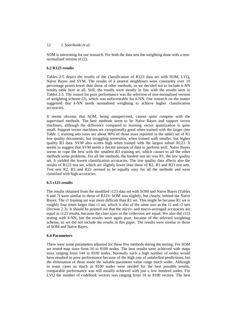
12 J. Saarikoski et al.

SOM is interesting for our research. For both the data sets the weighting done with a non-normalised version of (2). 6.2 R123 results Tables 2-5 depict the results of the classification of R123 data set with SOM, LVQ, Naive Bayes and SVM. The results of k nearest neighbours were constantly over 10 percentage points lower than those of other methods, so we decided not to include k-NN results table here at all. Still, the results were mostly in line with the results seen in Tables 2-5. The reason for poor performance was the selection of non-normalised version of weighting scheme (2), which was unfavourable for k-NN. Our research on the matter suggested that k-NN needs normalised weighting to achieve higher classification accuracies. It seems obvious that SOM, being unsupervised, cannot quite compete with the supervised methods. The best methods seem to be Naïve Bayes and support vector machines, although the difference compared to learning vector quantization is quite small. Support vector machines are exceptionally good when trained with the larger (see Table 1, training sets sizes are about 90% of those sizes reported in the table) set of R1 low quality documents, but struggling somewhat, when trained with smaller, but higher quality R3 data. SVM also scores high when trained with the largest subset R123. It seems to suggest that SVM needs a decent amount of data to perform well. Naïve Bayes seems to cope the best with the smallest R3 training set, which causes to all the other methods some problems. For all the methods, the hardest test set was R1, the low quality set. It yielded the lowest classification accuracies. The low quality data affects also the results of R123 test set, which are slightly lower than those of R2, R3 and R23 test sets. Test sets R2, R3 and R23 seemed to be equally easy for all the methods and were classified with high accuracies. 6.3 r123 results The results obtained from the modified r123 data set with SOM and Naive Bayes (Tables 6 and 7) were similar to those of R123: SOM was slightly, but clearly, behind the Naïve Bayes. The r1 training set was more difficult than R1 set. This might be because R1 set is roughly four times larger than r1 set, which is also of the same size as the r2 and r3 sets (Section 2.3). It should be pointed out that the micro- and macro-averaged accuracies are equal in r123 results, because the class sizes in the collection are equal. We also did r123 testing with k-NN, but the results were again poor, because of the selected weighting scheme, so we did not include the results in this paper. The results were similar to those of SOM and Naïve Bayes. 6.4 Parameters There were some parameters adjusted for these five methods during the testing. For SOM we tested map sizes from 16 to 8100 nodes. The best results were achieved with maps sizes ranging from 144 to 8100 nodes. Normally such a high number of nodes would have resulted in poor performance because of the high rate of unlabelled predictions, but the elimination of those made the suitable parameter value range much wider. Although in some cases as much as 8100 nodes were needed for the best possible results, comparable performance was still usually achieved with just a few hundred nodes. For LVQ the number of codebook vectors was ranging from 16 to 8100 vectors. The best

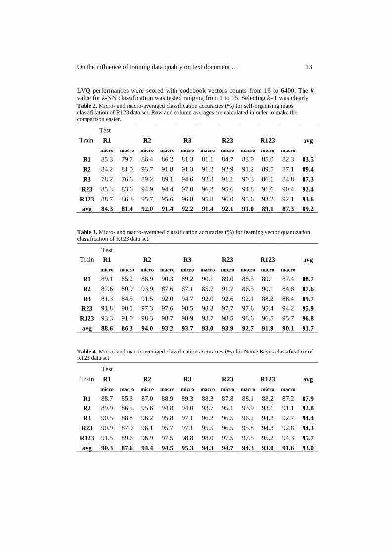
On the influence of training data quality on text document … 13

LVQ performances were scored with codebook vectors counts from 16 to 6400. The k value for k-NN classification was tested ranging from 1 to 15. Selecting k=1 was clearly Table 2. Micro- and macro-averaged classification accuracies (%) for self-organising maps classification of R123 data set. Row and column averages are calculated in order to make the comparison easier.

Test

Train R1 R2 R3 R23 R123 avg

micro macro micro macro micro macro micro macro micro macro

R1 85.3 79.7 86.4 86.2 81.3 81.1 84.7 83.0 85.0 82.3 83.5

R2 84.2 81.0 93.7 91.8 91.3 91.2 92.9 91.2 89.5 87.1 89.4

R3 78.2 76.6 89.2 89.1 94.6 92.8 91.1 90.3 86.1 84.8 87.3

R23 85.3 83.6 94.9 94.4 97.0 96.2 95.6 94.8 91.6 90.4 92.4

R123 88.7 86.3 95.7 95.6 96.8 95.8 96.0 95.6 93.2 92.1 93.6

avg 84.3 81.4 92.0 91.4 92.2 91.4 92.1 91.0 89.1 87.3 89.2 Table 3. Micro- and macro-averaged classification accuracies (%) for learning vector quantization classification of R123 data set.

Test

Train R1 R2 R3 R23 R123 avg

micro macro micro macro micro macro micro macro micro macro

R1 89.1 85.2 88.9 90.3 89.2 90.1 89.0 88.5 89.1 87.4 88.7

R2 87.6 80.9 93.9 87.6 87.1 85.7 91.7 86.5 90.1 84.8 87.6

R3 81.3 84.5 91.5 92.0 94.7 92.0 92.6 92.1 88.2 88.4 89.7

R23 91.8 90.1 97.3 97.6 98.5 98.3 97.7 97.6 95.4 94.2 95.9

R123 93.3 91.0 98.3 98.7 98.9 98.7 98.5 98.6 96.5 95.7 96.8

avg 88.6 86.3 94.0 93.2 93.7 93.0 93.9 92.7 91.9 90.1 91.7 Table 4. Micro- and macro-averaged classification accuracies (%) for Naïve Bayes classification of R123 data set.

Test

Train R1 R2 R3 R23 R123 avg

micro macro micro macro micro macro micro macro micro macro

R1 88.7 85.3 87.0 88.9 89.3 88.3 87.8 88.1 88.2 87.2 87.9

R2 89.9 86.5 95.6 94.8 94.0 93.7 95.1 93.9 93.1 91.1 92.8

R3 90.5 88.8 96.2 95.8 97.1 96.2 96.5 96.2 94.2 92.7 94.4

R23 90.9 87.9 96.1 95.7 97.1 95.5 96.5 95.8 94.3 92.8 94.3

R123 91.5 89.6 96.9 97.5 98.8 98.0 97.5 97.5 95.2 94.3 95.7

avg 90.3 87.6 94.4 94.5 95.3 94.3 94.7 94.3 93.0 91.6 93.0

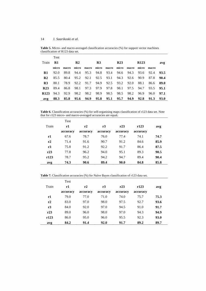
14 J. Saarikoski et al.

Table 5. Micro- and macro-averaged classification accuracies (%) for support vector machines classification of R123 data set.

Test

Train R1 R2 R3 R23 R123 avg

micro macro micro macro micro macro micro macro micro macro

R1 92.0 89.8 94.4 95.3 94.8 93.4 94.6 94.3 93.6 92.4 93.5

R2 85.5 80.4 95.2 92.1 92.5 93.1 94.3 92.6 90.9 87.8 90.4

R3 80.1 78.9 92.2 91.7 94.9 92.5 93.2 92.0 88.1 86.6 89.0

R23 89.4 86.8 98.1 97.3 97.9 97.8 98.1 97.5 94.7 93.5 95.1

R123 94.3 92.9 98.2 98.2 98.9 98.5 98.5 98.2 96.9 96.0 97.1

avg 88.3 85.8 95.6 94.9 95.8 95.1 95.7 94.9 92.8 91.3 93.0

Table 6. Classification accuracies (%) for self-organising maps classification of r123 data set. Note that for r123 micro- and macro-averaged accuracies are equal.

Test

Train r1 r2 r3 r23 r123 avg accuracy accuracy accuracy accuracy accuracy

r1 67.6 78.7 76.0 77.4 74.1 74.7

r2 71.4 91.6 90.7 91.2 84.6 85.9

r3 75.8 91.2 92.2 91.7 86.4 87.5

r23 77.8 96.2 94.0 95.1 89.3 90.5

r123 78.7 95.2 94.2 94.7 89.4 90.4

avg 74.3 90.6 89.4 90.0 84.8 85.8

Table 7. Classification accuracies (%) for Naïve Bayes classification of r123 data set.

Test

Train r1 r2 r3 r23 r123 avg accuracy accuracy accuracy accuracy accuracy

r1 79.0 77.0 71.0 74.0 75.7 75.3

r2 83.0 97.0 98.0 97.5 92.7 93.6

r3 84.0 92.0 97.0 94.5 91.0 91.7

r23 89.0 96.0 98.0 97.0 94.3 94.9

r123 86.0 95.0 96.0 95.5 92.3 93.0

avg 84.2 91.4 92.0 91.7 89.2 89.7

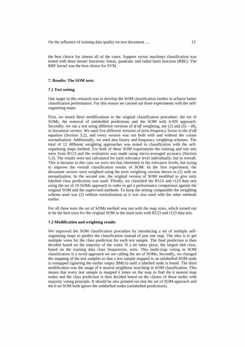
On the influence of training data quality on text document … 15

the best choice for almost all of the cases. Support vector machines classification was tested with three kernel functions: linear, quadratic and radial basis function (RBF). The RBF kernel was the best choice for SVM. 7. Results: The SOM tests 7.1 Test setting One target in this research was to develop the SOM classification further to achieve better classification performance. For this reason we carried out three experiments with the self-organising maps. First, we tested three modifications to the original classification procedure: the set of SOMs, the removal of unlabelled predictions and the SOM with k-NN approach. Secondly, we ran a test using different versions of tf·idf weighting, see (2) and (5) – (8), in document vectors. We used five different versions of term frequency factor in the tf·idf equation (Section 3.2), and every version was run both with and without the cosine normalisation. Additionally, we used also binary and frequency weighting schemes. The total of 12 different weighting approaches was tested in classification with the self-organising maps method. For both of these SOM experiments the training and test sets were from R123 and the evaluation was made using micro-averaged accuracy (Section 5.3). The results were not calculated for each relevance level individually, but in overall. This is because in this case we were not that interested in the relevance levels, but trying to improve the overall classification results of SOM. In the first experiment, the document vectors were weighted using the term weighting version shown in (2) with no normalisation. In the second one, the original version of SOM modified to give only labelled class predictions was used. Thirdly, we classified the R123 and r123 data sets using the set of 10 SOMs approach in order to get a performance comparison against the original SOM and the supervised methods. To keep the setting comparable the weighting scheme used was (2) without normalisation as it was also used with the other methods earlier. For all these tests the set of SOMs method was run with the map sizes, which turned out to be the best sizes for the original SOM in the main tests with R123 and r123 data sets. 7.2 Modification and weighting results We improved the SOM classification procedure by introducing a set of multiple self-organising maps to predict the classification instead of just one map. The idea is to get multiple votes for the class prediction for each test sample. The final prediction is then decided based on the majority of the votes. If a tie takes place, the largest tied class, based on the training data class frequencies, wins. This multi-map voting in SOM classification is a novel approach we are calling the set of SOMs. Secondly, we changed the mapping of the test samples so that a test sample mapped to an unlabelled SOM node is remapped (ignoring the earlier empty BMUs) until a labelled node is found. The third modification was the usage of k nearest neighbour searching in SOM classification. This means that every test sample is mapped k times on the map to find the k nearest map nodes and the class prediction is then decided based on the classes of those nodes with majority voting principle. It should be also pointed out that the set of SOM approach and the k-nn SOM both ignore the unlabelled nodes (unlabelled predictions).

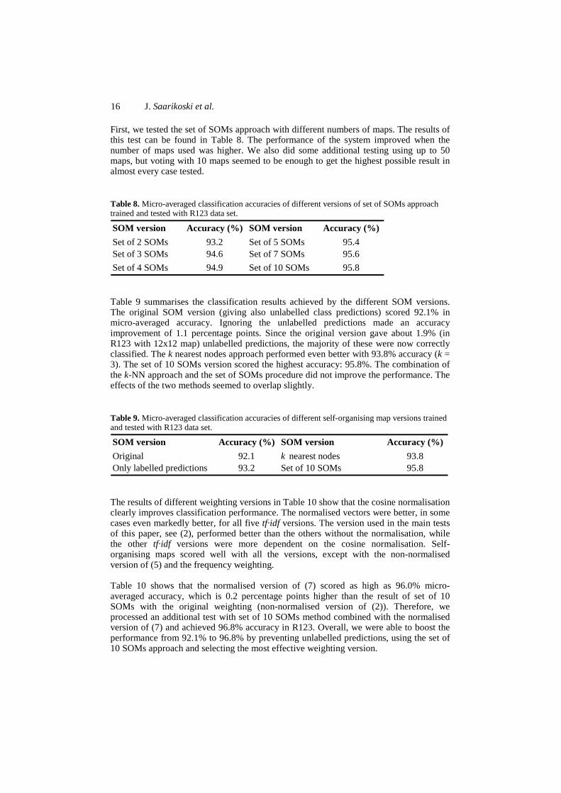
16 J. Saarikoski et al.

First, we tested the set of SOMs approach with different numbers of maps. The results of this test can be found in Table 8. The performance of the system improved when the number of maps used was higher. We also did some additional testing using up to 50 maps, but voting with 10 maps seemed to be enough to get the highest possible result in almost every case tested. Table 8. Micro-averaged classification accuracies of different versions of set of SOMs approach trained and tested with R123 data set.

SOM version Accuracy (%) SOM version Accuracy (%)

Set of 2 SOMs 93.2 Set of 5 SOMs 95.4Set of 3 SOMs 94.6 Set of 7 SOMs 95.6

Set of 4 SOMs 94.9 Set of 10 SOMs 95.8 Table 9 summarises the classification results achieved by the different SOM versions. The original SOM version (giving also unlabelled class predictions) scored 92.1% in micro-averaged accuracy. Ignoring the unlabelled predictions made an accuracy improvement of 1.1 percentage points. Since the original version gave about 1.9% (in R123 with 12x12 map) unlabelled predictions, the majority of these were now correctly classified. The k nearest nodes approach performed even better with 93.8% accuracy (k = 3). The set of 10 SOMs version scored the highest accuracy: 95.8%. The combination of the k-NN approach and the set of SOMs procedure did not improve the performance. The effects of the two methods seemed to overlap slightly. Table 9. Micro-averaged classification accuracies of different self-organising map versions trained and tested with R123 data set.

SOM version Accuracy (%) SOM version Accuracy (%)

Original 92.1 k nearest nodes 93.8Only labelled predictions 93.2 Set of 10 SOMs 95.8 The results of different weighting versions in Table 10 show that the cosine normalisation clearly improves classification performance. The normalised vectors were better, in some cases even markedly better, for all five tf·idf versions. The version used in the main tests of this paper, see (2), performed better than the others without the normalisation, while the other tf·idf versions were more dependent on the cosine normalisation. Self-organising maps scored well with all the versions, except with the non-normalised version of (5) and the frequency weighting. Table 10 shows that the normalised version of (7) scored as high as 96.0% micro-averaged accuracy, which is 0.2 percentage points higher than the result of set of 10 SOMs with the original weighting (non-normalised version of (2)). Therefore, we processed an additional test with set of 10 SOMs method combined with the normalised version of (7) and achieved 96.8% accuracy in R123. Overall, we were able to boost the performance from 92.1% to 96.8% by preventing unlabelled predictions, using the set of 10 SOMs approach and selecting the most effective weighting version.

On the influence of training data quality on text document … 17

Table 10. Micro-averaged accuracies of self-organising maps classification of R123 data set using different weighting versions. The weighting versions are presented in equations (2) and (5) - (8). For example, eq2 means the version specified in (2) and cn refers to cosine normalisation.

Weighting version Accuracy (%) Weighting version Accuracy (%)

eq2 94.1 eq7 93.4eq2 + cn 94.3 eq7 + cn 96.0

eq5 81.2 eq8 93.9

eq5 + cn 94.3 eq8 + cn 95.5eq6 93.4 binary 89.4eq6 + cn 95.9 frequency 69.6 7.3 R123 and r123 results We classified the R123 and r123 data sets using the set of 10 SOMs to get comparison against the original SOM and supervised methods used in the main tests. The results in Tables 11 and 12 show mostly the same overall patterns found in the main tests with the other methods. When compared to the results of the original SOM (Tables 2 and 6), it is clear that the set of 10 SOMs is performing better. Comparison with the supervised methods suggests that the set of 10 SOMs is comparable against Naive Bayes and SVM and even slightly better than LVQ. Table 11. Micro- and macro-averaged classification accuracies (%) for the set of 10 SOMs classification of R123 data set.

Test

Train R1 R2 R3 R23 R123 avg

micro macro micro macro micro macro micro macro micro macro

R1 88.8 85.6 91.2 91.2 88.3 87.1 90.3 88.4 89.7 87.4 88.8

R2 87.3 83.7 95.8 94.2 93.7 93.9 95.1 93.9 92.1 89.6 91.9

R3 83.5 81.3 92.7 92.4 95.5 93.8 93.7 92.8 89.7 88.1 90.4

R23 88.7 87.0 97.6 97.1 97.8 97.4 97.6 97.0 94.2 93.0 94.7

R123 93.0 91.3 97.6 97.6 97.7 97.1 97.6 97.3 95.8 94.8 96.0

avg 88.3 85.8 95.0 94.5 94.6 93.9 94.9 93.9 92.3 90.6 92.4

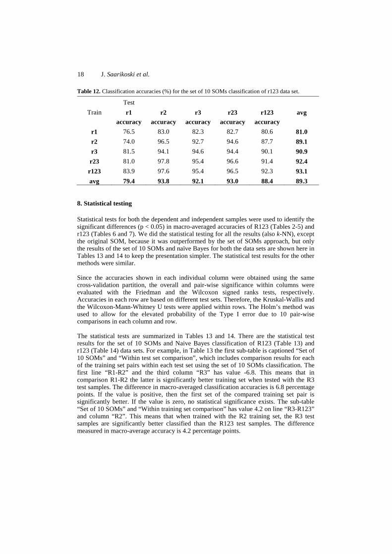
18 J. Saarikoski et al.

Table 12. Classification accuracies (%) for the set of 10 SOMs classification of r123 data set.

Test

Train r1 r2 r3 r23 r123 avg accuracy accuracy accuracy accuracy accuracy

r1 76.5 83.0 82.3 82.7 80.6 81.0

r2 74.0 96.5 92.7 94.6 87.7 89.1

r3 81.5 94.1 94.6 94.4 90.1 90.9

r23 81.0 97.8 95.4 96.6 91.4 92.4

r123 83.9 97.6 95.4 96.5 92.3 93.1

avg 79.4 93.8 92.1 93.0 88.4 89.3 8. Statistical testing Statistical tests for both the dependent and independent samples were used to identify the significant differences (p < 0.05) in macro-averaged accuracies of R123 (Tables 2-5) and r123 (Tables 6 and 7). We did the statistical testing for all the results (also k-NN), except the original SOM, because it was outperformed by the set of SOMs approach, but only the results of the set of 10 SOMs and naïve Bayes for both the data sets are shown here in Tables 13 and 14 to keep the presentation simpler. The statistical test results for the other methods were similar. Since the accuracies shown in each individual column were obtained using the same cross-validation partition, the overall and pair-wise significance within columns were evaluated with the Friedman and the Wilcoxon signed ranks tests, respectively. Accuracies in each row are based on different test sets. Therefore, the Kruskal-Wallis and the Wilcoxon-Mann-Whitney U tests were applied within rows. The Holm’s method was used to allow for the elevated probability of the Type I error due to 10 pair-wise comparisons in each column and row. The statistical tests are summarized in Tables 13 and 14. There are the statistical test results for the set of 10 SOMs and Naive Bayes classification of R123 (Table 13) and r123 (Table 14) data sets. For example, in Table 13 the first sub-table is captioned “Set of 10 SOMs” and “Within test set comparison”, which includes comparison results for each of the training set pairs within each test set using the set of 10 SOMs classification. The first line “R1-R2” and the third column “R3” has value -6.8. This means that in comparison R1-R2 the latter is significantly better training set when tested with the R3 test samples. The difference in macro-averaged classification accuracies is 6.8 percentage points. If the value is positive, then the first set of the compared training set pair is significantly better. If the value is zero, no statistical significance exists. The sub-table “Set of 10 SOMs” and “Within training set comparison” has value 4.2 on line “R3-R123” and column “R2”. This means that when trained with the R2 training set, the R3 test samples are significantly better classified than the R123 test samples. The difference measured in macro-average accuracy is 4.2 percentage points.

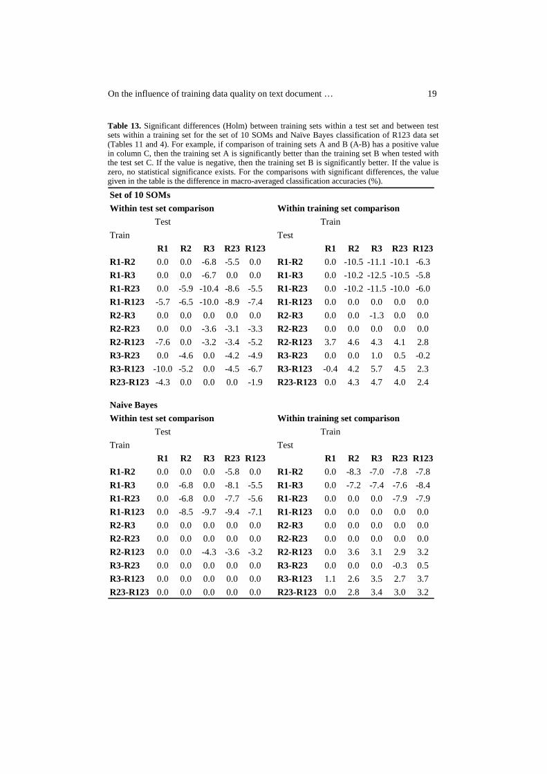
On the influence of training data quality on text document … 19

Table 13. Significant differences (Holm) between training sets within a test set and between test sets within a training set for the set of 10 SOMs and Naïve Bayes classification of R123 data set (Tables 11 and 4). For example, if comparison of training sets A and B (A-B) has a positive value in column C, then the training set A is significantly better than the training set B when tested with the test set C. If the value is negative, then the training set B is significantly better. If the value is zero, no statistical significance exists. For the comparisons with significant differences, the value given in the table is the difference in macro-averaged classification accuracies (%).

Set of 10 SOMs

Within test set comparison Within training set comparison

Test Train

Train Test

R1 R2 R3 R23 R123 R1 R2 R3 R23 R123

R1-R2 0.0 0.0 -6.8 -5.5 0.0 R1-R2 0.0 -10.5 -11.1 -10.1 -6.3

R1-R3 0.0 0.0 -6.7 0.0 0.0 R1-R3 0.0 -10.2 -12.5 -10.5 -5.8

R1-R23 0.0 -5.9 -10.4 -8.6 -5.5 R1-R23 0.0 -10.2 -11.5 -10.0 -6.0

R1-R123 -5.7 -6.5 -10.0 -8.9 -7.4 R1-R123 0.0 0.0 0.0 0.0 0.0

R2-R3 0.0 0.0 0.0 0.0 0.0 R2-R3 0.0 0.0 -1.3 0.0 0.0

R2-R23 0.0 0.0 -3.6 -3.1 -3.3 R2-R23 0.0 0.0 0.0 0.0 0.0

R2-R123 -7.6 0.0 -3.2 -3.4 -5.2 R2-R123 3.7 4.6 4.3 4.1 2.8

R3-R23 0.0 -4.6 0.0 -4.2 -4.9 R3-R23 0.0 0.0 1.0 0.5 -0.2

R3-R123 -10.0 -5.2 0.0 -4.5 -6.7 R3-R123 -0.4 4.2 5.7 4.5 2.3

R23-R123 -4.3 0.0 0.0 0.0 -1.9 R23-R123 0.0 4.3 4.7 4.0 2.4

Naive Bayes

Within test set comparison Within training set comparison

Test Train

Train Test

R1 R2 R3 R23 R123 R1 R2 R3 R23 R123

R1-R2 0.0 0.0 0.0 -5.8 0.0 R1-R2 0.0 -8.3 -7.0 -7.8 -7.8

R1-R3 0.0 -6.8 0.0 -8.1 -5.5 R1-R3 0.0 -7.2 -7.4 -7.6 -8.4

R1-R23 0.0 -6.8 0.0 -7.7 -5.6 R1-R23 0.0 0.0 0.0 -7.9 -7.9

R1-R123 0.0 -8.5 -9.7 -9.4 -7.1 R1-R123 0.0 0.0 0.0 0.0 0.0

R2-R3 0.0 0.0 0.0 0.0 0.0 R2-R3 0.0 0.0 0.0 0.0 0.0

R2-R23 0.0 0.0 0.0 0.0 0.0 R2-R23 0.0 0.0 0.0 0.0 0.0

R2-R123 0.0 0.0 -4.3 -3.6 -3.2 R2-R123 0.0 3.6 3.1 2.9 3.2

R3-R23 0.0 0.0 0.0 0.0 0.0 R3-R23 0.0 0.0 0.0 -0.3 0.5

R3-R123 0.0 0.0 0.0 0.0 0.0 R3-R123 1.1 2.6 3.5 2.7 3.7

R23-R123 0.0 0.0 0.0 0.0 0.0 R23-R123 0.0 2.8 3.4 3.0 3.2

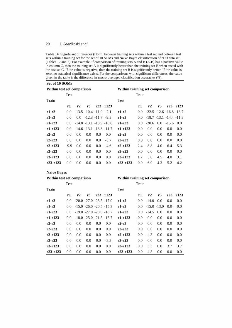
20 J. Saarikoski et al.

Table 14. Significant differences (Holm) between training sets within a test set and between test sets within a training set for the set of 10 SOMs and Naïve Bayes classification of r123 data set (Tables 12 and 7). For example, if comparison of training sets A and B (A-B) has a positive value in column C, then the training set A is significantly better than the training set B when tested with the test set C. If the value is negative, then the training set B is significantly better. If the value is zero, no statistical significance exists. For the comparisons with significant differences, the value given in the table is the difference in macro-averaged classification accuracies (%).

Set of 10 SOMs

Within test set comparison Within training set comparison

Test Train

Train Test

r1 r2 r3 r23 r123 r1 r2 r3 r23 r123

r1-r2 0.0 -13.5 -10.4 -11.9 -7.1 r1-r2 0.0 -22.5 -12.6 -16.8 -13.7

r1-r3 0.0 0.0 -12.3 -11.7 -9.5 r1-r3 0.0 -18.7 -13.1 -14.4 -11.5

r1-r23 0.0 -14.8 -13.1 -13.9 -10.8 r1-r23 0.0 -20.6 0.0 -15.6 0.0

r1-r123 0.0 -14.6 -13.1 -13.8 -11.7 r1-r123 0.0 0.0 0.0 0.0 0.0

r2-r3 0.0 0.0 0.0 0.0 0.0 r2-r3 0.0 0.0 0.0 0.0 0.0

r2-r23 0.0 0.0 0.0 0.0 -3.7 r2-r23 0.0 0.0 0.0 0.0 0.0

r2-r123 -9.9 0.0 0.0 0.0 -4.6 r2-r123 2.4 8.8 4.0 6.4 5.3

r3-r23 0.0 0.0 0.0 0.0 0.0 r3-r23 0.0 0.0 0.0 0.0 0.0

r3-r123 0.0 0.0 0.0 0.0 0.0 r3-r123 1.7 5.0 4.5 4.0 3.1

r23-r123 0.0 0.0 0.0 0.0 0.0 r23-r123 0.0 6.9 4.3 5.2 4.2

Naive Bayes

Within test set comparison Within training set comparison

Test Train

Train Test

r1 r2 r3 r23 r123 r1 r2 r3 r23 r123

r1-r2 0.0 -20.0 -27.0 -23.5 -17.0 r1-r2 0.0 -14.0 0.0 0.0 0.0

r1-r3 0.0 -15.0 -26.0 -20.5 -15.3 r1-r3 0.0 -15.0 -13.0 0.0 0.0

r1-r23 0.0 -19.0 -27.0 -23.0 -18.7 r1-r23 0.0 -14.5 0.0 0.0 0.0

r1-r123 0.0 -18.0 -25.0 -21.5 -16.7 r1-r123 0.0 0.0 0.0 0.0 0.0

r2-r3 0.0 0.0 0.0 0.0 0.0 r2-r3 0.0 0.0 0.0 0.0 0.0

r2-r23 0.0 0.0 0.0 0.0 0.0 r2-r23 0.0 0.0 0.0 0.0 0.0

r2-r123 0.0 0.0 0.0 0.0 0.0 r2-r123 0.0 4.3 0.0 0.0 0.0

r3-r23 0.0 0.0 0.0 0.0 -3.3 r3-r23 0.0 0.0 0.0 0.0 0.0

r3-r123 0.0 0.0 0.0 0.0 0.0 r3-r123 0.0 5.3 6.0 3.7 3.7

r23-r123 0.0 0.0 0.0 0.0 0.0 r23-r123 0.0 4.8 0.0 0.0 0.0

On the influence of training data quality on text document … 21

9. Discussion and conclusions The main focus of this paper was the influence of training data quality on machine learning classification. The relevance level and the quality of the document data are related. The R1 documents had on average 8.4% of active words in their document vectors (words with non-zero weights), while R3 documents had 12.6%. The r1 and r3 documents had 11.5% and 14.1% active words, respectively. This gives an idea of how much more topical information, quality, there is in the highly relevant documents and also explains why classifiers trained with them perform better.

The results revealed that the best classifier performance was achieved using all three relevance levels (R123 / r123) in training set. Still, using the highest two levels (R23 / r23) gave almost equal results with fewer training samples. The use of only the highest relevance level (R3 / r3) documents was not enough to achieve the best results, especially when the number of samples of that type was small compared to the number of lower quality samples available, which is the case in R123 set. For example, starting from R3 training set, the performance was improved both after adding R2 samples and still when adding R1 training samples to the training set. This was the case even if we measured the classification accuracy of R2 and R3 test samples. With r123 data set there was no improvement in r2 and r3 test set results, if r1 was added to r23 training set, presumably because r1, r2 and r3 were of the equal size. It seems to be that the training data size matters as well as the quality. To conclude, the training data should be large enough and of high quality (relevance levels 2 and 3, fairly to highly relevant documents), and low quality data (level 1, marginally relevant) should be added to the training set only if there is very much of it compared to the amount of higher quality data and, of course, if the processing time is not an issue. The higher quality data seems to be the key, but only if there is enough of it. Usually highly relevant data (relevance level 3) is not available in large numbers, so it could be wise to train a classifier with all but the marginally relevant (relevance level 1), if there is enough of higher quality training data (relevance levels 2 and 3). Especially when aiming to classify the highly relevant test samples effectively, the marginally relevant training samples could be ignored. Our findings in Tables 2-7, 11 and 12 also indicate that marginal documents (relevance level 1) are misclassified clearly more often than level 2-3 documents unless training is by marginal documents alone. While misclassifications cannot be avoided, it is encouraging to know that better documents tend to be better classified. The results of the statistical tests support our findings. The within test set comparison revealed that R123 training set was in most cases significantly better than R1 and R2. However, compared to the R3 training it was better only in SOM tests excluding the R3 test set. When comparing to the R23 training, there were even less significant differences: only with SOM and testing with R1 and R123. Thus, the R23 training or even the R3 only, seems to be enough, if the aim is to classify the highly relevant documents effectively. When the number of documents was the same in all the relevance levels, the r123 training significantly outperformed the r1 training in all other cases than the r1 test set. When compared to r2 training, r123 was significantly better only in SOM tests when test set included r1 samples. In comparison with r3 and r23 training sets no significant differences were found at all. It seems that when marginal documents are available in high numbers, it is advisable to use all the three relevance levels in training. If not, then two highest levels, or even the highest level only, might be enough. The tests concerning

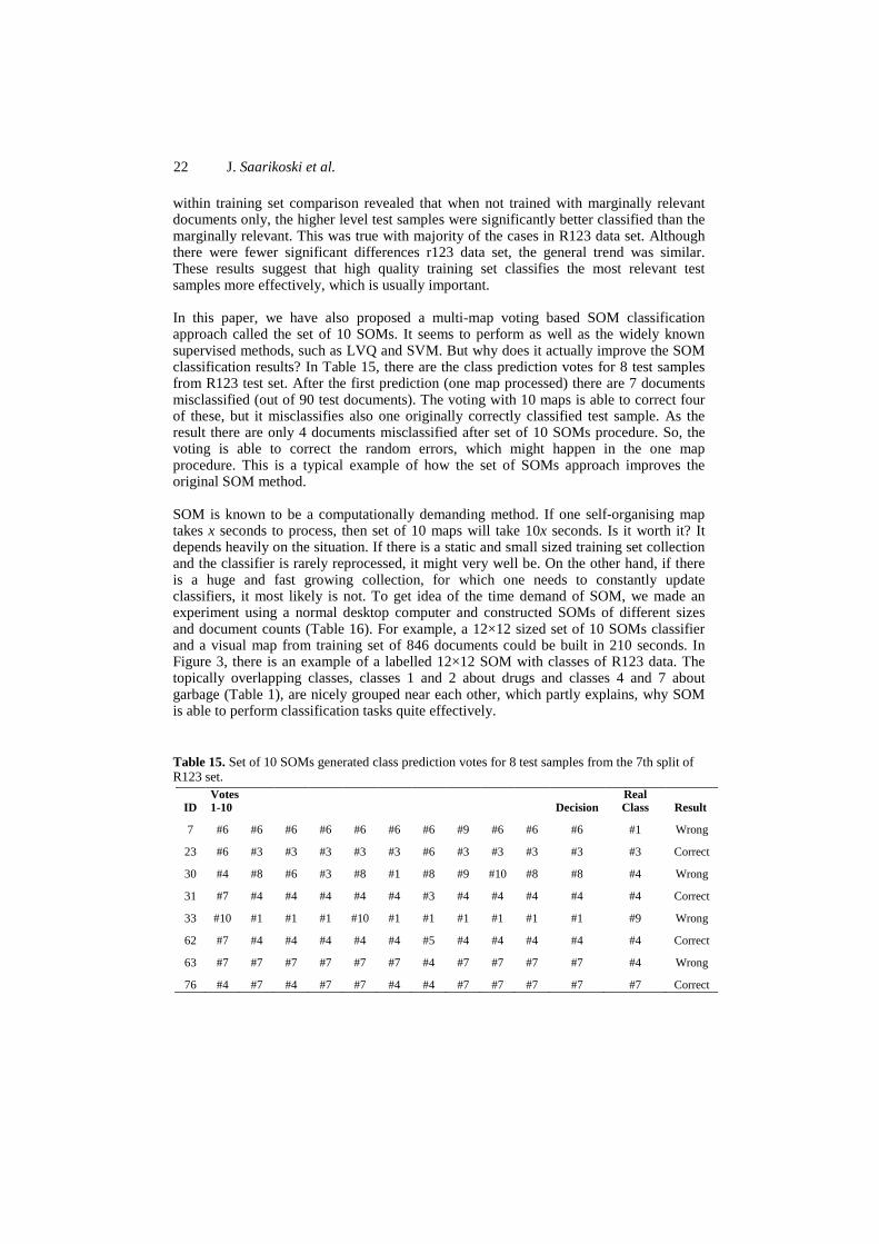
22 J. Saarikoski et al.

within training set comparison revealed that when not trained with marginally relevant documents only, the higher level test samples were significantly better classified than the marginally relevant. This was true with majority of the cases in R123 data set. Although there were fewer significant differences r123 data set, the general trend was similar. These results suggest that high quality training set classifies the most relevant test samples more effectively, which is usually important. In this paper, we have also proposed a multi-map voting based SOM classification approach called the set of 10 SOMs. It seems to perform as well as the widely known supervised methods, such as LVQ and SVM. But why does it actually improve the SOM classification results? In Table 15, there are the class prediction votes for 8 test samples from R123 test set. After the first prediction (one map processed) there are 7 documents misclassified (out of 90 test documents). The voting with 10 maps is able to correct four of these, but it misclassifies also one originally correctly classified test sample. As the result there are only 4 documents misclassified after set of 10 SOMs procedure. So, the voting is able to correct the random errors, which might happen in the one map procedure. This is a typical example of how the set of SOMs approach improves the original SOM method. SOM is known to be a computationally demanding method. If one self-organising map takes x seconds to process, then set of 10 maps will take 10x seconds. Is it worth it? It depends heavily on the situation. If there is a static and small sized training set collection and the classifier is rarely reprocessed, it might very well be. On the other hand, if there is a huge and fast growing collection, for which one needs to constantly update classifiers, it most likely is not. To get idea of the time demand of SOM, we made an experiment using a normal desktop computer and constructed SOMs of different sizes and document counts (Table 16). For example, a 12×12 sized set of 10 SOMs classifier and a visual map from training set of 846 documents could be built in 210 seconds. In Figure 3, there is an example of a labelled 12×12 SOM with classes of R123 data. The topically overlapping classes, classes 1 and 2 about drugs and classes 4 and 7 about garbage (Table 1), are nicely grouped near each other, which partly explains, why SOM is able to perform classification tasks quite effectively. Table 15. Set of 10 SOMs generated class prediction votes for 8 test samples from the 7th split of R123 set.

ID

Votes 1-10 Decision

Real Class Result

7 #6 #6 #6 #6 #6 #6 #6 #9 #6 #6 #6 #1 Wrong

23 #6 #3 #3 #3 #3 #3 #6 #3 #3 #3 #3 #3 Correct

30 #4 #8 #6 #3 #8 #1 #8 #9 #10 #8 #8 #4 Wrong

31 #7 #4 #4 #4 #4 #4 #3 #4 #4 #4 #4 #4 Correct

33 #10 #1 #1 #1 #10 #1 #1 #1 #1 #1 #1 #9 Wrong

62 #7 #4 #4 #4 #4 #4 #5 #4 #4 #4 #4 #4 Correct

63 #7 #7 #7 #7 #7 #7 #4 #7 #7 #7 #7 #4 Wrong

76 #4 #7 #4 #7 #7 #4 #4 #7 #7 #7 #7 #7 Correct

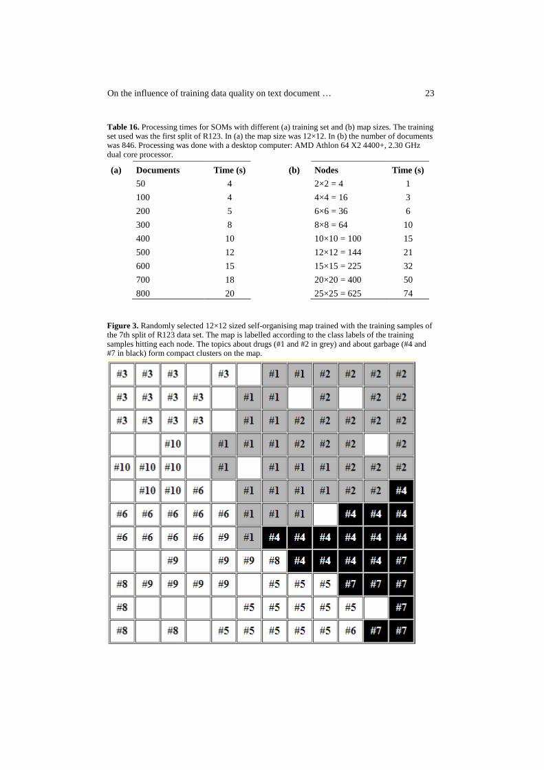
On the influence of training data quality on text document … 23

Table 16. Processing times for SOMs with different (a) training set and (b) map sizes. The training set used was the first split of R123. In (a) the map size was 12×12. In (b) the number of documents was 846. Processing was done with a desktop computer: AMD Athlon 64 X2 4400+, 2.30 GHz dual core processor.

(a) Documents Time (s) (b) Nodes Time (s)

50 4 2×2 = 4 1

100 4 4×4 = 16 3

200 5 6×6 = 36 6

300 8 8×8 = 64 10

400 10 10×10 = 100 15

500 12 12×12 = 144 21

600 15 15×15 = 225 32

700 18 20×20 = 400 50

800 20 25×25 = 625 74 Figure 3. Randomly selected 12×12 sized self-organising map trained with the training samples of the 7th split of R123 data set. The map is labelled according to the class labels of the training samples hitting each node. The topics about drugs (#1 and #2 in grey) and about garbage (#4 and #7 in black) form compact clusters on the map.

24 J. Saarikoski et al.

In the future, we are going to study much larger collections to learn more about the effects of training set size and quality on the classification performance. Also, it would be interesting to study the possibility to develop a classifier capable of predicting both the class and the relevance level of the document. The set of SOMs classification could be also developed further by using different maps instead of just multiple copies of one type of map. Acknowledgements Jyri Saarikoski was supported by Tampere Doctoral Programme in Information Science and Engineering (TISE), Alfred Kordelin Trust Fund, The Finnish Cultural Foundation, Oskar Öflund Foundation and the City of Tampere Science Fund. Supercomputer resources of the Finnish IT Center for Science (CSC) were used in the processing of the data. The SNOWBALL stemmer was by Martin Porter.

On the influence of training data quality on text document … 25

References Ai-Xiang, S. (2010), “Improved SOM Algorithm-HDSOM applied in text clustering”, in Proceedings of the International Conference on Multimedia Information Networking and Security (MINES) 2010, IEEE, pp. 306-309.

Asy'arie, A.D. and Pribadi, A.W. (2009), “Automatic news articles classification in Indonesian language by using Naive Bayes classifier method” in Proceedings of the 11th International Conference on Information Integration and Web-based Applications & Services (iiWAS) 2009, ACM, New York, USA, pp. 658-662.

Beckel, C., Sadamori, L. and Santini, S. (2012), “Towards automatic classification of private households using electricity consumption data”, in Proceedings of the ACM Workshop on Embedded Sensing Systems for Energy-Efficiency in Buildings (BuildSys) 2012, ACM, New York, USA, pp. 169-176.

Borlund, P. (2003), “The concept of relevance in IR”, Journal of the American Society for Information Science and Technology, Vol. 54 No. 10, pp. 913-925.

Cheng, W., Dembczynski, K. and Hüllermeier, E. (2010), “Graded multilabel classification: the ordinal case”, in Proceedings of the 27th International Conference on Machine Learning (ICML) 2010, Omnipress, pp. 223-230.

Cho, S. and Won, H. (2003), “Machine learning in DNA microarray analysis for cancer classification”, in Proceedings of the First Asia-Pacific Bioinformatics Conference (APBC) 2003, Volume 19, Australian Computer Society Inc, Darlinghurst, Australia pp. 189-198.

Christianini, N. and Shawe-Taylor, J. (2000), An Introduction to Support Vector Machines and Other Kernel-Based Learning methods, Cambridge University Press, Cambridge, UK.

Chumwatana, T., Wong, K. and Xie, H. (2010), “A SOM-based document clustering using frequent max substring for non-segmented texts”, Journal of Intelligent Learning Systems & Applications, Vol. 2 No. 3, pp. 117-125.

Cosijn, E. and Ingwersen, P. (2000), “Dimensions of relevance”, Information Processing and Management, Vol. 36 No. 4, pp. 533-550.

Duda, R.O., Hart, P.E. and Stork, D.G. (2001), Pattern Classification, second edition, John Wiley & Sons, New York, USA.

Fernandez, J., Mones, R., Diaz, I., Ranilla, J. and Combarro, E.F. (2004), “Experiments with self organizing maps in CLEF 2003”, Comparative Evaluation of Multilingual Information Access Systems, Lecture Notes in Computer Science, Vol. 3237, pp. 358-366.

Furletti, B., Gabrielli, L., Renso, C. and Rinzivillo, S. (2012), “Identifying Users Profiles From Mobile Calls Habits”, in Proceedings of the ACM SIGKDD International Workshop on Urban Computing (UrbComp) 2012, ACM, New York, USA, pp. 17-24.

Guyon, I. and Elisseef, A. (2003), “An introduction to variable and feature selection”, The Journal of Machine Learning Research, Vol. 3 No. 3/1/2003, pp. 1157-1182.

26 J. Saarikoski et al.

Hagenbuchner, M. and Tsoi, A.C. (2005), “A supervised training algorithm for self-organizing maps for structures”, Pattern Recognition Letters, Vol. 26 No. 12, pp. 1874-1884.

Hjørland, B. (2010), “The foundation for the concept of relevance”, Journal of the American Society for Information Science and Technology, Vol. 61 No. 2, pp. 217-237.

Hsu, C. and Lin, C. (2002), “A comparison of methods for multiclass support vectors machines”, IEEE Transactions of Neural Networks, Vol. 13 No. 2, pp. 415-425.

Hsu, C., Chang, C. and Lin, C. (2010), “A practical guide to support vector classification”, Technical report, available at: http://www.csie.ntu.edu.tw/~cjlin/papers/guide/guide.pdf (accessed 3rd April 2013).

Joutsijoki, H. and Juhola, M. (2011a), “Kernel selection in multi-class support vector machines and its consequence to the number of ties in majority voting method”, in Artificial Intelligence Review. DOI: 10.1007/s10462-011-9281-3

Joutsijoki, H. and Juhola, M. (2011b), “Comparing the one-vs-one and one-vs-all methods in benthic macroinvertebrate image classification”, in Proceedings of the 7th International Conference on Machine Learning and Data Mining in pattern recognition (MLDM) 2011, pp. 399–413.

Järvelin, K. and Kekäläinen J. (2002), “Cumulated gain-based evaluation of IR tecniques”, ACM Transactions on Information Systems, Vol. 20 No. 4, pp. 422-446.

Kekäläinen, J. (2005), “Binary and graded relevance in IR evaluations - comparison of the effects on ranking of IR systems”, Information Processing and Management: an International Journal, Vol. 31 No. 5, pp. 1019-1033.

Kohonen, T. (1986), Learning Vector Quantization for Pattern Recognition, Helsinki University of Technology, Espoo, Finland.

Kohonen, T. (2001), Self-Organizing Maps, Springer, Berlin, Germany.

Kohonen, T., Hynninen, J., Kangas, J. and Laaksonen, J. (1996a), “SOM_PAK: the self-organizing map program package”, Technical Report A31, Helsinki University of Technology, Laboratory of Computer and Information Science, Espoo, Finland, available at: http://www.cis.hut.fi/research/papers/som_tr96.ps.Z (accessed 3rd April 2013).

Kohonen, T., Hynninen, J., Kangas, J., Laaksonen, J. and Torkkola, K. (1996b), “LVQ_PAK: the learning vector quantization program package”, Technical Report A30, Helsinki University of Technology, Laboratory of Computer and Information Science, Espoo, Finland, available at: http://www.cis.hut.fi/research/papers/lvq_tr96.ps.Z (accessed 3rd April 2013).

Korenius, T., Laurikkala, J., Juhola, M. and Järvelin, K. (2006), “Hierarchical clustering of a Finnish newspaper article collection with graded relevance assessments”, Information Retrieval, Vol. 9 No. 1, pp. 33-53.

On the influence of training data quality on text document … 27

Lagus, K. (2000), “Text mining with the WEBSOM”, Academic Dissertation, Helsinki University of Technology, Finland.

Lagus, K. (2002), “Text retrieval using self-organized document maps”, Neural Processing Letters, Vol. 15 No. 1, pp. 21-29.

Li, Y. and Bontcheva, K. (2008), “Adapting support vector machines for F-term-based classification of patents”, ACM Transactions on Asian Language Information Processing, Vol. 7 No. 2, Article 7.

Mitchell, T.M. (1997), Machine Learning, McGraw-Hill, USA.

Naoum, R.S. and Al-Sultani, Z.N. (2012), “Learning vector quantization (LVQ) and k-nearest neighbor for intrusion classification”, World of Computer Science and Information Technology Journal, Vol. 2 No. 3, pp. 105-109.

Papoulis, A. (1987), Probability, Random Variables, and Stochastic Processes, McGraw-Hill, Auckland, New Zealand.

Patra, J.C., Abraham, J., Meher, P.K. and Chakraborty, G. (2010), “An improved SOM-based visualization technique for DNA microarray data analysis”, in Proceedings of the International Joint Conference on Neural Networks (IJCNN) 2010, IEEE, pp. 1-7.

Plonski, P. and Zaremba, K. (2012), “Self-organising maps for classification with Metropolis-Hastings algorithm for supervision”, in Proceedings of the 19th International Conference on Neural Information Processing (ICONIP) 2012, Volume Part III, Springer-Verlag Berlin, Heidelberg, pp- 149-156.

Porter, M. (2001), “Snowball: a language for stemming algorithms”, available at: http://snowball.tartarus.org/texts/introduction.html (accessed 3rd April 2013).

Redi, M. and Merialdo, B. (2012), “A multimedia retrieval framework based on automatic graded relevance judgments”, in Proceedings of the 18th International Conference on Advances in Multimedia Modeling (MMM) 2012, Springer-Verlag Berlin, Heidelberg, pp. 300-311.

Robertson, S.E., Kanoulas, E. and Yilmaz, E. (2010), “Extending average precision to graded relevance judgments”, in Proceedings of the 33rd International ACM SIGIR Conference on Research and Development in Information Retrieval 2010, ACM, New York, USA, pp. 603-610.

Saarikoski, J., Laurikkala, J., Järvelin, K. and Juhola, M. (2009), “A study of the use of self-organising maps in information retrieval”, Journal of Documentation, Vol. 65 No. 2, pp. 304-322.

Saarikoski, J., Laurikkala, J., Järvelin, K. and Juhola, M. (2011), “Self-organising maps in document classification: a comparison with six machine learning methods”, in Proceedings of the 10th International Conference on Adaptive and Natural Computing Algorithms (ICANNGA) 2011, Lecture Notes in Computer Science, Vol. 6593, Springer-Verlag Berlin, Heidelberg, pp. 260-269.

28 J. Saarikoski et al.

Saarikoski, J., Laurikkala, J., Järvelin, K., Siermala, M. and Juhola, M. (2014), “Dimensionality reduction in text classification using scatter method”, accepted to International Journal of Data Mining, Modelling and Management.

Sakai, T. (2007), “On the reliability of information retrieval metrics based on graded relevance”, Information Processing and Management: an International Journal, Vol. 43 No. 2, pp. 531-548.

Salton, G. (1989), Automatic Text Processing: The Transformation, Analysis and Retrieval of Information by Computer, Addison-Wesley, Boston, USA.

Salton, G. and Buckley, C. (1988), “Term-weighting approaches in automated text retrieval”, Information Processing and Management: an International Journal, Vol. 24 No 5, pp. 513-523.

Saracevic, T. (2007), “Relevance: a review of the literature and a framework for thinking on the notion in information science. Part II: nature and manifestations of relevance”, Journal of the American Society for Information Science and Technology, Vol. 58 No. 13, pp- 1915-1933.

Sebastiani, F. (2002), “Machine learning in automated text categorization”, ACM Computing Surveys, Vol. 34 No. 1, pp. 1-47.

Sormunen, E. (2000), “A method for measuring wide range performance of Boolean queries in full-text databases”, Academic Dissertation, Tampere University Press, Tampere, Finland.

Sormunen, E. (2002), “Liberal relevance criteria of TREC - counting on negligible documents?”, in Proceedings of the 25th Annual International ACM SIGIR Conference on Research and Development in Information Retrieval 2012, ACM, New York, USA, pp. 324-330.

Suykens, J.A.K. and Vandewalle, J. (1999), “Least squares support vector machine classifiers”, Neural Processing Letters, Vol. 9 No. 3, pp. 293–300.

Suykens, J.A.K., Van Gestel, T., De Brabanter, J., De Moor, B and Vandewalle, J. (2002), Least Squares Support Vector Machines, World Scientific, New Jersey, USA.

TREC (2013): The Text REtrieval Conference homepage, available at: http://trec.nist.gov/ (accessed 3rd April 2013).

Vakkari, P. and Sormunen, E. (2004), “The influence of relevance levels on the effectiveness of interactive information retrieval”, Journal of the American Society for Information Science and Technology, Vol. 55 No. 11, pp. 963-969.

Varpa, K., Joutsijoki, H., Iltanen, K. and Juhola, M. (2011) “Applying one-vs-one and one-vs-all classifiers in k-nearest neighbour method and support vector machines to an otoneurological multi-class problem”, In Proceedings of the 23rd International Conference of the European Federation for Medical Informatics (MIE) 2011, Studies in Health Technology and Informatics, Vol. 169, IOS Press, pp. 579–583.

On the influence of training data quality on text document … 29

Voorhees, E.N. (2001), “Evaluation by highly relevant documents”, in Proceedings of the 24th Annual International ACM SIGIR Conference on Research and Development in Information Retrieval 2001, ACM, New York, USA, pp. 74-82.

Zellhöfer, D. (2012), “An extensible personal photograph collection for graded relevance assessments and user simulation”, in Proceedings of the 2nd ACM International Conference on Multimedia Retrieval (ICMR) 2012, ACM, New York, USA, Article 29.

Zhang, C., Xue, G., Yu, Y. and Zha, H. (2009), “Web-scale classification with Naive Bayes”, in Proceedings of the 18th International Conference on World Wide Web (WWW) 2009, ACM, New York, USA, pp. 1083-1084.