On Null Spaces and their

Application to Model

Randomisation and Interleaving

in Cache MemoriesHans Vandierendonck and Koen De Bosschere

ELIS Technical Report DG 02-02July 2002

VAKGROEP ELEKTRONICA

EN INFORMATIESYSTEMEN

St.-Pietersnieuwstraat 41B-9000 Gent

Contents

1 Introduction 1

2 Modelling XOR-based Randomisation Functions 2

2.1 Randomisation Functions . . . . . . . . . . . . . . . . . . . . . . . . . . . . . . 32.2 Null Spaces: Examples . . . . . . . . . . . . . . . . . . . . . . . . . . . . . . . 52.3 Properties of Randomisation Functions . . . . . . . . . . . . . . . . . . . . . . 62.4 Local Dispersion . . . . . . . . . . . . . . . . . . . . . . . . . . . . . . . . . . 82.5 Switching between Representations . . . . . . . . . . . . . . . . . . . . . . . . 92.6 The Lattice of Randomisation Functions . . . . . . . . . . . . . . . . . . . . . 9

3 Skewed-Associative and Multi-Module Caches 11

3.1 Inter-Bank Dispersion . . . . . . . . . . . . . . . . . . . . . . . . . . . . . . . 133.2 Example . . . . . . . . . . . . . . . . . . . . . . . . . . . . . . . . . . . . . . . 153.3 More Than Two Banks . . . . . . . . . . . . . . . . . . . . . . . . . . . . . . . 16

4 Multi-Bank Caches 17

4.1 Block-Level Interleaving . . . . . . . . . . . . . . . . . . . . . . . . . . . . . . 184.2 Word-Level Interleaving . . . . . . . . . . . . . . . . . . . . . . . . . . . . . . 194.3 Requirements for Interleaving Skewed-Associative caches . . . . . . . . . . . . 21

5 Undoing a Randomisation Function 22

6 Optimising the Implementation of a Function 23

7 Conclusion 24

i

Abstract

Cache memories bridge the growing access-time gap between the processor and themain memory. Cache memories use randomisation functions for two purposes: (i) tolimit the amount of search when looking up an address in the cache and (ii) to interleavethe access stream over multiple independent banks, allowing multiple simultaneous ac-cesses. Since the evaluation of these functions occurs in the critical path, they haveto be quite simple. Most often, XOR-based functions are used because they can beevaluated with low overhead. In order to provide a deeper understanding of this type offunctions, we developed a mathematical model of XOR-based randomisation functions.The presented model is based on the null space representation of the functions. Thisrepresentation allows one to think in terms of when conflicts occur, rather than what

block is mapped where. The model is used to characterise several aspects of their be-haviour, including local dispersion, inter-bank dispersion in skewed-associative cachesand the interaction between set index functions and interleaving functions in interleavedcaches.

1

1 Introduction

Research in microprocessor architecture is heavily influenced by the specific properties ofmemories. Memories are notably slower than the microprocessor core. Therefore, cachememories have been introduced. A cache memory is a small, intermediate memory whichonly contains the most often used data. It works in an associative way, which means that anaddress is used as a search key to find the requested data in the cache. In order to limit theamount of searching, caches are organised in a set-associative way. In a set-associative cache,the cache frames are organised into sets. Each cache block can be placed in only one set, butit can be placed in any frame in the set. The relation between a cache block and the set inthe cache is established by the set index function, which maps the address of the cache blockto the number of the set. A simple set index function would select some of the address bitsto compute an index, but more complex functions that, e.g., XOR some bits together, havebeen proven to be more useful [TGG97, Sez93, SSS93, VDB02].

Interleaving is frequently applied when the bandwidth in or out of a memory forms abottleneck. An interleaved memory consists of multiple banks, each of which can respond toa memory request independently of the other banks. Data can be placed only in one bank,so the data has to be addressed to the correct bank. The relationship between the addressof data and the bank is specified by a bank selection function that maps the address on abank number. This function is similar in nature to a set index function. It could select somebits from the address, but it could do more complex calculations too [Rau91, FJL85, RH90,YL92, Smi82, Soh93]. We use the term randomisation function for both set index functionsand interleaving functions.

Interleaving can be useful too for a level 1 data cache, especially when the superscalarparadigm is extended to higher issue widths [SF91, NVDB00]. Current processors alreadymake provisions for the simultaneous execution of several LOAD/STORE operations per cycleby wave-pipelining or “double-pumping” the cache [KMW98, WS94] or by interleaving thedata cache [CS99, GL96].

This paper develops a model to describe XOR-based randomisation functions and inves-tigate several aspects of these functions. Randomisation functions are presented by their nullspace, i.e.: the set of all binary vectors that are mapped to set 0. This set is a vector subspaceof all binary vectors. Every pair of addresses that are mapped to the same set, have theirXOR-based sum inside the null space.

Previous studies of randomisation functions have used different models, e.g.: functionsoperating on integers. In other work, the primary operation used by the randomisationfunctions is the XOR (exclusive or) [Rau91, HIL89, FJL85, RH90, Soh93]. Rau [Rau91]made the bridge from integer arithmetic to XOR-arithmetic and showed how to constructXOR-based functions that map strided vectors conflict-free. Raghavan and Hayes [RH90]discovered some deficiencies in linear mapping functions (including Rau’s). These functionscannot produce good steady state solutions in the presence of multiple vectors. Frailong, Jalbyand Lenfant [FJL85] used concepts similar to ours. They describe randomisation functions

1

as binary matrices and a set of addresses that has to be mapped conflict-free is describedas a vector subspace. The set can be mapped conflict-free by a randomisation function iffthe vector subspace has the same dimension after the mapping as before. This model iscomplementary to ours: while they describe which addresses have to be mapped conflict-free,the null space describes the addresses that will conflict.

This report studies only the mathematical properties of XOR-based randomisation func-tions. It should be clear to the reader that there is a second important aspect to randomisa-tion, namely the properties of the program being executed and the processor executing thatprogram. It is not possible to say what randomisation functions will lead to the best perfor-mance without the knowledge of these properties. This topic is not covered in this report.The main body of research in this are presumes that some pattern of addresses is prominent,e.g., a stride pattern [YMRJ99] or a chessboard pattern [FJL85]. Recently, a profile-basedapproach was developed, which omits the step of presumptions and measures the programsinstead, to find out which patterns are occur frequently [VDB01, VDB02].

The remainder of this report is organised as follows. After the related work, we present ourdescription of randomising set index functions and interleaving functions. In section 3 we showsome properties specific to multi-module and skewed-associative caches. Then we investigatethe simultaneous use of randomising and interleaving in cache memories in section 4. Insection 5 we show that it is possible to undo the effect of a built-in randomisation functionby applying a transformation on the address space. We present a technique to reduce thehardware cost of a function without changing its properties in section 6. Section 7 summarisesthe main achievements of this report.

2 Modelling XOR-based Randomisation Functions

In this section we explain XOR-based interleaving functions and randomisation functions. Wedefine them first in a general way and then we describe their representation by a vector-matrixproduct.

Modelling index functions to derive useful properties from them requires a correct butflexible definition. An index function maps an address (e.g. a 64 bit virtual or physicaladdress) to an index (e.g. a set in a set-associative cache). It is most important that allindices are used, implying that the function should be a surjection.

Definition 1 An index function is a function from a domain {0 . . . 2n − 1} of addresses to adomain {0 . . . 2m − 1} of indices, that is a surjection.

In [Sez93], the property of equitability is introduced. This property requires that thenumber of addresses mapped to each index should be equal. We do not include this propertyin our definition of an index function, since it is almost automatically fulfilled when thenumber of indices is a power of two (for a counter-example, see e.g. [YL92]). We rather useit to distinguish good index functions from bad ones.

2

An index function f induces an equivalence class or partition on the address space. Twoaddresses are equivalent when they are mapped to the same index. When two functions f andg are mathematically different, i.e., there is some x in their domain such that f(x) 6= g(x),then these functions can still induce the same partition on the address space. Assume g andf are equal for all addresses, except in the following cases. If f maps an address to index 0,then g maps it to index 1 and when f maps an address to index 1, then g maps it to index0. In this example, g would simply swap the contents of the sets 0 and 1, and the cache withfunction g would suffer from exactly the same cache misses as the cache using function f .The cause of this situation is that the equivalence relations induced by f and g are identical.Therefore, we define equivalence between index functions as follows:

Definition 2 Two index functions f and g are equivalent (f ∼ g) iff for all addresses x andy, f(x) = f(y) ⇔ g(x) = g(y).

The existence of this equivalence relation has some interesting consequences, e.g.: the hard-ware implementation of a function can be optimised by selecting an equivalent but in somesense cheaper function (see section 6), or it can be used to prune the space of all randomisationfunctions by filtering out equivalent functions [VDB02].

2.1 Randomisation Functions

Several researchers have advocated the use of randomisation over bit selection for index func-tions, both for interleaving [Rau91, FJL85, VLL+89, VLA92, HIL89, RH90, Soh93, Soh88]and for set index functions [TGG97, GVTP97, TG99, GVTP96, SSS93, SCE99, Sez93, BS95,AP93, AHH88]. Randomisation functions have the benefit that they can avoid stereotypicalbad behaviour that occurs when the distance between addresses is a power of 2. Randomisa-tion functions can be constructed that provide conflict-free mapping for the frequently useddistances between addresses.

Randomisation functions perform some computation on the address bits. The amount ofcomputation required should be kept small, to keep memory latency low. Therefore, a generalclass of index functions is studied which can be computed using one level of XOR-gates. Thismeans that each bit of the index can be computed by XOR-ing some address bits together.This class of functions is also considered in [Rau91, Sez93, Soh93].

Functions that can be implemented using only XOR-gates can be described by means ofa matrix of 0’s and 1’s [Rau91]:

H =

H(n − 1, m − 1) . . . H(n − 1, 0)...

...H(0, m− 1) . . . H(0, 0)

The coefficient H(i, j) is 1 if and only if the i-th bit of the address is an input to the XOR-gatewhich computes the j-th bit of the set number. Addresses are represented by a vector, i.e.

3

address a = an−1 . . . a1a0 corresponds to vector a = [an−1, . . . , a1, a0]. The index of address ais computed as aH .

A matrix that reduces n bits to m has n rows and m columns. Since we require that eachindex is the image of some address, the rank1 of the matrix should be m.

The set index functions evaluated with a vector-matrix product include bit selection, thepolynomial index functions [Rau91, TGG97], and the skewing functions presented in [Sez93,BS95]. Some functions, like those squaring an address [SSS93, Smi78], are excluded.

When matrices are used as linear transforms, i.e. they map one vector to another, thenthey can be characterised by their null space. The null space of a matrix is the set of alladdresses which map to index 0.

Definition 3 The null space N(H) of a matrix H is the set {x : xH = 0}.

We will show the purpose of the null space soon, but first we review the most importantproperties of vector spaces, because the null space is a vector space. A set V with operations+ (addition) and · (product) is a vector space over a field F (e.g. the set of real numbers),when V, + is a commutative group and when (using bold face letters for vectors),

a(bx) = (ab)x, (a + b)x = ax + bx, a(x + y) = ax + ay

Any vector space V can be represented by a finite basis. A finite basis is a set of vectorse1, . . . , en such that every x ∈ V has a unique representation as a linear combination of thebasis vectors ei. The dimension of a vector space is n, the number of linearly independentbasis vectors.

A set of vectors e1, . . . , ek is linearly independent when a1e1 + . . .+akek = 0 implies thatall the ai, 1 ≤ i ≤ k are zero. If the set is not linearly independent then one of the vectors ei

can be expressed as a linear combination of the others.A set of linearly independent vectors e1, . . . , ek spans a vector space with dimension k.

This vector space is a subspace of V , i.e. it is completely contained in V and it is itself avector space. A consequence of this definition is that when vectors x and y are in a subspace,then so is their sum.

The span span(v1, . . . ,vk) of a set of vectors v1, . . . ,vk is the vector space containingall linear combinations of the vectors v1, . . . ,vk. A vector space equals the span of its basisvectors.

The null space of a matrix is a vector subspace. It always contains the zero (0) vector.For our applications, the field F is the Galois Field of order 2, denoted by GF (2). This

field contains the numbers 0 and 1. Addition in GF (2) corresponds to the XOR (⊕) andmultiplication corresponds to the logical and. An important consequence is that there isno distance measure in this vector space (it is not euclidic) and there is also no notion oforthogonality.

1The rank of the matrix is the maximum of the number of linearly independent rows and the number oflinearly independent columns.

4

An interesting basis for GF (2)1×n is the set {e0, . . . , en−1}, where ei has a 1-bit at positioni and all other positions are 0. A matrix H which performs bit selection always has a basisthat is a subset of the ei. This is easy to see, since the rows in H corresponding to not-selectedbits are all zeroes. Therefore, the vectors with only a 1-bit corresponding to such a row is inthe null space N(H).

2.2 Null Spaces: Examples

Two examples illustrate the concept of null space. Bit selection for 256 sets (m = 8) selectsthe 8 least significant bits of the block address to index the cache (Figure 1). We assumen = 14 address bits are available for randomisation. Hence the null space has dimensionn−m = 6 and can be represented by a basis containing 6 linearly independent 14-bit vectors.A vector is a member of the null space when it is mapped to the zero vector. For this tohappen, the internal vector-product with each column should be zero. For the bit selectionmatrix, only the lower 8 address bits are used in the randomisation. Hence, every vector withthe lower 8 bits equal to zero will be mapped to the zero vector. On the other hand, if avector has the ith bit equal to 1 (i = 0, . . . , 7), then the ith bit of the set index will also be1. Therefore, the null space contains the vectors with the lowest 8 bits equal to zero and noother vectors. A basis for the null space could consist of the vectors with exactly one 1-bit inone of the positions i = 8, . . . , 13.

Matrix Basis for null spacerow13 . . . . . . . .12 . . . . . . . .11 . . . . . . . .10 . . . . . . . .9 . . . . . . . .8 . . . . . . . .7 1 . . . . . . .6 . 1 . . . . . .5 . . 1 . . . . .4 . . . 1 . . . .3 . . . . 1 . . .2 . . . . . 1 . .1 . . . . . . 1 .0 . . . . . . . 1

13 bit position 0b0 : . . . . . 1 . . . . . . . .b1 : . . . . 1 . . . . . . . . .b2 : . . . 1 . . . . . . . . . .b3 : . . 1 . . . . . . . . . . .b4 : . 1 . . . . . . . . . . . .b5 : 1 . . . . . . . . . . . . .

Figure 1: Bit selection matrix and a basis for its null space for 14-bit vectors.

In the second example we compute the null space for the randomisation function corre-

5

sponding to the polynomial 257 [Rau91]. This is the well-known function that XORs twoslices of equal length of the address (Figure 2). For this function, a vector will be mappedto the zero vector when its lower half equals its upper half. E.g., the rightmost column ofthe matrix XORs address bits a0 and a8. When a0 is 1, then the rightmost column evaluatesto 1 if a8 is 0 and it evaluates to 0 if a8 is 1. Hence, the vectors in the null space will havea0 = a8. Through similar reasoning, the reader can observe that the vectors in the null spacehave ai+8 = ai, for i = 0, . . . , 7.

The simplest basis for this matrix consists of the vectors that have only two 1-bits. Ev-ery other vector in the null space is the linear combination of some of these vectors, e.g.0110001001100010 is the XOR of the basis vectors b1, b5 and b6.

Matrix Basis for null spacerow15 1 . . . . . . .14 . 1 . . . . . .13 . . 1 . . . . .12 . . . 1 . . . .11 . . . . 1 . . .10 . . . . . 1 . .9 . . . . . . 1 .8 . . . . . . . 17 1 . . . . . . .6 . 1 . . . . . .5 . . 1 . . . . .4 . . . 1 . . . .3 . . . . 1 . . .2 . . . . . 1 . .1 . . . . . . 1 .0 . . . . . . . 1

15 bit position 0b0 : . . . . . . . 1 . . . . . . . 1b1 : . . . . . . 1 . . . . . . . 1 .b2 : . . . . . 1 . . . . . . . 1 . .b3 : . . . . 1 . . . . . . . 1 . . .b4 : . . . 1 . . . . . . . 1 . . . .b5 : . . 1 . . . . . . . 1 . . . . .b6 : . 1 . . . . . . . 1 . . . . . .b7 : 1 . . . . . . . 1 . . . . . . .

Figure 2: Matrix for polynomial 257 and a basis for its null space for 16-bit vectors.

In other cases, the null space is more difficult to compute by hand. E.g.: when an addressbit is used multiple times, then it will be more difficult to find vectors that are mapped tozero on every bit of the set index, as the constraints imposed by the different columns thatuse that address bit have to be satisfied simultaneously.

2.3 Properties of Randomisation Functions

A number of more-or-less obvious properties of the index functions can be stated and provedusing null spaces. First of all, two addresses map to the same index iff their XOR, i.e., their

6

carry-less sum, is a vector which lies in the null space of the mapping function.

Theorem 1 For a matrix H and addresses x and y: xH = yH iff x ⊕ y ∈ N(H).

Proof: Since the XOR is it’s own inverse (z ⊕ z = 0), xH = yH iff (x ⊕ y)H = 0 orx ⊕ y ∈ N(H). �

Based on this result, it is possible to make an interesting link to set refinement [HS89].An index function H1 refines index function H2 whenever the sets which H2 induces are theunion of a number of sets of H1. This is mathematically expressed as follows using matricesas index functions and representing the refinement relation by ⊑:

Definition 4 For matrices H1 and H2, H1 ⊑ H2 iff for all addresses x and y, xH1 = yH1 ⇒xH2 = yH2.

When matrix H refines matrix G, then whenever H maps two addresses x and y to thesame index, then so should G. Therefore, x⊕ y is in the null space of H , but also in the nullspace of G. This leads to the following theorem:

Theorem 2 For matrices H and G, H ⊑ G iff N(H) ⊆ N(G).

Proof: The definition of ⊑ states that for all addresses x and y, if xH = yH then xG = yG.Equivalently, using theorem 1, for all x and y, if x ⊕ y ∈ N(H) then x ⊕ y ∈ N(G). Sinceany vector can be written as the XOR of two vectors x and y, this is equivalent to demandingthat N(H) ⊆ N(G). �

We can also give an expression for the case when two matrices induce the same equivalenceclass on the address space (i.e.: H ∼ G):

Theorem 3 Matrices H and G are equivalent (H ∼ G) iff N(H) = N(G).

Proof: Since H ∼ G iff H ⊑ G and G ⊑ H , the theorem follows from N(H) = N(G) iffN(H) ⊆ N(G) and N(G) ⊆ N(H) and from theorem 2. �

For index functions represented by a matrix, the knowledge of one equivalence class ofaddresses implies the knowledge of all equivalence classes and hence gives a complete definitionof the index function. This property does not hold for general index functions, since knowingwhich addresses map to index 0, does not say which addresses map to index 1, only whichaddresses do not map to index 1. We now show this property does hold for XOR-basedfunctions.

Theorem 4 For a boolean matrix H and an address x, the set of addresses y mapping tothe same index as the address x is a translation of the null space. Specifically: yH = xH iffy = x ⊕ v for some v ∈ N(H).

7

Proof: Using theorem 1, yH = xH iff y ⊕ x ∈ N(H). Put differently, y ⊕ x = v for somev ∈ N(H), or y = x ⊕ v. �

Hence, the null space shows how to construct all the addresses in an equivalence class ofthe index function, given one address in that equivalence class. Consequently, all equivalenceclasses have a similar structure and contain the same number of addresses and every XOR-based index function is equitable (provided it is a surjection).

Each matrix induces a fixed number of sets or equivalence classes on the address space:

Definition 5 An n × m matrix H induces #H sets on the address space, with log2 #H =n − dim N(H).

A result from algebra is that for a n × m matrix H , n = dim Im H + dim N(H). The setIm H is called the image of H and is a vector space as well. It contains all indices (1 × mvectors) that are the image of some 1×n vector. Since we assumed that index functions mapat least one vector to each index, dim Im H = m. Therefore n = m + dim N(H) and

dim N(H) = n − log2 #H (1)

Thus, if an index function induces more sets on the address space, then the dimension of itsnull space decreases if n stays fixed.

2.4 Local Dispersion

Spatial locality is a prevalent program property, stating that spatially close data items arelikely to be used shortly after one another. Hence, spatially local blocks have to mapped ina conflict-free way. The ability to do so is described by local dispersion.

It is convenient to describe local dispersion for chunks of 2k consecutive and aligned blockswhen working with XOR-based randomisation functions, because these functions permutechunks of 2m or more blocks independently. For each value of k, it can be checked whetherthe 2k consecutive blocks are mapped in a conflict-free manner by the randomisation function.

The first block in a chunk of 2k consecutive blocks that are aligned on a 2k-block boundaryhas a n-bit block address of the form [an−1, . . . , ak, 0, . . . , 0] (alignment criterion). All the re-maining blocks have the same n−k most significant bits. Hence, two blocks [an−1, . . . , ak, bk−1, . . . , b0]and [an−1, . . . , ak, ck−1, . . . , c0] will be mapped to the same set by a randomisation functionH only if the null space N(H) contains the conflict vector [an−1 ⊕ an−1, . . . , ak ⊕ ak, bk−1 ⊕ck−1, . . . , b0 ⊕ c0] or, equivalently, when the null space N(H) contains a vector where then− k most significant bits are zero and at least one of the k least significant bits is non-zero.Every such vector is the sum of some of the vectors ei that are all zeroes except at positioni. Consequently, local dispersion holds for 2k blocks when span(e0, . . . , ek−1) ∩ N(H) = {0}.This is a criterion that can be easily checked.

Definition 6 A randomisation function H has local dispersion for 2k consecutive blocksaligned to a 2k-block boundary when span(e0, . . . , ek−1) ∩ N(H) = {0}.

8

Local dispersion can hold for at most 2m blocks. When 2m blocks are not aligned on a 2m-block boundary, then there will typically be some conflicts. The only exception occurs for bitselection.

Permutation-based [Soh93] functions map each block of 2m consecutive blocks that isaligned on a 2m-block boundary in a different manner. Every block of 2m blocks is mappedconflict-free. Therefore, permutation-based functions have local dispersion for 2m blocks.

2.5 Switching between Representations

Figure 3 represents the different representations of interleaving and randomisation functionsthat we use. We start with the matrix representation (left). Some matrices are equivalent,so we can construct the quotient set of equivalence classes or representatives of these classes(bottom). This set contains one matrix per possible null space, that is used to represent allthe matrices having that null space. The most important set on the figure is that of nullspaces (right). It is bijective to the quotient set.

A matrix H can be mapped to its null space N(H). It is also possible to reconstruct amatrix H

′

from the null space. However, the reverse mapping will yield a matrix with thesame null space as H : N(H

′

) = N(H) but not necessarily the same matrix. Therefore, thereverse mapping yields a representative of the equivalence class containing H .

Matrices

Representatives ofequivalence classes

Null spaces

null space

equivalence

optimisation

null space

reconstruction

Figure 3: The different representations of matrices and their relationship.

2.6 The Lattice of Randomisation Functions

The set of the vector subspaces of GF (2)1×n is a lattice. A lattice is a mathematical structureobeying certain properties. Well-known examples of lattices are the set GF (2) = {0, 1} ofboolean numbers and the power set P(U) of all sub-sets of the set U . A similar lattice can bedefined for vector spaces. The lattice consists of the partial ordering relation ⊆ (the subsetrelation on vector spaces), the intersection ∩ on vector spaces and the sum + of vector spaces.

9

This lattice has very similar properties to the power set P (U). We use the sum of vector spacesrather than the union of vector spaces, because the union of two vector spaces is not necessarilya vector space. The sum of two vector spaces U and V is defined as the vector space containingall linear combinations of the elements of U and V : U + V = {u ⊕ v|u ∈ U and v ∈ V }. Itfollows immediately that U ⊆ U + V and V ⊆ U + V .

GF(2)3x1

000

000001010011

000001100101

000001110111

000010100110

000010101111

000011100111

000011101110

000001

000010

000011

000100

000101

000110

000111

A B

C

D

3D space,1 set}

2D space,2 sets}

1D space,4 sets}

0D space,8 sets}

Figure 4: Lattice of null spaces for the case of n = 3 dimensions (bits).

This lattice is worked out for the 3-dimensional space GF (2)1×3 (Figure 4). At each nodein the graph, a vector subspace of GF (2)1×3 is shown by listing all its members. The vectorsubspaces are connected by arrows indicating the subset relationship, i.e.: an arrow pointsfrom vector space U to vector space V when U ⊆ V . All the vector spaces with equal size(dimension) can be laid out at the same level (vertical position) in the graph. Within eachlevel, the subset relation does not hold (except for the trivial case of a vector space being asubset of itself). The subset relation is not shown over multiple levels (e.g.: between GF (2)1×n

and the singleton {0}).The sum and intersection of null spaces can be easily read from the graph. It is a property

of the lattice that the sum of two vector spaces U and V is the smallest vector space of whichboth U and V are subsets. E.g., for the vector spaces labelled A and B in the graph, thevector space C is the smallest vector space of which both A and B are subsets. This followsfrom following the arrows from A and B to the higher level and seeing where they meet. Theintersection of the null spaces can be read from the graph in the same way. The intersectionis the largest null space that is a subset of both U and V . Hence, we need only follow thearrows back from A and B to the lower level and find out where they meet (vector space D).Should the arrows not meet at the level of 1-dimensional vector spaces, then they have to betracked over multiple levels.

The dimensions of the intersection and sum of two vector spaces is related to the dimen-sions of the vector spaces. The sum of the vector spaces U and V equals the span of the

10

basis vectors of both U and V . Hence, its dimension cannot be larger than the sum of thedimensions of U and V . The dimension of the sum will be less when there is some overlapbetween U and V . This overlap equals the dimension of the intersection, hence the followingrelationship:

Theorem 5 For two vector spaces U and V ,

dim(U + V ) = dim(U) + dim(V ) − dim(U ∩ V ) (2)

A similar lattice can be constructed on the set of representatives of matrices (Section 2.5),because this set is isomorphic to the set of null spaces. To this purpose, we work with setrefinement (⊑) instead of the subset relationship between vector spaces. The intersection andsum of vector spaces are replaced by the infinum and supremum randomisation functions.These functions are defined as the greatest lower bound and least upper bound of the setrefinement relationship.

Definition 7 The infinum L = inf(G, H) of two randomisation functions G and H is thegreatest lower bound of G and H, i.e.: L ⊑ G and L ⊑ H and for every other L

′

for whichL

′

⊑ G and L′

⊑ H, it holds that L′

⊑ L.

Definition 8 The supremum S = sup(G, H) of two randomisation functions G and H is theleast upper bound of G and H, i.e.: G ⊑ S and H ⊑ S and for every other S

′

for whichG ⊑ S

′

and H ⊑ S′

, it holds that S ⊑ S′

.

From these definitions, it easy to show that

N(inf(G, H)) = N(G) ∩ N(H) (3)

N(sup(G, H)) = N(G) + N(H) (4)

A similar graph to the one in Figure 4 can be constructed, by replacing each vector space by amatrix with the given null space. The lattice of null spaces and the lattice of representativesof matrices are completely interchangeable.

3 Skewed-Associative and Multi-Module Caches

A multi-module cache, sometimes called multi-lateral cache, contains several cache modules orbanks that are accessed in parallel [Tam99, RTT+98, GAV95, MTMT96, VDB00a, VDB00b,Sez93, BS95, THG95]. Data can be stored in either bank, but it is usually not stored morethan once. It is the task of the replacement policy to select a bank to load a block into.Each module can have different parameters, e.g.: block size, write-through or write-back,prefetching etc. This paper focuses on randomisation functions. Hence the block size is the

11

effective address

bank0hash

bank1

way 0 1 2

select

(a) Differently sizedbanks.

effective address

se

t

bank0hash

bank1hash

select

(b) Skewed-associative cache.

block A

block B

bank0 bank1

(c) Avoiding conflicts.

Figure 5: Multi-module cache organisations.

same in all modules and we neglect all of the other parameters. Furthermore, we limit ourdiscussion to two modules and discuss the case of more modules afterwards.

In most cases, one of the banks in a multi-module cache is fully associative [Tam99,RTT+98, JH97, SGV97, GAV95, SG99, MTMT96, VDB00a]. Such caches obtain a largebenefit from the fully associative module with respect to cache misses. Figure 5(a) shows a2-module cache with a direct mapped bank 0 and a fully associative bank 1. Another typeof multi-module cache is the skewed-associative cache [Sez93, SB93, Sez97, BS95]. In theskewed-associative cache, each bank has the same size, is direct mapped and is indexed bya different randomisation function (Figure 5(b)). The choice of randomisation functions hasan important impact on the performance of the skewed-associative cache. It is the intentionthat blocks that map to the same set in one bank, map to a different set in the other bank(Figure 5(c)).

Four properties describe the quality of randomisation functions for skewed-associativecaches and, by extension, for multi-module caches [Sez93, BS95].

1. Equitability requires that the same number of blocks is mapped to every set, such thateach set is equally used. This property was shown in section 2 to hold for all surjectiveXOR-based functions (i.e.: they map at least one address to every set).

2. Local dispersion occurs when spatially local blocks are mapped to different sets. This isimportant, as most applications exhibit significant amounts of spatial locality. It wouldbe undesirable if these blocks conflict with each other in either of the banks. The abovetwo properties are equally important for set-associative caches and were discussed inSection 2.

3. Inter-bank dispersion is what makes the skewed-associative cache better than ran-domised set-associative caches. When A + 1 blocks map to the same set in a A-way

12

set-associative cache, then only A of these blocks can be stored in the cache. In a A-wayskewed-associative cache, all A+1 blocks can be stored when they map to the same setin one bank, provided that they map to different sets in the other banks. The numberof sets in the second bank that can hold blocks mapping to a specific set in the firstbank determines the degree of inter-bank dispersion.

4. Implementation complexity should be small. This topic is covered in section 6.

We show how inter-bank dispersion can be quantified for XOR-based randomisation func-tions.

3.1 Inter-Bank Dispersion

Inter-bank dispersion concerns the number of sets in one bank that can store blocks thatconflict in the other bank. We define the degree of inter-bank dispersion as the number ofsets that can store these conflicting blocks. It determines the number of conflicts that can betolerated in a single bank.

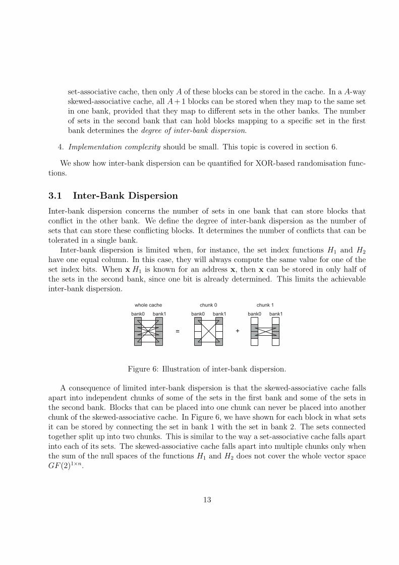
Inter-bank dispersion is limited when, for instance, the set index functions H1 and H2

have one equal column. In this case, they will always compute the same value for one of theset index bits. When x H1 is known for an address x, then x can be stored in only half ofthe sets in the second bank, since one bit is already determined. This limits the achievableinter-bank dispersion.

whole cache chunk 0 chunk 1

= +

bank0 bank1 bank0 bank1bank0 bank1

Figure 6: Illustration of inter-bank dispersion.

A consequence of limited inter-bank dispersion is that the skewed-associative cache fallsapart into independent chunks of some of the sets in the first bank and some of the sets inthe second bank. Blocks that can be placed into one chunk can never be placed into anotherchunk of the skewed-associative cache. In Figure 6, we have shown for each block in what setsit can be stored by connecting the set in bank 1 with the set in bank 2. The sets connectedtogether split up into two chunks. This is similar to the way a set-associative cache falls apartinto each of its sets. The skewed-associative cache falls apart into multiple chunks only whenthe sum of the null spaces of the functions H1 and H2 does not cover the whole vector spaceGF (2)1×n.

13

Theorem 6 Assume that the vector v is not a member of N(H1) + N(H2) and that block x

maps to set x H1 in bank 1 and to set x H2 in bank 2. Then it follows that there does notexist a block y that maps to the same set y H1 = x H1 in bank 1, but to the different sety H2 = (x ⊕ v) H2 in bank 2.

Proof: We present a proof by contradiction. Assume such a block y does exist, then wewill show a contradiction with the assumptions. Because x and y conflict in the first bank, itfollows that (x ⊕ y) ∈ N(H1). If x and y also map to the same set in the second bank, thenit follows that (x⊕y⊕v) ∈ N(H2). Thus v can be written as the sum of the vector x⊕y (amember of N(H1)) and the vector w = x⊕ y⊕ v (a member of N(H2)). Hence the vector v

is a member of the sum of N(H1) and N(H2). This contradicts our assumption about v. �This proves that the skewed-associative cache falls apart into chunks between which inter-

bank dispersion is impossible. Because of the symmetric structure of the randomisationfunctions, if follows that the number of sets in bank 2 where blocks that conflict in bank 1can be placed is equal for all sets. Furthermore, when both banks have an equal number ofsets, then the same number of such sets in bank 1 exist for blocks that conflict in bank 2.

We define the degree of inter-bank dispersion for bank b as the 2-logarithm of the numberof sets in the other bank that can store blocks that all map to the same set in bank b. Thenumber of such sets is given by the number of sets in the bank, divided by the number ofchunks into which the skewed-associative cache is split.

Definition 9 The degree of inter-bank dispersion for bank b = 1, 2 is given by

IBDb = dim(N(H1) + N(H2)) − dim(N(Hb)) (5)

= dim(N(H3−b)) − dim(N(H1) ∩ N(H2)) (6)

This definition is motivated as follows. A skewed-associative cache with randomisation func-tions H1 and H2 falls apart into #sup(H1, H2) chunks, or, using Definition 5, 2n−dim(N(sup(H1,H2)))

chunks, which equals 2n−dim(N(H1)+N(H2)) by Equation 4. The number of sets in bank b equals2n−dim(N(Hb)), hence the number of sets involved in the inter-bank dispersion is

2dim(N(H1)+N(H2))−dim(N(Hb))

The second equality in the definition follows from Theorem 5.

Corollary 1 Inter-bank dispersion is maximal iff the supremum of the null spaces of therandomisation functions equals the whole vector space:

IBDb = mb iff dim sup(H1, H2) = n (7)

where mb signifies the number of sets in bank b.

14

Proof: From Equation 5, the left-hand side of Equation 7 holds true when dim(N(H1) +N(H2)) − dim(N(Hb)) = mb. From Equation 1, it follows that mb + dim(N(Hb)) = n andfurther using Equations 4 and 2, the right-hand side follows. �

Maximal inter-bank dispersion can be recognised when the supremum is at the top of thelattice of randomisation functions. Another means of identification is to say that the functionsH1 and H2 have no columns in common, but this may be harder to spot on first sight.

It is reasonable to ask whether it is always possible to obtain maximal inter-bank disper-sion. From the definition of the supremum (Definition 8), it follows that dim sup(H1, H2) ≥m1 + m2. By linking this to Equation 7, the following corollary follows:

Corollary 2 Maximal inter-bank dispersion can be obtained when

n ≥ m1 + m2

where mb signifies the number of sets in bank b.

In other words, a sufficient number of address bits (n) have to be hashed in order to obtainmaximal inter-bank dispersion.

Maximal inter-bank dispersion does not interfere with local dispersion, i.e., obtainingmaximal inter-bank dispersion does not imply that local dispersion has to be sacrificed orvice versa.

3.2 Example

We illustrate the infinum and supremum randomisation functions and their relationship tointer-bank dispersion by means of an example. Table 1 lists two randomising set indexfunctions, defined in [BS95]. The part y in the address refers to the block offset and the partx bears no relevance to the value of the index functions. The index functions H1 and H2 aredefined by

[b3|b2|b1|b0]H1 = [b1 ⊕ b3|b0 ⊕ b2]

[b3|b2|b1|b0]H2 = [b0 ⊕ b3|b1 ⊕ b2]

The columns labelled Hinf and Hsup show the values of the infinum and supremum set indexfunctions.

The limited inter-bank dispersion can be spotted from Table 1 right away: the addressesthat map to index 00 in bank 1 are always mapped to either index 00 or index 11 in bank 2.Hence, inter-bank dispersion is limited to 2 sets.

Some blocks will be mapped to some pairs of set indices (i1, i2), where i1 designates a setin the first bank and i2 designates a set in the second bank, while for other pairs, there willnot be a single block that is mapped to i1 in the first bank and to i2 in the second bank at

15

Table 1: The values of the example randomisation functions.

address H1 H2 Hinf Hsup

x0000y 00 00 000 0x0001y 01 10 100 1x0010y 10 01 111 1x0011y 11 11 011 0x0100y 01 01 110 1x0101y 00 11 010 0x0110y 11 00 001 0x0111y 10 10 101 1x1000y 10 10 101 1x1001y 11 00 001 0x1010y 00 11 010 0x1011y 01 01 110 1x1100y 11 11 011 0x1101y 10 01 111 1x1110y 01 10 100 1x1111y 00 00 000 0

the same time (e.g.: for i1 = 00 and i2 = 01). This is a consequence of the skewed-associativecache falling apart in parts between which no inter-bank dispersion is possible.

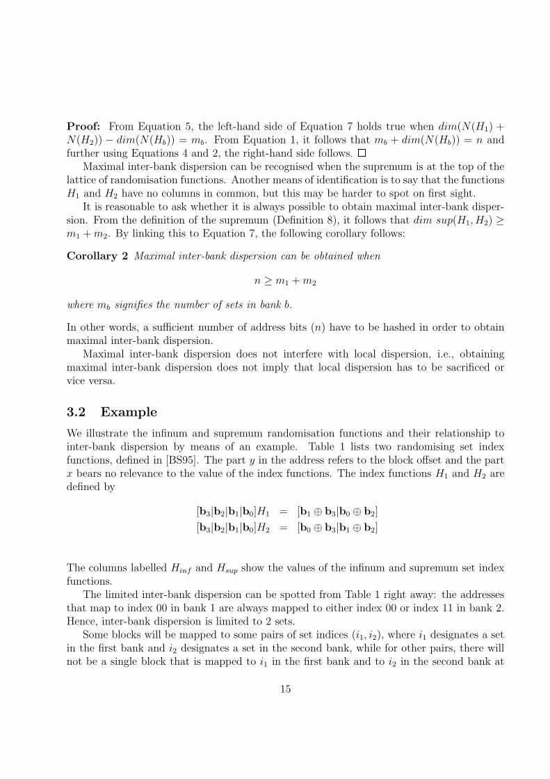
The possible combinations of set-numbers are graphically illustrated in Figure 7. The setindex in the first bank (H1) is shown on the horizontal axis and the set index in the secondbank (H2) is shown on the vertical axis. For each possible address, we mark the square inthe plot corresponding to the set indices listed in Table 1. Empty squares show impossiblecombinations of set indices. The other squares are filled with the value of Hinf .

By arranging the set indices in a suitable order, the graph clearly shows two independentparts. These two parts correspond to the two sets induced by the supremum set index functionHsup = sup(H1, H2). The reader can check that the set indices adjacent to the upper left-hand part correspond to the Hsup = 0 in Table 1 and the lower right-hand part correspondsto Hsup = 0. This is another way of showing the structure imposed on the skewed-associativecache by the randomisation functions H1 and H2.

3.3 More Than Two Banks

When a multi-module or skewed-associative cache contains more than 2 banks, then thedegree of inter-bank dispersion needs to be defined between two banks, i.e.: it is defined as

16

Value of H1

set 101of infinum

set 1 ofsupremum

set 0 ofsupremum

impossiblecombination

Valu

e o

f H

2

00

11

01

10

00

000

010

001

011

100

110

101

111

11 01 10

Figure 7: Illustration of Hinf , Hsup and inter-bank dispersion.

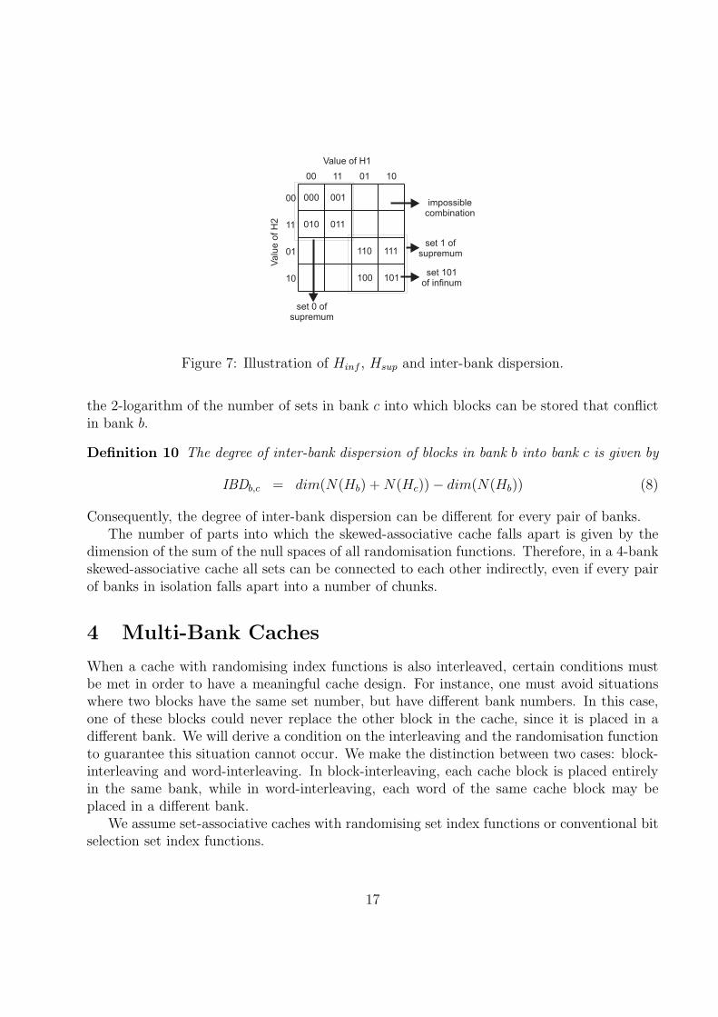
the 2-logarithm of the number of sets in bank c into which blocks can be stored that conflictin bank b.

Definition 10 The degree of inter-bank dispersion of blocks in bank b into bank c is given by

IBDb,c = dim(N(Hb) + N(Hc)) − dim(N(Hb)) (8)

Consequently, the degree of inter-bank dispersion can be different for every pair of banks.The number of parts into which the skewed-associative cache falls apart is given by the

dimension of the sum of the null spaces of all randomisation functions. Therefore, in a 4-bankskewed-associative cache all sets can be connected to each other indirectly, even if every pairof banks in isolation falls apart into a number of chunks.

4 Multi-Bank Caches

When a cache with randomising index functions is also interleaved, certain conditions mustbe met in order to have a meaningful cache design. For instance, one must avoid situationswhere two blocks have the same set number, but have different bank numbers. In this case,one of these blocks could never replace the other block in the cache, since it is placed in adifferent bank. We will derive a condition on the interleaving and the randomisation functionto guarantee this situation cannot occur. We make the distinction between two cases: block-interleaving and word-interleaving. In block-interleaving, each cache block is placed entirelyin the same bank, while in word-interleaving, each word of the same cache block may beplaced in a different bank.

We assume set-associative caches with randomising set index functions or conventional bitselection set index functions.

17

4.1 Block-Level Interleaving

In the case of block-interleaving, it suffices to require that each set of the cache is placedentirely in the same bank. Thus, if the addresses x and y have the same set number thentheir bank numbers should be equal too. For an interleaving function B and a randomisationfunction H , we write H ⊑ B. In this case, two blocks in the same set can always displace oneanother from the cache.

Note that it is possible to combine a regular set-associative cache using bit selection withhigh-order interleaving using randomisation, as long as the interleaving of the cache only usesbits which are selected by the set index function. In this case, the null space of B contains allthe vectors ei corresponding to the bits i that are not used by H , in addition to some othervectors that are not in the null space of H .

Now we show how to compute the per-bank index function, derived from H and B, forwhich H ⊑ B. This function is called G. In the implementation of a multi-bank cache,the function H is evaluated in two steps. First, B computes the bank number and then Gcomputes the per-bank set index number. Note that G is the same for all banks. It is requiredfor G that it maps two addresses to the same index when they map to the same bank and Hmaps these addresses to the same set index. If the addresses map to the same bank, but Hmaps them to a different index, then G should map them to a different index. If the addressesmap to different banks, then the result of G is not defined.

The null spaces of H , B and G are shown in Figure 8. Assume there are 2b banks (Bis a n × b matrix) and that there are 2m sets in the cache (H is a n × m matrix). SinceN(H) ⊆ N(B), a basis of N(B) can be constructed by starting with the basis vectors ofN(H) and adding an additional m − b basis vectors.

GF(2)1xn

m-b additinaldim. for N(B)

b additionaldim. for N(G)

0-vector

N(H)n-m dim.

N(B)

N(G)

Figure 8: Null spaces in the case of block-interleaving.

We now construct a basis for N(G). When the bank number of an address is known, thenthere are only 2m/2b possible sets left to which the address can be mapped. Therefore, G is an×(m−b) matrix and N(G) has dimension n−m+b. A basis of N(G) thus consists of n−m+b

18

linearly independent vectors. Furthermore, the function G should be such that when H mapstwo addresses to the same set, then so should G. Therefore H ⊑ G and N(H) ⊆ N(G). Thisrelationship defines n−m of the linearly independent basis vectors of N(G). The remaining blinearly independent vectors are chosen complementary to N(B). Note that any vector whichis not an element of N(B) is also not an element of N(H), so these b vectors are no part ofthe n − m vectors already chosen and they are linearly independent of them.

There is, however, another point we need to take care off. Since the complement of avector space is not uniquely defined2, we could choose a different G for each complement.However, each choice of G is a correct choice, as we show now.

Let G1 and G2 be n × (m − b) matrices with H ⊑ G1 and H ⊑ G2. We will show thatwhen G1 and G2 classify two addresses x and y differently, then these addresses map todifferent banks. We argued above that in this situation, the result of the functions G1 andG2 is arbitrary. Now, let v = x ⊕ y, then G1 and G2 take different actions when v ∈ N(G1)but v 6∈ N(G2). Note that N(H) ⊆ N(G1) ∩ N(G2) because H refines G1 and G2. In thiscase v 6∈ N(H) and v is thus one of the vectors complementary to N(B), i.e., v 6∈ N(B).Therefore, x and y map to different banks and the result of G1 and G2 is undefined.

Note that G is the same matrix in every bank. To conclude, we state that it is possibleto show that H = inf(B, G) when the above conditions are met.

4.2 Word-Level Interleaving

To facilitate reading, we identify the offset in a cache block by drawing a vertical bar betweenthe block number and the offset in the block. When a cache block is 2nl bytes large, wewrite x = [xn−1xn−2 . . . xnl

|xnl−1 . . . x0] or x = [xh|xl] to refer to the high-order part and thelow-order part explicitly. Note that xh is a 1 × nh vector and xl is a 1 × nl vector withnh + nl = n.

Now we show that interleaving functions which can be represented using a vector-matrixproduct impose a certain restriction on the possible ways that low-order interleaving can beused. As is shown next, the set of cache banks is always divided into a number of subsetsof the banks. Each cache block is spread out over all the banks in one of these subsets, butnot over any other bank. This limits the possible interleaving functions. For instance, aninterleaving where a block is stored in banks 0 and 1 and where another block is stored inbanks 1 and 2 can not be accomplished using matrices.

Theorem 7 For two cache blocks x = [xh|0] and y = [yh|0] and a word-interleaving functionB, either the cache blocks are placed in exactly the same cache banks or they are placed inentirely different cache banks.

Proof: Let the set Vl be the set of all possible nl-bit vectors. We let the variables xl

and yl iterate over the set Vl. Then the complete cache block at address [xh|0] can be

2A vector space V is a complement of a vector space U , iff V + U = GF (2)1×n, the set of all vectors.When U is fixed, there can be multiple V s that satisfy this condition.

19

produced as [xh|xl] (similarly for [yh|0]). The words in cache block x have bank number[xh|xl]B = xhBh ⊕ xlBl and the words in cache block y have bank number yhBh ⊕ ylBl.

Now we prove that he sets {xhBh ⊕ xlBl : xl ∈ Vl} and {yhBh ⊕ ylBl : yl ∈ Vl} are eitherequal or non-overlapping.

1. If xhBh ⊕ x′

lBl equals yhBh ⊕ y′

lBl, then the sets {xhBh ⊕ xlBl : xl ∈ Vl} and {yhBh ⊕ylBl : yl ∈ Vl} are equal. We prove that the first set is a subset of the second. Forevery x

′′

l , there is a y′′

l such that xhBh ⊕ x′′

l Bl = yhBh ⊕ y′′

l Bl. This occurs for y′′

l =x

′′

l ⊕x′

l ⊕y′

: xhBh ⊕x′′

l Bl = yhBh ⊕y′′

l Bl iff xhBh ⊕x′′

l Bl = yhBh ⊕x′′

l Bl ⊕x′

lBL ⊕y′

Bl

and by cancelling the x′′

l Bl on both sides of the equation and rearranging the terms:xhBh ⊕ x

′

lBl = yhBh ⊕ y′

lBl.

It can be proved in a similar manner that the second set is a subset of the first, whichproves that both are equal.

2. If, on the other hand, xhBh ⊕xlBl differs from all yhBh ⊕ylBl, then so must any otherxhBh ⊕ x

′

lBl, since xhBh ⊕ x′

lBl = yhBh ⊕ y′

lBl implies xhBh ⊕ xlBl = yhBh ⊕ y′′

l Bl fory

′′

l = xl ⊕ (x′

l ⊕ y′

l).

This concludes the proof. �bank 0 bank 2 bank 4 bank 6 bank 1 bank 3 bank 5 bank 7

Locations ofthe words incache block x

first group of banks second group of banks

Figure 9: Example low-order interleaving scheme with 8 banks.

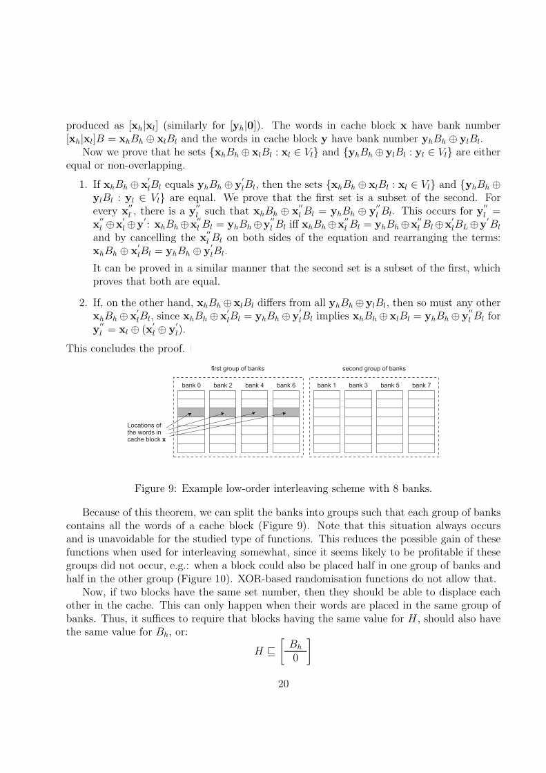
Because of this theorem, we can split the banks into groups such that each group of bankscontains all the words of a cache block (Figure 9). Note that this situation always occursand is unavoidable for the studied type of functions. This reduces the possible gain of thesefunctions when used for interleaving somewhat, since it seems likely to be profitable if thesegroups did not occur, e.g.: when a block could also be placed half in one group of banks andhalf in the other group (Figure 10). XOR-based randomisation functions do not allow that.

Now, if two blocks have the same set number, then they should be able to displace eachother in the cache. This can only happen when their words are placed in the same group ofbanks. Thus, it suffices to require that blocks having the same value for H , should also havethe same value for Bh, or:

H ⊑

[

Bh

0

]

20

bank 0 bank 2 bank 4 bank 6 bank 1 bank 3 bank 5 bank 7

cacheblock x

cacheblock y

first group of banks second group of banks

Figure 10: Impossible situation for low-order interleaving with XOR-based randomisationfunctions.

Note that we have reduced the situation from a 2b-bank cache with a mixed form of low-orderand high-order interleaving to a 2bh-bank cache with only high-order interleaving (bh is therank of Bh). Computation of the per-bank randomisation function is now similar to the caseof block-interleaving, assuming Bl = 0.

In the case of pure word-interleaving (i.e.: only the low-order bits, which form the blockoffset, are used by the interleaving scheme) the high-order interleaving matrix Bh is zero andN(Bh) = GF (2)1×nh. Thus, any H matrix will do. This is exactly the result that we want toobtain and it validates the preceding argument.

Another point to make is that when H does bit selection, but B does randomisation, then,G does not necessarily do randomisation too. Often, it is possible to find a G, subject to theabove conditions, that uses bit selection (i.e.: each XOR-gate has only one input).

4.3 Requirements for Interleaving Skewed-Associative caches

For a skewed-associative cache, the same rule applies as to other cache organisations: whena block can cause another block to be removed from the cache, then these blocks should beplaced in the same bank. In this case, the infinum of the set index functions of the cacheshould refine the interleaving function. Equivalently, each set index function Hi should refinethe interleaving function: Hi ⊑ B for i = 1, . . . , W . The per-bank index functions Gi can nowbe computed as in the case of a set-associative cache. In the case of low-order interleaving,one can set up a similar argument as for set-associative caches and find that Hi ⊑ [Bh

0] for

i = 1, . . . , W .An important consequence of interleaving a skewed-associative cache is that it will not

be possible to achieve maximum inter-bank dispersion, because the intersection of the nullspaces of the set index functions is forced to be non-empty.

21

5 Undoing a Randomisation Function

In certain cases, equipping the data cache with randomisation functions is not the best solu-tion. Instead, regular bit selection can be the best choice (e.g.: for the SPEC’95 benchmarkapplu, the set index function using bit selection is one of the best possible choices in a 8 KBdirect mapped cache). Therefore, it could be useful if the randomisation function of a cachecould be undone or changed by some means.

A simple idea is to provide each program with its own randomisation function by makingthe logic to compute the set index reconfigurable. This, however, increases the delay of acache access. Alas, it causes unwanted complexities when a single piece of data is present inthe memory space of multiple programs with different randomisation functions. In this case,different programs would search the data in different sets of the cache, possibly resulting instale data being fetched from the cache.

Therefore, we look at the possibility of defeating the randomisation function of the datacache by having the compiler perform a transformation on the data addresses. We assumethe architecture provides fast instructions that apply some permutation-based transformation(i.e.: a matrix) to an address. These instructions would be inserted by the compiler beforeevery memory access instruction. We show that when the cache implements randomisationfunction H , then it is possible to construct a function G, such that xGH = xB, for all x.Here, B is the matrix performing bit selection of m bits. Put differently, when the addressspace is transformed explicitly by the program using function G, then the cache will in effectbehave as if it used bit selection to determine the set number.

A possible G is [H∗|H ]−1, where H∗ can be any n × (n − m) matrix, as long as [H∗|H ]is invertible (i.e.: all the columns in [H∗|H ] should be linearly independent). Practically,this means that N(H∗) is complementary to N(H). We have to prove that for all addressesx: xGH = xB. Let y = xG. Since G is invertible, x = yG−1 and xGH = xB iff yH =y[H∗|H ]B. Using the definition of B

B =

[

0Im×m

]

the latter equality holds.The interpretation of this result is that, in order to invert the function H , one has to

first apply a function G which moves the null space N(B) on to the null space N(H) (howthe other vectors are transformed is not immediately relevant). Then, after applying H , anyperceived conflict vector will in fact originate from the null space N(B) instead of N(H)(Figure 11).

It is also possible to enforce any function F on the cache, even when it implements H (theonly constraint is that F and H are both n × m matrices with maximum rank). Note thatin the above we have shown how to map N(B) on N(H). This map is reversible, so we candeduce a map from N(F ) to N(B) from it by constructing the map for F and reversing it.Thus, for all addresses x: xGH = 0 iff xF = 0 when G = [F ∗|F ][H∗|H ]−1. Now, xGH = 0 iff

22

address space,vector " "x

G H

B

transformed address space,vector " = G"y x

bank number space,vector " GH"x

N(B)

N(H)

Figure 11: Transformation of address space when undoing a randomisation function.

x[F ∗|F ][H∗|H ]−1H = 0. From the above, [H∗|H ]−1H has the same null space as B, thus thereexists an invertible m×m matrix C such that [H∗|H ]−1H = BC. Using this, x[F ∗|F ]BC = 0

iff xFC = 0 iff xF = 0.A graph similar to Figure 11 can be drawn. It would include one extra step at the

beginning such that N(F ) is first transformed to N(B).

6 Optimising the Implementation of a Function

When interleaving functions or randomisation functions are used in the level 1 data cache,then these functions are in the critical path of the data cache access. Therefore, it is importantthat the latency of the circuit evaluating the function is as small as possible. We will showthat this circuit can be optimised by manipulating its matrix representation. This techniquemakes use of the property that different matrices can have the same null space and thus thesame behaviour [VDB02].

The latency of the circuit is mainly determined by two factors: the number of inputs ofa XOR-gate (fan-in) and the number of outputs of the drivers (fan-out). These correspondrespectively to the number of ones in a column and the number of ones in a row of the Hmatrix.

The exact latency of the circuit depends on a combination of these. We will only pro-vide a framework to do the optimisations, while the actual latency of the circuit dependson the specific trade-off made between fan-in and fan-out and the way the XOR-gates areimplemented.

By using the property that different matrices can have the same null space, a suitablematrix can be chosen for implementation. Assuming a matrix H with good randomisa-tion properties has been found, then a different matrix with the same null space can beconstructed by right-multiplying the matrix H with an invertible matrix C with dimen-sion m × m. This transform leaves the null space unchanged, since for any address x:xHC = 0 ⇔ xH = 0C−1 ⇔ xH = 0. An invertible matrix can be written as the prod-uct of elementary operations, e.g., swapping two columns, multiplying a column with a non-zero constant and adding one column to another. Only the third type is interesting for this

23

purpose.Figure 12 contains four matrices with the same null space. To improve readability, we have

replaced zeros by dots. Matrix 1 implements a polynomial mapping scheme for polynomial505 and was generated using Rau’s procedure [Rau91]. By adding column 0 to column 3, thefan-in of the XOR-gate computing bit 3 of the index is reduced from 5 to 4. Other reductionsof the fan-in occur when adding column 7 to column 4 and when adding 7 to column 5. Themaximum fan-in of matrix 4 is now 4. We also see that the maximum fan-out of matrix 4 islower than that of the matrix 1.

The important thing here is that the rightmost matrix has the same behaviour as theother ones, but its implementation is likely to be faster.

Matrix 1 Matrix 2 Matrix 3 Matrix 4column 7 6 5 4 3 2 1 0

1 . 1 1 . . . .. 1 . 1 1 . . .. . 1 . 1 1 . .. . . 1 . 1 1 .. . . . 1 . 1 11 1 1 1 1 . . 11 . . . . . . .. 1 . . . . . .. . 1 . . . . .. . . 1 . . . .. . . . 1 . . .. . . . . 1 . .. . . . . . 1 .. . . . . . . 1

fan-in 3 3 4 5 5 3 3 3max. fan-out 6

7 6 5 4 3 2 1 01 . 1 1 . . . .. 1 . 1 1 . . .. . 1 . 1 1 . .. . . 1 . 1 1 .. . . . . . 1 11 1 1 1 . . . 11 . . . . . . .. 1 . . . . . .. . 1 . . . . .. . . 1 . . . .. . . . 1 . . .. . . . . 1 . .. . . . . . 1 .. . . . 1 . . 13 3 4 5 4 3 3 3

5

7 6 5 4 3 2 1 01 . 1 . . . . .. 1 . 1 1 . . .. . 1 . 1 1 . .. . . 1 . 1 1 .. . . . . . 1 11 1 1 . . . . 11 . . 1 . . . .. 1 . . . . . .. . 1 . . . . .. . . 1 . . . .. . . . 1 . . .. . . . . 1 . .. . . . . . 1 .. . . . 1 . . 13 3 4 4 4 3 3 3

4

7 6 5 4 3 2 1 01 . . . . . . .. 1 . 1 1 . . .. . 1 . 1 1 . .. . . 1 . 1 1 .. . . . . . 1 11 1 . . . . . 11 . 1 1 . . . .. 1 . . . . . .. . 1 . . . . .. . . 1 . . . .. . . . 1 . . .. . . . . 1 . .. . . . . . 1 .. . . . 1 . . 13 3 3 4 4 3 3 3

3

Figure 12: Four equivalent matrices.

7 Conclusion

A theory of XOR-based interleaving functions and (randomising) set index functions is pre-sented. The functions are represented by a vector-matrix product. The matrices are trans-formed to their null space to remove redundancy of representation and to allow for easiercomputations.

24

The presented theory of randomisation functions can be used for a variety of applications.We briefly review the benefits of modelling interleaving functions and randomisation functionsusing null spaces and its applications.

• The null space makes it easy to determine if two matrices “do the same thing.”

• Local dispersion describes the way a randomisation function handles spatial locality.

• Evaluate inter-bank dispersion in skewed-associative caches.

• Conditions to check whether an interleaving function and a randomisation function cancoexist in a cache memory.

• The per-bank set index function can be easily computed when interleaving and ran-domisation are combined in a cache memory.

• XOR-based interleaving and randomisation functions can be replaced by the softwareor the compiler by applying an additional transformation on the address space.

• High-level optimisation of matrices with respect to cheaper implementation.

Acknowledgements

Hans Vandierendonck is supported by the Flemish Institute for the Promotion of Scientific-Technological Research in the Industry (IWT).

References

[AHH88] A. Agarwal, J. Hennessy, and M. Horowitz. Cache performance of operating sys-tem and multiprogramming workloads. ACM Transactions on Computer Systems,6(4):393–431, November 1988.

[AP93] A. Agarwal and S. D. Pudar. Column-associative caches: A technique for reduc-ing the miss rate of direct mapped caches. In Proceedings of the 20th AnnualInternational Symposium on Computer Architecture, pages 179–190, 1993.

[BS95] F. Bodin and A. Seznec. Skewed associativity enhances performance predictabil-ity. In Proceedings of the 22nd Annual International Symposium on ComputerArchitecture, pages 265–274, June 1995.

[CS99] M.A. Check and T.J. Slegel. Custom S/390 G5 and G6 microprocessors. IBMJournal on Research and Development, 43(5/6):671–680, 1999.

25

[FJL85] J. M. Frailong, W. Jalby, and J. Lenfant. XOR-schemes: A flexible data organi-zation in parallel memories. In Proceedings of the 1985 International Conferenceon Parallel Processing, pages 276–283, August 1985.

[GAV95] A. Gonzalez, C. Aliagas, and M. Valero. A data cache with multiple cachingstrategies tuned to different types of locality. In ICS’95. Proceedings of the 9thACM International Conference on Supercomputing, pages 338–347, 1995.

[GL96] N. Gaddis and J. Lotz. A 64-b quad-issue CMOS RISC microprocessor. IEEEJournal of Solid-State Circuits, 31(11):1697–1702, November 1996.

[GVTP96] A. Gonzalez, M. Valero, N. Topham, and J.M. Parcerisa. On the effectivenessof XOR-mapping schemes for cache memories. Technical Report UPC-CEPBA-1996-14, Universitat Politecnica de Catalunya, 1996.

[GVTP97] A. Gonzalez, M. Valero, N. Topham, and J.M. Parcerisa. Eliminating cacheconflict misses through XOR-based placement functions. In ICS’97. Proceedingsof the 1997 International Conference on Supercomputing, pages 76–83, July 1997.

[HIL89] D .T. Harper III and D.A. Linebarger. A dynamic storage scheme for conflict-free vector access. In Proceedings of the 16th Annual International Symposiumon Computer Architecture, pages 72–77, May 1989.

[HS89] M. D. Hill and A. J. Smith. Evaluating associativity in CPU caches. IEEETransactions on Computers, 38(12):1612–1630, December 1989.

[JH97] Teresa L. Johnson and Wen-mei W. Hwu. Run-time adaptive cache hierarchymanagement via reference analysis. In Proceedings of the 24th Annual Interna-tional Symposium on Computer Architecture, pages 315–326, 1997.

[KMW98] R. E. Kessler, E. J. McLellan, and D. A. Webb. The Alpha 21264 microprocessorarchitecture. In The International Conference on Computer Design. IEEE Com-puter Society, IEEE Circuits and Systems Society and IEEE Electron DevicesSociety, 1998.

[MTMT96] V. Milutinovic, M. Tomasevic, B. Markovic, and M. Tremblay. The split tem-poral/spatial cache: Initial complexity analysis. In Proceedings of the SCIzzL-6,September 1996.

[NVDB00] H. Neefs, H. Vandierendonck, and K. De Bosschere. A technique for high band-width and deterministic low latency load/store accesses to multiple cache banks.In Proceedings of the 6th International Symposium on High Performance Com-puter Architecture, pages 313–324, January 2000.

26

[Rau91] B. R. Rau. Pseudo-randomly interleaved memory. In Proceedings of the 18thAnnual International Symposium on Computer Architecture, pages 74–83, May1991.

[RH90] R. Raghavan and J. P. Hayes. On randomly interleaved memories. In SC90:Proceedings on Supercomputing ’90, pages 49–58, November 1990.

[RTT+98] J. A. Rivers, E. S. Tam, G. S. Tyson, E. S. Davidson, and M. Farrens. Utilizingreuse information in data cache management. In ICS’98. Proceedings of the 1998International Conference on Supercomputing, pages 449–456, 1998.

[SB93] A. Seznec and Francois Bodin. Skewed-associative caches. In PARLE’93: Par-allel Architectures and Programming Languages Europe, pages 305–316, Munich,Germany, June 1993.

[SCE99] T. Sherwood, B. Calder, and J. Emer. Reducing cache misses using hardwareand software page placement. In International Conference on Supercomputing,pages 155–164, 1999.

[Sez93] A. Seznec. A case for two-way skewed associative caches. In Proceedings of the20th Annual International Symposium on Computer Architecture, pages 169–178,May 1993.

[Sez97] A. Seznec. A new case for skewed-associativity. Technical Report PI-1114, IRISA,July 1997.

[SF91] G.S. Sohi and M. Franklin. High-bandwidth data memory systems for super-scalar processors. In Proceedings of the 18th Annual International Symposium onComputer Architecture, pages 53–62, May 1991.

[SG99] J. Sanchez and A. Gonzalez. A locality sensitive multi-module cache with explicitmanagement. In ICS’99. Proceedings of the 1999 International Conference onSupercomputing, pages 51–59, Rhodes, Greece, June 1999.

[SGV97] F. Jesus Sanchez, Antonio Gonzalez, and Mateo Valero. Software managementof selective and dual data caches. IEEE Technical Committee on Computer Ar-chitecture Newsletter, pages 3–10, March 1997.

[Smi78] A. J. Smith. A comparative study of set associative memory mapping algorithmsand their use for cache and main memory. IEEE Transactions on Software En-gineering, SE-4(2):121–130, March 1978.

[Smi82] A. J. Smith. Cache memories. ACM Computing Surveys, 14(3):473–530, Septem-ber 1982.

27

[Soh88] G.S. Sohi. Logical data skewing schemes for interleaved memories in vector pro-cessors. Technical Report 753, University of Wisconsin-Madison, February 1988.

[Soh93] G.S. Sohi. High-bandwidth interleaved memories for vector processors - a simu-lation study. IEEE Transactions on Computers, 42(1):34–44, January 1993.

[SSS93] M. Schlansker, R. Shaw, and S. Sivaramakrishnan. Randomization and associa-tivity in the design of placement-insensitive caches. Technical Report HPL-93-41,HP Laboratories, June 1993.

[Tam99] E. S. Tam. Improving Cache Performance Via Active Management. PhD thesis,University of Michigan, 1999.

[TG99] N. Topham and A. Gonzalez. Randomized cache placement for eliminating con-flicts. IEEE Transactions on Computers, 48(2):185–192, February 1999.

[TGG97] N. Topham, A. Gonzalez, and J. Gonzalez. The design and performance of aconflict-avoiding cache. In Proceedings of the 30th Annual International Sympo-sium on Microarchitecture, pages 71–80, December 1997.

[THG95] K. B. Theobald, H. H. J. Hum, and G. R. Gao. A design framework for hybrid-access caches. In Proceedings of the 1st International Symposium on High Per-formance Computer Architecture, pages 144–153, January 1995.

[VDB00a] H. Vandierendonck and K. De Bosschere. A comparison of locality-based andrecency-based replacement policies. In Proceedings of the 3rd International Sym-posium on High-Performance Computing (ISHPC2k), pages 310–318, October2000.

[VDB00b] H. Vandierendonck and K. De Bosschere. An optimal replacement policy for bal-ancing multi-module caches. In Proceedings of the 12th Symposium on ComputerArchitecture and High Performance Computing, October 2000.

[VDB01] H. Vandierendonck and K. De Bosschere. Efficient profile-based evaluation of ran-domising set index functions for cache memories. In 2nd International Symposiumon Performance Analysis of Systems and Software, pages 120–127, November2001.

[VDB02] H. Vandierendonck and K. De Bosschere. Evaluation of the performance of poly-nomial set index functions. In WDDD: Workshop on Duplicating, Deconstructingand Debunking, held in conjunction with the 29th International Symposium onComputer Architecture (ISCA-29), pages 31–41, May 2002.

28

[VLA92] M. Valero, T. Lang, and E. Ayguade. Conflict-free access of vectors with power-oftwo strides. In ICS’92. Proceedings of the 1992 ACM International Conferenceon Supercomputing, pages 149–156, July 1992.

[VLL+89] M. Valero, T. Lang, J.M. Llaberia, M. Peiron, E. Ayguado, and J.J. Navarro.Increasing the number of strides for conflict-free vector access. In Proceedingsof the 16th Annual International Symposium on Computer Architecture, pages372–381, May 1989.

[WS94] S. Weiss and J.E. Smith. POWER and PowerPC. Morgan Kaufmann Publishers,Inc., 1994.

[YL92] Q. Yang and W. LiPing. A novel cache design for vector processing. In Proceedingsof the 19th Annual International Symposium on Computer Architecture, pages362–371, May 1992.

[YMRJ99] A. Yoaz, E. Mattan, R. Ronen, and S. Jourdan. Speculation techniques forimproving load related instruction scheduling. In Proceedings of the 26th AnnualInternational Symposium on Computer Architecture, pages 42–53, May 1999.

29