On anomalous diffusion and the out of equilibrium response function in one-dimensional models

arX

iv:1

101.

4097

v1 [

cond

-mat

.sta

t-m

ech]

21

Jan

2011

On anomalous diffusion and the out of equilibrium

response function in one-dimensional models

D Villamaina, A Sarracino, G Gradenigo, A Puglisi and A

Vulpiani

CNR-ISC and Dipartimento di Fisica, Universita Sapienza - p.le A. Moro 2, 00185,

Roma, Italy

E-mail:

[email protected],[email protected]

[email protected],[email protected]

[email protected]

PACS numbers: 05.40.-a,05.60.-k,05.70.Ln

Abstract. We study how the Einstein relation between spontaneous fluctuations

and the response to an external perturbation holds in the absence of currents, for the

comb model and the elastic single-file, which are examples of systems with subdiffusive

transport properties. The relevance of nonequilibrium conditions is investigated: when

a stationary current (in the form of a drift or an energy flux) is present, the Einstein

relation breaks down, as it is known to happen in systems with standard diffusion. In

the case of the comb model, a general relation - appeared in the recent literature -

between response function and an unperturbed suitable correlation function, allows us

to explain the observed results. This suggests that a relevant ingredient in breaking

the Einstein formula, for stationary regimes, is not the anomalous diffusion but the

presence of currents driving the system out of equilibrium.

http://arxiv.org/abs/1101.4097v1

On anomalous diffusion and the out of equilibrium response function... 2

1. Introduction

In his seminal paper on the Brownian Motion, Einstein, beyond the celebrated relation

between the diffusion coefficient D and the Avogadro number, found the first example

of fluctuation-dissipation relation (FDR). In the absence of external forcing one has, for

large times t → ∞,

〈x(t)〉 = 0 , 〈x2(t)〉 ≃ 2Dt , (1)

where x is the position of the Brownian particle and the average is taken over the

unperturbed dynamic. Once a small constant external force F is applied one has a

linear drift

δx(t) = 〈x(t)〉F − 〈x(t)〉 ≃ µFt (2)

where 〈. . .〉F indicates the average on the perturbed system, and µ is the mobility of

the colloidal particle. It is remarkable that 〈x2(t)〉 is proportional to δx(t) at any time:

〈x2(t)〉

δx(t)=

2

βF, (3)

and the Einstein relation (a special case of the fluctuation-dissipation theorem [1]) holds:

µ = βD, with β = 1/kBT the inverse temperature and kB the Boltzmann constant.

On the other hand it is now well established that beyond the standard diffusion, as

in (1), one can have systems with anomalous diffusion (see for instance [2, 3, 4, 5, 6]),

i.e.

〈x2(t)〉 ∼ t2ν with ν 6= 1/2. (4)

Formally this corresponds to have D = ∞ if ν > 1/2 (superdiffusion) and D = 0 if

ν < 1/2 (subdiffusion). In this letter we will limit the study to the case ν < 1/2. It

is quite natural to wonder if (and how) the FDR changes in the presence of anomalous

diffusion, i.e. if instead of (1), Eq. (4) holds. In some systems it has been showed

that (3) holds even in the subdiffusive case. This has been explicitly proved in systems

described by a fractional-Fokker-Planck equation [7], see also [8, 9]. In addition there is

clear analytical [10] and numerical [11] evidences that (3) is valid for the elastic single

file, i.e. a gas of hard rods on a ring with elastic collisions, driven by an external

thermostat, which exhibits subdiffusive behavior, 〈x2〉 ∼ t1/2 [12].

The aim of this paper is to discuss the validity of the fluctuation-dissipation relation

in the form (3) for systems with anomalous diffusion which are not fully described by

a fractional Fokker-Planck equation. In particular we will investigate the relevance of

the anomalous diffusion, the presence of non equilibrium conditions and the (possible)

role of finite size. Since we are also interested in the study of transient regimes, we

will consider models with microscopic dynamics described in terms of transition rates

or microscopic interactions.

First, we focus on the study of a particle moving on a “finite comb” lattice with teeth

of size L [13]. In the limit L = ∞ an anomalous subdiffusive behavior, 〈x2〉 ∼ t1/2, holds

and the system can be mapped, for large times, onto a continuous time random walk [13].


For finite L the subdiffusion is only transient and at very large time t > t∗(L) ∼ L2

one has a standard diffusion: 〈x2〉 ∼ t. We will see that Eq. (3), where in this case the

perturbed average is obtained with unbalanced transition rates driving the particle along

the backbone of the comb, holds both for t > t∗(L) and t < t∗(L) with the same constant.

This in spite of the fact that the probability densities P (x, t) in the two regimes are very

different. The scenario changes in the presence of “non equilibrium” conditions, i.e. with

a drift, which induces a current, in the unperturbed state: the relation (3) does not hold

anymore. On the other hand, in this case it is possible to use a generalized fluctuation-

dissipation relation, derived by Lippiello et al. in [14], which gives the response function

in terms of unperturbed correlation functions and is an example of non equilibrium FDR

valid under rather general conditions [15, 16, 14, 17, 18, 19, 20, 21]. A generalization of

the Einstein formula was also proved in the framework of continuous time random walks

in [22]. So we can say that the Einstein relation (3) also holds in cases with anomalous

diffusion when no current is present, but it is necessary to introduce suitable corrections

when a perturbation is applied to a system with non zero drift.

In addition we compare the results found in comb models, with those obtained for

single-file diffusion with a finite number of particles. There we will also consider a non

equilibrium case, with the introduction of inelastic collisions which induce an energy flux

crossing the system. Our results suggest that the presence of non equilibrium currents

plays a relevant role in modifying Eq. (3) in stationary states.

2. Comb: diffusion and response function

The comb lattice is a discrete structure consisting of an infinite linear chain (backbone),

the sites of which are connected with other linear chains (teeth) of length L [13]. We

denote by x ∈ (−∞,∞) the position of the particle performing the random walk along

the backbone and with y ∈ [−L, L] that along a tooth. The transition probabilities

from (x, y) to (x′, y′) are:

W d[(x, 0) → (x± 1, 0)] = 1/4± d

W d[(x, 0) → (x,±1)] = 1/4

W d[(x, y) → (x, y ± 1)] = 1/2 for y 6= 0,±L. (5)

On the boundaries of each tooth, y = ±L, the particle is reflected with probability

1. The case L = ∞ is obtained in numerical simulations by letting the y coordinate

increase without boundaries. Here we consider a discrete time process and, of course,

the normalization∑

(x′,y′) Wd[(x, y) → (x′, y′)] = 1 holds. The parameter d ∈ [0, 1/4]

allows us to consider also the case where a constant external field is applied along the

x axis, producing a non zero drift of the particle. A state with a non zero drift can be

considered as a perturbed state (in that case we denote the perturbing field by ε), or

it can be itself the starting state where a further perturbation can be added changing

d → d+ ε.


0.0001 0.01 1 100

t/L2

0.01

1

100

<x(

t)2 >

/ L

L=16L=32L=64L=128L=256L=512

~t1/2

~t

t*/L2

100 1000 10000

<x(t)2>

0

100

1000

10000

δxd(t

)

1000 10000 1e+05 1e+06 1e+07

t

100

10000

δx(t)

<x(t)2>

0

d=0 ε=0.1

Figure 1. Left panel: 〈x2(t)〉0/L vs t/L2 is plotted for several values of L in the comb

model. Right panel: 〈x2(t)〉0 and the response function δx(t) for L = 512. In the inset

the parametric plot δx(t) vs 〈x2(t)〉0 is shown.

Let us start by considering the case d = 0. For finite teeth length L < ∞, we have

numerical evidence of a dynamical crossover from a subdiffusive to a simple diffusive

asymptotic behaviour (see Fig. 1)

〈x2(t)〉0 ≃

{

Ct1/2 t < t∗(L)

2D(L)t t > t∗(L),(6)

where C is a constant and D(L) is an effective diffusion coefficient depending on L. The

symbol 〈. . .〉0 denotes an average over different realizations of the dynamics (5) with

d = 0 and initial condition x(0) = y(0) = 0. We find t∗(L) ∼ L2 and D(L) ∼ 1/L and

in the left panel of Fig. 1 we plot 〈x2(t)〉0/L as function of t/L2 for several values of L,

showing an excellent data collapse.

In the limit of infinite teeth, L → ∞, D → 0 and t∗ → ∞ and the system shows a

pure subdiffusive behaviour [23]

〈x2(t)〉0 ∼ t1/2. (7)

In this case, the probability distribution function behaves as

P0(x, t) ∼ t−1/4e−c

(

|x|

t1/4

)4/3

, (8)

where c is a constant, in agreement with an argument a la Flory [2]. The behaviour (8)

also holds in the case of finite L, provided that t < t∗. For larger times a simple

Gaussian distribution is observed. Note that, in general, the scaling exponent ν, in

this case ν = 1/4, does not determine univocally the shape of the pdf. Indeed, for the

single-file model, discussed below, we have the same ν but the pdf is Gaussian [24].

In the comb model with infinite teeth, the FDR in its standard form is fulfilled,

namely if we apply a constant perturbation ε pulling the particles along the 1-d lattice

one has numerical evidence that

〈x2(t)〉0 ≃ Cδx(t) ∼ t1/2. (9)


In the following section we derive this result from a generalized FDR. Moreover, the

proportionality between 〈x2(t)〉0 and δx(t) is fulfilled also with L < ∞, where both

the mean square displacement (m.s.d.) and the drift with an applied force exhibit the

same crossover from subdiffusive, ∼ t1/2, to diffusive, ∼ t (see Fig. 1, right panel).

Therefore what we can say is that the FDR is somehow “blind” to the dynamical

crossover experienced by the system. When the perturbation is applied to a state

without any current, the proportionality between response and correlation holds despite

anomalous transport phenomena.

Our aim here is to show that, differently from what depicted above about the zero

current situation, within a state with a non zero drift [25] the emergence of a dynamical

crossover is connected to the breaking of the FDR. Indeed, the m.s.d. in the presence

of a non zero current, even with L = ∞, shows a dynamical crossover

〈x2(t)〉d ∼ a t1/2 + b t, (10)

where a and b are two constants, whereas

δxd(t) ∼ t1/2, (11)

with δxd(t) = 〈x(t)〉d+ε − 〈x(t)〉d: at large times the Einstein relation breaks down (see

Fig. 2). The proportionality between response and fluctuations cannot be recovered by

simply replacing 〈x2(t)〉d with 〈x2(t)〉d − 〈x(t)〉2d, as it happens for Gaussian processes

(see discussion below), namely we find numerically

〈[x(t)− 〈x(t)〉d]2〉d ∼ a′ t1/2 + b′ t, (12)

where a′ and b′ are two constants, as reported in Fig. 2.

3. Comb: application of a generalized FDR

The discussion of the previous section shows that the first moment of the probability

distribution function with drift Pd(x, t) and the second moment of P0(x, t) are always

proportional. Note that in the presence of a drift the pdf is strongly asymmetric with

respect to the mean value, as shown in Fig. 3 for a system with L = ∞. Differently, the

first moment of Pd+ε(x, t) is not proportional to the second moment of Pd(x, t), namely

〈x(t)〉d+ε ≁ 〈x2(t)〉d − 〈x(t)〉2d. In order to find out a relation between such quantities,

we need a generalized fluctuation-dissipation relation.

According to the definition (5), one has for the backbone

W d+ε[(x, y) → (x′, y′)] = W d[(x, y) → (x′, y′)]

(

1 +ε(x′ − x)

W 0 + d(x′ − x)

)

≃ W deε

W0 (x′−x),

(13)

where W 0 = 1/4, and the last expression holds under the condition d/W 0 ≪ 1.

Regarding the above expression as a local detailed balance condition for our Markov

process we can rewrite it, for (x, y) 6= (x′, y′), as

W d+ε[(x, y) → (x′, y′)] = W d[(x, y) → (x′, y′)]eh(ε)2

(x′−x), (14)


1000 10000 1e+05 1e+06 1e+07

t10

100

1000

10000 δxd(t)/h(ε)

<x(t)2>

d

<x(t)2>

d- <x(t)>

d<x(t)A(t,0)>

d

1/2[<x(t)2>

d- <x(t)A(t,0)>

d]

~t1/2

~t

~t1/2

d = 0.01 ε = 0.002

2

Figure 2. Response function (black line), m.s.d. (red dotted line) and second

cumulant (black dotted line) measured in the the comb model with L = ∞, field

d = 0.01 and perturbation ε = 0.002. The correlation with activity (green dotted line)

yields the right correction to recover the full response function (blue dotted line), in

agreement with the FDR (15).

where h(ε) = 2ε/W 0. For general models where the perturbation enters the transition

probabilities according to Eq. (14), the following formula for the integrated linear

response function has been derived [14, 19, 21]

δOd

h(ε)=

〈O(t)〉d+ε − 〈O(t)〉dh(ε)

=1

2[〈O(t)x(t)〉d − 〈O(t)x(0)〉d − 〈O(t)A(t, 0)〉d] , (15)

where O is a generic observable, and A(t, 0) =∑t

t′=0B(t′), with

B[(x, y)] =∑

(x′,y′)

(x′ − x)W d[(x, y) → (x′, y′)]. (16)

The above observable yields an effective measure of the propensity of the system to leave

a certain state (x, y) and, in some contexts, it is referred to as activity [26]. Recalling

the definitions (5), from the above equation we have B[(x, y)] = 2dδy,0 and therefore the

sum on B has an intuitive meaning: it counts the time spent by the particle on the x

axis. The results described in the previous section can be then read in the light of the

fluctuation-dissipation relation (15):

i) Putting O(t) = x(t), in the case without drift, i.e. d = 0, one has B = 0 and,

recalling the choice of the initial condition x(0) = 0,

δx

h(ε)=

〈x(t)〉ε − 〈x(t)〉0h(ε)

=1

2〈x2(t)〉0. (17)

This explains the observed behaviour (9) even in the anomalous regime and predicts the

correct proportionality factor, δx(t) = ε/W 0〈x2(t)〉0.

ii) Putting O(t) = x(t), in the case with d 6= 0, one has

δxd

h(ε)=

1

2

[

〈x2(t)〉d − 〈x(t)A(t, 0)〉d]

. (18)


This explains the observed behaviours (10) and (11): the leading behavior at large

times of 〈x2(t)〉d ∼ t, turns out to be exactly canceled by the term 〈x(t)A(t, 0)〉d, so

that the relation between response and unperturbed correlation functions is recovered

(see Fig. 2).

iii) As discussed above, it is not enough to substitute 〈x2(t)〉d with 〈x2(t)〉d−〈x(t)〉2dto recover the proportionality with δxd(t) when the process is not Gaussian. This can be

explained in the following manner. By making use of the second order out of equilibrium

FDR derived by Lippiello et al. in [27, 28, 29], which is needed due to the vanishing of

the first order term for symmetry, we can explicitly evaluate

〈x2(t)〉d = 〈x2(t)〉0 + h2(d)1

2

[

1

4〈x4(t)〉0 +

1

4〈x2(t)A(2)(t, 0)〉0

]

, (19)

where A(2)(t, 0) =∑t

t′=0B(2)(t′) with B(2) = −

∑

x′(x′ − x)2W [(x, y) → (x′, y′)] =

−1/2δy,0. Then, recalling Eq. (17), we obtain

〈x2(t)〉d − 〈x(t)〉2d = 〈x2(t)〉0 + h2(d)

[

1

8〈x4(t)〉0 +

1

8〈x2(t)A(2)(t, 0)〉0 −

1

4〈x2(t)〉20

]

. (20)

Numerical simulations show that the term in the square brackets grows like t yielding

a scaling behaviour with time consistent with Eq. (12). On the other hand, in the case

of the simple random walk, one has B(2) = −1 and A(2)(t, 0) = −t and then

〈x2(t)〉d − 〈x(t)〉2d = 〈x2(t)〉0 + h2(d)

[

1

8〈x4(t)〉0 −

1

8t〈x2(t)〉0 −

1

4〈x2(t)〉20

]

. (21)

Since in the Gaussian case 〈x4(t)〉0 = 3〈x2(t)〉20 and 〈x2(t)〉0 = t, the term in the square

brackets vanishes identically and that explains why, in the presence of a drift, the second

cumulant grows exactly as the second moment with no drift.

-50 0 50 100 150 200 250 300x

0.001

0.01

0.1

P d(x,t)

t=105

t=106

t=5.106

d=0.01

Figure 3. Pd(x, t) in the comb model with L = ∞ and d = 0.01 at different times.

Notice that the mean value increases with time mostly due to the spreading, while the

most probable value remains always close to zero.


4. Conclusions and perspectives

In order to evaluate the generality of the above results, let us conclude by discussing

another system. Indeed, subdiffusion is present in many different problems where

geometrical constraints play a central role. In this framework, a well studied

phenomenon is the so-called single-file diffusion. Namely, we have N Brownian rods

on a ring of length L interacting with elastic collisions and coupled with a thermal bath.

The equation of motion for the single particle velocity between collisions is

mv(t) = −γv(t) + η(t), (22)

where m is the mass, γ is the friction coefficient, and η is a white noise with variance

〈η(t)η(t′)〉 = 2Tγδ(t− t′). The combined effect of collisions, noise and geometry (since

the system is one-dimensional the particles cannot overcome each other) produces a

non-trivial behaviour. In the thermodynamic limit, i.e. L,N → ∞ with N/L → ρ, a

subdiffusive behaviour occurs [12].

Analogously to the comb model, the case of N and L finite presents some interesting

aspects. In order to avoid trivial results due to the periodic boundary conditions on

the ring, it is suitable to define the position of a tagged particle as s(t) =∫ t

0v(t′)dt′,

where v(t) is its velocity. For the m.s.d. 〈s2(t)〉, averaged over the thermalized initial

conditions and over the noise, we find, after a transient ballistic behaviour for short

times, a dynamical crossover between two different regimes:

〈s2(t)〉 ≃

{

2(1−σρ)ρ

√

Dπt1/2 t < τ ∗(N)

2DNt t > τ ∗(N),

(23)

where σ is the length of the rods and D is the diffusion coefficient of the single Brown-

ian particle [12]. Note that the asymptotic behaviour is completely determined by the

motion of the center of mass, which is not affected by the collisions and simply diffuses.

Moreover, as evident from numerical simulations, τ ∗ ∼ N2 and in the limit of infinite

number of particles the behaviour becomes subdiffusive, in perfect analogy with what

observed for the comb model, where the role of L is here played by N . The main differ-

ence is that, in this case, the probability distribution is Gaussian in both regimes. As a

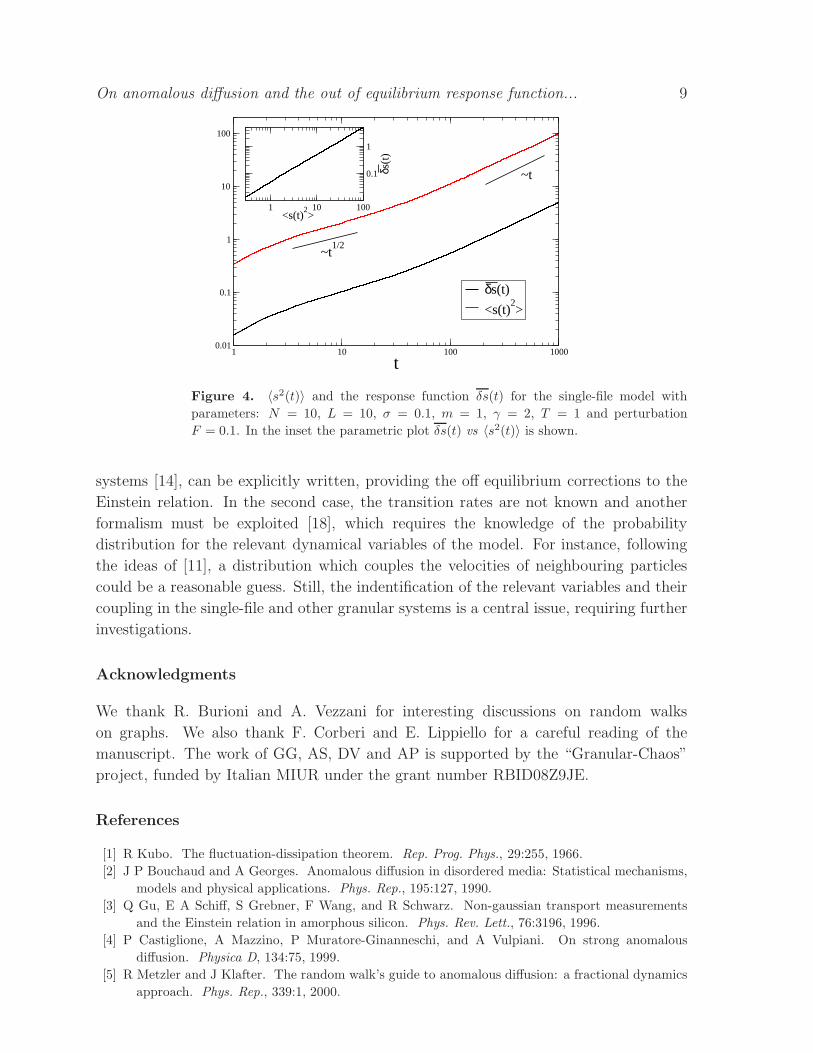
consequence of the Gaussian nature of the problem, applying a perturbation as a small

force F in Eq. (22), one finds that the Einstein relation is always fulfilled [11, 10, 18, 30],

also for finite N and L (see Fig. 4). Strong violations of the Einstein relation, can be

obtained, in dense cases, when the collisions between the rods are inelastic so that a

homogeneous energy current crosses the system [11].

In this note we have considered systems with subdiffusive behaviour, showing that

the proportionality between response function and correlation breaks down when “non

equilibrium” conditions are introduced. In the comb model, non equilibrium effects are

induced by unbalanced transition probabilities driving the particle along the backbone,

while the single-file model is driven away from equilibrium by inelastic collisions. In

the first case, the generalized FDR of Eq. (15), developed in the framework of aging


1 10 100 1000

t0.01

0.1

1

10

100

δs(t)

<s(t)2>

1 10 100<s(t)

2>

0.1

1

δs(t

)

~t

~t1/2

Figure 4. 〈s2(t)〉 and the response function δs(t) for the single-file model with

parameters: N = 10, L = 10, σ = 0.1, m = 1, γ = 2, T = 1 and perturbation

F = 0.1. In the inset the parametric plot δs(t) vs 〈s2(t)〉 is shown.

systems [14], can be explicitly written, providing the off equilibrium corrections to the

Einstein relation. In the second case, the transition rates are not known and another

formalism must be exploited [18], which requires the knowledge of the probability

distribution for the relevant dynamical variables of the model. For instance, following

the ideas of [11], a distribution which couples the velocities of neighbouring particles

could be a reasonable guess. Still, the indentification of the relevant variables and their

coupling in the single-file and other granular systems is a central issue, requiring further

investigations.

Acknowledgments

We thank R. Burioni and A. Vezzani for interesting discussions on random walks

on graphs. We also thank F. Corberi and E. Lippiello for a careful reading of the

manuscript. The work of GG, AS, DV and AP is supported by the “Granular-Chaos”

project, funded by Italian MIUR under the grant number RBID08Z9JE.

References

[1] R Kubo. The fluctuation-dissipation theorem. Rep. Prog. Phys., 29:255, 1966.

[2] J P Bouchaud and A Georges. Anomalous diffusion in disordered media: Statistical mechanisms,

models and physical applications. Phys. Rep., 195:127, 1990.

[3] Q Gu, E A Schiff, S Grebner, F Wang, and R Schwarz. Non-gaussian transport measurements

and the Einstein relation in amorphous silicon. Phys. Rev. Lett., 76:3196, 1996.

[4] P Castiglione, A Mazzino, P Muratore-Ginanneschi, and A Vulpiani. On strong anomalous

diffusion. Physica D, 134:75, 1999.

[5] R Metzler and J Klafter. The random walk’s guide to anomalous diffusion: a fractional dynamics

approach. Phys. Rep., 339:1, 2000.


[6] R Burioni and D Cassi. Random walks on graphs: ideas, techniques and results. J. Phys. A:Math.

Gen., 38:R45, 2005.

[7] R Metzler, E Barkai, and J Klafter. Anomalous diffusion and relaxation close to thermal

equilibrium: A fractional Fokker-Planck equation approach. Phys. Rev. Lett, 82:3563, 1999.

[8] E Barkai and V N Fleurov. Generalized Einstein relation: A stochastic modeling approach. Phys.

Rev. E, 58:1296, 1998.

[9] A V Chechkin and R Klages. Fluctuation relations for anomalous dynamics. J. Stat. Mech., page

L03002, 2009.

[10] L Lizana, T Ambjornsson, A Taloni, E Barkai, and M A Lomholt. Foundation of fractional

Langevin equation: Harmonization of a many-body problem. Phys. Rev. E, 81(5):51118, 2010.

[11] D Villamaina, A Puglisi, and A Vulpiani. The fluctuation-dissipation relation in sub-diffusive

systems: the case of granular single-file diffusion. J. Stat. Mech., page L10001, 2008.

[12] K Hahn, J Karger, and V Kukla. Single-file diffusion observation. Phys. Rev. Lett., 76(15):2762,

1996.

[13] S Redner. A Guide to First-Passages Processes. Cambridge University Press, 2001.

[14] E Lippiello, F Corberi, and M Zannetti. Off-equilibrium generalization of the fluctuation

dissipation theorem for Ising spins and measurement of the linear response function. Phys.

Rev. E, 71:036104, 2005.

[15] L F Cugliandolo, J Kurchan, and G Parisi. Off equilibrium dynamics and aging in unfrustrated

systems. J. Phys. I, 4:1641, 1994.

[16] G Diezemann. Fluctuation-dissipation relations for Markov processes. Phys. Rev. E, 72:011104,

2005.

[17] T Speck and U Seifert. Restoring a fluctuation-dissipation theorem in a nonequilibrium steady

state. Europhys. Lett., 74:391, 2006.

[18] U Marini Bettolo Marconi, A Puglisi, L Rondoni, and A Vulpiani. Fluctuation-dissipation:

Response theory in statistical physics. Phys. Rep., 461:111, 2008.

[19] M Baiesi, C Maes, and B Wynants. Fluctuations and response of nonequilibrium states. Phys.

Rev. Lett., 103:010602, 2009.

[20] U Seifert and T Speck. Fluctuation-dissipation theorem in nonequilibrium steady states.

Europhys. Lett., 89:10007, 2010.

[21] F Corberi, E Lippiello, A Sarracino, and M Zannetti. Fluctuation-dissipation relations and field-

free algorithms for the computation of response functions. Phys. Rev. E, 81:011124, 2010.

[22] Y He, S Burov, R Metzler, and E Barkai. Random time-scale invariant diffusion and transport

coefficients. Phys. rev. Lett., 101:058101, 2008.

[23] S Havlin and D Ben Avraham. Diffusion in disordered media. Adv. Phys., 36:695, 1987.

[24] Q HWei, C Bechinger, and P Leiderer. Single-file diffusion of colloids in one-dimensional channels.

Science, 287:625, 2000.

[25] R Burioni, D Cassi, G Giusiano, and S Regina. Anomalous diffusion and Hall effect on comb

lattices. Phys. Rev. E, 67:016116, 2003.

[26] C Appert-Rolland, B Derrida, V Lecomte, and F van Wijland. Universal cumulants of the current

in diffusive systems on a ring. Phys. Rev. E, 78:021122, 2008.

[27] E Lippiello, F Corberi, A Sarracino, and M Zannetti. Nonlinear susceptibilities and the

measurement of a cooperative length. Phys. Rev. B, 77:212201, 2008.

[28] E Lippiello, F Corberi, A Sarracino, and M Zannetti. Nonlinear response and fluctuation-

dissipation relations. Phys. Rev. E, 78:041120, 2008.

[29] F Corberi, E Lippiello, A Sarracino, and M Zannetti. Fluctuations of two-time quantities and

non-linear response functions. J. Stat. Mech., page P04003, 2010.

[30] A Puglisi, A Baldassarri, and A Vulpiani. Violations of the Einstein relation in granular fluids:

the role of correlations. J. Stat. Mech., page P08016, 2007.

On anomalous diffusion and the out of equilibrium response function in one-dimensional models

Documents

Transcript of On anomalous diffusion and the out of equilibrium response function in one-dimensional models