OLAP expressions are an extremely powerful tool in SQL that enable advanced

reporting features such as ranking, counting, averaging, adding, and more within a

set of data processed in an SQL statement. This feature allows for data to be

aggregated based upon values in a query in a manner very similar to coding control

breaks in a program process. This allows for entire programs, or even applications,

to be replaced by much more flexible and portable SQL statements. Reduce

programming time and complexity, and improve flexibility and performance, by

deploying OLAP expressions. This session will show you how!

1

2

3

If you’re keep up with IT news in recent times you’ll easily agree that analytics is a

hot topic. The amount of data stored in our operational systems is increasing on a

daily basis, and management is quickly learning that this information can and

should be quickly harnessed in order for the business to make quick decisions

concerning things such as sales directions, talent acquisition, cost containment, and

more! One of the biggest challenges is to formulate answers to these questions that

utilize the most current information, are inexpensive and easy to create, and can

deliver the answers quickly. Many times great expense is incurred in moving data,

creating data warehouses, and using specialized software to produce various reports.

In addition to this, many times these reporting tools issue complex and redundant

SQL to the data server that can result in excessive reporting costs.

Having OLAP functionality built into the DB2 engine can help reduce some of the

operational and software costs associated with getting answers to complex

questions. This functionality can be used in data warehouses, but also against OLTP

databases with equal results. One more tool in the IT department’s tool box for

answering complex business questions.

4

Analytics is a widely growing segment of database (and non-database) processing.

DB2 has the ability to perform analytics via built-in expressions. Once again, this

means that instead of purchasing an expensive product, or writing thousands of lines

of code, you can simply write an SQL statement that does the processing for you

and creates output that is report ready!

This type of processing is called Online Analytical Processing, OLAP. The

constructs within the DB2 engine can be referred to as:

• OLAP expressions

• OLAP specification

• OLAP functions

• Window functions

5

DB2 provides for several OLAP specific functions, as well as a host of aggregate

functions in support of OLAP expressions. Each of these functions returns a scalar

result to the row being processed. The operations supporting OLAP processing can

process a single row, multiple rows, or an entire result set in the calculation of the

scalar value returned.

A feature of this type of processing is the window. This window is a logical

grouping of data within the result set, and the default window is the entire result set.

Within a window OLAP processing can number or rank rows based upon an

ordering. In addition, aggregation of values within an entire window or via a

grouping within a window can be performed. Multiple OLAP functions can be

specified in a SELECT clause mixing numbering, ranking, and aggregation. This

results in some extremely powerful and flexible data analytics within the SQL

language.

6

The key aspects to OLAP processing are the concepts of windowing and ordering.

As stated before a window is a portion or grouping of the data in the result set. If no

window is specified then the default window is the entire result set, and any

ordering is applied to the entire result. If a window is specified then any ordering is

within that window, and thus any calculations are based only upon the data in that

window. You can specify many OLAP expressions in a single query, each of which

can have its own independent windowing and ordering.

7

The first OLAP expression to explore is the numbering specification. Row

numbering is the easiest concept to understand as it does exactly what its name

implies, numbers rows in the output. Since windowing and ordering can be applied

to row number, it is the perfect function to use to learn about these features since

numbering is extremely easy to understand.

Numbering is enabled via the ROW_NUMBER() function. There are no parameters

to this function. One extremely important thing to remember is that row numbering

is arbitrary to the final ordering of the result. You can number within windows and

you can also apply an order to the numbering. However, the numbering itself is

done arbitrarily. Despite the limited functionality this function can be extremely

useful for things such as determining the minimum and maximum row according to

an order, data sampling, and pagination (although there are some performance

implications).

8

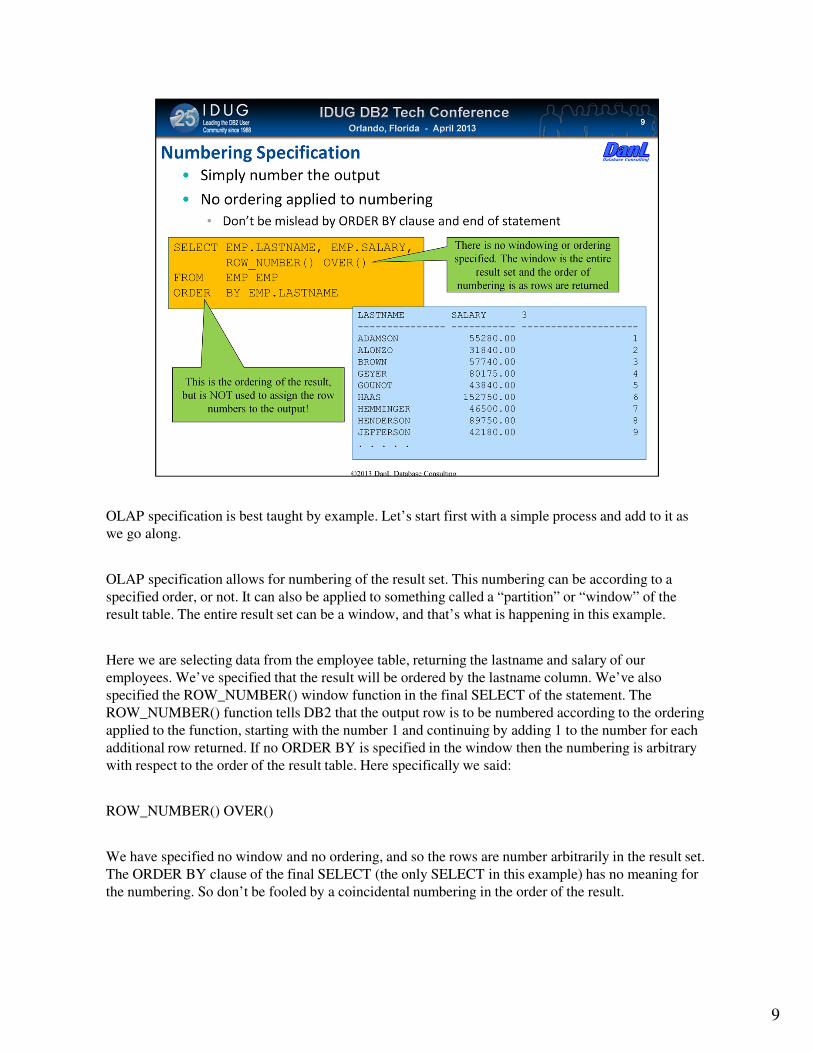
OLAP specification is best taught by example. Let’s start first with a simple process and add to it as

we go along.

OLAP specification allows for numbering of the result set. This numbering can be according to a

specified order, or not. It can also be applied to something called a “partition” or “window” of the

result table. The entire result set can be a window, and that’s what is happening in this example.

Here we are selecting data from the employee table, returning the lastname and salary of our

employees. We’ve specified that the result will be ordered by the lastname column. We’ve also

specified the ROW_NUMBER() window function in the final SELECT of the statement. The

ROW_NUMBER() function tells DB2 that the output row is to be numbered according to the ordering

applied to the function, starting with the number 1 and continuing by adding 1 to the number for each

additional row returned. If no ORDER BY is specified in the window then the numbering is arbitrary

with respect to the order of the result table. Here specifically we said:

ROW_NUMBER() OVER()

We have specified no window and no ordering, and so the rows are number arbitrarily in the result set.

The ORDER BY clause of the final SELECT (the only SELECT in this example) has no meaning for

the numbering. So don’t be fooled by a coincidental numbering in the order of the result.

9

In this example we have specified:

ROW_NUMBER() OVER(ORDER BY SALARY DESC)

There is no window specified and so the numbering is over the entire result set.

However, we have specified the order in which the rows are to be numbered in the

result set. So the rows are numbered in the entire result set in the order of the

SALARY column by descending value. Each row returned gets a number one

greater than the previous row. Also notice that the ORDER BY clause of the final

result table is dictating an order by LASTNAME. So the numbering is in the

different sequence (SALARY DESC) than the result set (LASTNAME ASC).

Already it’s becoming clear that we can create some outstanding reports simply

from SQL. Cool!

10

In this example we have numbered the result over the entire result set, and so our

window is the entire result table. We have numbered according to the SALARY

column descending, and also ordered the result by the SALARY column

descending. So our result table is in the same order as the numbers.

11

This example demonstrates a numbering of the entire result set over one order

(SALARY DESC) and the ordering of that result set in a different order

(WORKDEPT ASC, SALARY DESC).

12

It’s critical to the understanding of OLAP processing to understand the idea of

windows, keeping in mind that windows can also be called partitions or groups.

Basically a window is a logical grouping of data based upon a key value. That key

value is determined by the specification of one or more expressions derived from

the columns of the table or tables referenced in the FROM clause. For example:

PARTITION BY WORKDEPT

Will create one window for each department in the employee table. The window

function being applied is then applied inside each window defined by each key

value. Any ordering specified within the expression is applied within the scope of

each window. In the following example the ordering of employees within a

department will be by the date they were hired

PARTITION BY WORKDEPT ORDER BY HIREDATE

13

In this example partitioning, also called windowing, has been introduced. In the

specification of what the numbering will be over is:

OVER(PARTITION BY EMP.WORKDEPT ORDER BY EMP.SALARY DESC)

This tells DB2 that the result table is to be divided up by the values of the

WORKDEPT column and within each of those “windows” the numbering of the

rows will be based upon the SALARY column in descending sequence. So, the

numbering is no longer over the entire result set, but instead it is established afresh

inside each partition or window.

The result table is also ordered by the same two columns in the same sequence as

specified by the ORDER BY clause of the final SELECT (the only SELECT in this

case). So the numbering of the rows appears consistent with the ordering of the

output.

The numbering of the output is simply that. There is no respect to the data in the

result table and the next number is simply 1 more than the previous row within the

window. So, even though Nicholls and Natz have the same salary they do not

receive the row number.

14

Ranking differs from numbering in that if two or more rows within the window are

not distinct they will receive the same rank. So, while numbering is based upon the

number of rows that precede the current row, ranking is based upon the number of

rows that strictly precede the current row. That is, a rank represents the number of

rows that precede the current row based upon the values as defined in the ordering

within the window. Thus, if two or more rows have the same set of values (are not

distinct from each other) then there will be gaps in the ranking.

In our example here within the window represented by department number C01,

Nicholls and Natz have the same salary. Thus the number of rows that strictly

precede them is 2 (Kwan and Quintana) and thus they both get the rank of 3. If there

was another single person in the department with a lower salary than Nicholls and

Natz then their rank would be 5 as the tie between Nicholls and Natz created a gap.

15

DENSE_RANK() works much like RANK(), except that it closes the gaps that

RANK() would otherwise create. In this example we did not specify a window and

so the entire result set is the window. The first query ranks the people working for

the company by salary descending. As you can see in the result Nicholls and Natz

are tied with the same salary within the window with a rank of 11, and so the next

rank assigned to Jones is 13 due to the gap caused by the tie. The DENSE_RANK()

window function will close these gaps, and so in the second example Jones receives

a rank of 12.

16

Let’s take a look at the power of OLAP processing applied to a common business

activity…to determine which employee is offered the voluntary separation package.

The boss is interested in offering early retirement to the oldest employees, but is

also interested in saving the company as much money as possible. So, he’d like to

see first the employees that are oldest along with those that are highest paid. A

complete list of employees is desired and so we can do that in a single query using

OLAP expressions. This query here lists all employees and ranks them in two ways,

by birthdate ascending and by salary descending. There are no windows so the

application of these rankings are across the entire set of employees.

17

In the result set the employees have been ordered by their age and so the age

ranking correlates to the result order. The salary ranking doesn’t correlate to the age

ranking as well as the boss had hoped, and so this first run at finding the oldest and

highest paid employee is not bearing enough fruit to make a decision.

18

In response to the lack of decision making information in the previous request, the

boss comes back and requests more information. In addition to the rankings

company wide, rankings by department are also desired. Perhaps there are highly

paid older employees relative to those other employees in each department that can

be offered the package. In response two new OLAP expressions are added to the

existing query. These new expressions include windowing by the department so that

the ordering and ranking are applied for each value of the department code. The

powerful OLAP processing built into DB2 can process distinct windows within the

same statement.

The boss doesn’t like a really cluttered report, and that last report had too many

numbers. So, the query containing the OLAP expressions is placed in a nested table

expression and the result is filtered to return only the highest paid and oldest

employees in each department. While the equivalent filtered result could be

returned using subqueries it would be far more complicated and potentially more

expensive to do so.

19

Now the boss is excited! This looks like a pretty good list of potential candidates for

the package. Some bosses would pull the trigger at this point, but the smarter ones

may realize that there is a catch. How many employees are actually in these

departments? We’d hate to lay off everyone in a department so we better make sure

we’re covered before letting the axe fall.

20

New to DB2 10 for z/OS, but available on all currently in service versions of DB2

for LUW, aggregate OLAP functionality takes this type of processing and reporting

to a new level. Common aggregate functions can be applied within windows to

enable complex and diverse reporting simply by running SQL statements. To add

further dimension to this type of reporting is the concept of aggregation groups

which allow for further refinement of aggregation within a window.

This really opens the door to the ability to create complex reports with varying

degree of analytics incorporated into the SQL statement!

21

Let’s take a look at our previous example of the company that is looking to reduce

their employee headcount but do it in somewhat of an intelligent manner by looking

for the older and higher paid employees in each department such that an early

retirement package can be offered. The previous incarnation of this query used

OLAP functionality to find the top two employees in each department ranked by

ages and salary. Then it filtered to return any employee that fell into the range of the

top two for age and salary. However, there was a piece of critical information

lacking from that query. What if a department that had employees designation for

the package had only one or two employees? This question can be easily answered

by adding yet another OLAP expression to the existing query. In this example a

COUNT function has been added, specifying a window based on the department

column. This basically returns an employee count for each department much like if

a separate statement was issued such as:

SELECT WORKDEPT, COUNT(*) FROM EMP GROUP BY WORKDEPT;

The difference is that this information is returned row by row along with the results

of the other OLAP expressions (which could also be accomplished using a scalar

fullselect in the SELECT list). Nonetheless, the addition of one relatively simple

OLAP expression gets the needed information into the report.

22

This final report contains critical information relative to the impact of employee

headcount reduction on a department level. All in one statement!

23

In the case of aggregate functions in an OLAP expression there can be further

refinement of the range of values used for the computation within a window. This

grouping is specified using either the RANGE or ROW keywords to specify the

range over which the aggregation is applied. This enables “moving” values inside

the window.

24

It’s important to understand how the aggregation group is controlled depending

upon a number of rows or a range of rows. The ROWS keyword is used to designate

that the set of rows to base an aggregation upon is a count of the number of rows

before and after the current row being processed. It’s as simple as that. Using

ROWS is most significant if the key value supplied in the ordering is distinct. That

is, there is one row per unique value in the aggregation group. The RANGE

keyword is used to indicate that the set of rows is not based upon counting, but

instead a key value. There are significant restrictions to the key value used in that it

has to be numeric and the data type comparable to the range values provided. The

RANGE keyword is best if there are multiple rows per key value, as long as you can

make sure that key value is numeric.

25

There are several keywords used to designation how to determine the scope of the

aggregation within a window. If no grouping is defined then the scope is the entire

window. If a grouping is desired than a start and end value is determined using

various keywords that designate a position relative to the current row being

processed. It’s best at this point to think of the processing of the SQL statement as a

program loop, where that loop is processing the set of rows in a window one at a

time.

The choices for determining the group are either unbounded, meaning no limit from

the start or end of the window to the current row, or a certain set of rows either

before or after the current position. The number of rows designated before or after

the current position is dependent upon the use of RANGE or ROW, and if no start or

end position is specified then the position of the current row is used.

26

I, being a home brewer and DB2 consultant, have combined both of my passions

and have started recording some of my brewing activities in DB2. My first effort

into this has been to set up a simple table that contains the date of a brew, the name

of the beer, the style of beer, and the quantity of beer brewed in gallons. This simple

record can be analyzed to determine various trends in brewing, as well as how much

of each beer has been brewed. In this example I wanted to simply demonstrate the

difference between using ROW and RANGE in an aggregation within a window.

This query produces multiple totals of beer brewed over two different windows. The

first expression totals the quantity of beer brewed by month. Since there are several

years of brewing recorded each month total reflects multiple years. The second two

totals are calculated over a window that is the entire result set. The first of these

totals the current brew date total as well as the previous brew date. Provided that

there is NOT more than one beer brewed per day then this total reflects the total of

the last two brews. The last total is ordered by the month of brewing and totals the

current and previous month value. RANGE is used because there are multiple rows

per month and the number of those rows are unknown.

Two additional things to note here is that there is a lack of the FOLLOWING clause

in the aggregation group. This means that the end point of the group aggregation is

the current row. The second thing to note is that since RANGE is used the key value

in the ORDER BY specification has to be numeric, as is the result of the

MONTH(BREW_DATE) function invocation.

27

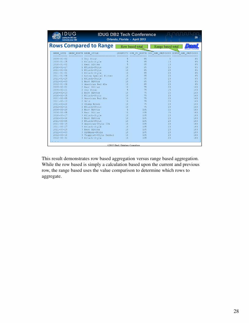
This result demonstrates row based aggregation versus range based aggregation.

While the row based is simply a calculation based upon the current and previous

row, the range based uses the value comparison to determine which rows to

aggregate.

28

This example is from the DB2 for LUW sample database. It uses aggregation to

calculate the average sale quantity company wide on a month-by-month basis. So, a

window is established for each month of sales, and the AVG function is used to

calculate the average sale quantity for each month. A SUM function is also used to

calculate total sales. There is no window specified for this total, but an aggregation

group has been specified designating an unbounded start (from the start of the

window) and the current row. This provides a running total of sales in the result.

A variety of functions, windows, and grouping can be specified to produce all sorts

of running values!

29

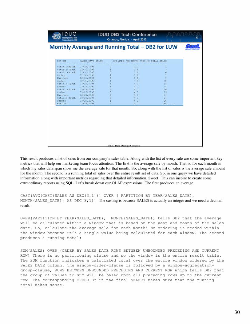
This result produces a list of sales from our company’s sales table. Along with the list of every sale are some important key

metrics that will help our marketing team focus attention. The first is the average sale by month. That is, for each month in

which my sales data span show me the average sale for that month. So, along with the list of sales is the average sale amount

for the month. The second is a running total of sales over the entire result set of data. So, in one query we have detailed

information along with important metrics regarding that detailed information. Sweet! This can inspire to create some

extraordinary reports using SQL. Let’s break down our OLAP expressions: The first produces an average

CAST(AVG(CAST(SALES AS DEC(3,1))) OVER ( PARTITION BY YEAR(SALES_DATE),

MONTH(SALES_DATE)) AS DEC(3,1)) The casting is because SALES is actually an integer and we need a decimal

result.

OVER(PARTITION BY YEAR(SALES_DATE), MONTH(SALES_DATE)) tells DB2 that the average

will be calculated within a window that is based on the year and month of the sales

date. So, calculate the average sale for each month! No ordering is needed within

the window because it’s a single value being calculated for each window. The second

produces a running total:

SUM(SALES) OVER (ORDER BY SALES_DATE ROWS BETWEEN UNBOUNDED PRECEDING AND CURRENT

ROW) There is no partitioning clause and so the window is the entire result table.

The SUM function indicates a calculated total over the entire window ordered by the

SALES_DATE column. The window-order-clause is followed by a window-aggregation-

group-clause, ROWS BETWEEN UNBOUNDED PRECEDING AND CURRENT ROW Which tells DB2 that

the group of values to sum will be based upon all preceding rows up to the current

row. The corresponding ORDER BY in the final SELECT makes sure that the running

total makes sense.

30

This query is valid on both DB2 for z/OS and DB2 for LUW. It takes the time

recorded by employees working on projects and calculates the average time entry

quantity recorded each month, as well as the running total of all time recorded.

31

32

OLAP processing can be a performance gain or a detriment to performance. As with

anything else the query performance is relative to the task accomplished and the

alternatives to accomplishing the same tasks by other means:

1. All data returned and program loops

2. Multiple queries issued by the program each collecting a different value

3. Using more traditional SQL, including grouping, subqueries, table expressions,

etc.

4. The portability of the report process (some programming languages might not

be very portable across platforms)

5. The amount of time it takes to code the solution

For OLAP expressions themselves there are potentially big workfile and sort

consumers within DB2. So, you need to make sure that there are adequate shared

resources (workfile, CPU, I/O) to handle the OLAP queries. Using the EXPLAIN

facility and running benchmarks are critical to understanding the impact of OLAP

processing.

33

This explain (DB2 for z/OS) shows a relatively simple OLAP query and two sorts

and workfiles allocated in support of the query. One sort is in support of the OLAP

expression and the second is to order the result set.

Be mindful of the fact that on DB2 for z/OS workfiles are allocated as needed, but

are not released until the query terminates (except for child tasks in parallel queries)

so workfile utilization can be significant. On DB2 for LUW they workfiles can be

truncated when no longer needed, as controlled by the

DB2_SMS_TRUNC_TMPTABLE_THRESH environment variable. As additional

OLAP expressions are added to a query, additional sorts and workfile allocations

will occur.

34

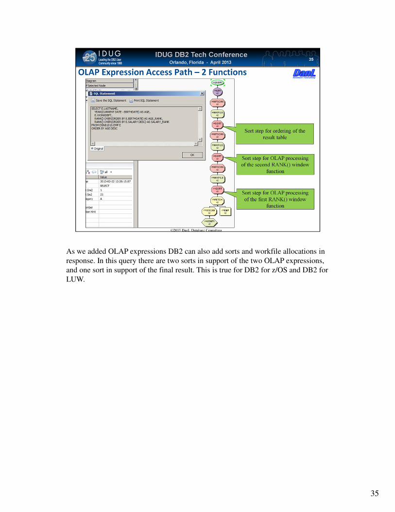
As we added OLAP expressions DB2 can also add sorts and workfile allocations in

response. In this query there are two sorts in support of the two OLAP expressions,

and one sort in support of the final result. This is true for DB2 for z/OS and DB2 for

LUW.

35

OLAP processing cannot only be a choice for business analytics and reporting, but

could also be a potential performance improvement for OLTP and/or batch

transaction processing. In this example here we can see two queries that return the

most recent accounting history record for a history table. The original query uses a

correlated subquery to find the most recent row for each primary key. Since there is

no filtering by key value then the entire table is processed and the correlated

subquery executed for each row in the history table. In comparison, the equivalent

OLAP query in a nested table expression is used to read the entire table once and

rank the rows. Subsequent filtering returns the same result as the correlated

subquery example. Which is the better performer? Well, that depends of course, but

in this example the OLAP query was a significant performance improvement over

the subquery.

36

Here is an example of the same situation using the DB2 sample database. The

queries are finding the oldest employee in each department, one via correlated

subquery and the other using OLAP.

37

An EXPLAIN of the subquery solution shows the execution of the correlated

subquery in a separate query block. This separate query block is executed once per

row processed in the outer portion of the query (query block one), but no sorts or

workfiles are utilized.

38

An EXPLAIN of the OLAP based solution shows two query blocks, but in this case

there is only a single execution of each block. The second query block shows the

table being read and sorted to perform the OLAP processing. The first query block

shows the workfile being read to produce the final result.

Which is better? I don’t know! Try them both, explain them, and benchmark them.

The thing to keep in mind is exactly how much data is being processed. If a lot of

data is going to be processed and there is little or no filtering then the OLAP

solution may be better provided there are adequate workfile resources available. If

there is significant filtering of the data in the outer portion of the query and/or

workfile availability is limited, then the subquery solution should be better given

appropriate indexing.

39

Here is another great example of using the power of OLAP processing to retrieve

some sample data. In this particular case a sample of employee data is desired base

upon certain rules. The rule applied here is that a sample of two employees per

department is desired. Rather than running a series of queries or a single query with

complicated subqueries, only one OLAP query can be used to get the desired result.

40

OLAP processing in DB2 is extremely powerful, and an important tool that can be

utilized quickly to perform complex data analytics. The OLAP specification takes

some time to get used to, and so you need to reserve some time for programmer

education and experimentation. Once this knowledge is acquired this type of

processing can be used to quickly answer complex business questions, but can also

be a performance advantage for certain types of reports. This is especially true in

situations where several queries can be replaced by a single query.

41

Dan Luksetich is a senior DB2 DBA consultant. He works as a DBA, application

architect, presenter, author, and teacher. Dan has been in the information technology

business for over 28 years, and has worked with DB2 for over 23 years. He has been

a COBOL and BAL programmer, DB2 system programmer, DB2 DBA, and DB2

application architect. His experience includes major implementations on z/OS, AIX,

i Series, and Linux environments. Dan's experience includes: Application design

and architecture, database administration, complex SQL, SQL tuning, DB2

performance audits, replication, disaster recovery, stored procedures, UDFs, and

triggers. Dan works everyday on some of the largest and most complex DB2

implementations in the world. He is a certified DB2 DBA, system administrator,

and application developer, and has worked with the teams that have developed

several DB2 for z/OS certification exams. He is the author of several DB2 related

articles as well as co-author of the DB2 9 for z/OS Certification Guide and the DB2

10 for z/OS Certification Guide.

42