arX

iv:c

ond-

mat

/041

0772

v1 [

cond

-mat

.sta

t-m

ech]

29

Oct

200

4

Numerical Study of the Cahn-Hilliard Equation in One, Two and

Three Dimensions

E. V. L. de Mello

Instituto de Fısica,

Universidade Federal Fluminense,

Niteroi, RJ 24210-340, Brazil

Otton Teixeira da Silveira Filho

Instituto de Computacao,

Universidade Federal Fluminense,

Niteroi, RJ 24210-340, Brazil

(Dated: February 2, 2008)

Abstract

The Cahn-Hilliard equation is related with a number of interesting physical phenomena like the

spinodal decomposition, phase separation and phase ordering dynamics. On the other hand this

equation is very stiff an the difficulty to solve it numerically increases with the dimensionality

and therefore, there are several published numerical studies in one dimension (1D), dealing with

different approaches, and much fewer in two dimensions (2D). In three dimensions (3D) there are

very few publications, usually concentrate in some specific result without the details of the used

numerical scheme. We present here a stable and fast conservative finite difference scheme to solve

the Cahn-Hilliard with two improvements: a splitting potential into a implicit and explicit in time

part and a the use of free boundary conditions. We show that gradient stability is achieved in one,

two and three dimensions with large time marching steps than normal methods.

PACS numbers: 64.75.+g, 02.30.Jr, 02.70.Bf, 74.80.-g

1

I. INTRODUCTION

The theory of the phase-ordering dynamics following a rapid cooling down (or quenching)

through the critical temperature from a homogeneous or disordered phase into an inhomo-

geneous or ordered state has been studied for decades[1, 2, 3, 4]. This phenomenon is

known as spinodal decomposition. Part of the fascination of the field is because the or-

dering does not occur instantaneously. Instead, a network of domains of the equilibrium

phases develops, and the typical length scale associated with these domains increases with

the time. In order words, the length scale of the ordered regions growth with time as the

different (broken-symmetry) phases compete in order to achieve the equilibrium state. One

of the leading models devised for the theoretical study of this phenomenon is based on the

Cahn-Hilliard formulation[5]. The Cahn-Hilliard (CH) theory was originally proposed to

model the quenching of binary alloys through the critical temperature[5] but it has subse-

quently been adopted to model many other physical systems which go through a similar

phase separation[2, 3, 4].

Recently it has been discovered that high critical temperature superconductors have

an intrinsic inhomogeneous phase which exhibit patternings which involve nanoscale re-

gions of phase separations, often referred as stripes as revealed by neutron diffraction

studies[6] and EXAFS[7]. Similar findings were measured by very fine scanning tunnel-

ing microscopy/spectroscopy (STM/S) data[8, 9] which have shown the local charge and the

superconducting gap spatial variation through the differential conductance. The ubiquity

of such intrinsic inhomogeneities, as well as the importance of the materials that exhibit

them has motivated intense experimental and theoretical research into the details of the

phenomena[10, 11, 12, 13, 14]. Recently a theory of the critical field Hc2 based on a distri-

bution of superconducting regions with different critical temperatures due to these intrin-

sic inhomogeneities has explained some nonconventional features of current data on some

cuprates[15]. The manganites which exhibit a colossal magnetoresistance have also some

properties which may be linked with clusters formation upon cooling or an intrinsic phase

separation[16, 17]. Researches on these materials are currently been investigated by a sizable

fraction the condensed matter community. Therefore, studies based on the CH equation may

be useful to understand the puzzle of the origins of such intrinsic phase separation in these

materials and how it affects their physical properties. Here we want to study specifically

2

the Cahn-Hilliard equation and we will deal with the problem of phase separation in high-Tc

superconductors in another publication.

In an alloy system composed by a binary mixture we can define the local phase variable

u(~x) as the difference in concentration between the two (incompressible) components or

simply, the concentration of one of the components over the domain Ω (~x ∈ Ω) which

represents the system. It is clear that this type of phase variable or order parameter is always

conserved for an isolated system and we will use below this property as the main guide for

our numerical method. In the CH theory, the time variation of the order parameter u(~x, t) is

given in terms of the functional derivative of a time-dependent free-energy functional F (u)

leading to an equation of motion to diffusive transport of the order parameter, namely

∂u

∂t= M∇2

δf

δu(1)

where f is the free-energy density and the (constant) mobility M will hereafter be absorbed

into the time scale although there are cases in which the mobility can be a function of the

position[18]. The free-energy functional is assumed, to most of the physical applications, to

follow the Ginzburg-Landau (GL) form:

f =1

2ε2|∇u|2 + V (u) (2)

where the potential V (u) may have a double-well structure like, for instance, V (u) = (u2 −

1)2/4 as many authors have used[19, 20, 21, 22] and, for the sake of comparison with

these previous works, we will adopt it below. There are other possibilities like V (u) =

au2/2 + bu4/4 + ... which is more convenient for physical applications since, usually the

GL free energy is a power expansion in u with coefficients (a, b, ...) which depend on

the temperature, the applied field, and on other physical properties. It is easy to see that

the above double well potential will favor two phases with densities u = ±1. If one uses a

potential with three minima, it will appear three major phases and so on. Bray[4] pointed out

that one can explore the fact that the order parameter is conserved and the CH equation can

be written in the form of a continuity equation, ∂tu = −∇.J, with the current J = ∇(δf/δu).

Therefore we may write the CH equation as following,

∂u

∂t= −∇2(ε2∇2u + u − u3) (3)

Normally, 0 < ε ≪ 1 because the fourth derivative term requires a large stencil and it is

related with the size of the interface between regions of two different phase. To accurately

3

resolve these interfaces a fine space discretization ∆x is necessary. The linear term is re-

sponsible for the interesting dynamics including the instability of constant solutions near

u = 0 and the nonlinear term is the one which mainly stabilizes the flow[19]. As it has

already been pointed out[19, 20, 21, 22], both the ∇4 and the nonlinear term make the CH

equation very stiff and it is difficult to solve it numerically. The nonlinear term in principle,

forbids the use of common Fast Fourier Transform (FFT) methods and brings the additional

problem that the usual stability analysis like von Newmann criteria cannot be used. These

difficulties make most of the finite difference schemes to use time steps of many order of

magnitude smaller than ∆x and consequently, it is numerical expensive to reach the time

scales where the interesting dynamics occur. This is the reason why numerical simulations

based on Runge-Kutta schemes had to be performed in large supercomputers[23, 24].

In order to deal with such restrictions, Eyre developed a semi-implicit method[19] which

resolves the problems associated with both the stiffness and solvability. Furthermore Eyre

proved that his algorithms are unconditionally gradient stable for the CH and also for the

Allen-Cahn equation, which means that the free energy does not increase with time. Both

gradient stability and the conservation of mass provide us with a simple and rational form

to establish the stability criterion for the CH equation that replaced the von Neumann

stability criteria. Furthermore, mostly either finite difference calculations[23, 24] or Monte

Carlo simulations[25] uses periodic boundary conditions as a tentative to mimic a large

system and we show here that, as concerns phase separation, that free boundary conditions

are less stiff and more faster achieved.

The goal of this paper is to make a combinations of a systematic study of the CH equation

in 1D, 2D and 3D using a simplification of the Eyre’s method and free boundary conditions.

To give a better perspective to the approach, we make also calculations with a Crank-

Nicholson like (CN) implicitly scheme[26], which is unconditionally convergent in 1D and,

using the concept of alternating direction interaction (ADI) method[26, 27], in 2D. These

calculations demonstrate the advantage of the Eyre’s method over the CN scheme. Therefore

we apply Eyre’s method in 3D and study the phenomenon of spinodal decomposition in three

dimensions. The application to the high Tc superconductors and manganites with the study

of the relevant parameters to their phase diagrams is under current investigation and will

be discussed in a future work.

4

II. THE PROPERTIES OF THE CAHN-HILLIARD EQUATION

In order to solve numerically Eq.(3) by means of a finite difference scheme, we need an

initial condition over the entire domain, u(~x, 0), which usually is a random function or some

small fluctuations over a specific average and also some type of boundary conditions (BCs).

During our simulations we have found that these initial conditions, the BCs and the size of

the system greatly influence the solution u(~x, t). The general convenient and flux-conserving

boundary conditions are[20]

∇u.~n|~x∈∂Ω = (∇3u).~n|~x∈∂Ω = 0 (4)

where ~n is the outward normal vector on the boundary of the domain Ω which we represent

by ∂Ω. These two equations together are equivalent to

∇(δf/δu)~x∈∂Ω = 0. (5)

These BCs lead to the two very important properties which will be our guide to know

whether our CH numerical solutions are convergent, namely, the conservation of the total

mass of the system Mt;

d

dtMt =

d

dt

∫

Ω

u(~x, t)d~x =

∫

Ω

∂u(~x, t)

∂td~x

=

∫

Ω

∇2 δf

δud~x =

[

∇δf

δu

]

~x∈∂Ω

= 0 (6)

and the dissipation or decrease of the total energy F ;

d

dtF (u) =

d

dt

∫

Ω

f(u(~x, t))d~x =

∫

Ω

δf

δu

∂u(~x, t)

∂td~x

= −

∫

Ω

[

∇δf

δu

]2

d~x ≤ 0 (7)

This last equation shows that appropriate solutions of the CH equation must dissipate

energy and this is called gradient flow. Therefore a time stepping finite difference scheme is

defined to be gradient stable only if the free energy F (u) does not increase with the time,

i.e., obeys Eq.(7). Since it is not convenient to use the von Neumann stability analysis,

gradient stability is regarded as the best stability criterion for finite difference numerical

solutions of the CH equation [22]. Furthermore, unconditional gradient stability means that

the conditions for gradient stability is satisfied for any size of time step and this will be

5

our guide through the simulations. This way to examine the stability of a central difference

scheme by following the energy was already proposed to nonlinear problems a long time ago

by Park[28]. We should mention that a similar analysis, based also on the Eyre’s approach,

performing numerical tests of stability and with a very complete classification scheme for the

stable values of ∆t for the CH and Allen-Cahn equation in 2D was recently developed[22].

III. THE DISCRETIZATION METHOD

Eyre has proposed a semi-implicit method that is unconditional gradient stable if the V (u)

is the usual two minima potential used in a typical GL free energy and can be divided in

two parts: V (u) = Vc(u)+Ve(u) where Vc is called contractive and Ve is called expansive[19].

He showed that it is possible to achieve unconditional gradient stability if one treats the

contractive part implicitly and the expansive part explicitly. In our case, since we are using

V (u) = (u2 − 1)2/4, we have:

Vc(u) =u4 + 1

4and Ve(u) = −

u2

2.

To implement Eyre’s scheme we define Unijk(i, j, k = 1, 2, ..., N ; n = 0, 1, 2, ...) to be the

approximation to u(~x, t) at location x = ih, y = jh, z = kh and t = nK, where h = ∆x =

∆y = ∆z, K = ∆t and N = L/∆x. L is the linear size of the system, assuming to be cubic,

for simplicity. With these definitions, we can write the method for the CH equation as

Un+1

ijk − Unijk

K= −ε2∇4Un+1

ijk + ∇2(

(Un+1

ijk )3 − Unijk

)

. (8)

In this equation the standard centered difference approximation of the 3D Laplacian operator

∇2 is

∇2Unijk =

(

Uni+1jk + Un

ij+1k + Unijk+1 − 6Un

ijk + Uni−1jk + Un

ij−1k + Unijk−1

)

/h2 (9)

which is second order in the spatial step h. The Eq.(8) represents a large coupled set

of nonlinear equations due to the cubic term. The way to go around this problem is to

splitting or to linearize it at every time step. Consequently the term (Un+1

ijk )3 is transformed

into (Unijk)

2Un+1

ijk leading the Eq.(8) into a set of linear equations in the step of time n+1. It

has been argued that this nonlinear splitting has the smallest local truncation error[19, 22]

6

and therefore it will be the scheme adopted in this work. Then we finally obtain the proposed

finite difference scheme for the CH equation which is linear (in the above sense), namely,

Un+1

ijk − Unijk

K= −ε2∇4Un+1

ijk + ∇2(

(Unijk)

2Un+1

ijk − Unijk

)

. (10)

or, separating in different times to see the semi-implicit character of the approach,

Un+1

ijk + K(ε2∇4Un+1

ijk + ∇2(Unijk)

2Un+1

ijk ) = Unijk − K∇2Un

ijk. (11)

As noted by Furihata et al[20], the discrete associated boundary conditions equivalent to

Eq.(4), second order in the spatial variable, become

Un1jk = Un

5jk , Un2jk = Un

4jk (12)

UnNjk = Un

N−4jk , UnN−1jk = Un

N−3jk (13)

and similar equations for the boundary conditions over the second and third indices repre-

senting the y and z-directions, respectively. Notice that, differently than most numerical

simulations applied to physical systems[29], these boundary conditions are not periodical.

Imposing periodical BCs which is common in physical applications and which is largely used

to artificially simulate a larger system, would bring additional constraint to the solutions

and, as we show below, the solutions will be more stiff. Therefore the above boundary

conditions minimize the finite size effects and should be preferably used as shown below.

The Eq.(11) with the above boundary conditions define the finite difference scheme which

we use in this present work. In the following section, we analyze the numerical results and

compare with different CN semi-implicit approaches for several dimensions with the same

double-well potential.

IV. THE RESULTS OF THE SIMULATIONS

We start with the study of the CH equation in 1D because it is faster then 2D and 3D

and there are many results which can be used to compare with our simulations. The usual

semi-implicit and explicit Euler’s schemes for the 1D CH equation are not gradient stable

and require very short time intervals ∆t = K, while the implicit Euler’s scheme is gradient

stable with K ≤ h2/4 = 6.25 × 10−6 [19, 21, 30]. The CN-like scheme that we will use

7

for comparison also suffers from this solvability restriction, and requires a minimum time

interval K ≤ h2/9.

We performed calculations with linear chains of N = 54, 104 and 504 sites and with

∆x = h = 1/(N − 4), and 0 ≤ x ≤ 1. For all these cases we used K = h/2 which is clearly

several order of magnitude larger than typical Euler’s schemes and, despite this large time

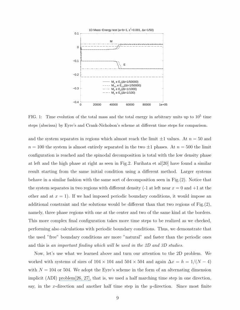
step, the gradient stability is observed at all times. In Fig.1 we show the results for the

total mass and the free energy F in arbitrary units as function of the running time. In fact,

using shorter times as shown in Fig.1, we observe that there is an initial transient period in

the time evolution before gradient stability is achieved. This can be easily seen at at most

small values of ∆t in Fig.1 for either Eyre’s or CN-like methods. This transient before the

stability takes place is connected to the finite size of the system, the initial conditions and

the BCs.

As already mentioned, in order to compare our calculations based on Eyre’s method with

other schemes, we have also performed similar simulations with a widely used method[19, 21],

a semi implicit CN-like scheme[26, 30]. Briefly, the CN method consists in an average of the

right hand side of Eq.(3) at different times: 1/2 at n and 1/2 at n+1 what clearly results in

a semi-implicit scheme in time. According to the above formula, for h = 1/50, this scheme

will converge for K ≤ 1/(2500 × 9) ≈ 1/20000). Indeed we can see in Fig.1 that the CN

simulations agree very well with the the Eyre’s results for the case with K = 1/50000 and a

similar transient period before the stability is achieved is observed. To compare with other

studies which use the same parameters for the CH equation, we used an initial condition for

the linear chain similar to one used by Furihata et al[20], namely,

U0i = 0.1sin(2.π(i − 3)h) + 0.01cos(4π(i− 3)h)

+0.06sin(4π(i − 3)h) + 0.02cos(10π(i− 3)h) (14)

for 3 ≤ i ≤ N − 2 and U0i = 0.03 otherwise (at the borders). This function is shown in

Fig.(2).

Now that the parameters which gradient stability is established in our system, we study

the process of spinodal decomposition in 1D starting with the initial condition given by

Eq.(14). Using the long time step ∆t = 1/100, we see for the different Uni time profile in

Fig.2, that at very few time evolution (n = 5) the system shows a tendency to decompose

in one high and other low density phases. At n = 10 the difference in densities increases

8

0 20000 40000 60000 80000 1e+05−0.4

−0.3

−0.2

−0.1

0

0.11D Mass−Energy test (a=b=1, ε2

=0.001, ∆x=1/50)

ME e EE(∆t=1/50000)MCN e ECN(∆t=1/50000)ME e EE(∆t=1/1000)ME e EE(∆t=1/100)

M

E

FIG. 1: Time evolution of the total mass and the total energy in arbitrary units up to 105 time

steps (abscissa) by Eyre’s and Crank-Nicholson’s scheme at different time steps for comparison.

and the system separates in regions which almost reach the limit ±1 values. At n = 50 and

n = 100 the system is almost entirely separated in the two ±1 phases. At n = 500 the limit

configuration is reached and the spinodal decomposition is total with the low density phase

at left and the high phase at right as seen in Fig.2. Furihata et al[20] have found a similar

result starting from the same initial condition using a different method. Larger systems

behave in a similar fashion with the same sort of decomposition seen in Fig.(2). Notice that

the system separates in two regions with different density (-1 at left near x = 0 and +1 at the

other and at x = 1). If we had imposed periodic boundary conditions, it would impose an

additional constraint and the solutions would be different than that two regions of Fig.(2),

namely, three phase regions with one at the center and two of the same kind at the borders.

This more complex final configuration takes more time steps to be realized as we checked,

performing also calculations with periodic boundary conditions. Thus, we demonstrate that

the used ”free” boundary conditions are more ”natural” and faster than the periodic ones

and this is an important finding which will be used in the 2D and 3D studies.

Now, let’s use what we learned above and turn our attention to the 2D problem. We

worked with systems of sizes of 104 × 104 and 504 × 504 and again ∆x = h = 1/(N − 4)

with N = 104 or 504. We adopt the Eyre’s scheme in the form of an alternating dimension

implicit (ADI) problem[26, 27], that is, we used a half marching time step in one direction,

say, in the x-direction and another half time step in the y-direction. Since most finite

9

0 0.2 0.4 0.6 0.8 1−1

−0.5

0

0.5

1U(t) (a=1, b=1, ε2=0.001, ∆t=1/100 ∆x=1/50)

t=0t=5∆tt=10∆tt=50∆tt=100∆tt=500∆t

FIG. 2: The time evolution of the profile of Uni for different times starting at the initial condition

(t = 0) till the total spinodal decomposition is attained at n = 500. The size of the system is

L = 1.

difference methods for partial differential equations like the diffusion or heat equation in 2D

uses the Crank-Nicholson scheme[26, 27], we again made simulations with this scheme which

is appropriate to be used in connection with the ADI[26, 27, 31].

In Fig.3 we plot the results for the 2D mass and energy in arbitrary units. We used

ε = 0.01 which is slightly bigger than the 1D value in order to have larger phase domains

and we kept the other parameters equal. The initial conditions were chosen to be small

variation around the average value Unij = 0.5 although variation around zero give the same

type of result. Thus the initial condition is

U0ij = 0.5 + εsin(π(i − 3)20h)sin(π(j − 3)20h) (15)

for i, j toward the middle and with U0ij = 0.5 toward the boundaries of our square systems.

The choice of a different initial condition than U0ij = 0 is to brake the symmetry and, in

this way, better identify the formation of the two ±1 density phases (see Fig.(4) below).

Studying the stability conditions, we see that the 2D system requires smaller values of ∆t

than the 1D system. This is because the boundaries are much larger in 2D and the possibility

to mass and energy flow is greatly enhanced and the instability during the initial transient

period is larger. For instance, the initial instabilities in the 504× 504 is even bigger than in

the 104 × 104 system.

10

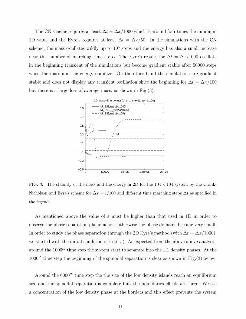
The CN scheme requires at least ∆t = ∆x/1000 which is around four times the minimum

1D value and the Eyre’s requires at least ∆t = ∆x/50. In the simulations with the CN

scheme, the mass oscillates wildly up to 105 steps and the energy has also a small increase

near this number of marching time steps. The Eyre’s results for ∆t = ∆x/1000 oscillate

in the beginning transient of the simulations but become gradient stable after 50000 steps

when the mass and the energy stabilize. On the other hand the simulations are gradient

stable and does not display any transient oscillation since the beginning for ∆t = ∆x/100

but there is a large loss of average mass, as shown in Fig.(3).

0 50000 1e+05 1.5e+05 2e+05−0.5

−0.3

−0.1

0.1

0.3

0.5

0.7

0.9

2D Mass−Energy test (a=b=1, ε=0.01, ∆x=1/100)

ME & EE(∆t=∆x/1000)MCN & ECN(∆t=∆x/1000)ME & EE(∆t=∆x/100)

E

M

FIG. 3: The stability of the mass and the energy in 2D for the 104 × 104 system by the Crank-

Nicholson and Eyre’s scheme for ∆x = 1/100 and different time marching steps ∆t as specified in

the legends.

As mentioned above the value of ε must be higher than that used in 1D in order to

observe the phase separation phenomenon, otherwise the phase domains become very small.

In order to study the phase separation through the 2D Eyre’s method (with ∆t = ∆x/1000),

we started with the initial condition of Eq.(15). As expected from the above above analysis,

around the 1000th time step the system start to separate into the ±1 density phases. At the

1000th time step the beginning of the spinodal separation is clear as shown in Fig.(3) below.

Around the 6000th time step the the size of the low density islands reach an equilibrium

size and the spinodal separation is complete but, the boundaries effects are large. We see

a concentration of the low density phase at the borders and this effect prevents the system

11

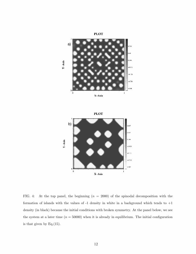
FIG. 4: At the top panel, the beginning (n = 2000) of the spinodal decomposition with the

formation of islands with the values of -1 density in white in a background which tends to +1

density (in black) because the initial conditions with broken symmetry. At the panel below, we see

the system at a later time (n = 50000) when it is already in equilibrium. The initial configuration

is that given by Eq.(15).

12

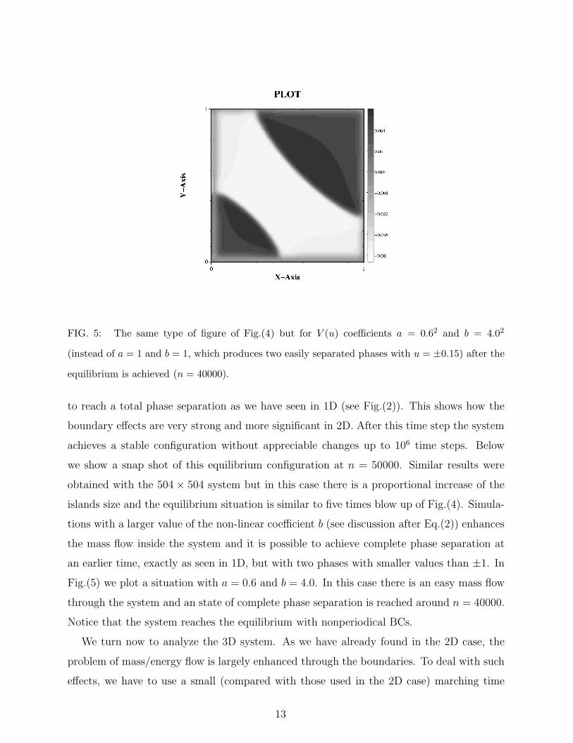
FIG. 5: The same type of figure of Fig.(4) but for V (u) coefficients a = 0.62 and b = 4.02

(instead of a = 1 and b = 1, which produces two easily separated phases with u = ±0.15) after the

equilibrium is achieved (n = 40000).

to reach a total phase separation as we have seen in 1D (see Fig.(2)). This shows how the

boundary effects are very strong and more significant in 2D. After this time step the system

achieves a stable configuration without appreciable changes up to 106 time steps. Below

we show a snap shot of this equilibrium configuration at n = 50000. Similar results were

obtained with the 504 × 504 system but in this case there is a proportional increase of the

islands size and the equilibrium situation is similar to five times blow up of Fig.(4). Simula-

tions with a larger value of the non-linear coefficient b (see discussion after Eq.(2)) enhances

the mass flow inside the system and it is possible to achieve complete phase separation at

an earlier time, exactly as seen in 1D, but with two phases with smaller values than ±1. In

Fig.(5) we plot a situation with a = 0.6 and b = 4.0. In this case there is an easy mass flow

through the system and an state of complete phase separation is reached around n = 40000.

Notice that the system reaches the equilibrium with nonperiodical BCs.

We turn now to analyze the 3D system. As we have already found in the 2D case, the

problem of mass/energy flow is largely enhanced through the boundaries. To deal with such

effects, we have to use a small (compared with those used in the 2D case) marching time

13

step of ∆t = ∆x/10000 with ∆x = 1/100 for the (104)3 system to minimize errors in the

derivatives near the boundaries. Notice that this time step is much smaller than the one in

1D and one-two orders of magnitude smaller than in 2D. This is small but still feasible to

reach the interesting dynamics even in a typical PC of 1GHz. Since Eyre’s method is very

efficient and faster than the majority of other methods used in 3D, this is the only approach

that we used in 3D. The generalization of basic Euler or Runge-Kutta methods to the CH

equation in 3D are much more slower, and we can see why there are very few studies of the

CH equation in 3D. Indeed the values of ∆t ≈ 10−6 used in our 3D simulations are of the

same order of magnitude of typical Euler’s method[19, 21, 30] used in 1D simulation as we

discussed in the beginning of this section. The adopted initial condition for the 3D system

is:

U0ijk = 0.01 + εsin(π(i − 3)20h)sin(π(j − 3)20h)sin(π(k − 3)20h). (16)

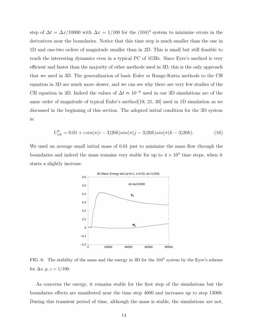
We used an average small initial mass of 0.01 just to minimize the mass flow through the

boundaries and indeed the mass remains very stable for up to 4 × 104 time steps, when it

starts a slightly increase.

0 20000 40000 60000 80000−0.2

−0.1

0

0.1

0.2

0.3

0.4

0.5

0.63D Mass−Energy test (a=b=1, ε=0.03, ∆x=1/100)

∆t=∆x/10000

EE

ME

FIG. 6: The stability of the mass and the energy in 3D for the 1043 system by the Eyre’s scheme

for ∆x, y, z = 1/100.

As concerns the energy, it remains stable for the first step of the simulations but the

boundaries effects are manifested near the time step 4000 and increases up to step 13000.

During this transient period of time, although the mass is stable, the simulations are not,

14

as one can conclude by the energy increase in this interval as shown in Fig.(6). After this

time interval (n ≈ 13000) the system stabilizes itself and remains gradient stable up to the

rest of the calculations (up to n = 80000) as can be seen by the decrease of the energy in

Fig.(6). Comparison with the 1D and 2D systems reveals clearly that the stability is more

difficult to be established as the dimensionality increases, as it is natural when one uses any

finite difference scheme. As Fig.(6) shows, the system relax from the initial conditions and

becomes uniform around n = 3000. Around n = 6000 a spinodal decomposition is happening

and the oscillation in the densities forms an almost uniform pattern as shown in the top

panel of Fig.(7). This figure shows the configuration of the middle plane in the z-direction

(k = 52) of the 104 × 104 × 104. At the down panel of Fig.(7) we show a snap-shot of

n = 8000 which shows the beginning of of the phase separation process as the time flows.

Above n = 20000 the two phases start to segregate and this segregation process is smooth

and unconditionally gradient stable as seen in Fig.(8).

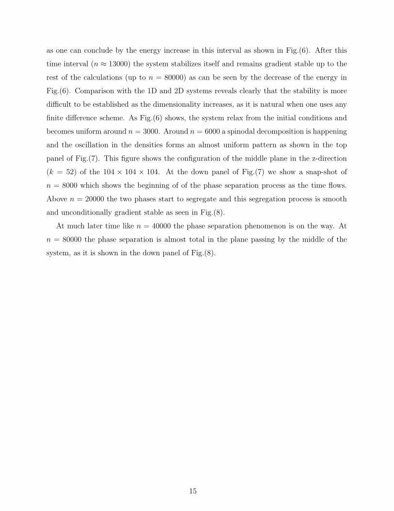
At much later time like n = 40000 the phase separation phenomenon is on the way. At

n = 80000 the phase separation is almost total in the plane passing by the middle of the

system, as it is shown in the down panel of Fig.(8).

15

FIG. 7: After relaxing from the initial condition (Eq.(16)), we show at the top panel the beginning

(n = 6000) of the spinodal decomposition with the formation of small islands with the ±1 values

because the initial condition with broken symmetry. At the down panel, the system at a later time

(n = 8000) during the process of phase separation.

16

FIG. 8: The continuation of Fig.(7) for many time steps later. On the top panel we plot the case

for n = 40000 and on the down panel the n = 80000.

V. CONCLUSION

We have shown in this work that the semi-implicit method due to Eyre, which divides the

potential V (u) in two parts and treats the contractive part implicitly and the expansive ex-

17

plicitly combined with free boundary conditions achieves unconditional gradient stability in

1D, 2D and 3D. The method also allows the use of very long marching time steps, compared

with usual explicit or implicit Euler’s schemes, what is convenient because it captures very

easily the short and long dynamics, characteristic of the Cahn-Hilliard equation. Our sim-

ulations have demonstrated that gradient stability and spinodal decomposition is achieved

faster than the normal Euler and Crank-Nicholson methods what is highly deseirable spe-

cially in 3D where normal methods fail to capture the long dynamics due to the required very

short time steps. The use of ”nonflow” free BCs are more appropriated and also converges

faster to a final equilibrium configuration than the widely used periodic BCs.

We believe that the present systematic study may be pertinent to the several branchs of

physics. The fast scheme developed here are suitable to the study of the spinodal dynamics

and also to high correlated electron systems with phase separation. We expect therefore, to

perform these works in the near future.

VI. ACKNOWLEDGMENT

We gratefully acknowledge partial financial aid from Brazilian agencies CNPq and

FAPERJ.

[1] I.M. Lifshitz and V.V.Slyozov, J. Phys. Chem. Solids 19, 35 (1961).

[2] P.C. Hohenberg and B.I Halperin, Rev. Mod. Phys. 49, 435 (1977).

[3] J.D. Gunton, M. San Miguel, and P.S. Sahni, in ”Phase Transitions and Critical Phenomena”

Vol. 8, edited by C. Domb and J.L. Lebowitz (New York, Academic Press, 1983).

[4] A.J. Bray, Adv. Phys. 43, 347 (1994).

[5] J.W. Cahn and J.E. Hilliard, J. Chem. Phys, 28, 258 (1958).

[6] J.M.Traquada, B.J. Sternlieb, J.D, Axe, Y. Nakamura, and S. Uchida, Nature (London),375,

561 (1995).

[7] A. Bianconi N. L Saini, A. Lanzara, M. Missori, T. Rossetti, H. Oyanagi, H. Yamaguchi, K.

Oka, T.Ito, Phys. Rev. Lett. 76, 3412 (1996).

[8] C. Howald, P. Fournier, and A. Kapitulnik, Phys. Rev. B64, 100504 (2001).

18

[9] S. H. Pan, J. P. ONeal, R. L. Badzey, C. Chamon, H. Ding, J. R. Engelbrecht, Z. Wang, H.

Eisaki, S. Uchida, A.K. Gupta, K. W. Ng, E. W. Hudson, K. M. Lang, J. C. Davis Nature,

413, 282-285 (2001) and cond-mat/0107347.

[10] Yu.N. Ovchinnikov, S.A. Wolf, V.Z. Kresin, Phys. Rev. B63, 064524, (2001), and Physica

C341-348, 103, (2000).

[11] E.V.L. de Mello, M.T.D. Orlando, E.S. Caixeiro, J.L. Gonzalez, and E. Baggio-Saitovich,

Phys. Rev. B66, 092505 (2002).

[12] D. Mihailovic, V.V. Kabanov, K.A. Muller, Europhys. Lett. 57, 254 (2002).

[13] E.V.L. de Mello, E.S. Caixeiro, and J.L. Gonzalez, Phys. Rev. B67, 024502 (2003).

[14] See several articles in ”Proceedings of the Workshop on Intrinsic Multiscale Structure and

Dynamics of Complex Eletronic Oxides”, I.C.T.P., A.R. Bishop, S.R. Shenoy, and S. Sridhar,

Eds., World Scientific, New Jersey (2002).

[15] E.S. Caixeiro, J.L. Gonzalez, and E.V.L. de Mello. Phys. Rev. B69, 024521 (2004).

[16] E. Dagotto, T. Hotta and, A. Moreo, Phys. Rep. 344, 1 (2001).

[17] E. Dagotto, J. Burgy, A. Moreo, Sol. St. Comm. 126, 9, (2003).

[18] J.S Kim, K. Kang and J.S. Lowengrub, ”Conservative multigrid methods for Cahn-Hilliard

fluids”, J. Comput. Phys. In press

[19] D.J. Eyre, ”Unconditionally gradient stable time marching the Cahn-Hilliard equation”

preprint, (1998), and ”An Unconditional stable one-step scheme for gradient systems”

(http://www.math.utah.edu∼eyre/research/methods/stable.ps) (1998).

[20] D. Furihata and T. Matuso, RIMS Preprint no.1271, Kyoto University, (2000).

[21] C.M. Elliot and D.A. French, IMA J. Appl. Math, 38, 97 (1987)

[22] B.P. Vollmayr-Lee and A.D. Rutenberg, cond-mat/0308174, (2003).

[23] A. Chakrabarti, R. Toral, J.D. Gunton, and M. Muthukumar, Phys. Rev. Lett. 63, 2072

(2001).

[24] R. Toral, A. Chakrabarti and J.D. Gunton, Phys. Rev.A45, R2147 (1992).

[25] A. Milchev, D.W. Heermann, and K. Binder, Acta Metal 36, 377 (1988).

[26] W.F. Ames, ”Numerical Methods for Partial Differential Equations”, Academic Press, New

York (1977).

[27] J. Douglas Jr., R. Duran and P. Pietra, in ”Numerical Approximation of Partial Differential

Equations”, E. Ortiz, ed., North-Holland, Amsterdam (1987).

19

[28] K.C. Park in ”Computer and Structure”, Vol.7, pp 343-353, Pergamon Press, London (1977).

[29] J. Wang, D.Y. Xing, J. Dong and P.H. Hor, Phys. Rev. B62, 9827 (2000).

[30] J.H. Mathews, ”Numerical Methods for Mathemathics, Science, and Engineering”, Prentice

Hall, Englewood Cliffs, N.J. (1992).

[31] C.E. Elliot in ”Mathematical Models for Phase Change Problems”, J.F. Rodriguez Ed.,

Birkhauser Verlag, Basel (1989).

20