!∀#!#∀ ∃∀!%&!∀∋∀()!∗& ∃%∋&∀∗+

,∀−∃!(

∃+. /

01!∃!∀203!(∋∀2 0∃!∃20(20∋∋∃20∃(∋∃4%%

!∀# ∃%&∋%∋%%&()∗∃%&∋%∋+&

5

,−. /0 1.−2,/

,./.,3..,.,1∀4350

6 ∀7,, 8 ::;. 3 <.. 3 =3> 3 < 3 ?43 3

:..30037−>.3..,..4,4,;>..−.:,.;

3;40>3,4..37..;.≅3,,,−:;;,3−.;

Numerical simulation of drug eluting coronary

stents: mechanics, fluid dynamics and drug release

P. Zunino♯, C. D’Angelo♯, L. Petrini⋄, C. Vergara∗, C. Capelli⋄, F. Migliavacca⋄

December 21, 2007

♯ Modelling and Scientific Computing (MOX),

Department of Mathematics,

Politecnico di Milano, Italy∗ Department of Information Technology and Mathematical Methods,

Universita degli Studi di Bergamo, Italy⋄ Laboratory of Biological Structure Mechanics (LaBS),

Department of Structural Engineering,

Politecnico di Milano, Italy

Abstract

Mathematical models and numerical methods have emerged as funda-

mental tools in the investigation of life sciences. In particular, this is the case

of medical devices as cardiovascular drug eluting stents where experimen-

tal/clinical evidence may often be very expensive and extremely variable.

We present here a complete overview of mathematical models and numerical

methods applied to the modelling of drug eluting stents and of their interac-

tion with the coronary arteries. This is a challenging task because it involves

mechanics, fluid dynamics and mass transfer processes. In particular, we will

focus on the importance of the interplay between all these factors to deter-

mine the efficacy of the device.

Keywords: mechanical analysis, blood flow, mass transfer, coupled problems,

finite elements, medical devices

1 Introduction

A stent is a small mesh tube that is inserted permanently into a stenotic artery. The

stent restores the original value of the arterial section to ensure the physiological

1

flow rate. One of the problems caused by the stent insertion is the re-narrowing of

the treated vessel. To overcome this phenomenon drug-eluting stents (DES) have

been recently introduced. Referred to as a coated or medicated stent, a DES is a

normal metal stent that has been coated with a pharmacologic agent (drug) that is

known to interfere with the process of restenosis (reblocking). However, the design

of such devices is a very complex task because their performance in widening the

arterial lumen and preventing further restenosis is influenced by many factors such

as the geometrical design of the stent, the mechanical properties of the materials

and the chemical properties of the drug that is released. Mathematical models and

numerical simulation techniques are appropriate to study such phenomena with the

aim to be used as a predictive tool for the effective design of drug eluting stents.

We present in this work a complete review of the mechanics, fluid dynamics

and drug release models developed by the authors for the numerical simulation of

drug eluting coronary stents. In particular, we will focus on the importance of the

interplay between several factors, as the mechanical action exerted by the stent on

the wall to determine the final configuration of the artery, as well as the interaction

of the blood flow with the drug release process. Indeed, these topics have been

already analyzed separately, see [12, 16, 17], but the study of their interaction is

still rather new in literature. For example, since the role of the drug is to heal

the artery after the implantation of the stent, most of the computational studies on

the efficacy of DES have focused their attention on the transport of the drug into

the arterial walls, we refer to [15] and references therein for some examples. In

most cases, the blood flow is assumed to have a minor influence on the distribution

of the drug into the walls. In particular, it is common to consider that the arte-

rial lumen acts as a perfect sink with respect to the drug concentration, because it

is rapidly transported away from the location of the stent. Recently, the analysis

pursued in [2] suggested that this assumption is not really justified. Indeed, the

drug that is apparently lost in the blood stream significantly affects the drug de-

position in the portion of the arterial walls downstream to the stent. In this work,

we aim to better understand the interaction of the blood flow and the drug deposi-

tion into the artery by means of mathematical models and numerical approximation

methods, because experimental/clinical evidence for the problem at hand is expen-

sive, extremely variable and provides indirect data that is difficult to correlate with

the phenomena we aim to analyze. By consequence, we propose and collect here

suitable mathematical models for the stent expansion, the description of hemody-

namics and drug release and we focus on their interaction in order to describe the

2

behavior of realistic drug eluting stents.

The outline of the paper is as follows: in section 2 we introduce the mathemat-

ical modelization of the problem at hand, in particular the mechanical stent expan-

sion (section 2.1), the fluid dynamics (section 2.2) and the drug release (section2.3).

In section 3 we describe the numerical methods used for the discretization of the

proposed problem and in the end in section 4 we present a case study starting fron

realistic geometry and data.

2 Mathematical models

The proposed analysis of the stent expansion and the drug elution is made of two

consecutive phases. During the former one, a stent is expanded into an atheroscle-

rotic coronary artery. Then, in the latter phase, the configuration of the artery and

stent are used for the analysis of the fluid dynamics and drug release.

2.1 Mechanical analysis of the stent expansion into a coronary artery

A previous study [8] showed that the stent expansion modelling techniques influ-

ence the output in terms of arterial wall stresses and strains. Hence, for a more

reliable description of the deformation induced in an artery by stenting, it is nec-

essary to model the inflation of a polymeric deformable balloon. Nevertheless, the

simulation of the stent-balloon expansion in a coronary artery is not a trivial prob-

lem: the balloon is typically folded around the catheter and blocked by the crimped

stent. Accordingly, the unfolding process requires the solution of a very complex

contact problem with large sliding between the surfaces of the balloon itself, the

stent struts, the plaque and the inner arterial wall. In this work, we use a simplified

model constituted by a balloon, a stent and a coronary artery that are shown in fig-

ure 1 (left) in their initial configuration. The analysis is performed in the frame of

classical continuum mechanics under the hypothesis of large strain conditions.

In particular for the balloon we consider an initial configuration obtained deflat-

ing the full expanded model, developed according to the manufacturer information.

In this way, as shown in section 4.1, it is possible to describe the characteristic be-

havior of a semi-compliant balloon and in particular the strong stiffening at higher

pressure, even using an isotropic, linear-elastic material model. Assuming that the

elastic strain is small and that the rate of deformation can be regarded as the to-

tal strain rate measure, namely ε = sym(L) where L is the velocity gradient in

the current configuration, the material constitutive model of the implanted baloon,

3

conveniently written in the incremental form, reads:

σ = D : ε

where σ is the increment of the Cauchy stress tensor with the elastic tensor D

depending only by the Young’s modulus E and the Poisson’s ratio ν . Furthermore,

also the contribution of the average incremental rigid body rotation of the material

has to be taken into account. A different approach may be found in [7].

A realistic geometry is considered for the stent model, which is assumed to be

made of 316L stainless steel. The steel is modelled as a homogeneous, isotropic,

elasto-plastic material through a Von Mises plasticity model. Assuming again the

elastic strain small and the rate of deformation as total strain rate measure, it is

possible to describe the inelastic behavior of the stent using the additive strain rate

decomposition:

ε = εel+ ε pl

where εel and ε pl are the elastic and plastic components of the total strain rate ε , re-

spectively. Accordingly with classical plasticity theory, the mathematical descrip-

tion of the stent can be given by the following incremental constitutive equation

and associative flow rule:

σ = D : (ε − ε pl), ε pl = λ∂F(σ)

∂σ.

The limit function is

F(σ) =

√

2

3J′2−K(α) ≤ 0,

where J′2is the second invariant of the deviatoric stress tensor s = σ + pI, with

p=−1/3tr(σ) the equivalent pressure stress and I the second order identity tensor

and K(α) is the linear isotropic hardening function:

K(α) = σy+K ε pl.

The constant σy is the yield stress and K is the hardening modulus. The quantity

ε pl is the equivalent plastic strain given by:

ε pl =

√

3

2ε pl : ε pl .

Finally, the consistency parameter λ has to satisfy the following Kuhn-Tucker com-

4

plementary conditions:

λ ≥ 0; F(σ) ≤ 0; λF(σ) = 0

and the consistency requirement λ F(σ) = 0.

Concerning the arterial wall, we remind that it is a complex structure that con-

sists mainly in three concentric layers: the intima, the media and finally the ad-

ventitia. These layers are principally composed of collagene fibers and elastin that

give properties of anisotropy and incompressibility. We refer to [10] and the re-

ported references for a more detailed description of the biological aspects and of

the advanced computational models available in literature.

In our simplified model, the coronary artery is described as a hollow cylinder

partitioned into three layers of equal thickness, representing the intima, the media

and the adventitia. A bond of perfect adhesion exists between each pair of vessel

layers. For describing the mechanical behavior of each layer, we use a hyperelastic

isotropic constitutive model based on a reduced polynomial strain energy density

function U , of sixth order:

U =C10(I1−3)+C20(I1−3)2+C30(I1−3)3

+C40(I1−3)4+C50(I1−3)5+C60(I1−3)6, (1)

where I1 is the first invariant of the Cauchy-Green tensor

I1 = λ 21 + λ 22 + λ 23 , with λi = J−1/3λi,

where λi are the principal stretches and J is the total volume ratio.

The model is not able to take into account residual stresses present in the load-

free artery configuration and the overstretch of the non-diseased part of the lesion

due to supraphysiological loading induced by balloon expansion: we refer to [7]

for a deeply discussion of these aspects. Moreover, in our work the plaque is

not considered. This choice was motivated by the observation that the lack of

experimental data about the material properties as well as the poor knowledge of

the atherosclerotic plaque growing process make totally arbitrary any modelling

choice. It is clear that the availability of more information about the mechanical

behavior and the use of more refined models of atherosclerotic tissue could give

more precise information about the effects of the stenting process. However, we

believe that even the simplified model herein introduced does not play down our

5

methodology.

To reduce the computational time we study the expansion of only a single stent

unit, i.e. a closed axial stent segment. A previous analysis [8] showed that this

choice is sufficient to represent the mechanical behavior of the stent. Accordingly,

we perform the analysis on a portion of the coronary artery whose length is suf-

ficient to avoid boundary effects. The dimension of the balloon is coherently set,

conserving the stent/balloon length ratio usually adopted in the practice.

As regards the boundary conditions of the model, the outer cross sections of

the artery indicated with Γn,w in figure 1 (left) are constrained in the longitudinal

direction to simulate the fact that the considered model is not a stand-alone seg-

ment but is part of a whole coronary artery. Furthermore, in a axial section located

in the center of the artery, three nodes forming the vertexes of an equilateral trian-

gle are constrained in the tangential direction to avoid the rotation of the structure.

These conditions allow the radial expansion of the artery. As regards the stent,

we apply boundary conditions which constrain in the longitudinal and tangential

directions three nodes forming the vertexes of an equilateral triangle in the medial

cross section of the stent itself, indicated with Γn,sc in figure 2. To avoid potential

rigid displacements in the balloon, three nodes forming an equilateral triangle are

constrained in axial and circumferential directions in the central cross section, in-

dicated with Γn,bc in figure 2. In addition, the radial and tangential displacements

of the two nodes located on the heads of the balloon are restricted to mimic the

bond to the catheter. The expansion of the device is simulated imposing a pressure

on the internal surface of the deflated balloon. Denoted with Γ the internal surface

of the artery, with Γs the surface of the stent and with Γb the surface of the balloon,

see figure 1 (left), during the analysis the interaction between these parts is taken

into account introducing a frictionless contact.

2.2 Fluid dynamics models in the lumen and in the arterial walls

Thanks to the assumption that coronary arteries treated with cardiovascular stents

are large enough to apply a Newtonian model for blood rheology, we consider the

Navier-Stokes equations for the fluid dynamics in the arterial lumen. We denote

with Ω f a portion of a coronary artery where we set up our analysis. This is the

cylindric channel deformed by the introduction and the expansion of a stent, as

described in the previous sections. We denote with Γin and Γout the proximal and

distal sections since they coincide with the inflow and outflow sections of the do-

mainΩ f . The remaining part of the boundary ofΩ f can be subdivided in two parts,

6

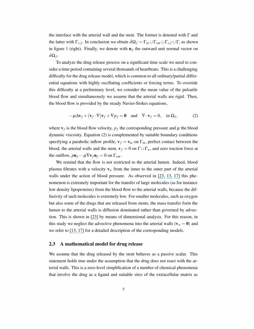
the interface with the arterial wall and the stent. The former is denoted with Γ and

the latter with Γs, f . In conclusion we obtain ∂Ω f = Γin∪Γout ∪Γs, f ∪Γ, as shown

in figure 1 (right). Finally, we denote with n f the outward unit normal vector on

∂Ω f .

To analyze the drug release process on a significant time scale we need to con-

sider a time period containing several thousands of heartbeats. This is a challenging

difficulty for the drug release model, which is common to all ordinary/partial differ-

ential equations with highly oscillating coefficients or forcing terms. To override

this difficulty at a preliminary level, we consider the mean value of the pulsatile

blood flow and simultaneously we assume that the arterial walls are rigid. Then,

the blood flow is provided by the steady Navier-Stokes equations,

−µ∆v f +(v f ·∇)v f +∇p f = 0 and ∇ ·v f = 0, in Ω f , (2)

where v f is the blood flow velocity, p f the corresponding pressure and µ the blood

dynamic viscosity. Equation (2) is complemented by suitable boundary conditions

specifying a parabolic inflow profile, v f = vin on Γin, perfect contact between the

blood, the arterial walls and the stent, v f = 0 on Γ∪Γw, and zero traction force at

the outflow, pn f −µ∇v fn f = 0 on Γout .

We remind that the flow is not restricted to the arterial lumen. Indeed, blood

plasma filtrates with a velocity vw from the inner to the outer part of the arterial

walls under the action of blood pressure. As observed in [23, 13, 17] this phe-

nomenon is extremely important for the transfer of large molecules (as for instance

low density lipoproteins) from the blood flow to the arterial walls, because the dif-

fusivity of such molecules is extremely low. For smaller molecules, such as oxygen

but also some of the drugs that are released from stents, the mass transfer form the

lumen to the arterial walls is diffusion dominated rather than governed by advec-

tion. This is shown in [23] by means of dimensional analysis. For this reason, in

this study we neglect the advective phenomena into the arterial walls (vw = 0) and

we refer to [13, 17] for a detailed description of the corresponding models.

2.3 A mathematical model for drug release

We assume that the drug released by the stent behaves as a passive scalar. This

statement holds true under the assumption that the drug does not react with the ar-

terial walls. This is a zero-level simplification of a number of chemical phenomena

that involve the drug as a ligand and suitable sites of the extracellular matrix as

7

receptors. It is well known that such phenomena may strongly influence the distri-

bution of the drug into the arterial walls, as discussed in [22, 24]. However, it is

not definitely clarified how to translate these phenomena into equations and how to

feed them with parameters. By consequence, our drug release model features just

one chemical specie, the drug, that is governed by standard advection-diffusion

equations. Furthermore, the drug we will consider in the numerical experiments is

heparin, a relatively small molecule with non negligible diffusive properties. Then,

for the interaction of the mass transfer in the lumen and in the arterial walls we

address the model described and analyzed in [19] for the transport of oxygen. As

already mentioned, in this case the advective phenomena into the arterial walls

are neglected. Concerning the coronary artery, we make here a simplification of

the complex multilayered structure of the wall, more precisely we assume that the

arterial wall is an homogeneous medium, whose physical properties are, for sim-

plicity, the ones corresponding to the intermediate layer, namely the media. This

assumption can be easily removed at the computational level because the deformed

configuration of the three layers of the artery is provided by the mechanical anal-

ysis described in section 2.1. However, this improvement becomes troublesome

in practice, because of the lack of reliable data on the transport properties of each

layer with respect to the drug. To our knowledge, only average values for the com-

plete arterial wall are available, we refer to [14] for the case of heparin. In this

setting, let Ωw be the truncated portion of the arterial walls corresponding to Ω f .

We denote with Γa the interface of the arterial wall with the outer tissue, with Γn,w

the artificial sections originated by the truncation of the artery and with Γs,w the

interface of the stent with the arterial wall. Moreover, let nw be the outward unit

normal vector relative to Ωw. Furthermore, contrarily to the assumptions adopted

for the fluid dynamics, we consider the time dependent case, because the drug re-

lease process is intrinsically transient and it dies out in a long but finite time. Then,

the governing equation for the drug concentration read as follows,

∂tc∗ +∇ · (−D∗∇c∗ +v∗c∗) = 0 in Ω∗, with ∗ = f ,w, (3)

together with a condition prescribing the initial state of the concentration in the

blood stream and into the arterial walls, c∗(t = 0) = 0 in Ω∗ and suitable boundary

conditions. For the arterial lumen, Ω f , on the inflow boundary we prescribe c f = 0

on Γin since the blood does not contain drug proximally to the stent. Assuming

that the outflow boundary is far enough to the stent, we can neglect any diffusive

8

effects across this section and set ∇c f ·n f = 0 on Γout . Also for the arterial wall

we prescribe ∇cw ·n f = 0 on Γa ∪Γn,w. According to [19], for the transmission

conditions between Ω f and Ωw we take into account the endothelium, a single

layer of cells impermeable to the blood flow. The endothelium is modelled as a

membrane at the interface between the lumen and the arterial walls, corresponding

to Γ, having a permeability P with respect to the transfer of drug. This model

allows to take into account the possible shear-dependent behavior of mass flux

through the endothelium. This is an interesting problem that has been addressed in

[20] and [21] for oxygen and albumin transport respectively. A similar discussion

can be also addressed for the diffusion parameter in the blood flow, namely D f .

Indeed, according to [26] the rotation of red blood cells due to flow vorticity may

lead to augmented transport properties. However, the intrinsic difficulty of this

studies is to quantify the dependence of the endothelial permeability and blood

diffusivity with respect to the fluid dynamics quantities as shear stresses or shear

rates. Since to our knowledge there are no available data on this dependence in the

case of drugs, we do not include this feature in our model and we assume that the

permeability P and the diffusivity D f are constant and uniform. Then, the coupling

between equations (3) is provided by the following conditions,

−D f∇c f ·n f = −Dw∇cw ·n f and −Dw∇cw ·nw = P(cw− c f ), on Γ.

We observe that these conditions can be rewritten as follows,

−D f∇c f ·n f = P(c f − cw) and −Dw∇cw ·nw = P(cw− c f ) on Γ. (4)

The latter formulation has the advantage to be symmetric with respect to the lumen

and the arterial walls. As shown in [19] this represents an advantage both for the

analyis and the numerical approximation of the coupled problem.

Finally, particular attention should be dedicated to the condition on the inter-

face between the stent and the lumen, because it is primarily responsible to deter-

mine the drug release rate. We remind that DES for cardiovascular applications

are miniaturized metal structures that are coated with a micro-film containing the

drug that will be locally released into the arterial walls for healing purposes. The

thickness of this film generally lays within the range of microns. Owing to the fact

that the stent coating is extremely thin, we apply the model proposed in [25] where

9

it has been derived the following formula for the release rate,

J(t,x) = ϕ(t)(c0s − c∗) on Γs,∗ with ∗ = f ,w, t > 0, for any x ∈ Γ, (5)

being c0s the initial drug charge of the stent that is equal to the unity in the undi-

mensional setting for the concentration. Given the thickness of the stent coating,

∆l, and its diffusion parameter, Ds, the scaling function ϕ(t) is defined as follows,

ϕ(t) =2Ds

∆l

∞

∑n=0

e−(n+1/2)2kt with k = π2Ds/∆l2. (6)

The derivation of (5) is similar to the procedure that leads to the well known

Higuchi formula [9], that provides the drug concentration cs into a semi-indefinite

planar slab (with axial coordinate z) representing the stent coating, under the as-

sumption that the external medium acts as a prefect sink,

cs(t,z)

c0s= 1− erf

(

z√4Dst

)

, z ∈ (−∞,0), t > 0, for any x ∈ Γ. (7)

However, equation (6) has the advantage to avoid the restrictive assumptions of

Higuchi formula (7). Owing to (5), the boundary condition on Γs, f and Γs,w for

equation (3) turns out to be the following Robin type condition,

−D∗∇c∗ ·n∗+ϕ(t)(c0s − c∗) = 0 on Γs,∗ with ∗ = f ,w.

The initial/boundary value problems relative to equations (2) and (3) are now

ready to be approximated by means of suitable numerical methods.

3 Numerical methods

3.1 Numerical simulation of the stent expansion

The strong nonlinearity of the problem, due to material and contact constraints,

suggested the use of an explicit dynamics analysis procedure for its solution in the

frame of the finite element method. In particular, the commercial code ABAQUS/

Explicit v. 6.4 is employed. The space dependence of the mechanical model is

discretized with eight-node iso-parametric brick elements with reduced integration

for the stent and the artery, while we adopt four-nodes or three-nodes membrane

elements with reduced integration to discretize the balloon.

10

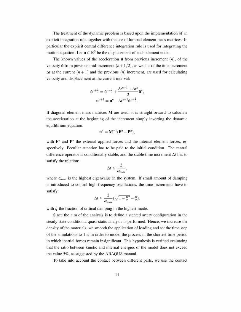
The treatment of the dynamic problem is based upon the implementation of an

explicit integration rule together with the use of lumped element mass matrices. In

particular the explicit central difference integration rule is used for integrating the

motion equation. Let u ∈ R3 be the displacement of each element node.

The known values of the acceleration u from previous increment (n), of the

velocity u from previous mid-increment (n+1/2), as well as of the time increment

∆t at the current (n+ 1) and the previous (n) increment, are used for calculating

velocity and displacement at the current interval:

un+1

2 = un−1

2 +∆tn+1+∆tn

2un,

un+1 = un+∆tn+1un+1

2 .

If diagonal element mass matrices M are used, it is straightforward to calculate

the acceleration at the beginning of the increment simply inverting the dynamic

equilibrium equation:

un =M−1(Fn−Pn),

with Fn and Pn the external applied forces and the internal element forces, re-

spectively. Peculiar attention has to be paid to the initial condition. The central

difference operator is conditionally stable, and the stable time increment ∆t has to

satisfy the relation:

∆t ≤ 2

ωmax,

where ωmax is the highest eigenvalue in the system. If small amount of damping

is introduced to control high frequency oscillations, the time increments have to

satisfy:

∆t ≤ 2

ωmax(√

1+ξ 2−ξ ),

with ξ the fraction of critical damping in the highest mode.

Since the aim of the analysis is to define a stented artery configuration in the

steady state condition,a quasi-static analysis is performed. Hence, we increase the

density of the materials, we smooth the application of loading and set the time step

of the simulations to 1 s, in order to model the process in the shortest time period

in which inertial forces remain insignificant. This hypothesis is verified evaluating

that the ratio between kinetic and internal energies of the model does not exceed

the value 5%, as suggested by the ABAQUS manual.

To take into account the contact between different parts, we use the contact

11

pair algorithm proposed in ABAQUS/Explicit, see ABAQUS version 6.5 Online

Documentation, and we adopt a kinematic predictor/corrector contact algorithm

to strictly enforce contact constraints (no penetrations are allowed), coupled with

a finite sliding approach to account for the relative motion of the two surfaces

forming the contact pair, and an exponential pressure-overclosure relationships to

specify the interaction behavior.

3.2 Numerical simulation of the fluid dynamics and of the drug re-

lease

As already seen, our drug release model involves the coupling of the blood flow

equations with an advection-diffusion problem, namely equations (2) and (3). In

these models, the advection-diffusion equations depend on the fluid dynamics through

the advective field. Hence the fluid dynamics problem is solved at a first step, and

then we solve the mass transfer problem.

For the space discretization of the space-dependent partial differential oper-

ators, we apply the finite element method. In particular, for what concerns the

Navier–Stokes equations we have adopted a linear approximation based on P1−P

1

elements that have been stabilized with respect to pressure/velocity coupling and to

a high local Reynolds number by means of the interior penalty scheme proposed in

[3]. Furthermore, we have adopted the classical Picard’s scheme for the treatment

of the nonlinear term.

Concerning the advection-diffusion equations we apply P1 elements for the

space discretization and implicit Euler scheme for the approximation of the time

dependence. We observe that equation (3) is advection dominated in Ω f . As it

is well known, finite element techniques could be inaccurate when facing such

problems and resorting to a stabilization technique becomes mandatory. Different

strategies can be pursued in this regard, we apply again interior penalty schemes,

developed in [4] for advection-diffusion-reaction problems and also applied to cou-

pled problems in [5].

A further difficulty is related to the fact that we consider phenomena that take

place both into the blood flow and into the arterial tissues. In particular, the coupled

problem given by equations (3) and by the matching conditions (4) can not be

reformulated as a problem governed by a unique differential operator on a single

domain. For this reason, we focus our attention on suitable iterative methods in

order to split (3)-(4) into a sequence of independent problems. To this purpose, a

general theory is discussed for instance in [18], for the case of linear symmetric

12

problems. However, the presence of a non negligible advection term makes our

case to be governed by a strongly unsymmetric operator into Ω f . For this reasons,

we refer to [19] where a case equivalent to (3)-(4) is analyzed. The main features

of this approach are reported in the following section.

All the aforementioned schemes are implemented into a the finite element li-

brary LIFE V, developed at MOX - Politecnico di Milano, INRIA - Paris and

CMCS - EPFL - Lausanne, see www.lifev.org .

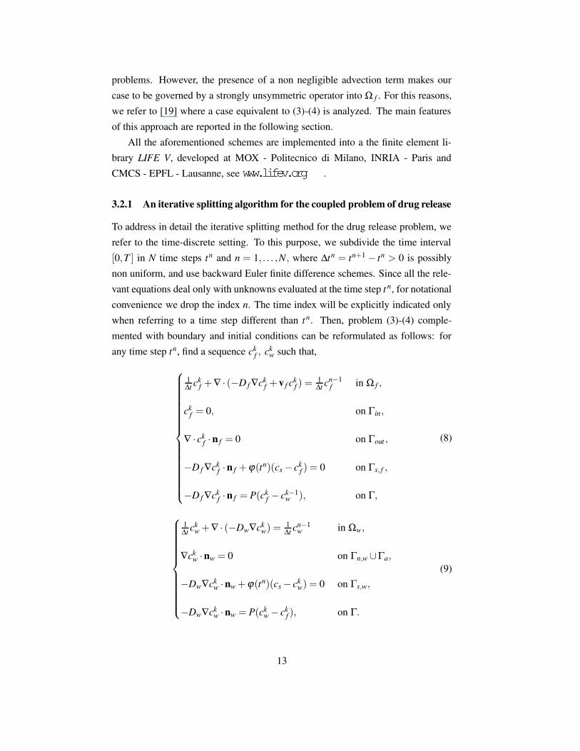
3.2.1 An iterative splitting algorithm for the coupled problem of drug release

To address in detail the iterative splitting method for the drug release problem, we

refer to the time-discrete setting. To this purpose, we subdivide the time interval

[0,T ] in N time steps tn and n = 1, . . . ,N, where ∆tn = tn+1− tn > 0 is possibly

non uniform, and use backward Euler finite difference schemes. Since all the rele-

vant equations deal only with unknowns evaluated at the time step t n, for notational

convenience we drop the index n. The time index will be explicitly indicated only

when referring to a time step different than tn. Then, problem (3)-(4) comple-

mented with boundary and initial conditions can be reformulated as follows: for

any time step tn, find a sequence ckf , ckw such that,

1

∆tckf +∇ · (−D f∇ckf +v f ckf ) = 1

∆tcn−1f in Ω f ,

ckf = 0, on Γin,

∇ · ckf ·n f = 0 on Γout ,

−D f∇ckf ·n f +ϕ(tn)(cs− ckf ) = 0 on Γs, f ,

−D f∇ckf ·n f = P(ckf − ck−1w ), on Γ,

(8)

1

∆tckw+∇ · (−Dw∇ckw) = 1

∆tcn−1w in Ωw,

∇ckw ·nw = 0 on Γn,w∪Γa,

−Dw∇ckw ·nw+ϕ(tn)(cs− ckw) = 0 on Γs,w,

−Dw∇ckw ·nw = P(ckw− ckf ), on Γ.

(9)

13

Equations (8) and (9) can be reformulated weakly. It consists of linear second-order

problems whose well-posedness in the classical Sobolev spaces H 1(Ω f ), H1(Ωw)

can be easily proven by means of the Lax-Milgram lemma, which also ensures the

existence and uniqueness of solutions at the discrete level. The well posedness at

the discrete level is maintained also when the Galerkin approximation of problem

(8) is stabilized by means of the interior penalty scheme. We refer to [4] for a

complete analysis of this method. Finally, it is possible to prove the convergence

of the sequence ckf , ckw to the solution of the coupled problem, denoted with c f , cw.

We remind the main result in the following proposition.

Proposition 1 (Convergence of the iterative splitting method) The iterative method

defined by equations (8) and (9) is convergent. Let ek∗= c∗−ck∗ be the iterative split-

ting error with ∗= f ,w, where c∗ is the solution of the coupled problem (3)-(4) and

ck∗is the sequence generated by (8) and (9). More precisely we have:

limk→∞

‖c∗− ck∗‖H1(Ω∗) = 0 with ∗ = f ,w.

A similar result holds true at the discrete level for both the Galerkin and the in-

terior penalty stabilized discretizations. The convergence rate may depend on the

physical data but not on the mesh size h.

Proof. By subtracting (8)-(9) from the equations of the coupled problem, namely

(3)-(4), we obtain the governing equations from the splitting error ek∗. Their weak

formulation reads as follows,

a f (ekf ,v f )+

∫Γ

Pekf v f =

∫Γ

Pek−1w v f , ∀v f ∈H1(Ω f ),

aw(ekw,vw)+

∫Γ

Pekwvw =

∫Γ

Pekf vw, ∀vw ∈H1(Ωw),

being a f (·, ·) and aw(·, ·) the bilinear forms associated to problems (8) and (9) with-out the contributions of the coupling terms, which have been explicitly reported.

It is easily seen that these bilinear forms are coercive with respect to the stan-

dard H1-norm on Ω∗ with suitable constants α∗ that may depend on the diffusivity

parameter D∗. Choosing v∗ = ek∗,∗ = f ,w and exploiting the coercivity and the

Cauchy-Schwarz inequality we obtain,

α f ‖ekf ‖2H1(Ω f ) +‖P 12 ekf‖2L2(Γ) ≤ ‖P 12 ekf‖L2(Γ)‖P1

2 ek−1w ‖L2(Γ),

αw‖ekw‖2H1(Ωw) +‖P 12 ekw‖2L2(Γ) ≤ ‖P 12 ekf‖L2(Γ)‖P1

2 ekw‖L2(Γ).

14

Owing to the trace theorem there exists a constantC∗ such that ‖v‖2L2(Γ)≤C∗‖v∗‖2H1(Ω∗)

.

The application of this inequality into the equations above, together with the sim-

plifying assumption that P is a constant parameter, leads to the following results,

(

1+α fC∗P

)

‖P 12 ekf ‖L2(Γ) ≤‖P 12 ek−1w ‖L2(Γ),(

1+αwC∗P

)

‖P 12 ekw‖L2(Γ) ≤‖P 12 ekf ‖L2(Γ),

that can be combined in order to obtain,

‖P 12 ekf ‖L2(Γ) ≤(

1+α fC∗P

)

−1(

1+αwC∗P

)

−1

‖P 12 ek−1f ‖L2(Γ).

Together with the trace inequality, this proves the desired result.

Finally, we observe that the proof can be immediately extended to the case of

the Galerkin discretization method. Since the constants that determine the error

reduction factor in the final inequality do not depend on the discretization method,

we conclude that the convergence rate is always independent on the discretization

parameter h. We also observe that the introduction of the interior penalty stabi-

lization term in the discrete equation for c f does not prevent the convergence of

the iterations. Indeed, the proof remains unchanged if we replace to a f (·, ·) thefollowing stabilized bilinear form,

a f (c f ,v f ) = a f (c f ,v f )+ J f (c f ,v f ), with

J f (c f ,v f ) = ∑e∈F ih

γiph2

e‖v f ·ne‖L∞(e)

∫e[∇c f ·ne][∇v f ·ne],

being F ih the collection of all the internal edges (d = 2) or faces (d = 3) e of the

computational mesh on Ω f ⊂ Rd, whose normal vector and (d− 1)-dimensional

measure are denoted with ne and he respectively.

Remark 1 (Robustness with respect to singularly perturbed problems) We ob-

serve that the proof of proposition 1 suggests that the iterative method may not con-

verge in the case of singularly perturbed problems, namely when D∗ → 0. In thiscase the coercivity constants vanish and correspondingly the estimate of the error

reduction constant at each iteration approaches the unity. This is not an intrinsic

problem of the iterative method. In fact, the proof can be easily adapted to the case

of singularly perturbed problems by virtue of the introduction of the energy norm,

|||v∗|||2 = ‖D1

2

∗ v∗‖2H1(Ω∗)+‖(∆t)− 12 v∗‖2L2(Ω∗)

.

15

We notice that the bilinear forms a∗(·, ·) are coercive with respect to this norm,uniformly with respect to the diffusivity parameter D∗, namely a∗(v,v) ≥ |||v∗|||2for any v∈H1(Ω∗). The proof of proposition 1 can be straightforwardly adapted to

this case. Indeed, starting from the splitting error equations we easily obtain that,

|||ekf |||2+‖P 12 ekf‖2L2(Γ) ≤1

2‖P 12 ekf ‖L2(Γ) +

1

2‖P 12 ek−1w ‖L2(Γ),

|||ekw|||2+‖P 12 ekw‖2L2(Γ) ≤1

2‖P 12 ekf‖L2(Γ) +

1

2‖P 12 ekw‖L2(Γ).

Combining these inequalities and summing up from k = 1 to k =M we get,

M

∑k=1

(

|||ekf |||2+ |||ekw|||2)

+1

2‖P 12 eMw ‖2L2(Γ) ≤

1

2‖P 12 e0w‖2L2(Γ).

The convergence of the sequences ckf and ckw is obtained passing to the limit for

M → ∞. However, in this case the convergence rate of the iterations can not be

explicitly characterized.

3.2.2 A-priori adapted time stepping

The drug release form the stent is a transient process that features a very fast initial

phase that progressively slows down until almost all the drug has been delivered.

The dynamics of the release rate with respect to time can be approximated by

means of the Higuchi formula, namely equation (7), which provides an explicit

estimate for the flux of drug outgoing the stent,

Jhig(t,x) =

√

Dsc2sπt

, t ∈ (0,T ], x ∈ Γ.

This formula, which is exact for the limit case t → 0 but inaccurate for long timeperiods, provides an effective way to adapt the time advancing step to the transient

release process, as discussed in [25]. For simplicity, we set up an adaptivity strat-

egy based on the increment of the amount of drug that is released from the stent

to the arterial walls. More precisely, we aim to find a suitable sequence of time

steps, tn, such that a constant fraction of the total amount of drug is released in

each time slab. We notice that this problem can be solved exactly in the framework

of the Higuchi model. In particular, let η be the constant fraction of drug that we

aim to release at each time step. Let us introduce a uniform partition of [0,1] into

sub-intervals of length η , such that N := 1/η is an integer, for simplicity. Cor-

16

respondingly, we define the sequence f n = nη with n = 0, . . . ,N . The time steps

that we look for, correspond to the mapping of the sequence f n into the interval

[0, te := (π∆l2)/(4Ds)] by means of the incremental version of equation (7),

tn =π∆l2

4Ds( f n)2, n= 0, . . . ,N,

∆tn =π∆l2

4Ds

[

( f n)2− ( f n−1)2]

=π∆l2

4Dsη2(2n−1), n= 1, . . . ,N.

We notice that ∆tn grows linearly with respect to η . After N steps, this scheme

reaches the time te where all the drug should have been delivered, according to

the inexact Higuchi model. Then the time step can be maintained constant and

equal to ∆tN . For a time interval of 1 day, the numerical experiments presented

in [25] show that this a-priori adapted time stepping ensures that the amount of

drug delivered in each time slab is almost constant also in the case of the release

model (6) applied in our case. Reminding that our time discretization scheme is

only first order accurate, the key point is to choose a suitably small increment, η ,

that ensures an effective compromise between computational efforts and accuracy,

in particular mass conservation.

4 A case study: influence of the arterial stent positioning

on blood flow and the drug release

We aim to study the interaction of the blood flow with the drug released from the

stent. This task is particularly challenging because the complex geometry of the

stent highly perturbs the local flow and this significantly influences the path of the

drug released into the lumen. We split this analysis in three parts. First of all we

focus on the structural mechanics generated by the stent expansion; secondly we

analyzed the fluid dynamics, trying to put into evidence the main features of the

flow around the stent. Lastly, we study how this flow influences the drug release.

4.1 Analysis of the stent expansion

The stent used in this study resembles the coronary Cordis BX-Velocity (Johnson &

Johnson, Interventional System, Warren, NJ, USA). The stent geometry, see figure

2 (left), is created using Rhinoceros 3.0 Evaluation CAD program (McNeel & As-

sociates, Indianapolis, IN, USA), after an acquisition of the Cordis dimensions by

17

the use of a Nikon SMZ800 stereo microscope (Nikon Corporation, Tokyo, Japan).

The length of the unit of the stent considered in the analysis is 3.62 mm, the inner

radius 0.6 mm and the thickness 0.14 mm. A mesh of 14951 8-node cubic ele-

ment is generated. For the material parameters we refer to [1] where the Young’s

modulus is E=193 GPa, the Poisson’s coefficient ν=0.3 and the yield stress σy=

205 MPa; we take into account the degradation of the hardening modulus, vary-

ing from K=1500 MPa and K=97 MPa, using the ABAQUS option of defining a a

linear piecewise isotropic hardening.

The balloon is designed with a radius of 1.5 mm and length of 8 mm. The

mesh consists of 11650 4-nodes membrane elements and 220 3-nodes membrane

elements (thickness = 0.05 mm) in order to obtain the balloon heads. The char-

acteristic parameters of the material are the Young’s modulus E=900 GPa and the

Poisson’s coefficient ν=0.3. To obtain the initial deflated configuration of the bal-

loon, a preliminary analysis is run, in which a negative pressure of 0.01 MPa is

applied to its inner surface of the inflated configuration, see figure 2 (top). Once

deflated, the folded balloon can be inserted inside the stent, as shown in figure 2

(bottom). The expansion process of the stent-balloon system is reported in the pres-

sure vs. diameter diagram of figure 3. We notice that, once the balloon has reached

its nominal diameter, further increases in pressure have no significant effect on its

size. This finding is consistent with the hypothesis of the semi-compliant balloon

used in the reality, as shown by the comparison of the numerical results with the

data supplied by the manufacturer reported in figure 3.

The coronary artery is modelled with an internal radius of 1.25 mm, a thickness

of 0.5 mm and a length of 10 mm. The artery is meshed with 87750 8-node cubic

solid elements. The material parameters used for the strain energy function, see

equation 1, are defined referring to the mean values of experimental results in the

circumferential direction obtained in [11] and are reported in table 1.

In order to verify the adequacy of the mesh density used in the simulations, a

mesh dependency study expanding either the stent and artery to a diameter of 3

mm is performed. The unit stent mesh density is increased from 9969 to 19937

elements. The percentage difference of Von Mises stresses between the finest and

selected meshes is of 0.3%. The artery mesh density is increased from 7050 to

280098 elements. No appreciable difference in Von Mises stresses between the

finest and the selected meshes is observed.

The expansion of the balloon/stent device is computed following three main

steps. First of all a pressure of 100 mmHg is imposed to the internal surface of the

18

artery to mimic the physiological conditions, see figure 4 (a). Then, the stent is

expanded by applying a pressure of 1.5 MPa to the internal surface of the balloon.

In particular, at a pressure p=0.135 MPa the balloon enters in contact with the

stent, as shown in figure 4 (b). At a pressure p=0.285 MPa the balloon enters in

contact with the artery showing the well-known dogboning-shape, see panel 4 (c).

Increasing the pressure also the central part of the stent is expanded, as illustrated

in panel 4 (d), up to the maximum expansion reached at p=1.5 MPa, corresponding

to figure 4 (e). In this configuration the artery reaches a maximum internal diameter

of 3.47 mm. Finally, the balloon is deflated, see figure 4 (f). The final artery lumen

is of 3.06 mm. The deformed geometry of artery and stent obtained at the end of

the simulation are stored to be used in the fluid dynamic analysis. Observing figure

4 (f) we notice that the parameters useful to quantify the interaction between the

stent and artery and consequently the efficacy of drug elution may be:

1. the metal to artery ratio in the expanded configuration that measures the

artery surface covered by the stent and hence of the area prone to a direct

diffusion of the drug. In this case it is equal to 18%.

2. the foreshortening effect that is a measure of the contraction of the stent

during the expansion and hence it gives an information about the length of

the area interested by the drug release process..

3. the dogboning effect that quantifies the irregular expansion of the stent (grater

in the external part than in the central one) and hence it is related with the ir-

regularity of the artery internal surface that may influences the fluid dynamic

phenomena.

In figure 5 are also reported radial, circumferential and axial Cauchy stress

components: even if not directly used in the following analysis, they may be useful

to better understand the effects of stent-balloon expansion on the artery configura-

tion and eventually to highlight local conditions particularly unsafe.

Finally, we recall that refinements of the stent expansion geometrical and con-

stitutive models will be useful for a more detailed and precise description of the

process and hence for more precise initial conditions of blood flow and the drug

deposition problem.

19

4.2 Analysis of the fluid dynamics around the struts

The lumen and the wall of the artery are subdivided with Gambit (ANSYS Inc.,

Canonsburg, PA, USA) into 1,637,336 and 1,118,420 tetrahedra respectively. In

order to obtain an accurate resolution with a reasonable computational cost and

memory storage, we have applied a nonuniform spacing for the mesh generation.

In particular, the central part of the domain have been subdivided by means of

variable size elements, particularly refined around the stent.

Looking at the Cordis BX-Velocity stent, it is possible to identify two kinds of

structures, the struts and the links. The former are twisted rings that provide the

circumferential strength of the stent, while the latter are tiny connections along the

longitudinal axis between subsequent struts.

An important feature of the struts is to be twisted in the circumferential di-

rection. For this reason, the blood flow hits the struts with different angles. The

preliminary results obtained in [6] suggest that the flow pattern downstream the

struts may be substantially different from the well-known flow after a backward

facing step that corresponds to the ideal case of a perfectly circular ring that is

orthogonal to the flow. This conjecture is confirmed by the fluid dynamics simu-

lations. Indeed, in figure 6 we visualize the streamlines of the blood flow around

the stent. This picture shows that we deal with a fully three dimensional flow with

recirculations, vortexes and secondary motions. For instance, we observe that the

vortex induced by the presence of the link on the top left corner is stretched and

absorbed in the main stream on its right side. This suggests that this vortex is not

only characterized by a planar rotating flow but an out of plane motion is present.

This secondary motion generates the displacement of the fluid form the center of

the vortex to the extrema and the fluid is thus cast out the vortex into the main

stream.

In conclusion, there is evidence that the interaction between the stent and the

blood stream generates very complex flow patterns where the recirculation zones

downstream the obstacles interact with the main stream. By this way, the fluid that

was at some time trapped into a recirculation may join the high speed flow. We will

see in the next section that this behavior has important consequences on the drug

release process.

20

4.3 Analysis of the drug release

As already mentioned, we simulate the release of heparin. According to the ex-

perimental investigations presented in [14], this corresponds to set D f = 1.5 10−4

mm2/s, Dw = 7.7 10−6 mm2/s and P = 4 10−4 mm/s. The diffusivity of the drug

into the stent coating typically ranges from 10−8 to 10−12 mm2/s, depending on the

mechanical properties of the polymeric substrate. To avoid too stiff parameters we

set Ds = 10−8 mm2/s.

The numerical simulation based on equation (3) shows that the drug released

into the lumen is very quickly washed out by the blood flow. Indeed, the peaks of

drug concentration into the lumen are reached about 40 seconds after the beginning

of the process. This corresponds to only 1% of the time necessary to release almost

all the drug form the stent. Conversely, the drug dynamics into the arterial walls

is much slower, but after 1 hour the drug has reached the outer boundary of the

arterial walls, as can be seen in figure 8 (bottom).

The drug concentration into the lumen is reported in figure 7. The highest

peaks of drug concentration appear in the neighborhood of the links. In these

regions, the contour plot of the concentration suggests that the recirculation of

the blood flow interacts with the drug accumulation. The smooth and concave

shape of the contours suggests that part of the drug released and accumulated in

the neighborhood of the links is transported away and may affect the arterial walls

located downstream. Indeed, regions related to non negligible concentration levels

are clearly visible downstream the stent in figure 8 (top), where the presence of the

drug in the lumen is visualized by means of the isosurface of the concentration.

This means that a wide portion of the endothelium, which is often severely injured

by the stent implantation, is exposedto a non negligible drug concentration. When

the drug has anti-proliferative properties, the re-endothelialization process mey be

slowed down. This seems to be one of the major drawbacks of DES, and it should

be further investigated.

Concerning the struts, the accumulation of drug is unexpectedly prominent up-

stream with respect to the blood flow. High concentration levels take place where

the struts are highly curved and their curvature is convex with respect to the blood

flow. This is in contrast to the results obtained in [2], but can be explained observ-

ing that blood transports the drug downstream to the location where it has been

released. The accumulation of the drug takes place where this effect is hindered by

the convex stent pattern with respect to the blood flow.

The results reported in figure 7 (right) suggest that part of the drug released into

21

the lumen is absorbed by the wall. However, depending on the sign of the quantity

P(c f − cw) of equation (4), the opposite process is simultaneously happening, be-cause the drug concentration in the wall is much higher than the one into the lumen

in the surroundings of the interface of contact between the stent and the artery.

Indeed, the interface Γ between the lumen and the walls can be subdivided into

a region where the drug is absorbed into the wall and the complementary region

where the drug is released by the wall and definitely lost into the blood flow.

This balance can be analyzed by means of more quantitative results. After 1

hour from the stent implantation, almost all the drug has been released. The contact

interface between the stent and the walls ensures that 15% of the total amount

of drug is released into the walls. However, more than a half of this fraction is

simultaneously transferred into the lumen because of the negative concentration

gradient between the lumen and the walls. Then, for the case analyzed here, the

drug released into the lumen does not significantly contribute to the permanent

drug deposition into the arterial wall. However, to come up to a general conclusion,

further investigations are mandatory.

5 Conclusions

We have analyzed the interactions between the stent shape and positioning, the

blood flow and the drug release from a stent, showing that a 3-dimensional analysis

of the problem accounting for the complex geometry of the stent is mandatory to

capture the phenomena into play. In this setting, we have studied the contribution of

the drug released into the blood flow with respect to the efficacy of drug deposition

and penetration into the arterial walls.

Acknowledgments

This work has been supported by the Italian Institute of Technology with the project

”NanoBiotechnology -Models andMethods for Local Drug Delivery from Nano/Micro

Structured Materials”.

References

[1] F. Auricchio, M. Di Loreto, and E. Sacco. Finite-element analysis of

a stenotic revascularization through a stent insertion. Comput. Methods.

22

Biomech. Biomed. Engin, 4:249–264, 2001.

[2] B. Balakrishnan, A.R. Tzafriri, P. Seifert, A. Groothuis, C. Rogers, and E.R.

Edelman. Strut position, blood flow, and drug deposition. implications for sin-

gle and overlapping drug-eluting stents. Circulation, 111:2958–2965, 2005.

[3] Erik Burman, Miguel A. Fernandez, and Peter Hansbo. Continuous interior

penalty finite element method for Oseen’s equations. SIAM J. Numer. Anal.,

44(3):1248–1274 (electronic), 2006.

[4] Erik Burman and Peter Hansbo. Edge stabilization for Galerkin approxi-

mations of convection-diffusion-reaction problems. Comput. Methods Appl.

Mech. Engrg., 193(15-16):1437–1453, 2004.

[5] Erik Burman and Paolo Zunino. A domain decomposition method based on

weighted interior penalties for advection-diffusion-reaction problems. SIAM

J. Numer. Anal., 44(4):1612–1638 (electronic), 2006.

[6] Carlo D’Angelo and Paolo Zunino. A numerical study of the interaction

of blood flow and drug release from cardiovascular stents. Proceedings of

the Enumath Conference, Austria, September 2007, MOX, Department of

Mathematics, Politecnico di Milano, 2007. Submitted.

[7] C.T. Gasser and G.A. Holzapfel. Finite element modeling of balloon angio-

plasty by considering overstretch of remnant non-diseased tissues in lesions.

Comput. Mech., 40:47–60, 2007.

[8] F. Gervaso, C. Capelli, L. Petrini, S. Lattanzio, L. Di Virgilio, and F. Migli-

avacca. On the effects of different strategies in modelling balloon-expandable

stenting by means of finite element method. J. Biomech., 2007. Submitted.

[9] T. Higuchi. Rate of release of medicaments from ointment bases containing

drugs in suspension. J. Pharmac. Sci., 50:874–875, 1961.

[10] G.A. Holzapfel. Encyclopedia Of Computational Mechanics, pages 605–635.

John Wiley & Sons, Ltd, Chichester, 2004. Edited by Erwin Stein, Rene de

Borst and Thomas J.R. Hughes.

[11] G.A. Holzapfel, G. Sommer, C.T. Gasser, and P. Regitnig. Determi-

nation of layer-specific mechanical properties of human coronary arteries

23

with nonatherosclerotic intimal thickening and related constitutive mod-

elling. American Journal of Physiology, Heart and Circulatory Physiology,

289:2048–58, 2005.

[12] D.R. Hose, A.J. Narracott, B. Griffiths, S. Mahmood, J. Gunn, D. Sweeney,

and P.V. Lawford. A thermal analogy for modelling drug elution from car-

diovascular stents. Comput. Methods. Biomech. Biomed. Engin, 7:257–264,

2004.

[13] G. Karner and K. Perktold. Effect of endothelial injury and increased blood

pressure on albumin accumulation in the arterial wall: a numerical study. J.

Biomech., 33:709–715, 2000.

[14] M.A. Lovich and E.R. Edelman. Mechanisms of transmural heparin transport

in the rat abdominal aorta after local vascular delivery. Circ. Res., 77:1143–

1150, 1995.

[15] F. Migliavacca, F. Gervaso, M. Prosi, P. Zunino, S. Minisini, L. Formaggia,

and G. Dubini. Expansion and drug elution model of a coronary stent. Com-

put. Methods. Biomech. Biomed. Engin, 10:63–73, 2007.

[16] F. Migliavacca, L. Petrini, M. Colombo, F. Auricchio, and R. Pietrabissa.

Mechanical behavior of coronary stents investigated by the finite element

method. J. Biomech., 35:803–811, 2002.

[17] M. Prosi, P. Zunino, K. Perktold, and A. Quarteroni. Mathematical and nu-

merical models for transfer of low-density lipoproteins through the arterial

walls: a new methodology for the model set up with applications to the study

of disturbed lumenal flow. J. Biomech., 38:903–917, 2005.

[18] Alfio Quarteroni and Alberto Valli. Domain decomposition methods for par-

tial differential equations. Numerical Mathematics and Scientific Computa-

tion. The Clarendon Press Oxford University Press, New York, 1999. Oxford

Science Publications.

[19] Alfio Quarteroni, Alessandro Veneziani, and Paolo Zunino. Mathematical

and numerical modeling of solute dynamics in blood flow and arterial walls.

SIAM J. Numer. Anal., 39(5):1488–1511 (electronic), 2001/02.

[20] G. Rappitsch and K. Perktold. Pulsatile albumin transport in large arteries: a

numerical simulation study. J. Biomech. Eng., 118:511–519, 1996.

24

[21] G. Rappitsch, K. Perktold, and E. Pernkopf. Numerical modelling of shear-

dependent mass transfer in large arterie. Int. J. Numer. Meth. Fluid, 25:847–

857, 1997.

[22] D.V. Sakharov, L.V. Kalachev, and D.C. Rijken. Numerical simulation of

local pharmacokinetics of a drug after intravascular delivery with an eluting

stent. J. Drug Targ., 10(6):507–513, 2002.

[23] D.K. Stangeby and C.R. Ethier. Computational analysis of coupled blood-

wall arterial ldl transport. J. Biomech. Eng., 124:1–8, 2002.

[24] A.R. Tzafriri and E.R. Edelman. On the validity of the quasi-steady state

approximation of bimolecular reactions in solution. J. Theor. Biol., 233:343–

350, 2005.

[25] Christian Vergara and Paolo Zunino. Multiscale modeling and simulation of

drug release from cardiovascular stents. Technical Report 15, MOX, Depart-

ment of Mathematics, Politecnico di Milano, 2007. Submitted.

[26] N.L. Wang and K.H. Keller. Augmented transport of extracellular solutes

in concentrated erytrocyte suspensions in couette flow. J. Colloid Inter. Sci.,

103:210–225, 1985.

25

Figures

ΓbΓs

Γn,w

Γ

Γn,w

Γa

Γ

Γn,w

Γout

ΓinΓs, f

Γs,w

Figure 1: The lumen and the arterial wall with the partition of their boundaries for

the set up of the mechanical model of the expansion of the stent (left) and of the

drug release after the expansion (right).

Γn,sc

Γn,bc

Figure 2: Boundary conditions and computational mesh of the balloon-stent model.

26

Figure 3: Pressure-diameter curve of the balloon-stent model compared to the data

available from the manufacturer

.

27

(a) (d)

(b) (e)

(c) (f)

Figure 4: The sequence of steps describing the expansion of the stent.

Figure 5: Radial, circumferential and axial Cauchy stresses on the artery.

28

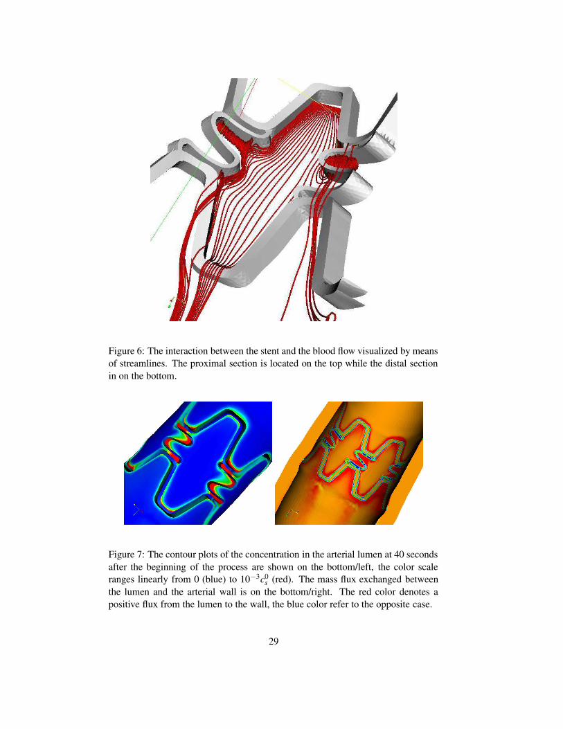
Figure 6: The interaction between the stent and the blood flow visualized by means

of streamlines. The proximal section is located on the top while the distal section

in on the bottom.

Figure 7: The contour plots of the concentration in the arterial lumen at 40 seconds

after the beginning of the process are shown on the bottom/left, the color scale

ranges linearly from 0 (blue) to 10−3c0s (red). The mass flux exchanged between

the lumen and the arterial wall is on the bottom/right. The red color denotes a

positive flux from the lumen to the wall, the blue color refer to the opposite case.

29

Figure 8: The isosurface corresponding to the value 10−5c0s for the drug concen-

tration in the arterial lumen and contour plots into the arterial walls, at 40 seconds

(top) and 1 hour (bottom) after the beginning of the process. The color scale ranges

linearly form 0 (blue) to 10−3c0s

30

Tables

C10 C20 C30 C40 C50 C60

Intima 6.79E-03 0.54 -1.11 10.65 -7.27 1.63

Media 6.52E-03 4.89E-02 9.26E-03 0.76 -0.43 8.69E-02

Adventitia 8.27E-03 1.20E-02 0.52 -5.63 21.44 0.00

Table 1: Coronary artery model parameters.

31