numerica

Andrew Parsloe(ajparsloe@gmail.com)

December 11, 2021

Abstract

The numerica package defines a command to numerically evaluate mathemati-cal expressions in the LaTeX form in which they are typeset. For programs likeLyX with a preview facility, or compile-as-you-go systems, interactive back-of-envelope calculations and numerical exploration are possible within the doc-ument being worked on. The package requires the bundles l3kernel andl3packages, and the amsmath and mathtools packages.

Note:• This document applies to version 2.0.0 of numerica.sty.

• Reasonably recent versions of the LATEX3 bundles l3kernel andl3packages are required (although much of l3kernel has been incor-porated into LATEX 2ε since February 2020).

• The package requires amsmath and mathtools.

• I refer many times in this document (especially §3.4) to Handbook of Math-ematical Functions, edited by Milton Abramowitz and Irene A. Segun,Dover, 1965. This is abbreviated to HMF , often followed by a numberlike 1.2.3 to locate the actual expression referenced.

• Version 2.0.0 of numerica

– splits into distinct packages the additional functionality previouslyavailable with the plus and tables package options of version 1;

– allows for user-defined macros and constants (with the \nmcMacrosand \nmcConstants commands) to be used in expressions to be eval-uated;

– rewrites the code and changes the behaviour of \nmcReuse to main-tain uniformity across all commands (\nmcEvaluate, \nmcInfo,\nmcMacros, \nmcConstants, \nmcReuse); this command is nolonger compatible with its use in v.1;

– changes the behaviour of \text and \mbox in the \eval command;adds \textrm, \textsf, and \texttt to compensate;

– includes many adjustments to the code, including around nesting ofcommands;

– adds to and amends documentation.

1

Contents

1 Introduction 71.1 How to use numerica . . . . . . . . . . . . . . . . . . . . . . . . 8

1.1.1 Package options . . . . . . . . . . . . . . . . . . . . . . . 91.1.2 Associated packages . . . . . . . . . . . . . . . . . . . . . 91.1.3 Simple examples of use . . . . . . . . . . . . . . . . . . . 91.1.4 Display of the result . . . . . . . . . . . . . . . . . . . . . 101.1.5 Checking . . . . . . . . . . . . . . . . . . . . . . . . . . . 121.1.6 Exploring . . . . . . . . . . . . . . . . . . . . . . . . . . . 121.1.7 Reassuring . . . . . . . . . . . . . . . . . . . . . . . . . . 13

2 \nmcEvaluate (\eval) 162.1 Syntax of \nmcEvaluate (\eval) . . . . . . . . . . . . . . . . . 162.2 The variable=value list . . . . . . . . . . . . . . . . . . . . . . . . 17

2.2.1 Variable names . . . . . . . . . . . . . . . . . . . . . . . . 172.2.2 The vv-list and its use . . . . . . . . . . . . . . . . . . . . 18

2.2.2.1 Evaluation from right to left . . . . . . . . . . . 192.2.2.2 Expressions in the variable=value list . . . . . . 192.2.2.3 Constants . . . . . . . . . . . . . . . . . . . . . . 20

2.2.3 Display of the vv-list . . . . . . . . . . . . . . . . . . . . . 212.2.3.1 Star option: suppressing display of the vv-list . . 212.2.3.2 Suppressing display of items . . . . . . . . . . . 222.2.3.3 Empty vv-list suppressed . . . . . . . . . . . . . 222.2.3.4 Changing the display format . . . . . . . . . . . 222.2.3.5 Abusing multi-token variable names . . . . . . . 23

2.3 Formatting the numerical result . . . . . . . . . . . . . . . . . . . 232.3.1 Rounding value . . . . . . . . . . . . . . . . . . . . . . . 242.3.2 Padding with zeros . . . . . . . . . . . . . . . . . . . . . 262.3.3 Scientific notation . . . . . . . . . . . . . . . . . . . . . . 26

2.3.3.1 Numbers in the interval [1,10) . . . . . . . . . 272.3.3.2 \eval* and scientific notation . . . . . . . . . . . 27

2.3.4 Boolean output . . . . . . . . . . . . . . . . . . . . . . . . 282.3.4.1 Outputting T or F . . . . . . . . . . . . . . . . . 282.3.4.2 Rounding error tolerance . . . . . . . . . . . . . 292.3.4.3 And, Or, Not . . . . . . . . . . . . . . . . . . . . 29

2

2.3.4.4 Chains of comparisons . . . . . . . . . . . . . . . 302.3.4.5 amssymb comparison symbols . . . . . . . . . . . 30

2.4 Calculational details . . . . . . . . . . . . . . . . . . . . . . . . . 312.4.1 Arithmetic . . . . . . . . . . . . . . . . . . . . . . . . . . 31

2.4.1.1 Square roots and nth roots . . . . . . . . . . . . 312.4.1.2 nth roots of negative numbers . . . . . . . . . . 322.4.1.3 Inverse integer powers . . . . . . . . . . . . . . 32

2.4.2 Precedence, parentheses . . . . . . . . . . . . . . . . . . . 332.4.2.1 Command-form brackets . . . . . . . . . . . . . 33

2.4.3 Modifiers (\left \right, etc.) . . . . . . . . . . . . . . . 332.4.4 Trigonometric & hyperbolic functions . . . . . . . . . . . 342.4.5 Logarithms . . . . . . . . . . . . . . . . . . . . . . . . . . 342.4.6 Other unary functions . . . . . . . . . . . . . . . . . . . . 352.4.7 Squaring, cubing, . . . unary functions . . . . . . . . . . . . 352.4.8 n-ary functions . . . . . . . . . . . . . . . . . . . . . . . . 362.4.9 Delimiting arguments with brackets & modifiers . . . . . 362.4.10 Absolute value, floor & ceiling functions . . . . . . . . . . 36

2.4.10.1 Squaring, cubing, . . . absolute values, etc. . . . 372.4.11 Factorials, binomial coefficients . . . . . . . . . . . . . . . 38

2.4.11.1 Double factorials . . . . . . . . . . . . . . . . . . 382.4.11.2 Binomial coefficients . . . . . . . . . . . . . . . . 39

2.4.12 Sums and products . . . . . . . . . . . . . . . . . . . . . . 392.4.12.1 Infinite sums and products . . . . . . . . . . . . 41

2.4.13 Formatting commands . . . . . . . . . . . . . . . . . . . . 412.4.13.1 Spaces, phantoms, struts . . . . . . . . . . . . . 422.4.13.2 \splitfrac . . . . . . . . . . . . . . . . . . . . 422.4.13.3 Colour . . . . . . . . . . . . . . . . . . . . . . . 432.4.13.4 \text, \mbox, font commands . . . . . . . . . . 442.4.13.5 \ensuremath, $, \(, \), \[, \] . . . . . . . . . 44

2.5 Error messages . . . . . . . . . . . . . . . . . . . . . . . . . . . . 452.5.1 Mismatched brackets . . . . . . . . . . . . . . . . . . . . . 452.5.2 Unknown tokens . . . . . . . . . . . . . . . . . . . . . . . 452.5.3 Overlooked value assignments . . . . . . . . . . . . . . . . 462.5.4 Integer argument errors . . . . . . . . . . . . . . . . . . . 462.5.5 Comparison errors . . . . . . . . . . . . . . . . . . . . . . 472.5.6 Invalid base for \log . . . . . . . . . . . . . . . . . . . . . 472.5.7 l3fp errors . . . . . . . . . . . . . . . . . . . . . . . . . . 47

2.5.7.1 Dividing by zero . . . . . . . . . . . . . . . . . . 482.5.7.2 Invalid operation . . . . . . . . . . . . . . . . . . 482.5.7.3 Overflow/underflow . . . . . . . . . . . . . . . . 48

3 Settings 503.1 Settings option . . . . . . . . . . . . . . . . . . . . . . . . . . . . 50

3.1.1 ‘Debug’ facility . . . . . . . . . . . . . . . . . . . . . . . . 503.1.2 Negative dbg values . . . . . . . . . . . . . . . . . . . . . 533.1.3 view setting . . . . . . . . . . . . . . . . . . . . . . . . . . 54

3

3.1.4 Inputting numbers in scientific notation . . . . . . . . . . 543.1.5 Multi-token variables . . . . . . . . . . . . . . . . . . . . . 553.1.6 Parsing arguments of trigonometric functions . . . . . . . 553.1.7 Using degrees rather than radians . . . . . . . . . . . . . 553.1.8 Specifying a logarithm base . . . . . . . . . . . . . . . . . 563.1.9 Calculation mode . . . . . . . . . . . . . . . . . . . . . . . 563.1.10 Changing the vv-list display format . . . . . . . . . . . . 573.1.11 Displaying the vv-list on a new line . . . . . . . . . . . . 583.1.12 Punctuation . . . . . . . . . . . . . . . . . . . . . . . . . . 593.1.13 Reuse setting . . . . . . . . . . . . . . . . . . . . . . . . . 60

3.2 Infinite sums and products . . . . . . . . . . . . . . . . . . . . . . 603.2.1 Premature ending of infinite sums . . . . . . . . . . . . . 633.2.2 Double sums or products . . . . . . . . . . . . . . . . . . 65

3.3 Changing default values . . . . . . . . . . . . . . . . . . . . . . . 663.3.1 Location of numerica.cfg . . . . . . . . . . . . . . . . . 69

3.3.1.1 Personal texmf tree? . . . . . . . . . . . . . . . 693.3.2 Rounding in ‘int-ifying’ calculations . . . . . . . . . . . . 69

3.4 Parsing mathematical arguments . . . . . . . . . . . . . . . . . . 703.4.1 The cleave commands \q and \Q . . . . . . . . . . . . . . 70

3.4.1.1 Mnemonic . . . . . . . . . . . . . . . . . . . . . 713.4.2 Parsing groups . . . . . . . . . . . . . . . . . . . . . . . . 71

3.4.2.1 Parsing group I . . . . . . . . . . . . . . . . . . 723.4.2.2 Parsing group II . . . . . . . . . . . . . . . . . . 733.4.2.3 Parsing group III . . . . . . . . . . . . . . . . . 763.4.2.4 Parsing group IV . . . . . . . . . . . . . . . . . . 793.4.2.5 Parsing group V . . . . . . . . . . . . . . . . . . 803.4.2.6 Parsing group VI . . . . . . . . . . . . . . . . . . 803.4.2.7 Disclaimer . . . . . . . . . . . . . . . . . . . . . 81

4 Supplementary commands 824.1 Feedback on ‘infinite’ processes: \nmcInfo . . . . . . . . . . . . 82

4.1.1 Suppressing the descriptor: \nmcInfo* . . . . . . . . . . . 834.1.2 Errors . . . . . . . . . . . . . . . . . . . . . . . . . . . . . 844.1.3 view setting . . . . . . . . . . . . . . . . . . . . . . . . . . 84

4.2 User-defined macros: \nmcMacros . . . . . . . . . . . . . . . . . . 844.2.1 What can be stored in a macro? . . . . . . . . . . . . . . 86

4.2.1.1 Macros containing formulas . . . . . . . . . . . 864.2.1.2 Vv-list . . . . . . . . . . . . . . . . . . . . . . . . 87

4.2.2 Seeing what macros are available . . . . . . . . . . . . . . 874.2.2.1 Freeing macros from storage . . . . . . . . . . . 884.2.2.2 Counting how many macros are available . . . . 88

4.2.3 Errors . . . . . . . . . . . . . . . . . . . . . . . . . . . . . 884.2.3.1 Display of macros . . . . . . . . . . . . . . . . . 89

4.2.4 Rounding value . . . . . . . . . . . . . . . . . . . . . . . . 904.3 User-defined constants: \nmcConstants . . . . . . . . . . . . . 91

4.3.1 New list replaces old by default . . . . . . . . . . . . . . . 92

4

4.3.2 Adding constants to a list . . . . . . . . . . . . . . . . . . 924.3.3 Examples of use . . . . . . . . . . . . . . . . . . . . . . . 92

4.3.3.1 Example 1: atomic constants . . . . . . . . . . . 924.3.3.2 Example 2: local constants . . . . . . . . . . . . 934.3.3.3 Example 3: macros and constants . . . . . . . . 94

4.3.4 Viewing, counting constants . . . . . . . . . . . . . . . . . 954.3.5 Errors . . . . . . . . . . . . . . . . . . . . . . . . . . . . . 96

4.4 Saving and reusing results: \nmcReuse . . . . . . . . . . . . . . . 964.4.1 Use of \nmcReuse . . . . . . . . . . . . . . . . . . . . . . 96

4.4.1.1 What is saved? . . . . . . . . . . . . . . . . . . . 974.4.1.2 The .nmc file . . . . . . . . . . . . . . . . . . . . 974.4.1.3 Messages . . . . . . . . . . . . . . . . . . . . . . 984.4.1.4 Deleting and renewing . . . . . . . . . . . . . . . 984.4.1.5 Viewing what has been saved . . . . . . . . . . . 994.4.1.6 Counting saved control sequences: \nmcReuse* . 100

4.4.2 reuse setting of \eval command . . . . . . . . . . . . . . 100

5 Nesting commands 1025.1 Nesting in the formula . . . . . . . . . . . . . . . . . . . . . . . . 102

5.1.1 Math delimiters and double evaluations . . . . . . . . . . 1035.2 Nesting in the vv-list . . . . . . . . . . . . . . . . . . . . . . . . . 1035.3 Nesting in the settings option . . . . . . . . . . . . . . . . . . . . 1045.4 Rounding and display . . . . . . . . . . . . . . . . . . . . . . . . 1045.5 Error messages . . . . . . . . . . . . . . . . . . . . . . . . . . . . 1055.6 Debugging . . . . . . . . . . . . . . . . . . . . . . . . . . . . . . . 105

6 Using numerica with LYX 1076.1 Instant preview . . . . . . . . . . . . . . . . . . . . . . . . . . . . 107

6.1.1 Document location . . . . . . . . . . . . . . . . . . . . . . 1086.1.2 Global vs local previewing . . . . . . . . . . . . . . . . . . 108

6.1.2.1 Forcing a global preview run . . . . . . . . . . . 1096.2 Mathed . . . . . . . . . . . . . . . . . . . . . . . . . . . . . . . . 109

6.2.1 LATEX braces { } . . . . . . . . . . . . . . . . . . . . . . . 1096.3 Preview insets . . . . . . . . . . . . . . . . . . . . . . . . . . . . . 1106.4 Errors . . . . . . . . . . . . . . . . . . . . . . . . . . . . . . . . . 111

6.4.1 Temporary directory of LYX . . . . . . . . . . . . . . . . . 1116.4.2 CPU usage, LATEX processes . . . . . . . . . . . . . . . . . 111

6.5 Hyperref support vs speed . . . . . . . . . . . . . . . . . . . . . . 1126.6 Supplementary commands in LYX . . . . . . . . . . . . . . . . . . 112

6.6.1 Reuse of earlier previews . . . . . . . . . . . . . . . . . . . 1126.6.2 ‘Stalled’ previews . . . . . . . . . . . . . . . . . . . . . . . 1136.6.3 Using \nmcMacros . . . . . . . . . . . . . . . . . . . . . . 1136.6.4 Using \nmcConstants . . . . . . . . . . . . . . . . . . . . 1146.6.5 Using \nmcReuse . . . . . . . . . . . . . . . . . . . . . . . 114

6.6.5.1 A final tweak? . . . . . . . . . . . . . . . . . . . 1156.6.5.2 Use of LYX notes . . . . . . . . . . . . . . . . . . 115

5

7 Reference summary 1167.1 Commands defined in numerica . . . . . . . . . . . . . . . . . . . 1167.2 ‘Digestible’ content . . . . . . . . . . . . . . . . . . . . . . . . . . 1177.3 Settings . . . . . . . . . . . . . . . . . . . . . . . . . . . . . . . . 119

7.3.1 Available \nmcEvaluate settings . . . . . . . . . . . . . . 1197.3.2 Available settings for supplementary commands . . . . . . 1197.3.3 Available configuration file settings . . . . . . . . . . . . . 120

6

Chapter 1

Introduction

numerica is a LATEX package offering the ability to numerically evaluate math-ematical expressions in the LATEX form in which they are typeset.1

There are a number of packages which can do calculations in LATEX,2 butthose I am aware of all require the mathematical expressions they operate onto be changed to an appropriate syntax. Of these packages xfp comes closestto my objective with numerica. For instance, given a formula

\frac{\sin (3.5)}{2} + 2\cdot 10^{-3}

(in a math environment), this can be evaluated using xfp by transforming theexpression to sin(3.5)/2 + 2e-3 and wrapping this in the command \fpeval.In numerica you don’t need to transform the formula, just wrap it in an \evalcommand:

\eval{ \frac{\sin (3.5)}{2} + 2\cdot 10^{-3} }.

(for the acutal calculation see §1.1.3).numerica, like xfp and a number of other packages, uses l3fp (the LATEX3

floating point module in l3kernel) as its calculational engine. To some extentthe main command, \nmcEvaluate, short-name form \eval, is a pre-processorto l3fp, converting mathematical expressions written in the LATEX form inwhich they will be typeset into an ‘fp-ified’ form that is digestible by l3fp. Theaim is to make the command act as a wrapper around such formulas. Ideally,one should not have to make any adjustment to them, although any text on

1numerica evolved from the author’s calculyx package that was designed for use with thedocument processor LYX (and available for download from a link on the LYX wiki website butnot CTAN).

2A simple search finds the venerable calc in the LATEX base, calculator (including anassociated calculus package), fltpoint, fp (fixed rather than floating point), spreadtab(using either fp or l3fp as its calculational engine) if you want simple spreadsheeting withyour calculations, the elaborate xint, pst-calculate (a limited interface to l3fp), l3fp in theLATEX3 kernel, and xfp, the LATEX3 interface to l3fp. Other packages include a calculationalelement but are restricted in their scope. (longdivision for instance is elegant, but limitedonly to long division.)

7

Fourier series suggests that hope in full generality is delusional. Surprisinglyoften however it is possible. We shall see shortly that even complicated formulaslike

cos mn π − (1 − 4 sin2 m

3n π)sin 1

n π sin m−1n π

2 sin2 m3n π

,

and (1 − 4 sin2 m3n π

2 sin2 m3n π

)sin 2m−3

3n π sin m−33n π,

can be evaluated ‘as is’ (see below, §1.1.7). There is no need to shift the positionof the superscript 2 on the sines, no need to parenthesize the arguments ofsin and cos, no need to insert asterisks to indicate multiplication, no need tochange the \frac and \tfrac-s to slashes, /, no need to delete the \leftand \right that qualify the big parentheses (in the underlying LATEX) in thesecond expression. Of course, if there are variables in an expression, as inthese examples, they will need to be assigned values. And how the result ofthe evaluation is presented also requires specifying, but the aim is always: toevaluate mathematical expressions in LATEX with as little adjustment as possibleto the form in which they are typeset.

numerica is written in expl3, the programming language of the LATEX3project. It uses the LATEX3 module l3fp (part of l3kernel) as its calculationalengine. This enables floating point operations to 16 significant figures, withexponents ranging between −10000 and +10000. Many functions and opera-tions are built into l3fp – arithmetic operations, trigonometric, exponentialand logarithm functions, factorials, absolute value, max and min. Others havebeen constructed for numerica from l3fp ingredients – binomial coefficients,hyperbolic functions, sums and products – but to the user there should be nodiscernible difference.

Associated packages provide for additional operations: iteration of functions,finding zeros of functions, recurrence relations, mathematical table building;others are planned (e.g. calculus).

1.1 How to use numerica

The package is invoked in the usual way: put

\usepackage{numerica}

in the LATEX preamble. numerica requires the amsmath and mathtools packagesand loads these automatically. numerica will also accept use of some relationalsymbols from the amssymb package provided that package is loaded by the user;see §2.3.4.

8

1.1.1 Package optionsCurrently there are none. With version 2.0.0 of numerica a change has beenmade to how additional functionality for the package is invoked; see §1.1.2 below.This means that the options available in version 1 have been discontinued.

1.1.2 Associated packagesIn version 1 of numerica some additional functionality for the package couldbe gained by specifying package options – for instance the ability to createtables of function values or to iterate or find fixed points of functions. Howeverthis manner of invoking the addtional functionality makes the maintaining ofsemantic version numbering across the whole numerica package difficult. Withversion 2.0.0 of the package, the addtional functionality has been separated intoseparate LATEX packages. Currently there are two of these, numerica-plus andnumerica-tables. They are loaded with the familiar \usepackage commandin the document preamble and require the availability of the numerica packagein your TEX distribution. Neither package requires a \usepackage{numerica}statement; they take care of that themselves. So, if you enter

\usepackage{numerica-plus}

in the preamble of your document you gain access not only to the commands inthe numerica package but also to the commands \nmcIterate, \nmcSolve, and\nmcRecur. \nmcIterate enables the iteration of functions of a single variable,including finding fixed points. \nmcSolve enables the solving of equations ofthe form f(x) = 0 (i.e. finding the zeros of f), or the finding of local maxima orminima of a function of one variable. \nmcRecur enables the calculation of termsin recurrence relations, like the terms of the Fibonacci series, or othogonal poly-nomials defined recurrently. See the associated document numerica-plus.pdffor details.

If you enter

\usepackage{numerica-tables}

in the preamble of your document you gain access not only to the commands inthe numerica package but also to the command \nmcTabulate which enablesthe creation of (possibly multi-column) tables of function values and makesavailable most of the table formats evident in HMF. See the associated documentnumerica-tables.pdf for details.

A package numerica-calculus is currently being developed.

1.1.3 Simple examples of useA simple example of use is provided by the document

\documentclass{article}\usepackage{numerica}

9

\begin{document}

\eval{$ mc^2 $}[m=70,c=299 792 458][8x]

\end{document}

We have a formula between math delimiters: $ mc^2 $. We have wrapped acommand \eval around the lot, added an optional argument in parenthesesspecifying numericaal values for the quantities m and c, and concluded it allwith a trailing optional argument specifying that the result should be presentedto 8 places of decimals and in scientific notation (the x). Running pdflatex onthis document generates a pdf displaying

mc2 = 6.29128625 × 1018, (m = 70, c = 299792458)

where the formula (mc2) is equated to the numerical value resulting from substi-tuting the given values of m and c. Those values are displayed in a list followingthe result. The calculation is presented to 8 decimal places in scientific notation.(According to Einstein’s famous equation E = mc2 this is the enormous energycontent, in joules, of what was once considered an average adult Caucasian male.Only a minute fraction is ever available.)

A second example is provided by the formula in earlier remarks:

\documentclass{article}\usepackage{numerica}\begin{document}

\eval{\[ \frac{\sin(3.5)}{2} + 2\cdot 10^{-3} \]}

\end{document}

Running pdflatex on this document produces the result

sin(3.5)2 + 2 · 10−3 = −0.173392

The \eval command used in these examples is the main command of thenumerica package. It is discussed in full in the next chapter, but first somepreliminaries.

1.1.4 Display of the resultIn what follows I shall write things like (but generally more complicated than)

$ \eval{ 1+1 } $ =⇒ 2

10

to mean: run pdflatex on a document containing \eval{1+1} in the documentbody to generate a pdf containing the calculated result (2 in this instance). Thereader will note that I have used dollar signs to delimit the math environment.I could (and perhaps should) have used the more LATEX-pure \( \), which willdo equally well, but habit has won out. In the example the \eval command isused within a math environment (delimited by the dollar signs). It is not limitedto this behaviour. The command can also wrap around the math delimiters (aswe saw in the previous examples):

\eval{$ 1+1 $} =⇒ 1 + 1 = 2.

As you can see, the display that results is different.

• When the \eval command is used within a math environment, only theresult, followed possibly by the variable = value list (see §2.2) is displayed.

Environments may include the various AMS environments as well as the stan-dard LATEX inline ( $ $ or \( \) ), equation ( \[ \] ) and eqnarray envi-ronments. For an example of \eval within an align* environment see §1.1.6below.

• When the \eval command is wrapped around a math environment, theresult is displayed in the form, formula = result (followed possibly by thevariable = value list) within that environment,

– If the formula is long or contains many variables then it may bedesirable to split the display over two lines; see §2.2.3.4 and §3.1.11,

the whole presented as an inline expression if $ delimiters are used, or as adisplay-style expression otherwise. (See the mc2 example for an illustration.)

It is not clear to me that wrapping \eval around the AMS environments,except for multline, makes much sense, although it can be done. Here is anexample of \eval wrapped around a multline* environment (the phantom isthere so that the hanging + sign spaces correctly),

\eval{ \begin{multline*}1+2+3+4+5+6+7+8+9+10+\phantom{0}\\

11+12+13+14+15+16+17+18+19\end{multline*} }

=⇒1 + 2 + 3 + 4 + 5 + 6 + 7 + 8 + 9 + 10 +

11 + 12 + 13 + 14 + 15 + 16 + 17 + 18 + 19 = 190

• It is also possible to dispense with math delimiters entirely, neither wrappedwithin nor wrapped around the \eval command, but in that case numericaacts as if \eval had been used within \[ and \] and displays the resultaccordingly.

11

1.1.5 CheckingA question I found on the internet that caught my attention was to simplify√

220 − 30√

35. I found myself intrigued. After some bumbling and fumbling,I let

x =√

220 − 30√

35, y =√

220 + 30√

35,

(which seems an obvious thiing to do). Then

xy = 10√

484 − 315 = 10√

132 = 130.

Since x2 + y2 = 440 it was then easy to form both (x + y)2 and (x − y)2 andby separating the resulting numbers into their prime factors, to work out thatx = 5

√7 − 3

√5. Was I right?

\eval{$ \sqrt{220-30\sqrt{35}} $} =⇒√

220 − 30√

35 = 6.520553,\eval{$ 5\sqrt{7}-3\sqrt{5} $} =⇒ 5

√7 − 3

√5 = 6.520553.

Yes, the simplification was correct. And indeed y = 5√

7 + 3√

5:

\eval{$ \sqrt{220+30\sqrt{35}} $} =⇒√

220 + 30√

35 = 19.93696,\eval{$ 5\sqrt{7}+3\sqrt{5} $} =⇒ 5

√7 + 3

√5 = 19.93696.

As a final flourish,

\eval{$ xy $}[ x=5\sqrt{7}-3\sqrt{5},

y=5\sqrt{7}+3\sqrt{5} ]

=⇒ xy = 130, (x = 5√

7 − 3√

5, y = 5√

7 + 3√

5).

1.1.6 ExploringWhen working on numerica’s predecessor package, I constantly tested it againstknown results to check for coding errors. One test was to ensure that(

1 + 1n

)n

did indeed converge to the number e as n increased. Let’s do that here. Tryfirst n = 10:

\eval{$ e-(1+1/n)^n $}[n=10][x] =⇒e − (1 + 1/n)n = 1.245394 × 10−1, (n = 10).

(The default number of decimal places displayed is 6.) The difference betweene and (1 + 1/n)n is about an eighth (0.125) when n = 10, which is encouragingbut hardly decisive. The obvious thing to do is increase the value of n. I’ll usean align* environment to ‘prettify’ the presentation of the results:

12

\begin{align*}e-(1+1/n)^{n} & =\eval{e-(1+1/n)^n}[n=1\times10^5][*x],\\e-(1+1/n)^{n} & =\eval{e-(1+1/n)^n}[n=1\times10^6][*x],\\e-(1+1/n)^{n} & =\eval{e-(1+1/n)^n}[n=1\times10^7][*x],\\e-(1+1/n)^{n} & =\eval{e-(1+1/n)^n}[n=1\times10^8][*x].

\end{align*}

(most of which was written using copy and paste) which produces

e − (1 + 1/n)n = 1.359128 × 10−5, (n = 1 × 105),e − (1 + 1/n)n = 1.359140 × 10−6, (n = 1 × 106),e − (1 + 1/n)n = 1.359141 × 10−7, (n = 1 × 107),e − (1 + 1/n)n = 1.359141 × 10−8, (n = 1 × 108).

Clearly (1+1/n)n converges to e, the difference between them being of order 1/n,but that is not what catches the eye. There is an unanticipated regularity here.1.35914? Double the number: $\eval{2\times 1.35914}[5]$ =⇒ 2.71828which is close enough to e to suggest a relationship, namely,

limn→∞

n

(e −

(1 + 1

n

)n)= 1

2 e.

This was new to me. Is it true? From the familiar expansion of the logarithm

ln(

1 + 1n

)n

= n ln(

1 + 1n

)= n

(1n

− 12

1n2 + 1

31n3 − . . .

)= 1 − 1

2n

(1 − 2

31n

+ 24

1n2 −

)≡ 1 − 1

2nEn,

say. Since En is an alternating series and the magnitudes of the terms of theseries tend to 0 monotonically, 1 > En > 1−2/3n. From this and the inequalities1/(1 − x) > ex > 1 + x when x < 1 it proved a straightforward matter to verifythe proposed limit.

1.1.7 ReassuringIn the course of some hobbyist investigations in plane hyperbolic geometry Iderived the formula

Φ1(m, n) = cos mn π − (1 − 4 sin2 m

3n π)sin 1

n π sin m−1n π

2 sin2 m3n π

,

13

for m = 2, 3, . . . and integral n ≥ 2m + 1. A key concern was: when is Φ1positive? After an embarrassingly laborious struggle, I managed to work thisexpression into the form

Φ2(m, n) =(1 − 4 sin2 m

3n π

2 sin2 m3n π

)sin 2m−3

3n π sin m−33n π,

in which the conditions for positivity are clear: with n ≥ 2m + 1, so thatmπ/3n < π/6, the first factor is always positive, the second is positive form ≥ 2, and the third is positive for m ≥ 4. All well and good, but given thestruggle to derive Φ2, was I confident that Φ1 and Φ2 really are equal? It feltall too likely that I had made a mistake.

The simplest way to check was to see if the two expressions gave the same nu-merical answers for a number of m, n values. I wrote \eval{\[ \]}[m=2,n=5]twice and between the delimiters pasted the already composed expressions forΦ1 and Φ2, namely:

\eval{\[\cos\tfrac{m}{n}\pi-(1-4\sin^{2}\tfrac{m}{3n}\pi)\frac{\sin\tfrac{1}{n}\pi\sin\tfrac{m-1}{n}\pi}{2\sin^{2}\tfrac{m}{3n}\pi}

\]}[m=2,n=5]\eval{\[

\left(\frac{1-4\sin^{2}\tfrac{m}{3n}\pi}{2\sin^{2}\tfrac{m}{3n}\pi}

\right)\sin\tfrac{2m-3}{3n}\pi\sin\tfrac{m-3}{3n}\pi

\]}[m=2,n=5]

I have added some formatting – indenting, line breaks – to make the formulasmore readable for the present document but otherwise left them unaltered. The\eval command can be used for even quite complicated expressions withoutneeding to tinker with their LATEX form, but you may wish – as here – to adjustwhite space to clarify the component parts of the formula. Running pdflatexon these expressions, the results were

cos mn π − (1 − 4 sin2 m

3n π)sin 1

n π sin m−1n π

2 sin2 m3n π

= −0.044193, (m = 2, n = 5)

(1 − 4 sin2 m3n π

2 sin2 m3n π

)sin 2m−3

3n π sin m−33n π = −0.044193, (m = 2, n = 5)

which was reassuring. Doing it again but with different values of m and n, againthe results coincided:

14

cos mn π − (1 − 4 sin2 m

3n π)sin 1

n π sin m−1n π

2 sin2 m3n π

= 0.107546, (m = 5, n = 13)

(1 − 4 sin2 m3n π

2 sin2 m3n π

)sin 2m−3

3n π sin m−33n π = 0.107546, (m = 5, n = 13)

Thus reassured that there was not an error in my laborious derivation of Φ2 fromΦ1, it was not difficult to work back from Φ2 to Φ1 then reverse the argumentto find a straightforward derivation.

15

Chapter 2

\nmcEvaluate (\eval)

The main calculational command in numerica is \nmcEvaluate. Unlike someother commands which are loaded optionally, \nmcEvaluate is always loaded,and therefore always available. Because \nmcEvaluate would be tiresome towrite too frequently, particularly for back-of-envelope calculations, there is anequivalent short-name form, \eval, used almost exclusively in the following.But note: wherever you see the command \eval, you can substitute \nmcEvaluateand obtain the same result.

\eval (like other short-name forms of other commands in the numericasuite) is defined using \ProvideDocumentCommand from the xparse package.Hence if \eval has already been defined in some other package already loaded,it will not be redefined by numerica. It will retain its meaning in the other pack-age. Its consequent absence from numerica may be an irritant, but only that;\nmcEvaluate is defined using xparse’s \DeclareDocumentCommand which wouldoverride any (freakishly unlikely) previous definition of \nmcEvaluate in anotherpackage and would therefore still be available.

2.1 Syntax of \nmcEvaluate (\eval)

There are five arguments to the \nmcEvaluate (or \eval) command, of whichonly one, the third, is mandatory. All others are optional. If all are deployedthe command looks like

\nmcEvaluate*[settings]{expr.}[vv-list][num. format]

I discuss the various arguments in the referenced sections.

1. * optional switch; if present ensures display of only the numerical result(suppresses display of the formula and vv-list); see §2.2.3.1

2. [settings] optional comma-separated list of key=value settings for thisparticular calculation; see §3.1

16

3. {expr.} the only mandatory argument; the mathematical expression/formulain LATEX form that is to be evaluated

4. [vv-list] optional comma-separated list of variable=value items; see §2.2

5. [num. format] optional format specification for presentation of the nu-merical result (rounding, padding with zeros, scientific notation, booleanoutput); see §2.3

Note that arguments 4 and 5 are both square-bracket delimited optional argu-ments. Should only one such argument be used, numerica determines whichis intended by looking for an equals sign within the argument. Its presenceindicates the argument is the vv-list; its absence indicates the argument is thenumber format specification.

The vv-list and number-format specification are trailing optional arguments.They do not need to be hard against their preceding arguments; interveningspaces are allowed. This means there is a possibility that should the \evalcommand be followed by a square-bracketed mathematical expression numericamight confuse it with one of its trailing arguments. Experience using numericasuggests that this will be a (very) rare occurrence and is easily prevented byinserting an empty brace pair ({}) before the offending square-bracketed expres-sion. Allowing spaces between the arguments enables complicated expressionsand large vv-lists to be formatted with new lines and white space to aid clarity– without requiring the insertion of comment characters (%).

Recommended practice is to minimise the number of optional argumentsused in LATEX commands by consolidating such arguments into a single key=valuelist. Although numerica uses such an argument, the vv-list does not fit natu-rally into that scheme. And practice suggests that separating out the elementsof the number format specification (rounding value, padding with zeros, scien-tific notation, boolean output) and placing them in a trailing argument is bothconvenient and intuitive for the kind of back-of-envelope calculations envisagedfor numerica.

2.2 The variable=value listTo evaluate algebraic, trigonometric and other formulas that involve variableswe need to give those variables values. This is done in the variable=value list – orvv-list for short. This is the fourth argument of the \nmcEvaluate command andis a square-bracket delimited optional argument (optional because an expressionmay depend only on constants and numbers).

2.2.1 Variable namesIn mathematical practice, variable names are generally single letters of theRoman or Greek alphabets, sometimes also from other alphabets, in a va-riety of fonts, and often with subscripts or primes or other decorations. In

17

numerica a variable name is what lies to the left of the equals sign in an itemof the vv-list. Thus variables can be multi-token affairs: x′, x′′, xiv, xn, x′

n, x′′mn,

kCn, var, var, F red, Fred, FRED . . . (This criterion for what makes a variablename means a name may contain spaces – for instance x x should not cause anumerica error – but such names are not part of mathematical practice.) Usu-ally, for the kind of back-of-envelope calculations envisaged for numerica, andfor ease of typing, most variables will be single letters from the Roman or Greekalphabets.

Because equals signs and commas give structure to the vv-list, it should alsobe clear that a variable name should not contain a naked equals sign or a nakedcomma. They can be incorporated in a variable name but only when decentlywrapped in braces, like R_{=} displaying as R= or X_{,i} displaying as X,i.

Note that x and x will be treated by numerica as different variables since,in the underlying LATEX, one is x and the other \mathrm{x}. Even names thatlook identical in the pdf may well be distinct in LATEX. This is true particularlyof superscripts and subscripts: x_0 and x_{0} appear identical in the pdf but inthe underlying LATEX they are distinct, and will be treated as distinct variablesby numerica.

Although multi-token variables are perfectly acceptable, internally numericaworks with single tokens. Variable names can be so different in structure, onefrom another, that to ease the parsing of formulas, all internal variable namesare assumed to be single tokens. Hence a necessary initial step for the packageis to map all multi-token variable names in the vv-list and the formula to singletokens. numerica does this by turning the multi-token variable names intocontrol sequences with names in the sequence \nmc_a, \nmc_b, \nmc_c, etc.,then searches through the vv-list and the formula for every occurrence of themulti-token names and replaces them with the relevant control sequences. Itdoes this in order of decreasing size of name, working from the names thatcontain most tokens down to names containing only two tokens. (Doing thereplacing in this order prevents parts of longer names possibly being mistakenfor shorter variable names.)

The conversion process uses computer resources. Even if there are no multi-token variables present, numerica still needs to check that this is so – un-less the user alerts the program to the fact. This can be done by makinga brief entry xx=0 in the settings option (the second optional argument of\nmcEvaluate); see §3.1.5. If the user never (or hardly ever) uses multi-tokenvariables, then a more permanent solution is to create a file numerica.cfg withthe line multitoken-variables = false; see §3.3 for this.

2.2.2 The vv-list and its useA vv-list is a comma-separated list where each item is of the form variable=value.It might be something simple like

[g=9.81,t=2]

or something more complicated like

18

[V_S=\tfrac43\pi r^3,V_C=2\pi r^2h,h=3/2,r=2].

Spaces around the equals signs or the commas are stripped away during pro-cessing so that

[g=9.81,t=2] and [ g = 9.81 , t = 2]

are the same variable=value list.

2.2.2.1 Evaluation from right to left

In these examples, with variables depending on other variables, there is animplication: that the list is evaluated from the right. Recall how a function ofa function is evaluated, say y = f(g(h(x))). To evaluate y, first x is assigneda value then h(x) is calculated, then g(h(x)) then f(g(h(x))) = y. We workfrom right to left, from the innermost to the outermost element. Or consider anexample like calculating the area of a triangle by means of the formula

A =√

s(s − a)(s − b)(s − c).

First we write the formula; then we state how s depends on a, b, c, namelys = 1

2 (a + b + c), then we give values to a, b, c. In numerica this is mirrored inthe layout of the \eval command:

\eval{$ \sqrt{s(s-a)(s-b)(s-c)} $}[s=\tfrac12(a+b+c),a=3,b=4,c=5]

The formula in a sense is the leftmost extension of the vv-list. The entireevaluation occurs from right to left.

This means that the rightmost variable in the vv-list can depend only onconstants and numbers – although it may be a complicated expression of thoseelements. Other variables in the vv-list can depend on variables to their rightbut not to their left.

2.2.2.2 Expressions in the variable=value list

Suppose our expression is 43 πr3, the volume VS of a sphere in terms of its radius

r, and we want to calculate the volume for different values of r to get a senseof how rapidly volume increases with radius.

$ V_S=\eval{ \tfrac43\pi r^3 }[r=1] $ =⇒ VS = 4.18879, (r = 1).

Having set up this calculation it is now an easy matter to change the value of rin the vv-list:

$ V_S=\eval{ \tfrac43\pi r^3 }[r=1.5] $ =⇒ VS = 14.137167, (r = 1.5).$ V_S=\eval{ \tfrac43\pi r^3 }[r=2] $ =⇒ VS = 33.510322, (r = 2).

To compute the volume VC = πr2h of a cylinder, we have two variables to assignvalues to:

19

$ V_C=\eval{ \pi r^2h }[h=4/3,r=1] $ =⇒VC = 4.18879, (h = 4/3, r = 1).

Although values in the vv-list are generally either numbers or simple expressions(like 4/3), that is not essential. A little more complicated is

$ V_C=\eval{ hA_C }[A_C=\pi r^2,h=4/3,r=1] $ =⇒VC = 4.18879, (AC = πr2, h = 4/3, r = 1).

where calculation of the volume of the cylinder has been split into two: firstcalculate the area AC of its circular base and then, once that has been effected,calculate the volume.

A second example is provided by Brahmagupta’s formula for the area of atriangle in terms of its semi-perimeter. In a triangle ABC, the sides are a = 3,b = 4 and c = 5. (Of course we know this is a right-angled triangle with area12 ab = 6.) The semi-perimeter s = 1

2 (a + b + c) and the area of ABC is

\eval{$ \sqrt{s(s-a)(s-b)(s-c) $}[s=\tfrac12(a+b+c),a=3,b=4,c=5]

=⇒√

s(s − a)(s − b)(s − c) = 6, (s = 12 (a + b + c), a = 3, b = 4, c = 5).

2.2.2.3 Constants

numerica has five built-in constants and can also accept user-defined constants.For the latter, see §4.3. The five built-in constants known to numerica are\pi, the ratio of circumference to diameter of a circle; e, the base of naturallogarithms; Euler’s constant \gamma, the limit of

(∑N1 1/n

)− ln N as N → ∞;

the golden ratio \phi, equal to 12 (1 +

√5); and the utilitarian constant \deg,

the number of radians in a degree.

\eval{$ \pi $} =⇒ π = 3.141593,\eval{$ e $} =⇒ e = 2.718282,

\eval{$ \gamma $} =⇒ γ = 0.577216,\eval{$ \phi $} =⇒ ϕ = 1.618034,

\eval{$ \deg $} =⇒ deg = 0.017453,

so that \eval{$ 180\deg $} =⇒ 180 deg = 3.141593 (as it should).Let’s combine two of these in a formula:

\eval{$ e^\pi-\pi^e $} =⇒ eπ − πe = 0.681535,

which is close-ish to 14 e: \eval{$ \tfrac14e $} =⇒ 1

4 e = 0.67957.

20

In some contexts it may feel natural to use any or all of \pi, e, \gamma and\phi as variables by assigning values to them in the vv-list. numerica doesnot object. The values assigned in this way override the constants’ values. Forexample, if the triangle we labelled ABC previously was instead labelled CDEthen it has sides c = 3, d = 4 and (note!) e = 5. It’s area therefore is

\eval{$ \sqrt{s(s-c)(s-d)(s-e)} $}[s=\tfrac12(c+d+e),c=3,d=4,e=5]

=⇒√s(s − c)(s − d)(s − e) = 6, (s = 1

2 (c + d + e), c = 3, d = 4, e = 5).

Since this is the correct area we see that e has been treated as a variable withthe assigned value 5, not as the constant. But if e (or \pi or \gamma or \phi)is not assigned a value in the vv-list then it has, by default, the value of theconstant. In the case of e, if you wish to use it as a variable, the constant isalways available as \exp(1). There is no similar alternative available for \pi,\gamma or \phi.

2.2.3 Display of the vv-listBy default, the vv-list is displayed with (in fact following) the numerical result.That and the format of the display can both be changed.

2.2.3.1 Star option: suppressing display of the vv-list

If display of the vv-list is not wanted at all, only the numerical result, it sufficesto attach an asterisk (star) to the \eval command:

$ V_C=\eval*{ hA_C }[A_C=\pi r^2,h=4/3,r=1] $ =⇒ VC = 4.18879,

or simply the naked result:

\eval*{$ hA_C $}[A_C=\pi r^2,h=4/3,r=1] =⇒ 4.18879.

In the latter case, note that a negative result will display with a hyphen forthe minus sign unless you, the user, explicitly write math delimiters around the\eval* command as a whole. Wrapping them around the formula has no effect:

\eval*{$ y $}[y=ax+b,x=2,a=-2,b=2] =⇒ -2,$ \eval*{ y }[y=ax+b,x=2,a=-2,b=2] $ =⇒ −2.

The star option delivers a number as result, pure and simple.

21

2.2.3.2 Suppressing display of items

You may wish to retain some variables in the vv-list display, but not all. Forthose variables you wish omitted from the display, wrap each variable (but notthe equals sign or value) in braces. When calculating the volume of a cylinderin the previous examples, the base area AC has a different status from the‘fundamental’ variables r and h. It is an intermediate value, one that we passthrough on the way to the final result. To suppress it from display enclose thevariable in braces:

$ V_C=\eval{ hA_C }[{A_C}=\pi r^2,h=4/3,r=1] $ =⇒VC = 4.18879, (h = 4/3, r = 1).

As you can see, AC no longer appears in the displayed vv-list. Of course thename and its value are still recorded ‘behind the scenes’ and can still be usedin calculations.

2.2.3.3 Empty vv-list suppressed

Should the vv-list be empty, or display of all variables is suppressed by wrappingeach in braces, then nothing is displayed where the vv-list would normally be,not even any punctuation:

$ V_C=\eval{ hA_C }[{A_C}=\pi r^2,{h}=4/3,{r}=1] $ =⇒ VC = 4.18879

If you want a full stop after the result then you will need to add it by hand oruse the p=. setting of §3.1.12.

2.2.3.4 Changing the display format

In two examples above, we have calculated the area of a triangle using Brah-magupta’s formula. Display of the result is crowded. Two remedies have justbeen suggested, but a third one and preferable in this case would be to forcedisplay of the vv-list and result to a new line. This can be done through the set-tings option to the \eval command, discussed in §3.1.11. However, if \eval iswrapped around an appropriate environment (like multline, but not equation)it can also be done simply by including \\ at the end of the formula.

In the following example I use Brahmagupta’s formula for calculating thearea of a cyclic quadrilateral (of which his formula for a triangle is a specialcase). The cyclic quadrilateral in the example is formed by a 45-45-90 triangleof hypotenuse 2 joined along the hypotenuse to a 30-60-90 triangle. The sides aretherefore

√2,

√2,

√3, 1. Adding the areas of the two triangles, the area of the

quadrilateral is A = 1+ 12√

3, or in decimal form, $\eval{1+\tfrac12\surd3}$=⇒ 1.866025. Let’s check with Brahmagupta’s formula:

\eval{\begin{multline*}

\sqrt{(s-a)(s-b)(s-c)(s-d)}\\

22

\end{multline*}}[s=\tfrac12(a+b+c+d),

a=\surd2,b=\surd2,c=\surd3,d=1]

=⇒√(s − a)(s − b)(s − c)(s − d)

= 1.866025, (s = 12 (a + b + c + d), a =

√2, b =

√2, c =

√3, d = 1)

2.2.3.5 Abusing multi-token variable names

A variable name is what lies to the left of the equals sign of an item in thevv-list. Since multi-token variables are converted to single tokens (like \nmc_a)before any calculating is done, it is possible to sin. Thus :

\eval{$ \sin\pi $}[{\sin\pi}=1] =⇒ sin π = 1;

and (more?) egregiously,

\eval{$ 10 $}[{10}=20] =⇒ 10 = 20.

What is happening here is that the multi-token ‘variables’ \sin\pi and 10 arebeing converted, right at the start of proceedings, to single tokens like \nmc_a,which in TEX-speak are macros containing their respective multiple tokens. Fordisplay purposes they expand to those multiple tokens, but for calculating withinnumerica the single token is used. By this means one can easily create furthergrotesqueries:

\eval{$ ++ + ++ $}[{++}=1] =⇒ + + + + + = 2,\eval{$ 2(1+1) $}[{2(1}=3,{+1)}=5] =⇒ 2(1 + 1) = 15,

\eval{$ 1!! $}[{!!}=42] =⇒ 1!! = 42.

Should numerica try to check variable names to avoid consequences like this? Idon’t see any reasonable way of doing that. Symbols like ( and + can easily bepart of valid variable names – k+, k−, C

(0)n and so on. It is left to the user, in

any public document, to avoid such sins. (And they could easily construct thedisplayed expressions in LATEX if they so wished without recourse to \eval atall.) See also §4.2.3.1 where a similar issue arises with user-defined macros.

2.3 Formatting the numerical resultInternally, values are stored to 16 significant figures (if available), calculationsare carried out to 16 significant figures, but only rarely do we want to view theresult to 16 figures. Generally, we round to some smaller number of figures.The default rounding value is 6, meaning by default at most 6 decimal places

23

are shown. So far, all results have been rounded to this figure, although not alldigits are always displayed – for instance if the sixth one is 0, or the result is aninteger.

Like other elements of the display, both rounding value and the (dis)appearanceof trailing zeros can be customized, in this case by means of an optional argu-ment following the vv-list (or the formula if there is no vv-list). This optionalargument may contain up to four juxtaposed items from six possibilities:

• a question mark ?, which gives boolean output, or

• an integer, the rounding value, positive, negative or zero, specifying howmany decimal places to display the result to, or

• an asterisk *, which pads the result with zeros should it not have as manydecimal places as the rounding value specifies, or

• the character x (lower case!) which presents the result in ‘proper’ scientificnotation (a form like 1.2345 × 105 for 123450), or

• the character t (lower case!) which presents the result in a bastardizedscientific notation useful in tables (a form like (5)1.2345 for 123450), or

• a character other than ?, *, x, t or an integer, usually one of the letters ed E D, which presents the result in scientific notation with that characteras the exponent mark (a form like 1.2345e5 for 123450).

If you use ? in the same specification as some other character, the ? prevails;if you use x in the same specification as some other character except for ?, thex prevails; if you use t in the same specification as some other character exceptfor ? or x, the t prevails.

If you repeat the character serving as the exponent mark in scientific notation– say xx or dd – then scientific notation extends to numbers in the interval[1,10).

If you repeat a question mark specifying boolean output, then the formattingof that output is changed from 1/0 to T/F or T/F depending as there are twoor three question marks used.

2.3.1 Rounding valueIf the number is displayed as a decimal, the rounding value specifies the numberof decimal places displayed. If a number is displayed in scientific notation (seebelow §2.3.3) that is still true, but it can mean differences in the overall numberof digits displayed. For the moment, I show the effect of rounding in a purelydecimal display:

$ \eval{ 1/3 }[4] $ =⇒ 0.3333

In this case 4 was entered in the number-format option and the result is displayedto four decimal places. The default rounding value is 6:

24

$ \eval{ 35/3 } $ =⇒ 11.666667

Following the default behaviour in l3fp, the calculational engine which numericauses, ‘ties’ are rounded to the nearest even digit. Thus a number ending 55 witha ‘choice’ of rounding to 5 or 6 rounds up to the even digit 6, and a numberending 65 with a ‘choice’ of rounding to 6 or 7 rounds down to the even digit 6:

$ \eval{ 0.1234555 } $ =⇒ 0.123456$ \eval{ 0.1234565 } $ =⇒ 0.123456

l3fp works to 16 significant figures and never displays more than that number(and often fewer).

• In the first of the following although I have specified a rounding value of19 only 16 decimal places are displayed, with the final digit rounded upto 7;

• in the second I have added 10 zeros after the decimal point, meaning thatall 19 decimal places specified by the rounding value can be displayed sincethe 10 initial zeros do not contribute to the significant figures;

• in the third I have changed the figure before the decimal point to 1 so thatthe 10 added zeros are now included among the significant figures;

• and in the fourth, I have added 9 digits before the decimal point:

$ \eval{ 0.1234567890123456789 }[19] $ =⇒ 0.1234567890123457$ \eval{ 0.00000000001234567890123456789 }[19] $ =⇒

0.0000000000123456789$ \eval{ 1.00000000001234567890123456789 }[19] $ =⇒

1.000000000012346$ \eval{ 987654321.1234567890123456789 }[19] $ =⇒

987654321.1234568

In all cases, no more than 16 significant figures are displayed, although thenumber of decimal places displayed may exceed 16 as in the second example.

It is possible to use negative rounding values. Such a value zeroes the spec-ified number of digits before the decimal point.

$ \eval{ 987654321.123456789 }[-4] $ =⇒ 987650000

A rounding value of 0 rounds to the nearest integer:

$ \eval{ 987654321.123456789 }[0] $ =⇒ 987654321

If you wish to change the default rounding value from 6 to some other value,this can be done by creating or editing a file numerica.cfg in a text editor; see§3.3.

25

2.3.2 Padding with zerosA result may contain fewer decimal places than the rounding value specifies, thetrailing zeros being suppressed by default (this is how l3fp does it). Sometimes,perhaps for reasons of presentation like aligning columns of figures, it may bedesirable to pad results with zeros. This is achieved by inserting an asterisk, *,into the final optional argument of the \eval command:

$ \eval{ 1/4 }[4] $ =⇒ 0.25,$ \eval{ 1/4 }[4*] $ =⇒ 0.2500.

2.3.3 Scientific notationl3fp can output numbers in scientific notation. For example, 1234 is renderedas 1.234e3, denoting 1.234 × 103 , and 0.008 as 8e-3, denoting 8 × 10−3. The‘e’ here, the exponent mark, separates the significand (1.234) from the exponent(3). In scientific notation, the significand always has one non-zero digit beforethe decimal point.1

For scientific notation rounding still means the number of decimal placesdisplayed, but it can result in very different numbers of digits being shown fromthe number shown in decimal form. To switch on output in scientific notationin numerica enter e in the trailing optional argument:

$ \eval{ 123.456789 }[e] $ =⇒ 1.234568e2.

The default rounding value 6 is in play here, with seven digits of the significanddisplayed overall, one preceding the decimal point, six following it. Comparethis with the same number rounded in decimal form:

$ \eval{ 123.456789012345 } $ =⇒ 123.456789.

In this instance, nine digits are displayed, three before the decimal point andsix after. Similarly compare

$ \eval{ 0.0123456789 }[e] $ =⇒ 1.234568e-2

with

$ \eval{ 0.0123456789 } $ =⇒ 0.012346.

This time scientific notation has gained two extra decimal digits to display.Negative rounding values are pointless for scientific notation. A zero might

on occasion be relevant:

$ \eval{ 987654321 }[0e] $ =⇒ 1e9.

Sometimes letters other than ‘e’ are used to indicate scientific notation, like ‘E’or ‘d’ or ‘D’. With a few exceptions, numerica allows any letter or text characterto be used as the exponent marker:

1Except for 0 itself.

26

\eval{$ 1/23456789 $}[4d] =⇒ 1/23456789 = 4.2632d-8.

But when x is inserted in the trailing optional argument, the output is in theform d0.d1 . . . dm × 10n (except when n = 0), where each di denotes a digit.

\eval{$ 1/23456789 $}[4x] =⇒ 1/23456789 = 4.2632 × 10−8 .

The requirements of tables leads to another form of scientific notation. Placingt in the trailing argument turns on this table-ready form of notation:

\eval{$ 1/23456789 $}[4t] =⇒ 1/23456789 = (−8) 4.2632.

This is discussed more fully in the documentation for the numerica-tablespackage.

In the next example three options are used in the trailing argument. Theorder in which the items are entered does not matter:

\eval{$ 1/125 $}[*e4] =⇒ 1/125 = 8.0000e-3.

Finally, to illustrate that ‘any’ text character2 save for x or t can be used todistinguish the exponent, I use an @ character:

\eval{$ 1/125 $}[@4] =⇒ 1/125 = 8@-3.

2.3.3.1 Numbers in the interval [1,10)

Usually when scientific notation is being used, numbers with magnitude in theinterval [1, 10) are rendered in their normal decimal form, 3.14159 and the like.Occasionally it may be desired to present numbers in this range in scientificnotation (this can be the case in tables where the alignment of a column of figuresmight be affected). numerica offers a means of extending scientific notation tonumbers in this range by repeating the letter chosen as the exponent mark inthe trailing optional argument.

\eval{$ \pi $}[4tt] =⇒ π = (0) 3.1416

2.3.3.2 \eval* and scientific notation

Scientific notation can be used for the numerical result output by \eval*:

\eval*{ \pi }[ee] =⇒ 3.141593e0

There is one catch: if you substitute x for e here, LATEX will complain about amissing $. An x in the number-format option produces a \times in the outputwhich requires a math environment. It is up to you, as the user, to providethe necessary delimiters outside the \eval* command. (This applies even when\eval* wraps around math delimiters.)

2Be sensible! An equals sign for instance might confuse numerica into thinking the number-format option is the vv-list, and will certainly confuse the reader.

27

2.3.4 Boolean outputl3fp can evaluate comparisons, outputting 0 if the comparison is false, 1 if itis true. By entering a question mark, ?, in the trailing optional argument, youcan force numerica to do the same depending as the result of a calculation iszero or not. The expression being evaluated does not need to be a comparison,$ \eval{\pi}[?] $ =⇒ 1, but comparisons are what this is designed for.

Possible comparison relations are =, <, >, \ne, \neq, \ge, \geq, \le, \leq.Although programming languages use combinations like <= or >=, numericadoes not accept these (they are not part of standard mathematical usage) andwill generate an error. An example where the relation is equality exhibits anumerological curiosity:3

\eval[p=.]{\[ \frac1{0.0123456789}=81 \]}[5?] =⇒

10.0123456789 = 81 → 1.

Notice the 5 alongside the question mark in the trailing argument. That iscritical. Change the 5 to a 6 (or omit it since the default rounding value is 6)and the outcome is different:

\eval[p=.]{\[ \frac1{0.0123456789}=81 \]}[6?] =⇒

10.0123456789 = 81 → 0.

Now the relation is false. Evaluating the fraction to more than 6 places, say to9, we can see what is going on:

\eval{$ 1/0.0123456789 $}[9] =⇒ 1/0.0123456789 = 81.000000737.

2.3.4.1 Outputting T or F

To my eye, outputting 0 or 1 in response to a ‘question’ like 1/0.0123456789 =81 is confusing. It is easy to change the boolean output from 0, 1 to a moreappropriate F, T , or F,T by adding one or two more question marks respectivelyin the number-format option.

\eval[p=.]{\[ \frac1{0.0123456789}=81 \]}[6???] =⇒

10.0123456789 = 81 → F.

The default boolean output format is chosen to be 0, 1 in case an \eval com-mand is used within another \eval command (‘nesting’– see Chapter 5 ). Theinner command needs to output a numerical answer.

3The [p=.] of this and the next example ensures a full stop appears in the correct place;see §3.1.12.

28

2.3.4.2 Rounding error tolerance

If at least one of the terms in a comparison is the result of a calculation, thenit’s value is likely to contain rounding errors. What level of rounding error canwe tolerate before such errors interfere with the comparison being made? l3fptolerates none. It decides the truth or falsity of a comparison to all 16 significantfigures: 1.000 0000 0000 0000 and 1.000 0000 0000 0001 are not equal in l3fp.But for most purposes this will be far too severe a criterion.

Suppose our comparison relation is ϱ, denoting one of =, <, >, \le, etc.If X ϱ Y then X − Y ϱ Y − Y , i.e. X − Y ϱ 0. This is what numerica does.It takes the right-hand side of the relation from the left-hand side and thencompares the rounded difference under ϱ to 0. The rounding value used is thenumber specified with the question mark in the trailing argument of the \evalcommand or, if no number is present, the default rounding value (‘out of thebox’ this is 6). Thus, in a recent example, 1/0.0123456789−81 when rounded to5 decimal places is 0.00000, indistinguishable from zero at this rounding value;hence the equality 1/0.0123456789 = 81 is true. But when rounded to 6 placesit is 0.000001 which is distinguishable from zero and so the equality is false.Truth or falsity depends on the rounding value.

When dealing with numbers generated purely mathematically, rounding val-ues of 5 or 6 are likely to be too small. More useful would be rounding valuescloser to l3fp’s 16 – perhaps 14? – depending on how severe the calculationsare that generate the numbers. However if the numbers we are dealing withcome from outside mathematics, from practical experiments perhaps, then evena rounding value of 5 or 6 may be too large.

Mathematically, the claim that X = Y at a rounding value n is the claim that

|X − Y | ≤ 5 × 10−(n+1).

since this rounds down to zero at n places of decimals. This gives a more accuratetest of equality than doing things in the opposite order – rounding each numberfirst and then taking the difference. One might, for instance, have numbers likeX = 0.12345, Y = 0.12335. Rounding to n = 4 places, both round to 0.1234 andyet the difference between them is 0.0001 – they are distinguishable numbers to4 places of decimals. This is why numerica forms the difference before doingthe rounding.

2.3.4.3 And, Or, Not

For logical And LATEX provides the symbols \wedge and \land, both displayingas ∧ , but numerica adds thin spaces ( \, ) around the symbol for \land(copying the package gn-logic14.sty). For logical Or LATEX provides thesymbols \vee and \lor, both displaying as ∨ , but again numerica adds thinspaces around the symbol for \lor.

29

\eval{$ 1<2 \wedge 2<3 $}[??] =⇒ 1 < 2 ∧ 2 < 3 → T ,\eval{$ 1<2 \land 2<3 $}[???] =⇒ 1 < 2 ∧ 2 < 3 → T.

To my eye the second of these with its increased space around the wedge sym-bol displays the meaning of the overall expression better than the first. BothAnd and Or have equal precedence; in cases of ambiguity the user needs toparenthesize as necessary to clarify what is intended.

LATEX provides two commands for logical Not, \neg and \lnot, both dis-playing as ¬ . Not binds tightly to its argument:

\eval{$ \lnot A \land B $}[A=0,B=0] =⇒ ¬A ∧ B = 0, (A = 0, B = 0).Here \lnot acts only on the A; if it had acted on A ∧ B as a whole the resultwould have been different:

\eval{$ \lnot(A \land B) $}[A=0,B=0] =⇒¬(A ∧ B) = 1, (A = 0, B = 0).

For a little flourish, I evaluate a more complicated logical statement:4

\eval{$(A\lor\lnot C)\land(C\lor B)\land(\lnot A\lor\lnot B)$}[A=1,B=0,C=1][???]

=⇒ (A ∨ ¬C) ∧ (C ∨ B) ∧ (¬A ∨ ¬B) → T, (A = 1, B = 0, C = 1).

2.3.4.4 Chains of comparisons

numerica can handle chains of comparisons like 1 < 2 < 1 + 2 < 5 − 1. ‘Behindthe scenes’ it inserts logical And-s into the chain, 1 < 2 ∧ 2 < 1+2 ∧ 1+2 < 5−1,and evaluates the modified expression:

\eval{$ 1<2<1+2<5-1 $}[?''] =⇒ 1 < 2 < 1 + 2 < 5 − 1 → T.

2.3.4.5 amssymb comparison symbols

numerica accepts some alternative symbols for the basic comparison relationsfrom the amssymb package provided that package is loaded, i.e. the preambleof your document includes the statement

\usepackage{amssymb}

The variants from this package are: \leqq ( ≦ ), \leqslant ( ⩽ ), \geqq ( ≧ ),and \geqslant ( ⩾ ).5 There are also negations: \nless ( ≮ ), \nleq ( ≰ ),\nleqq ( ≦̸ ), \nleqslant ( ⩽̸ ), \ngtr ( ≯ ), \ngeq ( ≱ ), \ngeqq ( ≧̸ ),\ngeqslant ( ⩾̸ ).

4Quoting from an article in Quanta Magazine (August 2020) by Kevin Hartnett: ‘Let’ssay you and two friends are planning a party. The three of you are trying to put togetherthe guest list, but you have somewhat competing interests. Maybe you want to either inviteAvery or exclude Kemba. One of your co-planners wants to invite Kemba or Brad or both ofthem. Your other co-planner, with an ax to grind, wants to leave off Avery or Brad or bothof them. Given these constraints, you could ask: Is there a guest list that satisfies all threeparty planners?’ I have written C for Kemba, A and B for Avery and Brad.

5No, that is not eggplant.

30

2.4 Calculational details2.4.1 ArithmeticAddition, subtraction, multiplication, division, square roots, nth roots, andexponentiating (raising to a power) are all available.

Multiplication can be rendered explicitly with an asterisk,

\eval{$ 9*9 $} =⇒ 9 ∗ 9 = 81,

but that’s ugly. More elegant is to use \times:

\eval{$ 9\times9 $} =⇒ 9 × 9 = 81.

\cdot is also available and in many cases juxtaposition alone suffices:

\eval{$ \surd2\surd2 $} =⇒√

2√

2 = 2,\eval{$ ab $}[a=123,b=1/123] =⇒ ab = 1, (a = 123, b = 1/123).

Division can be rendered in multiple ways too:

\eval{$ 42/6 $} =⇒ 42/6 = 7,\eval{$ 42\div6 $} =⇒ 42 ÷ 6 = 7,

or by using \frac or \tfrac or \dfrac as in

\eval{$ \frac{42}6 $} =⇒ 426 = 7.

But note that since juxtaposition means multiplication, it is also true that 42 16

evaluates to 7 inside an \eval command rather than denoting ‘forty two and asixth’. Hence if you want to use ‘two and a half’ and similar values in numerica,they need to be entered as improper fractions like 5

2 or in decimal form, 2.5(as one does automatically in mathematical expressions anyway because of theambiguity in a form like 2 1

2 ).Powers are indicated with the superscript symbol ^:

\eval{$ 3^{2^2} $} =⇒ 322 = 81 .

2.4.1.1 Square roots and nth roots

Let us check that 3, 4, 5 and 5, 12, 13 really are Pythagorean triples (I use\sqrt in the first, \surd in the second):

\eval{$ \sqrt{3^2+4^2} $} =⇒√

32 + 42 = 5,\eval{$ \surd(5^2+12^2) $} =⇒

√(52 + 122) = 13.

The \sqrt command has an optional argument which can be used for extractingnth roots of a number. This notation is generally used when n is a small positiveinteger like 3 or 4. This practice is followed in numerica: n must be a (notnecessarily small) positive integer :

31

\eval{$ \sqrt[4]{81} $} =⇒ 4√

81 = 3,\eval{$ \sqrt[n]{125} $}[n=\floor{\pi}] =⇒ n

√125 = 5, (n = ⌊π⌋).

If n should not be a positive integer, an error message is generated; see §2.5.For display-style expressions, the \sqrt command grows to accommodate

the extra vertical height; the surd doesn’t. Here is an example which anticipatesa number of matters not discussed yet. It shows \eval wrapping around asquare root containing various formatting commands (negative spaces, \leftand \right nested within \bigg commands), all digested without complaint(see §2.4.13; and see §3.1.12 for the [p=.]):

\eval[p=.]{\[ \sqrt[3]{\!\biggl(\!\left.\frac AD\right/\!\frac BC\biggr)

}\]}[A=729,B=81,C=9,D=3]

=⇒3

√(A

D

/B

C

)= 3, (A = 729, B = 81, C = 9, D = 3).

As implemented in numerica, nth roots found using \sqrt[n] are n=<integer>roots. This raises an interesting question: if the ‘n’ of an nth root is the resultof a calculation, what happens with rounding errors? The calculation may notproduce an exact integer. (This problem also arises with factorials; see §2.4.11.)The solution employed in numerica is to make what is considered an integerdepend on a rounding value. Most calculations will produce rounding errors indistant decimal places. For ‘int-ifying’ calculations, numerica uses a roundingvalue of 14: a calculation produces an integer if, when rounded to 14 figures, theresult is an integer. Since l3fp works to 16 significant figures, a rounding valueof 14 allows ample ‘elbowroom’ for rounding errors to be accommodated whenjudging what is an integer and what is not. As a practical matter problemsshould not arise.

2.4.1.2 nth roots of negative numbers

Odd (in the sense of ‘not even’) integral roots of negative numbers are availablewith \sqrt,

\eval{$ \sqrt[3]{-125} $} =⇒ 3√

−125 = −5,\eval{$ \sqrt[3]{-1.25} $} =⇒ 3

√−0.125 = −0.5.

2.4.1.3 Inverse integer powers

Of course to find an nth root we can also raise to the inverse power,

\eval{$ 81^{1/4} $} =⇒ 811/4 = 3.

However, raising a negative number to an inverse power generates an error evenwhen, mathematically, it should not. This matter, which is a product of floatingpoint representation of numbers, is discussed below in §2.5.7.2.

32

2.4.2 Precedence, parenthesesThe usual precedence rules apply: multiplication and division bind equallystrongly and more strongly than addition and subtraction which bind equallystongly. Exponentiating binds most strongly. Evaluation occurs from the left.

\eval{$ 4+5\times6+3 $} =⇒ 4 + 5 × 6 + 3 = 37,\eval{$ 6\times10^3/2\times10^2 $} =⇒ 6 × 103/2 × 102 = 300000,

which may not be what was intended. Parentheses (or brackets or braces)retrieve the situation:

\eval{$ (4+5)(6+3) $} =⇒ (4 + 5)(6 + 3) = 81,\eval{$ (6\times10^3)/(2\times10^2) $} =⇒ (6 × 103)/(2 × 102) = 30.

Because exponentiating binds most strongly, negative values must be parenthe-sized when raised to a power. If not,

\eval{$ -4^2 $} =⇒ −42 = −16,which is clearly not (−4)2. But

\eval{$ (-4)^2 $} =⇒ (−4)2 = 16.

2.4.2.1 Command-form brackets

Note that brackets of all three kinds are available also in command form:\lparen \rparen (from mathtools) for ( ), \lbrack \rbrack for [ ], and\lbrace \rbrace for \{ \}.

2.4.3 Modifiers (\left \right, etc.)The \left and \right modifiers and also the series of \big... modifiers(\bigl \bigr, \Bigl \Bigr, \biggl \biggr, \Biggl \Biggr) are availablefor use with all brackets (parentheses, square brackets, braces):

\eval[p=.]{\[ \exp\left(\dfrac{\ln2}{4}+\dfrac{\ln8}{4}

\right) \]}

=⇒exp

(ln 24 + ln 8

4

)= 2.

numerica also accepts their use with . (dot) and with / (as noted earlier,the [p] and [p=.] are explained at §3.1.12):

\eval[p]{\[ \left.\dfrac{3+4}{2+1}\right/\!\dfrac{1+2}{4+5} \]}=⇒

3 + 42 + 1

/1 + 24 + 5 = 7.

They can be nested.

33

2.4.4 Trigonometric & hyperbolic functionsLATEX provides all six trignometric functions, \sin, \cos, \tan, \csc, \sec,\cot and the three principal inverses \arcsin, \arccos, \arctan. It also pro-vides four of the six hyperbolic functions: \sinh, \cosh, \tanh, \coth, andno inverses. numerica provides the missing hyperbolic functions, \csch and\sech, and all missing inverses, the three trigonometric and all six hyperbolic:\arccsc, \arcsec, \arccot, and \asinh, \acosh, \atanh, \acsch, \asech,\acoth. (HMF writes arcsinh, arccosh, etc. and ISO recommends arsinh,arcosh, etc. The first seems ill-advised, the second not widely adopted. Atpresent neither is catered for in numerica.)

\eval{$ \arctan1/1\deg $} =⇒ arctan 1/1 deg = 45 ,\eval{$ \atanh\tanh3 $} =⇒ atanh tanh 3 = 3 .

Inverses can also be constructed using the ‘−1’ superscript notation. Thus

\eval{$ \sin^{-1}(1/\surd2)/1\deg $} =⇒ sin−1(1/√

2)/1 deg = 45 ,\eval{$ \tanh\tanh^{-1}0.5 $} =⇒ tanh tanh−1 0.5 = 0.5 .

Hyperbolic functions

Please note that l3fp does not (as yet) provide any hyperbolic functions na-tively. The values numerica provides for these functions are calculated valuesusing familiar formulas involving exponentials (for the direct functions) and nat-ural logarithms and square roots for the inverses. Rounding errors mean thevalues calculated may not have 16-figure accuracy. The worst ‘offenders’ arelikely to be the least used, \acsch and \asech. For instance,

acsch x = ln[

1x

+(

1x2 + 1

)1/2]

,

\eval{$ \csch \acsch 7 $}[16] =⇒ csch acsch 7 = 6.999999999999983.

2.4.5 LogarithmsThe natural logarithm \ln, base 10 logarithm \lg, and binary or base 2 loga-rithm \lb are all recognized, as is \log, preferably with a subscripted base:

\eval{$ \log_{12}1728 $} =⇒ log12 1728 = 3

If there is no base indicated, base 10 is assumed. (The notations \ln, \lg,and \lb follow ISO 80000-2 recommendation, which frowns upon the use of theunsubscripted \log although only \ln appears widely used.) The base need notbe explicitly entered as a number. It could be entered as an expression or bespecified in the vv-list:

34

\eval*{$ \log_b c $}[b=2,c=1024] =⇒ 10,

the log to base 2 in this case. It is possible to use the unadorned \log with abase different from 10; if you wish to do this only for a particular calculationsee §3.1.8, or see §3.3 if you want to make this default behaviour.

2.4.6 Other unary functionsOther unary functions supported are the exponential function \exp and signa-ture function \sgn (equal to −1, 0, or 1 depending as its argument is < 0, = 0,or > 0).

2.4.7 Squaring, cubing, . . . unary functionsnumerica has no difficulty reading a familiar but ‘incorrectly formed’ expressionlike

sin2 1.234 + cos2 1.234.

You do not have to render it (sin 1.234)2 + (cos 1.234)2 or (heaven forbid)(sin(1.234))2 + (cos(1.234))2. The everyday usage is fine:

\eval{$ \sin^2\theta+\cos^2\theta $}[\theta=1.234] =⇒sin2 θ + cos2 θ = 1, (θ = 1.234) .

Equally numerica has no difficulty reading the ‘correct’ but pedantic form

\eval{$ (\sin(\theta))^2+(\cos(\theta))^2 $}[\theta=1.234] =⇒(sin(θ))2 + (cos(θ))2 = 1, (θ = 1.234) .

A hyperbolic identity is corroborated in this example:

\eval{$ \sinh 3x $}[x=1] =⇒ sinh 3x = 10.017875, (x = 1),

\eval{$ 3\sinh x+4\sinh^3x $}[x=1] =⇒3 sinh x + 4 sinh3 x = 10.017875, (x = 1).

In fact all named unary functions in numerica can be squared, cubed, etc., inthis ‘incorrect’ but familiar way, although the practice outside the trigonometricand hyperbolic context seems (vanishingly?) rare.

When the argument of the function is parenthesized and raised to a power– like sin(π)2 – it is read by numerica as the ‘sine of the square of pi’, sin(π2),and not as the ‘square of the sine of pi’, (sin π)2:

\eval{$ \sin(\pi)^2 $} =⇒ sin(π)2 = −0.430301 .

Things are done like this in numerica above all to handle the logarithm in anatural way. Surely ln xn = n ln x, i.e. ln xn = ln(xn) rather than (ln x)n? Andif we wish to write (as we do) ln(1+1/n)n = n ln(1+1/n) = 1−1/2n+1/3n2−. . .to study the limiting behaviour of (1 + 1/n)n, then we cannot avoid ln(x)n =n ln(x) = ln(xn) too.

35

2.4.8 n-ary functionsThe functions of more than one variable (n-ary functions) that numerica sup-ports are \max, \min and \gcd, greatest common divisor. The comma list ofarguments to \max, \min or \gcd can be of arbitrary length. The argumentsthemselves can be expressions or numbers. For \gcd, non-integer arguments aretruncated to integers. Hence both y and 3y are independently truncated in thefollowing example – to 81 and 243 respectively:

\eval{$ \gcd(12,10x^2,3y,y,63) $}[y=1/0.0123456789,x=3] =⇒gcd(12, 10x2, 3y, y, 63) = 3, (y = 1/0.0123456789, x = 3) .

(The truncation occurs in the argument of \gcd, not in the vv-list.)For n-ary functions, squaring, cubing, etc. follows a different pattern from

that for unary functions. For \max, \min, \gcd the argument of the functionis a comma list. Squaring the argument makes no sense. We understand thesuperscript as applying to the function as a whole. (Consistency is not the pointhere; it is what mathematicians do that numerica tries to accommodate.)

\eval{$ \gcd(3x,x,\arcsin 1/\deg)^2 $}[x=24] =⇒gcd(3x, x, arcsin 1/ deg)2 = 36, (x = 24) .

2.4.9 Delimiting arguments with brackets & modifiersArguments of unary and n-ary functions can be delimited not only with paren-theses, but also with square brackets and braces, both in explicit character formand also in the command form of §2.4.2.1. The brackets, of whatever kind, canbe qualified with \left \right, \bigl \bigr, etc.6

\eval[p=.]{\[ \sin\left\lbrack \dfrac\pi{1+2+3}\right\rbrack \]}=⇒

sin[

π

1 + 2 + 3

]= 0.5.

2.4.10 Absolute value, floor & ceiling functionsIt is tempting to use the | key on the keyboard for inserting an absolute valuesign. numerica accepts this usage, but it is deprecated. The spacing is incorrect– compare | − l| using | against |−l| using \lvert \rvert. Also, the identityof the left and right delimiters makes nested absolute values difficult to parse.numerica does not attempt to do so. Placing an absolute value constructed with| within another absolute value constructed in the same way is likely to producea compilation error or a spurious result. \lvert \rvert are better in every wayexcept ease of writing. To aid such ease numerica provides the \abs function

6See §3.1.12 for the [p=.] (which ensures the concluding full stop appears in the correctplace.

36

(using the \DeclarePairedDelimiter command of the mathtools package).This takes a mutually exclusive star (asterisk) or square bracketed optionalargument, and a mandatory braced argument. The starred form expands to\left\lvert #1 \right\rvert where #1 is the mandatory argument:

\eval[p=.]{\[ 3\abs*{\frac{\abs{n}}{21}-1} \]}[n=-7] =⇒

3∣∣∣∣ |n|21 − 1

∣∣∣∣ = 2, (n = −7).

The optional argument provides access to the \big... modifiers:

\eval[p=.]{\[\abs[\Big]{\abs{a-c}-\abs[\big]{A-C}}

\]}[A=12,a=-10,C=7,c=-5]

=⇒ ∣∣∣|a − c| −∣∣A − C

∣∣∣∣∣ = 0, (A = 12, a = −10, C = 7, c = −5).

The form without either star or square bracket option dispenses with themodifiers altogether:

\eval{$ \tfrac12(x+y)+\tfrac12\abs{x-y} $}[x=-3,y=7]. =⇒12 (x + y) + 1

2 |x − y| = 7, (x = −3, y = 7).

As noted, the star and square bracketed option are mutually exclusive argu-ments.

numerica also provides the functions \floor and \ceil, defined in the sameway, taking a mutually exclusive star or square bracketed optional argumentand for the starred forms expanding to \left\lfloor #1 \right\rfloor and\left\lceil #1 \right\rceil where #1 is the mandatory argument, and forthe square bracket option forms replacing the \left and \right with the cor-responding \big commands. The form without star or square-bracket optiondispenses with any modifier at all.

\eval{$ \floor{-\pi} $} =⇒ ⌊−π⌋ = −4,\eval{$ \ceil{\pi} $} =⇒ ⌈π⌉ = 4.

The floor function, ⌊x⌋, is the greatest integer ≤ x; the ceiling function, ⌈x⌉ isthe smallest integer ≥ x. Like the absolute value, the floor and ceiling functions,can be nested:

\eval{$ \floor{-\pi+\ceil{e}} $} =⇒ ⌊−π + ⌈e⌉⌋ = −1.

2.4.10.1 Squaring, cubing, . . . absolute values, etc.

These three functions can be raised to a power without extra parentheses:

\eval{$ \ceil{e}^2 $}, =⇒ ⌈e⌉2 = 9,\eval{$ \abs{-4}^2 $}. =⇒ |−4|2 = 16.

37

2.4.11 Factorials, binomial coefficientsFactorials use the familiar trailing ! notation:

\eval{$ 7! $} =⇒ 7! = 5040,\eval{$ (\alpha+\beta)!-\alpha!-\beta! $}[\alpha=2,\beta=3] =⇒

(α + β)! − α! − β! = 112, (α = 2, β = 3).

The examples illustrate how numerica interprets the argument of the factorialsymbol: it ‘digests’

• a preceding (possibly multi-digit) integer, or

• a preceding variable token, or

• a bracketed expression, or

• a bracket-like expression.

A bracket-like expression is an absolute value, floor or ceiling function, sincethey delimit arguments in a bracket-like way:

\eval{$ \abs{-4}!+\floor{\pi}!+\ceil{e}! $} =⇒|−4|! + ⌊π⌋! + ⌈e⌉! = 36.

The result of feeding the factorial an expression different in kind from one ofthese four cases may give an error message or an unexpected result. Use paren-theses around such an expression; for example write (32)!, rather than 32!.

Nesting of brackets for factorials is accepted:

\eval{$ ((5-2)!+1)! $} =⇒ ((5 − 2)! + 1)! = 5040.

The factorials of negative integers or of non-integers are not defined in numerica,and again there is the problem met in relation to nth roots of what happensif the argument of a factorial is the result of a calculation and rounding errorsmean it is not an exact integer. This problem is unlikely to be of practicalconcern since numerica rounds the result of such a calculation by default to14 significant figures before offering it to the factorial. Since l3fp works to 16significant figures, there is ample ‘elbowroom’ to accommodate rounding errorsbefore the result of a calculation ceases to round to an integer.

2.4.11.1 Double factorials

The double factorial, written n!!, is the product n(n − 2)(n − 4) . . . × 4 × 2 whenn is even and the product n(n − 2)(n − 4) . . . × 3 × 1 when n is odd.

\eval{$ 6!! $} =⇒ 6!! = 48,\eval{$ n!! $}[n=\sqrt{49}] =⇒ n!! = 105, (n =

√49),

38

Since n! = n!!(n − 1)!! it follows that

n!! = n!(n − 1)!! = (n + 1)!

(n + 1)!! .

Putting n = 0 in the outer equality shows that 0!! = 1. Now putting n = 0in the left equality gives (−1)!! = 1. Double factorials therefore are defined forintegers ≥ −1.

2.4.11.2 Binomial coefficients

Binomial coefficients are entered in LATEX with the \binom command. It takestwo arguments and has a text-style version \tbinom and a display-style version\dbinom. As implemented in numerica, these are generalised binomial coeffi-cients: (

x

k

)= x(x − 1) . . . (x − k + 1)

k(k − 1) . . . 1 , (x ∈ R, k ∈ N),

where x need not be a non-negative integer, and where(

x0)

= 1 by definition.Although the first (or upper) argument can be any real number, the lowerargument must be a non-negative integer. Thus, \eval{$ \tbinom53 $} =⇒(5

3)

= 10, \eval{$ \tbinom70 $} =⇒(7

0)

= 1, \eval{$ \tbinom{4.2}3 $}=⇒

(4.23

)= 4.928, but if the second (or lower) argument of \binom is not a

non-negative integer, numerica displays a message; see §2.5.4.

2.4.12 Sums and productsnumerica recognizes sums (\sum displaying as

∑) and products (\prod dis-

playing as∏

), and expects both symbols to have lower and upper summa-tion/product limits specified. The lower limit must be given in the form sum/prodvariable = initial value; the upper limit requires only the final value to be speci-fied (although it can also be given in the form sum/prod variable = final value).The values may be expressions depending on other variables and values but mustevaluate to integers (or infinity – see §3.2). Evaluating to an integer means thatthey round to an integer, using a rounding value that is set by default to 14;(recall that l3fp works to 16 significant figures). If a limit evaluates to a non-integer at this ‘int-ifying’ rounding value, an error message results. (To changethis ‘int-ifying’ rounding value, see §3.3.2.)

As an example of expressions in the limits, this example uses the floor andceiling functions to convert combinations of constants to integers (the [p] isexplained in §3.1.12),

\eval[p]{\[ \sum_{n=\floor{\pi/e}}^{\ceil{\pi e}}n \]} =⇒

⌈πe⌉∑n=⌊π/e⌋

n = 45,

39

(which is∑9

n=1 n). If the upper limit is less than the lower limit the result iszero. Notice that there is no vv-list. The summation variable does not need tobe included there unless there are other variables that depend on it. However,in the case

\eval[p]{\[ \sum_{k=1}^N\frac1{k^3} \]}[N=100][4] =⇒

N∑k=1

1k3 = 1.202, (N = 100),

the upper limit N is necessarily assigned a value in the vv-list.To the author it seems natural to enter the lower limit first, immediately

after the \sum command (the sum is from something to something), but noproblem will accrue if the upper limit is placed first (after all, the appearanceof the formula in the pdf is the same):

\eval[p=.]{\[ \sum^N_{k=1}\frac1{k^3} \]}[N=100][4] =⇒

N∑k=1

1k3 = 1.202, (N = 100).

Another example of a sum, using binomial coefficients this time, is

\eval[p]{\[ \sum_{m=0}^5\binom{5}{m}x^m y^{5-m} \]}[x=0.75,y=2.25]=⇒

5∑m=0

(5m

)xmy5−m = 243, (x = 0.75, y = 2.25),

which is just \eval{$(x+y)^5$}[x=0.75,y=2.25] =⇒ (x + y)5 = 243, (x =0.75, y = 2.25), or 35.

Now let’s calculate a product:

\eval[p]{\[\prod_{k=1}^{100}

\biggl(\frac{x^2}{k^2\pi^2} +1\biggr)\]}[x=1][3]

=⇒100∏k=1

(x2

k2π2 + 1)

= 1.174, (x = 1),

to be compared with \eval{$ \sinh 1 $}[3] =⇒ sinh 1 = 1.175. Obviouslymore terms than 100 are required in the product to achieve 3-figure accuracy.

40

2.4.12.1 Infinite sums and products

How many more? Let’s ‘go the whole hog’ and put ∞ in the upper limit of thisproduct:

\eval[p=.]{\[\prod_{k=1}^{\infty}

\biggl(\frac{x^2}{k^2\pi^2} +1\biggr)\]}[x=1][3]

=⇒∞∏

k=1

(x2

k2π2 + 1)

= 1.174, (x = 1).

Disappointingly, we still get the same result, deficient by 1 in the third decimalplace. Obviously numerica has not multiplied an infinite number of terms and,just as obviously, the finite number of terms it has multiplied are too few. Hownumerica decides when to stop evaluating additional terms in an infinite sumor product is discussed later, §3.2.

For this particular product the problem is that it converges slowly. Anycriterion for when to stop multiplying terms or, for an infinite sum addingterms, seems bound to fail for some product or series. Presumably any stoppingcriterion must measure smallness in some way. But terms of, for example, thedivergent harmonic series

∑(1/n) can always be found smaller than any value

we care to specify. It is not surprising that a sufficiently slowly convergingproduct or series falls foul of a given criterion.

The default criterion however can be changed. Because this involves valuesassigned in the settings option of the \eval command, I discuss infinite sumsand products in the section discussing that optional argument; see §3.2.

Other infinite sums converge more rapidly, and the default settings work ad-mirably. For example \eval{$ (1+0.1234)^{4.321} $} =⇒ (1+0.1234)4.321 =1.653329. Using binomial coefficients we can express this as an infinite sum:

\eval[p=.]{\[\sum_{n=0}^{\infty}\binom{\alpha}{n}x^{n}

\]}[\alpha=4.321,x=0.1234]

=⇒∞∑

n=0

(α

n

)xn = 1.653329, (α = 4.321, x = 0.1234).

2.4.13 Formatting commandsThere are many formatting commands which change the layout of a formula onthe page but do not alter its calculational content. numerica copes with a greatmany of these formatting commands, although there will surely be some that ithas overlooked and which will trigger an ‘Unknown token’ message; see §2.5. 7

7Please contact the author in that case: ajparsloe@gmail.com

41

2.4.13.1 Spaces, phantoms, struts

These include cryptic forms like \, \: and \>, \; and the corresponding ‘ver-bose’ forms, \thinspace, \medspace and \thickspace and their negative equiv-alents \! or \negthinspace, \negmedspace and \negthickspace:

\eval{$ 1\negthickspace+\negthickspace 1 $} =⇒ 1+1 = 2

which gives the text spacing of 1+1 as against the usual math spacing 1 + 1 butdoesn’t affect the result of the calculation.

Other spacing commands are \quad and \qquad, and \hspace{arg} and\mspace{arg}. For \hspace there is also a starred form, \hspace*{arg}.Phantoms similarly take an argument: \phantom{arg}, \hphantom{arg} and\vphantom{arg}.

\eval{$ 1\hphantom{mmm}+\hphantom{mmm}1 $} =⇒ 1 + 1 = 2.

Like \vphantom, struts allow vertical spacing adjustments. numerica shoulddigest both \xmathstrut[optarg]{arg} from mathtools and its ‘baby cousin’\mathstrut from TEX. An example from The TEX book demonstrating the useof \mathstrut is

\eval{$\sqrt{\mathstrut a}+\sqrt{\mathstrut d}+\sqrt{\mathstrut y}$}[a=4,d=9,y=16]

=⇒√

a +√

d +√

y = 9, (a = 4, d = 9, y = 16),And here is an evaluation of an expression from the mathtools documenta-

tion using \xmathstrut:

\eval{\[ \frac{ \frac{ \xmathstrut{0.1} x-1 }{ \xmathstrut{0.25} x-\sin{ x} } }

{\xmathstrut{0.4} \sqrt{ 10-x } } \]}[x=\pi/6]

=⇒x−1

x−sin x

√1 − x

= −29.248053, (x = π/6)

2.4.13.2 \splitfrac

The mathtools package provides \splitfrac and \splitdfrac to aid handlingof clumsy fractions. The documentation gives an (artificial) example of use. I’vemangled it to produce an even more ridiculous illustration, adding to the messan enormous square root, the modifiers \left and \right, and the command-form alternatives to parentheses, \lparen and \rparen; also the use of \dfrac.A little mental arithmetic will convince that we are evaluating the square rootof (9 × 7)2 which indeed is what we get:8

8For the [p=.,vvd=] see §3.1.12 and §3.1.10. The first puts the concluding full stop in theright place; the second suppresses the vv-list.

42

\eval[p=.,vvd=]{\[\sqrt{\left\lparen

\frac{ \splitfrac{xy + xy + xy + xy + xy}{+ xy + xy + xy + xy}

}{ \dfrac z7}

\right\rparen \left\lparen\frac{ \splitdfrac{xy + xy + xy + xy + xy}

{+ xy + xy + xy + xy}}{\dfrac z7}\right\rparen}

\]}[x=2,y=5,z=10]

=⇒√√√√√√√ xy + xy + xy + xy + xy

+ xy + xy + xy + xyz

7

xy + xy + xy + xy + xy

+ xy + xy + xy + xyz

7

= 63.

2.4.13.3 Colour

(Anglicised spelling at least for the heading!) If you add to the preamble of yourdocument the line

\usepackage{color}

two commands become available, \textcolor[optarg]{arg1}{arg2} and thedeclaration form of command, \color[optarg]{arg}. numerica readily ac-cepts the former in a formula to be evaluated:

\eval{$ \sin \tfrac\pi6n\textcolor{red}{T}+1 $}[T=9,n=3] =⇒sin π

6 nT + 1 = 2, (T = 9, n = 3)

(assuming you had some wish to highlight the time T ).However there are restrictions on the use of \color in \eval commands.

\color is a declaration form of command. It has effect until the end of thecurrent group or environment. If you want to restrict it to only part of thatgroup you need to em-brace the command and what it is to apply to,

<pre-stuff>{\color{red}<red-stuff>}<post-stuff}

but that is where the problem arises. numerica does not check for ‘unan-nounced’ brace groups. It expects a brace group to be introduced by a pre-ceding instruction like \sqrt or \frac or ^. When announced in this way,numerica can handle the brace group appropriately. But the brace group{\color{red}<red-stuff>} is not so announced. numerica’s parsing routinewill not recognize what it has just swallowed and a LATEX error will result. So,

43

\color cannot be used in a formula in a ‘naked’ or unannounced brace group.Writing \eval{$ \color{red} \sin \tfrac\pi6nT+1 $}[T=9,n=3] is fine, asis

\eval{$ \sin \tfrac\pi6nT+1 \color{red} $}[T=9,n=3] =⇒sin π

6 nT + 1 = 2, (T = 9, n = 3).

So too, because the \frac introduces the confining brace group, is

\eval{$ \frac{\color[gray]{0.5}A}B $}[A=12,b=4]=⇒ A

B = 3, (A = 12, B = 4),

where both arguments of the \color command are used for grayscale output.But trying something like \eval{$ 3{\color[gray]{0.5}x}+1 $}[x=2] will

cause a LATEX error and halt compilation since there is no command announcingthe brace group confining the \color command.

2.4.13.4 \text, \mbox, font commands

Following a rethink of the behaviour of a number of font and formatting com-mands, in version 2 of numerica the content of a \text or \mbox command isinvisible to the \eval command. This behaviour is different from that of version1. Now the content is ignored in a calculation,

\eval*{ 1/0.0123456789 \mbox{approx.} }[5] =⇒ 81,

even when the \text or \mbox contains mathematical content.Conversely, the content of font commands (like \mathbf or \mathcal) is

visible to \eval. This becomes useful should numbers be input in scientificnotation (see §3.1.4). As well as the math font commands, \eval also accepts\textrm, \textsf and \texttt. Thus a number in scientific notation like 2e-1appearing in the formula or the vv-list can display correctly by wrapping it ina \textrm or \texttt command, rather than displaying inappropriately as thealgebraic expression 2e − 1.

2.4.13.5 \ensuremath, $, \(, \), \[, \]

Should \ensuremath be included in a formula for evaluation (but why?) it isdigested without demur, irrespective of whether explicit math delimiters arepresent or not. More generally, should math delimiters (through some mo-mentary oversight) be used both within and outside an \eval command, thecommand is processed as if only the outside environment is involved; the innerdelimiters are ignored:

$ \eval{\[ -4^2 \]} $ =⇒ −16.

44

2.5 Error messagesThere are two kinds of error in numerica: those in the underlying LATEX whichare reported in the LATEX log, shown on the terminal, and generally halt com-pilation, and specifically numerica-related errors which do not halt compilationand produce messages displayed in the pdf where one would expect the resultof the calculation to be. The original reason for doing things this way was toenable numerica to be used effectively with the instant preview facility of thedocument processor LYX. More philosophically, one might view such errors assimilar to errors of grammar or spelling mistakes in text. It is not clear thatthey should halt compilation. Hence strictly numerica-related errors leave briefmessages in the pdf at the offending places.

Before discussing specific error messages, note that there is a debug facility(of a sort) discussed below in §3.1.1.

Error messages are in two parts: a what part and a where part.

2.5.1 Mismatched bracketsAn unmatched left parenthesis or other left bracket (in this case a missing rightparenthesis) usually results in a numerica error:

$\eval{\sin(\pi/(1+x)}[x=1]$ =⇒ !!! Unmatched ( in: formula. !!!

For the same error in the vv-list, the what-part remains unchanged but thewhere-part is altered:

$\eval{ 1+y }[x=1,y=\sin(\pi/(1+x)]$ =⇒!!! Unmatched ( in: variable = value list. !!!

The what message is the same; the where is different.An unmatched right parenthesis or other right bracket (in this case a missing

left parenthesis) usually results in a similar numerica error:

$\eval{2((x+y)/(y+z)))^2}[x=1,y=2,z=3]$ =⇒!!! Unmatched ) in: formula. !!!

But note that an unmatched modifier like \left or \right is a LATEX error andis caught by LATEX before numerica can respond and so results in a terminaland logfile message.

2.5.2 Unknown tokensAn ‘Unknown token’ message can arise in a number of ways. If an expressioninvolves a number of variables, some of which depend on others, their order inthe vv-list matters:

$\eval{\tfrac12 vt}[t=2,v=gt,g=9.8]$ =⇒!!! Unknown token t in: variable = value list. !!!

45

The vv-list is evaluated from the right so that in this example the variablev depends on a quantity t that is not yet defined. Hence the message. Theremedy is to move t to the right of v in the vv-list.

Similarly, if we use a variable in the formula that has not been assigned avalue in the vv-list, we again get the ‘Unknown token’ message, but this timethe location is the formula:

$\eval{\pi r^2h}[r=3]$ =⇒ !!! Unknown token h in: formula. !!!

The remedy obviously is to assign a value to h in the vv-list.The same message will result if a mathematical operation or function is used

that has not been implemented in numerica:

$\eval{u \bmod v }[v=7,u=3]$ =⇒!!! Unknown token \bmod in: formula. !!!

A missing comma in the vv-list will generally result in an unknown token mes-sage:

$\eval{axy}[a=3 y=2,x=1]$ =⇒!!! Unknown token y in: variable = value list. !!!

Because of the missing comma, numerica assumes a has the ‘value’ 3y=2, anexpression which it then tries to evaluate, but the variable y in this expressionhas not been assigned a value, which generates the message.

Extra commas in the vv-list should cause no problems:

$\eval{axy}[,a=3,,y=2,x=1,]$ =⇒ 6, (a = 3, y = 2, x = 1)

The presence of multi-token variables can also cause an unknown token messageif the check for such variables is turned off; see §3.1.5.

2.5.3 Overlooked value assignmentsPerhaps if one is evaluating a formula with a number of variables and assigningdifferent experimental values to them to see the effect, a variable might beoverlooked:

$\eval{axy}[a=3,y=,x=1]$ =⇒ !!! No value for y in: variable = value list. !!!

In the example the variable y has been overlooked. The remedy is obvious –assign a value to it.

2.5.4 Integer argument errorsSome functions require integer arguments – factorials, the second argument of abinomial coefficient, and (in numerica) nth roots using the optional argumentof \sqrt; also summation and product variables. If integers are explicitly en-tered for these arguments there is no problem, but if the value of the argument

46

is the result of a calculation, rounding errors require thinking about. Whataccumulation of rounding errors is too much so that the result of the calculationcannot be considered an integer? numerica is generous: in the default setup, ifa calculation rounds to an integer at rounding value 14 the result of the calcula-tion is considered an integer (obviously, the value resulting from the rounding).Since l3fp works to 16 significant figures that gives ample room for roundingerrors to ‘get lost in’ and be ignored, while still ruling out such things as (recallthe example in §2.3.4),

\eval{\[ \sum_{n=1}^N n \]}[N=1/0.0123456789] =⇒!!! Integer required in: sum limits. !!!

where N differs from 81 not until the seventh decimal place.The default rounding value of 14 for ‘int-ifying’ calculations can be changed:

see §3.3.2.

2.5.5 Comparison errorsShould a user try to make a comparison using a combination like >= rather than\geq, numerica admonishes like this:

$\eval{ e^\pi >= \pi^e }[?]$ =⇒!!! Multi-token comparison in: formula. !!!

(The relation is true by the way.) The same error is generated by other multi-token comparisons. They are used in programming languages, yes, but not inmathematics.

2.5.6 Invalid base for \log

ISO recommends using \log only with a subscripted base specified. Otherwisehow is one to know whether the base is e or 10 or 2 or whatever? Nonethe-less numerica assumes that when \log is used unsubscripted, the base is 10.Suppose you want to make 12 the base, but forget to put braces around the 12:

$\eval{ \log_12 1728 }$ =⇒!!! Valid base required for \log in: formula. !!!

Here, numerica has taken 1 as the base (and 21728 as the argument) of thelogarithm and responds accordingly.

2.5.7 l3fp errorsSome errors arising at the l3fp level are trapped and a message displayed.

47

2.5.7.1 Dividing by zero

$\eval{1/\sin x}[x=0]$ =⇒ !!! l3fp error ‘Division by zero’ in: formula. !!!

Note however that $\eval{1/\sin x}[x=\pi]$ =⇒ 4193528956200936, (x =π), because of rounding errors in distant decimal places. No doubt this is truefor other functions as well.

2.5.7.2 Invalid operation

Finding inverse integer powers of positive numbers should always be possible,but raising a negative number to an inverse power generates an error even when– mathematically – it should not:

\eval{$ (-125)^{1/3} $} =⇒!!! l3fp error ‘Invalid operation’ in: formula. !!!

This is a feature of floating point arithmetic. When a number is raised to arational power, say p/q where p and q are non-zero integers, then the resultis the pth power of the qth root of the number. Can a qth root be taken? Ifour floating point system used (for ease of illustration) only 4 significant digits,p/q = 1/3 would be the fraction 3333/104, an odd numerator over an evendenominator. But a negative number does not possess an even (104th) root.

Trying to evaluate a function like a factorial or square root or inverse trig.function outside its domain of definition also produces this error:

$\eval{\arccos x}[x=2]$ =⇒!!! l3fp error ‘Invalid operation’ in: formula. !!!

In this case the inverse cosine, which is defined only on the interval [−1, 1], hasbeen fed the value 2.

Trying to evaluate an expression that resolves to 0/0 also produces thismessage:

$\eval{\frac{1-y}{x-2}}[x=2,y=1]$ =⇒!!! l3fp error ‘Invalid operation’ in: formula. !!!

2.5.7.3 Overflow/underflow

The factorial (discussed in §2.4.11) provides an example of overflow:

$\eval{3249!}$ =⇒ !!! l3fp error ‘Overflow’ in: formula. !!!

This is hardly surprising since

$\eval{3248!}[x]$ =⇒ 1.973634 × 109997.

48

There is a limit on the size of exponents that l3fp can handle. A number in theform a × 10b must have −10001 ≤ b < 10000. If this is not the case an overflowor underflow condition occurs. As the examples show, an overflow conditiongenerates a numerica error.

For underflow, where the number is closer to 0 than 10−10001, l3fp assignsa zero value to the quantity. numerica accepts the zero value and the error isignored.

49

Chapter 3

Settings

A calculation is effected against a background of default values for various quan-tities. For a particular calculation, these values may not be appropriate; or youmay have different preferences. The way to change settings for a particularcalculation is through the settings option of \nmcEvaluate discussed next. Theway to change a default setting is by creating a configuration file numerica.cfgdiscussed in §3.3.

3.1 Settings optionThe second argument of the \nmcEvaluate command is the settings option,delimited by square brackets. This option is a key=value list, hence comma-separated. Key=value lists tend to be wordy. For back-of-envelope calculationsone wants to be able to ‘dash off’ the calculation, hence the short, cryptic natureof the keys. Most settings are generic, applicable not only to \nmcEvaluate butalso to other commands that are available if the packages numerica-plus ornumerica-tables are loaded; see §1.1.2.

3.1.1 ‘Debug’ facilityIt is rather grandiose to call this a debug facility, but if a calculation goes wrongor produces a surprising result, numerica offers a means of examining variousquantities at some intermediate stages on the way to the final result. To usethe facility, enter

dbg = <integer>

into the settings option. (White space around the equals sign is optional.)

• dbg=0 turns off the debug function, displays the result or error message(this is the default);

• dbg=1 equivalent to dbg=2*3*5*7;

50

Table 3.1: Settings options

key type meaning default

dbg int debug ‘magic’ integer 0view equivalent to dbg=1^ char exponent mark for sci.

notation inpute

xx int (0/1) multi-token variable switch 1() int (0/1/2) trig. arg. parsing 0o int (0/1) degree switch for trig.

functions1

log num base of logarithms for \log 10vv@ int (0/1) vv-list calculation mode 0vvd token(s) vv-list display-style spec. {,}\mskip 12mu 6mu minus

9mu(vv)vvi token(s) vv-list text-style spec. {,}\mskip 36mu minus

24mu(vv)* suppress equation

numbering if \\ in vvdp token(s) punctuation (esp. in

display-style),

reuse int form of result saved with\nmcReuse

0

The ‘magic’ integers are the following primes and their products

• dbg=2 displays the vv-list after multi-token variables have been convertedto their single token form, \nmc_a, \nmc_b, etc.;

• dbg=3 displays the formula after multi-token variables have been convertedto their single token form;

• dbg=5 displays the stored variables and their evaluated values (dbg=2 liststhe values as expressions);

• dbg=7 displays the formula after it has been fp-ified but before it has beenfed to l3fp to evaluate;

– should the formula successfully evaluate, the result of the evaluationis also displayed (but without any formatting).

To display two or more of the debug elements simultaneously, use the productof their debug numbers for the magic integer. This can be entered either asthe multiplied-out product, or as the ‘waiting to be evaluated’ product withasterisks (stars) between the factors. Thus dbg=6 or dbg=2*3 display both the

51

vv-list and formula after multi-token variables have been converted to singletoken form; dbg=10 or dbg=2*5 display both the vv-list after multi-token vari-ables have been converted to single token form and the recorded variables withtheir evaluated values. And similarly for the other magic integers listed. Forother integers, if they are divisible by 2 or 3 or 5 or 7, they will display thecorresponding component. Both dbg=210 and dbg=2*3*5*7 display all four ele-ments, but rather than remembering this product, it suffices to put dbg=1. Thisis equivalent and displays all elements.

The debug option uses an aligned or align* environment to display itswares, depending on the presence or absence of math delimiters around the\eval command. The following uses align* and shows how multi-token vari-ables are handled, how a chain of comparisons is evaluated (§2.3.4) and howformatting instructions in the number-format option are ignored in the debugdisplay:

\eval[dbg=1]{ a < 2a' < 3a'' }[a=\pi,a'=\phi,a''=e\gamma][4???]

=⇒

vv-list: a=\pi , \nmc_m =\phi , \nmc_l =e\gammaformula: a < 2\nmc_m < 3\nmc_l

stored: a=3.141592653589793, \nmc_m =1.618033988749895, \nmc_l=1.569034853003742

fp-form: round((3.141592653589793)-(2(1.618033988749895)),4)<0&&round(2(1.618033988749895)-(3(1.569034853003742)),4)<0

result: 1

The various items are displayed in chronological order. First comes the vv-list after conversion of multi-token to single-token variables, then the formulain those single-token variables; these are created essentially at the same time.Next the stored values of the variables are displayed. These are the values afterevaluation. The fourth element both in the display and chronologically is thefp-ified formula. Often this can be a thicket of parentheses, especially if unaryfunctions or fractions are involved. The final element of both the display andchronologically is the result from evaluating the formula. This is shown only if7 is a factor of the dbg integer, and there is no error. Despite the appearanceof ??? in the number-format option, the result displays as 1. Results are neverrounded or formatted in the debug display, although as is apparent here, therounding number 4 is used in the comparisons.

When interpreting the fp-form, differences in the ways numerica and l3fpread formulas can lead to more or less parentheses than seem strictly necessary.In particular be aware that in l3fp function calls bind most tightly so that, forexample, sin 2pi evaluates not to zero but to (sin 2)×π, and sin x^2 evaluates

52

to (sin x)2. numerica takes care of the former by inserting extra parenthesesand exploits the latter by not inserting parentheses:

\eval[dbg=1]{ \sin 2x \cos^2 y }[x=\pi/12,y=\pi/4]

=⇒

vv-list: x=\pi /12, y=\pi /4formula: \sin 2x \cos ^2 y

stored: x=0.2617993877991494, y=0.7853981633974482fp-form: sin(2(0.2617993877991494))cos((0.7853981633974482))^(2)

result: 0.25

Finally, note that those mathematical operations that have no direct representa-tion in l3fp contribute only their value to the fp-form. This applies to sums andproducts, double factorials, partly to binomial coefficients, and also to \evaland other commands when nested one within another (see Chapter 5). Thefollowing (ridiculous) example illustrates the matter:

\eval[dbg=1]{\[\sum_{n=1}^k n + \binom{2k}{m} - \frac1{4k} +

\prod_{n=2}^k (1-1/n) + m!! \]}[m=6,k=5]

=⇒

vv-list: m=6, k=5formula: \sum _{n=1}^k n + \binom {2k}{m} - \frac 1{4k} + \prod _{n=2}^k

(1-1/n) + m!!stored: m=6, k=5

fp-form: 15+(151200/720)-((1)/(4(5)))+0.2+(48)result: 273.15

(0° C in kelvin!) In the fp-form line, the various contributions to the overallresult are displayed simply as numbers because l3fp does not (at least as yet)handle these elements natively.

3.1.2 Negative dbg valuesNegative dbg values are possible: dbg=-2, dbg=-3, etc. (and dbg=-1 meaningdbg=-210) have exactly the same effects as the corresponding positive valuesexcept for some details of display. The display for positive dbg values is the oneevident in the examples above. Lines wrap, the left margin is not indented andthe display occupies the page width. For negative dbg values, lines do not wrap,the left margin is indented and the display occupies the text width. An exampleis presented in §5.6 below where the display for a nested \eval is significantlyimproved with a negative dbg value.

53

3.1.3 view settingPutting dbg=1 may seem a little obscure in order to view internal values ofnumerica. In that case, simply writing view in the settings option will producethe same effect as entering dbg=1.

3.1.4 Inputting numbers in scientific notationOutputting numbers in scientific notation is controlled by the final trailing ar-gument of the \eval command. Such output is turned off by default and needsto be explicitly ordered. Similarly, inputting numbers in scientific notation isturned off by default and needs to be explicitly ordered. To turn it on, write

^ = <char>

in the settings option, where <char> is any single character, usually e or d ortheir upper-casings, but not restricted to them: ^=@ for instance is perfectlypossible, and has the advantage over e or d that it doesn’t conflict with the useof the character as a variable or constant.

$ \eval[^=@]{ 1.23@-1 } $ =⇒ 0.123.

With letters for the exponent mark – say d or e – the problem is interpretingforms like 8d-3 or 2e-1. Does such a form denote a number in scientific notationor an algebraic expression? In numerica, if the settings option shows ^=d, thena form like 8d-3 is treated as a number in scientific notation. Similarly for e orany other letter used as the exponent marker for the input of scientific numbers.(But only one character can be so used at a time.) Note that the number muststart with a digit: e-1 for instance does not, and will be treated as an algebraicexpression involving the exponential constant:

$ \eval[^=e]{ x+e-1 }[x=1] $ =⇒ 2.718282, (x = 1)

but

$ \eval[^=e]{ x+1e-1 }[x=1] $ =⇒ 1.1, (x = 1).

A problem of appearance arises if scientific numbers appear in the vv-list orformula and either is displayed in the result. A number like 2e-1 will displayas 2e − 1, as if it were an algebraic expression. In version 1 of numerica thecure was to wrap 2e-1 in a \text or \mbox command. In version 2 of numericathe behaviour of \text and \mbox has been re-thought; see §2.4.13.4. Theircontents are now invisible to the \eval command. The solution is to wrap 2e-1in a \textrm or \textsf or \texttt command. These commands were notrecognized by \eval in version 1 but are in version 2:

\eval[^=e]{$ 5x $ }[x=\texttt{2e-1}] =⇒ 5x = 1, (x = 2e-1) ,\eval[^=e]{$ 5\texttt{2e-1} $ } =⇒ 5(2e-1) = 1 .

54

If you use a particular character as the exponent marker for inputting numbersin scientific notation, it is good practice not to use that character as a variable,not because it will cause an error but because it makes expressions harder toread.

3.1.5 Multi-token variablesVariables need not consist of a single character or token (like x or α). Multi-token symbols like x′ or ti or var are perfectly acceptable. For its internaloperations, numerica converts such multi-token names to single tokens (as dis-cussed in §2.2.1). This conversion takes time. Even if there are no multi-tokenvariables used at all, numerica still needs to check that that is so. There is asetting that allows a user to turn off or turn on the check for such variables byentering

xx = <integer>

into the settings option. If <integer> is 0, the check for (and conversion of)multi-token variables is turned off; if <integer> is 1 (or any other non-zerointeger), the check, and conversion if needed, goes ahead. By default, checkingfor multi-token variables and converting them if found is turned on. (The namefor the key, xx, is chosen because x is the most familiar variable of all, introducedin elementary algebra, and doubling it like this suggests multi-token-ness.)

If checking is turned off when a multi-token variable is present, an errorresults. We don’t need to enter xx=1 in the first of the following examplesbecause the check for multi-token variables is on by default. Explicitly turningit off in the second produces an error.

\eval{$ x_0^{\,2} $}[x_0=5] =⇒ x 20 = 25, (x0 = 5),

\eval[xx=0]{$ x_0^{\,2} $}[x_0=5] =⇒!!! Unknown token x in: formula. !!!

3.1.6 Parsing arguments of trigonometric functionsThis setting allows a wider range of arguments to trigonometric functions tobe parsed (think Fourier series) without needing to insert extra parentheses inorder for them to be read correctly by \eval; see §3.4.2.3.

3.1.7 Using degrees rather than radiansYou may find it more convenient to use degrees rather than radians with trigono-metric functions. This can be switched on simply by entering a lowercase o inthe settings option. (The author hopes the charitable eye sees a degree symbolin the o.) Thus

\eval[o]{$ \sin 30 $} =⇒ sin 30 = 0.5,\eval[o]{$ \arcsin 0.5 $} =⇒ arcsin 0.5 = 30.

55

This is a 0/1 switch, 0 signifying off or ‘don’t use degrees’, 1 signifying on or‘do use degrees’. Although the o default is 1, out-of-the-box numerica assumesradians are being used. Thus if o is absent from the settings option of an \evalcommand, the out-of-the-box setting prevails and radians are used, but if o ispresent, it is equivalent to o=1. To explicitly turn off the use of degrees requiresthe full setting, o=0.

If you want to change the out-of-the-box setting you need to put the lineuse-degrees = 1 into a configuration file; see §3.3.

3.1.8 Specifying a logarithm baseIf you wish to use \log without a subscripted base in a particular calculation,then add an entry like

log = <positive number>

where <positive number> ̸= 1 to the settings option of the \eval command.The <positive number> does not need to be an integer. It could be e (ifyou object to writing \ln) but is more likely to be 2 or another small integer;10 is the default. If you want to use this changed base not for one but mostcalculations, then add an entry with your choice of base to a configuration file;see §3.3.

3.1.9 Calculation modeA variable may change in the course of a calculation. This is certainly true ofsums and products. If a parameter in the vv-list depends on the variable thenthat parameter will need to be recalculated, perhaps repeatedly, in the courseof a calculation. By entering either

vv@ = <integer>

or (as in version 1 of numerica),

vvmode = <integer>

in the settings option it is possible to turn on or off the ability to repeatedlyevaluate the vv-list; <integer> here takes two possible values, 0 or 1. vv@=0(or vvmode=0) means the vv-list is evaluated once at the start of the calculation;vv@=1 (or vvmode=1) means the vv-list is recalculated every time the relevantvariable changes.1

For example, in a sum it may be desirable to place the summand, or somepart of it, in the vv-list. Since the summation variable obviously changes duringthe course of the calculation, we need to enter vv@=1 in the settings option.Repeating an earlier sum (the seting p=. is discussed in §3.1.12),

1In version 1 of numerica only the vvmode name for this setting was available. To theauthor’s eye, the @ sign seems sufficiently close to a symbol like ⟲, suggesting redo or recal-culate, that vv@ is now preferred. The @ symbol is – universally? – available on keyboardsand vv@ is only half as many keypresses as vvmode.

56

\eval[p=.,vv@=1]{\[ \sum_{k=1}^N f(k) \]}[N=100,f(k)=1/k^3,{k}=1][4]

=⇒N∑

k=1f(k) = 1.202, (N = 100, f(k) = 1/k3).

As you can see, the summand f(k) has been given explicit form in the vv-list – equated to 1/k^3. That means we need to give a preceding value to kin the vv-list to avoid an unknown token message, hence the rightmost entry.But we don’t want k=1 appearing in the final display, so we wrap k in braces(see §2.2.3.2). Since the value k=1 applies only to the first term in the sum,to ensure it is not used for all terms, we enter vv@=1 in the settings option.This turns vv-recalculation mode on and ensures k=1 is overwritten by k=2, k=3and so on, and the vv-list recalculated each time. The final result is the sameas before, although recalculating the vv-list at each step is a more resource-hungry process. The difference may not be marked for this example; with morecomplicated expressions it noticeably takes longer.

Because it is necessary to activate this switch when using implicit notations– like f(k) in the example – rather than the explicit form of the function inthe main argument, it seems natural to call vv@=1 implicit mode and vv@=0(the default) explicit mode. Most calculations are explicit mode – the vv-list isevaluated only once.

3.1.10 Changing the vv-list display formatIn previous formulas with variables the vv-list has been displayed following theresult. It is wrapped in parentheses following a comma followed by a space.These formatting elements – comma, space, parentheses – can all be changedwith the settings option.

The default format specification is

{,}\mskip 12mu plus 6mu minus 9mu(vv)

for a text-style display (an inline formula) and

{,}\mskip 36mu minus 24mu(vv)

in a display-style context. The commas are wrapped in braces because these areitems in a comma-separated list. Both entries exhibit the elements: punctuation(comma), preceding a variable space, preceding the parenthesized vv-list (the vvplaceholder). No full stop is inserted after the closing parentheses because the\eval command may occur in the middle of a sentence (even in display style).For inline use, the elasticity of the space becomes relevant when TEX is adjustingindividual lines to fit sentences into paragraphs and paragraphs into pages. Thelargest spacing that can be stretched to is a quad, 18 mu (mu = math unit), andthe smallest that can be shrunk to is a thin space, 3 mu. In display style, the

57

largest spacing specified is the double quad, in line with the recommendation inThe TEX Book, Chapter 18, but this can shrink to a single quad, for instanceif the vv-list is heavily populated with variables so that the evaluated result ispushed well to the left by the vv-list. (But see below, §3.1.11.)

If you want to change these defaults, enter in the settings option

vvi = <new specification>

to change the inline display and

vvd = <new specification>

to change the display-style display For example the settings

vvi = {,}\quad(vv)vvd = {,}\qquad(vv)

would give a comma (in braces since the settings option is a comma-separatedlist) and a fixed space (of one or two quads) between the result and the paren-thesized vv-list.

The vv-list itself in the display specification is represented by the placeholdervv. If the vv is omitted from the specification, then the vv-list will not appearat all:

\eval[vvi=?!]{$ \pi $}[\pi=3] =⇒ π = 3?!

More relevantly, it may well be the case that all variables in the vv-list aresuppressed (wrapped in braces). In that case nothing is displayed. Comparethe last example with

\eval[vvi=?!]{$ \pi $}[{\pi}=3] =⇒ π = 3

and

\eval[vvi=?!]{$ \pi $} =⇒ π = 3.141593

See also the punctuation setting below, §3.1.12.

3.1.11 Displaying the vv-list on a new lineDisplay of a long formula with many variables, hence a full vv-list, may not fitcomfortably on a line. In an earlier example I used Brahmagupta’s formula tocalculate the area of a triangle. It squeezed onto a line. I shall now use hisformula for the area of a cyclic quadrilateral:

A =√

(s − a)(s − b)(s − c)(s − d).

The extra side (quadrilateral as against triangle) means there is a further vari-able to accommodate, not only in the formula but also in the vv-list. In the

58

following example, the cyclic quadrilateral is formed by a 45-45-90 triangle ofhypotenuse 2 joined along the hypotenuse to a 30-60-90 triangle. The sides aretherefore

√2,

√2,

√3, 1. Adding the areas of the two triangles, the area of the

quadrilateral is A = 1+ 12√

3, or in decimal form, $\eval{1+\tfrac12\surd3}$=⇒ 1.866025. Let’s check with Brahmagupta’s formula:

\eval[p=.,vvd={,}\\(vv),*]{\[ \sqrt{(s-a)(s-b)(s-c)(s-d)} \]}

[s=\tfrac12(a+b+c+d),a=\surd2,b=\surd2,c=\surd3,d=1]

=⇒√(s − a)(s − b)(s − c)(s − d) = 1.866025,

(s = 12 (a + b + c + d), a =

√2, b =

√2, c =

√3, d = 1).

The values agree. The point to note here is the vvd={,}\\(vv) and the * in thesettings option. The \\ in a specification for vvd acts as a trigger for numericato replace whatever math delimiters are enclosed by the \eval command witha multline environment. As you can see, the specification inserts a commaafter the formula and places the parenthesized vv-list on a new line. The star* if present suppresses equation numbering by turning the multline into amultline* environment.

Things to note in the use of \\ in a vvd specification are that

• it applies only to the vvd specification, not the vvi spec.;

• it applies only when \eval wraps around a math environment of somekind;

• it has no effect when the \eval command is used within a math envi-ronment when the presentation of the result is of the form result, vv-list.The formula is not displayed and so the pressure on space is less and the‘ordinary’ vv-list specification is used.

3.1.12 PunctuationThe \eval command can be used within mathematical delimiters or it can bewrapped around mathematical delimiters. The latter gives a formula=resultstyle of display automatically, which is convenient. One doesn’t need to writethe formula= part of the expression, but it causes a problem when \eval wrapsaround a display-style or similar environment: how to display a following punc-tuation mark? For an inline display we can simply follow the \eval commandwith the appropriate punctuation, for instance: \eval{$ 1+1 $}. =⇒ 1+1 = 2.But with \[ \] delimiters used within the \eval command a trailing fullstopwill slide off to the start of the next line, since it is beyond the closing delimiter.We want it to display as if it were the last element before the closing delimiter.

59

Explicitly putting it there – \eval{\[ 1+1. \]} – means the punctuationmark becomes part of the formula. Potentially numerica then needs to checknot just for a fullstop but also other possible punctuation marks like comma,semicolon, perhaps even exclamation and question marks. All these marks haveroles in mathematics or l3fp. Including them in the formula means distin-guishing their punctuation role from their mathematical role and can only causedifficulties and slow evaluation.

Instead, numerica uses the setting

p = <char(s)>

to place the <char(s)> after the result but within the environment delimiters.The default punctuation mark is the comma so that simply entering p willproduce a comma in the appropriate place. This saves having to write p={,}as would otherwise be required, since the settings option is a comma-separatedlist.

Nor is one limited to a single punctuation mark:

\eval[p=\ (but no 8!)]{\[ \frac{1}{81} \]}[9] =⇒

181 = 0.012345679 (but no 8!)

3.1.13 Reuse settingThis setting determines whether the entire display or only the numerical resultis saved to file with the \nmcReuse command. See below, §4.4.2.

3.2 Infinite sums and productsThere are ways of tweaking various default settings to nudge infinite sums andproducts to a correct limit. These tweaks are applied via the settings option ofthe \eval command.

The normal convergence criterion used by numerica to determine when tostop adding/multiplying terms in an infinite sum/product is when the next termadded/multiplied leaves the total unaltered when rounded to 2 more digits thanthe specified rounding value. Suppose Tk is the sum/product after the inclusionof k terms, and r is the rounding value. Denote Tk rounded to r figures by(Tk)r. The infinite sum or product stops at the (k + 1)th term (and the value isattained at the kth term) when (Tk+1)r+2 = (Tk)r+2. The hope is that if this istrue at rounding value r + 2 then at rounding value r the series or product willhave attained a stable value at that level of rounding.

For a series of monotonic terms converging quickly to a limit, this stoppingcriterion works well, less so if convergence is slower, as seen earlier with theinfinite product for sinh 1. The criterion can fail completely when terms behavein a non-monotonic manner. Terms of a Fourier series, for example, may takezero values; the criterion is necessarily satisfied but the series may still be far

60

Table 3.2: Settings for infinite sums & products

key type meaning default

S+ int extra rounding for stoppingcriterion

2

S? int ≥ 0 stopping criterion queryterms for sums

0

P+ int extra rounding for stoppingcriterion

2

P? int ≥ 0 stopping criterion queryterms for products

0

from its limit. In a product the equivalent would be a term taking unit value.Sometimes the initial terms of series or products are ‘irregular’ and take these‘stopping’ values meaning sum or product would stop after only one or twoadditions/multiplications and far from any limit.

To cope with these possibilities, numerica offers two settings for sums, twofor products, summarized in Table 3.2. These are entered in the settings optionof the \eval command.

• S+=<integer> or P+=<integer> additional rounding on top of the speci-fied (or default) rounding for the calculation; default = 2

– the larger the additional <integer> is, the more likely that sum orproduct has attained a stable value at the specified rounding r

• S?=<integer ≥ 0> or P?=<integer ≥ 0> the number of final terms toquery after the stopping criterion has been achieved to confirm that itis not an ‘accident’ of particular values; default = 0

– a final few terms to be summed/multiplied and the rounded resultafter each such operation to be compared with the rounded resultat the time the stopping criterion was achieved. Suppose the ad-ditional rounding (S+ or P+) is n on top of the specified round-ing r and let the number of final checking terms be m. SupposeTk0 is the first term at which the stopping criterion is achieved:(Tk0)r+n = (Tk0+1)r+n. What we require of the final query termsis that (Tk0)r+n = (Tk0+1+j)r+n for j = 0, 1, . . . , m.

Previously we found that the infinite product for sinh 1 with the default settingsgave the wrong value, 0.174, deficient by 1 in the last digit. We now have themeans to tweak the stopping criterion by increasing the additional rounding:

\eval[p,P+=3]{\[\prod_{k=1}^{\infty}\biggl(\frac{x^2}{k^2\pi^2} +1\biggr)

\]}[x=1][3] \nmcInfo{prod}.

61

=⇒∞∏

k=1

(x2

k2π2 + 1)

= 1.175, (x = 1),

350 factors.To obtain that last item of information (350 factors), I’ve anticipated a little andused the command \nmcInfo with the argument prod; see §4.1. The productnow produces the correct three-figure value, but it takes 350 factors to do so.

Knowing how many terms or factors have been needed helps assess howtrustworthy the result from an infinite sum or product is. For example, for theexponential series,

\eval[p]{\[\sum_{k=0}^\infty \frac1{k!}

\]}[9] \nmcInfo{sum}.

=⇒∞∑

k=0

1k! = 2.718281828,

15 terms.To 9 places of decimals, using the default value S+=2, the exponential series

arrives at the right sum after only 15 terms. Convergence is rapid. We cantrust this result (and it is in fact the correct nine-figure value). By contrast,if we didn’t know the value of sinh 1 beforehand, noting the number of factorsrequired would make us justly cautious about accepting the result of the infiniteproduct calculation.

62

One way to gain confidence in a result is to choose a possibly unrealistic roundingvalue – say, the default 6 for the infinite product – then use negative valuesfor the extra rounding, S+=-5, S+=-4, . . . , so that the stopping criterionapplies at rounding values s of 6 + (−5) = 1, one decimal place, 6 + (−4) = 2,two decimal places, and so on, but the result is always presented to 6 decimalplaces. You can then see how the 6-figure results behave relative to the numberof terms it takes to meet the stopping criterion. A little experimenting showsthat for the infinite product for sinh 1 the number of factors Ns required at astopping rounding value s increases in geometric proportion with a scale factorof about 3: Ns ≈ const × 3s. This rapidly becomes large (34 = 81, 35 =243 . . . ). For the exponential series on the other hand Ns = 4 + s, the numberof terms increases only slowly, in direct proportion to the stopping roundingvalue. Similar experiments with the sums of inverse fourth, third and secondpowers of the integers using \nmcInfo to find how many terms are required ateach stopping rounding value, show that at least over the rounding value range1 to 8, for inverse fourth powers Ns ≈ const × 1.7s, for inverse third powersNs ≈ const × 2s and for inverse squares Ns ≈ const × 3s. All are geometricrather than arithmetic progressions, but for inverse fourth powers the scalefactor (≈ 1.7) is sufficiently small that for these low values of s the number ofterms required does not grow too quickly (e.g. 1.76 ≈ 24). It is a standard result(Euler) that the series sums to π4/90: $ \eval{ \pi^4/90 } $ =⇒ 1.082323to six places, and indeed, with the default S+=2,

\eval[p]{\[ \sum_{k=1}^\infty \frac1{k^4} \]} =⇒

∞∑k=1

1k4 = 1.082323.

3.2.1 Premature ending of infinite sumsAll the series considered so far have been monotonic. Trigonometric series willgenerally not be so, nor even single-signed.

Trigonometric sums are computationally intensive and so, for the followingexample, I have specified a rounding value of 2. The series

∞∑n=1

4n2π2 (1 − cos nπ) cos 2πnt

is the Fourier series for the triangular wave function \/\/\/\ . . . of period 1,symmetric about the origin where it takes its maximum value 1, crossing theaxis at t = 0.25 and descending to its minimum −1 at t = 0.5, before ascendingto a second maximum at t = 1 (and so on). In the interval [0, 0.5) the seriesshould sum to 1−4t. The problem is that the summand 4

n2π2 (1−cos nπ) cos 2πnt

63

vanishes both when n is even and when 4nt is an odd integer. If t = 0.1 then4nt is never an odd integer so the summand vanishes only for n even, everysecond term. We expect the result to be 1 − 4 × 0.1 = 0.6.

\eval[p]{\[\sum_{n=1}^{\infty}

\frac{4}{n^{2}\pi^{2}}(1-\cos n\pi)\cos2\pi nt

\]}[t=0.1][2] \nmcInfo{sum}.

=⇒∞∑

n=1

4n2π2 (1 − cos nπ) cos 2πnt = 0.66, (t = 0.1),

1 term.Only one term? Of course – since for the second term n is even, the termvanishes and the stopping criterion is satisfied. The way around this problemis to query terms beyond the one where the stopping criterion is achieved, i.e.,to set S? to a nonzero value. We try S?=1:

\eval[p,S?=1]{\[\sum_{n=1}^{\infty}

\frac{4}{n^{2}\pi^{2}}(1-\cos n\pi)\cos2\pi nt

\]}[t=0.1][2] \nmcInfo{sum}.

=⇒∞∑

n=1

4n2π2 (1 − cos nπ) cos 2πnt = 0.6, (t = 0.1),

65 terms.

Table 3.3: Finite sums

N Σ63 0.600164 0.600165 0.599966 0.599967 0.5999

Table 3.3 lists the results of evaluating the finitesums from n = 1 to N for values of N around65. Since the specified rounding value is 2 forthe calculation, the stopping criterion applies ata rounding value of 2 more than that, 4. SinceN = 64 is even, the summand for the 64th termis zero and the sum takes the same value as forN = 63. The 65th term is the query term andthe sum differs, so the summation continues. The66th term vanishes, so the stopping criterion ismet. This time for the query term, the 67th, the sum retains the same 4-figurevalue, and the summation stops. The result was attained at the 65th term.Should we be confident in the result? Increase the number of query terms to3 (there is no point in increasing S? to 2 because of the vanishing of the eventerms), the sum stops after 113 terms, with the same 0.6 result.

64

For a final example, consider the error function

erf z = 2√π

∫ z

0e−t2

dt

which can also be rendered as an infinite sum (HMF 7.1.5):

erf z =∞∑

n=0(−1)n z2n+1

n!(2n + 1) .

(\erf expanding to erf has been defined in the preamble to this documentusing \DeclareMathOperator.) We calculate this sum for z = 2 to 10 places ofdecimals. Although this is an alternating series, it is obvious that the summandnever vanishes when z ̸= 0 as here. Hence there seems no need to change thedefault value S?=0.

\eval[p]{\[\frac2{\sqrt{\pi}}

\sum_{n=0}^\infty(-1)^n\frac{z^{2n+1}}{n!(2n+1)}

\]}[z=2][10*] \nmcInfo{sum}.

=⇒2√π

∞∑n=0

(−1)n z2n+1

n!(2n + 1) = 0.9953222650, (z = 2),

26 terms.According to HMF Table 7.1, this calculated value of erf 2 is correct to all

10 places. But beyond z = 2 errors will begin to interfere with the result. Notethat 26 terms means n = 26 was the last value of n for which the summand wasevaluated. (The sum stops at the 26th term, n = 25, but the next term n = 26needs to be calculated for the stopping criterion.) Fortuitously, 22×26+1 = 253 isthe greatest power of 2 that can be exactly rendered to the 16 significant figuresthat l3fp uses. But n! exceeds the 16-significant figure limit of l3fp whenn > 21, so despite the 10-figure result, errors have already begun to occur in thedenominator of the summand and accrue in the sum when z = 2. For larger zvalues the errors can only get worse and at some point will render the calculatedvalue worthless at any meaningful rounding value. For example, when z = 7the sum apparently ‘evaluates’ to over 929 whereas we know that

erf z <2√π

∫ ∞

0e−t2

dt = 1.

3.2.2 Double sums or productsSums or products can be iterate d. For instance, the exponential function canbe calculated this way:

65

\eval[p]{\[ \sum_{k=0}^{\infty}

\prod_{m=1}^{k}\frac{x}{m} \]}[x=2]

=⇒∞∑

k=0

k∏m=1

x

m= 7.389056, (x = 2),

which is \eval{$ e^2 $} =⇒ 7.389056.A second example is afforded by Euler’s transformation of series (HMF 3.6.27).

To calculate e−1 we use

\eval[p]{\[ \sum_{n=0}^{\infty}

\frac{(-1)^{n}}{n!} \]}[3] \info{sum}.

=⇒∞∑

n=0

(−1)n

n! = 0.368,

9 terms.Following Euler, this series can be transformed to the form

\eval[p,S?=1]{\[\sum_{k=0}^\infty \frac{(-1)^k}{2^{k+1}}\sum_{n=0}^k(-1)^n\binom kn \frac1{(k-n)!}

\]}[3] \nmcInfo{sum}.

=⇒∞∑

k=0

(−1)k

2k+1

k∑n=0

(−1)n

(k

n

)1

(k − n)! = 0.368,

16 terms.Note the setting S?=1. Without it, the summation stops after 1 term, the k = 0term, because the k = 1 term vanishes. With S?=1 it takes 16 terms of theouter sum to reach the stopping criterion. Since that sum starts at 0, thatmeans that changing the upper limit from ∞ to 15 should give the same result– which it does – but it takes 1

2 × 16 × 17 = 136 terms in total to get there,to be compared with the 9 terms of the earlier simpler sum, and the terms aremore complicated. Obviously such double sums are computationally intensive.

3.3 Changing default valuesThe settings option enables various settings to be changed for an individualcalculation. You may find yourself wanting to make such changes sufficientlyoften that a change of default value is a better plan than encumbering eachcalculation with a list of settings.

66

Table 3.4: Default values, \eval command

key value

rounding 6pad 0output-sci-notation 0output-exponent-char e%input-sci-notation 0input-exponent-char emultitoken-variables 1use-degrees 0logarithm-base 10vv-display {,}\mskip 36mu minus 24mu(vv)vv-inline {,}\mskip 12mu 6mu minus 9mu(vv)%sum-extra-rounding 2sum-query-terms 0prod-extra-rounding 2prod-query-terms 0%intify-rounding 14eval-reuse 0

The way to do that is to create a configuration file named numerica.cfg ina text editor. Its entries are of the form key=value followed by a comma, andfor clarity preferably one entry per line (although this is not essential).The keynames are noticeably more verbose than the corresponding keys of the settingsoption. The possible keys are listed in Table 3.4, together with their currentdefault values.

Keys taking one of two possible values, 0 (for false/off) or 1 (for true/on),are pad (the result with zeros), output-sci-notation, input-sci-notation,(check for) multitoken-variables, and use-degrees (for trig. functions).

The table is divided into four parts.

• The top four rows concern elements that can be changed for individual cal-culations with the trailing optional argument of \eval: rounding, paddingwith zeros, and outputting in scientific notation; see §2.3.

– Note that to output the result always in scientific notation requirestwo settings, first setting output-sci-notation to 1, and then choos-ing a character to act as the exponent marker. Because l3fp uses efor this character, numerica has made e its default. But this optionis turned off by default (hence the 0 against this key).

67

• The next block of rows concern general elements that can be changed forindividual calculations with the settings option of \eval; see §3.1. Thekey names are more expansive here but the effect is the same.

– Note that to input numbers in scientific notation requires two set-tings, first setting input-sci-notation to 1, and then choosing acharacter to act as the exponent marker. Because l3fp uses e for thischaracter, numerica has made e its default. The option is turned offby default (hence the 0 against this key).

• The third block of rows concern default settings for infinite sums andproducts. These correspond to the keys S+, S? and P+, P? of the settingsoption that can be used to tweak the behaviour of the stopping criterionfor such sums or products; see §3.2.

• The last block is for ‘left-overs’: specifying at what rounding value a float-ing point should be considered an integer (see §3.3.2 below), and specifyingwhat kind of result is saved to file when the \nmcReuse command is used(see §4.4.2).

If you are dissatisfied with any of the default values listed, then in a text editorcreate a new file called numerica.cfg and assign your values to the relevantkeys. For instance, if you find yourself working to 4 figures, that rounding to 6is too many, then make the entry rounding = 4. If also you want results alwayspresented in proper scientific notation, d.d1d2d3d4 × 10n, then add a commaafter 4 and enter on a new line (recommended but not strictly necessary; thecomma is the crucial thing), output-sci-notation = 1, (note the comma)and on another new line, output-exponent-char = x.

Perhaps you also want a non-zero setting for the final query terms for infinitesums and products. This makes sense if you are largely dealing with non-monotonic series – like Fourier series. Even the Euler transformation of theexponential series for e−1 discussed above required a non-zero S?. If you wishto make this change then add a comma and on a new line add (for instance)sum-query-terms = 1, and again on a new line, prod-query-terms = 1. Ifthis is all you wish to change, then no comma is necessary after this final entry.Your newly created file should look something like

rounding = 4,output-sci-notation = 1,output-exponent-char = x,sum-query-terms = 1,prod-query-terms = 1

The white spacing may be different; white space is ignored by numerica whenreading the file. Using it to align the equals signs helps us read the file. Notethat the last entry, because it is the last entry, lacks a comma. Now save thefile with the name numerica.cfg. This file will be read by numerica near theend of its loading process. These settings will be numerica’s defaults for therelevant keys.

68

3.3.1 Location of numerica.cfg

Save, yes, but where to? If the new settings are likely to apply only to yourcurrent document, then the document’s directory is a sensible place to put it andnumerica will certainly find it there since it is part of LATEX3 file handling thatfile searches are not limited to the TEX distribution (including your personaltexmf tree) but also include the current document directory. But what happenswhen you start working on another document? Will you remember to copynumerica.cfg to its new location? That is why your personal texmf tree is abetter place.

3.3.1.1 Personal texmf tree?

This is a directory for ‘waifs and strays’ of the TEX system that are not includedin the standard distributions like MiKTEX or TEXLive. Here you place personalpackages designed for your own particular circumstances. These may includeyour own TEX or LATEX package, say mypackage.sty, achieving some smallor singular effect that doesn’t warrant wider distribution on CTAN. Here youmight place configuration files for other packages with your preferences (unlessthe package requires some specific location). Here you can put your personalbibliography files.

Your personal texmf tree is structured like the standard MiKTEX or TEXLivehierarchy but placed in another location so that there is no chance of its beingoverwritten when packages in MiKTEX or TEXLive are updated. But thesedistributions need to be alerted to its existence.

For example, in the MiKTEX console, click on Settings, and then on theDirectories tab of the resulting dialog. Here you get to add your personal texmfhierarchy to the list of paths that MiKTEX searches, by clicking on the + button,browsing to your texmf folder and selecting it. By using the up and down arrowkeys that the MiKTEX console provides, ensure that it lies above the the entryfor the main MiKTEX tree. That way, files in your personal texmf tree willbe found first and loaded. Now go to the Tasks menu and click on Refresh thefilename database. This will let MiKTEX know what is held in your personaltexmf tree. Files there can then be used like standard LATEX packages.

3.3.2 Rounding in ‘int-ifying’ calculationsFactorials, binomial coefficients, summation and product variables, and (innumerica) nth roots from the \sqrt command, all require integer arguments.These integers may indeed be entered explicitly as integers, but they can alsobe determined as the result of a calculation. Rounding errors may mean theresult is not an exact integer. How much leeway should be allowed before it isclear that the calculation did not give an integer result? In the default setup,numerica is generous. A number is considered an integer if it rounds to an in-teger when the rounding value is 14. Since l3fp works to 16 significant figuresthis provides more than enough ‘elbowroom’ for innocuous rounding errors to

69

be accommodated. If a calculation does not round to an integer at a roundingvalue of 14 then it seems reasonable to conclude that it has really not given aninteger answer, not just that rounding errors have accumulated. If you wantto change this ‘int-ifying’ value for a particular calculation, then add a line tonumerica.cfg like

intify-rounding = <integer>

Since l3fp works to 16 significant figures, values of <integer> greater than 16are pointless. Generally int-ifying rounding values will be less than but close to16 (although when testing the code I used some ridiculous values like 3 or 4).If other entries follow this one in the file, then conclude the line with a comma.

3.4 Parsing mathematical argumentsA main aim of the numerica package is to require minimal, preferably no, ad-justment to the LATEX form in which an expression is typeset in order to evaluateit. But mathematicians do not follow codified rules of the kind programminglanguages insist on when writing formulas – like parenthesizing the argumentsof functions, or inserting explicit multiplication signs (*) between juxtaposedterms. Hence the question of where the arguments of mathematical functionsend is acute. For a few functions LATEX delimits the argument: think of \sqrt,\frac, \binom; also ^. But for functions like \sin or \tanh or \ln, unaryfunctions, this is not so; nor is it for sums and products, and comparisons.

Before discussing the parsing rules for different groups of functions, I discussthe means numerica provides to handle exceptions to those rules, when one doesneed to make some adjustment to a formula.

3.4.1 The cleave commands \q and \Q

The word cleave has two opposed meanings: to adhere or cling to, and tosplit apart or separate. numerica defines two commands, \q and \Q to achievethese opposite effects. When a mathematical argument is being parsed, the \qcommand joins the next token to the argument (cleaves to); the \Q commandsevers the next token from the argument (cleaves apart). Neither command isadded to the argument nor leaves a visible trace in the output.

Thus, without \q,

\eval{$ \sin(n+\tfrac12)(x-t) $}[n=3,x=t+\pi,t=1.234] =⇒sin(n + 1

2 )(x − t) = −1.102018, (n = 3, x = t + π, t = 1.234),

which is (sin 72 ) × π. With \q between the bracketed factors,

\eval{$ \sin(n+\tfrac12)\q(x-t) $}[n=3,x=t+\pi,t=1.234] =⇒sin(n + 1

2 )(x − t) = −1, (n = 3, x = t + π, t = 1.234),

which is sin( 72 π). Similarly, without \q,

70

\eval[p]{\[ \cos\frac{2\pi}{T}n(t+\tfrac12T) \]}[T=2,t=1,n=3] =⇒

cos 2π

Tn(t + 1

2 T ) = −6, (T = 2, t = 1, n = 3),

which is (cos π) × 3 × (1 + 12 × 2). With \q used twice, once after the fraction

and once before the left parenthesis,

\eval[p]{\[\cos\frac{2\pi}{T}\q n\q(t+\tfrac12T)

\]}[T=2,t=1,n=3]

=⇒cos 2π

Tn(t + 1

2 T ) = 1, (T = 2, t = 1, n = 3),

which is cos(π × 3 × 2).It should be noted that for trigonometric functions, because of their use

in Fourier series especially, there is another way of handling arguments thatcontain parentheses (and fractions). This is discussed in §3.4.2.3 below.

For the \Q command which splits an argument we have, without it,

\eval{$ 1/2e $} =⇒ 1/2e = 0.18394,

which is the reciprocal of 2e, whereas with the \Q command inserted before e,

\eval{$ 1/2\Q e $} =⇒ 1/2e = 1.359141,

which is one half of e, although it is unlikely to be read that way. If one half ofe is intended then parenthesize the 1/2 or present as a \tfrac.

3.4.1.1 Mnemonic

As mnemonic, best seen in sans serif for the Latin Modern fonts used in thisdocument, think of the letter q as a circle cleaving to a vertical descender; thinkof the letter Q as a circle cleaved apart by the diagonal stroke.

3.4.2 Parsing groupsThe arguments of different groups of functions are handled in different ways.The criterion used for deciding when an argument ends for one group will not bethat used for others. Table §3.3.2 lists the different groups that numerica takesaccount of. At the top are functions or operations that have the smallest reachwhen determining where their arguments end; at the bottom are operationsthat have the greatest reach. The denominator of a slash fraction is treated asa unary function and is assigned to group II. By default trigonometric functionsare treated the same as other unary functions but there is a setting which enablesthe direct (rather than inverse) trigonometric functions to accept a wider rangeof arguments, as occurs in Fourier series. Hence they are separated into theirown group.

71

Table 3.5: Parsing groupsgroup function/operation

I surd, logical NotII unary functions (direct trig. functions default), /III direct trig. functions with special settingIV sums, productsV comparisonsVI logical And, logical Or

A formula is a sequence of tokens and brace groups. All parsing occurs fromthe left, LATEX argument by LATEX argument, where argument means eithera token (an N-type argument in expl3-speak) or a brace group (an n-typeargument). To distinguish LATEX arguments from mathematical arguments Ishall when necessary refer to L-args and M-args. A mathematical argumentmay end at an L-arg, meaning immediately before the L-arg, or end with the L-arg, meaning immediately after the L-arg. Ending or not will in general dependon whether the argument is in first position – the position immediately followinga function token like \sin or \log – or in general position – any later position(although for trigonometric functions we will also need to consider second andeven third positions).

For counting position, we need to allow for formatting elements and multi-token numbers – in both decimal and scientific formats. Formatting elementsdo not change the position count. This applies to things like thin spaces orphantoms (and their arguments) or modifiers like \left or \biggl. Multi-token numbers (in decimal or scientific formats) are treated as single items;they advance the position count by exactly one. LATEX functions – like \frac– which take LATEX arguments again advance the position count only by one.Mathematically, the fraction is viewed as a single unit.

I shall refer to a token or a token and its LATEX arguments – like \frac andits arguments – as an item. Similarly, a (possibly multi-token) number is anitem. Also it will help to distinguish tokens within brackets where both bracketslie to the right of a function from those that do not. The former I call clothed;the latter are naked. Thus the plus sign in (sin x + y) is naked relative to thesine (one bracket to the left of the function), but is clothed in sin(x + y) (bothbrackets to the right of the function).

3.4.2.1 Parsing group I

The only functions in this category are the surd and logical Not.Why distinguish the surd from other unary functions? Surely we all agree

that \sin2\pi, displaying as sin 2π, vanishes? The argument of the sine extendsbeyond the 2 to include the π. But \surd2\pi, displaying as

√2π, is understood

to be the product√

2 × π. The argument of the surd ends with the 2. The surdbinds more tightly to its argument than is true of unary functions generally.

72

For parsing group I

1. if a left bracket is in first position, the mathematical argument ends withthe matching right bracket; otherwise

2. the argument ends with the item in first position and any L- or M-argsrequired by that item.

If the factorial sign ! preceded its argument, it too would belong to this parsingstate, for it also binds tightly like the surd. This means that an expression like√

4! is intrinsically ambiguous. Is it the square root of 24 or the factorial of 2?In numerica it produces the (perhaps rather odd) error

\eval{$ \surd 4! $} =⇒ !!! Empty argument to fp-ify in: factorial. !!!

The surd has seized the argument; there is nothing for the factorial to operateon. The same error arises if the 4 is parenthesized, but parenthesizing like either(\surd 4)! or \surd(4!) repairs the situation. Because other unary functions(like the sine or logarithm) do not bind as tightly, this ambiguity does not arisefor them.

Exponents cause no problem because taking square roots and raising to apower are commutative operations – the result is the same whichever is per-formed first.

\eval{$ \surd 3^4 $} =⇒√

34 = 9.

3.4.2.2 Parsing group II

In the default setup this category includes the trigonometric and hyperbolicfunctions, their inverses, the various logarithms and the exponential functions,the signum function \sgn, and the denominators of slash fractions /. Notehowever that there is a setting switch which enables trigonometric functions tohandle parentheses in arguments more generally; see §3.4.2.3.

• In parsing group II we wish to accommodate usages like ln zn = n ln z(HMF 4.1.11), or gd z = 2 arctan ez − 1

2 π (HMF 4.3.117), defining theGudermannian. The exponent is included in the argument. Consideringln(1 + 1/n)n exponents must also be part of parenthesized arguments.

• An approximation to Stirling’s formula for the factorial is often writtenln N ! ≈ N ln N −N (widely used in texts on statistical mechanics). Hencethe factorial sign should also be considered part of the argument.

• ln xy = ln x + ln y means the argument must reach over a product ofvariables. Identities like sin 2z = 2 sin z cos z mean the argument alsoreaches over numbers, and expressions like sin 1

2 πx (HMF 4.3.104) meanthat it further reaches over \tfrac-s and constants.

• Essentially anything can be in first position, and without parentheses; e.g.

73

– unary functions: ln ln z (HMF 4.1.52), ln tan z

2 (HMF 4.3.116),

– fractions: ln z1

z2(HMF 4.1.9), arcsin (2ax + b)

(b2 − 4ac)1/2 (HMF 3.3.36),

ln tan z

z(HMF 4.3.73),

– absolute values: ln∣∣∣∣a + x

a − x

∣∣∣∣ (HMF 3.3.25),

– square roots: arctan√

ν1

ν2F (HMF 26.6.8)

With these examples in mind, for parsing group II

1. if a left bracket is in first position, the mathematical argument ends withthe matching right bracket and any attached exponent, or factorial ordouble factorial sign; otherwise

2. the mathematical argument includes the item in first position and any L-or M-args required by that item;

(a) if the item in first position is a number, variable, constant or \tfrac

i. the argument appends the next item if it is a number, variable,constant or \tfrac, and so on recursively; or

ii. the argument appends the next item if it is an exponent, orfacorial or double factorial sign, and ends there; otherwise

iii. the argument ends.(b) if the item in first position is not a number, variable, constant or

\tfrac

i. the argument appends the next item if it is an exponent, orfactorial or double factorial sign, and ends there; otherwise

ii. the argument ends.

An argument may extend over (see 2(a)i) numbers, constants, variables and\tfrac-s, as instanced with sin 2 p

q πx which exhibits all elements.Illustrating 1, the exponent is included in the argument but not the following

variable:

\eval{$ \log_{10}(1+2+3+4)^3n $}[n=5] =⇒log10(1 + 2 + 3 + 4)3n = 15, (n = 5).

For the sake of the reader, and as one naturally does in any case to avoidambiguity, the formula should be written with the variable n preceding thelogarithm: n log10(1+2+3+4)3. The way the example is written suggests thatthe writer wished the n to be considered part of the argument of the logarithm.If that is the case, inserting a \q command before n would achieve this, but thatwould still be confusing for the reader of the pdf. Inserting parentheses is theonly sensible thing to do.

74

Illustrating 2(a)ii, again the exponent is included in the argument but notthe following variable:

\eval{$ \log_{10}m^3n $}[m=10,n=5] =⇒log10 m3n = 15, (m = 10, n = 5).

Again, for the sake of the reader and as one naturally does to avoid ambiguity,the variable n should precede the logarithm. If in fact the intention was for then to be included in the argument of the logarithm, then again the \q commandcould be used or, better in this case, the n could be shifted to precede the m,which illustrates 2(a)i:

\eval{$ \log_{10}nm^3 $}[m=10,n=5] =⇒log10 nm3 = 3.69897, (m = 10, n = 5),

the logarithm of 5000, or better still, m3n could (and should) be parenthesizedfor the sake of the reader.

Why the difference between nm3 where n and m3 are included in the argu-ment, and m3n where n is not? Any criterion is going to miss some instanceswhere a different outcome might be desirable. Where an argument ends is af-fected by visual appearance in the pdf. It is simple and easy to remember if it isunderstood that anything that breaks the ‘visual flow’ of juxtaposed numbers,variables, constants and \tfrac-s ends the argument. An exponent does justthat. If you feel there is ambiguity, parenthesize to clarify.

Illustrating 2(b)ii, the argument stops with the \dfrac and its argumentsand does not extend to the following constant:

\eval{$ \sin\dfrac12\pi $} =⇒ sin 12π = 1.50616.

Obviously, someone writing an expression like this intends the π to be part ofthe argument. In that case, a \tfrac should be used since the \dfrac breaksthe ‘visual flow’ of the argument.

FractionsBut why not a plain \frac? After all, for an inline expression it displays inthe same way as a \tfrac. I considered making the argument-behaviour of\frac the same as \tfrac for text-style contexts, and the same as \dfracfor display-style contexts, but that would have meant the same expressionevaluating to different results depending on whether it lay between $ $ or\[ \] delimiters, which ruled it out. Because \frac sometimes displaysas \dfrac, it is treated like \dfrac (but see §3.4.2.3, specifically ()=2).

Slash fractionsIt is easy to write ambiguous expressions using the slash / to indicatefractions or division. How should π/2n be interpreted? With from-the-left evaluation and calculator precedence rules which give equal prece-dence to * (multiplication) and / (division), this would be interpreted as

75

(π/2) × n, but most people will instinctively interpret it as π/(2n). Byplacing / in parsing group II, this is what numerica does. It treats theright-hand argument of the slash as if it were the argument of a namedfunction. This means that 1/2 sin(π/6) is parsed as (1/2) sin(π/6) ratherthan as 1/(2 sin(π/6)). It also means that 1/2 exp(1) and 1/2e give differ-ent results, which (in the author’s view) is acceptable since they displaydifferently and are not instinctively read in the same way.

3.4.2.3 Parsing group III

By default trigonometric functions are set to parsing group II. This accom-modates many instances of how arguments are used with these functions, butFourier series in particular require more. For them we need to take account ofhow parentheses are used in arguments. I find tan 1

2 (A + B) (HMF 4.3.148),sec π( 1

4 + 12 az) (HMF 19.3.3), cos(2m + p)z (HMF 20.2.3), sin(2n + 1)v (HMF

16.38.1). Looking through various texts discussing Fourier series it is easy tofind examples like

cos 2π

Tnt, cos 2π

Tn(t + 1

2 T ),

andcos(N + 1

2 )2πτ

T, sin 2π

(x

λ− t

T

).

In the last of these \left and \right have been used to enlarge the parentheses.All these usages can be accommodated by adjusting a setting in the settings

option (§3.1) of the \eval command:

() = <integer>

where <integer> is one of 0, 1, 2.

I remain unsure whether to persist with the () setting. A principal aim ofnumerica is to avoid having to modify a formula to bring it into a form that canbe evaluated. The () setting arose in that context, but it complicates the codeand may well confuse the user. Inserting cleave functions, \q or \Q, to achievethe same effects does mean modifying formulas, but is straightforward and easierto understand. (And \q and \Q have no effect on the visual appearance offormulas.)

For convenience of statement in what follows call parentheses, square brack-ets or braces brackets. If preceded by a \left or \right or \biggl or \biggretc. modifier, call them Brackets, with an uppercase ‘B’. Modifiers do not con-tribute to the position count, so that a left Bracket in first position means themodifier and left bracket are both considered to be in first position. When itis immaterial whether it is a bracket or a Bracket I write b/Bracket. The rulesthat follow do not prescribe what mathematicians ought to do but are intendedto be descriptive of certain patterns of mathematical practice as discerned inHMF and a number of texts (about half a dozen) on Fourier series.

76

()=0 is the default setting, parsing group II behaviour; b/Brackets are includedin the argument only if

• the left b/Bracket is in first position;– if the first item beyond the matching right b/Bracket is an expo-

nent, or factorial or double factorial sign, it is appended to theargument, which ends there, otherwise

– the argument ends with the right b/Bracket.

The default setting allows things like sin 12 a, cos 2πnt and tan(A + B). It does

not encompass examples like tan 12 (A + B) or cos 2(n + 1

2 )π. For that we needthe setting ()=1:

()=1 includes a b/Bracketed expression in the argument, provided

• the left Bracket is in first position;– if the first item beyond the matching right Bracket is an expo-

nent, or factorial or double factorial sign, it is appended to theargument, which ends there, otherwise

– the argument ends with the right Bracket.• or the item in first position is a number, variable, constant or \tfrac

and the left bracket is in second position;– if the first item beyond the matching right bracket is an expo-

nent, or factorial or double factorial sign, it is appended to theargument, which ends there, or

– if the first item beyond the matching right bracket is a number,variable, constant, or \tfrac it is appended to the argument,and so on recursively, until

∗ an exponent, or factorial or double factorial sign is met,which is appended to the argument which ends there, or

∗ an item is met which is not an exponent, or factorial or dou-ble factorial sign, or a number, variable, constant or \tfrac,at which point the argument ends, or

∗ the end of the formula is reached.

With the ()=1 setting, the arguments of tan 12 (A+B), sec π( 1

4 + 12 az), cos(2m+

p)z, sin(2n + 1)v are all accommodated, as is sin 12 (m + n)π with items on both

sides of the parentheses. But, note, there must be at most one item before theleft parenthesis:

\eval[()=1]{$ \sin\tfrac16(m+n)\pi $}[m=1,n=2]. =⇒sin 1

6 (m + n)π = 1, (m = 1, n = 2),

whereas, with two items before the left parenthesis,

\eval[()=1]{$ \sin2\tfrac1{12}(m+n)\pi $}[m=1,n=2]. =⇒sin 2 1

12 (m + n)π = 1.563534, (m = 1, n = 2).

77

Whatever the () setting, numerica does not check what is included between theparentheses (or brackets generally) – it could be anything. However inserting\left, \right or other modifiers before the parentheses restricts the argumentof the sine in this example, despite the ()=1 setting, to the \tfrac:

\eval[()=1]{$ \sin\tfrac16\left(m+n\right)\pi $}[m=1,n=2] =⇒sin 1

6 (m + n) π = 1.563534, (m = 1, n = 2).

Although ()=1 serves well for the kinds of expressions and identities involved intrigonometry, perusal of any text on Fourier series will show it does not coverthe kinds of expressions met there. For that we need

()=2 includes a b/Bracketed expression in the argument provided

• the left b/Bracket is in first position, or the item in first positionis a number, variable, constant, \dfrac, \frac or \tfrac and theleft b/Bracket is in second position, or the items in first and sec-ond positions are numbers, variables, constants, \dfrac-s, \frac-sor \tfrac-s and the left b/Bracket is in third position;

– if the first item beyond the matching right b/Bracket is an expo-nent, or factorial or double factorial sign, it is appended to theargument, which ends there, or

– if the first item beyond the matching right b/Bracket is a number,variable, constant, \dfrac, \frac or \tfrac it is appended tothe argument, and so on recursively, until

∗ an exponent, or factorial or double factorial sign is met,which is appended to the argument which ends there, or

∗ an item is met which is not an exponent, or factorial or dou-ble factorial sign, or a number, variable, constant, \dfrac,\frac or \tfrac, at which point the argument ends, or

∗ the end of the formula is reached.

()=2 draws no distinction between brackets and Brackets. It allows all ()=1possibilities but also two items (of a suitable kind) before a left b/Bracket; italso treats \dfrac-s and \frac-s like \tfrac-s for determining the scope ofarguments.

The following examples are taken from different texts on Fourier series. Thefirst shows a \frac being included in the argument, the second shows two items– including a \frac – preceding the left parenthesis, the third shows a \fracto the right of the parentheses, and the fourth shows parentheses using \left-\right modifiers with two items preceding them:

cos 2π

Tnt, cos 2π

Tn(t + 1

2 T ), sin(N + 12 )2πτ

Tand sin 2π

(x

λ− t

T

).

All these usages are accommodated by the ()=2 setting. For instance

78

\eval[p,()=2]{

\[ \sin(N+\tfrac12)\frac{2\pi\tau}T \]}[N=1,\tau=2,T=3]

=⇒sin(N + 1

2 )2πτ

T= 0, (N = 1, τ = 2, T = 3),

which is the sine of 2π = ( 32 ) × ( 4

3 π) where a \frac trailing the parentheses hasbeen included in the argument, and not (sin 3

2 )( 43 π). Or consider

\eval[p,()=2]{\[

\sin2\pi\left(\frac{x}{\lambda}-\frac{t}{T}\right)

\]}[x=1,\lambda=2,t=3,T=4]

=⇒sin 2π

(x

λ− t

T

)= −1, (x = 1, λ = 2, t = 3, T = 4),

which is the sine of − 12 π = 2π×(− 1

4 ) where there are two items before the paren-theses and \left and \right modifiers, and not sin 2π times the parenthesisedexpression.

However a usage like sin(n + 12 )(x − t), noted in two different texts, is not

available without explicit use of the \q command between the parenthesizedgroups.

3.4.2.4 Parsing group IV

The only members of this group are \sum and \prod.For parsing group IV

1. the argument ends

(a) at the first naked plus or minus sign encountered, or(b) at the first comparison sign or comparison command encountered, or(c) at the first logical And or logical Or sign encountered, or(d) at the end of the formula.

In practice this means mainly (a) and (d), and seems to be the instinctivepractice. HMF has multiple examples in multiple chapters of the argument toa sum ending at a naked plus sign: 7.3.12 & 7.3.14, 9.1.11 & 9.1.77, 9.6.35 &9.6.43, 11.1.9, . . . (at that point I stopped looking). They were all of the form∑

argument + . . .

A minus sign serving the same purpose was harder to find but HMF 10.4.65& 10.4.67 are two instances. I considered whether a \times or slash fraction

79

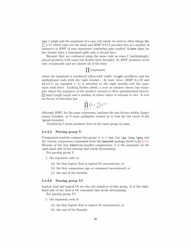
sign / might end the argument of a sum, but surely we need to allow things like∑1/n2 which rules out the slash and HMF 9.9.11 provides two of a number of

instances in HMF of sum arguments continuing past explicit \times signs (atline breaks when a summand spills onto a second line).

Because they are evaluated using the same code as sums I (unthinkingly)placed products with sums but doubts later intruded. In HMF products occuronly occasionally and are almost all of the form∏

(argument)

where the argument is bracketed (often with \left \right modifiers) and themultiplicand ends with the right bracket. At least twice (HMF 6.1.25 and24.2.2.1) an exponent (−1) is attached to the right bracket and the argu-ment ends there. Looking further afield, a text on number theory has exam-ples where the argument of the product extends to three parenthesised factors,∏

(arg1) (arg2) (arg3) and a number of others where it extends to two. A texton theory of functions has

∞∏n=1

(1 + z

n

)ez/n

although HMF, for the same expression, encloses the two factors within (large)square brackets, as if some ambiguity existed as to how far the reach of the\prod extended.

Tentatively I retain products here in the same group as sums.

3.4.2.5 Parsing group V

Comparison symbols compose this group: =, <, >, \ne, \le, \ge, \leq, \geq, andthe various comparison commands from the amssymb package listed in §2.3.4.5.Because of the way numerica handles comparisons, it is the argument on theright-hand side of the relation that needs determining.

For parsing group V1. the argument ends at

(a) the first logical And or logical Or encountered, or(b) the first comparison sign or command encountered, or(c) the end of the formula.

3.4.2.6 Parsing group VI

Logical And and logical Or are the sole members of this group. It is the right-hand side of the And or Or command that needs determining.

For parsing group VI1. the argument ends at

(a) the first logical And or logical Or encountered, or(b) the end of the formula.

80

3.4.2.7 Disclaimer

The parsing rules of the different groups are not normative; they are not state-ments of how mathematical formulas should be written. Rather they are at-tempts to discern regularities in how mathematicians often do write formulas.It is how things look in the pdf, not LATEX, that is the guide. You are alwaysfree to parenthesize as you see fit and to insert cleave commands (\q or \Q) toforce outcomes.

(But note that parenthesizing has its limits. For sums, writing∑(< stuff >) < more stuff >

does not necessarily end the summand at the right parenthesis: it ends at thefirst naked + or − sign, or \Q command, encountered.)

The rule should always be to write expressions that are clear to the readerof the pdf. An expression that is ambiguous to the reader, even if it fits withinthe parsing rules, is to be deprecated. The intent is that \eval can parseunambiguous expressions correctly.

81

Chapter 4

Supplementary commands

This chapter introduces four commands, \nmcInfo (which we have already met),\nmcMacros, \nmcConstants and \nmcReuse, supplementary to the principalcommand \nmcEvaluate. They use the same machinery as \nmcEvaluate andso have the same syntax. If all arguments are present it is

\nmc<cmd>*[settings]{main arg}[vv-list][rounding]

where <cmd> is one of Info, Macros, Constants and Reuse. All four commandshave short-name forms: \info, \macros, \constants, \reuse.

Generally the final two optional arguments will not be used. The user shouldbe aware of this if following a command with a square bracketed expression – theexpression will be absorbed without trace unless it is preceded by, for example,an empty brace pair.

Because the commands share the machinery of \nmcEvaluate, the settingsdiscussed earlier (Chapter 3) for the \eval command are also available for thesecommands, although they will, in the main, be irrelevant. The ‘debug’ code hasbeen used by the view setting of some of these supplementary commands toproduce its effects.

The starred form of command is available in all four cases and in all casesproduces a pure number. If both star and view are used at the same time, theview setting prevails over starring.

4.1 Feedback on ‘infinite’ processes: \nmcInfo

Used after the evaluation of an ‘infinite’ process, the \nmcInfo command, orits short-name form \info will tell you how many terms or factors or otheroperations1 were needed to arrive at the result.The main argument contains anidentifier for the ‘infinite’ process:

1It also applies to the commands \nmcIterate and \nmcSolve from the numerica-pluspackage and to derivatives and integrals from the numerica-calculus package.

82

\nmcInfo{<arg>}

(or \info{<arg>}) where, at this stage, <arg> is either sum or prod. Thedisplay, as we have seen in earlier examples, is a number followed by a space thena descriptor. For sum and prod the descriptors are terms and factors. Starring\nmcInfo – \nmcInfo*{arg} or \info*{arg} – suppresses the descriptor andleaves only the number. This allows the starred form to be nested in an \evalcommand, which might sometimes be convenient.

As an example, let’s test ‘the hard way’ a standard identity, cosh2 x −sinh2 x = 1. We know that cosh x =

∑∞n=0

x2n

(2n)! and sinh x = x∏∞

k=1

(1 + x2

k2π2

).

The difference of their squares should be 1:

\eval{\[\left[\sum_{n=0}^{\infty}

\frac{x^{2n}}{(2n)!}\right]^2-

\left[x\prod_{k=1}^{\infty}\left(1+\frac{x^{2}}{k^{2}\pi^{2}}\right)

\right]^2\]}[x=1][3] \info{sum},\quad \info{prod}

=⇒ [ ∞∑n=0

x2n

(2n)!

]2

−

[x

∞∏k=1

(1 + x2

k2π2

)]2

= 1.002, (x = 1)

5 terms, 119 factors.Nearly right. Obviously the product converges only slowly which is where

the error comes from (see the discussion in §3.2, where we needed the extrarounding setting P+=3 and 350 factors to get a correct 3-figure value). Thepoint of the example is to show the information command being used for bothsum and product in the one evaluation. One does not exclude the other.

4.1.1 Suppressing the descriptor: \nmcInfo*

The starred form of the \info command suppresses the descriptor (‘terms’,‘factors’) and gives a purely numerical result:

\eval{$\sum_{k=0}^{\infty}\binom \alpha k x^k

$}[x=1/2,\alpha=3],requiring $ \info*{sum}-1 $ additions.

=⇒∑∞

k=0(

αk

)xk = 3.375, (x = 1/2, α = 3), requiring 4 − 1 additions. (Four

terms added, therefore 3 additions.)

83

4.1.2 ErrorsShould the wrong argument be used in the \nmcInfo command, no harm isdone:

\eval{$\sum_{k=0}^{\infty}\binom \alpha k x^k

$}[x=1/2,\alpha=3], \ \info{prod}

=⇒∑∞

k=0(

αk

)xk = 3.375, (x = 1/2, α = 3), 119 factors.

119 factors? The information command is remembering a previous result,the last time prod was used as its argument. Changing the argument from prodto sum reveals the correct number of terms.

Should a non-existent argument be used, an error message is generated:

\eval{$\sum_{k=0}^{\infty}\binom \alpha k x^k

$}[x=1/2,\alpha=3], \\ \info{Fred}

=⇒∑∞

k=0(

αk

)xk = 3.375, (x = 1/2, α = 3),

!!! Unknown process Fred in: \nmcInfo command. !!!

4.1.3 view settingAs noted at the start of this chapter, \nmcInfo uses the ‘machinery’ of \nmcEvaluate.Most of the settings available for \eval are also available for \info but of theseonly one seems relevant: the dbg setting. However, rather than use the obscuredbg=<integer> (which is possible), it suffices to enter view in this argument:

\info[view]{} =⇒

process: sum {4}, prod {119}

The result is a display of all the current values of all the ‘infinite’ processesavailable. All such values are initialized to 0. (Further processes iter and solvebecome relevant if the numerica-plus package is used; deriv and integ becomerelevant if the numerica-calculus package, currently under development, isused.)

4.2 User-defined macros: \nmcMacros

The \nmcMacros and \nmcConstants commands were prompted by a questionon TEX Stack Exchange.2 Some time later the maintainer of the mandi package3

2A question from Giacomo Petrillo on TEX Stack Exchange and a response by‘egreg’ prompted the introduction of the \nmcMacros and \nmcConstants commands. Seehttps://tex.stackexchange.com/questions/602993/use-macros-in-numerica-vv-list/602998#602998

3The maintainer is Joe Heafner, who explains that ‘mandi’ is an abbreviation of ‘matterand interactions’ after a physics textbook of that name (by different authors). Among other

84

approached me with a similar problem. Suppose one has defined a macro tocontain a value, say

• \def\myvalue{0.35}, or

• \newcommand\myvalue{0.35}, or

• \NewDocumentCommand\myvalue{}{0.35}, if you’re using xparse.

(If you’re using the document processor LYX then there is good reason to prefer\gdef to define your macro, \gdef\myvalue{0.35}; see Chapter 6). After oneof these commands, \myvalue is now known to LATEX, but it is not knownto numerica. The quantities numerica does know about are variables in thevv-list of an \eval command, and those LATEX (and amsmath and mathtools)commands used for writing mathematical expressions. These quantities arestored in numerica in structures called property lists. Since \myvalue is notrecorded in these lists yet, putting x=\myvalue in the formula or vv-list of an\eval command will produce an ‘Unknown token’ error message:

\NewDocumentCommand \myvalue {} {0.35}\eval{ \myvalue }

=⇒ !!! Unknown token \myvalue in: formula. !!!With version 2 of numerica a command is now available, \nmcMacros, to reg-

ister macros and their values with the property lists used internally by numerica.(This command was not available in version 1.) The macro must have been de-fined earlier in the document or in a supporting package.

The basic usage is simple. If you have a list of macros you wish to make avail-able to \nmcEvaluate, enter them in a comma list in the mandatory argumentof \nmcMacros:

\nmcMacros{ \macro1, \macro2, ... }

There is an equivalent short-name form of the command, \macros.Multiple \nmcMacros commands can be used in a document. If the com-

mand is placed in the preamble (after the definition of the macros) then theuser-defined macros and their values are available throughout the document,otherwise they are available from the position of the \macros statement. How-ever, macros do not need to be defined in your current document provided theyare defined and accessible from elsewhere – for example from a loaded LATEXpackage. But always an \nmcMacros command is required to ‘register’ themwith numerica for use in an \eval command.things, the package defines a long list of macros, each containing the value of a physicalconstant.

85

4.2.1 What can be stored in a macro?Generally a user-defined macro will store a number. This macro might well bedefined in an external package – for example the mandi package defines a largenumber of macros containing the values of physical constants, some fundamentallike the speed of light, others contingent like the earth–moon distance. If themandi package is loaded then writing, for instance,

\macros{ \electronmassprecisevalue,\protonmassprecisevalue }

will make these two macros available for use in numerica. One could then writein the vv-list of an \eval command

m_e=\electronmassprecisevalue,m_p=\protonmassprecisevalue

which would allow (among other things) calculation of the mass ratio mp/me

of proton to electron. (The length of name of some of the macros in the mandipackage has a pedagogical purpose, but makes them unwieldy for direct use inmathematical expressions.)

4.2.1.1 Macros containing formulas

Numbers are not the only quantities that can be stored in a macro for use innumerica. In fact any mathematical expression that can be \eval-uated canbe stored in a macro:

\NewDocumentCommand \mysumC {}{ \sum_{n=1}^{100}1/n - \ln 100 }

\macros{ \mysumC }\eval{$ \mysumC $}[4]

=⇒∑100

n=1 1/n − ln 100 = 0.5822,

(to be compared with Euler’s constant γ = 0.5772 – obviously many more termsare needed). The \eval command wraps around math delimiters in the example.Hence the result is presented in the form formula=result. In that presentation,note how \mysumC displays as the formula it contains.

The essential space: But the critical thing to notice in the example is thespace preceding \sum in the definition of \mysumC. When a formula starts withan expandable token, this space is essential. For macros to register successfullywith numerica, the first character in their definition must be unexpandable.Thus a digit is fine: storing a number in a macro is straightforward and youdon’t need to fuss about such niceties. But a control sequence like \sum doesexpand (to

∑). If it is the initial token of the formula, then it will cause a

possibly obscure error – see §4.2.3 – unless preceded by an unexpandable token.Hence the space before \sum in the \NewDocumentCommand statement. (On theother hand the spacing in the \macros statement is purely aesthetic.)

86

When using macros from another package, this is a matter to be aware of.If the macros contain only numbers, there should be no problem, but if theycontain more complicated expressions, the absence of an initial space could makethem unusable in numerica.

4.2.1.2 Vv-list

In the example it would be nice to be able to vary the number of terms summed.This is easily done by using a vv-list in the \macros statement:

\NewDocumentCommand \mysumN {}{ \sum_{n=1}^{N}1/n - \ln N }

\macros{ \mysumN }[N=150]\eval{$ \mysumN $}

=⇒∑N

n=1 1/n − ln N = 0.580545.

numerica needs a definite value to store; it does not store the formula as such.To give \mysumN a definite value, give the variable N a value. This is done inthe vv-list added to the \macros statement: N=150. In this way a definite valueis stored in numerica against the macro \mysumN. The definition of the macrois unaffected. If a new value is given to N in the \macros statement (which isthe point of using a variable), the old value is overwritten and the new value isused in subsequent calculations.

4.2.2 Seeing what macros are availablePerhaps your document has a number of \nmcMacros statements scatteredthrough it and you want to remind yourself of what exactly has been stored.\nmcMacros has the view setting for this purpose. Writing

\macros[view]{} =⇒

macros: \mysumN { \sum _{n=1}^{N}1/n - \ln N },\mysumC { \sum_{n=1}^{100}1/n - \ln 100 }

stored: \mysumN =0.580545294547621, \mysumC =0.582207331651529

produces a list of all macros registered with numerica and their values, as youcan see.

If the braced argument is not empty, the display is slightly modified:

\def\mydef{ \sin(m\pi/n) }\newcommand\mynewcmd{ \cos(m\pi/n) }\macros[view]{ \mydef,\mynewcmd }[m=3,n=18]

87

=⇒

vv-list: m=3, n=18added: \mydef { \sin (m\pi /n) },\mynewcmd { \cos (m\pi /n) }stored: \mydef =0.4999999999999999, \mynewcmd =0.8660254037844387, \mysumN

=0.580545294547621, \mysumC =0.582207331651529

\mydef and \mynewcmd have been added to those available for use in numerica.

4.2.2.1 Freeing macros from storage

Rather than cluttering numerica’s property lists with no-longer-needed macros,it is possible to remove them from there with the free setting. This has no effecton the LATEX definition of the macro. It merely ‘de-registers’ the macro withnumerica.

\macros[free,view]{ \mysumC } =⇒

freed: \mysumC { \sum _{n=1}^{100}1/n - \ln 100 }stored: \mydef =0.4999999999999999, \mynewcmd =0.8660254037844387, \mysumN

=0.580545294547621

If you want to free all macros registered with numerica use an empty mainargument with the free setting. For an example, see just below.

4.2.2.2 Counting how many macros are available

You can count how many macros are currently registered with numerica bystarring the \nmcMacros command:

\macros*{} =⇒ 3.

If the braced argument is not empty, the list of macros it contains will be addedto those registered with numerica and included in the overall count.

Note that the view setting prevails over starring if both are used.The star can also be used with the free setting. As mentioned above, if the

main argument is empty, then all macros are freed:

\macros*[free]{} =⇒ 0

4.2.3 ErrorsIf a macro is used in a \macros statement and the macro has not been definedin the document or a supporting package it will cause an error:

\macros{ \mymacro }

88

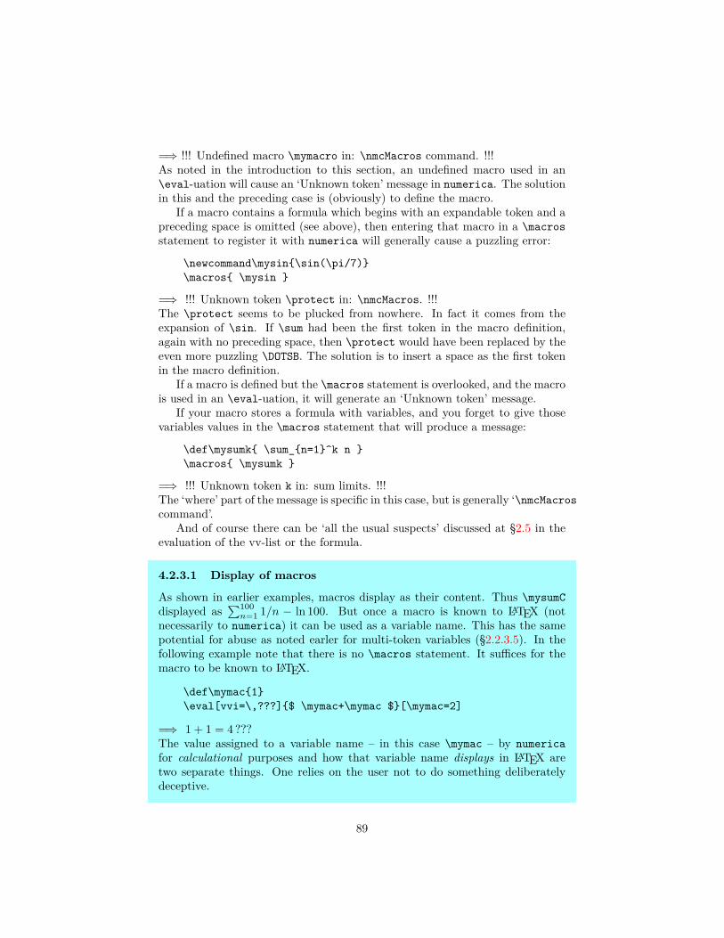
=⇒ !!! Undefined macro \mymacro in: \nmcMacros command. !!!As noted in the introduction to this section, an undefined macro used in an\eval-uation will cause an ‘Unknown token’ message in numerica. The solutionin this and the preceding case is (obviously) to define the macro.

If a macro contains a formula which begins with an expandable token and apreceding space is omitted (see above), then entering that macro in a \macrosstatement to register it with numerica will generally cause a puzzling error:

\newcommand\mysin{\sin(\pi/7)}\macros{ \mysin }

=⇒ !!! Unknown token \protect in: \nmcMacros. !!!The \protect seems to be plucked from nowhere. In fact it comes from theexpansion of \sin. If \sum had been the first token in the macro definition,again with no preceding space, then \protect would have been replaced by theeven more puzzling \DOTSB. The solution is to insert a space as the first tokenin the macro definition.

If a macro is defined but the \macros statement is overlooked, and the macrois used in an \eval-uation, it will generate an ‘Unknown token’ message.

If your macro stores a formula with variables, and you forget to give thosevariables values in the \macros statement that will produce a message:

\def\mysumk{ \sum_{n=1}^k n }\macros{ \mysumk }

=⇒ !!! Unknown token k in: sum limits. !!!The ‘where’ part of the message is specific in this case, but is generally ‘\nmcMacroscommand’.

And of course there can be ‘all the usual suspects’ discussed at §2.5 in theevaluation of the vv-list or the formula.

4.2.3.1 Display of macros

As shown in earlier examples, macros display as their content. Thus \mysumCdisplayed as

∑100n=1 1/n − ln 100. But once a macro is known to LATEX (not

necessarily to numerica) it can be used as a variable name. This has the samepotential for abuse as noted earler for multi-token variables (§2.2.3.5). In thefollowing example note that there is no \macros statement. It suffices for themacro to be known to LATEX.

\def\mymac{1}\eval[vvi=\,???]{$ \mymac+\mymac $}[\mymac=2]

=⇒ 1 + 1 = 4 ???The value assigned to a variable name – in this case \mymac – by numericafor calculational purposes and how that variable name displays in LATEX aretwo separate things. One relies on the user not to do something deliberatelydeceptive.

89

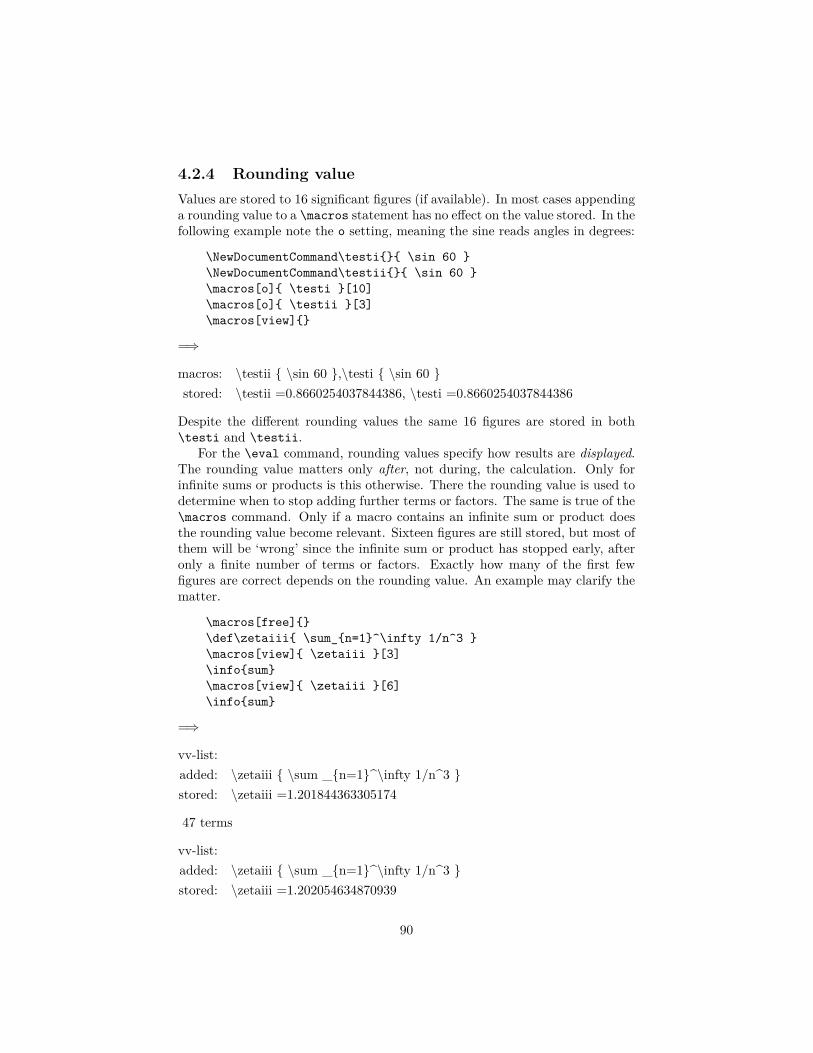
4.2.4 Rounding valueValues are stored to 16 significant figures (if available). In most cases appendinga rounding value to a \macros statement has no effect on the value stored. In thefollowing example note the o setting, meaning the sine reads angles in degrees:

\NewDocumentCommand\testi{}{ \sin 60 }\NewDocumentCommand\testii{}{ \sin 60 }\macros[o]{ \testi }[10]\macros[o]{ \testii }[3]\macros[view]{}

=⇒

macros: \testii { \sin 60 },\testi { \sin 60 }stored: \testii =0.8660254037844386, \testi =0.8660254037844386

Despite the different rounding values the same 16 figures are stored in both\testi and \testii.

For the \eval command, rounding values specify how results are displayed.The rounding value matters only after, not during, the calculation. Only forinfinite sums or products is this otherwise. There the rounding value is used todetermine when to stop adding further terms or factors. The same is true of the\macros command. Only if a macro contains an infinite sum or product doesthe rounding value become relevant. Sixteen figures are still stored, but most ofthem will be ‘wrong’ since the infinite sum or product has stopped early, afteronly a finite number of terms or factors. Exactly how many of the first fewfigures are correct depends on the rounding value. An example may clarify thematter.

\macros[free]{}\def\zetaiii{ \sum_{n=1}^\infty 1/n^3 }\macros[view]{ \zetaiii }[3]\info{sum}\macros[view]{ \zetaiii }[6]\info{sum}

=⇒

vv-list:added: \zetaiii { \sum _{n=1}^\infty 1/n^3 }stored: \zetaiii =1.201844363305174

47 terms

vv-list:added: \zetaiii { \sum _{n=1}^\infty 1/n^3 }stored: \zetaiii =1.202054634870939

90

468 termsHMF Table 23.3 tells me that ζ(3) = 1.202056903159594 . . . The different

rounding numbers have restricted the infinite sums to the very finite 47 and468 terms respectively. Although 16 figures are stored, only the first few arecorrect. Just how many depends on the number of terms summed which dependson when the stopping criterion is met which depends on the rounding value.

4.3 User-defined constants: \nmcConstants

As noted much earlier in this document (§2.2.2.3), there are five built-in con-stants: \pi, e, \phi, \gamma and \deg, but a user may well want to define theirown constant or constants. There are contexts where it would make sense topermanently record fundamental constants like the speed of light or Planck’sconstant, or more down-to-earth constants like the acceleration due to gravityor the viscosity of water, rather than having to enter them in the vv-list for eachcalculation. Or a parameter might be held constant for a particular problem orclass of problems where other variables change – for example triangles of con-stant perimeter but varying sides. This is the purpose of the \nmcConstantscommand.

The symbols used to denote constants are subject to exactly the same con-straints and freedoms as the symbols used to denote variables. They might besingle latin letters like c (e.g. c = 3 × 108), or greek letters like \alpha (e.g.α = 1/137), or multitoken combinations like the Rydberg constants R_\inftyor R_{\mathrm{H}} from atomic physics, or \mu_0 and \epsilon_0 used to de-note the permeability and permittivity of free space, or personal constants liketotal of no wider significance. numerica handles all these different forms ofconstant with the command \nmcConstants:

\nmcConstants{ const-n=value-n, ... ,const2=value2, const1=value1 }

This is the simplest use – each constant is assigned a (numerical) value. But itis easy to envisage situations where it would be convenient to have a constantwith value 1/

√2π say, or another with value e

π2 , and so on. That is easy: simply

put the expession for the value on the right:

\constants{ a=1/\sqrt{2\pi},b=e^{\tfrac\pi2} }

Or the values could be expressions depending on parameters:

\constants{ s=\tfrac12(a+b+c) }[a=3,b=5,c=7]

Some constants might depend on earlier constants in the list:

\constants{ A=\sqrt{s(s-a)(s-b)(s-c),s=\tfrac12(a+b+c) }[a=3,b=5,c=7]

Or the values could involve an ‘infinite’ process, requiring a rounding number:

91

\constants{ \zeta=\sum_{n=1}^\infty(1/n^k) }[k=4][5]

In this, although 16 figures will be stored, only the first few will be accurate,the precise number depending on the value of k and the rounding number (5 inthe example); see the discussion on this issue for user-defined macros, §4.2.4.

4.3.1 New list replaces old by defaultA particular group of constants may be relevant only to a particular part of adocument. Another part of the document may use other constants. By default,a second list of constants replaces the first list. Thus each of the \constantsstatements above would replace the previous one.

There is a technical reason why replacing rather than appending is the de-fault. For each calculation all multi-token constants (e.g. R_\infty, N_0, . . . )are added internally to the start of the vv-list of the \eval command. Even if thevv-list is empty, this is still the case since the formula might well use constants.Like multi-token variables and for the same reason (see §2.2.1), multi-tokenconstants are mapped internally to single tokens. This occurs afresh for eachcalculation. If there are a lot of multi-token constants then each calculationis going to involve not only this mapping from multi- to single tokens but theevaluation of a long vv-list. In that case it seems better to make the defaultbehaviour replacement of one constant list by another, rather than appendingthem.

4.3.2 Adding constants to a listDespite the default behaviour, there will be occasions when you want to add anew constant or constants to the current list. This is easily done with the addsetting. For instance,

\nmcConstants[add]{ \sigma=5.67\times10^{-8},k_B = 1.381\times10^{-23} }

would add \sigma and k_B to the current list. The presence of the add settingtriggers appending rather than replacement.

4.3.3 Examples of use4.3.3.1 Example 1: atomic constants

In the following example, the values of various atomic constants are taken fromthe mandi package. I use two \constants statements in order to show the useof the add setting. I’ve also included a view setting in the second \constantsstatement.

The constants are used to calculate the fine-structure constant \alpha inthe vv-list of the \eval command, and its well-known reciprocal (close to 137)in the main argument. Note that the constants do not need to be entered in the

92

vv-list of the \eval command. Their values are available from the \constantsstatements.

\constants{ c=2.99792458\times10^{8},h=6.62607015\times10^{-34},e=1.602176634\times10^{-19} }

\constants[view,add]{ \epsilon_0=8.854187817\times10^{-12} }

\eval{$ 1/\alpha $}[\alpha=e^2/2\epsilon_0hc]

=⇒

vv-list:added: \nmc_p =8.854187817\times 10^{-12}

constants: e=1.602176634e-19, h=6.62607015e-34, c=299792458, \epsilon_0=8.854187817e-12

1/α = 137.035999, (α = e2/2ϵ0hc).The view setting produces a now familiar kind of display. It shows that the

three-token \epsilon_0 (the control sequence \epsilon, the underscore _ andthe digit 0) has been replaced by \nmc_q – which may look as if it is also threetokens but is in fact a single control sequence.

4.3.3.2 Example 2: local constants

Long ago, when there were such creatures as reference librarians, I was askedabout a school physics project along these lines.

A car is travelling at 50 km/hr when it hits a lamppost. The bonnet crumples1 metre and the car comes to an immediate halt. Although she herself is wearinga seat-belt, a woman in the passenger cabin is holding her 5 kg baby. Does thebaby survive?

The enquirer was familiar with the equations describing constant accelera-tion,

x = ut + 12 at2, and v2 − u2 = 2ax,

and Newton’s second law, F = ma, force equals mass times acceleration. Thequestion was really about understanding these laws and how to think with them.Here, s is the distance travelled in time t, with initial speed u at t = 0, speed vat time t, and constant acceleration a – a deceleration in this case.

The given data provide our constants: distance x = 1 metre, initial speedu = 1000 ∗ 50/(60 ∗ 60) = (10/36) ∗ 50 metres per second, final speed v = 0. Toestimate whether the woman can hold on to her baby, we will need to make acomparison with forces we have personally experienced. Most of us have triedlifting someone else, so let’s use a characteristic human weight as our test mass.Thus, we have the (baby’s) mass m = 5 kilograms, and a test mass, M say,which we will leave as a variable. But dealing with weight, we will need theacceleration due to gravity. For the kind of rough estimating we are doing,g = 10 metres per second per second will be an adequate approximation.

93

\constants{ x=1,v=0,u=(10/36)50,m=5,g=10 }

The deceleration experienced by the woman is found from the second equation ofconstant acceleration, a = (v2 − u2)/2x. Even if the deceleration isn’t constantthis will give an estimate of its magnitude. (If some of the deceleration is lessthan this a, some must be greater.) This is also the deceleration experienced bythe baby as long as the woman holds onto her. Hence the magnitude of the forceexerted by the baby on the woman’s arms is ma = m(v2 − u2)/2x = −mu2/2xwhich we want to compare with our test force, say that required to lift M = 70kilograms, which was once considered the mass of an average western adultmale (but is doubtless a considerable underestimate now). Hence the test forceis Mg. Let’s do the calculations. (I have altered the \constants statement toallow for a later comparison with the effect of a small increase in speed.)

\constants{ x=1,u=(10/36)U,m=5,g=10 }[U=50]\eval{$ mu^2/2x $}[0], \par\eval{$ Mg $}[M=70].

=⇒ mu2/2x = 482,Mg = 700, (M = 70).The force required to hold on to the baby is noticeably less than that required

to lift a 70 kg person – in fact about the same as that needed to lift a 50 kgperson. But we have ignored the force experienced by the mothers forearms –perhaps doubling m (baby plus forearms) would give a better estimate of theforce she experiences. In that case mu2/2x obviously doubles and the total forcerequired by the woman to retain her baby – now 964 newtons – is significantlymore than that required to lift a 70 kg person. I think it almost certain thatthe baby is torn from her arms.

What difference does increasing the speed to 60 km/hr make?

\constants{ x=1,u=(10/36)U,m=5,g=10 }[U=60]\eval{$ mu^2/2x $}[1], \par\eval{$ Mg $}[M=70].

=⇒ mu2/2x = 694,Mg = 700, (M = 70).Now the force of baby alone is comparable to that required to lift a 70 kg

person. Including the woman’s forearms in m, doubling m say, will result in aforce twice as great – like that required to lift two 70 kg people or one 140 kgperson. There is no chance of the woman holding on to her baby. The force istoo great.

4.3.3.3 Example 3: macros and constants

Constants can depend on previously defined and registered user macros. Sup-pose I have defined two macros

\NewDocumentCommand\electronmassprecisevalue {}

94

{9.1093837015\times10^{-31}}\NewDocumentCommand\protonmassprecisevalue {}

{1.672621898\times10^{-27}}

(I have taken both the names and the values from the mandi package.) Thelong explicit names of the macros has a pedagogic purpose, but they are toocumbersome to use in calculations. For that purpose we need, first, a \macrosstatement registering the two macros with numerica, and then a \constantsstatement like

\nmcConstants{ m_e=\electronmassprecisevalue,m_p=\protonmassprecisevalue }

With that m_e and m_p could be entered in formulas, taking the values containedin the macros. Let’s do it:

\NewDocumentCommand\electronmassprecisevalue {}{9.1093837015\times10^{-31}}

\NewDocumentCommand\protonmassprecisevalue {}{1.672621898\times10^{-27}}

\nmcMacros{ \electronmassprecisevalue,\protonmassprecisevalue }

\nmcConstants{ m_e=\electronmassprecisevalue,m_p=\protonmassprecisevalue }

\eval{$ m_p/m_e $}

=⇒ mp/me = 1836.152645,the familiar mass ratio of proton and electron.

4.3.4 Viewing, counting constantsTo see all constants currently ‘in play’, use the view setting in the \constantscommand. The main argument can be empty,

\constants[view]{} =⇒

constants: m_p=1.672621898e-27, m_e=9.1093837015e-31

or contain a list of constants. In the latter case, the display is of the aboveform but featuring the constants of the new list or, if the add setting is used,featuring the joined lists, old and new:

\constants[view,add]{X=42} =⇒

vv-list:added: X=42

constants: m_p=1.672621898e-27, m_e=9.1093837015e-31, X=42

95

To count how many constants are currently in play, star the \constants com-mand. The number will depend on whether the main argument is empty or not,and whether the add setting is active:

\constants*{} =⇒ 3.

If the view setting is being used at the same time as the star, the view prevails.

4.3.5 ErrorsWhen contemplating error messages from numerica it needs to be rememberedthat multi-token constants are added to the vv-list for every calculation. Hencean error may not be in the vv-list as indicated in the message but in the\constants statement, specifically, the multi-token constants.

4.4 Saving and reusing results: \nmcReuse

You may want to use at some place in a document a result calculated earlier.It would be good to be able to do so without having to do the calculationagain at the new location. numerica offers a command \nmcReuse (short-nameform, \reuse) which saves a result to a control sequence that can then be usedelsewhere in the document, expanding to the saved result. The control sequenceand its content are also saved to file, allowing the possibility of using the resultin other documents.

The \nmcReuse command in version 2 of numerica has been completely rewrit-ten. Its use is not compatible with how the command was used in version 1. Ifound that I could bring \nmcReuse along with \nmcMacros and \nmcConstantsinto the coding scheme used for \nmcEvaluate and the reasons for doing so weretoo compelling.

4.4.1 Use of \nmcReuse

As noted, all the supplementary commands share the syntax of the \eval com-mand, so that \nmcReuse has an optional settings argument preceding a manda-tory main argument, followed by two trailing optional arguments. \nmcReusedoes not use the last two. The command is used mainly in two ways:

1. \nmcReuse{}, which loads the saved control sequences from file, if not alreadyloaded; and

2. \nmcReuse{csname}, which loads the saved control sequences from file, if notalready loaded, assigns the latest result from \eval to the control sequence\csname, and saves \csname to file.

You may wish to put \nmcReuse{} in the preamble of your document (after\usepackage{numerica} of course). In that way, saved control sequences are

96

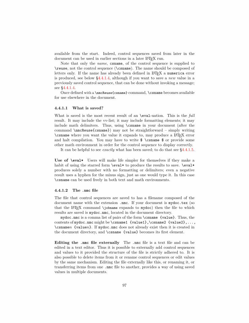
available from the start. Indeed, control sequences saved from later in thedocument can be used in earlier sections in a later LATEX run.

Note that only the name, csname, of the control sequence is supplied to\reuse, not the control sequence (\csname). The name should be composed ofletters only. If the name has already been defined in LATEX a numerica erroris produced, see below §4.4.1.4, although if you want to save a new value in apreviously saved control sequence, that can be done without invoking a message;see §4.4.1.4.

Once defined with a \nmcReuse{csname} command, \csname becomes availablefor use elsewhere in the document.

4.4.1.1 What is saved?

What is saved is the most recent result of an \eval-uation. This is the fullresult. It may include the vv-list; it may include formatting elements; it mayinclude math delimiters. Thus, using \csname in your document (after thecommand \nmcReuse{csname}) may not be straightforward – simply writing\csname where you want the value it expands to, may produce a LATEX errorand halt compilation. You may have to write $ \csname $ or provide someother math environment in order for the control sequence to display correctly.

It can be helpful to see exactly what has been saved; to do that see §4.4.1.5.

Use of \eval* Users will make life simpler for themselves if they make ahabit of using the starred form \eval* to produce the results to save. \eval*produces solely a number with no formatting or delimiters; even a negativeresult uses a hyphen for the minus sign, just as one would type it. In this case\csname can be used freely in both text and math environments.

4.4.1.2 The .nmc file

The file that control sequences are saved to has a filename composed of thedocument name with the extension .nmc. If your document is mydoc.tex (sothat the LATEX command \jobname expands to mydoc) then the file to whichresults are saved is mydoc.nmc, located in the document directory.

mydoc.nmc is a comma list of pairs of the form \csname {value}. Thus, thecontents of mydoc.nmc might be \csname1 {value1},\csname2 {value2},...,\csnamen {valuen}. If mydoc.nmc does not already exist then it is created inthe document directory, and \csname {value} becomes its first element.

Editing the .nmc file externally The .nmc file is a text file and can beedited in a text editor. Thus it is possible to externally add control sequencesand values to it provided the structure of the file is strictly adhered to. It isalso possible to delete items from it or rename control sequences or edit valuesby the same mechanism. Editing the file externally like this, or renaming it, ortransferring items from one .nmc file to another, provides a way of using savedvalues in multiple documents.

97

4.4.1.3 Messages

If a control sequence \csname is already known to LATEX, then writing \reuse{csname} will produce a numerica message and the result of the latest \eval-uation will not be saved:

\eval*{\sum_{n=1}^{10}n}\par\reuse{sigma}

=⇒ 55!!! \sigma already defined in: \nmcReuse command. !!!

If there is no result to save – perhaps an \eval-uation produces an errormessage instead – then another message is generated:

\eval*{1/0}\par\reuse{oops}

=⇒ !!! l3fp error ‘Division by zero’ in: formula. !!!!!! No result available for oops in: \nmcReuse command. !!!

4.4.1.4 Deleting and renewing

There may be occasions when you wish to change a previously saved value andyet, irritatingly, the control sequence name will now be known to LATEX and sowill generate an ‘already known’ message. If you choose a different name for thecontrol sequence to save the new value to, do you want the old name clutteringthe .nmc file? Deleting and renewing the values of saved control sequences arecontrolled by the settings delete and renew.

Entering delete in the settings option deletes a control sequence and itsvalue from the .nmc file and undefines it in LATEX terms. Thus \reuse[delete]{csname} would delete \csname and its value from the .nmc file and undefine\csname. If \csname is not present in the file, nothing happens. Entering renewreplaces the value of a saved control sequence with a new value. If there is nosuch saved control sequence but the control sequence is otherwise known toLATEX the ‘already defined’ message will still be generated. This prevents givingcontrol sequences like \sin or \frac new meanings with the renew setting.

• \reuse[delete]{csname} deletes \csname and its value from the .nmcfile and from memory if present; otherwise has no effect;

• \reuse{csname} (the default) saves the result of the latest \eval com-mand to \csname, provided \csname is not already defined; in that casea warning message is presented and the result is not saved;

• \reuse[renew]{csname} behaves like the default mode unless \csname isalready a saved control sequence in the .nmc file, in which case its previousvalue is replaced by the result of the latest \eval command;

• if delete and renew are used together, whichever occurs second prevails.

98

In the following example, the first \reuse deletes \suma should it be presentin the .nmc file, the second saves the result, 55, of the latest \eval-uation (infact an \eval*-uation) and the third overwrites that saved value with the newvalue, 210.

\reuse[delete]{suma}\eval*{\sum_{n=1}^{10}n} \par\reuse{suma}\eval*{\sum_{n=1}^{20}n} \par\reuse[renew]{suma}

=⇒ 55210

4.4.1.5 Viewing what has been saved

It would be good in this example to see that the new value 210 has in fact beensaved. That is easy. Simply enter view in the settings option of \nmcReuse(I’ve removed the now unnecessary \par tokens from the example.)

\reuse[delete]{suma}\eval*{\sum_{n=1}^{10}n}\reuse[view]{suma}\eval*{\sum_{n=1}^{20}n}\reuse[renew,view]{suma}

=⇒ 55

saved: \suma {55}

210

saved: \suma {210}

First the original value 55 was saved to \suma but then the value was overwrittenby the new value 210.

The view setting allows us to see how formatting is stored if the unstarredform of the \eval command is used. In the following example, \eval wrapsaround math delimiters:

\eval{$ 1+1 $} \reuse[view,renew]{two} =⇒ 1 + 1 = 2

saved: \two {$1+1=2$}

The full formula=result display has been captured in \two along with the mathdelimiters. If a vv-list is also involved, things become messy (but informative):

\eval{$ x+y $}[x=1,y=2]\reuse[view,renew]{three}

99

=⇒ x + y = 3, (x = 1, y = 2)

saved: \three {$x+y=3\mathchoice {{,}\mskip36muminus24mu(x=1,y=2)}{{,}\mskip12muplus6muminus9mu(x=1,y=2)}{}{}$}

You may want to see all saved control sequences. In that case use an emptymain argument: \nmcReuse[view]{}. We now have enough saved control se-quences to make this worthwhile:

\reuse[view]{}

=⇒

saved: \three {$x+y=3\mathchoice {{,}\mskip36muminus24mu(x=1,y=2)}{{,}\mskip12muplus6muminus9mu(x=1,y=2)}{}{}$}, \two {$1+1=2$}, \suma {210},\seven {7}

(The \seven that appears here is defined shortly. Its appearance before defi-nition is presumably due to LATEX making a number of passes when compilingthis document.)

4.4.1.6 Counting saved control sequences: \nmcReuse*

Because \nmcReuse uses the same machinery as \nmcEvaluate, it has a starredform, \nmcReuse*, which produces a purely numerical result (just like \eval*,info*, \macros* and \constants*). In this case, the number is the count ofhow many control sequences have been saved:

\reuse*{} =⇒ 4.

4.4.2 reuse setting of \eval commandUsing \eval* for a calculation ensures a purely numerical result, with no vv-listor formatting in the display of the result. But sometimes we might want thefull display yet wish to save only the numerical result. This is the point of thereuse setting of the \eval command.

For the starred form of the \eval command it is always only the numericalresult that is saved, whatever the value of the reuse key in the settings optionof the \eval command.

For the unstarred form of the \eval command exactly what is saved with\nmcReuse depends on the reuse setting:

reuse = <integer>

where <integer> can take one of two values,

100

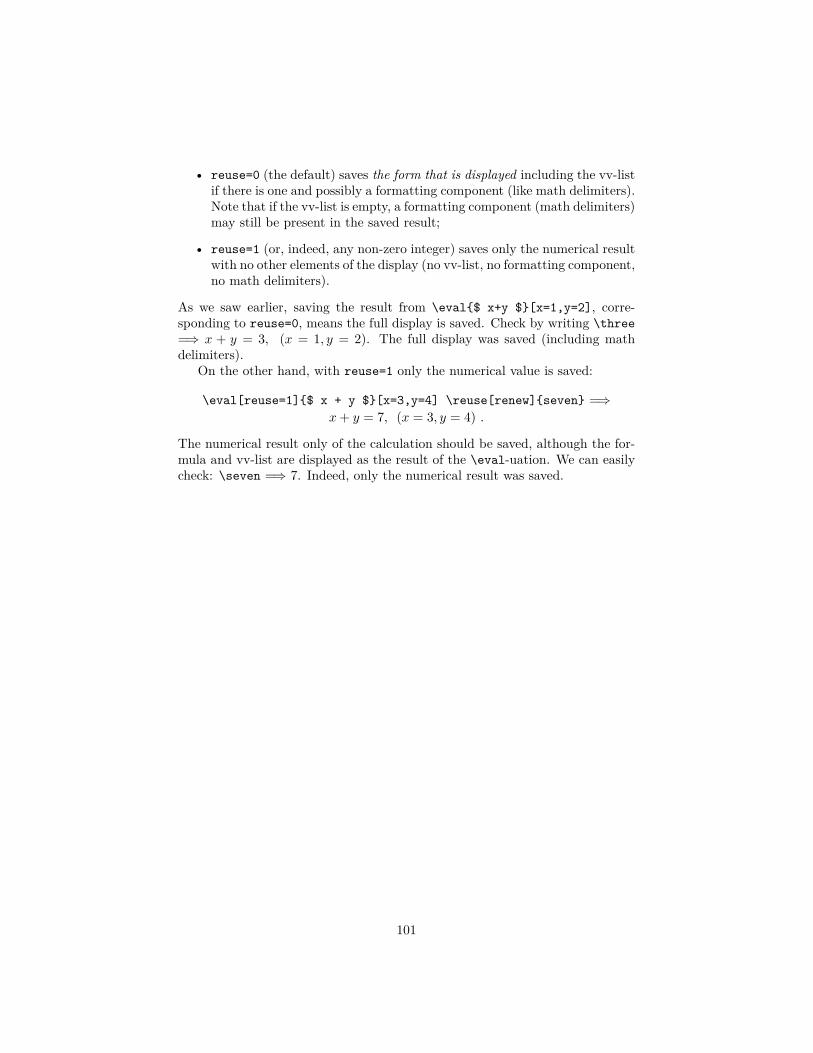
• reuse=0 (the default) saves the form that is displayed including the vv-listif there is one and possibly a formatting component (like math delimiters).Note that if the vv-list is empty, a formatting component (math delimiters)may still be present in the saved result;

• reuse=1 (or, indeed, any non-zero integer) saves only the numerical resultwith no other elements of the display (no vv-list, no formatting component,no math delimiters).

As we saw earlier, saving the result from \eval{$ x+y $}[x=1,y=2], corre-sponding to reuse=0, means the full display is saved. Check by writing \three=⇒ x + y = 3, (x = 1, y = 2). The full display was saved (including mathdelimiters).

On the other hand, with reuse=1 only the numerical value is saved:

\eval[reuse=1]{$ x + y $}[x=3,y=4] \reuse[renew]{seven} =⇒x + y = 7, (x = 3, y = 4) .

The numerical result only of the calculation should be saved, although the for-mula and vv-list are displayed as the result of the \eval-uation. We can easilycheck: \seven =⇒ 7. Indeed, only the numerical result was saved.

101

Chapter 5

Nesting commands

The \eval command and the supplementary commands of the previous chaptercan be nested – used within other \eval or supplementary commands. Nestingmay occur in the main argument, or the vv-list, or the settings option, or somecombination of all three. With the commands currently introduced, nesting isunlikely to be a major concern, but it becomes significant for the commandsdefined in the associated package numerica-plus (see §1.1.2). Since those ad-ditional commands are not available for this document, the examples belowuse the commands introduced earlier: \eval, \info, \macros, \constants and\reuse.

5.1 Nesting in the formulaConsider a statement like \eval{...\eval...}. There is an inner \eval andan outer \eval. The inner \eval ‘digests’ its LATEX formula to produce anl3fp-readable expression which is fed to l3fp to evaluate. The result is thenreturned to (the inner) \eval to display. In version 1 of numerica that meantthe inner command had to be starred, \eval*, so that no display formattingwas fed to the outer command to try to digest (and cause an error). In version2 of numerica this is no longer the case. numerica detects whether a commandis inner or outer, and if inner, suppresses all display formatting, producing onlya number, as if the command had been starred:

\eval{$ \sin(\eval{\sin x}[x=\pi/6]\pi) + 1 $} =⇒ sin(0.5π) + 1 = 2.In the presentation of the overall result, the inner \eval command is evaluated,displaying as a number.

In this example, the x=\pi/6 could be removed from the inner \eval andplaced in the vv-list of the outer command since outer variables are available tothe inner command:

\eval{$ \sin(\eval{\sin x}\pi) + 1 $}[x=\pi/6] =⇒sin(0.5π) + 1 = 2, (x = π/6).

102

Just to show that it is possible, the next example shows \eval being used in a\constants command. The o setting in the \constants command pervades itsargument; hence it needs to be explicitly turned off for the \eval if \sin(\pi/6)is to evaluate as expected.

\constants[o]{ y=\sin 30,x=\eval[o=0]{\sin(\pi/6)} }\eval{$ x+y $}

=⇒ x + y = 1.

5.1.1 Math delimiters and double evaluationsAny math delimiters in the inner \eval are ignored. (This also differs fromversion 1 of numerica where they caused an error.) Obviously it is simpler toomit them as I have done in the examples.

However, math delimiters in the outer \eval command still have their nor-mal effect and produce a formula = result, (vv-list) display. One consequenceof such a display is that the formula in the inner \eval command is evaluatedtwice – once when the overall result is being calculated (i.e. the formula of theouter \eval) and later when the overall display of the result is created. In theformula part of the formula = result, [vv-list] display, the tokens in the formulaare expanded to their display form. For example, \sin is expanded to sin, \piis expanded to π – and the inner \eval is expanded to the numerical result ofits evaluation – a second evaluation. If the inner formula is simple, this willbe of little moment, but should the inner formula contain, say, a slowly con-verging infinite series, then evaluating it twice is a bad idea and it would bebetter to remove the delimiters from the outer \eval. That prevents the secondevaluation.

The problem does not arise if the outer \eval lies within a math environment(e.g. $ \eval{...} $) since that produces a display of the form result, [vv-list].The formula is not displayed and so the second evaluation does not occur. Theinner \eval is evaluated once only to calculate the result.

5.2 Nesting in the vv-listThe inner \eval can be placed in the vv-list of the outer command. If the vv-listof the inner \eval contains a comma (meaning there are at least two variables),then the entire inner \eval and its LATEX arguments needs to be wrapped inbraces to hide the comma or commas of its vv-list from the outer \eval. Toshow the effect of not doing so, I have slightly complicated the previous exampleby adding a second (unnecessary) variable. The first example is with braces,the second without:

\eval{$ \sin k\pi + 1 $}[k={\eval{y\sin x}[x=\pi/6,y=1]}] =⇒sin kπ + 1 = 2, (k = 0.5).

\eval{$ \sin k\pi + 1 $}[k=\eval{y\sin x}[x=\pi/6,y=1]] =⇒!!! Unmatched ] in: variable = value list. !!!.

103

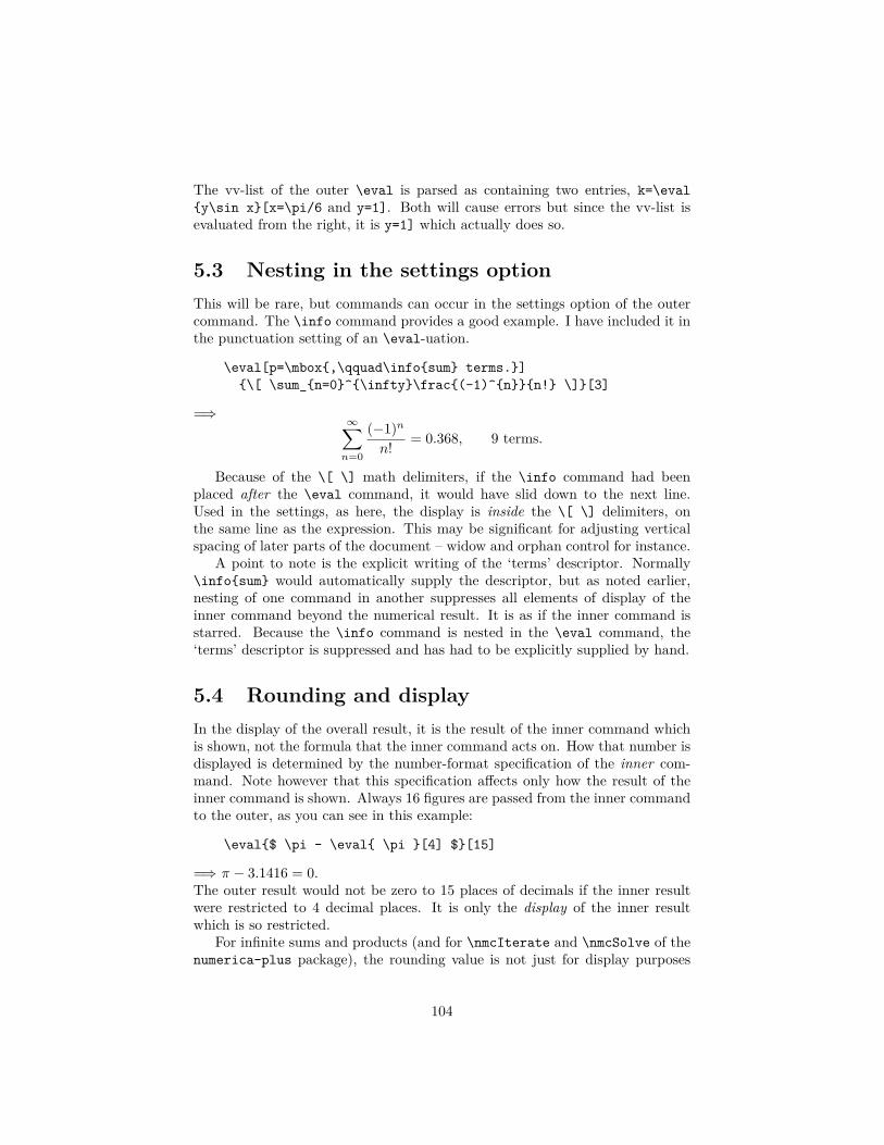
The vv-list of the outer \eval is parsed as containing two entries, k=\eval{y\sin x}[x=\pi/6 and y=1]. Both will cause errors but since the vv-list isevaluated from the right, it is y=1] which actually does so.

5.3 Nesting in the settings optionThis will be rare, but commands can occur in the settings option of the outercommand. The \info command provides a good example. I have included it inthe punctuation setting of an \eval-uation.

\eval[p=\mbox{,\qquad\info{sum} terms.}]{\[ \sum_{n=0}^{\infty}\frac{(-1)^{n}}{n!} \]}[3]

=⇒∞∑

n=0

(−1)n

n! = 0.368, 9 terms.

Because of the \[ \] math delimiters, if the \info command had beenplaced after the \eval command, it would have slid down to the next line.Used in the settings, as here, the display is inside the \[ \] delimiters, onthe same line as the expression. This may be significant for adjusting verticalspacing of later parts of the document – widow and orphan control for instance.

A point to note is the explicit writing of the ‘terms’ descriptor. Normally\info{sum} would automatically supply the descriptor, but as noted earlier,nesting of one command in another suppresses all elements of display of theinner command beyond the numerical result. It is as if the inner command isstarred. Because the \info command is nested in the \eval command, the‘terms’ descriptor is suppressed and has had to be explicitly supplied by hand.

5.4 Rounding and displayIn the display of the overall result, it is the result of the inner command whichis shown, not the formula that the inner command acts on. How that number isdisplayed is determined by the number-format specification of the inner com-mand. Note however that this specification affects only how the result of theinner command is shown. Always 16 figures are passed from the inner commandto the outer, as you can see in this example:

\eval{$ \pi - \eval{ \pi }[4] $}[15]

=⇒ π − 3.1416 = 0.The outer result would not be zero to 15 places of decimals if the inner resultwere restricted to 4 decimal places. It is only the display of the inner resultwhich is so restricted.

For infinite sums and products (and for \nmcIterate and \nmcSolve of thenumerica-plus package), the rounding value is not just for display purposes

104

but is also used to determine the result. This may require judicious use of theextra rounding setting to get a sensible display. In the first instance below, thesecond sum stops at an effective rounding value of 5 + 2 = 7, since the defaultextra rounding is +2, and the first sum (the inner one) also stops at 7 = 4 + 3.No surprise then that the overall result is 0. In the second instance, the innersum stops at a rounding value of 4 + 2 = 6. Although the left-hand side of thedisplay is unaltered, the result is no longer 0.

\eval{$ \eval[S+=3]{\sum_{n=1}^\infty 1/n^3}[4*]- \sum_{n=1}^\infty 1/n^3$}[5]

=⇒ 1.2020 −∑∞

n=1 1/n3 = 0whereas

\eval{$ \eval[S+=2]{\sum_{n=1}^\infty 1/n^3}[4*]- \sum_{n=1}^\infty 1/n^3$}[5]

=⇒ 1.2020 −∑∞

n=1 1/n3 = −0.00003.

5.5 Error messagesErrors in an inner command create a small change in error message display.

\eval{ 1 + \eval{ 1 + \eval{ k } } } =⇒!!! Unknown token k in: formula (2). !!!

\eval{ x + \eval{ k }[k=\arcsin 2] }[x=1] =⇒!!! l3fp error ‘Invalid operation’ in: variable = value list (1). !!!

An integer is added to the ‘where’ part of the error message. The integerindicates the level of nesting where the error occurs.

If there is no nesting where the error occurs, the integer is suppressed, eventhough there may be nesting elsewhere in the overall expression. This is inthe interests of straightforwardness when nesting is absent, which will be over-whelmingly the most common situation.

\eval{ k + \eval{ x }[x=1] }[k=\arcsin 2] =⇒!!! l3fp error ‘Invalid operation’ in: variable = value list. !!!

5.6 DebuggingIt is worth looking at the debug display when \eval commands are nested. Forthe outer \eval command:

105

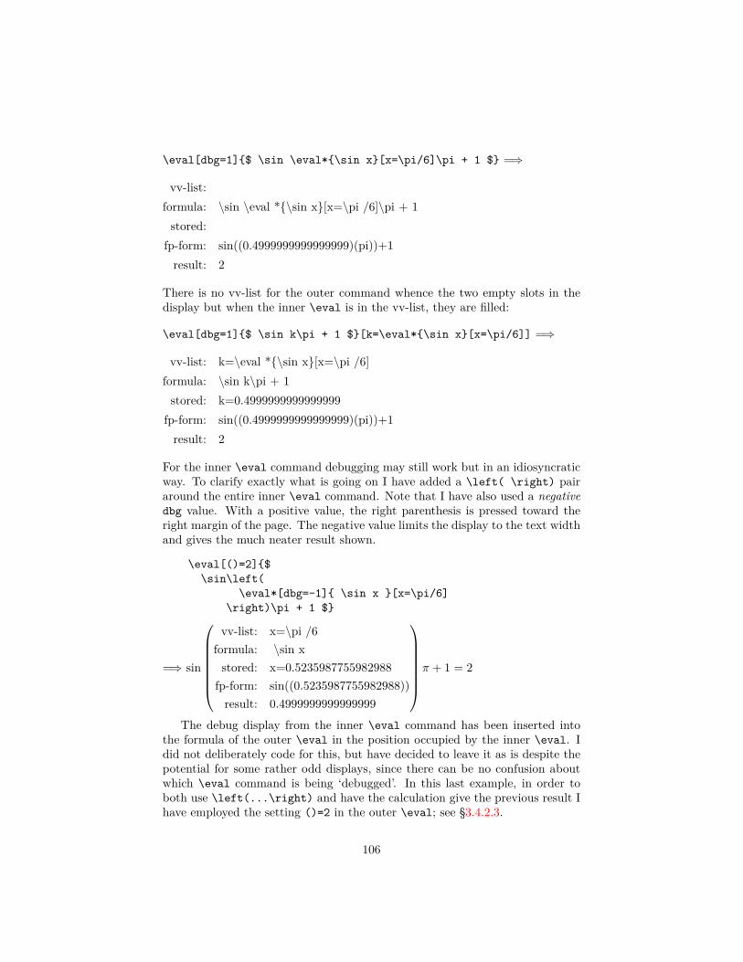
\eval[dbg=1]{$ \sin \eval*{\sin x}[x=\pi/6]\pi + 1 $} =⇒

vv-list:formula: \sin \eval *{\sin x}[x=\pi /6]\pi + 1

stored:fp-form: sin((0.4999999999999999)(pi))+1

result: 2

There is no vv-list for the outer command whence the two empty slots in thedisplay but when the inner \eval is in the vv-list, they are filled:

\eval[dbg=1]{$ \sin k\pi + 1 $}[k=\eval*{\sin x}[x=\pi/6]] =⇒

vv-list: k=\eval *{\sin x}[x=\pi /6]formula: \sin k\pi + 1

stored: k=0.4999999999999999fp-form: sin((0.4999999999999999)(pi))+1

result: 2

For the inner \eval command debugging may still work but in an idiosyncraticway. To clarify exactly what is going on I have added a \left( \right) pairaround the entire inner \eval command. Note that I have also used a negativedbg value. With a positive value, the right parenthesis is pressed toward theright margin of the page. The negative value limits the display to the text widthand gives the much neater result shown.

\eval[()=2]{$\sin\left(

\eval*[dbg=-1]{ \sin x }[x=\pi/6]\right)\pi + 1 $}

=⇒ sin

vv-list: x=\pi /6

formula: \sin xstored: x=0.5235987755982988

fp-form: sin((0.5235987755982988))result: 0.4999999999999999

π + 1 = 2

The debug display from the inner \eval command has been inserted intothe formula of the outer \eval in the position occupied by the inner \eval. Idid not deliberately code for this, but have decided to leave it as is despite thepotential for some rather odd displays, since there can be no confusion aboutwhich \eval command is being ‘debugged’. In this last example, in order toboth use \left(...\right) and have the calculation give the previous result Ihave employed the setting ()=2 in the outer \eval; see §3.4.2.3.

106

Chapter 6

Using numerica with LYX

The document processor LYX has a facility that enables snippets from a docu-ment to be compiled separately and the results presented to the user withouthaving to compile the entire document. The present document was written inLYX. The demonstration calculations were evaluated using this instant previewfacility.

To use numerica in LYX go to Document ▷ Settings ▷ LaTeX Preamble andenter

\usepackage{numerica}

then click OK. You may wish to follow the above line in the preamble with\nmcReuse{}:

\usepackage[lyx]{numerica}\nmcReuse{}

In that case, type the extra line and then click OK. The additional line ensuresall saved values are available in your document from the outset.

6.1 Instant previewThe instant preview facility of LYX performs mini-LATEX runs on selected partsof a document (for instance, the mathematical parts) and displays the results inLYX while the user continues to work on the surrounding document. numericauses these mini-LATEX runs to do its evaluations and display their results. Thatmeans you get feedback on your calculations almost immediately.

To use this facility first ensure that instant preview is turned on. This meansselecting Tools ▷ Preferences ▷ Look & Feel ▷ Display, ensuring that the Displaygraphics checkbox is checked, and against Instant preview selecting On, thenclicking OK.

107

6.1.1 Document locationIt also matters where your document is located. You may have your own localor personal texmf tree (see §3.3.1.1). If your document is located there, perhapsin the doc folder, then not all features of preview will work as expected. Pre-sumably this is because both LYX and your LATEX distribution (e.g. TEXLive orMiKTEX) are interacting with the location and interfere. Move your documentto another location which your LATEX distribution has no interest in, and openit in LYX there.

6.1.2 Global vs local previewingCompilation of previews occurs in two distinct modes.

Global preview generation: When a document is opened (and preview ison), all previews in the document are formed in sequence in the one LATEXrun. This is the global mode. The mini-LATEX run may well be substantial.It compiles a .tex file that begins with the document’s preamble with someadditions then comes \begin{document}. That is followed by a sequence ofpreview environments,

\begin{preview}<stuff>\end{preview}

one for each preview in the document. Finally there is an \end{document} state-ment. The critical point is that all previews are between the same \begin{document},\end{document} statements, and so earlier previews in the sequence can com-municate with later ones.

Local preview generation: The other mode in which preview operates islocal. Suppose you have your document open and want to add to it, for instancewith a simple evaluation, \eval{x+y}[x=1,y=2] in an ERT inset in a previewinset. The resulting mini-LATEX run is of the form

<preamble>\begin{document}\begin{preview}\eval{x+y}[x=1,y=2]\end{preview}\end{document}

The preamble is as before but there is only one preview between the \begin{document},\end{document} statements. That preview is isolated from all other, previouspreviews and will be isolated from all other, later previews.

This has implications for the supplementary commands of the previous chap-ter and means that if you want to transfer information (a macro, a constant,

108

a result) from one preview to another, you need to do it through the preambleor by means of an external file or, in some cases, by forcing a global previewrun in which all previews are recompiled between the same \begin{document},\end{document} statements.

6.1.2.1 Forcing a global preview run

Closing then opening a document is one way to force a global preview compi-lation. Another is to change the zoom level. This causes LYX to recompile allpreviews at the new zoom level. But you may not want to work at the new zoomlevel. Going back to the old zoom level will force a second recompilation of allpreviews. For a large document two recompilations is too heavy a burden. Thesecret is to combine a zoom in and a zoom out into one command and attach itto a shortcut.

If you go to Tools ▷ Preferences ▷ Editing ▷ Shortcuts, click on the Newbutton and enter

command-sequence buffer-zoom-in; buffer-zoom-out

then assign a shortcut to it (Alt+Z for zoom?) you will gain a simple means offorcing a global recompilation of previews.

6.2 Mathed(Mathed = the LYX mathematics editor.) If you have instant preview on thenone way to use numerica in LYX is to enter an \eval command in mathed.Clicking the cursor outside the editor with the mouse or moving it outside withthe arrow keys will then trigger formation of a preview of the editor’s contents– a snippet of what will be shown in the pdf. This will be displayed in mathed’splace after a generally short ‘pause for thought’ as the mini-LATEX run progressesbehind the scenes.

The original expression can be recovered by clicking on the preview. Thecontent of mathed is immediately displayed and can be edited.

6.2.1 LATEX braces { }LYX does not support numerica’s \eval command ‘out of the box’ as it does,say, \frac or \sqrt. To use the \eval command in mathed you will needto supply the braces used to delimit its mandatory argument. (For \frac and\sqrt by contrast, LYX supplies these automatically in the form of blue-outlinedboxes.) Unfortunately the { key1 does not insert a left brace into the documentbut rather an escaped left brace \{ as you can see by looking at View ▷ CodePreview Pane. Escaped braces like this are used for grouping terms in mathe-matics; they are not the delimiters of a LATEX argument.

1Shift+[ on my keyboard.

109

The brace delimiters for LATEX arguments are entered in mathed by typinga backslash \ then a left brace { – two separate key presses rather than asingle combined press. This enters a balanced pair of (unescaped) braces withthe cursor sitting between them waiting for input. Alternatively, if you havealready written an expression that you want to place between braces, select it,then type \ then {.

6.3 Preview insetsThere are problems with using mathed for calculations.

• Expressions entered in mathed are necessarily of the form $ \eval... $or more generally delimiter \eval... delimiter. But you may wishto wrap the \eval command around the math delimiters to produce aformula=result form of display. In mathed the only way to effect sucha display is to write the formula= part yourself – which may involve nomore than copy and paste but is still additional mouse work/key pressing.

• Mathed does not accept carriage returns. If you want to format a com-plicated expression for readability by breaking it into separate lines, youcan’t. The expression is jammed into the one line, along with the settingsoption content and the vv-list, often extending well beyond the edge ofthe screen.

For these reasons I have come to prefer not using mathed for calculations butinstead to use preview insets wrapped around TEX-code (ERT) insets. LYX usesthe shortcut Ctrl+L to insert an ERT inset. Since LYX now does no printingitself, the shortcut Ctrl+P that was formerly used for printing is available forother purposes. On my keyboard, the P key lies diagonally up and to the rightbut adjacent to the L key. I suggest assigning Ctrl+P to inserting a previewinset. Then typing Ctrl+P Ctrl+L – which means holding the Ctrl key downand tapping two diagonally adjacent keys, P followed immediately by L – willinsert an ERT inset inside a preview inset with the cursor sitting inside theERT inset waiting for input. In the ERT inset you can enter carriage returns,and so format complicated expressions. You can place the vv-list on a separateline or onto consecutive lines. And when you have finished, clicking outside thepreview inset will trigger preview into doing its thing and present the result‘before your eyes’.

To assign the suggested shortcut, go to Tools ▷ Preferences ▷ Editing ▷Shortcuts. Under Cursor, Mouse and Editing Functions in the main window onthe right, scroll down until you come to preview-insert, select it, then click Modify.Now press Ctrl+P. The shortcut will magically appear in the greyed, depressedkey. Click OK and then OK in the Preferences window to close it. (Most ofthe examples in this document have been evaluated in this way, using Ctrl+PCtrl+L.)

110

6.4 ErrorsInstant preview will display error messages generated by numerica in LYX justas it does the results of calculations. Clicking on the message will show theunderlying expression which can then be edited. However LATEX errors will notproduce a preview; formation of the preview will stall. To find precisely whathas gone wrong, you will need to look at the LATEX log, but not the log of theoverall document; rather the preview log.

6.4.1 Temporary directory of LYXUnfortunately this is tucked away in a temporary directory and is not imme-diately accessible in LYX (unlike the main LATEX log from Document ▷ LATEXLog). When LYX is started, it sets up a temporary directory in which to per-form various tasks. On Windows systems this will be located in C:\Users\<yourname>\AppData\Local\Temp and will have a name like lyx_tmpdir.XOsSGhBc1344.

One of the tasks LYX uses this temporary directory for is to create previewimages when a document is opened. If you look inside LYX’s temporary directorywhen a document is first loaded, you will see a subdirectory created, with aname like lyx_tmpbuf0. There may already be such directories there, in whichcase the number on the end will be greater than 0 – it depends on whetherother documents are or have been open in the current instance of LYX. Insidethe appropriate lyx_tmpbufn folder will be the preview log with a name likelyxpreviewZL1344.log. It will usually be accompanied by other files withextensions like .dvi, .tex, and – depending on the number of previews in yourdocument – a number, perhaps a lot, of image files with the extension .png,each one of which is a preview. For a document just loaded there will be onlythe one preview log, but if you have added preview insets or math insets to yourdocument in the current editing session there will be a number of such logs andyou will need to determine the relevant one by the time stamp.

The log files are text files and can be opened in a text editor. The relevantpart of the log is towards the end (just before the final statistical summary)where you will find a list of entries like Preview: Snippet 1 641947 1638407864588. If there is an error, it will be noted here among these snippets andwill generally make clear what needs remedying.

6.4.2 CPU usage, LATEX processesIt is possible when a preview stalls that the LATEX process associated withthe preview will continue to run, using CPU cycles, slowing overall computerperformance, and perhaps resulting in extra fan use giving a different soundto the computer. In Windows 10, the Task Manager (Ctrl+Shift+esc) underthe Details tab shows the current executables running. The CPU column willshow which processes are preoccupying the CPU. Check whether one or moreof these processes looks LATEX-related (e.g. latex.exe or pdflatex.exe, ormiktex-pdftex.exe if using MiKTEX). Click the Name column to sort the

111

processes by name and look for the relevant name in the list, select it, and endthe process (click the End Task button).

I am not familiar with the corresponding situation on Linux or Mac.

6.5 Hyperref support vs speedIf you want the pdf produced from your document to support hyperref linksand show an outline window in your pdf viewer (generally placed on the leftin the viewer) then you need to ensure the checkbox at Document Settings ▷PDF Properties ▷ Use Hyperref Support is indeed checked. But you don’t needto do this until the final compilation of the document. The advantage of leavingthis until the last is that in a large document with many previews the timefor preview generation is essentially halved. If hyperref support is enabled,preview generation not only creates all the individual image files that are thepreviews (files of extension .png) but also requires the compilation of a singlepdf document showing all the previews in sequence. (Like the previews, the pdfdocument ‘hides’ in the termporary directory where LYX does its work.) In otherwords, two images are created for each preview, the .png image which is theone LYX displays, and another image buried inside the pdf of all images. Thatsecond step does not occur if hyperref support is disabled. In a small document,this is not going to matter; in a large document it becomes significant. It is wellworth temporarily turning off hyperref support and then, when the time forfinal compilation comes, turning it back on.

6.6 Supplementary commands in LYXThere are some difficulties using the supplementary commands successfully withinstant preview.

6.6.1 Reuse of earlier previewsOne is that whenever LYX has generated a preview image for a particular LATEXexpression, it will use that same image whenever it meets that same LATEX ex-pression later. That means that a statement like \macros[view]{} and thesame statement later will display the same image, even though there may havebeen macros defined or freed in between. The same goes for all the other supple-mentary functions, including, for example, \info{sum}. A second instance of\info{sum} will display the image generated by the first instance even thoughfurther infinite sums may have been evaluated between the \info statements.

The remedy is to make some small but insignificant difference to the LATEXexpression in the second instance – generally a change in white space will do. Forexample: first time \macros[view]{}, second time \macros[view]{ } where aspace has been inserted between the braces; or: first time \info{sum}, secondtime \info{ sum} where a space has been inserted before sum. This will ensureLYX doesn’t fall back on the previously generated image.

112

6.6.2 ‘Stalled’ previewsIt is possible to put content into an ERT inset inside a preview inset (Ctrl+PCtrl+L) and for nothing to happen. The preview has apparently stalled. Cer-tainly this can be the case if there is an error in the input (e.g. a miss-ing brace) but it also occurs if there is no output to display. For instance\constants{ c=300000000 } does not produce any visual output. There isnothing for the preview to display and so the preview inset sits there, appar-ently stalled. This is a security measure for previews in LYX to provide at leastsome guard against malicious code being run in the preview. If the previewresolved, it would disappear completely from view in the LYX window.

If you find the visual appearance of such apparently stalled previews dis-tracting, the addition of some displayable content to the preview will result init resolving to that content; the content could be as small as a full stop.

6.6.3 Using \nmcMacros

As noted earlier, previews are mini-LATEX runs, either local or global. Each localpreview is of the form<preamble>

\begin{document}\begin{preview}<stuff>\end{preview}\end{document}

Whatever goes into or comes out of the preview is isolated from any other localpreview, unless it is through the preamble or an external file. Sometimes a globalpreview run can overcome this problem for then all the previews lie between thesame \begin{document}, end{document} statements. However, this does nothelp with macro definitions. \def, \newcommand, \NewDocumentCommand all pro-vide local definitions which remain trapped within their own \begin{preview},\end{preview}) statements. Another preview, say containing an \eval com-mand, between a different pair of \begin{preview}, \end{preview}) state-ments, will not know about the macro definition.

There are (at least) three ways out:

1. Confine everything to the same preview inset: the definition of a macro,the \macros statement, and the use of the macro in an \eval command.

2. Confine macro definitions to the preamble (Document ▷ Settings ▷ LATEXPreamble).

3. Within previews use \gdef (or \global\def) exclusively for making yourmacro definitions; this makes the macro available to all later previews.

113

6.6.4 Using \nmcConstants

Because \nmcConstants doesn’t use \def or \newcommand or \NewDocumentCommandit is not subject to the same localisation problem as \nmcMacros, but the reachof a \constants command will still be confined to its own preview unless aglobal preview run is forced; see above §6.1.2.

6.6.5 Using \nmcReuse

As noted earlier, LYX creates its previews in a temporary directory, not thedocument directory. If you want to save values from your current document –say, mydoc.lyx – to mydoc.nmc then you do so as described earlier (§4.4), butthe file mydoc.nmc containing the saved results will be located in the temporarydirectory. When LYX is closed the file will be deleted along with all the othercontents of that directory.

Fortunately LYX has a copying mechanism for getting files out of the tempo-rary directory and into the document directory. When a document is exported– say to pdf – it is possible to specify a copier to automatically copy back to thedocument directory or subdirectory various files in the temporary directory. Wewant the .nmc file containing the saved values to be copied back. Go to Tools▷ Preferences ▷ File Handling ▷ File Formats and find PDF (pdflatex) (assumingexport to pdf by this route) in the list of formats. In the Copier slot of thedialogue insert the following line of code:

python -tt $$s/scripts/ext_copy.py -e nmc,pdf -d $$i $$o

ext_copy.py is a python script that is supplied with LYX. The -e nmc,pdf -dpart of the line tells ext_copy.py that on export to pdf by the pdflatex routeto copy any files with the extensions .nmc or .pdf from the temporary directorywhere LYX does its work back to the document directory – the -d option (whichbecame available with LYX 2.3.0).

But if you have a complex document, it may take too much time to want toexport to pdf before closing LYX, particularly if there are a lot of evaluationsin the document. Much faster is to export to plain text, not because you wanta plain text version of your document but because it too can be used to triggerthe copier mechanism. Go to Tools ▷ Preferences ▷ File Handling ▷ File Formatsand find Plain text in the list of formats. In the Copier slot enter

python -tt $$s/scripts/ext_copy.py -e nmc -d $$i $$o

The only difference from the previous copier command is the absence of pdf.2This will copy mydoc.nmc with its saved values from the temporary directoryback to the document directory. To effect the export, go to File ▷ Export andfind Plain text in the list of formats and click on it.

2I’m assuming that you don’t actually want the plain text version of the file copied back.If you do, then change -e nmc to -e nmc,txt.

114

A shortcut would be nice. For that go to Tools ▷ Preferences ▷ Editing ▷Shortcuts, click on New, enter buffer-export text in the Function: slot, clickon the blank key against Shortcut: and type your shortcut. You may have totry a number before you find one that hasn’t already been assigned. (I’m usingCtrl+; for no particular reason beyond the fact that it fits under the fingerseasily and saving values to the document directory has a punctuation-like feelto it, a pause in the process of writing.) It is now an easy matter to press theshortcut at the end of a LYX session to copy all the values saved in mydoc.nmcback to a file of the same name in the document directory. And it is brisk, notleast because plain text export ignores ERT insets (and hence preview insetswrapped around ERT insets), nor does it evaluate \eval commands in mathinsets.

6.6.5.1 A final tweak?

But one still needs to remember to press the shortcut. The thought arises:can closing the current document trigger the copying process? LYX providesa means of linking two commands and assigning a keyboard shortcut to themwith its command-sequence LYX function. I suggest assigning a shortcut to

command-sequence buffer-export text; view-close

Indeed, why not reassign the current shortcut for view-close, which is Ctrl+Won my system, to this command sequence? (I use the cua key bindings – checkthe Bind file: slot in Tools ▷ Preferences ▷ Editing ▷ Shortcuts.)

Please note, however, that this will work as intended only from LYX 2.4.0.3For LYX 2.3 and earlier, the command sequence will generally fail becauseof ‘asynchronous’ processing – buffer-export and view-close use differentthreads and the latter may well start before the former is complete. From LYX2.4.0 this defect has been fixed. You press your shortcut, the export to plaintext occurs and the .nmc file is copied back to the document directory, then thecurrent view is closed.

Note that in the other direction, the .nmc file in your document directory isautomatically copied to the temporary directory when needed. Nothing needsto be done by you, the user.

6.6.5.2 Use of LYX notes

The central fact about a LYX note is that it does not contribute to the pdf. Butinstant preview still works there. This suggests a possibility: that a calculationbe performed within a LYX note and the result saved using \nmcReuse withinthe same note. The saved value is now available from file for use elsewhere inthe document. In this way, some selected content from a LyX note can find itsway into the pdf when the document is compiled.

3Due for release in 2021.

115

Chapter 7

Reference summary

7.1 Commands defined in numerica

1. \nmcEvaluate, \eval

2. \q, \Q (‘cleave’ commands)

3. \nmcInfo, \info

4. \nmcMacros, \macros

5. \nmcConstants, \constants

6. \nmcReuse, \reuse

Provided they have not already been defined when numerica is loaded, the fol-lowing commands are defined in numerica using \DeclareMathOperator fromamsmath :

1. \arccsc, \arcsec, \arccot

2. \csch, \sech

3. \asinh, \acosh, \atanh, \acsch, \asech, \acoth

4. \sgn, \lb

Provided they have not already been defined, the following commands are de-fined in numerica using \DeclarePairedDelimiter from mathtools:

\abs, \ceil, \floor

The following commands have been redefined in numerica to give more spacingaround the underlying \wedge and \vee symbols:

\land, \lor

116

7.2 ‘Digestible’ contentnumerica knows how to deal with the following content, meaning that any ofthese elements occurring within an \eval command should not of itself cause anumerica error. Not all formatting commands affect display of the output.

1. variable names (sequences of tokens given values in the variable = valuelist)

2. digits, decimal point

(a) 1, 2, 3, 4, 5, 6, 7, 8, 9, 0, .

3. constants

(a) e, \pi, \gamma, \phi, \deg, \infty

4. arithmetic operators

(a) +, -, *, /, ^, \times, \cdot, \div

5. logical operators

(a) \wedge, \land, \vee, \lor, \neg, \lnot

6. comparisons

(a) =, <, >, \ne, \neq, \le, \leq, \ge, \geq

(b) (if amssymb loaded) \nless, \ngtr, \geqq, \geqslant, \leqq,\leqslant, \ngeq, \ngeqq, \ngeqslant, \nleq, \nleqq, \nleqslant

7. brackets, bracket-like elements, modifiers

(a) ( ), [ ], \{ \}

(b) \lparen \rparen (from mathtools), \lbrack \rbrack, \lbrace\rbrace

(c) \lvert \rvert, \lfloor \rfloor, \lceil \rceil

(d) | | (no nesting, deprecated)(e) \left \right, \bigl \bigr, \Bigl \Bigr, \biggl \biggr, \Biggl

\Biggr

(f) . / | (used with a modifier)(g) \abs[]{}, \abs*{}, \floor[]{}, \floor*{}, \ceil[]{}, \ceil*{}

8. unary functions (in the mathematical sense)

(a) \sin, \cos, \tan, \csc, \sec, \cot

(b) \arcsin, \arccos, \arctan, arccsc, \arcsec, \arccot

(c) \sin^{-1}, \cos^{-1}, \tan^{-1}, \csc^{-1}, \sec^{-1}, \cot^{-1}

117

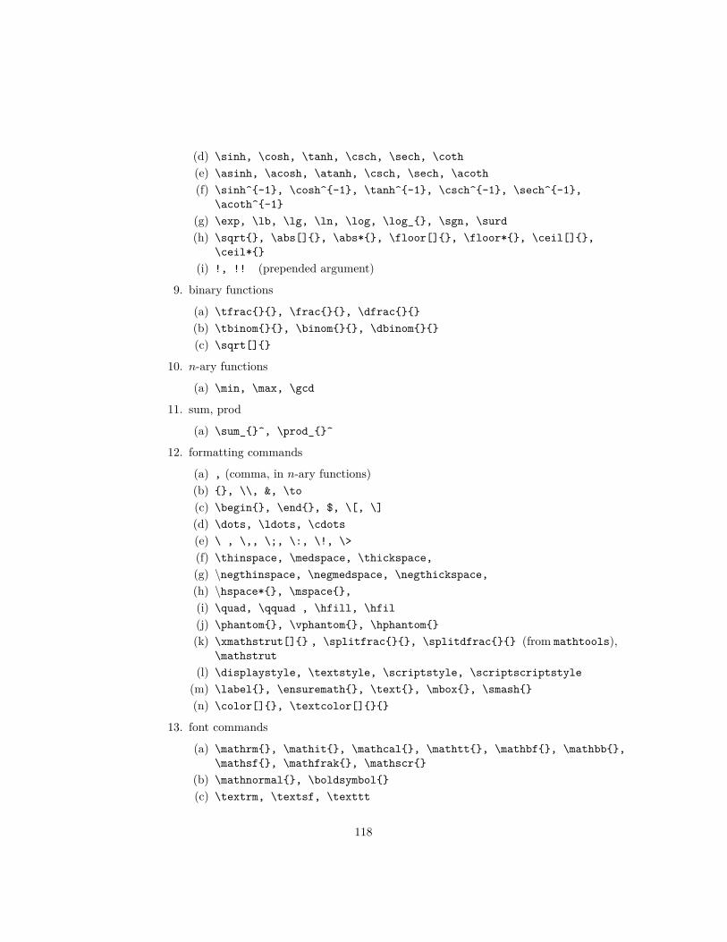
(d) \sinh, \cosh, \tanh, \csch, \sech, \coth(e) \asinh, \acosh, \atanh, \csch, \sech, \acoth(f) \sinh^{-1}, \cosh^{-1}, \tanh^{-1}, \csch^{-1}, \sech^{-1},

\acoth^{-1}(g) \exp, \lb, \lg, \ln, \log, \log_{}, \sgn, \surd(h) \sqrt{}, \abs[]{}, \abs*{}, \floor[]{}, \floor*{}, \ceil[]{},

\ceil*{}(i) !, !! (prepended argument)

9. binary functions

(a) \tfrac{}{}, \frac{}{}, \dfrac{}{}(b) \tbinom{}{}, \binom{}{}, \dbinom{}{}(c) \sqrt[]{}

10. n-ary functions

(a) \min, \max, \gcd

11. sum, prod

(a) \sum_{}^, \prod_{}^

12. formatting commands

(a) , (comma, in n-ary functions)(b) {}, \\, &, \to(c) \begin{}, \end{}, $, \[, \](d) \dots, \ldots, \cdots(e) \ , \,, \;, \:, \!, \>(f) \thinspace, \medspace, \thickspace,(g) \negthinspace, \negmedspace, \negthickspace,(h) \hspace*{}, \mspace{},(i) \quad, \qquad , \hfill, \hfil(j) \phantom{}, \vphantom{}, \hphantom{}(k) \xmathstrut[]{} , \splitfrac{}{}, \splitdfrac{}{} (from mathtools),

\mathstrut(l) \displaystyle, \textstyle, \scriptstyle, \scriptscriptstyle

(m) \label{}, \ensuremath{}, \text{}, \mbox{}, \smash{}(n) \color[]{}, \textcolor[]{}{}

13. font commands

(a) \mathrm{}, \mathit{}, \mathcal{}, \mathtt{}, \mathbf{}, \mathbb{},\mathsf{}, \mathfrak{}, \mathscr{}

(b) \mathnormal{}, \boldsymbol{}(c) \textrm, \textsf, \texttt

118

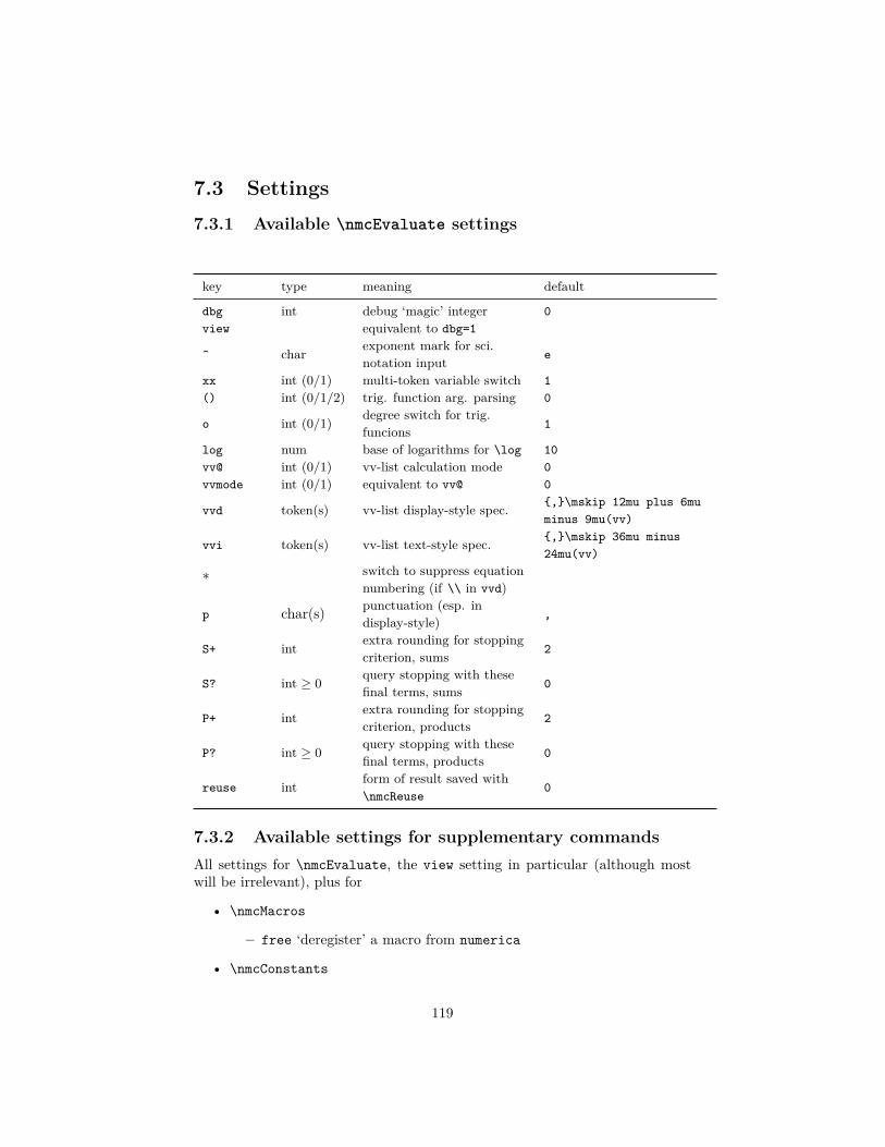
7.3 Settings7.3.1 Available \nmcEvaluate settings

key type meaning default

dbg int debug ‘magic’ integer 0view equivalent to dbg=1

^ char exponent mark for sci.notation input e

xx int (0/1) multi-token variable switch 1() int (0/1/2) trig. function arg. parsing 0

o int (0/1) degree switch for trig.funcions 1

log num base of logarithms for \log 10vv@ int (0/1) vv-list calculation mode 0vvmode int (0/1) equivalent to vv@ 0

vvd token(s) vv-list display-style spec. {,}\mskip 12mu plus 6muminus 9mu(vv)

vvi token(s) vv-list text-style spec. {,}\mskip 36mu minus24mu(vv)

* switch to suppress equationnumbering (if \\ in vvd)

p char(s) punctuation (esp. indisplay-style) ,

S+ int extra rounding for stoppingcriterion, sums 2

S? int ≥ 0 query stopping with thesefinal terms, sums 0

P+ int extra rounding for stoppingcriterion, products 2

P? int ≥ 0 query stopping with thesefinal terms, products 0

reuse int form of result saved with\nmcReuse

0

7.3.2 Available settings for supplementary commandsAll settings for \nmcEvaluate, the view setting in particular (although mostwill be irrelevant), plus for

• \nmcMacros

– free ‘deregister’ a macro from numerica

• \nmcConstants

119

– add add the new list of constants to the current one

• \nmcReuse

– delete remove the listed control sequences from the .nmc file– renew change the value of a control sequence in the .nmc file

7.3.3 Available configuration file settings

key defaultrounding 6pad 0output-sci-notation 0output-exponent-char einput-sci-notation 0input-exponent-char emultitoken-variables 1use-degrees 0logarithm-base 10intify-rounding 14vv-display {,}\mskip 36mu minus 24mu(vv)vv-inline {,}\mskip 12mu 6mu minus 9mu(vv)sum-extra-rounding 2sum-query-terms 0prod-extra-rounding 2prod-query-terms 0eval-reuse 0

120