Novel, Integrated and Revolutionary Well Test Interpretation ...

Novel, Integrated andRevolutionary Well Test

Interpretation and AnalysisFreddy Humberto Escobar Macualo

Acknowledgements

I am thankful to God and the Virgin Mary for all the blessing I have received duringmy whole life.

I also thank and dedicate this book to my wife Matilde and my children JenniferAndrea, Freddy Alonso and Mary Gabriela, Universidad Surcolombiana (USCO),and Dr. Djebbar Tiab, creator of TDS Technique which forms the main topic of thisbook.

I truly thank Yuly Andrea Hernández, who has been one of the top most brilliant 12students I have ever had, for taking part of her valuable time to review this bookand write its foreword.

Contents

Foreword VII

Introduction 2

Chapter 1 4Fundamentals

Chapter 2 55Pressure Drawdown Testing

Chapter 3 134Pressure Buildup Testing

Chapter 4 176Distance to Linear Discontinuities

Chapter 5 197Multiple Well Testing

Chapter 6 217Naturally Fractured Reservoirs

Chapter 7 240Hydraulically Fractured

Foreword

It was in 2002, the first opportunity I had about being in touch with pressure welltest interpretations. At that time, I could not be more inspired knowing the personfrom whose those words were coming from. That was exactly when I took my firstwell testing class with Doctor Escobar who just came from finishing his doctoralstudies. Absolutely, he put the first stone of motivation and enthusiasm to end upworking close to him applying Tiab’s direct synthesis (TDS) technique to reservoirwith channels and long structures. My passion for the subject even increased whenpublishing my first article from our research work in which we discovered a newflow regime: parabolic flow, and later, we saw the importance of geometrical skinfactor which, so far, in spite of a long transition time, has not been yet incorporatedinto commercial software.

Since that time and for about 15 years, as part of my role as a reservoir engineer,definitely I could not be luckier, not only for sharing academic and professionaldiscussion but also having the chance to be influenced by his creativity and deepthinking in different facets of his life. Dr. Escobar has been impacting the oilindustry along his extensive research work. Without counting the numerous situa-tions that as a professor who sees students as human beings with feelings that can gothrough multiple conditions of difficulties, can attest to the positive impact that as aperson he has had in our lives. It is why to write short words about him is such aprivilege to me.

As a reservoir engineer, I understand our challenge to describe, size, and develophydrocarbon deposits in an efficient way, but oil and gas remains trapped in areaswhere we are restricted to have a direct recognition by our senses. We cannot seethem. Neither, we cannot touch them nor we cannot design them. It requires thesymbiosis between geologist and engineers to use their technical knowledge mixedwith a great portion of imagination, creativity, and innovation to create models thathelp us to decrypt the way it will flow. This is the moment where Dr. Escobarattributes and his research work in well testing analysis is reflected.

Well testing analysis is an invaluable and low-cost tool in reservoir characterizationthat helps us to decode our reservoirs. From where we can obtain relevant infor-mation to model and understand them. Questions like: how many wells have to bedrilled? How much hydrocarbon will they produce? What is the optimumstrategy to obtain the best recovery factor with the highest interest return rate?Well, transient rate and pressure test analyses can be a contrivance for solvingthese issues. And, much better when there exist techniques such as Tiab’s directsynthesis (TDS), which allows us to make the interpretations in a direct and simplerway, by using main features of the different flow regimes responses in combinationwith simple equations to determine the parameters of interest. Escobar presents inthis book practical applications of this modern and revolutionary technique, helpingall types of petroleum engineers to understand the concept and its benefits. I wishthere were more examples, but for space-saving reasons, only the most practicalones are presented.

From this methodology I highlight the uncomplicated way to establish flow regimestypes, diverse options to confirm the results, the simplicity and common sense of itscalculations, and no need to use trial-and-error procedures, aspects that are notfound in any other present methodology in the literature; however, the author inthe book presents a comparison with other methodologies in an astonishing way.

The work of Dr. Escobar represents an important contribution to the hydrocarbonindustry in the field of reservoir characterization, where his research extending thescope of the TDS technique plays an important role. I have also had the opportunityto apply his results and interpretation procedures in different types of reservoir,attesting to its usefulness and the multiple advances over the last years where thistechnique can be applied to diverse reservoir characteristics and flow regimes.

Enjoy it!!!

Yuly Andrea HernándezHocol S.A., Colombia1

1 Yuly Andrea Hernández is a young Petroleum Engineer currently working for Hocol S.A. since July2011. In 2004, she obtained a BSc degree diploma with honors in Petroleum Engineering under the

author’s supervision and received a MBA degree in 2014. She worked first for Hocol S.A. from August

2004 to September 2008 and went to Columbus Energy Sucursal Colombia from October 2008 to June

2011. Then, she moved back to Hocol. Yuly Andrea has been a very active engineer and she has gained

experience in all the subjects of reservoir engineering. She is very familiar with the current and

sophisticated software used in the oil industry. She is a devoted user of the application of TDS Techniqueto her engineering work and actually has a couple of publications on this subject.

VIII

Novel, Integrated andRevolutionary Well TestInterpretation and AnalysisFreddy Humberto Escobar Macualo

Abstract

Well test interpretation is an important tool for reservoir characterization. Thereexist four methods to achieve this goal, which are as follows: type‐curve matching,conventional straight‐line method, non‐linear regression analysis, and TDS technique.The first method is basically a trial‐and‐error procedure; a deviation of a millimeterinvolves differences up to 200 psi and the difficulty of having so many matching charts.The second one, although very important, requires a plot for every flow regime, andthere is no way for verification of the calculated parameters, and the third one has aproblem of diversity of solutions but is the most used by engineers since it is automat-ically made by a computer program. This book focuses on the fourth method that uses asingle plot of the pressure and pressure derivative plot for identifying different lines andfeature for parameter estimation. It can be used alone and is applied practically to all theexisting flow regime cases. In several cases, the same parameter can be estimated fromdifferent sources making a good way for verification. Combination of this method alongwith the second and third is recommended and widely used by the author.

TDS technique is quite versatile. The user finds the different flow regimes and,then, draws a line through it. From an arbitrary point on each flow regime, a givenparameter can be calculated. Besides, the intersection point between the extrapolatedflow regimes, although do not have a physical meaning, is excellent to find anotherreservoir parameter or the verification of others. For instance, well‐drainage area canbe readily estimated from the intersect point formed between the radial flow regimeand the late pseudosteady state period. Every time someone starts working using TDStechnique, he or she never stops. The reader is invited to give it a try.

Keywords: TDS technique, permeability, well‐drainage area, flow regimes,intersection points, transient pressure analysis, conventional analysis

Author details

Freddy Humberto Escobar MacualoUniversidad Surcolombiana, Colombia

*Address all correspondence to: [email protected]

© 2018TheAuthor(s). Licensee IntechOpen. Distributed under the terms of the CreativeCommonsAttribution -NonCommercial 4.0 License (https://creativecommons.org/licenses/by-nc/4.0/), which permits use, distribution and reproduction fornon-commercial purposes, provided the original is properly cited. –NC

Introduction

Well testing is a valuable and economical formation evaluation tool used in thehydrocarbon industry. It has been supported by mathematical modeling, comput-ing, and the precision of measurement devices. The data acquired during a well testare used for reservoir characterization and description. However, the biggest draw-back is that the system dealt with is neither designed nor seen by well test inter-preters, and the only way to make contact with the reservoir is through the well bymaking indirect measurements.

Four methods are used for well test interpretation: (1) The oldest one is theconventional straight‐line method which consists of plotting pressure or thereciprocal rate—if dealing with transient rate analysis—in the y‐axis against afunction of time in the x‐axis. This time function depends upon the governingequation for a given flow. For instance, radial flow uses the logarithm of time andlinear flow uses the square root of time. The slope and intercept of such plot areused to find reservoir parameters. The main disadvantage of this method is thelack of confirmation and the difficulty to define a given flow regime. The methodis widely used nowadays. (2) Type‐curve matching uses predefined dimensionlesspressure and dimensionless time curves (some also use dimensionless pressurederivative), which are used as master guides to be matched with well pressuredata to obtain a reference point for reservoir parameter determination. Thismethod is basically a trial‐and‐error procedure which becomes into its biggestdisadvantage. The method is practically unused. (3) Simulation of reservoir con-ditions and automatic adjustment to well test data by non‐linear regression analy-sis is the method widely used by petroleum engineers. This method is also beingwidely disused since engineers trust the whole task to the computer. They evenperform inverse modeling trying to fit the data to any reservoir model withouttaking care of the actual conditions. However, the biggest weakness of thismethod lies on the none uniqueness of the solution. Depending on the inputstarting values, the results may be different. (4) The newest method known asTiab’s direct synthesis (TDS) [1, 2] is the most powerful and practical one as willbe demonstrated throughout the book. It employs characteristic points and fea-tures found on the pressure and pressure derivative versus time log‐log plot to beused into direct analytic equations for reservoir parameters’ calculation. It is evenused, without using the original name, by all the commercial software. One ofthem calls it “Specialized lines.” Because of its practicality, accuracy and applica-tion is the main object of this book. Conventional analysis method will be alsoincluded for comparison purposes.

The TDS technique can be easily implemented for all kinds of conventional orunconventional systems. It can be easily applied on cases for which the other methodsfail or are difficult to be applied. It is strongly based on the pressure derivative curve.The method works by sector or regions found on the test. This means once a givenflow regime is identified, a straight line is drawn throughout it, and then, anyarbitrary point on this line and the intersection with other lines as well are used intothe appropriate equations for the calculation of reservoir parameters.

2

The book contains the application and detailed examples of the TDS technique tothe most common or fundamental reservoir/fluid scenarios. It is divided into sevenchapters that are recommended to be read in the other they appear, especially foracademic purposes in senior undergraduate level or master degree level. Chapter 1contains the governing equation and the superposition principle. Chapter 2 is thelongest one since it includes drawdown for infinite and finite cases, elongatedsystem, multi‐rate testing, and spherical/hemispherical flow. All the interpretationmethods are studied in this chapter which covers about 45% of the book. Chapter 3deals with pressure buildup testing and average reservoir pressure determination.Distance to barriers and interference testing are, respectively, treated in Chapters 4and 5. Since the author is convinced that all reservoirs are naturally fractured,Chapter 6 covers this part which is also extended in hydraulically fractured wells inChapter 7. In this last chapter, the most common flow regime shown in fracturedwells: bilinear, linear, and elliptical are discussed with detailed for parameter char-acterization. The idea is to present a book on TDS technique as practical and short aspossible; then, horizontal well testing is excluded here because of its complexity andextension, but the most outstanding and practical publications are named here.

My book entitled “Recent Advances in Practical Applied Well Test Analysis,”published in 2015, was written for people having some familiarity with the TDStechnique, so that, it can be read in any order. This is not the case of the presenttextbook. It is recommended to be read in order from Chapter 1 and take especialcare in Chapter 2 since many equations and concepts will be applied in theremaining chapters. TDS technique applies indifferently to both pressure draw-down and pressure buildup tests.

Finally, this book is an upgraded and updated version of a former one published inSpanish. Most of the type curves have been removed since they have never beenused by the author on actual well test interpretations. However, the first motivationto publish this book is the author’s belief that TDS technique is the panacea for welltest interpretation. TDS technique is such an easy and practical methodology thathis creator, Dr. Djebbar Tiab, when day said to me “I still don’t believe TDS works!”But, it really does. Well, once things have been created, they look easy.

3

Introduction

Chapter 1

Fundamentals

1.1. Basic concepts

Pressure test fundamentals come from the application of Newton’s law, espe-cially the third one: Principle of action‐reaction, since it comes from a perturbationon a well, as illustrated in Figure 1.1.

A well can be produced under any of two given scenarios: (a) by keeping aconstant flow rate and recording the well‐flowing pressure or (b) by keeping aconstant well‐flowing pressure and measuring the flow rate. The first case is knownas pressure transient analysis, PTA, and the second one is better known as ratetransient analysis, RTA, which both are commonly run in very low permeableformations such as shales.

Basically, the objectives of the analysis of the pressure tests are:

• Reservoir evaluation and description: well delivery, properties, reservoir size,permeability by thickness (useful for spacing and stimulation), initial pressure(energy and forecast), and determination of aquifer existence.

• Reservoir management.

There are several types of tests with their particular applications. DST and pres-sure buildup tests are mainly used in primary production and exploration. Multipletests are most often used during secondary recovery projects, and multilayer andvertical permeability tests are used in producing/injectors wells. Drawdown, inter-ference, and pulse tests are used at all stages of production. Multi‐rate, injection,interference, and pulse tests are used in primary and secondary stages [3–7].

Pressure test analysis has a variety of applications over the life of a reservoir.DST and pressure buildup tests run in single wells are mainly used during primaryproduction and exploration, while multiple tests are used more often during sec-ondary recovery projects. Multilayer and vertical permeability tests are also run inproducing/injectors wells. Drawdown, buildup, interference, and pulse tests areused at all stages of production. Multi‐rate, injection, interference, and pulse testingare used in the primary and secondary stages. Petroleum engineers should take into

Figure 1.1.Diagram of the mathematical representation of a pressure test.

4

account the state of the art of interpreting pressure tests, data acquisition tools,interpretation methods, and other factors that affect the quality of the resultsobtained from pressure test analysis.

Once the data have been obtained from the well and reviewed, the pressure testanalysis comprises two steps: (1) To establish the reservoir model and the identifi-cation of the different flow regimes encountered during the test and (2) the param-eter estimation. To achieve this goal, several plots are employed; among them, wehave log‐log plot of pressure and pressure derivative versus testing time (diagnostictool), semilog graph of pressure versus time, Cartesian graph of the same parame-ters, etc. Pressure derivative will be dealt later in this chapter.

The interpretation of pressure tests is the primary method for determiningaverage permeability, skin factor, average reservoir pressure, fracture length andfracture conductivity, and reservoir heterogeneity. In addition, it is the only fastestand cheapest method to estimate time‐dependent variables such as skin factor andpermeability in stress‐sensitive reservoirs.

In general, pressure test analysis is an excellent tool to describe and define themodel of a reservoir. Flow regimes are a direct function of the characteristics of thewell/reservoir system, that is, a simple fracture that intercepts the well can beidentified by detection of a linear flow. However, whenever there is linear flow, itdoes not necessarily imply the presence of a fracture. The infinite‐acing behavioroccurs after the end of wellbore storage and before the influence of the limits of thedeposit. Since the boundaries do not affect the data during this period, the pressurebehavior is identical to the behavior of an infinite reservoir. The radial flow can berecognized by an apparent stabilization of the value of the derivative.

1.2. Type of well tests

Well tests can be classified in several ways depending upon the view point. Someclassifications consider whether or not the well produces or is shut‐in. Other engi-neers focus on the number of flow rates. The two main pressure tests are (a)pressure drawdown and (b) buildup. While the first one involves only one flowrate, the second one involves two flow rates, one of which is zero. Then, a pressurebuildup test can be considered as a multi‐rate test.

1.2.1 Pressure tests run in producer wells

Drawdown pressure test (see Figure 1.2): It is also referred as a flow test. Afterthe well has been shut‐in for a long enough time to achieve stabilization, the well isplaced in production, at a constant rate, while recording the bottom pressureagainst time. Its main disadvantage is that it is difficult to maintain the constantflow rate.

Pressure buildup test (see Figure 1.2): In this test, the well is shut‐in whilerecording the static bottom‐hole pressure as a function of time. This test allowsobtaining the average pressure of the reservoir. Although since 2010, average res-ervoir pressures can be determined from drawdown tests. Its main disadvantage iseconomic since the shut‐in entails the loss of production.

1.2.2 Pressure tests run in injector wells

Injection test (see Figure 1.3): Since it considers fluid flow, it is a test similar tothe pressure drawdown test, but instead of producing fluids, fluids, usually water,are injected.

5

FundamentalsDOI: http://dx.doi.org/10.5772/intechopen.81078

Falloff test (see Figure 1.3): This test considers a pressure drawdown immedi-ately after the injection period finishes. Since the well is shut‐in, falloff tests areidentical to pressure buildup tests.

1.2.3 Other tests

Interference and/or multiple tests: They involve more than one well and itspurpose is to define connectivity and find directional permeabilities. A well pertur-bation is observed in another well.

Figure 1.2.Schematic representation of pressure drawdown and pressure buildup tests.

Figure 1.3.Injection pressure test (left) and falloff test (right).

6

Novel, Integrated and Revolutionary Well Test Interpretation and Analysis

Drill stem test (DST):This test is used during or immediately after well drilling andconsists of short and continuous shut‐off or flow tests. Its purpose is to establish thepotential of the well, although the estimated skin factor is not very representativebecausewell cleaning can occurduring the first productive stage of thewell (Figure 1.4).

Short tests: There are some very short tests mainly run in offshore wells. Theyare not treated in this book. Some of them are slug tests, general close chamber tests(CCTs), surge tests, shoot and pool tests, FasTest, and impulse tests.

As stated before, in a pressure drawdown test, the well is set to a constant flowrate. This condition is, sometimes, difficult to be fulfilled; then, multi‐rate testshave to be employed. According to [8], multi‐rate tests fit into four categories:(a) uncontrolled variable rate [9, 10], series of constant rates [11, 12], pressurebuildup testing, and constant bottom‐hole pressure with a continuous changingflow rate [13]. This last technique has been recently named as rate transient analysis(RTA) which is included in PTA, but its study is not treated in this book.

1.3 Diffusivity equation

At the beginning of production, the pressure in the vicinity of the well fallsabruptly and the fluids near the well expand and move toward the area of lowerpressure. Such movement is retarded by friction against the walls of the well andthe inertia and viscosity of the fluid itself. As the fluid moves, an imbalance ofpressure is created, which induces the surrounding fluids to move toward the well.The process continues until the pressure drop created by the production dissipatesthroughout the reservoir. The physical process that takes place in the reservoir canbe described by the diffusivity equation whose deduction is shown below [5]:

According to the volume element given in Figure 1.5,

Mass entering

the element

� �� Mass coming out

from the element

� �¼ System

accumulation rate

� �(1.1)

The right‐hand side part of Eq. (1.1) corresponds to the mass accumulated in thevolume element. Darcy’s law for radial flow:

q ¼ � kAμ

dPdr

(1.2)

The cross‐sectional area available for flow is provided by cylindrical geometry,2πrh. Additionally, flow rate must be multiplied by density, ρ, to obtain mass flow.With these premises, Eq. (1.2) becomes:

Figure 1.4.Well test classification based on the number of flow rates.

7


q ¼ � kμ2π rh

∂P∂ r

(1.3)

Replacing Eq. (1.3) into (1.1) yields:

� kρμ

2π rhð Þ ∂P∂ r

��rþ kρ

μ2π rhð Þ ∂P

∂ r

��rþdr

¼ ∂∂t

½2πrhdrϕ�ρð Þ (1.4)

If the control volume remains constant with time, then, Eq. (1.4) can berearranged as:

�2π hkρμr∂P∂ r

��rþ 2π h

kρμr∂P∂ r

��rþdr

¼ 2πrhdr∂∂t

ϕρð Þ (1.5)

Rearranging further the above expression:

1r

kρμr∂P∂ r

��rþdr � kρμr∂P∂ r

��r� �

dr¼ ∂

∂tϕρð Þ (1.6)

The left‐hand side of Eq (1.6) corresponds to the definition of the derivative;then, it can be rewritten as:

1r∂∂ r

kρμr∂P∂ r

� �¼ ∂

∂ tϕρð Þ (1.7)

The definition of compressibility has been widely used;

c ¼ � 1V∂ V∂P

¼ 1ρ

∂ρ∂P

(1.8)

By the same token, the pore volume compressibility is given by:

cf ¼ 1ϕ

∂ ϕ∂P

(1.9)

The integration of Eq. (1.8) will lead to obtain:

Figure 1.5.Radial volume element.

8


ρ ¼ ρoecðP�PoÞ (1.10)

The right‐hand side part of Eq. (1.7) can be expanded as:

∂∂ t

ϕρð Þ ¼ ϕ∂∂ t

ρþ ρ∂∂ t

ϕ ¼ ϕ∂ρ∂t

þ ρ∂ϕ∂P

∂P∂ρ

∂ρ∂t

(1.11)

Using the definitions given by Eqs. (1.9) and (1.10) into Eq. (1.11) leads to:

∂∂ t

ϕρð Þ ¼ ϕ∂ρ∂t

þ ρ ϕ cfcρ

∂ρ∂t

¼ ϕ∂ρ∂t

1þ cfc

h i¼ ϕ

ccf þ c� � ∂ρ

∂t(1.12)

Considering that the total compressibility, ct, is the result of the fluid compress-ibility, c, plus the pore volume compressibility, cf, it yields:

1r∂∂ r

kρμr∂P∂ r

� �¼ ϕct

c∂ρ∂t

(1.13)

The gradient term can be expanded as:

∂P∂r

¼ ∂P∂ρ

∂ρ∂r

¼ 1cρ

∂ρ∂r

(1.14)

Combination of Eqs. (1.14) and (1.13) results in:

1r∂∂ r

krμc

∂ρ∂ r

� �¼ ϕ

cct∂ρ∂t

(1.15)

Taking derivative to Eq. (1.10) with respect to both time and radial distance andreplacing these results into Eq. (1.15) yield:

1r∂∂ r

krμc

ρoecðP�PoÞc

∂P∂r

� �¼ ϕ

cctρoe

cðP�PoÞc∂P∂t

(1.16)

After simplification and considering permeability and viscosity to be constant,we obtain:

1rkμ

∂∂r

r∂P∂r

� �¼ ϕ ct

∂P∂t

(1.17)

The hydraulic diffusivity constant is well known as

1η¼ ϕμct

k(1.18)

Then, the final form of the diffusivity equation in oilfield units is obtained bycombination of Eqs. (1.17) and (1.18):

1r∂∂r

r∂P∂r

� �¼ ϕμct

0:0002637k∂P∂t

¼ 1η

∂P∂t

(1.19)

In expanded form:

∂2P∂r2

þ 1r∂P∂r

¼ 10:0002637η

∂P∂t

(1.20)

9


The final form of the diffusivity equation strongly depends upon the flowgeometry. For cylindrical, [11, 14], spherical [14], and elliptical coordinates [15],the diffusivity equation is given, respectively,

∂ 2P∂ r2

þ 1r∂P∂r

þ kθkr

1r2

∂2P∂ θ2

þ kzkr

∂2P∂z2

¼ ϕμctkr

∂P∂t

(1.21)

1r

∂∂r

r2∂P∂r

� �þ 1

sin θ∂∂θ

sin θ∂P∂θ

� �þ 1

sin 2θ∂2P∂ϕ2

� �¼ ϕcμ

k∂P∂t

(1.22)

∂2P∂ξ2

þ ∂2P∂η2

¼ 12a2 cosh 2ξ� cos 2ηð Þϕcμ

k∂P∂t

(1.23)

Here, ξ is a space coordinate and represents a family of confocal ellipses. Thefocal length of these ellipses is 2a. The space coordinate, η, represents a family ofconfocal hyperbolas that represent the streamlines for elliptical flow. These twocoordinates are normal to each other.

1.4. Limitations of the diffusivity equation

a. Isotropic, horizontal, homogeneous porous medium, permeability, andconstant porosity

b.A single fluid saturates the porous medium

c. Constant viscosity, incompressible, or slightly compressible fluid

d.The well completely penetrates the formation. Negligible gravitational forces

The density of the fluid is governed by an equation of state (EOS). For the caseof slightly compressible fluid, Eq. (1.8) is used as the EOS.

1.5. Multiphase flow

Similar to the analysis of gas well tests as will be seen later, multiphase tests canbe interpreted using the method of pressure approximation (Perrine method), [6, 7,16], which is based on phase mobility:

λt ¼ koμo

þ kgμg

þ kwμw

¼ kroμo

þ krgμg

þ krwμw

(1.24)

The total compressibility is defined by [17, 18]:

ct ¼ coSo þ cgSg þ cwSw þ cf þSoBg

5:615Bo

∂Rs

∂Pþ SwBg

5:615Bw

∂Rsw

∂P(1.25)

For practical purposes, Eq. (1.25) can be expressed as:

ct ≈ coSo þ cgSg þ cwSw þ cf (1.26)

As commented before Eq. (1.19) is limited to a single fluid. However, it can beextended to multiphase flow using the concept expressed by Eq. (1.24):

10


1r∂∂r

r∂P∂r

� �¼ ϕct

0:00026371λt

∂P∂t

(1.27)

Perrine method assumes negligible pressure and saturation gradients. Martin[19] showed that (a) the method loses accuracy as the gas saturation increases, (b)the estimation of the mobility is good, and (c) the mobility calculations are sensitiveto the saturation gradients. Better estimates are obtained when the saturation dis-tribution is uniform and (d) underestimates the effective permeability of the phaseand overestimates the damage factor.

1.6. Gas flow

It is well known that gas compressibility, gas viscosity, and gas density arehighly dependent pressure parameters; then, the liquid diffusivity equation may failto observe pressure gas behavior. Therefore, there exist three forms for a betterlinearization of the diffusivity equation to better represent gas flow: (a) thepseudopressure approximation [20], (b) the P2 approximation, and (c) linearapproximation. The first one is valid for any pressure range; the second one is validfor reservoir pressures between 2000 and 4000 psia, and the third one is forpressures above 4000 psia [20].

Starting from the equation of continuity and the equation of Darcy:

1r∂∂r

rρurð Þ ¼ � ∂∂t

ϕρð Þ (1.28)

ur ¼ � kμ∂P∂r

(1.29)

The state equation for slightly compressible liquids does not model gas flow;therefore, the law of real gases is used [21, 22]:

ρ ¼ � PMzRT

(1.30)

Combining the above three equations:

1r∂∂r

rkPMμzRT

∂p∂t

� �¼ ∂

∂tϕPMzRT

� �(1.31)

Since M, R, and T are constants and assuming that the permeability is constant,the above equation reduces to:

1r∂∂r

rPμz

∂P∂r

� �¼ 1

k∂∂t

ϕPz

� �(1.32)

Applying the differentiation chain rule to the right‐hand side part of Eq. (1.32)leads to:

1r∂∂r

rPμz

∂P∂r

� �¼ 1

kPz∂ϕ∂t

þ ∂ϕ∂t

Pz

� �� (1.33)

Expanding and rearranging,

11


1r∂∂r

rPμz

∂P∂r

� �¼ Pϕ

zk∂P∂t

1ϕ∂ϕ∂P

þ zP

∂∂P

Pz

� �� (1.34)

Using the definition of compressibility for gas flow:

cg ¼ 1ρ

∂ρ∂P

¼ zRTPM

∂∂P

PMzRT

� �¼ z

P∂∂P

Pz

� �(1.35)

Using Eqs. (1.9) and (1.35) into Eq. (1.34),

1r∂∂r

rPμz

∂P∂r

� �¼ Pϕ

zk∂P∂t

cf þ cg

(1.36)

If ct ¼ cg þ cf then,

1r∂∂r

rPμz

∂P∂r

� �¼ Pϕct

zk∂P∂t

(1.37)

The above is a nonlinear partial differential equation and cannot be solveddirectly. In general, three limiting assumptions are considered for its solution,namely: (a) P/μz is constant; (b) μct is constant; and (c) the pseudopressure trans-formation, [20], for an actual gas.

1.6.1 The equation of diffusivity in terms of pressure

Assuming the term P/μz remains constant with respect to the pressure,Eq. (1.17) is obtained.

1.6.2 The equation of diffusivity in terms of pressure squared

Eq. (1.37) can be written in terms of squared pressure, P2, starting from the factthat, [3–7, 9, 17, 21, 22]:

P∂P∂r

¼ 12∂P2

∂r(1.38)

P∂P∂t

¼ 12∂P2

∂t(1.39)

1r∂∂r

rμz

∂P2

∂r

� �¼ ϕct

kz∂P2

∂t(1.40)

Assuming the term μz remains constant with respect to the pressure, and ofcourse, the radius, then the above equation can be written as:

1r∂∂r

r∂P2

∂r

� �¼ ϕμct

k∂P2

∂t(1.41)

This expression is similar to Eq. (1.37), but the dependent variable is P2.Therefore, its solution is similar to Eq. (1.17), except that it is given in terms of P2.This equation also requires that μct remain constant.

12


1.6.3 Gas diffusivity equation in terms of pseudopressure, m(P)

The diffusivity equation in terms of P2 can be applied at low pressures, andEq. (1.17) can be applied at high pressures without incurring errors. Therefore, asolution is required that applies to all ranges. Ref. [20] introduced a more rigorouslinearization method called pseudopressure that allows the general diffusivityequation to be solved without limiting assumptions that restrict certain propertiesof gases to remain constant with pressure [3–7, 9, 17, 20–22]:

mðPÞ ¼ 2ðPP0

Pμz

dP (1.42)

Taking the derivative with respect to both time and radius and replacing therespective results in Eq. (1.37), we obtain:

1r∂∂r

rPμz

μz2P

∂mðPÞ∂r

� �� ¼ Pϕct

zkμz2P

∂mðPÞ∂t

� �(1.43)

After simplification,

1r∂∂r

r∂mðPÞ∂r

� �¼ ϕμct

k∂mðPÞ∂t

(1.44)

Expanding the above equation and expressing it in oilfield units:

∂2mðPÞ∂r2

þ 1r∂mðPÞ∂r

¼ ϕμgict0:0002637kgi

∂mðPÞ∂t

(1.45)

The solution to the above expression is similar to the solution of Eq. (1.17),except that it is now given in terms of m(P) which can be determined by numericalintegration if the PVT properties are known at each pressure level.

For a more effective linearization of Eq. (1.45), [23] introduced pseudotime, ta,since the product μgct in Eq. (1.45) is not constant:

ta ¼ 2ðt0

dςμct

(1.46)

With this criterion, the diffusivity equation for gases is:

1r∂∂r

r∂mðPÞ∂r

� �¼ 2ϕðcf þ cgÞ

k cg

∂mðPÞ∂ta

(1.47)

The incomplete linearization of the above expression leads to somewhat longersemilog slopes compared to those obtained for liquids. Sometimes it isrecommended to use normalized variables in order to retain the units of time andpressure, [6]. The normalized pseudovariables are:

mðPÞn ¼ Pi þ μiρi

ðPP0

ρðςÞμðςÞ dς (1.48)

13


tan ¼ μicti þðt0

dςμðςÞZðςÞ (1.49)

1.7. Solution to the diffusivity equation

The line‐source solution: The line‐source solution assumes that the wellbore radiusapproaches zero. Furthermore, the solution considers a reservoir of infinite extentand the well produces as a constant flow rate. Ref. [4] presents the solution of thesource line using the Boltzmann transform, the Laplace transform, and Bessel func-tions. The following is the combinations of independent variables method, which isbased on the dimensional analysis of Buckingham’s theorem [24]. This takes a func-tion f = f(x, y, z, t), it must be transformed into a group or function containing fewervariables, f = f(s1,s2…). A group of variables whose general form is proposed as [24]:

s ¼ arbtc (1.50)

The diffusivity equation is:

1r∂∂ r

r∂ f∂ r

� �¼ ∂ f

∂ t(1.51)

where f is a dimensionless term given by:

f ¼ P� Pwf

Pi � Pwf(1.52)

Eq. (1.51) is subjected to the following initial and boundary conditions:

f ¼ 0, 0 ≤ r ≤∞, t ¼ 0 (1.53)

r∂ f∂ r

¼ 1, r ¼ 0, t>0 (1.54)

f ¼ 0, r ! ∞, t>0 (1.55)

Multiplying the Eq. (1.51) by ∂s/∂s:

1r∂ s∂ s

∂∂ r

r∂ s∂ s

∂ f∂ r

� �¼ ∂ s

∂ s∂ f∂ t

(1.56)

Exchanging terms:

1r∂ s∂ r

∂∂ s

r∂ s∂ r

∂ f∂ s

� �¼ ∂ s

∂ t∂ f∂ s

(1.57)

The new derivatives are obtained from Eq. (1.50):

∂ s∂ r

¼ abrb�1tc (1.58)

∂ s∂ t

¼ acrbtc�1 (1.59)

14


Replacing the above derivatives into Eq. (1.56) and rearranging:

1ra2b2

rb

rt2c

∂∂ s

r � rb

r∂ f∂ s

� �¼ acrbtc�1 ∂ f

∂ s(1.60)

Solving from rb from Eq. (1.50) and replacing this result into Eq. (1.6). Afterrearranging, it yields:

∂∂s

s∂f∂s

� �¼ c

b2r2t�1� �

s∂f∂s

(1.61)

Comparing the term enclosed in square brackets with Eq. (1.50) shows thatb = 2, c = �1, then

s ¼ ar2

t (1.62)

From Eq. (1.61) follows r2t‒1 = s/a, then

∂∂s

s∂f∂s

� �¼ c

b2a

� �s∂f∂s

(1.63)

The term enclosed in square brackets is a constant that is assumed equal to 1 forconvenience. Since c/(b2a) = 1, then a = �1/4. Therefore, the above expression leadsto:

∂∂s

s∂f∂s

� �¼ s

∂f∂s

(1.64)

Writing as an ordinary differential equation:

dds

sdfds

� �¼ s

dfds

(1.65)

The differential equation is now ordinary, and only two conditions are requiredto solve it. Applying a similar mathematical treatment to both the initial andboundary conditions to convert them into function of s. Regarding Eq. (1.62) andreferring to the initial condition, Eq. (1.53), when the time is set to zero; then, then sfunction tends to infinite:

at t ¼ 0, f ¼ 0 when s ! ∞ (1.66)

Darcy’s law is used to convert the internal boundary condition. Eq. (1.54)multiplied by ∂s/∂s gives:

r∂ f∂ s

∂ s∂ r

¼ 1 (1.67)

Replacing Eqs. (1.57) in the above equation; then, replacing Eq. (1.62) into theresult, and after simplification, we obtain

∂ f∂ s

absatc

tc ¼ 1 (1.68)

15


Since b = 2, then,

s∂ f∂ s

¼ 12

(1.69)

For the external boundary condition, Eq. (1.55), consider the case of Eq. (1.62)when r ! ∞ then:

s ¼ ar2

t ! ∞; f ¼ 0, s ! ∞ (1.70)

Then, the new differential equation, Eq. (1.65) is subject to new conditions givenby Eqs. (1.66), (1.69), and (1.70). Define now,

g ¼ sdfds

(1.71)

Applying this definition into the ordinary differential expression given byEq. (1.65), it results:

dds

g ¼ g (1.72)

Integration of the above expression leads to:

ln g ¼ sþ c1 (1.73)

Rearranging the result and comparing to Eq. (1.71) and applying the boundarycondition given by Eq. (1.69):

g ¼ c1es ¼ sdfds

¼ 12

(1.74)

Solving for df and integrating, ðdf ¼ c1

ðes

sds (1.75)

Eq. (1.75) cannot be analytically integrated (solved by power series). Simplifyingthe solution:

f ¼ c1ðes

sdsþ c2 (1.76)

When s = 0, es = 0, then c1 = ½ and Eq. (1.76) becomes:

f ¼ 12

ðs0

es

sdsþ c2 (1.77)

Applying the external boundary condition, Eq. (1.69), when s ! ∞, f = 0,therefore, Eq. (1.77) leads,

c2 ¼ � 12

ð�∞

0

es

sds (1.78)

16


Replacing c1 and c2 into Eq. (1.76) yields:

f ¼ 12

ðs0

es

sds� 1

2

ð�∞

0

es

sds (1.79)

This can be further simplified to:

f ¼ � 12

ð∞s

e�s

sds (1.80)

The integral given in Eq. (1.80) is well known as the exponential integral,Ei(�s). If the f variable is changed by pressure terms:

Pðr, tÞ ¼ � 12Ei

�r2

4t

� �(1.81)

In dimensionless form,

PDðrD, tDÞ ¼ � 12Ei � r2D

4tD

� �¼ � 1

2Ei �xð Þ (1.82)

The above equation is a very good approximation of the analytical solution whenit is satisfied (Mueller and Witherspoon [2, 9, 18, 19, 25, 26]) that rD ≥ 20 or tD/rD

2

≥ 0.5, see Figure 1.6. If tD/rD2 ≥ 5, an error is less than 2%, and if tD/rD2 ≥ 25, the

error is less than 5%. Figure 1.7 is represented by the following adjustment whichhas a correlation coefficient, R2 of 0.999998. This plot can be easily rebuilt using thealgorithm provided in Figure 1.8. The fitted equation was achieved with the datagenerated from simulation.

PD ¼ 10�0:2820668952451542þ0:4472760048082251xþ0:2581584173632316x2þ0:04998332927590892x3

1þ1:047015081287319xþ0:3493329681392351x2þ0:02955955788180784x3�0:000163604729430738x4 (1.83)

being x = log(tD/rD2) > �1.13.

Figure 1.6.Dimensionless pressure for different values of the dimensionless radius, taken from [9, 25].

17


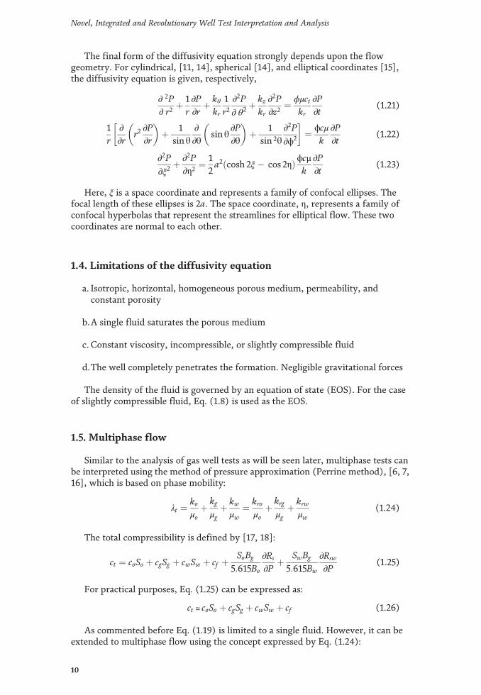
The exponential function can be evaluated by the following formula, [27], forx ≤ 25:

EiðxÞ ¼ 0:57721557 þ ln x� xþ x2

2 � 2!�x3

3 � 3!þx4

4 � 4!…: (1.84)

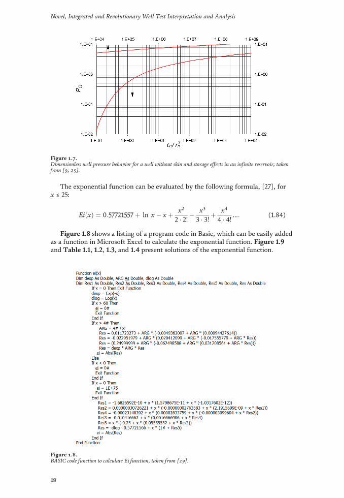
Figure 1.8 shows a listing of a program code in Basic, which can be easily addedas a function in Microsoft Excel to calculate the exponential function. Figure 1.9and Table 1.1, 1.2, 1.3, and 1.4 present solutions of the exponential function.

Figure 1.7.Dimensionless well pressure behavior for a well without skin and storage effects in an infinite reservoir, takenfrom [9, 25].

Figure 1.8.BASIC code function to calculate Ei function, taken from [29].

18


1.8. Dimensionless quantities

Dimensional parameters do not provide a physical view of the parameter beingmeasured but rather a general or universal description of these parameters. Forexample, a real time of 24 hours corresponds to a dimensionless time of approxi-mately 300 hours in very low permeability formations or more than 107 in verypermeable formations [3, 9, 21, 25, 28].

A set number of Ei values for 0.0001 ≤ x ≤ 25 with the aid of the algorithm givenin Figure 1.8. Then, a fitting of these data was performed to obtain the polynomialsgiven by Eqs. (1.85) and (1.90). The first one has a R2 of 1, and the second one has aR2 of 0.999999999 which implies accuracy up to the fifth digit can be obtained.

Eið�xÞ ¼ aþ bxþ cx2:5 þ d ln xþ e � expð�xÞ; x ≤ 1 (1.85)

ln Eið�xÞ ¼ aþ cxþ ex2

1þ bxþ dx2 þ f x3; x > 1 (1.86)

Adapted from [29] and generated with the Ei function code given in Figure 1.8.Define dimensionless radius, dimensionless time, and dimensionless pressure as:

rD ¼ r=rw (1.87)

tD ¼ tto

(1.88)

PD ¼ khðPi � PÞ141:2qμB

(1.89)

Adapted from [29] and generated with the Ei function code given in Figure 1.8.For pressure drawdown tests, ΔP = Pi � Pwf. For pressure buildup tests, ΔP = Pws

� Pwf (Δt = 0).This means that the steady‐state physical pressure drop for radial flow is equal

to the dimensionless pressure multiplied by a scalable factor, which in this casedepends on the flow and the properties of the reservoir, [3–7, 9, 21, 26, 30].

Figure 1.9.Values of the exponential integral for 1 ≤ x ≤ 10 (left) and 0.0001 ≤ x ≤ 1 (right).

19


ab

cd

ef

�0.090

6765673563

653

0.51339598

4549

1270

�0.024

3644

3074

28167

�0.000

0014

3468

6080

0�0

.486

5489

789766

050

�0.74

8020

2919199570

1.36

295989

9386

6700

�0.596

009196

1168

400

0.02

756534

8699

0893

�0.776878206

4908

800

�0.001

0740

336145

794

Tab

le1.1.

Constan

tsforEqs.(

1.85

)an

d(1.86).

20


x0

12

34

56

78

9

0.00

08.63

322

7.94

018

7.5348

17.24

723

7.02

419

6.84

197

6.68

791

6.5544

86.43

680

0.00

16.33154

6.2363

36.14

942

6.06

948

5.99

547

5.92657

5.86

214

5.80

161

5.74

455

5.69

058

0.00

25.63

939

5.5907

05.54

428

5.49

993

5.45

747

5.41

675

5.37763

5.3399

95.30

372

5.26

873

0.00

35.2349

35.20

224

5.1705

95.1399

15.1101

65.08

127

5.05

320

5.02

590

4.99

934

4.9734

6

0.00

44.94

824

4.9236

54.89

965

4.8762

24.85333

4.83

096

4.80

908

4.78767

4.76672

4.74

620

0.00

54.72610

4.70

639

4.68

707

4.66

813

4.64

953

4.63

128

4.61337

4.59577

4.5784

74.5614

8

0.00

64.54

477

4.5283

44.51218

4.49

628

4.48

063

4.46

523

4.45

006

4.43

512

4.42

041

4.40

591

0.00

74.39

162

4.37753

4.36

365

4.34

995

4.3364

54.32312

4.30

998

4.2970

04.2842

04.27156

0.00

84.2590

84.24

676

4.2345

94.22257

4.2106

94.1989

64.18736

4.17590

4.1645

74.15337

0.00

94.14

229

4.13134

4.1205

24.10

980

4.09

921

4.08

873

4.07

835

4.06

809

4.05

793

4.04

788

0.01

4.03

793

3.94

361

3.85760

3.77855

3.70

543

3.63

743

3.5738

93.5142

53.45

809

3.40

501

0.02

3.3547

13.30

691

3.26

138

3.21791

3.1763

43.13651

3.09

828

3.06

152

3.02

614

2.99

203

0.03

2.95912

2.92731

2.89

655

2.86

676

2.83

789

2.80

989

2.78270

2.7562

82.7306

02.70

560

0.04

2.68

126

2.65755

2.63

443

2.61188

2.5898

72.5683

82.54

737

2.5268

52.50

677

2.48

713

0.05

2.46

790

2.44

907

2.43

063

2.41

255

2.39

484

2.3774

62.36

041

2.34

369

2.32727

2.31114

0.06

2.29531

2.27975

2.26

446

2.24

943

2.2346

52.2201

12.20

581

2.19174

2.17789

2.1642

6

0.07

2.1508

42.13762

2.1246

02.11177

2.09

913

2.08

667

2.07

439

2.06

228

2.05

034

2.03

856

0.08

2.02

694

2.01

548

2.00

417

1.99

301

1.98

199

1.97112

1.96

038

1.94

978

1.93

930

1.9289

6

0.09

1.91874

1.90

865

1.89

868

1.88

882

1.8790

81.86

945

1.8599

41.8505

31.84

122

1.83

202

0.10

1.82292

1.8139

31.80

502

1.7962

21.78751

1.7788

91.7703

61.76192

1.75356

1.74

529

0.11

1.73711

1.7290

01.7209

81.7130

41.70

517

1.69

738

1.68

967

1.68

203

1.6744

61.66

697

0.12

1.65954

1.65219

1.64

490

1.63

767

1.63

052

1.62

343

1.6164

01.60

943

1.60

253

1.59568

21


x0

12

34

56

78

9

0.13

1.5889

01.58217

1.57551

1.5689

01.56234

1.55584

1.54

940

1.54

301

1.5366

71.5303

8

0.14

1.5241

51.51796

1.51183

1.50

574

1.49

970

1.49

371

1.48

777

1.48

188

1.47

603

1.47

022

0.15

1.46

446

1.45

875

1.45

307

1.44

744

1.44

186

1.43

631

1.43

080

1.42

534

1.41

992

1.41

453

0.16

1.40

919

1.40

388

1.39

861

1.39

338

1.38

819

1.38

303

1.37791

1.37282

1.36

778

1.36

276

0.17

1.35778

1.35284

1.34

792

1.34

304

1.33820

1.33339

1.3286

01.3238

61.31914

1.3144

5

0.18

1.30

980

1.30

517

1.30

058

1.2960

11.2914

71.2869

71.2824

91.2780

41.2736

21.26

922

0.19

1.26

486

1.26

052

1.2562

11.25192

1.24

766

1.24

343

1.23922

1.2350

41.2308

91.22676

0.2

1.2226

51.21857

1.2145

11.2104

81.20

647

1.20

248

1.19852

1.1945

81.1906

71.18677

Tab

le1.2.

Valuesof

theexponentialintegral

for0.00

01≤x≤0.20

9.

22


x0

12

34

56

78

9

437.794

0000

37.7927530

33.488

8052

29.68762

0926

.3291192

23.360

1005

20.734

0078

18.410

0584

16.35249

5014

.52993

93

511.483

9049

11.4829557

10.21300

089.08

62158

8.08

6083

07.1980

442

6.40

9260

35.70

8401

55.08

5464

74.5316127

63.60

17735

3.60

0824

53.2108

703

2.86

3763

42.5547

143

2.2794

796

2.03

4298

71.8158374

1.62

1138

51.44

75779

71.155766

31.1548

173

1.03

17127

0.9218812

0.8238

725

0.7363

972

0.6583

089

0.5885877

0.5263

261

0.47

07165

80.377605

20.3766

562

0.3369

951

0.30

1548

60.26

9864

10.24

1538

20.2162

112

0.193562

50.173306

00.155186

6

90.1254

226

0.1244

735

0.1114

954

0.09

9880

70.08

9484

90.08

01790

0.07

1847

70.06

4388

30.05

7708

60.05

1726

7

100.04

25187

0.04

1569

70.03

7270

40.03

34186

0.02

99673

0.02

6874

70.02

4103

10.02

16191

0.01

93925

0.01

7396

6

110.01

49520

0.01

4003

00.01

2564

50.01

1274

60.01

01178

0.00

9080

40.00

8149

80.00

73151

0.00

6566

30.00

5894

6

120.00

5700

10.00

47511

0.00

42658

0.00

3830

30.00

3439

50.00

3088

80.00

27739

0.00

24913

0.00

22377

0.00

2009

9

130.00

2570

90.00

16219

0.00

14570

0.00

1309

00.00

11761

0.00

10567

0.00

0949

50.00

08532

0.00

0766

70.00

0689

0

140.00

1505

60.00

05566

0.00

0500

20.00

0449

60.00

0404

20.00

0363

30.00

0326

60.00

0293

60.00

0264

00.00

02373

150.00

1140

90.00

019186

0.00

017251

0.00

015513

0.00

0139

500.00

012545

0.00

011282

0.00

0101

469.1257E�0

58.20

79E�0

5

160.00

10155

6.64

05E�0

95.9732E�0

95.3732E�0

94.83

36E�0

94.34

83E�0

93.9119E�0

93.5194

E�0

93.1664

E�0

92.84

89E�0

9

170.00

09725

2.30

64E�0

92.07

54E�0

91.86

75E�0

91.68

05E�0

91.5123E�0

91.36

09E�0

91.2248

E�0

91.10

22E�0

99.9202

E�1

0

180.00

09563

8.03

61E�1

07.2331E�1

06.5105

E�1

05.86

03E�1

05.2752E�1

04.74

86E�1

04.2747

E�1

03.84

82E�1

03.46

43E�1

0

190.00

09511

2.80

78E�1

02.5279E�1

02.2760

E�1

02.04

92E�1

01.84

51E�1

01.66

13E�1

01.49

59E�1

01.34

70E�1

01.2129E�1

0

200.00

09526

9.83

55E�1

18.8572E�1

17.9764

E�1

17.1833E�1

16.46

92E�1

15.8263

E�1

15.24

73E�1

14.7260

E�1

14.2566

E�1

1

210.00

0924

83.45

32E�1

13.1104

E�1

12.80

17E�1

12.5237E�1

12.2733E�1

12.04

78E�1

11.84

47E�1

11.66

17E�1

11.49

70E�1

1

220.00

09183

1.2149

E�1

11.09

45E�1

19.86

10E�1

28.88

42E�1

28.00

43E�1

27.2117E�1

26.49

76E�1

25.8544

E�1

25.2750

E�1

2

230.00

0946

44.2827E�1

23.8590

E�1

23.47

73E�1

23.1334

E�1

22.8236

E�1

22.54

44E�1

22.2929E�1

22.06

63E�2

1.86

21E�1

2

240.00

09316

1.5123E�1

21.36

29E�1

21.2283

E�1

21.10

70E�1

29.9772E�1

38.99

22E�1

38.10

46E�1

37.30

48E�1

36.5839

E�1

3

250.00

00779

5.34

89E�1

34.8213E�1

34.34

58E�1

33.9172E�1

33.5310

E�1

33.1829E�1

32.86

92E�1

32.5864

E�1

32.3315E�1

3

Tab

le1.3.

Valuesof

theexponentialintegral,Ei(�x

)�

10�4,for4≤x≤25

.9.

23


x0

12

34

56

78

9

0.20

1.2226

511.182902

1.14

5380

1.10

9883

1.07

6236

1.04

4283

1.01

3889

0.98

4933

0.957308

0.93

0918

0.30

0.90

5677

0.88

1506

0.8583

350.83

6101

0.8147

460.7942

160.7744

620.7554

420.737112

0.7194

37

0.40

0.70

2380

0.68

5910

0.66

9997

0.6546

140.63

9733

0.62

5331

0.611387

0.597878

0.5847

840.5720

89

0.50

0.559774

0.54

7822

0.5362

200.5249

520.5140

040.50

3364

0.49

3020

0.48

2960

0.47

3174

0.46

3650

0.60

0.45

4380

0.44

5353

0.43

6562

0.42

7997

0.41

9652

0.41

1517

0.40

3586

0.39

5853

0.38

8309

0.38

0950

0.70

0.373769

0.36

6760

0.3599

180.353237

0.34

6713

0.34

0341

0.3341

150.3280

320.3220

880.3162

77

0.80

0.3105

970.30

5043

0.2996

110.2942

990.289103

0.2840

190.2790

450.2741

770.26

9413

0.26

4750

0.90

0.26

0184

0.255714

0.251337

0.24

7050

0.24

2851

0.238738

0.2347

080.2307

600.2268

910.223100

1.00

0.2193

840

0.215741

70.2121712

0.20

8670

70.20

5238

40.20

18729

0.1985724

0.1953355

0.192160

60.1890

462

1.10

0.1859910

0.182993

60.1800

526

0.177166

70.1743

347

0.1715554

0.1688

276

0.166150

10.1635218

0.1609

417

1.20

0.1584

085

0.1559214

0.1534

793

0.1510

813

0.14

8726

30.14

64135

0.14

4141

90.14

1910

70.1397191

0.137566

1

1.30

0.1354

511

0.1333731

0.1313314

0.1293

253

0.127354

10.1254

169

0.1235132

0.121642

30.1198

034

0.117996

0

1.40

0.1162

194

0.1144

730

0.1127562

0.1110

684

0.10

9409

00.10

77775

0.10

61734

0.10

4596

00.10

3045

00.10

15197

1.50

0.10

00197

0.09

8544

50.09

7093

60.09

5666

50.09

4262

90.09

28822

0.09

1524

10.09

0188

00.08

88737

0.08

7580

6

1.60

0.08

6308

40.08

50568

0.08

38252

0.08

26134

0.08

14211

0.08

0247

70.07

9093

10.07

79568

0.07

6838

50.07

57379

1.70

0.07

4654

70.07

3588

60.07

2539

20.07

1506

30.07

0489

60.06

9488

80.06

8503

50.06

75336

0.06

65788

0.06

5638

7

1.80

0.06

47132

0.06

3802

00.06

2904

80.06

20214

0.06

11516

0.06

02951

0.05

94516

0.05

86211

0.05

7803

20.05

69977

1.90

0.05

6204

50.05

54232

0.05

46538

0.05

3896

00.05

3149

60.05

2414

50.05

1690

40.05

09771

0.05

0274

50.04

95824

2.00

0.04

8900

60.04

82290

0.04

75673

0.04

69155

0.04

62733

0.04

5640

70.04

50173

0.04

4403

20.04

3798

10.04

3201

9

2.10

0.04

2614

40.04

20356

0.04

14652

0.04

0903

20.04

0349

30.03

9803

60.03

92657

0.03

87357

0.03

82133

0.03

7698

6

2.20

0.03

71912

0.03

66912

0.03

6198

40.03

57127

0.03

5234

00.03

4762

20.03

42971

0.03

3838

70.03

3386

80.03

2941

4

2.30

0.03

2502

40.03

2069

60.03

1642

90.03

12223

0.03

0807

70.03

0399

00.02

9996

10.02

9598

80.02

9207

20.02

88210

24


x0

12

34

56

78

9

2.40

0.02

8440

40.02

80650

0.02

76950

0.02

7330

10.02

6970

40.02

66157

0.02

62659

0.02

59210

0.02

55810

0.02

5245

7

2.50

0.02

49150

0.02

4589

00.02

42674

0.02

3950

40.02

36377

0.02

33294

0.02

30253

0.02

27254

0.02

24296

0.02

2138

0

2.60

0.02

1850

30.02

1566

60.02

1286

80.02

1010

90.02

0738

70.02

0470

20.02

0205

40.01

9944

30.01

9686

70.01

94326

2.70

0.01

91820

0.01

8934

80.01

8690

90.01

8450

40.01

82131

0.01

79790

0.01

7748

10.01

7520

40.01

72957

0.01

7074

0

2.80

0.01

68554

0.01

6639

70.01

6426

90.01

62169

0.01

6009

80.01

5805

50.01

5603

90.01

5405

00.01

5208

70.01

50151

2.90

0.01

4824

10.01

46356

0.01

4449

70.01

4266

20.01

40852

0.01

3906

60.01

3730

30.01

35564

0.01

3384

90.01

32155

3.00

0.01

3048

50.01

2883

60.01

2720

90.01

2560

40.01

2402

00.01

2245

70.01

20915

0.01

1939

20.01

1789

00.01

1640

8

3.10

0.01

1494

50.01

1350

20.01

1207

70.01

10671

0.01

09283

0.01

07914

0.01

06562

0.01

05229

0.01

03912

0.01

02613

3.20

0.01

01331

0.01

0006

50.00

98816

0.00

97584

0.00

9636

70.00

95166

0.00

9398

10.00

92811

0.00

91656

0.00

90516

3.30

0.00

8939

10.00

88281

0.00

87185

0.00

8610

30.00

8503

50.00

8398

10.00

8294

00.00

81913

0.00

8089

90.00

7989

9

3.40

0.00

78911

0.00

7793

50.00

76973

0.00

7602

20.00

7508

40.00

74158

0.00

7324

40.00

7234

10.00

7145

00.00

70571

3.50

0.00

6970

20.00

6884

50.00

6799

90.00

67163

0.00

66338

0.00

65524

0.00

64720

0.00

63926

0.00

6314

30.00

6236

9

3.60

0.00

6160

50.00

60851

0.00

6010

60.00

59371

0.00

5864

50.00

57929

0.00

57221

0.00

56523

0.00

5583

30.00

55152

3.70

0.00

5447

90.00

53815

0.00

53160

0.00

52512

0.00

51873

0.00

5124

20.00

50619

0.00

5000

30.00

4939

60.00

48796

3.80

0.00

4820

30.00

47618

0.00

4704

10.00

4647

00.00

4590

70.00

45351

0.00

4480

20.00

44259

0.00

43724

0.00

43195

3.90

0.00

42672

0.00

42157

0.00

4164

70.00

4114

40.00

4064

80.00

40157

0.00

39673

0.00

39194

0.00

38722

0.00

38255

4.00

0.00

37794

0.00

37339

0.00

3689

00.00

3644

60.00

3600

80.00

35575

0.00

3514

80.00

34725

0.00

3430

80.00

3389

6

Tab

le1.4.

Valuesof

theexponentialintegral

for0.1≤x≤4.09

.

25


The same concept applies to transient flow and to more complex situations, but inthis case, the dimensionless pressure is different. For example, for transient flow,the dimensionless pressure is always a function of dimensionless time.

Taking derivative to Eqs. (1.87) and (1.88),

∂ r ¼ rw∂ rD (1.90)

∂ t ¼ to∂ tD (1.91)

Replacing the above derivatives into Eq. (1.20),Adapted from [5] and generated with the Ei function code given in Figure 1.8.

∂ 2P∂ r2D

þ 1 rD

∂ P∂ rD

¼ ϕ μ ct r2wkto

∂ P∂ tD

(1.92)

Definition of to requires assuming ϕμctr2wkto

= 1, [24], then;

to ¼ ϕ μ ct r2wk

(1.93)

Replacing this definition into Eq. (1.88) and solving for the dimensionless time(oilfield units),

tD ¼ 0:0002637ktϕμctr2w

(1.94)

Replacing Eq. (1.93) in Eq. (1.92) leads, after simplification, to:

∂ 2P∂ r2D

þ 1 rD

∂ P∂ rD

¼ ∂ P∂ tD

(1.95)

The dimensionless pressure is also affected by the system geometry, otherwell systems, storage coefficient, anisotropic characteristics of the reservoir,fractures, radial discontinuities, double porosity, among others. In general, thepressure at any point in a single well system that produces the constant rate, q, isgiven by [25]:

½Pi � Pðr, tÞ� ¼ qBμ kh

PDðtD, rD, CD, geometry,…:Þ (1.96)

Taking twice derivative to Eq. (1.87), excluding the conversion factor, willprovide:

∂ PD ¼ � kh qBμ

∂P (1.97)

∂ 2PD ¼ � kh qBμ

∂2P (1.98)

Replacing Eqs. (1.97) and (1.98) in Eq. (1.95) and simplifying leads to:

∂2PD

∂ r2Dþ 1 rD

∂PD

∂ rD¼ 1

rD

∂∂rD

rD∂PD

∂rD

� �¼ ∂PD

∂tD(1.99)

26


If the characteristic length is the area, instead of wellbore radius, Eq. (1.92) canbe expressed as:

tDA ¼ 0:0002637ktϕ μ ct A

¼ tDr2wA

� �(1.100)

Example 1.1

A square shaped reservoir produces 300 BPD through a well located in thecenter of one of its quadrants. See Figure 1.10. Estimate the pressure in the wellafter 1 month of production. Other relevant data:

Pi = 3225 psia, h = 42 ftko = 1 darcy, ϕ = 25%μo = 25 cp, ct = 6.1 � 10�6/psiaBo = 1.32 bbl/BF, rw = 6 inA = 150 Acres, q = 300 BPD

Solution

Assuming the system behaves infinitely, it means, during 1 month of productionthe transient wave has not yet reached the reservoir boundaries, the problem can besolved by estimating the Ei function. Replacing Eqs. (1.82) and (1.92) into theargument of Eq. (1.82), it results:

x ¼ � r2D4tD

¼ � 948ϕμctr2

kt(1.101)

Using Eq. (1.101) with the above given reservoir and well data:

x ¼ � 948ð0:25Þð25Þð6:1� 10�6Þð0:52Þð1000Þð720Þ ¼ 1:25� 10�8

This x value allows finding Ei(�x) = 17.6163 using the function provided inFigure 1.8. From the application of Eq. (82), PD = 8.808. This dimensionless pres-sure is meaningless for practical purposes. Converting to oilfield units by means ofEq. (1.87), the well‐flowing pressure value after 1 month of production is given as:

8:808 ¼ ð1000Þð42Þð141:2Þð300Þð1:32Þð25Þ ð3225� Pwf Þ

Pwf = 2931.84 psia.

Figure 1.10.Geometry of the reservoir for example 1.1.

27


How it can be now if the example was correctly done? A good approximationconsists of considering a small pressure drop; let us say � 0.002 psia (smallest valuethat can be read from current pressure recorders) at the closest reservoir boundary.Use Eq. (1.87) to convert from psia to dimensionless pressure:

PD ¼ ð1000Þð42Þð141:2Þð300Þð1:32Þð25Þ ð0:002Þ ¼ 6:0091� 10�5

Eq. (1.82) allows finding Ei(�x) = 0.00012. This value can be used to determinean x value from Table 1.2. However, a trial‐and‐error procedure with the functiongiven in Figure 1.8 was performed to find an x value of 6.97. Then, the time atwhich this value takes place at the nearest reservoir boundary is found fromEq. (1.101). The nearest boundary is obtained from one‐fourth of the reservoir sizearea (3.7 Ac or 1663500 ft2). Then, for a square geometry system (the system mayalso be approached to a circle):

L ¼ffiffiffiffiffiffiffiffiffiffiffiffiffiffiffiffiffiffi1663500

p¼ 1278:09 ft

The radial distance from the well to the nearest boundary corresponds to onehalf of the square side, the r = 639.04 ft. Solving for time from Eq. (1.101);

t ¼ 948ϕμctr2

kx¼ 948ð0:25Þð25Þð6:1� 10�6Þð639:042Þ

ð1000Þð6:97Þ ¼ 2:118 h

This means that after 2 h and 7 min of flow, the wave has reached the nearestreservoir boundary; therefore, the infinite‐acting period no longer exists for thisreservoir, then, a pseudosteady‐state solution ought to be applied (Figures 1.11–1.14). To do so, Eq. (1.98) is employed for the whole reservoir area:

tDA ¼ ð0:0002637Þð1000Þð720Þð0:25Þð25Þð6:1� 10�6Þð6534000Þ ¼ 0:76

With this tDA value of 0.76, the normal procedure is to estimate the dimension-less pressure for a given reservoir‐well position configuration, which can befound in Figures C.13 through C.16 in [25] for which data were originally presentedin [31]. These plots provide the pressure behavior for a well inside a

Figure 1.11.Pressure versus distance plot for example 1.2.

28


Figure 1.12.Pressure versus time plot for example 1.3.

Figure 1.14.Skin factor influence.

Figure 1.13.Pressure distribution in the reservoir.

29


rectangular/square no-flow system, without storage wellbore and skin factor;A0.5/rw = 2000 can also be found in [3, 9, 26]. This procedure is avoided in thistextbook. Instead new set of data was generated and adjusted to the followingpolynomial fitting in which constants are reported in Table 1.5:

PD ¼ aþ b*tDA þ c*t2DA þ d*t0:5DA ln tDA þ et0:5DA

(1.102)

Using Eq. (1.102) will result:

PD ¼ 4:4765þ 9:3437ð12Þ � 0:2798ð122Þ � 2:7516ffiffiffiffiffi12

pln ð12Þ � 0:016098ffiffiffiffiffi

12p

PD = 12.05597.The well‐flowing pressure is estimated with Eq. (1.87); thus,

12:056 ¼ ð1000Þð42Þð141:2Þð300Þð1:32Þð25Þ ðPi � Pwf Þ

Pwf = 2823.75 psia.

1.9. Application of the diffusivity equation solution

A straight‐line behavior can be observed in mostly the whole range on the right‐hand plot of Ei versus x plot given in Figure 1.9. Then, it was concluded, [3–7, 9,11, 19, 21, 26, 30], when x < 0.0025, the more complex mathematical representationof Eq. (1.82) can be replaced by a straight line function, given by:

Eið�xÞ ¼ ln ð1:781xÞ (1.103)

this leads to,

Eið�xÞ ¼ ln xþ 0:5772 (1.104)

Replacing this new definition into Eq. (1.82) will result in:

PD ¼ � 12

lnr2D4tD

� �þ 0:5772

� �(1.105)

At the well rD = 1, after rearranging,

PD ¼ 12

ln tD þ 0:80907½ � (1.106)

The above indicates that the well pressure behavior obeys a semi‐logarithmicbehavior of pressure versus time.

Example 1.2

A well and infinite reservoir has the following characteristics:

q = 2000 STB/D, μ = 0.72 cp, ct = 1.5 � 10�5 psia�1

ϕ = 23%, Pi = 3000 psia, h = 150 ftB = 1.475 bbl/STB, k = 10 md, rw = 0.5 ft

30


Reservo

irco

nfigur

ation

ab

cd

e

4.8700

3665

6.40

2094

211.3534

672

�2.05539

6�0

.02242

77

4.69

7986

557.721670

530.6194

0345

�2.35998

96�0

.01966

33

4.47

647322

9.34

3742

7�0

.2797873

�2.75162

4�0

.01609

74

4.1706

8525

9.09

4898

510.43

617914

�3.52534

09�0

.01243

89

5.2269

6199

6.871138

630.70

426794

�1.643

7779

�0.03514

73

5.24

5047

168.97155258

�0.639

7168

�1.51984

08�0

.034

5266

4.65131893

7.7836

1646

0.66

507635

�2.62547

29�0

.0221728

4.565200

779.9133152

�0.5332832

�2.66104

36�0

.0189231

4.5274

8153

9.03

2441

483

�0.090

48377

�2.669

107599

�0.01705

7535

4.672817379

16.5287314

9�3

.575335215

�2.190

0648

49�0

.01840

2371

3.9506

0284

98.526796

474

1.211519573

�4.2322354

98�0

.010

5806

81

31


Reservo

irco

nfigur

ation

ab

cd

e

3.90

027164

212.82720

551

�1.310

8942

3�4

.18134

4004

�0.009

0045

82

4.42

301913

10.240

4644

�0.798

0823

�2.854

0283

�0.0153571

4.80

2402

711.25794

71�1

.234

2193

�2.08189

88�0

.0211339

4.40

8408

8511.6323106

�0.8617361

�3.000

3158

�0.01590

63

4.14

4944

619.44

257591

0.2183

3578

�3.56549

96�0

.01201

38

Tab

le1.5.

Constan

tsforEq.

(1.102

).

32


Estimate the well‐flowing pressure at radii of 0.5, 1, 5, 10, 20, 50, 70, 100, 200,500, 1000, 2000, 2500, 3000, and 4000 feet after 1 month of production. Plot theresults.

Solution

For the wellbore radius, find x with Eq. (1.101);

x ¼ 948ð0:23Þð0:72Þð1:5� 10�5Þð0:52Þð10Þð720Þ ¼ 8:177 � 10�8

Using the function given in Figure 1.9 or Eq. (1.103), a value of Ei(�x) of15.7421 is found. Then, Eq. (1.82) indicates that PD = 7.871. Use of Eq. (1.87) allowsestimating both pressure drop and well‐flowing pressure:

ΔP ¼ Pi � Pwf ¼ 141:2qμBkh

PD ¼ 141:2ð2000Þð0:72Þð1:475Þð10Þð150Þ 7:871 ¼ 1573:74 psia

The remaining results are summarized in Table 1.6 and plotted in Figure 1.11.From this, it can be inferred that the highest pressure drop takes place in the near‐wellbore region which mathematically agrees with the continuity equation statingthat when the area is reduced, the velocity has to be increased so the flow rate canbe constant. The higher the fluid velocity, the higher the pressure drops.

Example 1.3

Re‐work example 1.2 to estimate the sand‐face pressure at time values startingfrom 0.01 to 1000 h. Show the results in both Cartesian and semilog plots. Whatdoes this suggest?

Solution

Find x with Eq. (1.101);

r, ft x Ei(�x) P, psia Pwf, psia

0.5 8.18E�08 15.7421 1537.74 1462.26

1 3.27E�07 14.3558 1435.15 1564.85

5 8.18E�06 11.137 1113.36 1886.64

10 3.27E�04 9.75 974.78 2025.22

20 1.31E�04 8.365 836.2 2163.8

50 8.18E�04 6.533 653.07 2346.93

70 1.60E�03 5.86 585.87 2414.13

100 3.27E�03 5.149 514.72 2485.28

200 1.31E�02 3.772 377.11 2622.89

500 8.17E�02 2.007 200.616 2799.384

1000 3.27E�01 0.8425 84.225 2915.775

2000 1.31Eþ00 0.1337 13.368 2986.632

2500 2.04Eþ00 0.046 4.6 2995.4

3000 2.94Eþ00 0.014 1.401 2998.599

4000 5.23Eþ00 0.0009 0.087 2999.913

Table 1.6.Summarized results for example 1.2.

33


x ¼ 948ð0:23Þð0:72Þð1:5� 10�5Þð0:52Þð10Þð0:01Þ ¼ 0:000948

A value of Ei(�x) of 6.385 is found with Eq. (1.103). Then, Eq. (1.82) gives a PDvalue of 3.192 and Eq. (1.87) leads to calculate a well‐flowing pressure of;

Pwf ¼ Pi � 141:2qμBkh

PD ¼ 3000� 141:2ð2000Þð0:72Þð1:475Þð10Þð150Þ 3:192 ¼ 2361:71 psia

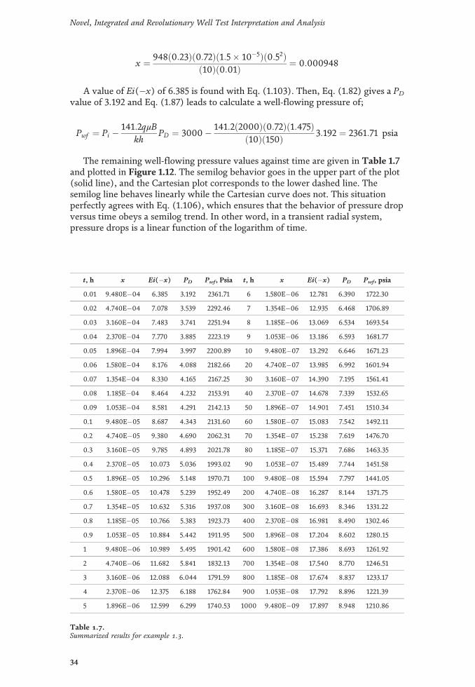
The remaining well‐flowing pressure values against time are given in Table 1.7and plotted in Figure 1.12. The semilog behavior goes in the upper part of the plot(solid line), and the Cartesian plot corresponds to the lower dashed line. Thesemilog line behaves linearly while the Cartesian curve does not. This situationperfectly agrees with Eq. (1.106), which ensures that the behavior of pressure dropversus time obeys a semilog trend. In other word, in a transient radial system,pressure drops is a linear function of the logarithm of time.

t, h x Ei(�x) PD Pwf, Psia t, h x Ei(�x) PD Pwf, psia

0.01 9.480E�04 6.385 3.192 2361.71 6 1.580E�06 12.781 6.390 1722.30

0.02 4.740E�04 7.078 3.539 2292.46 7 1.354E�06 12.935 6.468 1706.89

0.03 3.160E�04 7.483 3.741 2251.94 8 1.185E�06 13.069 6.534 1693.54

0.04 2.370E�04 7.770 3.885 2223.19 9 1.053E�06 13.186 6.593 1681.77

0.05 1.896E�04 7.994 3.997 2200.89 10 9.480E�07 13.292 6.646 1671.23

0.06 1.580E�04 8.176 4.088 2182.66 20 4.740E�07 13.985 6.992 1601.94

0.07 1.354E�04 8.330 4.165 2167.25 30 3.160E�07 14.390 7.195 1561.41

0.08 1.185E�04 8.464 4.232 2153.91 40 2.370E�07 14.678 7.339 1532.65

0.09 1.053E�04 8.581 4.291 2142.13 50 1.896E�07 14.901 7.451 1510.34

0.1 9.480E�05 8.687 4.343 2131.60 60 1.580E�07 15.083 7.542 1492.11

0.2 4.740E�05 9.380 4.690 2062.31 70 1.354E�07 15.238 7.619 1476.70

0.3 3.160E�05 9.785 4.893 2021.78 80 1.185E�07 15.371 7.686 1463.35

0.4 2.370E�05 10.073 5.036 1993.02 90 1.053E�07 15.489 7.744 1451.58

0.5 1.896E�05 10.296 5.148 1970.71 100 9.480E�08 15.594 7.797 1441.05

0.6 1.580E�05 10.478 5.239 1952.49 200 4.740E�08 16.287 8.144 1371.75

0.7 1.354E�05 10.632 5.316 1937.08 300 3.160E�08 16.693 8.346 1331.22

0.8 1.185E�05 10.766 5.383 1923.73 400 2.370E�08 16.981 8.490 1302.46

0.9 1.053E�05 10.884 5.442 1911.95 500 1.896E�08 17.204 8.602 1280.15

1 9.480E�06 10.989 5.495 1901.42 600 1.580E�08 17.386 8.693 1261.92

2 4.740E�06 11.682 5.841 1832.13 700 1.354E�08 17.540 8.770 1246.51

3 3.160E�06 12.088 6.044 1791.59 800 1.185E�08 17.674 8.837 1233.17

4 2.370E�06 12.375 6.188 1762.84 900 1.053E�08 17.792 8.896 1221.39

5 1.896E�06 12.599 6.299 1740.53 1000 9.480E�09 17.897 8.948 1210.86

Table 1.7.Summarized results for example 1.3.

34


1.10. Pressure distribution and skin factor

Once the dimensionless parameters are plugged in Eq. (1.82), this yields:

Pðr, tÞ ¼ Pi � 70:6qBμkh

Ei � 948ϕμctr2

kt

� (1.107)

At pointN, Figure 1.13, the pressure can be calculated by Eq. (1.107). At thewellbore rD = r/rw = 1, then, r = rw and P(r,t) = Pwf. Note that application of the line‐source solution requires the reservoir to possess an infinite extent, [3, 9, 18, 21, 25, 26].

There are several ways to quantify damage or stimulation in an operatingwell (producer or injector). These conditions are schematically represented inFigure 1.14. The most popular method is to represent a well condition by a steady‐state pressure drop occurring at the wellbore, in addition to the transient pressuredrop normally occurring in the reservoir. This additional pressure drop is called“skin pressure drop” and takes place in an infinitesimally thin zone: “damage zone,”[4, 5, 9, 11, 19, 30]. It can be caused by several factors:

1. Invasion of drilling fluids

2. Partial well penetration

3. Partial completion

4. Blocking of perforations

5. Organic/inorganic precipitation

6. Inadequate drilling density or limited drilling

7. Bacterial growth

8. Dispersion of clays

9. Presence of cake and cement

10. Presence of high gas saturation around the well

Skin factor is a dimensionless parameter; then, it has to be added to the dimen-sionless pressure in Eq. (1.87), so that:

Pi � Pwf ¼ 141:2qμBkh

PD þ sð Þ (1.108)

From the above expression can be easily obtained:

Pi � Pwf ¼ 141:2qμBkh

PD þ 141:2qμBkh

s (1.109)

Therefore, the skin factor pressure drop is given by:

ΔPs ¼ 141:2qμBkh

s (1.110)

35


Assuming steady state near the wellbore and the damage area has a finiteradius, rs, with an altered permeability, ks, the pressure drop due to the damage isexpressed as the pressure difference between the virgin zone and the altered zone,that is to say:

ΔPs ¼ 141:2qμBksh

lnrsrw

� 141:2qμBkh

lnrsrw

(1.111)

Rearranging;

ΔPs ¼ 141:2qμBkh

kks

� 1� �

lnrsrw

(1.112)

Comparing Eqs (1.112) and (1.107), the following can be concluded:

s ¼ kks

� 1� �

lnrsrw

(1.113)

rs and ks are not easy to be obtained.Equation (1.82) and (1.106) can be respectively written as:

PD þ s ¼ � 12Ei �xð Þ (1.114)

PD þ s ¼ 12

ln tD þ 0:80907½ � (1.115)

Replacing the dimensionless quantities given by Eqs. (1.87) and (1.95) inEq. (1.115) will result:

Pi ¼ Pwf þ 70:6qμBkh

ln0:0002637kt

ϕμctr2w

� �þ 0:80908þ 2s

� �(1.116)

Taking natural logarithm to 0.0002637 and adding its result to 0.80908results in:

Pi ¼ Pwf þ 70:6qμBkh

�7:4316þ lnkt

ϕμctr2w

� �þ 2s

� �(1.117)

Multiplying and dividing by the natural logarithm of 10 and solving for the well‐flowing pressure:


logkt

ϕμctr2w

� �� 3:2275þ 0:8686s

� �(1.118)

Thus, a straight line is expected to develop from a semilog plot of pressureagainst the time, as seen on the upper curve of Figure 1.12.

1.11. Finite reservoirs

In closed systems, the radial flow is followed by a transition period. This in turnis followed by the pseudosteady, semi‐stable, or quasi‐stable state, which is a

36


transient flow regime where the pressures change over time, dP/dt, is constant at allpoints of the reservoir:

dPdt

¼ �qcVp

(1.119)

Eq. (1.99) is now subjected to the following initial and boundary conditions:

PD rD, tD ¼ 0ð Þ ¼ 0 (1.120)

∂PD

∂rD

� �reD

¼ 0 (1.121)

∂PD

∂rD

� �rD¼1

¼ �1 (1.122)

Which solution is [9, 30]:

PDðrD, tDÞ ¼ 2ðr2eD � 1Þ

r2D4þ tD

� �� r2eD ln rDðr2eD � 1Þ �

ð3r4eD � 4r4eD ln reD � 2r2eD � 1Þ4ðr2eD � 1Þ2

þπ∑∞

n¼1

(e�a2ntD J21ðanreDÞ½J1ðanÞY0ðanrDÞ � Y1ðanÞðJ0ÞðanrDÞ�

an½J21 ðanreDÞ � J21ðanÞ�

)

(1.123)

The pseudosteady‐state period takes place at late times (t > 948ϕμctre2/k), so that

as time tends to infinity, summation tends to zero, then:

PD rD, tDð Þ ¼ 2r2eD � 1 r2D

4þ tD

� �� r2eD ln rD

r2eD � 1 � 3r4eD � 4r4eD ln reD � 2r2eD � 1

4 r2eD � 1 2

(1.124)

At the well, rD = 1 and as reD >>>> 1, the above expression is reduced to:

PDðtDÞ ¼ 2r2eD

þ 2tDr2eD

� 34þ ln reD þ 1

2r2eD� 14r4eD

(1.125)

This can be approximated to:

PDðtDÞ ffi 2tDr2eD

þ ln reD � 34

(1.126)

Invoking Eq. (1.98) for a circular reservoir area,

tDA ¼ tDr2wπr2e

¼ tDπr2eD

(1.127)

It follows that;

πtDA ¼ tDr2eD

(1.128)

The final solution to the pseudosteady‐state diffusivity equation is obtainedfrom using the definition given by Eq. (1.128) in Eq. (1.129):

37


PDðtDÞ ¼ 2πtDA þ ln reD � 34

(1.129)

The derivative with respect to time of the above equation in dimensional formallows obtaining the pore volume:

dPðr, tÞdt

¼ � 1:79qBhϕctr2e

(1.130)

An important feature of this period is that the rate of change of pressure withrespect to time is a constant, that is, dPD/dtDA = 2π.

When the reservoir pressure does not change over time at any point, the flow issaid to be stable. In other words, the right side of Eq. (1.99) is zero, [3]:

1rD

∂∂rD

rD∂PD

∂rD

� �¼ 0 (1.131)

Similar to the pseudosteady‐state case, steady state takes place at late times.Now, its initial, external, and internal boundary conditions are given by:

PD rD, tD ¼ 0ð Þ ¼ 0 (1.132)

PD rDe,0ð Þ ¼ 0 (1.133)

∂PD

∂rD

� �rD¼1

¼ �1 (1.134)

The solution to the steady‐state diffusivity equation is [3]:

PD rD, tDð Þ ¼ ln reD � 2∑∞

n¼1

e�β2ntDn J20ðβnreDÞ

β2n J21 βn � J20 βnreD

� �( )

(1.135)

As time tends to infinity, the summation tends to infinity, then:

ðPDÞssr ¼ ln reD ¼ lnrerw

(1.136)

In dimensional terms, the above expression is reduced to Darcy’s equation. Thedimensionless pressure function for linear flow is given by:

ðPDÞssL ¼ 2πLhA

(1.137)

Steady state can occur in reservoirs only when the reservoir is fully recharged byan aquifer or when injection and production are balanced. However, a reservoirwith a very active aquifer will not always act under steady‐state conditions. First,there has to be a period of unsteady state, which will be followed by the steady stateonce the pressure drop has reached the reservoir boundaries. Extraction of fluidsfrom a pressurized reservoir with compressible fluids causes a pressure disturbancewhich travels throughout the reservoir. Although such disturbance is expected totravel at the speed of sound, it is rapidly attenuated so that for a given duration ofproduction time, there is a distance, the drainage radius, beyond which no substan-tial changes in pressure will be observed. As more fluid is withdrawn (or injected),the disturbance moves further into the reservoir with continuous pressure decline

38


at all points that have experienced pressure decline. Once a reservoir boundary isfound, the pressure on the boundary continues to decline but at a faster rate thanwhen the boundary was not detected. On the other hand, if the pressure transientreaches an open boundary (water influx), the pressure remains constant at somepoint; the pressure closest to the well will decline more slowly than if a closedboundary were found. Flow changes or the addition of new wells cause additionalpressure drops that affect both the pressure decline and the pressure distribution.Each well will establish its own drainage area that supplies fluid. When a flowboundary is found, the pressure gradient—not the pressure level—tends to stabilizeafter sufficiently long production time. For the closed boundary case, the pressurereaches the pseudosteady state with a constant pressure gradient and general pres-sure drop everywhere, which is linear over time. For constant‐pressure boundaries,steady state is obtained; both the pressure and its gradient remain constantover time.

1.12. The pressure derivative function

Pressure derivative has been one of the most valuable tools ever introduced to thepressure transient analysis field. In fact, [32] affirms that pressure derivative anddeconvolution have been the best elements added for well test interpretation. How-ever, here it is affirmed that besides these two “blessings,” TDS technique, [1, 2], isthe best and practical well test interpretation method in which application will bevery devoted along this textbook. Actually, in the following chapters,TDS is extendedfor long, homogeneous reservoirs, [33], interference testing [34], drainage areadetermination in constant‐pressure reservoirs, [35], and recent applications on frac-tured vertical wells, [36], among others. More complex scenarios, for instance finite‐conductivity faults, [37], are treated extensively in [38].

Attempts to introduce the pressure derivative are not really new. Some of themtry to even apply the derivative concept to material balance. Just to name a few ofthem, [39] in 1961, tried to approach the rate of pressure change with time fordetection of reservoir boundaries. Later, in 1965, [40] presented drawdown curvesof well pressure change with time for wells near intersecting faults (36 and 90°).These applications, however, use numerical estimations of the pressure rate changeon the field data regardless of two aspects: (1) an understanding of the theoreticalsituation behind a given system and (2) noise in the pressure data.

Between 1975 and 1976, Tiab’s contributions on the pressure derivative wereremarkable. Actually, he is the father of the pressure derivative concept as usednowadays. Refs. [41, 42] include detailed derivation and application of the pressurederivative function. These results are further summarized on [41–45]. Ref. [46]applied Tiab’s finding to provide a type‐curve matching technique using the naturallogarithm pressure derivative.

It was required to obtain the pressure derivative from a continuous function,instead of attempting to work on discrete data in order to understand the pressurederivative behavior in an infinite system. Then, Tiab decided to apply the Leibnitz’srule of derivation of an integral to the Ei function.

∂∂x

ðhðxÞf ðxÞ

gðuÞdu g hðxÞ½ � ∂ hðxÞ½ �∂x

� g f ðxÞ½ � ∂ f ðxÞ½ �∂x

� (1.138)

Applying Leibnitz’s rule to the Ei function in Eq. (1.81) to differentiate withrespect to tD (see Appendix B in [42]),

39


ΔΔtD

Ei�r2D4tD

� �� ¼ �

ð∞rD24tD

e�u

u Δu ¼ � e�u

u ΔuΔtD

��∞

r2D

4tD

(1.139)

Taking the derivative Δu/ΔtD and replacing u by rD2/4tD,

ΔΔtD

Ei � r2D4tD

� �� ¼ e� r2D=4tD

r2D=4tD

� r2D4t2D

� �(1.140)

After simplification,

ΔΔtD

Ei � r2D4tD

� �� ¼ � 1

tDe� r2D=4tD

(1.141)

From inspection of Eq. (1.81) results:

∂PD

∂tD¼ � 1

21tD

e�r2D

4tD (1.142)

In oilfield units,

ΔPwf

Δt¼ 70:6qμB

khte

� 948ϕμctkt

� �(1.143)

At the well, rD = 1, then, Eq. (1.142) becomes:

PD0 ¼ 1

2tDe�

14tD (1.144)

For tD > 250, e�1/4tD = 1; then, Eq. (1.144) reduces to

PD0 ¼ 1

2tD(1.145)

The derivative of equation (1.145) is better known as the Cartesian derivative.The natural logarithmic derivative is obtained from:

tD*PD0 ¼ tD

∂PD

∂tD¼ tD

∂PD

ð∂ ln tDÞ=tD ¼ ∂PD

∂ ln tD(1.146)

Later on, [46] use the natural logarithmic derivative to develop a type‐curvematching technique.

Appendix C in [42] also provides the derivation of the second pressure derivative:

∂PD″ ¼ PD0 1tD

r2D4tD

� 1� �

(1.147)

Conversion of Eq. (1.145) to natural logarithmic derivative requires multiplyingboth sides of it by tD; then, it results:

tD*PD0 ¼ 1

2(1.148)

40


Eq. (1.148) suggests that a log‐log plot of dimensionless pressure derivativeagainst dimensionless time provides a straight line with zero slope and interceptof ½. Taking logarithm to both sides of Eq. (1.145) leads to:

logPD0 ¼ �log tD � 0:301 (1.149)

Pwf0 ¼ ∂Pwf

∂t¼ 1

t70:6qμB

kh

� �(1.150)

The above expression corresponds of a straight line with negative unit slope. Indimensional form:

Taking logarithm to both sides of the above expression:

logPwf0 ¼ �log tþ log

70:6qμBkh

� �(1.151)

As shown in Figure 1.15, Eq. (1.151) corresponds to a straight line with negativeunit slope and intercept of:

P01hr ¼ 70:6qμB

kh(1.152)

Eq. (1.152) is applied to find permeability from the intersect plot of the Cartesianpressure derivative versus time plot. This type of plot is also useful to detect thepresence of a linear boundary (fault) since the negative unit slope line displaceswhen the fault is felt as depicted in Figure 1.16.

The noise that occurs in a pressure test is due to such factors as (1) turbulence,(2) tool movements, (3) temperature variations, (4) opening and closing wells inthe field, and (5) gravitational effects of the sun and moon on the tides (near thegreat lakes the noise is about 0.15 psia and offshore up to 1 psia).

The estimation of the pressure derivative with respect to time to actual data, ofcourse, must be performed numerically since data recorded from wells are alwaysdiscrete. During the derivative calculation, the noise is increased by the rate ofchange that the derivative imposes, so it is necessary to soften the derivative or touse smoothing techniques. The low resolution of the tool and the log‐log paper alsoincrease or exaggerate the noise. Therefore, calculating the derivative of pressure

Figure 1.15.Log‐log plot of Pwf

0 against t.

41


requires some care because the process of data differentiation can amplify any noisethat may be present. Numerical differentiation using adjacent points will produce avery noisy derivative, [8, 47, 48].

Ref. [8] conducted a comparative study of several algorithms for estimation ofthe pressure derivative. They obtained synthetic pressure derivatives for sevendifferent reservoir and well configuration scenarios and, then, estimated the pres-sure derivative using several comparative methods. They found that the Splinealgorithm (not presented here) is the best procedure to derive pressure versus timedata since it produces minimal average errors. It is the only algorithm of polynomialcharacter that to be continuous can be smoothed during any derivation process andthe form of the curve obtained is in agreement with the worked model. The Horneand Bourdet algorithms when the smoothing window is of either 0.2 or 0.4 are goodoptions for derivation processes. Ref. [8] also found the best procedure for dataanalysis of pressure against time is to differentiate and then smooth the data.

By itself, the central finite difference formula fails to provide goodderivative computation. Instead, some modifications are introduced by [18, 20,46], respectively:

Horne equation [32]:

t∂P∂t

� �i¼ t

∂P∂ ln t

� �i¼

ln ðti=ti�kÞΔPiþj

ln ðtiþj=tiÞ ln ðtiþj=ti�kÞ þln ðtiþjti�k=t2i ÞΔPi

ln ðtiþ1=tiÞ ln ðti=ti�1Þ�

ln ðtiþj=tiÞΔPi�1

ln ðti=ti�kÞ ln ðtiþj=ti�kÞ

8>>>>><>>>>>:

9>>>>>=>>>>>;

(1.153)

ln tiþj � ln ti≥0:2 and ln ti � ln ti�k≥0:2When the data are distributed in a geometrical progression (with the time

difference from one point to the next much larger as the test passes), then thenoise in the derivative can be reduced using a numerical differentiation withrespect to the logarithm of time. The best method to reduce noise is to use datathat is separated by at least 0.2 logarithmic cycles, rather than points that areimmediately adjacent. This procedure is recognized as smoothing and is bestexplained in Figure 1.17.

Figure 1.16.Fault identification by means of a log‐log plot of PD0 vs. tD.

42


Equation of Bourdet et al. [46]:

dPdx

� �i¼

Pi�Pi�1Xi�Xi�1

Xiþ1 � Xið Þ þ Piþ1�PiXiþ1�Xi

Xi � X�1ið ÞXiþ1 � Xi�1

(1.154)

Let X is the natural logarithm of the time function.This differentiation algorithm reproduces the test type curve over the entire

time interval. It uses a point before and a point after the point of interest, i, tocalculate the corresponding derivative and places its weighted mean for the objec-tive point. Smoothing can also be applied.

1.13. The principle of superposition

This principle is not new. It was first introduced to the petroleum literature byvan Everdingen and Hurst in 1949, [49]. However, its application is too importantand many field engineers fail or neglect to use it. Superposition is too useful forsystems having one well producing at variable rate or the case when more than onewell produces at different flow rates.

As quoted from [25], the superposition principle is defined by:“Adding solutions to the linear differential equation will result in a new solution of

that differential equation but for different boundary conditions,” which mathematicallytranslates to:

ψ ¼ ψ1 f 1 þ ψ2 f 2 þ ψ3 f 3… (1.155)

where ψ is the general solution and ψ1 f1, ψ2 f2 and ψ3 f3… are the particularsolutions.

1.13.1 Space superposition

If the wells produce at a constant flow rate, the pressure drop at point N,Figure 1.18, will be [3, 9, 19, 21, 25]:

ΔPN ¼ ΔPN,1 þ ΔPN,2 þ ΔPN,3 (1.156)

Figure 1.17.Smoothing diagram.

43


If reservoir and fluid properties are considered constant, then, Eq. (1.87) can beapplied to the above expression, so that:

ΔPN ¼ 141:2μ kh

qBoð Þ1PDðrD1, tDÞ þ qBoð Þ2PDðrD2, tDÞ þ qBoð Þ3PDðrD3, tDÞ� �

(1.157)

The dimensionless radii are defined by:

rDn ¼ rnrw

; n ¼ 1, 2, 3 (1.158)

Extended to n number of wells:

ΔPN ¼ ∑n

i¼1

141:2qμBkh

PDðrDi, tDÞ½ � (1.159)

If point N is an active well, its contribution to the total pressure drop plus theskin factor pressure drop, Eq. (1.108), must be included in Eq. (1.159), then,

ΔPN ¼ ∑n

i¼1

141:2qμBkh

PDðrDNi, tDÞ½ � þ 141:2qμBkh

sjN (1.160)

Notice that in Eqs. (1.159) and (1.160), changes of pressures or dimensionlesspressures are added. If the point of interest is a well in operation, the damage factorshould be added to the dimensionless pressure of that well only.

1.13.2 Time superposition

Sometimes there are changes in flow rate when a well produces as referred inFigures 1.19 and 1.22. Then, the superposition concept must be applied. To do this,[25], a single well is visualized as if there were two wells at the same point, one witha production rate of q1 during a time period from t = 0 to t and another imaginarywell with a production rate of q2 � q1 for a time frame between t1 and t � t1. Thetotal rate after time t1 is q1 þ (q2 � q1) = q2. The change in well pressure due to therate change [19, 25] is,

Figure 1.18.Pressure at the point N.

44


ΔP ¼ 141:2μBkh

q1PDðrD, tD1Þ þ ðq2 � q1ÞPDðrD, tD2 þ sÞ� �(1.161)

where tD2 = (t�t1)D. If there are more variations in flow rate,

ΔP ¼ 141:2μkh

∑n

i¼1ðqBÞi � ðqBÞi�1

� �PDðrD, ðt� tiÞD þ s

� �(1.162)

Example 1.4

This example is taken [25]. The below data and the schematic given inFigure 1.20 correspond to two wells in production:

k = 76 md, ϕ = 20 %, B = 1.08 bbl/STBPi = 2200 psia, μ = 1 cp, ct = 10 � 10�6/psiah = 20 ft

Calculate the pressure in (a) well 1 after 7 h of production and (b) in well 2 after11 h of production. Assume infinite behavior.

Solution

Part (a):ΔP(7 hr)= ΔP caused by production from well 1 to well 1 þ ΔP caused by

production from well 2 to well 1. Mathematically,

Figure 1.19.Time superposition.

Figure 1.20.Flow rate changes for example 1.4.

45


ΔP7hr @ well1 ¼ 141:2μq1Bkh

PDðrD1, tDÞ þ s½ � þ 141:2μq2Bkh

PDðrD2, tDÞð Þ

Using Eq. (1.101) for the well,

x ¼ � 948ϕμctr2

kt¼ 948ð0:2Þð1Þð1� 10�5Þ12

ð76Þð7Þ ¼ 3:56� 10�6

Since x << << 0.0025, it implies the use of Eq. (1.82) with Eq. (1.103); then,

PDðrD, tDÞ ¼ � 12ln 1:781xð Þ (1.163)

PD ¼ 12

�� ln 1:781*3:56� 10�6 � �� ¼ 5:98

In well 2, x = 0.03564 from Eq. (1.101). Interpolating this value in Table 1.2,Ei(�x) = 2.7924; then, PD ffi 1.4. Estimating ΔP in well 1 will result:

ΔP7hr, rD¼1 ¼ 141:2ð100Þð1:08Þð1Þð76Þð20Þ 5:98þ 5ð Þ þ 141:2ð100Þð1:08Þð1Þ

ð76Þð20Þ 1:4ð Þ ¼ 113:7

Pwf @ well1 = 2200�113.7 = 2086.4 psia (notice that skin factor was only applied towell 1)

Part (b);At 11 h, it is desired to estimate the pressure in well 2. Two flow rates should be

considered for in each well. Then, the use of Eq. (1.162) will provide:

ΔPð11 hr;well 2Þ ¼ ΔPwell 1!Well 2;t=11 hr;q=100 BPD; rD=100 þ ΔPwell 1!Well 2;t=ð11 �10Þ hr;q=ð50‐100Þ BPD; rD=100 ΔPwell 1!Well 1;t=11 hr;q=25 BPD; rD=1;s2 þ ΔPwell 1!Well 1;t=ð11 �8Þ hr;q=ð100‐25Þ BPD; rD=1;s2

Using Eq. (1.101), the four respective values of x are: x =0.02268, 0.2494,2.268 � 10�6, and 8.316 � 10�6. Estimation of Ei requires the use of Table 1.2 forthe first two values and use of Eq. (1.103) for the last two values. The four values ofEi(�x) are: 0.0227, 0.811, 12.42, and 11.12. Therefore, the respective values of PDare 1.605, 0.405, 6.209, and 5.56. The total pressure drop is found with Eq. (1.161)as follows:

ΔPwell 2; 11 hrÞ ¼ 141:2ð1Þð1:08Þð76Þð20Þ

ð100Þð1:605Þ þ ð50� 100Þð0:405Þþð25Þð6:209þ 1:7Þ þ ð100� 25Þð5:56þ 1:7Þ

� ¼ 87:75 psia

Pwf @ well2 = 2200 � 87.75 = 2112.25 psia

1.13.3 Space superposition—method of images

The method of images applies to deal with either no‐flow or constant‐pressureboundaries. If a well operates at a constant flow rate at a distance, d, from animpermeable barrier (fault), the systems acts as if there were two wells separated 2dfrom each other [3, 25]. For no‐flow boundaries, the image well corresponds to thesame operating well. For constant‐pressure boundary, the resulting image corre-sponds to an opposite operating well. In other words, if the well is a producer near afault, the image well corresponds to an injector well. These two situations aresketched in Figure 1.21. For the no‐flow boundary, upper system in Figure 1.21, thedimensionless pressure can be expressed as:

46


PD at real well ¼ PD at real well; rD=1;s þ PD at image well ! real well; rD = 2d=rw (1.164)

For the constant‐pressure boundary, lower part in Figure 1.21, the dimension-less pressure can be expressed as:

PD at real well ¼ PD at real well; rD=1;s � PD at image well ! real well; rD = 2d=rw (1.165)

The negative sign in Eq. (1.165) is because of dealing with an imaginary injectorwell.

For the case of two intersecting faults, the total number of wells depends on thevalue of the angle formed by the two faults, thus:

nwells ¼ 360θ

(1.166)

The image method is limited to one well per quadrant. If this situation failsto be fulfilled, then, the method cannot be applied. In the system of Figure 1.22, anangle of 90° is formed from the intersecting faults. According to Eq. (1.166),nwells = 360/90 = 4 wells, as shown there. The ratio of the distances from the wellto each fault is given by:

yD ¼ by=bx (1.167)

Figure 1.21.Well near a linear barrier.

Figure 1.22.Well between two intersecting faults.

47


The practical way to apply space superposition for generating the well systemresulting from two intersecting faults consist of extending the length of the faultsand setting as many divisions as suggested by Equation (1.166); that is, for example,1.5, Figure 1.23 left, six well spaces are obtained. Then, draw a circle with center atthe fault intersection and radius at well position. This guarantees that the totallength corresponds to the double length value from the well to the fault. Draw fromthe well a line to be perpendicular to the nearest fault and keep drawing the lineuntil the circle line has been reached. See Figure 1.24 left. Set the well. A sealingfault provides the same type of well as the source well, that is, a producing wellgenerates another producing well to the other side of the fault. A constant‐pressureboundary provides the opposite well type of the source well, that is, a producingwell generates an injector well on the other side of the line. Draw a new line fromthe just drawn imaginary well normal to the fault and keep drawing the line untilthe line circle is reached. See Figure 1.24 right. Repeat the procedure until thecomplete well set system has been drawn.

For more than six well spaces generated, that is angles greater than 60°, as thecase of example 1.5, when a fault intersects a constant‐pressure boundary injectorand producer imaginary wells ought to be generated. What type of line should bedrawn? A solid line representing a sealing fault, or a dash line, representing aconstant‐pressure boundary? The answer is any of both. The lines should be

Figure 1.23.Location of well A and resulting well number system for example 1.5.

Figure 1.24.Generating the well system for two intersecting faults.

48


drawn alternatively and as long as the system closes correctly, superpositionworks well.

Example 1.5

Well A in Figure 1.23 has produced a constant rate of 380 BPD. It is desired(a) to estimate the well‐flowing pressure after one week of production. The prop-erties of the reservoir, well and fluid are given as follows:

Pi = 2500 psia, B = 1.3 bbl/STB, μ = 0.87 cph = 40 ft, ct = 15�10�6/psia, ϕ = 18 %rw = 6 in, k = 220 md, s = �5

(b) What would be the well‐flowing pressure after a week of production if thewell were in an infinite reservoir?

Solution

Part (a)The pressure drop in well A is affected by its own pressure drop and pres-

sure drop caused by its well images. The distance from well A to its imaginarywells is shown in Figure 1.23 (right‐hand side). The total pressure drop for wellA is:

ΔPA ¼ ΔPA,r¼rw þ ΔPimage 1!well A,r¼500 f t þ ΔPimage 2!well A,r¼866 f t

þΔPimage 3!well A,r¼1000 f t þ ΔPimage 4!well A,r¼866 f t þ ΔPimage 5!well A,r¼500 f t

By symmetry, the above expression becomes:

ΔPA ¼ ΔPA,r¼rw þ 2ΔPimage 1!well A,r¼500 f t þ 2ΔPimage 2!well A,r¼866 f t

þ ΔPimage 3!well A,r¼1000 f t

Using Eq. (1.101) for the well:

948ð0:18Þð0:87Þð1:5� 10�5Þð0:5Þ2ð220Þð168Þ ¼ 1:5� 10�8

Since x << << 0.0025, Eq. (1.163) applies:

PDðrD, tDÞ ¼ � 12

�� ln 1:781ð1:5� 10�8Þ� �� ¼ 8:72

Estimation for the image wells are given below. In all cases, x > 0.0025, then,Table 1.2 is used to find Ei and the resulting below divided by 2 for the estimationof PD,

ximage well 1 or 5 ¼ 948ð0:18Þð0:87Þð1:5� 10�5Þð500Þ2ð220Þð168Þ ¼ 0:015, PD ¼ 1:816

ximage well 2 or 4 ¼ 948ð0:18Þð0:87Þð1:5� 10�5Þð8662Þð220Þð168Þ ¼ 0:0452, PD ¼ 1:282

ximage well 3 ¼ 948ð0:18Þð0:87Þð1:5� 10�5Þð10002Þð220Þð168Þ ¼ 0:06, PD ¼ 1:145

Then, the pressure drop in A will be:

49


ΔPA ¼ 141:2qμ Bkh

ðPDA,r¼rw þ sÞ þ 2PD image 1, r¼500 f t þ 2PD image 2, r¼866 f t þ PD image 3, r¼1000 f t� �

ΔPA ¼ 141:2ð380Þð0:87Þð1:3Þð220Þð40Þ ð8:72� 5Þ þ 2ð1:816Þ þ 2ð1:282Þ þ 1:145½ � ¼ 76:3 psia

Pwf @ well A = 2500 � 76.3 = 2423.7 psiaPart (b)If the well were located inside an infinite reservoir, the pressure drop would not

include imaginary wells, then:

ΔPA ¼ 141:2qμ Bkh

PD,r¼rw þ s½ �

ΔPA ¼ 141:2ð380Þð0:87Þð1:3Þð220Þð40Þ 8:72� 5½ � ¼ 25:63 psia

The well‐flowing pressure would be (2500 � 25.3) = 2474.4 psia. It was observedthat the no‐flow boundaries contribute with 66.4% of total pressure drop in well A.

Nomenclature

A area, ft2 or AcBg gas volume factor, ft3/STBBo oil volume factor, bbl/STBBw oil volume factor, bbl/STBbx distance from closer lateral boundary to well along the x‐direction, ftby distance from closer lateral boundary to well along the y‐direction, ftc compressibility, 1/psiacf pore volume compressibility, 1/psiact total or system compressibility, 1/psiad distance from a well to a fault, ftf a given functionh formation thickness, ftk permeability, mdks permeability in the damage zone, mdkrf phase relative permeability, f = oil, water or gasL reservoir length, ftm slopem(P) pseudopressure function, psia2/cpM gas molecular weight, lb/lbmolP pressuredP/dr pressure gradient, psia/ftPD0 dimensionless pressure derivativePD″ dimensionless second pressure derivativePD dimensionless pressurePi initial reservoir pressure, psiaPwf well flowing pressure, psiaq flow rate, bbl/D. For gas reservoirs the units are Mscf/DRs gas dissolved in crude oil, SCF/STBRsw gas dissolved in crude water, SCF/STBrD dimensionless radius

50


rDe dimensionless drainage radius = re/rwr radial distance, radius, ftre drainage radius, ftrs radius of the damage zone, ftrw well radius, ftSf fluid saturation, f = oil, gas or waters skin factorT reservoir temperature, ºRt time, hta pseudotime, psia h/cpto dummy time variableur radial flow velocity, ft/htD dimensionless time based on well radiustDA dimensionless time based on reservoir areatD*PD0 logarithmic pressure derivativeV volume, ft3

z vertical direction of the cylindrical coordinate, real gas constant

Greek

Δ change, dropΔt shut‐in time, hϕ porosity, fraction. Spherical coordinateλ phase mobility, md/cpη hydraulic diffusivity constant, md‐cp/psiaρ density, lbm/ft3

θ cylindrical coordinateμ viscosity, cpζ time function

Suffices

1 hr reading at time of 1 hD dimensionlessDA dimensionless with respect to areaf formationg gasi initial conditionso oil, based conditionw well, waterp pore

51


References

[1] Tiab D. Analysis of pressure andpressure derivative without type‐curvematching: 1‐skin and wellbore storage.Journal of Petroleum Science andEngineering; 1995;12:171‐181

[2] Tiab D. Analysis of pressure andpressure derivatives without type‐curvematching: I‐skin and wellbore storage.Society of Petroleum Engineers. 1993.DOI: 10.2118/25426‐MS

[3] Lee J, Rollins JB, Spivey JP. PressureTransient Testing. Society of PetroleumEngineers. SPE Textbook. Vol. 9.Richardson, TX; 2003. 336 p

[4] Sabet M. Well Testing. Houston, TX:Gulf Publishing Co.; 1991. 460 p

[5] Slider HC. Wordlwide PracticalPetroleum Reservoir EngineeringMethods. Revised ed. Tulsa, Oklahoma,USA: PennWell Publishing Co.; 1983.826 p

[6] Stanislav JF, Kabir CS. PressureTransient Analysis. New Jersey: PrenticeHall; 1990. 320 p

[7] Strelsova TD. Well Testing inHeterogeneous Formations. New York:John Wiley and Sons; 1988. 377 p

[8] Escobar FH, Navarrete JM, LosadaHD. Evaluation of pressure derivativealgorithms for well‐test analysis. Societyof Petroleum Engineers. 2004. DOI:10.2118/86936‐MS

[9] Mathews CS, Russell DG. Pressurebuildup and flow tests in wells. SPEMonograph Series. 1967;1:163

[10] Odeh AS, Jones LG. Pressuredrawdown analysis, variable‐rate case.Society of Petroleum Engineers. 1965:960‐964. DOI: 10.2118/1084‐PA

[11] Russell DG. Determination offormation characteristics from two‐rate

flow tests. Society of PetroleumEngineers. 1963:1347‐1355. DOI:10.2118/645‐PA

[12] Doyle RE, Sayegh EF. Real gastransient analysis of three-rate flowtests. Society of Petroleum Engineers.1970:1347‐1356. DOI: 10.2118/2607‐PA

[13] Jacob CE, Lohman SW. Nonsteadyflow to a well of constant drawdown inan extensive aquifer. Transactions,American Geophysical Union. 1952;33(4):559‐569. https://doi.org/10.1029/TR033i004p00559

[14] Joseph JA. Unsteady‐statecylindrical, spherical and linear flow inPorous Media [Ph.D. dissertation].University of Missouri‐Rolla; 1984

[15] Kucuk F, Brigham WE. Transientflow in elliptical systems. SPE Journal.1979:401‐410. DOI: 10.2118/7488‐PA

[16] Dykstra H, Kazemi H, Raghavan R,Gulati MS. Pressure Transient TestingMethods, SPE Reprint Series No. 14.Dallas, Texas: Society of PetroleumEngineers; 1967. 264 p

[17] Perrine RL. Analysis of Pressure‐buildup Curves. American PetroleumInstitute, Drilling and ProductionPractices, API, Washington, D.C.; 1956.pp. 482‐509. ID API‐56‐482

[18] Horne RN. Modern Well TestAnalysis: A Computer‐aided Approach.Palo Alto, CA: Petroway Inc.; 1990. 185 p

[19] Dake LP. The Practice of ReservoirEngineering (Revised edition).Amsterdam, Netherlands: ElsevierDevelopments in Petroleum Science(Second Printing); 2004. 544 p

[20] Al‐Hussainy R, Ramey HJ Jr,Crawford PB. The flow of real gasesthrough porous media. Journal of

52


Petroleum Technology. 1966;237:624‐636. DOI: 10.2118/1243‐A‐PA

[21] Lee J. Well Testing. SPE TextbookSeries. Society of Petroleum Engineers,Richardson, TX. Vol. 1. 1982. 159 p

[22] Lee J, Wattenberger RA. GasReservoir Engineering. Society ofPetroleum Engineers. SPE TextbookSeries No. 05. Second Printing.Richardson, TX; 2002. 349 p

[23] Agarwal RG. Real gas pseudo‐time—A new function for pressure buildupanalysis of MHF gas wells. Society ofPetroleum Engineers. 1979. DOI:10.2118/8279‐MS

[24] Civan F. PE‐5143: Fluid Flow inPorous Media. Lecture Notes. Fall 1993.The University of Oklahoma, Norman,OK; 1993

[25] Earlougher RC Jr. Advances in WellTest Analysis. Monograph Series. Vol. 5,Dallas, TX: SPE; 1977

[26] Horner DR. Pressure buildup inwells. In: Proceedings of the ThirdWorld Petroleum Congress. Section II,Preprint 7. Leiden, Netherlands; 1951.pp. 25‐43

[27] Nisle RG. How to use theexponential integral. PetroleumEngineering. 1956:171‐173

[28] Tracy GW. Pressure AnalysisMethods, SPE Reprint Series No. 9.Society of Petroleum Engineers ofAIME, Richardson, TX. 1967

[29] Sprott JC. Numerical recipes routinesand examples in BASIC. In: CompanionManual to Numerical Recipes Routinesand Examples in BASIC. 3rd ed.Cambridge, UK: Cambridge UniversityPress; 2007. 1256 p

[30] Rhagavan R. Well Test Analysis.New Jersey: Prentice Hall; 1993. 558 p

[31] Earlougher RC, Ramey HJ.Interference Analysis in BoundedSystems Technology. Montreal:Petroleum Society of Canada; 1973. DOI:10.2118/73‐04‐04

[32] Gringarten AC. From straight linesto deconvolution: The evolution of thestate of the art in well test analysis. SPEReservoir Evaluation and Engineering.2008:41‐62. DOI: 10.2118/102079‐PA

[33] Escobar FH, Hernández YA,Hernández CM. Pressure transientanalysis for long homogeneousreservoirs using TDS technique. Journalof Petroleum Science and Engineering.2007;58:68‐82. DOI: 10.1016/j.petrol.2006.11.010

[34] Escobar FH, Cubillos J, MontealegreM. Estimation of horizontal reservoiranisotropy without type‐curvematching. Journal of Petroleum Scienceand Engineering 2008;60:31‐38. DOI:10.1016/j.petrol.2007.05.003

[35] Escobar F‐H, Hernández YA, TiabD. Determination of reservoir drainagearea for constant‐pressure systems usingwell test data. CT&F—Ciencia,Tecnologia y Futuro. 2010;4:51‐62

[36] Escobar FH, Ghisays‐Ruiz A,Bonilla LF. New model for ellipticalflow regime in hydraulically‐fracturedvertical wells in homogeneous andnaturally‐fractured systems. ARPNJournal of Engineering and AppliedSciences. 2014;9:1629‐1636

[37] Escobar FH, Martínez JA,Montealegre M. Pressure transientanalysis for a reservoir with a finite‐conductivity fault. CT&F—Ciencia,Tecnologia y Futuro. 2013;5:5‐18

[38] Escobar FH. Recent Advances inPractical Applied Well Test Analysis.New York: Nova Science Publishers,Inc.; 2015. 422 p

53


[39] Jones P. Reservoir limit test on gaswells. Journal of petroleum Technology.1962:613‐619. DOI: 10.2118/24‐PA

[40] Van Poolen HK. Drawdown curvesgive angle between–intersecting faults.The Oil & Gas Journal. 1965;20:71‐75

[41] Tiab D. A new approach to detectand locate multiple reservoir boundariesby transient well pressure data [M.S.thesis]. Socorro, New Mexico: NewMexico Institute of Mining andTechnology; 1975. 274 p

[42] Tiab D. Analysis of multiple‐sealing‐fault systems and closed rectangularreservoirs by type curve matching [PhDdissertation]. The University ofOklahoma; 1976. 343 p

[43] Tiab D, Crichlow HB. Pressureanalysis of multiple‐sealing‐faultsystems and bounded reservoirs bytype‐curve matching. SPE Journal. 1979:378‐392. DOI: 10.2118/6755‐PA

[44] Tiab D, Kumar A. Application of thePD’ function to interference analysis.Journal of Petroleum Technology. 1980:1465‐1470. DOI: 10.2118/6053‐PA

[45] Tiab D, Kumar A. Detection andlocation of two parallel sealing faultsaround a well. Journal of PetroleumTechnology. 1980:1701‐1708. DOI:10.2118/6056‐PA

[46] Bourdet D, Ayoub JA, Pirard YM.Use of pressure derivative in well testinterpretation. Society of PetroleumEngineers. 1989:293‐302. DOI: 10.2118/12777‐PA

[47] Escobar FH, Alzate HD, Moreno L.Effect of extending the radialsuperposition function to other flowregimes. Journal of Engineering andApplied Sciences. 2013;8(8):625‐634

[48] Escobar FH, Alzate HD, Moreno‐Collazos L. Effect of Extending the RadialSuperposition Function to Other Flow

Regimes. Society of Petroleum Engineers;2014. DOI: 10.2118/169473‐MS

[49] Van Everdingen AF, Hurst W.The application of the Laplacetransformation to flow problems inreservoirs. Society of PetroleumEngineers. 1949;186:305‐324. DOI:10.2118/949305‐G

54


Chapter 2

Pressure Drawdown Testing

As can be seen in Figure 1.4, well pressure test analysis (PTA) considers this asthe most basic and simple test, which does not mean that it is not important.In these tests, bottom-hole well-flowing pressure, Pwf, is continuously recordedkeeping the flow constant. These tests are also referred as flow tests. Similar to aninjection test, these tests require either production/injection from/into the well.

These tests are performed with the objective of (a) obtaining pore volume of thereservoir and (b) determining heterogeneities (in the drainage area). In fact, what isobtained is (a) transmissibility and (b) porous volume by total compressibility.In fact, a recent study by Agarwal [1] allows using drawdown tests to estimate theaverage permeability in the well drainage area. To run a pressure decline test, thefollowing steps are generally followed:

• The well is shut-in for a long enough time to achieve stabilization throughoutthe reservoir, if this is not achieved, multirate testing is probably required;

• The recording pressure tool is lowered to a level immediately above theperforations. This is to reduce Joule-Thompson effects. It is important to haveat least two pressure sensors for data quality control purposes;

• The well opens in production at constant flow and in the meantime the well-flowing pressure is continuously recorded.

Ideally, the well is closed until the static reservoir pressure. The duration of adrawdown test may last for a few hours or several days, depending upon the testobjectives and reservoir characteristics. There are extensive pressure drawdowntests or reservoir limit tests (RLT) that run to delimit the reservoir or estimate thewell drainage volume. Other objectives are the determination of: well-drainage areapermeability, skin factor, wellbore storage coefficient (WBS), porosity, reservoirgeometry, and size of an adjacent aquifer.

2.1. Wellbore storage coefficient

It is the continuous flow of the formation to the well after the well has beenshut-in for stabilization. It is also called after-flow, postproduction, postinjection,loading, or unloading (for flow tests). The flow occurs by the expansion of fluids inthe wellbore. In pressure buildup tests, after-flow occurs. Figure 2.1 illustrates theabove [2].

Traditional pressure tests had to be long enough to cope with both wellborestorage and skin effects so that a straight line could be obtained indicating the radialflow behavior. Even this approach has disadvantages since more than oneapparent line can appear and analysts have problems deciding which line to use. Inaddition, the scale of the graph may show certain pressure responses as straightlines when in fact they are curves. To overcome these issues, analysts developed themethod the type-curve matching method.

There is flow in the wellbore face after shutting-in the well in surface. Wellborestorage affects the behavior of the pressure transient at early times. Mathematically,

55

the storage coefficient is defined as the total volume of well fluids per unit change inbottom-hole pressure, or as the capacity of the well to discharge or load fluids perunit change in background pressure:

C ¼ ΔVΔP

(2.1)

As commented by Earlougher [2], wellbore storage causes the flow rate at theface of the well to change more slowly than the surface flow rate. Figure 2.2schematizes the relation qsf/q when the surface rate is changed from 0 to q, whenC = 0, qsf/q = 1, while for C > 0, the relation qsf/q gradually changes from 0 to 1. Thegreater the value of C, the greater the transition is. As the storage effects becomeless severe, the formation begins to influence more and more the bottom-holepressure until the infinite behavior is fully developed. Pressure data that areinfluenced by wellbore storage can be used for interpretation purposes since fluidsunload or load has certain dependence on reservoir transmissibility; however, thisanalysis is risky and tedious. TDS technique, presented later in this chapter, canprovide a better solution to this problem.

Typically, the flow rate is surface-controlled (unless there is a bottom shut-intool), the fluids in the well do not allow an immediate transmission of thedisturbance from the subsurface to the surface, resulting in uneven surface andwellbore face flow [2–7]. Wellbore storage can change during a pressure test in bothinjector and producer wells. Various circumstances cause changes in storage, suchas phase redistribution and increase or decrease in storage associated with pressure

Figure 2.1.Effects of wellbore storage on buildup and drawdown tests, taken from [2].

Figure 2.2.Effect of storage on the flow rate at the face of the well, C3>C2>C1, taken from [2].

56


tests in injector wells. In injector wells, once the well is closed, the surface pressureis high but could decrease to atmospheric pressure and go to vacuum if the staticpressure is lower than the hydrostatic pressure. This causes an increase in storage(up to 100 times) of an incompressible system to one in a system where the liquidlevel drops [2]. The inverse situation occurs in injector wells with a high level ofincrease of liquid storage level and in producing wells with a high gas-oil ratio or byredissolution of the free gas. Both for increase or decrease of storage, the secondstorage coefficient determines the beginning of the semilogarithmic straight line.

When the relationship between ΔV and ΔP does not change during the test,the wellbore storage coefficient is constant and can be estimated from completiondata [2–4].

C ¼ 144ρ

� �Vu (2.2)

where Vu is the wellbore volume/unit length, bbl/ft, r is the density of the fluidin the wellbore, lbm/ft3, and C is the wellbore storage coefficient, bbl/psia.

For injector wells or wells completely filled with fluids:

C ¼ cwbVwb (2.3)

where Cwb is the wellbore fluid compressibility = 1/Pwb, Vwb is the total wellborevolume, and Vu can be estimated with internal casing, IDcsg, and external tubing,ODtbg, diameters.

Vu ¼ 0:0009714ðID2csg � OD2

tbgÞ (2.4)

When opening a well, see Figure 2.3, the oil production will be given by thefluid that is stored in the well, qsf = 0. As time goes by, qsf tends to q and storage isneglected and the amount of liquid in the wellbore will be constant. The net accu-mulation volume will be (assuming constant B) [3, 5]:

Figure 2.3.Schematic representation of wellbore storage, taken from [3].

57

Pressure Drawdown TestingDOI: http://dx.doi.org/10.5772/intechopen.81078

Vwb ¼ AwbðZÞ (2.5)

The flow rate is given by:

dVwb

dt¼ Awb

dZdt

(2.6)

The rate of volume change depends upon the difference between the subsurfaceand surface rates:

dVwb

dt¼ ðqsf � qÞB ¼ 24

5:615Awb

dZdt

(2.7)

Since (assuming g/gc = 1):

Pw � Pt ¼ ρZ144

(2.8)

Taking the derivative to Eq. (2.8),

ddt

ðPw � PtÞ ¼ ρ

144dZdt

(2.9)

Combining Eqs. (2.7) and (2.9) will result:

ðqsf � qÞB ¼ 24ð144Þ5:615

Awb

ρ

dðPw � PtÞdt

(2.10)

Define

C ¼ 1445:615

Awb

ρ(2.11)

Assuming constant, Pt, replacing the definition given by Eq. (2.11) and solvingfor the wellbore face flow rate, qsf, leads to:

qsf ¼ qþ 24CB

dPw

dt(2.12)

Taking derivative to Eqs. (1.89) and (1.94) with respect to time and taking theratio of these will yield:

dPw

dt¼ �0:0373qB

ϕ h ct r2w

� �dPD

dtD(2.13)

Combining Eqs. (2.12) and (2.13);

qsf ¼ q� 0:894qCϕ cthr2w

dPwD

dtD(2.14)

Defining the dimensionless wellbore storage coefficient;

CD ¼ 0:894Cϕcthr2w

(2.15)

58


Rewriting Eq. (2.14);

qsfq

¼ 1� CDdPwD

dtD(2.16)

The main advantage of using downhole shut-in devices is the minimization ofwellbore storage effects and after-flow duration.

Rhagavan [5] presents the solution for the radial flow diffusivity equation consid-ering wellbore storage and skin effects in both Laplace and real domains, respectively:

PD ¼ K0ffiffiffiu

p� �þ sffiffiffiu

pK1

ffiffiffiu

p� �u

ffiffiffiu

pK1

ffiffiffiu

p� �þ CDu K0ffiffiffiu

p� �þ sffiffiffiu

pK1

ffiffiffiu

p� �� (2.17)

PD ¼ 4π2

ð∞0

1� e�x2tD

x3 vCDJ0 xð Þ � f xð ÞJ1 xð Þ½ �2 þ xCDY0 xð Þ � f xð ÞY1 xð Þ½ �2n odv (2.18)

where f(x) = 1�CD(s) x2, and K0, K1, J0, J1,Y0, and Y1 are Bessel functions.

2.2. Well test interpretation methods

There exist four methods for well test interpretation as follows: (a) conventionalstraight-line, (b) type-curve matching, (c) regression analysis, and (d) modernmethod: TDS technique. Although they were named chronologically, from oldest tomost recent, they will be presented in another way:

2.2.1 Regression analysis

This is the most widely used method. It consists of automatically matching thepressure versus time data to a given analytical solution (normally) of a specificreservoir model. The automatic procedure uses nonlinear regression analysis bytaking the difference between a given matching point and the objective point fromthe analytical solution.

This method has been also widely misused. Engineers try to match the data withany reservoir model without considering the reservoir physics. The natural problemarid=sing with this method is the none-uniqueness of the solution. This means thatfor a given problem, the results are different if the starting simulation valueschange. This can be avoided if the starting values for the simulation values areobtained from other techniques, such as TDS technique or conventional analysis,and then, the range of variation for a given variable is reduced. This technique willnot be longer discussed here since this book focused on analytical and handyinterpretation techniques.

2.2.2 Type-curve matching

As seen before, this technique was the second one to appear. Actually, it came asa solution to the difficulty of identity flow regimes in conventional straight-lineplots. However, as observed later, the technique is basically a trial-and-error proce-dure. This makes the technique tedious and risky to properly obtain reservoirparameters.

The oldest type-curve method was introduced by Ramey [2, 8, 9]. If CD = 0 inEq. (2.16), then, qsf = q. Therefore;

59


1� CDdPD

dtD¼ 0 (2.19)

By integration between 0 and a given PwD and from dimensionless time zero totD, and taking logarithm to both terms, it yields:

log PD ¼ log tD � log CD (2.20)

Suffix w is used to emphasize that the pressure drop takes place at the wellborebottom-hole. This will be dropped for practical purposes. It is clearly observed inEq. (2.19) that the slope is one. Then in any opportunity that is plotted PD vs. tD anda straight line with a unitary slope is observed at early times, is a good indicationthat storage exists. Substituting the dimensionless quantities given by Eqs. (1.89),(1.94) and (2.15) in Eq. (2.20), we have:

C ¼ qB24

tΔP

¼ qB24

tNðPi � Pwf ÞN

(2.21)

Eq. (2.21) serves to determine the storage coefficient from data from a pressuredecline test using a log-log plot of ΔP versus time. Any point N is taken from theunit-slope straight line portion. The value of C obtained using Eq. (2.21) mustmatch the value obtained from Eq. (2.5). Otherwise, there may be an indication thatthe liquid level is going down or rising inside the well. The reasons most commonlyattributed to this phenomenon are high gas-oil ratios, highly stimulated wells,exhaust gaskets or spaces in the well connections caused by formation collapse orpoor cementation and wells used for viscous fluid injection. In conclusion, theproperties of Ramey's type curves allow (a) a unitary slope to be identified whichindicates wellbore storage and (b) the fading of wellbore storage effects.

It can also be seen that each curve deviates from the unitary slope and forms atransition period lasting approximately 1.5 logarithmic cycles. This applies only toconstant wellbore storage, otherwise, refer to [10]. If every ½ cycle is equal to(100.5 = 3.1622), it means that three half cycles (3.16223 = 31.62) represent approx-imately a value of 30. That is to say that a line that deviates at 2 min requires 1 hforming the transient state or radial flow regime. In other words, the test is maskedfor 1 h by wellbore storage effects [2, 5, 11]. It is also observed that a group of curvesthat present damage are mixed at approximately a dimensionless time,

tD ffi ð60þ 3:5sÞCD (2.22)

After which time, the test is free of wellbore storage effects [2, 5, 6]. Along withTDS technique [10, 12–73] which will be discussed later in this chapter, type-curvematching is the only manual procedure that can be applied in short tests whereradial flow has not been developed (semilog line). However, type-curve matching isrisky because it is a trial-and-error technique, but can provide approximate resultseven when conventional methods fail. One millimeter shifting can cause pressuredifferences of up to 200 psia. The procedure is as follows [2, 9]:

1. Prepare a plot of DP vs. t on logarithmic paper using the same scale as themaster curve given in Figure 2.4. This is recognized as the field data plot, fdp.

2. Place the fdp on the master curve so that the axes are parallel.

3. Find the best match with one of the curves in Figure 2.4.

60


4.Choose a suitable match point and read the corresponding coordinates DPM,tM, PDM, tDM, and CDM. The two first parameters are read from the fdp. Theremaining from the type-curve (Figure 2.4).

5. Estimate permeability, porosity, and wellbore storage coefficient, respectively:

k ¼ 141:2qμBh

PDM

ΔPM

� �(2.23)

ϕ ¼ 0:0002637kμ ct r2w

tMtDM

� �(2.24)

C ¼ ϕcth r2w 0:8936

CDM (2.25)

The results from the Ramey’s type curve must be verified with some other typecurve. For instance, Earlougher and Kersch [8], formulated another type curve,Figure 2.5, which result should agree with those using Ramey method. The proce-dure for this method [8] is outlined as follows:

1. Plot ΔP/t vs. t (fdp) on logarithmic paper using the same scale as themaster curve given in Figure 2.5. Match the plotted curve, fdp, with theappropriate curve of Figure 2.5. Choose any convenient point and read fromthe master graph (CDe2s)M, (ΔP/t 24C/qB)M and (kh/µ t/C)M. Read from thefdp: (ΔP/t)M and tM.

Find wellbore storage coefficient, formation permeability, and skin factor using,respectively, the below expressions:

C ¼ qB24

ΔPt24CqB

� �M

�ΔPt

� �M

(2.26)

k ¼ μCh

khμ

tc

� �M

�tM (2.27)

Figure 2.4.Type curve of dimensionless pressure against dimensionless time for a well in an infinite reservoir (wellborestorage and skin), taken from [2, 9].

61


s ¼ 12ln

ϕ μ ct h r2w0:89359C

ðCDe2sÞM�

(2.28)

Another important type curve that is supposed to provide a better match waspresented by Bourdet et al. [73], Figure 2.6. This includes both pressure and pres-sure derivative curves. The variables to be matched are ΔPM, (t*ΔP 0)M, (PD)M,[(tD/CD)PD 0]M, tM, (tD/CD)M, and (CDe

2s)M. The equations use after the matchingare [73]:

k ¼ 141:2qμ Bh

PDM

ΔPM(2.29)

C ¼ 0:000295khμ

� �tM

ðtD=CDÞM (2.30)

k ¼1412qμB

h ½ðtD=CDÞPD0�M

ðt � ΔP 0ÞM(2.31)

s ¼ 12ln

ðCDe2sÞMC

(2.32)

2.2.3 Straight-line conventional analysis

The conventional method implies plotting either pressure or pressure dropagainst a given time function. The intercept and slope of such plot is used forreservoir and well parameters estimation. When the fluid initiates its path from thefarthest reservoir point until the well head, several states and flow regimes areobserved depending on the system geometry. For instance, if the reservoir has anelongated shape, probably linear flow will be observed. Linear flow obeys a pressuredependency on the square-root of time, or, if the fluid experiences radial flowregime, the relation between pressure and time observes a semilog behavior, or,either inside the well or the limitation of the reservoir boundaries imply apseudosteady-state condition, then, pressure is a linear function of time.

Figure 2.5.Earlougher and Kersch type-curve for a well in infinite reservoir with wellbore storage and skin, taken from[2, 8].

62


P α f ðtÞ (2.33)

The time function depends on the system geometry and could be any of thekinds described by Eq. (2.34).

Normally, the pressure or pressure drop are plotted in Cartesian coordinates,except certain few cases as for the Muskat method, see Chapter 3, which requiresa potential plot, meaning, logarithm scale of pressure drop in the y-axis andCartesian scale for time in the x-direction.

2.2.3.1 Semilog analysis

It is commonly referred as the “semilog method” since the radial flow is themost important regime found on a pressure test. Then, a semilogarithm plot iscustomary used in well test analysis.

f ðtÞ ¼

log t � Radial flow

logtp þ ΔtΔt

� Radial flow ðHorner plotÞt � Pseudosteady state

t0:135 � Ellipsoidal flow

t0:25 � Bilinear flow

t0:36 � Birradial flow

t0:5 � Linear flow

1=t0:5 � Spherical=Hemispherical flow

ðtp þ ΔtÞξ � Δtξ; ξ ¼ 0:135� Ellipsoidal, 0:25, 0:36, 0:5

1=ffiffiffiffitp

p þ 1=ffiffiffiffiffiΔt

p � 1=ffiffiffiffiffiffiffiffiffiffiffiffiffiffiffitp þ Δt

p � Spherical=Hemispherical flow

1=ffiffiffiffiffiΔt

p � 1=ffiffiffiffiffiffiffiffiffiffiffiffiffiffiffitp þ Δt

p � Spherical=Hemispherical flow

8>>>>>>>>>>>>>>>>>>>>>>>><>>>>>>>>>>>>>>>>>>>>>>>>:

(2.34)

Starting by including the skin factor in Eq. (1.106);

PD ¼ 12

ln tD þ 0:80907½ � þ 2s (2.35)

Figure 2.6.Bourdet et al. [73] pressure and pressure-derivative versus time-type curve.

63


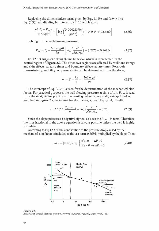
Replacing the dimensionless terms given by Eqs. (1.89) and (1.94) intoEq. (2.35) and dividing both terms by ln 10 will lead to:

khðPi � Pwf Þ162:6qμB

¼ log0:0002637kt

ϕμctr2w

� �þ 0:3514þ 0:8686s

� (2.36)

Solving for the well-flowing pressure;

Pwf ¼ Pi � 162:6 qμBkh

logkt

ϕμctr2w

� �� 3:2275þ 0:8686s

� (2.37)

Eq. (2.37) suggests a straight-line behavior which is represented in thecentral region of Figure 2.7. The other two regions are affected by wellbore storageand skin effects, at early times and boundary effects at late times. Reservoirtransmissivity, mobility, or permeability can be determined from the slope;

m ¼ T ¼ khμ

¼�� 162:6 qBm

�� (2.38)

The intercept of Eq. (2.34) is used for the determination of the mechanical skinfactor. For practical purposes, the well-flowing pressure at time of 1 h, P1hr, is readfrom the straight-line portion of the semilog behavior, normally extrapolated assketched in Figure 2.7, so solving for skin factor, s, from Eq. (2.34) results:

s ¼ 1:1513P1hr � Pi

m� log

kϕμctr2w

� �þ 3:23

� (2.39)

Since the slope possesses a negative signed, so does the P1hr� Pi term. Therefore,the first fractional in the above equation is always positive unless the well is highlystimulated.

According to Eq. (2.39), the contribution to the pressure drop caused by themechanical skin factor is included to the last term: 0.8686smultiplied by the slope. Then:

ΔPs ¼ j0:87ðmÞjs, if s>0 ! ΔPs>0

if s <0 ! ΔPs <0

�(2.40)

Figure 2.7.Behavior of the well-flowing pressure observed in a semilog graph, taken from [68].

64


Eq. (2.40) is similar to Eq. (1.110) and works for either pressure drawdown orpressure buildup tests.

ΔPs ¼ �0:87ðmÞ kks

� 1� �

lnrsrw

(2.41)

Eq. (1.110) is useful to find either skin factor, s, formation damaged permeability,ks, or the damaged or affected skin zone radius, rs. However, since the skin zonecovers an infinitely thin area and the pressure wave travels at high speed, it is difficultto detect transmissivity changes, then, rs and ks are difficult to be measured.

Eqs. (1.110) and (2.37) imply the skin factor along flow rate just increases ordecreases the well pressure drop. However, this occurs because the well radiusbehaves as if its radius was modified by the value of the skin factor. Brons andMiller [74] defined the apparent or effective wellbore radius, rwa, to be used inEqs. (1.89), (1.94), and (1.100)

rwa ¼ rwe�s (2.42)

Example 2.1

A well with a radius of 0.25 ft was detected to have a skin factor of 2. A skinfactor of �2 was obtained after a stimulation procedure. Find the apparent radii andthe percentage of change in the radius due to the stimulation. What conclusion canbe drawn?

Solution

Application of Eq. (2.42) for the damaged-well case gives:

rwa ¼ rwe�s ¼ 0:25e�2 ¼ 0:034 ft ¼ 0:406 in

Application of Eq. (2.42) for the damaged-well case gives:

rwa ¼ rwe�s ¼ 0:25e�ð�2Þ ¼ 1:848 ft ¼ 22:17 in

It can be observed that 1.847�100/0.034 ffi 5460%, meaning that the stimula-tion helps the well to increase its radius 55 times. It can be concluded from theexample that for positive skin factor values, the effective wellbore radius decreases(rwa<rw) and for negative skin factor values, the effective wellbore radius increases(rwa>rw).

The starting time of the semilog straight line defined by Ramey [9] in Eq. (2.22)allows determining mathematically where the radial flow starts, i.e., the momentwellbore storage effects no longer affect the test. Replacing into Eq. (2.22) thedimensionless parameters given by Eqs. (1.94) and (2.15) results [2]:

tSSL ¼ ð200000þ 12000sÞμCkh

(2.43)

The application of Eq. (2.40) is twofolded. (1) It can be used for test designpurposes. The duration of a pressure drawdown test should be last 10 times thevalue of tSSL, so a significant portion of the radial flow regime can be observed andanalyzed and (2) finding the semilog slope can be somehow confusing. Once thesemilog line is drawn and permeability, skin factor, and wellbore storage are calcu-lated, then, Eq. (2.40) can be used to find the starting point of the radial flowregime. Radial flow is correctly found if the tSSL value agrees with the one chosen in

65


the plot. This last situation is avoid if the pressure and pressure derivative plot isavailable since radial flow is observed once the pressure derivative curve gets flat asseen in Figure 2.6.

The declination stabilization time (time required to reach the boundaries anddevelop the pseudosteady-state period) during the test can be from the maximumtime at which the maximum pressure drops (not shown here) take place. This is:

tmax ¼ 948ϕμctr2

k(2.44)

From which;

tpss ¼ 948ϕμctr2ek

(2.45)

For square or circular geometries, tDA = 0.1 from Table 2.1. Replacing this valuein Eq. (1.100) and solving for time leads to:

tpss ¼ 1190ϕμctr2ek

(2.46)

from

rinv ¼ 0:0325

ffiffiffiffiffiffiffiffiffiffiktpμϕct

s(2.47)

For any producing time, tp, the radius of investigation—not bigger than re—canbe found.

The point reached by the disturbance does not imply fluid movement occursthere. The drainage radius is about 90% that value, then

rd ¼ 0:029

ffiffiffiffiffiffiffiffiffiffiktpμϕct

s(2.48)

Skin factor is a dimensionless quantity. This does not necessarily reflect thedegree of either damage or stimulation of a well. Then, more practical measurementparameters ought to be used. One of this is the flow efficiency, FE, which implieswhat percentage of the total pressure drawdown is due to skin factor. The flowefficiency is defined as the ratio between the actual productivity index, J, and theideal productivity index. The productivity index involves money since it is definedas the amount of pressure drop needed to produce a barrel of fluid per day. In otherwords, it is the energy required to produce one BPD. Mathematically;

J ¼ qP� Pwf

(2.49)

Jideal ¼q

P� Pwf � ΔPs(2.50)

FE ¼ JJideal

¼ 1� ΔPs

P� Pwf(2.51)

FE < 1 is an indication that well damage exists, otherwise there is stimulation.The productivity index can be increased by:

66


• Increasing the permeability in the zone near the well—hydraulic fracturing;

• Reduce viscosity—steam injection, dissolvent, or in situ combustion;

• Damage removing—acidification;

• Increase well penetration;

• Reduce volumetric factor—choosing correct surface separators.

Other parameters to quantify well damage are [68]:

Table 2.1.Shape factors for different drainage areas, taken from [8, 75].

67


Damage ratio, DR

DR ¼ 1=FE (2.52)

Damage ratios less than the unity indicate stimulation.

Damage factor, DF

DR ¼ 1� FE (2.53)

Negative values of damage factors indicate stimulation. The damage factor canalso be estimated from [68]:

DF ¼ ssþ ln ðre=rwÞ ¼ 1� qðactualÞ

qðidealÞ (2.54)

Eq. (2.54) applies to circular-shaped reservoir.

Productivity ratio, PR

PR ¼ qqa

¼ qðidealÞqðactualÞ ¼

ln ðre=rwÞln ðre=rwÞ þ s

(2.55)

Annual loss income, FD$L (USD$)

FD$L ¼ 365qðOPÞDF (2.56)

where OP is oil price.

Example 2.2

What will be the annual loss of a well that produces 500 BFD, which has adamage factor of 8, drains an area of 120 acres and has a radius of 6 inches? Assumecircular reservoir area and a price of oil crude of USD $ 55/barrel.

Solution

120 acres = 5,227,200 ft2. If the area is circular, then: r = 1290 ft. Find the damagefactor from Eq. (2.54);

DF ¼ ssþ ln ðre=rwÞ ¼

88þ ln ð1290=0:5Þ ¼ 0:5046

Find the yearly loss income using Eq. (2.56)

FD$L ¼ 365qðOPÞDF ¼ 365ð Þ 500ð Þ 55ð Þ 0:5046ð Þ ¼ USD$ 5064922

This indicates that the well requires immediate stimulation.

2.2.3.2 Reservoir limit test, RLT

It is a drawdown test run long enough to reach the reservoir boundaries.Normal pressure drawdown tests, during either radial flow or transient period test,are used to estimate formation permeability and artificial well conditions (C and s),while an RLT test—introduced by [76]—deals with boundaries and is employed todetermine well drainage area or well drainage pore volume. In a Cartesian graph for

68


a closed boundary system, Figure 2.8, three zones are distinguished [8, 68]: (i) skinand wellbore storage dominated zone, (ii) transient zone (radial flow), and (iii)pseudosteady-state zone. As indicated by Eq. (1.129), the pressure drop is a linearfunction of time. Eq. (1.129) is given for circular reservoir geometry. For anygeometry, the late time pseudosteady-state solution involves the Dietz shape factor,[75], to extent the use of Eq. (1.129) for other reservoir geometries, as described inTable 2.1. Under this condition, Eq. (1.129) becomes [77]:

PD ¼ 2πtDA þ 12ln

Ar2w

� �þ ln

2:2458CA

� �(2.57)

Replacing in the above expression the dimensionless quantities given byEqs. (1.89) and (1.94), it results:

Pwf ¼ � 0:23395qBϕctAh

� tþ Pi � 70:6qμB

khln

Ar2w

þ ln2:2458CA

� �þ 2s

� (2.58)

From the slope, m*, and intercept, PINT, of Eq. (2.58), the reservoir pore volumeand Dietz shape factor [74] can be obtained from either:

Vp ¼ �0:23395qB ctm� (2.59)

CA ¼ 5:456mm� e

2:303P1hr�PINT

m (2.60)

Once the value of CA is obtained from Eq. (2.60), the reservoir geometry can beobtained from Table 2.1 by using the closest tabulated value (“exact for tDA”) andconfront with the time to develop pseudosteady-state regime, (tDA)pss which isfound from:

ðtDAÞpss ¼ 0:1833m�

mtpss (2.61)

tpss can be read from the Cartesian plot. However, this reading is inexact; there-fore, it is recommended to plot the Cartesian pressure derivative and to find theexact point at which this becomes flat.

2.2.4 Tiab’s direct synthesis (TDS) technique

TDS technique is the latest methodology for well test interpretation. Its basisstarted in 1989 [70]. TDS’ creator was Tiab [71], who provided analytical andpractical solutions for reservoir characterization using characteristic points orfeatures—called by him “fingerprints”—read from a log-log plot of pressure andpressure derivative [15], versus time. Since the introduction of TDS in 1995, severalscenarios, reservoir geometries, fluid types, well configurations, and operationconditions. For instance, extension of TDS technique to elongated systems can befound in [13, 14, 16–19, 23, 24, 28, 30, 31]. Some applications of conventionalanalysis in long reservoirs are given in [20, 29, 38, 54]. For vertical and horizontalgas wells with and without use of pseudotime, refer to [22, 36, 39]. Special casesof horizontal wells are found in [12, 47]. For transient rate analysis, refer to[27, 35, 49]. Applications on heavy oil (non-Newtonian fluids) can be found in[32, 34, 41, 42, 45, 52, 56, 62, 64]. For cases on shales reservoirs, refer to[49, 51, 56, 78]. Well test analysis by the TDS technique on secondary and tertiary

69


oil recovery is presented by [25, 33, 60, 79]. For multirate testing in horizontal andvertical wells, refer, respectively, to [65, 67]. References [43, 46] are given forconductive faults. For deviated and partially penetrated wells, refer to [37, 64],respectively. TDS technique extended to multiphase flow was presented by [26].Wedged and T-shaped reservoirs can be found in [48] and coalbed-methane reser-voirs with bottom water drive are given in [53]. TDS technique is excellent forinterpreting pressure test in hydraulically fractured vertical wells since unseen flowregimes can be generated [50, 69, 80]. The first publications on horizontal wells innaturally fractured and anisotropic media are given in [81, 82]. The thresholdpressure gradient is dealt by [57, 72]. For vertical wells in double porosity anddouble permeability formations, refer, respectively, to [41, 83]. A book publishedby Escobar [56] presents the most recent topics covered by the TDS technique, anda more comprehensive state-of-the-art on TDS technique is given by [58]. Thisbook revolves around this methodology; therefore, practically, the whole content of[71]—pioneer paper of TDS technique—will be brought here:

The starting point is the definition of the dimensionless pressure derivative fromEq. (1.89);

tD � PD0 ¼ khðt � ΔP 0Þ

141:2qμB(2.62)

By looking at Eqs. (2.17) and (2.18), we can conclude the difficulty of using handmathematical operations with them. Instead of using these general solutions, Tiab[71] obtained partial solutions to the differential equation for each flow regime ortime period. For instance, during early pseudosteady-state, the governing equationreduces to:

PD ¼ tDCD

(2.63)

Combination of Eqs. (1.94) and (2.15) results in:

tDCD

¼ 2:95 � 10�4 hμ

� �tC

(2.64)

Replacing Eq. (1.89) in the above expression yields;

kh141:2qμB

� �ΔP ¼ 2:95� 10�4 kh

μ

� �tC

(2.65)

Solving for C;

C ¼ qB24

� �tΔP

(2.66)

The pressure derivative curve also has a straight line of unitary slope atearly times. The equation of this line is obtained by taking the derivativeof Eq. (2.63) with respect to the natural logarithm of tD/CD. So:

tDCD

� �PD

0 ¼ tDCD

(2.67)

Where the derivative of the dimensionless pressure is:

70


PD0 ¼ dPD=dtD ¼ kh

141:2qμB

� �dP�

0:0002637kϕμctr2w

� �dt (2.68)

Rearranging;

PD0 ¼ 26:856r2wϕcth

qB

� �ΔP 0 (2.69)

Converting to dimensional form, the left-hand side of Eq. (2.67) by using thedefinitions given by Eqs. (2.64) and (2.68):

tDCD

� �PD

0 ¼ 0:00792252khqμB

� �ϕcthr2w

C

� �ðt � ΔP 0Þ (2.70)

Multiplying and dividing by 0.8935;

tDCD

� �PD

0 ¼ 0:007087khqμB

� �ϕcthr2w0:8935C

� �ðt � ΔP 0Þ (2.71)

Recalling Eq. (2.15), the above becomes:

tDCD

� �PD

0 ¼ 0:007087khqμB

� �1CD

� �ðt � ΔP 0Þ (2.72)

Since the unit slope is one, then CD = 1, thus;

tDCD

� �PD

0 ¼ khðt � ΔP'Þ141:2qμB

(2.73)

From looking at Figure 2.6, both pressure and pressure derivative curvesdisplay a unitary slope at early times. Replacing Eqs. (2.64), (2.73) in (2.67) andsolving for C will result:

C ¼ qB24

� �t

t � ΔP0 (2.74)

As seen in Figure 2.6, the infinitely acting radial flow portion of the pressurederivative is a horizontal straight line with intercept of 1/2. The governingequation is:

tDCD

� �PD

0�

r¼ 1

2(2.75)

Combining the above equation with Eq. (2.73) results the best expression toestimate reservoir permeability:

k ¼ 70:6qμBhðt � ΔP 0Þr

(2.76)

Subscript r stands for radial flow line. A customary use of TDS, as establishedby Tiab [71], is to provide suffices to identify the different flow regimes. Forinstance, pss stands for pseudosteady state, i stands for either initial or intercept,etc. In terms of pressure, the equation of this line is:

71


PDr ¼ 0:5 lntDCD

� �rþ 0:80907 þ ln CDe2s

� �� (2.77)

It is recommended to draw a horizontal line throughout the radial flow regimeand choose one convenient value of (t*ΔP')r falling on such line.

Tiab [71] also obtained the start time of the infinite line of action of the pressurederivative is:

tDCD

� �sr¼ 10 log ðCDe2sÞ10 (2.78)

Replacing Eqs. (1.92) and (2.15) in the above equation will yield:

tsr ¼ μ C6:9 � 10�5kh

ln0:8935Cϕcthr2w

� �þ 2s

� (2.79)

A better form of Eq. (2.78) was given by [84];

tDCD

� �sr¼ 1

αln ðCDe2sÞ þ ln

tDCD

� �SR

� (2.80)

Setting a = 0.05 in the above equation and solving for C:

C ¼ 0:056ϕcthr2w tDsr

2sþ ln tDsr

� �(2.81)

tDsr is calculated with Eq. (1.94) letting t = tsr.The point of intersection, i, between the early time unit-slope line defined by

Eqs. (2.63) and (2.67) and the late-time infinite-acting line of the pressure deriva-tive, defined by Eq. (2.75), is given by:

tDCD

PD0

� �i¼ 0:5 (2.82)

tDCD

� �i¼ 0:5 (2.83)

where i stands for intersection. After replacing the definitions given byEqs. (1.94), (2.15), and (2.72) will, respectively, provide:

t � ΔP 0ð Þi ¼70:6qμB

kh(2.84)

k ¼ 1695μChti

(2.85)

For the unit-slope line, the pressure curve is the same as for the pressurederivative curve. Then, at the intersection point:

ðΔPÞi ¼ ðt � ΔPÞi ¼ ðt � ΔP 0Þr (2.86)

Tiab [71] correlated for CDe2s > 100 permeability, wellbore storage coefficient,

and skin factor with the coordinates of the maximum point—suffix x—displayedonce the “hump” observed once wellbore storage effects start diminishing. Thesecorrelations are given as follows:

72


tDCD

PD0

� �x¼ 0:35717

tDCD

� �x� 0:50 (2.87)

log ðCDe2sÞ ¼ 0:35tDcD

� �1:24

(2.88)

log ðCDe2sÞ ¼ 1:71tDCD

PD0

� �1:24

(2.89)

Replacing Eqs. (2.64) and (2.73) into Eq. (2.87) leads to:

t � ΔP 0ð Þx ¼ 0:015qBC

� �tx � 0:42

141:2qμBkh

� �(2.90)

Either formation permeability or wellbore storage coefficient can be determinedusing the coordinates of the peak, tx and (t*ΔP 0)x. Solving for both of theseparameters from Eq. (2.90) results:

k ¼ 70:6qμBh

� �1

0:014879qB=Cð Þ tx � ðt � ΔP 0Þx(2.91)

C ¼ 0:014879qBtxðt � ΔP 0Þx þ ðt � ΔP 0Þr

(2.92)

The constants in Eqs. (2.91) and (2.92) are slightly different as those in [58].These new unpublished versions were performed by TDS’ creator.

Eq. (2.91) is so helpful to find reservoir permeability in short test when radialflow is absent which is very common in fall-off tests. Once permeability is foundfrom Eq. (2.91), solved for (t*ΔP 0)r from Eq. (2.76) and plot on a horizontal linethroughout this value. Then, compare with the actual derivative plot and use engi-neering criterion to determine if the permeability value is acceptable. This means, ifthe straight line is either lower or higher than expected. Otherwise, new coordinatesof the peak ought to be read for repeating the calculations since the hump shouldlook some flat.

Figure 2.8.Characteristics found in the Cartesian graph, taken from [68].

73


Substitution of Eqs. (2.64) and (2.73) in Eqs. (2.88) and (2.89) allowsobtaining two new respective correlations for the determination of the mechanicalskin factor:

s ¼ 0:171txti

� �1:24

� 0:5 ln0:8935Cϕ hctr2w

� �(2.93)

s ¼ 0:921ðt � ΔP 0Þxðt � ΔP 0Þi

� �1:1

� 0:5 ln0:8935Cϕhctr2w

� �(2.94)

Sometimes, the reading of the peak coordinates may be wrong due to the flatappearance of it. Then, it should be a good practice to estimate the skin factor usingboth Eqs. (2.93) and (2.94). These values should match each other.

Divide Eq. (2.87) by Eq. (2.75); then, in the result replace Eqs. (2.64) and (2.73)and solve for both permeability and wellbore storage:

k ¼ 4745:36μChtx

ðt � ΔP 0Þxðt � ΔP 0Þr

þ 1� �

(2.95)

C ¼ 0:014879qBtxðt � ΔP'Þx þ ðt � ΔP 0Þr

(2.96)

This last expression is useful to find wellbore storage coefficient when the earlyunitary slope line is absent.

TDS technique has a great particularity: for a given flow regime, the skin factorequation can be easily derived from dividing the dimensionless pressure equationby the dimensionless derivative equation of such flow regime. Then, the division ofEq. (2.77) by Eq. (2.75) leads to the below expression once the dimensionlessparameters given by Eqs. (1.89), (1.94), and (2.73) are replaced in the resultingquotient. Solving for s from the final replacement leads to:

s ¼ 0:5ΔPr

ðt � ΔP 0Þr� ln

k trϕμctr2w

� þ 7:43

� �(2.97)

being tr any convenient time during the infinite-acting radial flow regimethroughout which a horizontal straight line should have been drawn. Read the ΔPrcorresponding to tr. Comparison between Eqs. (2.38) and (2.76) allows concluding:

m ¼ 2:303ðt � ΔP 0Þr ¼ ln ð10Þðt � ΔP 0Þr (2.98)

which avoids the need of using the semilog plot if the skin pressure drop isneeded to be estimated by Eq. (2.40), otherwise, Eq. (2.40) becomes:

ΔPs ¼ j2ðt � ΔP 0Þrjs, if s>0 ! ΔPs>0

if s <0 ! ΔPs <0

�(2.99)

For the determination of well-drainage area, Tiab [69] expressed Eq. (2.75) as:

ðtD � PD0Þr ¼

12

(2.100)

Also, Tiab [69] differentiated the dimensionless pressure with respect to dimen-sionless time in Eq. (2.57), so:

tD � PD0 ¼ 2πtDA (2.101)

74


Then, Tiab [69] based on the fact that two given flow regime governing equa-tions can be intersected each other, regardless the physical meaning of such inter-section, and solving for any given parameter, intercepted Eqs. (2.100) with (2.101),then, replaced in the resulting expression the dimensionless quantities given byEqs. (2.92), (2.97), and (2.62) and solved for the area given in ft2:

A ¼ ktrpssi301:77ϕμct

(2.102)

Furthermore, Chacon et al. [85] replaced the dimensionless time given byEq. (1.100) and the dimensionless pressure derivative of Eq. (2.62) into Eq. (2.102)and also solved for the area in ft2:

A ¼ 0:234qBtpssϕcth ðt � ΔP 0Þpss

(2.103)

The above expression uses any convenient point, tpss and (t*ΔP’)pss, during the latetime pseudosteady-state period. Because of noisy pressure derivative data, the read-ings of several arbitrary points may provide, even close, different area values. There-fore, it is convenient to use an average value. To do so, it is recommended to draw thebest late-time unit-slope line passing through the higher number of pressure deriva-tive points and extrapolate the line at the time of 1 h and read the pressure derivativevalue, (t*ΔP')pss1. Under these circumstances, Eq. (2.103) becomes:

A ¼ 0:234qBϕcth ðt � ΔP 0Þpss1

(2.104)

Eqs. (2.102) through (2.104) apply only to closed-boundary reservoirs of anygeometrical shape. For constant-pressure reservoirs, the works by Escobar et al.[28, 54] for TDS technique (summary given in Table 2.2) and for conventionalanalysis are used for well-drainage area determination in circular, square, andelongated systems.

TDS technique has certain step-by-step procedures which not necessarily are tobe followed since the interpreter is welcome to explore and use TDS as desired.Then, they are not provided here but can be checked in [69, 71].

Example 2.3

Taken from [68]. The pressure and pressure derivative data given in Table 2.3corresponds to a drawdown test of a well. Well, fluid, and reservoir data aregiven below:

Find permeability, skin factor, drainage area, and flow efficiency by conven-tional analysis. Find permeability, skin factor, and three values of drainage areausing TDS technique:

Solution

Conventional analysis. Figure 2.9 and 2.10 present the semilog and Cartesianplots, respectively, to be used in conventional analysis. From Figure 2.9, the semi-log slope,m, is of 18 psia/cycle and P1hr = 2308 psia. Permeability and skin factor arecalculated using Eqs. 2.38 and 2.39, respectively, thus:

rw = 0.267 ft q = 250 BPD μ = 1.2 cp

ct = 26.4 � 10�5psi�1 h = 16 pies ϕ = 18% B = 1.229 bbl/BF

75


k ¼�� 162:6 ð250Þð1:2Þð1:229Þð�18Þð16Þ

�� ¼ 208 md

s ¼ 1:15132308� 2733

�18� log

208

0:18ð1:2Þð26:4� 10�5Þð0:267Þ2 !

þ 3:23

" #¼ 22:15

Find the pressure loss due to skin factor with Eq. (2.40);

Constant, Ξ Equation Reservoir geometries Equation number

301.77 A ¼ ktrpssiΞϕμct

(2.100)

283.66 (2.101)

4066 A ¼ffiffiffiffiffiffiffiffiffiffiffiktssriY4

EΞϕμct

3q

(2.102)

482.84

7584.2

2173.52A ¼ ktss1ri, ss2ri

Ξϕμct

� �2=3Y5=3Ebx

(2.103)

6828.34

41.82XE ¼ 1

Ξ

ktxϕμct

� �0:5 (2.104)

20.91

Table 2.2.Summary of equations, taken from [28].

76


t, h Pwf, psia DP, psia t*DP 0, psia/h t, h Pwf, psia DP, psia t*DP 0, psia/h

0.00 2733 0 5 2312 421 65.42

0.10 2703 30 31.05 7 2293 440 35.32

0.20 2672 61 58.95 9.6 2291 442 5.86

0.30 2644 89 84.14 12 2290 443 5.85

0.40 2616 117 106.30 16.8 2287 446 7.63

0.65 2553 180 129.70 33.6 2282 451 7.99

1.00 2500 233 135.15 50 2279 454 7.94

1.50 2440 293 151.90 72 2276 457 10.50

2.00 2398 335 127.26 85 2274 459 12.18

3.00 2353 380 102.10 100 2272 461 13.36

4.00 2329 404 81.44

Table 2.3.Pressure and pressure derivative versus time data for example 2.3.

Figure 2.9.Semilog plot for example 2.3.

Figure 2.10.Cartesian plot for example 2.3.

77


ΔPs ¼ j0:87ð�18Þj22:15 ¼ 346:7 psia

Since the average reservoir pressure is not reported, then, the initial pressurevalue is taken instead. Eq. (2.51) allows estimating the flow efficiency.

FE ¼ 1� 346:92733� 2272

¼ 24:75 %

From the Cartesian plot, Figure 2.10, is read the following data:

Use Eq. (2.59) to find well drainage area:

A ¼ �0:234qB ϕhctm� ¼ � 0:234ð250Þð1:229Þ

ð0:18Þð16Þð26:4� 10�5Þð�0:13Þ ¼ 727391:1 ft2 ¼ 16:7 Ac

Find the Dietz shape factor with Eq. (2.60);

CA ¼ 5:456�18�0:13

e

2:303 2308� 2285ð Þ�18

� ¼ 39:82

As observed in Table 2.1, there exist three possible well drainage area geometryvalues (hexagon, circle, and square) close to the above value. To discriminate whichone should be the appropriate system geometry find the dimensionless time inwhich pseudosteady-state period starts by using Eq. (2.61):

tDAð Þpss ¼ 0:1833�0:13�18

50 ¼ 0:066 ≈0:1

TDS technique. The following are the characteristic points read fromFigure 2.11:

Find permeability and skin factor with Eqs. (2.76) and (2.97), respectively:

k ¼ 70:6qμBhðt � ΔP'Þr

¼ 70:6ð250Þð1:2Þð1:229Þð16Þð7:7Þ ¼ 211:3 md

s ¼ 0:54517:7

� ln211:3ð33:6Þ

0:18ð1:2Þð26:4� 10�5Þð0:2672Þ

� �þ 7:43

� ¼ 22:4

Determine the well drainage area with Eqs. (2.102) and (2.103), thus;

A ¼ 211:3ð58Þ301:77ð0:18Þð1:2Þð26:4� 10�5Þð43560Þ ¼ 16:35 Ac

A ¼ 0:234ð250Þð1:229Þð85Þð0:18Þð26:4� 10�5Þð16Þð12:18Þð43560Þ ¼ 15:15 Ac

m* = �0.13 psia/h PINT = 2285 psia tpss ≈ 50 h

(t*ΔP')r = 7.7 psia tr = 33.6 h ΔPr = 451 psia

tpss = 85 h (t*ΔP')pss = 12.18 psia trpi = 58 h

(t*ΔP')pss1 = 0.14 psia

78


A ¼ 0:234ð250Þð1:229Þð0:18Þð26:4� 10�5Þð16Þð0:14Þð43560Þ ¼ 15:5 Ac

Even, more parameters can be reestimated with TDS technique for verificationpurposes but it will not be performed for saving-space reasons. However, the readeris invited to read the coordinates of the peak and the intersection point of thewellbore storage and radial flow lines. Then, estimate formation permeability withEqs. (2.84), (2.85), and (2.91). Also, find the wellbore storage coefficient usingEqs. (2.74), (2.81), (2.92), and (2.96) and skin factor with Eqs. (2.93) and (2.94).

Example 2.4

Taken from [68] with the data from the previous example, Example 2.3, deter-mine tSSL and find if the well fluid level is increasing or decreasing in the annulus ifthe well has a drill pipe with 2 in external diameter inside a liner with 5 in of innerdiameter including joint gaskets. The density of the wellbore fluid is 42.5 lbm/ft3.

Solution

From Figure 2.11, a point is chosen on the early unit-slope line. This point hascoordinates: DP = 59 psia and t = 0.2 h. Wellbore storage coefficient is found withEq. (2.21):

C ¼ ð250Þð1:229Þ24

0:259

¼ 0:0434 bbl=psia

Solving for annulus capacity from Eq. (2.5);

Vu ¼ ρ

144

� �C ¼ 42:5

144

� �0:0434 ¼ 0:0128 bbl=ft

The theoretical capacity is found with Eq. (2.45), so:

Vu ¼ 0:0009714ð52 � 22Þ ¼ 0:0204 bbl=ft

This leads to the conclusion that the annular liquid is falling.

Figure 2.11.Pressure and pressure derivative plot for example 2.3.

79


2.3. Multiphase flow

According to Perrine [86], the single fluid flow may be applied to the multiplefluid flow systems when the gas does not dominate the pressure tests, it meansliquid production is much more relevant than gas flow. Under this condition, thediffusivity equation, Eq. (1.27), will result and the total fluid mobility is determinedby Eq. (1.24). We also mentioned in Chapter 1 that Martin [63] provided some tipsfor a better use of Perrine method. Actually, Perrine method works very well inliquid systems.

The semilog equations for drawdown and build tests are, respectively, given below:

Pwf ¼ Pi � 162:6qtλth

logλtt

1688ϕctr2wþ 0:869s

� �(2.105)

Pws ¼ Pi � 162:6qtλth

logtp þ ΔtΔt

� �(2.106)

The flow rate is estimated by:

qt ¼ qoBo þ ðqg � qoRs=1000ÞBg þ qwBw

� �=Bo (2.107)

Eq. (2.107) is recommended when oil flow dominates the test. It is removedfrom the denominator, otherwise. It advised to use consistent units in Eq. (2.107)meaning that the gas flow rate must be in Mscf/D and the gas volume factorbbl/SCF.

Once the semilog slope has been estimated, the total mobility, the phase effec-tive permeabilities, and the mechanical skin factor are found from:

λt ¼ � 162:6qtmh

(2.108)

kL ¼ � 162:6qLBLμLmh

; L ¼ water or oil (2.109)

kg ¼ �162:6 qg � qoRs=1000

� �Bgμg

mh(2.110)

s ¼ 1:1513Pwf � P1hr

m� log

λtϕctr2w

� �þ 3:23

� �(2.111)

The best way of interpreting multiphasic flow tests in by using biphasic and/ortriphasic pseudofunctions. Normally, well test software uses empirical relationshipsto estimate relative permeability data. The accuracy of the following expression issensitive to the relative permeability data:

mðPÞ ¼ðPP0

kroμoBo

dP (2.112)

The expressions used along this textbook for reservoir characterization mayapply for both single fluid and multiple fluid production tests. Single mobility has tobe changed by total fluid mobility and individual flow rate ought to be replaced bythe total fluid rate. Just to cite a few of them, Eqs. (2.66), (2.76), (2.85), (2.91),(2.92), and (2.97) become:

80


C ¼ qt24

� � tΔP

(2.113)

λt ¼ kμ

��t ¼ 70:6qthðt � ΔP'Þr

(2.114)

kμ

� �t¼ 1695C

hti(2.115)

λt ¼ 70:6qth

� �1

ð0:014879qt=CÞtx � ðt � ΔP 0Þx(2.116)

C ¼ 0:014879qttxðt � ΔP'Þx þ ðt � ΔP 0Þr

(2.117)

s ¼ 0:5ΔPr

ðt � ΔPÞr� ln

λttrϕctr2w

� �þ 7:43

� (2.118)

Also, the effective liquid permeabilities are found using the individual viscosity,rate, and volume factor. Then, Eq. (2.76) applied to oil and water will yield:

ko ¼ 70:6qoμoBo

hðt � ΔP 0Þr(2.119)

kw ¼ 70:6qwμwBw

hðt � ΔP'Þr(2.120)

However, from a multiple fluid test, it is a challenge to find the reservoirabsolute permeability. Several methods have been presented. For instance,Al-Khalifah et al. [87] presented a sophisticated method applied to either drawdownor multiple rate tests. Their method even includes the estimating of the saturationchange respect to pressure. However, we presented the method by Kamal and Pan[88] which applies well for liquid fluid. Relative permeabilities must be known forits application. Once effective permeabilities are found, let us say from Eqs. (2.119)and (2.120), estimate the permeability ratio ko/kw and find the water saturationfrom the relative permeability curves as schematically depicted in Figure 2.12(left). Then, using the estimated water saturation value, enter Figure 2.12 (right)and read a value from a relative permeability curve. Use the most dominant flowcurve. The dominant phase is assumed to be oil for the example in Figure 2.12.Since both phase effective permeability and phase relative permeability are known,the absolute permeability is found from the definition of relative permeability:

k ¼ kokro

(2.121)

Further recommendations for handling multiphase flow tests are presented byAl-Khalifah et al. [89] and are also reported by Stanislav and Kabir [7].

2.4. Partial penetration and partial completion

When a well penetrates a small part of the formation thickness, hemisphericalflow takes place. See Figure 2.13 top. When the well is cased above the producer

81


range and only a small part of the casing is perforated, spherical flow occurs in theregion near the face of the well. See Figure 2.13 bottom. As the transient movesfurther into depth of the formation, the flow becomes radial, but if the test is short,the flow will be spherical. Both types of flow are characterized by a slope of �1/2 inthe log-log plot of pressure derivative versus time [90, 91]. Theoretically, beforeeither hemispherical or spherical flow takes place, there exists a radial flow regimeoccurring by fluids withdrawn from the formation thickness that is close in heightto the completion interval. This represents the transmissibility of the perforatedinterval. Actually, this flow regime is unpractical to be seen mainly because ofwellbore storage effects. We will see further in this chapter that there are especial

Figure 2.12.Determination of absolute permeability as outlined by Kamal and Pan [88].

Figure 2.13.Ideal flow regimes in partial penetration (top) and partial completion (bottom) systems, after [66].

82


conditions for hemispherical/spherical flow to be observed which occur later thatthe completion-interval-limited radial flow regime. Both hemispherical and spheri-cal flow vanished when the top and bottom boundaries have been fully reached bythe transient wave; the true radial flow is developed throughout the full reservoirthickness.

The apparent skin factor, sa, obtained from pressure transient analysis is acombination of several “pseudoskin” factors such as [91]:

sa ¼ sþ sp þ sθ þ scp þ…… (2.122)

where s is the true damage factor caused by damage to the well portion, sp is thepseudoskin factor due to the restricted flow entry, sq is the pseudoskin factorresulting from a well deviation angle, and scp is the pseudoskin due to a change inpermeability near the face of the well. sp can be estimated from [92]:

sp ¼ hhp

� 1� �

ln hD (2.123)

hp = length of perforated or open interval. The equations of dimensionlessthickness, hD, for hemispherical and spherical flow, respectively:

hD ¼ hrw

ffiffiffiffiffikhkz

s(2.124)

hD ¼ h2rw

ffiffiffiffiffikhkz

s(2.125)

where kh is the horizontal permeability, kz = kv is the vertical permeability. Thecontribution of the pseudoskin of an inclined well is given by Cinco et al. [92]:

ψ 0 ¼ tan �1

ffiffiffiffiffikzkh

stanψ

!(2.126)

sθ ¼ � ψ 0

41

� �2:06

� ψ 0

56

� �1:865

� logh

100rw

� �(2.127)

According to Cinco et al. [92], the above equation is valid for 0° ≤ q ≤ 75°,h/rw > 40, and tD > 100. Note that Eq. (2.127) could provide a negative value. This isbecause the deviation at the face of the well increases the flow area or presentsreservoir pseudothickness. The pseudoskin responding for permeability changesnear wellbore is given by [93]:

scp ¼ hhp

1� 0:2rs � rwhp

� �� k� ksks

� �ln

rsrw

(2.128)

Example 2.4

Taken from [91]. A directional well which has an angle to the vertical of 24.1°has a skin factor s = �0.8. The thickness of the formation is 100 ft, the radius of thewellbore is 0.3 ft, and the horizontal to vertical permeability ratio is 5. Whichportion of the damaged corresponds to the deviation of the well?

83


Solution

The deviation angle affected by the anisotropy is estimated with Eq. (2.126);

ψ 0 ¼ tan �1ffiffiffi5

ptan ð24:1Þ

� �¼ 45°

The pseudoskin factor caused by well deviation is found from Eq. (2.127):

sθ ¼ � 4541

� �2:06

� 4556

� �1:865

log100

100ð0:3Þ� �

¼ �1:56

From Eq. (2.122);

sa ¼ sþ sθ ¼ �0:8� 1:56 ¼ �2:36

Therefore, 66.1 % of the skin factor is due to the well deviation.

2.4.1 Conventional analysis for spherical flow

The diffusivity equation for spherical flow assuming constant porosity,compressibility, and mobility is given by Abbott et al. [90]:

1r2

∂∂r

r2∂P∂r

� �¼ ϕμct

ksp

∂P∂t

(2.129)

where ksp is the spherical permeability which is defined as the geometrical meanof the vertical and horizontal permeabilities:

ksp ¼ffiffiffiffiffiffiffiffiffikvk

2h

3q

¼ khs (2.130)

The physical system is illustrated in Figure 2.14, right. This region is called a“spherical sink.” rsw is given by:

Figure 2.14.Cylindrical, hemispherical, and spherical sinks, after [66].

84


rsw ¼ hp

2 lnhprw

� � (2.131)

The spherical flow equations for pressure drawdown and pressure buildup whenthe flow time is much longer than the shut-in time were presented by [94]:

Pwf ¼ Pi � 70:6qμBksprsw

ð1þ sspÞ þ 2453qμB

k3=2sp

ffiffiffiffiffiffiffiffiffiϕμct

p 1ffiffit

p (2.132)

Pws ¼ Pwf þ 70:6qμBksprsw

ð1þ sspÞ � 2453qμB

k3=2sp


p 1ffiffiffiffitp

p þ 1ffiffiffiffiffiΔt

p � 1ffiffiffiffiffiffiffiffiffiffiffiffiffiffiffitp þ Δt

p" #

(2.133)

The spherical pressure buildup equation when the flow time is shorter than theshut-in time:

Pws ¼ Pi � 2453qμB

k3=2sp


p 1ffiffiffiffiffiΔt


p" #

þ 70:6qμBksprsw

ssp (2.134)

Then, from a Cartesian plot of Pwf as a function of t �1/2, for drawdown, or Pws asa function of either [tp

�1/2 þ Δt�1/2�(tp þ Δt)�1/2] or [Δt�1/2�(tp þ Δt)�1/2] forbuildup, we obtain a line which slope, m, and intercept, I, can be used to estimatetridimensional permeability and geometrical (spherical) skin factor.

ksp ¼ � 2453qμBm


p� �2=3

(2.135)

ssp ¼ðI � Pwf Þksprsw

70:6qμB� 1 (2.136)

Once the spherical permeability is known, we solve for the vertical permeabilityfrom Eq. (2.130), and then, estimate the value of skin effects due to partial pene-tration [94]:

sc ¼ 1b� 1

� �ln hD �G½ � (2.137)

where b = hp/h. hD can be estimated from Eq. (2.125), and G is found from [94]:

G ¼ 2:948� 7:363bþ 11:45b2 � 4:576b3 (2.138)

2.4.2 Conventional analysis for hemispherical flow

The model for hemispheric flow is very similar to that of spherical flow [94].The difference is that a boundary condition considers half sphere. Figure 2.14 (left)outlines the geometry of such system. The drawdown and pressure equations aregiven below [94]:

Pwf ¼ Pi � 141:2qμBksprsw

ð1þ sspÞ þ 4906qμB

k3=2sp


p 1ffiffit

p (2.139)

85


Pws ¼ Pwf þ 141:2qμBksprsw

ð1þ sspÞ � 4906qμB

k3=2sp


p 1ffiffiffiffitp



p" #

(2.140)

Pws ¼ Pi � 4906qμB

k3=2sp


p 1ffiffiffiffiffiΔt


p" #

þ 141:2qμBksprsw

ssp (2.141)

As for the spherical case, from a Cartesian plot of Pwf as a function of t�1/2,for drawdown, or Pws as a function of either [tp

�1/2 þ Δt�1/2�(tp þ Δt)�1/2] or[Δt�1/2� (tp þ Δt)�1/2] for buildup, we obtain a line which slope, m, and intercept,I, can be used to estimate spherical permeability and geometrical (spherical) skinfactor.

ksp ¼ � 4906qμBm


p� �2=3

(2.142)

ssp ¼ðI � Pwf Þksprsw

141:2qμB� 1 (2.143)

2.4.3 TDS for spherical flow

Moncada et al. [66] presented the expressions for interpreting both pressuredrawdown or buildup tests in either gas or oil reservoirs using the TDS methodol-ogy. Spherical permeability is estimated by reading the pressure derivative at anyarbitrary time during which spherical flow can calculate spherical permeability andthe spherical skin factor also uses the pressure reading at the same chosen time:

ksp ¼ 1227qBμðt � ΔP'Þsp

ffiffiffiffiffiffiffiffiffiϕμcttsp

s !2=3

(2.144)

ssp ¼ 34:74

ffiffiffiffiffiffiffiffiffiffiffiffiffiffiffiϕμctr2swksptsp

sΔPð Þsp

2 t � ΔP 0ð Þspþ 1

" #� 1 (2.145)

The total skin, st, is defined as the sum of all skin effects at the well surroundings:

st ¼ sbþ sc þ ssp (2.146)

If the radial flow were seen, the horizontal permeability can be estimated from:

kH ¼ k ¼ 70:6qBμhpðt � ΔP 0Þr1

(2.147)

The suffix r1 implies the first radial flow.Moncada et al. [66] observed that the value of the derivative for the late radial

flow in spherical geometry is equivalent to 0.0066 instead of 0.5 as of the radialsystem. In addition, the slope line �½ corresponding to the spherical flow and thelate radial flow line of the curve of the dimensionless pressure derivative in spher-ical symmetry intersect in:

tD � PD0ð Þi ¼

12ffiffiffiπ

p t�1=2Dsp ¼ 0:0066 (2.148)

86


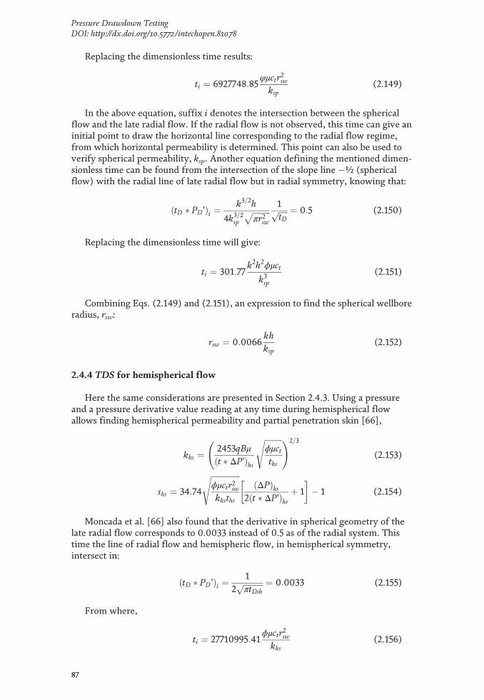
Replacing the dimensionless time results:

ti ¼ 6927748:85φμctr2swksp

(2.149)

In the above equation, suffix i denotes the intersection between the sphericalflow and the late radial flow. If the radial flow is not observed, this time can give aninitial point to draw the horizontal line corresponding to the radial flow regime,from which horizontal permeability is determined. This point can also be used toverify spherical permeability, ksp. Another equation defining the mentioned dimen-sionless time can be found from the intersection of the slope line �½ (sphericalflow) with the radial line of late radial flow but in radial symmetry, knowing that:

tD � PD'ð Þi ¼k3=2h

4k3=2sp

ffiffiffiffiffiffiffiffiffiπr2sw

p 1ffiffiffiffiffitD

p ¼ 0:5 (2.150)

Replacing the dimensionless time will give:

ti ¼ 301:77k2h2ϕμct

k3sp(2.151)

Combining Eqs. (2.149) and (2.151), an expression to find the spherical wellboreradius, rsw:

rsw ¼ 0:0066khksp

(2.152)

2.4.4 TDS for hemispherical flow

Here the same considerations are presented in Section 2.4.3. Using a pressureand a pressure derivative value reading at any time during hemispherical flowallows finding hemispherical permeability and partial penetration skin [66],

khs ¼ 2453qBμðt � ΔP'Þhs

ffiffiffiffiffiffiffiffiffiϕμctths

s !2=3

(2.153)

shs ¼ 34:74

ffiffiffiffiffiffiffiffiffiffiffiffiffiffiffiϕμctr2swkhsths

sΔPð Þhs

2 t � ΔP'ð Þhsþ 1

� � 1 (2.154)

Moncada et al. [66] also found that the derivative in spherical geometry of thelate radial flow corresponds to 0.0033 instead of 0.5 as of the radial system. Thistime the line of radial flow and hemispheric flow, in hemispherical symmetry,intersect in:

tD � PD'ð Þi ¼1

2ffiffiffiffiffiffiffiffiffiffiπtDsh

p ¼ 0:0033 (2.155)

From where,

ti ¼ 27710995:41ϕμctr2swkhs

(2.156)

87


As for the spherical case, there exists an expression to define the intersectiontime of the �½ slope line of the hemispherical flow regime pressure derivative andthe late radial flow line pressure derivative but, now, in radial symmetry:

tD � PD'ð Þi ¼k3=2h

2k3=2hs

ffiffiffiffiffiffiffiffiffiπr2sw

p 1ffiffiffiffiffitD

p ¼ 0:5 (2.157)

ti ¼ 1207:09k2h2ϕμct

k3hs(2.158)

This point of intersection in radial symmetry gives the following equation:

rsw ¼ 0:0033khkhs

(2.159)

Skin factors are estimated in a manner similar to Section 2.4.3.

2.4.5 Wellbore storage and perforation length effects onhemispherical/spherical flow

It is important to identify the range of WBS values, which can influence theinterpretation of the spherical and hemispheric flow regime. Figure 2.15 is a plot ofPD vs. tD providing an idea of the storage effect. As can be seen, the pressureresponse for several CD values can be distinguished when storage is low (<10),whereas for larger CD values, the response is almost identical. For CD < 10, the slopeof �½ that characterizes both spherical and hemispherical flow is well distin-guished. For values of 10 < CD < 100, the slope of �½ is more difficult to identify.For values of CD > 100, the spherical flow regime has been practically masked bystorage, which makes it impossible to apply the technique presented above toestimate the vertical permeability. Then, to ensure there is no CD masking, it shouldbe less than 10 [66].

The length of the completed interval or the length of the partial penetration, hp,plays an important role in defining the spherical/hemispherical flow. The presenceof spherical or hemispheric flow is characterized by a slope of �½. This character-istic slope of �½ is absent when the penetration ratio, b = hp/h, is greater than 20%[66], as shown in Figure 2.16.

Figure 2.15.Pressure derivative spherical source solution for a single well in an infinite system including WBS and no skin,after [66].

88


Example 2.5

Abbott et al. [90] presented pressure-time data for a pressure drawdown test.Well no. 20 is partially completed in a massive carbonate reservoir. The well wasshut-in for stabilization and then flowed to 5200 BOPD for 8.5 h. The pressure dataare given in Table 2.4 and reservoir and fluid properties are given below:

Solution by conventional analysis

Using the slope value of �122 psia/cycle read from the semilog plot ofFigure 2.17, the reservoir permeability is calculated with Eq. (2.38);

k ¼ 162:6qBμmh

¼�� 162:6ð5200Þð1:7Þð0:21Þð�122Þð302Þ

�� ¼ 8:19 md

The mechanical skin factor is determined with Eq. (2.39) once the intercept of2252 psia is read from Figure 2.17.

s ¼ 1:1513

2252� 2298�122

�

log

8:19

ð0:2Þð0:21Þð34:2� 10�6Þð0:246Þ2�þ 3:2275

26664

37775 ¼ �5:03

Figure 2.18 contains a Cartesian graph of Pwf as a function of t�1/2. Fromthere, the observed slope is m = 250 psia (h�1/2) and intercept, I = 2060 psia,spherical permeability, and spherical skin factors are calculated using Eqs. (2.239)and (2.240), respectively:

ksp ¼ 2453qμBm


p� �2=3

¼2453ð5200Þð0:21Þð1:7Þ

250ffiffiffiffiffiffiffiffiffiffiffiffiffiffiffiffiffiffiffiffiffiffiffiffiffiffiffiffiffiffiffiffiffiffiffiffiffiffiffiffiffiffiffiffiffiffiffiffiffiffiffiffið0:2Þð0:21Þð34:2� 10 �6

q0B@

1CA

2=3

¼ 7:81 md

Figure 2.16.Pressure derivative behavior for a single well in an infinite reservoir with different partial penetration lengths(CD = 0, s = 0), after [66].

h = 302 ft rw = 0.246 f Pi = 2298 psia

hp = 20 ft q = 5200 BPD B = 1.7 bbl/STB

φ = 0.2 μ = 0.21 cp ct = 34.2 � 10�6 psia�1

89


ssp ¼Pi � Ið Þksprsw70:6qμB

� 1 ¼ 2298� 2060ð Þð7:81Þð9:69Þ70:6ð5200Þð0:21Þð1:7Þ � 1 ¼ �0:86

Vertical permeability and spherical wellbore radius are found with Eq. (2.130)and (2.131), respectively,

kv ¼k3spk2h

¼ 7:813

8:192¼ 7:1 md

rsw ¼ b

2 lnbrw

� � ¼ 120

2 ln1200:246

� � ¼ 9:69 ft

t, h t�0.5, h�0.5 Pwf, psia ΔP, psia t*ΔP 0, psia

0.0 2266 0

0.5 1.414 2255 11 11.5

1.0 1.000 2243 23 24.5

1.6 0.791 2228 38 40.0

2.0 0.707 2218 48 45.0

2.5 0.632 2208 58 52.5

3.0 0.577 2197 69 69.0

3.5 0.535 2185 81 66.5

4.0 0.500 2178 88 60.0

4.5 0.471 2170 96 56.3

5.5 0.426 2161 105 46.8

6.0 0.408 2157 109 48.0

6.5 0.392 2153 113 52.0

7.0 0.378 2149 117 49.0

7.5 0.365 2146 120 52.5

8.0 0.354 2142 124 48.0

8.5 0.343 2140 126

Table 2.4.Pressure and pressure derivative versus time data for example 2.5.

Figure 2.17.Semilog plot for well no. 20.

90


With the value of the vertical permeability, it is possible to estimate theskin factor caused by partial penetration with Eqs. (2.125), (2.138), and (2.137),thus:

hD ¼ffiffiffiffiffikhkv

shrw

� �¼

ffiffiffiffiffiffiffiffiffi8:267:1

r3020:246

� �¼ 1324:1

G ¼ 2:948� 7:363bþ 11:45b2 � 4:675b3

¼ 2:948� 7:363�120302

�þ 11:45

�120302

�2

� 4:675�120302

�3

¼ 1:57

sc ¼ 1hp=h

� 1� �

½ ln hD �G� ¼ 1120=302

� 1� �

½ ln 1318:5� 1:57� ¼ 8:51

Solution by TDS technique

The following data points were read from Figure 2.19.

Wellbore storage coefficient is found from Eq. (2.66)

tN = 1 h ΔP = 23 psia

(t*ΔP 0)sp = 56.25 psia ΔPs = 96 psia tsp = 4.5 h

(t*ΔP 0)r2 = 52.5 psia ΔPr2 = 96 psia tr2 = 7.5 h

Figure 2.18.Cartesian spherical plot for well no. 20.

Figure 2.19.Pressure and pressure derivative versus time log-log plot for well no. 20.

91


C ¼ qB24

� �tNΔPð ÞN

¼ ð5200Þð1:7Þ24

� �123

¼ 16:01 bbl=psi

From the spherical flow pressure derivative line, m = �1/2, the spherical perme-ability and mechanical spherical skin factor are, respectively, estimated byEqs. (2.144) and (2.145);

ksp ¼ 1227qBμðt � ΔP'Þsp

ffiffiffiffiffiffiffiffiffiϕμcttsp

s !2=3

¼1227 ð5200Þð1:7Þð0:21Þ

56:25ffiffiffiffiffiffiffiffiffiffiffiffiffiffiffiffiffiffiffiffiffiffiffiffiffiffiffiffiffiffiffiffiffiffiffiffiffið0:2Þð0:21Þð34:2�10 �6Þ

4:5

q0@

1A

2=3

¼ 8:05 md

ssp ¼ 34:74

ffiffiffiffiffiffiffiffiffiffiffiffiffiffiffiϕμctr2swksptsp

s " ðΔPwÞsp2ðt � ΔP'Þsp

#� 1

ssp ¼ 34:74

ffiffiffiffiffiffiffiffiffiffiffiffiffiffiffiffiffiffiffiffiffiffiffiffiffiffiffiffiffiffiffiffiffiffiffiffiffiffiffiffiffiffiffiffiffiffiffiffiffiffiffiffiffiffiffiffiffiffiffiffiffiffiffiffiffiffiffið0:2Þð0:21Þð34:2 x 10 �6Þð9:692Þ

ð8:05Þð4:5Þ

s "ð96Þ

2ð56:25Þ

#� 1 ¼ �0:93

The horizontal permeability and mechanical skin are found during the late radialflow using Eqs. (2.76) and (2.97), respectively;

kr ¼ 70:6qBμhðt � ΔP'Þr

¼ 70:6ð5200Þð1:7Þð0:21Þð302Þð52:5Þ ¼ 8:26 md

s ¼ 0:5

ΔPr

ðt � ΔP'Þr�

ln� krtrϕμctr2w

�þ 7:43

2664

3775 ¼ 0:5

12052:5

�

ln

ð8:26Þð7:5Þ

ð0:2Þð0:21Þð34:2� 10 �6Þð0:2462Þ

!þ 7:43

26664

37775 ¼ �5:33

Vertical permeability is determined from Eq. (2.130);

kv ¼k3spk2h

¼ 8:053

8:262¼ 7:65 md

Table 2.5 presents the comparison of the results obtained by the conventionalmethod and TDS technique.

2.5. Multirate testing

So far, the considerations revolve around a single flow test, meaning theproduction rate is kept constant for the application of the solution of the diffusivityequation. However, there are cases in which the flow rate changes; in such cases,

Parameter Conventional TDS

ksp, md 7.01 8.05

ssp �0.86 �0.93

k, md 8.19 8.26

sr �5.03 �5.53

kv, md 7.10 7.65

Table 2.5.Comparison of results.

92


the use of the solution to the diffusivity equation requires the application of thetime superposition principle already studied in Section 1.14.2. Some reasons for theuse of multirate testing are outlined as follows:

• It is often impractical to keep a constant rate for a long time to perform acomplete pressure drawdown test.

• When the well was not shut-in long enough to reach the static pressure beforethe pressure drawdown test started. It implies superposition effects.

• When, it is not economically feasible shutting-in a well to run a pressurebuildup test.

Whether the production rates are constant or not during the flow periods, thereare mainly four types of multirate tests:

1. Uncontrolled variable flow rate;

2. Series of constant flow rates;

3.Variable flow rate while keeping constant bottom-hole pressure, Pwf. This testis common in gas wells producing very tight formations and more recentlyapplied on testing of shale formations;

4.Pressure buildup (fall-off) tests.

Actually, a holistic classification of transient well testing is given in Figure 1.4. Itstarts with PTA which is known in the oil argot as pressure transient analysis. Asseen in the figure, it is divided in single well tests, normally known as drawdown(flow) tests for production cases or injection tests for injection fluid projects. Ourfield of interest focuses on more than one rate operation (multirate testing) whichincludes all the four types just above described. It is worth to mention types 3 and 4.Type three is also known as rate transient analysis (RTA) which has been dealt within a full chapter by this book's author in reference [56]. As far as case 4 isconcerned, pressure buildup testing is the most basic multirate test ever existedsince it comprises two flow rates: (1) one time period at a given q value differentthan zero and (2) another time period with a zero flow rate. This is because when awell is shut-in, the flow stops at surface by the formation keeps still providing fluidto the well due to inertia.

2.5.1 Conventional analysis

Considering the sketch of Figure 2.20, application of the superposition principle[2–4, 6, 7, 11, 27, 44, 56, 60, 65, 67, 95, 96, 97] leads to:

Pwf ðtÞ ¼ Pi � 141:2μBkh

q1½PDðtDÞ þ s� þ ðq2 � q1Þ½PDð½t� t1�DÞ þ s�þðq3 � q2Þ½PDð½t� t2�DÞ þ s� þ ðq4 � q3Þ½PDð½t� t3�DÞ þ s�þ…:þ ðqN � qN�1Þ½PDð½t� tN �DÞ þ s�

8>><>>:

9>>=>>;

(2.160)

Rearranging;

93



q1{PDðtDÞ � PDð½t� t1�D}þ q2{PDð½t� t1�ÞD�PDð½t� t2�ÞD}þ…þ qN�1{PDð½t� tN�2�ÞD�PDð½t� tN�1�ÞD}þþqN{PDð½t� tN�1�ÞD}þ s

8><>:

9>=>; (2.161)

Next step is to replace PD by an appropriate diffusivity equation solution whichdepends upon the flow regime dealt with. Figure 2.21 presents the most typicalsuperposition functions applied to individual flow regimes. The normal case is touse radial flow, top function in Figure 2.21. However, Escobar et al. [44] presentedthe inconvenience of not applying the appropriate superposition function for agiven flow regime. They found, for instance, that if the radial superposition is used,instead of the linear, for characterization of an infinite-conductivity hydraulic frac-ture, the estimated half-fracture length would be almost three times longer than theactual one.

Coming back to Eq. (2.161), the assumed superposition function to be used is theradial one; then, this equation becomes:

Figure 2.20.Schematic representation of a multirate test (typ. 1).

Figure 2.21.Flow regime superposition functions.

94



q1 ln�

tt� t1

�þ q2 ln

�t� t1t� t2

�þ q3 ln

�t� t2t� t3

�þ

qN�1 ln�t� tN�2

t� tN�1

�þ qN{ ln ðt� tN�1Þ}þ

lnk

ϕμctr2w� 7:4316þ 2s

8>>>>>>>>><>>>>>>>>>:

9>>>>>>>>>=>>>>>>>>>;

(2.162)

Since it is uneasy to find natural log paper in the stationary shops, then, dividingfor the natural log of 10 is recommended to express Eq. (2.162) in decadic log; then,


∑N�1

j¼1qj log

�t� tj�1

t� tj

�þ qN{ log ðt� tN�1Þ}þ

logk

ϕμctr2w� 3:2275þ 0:8686s

8>>>><>>>>:

9>>>>=>>>>;

(2.163)

Simplifying;

Pi � Pwf ðtÞqN

¼ 162:6μBkh

∑N

j¼1

qj � qj�1

qN

� �log ðt� tj�1Þ þ log

kϕμctr2w

�3:2275þ 0:8686s

8><>:

9>=>; (2.164)

Let;

s' ¼ logk

ϕμctr2w� 3:23þ 0:87 � s (2.165)

m' ¼ 162:6μBkh

(2.166)

Solving for skin factor from Eq. (2.165);

s ¼ 1:1513b'm'

� logk

ϕμctr2wþ 3:23

� (2.167)

Xn ¼ ∑n

i¼1

qi � qi�1

qn

� �log ðt� ti�1Þ (2.168)

Plugging Eqs. (2.165), (2.166), and (2.168) into Eq. (2.164) will lead to:

Pi � Pwf tð Þqn

¼ m'Xn þm's' (2.169)

which indicates that a Cartesian plot of ΔP/qn against the superposition time, Xn,provides a straight line which slope, m', and intercept, m'b’ allows finding reservoirpermeability and skin factor using Eqs. (2.166) and (2.167), respectively. However,it is customary for radial flow well interpretation to employ a semilog plot insteadof a Cartesian plot. This issue is easily solved by taking the antilogarithm to thesuperposition function resulting into the equivalent time, teq. Under this situation,Eq. (2.169) becomes:

95


Pi � Pwf tnð Þqn

¼ mn log teq þ bn (2.170)

And the equivalent time is then defined by,

Pi � Pwf tnð Þqn

¼ mn log teq þ bn (2.171)

teq ¼Yni¼1

ðtn � ti�1Þðqi�qi�1Þ=qn ¼ 10Xn (2.172)

For a two-rate case, Russell [96] developed the governing well-flowing pressureequation, as follows:

Pwf ¼ m'1 logt1 þ ΔtΔt

� �þ q2

q1log Δtð Þ

� þ PINT (2.173)

Therefore, the slope, m'1, and intercept, PINT, of a Cartesian plot of Pwf versuslog[(t1þΔt)/Δt] þ (q2/q1)log(Δt) allows finding permeability and skin factor fromthe following relationships:

k ¼ � 162:6q1μBm1'h

(2.174)

s ¼ 1:1513q1

q1 � q2

Pwf Δt ¼ 0ð Þ � P1hr

m'1

� �� log

kϕμctr2w

þ 3:23�

(2.175)

In general, the lag time, tlag, transition occurred during the rate change, isshorter when there is a rate reduction than a rate increment, i.e., if q2 < q1, then thetlag will be short and if q2 > q1, then the tlag will be longer due to wellbore storageeffects.

The pressure drop across the damage zone is:

ΔPsðq1Þ ¼ �0:87 m'1ð Þs (2.176)

ΔPsðq2Þ ¼ �0:87q2q1

m'1ð Þs (2.177)

And;

P∗ ¼ Pint � q1q2 � q1� � Pwf Δt ¼ 0ð Þ � P1hr

� � (2.178)

P* is known as “false pressure” and is often used to estimate the average reser-voir pressure which is treated in Chapter 3.

2.5.2 TDS technique

The mathematical details of the derivation of the equations are presented indetail by Perrine [86]. Application of TDS technique requires estimating the fol-lowing parameters:

ΔPq ¼ Pi � PðtnÞqn

(2.179)

96


tn ¼ tn�1 þ Δt (2.180)

And equivalent time, teq, estimation is achieved using Eq. (2.172). Mongi andTiab [67] suggested for moderate flow rate variation, to use real time rather thanequivalent time with excellent results. In contrast, sudden changes in the flow rateprovide unacceptable results. However, it is recommended here to always useequivalent time as will be demonstrated in the following exercise where usingequivalent time the pressure derivative provides a better description. Mongi andTiab [67] also recommended that test data be recorded at equal intervals of time toobtain smoother derivatives. However, it is not a practical suggestion since deriva-tive plot is given in log coordinates. TDS is also applicable to two-rate tests andthere is also a TDS technique where there is a constant flow rate proceeded by avariable flow rate. For variable injection tests, refer to [60].

With the equivalent time, Eq. (2.172) determines the pressure derivative, teq*(DP/q)', and plot the derivative in a similar fashion as in Section 2.2.4; wellborestorage coefficient can be obtained by taking any point on the early-time unit-slopeline by:

C ¼ B24

� �t

ΔPq

� �(2.181)

Permeability and mechanical skin factor are estimated from:

k ¼ 70:6μBhðteq � ΔP0

qÞr(2.182)

s ¼ 0:5ðΔPqÞr

ðteq � ΔPq'Þr� ln

kðteqÞrϕμctr2w

� �þ 7:43

� (2.183)

Once again, rigorous time instead of equivalent time can be used in Eqs. (2.182)and (2.183); however, a glance to Figure 2.23 and 2.24 tells us not to do so.

Example 2.6

Earlougher and Kersch [8] presented an example to estimate permeability usinga Cartesian plot of flowing pressure, Pwf, versus superposition time, Xn, and dem-onstrated the tedious application of Eq. (2.168). A slope of 0.227 psia/(BPD/cycle)was estimated which was used in Eq. (2.166) to allow finding a permeability valueof 13.6. We determined an intercept of 0.5532 psia/(BPD/cycle) which led us to finda skin factor of �3.87 with Eq. (2.167).

Use semilog conventional analysis and TDS technique to find reservoir perme-ability and skin factor, as well. Pressure and rate data are given in Table 2.6 alonganother parameters estimated here. Reservoir, fluid, and well parameters are givenbelow:

Solution by semilog conventional analysis

Figure 2.22 is a semilog graph of [Pi�Pwf(t)]/qn versus t and teq. The purpose ofthis graph is to compare between the rigorous analysis using equivalent time, teq, andanalysis using the real time of flow, t. Note that during the first cycle, the graphs of t

Pi = 2906 psia B = 1.27 bbl/STB µ = 0.6 cp

h = 40 ft rw = 0.29 ft φ = 11.2% ct = 2.4 � 10�61/psia

97


and teq are practically the same. By regression for the real-time case gave a slopem' = 0.2411 psia/BPD/cycle and intercept ΔP/q(1hr) = 0.553 psia/BPD/cycle. Perme-ability and skin factors are calculated with the Eqs. (2.166) and (2.167), respectively:

n t, h q, BPD Pwf, psia ΔP, psia ΔP /q,psia/BPD

Xn teq, h t*(ΔP/q)',psia/BPD

teq*(ΔP/q)',psia/BPD

0 2906

1 1 1580 2023 883 0.559 0.000 1.000 0.559 0.261

1 1.5 1580 1968 938 0.594 0.176 1.500 0.594 0.131

1 1.89 1580 1941 965 0.611 0.276 1.890 0.611 0.102

1 2.4 1580

2 3 1490 1892 1014 0.681 0.519 3.306 0.681 0.099

2 3.45 1490 1882 1024 0.687 0.569 3.707 0.687 0.103

2 3.98 1490 1873 1033 0.693 0.624 4.208 0.693 0.099

2 4.5 1490 1867 1039 0.697 0.673 4.712 0.697 0.095

2 4.8 1490

3 5.5 1440 1853 1053 0.731 0.787 6.124 0.731 0.104

3 6.05 1440 1843 1063 0.738 0.819 6.596 0.738 0.111

3 6.55 1440 1834 1072 0.744 0.849 7.056 0.744 0.120

3 7 1440 1830 1076 0.747 0.874 7.481 0.747 0.128

3 7.2 1440

4 7.5 1370 1827 1079 0.788 0.974 9.412 0.788 0.148

4 8.95 1370 1821 1085 0.792 1.009 10.212 0.792 0.154

4 9.6 1370

5 10 1300 1815 1091 0.839 1.124 13.311 0.839 0.192

5 12 1300 1797 1109 0.853 1.153 14.239 0.853 0.188

6 14.4 1260

7 15 1190 1775 1131 0.950 1.337 21.746 0.950 0.205

7 18 1190 1771 1135 0.954 1.355 22.662 0.954 0.206

7 19.2 1190

8 20 1160 1772 1134 0.978 1.423 26.457 0.978 0.208

8 21.6 1160

9 24 1137 1756 1150 1.011 1.485 30.553 1.011 0.208

10 28.8 1106

11 30 1080 1751 1155 1.069 1.607 40.426 1.069 0.248

11 33.6 1080

12 36 1000

13 36.2 983 1756 1150 1.170 1.788 61.414 1.170 0.447

13 48 983 1743 1163 1.183 1.799 63.020 1.183 0.463

*The three last columns are not given in [8].

Table 2.6.Pressure and rate data for example 2.6, after [8].*

98


k ¼ 162:6μBm'h

¼ 162:6ð1:27Þð0:6Þ0:2411ð40Þ ¼ 12:84 md

s ¼ 1:15130:5530:2411

� log12:84

ð0:112Þð0:6Þð2:4� 10�6Þð0:292Þ

� �þ 3:23

� ¼ �3:98

The straight line with teq has a slope m’ = 0.2296 psia/BPD/cycle, and interceptΔP/q(1hr) = 0.5532 psia/BPD/cycle. Then, permeability and skin factor estimated byEqs. (2.166) and (2.167) are 13.49 md and �3.87, respectively.


The derivative of normalized pressure is also reported in Table 2.6. Figure 2.23illustrates a log-log plot of ΔPq versus teq and (t*ΔP'q) and (teq*ΔP'q) versus t and teq.Both derivatives were estimated with a smooth value of 0.5. During the first cycle,the two sets of data have roughly the same trend; also the flow regimes are quitedifferent. Also, the equivalent normalized pressure derivative suggests a faultedsystem and possibly the pseudosteady-state period has been reached. This lastsituation is unseen in the normalized pressure derivative. From this graph, thefollowing values are read:

Permeability and skin factor are estimated, respectively, using Eqs. (2.182) and(2.183):

k ¼ 70:6μBhðt � ΔP0

qÞr¼ ð70:6Þð1:27Þð0:6Þ

0:097ð40Þ ¼ 13:86 md

s ¼ 0:50:6930:097

� lnð13:86Þð4:208Þ

ð0:112Þð0:6Þð2:4� 10�6Þð0:292Þ

� �þ 7:43

� ¼ �3:804

The comparison of the results obtained by the different methods is summarizedin Table 2.7. The permeability absolute deviation with respect to arithmetic mean isless than 5% using actual time. Note that all results agree well. Even though, whenEarlougher and Kersch [8] written, pressure derivative function was still in diapers;then, it was not possible to differentiate the second straight-line which forEarlougher and Kersch [8] corresponded to pseudosteady-state period instead of afault as clearly seen in Figure 2.23. Also, the absolute deviation of the flow rate(referred to the first value) is less than 10% during radial flow regime. However,

(t*ΔP'q)r = 0.097 psia/BPD/cycle (ΔPq)r = 0.693 psia/BPD/cycle (teq)r = 4.208 h

Figure 2.22.Semilog of normalized pressure versus actual and equivalent time for example 2.6.

99


when using real time, the radial flow regime is different; then, the recommendationis to always use equivalent time.

2.6. Pressure drawdown tests in developed reservoirs

Slider [11, 98, 99] suggested amethodology to analyze pressure tests when there areno constant conditions prior to the test. Figure 2.24 schematizes a well with the shut-ting-in pressure declining (solid line) before the flow test started at a time t1. The dotted

Methodology k, md s

Superposition time, Cartesian plot 13.6 �3.87

Equivalent time, semilog plot 13.49 �3.87

Actual time, semilog plot 12.84 �3.98

TDS 13.86 �3.794

Average 13.45 �3.88

Table 2.7.Comparison of estimated results of example 2.6.

Figure 2.23.Normalized pressure and pressure derivative versus time and equivalent time log-log plot for example 2.6.

Figure 2.24.Behavior of a declination test in a depleted well, after [11, 21].

100


line represents future extrapolation without the effect of other wells in the reservoir.The production starts at t1 and the pressure behaves as shown by the solid line [11].


The procedure suggested by Slider [11, 99] to correctly analyze such tests ispresented below:

a. Extrapolate the shutting-in pressure correctly (dotted line in Figure 2.24).

b.Estimate the difference between the observed well-flowing pressure and theextrapolated pressure, ΔPΔt.

c. Graph ΔPΔt vs. Log Δt. This should give a straight line which slope andintercept can be used for estimation of permeability and skin factor usingEqs. (2.38) and (2.39), respectively. For this particular case, Eq. (2.39) isrewritten as:

s ¼ 1:1513ΔPΔtð Þ1hr

m� log

kϕμctr2w

� �þ 3:23

� (2.184)

However, this analysis could be modified as follows [8, 11, 21, 98, 99]. Considera shut-in developed with other wells in operation. There is a pressure decline inthe shut-in well resulting from the production of the other wells (superposition).After the test, well has been put into production at time t1, its pressure will be:


PDðΔtD, rD ¼ 1,…Þ þ s½ � � ΔPowðtÞ (2.185)

According to Figure 2.24, ΔPwo(t) is the pressure drop referred to Pi caused byother wells in the reservoir and measured at a time t = t1 þ Δt. ΔPwo(t) can beestimated by superposing by:

ΔPowðtÞ ¼ Pi � PwðtÞ ¼ 141:2μkh

∑n

j¼2qjBjPDðtD, rDj…Þ (2.186)

Eq. (2.186) assumes that all wells start to produce at t = 0. This is not always true.Including wells that start at different times require a more complex superposition. Ifthe other wells in the reservoir operate under pseudosteady-state conditions, as isusually the case, Eq. (2.152) becomes:

ΔPowðtÞ ¼ b�m�t (2.187)

The slope, m*, is negative when ΔPwo(t) vs. t is plotted. Instead, it is positive, ifPw vs. t is plotted. m* is estimated before the test well is opened in production at thepressure decline rate:

m� ¼ dPws

dt¼ ðPwsÞ2 � ðPwsÞ1

t2 � t1(2.188)

If pressure data is available before the test, m* can be easily estimated. Also, itcan be estimated by an equation resulting from replacing Eq. (2.57) in (2.186):

101


m� ¼ �0:23395ϕcthA

∑n

j¼2qjBj (2.189)

The reservoir volume is given in ft3. Combining Eq. (1.106) with rD = 1, (1.94),(2.185), and (2.187), results:

Pwf �m�Δt ¼ m log Δtþ ΔP1hr (2.190)

Eq. (2.190) indicates that a graph of Pwf�m*Δt vs. log Δt gives a straight line ofslope m and intercept ΔP1hr at Δt = 1 h. The permeability can be found fromEq. (2.38). The skin is estimated from an arrangement of Eq. (2.39):

s ¼ 1:1513ΔP1hr � PwsðΔt ¼ 0Þ

m� log

kϕμctr2w

� �þ 3:23

� (2.191)

2.6.2 TDS technique

TDS technique for developed reservoirs was extended by Escobar andMontealegre [21]. Escobar and Montealegre [21] showed that the technique couldbe applied taking the derivative to the pressure in a rigorous way, that is to say,without considering the effect of the production of other wells. As it will be seen inthe example 2.7, this is not recommended since the derivative is not correctlydefined and, therefore, the results could include deviations above 10%. In this case,it is advisable to correct or extrapolate the pressure by means of Eq. (2.192) and,then, take the extrapolated pressure derivative and apply the normal equations ofthe TDS technique given in Section 2.2.4. Needless to say that any TDS techniqueequation can also be used once the pressure derivative has been properly estimatedwith the extrapolated pressure:

Pext ¼ Pwf �m�Δt (2.192)

Example 2.7

Escobar and Montealegre [21] presented a simulated pressure test of a square-shaped reservoir with an area of 2295.7 acres having a testing well 1 in the centerand another well 2 at 1956 ft north of well 1. Well 2 produced at a rate of 500 BPDduring 14000 h. After 4000 h of flow, well 1 was opened at a flow rate of 320 BPDto run a pressure drawdown test which data are reported in Table 2.8 andFigure 2.26. The data used for the simulation were:

Interpret this test using conventional and TDS techniques considering andwithout considering the presence of well 2.


A pressure change is observed in well 1 up to a time of 4000 h, after which it isput into production for the declination test, as shown in Figure 2.25. Figure 2.26presents a plot of Pwf vs. log Δt obtained with the information in Table 2.9. Hence,the slope and intercept are, respectively, �230 psia/cycle and 3330.9 psia. Perme-ability and skin factor are, respectively, estimated from Eqs. (2.38) and (2.191):

rw = 0.3 pie μ = 3 cp ct = 3 � 10�6 psia�1 h = 30 pies

ϕ = 10% B = 1.2 bbl/BF k = 33.33 md s = 0

102


k ¼ 162:2qμBhm

¼ 162:6ð320Þð3Þð1:2Þ30ð230Þ ¼ 27:15 md

s ¼ 1:15133330:9� 4278:93

�230� log

27:15ð0:1Þð3Þð3� 10�6Þð0:32Þ

!þ 3:23

" #¼ �1:35

Table 2.9 also reports the data of Pwf�m*Δt. Figure 2.26 presents, in addition,the plot of Pwf�m*Δt vs. log Δt. Now, the slope and intercept are, respectively,193.9 psia/cycle and 3285.9 psia. A permeability of 32.2 md is found from Eq. (2.38)and a skin factor of �0.28 is estimated from Eq. (2.191).

t, h Pwf, psia t, h Pwf, psia t, h Pwf, psia

0 5000 4000.00 4278.93 7091.28 2007.41

4.51 5000.0001 4000.10 4134.44 7511.28 1899.99

10.10 4999.98 4000.20 4015.56 7931.28 1792.61

56.79 4991.08 4000.40 3830.82 8351.28 1685.19

100.98 4970.97 4000.64 3676.32 8771.28 1577.72

201.48 4926.98 4001.13 3478.40 9191.28 1470.25

319.33 4887.16 4001.80 3345.40 9611.28 1362.85

402.02 4864.59 4005.06 3166.11 10031.28 1255.45

506.11 4840.13 4017.96 3039.90 10451.28 1148.04

637.15 4813.27 4090.00 2891.65 10871.28 1040.57

802.13 4782.99 4201.48 2807.85 11291.28 933.06

1009.82 4747.74 4402.02 2720.00 11711.28 825.63

1271.28 4705.41 4637.15 2644.70 12131.28 718.26

1551.28 4661.10 5009.82 2542.16 12551.28 610.85

2111.28 4573.46 5411.28 2437.61 12971.28 503.40

2671.28 4486.12 5831.28 2329.70 13391.28 395.95

3091.28 4420.63 6251.28 2222.26 13811.28 288.51

3511.28 4355.13 6671.28 2114.85 14000.00 240.23

Table 2.8.Pressure data of a developed reservoir in example 2.7, after [21].

Figure 2.25.Cartesian plot of pressure versus time data simulated for well 1, after [21].

103


From the derivative plot, Figure 2.27, we can observe that the pseudosteady-state period has been perfectly developed; as a consequence, we can obtain theCartesian slopes performing a linear regression with the last 10 pressure points,namely: m* (Pwf vs. Δt) = �0.256 psia/h and m* (Pext vs. Δt) = �0.0992 psia/h.Eq. (2.59) allows obtaining the well drainage area of well 2:

AðPwf Þ ¼ �0:23395qBϕcthm� ¼ 0:23395ð320Þð1:2Þ

ð0:1Þð3� 10�6Þð30Þð0:256Þð43560Þ ¼ 895:2 Ac

AðPextÞ ¼ �0:23395qBϕcthm� ¼ 0:23395ð320Þð1:2Þ

ð0:1Þð3� 10�6Þð30Þð0:0992Þð43560Þ ¼ 2310 Ac


Application of TDS, the pressure derivative is initially taken to the well-flowingpressure data, see Table 2.9. Then, the derivative is taken to the corrected pressure,Pwf�m*Δt. Both pressure derivatives are reported in Figure 2.27. For theuncorrected pressure, the following information was read from Figure 2.27:

Permeability and skin factor are calculated with Eqs. (2.76) and (2.97);

k ¼ 70:6qμBhðt � ΔP'Þr

¼ 70:6ð320Þð3Þð1:2Þ30ð90:4Þ ffi 30 md

s ¼ 0:51301:790:4

� lnð30Þð35:826Þ

ð0:1Þð3Þð3� 106Þð0:32Þ

� �þ 7:43

� ¼ �0:74

Then, for the corrected pressure case, the following data were read fromFigure 2.27;

With these data, Eq. (2.76) provided a permeability value of 33.07 md andEq. (2.97) allows estimating a skin factor of �0.087. Eq. (2.102) is used to find thewell drainage area using trpi = 376.6049 h (uncorrected pressure) and trpi = 800.5503 h(corrected pressure) read from Figure 2.28, then,

Figure 2.26.Semilog plot for example 2.7, after [21].

tr = 35.826 h (t*ΔP 0)r = 90.4 psia ΔPr = 1301.7 psia

tr = 319.3321 h (t*ΔP 0)r = 82.1177 psia ΔPr = 1477.3508 psia

104


Δt, h Pwf, psia ΔPwf, psia t*ΔPwf0, psia Pext, psia ΔPext, psia t*ΔPext

0, psia

0.00 4278.93 0.00 0.00 4278.93 0.00 0.00

0.01 4263.17 15.76 16.17 4263.17 15.76 16.17

0.02 4247.80 31.13 31.50 4247.80 31.13 31.50

0.03 4232.77 46.16 46.15 4232.77 46.16 46.14

0.05 4203.65 75.28 73.43 4203.66 75.27 73.42

0.06 4189.53 89.40 86.24 4189.54 89.39 86.23

0.08 4162.11 116.83 110.14 4162.12 116.81 110.13

0.113 4118.69 160.24 145.70 4118.71 160.22 145.69

0.160 4062.04 216.89 187.89 4062.06 216.87 187.86

0.226 3989.51 289.42 234.79 3989.55 289.38 234.75

0.319 3899.81 379.12 281.46 3899.86 379.07 281.41

0.451 3793.92 485.01 319.72 3793.99 484.94 319.65

0.637 3676.32 602.61 339.60 3676.42 602.51 339.50

0.900 3555.47 723.47 333.33 3555.61 723.33 333.19

1.271 3442.11 836.82 300.48 3442.31 836.63 300.27

1.796 3345.40 933.53 250.08 3345.68 933.25 249.79

2.537 3269.25 1009.68 196.69 3269.65 1009.28 196.28

3.583 3211.35 1067.58 152.72 3211.91 1067.02 152.14

5.061 3166.11 1112.82 123.22 3166.90 1112.03 122.39

7.149 3128.10 1150.84 106.39 3129.21 1149.72 105.23

10.098 3093.70 1185.23 97.75 3095.28 1183.65 96.11

16.005 3050.46 1228.47 92.62 3052.96 1225.97 90.01

22.61 3018.94 1259.99 91.11 3022.47 1256.46 87.43

31.93 2987.69 1291.25 90.86 2992.67 1286.26 85.67

45.11 2956.32 1322.61 91.76 2963.37 1315.57 84.42

63.72 2924.46 1354.47 93.89 2934.41 1344.52 83.53

90.00 2891.65 1387.28 97.54 2905.70 1373.23 82.89

127.13 2857.33 1421.60 103.15 2877.17 1401.76 82.47

179.57 2820.74 1458.19 111.39 2848.77 1430.16 82.17

253.65 2780.81 1498.12 123.24 2820.41 1458.52 81.97

358.30 2736.24 1542.70 140.71 2792.17 1486.76 82.41

506.11 2684.75 1594.18 167.76 2763.76 1515.17 85.41

714.90 2622.34 1656.59 211.07 2733.94 1544.99 94.76

1009.82 2542.16 1736.77 279.69 2699.80 1579.13 115.40

1411.28 2437.61 1841.32 380.45 2657.93 1621.01 150.84

1831.28 2329.70 1949.23 489.81 2615.59 1663.35 191.86

2251.28 2222.26 2056.67 600.72 2573.71 1705.22 234.44

2811.28 2079.04 2199.90 749.48 2517.91 1761.03 292.10

3371.28 1935.78 2343.15 898.68 2462.07 1816.86 350.18

4071.28 1756.82 2522.11 1085.26 2392.38 1886.55 422.88

105


Δt, h Pwf, psia ΔPwf, psia t*ΔPwf0, psia Pext, psia ΔPext, psia t*ΔPext

0, psia

4771.28 1577.72 2701.21 1271.94 2322.57 1956.36 495.67

5611.28 1362.85 2916.08 1495.85 2238.83 2040.10 582.91

6451.28 1148.04 3130.89 1719.92 2155.15 2123.78 670.32

6591.28 1112.23 3166.71 1757.27 2141.19 2137.74 684.89

7711.28 825.63 3453.31 2055.97 2029.43 2249.50 801.38

8831.28 539.22 3739.71 2354.68 1917.88 2361.06 917.87

9951.28 252.69 4026.24 2653.47 1806.19 2472.74 1034.44

10000.00 240.23 4038.70 2666.47 1801.33 2477.60 1039.51

Table 2.9.Data of Pwf, Pext = Pwf�m*Δt, t*ΔPwf 0, t*ΔPext 0 for example 2.7, after [21].

Figure 2.27.Log-log plot of pressures and pressure derivatives versus time for example 2.7, after [21].

Figure 2.28.Reservoir geometry and description of flow regimes. (a) Reservoir approximated geometry, (b) Dual linearflow, (c) Single linear or hemilinear flow.

106


APwf ¼ktrpssi

301:77ϕμct¼ ð30Þð376:604Þ

301:77ð0:1Þð3Þð3� 10�6Þ1

43560¼ 955 Ac

APext ¼ktrpssi

301:77ϕμct¼ ð33:07Þð800:5503Þ

301:77ð0:1Þð3Þð3� 10�6Þ1

43560¼ 2237:8 Ac

Figure 2.28 provides a comparison of the derivative of the flowing bottompressure ignoring the effect of well 2 and the pressure derivative including theeffect of well 2. It is noted there that the radial flow zone is shorter and less defined.On the other hand, the pseudosteady-state zone appears first when the effect of theadjacent well is not included, indicating that the well drainage area, and therefore,the reserves present therein will be substantially underestimated. Table 2.10 showsall the permeability and skin factor values obtained for this example with theirrespective absolute errors with reference to the input simulation value. TDS whencorrected pressure is taken gives the best results.

2.7. Elongated systems

These deposits can be approximated to the geometry described by Figure 2.28.They mainly result from fluvial depositions (deltaic), commonly called channels,terrace faulting, and carbonate reefs. The possible flow regimes when the well iscompletely off-center are presented in Figure 2.28b when the parallel reservoirboundaries are no-flow type (closed). Once radial flow vanishes, two linear flowstake place at both sides of the reservoir. This flow regime is normally known aslinear flow regime, see Figure 2.27b; actually, it consists of two linear flow regimesforming a 180° angle between each other. Therefore, Escobar et al. [19] named itdual-linear flow. Once the shorter reservoir boundary has been reached by thetransient wave, only a unique linear flow is kept and lasts until the other boundaryis reached. This unique flow is referred as single-linear flow by Escobar et al. [19].However, since linear flow is taken on one side of the reservoir, it is also known ashemilinear flow regime. This is the only linear flow taken place in the systemdepicted in Figure 2.28c.

Both linear flows are characterized by a slope of 0.5 in the pressure derivativecurve. Figure 2.29 sketches the pressure derivative behavior of the mentionedsystems.

2.7.1 TDS technique

The governing pressure and pressure derivative equations for thesingle-linear and dual-linear flow regimes are, respectively, given below[13, 16–20, 23, 24, 28, 29, 31, 35, 38, 55, 56]:

Method k, md Abs. error, % s Abs. error, %

Simulation 33.33 0

Semilog with Pwf 27.15 18.54 �1.35 135

Semilog with Pext 32.2 3.39 �0.29 29

TDS with Pwf 30 9.99 �0.74 74

TDS with Pext 33.07 0.78 �0.087 8.7

Table 2.10.Permeability and skin factor results for example 2.7, after [21].

107


ðPDÞL ¼ 2πffiffiffiffiffiffitDL

p þ sL ¼ 2πffiffiffiffiffitD

pWD

þ sL (2.193)

ðtD � PD'ÞL ¼ πffiffiffiffiffitD

pWD

(2.194)

ðPDÞDL ¼ 2ffiffiffiffiffiffiffiπtD

pWD

þ sDL (2.195)

ðtD � PD'ÞDL ¼ffiffiffiffiffiffiffiπtD

pWD

(2.196)

Being sL is the geometrical skin factor caused by converging from either radial tolinear flow regime (well located at one end of reservoir sides, Figure 2.28c or fromdual-linear to linear flow (well off-center well). sDL is the geometrical skin factorcaused by converging from either radial to linear flow regime. The dimensionlessparameters are defined by Escobar et al. [19] as:

WD ¼ YE

rw(2.197)

tDL ¼ tDW2

D(2.198)

The dimensionless distances are given by:

XD ¼ 2bxXE

(2.199)

YD ¼ 2byYE

(2.200)

Variables bx and by correspond to the nearest distances from the well to thereservoir boundaries in the directions x and y, respectively. See Figure 2.28a.Replacing Eqs. (1.94), (2.62) and (2.197) in Eq. (2.194) and solving for the rootproduct of permeability by the reservoir width, YE, will yield:

Figure 2.29.Dimensionless well pressure derivative versus time behavior for a rectangular reservoir with the well locatedoff-center, after [19].

108


ffiffiffik

pYE ¼ 7:2034qB

hðt � ΔP'ÞL

ffiffiffiffiffiffiffitLμϕct

r(2.201)

Since,TDS equations apply to either drawdown or buildup tests; then, wheneither t or Δt = 1 h, Eq. (2.200) becomes:

ffiffiffik

pYE ¼ 7:2034qB

hðt � ΔP'ÞL1

ffiffiffiffiffiffiffiμ

ϕct

r(2.202)

The root product of permeability by the reservoir width can be also calculatedfrom the dual-linear flow, DL. This can be performed by replacing also Eqs. (1.94),(2.62), and (2.197) into the dimensionless pressure derivative equation intoEq. (2.196) leading to:

ffiffiffik

pYE ¼ 4:064qB

hðt � ΔP'ÞDL

ffiffiffiffiffiffiffiffiffitDLμ

ϕct

r(2.203)

Again at either t or Δt = 1 h, the above equation becomes:

ffiffiffik

pYE ¼ 4:064qB

hðt � ΔP'ÞDL1

ffiffiffiffiffiffiffiμ

ϕct

r(2.204)

2.7.1.1 Intersection points

For long production times, the pseudosteady-state period is reached. Both pres-sure and pressure derivative are joined into a unit-slope line, we obtain a straight line.The governing pressure derivative equation at this time is given by Eq. (2.101). Forthe systems dealt with in this section, Eq. (2.102) which uses the point of intersectionradial-pseudosteady state, Eq. (2.103) and (2.104) also apply. The straight line givenby Eq. (2.101) also intersects the lines given by Eqs. (2.96) and (2.98); then, reservoirarea can be found from such intersection times, thus, [13, 19]:

A ¼ffiffiffiffiffiffiffiffiffiffiffiffiffiffiffiffiffiffiffiffiffiffiktDLpssiY2

E

301:77ϕμct

s(2.205)

A ¼ffiffiffiffiffiffiffiffiffiffiffiffiffiffiffiffiffiffiffiffiffiffiffiffiffiffiktLpssiY2

E

948:047ϕμct

s(2.206)

Likewise, the intersection times of the line of infinite radial behavior of thepressure derivative (horizontal straight line) with the hemilinear and dual-linearflow regimes lead to obtain reservoir width from:

YE ¼ 0:05756

ffiffiffiffiffiffiffiffiffiffiffiffiktrDLi

ϕμct

s(2.207)

YE ¼ 0:102

ffiffiffiffiffiffiffiffiffiktrLiϕμct

s(2.208)

As indicated by Tiab [71], the geometrical skin factors, or any skin factor, can beobtained by dividing the pressure equation by its derivative equation and solving

109


for the skin factor. Following this, Escobar et al. [19] divided Eqs. (2.195) and(2.193) by Eqs. (2.196) and (2.194), respectively, after replacing the dimensionlessquantities given by Eqs. (1.94), (1.89), (2.62), and (2.197) and solving for thegeometrical skin factor will provide:

sDL ¼ ΔPDL

ðt � ΔP'ÞDL� 2

� �1

19:601YE

ffiffiffiffiffiffiffiffiffiktDL

ϕμct

s� s (2.209)

sL ¼ ΔPL

ðt � ΔP'ÞL� 2

� �1

34:743YE

ffiffiffiffiffiffiffiffiffiktLϕμct

s� sDL (2.210)

where both tDL and tL are read at any convenient point during each respectivelinear flow regime. The pressure and pressure derivative values, ΔPDL, t*ΔPDL

0,ΔPL, and t*ΔPL 0, used in either Eqs. Eqs. (2.209) or (2.210) are read at thesearbitrary times. The characteristic points used so far in this section are betterexplained in Figure 2.29.

In linear deposits, when the well is off-centered and there is a simultaneousaction of the linear flow on one reservoir side and the steady state on the other side,a slope flow of �1/2 develops, which does not correspond to either spherical orhemispherical flows, see Figure 2.30. Given the isobaric geometry, this flow regimeis called parabolic flow [19]. Although Sui et al. [100] called it dipolar flow, Escobaret al. [16, 17] performed numerical simulation and plotted the isobaric lines andfound that the closest geometry shape corresponds to a parabola. The governingequations of this flow regime are:

PD ¼ �ðWDÞ XDð Þ2 XE

YE

� �2

t�0:5D þ sPB (2.211)

tD � PD' ¼ WD

2XDð Þ2 XE

YE

� �2

t�0:5D (2.212)

Once the division of the pressure equation by the pressure derivative equationis attained and the appropriate dimensionless expressions are replaced in theresulting division, the parabolic skin factor equation is obtained:

Figure 2.30.Dimensionless pressure derivative versus time behavior for a well displaying parabolic flow regime, after [19].

110


sPB ¼ ΔPPB

t � ΔP'ð ÞPBþ 2

� �123:16 bx

YE

ffiffiffiffiffiffiffiffiffiϕμctktPB

r� sDL (2.213)

Also, by substituting the dimensionless quantities into Eq. (2.212), the followingequation is derived:

k1:5YE

b2x¼ 17390

qμBh t � ΔP'ð ÞPB

� ϕμcttPB

� 0:5(2.214)

In the above two equations, the pressure and pressure derivative values are readto a convenient or arbitrary point, tPB.

The total skin factor for this type of reservoir is evaluated according to the flowregimes that are presented:

• Well near a closed boundary. In this case, radial, dual-linear, and hemilinearflows are presented.

s ¼ sr þ sDL þ sL (2.215)

• Well near an open boundary. In this case, radial, dual-linear, and parabolic flowsare presented.

st ¼ sþ sDL þ sPB (2.216)

If dual-linear is unseen, as presented in Figure 2.28c, Eq. (2.215) reduces to;

st ¼ s þ sL (2.217)

Escobar and Montealegre [18] performed a detailed analysis of the geometricalskin factor causes.

The points of intersection, see Figures 2.30 and 2.31, found between the differ-ent lines of the pressure derivative curve allows developing the following equations:

bx ¼ 165:41

ffiffiffiffiffiffiffiffiffiffiffiffiffiffiktDLPBi

ϕμct

s(2.218)

Figure 2.31.Dimensionless pressure derivative versus time behavior for an off-centered well near a no-flow boundary andthe far boundary is either at constant pressure or no flow, after [19].

111


bx ¼ffiffiffiffiffiffiffiffiffiffiffiffiffiffiffiffiffiffiffiffiffiffiffiffiffiffiffiffiffiffiffiffiffiffiffiffiffiffiffiffiffiffiffiffiffiffiffiffi

YE

246:32

� �� ktrPBi

ϕμct

� �0:5s

(2.219)

For steady-state cases, a negative unit-slope line, SS1, tangent to the pressurederivative curve during late time is drawn. This occurs when the far boundary is atconstant pressure. Its intercept with the parabolic flow straight line makes it possi-ble to estimate the length of the reservoir, see Figure 2.30.

X3E¼ 1

77:9ktPBSS1iϕμct

� �bx (2.220)

Several scenarios arise for cases of lateral constant-pressure boundaries:

• Intersection of the �1-slope line with the dual-linear flow regime line:

X3E¼ 1

1:426� 109

� �ktDLSS1i

ϕμct

� �3 1

b3x

!(2.221)

• Intersection of the �1-slope line with the radial flow regime line:

X3E¼ 1

4:72� 106

� �ktrSS1iϕμct

� �2 Y2E

b3x

!(2.222)

• Intersection of the �1-slope line with the parabolic flow regime line:

X3E¼ 1

77:9ktPBSS1iϕμct

� �bx (2.223)

Again, a negative unit-slope line, SS2, tangent to the pressure derivative curveduring late time is drawn. This takes place when a no-flow far boundary exists. Itsintercept with the dual-linear, radial, and parabolic flow straight lines can provideequations to estimate the length of the reservoir, see Figure 2.30.

• Intersection of the �1-slope line with the dual-linear flow regime line:

X3E¼ 1

1:42� 1010

� �ktDLSS2i

ϕμct

� �3 1

b3x

!(2.224)

• Intersection of the �1-slope line with the radial flow regime line:

X3E¼ 1

4:66� 107

� �ktrSS2iϕμct

� �2 Y2E

b3x

!(2.225)

• Intersection of the �1-slope line with the parabolic flow regime line:

X3E¼ 1

768:4ktPBSS2iϕμct

� �bx (2.226)

112


From the inflection point between linear and dual-linear flow, the position of thewell can be obtained by any of the following relationships:

bx ¼ffiffiffiffiffiffiffiffiffiffiffiffiffiffiffiffiffiffiffiffiffiffiffi

ktF5448:2ϕμct

s(2.227)

bx ¼ khYEðt � ΔP'ÞF415:84qμB

(2.228)

2.7.1.2 Maximum points

As seen in Figure 2.30, when the well is located near a constant-boundarypressure but the far boundary has no-flow, both parabolic flow regime and amaximum point, X1 (between dual linear and parabolic) are observed. If the farboundary is at constant pressure, another maximum, X2, can be developed. Thefirst maximum is governed by:

ðtD � PD'ÞX1 ¼23

ffiffiffiπ

pWD

t0:5DX1(2.229)

XE

YE ¼

23

ffiffiffiπ

pWDXD

� �t0:5DX1

(2.230)

XE

YE ¼

23

ffiffiffiπ

pWDXD

� �t0:5DX1

(2.231)

From which it is obtained:

bx ¼ 1

58:8

� � ffiffiffiffiffiffiffiffiffiffiffiffiffiffiffiffiktX1ϕμct

� �s(2.232)

bx ¼ khYEðt � ΔP'ÞX1159:327qμB

(2.233)

The second maximum has a governing equation given by:

ðtD � PD'ÞX2 ¼ffiffiffiπ

pWD

X2D

� �t0:5DX2

(2.234)

XE

YE ¼

π

2WD

� �t0:5DX2

(2.235)

XE

YE ¼

ffiffiffiπ

p2X2

D

� �ðtD � PD'ÞX2 (2.236)

From which is obtained:

XE ¼ 637:3b2xYE

! qμBkh

� �1

ðt � ΔP'ÞX2

� �(2.237)

XE ¼ 139:2

ktX2ϕμct

� �0:5

(2.238)

When a rectangular reservoir has mixed boundaries and the well is near the no-flow boundary, see Figure 2.31, another maximum point, X3, can be displayed on

113


the pressure derivative once the constant-pressure boundary is felt. The governingequation for this maximum point is:

XE

YE ¼ π1:5

41

WD

� �t0:5DX3

(2.239)

After replacing the dimensionless parameters and solving for the reservoirlength, it will result:

XE ¼ 144:24

ffiffiffiffiffiffiffiffiffiktX3ϕμct

s(2.240)

Another steady-state period is depicted in Figure 2.31 when the well is near ano-flow boundary and the farther one is at constant pressure. Again, one negative-unit-slope line is drawn tangent to the pressure derivative curve. In this case, bothdual-linear flow and single linear flow regimes are developed. This is followed by amaximum. The governing equation of the mentioned negative slope line is:

tD � PD' ¼ XE

YE

� �3 W2D

tD(2.241)

Equating Eq. (2.75) with Eq. (2.241), an equation will be obtained that uses theradial and steady-state intercept to find reservoir length:

XE ¼ffiffiffiffiffiffiffiffiffiffiffiffiffiffiffiffiffiffiffiffiffiffiktrSSiYE

7584:2ϕμct3

s(2.242)

If it is assumed that the area is obtained from the product of the width by thelength of the reservoir, A = XEYE, then,

A ¼ffiffiffiffiffiffiffiffiffiffiffiffiffiffiffiffiffiffiffiffiffiffiktrSSiY4

E

7584:2ϕμct

3

s(2.243)

When the well is centered along the rectangular reservoir, different behavioroccurs if one or both boundaries are at constant pressure as seen in Figure 2.32. The

Figure 2.32.Dimensionless pressure derivative versus time behavior for a centered well when one or both boundaries are atconstant pressure, after [28].

114


equations of the straight line with unit slope passing tangentially to the pressurederivative curve are, respectively, given by the following expressions:

tD � PD' ¼ 32W2D

19πXE

YE

� �3

t�1D (2.244)

tD � PD' ¼ W2D

5πXE

YE

� �3

t�1D (2.245)

The equations to estimate the drainage area is obtained from the intercept ofEqs. (2.140) and (2.141) with Eq. (2.75). After replacing the dimensionless param-eters and assuming perfect rectangular geometry, we, respectively, have:

A ¼ffiffiffiffiffiffiffiffiffiffiffiffiffiffiffiffiffiffiffiffiktrSSiY4

E

4066ϕμct

3

s(2.246)

A ¼ffiffiffiffiffiffiffiffiffiffiffiffiffiffiffiffiffiffiffiffiffiffiffiktrSSiY4

E

482:84ϕμct

3

s(2.247)

The maximum point when one of the two boundaries is at constant pressure isgiven by:

XE

YE ¼ 15

32π

1WD

� �t0:5Dxc (2.248)

And, for the other case, when both extreme boundaries are subjected to aconstant pressure:

XE

YE ¼ 15

16π

1WD

� �t0:5Dxc (2.249)

After replacing the dimensionless quantities in Eqs. (2.248) and (2.249), itis possible to find expressions to determine reservoir length and area, respectively:

XE ¼ 141:82

ktxcϕμct

� �0:5

(2.250)

A ¼ YE

41:82ktxcϕμct

� �0:5

(2.251)

A ¼ YE

41:82ktxcϕμct

� �0:5

(2.252)

XE ¼ 120:91

ktxcϕμct

� �0:5

(2.253)

A ¼ YE

20:91ktxcϕμct

� �0:5

(2.254)

Escobar et al. [28] determined the pressure derivative governing equation forconstant pressure both circular or square systems;

tD � PD' ≈π

84tDA(2.255)

115


which intercept with the radial flow pressure derivative equation, Eq. (2.75),allows finding the well-drainage area:

A ¼ ktrSSi283:66ϕμct

(2.256)

Table 2.11 presents a summary of the different equations to determine thedrainage area in constant-pressure systems, since Escobar et al. [28] showed thatEq. (2.102) hugely fails in constant-pressure systems.

Escobar et al. [23] presented TDS technique for long reservoirs when the widthis known from another source, like seismic. Under this condition, the reservoir arealanisotropy and even the anisotropy angle can be determined. Later, Escobar et al.

Constant, Ξ Equation Reservoir geometries

301.77 A ¼ ktrpssiΞϕμct

283.66

4066 A ¼ffiffiffiffiffiffiffiffiffiffiffiffiktrSSiY4

EΞϕμct

3q

482.84

7584.2

2173.52A ¼ ktrSS1i, rSS2i

Ξϕμct

� �2=3Y5=3Ebx

6828.34

41.82XE ¼ 1

Ξ

ktxϕμct

� �0:5

20.91

Table 2.11.Equations for area determination in constant-pressure systems, after [28].

116


[29, 30] presented conventional analysis and TDS technique, respectively, whenchanges in either reservoir width or facies are seen in elongated systems.

2.7.2 Conventional method

The dimensional pressure governing equation for dual-linear flow regime is[20, 24]:

ΔP ¼ 8:1282YE

qBkh

μ

ϕctk

� �0:5 ffiffit

p þ 141:2qμBkh

ðsDL � sÞ (2.257)

For pressure buildup tests, the superposition principle leads to find:

ΔP ¼ 8:1282YE

qBkh

μ

ϕctk

� �0:5 ffiffiffiffiffiffiffiffiffiffiffiffiffiffiffitp þ Δt

p �ffiffiffiffiffiΔt

p� �(2.258)

Eqs. (2.257) and (2.258) indicate that a linear plot of pressure drop or pressureversus either t0.5 (for drawdown tests) or (tpþ Δt)0.5 � Δt0.5 (for buildup tests),tandem square root, will yield a straight line which slope,mDLF, and intercept, bDLF,are used to, respectively, find reservoir width, YE, and dual-linear (geometrical)skin factor, sDL;

YE ¼ 8:1282qB

mDLFhμ

kϕct

� 0:5(2.259)

sDL ¼ khbDLF

141:2qμB� s (2.260)

Wong et al. [101] presented another version of the skin equation:

sDL ¼ 12

khbDLF

141:2qμB þ ln

rwYE

� �� (2.261)

Escobar and Montealegre [20] found that Eq. (2.260) compared quite well withthe results of [59, 102]. The governing equations for drawdown and buildup,respectively, for hemilinear flow regime are [20, 24, 28]:

ΔPwf ¼ 14:407YE

qμBkh

ffiffiffiffiffiffiffiffiffiktϕμct

sþ 141:2qμB

khsL (2.262)

ΔPws ¼ 14:407YE

qμBkh

ffiffiffiffiffiffiffiffiffik

ϕμct

s ffiffiffiffiffiffiffiffiffiffiffiffiffiffiffitp þ Δt

p �ffiffiffiffiffiΔt

p� �(2.263)

Similar to the dual-linear case, when plotting in Cartesian coordinates either P orΔP versus either t0.5 (for drawdown tests) or (tpþ Δt)0.5�Δt0.5 (for buildup tests), astraight line influenced by the linear flow will be obtained. Its slope, mLF, andintercept, bLF, are used, respectively, to estimate reservoir width, YE, and skinfactor, sL.

YE ¼ 14:407mLF

qBh

μ

ϕctk

� �0:5

(2.264)

117


sL ¼ khbLF141:2qμB

� sDL (2.265)

The governing equations for parabolic flow regime under drawdown andbuildup conditions are given by [13, 19, 20, 24]:

ΔPwf ¼ � 34780:8qBb2xffiffiffiffiffiffiffiϕct

phYE

μ

k

� �1:5 1ffiffit

p þ 141:2qμBkh

sPB (2.266)

ΔPws ¼ � 34780:8qBb2xffiffiffiffiffiffiffiϕct

phYE

μ

k

� �1:5 1ffiffiffiffiffiffiffiffiffiffiffiffiffiffiffitp þ Δt

p � 1ffiffiffiffiffiΔt

p !

(2.267)

A straight line will be observed on a Cartesian plot of either P or ΔP versus either1/t0.5 (for drawdown tests) or 1/(tpþΔt)0.5�1/Δt0.5 (for buildup tests). Its mPB andintercept, bPB, lead to obtain well position along the x-direction, bx, and parabolicskin factor, sPB, respectively, from:

bx ¼ffiffiffiffiffiffiffiffiffiffiffiffiffiffiffiffiffiffiffiffiffiffiffiffiffiffiffiffiffiffiffiffiffiffiffiffiffiffiffiffiffiffiffiffiffiffiffiffiffiffiffi� mPBhYE

34780:8qBffiffiffiffiffiffiffiϕct

p kμ

� �1:5s

(2.268)

sPB ¼ khbPB141:2qμB

� sDL (2.269)

Area, A = XEYE, can be found from the Cartesian plot of pressure versus timeusing Eq. (2.59).

Example 2.8

Escobar et al. [19] presented a pressure test run in a reservoir in South America.Test data are given in Table 2.12 and other relevant information is given below:

It is required to conduct the interpretation of the test by TDS and conventionalanalysis.


The following information was read from Figure 2.33;

Permeability is obtained from Eq. (2.76) and reservoir width with Eq. (2.203),respectively:

k ¼ 70:6qμBh t � ΔP'ð Þr

¼ 70:6ð1400Þð3:5Þð1:07Þð14Þð60Þ ¼ 440:7 md

q = 1400 BPD h = 14 ft ct = 9 � 10�6 psia�1 Pi = 1326.28 psia

rw = 0.51 pies ϕ = 24% B = 1.07 bbl/STB μ = 3.5 cp

(t*ΔP 0)r = 60 psia ΔPr = 122.424 psia tDL = 2 h

(t*ΔP 0)DL = 105.81 psia ΔPDL = 265.942 psia tRDLi = 0.7 h

tPB = 10.157 h (t*ΔP 0)PB = 132.873 psia ΔPPB = 458.466 psia

tPBDLi = 6 h tPBRi = 50 h tDLSS1i = 7.5 h

tRSS1i = 24 h tPBSS1i = 12 h

118


YE ¼ 4:064qBffiffiffik

phðt � ΔP'ÞDL

ffiffiffiffiffiffiffiffiffiffiffiffiffiΔtDLμ

ϕct

s¼ 4:064ð1400Þð1:07Þffiffiffiffiffiffiffiffiffiffiffiffi

440:7p ð14Þð105:81Þ

ffiffiffiffiffiffiffiffiffiffiffiffiffiffiffiffiffiffiffiffiffiffiffiffiffiffiffiffiffiffiffiffiffiffiffið2Þð3:5Þ

ð0:24Þð9� 10�6Þ

s¼ 352:4 ft

Verify YE with Eq. (2.207):

YE ¼ 0:05756

ffiffiffiffiffiffiffiffiffiffiffiffiktRDLi

ϕμct

s¼ 0:05756

ffiffiffiffiffiffiffiffiffiffiffiffiffiffiffiffiffiffiffiffiffiffiffiffiffiffiffiffiffiffiffiffiffiffiffiffiffiffiffiffiffiffiffiffiffið440:7Þð0:7Þ

ð0:24Þð3:5Þð9� 10�6Þ

s¼ 367:7 ft

The well position along the reservoir is found with Eq. (2.214):

bx ¼ffiffiffiffiffiffiffiffiffiffiffiffiffiffiffiffiffiffiffiffiffiffiffiffiffiffiffiffiffiffiffiffiffiffiffiffiffiffiffiffiffiffiffiffiffiffiffiffiffiffiffiffiffiffiffiffiffiffiffiffiffiffiffiffiffiffiffiffiffiffiffiffiffiffiffiffiffiffiffiffiffiffiffiffiffiffiffiffiffiffiffiffiffiffiffiffiffiffiffiffiffiffiffiffiffiffiffiffiffiffiffiffiffiffiffiffiffiffiffiffiffiffiffi

440:71:5ð367:8Þ

173901400ð3:5Þð1:07Þ14ð132:873Þ

� 0:24ð3:5Þ 9� 10�6� �

10:157

" #0:5 ¼ 283:7 ft

vuuuuut

t, h ΔP, psia t*ΔP 0, psia t, h ΔP, psia t*ΔP 0, psia t, h ΔP, psia t*ΔP 0, psia

0.165 49.00 51.00 4.331 331.24 147.65 9.824 458.47 136.70

0.332 99.00 67.00 4.498 336.89 149.17 10.157 463.23 132.87

0.498 122.42 60.38 4.665 342.30 151.39 10.490 467.44 134.03

0.665 140.49 66.57 4.831 347.70 152.79 10.824 471.48 132.58

0.831 156.07 73.69 4.998 352.84 154.09 11.157 475.61 130.61

0.998 170.14 80.12 5.165 358.01 155.83 11.490 479.47 127.78

1.165 182.92 84.74 5.331 362.96 156.87 11.824 483.19 126.71

1.331 194.48 88.67 5.498 367.77 157.85 12.157 486.70 125.21

1.498 205.17 92.44 5.665 372.54 159.51 12.490 489.94 122.97

1.665 215.09 96.63 5.831 377.15 159.55 12.824 493.12 119.84

1.831 224.53 101.16 5.998 381.67 159.94 13.157 496.26 117.32

1.998 233.54 105.28 6.165 386.10 161.25 13.490 499.19 115.01

2.165 242.11 109.19 6.331 390.50 161.31 13.824 502.05 113.78

2.331 250.33 113.12 6.498 394.60 161.74 14.157 504.71 111.16

2.498 258.24 116.37 6.665 398.63 161.58 14.490 507.15 109.55

2.665 265.94 120.68 6.831 402.76 161.88 14.990 510.78 106.05

2.831 273.23 124.15 6.998 406.64 161.66 15.490 514.29 102.52

2.998 280.57 126.97 7.165 410.42 161.90 15.990 517.45 99.40

3.165 287.49 130.91 7.331 414.19 161.66 16.490 520.59 97.21

3.331 294.22 133.24 7.657 421.18 161.21 16.990 523.48 93.62

3.498 300.85 136.37 7.990 428.16 160.73 17.490 526.10 90.44

3.665 307.28 138.93 8.324 434.62 153.77 17.990 528.57 86.87

3.831 313.54 141.42 8.657 440.94 149.99 20.474 470.79 50.29

3.998 319.60 143.73 8.990 446.87 146.59 22.640 538.42 10.60

4.165 325.50 145.48 9.490 453.81 140.47

Table 2.12.Pressure and pressure derivative data versus time for example 2.8.

119


Verify bx of Eqs. (2.218) and (2.219):

bx ¼ 165:41

ffiffiffiffiffiffiffiffiffiffiffiffiffiffiktDLPBi

ϕμct

s¼ 1

65:41

ffiffiffiffiffiffiffiffiffiffiffiffiffiffiffiffiffiffiffiffiffiffiffiffiffiffiffiffiffiffiffiffiffiffiffiffiffiffiffiffiffi440:7 � 6

0:24ð3:5Þð9� 10�6Þ

s¼ 285:9 ft

bx ¼ffiffiffiffiffiffiffiffiffiffiffiffiffiffiffiffiffiffiffiffiffiffiffiffiffiffiffiffiffiffiffiffiffiffiffiffiffiffiffiffiffiffiffiffiffiffiffiffi

YE

246:32

� �� ktrPBi

ϕμct

� �0:5s

¼ffiffiffiffiffiffiffiffiffiffiffiffiffiffiffiffiffiffiffiffiffiffiffiffiffiffiffiffiffiffiffiffiffiffiffiffiffiffiffiffiffiffiffiffiffiffiffiffiffiffiffiffiffiffiffiffiffiffiffiffiffiffiffiffiffiffiffiffiffiffiffiffiffi

367:7246:32

� �440:7ð50Þ

0:24ð3:5Þð9� 10�6Þ

� �0:5s

¼ 283:9 ft

Observe on the pressure derivative curve that once the parabolic flow is fin-ished, before falling, it rises a little, from which it is inferred that the far boundaryis of no flow, this maximum point is not observed with much clarity; then,Eqs. (2.224), (2.226), and (2.225), using the intersection of the �1-slope line withthe dual linear, parabolic, and radial flow lines are used:

X3E¼ 1

1:41� 1010

� �440:7 � 7:5

0:24� 3:5� ð9� 10�6Þ

� �3 12843

� �¼ 637:2 ft

X3E¼ 1

4:66� 107

� �440:7 � 24

0:24� 3:5� ð9� 10�6Þ

� �2 367:72

2843

� �¼ 628:2 ft

XE¼ 1

768:4440:7 � 12

0:24� 3:5� ð9� 10�6Þ

� �� 284

� �1=3

¼ 637:1 ft

Skin factor are found with Eqs. (2.97), (2.209), (2.210), and (2.213):

s ¼ 0:5122:424

60� ln

440:7 � 0:50:24� 3:5� 9� 10�6 � 0:332

� �þ 7:43

� ¼ �4:9

sDL ¼ 265:942105:81

� 2� �

134:743� 367:7

ffiffiffiffiffiffiffiffiffiffiffiffiffiffiffiffiffiffiffiffiffiffiffiffiffiffiffiffiffiffiffiffiffiffiffiffiffiffiffiffiffiffiffiffiffi440:7 � 2

0:24� 3:5� 9� 10�6

r¼ 0:4þ 4:9 ¼ 5:3

sPB ¼ 458:466132:873

þ 2� �

123:16 ð283:72Þ352:4

ffiffiffiffiffiffiffiffiffiffiffiffiffiffiffiffiffiffiffiffiffiffiffiffiffiffiffiffiffiffiffiffiffiffiffiffiffiffiffiffiffiffiffiffiffið0:24Þð3:5Þð9� 10�6Þ

ð440:7Þð10:157Þ

s¼ 6:3-5:3 ¼ 1

Figure 2.33.Log-log plot of pressure and pressure derivative versus time for example 2.8, after [19].

120


The total skin factor is calculated from the sumof thepartial skin factors, Eq. (2.216):

s = sr þ sDL þ sPB = �4.9 þ 5.3 þ 1 = 1.4


The following information was read from Figure 2.34, 2.35, and 2.36;

Permeability is determined using the slope of the semilog plot, m, by means ofEq. (2.38) and mechanical skin factor with Eq. (2.39);

k ¼�� 162:6qμBhm

�� ¼�� 162:6ð1400Þð3:5Þð1:07Þð14Þð140Þ

�� ¼ 434:96 md

m = 140 psia/cycle mDLF = �150.8 bDLF = 19.4

mPB= �851.6 bPB = 730.64 P1hr = 1158 psia

Figure 2.34.Semilog plot for example 2.8, after [20].

Figure 2.35.Cartesian plot of ΔP vs. t0.5 for example 2.8, after [20].

121


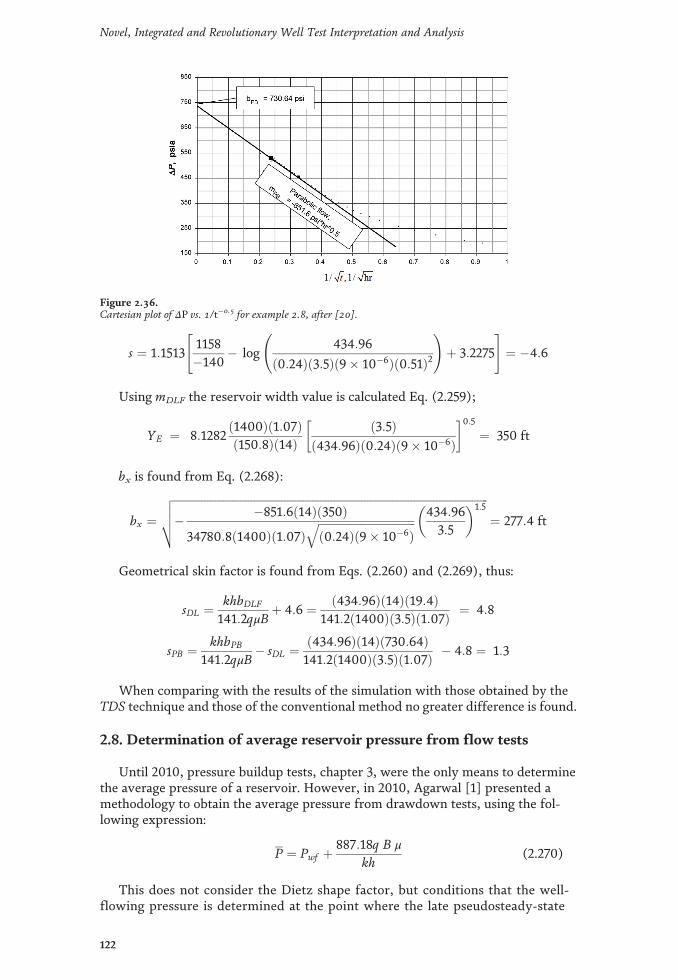
s ¼ 1:15131158�140

� log434:96

ð0:24Þð3:5Þð9� 10�6Þð0:51Þ2 !

þ 3:2275

" #¼ �4:6

Using mDLF the reservoir width value is calculated Eq. (2.259);

YE ¼ 8:1282ð1400Þð1:07Þð150:8Þð14Þ

ð3:5Þð434:96Þð0:24Þð9� 10�6Þ

� 0:5¼ 350 ft

bx is found from Eq. (2.268):

bx ¼ffiffiffiffiffiffiffiffiffiffiffiffiffiffiffiffiffiffiffiffiffiffiffiffiffiffiffiffiffiffiffiffiffiffiffiffiffiffiffiffiffiffiffiffiffiffiffiffiffiffiffiffiffiffiffiffiffiffiffiffiffiffiffiffiffiffiffiffiffiffiffiffiffiffiffiffiffiffiffiffiffiffiffiffiffiffiffiffiffiffiffiffiffiffiffiffiffiffiffiffiffiffiffiffiffiffiffiffiffiffiffiffiffiffi� �851:6ð14Þð350Þ34780:8ð1400Þð1:07Þ

ffiffiffiffiffiffiffiffiffiffiffiffiffiffiffiffiffiffiffiffiffiffiffiffiffiffiffiffiffiffiffiffiffiffiffið0:24Þð9� 10�6Þ

q 434:963:5

� �1:5vuut ¼ 277:4 ft

Geometrical skin factor is found from Eqs. (2.260) and (2.269), thus:

sDL ¼ khbDLF

141:2qμBþ 4:6 ¼ ð434:96Þð14Þð19:4Þ

141:2ð1400Þð3:5Þð1:07Þ ¼ 4:8

sPB ¼ khbPB141:2qμB

� sDL ¼ ð434:96Þð14Þð730:64Þ141:2ð1400Þð3:5Þð1:07Þ � 4:8 ¼ 1:3

When comparing with the results of the simulation with those obtained by theTDS technique and those of the conventional method no greater difference is found.

2.8. Determination of average reservoir pressure from flow tests

Until 2010, pressure buildup tests, chapter 3, were the only means to determinethe average pressure of a reservoir. However, in 2010, Agarwal [1] presented amethodology to obtain the average pressure from drawdown tests, using the fol-lowing expression:

P ¼ Pwf þ 887:18q B μ

kh(2.270)

This does not consider the Dietz shape factor, but conditions that the well-flowing pressure is determined at the point where the late pseudosteady-state

Figure 2.36.Cartesian plot of ΔP vs. 1/t�0.5 for example 2.8, after [20].

122


period develops. According to Agarwal [1], this point is determined using thearithmetic derivative (not multiplied by time). In the arithmetic derivative, theradial flow is presented with a slope of �1. The pseudosteady-state period(postradial) takes place when the slope of the arithmetic derivative becomeszero (flat). That is the right moment where the well-flowing pressure, Pwf, isread.

Nomenclature

A area, ft2

Bg gas volume factor, ft3/STBBo oil volume factor, bbl/STBBw oil volume factor, bbl/STBb fraction of penetration/completionbDLF intercept of P vs t0.25 plot during dual-linear flow, psia0.5

bLF intercept of P vs t0.5 plot during hemilinear flow, psia0.5

bPB intercept of P vs 1/t0.5 plot during hemilinear flow, h�1

bx distance from closer lateral boundary to well along the x-direction, ftby distance from closer lateral boundary to well along the y-direction, ftc compressibility, 1/psiaC wellbore storage coefficient, bbl/psiaCA reservoir shape factorct total or system compressibility, 1/psiaDF damage factorDR damage ratioFE flow indexf(t) time functionh formation thickness, fthp length of perforations, ftI interceptJ productivity index, bbl/psiak permeability, mdkg gas effective permeability, mdko oil effective permeability, mdkw water effective permeability, mdIDcsg internal casing diameter, inm slope of P vs log t plot, psia/h/cyclem* slope of P vs t plot, psia/hmDLF slope of P vs t0.25 plot during dual-linear flow, psia0.5/hmLF slope of P vs t0.5 plot during hemilinear flow, psia0.5/hmPB slope of P vs 1/t0.5 plot during hemilinear flow, (psia0.5/h)�1

m 0 slope of superposition or equivalent time plot, psia/BPD/cyclem 0b 0 intercept of superposition or equivalent time plot, psia/BPD/cyclem(P) pseudopressure, psia/cpODcsg external casing diameter, inP pressure, psiaP average reservoir pressure, psiaPD 0 dimensionless pressure derivativePD dimensionless pressurePi initial reservoir pressure, psiaPR productivity ratio

123


Pt shut-in casing pressure, psiaPwf well flowing pressure, psiaPws well shut-in or static pressure, psiaP1hr intercept of the semilog plot, psiaP* false pressure, psiaΔPs pressure drop due to skin conditions, psiaq liquid flow rate, bbl/Dqsc gas flow rate, Mscf/DrD dimensionless radiusr radius, ftre drainage radius, ftRs gas dissolved in oil, scf/STBrw well radius, fts skin factorsc skin due to partial penetrationscp skin due to a change in permeabilitysDL geometrical skin factor converging from radial to dual-linear flowsL geometrical skin factor converging from dual-linear to linear flowsp skin factor due to the restricted flow entrysPB geometrical skin factor converging from dual-linear to parabolic flowst total skin factorsθ skin factor resulting from a well deviation angleT reservoir temperature, ºR, Transmissivity, md-ft/cpt time, htp production (horner) time before shutting-in a well, htD dimensionless time based on well radiustDA dimensionless time based on reservoir areat*DP 0 pressure derivative, psiaV volume, ft3

Vu wellbore volume/unit length, bbl/ftX distance in the x-directionXE reservoir length, ftXN superposition time, hY distance in the y-directionYE reservoir width, ftWD dimensionless reservoir widthZ height, ft

Greek

Δ change, dropΔt shut-in time, hφ porosity, fractionλ mobility, md/cpρ fluid density, lbm/ft3

θ deviation angle, °ψ measured deviation angle, °ψ' corrected deviation angle, °μ viscosity, cp

124


Suffices

0 base conditions1hr time of 1 ha actuald drainageD dimensionlessDA dimensionless with respect to areaDL dual linear flowDL1 dual linear flow at 1 hDLpssi intersection of pseudosteady-state line with dual-linear lineDLSS1 intercept between dual-linear line and the �1-slope line (SS1)DLSS2 intercept between dual-linear line and the �1-slope line (SS2)eq equivalentF inflectiong gash horizontalhs hemisphericali intersection or initial conditionsideal idealINT interceptinv investigationL linear or hemilinear flowL1 linear flow at 1 hlag lagLpssi intercept of linear and pseudosteady state linesN an arbitrary point during early pseudosteady-state periodmax maximumo oilOP oil price, US$/STBp production, porousPB parabolic flowPBSS1 intercept between parabolic line and the �1-slope line (SS1)PBSS2 intercept between parabolic line and the �1-slope line (SS2)pss pseudosteady statepss1 pseudosteady state at 1 hr radial flowrDLi intercept of radial and dual linear linesr1 radial flow before spherical/hemispherical flowrg relative to gasrLi intercept of radial and linear linesro relative to oilrpssi intersection of pseudosteady-state line with radial linerSSi intersection between the radial line and the �1-slope linerSS1i intersection between the radial line and the �1-slope line (SS1)rSS2i intersection between the radial line and the �1-slope line (SS2)rw relative to waters skinsf sandfacesp spherical

125


SS steadySSL start of semilog line (radial flow)SS1 �1-slope line formed when the parabolic flow ends and steady-state

flow regime starts. Well is near the open boundary and the far boundaryis opened

SS2 �1-slope line formed when the parabolic flow ends and steady-stateflow regime starts. Well is near the open boundary and the far boundaryis closed

sw spherical/hemispherical wellborew well, waterwa apparent wellborewb wellborewD dimensionless emphasizing at wellborewf well flowingws well shut-inx maximum point (peak) during wellbore storagexc maximum point for centered wellsX1 maximum point between dual linear and parabolic linesX2 maximum point between parabolic and negative unit slope linesX3 maximum point between hemilinear and negative unit slope linesz vertical direction

126


References

[1] Agarwal RG. Direct Method ofEstimating Average Reservoir Pressurefor Flowing Oil and Gas Wells. Societyof Petroleum Engineers; 2010. DOI:10.2118/135804-MS

[2] Earlougher RC Jr. Advances in WellTest Analysis. Monograph Series. Vol. 5.Dallas, TX: SPE; 1977

[3] Lee J, Rollins JB, Spivey JP. PressureTransient Testing. Vol. 9. Richardson,TX: SPE Textbook; 2003. 336p

[4] Mathews CS, Russell DG. PressureBuildup and Flow Tests in Wells. SPEMonograph Series. Vol. 1. Dallas, TX:Society of Petroleum Engineers ofAIME; 1967. 163p

[5] Rhagavan R. Well Test Analysis. NewJersey: Prentice Hall; 1993. 558p

[6] Sabet M. Well Testing. GulfPublishing Co; 1991. 460p

[7] Stanislav JF, Kabir CS. PressureTransient Analysis. New Jersey: PrenticeHall; 1990. 320p

[8] Earlougher RC, Kersch KM. Analysisof short-time transient test data by type-curve matching. Journal of PetroleumTechnology. Society of PetroleumEngineers. 1974. pp. 793-800. DOI:10.2118/4488-PA

[9] Ramey HJ. Short-time well test datainterpretation in the presence of skineffect and wellbore storage. Journal ofPetroleum Technology. Society ofPetroleum Engineers. 1970:97-104. DOI:10.2118/2336-PA

[10] Escobar FH, Olaya DA, Medina MV.Approximation of the starting time ofradial flow regime under variablewellbore storage conditions invertical wells. Journal of Engineeringand Applied Sciences. 2014;9(7):1047-1052

[11] Slider HC. Wordlwide PracticalPetroleum Reservoir EngineeringMethods. Revised Edition. Tulsa,Oklahoma, USA: PennWell PublishingCo.; 1983. 826p

[12] Escobar FH, Muñoz OF, SepúlvedaJA. Horizontal permeabilitydetermination from the elliptical flowregime for horizontal wells. RevistaCT&F—Ciencia Tecnología y Futuro.2004;2(5):83-95

[13] Escobar FH, Saavedra NF,Hernandez CM, Hernandez YA, PilataxiJF, Pinto DA. Pressure and PressureDerivative Analysis for LinearHomogeneous Reservoirs without usingType-Curve Matching. Society ofPetroleum Engineers; 2004. DOI:10.2118/88874-MS

[14] Escobar FH, Muñoz OF, SepulvedaJA, Montealegre M, Hernández YA.Parabolic flow: A new flow regimefound in long, narrow reservoirs. In: XICongreso Colombiano del Petróleo;October; 2005. pp. 18-21

[15] Escobar FH, Navarrete JM, LosadaHD. Evaluation of Pressure DerivativeAlgorithms for Well-Test Analysis.Society of Petroleum Engineers; 2004.DOI: 10.2118/86936-MS

[16] Escobar FH, Muñoz OF, SepulvedaJA, Montealegre M. New finding onpressure response in long, narrowreservoirs. CT&F—Ciencia, Tecnologíay Futuro. 2005:131-140

[17] Escobar FH, Muñoz OF, SepulvedaJA, Montealegre-MM, Hernandez YA.Parabolic flow: A new flow regimefound in long, narrow reservoirs. XICongreso Colombiano del Petróleo(Colombian Petroleum Symposium);October; 2005. pp. 18-21

[18] Escobar FH, Montealegre-MM.Effect of well stimulation on the skin

127


factor in elongated reservoirs. CT&F—Ciencia, Tecnología y Futuro. 2006;3(2):109-119. ISSN 0122-5383

[19] Escobar FH, Hernández YA,Hernandez CM. Pressure transientanalysis for long homogeneousreservoirs using TDS technique. Journalof Petroleum Science and Engineering.2007;58(1–2):68-82

[20] Escobar FH, Montealegre M. Acomplementary conventional analysisfor channelized reservoirs. CT&F—Ciencia, Tecnología y Futuro. 2007;3(3):137-146

[21] Escobar FH, Montealegre-MM.Application of TDS technique todeveloped reservoirs. Journal ofPetroleum Science and Engineering.2007;55(3–4):252-258

[22] Escobar FH, Lopez AM, Cantillo JH.Effect of the pseudotime function on gasreservoir drainage area determination.CT&F—Ciencia, Tecnología y Futuro.2007;3(3):113-124

[23] Escobar FH, Tiab D, Tovar LV.Determination of areal anisotropy froma single vertical pressure test andgeological data in elongated reservoirs.Journal of Engineering and AppliedSciences. 2007;2(11):1627-1639

[24] Escobar FH. Recent advances in welltest analysis for long and narrowreservoirs. In: Korin L. Montclaire,editor. Petroleum Science ResearchProgress. Nova Publisher; 2008

[25] Escobar FH, Martinez JA,Montealegre M. Pressure and pressurederivative analysis for injection testswith variable temperature without type-curve matching. CT&F—Ciencia,Tecnología y Futuro. 2008;4(4):83-91

[26] Escobar FH, Montealegre M.Application of TDS technique tomultiphase flow. CT&F—Ciencia,Tecnología y Futuro. 2008;4(4):93-105

[27] Escobar FH, Sanchez JA, CantilloJH. Rate transient analysis forhomogeneous and heterogeneous gasreservoirs using the TDS technique.CT&F—Ciencia, Tecnología y Futuro.2008;4(4):45-59

[28] Escobar FH, Hernandez YA, Tiab D.Determination of reservoir drainagearea for constant-pressure systems usingwell test data. CT&F—Ciencia,Tecnología y Futuro. 2010;4(1):51-72

[29] Escobar FH, Montealegre M,Carrillo-Moreno D. Straight linemethods for estimating permeability orwidth for two-zone compositechannelized reservoirs. CT&F—Ciencia, Tecnología y Futuro. 2009;3(5):107-124

[30] Escobar FH, Montealegre-MM,Carrillo-Moreno D. Pressure andpressure derivative transient analysiswithout type-curve matching forelongated reservoirs with changes inpermeability or width. CT&F—Ciencia,Tecnología y Futuro. 2010;4(1):75-88

[31] Escobar FH, Hernandez DP,Saavedra JA. Pressure and pressurederivative analysis for long naturallyfractured reservoirs using the TDStechnique. Dyna. 2010;77(163):102-114

[32] Escobar FH, Martínez JA,Montealegre M. Pressure and pressurederivative analysis for a well in a radialcomposite reservoir with a non-Newtonian/Newtonian interface. CT&F. 2010;4(1):33-42

[33] Escobar FH, Martinez JA, BonillaLF. Pressure and pressure derivativeanalysis different of type-curvematching for thermal recoveryprocesses. CT&F. 2011;4(4):23-35

[34] Escobar FH. Transient pressure andpressure derivative analysis for non-Newtonian fluids. In: New Technologiesin the Oil and Gas Industry. Rijeka:Intech; 2012. http://www.intechopen.

128


com/books/export/citation/Zotero/new-technologies-in-the-oil-and-gas-industry/transient-pressure-and-pressure-derivative-analysis-for-non-newtonian-fluids

[35] Escobar FH, Rojas MM, Bonilla LF.Transient-rate analysis for longhomogeneous and naturally fracturedreservoir by the TDS technique. Journalof Engineering and Applied Sciences.2012;7(3):353-370

[36] Escobar FH, Martinez LY, MéndezLJ, Bonilla LF. Pseudotime applicationto hydraulically fractured vertical gaswells and heterogeneous gas reservoirsusing the TDS technique. Journal ofEngineering and Applied Sciences. 2012;7(3):260-271

[37] Escobar FH, Corredor CM, GomezBE, Cantillo JH, Prent LA. Pressure andpressure derivative analysis for slantedand partially penetrating wells. Journalof Engineering and Applied Sciences.2012;7(8):932-938

[38] Escobar FH, Rojas MM, Cantillo JH.Straight-line conventional transient rateanalysis for long homogeneous andheterogeneous reservoirs. Dyna. 2012;79(172):153-163

[39] Escobar FH, Muñoz YEM, CerqueraWM. Pseudotime function effect onreservoir width determination inhomogeneous and naturally fracturedgas reservoir drained by horizontalwells. Entornos Journal. 2012;(24):221-231

[40] Escobar FH, Vega J, Diaz MR.Pressure and pressure derivativeanalysis for double-permeabilitysystems without type-curve matching.Journal of Engineering and AppliedSciences. 2012;7(10)

[41] Escobar FH, Vega LJ, Bonilla LF.Determination of well-drainage area forpower-law fluids by transient pressureanalysis. CT&F. 2012;5(1):45-55

[42] Escobar FH, Martinez JA, BonillaLF. Transient pressure analysis forvertical wells with spherical power-lawflow. CT&F. 2012;5(1):19-25

[43] Escobar F-H, Martínez JA,Montealegre M. Pressure transientanalysis for a reservoir with a finite-conductivity fault. CT&F—Ciencia,Tecnología y Futuro. 2013;5:5-18

[44] Escobar FH, Alzate HD, Moreno L.Effect of extending the radialsuperposition function to other flowregimes. Journal of Engineering andApplied Sciences. 2013;8(8):625-634

[45] Escobar FH, Ascencio JM, Real DF.Injection and fall-off tests transientanalysis of non-Newtonian fluids.Journal of Engineering and AppliedSciences. 2013;8(9):703-707

[46] Escobar FH, Martinez JA,Montealegre M. Pressure and pressurederivative analysis in a reservoir with afinite-conductivity fault and contrast ofmobilities. Fuentes Journal. 2013;11(2):17-25

[47] Escobar FH, Meneses AR, LosadaLM. Straight-line conventional transientpressure analysis for horizontal wellswith isolated zones. Dyna. 2014;81(185):78-85

[48] Escobar FH, Polanco MP, BenavidezW. Pressure and pressure derivativeanalysis for a vertical well in wedgedand T-shaped reservoirs. Journal ofEngineering and Applied Sciences.2014;9(6):845-851

[49] Escobar FH, Montenegro LM,Bernal KM. Transient-rate analysis forhydraulically-fractured gas shale wellsusing the concept of inducedpermeability field. Journal ofEngineering and Applied Sciences.2014;9(8):1244-1254

[50] Escobar FH, Ghisays-Ruiz A, BonillaLF. New model for elliptical flow regime

129


in hydraulically-fractured vertical wellsin homogeneous and naturally-fracturedsystems. Journal of Engineering andApplied Sciences. 2014;9(9):1629-1636

[51] Escobar FH, Bernal KM, Olaya-Marin G. Pressure and pressurederivative analysis for fracturedhorizontal wells in unconventional shalereservoirs using dual-porosity models inthe stimulated reservoir volume. Journalof Engineering and Applied Sciences.2014;9(12):2650-2669

[52] Escobar FH, Salcedo LN, Pinzon C.Pressure and pressure derivativeanalysis for fractal homogeneousreservoirs with power-law fluids.Journal of Engineering and AppliedSciences. 2015;10(11):4763-4772

[53] Escobar FH, Srivastava P, Wu X. Apractical method to determine aquiferleakage factor from well test data inCBM reservoirs. Journal of Engineeringand Applied Sciences. 2015;10(11):4857-4863

[54] Escobar FH, Fahes M, Gonzalez R,Pinchao DM, Zhao YL. Determinationof reservoir drainage area for constant-pressure systems by conventionaltransient pressure analysis. Journal ofEngineering and Applied Sciences. 2015;10(12):5193-5199

[55] Escobar FH, Ghisays-Ruiz A,Srivastava P. Characterization of thespherical stabilization flow regime bytransient pressure analysis. Journal ofEngineering and Applied Sciences. 2015;10(14):5815-5822. ISSN 1819-6608

[56] Escobar FH. Recent Advances inPractical Applied Well Test Analysis.New York: Nova publishers; 2015. 422p

[57] Escobar FH, Zhao YL, Pournik M,Liu QG, Olaya-Marin G. Interpretationof pressure tests in uniform-fluxfractured vertical wells with thresholdpressure gradient in low permeability

reservoirs. Journal of Engineering andApplied Sciences. 2015;10(20):9364-9372

[58] Escobar FH, Jongkittnarukorn J,Hernandez CM. The power of TDStechnique for well test interpretation: Ashort review. Switzerland AG: Journal ofPetroleum Exploration and ProductionTechnology. 2018. DOI: 10.1007/s13202-018-0517-5

[59] Ehlig-Economides C, EconomidesMJ. Pressure transient analysis in anelongated linear flow system. Society ofPetroleum Engineers Journal. 1985:839-847. DOI: 10.2118/12520-PA

[60] Hachlaf H, Tiab D, Escobar FH.Effect of Variable Injection Rate onFalloff and Injectivity Tests. Society ofPetroleum Engineers; 2002. DOI:10.2118/76714-MS

[61] Jongkittinarukorn K, Tiab D,Escobar FH. Interpretation ofHorizontal Well Performance inComplicated Systems by the BoundaryElement Method. Society of PetroleumEngineers; 1998. DOI: 10.2118/50437-MS

[62] Martinez JA, Escobar FH,Montealegre M. Vertical well pressureand pressure derivative analysis forbingham fluids in a homogeneousreservoirs. Dyna. 2011;78(166):21-28

[63] Martin JC. Simplified Equations ofFlow in Gas Drive Reservoirs and theTheoretical Foundation of MultiphasePressure Buildup Analyses. Society ofPetroleum Engineers; 1959

[64] Martinez JA, Escobar FH, CantilloJH. Application of the TDS technique todilatant non-Newtonian/Newtonianfluid composite reservoirs. Ingeniería eInvestigación journal. 2011;31(3):130-134

[65] Merzouk K, Tiab D, Escobar FH.Multirate Test in Horizontal Wells.

130


Society of Petroleum Engineers; 2002.DOI: 10.2118/77951-MS

[66] Moncada K, Tiab D, Escobar FH,Montealegre-MM, Chacon A, ZamoraRA, Nese SL. Determination of verticaland horizontal permeabilities forvertical oil and gas wells with partialcompletion and partial penetrationusing pressure and pressure derivativeplots without type-curve matching.CT&F—Ciencia, Tecnología y Futuro.2005;2(6)

[67] Mongi A, Tiab D. Application ofTiab’s Technique to Multi-Rate Tests.Society of Petroleum Engineers; 2000.DOI: 10.2118/62607-MS

[68] Tiab D. PE-5553: Well test analysis.Lecture notes. Fall 1993. The Universityof Oklahoma

[69] Tiab D. Analysis of pressurederivative without type-curve matching:Vertically fractured wells in closedsystems. Journal of Petroleum Scienceand Engineering. 1994;11:323-333. Thispaper was originally presented as TiabD. Analysis of Pressure and PressureDerivative without Type-CurveMatching—III. Vertically FracturedWells in Closed Systems. Society ofPetroleum Engineers; 1993. DOI:10.2118/26138-MS

[70] Tiab D. Direct Type-CurveSynthesis of Pressure Transient Tests.Society of Petroleum Engineers; 1989.DOI: 10.2118/18992-MS

[71] Tiab D. Analysis of pressure andpressure derivative without type-curvematching: 1—Skin and wellbore storage.Journal of Petroleum Science andEngineering. 1995;12:171-181. Also TiabD. Analysis of Pressure and PressureDerivatives Without Type-CurveMatching: I—Skin and WellboreStorage. Society of PetroleumEngineers; 1993. DOI: 10.2118/25426-MS

[72] Zhao YL, Escobar FH, Jamili A,Olaya-Marin G, Ghisays-Ruiz A. Effectof wellbore storage on the vertical wellpressure behavior with thresholdpressure gradient in low permeabilityreservoirs. Journal of Engineering andApplied Sciences. 2015;10(22):10659-10664

[73] Bourdet D, Ayoub JA, Pirard YM.(June 1). Use of Pressure Derivative inWell Test Interpretation. SPEFE.Society of Petroleum Engineers; 1989.pp. 293-302. DOI: 10.2118/12777-PA

[74] Brons F, Miller WC. (August 1). Asimple method for correcting spotpressure readings. Journal of PetroleumTechnology; Transactions of the AIME.Society of Petroleum Engineers. 1961;222. pp. 803-805. DOI: 10.2118/1610-G-PA

[75] Dietz DN. Determination of averagereservoir pressure from build-upsurveys. Journal of PetroleumTechnology. Transactions AIME.Society of Petroleum Engineers. 1965;234. pp. 955-959. DOI: 10.2118/1156-PA

[76] Jones P. Reservoir limit test. Oil andGas Journal. 1956:184-196

[77] Ramey HR Jr, Cobb WM. A generalbuildup theory for a well in a closeddrainage area. JPT. Society of PetroleumEngineers. 1971:1493-1505. DOI:10.2118/3012-PA

[78] Bernal KM, Escobar FH, Ghisays-Ruiz A. Pressure and pressure derivativeanalysis for hydraulically-fracturedshale formations using the concept ofinduced permeability field. Journal ofEngineering and Applied Sciences.2014;9(10):1952-1958

[79] Boussalem R, Djebbar T, EscobarFH. Effect of Mobility Ratio on thePressure and Pressure Derivative ofWells in Closed Composite Reservoirs.Society of Petroleum Engineers; 2002.DOI: 10.2118/76781-MS

131


[80] Tiab D, Bettam Y. PracticalInterpretation of Pressure Tests ofHydraulically Fractured Wells in aNaturally Fractured Reservoir. Societyof Petroleum Engineers; 2007. DOI:10.2118/107013-MS

[81] Engler T, Tiab D. Analysis ofpressure and pressure derivativewithout type-curve matching, 5.Horizontal well tests in naturallyfractured reservoirs. Journal ofPetroleum Science and Engineering.1996;15:139-151

[82] Engler T, Tiab D. Analysis ofpressure and pressure derivativewithout type-curve matching, 6.Horizontal well tests in anisotropicmedia. Journal of Petroleum Science andEngineering. 1996;15:153-168

[83] Engler T, Tiab D. Analysis ofpressure and pressure derivativewithout type curve matching, 4.Naturally fractured reservoirs. Journalof Petroleum Science and Engineering.1996;15:127-138

[84] Vongvuthipornchai S, Raghavan R.A Note on the Duration of theTransitional Period of ResponsesInfluenced by Wellbore Storage andSkin. SPE Formation Evaluation. Societyof Petroleum Engineers; 1988. pp. 207-214. DOI: 10.2118/15273-PA.

[85] Chacon A, Djebrouni A, Tiab D.Determining the Average ReservoirPressure from Vertical and HorizontalWell Test Analysis Using the Tiab’sDirect Synthesis Technique. Society ofPetroleum Engineers; 2004. DOI:10.2118/88619-MS

[86] Perrine RL. Analysis of pressure-buildup curves. In: Drilling andProduction Practices; AmericanPetroleum Institute (API); 1956.pp. 482-509. ID API-56-482

[87] Al-Khalifah A-JA, Horne RN, AzizK. In-Place Determination of Reservoir

Relative Permeability Using Well TestAnalysis. Society of PetroleumEngineers; 1987. DOI: 10.2118/16774-MS

[88] Kamal MM, Pan Y. Use of TransientData To Calculate Absolute Permeabilityand Average Fluid Saturations. Societyof Petroleum Engineers; 2010. DOI:10.2118/113903-PA

[89] Al-Khalifah A-JA, Aziz K, HorneRN. A New Approach to MultiphaseWell Test Analysis. Society of PetroleumEngineers; 1987. DOI: 10.2118/16743-MS

[90] Abbott WA, Collins T, Tippie DB.Practical Application of Spherical FlowTransient Analysis. Society of PetroleumEngineers; 1978. DOI: 10.2118/7485-MS

[91] Dykstra H, Kazemi H, Raghavan R,Gulati MS. Pressure Transient TestingMethods, SPE Reprint Series No. 14.Dallas, Texas: Society of PetroleumEngineers; 1967. 264p

[92] Cinco H, Miller FG, Ramey HJ.Unsteady-state pressure distributioncreated by a directionally drilled well.Journal of Petroleum Technology,Transactions of AIME. Society ofPetroleum Engineers. 1975;259.pp. 1392-1400. DOI: 10.2118/5131-PA

[93] Jones LG, Watts JW. Estimatingskin effect in a partially completeddamaged well. Journal of PetroleumTechnology, Transactions of AIME.Society of Petroleum Engineers. 1971;251:249-252. DOI: 10.2118/2616-PA

[94] Joseph JA. Unsteady-statecylindrical, spherical and linear flow inporous media [PhD Dissertation]. Rolla:University of Missouri; 1984

[95] Merzouk K, Tiab D, Escobar FH.Multirate Test in Horizontal Wells.Society of Petroleum Engineers; 2002.DOI: 10.2118/77951-MS

[96] Russell DG. Determination offormation characteristics from two-rate

132


flow tests. Journal of PetroleumTechnology; Transactions of AIME.Society of Petroleum Engineers. 1963;228:1347-1355. DOI: 10.2118/645-PA

[97] Tracy GW, Coats KH, Kazemi H,Odeh AS, Lebourg M, Prats M, et al.Pressure Analysis Methods. SPE ReprintSeries No. 9. Society of PetroleumEngineers of AIME; 1967

[98] Slider HC. Application of Pseudo-Steady-State Flow to Pressure-BuildupAnalysis. Society of PetroleumEngineers; 1966. DOI: 10.2118/1403-MS

[99] Slider HC. A simplified method forpressure buildup analysis for a stabilizedwell. Journal of Petroleum Technology.1971:1155-1160. Slider HC. A SimplifiedMethod of Pressure Buildup Analysis fora Stabilized Well. Society of PetroleumEngineers; 1967. DOI: 10.2118/1765-MS

[100] Sui W, Mou J, Bi L, Deng J, Ehlig-Economides CA. New Flow Regimes forWell Near Constant Pressure Boundary.Society of Petroleum Engineers; 2007.DOI: 10.2118/106922-MS

[101] Wong DW, Mothersele CD,Harrington AG, Cinco-Ley H. PressureTransient Analysis in Finite LinearReservoirs Using Derivative andConventional Techniques: FieldExamples. Society of PetroleumEngineers; 1986. DOI: 10.2118/15421-MS

[102] Nutakki R, Mattar L. PressureTransient Analysis of Wells in VeryLong Narrow Reservoirs. Society ofPetroleum Engineers; 1982. DOI:10.2118/11221-MS

[103] Horne RN. Modern Well TestAnalysis: A Computer-aided Approach.Palo Alto, CA: Petroway Inc.; 1990. 185p

[104] Jones P. Drawdown ExplorationReservoir Limit, Well and FormationEvaluation. Society of PetroleumEngineers; 1957. DOI: 10.2118/824-G

[105] Jones P. Reservoir limit test on gaswells. Journal of Petroleum Technology.Society of Petroleum Engineers. 1962:613-619. DOI: 10.2118/24-PA

[106] Odeh AS, Jones LG. PressureDrawdown Analysis, Variable-RateCase. JPT; Transactions of AIME.Society of Petroleum Engineers. 1965;234:960-964. DOI: 10.2118/1084-PA

[107] Smith CR, Tracy GW. AppliedReservoir Engineering. Tulsa, OK: Oil &Gas Consultants, Inc.; 1987

133


Chapter 3

Pressure Buildup Testing

A pressure buildup test has been a very popular technique used in the hydrocar-bon industry. Several reasons have become a very popular test, some of these are:(a) it does not require very detailed supervision and (b) permeability and skinfactor can be determined from both pressure buildup and drawdown tests.However, as studied in Section 2.8, until 2010, a flow test did not allow estimatingthe average reservoir pressure, while a pressure test does [7–10, 25, 26, 28, 30].

Figure 3.1 shows a plot of an ideal pressure buildup test. In general terms, itrequires shutting‐in a producer well after it has produced for some time, tp, with astable flow rate. A pressure buildup test is run as follows:

1. Place the pressure sensors in the selected site. It is recommended as close aspossible to the perforations.

2. Stabilize the well to a constant production rate, q.

3. Close the well and record the Pwf value (just before closing).

4.Read the well bottom-hole pressure, Pws, at short time intervals of 15 s for thefirst few minutes (10–15 min), then I could be every 10 min for the first hour.During the next 10 h, hourly pressure readings should be taken. When the testprogresses, the time intervals can be expanded to 5 h. With recently introducedpressure recorders, the readings can be taken at shorter intervals. It can startreading every second or less.

To run a pressure buildup test, the well produces a constant rate for a period oftime, tp. A pressure recorder is lowered to the well immediately before closing. tpshould not be too small to avoid problems associated with superposition and inves-tigation radius [12].

3.1. Superposition principle

Suppose that after the well has produced a constant rate for a time period, tp, it isdecided to shut‐in the well to obtain a pressure buildup test. Intuitively, fluidmovement is expected at the reservoir after the well is shut‐in, but at surface q = 0.A similar situation arises in fall‐off testing, but injections takes place instead ofproduction. An analogy is made to the fluid movement at the reservoir [10–12, 28,37, 40] as follows: the well is allowed to produce indefinitely at a flow rate, q, and atthe instant of shutting‐in the well, the same flow rate, q, is injected into the samewell, and then the pressure drop is added due to the production of q and samepressure data multiplied by �1 and displaced at the time the well is shut‐in. This,however, is not easy to understand. The better way is to understand, refer toFigure 3.1, is to estimate the well pressure drop at a time, tp þ Δt, and then subtractthe pressure drop during a time, Δt. Mathematically;

PDws ¼ PDðtp þ ΔtÞD � PDðΔtÞD (3.1)

134

If tp is not given, it can be estimated if cumulative production, Np, is known,

tp ¼ 24Npq

(3.2)

Assuming wellbore storage is neglected and the reservoir is of infinite size; then,Eq. (1.115) applies:

PDðtp þ ΔtÞD ¼ 12

ln ðtp þ ΔtÞD þ 0:80907� �� s (3.3)

PDðΔtÞD ¼ 12

ln ðΔtÞD þ 0:80907� �� s (3.4)

Combining Eqs. (3.3) and (3.4) in Eq. (3.1), then replacing in the resultingcombination the dimensionless parameter given by Eqs. (1.89) and (1.94) yields:

Pws ¼ Pi � 162:6qμ Bkh

logtp þ ΔtΔt

� �(3.5)

This is known as Horner equation. As a result of the application of the superpo-sition principle is that the skin factor, s, disappears in the Horner’s simplifiedequation. That means the slope of the Horner plot is not affected by the skin factor.However, the skin factor alters, even greater than in flow tests, the shape of thepressure buildup curve. The skin factor affects the buildup test more than thedrawdown test because wellbore storage persists.

3.2. Buildup test methods

3.2.1 Horner method

Eq. (3.5) suggests that a semi‐log plot of well‐shut‐in pressure versus (tpþΔt)/Δtwill yield a straight line which slope allows finding the permeability fromEq. (2.34). Estimating the Horner time, (tpþΔt)/Δt was tedious before 1970 when

Figure 3.1.Schematic representation of pressure restoration.

135

Pressure Buildup TestingDOI: http://dx.doi.org/10.5772/intechopen.81078

computer power was limited which is not today’s case. When superposition isovercome, the semi‐log plot of Pws versus Δt can be applied. In pressure builduptesting, this semi‐log plot is rather known as MDH plot, as shown later.

Horner plot is generally not preferred, since it requires more work than MDH. Itis strongly recommended to be used when tp < tpss [12, 26]. This is because super-position effects make the semi‐log straight line difficult to identify. Actually,Horner plot virtually increases about four times the length of the semi‐log slope. Iftp is at least twice the size of tpss, it is then justified to plot using tpss instead of tpss infinite systems [12, 26], since the Horner plot tends to prolong the semi‐log line.Preparing a Horner plot with tpss instead of tp has meaning to minimize errors in theestimation of the average pressure. However, with the advent of the pressurederivative function, the identification of radial flow became easier [6, 13, 25].

Just to look alike a MDH plot, Horner plot uses inverted abscissa scale as shownin Figure 3.2. For long producing times, a slight variation of Eq. (2.34) is used tofind skin factor when tp> 1;

s ¼ 1:1513P1hr � Pwf

m� log

kϕμctr2w

� �þ 3:23

� �(3.6)

Here Pwf is used instead of Pi. Pwf is the registered pressure just before shutting‐in the well. Finding P1hr requires using tp and adding one to that value. Use thatestimated (tpþΔt)/Δt value and enter the Horner plot and read on the semi‐log linethe value of P1hr. It is meaningless to estimate (tpþΔt)/Δt=1. However, such read-ing will be used later to estimate the average reservoir pressure. When tp< 1, thefollowing expression ought to be used to find skin factor:

s ¼ 1:1513P1hr � Pwf

mþ log 1þ 1

tp

� �� log

kϕμctr2w

� �þ 3:2275

� �(3.7)

Once the skin factor is estimated, the skin pressure drop and flow efficient canbe found using Eqs. (2.35) and (2.46).

When the well is shut‐in for a buildup test, the formation fluid keeps flowing,even though using downhole devise shutting. Again, this after‐flow duration can bedetermined easily from the pressure derivative plot once radial flow starts. This wasnot the case before 1980s. This after‐flow rate, qaf, due to the wellbore storage, has asignificant influence on the pressure data. This occurs because the head pressure isnot equal to the bottom shut‐in pressure, and therefore the fluid continues to flow

Figure 3.2.Typical Horner plot, tp = 83 hr.

136


from the formation to the well. Then the pressure does not recover as fast asexpected. As the flow rate tends to zero, the pressure increases rapidly. The semi‐log graph is pronounced and linear in this period and can be confused with thesemi‐log slope [10, 12, 26, 28, 37, 40].

qaf ¼24CVw

BdPws

d Δtð Þ (3.8)

C is found from transient pressure analysis using Eq. (2.18). For producer andinjector wells, respectively, the after‐flow duration can be estimated from [40];

Δtaf ¼ 204CB J

� �(3.9)

Δtaf ffi 204CVu

B J

� �(3.10)

where J is the productivity index, Eq. (2.44), B is the volume factor and, Vu, thewellbore capacity, Eq. (2.4), and C is the wellbore storage coefficient found fromEq. (2.18). When qaf/q < 0.01, it is concluded that wellbore storage does not affectthe semi‐log slope. In other words, after this time, WBS effects are negligible.

Because of superposition, skin and wellbore storage effects, the start time of thesemi‐log slope, ΔtSSL, is given by [12],

ðΔtDÞSSL ¼ 50CDe0:14s (3.11)

By taking a glance to Eq. (2.19), it is appreciated a higher effect of skin factorand wellbore storage in the above expression. After replacing the dimensionlessparameters, Eqs. (2.14) and (1.94), in Eq. (3.11), it results:

ΔtSSL ¼ 170000μCe0:14s

kh(3.12)

Eq. (3.5) applies to infinite‐size reservoir. For finite reservoirs, Eq. (3.59),becomes [12, 40],

Pws ¼ P � � 162:6qμ Bkh

logtp þ ΔtΔt

� �¼ P � �m log

tp þ ΔtΔt

� �(3.13)

However, this equation applies similar to Eq. (2.5). The false pressure, P*, is readat a Horner time, (tpþΔt)/Δt=1, and does not have physical meaning, but is usefulto determine the average reservoir pressure [28].

3.2.2 Miller‐Dyes‐Hutchinson (MDH) method

This is based on the assumption that the production time, tp, is long enough toreach the pseudo‐steady‐state period; then, it is more representative to use averagepressure than initial pressure. The MDH method is preferred in old wells ordepleted formations, which would make it difficult to obtain stabilization beforeshutting‐in [40]. The Horner plot can be simplified [12, 28, 40], if Δt ⋘ tp, then:

tp þ Δt ffi tp (3.14)

Then,

137


logtp þ ΔtΔt

� �≈ log tp � log Δt (3.15)

Combining Horner equation, Eq. (3.13) with Eq. (3.15), it yields [12, 41]:

Pws ¼ P � �m log tp þm log Δt (3.16)

If P* � m log tp = constant = intercept; then,

Pws ¼ P1hr þ 162:6qμ Bkh

log Δt (3.17)

This suggests that a semi‐log plot of Pws versus Δt will yield a straight line whichslope, m, and intercept, P1hr, are used to find reservoir permeability with Eq. (2.33)and skin factor with Eq. (3.6).

Some expressions and plots [12] can be used to estimate the end of the semi‐logstraight line. However, the use of the pressure derivative [6, 13, 25] avoids usingthem. Therefore, they are omitted in this chapter.

3.2.3 Extended Muskat method

It is a trial‐and‐error method that is more attractive in cases of constant pressureor water injection systems (filling) because in these cases, the straight line would belonger and, therefore, easier to identify [12, 32]. Muskat [32] proposed to build apotential plot (log(ΔP) versus Δt), see Figure 3.3. Cobb and Smith [8] and Rameyand Cobb [39] recommended using it only as a method of late‐time analysis. For theapplication of the method, the average reservoir pressure is assumed as many timesas a straight line results in the plot. This author found that changing the averagereservoir pressure in a range of 30 psia above or below the target average pressurealways provides a straight line. Permeability and skin factor are found from theintercept of such plot, ΔPMint, read at Δt = 0:

Figure 3.3.Schematic representation of the Muskat plot for the analysis of pressure buildup tests, after [12].

138


k ¼ 141:2qμ Bh

PDðtDAÞintΔPMint

(3.17.1)

s ¼ PDðtDAÞintΔPint

� �P� Pwf ðΔt ¼ 0Þ� �� ln

rerw

þ 0:75 (3.18)

PD(tpDA) is normally found from plots [12]. However, this author fitted thecurves of such plots to polynomials. For a well within a square shaped reservoir—constant pressure case:

PDM int ¼ �0:0118157 þ 1:3509395 1� exp ð�21:692995 tpDA�

(3.18.1)

For a well within a square geometry reservoir—no‐flow boundary case.

PDM int ¼ �0:02056þ 0:682297 1� exp ð�50:7038508 tpDA�

(3.19)

where

tpDA ¼ 0:0002637ktpϕμctA

� �(3.20)

The slope of the Muskat, mM, plot can be used to find the drain area:

A ¼ kϕμctmM

� �MSF (3.21)

For the values of tpDA>1, the Musk shape factor, MSF, is 0.67, 1.34, and 0.84 forno‐flow boundary square reservoirs, constant‐pressure boundary square reservoirsand no‐flow boundary circular reservoirs, respectively, with a unique well in thecenter of such systems [12].

If A is known, then,

ϕ ct h ¼ St ¼ kh43560μ

MSF

mMA¼ T

MSF

43560mMA(3.22)

It can be concluded that MDH is generally preferred because it is easy to use. Forshort production times, it is recommended to use the Horner method since thesemi‐log line is longer than that provided by MDH. Earlougher [12] and Tiab [40]recommend the following aspects:

a. The Horner method could be used to analyze pressure buildup data, assumingtp is known. However, MDH, and then Horner, are usually used as the firstchoice. If tp is unknown, then use MDH.

b.Use MDH as the first test unless tp < tpss (reservoir acting as infinity, thenHorner is applied) or unless the well is in the center of a square shapedreservoir with open boundaries, such as an injection pattern of five points.

c. The Muskat method is used as a last option. It also provides the determinationof the drainage area.

As for the MDH case, the starting and the end of the Muskat straight line can beestimated only for square shape reservoirs with the well at the center within it. For

139


this reason and the help of the pressure derivative, it is not presented here. How-ever, these procedures can be found in [12, 39].

3.2.4 Type‐curve matching

Such type curves as the given in Figure 2.4 and 2.6 and their accompanyingequations also apply for buildup tests. However, superposition may cause trouble ascan be seen in Figure 3.4. This was reported by Gringarten [23] when demonstrat-ing the importance of deconvolution. Then, both pressure and pressure derivativemust be corrected [3], before applying type‐curve matching. To overcome thisissue, Agarwal [1] introduced the equivalent time, given by:

Δte ¼tpΔt

Δtþ tp(3.23)

Eq. (3.23) is the most common equivalent‐time equation. However, it wasdeveloped only for radial flow regime; therefore, it may fail providing good resultsif applied to other flow regimes. Then, the equivalent‐time equations for bilinear[38], linear, [38], birradial (elliptical), and spherical/hemispherical/parabolic flowregimes are, respectively, given as follows:

ΔteBL ¼ ffiffiffiffitp4

p þffiffiffiffiffiΔt4

p� ffiffiffiffiffiffiffiffiffiffiffiffiffiffiffi

tp þ Δt4p �4

h(3.24)

ΔteL ¼ ffiffiffiffitp

p þffiffiffiffiffiΔt

p� ffiffiffiffiffiffiffiffiffiffiffiffiffiffiffi

tp þ Δtph i2

(3.25)

ΔteBR ¼ffiffiffiffit9p

25q

þffiffiffiffiffiffiffiΔt925

q�

ffiffiffiffiffiffiffiffiffiffiffiffiffiffiffiffiffiffiffiffiffiðtp þ ΔtÞ925

q� �25=9(3.26)

ΔteSP ¼ 1

1ffiffiffiffitp



p" #2 (3.27)

Figure 3.4.Drawdown versus buildup log‐log derivative shapes, after [23].

140


Once, the equivalent time is determined, then, the equivalent pressure deriva-tive is estimated by:

Δte � ΔP 0 ¼ ΔtedðΔPÞdðΔteÞ� �

(3.28)

Since Eq. (3.23) is normally used for time corrections, possibly, some recom-mendations given by [38] regarding the use of equivalent time were provided:

• teq is primarily useful for homogeneous infinite‐acting radial flow systemswhen tp>>Δt.

• teq is not recommended for fractured wells where linear flow dominates earlytime.

• teq should not be used if multiphase flow is dominant.

• Pressure data affected by boundaries are usually better plotted with Δt.

3.2.5 TDS technique

Good news! TDS technique applies to drawdown, buildup and, of course, drillstem tests. The equations already seen in Chapter 2 also apply here. Care must betaken while taking the pressure derivative. If superposition effects are observed;then, it is recommended to use equivalent time, Section 3.2.4, for the pressurederivative estimation. Drawdown pressure derivative may be taken, otherwise.

Once the derivative is estimated and the log‐log of pressure and pressure deriv-ative versus time is built, Equations provided in Chapter 2 also apply for pressurebuildup test analysis. Just to name a few references [15–22, 31, 41, 42] also applyhere.

3.3. Pressure buildup tests in developed reservoirs

The methods presented above may yield erroneous results when the test wellproduces under pseudo‐steady‐state conditions before shutting‐in for a pressurebuildup test or undergoes a pressure drawdown due to the production of adjacentwells in the reservoir. In such cases, it is better to use Eq. (3.1) in a more generalway. Slider [34–37] has suggested a technique to treat the case of pressure tests inwells where the pressure drop contains the contribution of nearby wells. A proce-dure similar to that presented for the case of pressure drawdown, Section 2.6, ispresented.

3.3.3 Conventional buildup analysis for developed reservoirs

It is required to extrapolate the well‐flowing pressure over the pressure buildupperiod to estimate, Pw ext, see Figure 3.5. Then, find the difference between theobserved shut‐in pressure and the extrapolated well‐flowing pressure, ΔPΔt, andplot this as a function of Δt. The data should be adjusted to the following equation[34–37]:

ΔPΔt ¼ Pws � Pwext ¼ ΔP1hr þm logΔt (3.29)

141


A straight line on this plot gives a slope m given by Eq. (2.33) and intercept:

ΔP1hr ¼ 162:6 qμBkh

logk

ϕμ ctr2w

� �� 3:2275þ 0:86859s

� �(3.30)

The permeability is found with Eq. (2.33) and skin factor with a modifiedversion of Eq. (3.6) resulting from changing P1hr by ΔP1hr*.

s ¼ 1:1513ΔP�

1hr

m� log

kϕμ ctr2w

� �þ 3:2275

� �(3.31)

If the pressure drop is linear before shutting‐in the well, which normally occursbecause of the existence of the pseudo‐steady state, Eq. (3.29) becomes:

Pws �m � Δt ¼ ΔP�1hr þm logΔt (3.32)

where m*, usually has a negative value, is the linear change of pressure dropbefore shutting‐in the well:

m� ¼ dPwf

dt when t < tp (3.33)

Normally, m* is negative. The value of ΔP*1hr in Eq. (3.32) is derived fromEq. (3.30) for the extrapolated linear behavior [37], which is:

ΔP1hr� ¼ Pwf ðΔt¼0Þ þm � logk

ϕμ ctr2w

� �þ 3:2275� 0:86859s

� �(3.34)

So, when the pressure declines linearly before the test, a plot of (Pws � m*Δt) vs.log Δt should give a straight line. The permeability is calculated with Eq. (2.33) andthe skin factor with Eq. (3.31) by changing P1hr instead of ΔP1hr*. Usually, produc-tion occurs under pseudo‐steady‐state conditions; therefore, the pressure that thewell would have if production were to continue would be given by:

Figure 3.5.Schematization of pressure buildup in a developed reservoir, after [34–37].

142


Pext ¼ Pwf ðΔt ¼ 0Þ �m � Δt (3.35)

And, ΔP* is calculated as the difference between the observed pressure and theextrapolated pressure:

ΔP� ¼ Pws � Pext (3.36)

3.3.4 TDS buildup analysis for developed reservoirs

As demonstrated by Escobar and Montealegre [14],TDS technique is also appli-cable to developed reservoirs deriving DP* and using the traditional equations of thetechnique.

Example 3.1

Slider [36, 37] first presented this example and then Escobar and Montealegre[14] reworked by TDS technique. A well drilled in a field with a uniform spacing of40 acres has produced an average flow rate of 280 STB/D for 10 days. The well isshut‐in for a pressure buildup study. In the five days prior to shutting‐in, the flowpressure at the wellhead drops to around 24 psia/day (1 psia/hr). The oil‐gas ratioremained constant during production. The test data are reported in Table 3.1. Thefollowing information is also available:

B= 1.31 rb/STB, μ = 2 cp, h = 40 ft, rw = 0.33 ft


Estimate Pext by means of Eq. (3.35),

Pext ¼ Pwf ðΔt ¼ 0Þ �m � Δt ¼ 1123� ð1Þð0Þ ¼ 1123 psia

Estimate ΔP* using the observed pressure minus the extrapolated pressure,Eq. (3.36);

ΔP� ¼ Pws � Pext ¼ 1123� 1123 ¼ 0 psia

The remaining estimated values are given in Table 3.1.Figure 3.6 shows a graph of ΔP* against the log Δt, from which a slope of 192.92

psia/cycle is obtained, which allows estimating the permeability value withEq. (2.33):

k ¼ 162:2qμBhm

¼ 162:6ð280Þð2Þð1:31Þ40ð192:92Þ ¼ 15:42 md

As dP/dt is known, assuming that the drainage area approaches a circle, (re = 745ft) product ϕct is solved from Eq. (1.130):

ϕct ¼ 1:79qBhr2e ðdP=dtÞ

¼ 1:79ð280Þð1:31Þð40Þð7452Þð24Þ ¼ 1:24� 10�6 =psia

It is seen from Figure 3.6 that the intercept, ΔP*1hr = 1287.6 psia. The skin factoris calculated from Eq. (3.31):

s ¼ 1:15131287:6192:92

� log15:42

ð2Þð1:24� 10�6Þð0:332Þ

� �þ 3:2275

� �¼ 2:47

143



To apply TDS technique to this example, derivative of ΔP*, see the last columnin Table 3.1. The pressure and pressure derivative plot is built and given inFigure 3.8. Read from this plot the characteristic points, namely, tr = 24 hr, [t*(ΔP*) 0]r = 70.998 psia, and (ΔP*)r = 1551 psia. The permeability and the skin factorare found with Eqs. (2.71) and (2.92), respectively:

k ¼ 70:6qμBhðt � ½ΔP�� 0Þr

¼ 70:6ð280Þð2Þð1:31Þ40ð84Þ ¼ 15:4 md

s ¼ 0:51551

70:998� ln

ð24Þð15:4Þð2Þð1:24� 10�8Þð0:332Þ

� �þ 7:43

� �¼ 1:81

A good approximation to the data estimated by the two methods is observed inExample 3.1.

t, hr Pws, psia Pext, psia ΔP*, psia [t*(ΔP*)’], psia

0 1123 1123 0

2 2290 1121 1169 606.577

4 2514 1119 1395 225.854

8 2584 1115 1469 97.372

12 2612 1111 1501 83.543

16 2632 1107 1525 73.916

20 2643 1103 1540 70.157

24 2650 1099 1551 70.988

30 2658 1093 1565 77.176

Table 3.1.Pressure data for Example 3.1 of developed reservoir, after [14] and [35].

Figure 3.6.Semi‐log plot of DP* against Dt.

144


3.4. Average reservoir pressure

The average pressure for a reservoir without water intrusion is the pressure thatthe reservoir would reach if all the wells shut‐in for infinite time. The averagepressure is useful for [10, 12, 22, 28, 37, 40] (Figure 3.7):

1. For reservoir characterization:

a.ΔP = P � Pwf is small per unit of production, what is known asproductivity index, J, indicates that there is an active water influx or avery large reservoir.

b.If P is large per unit of production, it involves drainage from a smallreservoir, sand lens, or faulted reservoir.

2. To calculate in‐site oil.

3. For ultimate reservoir recovery.

4.The average pressure is a fundamental parameter that must be understood inprocesses of primary, secondary, and pressure maintenance projects.

The average reservoir pressure in the drainage region can be obtained by usingwell pressure test analysis. Most of the methods to estimate this parameter will bepresented now.

3.4.3 Matthew‐Bronz & Hazebrock (MBH) method

This method is considered the most accurate [12, 28] and was corrected by Odeh[37]. Use a Horner plot. It is applied in most situations where it is desired to find theaverage pressure in a closed reservoir for any well location within a variety of drainforms. The method assumes that there are no variations in fluid mobilities or fluidcompressibilities within the drain region. This limitation can be overcome by usinga production time tp equal tpss. The procedure is outline below:

Figure 3.7.Pressure and pressure derivative of ΔP* versus Δt.

145


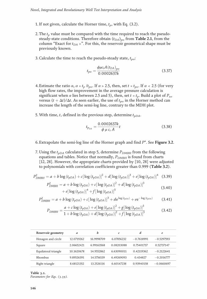
1. If not given, calculate the Horner time, tp, with Eq. (3.2).

2. The tp value must be compared with the time required to reach the pseudo‐steady‐state conditions. Therefore obtain (tDA)pss from Table 2.1, from thecolumn “Exact for tDA >”. For this, the reservoir geometrical shape must bepreviously known.

3.Calculate the time to reach the pseudo‐steady state, tpss:

tpss ¼ϕμctAðtDAÞpss0:0002637k

(3.37)

4.Estimate the ratio α, α = tp /tpss. If α > 2.5, then, set t = tpss. If α < 2.5 (for veryhigh flow rates, the improvement in the average pressure calculation issignificant when α lies between 2.5 and 5), then, set t = tp. Build a plot of Pwsversus (t þ Δt)/Δt. As seen earlier, the use of tpss in the Horner method canincrease the length of the semi‐log line, contrary to the MDH plot.

5.With time, t, defined in the previous step, determine tpDA.

tpDA¼ 0:0002637k

ϕ μ ct At (3.38)

6.Extrapolate the semi‐log line of the Horner graph and find P*. See Figure 3.2.

7. Using the tpDA calculated in step 5, determine PDMBH from the followingequations and tables. Notice that normally, PDMBH is found from charts[12, 28]. However, the appropriate charts provided by [10, 28] were adjustedto polynomials with correlation coefficients greater than 0.999 (Table 3.2).

P2DMBH ¼ aþ b log ðtpDAÞ þ c½ log ðtpDAÞ�2 þ d½ log ðtpDAÞ�3 þ e½ log ðtpDAÞ�4 (3.39)

P2DMBH ¼ aþ b log ðtpDAÞ þ c½ log ðtpDAÞ�2 þ d½ log ðtpDAÞ�3

þ e½ log ðtpDAÞ�4 þ f ½ log ðtpDAÞ�5(3.40)

P2DMBH ¼ aþ b log ðtpDAÞ þ c½ log ðtpDAÞ�3 þ de log ðtpDAÞ þ ee� log ðtpDAÞ (3.41)

PDMBH ¼ aþ c log ðtpDAÞ þ e½ log ðtpDAÞ�2 þ g½ log ðtpDAÞ�31þ b log ðtpDAÞ þ d½ log ðtpDAÞ�2 þ f ½ log ðtpDAÞ�3

(3.42)

Reservoir geometry a b c d e

Hexagon and circle 12.0719262 16.9998709 6.07856232 �0.7618991 �0.5297593

Square 2.06652421 6.99163568 0.08203088 0.75401737 0.52737147

Equilateral triangle 10.1620678 14.9552862 6.63090011 0.42119362 �0.2122641

Rhombus 9.89526391 14.5756539 6.49269093 0.434827 �0.2016777

Right triangle 8.68121352 13.2526116 6.60147238 0.93940158 �0.0660697

Table 3.2.Parameters for Eqs. (3.39).

146


PDMBH ¼ aþ c log ðtpDAÞ þ e½ log ðtpDAÞ�21þ b log ðtpDAÞ þ d½ log ðtpDAÞ�2 þ f ½ log ðtpDAÞ�3

(3.43)

PDMBH ¼ aþ b log ðtpDAÞ þ c½ log ðtpDAÞ�2 þ d½ log ðtpDAÞ�3 þ e½ log ðtpDAÞ�4

þ f ½ log ðtpDAÞ�5 þ g½ log ðtpDAÞ�6 þ h½ log ðtpDAÞ�7 þ i½ log ðtpDAÞ�8

� 0:082557382½ log ðtpDAÞ�9 � 0:012745849½ log ðtpDAÞ�10(3.44)

8.Calculate the average reservoir pressure from:

P ¼ P� � m2:3025

� �PDMDH (3.45)

Due to the compensation factors (low values of P* with corresponding smallcorrections), any value of tp used with the MBH method will theoretically giveidentical results for average reservoir pressure. Practically, a relatively short tp caneliminate serious numerical problems in the calculation of average pressure. Thisincludes errors caused by long extrapolations and deviations from theoreticalassumptions: (1) lack of stabilization of the flow rate prior to closure, (2) migrationand change of drainage areas in reservoirs with multiple wells and (3) variations inthe compressibility of the system and mobility [12, 28].

3.4.4 Dietz method

This method [12, 28]‐assumes that the well flowed sufficiently until it reachedthe pseudo‐steady‐state period before shutting‐in and that the semi‐log straightdeveloped properly. This method is simple and is usually preferred in wells withoutsignificant skin factor, s > �3 or rw 0 = 0.05 re. The procedure for this method is:

1. Knowing the reservoir shape and the well location, read CA from Table 2.1.

2. Calculate the Dietz shutting‐in time, ðΔtÞP.

ΔtP ¼ ϕμctA0:0002637CAk

(3.46)

3. Prepare a MDH plot (optionally find k and s).

4.Enter the MDH plot with the Dietz shutting‐in time calculated in step 2 andread the corresponding average reservoir pressure value on the semi‐logstraight line.

3.4.5 Miller‐Dietz‐Hutchinson (MDH) method

This was elaborated to estimate the average pressure in circular or square reser-voirs. It is applied only in wells that operate under pseudo‐steady‐state conditions[8, 28]. The procedure is presented as follows:

1. On an MDH graph, choose any point on the semi‐log trend and read itscoordinates, (Pws)N and ΔtN.

147


ΔtDAjN ¼ 0:0002637kϕμctA

ΔtN (3.47)

2. Calculate ΔtDA.

3.Determine PDMDH corresponding to (ΔtDA)N. This was traditionally done oncharts. Again, fitted polynomials are presented here.

PDMDH ¼ aþ bΔtDA þ cΔt2DA ln ðΔtDAÞ þ d½ ln ðΔtDAÞ�2 þ e ln ðΔtDAÞ (3.48)

4.Calculate the average reservoir pressure from Table 3.3:

P ¼ PwsjN þ m1:1513

� �PD MDH (3.49)

3.4.6 Ramey‐Cobb method

They presented a method to extrapolate the average pressure of a Horner plotwhen t ≥ tpss|. This method [12, 28, 40] requires information on the shape of thedrainage area, the location of the well, and the confirmation that the boundaries areclosed. The Ramey‐Cobb procedure is (Table 3.4):

1. Knowing the reservoir shape and the well location, obtain (tDA)pss, andcalculate tp and tpss.

tpss ¼ϕ μ ctAðtDAÞpss0:0002637k

(3.50)

2. If tp < tpss, then, the method is not reliable. Calculate the Horner timecorresponding to the average reservoir pressure.

tp þ ΔtΔt

� �P¼ 0:0002637kCA

ϕμctAtP ¼ CAtpDA (3.51)

When (tp þ Δt) = tp, Eq. (3.51) reduces to Eq. (3.46).

3. Prepare a Horner plot (optionally find k and s) (Tables 3.5 and 3.6).

4.Enter the Horner plot with the result from Eq. (3.51) and read the averagereservoir pressure on the straight line trend.

Reservoirgeometry

a b c d e f Equationnumber

11.3521634 16.1909297 6.18077696 �0.4318785 �0.4463139 0 (3.39)

6.51259739 11.7744452 6.73932956 0.04016071 �1.1494588 ‐0.2753853 (3.40)

1.94527256 5.8770907 5.91449487 1.72037863 �0.3879657 ‐0.1920816

0.03487786 ‐5.9476006 �1.7074107 4.59461702 �3.5455711 0 (3.41)

Table 3.3.Parameters for Eqs. (3.39)–(3.41).

148


Reservo

irge

ometry

ab

cd

ef

gEqu

ationnu

mbe

r

8.6598

8165

13.520

0374

6.80

1766

250.89

4660

84�0

.103

974

00

(3.39)

5.40

959238

11.624

314

7.43

9599

27�0

.126

5869

�1.6111914

�0.402

4905

0(3.40)

1.5786

2998

1.36

493165

4.38

0066

891.68

9494

996.42

0190

58�0

.220

711

2.40

1439

18(3.42)

1.121849

580.42

9101

052.8162

6528

0.14

8324

391.03

977832

�0.136

8335

0(3.43)

0.7530

2615

0.532368

012.38

3842

740.7187976

2.48

6766

28�0

.21808

520.6742

364

(3.42)

‐0.51843

360.731805

681.38

5083

460.93

697751

2.5764

2261

�0.338

9924

0.781949

03(3.42)

Tab

le3.4.

ParametersforEqs.(

3.39

)–(3.42).

149


Reservo

irge

ometry

ab

cd

ef

gh

iEqu

ationnu

mbe

r

1.70

317185

0.70

756769

3.57593515

0.50

721899

2.93

9603

140.02

349566

0.7610

7064

00

(3.42)

1.06

3407

392

0.30

4229597

2.66

8344

404

0.42

7947

675

1.1666

4094

�0.276857388

00

0(3.43)

0.9169

32173

1.03

0678375

3.271385125

0.78598580

23.3536

25853

�0.21393

5954

0.89

4001

955

00

(3.42)

�1.02596

7698

0.2307

67114

�0.33785184

1.61153108

12.7641

60677

�0.020

4684

11.191846

817

00

(3.42)

�1.690

4466

15�0

.29574

1667

3.877346

514

1.592302

604

�3.6753563

43�2

.030

985974

1.40

5207

073

1.1202

4680

80.06

4244

461

(3.44)

Tab

le3.5.

ParametersforEq.

(3.42)

–(3.44).

150


3.4.7 Arari or direct method

Arari [4] presented in 1987 a simple method to calculate the average reservoirpressure during production or buildup without the help of any graph. This methodrequires knowing the distance from the well to which the reservoir pressure is thesame average pressure. For no‐flow boundary reservoirs:

P ¼ Pwfþ 162:6qμBkh

2 logrerw

� 0:5203þ 0:87s� �

(3.52)


logAr2w

� 1:1224þ 0:87s� �

(3.53)

For constant‐pressure boundary reservoirs:


2 logrerw

� 0:4342þ 0:87s� �

(3.54)

P ¼ Pwf þ 162:6qμBkh

logAr2w

� 1:036þ 0:87s� �

(3.55)

In order to consider different well positions and different reservoir geometries,the flow equations were developed by introducing the Dietz shape geometricalfactors in Eqs. (3.539) and (3.55) which are, respectively, transformed into:


logA

CAr2wþ 0:368þ 0:87s

� �(3.56)

P ¼ Pwf þ 162:6qμBkh

logA

CAr2wþ 0:454þ 0:87s

� �(3.57)

3.4.8 TDS technique

3.4.8.1 Circular reservoirs

For a well in the center of a circular reservoir, the average reservoir pressure isobtained from a log‐log plot of pressure and pressure derivative versus timeaccording to the following expression [7, 29]:

P ¼ Pi �141:2qμB

kh

ðt � ΔP 0ÞpssðΔPÞpss � ðt � ΔP 0Þpss

!ln

rerw

� 34

� �" #(3.58)

Geometry a b c d e

�1.8936132 11.06446069 20.39748447 �0.003556014 0.5555625414

�1.106364859 1.291801492 �0.814213632 �0.002247086 �0.536018398

�1.05158653 �0.382513988 �5.024281518 �0.001277198 �0.514385212

Table 3.6.Parameters for Eq. (3.48).

151


where Piis the initial pressure (in some cases, it can approximate P*), (ΔP)pss and(t*ΔP')pss are the values of (ΔP) and (t*ΔP') in the late straight line of pseudo‐steady‐state period.

3.4.8.2 Naturally fractured reservoirs

For naturally fractured reservoirs with the dimensionless average pressure andthe average reservoir pressure are defined as [29]:

PD ¼ kh141:2qμB

ðP� PwsÞ (3.59)

P ¼ Pwf þ ΔPpss þ ðt � ΔP 0Þpss 1þ 3792:2ϕμctr2wð1� ωÞ2λktpss

!(3.60)

Being ω and λ the naturally fractured reservoir parameters which will bediscussed about in Chapter 6.

P ¼ Pwf þ ΔPpss þ 141:2qμBkh

ðt � ΔP 0ÞpssΔPpss � ðt � ΔP 0Þpss

! ln

rerw

� 34þ 2πr2wð1� ωÞ2

λA

!2666664

3777775 (3.61)

P ¼ Pwf þ ΔPpss þ 141:2qμBkh


! ln

rerw

� 34þ 0:1987CAr2wð1� ωÞ2

λA

!2666664

3777775 (3.62)

If the dimensionless average pressure is defined as [29]:

PD ¼ khðPi � PÞ141:2qμB

(3.63)

The average reservoir pressure is given by [29]:

P ¼ Pi � ðt � ΔP 0Þpss 1þ 3792:2ϕμctr2wð1� ωÞ2λktpss

!(3.64)

P ¼ Pi � 141:2qμBkh


! ln

rerw

� 34þ 2πr2wð1� ωÞ2

λA

!2666664

3777775 (3.65)



! ln

rerw

� 34þ 0:1987CAr2wð1� ωÞ2

λA

!2666664

3777775 (3.66)

152


The Dietz shape factor can be estimated by [7]:

CA¼ 2:2458Ar2w

e

ktpss301:77ϕμctA

ðΔPÞpssðt � ΔP 0Þpss

� 1

!8>>><>>>:

9>>>=>>>;

�1

(3.67)

For a circular geometry with the well at the center, [26�] arrived to the follow-ing expression:

P ¼ Pi � 1:26ðt � ΔP 0Þr � 2ðt � ΔP 0Þr2πr2wð1� ωÞ2

λA

!" #(3.68)

They also assumed that:

PD ¼ 2πtDA (3.69)

and,

2πtDA>>2πr2wð1� ωÞ2

λA(3.70)

After some manipulations, Igbokoyi and Tiab [27] also obtained an expressionfree of the naturally fractured reservoir parameters:

P ¼ Pi � ðt � ΔP 0Þrðt � ΔP 0Þpss

ðΔPwÞpss � ðt � ΔP 0Þpss

!ln

2:2458ACAr2w

� �þ 2s

" #(3.71)

3.4.8.3 Bounded elongated systems

The shape factor is given by Eq. (3.67), and the average reservoir pressureequation for these systems is given below [7]:


ðt � ΔP 0ÞpssðΔPwÞpss � ðt � ΔP 0Þpss

!ln

2:2458ACAr2w

� �" #(3.72)

3.4.8.4 Hydraulically fractured vertical well in no‐flow boundary reservoirs

The shape factor is estimated with Eq. (3.67), and the average reservoir pressurewith Eq. (3.69) [7]:

P ¼ Pi �qμBkh

0:23373ktpssϕμctA

ðΔPÞpssðt � ΔP 0Þpss

!� 70:6 ln

xexf

!22:2458CA

� �24

35

8<:

9=; (3.73)

When birradial flow occurs, the area and the average reservoir pressure can bedetermined from the following equations [7]:

A ¼ kBRpssi142:43ϕμctðxe=xf Þ1:123

(3.74)

153



xexf

!0:72k

ϕμctA

� �0:3624

35t0:36BRpssi (3.75)

For uniform flow fractures and when xe/xf < 8, birradial flow is difficult tobe observed, then the intersection between the linear flow and the pseudo‐steady state line, tLpssi, is used. Then, the area and the average pressure areobtained from:

A ¼ 0:0033144k

ϕμct

� �xfxe

� �2" #

tLpssi (3.76)

P ¼ Pi � 4:06qB

ffiffiffiμ

p

hffiffiffiffiffiffiffiffiffiϕctk

p xexf

!" # ffiffiffiffiffiffiffiffiffitLpssi

q(3.77)

3.4.8.5 Hydraulically fractured vertical wells in elongated systems

For these systems, the transition between the line of infinite behavior and that ofthe pseudo‐steady‐state period is longer compared to the case of square systems inboth cases of fracture: infinite conductivity and uniform flux. When the birradialflow line is difficult to be observed, such is the case of xe/xf < 8, the followingequation is used to determine permeability [7]:

k ¼ μ

ϕctA

� �8:128qB

hðt � ΔP0ÞDL1

� �2(3.78)

Since there may be two linear flow regimes, once before radial flowcorresponding to flow from the formation to the fracture and the other once radialvanishes, then, (t*ΔP')DL1 is the value of (t*ΔP') at t = 1 hr on the dual‐linear flowregime—solving for area it yields [7]:

A ¼ μ

ϕctk

� �8:128qB

hðt � ΔP0ÞDL1

� �2(3.79)

The point of intersection between the closest parallel‐linear line flow: thesecond linear flow regime, for example, dual‐linear and the pseudo‐steady‐stateline, tDLpssi, is unique. With this point, determine the area of the followingequation [7]:

A ¼ ktDLpssi

1207:09ϕμct(3.80)

This equation should be used for verification purposes of the permeability andarea values obtained by Eqs. (3.78) and (3.79). The average reservoir pressure isobtained from [7]:

P¼ Pi �qBh

ffiffiffiffiffiffiffiffiffiffiffiffiffiffiffiffiffiffiffiffiffiffiffiffiffiffiffiffiffiffiffiffiffiffiffiffiffiffiffiffiffiffiffiffiffiffiμ

11913:6ϕctkA

� �tDLpssi

s(3.81)

This equation should be used if k and A can be determined from the nearestparallel boundary; in other words, from the dual‐linear flow regime.

154


3.4.9 Total average reservoir pressure

Golan and Whitson [24] presented a method to estimate the drainage area ofwells that produce from a common reservoir. They assumed that the volumedrained by a well is proportional to its flow rate. If the properties of the reservoirsare constant and uniform:

Aw ¼ ATqwqT

� �(3.82)

All of the above studied methodologies give the value of the average reservoirpressure in the well drainage area. If a number of wells produce from the samereservoir, each well is analyzed separately to give the average reservoir pressure forits own drainage area. The average reservoir pressure can be estimated from theindividual average pressures by (possibly from [38] less probably from [9, 24], theauthor does not remember the exact reference):

P ¼ ∑i½PiΔðFÞ=ΔP�i∑i½ΔðFÞ=ΔP�i

(3.83)

ΔðFÞ ¼ FtþΔt þ Ft (3.84)

FtþΔt ¼ðtþΔt

0qoBo þ qwBw þ ðqg � qoRs � qwRswÞBg

h i dt (3.85)

Ft ¼ðt0

qoBo þ qwBw þ ðqg � qoRs � qwRswÞBg

h i dt (3.86)

Bossie‐Codreanu [5] suggest that the drainage area can be determined from aHorner or MDH plot by selecting the 3‐point coordinates in the straight section ofthe semi‐log graph to determine the slope of the pseudo‐steady‐state period line,m*:

• Shutting‐in time Δt1 with corresponding shutting‐in pressure Pws1



The selected shutting‐in times satisfy t1 <t2 < t3. Then, m* is approximated by:

m� ¼ ðPws2 � Pws1Þ log ðΔt3=Δt1Þ � ðPws3 � Pws1Þ log ðΔt2=Δt1ÞðΔt3 � Δt1Þ log ðΔt2Δt1Þ � ðΔt2 � Δt1Þ log ðΔt3Δt1Þ (3.87)

Example 3.2

The data of a pressure buildup test, taken from [40], are reported in Table 3.7,along the Horner time and the pressure derivative estimated (using equivalent time,Eq. (3.23)) with a smooth value of 0.1 cycles. The reservoir properties wereobtained from a well located in the center of a square shaped reservoir. Given thefollowing data:

rw=4 in, h = 44 ft, ϕ = 12%μ = 0.76 cp, B = 1.24 rb/STB, Np = 4550 STBA = 40 acres, q = 340 BPD, ct= 36�10�6 psia�1

Pwf = 2980 psia

155


It is required to estimate reservoir permeability and skin factor. Then, find theaverage reservoir pressure using all the studied methods.

Solution

Find tp with Eq. (3.2);

tp ¼24Np

q¼ ð24Þð4550Þ

340¼ 321:176 hr

Estimate the Horner time, (tpþΔt)/Δt, for each pressure value. This is reportedin the third column of Table 3.7 and builds the Horner plot given in Figure 3.8.From the Horner plot given in Figure 3.8, the slope and intercept are read to be 44psia/cycle and 3306 psia. They are, respectively, used to find permeability,Eq. (2.33), and skin factor, Eq. (3.6), thus:

k ¼ 162:6qμBmh

¼ ð162:6Þð340Þð0:76Þð1:24Þð44Þð44Þ ¼ 26:91 md

s ¼ 1:15133306� 2980

ð44Þ � log26:91

ð0:12Þð0:76Þð36� 10�6Þð0:333Þ2 !

þ 3:2275

" #¼ 3:18

Δt, hr Pws, psia (tp þ Δt)/Δt (tpss þ Δt)/Δt ΔP, psia t*ΔP', psia

0 2980 0 0

0.1 3100 3213.00 807.450 120 83.41

0.2 3150 1607.00 404.225 170 100.23

0.3 3200 1071.67 269.817 220 110.92

0.5 3250 643.40 162.290 270 85.89

0.75 3275 429.27 108.527 295 59.48

1 3290 322.20 81.645 310 41.84

2 3315 161.60 41.323 335 34.48

3 3325 108.07 27.882 345 22.35

4 3330 81.30 21.161 350 20.29

5 3335 65.24 17.129 355 21.45

7 3342 46.89 12.521 362 21.96

10 3350 33.12 9.065 370 23.97

15 3360 22.41 6.376 380 21.42

20 3364 17.06 5.032 384 14.87

30 3370 11.71 3.688 390 12.65

40 3372 9.03 3.016 392 9.02

50 3374 7.42 2.613 394 8.47

60 3375 6.35 2.344 395 7.14

70 3376 5.59 2.152 396 8.55

80 3377 5.02 2.008 397 9.76

Table 3.7.Pressure buildup test data.

156


Average reservoir pressure by MBH method

Determine (tDA)pss from Table 2.1 for square shaped reservoirs. It is read(tDA)pss = 0.1. Calculate tpss with Eq. (3.37):

tpss ¼ϕμctAðtDAÞpss0:0002637k

¼ ð0:12Þð0:76Þð36� 10�6Þð40Þð43560Þð0:0002637Þð26:91Þ ð0:1Þ ¼ 80:645 hr

Estimate the ratio a = tp /tpss = 312.176/80.645 = 3.982. Since α > 2, then t = tpss.Rebuild the Horner plot as Pws vs. log(tpss þ Δt)/Δt, (see Table 3.7). In Figure 3.9,draw a straight line along the infinite‐acting period (radial flow) and extrapolate toa Horner time of 1. Read the false pressure value, P*=3398 psia.

Find the dimensionless production time using Eq. (3.38):

tpDA ¼ 0:0002637ktϕμctA

¼ ð0:0002637Þð26:91Þð80:645Þð0:12Þð0:76Þð36� 10�6Þð40 � 43560Þ ¼ 0:0999≈0:1

Figure 3.9.Horner plot with tpss for Example 3.2.

Figure 3.8.Horner plot for Example 3.2.

157


Using Eq. (3.39) with data from Table 3.3 (first row), the MBH dimensionlesspressure is PDMBH=1.152. Then, estimate the average reservoir pressure withEq. (3.45).

P ¼ P� �m PDMBH

2:303¼ 3398� ð44Þð1:152Þ

2:303¼ 3376 psia

Average reservoir pressure by Dietz method

Prepare a MDH, Pws vs. log(Δt). See Figure 3.10. Determine the shape factor CA

from Table 2.1 for a well at the center of a square reservoirs. CA = 30.8828. FindDietz shutting‐in time with Eq. (3.46),

ΔtP� ¼ ϕμctA0:0002637kCA

¼ ð0:12Þð0:76Þð36� 10�6Þð40Þð43560Þð0:0002637Þð26:91Þð30:8828Þ ¼ 26:1136 hr

Enter with this value in Figure 3.10 and read an average reservoir pressure of3368 psia.

Average reservoir pressure by Ramey‐Cobb method

Having tp, tpss, and CA from previous methods and since tp >> tpss, then estimateRamey‐Cobb shutting‐in time from Eq. (3.51);

tþ ΔtΔt

� �P¼ ð0:0002637Þð26:91Þð30:8828Þð312:176Þ

ð0:12Þð0:76Þð36� 10�6Þð40Þð43560Þ ¼ 12:299

Enter with this value in the Horner plot, Figure 3.8, and read an average pres-sure value of 3368 psia.

Average reservoir pressure by MDH method

Prepare a MDH plot, Figure 3.10 and choose any convenient point on the semi‐log straight line. For this case, ΔtN = 10 hr and (Pws)N = 3350 psia were chosen.Calculate the dimensionless shutting‐in time using the chosen time in Eq. (3.47):

ΔtDA ¼ 0:0002637kφμctA

� �ΔtN ¼ ð0:0002637Þð26:91Þ

ð0:12Þð0:76Þð36� 10�6Þð40Þð43560Þ ð10Þ ¼ 0:0124

Figure 3.10.MDH plot for Example 3.2.

158


Use this value of ΔtDA and estimate PDMDH from Eq. (3.48) and Table 3.6 for ano‐flow boundary square reservoir (first row), this gives PDMDH = 0.6. Estimate theaverage reservoir pressure with Eq. (3.49);

P ¼ PwsN þmðPDMDHÞ1:1513

¼ 3350þ 44ð0:6Þ1:1513

¼ 3372:9 psia

Average reservoir pressure by direct (Arari) method

Using Eq. (3.53), for no‐flow boundaries;

P ¼ 2980þ162:6ð340Þð0:76Þð1:24Þ

ð23:52Þð44Þð log 40ð43560Þ

0:3332� 1:1224þ 0:87ð1:93ÞÞ

26664

37775 ¼ 3365:2 psia

Average reservoir pressure by TDS technique

The pressure and pressure derivative versus time log‐log plot for Example 3.2 isgiven in Figure 3.11. Notice that after radial flow, the pressure derivative takes aslope of negative one. This may be due to the changes in transmissibility. Anyhow,the pseudo‐steady‐state period starts at 60 hr. On that line, a point will be chosenfor the estimation of the average reservoir pressure. From this plot, the followingdata are read:

tr = 7 hr, ΔPr = 396 psia, (t*ΔP 0)pss = 8.55 psiaΔPpss = 384 psia, tpss = 70 h, (t*ΔP 0)r = 21.86 psia

Estimate permeability and skin factor with Eqs. (2.71) and (2.92),

k ¼ 70:6qμBhðt � ΔP 0Þr

¼ ð70:6Þð340Þð0:76Þð1:24Þ44ð21:86Þ ¼ 23:52 md

s ¼ 0:536221:86

� ln23:52ð7Þ

ð0:12Þð0:76Þð36� 10�6Þð0:32Þ

� �þ 7:43

� �¼ 1:93

Figure 3.11.Log‐log plot of pressure and pressure derivative against time for Example 3.2.

159


Taking the case of no‐flow boundary rectangular system, Eqs. (3.67) and (3.72),find the shape factor and the average reservoir pressure. Here, the last pressurevalue, that is, 3377 psia, is taken as Pi.

CA ¼ 2:2458ð40Þð43560Þ0:3332

exp

0:003314ð23:52Þð20Þ0:12ð0:76Þð30� 10�6Þð40Þð43560Þ

3968:55

� 1� �� 8><

>:9>=>;

�1

¼ 12:943

P ¼ 3377 � 70:6ð340Þð0:76Þð1:24Þ

ð23:52Þð44Þ

8:55

396� 8:55

!

ln

2:2458ð40Þð43560Þ12:943ð0:3332Þ

!2666664

3777775 ¼ 3369:9 psia

The results of the estimation of the average reservoir pressure are reported inTable 3.8.

3.4.10 Average reservoir pressure in naturally fractured reservoirs fromtransient‐rate analysis

Amin et al. [2] follow the philosophy of the TDS technique to determine theaverage reservoir pressure from TRA (even though, this book does not include suchanalysis) by means of the following expression (slight simplification is shown here):

P ¼ Pi � 887:186qμBkh

kf tpss3792:19ðϕctÞmþfμ

!þ r2wð1� ωÞ2

λA

!" #(3.88)

Amin et al. [2] pointed out that from a curve of production rate versus time, apoint qpss and tpss that satisfy tD > ω(1�ω)/λ (pseudo‐steady‐state period). In addi-tion, qpss and tpss selected should be those when the flow rate becomes almostconstant.

3.4.11 Average reservoir pressure from two‐rate tests

Sabet [33] and Dake [10] presented the mathematical development to find theaverage reservoir pressure from two‐rate tests. The final equation uses the value ofthe first semi‐log straight line and the well‐flowing pressure after the flow rate hasbeen changed. It is given by:

P ¼ 2m1 log2:241ACAr2w

� �2

þ 0:435s

( )þ Pwf@Δt0¼0 (3.89)

Example 3.3

Sabet [34] presented a two‐rate test which pressure versus time values areshown in Table 3.9. To interpret the test, the following reservoir information, PVT,and flow parameters are given:

re = 745 ft rw = 0.25 ft f = 15% h = 20 ft

m = 1.2 cp ct = 20�10�6psia�1 B = 1.25 bbl/STB tp = 300 hr

q1 = 100 STB/D q2 = 50STB/D Pwf@Dt'=0 = 1603.2 psia

160


Determine average reservoir pressure, skin factor, and demonstrate that the testhas not reached the transient period when the flow rate was changed.

Solution

A value of m1 = 274 psia/cycle and P1hr = 2485 psia were read from the Cartesiangraph presented in Figure 3.12. Permeability and skin factors are calculated withEqs. (2.271) and (2.272), respectively, and were found to be 4.5 md and

Before flow rate change After flow rate change

t, hr Pwf, psia t, hr Pwf, psia Dt’

288 1607.5 0.33 2475 2.72

289 1607.2 0.42 2482 2.67

290 1606.8 0.5 2487 2.63

291 1606.4 0.58 2492 2.6

292 1606.1 0.67 2497 2.56

293 1605.7 0.75 2500 2.54

294 1605.4 0.83 2502 2.52

295 1605 0.92 2505 2.5

296 1604.6 1 2508 2.48

297 1604.3 1.25 2514 2.43

298 1603.9 1.5 2520 2.39

299 1603.6 1.75 2525 2.36

300 1603.2 2 2531 2.33

2.5 2542 2.28

3 2552 2.24

4 2568 2.18

5 2582 2.13

6 2590 2.1

7 2600 2.06

7.5 2604 2.05

Table 3.9.Two‐rate test data for Example 3.3, after [34].

Method Average reservoir pressure, psia

Ramey & Cobb 3368

MBH 3376

MDH 3372.9

Dietz 3368

TDS 3371.4

Arari 3365.2

Average 3370.25

Table 3.8.Summary of average reservoir pressure results.

161


approximately 3.0. The time to reach the pseudo‐steady‐state period in the test isestimated with Eq. (2.40) with r = re, as follows:

tpss ¼ 948 ϕμ ctr2

k¼ 948ð0:15Þð1:2Þð20� 10�6Þð7452Þ

4:5¼ 420 hr

Assuming the well is in the center of a rectangular or circular reservoir, it ispossible to appreciate the change (t = 300 hr) occurred before reaching the pseudo‐steady‐state conditions. Eq. (3.89) is used to calculate the average reservoir pres-sure, thus:

P ¼ 325:2ð100Þð1:2Þð1:25Þð84:5Þð20Þ log

0:472ð745Þ0:33

þ 0:87ð274Þð3Þ þ 1603:2 ¼ 2405:8 psi

Note that the average pressure value is not correct (it was obtained for explan-atory effects) because the well was not producing under pseudo‐steady‐state periodbefore changing to the second rate.

3.4.12 Average reservoir pressure from multi‐rate tests

For this type of tests, it is necessary to construct a Cartesian graph of pressureagainst the superposition time, Xn, Eq. (2.267), to obtain permeability and damage.Then, an MDH graph is made, and the Dietz method is applied. For this, it isnecessary to determine the Dietz shutting‐in time by Eq. (3.46). With this value, theaverage reservoir pressure is read from the MDH plot. Actually, it is possible, then,to apply any of the average pressure methods seen in this chapter. However, forsome of the methods, that is, MBH and Ramey‐Cobb, the production time, tp, isrequired. By definition, it refers to a constant flow rate before shutting‐in the well.It does not exist in this case. So, as a recommendation, the equivalent time should beestimated with Eq. (2.269) and this can be used as tp, and the flow rate is weightedwith each period of duration.

However,TDS technique plays an important role. Escobar [15] obtained theaverage pressure equation for circular systems as given below.

Figure 3.12.Cartesian plot for two‐rate test of Example 3.3.

162


P ¼ Pi � 141:2qnμBkh

ðt � ΔPq0Þpss

ðΔPqÞpss � ðt � ΔPq0Þpss

!ln

rerw

� 0:75� �" #

(3.90)

where Piis the initial pressure. (ΔPq)pss and (t*ΔPq')pss are the correspondingnormalized pressure values and their derivative given at an arbitrary time, tpss. Forany geometry, the resulting equation is [15]:


ðt � ΔPq0Þpss


!ln

2:2458ACAr2w

� �" #(3.91)

where CA is found from a slight modification of Eq. (3.67):

CA¼ 2:2458Ar2w

e

ktpss301:77ϕμctA

ðΔPqÞpssðt � ΔPq

0Þpss� 1

!8>>><>>>:

9>>>=>>>;

�1

(3.92)

For multi‐rate tests in naturally fractured reservoirs, the respective equations[15] are:


ðt � ΔPq0Þpss


lnrerw

� 0:75þ 2r2wð1� ωÞ2λr2e

!" #

(3.93)


ðt � ΔPq0Þpss


lnrerw

� 0:75þ 0:198CAr2wð1� ωÞ2λA

!" #

(3.94)

Example 3.4

This actual field example presented by Escobar [15] comprises two pressure testsperformed on an exploratory well in a reservoir which is believed to possess anapproximated circular shape. A pressure buildup test, Table 3.10, was run so thatthe average reservoir pressure can be determined by conventional methods. Pro-duction was inactive during the following eight months; then, a multi‐rate test wasperformed. Its data are given in Table 3.11. The well had produced 190000 STB at aflow rate of 305 BPD before shut‐in it for the pressure buildup test. The well dataand properties of rock and fluid are as follows:

rw = 0.33 ft, ϕ = 13%, h = 80 ftμ = 0.9 cp, ct = 1.9 � 10�5 psia�1 B = 1.3 bbl/STBA = 62 Ac, Pwf (t = 0) = 2143.4 psia, for the pressure buildup testPi = 2554 psia, for the multi‐rate test.

It is required to estimate the average pressure test from the buildup test usingthe MBH method and from the multi‐rate test using the TDS technique.

Solution by MBH method

The production time, tp, resulted to be 14950.8 hr with Eq. (3.2). From theHorner plot given in Figure 3.13, the slope and intercept are read to be 57 psia/cycleand 2427 psia. Permeability is found with Eq. (2.33) and skin factor with Eq. (3.6),

163


k ¼ 162:6qμBmh

¼ ð162:6Þð305Þð0:9Þð1:3Þð57Þð80Þ ¼ 26:72 md

s ¼ 1:15132427 � 2143:4

57� log

12:7

ð0:13Þð0:9Þð1:9� 10�5Þð0:33Þ2 !

þ 3:2275

" #¼ 0:56

For the given reservoir, (tDA)pss from Table 2.1 is 0.1. Next, tpss = 179.3 hr fromEq. (3.37) and α ratio is, α = tp/tpss = 14950.8/179.3= 80.3; then, set t = tpss = 179.3.With this value, a new Horner plot is built and provided in Figure 3.14, from whichP* = 3580 psia. Now, determine the dimensionless production time using Eq. (3.38):

tpDA ¼ 0:0002637ktϕμctA

¼ ð0:0002637Þð12:7Þð179:3Þð0:13Þð0:9Þð1:9� 10�5Þð62Þð43560Þ ¼ 0:1

Using Eq. (3.39) with data from Table 3.3 (first row), the MBH dimensionlesspressure is PDMBH =1.175. The average reservoir pressure is found with Eq. (3.45).

Δt, hr Pws, psia ΔPws, psia (Δt þ tp)/Δt (tpss þ Δt)/Δt

0 2143.4 0

0.013 2167.8 24.4 1150062.54 13793.31

0.019 2195.5 52.1 786885.21 9437.84

0.028 2229.8 86.4 533958.14 6404.57

0.037 2265.6 122.2 404076.68 4846.95

0.056 2302.3 158.9 266979.57 3202.79

0.067 2323.5 180.1 223147.27 2677.12

0.079 2341.4 198.0 189251.63 2270.62

0.112 2361.0 217.6 133490.29 1601.89

0.153 2375.6 232.3 97718.65 1172.90

0.214 2389.5 246.1 69864.55 838.85

0.329 2401.7 258.3 45444.16 545.98

0.479 2411.5 268.1 31213.53 375.32

0.608 2416.8 273.4 24591.13 295.90

0.840 2425.4 282.0 17799.57 214.45

1.099 2432.7 289.3 13605.00 164.15

1.486 2437.6 294.2 10062.10 121.66

1.988 2444.9 301.5 7521.52 91.19

2.660 2448.2 304.8 5621.60 68.41

3.482 2455.0 311.6 4294.74 52.49

4.510 2465.3 321.9 3316.03 40.76

5.535 2472.6 329.2 2702.14 33.39

6.506 2479.8 336.4 2299.00 28.56

7.648 2487.3 343.9 1955.86 24.44

Table 3.10.Pressure buildup test data for Example 3.4.

164


t, hr teq, hr ΔPq, psia/(STB/D) t*ΔP’q, psia/(STB/D) teq*ΔP’q, psia/(STB/D) qn,STB/D

0.203 0.214 1.7907 1.2485 1.2969 296

0.253 0.262 2.2985 1.6026 1.6819 295

0.328 0.314 2.9504 2.0571 2.0251 293

0.436 0.456 4.3507 2.2356 2.1813 291

0.602 0.621 5.7416 2.2356 2.0251 292

0.875 0.902 7.1684 1.5587 1.5046 290

1.289 1.327 8.2350 1.1174 1.0771 286

1.924 1.903 9.2014 0.8010 0.7159 285

2.622 2.693 10.0000 0.5742 0.4938 281

3.621 3.762 10.2813 0.4473 0.3808 279

5.335 5.534 10.2813 0.3119 0.2936 278

8.064 8.245 10.2813 0.2001 0.1951 274

13.691 14.336 10.5705 0.1149 0.1000 270

19.910 19.774 10.5705 0.0779 0.0716 266

29.710 30.231 10.5705 0.0920 0.0895 265

44.909 44.468 10.5705 0.0758 0.0743 263

61.223 62.129 10.5705 0.0870 0.0743 258

89.029 89.068 10.8679 0.0823 0.0831 256

124.545 123.500 10.5705 0.1117 0.1136 255

161.241 161.230 10.8679 0.1357 0.1296 253

211.463 211.963 10.8679 0.1648 0.1548 251

Table 3.11.Multi‐rate test data for Example 3.4.

Figure 3.13.Horner plot for Example 3.4.

165


P ¼ P� �m PDMBH

2:303¼ 2580

ð57Þð1:175Þ2:303

¼ 2550:9 psia

Solution by the TDS technique

The following information is read from the pressure derivative plot, Figure 3.15,

(t*ΔP'q)r = 0.087 psia/BPD, (ΔPq)r = 10.86 psia/BPD, (teq)pss = 211.963 hr(t*ΔP'q)pss = 0.1548 psia/BPD, (ΔPq)pss = 10.86 psia/BPD

Permeability is found from Eq. (2.279), and the average reservoir pressure withEq. (3.90);

k ¼ 70:6μBhðt � ΔP 0

qÞr¼ 70:6ð0:9Þð1:3Þ

ð80Þð0:087Þ ¼ 11:8 md

Figure 3.14.Horner plot with tpss for Example 3.4.

Figure 3.15.Normalized pressure and pressure derivative versus equivalent time log‐log plot for Example 3.4.

166


P ¼ 2554� 141:2ð251Þð0:9Þð1:3Þð11:8Þð80Þ

0:1648

10:86� 0:1648

! ln

927:180:33

!� 34

!2666664

3777775 ¼ 2549:1 psia

Escobar [15] reports the results of this example, Table 3.12, along with thosefrom other methods already seen in this chapter. It is observed a very close agree-ment among the results.

3.4.13. Other methods for estimating the average reservoir pressure

The average pressure can also be estimated using material balance [37],

P ¼ Pi � 5:615q � tctVp

; Vp in ft3 (3.95)

Another formulation to calculate the average reservoir pressure [37] is basedupon integrating the reservoir pressure and the volume, thus:

P ¼ ∑PrΔVV

(3.96)

If ΔV is replaced as 2πrΔrhϕ and the pseudo‐steady‐state solution of the radialflow equation and after several manipulations will give:

P ¼ Pw þ 0:8687m lnrerw

� 0:75� �

þ ΔPs (3.97)

For wells that are in steady state at the time of shutting‐in, constant 0.75 ischanged by 0.5.

Slider [37] proposed an equation for the case where there is interference withother wells which includes obtaining the static pressure by extrapolating orcorrecting the pressure at a time equal to the stabilization time or time to reach thepseudo‐steady state, so that:

ΔPq ¼ pw � Pwf þm � Δt (3.98)

Type of test Method Average reservoir pressure, psia

Buildup MBH(Matthews‐Brons‐Hazebroek)

2550.9

Buildup Dietz 2542.6*

Buildup Ramey‐Cobb 2538.2*

Buildup MDH(Miller‐Dyes‐Hutchinson)

2537.3*

Buildup Azari 2535.4*

Multi‐rate TDS 2549.1

*Reported in [15].

Table 3.12.Comparison of results for Example 3.4, after [15].

167


According to Eqs. (1.130) and (2.40) (with the permeability in Darcies), theabove equation becomes:

P ¼ Pwf � 0:04ϕμctr2ek

1:79qϕhctr2e

þ ΔPq�

tpss(3.99)

Rearranging:

P ¼ Pwf � 0:439mþ ðΔPqÞtpss (3.100)

In summary, Slider [37] recommends the following methods for the determina-tion of the average reservoir pressure at the shut‐in time:

1. If the well is not acting under either steady or pseudo‐steady state, use materialbalance, Eq. (3.95). This includes wells under infinite behavior or in transitionbetween infinite behavior and steady or pseudo‐steady state.

2. If the well is in the center of its drainage area and is in either a steady orpseudo‐steady state, use Eq. (3.97), which does not require knowing either theporosity or the compressibility.

3. If the well is located near the center of its drain area and is operating underpseudo‐steady state and the change in pressure with respect to time, m*, isknown, Eq. (3.100) can be used.

4.If the well is off‐center within the drain area and operates under pseudo‐stablestate but m* is unknown, the MBH method is recommended by Slider [37].

5. None of the methods are recommended for a well that is off‐center andoperates in steady‐state conditions at shut‐in time.

6.The above recommendations were produced when the pressure derivative didnot exist. As could be seen,TDS technique is much more practical, and it is notlimited to a few shape factors since this parameter is easily found with thetechnique. Also,TDS applies involve equations for fractured wells, horizontalwells (although not given here), and naturally fractured reservoirs. Since drillsteam testing, DST consists of some small periods of buildup and drawdown,Chapters 2 and 3 apply to DST.

Nomenclature

A area, ft2

AT total field drainage area, AcresAw well drainage area, AcresBg gas volume factor, ft3/STBBo oil volume factor, bbl/STBBw oil volume factor, bbl/STBb fraction of penetration/completionbDLF intercept of P‐vs.‐t0.25 plot during dual‐linear flow, psia0.5

bLF intercept of P‐vs.‐t0.5 plot during hemilinear flow, psia0.5

bPB intercept of P‐vs‐1/t0.5 plot during hemilinear flow, hr�1

bx distance from closer lateral boundary to well along the x‐direction, ft

168


by distance from closer lateral boundary to well along the y‐direction, ftc compressibility, 1/psiaC wellbore storage coefficient, bbl/psiaCA reservoir shape factorct total or system compressibility, 1/psiaDF damage factorDR damage ratioFE flow indexf(t) time functionh formation thickness, fthp length of perforations, ftI interceptJ productivity index, bbl/psiak permeability, mdkg gas effective permeability, mdko oil effective permeability, mdkw water effective permeability, mdIDcsg internal casing diameter, inNp oil produced since last stabilization, bblm slope of P‐vs.‐log t plot, psia/hr/cyclem* slope of P‐vs.‐t plot, psia/hrmDLF slope of P‐vs.‐t0.25 plot during dual‐linear flow, psia0.5/hrmLF slope of P‐vs.‐t0.5 plot during hemilinear flow, psia0.5/hrmPB slope of P‐vs.‐1/t0.5 plot during hemilinear flow, (psia0.5/hr)�1

m' slope of superposition or equivalent time plot, psia/BPD/cyclem‘b’ intercept of superposition or equivalent time plot, psia/BPD/cyclem(P) pseudopressure, psia/cpODcsg external casing diameter, inP pressure, psiaP average reservoir pressure, psiaPD 0 dimensionless pressure derivativePD dimensionless pressurePi initial reservoir pressure, psiaPR productivity ratioPr reservoir pressure, psiaPt shut‐in casing pressure, psiaPwf well flowing pressure, psiaPws well shut‐in or static pressure, psiaP1hr intercept of the semi‐log plot, psiaP* false pressure, psiaΔPs pressure drop due to skin conditions, psiaq liquid flow rate, BPDqT total field flow rate, BPDqw well flow rate, BPDqsc gas flow rate, Mscf/DrD dimensionless radiusr radius, ftre drainage or external radius, ftRs gas dissolved in oil, scf/STBrw well radius, fts skin factorsc skin due to partial penetrationscp skin due to a change in permeability

169


sDL geometrical skin factor converging from radial to dual‐linear flowsL geometrical skin factor converging from dual‐linear to linear flowsp skin factor due to the restricted flow entrysPB geometrical skin factor converging from dual‐linear to parabolic flowst total skin factorsθ skin factor resulting from a well deviation angleT reservoir temperature, ºR, transmissivity, md‐ft/cpt time, hrtp production (Horner) time before shutting‐in a well, hrtD dimensionless time based on well radiustDA dimensionless time based on reservoir areat*ΔP 0 pressure derivative, psiaV volume, ft3

Vu wellbore volume/unit length, bbl/ftX distance in the x‐directionXE reservoir length, ftXN superposition time, hrY distance in the y‐directionYE reservoir width, ftWD dimensionless reservoir widthZ height, ft

Greek

Δt change, drop, hut‐in time, hrΔt 0 flow time after rate change in two‐rate testsϕ porosity, fractionλ mobility, md/cp. Also, interporosity flow coefficientρ fluid density, lbm/ft3θ deviation angle, o

ψ measured deviation angle, o

ψ 0 corrected deviation angle, o

μ viscosity, cpω dimensionless storativity ratio

Suffices

0 base conditions1hr time of 1 ha actualaf after flowBRpssi birradial and pseudo‐steady‐state lines intersectiond drainageD dimensionlessDA dimensionless with respect to areaDL dual linear flowDL1 dual linear flow at 1 hrDLpssi intersection of pseudo‐steady‐state line with dual‐linear lineDLSS1 intercept between dual‐linear line and the �1‐slope line (SS1)DLSS2 intercept between dual‐linear line and the �1‐slope line (SS2)eq equivalent

170


eBL equivalent bilineareBR equivalent birradialeL equivalent lineareSP equivalent sphericalF inflectiong gash horizontalhs hemisphericali intersection or initial conditionsideal idealINT interceptinv investigationL linear or hemilinear flowL1 linear flow at 1 hrlag lagLpssi intercept of linear and pseudo‐steady state linesN an arbitrary point during early pseudo‐steady‐state periodM muskatMint intercept of Muskatmax maximumo oilp production, porouspDA dimensionless based on area and production timePB parabolic flowPBSS1 intercept between parabolic line and the �1‐slope line (SS1)PBSS2 intercept between parabolic line and the �1‐slope line (SS2)pss pseudo‐steady statepss1 pseudo‐steady state at 1 hrr radial flowrDLi intercept of radial and dual linear linesr1 radial flow before spherical/hemispherical flowrg relative to gasrLi intercept of radial and linear linesro relative to oilrpssi intersection of pseudo‐steady‐state line with radial linerSSi intersection between the radial line and the �1�slope linerSS1i intersection between the radial line and the �1‐slope line (SS1)rSS2i intersection between the radial line and the �1‐slope line (SS2)rw relative to waters skinsf sandfacesp sphericalSS steadySSL start of semi‐log line (radial flow)SS1 �1‐slope line formed when the parabolic flow ends and steady‐state

flow regime starts. Well is near the open boundary, and the farboundary is opened

SS2 �1‐slope line formed when the parabolic flow ends and steady‐stateflow regime starts. Well is near the open boundary, and the farboundary is closed

sw spherical/hemispherical wellborew well, waterwa apparent wellbore

171


wb wellborewD dimensionless emphasizing at wellborewf well flowingwf@Δt 0=0 well flowing at flow rate changews well shut‐inx maximum point (peak) during wellbore storagexc maximum point for centered wellsX1 maximum point between Dual linear and parabolic linesX2 maximum point between parabolic and negative unit slope linesX3 maximum point between hemilinear and negative unit slope linesz vertical direction

172


References

[1] Agarwal RG. A New method toaccount for producing time effectswhen drawdown type curves are used toanalyze pressure buildup and other testdata. Society of Petroleum Engineers.1980. DOI: 10.2118/9289‐MS

[2] Amin D, Iman A, Mohammad F,Riyaz K, Milad J. Application of thetransient rate decline analysis fordetermining average reservoir pressurein naturally fractured reservoirs.Petroleum Exploration andDevelopment. 2015;42:254-258. DOI:10.1016/S1876‐3804(15)30013‐6

[3] Anderson D, Jordan CL, Mattar L.Why plot the equivalent time derivativeon shut‐in time coordinates?. Society ofPetroleum Engineers. 2002. DOI:10.2118/75703‐MS

[4] Arari M. Non‐graphical solutions foraverage reservoir pressure fromproduction or buildup data. Society ofPetroleum Engineers. 1987. DOI:10.2118/17049‐MS

[5] Bossie‐Codreanu D. A simple buildupanalysis method to determine welldrainage area and drawdown pressurefor a stabilized well. Society ofPetroleum Engineers. 1989. DOI:10.2118/15977‐PA

[6] Bourdet D, Ayoub JA, Pirard YM.Use of pressure derivative in well testinterpretation. SPE FormationEvaluation; 1989. pp. 293‐302. DOI:10.2118/12777‐PA

[7] Chacon A, Djebrouni A, Tiab D.Determining the average reservoirpressure from vertical and horizontalwell test analysis using the Tiab’s directsynthesis technique. Society ofPetroleum Engineers. 2004. DOI:10.2118/88619‐MS

[8] Cobb WM, Smith JT. Aninvestigation of pressure‐buildup tests

in bounded reservoirs. Society ofPetroleum Engineers. 1975. DOI:10.2118/5133‐PA

[9] Craft BC, Hawkins MF. AppliedReservoir Engineering. New Jersey,USA: Prentice‐Hall International.Englewood Cliffs; 1991. p. 431

[10] Dake LP. The Practice of ReservoirEngineering—Revised edition.Amsterdam, Holland: ElsevierDevelopments in Petroleum Science.2nd Printing; 2004

[11] Dykstra H, Kazemi H, Raghavan R,Gulati MS. Pressure Transient TestingMethods. SPE Reprint Series No. 14,Dallas, Texas: SPE; 1967

[12] Earlougher RC Jr. Advances in WellTest Analysis, Monograph Series Vol. 5.Dallas, TX: SPE; 1977

[13] Escobar FH, Navarrete JM, LosadaHD. Evaluation of pressure derivativealgorithms for well‐test analysis. Societyof Petroleum Engineers. 2004. DOI:10.2118/86936‐MS

[14] Escobar FH, Montealegre MM.Application of TDS technique todeveloped reservoirs. Journal ofPetroleum Science and Engineering.2007;55(3-4):252-258

[15] Escobar FH, Ibagón OE,Montealegre MM. Average reservoirpressure determination forhomogeneous and naturally fracturedformations from multi‐rate testing withthe TDS technique. Journal of PetroleumScience and Engineering. 2007;59:204-212

[16] Escobar FH, Hernández YA,Hernandez CM. Pressure transientanalysis for long homogeneousreservoirs using TDS technique. Journalof Petroleum Science and Engineering.2007;58(1–2):68-82

173


[17] Escobar FH, Tiab D, Tovar LV.Determination of areal anisotropy froma single vertical pressure test andgeological data in elongated reservoirs.Journal of Engineering and AppliedSciences. 2007;2(11):1627-1639

[18] Escobar FH, Hernandez YA, Tiab D.Determination of reservoir drainagearea for constant‐pressure systems usingwell test data. CT&F—Ciencia,Tecnología y Futuro. 2010;4(1):51-72

[19] Escobar FH, Montealegre M,Carrillo‐Moreno D. Straight linemethods for estimating permeability orwidth for two‐zone compositechannelized reservoirs. CT&F—Ciencia, Tecnología y Futuro. 2009;3(5):107-124

[20] Escobar FH, Montealegre MM,Carrillo‐Moreno D. Pressure andpressure derivative transient analysiswithout type‐curve matching forelongated reservoirs with changes inpermeability or width. CT&F—Ciencia,Tecnología y Futuro. 2010;4(1):75-88

[21] Escobar FH, Srivastava P, Wu X.A practical method to determine aquiferleakage factor from well test data inCBM reservoirs. Journal of Engineeringand Applied Sciences. 2015;10(11):4857-4863

[22] Escobar FH, Ghisays‐Ruiz A,Srivastava P. Characterization of thespherical stabilization flow regime bytransient pressure analysis. Journal ofEngineering and Applied Sciences.2007;10(14):5815-5822. ISSN 1819‐6608

[23] Gringarten AC. From straight linesto deconvolution: The evolution of thestate of the art in well test analysis.Society of Petroleum Engineers. SPEFormation Evaluation; 2008. pp. 41‐62.DOI: 10.2118/102079‐PA

[24] Golan M, Whitson CH. WellPerformance. Boston, MA, USA:

International Human ResourcesDevelopment Corp.; 1986. p. 617

[25] Horne RN. Modern Well TestAnalysis: A Computer‐Aided Approach.Palo Alto, CA: Petroway Inc.; 1990.p. 185

[26] Horner DR. Pressure buildup inwells. In: Proceeding Third WorldPetroleum Congress. Leiden,Netherlands. 1951

[27] Igbokoyi AO, Tiab D. Estimation ofaverage reservoir pressure and drainagearea in naturally fractured reservoirs.Society of Petroleum Engineers. 2006.DOI: 10.2118/104060‐MS

[28] Mathews CS, Russell DG. Pressurebuildup and flow tests in wells. SPEMonograph Series. Vol. 1. Dallas, TX:Society of Petroleum Engineers ofAIME; 1967. p. 163

[29] Molina MD, Escobar FH,Montealegre MM, Restrepo DP.Application of the TDS technique fordetermining the average reservoirpressure for vertical wells in naturallyfractured reservoirs. CT&F—Ciencia,Tecnología y Futuro. 2005;2(6):45-55

[30] Mongi A, Tiab D. Application ofTiab’s technique to multi‐rate tests.Society of Petroleum Engineers. 2000.DOI: 10.2118/62607‐MS

[31] Moncada K, Tiab D, Escobar FH,Montealegre MM, Chacon A, ZamoraRA, Nese SL. Determination of verticaland horizontal permeabilities forvertical oil and gas wells with partialcompletion and partial penetrationusing pressure and pressure derivativeplots without type‐curve matching.CT&F—Ciencia, Tecnología y Futuro.2005;2(6)

[32] Muskat M. Use of data oil the build‐up of bottom‐hole pressures.Transactions of AIME. 1937;123:44‐48.DOI: 10.2118/937044‐G

174


[33] Sabet M. Well Testing. Houston,TX, USA: Gulf Publishing Co; 1991.p. 460

[34] Slider HC. Application of pseudo‐steady‐state flow to pressure‐buildupanalysis. 1966. DOI: 10.2118/1403‐MS

[35] Slider HC. A Simplified method forpressure buildup analysis for a stabilizedwell. Journal of Petroleum Technology.1971:1155-1160

[36] Slider HC. A Simplified method ofpressure buildup analysis for a stabilizedwell. Society of Petroleum Engineers.1967. DOI: 10.2118/1765‐MS

[37] Slider HC. Worldwide PracticalPetroleum Reservoir EngineeringMethods. Revised Edition. Tulsa,Oklahoma, USA: PennWell PublishingCo.; 1983. p. 826

[38] Stewart G. Well Test design &Analysis. Tulsa, Oklahoma, USA:PennWell Corporation; 2011. p. 1940

[39] Ramey HR Jr, Cobb WM. A generalpressure buildup theory for a well in aclosed drainage area (includesassociated paper 6563). Society ofPetroleum Engineers. JPT. 1971.pp. 1493‐1505. DOI: 10.2118/3012‐PA

[40] Tiab D. PE‐5553: Well Test analysis.Lecture notes. The University ofOklahoma; 1993

[41] Tiab D. Analysis of pressure andpressure derivative without type‐curvematching: 1‐skin and wellbore storage.Journal of Petroleum Science andEngineering. 1995;12:171-181.

[42] Tiab D. Analysis of pressure andpressure derivatives without type‐curvematching: 1‐skin and wellbore storage.Society of Petroleum Engineers. 1993.DOI: 10.2118/25426‐MS

175


Chapter 4

Distance to Linear Discontinuities

The available pressure analysis methods are based on assumptions of Darcy’slaw, for example, a homogeneous and horizontal formation of uniform thickness,with isotropic and constant porosity and permeability distributions. The issue ofpressure behavior in heterogeneous reservoirs has received considerable attentionin recent years. The main reason for this is the need for greater accuracy in reservoirdescription, which has a significant effect on the design, operation, and therefore,the economic success of the projects involved. Since these methods can be appliedonly once to the reservoir, the need for a reliable description of the reservoir isobvious [5, 6, 13, 22].

Two techniques can be used in the fields to describe reservoirs: radioactivetracers and pressure transient tests. Pressure transient tests have been usedmore (and with better results) than tracers. The determination of the volumetricswept efficiency is a problem that has a better potential to be solved by thetracers. Currently, the description of the heterogeneity of the reservoir byadjusting the tracer behavior is affected by the lack of adequate numericalmodels, the long time spent to obtain the results, and the dependence of theadjustment to the additional parameters that are introduced by tracers themselves(e.g., dispersion coefficients, tracer retention, etc.). It is quite possible that tracersand future pressure transient tests will be used at the same time for the descriptionof the reservoir [6].

Normally, any type of flow barrier cannot be seen in a DST since the time is tooshort to affect deep the reservoir. However, in cases where flow periods are so longto observe deviations from the semilog slope or deviation from the flat trend of thepressure derivative, which reflects changes in reservoir transmissibility, faults,discontinuities, boundary conditions, or reservoir geometry as illustrated inFigure 4.1. Some of the methods for estimating distance to linear boundaries will beshown later [4, 6, 14, 15].

4.1. Types of reservoir discontinuities

The heterogeneities of the reservoir (see Figure 4.1) are variations in rock andfluid properties resulting from deposition, folding, faulting, postdepositionalchanges in reservoir lithology, and changes in properties or types of fluids. Thereservoir heterogeneities of the deposit may be small scale, as in carbonate reser-voirs where the rock has two constituents, matrix and fractures, and cavities andcaves. These can also be larger scale, such as physical barriers, faults, fluid‐fluidcontacts, thickness changes, lithology changes, several layers with different prop-erties in each layer, etc. In addition to these natural heterogeneities, man can induceartificial heterogeneities around wellbore during drilling (mud invasion), hydraulicfracturing, or fluid injection [6].

Another related feature is the anisotropy in the permeability, when this propertyvaries with flow direction. Anisotropy can also be caused by sedimentary processes(filled cannel deposits) or by tectonism (fractures orientated parallel). Anisotropytakes place in both homogeneous and heterogeneous reservoirs. Therefore,

176

anisotropy does not imply heterogeneity. Most reservoirs have vertical permeabilityless than horizontal, so there is anisotropy in that sense [5, 6].

4.2. Single‐boundary systems

Large‐scale heterogeneities can be detected by seismic. However, this techniquecan be up to one mile or more in error when estimating the well‐fault distance.Transient pressure analysis is the cheapest and most accurate form to obtain thedistance from a well to a given barrier. In general, to locate faults [23, 24], a testlong enough to explore the reservoir in depth is required, at least four times thedistance to the fault.

4.2.1 Well‐fault distance from pressure buildup tests

Applying the superposition principle, the dimensionless shut‐in pressure for awell near a p boundary is given, respectively, by [4–25]:

PDS = ½PDð1, ðtp þ ΔtÞDÞ þ s� � ½PDð1, ΔtDÞ þ s�

þ PD2drw

, ðtp þ ΔtÞD� �

� PD2drw

, ΔtD� �

(4.1)

The Ei(�s) easily applies to find wellbore pressure, practically, at any time.Then, it can be applied to the two first terms of Eq. (4.1). For a production time, tp,long enough and for testing times very close to the shut‐in time, the Ei(�) solutioncan be fully applied to find the dimensionless pressure drops of Eq. (4.1), so that:

Figure 4.1Types of discontinuities: (a) no‐flow boundary (fault), (b) change of fluid type, (c) change of formationthickness, and (d) permeability change (facies), after [6].

177

Distance to Linear DiscontinuitiesDOI: http://dx.doi.org/10.5772/intechopen.81078

Pi � Pws =70:6qμB

kh�Ei

�3792ϕμctd2

kΔt

!þ Ei

�3792ϕμctd2

kðtp þ ΔtÞ

!� Ei

�3792ϕμctd2

ktp

!" #

(4.2)

d can be calculated by a trial‐and‐error procedure using the above equation. Thisis exact but tedious. However, whenever tp >> Δt, the logarithmic approach forEi(�x) function applies; therefore, Eq. (4.2) becomes:

Pws =Pi � 325:2qμBkh

logtp þ ΔtΔt

� �(4.3)

Comparison between Eqs. (3.6) and (5.3) shows a doubled slope in the last one.It means that the detection of a fault leads to observe a doubled slope in the Hornerplot since Eq. (4.3) can be expressed as:

Pws =Pi � 2m logtp þ ΔtΔt

� �(4.4)

Once the slope is folded, d can be easily calculated by reading the intercepttime of the straight line of slope m with the slope straight line 2m, as illustrated inFigure 4.2(b) and (c). This behavior is also presented in a graph of drawdown

Figure 4.2Identification of linear boundaries from conventional (semilog) plots: (a) drawdown test—semilog plot,(b) buildup test—Horner plot, (c) buildup test—MDH plot, after [13].

178


pressure test indicated in Figure 4.2(a). However, the slope of a normal pressurebuildup plot will not change at early times. Thus, this early straight line portionwith slope m can be used to calculate k, s, and C as discussed in Chapter 3 sec-tion 3.2. Extrapolation of the double slope straight line is used for the estimation ofthe average reservoir pressure as studied in Chapter 3. Care must be taken since asimilar behavior, double slope, is presented in multirate tests, injection tests, draw-down tests, etc. Different characteristics of the pressure transient may occur when awell is near multiple barriers. For example, when there are two faults intersecting atright angles to one well (one closer to the other), the slope will double and thendoubled again. In general terms, the slopes that are obtained are function of theangles of intersection given by the following equation [20]:

New slope =360θ

m (4.5)

Similarly, the flat lines of radial flow regime will provide another flat pressurederivative line given by:

ðt*ΔP 0ÞNew =3602θ

ðt*ΔP 0Þr (4.6)

4.2.2 Methods for estimating the distance from a well to a discontinuity

Table 4.1 summarizes the available methods and provides some comments.Notice that developing the double slope takes a long time, actually, more than twolog cycles.

Example 4.1

Taken from [25]. The following pressure data were obtained from the Bravo‐1well in West‐Texas. This is a limestone reservoir with water influence only in thesouthern portion. Geological data indicate the presence of a fault (Raven) to the eastof the well. See the pressure buildup along with pressure derivative and Horner timedata in Table 4.2. The properties of rock and fluid are as follows:

rw = 5 in, h = 18 ft, ϕ = 14%,ct = 22 � 10�5/psia, μ = 1.8 cp, B = 1.31 bbl/STBPi = 3750 psia, r = 56.8 lbm/ft3, q = 180 BPD,Np = 9000 STBFind permeability of the reservoir, flow efficiency, and distance to the Raven

fault, using the methods of Horner, Earlougher and Kazemi, Kucuk and Kabir,Earlougher, Gray‐Martinez and Cinco‐Ley, and TDS technique [25].

Solution

Reservoir permeability. A Horner plot is given in Figure 4.2(a) Horner graph isgiven (semilog of Pws vs. (tpþΔt)/Δt), where tp = 24Np/q = (24)(9000)/80 = 1200 hr,Eq. (3.2). Take the straight‐line portion with slopem = 66 psia/cycle (infinite behav-ior line). The permeability of the straight line is estimated with Eq. (2.33):

k =162:6qμB

mh=162:6ð180Þð1:8Þð1:31Þ

66ð18Þ = 58:1 md

179


Method Equation Equation numberand comment

Horner[5, 6] d =

ffiffiffiffiffiffiffiffiffiffiffiffiffiffiffiffiffiffiffiffiffiffiffiffiffiffiffiffiffiffiffiffiffiffiffiffiffiffiffiffiffiffiktpϕμct

1:48109� 10�4

½ðtp þ Δt�=ΔtÞ�x

s(4.7)

It applies for ΔtD> 25. Less accuratefor small tp values.

ΔtD =0:0002637kΔt

ϕμctd2 (4.8)

EarlougherandKazemi,[7, 20, 25]

d=0:01217

ffiffiffiffiffiffiffiffiffiffikΔtxϕμ ct

s(4.9)

It uses eitherMDH or Hornerplot. Strictly validfor [(tpþΔt)/Δt]x≥ 30. It requireslong times for theslope to bedouble. UseEq. (4.10) to findsuch time.

Δt =380000ϕμctd

2

k(4.10)

Kucuk andKabir [16] d =0:00431

ffiffiffiffiffiffiffiffiffikts2rϕμct

s(4.11)

They modifiedEquation (4.9).ts2r is thebeginning of thesecond semilogline. It is betterfound on thegraph of thederivative.

Earlougher[5, 6, 18] d =0:008119

ffiffiffiffiffiffiffiffiffiffiffiffiffiffiffiffiffiffiffiffiffiffiffiffiffiktp

ϕμ ctðtD=r2DÞ

s(4.12)

It is accurate forany time. PD isfound withEq. (4.13). It failsfor tp >> Dt.

PD =12ln

tp þ ΔtΔt

� �x

(4.13)Find (tD/rD

2)from Figure 1.7 orfrom Eq. (4.14)with x=log(PD).

tDr2D

= 100:53666069þ1:843195406x

1�0:8502854913xþ0:1199676223x2 (4.14)

MDH[20, 21] d =0:01217

ffiffiffiffiffiffiffiffiffiffiffiffiffiffiffiktp

ϕμctΔts

s(4.15)

Dts is the timefound byextrapolating thefirst slope to thevalue of Pi.

Sabet [20]

d =0:5� 10

�P2m�Pwf

|2m| � log t2m�log k

ϕμctr2wþ 3:23� 0:435s

8<:

9=;

(4.16)

Gray [12],Martinezand Cinco‐Ley [17]

d =

ffiffiffiffiffiffiffiffiffiffiffiffiffiffiffiffiffiffiffiffiffiffiffiffiffiffiffiffiffiffiffiffiffiffiffiffiffitdv ln ð0:86859m1Þ

3792:19ϕμct

s(4.17)

180


From Figure 4.2, P1hr = 3245 psia. Therefore, the mechanical skin factor isobtained from Eq. (3.6), thus:

s = 1:15133245� 2900

66� log

58:10:14ð1:8Þð22� 10�5Þð0:4172Þ

� �þ 3:23

� �= 1:7

The skin pressure drop is found with Eq. (2.35):

ΔPs =0:87ð66Þð1:7Þ psia

Δt, hr Pws, psia (tpþΔt)/Δt ΔP, psia t*ΔP 0, psia

0 2900 0

0.5 3090 2401 190 119.12

0.7 3118 1715.29 218 111.80

1.1 3170 1091.91 270 95.56

1.6 3199 751 299 91.80

2.5 3240 481 340 89.52

3.5 3278 343.86 378 72.10

5 3290 241 390 46.45

7 3302 172.43 402 32.60

9 3310 134.33 410 30.91

13 3320 93.31 420 29.23

20 3333 61 433 27.72

30 3343 41 443 33.68

40 3350 31 450 42.54

50 3363 25 463 48.26

70 3382 18.14 482 57.39

100 3400 13 500 58.58

150 3423 9 550 62.50

250 3450 5.8 550 80.31

Table 4.2.Pressure buildup test data.

Method Equation Equation numberand comment

TDS [14],and [15] d =

ffiffiffiffiffiffiffiffiffiffiffiffiffiffiffiffiffiffiffiffiffiffiffiffiffiffiffi0:000422ktre

ϕμct

s(4.18)

Corrected in thisbook

d=0:01217

ffiffiffiffiffiffiffiffiffiktFϕμct

s(4.19)

Table 4.1.Methods to determine distance well‐discontinuity.

181


P* = 3435 psia from the Horner plot, then flow efficiency is estimated withEq. (2.46):

FE = 1� 97:63435� 2900

= 81:8 %

This means that stimulation is necessary. The distance to the linear boundary isfound from the following methods:

Horner methodFrom the Horner plot, a value of (tpþΔt)/Δt)x was found to be 27. Then, using it

into Eq. (4.6) will provide:

d =0:01217

ffiffiffiffiffiffiffiffiffiffiffiffiffiffiffiffiffiffiffiffiffiffiffiffiffiffiffiffiffiffiffiffiffiffiffiffiffiffikΔtpϕμct

1tp þ Δt=Δt� �

x

s=0:01217

ffiffiffiffiffiffiffiffiffiffiffiffiffiffiffiffiffiffiffiffiffiffiffiffiffiffiffiffiffiffiffiffiffiffiffiffiffiffiffiffiffiffiffiffiffiffiffiffiffiffiffiffiffiffiffi58:1ð1200Þ

ð0:14Þð1:8Þð22� 10�5Þð27Þ

s= 83ft

Earlougher and Kazemi methodFrom the MDH plot, a value of Δtx of 45 hr is read (Figure 4.3). Using it in

Eq. (4.9),

d =0:01217

ffiffiffiffiffiffiffiffiffiffikΔtxϕμ ct

s=

ffiffiffiffiffiffiffiffiffiffiffiffiffiffiffiffiffiffiffiffiffiffiffiffiffiffiffiffiffiffiffiffiffiffiffiffiffiffiffiffiffiffiffiffiffiffiffiffi0:0001481ð58:1Þð45Þð0:14Þð1:8Þð22� 10�5Þ

s= 83:6 ft

This method is supposed to work for [(tpþΔt)/Δt]x ≥ 30 and [(tpþΔt)/Δt]x = 27.Use Eq. (4.10) to find the time for the slope to be double:

Δt =380000ϕμctd

2

k=380000ð0:14Þð1:8Þð22� 10�5Þð83:6Þ2

58:1= 253:4 hr

From the pressure derivative plot (Figure 4.4), it is possible to see the secondplateau at about 70 hr.

Kucuk and Kabir methodThe pressure derivatives indicate that ts2r is about 70 hr. Using Eq. (4.11) gives:

Figure 4.2Horner plot for Example 4.1.

182


d=0:00431

ffiffiffiffiffiffiffiffiffikts2rϕμct

s=

ffiffiffiffiffiffiffiffiffiffiffiffiffiffiffiffiffiffiffiffiffiffiffiffiffiffiffiffiffiffiffiffiffiffiffiffiffiffiffiffiffiffiffiffiffiffiffiffið58:1Þð70Þ

ð0:14Þð1:8Þð22� 10�5Þ

s= 116:73 ft

Earlougher methodIt is obtained from Eq. (4.13):

PD =12ln

tp þ ΔtΔt

� �x=12ln ð27Þ = 1:648

Then, x=log(PD)=0.217. Use this value in Eq. (4.14),

tDr2D

= 100:53666069þ1:843195406ð0:217Þ

1�0:8502854913ð0:217Þþ0:1199676223ð0:217Þ2 = 13:82

Figure 4.3MDH plot for Example 4.1.

Figure 4.4Pressure and pressure derivative versus time log‐log plot for Example 4.1.

183


This can be verified in Figure 1.7. Use the tD/rD2 value in Eq. (4.12):

d =0:008119

ffiffiffiffiffiffiffiffiffiffiffiffiffiffiffiffiffiffiffiffiffiffiffiffiffiktp

ϕμ ctðtD=r2DÞ

s=0:008119

ffiffiffiffiffiffiffiffiffiffiffiffiffiffiffiffiffiffiffiffiffiffiffiffiffiffiffiffiffiffiffiffiffiffiffiffiffiffiffiffiffiffiffiffiffiffiffiffiffiffiffiffiffiffiffiffiffiffiffiffiffiffiffið58:1Þð1200Þ

ð0:14Þð1:8Þð22� 10�5Þ ð13:82Þ

s= 77:5 ft

Gray, Martinez, and Cinco‐Ley methodtdv = tre = 20 hr from the derivative plot (Figure 4.4). Use of Eq. (4.17) leads to:

d =

ffiffiffiffiffiffiffiffiffiffiffiffiffiffiffiffiffiffiffiffiffiffiffiffiffiffiffiffiffiffiffiffiffiffiffiffiffitdv ln ð0:86859m1Þ

3792:19ϕμct

s=

ffiffiffiffiffiffiffiffiffiffiffiffiffiffiffiffiffiffiffiffiffiffiffiffiffiffiffiffiffiffiffiffiffiffiffiffiffiffiffiffiffiffiffiffiffiffiffiffiffiffiffiffiffiffiffiffiffiffiffiffiffiffiffi20 ln ð0:86859½66�Þ

3792:19ð0:14Þð1:8Þð22� 10�5Þ

s= 19:62

TDS techniqueThe buildup pressure derivative with a production time, tp, of 1200 hr was

estimated and reported in Table 4.2. The second pressure derivative (not shown inhere) was used to better define the inflection point. The pressure derivative wasobtained and given in Figure 4.4 from which the following information was read:

tr = 9 hr, (t*ΔP 0)r = 29.3 psia, ΔPr = 420 psia,tre = 20 hr, tre = 45.39 hrFind permeability and skin factor with Eqs. (2.71) and (2.92), respectively:

k =70:6qμBhðt*ΔP 0Þr

=70:6ð180Þð1:8Þð1:31Þ

18ð29:3Þ = 56:82 md

s =0:542029:3

� lnð56:82Þð9Þ

ð0:14Þð1:8Þð22� 10�5Þð0:4172Þ

� �þ 7:43

� �= 1:98

Use Eqs. (4.18) and (4.19) to find the distance from Bravo‐1 well to the Raven fault:

d =

ffiffiffiffiffiffiffiffiffiffiffiffiffiffiffiffiffiffiffiffiffiffiffiffiffiffiffi0:000422ktre

ϕμct

s=

ffiffiffiffiffiffiffiffiffiffiffiffiffiffiffiffiffiffiffiffiffiffiffiffiffiffiffiffiffiffiffiffiffiffiffiffiffiffiffiffiffiffiffiffiffiffiffi0:000422ð56:82Þð20Þð0:14Þð1:8Þð22� 10�5Þ

s= 92:95 ft

d=0:01217

ffiffiffiffiffiffiffiffiffiktFϕμct

s=0:01217

ffiffiffiffiffiffiffiffiffiffiffiffiffiffiffiffiffiffiffiffiffiffiffiffiffiffiffiffiffiffiffiffiffiffiffiffiffiffiffiffiffiffiffiffiffiffiffið56:82Þð45:39Þ

ð0:14Þð1:8Þð22� 10�5Þ

s= 83 ft

4.2.3 Methods for estimating the distance well‐discontinuity from DST

Table 4.3 presents some of the available methods to find linear discontinuity‐to‐well distance from drill stem tests.

Example 4.2

Earlougher [6] presented DST data from the Red Formation of Major County,Oklahoma. The well was treated for completion work with approximately 480 bbl.The Horner chart is provided below.

q = 118 BPD, ct = 8.2 � 10�6 1/psia, μ = 1.3 cp,ϕ = 12%, B = 1.1 bbl/STB, m = 1321 psia/cycle,tp = 4 hr

184


Determine the permeability.

Determine the distance to the discontinuity using the methods mentioned.

Since there is no fault near the well, which suggests that it may be discontinuity?

Solution

(a) Permeability. Since the slope is given, permeability is found from Eq. (2.33):

k =162:6qμB

mh=162:6ð118Þð1:1Þð1:3Þ

ð15Þð1321Þ = 1:38 md

(b) Distance to the discontinuityHorner methodFrom Figure 4.5, [(tpþΔt)/Δt]x = 1.55. Using Eq. (4.20),

�Ei � 948ð0:12Þð1:3Þð8:2� 10�6Þd21:38ð4Þ

!= ln 1:55

Figure 4.5Horner plot for Example 4.2, after [13].

Method Equation Equation number and comment

Horner [4] �Ei � 948ϕμctd2

ktp

= ln tpþΔt

Δt

x

(4.20)For buildup

Dolan, Einarsen, and Hill [13] d =0:024337ffiffiffiffiffiffiffiffiffiffiffiffiffiffiffiffiffiffiffiffiffiffiffiffiffiffiffi

ktpϕμct ½ðtpþΔt�=ΔtÞ�x

q(4.21)

For buildup

Ishteiwy and Van Poollen [13] d =0:015276ffiffiffiffiffiffiffiffiffiffiffiffiffiffiffiffiffiffiffiffiffiffiffiffiffiffiffi

ktpϕμct ½ðtpþΔt�=ΔtÞ�x

q(4.22)

For buildup

tpþΔtΔt

x= tpD

1:13(4.23)

tpD = 0:0002637ϕμctd

2 (4.24)

Bixel, Larkin, and Van Poolen [2]and Bixel and Van Poolen [3]

d =0:0307ffiffiffiffiffiffiffiktxϕμct

q(4.25)

For drawdown

Table 4.3.Methods to determine distance well‐discontinuity from DST.

185


�Ei ð�2:1969� 10�4Þd2� �=0:4383

Interpolating from Table 1.4,

2:1969� 10�4d2 = 0:618

Then, d = 53 ftDolan, Einarsen, and Hill methodUsing Eq. (4.21),

d =

ffiffiffiffiffiffiffiffiffiffiffiffiffiffiffiffiffiffiffiffiffiffiffiffiffiffiffiffiffiffiffiffiffiffiffiffiffiffiffiffi0:00059229 ktp

ϕμct½ðtp þ Δt�=ΔtÞ�x

s=

ffiffiffiffiffiffiffiffiffiffiffiffiffiffiffiffiffiffiffiffiffiffiffiffiffiffiffiffiffiffiffiffiffiffiffiffiffiffiffiffiffiffiffiffiffiffiffiffiffiffiffiffiffiffiffiffiffiffiffi0:00059229ð1:38Þð4Þ

ð0:12Þð1:3Þð8:2� 10�6Þð1:55Þ

s=40:7 ft

Ishteiwy and van Poollen methodUsing Eq. (4.22),

d =

ffiffiffiffiffiffiffiffiffiffiffiffiffiffiffiffiffiffiffiffiffiffiffiffiffiffiffiffiffiffiffiffiffiffiffiffiffiffiffiffi0:0002484 ktp

ϕμct½ðtp þ Δt�=ΔtÞ�x

s=

ffiffiffiffiffiffiffiffiffiffiffiffiffiffiffiffiffiffiffiffiffiffiffiffiffiffiffiffiffiffiffiffiffiffiffiffiffiffiffiffiffiffiffiffiffiffiffiffiffiffiffiffiffiffiffiffiffiffiffi0:0002484ð1:38Þð4Þ

ð0:12Þð1:3Þð8:2� 10�6Þð1:55Þ

s= 25:5 ft

(c) Since there is no fault near the well, which suggests that it may be discontinuity?The slope decreases; however, there is evidence of a “constant pressure bound-

ary.” The improvement in the transmissibility could be due to the treatment thatwell received before the test.

4.3. Leaky faults

There are cases in which the fault does not fully seal. A nonsealing fault allowsthe transient wave to cross over the fault and keep traveling. There probably exists acontrast in mobility. Meaning the formation on the other side of the fault may haveor not the same properties. There are some other cases where the reservoir has alinear constant‐pressure boundary. The aquifer may act either fully or partially.

4.3.1 Nonsealing fault

Escobar et al. [8] used the dimensionless conductivity of the fault/boundary as:

FCD =kfkwf

L(4.25)

The FCD value typically ranges from 0 to 1.0 or more. A value of zero indicates asealed boundary or absence of the boundary, and an infinite value indicates aconstant pressure or a completely sealed fault.

4.3.1.1 Partially active aquifer

The expected behavior is given in Figure 4.6. At late time, the pressure deriva-tive will display a negative slope of 1 (radial stabilization), which reduces its valueas τ decreases. A second derivative in this zone will provide a maximum value.

A scalable dimensionless conductivity of the boundary, τ, is defined as [9]:

τ = e�FCD � 1; � 1 < τ <0 (4.26)

186


Negative values of τ indicate the presence of an act aquifer. Note that when τ = 0,FCD = 0 indicating that L = 0, and when t = �1, FCD= ∞, indicating that theboundary conductivity is infinite. Escobar et al. [8] presented the following corre-lation to find the acting degree of the aquifer.

τ =0:00375902� 3:1638126ðt*ΔP 0Þ 02xðt*ΔP 0Þr

(4.27)

If exists a second‐flat line below the radial flow pressure derivative line, thefollowing expression applies:

τ =0:983396� 0:98603107ðt*ΔP 0Þ 02xðt*ΔP 0Þr

(4.28)

4.3.1.2 Partially sealing (leaky) fault

This case is given in Figure 4.7 assuming there is no permeability contrast. Thismay be an explanation of why sometimes the second slope on the semilog plot is notdoubled. A scalable dimensionless conductivity of the boundary (fault transpar-ency), τ, is defined as [9]:

τ = 1� FCD; 0< τ < 1 (4.29)

Positive values of τ indicate the presence of no‐flow boundaries. A value of zeroindicates that there is no fault/boundary, so the permeability on both sides of theborder is the same. Note that when τ = 0, FCD= 1, and when τ = 1, FCD = 0, whichindicate that the barrier has a permeability of zero. Escobar et al. [9] presented thefollowing expressions to determine the fault transparency:

τ = 3:173803ðt*ΔP 0Þ 02xðt*ΔP 0Þr

� 0:0015121 (4.30)

τ = 1:01338389ðt*ΔP 0Þr2ðt*ΔP 0Þr

� 1:0146535 (4.31)

Figure 4.6Pressure and pressure derivative behavior for a partially active aquifer, after [9].

187


Example 4.3.

Escobar et al. [9] presented an example of a well near a leaky fault and it isrequired to confirm the transparency fault value. Pressure, pressure derivative, andsecond‐pressure derivative versus time data are given in Figure 4.8. Other relevantinformation is found below:

k = 10 md, h = 50 ft, d = 730 ft, τ = 0.22, ϕ = 23%, ct = 1.38 � 10�5 1/psia,μ = 0.3 cp, q = 200 BPD, B = 1.48 rb/STB, rw = 0.4 ft, CD = 70, s = 2, Pi = 5200 psia

Solution

The following information was read from Figure 4.8.(t*ΔP 0)r = 12.6 psia, (t*ΔP 0)2r = 15 psia, (t*ΔP 0) 02x = 0.865 psiaUse of Eqs. (4.30) and (4.31) allows finding the fault transparency:

τ = 3:1738030:86512:6

� 0:0015121 =0:217

Figure 4.7Pressure and pressure derivative behavior for a leaky fault, after [9].

Figure 4.8Pressure, pressure derivative, and second pressure derivative against time log‐log plot for Example 4.3, after [9].

188


τ = 1:0133838915

12:6 � 1:0146535 =0:192

Notice that both values closely match the original transparency fault valueof 0.22.

4.3.2 Finite‐conductivity faults

Escobar et al. [10, 11] presented TDS technique extension for finite‐conductivityfaults with mobility contrast and without it, respectively. The nonmobility contrastwill be shortly discussed here. In these systems in which model was presented byRahman et al. [19], the reservoir permeability has a lower permeability than that ofthe fault. Fluid flow takes place both across and along the fault plane (seeFigure 4.9). The fault enhances the drainage reservoir capacity. It is observed inFigure 4.9, a normal flow radial regime is developed at early time around the well.When the transient reaches the fault (the fault may have some damage, sf), thepressure derivative declines along a negative‐unit slope. At this moment, the faultacts as constant pressure linear boundary. Then, as the pressure drops in the fault, abilinear flow regime results when the flow is established in the fault plane thicknessas shown in Figure 4.10. Finally, the pressure derivative response comes back to aplateau when radial is restored. This part is not shown in Figure 4.10.

New dimensionless quantities are presented here [10]:

tDf =0:0002637kt

ϕμctd2 (4.32)

hD =hd

(4.33)

FCD =kfwf

k � d (4.34)

Figure 4.9Schematic of a typical fault system and flow lines, after [1].

189


4.3.2.1 TDS technique

For the bilinear flow case, Escobar et al. [10] presented the following expres-sions for finding the fault conductivity, fault skin factor, and distance from well tofault. Escobar et al. [10] also presented equations for gas flow. Not all the expres-sions developed by Escobar et al. [10] are reported here.

d =0:0325

ffiffiffiffiffiffiffiffiffiktreϕμct

s(4.35)

d =

ffiffiffiffiffiffiffiffiffiffiffiffiffiffiffiffiffiffiffiffiffiffiffiffiffiffiffiffiffiffiffi0:0002637ktrssi

ϕμct

s� sf h (4.36)

sf =dh

ffiffiffiffiffiffiffiffiffiffiffiffiffiffiffiffiffiffiffiffiffiffiffiffiffiffiffiffiffiffiffiffiffiffiffiffiffiffiffiffiffiffiffiffiffiffiffiffiffiffiffiffiffiffiffiffiffiffiffiffiffiffiffiffi3:7351� 10�6k2htss t*ΔP 0ð Þss

qμ2Bϕctd2

!vuut � 1

24

35 (4.37)

kfwf = 121:461qμB

hðt*ΔP 0ÞBL

� �2 tBLkϕμct

� �0:5

(4.38)

kfwf = 1:694� 10�9kdktBLssiϕμctL2

F

� �2:5

1= 1þ sfhLF

� �4

(4.39)

If the dimensionless fault conductivity is larger than 2.5� 108, linear flow will bedeveloped instead of bilinear and the fault has infinite conductivity and the distancefrom the well to it is found from:

d=6:42� 10�6qB

h t*ΔP 0ð ÞL

ffiffiffiffiffiffiffiffiffiμtLkϕct

r(4.40)

4.3.2.2 Conventional analysis

The bilinear flow model is given by:

ΔP=44:1qμBt1=4

hffiffiffiffiffiffiffiffiffiffikfwf

p ffiffiffiffiffiffiffiffiffiffiffiffiϕμctk4

p þ 141:2qμBkh

sBL (4.41)

Figure 4.10Dimensionless pressure derivative for a well near finite‐conductivity fault. sf = 0 and 20, after [10].

190


The above equation suggests that a Cartesian plot of ΔPwf versus t0.25 gives alinear trend in which slope allows for the estimation of the fault conductivity:

kfwf =44:1qμB

mBLhffiffiffiffiffiffiffiffiffiffiffiffiϕμctk4

p" #2

(4.42)

The above equation was also found by Trocchio [28].The pressure equation for the linear flow is:

ΔP =1:33� 10�5qμBt1=2

h � d ϕμctkð Þ1=2þ 141:2qμB

khsL (4.43)

As indicated before, Eq. (4.32) suggests that a Cartesian plot of ΔPwf versus t0.5

gives a linear trend in which slope allows the estimation for the distance from thewell to the fault:

d =1:33� 10�5qμB

mLhffiffiffiffiffiffiffiffiffiffiffiffiϕμctk

p (4.44)

The governing pressure equation for the steady state caused by the fault is:

ΔP = � qμ2Bϕctd2

3:7351� 10�6k2h1þ sf

hd

� �2 1tþ 70:6qμB

khln

4d2

r2wþ 8� 105 ss

hd

� �2 !

(4.45)

Also a Cartesian plot of ΔPwf versus 1/t gives a linear trend in which slope allowsthe estimation of fault skin factor:

sf =dh

ffiffiffiffiffiffiffiffiffiffiffiffiffiffiffiffiffiffiffiffiffiffiffiffiffiffiffiffiffiffiffiffiffiffiffiffiffiffiffiffiffiffiffiffiffiffiffiffiffi3:7351� 10�6k2hmss

qμ2Bϕctd2

!vuut � 1

24

35 (4.46)

Trocchio [28] presented minimum fault length, xfmin, the following expressionto find the dimensionless end time of the bilinear flow regime and the minimumfracture length:

xfmin=

2:5

4:55ffiffiffiffiffiffiffik

kf wf

q�

ffiffiffiffiffiffiffiffiffiffiffiffiffiffiffiffiffiffiffiffiffiffiϕμct

0:0002637ktebf4q

0B@

1CA

2

(4.47)

Example 4.4

Escobar et al. [10] presented a pressure test of a well inside finite‐conductivityfaulted reservoir. Pressure and pressure derivative data are reported in Figure 4.11.It is required to estimate distance to fault and fault conductivity using both TDS andconventional methodologies.

k = 100 md, h = 100 ft, d = 730 ft, ϕ = 25%, ct = 1.3792 � 10�5 1/psia,μ = 0.7747 cp, q = 100 BPD, B = 1.553 rb/STB, rw = 0.3 ft, d = 250 ft

191


Figure 4.12Cartesian plot of pressure drop versus the fourth root of time for Example 4.4, after [10].

Parameter Equation used Result

d, ft (4.35) 247.85

d, ft (4.36) 243.43

sf (4.37) 0.00225

kfwf, md‐ft (4.38) 1.14 � 109

kfwf, md‐ft (4.3) 1.227 � 109

kfwf, md‐ft (4.42)* 1.128 � 109

FCD (4.34) 458900.15*Conventional analysis.

Table 4.4.Summary of results for Example 4.4, after [10].

Figure 4.11Pressure and pressure derivative plot for Example 4.4, after [10].

192


Solution

The log‐log plot of pressure and pressure derivative against production time isgiven in Figure 4.11 from which the following information was read:

(t*ΔP 0)r = 8.474 psia, ter = 15.5 hr, tss = 551.93 hr, (t*ΔP 0)ss = 0.955 psia,tBL = 983010 hr, (t*ΔP 0)BL = 0.172 psia, trssi = 60 hr, tssBLi= 10000 hr,(t*ΔP 0)min = 0.0912 psia

With the read parameters from Figure 4.11, the parameters were estimated andreported in Table 4.4. For straight‐line conventional analysis, only the bilinear flowregime part is plotted in Figure 4.12 from which a slope value of 0.0719 psia/hr0.25

was estimated. Then, Eq. (4.42) to find a finite conductivity of 1.128 � 109 md‐ft,which is also reported in Table 4.4.

Nomenclature

B oil volume factor, bbl/STBc compressibility, 1/psiad distance from well to linear boundary, ftct total or system compressibility, 1/psiaFCD fault dimensionless conductivityFE flow indexh formation thickness, ftk permeability, mdkf wf fault conductivity, md‐ftNp oil produced since last stabilization, bblm slope of P‐vs‐log t plot, psia/hr/cyclem1 slope of first semilog straight line, psia/hr/cycleP pressure, psiaPD 0 dimensionless pressure derivativePD dimensionless pressurePi initial reservoir pressure, psiaPwf well flowing pressure, psiaPws well shut‐in or static pressure, psiaP1hr intercept of the semilog plot, psiaP* false pressure, psiaΔPs pressure drop due to skin conditions, psiaq liquid flow rate, BPDr radius, ftrw well radius, fts skin factort time, hrt*ΔP 0 pressure derivative, psiat2*ΔP″ second pressure derivative, psiatp production (Horner) time before shutting‐in a well, hrtD dimensionless time based on well radiustdv time at which either pressure or derivative deviate from first

radial line, hr

Greek

Δ change, dropΔt shut‐in time, hr

193


ϕ porosity, fractionρ fluid density, lbm/ft3

τ scalable dimensionless conductivityμ viscosity, cp

Suffices

1hr time of 1 hr2m second semilog straight line2x maximum in the second pressure derivativeBL bilinear flow regimeBLssi intercept of bilinear and steady‐state linesd distanceD dimensionlessDA dimensionless with respect to areaDf dimensionless with respect to fault lengthf faultebf end of bilinear flowF inflection, better found from second derivativei intersection or initial conditionsL linear flow regimep production, porousr radial flowre end of radial flow regimer2 second plateau, hemiradial flowrssi intercept of radial and steady‐state liness skinss a point on the steady‐state periods2r start of second semilog straight linew wellwf well flowingws well shut‐in

194


References

[1] Abbaszadeh MD, Cinco‐Ley H.Pressure‐transient behavior in areservoir with a finite‐conductivityfault. SPE Formation Evaluation. 1995;10(3):26-32

[2] Bixel HC, Larkin BK, Van PoollenHK. Effect of linear discontinuities onpressure build‐up and drawdownbehavior. Richardson, TX: Journal ofPetroleum Technology. 1963;(Aug):85.DOI: 10.2118/611‐PA

[3] Bixel HC, Van Poollen HK. Pressuredrawdown and build‐up in the presenceof radial discontinuities. Journal ofPetroleum Engineering. 1967;(Sept):301

[4] Boussalem R, Tiab D, Escobar FH.Effect of mobility ratio on the pressureand pressure derivative of wells inclosed composite reservoirs. Society ofPetroleum Engineers. 2002. DOI:10.2118/76781‐MS

[5] Dake LP. The Practice of ReservoirEngineering. Revised edition.Amsterdam, Holland: ElsevierDevelopments in Petroleum Science;2004. 2nd printing

[6] Earlougher RC Jr. Advances in WellTest Analysis, Monograph Series Vol. 5,SPE, Dallas, TX;1977

[7] Earlougher RC, Kazemi H.Practicalities of detecting faults frombuildup testing. Society of PetroleumEngineers. 1980. DOI: 10.2118/8781‐PA

[8] Escobar FH, Tiab D, Berumen‐Campos S. Well pressure behavior of afinite‐conductivity fracture intersectinga finite sealing‐fault. Society ofPetroleum Engineers. 2003. DOI:10.2118/80547‐MS

[9] Escobar FH, Tiab T, Jokhio SA.Characterization of leaky boundariesusing transient pressure analysis.

Society of Petroleum Engineers. 2003.DOI: 10.2118/80908‐MS

[10] Escobar FH, Martinez JA,Montealegre‐Madero M. Pressuretransient analysis for a reservoir with afinite‐conductivity fault. CT&F. 2013;5(2):5-18

[11] Escobar FH, Martinez JA,Montealegre‐Madero M. Pressure andpressure derivative analysis in areservoir with a finite‐conductivity faultand contrast of mobilities. “Fuentes”Journal. 2013;11(2):17-25. ISSN:1657‐6527

[12] Gray KE. Approximating well‐to‐fault distance from pressure build‐uptests. Journal of Petroleum Technology.Society of Petroleum Engineers. 1965:761‐767. DOI: 10.2118/968‐PA

[13] Gibson JA, Campbell AT.Calculating the distance to adiscontinuity from D.S.T. Data. Societyof Petroleum Engineers. 1970. DOI:10.2118/3016‐MS

[14] Guira B, Tiab D, Escobar FH.Pressure behavior of a well in ananisotropic reservoir. Society ofPetroleum Engineers. 2002. DOI:10.2118/76772‐MS

[15] Ispas V, Tiab D. New method ofanalyzing the pressure behavior of awell near multiple boundary systems.Society of Petroleum Engineers. 1999.DOI: 10.2118/53933‐MS

[16] Kucuk FJ, Kabir S. Well testinterpretation for reservoirs with asingle linear no‐flow barrier. Journal ofPetroleum Science and Engineering.1988 August;1(3):195-221

[17] Martinez‐Romero N, Cinco‐Ley H.Detection of linear impermeablebarriers by transient pressure analysis.

195


Society of Petroleum Engineers. 1983.DOI: 10.2118/11833‐MS

[18] Odeh AS. Flow test analysis for awell with radial discontinuity. Society ofPetroleum Engineers. 1969:328-334.DOI: 10.2118/2157‐PA

[19] Rahman NMA, Miller MD, Mattar L.Analytical solution to the transient‐flowproblems for a well located near a finite‐conductivity fault in compositereservoirs. Society of PetroleumEngineers. 2003. DOI: 10.2118/84295‐MS

[20] Sabet M. Well Testing. Houston, TX,USA: Gulf Publishing Co.; 1991.460 p

[21] Stanislav JF, Kabir CS. PressureTransient Analysis. New Jersey: PrenticeHall; 1990. 320 p

[22] Strelsova TD. Well Testing inHeterogeneous Formations. New York:John Wiley and Sons; 1988. 377 p

[23] Tiab D, Crichlow HB. Pressureanalysis of multiple‐sealing‐faultsystems and bounded reservoirs bytype‐curve matching. Society ofPetroleum Engineers. 1979:378-392.DOI: 10.2118/6755‐PA

[24] Tiab D, Kumar A. Detection andlocation of two parallel sealing faultsaround a well. Society of PetroleumEngineers. 1980:1701-1708. DOI:10.2118/6056‐PA

[25] Tiab D. PE‐5553: Well Test Analysis.Lecture Notes. The University ofOklahoma, Norman, OK; 1993

[26] Tiab D. Analysis of pressure andpressure derivative without type‐curvematching: 1‐skin and wellbore storage.Journal of Petroleum Science andEngineering. 1995;12:171-181

[27] Tiab D. Analysis of pressure andpressure derivatives without type‐curve

matching: I‐skin and wellbore storage.Society of Petroleum Engineers. 1993.DOI: 10.2118/25426‐MS

[28] Trocchio JT. Investigation of fatehMishrif fluid‐conductive faults. Societyof Petroleum Engineers. 1990:1038-1045. DOI: 10.2118/17992‐PA

196


Chapter 5

Multiple Well Testing

The simplest form of interference testing involves two wells: a producer(or injector) and an observation well. The general idea is to produce in onewell and observe the pressure drop in another. Multi‐interference testingusually involves a producer (or injector) and several observation wells. This ishelpful to find horizontal anisotropy as explained by Earlougher and Kazemi[1] by type‐curve matching and [2] using TDS technique. To perform an inter-ference test, all wells involved shut‐in to stabilize their bottom pressures. Then,the pressure recording tools are lowered into the observation well, and theproducer (or injector) is opened to production (injection). If there is interfer-ence, a pressure drop is recorded in the observation well(s) within a reasonablelength of time. Most of the multiple tests are performed in closed reservoirs[1, 3]. Multiple tests are performed for a number of reasons:

• Search for reservoir connectivity and/or continuity of the reservoir [1, 4].

• Detecting directional permeability and other heterogeneities [1].

• Estimate reservoir volume [1].

• Orientation (azimuth) of hydraulic fractures [5, 6].

For a two‐well system, the radius of investigation is given by [1]:

rinv =0:029

ffiffiffiffiffiffiffiffiffiktϕμct

s(5.1)

The skin in the active well does not affect the pressure in the observation well.There are two types of tests: interference and pulse.

5.1. Interference testing

These are used to determine [1, 7]:

• Connectivity of the reservoir and transmissibility.

• Direction of flow patterns. This is done by selective opening of wells aroundthe observation well.

• Storage capacity (storage factor)=St=ϕ ct h.

• Determination of the nature and magnitude of the anisotropy. Thepermeability of the reservoir is found in all directions and the direction, θ, ofthe anisotropy angle [1, 2].

197


5.1.1.1 Earlougher method

Two wells: One active (injector or producer) and the other one of observationpreferably shut‐in. The pressure in the observation well is [1]:

Pws =P1hr þm log t (5.2)

When t=1h, Pws≈P1hr≈Pi for new reservoirs. Eq. (5.2) is valid if tD/rD2>100 (x <

0.0025), being r the distance between wells. The restriction of tD/rD2>100 is applied

with a 1% error [1].When a plot of Pws versus log t is built, one should obtain a straight line which

slope and intercept gives the transmissibility, Eq. (2.33) and porosity, respectively,

St =ϕctμ =Tr2e2:302

Pi � P1hr

m� 7:41316

� �(5.3)

Note that the skin factor does not appear in this equation since there is only fluidflow in the active well and not in the observation well. However, there are excep-tions when the well is highly stimulated. Wellbore storage is also minimized inmultiple tests but not entirely [1].

Two shut‐in wellsThe buildup equation is given by [1]:

Pws =Pi þm logtþ ΔtΔt

(5.4)

t is the total production time (same as tp in normal buildup) in the active well.Prepare a Horner graph and using the slope value find the transmissibility withEq. (5.3). Find porosity from:

St =Tr2e2:302

Pi � Pwf ðΔt =0Þm

� ln 1þ 1t

� �� 7:41316

� �(5.5)

5.1.1.2 Ramey method

It includes one active well (producer or injector) and the one of observationpreferably shut‐in. This method requires type‐curve matching with Figure 1.7. OnceΔPws=Pi�Pws versus at the observation well has been plotted and the best match isobtained:

(PD)M, (tD/rD2)M, ΔPM, tM

Use the following equations:

T = 162:6qBPDM

ΔPM(5.6)

St =0:0002637T

r2tM

ðtD=r2DÞM(5.7)

Limitations:rD>20 (see Figure 1.6)tD/rD

2>50 or 100

198


5.1.1.3 Tiab and Kumar method

As sketched in Figure 5.1, it uses some specific points:P 0

m=the maximum value of the pressure derivative in the observation wellwhich is placed at a distance r from the active well [8]. The units are psia/h.

tm= The time at which P 0m occurs, h

Procedure:

a. Obtain ΔP versus time in the observation well which is preferably shut‐in.

b.Calculate P 0 = Δ(ΔP)/Δt = change of ΔP/change in test time (later, it wasknown as the arithmetic derivative).

c. Graph P 0 versus t in log‐log paper, see Figure 5.2.

d.Calculate St and transmissibility:

Figure 5.1.Log‐log plot of the arithmetic derivative, after [7, 8].

Figure 5.2.Cartesian plot to find the inflection point, after [7, 8].

199

Multiple Well TestingDOI: http://dx.doi.org/10.5772/intechopen.81078

St =0:0274qBr2

1P 0

m

� �(5.8)

T = 948Str21tm

(5.9)

From the Cartesian plot (verification purposes):

T = 382:2Str21to

(5.10)

It is very difficult to obtain the P’ due to noisy pressure values. Then, it isrecommended to use the Cartesian plot. Select the inflection point there. Extrapo-late the line and read the value of t0 as sketched in Figure 5.2.

5.1.2 TDS technique

When plotting dimensionless pressure and pressure derivative versus dimen-sionless time divided by the dimensionless radius squared, a single profile willalways be obtained as shown in Figure 5.3. This gives two characteristic features:(1) the radial flow regime is similar to that of a wellbore test with a flat derivativewith a value of 0.5, Eq. (2.70), which allows finding the permeability fromEq. (2.71) and (2) a unique intersection point between the pressure and the pressurederivative that takes place before the actual flow regime is seen. These featuresallow obtaining the following observations [9]:

ðtD=r2DÞint = 0:574952929 (5.11)

where suffix int denotes intersection. The corresponding values of dimensionlesspressure and the dimensionless derivative at this point of intersection are:

ðPDÞtD=r2D =0:57495 = 0:32369 (5.12)

ðtD*PD0ÞtD=r2D =0:57495 = 0:32369 (5.13)

Figure 5.3.Log‐log plot of PD and tD*PD 0 versus tD/r2D for an infinitive reservoir (line source) [2, 9].

200


Replacing Eqs. (1.89), (1.94), and (2.57) into the above expressions leads toobtain the following expressions:

T =khμ

=45:705qB

ðΔPÞint(5.14)

T =khμ

=45:705qB

ðt*ΔP 0Þint(5.15)

St =ϕcth =0:000458646Tr2tint (5.16)

And,

T =khμ

=70:6qBðt*ΔP 0Þr

(2.76)

Ref. [2] extended the application of the TDS technique in interference testing todetermine areal anisotropy.

Example 5.1

Taken from [7], during an interference test, 3125 STB (stock-tank barrel) of oilwas produced by well A. The pressure response was observed at well B, 138 ft awayfrom well A for 300 hr. Test data are reported in Tables 5.1 and 5.2. Then, well Awas shut‐in too, and the pressure response was observed at well B for 100 hr.Additionally, the following data are given:

μ = 1.3 cp, B=1.14 bbl/STB, h=31 ftPi =2600 psia, ρ=55.4 lbm/ft3, s=�2.2 (well A)ct=16�10�6/psia, Vu=0.00697 bbl/ft

1. Calculate permeability and porosity using: (A) Earlougher's method when wellA is active and shut‐in, (B) the method of Tiab and Kumar, and (C) TDStechnique

2. Show that the wellbore storage effects are not important at well A.

Solution

1. Calculate permeability and porosity using A) The Earlougher Method: Well Ais active.

t, h P, psia ΔP, psia t*ΔP, psia t, h P, psia ΔP, psia t*ΔP, psia

1.1 2595.6 4.4 5.15 10 2575.5 24.5 11.19

1.5 2593.5 6.5 6.29 15 2571 29 11.60

2 2591.4 8.6 8.25 25 2565 35 11.39

2.5 2590 10 8.68 35 2561 39 11.71

3 2587.5 12.5 9.05 60 2555 45 11.50

4 2585 15 9.76 100 2549 51 12.74

5 2583 17 9.46 150 2543.5 56.5 15.61

7.5 2579 21 10.53 300 2530 70 28.14

Table 5.1.Pressure and pressure derivative data for well B (active).

201


It is necessary to construct a graph in semilog of shut‐in pressure against time(see Figure 5.8). In this graph, a straight line is drawn whose slope, m = �25.517psia/cycle. Since 3125 STB of oil were recovered during 300 hours of production,then flow rate, q, is 250 BPD. The permeability was then calculated using Eq. (2.33):

k = � 162:6qμBmh

=162:6ð250Þð1:3Þð1:14Þ

ð25:518Þð31Þ = 76:15 md

By linear regression analysis, we find that P1hr = 2600.53 psia. Use Eq (5.2) tofind porosity (Figure 5.4):

ϕ =76:15

ð1:3Þð1382Þð16� 10�6Þ e2:302 2600� 2600:53ð Þ

�25:518� 7:4316

� �= 11:94%

Earlougher method: well A is shut‐inFigure 5.5 presents a semilog graph of Pws versus (t1þΔt)/Δt. From the straight

line, we have: m = �25.749 psia/cycle and P1hr = 2532.55 psia. Again, permeability isestimated with Eq. (2.33):

k =162:6ð250Þð1:3Þð1:14Þ

ð26:749Þð31Þ = 72:65 md

Find porosity with Eq. (5.5), thus:

t, h Pws, psia (t1þΔt)/Δt t, h Pws, psia (t1þΔt)/Δt

1.0 2541.0 301.00 10.0 2559.0 31.00

2.0 2544.0 151.00 15.0 2563.5 21.00

3.5 2547.0 85.71 25.0 2569.0 13.00

5.0 2551.0 61.00 40.0 2574.0 7.50

7.0 2555.0 43.86 60.0 2577.0 5.00

100.0 2580.0 4.00

Table 5.2.Pressure response at well B (shut‐in).

Figure 5.4.Semilog plot of Pwf versus Δt, after [7].

202


ϕ =72:65

ð1:3Þð1382Þð16� 10�6Þ e2:303ð2532:55� 2530Þ

�26:749� ln 1þ 1

300

� �� 7:431

� �= 8:7%

Tiab‐Kumar methodThe derivative has a smooth of 0.5 cycles; then, it is smoothed possible deriva-

tive value. Figure 5.6 shows P'm=4.19psia and tm=1.5h. Eqs. (5.8) and Eqs. (5.9) areused to find porosity and permeability, respectively:

ϕ =0:0274qB

hr2ct

1P 0

m

� �=

0:0274ð250Þð1:14Þð31Þð1382Þð16� 10�6Þ

14:19

� �= 19:7%

k = 948ϕctμr21tm

� �= 948ð0:1574Þð16� 10�6Þð1:3Þð1382Þ 1

1:5

� �= 39:4 md

TDS techniqueThe pressure derivative plot gives a better understanding of the reservoir model.

A very clear radial flow regime is seen, and actually, it is possible to observe latepseudosteady‐state period meaning that the reservoir boundaries have been felt.

Figure 5.5.Horner plot of Pws versus (t1þΔt)/Δt, after [7].

Figure 5.6.Arithmetic pressure derivative versus time log‐log plot for Example 5.1, after [7].

203


Since actual radial flow regime is observed, the permeability value found from thereshould be the most accurate one. The following information was read fromFigure 5.7:

tint=1.7h, (t*ΔP')r=11.5psia, ΔPint=(t*ΔP')int=7.5psiaFind permeability from Eqs. (2.76) and (5.14/5.15) and porosity from Eq. (5.16):


=70:6ð250Þð1:2Þð1:14Þ

31ð11:6Þ = 73:37 md

k =45:705qμBhðt*ΔP 0Þint

=45:705ð250Þð1:2Þð1:14Þ

ð31Þð7:5Þ = 72:83 md

ϕ =0:000458646ktint

μctr2=0:000458646ð72:83Þð1:7Þð1:3Þð12� 10�6Þð1382Þ = 19:1%

2. Show that the wellbore storage effects are not important at well AAs seen in Section 3.2.1, if qaf/q < 0.01, it can be concluded that the afterflow or

wellbore storage is not affecting the pressure data. To calculate qaf, find wellborestorage coefficient with Eq. (2.5) and then qaf with Eq. (3.8):

C = 144Vu

ρ= 144

0:0069756:4

=0:0178 bbl=psi

qaf =24CB

dPws

dΔt=24ð0:0178Þ

1:144:682 = 1:755 BPD

The remaining calculations are shown in Table 5.3. In this table, it can be seenthat the condition qaf/q < 0.01 is always fulfilled, so the effects of wellbore storageare not important.

A summary of the results of porosity and permeability is given in Table 5.4 forcomparison purposes. Definitely the radial flow is observed and provided a perme-ability of 73.37 md from Eq. (2.71). This value closely matches with those fromconventional analysis, Eq. (2.33). The intersection point, Eq. (5.14), provided anexcellent permeability value which means that that point was properly selected;therefore, the porosity should be about 19% which is well‐reported by TDS tech-nique and Tiab‐Kumar method, but far from conventional analysis. Actually, fromthe derivative plot, Figure 5.7, the intersection point does not coincide with any

Figure 5.7.Pressure and pressure versus time log‐log plot for Example 5.1, after [7].

204


datum in the test, but it was easily eyed interpolated which is not the case for theTiab‐Kumar method which cannot be either interpolated or extrapolated. This oldtest does not have enough points but recently pressure well tests data have thou-sands of data points which enabled the use of Tiab‐Kumar method.

5.2. Pulse testing

This technique uses a series of short pulses of the flow rate. The pulses arealternating periods of production (or injection) and shut‐in with the same flow ratein each production. The pressure response to the pulses is measured in the observa-tion well. The main advantage of pulse testing is the short duration of the pulse. Apulse can last for a few hours or a few days, which disrupts normal operationslightly compared to interference tests [1]. Besides determining conductivity (then,transmissibility and porosity), pulse testing has several applications, that is [6] usethem to find the azimuth of a hydraulic fracture ([5] does the same with interfer-ence testing) and [10] for estimating permeability distributions.

The nomenclature of a pulse test is given in Figure 5.8. The following variablesare defined as [1]:

tL (time lag), is the time between the end of the pulse and the pressure peakcaused by the pulse.

ΔP/q (amplitude). The vertical distance between the tangent to two consecutivepeaks and the line parallel to that tangent at the peak of the pulse to bemeasured, psia

Δtc, pulse cycle. Time from start to end of a flow period, h.Δtp, pulse shut‐in period, h.

t, h P 0, psia/h qaf, BPD qaf/q t, h P 0, psia/h qaf, BPD qaf/q

1.1 4.680 1.754 0.00702 10 1.119 0.419 0.00168

1.5 4.190 1.570 0.00628 15 0.773 0.290 0.00116

2 4.125 1.546 0.00618 25 0.456 0.171 0.00068

2.5 3.470 1.300 0.00520 35 0.335 0.125 0.00050

3 3.017 1.130 0.00452 60 0.192 0.072 0.00029

4 2.440 0.914 0.00366 100 0.127 0.048 0.00019

5 1.892 0.709 0.00284 150 0.104 0.039 0.00016

7.5 1.404 0.526 0.00210 300 0.094 0.035 0.00014

Table 5.3.Arithmetic pressure derivative and afterflow data.

Method Permeability, md Porosity, % Equation number

Earlougher—Active 76.15 11.94 (2.33) and (5.2)

Earlougher—shut‐in 72.65 8.7 (2.33) and (5.5)

Tiab‐Kumar 39.4 19.7 (5.9) and (5.8)

TDS 73.37 (2.71)

TDS 72.83 19.1 (5.14/5.15) and (5.16)

Table 5.4.Comparison of results of Example 5.1.

205


The sign convention for ΔP is [1, 7]:ΔP>0 if q>0 (active producer well), ΔP/q>0ΔP <0 if q <0 (active injector well), ΔP/q>0ΔP <0 for odd peaksΔP>0 for even peaks

5.2.1 Interpretation methods

5.2.1.1 Kamal‐Birgham method

Although the methodology was presented by [11], the charts and some equationswere corrected later by [12]. The procedure is outline below:

1. Plot ΔP/q versus t on Cartesian paper

2. From this plot obtain the values of tL, Δtc and Δtp.

3. Calculate the relation tL/Δtc and F’=Δtp/Δtc.

4.Find [ΔPD(tL/Δtc)2] from Figures 5.9–5.12, depending on the pulse,corresponding to F’ and tL/Δtc from step 3 and calculate transmissibility,T,from:

Figure 5.8.Sketch of a pulse test, after [1].

206


T =141:2B

ðΔP=qÞðtL=ΔtcÞ2ΔPD ðtL=ΔtcÞ2h i

(5.17)

Analyze all pulses since the first one may be affected by wellbore storage.

1. Determine tLD/rD2, dimensionless time lag, from Figures 5.13–5.16

corresponding to F’ y tL/Δtc obtained in step 3.

2. Calculate St:

St =0:000263Tr2

� �tL

ðtLD=r2DÞ(5.18)

Wellbore storage effects in the observation well increase with lag time and tendto reduce the amplitude of the first pulses. However, if r >32(C/St)

0.54 in theresponse well, storage effects are less than 5% of increase in the transition time andwill not affect the amplitude. This is valid if [13]:

Figure 5.9.Relationship between transition time and amplitude response for the first odd pulse, after [12].

Figure 5.10.Relationship between transition time and amplitude response for the first even pulse, after [12].

207


Figure 5.11.Relationship between transition time and amplitude response for the all even pulses but first, after [12].

Figure 5.12.Relationship between transition time and amplitude response for the all odd pulses but first, after [12].

Figure 5.13.Relationship between transition time and cycle length for the first even pulse, after [12].

208


Figure 5.15.Relationship between transition time and cycle length for all even pulses but first, after [12].

Figure 5.14.Relationship between transition time and cycle length for the first odd pulse, after [12].

Figure 5.16.Relationship between transition time and cycle length for all odd pulses but first, after [12].

209


tDrD2 >ð230þ 15sÞ CD

rD2

� �0:86

(5.19)

Example 5.2

Taken from [7]. The pressure response data given in Table 5.4 were obtainedfrom a producer well during a multiple test. Additional data concerning this test areshown below (Table 5.5):

μ=2.8cp, B=1.20 bbl/STB, h=30ftct=12�10�6/psia, C=0.002bbl/psia at observation wellShut‐in period=0.7h, flow period=1.63hWell distance=140 ft, q=350STB/D

1. Calculate the formation permeability and porosity from the third pulse

2. Recalculate k and φ with the other two pulses and compare. Explain thedifference.

Solution

The following information was read from Figure 5.17:ΔP1/q = 0.007041 psia/BPD, tL1 = 0.55 hΔtC1 = ΔtC2 = ΔtC3 = 2.33 h, Δtp1 = Δtp2 = Δtp3 = 0.7 hΔP2/q = 0.0066992 psia/BPD, tL2 = �0.0799 hΔP3/q = 0.007455 psia/BPD, tL3 = 0.47 h

1.Calculate the formation permeability and porosity from the third pulse

First the ratios tL/ΔtC and F’ = Δtp/ΔtC are estimated to be tL3/ΔtC = 0.47/2.33 =0.2017 and F’ = 0.7/2.33 = 0.3004. With these values, enter Figure 5.11 and read[ΔPD (tL/ΔtC)2] = 0.0033. Calculate permeability with Eq. (5.17),

k =141:2μB ΔPDðtL=ΔtcÞ2

h iðΔP=qÞðtL=ΔtcÞ2h

=141:2ð2:8Þð1:2Þð0:0033Þð0:007455Þð0:20172Þð30Þ = 172:07 md

The dimensionless time lag divided by the dimensionless squared radius is foundfrom Figure 5.15 to be tLD/r2D = 0.52. Estimate porosity with Eq. (5.18):

t, h ΔP, psia ΔP/q, psia/BPD t, h ΔP, psia ΔP/q, psia/BPD

0.25 0.175 0.0005 2.75 1.925 0.0055

0.50 0.560 0.0016 3.00 2.975 0.0085

0.75 1.400 0.0040 3.25 3.850 0.0110

1.00 2.625 0.0075 3.50 4.270 0.0122

1.25 3.150 0.0090 3.75 4.060 0.0116

1.50 2.940 0.0084 4.00 3.360 0.0096

1.75 1.890 0.0054 4.25 2.590 0.0074

2.00 1.400 0.0040 4.50 2.100 0.0060

2.25 1.260 0.0036 4.75 2.100 0.0060

2.50 1.505 0.0043 5.00 2.555 0.0073

Table 5.5.Pulse test data.

210


ϕ =0:0002637k

μr2ct

tLðtLD=r2DÞ

=0:0002637ð172:07Þ

ð2:8Þð1402Þð12� 10�6Þð0:47Þð0:52Þ = 6:22 %

2. Recalculate k and φ with the other two pulses and compare. Explain thedifference.

For pulse 1, tL/ΔtC = 0.55/2.33 = 0.236 and F’ = 0.7/2.33 = 0.3004. FromFigure 5.10, [ΔPD (tL/ΔtC)2] = 0.0037. Calculate permeability with Eq. (5.17),

k =141:2μB ΔPDðtL=ΔtcÞ2

h iðΔP=qÞðtL=ΔtcÞ2h

=141:2ð2:8Þð1:2Þð0:0037Þð0:007041Þð0:2362Þð30Þ = 149:21 md

From Figure 5.14, tLD/r2D = 0.25. Porosity is then estimated with Eq. (5.18),

ϕ =0:0002637ð55:98Þ

ð2:8Þð1402Þð12� 10�6Þð0:55Þð0:26Þ = 12:64%

For Pulse 2: Since the transition time, tlag, is negative (see Figure 5.17), whichimplies that the pressure is beginning to increase after the well is shut‐in, as shownin the graph. This behavior is not physically logical and may be caused by someerror that occurred during the test.

At the first pulse, the permeability was reduced by 87%, and the porosity wasincreased by 203%. This was due to an increase in tL and reduction in the value ofpulse amplitude. This can be caused by wellbore storage.

5.2.1.2 TDS technique

Figure 5.18 was built for different distance between wells and different ratiosof production‐shut‐in periods. Comparing to Figure 5.3, the same intersection pointis given. Also, the radial flow displays the same behavior plus some times thisbehavior is repeated among the pulses. Based on the above, it is concluded thatEqs. (5.14)—(5.16) and (2.71) also work for pulse testing.

Figure 5.17.Cartesian plot for Example 5.2.

211


Example 5.3

A synthetic pulse test is presented in Table 5.6 and Figure 5.19. The below datawere used to generate the test.

μ = 2 cp, B = 1.2 bbl/STB, h = 100 ftPi = 3200 psia, r = 100 lbm/ft3, q = 350 BPDct= 1.2 � 10�5/psia, rw= 0.3 ft, φ = 10%k = 400 mdFind permeability and porosity for this example using TDS technique.

Figure 5.18.Dimensionless pressure and pressure derivative against dimensionless both time and radius squared,finite‐source solution.

t, h ΔP, psia t*ΔP, psia t, h ΔP, psia t*ΔP, psia t, h ΔP, psia t*ΔP, psia

0.001 0.011 6.000 6.065 1.468 10.685 1.315 1.095

0.014 0.004 0.024 6.015 6.062 0.030 10.720 1.509 1.149

0.016 0.009 0.046 6.017 6.056 0.055 10.762 1.713 1.197

0.019 0.020 0.079 6.021 6.044 0.091 10.812 1.924 1.238

0.023 0.038 0.125 6.024 6.024 0.139 10.871 2.142 1.274

0.027 0.065 0.183 6.029 5.995 0.199 10.941 2.366 1.304

0.032 0.103 0.254 6.034 5.955 0.270 11.025 2.596 1.330

0.039 0.156 0.336 6.040 5.902 0.350 11.125 2.829 1.353

0.046 0.223 0.426 6.048 5.835 0.436 11.244 3.066 1.372

0.055 0.305 0.520 6.057 5.754 0.526 11.385 3.307 1.388

0.065 0.405 0.616 6.067 5.657 0.616 11.553 3.550 1.402

0.077 0.520 0.710 6.079 5.546 0.704 11.753 3.796 1.414

0.092 0.651 0.801 6.094 5.421 0.788 11.992 4.043 1.425

0.110 0.798 0.885 6.111 5.283 0.865 12.275 4.292 1.434

0.131 0.958 0.963 6.131 5.132 0.934 12.612 4.543 1.441

0.155 1.131 1.033 6.156 4.970 0.996 13.014 4.794 1.448

0.185 1.315 1.095 6.184 4.799 1.050 13.492 5.047 1.453

0.220 1.509 1.149 6.218 4.619 1.095 14.060 5.300 1.458

212


Solution

The following characteristic features were read from Figure 5.19:tint = 0.131 h, (t*ΔP 0)r = 1.5 psia, ΔPint = (t*ΔP 0)int = 0.97 psiaFind permeability from Eq. (2.71) and (5.14/5.15) and porosity from Eq. (5.16):


=70:6ð350Þð2Þð1:2Þ

100ð1:5Þ = 395:4 md

t, h ΔP, psia t*ΔP, psia t, h ΔP, psia t*ΔP, psia t, h ΔP, psia t*ΔP, psia

0.262 1.713 1.197 6.258 4.433 1.133 14.737 5.555 1.462

0.312 1.924 1.238 6.305 4.240 1.162 15.542 5.809 1.465

0.371 2.142 1.274 6.361 4.043 1.185 16.500 6.065 1.468

0.441 2.366 1.304 6.427 3.842 1.201 16.758 5.885 1.170

0.525 2.596 1.330 6.505 3.640 1.211 16.805 5.685 1.207

0.625 2.829 1.353 6.598 3.435 1.214 16.861 5.480 1.237

0.744 3.066 1.372 6.707 3.231 1.212 16.927 5.270 1.261

0.885 3.307 1.388 6.837 3.028 1.203 17.005 5.056 1.281

1.053 3.550 1.402 6.990 2.826 1.189 17.098 4.839 1.296

1.253 3.796 1.414 7.171 2.627 1.170 17.207 4.620 1.306

1.492 4.043 1.425 7.386 2.432 1.145 17.337 4.400 1.312

1.775 4.292 1.434 7.640 2.241 1.114 17.490 4.178 1.314

2.112 4.543 1.441 7.940 2.057 1.078 17.671 3.957 1.312

2.514 4.794 1.448 8.296 1.878 1.037 17.886 3.736 1.306

2.992 5.047 1.453 8.717 1.707 0.991 18.140 3.517 1.296

3.560 5.300 1.458 9.214 1.544 0.941 18.796 3.085 1.264

4.237 5.555 1.462 9.803 1.390 0.888 19.714 2.667 1.214

5.042 5.809 1.465 10.500 1.246 0.831 21.000 2.269 1.146

Table 5.6.Pressure and pressure derivative versus time data for Example 5.3.

Figure 5.19.Pressure and pressure derivative versus time for simulated pulse test of Example 5.3.

213


k =45:705qμBhðt*ΔP 0Þint

=45:705ð350Þð2Þð1:2Þ

100ð0:97Þ = 395:8 md

ϕ =0:000458646ktint

μctr2=0:000458646ð395:4Þð0:131Þ

ð2Þð1:2� 10�5Þð1002Þ = 9:9%

The results match quite well with the given porosity and permeability values.

Nomenclature

B oil volume factor, bbl/STBc compressibility, 1/psiaC wellbore storage coefficient, bbl/psiad distance from well to linear boundary, ftct total or system compressibility, 1/psiaFCD fault dimensionless conductivityFE flow indexh formation thickness, ftk permeability, mdkfwf fault conductivity, md‐ftNp oil produced since last stabilization, bblm slope of P‐vs‐log t plot, psia/h/cyclem1 slope of first semilog straight line, psia/h/cycleP pressure, psiaPD 0 dimensionless pressure derivativePD dimensionless pressurePi initial reservoir pressure, psiaP'm maximum arithmetic pressure derivative, psia/hP' arithmetic pressure derivative, psia/hPwf well flowing pressure, psiaPws well shut‐in or static pressure, psiaP1hr intercept of the semilog plot, psiaP* false pressure, psiaΔPs pressure drop due to skin conditions, psiaq liquid flow rate, BPDr radius, ftrw well radius, fts skin factorSt reservoir storativity, ft/psiat time, htL lag time, htm time at which P'm occurst0 extrapolated time for the inflection point, ht*ΔP 0 pressure derivative, psiat2*ΔP″ second pressure derivative, psiatp production (Horner) time before shutting‐in a well, htD dimensionless time based on well radiustdv time at which either pressure or derivative deviate from first radial

line, hrT reservoir transmissibility, md‐ft/cp

214


Greek

ΔP/q pulse amplitudeΔt shut‐in time, hΔtc pulse cycle, hΔtp pulse shut‐in periodΔ drop, changeφ porosity, fractionρ fluid density, lbm/ft3

τ scalable dimensionless conductivityμ viscosity, cp

Suffices

1hr time of 1 h2m second semilog straight line2x maximum in the second pressure derivativeBL bilinear flow regimeBLssi intercept of bilinear and steady‐state linesd distanceD dimensionlessDA dimensionless with respect to areaDf dimensionless with respect to fault lengthf faultebf end of bilinear flowF Inflection. Better found from second derivativei intersection or initial conditionsint intersection between pressure and pressure derivative before radial flowL linear flow regimeM matching pointp production, porousr radial flowre end of radial flow regimer2 second plateau, hemi radial flowrssi intercept of radial and steady‐state liness skinss a point on the steady‐state periods2r start of second semilog straight linew wellwf well flowingws well shut‐in

215


References

[1] Earlougher RC, Kazemi H.Practicalities of detecting faults frombuildup testing. Society of PetroleumEngineers. 1980. DOI: 10.2118/8781‐PA

[2] Escobar FH, Cubillos J,Montealegre‐MM. Estimation ofhorizontal reservoir anisotropy withouttype‐curve matching. Journal ofPetroleum Science and Engineering.2008;60:31‐38

[3] Sabet M. Well Testing. Houston, TX,USA: Gulf Publishing Co.; 1991. 460 p

[4] Ramey HJ. Interference analysis foranisotropic formations—A case history(includes associated paper 6406).Society of Petroleum Engineers. 1975:1290‐1298. DOI: 10.2118/5319‐PA

[5] Cherifi M, Tiab D, Escobar FH.Determination of fracture orientationby multi‐well interference testing.Society of Petroleum Engineers. 2002.DOI: 10.2118/77949‐MS

[6] Tiab D, Abobise EO. Determiningfracture orientation from pulse testing.Society of Petroleum Engineers. 1989.DOI: 10.2118/11027‐PA

[7] Tiab D. PE‐5553: Well Test Analysis.Lecture notes. The University ofOklahoma, Norman, OK; Fall 1993

[8] Tiab D, Kumar A. Application of thePD’ function to interference analysis.Society of Petroleum Engineers. 1980.DOI: 10.2118/6053‐PA

[9] Ouandlous A. Interpretation ofinterference tests by Tiab's directsynthesis technique [MSc thesis].University of Oklahoma; 1999

[10] Ahn S, Horne RN. Estimatingpermeability distributions frompressure pulse testing. Society of

Petroleum Engineers. 2010. DOI:10.2118/134391‐MS

[11] Kamal M, Brigham WE. Pulse‐testing response for unequal pulse andshut‐in periods (includes associatedpapers 14253, 19365, 20792, 21608,23476 and 23840). Society of PetroleumEngineers. 1975. DOI: 10.2118/5053‐PA

[12] Al‐Khalifah AA, Al‐Hashim HS,Menouar HK. Revised Pulse TestingCorrelation Charts. SPE paper 14253,presented at the 60th TechnicalConference and Exhibition of theSociety of Petroleum Engineers held inLas Vegas; September 1985

[13] Chu WC, Garcia‐Rivera J,Rajagopoal R. Analysis of interferencetest data influenced by wellbore storageand skin at the flowing well. Society ofPetroleum Engineers. Transactions ofAIME 237. 1980:171‐78. DOI: 10.2118/8029‐PA

216


Chapter 6

Naturally Fractured Reservoirs

In these reservoirs, two different types of porosity are observed. The matrix hasless permeability, and its porosity is small compared to that of the fractures, whichalso has high permeability. However, there are cases where the matrix has zeroporosity and permeability, so the flow only occurs from the fractures. This type ofbehavior occurs in reservoirs with igneous or metamorphic rocks [4].

Naturally, fractured deposits have fractures with permeability, kf, and porosity,ϕf, and a matrix with permeability, km, and porosity, ϕm. Some reservoirs act as ifthey were naturally fractured, but they are not. This is the case of dissolved chan-nels, interlayered systems with different permeability (interlayer dolomitic withlimestones which have less density or interstratified sandstones with other limolitesand fine‐grained sandstones). However, naturally fractured models can be appliedto these types of reservoirs [29].

In this class of naturally fractured deposits, the two different types of porosityare found as shown on the left side of Figure 6.1. A very low porosity is presented inthe fine pores, and another high porosity is represented by fissures, cavities, andfractures [46].

When the classification of the naturally fractured reservoirs from the point ofview of the flow (engineering) is carried out, the permeability and the porosity ofthe fracture must be taken into account and a comparison with the permeability andporosity of the matrix must be made. According to the above, Nelson [33] talksabout the four types of fracture systems. Type I consists of those fractures thatprovide the storage capacity and permeability of the reservoir. Type II is that groupof fractures that has a better permeability than that of the matrix. Type III iscomposed of those fractures in which the permeability is negligible, but the storagecapacity of hydrocarbons is high. Finally,Type IV corresponds to those in which thefractures are filled with minerals, and it is generally not very feasible for the flow todevelop [33].

Because of the above, this type of reservoirs is normally known as doubleporosity reservoirs. Their matrix permeability is negligible compared to that of thebulk fractured systems. Then, it is expected that the well to be fed only by thefractures as sketched in Figure 6.2.a. This chapter will devote on this type ofsystems. There is another kind in which the matrix porosity is not negligible andonce depletion caused by fluid withdrawal takes place inside the fracture system,some fluid to the well once comes from the matrix as schematically shown inFigure 6.2.b. They are called double‐porosity double‐permeability reservoirs andTDS technique for this type of deposits is provided in [19].

As this point, the reader ought to be aware of one important issue. Most reser-voirs, not all of them, are heterogeneous since porous media have chaotic andrandom distribution. However, as seen in Figure 6.2, the fluid comes from one ortwo media: either matrix or fractures. From the well testing point of view, when aunique system acts, then, the reservoir is recognized as a homogeneous, eventhough it is really heterogeneous. When two, as depicted in Figure 6.2, or moresystems act, then the reservoir is meant to be heterogeneous.

Based upon the above, naturally fractured reservoirs are heterogeneous. Theidea of a homogeneous channel occurs outside of reality. However, the rock isfractured homogeneously, the percolation of the water causes mineral deposition,

217

which reduces the permeability or completely blocks the channels of the fluid.Therefore, the fractures of homogeneous character change over time, and a hetero-geneous rock is obtained. The porosity of the fracture is rarely greater than 1.5 or2%. Usually, this is less than 1%. The storage capacity of the fracture, Sf=ϕfcfhf, isvery small, because ϕf is small and hf is extremely low. In contrast, kf is very high.The storage capacity of the matrix, Sm = ϕmcmhm, is greater than the storage capacityof the fractures. Normally, the permeability of the matrix is less than the perme-ability of the fractures. If these have the same value, the system behaves as homo-geneous and without fractures. If the permeability of the matrix is zero and thefractures are randomly distributed, the system has a homogeneous behavior. How-ever, if the permeability of the matrix is zero, but the fractures have a preferentialdirection, then there is a linear flow. In addition, if the permeability of the matrix is

Figure 6.1.Illustration of a naturally fractured deposit and its ideal representation [46].

Figure 6.2.Schematic representation of (a) double‐porosity and (b) double‐permeability systems, after [27].

218


small (usually less than 0.01 md) and the reservoir is widely fractured, the systembehaves as homogeneous and without fractures. From the well testing point ofview, three conditions must be met to determine if it is actually a naturally frac-tured deposit [34]:

a. the porosity of the matrix is greater than the porosity of the fractures;

b.the permeability of the matrix is not zero, but its permeability is much smallerthan the permeability of the fractures; and

c. the well intercepts the fractures.

6.1. Conventional analysis for characterization of naturally fracturedreservoirs

Mavor and Cinco‐Ley [31] defined two parameters to characterize naturallyfractured formations: the dimensionless storativity ratio, ω, and the interporosityflow parameter or flow capacity ratio, λ. As defined by Eq. (2.1), ω gives whatfraction of the total porosity is provided by the fractures, and λ, Eq. (2.2), describesthe matrix flow capacity available to the fractures.

ω=ðϕctÞf

ðϕctÞf þ ðϕctÞm(6.1)

λ =4nðnþ 2Þkmr2w

kf h2m

(6.2)

n in Eq. (6.2) depends on the model, n = 1 for strata mode, n = 2 for matchsticksmodel, and n= 3 for cubic model.

Odeh [34] examined several theoretical models and concluded that fractureddeposits (especially with secondary porosity) generally behave as homogenousreservoirs. According to Warren and Root [46], a closure versus log pressure graph(tpþΔt)/Δt will yield two portions of parallel straight lines as shown in Figure 6.3.The first straight line portion, if seen, can be used to calculate the total product khby the conventional Horner method. Note that P1hr is taken from the second straightline. The average reservoir pressure is estimated by extrapolating, also, the secondline to (tpþΔt)/Δt = 1 to obtain P* and, then, using conventional techniques. Also,TDS technique is recommended [28, 32], as studied in Chapter 3. The verticaldistance between the two semilog straight lines, see Figure 6.3, identified as ∂P canbe used to estimate dimensionless storativity ratio [46]:

ω= e�2:303∂ Pm = 10�∂ Pm (6.3)

From the above equation, if ∂P < 100, the storage capacity parameter, ω, may bein error. The Warren‐and‐Root parameter can also be estimated by reading theintersection points among the lines:

ω= t1=t2 (6.4)

λ =ðϕctÞfμr2w1:781kt1

=ðϕctÞfþmμr

2w

1:781kt2(6.5)

219

Naturally Fractured ReservoirsDOI: http://dx.doi.org/10.5772/intechopen.81078

when ω approaches zero and λ ≤ 1�10�9, all permeability comes from thefractures. Figure 6.3 can be used to further understand the flow mechanics innaturally fractures formations. At the beginning of the flow, neglecting wellborestorage effects, all the flow comes from the fracture to the well in a radial flowmanner; therefore, a flat line will be displayed in the pressure derivative curve. Thisis labeled as number 1 in Figure 6.3. Since the fracture porosity and height aresmall, it is expected that the fluid depletes inside the fracture system and pressuredecline inside the fracture forces the fluid to come from the matrix to the fracture.That transition period is labeled as number 2 and is reflected as a “v” shape in thepressure derivative curve. At this point, it is good to know that flow from matrix tofractures can flow under pseudosteady‐state (mentioned “v”) of transient condi-tions. Once the fractures are filled with fluid, the radial flow regime (horizontal lineon the pressure derivative curve) develops and the system behaves as homoge-neous.

It is customary to assume that (ct)m = (ct)f and that is what is going to be treatedin this book, just for academic purposes. However, Tiab et al. [43] demonstratedthat the fracture compressibility is at least one order of magnitude higher than thematrix compressibility. Neglecting this reality can lead to a huge overestimation offracture porosity. Actually, the determination of fracture compressibility is a labo-ratory challenge. The recommended way is using transient pressure analysis asdemonstrated by Tiab et al. [43].

The interporosity flow parameter, λ, is a function of the ratio between the matrixpermeability and the permeability of the fractures, the shape factor and wellboreradius [38, 46].

λ = αkmkf

!r2w (6.6)

The α factor is the block shape parameter that depends on the geometry and theshape characteristics of the matrix‐fissures system, and is defined by:

Figure 6.3.Horner plot for a naturally fractured reservoir [31].

220


α =AVx

(6.7)

where A = surface area of matrix block, ft2; V = matrix block volume, ft3; andx = characteristic length of the matrix block.

For the case of cubic block matrix separated by fractures, λ is given by:

λ =60

l2m

kmkf

!r2w (6.8)

Being lm the length of the side of the block. For the case of spherical block matrixseparated by fractures, λ is given by:

λ =15r2m

kmkf

!r2w (6.9)

where rm = radius of the sphere and finally, when the matrix is of blocks ofhorizontal strata (rectangular slab) separated by fractures, λ is given by(Figure 6.4):

λ =12

h2f

kmkf

!r2w (6.10)

hf = thickness of a particular fracture or a high permeability layer.Another method for estimating the interporosity parameter, λ, was proposed by

Uldrich and Ershaghi [45]. This method used the inflection point time described inFigure 6.3. However, it is considered here not of practical use since it requiresestimation of the Ei(‐x) function and chart‐information reading.

Eqs. (6.3)–(6.5) has a strong drawback. Since the fractures promote increasingwellbore storage than the expected for a homogeneous system; then, the first orearly semilog line is usually masked by wellbore storage. Therefore, conventionalanalysis cannot be used. To overcome this issue, Tiab and Bettam [42] provided anequation, Eq. (6.11), to find the interporosity flow parameter form the inflectionpoint as Uldrich and Ershaghi [45] did. This equation is applicable to both

Figure 6.4.Definition of the intersection point.

221


drawdown and buildup tests. Once λ is known, t1 of Eqs. (6.4) and (6.5) can beknown. Actually, Tiab et al. [43] demonstrated that wellbore storage affects morethe estimation of ω than λ. In other words, the though occurred during the transi-tion is more affected in the pressure scale than in the time scale; therefore, theestimation of the interporosity flow parameter may be acceptable.

λ =3792ðϕ ctÞfþmμ r

2w

kfbΔtFωln

1ω

� �� (6.11)

Another good approximation for finding the interporosity flow parameter ispresented by Stewart [38] with the aid of a MDH plot (although a Horner plot canalso be taken) as the one given in Figure 6.5. A horizontal line passing throughoutthe transition period is drawn. The intersection of this line with the second semilogline provides tI which is used in the following expression:

λ =1:732ðϕ ctÞmþfμ r

2w

ktI(6.12)

The beginning of the second semilog straight line, tb2, actual total system behav-ior response, can also be used. Under this condition, Eq. (6.11) becomes:

λ =4ðϕ ctÞmþfμ r

2w

ktb2(6.13)

Bulk‐fracture permeability is found from an expression similar to Eq. (2.33);

kfb =162:6qμB

mh(6.14)

The skin factor can be determined from the first and second semilog line(recommended), respectively:

s = 1:1513P1hr � Pi

m� logt

kϕf cfμr2w

1ω

!� 3:23

" #(6.15)

Figure 6.5.MDH plot well R‐6, Example 6.1, after [36].

222


s = 1:1513P1hr � Pi

m� logt

kðϕctÞfþmμr2w

!� 3:23

" #(6.16)

For pressure buildup analysis, change Pi by Pwf in Eqs. (6.15) and (6.16).

Example 6.1

Determine the bulk fracture permeability and ω and λ from a pressure test run inwell R‐6 [36], according to the information given below and Table 6.1.

h = 1150 ft, rw= 0.292 ft, q = 17000 STB/DPwf = 5223 psia, tp = 408000 h, B = 1.74 rb/STBμ = 0.47 cp, (ϕ ct)mþf = 1.4 � 10�06 psia�1, km = 0.148 md

Solution

TheMDH graph given in Figure 6.6 confirms the existence of a systemwith doubleporosity (also, it can be verified in Figure 6.7). The following is read from there:

m = 25.35 psia/cycle, ΔtF = 0.23 h, ∂P = 17.55 psiaThe storativity capacity, ω, is estimated from the separation of the parallel lines

using Eq. (6.3):

ω = exp �2:303∂ Pm

� �= exp �2:303

17:5525:35

� �=0:2031

Use Eq. (6.14) to find permeability,

kfb =141:2qμB

mh=162:6ð17000Þð0:47Þð1:74Þ

ð22Þð1150Þ = 89:4 md

Find the interporosity flow parameter from Eq. (6.11):

λ =3792ðϕ cÞfþmμ r

2w

kfbΔtFωln

1ω

� ��

λ =3792ð1:4� 10�6Þð0:47Þð0:2922Þ

ð77:54Þð0:23Þ 0:2031ln1

0:2031

� �� = 3:86� 10�6

Stewart and Asharsobbi [36] found a value of λ = 3.1�10�6.

Δt, hr Pws, psia t*ΔP0, psia Δt, hr Pws, psia t*ΔP0, psia

0.000 5223 1.4 5269 9.87

0.010 5232 5.61 2.0 5272 9.40

0.023 5239 9.56 2.4 5274 11.72

0.058 5250 8.48 2.7 5275 10.81

0.230 5256 5.06 3.45 5277 8.54

0.780 5263 8.80 3.7 5281 7.78

1.400 5269 9.87 4.0 5281 6.91

Table 6.1.Pressure and pressure derivative data for well R‐6, after [36].

223


6.2. Type‐curve matching for heterogeneous formations

There are several kinds of type curves available for naturally fracturedreservoirs.

Some of the pressure type curves are free of wellbore storage effects along withtheir equation can be found in [29, 34, 39]. Some of them including the pressurederivative function can be found in [31, 35]. However, neither the equations northe type curves are presented here since TDS technique precisely avoids them.Actually, the purpose of this book is to compile TDS technique application toseveral scenarios.

Figure 6.7.Points and characteristic lines of a naturally fractured reservoir with pseudosteady‐state interporosity flow,ω = 0.01, λ = 1 � 10�6, after [6].

Figure 6.6.Pressure and pressure derivative plot for well R‐6, Example 6.1, after [36].

224


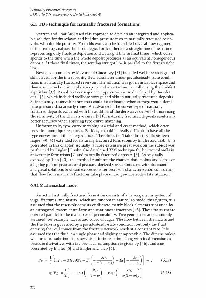
6.3. TDS technique for naturally fractured formations

Warren and Root [46] used this approach to develop an integrated and applica-ble solution for drawdown and buildup pressure tests in naturally fractured reser-voirs with double porosity. From his work can be identified several flow regimesof the semilog analysis. In chronological order, there is a straight line in near timerepresenting only fracture depletion and a straight line in final times, which corre-sponds to the time when the whole deposit produces as an equivalent homogeneousdeposit. At these final times, the semilog straight line is parallel to the first straightline.

New developments by Mavor and Cinco‐Ley [31] included wellbore storage andskin effects for the interporosity flow parameter under pseudosteady‐state condi-tions in a naturally fractured reservoir. The solution was given in Laplace space andthen was carried out in Laplacian space and inverted numerically using the Stehfestalgorithm [37]. As a direct consequence, type curves were developed by Bourdetet al. [3], which included wellbore storage and skin in naturally fractured deposits.Subsequently, reservoir parameters could be estimated when storage would domi-nate pressure data at early times. An advance in the curves type of naturallyfractured deposits occurred with the addition of the derivative curve [3]. Increasingthe sensitivity of the derivative curve [9] for naturally fractured deposits results in abetter accuracy when applying type‐curve matching.

Unfortunately, type‐curve matching is a trial‐and‐error method, which oftenprovides nonunique responses. Besides, it could be really difficult to have all thetype curves for all the emerged cases. Therefore, the Tiab’s direct synthesis tech-nique [40, 41] extended for naturally fractured formations by Engler and Tiab [6] ispresented in this chapter. Actually, a more extensive great work on the subject wasperformed by Engler [5] who also developed TDS technique for horizontal wells inanisotropic formations [7] and naturally fractured deposits [8]. As originallyexposed by Tiab [40], this method combines the characteristic points and slopes ofa log‐log plot of pressure and pressure‐derived versus time data with the exactanalytical solutions to obtain expressions for reservoir characterization consideringthat flow from matrix to fractures take place under pseudosteady‐state situation.

6.3.1 Mathematical model

An actual naturally fractured formation consists of a heterogeneous system ofvugs, fractures, and matrix, which are random in nature. To model this system, it isassumed that the reservoir consists of discrete matrix block elements separated byan orthogonal system of uniform and continuous fractures [46]. These fractures areoriented parallel to the main axes of permeability. Two geometries are commonlyassumed, for example, layers and cubes of sugar. The flow between the matrix andthe fractures is governed by a pseudosteady‐state condition, but only the fluidentering the well comes from the fracture network reach at a constant rate. It isassumed that the fluid is a single phase and slightly compressible. The dimensionlesswell pressure solution in a reservoir of infinite action along with its dimensionlesspressure derivative, with the previous assumptions is given by [46], and alsopresented by Engler [5] and Engler and Tiab [6]:

PD = 12

ln tD þ 0:80908þ Ei � λtDωð1� ωÞ

� �� Ei � λtD

1� ω

� �� þ s (6.17)

tD*PD0 =

12

1� exp � λtD1� ω

� �þ exp � λtD

ωð1� ωÞ� ��

(6.18)

225


The dimensionless quantities given by Eqs. (1.94), (1.89), and (2.57) are nowrewritten as:

tD =0:0002637kfbtμðϕctÞmþf r2w

(6.19)

PD =kfbhðPi � PÞ141:2qμB

(6.20)

tD*PD0 =

kfbhðt*ΔP0Þ141:2qμB

(6.21)

6.3.2 Characteristic points and lines

Refer to Figure 6.7 and notice that the radial flow has been interrupted by thetransition period during which fractured are fed from the matrix. Each radial flow islabeled r1 and r2 for distinguishing purposes. As for the case of a homogeneoussystem, Eq. (2.70) applies (do not consider the dimensionless wellbore storagecoefficient), so that Eq. (2.71) applies, now rewritten as:

kfb =70:6qμBhðt*ΔP0Þr1

=70:6qμBhðt*ΔP0Þr2

(6.22)

Needless to say that in case that both radial flow regimes are seen, bulk fracturepermeability can be obtained from any of them using the above expression.

The transition period is affected by the dimensionless storativity coefficient,but independent of the interporosity flow parameter. Engler [5] and Engler andTiab [6] found an analytical expression for the minimum coordinates by taking thederivative of Eq. (6.18) and equating the result to zero. Subsequently, the dimen-sionless minimum coordinates are given by:

ðtDÞmin = ω

λln

1ω

(6.23)

and,

ðtD*PD0Þmin =0:5 ð1þ ω1=ð1�ωÞ � ωω=ð1�ωÞÞ (6.24)

Eq. (6.23) was based for [42] to derive Eq. (6.11) which is now rewritten as:

λ =3792ðϕ ctÞfþmμr

2w

kfbΔtminωln

1ω

� �� (6.25)

To set Eq. (6.24) in oil‐field unit, Engler [5] and Engler and Tiab [6] developed aform to normalize it by division with the radial flow derivative, Eq. (2.70), to yield:

ðt*ΔP 0Þmin =ðt*ΔP 0Þmin = ð1þ ω1=ð1�ωÞ � ωω=ð1�ωÞÞ (6.26)

Engler [5] and Engler and Tiab [6] developed the following empiricalcorrelation:

ω = 0:15866ðt*ΔP 0Þmin

ðt*ΔP 0Þr

� �þ 0:54653

ðt*ΔP 0Þmin

ðt*ΔP 0Þr

� �2

(6.27)

226


which is valid from 0 ≤ ω ≤ 0.10 with an error less than 1.5%. An alternativemethod for determining ω arises from the defined characteristic times of pressurederivative curve shown in Figure 6.7. These include the end of the first horizontalstraight line, tDe1, the start of the second horizontal straight line, tDb2, and the timecorresponding to the minimum derivative, tDmin. Engler and Tiab [6] developedseveral empirical correlations by relating such times:

λ = ωð1� ωÞ50βte1

= ωlnð1=ωÞβtmin

= 1

β tusi =

5ð1� ωÞβtb2

(6.28)

where

β = 0:0002637kfbðϕctÞfþmμr2w

(6.29)

ω = exp � 10:9232

tmin

50te1� 0:4386

� �� (6.30)

The correlation for the ratio of the minimum time to the time for the end of thefirst straight line has an error less than 5% [6].

ω=0:192115tmin

tb2

� �þ 0:80678

5tmin

tb2

� �2

(6.31)

The correlation using the ratio of the minimum time to the start time of thesecond straight line, valid for ω ≤ 0.1, has with an error less than 2%.

For a given dimensionless storativity coefficient, the minimum dimensionlesspressure coordinate is independent of the interporosity flow parameter, while theminimum dimensionless time coordinate is a function of λ. Subsequently, Englerand Tiab [6] found that a log plot (tD*P'D)min versus log (λtD)min results in a straightline with unit slope. The corresponding empirical equation is:

lnðtD*PD0Þmin = lnðλ � tDminÞ þ lnð0:63Þ (6.32)

From which was obtained:

λ =42:5hðϕctÞfþmrw

2

qB

" #ðt*ΔP 0Þmin

tmin(6.33)

An alternative method for determining λ can be carried out by observing astraight line with unit slope characteristic during the last transition period. Thesmaller dimensionless storativity coefficient (lowest point of the curve) adjusts thedata more exactly to the unit slope line. A ω < 0.05 results in a more accurateestimate of λ. For ω > 0.05, λ will be overestimated. The analytical equation for thisbehavior of the last transition time is [6]:

ln ðtD*PD0Þus = ln ðλ � tDus=2Þ (6.34)

The intersection of the unit slope line of the transition period with the line of theradial flow regime pressure derivative, Eq. (2.70), shown in Figure 6.7, allowedfinding a simple expression to determine λ [6]:

λ = 1=tDusi (6.35)

227


Replacing Eq. (1.94) in the above expression leads to:

λ = ðϕctÞfþmμr

2w

0:0002637kfb

!1tusi

(6.36)

As for the case of Eq. (2.92), the mechanical skin factor, expected always to benegative for naturally fractured formations, is, found for each one of the radial flowregimes, r1 and r2, thus, [6]:

s = 12

ΔPt*ΔP 0

� �r1� ln

kfb tr1ðϕctÞfμr2wω

! þ 7:43

" #(6.37)

s = 12

ΔPt*ΔP 0

� �r2� ln

kfb tr2ðϕctÞfþmμr2w

! þ 7:43

" #(6.38)

Eq. (6.37) may be of not practical use since as commented before on the diffi-culty to obtain a representative value of the fracture compressibility.

6.3.3 Wellbore storage effects

As discussed earlier in this chapter, a direct consequence of wellbore storage isthe tendency to mask the early time radial flow period. Therefore, the late or secondradial flow line of infinite action is essential for estimating the skin factor and thepermeability of the net of fractures. If wellbore storage is presented, it can beobtained, from the early unit slope, by using Eqs. (2.61), (2.69), and (2.80). Wemust be aware that Eqs. (2.81) and (2.87) were developed for higher skin factors,then, they are not recommended to apply in naturally fractured reservoirs.

The influence of wellbore storage on minimum coordinates is of great impor-tance in the analysis. As Figure 6.8 shows, the dilemma is whether the minimumobserved point is the actual minimum or a “pseudo‐minimum” as a direct result ofwellbore storage. Engler [5] and Engler and Tiab [6] have shown that the minimumpoint is not affected by storage for all ω and λ, provided that,

Figure 6.8.Wellbore storage effect on the minimum value of the pressure derivative, ω = 0.05 and s = 0, after [6].

228


ðtDÞmin, o

ðtDÞx ≥ 10 (6.39)

Accordingly, the procedures described above are valid. When the ratio of theminimum time to the time at the peak is less than the limit defined by Eq. (6.39), a“pseudo‐minimum” occurs in the curve of the pressure derivative. An empiricalcorrelation generated during this region provides a method to calculate theinterporosity flow parameter [6],

½λlogð1=λÞ�min = 1CD

5:565tx

tmin,o

� �10(6.40)

where,

λ = ½λlogð1=λÞ�min

1:924

� �1:0845

(6.41)

The corrected ω is found from Figure 6.9.An alternative method for determining λ is based on the ratio of the coordinate

of the minimum pressure derivative to the coordinate of the pressure derivativeat the peak. This correlation is valid only for CDλ > 0.001 [6], and CD is foundfrom Eq. (2.14);

λ = 1

10CD

ðt*ΔP 0Þmin

ðt*ΔP 0Þx(6.42)

Tiab et al. [43] determined that the minimum is not affected by wellborestorage for any value w, provided the conditions given in Table 6.2 are fulfilled.Then, they proposed a better expression for correcting the minimum:

ðt*ΔP 0Þmin = ðt*ΔP 0Þr þðt*ΔP 0ÞminO � ðt*ΔP 0Þr 1þ 2D1D2½ �

1þD2 lnC

ðϕctÞfþmhr2w

!þ 2s� 0:8801

" # (6.43)

Figure 6.9.Determination of the dimensionless storativity coefficient using the ratio of the radial with the minimumpressure derivatives, after [6].

229


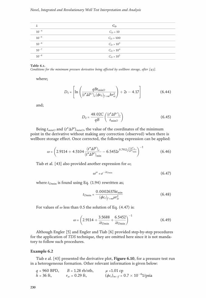
where;

D1 = lnqBtminO

ðt*ΔP 0ÞrðϕctÞfþmhr2w

!þ 2s� 4:17

" #(6.44)

and;

D2 =48:02C

qBðt*ΔP 0ÞrtminO

� �(6.45)

Being tminO and (t*ΔP')minO, the value of the coordinates of the minimumpoint in the derivative without making any correction (observed) when there iswellbore storage effect. Once corrected, the following expression can be applied:

ω = 2:9114þ 4:5104ðt*ΔP0Þrðt*ΔP0Þmin

� 6:5452e0:7912ðt*ΔP0 Þr

ðt*ΔP0Þmin

� ��1

(6.46)

Tiab et al. [43] also provided another expression for ω;

ωω = e�λtDmin (6.47)

where tDmin is found using Eq. (1.94) rewritten as;

tDmin =0:0002637ktmin

ðϕctÞfþmμr2w(6.48)

For values of ω less than 0.5 the solution of Eq. (4.47) is:

ω= 2:9114þ 3:5688λtDmin

þ 6:5452λtDmin

� ��1

(6.49)

Although Engler [5] and Engler and Tiab [6] provided step‐by‐step proceduresfor the application of TDS technique, they are omitted here since it is not manda-tory to follow such procedures.

Example 6.2

Tiab e al. [43] presented the derivative plot, Figure 6.10, for a pressure test runin a heterogeneous formation. Other relevant information is given below:

q = 960 BPD, B = 1.28 rb/stb, μ =1.01 cph = 36 ft, rw = 0.29 ft, (ϕct)mþf = 0.7 � 10�61/psia

λ CD

10�4 CD > 10

10�5 CD > 100

10�6 CD > 103

10�7 CD > 104

10�8 CD > 105

Table 6.2.Conditions for the minimum pressure derivative being affected by wellbore storage, after [43].

230


It is required the interpretation of this test to provide permeability, skin factor,and the Warren‐and‐Root parameters.

Solution

As observed in the pressure derivative plot, Figure 6.10, this pressure test maynot be interpretable using conventional analysis since the first radial flow regime isabsolutely masked by wellbore storage. The following information is read fromsuch plot:

tN = 0.00348 h, ΔPN = 11.095 psia, tr2 = 1.8335 hΔPr2 = 61.5 psia, (t*ΔP0)r2 = 10.13 psia, tmin,o = 0.07 h, (t*ΔP')minO = 5.32 psiaPermeability is found from Eq. (6.22);

kfb =70:6qμBhðt*ΔP 0Þr2

=70:6� 960� 1:01� 1:28

10:13� 36= 238 md

The wellbore storage coefficient and the dimensionless wellbore storage coeffi-cient are determined with Eqs. (2.61) and (2.14) to be:

C =qB24

tΔP

� N=

960ð1:28Þ24

� �0:0034811:095

=0:0161 bbl=psia

CD =0:894C

ðϕctÞfþmhr2w=

0:894ð0:0161Þ0:7 � 10�6ð36Þð0:292Þ = 6792

Estimate skin factor from Eq. (6.38):

s = 12

61:510:13

� lnð238Þð1:8335Þ

0:7 � 10�6ð1:01Þð0:292Þ

� � þ 7:43

� �= � 4:6

The interporosity flow parameter is found with Eq. (6.33)

Figure 6.10.Pressure and pressure derivative against time log‐log plot for Example 6.2, after [43].

231


λ =42:5hðϕctÞfþmrw

2

qB

" #ðt*ΔP 0Þmin

tmin=

42:5ð37Þ0:7 � 10�6ð0:292Þ960ð1:28Þ

� �5:320:07

= 5:57 � 10�6

Since λ = 5.57 � 10�6 and CD = 6792, by looking at the third row in Table 6.2, thecoordinates of the minimum point must be corrected before finding ω. Therefore,use Eqs. (6.44), (6.45), and (6.43), so that:

D1 = ln960ð1:28Þð0:07Þ

ð10:13Þ� �

þ 2ð�4:6Þ � 4:17� �

= 1:8334

D2 =48:02ð0:0161Þ960ð1:28Þ

10:130:07

� �=0:09105

ðt*ΔP 0Þmin= 10:13þ5:32� ð10:13Þ½1þ 2ð1:8334Þð0:09105Þ�

1þ 0:09105½ln

0:01610:7 � 10�6ð36Þð0:292Þ

!þ 2ð�4:6Þ � 0:8801�

=0:9849

Then, ω is found from Eq. (6.46), and the correlation is given by Eq. (6.27):

ω= 2:9114þ 4:510410:130:9849

� 6:5452e0:791210:130:9849

� ��1

= 0:024

ω = 0:158660:984910:13

� �þ 0:54653

0:984910:13

� �2

= 0:0206

Without correction, Eq. (6.27) would have given a value of ω = 0.234.

Example 6.3

This was also worked by Tiab et al. [43]. Pressure and pressure derivativeagainst time data are given in Table 6.3 and plotted in Figure 6.11 for its interpre-tation. Other important data are given below:

q = 3000 BPD, ϕ = 0.10, μ = 1.0 cpct = 3.0 � 10�5 psia�1, B = 1.25 bbl/stb, h = 100 ftrw = 0.40 ft, Pi(t=0) = 4473 psia

Calculate the permeability of the fractured system, skin factor, wellbore storagecoefficient, interporosity flow parameter, and dimensionless storativity coefficient.

Solution

The following information was read from Figure 6.11:

ΔPN = 99.6 psia, (t*ΔP0)N = 116.4 psia, tN = 0.093 htb2 = 14.4 h, tr2 = 20.43 h, ΔPr2 = 714.3 psia(t*ΔP0)r2= 138.5 psia, tx = 0.43, tmin,o = 2.427 htmin,o/tx = 5 < 10, ti = 0.14 h, (t*ΔP0)min = 72.087 psia

Solution

Use Eq. (6.22) to estimate permeability

kfb =70:6qμBhðt*ΔP 0Þr2

= 70:6ð3000Þð1:0Þð1:25Þ

100ð138:5Þ = 19:1 md

232


Find the wellbore storage coefficient using Eqs. (2.61), (2.69), and (2.80).

C = qB24

� �tNΔPN

= 3000ð1:25Þ

24

� �0:09399:6

=0:146 bbl=psia

C = qB24

� �tN

ðt*ΔP 0ÞN=

3000ð1:25Þ24

� �0:093116:4

=0:129 bbl=psia

C = kfbhti1695μ

= 19:1ð100Þð0:14Þ

1695μ=0:158 bbl=psia

Estimate skin factor from Eq. (6.38):

Figure 6.11.Pressure and pressure derivative against time log‐log plot for Example 6.3, after [43].

t, h Pwf, psia t*ΔP', psia t, h Pwf, psia t*ΔP', psia t, h Pwf, psia t*ΔP', psia

0.0933 4373.4 84.473 1.0930 4060.3 87.234 12.43 3824.2 137.651

0.1766 4299.1 133.483 1.26 4043.1 84.384 14.43 3804.1 136.857

0.2600 4246.1 146.776 1.427 4032.2 76.719 20.43 3758.7 138.810

0.3433 4203.6 151.595 2.427 4002.8 75.401 26.43 3720.3 135.210

0.4266 4173.8 157.618 3.427 3971.3 90.502 32.43 3695.1 134.790

0.5100 4139.7 150.295 4.427 3948.3 87.168 38.43 3674.6 134.116

0.5933 4118.5 141.355 5.427 3931.6 95.595 44.43 3652.4 156.278

0.6766 4103.5 111.676 6.427 3917.1 108.303 50.43 3636.9 183.611

0.7600 4086.4 99.694 7.427 3898.4 122.336 53.43 3625.2 196.734

0.9266 4075.4 95.720 9.427 3865.3 142.426

Table 6.3.Pressure and pressure derivative data against time for Example 6.3, after [43].

233


s =12

714:3138:5

� ln19:1ð20:43Þ

3� 10�6ð0:1Þð1Þð0:42Þ þ 7:43� �

= � 5:13

The ratio between the minimum time and the time in the peak suggests that theminimum coordinates are influenced by wellbore storage. Then, find the dimen-sionless wellbore storage using Eq. (2.14) with an average C of 0.143 bbl/psia:

CD =0:8935Cϕhctr2w

=0:8935ð0:143Þ

0:1ð100Þð3� 10�6Þð0:42Þ = 26618

Eq. (6.40) leads to find:

½λ log ð1=λÞ�min = 1CD

5:565tx

tmin,o

� �10 =

126618

5:5650:432:427

� �10= 0:000032

Then, λ = 5.2 � 10�7. Find again λ with Eq. (6.42):

λ =1

10CD

ðt*ΔP 0Þmin

ðt*ΔP 0Þx=

110ð26618Þ

72:087151:94

= 1:78� 10�6

For the determination of ω, estimate the ratio between the pressure derivativesof minimum point and radial flow regime, (t*ΔP0)min/(t*ΔP0)r = 72.078/138.5 = 0.52.Then, find the parameter needed to enter in Figure 6.9, thus:

CDλ log1λ

� �þ 0:8686s

� �= 26618ð1:78� 10�6Þ log

1

1:78� 10�6

!þ

0:8686ð�5:13Þ

264

375 =0:061

From Figure 6.9, it is found that ω = 0.07.The reader may think that the subject covered by the TDS technique in this

chapter is the only one as far as naturally fractured reservoirs are concerned. Thematerial exposed in this chapter was the first one ever introduced. TDS technique iscertainly rich in applications. Regarding naturally fractured systems can be named:double porosity and double permeability for vertical wells [19], already mentionedat the beginning of this chapter, and for horizontal wells [30]. For triple porosity,reservoirs referred to [10]. For horizontal wells in both homogeneous and hetero-geneous deposits including the effect of the threshold pressure gradient, the readeris invited to read [21]. The work originally presented for long homogeneous reser-voirs [11] was extended to naturally fractured deposits by Escobar et al. [13, 14]. Forhydraulically fractured wells, draining heterogeneous formations refer to [13, 20,26, 44]. Escobar et al. [15] presented TDS technique for gas wells in naturallyfractured systems. The effect of pseudotime on the Warren‐and‐Root parameterswas observed by [18] for vertical wells and [17] for horizontal wells. TS techniquefor rate transient analysis of homogeneous and heterogeneous formations waspresented by [1] and extended to long reservoirs by [16] and gas bearing longfractured formations by [12]. However, there are publications written by someother researchers and are not reported here.

234


Lately, shale reservoirs have been the target of many oil and gas companies. Gasreservoirs must be hydraulically fractured for production to occur. Their behaviornormally follows those of naturally fractured formations. Some publicationsregarding shales tested either at constant bottom‐hole pressure or constant rateusing TDS technique are [2, 22–25].

Nomenclature

B oil volume factor, bbl/STBb fraction of penetration/completionc compressibility, 1/psiaC wellbore storage coefficient, bbl/psiaD1 minimum point correction parameterD2 minimum point correction parameterct total or system compressibility, 1/psiah formation thickness, ftkef bulk fractured network permeability, mdm slope of P‐vs‐log t plot, psia/h/cycleP pressure, psiaPD0 dimensionless pressure derivativePD dimensionless pressurePi initial reservoir pressure, psiaPwf well flowing pressure, psiaPws well shut‐in or static pressure, psiaP1hr intercept of the semilog plot, psiaP* false pressure, psiaq liquid flow rate, BPDrD dimensionless radiusr radius, ftrw well radius, fts skin factort time, htp production (Horner) time before shutting‐in a well, htD dimensionless time based on well radiust*DP0 pressure derivative, psiaV volume, ft3

Greek

α shape factorΔ change, dropΔt shut‐in time, h∂ P parallel difference between the two radial flow regime slopes, psiaϕ porosity, fractionλ interporosity flow coefficientμ viscosity, cpρ fluid density, lbm/ft3

ω dimensionless storativity coefficient

235


Suffices

1 intercept between first semilog radial flow and the transition line1hr time of 1 h2, I intercept between second semilog radial flow and the transition lineb2 start of second radial flow regimeD dimensionlesse1 end of first radial flow regimeF inflectionf fracture networki intersection or initial conditionsN an arbitrary point during early pseudosteady‐state periodm matrixmax maximum pointmin minimum pointminO observed minimum pointr radial flowr1 radial flow before transition periodr2 radial flow after transition periods skinusi intersect of the pressure derivative lines of the unit‐slope line during the

transition and second radial flow regimew wellwf well flowingws well shut‐in

236


References

[1] Arab N. Application of Tiab's directsynthesis technique to constant bottomhole pressure test [M.Sc. thesis]. TheUniversity of Oklahoma; 2003

[2] Bernal KM, Escobar FH, Ghisays‐Ruiz A. Pressure and pressure derivativeanalysis for hydraulically fractured shaleformations using the concept of inducedpermeability field. Journal ofEngineering and Applied Sciences.2003;9(10):1952‐1958

[3] Bourdet D, Ayoub JA, Whittle TM,Pirard YM, Kniazeff V. Interpreting welltests in fractured reservoirs. World Oil.1983;197(5):77‐87

[4] Earlougher RC Jr. Advances in welltest analysis. Monograph Series, Vol. 5.Dallas, TX: Second printing; SPE; 1977

[5] Engler TW. Interpretation ofpressure tests in naturally fracturedreservoirs by the direct synthesistechnique [Ph.D. dissertation].University of Oklahoma; 1995

[6] Engler T, Tiab D. Analysis ofpressure and pressure derivativewithout type curve matching, 4Naturally fractured reservoirs. Journalof Petroleum Science and Engineering.1996;15:127‐138

[7] Engler TW, Tiab D. Analysis ofpressure and pressure derivativeswithout type‐curve matching. 6‐Horizontal well tests in anisotropicreservoirs. Journal of Petroleum Scienceand Engineering. 1996;15:153‐168

[8] Engler TW, Tiab D. Analysis ofpressure and pressure derivativeswithout type‐curve matching. 5‐Horizontal well tests in naturallyfractured reservoirs. Journal ofPetroleum Science and Engineering.1996;15:139‐151

[9] Escobar FH, Navarrete JM, LosadaHD. Evaluation of Pressure DerivativeAlgorithms for Well‐Test Analysis.Society of Petroleum Engineers. 2004.DOI: 10.2118/86936‐MS

[10] Escobar FH, Saavedra NF, EscorciaGD, Polania JH. Pressure and PressureDerivative Analysis without Type‐CurveMatching for Triple Porosity Reservoirs.Society of Petroleum Engineers. 2004.DOI: 10.2118/88556‐MS

[11] Escobar FH, Hernandez YA,Hernandez CM. Pressure transientanalysis for long homogeneousreservoirs using TDS technique. Journalof Petroleum Science and Engineering.2007; 58(1‐2):68‐82

[12] Escobar FH, Sanchez JA, CantilloJH. Rate transient analysis forhomogeneous and heterogeneous gasreservoirs using the TDS technique.CT&F – Ciencia, Tecnología y Futuro.2008;4(4):45‐59

[13] Escobar FH, Martinez J, Cantillo JH.Pressure‐Transient Analysis forNaturally Fractured Reservoirs WithTransition Period Before and After theRadial‐Flow Regime. Society ofPetroleum Engineers. 2010. DOI:10.2118/138490‐MS

[14] Escobar FH, Hernandez DP,Saavedra JA. Pressure and pressurederivative analysis for long naturallyfractured reservoirs using the TDStechnique. Dyna. 2010;77(163):102‐114

[15] Escobar FH, Muñoz YEM, CerqueraWM. Pressure and pressure derivateanalysis vs. pseudotime for a horizontalgas well in a naturally fracturedreservoir using the TDS technique.Entornos Journal. 2011;24:39‐54. ISSN0124‐7905

237


[16] Escobar FH, Rojas MM, Bonilla LF.Transient‐rate analysis for longhomogeneous and naturally fracturedreservoir by the TDS technique. Journalof Engineering and Applied Sciences.2012;7(3):353‐370

[17] Escobar FH, Muñoz YEM, CerqueraWM. Pseudotime function effect onreservoir width determination inhomogeneous and naturally fracturedgas reservoir drained by horizontalwells. Entornos Journal. 2012;24:221‐231

[18] Escobar FH, Martinez LY, MéndezLJ, Bonilla LF. Pseudotime applicationto hydraulically fractured vertical gaswells and heterogeneous gas reservoirsusing the TDS technique. Journal ofEngineering and Applied Sciences. 2012;7(3):260‐271

[19] Escobar FH, Vega J, Diaz MR.Pressure and pressure derivativeanalysis for double‐permeabilitysystems without type‐curve matching.Journal of Engineering and AppliedSciences. 2012;7(10):1314-1320

[20] Escobar FH, Ghisays‐Ruiz A, BonillaLF. New model for elliptical flow regimein hydraulically fractured vertical wellsin homogeneous and naturallyfractured systems. Journal ofEngineering and Applied Sciences.2014;9(9):1629‐1636

[21] Escobar FH, Zhao YL, Zhang LH.Interpretation of pressure tests inhorizontal wells in homogeneous andheterogeneous reservoirs with thresholdpressure gradient. Journal ofEngineering and Applied Sciences.2014;9(11):2220‐2228

[22] Escobar FH, Montenegro LM,Bernal KM. Transient‐rate analysis forhydraulically fractured gas shale wellsusing the concept of inducedpermeability field. Journal of

Engineering and Applied Sciences.2014;9(8):1244‐1254

[23] Escobar FH, Bernal KM, Olaya‐Marin G. Pressure and pressurederivative analysis for fracturedhorizontal wells in unconventional shalereservoirs using dual‐porosity models inthe stimulated reservoir volume. Journalof Engineering and Applied Sciences.2014;9(12):2650‐2669

[24] Escobar FH, Bernal KM, Olaya‐Marin G. Pressure and pressurederivative analysis for fracturedhorizontal wells in unconventional shalereservoirs using dual‐porosity models inthe stimulated reservoir volume. Journalof Engineering and Applied Sciences.2014;9(12):2650‐2669

[25] Escobar FH, Rojas JD, Ghisays‐RuizA. Transient‐rate analysis hydraulically‐fractured horizontal wells in naturally‐fractured shale gas reservoirs. Journal ofEngineering and Applied Sciences.2014;10(1):102‐114

[26] Escobar FH, Zhao YL, Fahes M.Characterization of the naturallyfractured reservoir parameters ininfinite‐conductivity hydraulicallyfractured vertical wells by transientpressure analysis. Journal ofEngineering and Applied Sciences. 2015;10(12):5352‐5362

[27] Escobar FH. Recent Advances inPractical Applied Well Test Analysis.New York: Nova Science Publishers,Inc.; 2015. p. 422

[28] Igbokoyi AO, Tiab D. Estimation ofAverage Reservoir Pressure andDrainage Area in Naturally FracturedReservoirs. Society of PetroleumEngineers. 2006. DOI: 10.2118/104060‐MS

[29] Kazemi H. Pressure transientanalysis of naturally fractured reservoirs

238


with uniform fracture distribution.Society of Petroleum Engineers. 1969:451-462. DOI: 10.2118/2156‐A

[30] Lu J, Zhu T, Tiab D, Escobar FH.Pressure behavior of horizontal wells indual‐porosity, dual‐permeabilitynaturally‐fractured reservoirs. Journalof Engineering and Applied Sciences.2015;10(8):3405‐3417. ISSN 1819‐6608

[31] Mavor MJ, Cinco‐Ley H. TransientPressure Behavior of NaturallyFractured Reservoirs. Society ofPetroleum Engineers. 1979. DOI:10.2118/7977‐MS

[32] Molina MD, Escobar FH,Montealegre MM, Restrepo DP.Application of the TDS technique fordetermining the average reservoirpressure for vertical wells in naturallyfractured reservoirs. CT&F—Ciencia,Tecnología y Futuro. 2005;3(5):45-55.ISSN 0122‐5383

[33] Nelson R. Geologic Analysis ofNaturally Fractured Reservoirs. 2nd ed.Houston, TX: Gulf ProfessionalPublishing; 2001. p. 352

[34] Odeh AS. Unsteady‐state behaviorof naturally fractured reservoirs. SPEJ;Transactions of AIME. 1965;234:64‐65.Society of Petroleum Engineers. DOI:10.2118/966‐PA

[35] Petak KR, Soliman MY, AndersonMF. Type Curves for AnalyzingNaturally Fractured Reservoirs. Societyof Petroleum Engineers. 1986. DOI:10.2118/15638‐MS

[36] Stewart G, Asharsobbi F. Well TestInterpretation for Naturally FracturedReservoirs. Society of PetroleumEngineers. 1988. DOI: 10.2118/18173‐MS

[37] Stephest H. Numerical inversion of39 Laplace transform. Communicationsof the ACM. 1970;13(1):47‐49

[38] Stewart G. Well Test Design &Analysis. Tulsa, Oklahoma, USA:PennWell Corporation; 2011. p. 1940

[39] Strobel CJ, Gulati MS, Ramey HJ.Reservoir limit tests in a naturallyfractured reservoir—A field case studyusing type curves. Society of PetroleumEngineers. 1976:1097‐1106. DOI:10.2118/5596‐PA

[40] Tiab D. Analysis of pressure andpressure derivative without type‐curvematching: 1‐skin and wellbore storage.Journal of Petroleum Science andEngineering. 1995;12:171‐181

[41] Tiab D. Analysis of Pressure andPressure Derivatives Without Type‐Curve Matching: I—Skin and WellboreStorage. Society of Petroleum Engineers.1993. DOI: 10.2118/25426‐MS

[42] Tiab D, Escobar FH. Determinacióndel Parámetro de Flujo Interporoso deun Gráfico Semilogarítmico. X CongresoColombiano del Petróleo. 2003

[43] Tiab D, Igbokoyi AO, Restrepo DP.Fracture porosity from pressuretransient data. In: InternationalPetroleum Technology Conference.2007. DOI: 10.2523/IPTC‐11164‐MS

[44] Tiab D, Bettam Y. PracticalInterpretation of Pressure Tests ofHydraulically Fractured Wells in aNaturally Fractured Reservoir. Societyof Petroleum Engineers. 2007. DOI:10.2118/107013‐MS

[45] Uldrich DO, Ershaghi I. A Methodfor Estimating the Interporosity FlowParameter in Naturally FracturedReservoirs. Society of PetroleumEngineers. 1976. DOI: 10.2118/7142‐PA

[46]Warren JE, Root PJ. The behavior ofnaturally fractured reservoirs. Society ofPetroleum Engineers. 1963.245-255.DOI: 10.2118/426‐PA

239


Chapter 7

Hydraulically Fractured

Hydraulic fracturing is a technique consisting of cracking the rock with a liquidfluid, normally of non‐Newtonian nature, which carries some solid particles (sandor synthetic material) so that reservoir fluids can move easier toward the well. Thefluid has three main uses: (1) as pressuring fracturing tool by overpassing theformation fracture gradient, (2) as carrying agent to transport the solid material,called proppant, to the fracture face so, when reducing the pressure, avoids thefracture to close completely and provides flow capability to the fracture, calledconductivity, and (3) as lubrication agent. In unconventional fracturing, the frac-turing fluid is water and about 4% of the injected mass corresponds to sand.

The orientation of the hydraulic fractures is a function of the distribution ofstress in the formation [3, 14]. If the least stress in the formation is horizontal, thena vertical fracture will be obtained. On the other hand, if the least important stress isvertical, then a horizontal fracture will occur [4, 8, 30]. However, there is a generalbelief that vertical fractures are obtained at depths greater than 3000 ft.

Figure 7.1 is a plane of a bounded circular system, which is a well with a verticalfracture. The fracture length has been exaggerated for explanatory purposes. Gen-erally, the fluid enters the fracture at a uniform flow rate per unit area of the face ofthe fracture so that there is a pressure drop in the fracture. In this case, the fracturerefers to a “uniform flow fracture.” However, for some fractures that have infinitepermeability (conductivity), the pressures are uniform throughout. Except forfractures with a high content of support material and conductive fractures, it isthought that the uniform flow fracture represents much better reality than thefracture of infinite conductivity [7, 12, 39].

7.1. Well drawdown pressure behavior

The dimensionless pressure in the well for the case of a uniform flow fracture is[4, 5, 7, 8]:

PD =ffiffiffiffiffiffiffiffiffiffiffiπtDxf

perf ð1=2 ffiffiffiffiffiffiffiffi

tDxfp Þ � 0:5Eið�1=4tDxf Þ (7.1)

And for the case of an infinite conductivity, fracture is:

PD =0:5ffiffiffiffiffiffiffiffiffiffiffiπtDxf

p erf ð0:134= ffiffiffiffiffiffiffiffitDxf

p þerf ð0:866= ffiffiffiffiffiffiffiffi

tDxfp Þ

" #� 0:067Eið�0:018=tDxf Þ�

0:433Eið�0:75=tDxf Þ

" #(7.2)

where

tDxf = tDðrw=xf Þ2 (7.3)

If tDxf < 0.1 in Eq. (7.1) and tDxf < 0.1 in Eq. (7.2), these two equations become:

PD =ffiffiffiffiffiffiffiffiffiffiffiπtDxf

ξ

r(7.4)

240

It is important to note that Eq. (7.4) is a new version proposed by Bettam et al.[2], which considers both homogeneous deposits, ξ=1, and heterogeneous (natu-rally fractured double porosity) deposits, ξ=ω (dimensionless storage coefficient).Eq. (7.4) also indicates that at early times the flow within the fracture is linear. Inreal units, Eq. (7.4) can be written as [8]:

Pwf =Pi �mlfffiffit

p(7.5)

where

mlf =�4:064qB

h

ffiffiffiffiffiffiffiffiffiffiffiffiffiffiffiffiμ

kξϕctx2f

s(7.6)

mvf is the slope of the Cartesian plot of Pwf against t1/2, which can be used to

calculate:

kx2f =�4:064qB

hmlf

!2μ

ξϕct(7.7)

If certainty exists in the determination of the linear flow regime, let us say thepressure derivative is available and reservoir permeability is accurate (it does notneed correction), then use Eq. (7.7) directly and find the half‐fracture length. Thefollowing procedure should be flowed, otherwise. In which the conventional semi-log analysis applies to tDxf > 10. Eqs. (7.1) and (7.2) are, respectively, converted to[5, 6, 26, 33]:

PD =12

ln ðtDxf Þ þ 2:80907� �

(7.8)

PD =12

ln ðtDxf Þ þ 2:2� �

(7.9)

Figure 7.1Schematic representation of a vertical fracture, after [6].

241

Hydraulically FracturedDOI: http://dx.doi.org/10.5772/intechopen.81078

These two equations give the dimensionless pressure for pseudoradial flow, aslong as the boundary effects are not found. In a bounded reservoir, the period ofinfinite action pseudoradial flow only develops completely if xe/xf > 5.

There is an approximate relationship between the pressure change at the end ofthe linear flow period, ΔPel, and at the beginning of the semilog straight line, Pbsl,[26, 33]:

ΔPsbl≥2ΔPel (7.10)

If this relationship is not met, it is because the linear flow period or the radialflow period was incorrectly selected. A couple of pertinent observations:

• A graph of ΔP versus time on a log‐log paper will produce a straight line ofmean slope during the linear period.

• The above analysis is valid for pressure decline and injection tests.

7.2. Conventional analysis

In vertically fractured wells, pressure buildup and falloff tests are similar tononfractured wells. As shown in Figure 7.2, the semilog slope, m, obtained fromtraditional analysis of a fractured well is erroneously very small and the value of mdecreases progressively as xf increases [32]. In other words, the fracture presencepartially masks the radial flow regime. The pressure derivative certainly allowsfinding the true start of the semilog line. Because of that fracture effect, permeabil-ity, estimated from the Horner or MDH graph, should be corrected as follows:

k = kcFcor (7.11)

where

Fcor = ðkhÞtrue=ðkhÞapparent (7.12)

And the uncorrected permeability is found from Eq. (2.33),

kc = 162:6qμ Bmh

(7.13)

Figure 7.2Effect of fracture length on the semilog slope [32].

242


The correction factor, Fcor, is read from Figure 7.3. The Horner plot is stronglyrecommended for data analysis of vertically fractured wells. xe/xf must be known(normally assumed by a trial‐and‐error procedure) to use Figure 7.3. xf is simply thehalf‐fracture length, which can be estimated from the slope of the Cartesian plot ofpressure versus square root of time, using Eq. (7.7).

Fcor can be estimated iteratively as follows:

1. Estimate kxf2 from Eq. (7.7).

2. Estimate kc using Eq. (7.13).

3.Calculate k from Eq. (7.11) using a reasonable assumed value of xe/xf (As a firsttry, assume xf=0.5xe) in Figure 7.3.

4.Use the value of k from step 3 to estimate xf with Eq. (7.7).

5. Find xe with Eq. (7.14).

xe =0:029

ffiffiffiffiffiffiffiffiffiktpϕμct

s(7.14)

6.This new value of xf is used to compute a new value of xe/xf to be used inFigure 7.3. This would improve the estimation of k.

7. This process continues until two successive xe/xf values are equal.

Figure 7.3Correction factor for kh estimated from pressure buildup tests in vertically fractured wells, after [31].

243


Example

The pressure buildup data obtained after a hydraulic fracturing treatment areshown in Table 7.1. The characteristics of the reservoir and well for this test are asfollows:

q=101 BPD, rw=0.198 ft, h= 42 ft, φ=8%, μ=0.45 cp, B=1.507 bbl/STB, ct=17.7�10�6/psia, tp=364 hr

Find permeability, skin factor, and half‐fracture length using conventionalanalysis.

Solution

Taken from [34]. In this example, ξ=1 because it is a homogenous deposit. AHorner graph for the data given in Table 7.1 is presented in Figure 7.4. Thepressure and pressure derivative plot was just built for verification purposes(Figure 7.5). In fact, an early slope of ½ is shown in such plot. An infinite‐conductivity or uniform‐flux fracture is dealt with since during that period thepressure doubles the pressure derivative. The slope is –510 psia/cycle. The perme-ability can be estimated from the slope of the semilog straight line, using Eq. (7.13):

kc =162:6qμB

mh=ð162:6Þð101Þð0:45Þð1:507Þ

ð510Þð42Þ =0:52 md

Figure 7.6 contains a Cartesian plot of pressure versus the square root of time(actually, a tandem time function is recommended to be used instead of a normalsquare root of time function). To estimate permeability, the trial‐and‐error processis evoked, so that:

Δt, hr Pws, psia Δt0.5, hr0.5 ΔP, psia (tpþΔt)/Δt t*ΔP’, psia

0.0 1170 0.000

0.5 1329 0.707 159 729.00 101.02

1.0 1388 1.000 218 365.00 134.47

1.5 1464 1.225 294 243.67 157.31

2 1501 1.414 331 183.00 170.63

3 1570 1.732 400 122.33 204.95

4 1639 2.000 469 92.00 243.36

6 1748 2.449 578 61.67 285.81

10 1899 3.162 729 37.40 300.65

18 2075 4.243 905 21.22 333.95

27 2209 5.196 1039 14.48 357.02

36 2304 6.000 1134 11.11 362.66

45 2375 6.708 1205 9.09 360.86

54 2434 7.348 1264 7.74 375.13

63 2481 7.937 1311 6.78 391.74

71 2516 8.426 1346 6.13 415.29*Pressure derivative was not given in [34].

Table 7.1.Pressure, pressure drop, and pressure derivative versus time data for Example 7.1, after [34]*.

244


Figure 7.4Horner plot for Example 7.1, after [34].

Figure 7.5Log‐log plot of pressure and pressure derivative against time.

Figure 7.6Cartesian plot of Pws against t

0.5, after [34].

245


1. Assume xf/xe=0.5.

2.With the value of step 1, a correction factor, Fcor=0.46, was read fromFigure 7.3 (Horner curve).

3. From Figure 7.6, Cartesian plot of Pws versus t0.5, the slope mlf is 141.3 psia/h

0.5.

4.Estimate the kxf2 from Eq. (7.7):

kx2f =ð4:064Þð101Þð1:507Þ

ð42Þð141:3Þ� �2 ð0:45Þ

ð0:08Þð17:7 � 10�6Þ = 3452:6 md� ft2

5. Apply the correction factor on Eq. (7.11) to find:

k = kcFcor = ð0:52Þð0:46Þ =0:2392 md

6.Estimate the half‐fracture length:

xf =

ffiffiffiffiffiffiffikx2fk

s=

ffiffiffiffiffiffiffiffiffiffiffiffiffiffi3452:60:2392

r= 120:14 ft

7. Find xe from Eq. (7.14):

xe =0:029

ffiffiffiffiffiffiffiffiffiktpϕμct

s=0:029

ffiffiffiffiffiffiffiffiffiffiffiffiffiffiffiffiffiffiffiffiffiffiffiffiffiffiffiffiffiffiffiffiffiffiffiffiffiffiffiffiffiffiffiffiffiffiffiffiffiffiffiffiffiffið0:2392Þð364Þ

ð0:08Þð0:45Þð17:7 � 10�6Þ

s= 339 ft

8.Calculate the ratio xf/xe:

xfxe

=120:14339

=0:356

Repeat step. 2 through 7 for n iterations until xf(i) ≈ xf(i‐1). After 12 steps, thepermeability is k=0.475493 md. A computer program was written for this purpose.The remaining results are reported in Table 7.2. Once the final iteration is achieved,the half‐fracture length is found from:

xf =

ffiffiffiffiffiffiffikx2fk

s=

ffiffiffiffiffiffiffiffiffiffiffiffiffiffi3452:60:4754

r= 85:2 ft

Assumed xf/xe xe, ft Fcor k, md xf, ft New xf/xe

0.5 337.9897 0.45728 0.237785 120.4982 0.356514

0.356514 385.9966 0.596406 0.310131 105.5117 0.273349

0.273349 449.9846 0.810533 0.421477 90.50785 0.201135

0.201135 471.3004 0.889141 0.462354 86.41439 0.183353

0.183353 476.4818 0.908799 0.472575 85.47472 0.179387

0.179387 477.6316 0.913190 0.474859 85.26894 0.178525

246


Since P1h=1138 psia and using Pwf=1170 psia known from Table 7.1, the skinfactor is estimated with Eq. (3.6):

s = 1:15131170� 1138

320� log

0:671ð0:08Þð0:45Þð17:7 � 10�6Þð0:282Þ

� �þ 3:23

� �= � 4:37

As expected, the well is stimulated.

7.3. Type‐curve matching

As mentioned before, type‐curve matching is attempted to be avoided with TDStechnique. However, for the interest of the reader, several type‐curves have beenpresented. For this goal, the reader may refer to [5, 7, 29, 31, 32, 39]. The last oneincluded pressure derivative and wellbore storage.

7.4. Fracture conductivity

The product of fracture permeability, kf, and fracture width, wf, is known asfracture conductivity, kf wf,. The conductivity of the dimensionless fracture isexpressed mathematically as [6]:

CfD =kfwf

k � xf (7.15)

The above expression can also be found multiplied by π. However, it is custom-ary, in well test analysis, to be used as given in Eq. (7.15). The uniform flow fracture[25, 26, 35] is one of the concepts introduced in the literature for the interpretationof well test data in fractured wells. This type of conductivity assumes that the flowfrom the reservoir to the fracture is uniform and a small pressure drop occurs alongthe fracture [25]. This type of conductivity can be observed in fractures with highdamage caused by a zone of low permeability around the fracture. An infinite‐conductivity fracture has a conductivity such that the pressure drop along thefracture is considered to be zero. In a log‐log plot, this type of fracture is identifiedby a half slope on the pressure and pressure‐derived early data. A fracture isconsidered to have infinite conductivity and the separation between these twocurves should be two times. When its dimensionless fracture conductivity is greaterthan 300, the fracture has finite conductivity, otherwise [6], which is identified in alog‐log plot by a slope of ¼ of the early data on both pressure and pressure deriva-tive. The separation between these two curves should be four times. If this number

Assumed xf/xe xe, ft Fcor k, md xf, ft New xf/xe

0.178525 477.8814 0.914146 0.475356 85.22437 0.178338

0.178338 477.9355 0.914352 0.475463 85.21473 0.178298

0.178298 477.9471 0.914397 0.475487 85.21265 0.178289

0.178289 477.9497 0.914407 0.475492 85.2122 0.178287

0.178287 477.9502 0.914409 0.475493 85.2121 0.178287

0.178287 477.9503 0.914409 0.475493 85.21208 0.178287

Table 7.2.Summary of iterations for Example 7.1.

247


is higher than four, possible, pseudoskin due to high gas flow rate is presented. Aslope ½ may or may not be displayed later. A finite‐conductivity fracture involves apressure drop along the fracture. This pressure drop contributes to the formation ofa simultaneous linear flow in the fracture and a linear flow from the formation tothe fracture, called bilinear. The long duration of the bilinear flow is a consequenceof low fracture conductivity. Figure 7.7 clearly explains how the flux from forma-tion to the fracture is. There exists a linear flow inside the fracture for finite‐conductivity fracture cases.

In infinite‐conductivity fractures, Tiab [35] showed that the ratio of the length,xe, with the fracture length, xf, has some influence on the flow pattern (seeFigure 7.10). Theoretically, if xe=xf, only a slope of ½ will be observed indicatingthe presence of pure linear flow in the formation. However, as the increase of xe/xf≥ 16 in the straight line of unit slope is short, then only a slop. 0.36 is formed. This isdue to the biradial flow, Tiab [35] calls it. Other authors have called it elliptical flow.When the relation xe/xf ≥ 16, only the slop. 0.36 is developed and observed.

7.5. Cartesian plot of pressure against one‐fourth root of time

The modified bilinear flow equation [2] (originally presented by Cinco et al.[6]), to respond for homogeneous and heterogeneous reservoirs, is presentedbelow:

PD =2:45

C1=2fD

ffiffiffiffiffiffiffiffitDxf

ξ4

r(7.16)

After replacing the dimensionless variables (Eqs. 1.89, 7.15, and 7.45), the fol-lowing expression is obtained:

Figure 7.7Flow distribution along the fracture, after [6].

248


ΔP =44:1qμB

hfffiffiffiffiffiffiffiffiffiffikfwf

p ðξϕμctkÞ0:25t0:25 (7.17)

The fracture conductivity can be found from the slope, mbf, so that:

ffiffiffiffiffiffiffiffiffiffikfwf

q=

44:1qμB

mbf ðξϕμctkÞ0:25hft0:25 (7.18)

For this case, xf can also be expressed using the abovementioned test and errorprocedure. When the bilinear flow ends, the graph exhibits curvature either con-cave up or down depending on CfD. If CfD < 1.6, there will be concavity downward.If CfD > 1.6, the concavity up toward that indicates that the tip of the fracture beginsto affect the pressure well behavior.

If the test is not run long enough to terminate the bilinear flow when CfD > 1.6, itis not possible to determine the half‐fracture length. When CfD < 1.6, the flow offluid in the reservoir has changed from a predominant one‐dimensional linear flowand a two‐dimensional flow regime. In this case, it is not possible to properlydetermine xf even if the bilinear flow ends during the test. These rules can beavoided with TDS technique and the pressure derivative curve.

Cinco et al. [6] indicated that CfD can be estimated from a Cartesian graph of Pversus t1/4 reading the value of ΔP when bilinear flow ends, ΔPebf by:

CfD≈194:9qμBkhΔPebf

(7.19)

Cinco et al. [6] also showed that the end of the bilinear flow line “ebf ” dependson CfD and can be estimated from:

tDebf≈0:1C2fD

; CfD>3 (7.20)

tDebf≈0:0205 CfD � 1:5� ��1:53; 1:6≤CfD≤3 (7.21)

tDebf≈4:55ffiffiffiffiffiffiffiffiCfD

p � 2:5

" #�4

; CfD≤1:6 (7.22)

Since CfD and kfwf are known, then xf can be estimated from the definition ofCfD.

7.6. Cartesian plot of pressure against the square root of time

Cinco et al. [6] and Cinco‐Ley and Samaniego [7] presented the followingexpressions:

ΔP =4:064qBhf xf

ffiffiffiffiffiffiffiffiffiffiffiμt

ξϕctk

r(7.23)

Eq. (7.23) has the modification given by Bettam et al. [2]. The slope mlf isobtained from the Cartesian plot and is useful to find the half‐fracture length:

xf =4:064qBmlf hf

ffiffiffiffiffiffiffiffiffiffiffiμ

ξϕctk

r(7.24)

249


The outer boundary can distort the semilog line if xf > xe/3. The pressure behav-ior during the infinite‐acting period is very dependent on xf. For relatively shortfractures, the flow is radial but becomes linear as xf grows and reaches xe. The m(semilog) obtained from conventional analysis of a fractured well is erroneouslyvery small and the value of m decreases progressively as xf increases [6, 7, 26, 33],and hence the calculation of the half‐fracture length requires trial and error.

The smaller the flow capacity, the longer the curved portion. The beginning ofthe linear flow in the formation “blf” depends on CfD and can be approximated by[6, 7, 26, 33]:

tDblf =100

ðCfDÞ2(7.25)

And at the end of the linear flow period, “elf” occurs approximately at:

tDblf =0:016 (7.26)

telf and tblf are the times for the end and beginning of the linear flow regime andserve to determine the dimensionless conductivity of fracture.

CfD =0:0125

ffiffiffiffiffiffitelftblf

s(7.27)

The linear flow in the fracture ends as a function of the value of the dimension-less hydraulic diffusivity of the fracture [7] ηfD:

tDxf =0:01ðCfDÞ2

ðηfDÞ2(7.28)

ηfD =kfϕcf tkfϕct

(7.29)

The pressure data during the transition period show a curved portion before theline representing the linear flow is obtained. The duration of the curved part repre-sents the transition and depends on the flow capacity of the fracture. For CfD > 0.5,the start time of the linear flow regime is governed by:

tblf =227:8μctx2f

kðC�1:39

fD Þ (7.30)

The linear flow ends at a dimensionless time of approximately 0.016 and thepseudoradial flow starts at a tD of about 3 and continues until the boundaries havebeen felt. The pseudoradial flow does not appear if the distance to the border is 10times smaller than xf. The equation that approximates this flow regime is [26, 33]:

PDf =0:5 ln tDlf þ 1:1 (7.31)

The uniform flux has less duration than the linear. In the linear, the pseudoradialperiod is achieved earlier at a tD ≈ 1. For uniform flow, the fracture length is:

xf = rwe�sþ1 (7.32)

s = � lnxfrw

� 1 (7.33)

250


In fractured wells, the pseudoradial flow is governed by:

PDf =0:5 ln tDf þ f ðCfDÞ (7.34)

The pseudoradial flow period is identical to the radial flow of an unfracturedwell but with a negative damage factor caused by the influence of the fracture.During this period, the behavior of the pressure is described by:

PDf =0:5 lnx2f tDxf

r2w

!þ 0:404þ s (7.35)

The start of the semilog line is given by [6]:

tDssl = 5 exp ½�0:5ðC�0:6fD Þ� (7.36)

There is an approximate relationship [6, 26, 33] between ΔPelf and ΔPbrf:

ΔPbrf = 2ΔPelf (7.37)

This rule is known as the “double P rule.” For fractured wells, twice the Pelfmarks the beginning of the pseudoradial flow. Equivalently, a time rule referred toas “rule 10t” can be applied at the beginning of the pseudoradial flow, tbrf, by:

tbrf = 10telf (7.38)

Another approach that can be used to mark the beginning of the radial flow forfinite‐conductivity fractures is:

tDbrf≈5 exp ðC�0:6fD Þ; CfD>0:1 (7.39)

The fracture length can be determined with the following expressions and theaid of Figure 7.8 for the determination of n [6, 7, 26].

xf = nrwe�s (7.40)

s = � lnxfnrw

(7.41)

Figure 7.8Determination of n, after [6, 7, 26].

251


Alternatively, instead of using Figure 7.8, the below polynomial fit can be used:

y =0:958169221� 0:414066786xþ 0:308171775x2þ 0:05438571x3 � 0:197400959ex

(7.42)

x = logðCfDÞ (7.43)

n= 10y (7.44)

Theoretically, bilinear flow regime takes place at a dimensionless time given by:

tDxf =0:1C2fD

; CfD>16 (7.45)

tDxf =4:55

C1=2fD

� 2:5

0@

1A� 4; CfD < 16 (7.46)

On the other hand, the occurrence of linear flow formation is characterized by aslope of 1/2 in the graph log‐log of pressure and pressure derivative. This flowregime will normally be evident and analyzable for fractures with high conductivity(CfD > 100). The beginning of the linear flow regime occurs in:

tDfC2fD = 100 (7.47)

To verify that the data used for the analysis actually represent linear flow,Eq. (7.7) was properly applied; the valid range of data occurs during:

100C2fD

< tDxf <0:016 (7.48)

Based on the time at which the linear flow ends, tDxf=0.016, it is possible toestimate the permeability of the formation. At the end of the linear flow, the data ofP versus Dt1/2 deviate from the straight line. Using the time of this deviation withEqs. (7.15) and (7.50) will yield:

k =101:1qμB

h �mvfffiffiffiffiffiffitelf

p (7.49)

In Eq. (7.49), telf represents the end of the linear flow regime.Further in this chapter, the biradial flow will be characterized (Figure 7.11). The

pressure equation for such flow was presented by [16]:

PD = 2:14xexf

!0:72tDA

ξ

� �0:36

(7.50)

After replacing the dimensionless quantities in the above expression:

ΔP =mellt0:36 (7.51)

where

mell = 15:53qBμkh

� �xexf

!0:72k

ξμϕctA

� �0:36

(7.52)

252


which indicates that a straight line will be obtained from a Cartesian plot of ΔPversus t0.36 (for drawdown) or ΔP versus [(tpþΔt)0.36 � Δt0.36] (for buildup). Theslope, mell, of such line will be useful to find the half‐fracture length:

xf = 45:124xeqBμkhmell

� �25=18ffiffiffiffiffiffiffiffiffiffiffiffiffiffiffi

kξμϕctA

s(7.53)

7.7. TDS technique for hydraulically fractured vertical wells

This section deals with the analysis of test data from wells that have beenfractured hydraulically. Initially, hydraulic fracturing became a good way toincrease the productivity of completed wells in low permeability reservoirs. How-ever, lately, it has become a common practice thanks to its impact to increase wellproductivity and remove damage. The purpose of fracture well tests is to determinefracture and reservoir properties to provide an effective assessment of fracturetreatment and to predict long‐term productivity for the reservoir. The fracture doesnot alter the permeability of the reservoir but it alters the average permeability ofthe system. Basically, fracturing increases the effective radius of the face of the well:

rwa = xf=2 = rwe�s (7.54)

After a well has been fractured, a new group of flow regimes is formed. Themain flow regimes are presented in Figure 7.9 and are as follows [6, 26, 33].

• Linear flow in the fracture

• Bilinear flow (fracture and formation)

• Linear flow in the formation (or elliptical)

• Pseudoradial flow

Figure 7.9Flow regimes governing pressure behavior in a with a finite‐conductivity fracture [6, 36].

253


For infinite conductivity and uniform flow fracture systems, only the third andfourth flow regimes can be seen in the pressure data. Linear flow usually occurs at avery early time, since it is normally masked by wellbore storage effects. The onset ofpseudoradial flow can occur at a time that is economically unachievable and there-fore cannot occur at any time during a well test. To determine kh of the reservoir, itis necessary that the reservoir is in radial flow, unless the interpretation isconducted by TDS technique that, in most cases, may be successfully interpretedwith having the radial flow regime. A typical case of this is when the fracture is offinite conductivity and the slopes of a half and a quarter are observed; it is possibleto obtain the permeability of the point of intersection between these lines. Sowhenever an analysis of a fractured well test is required, it is important that aprefracture test is involved to determine the kh of the reservoir, if conventionalmethods or type curves are used. If this does not occur, a unique analysis of the datamay not be possible, since there are two unknowns: reservoir permeability andfracture length [35, 36].

Wellbore storage may mask the first of the three flow regimes. If this occurs,analysis to determine fracture length is not possible. In this case, the success of thefracture treatment will have to be determined using the calculated skin factor. As ageneral rule, a fracture is successful if the skin factor is reduced to less than �3. Ifthe effects of storage are short‐lived, then bilinear flow or linear flow can beanalyzed to determine fracture length and conductivity. For analysis of fracturedwells, a new set of dimensionless parameters is used. These are the dimensionlesstime for a fractured well, tDxf, (Eq. 7.45) and the dimensionless fracture conductiv-ity, CfD (Eq. 7.15).

tDxf =0:0002637kt

ϕμ ctx2f(7.55)

7.7.1 Hydraulic fractured wells in bounded systems

For the case of a uniform‐flux fracture, the pressure derivative plots for variousxe/xf ratios reveal three dominant flow periods. During early times, the flow offluids is linear and can be identified by a straight line of a slope of 0.5. The linearflow line is used to calculate the average half‐fracture length. The infinite‐actionradial flow regime, which can be identified by a horizontal straight line, is domi-nated by xe/xf > 8. This flow regime is used to calculate permeability and skin factor.The third straight line, which corresponds to the pseudosteady‐state period, has aunit slope. This line is used to calculate the drainage area and the shape factor. Forthe case of infinite‐conductivity fracture, pressure derivative plots show a fourthdominant flow regime, referred to here as biradial flow. This flow regime, whichcan be identified by a straight line of slop. 0.36, can also be used to calculate thehalf‐fracture length and permeability [35].

7.7.2 Characteristics of uniform‐flux fracture

Figure 7.10 shows a log‐log plot of pressure and the pressure derivative groupversus dimensionless time for three values of xe /xf. These curves have severalunique characteristics, which can be used to interpret pressure transient tests infractured wells without using type‐curve matching [35].

(1) For short production times, the flow in the fracture is linear. The duration ofthis flow regime is a function of the penetration ratio xe /xf. The equationcorresponding to this straight line at early times is:

254


tDA*PD0 = 1:772

xexf

ffiffiffiffiffiffiffitDA

ξ

r(7.56)

Taking logarithm at both sides, it yields:

logðtDA*PD0Þ =0:5log tDA

ξ

� �þ log

ffiffiffiffiffiffiffiπxe

pxf

!(7.57)

The slope of this straight line is 0.5, which in itself is a unique feature of thelinear flow regime. Substituting the dimensionless quantities in Eq. (7.4) and solv-ing for the well pressure derivative, the following is obtained:

t*ΔP 0 =0:5mLffiffit

p(7.58)

where

mL =4:064qB

h

ffiffiffiffiffiffiffiffiffiffiffiffiffiffiffiffiμ

ξϕctkx2f

s(7.59)

Taking logarithm at both sides of the above expression:

logðt*ΔP 0Þ =0:5logðtÞ þ logð0:5mLÞ (7.60)

This expression shows that a graph of t*ΔP 0 versus time in a log‐log graph willproduce a straight line of slop. 0.5 if the linear flow regime is dominant. Let(t*ΔP 0)L1 be the value of (t*ΔP 0)L1 at a time t=1 hr in the straight line of the linearflow regime (extrapolated, if necessary). Then, combining Eqs. (7.59) and (7.60)and solving for the half‐fracture length, xf, gives [23] and [35]:

xf =2:032qB

hðt*ΔP 0ÞL1


ξϕctk

r(7.61)

Figure 7.10Pressure derivative behavior for a uniform‐flux fracture inside a square reservoir, after [35].

255


The equation of the linear flow line portion of the pressure curve is:

ΔP =mLffiffit

p(7.62)

Let (ΔP)L1 be the value of ΔP in the straight line (extrapolated if necessary) attime t=1 hr. Thus, after substituting for mL of Eq. (7.62), it results:

xf =4:064qBhðΔP 0ÞL1


ξϕctk

r(7.63)

(2) After the linear flow regime, radial flow is developed. It is used as seen inChapter 2. Then, Eqs. (2.71) and (2.92) apply for the estimation of permeability andskin factor.

(3) For long production times, the pressure derivative function will produce aunit‐slope straight line. This line corresponds to the pseudosteady‐state period,starting at a tDA value of approximately 0.2. The equation of this straight line isgiven by Eq. (2.96) and it is useful to estimate the drainage area. If the dimension-less quantities are substituted in Eq. (2.96), and solving for ΔP will yield,

t*ΔP 0 =qB

4:27ϕct

� �t (7.64)

This expression leads to find Eqs. (2.98) and (2.99).(4) The dimensionless pressure during pseudosteady‐state period is a linear

function of the dimensionless time. The equation corresponding to this periodis [35]:

PD = 2πtDA þ lnðxe=xf Þlnffiffiffiffiffiffiffiffiffiffiffiffiffiffi2:2458CA

r(7.65)

Dividing Eq. (7.65) by Eq. (7.56),

PD

tDA*PD0 = 1þ

12π tD

lnxexf

ffiffiffiffiffiffiffiffiffiffiffiffiffiffi2:2458CA

r !(7.66)

From which is obtained after replacing the dimensionless variables:

CA = 2:2458xexf

!2

exp0:000527ktps

ϕμ ctA1� ðΔPÞps

ðt*ΔP 0Þps

!" #(7.67)

or

CA = 2:2458ðxe=xf Þ2 (7.68)

If (ΔP)ps=(t*ΔP 0)pss(5) The point of intersection of the linear flow line and the infinite‐action radial

flow line is unique. The coordinates of this point can be obtained by settingEq. (7.56) to 0.5 and solving for the dimensionless intersection time:

tDALri =14π

xfxe

� �2

(7.69)

Substituting Eq. (1.100), setting A=4xe2, and solving for xf

2/k, it yields:

256


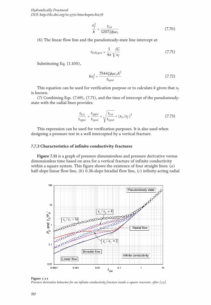
x2fk

=tLri

1207ξϕμct(7.70)

(6) The linear flow line and the pseudosteady‐state line intercept at:

tDALpssi =14π

ffiffiffiffiffixexf

r(7.71)

Substituting Eq. (1.100),

kx2f =7544ξϕμctA2

tLpssi(7.72)

This equation can be used for verification purpose or to calculate k given that xfis known.

(7) Combining Eqs. (7.69), (7.71), and the time of intercept of the pseudosteady‐state with the radial lines provides:

tLritrppsi

=trppsitLpssi

=

ffiffiffiffiffiffiffiffiffitLritLpssi

s= ðxe=xf Þ2 (7.73)

This expression can be used for verification purposes. It is also used whendesigning a pressure test in a well intercepted by a vertical fracture.

7.7.3 Characteristics of infinite‐conductivity fractures

Figure 7.11 is a graph of pressure dimensionless and pressure derivative versusdimensionless time based on area for a vertical fracture of infinite conductivitywithin a square system. This figure shows the existence of four straight lines: (a)half‐slope linear flow line, (b) 0.36‐slope biradial flow line, (c) infinity‐acting radial

Figure 7.11Pressure derivative behavior for an infinite‐conductivity fracture inside a square reservoir, after [35].

257


flow line (horizontal line), and (d) unit‐slope pseudosteady‐state flow line. For xe/xf> 8, the linear flow regime is almost nonexistent, and the biradial flow line isobserved first. For xe/xf < 8, the biradial flow line disappears [34]. Only the char-acteristics of the biradial flow regime will be discussed here. The characteristics andinterpretation of the other three flow regimes (linear, radial, and pseudosteadystate) are the same as discussed above for uniform‐flow fracture.

(1) The equation of the biradial flow regime line introduced by [35] and modi-fied by Bettam et al. [2] is:

tDA*PD0 =0:769

xexf

!0:72tDA

ξ

� �0:36

(7.74)

Taking logarithm to both members of the above equation leads to:

logðtDA*PD0Þ =0:36log tDA

ξ

� �þ log 0:769

xexf

!0:7224

35 (7.75)

In dimensional form, Eq. (7.74) becomes:

t*ΔP 0 =0:769CBRðxe=xf Þ2t0:36 (7.76)

where

CBR = 7:268qμBkh

kξϕμctA

� �9=25

(7.77)

Taking logarithm to both sides of Eq. (7.76) yields:

log t*ΔP 0ð Þ =0:36 log tþ log 0:7699CBRxexf

!0:720@

1A (7.78)

Thus, the biradial flow line can be identified by its slope of 0.36. Let (t*ΔP 0)BR1be the value of pressure derivative at a time t=1hr in the straight line (extrapolatedif necessary). An expression to find the half‐fracture length is found from Eq. (7.76)when linear flow regime is absent:

xf =0:694xeCBR

ðt*ΔP 0ÞBR1

� �1:388(7.79)

CBR is found from Eq. (7.77).(2) The time of intersection between the linear flow and biradial flow regimes is

given by Eqs. (7.56) and (7.74):

tDALBRi =0:00257xfxe

� �2

(7.80)

Substituting the dimensionless time and solving for xf2/k yields:

x2fk

=tLBRi

39ξϕμct(7.81)

258


If the radial flow is too short, permeability can be found from an expressionobtained by combining the above expression and Eq. (7.61):

k =12:67qμBhðt*ΔP 0ÞL1

� �1ffiffiffiffiffiffiffiffiffitLBRi

p (7.82)

(3) The time of intersection between the biradial and radial flow regime linescan be used to verify k and xf:

tDArBRi =0:3023xfxe

� �2

(7.83)

Substituting the dimensionless time in the above expression and solve for xf2/k:

x2fk

=tBRri

4587ξϕμct(7.84)

(4) The time of intersection between the biradial flow regime line and thepseudosteady‐state line (Eqs. 2.96 and 7.74) provides:

tDABRpssi =0:03755xexf

!1:125

(7.85)

After substituting the dimensionless time based on area, Eq. (1.100) in Eq. (7.85)leads to:

k =142:3ξϕμctA

tBRpssi

xexf

!1:125

(7.86)

(5) Combination of Eqs. (7.81) with (7.84) and (7.83) with (7.85) will, respec-tively, yield:

tBRri = 117:6tLBRi (7.87)

tBRri = 8xfxe

� �2:125

tBRpssi (7.88)

which can be used for either verification or test design purposes.

7.7.4 Rectangular systems

For both types of fractures in rectangular systems, the transition between theinfinite‐action radial flow and the pseudosteady‐state period is much longer than fora square system since, in the first one, formation linear flow exists as described inSection 2.7. The equation of this straight line proposed by Tiab [35] and modified byEscobar et al. [16] to include naturally fractured formations is:

tDA*PD0 = 3:545

ffiffiffiffiffiffiffitDA

ξ

r(7.89)

Substituting the dimensionless terms:

t*ΔP0 =mCBffiffit

p(7.90)

259


where

mCB = 8:128qBh

μ

ξϕctA

� �0:5

(7.91)

where (t*ΔP 0)CB1 is the value of (t*ΔP 0) at a time t=1hr on the formation linearflow straight line (extrapolated if necessary). Permeability can be solved from theabove equation, so that:

k = 66:0712qB

h t*ΔP 0ð ÞCB1

� �2 μ

ξϕctA(7.92)

Tiab [35] presents step‐by‐step procedures for the interpretation of pressuretests in fractured wells. These procedures are not included here.

Example 7.2

Tiab [35] presented an example of a pressure test in a highly productive frac-tured well. Pressure and pressure derivative [13] data versus time are reported inFigure 7.12 and Table 7.2. Other relevant data are given below:

q=2000 STB/D, ϕ =0.24, m=0.3 cp, ct=14.8�10�6 psia�1, B=1.5 bbl/STB, h=50ft, rw=0.4 ft, Pi=5200 psia

Find permeability, skin factor, and half‐fracture length. Verify the value of thehalf‐fracture length.

Solution

Since it is a homogenous reservoir, then ξ=1. The following characteristic pointswere read from Figure 7.12 and Table 7.3:

tr=48 hr, ΔPr=507 psia, (t*ΔP 0)r =105.5 psia, tLRi=1.2 hr, tLBRi=0.047 hr, trBRi=4.5 hr

Estimate permeability using Eq. (2.71) and skin factor with Eq. (2.92):


=70:6ð2000Þð0:3Þð1:5Þ

50ð105:5Þ = 12 md

Figure 7.12Pressure and pressure derivative against time log‐log plot of Example 7.3.

260


s =0:5 507105:5

� ln12 � 48

ð0:24Þð0:3Þð14:8� 10�6Þð0:4Þ2 !

þ 7:43

" #= � 4:85

Find half‐fracture length with Eq. (7.63):

xf =2:032qBh t*ΔP 0ð ÞL1

ffiffiffiffiffiffiffiffiffiffiμ

ϕ ctk

r=2:032ð2000Þð1:5Þ

50ð97Þ

ffiffiffiffiffiffiffiffiffiffiffiffiffiffiffiffiffiffiffiffiffiffiffiffiffiffiffiffiffiffiffiffiffiffiffiffiffiffiffiffiffiffiffiffiffiffi0:3

0:24ð14:8� 10�6Þð12Þ

s= 105:4 ft

Recalculate the half‐fracture length with Eqs. (7.70), (7.81), and (7.84), respec-tively.

xf =

ffiffiffiffiffiffiffiffiffiffiffiffiffiffiffiffiffiffiffiffiffitLrik

1207ξϕμct

s=

ffiffiffiffiffiffiffiffiffiffiffiffiffiffiffiffiffiffiffiffiffiffiffiffiffiffiffiffiffiffiffiffiffiffiffiffiffiffiffiffiffiffiffiffiffiffiffiffiffiffiffiffiffiffiffiffiffiffiffiffiffið1:2Þð12Þ

1207ð0:24Þð0:3Þð14:8� 10�6Þ

s= 105:81 ft

xf =

ffiffiffiffiffiffiffiffiffiffiffiffiffiffiffiffitBRLik39ξϕμct

s=

ffiffiffiffiffiffiffiffiffiffiffiffiffiffiffiffiffiffiffiffiffiffiffiffiffiffiffiffiffiffiffiffiffiffiffiffiffiffiffiffiffiffiffiffiffiffiffiffiffiffiffiffiffiffiffiffið0:047Þð12Þ

39ð0:24Þð0:3Þð14:8� 10�6Þ

s= 116:5 ft

xf =

ffiffiffiffiffiffiffiffiffiffiffiffiffiffiffiffiffiffiffiffiffitBRrik

4587ξϕμct

s=

ffiffiffiffiffiffiffiffiffiffiffiffiffiffiffiffiffiffiffiffiffiffiffiffiffiffiffiffiffiffiffiffiffiffiffiffiffiffiffiffiffiffiffiffiffiffiffiffiffiffiffiffiffiffiffiffiffiffiffiffiffið5:5Þð12Þ

4587ð0:24Þð0:3Þð14:8� 10�6Þ

s= 116:2 ft

7.7.5 Finite‐conductivity fractured vertical wells

A log‐log plot of pressure and pressure derivative versus test time for a fracturedwell in a closed system may reveal the presence of several straight linescorresponding to different flow regimes, excluding wellbore storage, such as (a)bilinear flow characterized by a slope of ¼ in the pressure and pressure derivativecurve, (b) linear flow, (c) infinite‐action radial flow, and (d) pseudosteady‐stateperiod. The slopes and points of intersection of these straight lines are unique andwere used by Tiab et al. [36, 38] to find expressions for well test interpretation.

t, hr P, psia t*DP’, psia t, hr P, psia t*DP’, psia

0.017378 5174.322 12.605 1.44544 5019.68 68.901

0.025119 5169.16 15.287 2.089296 4992.606 76.039

0.036308 5163.033 18.027 3.019952 4962.879 83.251

0.052481 5155.836 21.039 4.365158 4930.874 88.885

0.075858 5147.48 24.541 6.309573 4897.025 93.405

0.109648 5137.868 28.044 9.120109 4861.749 98.014

0.131826 5132.556 29.705 13.18257 4825.404 100.147

0.190546 5120.828 33.792 15.84893 4806.922 99.820

0.275423 5107.467 38.787 22.90868 4769.489 100.962

0.398107 5092.232 44.292 33.11311 4731.58 103.280

0.57544 5074.815 50.627 47.86301 4693.335 109.456

0.831764 5054.879 58.306 69.1831 4654.853 109.456

1.202264 5032.142 65.746 100 4616.205 109.456

Table 7.3.Pressure and pressure derivative against time data of Example 7.3.

261


The characteristics of bilinear flow were first discussed by Cinco et al. [6]. It iscalled bilinear flow because it is the result of two linear flow regimes. A flow regimeis the incompressible linear flow of the fracture and the other flow regime is thecompressible linear flow in the formation, as shown in Figure 7.9. They showedmathematically that bilinear flow exists whenever (a) most of the fluid entering thewell face comes from the formation and (b) the effects of the fracture do not affectwell behavior.

During the bilinear flow regime, the behavior of the dimensionless pressure ofthe well given by Tiab et al. [36] and modified by Bettam et al. [2] is:

PD =2:45

C1=2fD


ξ4

r(7.192)

Replacing the dimensionless parameters given by Eqs. (1.89), (7.3), and (7.15),Eq. (7.92) becomes:

ΔP=mBLffiffit4

p(7.93)

mBL =44:13

ðξϕμctkÞ0:25qμB

hfffiffiffiffiffiffiffiffiffiffikfwf

p (7.94)

The fracture conductivity is solved from Eq. (7.93):

kfwf = 1947:461ffiffiffiffiffiffiffiffiffiffiffiffiffiffi

ξϕμctkp qμB

hðΔPÞBL1

� �2

(7.95)

The derivative of Eq. (7.92) is:

tD*PD0 =

0:6125

C1=2fD


ξ4

r(7.96)

Replacing the dimensionless quantities, given by Eqs. (2.57), (7.3), and (7.15), inEq. (7.96) and solving for the fracture conductivity:

kfwf =121:74ffiffiffiffiffiffiffiffiffiffiffiffiffiffiξϕμctk

p qμBhðt*ΔP 0ÞBL1

� �2

(7.97)

Since this is linear flow, Eqs. (7.61) and (7.63) also apply for finite‐conductivityfractures.

The intercept between linear flow and bilinear flow lines given by the governingpressure derivative solutions (Eqs. 7.4 and 7.92) leads to:

tBLLi = 13910ξϕμctx2f

ffiffiffik

p

kfwf

!(7.98)

Solving for k,

k =kfwf

x2f

!2tBLLi

13910ξϕμct(7.99)

The pressure derivative of Eq. (7.4) is:

262


tD*PD =12

ffiffiffiffiffiffiffiffiffiffiffiπtDxf

ξ

r(7.100)

The intercept between linear flow and bilinear flow lines given by the governingpressure derivative solutions (Eqs. 7.100 and 7.96) leads to:

k =kfwf

x2f

!216t 0BLLi

13910ξϕμct(7.101)

Eqs. (7.99) and (7.101) can be used for verification purposes, if all three flowregimes are observed. If the test is too short to observe the radial flow line, or aprefracture test is not possible as in the low permeability formation, thenEqs. (7.99) and (7.101) can be used to calculate the permeability of the formation.Also, needless to say that Eqs. (2.71) and (2.93), along with many other relation-ships in Chapters 2 and 3, will apply to fractured wells.

The intersection of Eq. (2.70), neglect CD, and Eq. (7.96) leads after rearranging:

0:25mBLt0:25BLri =70:6qμB

kh(7.102)

Solving for the intersection time,

tBLri = 1677ξϕμctk3

ðkfwf Þ2 (7.103)

which Tiab et al. [36] recommend to be used for verification purpose.The intersection of the biradial flow regime pressure derivative (Eq. 7.74) with

the bilinear flow regime pressure derivative (Eq. 7.96), lines will result in:

t0:11BLBRi =0:25mBL

0:7699CBRxexf

!0:72 =1:197k0:39ðξϕμctkÞ0:11x0:72f

ffiffiffiffiffiffiffiffiffiffikfwf

p xexf

!0:72 (7.104)

being mBL and CBR defined by Eqs. (7.94) and (7.77), respectively. Either half‐fracture length or conductivity can be solved from Eq. (7.104).

The intersect of the pressure derivative bilinear governing expression (Eq. 7.96)with the pressure derivative pseudosteady‐state period Eq. (2.96) will lead to:

kfwf = 2220:603A2kξϕμctktBLpssi

� �3=2

(7.105)

7.7.6 Special Cases

As also mentioned by Tiab et al. [36, 38], the above assumption assumes that allthree flow regimes (bilinear, linear formation, and radial) are observed during thepressure test and that these are well defined in the pressure derivative curve. Inmany instances, at least one of the flow regimes is not observed or defined. Forexample, when the fracture has low conductivity, let us say, CfD < 5, probably linearflow regime is not seen. In the contrary case, when CfD > 50, probably bilinear flowis absent or maybe masked by wellbore storage effects. In such cases, the belowcorrelations [37], which are excellent, can be used to find one parameter (Eq. 7.107)as a function of the other one or vice versa (Eq. (7.108)).

263


xf =1:92173

1=rwa � 3:31739k=kfwf(7.106)

where rwa is the effective wellbore radius given by Eq. (7.54), so Eq. (7.106) canbe rewritten as:

xf =1:92173

es=rw � 3:31739k=kfwf(7.107)

kfwf =3:31739k

es=rw � 1:92173=xf(7.108)

When radial flow is absent, this can be artificially from Eq. (2.71) by solving forthe pressure derivative during the radial flow regime. Once estimated, a horizontalline can be drawn through this value, which corresponds to the place where radialflow really exists. Intersection of this line with others can be used without anyproblem. However, to find skin factor, the below correlation developed byEconomides et al. [9] is recommended to be used:

s = ln rw1:92173

xf

!� 3:31739

kfwf

" #(7.109)

The internal result between parentheses may be considered in absolute value.Skin factor can also be estimated by a graphical procedure formulated by Cinco‐Leyand Samaniego [7], type‐curve matching, or the following correlation [9]:

s = lnrwxf

þ 1:65� 0:32uþ 0:11u2

1þ 0:18uþ 0:064u2 þ 0:005u3(7.110)

where

u= lnkfwf

k � xf

!= ln CfD (7.111)

Finally, Tiab et al. [36, 38] also provided more relationships, which are notreported because of their relevance. Neither the step‐by‐step procedures arereported.

Alternatively, Eqs. (7.40), (7.41), and Figure 7.8 can be used.Fracture conductivity can be found by a graphical correlation (Figure 7.13),

given by Economides et al. [9], which polynomial fitting is given here:

x = sþ lnxfrw

� �; 0:67≤x≤2:8 (7.112)

CfD = 10

0:59222806� 1:77955xþ 0:86571983x2

1� 1:5944514xþ 0:010112x2

� �(7.113)

Example 7.4

Tiab et al. [36, 38] presented pressure data for a buildup test run in a fracturedwell. Pressure and pressure derivative data are reported in Table 7.4 andFigure 7.14. Other important information concerning this test is given below. Findthe fracture and reservoir parameters for this well.

264


q=101 STB/D, ϕ=0.08, μ=0.45 cp, ct=17.7�10�6 psia�1, B=1.507 bbl/STB,h = 42 ft, rw=0.28 ft, tp=2000 hr, Pi=2200 psia, ξ=1

Solution

The following characteristic features were read from Figure 7.14:tr=30 hr, ΔPr=471 psia, (t*ΔP’)r=150 psia, (t*ΔP’)BL1=160 psia, ΔPBL1=40 psia,

ΔPL1=120 psia, tLri=8.2 hr, tBLri=195 hrEstimate permeability and skin factor from Eqs. (2.71) and (2.92):


=ð70:6Þð101Þð0:45Þð1:507Þ

ð42Þð150Þ =0:76 md

Figure 7.13Effect of skin factor on fracture conductivity, after [9].

t, hr DP, psia t*DP', psia t, hr DP, psia t*DP', psia

0.23 102 26.3 15 390 117

0.39 115 30 20 423 112

0.6 130 35.8 25 446 120

1 145 40.8 30 471 141

1.8 183 57.2 35 493 136.5

2.4 195 67 40 510 132

3.8 260 83.3 45 526 135

4.1 265 69.2 50 540 150

4.96 280 96.9 55 556 137.5

6.2 308 102.3 60 565 144

8.5 320 103.3 65 580 121.1

10 345 149 71 583

Table 7.4.Pressure data for Example 7.4. Derivative digitized from [38].

265


s =12

471150

� lnð0:76Þð30Þ

ð0:08Þð0:45Þð17:7 � 10�6Þð0:282Þ

� �þ 7:43

� �= � 4:68

Estimate fracture conductivity using Eqs. (7.95) and (7.97):

kfwf = 1947:46ffiffiffiffiffiffiffiffiffiffiffiffiffiffiffiffiffiffiffiffiffiffiffiffiffiffiffiffiffiffiffiffiffiffiffiffiffiffiffiffiffiffiffiffiffiffiffiffiffiffiffiffiffiffiffiffiffiffiffiffiffiffiffiffiffiffi

ð0:08Þð0:45Þð17:7 � 10�6Þð0:76Þq

ð101Þð0:45Þð1:507Þð42Þð160Þ

� �2

= 290:7 md‐ft

kfwf =121:74ffiffiffiffiffiffiffiffiffiffiffiffiffiffiffiffiffiffiffiffiffiffiffiffiffiffiffiffiffiffiffiffiffiffiffiffiffiffiffiffiffiffiffiffiffiffiffiffiffiffiffiffiffiffiffiffiffiffiffiffiffiffiffiffiffiffi

ð0:08Þð0:45Þð17:7 � 10�6Þð0:76Þq ð101Þð0:45Þð1:507Þ

ð42Þð40Þ� �2

= 290:77 md‐ft

Find the intercept between bilinear and biradial flow regimes with Eq. (7.103):

tBLri = 1677ð0:08Þð0:45Þð17:7 � 10�6Þ

ð0:76Þ3 ð310:8Þ2 = 235 hr

This is in the range of 195 hr read from Figure 7.13. Use Eqs. (7.63) and (7.70) tofind half‐fracture length:

xf = 4:064ð101Þð1:507Þð42Þð120Þ

� � ffiffiffiffiffiffiffiffiffiffiffiffiffiffiffiffiffiffiffiffiffiffiffiffiffiffiffiffiffiffiffiffiffiffiffiffiffiffiffiffiffiffiffiffiffiffiffiffiffiffiffiffiffiffi0:45

ð0:08Þð17:7 � 10�6Þð0:76Þ

s= 79 ft

xf =

ffiffiffiffiffiffiffiffiffiffiffiffiffiffiffiffiffiffiffiffiffiktLri

1207ξϕμct

s=

ffiffiffiffiffiffiffiffiffiffiffiffiffiffiffiffiffiffiffiffiffiffiffiffiffiffiffiffiffiffiffiffiffiffiffiffiffiffiffiffiffiffiffiffiffiffiffiffiffiffiffiffiffiffiffiffiffiffiffiffiffiffiffið0:76Þð10Þ

1207ð0:08Þð0:76Þð17:7 � 10�6Þ

s= 76:5 ft

From Eq. (7.98), the time intercept of bilinear and linear flow regimes is foundto be:

tBLLi = 13910ð0:08Þð0:45Þð17:7 � 10�6Þ 792ffiffiffiffiffiffiffiffiffi0:76

p

290:7

� �2

= 1:48 hr

This is very close to the value of 1.4 hr found from the derivative plot. UseEq. (7.107) to estimate the half‐fracture length:

Figure 7.14Pressure and pressure derivative against time log‐log plot for Example 7.4.

266


xf =1:92173

esrw� 3:31739k

wf kf

=1:92173

e�4:6844

0:28 � 3:31739ð0:76Þ290:7

= 79 ft

And the dimensionless fracture conductivity is found from Eq. (7.15), so that:

CfD =wfkfxf k

=290:7

79ð0:76Þ = 4:8

Example 7.5

Tiab et al. [36, 38] presented a short buildup test run in a fractured well. Radialflow was not developed, but the reservoir permeability was measured from anotherto be 12.4 md. The pressure and pressure derivative [13] data are reported inTable 7.5 and Figure 7.15. Additional data:

q=411.98 STB/D, f=0.2, m=0.53 cp, ct=101�10�6 psia�1, B=1.258 bbl/STB,h =21 ft, rw=0.689 ft, tp=3000 hr, Pi=479.61 psia, ξ=1

Solution

Since permeability is known, the pressure derivative during infinite‐acting radialflow is found from Eq. (2.71):

t, hr DP, psia t*DP 0, psia t, hr DP, psia t*DP 0, psia

0.017 27.45 26.62 3.78 93.59 24.85

0.019 42.39 24.98 4.78 99.56 26.61

0.082 48.5 5.19 5.78 104.26 28.49

0.28 56.18 10.50 7.78 113.36 30.37

0.33 61.87 9.67 9.78 121.04 33.32

0.78 63.72 10.91 11.78 126.87 35.17

1.08 72.11 13.18 13.78 131.85 35.67

1.78 76.38 15.36 17.78 142.66 38.51

2.78 86.34 22.58 19.78 146.07 40.70

Table 7.5.Pressure data for Example 7.5. Derivative digitized from [38].

Figure 7.15Pressure and pressure derivative against time log‐log plot for Example 7.5.

267


ðt*ΔP 0Þr =70:6qμB

hk=ð70:6Þð411:98Þð0:53Þð1:258Þ

ð21Þð12:4Þ = 74:5 psia

A horizontal line is drawn throughout (t*ΔP')r of 74.5 psia. This corresponds toan arterially created radial flow regime line. The following data were then read fromFigure 7.15:

tLri=75 hr, tBLLi=14 hr, (t*ΔP 0)BL1=18 psia, ΔPBL1=72 psia, ΔPL1=10 psia,Use Eqs. (7.95) and (7.97) to determine fracture conductivity:

kfwf =1947:46ffiffiffiffiffiffiffiffiffiffiffiffiffiffiffiffiffiffiffiffiffiffiffiffiffiffiffiffiffiffiffiffiffiffiffiffiffiffiffiffiffiffiffiffiffiffiffiffiffiffiffiffiffiffiffiffiffiffiffiffiffiffi

ð0:2Þð0:53Þð101� 10�6Þð12:4Þq ð411:98Þð0:53Þð1:258Þ

ð21Þð72Þ� �2

= 5578:35 md‐ft

kfwf =121:74ffiffiffiffiffiffiffiffiffiffiffiffiffiffiffiffiffiffiffiffiffiffiffiffiffiffiffiffiffiffiffiffiffiffiffiffiffiffiffiffiffiffiffiffiffiffiffiffiffiffiffiffiffiffiffiffiffiffiffiffiffiffi

ð0:2Þð0:53Þð101� 10�6Þð12:4Þq ð411:98Þð0:53Þð1:258Þ

ð21Þð18Þ� �2

= 5579:44 md‐ft

Find the half‐fracture length with Eqs. (7.61) and (7.71):

xf = 4:064411:98ð1:258Þ

ð21Þð10Þ� � ffiffiffiffiffiffiffiffiffiffiffiffiffiffiffiffiffiffiffiffiffiffiffiffiffiffiffiffiffiffiffiffiffiffiffiffiffiffiffiffiffiffiffiffiffiffiffiffiffi

0:53ð0:2Þð101� 10�6Þð12:4Þ

s= 260:5 ft

xf =

ffiffiffiffiffiffiffiffiffiffiffiffiffiffiffiffiffiffiffiffiffiktLri

1207ξϕμct

s=

ffiffiffiffiffiffiffiffiffiffiffiffiffiffiffiffiffiffiffiffiffiffiffiffiffiffiffiffiffiffiffiffiffiffiffiffiffiffiffiffiffiffiffiffiffiffiffiffiffiffiffiffiffiffiffiffiffiffiffið12:4Þð75Þ

1207ð0:2Þð0:53Þð101� 10�6Þ

s= 268:3 ft

Use Eq. (7.109) to find skin factor:

s = ln0:689 1:92173

264� 3:31739ð12:4Þ

5578:9

� ��

= � 9:6

Estimate the dimensionless fracture conductivity by means of Eq. (7.15):

CfD =kfwf

kxf=

5578:912:4ð264Þ = 1:7

Figure 7.16Pressure and pressure derivative behavior against dimensionless time for a vertical well with infinite‐conductivity fracture in a heterogeneous reservoir with λ=1 � 10�8 and ω=0.1, after [23].

268


7.8. New elliptical or biradial flow model

It was not possible to use Eq. (7.79) to find half‐fracture length in Example 7.2.This is because Eq. (7.74) depends on area, which should not be the case since thiscauses the test to be very long and therefore costly, which is not well accepted bymost operators who in many circumstances do not allow fractured wells to developradial flow during a well test. This implies the impossibility of determining themean fracture length by means of Eq. (7.79) when at early times only biradial orelliptical flow is observed. In cases where the radial flow is observed or the perme-ability is known, it is possible to determine the mean fracture length usingEq. (7.84).

To overcome the above issue, Escobar et al. [23] presented a new model (seeFigure 7.17) for biradial/elliptical flow, which excludes the drainage area and ispresented below for homogeneous reservoirs (ξ=1) or heterogeneous reservoirs(ξ=ω):

PD =259

πtDxf

26ξ

� �0:36

(7.114)

which pressure derivative is given by:

tD*PD0 =

πtDxf

26ξ

� �0:36

(7.115)

7.8.1 TDS technique for the new biradial flow model

Once the dimensionless parameters given by Eqs. (1.89), (7.55) and (2.57) in theabove expressions solve for the half‐fracture length, it yields:

xf = 22:5632qB

hðΔPÞBR

� �1:3889ffiffiffiffiffiffiffiffiffiffiffiffiffiffiffiffiffiffiffiffiffiffiffiffiffitBRξϕct

μ

k

�1:778s(7.116)

xf = 5:4595qB

hðt*ΔP 0ÞBR

� �1:3889ffiffiffiffiffiffiffiffiffiffiffiffiffiffiffiffiffiffiffiffiffiffiffiffiffitBRξϕct

μ

k

�1:778s(7.117)

Figure 7.17Pressure and pressure derivative against time log‐log plot for Example 7.6, after [18].

269


Normally, the well test data are affected by noise, so it is recommended to drawthe best line on the dealt flow (in this case, biradial) and read the value on thatstraight line at a time t=1 hr (extrapolated if required), which leads to Eqs. (7.116)and (7.117) being rewritten as:

xf = 22:5632qB

hðΔPÞBR1

� �1:3889ffiffiffiffiffiffiffiffiffiffiffiffiffiffiffiffiffiffiffiffiffiffiffiffiffi1

ξϕct

μ

k

�1:778s(7.118)

xf = 5:4595qB

hðt*ΔP 0ÞBR1

� �1:3889ffiffiffiffiffiffiffiffiffiffiffiffiffiffiffiffiffiffiffiffiffiffiffiffiffi1

ξϕct

μ

k

�1:778s(7.119)

The intercept between the straight lines of the derivatives of bilinear and bira-dial flows tBLBRi (Eqs. 7.96 and 7.115) allows obtaining an expression to determinethe half‐fracture length, xf,

kfwf = 10:5422ξϕμctk

3:5454x6:5454f

tBLBRi

!0:22

(7.120)

The intercept between the straight lines of the derivatives of linear and biradialflows tLBRi (Eqs. 7.89 and 7.115) also allows obtaining an expression to determine thehalf‐fracture length, xf,

xf =

ffiffiffiffiffiffiffiffiffiffiffiffiffiffiffiffiffiffiffiffiffiffiffiffiffiffiktBRLi

39:044ξϕμct

s(7.121)

Another way to obtain the half‐fracture length is the intercept of the straightlines of the radial flow derivatives (Eq. 2.70) and biradial flow regime (Eq. 7.115)tBRri,

xf =1

4584:16

ffiffiffiffiffiffiffiffiffiffiffiktBRriξϕμct

s(7.122)

The intersection formed by the line of the derivative of the biradial flow with theline of the derivative of pseudosteady state (Eq. 2.96), called tBRpssi, leads to:

xf =41:0554A1:3889 ξϕμctktBRpssi

� �0:8889

(7.123)

For circular/square constant pressure systems which pressure derivativeis governed by Eq. (2.349), when intercepts with Eq. (7.115), called tBRSSi, alsoleads to:

xf =1

4247:92A25=18 ffiffiffiffiω

p ktBRSSiϕμct

� �179

(7.124)

Other recent publications dealing with elliptical/biradial flow regime in hori-zontal and vertical wells can be found in Refs. [15–18, 28].

7.8.2 Conventional analysis for the new biradial flow model

After replacing Eqs. (1.89) and (7.55), kin Eq. (7.114) leads to:

270


ΔP = 9:4286qμBkh

kξϕμctx2f

!0:36

t0:36 (7.125)

or

ΔP =mbirt0:36 (7.126)

Eq. (7.126) implies that a Cartesian graph of ΔP versus t0.36 (for drawdowntests) or ΔP versus ΔP versus [(tpþΔt)0.36 � Δt0.36] (for buildup tests) provides aline which slope, mell, allows obtaining the half‐fracture length,

xf =

ffiffiffiffiffiffiffiffiffiffiffiffiffiffiffiffiffiffiffiffiffiffiffiffiffiffiffiffiffiffiffiffiffiffiffiffiffiffiffiffiffiffiffiffiffiffiffiffiffiffiffiffiffi9:4286

qμBkhmbir

kξϕμct

� �0:36s

(7.127)

Example 7.6

Determine the half‐fracture length for a pressure test which data are reported inTable 7.6 and plotted in Figure 7.17 for a hydraulically fractured well in a hetero-geneous reservoir. Other relevant information for this test is given below:

B=1.25 bbl/STB, q=350 STB/D, h=100 ft, μ=3 cp, rw=0.4 ft, ct=1�10�5 psia�1,Pi=5000 psia, φ=20%, k=300 md, ω=0.1, λ=1�10�7, xf=100 ft

t, hr ΔP, psia t*ΔP, psia t, hr ΔP, psia t*ΔP, psia t, hr ΔP, psia t*ΔP, psia

0.001 1.246 0.608 0.101 8.159 2.624 8.021 19.566 1.680

0.002 1.722 0.797 0.127 8.775 2.696 10.098 19.932 1.484

0.003 2.063 0.920 0.160 9.405 2.753 14.264 20.397 1.234

0.004 2.336 1.015 0.201 10.048 2.798 20.148 20.777 1.074

0.005 2.569 1.088 0.254 10.697 2.832 28.460 21.108 1.012

0.006 2.773 1.166 0.319 11.354 2.852 40.202 21.442 1.093

0.007 2.956 1.224 0.402 12.015 2.863 55.107 21.797 1.283

0.008 3.122 1.286 0.506 12.677 2.863 70.107 22.121 1.474

0.009 3.277 1.341 0.637 13.336 2.849 85.107 22.423 1.678

0.010 3.433 1.398 0.802 13.992 2.825 100.107 22.707 1.838

0.013 3.768 1.521 1.010 14.641 2.788 140.107 23.390 2.200

0.016 4.132 1.650 1.271 15.280 2.737 185.107 24.051 2.472

0.020 4.528 1.790 1.600 15.906 2.671 240.107 24.734 2.691

0.025 4.956 1.928 2.015 16.514 2.590 330.107 25.637 2.903

0.032 5.418 2.066 2.537 17.102 2.488 420.107 26.355 2.999

0.040 5.911 2.200 3.193 17.667 2.367 545.107 27.147 3.009

0.051 6.434 2.324 4.020 18.198 2.226 685.107 27.852 3.194

0.064 6.985 2.437 5.061 18.695 2.063 985.107 28.973 3.194

0.080 7.562 2.538 6.372 19.153 1.879

Table 7.6.Pressure and pressure derivative versus time data for Example 7.6, after [16].

271


Solution

The pressure derivative value during biradial flow regime at a time of 1 hr,(t*ΔP 0)BR1=7 psia. Use Eq. (7.119) to find the half‐fracture length:

xf = 5:4595350ð1:25Þ100ð7Þ

� �1:3889

ffiffiffiffiffiffiffiffiffiffiffiffiffiffiffiffiffiffiffiffiffiffiffiffiffiffiffiffiffiffiffiffiffiffiffiffiffiffiffiffiffiffiffiffiffiffiffiffiffiffiffiffiffiffiffiffiffiffiffiffiffiffiffiffiffi1

ð0:1Þð0:2Þð1� 10�5Þ3

300

� �1:778s

= 105:96 ft

The estimation of the naturally fractured parameters can be found in [18].

7.9. Horizontal wells

This last topic was left last since horizontal wells and fractured wells behavesimilarly. Actually, Escobar et al. [19] presented an approach for estimating theaverage reservoir pressure for horizontal wells under multirate testing using themathematical solution of a vertical fractured well. The use of the TDS technique forhorizontal wells is so extensive and deserves more than a chapter, for that reason itis only mentioned here. The pioneer papers on TDS technique for horizontal wellswhere presented by Engler and Tiab for naturally fractured deposit [10] and foranisotropic homogeneous formations [11]. The reader may not understand laterpublications without going them first. TDS technique for horizontal wells is so rich.Just to name so few cases, let us refer to treatment of zonal isolations by Al Rbeawiand Tiab [1] that even has conventional analysis by Escobar et al. [21]. Lu et al. [27]dealt with double permeability systems, and Escobar et al. [22] presented TDStechnique for heterogeneous and homogeneous formations when the thresholdgradient plays an important role for the flow to start flowing. Some applications onshale formations are summarized by Escobar [24].

Nomenclature

A area, ft2

B oil volume factor, bbl/STBb fraction of penetration/completionc compressibility, 1/psiaC wellbore storage coefficient, bbl/psiaCA reservoir shape factorCfD dimensionless fracture conductivityct total or system compressibility, 1/psiaFcor correction factorh formation thickness, ftk permeability, mdkh reservoir flow capacity, md‐fthf fracture height, ftkc uncorrected reservoir permeability, mdkf fracture permeability, mdkfwf fracture conductivity, md‐ftm slope of P versus log t plot, psia/hr/cyclembir slope of P versus t0.36 plot during elliptical/biradial flow, psia0.36/hrmlf slope of P versus t0.5 plot during linear flow, psia0.5/hrmvf slope of P versus t0.5 plot during linear flow, psia0.5/hr

272


mbf slope of P versus t0.25 plot during bilinear flow, psia0.25/hrP pressure, psiaPD 0 dimensionless pressure derivativePD dimensionless pressurePi initial reservoir pressure, psiaPwf well flowing pressure, psiaPws well shut‐in or static pressure, psiaP* false pressure, psiaΔPs pressure drop due to skin conditions, psiaq liquid flow rate, bbl/DqfD dimensionless flow raterD dimensionless radiusr radius, ftre drainage radius, ftrw well radius, ftrwa apparent wellbore radius, fts skin factort time, hrtp production (Horner) time before shutting‐in a well, hrtD dimensionless time based on well radiustDA dimensionless time based on reservoir areatDxf dimensionless time based on half‐fracture lengthtpDA dimensionless Horner time based on areaX distance along the x directionxe half‐reservoir side, ft (square system)xf half‐fracture length, ftt*ΔP 0 pressure derivative, psiawf fracture width, ft

Greek

Δ change, dropΔt shut‐in time, hrη diffusivity constant, φµct/kξ indicator of either heterogeneous, ξ=ω, or homogeneous, ξ=1, reservoirφ porosity, fractionρ fluid density, lbm/ft3

μ viscosity, cpω dimensionless storativity coefficient

Suffices

1h read at a time of 1 hrD dimensionlessDA dimensionless with respect to areaDxf dimensionless with respect to areaBL bilinear flowBL1 bilinear flow at 1 hrBLLi intercept of bilinear and linear lines in pressure curveBLLi intercept of bilinear and linear lines in pressure derivative curveBLBRi intercept of bilinear and biradial lines in pressure curve

273


BLri intercept of bilinear and radial lines in pressure curveblf beginning of linear flowbrf beginning of radial flowbsl beginning of semilog lineBRLi intercept of biradial and linear linesBRri intercept of biradial and radial linesBRSSi intercept of biradial and steady‐state linesBRpssi intercept of biradial and pseudosteady‐state linesCB formation linear flow regimeebf end of bilinear flowel end of linear flowf fracturei intersection or initial conditionsL linear flowL1 linear flow at 1 hrLpssi intercept of linear and pseudosteady state linesLri intercept of linear and radial linesp productionpss pseudosteady statepss1 pseudosteady state at 1 hrr radial flowLri intercept of linear and radial linesrSSi intersection between the radial line and the �1‐slope lines skinSS steadyvf vertical fracturew well, waterwa apparent wellborewf well flowingws well shut‐in

274


References

[1] Al Rbeawi SJH, Tiab D. Effect of thenumber and length of zonal isolationson pressure behavior of horizontal wells.2011. DOI: 10.2118/142177‐MS

[2] Bettam Y, Zerzar A, Tiab D.Interpretation of multi‐hydraulicallyfractured horizontal wells in naturallyfractured reservoir. 2005. DOI: 10.2118/95535‐MS

[3] Cherifi M, Tiab D, Escobar FH.Determination of fracture orientationby multi‐well interference testing.Society of Petroleum Engineers. 2002.DOI: 10.2118/77949‐MS

[4] Chukwu IF. Pressure derivativeanalysis of vertically fractured wells inbounded reservoirs [M.Sc. thesis].Norman, OK: The University ofOklahoma; 1989. p. 132

[5] Cinco-Ley H, Samaniego F.Evaluation of hydraulic transientpressure analysis for fractured wells.Society of Petroleum Engineers. 1982.DOI: 10.2118/7490-PA

[6] Cinco LH, Samaniego VF,Dominguez AN. Transient pressurebehavior for a well with a finite‐conductivity vertical fracture. SPEJournal. 1978;18(4):253-264.DOI: 10.2118/6014‐PA

[7] Cinco-Ley H, Samaniego F. Transientpressure analysis for fractured wells.Society of Petroleum Engineers. 1981.DOI: 10.2118/7490-PA

[8] Earlougher RC, Jr. Advances in WellTest Analysis, Monograph Series. Vol. 5.Dallas, TX: SPE

[9] Economides MJ, Watters LT, Dunn‐Norman S. Petroleum WellConstruction. New York: John Wiley &Sons. 622 p

[10] Engler T, Tiab D. Analysis ofpressure and pressure derivativewithout type‐curve matching, 5.Horizontal well tests in naturallyfractured reservoirs. Journal ofPetroleum Science and Engineering.1996;15:139-151

[11] Engler T, Tiab D. Analysis ofpressure and pressure derivativewithout type‐curve matching, 6.Horizontal well tests in anisotropicmedia. Journal of Petroleum Science andEngineering. 1996;15:153-168

[12] Escobar FH, Tiab D, Berumen-Campos S. Well pressure behavior of afinite-conductivity fracture intersectinga finite sealing-fault. Society ofPetroleum Engineers. 2003.DOI: 10.2118/80547-MS

[13] Escobar FH, Navarrete JM, LosadaHD. Evaluation of pressure derivativealgorithms for well-test analysis. Societyof Petroleum Engineers. 2004.DOI: 10.2118/86936-MS

[14] Escobar FH, Tiab D, Jokhio SA.Pressure analysis for a well intersectedby a hydraulic fracture with multiplesegments. Society of PetroleumEngineers. 2001. DOI: 10.2118/71035-MS

[15] Escobar FH, Muñoz OF, SepúlvedaJA. Horizontal permeabilitydetermination from the elliptical flowregime for horizontal wells. CT&F—Ciencia, Tecnología y Futuro. 2004;2(5):83-95. ISSN: 0122‐5383

[16] Escobar FH, Montealegre M,Cantillo JH. Conventional analysis forcharacterization of bi‐radial (elliptical)flow in infinite‐conductivity verticalfractured wells. CT&F—Ciencia,Tecnología y Futuro. 2006;3(2):141-147.ISSN: 0122‐5383

275


[17] Escobar FH. Montealegre M.Determination of horizontalpermeability from the elliptical flow ofhorizontal wells using conventionalanalysis. Journal of Petroleum Scienceand Engineering. 2008;61:15-20. ISSN:0920‐4105

[18] Escobar FH, Montealegre M.Conventional analysis for thedetermination of the horizontalpermeability from the elliptical flowof horizontal wells. Society ofPetroleum Engineers. 2007. DOI:10.2118/105928-MS

[19] Escobar FH, Cantillo JH, Santos N.A practical approach for the estimationof the average reservoir pressure frommulti‐rate tests in long horizontal wells.Fuentes: El Reventón Energético. 2011;9(1):13-20. First Semester

[20] Escobar FH, Zhao YL, Zhang LH.Interpretation of pressure tests inhorizontal wells in homogeneous andheterogeneous reservoirs with thresholdpressure gradient. Journal ofEngineering and Applied Sciences.2014;9(11):2220-2228

[21] Escobar FH, Meneses AR, LosadaLM. Straight‐line conventional transientpressure analysis for horizontal wellswith isolated zones. Dyna. 2014;81(185):78-85

[22] Escobar FH, Zhao YL, Zhang LH.Interpretation of pressure tests inhorizontal wells in homogeneous andheterogeneous reservoirs with thresholdpressure gradient. Journal ofEngineering and Applied Sciences.2014;9(11):2220-2228

[23] Escobar FH, Ghisays‐Ruiz A, BonillaLF. New model for elliptical flow regimein hydraulically‐fractured vertical wellsin homogeneous and naturally‐fracturedsystems. Journal of Engineering andApplied Sciences. 2014;9(9):1629-1636

[24] Escobar FH. Recent Advances inPractical Applied Well Test Analysis.New York: Nova publishers; 2015. 422 p

[25] Gringarten AC, Ramey HJ,Raghavan R. Applied pressure analysisfor fractured wells. Society of PetroleumEngineers. 1975. DOI: 10.2118/5496-P

[26] Kamal MM. Transient Well testing.SPE Monograph. Vol. 23. Henry L.Doherty Series. Richardson, TX; 850 p.Chapter 11

[27] Lu J, Zhu T, Tiab D, Escobar FH.Pressure behavior of horizontal wells indual‐porosity, dual‐permeabilitynaturally‐fractured reservoirs. Journalof Engineering and Applied Sciences.2015;10(8):3405-3417. ISSN: 1819‐6608

[28] Martinez JA, Escobar FH, BonillaLF. Reformulation of the elliptical flowgoverning equation for horizontal wells.Journal of Engineering and AppliedSciences. 2012;7(3):304-313. ISSN: 1819‐6608

[29] Tiab D, Puthigai SK. Pressure-derivative type curves, forvertically fractured wells. Society ofPetroleum Engineers. 1988. DOI:10.2118/11028-PA

[30] Noureddine R, Tiab D, AzzoughenA, Mazouzi A, Escobar FH, Zhu T.Evaluation of hydraulic fracturing andre‐entries in the Hassi‐Messaoud field,Algeria. 2002. DOI: 10.2118/76775‐MS

[31] Raghavan R, Cady GV, Ramey HJ.Well-Test Analysis for VerticallyFractured Wells. Society of PetroleumEngineers. 1972. DOI:10.2118/3013-PA

[32] Russell DG, Truitt NE. Transientpressure behavior in vertically fracturedreservoirs. Journal of PetroleumTechnology. 1964:1159-1170. Trans.AIME, 231. DOI: 10.2118/967‐PA

276


[33] Stewart G. Well Test Design &Analysis. Tulsa, Oklahoma, USA:PennWell Corporation; 2011. 1940 p

[34] Tiab D. PE-5553:Well Test Analysis.Lecture Notes. Norman, OK: TheUniversity of Oklahoma; 1993

[35] Tiab D. Analysis of pressurederivative without type curve matching:vertically fractured wells in closedsystems. Journal of Petroleum Scienceand Engineering. 1994;11:323-333. DOI:10.2118/26138-MS

[36] Tiab D, Azzougen A, Escobar FH,Berumen_Campos S. Analysis ofpressure derivative data of finite-conductivity fractures by the “DirectSynthesis” technique. Society ofPetroleum Engineers. 1999. DOI:10.2118/52201-MS

[37] Tiab D. Advances in PressureTransient Analysis—TDS technique.Lecture Notes Manual. Norman,Oklahoma, USA: The University ofOklahoma; 2003. 577 p

[38] Tiab D. Analysis of pressurederivative data of hydraulicallyfractured wells by the Tiab’s directsynthesis technique. Journal ofPetroleum Science and Engineering.2005;49:1-21. DOI: 10.1016/j.petrol.2005.07.001

[39] Wong DW, Harrington AG, CincoLey H. Application of the pressurederivative function in the pressuretransient testing of fractured wells.1986. DOI: 10.2118/13056 PA

277


Novel, Integrated and Revolutionary Well Test Interpretation ...

Documents

Transcript of Novel, Integrated and Revolutionary Well Test Interpretation ...