HAL Id: tel-01566938https://hal.archives-ouvertes.fr/tel-01566938

Submitted on 21 Jul 2017

HAL is a multi-disciplinary open accessarchive for the deposit and dissemination of sci-entific research documents, whether they are pub-lished or not. The documents may come fromteaching and research institutions in France orabroad, or from public or private research centers.

L’archive ouverte pluridisciplinaire HAL, estdestinée au dépôt et à la diffusion de documentsscientifiques de niveau recherche, publiés ou non,émanant des établissements d’enseignement et derecherche français ou étrangers, des laboratoirespublics ou privés.

Novel approaches for the exploitation of highthroughput sequencing data

Antoine Limasset

To cite this version:Antoine Limasset. Novel approaches for the exploitation of high throughput sequencing data. Bioin-formatics [q-bio.QM]. Université Rennes 1, 2017. English. tel-01566938

ANNÉE 2017

THÈSE / UNIVERSITÉ DE RENNES 1sous le sceau de l’Université Bretagne Loire

pour le grade deDOCTEUR DE L’UNIVERSITÉ DE RENNES 1

Mention : InformatiqueEcole doctorale MATISSE

présentée par

Antoine Limassetpréparée à l’unité de recherche 6074 IRISA

INSTITUT DE RECHERCHE EN INFORMATIQUE ETSYSTEMES ALEATOIRES

ISTIC

Nouvelles approchespour l’exploitationdes données desequençage haut débit

Thèse soutenue à Rennesle 12 Juillet 2017devant le jury composé de :Hélène TOUZETDirecteur de recherche, CRYSTAL/ rapporteurThierry LECROQDirecteur de recherche, LITIS / rapporteurChristophe KLOPPIngenieur de recherche, BIA / examinateurVincent LACROIXMaitre de conférence, LBBE/ examinateurGregory KUCHEROVDirecteur de recherche, LIGM/ examinateurRumen ANDONOVProfesseur, IRISA/ examinateurDominique LAVENIERDirecteur de recherche, IRISA/directeur de thèsePierre PETERLONGOChargé de recherche, IRISA/ co-directeur de thèse

Acknowledgments

AdministrationJe voudrais tout d’abord remercier l’école doctorale Matisse, l’Université Rennes 1,

IRISA et INRIA ainsi que leur personnels sans qui cette thèse et plus généralement cetenvironnement de recherche et d’enseignement scientifique n’existeraient tout simplementpas. Je remercie doublement les personnels d’administration à qui j’ai eu affaire et à quij’ai dû donner du fil à retordre. Une pensée spéciale à Marie Le Roïc qui n’a jamais parueffrayée par mon organisation plus que doûteuse et à l’administration de l’école doctoralepour avoir réussi à me faire remplir un dossier correctement pour la première fois en 26ans.

Recherche Je voudrais bien évidemment remercier tous mes collaborateurs. Merci àEric Rivals de m’avoir jeté dans le monde de la bioinformatique et de m’y avoir donnégoût pendant mon stage de L3. Merci à Dominique Lavenier de m’avoir non seulementconseillé mais guidé vers un stage puis une thèse entre de très bonnes mains. Merci aRayan Chikhi et Paul Medvedev de m’avoir lancé dans le petit monde du graphe de DeBruijn, je me demande souvent quand est-ce que je vais pouvoir en sortir. Je remercie ici,avec quelques années de retard, Rayan de m’avoir accueilli en ami plus qu’en encadrant, jegarde de très bons souvenirs, peut-être un peu trop français, de ce voyage aux Etats-Unis.Je voudrais spécialement remercier ces premiers encadrants pour leur bienveillance quim’a permis de me conforter dans ma capacité à contribuer à la formidable constructionqu’est la recherche, je ne suis plus tout à fait le même depuis.

Je ne vais pas prendre assez de place pour remercier Pierre Peterlongo pour m’avoirencadré et suivi pendant plus de trois ans. Je pense avoir été une thésard difficile etmalgré nos disjonctions tu m’as toujours laissé libre dans mon fonctionnement. Je nepense pas que j’aurais pu trouver une meilleure personne pour cette aventure. Je trouveque nous avons formé une belle paire et je suis impressionné par la vitesse à laquelle leschoses avancent.

Merci également à tout le groupe Colib’read, plein de grandes rencontres ont eu lieupour moi lors de ces réunions. Si je garde la vision d’un groupe de recherche comme ungroupe d’amis c’est un peu grâce à vous.

Je voulais aussi remercier Romain Feron, je pourrais me targuer sûrement longtempsque mon premier encadrement se soit si bien passé. J’espère que tu en garderas de bonssouvenirs et que tu continueras dans ta lancée.

1

Petite pensée pour Thomas Rokicki et Dianne Puges qui ont trouvé l’assemblagegénomique suffisamment intéressant pour participer à un petit projet avec moi. Je re-grette un peu que celui-ci n’ait jamais abouti mais il n’est jamais trop tard.

Merci à Jean-Francois Flot de m’avoir invité à Bruxelles et d’être aussi enthousiaste.Je nous souhaite beaucoup de succès à l’avenir.

Merci à tous mes co-bureaux de m’avoir supporté, et je souhaite à Marie Chevallierune bonne et heureuse année. Plus généralement je remercie toute l’équipe GenScale dem’avoir acueilli et pour cette bonne ambiance au travail qui n’a tout simplement pas deprix.

TheseJe remercie très solennellement Yannick Zakowski Hugo Bazille Camille Marchet et

Pierre Peterlongo d’avoir accompli un travail digne des travaux d’Asterix: corriger maprose. Je regrette presque de ne pas avoir compté le nombres de fautes corrigées par vossoins mais sachez que votre tâche a été colossale. Une pensée pour Pierre qui a dû passerplusieurs nuits blanches à relire les différentes versions de celle-ci, à se fouler le bras enrayant des centaines de pages. Un très très grand merci à Camille pour l’organisationde mon pot de thèse et des festivités, si j’avais moins procrastiné j’aurais pu davantagemettre la main a la pâte et j’aurais pu mettre Paris en bouteille.

EnseignementJ’ai eu le plus grand des plaisirs lors des missions d’enseignement qui m’ont été ac-

cordées par l’ISTIC. Je ne peux remercier tous mes élèves mais sait-on jamais, merci devotre interêt (parfois) et de votre sympathie (souvent), vous avez été super. Je voudraiségalement profiter de cette occasion pour remercier quelques-un de mes professeurs. Mercia Mohamed Rebbal de m’avoir fait comprendre l’essence de la résolution de problèmes.Merci à Nicolas De Granrut et Gérard Debeaumarché pour m’avoir fait confiance et per-mis d’accéder aux études supérieures auxquelles j’aspirais. Ma vie serait bien différentesans votre soutien et je travaille à rester digne de celui-ci.

AmisCes années à Rennes m’ont vu changer d’une manière saisissante et je vais remercier

ici essentiellement des Rennais qui m’ont entouré lors de mes péripéties dans ce beaupays, que personne n’en prenne ombrage. Merci à Justine de m’avoir suivi jusque ici etd’avoir été ma première experience de vie commune. J’espère que tu garderas une placespéciale à nos élucubrations et diverses aventures farfelues en pays breton, elles ont pourma part toute leur place dans la boite des bons souvenirs. Merci a Simon Rokicki etBastien Pasdeloup d’avoir les premiers accueilli un Cachannais expatrié et d’avoir faitde moi un des vôtres. Je remercie tout les membres des Projet C2Silicium et UberML,pour avoir contribué au lignes les plus hilarantes de mon CV. Encore une fois je ne vaispas prendre assez de temps pour remercier suffisament la Complexiteam. Merci pourtout ces super moments, je m’excuse officiellement pour mon Warwick Top et j’accuse lemauvais matchup. Plus sérieusement quoi que l’on vous dise, sachez-le, dans mon coeur,nous sommes au moins Diamant. Merci à Joris Lamare d’avoir gardé le contact malgréla distance et d’être toujours là pour accueillir des voyageurs déglingués et pour nousproposer les meilleurs plan de la Terre, pas moins. Un des plus grand merci à GaëtanBenoit pour avoir été mon plus proche collègue pendant toutes ces années. Pour ne citerqu’une de nos nombreuses aventures, merci d’avoir porté le projet de court-métrage surl’assemblage génomique et sache que, quoi que le président du jury en dise, notre film

2

reste le meilleur. Je vais également remercier les Doudous, pour tout votre soutien, vousn’avez jamais répondu absents lorsque j’avais besoin d’aide, je serais etonné de vous enavoir rendu le dixième. Je n’oublie pas un remerciement spécial à Simon pour son aideet ses discussions précieuses sur la compilation et les serveurs Minecraft. Merci à OlivierRuas et Hugo Bazille pour avoir essayé de me maintenir en forme le long de cette thèse.Merci à Gurvan Cabon d’avoir été le coloc le moins chiant du monde. Dur à classer je vaisremercier également mes amis à quatre pattes. Merci Belial pour avoir écrit plus que moisur mon document de thèse (notamment le fameux éedfffffffffffffffffffffffffffffffffffffffffffff).Merci à Lux d’avoir été la plus gentille des chattes et mon premier animal. Merci àJelly d’être un si bon petit tambour. Merci a BBhash de m’avoir laissé des doigts pourtravailler.

Famille Je voudrais remercier mes parents sans qui rien de tout cela n’aurait étépossible. Plus sérieusement, je vous remercie de m’avoir donné les clefs pour en arriverlà. Merci pour tout votre amour et tout votre soutien. Tout ce que vous m’avez apportéa fait de moi quelqu’un d’entier et pour cela je vous remercie infiniment. Je voudraisfinalement remercier ici Camille Marchet que je considère aujourd’hui comme la meilleurechose qui me soit arrivé. Si un des remerciements n’est pas assez developpé c’est celui-ci.Je n’aurais pas été jusqu’ici sans toi, merci pour ces bons moments.

Divers A mon grand regret ceux-ci ne pourront jamais lire ces remerciements. Mercia Nadine et Griffin, mes deux ordinateurs de travail, pour leur fidélité. Que Nadine mepardonne mon inattention, j’espère que tu vis heureux avec ton nouveau propriétairequi a dû avoir bien du mal à réinstaller MacOS sur un Linux. Merci au Genocluster dem’avoir supporté tout ce temps, pardonne-moi si je t’en ai parfois trop demandé. Pourfinir sur une note sérieuse je voudrais remercier les projets suivants et leurs collaborateurs: Libreoffice Linux Scihub Github Travis Gnu.

3

Abstract

Novel approaches for the exploitation of high throughput sequencing dataIn this thesis we discuss computational methods to deal with DNA sequences provided byhigh throughput sequencers. We will mostly focus on the reconstruction of genomes fromDNA fragments (genome assembly) and closely related problems. These tasks combinehuge amounts of data with combinatorial problems. Various graph structures are usedto handle this problem, presenting trade-off between scalability and assembly quality.

This thesis introduces several contributions in order to cope with these tasks. First,novel representations of assembly graphs are proposed to allow a better scaling. We alsopresent novel uses of those graphs apart from assembly and we propose tools to use suchgraphs as references when a fully assembled genome is not available. Finally we show howto use those methods to produce less fragmented assembly while remaining tractable.

3

Nouvelles approches pour l’exploitation des données de séquencage haut débit

Cette thèse a pour sujet les méthodes informatiques traitant les séquences ADN provenantdes séquenceurs haut débit. Nous nous concentrons essentiellement sur la reconstructionde génomes à partir de fragments ADN (assemblage génomique) et sur des problèmesconnexes. Ces tâches combinent de très grandes quantités de données et des problèmescombinatoires. Différentes structures de graphe sont utilisées pour répondre à ces prob-lèmes, présentant des compromis entre passage à l’échelle et qualité d’assemblage.

Ce document introduit plusieurs contributions pour répondre à ces problèmes. Denouvelles représentations de graphes d’assemblage sont proposées pour autoriser un meilleurpassage à l’échelle. Nous présentons également de nouveaux usages de ces graphes, dif-férent de l’assemblage, ainsi que des outils pour utiliser ceux-ci comme références dans lescas où un génome de référence n’est pas disponible. Pour finir nous montrons commentutiliser ces méthodes pour produire un meilleur assemblage en utilisant des ressourcesraisonnables.

4

Contents

Acknowledgments 1

Abstract 3

Table of contents 4

1 Introduction 71.1 DNA, genomes and sequencing . . . . . . . . . . . . . . . . . . . . . . . . 81.2 Genome assembly . . . . . . . . . . . . . . . . . . . . . . . . . . . . . . . 11

1.2.1 Greedy . . . . . . . . . . . . . . . . . . . . . . . . . . . . . . . . . 141.2.2 Overlap Layout Consensus . . . . . . . . . . . . . . . . . . . . . . 151.2.3 De Bruijn graphs . . . . . . . . . . . . . . . . . . . . . . . . . . . 20

1.3 Assembly hardness . . . . . . . . . . . . . . . . . . . . . . . . . . . . . . 311.3.1 Repeats . . . . . . . . . . . . . . . . . . . . . . . . . . . . . . . . 311.3.2 Scaffolding . . . . . . . . . . . . . . . . . . . . . . . . . . . . . . . 331.3.3 Multiple genomes . . . . . . . . . . . . . . . . . . . . . . . . . . . 34

1.4 Outline of the thesis . . . . . . . . . . . . . . . . . . . . . . . . . . . . . 36

2 Handling assembly 372.1 The assembly burden . . . . . . . . . . . . . . . . . . . . . . . . . . . . . 382.2 Overlap graph scalability . . . . . . . . . . . . . . . . . . . . . . . . . . . 412.3 The scaling story of the de Bruijn graph representation . . . . . . . . . . 43

2.3.1 Generic graphs . . . . . . . . . . . . . . . . . . . . . . . . . . . . 442.3.2 Theoretical limits . . . . . . . . . . . . . . . . . . . . . . . . . . 452.3.3 Kmer Counting . . . . . . . . . . . . . . . . . . . . . . . . . . . . 462.3.4 Probabilistic de Bruijn graphs . . . . . . . . . . . . . . . . . . . . 462.3.5 Navigational data structures . . . . . . . . . . . . . . . . . . . . . 472.3.6 Massively parallel assembly . . . . . . . . . . . . . . . . . . . . . 48

2.4 Efficient de Bruijn graph representation . . . . . . . . . . . . . . . . . . . 492.4.1 Compacted de Bruijn graph . . . . . . . . . . . . . . . . . . . . . 492.4.2 De Bruijn graph construction . . . . . . . . . . . . . . . . . . . . 492.4.3 Unitig enumeration in low memory: BCALM . . . . . . . . . . . . 512.4.4 Assembly in low memory using BCALM . . . . . . . . . . . . . . 54

2.5 Efficient de Bruijn graph construction . . . . . . . . . . . . . . . . . . . . 562.5.1 BCALM2 algorithm . . . . . . . . . . . . . . . . . . . . . . . . . 562.5.2 Implementation details . . . . . . . . . . . . . . . . . . . . . . . . 57

5

2.5.3 Large genome de Bruijn graphs . . . . . . . . . . . . . . . . . . . 592.6 Indexing large sets . . . . . . . . . . . . . . . . . . . . . . . . . . . . . . 62

3 The de Bruijn graph as a reference 813.1 Genome representations . . . . . . . . . . . . . . . . . . . . . . . . . . . 82

3.1.1 Reference sequences . . . . . . . . . . . . . . . . . . . . . . . . . . 823.1.2 Genome graphs . . . . . . . . . . . . . . . . . . . . . . . . . . . . 843.1.3 De Bruijn graphs as references . . . . . . . . . . . . . . . . . . . . 85

3.2 Read mapping on the de Bruijn graph . . . . . . . . . . . . . . . . . . . 913.2.1 An efficient tool for an NP-Complete problem . . . . . . . . . . . 913.2.2 Mapping refinements . . . . . . . . . . . . . . . . . . . . . . . . . 92

3.3 De novo, reference guided, read correction . . . . . . . . . . . . . . . . . 933.3.1 Limits of kmer spectrum . . . . . . . . . . . . . . . . . . . . . . . 933.3.2 Reads correction by de Bruijn graph mapping . . . . . . . . . . . 94

4 Improving an assembly paradigm 1114.1 Assembly challenges . . . . . . . . . . . . . . . . . . . . . . . . . . . . . 112

4.1.1 Two assembly paradigms . . . . . . . . . . . . . . . . . . . . . . 1124.1.2 Why read length matters: polyploid assembly . . . . . . . . . . . 1124.1.3 Taking the best of both worlds . . . . . . . . . . . . . . . . . . . 113

4.2 Building very high order de Bruijn graph . . . . . . . . . . . . . . . . . . 1164.2.1 Successive mapping strategy . . . . . . . . . . . . . . . . . . . . . 1164.2.2 Beyond read length . . . . . . . . . . . . . . . . . . . . . . . . . . 121

4.3 Assembly results . . . . . . . . . . . . . . . . . . . . . . . . . . . . . . . 1234.3.1 Haploid genome . . . . . . . . . . . . . . . . . . . . . . . . . . . . 1234.3.2 Diploid genome . . . . . . . . . . . . . . . . . . . . . . . . . . . . 1244.3.3 Future works . . . . . . . . . . . . . . . . . . . . . . . . . . . . . 125

5 Conclusions and perspectives 1295.1 Conclusion . . . . . . . . . . . . . . . . . . . . . . . . . . . . . . . . . . . 1305.2 Proposed methods . . . . . . . . . . . . . . . . . . . . . . . . . . . . . . 1325.3 Future of sequencing . . . . . . . . . . . . . . . . . . . . . . . . . . . . . 133

5.3.1 Third generation sequencing . . . . . . . . . . . . . . . . . . . . . 1335.3.2 Long range short reads sequencing . . . . . . . . . . . . . . . . . 133

5.4 Future of this work and perspectives . . . . . . . . . . . . . . . . . . . . 134

Bibliography 148Table of contents

6

Chapter 1

Introduction

"People say they want simple things, but they don’t. Not always."

John D. Cook

7

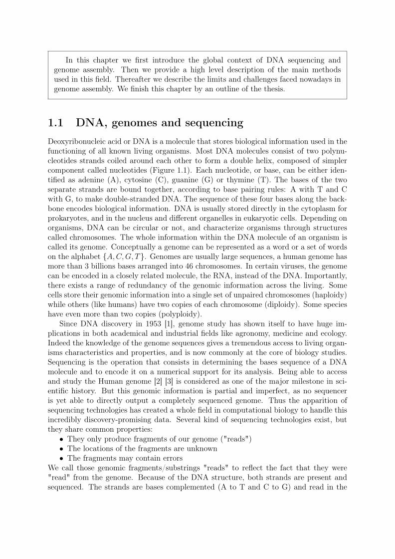
In this chapter we first introduce the global context of DNA sequencing andgenome assembly. Then we provide a high level description of the main methodsused in this field. Thereafter we describe the limits and challenges faced nowadays ingenome assembly. We finish this chapter by an outline of the thesis.

1.1 DNA, genomes and sequencing

Deoxyribonucleic acid or DNA is a molecule that stores biological information used in thefunctioning of all known living organisms. Most DNA molecules consist of two polynu-cleotides strands coiled around each other to form a double helix, composed of simplercomponent called nucleotides (Figure 1.1). Each nucleotide, or base, can be either iden-tified as adenine (A), cytosine (C), guanine (G) or thymine (T). The bases of the twoseparate strands are bound together, according to base pairing rules: A with T and Cwith G, to make double-stranded DNA. The sequence of these four bases along the back-bone encodes biological information. DNA is usually stored directly in the cytoplasm forprokaryotes, and in the nucleus and different organelles in eukaryotic cells. Depending onorganisms, DNA can be circular or not, and characterize organisms through structurescalled chromosomes. The whole information within the DNA molecule of an organism iscalled its genome. Conceptually a genome can be represented as a word or a set of wordson the alphabet A,C,G, T. Genomes are usually large sequences, a human genome hasmore than 3 billions bases arranged into 46 chromosomes. In certain viruses, the genomecan be encoded in a closely related molecule, the RNA, instead of the DNA. Importantly,there exists a range of redundancy of the genomic information across the living. Somecells store their genomic information into a single set of unpaired chromosomes (haploidy)while others (like humans) have two copies of each chromosome (diploidy). Some specieshave even more than two copies (polyploidy).

Since DNA discovery in 1953 [1], genome study has shown itself to have huge im-plications in both academical and industrial fields like agronomy, medicine and ecology.Indeed the knowledge of the genome sequences gives a tremendous access to living organ-isms characteristics and properties, and is now commonly at the core of biology studies.Sequencing is the operation that consists in determining the bases sequence of a DNAmolecule and to encode it on a numerical support for its analysis. Being able to accessand study the Human genome [2] [3] is considered as one of the major milestone in sci-entific history. But this genomic information is partial and imperfect, as no sequenceris yet able to directly output a completely sequenced genome. Thus the apparition ofsequencing technologies has created a whole field in computational biology to handle thisincredibly discovery-promising data. Several kind of sequencing technologies exist, butthey share common properties:

• They only produce fragments of our genome ("reads")• The locations of the fragments are unknown• The fragments may contain errors

We call those genomic fragments/substrings "reads" to reflect the fact that they were"read" from the genome. Because of the DNA structure, both strands are present andsequenced. The strands are bases complemented (A to T and C to G) and read in the

opposite way. A genome containing ACCTGC therefore may present reads as CCTG orCAGG: CAGG being the reverse-complement of CCTG read from the opposite strand.Several methods have been proposed to sequence DNA based on a wide range of tech-nologies that will not be described here. The differences between sequencing technologiesare essentially errors and read length distribution. We can define an error rate of a readby the ratio of the number of incorrectly sequenced bases by the size of the read.

The sequencing technologies are therefore categorized in three generations accordingto these characteristics and order of appearance.

• Sanger sequencing [4] was the first method available. It produce sequences of somekilo-bases length with a high accuracy (error rate around 1%).

• Next generation sequencing (NGS), often referred to as Illumina/Solexa sequenc-ing [5], is the most broadly used technology. It produces shorter reads (hundreds ofbases) with high accuracy (< 1%). This technology presents an order of magnitudehigher throughput and cheaper sequencing than the former technology.

• Third generation sequencing (TGS) is the last generation of sequencing technology,which includes Single Molecule Real Time sequencing [6] and Nanopore sequenc-ing [7], producing very long sequences, up to hundreds kilo-bases. However, theyexhibit a very high error rate (up to 30%).

In addition to those properties, each method may show different biases due to the protocolemployed. We can mention that in the short reads from NGS, some regions rich in G/Cbases are less covered [8] and read ends present higher error rate [9].

Sanger sequencing is almost no longer used because of its cost and low throughput.As for the third sequencing generation, the different technologies are extremely recent

Figure 1.1: DNA representation.

9

and are still currently being developed in a fast moving environment. Nowadays, NGSremains the most popular technique and we will focus on this type of sequencing in thisdocument. However TGS will eventually become widely used and the present work waspartially designed to open onto the usage of such data.

For all existing technologies, the main challenge comes from the lack of informationabout the origin of a read. Each read could come from any strand in any position of anyDNA molecule introduced in the sequencer. This absence of context and the small sizeof the sequences obtained, relatively to a genome size, make it difficult to use reads assuch. Ideally, we would need the access to the underlying genomes in their entirety.

Since the beginning of sequencing of DNA molecules, genomes are produced by struc-turing and ordering reads information. Then these reconstructed genomes can be usedas references. Reference genomes are the best insight we have about the one-dimensionalorganization of information in living cells. They give access not only to the gene se-quences that lead to proteins, but also to flanking sequences that altogether impact thefunctioning of living beings [10]. They also reveal the inner organization of the genomesuch as genes relative positions or chromosomes structure. Helping understanding thegenomes and organisms evolution, as well as how all the living is ruled by the encodedinformation. Besides, reference genomes can be seen as an entry point for biologists touse other kinds of data. For instance, they may add information about the known genespositions and functions to annotate the genome [11] [12].

Reference genome reconstruction is therefore crucial in various domains where raw,out of context reads are unusable. The task of reordering the reads to recompose thesequenced genome is called genome assembly. Tools designed for this task, called assem-blers, have to make no a priori hypothesis over the location or the strand of each readand try to reconstruct the original sequences by ordering the reads relatively. As it willbe detailed further, genome assembly is especially complex as the bases distribution is farfrom being uniform. Genomes present specific patterns such as large repeated sequences(repeats), regions with very specific distributions of nucleotides or extremely repeatedsequences of nucleotides. Such patterns make genomes different from a uniformly dis-tributed sequence of nucleotides. [13] shows that a human genome is largely constitutedof repeated sequences of significant lengths.

Reference genomes used in this documentIn this document we will present various results based on different genomes. For thesake of consistency, we choose a small number of well known and well studied genomes.The first one is the genome of the Escherichia coli (E. coli). E. coli is a bacteria with agenome of 4.6 megabase pairs constituted of one circular chromosome. The second oneis the genome of Caenorhabditis elegans (C. elegans). C. elegans is a nematode and wasthe first multicellular organism to have its whole genome sequenced. Its genome counts6 chromosomes and is 100 megabase pairs long. Pictures of the two organisms are shownon Figure 1.2. The third genome is the human reference genome. The version usedwas GRCh38, accessible at https://www.ncbi.nlm.nih.gov/grc/human. The genomecounts 23 chromosomes and is 3,234 megabase pairs long.

10

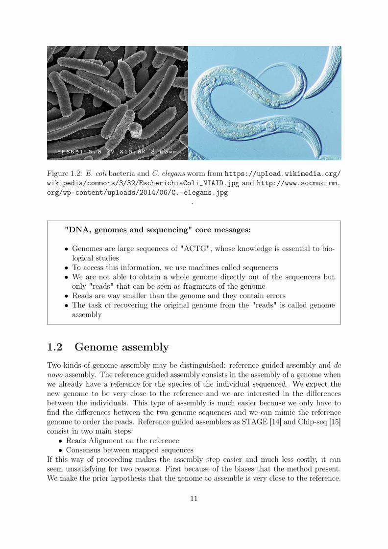
Figure 1.2: E. coli bacteria and C. elegans worm from https://upload.wikimedia.org/wikipedia/commons/3/32/EscherichiaColi_NIAID.jpg and http://www.socmucimm.org/wp-content/uploads/2014/06/C.-elegans.jpg

.

"DNA, genomes and sequencing" core messages:

• Genomes are large sequences of "ACTG", whose knowledge is essential to bio-logical studies

• To access this information, we use machines called sequencers• We are not able to obtain a whole genome directly out of the sequencers but

only "reads" that can be seen as fragments of the genome• Reads are way smaller than the genome and they contain errors• The task of recovering the original genome from the "reads" is called genome

assembly

1.2 Genome assemblyTwo kinds of genome assembly may be distinguished: reference guided assembly and denovo assembly. The reference guided assembly consists in the assembly of a genome whenwe already have a reference for the species of the individual sequenced. We expect thenew genome to be very close to the reference and we are interested in the differencesbetween the individuals. This type of assembly is much easier because we only have tofind the differences between the two genome sequences and we can mimic the referencegenome to order the reads. Reference guided assemblers as STAGE [14] and Chip-seq [15]consist in two main steps:

• Reads Alignment on the reference• Consensus between mapped sequences

If this way of proceeding makes the assembly step easier and much less costly, it canseem unsatisfying for two reasons. First because of the biases that the method present.We make the prior hypothesis that the genome to assemble is very close to the reference.

11

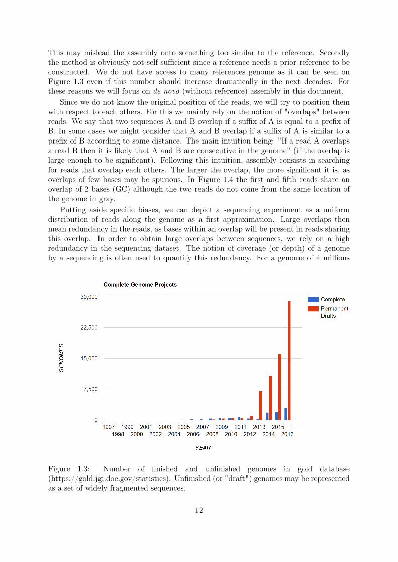
This may mislead the assembly onto something too similar to the reference. Secondlythe method is obviously not self-sufficient since a reference needs a prior reference to beconstructed. We do not have access to many references genome as it can be seen onFigure 1.3 even if this number should increase dramatically in the next decades. Forthese reasons we will focus on de novo (without reference) assembly in this document.

Since we do not know the original position of the reads, we will try to position themwith respect to each others. For this we mainly rely on the notion of "overlaps" betweenreads. We say that two sequences A and B overlap if a suffix of A is equal to a prefix ofB. In some cases we might consider that A and B overlap if a suffix of A is similar to aprefix of B according to some distance. The main intuition being: "If a read A overlapsa read B then it is likely that A and B are consecutive in the genome" (if the overlap islarge enough to be significant). Following this intuition, assembly consists in searchingfor reads that overlap each others. The larger the overlap, the more significant it is, asoverlaps of few bases may be spurious. In Figure 1.4 the first and fifth reads share anoverlap of 2 bases (GC) although the two reads do not come from the same location ofthe genome in gray.

Putting aside specific biases, we can depict a sequencing experiment as a uniformdistribution of reads along the genome as a first approximation. Large overlaps thenmean redundancy in the reads, as bases within an overlap will be present in reads sharingthis overlap. In order to obtain large overlaps between sequences, we rely on a highredundancy in the sequencing dataset. The notion of coverage (or depth) of a genomeby a sequencing is often used to quantify this redundancy. For a genome of 4 millions

Figure 1.3: Number of finished and unfinished genomes in gold database(https://gold.jgi.doe.gov/statistics). Unfinished (or "draft") genomes may be representedas a set of widely fragmented sequences.

12

AAAATCGAGCGCGGATCGATTGCATTTAGTCCTACG1 AAAATCGAGC2 CGAGCGCGGA3 GCGGATCGATT4 CGATTGCATT5 GCATTTAGTC6 TAGTCCTACG

Reads: Yellow compactions: Cyan compactions:

GCATTTAGTC AAAATCGAGCGCGGA AAAATCGAGCGCGGATCGATTGCATTTAGTCCTACG GCGGATCGATT GCGGATCGATTGCATT TAGTCCTACG GCATTTAGTCCTACGCGATTGCATTAAAATCGAGCCGAGCGCGGA

Figure 1.4: Intuition of how assembly is possible. The first set of sequences on the leftare the reads to be assembled. Overlaps between those reads are computed before we cancompact the reads according to the large overlaps found. Compaction between two readsAO and OB according to the overlap O is obtained by concatenating AO with the suffix Bexcluding O (AAAATCGAGC and CGAGCGCGGA become AAAATCGAGCGCGGA). In this toy example, in a first step, we compact the yellow overlaps and obtain longersequences. In the second step we compact the cyan overlaps and get the original sequencedgenome. Double strand aspect of the DNA is not considered here.

Genome coverage % Genome not sequenced % Genome sequenced0.25 78 220.5 61 390.75 47 531 37 632 14 865 0.6 99.410 0.0005 99.995

Table 1.1: Expected missing fraction of the genome according to the sequencing depth.Source: adapted from http://www.genome.ou.edu/poisson_calc.html.

bases, a sequencing of 4 millions reads of 100 base pairs will present a coverage of 100Xbecause it contains 100 times more nucleotides than the genome. A high coverage is animportant factor for at least 3 reasons. The higher the coverage:

• The larger the overlaps between reads are (on average)• The less chance we have to miss regions of the genome because they are not se-

quenced (Table 1.1)• The easier it is to deal with sequencing errors

With a high degree of redundancy we will be able via statistical methods to detectstochastic errors and remove them. Some assembly strategies try to correct reads beforeassembling them.

13

Genome: AAAATCGAGCGCGGATCGATTTReads: AAAATCGA CGAGCGCG GCGGATCG ATCGATTT

AAAATCGA

CGAGCGCG GCGGATCG

ATCGATTT

3

3 4

5

Greedy solution:AAAATCGATTTCGAGCGCGGATCG

Overlaps:

Figure 1.5: Example of greedy assembly. The overlaps between the first and last reads(AAAATCGA and ATCGATTT) is the largest and therefore compacted first in a greedymanner. This first compaction produces AAAATCGATTT. Then the largest overlap isbetween the two other reads (CGAGCGCG and GCGGATCG) that are compacted intoCGAGCGCGGATCG. The assembler produced two misassembled sequences that are notthe shortest common superstring.

We can distinguish three main families of assemblers: "Greedy", "Overlap LayoutConsensus" and "de Bruijn graph " as detailed in the three following sections.

1.2.1 Greedy

This family of assemblers is the conceptually simpler. The idea is to find a shortestcommon superstring (SCS) of a set of sequences. Given a set of reads, a SCS is a stringT of minimal size such that every read is a substring of T. Since finding the shortestcommon superstrings is an NP-complete problem [16], greedy assemblers, as their namesuggests, apply greedy heuristics. The heuristic performs the compaction of the largestoverlap if a read overlaps with several reads. The algorithm can be outlined by:

• Index reads• Select two reads with the largest overlap• Merge the two reads• Repeat

The result is of course not guaranteed to be optimal as the greedy strategy may induceassembly errors, especially around repeated sequences (Figure 1.5). Popular Sanger as-sembler such as TIGR [17] or CAP3 [18] were greedy and broadly used because of theirefficiency. This strategy was also reintroduced later to handle very short reads (around25 to 50 bases) and implemented in assemblers like Ssake [19] and Vcake [20]. Thosetools produce acceptable results on simple genomes. On more redundant genomes, suchapproaches produce too much assembly errors and other techniques are now favored.We can also criticize the model of the shortest common superstring, as in the presence

14

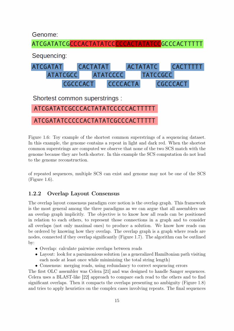
Figure 1.6: Toy example of the shortest common superstrings of a sequencing dataset.In this example, the genome contains a repeat in light and dark red. When the shortestcommon superstrings are computed we observe that none of the two SCS match with thegenome because they are both shorter. In this example the SCS computation do not leadto the genome reconstruction.

of repeated sequences, multiple SCS can exist and genome may not be one of the SCS(Figure 1.6).

1.2.2 Overlap Layout Consensus

The overlap layout consensus paradigm core notion is the overlap graph. This frameworkis the most general among the three paradigms as we can argue that all assemblers usean overlap graph implicitly. The objective is to know how all reads can be positionedin relation to each others, to represent those connections in a graph and to considerall overlaps (not only maximal ones) to produce a solution. We know how reads canbe ordered by knowing how they overlap. The overlap graph is a graph where reads arenodes, connected if they overlap significantly (Figure 1.7). The algorithm can be outlinedby:

• Overlap: calculate pairwise overlaps between reads• Layout: look for a parsimonious solution (as a generalized Hamiltonian path visiting

each node at least once while minimizing the total string length)• Consensus: merging reads, using redundancy to correct sequencing errors

The first OLC assembler was Celera [21] and was designed to handle Sanger sequences.Celera uses a BLAST-like [22] approach to compare each read to the others and to findsignificant overlaps. Then it compacts the overlaps presenting no ambiguity (Figure 1.8)and tries to apply heuristics on the complex cases involving repeats. The final sequences

15

Figure 1.7: Overlap graph toy example where only overlaps of size 3 or more are consid-ered.

ATCGGCGGACTG CGGACTGCAGACT

TGCAGACTTCGATT

TGCAGACTACTGCC

GATCTGCATCGGC6 7

8

8

Figure 1.8: Example of non ambiguous compactions in green and unsafe compactions inred. The green compactions are the only possible choices, thus there is no ambiguity onwhich compaction should be performed. But the third read could be compacted with twoother reads, the two compactions are indistinguishable. Choosing one compaction overthe other could lead to assembly error.

16

A

B

Assembly graph:

Minimal superstring solutions:

Genomes:

Figure 1.9: How repeated sequences can result in unsolvable graph. Two genomes A andB are sequenced, the reads covering their different regions are compacted into a simplifiedassembly graph of unambiguous sequences represented by blocks. Two repeats are presentin red an purple. Several remarks can be made. First, the two genome A and B sharethe same simplified assembly graph structure despite being different. Secondly, severalminimal solution may exist for a given assembly graph. Thirdly, because of repeats, thegenome B will not be a minimal solution of the given assembly graph.

are produced via a consensus to remove most sequencing errors. For comparison, in thetoy example of Figure 1.5, the OLC approach would achieve to solve the assembly byconsidering even non maximal overlaps and to produce the correct path, composed ofstrictly less nucleotides than the greedy solution.

The fact is that, with either paradigm, a perfect assembly is in most cases impossibleto obtain. Sometimes the information available is not sufficient to make sound choices.In those cases the parsimonious strategy of no choosing between two indistinguishablepossibilities is applied (Figure 1.8). This results into fragmented assemblies constituted ofconsensus sequences that are supposed to be genome substrings. We call those sequences"contigs" for contiguous consensus sequence [23]. In the example of the Figure 1.9 anassembly graph is created from the reads information. The graph can be simplifiedby compacting reads that overlap unambiguously into contigs. Assembly can becomecomplex in multiple ways. First, different assemblies can be proposed from this graph evenconsidering only minimal solutions. The green and yellow contigs are interchangeable inthe two minimal solutions of Figure 1.9. Secondly, different genomes can share very similarassembly graphs. In Figure 1.9, both genomes A and B would be represented by the samesimplified assembly graph. Thirdly, sometimes the solution is not a minimal substring:the genome B is not generated as minimal solution of the assembly graph. The mostparsimonious way is therefore to output the proposed contigs represented by the coloredblocks. To give orders of magnitude of the fragmentation of a genome into contigs we canlook at published assemblies. A E. coli genome has almost a hundred contigs https://www.ncbi.nlm.nih.gov/assembly/GCF_002099405.1, a C. elegans genome count morethan 5,000 contigs https://www.ncbi.nlm.nih.gov/assembly/GCA_000939815.1/.

But even by applying parsimonious rules, assemblers may make mistakes and pro-duce assembly errors (misassemblies). Some tools, such as QUAST [24], are designed

17

A B C

A C

Misassembled contig:

Reference genome:

A B

Possible assembly graph:

C?

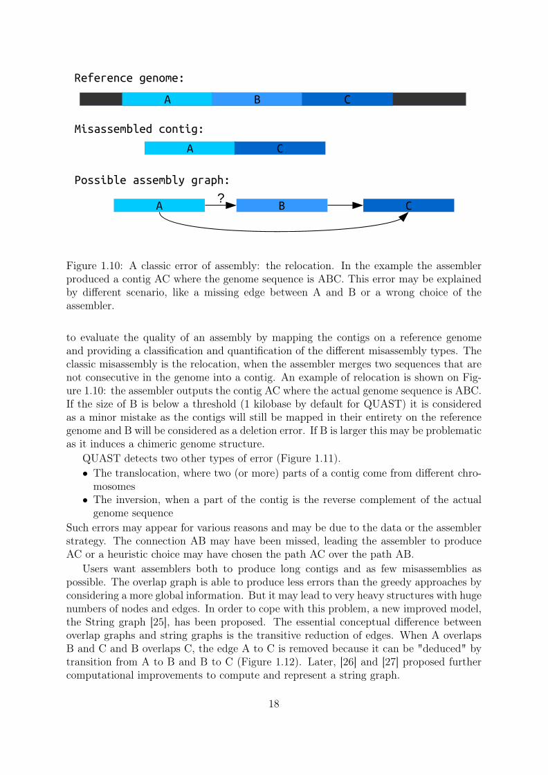
Figure 1.10: A classic error of assembly: the relocation. In the example the assemblerproduced a contig AC where the genome sequence is ABC. This error may be explainedby different scenario, like a missing edge between A and B or a wrong choice of theassembler.

to evaluate the quality of an assembly by mapping the contigs on a reference genomeand providing a classification and quantification of the different misassembly types. Theclassic misassembly is the relocation, when the assembler merges two sequences that arenot consecutive in the genome into a contig. An example of relocation is shown on Fig-ure 1.10: the assembler outputs the contig AC where the actual genome sequence is ABC.If the size of B is below a threshold (1 kilobase by default for QUAST) it is consideredas a minor mistake as the contigs will still be mapped in their entirety on the referencegenome and B will be considered as a deletion error. If B is larger this may be problematicas it induces a chimeric genome structure.

QUAST detects two other types of error (Figure 1.11).• The translocation, where two (or more) parts of a contig come from different chro-

mosomes• The inversion, when a part of the contig is the reverse complement of the actual

genome sequenceSuch errors may appear for various reasons and may be due to the data or the assemblerstrategy. The connection AB may have been missed, leading the assembler to produceAC or a heuristic choice may have chosen the path AC over the path AB.

Users want assemblers both to produce long contigs and as few misassemblies aspossible. The overlap graph is able to produce less errors than the greedy approaches byconsidering a more global information. But it may lead to very heavy structures with hugenumbers of nodes and edges. In order to cope with this problem, a new improved model,the String graph [25], has been proposed. The essential conceptual difference betweenoverlap graphs and string graphs is the transitive reduction of edges. When A overlapsB and C and B overlaps C, the edge A to C is removed because it can be "deduced" bytransition from A to B and B to C (Figure 1.12). Later, [26] and [27] proposed furthercomputational improvements to compute and represent a string graph.

18

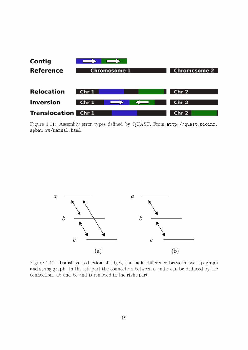
Figure 1.11: Assembly error types defined by QUAST. From http://quast.bioinf.spbau.ru/manual.html.

Figure 1.12: Transitive reduction of edges, the main difference between overlap graphand string graph. In the left part the connection between a and c can be deduced by theconnections ab and bc and is removed in the right part.

19

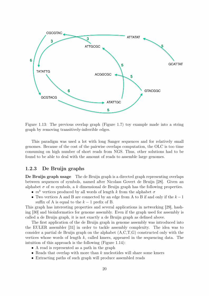
Figure 1.13: The previous overlap graph (Figure 1.7) toy example made into a stringgraph by removing transitively-inferrible edges.

This paradigm was used a lot with long Sanger sequences and for relatively smallgenomes. Because of the cost of the pairwise overlaps computation, the OLC is too timeconsuming on high number of short reads from NGS. Thus, other solutions had to befound to be able to deal with the amount of reads to assemble large genomes.

1.2.3 De Bruijn graphs

De Bruijn graph usage The de Bruijn graph is a directed graph representing overlapsbetween sequences of symbols, named after Nicolass Govert de Bruijn [28]. Given analphabet σ of m symbols, a k dimensional de Bruijn graph has the following properties.

• mk vertices produced by all words of length k from the alphabet σ• Two vertices A and B are connected by an edge from A to B if and only if the k−1

suffix of A is equal to the k − 1 prefix of B.This graph has interesting properties and several applications in networking [29], hash-ing [30] and bioinformatics for genome assembly. Even if the graph used for assembly iscalled a de Bruijn graph, it is not exactly a de Bruijn graph as defined above.

The first application of the de Bruijn graph in genome assembly was introduced intothe EULER assembler [31] in order to tackle assembly complexity. The idea was toconsider a partial de Bruijn graph on the alphabet (A,C,T,G) constructed only with thevertices whose words of length k, called kmers, appeared in the sequencing data. Theintuition of this approach is the following (Figure 1.14):

• A read is represented as a path in the graph• Reads that overlap with more than k nucleotides will share some kmers• Extracting paths of such graph will produce assembled reads

20

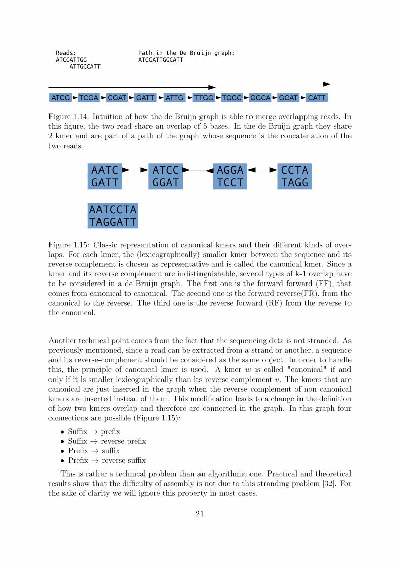
ATCG TCGA CGAT GATT ATTG TTGG TGGC GGCA GCAT CATT

Reads: Path in the De Bruijn graph:ATCGATTGG ATCGATTGGCATT ATTGGCATT

Figure 1.14: Intuition of how the de Bruijn graph is able to merge overlapping reads. Inthis figure, the two read share an overlap of 5 bases. In the de Bruijn graph they share2 kmer and are part of a path of the graph whose sequence is the concatenation of thetwo reads.

AATCGATT

ATCCGGAT

AGGATCCT

CCTATAGG

AATCCTATAGGATT

Figure 1.15: Classic representation of canonical kmers and their different kinds of over-laps. For each kmer, the (lexicographically) smaller kmer between the sequence and itsreverse complement is chosen as representative and is called the canonical kmer. Since akmer and its reverse complement are indistinguishable, several types of k-1 overlap haveto be considered in a de Bruijn graph. The first one is the forward forward (FF), thatcomes from canonical to canonical. The second one is the forward reverse(FR), from thecanonical to the reverse. The third one is the reverse forward (RF) from the reverse tothe canonical.

Another technical point comes from the fact that the sequencing data is not stranded. Aspreviously mentioned, since a read can be extracted from a strand or another, a sequenceand its reverse-complement should be considered as the same object. In order to handlethis, the principle of canonical kmer is used. A kmer w is called "canonical" if andonly if it is smaller lexicographically than its reverse complement v. The kmers that arecanonical are just inserted in the graph when the reverse complement of non canonicalkmers are inserted instead of them. This modification leads to a change in the definitionof how two kmers overlap and therefore are connected in the graph. In this graph fourconnections are possible (Figure 1.15):

• Suffix → prefix• Suffix → reverse prefix• Prefix → suffix• Prefix → reverse suffix

This is rather a technical problem than an algorithmic one. Practical and theoreticalresults show that the difficulty of assembly is not due to this stranding problem [32]. Forthe sake of clarity we will ignore this property in most cases.

21

De Bruijn graph and overlap graph The de Bruijn graph theoretically achievesthe same tasks than the overlap graph, while being conceptually simpler and much moreefficient for the three reasons detailed in the following:

• No alignment• Abstracted coverage• No consensus

The Figure 1.14 shows how the de Bruijn graph finds (exact) overlaps of length superiorto k − 1 between two reads. The de Bruijn graph does not explicitly compact readstogether. However, selecting long paths from the de Bruijn graph is very similar tocompacting overlapping reads in the OLC.

The de Bruijn graph became widely used when the shorts reads from NGS appeared,as it was better suited than the OLC to handle this kind of sequencing data. The OLCapproach did not scale well on the high number of sequences generated by NGS. Theuse of the de Bruijn graph is very interesting for short read assembly for its ability todeal with the high redundancy of such sequencing in a very efficient way. Indeed a kmerpresents dozens of time in the sequencing dataset appears only once in the graph. Thismakes the de Bruijn graph structure not very sensible to the high coverage, unlike theOLC. The de Bruijn graph was first proposed as an alternative structure [31] because itwas less sensible to repeats. Repeats that were problematic in the OLC, creating verycomplex and edges heavy zones, are collapsed in the de Bruijn graph.

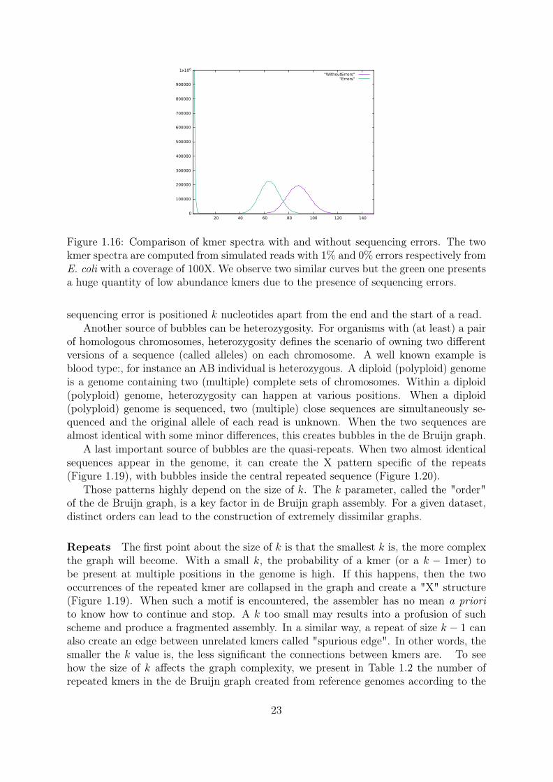
Redundancy The high redundancy in the sequencing data can also be used to effi-ciently filter the sequencing errors. The first highly used de Bruijn graph short readsassembler was Velvet [33]. It introduced core notions of de Bruijn graph assembly, as theidea of error filtering based on kmer abundances. With a high coverage, we expect a highabundance for most kmers. A kmer with very low amount of occurrences is thereforevery likely not a genomic kmer (a kmer present in the genome) but rather an erroneousone (not present in the genome and coming from a sequencing error). By admitting inthe de Bruijn graph only kmers with a coverage above a threshold, we can get rid ofmost erroneous kmers almost without losing genomic kmers, but the ones that has anunexpectedly low abundance. Kmers whose abundance are over the abundance threshold(or solidity threshold) are called "solid". In Figure 1.16 we can see that sequencing errorsgenerate a huge number of low abundance kmers.

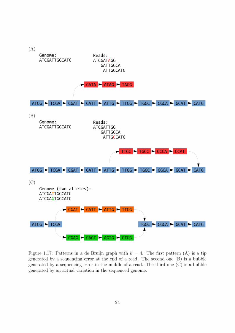
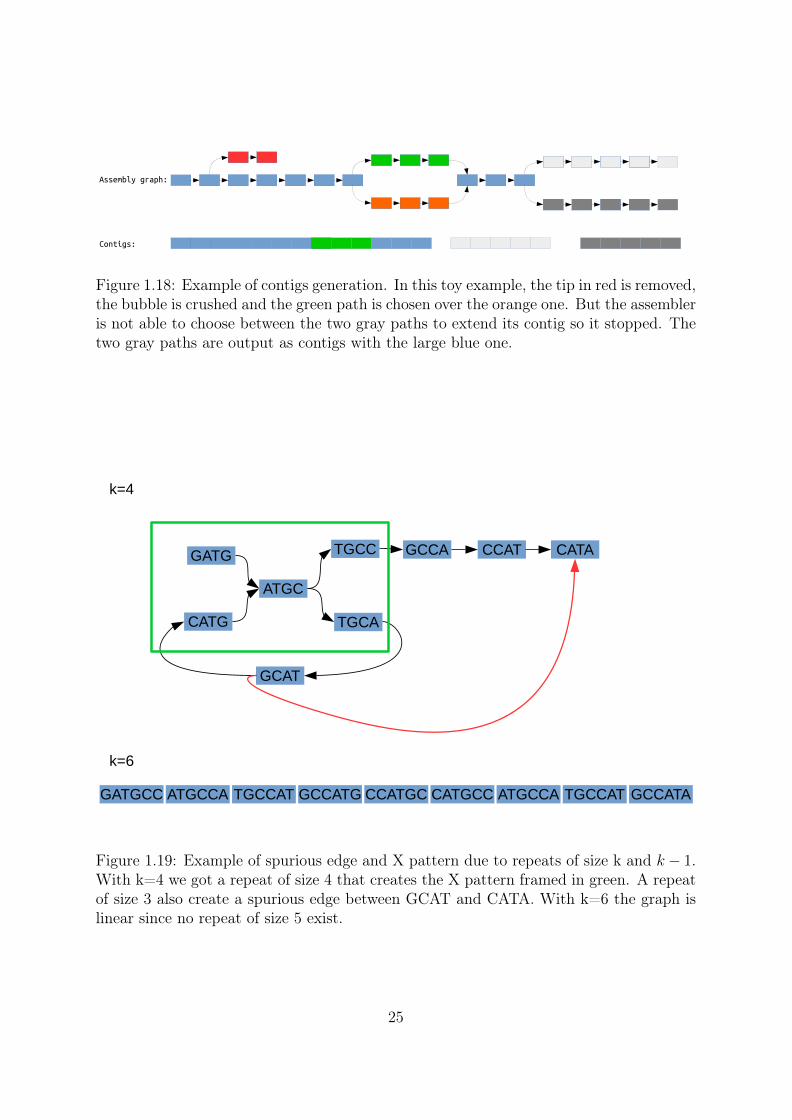
De Bruijn graph patterns De Bruijn graph assembly basically consists in graphsimplification by applying heuristics on knowns patterns (Figure 1.17). They rely onpath exploration, applying different strategies to handle recurring motifs. After graphsimplification, they output the long simple paths as their contigs (Figure 1.18).

The simplest pattern is the tip (or dead end), a short path in the graph that is notextensible because its last kmer has no successor. If the tip is short, shorter than theread length for example, then it is very likely to be due to a sequencing error. But if it islarge it could just be the beginning or an end of a chromosome. A basic assembly step isto recognize those short tips and remove them from the graph to simplify it and to allowlonger contigs.

Another frequent pattern is the bubble. A bubble arises when several paths startfrom a kmer and end in another kmer. A sequencing error can create a bubble if the

22

0

100000

200000

300000

400000

500000

600000

700000

800000

900000

1x106

20 40 60 80 100 120 140

"WithoutErrors""Errors"

Figure 1.16: Comparison of kmer spectra with and without sequencing errors. The twokmer spectra are computed from simulated reads with 1% and 0% errors respectively fromE. coli with a coverage of 100X. We observe two similar curves but the green one presentsa huge quantity of low abundance kmers due to the presence of sequencing errors.

sequencing error is positioned k nucleotides apart from the end and the start of a read.Another source of bubbles can be heterozygosity. For organisms with (at least) a pair

of homologous chromosomes, heterozygosity defines the scenario of owning two differentversions of a sequence (called alleles) on each chromosome. A well known example isblood type:, for instance an AB individual is heterozygous. A diploid (polyploid) genomeis a genome containing two (multiple) complete sets of chromosomes. Within a diploid(polyploid) genome, heterozygosity can happen at various positions. When a diploid(polyploid) genome is sequenced, two (multiple) close sequences are simultaneously se-quenced and the original allele of each read is unknown. When the two sequences arealmost identical with some minor differences, this creates bubbles in the de Bruijn graph.

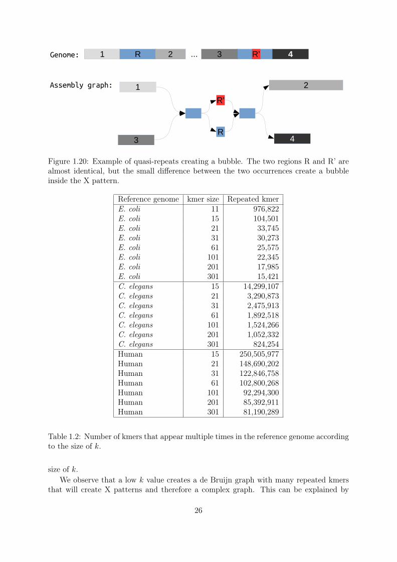
A last important source of bubbles are the quasi-repeats. When two almost identicalsequences appear in the genome, it can create the X pattern specific of the repeats(Figure 1.19), with bubbles inside the central repeated sequence (Figure 1.20).

Those patterns highly depend on the size of k. The k parameter, called the "order"of the de Bruijn graph, is a key factor in de Bruijn graph assembly. For a given dataset,distinct orders can lead to the construction of extremely dissimilar graphs.

Repeats The first point about the size of k is that the smallest k is, the more complexthe graph will become. With a small k, the probability of a kmer (or a k − 1mer) tobe present at multiple positions in the genome is high. If this happens, then the twooccurrences of the repeated kmer are collapsed in the graph and create a "X" structure(Figure 1.19). When such a motif is encountered, the assembler has no mean a priorito know how to continue and stop. A k too small may results into a profusion of suchscheme and produce a fragmented assembly. In a similar way, a repeat of size k − 1 canalso create an edge between unrelated kmers called "spurious edge". In other words, thesmaller the k value is, the less significant the connections between kmers are. To seehow the size of k affects the graph complexity, we present in Table 1.2 the number ofrepeated kmers in the de Bruijn graph created from reference genomes according to the

23

(A)Genome:ATCGATTGGCATG

ATCG TCGA CGAT GATT ATTG TTGG TGGC GGCA GCAT CATG

Reads:ATCGATAGG GATTGGCA ATTGGCATG

GATA ATAG TAGG

(B)Genome:ATCGATTGGCATG

ATCG TCGA CGAT GATT ATTG TTGG TGGC GGCA GCAT CATG

Reads:ATCGATTGG GATTGGCA ATTGCCATG

TTGC TGCC GCCA CCAT

(C)Genome (two alleles):ATCGATTGGCATGATCGAGTGGCATG

ATCG TCGA

CGAT GATT ATTG TTGG

TGGC GGCA GCAT CATG

CGAG GAGT AGTG GTGG

Figure 1.17: Patterns in a de Bruijn graph with k = 4. The first pattern (A) is a tipgenerated by a sequencing error at the end of a read. The second one (B) is a bubblegenerated by a sequencing error in the middle of a read. The third one (C) is a bubblegenerated by an actual variation in the sequenced genome.

24

Assembly graph:

Contigs:

Figure 1.18: Example of contigs generation. In this toy example, the tip in red is removed,the bubble is crushed and the green path is chosen over the orange one. But the assembleris not able to choose between the two gray paths to extend its contig so it stopped. Thetwo gray paths are output as contigs with the large blue one.

GATG

ATGC

TGCC GCCA CCAT CATA

TGCA

GCAT

CATG

GATGCC ATGCCA TGCCAT GCCATG CCATGC CATGCC ATGCCA TGCCAT GCCATA

k=4

k=6

Figure 1.19: Example of spurious edge and X pattern due to repeats of size k and k − 1.With k=4 we got a repeat of size 4 that creates the X pattern framed in green. A repeatof size 3 also create a spurious edge between GCAT and CATA. With k=6 the graph islinear since no repeat of size 5 exist.

25

1 R 2 RR’3

1 2

3

4...

4

R’

R

Assembly graph:

Genome:

Figure 1.20: Example of quasi-repeats creating a bubble. The two regions R and R’ arealmost identical, but the small difference between the two occurrences create a bubbleinside the X pattern.

Reference genome kmer size Repeated kmerE. coli 11 976,822E. coli 15 104,501E. coli 21 33,745E. coli 31 30,273E. coli 61 25,575E. coli 101 22,345E. coli 201 17,985E. coli 301 15,421C. elegans 15 14,299,107C. elegans 21 3,290,873C. elegans 31 2,475,913C. elegans 61 1,892,518C. elegans 101 1,524,266C. elegans 201 1,052,332C. elegans 301 824,254Human 15 250,505,977Human 21 148,690,202Human 31 122,846,758Human 61 102,800,268Human 101 92,294,300Human 201 85,392,911Human 301 81,190,289

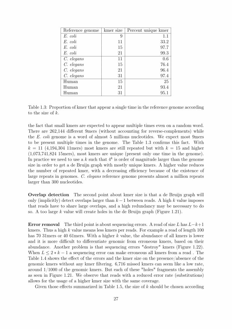
Table 1.2: Number of kmers that appear multiple times in the reference genome accordingto the size of k.

size of k.We observe that a low k value creates a de Bruijn graph with many repeated kmers

that will create X patterns and therefore a complex graph. This can be explained by

26

Reference genome kmer size Percent unique kmerE. coli 9 1.1E. coli 11 33.2E. coli 15 97.7E. coli 21 99.3C. elegans 11 0.6C. elegans 15 76.4C. elegans 21 96.4C. elegans 31 97.4Human 15 25Human 21 93.4Human 31 95.1

Table 1.3: Proportion of kmer that appear a single time in the reference genome accordingto the size of k.

the fact that small kmers are expected to appear multiple times even on a random word.There are 262,144 different 9mers (without accounting for reverse-complements) whilethe E. coli genome is a word of almost 5 millions nucleotides. We expect most 9mersto be present multiple times in the genome. The Table 1.3 confirms this fact. Withk = 11 (4,194,304 11mers) most kmers are still repeated but with k = 15 and higher(1,073,741,824 15mers), most kmers are unique (present only one time in the genome).In practice we need to use a k such that 4k is order of magnitude larger than the genomesize in order to get a de Bruijn graph with mostly unique kmers. A higher value reducesthe number of repeated kmer, with a decreasing efficiency because of the existence oflarge repeats in genomes. C. elegans reference genome presents almost a million repeatslarger than 300 nucleotides.

Overlap detection The second point about kmer size is that a de Bruijn graph willonly (implicitly) detect overlaps larger than k−1 between reads. A high k value imposesthat reads have to share large overlaps, and a high redundancy may be necessary to doso. A too large k value will create holes in the de Bruijn graph (Figure 1.21).

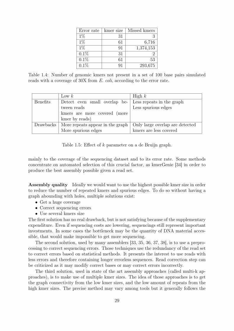
Error removal The third point is about sequencing errors. A read of size L has L−k+1kmers. Thus a high k value means less kmers per reads. For example a read of length 100has 70 31mers or 40 61mers. With a higher k value, the abundance of all kmers is lowerand it is more difficult to differentiate genomic from erroneous kmers, based on theirabundance. Another problem is that sequencing errors "destroy" kmers (Figure 1.22).When L ≤ 2 ∗ k − 1 a sequencing error can make erroneous all kmers from a read . TheTable 1.4 shows the effect of the errors and the kmer size on the presence/absence of thegenomic kmers without any kmer filtering. 6,716 missed kmers can seem like a low rate,around 1/1000 of the genomic kmers. But each of these "holes" fragments the assemblyas seen in Figure 1.21. We observe that reads with a reduced error rate (substitutions)allows for the usage of a higher kmer size with the same coverage.

Given those effects summarized in Table 1.5, the size of k should be chosen according

27

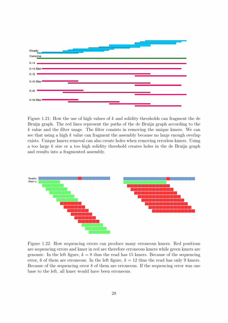
Figure 1.21: How the use of high values of k and solidity thresholds can fragment the deBruijn graph. The red lines represent the paths of the de Bruijn graph according to thek value and the filter usage. The filter consists in removing the unique kmers. We cansee that using a high k value can fragment the assembly because no large enough overlapexists. Unique kmers removal can also create holes when removing errorless kmers. Usinga too large k size or a too high solidity threshold creates holes in the de Bruijn graphand results into a fragmented assembly.

Reads:Kmers:

Figure 1.22: How sequencing errors can produce many erroneous kmers. Red positionsare sequencing errors and kmer in red are therefore erroneous kmers while green kmers aregenomic. In the left figure, k = 8 thus the read has 15 kmers. Because of the sequencingerror, 6 of them are erroneous. In the left figure, k = 12 thus the read has only 9 kmers.Because of the sequencing error 8 of them are erroneous. If the sequencing error was onebase to the left, all kmer would have been erroneous.

28

Error rate kmer size Missed kmers1% 31 31% 61 6,7161% 91 1,374,1530.1% 31 20.1% 61 530.1% 91 293,675

Table 1.4: Number of genomic kmers not present in a set of 100 base pairs simulatedreads with a coverage of 30X from E. coli, according to the error rate.

Low k High kBenefits Detect even small overlap be-

tween readskmers are more covered (morekmer by reads)

Less repeats in the graphLess spurious edges

Drawbacks More repeats appear in the graphMore spurious edges

Only large overlap are detectedkmers are less covered

Table 1.5: Effect of k parameter on a de Bruijn graph.

mainly to the coverage of the sequencing dataset and to its error rate. Some methodsconcentrate on automated selection of this crucial factor, as kmerGenie [34] in order toproduce the best assembly possible given a read set.

Assembly quality Ideally we would want to use the highest possible kmer size in orderto reduce the number of repeated kmers and spurious edges. To do so without having agraph abounding with holes, multiple solutions exist:

• Get a huge coverage• Correct sequencing errors• Use several kmers size

The first solution has no real drawback, but is not satisfying because of the supplementaryexpenditure. Even if sequencing costs are lowering, sequencings still represent importantinvestments. In some cases the bottleneck may be the quantity of DNA material acces-sible, that would make impossible to get more sequencing.

The second solution, used by many assemblers [33, 35, 36, 37, 38], is to use a prepro-cessing to correct sequencing errors. Those techniques use the redundancy of the read setto correct errors based on statistical methods. It presents the interest to use reads withless errors and therefore containing longer errorless sequences. Read correction step canbe criticized as it may modify correct bases or may correct errors incorrectly.

The third solution, used in state of the art assembly approaches (called multi-k ap-proaches), is to make use of multiple kmer sizes. The idea of those approaches is to getthe graph connectivity from the low kmer sizes, and the low amount of repeats from thehigh kmer sizes. The precise method may vary among tools but it generally follows the

29

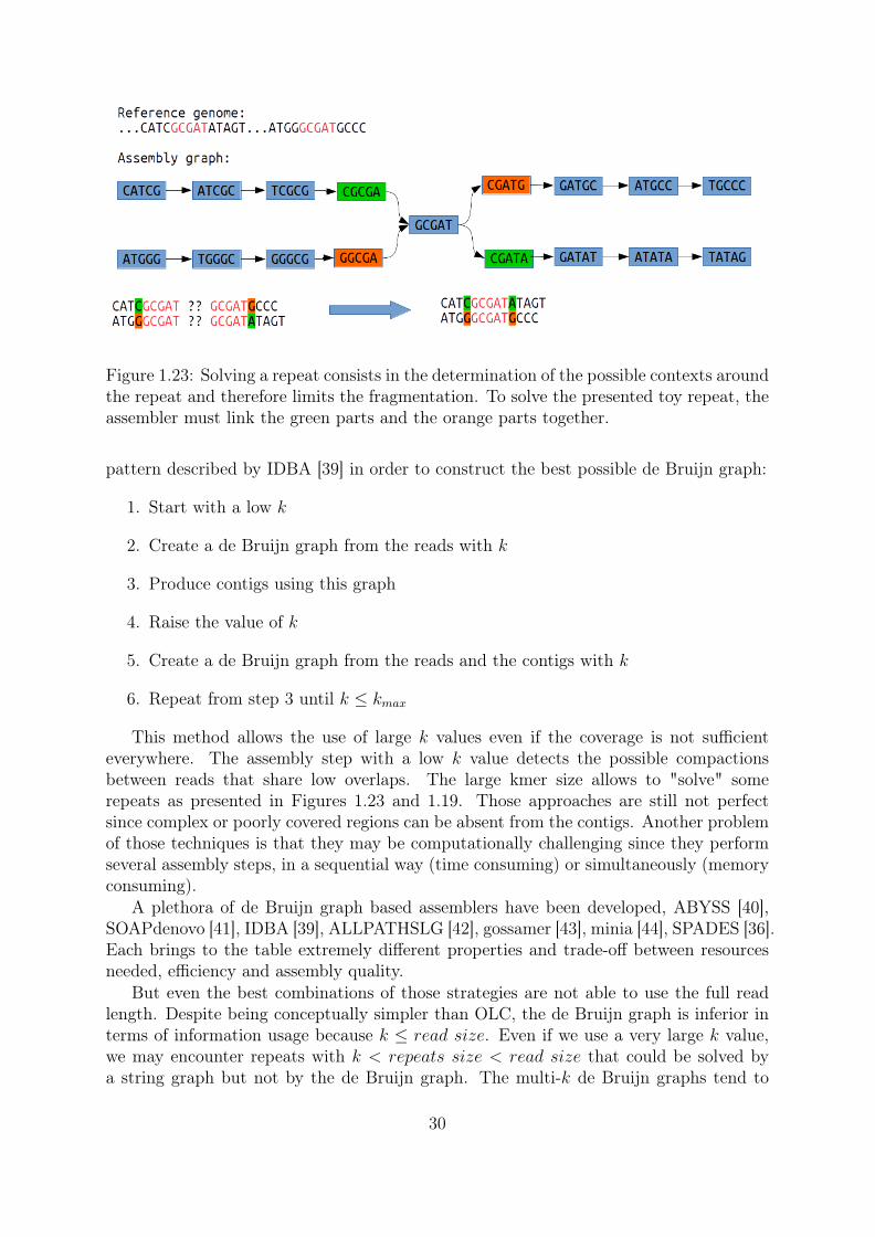
Figure 1.23: Solving a repeat consists in the determination of the possible contexts aroundthe repeat and therefore limits the fragmentation. To solve the presented toy repeat, theassembler must link the green parts and the orange parts together.

pattern described by IDBA [39] in order to construct the best possible de Bruijn graph:

1. Start with a low k

2. Create a de Bruijn graph from the reads with k

3. Produce contigs using this graph

4. Raise the value of k

5. Create a de Bruijn graph from the reads and the contigs with k

6. Repeat from step 3 until k ≤ kmax

This method allows the use of large k values even if the coverage is not sufficienteverywhere. The assembly step with a low k value detects the possible compactionsbetween reads that share low overlaps. The large kmer size allows to "solve" somerepeats as presented in Figures 1.23 and 1.19. Those approaches are still not perfectsince complex or poorly covered regions can be absent from the contigs. Another problemof those techniques is that they may be computationally challenging since they performseveral assembly steps, in a sequential way (time consuming) or simultaneously (memoryconsuming).

A plethora of de Bruijn graph based assemblers have been developed, ABYSS [40],SOAPdenovo [41], IDBA [39], ALLPATHSLG [42], gossamer [43], minia [44], SPADES [36].Each brings to the table extremely different properties and trade-off between resourcesneeded, efficiency and assembly quality.

But even the best combinations of those strategies are not able to use the full readlength. Despite being conceptually simpler than OLC, the de Bruijn graph is inferior interms of information usage because k ≤ read size. Even if we use a very large k value,we may encounter repeats with k < repeats size < read size that could be solved bya string graph but not by the de Bruijn graph. The multi-k de Bruijn graphs tend to

30

come close to the string graph (various overlap sizes detection, usage of a large part ofthe reads) but also tend to lose their performances advantages.

"Genome assembly" core messages:

• Assemblers goal is to order the reads and concatenate them into larger sequenceswhile removing the sequencing errors

• In most cases, the assembler is not able to completely recover the genome andwill output "contigs" that are sequences supposed to be substring of the genomelarger than the reads

• Greedy approaches are efficient but are not suited to large or complex genomesas they handle repeats very poorly, resulting into erroneous assembly.

• Overlap graph is a framework where the overlaps between the reads are com-puted and put in a graph where reads are nodes, connected if they overlap.

• The de Bruijn graph is a more restricted framework where the words of lengthk from the reads are nodes, connected if they share an overlap of k − 1.

• OLC and de Bruijn graph approaches select paths from their graphs usingheuristics in order to produce contigs based on the graph structure

• The overlap graph approaches relies on heavy data structures while the de Bruijngraph, conceptually simpler, scales better on large datasets

1.3 Assembly hardness

Assemblers are supposed to produce the largest possible contigs while making as fewassembly errors as possible from the available read information. Here we describe thechallenges that genome assembly may present and the limitations of existing approaches.

1.3.1 Repeats

As we have seen, one of the problems of assembly is the repeated sequences. In fact repeatsmay be the fundamental problem in genome assembly. An analysis of the complexity ofthe assembly problem according to the type of data available has been made in [45]. Theprincipal conclusion of the paper is that repeats larger than reads are impossible to solve.In fact, for most genomes, the perfect assembly is not achievable using only NGS reads.It may seem odd that such large repeats exist. The fact is that genomes are absolutelynot random sequences. When we compare Table 1.6 with Table 1.2, we see that there isno large repeated kmers in random sequences whereas E. coli genome has thousands ofrepeated 301mers. The conclusion is that NGS reads sequences are not enough to producea complete assembly. [46] has shown the effort necessary to finish short reads assembly.Therefore longer range information is required in order to solve the large repeats andproduce more continuous assembly.

31

Reference genome kmer size Repeated kmerRandom Genome (E. coli) 15 84,148Random Genome (E. coli) 21 28Random Genome (E. coli) 31 0Random Genome (C. elegans) 15 34,050,959Random Genome (C. elegans) 21 17,953Random Genome (C. elegans) 31 0

Table 1.6: Number of repeats of size k in a random genome of the same size than E. colior C. elegans.

A B

B A AB A

Paired End reads orientation:

Mate Pairs reads orientation:

B

A B

DNA fragments: Sequencing from both ends:

Figure 1.24: Differences between Paired End sequencing and Mate Pairs sequencing. InPaired End, small DNA fragment are selected and sequenced from both end. For MatePairs, longer fragment are selected, both ends are marked and connected into a circularsequence. The sequence is then cut and the marked part is sequenced from both andgenerates an opposite sequencing orientation.

32

1.3.2 Scaffolding

As denoted before, most assemblers use the reads sequences to produce contigs, thatare a set of fragments of the genome. In order to improve such genome drafts, otherinformations and techniques can be used. It is possible via sequencing techniques toobtain short reads that are associated by pairs coming from related positions of thegenome. There are two main sequencing techniques called "Paired End" and "MatePairs" sequencing (Figure 1.24). In both cases, we get a pair a short reads with the samecharacteristics than short reads described previously. The additional information is thatwe have an estimation of the distance covered by the read pair, called the fragment size,since we know that both come from the same DNA fragment. For example, a pairedend sequencing of 2*250 base pairs with an fragment size of 800 will produce pairs ofreads of 250 bases pair reads spaced by 300 nucleotides in the genome (on average). Thepaired end sequencing can handle fragment size up to 2,000 bases while mate pair canproduce fragment size from 2 to 20 kilo-bases. Another difference is that in Paired Endsequencing, the first fragment is read forward and the second is reversed while in MatePairs this is the opposite, as shown in Figure 1.24. This can be explained by the differencebetween the two protocols. In paired end sequencing, fragments of the desired size areselected and sequenced from both ends. In mate pairs sequencing long fragments end aremarked, circularized, fragmented, and sequences with marker are sequenced from bothends.

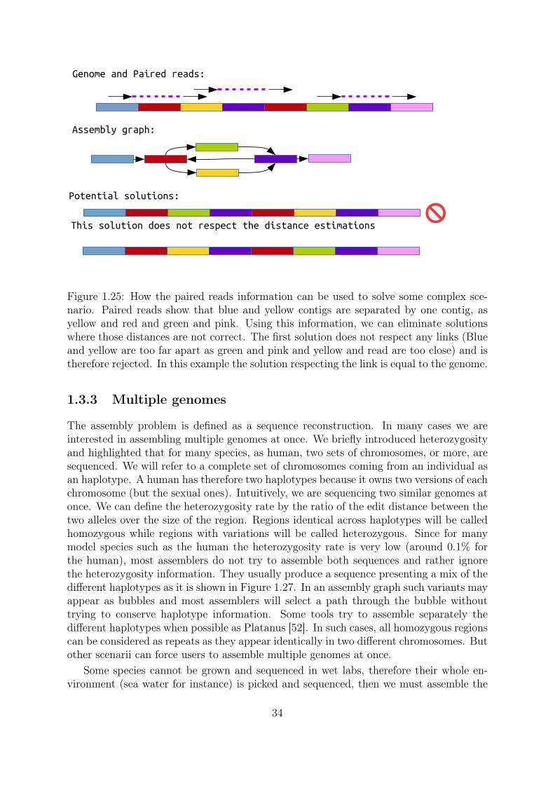
The standard way to use those linking information is to align paired reads on thecontigs and use the pair of reads that map on different contigs to order and orient themwith respect to each other. This task is frequently called scaffolding, because contigs arearranged together into "scaffolds", based on estimations of the distance between them(Figure 1.25). A complete assembly workflow is summarized in Figure 1.26.

[47] formally defined the problem and showed its NP-completeness and therefore itspotential intractability. Most scaffolders try to optimize the number of satisfied linksin order to produce scaffolds. The main problem of scaffolds is that they may contain"holes". Scaffolds are basically ordered contigs. When the different contigs used arenot overlapping, the scaffolder usually estimates the distance between them and fillsthe "holes" with ’N’ characters to inform that the sequences here are unknown. Thescaffolders may be able to order large contigs, but can fail to find the contigs separatingthem. This may be the case if those contigs are too small or simply if they were notoutput by the contig generation step. Since the scaffold approach is based on mappingthe reads on the contigs, very short contigs (shorter than reads) cannot be consideredthis way because of multiple mapping problems (when a read maps on several contigs).

Recent scaffolders like SSPACE [48] try to extend contigs using the pairs informationearlier to connect them in order to reduce the potential gaps in the later phase. Somestandalone tools called gap-giller, as MindTheGap [49], are specifically designed to fillsuch holes. Other kinds of information start to be used for scaffolding such as long readsfrom third generation sequencing [50] and 3C [51] a sequencing technology liking readscoming from the same chromosome.

33

Assembly graph:

Potential solutions:

This solution does not respect the distance estimations

Genome and Paired reads:

Figure 1.25: How the paired reads information can be used to solve some complex sce-nario. Paired reads show that blue and yellow contigs are separated by one contig, asyellow and red and green and pink. Using this information, we can eliminate solutionswhere those distances are not correct. The first solution does not respect any links (Blueand yellow are too far apart as green and pink and yellow and read are too close) and istherefore rejected. In this example the solution respecting the link is equal to the genome.

1.3.3 Multiple genomes

The assembly problem is defined as a sequence reconstruction. In many cases we areinterested in assembling multiple genomes at once. We briefly introduced heterozygosityand highlighted that for many species, as human, two sets of chromosomes, or more, aresequenced. We will refer to a complete set of chromosomes coming from an individual asan haplotype. A human has therefore two haplotypes because it owns two versions of eachchromosome (but the sexual ones). Intuitively, we are sequencing two similar genomes atonce. We can define the heterozygosity rate by the ratio of the edit distance between thetwo alleles over the size of the region. Regions identical across haplotypes will be calledhomozygous while regions with variations will be called heterozygous. Since for manymodel species such as the human the heterozygosity rate is very low (around 0.1% forthe human), most assemblers do not try to assemble both sequences and rather ignorethe heterozygosity information. They usually produce a sequence presenting a mix of thedifferent haplotypes as it is shown in Figure 1.27. In an assembly graph such variants mayappear as bubbles and most assemblers will select a path through the bubble withouttrying to conserve haplotype information. Some tools try to assemble separately thedifferent haplotypes when possible as Platanus [52]. In such cases, all homozygous regionscan be considered as repeats as they appear identically in two different chromosomes. Butother scenarii can force users to assemble multiple genomes at once.

Some species cannot be grown and sequenced in wet labs, therefore their whole en-vironment (sea water for instance) is picked and sequenced, then we must assemble the

34

4,6 Mb1 seq4.6Mb mean lengthNo error

500 Mb5 000 000 seq100b mean length10^-2 error

4,4 Mb300 seq20kb mean length10^-5 error

SequencingSequencing ‘’Assembly’’

≈1kbp

≈2kbp

Scaffolding

Mate-pairs

Figure 1.26: Summary of assembly steps. The global picture of an assembly of E. colifrom simulated reads with SPAdes. Some refer to assembly for contigs generation andscaffolding steps while other call the contigs generation step as assembly and separate itfrom the scaffolding.

Figure 1.27: Example on how an assembler may crush haplotypes. The assembler detectstwo bubbles and crushes them, choosing one path over another. The resulting contigsmay contain sequences from both haplotype mixed.

35

whole data (meta-genomic). Some assemblers are designed to assemble meta-genome asmeta-IDBA [53] or meta-velvet [54]. As their names suggest, they are usually based ona regular genome assembler adapted to fit to the proposed scenario. In some cases, asingle species is sequenced but with several individuals having different, however closelyrelated, genomes (pool-seq). Since repeats assess the toughness of assembly, we can sortscenarii by their apparent hardness:

• Single haploid genomes (some repeats)• Heterozygous genomes (each homozygous regions is a repeat)• Pool-seq, multiple related genomes (genome sized repeat)• Meta-genomic, multiple non-related genomes (genome size repeats, some repeat

shared among species)It seems obvious that perfect assembly and distinguishing closely related genomes are

currently out of reach. But this gives objectives to be met in the assembly field.

"Assembly challenges" core messages:

• Finished assembly is often impossible because of repeats longer than the reads• Other kinds of data may be used to order contigs in larger sequences called

"scaffolds"• Polyploid, meta-genome and pool-seq assembly are even harder than regular

assembly because of systematic repeats

1.4 Outline of the thesisIn this introduction, we highlighted three "challenges" of the assembly process of NGSdata:

• The high amount of resources required• The fragmentation of produced assembly• The hardness to assemble complex (large and/or repeat-rich) genomes

To address those issues, we will present new approaches based on the de Bruijn graph.In the first chapter we present new ways to represent and construct the de Bruijn graphin order to make it more scalable and more efficient. In the second chapter we introducenew methods to use the de Bruijn graph as a reference and show the interest of suchstructures over a set of fragmented contigs. In the third chapter we propose techniquesto construct high order de Bruijn graphs, allowing the use of the reads information, asthe string graph does, without losing the de Bruijn graph efficiency.

36

Chapter 2

Handling assembly

37

In this chapter we will assess the computational aspect of assembly. We showwhy the scalability of methods used for genome assembly can be critical (Section 1).We provide an overview of the state of the art of efficient methods and structuresto address such problems for both overlap graph (Section 2) and de Bruijn graph(Section 3) frameworks. Then we present our theoretical and practical contributions.We show that de Bruijn graph assembly may be done using a Navigational DataStructure, a novel model that we introduce, which shows lower theoretical memorybounds. We also propose a new proof of concept assembler that shows practicalresources improvement over state of the art tools (Section 4). Those implementationsare based on the idea to enumerate and index simple paths of the graph. We arguethat such enumeration is a bottleneck in many assembly methods and we provideresources efficient methods to answer this need (Section 5). To do so, we make use ofminimal perfect hashing functions as very efficient indexes and provide a new methodto compute such functions on very large sets of keys (Section 6).

2.1 The assembly burdenIn the last section we described the sequencing data but we gave no clue about thetypical size of a genome. The fact is that this size can vary a lot among living organisms(Figure 2.2). Though we can indicate some orders of magnitude on genomes size:

• Virus : Thousands base pairs• Bacteria: Millions base pairs• Mammals : Billions base pairsSome species, yet to be sequenced, are expected to present order of magnitude larger

genome (Paris japonica, Polychaos dubium) [55] with presumed hundred of billions basepairs. The struggle for assembling such genomes may not be seen directly. Since highcoverages are needed for assembly, sequencing datasets represent huge amount of infor-mation. Most assemblies typically rely on a mean coverage ranging from 30X to 100Xand higher. Consequently, assemblers have to handle millions of reads, even for bacterialgenomes. Larger genomes can count hundreds of millions base pairs for most prokaryotes,and up to billions for some mammals or plants genomes. Such sets can reach billions ofreads and represent hundreds of gigabytes or even terabytes of data.

Dealing with this tremendous amount of information require either to use huge com-putational resources or to conceive specific algorithms and data structures designed for re-source efficiency. As sequencing cost continues to decrease, sequencing very large genomesbecomes affordable, but assembly of such genome is barely possible. If the running timeis an important concern, it is usually not the source of intractability. Most assemblersrely on very large graph structure and index, that can require terabytes of RAM on largedatasets. Most of the time, such memory requirement is more concerning than runningtime, as large scale clusters may not be easily accessible. Besides facing the challenge toproduce correct assemblies, the future assemblers will have to handle larger and largerdatasets, in order to deal with large genomes or meta-genomes while providing a highthroughput to follow the sequencing rate. As sequencing costs are dropping (Figure 2.1),the computational resources necessary to treat them is becoming the financial bottleneck.

$100

$1k

$10k

$100k

$1M

$10M

$100M

2001 2003 2005 2007 2009 2011 2013 2015 2017

Cost to sequence a human genome (USD)

Figure 2.1: Evolution of the cost of human sequencing. From https://upload.wikimedia.org/wikipedia/commons/e/e7/Historic_cost_of_sequencing_a_human_genome.svg.

39

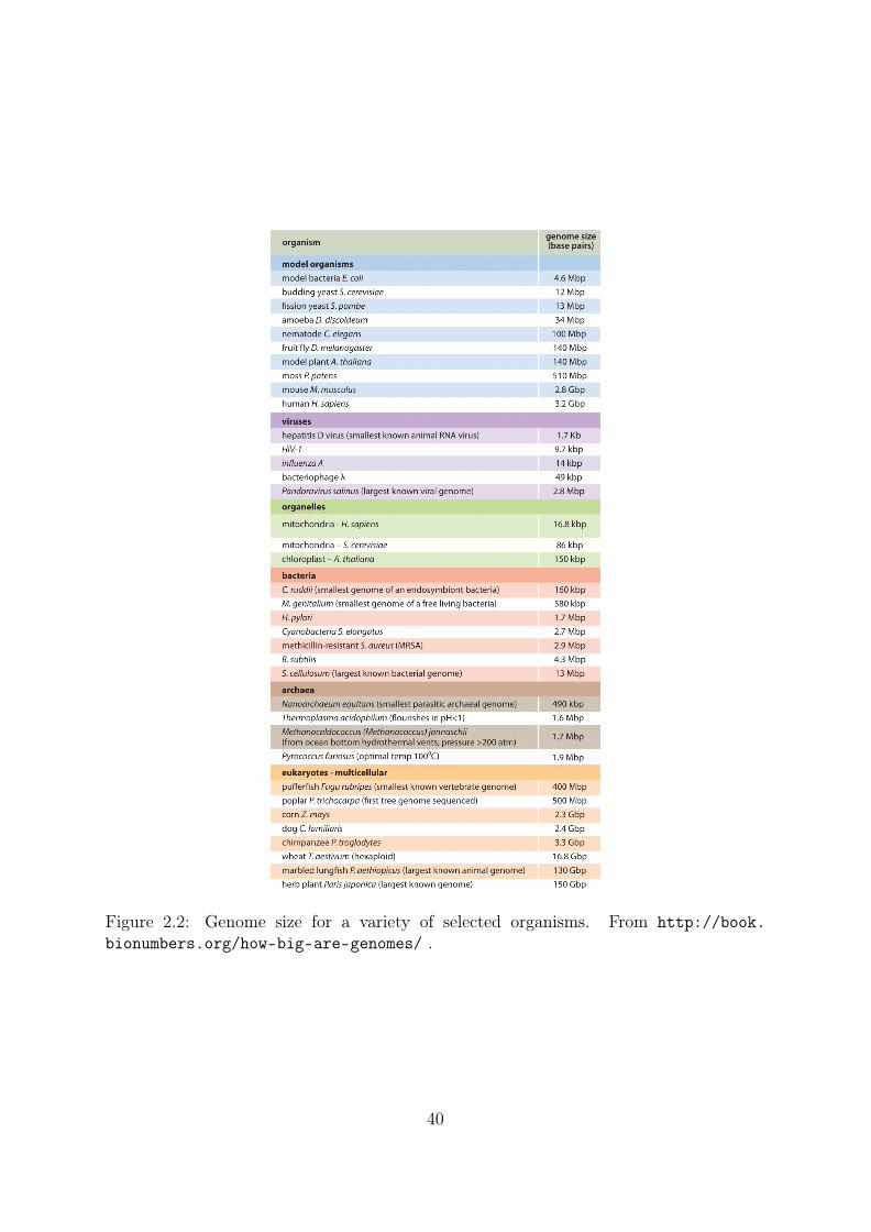
Figure 2.2: Genome size for a variety of selected organisms. From http://book.bionumbers.org/how-big-are-genomes/ .

40

This fast evolving sequencing environment pushes assembly designers to conceive increas-ingly efficient dedicated methods and data structures. In this chapter, we will present astate of the art of such techniques with a focus on the scalability of the de Bruijn graphassembly.

"The assembly burden" core messages:

• Genomes may count billions of bases• Sequencing datasets can be composed of billions of reads and represent terabytes

of data• Genome assembly is a High Performance Computing issue• Efficient and dedicated structures are needed especially to reduce the memory

usage• Decreasing sequencing costs raise the need to efficient assembly

2.2 Overlap graph scalability

The problem of assembly scalability appeared with the overlap graphs and large genomes.Tools such as TIGR [17] or CAP3 [18] can be considered as brute force approaches andwere suitable only for small genomes. When the concern about repeat misassembliesarose, the overlap graph approaches have become preferred. The core operation of theoverlap graph is to find all overlaps between reads from pairwise alignment. Thereforestandard overlap graph assembly methods have a worst time complexity quadratic withthe number of reads. This fact may be moderated as only significant overlaps are consid-ered. Heuristics are used in order to quickly find significant alignment. Tools mainly useBLAST [22], or other aligners following the "seed and extend" paradigm. The principleof the seed and extend paradigm is to look for words in common between the query andthe reference (called seeds or anchors) and to try to extend the alignment from the sharedwords. Unlike Smith-Waterman algorithm [56], such approaches are not guaranteed tofind all optimal alignments. But they are dramatically faster while providing almost iden-tical results. Using such anchoring heuristics implies that finding the overlaps of a readis roughly linear in the number of similar reads (according to the method and parameterused) instead of being linear in the total number of reads.

However, with high coverage, one read presents a high amount of high quality overlaps(Figure 2.3). This will impact the running time of each query trying to find the overlapsshared by a read. Such alignment based approaches were quite efficient with Sangersequencing, since the number of reads remained relatively low. With a very low errorrate, low coverage is sufficient to complete correct assemblies, around 10X or 20X. Sincethe sequences are also longer (around thousands of base pairs), the number of Sanger readsis lower than the number of NGS reads for a given coverage. In practice the number ofreads, even for large genome assembly, was not above the million. The number of overlapsneeded to be stored in order to work on the graph could still be challenging. Furthermore,repeated regions resulted in dense zones (called hub) with very high numbers of overlaps.Celera [21] and Arachne [57] improved the running time by masking repeated regions to

41

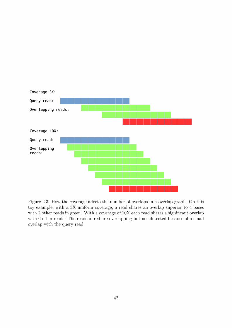
Coverage 3X:

Query read:

Overlapping reads:

Coverage 10X:

Query read:

Overlapping reads:

Figure 2.3: How the coverage affects the number of overlaps in a overlap graph. On thistoy example, with a 3X uniform coverage, a read shares an overlap superior to 4 baseswith 2 other reads in green. With a coverage of 10X each read shares a significant overlapwith 6 other reads. The reads in red are overlapping but not detected because of a smalloverlap with the query read.

42

simplify the overlap graph. Later, the string graph [25] was proposed to abstract theredundancy present in the sequencing data, as does the de Bruijn graph, using transitivereduction. The assembler BOA [25] was designed to assemble Sanger reads with suchstring graphs. However with NGS technologies, deeper sequencing was affordable andhelped to cope with the error rate. This raised up the number of reads by orders ofmagnitude, themselves leading to orders of magnitude higher numbers of overlaps tohandle. The overlap graph and string graph need enormous resources to process suchdatasets. Thus de Bruijn graphs were preferred to handle this kind of data.

However, because of the fact that the string graph should theoretically lead to betterassembly by using the whole reads instead of kmers, several contributions were proposedin order to allow the string graph to scale up with the tremendous number of short reads.The introduction of the very popular FM-index structure [58] in bioinformatics allowedmemory efficient indexing of large DNA sequences. It was first used to index referencesand enabled very efficient read mapping (fast and stringent local alignment of short readson a reference). Notable examples of such tools based on a FM-index are Bowtie [59]and BWA [60]. [26] used the same idea to improve the string graph performances.The rationale is to index the reads with a FM-index and to use the research operationto detect overlaps between sequences. The memory usage of the assembly of a humangenome has been extrapolated by the author to 700GB, which is not intractable but stillvery expensive. The time required for assembly is also tractable, days for 100 mega-basesgenome, but this is yet very slow compared to most de Bruijn graph assemblers. A moreefficient implementation called SGA [27] proposed a distributed FM-index construction.Using multiple small indexes allows for the construction of a global FM-index using lessthan 60 GB of RAM for a human sequencing dataset of more than 1.2 billions reads. Theefficient use of the FM-index allowed the string graph to scale up to large genomes withmoderate memory usage, but the computational resources remained high. The humangenome assembly of SGA used more than 1500 CPU hours over 6 days.

"Overlap graph scalability" core messages:

• Overlap graphs and string graphs usually rely on memory heavy data structure• Compressed data structures may be used but still lead to very long assembly

processes• String graphs grow roughly with the size of the dataset when de Bruijn graph

grow with the size of the sequenced genome

2.3 The scaling story of the de Bruijn graph represen-tation

The main difference between the overlap graph and the de Bruijn graph is the memoryusage. The overlap graph grows linearly with the size of the sequencing data. The deBruijn graph memory usage can (with kmer filtering) be linear in the size of the genome,since we only have roughly GenomeSize different kmers in the genome, estimated throughtheir abundances. A very low abundance threshold would keep too much kmers and

43

therefore use too much memory. However, even with a very low threshold the numberof non genomic kmers is hardly very high (Table 2.1). Thus the memory usage used bya de Bruijn graph is rather function of the size of the genome than of the size of thesequencing dataset.

Largest genomes still lead to graphs with billions of nodes and edges, that are noteasy to represent with a decent amount of memory. In this section we concentrate on theproblem of storing a huge de Bruijn graph in memory. We present here an overview ofthe main milestones and a state of the art of the data structures used to represent a deBruijn graph. We describe the first representations that were based on classical graphimplementation and exhibit very high memory footprints. Next we introduce the work ofConway and Bromage that proposed a lower bound on the necessary memory to representa de Bruijn graph. Then we see how the use of external memory highly impacted thememory usage of most assemblers. And finally we present very efficient techniques basedon probabilistic data structures. We also present several works on the scaling of de Bruijngraph assembly on a massive number of cores.

2.3.1 Generic graphs

The earliest representations of a de Bruijn graph were based on classical and genericgraph representations and were not memory efficient. The first graph representations

Reference genome Abundance Threshold Erroneous kmers Missing kmerE. coli 1 89,044,977 5E. coli 2 3,889,707 6E. coli 3 200,173 11E. coli 4 15,198 11E. coli 5 1,913 13E. coli 6 312 16E. coli 7 33 20E. coli 8 0 21C. elegans 1 1,909,728,320 6C. elegans 2 89,087,143 7C. elegans 3 7,294,417 11C. elegans 4 2,003,946 15C. elegans 5 1,049,812 21C. elegans 6 643,918 26C. elegans 7 425,435 26C. elegans 8 293,457 75C. elegans 9 208,539 213C. elegans 10 150,939 589

Table 2.1: Number of erroneous and missing kmers in a de Bruijn graph after an abun-dance filtering. On simulated reads with a 100X coverage, 1% error rate and k=51 fromthe E. coli. The E. coli genome presents 4,554,207 genomic 51mers. The C. elegansgenome presents 100,286,051 genomic 51mers.

44

were based on hash tables indexing kmers associated with informations allowing graphtraversal, as in EULER [31] or Velvet [33] assemblers. The use of a dynamic hash tablefor indexing millions of elements rapidly lead to very high memory usage. Velvet’s paperreports a memory usage of 2GB for a Streptococcus genome of 2.2 millions bases. Theproposed solution considered for scaling was the use of disk in order to store the graphstructure. However this kind of solutions was never really put in practice since diskaccesses are very slow compared to RAM accesses. Thus such methods would presentorders of magnitude longer running time. Such data structure is adapted to bacterialgenomes assembly but impracticable on larger one.

In order to address this scalability issue, Abyss [40] introduced several solutions. Firstthe indexing method changed, using an interesting property of the de Bruijn graph: thenumbers of fathers and of sons of a node is bounded by four (the size of the nucleicalphabet). In Abyss, all kmers are indexed and the value associated is just eight bitscoding the presence or absence of its eight possible neighbors. Secondly, the main costof a hash table is usually the pointers used for its internal structure. Instead of this,they used open addressing hash tables that represent a low overhead of a few bits byelements. Thirdly they proposed the distribution of the graph on several machines.The idea of their distributed de Bruijn graph is to use a first hash to decide on whichhashtable/machine the kmer will be inserted. On large genome, memory usage was stillhigh and some informations had to be transferred via the network between machines. Still,Abyss was the first assembler scalable enough to assemble a human genome. Today someassemblers still require Terabyte level of memory to assemble large genomes as ABYSSthat assembled the white spruce using 4.3TB of memory distributed on large memoryservers [61] or DiscovarDenovo that used almost 2 terabytes for a human assembly [62].The main reason is their too memory expensive indexing methods. In the following wepresent several works that assess the problem of designing smaller data structures tomake large genomes assembly more tractable.

2.3.2 Theoretical limits

Conway and Bromage [63] analyzed the theoretical minimal number of bits necessary toencode a de Bruijn graph. They first noted that only the nodes need to be encoded, sinceedges could simply be deduced from the presence of nodes. Thus a de Bruijn graph canbe defined as its set of kmers. Therefore the minimal number of bits needed to encode ade Bruijn graph of n kmers is

bits = log

(4k

n

)That is Ω(n.log(n)) if 4k > n. The paper gives the example of a human genome with5 billions 25-mer that needs at least 12 GB of memory. A regular bit array that maycontain all possible kmers would be impossible to store for k larger than 20. Such bitarray would be extremely sparse. They therefore propose the use of succinct data struc-tures to represent such arrays that can be extremely compressed based on Elias-Fanoencoding (Sarray) [64]. They provide an implementation of this technique in a tool calledGossamer [43]. It achieved a memory usage close to their proposed bound and a proof ofconcept assembly of a human genome.

45

2.3.3 Kmer Counting

One may be surprised by the apparent contradiction between the assertion that a deBruijn graph assembler use memory according to the number of genomic kmer and thefact that previously presented tools showed so high memory usage. The problem is thatsuch tools have to deal with all kmers from the reads, not just the genomic ones. Becauseof sequencing errors, the number of different kmers before filtering is huge. For examplea simulated 100X coverage dataset of E. coli with 1% error rate contains 79,917,279erroneous kmers for only 4,554,207 genomic ones. In order to avoid the indexing of ahuge amount of erroneous kmer, a new category of tools called kmer counters has beenproposed. The goal of a kmer counter is to associate to each kmer of a dataset itsabundance, in order to keep only the solid ones for the assembly, using the lowest amountof resources. Jellyfish [65] proposed the use of an open addressing hash table [66]. Theuse of this pointer-less table allows the counting operation to use order of magnitude lessmemory.

DSK [67] proposed a disk based algorithm with an extremely low memory footprintand achieved to count the kmers of a human genome using only 4 GB of memory whereJellyFish used 70GB. Although the use of disk operations slowed the process, using 18hours instead of 3.5 for Jellyfish. However the use of Solid State Drive (SSD) allows DSKto be as fast as jellyfish. KMC2 [68] improved the DSK paradigm by compacting somekmers together reducing the disk footprint. This approach enables a great speedup andis even faster than JellyFish.

These algorithms allowed the filtering of a huge part of the erroneous kmers with alow memory usage. Following assemblers could rely on such techniques in order to workon a set of mostly genomic kmers and therefore present order of magnitude lower memoryusage.

2.3.4 Probabilistic de Bruijn graphs

Several approaches proposed the use of probabilistic structures in order to leverage thememory footprint. SparseAssembler [69] or LightAssembler [70] propose a sub-samplingof kmers based on the fact that most genomic kmers will appear a high number of times.They index only a subsample, storing 1 out of g read kmers. It ensues that most ge-nomic kmer are still contained in the sub-sample, while the number of erroneous kmeris roughly divided by g. A more aggressive sub-sampling can be done on high coverage.LightAssembler proposes by default g = 3 with 25X and a sub-sampling up to g = 25for 280X. Even if those parameters are conservative, such techniques are still more likelyto lose kmers than exact approaches because they highly rely on uniform coverage anderror distribution. Such techniques may be criticized for not using the whole informationpresent in their data and possibly missing genomic kmers.

Another proposition was to index the kmers thanks to a Bloom filter [71]. The Bloomfilter is a probabilistic set presenting false positives but no false negatives, and havingthe property of using very low memory. A query to a Bloom filter is of the type "Is thiskmer in the set ?". If the answer is "no", then we are sure that the kmer is not in the set,meaning there is no false negative. If the answer is "yes", then the queried kmer is likelyto be in the set. A query on a kmer not inserted in the set may return "yes". Such errors

46

Figure 2.4: How Minia represent an exact de Bruijn graph storing a set of critical falsepositive. Source http://minia.genouest.org/. The Bloom filter creates false positivesin black and red. False positives not connected to the graph do not matter since they willnot be queried. Only false positives that are connected to the graph are indexed. Thisway an assembly on the real kmer can be performed.

are false positives. The probability of such an error to appear can be controlled by usingmore memory, a dozen of bits per kmer can lead to a false positive rate around 1%. In thecontext of assembly, kmers are usually inserted into the Bloom filter during an indexingphase and the filter is queried during the assembly step. Most of the false positives areharmless to the assembly process, most of them are kmers disconnected from the graphand will never be visited or queried. But in some rare cases, some false positive kmerscan be connected to the graph and induce errors or fragmentations.

An improvement was proposed in Minia [72], that stores those "critical false positives"in order to obtain a lossless de Bruijn graph representation(Figure 2.4). This structurewas itself improved using several Bloom filters in order to store the critical false posi-tives [73]. Minia successfully assembled a human genome with less than 6 GB and lessthan one day with one processor. On the same dataset, Gossamer used more than 30 GBand 50 hours and AByss more than 300 GB and 15 hours.

2.3.5 Navigational data structures

One may be surprised to see that Minia achieved the assembly of a human genome withonly 6 GB (less than 16 bits per kmer) where the theoretical limit was supposed to be thedouble. The Conway and Bromage theoretical limit was the number of bits necessary toindex a set of kmer. The lower memory usage of Minia is due to the fact that it relies on adata structure specific to assembly. Minia structure may answer wrongly to membershipquery, because the storing of the critical false positives are only designed to block theassembler to "exit" from the de Bruijn graph. The Minia structure is therefore not anexact representation of the set of kmers which explains why it is able to use less memory

47

than the theoretical limit. Minia takes advantage of the fact that during the assemblystep, kmer membership queries are not random as we are interested in the existence ofa neighbor in order to go through the paths of the graph. The membership operationitself is thus not primordial. Minia is able to answer correctly to neighbor-ship queries(membership of neighbors of a node), used for assembly, with a lower memory usagethan needed to index exactly all kmers. We call such representation a "navigational datastructure" as introduced by [74] as opposed to a "membership data structure". Thispaper introduces the notion of Navigational Data Structure (NDS) and shows that it canbe used to perform de Bruijn graph assembly. The interest of such structures is the lowerbound on their sizes, a NDS needs at least 3.24 bits per kmer to represent a de Bruijngraph. Future assemblers could rely on implementation of such data structure to providehighly reduced memory usage.

2.3.6 Massively parallel assembly

In previous sections we talked mostly about the memory bottleneck of assembly. But thetime required to perform the assembly step can also be a limitation in many analyses,especially for large genomes or large collections of genomes.

Several contributions were proposed in order to offer fast genome assembly thought theuse of massive multi-core servers. Since most assembly algorithms consist mainly in graphtraversal operations, it is difficult to really increase the throughput by optimizing theseoperations since they essentially rely on memory accesses. The main way to improve thewall clock time is to perform the graph traversal operations in parallel. Some assemblersare able to use multiple threads to accelerate their processing but the gain is usuallylimited. In its benchmark, HipMer [75] performed a human assembly in less than onehour on a thousand cores server while other parallel assemblers like Abyss were not ableto make an efficient use of such architectures and were more than ten time slower. Thechallenge in order to enable massive parallelization is to limit the threads communications.The question of memory access is also critical, when the massive parallelization requiresthe use of multiple machines communicating via very slow network accesses. Massivelyparallel assemblers rely on efficient graph partitioning strategies following the divide andconquer paradigm in order to improve data locality and to limit synchronization messagesbetween threads dealing with a local task. If tools like HipMer or SWAP [76, 77] are ableto use thousands of cores, those optimizations lead to a very high memory usage andmore generally very high resource consumption.

"The scaling story of the de Bruijn graph representation" core mes-sages:

• Regular data structures like hash table do not scale on large genome• Efficient use of external memory to filter erroneous kmer help assemblers to

index mostly genomic kmer• Memory efficient and specific data structures can lead to moderate memory

usage to assemble large genomes

48

Reference genome # Unitig N50 # kmerE. coli 1,520 67,344 4,567,544C. elegans 127,106 13,605 96,501,920Human 2,755,964 4,967 2,768,098,045

Table 2.2: Statistics on unitigs created from references genomes with k=63. The N50value is a metric to evaluate an assembly. Given a set of sequences of varying lengths,the N50 length is defined as the length N for which 50% of all bases in the sequencesare in a sequence of length L < N . Intuitively, we can cover 50% of the assembly withsequences larger than the N50 value.

2.4 Efficient de Bruijn graph representation

In this section we describe our contribution in the paper "On the representationof de Bruijn graphs" [74]

2.4.1 Compacted de Bruijn graph

In practice, an assembly de Bruijn graph can often be decomposed into a set of longsimple paths. A simple path is a path whose nodes exhibit in and out degrees of one,except the first and last nodes. A maximal simple path is a simple path that is notincluded in a larger simple path. A nodes-disjoint set of such maximal simple paths thatcover the de Bruijn graph can represent its set of kmers (Figure 2.5). We call the simplepaths from such a set "unitigs". But each unitig composed of p kmers can be representedas a string of length p+ k − 1. We can therefore represent a de Bruijn graph of n kmerswith less than

2(n+ (k − 1)#unitigs) bits

2n bits for the genome sequences and an overhead of 2(k − 1) bits for each unitig.This graph of unitigs is called the compacted de Bruijn graph. Unitigs construction isoften the first step of the assembly process. The unitig set can be considered as a safeassembly, since graph modification heuristics are applied on the unitigs in order to getlonger contigs sequences. Two points can be observed in Table 2.2:

• A genome presents orders of magnitude less unitigs than kmers• Unitigs can represent quite large sequences

Those points show the interest to consider unitigs instead of kmers as nodes of the graph.

2.4.2 De Bruijn graph construction

The question asked here is "Can we take advantage of the unitig representation in order topropose a data structure that achieves a memory consumption close to 2 bits per kmers?"The paper [74] propose a data structure called "DBGFM" to represent a De Bruin graphin low memory. The idea is to index the de Bruijn graph unitigs in a FM-index [58]. The

49

Figure 2.5: Toy example of a de Bruijn graph (left) and the corresponding compacted deBruijn graph (right). The nodes of the compacted de Bruijn graph are no longer kmersbut sequences of length ≥ k and called unitigs.

50

FM-index is a lightweight full-text index based on the Burrows-Wheeler transform [78].Such a structure can answer membership and neighborhood queries. It allows to countthe number of occurrences of a pattern q in O(|q|). We can therefore perform membershipqueries of a kmer in O(|k|). But the main interest is that we can access the in-neighborsof a node in constant time by querying the symbols preceding a kmer. Hence, DBGFMis a membership data structure that also provides fast in-neighbors query.

The DBGFM structure was integrated into the ABySS assembler as a proof of conceptof low memory assembly. But straightforward compacted de Bruijn graph constructionrequires to store the de Bruijn graph itself in memory. This de Bruijn graph compactionstep would therefore become the bottleneck of the assembly workflow. To fulfill this need,we proposed a new external memory based algorithm in order to compute the compactedde Bruijn graph with low memory called BCALM.

BCALM algorithm is based on the idea of minimizer [79]. The l minimizer of a string uis the smallest lmer that is a substring of u according to a total ordering of the strings e.g.lexicographical. We define the left minimizer Lmin(u) and the right minimizer Rmin(u)as the minimizer of the k − 1 prefix of u and the minimizer of the k − 1 suffix of urespectively. We use the binary relation u→ v between two strings that denotes an exactsuffix-prefix overlap of length k− 1 between u and v. The use of minimizers is motivatedby the following property: For two strings u and v, if u→ v then Rmin(u)=Lmin(v)

For describing the BCALM algorithm we will rely on the notions of compatibilityintroduced in the next paragraph.

Given a set of strings S, we say that (u, v) ∈ S2 are compactable in a set V ⊆ S ifu → v and, ∀w ∈ V , if w → v then w = u and if u → w then w = v. The compactionoperation is defined on a pair of compactable strings u, v in S. It replaces u and v bya single string w = u · v[k + 1 . . . |v|] where ’·’ is the string concatenation operator. Wesay that two strings (u, v) are m-compactable in V if they are compactable in V and ifm = Rmin(u) = Lmin(v). The m-compaction of a set V is obtained by applying thecompaction operation as much as possible in any order to all pairs of strings that arem-compactable in V . It is easy to show that the order in which strings are compacteddoes not lead to different m-compactions. Compaction is a useful notion because a simpleway to obtain the unitigs is to greedily perform compaction as long as possible.

2.4.3 Unitig enumeration in low memory: BCALM

The BCALM algorithm is described in Figure 2.6, and a step by step execution is pre-sented in Figure 2.7. The first step consists into placing the input kmers into differentfiles Fm according to their minimizers. Then, each file is processed starting from the filewith the smaller minimizer in increasing order. Each file Fm is loaded in memory andall possible m-compaction among the sequences of the file are applied. The idea is thateach file will be small enough to be compacted efficiently using low amounts of memory.Each sequence of the file are thereafter placed in the output file or in another file to beeventually further compacted. The rules of choosing which file to write a sequence isbased on its minimizers. If both the left and right minimizers are below m, the sequenceis output as a unitig in the output file. Otherwise we write the sequence in the file Fm′

where m′ is the smallest minimizer bigger than m of the sequence. Finally the file Fm isdiscarded and the next file is processed.

51

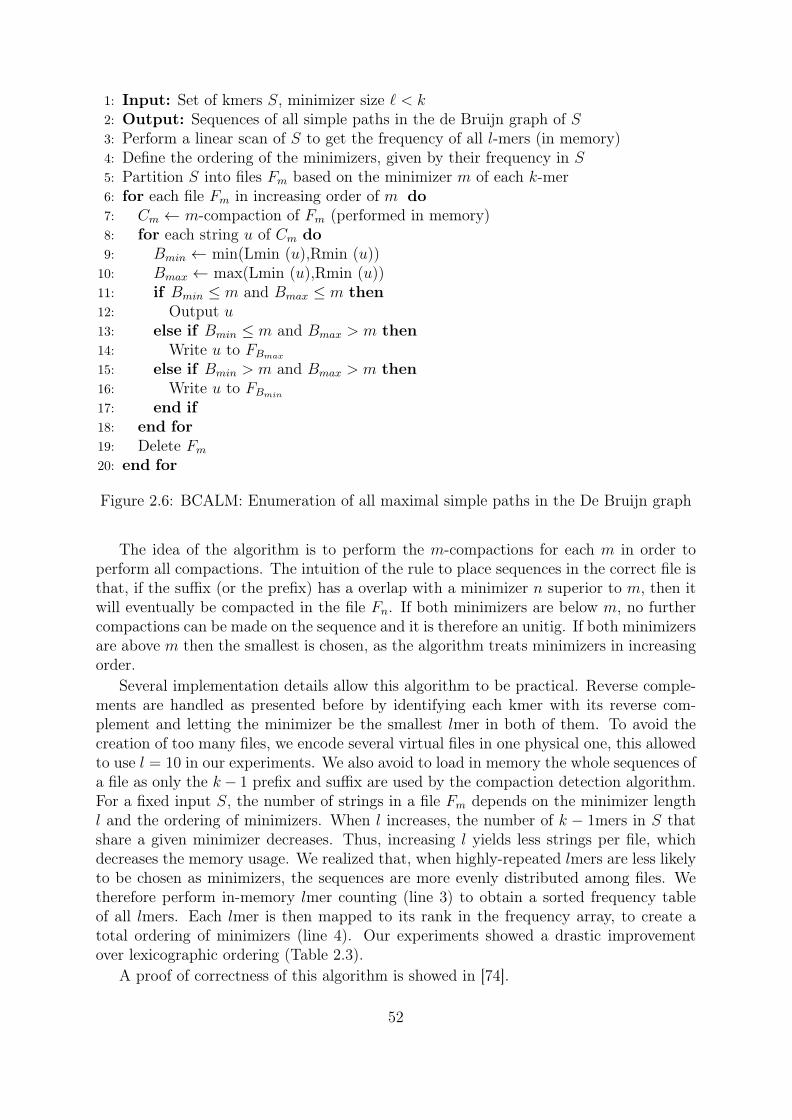
1: Input: Set of kmers S, minimizer size ` < k2: Output: Sequences of all simple paths in the de Bruijn graph of S3: Perform a linear scan of S to get the frequency of all l-mers (in memory)4: Define the ordering of the minimizers, given by their frequency in S5: Partition S into files Fm based on the minimizer m of each k-mer6: for each file Fm in increasing order of m do7: Cm ← m-compaction of Fm (performed in memory)8: for each string u of Cm do9: Bmin ← min(Lmin (u),Rmin (u))

10: Bmax ← max(Lmin (u),Rmin (u))11: if Bmin ≤ m and Bmax ≤ m then12: Output u13: else if Bmin ≤ m and Bmax > m then14: Write u to FBmax

15: else if Bmin > m and Bmax > m then16: Write u to FBmin

17: end if18: end for19: Delete Fm

20: end for

Figure 2.6: BCALM: Enumeration of all maximal simple paths in the De Bruijn graph

The idea of the algorithm is to perform the m-compactions for each m in order toperform all compactions. The intuition of the rule to place sequences in the correct file isthat, if the suffix (or the prefix) has a overlap with a minimizer n superior to m, then itwill eventually be compacted in the file Fn. If both minimizers are below m, no furthercompactions can be made on the sequence and it is therefore an unitig. If both minimizersare above m then the smallest is chosen, as the algorithm treats minimizers in increasingorder.

Several implementation details allow this algorithm to be practical. Reverse comple-ments are handled as presented before by identifying each kmer with its reverse com-plement and letting the minimizer be the smallest lmer in both of them. To avoid thecreation of too many files, we encode several virtual files in one physical one, this allowedto use l = 10 in our experiments. We also avoid to load in memory the whole sequences ofa file as only the k− 1 prefix and suffix are used by the compaction detection algorithm.For a fixed input S, the number of strings in a file Fm depends on the minimizer lengthl and the ordering of minimizers. When l increases, the number of k − 1mers in S thatshare a given minimizer decreases. Thus, increasing l yields less strings per file, whichdecreases the memory usage. We realized that, when highly-repeated lmers are less likelyto be chosen as minimizers, the sequences are more evenly distributed among files. Wetherefore perform in-memory lmer counting (line 3) to obtain a sorted frequency tableof all lmers. Each lmer is then mapped to its rank in the frequency array, to create atotal ordering of minimizers (line 4). Our experiments showed a drastic improvementover lexicographic ordering (Table 2.3).

A proof of correctness of this algorithm is showed in [74].

52

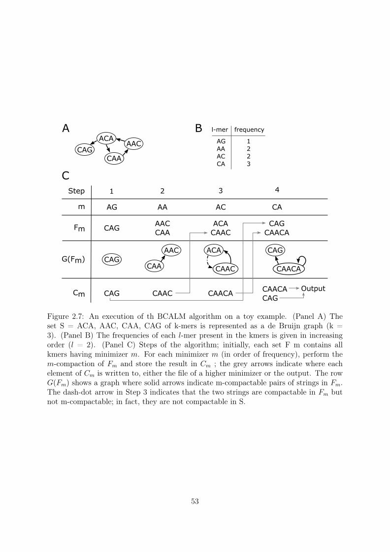
CAG

ACA

CAA

AAC

A l-mer frequency

AG AAACCA

1223

B

C1 2 3

AA ACAG CA

4

CAACACAG CAAC CAACACAG

Output

Step

m

Cm

ACACAAC

AACCAA

Fm CAGCAG

CAACA

CAGCAA

AAC

CAAC

CAG

CAACAG(Fm)

ACA

Figure 2.7: An execution of th BCALM algorithm on a toy example. (Panel A) Theset S = ACA, AAC, CAA, CAG of k-mers is represented as a de Bruijn graph (k =3). (Panel B) The frequencies of each l-mer present in the kmers is given in increasingorder (l = 2). (Panel C) Steps of the algorithm; initially, each set F m contains allkmers having minimizer m. For each minimizer m (in order of frequency), perform them-compaction of Fm and store the result in Cm ; the grey arrows indicate where eachelement of Cm is written to, either the file of a higher minimizer or the output. The rowG(Fm) shows a graph where solid arrows indicate m-compactable pairs of strings in Fm.The dash-dot arrow in Step 3 indicates that the two strings are compactable in Fm butnot m-compactable; in fact, they are not compactable in S.

53

Ordering used Lexicographical Uniformly random lmer frequencyMemory usage 840 MB 222 MB 19 MB

Table 2.3: Memory usage of BCALM with three different minimizer orderings: lexico-graphical, uniformly random, and according to lmer frequencies. The dataset used is thehuman chromosome 14 with k = 55 and l = 8

2.4.4 Assembly in low memory using BCALM

We tested the efficiency of our algorithm in two datasets. The first dataset is 36 million155bp Illumina human chromosome 14 reads (2.9 GB compressed fastq) from the GAGEbenchmark [80]. The second dataset is 1.4 billion Illumina 100bp reads (54 GB com-pressed) from the NA18507 human genome (SRX016231). We first processed the readswith kmer counting software. We used DSK for this operation for its low memory usage.We set k to 55 and applied a solidity theshold of 5 for chr14 and 3 for the whole genome.

First we evaluate (Table 2.3) the memory usage of BCALM on the chr14 dataset,according to the minimizer ordering used. We observe that the lexicographical orderdo not perform well. The lexicographical smallest lmer is Al, which is abundant in thehuman chromosomes, resulting in a large Fm0 and a high memory usage. A secondattempt has been made with a uniformly random ordering. If it performs better thanthe lexicographical one, it is still sensible to repeated lmer in the first files resulting inhigh memory usage. Finally, we ordered the lmers according to their frequency in thedataset. This resulted in a memory usage of 19 MB, a 40-fold improvement over the initiallexicographical ordering. The running times of all three orderings were comparable.

We also evaluated the effect of the size of the minimizer on the BCALM performancesin Table 2.4. Large l generally lead to small memory usage, however we did not see muchimprovement past l = 8 on this dataset.

Using BCALM, we evaluated the performances of the low memory assembly workflowwith DSK, BCALM and DBGFM in Table 2.5. For the whole genome dataset, BCALMused only 43 MB of memory to compact a set of 2.5 ∗ 109 55mers and output 40 millionsequences of total length 4.6 billions base pairs. DBGFM represented these paths inan index of size 1.5 GB. The overall construction time, including DSK, was roughly 24hours. In comparison, a subset of this dataset was used to construct the data structureof Salikhov et al [73] in 30.7 hours.

We also compared the memory usage of the proposed workflow with the other state ofthe art approaches in Table 2.6, showing the interest the proposed low memory assemblyworkflow.

Those results show that indexing unitigs instead of kmers can lead to a memoryefficient assembly steps. The BCALM algorithm, allows an memory efficient constructionof the unitig set by relying on external memory.

54

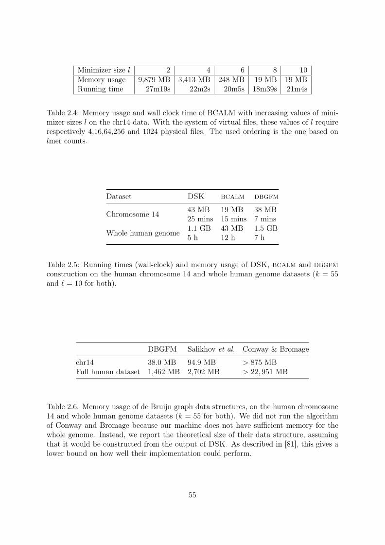
Minimizer size l 2 4 6 8 10Memory usage 9,879 MB 3,413 MB 248 MB 19 MB 19 MBRunning time 27m19s 22m2s 20m5s 18m39s 21m4s

Table 2.4: Memory usage and wall clock time of BCALM with increasing values of mini-mizer sizes l on the chr14 data. With the system of virtual files, these values of l requirerespectively 4,16,64,256 and 1024 physical files. The used ordering is the one based onlmer counts.

Dataset DSK bcalm dbgfm

Chromosome 14 43 MB 19 MB 38 MB25 mins 15 mins 7 mins

Whole human genome 1.1 GB 43 MB 1.5 GB5 h 12 h 7 h

Table 2.5: Running times (wall-clock) and memory usage of DSK, bcalm and dbgfmconstruction on the human chromosome 14 and whole human genome datasets (k = 55and ` = 10 for both).

DBGFM Salikhov et al. Conway & Bromage

chr14 38.0 MB 94.9 MB > 875 MBFull human dataset 1,462 MB 2,702 MB > 22, 951 MB

Table 2.6: Memory usage of de Bruijn graph data structures, on the human chromosome14 and whole human genome datasets (k = 55 for both). We did not run the algorithmof Conway and Bromage because our machine does not have sufficient memory for thewhole genome. Instead, we report the theoretical size of their data structure, assumingthat it would be constructed from the output of DSK. As described in [81], this gives alower bound on how well their implementation could perform.

55

"Efficient de Bruijn graph representations" core messages:

• Unitigs (maximal simple paths) are great abstractions to represent the de Bruijngraph

• Unitigs can be constructed with a low memory usage• Indexing unitigs with a compressed index achieves very low memory assembly

(less than 1.5GB for a human assembly)

2.5 Efficient de Bruijn graph construction

In this section we describe our contribution in the paper "Compacting de Bruijngraphs from sequencing data quickly and in low memory " [82]

We introduced an algorithm to construct the de Bruijn graph with very low memoryusage relying on external memory. But the approach does not exhibit straightforwardparallel patterns to exploit and is quite slow. In the proof of concept human assembly,BCALM took 12 hours to complete for a total running time of 24 hours for the wholeworkflow. As we said before, the kmer counting step tool reached a very high throughputand an extremely reduced memory footprint. The graph compaction step has thereforebecome the bottleneck for assembly. We showed before that unitigs could be used asatoms for assembly instead of kmers and it appears that most assemblers rely on themor even, in some cases, explicitly compute such sets of sequences [83, 40]. Some papersproposed solutions for fast graph compaction but are mostly based on parallel graphtraversal and no memory efficient method have been proposed. This is why we proposea fast and parallel algorithm for graph compaction presenting a low memory footprintcalled BCALM2.

2.5.1 BCALM2 algorithm

We give here a high level overview of the BCALM2 algorithm (Figure 2.8). As in BCALMthe first step of the algorithm is to distribute the input set of kmer into files. In BCALM2 akmer can be inserted in two different files, if it has different left and right minimizers. Thesecond step will consist into performing compactions on all the files in parallel accordingto the compaction procedure described in Figure 2.9. The last stage will need to glueback together the kmers that were duplicated in two files. The Figure 2.12 shows anexecution of BCALM2 on a toy example.

Since the size of the files are small, the compactions can be made with a in-memoryalgorithm in a parallel way. The resulting sequences are written on disk and are processedin the third stage when all compactions are finished. At the end of the compaction step,we notice that some kmers exist in two copies in the sequences produced. Such kmers arealways the prefix or the suffix of the compacted sequences. We record the sequences endsthat have a doubled kmers has "lonely" as they should be reunited in the third stage.The other sequences are output as unitigs.

56

In the last stage, we process the sequences that need to be reunited with the Reuniteprocedure (Figure 2.10). The goal of Reunite is to associate the sequences sharing a suffixor prefix kmer and to glue them together (Figure 2.11) by reuniting the two occurrencesof a doubled kmer. The lonely mark are transfered to the produced sequences and thisprocess is repeated until a sequence has a lonely end. After the reunite operation, thereis no duplicated kmer left and the output correspond to the unitig set. In order to beefficient, the reunite operation partitions the sequences in order to process the partitionsin a parallel and memory efficient way.

A proof of correctness of this algorithm is available in [82]

2.5.2 Implementation details

In this section we describe optimizations and important implementation details. As inBCALM, we do not use the lexical ordering for minimizers but the frequency based min-imizer order described previously. Files used in the algorithm are virtual files organizedinto groups, in order to introduce natural checkpoints in BCALM 2 in between parallelsections. BCALM2 iterates sequentially through the groups, but parallelizes the process-ing within a group. The For loop at line 1 of Figure 2.8 is executed in parallel within a

Input: the set of k-mers K.1: for all parallel x ∈ K do2: Write x to F (Lmin(x)).3: if Lmin(x) 6= Rmin(x) then4: Write x to F (Rmin(x)).5: end if6: end for7: for all parallel i ∈ 1, . . . , 4` do8: Run CompactBucket(i)9: end for

10: Reunite()

Figure 2.8: BCALM2(K)

1: Load F (i) into memory.2: U ← i-compaction of F (i).3: for all strings u ∈ U do4: Mark u’s prefix as “lonely” if i 6= Lmin(u).5: Mark u’s suffix as “lonely” if i 6= Rmin(u).6: if u’s prefix and suffix are not lonely then7: Output u.8: else9: Place u in the Reunite file

10: end if11: end for

Figure 2.9: CompactBucket(i)

57

Input: the set of strings R from the Reunitefile.1: UF ← Union find data structure whose elements are the distinct k-mer extremities

in R.2: for all parallel u ∈ R do3: if both ends of u are lonely then4: UF.union(sufk(u), prek(u))5: end if6: end for7: for all parallel classes C of UF do8: P ← all u ∈ R that have a lonely extremity in C9: while ∃u ∈ P that does not have a lonely prefix do

10: Remove u from P11: Let s = u12: while ∃ v ∈ P such that sufk(s) = prek(v) do13: s← Glue(s, v)14: Remove v from P15: end while16: Output s17: end while18: end for

Figure 2.10: Reunite()

Input: strings u and v, such that suffixk(u) = prefixk(v).1: Let w = uk v.2: Set lonely prefix bit of w to be the lonely prefix bit of u.3: Set lonely suffix bit of w to be the lonely suffix bit of v.4: return w

Figure 2.11: Glue(u, v)

58

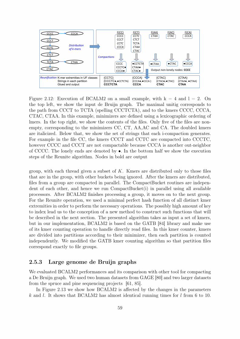
F(CC) CCCC CCCT CCTC CCCA

F(CT) CCTC CTCT TCTA CTAA CTAC

F(AA) CTAA

F(AC) CTAC

F(CA) CCCA

Compac)ons CCCC CCCTC CCCA

CCTCTA CTAA CTAC

CTAA CTAC CCCA

Distribu)on ofk-mers

Reunifica)on

CCCC CCCT CCTC CTCT TCTA CTAA

CCCA

Outputnon-lonelynodes:CCCC

K-mer extremities in UF classes CCTC CCCA CTAC CTAA Strings in each partition CCCTC,CCTCTACCCA,CCCACTAC,CTACCTAA,CTAA Glued and output CCCTCTA CCCA CTAC CTAA

CTAC

Figure 2.12: Execution of BCALM2 on a small example, with k = 4 and l = 2. Onthe top left, we show the input de Bruijn graph. The maximal unitig corresponds tothe path from CCCT to TCTA (spelling CCCTCTA), and to the kmers CCCC, CCCA,CTAC, CTAA. In this example, minimizers are defined using a lexicographic ordering oflmers. In the top right, we show the contents of the files. Only five of the files are non-empty, corresponding to the minimizers CC, CT, AA,AC and CA. The doubled kmersare italicized. Below that, we show the set of strings that each i-compaction generates.For example in the file CC, the kmers CCCT and CCTC are compacted into CCCTC,however CCCC and CCCT are not compactable because CCCA is another out-neighborof CCCC. The lonely ends are denoted by •. In the bottom half we show the executionsteps of the Reunite algorithm. Nodes in bold are output

group, with each thread given a subset of K. Kmers are distributed only to those filesthat are in the group, with other buckets being ignored. After the kmers are distributed,files from a group are compacted in parallel. The CompactBucket routines are indepen-dent of each other, and hence we run CompactBucket(i) in parallel using all availableprocessors. After BCALM2 finishes processing a group, it moves on to the next group.For the Reunite operation, we used a minimal perfect hash function of all distinct kmerextremities in order to perform the necessary operations. The possibly high amount of keyto index lead us to the conception of a new method to construct such functions that willbe described in the next section. The presented algorithm takes as input a set of kmers,but in our implementation, BCALM2 is based on the GATB [84] library and make useof its kmer counting operation to handle directly read files. In this kmer counter, kmersare divided into partitions according to their minimizer, then each partition is countedindependently. We modified the GATB kmer counting algorithm so that partition filescorrespond exactly to file groups.

2.5.3 Large genome de Bruijn graphs

We evaluated BCALM2 performances and its comparison with other tool for compactinga De Bruijn graph. We used two human datasets from GAGE [80] and two larger datasetsfrom the spruce and pine sequencing projects [61, 85].

In Figure 2.13 we show how BCALM2 is affected by the changes in the parametersk and l. It shows that BCALM2 has almost identical running times for l from 6 to 10.

59

1 2 4 8 16 320

4

8

12

16CompactionsReunificactions

Number of cores

Wal

l-cl

ock

time

(min

)

l=4 l=6 l=8 l=10200

400

600

k=21k=41k=61

Minimizer size

Wal

l-cl

ock

time

(s)

Figure 2.13: BCALM2 wall-clock running times with respect to parameters ` (left) andk (using 4 cores) and number of cores (using k = 55 and ` = 8), on the chromosome 14dataset (right).

Short minimizer sizes create fewer files and therefore limit parallel operations. We alsoshow how BCALM2 scales with multiples cores. We observe that the compactions scale ina nearly linear manner with the number of thread used. There remains overhead relatedto disk operations.

We also compared the BCALM2 performances with BCALM, ABYSS and Merac-ulous2 graph compaction steps in Table 2.7. We observe that BCALM2 is the fastestavailable tool while using order of magnitude less memory but compared to BCALM.We further evaluated BCALM 2 on two very large sequencing datasets: Illumina readsfrom the 20 Gbp Picea glauca genome (8.5 billion reads, 152–300 bp each, 1.1 TB com-pressed FASTQ, SRA056234), and Illumina paired-end reads from the 22 Gbp Pinus taedagenome (9.4 billion reads, 128–154 bp each, 1.2 TB compressed FASTQ, SRX016231).The k-mer counting step took around a day and less than 40 GB of memory for eachdataset.

Table 2.8 shows the performance of BCALM 2 on these two datasets, as well asunitigs statistics. Graph construction of the spruce dataset previously required 4.3 TBof memory and 2 days on a 1380-core cluster [61], while the assembly of the pine datasetpreviously required 800 GB of memory and 3 months on a single machine [85]. Althoughwe used the same sequencing datasets, several parameters differ between these previousreports and our results (e.g. k value, abundance cutoff, and whether reads were error-corrected). Hence, run time, memory usage, and unitigs statistics cannot be directlycompared. However, it seems reasonable to infer that BCALM 2 would remains 1–2orders of magnitude more efficient in time and memory.

60

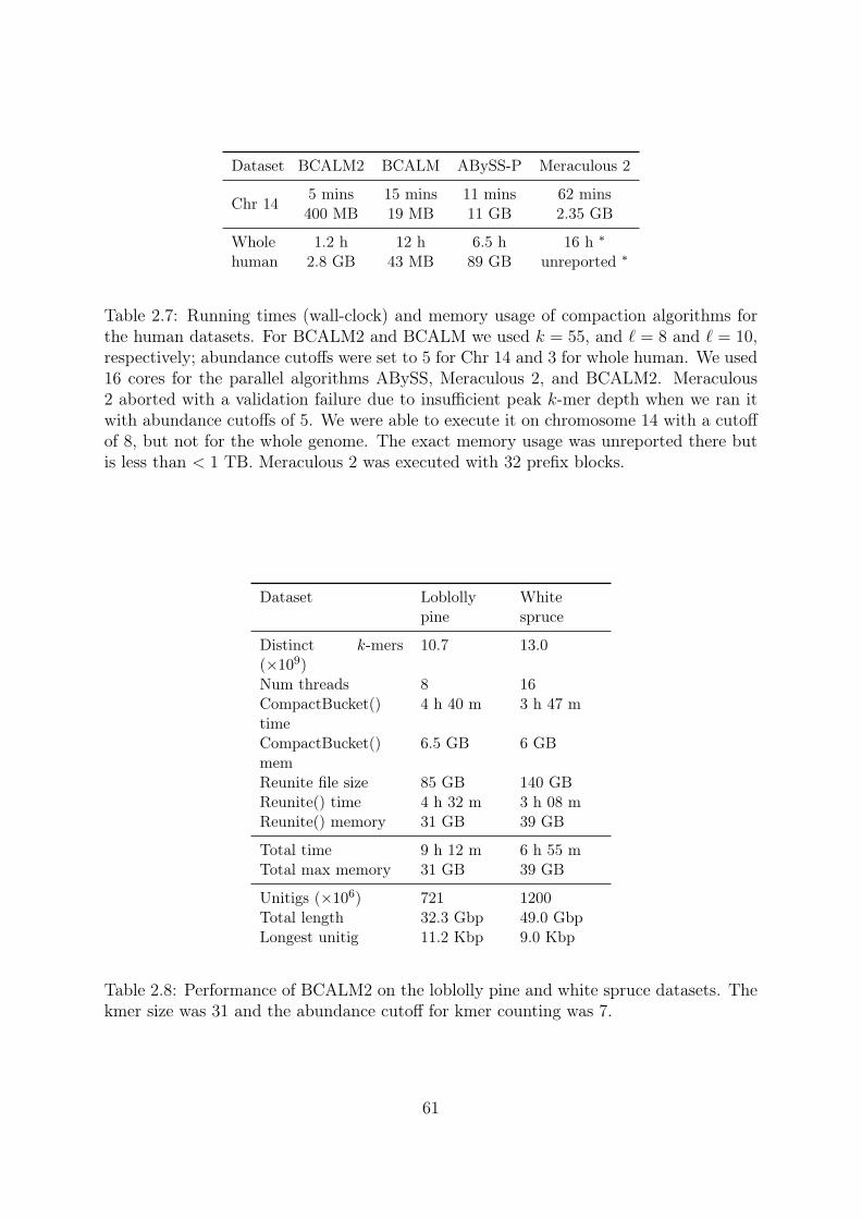
Dataset BCALM2 BCALM ABySS-P Meraculous 2

Chr 14 5 mins 15 mins 11 mins 62 mins400 MB 19 MB 11 GB 2.35 GB

Wholehuman

1.2 h 12 h 6.5 h 16 h ∗

2.8 GB 43 MB 89 GB unreported ∗

Table 2.7: Running times (wall-clock) and memory usage of compaction algorithms forthe human datasets. For BCALM2 and BCALM we used k = 55, and ` = 8 and ` = 10,respectively; abundance cutoffs were set to 5 for Chr 14 and 3 for whole human. We used16 cores for the parallel algorithms ABySS, Meraculous 2, and BCALM2. Meraculous2 aborted with a validation failure due to insufficient peak k-mer depth when we ran itwith abundance cutoffs of 5. We were able to execute it on chromosome 14 with a cutoffof 8, but not for the whole genome. The exact memory usage was unreported there butis less than < 1 TB. Meraculous 2 was executed with 32 prefix blocks.

Dataset Loblollypine

Whitespruce

Distinct k-mers(×109)

10.7 13.0

Num threads 8 16CompactBucket()time

4 h 40 m 3 h 47 m

CompactBucket()mem

6.5 GB 6 GB

Reunite file size 85 GB 140 GBReunite() time 4 h 32 m 3 h 08 mReunite() memory 31 GB 39 GB

Total time 9 h 12 m 6 h 55 mTotal max memory 31 GB 39 GB

Unitigs (×106) 721 1200Total length 32.3 Gbp 49.0 GbpLongest unitig 11.2 Kbp 9.0 Kbp

Table 2.8: Performance of BCALM2 on the loblolly pine and white spruce datasets. Thekmer size was 31 and the abundance cutoff for kmer counting was 7.

61

"Efficient de Bruijn graph construction" core messages:

• Graph construction is the bottleneck of most assemblers• Unitigs can be constructed in parallel and in low memory• Very large genomes can be addressed without huge need of RAM

2.6 Indexing large sets

We presented the interest of working on unitigs for assembly and how to efficiently com-pute them. We proposed DBGFM, a data structure able to index the set of unitigs usingless memory than previously best known data structures and fast enough to allow efficientassembly. Since DBGFM is more powerful than a NDS because it is a membership datastructure, can we propose a better structure that is just a NDS?

We are interested in a structure using less memory and providing faster access toneighbors. We remark that the unitig sequence representation is close to the 2 bits perkmer limit. Each unitig represents an overhead of 2 ∗ (k − 1) nucleotides to add to the 2bits per kmer. Raw unitig sequences is not an interesting structure in practice because aquery would be linear. Indexing the last and first k−1mers of each unitig and associatingto each k − 1mer the unitigs that start and end with it could lead to an NDS. The costof such a structure would be at least 8 ∗ log(#unitigs) bits per unitigs, as a k − 1mercan be associated to up to 8 unitigs (log(#unitigs) bits are needed to encode the indiceof an unitig), plus the indexing cost.

A better scheme would be to index the first and last kmer of each unitig and toassociate to each indexed kmer its unique unitig. Indeed a kmer appears in at most oneunitig due to the definition of the compacted de Bruijn graph. This way, an unitig canknow its sons by querying the index with the four possible kmers. In order to avoidperforming useless queries, we can add 8 bits to each unitig to precise which neighborsexist. This leads to a structure of at least 2 ∗ log(#unitigs) per unitig (to encode thethe unitig indice twice) bits plus 8 bits from the proposed optimization plus the cost ofindexing. This kind of structure would allow constant and fast queries, with a very lowmemory overhead. A regular hashing would be costly in memory and in query time. Thebest solution to keep a low memory usage would be an open addressing hash table thatwould offer a 2 ∗ log(#unitigs) ∗ (1/loadFactor) bits. In practice the load factor is setbelow 0.8. Practically we can consider that the unitig identifier would be represented bya 32 bits integer, thus the open addressing would cost roughly one byte by unitig andwould produce long queries when collisions occur. Can we do better ?

One may argue that we do not use the fact that our set of keys is static and thatwe could use a Minimal Perfect Hash Function (MPHF). Such structures use very fewmemory (as low as 3 bits per key) and guarantee constant query time and in practicevery fast access (hundred of nanoseconds). Beside, many applications in bioinformaticscould benefit from an efficient and lightweight structure to associate information to largesets of keys as kmers or unitigs: coverage, origin of the sequence or any properties. ButMPHF are costly to construct for very large sets of keys, both in running time and inmemory usage. We therefore present a technique able to efficiently construct efficient

62

MPHF from huge sets of keys with low memory and time.

This method is presented in the paper "Fast and scalable minimal perfect hashingconstruction for massive key sets" [86] included at the end of the chapter.

This paper observes that most methods to construct MPHF are designed to providethe smallest structures. However, most methods use way more memory during construc-tion than the size of the MPHF itself. Generally, available implementations showed veryhigh running time and memory requirement on large sets of keys, making them imprac-ticable to index billions of objects. The paper therefore proposes a new implementationof a simple algorithm providing efficient MPHF that scales on very large sets.

The algorithm used is pretty straightforward. First keys are hashed into a bit array.Second the positions in the bit array that received an unique key are marked with a oneand the corresponding keys are removed from the key set. The remaining keys are hashedin a second bit array and the process is repeated until there is not key left. At the endof the algorithm each key is associated to a unique position in one of the bit array. Tofind this position the key is hashed to the different bit array until a one is found.

The main interests of the method are the amount of memory needed for constructionthat is similar to the size of the MPHF and the parallel construction allowing a very shortrunning time. BBHASH constructed a MPHF from a billion key dataset in a minute with2GB of RAM were the best know MPHF library constructs it in more than 20 minutesusing more than 18GB. BBHASH also achieved to construct a trillion key MPHF on a750GB machine. This experiment is, to our knowledge, the largest MPHF constructed.

Applications BBhash MPHF has been used in several bioinformatics tools and wasintegrated in the GATB [84] library. It is used to associate information to kmers such ascoverage or origin. The unification operation of BCALM2 also relies on BBhash MPHFstructure. Another tool, called SRC [87, 88], integrated the BBhash MPHF in orderto propose an efficient data structure to index reads for read set comparisons and readcoverage estimation.

"Indexing large sets" core messages:

• We can build MPHF from huge sets of keys with low resources• Such MPHF are used for assembly and also for various applications in bioinfor-

matics

63

Fast and scalable minimal perfect hashing formassive key setsAntoine Limasset1, Guillaume Rizk1, Rayan Chikhi2, and PierrePeterlongo1

1 IRISA Inria Rennes Bretagne Atlantique, GenScale team, Campus deBeaulieu 35042 Rennes, France

2 CNRS, CRIStAL, Université de Lille, Inria Lille - Nord Europe, France

AbstractMinimal perfect hash functions provide space-efficient and collision-free hashing on static sets.Existing algorithms and implementations that build such functions have practical limitations onthe number of input elements they can process, due to high construction time, RAM or externalmemory usage. We revisit a simple algorithm and show that it is highly competitive with thestate of the art, especially in terms of construction time and memory usage. We provide aparallel C++ implementation called BBhash. It is capable of creating a minimal perfect hashfunction of 1010 elements in less than 7 minutes using 8 threads and 5 GB of memory, and theresulting function uses 3.7 bits/element. To the best of our knowledge, this is also the firstimplementation that has been successfully tested on an input of cardinality 1012. Source code:https://github.com/rizkg/BBHash

1998 ACM Subject Classification H.3.1 E.2

Keywords and phrases Minimal Perfect Hash Functions, Algorithms, Data Structures, Big Data

Digital Object Identifier 10.4230/LIPIcs...

1 Introduction

Given a set S of N elements (keys), a minimal perfect hash function (MPHF) is an injectivefunction that maps each key of S to an integer in the interval [1, N ]. In other words, anMPHF labels each key of S with integers in a collision-free manner, using the smallest possibleinteger range. A remarkable property is the small space in which these functions can bestored: only a couple of bits per key, independently of the size of the keys. Furthermore,an MPHF query is done in constant time. While an MPHF could be easily obtained using akey-value store (e.g. a hash table), such a representation would occupy an unreasonableamount of space, with both the keys and the integer labels stored explicitly.

The theoretical minimum amount of space needed to represent an MPHF is known tobe log2(e)N ≈ 1.44N bits [10, 14]. In practice, for large key sets (billions of keys), manyimplementations achieve less than 3N bits per key, regardless of the number of keys [2, 9].However no implementation comes asymptotically close to the lower bound for large key sets.Given that MPHFs are typically used to index huge sets of strings, e.g. in bioinformatics [6, 7, 8],in network applications [12], or in databases [5], lowering the representation space is of interest.We observe that in many of these applications, MPHFs are actually used to construct staticdictionaries, i.e. key-value stores where the set of keys is fixed and never updated [6, 8].Assuming that the user only queries the MPHF to get values corresponding to keys that areguaranteed to be in the static set, the keys themselves do not necessarily need to be stored inmemory. However the associated values in the dictionary typically do need to be stored, and

© Antoine Limasset, Guillaume Rizk, Rayan Chikhi and Pierre Peterlongo;licensed under Creative Commons License CC-BY

Leibniz International Proceedings in InformaticsSchloss Dagstuhl – Leibniz-Zentrum für Informatik, Dagstuhl Publishing, Germany

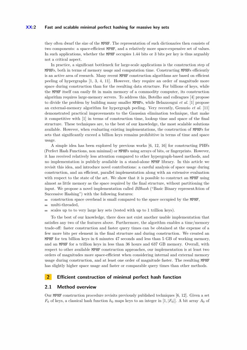
XX:2 Fast and scalable minimal perfect hashing for massive key sets

they often dwarf the size of the MPHF. The representation of such dictionaries then consists oftwo components: a space-efficient MPHF, and a relatively more space-expensive set of values.In such applications, whether the MPHF occupies 1.44 bits or 3 bits per key is thus arguablynot a critical aspect.

In practice, a significant bottleneck for large-scale applications is the construction step ofMPHFs, both in terms of memory usage and computation time. Constructing MPHFs efficientlyis an active area of research. Many recent MPHF construction algorithms are based on efficientpeeling of hypergraphs [1, 3, 4, 11]. However, they require an order of magnitude morespace during construction than for the resulting data structure. For billions of keys, whilethe MPHF itself can easily fit in main memory of a commodity computer, its constructionalgorithm requires large-memory servers. To address this, Botelho and colleagues [4] proposeto divide the problem by building many smaller MPHFs, while Belazzougui et al. [1] proposean external-memory algorithm for hypergraph peeling. Very recently, Genuzio et al. [11]demonstrated practical improvements to the Gaussian elimination technique, that makeit competitive with [1] in terms of construction time, lookup time and space of the finalstructure. These techniques are, to the best of our knowledge, the most scalable solutionsavailable. However, when evaluating existing implementations, the construction of MPHFs forsets that significantly exceed a billion keys remains prohibitive in terms of time and spaceusage.

A simple idea has been explored by previous works [6, 12, 16] for constructing PHFs(Perfect Hash Functions, non minimal) or MPHFs using arrays of bits, or fingerprints. However,it has received relatively less attention compared to other hypergraph-based methods, andno implementation is publicly available in a stand-alone MPHF library. In this article werevisit this idea, and introduce novel contributions: a careful analysis of space usage duringconstruction, and an efficient, parallel implementation along with an extensive evaluationwith respect to the state of the art. We show that it is possible to construct an MPHF usingalmost as little memory as the space required by the final structure, without partitioning theinput. We propose a novel implementation called BBhash (“Basic Binary representAtion ofSuccessive Hashing”) with the following features:

construction space overhead is small compared to the space occupied by the MPHF,multi-threaded,scales up to to very large key sets (tested with up to 1 trillion keys).To the best of our knowledge, there does not exist another usable implementation that

satisfies any two of the features above. Furthermore, the algorithm enables a time/memorytrade-off: faster construction and faster query times can be obtained at the expense of afew more bits per element in the final structure and during construction. We created anMPHF for ten billion keys in 6 minutes 47 seconds and less than 5 GB of working memory,and an MPHF for a trillion keys in less than 36 hours and 637 GB memory. Overall, withrespect to other available MPHF construction approaches, our implementation is at least twoorders of magnitudes more space-efficient when considering internal and external memoryusage during construction, and at least one order of magnitude faster. The resulting MPHFhas slightly higher space usage and faster or comparable query times than other methods.

2 Efficient construction of minimal perfect hash function

2.1 Method overviewOur MPHF construction procedure revisits previously published techniques [6, 12]. Given a setF0 of keys, a classical hash function h0 maps keys to an integer in [1, |F0|]. A bit array A0 of

A. Limasset, G. Rizk, R. Chikhi, P. Peterlongo XX:3

1

0

0

0

1

0

k6

k4,k2

k3

k1,k5

1

0

1

0

k5

k4,k2

k1

1

1 k4

k2 k1 k2 k3 k4 k5 k6

h0

A0 A1 A2

h1 h2

1 (1) 0 0 0 1 (2) 0 1 (3) 0 1 (4) 0 1 (5) 1 (6)

A0 A1 A2

A (rank of ’1’s are indicated in parenthesis)

h0(k2) h1(k2) h2(k2)

F0

k1 k2 k4 k5

F1

k2 k4

F2

Figure 1 MPHF construction and query example. The input is a set F0 composed of N = 6 keys(k1 to k6). All keys are hashed using a hash function h0 and are attempted to be placed in an arrayA0 at positions given by the hash function. The keys k3 and k6 do not have collisions in the array,thus the corresponding bits in A0 are set to ’1’. The other keys from F0 that are involved in collisionsare placed in a new set F1. In the second level, keys from F1 are hashed using a hash function h1.Keys k1 and k5 are uniquely placed while k2 and k4 collide, thus they are then stored in the setF2. With the hash function h2, the keys from F2 have no collision, and the process finishes. TheMPHF query operation is very similar to the construction algorithm. Let A be the the concatenationof A0, A1, A2 (see bottom part of the figure). To query k2, the key is first hashed with h0. Theassociated value in A0 is ’0’, so k2 is then hashed with h1. The value associated in A1 is again ’0’.When finally hashed with h2, the value associated in A2 is ’1’ and thus the query stops here. Theindex returned by the MPHF is the rank of this ’1’ (here, 5) in A. In this example, the MPHF valuesreturned when querying k1, k2, k3, k4, k5 and k6 are respectively 4,5,2,6,3, and 1.

size |F0| is created such that there is a 1 at position i if and only if exactly one element ofF0 has a hash value of i. We say that there is a collision whenever two keys in F0 have thesame hash value. Keys from F0 that were involved in a collision are inserted into a new setF1. The process repeats with F1 and a new hash function h1. A new bit array A1 of size|F1| is created using the same procedure as for A0 (except that F1 is used instead of F0, andh1 instead of h0). The process is repeated with F2, F3, . . . until one of these sets, Flast+1, isempty.

We obtain an MPHF by concatenating the bit arrays A0, A1, . . . , Alast into an array A.To perform a query, a key is hashed successively with hash functions h0, h1, . . . as long asthe value in Ai (i ≥ 0) at the position given by the hash function hi is 0. Eventually, byconstruction, we reach a 1 at some position of A for some i = d. We say that the level of thekey is d. The index returned by the MPHF is the rank of this one in A. See Figure 1 for anexample.

2.2 Algorithm details2.2.1 Collision detectionDuring construction at each level d, collisions are detected using a temporary bit array Cd ofsize |Ad|. Initially all Cd bits are set to ’0’. A bit of Cd[i] is set to ’1’ if two or more keys from

XX:4 Fast and scalable minimal perfect hashing for massive key sets

Fd have the same value i given by hash function hd. Finally, if Cd[i] = 1, then Ad[i] = 0.Formally:

Cd[i] = 1⇒ Ad[i] = 0;(hd[x] = i and Ad[i] = 0 and Cd[i] = 0)⇒ Ad[i] = 1 (and Cd[i] = 0) ;(hd[x] = i and Ad[i] = 1 and Cd[i] = 0)⇒ Ad[i] = 0 and Cd[i] = 1.

2.2.2 QueriesA query of a key x is performed by finding the smallest d such that Ad[hd(x)] = 1. The (nonminimal) hash value of x is then (

∑i<d |Fi|) + hd(x).

2.2.3 MinimalityTo ensure that the image range of the function is [1, |F0|], we compute the cumulative rankof each ’1’ in the bit arrays Ai. Suppose, that d is the smallest value such that Ad[hd(x)] = 1.The minimal perfect hash value is given by

∑i<d(weight(Ai) + rank(Ad[hd(x)]), where

weight(Ai) is the number of bits set to ’1’ in the Ai array, and rank(Ad[y]) is the number ofbits set to 1 in Ad within the interval [0, y], thus rank(Ad[y]) =

∑j<y Ad[j]. This is a classic

method also used in other MPHFs [3].

2.2.4 Faster query and construction times (parameter γ)The running time of the construction depends on the number of collisions on the Ad arrays,at each level d. One way to reduce the number of collisions, hence to place more keys at eachlevel, is to use bit arrays (Ad and Cd) larger than |Fd|. We introduce a parameter γ ∈ R,γ ≥ 1, such that |Cd| = |Ad| = γ|Fd|. With γ = 1, the size of A is minimal. With γ ≥ 2,the number of collisions is significantly decreased and thus construction and query times arereduced, at the cost of a larger MPHF structure size. The influence of γ is discussed in moredetail in the following analyses and results.

2.3 AnalysisProofs of the following observations and lemma are given in the Appendix.

2.3.1 Size of the MPHFThe expected size of the structure can be determined using a simple argument, previouslymade in [6]. When γ = 1, the expected number of keys which do not collide at level d is|Ad|e−1, thus |Ad| = |Ad−1|(1 − e−1) = |A0|(1 − e−1)d. In total, the expected number ofbits required by the hashing scheme is

∑d≥0 |Ad| = N

∑d≥0(1− e−1)d = eN , with N being

the total number of input keys (N = |F0|). Note that consequently the image of the hashfunction is also in [1, eN ], before minimization using the rank technique. When γ ≥ 1, theexpected proportion of keys without collisions at each level d is |Ad|e−

1γ . Since each Ad no

longer uses one bit per key but γ bits per key, the expected total number of bits required bythe MPHF is γe

1γ N .

2.3.2 Space usage during constructionWe analyze the disk space used during construction. Recall that during construction of leveld, a bit array Cd of size |Ad| is used to record collisions. Note that the Cd array is only

A. Limasset, G. Rizk, R. Chikhi, P. Peterlongo XX:5

needed during the d-th level. It is deleted before level d + 1. The total memory requiredduring level d is

∑i≤d(|Ai|) + |Cd| =

∑i<d(|Ai|) + 2|Ad|.

I Lemma 1. For γ > 0, the space of our MPHF is S = γe1γ N bits. The maximal space during

construction is S when γ ≤ log(2)−1, and 2S bits otherwise.A full proof of the Lemma is provided in the Appendix.

3 Implementation

We present BBhash, a C++ implementation available at http://github.com/rizkg/BBHash.We describe in this section some design key choices and optimizations.

3.1 Rank structureWe use a classical technique to implement the rank operation: the ranks of a fraction of the’1’s present in A are recorded, and the ranks in-between are computed dynamically using therecorded ranks as checkpoints.

In practice 64 bit integers are used for counters, which is enough for realistic use of anMPHF, and placed every 512 positions by default. These values were chosen as they offera good speed/memory trade-off, increasing the size of the MPHF by a factor 1.125 whileachieving good query performance. The total size of the MPHF is thus (1 + 64

512 )γe1γ N .

3.2 ParallelizationParallelization is achieved by partitioning keys over several threads. The algorithm presentedin Section 2 is executed on multiple threads concurrently, over the same memory space.Built-in compiler functions (e.g. sync_fetch_and_or) are used for concurrent access in theAi arrays. The efficiency of this parallelization scheme is shown in the Results section, butnote that it is fundamentally limited by random memory accesses to the Ai arrays whichincur cache misses.

3.3 Hash functionsThe MPHF construction requires classical hash functions. Other authors have observed thatcommon hash functions behave practically as well as fully random hash functions [2]. Wetherefore choose to use xor-shift based hash functions [13] for their efficiency both in termsof computation speed and distribution uniformity [15].

3.4 Disk usageIn the applications we consider, key sets are typically too big to fit in RAM. Thus we proposeto read them on the fly from disk. There are mainly two distinct strategies regarding thedisk usage during construction: 1/ during each level d, keys that are to be inserted in the setFd+1 are written directly to disk. The set Fd+1 is then read during level d+ 1 and erasedbefore level d+ 2; or 2/ at each level all keys from the original input key file are read andqueried in order to determine which keys were already assigned to a level i < d, and whichwould belong to Fd. When the key set becomes small enough (below user-defined threshold)it is loaded in ram to avoid costly re-computation from scratch at each level.

The first strategy obviously provides faster construction at the cost of temporary disk usage.At each level d > 0, two temporary key files are stored on disk: Fd and Fd+1. The highest disk

XX:6 Fast and scalable minimal perfect hashing for massive key sets

usage is thus achieved during level 1, i.e. by storing |F1|+|F2| = |F0|((1−e−1/γ)+(1−e−1/γ)2)elements. With γ = 1, this represents ≈ 1.03N elements, thus the construction overhead ondisk is approximately the size of the input key file. Note that with γ = 2 (resp. γ = 5), thisoverhead diminishes and becomes a ratio of ≈ 0.55 (resp. ≈ 0.21) the size of the input keyfile.

The first strategy is the default strategy proposed in our implementation. The secondone has also been implemented and can be optionally switched on.

3.5 TerminationThe expected number of unplaced keys decreases exponentially with the number of levelsbut is not theoretically guaranteed to reach zero in a finite number of steps. To ensuretermination of the construction algorithm, in our implementation a maximal number D oflevels is fixed. Then, the remaining keys are inserted into a regular hash table. Value D is aparameter, its default value is D = 25 for which the expected number of keys stored in thishash table is ≈ 10−5N for γ = 1 and becomes in practice negligible for γ ≥ 2, allowing thesize overhead of the final hash table to be negligible regarding the final MPHF size.

4 Results

We evaluated the performance BBhash for the construction of large MPHFs. We generatedfiles containing various numbers of keys (from 1 million to 1 trillion keys). In our tests, akey is a binary representation of a pseudo-random positive integer in [0; 264]. Within eachfile, each key is unique. We also performed a test where input keys are strings (n-grams) toensure that using integers as keys does not bias results. Tests were performed on a clusternode with a Intel© Xeon© CPU E5-2660 v3 2.60GH 20-core CPU, 256 GB of memory, anda mechanical hard drive. Except for the experiment with 1012 keys, running times includethe time needed to read input keys from disk. Note that files containing key sets may becached in memory by the operating system, and all evaluated methods benefit from thiseffect during MPHF construction. We refer to the Appendix for the specific commands andparameters used in these experiments.

We first analyzed the influence of the γ value (the main parameter of BBhash), thenthe effect of using multiple threads depending on the parallelization strategy. Second, wecompared BBhash with other state-of-the-art methods. Finally, we performed an MPHFconstruction on 1012 elements.

4.1 Influence of the γ parameterWe report in Figure 2 (left) the construction times and the mean query times, as well asthe size of the produced MPHF, with respect to several γ values. The main observation isthat γ ≥ 2 drastically accelerates construction and query times. This is expected since largeγ values allow more elements to be placed in the first levels of the MPHF; thus limiting thenumber of times each key is hashed to compute its level. In particular, for keys placedin the very first level, the query time is limited to a single hashing and a memory access.The average level of all keys is e(1/γ), we therefore expect construction and query timesto decrease when γ increases. However, larger γ values also incur larger MPHF sizes. Oneobserves that γ > 5 values seem to bring very little advantage at the price of higher spacerequirements. A related work used γ = 1 in order to minimize the MPHF size [6]. Here, we

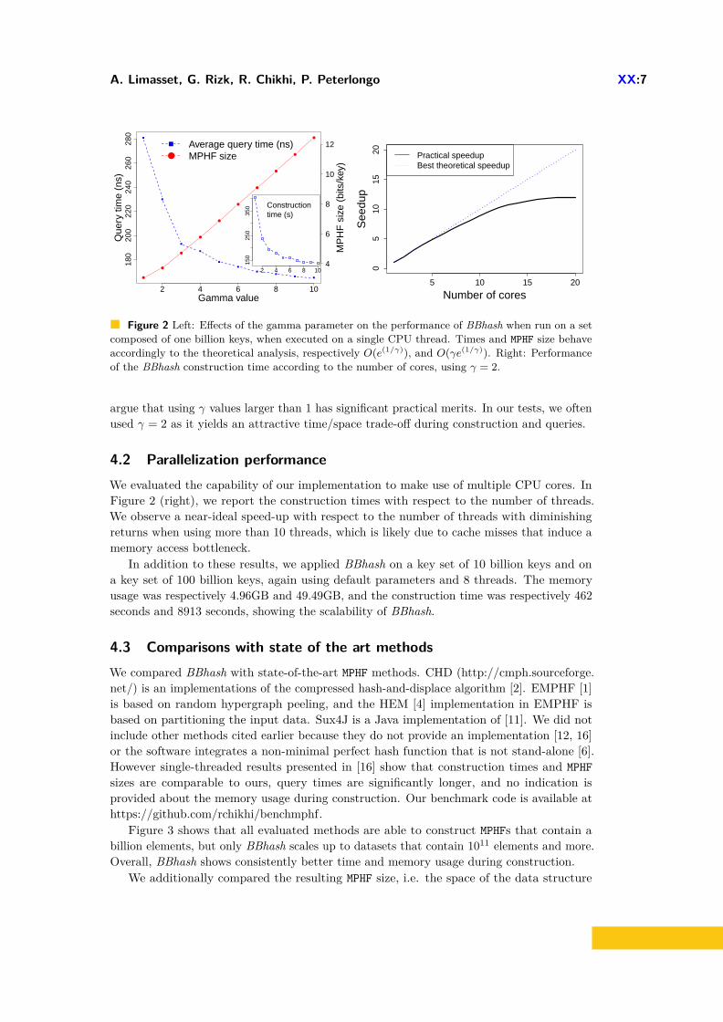
A. Limasset, G. Rizk, R. Chikhi, P. Peterlongo XX:7

2 4 6 8 10

180

200

220

240

260

280

Gamma value

Que

ry ti

me

(ns)

MP

HF

siz

e (b

its/k

ey)

4

6

8

10

12

Average query time (ns)MPHF size

2 4 6 8 10

150

250

350 Construction

time (s)

5 10 15 20

05

1015

20

Number of cores

See

dup

Practical speedupBest theoretical speedup

Figure 2 Left: Effects of the gamma parameter on the performance of BBhash when run on a setcomposed of one billion keys, when executed on a single CPU thread. Times and MPHF size behaveaccordingly to the theoretical analysis, respectively O(e(1/γ)), and O(γe(1/γ)). Right: Performanceof the BBhash construction time according to the number of cores, using γ = 2.

argue that using γ values larger than 1 has significant practical merits. In our tests, we oftenused γ = 2 as it yields an attractive time/space trade-off during construction and queries.

4.2 Parallelization performanceWe evaluated the capability of our implementation to make use of multiple CPU cores. InFigure 2 (right), we report the construction times with respect to the number of threads.We observe a near-ideal speed-up with respect to the number of threads with diminishingreturns when using more than 10 threads, which is likely due to cache misses that induce amemory access bottleneck.

In addition to these results, we applied BBhash on a key set of 10 billion keys and ona key set of 100 billion keys, again using default parameters and 8 threads. The memoryusage was respectively 4.96GB and 49.49GB, and the construction time was respectively 462seconds and 8913 seconds, showing the scalability of BBhash.

4.3 Comparisons with state of the art methodsWe compared BBhash with state-of-the-art MPHF methods. CHD (http://cmph.sourceforge.net/) is an implementations of the compressed hash-and-displace algorithm [2]. EMPHF [1]is based on random hypergraph peeling, and the HEM [4] implementation in EMPHF isbased on partitioning the input data. Sux4J is a Java implementation of [11]. We did notinclude other methods cited earlier because they do not provide an implementation [12, 16]or the software integrates a non-minimal perfect hash function that is not stand-alone [6].However single-threaded results presented in [16] show that construction times and MPHFsizes are comparable to ours, query times are significantly longer, and no indication isprovided about the memory usage during construction. Our benchmark code is available athttps://github.com/rchikhi/benchmphf.

Figure 3 shows that all evaluated methods are able to construct MPHFs that contain abillion elements, but only BBhash scales up to datasets that contain 1011 elements and more.Overall, BBhash shows consistently better time and memory usage during construction.

We additionally compared the resulting MPHF size, i.e. the space of the data structure

XX:8 Fast and scalable minimal perfect hashing for massive key sets

020

4060

80

Number of keys

Mem

ory

foot

prin

t (G

B)

1e+06 1e+07 1e+08 1e+09 1e+10 1e+11

BBhashCHDEMPHFEMPHF−HEMSux4J

0.1

10.0

1000

.0

Number of keys

Con

stru

ctio

n tim

e (s

)

1e+06 1e+07 1e+08 1e+09 1e+10 1e+11

Figure 3 Memory footprint and construction time with respect to the number of keys. Alllibraries were run using default parameters, including γ = 2 for BBhash. For a fair comparison,BBhash was executed on a single CPU thread. Except for Sux4J, missing data points correspond toruns that exceeded the amount of available RAM. Sux4J limit comes from the disk usage, estimatedat approximately 4TB for 1011 keys.

returned by the construction algorithm, and the mean query time across all libraries on adataset consisting of a billion keys (Table 1). MPHFs produced by BBhash range from 2.89bits/key (when γ = 1 and ranks are sampled every 1024 positions) to 6.9 bits/key (when γ = 5and a rank sampling of 512). The 0-0.8 bits/key size difference between our implementationand the theoretical space usage of the BBhash structure size is due to additional spaceused by the rank structure. We believe that a reasonable compromise in terms of querytime and structure size is 3.7 bits/key with γ = 2 and a rank sampling of 512, which ismarginally larger than the MPHF sizes of other libraries (ranging from 2.6 to 3.5 bits/key). Aswe argued in the Introduction, using one more bit per key seems to be a reasonable trade-offfor performance.

Construction times vary by one or two orders of magnitude across methods, BBhashbeing the fastest. With default parameters (γ = 2, rank sampling of 512), BBhash has aconstruction memory footprint 40× to 60× smaller than other libraries except for Sux4j, forwhich BBhash remains 4× smaller. Query times are roughly within an order of magnitude(179 − 1037 ns) of each other across methods, with a slight advantage for BBhash whenγ ≥ 2. Sux4j achieves an attractive balance with low construction memory and query times,but high disk usage. In our tests, the high disk usage of Sux4j was a limiting factor for theconstruction of very large MPHFs.

A. Limasset, G. Rizk, R. Chikhi, P. Peterlongo XX:9

Method Querytime (ns)

MPHF size(bits/key)

Const.time∗

(s)

Const.memory∗∗

Disk.usage(GB)

BBhash γ = 1 271 3.1 60 (393) 3.2 (376) 8.23BBhash γ = 1 minirank 279 2.9 61(401) 3.2 (376) 8.23BBhash γ = 2 216 3.7 35 (229) 4.3 (516) 4.45BBhash γ = 2 nodisk 216 3.7 80 (549) 6.2 (743) 0BBhash γ = 5 179 6.9 25 (162) 10.7 (1,276) 1.52EMPHF 246 2.9 2,642 247.1 (29,461)† 20.8EMPHF HEM 581 3.5 489 258.4 (30,798)† 22.5CHD 1037 2.6 1,146 176.0 (20,982) 0Sux4J 252 3.3 1,418 18.10 (2,158) 40.1Table 1 Performance of different MPHF algorithms applied on a key set composed of 109 64-bits

random integers, of size 8GB. Each time result is the average value over three tests. The ’nodisk’ rowimplements the second strategy described in Section 3.4, and the ’minirank’ row samples ranks every1024 positions instead of 512 by default. ∗The column “Const. time” indicates the constructiontime in seconds. In the case of BBhash, the first value is the construction time using eight CPUthreads and the second value in parenthesis is the one using one CPU thread. ∗∗The column “Const.memory” indicates the RAM used during the MPHF construction, in bits/key and the total in MB inparenthesis. † The memory usages of EMPHF and EMPHF HEM reflect the use of memory-mappedfiles (mmap scheme).

Note that EMPHF, EMPHF HEM and Sux4j implement a disk partitioning strategy, thatcould in principle also be applied to others methods, including ours. Instead of creating asingle large MPHF, they partition the set of input keys on disk and construct many small MPHFsindependently. In theory this technique allows to engineer the MPHF construction algorithm touse parallelism and lower memory, at the expense of higher disk usage. In practice we observethat the existing implementations that use this technique are not parallelized. While EMPHFand EMPHF HEM used relatively high memory in our tests (around 30 GB for 1 billionelements) due to memory-mapped files, they also completed the construction successfully onanother machine that had 16 GB of available memory. However, we observed what appears tobe limitations in the scalability of the scheme: we were unable to run EMPHF and EMPHFHEM on an input of 10 billion elements using 256 GB of memory. Regardless, we view thispartitioning technique as promising but orthogonal to the design of efficient "monolithic"MPHFs constructions such as BBhash.

4.4 Performance on an actual dataset

In order to ensure that using pseudo-random integers as keys does not bias results, we ranBBhash using strings as keys. We used n-grams extracted from the Google Books Ngramdataset1, version 20120701. On average the n-gram size is 18. We also generated randomwords of size 18. As reported in Table 2, we obtained highly similar results to those obtainedwith random integer keys.

1 http://storage.googleapis.com/books/ngrams/books/datasetsv2.html

XX:10 Fast and scalable minimal perfect hashing for massive key sets

Dataset Query time (ns) MPHF size(bits/key)

Const. time(s)

108 Random strings 325 3.7 35108 Ngrams 296 3.7 37

Table 2 Performance of BBhash (γ = 2, 8 threads) when using ASCII strings as keys.

4.5 Indexing a trillion keysWe performed a very large-scale test by creating an MPHF for 1012 keys. For this experiment,we used a machine with 750 GB of RAM. Since storing that many keys would require 8 TBof disk space, we instead used a procedure that deterministically generates a stream of 1012

pseudo-random integers in [0, 264 − 1]. We considered the streamed values as input keyswithout writing them to disk. In addition, key sets of cardinality below 20 billion (2% of theinput) were stored in memory to avoid re-computation from scratch at each subsequent level.Thus, the reported computation time should not be compared to previously presented resultsas this experiment has no disk accesses. The test was performed using γ = 2, 24 threads.

Creating the MPHF took 35.4 hours and required 637 GB RAM. This memory footprint isroughly separated between the bit arrays (≈ 459 GB) and the memory required for loading20 billion keys in memory (≈ 178 GB). The final MPHF occupied 3.71 bits per key.

5 Conclusion

We have proposed a resource-efficient and highly scalable algorithm for constructing andquerying MPHFs. Our algorithmic choices were motivated by simplicity: the method onlyrelies on bit arrays and classical hash functions. While the idea of recording collisions in bitarrays to create MPHFs is not novel [6, 12], to the best of our knowledge BBhash is the firstimplementation that is competitive with the state of the art. The construction is particularlytime-efficient as it is parallelized and mainly consists in hashing keys and performing memoryaccesses. Moreover, the additional data structures used during construction are provablysmall enough to ensure a low memory overhead during construction. In other words, creatingthe MPHF does not require much more space than the resulting MPHF itself. This aspect isimportant when constructing MPHFs on large key sets in practice.

Experimental results show that BBhash generates MPHFs that are slightly larger to thoseproduced by other methods. However BBhash is by far the most efficient in terms of construc-tion time, query time, memory and disk footprint for indexing large key sets (of cardinalityabove 109 keys). The scalability of our approach was confirmed by constructing MPHFs forsets as large as 1012 keys. To the best of our knowledge, no other MPHF implementation hasbeen tested on that many keys.

A time/space trade-off is achieved through the γ parameter. The value γ = 1 yields MPHFsthat occupy roughly 3N bits of space and have little memory overhead during construction.Higher γ values use more space for the construction and the final structure size, but theyachieve faster construction and query times. Our results suggest that γ = 2 is a goodtime-versus-space compromise, using 3.7 bits per key. With respect to hypergraph-basedmethods [1, 3, 4, 11], BBhash offers significantly better construction performance, but theresulting MPHF size is up to 1 bit/key larger. We however argue that the MPHF size, as longas it is limited to a few bits per key, is generally not a bottleneck as many applications useMPHFs to associate much larger values to keys. Thus, we believe that this work will unlockmany high performance computing applications where the possibility to index billions keys

A. Limasset, G. Rizk, R. Chikhi, P. Peterlongo XX:11

and more is a huge step forward.An interesting direction for future work is to obtain more space-efficient MPHFs using

our method. We believe that a way to achieve this goal is to slightly change the hashingscheme. We would like to explore an idea inspired by the CHD algorithm for testing severalhash functions at each level and selecting (then storing) one that minimizes the number ofcollisions. At the price of longer construction times, we anticipate that this approach couldsignificantly decrease the final structure size.

Acknowledgments

This work was funded by French ANR-12-BS02-0008 Colib’read project. We thank theGenOuest BioInformatics Platform that provided the computing resources necessary forbenchmarking. We thank Djamal Belazzougui for helpful discussions and pointers.

References1 Djamal Belazzougui, Paolo Boldi, Giuseppe Ottaviano, Rossano Venturini, and Sebastiano

Vigna. Cache-oblivious peeling of random hypergraphs. In Data Compression Conference(DCC), 2014, pages 352–361. IEEE, 2014.

2 Djamal Belazzougui, Fabiano C Botelho, and Martin Dietzfelbinger. Hash, displace, andcompress. In European Symposium on Algorithms, pages 682–693. Springer, 2009.

3 Fabiano C Botelho, Rasmus Pagh, and Nivio Ziviani. Simple and space-efficient minimalperfect hash functions. In Algorithms and Data Structures, pages 139–150. Springer, 2007.

4 Fabiano C Botelho, Rasmus Pagh, and Nivio Ziviani. Practical perfect hashing in nearlyoptimal space. Information Systems, 38(1):108–131, 2013.

5 Chin-Chen Chang and Chih-Yang Lin. Perfect hashing schemes for mining association rules.48(2):168–179, 2005. doi:10.1093/comjnl/bxh074.

6 Jarrod A Chapman, Isaac Ho, Sirisha Sunkara, Shujun Luo, Gary P Schroth, and Daniel SRokhsar. Meraculous: de novo genome assembly with short paired-end reads. PloS one,6(8):e23501, 2011.

7 Yupeng Chen, Bertil Schmidt, and Douglas L Maskell. A hybrid short read mappingaccelerator. BMC Bioinformatics, (1):67. doi:10.1186/1471-2105-14-67.

8 Rayan Chikhi, Antoine Limasset, and Paul Medvedev. Compacting de bruijn graphs fromsequencing data quickly and in low memory. Bioinformatics, 32(12):i201–i208, 2016.

9 Zbigniew J Czech, George Havas, and Bohdan S Majewski. Perfect hashing. TheoreticalComputer Science, 182(1):1–143, 1997.

10 Michael L Fredman and János Komlós. On the size of separating systems and families ofperfect hash functions. SIAM Journal on Algebraic Discrete Methods, 5(1):61–68, 1984.

11 Marco Genuzio, Giuseppe Ottaviano, and Sebastiano Vigna. Fast scalable construction of(minimal perfect hash) functions. In V. Andrew Goldberg and S. Alexander Kulikov, editors,Experimental Algorithms: 15th International Symposium, SEA 2016, St. Petersburg, Rus-sia, June 5-8, 2016, Proceedings, pages 339–352. Springer International Publishing, Cham,2016. doi:10.1007/978-3-319-38851-9_23.

12 Yi Lu, Balaji Prabhakar, and Flavio Bonomi. Perfect hashing for network applications.In 2006 IEEE International Symposium on Information Theory, pages 2774–2778. IEEE,2006.

13 George Marsaglia et al. Xorshift rngs. Journal of Statistical Software, 8(14):1–6, 2003.14 Kurt Mehlhorn. On the program size of perfect and universal hash functions. In Foundations

of Computer Science, 1982. SFCS’08. 23rd Annual Symposium on, pages 170–175. IEEE,1982.

XX:12 Fast and scalable minimal perfect hashing for massive key sets

15 Michael Mitzenmacher and Salil Vadhan. Why simple hash functions work: exploiting theentropy in a data stream. In Proceedings of the nineteenth annual ACM-SIAM symposiumon Discrete algorithms, pages 746–755. Society for Industrial and Applied Mathematics,2008.

16 Ingo Müller, Peter Sanders, Robert Schulze, and Wei Zhou. Retrieval and Perfect HashingUsing Fingerprinting, pages 138–149. Springer International Publishing, Cham, 2014. doi:10.1007/978-3-319-07959-2_12.

A. Limasset, G. Rizk, R. Chikhi, P. Peterlongo XX:13

Appendix

Proofs of MPHF size and memory required for constructionMPHF size with γ = 1.∑

d≥0|Ad| = N

∑

d≥0(1− e−1)d

= N1

1− (1− e−1) as limd→+∞

(1− e−1)d = 0

= eN

J

MPHF size using any γ ≥ 1. With γ ≥ 1 : |Ad| = γ|Ad−1|(1 − e−1γ ) = γ|A0|(1 − e

−1γ )d =

γN(1− e−1γ )d

Thus,∑

d≥0|Ad| = γN

∑

d≥0(1− e−1

γ )d

Moreover, as limd→+∞(1− e−1γ )d = 0 since for γ > 0, 0 < 1− e−1

γ < 1, on has:∑

d≥0|Ad| = γN

11− (1− e−1

γ )= γe

1γ N

J

Note that this proof stands for any γ value > 0, but that with γ < 1 the theoretical andpractical MPHF sizes increase exponentially as γ get close to zero.

Lemma 1. Let m(d) be memory required during level d and let R be the ratio between themaximal memory needed during the MPHF construction and the MPHF total size denoted by S.Formally,

R = maxd≥0(m(d))S

= maxd≥0(m(d))γe

1γ N

First we prove that limd→∞m(d)S = 1.

m(d) =∑

i<d

|Ai|+ 2|Ad| = γN

(1− (1− e−1

γ )d

e−1γ

+ 2(1− e−1γ )d

)

Since for γ > 0, 0 < 1− e−1γ < 1, then limd→∞m(d) = γe

1γ N . Thus limd→∞

m(d)S = 1.

Before going further, we need to compute m(d+ 1)−m(d):

m(d+ 1)−m(d) =∑

i<d+1|Ai|+ 2|Ad+1| −

∑

i<d

|Ai|+ 2|Ad|

= |Ad|+ 2|Ad+1| − 2|Ad| = 2|Ad+1| − |Ad|= 2γN(1− e−1

γ )d+1 − γN(1− e−1γ )d

= γN(1− e−1γ )d(2(1− e−1

γ )− 1)

= γN(1− e−1γ )d(1− 2e

−1γ )

We now prove R ≤ 1 when γ ≤ 1log(2) and also, R < 2 when γ > 1

log(2) .

XX:14 Fast and scalable minimal perfect hashing for massive key sets

Case 1: γ ≤ 1log(2)

We have m(0)S = 2e−

1γ ≤ 2e− log(2) = 1.

Moreover, as m(d + 1) − m(d) = γN(1 − e−1γ )d(1 − 2e

−1γ ) and as, with γ ≤ 1

log(2) :1 − e−1

γ ≥ 0.5, and 1 − 2e−1γ ≥ 0 then m(d + 1) −m(d) ≥ 0, thus, m is an increasing

function.To sum up, with γ ≤ 1

log(2) , we have 1/ that m(0)S ≤ 1, 2/ that limd→∞

m(d)S = 1, and 3/

that m is increasing, then R ≤ 1.Case 2: γ > 1

log(2) We have m(0)S = 2e−

1γ . With γ > 1

log(2) , 1 < m(0)S < 2. Moreover,

m(d+ 1)−m(d) = γN(1− e−1γ )d(1− 2e

−1γ ) is negative as: 1− e−1

γ > 0 and 1− 2e−1γ < 0

for γ > 1log(2) . Thus m is a decreasing function with d.

With γ > 1log(2) , we have 1/ that m(0)

S < 2, /2 that limd→∞m(d)S = 1 and /3 that m is

decreasing. Thus R < 2.J

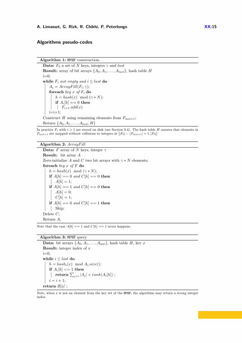
A. Limasset, G. Rizk, R. Chikhi, P. Peterlongo XX:15

Algorithms pseudo-codes

Algorithm 1: MPHF construction.Data: F0 a set of N keys, integers γ and lastResult: array of bit arrays A0, A1, . . . , Alast, hash table Hi=0;while Fi not empty and i ≤ last do

Ai = ArrayF ill(Fi, γ);foreach key x of Fi do

h = hash(x) mod (γ ∗N);if Ai[h] == 0 then

Fi+1.add(x)i=i+1;

Construct H using remaining elements from Flast+1;Return A0, A1, . . . , Alast, H

In practice Fi with i > 1 are stored on disk (see Section 3.4). The hash table H ensures that elements inFlast+1 are mapped without collisions to integers in [|F0| − |Flast+1|+ 1, |F0|]

Algorithm 2: ArrayF illData: F array of N keys, integer γResult: bit array AZero-initialize A and C two bit arrays with γ ∗N elements;foreach key x of F do

h = hash(x) mod (γ ∗N);if A[h] == 0 and C[h] == 0 then

A[h] = 1;if A[h] == 1 and C[h] == 0 then

A[h] = 0;C[h] = 1;

if A[h] == 0 and C[h] == 1 thenSkip;

Delete C;Return A;

Note that the case A[h] == 1 and C[h] == 1 never happens.

Algorithm 3: MPHF queryData: bit arrays A0, A1, . . . , Alast, hash table H, key xResult: integer index of xi=0;while i ≤ last do

h = hashi(x) mod Ai.size();if Ai[h] == 1 then

return∑j<i |Aj |+ rank(Ai[h]) ;

i = i+ 1;return H[x] ;

Note, when x is not an element from the key set of the MPHF, the algorithm may return a wrong integerindex.

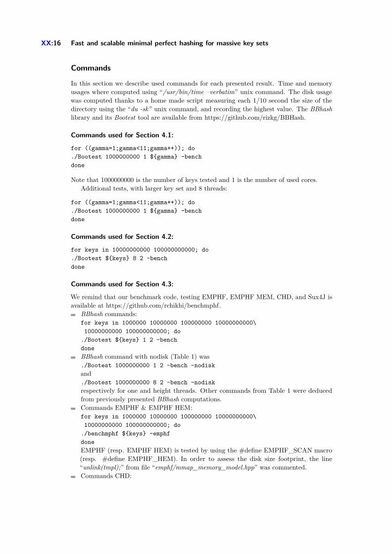
XX:16 Fast and scalable minimal perfect hashing for massive key sets

Commands

In this section we describe used commands for each presented result. Time and memoryusages where computed using “/usr/bin/time –verbatim” unix command. The disk usagewas computed thanks to a home made script measuring each 1/10 second the size of thedirectory using the “du -sk” unix command, and recording the highest value. The BBhashlibrary and its Bootest tool are available from https://github.com/rizkg/BBHash.

Commands used for Section 4.1:

for ((gamma=1;gamma<11;gamma++)); do./Bootest 1000000000 1 $gamma -benchdone

Note that 1000000000 is the number of keys tested and 1 is the number of used cores.Additional tests, with larger key set and 8 threads:

for ((gamma=1;gamma<11;gamma++)); do./Bootest 1000000000 1 $gamma -benchdone

Commands used for Section 4.2:

for keys in 10000000000 100000000000; do./Bootest $keys 8 2 -benchdone

Commands used for Section 4.3:

We remind that our benchmark code, testing EMPHF, EMPHF MEM, CHD, and Sux4J isavailable at https://github.com/rchikhi/benchmphf.

BBhash commands:for keys in 1000000 10000000 100000000 10000000000\10000000000 100000000000; do

./Bootest $keys 1 2 -benchdoneBBhash command with nodisk (Table 1) was./Bootest 1000000000 1 2 -bench -nodiskand./Bootest 1000000000 8 2 -bench -nodiskrespectively for one and height threads. Other commands from Table 1 were deducedfrom previously presented BBhash computations.Commands EMPHF & EMPHF HEM:for keys in 1000000 10000000 100000000 10000000000\10000000000 100000000000; do

./benchmphf $keys -emphfdoneEMPHF (resp. EMPHF HEM) is tested by using the #define EMPHF_SCAN macro(resp. #define EMPHF_HEM). In order to assess the disk size footprint, the line“unlink(tmpl);” from file “emphf/mmap_memory_model.hpp” was commented.Commands CHD:

A. Limasset, G. Rizk, R. Chikhi, P. Peterlongo XX:17

for keys in 1000000 10000000 100000000 10000000000\10000000000 100000000000; do

./benchmphf $keys -chddoneCommands Sux4J:for each size, the “Sux4J/slow/it/unimi/dsi/sux4j/mph/LargeLongCollection.java” wasmodified indicating the used size../run-sux4j-mphf.sh

Commands used for Section 4.4:

As explained Section 4.4, the keyString.txt file is composed of n-grams extracted fromthe Google Books Ngram dataset2, version 20120701../BootestFile keyStrings.txt 10 2

Commands used for Section 4.5:

BBhash command for indexing a trillion keys, with keys generated on the fly../Bootest 1000000000000 24 2 -onthefly

2 http://storage.googleapis.com/books/ngrams/books/datasetsv2.html

Chapter 3

The de Bruijn graph as a reference

81

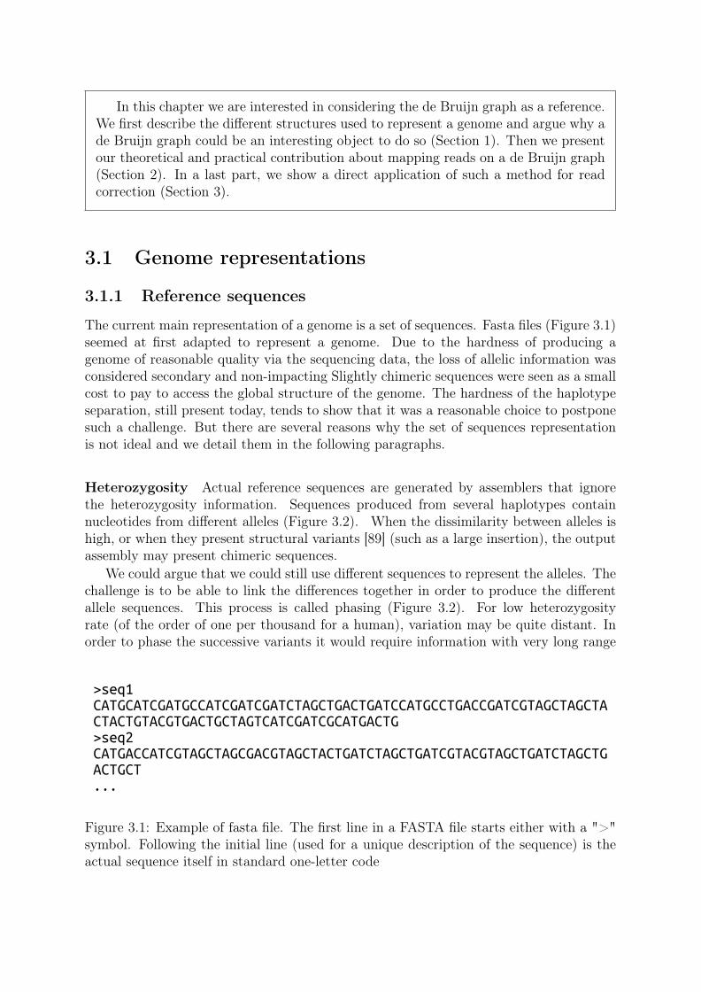
In this chapter we are interested in considering the de Bruijn graph as a reference.We first describe the different structures used to represent a genome and argue why ade Bruijn graph could be an interesting object to do so (Section 1). Then we presentour theoretical and practical contribution about mapping reads on a de Bruijn graph(Section 2). In a last part, we show a direct application of such a method for readcorrection (Section 3).

3.1 Genome representations

3.1.1 Reference sequences

The current main representation of a genome is a set of sequences. Fasta files (Figure 3.1)seemed at first adapted to represent a genome. Due to the hardness of producing agenome of reasonable quality via the sequencing data, the loss of allelic information wasconsidered secondary and non-impacting Slightly chimeric sequences were seen as a smallcost to pay to access the global structure of the genome. The hardness of the haplotypeseparation, still present today, tends to show that it was a reasonable choice to postponesuch a challenge. But there are several reasons why the set of sequences representationis not ideal and we detail them in the following paragraphs.

Heterozygosity Actual reference sequences are generated by assemblers that ignorethe heterozygosity information. Sequences produced from several haplotypes containnucleotides from different alleles (Figure 3.2). When the dissimilarity between alleles ishigh, or when they present structural variants [89] (such as a large insertion), the outputassembly may present chimeric sequences.

We could argue that we could still use different sequences to represent the alleles. Thechallenge is to be able to link the differences together in order to produce the differentallele sequences. This process is called phasing (Figure 3.2). For low heterozygosityrate (of the order of one per thousand for a human), variation may be quite distant. Inorder to phase the successive variants it would require information with very long range

>seq1CATGCATCGATGCCATCGATCGATCTAGCTGACTGATCCATGCCTGACCGATCGTAGCTAGCTACTACTGTACGTGACTGCTAGTCATCGATCGCATGACTG>seq2CATGACCATCGTAGCTAGCGACGTAGCTACTGATCTAGCTGATCGTACGTAGCTGATCTAGCTGACTGCT...

Figure 3.1: Example of fasta file. The first line in a FASTA file starts either with a ">"symbol. Following the initial line (used for a unique description of the sequence) is theactual sequence itself in standard one-letter code

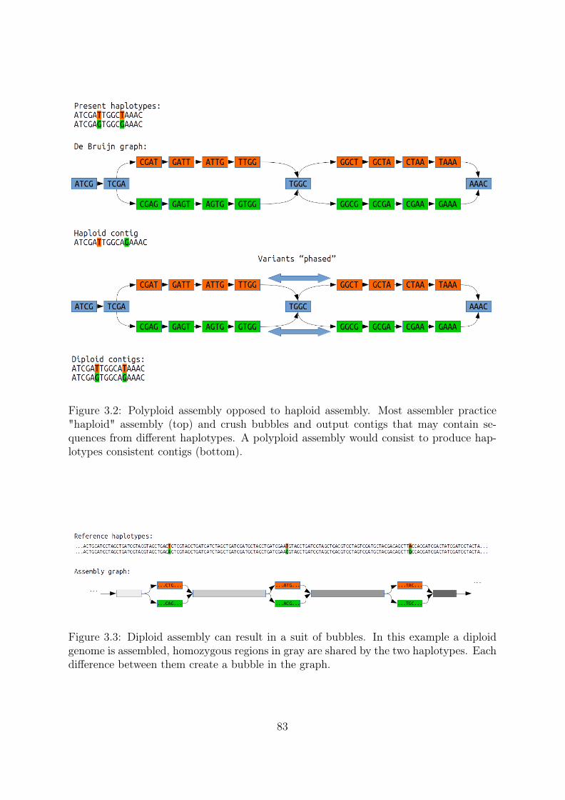
Figure 3.2: Polyploid assembly opposed to haploid assembly. Most assembler practice"haploid" assembly (top) and crush bubbles and output contigs that may contain se-quences from different haplotypes. A polyploid assembly would consist to produce hap-lotypes consistent contigs (bottom).

Figure 3.3: Diploid assembly can result in a suit of bubbles. In this example a diploidgenome is assembled, homozygous regions in gray are shared by the two haplotypes. Eachdifference between them create a bubble in the graph.

83

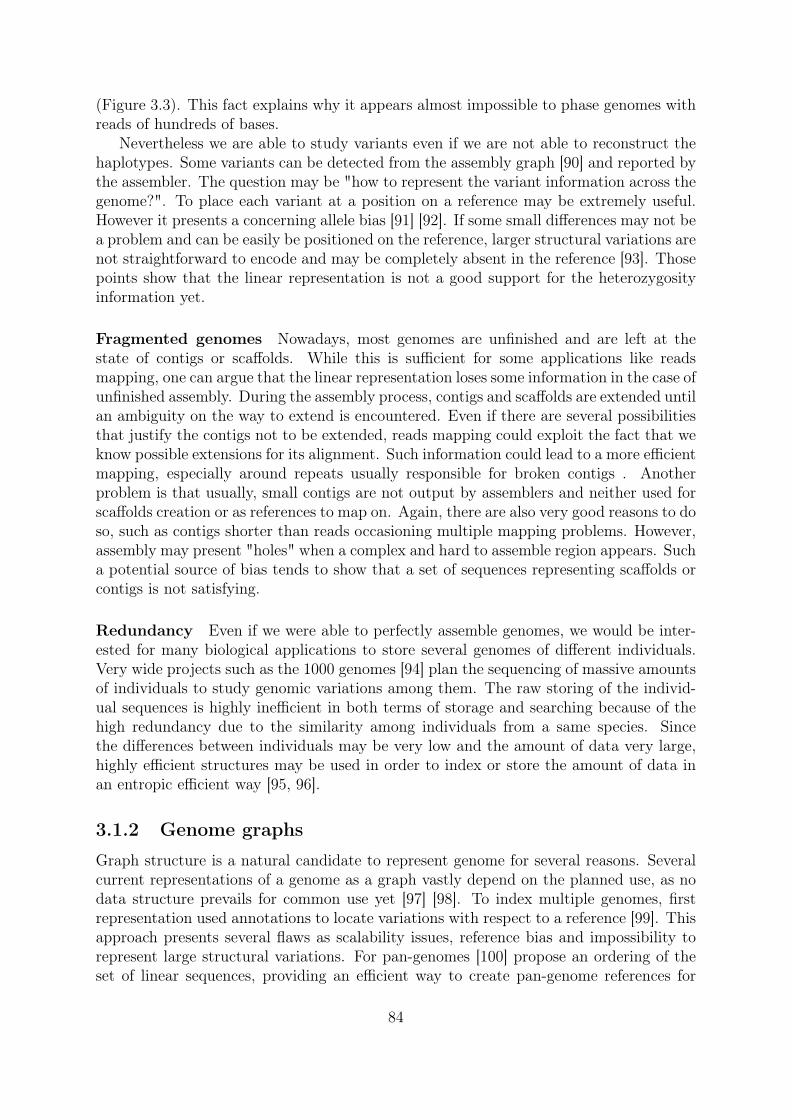
(Figure 3.3). This fact explains why it appears almost impossible to phase genomes withreads of hundreds of bases.

Nevertheless we are able to study variants even if we are not able to reconstruct thehaplotypes. Some variants can be detected from the assembly graph [90] and reported bythe assembler. The question may be "how to represent the variant information across thegenome?". To place each variant at a position on a reference may be extremely useful.However it presents a concerning allele bias [91] [92]. If some small differences may not bea problem and can be easily be positioned on the reference, larger structural variations arenot straightforward to encode and may be completely absent in the reference [93]. Thosepoints show that the linear representation is not a good support for the heterozygosityinformation yet.

Fragmented genomes Nowadays, most genomes are unfinished and are left at thestate of contigs or scaffolds. While this is sufficient for some applications like readsmapping, one can argue that the linear representation loses some information in the case ofunfinished assembly. During the assembly process, contigs and scaffolds are extended untilan ambiguity on the way to extend is encountered. Even if there are several possibilitiesthat justify the contigs not to be extended, reads mapping could exploit the fact that weknow possible extensions for its alignment. Such information could lead to a more efficientmapping, especially around repeats usually responsible for broken contigs . Anotherproblem is that usually, small contigs are not output by assemblers and neither used forscaffolds creation or as references to map on. Again, there are also very good reasons to doso, such as contigs shorter than reads occasioning multiple mapping problems. However,assembly may present "holes" when a complex and hard to assemble region appears. Sucha potential source of bias tends to show that a set of sequences representing scaffolds orcontigs is not satisfying.

Redundancy Even if we were able to perfectly assemble genomes, we would be inter-ested for many biological applications to store several genomes of different individuals.Very wide projects such as the 1000 genomes [94] plan the sequencing of massive amountsof individuals to study genomic variations among them. The raw storing of the individ-ual sequences is highly inefficient in both terms of storage and searching because of thehigh redundancy due to the similarity among individuals from a same species. Sincethe differences between individuals may be very low and the amount of data very large,highly efficient structures may be used in order to index or store the amount of data inan entropic efficient way [95, 96].

3.1.2 Genome graphs

Graph structure is a natural candidate to represent genome for several reasons. Severalcurrent representations of a genome as a graph vastly depend on the planned use, as nodata structure prevails for common use yet [97] [98]. To index multiple genomes, firstrepresentation used annotations to locate variations with respect to a reference [99]. Thisapproach presents several flaws as scalability issues, reference bias and impossibility torepresent large structural variations. For pan-genomes [100] propose an ordering of theset of linear sequences, providing an efficient way to create pan-genome references for

84

reads mapping. In order to represent the variations among haplotypes, the variationgraph has been introduced, where haplotypes are encoded as a set of walks through asequence graph. In order to perform queries on such heavy data structures, the Posi-tional BWT (PBWT) have been proposed [101] and improved in gPBWT [102] to betterrepresent the haplotypes added in the graph. Those structures are very similar to linearsequences since they are supposed to represent finished genomes. Even if these sequencesrepresent a real "map" of a genome with a coordinate system, this is still a hard taskto obtain such sequences. Several uses can benefit from a non fully positioned reference:quantification [103] [104], assembly, scaffolding and indexation of repeated sequences orfragmented references [105]. Assembly graphs are natural candidates for this task as theyare literally conceived to represent fragmented data. In the following, we present methodsand applications relying on assembly graphs as references. Even if such approaches couldbe based on any assembly graph, the following will focus on the use of a de Bruijn graph.

3.1.3 De Bruijn graphs as references

This part concentrates on the interest of the de Bruijn graph to represent genomes. Wewill present the following arguments:

• Easiness to construct from sequencing data• Efficient representation of repeated data• Represents variants and complex regions

Construct a reference de Bruijn graph To use a de Bruijn graph as a reference, ithas to contain the whole genomic information with almost no sequencing error. Buildinga de Bruijn graph from a reference genome is easy but has a limited interest since thetransformation in a de Bruijn graph is lossy as sequences respective positions may belost. To represent fragmented references such as contigs, we can argue that a graph maycontain more information than the contigs set itself. The real challenge is to produce agood reference from raw sequencing data. We present here different strategies to producea good reference de Bruijn graph and evaluate them. In order to do this, we simulatedreads from a known reference and compare the set of kmers from the reference and fromthe constructed graph. Two kinds of errors may appear:

• Some kmers are in the graph but not in the reference. They are erroneous kmers,also called "false positives"

• Some kmers are in the reference but not in the graph. They are missed kmers alsocalled "false negatives"

As described in the introduction, the main technique to get rid of erroneous kmers is toremove low abundance ones. Three zones can be observed in a kmer spectrum:

• A very high peak of low abundance kmers• A flat zone• A bell containing high abundance kmersThe essential idea is that genomic kmers will mostly be present in the third zone while

most erroneous kmer will be present in the first zone. By applying a coverage cutoff weonly keep the right part of the spectrum curves. The question is how to decide the cutoffparameter. Techniques exist to find the end of the first peak by trying to fit modelson the kmer spectrum curve such as kmerGenie [34]. A deeper sequencing makes easier

85

0

100000

200000

300000

400000

500000

600000

700000

800000

900000

1x106

10 20 30 40 50 60 70 80

"reads10010031""reads1005031""reads1003031"

0

20000

40000

60000

80000

100000

120000

140000

20 40 60 80 100 120

"realSequencing"

Figure 3.4: Spectrum of 31mer from simulated reads from de Bruijn graph reference(Left). Reads were of length 100 and with coverages of 30 (blue), 50 (green) and 100(purple) respectively. We observe that higher coverage results in a larger bell zone moredistant from the error peak. It is thus easier to separate the erroneous kmers from otherswith a high coverage. On the right a kmer spectrum of a real sequencing with k = 31 anda coverage around 100X from E. coli. We can see that unlike spectrum from simulateddataset, the "hole" between the peak and the bell do not reach a value of zero sincesimulated dataset may not represent all aspect of NGS sequences distribution.

the determination of such a cutoff, as can be seen in Figure 3.4 at left. We note thaton simulated datasets, the determination of the cutoff can seem easy because the flatzone has no element. In practice on real dataset (in Figure 3.4 at right), the situationis not this simple since a notable number of element are present with the unexpectedmedium abundances. The value of k also has a high influence on the kmer spectrum. InFigure 3.5 we observe that the larger the k, the lesser the genomic kmers are covered andthe closer to zone 1 and 3. If k is too high compared to the read length it may be difficultto separate the genomic and erroneous kmers since some genomic kmers will be presentwith a very low abundance. This is mainly due to the fact that when k comes close tothe read length, very few kmers are produced by each read. To reduce this problem withlarge kmers, a step of read correction highly reduces the amount of errors present in thereads and allow genomic kmers to be more covered and therefore to "move" the curve tothe right as shown in Figure 3.5.

Another way to remove sequencing errors it to remove "tips" or "short dead ends"from the graph. If k ≥ ReadSize/2, an isolated sequencing error will not form a bubblebut a tip in the graph. As we may be afraid of losing genomic kmers with the soliditycutoff, we advocate the use of low thresholds and therefore apply a tip removal step onthe graph. We now evaluate in Tables 3.1 and 3.2 the number of false positives and falsenegatives in the produced graph based on different strategies using the following methods:

• Kmer filtering with a given threshold• Using raw reads or reads corrected with the Bloocoo corrector [106]• Tipping of the graph, removing tips shorter than the read lengthWe can see that the combination of kmer filtering, read correction and tipping can

result in almost perfect reference graphs. Such tasks are the basic steps of assembly. Most

86

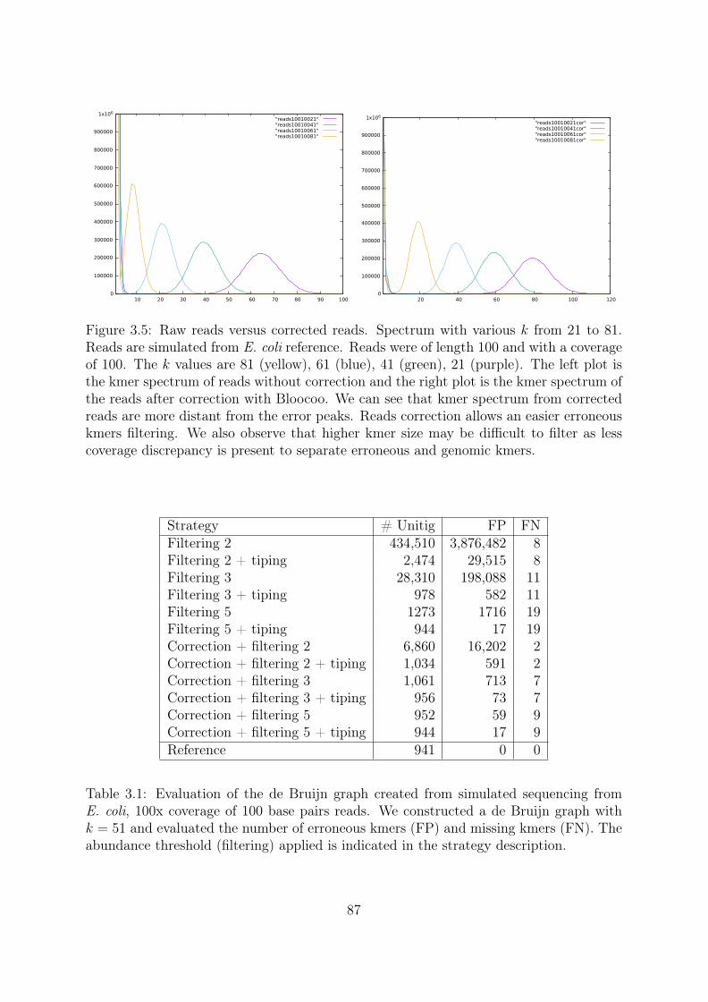
0

100000

200000

300000

400000

500000

600000

700000

800000

900000

1x106

10 20 30 40 50 60 70 80 90 100

"reads10010021""reads10010041""reads10010061""reads10010081"

0

100000

200000

300000

400000

500000

600000

700000

800000

900000

1x106

20 40 60 80 100 120

"reads10010021cor""reads10010041cor""reads10010061cor""reads10010081cor"

Figure 3.5: Raw reads versus corrected reads. Spectrum with various k from 21 to 81.Reads are simulated from E. coli reference. Reads were of length 100 and with a coverageof 100. The k values are 81 (yellow), 61 (blue), 41 (green), 21 (purple). The left plot isthe kmer spectrum of reads without correction and the right plot is the kmer spectrum ofthe reads after correction with Bloocoo. We can see that kmer spectrum from correctedreads are more distant from the error peaks. Reads correction allows an easier erroneouskmers filtering. We also observe that higher kmer size may be difficult to filter as lesscoverage discrepancy is present to separate erroneous and genomic kmers.

Strategy # Unitig FP FNFiltering 2 434,510 3,876,482 8Filtering 2 + tiping 2,474 29,515 8Filtering 3 28,310 198,088 11Filtering 3 + tiping 978 582 11Filtering 5 1273 1716 19Filtering 5 + tiping 944 17 19Correction + filtering 2 6,860 16,202 2Correction + filtering 2 + tiping 1,034 591 2Correction + filtering 3 1,061 713 7Correction + filtering 3 + tiping 956 73 7Correction + filtering 5 952 59 9Correction + filtering 5 + tiping 944 17 9Reference 941 0 0

Table 3.1: Evaluation of the de Bruijn graph created from simulated sequencing fromE. coli, 100x coverage of 100 base pairs reads. We constructed a de Bruijn graph withk = 51 and evaluated the number of erroneous kmers (FP) and missing kmers (FN). Theabundance threshold (filtering) applied is indicated in the strategy description.

87

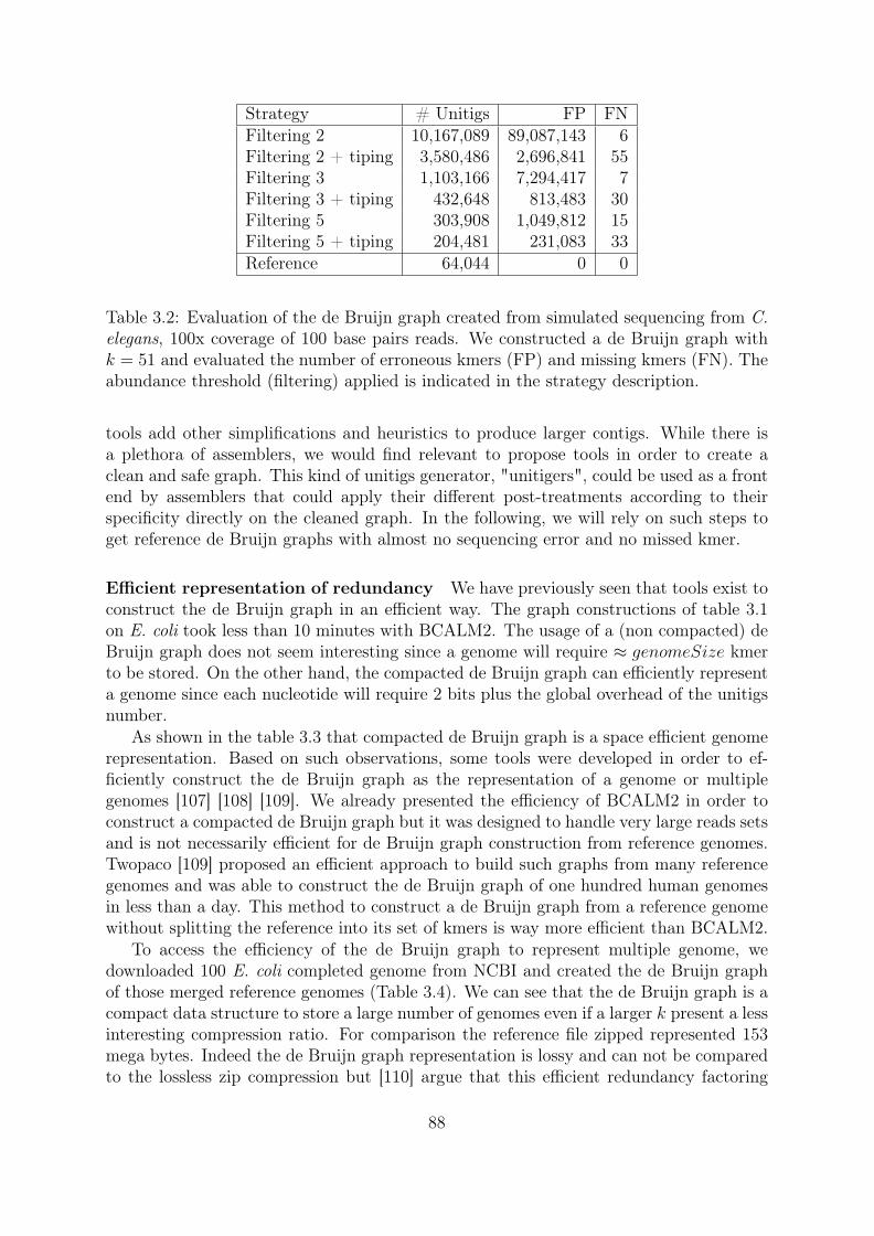
Strategy # Unitigs FP FNFiltering 2 10,167,089 89,087,143 6Filtering 2 + tiping 3,580,486 2,696,841 55Filtering 3 1,103,166 7,294,417 7Filtering 3 + tiping 432,648 813,483 30Filtering 5 303,908 1,049,812 15Filtering 5 + tiping 204,481 231,083 33Reference 64,044 0 0

Table 3.2: Evaluation of the de Bruijn graph created from simulated sequencing from C.elegans, 100x coverage of 100 base pairs reads. We constructed a de Bruijn graph withk = 51 and evaluated the number of erroneous kmers (FP) and missing kmers (FN). Theabundance threshold (filtering) applied is indicated in the strategy description.

tools add other simplifications and heuristics to produce larger contigs. While there isa plethora of assemblers, we would find relevant to propose tools in order to create aclean and safe graph. This kind of unitigs generator, "unitigers", could be used as a frontend by assemblers that could apply their different post-treatments according to theirspecificity directly on the cleaned graph. In the following, we will rely on such steps toget reference de Bruijn graphs with almost no sequencing error and no missed kmer.

Efficient representation of redundancy We have previously seen that tools exist toconstruct the de Bruijn graph in an efficient way. The graph constructions of table 3.1on E. coli took less than 10 minutes with BCALM2. The usage of a (non compacted) deBruijn graph does not seem interesting since a genome will require ≈ genomeSize kmerto be stored. On the other hand, the compacted de Bruijn graph can efficiently representa genome since each nucleotide will require 2 bits plus the global overhead of the unitigsnumber.

As shown in the table 3.3 that compacted de Bruijn graph is a space efficient genomerepresentation. Based on such observations, some tools were developed in order to ef-ficiently construct the de Bruijn graph as the representation of a genome or multiplegenomes [107] [108] [109]. We already presented the efficiency of BCALM2 in order toconstruct a compacted de Bruijn graph but it was designed to handle very large reads setsand is not necessarily efficient for de Bruijn graph construction from reference genomes.Twopaco [109] proposed an efficient approach to build such graphs from many referencegenomes and was able to construct the de Bruijn graph of one hundred human genomesin less than a day. This method to construct a de Bruijn graph from a reference genomewithout splitting the reference into its set of kmers is way more efficient than BCALM2.

To access the efficiency of the de Bruijn graph to represent multiple genome, wedownloaded 100 E. coli completed genome from NCBI and created the de Bruijn graphof those merged reference genomes (Table 3.4). We can see that the de Bruijn graph is acompact data structure to store a large number of genomes even if a larger k present a lessinteresting compression ratio. For comparison the reference file zipped represented 153mega bytes. Indeed the de Bruijn graph representation is lossy and can not be comparedto the lossless zip compression but [110] argue that this efficient redundancy factoring

88

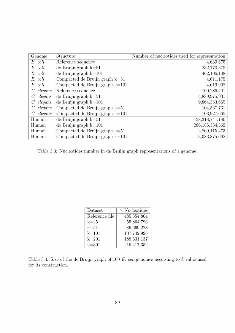
Genome Structure Number of nucleotides used for representationE. coli Reference sequence 4,639,675E. coli de Bruijn graph k=51 232,770,375E. coli de Bruijn graph k=101 462,106,108E. coli Compacted de Bruijn graph k=51 4,611,175E. coli Compacted de Bruijn graph k=101 4,619,908C. elegans Reference sequence 100,286,401C. elegans de Bruijn graph k=51 4,889,975,931C. elegans de Bruijn graph k=101 9,864,383,665C. elegans Compacted de Bruijn graph k=51 104,537,731C. elegans Compacted de Bruijn graph k=101 103,927,665Human de Bruijn graph k=51 138,318,741,180Human de Bruijn graph k=101 286,185,334,362Human Compacted de Bruijn graph k=51 2,809,115,473Human Compacted de Bruijn graph k=101 3,083,875,662

Table 3.3: Nucleotides number in de Bruijn graph representations of a genome.

Dataset # NucleotidesReference file 485,354,804k=25 55,864,796k=51 89,669,228k=101 137,742,996k=201 188,631,137k=301 215,417,352

Table 3.4: Size of the de Bruijn graph of 100 E. coli genomes according to k value usedfor its construction.

89

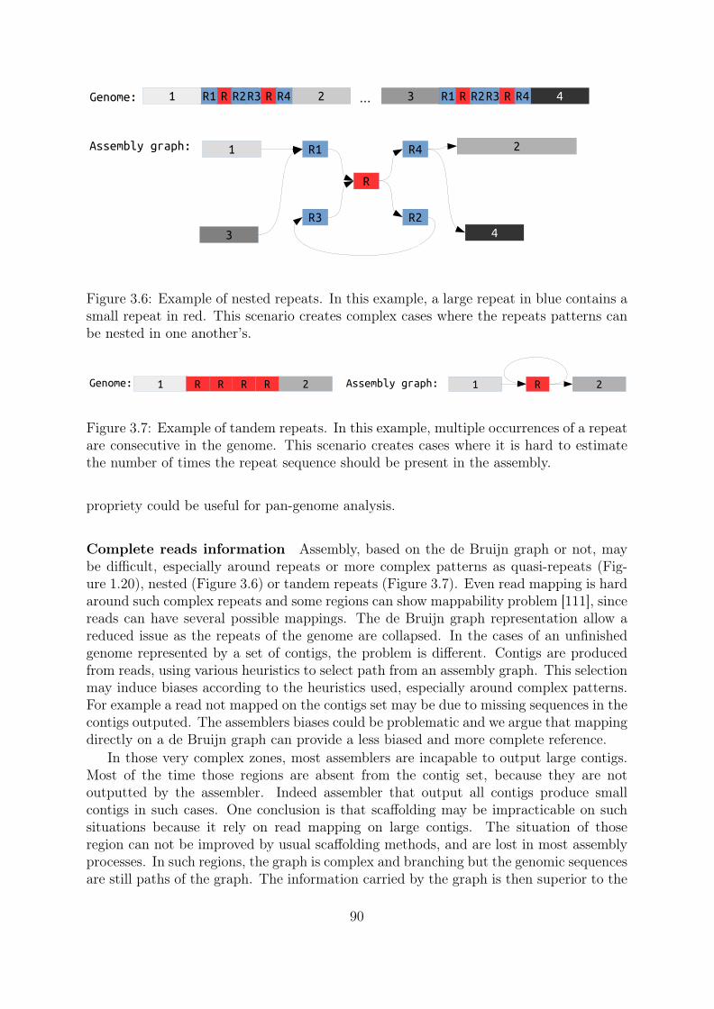
1 2

3 4

R1 R4Assembly graph:

Genome: 1 2RR1 R2R3 R R4 3 4RR1 R2R3 R R4

R

R3 R2

...

Figure 3.6: Example of nested repeats. In this example, a large repeat in blue contains asmall repeat in red. This scenario creates complex cases where the repeats patterns canbe nested in one another’s.

1Assembly graph:Genome: 1 2 RR R R R 2

Figure 3.7: Example of tandem repeats. In this example, multiple occurrences of a repeatare consecutive in the genome. This scenario creates cases where it is hard to estimatethe number of times the repeat sequence should be present in the assembly.

propriety could be useful for pan-genome analysis.

Complete reads information Assembly, based on the de Bruijn graph or not, maybe difficult, especially around repeats or more complex patterns as quasi-repeats (Fig-ure 1.20), nested (Figure 3.6) or tandem repeats (Figure 3.7). Even read mapping is hardaround such complex repeats and some regions can show mappability problem [111], sincereads can have several possible mappings. The de Bruijn graph representation allow areduced issue as the repeats of the genome are collapsed. In the cases of an unfinishedgenome represented by a set of contigs, the problem is different. Contigs are producedfrom reads, using various heuristics to select path from an assembly graph. This selectionmay induce biases according to the heuristics used, especially around complex patterns.For example a read not mapped on the contigs set may be due to missing sequences in thecontigs outputed. The assemblers biases could be problematic and we argue that mappingdirectly on a de Bruijn graph can provide a less biased and more complete reference.

In those very complex zones, most assemblers are incapable to output large contigs.Most of the time those regions are absent from the contig set, because they are notoutputted by the assembler. Indeed assembler that output all contigs produce smallcontigs in such cases. One conclusion is that scaffolding may be impracticable on suchsituations because it rely on read mapping on large contigs. The situation of thoseregion can not be improved by usual scaffolding methods, and are lost in most assemblyprocesses. In such regions, the graph is complex and branching but the genomic sequencesare still paths of the graph. The information carried by the graph is then superior to the

90

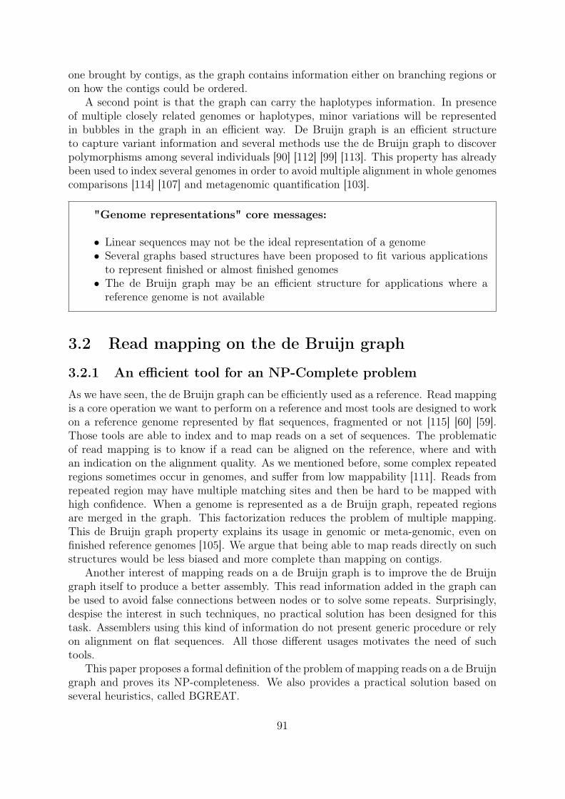
one brought by contigs, as the graph contains information either on branching regions oron how the contigs could be ordered.

A second point is that the graph can carry the haplotypes information. In presenceof multiple closely related genomes or haplotypes, minor variations will be representedin bubbles in the graph in an efficient way. De Bruijn graph is an efficient structureto capture variant information and several methods use the de Bruijn graph to discoverpolymorphisms among several individuals [90] [112] [99] [113]. This property has alreadybeen used to index several genomes in order to avoid multiple alignment in whole genomescomparisons [114] [107] and metagenomic quantification [103].

"Genome representations" core messages:

• Linear sequences may not be the ideal representation of a genome• Several graphs based structures have been proposed to fit various applications

to represent finished or almost finished genomes• The de Bruijn graph may be an efficient structure for applications where a

reference genome is not available

3.2 Read mapping on the de Bruijn graph

3.2.1 An efficient tool for an NP-Complete problem

As we have seen, the de Bruijn graph can be efficiently used as a reference. Read mappingis a core operation we want to perform on a reference and most tools are designed to workon a reference genome represented by flat sequences, fragmented or not [115] [60] [59].Those tools are able to index and to map reads on a set of sequences. The problematicof read mapping is to know if a read can be aligned on the reference, where and withan indication on the alignment quality. As we mentioned before, some complex repeatedregions sometimes occur in genomes, and suffer from low mappability [111]. Reads fromrepeated region may have multiple matching sites and then be hard to be mapped withhigh confidence. When a genome is represented as a de Bruijn graph, repeated regionsare merged in the graph. This factorization reduces the problem of multiple mapping.This de Bruijn graph property explains its usage in genomic or meta-genomic, even onfinished reference genomes [105]. We argue that being able to map reads directly on suchstructures would be less biased and more complete than mapping on contigs.

Another interest of mapping reads on a de Bruijn graph is to improve the de Bruijngraph itself to produce a better assembly. This read information added in the graph canbe used to avoid false connections between nodes or to solve some repeats. Surprisingly,despise the interest in such techniques, no practical solution has been designed for thistask. Assemblers using this kind of information do not present generic procedure or relyon alignment on flat sequences. All those different usages motivates the need of suchtools.

This paper proposes a formal definition of the problem of mapping reads on a de Bruijngraph and proves its NP-completeness. We also provides a practical solution based onseveral heuristics, called BGREAT.

91

Technical results are described in the paper "Read mapping on de Bruijngraphs" [116] included at the end of the chapter.

BGREAT is based on simple heuristics in order to be fast and scalable. It followsthe seed and extend paradigm by indexing the k − 1 suffix and prefix of the unitigs asanchors. Once an anchor is found on a read, the rest of the read sequence is mapped tothe graph unitigs. By indexing the prefix and suffix and associating them the indices ofthe unitigs sharing them, BGREAT is able to navigate through the graph unitigs as itwas presented in the last chapter. Some unitigs may not contain any anchor, for exampleif they map entirely on large unitigs. But in such cases those reads can be mapped witha regular mapping tool. Another essential heuristic of BGREAT is the greediness of itsmapping process. When several paths can be used, the path with the minimal numberof mismatches is picked. The use of those greedy heuristics allows very fast mapping ofreads even on a large de Bruijn graph. BGREAT is able to map a human dataset of 3billion reads on a de Bruijn graph created from it, in less than 5 hours using 20 cores and10GB. Another interesting conclusion is that we are able to map more reads on the deBruijn graph than on a set of contigs. An experiment on a human dataset showed thatonly 63% of the reads were mapped on the contig set where 85% were mapped on the deBruijn graph using the graph alignment method.

3.2.2 Mapping refinements

The amount of potential applications of read alignment on de Bruijn graph leads us tothe conception of several improvements of the BGREAT tool. We propose an advancedversion called BGREAT2 (unpublished) with following improvements that we will detail:

• Improved anchor system• Indexing based on a MPHF• Optimal mapping and multi-mapping management

In order to improve the performance of our anchoring scheme, we no longer use thek−1mer at the extremities of the unitigs. We index kmers from the unitigs and associateto each kmer its position in the unitigs. This modification allows two significant changes.

First, the size of the anchor can be chosen. Therefore a smaller k than the one selectedto construct the graph can be used. The order of the de Bruijn graph may be quite large,thus a k − 1mer would be a bad anchor in terms of sensibility. This way, a high ordergraph can be used without presenting a change in the anchoring scheme. Indexing allkmers of the graph can be costly, for a human graph indexing all kmers can use up to 200GB. A parameter can be defined in order to reduce the memory usage of BGREAT2 thatregulates which fraction of the kmers are indexed. We can show that even by indexingonly a fraction of the kmers (one out of 10 by default), the mapping performances ofBGREAT2 are not highly impacted. Indexing 1 out of 10 anchors in each unitig, withat least one anchor indexed by unitigs allowed BGREAT2 to reduce its memory usagefrom 6,898 MB to 928 MB to index a C. elegans reference graph. The indexing timealso dropped from 61 to 10 seconds while the ratio of mapped reads went from 99.6% to99.3%. The mapping time was also impacted, but in a less impressive way and improvedfrom 11k to 15k reads by second on a single thread.

92

The second interest of the new indexing scheme is that BGREAT2 is self containedand do not need a mapping tool like Bowtie. Since kmers are indexed along the wholelength of the unitigs, reads mapping inside a unitig can be anchored and mapped. Inorder to index kmers and the de Bruijn graph overlaps, BGREAT2 no longer uses adynamic hash table but the BBhash MPHF. This choice allows a highly reduced memoryusage and a faster access to the unitigs compared to previously used dynamic hashing.

We also improved the mapping rules. The algorithm tries to find a perfect mapping(without error), then a mapping with one error and so on until the maximal error numberallowed. This way, the obtained mapping is guaranteed to contain a minimal number ofmismatch. Several multiple mapping strategies are also proposed: output all equivalentmapping, output one mapping, or none. Albeit some optimizations and features have stillto be added, those improvements allow BGREAT2 to be more than a proof of concept.We will present in the following sections several uses of this tool.

"Read mapping on the de Bruijn graph" core messages:

• Mapping reads on a de Bruijn graph is a hard problem• With appropriate heuristics we can propose a satisfying and efficient mapping• Mapping on the de Bruijn graph may allow more mapping hits than mapping

on contigs

3.3 De novo, reference guided, read correction

We have shown previously that an almost errorless de Bruijn graph could be constructed.We therefore propose a new method of correction for short reads by aligning them ona reference represented by a de Bruijn graph constructed from the reads themselves.Correction methods based on alignment on a reference genome would have the two sameessential drawbacks than reference guided assembly:

• Need for a reference• Correction may be biased by the reference used

Here we propose to construct the reference directly from the reads to be corrected inorder to avoid biases. We argue that we do not need to produce a good assembly in orderto obtain a reference good enough to correct the reads. The idea of such a technique canbe summarized in the following steps:

• Graph construction• Graph cleaning• Read mapping on the graph

3.3.1 Limits of kmer spectrum

Most state of the art correctors are based on kmer spectrum techniques. Other techniquesbased on suffix array or on multiple alignment, are presented in [117]. Those techniquesare less used because they rely on memory expensive data structures and do not scalewell on large genomes and datasets. Kmer spectrum correction was proposed when NGS

93

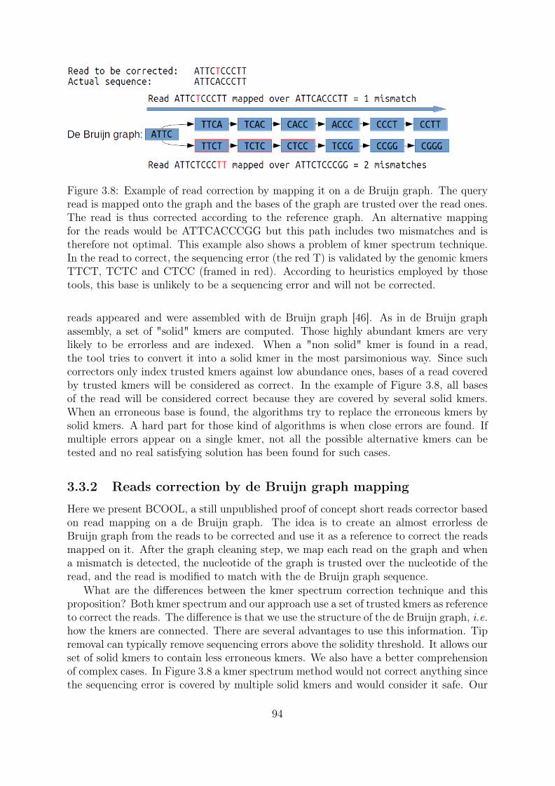
Figure 3.8: Example of read correction by mapping it on a de Bruijn graph. The queryread is mapped onto the graph and the bases of the graph are trusted over the read ones.The read is thus corrected according to the reference graph. An alternative mappingfor the reads would be ATTCACCCGG but this path includes two mismatches and istherefore not optimal. This example also shows a problem of kmer spectrum technique.In the read to correct, the sequencing error (the red T) is validated by the genomic kmersTTCT, TCTC and CTCC (framed in red). According to heuristics employed by thosetools, this base is unlikely to be a sequencing error and will not be corrected.

reads appeared and were assembled with de Bruijn graph [46]. As in de Bruijn graphassembly, a set of "solid" kmers are computed. Those highly abundant kmers are verylikely to be errorless and are indexed. When a "non solid" kmer is found in a read,the tool tries to convert it into a solid kmer in the most parsimonious way. Since suchcorrectors only index trusted kmers against low abundance ones, bases of a read coveredby trusted kmers will be considered as correct. In the example of Figure 3.8, all basesof the read will be considered correct because they are covered by several solid kmers.When an erroneous base is found, the algorithms try to replace the erroneous kmers bysolid kmers. A hard part for those kind of algorithms is when close errors are found. Ifmultiple errors appear on a single kmer, not all the possible alternative kmers can betested and no real satisfying solution has been found for such cases.

3.3.2 Reads correction by de Bruijn graph mapping

Here we present BCOOL, a still unpublished proof of concept short reads corrector basedon read mapping on a de Bruijn graph. The idea is to create an almost errorless deBruijn graph from the reads to be corrected and use it as a reference to correct the readsmapped on it. After the graph cleaning step, we map each read on the graph and whena mismatch is detected, the nucleotide of the graph is trusted over the nucleotide of theread, and the read is modified to match with the de Bruijn graph sequence.

What are the differences between the kmer spectrum correction technique and thisproposition? Both kmer spectrum and our approach use a set of trusted kmers as referenceto correct the reads. The difference is that we use the structure of the de Bruijn graph, i.e.how the kmers are connected. There are several advantages to use this information. Tipremoval can typically remove sequencing errors above the solidity threshold. It allows ourset of solid kmers to contain less erroneous kmers. We also have a better comprehensionof complex cases. In Figure 3.8 a kmer spectrum method would not correct anything sincethe sequencing error is covered by multiple solid kmers and would consider it safe. Our

94

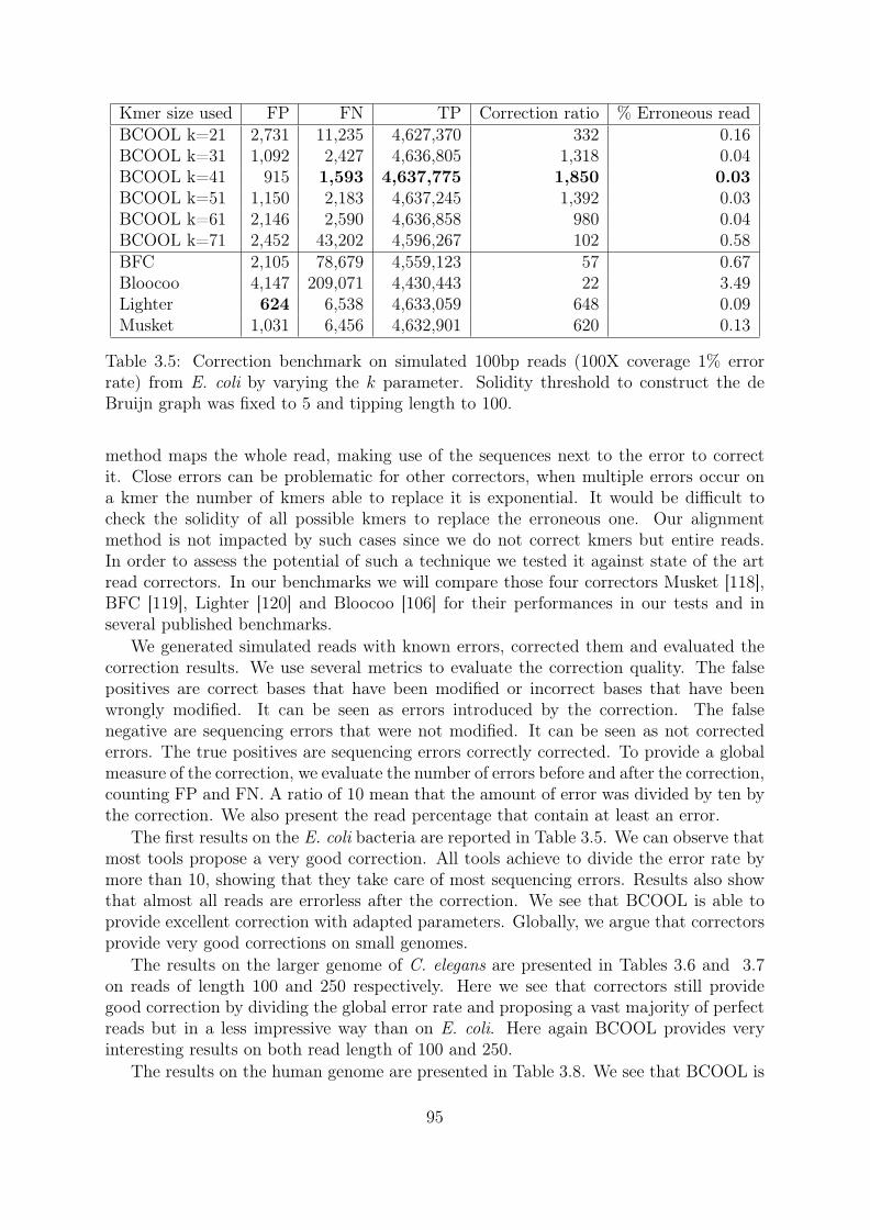
Kmer size used FP FN TP Correction ratio % Erroneous readBCOOL k=21 2,731 11,235 4,627,370 332 0.16BCOOL k=31 1,092 2,427 4,636,805 1,318 0.04BCOOL k=41 915 1,593 4,637,775 1,850 0.03BCOOL k=51 1,150 2,183 4,637,245 1,392 0.03BCOOL k=61 2,146 2,590 4,636,858 980 0.04BCOOL k=71 2,452 43,202 4,596,267 102 0.58BFC 2,105 78,679 4,559,123 57 0.67Bloocoo 4,147 209,071 4,430,443 22 3.49Lighter 624 6,538 4,633,059 648 0.09Musket 1,031 6,456 4,632,901 620 0.13

Table 3.5: Correction benchmark on simulated 100bp reads (100X coverage 1% errorrate) from E. coli by varying the k parameter. Solidity threshold to construct the deBruijn graph was fixed to 5 and tipping length to 100.

method maps the whole read, making use of the sequences next to the error to correctit. Close errors can be problematic for other correctors, when multiple errors occur ona kmer the number of kmers able to replace it is exponential. It would be difficult tocheck the solidity of all possible kmers to replace the erroneous one. Our alignmentmethod is not impacted by such cases since we do not correct kmers but entire reads.In order to assess the potential of such a technique we tested it against state of the artread correctors. In our benchmarks we will compare those four correctors Musket [118],BFC [119], Lighter [120] and Bloocoo [106] for their performances in our tests and inseveral published benchmarks.

We generated simulated reads with known errors, corrected them and evaluated thecorrection results. We use several metrics to evaluate the correction quality. The falsepositives are correct bases that have been modified or incorrect bases that have beenwrongly modified. It can be seen as errors introduced by the correction. The falsenegative are sequencing errors that were not modified. It can be seen as not correctederrors. The true positives are sequencing errors correctly corrected. To provide a globalmeasure of the correction, we evaluate the number of errors before and after the correction,counting FP and FN. A ratio of 10 mean that the amount of error was divided by ten bythe correction. We also present the read percentage that contain at least an error.

The first results on the E. coli bacteria are reported in Table 3.5. We can observe thatmost tools propose a very good correction. All tools achieve to divide the error rate bymore than 10, showing that they take care of most sequencing errors. Results also showthat almost all reads are errorless after the correction. We see that BCOOL is able toprovide excellent correction with adapted parameters. Globally, we argue that correctorsprovide very good corrections on small genomes.

The results on the larger genome of C. elegans are presented in Tables 3.6 and 3.7on reads of length 100 and 250 respectively. Here we see that correctors still providegood correction by dividing the global error rate and proposing a vast majority of perfectreads but in a less impressive way than on E. coli. Here again BCOOL provides veryinteresting results on both read length of 100 and 250.

The results on the human genome are presented in Table 3.8. We see that BCOOL is

95

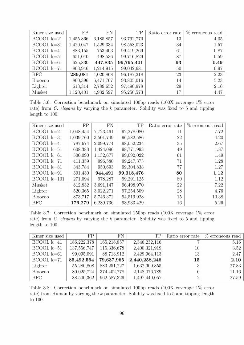
Kmer size used FP FN TP Ratio error rate % erroneous readBCOOL k=21 1,455,866 6,185,857 93,792,770 13 4.05BCOOL k=31 1,420,047 1,529,334 98,558,023 34 1.57BCOOL k=41 883,155 753,403 99,419,269 61 0.87BCOOL k=51 651,040 498,536 99,716,829 87 0.59BCOOL k=61 625,830 447,835 99,795,401 93 0.49BCOOL k=71 803,946 1,214,915 99,042,681 50 0.97BFC 289,081 4,020,868 96,187,218 23 2.23Bloocoo 800,396 6,471,767 93,805,016 14 5.23Lighter 613,314 2,789,652 97,490,978 29 2.16Musket 1,120,401 4,932,597 95,250,573 17 4.47

Table 3.6: Correction benchmark on simulated 100bp reads (100X coverage 1% errorrate) from C. elegans by varying the k parameter. Solidity was fixed to 5 and tippinglength to 100.

Kmer size used FP FN TP Ratio error rate % erroneous readBCOOL k=21 1,048,454 7,723,461 92,278,080 11 7.72BCOOL k=31 1,039,760 3,501,749 96,582,586 22 4.20BCOOL k=41 787,674 2,099,774 98,052,234 35 2.67BCOOL k=51 608,383 1,424,096 98,771,993 49 1.87BCOOL k=61 500,090 1,132,677 99,092,022 61 1.49BCOOL k=71 411,359 996,580 99,247,373 71 1.28BCOOL k=81 343,784 950,693 99,304,838 77 1.27BCOOL k=91 301,430 944,491 99,318,476 80 1.12BCOOL k=101 271,094 978,287 99,291,125 80 1.12Musket 812,832 3,691,147 96,498,970 22 7.22Lighter 520,365 3,022,271 97,254,509 28 4.76Bloocoo 873,717 5,746,372 94,519,928 15 10.38BFC 176,279 6,289,736 93,933,429 16 5.26

Table 3.7: Correction benchmark on simulated 250bp reads (100X coverage 1% errorrate) from C. elegans by varying the k parameter. Solidity was fixed to 5 and tippinglength to 100.

Kmer size used FP FN TP Ratio error rate % erroneous readBCOOL k=41 186,222,378 165,218,857 2,346,232,116 7 5.16BCOOL k=51 137,556,747 115,336,678 2,400,321,919 10 3.52BCOOL k=61 99,095,091 88,713,912 2,429,964,113 13 2.47BCOOL k=71 85,492,564 79,637,965 2,440,258,246 15 2.10Lighter 55,280,808 883,251,227 1,632,909,855 3 27.83Bloocoo 80,025,724 374,402,778 2,148,076,789 6 11.16BFC 88,500,362 962,587,329 1,497,440,057 2 27.59

Table 3.8: Correction benchmark on simulated 100bp reads (100X coverage 1% errorrate) from Human by varying the k parameter. Solidity was fixed to 5 and tipping lengthto 100.

96

able to scale up to large genome and dataset as the human one. Musket needs more than250 GB and was not able to correct this dataset on our testing server. Once again wesee that correctors provide less impressive results on larger genomes. Those results showthat BCOOL provides good read correction even compared to state of the art correctors.

Our proposed workflow can be summarized into:• Best kmer size and abundance threshold selection (Not done yet)• Graph construction• Graph cleaning• Reads mapping on the graph

We see that BCOOL can lead to significant improvements to reads correction and canscale up to very large genomes. But the approach is still parameter dependent. A high kvalue allows the construction of a high quality graph but can create holes. Furthermorewe only evaluated BCOOL on very high coverage dataset and the solidity threshold isalso an impactful parameter that can be non trivial to set for users not aware of de Bruijngraph properties. An automated evaluation of the kmer spectrum could infer the goodvalues to set, in order to get rid of most sequencing error without losing genomic kmers.In order to infer those parameters we could, as in Kmergenie, use a fast kmer spectrumestimator such as ntCard [121]. Many improvements and tuning have yet to be performedto propose an efficient and robust corrector but preliminary results are encouraging.

"De novo, reference guided, read correction" core messages:

• Mapping reads on a reference de Bruijn graph enables to correct them• All operations of such a method are scalable

97

Limasset et al. BMC Bioinformatics (2016) 17:237 DOI 10.1186/s12859-016-1103-9

RESEARCH ARTICLE Open Access

Read mapping on de Bruijn graphsAntoine Limasset1*, Bastien Cazaux2,3, Eric Rivals2,3 and Pierre Peterlongo1

Abstract

Background: Next Generation Sequencing (NGS) has dramatically enhanced our ability to sequence genomes, butnot to assemble them. In practice, many published genome sequences remain in the state of a large set of contigs.Each contig describes the sequence found along some path of the assembly graph, however, the set of contigs doesnot record all the sequence information contained in that graph. Although many subsequent analyses can beperformed with the set of contigs, one may ask whether mapping reads on the contigs is as informative as mappingthem on the paths of the assembly graph. Currently, one lacks practical tools to perform mapping on such graphs.

Results: Here, we propose a formal definition of mapping on a de Bruijn graph, analyse the problem complexitywhich turns out to be NP-complete, and provide a practical solution. We propose a pipeline called GGMAP (GreedyGraph MAPping). Its novelty is a procedure to map reads on branching paths of the graph, for which we designed aheuristic algorithm called BGREAT (de Bruijn Graph REAd mapping Tool). For the sake of efficiency, BGREAT rewrites aread sequence as a succession of unitigs sequences. GGMAP can map millions of reads per CPU hour on a de Bruijngraph built from a large set of human genomic reads. Surprisingly, results show that up to 22% more reads can bemapped on the graph but not on the contig set.

Conclusions: Although mapping reads on a de Bruijn graph is complex task, our proposal offers a practical solutioncombining efficiency with an improved mapping capacity compared to assembly-based mapping even for complexeukaryotic data.

Keywords: Read mapping, De Bruijn graph, NGS, Sequence graph, path, Hamiltonian path, Genomics, Assembly,NP-complete

BackgroundNext Generation Sequencing technologies (NGS) havedrastically accelerated the generation of sequencedgenomes. However, these technologies remain unable toprovide a single sequence per chromosome. Instead, theyproduce a large and redundant set of reads, with eachread being a piece of the whole genome. Because of thisredundancy, it is possible to detect overlaps between readsand to assemble them together in order to reconstruct thetarget genome sequence.Even today, assembling reads remains a complex task for

which no single piece of software performs consistentlywell [1]. The assembly problem itself has been shownto be computationally difficult, more precisely NP-hard[2]. Practical limitations arise both from the structure of

*Correspondence: antoine.limasset@irisa.fr1IRISA Inria Rennes Bretagne Atlantique, GenScale team, Campus de Beaulieu,35042 Rennes, FranceFull list of author information is available at the end of the article

genomes (repeats longer than reads cannot be correctlyresolved) and from the sequencing biases (non-uniformcoverage and sequencing errors). Applied solutions repre-sent the sequence of the reads in an assembly graph: thelabels along a path of the graph encode a sequence. Cur-rently, most assemblers rely on two types of graphs: eitherthe de Bruijn graph (DBG) for the short reads producedby the second generation of sequencing technologies [3],or for long reads the overlap graph (which was intro-duced in the Celera Assembler [4]) and variants thereof,like the string graph [5]. Then, the assembly algorithmexplores the graph using heuristics, selects some pathsand outputs their sequences. Due to these heuristics, theset of sequences obtained, called contigs, is biased andfragmented because of complex patterns in the graph thatare generated by sequencing errors, and genomic variantsand repeats. The set of contigs is rarely satisfactory and is

© 2016 Limasset et al. Open Access This article is distributed under the terms of the Creative Commons Attribution 4.0International License (http://creativecommons.org/licenses/by/4.0/), which permits unrestricted use, distribution, andreproduction in any medium, provided you give appropriate credit to the original author(s) and the source, provide a link to theCreative Commons license, and indicate if changes were made. The Creative Commons Public Domain Dedication waiver(http://creativecommons.org/publicdomain/zero/1.0/) applies to the data made available in this article, unless otherwise stated.

Limasset et al. BMC Bioinformatics (2016) 17:237 Page 2 of 12

usually post-processed, for instance, by discarding shortcontigs.The most frequent computational task for analyzing a

set of reads is mapping them on a reference genome.Numerous tools are available to map reads when the ref-erence genome has the form of a set of sequences (e.g.BWA [6] and Bowtie [7]). The goal of mapping on a fin-ished genome sequence is to say whether a sequence canbe aligned to this genome, and in this case, at which loca-tion(s). This is mostly done with a heuristic (semi-global)alignment procedure that authorizes a small edit or Ham-ming distance between the read and genome sequences.Read mapping process suffers from regions of lowmappa-bility [8]. Repeated genomic regions may not be mappedprecisely since the reads mapping on these regions havemultiple matches. When a genome is represented as agraph, the mappability issue is reduced, as occurrences ofeach repeated region are factorized, limiting the problemof multiple matches of reads.When the reference is not a finished genome sequence,

but a redundant set of contigs, the situation differs. Themapping may correctly determine whether the read isfound in the genome, but multiple locations may forinstance not be sufficient to conclude whether severaltrue locations exist. Conversely, an unfruitful mappingof a read may be due to an incomplete assembly or tothe removal of some contigs during post-processing. Insuch cases, we argue it may be interesting to consider theassembly graph as a (less biased and/or more complete)reference instead of the set of contigs. Then mapping onthe paths of this graph is needed to complement map-ping on set of contigs. This motivates the design andimplementation of BGREAT.In this context, we explore the problem of mapping

reads on a graph. Aligning or mapping sequences onsequence graphs (a generic term meaning a graph rep-resenting sequences along its paths) has already beenexplored in the literature in different application contexts:assembly, read correction, or metagenomics.In the context of assembly, once a DBG has been built,

mapping the reads back to the graph can help in elimi-nating unsupported paths or in computing the coverageof edges. To our knowledge, no practical solution hasbeen designed for this task. Cerulean assembler [9] men-tions this possibility, but only uses regular alignment onassembled sequences. Allpaths-LG [10] also performs asimilar task to resolve repeats using long noisy reads fromthird generation sequencing techniques. Its procedure isnot generic enough to suit the mapping of any read seton a DBG. From the theoretical view point, the ques-tion is related to the NP-hard read-threading problem(also termed Eulerian superpath problem [2, 11]), whichconsists in finding a read coherent path in the DBG (apath that can be represented as a sequence of reads as

defined in [5]). The assembler called SPADES [12] threadsthe reads against the DBG by keeping track of the pathsused during construction, which requires a substantialamount of memory. Here, we propose a more generalproblem, termedDe Bruijn Graph ReadMapping Problem(DBGRMP), as we aim atmapping to a graph any source ofNGS reads, either those reads used for building the graphor other reads.Recently, the hybrid error correction of long reads using

short reads has become a critical step to leverage the thirdgeneration of sequencing technologies. The error correc-tor LoRDEC [13] builds the DBG of the short reads, andthen aligns each long read against the paths of the DBGby computing their edit distance using a dynamic pro-gramming algorithm (which is slow for our purposes). Forshorts reads correction, several tools that evaluate the k-mer spectrum of reads to correct the sequencing errorsuse a probabilistic or an exact representation of a DBG asa reference [14, 15].In the context of metagenomics, Wang et al. [16] have

estimated the taxonomic composition of a metagenomicssample by mapping reads on a DBG representing sev-eral genomes of closely-related bacterial species. In fact,the graph collapses similar regions of these genomes andavoids redundantmapping. Their toolmaps the read usingBWA on the sequence resulting from the random con-catenation of unitigs of the DBG. Hence, a read cannotalign over several successive nodes of the graph (ER: ily a un pb ce n’est pas vrai). Similarly, several authorshave proposed to store related genomes into a single, lessrepetitive, DBG [17–19]. However, most of these toolsare efficient only when applied to very closely relatedsequences that result in flat graphs. The BlastGraph tool[19], is specifically dedicated to the mapping of reads ongraphs, but is unusable on real world graphs (see Resultssection).Here, we formalize the mapping of reads on a De Bruijn

graph and show that it is NP-complete. Then we presentthe pipeline GGMAP and dwell on BGREAT, a new toolwhich enables to map reads on branching paths of theDBG (Section GGMAP: a method to map reads on deBruijn Graph). For the sake of efficiency, BGREAT adoptsa heuristic algorithm that scales up to huge sequencingdata sets. In Section Results, we evaluate GGMAP interms of mapping capacity and of efficiency, and compareit to mapping on assembled contigs. Finally, we discuss thelimitations and advantages the of GGMAP and give somedirections of future work (Section Discussion).

MethodsWe formally define the problem of mapping reads on aDBG and investigate its complexity (Section Complex-ity of mapping reads on the paths of a DBG). Besides,we propose a pipeline called GGMAP to map short

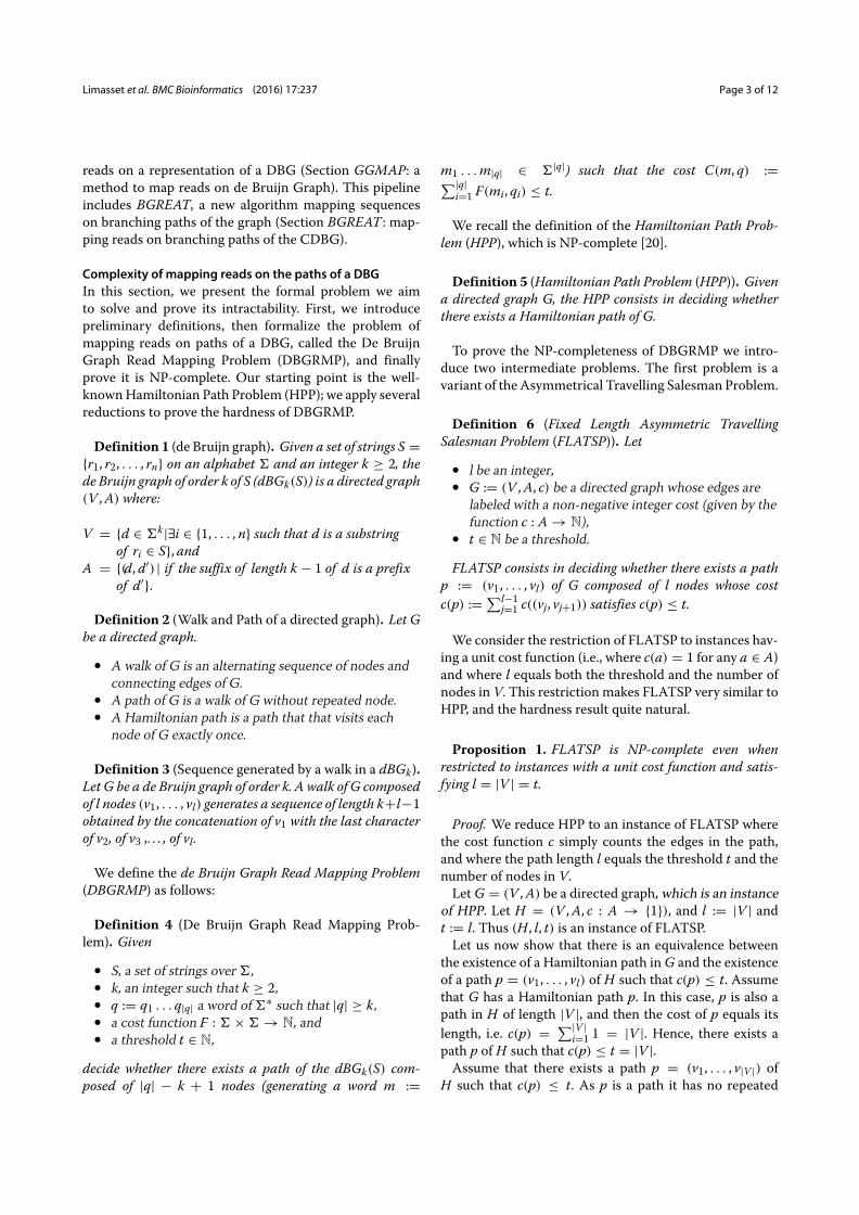
Limasset et al. BMC Bioinformatics (2016) 17:237 Page 3 of 12

reads on a representation of a DBG (Section GGMAP: amethod to map reads on de Bruijn Graph). This pipelineincludes BGREAT, a new algorithm mapping sequenceson branching paths of the graph (Section BGREAT : map-ping reads on branching paths of the CDBG).

Complexity of mapping reads on the paths of a DBGIn this section, we present the formal problem we aimto solve and prove its intractability. First, we introducepreliminary definitions, then formalize the problem ofmapping reads on paths of a DBG, called the De BruijnGraph Read Mapping Problem (DBGRMP), and finallyprove it is NP-complete. Our starting point is the well-knownHamiltonian Path Problem (HPP); we apply severalreductions to prove the hardness of DBGRMP.

Definition 1 (de Bruijn graph). Given a set of strings S =r1, r2, . . . , rn on an alphabet and an integer k ≥ 2, thede Bruijn graph of order k of S (dBGk(S)) is a directed graph(V ,A) where:

V = d ∈ k|∃i ∈ 1, . . . , n such that d is a substringof ri ∈ S, and

A = (d, d′) | if the suffix of length k − 1 of d is a prefixof d′.

Definition 2 (Walk and Path of a directed graph). Let Gbe a directed graph.

• A walk of G is an alternating sequence of nodes andconnecting edges of G.

• A path of G is a walk of G without repeated node.• A Hamiltonian path is a path that that visits each

node of G exactly once.

Definition 3 (Sequence generated by a walk in a dBGk).Let G be a de Bruijn graph of order k. A walk of G composedof l nodes (v1, . . . , vl) generates a sequence of length k+l−1obtained by the concatenation of v1 with the last characterof v2, of v3 ,. . . , of vl.

We define the de Bruijn Graph Read Mapping Problem(DBGRMP) as follows:

Definition 4 (De Bruijn Graph Read Mapping Prob-lem). Given

• S, a set of strings over ,• k, an integer such that k ≥ 2,• q := q1 . . . q|q| a word of ∗ such that |q| ≥ k,• a cost function F : × → N, and• a threshold t ∈ N,

decide whether there exists a path of the dBGk(S) com-posed of |q| − k + 1 nodes (generating a word m :=

m1 . . .m|q| ∈ |q|) such that the cost C(m, q) :=∑|q|i=1 F(mi, qi) ≤ t.

We recall the definition of the Hamiltonian Path Prob-lem (HPP), which is NP-complete [20].

Definition 5 (Hamiltonian Path Problem (HPP)). Givena directed graph G, the HPP consists in deciding whetherthere exists a Hamiltonian path of G.

To prove the NP-completeness of DBGRMP we intro-duce two intermediate problems. The first problem is avariant of the Asymmetrical Travelling Salesman Problem.

Definition 6 (Fixed Length Asymmetric TravellingSalesman Problem (FLATSP)). Let

• l be an integer,• G := (V ,A, c) be a directed graph whose edges are

labeled with a non-negative integer cost (given by thefunction c : A → N),

• t ∈ N be a threshold.

FLATSP consists in deciding whether there exists a pathp := (v1, . . . , vl) of G composed of l nodes whose costc(p) := ∑l−1

j=1 c((vj, vj+1)) satisfies c(p) ≤ t.

We consider the restriction of FLATSP to instances hav-ing a unit cost function (i.e., where c(a) = 1 for any a ∈ A)and where l equals both the threshold and the number ofnodes in V. This restriction makes FLATSP very similar toHPP, and the hardness result quite natural.

Proposition 1. FLATSP is NP-complete even whenrestricted to instances with a unit cost function and satis-fying l = |V | = t.

Proof. We reduce HPP to an instance of FLATSP wherethe cost function c simply counts the edges in the path,and where the path length l equals the threshold t and thenumber of nodes in V.LetG = (V ,A) be a directed graph, which is an instance

of HPP. Let H = (V ,A, c : A → 1), and l := |V | andt := l. Thus (H , l, t) is an instance of FLATSP.Let us now show that there is an equivalence between

the existence of a Hamiltonian path inG and the existenceof a path p = (v1, . . . , vl) of H such that c(p) ≤ t. Assumethat G has a Hamiltonian path p. In this case, p is also apath in H of length |V |, and then the cost of p equals itslength, i.e. c(p) = ∑|V |

i=1 1 = |V |. Hence, there exists apath p of H such that c(p) ≤ t = |V |.Assume that there exists a path p = (v1, . . . , v|V |) of

H such that c(p) ≤ t. As p is a path it has no repeated

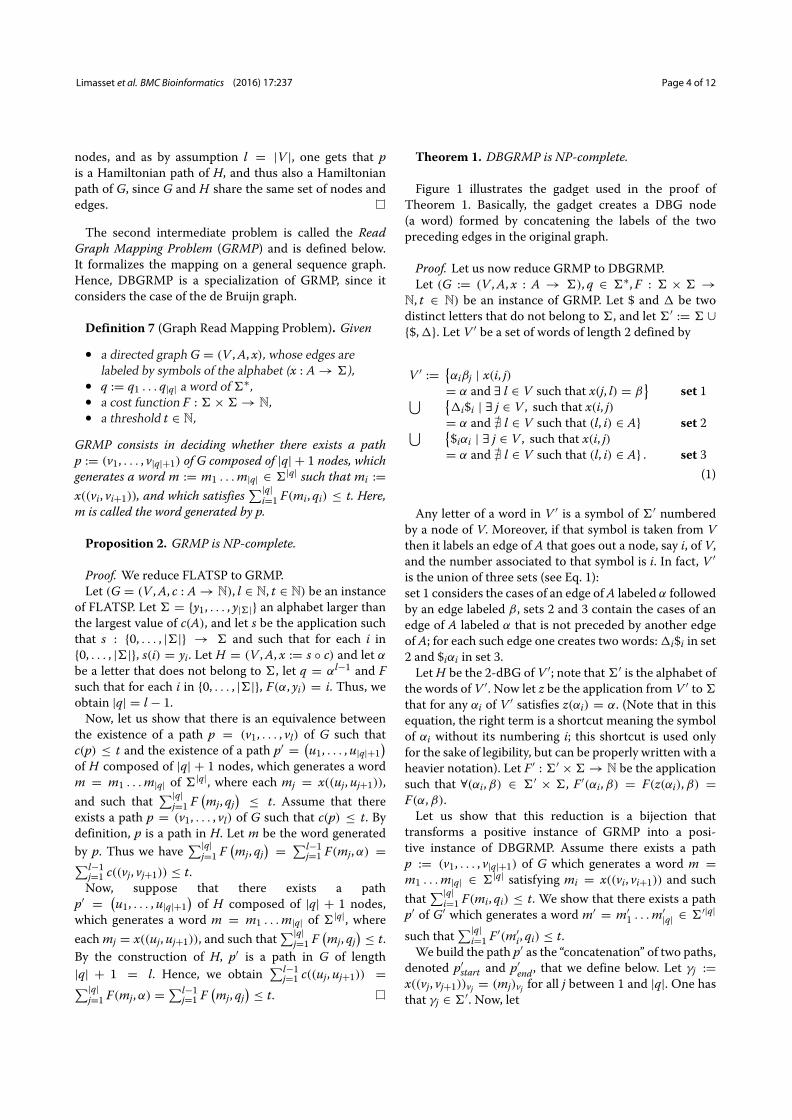
Limasset et al. BMC Bioinformatics (2016) 17:237 Page 4 of 12

nodes, and as by assumption l = |V |, one gets that pis a Hamiltonian path of H, and thus also a Hamiltonianpath of G, since G and H share the same set of nodes andedges.

The second intermediate problem is called the ReadGraph Mapping Problem (GRMP) and is defined below.It formalizes the mapping on a general sequence graph.Hence, DBGRMP is a specialization of GRMP, since itconsiders the case of the de Bruijn graph.

Definition 7 (Graph Read Mapping Problem). Given

• a directed graph G = (V ,A, x), whose edges arelabeled by symbols of the alphabet (x : A → ),

• q := q1 . . . q|q| a word of ∗,• a cost function F : × → N,• a threshold t ∈ N,

GRMP consists in deciding whether there exists a pathp := (v1, . . . , v|q|+1) of G composed of |q| + 1 nodes, whichgenerates a word m := m1 . . .m|q| ∈ |q| such that mi :=x((vi, vi+1)), and which satisfies

∑|q|i=1 F(mi, qi) ≤ t. Here,

m is called the word generated by p.

Proposition 2. GRMP is NP-complete.

Proof. We reduce FLATSP to GRMP.Let (G = (V ,A, c : A → N), l ∈ N, t ∈ N) be an instance

of FLATSP. Let = y1, . . . , y|| an alphabet larger thanthe largest value of c(A), and let s be the application suchthat s : 0, . . . , || → and such that for each i in0, . . . , ||, s(i) = yi. Let H = (V ,A, x := s c) and let α

be a letter that does not belong to , let q = αl−1 and Fsuch that for each i in 0, . . . , ||, F(α, yi) = i. Thus, weobtain |q| = l − 1.Now, let us show that there is an equivalence between

the existence of a path p = (v1, . . . , vl) of G such thatc(p) ≤ t and the existence of a path p′ = (

u1, . . . ,u|q|+1)

of H composed of |q| + 1 nodes, which generates a wordm = m1 . . .m|q| of |q|, where each mj = x((uj,uj+1)),and such that

∑|q|j=1 F

(mj, qj

) ≤ t. Assume that thereexists a path p = (v1, . . . , vl) of G such that c(p) ≤ t. Bydefinition, p is a path in H. Let m be the word generatedby p. Thus we have

∑|q|j=1 F

(mj, qj

) = ∑l−1j=1 F(mj,α) =∑l−1

j=1 c((vj, vj+1)) ≤ t.Now, suppose that there exists a path

p′ = (u1, . . . ,u|q|+1

)of H composed of |q| + 1 nodes,

which generates a word m = m1 . . .m|q| of |q|, whereeachmj = x((uj,uj+1)), and such that

∑|q|j=1 F

(mj, qj

) ≤ t.By the construction of H, p′ is a path in G of length|q| + 1 = l. Hence, we obtain

∑l−1j=1 c((uj,uj+1)) =∑|q|

j=1 F(mj,α) = ∑l−1j=1 F

(mj, qj

) ≤ t.

Theorem 1. DBGRMP is NP-complete.

Figure 1 illustrates the gadget used in the proof ofTheorem 1. Basically, the gadget creates a DBG node(a word) formed by concatening the labels of the twopreceding edges in the original graph.

Proof. Let us now reduce GRMP to DBGRMP.Let (G := (V ,A, x : A → ), q ∈ ∗, F : × →

N, t ∈ N) be an instance of GRMP. Let $ and be twodistinct letters that do not belong to , and let ′ := ∪$,. Let V ′ be a set of words of length 2 defined by

V ′ := αiβj | x(i, j)

= α and ∃ l ∈ V such that x(j, l) = β

set 1⋃ i$i | ∃ j ∈ V , such that x(i, j)

= α and l ∈ V such that (l, i) ∈ A set 2⋃ $iαi | ∃ j ∈ V , such that x(i, j)

= α and l ∈ V such that (l, i) ∈ A . set 3(1)

Any letter of a word in V ′ is a symbol of ′ numberedby a node of V. Moreover, if that symbol is taken from Vthen it labels an edge of A that goes out a node, say i, of V,and the number associated to that symbol is i. In fact, V ′is the union of three sets (see Eq. 1):set 1 considers the cases of an edge ofA labeled α followedby an edge labeled β , sets 2 and 3 contain the cases of anedge of A labeled α that is not preceded by another edgeof A; for each such edge one creates two words: i$i in set2 and $iαi in set 3.LetH be the 2-dBG of V ′; note that ′ is the alphabet of

the words of V ′. Now let z be the application from V ′ to

that for any αi of V ′ satisfies z(αi) = α. (Note that in thisequation, the right term is a shortcut meaning the symbolof αi without its numbering i; this shortcut is used onlyfor the sake of legibility, but can be properly written with aheavier notation). Let F ′ : ′ × → N be the applicationsuch that ∀(αi,β) ∈ ′ × , F ′(αi,β) = F(z(αi),β) =F(α,β).Let us show that this reduction is a bijection that

transforms a positive instance of GRMP into a posi-tive instance of DBGRMP. Assume there exists a pathp := (v1, . . . , v|q|+1) of G which generates a word m =m1 . . .m|q| ∈ |q| satisfying mi = x((vi, vi+1)) and suchthat

∑|q|i=1 F(mi, qi) ≤ t. We show that there exists a path

p′ of G′ which generates a word m′ = m′1 . . .m′|q| ∈ ′|q|

such that∑|q|

i=1 F ′(m′i, qi) ≤ t.

We build the path p′ as the “concatenation” of two paths,denoted p′

start and p′end, that we define below. Let γj :=

x((vj, vj+1))vj = (mj)vj for all j between 1 and |q|. One hasthat γj ∈ ′. Now, let

Limasset et al. BMC Bioinformatics (2016) 17:237 Page 5 of 12

Fig. 1 Illustration of the gadget used in the proof of Theorem 1. Encoding a directed graph into a DBG of order 2. The directed graph G (top) admitsthe same words than the 2-DBG G′ (bottom), if we ignore the numbers

p′start :=

⎧⎪⎪⎪⎪⎪⎪⎨⎪⎪⎪⎪⎪⎪⎩

(x((vl′ , vl))vl′ x((vl , v1))vl , x((vl , v1))vl x((v1, v2))v1

)

if ∃ l, l′ ∈ V such that (l, 1) ∈ A and (l′, l) ∈ A($vl x((vl , v1))vl , x((vl , v1))vl x((v1, v2))v1

)

if ∃ l∈V such that (l, 1)∈ A and l′ ∈V such that (l′, l) ∈ A(v1 $v1 , $v1x((v1, v2))v1

)

otherwise.

and let

p′end := (

γ1γ2, . . . , γ|q|−1γ|q|).

Let m′ denote the word generated by p′. Clearly, onesees that m′ = (m1)v1 . . . (m|q|)v|q| , and since mi =z((m′

i)vi), one gets that z(m′) = m and∑|q|

i=1 F ′ (m′i, qi

) =∑|q|i=1 F (mi, qi) ≤ t.In the other direction, the proof is similar since our

construction is a bijection.

GGMAP: a method to map reads on de Bruijn GraphWe propose a practical solution for solving DBGRMP. Weconsider the case of short (hundred of base pairs) readswith a low error rate (1% of substitution), which is a goodapproximation of widely used NGS reads. Since errorsare mostly substitutions, mapping is computed using theHamming distance.Our solution is designed formapping on a compacted de

Bruijn graph (CDBG) any set of short reads, either thoseused to build the graph or reads from another individualor species. We recall that a CDBG is representation of aDBG in which each non branching path is merged into asingle node. The sequence of each node is called a unitig.Figure 2 shows a DBG and the associated CDBG.In a CDBG, the nodes are not necessarily k-mers, words

of length k, but unitigs, with some unitigs being longerthan reads. Thus, while mapping on a CDBG, one dis-tinguishes between two mapping situations: i/ the readsmapping completely on a unitig of the graph, and ii/ thereads whose mapping spans two or more unitigs. For thelatter, we say that the readmaps on a branching path of thegraph.

Taking advantage of the extensive research carried outfor mapping reads on flat strings, GGMAP uses Bowtie2[7] to map the reads on the unitigs. In addition, GGMAPintegrates our proposed new tool, called BGREAT, formapping reads on branching paths of the CDBG. Figure 3provides an overview of the pipeline.GGMAP takes as inputs a query set of reads and a

reference DBG. To avoid including sequencing errors inthe DBG, we construct the reference DBG after filteringout all k-mers whose coverage lies below a user-definedthreshold c. This error removal step is a classical prepro-cessing step that is performed in k-mer based assemblers.The unitigs of the CDBG are computed using BCALM2(the parallel version of BCALM [21]), using the k-mershaving a coverage ≥ c. GGMAP uses such a set of unitigsas DBG.We now propose a detailed description of BGREAT.

BGREAT : mapping reads on branching paths of the CDBGAs previously mentioned, BGREAT is designed for map-ping reads on branching paths of a CDBG, using reason-able resources both in terms of time and memory. Ourapproach follows the usual “seed and extend” paradigm.More generally, the proposed implementation appliesheuristic schemes, both regarding the indexing and thealignment phases.

Indexing heuristicWe remind that our algorithm maps reads that span atleast two distinct unitigs. Such mapped reads inevitablytraverse one or more DBG edge(s). In a CDBG, edgesare represented by the prefix and suffix of size k − 1of each unitig. We call such sequences the overlaps. Inorder to limit the index size and the computation time,our algorithm indexes only overlaps that are later used asseeds. Those overlaps are good anchors for several rea-sons: they are long enough (k − 1) to be selective, theycannot be shared by more than eight unitigs (four startingand four ending with the overlap), and a CDBGusually hasa reasonable number of unitigs and then of overlaps. For

Limasset et al. BMC Bioinformatics (2016) 17:237 Page 6 of 12

Fig. 2 A toy example of a DBG of order k with k = 4 (top) and its compacted version (bottom)

instance, the CDBG in our experiment with human datahas 70 million unitigs and 87 million overlaps for 3 billionk-mers). In our implementation, the index is a minimalperfect hash table indicating for each overlap the unitig(s)starting or ending with this (k − 1)-mer. Using a minimalperfect hash function limits the memory footprint, whilekeeping efficient query times (see Table 3).

Read alignmentGiven a read, each of its k − 1-mers is used to querythe index. The index detects which k − 1-mers representan overlap of the CDBG. An example of a read togetherwith the matched unitigs are displayed on Fig. 4. Oncethe overlaps and their corresponding unitigs have beencomputed, the alignment of the read is performed fromleft to right as presented in Algorithm 1. Given an overlapposition i on the read, the unitigs starting with this overlapare aligned to the sequence of the read starting fromposition i. The best alignment is recorded. In addition, toimprove speed, if one of the at most four unitigs endingwith the same overlap is the next overlap detected on the

read, then this unitig is tested first, and if the alignmentcontains less mismatch than the user defined threshold,the other unitigs are not considered. Note that this opti-mization does not apply for the first and last overlaps of aread.

Algorithm 1: Greedy algorithm for mapping a read onmultiple unitigs once the potential overlaps present inthe read have been detected.Data: Read r, Integer nfor the n first overlaps of r do

Find a path begin that map the begin of rif begin found then

for the n last overlaps of r doFind a path end that maps the end of rif end found then

Find (in a greedy way) a path cover thatmap the read from begin to endif cover found then

write path;return

Fig. 3 Unitig construction, as used in the proposed experiments (upper part of the figure) and GGMAP pipeline. Reads to be mapped can be distinctfrom reads used for building the graph. Long unitigs are unitigs longer than the reads. We remind that tools BCALM and BOWTIE2 are respectivelypublished in [7, 21]

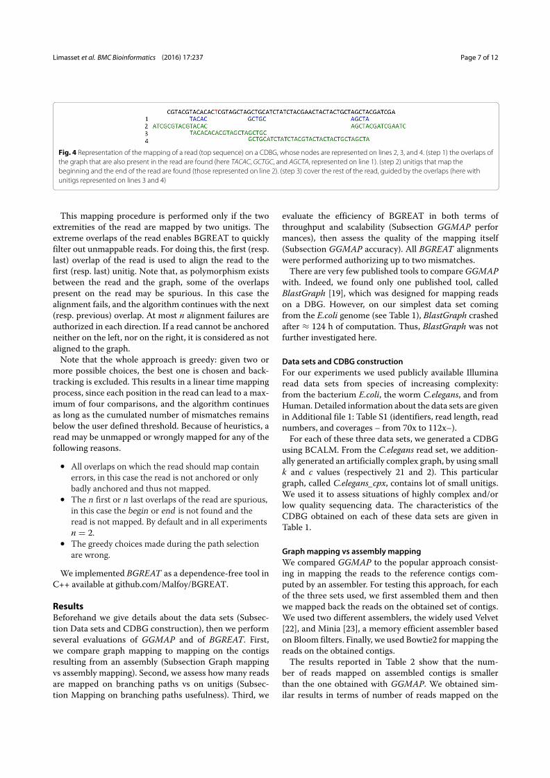
Limasset et al. BMC Bioinformatics (2016) 17:237 Page 7 of 12

Fig. 4 Representation of the mapping of a read (top sequence) on a CDBG, whose nodes are represented on lines 2, 3, and 4. (step 1) the overlaps ofthe graph that are also present in the read are found (here TACAC, GCTGC, and AGCTA, represented on line 1). (step 2) unitigs that map thebeginning and the end of the read are found (those represented on line 2). (step 3) cover the rest of the read, guided by the overlaps (here withunitigs represented on lines 3 and 4)

This mapping procedure is performed only if the twoextremities of the read are mapped by two unitigs. Theextreme overlaps of the read enables BGREAT to quicklyfilter out unmappable reads. For doing this, the first (resp.last) overlap of the read is used to align the read to thefirst (resp. last) unitig. Note that, as polymorphism existsbetween the read and the graph, some of the overlapspresent on the read may be spurious. In this case thealignment fails, and the algorithm continues with the next(resp. previous) overlap. At most n alignment failures areauthorized in each direction. If a read cannot be anchoredneither on the left, nor on the right, it is considered as notaligned to the graph.Note that the whole approach is greedy: given two or

more possible choices, the best one is chosen and back-tracking is excluded. This results in a linear time mappingprocess, since each position in the read can lead to a max-imum of four comparisons, and the algorithm continuesas long as the cumulated number of mismatches remainsbelow the user defined threshold. Because of heuristics, aread may be unmapped or wrongly mapped for any of thefollowing reasons.

• All overlaps on which the read should map containerrors, in this case the read is not anchored or onlybadly anchored and thus not mapped.

• The n first or n last overlaps of the read are spurious,in this case the begin or end is not found and theread is not mapped. By default and in all experimentsn = 2.

• The greedy choices made during the path selectionare wrong.

We implemented BGREAT as a dependence-free tool inC++ available at github.com/Malfoy/BGREAT.

ResultsBeforehand we give details about the data sets (Subsec-tion Data sets and CDBG construction), then we performseveral evaluations of GGMAP and of BGREAT. First,we compare graph mapping to mapping on the contigsresulting from an assembly (Subsection Graph mappingvs assembly mapping). Second, we assess how many readsare mapped on branching paths vs on unitigs (Subsec-tion Mapping on branching paths usefulness). Third, we

evaluate the efficiency of BGREAT in both terms ofthroughput and scalability (Subsection GGMAP performances), then assess the quality of the mapping itself(Subsection GGMAP accuracy). All BGREAT alignmentswere performed authorizing up to two mismatches.There are very few published tools to compare GGMAP

with. Indeed, we found only one published tool, calledBlastGraph [19], which was designed for mapping readson a DBG. However, on our simplest data set comingfrom the E.coli genome (see Table 1), BlastGraph crashedafter ≈ 124 h of computation. Thus, BlastGraph was notfurther investigated here.

Data sets and CDBG constructionFor our experiments we used publicly available Illuminaread data sets from species of increasing complexity:from the bacterium E.coli, the worm C.elegans, and fromHuman. Detailed information about the data sets are givenin Additional file 1: Table S1 (identifiers, read length, readnumbers, and coverages – from 70x to 112x–).For each of these three data sets, we generated a CDBG

using BCALM. From the C.elegans read set, we addition-ally generated an artificially complex graph, by using smallk and c values (respectively 21 and 2). This particulargraph, called C.elegans_cpx, contains lot of small unitigs.We used it to assess situations of highly complex and/orlow quality sequencing data. The characteristics of theCDBG obtained on each of these data sets are given inTable 1.

Graphmapping vs assembly mappingWe compared GGMAP to the popular approach consist-ing in mapping the reads to the reference contigs com-puted by an assembler. For testing this approach, for eachof the three sets used, we first assembled them and thenwe mapped back the reads on the obtained set of contigs.We used two different assemblers, the widely used Velvet[22], and Minia [23], a memory efficient assembler basedon Bloom filters. Finally, we used Bowtie2 for mapping thereads on the obtained contigs.The results reported in Table 2 show that the num-

ber of reads mapped on assembled contigs is smallerthan the one obtained with GGMAP. We obtained sim-ilar results in terms of number of reads mapped on the

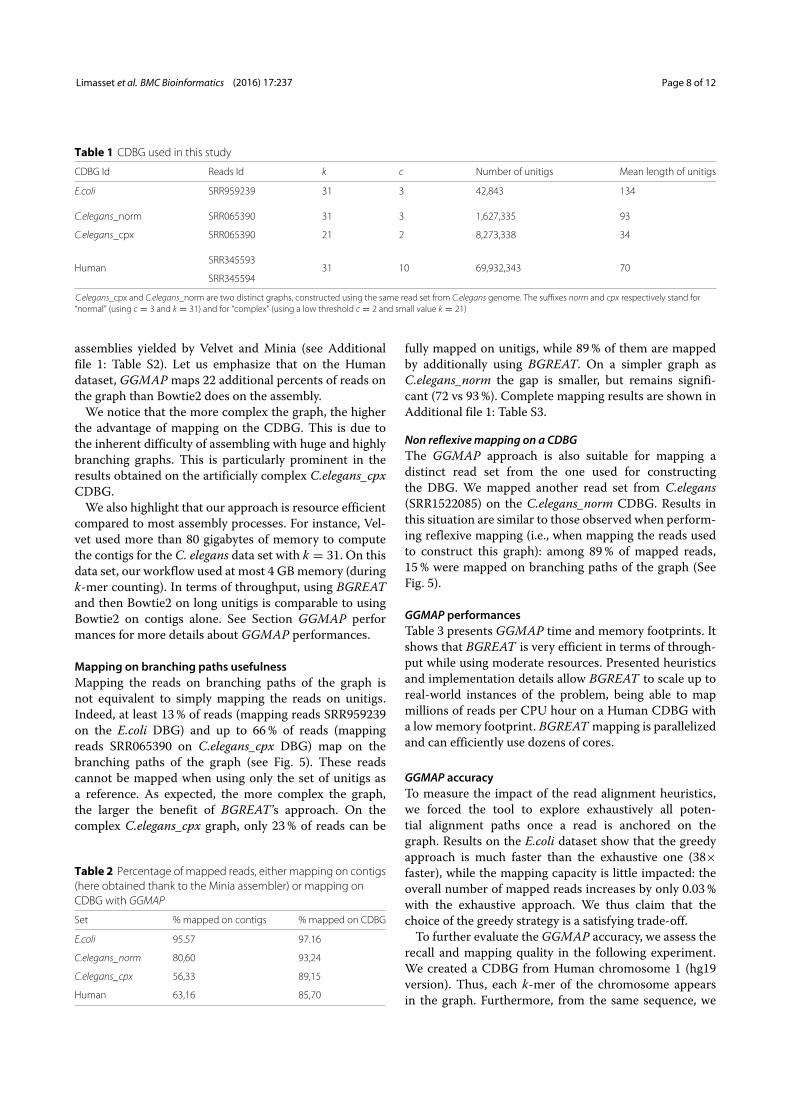
Limasset et al. BMC Bioinformatics (2016) 17:237 Page 8 of 12

Table 1 CDBG used in this study

CDBG Id Reads Id k c Number of unitigs Mean length of unitigs

E.coli SRR959239 31 3 42,843 134

C.elegans_norm SRR065390 31 3 1,627,335 93

C.elegans_cpx SRR065390 21 2 8,273,338 34

HumanSRR345593

31 10 69,932,343 70SRR345594

C.elegans_cpx and C.elegans_norm are two distinct graphs, constructed using the same read set from C.elegans genome. The suffixes norm and cpx respectively stand for“normal” (using c = 3 and k = 31) and for “complex” (using a low threshold c = 2 and small value k = 21)

assemblies yielded by Velvet and Minia (see Additionalfile 1: Table S2). Let us emphasize that on the Humandataset, GGMAP maps 22 additional percents of reads onthe graph than Bowtie2 does on the assembly.We notice that the more complex the graph, the higher

the advantage of mapping on the CDBG. This is due tothe inherent difficulty of assembling with huge and highlybranching graphs. This is particularly prominent in theresults obtained on the artificially complex C.elegans_cpxCDBG.We also highlight that our approach is resource efficient

compared to most assembly processes. For instance, Vel-vet used more than 80 gigabytes of memory to computethe contigs for the C. elegans data set with k = 31. On thisdata set, our workflow used at most 4 GBmemory (duringk-mer counting). In terms of throughput, using BGREATand then Bowtie2 on long unitigs is comparable to usingBowtie2 on contigs alone. See Section GGMAP performances for more details about GGMAP performances.

Mapping on branching paths usefulnessMapping the reads on branching paths of the graph isnot equivalent to simply mapping the reads on unitigs.Indeed, at least 13% of reads (mapping reads SRR959239on the E.coli DBG) and up to 66% of reads (mappingreads SRR065390 on C.elegans_cpx DBG) map on thebranching paths of the graph (see Fig. 5). These readscannot be mapped when using only the set of unitigs asa reference. As expected, the more complex the graph,the larger the benefit of BGREAT ’s approach. On thecomplex C.elegans_cpx graph, only 23% of reads can be

Table 2 Percentage of mapped reads, either mapping on contigs(here obtained thank to the Minia assembler) or mapping onCDBG with GGMAP

Set % mapped on contigs % mapped on CDBG

E.coli 95.57 97.16

C.elegans_norm 80,60 93,24

C.elegans_cpx 56,33 89,15

Human 63,16 85,70

fully mapped on unitigs, while 89% of them are mappedby additionally using BGREAT. On a simpler graph asC.elegans_norm the gap is smaller, but remains signifi-cant (72 vs 93%). Complete mapping results are shown inAdditional file 1: Table S3.

Non reflexivemapping on a CDBGThe GGMAP approach is also suitable for mapping adistinct read set from the one used for constructingthe DBG. We mapped another read set from C.elegans(SRR1522085) on the C.elegans_norm CDBG. Results inthis situation are similar to those observed when perform-ing reflexive mapping (i.e., when mapping the reads usedto construct this graph): among 89% of mapped reads,15% were mapped on branching paths of the graph (SeeFig. 5).

GGMAP performancesTable 3 presents GGMAP time and memory footprints. Itshows that BGREAT is very efficient in terms of through-put while using moderate resources. Presented heuristicsand implementation details allow BGREAT to scale up toreal-world instances of the problem, being able to mapmillions of reads per CPU hour on a Human CDBG witha lowmemory footprint. BGREAT mapping is parallelizedand can efficiently use dozens of cores.

GGMAP accuracyTo measure the impact of the read alignment heuristics,we forced the tool to explore exhaustively all poten-tial alignment paths once a read is anchored on thegraph. Results on the E.coli dataset show that the greedyapproach is much faster than the exhaustive one (38×faster), while the mapping capacity is little impacted: theoverall number of mapped reads increases by only 0.03%with the exhaustive approach. We thus claim that thechoice of the greedy strategy is a satisfying trade-off.To further evaluate the GGMAP accuracy, we assess the

recall and mapping quality in the following experiment.We created a CDBG from Human chromosome 1 (hg19version). Thus, each k-mer of the chromosome appearsin the graph. Furthermore, from the same sequence, we

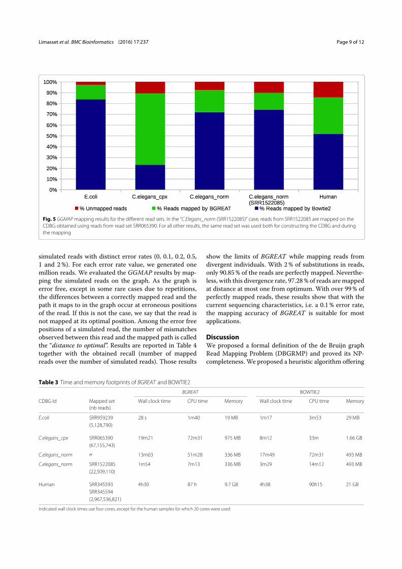
Limasset et al. BMC Bioinformatics (2016) 17:237 Page 9 of 12

Fig. 5 GGMAPmapping results for the different read sets. In the “C.Elegans_norm (SRR1522085)” case, reads from SRR1522085 are mapped on theCDBG obtained using reads from read set SRR065390. For all other results, the same read set was used both for constructing the CDBG and duringthe mapping

simulated reads with distinct error rates (0, 0.1, 0.2, 0.5,1 and 2%). For each error rate value, we generated onemillion reads. We evaluated the GGMAP results by map-ping the simulated reads on the graph. As the graph iserror free, except in some rare cases due to repetitions,the differences between a correctly mapped read and thepath it maps to in the graph occur at erroneous positionsof the read. If this is not the case, we say that the read isnot mapped at its optimal position. Among the error freepositions of a simulated read, the number of mismatchesobserved between this read and the mapped path is calledthe “distance to optimal”. Results are reported in Table 4together with the obtained recall (number of mappedreads over the number of simulated reads). Those results

show the limits of BGREAT while mapping reads fromdivergent individuals. With 2% of substitutions in reads,only 90.85% of the reads are perfectly mapped. Neverthe-less, with this divergence rate, 97.28% of reads aremappedat distance at most one from optimum. With over 99% ofperfectly mapped reads, these results show that with thecurrent sequencing characteristics, i.e. a 0.1% error rate,the mapping accuracy of BGREAT is suitable for mostapplications.

DiscussionWe proposed a formal definition of the de Bruijn graphRead Mapping Problem (DBGRMP) and proved its NP-completeness. We proposed a heuristic algorithm offering

Table 3 Time and memory footprints of BGREAT and BOWTIE2

BGREAT BOWTIE2

CDBG Id Mapped set Wall clock time CPU time Memory Wall clock time CPU time Memory(nb reads)

E.coli SRR959239 28 s 1m40 19 MB 1m17 3m53 29 MB(5,128,790)

C.elegans_cpx SRR065390 19m21 72m31 975 MB 8m12 33m 1.66 GB(67,155,743)

C.elegans_norm ′′ 13m03 51m28 336 MB 17m49 72m31 493 MB

C.elegans_norm SRR1522085 1m54 7m13 336 MB 3m29 14m12 493 MB(22,509,110)

Human SRR345593 4h30 87 h 9.7 GB 4h38 90h15 21 GBSRR345594(2,967,536,821)

Indicated wall clock times use four cores, except for the human samples for which 20 cores were used

Limasset et al. BMC Bioinformatics (2016) 17:237 Page 10 of 12

Table 4 GGMAPmapping results on simulated reads from thereference of the human chromosome 1 with default parameters

% Errors in Distance to optimum of BGREATsimulated reads mapped reads (percentage)

0 1 2 3 ≥ 4

0 100 0 0 0 0

0.1 99.31 0.52 0.09 0.04 0.04

0.2 98.79 0.91 0.21 0.07 0.02

0.5 97.2 2.17 0.41 0.17 0.05

1 94.88 3.72 0.92 0.41 0.07

2 90.85 6.43 1.79 0.83 0.1

Results show the recall of GGMAP and the quality of BGREAT mapping, asrepresented by the “distance to optimum” value. For instance 94.88% of the readswere mapped without error, 3.72% were mapped with a distance to the optimumof one etc. Due to approximate repeats in human chromosome 1, the reporteddistance to optimum is an upper bound

a practical solution. We developed a tool called BGREATimplementing this algorithm using a compacted de Bruijngraph (CDBG) as a reference.From the theoretical viewpoint, the problem DBGRMP

considers paths rather than walks in the graph. The cur-rent proof of its hardness does not seem to be adaptable tothe cases of walks. A perspective is to extend the hardnessresult to that more general case.We emphasize that our proposal does not enable

genome annotation. It has been designed for applicationsaiming at a precise quantification of sequenced data, or aset of potential variations between the reads and the ref-erence genome. In this context, it is essential to map asmuch reads as possible. Experiments show that a signifi-cant proportion of the reads (between ≈ 13and ≈ 66%depending on the experiment) can be only mapped onbranching paths of the graph. Hence, mapping only onthe nodes of the graph or on assembled contigs is thusinsufficient. This statement holds true when mapping thereads used for building the graph, but also with reads froma different experiment. Moreover, our results show thata potentially large number of reads (up to ≈ 32%) thatare mapped on a CDBG cannot be mapped on a classicalassembly.With GGMAP, the mapping quality is very high: using

Human chromosome 1 as a reference and reads with arealistic error rate (similar to that of Illumina technol-ogy), over 99% of the reads are correctly mapped. Thesame experiment also pointed out the limits of mappingreads on a divergent graph reference (≥ 2% substitu-tions): approximately 10% of the reads are mapped at asuboptimal position.A weak point of BGREAT lies in its anchoring tech-

nique. Reads mapped with BGREAT must contain at leastone exact k − 1-mer that is an arc of the CDBG, i.e., anoverlap between two connected nodes. This may be a seri-ous limitation when the original read set diverges greatly

from the reads to be mapped. Improving the mappingtechnique may be done by using not only unitig overlapsas anchors at the cost of higher computational resources.Another solution may consist in using a smarter anchor-ing approach, like spaced seeds, which can accommodateerrors in the anchor [24].A natural extension consists in adapting BGREAT for

mapping, on the CDBG obtained from short reads, thelong (a few kilobases in average) and noisy reads pro-duced by the third generation of sequencers, whose errorrate reaches up to 15% (with mostly insertion and dele-tion errors for e.g. Pacific Biosciences technology). Suchadaptation is not straightforward because of our seedingstrategy, which requires long exact matches. The anchor-ing process must be very sensitive and very specific, whilethe mapping itself must implement a Blast-like heuris-tic or an alignment-free method. However, mapping suchlong reads on a DBG could be of interest for correctingthese reads as in [13], or for solving repeats, if long readsare mapped on the walks (which main include cycles)of the DBG. Our NP-completeness proof only considersmapping on (acyclic) paths. Proving the hardness of theproblem of mapping reads on walks of a DBG remainsopen.Incidentally, using the same read set for constructing

the CDBG and for mapping opens the way to major appli-cations. Indeed, the graph and the exact location of eachread on it may be used for i/ read correction as in [15],by detecting differences between reads and the mappedarea of the graph in which low support k-mers likely dueto sequencing errors are absent, or for ii/ read compres-sion by recording additionally the mapping errors, or foriii/ both correction and compression by conserving onlyfor each read its mapping location on the graph.Having for each read (used for constructing the graph

or not) its location on the CDBG also provides the oppor-tunity to design algorithms for enriching the graph, forinstance enabling a quantification that is sensitive to localvariations. This would be valuable for applications suchas variant calling, analysis of RNA-seq variants [25], or ofmetagenomic reads [26].Additionally, BGREAT results provide pieces of

information for distant k-mers in the CDBG, abouttheir co-occurrences in the mapped read data sets. Thisoffers a way for the resolution, in the de Bruijn graph,of repeats larger than k. It could also allow to phase thepolymorphisms and to reconstruct haplotypes.

ConclusionA take home message is that read mapping can be sig-nificantly improved by mapping on the structure of anassembly graph rather than on a set of assembled con-tigs (respectively ≈22% and ≈ 32% of additional readsmapped for the Human and a complex C.elegans data

Limasset et al. BMC Bioinformatics (2016) 17:237 Page 11 of 12

sets). This is mainly due to the fact that assembly graphsretains more genomic information than assembled con-tigs, which also suffer from errors induced by the com-plexity of assembly. Moreover, mapping on a compactedDe Bruijn Graph can be fast. The availability of BGREATopens the door to its application to fundamental taskssuch as read error correction, read compression, variantquantification, or haplotype reconstruction.

Additional file

Additional file 1: Read mapping on De Bruijn graphs additional file. Threecomplementary tables are presented. Main characteristics of data sets usedin this study. Assembly and mapping approach comparison. Results ofBGREAT on real read sets. (PDF 40 kb)

AbbreviationsCDBG, Compacted De Bruijn graph; DBG, De Bruijn graph; DBGRMP, De Bruijngraph read mapping problem; FLATSP, fixed length assymetric travellingsalesman problem; GRMP, graph read mapping problem; HPP, Hamiltonianpath problem

AcknowledgementsWe would like to thank Yannick Zakowski, Claire Lemaitre and Camille Marchetfor proofreading the manuscript and discussions.

FundingThis work was funded by French ANR-12-BS02-0008 Colib’read project, byANR-11-BINF-0002, and by a MASTODONS project.

Availability of data andmaterialsOur implementations are available at github.com/Malfoy/BGREAT. In additionto the following pieces of information, Additional file 1: Table S1 presents themain characteristics of these datasets.SRR959239 http://www.ncbi.nlm.nih.gov/sra/?term=SRR959239SRR065390 http://www.ncbi.nlm.nih.gov/sra/?term=SRR065390SRR1522085 http://www.ncbi.nlm.nih.gov/sra/?term=SRR1522085SRR345593 and SRR345594 http://www.ncbi.nlm.nih.gov/sra/?term=SRR345593.

Authors’ contributionsPP initiated the work and designed the study. AL, BC and ER designed theformalism and the proofs of NP-hardness. AL designed the algorithmicframework, implemented the BGREAT and performed the tests. All authorswrote and accepted the final version of the manuscript.

Competing interestsThe authors declare that they have no competing interests.

Ethics approval and consent to participateNot applicable.

Author details1IRISA Inria Rennes Bretagne Atlantique, GenScale team, Campus de Beaulieu,35042 Rennes, France. 2L.I.R.M.M., UMR 5506, Université deMontpellier et CNRS,860 rue de St Priest, F-34392 Montpellier Cedex 5, France. 3Institut BiologieComputationnelle, Université de Montpellier, F-34392 Montpellier, France.

Received: 9 December 2015 Accepted: 26 May 2016

References1. Bradnam KR, Fass JN, et al. Assemblathon 2: evaluating de novo methods

of genome assembly in three vertebrate species. GigaScience. 2013;2:10.doi:10.1186/2047-217X-2-10.

2. Nagarajan N, Pop M. Parametric complexity of sequence assembly:theory and applications to next generation sequencing. J Comput Biol.2009;16(7):897–908. doi:10.1089/cmb.2009.0005.

3. Chaisson MJ, Pevzner PA. Short read fragment assembly of bacterialgenomes. Genome Res. 2008;18(2):324–30. doi:10.1101/gr.7088808.

4. Myers EW, Sutton GG, et al. A whole-genome assembly of Drosophila.Science (New York, N.Y.) 2000;287(5461):2196–204.doi:10.1126/science.287.5461.2196.

5. Myers EW. The fragment assembly string graph. Bioinformatics.2005;21(Suppl 2):79–85. doi:10.1093/bioinformatics/bti1114.

6. Li H, Durbin R. Fast and accurate short read alignment withBurrows-Wheeler transform. Bioinformatics. 2009;25(14):1754–60.doi:10.1093/bioinformatics/btp324.

7. Langmead B, Salzberg SL. Fast gapped-read alignment with Bowtie 2.Nat Methods. 2012;9(4):357–9. doi:10.1038/nmeth.1923.

8. Lee H, Schatz MC. Genomic dark matter: the reliability of short readmapping illustrated by the genome mappability score. Bioinformatics.2012;28(16):2097–105. doi:10.1093/bioinformatics/bts330.

9. Deshpande V, Fung EDK, Pham S, Bafna V. Cerulean: A Hybrid AssemblyUsing High Throughput Short and Long Reads. In: Lecture Notes inComputer Science vol. 8126 LNBI. Springer; 2013. p. 349–63.doi:10.1007/978-3-642-40453-5_27.

10. Ribeiro FJ, Przybylski D, Yin S, Sharpe T, Gnerre S, Abouelleil A, BerlinAM, Montmayeur A, Shea TP, Walker BJ, Young SK, Russ C, Nusbaum C,MacCallum I, Jaffe DB. Finished bacterial genomes from shotgunsequence data. Genome Res. 2012;22(11):2270–7.doi:10.1101/gr.141515.112.

11. Pevzner PA, Tang H, Waterman MS. An Eulerian path approach to DNAfragment assembly. Proc Natl Acad Sci. 2001;98(17):9748–53.doi:10.1073/pnas.171285098.

12. Bankevich A, Nurk S, Antipov D, Gurevich AA, Dvorkin M, Kulikov AS,Lesin VM, Nikolenko SI, Pham S, Prjibelski AD, Pyshkin AV, Sirotkin AV,Vyahhi N, Tesler G, Alekseyev MA, Pevzner PA. SPAdes: a new genomeassembly algorithm and its applications to single-cell sequencing. JComput Biol. 2012;19(5):455–77. doi:10.1089/cmb.2012.0021.

13. Salmela L, Rivals E. LoRDEC: accurate and efficient long read errorcorrection. Bioinformatics. 2014;30(24):3506–14.doi:10.1093/bioinformatics/btu538.

14. Yang X, Chockalingam SP, Aluru S. A survey of error-correction methodsfor next-generation sequencing. Brief Bioinform. 2013;14(1):56–66.doi:10.1093/bib/bbs015.

15. Benoit G, Lavenier D, Lemaitre C, Rizk G. Bloocoo, a memory efficientread corrector. In: European Conference on Computational Biology(ECCB); 2014. https://gatb.inria.fr/software/bloocoo/.

16. Wang M, Ye Y, Tang H. A de Bruijn graph approach to the quantificationof closely-related genomes in a microbial community. J Comput Biol.2012;19(6):814–25. doi:10.1089/cmb.2012.0058.

17. Huang L, Popic V, Batzoglou S. Short read alignment with populations ofgenomes. Bioinformatics. 2013;29(13):361–70.doi:10.1093/bioinformatics/btt215.

18. Dilthey A, Cox C, Iqbal Z, Nelson MR, McVean G. Improved genomeinference in the MHC using a population reference graph. Nat Genet.2015;47(6):682–8. doi:10.1038/ng.3257.

19. Holley G, Peterlongo P. Blastgraph: Intensive approximate patternmatching in sequence graphs and de-bruijn graphs. In: Stringology; 2012.p. 53–63. http://alcovna.genouest.org/blastree/.

20. Karp RM. Reducibility Among Combinatorial Problems. In: 50 Years ofInteger Programming 1958-2008. Berlin, Heidelberg: Springer; 2010. p.219–41. doi:10.1007/978-3-540-68279-0_8. http://link.springer.com/10.1007/978-3-540-68279-0_8.

21. Chikhi R, Limasset A, Jackman S, Simpson JT, Medvedev P. On therepresentationof debruijn graphs. In: Research in Computational MolecularBiology. Springer; 2014. p. 35–55. doi:10.1007/978-3-319-05269-4-4.

22. Zerbino DR, Birney E. Velvet: algorithms for de novo short read assemblyusing de Bruijn graphs. Genome Res. 2008;18(5):821–9.doi:10.1101/gr.074492.107.

23. Chikhi R, Rizk G. Space-efficient and exact de Bruijn graph representationbased on a Bloom filter. Algorithm Mol Biol. 2013;8(1):22.doi:10.1186/1748-7188-8-22.

24. Vroland C, Salson M, Touzet H. Lossless seeds for searching short patternswithhigherror rates. In: Combinatorial Algorithms. Springer; 2014. p. 364–75.

Limasset et al. BMC Bioinformatics (2016) 17:237 Page 12 of 12

25. Sacomoto GA, Kielbassa J, Chikhi R, Uricaru R, Antoniou P, Sagot MF,Peterlongo P, Lacroix V. Kissplice: de-novo calling alternative splicingevents from rna-seq data. BMC Bioinformatics. 2012;13(Suppl 6):5.

26. Ye Y, Tang H. Utilizing de Bruijn graph of metagenome assembly formetatranscriptome analysis. Bioinformatics. 2015btv510. Oxford UnivPress. arXiv preprint arXiv:1504.01304.

• We accept pre-submission inquiries

• Our selector tool helps you to find the most relevant journal

• We provide round the clock customer support

• Convenient online submission

• Thorough peer review

• Inclusion in PubMed and all major indexing services

• Maximum visibility for your research

Submit your manuscript atwww.biomedcentral.com/submit

Submit your next manuscript to BioMed Central and we will help you at every step:

110

Chapter 4

Improving an assembly paradigm

111

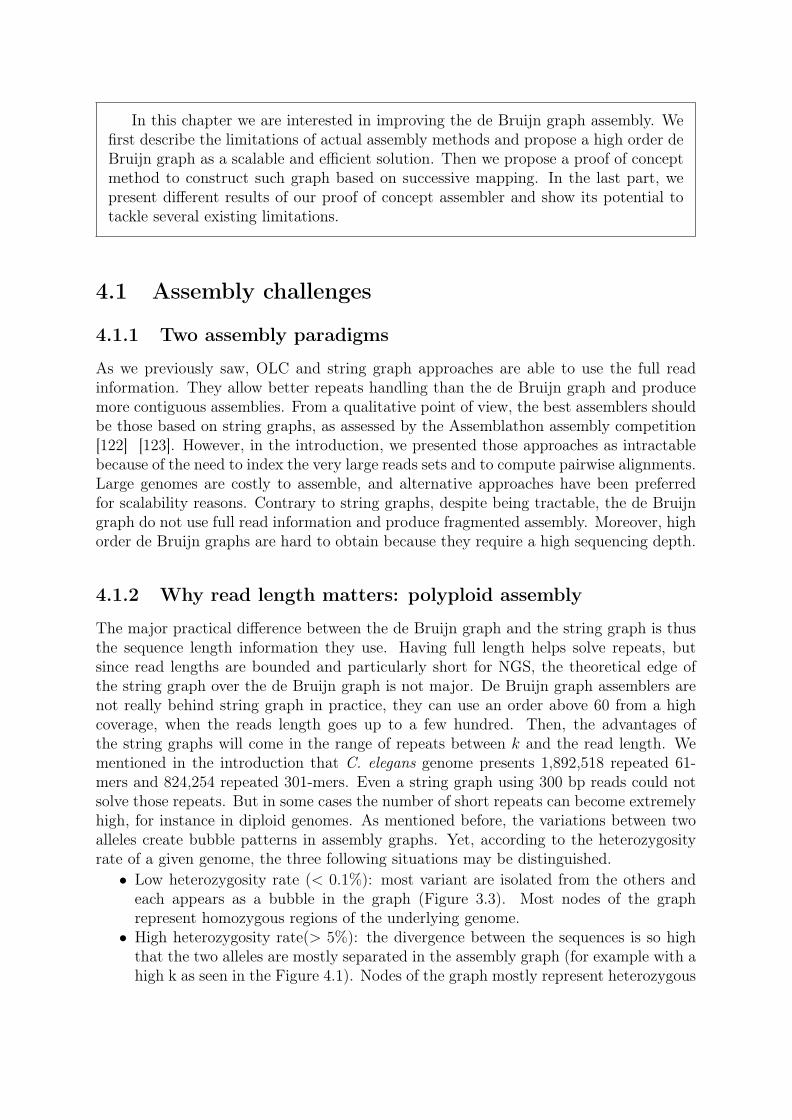
In this chapter we are interested in improving the de Bruijn graph assembly. Wefirst describe the limitations of actual assembly methods and propose a high order deBruijn graph as a scalable and efficient solution. Then we propose a proof of conceptmethod to construct such graph based on successive mapping. In the last part, wepresent different results of our proof of concept assembler and show its potential totackle several existing limitations.

4.1 Assembly challenges

4.1.1 Two assembly paradigms

As we previously saw, OLC and string graph approaches are able to use the full readinformation. They allow better repeats handling than the de Bruijn graph and producemore contiguous assemblies. From a qualitative point of view, the best assemblers shouldbe those based on string graphs, as assessed by the Assemblathon assembly competition[122] [123]. However, in the introduction, we presented those approaches as intractablebecause of the need to index the very large reads sets and to compute pairwise alignments.Large genomes are costly to assemble, and alternative approaches have been preferredfor scalability reasons. Contrary to string graphs, despite being tractable, the de Bruijngraph do not use full read information and produce fragmented assembly. Moreover, highorder de Bruijn graphs are hard to obtain because they require a high sequencing depth.

4.1.2 Why read length matters: polyploid assembly

The major practical difference between the de Bruijn graph and the string graph is thusthe sequence length information they use. Having full length helps solve repeats, butsince read lengths are bounded and particularly short for NGS, the theoretical edge ofthe string graph over the de Bruijn graph is not major. De Bruijn graph assemblers arenot really behind string graph in practice, they can use an order above 60 from a highcoverage, when the reads length goes up to a few hundred. Then, the advantages ofthe string graphs will come in the range of repeats between k and the read length. Wementioned in the introduction that C. elegans genome presents 1,892,518 repeated 61-mers and 824,254 repeated 301-mers. Even a string graph using 300 bp reads could notsolve those repeats. But in some cases the number of short repeats can become extremelyhigh, for instance in diploid genomes. As mentioned before, the variations between twoalleles create bubble patterns in assembly graphs. Yet, according to the heterozygosityrate of a given genome, the three following situations may be distinguished.

• Low heterozygosity rate (< 0.1%): most variant are isolated from the others andeach appears as a bubble in the graph (Figure 3.3). Most nodes of the graphrepresent homozygous regions of the underlying genome.

• High heterozygosity rate(> 5%): the divergence between the sequences is so highthat the two alleles are mostly separated in the assembly graph (for example with ahigh k as seen in the Figure 4.1). Nodes of the graph mostly represent heterozygous

regions, they yield large bubbles that relatively well represent and differentiate thediverging alleles.

• Medium heterozygosity rate (≈ 1%): present a mix of heterozygous and homozy-gous regions that may be difficult to distinguish. It results into complex graphs,hard to produce long contigs in practice.

The heterozygosity rates given are rather orders of magnitude than accurate values (Fig-ures 4.5 and 4.6). Furthermore, these rates are based on the use of hundred of basesNGS reads. If we were able to produce longer reads, we could use a higher k and aheterozygosity rate of 1% would be easier to manage.

Heterozygosity rates vary a lot across species as seen in Figure 4.2 from [124]. Fromour current knowledge, one of the lowest rates is present in Lynx individuals that havea rate of the order of 0.01%, where the heterozygous events are likely to be far apart.On the opposite, in species like C. remanei, with a rate of 5%, the variations should bequite close to each other on average and therefore a large order de Bruijn graph would beable to differentiate two alleles in the heterozygous regions. Most de Bruijn graph assem-blers present a "comfort zone" below the rate of 0.5%, where they are able to producelarge contigs by crushing bubbles. Medium rates (around 1%) result in extremely poorassemblies. As mentioned, very high rates (> 5%) genomes are manageable, although wecurrently count few of them among known assembled species.

4.1.3 Taking the best of both worlds

In any case, haploid or polyploid, the faculty to solve repeats is the key to more contiguousassemblies. Even if this problem is dramatically more frequent in polyploid assembly,enhancing this capacity would positively impact any assembly problem. We explainedthat each presented graph structure shows advantages as well as drawbacks. The questionwe should ask is "What kind of graph structure would we ideally want ?"

Figure 4.1: Example of phased and non-phased variants depending on k. With k = 4 thegraph presents two bubbles, and the assembler has no mean to output phased contigs.With k = 6 the variants are phased and the graph is reduced into a single heterozygousregion of two contigs.

113

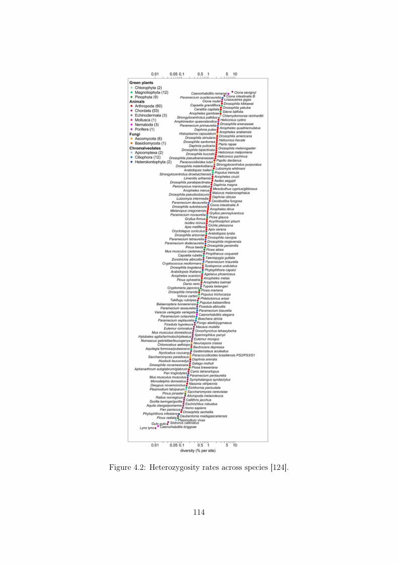
Figure 4.2: Heterozygosity rates across species [124].

114

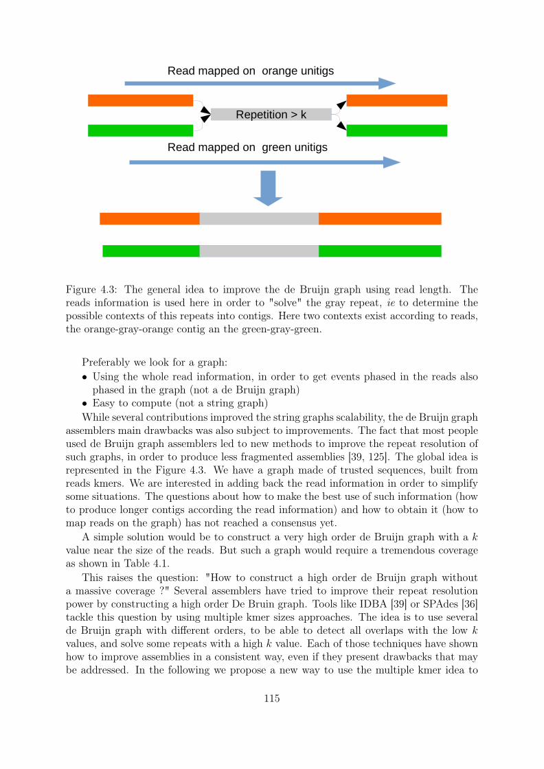
Repetition > k

Read mapped on orange unitigs

Read mapped on green unitigs

Figure 4.3: The general idea to improve the de Bruijn graph using read length. Thereads information is used here in order to "solve" the gray repeat, ie to determine thepossible contexts of this repeats into contigs. Here two contexts exist according to reads,the orange-gray-orange contig an the green-gray-green.

Preferably we look for a graph:• Using the whole read information, in order to get events phased in the reads also

phased in the graph (not a de Bruijn graph)• Easy to compute (not a string graph)While several contributions improved the string graphs scalability, the de Bruijn graph

assemblers main drawbacks was also subject to improvements. The fact that most peopleused de Bruijn graph assemblers led to new methods to improve the repeat resolution ofsuch graphs, in order to produce less fragmented assemblies [39, 125]. The global idea isrepresented in the Figure 4.3. We have a graph made of trusted sequences, built fromreads kmers. We are interested in adding back the read information in order to simplifysome situations. The questions about how to make the best use of such information (howto produce longer contigs according the read information) and how to obtain it (how tomap reads on the graph) has not reached a consensus yet.

A simple solution would be to construct a very high order de Bruijn graph with a kvalue near the size of the reads. But such a graph would require a tremendous coverageas shown in Table 4.1.

This raises the question: "How to construct a high order de Bruijn graph withouta massive coverage ?" Several assemblers have tried to improve their repeat resolutionpower by constructing a high order De Bruin graph. Tools like IDBA [39] or SPAdes [36]tackle this question by using multiple kmer sizes approaches. The idea is to use severalde Bruijn graph with different orders, to be able to detect all overlaps with the low kvalues, and solve some repeats with a high k value. Each of those techniques have shownhow to improve assemblies in a consistent way, even if they present drawbacks that maybe addressed. In the following we propose a new way to use the multiple kmer idea to

115

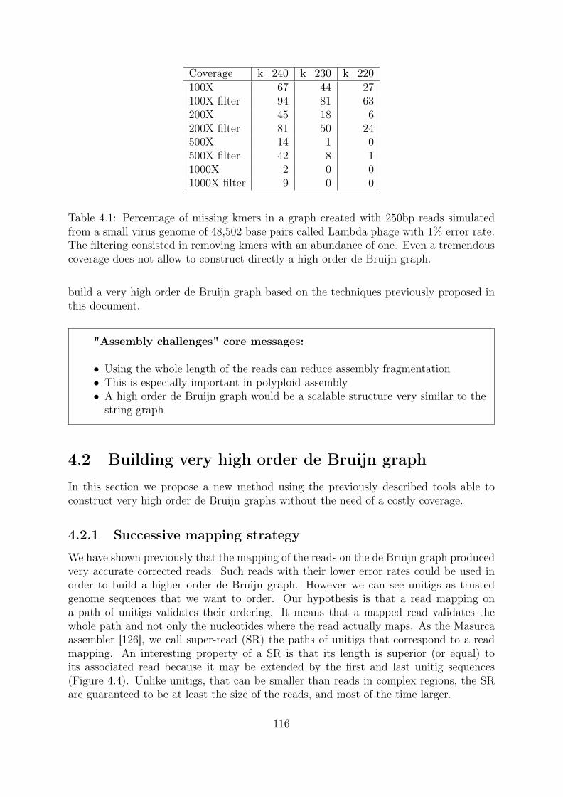
Coverage k=240 k=230 k=220100X 67 44 27100X filter 94 81 63200X 45 18 6200X filter 81 50 24500X 14 1 0500X filter 42 8 11000X 2 0 01000X filter 9 0 0

Table 4.1: Percentage of missing kmers in a graph created with 250bp reads simulatedfrom a small virus genome of 48,502 base pairs called Lambda phage with 1% error rate.The filtering consisted in removing kmers with an abundance of one. Even a tremendouscoverage does not allow to construct directly a high order de Bruijn graph.

build a very high order de Bruijn graph based on the techniques previously proposed inthis document.

"Assembly challenges" core messages:

• Using the whole length of the reads can reduce assembly fragmentation• This is especially important in polyploid assembly• A high order de Bruijn graph would be a scalable structure very similar to the

string graph

4.2 Building very high order de Bruijn graph

In this section we propose a new method using the previously described tools able toconstruct very high order de Bruijn graphs without the need of a costly coverage.

4.2.1 Successive mapping strategy

We have shown previously that the mapping of the reads on the de Bruijn graph producedvery accurate corrected reads. Such reads with their lower error rates could be used inorder to build a higher order de Bruijn graph. However we can see unitigs as trustedgenome sequences that we want to order. Our hypothesis is that a read mapping ona path of unitigs validates their ordering. It means that a mapped read validates thewhole path and not only the nucleotides where the read actually maps. As the Masurcaassembler [126], we call super-read (SR) the paths of unitigs that correspond to a readmapping. An interesting property of a SR is that its length is superior (or equal) toits associated read because it may be extended by the first and last unitig sequences(Figure 4.4). Unlike unitigs, that can be smaller than reads in complex regions, the SRare guaranteed to be at least the size of the reads, and most of the time larger.

116

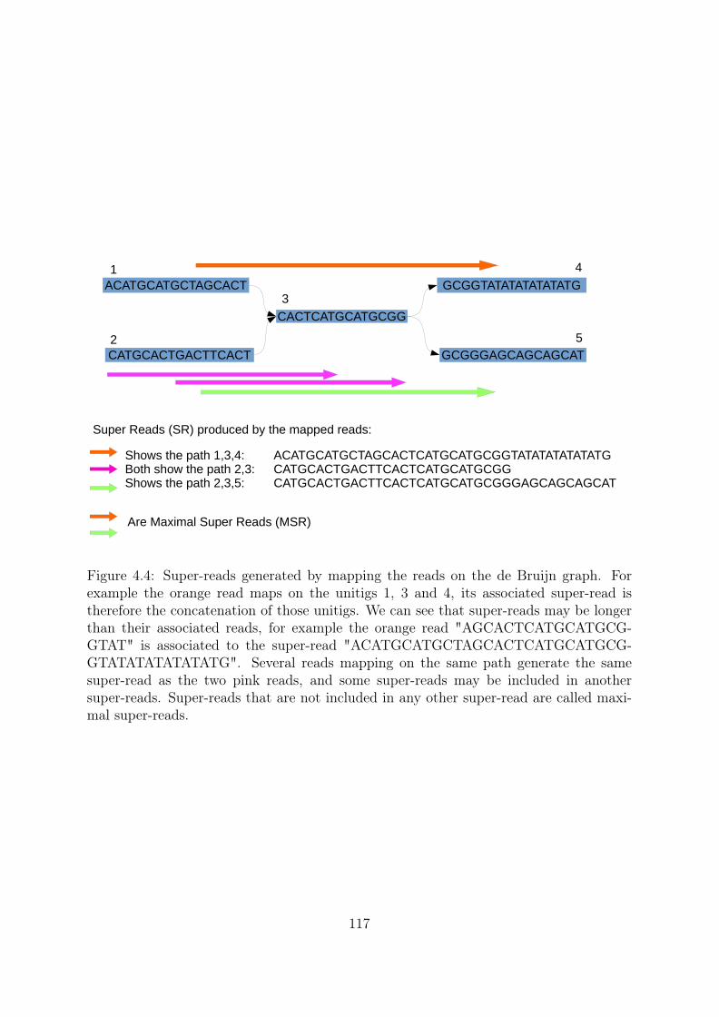
ACATGCATGCTAGCACT

CACTCATGCATGCGG

GCGGTATATATATATATG

GCGGGAGCAGCAGCATCATGCACTGACTTCACT

1

2

3

4

5

Shows the path 1,3,4: ACATGCATGCTAGCACTCATGCATGCGGTATATATATATATG Both show the path 2,3: CATGCACTGACTTCACTCATGCATGCGGShows the path 2,3,5: CATGCACTGACTTCACTCATGCATGCGGGAGCAGCAGCAT

Are Maximal Super Reads (MSR)

Super Reads (SR) produced by the mapped reads:

Figure 4.4: Super-reads generated by mapping the reads on the de Bruijn graph. Forexample the orange read maps on the unitigs 1, 3 and 4, its associated super-read istherefore the concatenation of those unitigs. We can see that super-reads may be longerthan their associated reads, for example the orange read "AGCACTCATGCATGCG-GTAT" is associated to the super-read "ACATGCATGCTAGCACTCATGCATGCG-GTATATATATATATG". Several reads mapping on the same path generate the samesuper-read as the two pink reads, and some super-reads may be included in anothersuper-reads. Super-reads that are not included in any other super-read are called maxi-mal super-reads.

117

...

...Reads:Unitigs:

Super Reads:

Figure 4.5: How the de Bruijn graph unitigs can enlarge the overlaps. In this examplethe two reads in blue share a small overlap. They are mapped on the de Bruijn graphand they both map on the gray unitig. Their SR in purple, enlarged with the unitigsequence, share a larger overlap than their associated reads.

To assess the quality of the SR obtained by mapping on a clean de Bruijn graph weconducted the following experiment.

• Simulation of 100X reads from a reference genome• Read correction with Bloocoo• de Bruijn graph construction with k=51• Tip removal• Read mapping on the graph to generate SR• Duplicates removal from SR• SR mapping on the reference genome

On the E. coli genome 1,642 different SR were obtained, all mapped on the referencegenome with a similarity of 99%. All SR but 5 mapped with a similarity of 100% on thereference. On the C. elegans genome 357,183 different SR were obtained. All SR but 38were mapped on the reference with a similarity of 95%. With a higher similarity of 99%,the number of unmapped SR was only of 260 and all SR but 502 mapped perfectly. Thoseexperiments show that SR are very accurate sequence that can be almost considered asgenome sequences.

Our idea is to use the sequences from such SR in order to produce higher orderde Bruijn graph (Figure 4.9). By constructing a de Bruijn graph from the SR witha augmented k, we obtain a simpler de Bruijn graph than the first one constructed,with longer unitigs, less repeats and less spurious edges. As in the classical multiple kapproaches like IDBA, the interest of starting with a low k is to be able to detect smalloverlaps between reads. Small overlaps are detected with the first value of k and keptin the latter graph with higher k because the overlaps between the SR are larger thanthe overlaps between reads. (Figure 4.5). However, if most of the time the overlapsare enlarged by the unitigs graph, it is possible that the augmented overlap is not largeenough to be kept in the later steps.

We can raise k more gradually in order for the unitigs of the overlaps to be larger,along with the simplification of the graph, to avoid loosing overlaps. Furthermore some

118

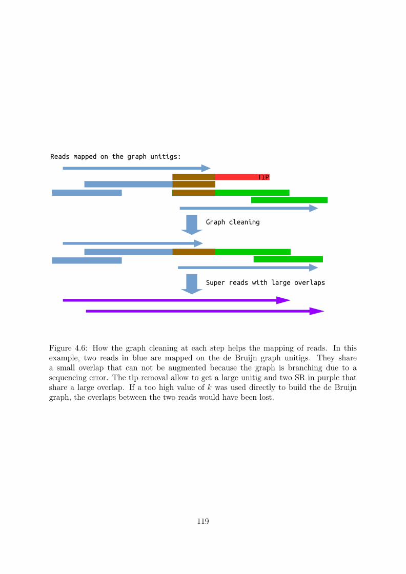
TIP

Graph cleaning

Reads mapped on the graph unitigs:

Super reads with large overlaps

Figure 4.6: How the graph cleaning at each step helps the mapping of reads. In thisexample, two reads in blue are mapped on the de Bruijn graph unitigs. They sharea small overlap that can not be augmented because the graph is branching due to asequencing error. The tip removal allow to get a large unitig and two SR in purple thatshare a large overlap. If a too high value of k was used directly to build the de Bruijngraph, the overlaps between the two reads would have been lost.

119

Using a low k:

Using a high k

Using a low k then a high k

Original situation:Reads A,B,C,Y,Z and the overlaps they share including a repeat in maroon

AA

AB

B

C

Z

Y

C

Z

Y

A

BC

YZ

ABC

YZ

Figure 4.7: This example shows the interest of using several value of k. In this situation,the reads A and B share a small green overlap and the reads B and C share a large onewith the reads Y and Z (in green and orange respectively). However, these overlaps sharea medium repeat in brown. The low k assembly is fragmented because of the repeatbut is able to detect the small overlap. The high k graph is able to avoid the repeatfragmentation but misses the small overlap. The successive construction allows to takeadvantages of both k values.

errors would become tips since the higher the k, the more sequencing errors become tips,so the graph can be cleaned in a better way at each step. Then the removal of such errorswould also allow the generation of more contiguous unitigs, and would help in mappingreads with a higher k as it is shown in Figure 4.6. The Figure 4.7 shows the interestof such an iterative approach. We propose a workflow based on the presented ideas asa proof of concept assembler called BWISE. We give a high level view of the BWISEworkflow and a more detailed version is presented in Figure 4.8.

• Read correction• de Bruijn graph construction• Graph tipping• Read mapping on the de Bruijn graph• Super-Reads selection• Higher de Bruijn graph construction

120

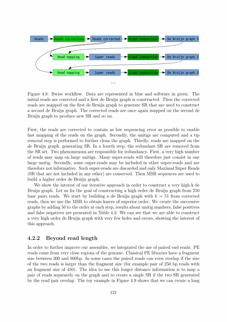
Reads Reads correction Reads corrected Graph compaction De Bruijn graph 1

Read mapping Super reads Graph compaction De Bruijn graph 2

Read mapping Super reads Graph compaction De Bruijn graph 3

...

Figure 4.8: Bwise workflow. Data are represented in blue and software in green. Theinitial reads are corrected and a first de Bruijn graph is constructed. Then the correctedreads are mapped on the first de Bruijn graph to generate SR that are used to constructa second de Bruijn graph. The corrected reads are once again mapped on the second deBruijn graph to produce new SR and so on.

First, the reads are corrected to contain as low sequencing error as possible to enablefast mapping of the reads on the graph. Secondly, the unitigs are computed and a tipremoval step is performed to further clean the graph. Thirdly, reads are mapped on thede Bruijn graph, generating SR. In a fourth step, the redundant SR are removed fromthe SR set. Two phenomenons are responsible for redundancy. First, a very high numberof reads may map on large unitigs. Many super-reads will therefore just consist in onelarge unitig. Secondly, some super-reads may be included in other super-reads and aretherefore not informative. Such super-reads are discarded and only Maximal Super Reads(SR that are not included in any other) are conserved. Then MSR sequences are used tobuild a higher order de Bruijn graph.

We show the interest of our iterative approach in order to construct a very high k deBruijn graph. Let us fix the goal of constructing a high order de Bruijn graph from 250base pairs reads. We start by building a de Bruijn graph with k = 51 from correctedreads, then we use the MSR to obtain kmers of superior order. We create the successivegraphs by adding 50 to the order at each step, results about unitig numbers, false positivesand false negatives are presented in Table 4.2. We can see that we are able to constructa very high order de Bruijn graph with very few holes and errors, showing the interest ofthis approach.

4.2.2 Beyond read length

In order to further improve our assembler, we integrated the use of paired end reads. PEreads come from very close regions of the genome. Classical PE libraries have a fragmentsize between 300 and 800bp. In some cases the paired reads can even overlap if the sizeof the two reads is larger than the fragment size (for example pair of 250 bp reads withan fragment size of 450). The idea to use this longer distance information is to map apair of reads separately on the graph and to create a single SR if the two SR generatedby the read pair overlap. The toy example in Figure 4.9 shows that we can create a long

121

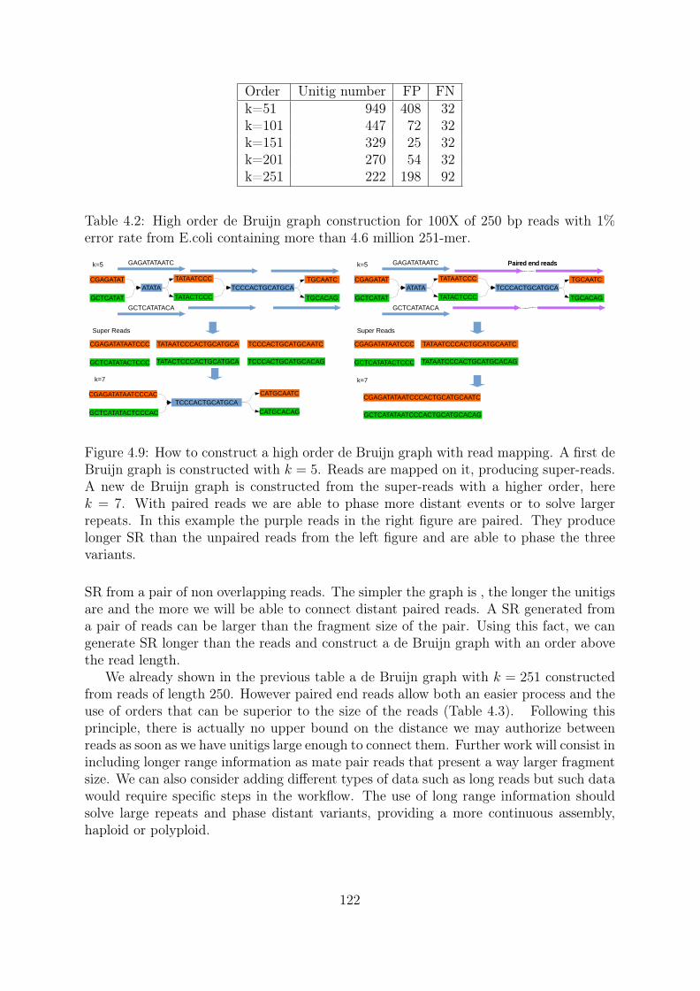
Order Unitig number FP FNk=51 949 408 32k=101 447 72 32k=151 329 25 32k=201 270 54 32k=251 222 198 92

Table 4.2: High order de Bruijn graph construction for 100X of 250 bp reads with 1%error rate from E.coli containing more than 4.6 million 251-mer.

CGAGATATATATA

GCTCATAT

TATAATCCC

TATACTCCC

GAGATATAATC

GCTCATATACA

CGAGATATAATCCC

GCTCATATACTCCC

TCCCACTGCATGCATGCAATC

TGCACAG

TATAATCCCACTGCATGCA

k=5

k=7

Super Reads

TATACTCCCACTGCATGCA

TCCCACTGCATGCAATC

TCCCACTGCATGCACAG

CGAGATATAATCCCACTCCCACTGCATGCA

GCTCATATACTCCCAC

CATGCAATC

CATGCACAG

CGAGATATATATA

GCTCATAT

TATAATCCC

TATACTCCC

GAGATATAATC

GCTCATATACA

CGAGATATAATCCC

GCTCATATACTCCC

TCCCACTGCATGCATGCAATC

TGCACAG

TATAATCCCACTGCATGCAATC

k=5

k=7

Super Reads

Paired end readsPaired end reads

TATAATCCCACTGCATGCACAG

CGAGATATAATCCCACTGCATGCAATC

GCTCATATAATCCCACTGCATGCACAG

Figure 4.9: How to construct a high order de Bruijn graph with read mapping. A first deBruijn graph is constructed with k = 5. Reads are mapped on it, producing super-reads.A new de Bruijn graph is constructed from the super-reads with a higher order, herek = 7. With paired reads we are able to phase more distant events or to solve largerrepeats. In this example the purple reads in the right figure are paired. They producelonger SR than the unpaired reads from the left figure and are able to phase the threevariants.

SR from a pair of non overlapping reads. The simpler the graph is , the longer the unitigsare and the more we will be able to connect distant paired reads. A SR generated froma pair of reads can be larger than the fragment size of the pair. Using this fact, we cangenerate SR longer than the reads and construct a de Bruijn graph with an order abovethe read length.

We already shown in the previous table a de Bruijn graph with k = 251 constructedfrom reads of length 250. However paired end reads allow both an easier process and theuse of orders that can be superior to the size of the reads (Table 4.3). Following thisprinciple, there is actually no upper bound on the distance we may authorize betweenreads as soon as we have unitigs large enough to connect them. Further work will consist inincluding longer range information as mate pair reads that present a way larger fragmentsize. We can also consider adding different types of data such as long reads but such datawould require specific steps in the workflow. The use of long range information shouldsolve large repeats and phase distant variants, providing a more continuous assembly,haploid or polyploid.

122

Order Unitig number FP FNk=51 949 408 32k=101 576 1,208 32k=151 356 341 32k=201 276 125 32k=251 224 210 108k=301 122 67 5,992

Table 4.3: High order de Bruijn graph construction for 100X of 250 bp reads from E.Colicontaining more than 4.6 million 301-mer.

"Building very high order de Bruijn graph" core messages:

• Super Reads created from read mapping can be seen as trusted sequences• Iterative mapping allows the construction of high order de Bruijn graph• Paired end reads allow the construction of a de Bruijn graph with k above the

reads length

4.3 Assembly results

4.3.1 Haploid genome

In Table 4.4 we present some assembly results on various haploid genomes to assess theefficiency of our proposed solution against other assemblers.

We observe that BWISE is able to produce contigs as long as state of the art as-semblers. We also note the scalability of BWISE that successfully performed a humangenome assembly with less than 60 GB of RAM in two days. SPAdes and Platanus were

Assembly #contigs N50 N80E. coli BWISE 56 210,994 126,805E. coliSPAdes 71 178,400 83,005E. coli Platanus 272 133,252 28,361E. coli Minia 309 107,878 40,937C. elegans BWISE 2,527 122,287 56,547C. elegansSPAdes 6,550 103,128 43,904C. elegans Platanus 21,413 52,661 18,330C. elegans Minia 35,317 23,641 6,906Human BWISE 132,272 74,148 29,705Human Minia 884,788 20,202 7,381

Table 4.4: Simulated of 100x datasets on various genomes. Simulated reads are pairedwith 250 base pairs and a fragment size of 800.

123

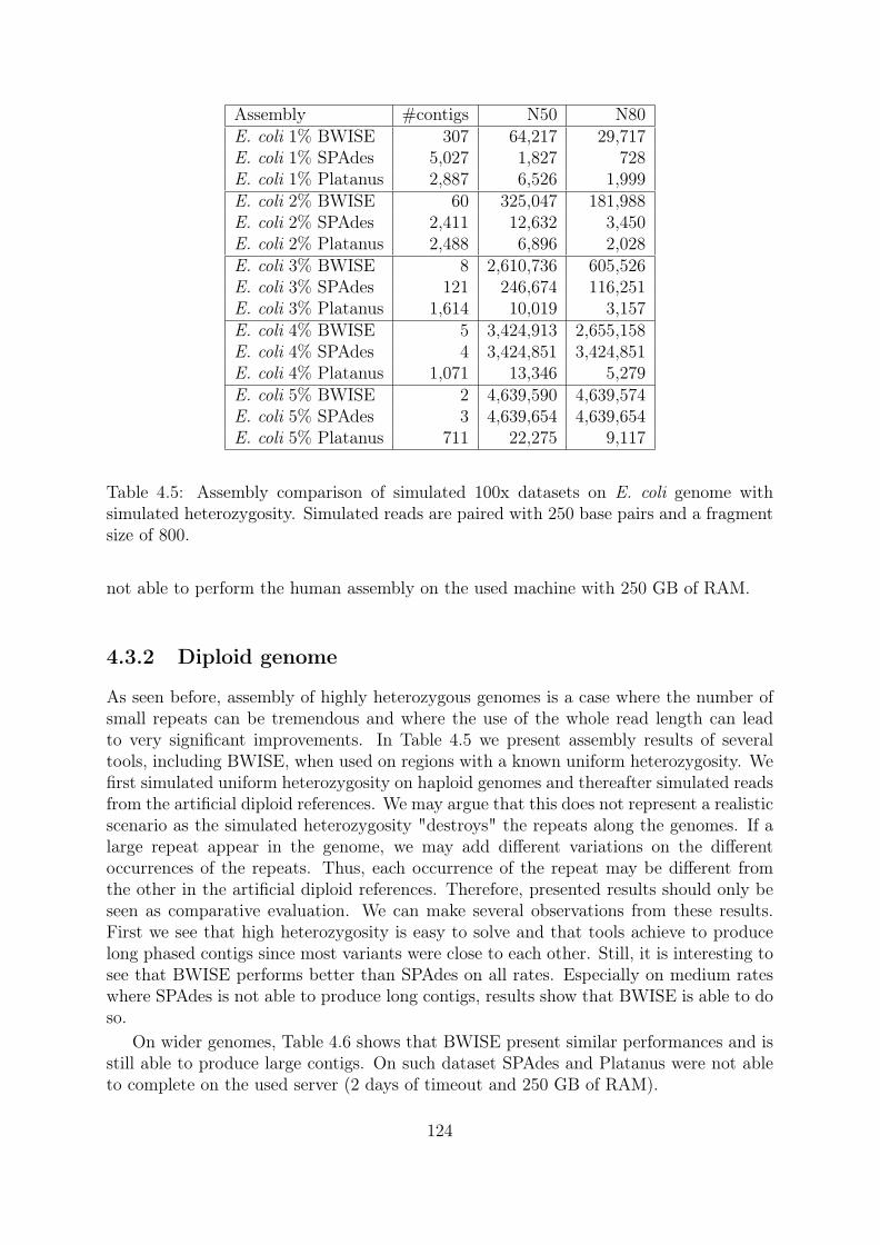
Assembly #contigs N50 N80E. coli 1% BWISE 307 64,217 29,717E. coli 1% SPAdes 5,027 1,827 728E. coli 1% Platanus 2,887 6,526 1,999E. coli 2% BWISE 60 325,047 181,988E. coli 2% SPAdes 2,411 12,632 3,450E. coli 2% Platanus 2,488 6,896 2,028E. coli 3% BWISE 8 2,610,736 605,526E. coli 3% SPAdes 121 246,674 116,251E. coli 3% Platanus 1,614 10,019 3,157E. coli 4% BWISE 5 3,424,913 2,655,158E. coli 4% SPAdes 4 3,424,851 3,424,851E. coli 4% Platanus 1,071 13,346 5,279E. coli 5% BWISE 2 4,639,590 4,639,574E. coli 5% SPAdes 3 4,639,654 4,639,654E. coli 5% Platanus 711 22,275 9,117

Table 4.5: Assembly comparison of simulated 100x datasets on E. coli genome withsimulated heterozygosity. Simulated reads are paired with 250 base pairs and a fragmentsize of 800.

not able to perform the human assembly on the used machine with 250 GB of RAM.

4.3.2 Diploid genome

As seen before, assembly of highly heterozygous genomes is a case where the number ofsmall repeats can be tremendous and where the use of the whole read length can leadto very significant improvements. In Table 4.5 we present assembly results of severaltools, including BWISE, when used on regions with a known uniform heterozygosity. Wefirst simulated uniform heterozygosity on haploid genomes and thereafter simulated readsfrom the artificial diploid references. We may argue that this does not represent a realisticscenario as the simulated heterozygosity "destroys" the repeats along the genomes. If alarge repeat appear in the genome, we may add different variations on the differentoccurrences of the repeats. Thus, each occurrence of the repeat may be different fromthe other in the artificial diploid references. Therefore, presented results should only beseen as comparative evaluation. We can make several observations from these results.First we see that high heterozygosity is easy to solve and that tools achieve to producelong phased contigs since most variants were close to each other. Still, it is interesting tosee that BWISE performs better than SPAdes on all rates. Especially on medium rateswhere SPAdes is not able to produce long contigs, results show that BWISE is able to doso.

On wider genomes, Table 4.6 shows that BWISE present similar performances and isstill able to produce large contigs. On such dataset SPAdes and Platanus were not ableto complete on the used server (2 days of timeout and 250 GB of RAM).

124

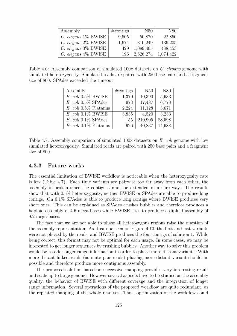
Assembly #contigs N50 N80C. elegans 1% BWISE 9,505 50,870 22,850C. elegans 2% BWISE 1,674 310,249 136,205C. elegans 3% BWISE 429 1,089,405 488,453C. elegans 4% BWISE 196 2,626,274 1,074,422

Table 4.6: Assembly comparison of simulated 100x datasets on C. elegans genome withsimulated heterozygosity. Simulated reads are paired with 250 base pairs and a fragmentsize of 800. SPAdes exceeded the timeout.

Assembly #contigs N50 N80E. coli 0.5% BWISE 1,370 10,390 5,633E. coli 0.5% SPAdes 973 17,487 6,778E. coli 0.5% Platanus 2,224 11,128 3,671E. coli 0.1% BWISE 3,835 4,520 3,233E. coli 0.1% SPAdes 55 210,905 88,598E. coli 0.1% Platanus 926 40,837 14,688

Table 4.7: Assembly comparison of simulated 100x datasets on E. coli genome with lowsimulated heterozygosity. Simulated reads are paired with 250 base pairs and a fragmentsize of 800.

4.3.3 Future works

The essential limitation of BWISE workflow is noticeable when the heterozygosity rateis low (Table 4.7). Each time variants are pairwise too far away from each other, theassembly is broken since the contigs cannot be extended in a sure way. The resultsshow that with 0.5% heterozygosity, neither BWISE or SPAdes are able to produce longcontigs. On 0.1% SPAdes is able to produce long contigs where BWISE produces veryshort ones. This can be explained as SPAdes crushes bubbles and therefore produces ahaploid assembly of 4.6 mega-bases while BWISE tries to produce a diploid assembly of9.2 mega-bases.

The fact that we are not able to phase all heterozygous regions raise the question ofthe assembly representation. As it can be seen on Figure 4.10, the first and last variantswere not phased by the reads, and BWISE produces the four contigs of solution 1. Whilebeing correct, this format may not be optimal for each usage. In some cases, we may beinterested to get longer sequences by crushing bubbles. Another way to solve this problemwould be to add longer range information in order to phase more distant variants. Withmore distant linked reads (as mate pair reads) phasing more distant variant should bepossible and therefore produce more contiguous assembly.

The proposed solution based on successive mapping provides very interesting resultand scale up to large genome. However several aspects have to be studied as the assemblyquality, the behavior of BWISE with different coverage and the integration of longerrange information. Several operations of the proposed workflow are quite redundant, asthe repeated mapping of the whole read set. Thus, optimization of the workflow could

125

Solution 1: output all contigs

Solution 2: Crush small bubbles

Solution 3: Crush small bubbles and extend contigs

Figure 4.10: Potential representations of non phases contigs. The first solution proposedis a bit redundant. To limit the redundancy we can crush the remaining small bubbles asshowed in solution 2. To further improve contigs length we could also extend the contigswith the merged bubbles sequences, as it is done in solution 3.

126

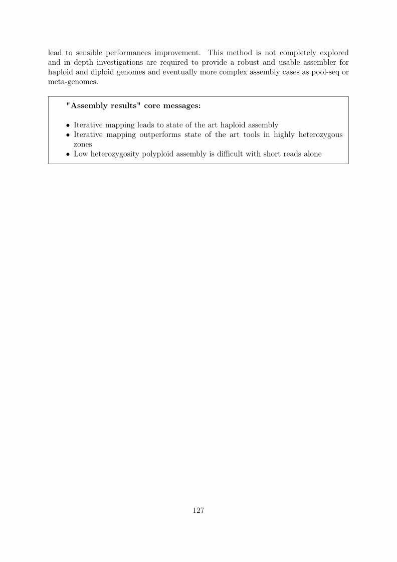
lead to sensible performances improvement. This method is not completely exploredand in depth investigations are required to provide a robust and usable assembler forhaploid and diploid genomes and eventually more complex assembly cases as pool-seq ormeta-genomes.

"Assembly results" core messages:

• Iterative mapping leads to state of the art haploid assembly• Iterative mapping outperforms state of the art tools in highly heterozygous

zones• Low heterozygosity polyploid assembly is difficult with short reads alone

127

128

Chapter 5

Conclusions and perspectives

129

5.1 Conclusion

Two main directions were explored during this thesis. The first aim was to proposenew structures to handle the scaling of de Bruijn graph usages. The second aim was topropose new methods and techniques to no longer consider the de Bruijn graph only asan assembler internal representation but as a proper reference structure that can be usedfor various applications. This part reminds and summarizes our contributions and mainresults toward those objectives.

Several reasons justify the need for the development of efficient data structures ingenome assembly. The assembly of human sized genomes still presents important scala-bility issues, with the need of very important resources. Very large genomes are commonacross the living organisms, especially plant genomes, and efficient assembly methodsfor such genomes are necessary to remove the present locks. The second interest of effi-cients techniques, for any genome, is to democratize the treatments of such datasets andmake their analysis less costly and more accessible. In order to address the large genomeassembly scalability using de Bruijn graphs, we proposed several practical and theoret-ical results. We described a new category of data structure called Navigational DataStructure that enable de Bruijn graph assembly with lower space requirements than thepreviously known bounds. Implementations of such structures could lead to extremelymemory efficient assemblers. We proposed a proof of concept low memory usage assem-bler called DBGFM. The core idea of this method is to index the simple paths (unitigs)of the de Bruijn graph instead of its kmers into a memory efficient data structure, here aFM-index. DBGFM present of very low memory usage and is able to assemble a humangenome with 1.5 GB of RAM. A take-home message is that considering a de Bruijn graphas a set of unitigs is an efficient practical choice. However the construction of such setsin low memory is not trivial. We therefore proposed a new method based on externalmemory to construct this set called BCALM. This method was slow and sequential, andthe construction of the compacted de Bruijn graph was the bottleneck of DBGFM as inmany assemblers. We therefore conceived a efficient and parallel method called BCALM2to compute de Bruijn graph unitigs. BCALM2, relying on external memory present orderof magnitude less memory that known implementation and was also significantly faster.Such a method can lead to a low memory assembly even for genome larger than thehuman one. In BCALM2, and in several other applications, we encountered the chal-lenge of indexing extremely large numbers of object. The need for memory efficient andfast structure lead us to use minimal perfect hash functions (MPHF). Existing MPHFlibrary presented very high memory usage and running time during construction. Thuswe proposed a new scalable MPHF library, designed to construct MPHF from very largekey set with moderate resources called BBHASH. The main property of BBHASH is theability to construct a MPHF without memory overhead, and the construction is alsoparallel and faster than other available implementations. This implementation could beused virtually in any HPC field. We believe that such an efficient data structure couldespecially benefit in numerous applications in bioinformatics, where the need to indexlarge number of objects is fundamental.

The de Bruijn graph is mainly seen as an assembly graph, a simple temporary struc-ture used to generate contigs. If the de Bruijn graph is mainly used for assembly, manyproperties of this structure have been used outside of its first domain of application. For

numerous reasons, the classical representation of a genome into linear sequences is not fit-ted for all application. To cope with these problems, several new genome representationsbased on graph are proposed. If the de Bruijn graph is not an efficient representation forfinished genomes, its properties can be used in advantageous ways in several applications.With efficient techniques to construct a (compacted) de Bruijn graph, we argued that itcould be a good reference to represent one or multiple genomes. We presented differentexamples of the interest of such a representation. The unfinished genomes, where the deBruijn graph may contain more information than the contigs sequences. Heterozygousgenomes, as a de Bruijn graph contain and can represent efficiently the different varia-tions that may be present in such genomes. Very redundant dataset that can be factoredby the efficient representation of the repeated sequences in a de Bruijn graph.

Multiple applications could use such a reference graph directly, as read set comparisonin meta-genomics or mapping read on the de Bruijn graph sequences. Thus, we arguedthat we need a read mapping method working directly on the de Bruijn graph structureto permit its versatile use as a reference. In order to enable the use of such representation,we provided a tool able to map reads efficiently on a de Bruijn graph called BGREAT.Despite the fact that we proved that mapping reads on a de Bruijn graph is a NP-Complete problem, the use of efficient heuristics allows BGREAT to be very efficienton current datasets. We presented several direct advantages of such a method. Resultsconfirm that mapping reads directly on the de Bruijn graph instead of mapping on contigsallows a higher ratio of read mapped, showing the interest of mapping on the de Bruijngraph over mapping on its sequences. We also proved that the de Bruijn graph is avery accurate reference with very few sequencing errors and keeping the heterozygosityinformation. This facts show the de Bruijn graph as a very sound and easy to constructstructure. Using this property, we presented an out of the box usage with the readcorrector BCOOL. Results of the proof of concept read correction by mapping them onthe de Bruijn graph are very interesting. BCOOL corrected several time more errors thanstate of the art correctors on high coverage simulated data. Outside of read correction, webelieve that such a method could be used in very diverse usage of NGS data as assembly,scaffolding, read compression or variant calling.

Applied to genome assembly, the de Bruijn graph is essentially used for its scalability,but the splitting of the reads into kmers fragments the assembly. One of the motiva-tion behind the conception of a tool like BGREAT was to improve the de Bruijn graphassembly continuity. The idea was to map reads on a de Bruijn graph in order to addback the reads information into de Bruijn graph assembly. To use this information, weproposed a new method to build a high order de Bruijn graph using the read length at areasonable cost. The idea is to map reads on the de Bruijn graph and to use the mappedpath sequences to build a de Bruijn graph with a higher order. We implemented thisidea into a proof of concept assembler called BWISE. Similarly to the string graphs, theproduced high order de Bruijn graph are able to use almost the whole length of the readsin order to solve repeats and produce more contiguous assembly than regular de Bruijngraph. We also showed that such an approach could benefit of paired end reads in orderto produce de Bruijn graph with kmer size above the read length. Using those pairedreads information improve the assembly continuity and the size of the contigs withouta scaffolding step as we work directly on the de Bruijn graph. Preliminary results onsimulated data on haploid genomes exhibit assemblies equivalent to state of the art as-

131

semblers. However, the most interesting results of this approach was a good assemblycontinuity in heterozygous regions were state of the art assemblers produce assembly ofvery poor quality. On our simulated data, BWISE is able to produce phased contigs andto assemble separately the different allele where other de Bruijn graph assembler are notable to make the distinction. We believe that the next assemblers will have to proposesuch heterozygosity awareness and that BWISE is a promising approach to do so.

Those results convey the idea that the de Bruijn graph as a data structure has notbeen used yet to the maximum of its potential.

5.2 Proposed methods

This thesis resulted in the following open-source softwares:

BCALM Proof of concept of de Bruijn graph compaction in low memory. BCALM wasused in the DBGFM assembler to compute the unitigs to index and is described in [74].Available https://github.com/Malfoy/BCALM

BCALM2 Efficient and parallel de Bruijn graph compaction in low memory. BCALM2was used for the de Bruijn graph results presented in this document. It is used for thede Bruijn graph compaction before the use of BGREAT2 in BCOOL and BWISE. It isdescribed in [82]. Available https://github.com/GATB/bcalm

BBHASH Scalable minimal perfect hash function construction. BBHASH MPHF isused in BCALM2, GATB and SRC softwares. It is described in [86]. Available https://github.com/rizkg/BBHash

BGREAT Proof of concept of read mapping on de Bruijn graph. It is described in [116].Available https://github.com/Malfoy/BGREAT

BGREAT2 Read mapping on de Bruijn graph. An improved and self contained versionof BGREAT. As said before it is used with BCALM2 in BCOOL and BWISE workflows.The improvements applied are described in chapter 3. Available https://github.com/Malfoy/BGREAT2

BCOOL de Bruijn graph based read correction. This read corrector and its preliminaryresults are presented in chapter 3. Available https://github.com/Malfoy/BCOOL

BWISE High order de Bruijn graph Assembly. This assembler and its preliminaryresults on haploid and diploid genomes are presented in chapter 4. Available https://github.com/Malfoy/BWISE

132

5.3 Future of sequencing

In 2008, the next generation sequencing revolutionized the genomic field. While it ishard to forecast the future of such fast evolving and diverse technologies, we can observeemerging usages of new kinds of data and imagine the potential benefits and challengesthey may bring.

5.3.1 Third generation sequencing

New sequencing technologies are arising. Called third generation sequencing, those tech-nologies propose order of magnitude longer sequences, but currently with a very high errorrate (up to 15% [127]). Both Pacific Bioscience [6] and Oxford Nanopore [7] technologiesare improving and may provide even longer reads with a low error rate in the near future.Those technologies have the potential to be a major shift in genome assembly. Withsuch long sequences, most repeats could be solved and the "one contig one chromosome"dream could be achieved. But those sequences still present huge challenges. Tools haveto deal with the important error rate. To make it worse, the type of error is mainly in-sertions and deletions errors which are harder to deal with than the substitutions usuallyencountered in NGS reads. The costs of such sequencing are currently high compared toNGS, while a high coverage is necessary in order to cope with the error rate. To assemblesuch sequences, the de Bruijn graph is not usable in a straightforward way. The stringgraph is therefore recovering its central place in assembly. But the computational costof such an assembly is going through the roof and many tools have been proposed tomake the overlap detection phase extremely efficient. Two approaches are advocated.The hybrid assembly approaches are based on the assumption that long reads could beused coupled with short reads to produce a high quality assembly in a cost efficient way.Either by correcting long reads with short reads [128] [129], or to scaffold short readscontigs with long reads [130] or assemble long and short reads together directly [131]).The pure assembly approaches [132] argues that long reads alone have the potential toproduce the best assemblies because of their less biased sequencing protocols and thatwe should work on the computational cost of the assemblers.

5.3.2 Long range short reads sequencing

New short reads based technologies are also making an entrance into bioinformatics. The3C protocol [133] could provide read pairs from the same chromosome with no upperbound on the insert size and therefore help phasing and solving repeats with no upperbound of size [51]. The 10X [134] technology provides short reads localized on shortgenome region of size around 10,000 bases. This kind of sequencing has shown greatpotential for phasing since reads from a pack come from the same allele [135] while itseems a priori harder to do so with long reads given their error rates. But for haploidassembly those technologies also great potential for solving repeats while being accuratesequences. The long reads present the advantages of representing a continuous sequenceswhile 10X, like paired reads give sequences separated by holes.

133

5.4 Future of this work and perspectives

The different methods proposed in this documents could be continued in many ways,with refinements, new applications or integrations of other kinds of information. Someperspective considered are presented here.

While assembly of shorts reads is often considered as a well know subject, largegenomes still require tremendous resources. But even for smaller genomes, faster struc-tures and assembly methods will be required for the throughput of assemblers to followthe sequencer one. An efficient assembler, implementing a NDS based on unitigs indexedon a MPHF, could provide a extremely efficient method to work on very large genomeswithout current scalability problems or provide assembly with a very high throughput.

We showed that, beyond assembly, the de Bruijn graph is an extremely efficient datastructure to represent a genome, or a set of genomes, with interesting properties thatcould be used in other fields than assembly. A scalable read corrector providing a veryhigh ratio of perfect read would be a very useful tool for applications as assembly orvariant calling. Our proposed corrector BCOOL could be tuned to adapt to real dataand to different coverage in order to provide almost perfect short reads.

Several other applications of mapping read on a de Bruijn graph can be found asquantification, variant calling or read compression could be proposed in the near future.As the read correction, reads could be mapped on the graph and we could encode theirpath in the de Bruijn graph instead of their sequences in order to compress them. Moredirect usages would be quantification in genomic, meta-genomic or RNA-seq by mappingthe read on a de Bruijn graph and extracting information from the amount of readsmapped on given components of the de Bruijn graph. Simple variant calling have beenshown to be done directly from a de Bruijn graph structure, an interesting perspectivewould be to use the reads mapping on this graph and use this information to capturemore complex cases.

Polyploid assembly is also a widely encountered problem while representing a verysmall part of the literature. We pointed those problems and presented new solutionsand perspectives to address those challenges. BWISE polyploid assembly methods havestill to be tuned to fit to the challenges of the real data but the door to the assembly ofpolyploid genomes is open. The use of paired reads directly on a de Bruijn graph couldalso inspire new scaffolding techniques that are mainly based on read mapping on contigs.The use of other kind of information in order to produce larger contigs is also a naturalprolongation of this work. 10X reads seems a really promising technique to improve thepolyploid assembly of BWISE, as the mapping method does not need important changes.The length of 10X DNA fragments could lead to extremely large and phased contigs.

We essentially talked about polyploid assembly but techniques used by BWISE couldalso be relevant for meta-genomic assembly. The read mapping could help distinguish thedifferent individuals present in a de Bruijn graph as it is used now to separate the differentalleles. To do so we have to address the challenges of heterogeneous coverages that canexist in meta-genomic. Almost the same argumentation could be used for transcriptomeassembly of RNA sequences, an efficient assembler able to use Paired End data couldtackle the combinatorial aspect of RNA assembly.

As BGREAT is able to align short reads on a de Bruijn graph, we are naturallyinterested to adapt our methods to be able to align long reads on a De Bruijn graph.

134

This kind of tool could have, as BGREAT, several applications. The alignment of thelong reads on the de Bruijn graph could be used to correct their errors, or the alignmentinformation could be used to order contigs or unitigs of the de Bruijn graph. Such amethod could also be used in the context of pure long reads assembly as a efficient meanto detect overlap between them. The computational cost of long reads assembly has alsoto be addressed and efficient data structures will be required as well in order to efficientlyassemble the future deluge of such datasets. We believe that with decreasing error ratethe de Bruijn graph could be useful even for pure long reads assembly [136] as the deBruijn graph paths represent easy to compute efficient consensus sequences.

135

136

Bibliography

[1] James D Watson and Francis HC Crick. A structure for deoxyribose nucleic acid.Nature, 171, 2004.

[2] Eric S Lander, Lauren M Linton, Bruce Birren, Chad Nusbaum, Michael C Zody,Jennifer Baldwin, Keri Devon, Ken Dewar, Michael Doyle, William FitzHugh, et al.Initial sequencing and analysis of the human genome. Nature, 409(6822):860–921,2001.

[3] J Craig Venter, Mark D Adams, Eugene W Myers, Peter W Li, Richard J Mural,Granger G Sutton, Hamilton O Smith, Mark Yandell, Cheryl A Evans, Robert AHolt, et al. The sequence of the human genome. science, 291(5507):1304–1351,2001.

[4] Frederick Sanger, Steven Nicklen, and Alan R Coulson. Dna sequencing withchain-terminating inhibitors. Proceedings of the National Academy of Sciences,74(12):5463–5467, 1977.

[5] David R Bentley, Shankar Balasubramanian, Harold P Swerdlow, Geoffrey P Smith,John Milton, Clive G Brown, Kevin P Hall, Dirk J Evers, Colin L Barnes, Helen RBignell, et al. Accurate whole human genome sequencing using reversible terminatorchemistry. nature, 456(7218):53–59, 2008.

[6] John Eid, Adrian Fehr, Jeremy Gray, Khai Luong, John Lyle, Geoff Otto, PaulPeluso, David Rank, Primo Baybayan, Brad Bettman, et al. Real-time dna se-quencing from single polymerase molecules. Science, 323(5910):133–138, 2009.

[7] Andrew H Laszlo, Ian M Derrington, Brian C Ross, Henry Brinkerhoff, AndrewAdey, Ian C Nova, Jonathan M Craig, Kyle W Langford, Jenny Mae Samson, RizaDaza, et al. Decoding long nanopore sequencing reads of natural dna. Naturebiotechnology, 32(8):829–833, 2014.

[8] Daniel Aird, Michael G Ross, Wei-Sheng Chen, Maxwell Danielsson, Timothy Fen-nell, Carsten Russ, David B Jaffe, Chad Nusbaum, and Andreas Gnirke. Analyzingand minimizing pcr amplification bias in illumina sequencing libraries. Genomebiology, 12(2):R18, 2011.

[9] Juliane C Dohm, Claudio Lottaz, Tatiana Borodina, and Heinz Himmelbauer. Sub-stantial biases in ultra-short read data sets from high-throughput dna sequencing.Nucleic acids research, 36(16):e105–e105, 2008.

137

[10] Project Encode. The encode (encyclopedia of dna elements) project. Science,306(5696):636–640, 2004.

[11] Sushmita Roy, Jason Ernst, Peter V Kharchenko, Pouya Kheradpour, NicolasNegre, Matthew L Eaton, Jane M Landolin, Christopher A Bristow, Lijia Ma,Michael F Lin, et al. Identification of functional elements and regulatory circuitsby drosophila modencode. Science, 330(6012):1787–1797, 2010.

[12] Jennifer Harrow, Adam Frankish, Jose M Gonzalez, Electra Tapanari, MarkDiekhans, Felix Kokocinski, Bronwen L Aken, Daniel Barrell, Amonida Zadissa,Stephen Searle, et al. Gencode: the reference human genome annotation for theencode project. Genome research, 22(9):1760–1774, 2012.

[13] Todd J Treangen and Steven L Salzberg. Repetitive dna and next-generationsequencing: computational challenges and solutions. Nature Reviews Genetics,13(1):36–46, 2012.

[14] Jonghwan Kim, Akshay A Bhinge, Xochitl C Morgan, and Vishwanath R Iyer.Mapping dna-protein interactions in large genomes by sequence tag analysis ofgenomic enrichment. Nature Methods, 2(1):47–53, 2005.

[15] David S Johnson, Ali Mortazavi, Richard M Myers, and Barbara Wold. Genome-wide mapping of in vivo protein-dna interactions. Science, 316(5830):1497–1502,2007.

[16] Kari-Jouko Räihä and Esko Ukkonen. The shortest common supersequence problemover binary alphabet is np-complete. Theoretical Computer Science, 16(2):187–198,1981.

[17] Granger G Sutton, Owen White, Mark D Adams, and Anthony R Kerlavage. Tigrassembler: A new tool for assembling large shotgun sequencing projects. GenomeScience and Technology, 1(1):9–19, 1995.

[18] Xiaoqiu Huang and Anup Madan. Cap3: A dna sequence assembly program.Genome research, 9(9):868–877, 1999.

[19] René L Warren, Granger G Sutton, Steven JM Jones, and Robert A Holt. Assem-bling millions of short dna sequences using ssake. Bioinformatics, 23(4):500–501,2007.

[20] William R Jeck, Josephine A Reinhardt, David A Baltrus, Matthew T Hick-enbotham, Vincent Magrini, Elaine R Mardis, Jeffery L Dangl, and Corbin DJones. Extending assembly of short dna sequences to handle error. Bioinformatics,23(21):2942–2944, 2007.

[21] Eugene W Myers, Granger G Sutton, Art L Delcher, Ian M Dew, Dan P Fasulo,Michael J Flanigan, Saul A Kravitz, Clark M Mobarry, Knut HJ Reinert, Karin ARemington, et al. A whole-genome assembly of drosophila. Science, 287(5461):2196–2204, 2000.

138

[22] Stephen F Altschul, Warren Gish, Webb Miller, Eugene W Myers, and David JLipman. Basic local alignment search tool. Journal of molecular biology, 215(3):403–410, 1990.

[23] R Staden. A mew computer method for the storage and manipulation of dna gelreading data. Nucleic Acids Research, 8(16):3673–3694, 1980.

[24] Alexey Gurevich, Vladislav Saveliev, Nikolay Vyahhi, and Glenn Tesler. Quast:quality assessment tool for genome assemblies. Bioinformatics, 29(8):1072–1075,2013.

[25] Eugene W Myers. The fragment assembly string graph. Bioinformatics, 21(suppl2):ii79–ii85, 2005.

[26] Jared T Simpson and Richard Durbin. Efficient construction of an assembly stringgraph using the fm-index. Bioinformatics, 26(12):i367–i373, 2010.

[27] Jared T Simpson and Richard Durbin. Efficient de novo assembly of large genomesusing compressed data structures. Genome research, 22(3):549–556, 2012.

[28] Nicolaas Govert De Bruijn. A combinatorial problem. 1946.

[29] Dmitri Loguinov, Anuj Kumar, Vivek Rai, and Sai Ganesh. Graph-theoretic anal-ysis of structured peer-to-peer systems: routing distances and fault resilience. InProceedings of the 2003 conference on Applications, technologies, architectures, andprotocols for computer communications, pages 395–406. ACM, 2003.

[30] M Frans Kaashoek and David R Karger. Koorde: A simple degree-optimal dis-tributed hash table. In International Workshop on Peer-to-Peer Systems, pages98–107. Springer, 2003.

[31] Pavel A Pevzner, Haixu Tang, and Michael S Waterman. An eulerian path ap-proach to dna fragment assembly. Proceedings of the National Academy of Sciences,98(17):9748–9753, 2001.

[32] Paul Medvedev, Konstantinos Georgiou, Gene Myers, and Michael Brudno. Com-putability of models for sequence assembly. In International Workshop on Algo-rithms in Bioinformatics, pages 289–301. Springer Berlin Heidelberg, 2007.

[33] Daniel R Zerbino and Ewan Birney. Velvet: algorithms for de novo short readassembly using de bruijn graphs. Genome research, 18(5):821–829, 2008.

[34] Rayan Chikhi and Paul Medvedev. Informed and automated k-mer size selectionfor genome assembly. Bioinformatics, page btt310, 2013.

[35] Ruibang Luo, Binghang Liu, Yinlong Xie, Zhenyu Li, Weihua Huang, JianyingYuan, Guangzhu He, Yanxiang Chen, Qi Pan, Yunjie Liu, et al. Soapdenovo2: anempirically improved memory-efficient short-read de novo assembler. Gigascience,1(1):18, 2012.

139

[36] Anton Bankevich, Sergey Nurk, Dmitry Antipov, Alexey A Gurevich, MikhailDvorkin, Alexander S Kulikov, Valery M Lesin, Sergey I Nikolenko, Son Pham,Andrey D Prjibelski, et al. Spades: a new genome assembly algorithm and its appli-cations to single-cell sequencing. Journal of Computational Biology, 19(5):455–477,2012.

[37] Mark J Chaisson and Pavel A Pevzner. Short read fragment assembly of bacterialgenomes. Genome research, 18(2):324–330, 2008.

[38] Jonathan Butler, Iain MacCallum, Michael Kleber, Ilya A Shlyakhter, Matthew KBelmonte, Eric S Lander, Chad Nusbaum, and David B Jaffe. Allpaths: de novoassembly of whole-genome shotgun microreads. Genome research, 18(5):810–820,2008.

[39] Yu Peng, Henry CM Leung, Siu-Ming Yiu, and Francis YL Chin. Idba–a practicaliterative de bruijn graph de novo assembler. In Annual International Conferenceon Research in Computational Molecular Biology, pages 426–440. Springer BerlinHeidelberg, 2010.

[40] Jared T Simpson, Kim Wong, Shaun D Jackman, Jacqueline E Schein, Steven JMJones, and Inanç Birol. Abyss: a parallel assembler for short read sequence data.Genome research, 19(6):1117–1123, 2009.

[41] Ruiqiang Li, Hongmei Zhu, Jue Ruan, Wubin Qian, Xiaodong Fang, Zhongbin Shi,Yingrui Li, Shengting Li, Gao Shan, Karsten Kristiansen, et al. De novo assemblyof human genomes with massively parallel short read sequencing. Genome research,20(2):265–272, 2010.

[42] Sante Gnerre, Iain MacCallum, Dariusz Przybylski, Filipe J Ribeiro, Joshua NBurton, Bruce J Walker, Ted Sharpe, Giles Hall, Terrance P Shea, Sean Sykes,et al. High-quality draft assemblies of mammalian genomes from massively parallelsequence data. Proceedings of the National Academy of Sciences, 108(4):1513–1518,2011.

[43] Thomas Conway, Jeremy Wazny, Andrew Bromage, Justin Zobel, and BryanBeresford-Smith. Gossamer—a resource-efficient de novo assembler. Bioinformat-ics, 28(14):1937–1938, 2012.

[44] Rayan Chikhi and Guillaume Rizk. Space-efficient and exact de bruijn graph rep-resentation based on a bloom filter. In International Workshop on Algorithms inBioinformatics, pages 236–248. Springer, 2012.

[45] Niranjan Nagarajan and Mihai Pop. Parametric complexity of sequence assembly:theory and applications to next generation sequencing. Journal of computationalbiology, 16(7):897–908, 2009.

[46] Mark Chaisson, Pavel Pevzner, and Haixu Tang. Fragment assembly with shortreads. Bioinformatics, 20(13):2067–2074, 2004.

140

[47] Daniel H Huson, Knut Reinert, and Eugene W Myers. The greedy path-mergingalgorithm for contig scaffolding. Journal of the ACM (JACM), 49(5):603–615, 2002.

[48] Marten Boetzer, Christiaan V Henkel, Hans J Jansen, Derek Butler, and Wal-ter Pirovano. Scaffolding pre-assembled contigs using sspace. Bioinformatics,27(4):578–579, 2011.

[49] Marten Boetzer and Walter Pirovano. Toward almost closed genomes with gapfiller.Genome biology, 13(6):1, 2012.

[50] Song Gao, Denis Bertrand, Burton KH Chia, and Niranjan Nagarajan. Opera-lg: Efficient and exact scaffolding of large, repeat-rich eukaryotic genomes withperformance guarantees. Genome biology, 17(1):1, 2016.

[51] Jean-François Flot, Hervé Marie-Nelly, and Romain Koszul. Contact genomics:scaffolding and phasing (meta) genomes using chromosome 3d physical signatures.FEBS letters, 589(20PartA):2966–2974, 2015.

[52] Rei Kajitani, Kouta Toshimoto, Hideki Noguchi, Atsushi Toyoda, YoshitoshiOgura, Miki Okuno, Mitsuru Yabana, Masayuki Harada, Eiji Nagayasu, HaruhikoMaruyama, et al. Efficient de novo assembly of highly heterozygous genomes fromwhole-genome shotgun short reads. Genome research, 24(8):1384–1395, 2014.

[53] Yu Peng, Henry CM Leung, Siu-Ming Yiu, and Francis YL Chin. Meta-idba: a denovo assembler for metagenomic data. Bioinformatics, 27(13):i94–i101, 2011.

[54] Toshiaki Namiki, Tsuyoshi Hachiya, Hideaki Tanaka, and Yasubumi Sakakibara.Metavelvet: an extension of velvet assembler to de novo metagenome assemblyfrom short sequence reads. Nucleic acids research, 40(20):e155–e155, 2012.

[55] Jaume Pellicer, Michael F Fay, and Ilia J Leitch. The largest eukaryotic genome ofthem all? Botanical Journal of the Linnean Society, 164(1):10–15, 2010.

[56] Temple F Smith and Michael S Waterman. Identification of common molecularsubsequences. Journal of molecular biology, 147(1):195–197, 1981.

[57] Serafim Batzoglou, David B Jaffe, Ken Stanley, Jonathan Butler, Sante Gnerre,Evan Mauceli, Bonnie Berger, Jill P Mesirov, and Eric S Lander. Arachne: awhole-genome shotgun assembler. Genome research, 12(1):177–189, 2002.

[58] Paolo Ferragina and Giovanni Manzini. Opportunistic data structures with ap-plications. In Foundations of Computer Science, 2000. Proceedings. 41st AnnualSymposium on, pages 390–398. IEEE, 2000.

[59] Ben Langmead, Cole Trapnell, Mihai Pop, and Steven L Salzberg. Ultrafast andmemory-efficient alignment of short dna sequences to the human genome. Genomebiology, 10(3):1, 2009.

[60] Heng Li and Richard Durbin. Fast and accurate short read alignment with burrows–wheeler transform. Bioinformatics, 25(14):1754–1760, 2009.

141

[61] Inanc Birol, Anthony Raymond, Shaun D Jackman, Stephen Pleasance, RobinCoope, Greg A Taylor, Macaire Man Saint Yuen, Christopher I Keeling, DanaBrand, Benjamin P Vandervalk, et al. Assembling the 20 gb white spruce (piceaglauca) genome from whole-genome shotgun sequencing data. Bioinformatics, pagebtt178, 2013.

[62] Shaun D Jackman, Benjamin P Vandervalk, Hamid Mohamadi, Justin Chu, SarahYeo, S Austin Hammond, Golnaz Jahesh, Hamza Khan, Lauren Coombe, Rene LWarren, et al. Abyss 2.0: Resource-efficient assembly of large genomes using abloom filter. Genome Research, pages gr–214346, 2017.

[63] Thomas C Conway and Andrew J Bromage. Succinct data structures for assemblinglarge genomes. Bioinformatics, 27(4):479–486, 2011.

[64] Daisuke Okanohara and Kunihiko Sadakane. Practical entropy-compressedrank/select dictionary. In Proceedings of the Meeting on Algorithm Engineering& Expermiments, pages 60–70. Society for Industrial and Applied Mathematics,2007.

[65] Guillaume Marçais and Carl Kingsford. A fast, lock-free approach for efficientparallel counting of occurrences of k-mers. Bioinformatics, 27(6):764–770, 2011.

[66] Chris Purcell and Tim Harris. Non-blocking hashtables with open addressing. InInternational Symposium on Distributed Computing, pages 108–121. Springer, 2005.

[67] Guillaume Rizk, Dominique Lavenier, and Rayan Chikhi. Dsk: k-mer countingwith very low memory usage. Bioinformatics, page btt020, 2013.

[68] Sebastian Deorowicz, Marek Kokot, Szymon Grabowski, and Agnieszka Debudaj-Grabysz. Kmc 2: Fast and resource-frugal k-mer counting. Bioinformatics,31(10):1569–1576, 2015.

[69] Chengxi Ye, Zhanshan Sam Ma, Charles H Cannon, Mihai Pop, and W Yu Douglas.Exploiting sparseness in de novo genome assembly. BMC bioinformatics, 13(6):1,2012.

[70] Sara El-Metwally, Magdi Zakaria, and Taher Hamza. Lightassembler: fast andmemory-efficient assembly algorithm for high-throughput sequencing reads. Bioin-formatics, page btw470, 2016.

[71] Jason Pell, Arend Hintze, Rosangela Canino-Koning, Adina Howe, James M Tiedje,and C Titus Brown. Scaling metagenome sequence assembly with probabilistic debruijn graphs. Proceedings of the National Academy of Sciences, 109(33):13272–13277, 2012.

[72] Rayan Chikhi and Guillaume Rizk. Space-efficient and exact de bruijn graph rep-resentation based on a bloom filter. Algorithms for Molecular Biology, 8(1):1, 2013.

[73] Kamil Salikhov, Gustavo Sacomoto, and Gregory Kucherov. Using cascading bloomfilters to improve the memory usage for de brujin graphs. Algorithms for MolecularBiology, 9(1):1, 2014.

142

[74] Rayan Chikhi, Antoine Limasset, Shaun Jackman, Jared T Simpson, and PaulMedvedev. On the representation of de bruijn graphs. In International Conferenceon Research in Computational Molecular Biology, pages 35–55. Springer Interna-tional Publishing, 2014.

[75] Evangelos Georganas, Aydın Buluç, Jarrod Chapman, Steven Hofmeyr, ChaitanyaAluru, Rob Egan, Leonid Oliker, Daniel Rokhsar, and Katherine Yelick. Hipmer:an extreme-scale de novo genome assembler. In Proceedings of the InternationalConference for High Performance Computing, Networking, Storage and Analysis,page 14. ACM, 2015.

[76] Jintao Meng, Bingqiang Wang, Yanjie Wei, Shengzhong Feng, and Pavan Balaji.Swap-assembler: scalable and efficient genome assembly towards thousands of cores.BMC bioinformatics, 15(Suppl 9):S2, 2014.

[77] Jintao Meng, Sangmin Seo, Pavan Balaji, Yanjie Wei, Bingqiang Wang, and Shen-zhong Feng. Swap-assembler 2: Optimization of de novo genome assembler atextreme scale. In Parallel Processing (ICPP), 2016 45th International Conferenceon, pages 195–204. IEEE, 2016.

[78] Michael Burrows and David J Wheeler. A block-sorting lossless data compressionalgorithm. 1994.

[79] Michael Roberts, Wayne Hayes, Brian R Hunt, Stephen M Mount, and James AYorke. Reducing storage requirements for biological sequence comparison. Bioin-formatics, 20(18):3363–3369, 2004.

[80] Steven L Salzberg, Adam M Phillippy, Aleksey Zimin, Daniela Puiu, Tanja Magoc,Sergey Koren, Todd J Treangen, Michael C Schatz, Arthur L Delcher, MichaelRoberts, et al. Gage: A critical evaluation of genome assemblies and assemblyalgorithms. Genome research, 22(3):557–567, 2012.

[81] T. C Conway and A. J Bromage. Succinct data structures for assembling largegenomes. Bioinformatics, 27(4):479, 2011.

[82] Rayan Chikhi, Antoine Limasset, and Paul Medvedev. Compacting de bruijn graphsfrom sequencing data quickly and in low memory. Bioinformatics, 32(12):i201–i208,2016.

[83] Jarrod A Chapman, Isaac Ho, Sirisha Sunkara, Shujun Luo, Gary P Schroth, andDaniel S Rokhsar. Meraculous: de novo genome assembly with short paired-endreads. PloS one, 6(8):e23501, 2011.

[84] Erwan Drezen, Guillaume Rizk, Rayan Chikhi, Charles Deltel, Claire Lemaitre,Pierre Peterlongo, and Dominique Lavenier. Gatb: Genome assembly & analysistool box. Bioinformatics, 30(20):2959–2961, 2014.

[85] Aleksey Zimin, Kristian A Stevens, Marc W Crepeau, Ann Holtz-Morris, MaximKoriabine, Guillaume Marçais, Daniela Puiu, Michael Roberts, Jill L Wegrzyn,

143

Pieter J de Jong, et al. Sequencing and assembly of the 22-gb loblolly pine genome.Genetics, 196(3):875–890, 2014.

[86] Antoine Limasset, Guillaume Rizk, Rayan Chikhi, and Pierre Peterlongo. Fastand scalable minimal perfect hashing for massive key sets. arXiv preprintarXiv:1702.03154, 2017.

[87] Camille Marchet, Antoine Limasset, Lucie Bittner, and Pierre Peterlongo. Aresource-frugal probabilistic dictionary and applications in (meta) genomics. arXivpreprint arXiv:1605.08319, 2016.

[88] Camille Marchet, Lolita Lecompte, Antoine Limasset, Lucie Bittner, and PierrePeterlongo. A resource-frugal probabilistic dictionary and applications in bioinfor-matics. arXiv preprint arXiv:1703.00667, 2017.

[89] Lars Feuk, Andrew R Carson, and Stephen W Scherer. Structural variation in thehuman genome. Nature Reviews Genetics, 7(2):85–97, 2006.

[90] Pierre Peterlongo, Nicolas Schnel, Nadia Pisanti, Marie-France Sagot, and VincentLacroix. Identifying snps without a reference genome by comparing raw reads. InInternational Symposium on String Processing and Information Retrieval, pages147–158. Springer Berlin Heidelberg, 2010.

[91] Jacob F Degner, John C Marioni, Athma A Pai, Joseph K Pickrell, EverlyneNkadori, Yoav Gilad, and Jonathan K Pritchard. Effect of read-mapping biaseson detecting allele-specific expression from rna-sequencing data. Bioinformatics,25(24):3207–3212, 2009.

[92] Débora YC Brandt, Vitor RC Aguiar, Bárbara D Bitarello, Kelly Nunes, JérômeGoudet, and Diogo Meyer. Mapping bias overestimates reference allele frequenciesat the hla genes in the 1000 genomes project phase i data. G3: Genes| Genomes|Genetics, 5(5):931–941, 2015.

[93] Peter H Sudmant, Tobias Rausch, Eugene J Gardner, Robert E Handsaker, AlexejAbyzov, John Huddleston, Yan Zhang, Kai Ye, Goo Jun, Markus Hsi-Yang Fritz,et al. An integrated map of structural variation in 2,504 human genomes. Nature,526(7571):75–81, 2015.

[94] 1000 Genomes Project Consortium et al. A global reference for human geneticvariation. Nature, 526(7571):68–74, 2015.

[95] Agnieszka Danek, Sebastian Deorowicz, and Szymon Grabowski. Indexes of largegenome collections on a pc. PloS one, 9(10):e109384, 2014.

[96] Guillaume Holley, Roland Wittler, and Jens Stoye. Bloom filter trie–a data struc-ture for pan-genome storage. In International Workshop on Algorithms in Bioin-formatics, pages 217–230. Springer, 2015.

[97] Benedict Paten, Adam M Novak, Jordan M Eizenga, and Erik Garrison. Genomegraphs and the evolution of genome inference. bioRxiv, page 101816, 2017.

144

[98] AdamMNovak, Glenn Hickey, Erik Garrison, Sean Blum, Abram Connelly, Alexan-der Dilthey, Jordan Eizenga, MA Saleh Elmohamed, Sally Guthrie, André Kahles,et al. Genome graphs. bioRxiv, page 101378, 2017.

[99] Alexander Dilthey, Charles Cox, Zamin Iqbal, Matthew R Nelson, and Gil McVean.Improved genome inference in the mhc using a population reference graph. Naturegenetics, 47(6):682–688, 2015.

[100] Ngan Nguyen, Glenn Hickey, Daniel R Zerbino, Brian Raney, Dent Earl, Joel Arm-strong, W James Kent, David Haussler, and Benedict Paten. Building a pan-genomereference for a population. Journal of Computational Biology, 22(5):387–401, 2015.

[101] Richard Durbin. Efficient haplotype matching and storage using the positionalburrows–wheeler transform (pbwt). Bioinformatics, 30(9):1266–1272, 2014.

[102] Adam M Novak, Erik Garrison, and Benedict Paten. A graph extension of the po-sitional burrows-wheeler transform and its applications. In International Workshopon Algorithms in Bioinformatics, pages 246–256. Springer, 2016.

[103] Mingjie Wang, Yuzhen Ye, and Haixu Tang. A de bruijn graph approach to thequantification of closely-related genomes in a microbial community. Journal ofComputational Biology, 19(6):814–825, 2012.

[104] Manuel Garber, Manfred G Grabherr, Mitchell Guttman, and Cole Trapnell. Com-putational methods for transcriptome annotation and quantification using rna-seq.Nature methods, 8(6):469–477, 2011.

[105] Bo Liu, Hongzhe Guo, Michael Brudno, and Yadong Wang. debga: read alignmentwith de bruijn graph-based seed and extension. Bioinformatics, page btw371, 2016.

[106] Gaëtan Benoit, Dominique Lavenier, Claire Lemaitre, and Guillaume Rizk.Bloocoo, a memory efficient read corrector. In European Conference on Computa-tional Biology (ECCB), 2014.

[107] Ilya Minkin, Anand Patel, Mikhail Kolmogorov, Nikolay Vyahhi, and Son Pham.Sibelia: a scalable and comprehensive synteny block generation tool for closelyrelated microbial genomes. In International Workshop on Algorithms in Bioinfor-matics, pages 215–229. Springer, 2013.

[108] Shoshana Marcus, Hayan Lee, and Michael C Schatz. Splitmem: a graphical algo-rithm for pan-genome analysis with suffix skips. Bioinformatics, 30(24):3476–3483,2014.

[109] Ilia Minkin, Son Pham, and Paul Medvedev. Twopaco: An efficient algorithm tobuild the compacted de bruijn graph from many complete genomes. Bioinformatics,page btw609, 2016.

[110] Timo Beller and Enno Ohlebusch. Efficient construction of a compressed de bruijngraph for pan-genome analysis. In Annual Symposium on Combinatorial PatternMatching, pages 40–51. Springer, 2015.

145

[111] Hayan Lee and Michael C Schatz. Genomic dark matter: the reliability of short readmapping illustrated by the genome mappability score. Bioinformatics, 28(16):2097–2105, 2012.

[112] Zamin Iqbal, Mario Caccamo, Isaac Turner, Paul Flicek, and Gil McVean. Denovo assembly and genotyping of variants using colored de bruijn graphs. Naturegenetics, 44(2):226–232, 2012.

[113] Gustavo AT Sacomoto, Janice Kielbassa, Rayan Chikhi, Raluca Uricaru, PavlosAntoniou, Marie-France Sagot, Pierre Peterlongo, and Vincent Lacroix. K is s plice:de-novo calling alternative splicing events from rna-seq data. BMC bioinformatics,13(6):S5, 2012.

[114] Son K Pham and Pavel A Pevzner. Drimm-synteny: decomposing genomes intoevolutionary conserved segments. Bioinformatics, 26(20):2509–2516, 2010.

[115] Ben Langmead and Steven L Salzberg. Fast gapped-read alignment with bowtie 2.Nature methods, 9(4):357–359, 2012.

[116] Antoine Limasset, Bastien Cazaux, Eric Rivals, and Pierre Peterlongo. Read map-ping on de bruijn graphs. BMC bioinformatics, 17(1):237, 2016.

[117] Xiao Yang, Sriram P Chockalingam, and Srinivas Aluru. A survey of error-correction methods for next-generation sequencing. Briefings in bioinformatics,14(1):56–66, 2013.

[118] Yongchao Liu, Jan Schröder, and Bertil Schmidt. Musket: a multistage k-mer spectrum-based error corrector for illumina sequence data. Bioinformatics,29(3):308–315, 2013.

[119] Heng Li. Bfc: correcting illumina sequencing errors. Bioinformatics, page btv290,2015.

[120] Li Song, Liliana Florea, and Ben Langmead. Lighter: fast and memory-efficientsequencing error correction without counting. Genome biology, 15(11):509, 2014.

[121] Hamid Mohamadi, Hamza Khan, and Inanc Birol. ntcard: A streaming algorithmfor cardinality estimation in genomics data. Bioinformatics, page btw832, 2017.

[122] Dent Earl, Keith Bradnam, John St John, Aaron Darling, Dawei Lin, Joseph Fass,Hung On Ken Yu, Vince Buffalo, Daniel R Zerbino, Mark Diekhans, et al. As-semblathon 1: a competitive assessment of de novo short read assembly methods.Genome research, 21(12):2224–2241, 2011.

[123] Keith R Bradnam, Joseph N Fass, Anton Alexandrov, Paul Baranay, MichaelBechner, Inanç Birol, Sébastien Boisvert, Jarrod A Chapman, Guillaume Cha-puis, Rayan Chikhi, et al. Assemblathon 2: evaluating de novo methods of genomeassembly in three vertebrate species. GigaScience, 2(1):10, 2013.

146

[124] Ellen M Leffler, Kevin Bullaughey, Daniel R Matute, Wynn KMeyer, Laure Segurel,Aarti Venkat, Peter Andolfatto, and Molly Przeworski. Revisiting an old riddle:what determines genetic diversity levels within species? PLoS Biol, 10(9):e1001388,2012.

[125] Anton Bankevich, Sergey Nurk, Dmitry Antipov, Alexey A. Gurevich, MikhailDvorkin, Alexander S. Kulikov, Valery M. Lesin, Sergey I. Nikolenko, Son K. Pham,Andrey D. Prjibelski, Alex Pyshkin, Alexander Sirotkin, Nikolay Vyahhi, GlennTesler, Max A. Alekseyev, and Pavel A. Pevzner. SPAdes: A new genome assemblyalgorithm and its applications to single-cell sequencing. Journal of ComputationalBiology, 19(5):455–477, 2012.

[126] Aleksey V Zimin, Guillaume Marçais, Daniela Puiu, Michael Roberts, Steven LSalzberg, and James A Yorke. The masurca genome assembler. Bioinformatics,29(21):2669–2677, 2013.

[127] Mark J Chaisson and Glenn Tesler. Mapping single molecule sequencing reads usingbasic local alignment with successive refinement (blasr): application and theory.BMC bioinformatics, 13(1):238, 2012.

[128] Kin Fai Au, Jason G Underwood, Lawrence Lee, and Wing Hung Wong. Improvingpacbio long read accuracy by short read alignment. PloS one, 7(10):e46679, 2012.

[129] Mohammed-Amin Madoui, Stefan Engelen, Corinne Cruaud, Caroline Belser, Lau-rie Bertrand, Adriana Alberti, Arnaud Lemainque, Patrick Wincker, and Jean-MarcAury. Genome assembly using nanopore-guided long and error-free dna reads. BMCgenomics, 16(1):327, 2015.

[130] Marten Boetzer and Walter Pirovano. Sspace-longread: scaffolding bacterial draftgenomes using long read sequence information. BMC bioinformatics, 15(1):211,2014.

[131] Viraj Deshpande, Eric DK Fung, Son Pham, and Vineet Bafna. Cerulean: A hybridassembly using high throughput short and long reads. In International Workshopon Algorithms in Bioinformatics, pages 349–363. Springer Berlin Heidelberg, 2013.

[132] Chen-Shan Chin, David H Alexander, Patrick Marks, Aaron A Klammer, JamesDrake, Cheryl Heiner, Alicia Clum, Alex Copeland, John Huddleston, Evan EEichler, et al. Nonhybrid, finished microbial genome assemblies from long-readsmrt sequencing data. Nature methods, 10(6):563–569, 2013.

[133] Job Dekker, Karsten Rippe, Martijn Dekker, and Nancy Kleckner. Capturing chro-mosome conformation. science, 295(5558):1306–1311, 2002.

[134] Jacob O Kitzman. Haplotypes drop by drop. Nature biotechnology, 34(3):296–298,2016.

[135] Neil I Weisenfeld, Vijay Kumar, Preyas Shah, Deanna Church, and David B Jaffe.Direct determination of diploid genome sequences. bioRxiv, page 070425, 2016.

147

[136] Leena Salmela, Riku Walve, Eric Rivals, and Esko Ukkonen. Accurate self-correction of errors in long reads using de bruijn graphs. Bioinformatics, pagebtw321, 2016.

148