1

STOCHACTIC TOURNAMENT SELECTION FOR CONSTRAINED EVOLUTIONARY OPTIMIZATION

Talaat El Gamel1 and Laura J. Harrell2, Associate Member

Abstract

Handling constraints in Evolutionary Algorithms (EA-) is a challenging issue, as EA couldn’t handle constraints explicitly, and thus developing a heuristic that can guide the search to feasible and good-performing solutions became the topic that got the most interest in EA field in last decades. In a previous work (El Gamel and Harrell, 2002) a Genetic Algorithm (GA) framework was applied for water supply and irrigation canal network operation problem to find an efficient management strategy that can minimize the total water consumed while preventing problems such as water shortage or flooding. The model was applied to a case study in Egypt. In that work, the model couldn’t satisfy all constraints. Therefore, in the current study, different constraint-handling techniques are investigated to improve the GA performance for this problem. The common way to handle constraints in EAs is to incorporate penalty functions into the fitness criterion to degrade the fitness of solutions that violate one or more constraints. Alternative techniques have also been reported in the literature, including multiobjective optimization techniques that treat the constraints in single objective problems as additional objectives (Coello, 2000) and stochastic techniques (Surry and Radcliffe, 1997 and Runarsson and Yao, 2000). This paper investigates the performance of five constraint-handling techniques (four techniques from the literature, and a new proposed technique). Three scenarios of the case study present different levels of the difficulty and different number of constraints are tested. All techniques are tested using two measures (the best solution found in the whole run and the improvement of the solution during the run). A comparison of the performances is made to help providing guidelines for the most promising constraint-handling techniques for EA-based management of water supply and irrigation canal operations and based on the difficulty level of the problem.

Keywords Genetic Algorithms, constraint-handling techniques, stochastic selection

Introduction

The inability of EA to handle constraints explicitly makes it a necessity to use a heuristic to guide the search toward feasible and good-performing solutions. However, this heuristic is affected by many things, including the complexity of the problem to be solved, type of constraints, and number of constraints. In this paper, the performance of various constraint handling techniques will be compared to determine which techniques perform the best for a water supply and irrigation canal network operation problems based on the difficulty of the problem and the number of the constraints (size of the

1 Research Assistance, Water Management Research Institute, Ministry of Water Resources and Irrigation, Egypt; phone (202) 218-9563; elgamalt@yahoo.com & elgamalt@gmail.com 2 Assistant Professor, Department of Civil and Environmental Engineering, Old Dominion University, Kaufman Hall Rm. 135, Norfolk, VA 23529-0241; (757) 683-6052; lharrell@odu.edu

2

network). According to Deb (2001), Michalewicz and Schoenauer (1996), and Michalewicz et al. (2000), most constraint handling techniques which exist in the literature, can be classified into five categories, which are methods based on preserving feasibility of solutions, methods based on penalty functions, methods biasing feasible over infeasible solutions, methods based on decoders, and hybrid methods. In the current study, three penalty functions techniques (static and dynamic) are investigated. These techniques are also related to the third category as they treated once with original tournament selection, and again with tournament selection with superiority of feasible solutions. Other methods are also bias feasible over infeasible solutions including multiobjective and stochastic methods. Penalty functions are by far the most commonly used constraint-handling technique. However, there are no specific regulations, but some guidelines that should be considered (Richardson et al. 1989), for creating penalty functions. There are many approaches to implement penalty functions including static, dynamic, adaptive and self-adaptive penalty functions. Regardless of its widespread use in GAs, penalty functions have main drawbacks including the requirement to fine-tuning and the possibility to be under-penalization or over-penalization (Runarsson and Yao, 2000). In multiobjective techniques, the constraints are treated as objectives; thus, there will be (1+m) objective functions, where (m) is the number of constraints. Thus, the ideal solution X would have ( ) 0=Xfi for mi ≤≤1 and ( ) ( )YfXf = for all FY ∈ . One main approach in multiobjective optimization is to use Pareto-optimal (non-dominated) solutions. Based on Pareto-optimal idea, Srinivas and Deb (1995) and Deb and Goal (2000), presented the Non-Dominated Sorting Genetic Algorithm (NSGA & NSGA-II). The idea of this technique is to rank the strings with Pareto fronts based on non-dominance and the fitness values of all the strings in any front will be the number (rank) of this front. In the last front, and to choose few strings to complete the population, a distance will be used as a way to select these few. Coello (2000) presented another technique that will be presented in details and investigated in the current study. Stochastic techniques were proposed to avoid the fine-tuning required by penalty functions. Among the stochastic methods, Surry and Radcliffe (1997) presented the COMOGA method that combine multiobjective optimization with stochastic selection. Runarsson and Yao (2000) proposed another approach, where all solutions are compared in order to rank them. This comparison is made for N times, and during any time, if there is no change in the ranking, the procedure will stop. The rank is made based on the objective value with probability fp or when both solutions are feasible, otherwise they rank based on constraints violations. They suggested the number of comparisons N to be equal to the population size, and fp to be between 0.4 and 0.5. They used this technique with an evolution strategy. A new stochastic technique is proposed in this study.

Optimization model

The objective of the model is to minimize the consuming water while preventing water shortage at any point in the network, preventing flooding at any point in the network, maintaining stability of the regulators, and preserving an adequate water volume in the network so that the next irrigation period will not be affected. The decisions variables in the model are the gate openings, the boundary conditions upstream of the main canal, and the boundary conditions downstream of each channel in the network.

3

The model formulation for this problem is as follows:

Minimize )........(, 12∑ ∑∑∈ ∈∈

−=NTt NOo

otNTt

t QQz

Subject to: )..........(..........,)( 22tpyty rp ∀∀> )..........(..........,)( 32tpFLtWL pp ∀∀≤

).....(,)()( 42tgMDtDSWLtUSWL ggg ∀∀≤− ).......(..........)( 52RPpRWLtWL pendp ∈∀≥

Where NT is the number of time steps of the flow routing, tQ is the discharge at

the inflow point during time step t, NO is the total number of outflow points, otQ , is the Discharge at the outflow point o during time step t, py is the water depth at point p, ry is the minimum required water depth, and for irrigation, it was considered as zero to just prevent the water shortage, pWL is the water level at point p, pFL is the maximum allowable water level at point p, gUSWL is the upstream water level of regulator g, g DSWL is the downstream water level of regulator g, gMD is the maximum allowable difference between upstream water level and downstream water level for regulator g, RP is the number of points that have required water levels at the end of simulation, pRWL is the Required water level at point p, t is the routing time step, and tend is the time at the end of the flow routing.

Constraint-Handling Techniques

Techniques that are tested in the current study can be categorized to three categories, which are penalty functions techniques, multiobjective optimization techniques, and stochastic techniques. A brief description about each technique is presented here.

1) Additive Static Penalty (ASP)

In this technique, the amount of the violation is multiplied by factors (penalty coefficients), and then added to the objective function. The fitness equation is as follows:

)......(......................................................................)( 11∑=

+=m

iiiVnxfFitness

where iV is the violation of constraint i, and in represents penalty coefficients for different constraints.

2) Multiplicative Static Penalty (MSP)

In this technique, the ratio between the amount of the violation and the total possible violation will be used in the fitness equation, which is defined as follows:

)(......................................................................)( 211

⎟⎟⎠

⎞⎜⎜⎝

⎛+⋅= ∑

=

m

i i

ii TV

nxfFitness

where iT is the maximum possible violation of constraint (i).

4

3) Additive Linear Dynamic Penalty (ALDP)

In this technique, the fitness equation is similar to equation 1, but the coefficients will be calculated based on the current generation, as follows.

)(................................................................................)( 31∑=

+=m

ii

gi VnxfFitness

)........(......................................................................** 4⎟⎠⎞

⎜⎝⎛ +=

Ggnnnn incbasei

gi

Where incbase nn & are coefficients, g is the current generations, and G is the total number of generations.

4) Multiobjective Optimization

This technique, proposed by Coello (2000), sorts the solutions based on their objective values and their violations of the constraints, and assigns fitness values for different solutions based on that sorting. In this technique, a feasible solution will always be superior to infeasible solutions. The procedure of this technique is as follows:

1) The count of all individuals in the current generation is initialized to zero. 2) Each individual will be tested against every other individual in the population

using pair wise comparison. 3) If both individuals are feasible, the count of both will remain unchanged. 4) If one of the individuals is feasible and the other is infeasible, the count of the

infeasible will be increased by one. 5) If both are infeasible and one violates more constraints than the other, the count of

the individual that violates more constraints will increase by one. 6) If both are infeasible, and both violate the same number of constraints, and one

has total amount of violations larger than the other, the count of that one will increase by one.

7) Rank the individuals and make selection based on rank. In this study, the procedure will be modified as follows: 1) The fitness of feasible solutions will be normalized between 0.0 and 1.0, so the

highest fitness value of a feasible solution will be 1.0. This normalized fitness is used as the fitness value for each feasible solution.

2) The fitness of any infeasible solution will be (1 + Count). 3) Binary tournament selection is used.

5) Stochastic Tournament Selection (STS)

This new proposed technique uses binary tournament selection, but instead of selecting based on the fitness value (a combination between the objective and the constraints), it will select based on only one of them. The technique considers the following points:

1) The category (objective values or constraint violations) that has more differences between the two compared solutions has more probability to be the basis of the selection.

2) If the number of feasible solutions is small, more pressure will be added to select based on the constraint violations.

5

3) More pressure will be applied to the category (objective function or constraints) that has less improvement in recent generations to prevent the model from diverging or converging to local optima.

4) The selection will be done stochastically. The technique works as follows: 1) Primary probabilities for both objective and constraints are calculated as follows:

)........(........................................*__

)()( 71OO BF

DiffMaxObjICICPP +−

=

)........(..............................**__

)()( 81 FFBFDiffMaxCons

IVIVPP CC+−

=

Where OPP , CPP are the primary probabilities for the objective and constraints respectively, )(),(),(),( 11 ++ IVIVICIC are the cost and constraint violation values for both individuals in the binary tournament selection, CO BFBF and are the balance factors for both objective and constraints respectively, and FF is the feasibility factor. Balance factors are used to put more pressure for selecting based on the criteria that improved less in the previous generations. These balance factors are calculated as follows:

( )( )( ) ).........(....................

*)()(

. 9

1

01 2

1

2

2

1

2

∑

∑

=

=

−+

+= G

GK

G

GKJ

K

KKAveABS

KAveKAve

BF

Where J refers to the objective functions or the constraints. )(KAve is the average of the objective values or constraints violation ratios during generation K.

1G and 2G refer to the first and last generation to be used in calculating the balance factors. 2G is the generation just before the current generation, and

UGGG −= 21 , where UG is the user-specified number of generations used in calculating the factor.

2) The feasibility factor can have one of the three following values: If one of the individuals is feasible and the other is not, the primary

probability for constraint violation ratios will be multiplied by the following feasibility factor:

)...(........................................solutions feasible ofNumber

Population 10=FF

If there are no feasible solutions, all primary probabilities for constraint violation will be multiplied by Gen , where Gen is the number of the current generation.

Otherwise FF=1.0. 3) Both primary probabilities are normalized to defined the final probabilities as

follows:

6

)......(...................................................................... 11CO

OO PPPP

PPFP

+=

)......(...................................................................... 12CO

CC PPPP

PPFP

+=

4) Based on the final probabilities, one of the categories (cost or constraints violations) is selected stochastically, and the solution that performs better in this category is the winner.

Case Study

An irrigation network in El Monofiya, Egypt is used as a case study to test the various constraint-handling techniques previously described. The entire network serves about 187,320 hectares. The part of the network that is considered in this case study serves about 18,564 hectares. The slope is mild and the flow is sub critical for all channels. A complete description of this network and the suggested scenarios can be found in El Gamel (2004). Three suggested scenarios of the case study are considered. They are different in the number of decisions variables, number of the constraints and in the difficulty to find a feasible solution as a result of some sudden changes in the flow conditions. The first scenario has 19 decision variables (11 initial gate openings and 8 boundaries) and checks about 156000 points at different time steps and for different constraints. There is no any sudden change in the gate openings or boundaries for this scenario. For the second scenario, there are 31 decision variables (19 initial gate openings, 7 gate operations, and 12 boundaries), and the number of points checked at different time steps and for different constraints is around 200000 points. There are few sudden changes in the gate openings and boundaries. For the third scenario, there are 52 decision variables (14 initial gate openings, 18 gate operations, and 20 boundaries), and the number of points checked at different time steps and for different constraints is around 210000 points. There are many sudden changes in the gate openings and boundaries

Results

There are five techniques that are tested in the current study, which are Additive Static Penalty, Multiplicative Static Penalty, Additive Linear Dynamic Penalty, Multiobjective technique, and Stochastic Tournament Selection. The penalty function techniques are tested twice, first with original tournament selection, and second with tournament selection with superiority of feasible solutions (in tables and figures, T term is used to refer to original tournament selection, and F term is used to refer to tournament selection with superiority of feasible solutions). Thus, there are a total of 8 techniques for each scenario. Each of these techniques will be used with five different initial random seed values. For STS, the effect of the previous 10 generations is considered.

Two measures are used to compare different techniques: The best feasible solution obtained during the whole run, and the improvement of the minimum feasible solution during the run. The objective of the second measure is to check if the technique will stop at local optima or if it will keep improving to the end. This measure is defined using the distance from the optimal feasible value, and it is calculated using the following procedure:

7

The best feasible obtained from all runs in the scenario is considered as the global optimum.

For each run, generations are divided into sub-generations, and for each sub-generation, the minimum feasible solution is defined.

The distance from the optimal value is calculated as follows: ( ) )(..................................................

___*)( 13

1∑=

−=

SG

J MGMGMSGJIDFO

Where DFO is the distance from optimal value, SG is the number of sub-generations, SG_M is the minimum value achieved in the sub-generation, and G_M is the global optimal (best value achieved in the scenario). According to the previous equation, the inability to get closer to the global minimum in the later sub-generation is worse that the inability to get closer to it in the early sub-generations.

Four different tests are considered to compare different technique, which are: 1) Best solution achieved by each technique. 2) The best five values and the worst value, regarding both measures, are recorded,

and the technique that produced each of them is noted. 3) Comparing techniques with the same seed value. 4) Means and standard deviations for the 5 runs of each technique, and regarding

both measurements. Test 1

0.0E+00

1.0E+05

2.0E+05

3.0E+05

4.0E+05

5.0E+05

6.0E+05

7.0E+05

Diff

eren

ce b

etw

een

best

sol

utio

ns fo

r m

easu

re 1

(m3 )

5 4

1-T

1-F

2-T

2-F

3-T

3-F

Constraint-handling techniques

Scenario 1Scenario 2Scenario 3

Measure 1

0.0

0.2

0.4

0.6

0.8

1.0

1.2

1.4

1.6

1.8

2.0

Diff

eren

t bet

wee

n be

st s

olut

ions

for

mea

sure

2

5 4

1-T

1-F

2-T

2-F

3-T

3-F

Constraint-handling techniques

Scenario 1Scenario 2Scenario 3

Measure 2

Figure 1: The total water consumed for the best run using each technique, relative to the best run

overall, for each scenario for both measures

From Figures 1 the following points can be noticed: 1) Technique 5 (STS) has the best values for the third scenario, technique 1-T has

the best technique for the second scenario, and technique 3-F has the best technique for the first scenario

2) In general, penalty function techniques work better with original tournament selection in second and third scenario, while working better with tournament selection with superiority of feasible solutions in the first scenario.

3) The differences between techniques in the third scenario are more significant than the differences in the first two scenarios.

4) Technique 1-F is least stable technique between different scenarios, while Technique 4 is most stable technique between different scenarios.

8

Test 2

Table 1 presents the best five techniques and the worst technique for each scenario.

Table 1: Techniques that produce the five best values and the worst value regarding both measurements

First measure Second measure Rank S 1 S 2 S 3 S 1 S 2 S 3 First 3-F 1-T 5 3-F 1-T 5 Second 3-F 1-F 5 1-F 5 5 Third 1-F 5 5 1-F 5 5 Fourth 3-T 5 1-T 4 3-F 4 Fifth 4 1-T 3-T 3-T 1-T 2-T Last 5 1-F 4 5 1-F 1-F

The following points can be noticed from these tables: 1) Consistent with the first test, techniques perform better in the first scenario when

they consider superiority of feasible solutions during the selection, while they perform better in second and third scenarios while they don’t consider it.

2) In the first scenario, techniques 1 and 3 have the best results. It is confirmed that technique 5 (STS) is the best technique in the third scenario, as they got the most of the five best values in both measures. For the second scenario, technique 1 is the least stable (has the best and the worst), while technique 5 is the one that repeated more than one among the best five.

Test 3

Table 2 presents the numbers of times each technique wins compared with other techniques that have the same seed value for both measurements.

Table 2: Number of times each technique wins from runs that have same seed value regarding both measurements

First measure Second measure Method S 1 S 2 S 3 S 1 S 2 S 3 5 0 1 3 0 2 3 4 2 0 1 1 0 1 1-T 0 1 1 1 1 1 1-F 1 1 0 1 0 0 2-T 0 1 0 0 2 0 2-F 0 0 0 1 0 0 3-T 0 1 0 0 0 0 3-F 2 0 0 1 0 0

From the table, it can be noticed that Technique 5 is the best technique for second and

third scenarios. For the first technique, the results are not clear but techniques perform better while using selection with superiority of feasible solution.

9

Test 4

1-T

1-F

2-T

2-F

3-T

3-F

Constraint-handling technique

Mea

n va

lue

(10^

5)

Mean value for different scenarios (Measure 1)

Scenario 1

Scenario 2

Scenario 3

1-T

1-F

2-T

2-F

3-T

3-F

Constraint-handling technique

Scenario 1

Scenario 2

Scenario 3

STD Dev for different scenarios (Measure 1)

STD

Dev

(10^

5)

Figure 2: Mean and standard deviation of the both measures of different scenarios

Figures 2 presents the mean and standard deviation of the difference between the best

value in each scenario and all other values for the five runs of each technique. From these charts, it can be noticed that:

1) Differences for the third scenario is clearer than it for first and second scenarios. Also in general, techniques that use selection with superiority of feasible solution perform better for the first scenario, while they perform worst for second and third scenarios.

2) Technique 5 (STS) has the best mean value and standard division for second and third scenarios. For the first scenario, technique 4 (Multiobjective technique) is the best candidate followed by technique 3-F, while technique 5 is the worst technique.

In summary, it could be concluded that techniques that consider superiority of feasible solutions during the selection, including multiobjective technique, outperform other techniques for the first scenario. The multiobjective technique is the technique that is the most consistent when using different seed values regarding this scenario. For second and third scenarios, technique 5 (STS) outperforms all other techniques in. This is clearer in the third scenario. The performance of STS technique

Considering the results that were displayed in the last part, STS performed well in third scenario, somewhat well in the second scenario, and poorly in the first scenario (the simplest example). An attempt to explain the performance of the technique is presented here. He claim is that the technique works well when its average probabilities (the average of probabilities of all solutions) of objective function value and constraints violations are interacting with each other around the value of 0.5. This is explained in the following paragraph. Figure 5 presents the population average probability of using objective function value and constraints violations as the basis for selection of STS for a specific initial seed value with which the technique performs poorly in the first scenario, and performs well in the third scenario. In the first scenario, and for the first four generations, the probabilities were around 0.5, and

10

constraints probability is higher. After this generation, the objective function value probability increases, and the constraints probability decreases with a diverging pattern. This means the selection is made mainly based on the objective function values without paying enough attention to the constraints violations. For the third scenario, both probabilities are fairly close to 0.5, and they alternate which is smaller and which is higher.

0.0

0.1

0.2

0.3

0.4

0.5

0.6

0.7

0.8

0.9

1.0

1 11 21 31 41 51 61 71 81 91Generation

Prob

abili

ty fo

r sel

ectin

g ba

sed

on c

ost o

r con

stra

ints

vi

olat

ions

Cost probabilityConstraints prrobability

Scenario 1

0.0

0.1

0.2

0.3

0.4

0.5

0.6

0.7

0.8

0.9

1.0

1 11 21 31 41 51 61 71 81 91Generation

Prob

abili

ty fo

r sel

ectin

g ba

sed

on c

ost o

r co

nstr

aint

s vi

olat

ions

Cost probabilityConstraints prrobability

Scenario 3

Figure 5: Average STS probabilities for a specific initial seed value in the first and third

scenarios.

The reason for this could be obtained from Figures 6 and 7. Figure 6 presents the average constraint violations and the ratio of feasible solutions per generation for each of the same two runs. From figure 6, the average constraint violations of the first scenario decreases suddenly and the number of the feasible solutions increases suddenly after a few generations in the first scenario given that the problem is simple, and it is easy to find feasible solutions. In the third scenario, the constraint violations decrease gradually, and number of feasible solutions increases gradually during generations. At the end of the run, third scenario performs better than the first scenario regarding ratio of the feasible solutions.

0.00

0.05

0.10

0.15

0.20

0.25

0.30

0.35

1 11 21 31 41 51 61 71 81 91Generation

Ave

rage

con

stra

ints

vio

latio

n

Scenario 1Scenario 3

0

0.1

0.2

0.3

0.4

0.5

0.6

0.7

1 11 21 31 41 51 61 71 81 91Generation

Rat

io o

f fea

sibl

e so

lutio

ns

Scenario 1Scenario 3

Figure 6: Average constraint violations and the ratio of feasible solutions for scenarios 1 and 3.

The reason is that for easiest problems, when it is easy to find a feasible solution, the

number of solutions that are feasible or close to feasibility increase rapidly in the first generations. So, the constraints balance factor and feasibility factor become small values.

11

Also there is a high probability that both compared solutions are close to each other. So, it is expected that the average probability of constraints violation is small value, and the average probability for cost is high value. As a result of selecting based on the objective function value without paying attention to the constraint violations in the first scenario, the minimum feasible solution doesn’t increase gradually after the first few generations, and it reached the minimum value at generation 4, which is not a good value compared to other runs in the same scenario (Figure 8). In the third scenario, the minimum feasible solution keeps decreasing gradually during generations until the end, and it reaches the minimum value at generation 94, which is a good value compared to other runs in the scenario.

1.70E+07

1.75E+07

1.80E+07

1.85E+07

1.90E+07

1.95E+07

1 11 21 31 41 51 61 71 81 91Generation

Tota

l wat

er c

onsu

med

(m3 )

Average feasible fitnessMinimum feasible fitnessScenario 1

2.20E+07

2.30E+07

2.40E+07

2.50E+07

2.60E+07

2.70E+07

1 11 21 31 41 51 61 71 81 91Generation

Tota

l wat

er c

onsu

med

(m3 )

Average feasible fitnessMinimum feasible fitnessScenario 3

Figure 8: Minimum and average feasible solutions for first and third scenarios

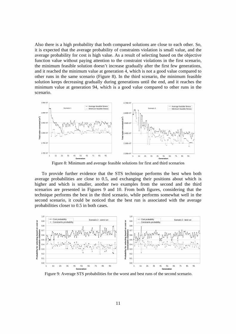
To provide further evidence that the STS technique performs the best when both

average probabilities are close to 0.5, and exchanging their positions about which is higher and which is smaller, another two examples from the second and the third scenarios are presented in Figures 9 and 10. From both figures, considering that the technique performs the best in the third scenario, while performs somewhat well in the second scenario, it could be noticed that the best run is associated with the average probabilities closer to 0.5 in both cases.

0.0

0.1

0.2

0.3

0.4

0.5

0.6

0.7

0.8

0.9

1.0

1 11 21 31 41 51 61 71 81 91Generation

Prob

abili

ty fo

r sel

ectin

g ba

sed

on c

ost o

r co

nstr

aint

s vi

olat

ions

Cost probabilityConstraints prrobability

Scenario 2 - worst run

0.0

0.1

0.2

0.3

0.4

0.5

0.6

0.7

0.8

0.9

1.0

1 11 21 31 41 51 61 71 81 91Generation

Prob

abili

ty fo

r sel

ectin

g ba

sed

on c

ost o

r co

nstr

aint

s vi

olat

ions

Cost probabilityConstraints prrobability

Scenario 2 - best run

Figure 9: Average STS probabilities for the worst and best runs of the second scenario.

12

0.0

0.1

0.2

0.3

0.4

0.5

0.6

0.7

0.8

0.9

1.0

1 11 21 31 41 51 61 71 81 91Generation

Prob

abili

ty fo

r sel

ectin

g ba

sed

on c

ost o

r co

nstr

aint

s vi

olat

ions

Cost probabilityConstraints prrobability

Scenario 3 - worst run

0.0

0.1

0.2

0.3

0.4

0.5

0.6

0.7

0.8

0.9

1.0

1 11 21 31 41 51 61 71 81 91Generation

Prob

abili

ty fo

r sel

ectin

g ba

sed

on c

ost o

r con

stra

ints

vi

olat

ions

Cost probabilityConstraints prrobability

Scenario 3 - best run

Figure 10: Average STS probabilities for the worst and best runs of the third scenario.

Conclusions and future work

Five different constraint-handling techniques were tested within water supply and irrigation canal network operation problem to check the most suitable technique that should be used with such problems based on the difficultly level of the problem. From the results, it could be noticed that techniques perform differently according to difficulty level of the problem. For simpler problems with relatively few decision variables, such as the first scenario, the multiobjective technique and penalty techniques that support superiority of feasible solutions perform better. Among these solutions, multiobjective seems to be the most consistent. It has the smallest standard deviation using different seed values, and since it does not require any fine-tuning, it is the most recommended technique for such cases of the model. For harder scenarios with many decision variables, such as the second and third scenarios, STS (Stochastic tournament selection) and penalty techniques that don’t support superiority of feasible solutions during selection perform better. STS outperforms other techniques in the their scenario. It is suggested that STS perform better when the average probabilities of objective function value and constraints violations are interacting and changing their position around 0.5. This suggestion could be used to check the quality of STS results when there are no other results to check with. As a future work, STS method should be tested with different type of problems to check its ability to handle the constraints in different situations, and to maintaining the balance between the probabilities for the constraints and the cost at different problems.

References

Coello, C. A. C., "Constraint-Handling Using an Evolutionary Multiobjective optimization Technique," Civil Engineering and Environmental Systems, Vol. 17, pp. 319-346, 2000.

Deb, K. and Goel, T., "Controlled Elitist Non-dominated Sorting Genetic Algorithm for Better Convergence" KanGAL Report No. 200004, 2000

Deb, K., Multi-objective optimization using evolutionary algorithms, John Wiley & Sons, Ltd, 2001

13

Michalewicz, Z., and Schoenauer, M. “Evolutionary Algorithms for Constrained Parameter Optimization Problems” Evolutionary Computation Journal vol. 4, No 1, 1996, pp. 1-32

Michalewicz, Z., Deb, K., Schmidt, M., and Stidsen, T., “Test-Case Generator for Nonlinear Continuous Parameter Optimization Techniques” IEEE Transactions on Evolutionary Computation Vol. 4, No 3, 2000, pp. 197-215

Richardson, J. T., Palmer, M. R., Liepins, G., and Hilliard, M. “Some Guidelines for Genetic Algorithms with Penalty Function”, proceedings of the third international Conference on Genetic Algorithms, 1989, pp. 191-197

Runarsson, T. P., and X. Yao, “Stochastic Ranking for Constrained Evolutionary Optimization,” IEEE Transactions on Evolutionary Computation, Vol. 4, SEP 2000, pp. 284-294

Srinivas, N. and Deb, K., “Multiobjective function optimization using nondominated sorting genetic algorithms”, Evolutionary Computation Journal, Vol. 2, No 3, 1995, pp. 221—248

Surry P.D., and Radcliffe, N.J., “The COMOGA method: Constrained Optimization by Multiobjective Genetic Algorithms” Control and Cybernetics, Vol. 26, No 3, 1997