NEUROMORPHIC INFORMATION TECHNOLOGY, GRADUATE CENTER NEUROMORF INFORMÁCIÓS TECHNOLÓGIA,...

ANALOGICAL AND NEURAL COMPUTING LABORATORYCOMPUTER AND AUTOMATION INSTITUTE

HUNGARIAN ACADEMY OF SCIENCES

RECEPTIVE FIELD ATLAS OF THE RETINOTOPICVISUAL PATHWAY AND SOME OTHER SENSORYORGANS USING DYNAMIC CELLULAR NEURAL

NETWORK MODELS

EDITORS: J. HÁMORI AND T. ROSKA

DNS-8-2000

BUDAPEST

NEUROMORPHIC INFORMATION TECHNOLOGY,

GRADUATE CENTER

NEUROMORF INFORMÁCIÓS TECHNOLÓGIA,

POSZTGRADUÁLIS MŰHELY

Receptive Field ATLAS of the Retinotopic VISUAL PATHWAY

and some other SENSORY ORGANS using Dynamic

CELLULAR NEURAL NETWORK

Models

Editors: J. Hámori and T. Roska

Contributing: D. Bálya, Zs. Borostyánkői, M. Brendel, V. Gál, J. Hámori, K. Lotz,

L. Négyessy, L. Orzó, I. Petrás, Cs. Rekeczky, T. Roska, J. Takács, P. Venetiáner, Z.

Vidnyánszky, Á Zarándy

retina

LGN

visual cortex

This work is based on the cooperation of four laboratories:

Analogical and Neural Computing Laboratory (T. Roska, Budapest)

Nonlinear Electronics Laboratory (L.O. Chua, Berkeley)

Neurobiology Research Unit (J. Hámori, Budapest)

Vision Research Laboratory (F. Werblin, Berkeley)

- 2 -

Receptive Field Atlas

1 INTRODUCTION (J. HÁMORI, T. ROSKA)....................................................................... 6

2 MORPHOLOGICAL AND PHYSIOLOGICAL DATA IN THE VISUAL SYSTEM... 7

2.1 INTRODUCTION(J. TAKÁCS, ZS. BOROSTYÁNKŐI) ........................................................................7

2.2 RETINA (J. TAKÁCS, ZS. BOROSTYÁNKŐI) ...................................................................................8

2.3 THALAMUS (J. TAKÁCS, ZS. BOROSTYÁNKŐI) .............................................................................9

2.4 VISUAL CORTEX (J. TAKÁCS, ZS. BOROSTYÁNKŐI)....................................................................11

2.4.1 Structure and function of the visual cortex .........................................................................12

2.5 SPATIAL CHARACTERISTICS (L. ORZÓ, CS. REKECZKY) .............................................................16

2.6 TEMPORAL CHARACTERISTICS (L. ORZÓ, CS. REKECZKY) .........................................................16

2.7 UNIQUENESS OF SPATIOTEMPORAL CHARACTERISTICS (T. ROSKA) ............................................16

2.8 MODELING WITH RECEPTIVE FIELD INTERACTION PROTOTYPES (T. ROSKA) .............................19

3 CNN MODELS IN THE VISUAL PATHWAY IN SPACE AND TIME ....................... 27

3.1 BASIC COMPARATIVE NOTIONS (TABLE), ELEMENTARY EFFECTS (K. LOTZ)...............................27

3.2 SINGLE NEURON MODELS AND PROTOTYPE EFFECTS (V. GÁL)....................................................31

3.2.1 Models of the neuron (I): analytical/theoretical approach ................................................313.2.1.1 The steady state of the neurons ..................................................................................................................................... 31

3.2.1.1.1 Distribution of the ions........................................................................................................................................... 32

3.2.1.1.2 The ‘Resting Potential’ .......................................................................................................................................... 33

3.2.1.2 Passive electrotonic effects: modeling the dendritic tree .............................................................................................. 34

3.2.1.2.1 Equivalent circuit representation............................................................................................................................ 34

3.2.1.2.2 Cable theory ........................................................................................................................................................... 35

3.2.1.2.3 Reduction of the dendritic tree: Rall-model ........................................................................................................... 36

3.2.1.3 Hodgkin-Huxley nonlinearities: modeling the soma..................................................................................................... 37

3.2.1.3.1 Action potential formation ..................................................................................................................................... 39

3.2.1.4 Propagating action potentials via axons........................................................................................................................ 41

3.2.1.5 Synaptic mechanisms.................................................................................................................................................... 41

3.2.2 Models of the neuron (II): compartment (discrete) models ................................................423.2.2.1 Single-compartment model ........................................................................................................................................... 43

3.2.2.2 Two-compartment model.............................................................................................................................................. 44

3.2.3 Highly nonlinear effects ......................................................................................................463.2.3.1 Band-filtering................................................................................................................................................................ 46

3.2.3.2 ‘Post-inhibitory rebound’.............................................................................................................................................. 47

3.2.3.3 Switching between firing-modes .................................................................................................................................. 48

3.3 RETINAL CELLS’ RECEPTIVE FIELD (CS. REKECZKY, K. LOTZ, L. ORZÓ, D. BÁLYA).................50

- 3 -

3.3.1.1 Cones, Horizontal cells’ RF.......................................................................................................................................... 51

3.3.1.1.1 Simple model of the horizontal cells ................................................................................................................... 52

3.3.1.1.2 Detailed neuromorf model of the horizontal cell’s dynamics ........................................................................... 53

3.3.1.2 Bipolar cells’ RF........................................................................................................................................................... 55

3.3.1.2.1 Simple model of the bipolar cells ........................................................................................................................ 55

3.3.1.2.2 Detailed neuromorf model of the outer retinal cells .......................................................................................... 57

3.3.1.2.3 Bipolar terminal simulation ................................................................................................................................ 58

3.3.1.3 Amacrine cells’ RF (Cs. Rekeczky).............................................................................................................................. 58

3.3.1.3.1 NFA ....................................................................................................................................................................... 59

3.3.1.3.2 Inner plexiform layer (bipolar cells - amacrine cells - ganglion cells).............................................................. 60

3.3.1.3.3 Design and Qualitative Analysis of the Wide-field Activity Model .................................................................. 62

3.3.1.4 Ganglion cells’ RF........................................................................................................................................................ 67

3.3.1.4.1 Ganglion cells’ spiking model (K. Lotz) ............................................................................................................. 69

3.3.1.4.2 Receptive fields of ganglion cells (center and antagonistic surround) ............................................................. 70

3.3.1.4.3 Simplified models ................................................................................................................................................. 71

3.4 THALAMIC CELLS’ RECEPTIVE FIELD PROPERTIES

(J. TAKÁCS, L. NÉGYESSY, Z. VIDNYÁNSZKY, P. VENETIÁNER, L. ORZÓ)..........................................81

3.4.1 CS RF spiking models .........................................................................................................81

3.4.2 Lagged cells’ RF .................................................................................................................91

3.5 CORTICAL CELLS’ RF (K. LOTZ, L. ORZÓ) ................................................................................91

3.5.1 Cortical Simple cells ...........................................................................................................913.5.1.1 Orientation sensitivity................................................................................................................................................... 92

3.5.1.2 Direction sensitivity...................................................................................................................................................... 94

3.5.1.2.1 Triadic synapse ...................................................................................................................................................... 94

3.5.1.2.2 Direction selective neural connection scheme ....................................................................................................... 95

3.5.1.2.3 Dynamic receptive field structure of the direction sensitive cortical simple cells .................................................. 97

3.5.1.3 Length tuning................................................................................................................................................................ 98

3.5.1.4 Edge enhancement ........................................................................................................................................................ 99

3.5.1.5 'Extraclassical' receptive fields (inhibitory-excitatory network of the cortical architecture) (M. Brendel) .................102

3.5.1.5.1 Psychophysical evidence......................................................................................................................................102

3.5.1.5.2 Model ...................................................................................................................................................................103

3.5.1.5.3 The two layer CNN model ...................................................................................................................................103

3.5.1.5.4 Results..................................................................................................................................................................104

3.6 INFEROTEMPORAL RF (K. LOTZ)..............................................................................................106

3.6.1 Mouth detection in color pictures - on face and on pepper ..............................................106

3.7 COLOR PROCESSING (Á. ZARÁNDY)..........................................................................................113

3.7.1 Single opponent and double opponent cells......................................................................113

3.7.2 Land’s Experiments...........................................................................................................1163.7.2.1 The structure of Land’s retinex model ........................................................................................................................117

3.7.2.2 Horn’s model for determining lightness .....................................................................................................................118

- 4 -

3.7.2.3 Land’s 1D continuous space method for determining lightness..................................................................................118

3.7.2.4 Horn’s 2D method for determining lightness..............................................................................................................119

3.7.3 The CNN implementation of Horn’s model.......................................................................120

3.7.4 A CNN based neuromorphic lightness determination method..........................................122

3.8 VISUAL ILLUSIONS (K. LOTZ, L. ORZÓ, Á ZARÁNDY) .............................................................127

3.8.1 Bottom up Illusions ...........................................................................................................1273.8.1.1 Center – Surround effects ...........................................................................................................................................127

3.8.1.1.1 Brightness illusions ..............................................................................................................................................127

3.8.1.1.2 Mach Bands .........................................................................................................................................................127

3.8.1.1.3 Müller-Lyer ..........................................................................................................................................................128

3.8.1.1.4 Café wall ..............................................................................................................................................................131

3.8.1.2 Distortion illusions......................................................................................................................................................132

3.8.1.3 Endpoint sensitivity (L. Orzó) ....................................................................................................................................135

3.8.2 Top down Illusions............................................................................................................1383.8.2.1 Face vase.....................................................................................................................................................................138

3.8.2.2 Sculpture illusion ........................................................................................................................................................139

3.9 PLASTICITY OF RECEPTIVE FIELDS (ZS. BOROSTYÁNKŐI) ........................................................141

4 SOMATOSENSORY RECEPTIVE FIELDS (L. NÉGYESSY AND I. PETRÁS)........ 142

4.1 GENERAL OVERVIEW ................................................................................................................142

4.2 HYPERACUITY ..........................................................................................................................143

4.2.1 Two-point discrimination..................................................................................................143

4.2.2 Representational plasticity................................................................................................143

4.2.3 Use/experience dependent RF modifications....................................................................144

4.3 CNN APPLICATIONS .................................................................................................................145

4.3.1 Two-point discrimination in neural networks...................................................................145

5 AUDITORY SYSTEM (K. LOTZ) .................................................................................... 154

5.1 HYPERACUITY IN TIME..............................................................................................................154

5.2 EXPERIMENTS WITH SIMULATED AND REAL-WORLD DATA........................................................163

6 SOME PROBABLE FUNCTION OF THE RFS ............................................................ 170

6.1 NOISE FILTERING IN THE VISUAL SYSTEM (L. ORZÓ) ................................................................170

6.1.1 Introduction.......................................................................................................................170

6.1.2 Method ..............................................................................................................................1706.1.2.1 Nonlinear outputs........................................................................................................................................................173

6.1.2.2 Reconstruction error ...................................................................................................................................................173

- 5 -

6.1.2.3 Invertable mapping .....................................................................................................................................................173

6.1.2.4 Invertable mapping effects on noise filtering..............................................................................................................174

6.1.3 Conclusion ........................................................................................................................176

6.2 BINDING PROBLEM (L. ORZÓ) ..................................................................................................177

6.2.1 Method ..............................................................................................................................178

6.2.2 Results ...............................................................................................................................183

7 APPENDICES .................................................................................................................... 187

7.1 APPENDIX A: A SINGLE NEURON COMPARTMENTAL MODEL SIMULATOR (GENESIS) (V. GÁL)

187

7.1.1 The GEneral NEural SImulation System. (GENESIS) ......................................................187

7.1.2 Structure of GENESIS.......................................................................................................187Copyright Notice ..........................................................................................................................................................................189

7.2 APPENDIX B: RECEPTIVE FIELD NETWORK CALCULUS (REFINE-C) SIMULATOR (D. BÁLYA).190

7.2.1 Understanding the Refine-C model design .......................................................................190

7.2.2 User interface basics.........................................................................................................190

7.2.3 Working with Refine-C......................................................................................................191

7.2.4 One of the advanced function in Refine-C ........................................................................192

- 6 -

1

2 Introduction

Since 1990, we have been working on modeling the visual and somatosensory pathways. This

multidisciplinary research of our laboratories, engineers and physicist in information technology, as well

as medical doctors and neurobiologists in brain research was a challenge for all of us. Fortunately, we

found a powerful modeling paradigm (the Cellular Neural Network, or CNN), dedicated researchers and

excellent cooperating partners.

This report contains mainly the modeling results. It shows that practically all the functionalities we

studied could be modeled in a neuromorphic way, by a receptive field calculus, defined on the analogic

cellular computer architecture (called CNN Universal Machine – CNN-UM).

This way all the results are directly applicable in artificial vision and in various forms in a visual

microprocessor (based on CNN).

The whole task is enormous. During the ten years, we learned how many special questions are waiting

for answers.

In addition to the modeling results, we have developed a modeling tool called REFINE-C as a special

version of the CANDY simulator1.

The support of the Hungarian Academy of Sciences in the Analogical and Neural computing Laboratory

(in MTA SZTAKI, Budapest) and the Neurobiology Research Unit (in MTA-SOTE EKSZ, Budapest),

the National Research Fund of Hungary (OTKA), the Office of Naval Research (US) the National

Science Foundation (US) and the ESPRIT Program (EU) are gratefully acknowledged.

The publications cited at the end of the chapters are containing the original results. The chapters and

sections are written by those indicated in the table of contents, simply writing a tutorial exposition of the

original results.

1 REFINE-C is available via our web site. Its companion, the GENESIS program for compartmental

modeling of neurons, is referred as well.

- 7 -

3 Morphological and physiological data in the visual system

1.1 Introduction

The basic function of the visual system is to provide the central nervous system the representation of the

external visible world. This function is taking place along the visual neuraxis via ascending and

descending mechanism. Ascending mechanism begin with the activity of the peripheral photoreceptors

in the retina, transducing the light (photon) signals into neural (electrical and neurochemical) activity

through populations of interneurons, interposed between them and retinal ganglion cells. The weak

signal (a single photon) can be greatly amplified through biochemical cascade mechanisms.

Visual signals are relayed to higher levels along the visual neuraxis in spatial order, in the form of

multiple (retinotopic) maps generated by retinal ganglion cells, providing and maintaining a division of

labor. During the processing of sensory maps considerable convergence and divergence is taking place.

In the visual system - similar to other sensory systems - parallel paths exist to handle separate modalities

(form, motion, color, stereopsis etc.).

The axons of the retinal ganglion cells (the optic nerve) cross in the midline (optic chiasm), prior

reaching the specific thalamic “visual nucleus” (LGN). In primates there is a complete hemidecussation:

nasal fibers do cross, and temporal ones do not. In the visual system of primates the decussation is

incomplete, at about half the axons project to the ipsilateral side of the thalamus. Besides carrying visual

information, the thalamus is not merely a simple relay station, but further processing is also taking place

at this level, under the control of cortical feed-back and other (secondary visual pathway) mechanisms.

Axons of the LGN innervate abundantly the primary - and partly the secondary - visual cortical areas,

maintaining the precise topographic map of the sensory periphery. Cortical nerve cells are organized into

0,5-1,0 mm wide regions, referred as columns. There is a clear anatomical correlate of columns in the

primary visual cortex of primates and some carnivores, alternating these regions dominated by the left

and right retinas. Each ocular dominance column contains neurons driven exclusively or predominantly

by one eye. Other properties such as the selectivity for the orientation of the visual stimulus and the

contrast center-surround differences are also arranged and “handled” by columns. This anatomical and

functional principle can be followed up to higher (association) visual cortical areas too. Areas of the

sensory cerebral cortex communicate each other in the same, and in the contralateral hemisphere, and,

also send axons to those nuclei in the thalamus and brainstem that provide ascending sensory

information. One of the main roles of this descending control is likely the focusing of sensory stimuli.

Higher areas can be arranged into additional or novel parallel paths, like the visuomotor and the

- 8 -

visuosensory functions and territories. At the highest levels of processing the cerebral cortex extracts

from the world the different qualities that we experience as visual perception.

3.2 Retina

The retina is the first “station” in the visual sensation, where the absorption of the light is taking place in

the photoreceptors, which is the beginning of the transformation of photo-quantum into electrical

signals. There are two specialized photoreceptor cells in the retina: the rods and the cones. In the retina

of the cat the number of rods overtakes the number of cones: in the central part the number of rods is

about ten times higher (density value: 275 x 103/mm2) in comparison to the number of cones (showing a

figure of 27 x 103/mm2 density). In the human retina there are about 92 x 106 rods (average density

94.85 x 103/mm2) and 4.6 x 106 cones (average density 4.62 x 103/mm2), however, in the fovea centralis

the density of cones proved to be as high as 199 x 103/mm2. (The approximate diameter of the human

fovea centralis is 0.35 mm, i.e. about 20000 cones, where rods are missing!) The highest density of rods

in the human retina is 176 x 103/mm2. The shortest distance between cones is 0.51-0.57 arc min and

between rods is 0.45-0.50 arc min. The photo-receptors are connected by electric junctions. Between

cones there is an effective connection at a distance of 100-120 µm, whereas between rods this value is

about 50 um in the photoreceptor layer.

The signals from the photoreceptors are received by two populations of the interneurons in the retina, the

bipolar cells and the horizontal cells. The “information” is processed via a similar route in the

vertebrates: receptor cells ---- bipolar cells ---- ganglion cells. (The horizontal cells could represent an

alternative route from the photoreceptor cells to the bipolar cells, building up a considerable feedback to

the photoreceptors). The horizontal cells (in the outer plexiform layer) and the amacrine cells (in the

inner plexiform layer) provide - first of all - the lateral connections. In the vertebrates the visual

information from the retina is delivered to higher levels of the visual neuraxis by the retinal ganglion

cells in the form of action potentials (spikes). Similarly to the bipolar cells, the retinal ganglion cells

could respond to the light stimulus by “ON” (depolarization) or “OFF” (hyperpolarization) showing

“center-surround” receptive field characteristics. On the basis of these characteristics and spatial

summation “X” (beta) “Y” (alpha) and “W” (gamma) types of retinal ganglion cell can be

distinguished. These neuronal cell types could be differentiated on the basis of their dendritic

morphology: the size of the dendritic arborization is significantly larger of the “Y” in comparison to the

“X” type cells. In the cat, at about 50 % of all retinal ganglion cells belong to X and 10 % to Y types. In

other species their number (and ratio) changes: in the monkey retina there are about 1 million X (P)

and/or Y (M) type ganglion cells, which corresponds to about 90% of all the ganglion cells. X type

cells give longer answer to permanent stimuli, showing a maximum at about 10 Hz frequency of stimuli,

- 9 -

and do not respond to stimuli characterized by frequency above 20-30 Hz. Y type retinal ganglion cells

respond to shorter stimuli, having a maximum at 20 Hz, and respond also at higher (up to 60-80 Hz)

stimulus frequency. Besides “temporal” differentiation of the Y type cells, most of the X type cells play

role in the processing of chromatic information (spectral differentiation). At about 93 % of these cells

show red/green center-surround type answer, while about 7 % of this population have yellow/blue center

surround characteristics. It is interesting, that the size of dendritic arbor of both type ganglion cells

increases with the excentricity, and at the periphery of the retina the size of the “anatomical” and

“physiological” receptive fields is about the same. There is also an overlapping in the receptive fields of

the retinal ganglion cells. As far as the X type neurons concerns, in the fovea 2 ganglion cells (one ON

and one OFF type) represent the smallest “sampling channel”, while at the periphery 3-5 overlapping X

type cells build up a channel. This measure of overlapping could be as high as 10 (or even higher) in

case of the Y type retinal ganglion cells. (The functional significance of the above mentioned

characteristics is the peripheral detection of the fast movements in the retina, and, at the same time, the

fovea centralis could deal with the processing of the fine details).

3.3 Thalamus

The axons of the retinal ganglion cells (nervus opticus) after decussating partially (chiasma opticum)

travel together in the optic tract, and innervate the ipsi- and contralateral specific visual thalamic nucleus

(lateral geniculate nucleus, LGN) in about equal ratio. In the cat, the LGN is built up three main laminae.

The principal A1 and A layers receive input from the ipsilateral and contralateral retinas, respectively.

The targeted relay neurons in these laminae are similar to the retinal X or Y ganglion cells, which

innervate them, and are also called X or Y type cells. The X-axon terminals innervate mainly the A and

A1 laminae, while Y-axon terminals innervate the A and C laminae, the latter is ventral to layers A and

A1. Cells that correspond to the W pathway (known as W cells) in the cat are found exclusively in the C

laminae. In the cat LGN the average size of the soma and the morphology of dendritic arbor of X and Y

type relay cells is different: The X cells are smaller (average 219 µm2), having a smaller dendritic arbor

(and receptive field!) and this arbor is located within the lamina and show a perpendicular orientation

within the lamina. These cells are responding better to visual stimuli of higher spatial frequency. Y type

relay cells are larger (average soma size 490 µm2) the thickness and size of their dendritic arbor is also

larger, the dendritic tree is more or less spherical in shape, which can be spread over laminar borders.

The thickness of their axons (and speed of velocity) is also higher in comparison to the X cell axons. Y

type relay cells give of frequently collaterals, first of all to the perigeniculate (reticular thalamic)

nucleus, and within the LGN also. In the cat visual thalamic nucleus one retinal X-type axon innervate

- 10 -

(minimum) 4-5 X-type relay cells, and one retinal Y-axon innervate about 20-30 thalamic Y-type relay

cells.

The visual thalamic nucleus of the primates (and also the human LGN) consist of 6 laminae: the 4

parvocellular layers, which are found dorsally and receive retinal P-cell input in alternating order from

the contra- and ipsilateral eyes. The two magnocellular layers receiving retinal M-cell input from the

ipsi- and contralateral eyes are positioned more ventrally. Between these principal laminae are placed

the so-called “intercalated” layers, targeted by koniocellular neurons. In the monkey (Macaque) the

LGN has an average dorso-ventral size of 7-9 mm, and lateral measure of 9-10mm. The thalamic

representation of the fovea centralis is found on the dorsal pole, while the peripheral parts of the retina is

represented ventrally in the LGN. The retinal superior quadrant is represented laterally, while the

inferior quadrant medially. The numerical density of neurons is relative constant in the magnocellular

laminae (21 x 103 cell/mm3) but changes in large scale (between 27-60 x103 neurons/mm3) in the

parvocellular laminae. The absolute number of neurons in the monkey LGN changes between 1.1-1.6 x

106: In average, 1.3 x 106 neuron, from which 1.0-1.2 x 106 cells can be found in the parvocellular, and

about 0.14-0.3 x 106 cells in the magnocellular laminae. In the monkey the number of retinal ganglion

cells and the number of neurons in the thalamic visual relay nucleus is approximately the same. (At the

same time, the number of nerve cells in the visual cortical areas significantly higher!)

Besides the relay neurons, there are local interneurons in the thalamic visual nucleus too, which

represent about 20-23% (cat, monkey) of all nerve cells. The connections of this neuronal population can

be found within the LGN, and, they are GABAergic, inhibitory cells. (There is another significant

inhibitory input to the LGN from the reticular thalamic nucleus (perigeniculate nucleus, PGN), which

can be found located around the LGN, and built up exclusively inhibitory (GABAergic) neurons.

As far as the innervation of the visual thalamic cells concerns, only about 20% of the axons comes from

the retina (at the same time, the proportion of axons with non-retinal origin is about 80%). A massive

innervation arrives in the LGN from the VIth layer of the primary and secondary visual cortical areas

(area 17, 18 and 19). Approximately 50-60% of the whole cortical “output” projects to the visual

thalamus, and each relay cell receives (excitatory) input from at least 10 cortical pyramidal cells,

providing a significant convergence. Cortical axons innervate the GABAergic interneurons in the LGN,

and the inhibitory PGN neurons too, providing a massive feed-back inhibition. There is a significant

input to the LGN via the brainstem reticular formation. There are at least three different “component” of

this innervation: i/ noradrenergic fibers arising from the locus coeruleus, ii/ serotonergic axons from the

dorsal raphe nucleus, and iii/ cholinergic fibers arriving from the parabrachial nucleus (in cat). The

functional role of these innervations could be a direct (inhibitory or excitatory) effect on the relay cells

- 11 -

as well as on the interneurons, and non-synaptic modulation of the excitability of the nerve cells in the

thalamic relay station (by changing their membrane permeability to Ca++ and K+).

The synaptology of the LGN (cat): The retinal axons are larger in size, and build up the “RLP”

terminals, characterized by round, large synaptic vesicles and by pale (moderately electron dense)

mitochondria. RLP terminals end mainly on proximal dendritic branches or processes, relatively near to

the cell body of the relay cells (and also of interneurons). These axons are excitatory, and their

neurotransmitter is the glutamate. From the visual cortical areas, the feedback connection is maintained

by “RSD” terminals, which are small, contain also round synaptic vesicles and dark (electron dense)

mitochondria. They synapse either on thin, distal dendritic branches of relay cells or on “intermediate”

dendrites (at about 50-150 µm distance from the soma) and also on the dendrites of interneurons. These

axons are also glutamatergic (excitatory) ones. In the LGN there are also axonal endings containing flat

or pleomorph synaptic vesicles, the “F” terminals, which can be divided into (at least) two groups: F1

and F2 terminals. The F1 terminals are the axonal endings arriving from the PGN neurons and/or from

the local interneurons (both are GABAergic). The F2 terminals are the presynaptic dendritic processes of

the local interneurons, located frequently near to the retinal (RLP) terminals, and taking part in the

formation of the complex synaptic arrangement in the LGN, the synaptic glomerulus. In the cat visual

thalamus, an “average” X-type relay cell receives about 4.000, while a Y-type cell about 5.000 synaptic

input. The significant difference between X and Y type relay cells is, that the RLP terminals targeting X

cells are always taking part the formation of synaptic triadic formation (together with F type presynaptic

dendrites of interneurons). Whereas the retinal axons targeting Y-type relay cells do not take part in the

formation of triadic arrangements. Another difference is, that F1 terminals synapsing on Y cells are

found in higher number, than that synapsing on X type relay neurons. Consequently, the type of

inhibition on X relay neurons is first of all a “feed-forward” inhibition, and arrives from the interneurons

of the LGN. On the Y cells, the “feed-back” type inhibition is dominant, and originates from the PGN

neurons.

3.4 Visual cortex

Visual information is transmitted to the visual cortex along parallel, labeled paths. Parallel paths

maintain a kind of division of labor. A number of maps generated from retinal ganglion cells can be

found in the visual system of higher mammals, e.g. the six separate laminae in the LGN in the thalamus.

Visual entities like color and form are transmitted and processed via separate channels separate from that

which handles three-dimensional features of motion and stereopsis. Retinotopic maps are well preserved

at each level of the retino-geniculo-cortical paths. The morphological basis of these maps is the strictly

positioned topographic pattern of neurons at each level, communicating each other along the neuraxis.

- 12 -

Lateral mechanisms of processing are also found at all levels, maintaining an integrated activity of

smaller or larger groups of neurons. The most common mechanism of this is the center-surround

activation-inhibition, to enhance spatial or chromatic contrast. Along the visual neuraxis is widespread a

considerable synthesis of different, simpler inputs to reconstruct more complex features of stimuli. In the

visual system several non-primary areas are involved in visuomotor functions, described as separate

“streams”, e.g. one is responsible for driving appropriate eye movements and the other dealing with the

tasks of visual perception.

3.4.1 Structure and function of the visual cortex

Axons from the thalamic visual nucleus (LGN) relay to the primary visual cortex (in the cat Brodmans’s

area 17, in primates V1), called also striate cortex, because of the strongly myelinated sublamina within

layer 4. The LGN receives segregated inputs from the two eyes, these binocular inputs arrive to both

hemispheres. Inputs from the left and right retinas arrive in alternating order and built up 0,5-1,0 mm

wide cortical columns (called ocular dominance columns) each of that contains cells driven exclusively

or predominantly by one eye. Neurons within a cortical column have similar receptive field

characteristics, such as orientation selectivity and receptive field location.

Areas of the primary visual cortex communicate with other (higher) cortical areas but also send axons

back to subcortical regions throughout the neuraxis. The number of corticothalamic axons considerably

exceeds the number of ascending sensory axons, permitting to control the activity of those neurons,

which relay information to the cortex. In this way a “tuning” of the ascending visual input can be

achieved, by strengthening a group of cortically “selected” signals.

In the cat primary visual cortex Hubel and Wiesel described two broad classes of neurons, simple cells

and complex cells. Simple cells respond to an oriented stimulus of a specific configuration and a specific

location, and have separate “on” and “off” subregions. Complex cells also respond to stimuli at one

orientation, but their receptive field is not segregated into on and off subregions. Simple cells can be

found more frequently in layers that receive direct thalamic input (mainly layer 4 of the six-layered

primary visual cortex). Complex cells are found more frequently in layers, which receive input primarily

from other cortical layers (hierarchical processing). However, there are several parallel streams present

at the same time, at different cortical levels. In the macaque there are at least three types of inputs:

parvocellular, magnocellular and koniocellular (segregated first within the LGN, as discussed earlier).

Each class of neurons project to specific subdivisions of the primary visual cortex: parvocellular axons

terminate in 4Cβ, magnocellular axons terminate in 4Cα, whereas koniocellular neurons project to

layers 2+3. Cortical columns are both physiological and anatomical units. There is about 50% overlap in

- 13 -

the spatial locations represented by adjacent ocular dominance columns, ensuring that cells that respond

to overlapping points in the visual space are always nearby within the cortex.

In superficial layers of V1 in the macaque, cytochrome oxidase staining revealed another pattern of

patches arranged in a grid-like fashion, and called “blobs”, which are the terminations of koniocellular

thalamic afferents. In V2, the secondary visual area in primates, the same staining showed regions of

high and low activity. V1 and V2 are strongly constrained interblobs, project to unstained strips, blobs

project to thin stained strips and neurons in layer 4B project to thick stained strips. Magnocellular stream

dominates the path from 4Cα to 4B (in V1) and from there projects both directly and indirectly via the

thick strips in V2 to motion sensitive neurons in MT (medial temporal) and MST (medial superior

temporal). In many primate species, greater than 50% of the cerebral cortex is mainly or exclusively

involved in processing of visual information. Extrastriate cortex - which involves areas V2 -V4 as well

as large portions of temporal and parietal lobes - is composed of some 30 subdivisions, each of these

extrastriate visual areas are thought to make unique functional contribution to visual perception. Parallel

and hierarchical processing are both characteristics of the higher visual cortical areas. P and M pathways

are partially segregated. For a schematic representation of the interconnected visual areas see Figure 2.

Where strong connections between two areas exist, these connections are usually bi-directional. A clear

hierarchy can be traced along the pathway V1→V2→V3→MT→MST (with several shortcuts such as

V1→MT). The “what” and “where” functions in the extrastriate cortex are divided into two distinct

streams. The temporal or ventral stream is devoted to object recognition while the parietal or dorsal

stream to action or spatial tasks. The temporal stream is dominated by parvocellular, the parietal stream

by magnocellular inputs.

The parietal stream, V1→V2→MT→MST is highly specialized for the processing of visual motion.

Fully 95 % of the neurons in the MT are highly selective for the direction of motion of a stimulus. In V1,

a significant fraction of the neurons are selective for the direction of motion, but the optimal speed may

vary depending on the spatial structure of the object that is moving. In MT (called also V5), speed tuning

is less dependent on other stimulus attributes. Receptive fields of individual neurons in MT integrate

motion information over large regions of visual space. This generation of motion signals can be achieved

in a simple manner, such as by adding together inputs over space, or in a complex manner, such as by

combining to component motions, into different directions, into a single coherent motion. Neurons in

MT respond to surprisingly broad scale of stimuli such as luminance, texture, or relative motion,

however, the preferred direction and speed are always the same for a neuron. In general, higher visual

areas respond to and integrate increasingly complex features of the visual world.

- 14 -

Figure 1 Locations of the visual pathway used in the CNN models

- 15 -

Figure 2. Schematic interconnection pattern of the human visual system's different areas (Science271:776-777, 1996).

- 16 -

3.5 Spatial characteristics

The spatial structure of the receptive fields can be constructed using two different methods. Either

appropriate convergence or lateral propagation of signals ensures the spatial extent of receptive fields.

Certainly these mechanisms form the spatial structure of the receptive fields. In different CNN models

both of these methods are used. In the first situation we can use an appropriately set, diffusion-like

feedback template. Whereas, in the second case suitable feedforward (control) templates have to be

applied. Even biological systems use these methods. In the case of cones, horizontal and midget bipolar

cells the receptive fields (surround) are formed by the propagation of the evoked signals in the horizontal

cells’ network. Oppositely, for example the α ganglion cells receptive field size is determined primarily

by the convergent bipolar and amacrine cells’ inputs. Due to different adaptive and plastic changes the

receptive fields spatial organization can change considerably.

3.6 Temporal characteristics

The receptive field notion is connecting the stimuli and the evoked neural responses. Such a way it is

inherently a spatiotemporal operator. The evoked response is determined by the stimulus characteristics

and alike by the underlying neural network’s electrophysiology and morphology. In the CNN models we

can determine the simulated receptive fields’ temporal characteristics by the adjustment of the network’s

time-constants, by adjusting appropriate parameters of the voltage-controlled conductance and by the apt

determination of the linear feedback templates. Even this property can show that there can not be given

separate models for the receptive fields spatial and temporal attributes.

3.7 Uniqueness of spatiotemporal characteristics

In principle, a continuous valued nonlinear operator is unique except scaling and delay. In practice,

several different template sequences could result practically in the same shape, especially, if the final

stage is a detection type operation resulting in binary values.

In the next example, we will show that 3 qualitatively different template sequences could result in a very

similar edge detection contour. A 3 layer CNN is depicted in Figure 3 below and the input is shown in

Figure 4.

- 17 -

Figure 3 General framework for spatial-temporal edge detectionThree cases will be differentiated:

Case 1: - tuning the model through time constants (τ)

λ λ λ τ τ τ σ σ σ σ1 2 3 2 3 1 1 2 13 23 1 2 13 23= = > > = = = = = =, , , r r r r

T T T T

T T T

1 2 13 23

11 22 33

1 1

0 75 05 0 7505 5 0 5

0 75 05 0 75

= = = − = −

= = = −��

��

, ,

. . .. .

. . .

1st Layer

3rd Layer

2nd Layer

- +

τ1

τ2

τ3

T1 (r1111====,,,,====σσσσ1)T11(λ1)

T2 (r2222====,,,,====σσσσ2)

T13 (r13131313====,,,,====σσσσ13) T23 (r23232323====,,,,====σσσσ23)

T22(λ2)

T33(λ3)

RF1

RF2

RF3 RF4

- 18 -

Case 2: - tuning the model through space constants (λ)

λ λ λ τ τ τ σ σ σ σ2 3 1 1 2 3 1 2 13 23 1 2 13 23> > = = = = = = = =, , , r r r r

T T T T

T T T

1 2 13 23

11 22 33

1 1

010 015 010015 1 015010 015 010

10 15 115 10 1510 15 10

0 75 0 5 0 7505 5 05

0 75 0 5 0 75

= = = − = −

= −��

��

= −�

�

��

��

= −�

�

��

��

, ,

. . .

. .

. . .,

. .

. .

. . . .,

. . .. .

. . .

Case 3: - tuning the model through receptive field shapes (σ) and sizes (r = r(σ))

λ λ λ τ τ τ σ σ σ σ1 2 3 1 2 3 23 13 1 2 23 13 1 2= = = = > > ≈ > > =, , , r r r r

T T

T T

1 2

13 23

1

0 05 01 0 0501 0 4 01

0 05 01 0 05

0 01 0 01 0 01 0 01 0 01 0 01 0 010 01 0 02 0 02 0 02 0 02 0 02 0 010 01 0 02 0 04 0 05 0 04 0 02 0 010 01 0 02 0 05 0 08 0 05 0 02 0 010 01 0 02 0 04 0 05 0

= =

= −��

��

=

,

. . .. . .

. . .,

. . . . . . .

. . . . . . .

. . . . . . .

. . . . . . .

. . . . . . .

. . . . . . .

. . . . . . .

04 0 02 0 010 01 0 02 0 02 0 02 0 02 0 02 0 010 01 0 01 0 01 0 01 0 01 0 01 0 01

011 22 33

�

�

��

��

= = =T T T

(a) (b)

Figure 4. Input of the 3-layer CNN model (a square flash that is moving to the right), (a) initialposition, (b) final position.

- 19 -

(a) (b) (c)

Figure 5. Output of the spatio-temporal 3-layer CNN model for three different parameter settings(the input is a moving square shown in Figure 4), (a) tuning the model through time constants -ττττ,

(b) tuning the model through space constants - λλλλ, (c) tuning the model through receptive fieldshapes σσσσ and sizes r = r(σσσσ)

(a) (b) (c)

Figure 6. Binary edge detection results performed by a single template operation on the output ofthe 3-layer CNN model given in Figure 5, (a) tuning the model through time constants - ττττ, (b)

tuning the model through space constants - λλλλ, (c) tuning the model through receptive field shapesσσσσ and sizes r = r(σσσσ)

3.8 Modeling with Receptive Field Interaction Prototypes

- Experimental simulation and modeling framework for elementary spatio-temporal phenomena -

Our goal is to provide the simplest, but nonetheless adequate spatio-temporal receptive field modeling

tools for researchers.

Our objective is to make a modeling and simulator framework with typical visual inputs and user

friendly visual outputs. The CNN simulator is modeling simple interactions of the receptive fields

defined on one or a few layers of two-dimensional cell arrays with simple cell models.

The following prototypes seem to be necessary:

• Synapse prototypes (Si)

• Receptive field prototypes (Rfi)

• Layer prototypes (Li)

- 20 -

These prototypes are defined and preprogrammed by their few controllable parameters.

With these prototypes the

• Receptive Field Interaction prototypes (RFIi) are composed.

These RFIi can be studied under various

• Visual Input prototypes (VIi) and

• Cell model prototypes (Ci).

Background and framework:

1, The model framework as it is described in [26].

2, Visual Mouse Software Platform with the new graphical presentation tools [27].

3, SimCNN simulator [27].

The applied synapse prototypes can be:

S1a: Linear;

-1.5 -1 -0.5 0 0.5 1 1.5-1.5

-1

-0.5

0

0.5

1

1.5

It represents linear electrical synapses, or simple signal transfer.

ijij vgI ,221,21 =

S1b: Saturated (Chua-type);

-1.5 -1 -0.5 0 0.5 1 1.5-1.5

-1

-0.5

0

0.5

1

1.5

It represents saturated linear synapses, e.g. chemical transfers.

)( ,221,21 ijChuaij vfgI =

- 21 -

S2a: Linear rectifier;

-1.5 -1 -0.5 0 0.5 1 1.5-1.5

-1

-0.5

0

0.5

1

1.5

2

It models a simplified nonlinear transfer function.

)( ,221,21 ijlrij vfgI =

S2b: Exponential rectifier;

-1.5 -1 -0.5 0 0.5 1 1.5-1

-0.5

0

0.5

1

1.5

2

2.5

3

3.5

It is an advanced version of the nonlinear rectifier.

),( ,221,21 svfgI ijerij = , where s is the slope of the curve.

S3a: Custom exponential;

-1.5 -1 -0.5 0 0.5 1 1.5-1

-0.8

-0.6

-0.4

-0.2

0

0.2

0.4

0.6

0.8

1

It represents a continuous synapse and stand for nonlinear dependence on the presynaptic voltage.

)int,,,,( ,24exp21,21 shiftmidposlopegainvfgI ijij =

- 22 -

S3b Fitted exponential;

-1.5 -1 -0.5 0 0.5 1 1.5-1

-0.8

-0.6

-0.4

-0.2

0

0.2

0.4

0.6

0.8

1

This transfer function is the same as in S3a except the parameters.

S4: The VCC template (mostly used for modeling neurons) defines a voltage-controlled ion channel

where the current flowing through the channel is:

( )( )xijrsourceykllkji

VCCxy vEvgClkjiI −⋅= ,;,),;,(

where C is a matrix of linear coefficients, g is the conductance function dependent on the output

voltage of unit ),( lk in the neighborhood of ( , )i j on the source layer, and Er is the value of the

series voltage source.

The receptive field prototypes

We can define the receptive field prototypes given by the pattern of weights.

For example: Symmetric, radius = 1:

gWWWWWWWWW

•

212

101

212

Specific prototypes can be:

RF0: Simple central gain;

00000000

G

- 23 -

RF1: Symmetric with radius 1;

RF1a: Diffusion-type;

333

338

3

333

222

222

222

λλλ

λλλ

λλλ

ggg

ggg

ggg

−

RF1b: Gaussian-type;

)2()1()2()1()0()1(

)2()1()2(

gGgGgGgGgGgGgGgGgG

RF1c: Trigger-type;

GGGGgGGGG

α

RF2: Symmetric with radius 2.

RF2a: Center-surround structure

33333

32223

32123

32223

33333

WWWWWWWWWWWWWWWWWWWWWWWWW

This symmetric template can be used for both ON center OFF surround (W1 >0,W2&W3<0)

RF3: Asymmetric (2-3 given pattern)

The visual input prototypes

VI1: small black-and-white (B/W) spot or special grayscale image;

- 24 -

dm

n

Image field:

e

t1 t2 t

Intensity

Umn(t1,t2)

Umn(t1,t2)

VI2: patterned object with convex and concave parts, still or moving;

V0 [pixel/sec]B/W or gray scale

±V0 [pixel/sec]

d

VI3: Gray scale visual scene, still or a sequence;

Cell model prototypes

C1: State and Output is the same;

- 25 -

CmGm

Im

Eq

yij=xijxij= vij: membrane potentialLayer m

q(one)Wij,ne

Gm=1/erIm: leakage current

C2: State and the output are separated and the output is saturated. (default)

Receptive field interaction prototypes

RFI-1:

Simple feedforward template determines the input of the next layer.

RF 1

Layer 1

τ1Er1

RFI-2:

Convergence of two layers

RF 1

Layer 1

τ1Er1

RF 2

- 26 -

RFI-3:

Convergence of two layers besides a feedback determines the next layer's state.

RF 1

Layer 1

τ1Er1

RF 2RF 3

λ

RFI-4:

Feedforward and feedback connections determines the network state.

RF 1

Layer 1

τ1Er1

RF 2

Layer 2

τ2

Er2

RF 3

Further RF prototypes can also be defined (see e.g. in 3.2.4.3).

First of all we have to define the biological concept of the receptive field in the visual system:

The receptive field of a single cell in any part of the visual system is that area in the retina where

stimulation with light causes either excitation or inhibition of the cell’s firing pattern [1].

Certainly for the characterization of the receptive fields’ structure we have to give further details of the

function which connects stimuli and the evoked neural responses. If this function is linear (That is, the

weighted sum of the stimuli evokes accordingly weighted sum of the responses.), then the impulse

response of the cell can characterize the neuron’s spatiotemporal receptive field. Otherwise only an

appropriately big set of stimulus and evoked response pairs can describe the cells nonlinear input-output

properties. In some cases the linear approximation seems to be adequate (retinal ganglion, thalamic relay

and cortical simple cells), but for a more scrutinized description even the nonlinear characteristics have

to be determined. In the CNN models we can use different methods to simulate different aspects of the

receptive fields.

- 27 -

4 CNN models in the visual pathway in space and time

In this Atlas we intend to show the dynamic cellular neural network (CNN) models of several known

receptive field structures in the retinotopic visual pathway. Cellular Neural Networks ([2], [3], [4]) have

proved to be adequate neuromorphic models of the visual pathway. We follow the standard textbook of

E. R. Kandel, J. H. Schwartz and T. M. Jessel [1]. It means that for almost all studied phenomena of this

textbook concerning vision, we provide the equivalent model with input/output images and signals. In

addition, some spiking neural models are also shown. As to the retina is concerned, the seminal results

of Frank Werblin (a summary is in [10]) and his laboratory are considered as a guideline.

References to the Kandel-Schwartz-Jessel [1] textbook are marked in the form of KSJpp1 or

KSJpp1-pp2 where pp1 and pp2 indicates the starting and closing pages of the corresponding part of the

book.

In this paper we give the CNN models of different receptive field types. We try to follow the structural

development of the receptive fields from the ‘simple’ retinal receptive fields toward the more

complicated cortical ones because the complexity of the cells’ receptive fields can be characterized by

the place where they are within the brain information processing system. At the samples we delineate

simple models of the corresponding receptive fields, later we show some more detailed simulations and

at last we try to introduce simple but even applicable receptive field simulating templates.

4.1 Basic comparative notions (table), Elementary effects

Some explanations to the CNN template files: These template files describe the connections and

interactions between the cells and layers of our CNN models. The keyword 'NEIGHBORHOOD' gives

the scope of interactions for the succeeding templates. This declaration is valid until the next

'NEIGHBORHOOD' declaration. For example if 'NEIGHBORHOOD' is 0, then the template contains

only 1 (1 by 1) element, if it is 1, it includes 9 (3 by 3) elements etc.

There are three main types of templates: feedback, control (feed-forward) and VCC (voltage-controlled

conductance). A feedback-type template describes interactions between the output voltages of the

neighboring cells (or the cell in question if the central element of the template is concerned) and the state

voltage of the individual cell. This kind of interaction is called feedback because it relates output

voltages to state voltage, however, in the case of interlayer connections this kind of interaction can be

considered feed-forward. A feed-forward-type template defines interactions between the input voltages

of the neighboring cells and the state voltage of the cell in question. This kind of template is used to feed

input signals (images) into the network. A VCC template (mostly used for modeling neurons) defines a

voltage-controlled ion channel where the current flowing through the channel is:

- 28 -

( )( )xijrsourceykllkji

VCCxy vEvgClkjiI −⋅= ,;,),;,( ( 1 )

where C is a matrix of linear coefficients (in the template following the 'VCC_FEEDBACK' keyword), g

is the conductance function dependent on the output voltage of unit ),( lk in the neighborhood of ( , )i j

on the source layer (in the template it is given after the 'XF' keyword by specifying the approximation

method, the number of points and the point coordinates similarly to the specification of nonlinear

functions, see below), and Er is the value of the series voltage source (reversal potential, in the template

'REVERSAL').

If a keyword is preceded by 'NONLIN' it indicates a nonlinear type of template, i.e. the template

elements are not all constants. In this case the template matrix contains at least one function identifier

followed by a number indicating the type of non-linearity. In the template given below this number is

always 0 which means that a given function of the neighboring cells' output voltages are involved in the

operations. This function is defined after the template matrix where the function identifier is given first

followed by the type of the function ('0' means step function), then the number of point pairs

determining the function is provided and finally the point pairs are given.

In this section we summarize the corresponding notions and notations of neurobiology and cellular

neural network models.

- 29 -

Neuroanatomy CNN model Notations/comments

neuron/cell analog processor/cell .. ++

-artificial

living

Signal

:afferent

: efferent

signal

: input

: output

Synapse

: inhibitory

: excitatory

: electrical

: chemical

connection weight

(template element)

: < 0

: > 0

: without delay

: with delay

−

+

−

+

D

signal path

: feedforward

: feedback/recurrent

connection direction

: feedforward

: feedback

stratum of neurons

lamina/layer

layer a 2D sheet of neurons

/processing elements

neural net grid (regular geometrical

grid); each node has the

same local connectivity

pattern

receptive field with

a given radius r

neighborhood of size r each cell is locally

connected within the

neighborhood

receptive field organization

(synapse strength pattern)

cloning template the local weight pattern

- 30 -

Isomorphism space/plane invariance of the

cloning template

the local weight pattern is

the same everywhere

Center-surround antagonism cloning template sign

dichotomy

ON-center OFF-surround

OFF-center ON-surround

2 = r e.g.

1 = r e.g.

�

��

�

�

++++++−−−++−−−++−−−++++++

��

��

�

�

−−−−+−−−−

tonic or phasic processing sensitive to intensity values

or intensity value-changes

responsive to slow or fast

input changes / low-pass or

high-pass filtering

Orientation slope on a still image

direction direction of an object in a

moving scene

orientation selectivity map orientation selectivity map

directional sensitivity map directional sensitivity map

"synapse on" "effect to"

Table 1

- 31 -

4.2 Single neuron models and prototype effects

In the following sections we try to give an overview about the familiar single-cell models of the neurons.

Even the most exhaustive realistic models imply rough simplifications.

Nonetheless simplifying real architectures have several purposes:

� to help the comprehension by highlighting the essential points of a process

� to enable simulation on computers with limited calculation-capacity

� etc.

One of the aims of this chapter is to emphasize the consequences of the highly nonlinear characteristics

of the neurons and the possible modeling-errors arising from simplifications.

4.2.1 Models of the neuron (I): analytical/theoretical approach

In general, a neuron cell can be divided into three main parts based on functional and morphological

principles.

� Dendrite: the ‘input-interface’ of the cell. Dendrites feed stimulus from other cells, and forward

passively towards the soma. The adjustment of the weight of connections between neurons occurs

mainly here.

� Soma (and axon-hillock): feed stimulus from other cells, integrates the electrotonic signals arising

in the dendrites. Beside a threshold operation it converts the signals in similar manner as the

frequency modulators.

� Axon: transmits the integrated and converted signals over long distances. Provides output interface

towards other cells.

The best way to understand the main functional features of the neurons is to focus on only certain

aspects of the universe of these cells: the charged particles in their extracellular (ec) and intracellular (ic)

space, the ohmic resistance of their intracellular space and the complex character of their cell-membrane.

While the ionic concentrations and the resistance are nearly space-invariant quantities (inside an

individual cell), one can divide a neuron into several distinct parts based on the local characteristics of

the membranes.

4.2.1.1 The steady state of the neurons

A neuron is in steady state when there are no net current through its membrane and/or no change in the

transmembrane voltage. Exploring the details characterize this state and modeling the passive and active

mechanisms that maintain stability we can make deductions about the dynamics of neurons.

- 32 -

4.2.1.1.1 Distribution of the ions

Space-charge neutrality holds for most parts of living tissues. This means that in a given volume, the

total charge of cations (positive charged particles) is approximately equal to the total charge of anions

(negative ions). However, when we focus on certain types of ions, we can find remarkable variability

among the different compartments of a tissue. The most important compartments of the nervous system

are the extracellular (ec) and intracellular (ic) spaces: the ic spaces are isolated by the cell membrane.

The membrane consists of

� a lipid bilayer, which is not permeable to ions, so it can serve as an excellent capacitor.

� associated hydrocarbonates

� integrated and associated proteins.

Several proteins form channels across the membrane, which enable ions to permeate from one side to the

other. Most of these channels show high selectivity for one or more ions. Transmembrane voltage or

chemical ligands can influence the extent of the permeability of certain channel types. The local

distribution of the different channels—and their current state—determines the local permeability for

each ion.

Figure 7 shows the distribution of the main ions across the membrane. In the background of these

inequalities are active transport mechanisms and selective permeabilities of ions of the plasma

membrane, so this is a dynamical equilibrium.

Ions

Na

KNa

K

Cl

Cl

Extracell.space

Intracellspace

Vm∪≥65mVENa∪30mV

Ek∪≥89.7mVECl∪≥89.7mVECa∪≥10mV

Figure 7 Distributions of the most important ions. Membrane permeabilities are also indicated bythe width of the arrows. Larger letters mean higher concentrations. Vm: resting potential, ENa, EK,ECl and ECa are the equilibrium potentials of the sodium, potassium, chloride and calcium ions.

Though in the ec space both the sodium and chloride concentrations are high (denoted by larger

letters), the flow of sodium current towards the ic space is low because of the low specific permeability

(narrow arrow) at rest. The membrane permeability to the chloride and potassium ions is high, and

potassium has a remarkable concentration gradient towards inside.

- 33 -

4.2.1.1.1.1 The ‘Equilibrium Potential’

Understanding of the electrochemical forces and charged particle movements may be simple

through the example of the potassium ion. The concentration gradient between the ic and ec space

induce ion currents (towards ec space, down the gradient): ions cumulate along the membrane—at the ec

side—establishing a voltage (the positive polarity is the ec side) across the membrane. Here the largest

(lipid) part of the membrane plays the role of a capacitor. Hence the space-charge neutrality principle

fails only in the close vicinity of the plasma membrane: only very small amount of uncompensated (by

negative chloride ions) ions are needed to charge the electric field—the concentration of potassium is

not changing considerably during the charging process. The current down the concentration gradient is

antagonized by the developing electrical gradient until the potassium reaches its steady state. This occurs

when the electrical force reaches the ‘equilibrium potential’ of the potassium.

In aqueous media the Nernst equation describes the ion currents in terms of concentration and

electric potential gradients. From the equation we can derive a formula for the equilibrium potential (Ek)

of each ion, where the net current is zero.

Ek∪RT

zF ln�C �out

�C �in

∪58mVln�C �out

�C�in

If we know the ec and ic concentration of an ion, the equilibrium potential is unequivocal.

Focusing on a single ion we can use the term ‘reversal potential’, which refers to the equilibrium

potential: when we increase or decrease the membrane potential around the equilibrium potential ion

current will occur in one or in the opposite direction, respectively. It means that the ion current changes

its direction at the point of the equilibrium potential.

4.2.1.1.2 The ‘Resting Potential’

In the last chapter the different ions were treated separately. In this chapter all the important ions and

their interaction are taken into account.

Although the system of more unequally distributed ions with different reversal potential and

permeability has a single steady-state potential—resting potential, explained below—, it does not

provide stability for each ion distribution. If the reversal potential of an ion is not equal to the resting

potential, ion current flows down the electrical gradient even at steady state conditions. This kind of

current is counterbalanced by ‘ion pump’ membrane proteins, which transport ions from one side to the

other against their electrochemical gradient. This process consumes extra energy coming from

hydrolysis of certain molecules and chemical potential of other ions.

By the help of the Goldman-Hodgkin-Katz (GHK) equation we can calculate the different ion currents

through the membrane channels and the potential of the cells at their steady state.

- 34 -

The key assumptions of the GHK model:

� Ion movement within the membrane obeys the Nernst Planck equation.

� Ions move across the membrane independently.

� The electric field in the membrane is constant.

In our case the steady state has special importance: at a certain potential there is no net current through

the membrane: the sum of the different currents flowing from inside to outside is equal to the sum of the

currents flowing from outside to inside.

zRTF

p c p cp c p ce i

k ek k ik

k ik k ek

= − =++

+ + − −

+ + − −1; ln ϕ ϕΣ ΣΣ Σ

where R, T and F are constants, p is the permeability of the kth cation(+) or anion(-), c is the

concentration of the kth ion in the ec (e) or ic (i) space. ϕe-ϕI denotes the resting potential, which is about

-70mV in living bodies (the ic side is the negative polarity).

4.2.1.2 Passive electrotonic effects: modeling the dendritic tree

The shape of many parts of the neuron can be approximated by cylinders. A cylinder has a conductive

core (ic plasma) and an outer shell (the membrane). In the following chapters we describe the electrical

properties of these parts and the behavior of such cylinders.

4.2.1.2.1 Equivalent circuit representation

An essential issue of the neuron modeling strategies is to find analogies between electric circuits and the

neurons. Table 2 shows these correspondences.

Biological termsElectric circuit

equivalent

The membrane capacitance—the dielectric property of the lipid part of the

membrane (quite constant in space and time)Capacitor

Channels with

changing

conductance

Voltage controlled

resistor, etc.Membrane resistance—the resistance of a certain patch

of a membrane depends on the conductance of the

different channel types and their local concentrationsPassive channels

Core (axial) resistanceOhmic resistor

Equilibrium potential of individual ions Electromotive force

Table 2.

- 35 -

The electric circuit representation of a cylindrical part of a neuron can be seen in Figure 8. First we

confine the explanation to a single unit of the circuit between point A and B (Figure 8.). It represents a

narrow segment of the cylinder shaped neuron process. The membrane is characterized by its

capacitance and conductance for each ion separately. Each ion has an equilibrium potential that serves as

an electromotive force: the extent of the ion current (Ii) through a specific conductance (gi) depends on

the difference between the membrane voltage and the equilibrium potential of the ion )( im EV − .

)( imii EVgI −=

The total current through the segment of the membrane can be written as

)()()( ClmClNamNakmK EVgEVgEVgdtdVCI −+−+−+=

At rest, I=0 and dtdV =0, hence

ClNaK

ClClNaNakKrest ggg

EgEgEgV

++++

=

EKENa ECl

A

B

inside

outside

gNa gK gCl

Cm

Figure 8. Equivalent circuit representation. gNa, gK, gCl: conductances of the membrane for Na, K,Cl ions, respectively. ENa, EK, ECl: equilibrium potential (electromotive force) of the individualions. Cm: membrane capacity. Voltage between A and B: membrane potential.

4.2.1.2.2 Cable theory

Connecting the units (segments) described above by resistors (Figure 8), we get more complex circuit

that can approximate the electrical properties of longer sections of dendrites. The connecting resistors

represent the axial resistance of the cytoplasm. We assume the ec space to be isopotential: in Figure 8

the resistance of the connecting elements outside is zero.

To such system the cable equation—well known in electrodynamics—could be applied.

- 36 -

1ri

℘2V m

℘x2∪cm

℘V m℘ t

≤V m

rm

�2℘

2V m

℘ x2∪ħm

℘V m℘ t

≤V m

x denotes distance along the axis, ri is the axial resistance and rm is the net cylindrical membrane

resistance.

Two important constants should be mentioned as well:

mmcr=τi

mrr

=λ

The membrane time constant (τ) and the length constant (λ) characterize the attenuation and spread of

electric signals in time and space (along a dendrite) well.

Solutions of the cable equation in case of a semi-finite cable are plotted in Figure 9.

Figure 9 Solutions of the cable equation for a step of current injected at x=0Among the many possible conditions the solution for finite length cable is of special importance:

V m ��, X �∪V 0cosh�L≥X �

cosh�L�

V m �t ,x�∪B0e≥T≤B1cos�υ1 X � e

≥�1≤υ12�T≤...≤Bncos�υn X �e

�≥1≤υn2�T

4.2.1.2.3 Reduction of the dendritic tree: Rall-model

Even the simplest dendritic arborization tree seems to be too complex to analyze its electrical properties.

With a couple of assumptions the task will be more convenient.

- 37 -

The key assumptions of the Role model is that all dendrites terminate at the same electrotonic length and

branches follow the so-called 3/2 power rule:

2323 = DP dd

where dP and dD is the diameters of the parent dendrite and its daughter dendrites, respectively.

d0d11

d211D3111

A1

A2

A3

Figure 10In Figure 10 it means:

2312

2311

230 ddd +=

It can be shown that the dendritic tree in Figure 10 can be reduced to a single equivalent cylinder

provided the assumptions above are true. The electrotonic length of the equivalent cylinder (with d0

diameter):

3111

3111

211

211

11

11

0

0λλλλllll

L +++=

4.2.1.3 Hodgkin-Huxley nonlinearities: modeling the soma

The last chapters dealt with passive electrotonic effects. The conductance of the ion channels was

constant. This approximation could be appropriate for the dendritic tree of several types of neurons.

However, it does not hold for the soma and the axon where special voltage (VCC) and/or ion

concentration controlled and time dependent channels are abundant and exhibit highly nonlinear

characteristics. We present only a simplified prototype of them.

The voltage controlled sodium channel has two states: closed (impermeable) and open (permeable). The

permeability of the aqueous pore depends primarily on the voltage across the membrane: raising the

voltage (the ic side becomes less negative) the probability of the opened state is growing. Moreover, the

ratio between the open and closed channels is changing slightly even at a given voltage in time. The net

current depends on the concentration of the opened channels and the transmembrane voltage.

- 38 -

These opening and closing mechanisms are implemented via 'gating particles', which has permissive and

non-permissive states. The Hodgkin-Huxley equations try to analyze the average behavior of these

particles.

The reaction between the two states is a first order kinetic reaction:

`````

closedopen

β(V)

α (V)y 1-y

where α (V), β(V) are the rate coefficients. y(V,t) is a normalized variable called gating variable that is

proportional to the total amount of gating particles in the open state. y(V,∞) is the probability of the

permissive state at V voltage:

)()()()(

VVVVyβα

α+

=∞

Hodgkin and Huxley found that the sodium and potassium conductances in the squid giant axon follow

power functions of exponentials:

gNa(V,t)=gNamaxm3h

gK=gKmaxn4

where gKmax and gNa

max are the maximum conductance of potassium and sodium channels. m, n and h

are gating variables, just like y(V,t). The kinetics of these variables can be outlined by the following

differential equation:

dx/dt = αx(V) (1-x) + βx(V)x x = m, h, n

Equations yield the following solutions:

dmdt

∪υm�1≥m�≥φmmdhdt∪υh�1≥h�≥φhh

m�t�∪m0≥��m0≥m��1≥e≥t≠ħm��

h�t�∪h0≥��h0≥h��1≥e≥t≠ħh��

m�∉m0, m0∋0h�∈h0, h�∋0

m�t�∪m��1≥e≥t≠ħm�

h�t�∪h0e≥t≠ħh

Figure 11 Time courses of m, h and n following a depolarizingVoltage step (duration is 20msec).

m

n

h

- 39 -

τx is the time constant of the gating variables. m0 and h∞ are neglectably small. n and m are activated by

depolarization (elevation of the ic voltage) whereas h is inactivated (see Figure s). . τm, τn, τh, and m∞, n∞

and h∞ are determined from experimental data.

α (V) and β(V) can be calculated from these parameters.

m��V �∪

υm �V �

υm �V �≤φm�V �

ħm∪1

υm�V �≤φm �V �

υm �V �∪0.1�≥V≤25� ≠�e≥V≤25

10 ≥1�

φm �V �∪4e≥V18

υh �V �∪0.07 e≥V20

φh �V �∪1 ≠�e≥V ≤30

10 ≤1�

The complex equation for the net current through a Hodgkin-Huxley type membrane segment (see

Figure 12 for equivalent circuit representation):

Cm dV/dt=gNamaxm3h(V-ENa)+gK

maxn4(V-EK)+gCl(V-El)

EKENa ECl

A

B

gNa gK gCl

Cm

Figure 12 Equivalent circuit representationwith voltage controlled resistors

4.2.1.3.1 Action potential formation

Due to the high nonlinearities of excitable membranes the neuron can function as a frequency modulator.

Depolarizing the cell, it can generate 'action potential' (AP, explained below) as a response. The

frequency of the APs is proportional to the extent of the depolarization in some cases.

Action potential is an abrupt raising of the membrane potential triggered by relatively small depolarizing

currents. In the background of the AP formation, there are special currents flowing through Hodgkin-

Huxley type channels.

- 40 -

A small depolarization opens further voltage gated sodium channels, and so larger and larger currents

are flowing through them. The trigger stimulus must be above a certain threshold to induce this

‘cascade’. Increasing currents elevate the voltage, which enables the opening of more pores. The upper

boundary of the elevation is the equilibrium potential of the sodium. Nevertheless, the potassium

conductance is also increasing with the voltage—but slowly due to the large time constant of n (τn)—, so

it serves as the main repolarizing power.(See Figure 13.)

0 5 10 150

0.5

1The formation of action potential

m,h

0 5 10 150

0.05

0.1

Gna

0 5 10 150

0.5

1

n

0 5 10 150

0.02

0.04

Gk

0 5 10 15-100

0

100

time

volta

ge

Figure 13. m, h, n: gating variables (h plotted with dashed line);GNa

,GK: conductances of sodium and potassium; voltage: membranevoltage. The time is given in msecs.

In Figure 14 we can see an example of the frequency modulation. If we inject constant currents with

different amplitudes, the frequency of the APs generated by the neuron will be different as well. A rough

explanation of the phenomenon is that the higher current not only interferes with the relaxation process

in a more drastic way but also drives the voltage above the threshold level faster.

- 41 -

0 5 10 15 20 25 30 35 400

0.05

0.1Frequency modulation

Gna

0 5 10 15 20 25 30 35 400

0.02

0.04G

k

0 5 10 15 20 25 30 35 40-100

-50

0

50

time

volta

ge

Figure 14 Frequency modulation via Hodgkin-Huxley type channels. Notations are the same as inFigure 13. The response to injection of 0.0002nA constant current plotted with solid lines and to0.0004nA current plotted with dashed lines.

4.2.1.4 Propagating action potentials via axons

The main role of the axons is to transmit the APs generated at the junction between the soma and the

axon (at the axon hillock, more exactly). Generally they have similar type of voltage gated channels

what we described in the previous chapter. Since the axon forms a long cylinder the AP could propagate.

Due to the self-exciter characteristic of the AP it can propagate along the long cylindrical axon without

attenuation. The propagation is rectified to a certain extent, because an activated part of the membrane

has a refractory period, during which it can not be excited again (it is straightforward from the Hodgkin-

Huxley equations). Hence, behind the wave front a longer part of the membrane is in its refractory state.

4.2.1.5 Synaptic mechanisms

The communication between neurons is ‘implemented’ via synapses, which mean connections between

axon-terminals and dendrites in general. The arriving action potential triggers the release of so called

neurotransmitters in the axon terminal. There are special ligand gated channels—‘ionotrop receptors’—

integrated in the membrane of the dendrite which bind the transmitters and can change their conductance

to specific ions accordingly. (It is beyond the scope of this atlas to present those receptors that act via

second messenger systems.). The increasing or decreasing conductance causes current flow that can

depolarize or hyperpolarize the cell. The direction of the change depends on the ion selectivity of the

channel.

- 42 -

Though this is an intimidating complexity, by the help of experimental data we can find a fairly simple

rule for synaptic transmission. After a single action potential the change of the synaptic conductance at

the dendrite can be written as a function of a single or double exponential:tetGtG αα −= )/()( max

It is frequently referred to as the ‘alpha function’ Figure 15. Gmax is the maximal conductance, α is a

constant that define the time course of the alpha function. For the synaptic current we get

))(()/()( max synt EtVetGtI −= −αα

Every single AP can initiate an elevation in synaptic conductance. Temporal summation occurs at higher

AP frequencies: the synaptic conductance fails to follow the attenuation phase of the alpha function.

Instead it remains high for the duration of the stimulus train (Figure 15).

0 20 40 60 800

0.2

0.4

0.6

0.8

1

time

stim

ulus

50Hz stimulus train

0 20 40 60 800

0.2

0.4

0.6

0.8

1200 Hz stimulus train

time

stim

ulus

0 20 40 60 800

1

2

3

4x 10

-6

time

Gsy

n

0 20 40 60 800

2

4

6

8x 10

-6

time

Gsy

n

Figure 15 Synaptic conductance-curves-response to events oftransmitter release. Stimulus: transmitter release caused by

APs arriving in the presynaptic element. Gsyn : synapticconductance

4.2.2 Models of the neuron (II): compartment (discrete) models

The most widely approved and used model of the neuron is the compartment model. The term

'compartment' stands for a hypothetically isolated unit of the cell. The philosophy of these models is to

divide the neuron into as many parts as the faithful reproduction of the neuron's function requires. Then

the compartments can be represented by equivalent electrical circuits based on experimentally collected

data (ion concentrations, membrane conductance, characteristics of the channels, type of synapses etc.).

Afterwards these units are connected via resistors, which model the axial (plasma) resistance (Figure

16). The dynamics of the individual compartments are characterized by the differential equation:

- 43 -

a

mm

a

mmClmClNamNakmKm R

VVR

VVEVgEVgEVgdtdVC −′′+

′−′+−+−+−= )()()(

You can find the annotations in Figure 16 and in Figure 8.

The inside of a single compartment is an isopotential space. Similarly, the concentration and character of

the membrane channels and the concentration of ions are space-invariant values in an individual unit.

Basically the shape of a unit is either spherical (approximating the soma) or cylindrical (mimicking part

of the dendrite tree or axon). Knowing the concentrations (geometry independent values), the shape

defines the resistance and capacitance of the whole compartment. The compartments differ from each

other mainly in the constitution of their membranes and their states. The state of a compartment at a

given moment is characterized by

� its membrane potential

� the value of gating variables (m, n, h etc)

� if synapse exists: the phase of the alpha-function(s)

Generally, the connections of cells are implemented via simplified synapses that controlled by alpha

functions (see 4.2.1.5). If synapse is present in a compartment, then another resistance (driven by

ligands) and electromotive force (equilibrium potential of the ion flowing through the synaptic channel)

have to be inserted into the equivalent circuit.

There are powerful computer simulators dedicated to build up a neuron model of compartments and to

solve numerically the respective system of differential equations. We created most of the figures based

on data calculated by a familiar simulator called GENESIS. GENESIS uses an object oriented high level

programming language with many predefined objects that describe different parts of the neuron.

EKENa ECl

gNa gK gCl

EKENa ECl

gNa gK gCl

Cm

EKENa ECl

gNa gK gCl

Cm Cm

VmVm''

Vm'

RaR'a

Figure 16 Three compartments attached in sequence. Ra and Ra’ represent axial resistors betweensubsequent compartments. Vm, Vm’ and Vm’’ are the current membrane voltages of the centraland the two neighboring compartments, respectively. Other notations are the same as in Figure 8.

4.2.2.1 Single-compartment model

The appropriate division of a neuron—the number of its compartments— depends on several factors:

- 44 -

� spatial variability of the membrane elements

� the environment of the neuron, the possible input patterns

� the effect we plan to model

� the features of the functioning neuron we want to emphasize

� the limits of numerical solutions: instability may be avoided by increasing the number of

compartments

� the ultimate aim of our model

In many cases even a single compartment approximation could be adequate and can reproduce many

complex, highly nonlinear effects of the real neuron.

4.2.2.2 Two-compartment model

Two-compartment models have exceptional significance for two reasons: probably they are the

most popular ones among neuroscientists, and what is more important for us, the majority of CNN

architectures described in this Atlas consist of such elementary units that can be interpreted as two

compartment neurons.

One of the advantage of two-compartment models that they have enough complexity for general

modeling purposes (namely, representing the soma and the dendritic tree), with moderate computation

demands.

Now, we compare the equivalent circuit representation of a classical two-compartment model of

a real neuron and a CNN 'cell' (see Figure 17 and Figure 18): at the first glance, you can find a couple of

analogies and dissimilarities as well.

- 45 -

EKENa ECl

gNa gK gCl

Cm

ESyn

gSyn

EKENa ECl

gNagK gCl

Cm

Synapse

IntraCell

ExtraCell

PreSynapticterminal

Axon-terminalCore

Vax

Synapse

Vax

Figure 17 Simplified two-compartment model of a non-Hodgkin-Huxley neuron. Gsyn representsthe synaptic conductance, which is nonlinear function of Vax, the transmembrane potential at thepresynaptic axon terminal.

Synapticsurface

ExtraCell

IntraCell

CorePreSynaptic

CleftPostSynaptic

Surface

Neighboring Cell

cc.Tcc.T

Axon-terminal+Synaptic cleft

Synapse Synapse

Figure 18 Basic CNN cell with 'neurobiological labels'. The output potential can symbolize thetransmitter concentration (cc.T) in synaptic clefts.You may compare the two kinds of cell models along our outlines below.

Similarities and analogies:� The state of a cell (potential at the core) represents either transmembrane voltage or action potential

frequency.

- 46 -

� We can find ohmic resistor(s) (membrane resistance) and capacitor(s) (membrane capacity) in both

system's core subunit.

� The outputs of the systems are separated from the core and are nonlinear functions of the core

voltage.

� The inputs of a unit are nonlinear functions of the output voltage of the presynaptic cell.

� One side (ground polarity or extracellular side) of each unit in a network can be treated as

equipotential surface.

Differences:� Action potentials are not generated in CNN cells, unless we use VCC templates.

� Electrochemical forces are not represented separately, since CNN do not distinguish between

different kinds of charged particles.

� Unlike neurons, CNN cells (of different layers) influence each other via a voltage dependent current

generator. The value of the input current depends on the output voltage of the 'presynaptic' cell. In

biological systems the transmembrane potential at axon-terminals has an indirect effect only on the

synaptic conductance. Thus, the input current depends also on the actual potential (state) of the

postsynaptic cell.

� The interactions between the two compartments of a neuron and of a CNN cell can be essentially

different. Basically there are ohmic resistors between the compartments of model neurons, and

sometimes a delay function is also added to it. Moreover, the potential in the output compartment has

always got backward effect on the core compartment. The relation of the two subunit of CNN cell is

based on a nonlinear (or picewise linear) voltage dependent voltage generator. Nevertheless, you can

apply a feedback circuit to a CNN cell as well, which would mean reciproc influence between the

core and output compartment.

� Desensivity and delay features can be implemented via extra layers (hidden members of networks).

You can view these extra cells as the third compartments of a classical neuron model.

4.2.3 Highly nonlinear effects

In this chapter we present three interesting effects, which can be observed at real neurons, and the

compartment models using Hodgkin-Huxley channels can reproduce them faithfully.

4.2.3.1 Band-filtering

We describe the behavior of a neuron, which consists of four compartments (one for soma and three for

a dendrite), to different repetitive stimulus (Figure 19, Figure 20). The stimuli are applied in the form of

synaptic excitation to the farthest compartment from the soma.

- 47 -

50Hz stimulation is transmitted reliably: the frequency of the generated APs is the same as the input

frequency. The response to 200Hz stimulation is a spike-train with about 50Hz due to the refractory

period of the formed APs. What may surprise the reader is the 66 Hz stimulation. The neuron does not

transmit the excitation at all. Actually it holds along the whole domain between 50Hz and 200Hz. The

main reason is that the n gating variable (of the potassium conductance) with a relatively large time

constant value can not relax till the subsequent excitation. At the same time the sodium inactivation

variable h is rather low because of the elevated potential.(see chapter 4.2.1.3 for details) Therefore the

relatively high potassium and low sodium current interfere with subsequent action potential formation.

0 10 20 30 40 50 60 70 800

0.5

1Filter effects: 50Hz stimulation

stim

ulus

0 10 20 30 40 50 60 70 800

0.5

1

m.h

0 10 20 30 40 50 60 70 800

0.05

0.1

Gna

0 10 20 30 40 50 60 70 800

0.5

1

n

0 10 20 30 40 50 60 70 800

0.02

0.04

Gk

0 10 20 30 40 50 60 70 80-100

0

100

time

volta

ge

0 10 20 30 40 50 60 70 800

0.5

1Filter effect: 200Hz stimulation

stim

ulus

0 10 20 30 40 50 60 70 800

0.5

1

m,h

0 10 20 30 40 50 60 70 800

0.05

0.1G

na

0 10 20 30 40 50 60 70 800

0.5

1

n

0 10 20 30 40 50 60 70 800

0.02

0.04

Gk

0 10 20 30 40 50 60 70 80-100

0

100

time

volta

ge

Figure 19 Stimulation at 50Hz and 200Hz. m, h, n: gating variables (h plotted with dashed line);GNa ,GK: conductances of sodium and potassium; voltage: membrane voltage. The time is given inmsecs.

Figure 20. Stimulation at 60 Hz. See Figure 19 for annotations

4.2.3.2 ‘Post-inhibitory rebound’

The model used in this experiment was the same as above, except the synapse was inhibitory. The

results show that a short (10msecs) hyperpolarizing stimulus can initiate AP formation (Figure 21. From

30 32 34 36 38 40 42 44 46 48 500

0.1

0.2Filter effect: relation of m, n, h and the mebrane voltage

m

30 32 34 36 38 40 42 44 46 48 50

0.5

0.6

h

30 32 34 36 38 40 42 44 46 48 500.3

0.35

0.4

n

30 32 34 36 38 40 42 44 46 48 50-75

-70

-65

-60

voltage

time

(ms)

0 10 20 30 40 50 60 70 800

0.5

1Filter effects: 67Hz stimulation

stim

ulus

0 10 20 30 40 50 60 70 800

0.5

1

m,h

0 10 20 30 40 50 60 70 800

0.05

0.1

Gna

0 10 20 30 40 50 60 70 800

0.5

1

n

0 10 20 30 40 50 60 70 800

0.02

0.04

Gk

0 10 20 30 40 50 60 70 80-100

0

100

time

volta

ge

- 48 -

5 to 15msec, during the pulse, the cell becomes hyperpolarized and h (the sodium inactivation

parameter) increases. At 15msec, by the time the pulse has ended, the Na activation parameter, m,

rapidly starts to increase towards its original resting value. However, when it gets there, h is still very

large, because of its much larger time constant to reach its final value. This causes an increase in the Na

conductance, which raises the membrane potential and allows m to increase even more. Sodium

conductance is proportional to m3h, hence the membrane potential could reach the threshold for AP

generation. The activation of gating variable n (potassium conductance) is delayed compared to m and h.

0 5 10 15 20 25 30 35 400

0.5

1Post-inhibitory rebound

m,h

0 5 10 15 20 25 30 35 400

0.005

0.01

Gna

0 5 10 15 20 25 30 35 400

0.5

1

n

0 5 10 15 20 25 30 35 400

0.02

0.04

Gk

0 5 10 15 20 25 30 35 40-100

0

100

time

volta

ge

Figure 21 Post-inhibitory rebound. See Figure 19 for annotations.

4.2.3.3 Switching between firing-modes

Pyramidal cells in the hippocampus show a range of interesting firing patterns. With no or moderate

external input, a cell fires bursts of action potentials every few seconds. With larger amounts of input,

the cell switches over to a pattern of regular firing instead of bursting (Figure 22).

The model neuron consists of 19 compartments is a simplified version of Traub’s model [2]. In addition

to the familiar Hodgkin-Huxley channels it uses a couple of special conductances.

Ca channels turn out to be particularly important. These are most concentrated in the middle and distal

dendrites. Ca can produce action potentials like Na. However, the Ca conductance only becomes

activated at high voltages, so it needs to be triggered by Na action potentials. There is also a much larger

time constant for inactivation.

- 49 -

Ca channels have not only a direct effect on the membrane potential, but an indirect effect as well. There

are two types of K channels whose activation depends on the concentration of Ca in the cell.

Applying small constant current to the soma a few APs are formed. The action potential propagates to

the dendrite, it raises the membrane potential. By the time the second one arrives, it has raised the

membrane potential high enough to activate the high threshold Ca channels. This produces a broad

action potential in the dendrite. The broad Ca peak is keeping the cell depolarized to allow Na spiking

while the Ca-dependent K channels are trying to repolarize it and stop the Na spikes. The K conductance

build up as calcium enters the cell, and they eventually win.

When we apply larger currents, the soma will dominate interfering with the oscillation of propagating

waves between the dendrite and the soma.

0 0.1 0.2 0.3 0.4 0.5 0.6 0.7-0.08

-0.06

-0.04

-0.02

0

0.02burst mode

volta

ge

0 0.1 0.2 0.3 0.4 0.5 0.6 0.7-0.08

-0.06

-0.04

-0.02

0

0.02spiking mode

time

volta

ge

Figure 22 Switching between firing modes. The membranevoltage in the soma is plotted against time

References (3.2)[1] D Johnston and S Miao-Sin Wu: ‘Cellular neurophysiology’ London: MIT Press, 1995.

[2] R.D. Traub, R. K. S. Wong, R. Miles, and H. Michelson, Journal of Neurophysiology, Vol. 66,

pp. 635 (1991)

[3] The freeware computer program GENESIS (short for GEneral NEural SImulation System),

California Institute of Technology, 1997 were extensively used for the creation of the figures

- 50 -

4.3 Retinal cells’ receptive field

The retinal design fundamentally fixes the limits the structure of thalamic and cortical neurons’ receptive

fields. In the outer retina all the information processing is accomplished by analog signals. On the

contrary, action potentials are involved as well, in the inner retinal processing. Here we shall present a

very simple model of the retinal receptive fields. Our goal was here to demonstrate, that the ganglion

cells’ receptive field structure can be the consequence of the processing of a well organized and

hierarchically ordered structure. Astonishingly the ganglion cells output, frequently show relatively

linear dynamic receptive field structure against the fact, that there is a lot of certainly nonlinear

processes within the retina.

The retina has five major classes of neurons: photoreceptors, horizontal cells, bipolar cells, amacrine

cells and ganglion cells. These cells are arranged in three nuclear layers and they synapse in two

synaptic layers. The photoreceptors, bipolar and horizontal cells contact in the outer plexiform layer

while the bipolar, amacrine and ganglion cells make synaptic connections in the inner plexiform layer

(see [9-11]). Below are given two schematic representations of the vertebrate retina (from [25]: a sketch

of the basic structure and a more detailed schema respectively).

Synaptic connections of the vertebrate retina:

Figure 23. Here can be seen the schematic organization of the vertebrate retinas.(Adapted from [25])

- 51 -

Figure 24. This schematic view depicts the different retinal cells and their interconnection pattern.(Adapted from [25]; Human retina)

Outer plexiform layer (photoreceptor - horizontal cells - bipolar cells)

Symbolic representation: outer plexiform layer of the retina (see KSJ412-414)

+ −

+

ON OFF

+ −

centersurround surround

CONES

HORIZONTAL CELL

BIPOLAR CELLS

Figure 25

4.3.1.1 Cones, Horizontal cells’ RF

Cones and rods are the retina’s light sensitive cells. The cones are responsible for the vision in the day

light conditions contrary to the rods, which are active in darkness or dim light. The cones are usually

poorly coupled to each another, but there are considerable differences between different species (For

example, in the turtle retina the same wavelength sensitive cones are strongly coupled.). These cells get

- 52 -

some feedback from the horizontal cells. Although cones can adapt to different average illuminating

conditions, using calcium ion at several concentration levels, this feedback seems to be essential in the

fast adaptation, or basic color perception processes. The cones’ responses are determined primarily by

their photo response and by the effects of horizontal feedback. Due to the strong coupling we have to

make the model of these cell layers. Hereafter we will show the simulated evoked impulse responses of

the modeled cells, but the exact sign of these cells response can be just the opposite of the presented

ones, due to the distinct electrochemical design of the cones. So we don’t want to simulate the exact

response of the cones for a light flash, which is actually hyperpolarization. We only want to reproduce

the developing structure of the receptive fields. The structure of the modeled cone receptive field is

similar to the bipolar one and will be shown over there.

The horizontal cells have indeed horizontally ramifying dendrite (and axon) structures. These dendrites

are connected within the outer plexiform layer to each another and to photoreceptors as well. The

horizontal cells’ interconnections can be either electric coupling trough gap junctions, or chemical

couplings through GABA neurotransmitter. So these cells form a network, or syntitium, within the

analog signals can propagate over the limits of the cells actual dendritic arborization. The number of the

active gap junctions depends on the local dopamine level, and so it has central role in the retinal

circuitry’s light/dark adaptation. The horizontal cells’ response exhibit wide spatial distribution and a

relatively slow temporal characteristic.

4.3.1.1.1 Simple model of the horizontal cells

The modeled cone and horizontal cells’ network is given by the next simple CNN templates:

[ ] [ ] [ ]25.0214.0116.01 === AAB

( 2 )

�

��

�

�

=0248.00248.001.0248.00248.00

22A [ ]04.012 −=A

Here A22 template grants the signal propagation within the horizontal layer. So the CNN cells do not

agree exactly with the real Horizontal cells, but they depict the activity of different points’ within the

network. The other templates accord with the cone horizontal interactions. From this we can conclude,

that due to the feedback connections this part of the retinal network can handle only as a non-separated

system. This type of RF model can be considered as a RF-1 receptive field prototype using C2 cells and

- 53 -

S1b synapse subtype and a variant of RFI-4 receptive field interaction prototype. On the next figure we

can see the response of this model network if we use the VI-1 input prototype.

The output of the simulated horizontal cell layer is depicted on the next figure.

Figure 26. On the first frame (A) we can see the simulated horizontal cell’s impulse response. Dueto the low evoked activity level we are not able to distinguish the exact shape of the elicitedresponse. To overcome on this problem, we tested the network with a big square stimulus (B).The brightness of the pictures corresponds to the intensity of the horizontal cell responses. On thelast frame the axonometric view of the evoked response is presented (C) after some delay.

4.3.1.1.2 Detailed neuromorf model of the horizontal cell’s dynamics

Implementing the GABA-erg positive auto feedback as well as the different types of voltage controlled

conductance in the CNN model the horizontal cells measured temporal characteristic can be more

adequately reproduced. Due to the big variability of the measured responses perfect parameters can only

be approximated. On the next figure the measured cone and horizontal cell and their models’ responses

can be compared. The used parameters can be found in [26].

A B

C

- 54 -

20 40 60 80 100 120-1

-0.5

0

0.5

1Cell responses in time (-r : sim, --b : meas)

Time [frames]

Nor

mal

ized

am

plitu

de

(a)

20 40 60 80 100 120-1

-0.5

0

0.5


Time [frames]

Nor

mal

ized

am

plitu

de

20 40 60 80 100 120-1

-0.5

0

0.5


Time [frames]

Nor

mal

ized

am

plitu

de

(b) (c)

20 40 60 80 100 120-1

-0.5

0

0.5


Time [frames]

Nor

mal

ized

am

plitu

de

20 40 60 80 100 120-1

-0.5

0

0.5


Time [frames]

Nor

mal

ized

am

plitu

de

(d) (e)

Figure 27. Comparison of the model output to measured cone and horizontal cell responses(temporal responses are shown from three neighboring cells located in the middle of the stimulus:red solid lines: simulation; dashed blue lines: measurement). The model is based on second ordercells. There is no feedback from the horizontals affecting the cone membrane potential. (a) cone,(b) horizontal (1st cell), (c) horizontal (2nd cell), (d) horizontal (average of the first two cells), (e)horizontal (average of three different cells).

- 55 -

4.3.1.2 Bipolar cells’ RF

The bipolar cells’ receptive fields are primarily defined by their inputs, which correspond to the cone or

rod terminals’ activity. There was a hypothesis earlier, stating the existence of a feedforward horizontal

bipolar pathway. However, there is no satisfactory proof for such an interaction, in contrast, considerable

amount of evidence accumulated against it.

4.3.1.2.1 Simple model of the bipolar cells

There are ‘On’ and ‘Off’ bipolar cells. These cells produce tonic light response with opposite signs, but

there is only minuscule alteration in their inner structure.

Their receptive field can be primarily characterized by concentric center-surround organization.

However, by the time it alters to a common inhibition (or activation depending on the bipolar cell class),

following the effects of the horizontal cells feedback to cones. In this simple model we assumed, that the

bipolar cells follow the output response of the cones, and we used the same RF prototypes and CNN

templates as we showed earlier ( 2).

- 56 -

Figure 28. On the first frame (A) we can see the simulated ’On bipolar cell’s impulse response. Fora better representation, we present here (B) the evoked response for big square stimuli. Thebrightness (darkness) value of different areas delineates the amplitude of inhibition (activation).On the last frames (C, D, E) we exhibit three different consequent snapshots of simulated bipolarcell response.

A B

C D

E

- 57 -

4.3.1.2.2 Detailed neuromorf model of the outer retinal cells

If we apply our knowledge about the detailed physiology of the outer retina’s cells and so on the existingmembrane currents we can achieve a little bit more complicated, but the same time considerably moreadequate retina model. In these CNN models templates of voltage controlled currents are used besidesimple linear templates. For the sake of comparison here we show (Figure 29) the measuredspatiotemporal response of four different retinal cells and their precise CNN model (Figure 30) as well.We have to notice the length of temporal axis (duration of the stimulus). The exact parameters of theCNN model can be found in [26].

Space [locations, shifted by 20µm]

Tim

e [fr

ames

, av

erag

ed in

25

mse

c]

Cone responses [mV]

20 40 60 80

20

40

60

80

100

120 -44

-43

-42

-41

-40

-39

-38


Tim

e [fr

ames

, av

erag

ed in

25

mse

c]

Horizontal responses [mV]

20 40 60 80

20

40

60

80

100

120 -65

-60

-55

-50

-45

-40

-35

-30


Tim

e [fr

ames

, av

erag

ed in

25

mse

c]

Bipolar ON responses [mV]

20 40 60 80

20

40

60

80

100

120 -70

-65

-60

-55

-50

-45

-40

-35


Tim

e [fr

ames

, av

erag

ed in

25

mse

c]

Bipolar OFF responses [mV]

20 40 60 80

20

40

60

80

100

120 -65

-60

-55

-50

-45

Figure 29. Measured spatiotemporal responses (spatiotemporal “patterns”) from cones (upperleft), horizontal (upper right), bipolar ON (lower left) and OFF (lower right) cells.

- 58 -


Tim

e [fr

ames

, av

erag

ed in

25

mse

c]

Cone responses [mV]

20 40 60 80

20

40

60

80

100

120 -44

-43

-42

-41

-40

-39

-38


Tim

e [fr

ames

, av

erag

ed in

25

mse

c]

Horizontal responses [mV]

20 40 60 80

20

40

60

80

100

120 -65

-60

-55

-50

-45

-40

-35

-30


Tim

e [fr

ames

, av

erag

ed in

25

mse

c]

Bipolar ON responses [mV]

20 40 60 80

20

40

60

80

100

120 -70

-65

-60

-55

-50

-45

-40

-35


Tim

e [fr

ames

, av

erag

ed in

25

mse

c]

Bipolar OFF responses [mV]

20 40 60 80

20

40

60

80

100

120 -65

-60

-55

-50

-45

Figure 30. Simulated spatiotemporal responses from cones (upper left), horizontal (upper right),bipolar ON (lower left) and OFF (lower right) cells.

4.3.1.2.3 Bipolar terminal simulation

In the case of retinal ganglion cells, however, the spatiotemporal characteristic seems to be quite

different. The spatial organization can be described by a concentric center surround antagonism, but the

response’s sign is almost completely reversed by time. So its receptive field is roughly separable to a

spatial and a temporal component oppositely to the bipolar ones.

How can be built from these non-separable bipolar responses a more or less separable ganglion cell

dynamic receptive field. This problem can be solved using the effects of the narrow field amacrine cells’

feedback on bipolar cell’s terminal.

4.3.1.3 Amacrine cells’ RF

The amacrine cells form a diverse group of neurons, whose dendritic arborization is within the inner

plexiform layer. The name of the Amacrine cells is coming from the lack of axons. These cells can be

classified by several different ways and so dozens of different amacrine cells are distinguished. The

- 59 -

simplest classification considers the size of the cells dendritic arborization. So there are narrow and wide

field amacrine cells.

4.3.1.3.1 NFA

The narrow field amacrine cells provide a slow and negative feedback to the bipolar cells’ activity. This

organization is necessary for the generation of the ganglion cells above mentioned receptive field

structure. So we used the next templates attached to the earlier (horizontal and cone layers ( 2 ) ).

[ ] [ ] [ ] [ ]2.145225987.044025.024 −==== AAAA ( 3 )

This model appropriate to the RFI-2 and RFI-3 receptive field interaction prototypes with S1-b synapses

and C2 cell subtypes.

We used a version of the VI-1 visual stimulation prototype. The results of this simulation can be seen on

the next figure.

- 60 -

A B

C D

E

Figure 31. On the first frame (A) we can see the simulated ganglion cell’s impulse response. For abetter representation, we present here (B) the evoked response for big square stimuli. Thebrightness (darkness) value of different areas delineates the magnitude of inhibition (activation).On the last frames (C, D, E) we exhibit three different consequent snapshots of simulation. Fromthese results we can see that the spatial and the temporal components are not fully separable.

4.3.1.3.2 Inner plexiform layer (bipolar cells - amacrine cells - ganglion cells)

The bipolar, amacrine and ganglion cells make synaptic connections with each other in the inner

plexiform layer. Each type of bipolar cell (On-center or Off-center) excites the corresponding type of

ganglion cell (solid vertical line in the figure below). It is suggested that each type of bipolar cell also

inhibit ganglion cells of the opposite type (dashed lines). Amacrine cells mediate antagonistic

interactions between bipolar and ganglion cells aiming at detecting change and motion of the input

signal. This holds for the transmission of cone signals. Rod signals during prolonged dark adaptation are

- 61 -

transferred by rod bipolar cells, which do not synapse directly to ganglion cells but via amacrine cells

(KSJ414-415 [1]).

Symbolic representation: inner plexiform layer of the retina

−

+ +

+ +−

−

−

−

optic nerve

ON OFF BIPOLAR CELLS

AMACRINE CELL

GANGLION CELLSON OFF

−

Figure 32

CNN template: example of a ganglion cell with a 3x3 receptive field (comment: delay-type templates are

used for modeling the change-detecting property of some kind of amacrine cells)

- 62 -

4.3.1.3.3 Design and Qualitative Analysis of the Wide-field Activity Model

By wide-field activity we mean the integration of the action potentials along the wide-field amacrine cellprocesses. A nearest neighbor CNN model of the wide-field activity, described by Jacobs et al. [18],uses two layers2 for action potential generation (the simplified Hodgkin-Huxley model must be at leastof second order), four layers to model the electrical coupling between the compartments and anadditional layer to integrate the action potentials. Action potential generation is solved by nonlineartemplates, while the electrical coupling between the compartments is implemented by space-variantlinear templates. The approach taken is truly neuromorphic, since exploring both the anatomical andphysiological observations a biologically faithful model has been designed. However, this model is fartoo complex: seven layers are used and space-variant programming of the network is necessary.Focusing on the output of the model one may realize that from signal processing point of view only aproper generation of a broadly extended transient lateral inhibition (the cloud of activity) is important.Here we show that this activity pattern, limited both in space and in time, can be reproduced by asignificantly simplified three-layer CNN model based on space-invariant templates.Physiological recordings suggest a simple characterization of the spatiotemporal wide-field activity: it isa traveling wave with a nearly constant amplitude that initiates at a bipolar terminal (around the soma ofthe wide-field amacrine cell) and activates the inner retinal regions up to a distance of 500µm (themaximum length of the amacrine cell processes) for a period less than 200 msec (150 msec is a typicalvalue) the timing is solved by explicitly modeling the action potentials and the spatial limit is introducedthrough space-variant templates that can describe the branched processes within a layer. In the currentapproach we present an entirely different solution (see Figure 33). Imagine that a “trigger event” initiatestraveling waves on two separate layers, but the wave-fronts expand at different speeds. The quicker layerinteracts with a third (control) layer that in turn solves the spatiotemporal timing of the trigger waves bya continuous control of the activation threshold of all cells in both the first and second layer. This modelis regenerative, it returns to its initial state therefore re-triggering is also possible.

2 Note that in this study a CNN layer always consists of first order cells.

- 63 -

Wide-field activity

Layer 2

v1

v2

gT2

g32

Erest

-80

-80

gT1

vA = v1

Layer 1

vT vT

0Layer 3 v3

g31g23

g11

g22

g33

ττττ1

ττττ2

ττττ3

Figure 33 A three-layer CNN model of the wide-field amacrine cell activity. The model is excitedby trigger signals of both bipolar terminals (vT). Consequently, trigger waves will be generated onthe first and second layer (the output of the first layer represents the wide-field activity). The thirdlayer controls the spatiotemporal properties of the trigger-waves (τ(τ(τ(τ1111====<<<<====ττττ2222====<<<<<<<<====ττττ3333)))) with a smoothlyand slowly changing output signal. A proper mutual connection in between the second and thirdlayer ensures that the spatial extension and the duration of the generated wide-field activity can beprogrammed without spoiling a unique feature of the model, i.e. it is capable of resetting itselfwithout any external control.

Figure 33 shows the three-layer CNN model capable of reproducing the wide-field amacrine cell activityand Figure 34 illustrates the corresponding conductance functions. Trigger waves3 are generated on thefirst and second layer while the third layer has a smoothly and slowly changing output (τ1 < τ2 << τ3).The first two layers are excited by a "trigger event" through identical conductance functions (gU1 = gU2)resulting in a wave propagation with constant amplitude (trigger wave) maintained and driven by astrong positive inter-cell coupling (g11 = g22 > 1). These waves are traveling at different speeds (thesecond layer is quicker) due to different cell time constants and activation thresholds. The expandingwave-front of the second layer sends an inhibitory signal to the third layer (g23, dashed line). Theinhibition is mutual: while the state voltage of the third layer decreases a proportional negative signal isfed back to the second (g32) and, with a shifted offset, to the first (g31) layer. There is a threshold levelwhere this ascending inhibition stops the wave propagation on the first layer and soon after the entirewave-front will collapse from the center (the location of the excitation). Since this inhibition is "driven"by the second layer, the corresponding trigger wave will reach the boundary cells but will also collapsefrom the center with some time-delay compared to the identical event on the first layer (the timingmainly depends on the offset levels of the synaptic connections g32 and g31). The second layer in itsnormal state (-80 mV) resets the third layer since the synaptic connection transfers an excitatory signal(g23, solid line). The third layer has a “limiter-type” self-feedback (g33) that keeps the cell values withinthe operating range (here [-80, 0] mV). In its normal state (0 mV) the synaptic connections from the

3 A trigger wave is a traveling wave with a constant amplitude.

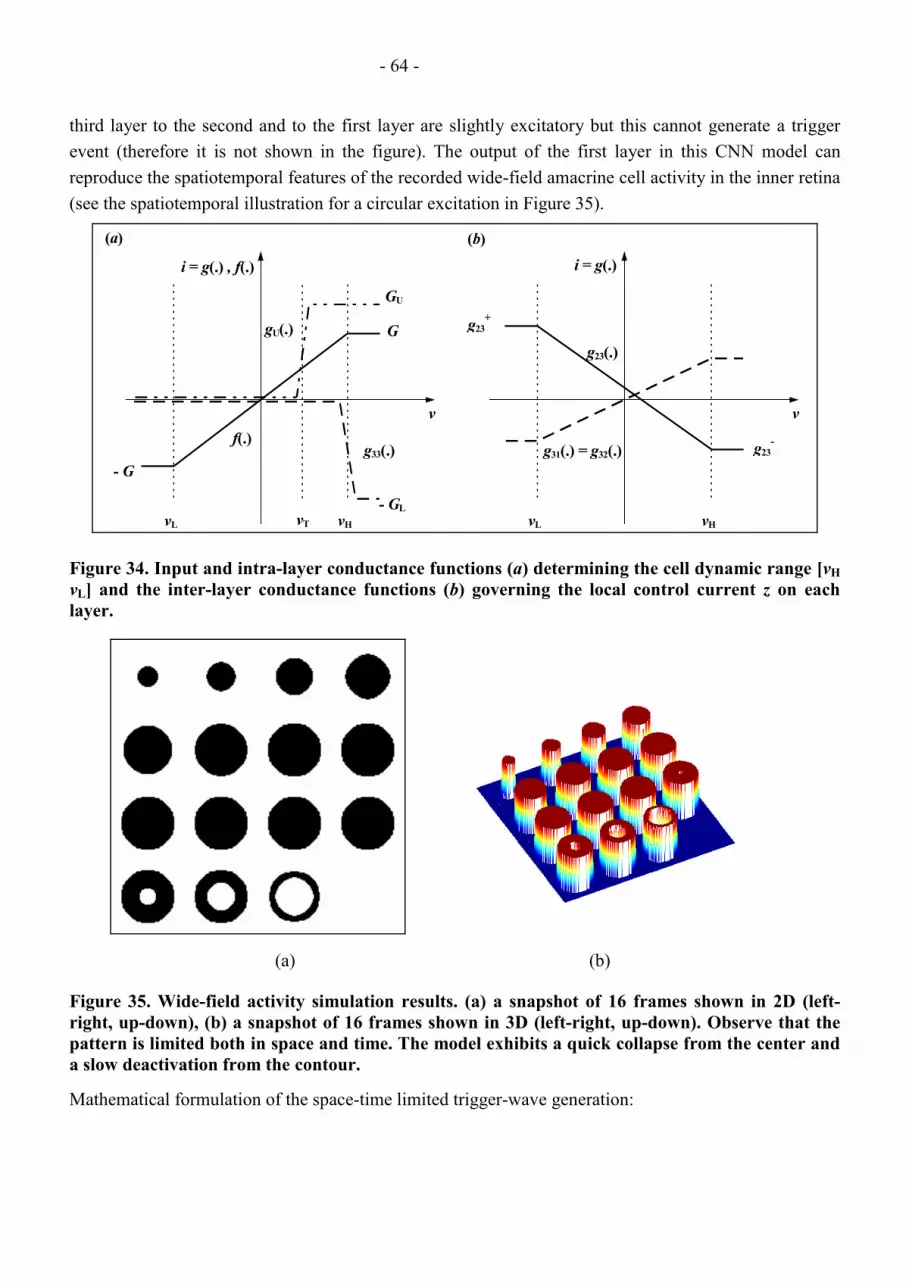
- 64 -

third layer to the second and to the first layer are slightly excitatory but this cannot generate a triggerevent (therefore it is not shown in the figure). The output of the first layer in this CNN model canreproduce the spatiotemporal features of the recorded wide-field amacrine cell activity in the inner retina(see the spatiotemporal illustration for a circular excitation in Figure 35).

g23(.)

g31(.) = g32(.)

vL vH

g23-

g23+

v

i = g(.)

f(.)

vL vH

v

i = g(.) , f(.)

g33(.)

G

- G

- GL

(a) (b)

gU(.)

GU

vT

Figure 34. Input and intra-layer conductance functions (a) determining the cell dynamic range [vHvL] and the inter-layer conductance functions (b) governing the local control current z on eachlayer.

(a) (b)

Figure 35. Wide-field activity simulation results. (a) a snapshot of 16 frames shown in 2D (left-right, up-down), (b) a snapshot of 16 frames shown in 3D (left-right, up-down). Observe that thepattern is limited both in space and time. The model exhibits a quick collapse from the center anda slow deactivation from the contour.

Mathematical formulation of the space-time limited trigger-wave generation:

- 65 -

Layer Cddt

v G v z g v W g v W v

Layer Cddt

v G v z g v W g v W v

Layer Cddt

v G v

ij ij U U ij kl klkl N

klkl N

kl

ij ij U U ij kl klkl N

kl klkl N

ij

1

2

3

1 1 1 1 1 1 31 31 3 11 1

2 2 2 2 2 2 32 32 3 22 2

3 3 3 3

1 1

1 1

: ( ) ( )

: ( ) ( )

:

, , , , , , ,

, , , , , , ,

, ,

= − + + + +

= − + + + +

= −

∈ ∈

∈ ∈

σ α

σ α

ij kl klkl N

ijz W g v g v+ + +∈

3 23 23 2 33 31

, , ,( ) ( )σ

(1)

The three-layer model of the wide-field amacrine cell activity can exhibit various wave phenomena.Trigger-waves initiating from cells that are switched to active state can collapse from the center ofexcitation or from the contour of the region occupied. These two effects are combined modeling theobserved spatiotemporal patterns of the wide-field amacrine activity (the model exhibits a quick collapsefrom the center and a slow deactivation from the contour). The patterns corresponding to the inner retinasimulations can be seen in Figure 36. Further illustration and explanation is given in Figure 37.

20 40 60 80 100 120-80

-70

-60

-50

-40

-30

-20Bipolar responses, trigger events and wide-field activity

Time [frames, averaged in 25 msec]

Mem

bran

e po

tent

ial [

mV

]


Tim

e [fr

ames

, ave

rage

d in

25

mse

c]Wide-field activity [mV]

20 40 60 80

20

40

60

80

100

120 -80

-60

-40

-20

0

(a) (b)

Figure 36. Spatiotemporal output of trigger event and wide-field activity simulations. (a) middlecell temporal responses for bipolar ON and OFF cells are shown with the trigger events and wide-field activity, (b) spatiotemporal patterns corresponding to wide-field activity simulations.

- 66 -

H

L

L1

L2

L3

H

LH

LH

L

III. Collapse

L1

L2

L3

H

LH

LH

L

II. Propagation

L1

L2

L3

H

LH

LH

L

IV. Reset

L1

L2

L3

H

LH

L

I. Initiation

Pos 1Pos 1 Pos 2Pos 2

RP

Pos 1

Pos 2

t

t

t

H

L

H

L

H

L

I. II. III. IV.

TW

TP

TA TRf(v1)

f(v2)

f(v3)

TW - impulse width

TP - propagation time

RP - propagation radius

TA - active period

TR - regenerative period

Figure 37. Spatiotemporal analysis of a wide-field activity generated by the three-layer CNNmodel. Four phases of the activity are shown for each CNN layer both in space (1D cross-section)and time (temporal responses of two selected cells in spatial positions 1 and 2). In phase I.(initiation) the first and second layer are triggered by the input and the second layer activates thethird one (control layer). In phase II. (propagation) trigger waves propagate in both the first andsecond layer, while in the control layer the cell output is decreasing in phase with the expandingwave-front in the second layer. In phase III. (collapse) feedback from the control layer to the firstlayer reaches the thresholds where (i) the active region starts collapsing from the center and (ii)where the velocity of the expanding wave-front (the motion direction of the “contour”) smoothlyreverses. Phase IV. (reset) is the regenerative period since all layers return to their initial settings(resting state). In this phase the activity completely disappears from the first layer. The wave-frontin the second layer also collapses from the center (as a result of the feedback from the controllayer) and this deactivation propagates over the entire layer. In return the second layer resets thecontrol layer.

- 67 -

4.3.1.4 Ganglion cells’ RF

In the following we shall use a simplistic model. In this case the width of the receptive fields’ spatial

component is delimited by the applied neighborhoods. The temporal response components of the model

is generated by the next templates:

A11= [0.7] B = [1] ( 4 )

A12 = [0.5] A22 = [0.3] ( 5 )

A13 = [-0.15] A33 = [0.9] ( 6 )

A24 = [1] A34 = [0.7] ( 7 )

The resulting transient can be seen on the next figure:

Layer1Layer2Layer3Layer4

0 5 10 15 20 25 30

-0.2

0

0.2

0.4

0.6

0.8

1

Layers together

Am

plitu

de

Time

Figure 38

These templates appropriate to the RFI-1, RFI-2 and RFI-3 receptive field interaction prototypes. In thismodel we use C2 cell type and S1b synapses. The receptive field prototype according to RF-0 and RF-2asubtypes. So the next template defines the model receptive field’s spatial component:

A 45(Center) =2 2 22 3 22 2 2

��

��

A 45(Surround)

1 1 1 1 1 1 11 1.2 1.2 1.2 1.2 1.2 11 1.2 1.2 1.2 1.2 1.2 11 1.2 1.2 1.2 1.2 1.2 11 1.2 1.2 1.2 1.2 1.2 11 1.2 1.2 1.2 1.2 1.2 11 1 1 1 1 1 1

=

− − − − − − −− − − − − − −− − − − − − −− − − − − − −− − − − − − −− − − − − − −− − − − − − −

��

��

( 8 )

By these templates we can build a dynamic receptive field structure (Figure 39), which characterize the

majority of retinal ganglion cells (X or β), the majority of thalamic relay cells, and with some

- 68 -

modification one class of the cortical simple cells. We used the VI-1 visual stimulation prototype and we

achieved the next spatiotemporal receptive field.

Time BA

X

Figure 39. The measured (A) (de Angelis, 1993: [16]) and the CNN modeled (B) cortical simplecell’s receptive fields. Here and on the following figures B is the false colored and topographicrepresentation of the CNN model results. The amount of green color indicates excitation and redappropriate to inhibition.

- 69 -

4.3.1.4.1 Ganglion cells’ spiking model

Ganglion cells of the retina transforms the light-induced potential changes of their membrane into trainsof action potentials (spikes). The rate of firing varies with the magnitude of the stimulus. Below a CNNmodel (template) for this rate coding is given. In the model the S4 synapse, C2 cell and RF-0 receptivefield prototypes are used. The stimulus is according to VI-1 prototype.

CNN template of a spiking ganglion cellLAYER 1 ( 9 )NEIGHBORHOOD 0CONTROL1REVERSAL 2VCC_FEEDBACK1XF 1 3 -1 0 0 0 1 5DELAY 3REVERSAL -1DELAYED_VCC_FEEDBACK1XF 1 4 -1 0 0 0 0.5 10 1 10

Response of a ganglion cell to a changing stimulus

Figure 40

- 70 -

4.3.1.4.2 Receptive fields of ganglion cells (center and antagonistic surround)

Ganglion cells have concentric receptive fields, which are divided into a center zone and a surround (seebelow, left column top figure). Below the responses of an On-center Off-surround CNN ganglion cellmodel are given. The left column contains four different illumination conditions (central spot: a lightspot illuminates the center; central illumination: the whole center is stimulated; surround illumination:the whole surround is illuminated; diffuse illumination: the whole center and surround are stimulated).The right column contains the corresponding responses of the ganglion cells. On-center Off-surroundcells are excited by the stimulation of their center zone (stimuli 1 and 2) and are inhibited when thesurround is stimulated by light (stimulus 4). The response (firing rate) is maximal when the whole centeris stimulated (stimulus 2). Diffuse illumination of the whole receptive field evokes a weak response.

Figure 41. The response of the simulated ganglion cell to different types of stimulation.

light

central spot

central illumination

1.

2.

surround illumination

diffuse illumination

3.

4.

- 71 -

4.3.1.4.3 Simplified models

This model framework is for the whole light-adapted retina. The developed models can reproduce all

fundamental effects of the retina as determined or measured by biologists. The modeling approach is

neuromorphic in its spirit, relying on both morphological and pharmacological information. However,

the primary motivation lies in fitting the spatial and temporal output of the model to the data recorded

from biological cells (tiger salamander and rabbit). In order to meet a low complexity (VLSI)

implementation, some structural simplifications have been made, while large neighborhood interaction

and inter-layer signal propagation are modeled through diffusion and wave phenomena.

Our goal is to develop a CNN based functional retinal model. The model should produce results

qualitatively similar to the living vertebrate retina measurements. The structure of the model can be

based on our knowledge about the retinal morphology. The CNN paradigm provides the basic structure

and connections for the modeling. The choice has several reasons: e.g. they have similar structure, and

so there is straightforward mapping from the biologic cell layers to CNN layers.

We will not try to model all cell layers of different types, just the functionally important ones. We

will not use the measurement results directly, moreover we do not aim to create an operationally

complete and exact cell model. Our goal is less ambitious: we try to develop a simple model using

correct cell, layer and structure properties and we are satisfied with qualitatively correct results. Our full

retina model, however, is able to reproduce all main retinal phenomena simultaneously.

4.3.1.4.3.1 Cell (and Layer) Prototypes

C1: First order

The required parameters are

• z, the bias or resting potential

• τ, the time constant is determined by the linear capacitor and the resistor and it can be expressed as τ

= RC

• A, the feedback template(s) or synapse(s) and the D matrix or matrices

4.3.1.4.3.2 Synapse Types

The following functions are multiplied by the weight parameters of the receptive field.

- 72 -

Transfer function

Linear bipolar

It represents linear

“electrical” synapses or

simple signal transfers.

f (x) = c x (S1a)

Linear rectifierIt models one kind of

nonlinear transfer function.�

�

�

−−+−

≥

<=

1)()1(

:

:)(

x

yxyx

yx

cccxc

cx

ccxxf (S2b)

The desensitivity synapse

Some synapse possess the desensitivity feature. The source layer of the synapse is active all the

time. The effect of the synapse on the destination layer becomes smaller and smaller with time. The

synapse becomes de-sensate. If the output of the source is the same the input of the destination is smaller

or even zero.

Desensitivity could be true or false, according to the type of the synapse. The parameters:

• Speed: the speed of the desensitivity

• Ratio: ratio between the transient- and the sustained-part of the input

We can implement this property using an additional working CNN-layer. It is a simple capacitor and

implements a feed-forward inhibition.

4.3.1.4.3.3 Receptive Field Types

RF1a: Simple central gain:

This is a simple feed-forward receptive field. The strength of the coupling is the gain value.

RF2: Diffusion-type

This type of spatial weighting can be used to describe the intra-layer diffusion-type phenomena. The

cells in layers are tightly coupled. The space constant (λ) is an appropriate value to determine the

strength of coupling. This is an A template.

gλ/2 gλ gλ/2

gλ -6 gλ gλ (RF2b)

gλ/2 gλ gλ/2

1 2 1

gλ2 2 -12 2 (RF2c)

1 2 1

- 73 -

4.3.1.4.3.4 Visual Input

VI1: Still image

The static image means, that the image is shown to the retina in gray background for a defined time

interval and after that the stimulus becomes a blank gray field. Still means the image is shown for a time

span and after that the visual input is a gray field. The adjustable parameters are: the waiting time before

the effective input image, the on-time when the input is the static image, the off-time when the visual

input is a gray field.

VI2: Video

During the video stimulus a video-flow is projected to the retina. A frame is shown constantly till the

next frame appears. The typical video speed is 30 frames per second, and the typical total time is some

seconds.

The basic video stimuli are the moving ball in different directions and the growing square.

4.3.1.4.3.5 The qualitative retina modeling framework

The key for a successful and useful model building is the incorporating all knowledge on

morphology, pharmacology and physiology. The starting-point of the model is the living retina, with

properties derived from the vertebrate retina measurements. The biological terms can correspond to the

following CNN terms. A CNN cell models a biological cell, one specific type of biological cells are

modeled with a CNN layer and the synapses (inter- and intra-layer, excitatory, inhibitory as well) are

transformed to CNN templates.

The input of the retina is the cone (photoreceptor) layer and the output is the ganglion spiking.

Almost every other cell in the retina are not spiking neurons. In the modeling, we use analog output for

the description of the state of every cell. It is reasonable for the ganglion cells, too, because the spiking

is considered as one type of analog signal representation. The outputs of the different cell layers are

transformed to grayscale video. Pixels in each video frame correspond to individual cells and color of

the point indicates the voltage of the cell.

The models have the following restrictions:

• In the retina just the cone (and rod) cells are able to transform the light to electrical signal, so in the

modeling the stimulus can be input (has a non-negative B template) just for one layer.

• A layer contains first or simple second order cells. Almost every cell type has a non-linear high order

transfer function, but it can be modeled as a first or second order system.

• The cell delay is continuos. The cells are working in analog mode.

- 74 -

• The steady state of a cell can be calculated from the state equation of the biological cell. In the model

we set this voltage to zero, because only the change conveys information. The model conserves the

basic properties of the behavior, but the computation is much easier.

• The interactions are space-invariant and use the nearest neighborhood. The different types of cells

have different size of interactions. With a diffusion feedback a bigger field can be modeled.

• The synapses are time invariant. In this modeling task we felt that this restriction is acceptable.

• The synapse transfer functions are monotonous and continuos.

• One type of cells has one type of transfer function. It does not mean, that the output (the effect) of

the cell is the same for every connected layer, because the receptive field can be different from layer

to layer.

• The synaptic feedbacks have to be negative (inhibitory). This condition provides the stability of the

system. In the retina the excitation (positive) can be directly feed-forward.

• According to experiences inhibitory layers have bigger space constants, than the feed-forward layers.

From the point of view of the system theory it guarantees the edge enhancement property.

• The outer retina is the same for each ganglion model. In the modeling we have to develop the

different type of ganglion responses using the same output retina model. We should modify only the

inner retina model.

The following differential equation system describes the system:

11 1||,1||

,,11||,1||,1

1||,1||,1,1,1

1,1 )(1 zxfguxxx

M

n jlikklnnijklnn

jlikklijkl

jlikklijklijij ++++−=

= <−<−

−

<−<−<−<−DBA

τ� (Q1)

= <−<−<−<−> +++−=

M

n jlikklnnijklmnnm

jlikklmijklmijm

mijm xfgzxxx

1 1||,1||,,

1||,1||,,,,1 )(1 DA

τ� (Qn)

where

• ττττ time-constant, which is an important cell type property

• z bias for connecting different type of layers

• f the transfer function of the synapse: S1-S3

• g this is the gain: positive value is an excitatory, negative value is an inhibitory weight (g-)

• A, B, D the different receptive fields:

• A intra-layer template, in this model it is diffusion: RF2

• B the stimulus input template in RF1a form

• D the receptive field of the synapse (inter-layer connection): RF1

4.3.1.4.3.6 The minimal number of structural elements representing vertebrate retinas

- 75 -

The vertebrate retina has two main parts: the outer and the inner retina. The outer retina is almost

invariant for all the different inner retina systems. The retina has several types of ganglion cells. The two

qualitatively different input types of the ganglion cell are the excitation and the inhibition. The excitation

comes from bipolar cells; the inhibition derives from amacrine cells. Each amacrine cell has connection

at least to one bipolar cell. The input of bipolar cells is the outer retina.

The outer retina has a cone and a horizontal layer. We try to model the time- and space-behavior

of the outer retina. The cone layer is responsible for the time-behavior. The horizontal layer is

responsible for the spatial-pattern. We need at least a second-order cone model for the correct result. The

space-constant on the horizontal layer should be large relative to the space-constant of the other layers.

In each ganglion cell model we use those layers which have direct or indirect connections to the

modeled ganglion cell. The inner retina is divided into independent parts each one representing a given

type of ganglion cells and its input layers. The model of the inner retina contains two parts: the

excitatory subsystem and the inhibitory subsystem.

The excitatory subsystem should have a bipolar layer. This layer transfers and transforms the

output of the outer retina to the ganglion excitation. If the time-shape of the measured excitation is

highly different from the general response of outer retina, one should use a desensitivity synapse and/or

an amacrine feedback system (at least one amacrine cell). If the space-shape of the measured excitation

is different from the pattern of the outer retina, you can use an amacrine feedback layer to improve the

quality of the model. In general we need a bipolar and an amacrine layer for modeling the excitatory

input of the ganglion cell.

The input of the inhibitory subsystem is a bipolar layer. The inhibitory input of the ganglion cell

is an amacrine cell therefore the inhibitory-part of the inner retina has an amacrine feed-forward cell. In

summary the model has a bipolar and an amacrine layer. The bipolar cell could be the same for the

excitation and the inhibitory feed-forward amacrine layer could have input from the excitation

subsystem.

The general minimal model contains a second-order cone and horizontal layer modeling the outer

retina, a bipolar and amacrine feedback layer creating the excitation, a bipolar and an amacrine feed-

forward layer for the inhibitory subsystem and the modeled ganglion cell. If the ganglion cell is either

the On or the Off type the model is complete. If the cell, however, is an On-Off type the outer retina is

unchanged but the excitation subsystem should be doubled. See figure 40 for the structure and figure 41

for some simple sample models.

- 76 -

Bipolar

Amacrine FB

Bipolar Inh.

Amacrine F

Ganglion

Cone

Horizontal

F

Figure 42. The general simple structure. The horizontal lines represent the layers; the verticallines show the synapses.

- 77 -

x

t

Figure 43. Some simple ganglion cell model. One column is one model (from left to right):Bistratified, OnSluggish, OnTransient, OffTransient, OffSluggish. The first row shows thestructure and parameters of the model. The second row shows the natural scene processing of theganglion cell. The last row shows the response of the On stimulus: standard space-time pattern.

4.3.1.4.3.7 Some qualitatively correct effects in vertebrate retinas

The vertebrate retina contains at least two different types of ganglion cells. The first one is a motion

detector cell (MD-ganglion) and the other is a local edge detector cell (LED-ganglion). The MD-cell

response is big at the beginning and at the end of the stimulus in the object, but the response is short in

time. The LED-cell indicates the edges of the object, so in the middle of the object the response is very

small. Cell activity can measure during and after the stimulus. We developed one CNN retina structure

for these two highly different types of ganglion model. Modification of two parameters is sufficient to

get the other model (bipolar diffusion and amacrine inhibition).

The structure of the model is quite simple. It contains three parts: outer retina model part, On and Off

inner retina model parts. The outer retina is modeled with a second order cone (photoreceptor layer) and

a horizontal layer. Both inner retina models have the same structure and parameters. The input of the

inner retina model is the cone layer (positive to the Off pathway and negative to the On pathway). The

- 78 -

bipolar layer get input from the cone layer (feed-forward) and from the amacrine layer (feedback link)

and has a non-linear positive feed-forward connection to the ganglion layer and to the amaFF layer (this

is an other amacrine layer). The ganglion layer has excitation from the bipolar layer and inhibition from

the amaFF layer. The two amacrine layers have a mutual negative coupling, which is called cross

inhibition. The output of the retina model is a non-linear transformation of the ganglion layer, this

additional layer called ganglion spike. The structure is retino-topic.

The synapses of the outer retina are linear. The inner retina model uses the linear rectifier non-

linearity (S2b). The diffusion (RF2b) works on each layer except the cone layer. The space and time

constants are different from layer to layer. The parameters are acceptable from biological point of view,

too.

Figure 44. The structure of the retina model. The layers are horizontal lines and the synapses arevertical arrows. The broken line indicates a non-linear transfer function. The circle represents thefeedback, which is the space-constant dependent diffusion.

- 79 -

The following two tables show the comparison of the three examined simulation and measurement

(recorded by Botond Roska). The model reproduces all basic features of the desired retina effects. One

model (structure and parameters) is able to reproduce the qualitatively correct response for all of the

three measured stimuli.

- 80 -

LED Measurement LED Simulation Properties

On stimulus (time: 1+1sec, size: 60pixels)Basic: activity only at the edges

Further properties:• strong initial answer• while stimulus on, strong outside edge• after stimulus strong inside edge

400 1000 2000 3000 6000

time

intensity

400 1000 2000 3000 6000

time

intensity

0.1

0.2

0.3

0.4

0.5Moving ball (speed in µm/sec)Basic: bigger speed smaller response

Further properties:• Off response is weak• Exponential envelope

time

intensity

0.5

1

1.5

2

2.5

time

intensity

Incremental square (size in µm)Basic: bigger size smaller response

Further properties:• Long time activity• Exponential envelope

Table 3. The examination of the Local Edge Detector Ganglion Model

MD Measurement MD Simulation Properties

On stimulus (time: 1+1sec, size: 60pixels)Basic: Response just at the beginning and at

the end of the stimulus

Further properties:• strong response at the beginning• sometimes longer response near theedges

1000400 2000 3000 6000

time

intensity

1000400 2000 3000 6000

time

intensity

Moving ball (speed in µm/sec)Basic: bigger speed smaller response

Further properties:• Off response is weak• Gauss envelope

10050 200 400 1000

time

intensity

10050 200 400 1000

time

intensity

Incremental square (size in µm)Basic: big response to middle square

Further properties:• Gauss envelope• Different On and Off response

Table 4. The examination of the Motion Detector Ganglion Model

time

space

time

space

time

space

time

space

- 81 -

The first one is the basic On stimulus. A white square is shown for a second and a blank gray

background during the next second. On the picture the time is on the vertical axes and the middle row of

the retina is the horizontal axes.

The second stimulus is the moving ball. A white circle is moving towards the right side of the retina

with different speed and the measurement is on the middle cell. The relationship between the speed and

the grade of the response is the task. The horizontal axes is the time, the vertical is the response. The

number above the curves indicates the speed of the object in micron per sec.

The third measurement is the growing square. A white square is shown to the retina. The connection

between the size of the object and the grade of the response is the question. The horizontal axes is the

time, the vertical is the response. The number above the curves indicates the size in micron. In the

simulation one pixel is 30 microns, this is an acceptable map according to the density of the cone cell in

a general vertebrate retina.

We could compute the retina transformation of any kind of video sequence, e.g. natural scenes. The

developed models are able to reproduce the key retina phenomena even their combinations. The CNN

simulations show qualitatively the same result as the in vitro measurements on the rabbit retina. The

produced effects are as follows:

• direction dependent, object level motion detection

• impulse noise filtering in space and time

• initiation of motion detection

• (limited) light adaptation and contrast effect

• edge detection in space and time

• size selectivity (with local interactions)

• object corner detection

• speed, size and intensity selective video-flow processing

• gradient effect

4.4 Thalamic cells’ receptive field properties

4.4.1 CS RF spiking models

(K. Lotz)

The most important ionic currents participating in the generation of the resting potential and responses to

electrical stimulation:

(1) Na+ leakage current

- 82 -

(2) K+ leakage current

(3) Fast transient Na+ current

(4) Transient K+ current

(5) Delayed rectifier K+ current

(6) Hyperpolarization-activated cation current

(7) Low-threshold Ca2+ current

C+- +- +- +- - -

+ +

extracellular side

intracellular side

Na K

leakage

I I I TI h

(1) (2) (3) (4)

I trNa

-+

(5) (6) (7)

I trK I dK

Figure 45.

- 83 -

CNN template of the electrical equivalent circuit of the relay cellNEIGHBORHOOD 0 DELAY 3

CONTROL REVERSAL -2

1 DELAYED_VCC_FEEDBACK

REVERSAL 1.5 1

VCC_FEEDBACK XF 1 5 -1 0 0.2 0 0.4 10 0.6 3 1 3

1

XF 1 2 -1 1 1 1 DELAY 5

REVERSAL 1

REVERSAL -2 DELAYED_VCC_FEEDBACK

VCC_FEEDBACK 1

1 XF 1 5 -1 0 -0.5 0 0 2 0.5 0 1 0XF 1 2 -1 1 1 1

REVERSAL -1

REVERSAL 1.5 VCC_FEEDBACK

VCC_FEEDBACK 1

1 XF 1 3 -1 0 0.5 0 1 4

XF 1 5 -1 0 0.2 0 0.4 10 0.6 3 1 3

REVERSAL -2.0

VCC_FEEDBACK

1

XF 1 5 -1 0 0.2 0 0.4 10 0.6 0 1 0

(a) Generation of the resting membrane potential

The resting membrane potential of relay cells is mainly due to the unequal distribution of the Na+ and

K+ ions across the cell membrane and their leakage currents (channels (1) and (2) in the circuit above).

(b) Tonic mode of action potential generation (single spike activity)

The single spike activity is evoked by the depolarization of the membrane potential (above -55mV). It

involves the activation of the currents (3), (4) and (5).

- 84 -

Figure 46Stimulation (depolarization) and response (single spikes) of the CNN model cell:

(c) Phasic mode of action potential generation (rhythmic bursts)

Burst firing is due to the activation of IT current ((7) in the equivalent circuit) which is activated by Ih

((6)) via hyperpolarization of the cell membrane.

Response of the model relay cell to hyperpolarization:

Figure 47

- 85 -

(a) Synaptic connections of the CNN model

Here a CNN model of a simplified LGN is shown. In the following picture (a) denotes the synaptic

connections of the simplified LGN model (without cortical feedback) and (b) shows the synaptic

connections of the corresponding 5-layer CNN architecture. Following the picture the employed CNN

template is given. The applied synapse models use almost all the available synapse prototypes like S1a,

S1b, S2a and S4 and the model use some more complicated nonlinear interactions as well. The used

receptive field prototypes can be classified as RF-0 and RF-3.

+ +-

+ --+

-

++

cortex

PGN/NR

interneuronrelaycell

opticalafferent

1

2

34

(a) (b)

Figure 48

- 86 -

CNN template of the simplified LGN model (five layer):

Layer 1 (Excitation)

�

��

�

�

−−−−−−−−−−−−−−−−

=

��

��

�

�

=

==

=

=

dddddcaddcbddddd

B

dddddcaddcbddddd

B

AA

11111

11111

]2.0[ ]79.0[

τ

τ

( 10 )

0.052

0.040

0.024

-0.0024-1 1-0.01

0.0003

uij

a

b

c

d

Layer 2 (Faster inhibition)

�

��

�

�

=

��

��

�

�

−−−−−−−−−−−−−−−−

=

==

=

=

dddddcaddcbddddd

B

dddddcaddcbddddd

B

AA

152121

32222

]46.0[ ]5.0[

τ

τ

( 11 )

0.066

0.046

0.0275

-0.00275-1

1-0.0116

0.0004

uij

a

b

c

d

- 87 -

Layer 3 (Slower inhibition)

�

��

�

�

=

��

��

�

�

−−−−−−−−−−−−−−−−

=

==

=

=

dddddcaddcbddddd

B

dddddcaddcbddddd

B

AA

263131

133333

]58.0[ ]4.0[

τ

τ

( 12 )

0.073

0.051

0.030

-0.003-1 1-0.013

0.0004

uij

a

b

c

d

Layer 4 (Sum of the exciting (1) and inhibiting (2,3) layers)

][][][

43

42

41

bAbAaA

===

yij

a1

1

yij

b-1

-1

( 13 )

Layer 5 (Spike output based on the output of layer 4)

][][

55

54

bAaA

== y

ij

a

10.1

0.03

-0.03

0.03

0.26

yij

b

1

0.3

0.25

3

0.02-1

( 14 )

- 88 -

(b) Luminance sensitivity of the LGN model cells

The figure below shows the cell responses of the above described LGN model. On the top of the figure

five stimuli (different shades of gray) are given. The lower part of the picture contains the cell responses.

Each column shows the responses of the 5 layers (one cell's of each layer) given to the stimulus above

the column (i.e. each column contains 5 cell transients). The frame of each cell transient window

indicates the number of layer (L) and the position of the cell (X, Y). Here the cell (2,3) is measured on

each layer. In each cell transient window the horizontal axis is time, the vertical is amplitude (voltage) in

the [-1, +1] interval. It is straightforward from the picture that the cell responses are proportional to the

magnitude of the stimuli.

Figure 49

- 89 -

(c) Center-surround receptive field properties of LGN cells

The following picture demonstrates the center-surround property of LGN cells. The figure shows two

different stimuli (top) and the response transients of an On-center Off-surround LGN cell using the

above studied 5-layer CNN model (bottom, Layer 5). In the first case (left) the whole center is dark and

the surround is illuminated, the second case (right) is vice versa. The second stimulus elicits a vigorous

response (because it is On-center!) while the first evokes practically no response.

Figure 50

(c) Response properties of LGN cells for Walsh patterns

The following picture demonstrates the LGN cells response for Walsh pattern stimuli. The figure shows

the responses of an Off-center On-surround LGN cell using the above studied 5-layer CNN model.

- 90 -

Figure 51. Spike responses to 16 Walsh patterns. (Compare to physiological results taken from[23a].)

- 91 -

4.4.2 Lagged cells’ RF

There is a strange class of the thalamic relay cells. The so termed lagged cells show a much slower

dynamics than the retinal ganglion and the other LGN relay cells. Even the sign of their response is

opposite that of the other thalamic cells. By an apt integration ( 15 ) it is easy to simulate their dynamic

receptive field structure. As we can see on Figure 52 the lagged cells’ spatiotemporal structure is

satisfactory reproduced. Here we used the above delineated retinal ganglion cell model (see the

templates: ( 5), ( 6), ( 7), ( 8)) and the RFI-2 subclass, beside the previously applied RFI prototypes.

A56 = [0.7] A66 = [0.4 ] ( 15 )

Time BA

X

Figure 52. We can compare the measured (A) (de Angelis et al., 1993: [16]) and the modeled (B)lagged cells’ receptive fields. The model was made by an appropriate “slow down” of a simple cellresponse by feedback. The time-course of the response is much slower (not shown), than in thecase of simple cells.

4.5 Cortical cells’ RF

4.5.1 Cortical Simple cells

The neurons within the visual cortex can be classified as simple, complex and hypercomplex cells.

Spatially separated inhibitory and excitatory sub-regions characterize the receptive field of the simple

cells. On the contrary, complex cells show overlapping inhibitory and excitatory regions. So

appropriately moving light and dark stimuli both can excite the complex cells as well. These cells thus

have immanently nonlinear character. Here we give different models of the cortical simple cells. To

achieve proper complex cell models we need a much deeper comprehension of the nonlinear

physiological processes underlying the formulation of these cells’ receptive fields.

- 92 -

A large class of the cortical simple cells shows close relationship to the receptive field structure of

retinal ganglion cells, or to thalamic relay cells. The only difference is that these cells spatial structure is

not rotational invariant. That is they prefer special stimulus orientations. However, their spatiotemporal

structure, in the optimal orientation, can be described by the above delineated models (see the templates:

( 5), ( 6), ( 7), ( 8)). We could make simulation of the simple cells receptive fields even in that case,

when their spatial structure do not follow the center-surround antagonistic scheme. Applying an

appropriate convergence ( 16 ), RFI-2 prototype, we can reproduce the desired structure (Figure 53).

Time

X

A B

Figure 53. We can compare the measured (A) (de Angelis et al., 1993: [16]) and the modeled (B)simple space-time separable cell’s receptive fields. The model was made by the sum of two simplethalamic or cortical cells’ response.

�

��

�

�

=00011-0000

A57 ( 16 )

4.5.1.1 Orientation sensitivity

Orientation sensitivity is one of the principal properties characterizing visual cortical neurons. They have

distinct responses to light or dark bars presented at various orientations in the visual field [1].

Below a CNN template is given which selects lines with -45° slope, then the simulation is displayed

with the input and output picture:

- 93 -

CNN template:

1 25.0000000025.0

]2[ −=�

��

�

�

== IBA ( 17 )

Simulation:

input picture output picture

Figure 54

- 94 -

4.5.1.2 Direction sensitivity

4.5.1.2.1 Triadic synapse

One of the neural direction selective motion detection architectures is the triadic synaptic

arrangement [24], which is given below left (a). White circles depict excitatory cells, the black one

represent inhibitory interneurons. On the right (b) an artificial model of the triadic synapse is shown

with two input signals (bottom) and the corresponding responses (top). The black triangle indicates the

delay of the inhibitory interneuron.

τ

++

-

+

t

zin1

t

t

t

z1out z

2out

z2in

τ

τ

(a) (b)

Figure 55

CNN templates corresponding to the triadic synapse:

A B a A B b I

a b a b

= = = = − = =

> = =

[ ] [ ] [ ] [ ]

, ;

0 0 0 1

0 1

example:

τ τ τ( 18 )

(RF-0 receptive field and S1b synapse prototypes with RFI-1 interactions using C2 cells.)

- 95 -

4.5.1.2.2 Direction selective neural connection scheme

Several neurons in the cortex show certain direction selective properties. This results from some special

spatial neural connections. The left part of the figure below (a) gives a concept diagram used in [12]

illustrating a neural connection scheme that might generate direction selectivity of moving stimuli. There

are feed-forward inhibitory connections directed to the right which cause a wave of inhibition

suppressing responses to stimuli moving to the right. In addition, the feed-back excitatory connections to

the opposite direction reinforce the stimulus response in this direction. Thus the upper neurons select the

stimulus moving to the left. Figure (b) shows an artificial representation of the direction selective

connection scheme together with two stimuli moving in opposite directions (bottom) and the responses

(top).

t 0~

t

t

t

1

0

1

~

~

~

τ ττ

-+

+- +

++

+

+

+- -

t0

t

t

t

1

0

1

(a) (b)

Figure 56

- 96 -

CNN template corresponding to the direction selective neural connection scheme (RF-3 prototype)

1 ;5.1 :example ;0,,

1 0 00000000

]0[ 000

0000

]0[

===>

==�

��

�

�

−==��

��

�

�

==

bcacba

IcBAbaBA τττ

( 19 )

Example for a direction selective motion detection where only those points (of the input) are detected

which move in a given (here right) direction. The input and output images were both sampled, three

snapshots from both the input and output are displayed below. Here the RF-3 receptive field and the VI-

2 stimulation prototypes were applied.

CNN template:

1 6.18.2 000005.1000

]0[ 00005.10000

]0[ =−<<−�

��

�

�

==��

��

�

�

== τττ IBABA ( 20 )

Simulation:

input 1 input 2 input 3

output 1 output 2 output 3

Figure 57

- 97 -

4.5.1.2.3 Dynamic receptive field structure of the direction sensitive cortical simple cells

Special, space-time inseparable types of receptive field structures characterize the direction sensitive

simple cells. This dynamic receptive field structure can be simulated again by an apt convergence of the

thalamic relay cells' output. However, we have to use either an appropriate delay ( 21 ) or the slower

lagged cell response ( 22 ) to reproduce the necessary spatiotemporal structure.

X

A BTime

Figure 58. Compare the measured (A) (de Angelis et al., 1993: [16]) and the modeled (B) space-time inseparable simple cell’s receptive fields. In this case the model was made by the delayed(d=15) sum of two simple cells’ response.

A0 0 00 1 00 0 0

57 =��

��

A0 0 00 0 10 0 0

57(delayed 15) = −��

��

( 21 )

Here we used the above detailed thalamic relay cell model (see the templates:

( 5), ( 6), ( 7), ( 8)) beside the lagged cell model ( 15 ). (Here we used the RFI-2 receptive field

interaction and the VI-1 stimulation prototypes.)

- 98 -

X

Time A B

Figure 59. We can compare the measured (A) (de Angelis et al., 1993: [16]) and the modeled (B) x-t inseparable simple cell’s receptive fields. In this case the model was made by the sum of a simpleand a lagged cell’s response.

�

��

�

�

=000010000

A57

�

��

�

�

=000100000

A67(lagged)( 22 )

4.5.1.3 Length tuning

Although certain neurons in the visual cortex give maximal response to an optimally oriented

bar of a certain length, increasing the length of the stimulus their responses decrease or completely

disappear. A possible explanation for this phenomenon might be that these "length sensitive" neurons

receive an excitatory input from the central region of their receptive field and an inhibitory input from

cells spatially displaced to either side of the cell providing the main excitatory input.

Below a simple example of "length tuning" is given where the input picture contains a number

of bars of different lengths and the following CNN template marks those whose length is less or equal to

3 pixels.

- 99 -

CNN template:

1

303030111031)(13

0111030303

]0[ −=

�

��

�

�

−−−

−−

−−−

== IxfBA

Simulation:

input picture output picture

Figure 60

4.5.1.4 Edge enhancement

The center surround antagonistic receptive field structure ensures certain edge enhancement

characteristics. Due to this property it can be understood that drawings of objects can be recognized

almost so well as their original pictures. For the demonstration of the edge enhancement here we show a

simple center-surround template which considerably intensifies the edges of test pictures. First we make

the diffused version of the image (the diffusion is run for forty times the CNN’s time constant) and then

it is subtracted from the original picture. (RF-0 and RF-1 receptive field and RFI-3 interaction prototype

were used beside the VI-2 like grayscale stimulation.)

44

)40(0225.00225.00225.00225.00

1.0

2122

1111

−==

===

AB

TAB τ( 24 )

1

-3

0.2 1-1 x

f(x)

- 100 -

This way we get the next edge enhancement:

Figure 61. Edge enhancement effects of the center-surround antagonistic RF organization. A andB pictures are corresponding to the original end to the edge enhanced images.There are further assumptions of the visual system’s edge enhancement capabilities. It is assumed that

within the inner plexiform layer the amacrine cell’s feedback can further emphasize and speeding up the

occurrence of the retinal network edge enhancement character [18].

References (4.1 - 4.4)

[1] E.R. Kandel, J.H. Schwartz and T.M. Jessel, “Principles of neural science’, 3rd edition, Elsevier,New York, 1991

[2] L.O. Chua and Yang, ”Cellular neural networks: Theory”, IEEE Trans. Circuits and Systems, Vol.35, pp. 1257-1272, 1988

[3] L.O. Chua and Yang, ”Cellular neural networks: Application”, IEEE Trans. Circuits and Systems,Vol. 35, pp. 1273-1290, 1988

[4] L.O. Chua, T. Roska, “The CNN paradigm”, IEEE. Trans. Circuits and Systems, Vol. 40, pp.147-156, 1993

[5] T. Roska, J. Hámori, E. Lábos, K. Lotz, L. Orzó, J. Takács, P.L. Venetiáner, Z. Vidnyánszky andÁ. Zarándy, “The use of CNN models in the subcortical visual pathway”, IEEE Trans. Circuit andSystems-I, Vol. 40, pp. 182-195, 1993

[6] K. Lotz, J. Vandewalle and T. Roska, “A multilayer cellular neural network model of the twopathways of the retina related to dark adaptation”, Report ESAT-SISTA/R 1993-331, KatholikUniversitet Leuven, 1993

[7] A. Jacobs, “Techniques for constructing physiologically-motivated neuromorphic models inCNN”, Report DNS-7-1993, Computer and Automation Institute, Hungarian Academy ofSciences, Budapest, 1993

[8] Z. Vidnyánszky, P.L. Venetiáner, J. Takács, J. Hámori and T. Roska, “A CNN model of thefeedforward part of the LGN” Report DNS-6-1993, Computer and Automation Institute,Hungarian Academy of Sciences, Budapest, 1993

[9] J.E.Dowling, “The retina: an approachable part of the brain”, Harward University Press, London,1987

[10] F.S. Werblin, “Synaptic connections, receptive fields and pattern of activity in the tiger salamanderretina”, Investigative Ophthalmology and Visual Science, Vol. 32, pp. 459-483, 1991

A B

- 101 -

[11] J.L. Teeteres and F.S. Werblin, „Real-time simulation of the retina allowing visualization of eachprocessing stage”, SPIE, Vol. 1472, Image Understanding and the Man-Machine Interface III,1991

[12] A.M. Sillito and P.C. Murphy, „GABAergic processes in the central visual system” pp. 167-185 inNeurotransmitters and cortical functions (eds. R.W. Dykes and P. Gloor), Plenum Publ. Co.., 1988

[13] C. Enroth-Cugell and J.G. Robson, „The contrast sensitivity of retinal ganglion cells of the cat”, J.Neurophysiology Vol. 187, pp.517-552, 1966

[14] D. Marr, „Vision”, San Francisco, 1982

[15] D.H. Hubel, „Eye, brain and vision”, Scientific American Library, New York, 1988

[16] G.C. DeAngelis, I. Ohzawa, R.D. Freeman, “Receptive-field dynamics in the central visual

pathways.” Trends in Neuroscience (TINS.) Vol. 18(10), pp. 451-458, 1995

[17] Daqing Cai, G.C. DeAngelis and R.D. Freeman, “Spatiotemporal Receptive Field Organization in

the Lateral Geniculate Nucleus of Cats and Kittens.” J. Neurophysiol. Vol.78, pp. 1045-1061, 1997

[18] A. Jacobs, F. Werblin, “Spatiotemporal patterns at the retinal output.” J. Neurophysiol. Vol. 80(1),

pp. 447-51, 1998

[19] S.M. Sherman, and C. Koch, "The Control of Retinogeniculate Transmission in the MammalianLateral Geniculate Nucleus", Exp. Brain Res. Vol. 63, pp. 1-20, 1986

[20] M. Steriade, E.G. Jones, and R.R. Llinás, "Thalamic Oscillations and Signaling", A NeurosciencesInstitute Publication, John Wiley & Sons, 1990

[21] D.A. McCormick, “Neurotransmitter Actions in the Thalamus and Cerebral Cortex and their Role

in Neuromodulation of Thalamocortical Activity” Progress in Neurobiology, Vol. 39, pp. 337-388,

1992

[22] V. Crunelli, N.Leresche, "A Role for GABAB Receptors in Excitation and Inhibition ofThalamocortical Cells", Trends in Neuroscience. Vol. 14, pp. 16-21, 1991

[23a] J.W. McLurkin, T.J. Gawne, B.J. Richmond, L.M. Optican, D.L. and Robinson, "LateralGeniculate Nucleus in Behaving Primates. I. Responses to Two-Dimensional Stimuli", Journal ofNeurophysiology Vol.66, No.3, pp.777-793, September, 1991

[23b] J.W. McLurkin, T.J. Gawne, L.M. Optican, and B.J. Richmond, "Lateral Geniculate Nucleus inBehaving Primates. II. Encoding of Visual Information in the Temporal Shape of the Response",IBID, pp. 794-808,

[23c] T.J. Gawne, J.W. McLurkin, B.J. Richmond, and L.M. Optican, "Lateral Geniculate Nucleus inBehaving Primates. III. Response Predictions of a Channel Model With Multiple Spatial-to-Temporal Filters", IBID, pp. 809-823,

[24] E. Lábos, P. Pasik, J. Hámori, and E. Nógrádi, "On the dynamics of triadic arrangements:computer experiments on formal neural nets of chaotic units", J. Hirnforschung, Vol. 31, pp. 715-722, 1990

[25] HTTP://INSIGHT.MED.EDU/WEBVISION

http://insight.med.edu/WEBVISION

- 102 -

[26] Cs. Rekeczky, B. Roska, E. Nemeth, T. Roska, and F. Werblin (1998) "A Spatiotemporal RetinaModel in CNN Based on First Order RC Cells, Nearest-neighbor Space-invariant Interactions andContinuous Monotonic Nonlinear Synaptic Characteristics", Memorandum UCB/ERL,(UCB/ERL), Berkeley, University of California at Berkeley

[27] T. Roska, P. Szolgay, T. Kozek, Á. Zarándy, Cs. Rekeczky, L. Nemes, L. Kék, K. László, I.Szatmári, M. Csapodi, "CADETWIN", CADETWIN, (CADETWIN), Budapest, MTA SZTAKI,1997

4.5.1.5 'Extraclassical' receptive fields (inhibitory-excitatory network of the corticalarchitecture)

4.5.1.5.1 Psychophysical evidence

Adini et al. [1] performed lateral masking experiments. In these experiments contrast detection

thresholds of foveal Gabor signal flankers were measured. The threshold elevation was measured in

function of distance. Figure 62 shows the experimental results of Adini et al.

-0.3

-0.2

-0.1

0

0.1

0.2

0.3

0.4

0.5

1 3 5 7 9 11

target-mask distance

ters

hold

eva

luat

ion

Figure 62 Threshold evaluation versus distance in experimentsThe experiment showed, that the flankers cause an inhibition at very close, excitation at larger distances,

and with further increase of distances the influence of the flankers subsides. They suggested an

inhibitory-excitatory network cortical architecture that was studied in detail previously [2]. A similar

network can be built up with CNN. We developed a two-layer CNN network to reproduce and examine

these effects. Our simulation results are in close correlation with the psychophysical results.

- 103 -

4.5.1.5.2 Model

4.5.1.5.2.1 Inhibitory-excitatory network cortical architecture

The model consists of populations of inhibitory and excitatory neurons. The state of the network is

described by the average activities Er(t) Ir(t), where r denotes the spatial location of the corresponding

hypercolumn. The network is defined by the following equations.

τ

τ

dEdt

E g J E J I e

dIdt

I g J E J I i

rr e rr

ee

rr rr

eir r

rr i rr

ie

rr rr

iir r

= − + − +

= − + − +

( )

' ( )

''

' ' '

''

' ' '

( 25)

In this equations ge and gi denote sigmoid type nonlinear response functions. er and ir are inputs that are

constant in time, they represent inputs coming from the LGN into the cortex. The strength of the

connections are modeled as follows:

)'()/)'(exp()'(

220'

00'

rrifrrJJrrifJJ

rr

rr

≠−−===

αβαβαβ

αβαβ

σ( 26)

In the referenced work of Adini et al. this model had a good qualitative correlation with the experimental

data.

4.5.1.5.3 The two layer CNN model

A two-layer CNN model may be introduced for a similar approach. The Jee, Jei, Jie, Jii connections can be

investigated by appropriate finite neighborhood templates. (27) shows the equations of the CNN model.

dEdt

E J f E J f I e

dIdt

I J f E J f I i

ijij k i j l

ee

k l S i jkl k i j l

eikl ij

ijij k i j l

ie

k l S i jkl k i j l

iikl ij

= − + − +

= − + − +

− −∈

− −

− −∈

− −

,( , ) ( , )

,

,( , ) ( , )

,

( ) ( )

( ) ( )(27)

where E and I represents the state of the two layers and f is the sigmoid function.

The psychophysical model and the CNN model are similar, however there are some differences. For

instance the nonlinear function is different. On the other hand the nonlinearity is applied outside the sum

- 104 -

in the referenced model, nevertheless it is applied directly on the variables in our model. However, we

suppose that the CNN model shows the same qualitative properties.

4.5.1.5.4 Results

Simulations were made for the lateral masking experiment. The CNN network model had the following

parameters:

11.011.0235.0

8.045.0

00

00

00

00

========

iiii

ieie

eiei

eeee

IIII

σσσσ

( 28)

The excitation of the flankers was measured and compared with the case where no flankers were used.

This way the level of inhibition is computed (Equation (29)).

I(d)=E(0)-E(d) (29)

where E(d) is the response intensity, if the flanker is at distance d (d=0 means that no flanker is

presented) and I(d) the inhibition respectively. Inhibition is plotted as the function of distance of the

flanker (Figure 63).

Inhibition versus distance

-0.04-0.03-0.02-0.01

00.010.020.030.040.05

1 2 3 4 5 6 7 8 9 10 11 12 13

distance (d)

strength of inhibition (I(d))

Figure 63 Inhibition versus distance plot of the current modelThe psychophysical results (Figure 62) and the CNN model results (Figure 63) are in good correlation.

They show the same qualitative properties. In both of the models flankers cause an inhibition at very

close distances, at larger distances the flankers cause excitation, and at larger distances the influence of

- 105 -

the flankers subsides. These effects can be explained as the result of the “Mexican hat” nature of the

function Iee+Iei.

References (4.9)[1] Y. Adini, D. Sagi, and M. Tsodyks (1997) Excitatory-inhibitory network in the visual cortex:

Psychophysical evidence. Proc. Natl. Acad. Sci., Vol. 94, pp.10426-10431

[2] H.R. Wilson, J. D. Cowan, “Excitatory and inhibitory interactions in localized populations of model

neurons,” Biophys. J., Vol. 12, 1-24, 1972.

- 106 -

4.6 Inferotemporal RF

Recently, Ichiro Fujita and his co-workers reported, that the anterior inferotemporal area of the

monkey cortex-a later stage in the visual cortical stream, which is crucial for object recognition- consists

of columns, each containing groups of cells responsive to similar visual features of objects. It was also

shown, however, that optimal stimulus and tuning properties differed even between adjacent neurons of

the same column. This finding suggests that the activation of a cortical column may encode an extracted

object feature, common to two similar shapes (like a red mouth and a part of a red pepper), while the

activity of individual neurons within the same column may assist signaling even small differences

between them. In this short note we show that simple analogic CNN algorithms can solve both tasks. A

possible sequence of receptive field organizations and processing may approximate it in a neuromorphic

way.

4.6.1 Mouth detection in color pictures - on face and on pepper

In [9] some other neurons were reported to respond most strongly to the lips of a face. Then the

tests revealed that the stimulus feature critical for activation was a horizontally elongated shape with an

upper half-dark, lower half-light pattern with the center darkest (Figure 64). It was also discovered that,

when a red pepper containing a pattern very similar to the lips of the face was presented to the monkeys,

the response of neurons selective for lips was very strong again. We have developed a CNN analogic

algorithm, which reproduces this phenomenon, i.e. detects the mouth on a face and on the pepper as

well. Our first trials on grayscale images failed to detect the pattern on the pepper, so we had to use color

information as well.

Figure 64

The input image containing the face and pepper is shown in Figure 65. As the color information is

important here, we scanned the image in red and grayscale, and through the whole processing we use

these two filtered versions of the original image.

- 107 -

Figure 65

The steps of the algorithm are as follows:

Step 1: Detection of the reddest patches (in the red filtered image)

First, we detect the reddest patches of the picture using the following threshold template:

A B I= = = −[ ] [ ] .2 0 0 5 ( 30 )

The result picture is shown below (Figure 66):

Figure 66Step 2: Detection of relatively dark patches (in grayscale filtered image)

The next step is the detection of dark patches in the grayscale image by another threshold template

(below) and the dark patches can be seen in Figure 67.

A B I= = =[ ] [ ] .2 0 0 3 ( 31 )

- 108 -

Figure 67

Step 3: Marking the upper lip of the mouth on the face

To do this, we use the following template operation on the previous image (Figure 67). The structure of

this template is similar to the shape of the lips of a mouth (horizontally elongated) and it marks longer

and thin horizontal lines. The result is given in Figure 68.

A B I= =− − − − − − −

− − − − − − −

��

��

= −[ ]. . . . . . .

. . . . . . .

. . . . . . .. . . . . . .

.0

0 0 0 0 0 0 00 0 0 0 0 0 001 01 01 01 01 01 01

01 01 01 01 01 01 0101 01 01 01 01 01 0101 01 01 01 01 01 010 0 0 0 0 0 0

2 4 ( 32 )

Figure 68Step 4: Recalling the upper lip of the mouth

From the patch in Figure 66 we can recall the upper lip of the mouth (Figure 67) using the RECALL

template (see also [5,10]). This template can restore an object of the original image (Figure 65) from

some points of the object (Figure 68).

- 109 -

Figure 69Step 5: Detection of the darkest patches (in grayscale filtered image)

To detect the darkest patches of the grayscale image we use the following threshold template and obtain

the image given in Figure 70.

A B I= = =[ ] [ ] .2 0 0 65 ( 33 )

Figure 70

Step 6: Marking the “mouth” points (in the grayscale, filtered image)

Then, we can detect “mouth” points on the gray image using a template (below) whose structure is the

same as the pattern to which the real cortical neurons respond strongly (lips of a face). “Mouth” points

(Figure 71) are the result of this template.

A B

a a a a aa a a a ab b b b bc c c c cc c c c c

I= =��

��

=[ ]0 0 ( 34 )

a

-0.3

0.2

0.1 0.3

0.3

0.3

-0.8

0.5

b c

0.2

-0.3 -0.1-0.2

vuij

- 110 -

Figure 71Step 7: Recalling the lower lip of the mouth on the face

From the points of the previous image (Figure 71), using a transformed version of the result image of

Step 2 (given in Figure 65, after each pixel differing from white is transformed to black) as original

image, the RECALL template restores the lower lip of the mouth (Figure 72).

Figure 72Step 8: Marking the “mouth” points on the pepper

Applying a slightly modified version of the template used in Step 6 to the red filtered input image, we

get the image shown in Figure 73.

Figure 73Step 9: Recalling the mouth-like pattern on the pepper

From the points of the previous image (Figure 73), using the result image of Step 5 (given in Figure 70)

as original image, the above mentioned RECALL template restores the mouth-like pattern on the pepper

resulting the image in Figure 74.

- 111 -

Figure 74Step 10: Generation of the mouth and the mouth-like pattern in the same image

After applying a logical OR function to the result images of Step 4, Step 7 and Step 9, and using a ‘patch

maker’ template ([5]) to obtain filled patterns, we get the mouth patterns on the face and on the pepper

shown in Figure 75.

Figure 75

Step 11: Restoration of the original colors

Finally, we have to restore the original colors to obtain the result image displayed in Figure 76 together

with the original image.

Figure 76

References (4.5)

[1a] L. O. Chua and L. Yang, "Cellular neural networks: Theory", IEEE Transactions on Circuits and

Systems, Vol. 35, pp. 1257-1272, 1988

- 112 -

[1b] L. O. Chua and L. Yang, "Cellular neural networks: Applications", IEEE Transactions on Circuits

and Systems, Vol. 35, pp. 1273-1290, 1988

[2] L. O. Chua and T. Roska, "The CNN paradigm", IEEE Transactions on Circuits and Systems-I,

Vol. 40, pp. 147-156, March 1993

[3] F. Werblin, "Synaptic connections, receptive fields and pattern of activity in the tiger salamander

retina", Investigative Ophthalmology and Visual Science, Vol. 32, pp. 459-483, 1991

[4] T. Roska and L. O. Chua, "The CNN Universal Machine: An analogic array computer", IEEE

Transactions on Circuits and Systems-II, Vol. 40, pp. 163-173, March 1993

[5] Á. Zarándy, F. Werblin, T. Roska and L. O. Chua, “Novel types of analogic CNN algorithms for

recognizing bank-notes”, Proceedings of the 3rd IEEE International Workshop on Cellular Neural

Networks and their Applications (CNNA-94), Rome, Italy, pp. 273-278, 1994

[6] T. Roska, J. Hámori, E. Lábos, K. Lotz, L. Orzó, J. Takács, P. L. Venetiáner, Z. Vidnyánszky and Á.

Zarándy, "The use of CNN models in the subcortical visual pathway", IEEE Transactions on

Circuits and Systems-I, Vol. 40, pp. 182-195, March 1993

[7] F. Werblin, T. Roska and L. O. Chua, "The analogic Cellular Neural Network as a Bionic Eye",

Report UCB-ERL, University of California at Berkeley, 1994

[8] K. Lotz, Z. Vidnyánszky, T. Roska, J. Vandewalle, J. Hámori, A. Jacobs and F. Werblin, “Some

cortical spiking neuron models using CNN”, Proceedings of the 3rd IEEE International Workshop

on Cellular Neural Networks and their Applications (CNNA-94), Rome, Italy, pp. 41-46, 1994

[9] I. Fujita, K. Tanaka, M. Ito and K. Cheng, “Columns for visual features of objects in monkey

inferotemporal cortex”, Nature 360, pp. 343-346, 1992

[10] Analogic CNN program library, Version 6.0, Analogical and Neural Computing Laboratory,

Computer and Automation Institute, Hungarian Academy of Sciences, Budapest, 1994

[11] A. Jacobs, F. Werblin and T. Roska, "Techniques for constructing physiologically motivated

neuromorphic models in CNN”, Proceedings of the 3rd IEEE International Workshop on Cellular

Neural Networks and their Applications (CNNA-94), Rome, Italy, pp. 53-58, 1994

[12] F. Werblin and A. Jacobs, “Using CNN to unravel space-time processing in the vertebrate retina”,

Proceedings of the 3rd IEEE International Workshop on Cellular Neural Networks and their

Applications (CNNA-94), Rome, Italy, pp. 33-40, 1994

[13] I. Fujita, Lecture in Conference of the European Neurobiologist Association (ENA), Vienna, Sept.

1994

- 113 -

4.7 Color processing

4.7.1 Single opponent and double opponent cells

In the retina, the lateral geniculate nucleus and within the visual cortex of primates color is

coded by the activity of single and double color opponent cells [KSJ388-393: [1]]. The receptive field of

single-opponent cells (see (a) in the figure below) is characterized by a center-surround antagonism but

the center and surround are stimulated by different light wavelengths (different sets of cones). Single

opponent cells transmit information about both brightness and color. The receptive field of double-

opponent cells (see (b) below) is formed by single-opponent neurons, is of center-surround type too, but

double opponent cells are sensitive only to color contrast. They are found only in the primate primary

visual cortex.

Figure 77

The template simulating the single-opponent cell has two layers. The input of the first layer is the

monochromatic red map, while the second layer gets the green map. The result appears on the second

layer. The CNN template is the following:

25.025.025.025.0025.025.025.025.0

000020000

2212

−−−−−−−−

== BB ( 35 )

By swapping the layers we get the template generating the G+R- single opponents. The output of the

R+G- and G+R- layers provide the input for the first and the second layer of the double-opponent

structure, respectively. The output appears on the second layer. The template is as follows:

- 114 -

02.002.002.002.002.002.002.002.00000002.002.00000002.002.00000002.002.00000002.002.00000002.002.002.002.002.002.002.002.0

000000000000000000000000002000000000000000000000000

2212 == BB ( 36 )

Simulations: color image processing by CNN:

Here some applications of the above described, single-opponent and double-opponent templates are

shown. Below a color input picture and the induced output picture are exhibited when using the single

opponent template. Here the RFI-2 prototypes were applied.

Figure 78

Next the input picture is the same, but the output is result of a double-opponent template.

Figure 79

- 115 -

Below an application of single-opponent templates to an original Ishihara test image (used frequently in

ophthalmology) is given. The first picture (a) is the Ishihara test image, the second (b) is the output

resulting from a red-green (R+G-) single-opponent template and the third (c) is the output after using a

green-blue (RG+B-) single-opponent template.

(a) (b) (c)

Figure 80

- 116 -

4.7.2 Land’s Experiments

In his famous experiments Land showed [2, 3, 4] that the received RGB triplet from a color object is not

in an unambiguous correlation with the natural color of the object. He showed, that under different

illumination conditions, the received triplets from objects with totally different colors can be the same,

however, human observer still can distinguish the colors.

In his experimental setup, there was a large laboratory display (he dubbed it “Mondrian”), utilizing

about 100 colored papers. A paper of a given color appeared many times in different positions of the

display, each time having different size and shape, and each time being surrounded by a different set of

other colored papers. The ‘Mondrian’ was illuminated by three independently controllable

monochromatic light sources with a long-wave, a middle-wave, and a short-wave. From now, we reserve

the name of the colors for those situations, when a human observer reports the chromatic property of an

object. In all other cases we will talk about bandwidths or bandwidth distributions. The bandwidth of the

light sources were relating roughly to the three visual pigments. A telescopic photometer was placed

next to the human observer. It received and measured the radiation from a very small area of the display.

The area was much smaller, than a colored paper piece. The experimental setup can be seen in Figure

81.

Measuredarea

adjustablelight

sources

narrow angle flux meter

measured values(R,G,B)=(1,1,1)

“Mondarian”/color display/

RG

B

humanobserver

Figure 81. The experimental setup of Land’s experiments.Four papers were selected on the display: a yellow, a white, a green, and a blue one. The telescope

was pointed to the yellow paper. The short-wave and the middle-wave illuminators were switched off,

and the whole Mondrian was illuminated with the long-wave light source. The illuminator was tuned

until the meter read exactly “one” (0.1W/Sr2/m2). The long-wave illuminator was turned off and the

middle-wave illuminator was turned on. It was adjusted until the meter reads the same value as before.

- 117 -

Finally, it was done for the third projector as well. This ensured that the amounts of long-wave, middle-

wave, and short-wave energy reaching the meter from that small patch are equal, when all the

illumination sources are on. If a true color digital image had been taken from this scene (with all the

three illuminators on) the same RGB pixel value triplet (1,1,1) would describe the color of that particular

location. In the forthcoming sections we will deal with these triplets.

Finally, all the three illuminators were switched on, and a human observer reported that the yellow

paper looks yellow. Then, the attention was turned to the white paper, and exactly the same adjustment

was done with the light sources. After turning all the illuminators on, one can expect, that the white

paper will appear yellow, because the same radiation is coming from it to the observer’s eye than in the

previous case. However, it appeared to be white! Then, the same was repeated with the green and the

blue papers, and the green paper was reported as green, the blue was reported as blue. We have to

emphasize here, that the observer looks to the whole Mondrian display, and can tell the local color based

on global comparisons with other patches [5].

4.7.2.1 The structure of Land’s retinex model

Knowing Land’s results one can ask: If the reflected wavelength composition not, than what is

responsible for the colors of an object? Physically, the reflectance coefficient is the only measurable

illumination independent (but certainly wavelength dependent) constant. This property of an object is

called lightness in a monochromatic environment. This seems to be the fact, which is responsible for the

natural color of objects. The reflectance coefficient can be calculated using the following form:

R EE

R

Iλ

λ

λ

= ( 37 )

where: Rλ is the reflectance coefficient, ERλ is the energy of the reflected radiation, and

EIλ is the energy of the illumination at a given wavelength (λ). If RL, RM, RS, (the reflectance

coefficients in the long, middle, and short wave regions) are known, the color of an object is assumed to

be known. Color scanners exactly do this. They use narrow bandwidth illumination sources with known

energy, and measure the energy of the reflected light. The triplets they get in this way (RL, RM, RS)

defines the colors.

Land proposed the retinex model, which is a three-channel model for color identification. Each channel

deals with a certain bandwidth (Long, Middle, Short: LMS) without interaction. An estimated

reflectance (or lightness) map of the scene is calculated in each channel. Figure 82 shows the structure of

Land’s retinex model. The incoming image is split to three individual monochromatic maps. In all

channels the same retinex computation (lightness determination) is done.

- 118 -

As we saw in the previous section, the LMS triplets of the incoming intensity image do not define

unambiguously the colors. Land stated in [0, 2] that with appropriate retinex processing methods the

LMS triplets of the processed image define the colors. The triplets can be visualized in the LMS space.

When the triplets from the incoming image are displayed in this chart, the dots are shuffled and dots

belonging to the same colors do not form separated groups. But when the triplets from the processed

images are displayed, the dots corresponding to particular colors form groups, and the different color

groups are clearly separated. We will see this kind of charts later.

Land introduced some methods for retinex computations [0, 2], but those are not very feasible from the

biological aspect, and on the other hand those work well on those types of images which contain large

unicolored areas separated by sharp edges. In the next sections we show two retinex (lightness)

computational methods.

incoming color image

splitting

middle wave channel

processed image ofthe middle wave

long wave channel

retinex (lightness)computation

processed image ofthe long wave

short wave channel

processed image ofthe short wave



Figure 82. The structure of Land’s three-channel retinex model.

4.7.2.2 Horn’s model for determining lightness

In this section as an introduction to the lightness determination method first we show Land’s 1D

continuous space method [6]. Then we show Horn’s 2D method, and finally its CNN model is

introduced.

4.7.2.3 Land’s 1D continuous space method for determining lightness

Land invented a simple method for separating the image components in one dimension. (Recall that we

would like to know Rλ , but we now only E RIλ λ .) First he took logarithms to convert the product of the

illumination and the reflectance into sum:

E E R E E RR I R Iλ λ λ λ λ λ= = +log log log ( 38 )

- 119 -

This is followed by differentiation. The derivative will be the sum of the derivatives of the two

components. The edges will produce sharp pulses of area proportional to the intensity steps between the

regions, while the spatial variation of illumination will produce only finite values everywhere. If the

finite values are discarded with a thresholding, the derivatives of the lightness (reflectance map)

remains. This can be restored by integration. Figure 83 shows the steps of the method.

logarithm of theoriginal image line

differentiation

thresholding

integration

Figure 83. Processing steps in Land’s 1D lightness determination method. The illumination on theoriginal image changes slowly, and the edges of the areas causes the steps in the function. After thederivation, the steps became pulses (indicated with arrows). Then, the small components arediscarded by a threshold operation. Finally, the lightness is calculated by integrating the pulses.

4.7.2.4 Horn’s 2D method for determining lightness

Horn generalized Land’s 1D method [6]. He used hexagonal pixel representation of an image (2D

signal). He replaced the differentiation operator with the Laplace operator. The Laplace operator was

calculated with the following hexagonal convolution kernel:

-1/6-1/6

-1/61-1/6

-1/6 -1/6 ( 39 )

The Laplace operator was followed by the thresholding. It was simple so far, but the inverse Laplace

transformation is not a trivial operation. For a well-defined hexagonal pixel array with well-defined

boundary conditions it can be done with matrix inversion. But while the original matrix (which

calculated the Laplace) was a sparse matrix with 1s in the diagonal and -1/6 scattered around, the

inverted matrix is not sparse any more [6]. This makes the direct matrix inversion method not very

- 120 -

feasible in the retina, because there are mostly local interconnections, which can be described with a

sparse matrix.

To overcome this problem, Horn introduced an iterative method for computing the inverse

transformation [6]. This applies local interconnections between linear summing devices only. The

schematic of his structure can be seen in Figure 84.

T 1

-1/6

-1/6 1/6

1/6

Σ Σ1

Figure 84. The scheme of Horn’s model: using summing and thresholding elements. Thefeedforward structure calculates the Laplace operator, while the feedback loop structurecalculates the inverse Laplace operation. Note that for the shake of clarity of the figure not all thefeedback and feedforward interconnections are indicated.The convolution kernel of the kernel loop is as follows:

1/61/6

1/601/6

1/6 1/6 ( 40 )

4.7.3 The CNN implementation of Horn’s model

If we analyze Horn’s model (Figure 84) we find its structure to be similar to the CNN. The feedforward

part can be implemented with a single B template, the threshold with a nonlinear element, and the

feedback loop with an A template. Though Horn suggested the hexagonal arrangement, here we

implement the model on a rectangular structure. The two-layer CNN model can be seen in Figure 85.

- 121 -

input of thefirst layer

A22

B21

A21output of the

first layer

output of thesecond layer

Figure 85. The proposed CNN structure for implementing Horn’s model. The first and the secondgrid represents the input and the output of the first layer, while the third grid stands for theoutput of the second layer.The templates are as follows:

B A a

A

11 21

22

0125 0125 01250125 1 01250125 0125 0125

0 0 00 00 0 0

0125 0125 01250125 1 01250125 0125 0125

=− − −− −− − −

��

��

=�

�

��

��

=�

�

��

��

. . .

. .

. . ., ,

. . .

. .

. . .

1

1a

t

t

-1

-1 vy1 ( 41 )

B11 calculates the Laplace operator, and transfers the result into the output of the first layer. The output

of the first layer is connected to the second layer through a nonlinear function A21. The inverse Laplace

function is calculated on the second layer A22. The central element of A22 is +1 for eliminating effect

of the resistor in the CNN cell.

- 122 -

(a) (b) (c) (d)

(e) (f) (g) (h)

Figure 86. Example for Horn’s lightness determination model. (a) is the original test image (beforeillumination) and (b) is the illumination pattern. (c) is the illuminated image, as the humanobserver perceives it. This is the input of the three-channel retinex model. (d) is the result. It isclearly seen on (d), that the method restored the yellow square, which became green due to thechromatic illumination on (c). Figures (e)-(h) show the processing steps in a single channel. (e) isthe short monochromatic channel of the original image (before illumination). (f) is the illuminatedimage. (g) is the result of the Laplace operator. (h) is the final result.

For illustrating the method, we show a simple example. In Figure 86a, a color image is given ( Rλ ). It is

illuminated with a light source. Figure 86b shows the chroma distribution of the illumination in space

( EIλ ). Figure 86c shows the illuminated image how a simple camera would perceive ( E RIλ λ ) it.

Following a logarithmic transformation this is the input of algorithm (). It is split into three

monochromatic channels. We applied the described CNN method on each channel, and combined the

monochromatic maps again (Figure 86d). Due to the greenish illumination, the yellow square turned to

greenish yellow (Figure 86c), but it is yellow again in the processed image (Figure 86d). Figure 86(e)-

(h) shows the processing steps in a single channel.

4.7.4 A CNN based neuromorphic lightness determination method

Recall that the basis of the color vision is the calculation (or estimation) of the lightness (reflectance

map) of the long, medium, and short channels. The lightness can be calculated dividing the reflected

light by the illumination. But for a human observer two problems arise. First of all, the human eye can

perceive (measure) the energy of the reflected light ( E E RR Iλ λ λ= ) only, but cannot perceive the energy

- 123 -

of the illumination. (For measuring the illumination energy, the sensor should be located on the surface

of the object!) The other problem is, that our neurons are very good at addition and subtraction of two

signals, but they cannot really divide.

Our neuromorphic lightness computation model finds solution for both problems. The model estimates

the illumination energy by large scale averaging of the visual scene. The lack of division can be bridged

by using logarithmic input characteristics (like our photosensitive cones do), and doing subtraction. The

model contains three stages: the input layer with logarithmic characteristics, the illumination estimator,

and the difference calculator. The operation of the model can be traced along in Figure 87., where E RIλ λ

is the incoming image. Rλ is the spatial reflectance map (lightness) distribution at the given wavelength.

EIλ is the energy of the illumination, which changes slowly in space. The sensory layer captures the

images, and does a pixel-wise logarithmic transformation on them. The illumination estimator calculates

the average in a large neighborhood. The spatial averaging of a 2D signal is denoted by a horizontal bar

above the term. log logE EI Iλ λ≅ , because EIλ changes slowly in space.

In the nature EIλ usually changes slowly. But there are some important cases, when the chromatic

distribution of the illumination changes rapidly. Consider a slide show. The human observer can see

different colors on the screen, however, the screen is a large white flat object without any Rλ changes.

How can it happen? What happens with the Color constancy in this case? The rapid chromatic changes

in the illumination cheat the eye, which is not prepared for them. This case shows that the color

constancy is true only under certain conditions. These conditions are usually satisfied in the nature. This

neuromorphic model deals only with those cases, when the color constancy is valid.

+a

EI λRλ

log EI λ+logRλ

log EI λ+logRλ

b(logRλ- logRλ) + (a-b)( logRλ+log EI λ)

sensory layer withlogarithmic input

characteristics

-b

illuminationestimator

Figure 87. The flow-chart of the process in a single monochromatic channel.At the end of the process, the weighted subtraction is calculated (Figure 87). Parameters a and b play

very important role in the model. For example, if we choose a = b, than we can get rid of the EIλ term,

- 124 -

hence we can eliminate the disturbing effect of the illumination. But than, the first term will carry visual

information only, which is not satisfactory. Consider the following example: someone is seated in a

closed room with red walls. He or she cannot see anything else, just the red walls everywhere. In this

case, the first term becomes zero, because the Rλ is constant in space, hence, log logR Rλ λ= , which

results, that no information will be transferred towards the brain. However, the observer will see red

color. So, it is better to chose a≠b. If we choose a a bit greater than b, our model will separate the colors

robustly. (a<b would lead to inversion, because with the increasing illumination the channel response

would decrease.)

Illuminationestimator layer

(horizontal cells)

Output layer(bipolar cells)

Sensory layer(cone cells)

A22B21

B32

B31

Figure 88. The CNN implementation of the proposed neuromorphic lightness determinationmethod.

We implemented our lightness determination algorithm on a 3-layer CNN structure (Figure 88). The first

layer is the sensory layer with logarithmic input characteristics. This represents the cone cell layer of the

retina. The second layer, which stands for the horizontal cells, is a lower density layer. It calculates the

spatial averaging. The third layer, which corresponds to the bipolar cell layer of the retina, calculates the

subtraction. We used the following templates to implement the process:

A22

0 012 0 012 0 012 0 012 0 012 0 012 0 0120 012 0 023 0 023 0 023 0 023 0 023 0 0120 012 0 023 0 029 0 029 0 029 0 023 0 0120 012 0 023 0 029 0 056 0 029 0 023 0 0120 012 0 023 0 029 0 029 0 029 0 023 0 0120 012 0 023 0 023 0 023 0 023 0 023 0 0120 012 0 012 0 012 0 012 0 012 0 012 0 012

=

��

��

. . . . . . .

. . . . . . .

. . . . . . .

. . . . . . .

. . . . . . .

. . . . . . .

. . . . . . .

,

B32

01 0 2 010 2 0 0 201 0 2 01

=− − −− −− − −

��

��

. . .. .. . .

, [ ]

[ ]B

B31

21

14

0 056

=

=

. ,

. ,( 42 )

We evaluated our model by reproducing Land’s second experiment. The input images were the same

Mondrian displays (Figure 81) under different illumination conditions. The illumination conditions are

the same as it was described above. We picked up intensity value triplets from the input image from 4

locations (yellow, white, green, and blue areas) under the four illumination conditions. The triplet values

- 125 -

can be found in Table 5. Figure 89a shows the triplets in a 3D plot. As it can be seen, the points

belonging to the same colors are completely shuffled and spread.

Yellow White Green Blue

Illumination

1

(1; 1; 1) (1.13; 1.33;

4.78)

(0.34; 0.64;

1.56)

(0.21; 0.27;

3.13)

Illumination

2

(0.87; 0.75;

0.21)

(1; 1; 1) (0.3; 0.48; 0.33) (0.19; 0.23;

0.66)

Illumination

3

(3.84; 1.54;

0.63)

(3.97; 2.06;

3.05)

(1; 1; 1) (0.76; 0.48;

2.03)

Illumination

4

(4.56; 3.21;

0.31)

(5.21; 4.29; 1.5) (1.17; 1.36;

1.16)

(1; 1; 1)

Table 5. Triplets received from 4 different locations of the image ( E E RR Iλ λ λ= ) under differentillumination conditions. Columns contain incoming triplets coming from the same location of theMondrian under different illumination conditions.

After the images were processed, we picked up triplets from the same locations. The triplets can be

found in Table 6. Figure 89b shows the 3D plot of the processed triplets. As it can be seen, the colors are

robustly separated.

Yellow White Green Blue

Illumination

1

(1.32; 1.37;

1.03)

(1.34; 1.44;

1.55)

(1.08; 1.28;

1.22)

(0.84; 0.99; 1.4)

Illumination

2

(1.30; 1.36;

0.94)

(1.33; 1.42;

1.45)

(1.07; 1.27;

1.13)

(0.84; 0.96;

1.31)

Illumination

3

(1.38; 1.4; 1) (1.4; 1.47; 1.52) (1.14; 1.32;

1.2)

(0.91; 1.01;

1.38)

Illumination

4

(1.41; 1.44;

0.96)

(1.44; 1.52;

1.47)

(1.17; 1.36;

1.16)

(0.94; 1.05;

1.34)

Table 6. The processed triplets from the same locations.

- 126 -

(a) (b)

Figure 89. The 3D plot of the triplets from the input images (a), and the 3D plot of triplets fromthe processed images from the same location (b). While the colors are coded ambiguously on theraw image, they are well separated after the processing.

References (4.7)

[1] E.M. Kandel, J.H. Schwartz, “Principles of Neural Science”, second edition, Elsevier New York,Amsterdam, Oxford, 1985.

[2] E.H. Land, “Recent advantages in retinex theory and some implications for cortical computations:Color vision and the natural image”, Proc. Natl. Acad. Sci. USA Vol. 80, pp. 5163-5169, August,1983, Physics

[3] E.H. Land and J.J. McCann, “Lightness and retinex theory”, J. Opt. Soc. Am. A, 61:1-11, 1971.[4] E.H. Land, “Color vision and the natural image, part I.” in Proceedings of National Academy of

Sciences, USA vol. 45 pp116-129, 1959.[5] B.A. Wandell “Foundations of Vision”, Sinauer Associates, 1995, ISBN 0-87893-853-2[6] B.K.P. Horn “Determining Lightness from an Image” Computer Graphics and Image Processing,

1974-3, pp.277-299, 1974.

- 127 -

4.8 Visual Illusions

Cellular Neural Networks (CNNs) show strong resemblance with biological visual systems. It is

therefore not surprising that several CNN models have been produced to unravel the processing in some

parts of the vertebrate visual pathway [2, 3, 4]. Most of these works were devoted to the examination of

the early vision stages (retina) [2, 4]; some others examined further parts of the visual pathway (LGN,

cortex) [3]. Here we try to apply this knowledge to prove the usefulness of these models in the

explanation of some of the visual illusions.

4.8.1 Bottom up Illusions

4.8.1.1 Center – Surround effects

4.8.1.1.1 Brightness illusions

Figure 90.a shows the brightness illusion. The two inner squares have the same brightness, but the different

brightness of the outer frames makes us judge them as different. This illusion is a consequence of the lightness

determination algorithm described in the previous section. The structure was shown there. If we put the original

image (Figure 90.a) to the sensory layer of the structure in Figure 85, we got a blurred image on the middle

Figure 90.b), and got the final result (Figure 90.c) on the third layer. The inner squares on Figure 90.c have

truly different brightness, just like human observers would see it.

(a) (b) (c)

Figure 90. The Brightness illusion: (a) the original image, (b) the blurred image, (c) the finalresult.

4.8.1.1.2 Mach Bands

The Mach band illusion demonstrates the above-mentioned type of fallacy of the human brightness

perception (Figure 91). We can perceive lightness changes within the vertical stripes, however their real

intensity is uniform (Figure 91a). If we use the lightness determination method as before, we can

reproduce the illusion’s outcome.

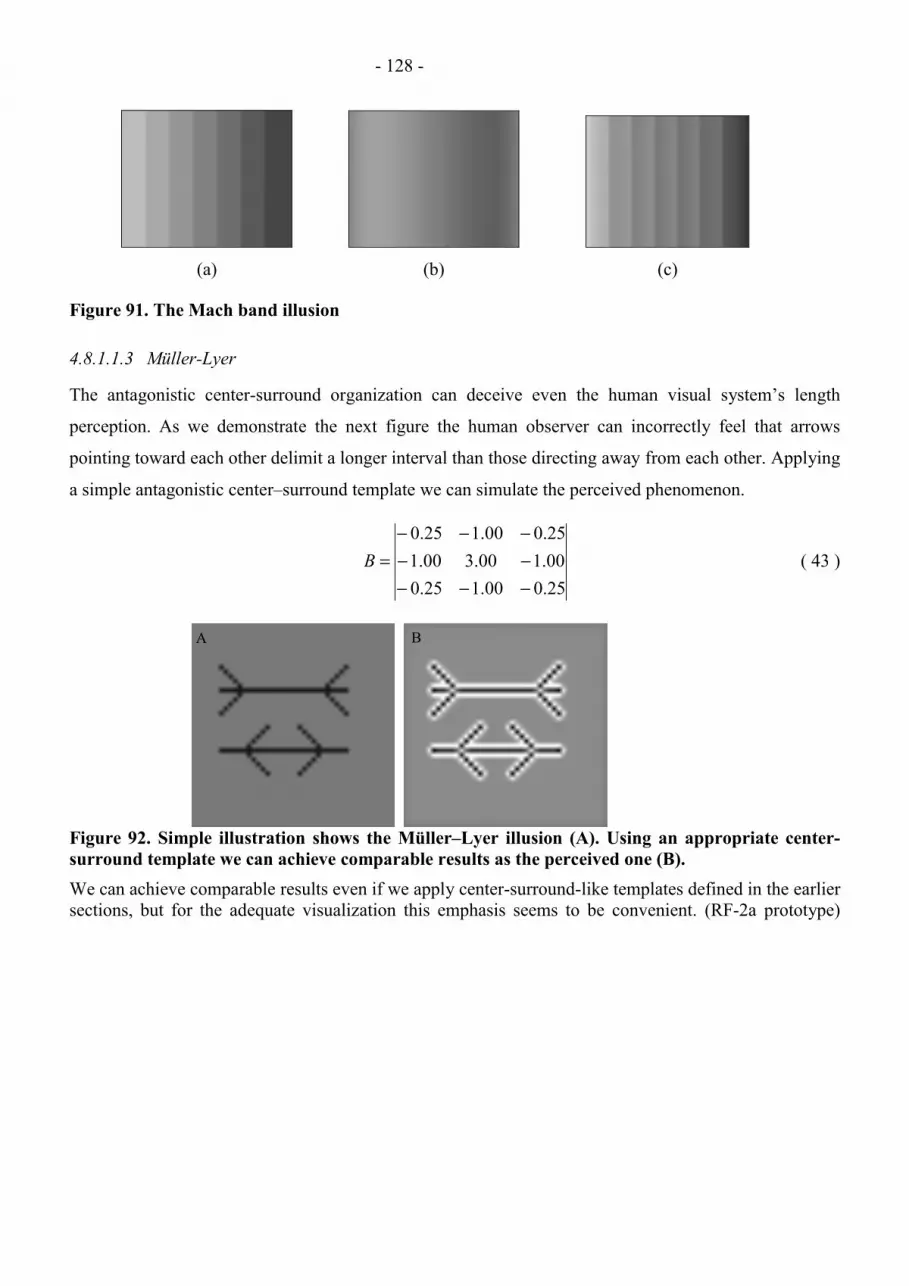
- 128 -

(a) (b) (c)

Figure 91. The Mach band illusion

4.8.1.1.3 Müller-Lyer

The antagonistic center-surround organization can deceive even the human visual system’s length

perception. As we demonstrate the next figure the human observer can incorrectly feel that arrows

pointing toward each other delimit a longer interval than those directing away from each other. Applying

a simple antagonistic center–surround template we can simulate the perceived phenomenon.

25.000.125.000.100.300.125.000.125.0

−−−−−−−−

=B ( 43 )

A B

Figure 92. Simple illustration shows the Müller–Lyer illusion (A). Using an appropriate center-surround template we can achieve comparable results as the perceived one (B).We can achieve comparable results even if we apply center-surround-like templates defined in the earliersections, but for the adequate visualization this emphasis seems to be convenient. (RF-2a prototype)

- 129 -

Herring gridIllusion: gray patches appear at the intersections of a grid of black squares on a white background.

Figure 93

CNN template of the retinal ganglion cells

This retina model integrates the features of the outer and inner plexiform layers to simulate the spatial-

type (spatial organization related, e.g. center-surround antagonism) analysis of visual input

characterizing the outer plexiform layer and the temporal-type (related to the intensity changes) analysis

performed in the inner plexiform layer.

In addition, the model exploits the fact that ganglion cells have an aggregated Difference-of-Gaussians

(DOG) spatial receptive field ([5,13,14]), where signals from the center and surround regions are

separately summed and the resulting center and surround signals have antagonistic effects on the

ganglion output signal (RF-2a receptive field prototype).

�

��

�

�

−−−−−−−−−−−−−−−−−−−−−−−−

==

0.00.00.00.00.00.00.00.01.01.01.01.01.00.00.01.03.03.03.01.00.00.01.03.033.01.00.00.01.03.03.03.01.00.00.01.01.01.01.01.00.00.00.00.00.00.00.00.0

]0[ τAA ( 44 )

- 130 -

( ).07.0)3(,222.0)2(,2.0)1(,45.4)0(

;55.0,5,1.2,7.0,9

)( ;)(

);()()(

;3 ;0

]0[

)3()3()3()3()3()3()3()3()2()2()2()2()2()3()3()2()1()1()1()2()3()3()2()1()0()1()2()3()3()2()1()1()1()2()3()3()2()2()2()2()2()3()3()3()3()3()3()3()3(

2

)()( 22

−=−=========

==

−=

==

=

�

��

�

�

=

−−

GGGGkkpprrkkc

ekrGekrG

rGrGrG

I

B

GGGGGGGGGGGGGGGGGGGGGGGGGGGGGGGGGGGGGGGGGGGGGGGGG

B

scscscs

prss

prcc

SC

sc

τ

τ

CNN simulation: If we apply a simple center-surround template to the above picture then an error occurs

simulating the illusion: bright patches appear in the middle of the black squares too (first picture below).

The CNN retina model given simulates the illusion correctly (second picture below).

Figure 94

- 131 -

4.8.1.1.4 Café wall

In the vertebrate retinas the ganglion cells have center-surround antagonistic receptive fields. It means

that the stimulation of the receptive field center of the neuron can be inhibited by the appropriate

stimulation of the surround. This arrangement of the representation can explain the Cafe Wall illusion

(Figure 95) [18]. On this illusion we can perceive convergence of the otherwise parallel edges of the

tiles. The illusion strength depends on the thickness and brightness of the mortar and on the shift

between the tiles.

( a ) ( c ) ( d )

( b ) ( e ) ( f)

The large values on the -30°orientation map indicate thatthe observed lines are skewedrather than horizontal.

( g )

Figure 95. The Cafe Wall illusion (a) is explained by a center-surround filtering (b). Theappearing tilt effect is exaggerated by +30° and -30° orientation filters (c, e). By thresholding theseoutputs we demonstrate the perceived illusion. On the enlarged inserts (g) the largest valuesindicate the existence of skewed lines in those particular positions. (d) and (f) demonstrate thatdifferent orientations observed in different positions according to the observed illusion.If we use the next simple template:

B11

01 01 0101 0 8 0101 01 01

=− − −− −− − −

��

��

. . .

. . .

. . .( 45 )

we can generate a representation (Figure 95b) of the visual stimulus (input image), which show some

orientation tilt in that particular direction the illusion can be perceived. For the further exaggeration of

- 132 -

this tilt effect we used +30° and -30° orientation filters and an appropriate threshold, which assumed to

be present in the mammalian cortex as well. The used CNN templates were the followings:

A12

01 01 01 01 0 201 01 01 0 2 0 2

0 2 0 2 0 2 0 2 0 20 2 0 2 01 01 010 2 01 01 01 01

=

− − − − −− − −

− − −− − − − −

��

��

. . . . .

. . . . .. . . . .. . . . .. . . . .

A14

0 2 01 01 01 010 2 0 2 01 01 010 2 0 2 0 2 0 2 0 201 01 01 0 2 0 201 01 01 01 0 2

=

− − − − −− − −

− − −− − − − −

��

��

. . . . .. . . . .. . . . .. . . . .. . . . .

( 46 )

Aif yif y23

1 0 481 0 48

=≥

− <..

Aif yif y45

1 0 481 0 48

=≥

− <��

.

.( 47 )

The results achieved by the CNN model can be seen on Figure 95.

4.8.1.2 Distortion illusions

Figure 96. shows the Zöllner illusion. The lines are parallel, but the crossing lines cause them to appear

to diverge.

To understand the phenomenon, one has to carefully examine, what kinds of effects are caused by the

crossing lines. The most important primary effect is that small black patches appear at the acute angles,

and no changes happen at the obtuse angles. This can even be seen by the naked eye (Figure 96.a). The

small black patches are exaggerated in Figure 96.b. We consider, that in a higher level of our visual

system the crossing lines are erased, but the patches still remain at the end of the line pieces (Figure

96.c).

The patches at the end of the line pieces fool the brain when it computes the orientation. It can be

imagined in the following way: the ends of the line pieces seem to be moved towards the patches, which

cause them to appear being rotated. Figure 96.d, shows an exaggerated draw, which illustrate what we

see with our eye.

(a) (b) (c) (d)

Figure 96. The original Zöllner illusion: (a). The magnified patches at the acute angles: (b). Thecut line pieces with the patches: (c). The magnified distortion caused by the crossing lines: (d).

- 133 -

We created structural-strategy model for this illusion. The appearance of the patches is derived from the

structure of the retina, while the rotation effect is explained by the behavior of the orientation selective

cells in the cortex [1].

The appearance of the patches is the result of a blurring effect we can find in the [5]. This can be

modeled by the following feedforward template:

[ ]A B I= =��

��

=0

0 023 0 023 0 023 0 023 0 0230 023 0 053 0 055 0 053 0 0230 023 0 055 0 2 0 055 0 0230 023 0 053 0 055 0 053 0 0230 023 0 023 0 023 0 023 0 023

0,

. . . . .

. . . . .

. . . . .

. . . . .

. . . . .

, ( 48 )

(The input can be seen in a, and the output can be seen in Figure 97b.)

(a) (b) (c)

(d) (e) (f)

Figure 97. The original test image (a). The blurred image (b). The result of the threshold function(c). Erasing the vertical crossing lines (d). Erasing the horizontal crossing lines (e). The line pieceswith the patches (f).

The result of this template is a grey-scale image. To get a black-and-white image again, we used this

threshold template.

[ ] [ ]A B I= = =2 0 0 3, , . ( 49 )

(The initial state can be seen in Figure 97b, the output in Figure 97c.) The following three templates

erase the crossing lines:

[ ] [ ]A B IT

= = − − − − − − = −2 0 2 0 2 0 2 1 0 2 0 2 0 2 13, . . . . . . , . ( 50 )

(The input and the initial state are shown in Figure 97c, the output in Figure 97d.)

[ ] [ ]A B I= = − − − − − − = −2 0 2 0 2 0 2 1 0 2 0 2 0 2 13, . . . . . . , . ( 51 )

- 134 -

(The input and the initial state are shown Figure 97d, the output in Figure 97e.)

[ ]A B I= ��

��

= =0 1 01 2 10 1 0

0 0, , ( 52 )

(The initial state is shown Figure 97e, the output in Figure 97f.) For computing the orientation, there are

orientation selective cells in the cortex. The receptive field organization of the cells can be seen in

Figure 98. Here we model a vertically oriented, orientation selective cortical cell type with the following

template:

[ ]A B= =

− − − −− − − −− − − −− − − −− − − −− − − −− −

0

0 095 0 048 0 071 014 0 071 0 048 0 0950 095 0 048 0 071 014 0 071 0 048 0 0950 095 0 048 0 071 014 0 071 0 048 0 0950 095 0 048 0 071 014 0 071 0 048 0 0950 095 0 048 0 071 014 0 071 0 048 0 0950 095 0 048 0 071 014 0 071 0 048 0 0950 095 0 048 0 071 014 0 071

,

. . . . . . .

. . . . . . .

. . . . . . .

. . . . . . .

. . . . . . .

. . . . . . .

. . . . . − −

��

��

=

0 048 0 095

0

. .

, I ( 53 )

The inputs can be seen in Figure 99. The orientation of the line piece in the receptive field of a cell

determines the output value of it. We tested the modeled orientation selective cell with three different

images (Figure 99). Two of them were line pieces with patches at the ends (from Figure 97f), and the

third was a same sized and oriented line piece without patches. This third one is considered as a

reference image (Figure 99). The values of the responses are also indicated in Figure 99. According to

the receptive field organization of the modeled cell type, the bigger the slope of the line in the receptive

field, the greater the response is. Note that the responses are not proportional with the deviations. It is

not surprising, because the way, how the cell computes the orientation is non-linear.- - + + + - -- - + + + - -- - + + + - -- - + + + - -- - + + + - -- - + + + - -- - + + + - -

Figure 98. The receptive field organization of the modeled orientation selective cortical cell type.

input image:

cell response: 0.24 0.08 0.19

Figure 99. The images in the receptive field of the modeled orientation selective cells, and theresponse of them.

- 135 -

The Poggendorff illusion (Figure 100 a,) is an old and still not totally understood illusion [13]. It has

close relationship to the Zöllner, the Herring and the Twisted cord illusions (Figure 100 b, c, d,). There

can be seen perceptual displacement of the oblique line in it. In the case of the Zöllner and Herring

illusion one can observe deformation and divergence of the otherwise parallel lines. The twisted cord

illusion pretends that the parallel cords are not straight as they really are. These illusions belong to the

group of distortion illusions. There are several theories, which try to explain the underlying mechanisms

of these illusions. We gave a model of Zöllner illusion earlier in this paper. One supposed that common

mechanisms are the exaggeration of the acute angles and minimization of the obtuse angles within the

image. It is assumed that the cortical lateral inhibition can produce corresponding effects. That is, every

orientation column is inhibiting the neighboring columns within the cortex and these interacting

neighbors have resembling orientation preferences.

(a) (b)

(c) (d)

Figure 100. Different illusions, which can be explained by angular displacement theory: ThePoggendorff (a), Herring (b), Zöllner (c) and the Twisted cord illusions (d).

4.8.1.3 Endpoint sensitivity

However, in the case of Poggendorff illusion, there is considerable deviation from this rule, if we use a

slightly different experimental condition. If we depict only the obtuse angles then we can still observe

- 136 -

the illusion (Figure 101a)[13]. But in that situation, when only the acute angles are delineated

exceptionally, the perceived illusion declines or even seems to disappear (Figure 101b).

(a) (b)

Figure 101. There are special variants of the Poggendorff illusion. The illusion can be stillperceived if all acute angles are erased (a), but decreases or disappears (even opposite effects canbe seen) if all the obtuse angles are eliminated (b).

We can not perceive such a strange behavior in case of the other mentioned illusions. How can be

explained such a deviation from the otherwise suitable explanation? We presumed that there has to be

another phenomenon, which can deteriorate the otherwise existing acute angle expansion. This can be

the apparent, illusory shift of the position of the acute angles. If there exists such a phenomenon within

the human visual information processing, then the other mentioned types of illusions will not be

sensitive for this kind of shifts. On Figure 102 we demonstrate that there exists such a phenomenon. We

can perceive that the tip positions alter depending on the acuteness of the different angles.

Figure 102. This image can demonstrate that one can perceive illusory shift in the tip position ofdifferent angles.

- 137 -

What type of mechanism causes the illusory shift of the position of the acute angles, but does not change

considerably the position of the obtuse angles and the intersecting lines? If we use the next simple CNN

template:

B11

1 1 105 05 051 1 1

=− − −

− − −

��

��

. . . Aif yif y12

1 0 30 0 3

=≥<

.

. B12 1= − ( 54 )

Using this orientation endpoint filter, we can detect the endpoints of the horizontal lines (Figure 103b1).

Apparently there is a slight overestimation or shift at the end position in case of acute angles (Figure

103b2) but there is no identified endpoints, neither the obtuse angles, nor the composite angle figures

(Figure 103b1, b3).

2

1

(a)

3

4

2

1

4

3

(b)

Figure 103. CNN model of a special horizontal endpoint detection: The input can be seen on (a)and the result on (b) inserts. It can detect the endpoints of acute angles (2), but it is not able todetect the endpoints of obtuse angles (3) and cross sections (1). By a distracting element (a(4)) thisdetector can be deceived (b(4)).

This way this simple orientation-endpoint filter can corrupt the effects of angle extensions. For

validation of the existence of such a mechanism we changed slightly the experimental conditions. We

draw additional points nearby to the acute angles. This modification distracts horizontal endpoint

detector (Figure 103b4), therefore the effects of deterioration decrease and the Poggendorff illusion

hopefully appears again. This suggested extension of the angular displacement theory and able to

provide explanation for the majority of the variations Poggendorff illusions. However, further

scrutinized psychological experiments are necessary to verify our proposed explanation of this problem.

- 138 -

4.8.2 Top down Illusions

(Á. Zarándy)

4.8.2.1 Face vase

Figure 104a shows the face-vase illusion. If the initial fixation point is inside the contour, we see a vase,

otherwise we see two faces.

If we cannot decide exactly at once on an ambiguous scene which is the object, and which is the

background, our brain will suppose that the fixation point is on the object. This happens here, if we look

first at inside the vase, we will see a vase, and when we look first at one of the face, we will see the

faces.

Our phenomenological model for this illusion contains a single layer CNN, having the following

propagation type template:

.0 ,000050000

,010121010

=�

��

�

�

−=��

��

�

�

= IBA ( 55 )

If we consider our initial fixation point as a black spot in the initial state of the CNN, and put the

original image (Figure 104a) to the input, the face or the vase will be extracted on the output of the CNN

respectively. Figure 104 shows the effect.

(a) (b) (c)

(d) (e)

Figure 104. The face-vase illusion: (a) original image, (b) the fixation point is in the face area, (c)and the output of the CNN (c). The vase is extracted. If the initial fixation point is in the vase area(d), the vase is extracted (e).

- 139 -

4.8.2.2 Sculpture illusion

The sculpture illusion (Salvador Dali’s painting) can be seen in Figure 105a. After watching the image

for a while, Voltaire’s sculpture will suddenly appear.

(a) (b)

Figure 105. The sculpture illusion. The original input image (a), and the result (b).There is a hidden sculpture in the center of the image, which can be considered as background at the

first quick look (Figure 105a). It has the same grayness than the other background objects in that area.

After watching the image for a while, our brain will segment the image by grayness, and analyze the

shape and the structure of the groups of patches having the same gray level. In this way after a while, our

brain will reconstruct and recognize Voltaire’s sculpture.

We made a phenomenological CNN model for this illusion. The model contains a single layer CNN,

which segments the image by grayness by using the following CNN template:

A B I= ��

��

=�

�

��

��

=0 0 5 0

0 5 4 0 50 0 5 0

0 5 0 5 0 50 5 1 0 50 5 0 5 0 5

35.

. ..

,. . .. .. . .

, . ( 56 )

The input and the initial state can be seen in Figure 105a and the output of the CNN is in Figure 105b.

In the output image, the sculpture is obviously visible.

References (4.8)

[1] E.M. Kandel, J.H. Schwartz, “Principles of Neural Science”, third edition, Elsevier New York,

Amsterdam, Oxford, 1991.

[1] L.O. Chua and L. Yang, “Cellular Neural Networks: Theory and Application”, IEEE Transactions

on Circuits and Systems, vol. 35, no. 10, October 1988, pp. 1257-1290

[2] L.O. Chua and T. Roska, “The CNN Paradigm”, IEEE Transactions on Circuits and Systems - I,

vol. 40, no. 3, March 1993, pp. 147-156

- 140 -

[3] T. Roska and L.O. Chua, “The CNN Universal Machine: An Analogic Array Computer”, IEEE

Transactions on Circuits and Systems - II, vol. 40, March 1993, pp. 163-173

[4] T. Roska, J. Hámori, E. Lábos, K. Lotz, L. Orzó, J. Takács, P. L. Venetiáner, Z. Vidnyánszky, Á.

Zarándy "The Use of CNN Models in the Subcortical Visual Pathway", IEEE Trans. Circuits and

Systems pp. 182-195, vol. 40, March 1993.

[5] T. Roska, Á. Zarándy, L.O. Chua "Color image processing using multi-layer CNN structure" H

Didiev(ed), Circuit Theory and Design 93, Elsevier, Amsterdam, 1993.

[6] F. Werblin, T. Roska, and L.O. Chua, “The Analogic Cellular Neural Network as a Bionic Eye”

International Journal of Circuit Theory and Applications, vol. 23, 541-569 (1995)

[7] Á. Zarándy, T. Yang, T. Roska, and L.O. Chua, “CNN Based Models for Visual Illusions”, 1995

International Symposium on Nonlinear Theory and Its Applications (NOLTA’95) pp. 471-476, Las

Vegas, USA, Dec 10-14, 1995.

[8] HTTP://INSIGHT.MED.EDU/WEBVISION

[9] F. Werblin, A. Jacobs, “Using CNN to Unravel Space-Time Processing in the Vertebrate Retina”,

Proc. of the third IEEE Int. Workshop on Cellular Neural Networks and their Application (CNNA-

94), pp. 33-40, Rome Dec. 1994.

[10] K. Lotz, Z. Vidnyánszky, T. Roska, J. Vandewalle, J. Hámori, A. Jacobs, F. Werblin “Some

Cortical Spiking Neuron Models Using CNN”, Proc. of the third IEEE Int. Workshop on Cellular

Neural Networks and their Application (CNNA-94), pp. 41-46, Rome Dec. 1994.

[11] A. Jacobs, T. Roska, F. Werblin “Techniques for constructing physiologically motivated

neuromorphic models in CNN”, Proc. of the third IEEE Int. Workshop on Cellular Neural

Networks and their Application (CNNA-94), pp. 53-60, Rome Dec. 1994.

[12] S. Coren and J.S. Girgus, “Seeing is deceiving: The psychology of visual illusions”, Lawrence

Erlbaum Associates, Inc., New Jersey: 1978.

[13] HTTP://WWW.ILLUSIONWORKS.COM

[14] E. Greene, “Both tilt and misalignment are manifestations of angular induction”, Percept. Mot.

Skills Vol. 73, pp. 329-330, 1993

[15] E. Greene, D. Levison, “Angular induction as a function of the length and position of segments and

gaps”, Perception Vol. 23(7), pp. 785-821, 1994

[16] R.H. Day, E.J. Stecher, A.C. Parker, “The Poggendorff illusion and apparent interparallel extents”,

Perception Vol. 21(5), pp. 599-610, 1992

http://insight.med.edu/WEBVISION

- 141 -

4.9 Plasticity of Receptive Fields

Synaptic plasticity is one of the elementary processes in the nervous system that underlies higher brain

function, such as learning and memory. This cellular level of plasticity means the alteration of the

effectiveness of synaptic information transfer. The change of synaptic efficacy can be either

strengthening, or weakening, called synaptic potentiation and depression, respectively. One isoform of

the synaptic plasticity, the long-term potentiation (LTP) were described in the primary visual cortex.

This phenomenon observed at thalamocortical synapses from the LGN relay cells to layer IV pyramids

of the visual cortex. Based on this process the visual information transfer to the cortex can be fastened

and sharpened. In early stages of development - the so-called sensitive period - the synaptic plasticity

(LTP) plays also a crucial role to form the functional columnar architecture of the visual cortex.

Plasticity in the nervous system can be examined not only at cellular level but neuronal network level.

For instance the receptive field plasticity was studied and explained best in sensory systems, such as

visual system. The visual cortical receptive fields are subjects to plastic changes (spreading, retraction,

rebuilt) according to the alteration in the activity pattern of their retino-thalamic inputs.

- 142 -

5 Somatosensory receptive fields

5.1 General overview

The somatosensory system involves those parts of the nervous system, which is responsible for

the mechanosensation inside and on the surface of the body (Kandel et al. 1991; Tracey and Waite,

1995: [1, 3]). There are four somatosensory modalities: discriminative touch, proprioception,

nociception, and temperature sense. These modalities are processed more or less separately in the brain.

Tactile sensation is based on the mechanoreceptors. The skin and the deeper tissues contain four types

of mechanoreceptors. Two of them, a slowly and a rapidly adapting type, can be found in the superficial

layer of the skin. The deeper tissue also contains two types of receptors. The vibration sensitive, rapidly

adapting and the slowly adapting which is sensitive to rapid indentation of the skin. The receptors

respond to the stimuli with different frequencies: stronger stimuli evoke higher frequency responses

while weaker ones evoke low frequency responses.

The construction of the somatosensory system reflects an organizational principle common to all

sensory systems: the sensory information is processed through a hierarchical order of structures from the

periphery to the cortex in parallel channels of the different submodalities. The somatosensory system is

characterized by a somatotopically organized representation of the body in the different structures. This

means that distinct population of neurons represents different parts of the body, and conversely, neurons

in the same population have their receptive fields (RF) localized on the same part of the body. The

density and size of the receptive fields are different along the body surface. On the most tactile-sensitive

parts of the body - such as the fingertips and the tongue – where the number of receptors is high in a unit

area, the receptive fields are small and densely spaced. (The highest receptor density on the fingertips of

the human is approximately 2500 receptors including all four types per square centimeter.) The cortical

representation is the best understood and characterized by the followings (for brief review, see

Recanzone, 1992: [2]). The somatotopic representation is distorted: those body parts have larger

representations (larger population of neurons) which have higher density of mechanoreceptors.

According to the reverse magnification rule the larger is the representation the smaller are the RFs. The

cortical representation of a defined body region is locally continuos and marked by shifted overlaps of

the RFs across the cortex. On the other hand, the representation of the different body parts is

discontinues. The overlaps of the RFs are linearly decreased with the distance of the cortical neurons.

The following description is focused on the vibrissal somatosensory system of the rodents where

structure-function relationship can be studied well.

- 143 -

5.2 Hyperacuity

5.2.1 Two-point discrimination

Two-point discrimination is known to depend on the density of the mechanoreceptors in the skin

(see in Kandel et al., 1991: [1]). Furthermore, it is assumed that smaller RFs result in better spatial

resolution (see Joublin et al., 1996: [18]). Accordingly, much more closely spaced dots can be

differentiated on the fingers, than on the back. It is also proposed that two objects can be better

discriminated if their neural representations are well separated, at least at the level of the primary

somatosensory cortex (Peterson et al., 1998: [15]). Some neural correlates of two-point discrimination is

shown below at the “CNN applications”.

An important aspect of the somatosensation is that practice can significantly improve the

discrimination ability which depends on central neural mechanisms (Recanzone et al., 1992; Buonomano

and Merzenich, 1998; Sterr et al., 1998, Gilbert, 1998: [2, 17, 19, 36]). According to our recent

knowledge the main site of short-term modifications induced by practice is the primary somatosensory

cortex where both body representation as well as the RFs were found to be substantially altered by

training (Donough, 1995; Buonomano and Merzenich, 1998: [20, 17]).

5.2.2 Representational plasticity

There is a lot of evidence indicating that the cortical representations of the frequently used body

parts are increased, e.g. Braille-readers and violinists have significantly larger finger representation than

the control subjects (Pascual-Leone and Torres, 1993; Elbert et al., 1995: [21, 22]). Similarly, overusing

a pair of whiskers (2 neighboring whiskers) results in that deflection of either of the paired whiskers

activates the neurons in both its own as well as the paired whisker’s barrels with equal efficiency

(Diamond et al., 1993: [23]). Artificial syndactilia (surgical connection of two neighboring fingers) also

results in the fusion of their cortical representation (Clarck et al., 1988; Allard et al., 1991: [24, 25]).

These latter as well as other experiments (Wang et al., 1995: [26]) provided evidences that input

synchrony is essential for the formation of body representation. Coincident inputs are thought to result in

the strengthening of the lateral excitatory connections by Hebbian learning, and/or the activation of

previously silent population of neurons (Donough, 1995; Xing et al., 1996; Buonomano and Merzenich,

1998; Gilbert, 1998: [20, 27, 17, 36). The supragranular layers (layers II/III) seems to be especially

important in the Hebbian learning (Donough, 1995; Buonomano and Merzenich, 1998: [27, 17]).

Indeed, NMDA receptors, which play an important role in long term synaptic modification, are

concentrated mainly in the supragranular layers. It is noteworthy, that the decrease in the strength of the

lateral inhibition may also contribute to the representational plasticity through unmasking of the

- 144 -

subthreshold excitatory connections (Donough, 1995; Buonomano and Merzenich, 1998; Gilbert, 1998:

[27, 17, 36]). Until now we have had only few data concerning the role of the other layers in these

processes (Diamond et al., 1994: [28]).

It is very important that representational changes are reversible (although chronic alterations,

such as loosing of body parts result in serious structural reorganizations after a long period of time (e.g.

Florance et al., 1998: [29]) i.e. cortical neurons form stimulus dependent assemblies, which indicates the

adaptive capability of the adult brain in the ever changing environment (Spengler and Dinse, 1994:

[30])). It should be noted that the actual behavioral state (e.g. attention) is decisive in forming new

representations (Recanzone, 1992: [2]). In addition, it seems that these changes are limited mainly to

neighboring, structurally based neuronal assemblies. The barrel cortical columns are good examples

because of the relatively rich interconnections of the neighboring columns comparing to the more distant

cortical areas (Buonomano and Merzenich , 1998; Gilbert, 1998: [17, 36). In summary, the dynamic

sensory representation is presumably established by competitive cortical networks engaged by the spatial

and temporal pattern of the peripheral stimuli and selectively supported by the actual behavioral

significance of the stimuli (Benuskova et al., 1994; Joublin et al., 1996; Xing and Gerstein, 1996: [31,

18, 27]).

As for the behavioral correlates of the representational plasticity, an interesting finding was that

Braille-readers, who use three fingers for reading, occasionally miss-localize which finger is stimulated

among the 3 reading ones (Sterr et al., 1998: [19]), suggesting that they have common cortical

representation. In an other, frequency discrimination study it was found that in addition to the

enlargement of the stimulated skin area, representation become more complex, characterized by a

discontinuous appearance (Recanzone et al., 1992: [2]). Nevertheless, only a mild, statistically non-

significant correlation could be detected between the representational changes and the improved

behavioral performance (Recanzone et al., 1992: [2]).

5.2.3 Use/experience dependent RF modifications

In most cases training was found to induce the increase of the size of the cortical RFs, although,

decrease could also be observed after some experimental procedures (Jenkins et al., 1990; Recanzone et

al., 1992; Buonomano and Merzenich, 1998: [32, 2, 17]). Interestingly, there could not be found any

correlation between the changes (mostly increase) of the RF size and the behavioral performance in the

frequency discrimination study (Recanzone et al., 1992: [2]). It is therefore uncertain whether the

decrease of the RF size would play a basic role in the improved discrimination ability following training.

In contrast, both experimental and modeling studies suggest that the most significant change is

the increased overlap of the RFs of the cortical neurons being even far from each other, on the overused

- 145 -

skin surface (Recanzone et al., 1992; Xing and Gerstein, 1996: [2, 27]). As it was reported the center of

the RFs on the stimulated area shifted closer to each other while they usually entirely overlapped.

Together these findings lead to the construction of the coarse coding hypothesis, which indicates that

particularly high resolution can be achieved by an ensemble of neurons with large RFs and suggests that

hyperacuity is resulted from the increase in the number of neurons representing the stimulated area

(Joublin et al., 1996; Eurich and Schwegler, 1997: [18, 33]).

5.3 CNN applications

5.3.1 Two-point discrimination in neural networks

The perception of textures involves the discrimination of fine tactile stimuli, like Braille-writing.

The simplest example for the spatial discrimination is the distinguishing of two closely placed point

stimuli (see in Kandel et al., 1991: [1]). When the skin is stimulated at one point several receptors are

activated also in the neighborhood of the stimuli. These impulses travel trough different structures of the

somatosensory system to the cortex. In the different relay stations neurons conveying the stimulus

activate only a set of the target cells where the activation of the inhibitory interneurons restrict the

population of these active neurons. When moving from the center to the edge of the active region, the

activity level gradually decreases, while the active zone is surrounded by an inhibited ring of neurons.

Inhibition increases the contrast of the stimulus.

When two distinct points of the skin surface are stimulated close to each other, the activated

areas will overlap and the two activity peaks could be merged. On the other hand, the inhibition will also

be summed resulting in that the activity peaks of the two populations become sharper. Such a better

spatial separation of the two active neuronal populations presumably plays important role in a better

spatial discrimination. This result can be achieved via a simple model constructed by a divergent input to

the different layers representing the different structures of the somatosensory system and by adding

feedback inhibition (see in Kandel et al., 1991: [1]).

- 146 -

Figure 106 Schematic view of the network of the modeled somatosensory system (Dudel, J. 1983:[34]). The inhibitory interneurons between the layers marked with red solid circles feed back theoutput of the cells with some delay.

- 147 -

Figure 107 Effect of lateral inhibition in a one dimensional view. (Dudel, J. 1983: [34]). During theprocessing steps, the inhibited region is getting deeper and deeper layer by layer around the activecell population.

- 148 -

Figure 108 Two-point discrimination (Mountcastle, Darian-Smith, 1968: [35]). The near drawingdisplays the case when the active neuron activates inhibitory interneurons so that accumulatedinhibition separates the activity peaks more effectively. On the distant drawing the case withoutinhibition is illustrated and, as a consequence, the activity peaks are overlapped and merged.Importantly, the peaks would become more intensive during subsequent processing steps.

According to the above-mentioned properties, the idea of the CNN implementation is easily

yielded. The model follows the structure indicated on Figure 106. In the case of the CNN model the

receptors and the first processing layer can be integrated. The A and B templates are two discretized

Gauss density functions which are sampled in the [-2, 2] interval integer points and have the following

form:

A:

σ=1.6a

x yx y

ij

ij

= −−

+� �

−+�

��

��3

1

222 2

2

2 2

2

expexp

σσ

B:

σ=0.8b

x yx y

ij

ij

=−

+� �

−+�

��

��4

1

222 2

2

2 2

2

expexp

σσ

( 57 )

where σ is the deviation, i, j are integers, i, j ∈ [-2, 2]. The 0,0 values of the i, j indices stand for

the central element of the A and B matrices.

- 149 -

The shape of A and B templates follow the property of the somatosensory system, that the

inhibition is mostly covered by the more effective excitation. The effect of the A template becomes less

important in the center of the activity region compared to the effect of B. In the somatosensory system,

the activity level of cells is coded by the frequency of action potentials. In CNN implementation the

activity is coded by a numerical value, which is represented by a certain gray level in the output. Lighter

pixels indicate greater activity.

Figure 109. The effect of feedback inhibition when only one, spot shaped stimulus is present(simulated result). The inhibited region around the patch on the output of the second layer is evendarker and broader than on the output of the first layer.

Figure 110. The effect of lateral inhibition. Simulation is based on the proposed model. Thepatches representing the stimuli are gradually separated on each layer, and the gaps are darkenedeven in those areas where the stimuli were close to each other. The contrast of the patches becamehigher.

The CNN model of the former phenomenon is defined by the following templates:

- 150 -

NRLAYERS 2

LAYER 1

NEIGHBORHOOD 2

CURRENT -0.01

FEEDBACK FROM 1

-0.05 -0.09 -0.11 -0.09 –0.05

-0.09 -0.16 -0.19 -0.16 –0.09

-0.11 -0.19 -0.24 -0.19 –0.11

-0.09 -0.16 -0.19 -0.16 –0.09

-0.05 -0.09 -0.11 -0.09 –0.05

CONTROL FROM 1

0.00 0.02 0.04 0.02 0.00

0.02 0.21 0.46 0.21 0.02

0.04 0.46 1.00 0.46 0.04

0.02 0.21 0.46 0.21 0.02

0.00 0.02 0.04 0.02 0.00

LAYER 2

NEIGHBORHOOD 2

CURRENT -0.01

FEEDBACK FROM 2

-0.05 -0.09 -0.11 -0.09 -0.05

-0.09 -0.16 -0.19 -0.16 -0.09

-0.11 -0.19 -0.24 -0.19 -0.11

-0.09 -0.16 -0.19 -0.16 -0.09

-0.05 -0.09 -0.11 -0.09 -0.05

FEEDBACK FROM 1

0.00 0.02 0.04 0.02 0.00

0.02 0.21 0.46 0.21 0.02

0.04 0.46 1.00 0.46 0.04

0.02 0.21 0.46 0.21 0.02

0.00 0.02 0.04 0.02 0.00

CONTROL FROM 2

0 0 0 0 0

0 0 0 0 0

0 0 0 0 0

0 0 0 0 0

0 0 0 0 0

CONTROL FROM 1

0 0 0 0 0

0 0 0 0 0

0 0 0 0 0

0 0 0 0 0

0 0 0 0 0

( 58 )

The results can be seen in Figure 109 and Figure 110. In Figure 109, the activity region (white pixels)

and the surrounding inhibited region of neurons (dark gray pixels) can be seen. In Figure 110, closely

located patches represent the stimuli. In the outputs of the layers a dark (inhibited) region can be

observed among the patches and the peaks are gradually discriminated.

- 151 -

References (5.)[1] E.R. Kandel, J. H. Schwartz, T. M. Jessel, ``Principles of Neural Science'', Elsevier, New York,

1991

[2] G.H. Recanzone, M.M. Merzenich, W.M. Jenkins, K.A. Grajski and H.R. Dinse, “Topographic

reorganization of the hand representation in cortical area 3b of Owl monkeys trained in a

frequency-discrimination task.” J. Neurophysiology Vol. 67, pp. 1031-1056, 1992

[3] D.J. Tracey and P.M. Waite, “Somatosensory system. & Trigeminal sensory system.” in The rat

nervous system pp 689-723 (ed. Paxinos G), Academic Press. 1995

[4] M. Brecht, B. Preilowski, M.M. Merzenich, “Functional architecture of the mystacial vibrissae.”

Behav-Brain-Res.Vol. 84, pp. 81-97, 1997

[5] S.M. Lee, M.H. Friedberg and F.F. Ebner, “The role of GABA-mediated inhibition in the rat

ventral posterior medial nucleus. I-II. Assessment of receptive field changes following thalamic

reticular nuclear lesions, Differential effects of GABAA and GABAB receptor antagonists on

responses of VPM neurons..” J-Neurophysiol. Vol. 71, pp.1702-1726, 1994

[6] P.V. Hoogland, E. Welker; H. Van-der-Loos, “Organization of the projections from barrel cortex

to thalamus in mice studied with Phaseolus vulgaris-leucoagglutinin and HRP.” Exp-Brain-Res.

Vol. 68, pp. 73-87, 1987

[7] J. Chmielowska, G.E. Carvell, D.J. “Simons Spatial organization of thalamocortical and

corticothalamic projection systems in the rat SmI barrel cortex.” J-Comp-Neurol. Vol. 285, pp.

325-38, 1989

[8] P.B. Arnold, C.X. Li and R.S. Waters, “Thalamocortical axons in the vibrissa and forepow barrel

subfield in rat primary somatosensory cortex project beyond individual barrels: an in vivo

intracellular recording and labeling study.” Soc. Neurosci. Abstr. Vol. 21, pp. 635, 1998

[9] D.J. Simons, „Temporal and spatial integration in the rat SI vibrissa cortex.” J. Neurophysiology

Vol. 54, pp. 615-635, 1985

[10] D.J. Simons and G.E. Carvell “Thalamocortical response transformation in the rat vibrissa/barrel

system.” J. Neurophysiology Vol. 61, pp. 311-330, 1989

[11] H.T. Kyriazi, G.E. Carvell, D.J. Simons, “OFF response transformations in the whisker/barrel

system.” J-Neurophysiol. Vol. 72, pp. 392-401, 1994

[12] J.C. Brumberg, D.J. Pinto and D.J. Simons, “Spatial gradients and inhibitory summation in the rat

whisker barrel system.” J. Neurophysiology Vol. 76, pp. 130-140, 1996

[13] J.S. McCasland and T.A. Woolsey, “High-resolution 2-deoxyglucose mapping of functional

cortical columns in mouse barrel cortex.” J. Comp. Neurol.Vol. 278, pp. 555-569, 1988

- 152 -

[14] D. Kleinfeld and K.R. Delaney, “Distributed representation of vibrissa movement in the upper

layers of somatosensory cortex revealed with voltage-sensitive dyes.” J. Comp. Neurol. Vol. 375,

pp. 89-108, 1996

[15] B.E. Peterson, D. Goldreich, M.M. Merzenich, “Optical imaging and electrophysiology of rat

barrel cortex. I. Responses to small single-vibrissa deflections.” Cereb-Cortex. Vol. 8, pp. 173-83,

1998

[16] D. Goldreich, B.E. Peterson, M.M. Merzenich, “Optical imaging and electrophysiology of rat

barrel cortex. II. Responses to paired-vibrissa deflections.” Cereb-Cortex. Vol. 8, pp. 184-92, 1998

[17] D.V. Buonomano and M.M. Merzenich, “Cortical plasticity: from synapses to maps.” Ann. Rev.

Neurosci. Vol. 21, pp. 149-186, 1998

[18] F. Joublin, F. Spengler, S. Wacquant, H.R. Dinse, “A columnar model of somatosensory

reorganizational plasticity based on Hebbian and non-Hebbian learning rules.” Biol. Cybern. Vol.

74, pp. 275-286, 1996

[19] A. Sterr, M.M. Müller, T. Elbert, B. Rockstroh, C. Pantev and E. Taub, “Perceptual correlates of

changes in cortical representation of fingers in blind multifinger braille readers.” J. Neuroscience

Vol. 18, pp. 4417-4423, 1998

[20] J.P. Donoughe, “Plasticity of adult sensorimotor representation.” Curr. Opinion Neurobiology Vol.

5, pp. 749-754, 1995

[21] A. Pascual-Leone, F. Torres, “Plasticity of the sensorimotor cortex representation of the reading

finger in Braille readers.” Brain. Vol. 116, pp. 39-52, 1993

[22] T. Elbert, C. Pantev, C. Wienbruch, B. Rockstroh and E. Taub, “Increased cortical representation

of the fingers of the left hand in string players.” Science Vol. 270, pp. 305-307, 1995

[23] M.E. Diamond, J.M. Armstrong, F.F. Ebner, “Experience-dependent plasticity in adult rat barrel

cortex.” Proc. Natl. Acad. Sci. USA. Vol. 90, pp. 2082-6, 1993

[24] S.A. Clark, T. Allard, W.M. Jenkins, M.M. Merzenich, “Receptive fields in the body-surface map

in adult cortex defined by temporally correlated inputs.” Nature Vol. 332, pp. 444-5, 1988

[25] T. Allard, S.A. Clark, W.M. Jenkins, M.M. Merzenich, “Reorganization of somatosensory area 3b

representations in adult owl monkeys after digital syndactyly.” J-Neurophysiol. Vol. 66, pp. 1048-

58, 1991

[26] X. Wang, M.M. Merzenich, K. Sameshima and W.M. Jenkins, “Remodeling of hand

representation in adult cortex determined by timing of tactile stimulation.” Nature Vol. 378, pp.

71-75, 1995

[27] J. Xing and G.L. Gerstein, “Networks with lateral connectivity. III. Plasticity and reorganization of

somatosensory cortex.” J. Neurophysiology Vol. 75 pp. 217-232, 1996

- 153 -

[28] M.E. Diamond, W. Huang, F.F. Ebner, “Laminar comparison of somatosensory cortical plasticity.”

Science Vol. 265, pp. 1885-8, 1994

[29] S.H. Florence, H.B. Taub, J.H. Kaas, ”Large scale sprouting of cortical connections after

peripheral injury in adult Macaque Monkeys.” Science Vol. 282, pp. 1117-1120, 1998

[30] F. Spengler, H.R. Dinse, “Reversible relocation of representational boundaries of adult rats by

intracortical microstimulation.” Neuroreport Vol. 5, pp. 949-53, 1994

[31] L. Benuskova, M.E. Diamond and F.F. Ebner, „Dynamic synaptic modification threshold:

computational model of experience-dependent plasticity in adult rat barrel cortex.” Proc. Natl.

Acad. Sci. USA Vol. 91, pp. 4791-4795, 1994

[32] W.M. Jenkins, M.M. Merzenich, M.T. Ochs, T. Allard and E. Guic-Robles, “Functional

reorganization of primary somatosensory cortex in adult owl monkeys after behaviorally controlled

tactile stimulation.” J. Neurophysiology Vol. 63, pp. 82-104, 1990

[33] C.W. Eurich and H. Schwegler, “Coarse coding: calculation of the resolution achieved by a

population of large receptive field neurons.” Biol-Cybern. Vol. 76, pp. 357-63, 1997

[34] J. Dudel, ``General sensory physiology'' In R. F. Schmidt and Thorson (trans.) Berlin: Springer, pp.

177-192, 1983

[35] V.B. Mountcastle and I. Darian-Smith, ”Neural mechanisms in somesthesia” In V. B. Mountcastle

(ed.), Medical Physiology, 12th ed., Vol. II. St. Louis: Mosby, pp. 1372-1423, 1968

[36] C.D. Gilbert, “Adult cortical dynamics. “ Physiological Reviews Vol. 78, pp. 467-485, 1998

- 154 -

6 Auditory System

6.1 Hyperacuity in time

The barn owl can catch its prey in total darkness relying on acoustic signals only. It can localize sound

within 1-2° in azimuth and elevation and can detect interaural time differences as short as some tens of

microseconds. The neural mechanism underlying this fascinating ability has been investigated for

decades, and now we know a lot about how the brain of birds localizes sounds using differences in the

arrival of time and intensity [1-5]. However, several open questions are still waiting for answers. Two

unsolved problems in sound localization we consider here are as follows:

• How can an owl detect interaural time differences as short as some tens of microseconds while a

single action potential persists considerably longer, on the order of 1000 microseconds at least?

• How can an owl resolve phase ambiguity which results from the fact, that time is measured by the

phase of the input signals? That is, higher order neurons receive phase-locked spikes from the left and

right ear, and these neurons, therefore, can give maximal response not only to one but to several

interaural time differences (see Figure 118).

The first question concerns the operation of the sound localization system of the owl and involves a type

of hyperacuity: the sound localization system can mark shorter delays of time arrivals of sound than the

duration of an impulse, which indicates the time arrival. So this is a kind of hyperacuity in time.

In our models we use spikes whose duration is much greater than the time an action-potential requires to

travel from one cell to the other. It is known ([1-4]) that the velocity of spikes on the axon of a

magnocellular cell is estimated to be 3-5 m/s and the NL neurons have large cell bodies (30-40 µm). If

we take the velocity of spikes 4 m/s and the distance of 2 NL neurons 100 µm, then the time which is

needed for a signal to pass between two neighboring neurons is 25 µm. It is known that the duration of a

spike is about 2 milliseconds. It is also evident that a spike has no distinct peak along the line of NL

neurons. Our model, however, show very good results in coincidence detection.

As we mentioned above, there is considerable evidence that in the nucleus laminaris (NL) of owls

interaural time differences are mapped into a neural place coding via coincidence detection of signals

from the left and right ear. The first model to explain the encoding of interaural time difference (ITD)

was proposed by Jeffress in 1948 (Figure 111). Here fibers from the left and right nucleus

magnocellularis (NM) converge on the nucleus laminaris (NL), and the place of the neuron responding

- 155 -

maximally denotes the corresponding ITD. The exactness of this model was verified by the experiments

of M. Konishi and his colleagues. Their findings indicate that the magnocellular afferents work as delay

lines, and the NL neurons work as coincidence detectors [8].

left input

right input

NL neurons

place code

Figure 111. The Jeffress model for encoding interaural time differencesWe have completed the original delay line-coincidence detector model (above), with a lateral

inhibition (via an interneuron) between the neighboring neurons. Though GABAA receptors have been

localized in nucleus laminaris, which can be contributors of inhibitory synapses, nor the origin of the

inhibitory axons neither their function is known yet. Notwithstanding we assumed that there is lateral

inhibition via interneurons and examined the effects of this inhibition on the neuron’s ability to detect

coincidence between the input signals. The new structure is shown below in Figure 112.

left input

right input

NL neurons. . .. . .

higher centers

excitatorysynapse

inhibitorysynapse

Figure 112. The Jeffress model completed by lateral inhibition. Each neuron synapse on aninhibitory interneuron (for the sake of simplicity only one is indicated in the figure) which inhibitsthe neighboring cells

- 156 -

In this new structure each NL neuron synapse on an inhibitory interneuron (for simplicity only one is

indicated in Figure 112), which inhibits the neighboring neurons (we took the neighborhood 3). The

number of NL neurons in the line is 15 in accordance with the neuromorphological data. The CNN

template for the coincidence detection is given later. Next we discuss the nature of the inhibitory

connections.

As neurons receive several inhibitory synapses, the net synaptic current originating from the

inhibitory synapses is:

I k g v E vm Ei ijj

m REV REV= − ⋅ −=−3

3( ) ( ) ( 59 )

Where kij is the strength of the synapse between the ith and jth neurons, and EREV is the reversal

potential characterizing the inhibitory synapse.

In our experiments we used a large number of different values of kij . As a result of many

experiments we have stated that the best coincidence detection was achieved when the spatial

distribution of the inhibitory connection strengths was set as displayed in Figure 113. Eventually it has

turned out, that self-inhibition must be little or zero to obtain good results.

synapses

strength of inhibitory synapses

i,ii,i-1i,i-2i,i-3 i,i+1 i,i+2 i,i+3

Figure 113. Spatial distribution of inhibitory synaptic strengthsNext we show the results of two experiments. In the first experiment we examined how the

effectiveness of coincidence detection depends on the strength of the inhibition. The effectiveness of the

coincidence detection is measured by the number of spikes of NL neurons. The responses of cells 5, 7, 8,

9 and 11 were recorded at different inhibition strengths. Results are displayed in Figure 114. We used

uniform inhibitory values, i.e. in the above equation (see Figure 113). When there was no inhibition at

all, all cells responded maximally (this is not displayed in Figure 114). With increasing inhibition,

coincidence detection is more and more robust. Figure 114 displays responses of cells at three different

- 157 -

strengths of inhibition ( k =01 04 05. , . . and ) in three columns. We can observe that in the third column

(strongest inhibition) practically only Cell 8 responds. According to this simulation, it is very likely that

inhibition plays a crucial role in coincidence detection.

In the second experiment we recorded the responses of 7 cells (cell 5-11) while the arrival time

difference of the left and right input signals was changed. The inhibition was the same during this

experiment ( k =04. ). Figure 115a shows the responses of the seven cells when the time difference is 0.

Coincidence is detected by Cell 8, which responded most vigorously. Delaying one of the input signals

by 30µs, Cell 7 detected the coincidence (Figure 115b). Further delaying the same input by the same

period, Cell 6 showed the strongest response (Figure 115c) etc.

The structure of Figure 112 can be considered as an aggregate model of coincidence detection. It is

very likely, however, that the auditory system of owls uses several stages for this task. We developed a

model, which basically consists of 3 layers. The first two are the layer of the NL neurons and the layer of

the ICc neurons (Figure 116). The third layer (ICx neurons) and the connection between the second and

third layers will be discussed in the following section. In this model, each NL neuron makes an

excitatory synapse on an ICc neuron and an inhibitory interneuron (of this latter only one is indicated).

The interneuron then inhibits the neighboring NL neurons (feedback inhibition) and the neighboring ICc

neurons (feedforward inhibition). On the other hand, each ICc neuron again inhibits - via an inhibitory

interneuron - all neighboring ICc cells (second feedback inhibition). So we model here three kinds of

inhibition: two feedbacks and one feedforward. By applying various sets of inhibitory connections, we

could observe some interesting facts:

• If the feedback inhibition in the NL and the feedforward inhibition is zero, the effect of the feedback

inhibition in the ICc is the same as displayed in Figure 114 and Figure 115 (the aggregate model).

Therefore the assumption of inhibition in the NL is not necessary (but cannot be ruled out).

• When only feedforward inhibition is used, with the same connection strengths as in the case of

feedback inhibition, the coincidence detection is much poorer in the higher frequency band.

• In the lower frequency band, however, feedback inhibition is insufficient to produce the same

selectivity as in the higher frequency band. In this case feedforward inhibition is indispensable.

- 158 -

k = 01. k = 0 4. k = 0 5.

Cell 5 0 100 200 300 400 500 600

-1

-0.8

-0.6

-0.4

-0.2

0

0.2

0.4

0.6

0.8

1

time

mem

bran

e po

tent

ial

0 100 200 300 400 500 600

-1

-0.8

-0.6

-0.4

-0.2

0

0.2

0.4

0.6

0.8

1

time

mem

bran

e po

tent

ial

0 100 200 300 400 500 600

-1

-0.8

-0.6

-0.4

-0.2

0

0.2

0.4

0.6

0.8

1

time

mem

bran

e po

tent

ial

Cell 7 0 100 200 300 400 500 600

-1

-0.8

-0.6

-0.4

-0.2

0

0.2

0.4

0.6

0.8

1

time

mem

bran

e po

tent

ial

0 100 200 300 400 500 600

-1

-0.8

-0.6

-0.4

-0.2

0

0.2

0.4

0.6

0.8

1

time

mem

bran

e po

tent

ial

0 100 200 300 400 500 600

-1

-0.8

-0.6

-0.4

-0.2

0

0.2

0.4

0.6

0.8

1

time

mem

bran

e po

tent

ial

Cell 8 0 100 200 300 400 500 600

-1

-0.8

-0.6

-0.4

-0.2

0

0.2

0.4

0.6

0.8

1

time

mem

bran

e po

tent

ial

0 100 200 300 400 500 600

-1

-0.8

-0.6

-0.4

-0.2

0

0.2

0.4

0.6

0.8

1

time

mem

bran

e po

tent

ial

0 100 200 300 400 500 600

-1

-0.8

-0.6

-0.4

-0.2

0

0.2

0.4

0.6

0.8

1

time

mem

bran

e po

tent

ial

Cell 9 0 100 200 300 400 500 600

-1

-0.8

-0.6

-0.4

-0.2

0

0.2

0.4

0.6

0.8

1

time

mem

bran

e po

tent

ial

0 100 200 300 400 500 600

-1

-0.8

-0.6

-0.4

-0.2

0

0.2

0.4

0.6

0.8

1

time

mem

bran

e po

tent

ial

0 100 200 300 400 500 600

-1

-0.8

-0.6

-0.4

-0.2

0

0.2

0.4

0.6

0.8

1

time

mem

bran

e po

tent

ial

Cell 110 100 200 300 400 500 600

-1

-0.8

-0.6

-0.4

-0.2

0

0.2

0.4

0.6

0.8

1

time

mem

bran

e po

tent

ial

0 100 200 300 400 500 600

-1

-0.8

-0.6

-0.4

-0.2

0

0.2

0.4

0.6

0.8

1

time

mem

bran

e po

tent

ial

0 100 200 300 400 500 600

-1

-0.8

-0.6

-0.4

-0.2

0

0.2

0.4

0.6

0.8

1

time

mem

bran

e po

tent

ial

(a) (b) (c)

Figure 114 Responses of cell 5, 7, 8, 9 and 11, respectively, at three different, increasing values ofinhibition. A row contain the responses of the same cell at different inhibition, a column displaysthe responses of different neurons at the same inhibition

- 159 -

∆t = 0 ∆t s= 30µ ∆t s= 60µ

Cell 5 0 100 200 300 400 500 600

-1

-0.8

-0.6

-0.4

-0.2

0

0.2

0.4

0.6

0.8

1

time

mem

bran

e po

tent

ial

0 100 200 300 400 500 600

-1

-0.8

-0.6

-0.4

-0.2

0

0.2

0.4

0.6

0.8

1

time

mem

bran

e po

tent

ial

0 100 200 300 400 500 600

-1

-0.8

-0.6

-0.4

-0.2

0

0.2

0.4

0.6

0.8

1

time

mem

bran

e po

tent

ial

Cell 6 0 100 200 300 400 500 600

-1

-0.8

-0.6

-0.4

-0.2

0

0.2

0.4

0.6

0.8

1

time

mem

bran

e po

tent

ial

0 100 200 300 400 500 600

-1

-0.8

-0.6

-0.4

-0.2

0

0.2

0.4

0.6

0.8

1

time

mem

bran

e po

tent

ial

0 100 200 300 400 500 600

-1

-0.8

-0.6

-0.4

-0.2

0

0.2

0.4

0.6

0.8

1

time

mem

bran

e po

tent

ial

Cell 7 0 100 200 300 400 500 600

-1

-0.8

-0.6

-0.4

-0.2

0

0.2

0.4

0.6

0.8

1

time

mem

bran

e po

tent

ial

0 100 200 300 400 500 600

-1

-0.8

-0.6

-0.4

-0.2

0

0.2

0.4

0.6

0.8

1

time

mem

bran

e po

tent

ial

0 100 200 300 400 500 600

-1

-0.8

-0.6

-0.4

-0.2

0

0.2

0.4

0.6

0.8

1

time

mem

bran

e po

tent

ial

Cell 8 0 100 200 300 400 500 600

-1

-0.8

-0.6

-0.4

-0.2

0

0.2

0.4

0.6

0.8

1

time

mem

bran

e po

tent

ial

0 100 200 300 400 500 600

-1

-0.8

-0.6

-0.4

-0.2

0

0.2

0.4

0.6

0.8

1

time

mem

bran

e po

tent

ial

0 100 200 300 400 500 600

-1

-0.8

-0.6

-0.4

-0.2

0

0.2

0.4

0.6

0.8

1

time

mem

bran

e po

tent

ial

Cell 9 0 100 200 300 400 500 600

-1

-0.8

-0.6

-0.4

-0.2

0

0.2

0.4

0.6

0.8

1

time

mem

bran

e po

tent

ial

0 100 200 300 400 500 600

-1

-0.8

-0.6

-0.4

-0.2

0

0.2

0.4

0.6

0.8

1

time

mem

bran

e po

tent

ial

0 100 200 300 400 500 600

-1

-0.8

-0.6

-0.4

-0.2

0

0.2

0.4

0.6

0.8

1

time

mem

bran

e po

tent

ial

Cell 10 0 100 200 300 400 500 600

-1

-0.8

-0.6

-0.4

-0.2

0

0.2

0.4

0.6

0.8

1

time

mem

bran

e po

tent

ial

0 100 200 300 400 500 600

-1

-0.8

-0.6

-0.4

-0.2

0

0.2

0.4

0.6

0.8

1

time

mem

bran

e po

tent

ial

0 100 200 300 400 500 600

-1

-0.8

-0.6

-0.4

-0.2

0

0.2

0.4

0.6

0.8

1

time

mem

bran

e po

tent

ial

Cell 11 0 100 200 300 400 500 600

-1

-0.8

-0.6

-0.4

-0.2

0

0.2

0.4

0.6

0.8

1

time

mem

bran

e po

tent

ial

0 100 200 300 400 500 600

-1

-0.8

-0.6

-0.4

-0.2

0

0.2

0.4

0.6

0.8

1

time

mem

bran

e po

tent

ial

0 100 200 300 400 500 600

-1

-0.8

-0.6

-0.4

-0.2

0

0.2

0.4

0.6

0.8

1

time

mem

bran

e po

tent

ial

(a) (b) (c)

Figure 115. Responses of cell 5, 6, 7, 8, 9, 10 and 11, respectively, at three different, increasingvalues of interaural time difference: (a) ∆t = 0 , (b) ∆t s= 30µ , (c) ∆t s= 60µ

- 160 -

left input

right input

NL neurons

ICc neurons

ICx

. . .. . .

. . .. . .

excitatorysynapse

inhibitorysynapse

Figure 116. Model of the nucleus laminaris and central nucleus of the inferior colliculus. Thefigure contains neurons tuned to one frequency. Dashed lines indicate inhibitory connections,filled circles are inhibitory interneurons. The figure shows only one interneuron in a layer, inreality each NL and ICc neuron synapses to its ‘own’ interneuron and inhibits all other neurons inthe layer

When we set feedback inhibition both in the NL and the ICc, then the selectivity of ICc neurons to

interaural time difference was better than that of NL neurons. This is in accordance with the observance

that ICc neurons are more selective for time disparity than NL neurons and that application of

bicuculline (GABAR blocker) to ICc reduces this improved selectivity which suggests that inhibitory

circuits between neurons tuned to different ITDs must be involved [1,6]. Figure 117 shows the result of

a simulation where both feedback inhibitions were set to the same magnitude ( k = 0 3. ), feedforward

inhibition is 0, and we measured the ITD-curve (number of spikes versus interaural time difference) of

an NL and an ICc neuron tuned to the same best ITD. It can be seen that the selectivity of the ICc neuron

is better.

- 161 -

-300 -200 -100 0 100 200 3000

20

40

60

80

100

120

NLneuron

(a)

-300 -200 -100 0 100 200 3000

20

40

60

80

100

120

ICcneuron

(b)

Interaural time difference (µsec)

Figure 117. ITD-curves of a neuron in the NL (a) and in the ICc (b). The graphs display thenormalized response of neurons versus ITD

Neurons in the nucleus laminaris and central nucleus of the inferior colliculus respond not only to one

ITD (τ) but also to time differences that are separated by integer multiples of the stimulus period

(τ + nTc where Tc is the period characterizing the given frequency channel). This phenomenon is called

phase ambiguity, which is a consequence of the fact that the NL receives phase-locked spikes [2]. We

call the value of τ “real ITD”, and the different τ + nTc values “virtual ITDs”. A simplified explanation

of this phenomenon is shown in Figure 118.

- 162 -

coincidencedetector

from left

from right

coincidencedetector

from left

from right

delay

(a)

(b)

Figure 118. Simplified explanation of phase ambiguity. (a) Coincidence detectors fire maximallywhen impulses from the left and right ears reach them in phase. (b) Phase ambiguity: coincidencedetectors also fire maximally when the delay between the two sound is a full period.

Phase ambiguity can be eliminated with the convergence of multiple frequency channels, because

the detection corresponding to τ, takes place at the same neuron in each channel, but the values of

τ + nTc vary from channel to channel. This convergence is the key to the resolution of phase ambiguity.

Experiments of M. Konishi and his co-workers show that a single space-specific neuron (in the ICx )

receives inputs from a tonotopically organized array of neurons which are tuned to the same ITD and its

phase equivalents [9].

Their physiological experiments also verified that axons of neurons situated in different frequency

laminae converge onto the external nucleus of the inferior colliculus (ICx). It has also been observed that

application of bicuculline to ICx results in phase ambiguity suggesting an inhibitory mechanism between

different frequency channels [6]. The convergence of frequency channels and the existence of inhibitory

connections are key parts of our model as shown in Figure 119.

The convergence of frequency channels enhances the peak corresponding to τ (primary peak)

compared to other peaks (secondary peak etc.) corresponding to virtual ITDs.

In our model the different frequency channels not only converge, but there is a feedback inhibition in the

Icx, which is assumed to cancel the responses to the virtual interaural time differences. The structure of

this part of the auditory pathway model is given in Figure 119. ICc neurons coding the same ITD but

- 163 -

tuned to different frequencies (situated in one line in the upper part of the figure) converge to an ICx

neuron (space-specific neuron). This neuron excites an inhibitory interneuron, which inhibits the

neighboring space-specific neurons. The line of ICx neurons in the lower part of Figure 119 represents a

map of the different interaural time differences, and, consequently, a map of azimuth angles. The CNN

template for the converging frequency channels with feedback inhibition is given later.

interaural time differences

f1

f2

f3

f4

frequencychannels

ICC

higher centers

ICXexcitatory

connections

inhibitoryconnections

Figure 119. Model of the circuit resolving phase ambiguity. ICc neurons coding the same ITD buttuned to different frequencies (situated in one line in the upper part of the figure) converge to anICx neuron (space-specific neuron). This neuron excites an inhibitory interneuron, which inhibitsthe neighboring space-specific neurons (ITD selectivity) and the neurons with differentfrequencies

6.2 Experiments with simulated and real-world data

Next we discuss the results of two experiments made with the above described model. In the first

experiment the input to the system (including the first two stages described in the previous section too)

was three tones of different frequencies: 5300 Hz, 6300 Hz and 7700 Hz, respectively. The feedback

inhibition in the NL was set to 0, the feedback inhibition in the ICc was 0.2 and the feedback inhibition

in the ICx was set to 0.5. The neighborhood (spatial extension) of the inhibitory connections was 3 in all

- 164 -

cases. We measured the ITD-curve of the ICx neuron characterized by an ITD of 0 (τ = 0 ). The ITD-

curve is given in Figure 120. It can be seen that the secondary peaks of the ITD-curve - which were of

equal height in the case of an NL and ICc neurons in Figure 120- are greatly suppressed (this

phenomenon is called secondary peak suppression in [5]).

In the second experiment the stimulus was a stereophonic signal of a short, sharp noise captured

with the SGI Indigo workstation and processed through a basilar membrane simulation. In this

experiment we used 10 frequency channels. The feedback inhibition in the NL was set to 0.4, in the ICc

this was set to 0.3. In these two cases the neighborhood was 3. First we recorded the ITD-curve of one

neuron in the fifth channel when there was no feedback inhibition in the ICx. Next, an inhibition of 0.2

was set in the ICx and the ITD-curve of the same cell was recorded. These two curves are given in

Figure 121. They testify that though the phase ambiguity is partly reduced even without inhibition,

feedback inhibition suppresses further the secondary peaks corresponding to virtual ITDs. It can also be

observed that the inhibition result a decrease in the number of spikes, which is in agreement with the

physiological data again (see [6]).

-300 -200 -100 0 100 200 300

0

20

40

60

80

100

120

normalizedresponse

interaural time difference (µsec.)

Figure 120. ITD-curve of an ICx neuron. The graph displays the normalized response of theneuron versus ITD

- 165 -

-300 -200 -100 0 100 200 300

0

10

20

30

40

50

60

70

interaural time difference (µsec.)

numberof

spikes

Figure 121. Elimination of phase ambiguity: ITD-curves of the same ICx neuron with noinhibition (dashed line) and with inhibition (solid line)

- 166 -

The CNN templates for the coincidence detection structure (Figure 112):

A BVCC a VCC b VCC cREV REV REV

22 22

221

222

223

221

222

223

4 4 151 1 11 2 2 15

= == = == = = −

[ ] [ . ][ ][ ] [ ][ ] [ ][ ]

. .

- 8

VCC d VCC d

dREVVCC a VCC b VCC cREV REV REV

311

322

343

334

335

336

334

335

336

0 3 0 30 4 0 4

0 35 0 35 0 35 0 00 0 35 0 35 0 35151 1 11 2 2 15

= == === −= = == = = −

[ . ][ ] [ . ][ ]. .

[ . . . . . . . ][ ].

[ ][ ] [ ][ ] [ ][ ]. .

I = -0.2 I = -0.2REV REVVCC

311

322

343

A BVCC a VCC b VCC cREV REV REV

11 11

111

112

113

111

112

113

4 4 151 1 11 2 2 15

= == = == = = −

[ ] [ . ][ ][ ] [ ][ ] [ ][ ]

. .

- 8

VCC d REVVCC a VCC b VCC cREV REV REV

431

431

442

443

444

442

443

444

0 6 051 1 11 2 2 15

= == = == = = −

[ . ][ ] .[ ][ ] [ ][ ] [ ][ ]

. .

left input

right input

NL neurons. . .

higher centers

Layer 1

Layer 2

Layer 3

Layer 4

Layer 1spike generation

Layer 2

Layer 3

Layer 4

- 167 -

This is the CNN template for the convergence of the different frequency channels according to

Figure 119.

VCC dREVVCC dREVVCC a VCC b VCC cREV REV REV

541

541

572

572

553

554

555

553

554

555

0 30 40 25 0 25 0 25 0 00 0 25 0 25 0 25151 1 11 2 2 15

==== −= = == = = −

[ . ][ ].

[ . . . . . . . ][ ].

[ ][ ] [ ][ ] [ ][ ]. .

I = -0.2

interaural time differences

f1

f2

f3

f4

frequencychannels

ICC

higher centers

ICX

Layer 5

Layer 6

Layer 7

Layer 5

spike generation

- 168 -

VCC d REV

VCC d REV

VCC a VCC b VCC cREV REV REV

651

651

672

672

663

664

665

663

664

665

0 30 0 30 0 30 0 30 0 30 0 30 0 30 0 4

0 350 350 350 000 350 350 35

15

1 1 11 2 2 15

= =

=

��

��

= −

= = == = = −

[ . . . . . . . ][ ] .

.

.

.

.

.

.

.

[ ] .

[ ][ ] [ ][ ] [ ][ ]. .

VCC d REVVCC a VCC b VCC cREV REV REV

761

431

772

773

774

772

773

774

05 0 61 1 11 2 2 15

= == = == = = −

[ . ][ ] .[ ][ ] [ ][ ] [ ][ ]

. .

Layer 7

Layer 6

References (6.)

[1] M. Konishi, T. T. Takahashi, H. Wagner, W. E. Sullivan and C. E. Carr, “Neurophysiological and

anatomical substrates of sound localization in the owl”, in Auditory Function: Neurobiological

Bases of Hearing, edited by G. M. Edelman, W. E. Gall and W. M. Cowan, John Wiley & Sons,

1988

[2] M. Konishi, “The neural algorithm for sound localization in the owl”, in The Harvey Lectures,

Series 86, pp. 47-64, 1992

[3] M. Konishi, “Listening with two ears”, Scientific American, April 1993

[4] M. Konishi, “Deciphering the brain’s codes”, Neural Computation 3, pp. 1-18, 1991

[5] T. T. Takahashi and M. Konishi, ”Selectivity for interaural time difference in the owl’s midbrain”,

J. Neuroscience 6, pp. 3413-3422, 1986

[6] I. Fujita and M. Konishi, “The role of GABAergic inhibition in processing of interaural time

difference in the owl’s auditory system”, J. Neuroscience 11, pp. 722-739, 1991

[7] J. Lazarro and C. Mead, “A silicon model of auditory localization”, in C. Mead: An introduction to

neural and electronic networks, MIT Press, 1988

- 169 -

[8] C.E. Carr and M. Konishi, “A circuit for detection of interaural time differences in the brain stem

of the barn owl”, J. Neuroscience 10, pp. 3227-3246, 1990

[9] H. Wagner, T. Takahashi and M. Konishi, “Representation of interaural time difference in the

central nucleus of the barn owl’s inferior colliculus”, J. Neuroscience 7, pp. 3105-3116, 1987

[10] K. Lotz, Z. Vidnyánszky, T. Roska, J. Vandewalle, J. Hámori, A. Jacobs and F. Werblin, "Some

cortical spiking neuron models using CNN", Proc. 3rd Int. Workshop on Cellular Neural Networks

and their Applications, Rome, Italy, pp. 41-46, 1994

[11] K. Lotz, A. Jacobs, J. Vandewalle, F. Werblin, T. Roska, Z. Vidnyánszky and J. Hámori, "Cellular

neural network models of cortical neurons with diverse spiking patterns", received as regular paper

by the International Journal of Circuit Theory and Applications, 1995

[12] A. Jacobs, "Techniques for constructing physiologically motivated neuromorphic models in CNN",

Report DNS-7-1993, Comp. Aut. Inst. Hungarian Academy of Sciences, 1993

[13] C. Koch and I. Segev (eds.), Methods in neural modeling: from synapses to networks, MIT Press,

Cambridge, MA, 1989

[14] E. de Boer and H. R. de Jongh, “On cochlear encoding: Potentialities and limitations of the reverse

correlations technique”, Journal of the Acoustical Society of America 63, pp. 115-135, 1978

[15] P.I.M. Johannesma, “The pre-response stimulus ensemble of neurons in the cochlear nucleus”,

Proceedings of the Symposium on Hearing Theory, IPO, Eindhoven, The Netherlands, pp. 58-69,

1972

[16] L.O. Chua and L. Yang, “Cellular neural networks: Theory”, IEEE Trans. CAS, Vol. 35, pp. 1257-

1272, 1988

[17] T. Roska and L.O. Chua, “The CNN Universal Machine - an Analogic Array Computer”, IEEE

Trans. CAS-II, Vol. 40, pp. 163-173, 1993

[18] W. Heiligenberg and T. Roska, “On biological sensory information processing principles relevant

to cellular neural networks”, in T. Roska and J. Vandewalle (eds.), ‘Cellular Neural Networks’, J.

Wiley and Sons, Chichester, London, New York, 1993

[19] F. Werblin, T. Roska and L. O. Chua, “The analogic cellular neural network as a bionic eye”, Int.

J. Circuit Theory and Applications, 1995 (to appear)

- 170 -

7 Some probable function of the RFs

7.1 Noise filtering in the visual system

7.1.1 Introduction

A lot of physiological experiments corroborate that spatiotemporal operators describe the cells’

excitability within the visual system (deAngelis, 1995; Jacobs & Werblin, 1998: [1-2]). Numerous

experimental data indicate, that up to the cortical simple cells, the neural responses can be characterized

by a relatively simple linear dynamic receptive field structure and a subsequent saturation like, nonlinear

behavior (Daqing et.al., 1997 [3]).

What can be the practical reason of the development of such receptive field structures? There is a

hypothesis, which assumes, that this type of dynamic receptive field structure enhances the high spatial

and temporal frequencies of the input image sequences (Atick, 1992 [4]). This high frequency

component augmentation can decrease the innate redundancy of the natural scenes. That is, it reduces

the correlation between the neighboring pixel values.

This property is based on the peculiar power spectral distribution of natural images. These scenes’

spatial frequency follows 1/|f | function (Olshausen, 1996 [5]). It is one of the consequences of their

scale invariance property.

This process can considerably decrease the effects of additive white noise bias. That is, it enhances the

noise filtering capabilities of the early visual processing. The same way it can decrease the required

dynamic range. Finally, we have to consider that retinal output is the bottleneck of the visual information

transmission pathway. So decreased redundancy can improve the information transfer efficacy.

7.1.2 Method

To be able to make the further computations relatively fast and to be able to map the parameter space we

have to build a further simplified model. The structure of this model is similar to our previous receptive

field simulations, but the neighborhood parameter is smaller (r=1) and the dynamics is simplified to

ensure a relatively simple inverse (RF-2 receptive field prototype).

�

��

�

�

500.-020.-500.-020.-01.1020.-500.-020.-500.-

=Suround)(Center-1B I = 0.0025 ( 60 )

Yn = 1.6Xn - 0.3Xn-1 - 0.15Xn-2 - 0.15Xn-3

- 171 -

On the next figure we demonstrate the effects of the dynamic receptive fields on an input image

sequence (VI-3 stimulation prototype).

A B

Figure 122. We can compare the effects of ganglion cells receptive field model (B) with theappropriate frame of the original test image sequences (A). There can be see the enhancement ofthe high spatial frequencies and the distinct augmentation of sequences’ changing parts.

Our dynamic receptive field model’s temporal and spatial parts are separable. So we can examine these

components' effects on noise filtering apart.

By an apt deconvolution method we can reconstruct the image from the representation (Miller et al.,

1993 [6]). This deconvolution method from the root mean square point of view is optimal (Szirányi,

1995: [7]). By this way we can approximate the system noise filtering properties even in the nonlinear

case as well.

First we tested the contribution of the dynamics on it. The next figure (Figure 123) shows the

experimentally measured results for test pictures. We could achieve up to 30% root mean square error

noise removal applying the next ( 61 ) inversion algorithm, if the bias noise amplitude was big enough.

The preprocessing template was given above ( 60 )and here we used a distinct gain. (In this case, the

gain amplified the spatial template values by 3.)

Xn = 0.625Yn + 0.1875 Xn-1 + 0.09375Xn-2 + 0.09375Xn-3 ( 61 )

- 172 -

Filter with Prep. Original Noise Filter without Prep.0.00

0.02

0.04

0.06

0.08

0.10

Noise Filtering by RF dynamics(-31%)

RMSE

Stefan Table Mobil Akiyo

Figure 123. There can be achieved in average 31% noise attenuation by the inversion of thedynamics. (All the image sequence contains 100 frames, which seems to be more then it is expectedto occur naturally between two consecutive eye movements.) The inverse of the dynamics can beconsidered as a special type of temporal equalization. Without the preprocessing, however, it couldcause motion smear.Only non-correlated noise can be filtered this way. This reconstruction method can decrease the noise on

the input image still regions.

The next type of templates can invert the spatial component of the simulated receptive fields.

�

��

�

�

00000.30300000

=Suround)(Center-B �

��

�

�

0.045450.181820.045450.1818200.181820.045450.181820.04545

=Suround)(Center-A I = 0.0042. ( 62 )

It could lead up to 20% decrease of noise for test pictures as it can be seen below.

Filter with Prep. Original Noise0.00

0.02

0.04

0.06

0.08

(-20.20%)

RM

SE Backgrnd Castle Samburu Amber Portrait

Figure 124. We can compare the results of the antagonistic center-surround receptive fieldstructure on noise filtering, for five different test pictures.By the combined spatiotemporal model 40% bias noise reduction was achievable.

- 173 -

7.1.2.1 Nonlinear outputs

Up to this point we applied the CNN cells’ built in nonlinear output behavior. Our results show that for

large amplitude noise, this type of preprocessing can ensure high degree of noise removal. Contrarily,

for smaller noise values, the noise filtering capability decreases, and close to zero input noise,

reconstruction leads to the relative increase of the output noise. Thus this preprocessing sometimes can

further deteriorate the picture quality. What could be the explanation of this property? Obviously the

nonlinear output cause this type of behavior. If some of the ganglion cells are overexcited, beyond the

limits of their dynamic range, saturation occurs and it causes information loss. Therefore, subsequently

the system can not reconstruct the original image perfectly, lacking these essential details.

7.1.2.2 Reconstruction error

How can the size of this reconstruction error be estimated? It certainly depends on the applied

parameters of the receptive field models. So we tested it for different rate of center surround elements

and for different gains. We have to find some kind of compromise between the (maximal) noise filtering

characteristics and the (minimal) reconstruction error values.

7.1.2.3 Invertable mapping

What can be done to avoid the appearance of reconstruction errors? The simplest way is to use some

type of nonlinear, piecewise linear mapping to prevent saturation (( 63) ‘Saturating’) and the loss of

information (( 63) ‘Mapped’). We can use a sigmoid like mapping (( 63) ‘Sigmoid’) as well, but the

implementation of this type of mapping, from practical point of view is worse than the piecewise linear

one. Such a way we can ‘expand’ the operating range of the modeled neurons.

- 3 - 2 - 1 0 1 2 3

- 1 . 0

- 0 . 5

0 . 0

0 . 5

1 . 0

S a t u r a t i n g M a p p e d S i g m o i dO

utpu

t

S t a t e( 63 )

By this method, due to the existence of the mapping exact inversion, we can reach a nearly errorless

reconstruction for zero bias noise. Hopefully, in this case only the noise filtering characteristics of the

system will decrease a bit.

Applying the above mentioned, appropriately set piecewise linear mapping to the output of the network,

we could really avoid the appearance of reconstruction errors.

- 174 -

7.1.2.4 Invertable mapping effects on noise filtering

What happens if we add some small amplitude noise to this nonlinearly mapped system? The effects are

depending on whether the noise was added before or after the mapping. In the former case it can be

shown that the applied gain simply re-scale the noise amplitude and lead to considerable noise

attenuation. This type of noise can be regarded, as it would arise within the retina (like photo

transduction’s noise, etc.).

Figure 125. Invertable nonlinear mapping (NL) can almost eliminate the reconstruction error forzero input noise, compared to the saturation like mapping (without NL). Its performance,however, becomes even worse than the simple saturation model, for larger noise amplitudes.Oppositely, the noise, which is biasing the output of the simulated ganglion cell responses, does not

manifest big reduction, even show worse noise filtering performance, than the original saturation (Figure

125). It can even lead to some reconstruction error like phenomenon. The optimal noise filtering

template parameters can be determined for all different noise distributions.

- 175 -

Figure 126. Small input noise can cause reconstruction error like behavior. The noise filteringcharacter is depending on the gain (amplification factor) and the rate of center and surroundcomponents (difference between the central and the summed surround template entries) of thesimulated receptive fields.Probably there are evidences for both the gain and the center surround rate changes in the real visual

systems. Increased gain in scotopic vision causes an enhanced noise level as well. In this case it is useful

to apply a bigger center/surround rate templates, because as it can be seen on the figures (Figure 126.

and Figure 127.), lead to a much bigger noise attenuation. However, this receptive field arrangement is

more sensitive for reconstruction errors. So depending on the noise distribution it is advantageous the

adaptive reorganization of the retinal receptive fields.

Figure 127. The noise filtering characteristics of the applied preprocessing depends on if the noiseis added before (B) or after (A) the mapping.We tested if another type of nonlinear mapping can solve the problem of reconstruction error. We

applied sigmoid like nonlinear mapping, although the inversion of this type of mapping is much harder

- 176 -

to solve, there were qualitatively no changes in the above delineated, noise filtering character of the

reconstruction.

7.1.3 Conclusion

We can conclude that one of the most important roles of the retinal processing is to ensure the possibility

of noise filtering. This result can be confirmed by the observed high noise attenuation values in the

model. Our results show that even with the use of invertable nonlinear mappings of the retinal like

preprocessing cause considerable amount of reconstruction error. It means, that the high contrast parts of

input pictures, are intrinsically biased by the retinal network and the exact perception of these details

seems to be infeasible. From our investigations we can assume, that the majority of the noise comes

from the retinal processing, and the further transmission and operations contribute to it by a much

smaller amount of additive noise. This fact, knowing the stochastic behavior of the synaptic transmission

and the big number of the probable noise sources within cortex, is particularly astonishing. The

operation of the invertable mapping can be confirmed, beside the saturating behavior of the individual

ganglion cells, by the structure of the measurable receptive fields. The ganglion cells receptive fields

show relatively balanced center and surround organizations. This structure would not have been

advantageous, if the system had used saturation-like nonlinear mapping, which simply cut the cell output

values off over the operating range. So our model indicates, that the visual system is somehow taking

into account the ganglion cells response even near their saturation level as well, in the further

information processing. This preprocessing is accomplished despite the fact that it can amplify some

type of noises.

References (4.6)

[1] G.C. DeAngelis, I. Ohzawa, R.D. Freeman, “Receptive-filed dymanics in the central visual

pathways.” Trends in Neuroscience (TINS.) Vol. 18(10), pp. 451-458, 1995

[2] A. Jacobs, F. Werblin, “Spatiotemporal patterns at the retinal output.” J. Neurophysiol. Vol. 80(1),

pp. 447-51, 1998

[3] Daqing Cai, G.C. DeAngelis and R.D. Freeman, ”Spatiotemporal Receptive Field Organization inthe Lateral Geniculate Nucleus of Cats and Kittens.” J. Neurophysiol. Vol.78, pp. 1045-1061, 1997

[4] J.J. Atick, A.N. Redlich, “What does the retina know about Natural Scenes?” Neural computation

Vol. 4, pp. 196-210, 1992

[5] B.A. Olshausen and D.J. Field ”Natural Image Statistics and Efficient Coding.” NetworkComputation in Neural Systems Vol. 7(2), pp. 333-339, 1996

- 177 -

[6] J.P. Miller, T. Roska, T. Szirányi, K.R. Crounse, L.O. Chua, L. Nemes, “Deblurring of Images byCellular Neural Networks with applications to Microscopy.” Proceedings of IEEE Int. Workshopon Cellular Neural Networks and Their Applications, (CNNA'94), pp. 237-242, 1994

[7] T. Szirányi, “Robustness of Cellular Neural Networks in Image Deblurring and Texture

Segmentation.” International Journal of Circuitry and Applications. Vol. 24, pp. 381-396, 1996

7.2 Binding Problem

An essential property of the visual cortical organization is the distributed processing of the

different features of sensory stimuli, such as orientation, color, disparity and motion etc. in parallel

arranged, functionally specialized cortical areas. This raises the exciting question, called ”binding

problem” (Engel et al., 1992, Stryker, 1989, Singer, 1993: [1, 2, 3]) i.e.: how these distributed cortical

activities would be integrated into unique representation of objects in the brain? It is a process, which is

crucial to the task of scene segmentation and figure-ground segregation in visual processing. One

hypothesis, developed to solve this problem proposed a temporal code in the form of neuronal

discharges’ synchronization for object integration in distributed neuronal networks and assemblies (Von

der Malsburg, 1986: [4]). Accordingly, cortical neurons responding to features of the same object

discharge in synchrony, whereas cells responding to different objects are assumed to fire in an

uncorrelated manner. This concept received support from several electrophysiological studies,

demonstrating synchronization of spatially separate cell groups within and between areas of the visual

cortex and even between the two cerebral hemispheres.

An important question concerns the generating mechanism of visual synchronization. It was suggested

that stimulus specific temporal correlation is established at the cortical level and is not triggered by

common input from the thalamus (Engel et al., 1990: [5]). Evidence for response synchronization by

cortico-cortical connections comes from experiments showing response synchronization between

hemispheres which disappears after the corpus callosum is sectioned (Engel et al., 1991: [6]). Further

support for the notion that tangential intracortical connections are the substrate for response

synchronization, were obtained from experiments with strabismic kittens (König et al., 1993: [7]). It was

found that response synchronization does not occur between cortical cell groups connected to different

eyes, while it is normal between cell groups connected to the same eye. Since strabismic cats lack

cortico-cortical connections between neurons and neuronal populations connected to different eyes,

these results support the intracortical origin of response synchronization.

Other data, however, supports that the corticothalamic loop also plays some role in the

generation of the cortical synchronization, i.e. in γ-spindles. These are the followings: The

- 178 -

corticothalamic feedback expresses its maximal strength at the frequency, which is close to the measured

oscillatory frequency (Lindström et al., 1990: [8]). The last step in the (visual) information processing,

in which the objects are locally represented, is taken within the thalamus. At further stages of cortical

processing the objects fall apart into different representations on different feature maps, which could be

in different, distant locations. There is a vast literature concerning the role of the thalamus in information

processing (e.g. Mumford, 1991: [9]) and it has been shown that the information transmitted by the

thalamus toward the cortex can be enhanced by cortical feedback (McLurkin et al., 1994: [10]).

Similarly, a well-defined impact of the cortical activity on the thalamic cells’ response dynamics was

demonstrated (Funke et al., 1991: [11]). Additionally, there are evidences which show that oscillations in

the same frequency range can be measured within the thalamus and even within the retina (Ghose et al.,

1992, Steriade et al. 1996 a,b, Neuenschwander et al., 1996: [12-15]]).

Recent studies by Silito’s group (Sillito et al., 1994: [16]), moreover provided evidence that the

corticothalamic feedback projection to the dorsal lateral geniculate nucleus can synchronize the

responses of dLGN relay cells in feature-linked manner. It appears that the firing patterns of those relay

cells activated by the same visual object become synchronized. This finding indicates that response

selection and binding by synchronization are present already at the thalamic level. This raises the

exciting question about the role of the thalamic synchronization in the visual information processing and

about the way the correlated discharge of the relay cells influences the activity of the cortical target

neurons. To analyze this question we developed a neuromorphic model - using the CNN paradigm - of

the thalamocortical loop, for the simulation of the visual information processing at different stages of

this interconnected system.

7.2.1 Method

We have developed a model of the corticothalamic feedback to elucidate its peculiar role in cortical

synchronization. In the model we assumed that the peripheral input sets the main response of the

thalamic relay cells, but the cortical feedback defines its apparent temporal structure.

To avoid the effects of the cortico-cortical interactions on the synchronization we omitted it

altogether from the model. So this model is not a biologically faithful simulation of the cortical

synchronization, and its aim is to analyze one well-defined component of the otherwise utterly

interacting processes. This process can simulate one type of synchronization where the local continuity

or vicinity of the input pattern defines the coupling of the representational units and so the binding of the

representation patterns of an object.

We used Cellular Neural Network, CNN (Chua & Roska, 1993: [17]) as a modeling frame. Our CNNM

simulator (in the CNN Workstation Toolkit: [18]) is an appropriate tool for this type of simulation.

- 179 -

The model shows that, in a special case, the corticothalamic feedback alone, without any intracortical

connection can produce feature linked cortical synchronization.

For modeling the neurons’ action potential generation we used two different spike generator models.

With the use of these methods we could avoid one probable source of the artifacts.

The “UPG” model (Universal Pattern generator) (Lábos, 1988, Tóth, 1986: [19-20]) is a simple iterative

algorithm, which generates spikes by interval mapping. yn+1=f(yn)+xn, where yn is the value of the unit

and xn is the input of the unit in the nth time step. The mapping is shown in (1). This method rapidly

generates spike-like activity. It has close relationship with the leaky integrator models. However, it is not

a detailed model of the biological spike generation, like the Hodgkin-Huxley model. It is sensitive to the

initial values, hence a network of such units, with small noise bias, will generate synchronized activity

only in the case if there is appropriate interaction between the elements.

To test our results we changed the spike generator units of the model to biologically more

faithful ones. This is the neuromorphic model (Jacobs 1993, Lotz et. al. 1994: [21-22]), where the

biologically existing membrane currents are simulated by voltage-gated conductance and serially

connected batteries. This is close to the Hodgkin-Huxley model of the spike generation and only the

complex dynamics of these conductance are replaced, for the sake of simplicity, by time delays. We

used three (four with the input) voltage gated conductance modeling the sodium, potassium and the

leakage currents.

During the usual neural information transmission the action potentials produce transmitter release from

the synaptic terminals. These transmitters, reaching the consecutive neuron’s membrane, open there ion

channels or lead to the opening (or closing) of channels by some second messenger mediated processes.

The dynamics of the opening time of the channels is specific for each channel. The potentials generated

on the innervated neuron are the excitatory postsynaptic potential (EPSP) or the inhibitory postsynaptic

potential (IPSP). These have usually much longer duration than the action potential itself. To incorporate

this type of behavior into our model we used another layer of units, where we could simulate these types

of properties. The modeled parameters can be seen on Table 7 at a, c, and f, g layers.

- 180 -

Input Membrane noiseMembrane noise Input

Thalamic units

Cortical unit

t2 t2t1 t1’

The corticalfeedbacksynchronizes thethalamic spikes

Figure 128 The schematic structure of the model shows that an elongated peripheral input andnoise determines the thalamic activity, which is fed forward to the cortex. The convergent EPSPsand IPSPs of the corticothalamic feedback cause common spike discharge of the relay cells withina neighborhood and lead to the cortical synchronization of the activities.

The time of the action potential transmission was modeled by the set of appropriate delays. We

tried to use biologically relevant propagation delays (2-3 ms, Steriade et al., 1996 b: [14]). In the case of

corticothalamic feedback we used zero (UPG) or very small delay between the direct and indirect

feedback, due to the special morphology of this innervation (see later).

To avoid the deterministic, model related appearance of the simulated action potentials and so

the synchronization, we added noise both to the modeled thalamic and to the cortical membrane

potentials. The modeled noise parameters can be seen on Table 7 at h-i, layers. It attempts to correspond

to the biologically existing membrane and synaptic noise, and the variance of the input. The noise input

of the model is changing much faster than the cells’ peripheral input and so it has some influence on the

exact timing of the action potentials. By this method we can avoid the effects of the common activation

of the switching on of the input (switch on effects). In the model there is no other source of the

desynchronization than this noise. There is a mechanism that promotes the synchronization but the

desynchronization of the activities is provided only by the random initial spike distribution, due to the

noise.

The models’ basic operations are depicted in Figure 128.

To generate these operations we had to use several layers. The structure of these layers is shown

on Figure 129.

- 181 -

Retinal input

2 Cortical layers

Spike generation d,

Spike generationb

Cortico thalamic EPSP e,

Inter neurons’ IPSP f,

Sum of the EPSP and IPSP g,

Membrane potential a,

The 3 layers of themodelled cortico-thalamic feedback

2 relay cell layers

Membrane potential c,

Membrane noise i,

Membrane noiseh

Figure 129 Schematic structure of the modeled layers.The template values establishing the layers processing and inter layer connections are shown in Table 7

- 182 -

a, A=[.2] B=[.5] Anoise=[.1]

Relay cell’ssub-thresholdevents

Testpatterns

b;

b, VCC1=[1][a]; REV1=3; VCC2=[.2][b]; REV2=0; VCC3=[1][c] REV3=-.3; delay=1;VCC(From a) =[.5] [d] REV=3; A(from g) = .2; delay=10;

-1 1

a4

.2 -1 1

.3

b

-1 1

8

.4

c d

-1 1

1

Relay cell’s

spike

generation

A; g; c;

c, 0 0 1 0 0 0 0 1 0 0

A =[.34]; VCC(From b)= 0 0 1 0 0 [a] Anoise =[.1] 0 0 1 0 0 0 0 1 0 0

-1 1

.3a

.3

Cortical

cell’s sub-

threshold

events

B; d;

d, VCC1=[1][a]; REV1=3; VCC2=[.2][b]; REV2=0; VCC3=[1][c]; REV3=-.3;delay=1; VCC(From c) =[.8] [d]; REV=3; delay=5;

-1 1

a4

.2 -1 1

.3

b

-1 1

8

.4

c

-1 1

1d

Cortical

cell’s spike

generation

C; e;

e,

1 1 1 A(From e) = [.2] A(From d) = 1 1 1 [a] delay=10;

1 1 1 -1 1

.35

a

.5

Corticalactivityevoked EPSP

D; f;g;

f, A(From e) =[.6] A(From f) =[.5]

Cortical

activity

evoked IPSP

E; g;

g,

.15 .15 .15 .15 .15 -.15 -.15 -.15 -.15 -.15.15 .15 .15 .15 .15 -.15 -.15 -.15 -.15 -.15

A(From e)= .15 .15 .15 .15 .15 A(From f)= -.15 -.15 -.15 -.15 -.15 B=[0].15 .15 .15 .15 .15 -.15 -.15 -.15 -.15 -.15.15 .15 .15 .15 .15 -.15 -.15 -.15 -.15 -.15

delay=5;

Convergenceof thecortico-thalamicfeedback

E; f; b;

h, i, A=[.2] B=[.7]

membranenoise

Noise a; c;

Table 7

- 183 -

7.2.2 Results

To test our model we tried to simulate the electrophysiological experiments of Engel (Engel et. al., 1992:

[1]). In that experiment they used different moving stimuli (Figure 130.) and measured if there is

synchronized cortical activity. The synchronicity of the cortical units can connect the different parts of

the distributed cortical representations and can bind the different fragments and aspects of an object.

How can an object be detected in a noisy environment? The local cues and the spatial continuity can link

the corresponding cortical units. The first stimulus they used was a moving bar that caused synchronous

activity of a sub-population of neurons.

a, b, c,

Figure 130. Within our experiments different stimuli were used. In the first experiment (a,) thestimulus was a bar, moving across the receptive fields of the cortical (and thalamic) cells. In thesecond experiment (b,) the stimuli were two bars moving coherently across the receptive field ofthe cells. In the third experiment (c,) the stimuli were two bars moving in opposite direction acrossthe cells’ receptive fields.

To show that our results are true not only for special noise conditions we computed the averaged cross

correlogram of the populations of two different groups of units for three different types of stimuli. The

cross correlograms, Figure 131 shows that there is evident oscillation and phase locking in the case of

the coherently moving object. From the averaged cross correlogram result we can not see any evident

synchrony or oscillation in the case of the bars moving in the opposite direction. However, during the

simulation it sometimes developed due to the special initial noise input condition.

- 184 -

Experiment 1. Experiment 2. Experiment 3.

A, Computed

B, Measured

Figure 131. The averaged cross correlogram of two cortical model cell groups for the threedifferent types of stimuli (A). Against the still apparent noise, it can be seen that the deviation(oscillation amplitude) from the average activity is decreasing from the moving bar stimuli to thestimuli when two independent bars were moving in the opposite direction. For a bettercomparison we depict here (B) the physiologically measured cross correlograms (Engel, 1992: [1]).

The frequency of this oscillation was about 40 Hz, if the modeled action potential duration was

taken as 1 millisecond. This frequency range was predetermined in the model primarily by the

appropriate EPSP and IPSP time constants. The model shows larger synchronization than the

physiologically measured data, where the synchronization can be seen predominantly exclusively by

cross correlation methods. The reason of this property is that the model incorporates only the simplified

version of the interconnection patterns and only the fraction of the noise, which really exists in

biological systems. From the model it can be seen clearly that there is correlation between the thalamic

and cortical units' responses. From several runs of the model with different bias, we could recognize that

- 185 -

there was no primary center of synchronization. Rather it was a dynamic process, where the

spontaneously appearing slight temporal correlation of the cortical cells’ activity developed to a

significant level of synchrony. The principal requirement of the synchronization of the units in the model

was the close spatiotemporal arrangements of the active units. These results suggest that no special

cortical wiring is necessary to achieve this goal. The evolution of synchrony was a relatively slow

process in the model, but at the time when the oscillation had developed, it became relatively stable

against the perturbations.

The correlation between the responses of the spatially segregated relay cells was the strongest when they

were activated by the same moving continuous light bar and the synchronization became weaker when

the bar was interrupted and two separate bars were moved in the same direction. The synchronization

completely disappeared in the case of the third configuration of the stimuli when two separate bars were

moved in opposite direction.

These results indicate that already at the thalamic level the selection and integration of the responses of

the different neurons depend on the global features of the object. For the simulation of the cortical

synchronization related to other types of binding, it is necessary to make a more detailed model, which

incorporate the intracortical processes as well.

References (4.10)

[1] A.K. Engel, P. König, A.K. Kreiter, “Temporal coding in the visual cortex: new vistas on

integration in the nervous system.” TINS. Vol. 15, No. 6, pp. 218-226, 1992

[2] M.P. Stryker, “Is grandmother an oscillation?” Nature Vol. 338, pp. 297-298, 1989

[3] W. Singer, “Synchronization of cortical activity and its putative role in information processing and

learning.” Annu. Rev. Physiol. Vol. 55, pp. 349-74, 1993

[4] C. von der Malsburg, W. Schneider, “A neural cocktail-party processor.” Biol. Cybern. Vol. 54,

pp. 29-40, 1986

[5] A.K. Engel, P. König, C.M. Gray, W. Singer, “Stimulus-Dependent Neuronal Oscillations in Cat

Visual Cortex: Inter-Columnar Interaction as Determined by Cross-Correlation Analysis.”

European Journal of Neuroscience Vol. 2, pp. 588-606, 1990

[6] A.K. Engel, P. König, A.K. Kreiter, W. Singer, “Interhemispheric Synchronization of Oscillatory

Neuronal Responses in cat Visual Cortex.” Science Vol. 252, pp. 1177-1179, 1991

[7] P. König, A.K. Engel, S. Löwel, W. Singer, “Squint Affects Synchronization of Responses in Cat

Visual Cortex.” European Journal of Neuroscience. Vol. 5, pp. 501-508, 1993

- 186 -

[8] S. Lindström, A. Wróbel, “Frequency dependent corticofugal excitation of principal cells in the

cat's dorsal lateral geniculate nucleus.” Exp. Brain Res. Vol. 79, pp. 313-318, 1990

[9] D. Mumford, “On the computational architecture of the neocortex. 1. The role of the thalamo-

cortical loop.” Biol. Cybern. Vol. 65, pp. 135-145, 1991

[10] J.W. McLurkin, L.M. Optican, “Cortical feedback increases visual information transmitted by

monkey lateral geniculate neurons.” Visual Neuroscience. Vol. 11, pp. 601-617, 1994

[11] K. Funke, U.T. Eysel, “EEG-dependent modulation of response dynamics of cat dLGN relay cells

and the contribution of corticogeniculate feedback.” Brain Research, Vol. 573, pp. 217-227, 1991

[12] G.M. Ghose, R.D. Freeman, “Oscillatory discharge in the visual system: Does it have a functional

role? J. Neurophysiol.” Vol. 68, pp. 1558-1574, 1992

[13] M. Steriade, F. Amzica, D. Contreras, “Synchronization of Fast (30-40 Hz) Spontaneous Cortical

Rhythms during Brain Activation.” The Journal of Neuroscience, Vol. 16(1), pp. 392-417, 1996

[14] M. Steriade, D. Contreras, F. Amzica, I. Timofeev, “Synchronization of Fast (30-40 Hz)

Spontaneous Oscillations in Intrathalamic and Thalamocortical Networks.” The journal of

Neuroscience, Vol. 16(8), pp. 2788-2808, 1996 b

[15] S. Neuenschwander, W. Singer, “Long-range synchronization of the oscillatory light response in

the cat retina and the lateral geniculate nucleus.” Nature Vol. 379(6567), pp. 728-732, 1996

[16] H.E. Sillito, G.L. Jones, G.L. Gerstein, “Feature linked synchronization of thalamic relay cell

firing induced by feedback from the visual cortex.” Nature Vol. 369, pp. 479-482, 1994

[17] L.O. Chua and T. Roska, “The CNN paradigm.” IEEE Trans. CAS-I, Vol. 40, pp. 147-156, 1993

[18] The cellular neural Network Workstation Toolkit, User’s Manual, Version 6.0, Computer and

Automation Institute, Hungarian Academy of Sciences, Budapest, 1994

[19] E. Lábos, “Neuronal operations on asynchronous time scale emulated with synchronous models

(chaotic interval maps).” Cybernetics and Systems’88 (Ed.: R. Trappl) Kluwer Academic

Publishers pp. 983-990, 1988

[20] T. Tóth, E. Lábos, “Interspike interval histograms in a simple network consisting of universal

pattern generators. Cybernetics and Systems' 88 (Ed. Trappl. R.) Kluwer Academic Publisher. pp.

975-982, 1988

[21] A. Jacobs, “Techniques for constructing physiologically-motivated neuromorphic models in

CNN.” Report DNS-7, Comp. Aut. Inst., Hung. Acad. Sci. Budapest, (1993), 1993

[22] K. Lotz, Z. Vidnyánszky, T. Roska, J. Vandewalle, J. Hámori, A. Jacobs, F. Werblin, “Some

cortical spiking neuron models using CNN.” Proceedings of third IEEE workshop on CNN

(CNNA-94). pp. 41-46, 1994

- 187 -

8 Appendices

8.1 Appendix A: A single neuron compartmental model simulator (GENESIS)

8.1.1 The GEneral NEural SImulation System. (GENESIS)

Probably GENESIS is the most popular modeling tool among neuroscientists and is frequently

used in education as well. The software supports the simulation of neural systems at distinct levels:

although its main goal is to help the creation of realistic models of single neurons, it also serves as a

platform for the simulation of large networks made up of more abstract cells. The most current freeware

version of GENESIS (2.1) is well-documented and run under the major UNIX based operating systems

(including Linux).

GENESIS and its graphical interface 'XODUS' are the result of the work of many users and

developers coordinated by the California Institute of Technology. The reader can find the documentation

and a lot of details about GENESIS on its official homepage (www.bbb.caltech.edu/GENESIS/), and

downloading the whole software-package from an ftp site( ftp://genesis.bbb.caltech.edu/pub/genesis) is

free of charge.

Precompiled version is not available for the time being, thus the source code of the complete

software (written in C) must be compiled under a UNIX-like system. The consequences are the

flexibility and the ability to accommodate novel mechanisms and elements. Specific patches, makefiles

and instructions for different platforms are also available via the ftp site.

8.1.2 Structure of GENESIS

GENESIS has a Script Language Interpreter (SLI) that provides a framework in which a

simulation programmer can define and manipulate GENESIS elements. The SLI interprets statements in

the GENESIS simulation language, and constitutes the operating system "shell" at work.

The simulator shell is an interpretive operating environment which enables:

to execute GENESIS routines (e.g., help, step, stop, openfile)

to execute operating system shell commands

to define variables

to evaluate arithmetic expressions

to invoke control structures such as conditionals and loops

to define and execute your own functions

These operations can be performed in either of two ways:

http://www.bbb.caltech.edu/GENESIS/

- 188 -

entering commands directly at the keyboard (the "command line")

reading commands from text files ("scripts")

The basic concept of the simulation language supports object-oriented programming broadly.

This language offers a fairly convenient way to build complex neurons from predefined basic units. The

object hierarchy reflects the relation between the different neuronal elements. An example for this

hierarchy:

Neuron

Compartment1 Compartment2

Channel1 Channel2 Channel3 Channel4

Creating an experiment

1. First of all the user is supposed to define the morphology of the neuron(s):

� the number of compartments

� the size and shape (cylindrical/spherical) of each compartment

� the spatial position of each compartment

After definition each compartment could be referred to via unique identifiers.

2. The next step is to describe the functional properties of every single compartment:

� axial resistance

� membrane capacitance

� type and concentration of different ion channels

� concentrations of ions

� synaptic elements

3. Afterwards the programmer should link the different objects together and define the type of

connections.

4. Before running the simulation the user can select from the supported integration methods,

choose the iteration time step and the total simulation time.

There are two ways to study the outcome of an experiment: saving and displaying it. GENESIS

provides different file formats to store the results: a special binary and a simple text format that can be

recognized and interpreted by popular data analyzers (such as MATLAB). A flexible way of displaying

simulation variables and manipulating its parameters at runtime is to use the easy-programmable

interactive graphical interface of GENESIS (XODUS).

- 189 -

ObjectsThere is an ample choice of predefined objects with default parameters taken from real

experiments. Altering the source code the behavior of these elements can be simply modified. Moreover,

the user is encouraged to implement further channel-types, synaptic elements (Hebbian or other

plasticity rules), ion diffusion mechanisms etc even at the simulation script level.

Not going into details, a special predefined channel type should be mentioned which is specific

to the computational modeling. This is the so-called tabchannel, which stands for 'tabulated channel'. It

means that the behavior of an element is described by tables created before simulation. Although its

overall characteristics may be very similar to a Hodgkin-Huxley type channel, the nonlinearities—the

voltage and other dependencies—are defined by look up tables (not by equations), thus speeding up the

computation.

The simplest synapse type is implemented by the following way. A spike detector implanted in

the presynaptic compartment (soma or axon) counts the elevations of voltage that exceed a certain

threshold level. A buffer attached to the postsynaptic element indicates the number of synaptic events

(transmitter release) to process. Each signal initiate a change in synaptic conductance: the time-course of

the increment/decrement is defined by the so-called alpha-function.

Copyright NoticeCopyright 1988, 1989, 1990, 1991, 1992, 1993, 1994, 1995, 1996, 1997 by the California Institute of

Technology

Permission to use, copy, modify, and distribute this software and its documentation for any purpose and

without fee is hereby granted, provided that the above copyright notice appear in all copies and that both

that copyright notice and this permission notice appear in supporting documentation, and that the name

of the California Institute of Technology not be used in advertising or publicity pertaining to distribution

of the software without specific, written prior permission. The California Institute of Technology makes

no representations about the suitability of this software for any purpose. It is provided "as is" without

express or implied warranty.

Some components are copyright by the originating institution and are used with the permission of the

authors. The conditions of these copyrights (none of which restrict the free distribution of GENESIS)

appear with these modules.

- 190 -

8.2 Appendix B: Receptive field network calculus (REFINE-C) Simulator

Refine-C is an abstract Receptive Field Network Calculus program. It works with the existing

Aladdin software package or as a stand-alone application package. Using Refine-C software, you can

create, organize and run your models. It is possible to share the results with others, even if they do not

own Refine-C, because result of the modeling can be saved in vector graphic format and the simulation

outputs are in common file types.

Refine-C is easy to use and intuitive for biologists as well as for engineers. If you are an engineer

it can be a powerful addition to your CNN application developer environment, if you are a biologist you

should not know anything about CNN, because Refine-C was designed keeping in mind you – the

person who will use.

8.2.1 Understanding the Refine-C model design

The concept behind the Refine-C neuron-net modeling tool is the following: you have one given

structure (called Project) and want to figure out what is the effect of the different model settings or what

is the response for different stimuli. A project includes information about the current model structure, all

the simulated and invented model settings (called Experiment). If you change the model structure you

should save it in a new project file. The software is able to show multiple model settings in different

windows.

Cell

ReceptorLayer

Synapse

ModelExperiment

Stimulus

The simulator engine is independent from the model creation. It means you can create models during

the simulation.

8.2.2 User interface basics

The Refine-C user interface has main parts: the Toolbar, Model Window and Status Bar, the

program has three input source: menu, toolbar and mouse.

The Model window is the area where the content of an experiment is displayed. You can open

several Model windows at a time and display them in cascades, horizontal tiles or as title bar. This

allows you to perform modifications using your mouse easily and quickly.

- 191 -

The stimulus is represented by a color-coded bar at the uppermost part of the model window. The

vertical green lines are the sampling points.

The layers are horizontal lines and the synapses are vertical lines. The color of the layer depends

on the parameters, the line type, color and shape of the line depends on the receptor type. The blue circle

represents the coupling between the cells.

The toolbar comprises several buttons for file and simulation operations.

The Status bar display information related to the simulator engine and each menu and toolbar

command.

8.2.3 Working with Refine-C

You can easily open a saved project clicking on the icon and selecting an *.lip file. Creating and

running simulation can be as easy as following these steps:

Step 1: Create a new project

• Click on the toolbar and set the structure of your project

Step 2: Create a new experiment

• Click on the toolbar and create a new experiment

• Click on the toolbar and set

• the parameters and

• recommended results of your model

• Click on the toolbar and set the stimulus of the experiment

• Click on the toolbar to finalize your experiment

Step 3: Start the simulator engine

• Click on the toolbar and run the simulation

- 192 -

8.2.4 One of the advanced function in Refine-C

You can examine the parameters of the experiment. The project manager tree-window shows the

abbreviated names of the parameters and values. The program displays only the changed parameters, i.e.

those whose are not the same as in the parent experiment (the experiment one tree-level up).

You can examine your model with the report tool of the program. In this version it runs the

simulation between predefined parameter values. The goal is the fast experiment generation.

The program will generate several new experiments. The experiments are identical but the

selected parameter-values are different. The value for the first experiment is the minimum (min); the last

generated experiment uses the maximum (max) value. The experiments will be below (one tree-level

down) the original one, all on the same tree-level.

NEUROMORPHIC INFORMATION TECHNOLOGY, GRADUATE CENTER NEUROMORF INFORMÁCIÓS TECHNOLÓGIA,...

Documents

Transcript of NEUROMORPHIC INFORMATION TECHNOLOGY, GRADUATE CENTER NEUROMORF INFORMÁCIÓS TECHNOLÓGIA,...