Current Bioinformatics, 2006, 1, 219-234 219

1574-8936/06 $50.00+.00 © 2006 Bentham Science Publishers Ltd.

Networks Everywhere? Some General Implications of an EmergentMetaphor

Maria Concetta Palumbo1, Lorenzo Farina

2, Alfredo Colosimo

1, Kyaw Tun

3, Pawan K. Dhar

3 and

Alessandro Giuliani*,4

1Department of Physiology and Pharmacology, University of Rome ‘La Sapienza’, P.le Aldo Moro 10, 00182, Rome,

Italy

2Department of Computer and Systems Science “A. Ruberti”, University of Rome, ‘La Sapienza’, Via Eudossiana 18,

00184, Rome, Italy

3Systems Biology Group, Bioinformatics Institute, 30 Biopolis Way, 138671, Singapore

4Department of Environment and Health, Istituto Superiore di Sanità, Viale Regina Elena 299, 00161, Rome, Italy

Abstract: The use of the term ‘network’ is more and more widespread in all fields of biology. It evokes a systemic

approach to biological problems able to overcome the evident limitations of the strict reductionism of the past twenty

years. The expectations produced by taking into considerations not only the single elements but even the intermingled

‘web’ of links connecting different parts of biological entities, are huge. Nevertheless, we believe the lack of

consciousness that networks, beside their biological ‘likelihood’, are modeling tools and not real entities, could be

detrimental to the exploitation of the full potential of this paradigm. In this mini review the basic concepts of network

analysis are presented, together with the relationships linking network approach to other more established modeling tools

as multivariate data analysis and differential equations. Some applications of network based modeling of different

biological phenomena are reported as well and the specific advantages of adopting such strategies are stressed together

with the inescapable limitations.

Keywords: Systems biology, metabolomics, genomics, computational biology.

INTRODUCTION

The network paradigm is the prevailing metaphor innowadays biology. We can read about gene networks [1-6],protein networks [7], metabolic networks [8-16], ecologicalnetworks [17-21], protein folding networks [22, 23], as wellas signaling networks [24-26]. The network paradigm is anhorizontal construct, basically different from the classicaltop-down molecular biology view, dominant until not somany years ago, in which there was a privileged flux ofcontrol from the genome (viewed as the general plan of theorganism) down to the physiology.

The general concept of network as a collection ofelements (nodes) and the relationships among those (arcs),cannot be separated by the definition of a "system" indynamical systems theory [27], where the basic elements(nodes) are time varying functions and relationships aredifferential or difference equations. In this respect, the twodefinitions are very similar, while the emphasis of the term"network" is on topology, the term "dynamical system"refers to the dynamics emerging from the interaction ofcomponents. This analogy is at the root of the recentlyrenewed interest for systems biology [28].

In its most basic definition, a network is a wiring diagramin which some elements (nodes) are connected by somerelations (arcs, edges). The network can be analyzed by both

*Address correspondence to this author at the Department of Environment

and Health, Istituto Superiore di Sanità, Viale Regina Elena 299, 00161,

Rome, Italy; E-mail: alessandro.giuliani@iss.it

purely topological approaches in which all the nodes andedges are considered as equivalent, and dynamical appro-aches in which the relations take the form of differentialequations (or correlations, conditional probabilities and soforth) changing the values the nodes can assume in time.Both the topological (static) and dynamic approaches havethe goal to derive some global level features of the modeledsystem not immediately apparent from the network structure.

In this work, we try and go deep into some consequencesof the network approach and suggest some modifications tothis paradigm starting from our experience on different kindsof biological networks.

1. TOPOLOGICAL APPROACHES

1.1. Network Scaling Laws and Modularity

The basic mathematical model to approach thetopological study of biological networks is the so called‘graph’. The graph is defined as a tuple (V , E) , with V as aset of vertices (or nodes) and E as a set of edges (or arrows,arcs). The vertices of a graph correspond to the elements ofinterest for the system under analysis, while the edges denoteinteractions among such elements. The ‘degree’ of a node isthe number of arcs connected to it.

In the case of ‘directed graph’, or digraph, the set ofedges is composed by directed arcs and is defined as a tuple(i, j) of vertices, where i denotes the head and j the tail ofthe edge. Arrows on the arcs are used to encode thedirectional information: an arc from vertex i to vertex j

220 Current Bioinformatics, 2006, Vol. 1, No. 2 Palumbo et al.

indicates the presence of a relation between i and j nodes, butdoes not imply a relation between j and i.

In a directed graph, vertices have both ‘in-degree’ and‘out-degree’: the in-degree is the number of distinct arcsleading to that vertex, and the out-degree is the number ofarcs leading away from that vertex. A walk through adirected graph is a sequence of nodes connected by arcscorresponding to the order of the nodes in the sequence; apath is a walk with no repeated nodes. The distance betweentwo vertices is the number of arcs in the minimum path.

For example, a metabolic process can be represented byusing nodes for metabolites and arrows for chemicalreactions catalyzed by different enzymes. Generallyspeaking, the actors of a process correspond to the nodes,while the arc is the relation linking the two interactingelements, such as ‘is transformed into...’ or ‘…binds to...’,‘cooperates with...’ or any other. This representation is notcomplete, since the same metabolites can be involved indifferent reactions, so that a multi-digraph would be moreappropriate.

From this, it is clear how a number of biological systemscan be represented as networks, at the same time, it isunderstandable that per se a network representation is notnecessarily useful, although new questions can be addressedin this framework. We will briefly discuss later someexamples of misuse of this metaphor and the pitfalls that onemay encounter when using this attractive visual tool. Apartfrom the above cited metabolic network, the proteininteraction network (here the proteins are the nodes of thenetworks, as opposed to metabolic networks where enzymesare the arcs connecting two metabolites) and the geneticregulatory network have to be mentioned.

The expression of a gene, i.e. the production of mRNAby transcription and the successive translation into a proteinfor which the gene codes, is tightly regulated by a largenumber of molecular events, including protein-DNAinteractions (transcription factors) acting as transcriptionactivators or repressors. In this respect, the genome itselfmay be viewed as a switching network with verticesrepresenting genes and directed edges representingdependence between a gene encoding a transcription factorand the target (regulated) genes. Such network should betermed “transcriptional regulation gene network”, sinceregulation of gene expression is a multi-level/multi-feedbackphenomenon, and it is important to specify the kind of gene-to-gene interaction we are interested in. For example, thedecay rate of an mRNA species is specifically regulated byRNA binding proteins (like the yeast Puf family), thusresulting in a “decay regulation gene network”, tightlycoordinated with the other networks. In the limit, we shouldconsider a network of networks, and so on.

Furthermore, an important issue is network coordination[29], as opposed to regulation. Regulatory networks were infact one of the first networked dynamical systems for whichlarge-scale modeling attempts were made, with limited butencouraging success.

Another much studied example of a biological network isthe food web [30-37], in which the vertices represent speciesin an ecosystem and a directed edge from species A tospecies B indicates that A preys on B. Construction of

complete food webs is a huge task, but a number of detaileddata sets are now available. On a slightly different theme(plant-animal interactions), we found of utmost interest thestudy by Jordano in [38], which includes statistics for no lessthan 53 different networks.

Neural networks are another class of important biologicalnetworks. Measuring the topology of real neural networks isextremely difficult, but it has been done successfully in afew cases. The best known example is the reconstruction ofthe 282-neuron neural network of the nematode C. Elegansby White in [39]. The network structure of the brain at largerscales than individual neurons, functional areas andpathways, has been investigated by Sporns and colleagues in[40].

All these different applications of the network paradigmare based on the same basic concepts, the most basic of thembeing the possibility to operate a classification of theelements of the network relying on their connectivity pattern,instead of specific (external to the network) properties of thenodes. In fact, the possibility to reach a given node i startingfrom another node j by a path along a graph defines anequivalence relation ‘to be connected to’, that partitions agiven graph G in equivalence classes, called ‘components’,made by all the nodes that are connected among them. Theset of nodes mutually reachable inside a given graph is called‘connected component’. A graph G is called connected if it ismade by only one component. The number of distinct pathsconnecting two nodes can be considered as an ‘index ofconnectivity’ on the graph nodes: the greater the number ofpaths connecting the two nodes, the greater the two nodesare correlated, and the higher is their connectivity index.This allows for the straightforward application of clusteringalgorithms able to individuate ‘supernodes’, i.e. groups ofnodes highly connected among each other and forming afunctional module. This metric property of topological graphrepresentation was exploited in many different fieldsextending from organic chemistry (where the graphs are themolecules with atoms as nodes and chemical bonds as edges)[42], to protein domains, social networks and bibliographicreferences [43-49].

In the case of digraphs, there exist two different kinds ofconnection: the ‘weakly’ and the ‘strongly’ connection. Twonodes i and j are weakly connected if there is a path betweenthem, whereas i and j are strongly connected if there is a pathbetween i and j and between j and i.

Starting from 1950, the interest of the scientists wasdirected toward very complex graphs for which detailedtopological information was lacking. In this realm, thepioneering work of two Hungarian mathematicians, Erdosand Renyi can be considered of much importance: theyintroduced the concept of ‘random graphs’ [50], in which thenumber of connections linking the different nodes is definedby stochastic variables. Each node of the graph can bedefined by the number of nodes connected to it: this givesrise to the degree distributions P(k) describing the ‘generalwiring pattern’ of the network having as abscissa as thenumber k of connections and as y axis the number of nodeshaving k connections. In analogy with statistical mechanics,these distributions are defined as ‘scaling laws’.

Networks Everywhere Current Bioinformatics, 2006, Vol. 1, No. 2 221

Fig. 1 shows two different kinds of distributions: panel a)shows a Poisson distribution in which there is a privilegedscale of number of connections and a decreasing number ofnodes having less than average or more than average links;panel b) depicts a so-called ‘scale free’ network [51,52], inwhich there is a huge majority of nodes with a low numberof connections and a very small number of nodes having ahuge number of links. These highly connected nodes arecalled ‘hubs’.

In addition, this architecture often leads to a ‘small-world’ property [53-57], i.e. each node is, on average, "near"to any other in terms of number of arcs connecting them.

Barabasi and coworkers in [52, 58, 59] investigated thetolerance of both random and scale-free networks after theremoval of several nodes. The deletion of a node causes theaugmentation of the distance between the nodes in thenetwork. The authors distinguish between two differentkinds of deletion: failure and attack. The former consists inthe removal of a randomly selected set of nodes, while thelatter consists in the deletion of the most connected nodes ofthe network. The robustness of a scale-free network is due toits particular connection distribution: as a few nodes arehighly connected, an informed attack will provoke thedeletion of a hub and, as a consequence, the isolation ofmany nodes. On the other hand, a random failure has only asmall probability to significantly alter the structure of thescale-free network , because the majority of the nodes have afew connections and the probability to damage a lightlyconnected node (with consequently limited effects on theentire network) is quite high.

There is a vast literature giving contrasting evidence ofdifferent distributions for the same biological networks [60,61]; these discrepancies come from the experimental data onwhich these distributions are based upon that in many casesare still incomplete or biased by the particular definition ofconnection. A particularly enlightening example are proteinnetworks for which there is a big debate on how to measureprotein-protein interactions. Thus, we will not go deep intothe general degree distribution of biological networks, butprefer to use the simple possibility to describe biologicalnetworks by means of statistical indexes derived from P(k)

distributions.

The above-mentioned tendency of having subsets ofnodes strongly connected among them can be measured bythe so-called aggregation coefficient. Let us consider a

generic i node of the network having ki

edges connecting itto other k

i nodes. In order that these nodes possess the

maximal connectivity (each node connected to each other),we should have a total number of edges equal to

ki

ki

1

2(1)

Expression (1) corresponds to the maximal number ofconnections among k

inodes when self connections are

avoided. Thus, it is perfectly natural to define theaggregation coefficient in terms of the ratio between thenumber of actually observed connections E

i and the

maximal number of connections expressed by (1). Thus, theaggregation coefficient C

i is expressed as

Ci= 2

Ei

ki

ki

1( ) (2)

The aggregation coefficient for the entire networkcorresponds to the average over all the i nodes.

Going back to the analogy between connectivity andmetric spaces, it is immediate to note how the aggregationcoefficient in (2) corresponds to a clustering coefficient [52,53] in a metric space, the maximum of clustering beingconstituted by a space in which each statistical unit isidentical to all the other units inside its cluster and differentfrom the units pertaining to different clusters. Obviously, thisanalogy needs to take into consideration the sign of therelation: as a matter of fact, a strong negative correlationneeds to be considered as a marker of proximity in thecorrespondent metric space moreover, in the case of adigraph, the metrics loses its natural symmetric character (Acould be reached by B and thus it is proximal to B, but thevice versa could not be true). In any case, taking intoconsiderations the above caveats, the ‘clustering tendency’of a data set is given by the ratio between clustersdistance/within cluster distance at the basis of algorithmslike k-means clustering [62] or Self-Organizing-Maps(SOM) [63] and roughly corresponds to the aggregationcoefficient of networks.

The biological counterpart of clustering tendency ofnetwork is the concept of modularity, that is the possibilityto isolate portions of a more general network that can beconsidered as partially independent sub-networks, i.e.‘modules’ that can be studied as such, without necessarilyreferring to the whole network, given the by far greater

Fig. (1). Poisson distribution (left panel) and scale free distribution (right panel).

222 Current Bioinformatics, 2006, Vol. 1, No. 2 Palumbo et al.

relevance of ‘inside-module’ links with respect to ‘between-modules’ ones. Again, this is the classical definition of awell-behaved (stable), cluster solution of a metric data set. In[64], the authors highlight that 43 metabolic networks ofdifferent organisms possess high clustering coefficients,suggesting the existence of an high modular organizationinside the networks made of small modules inside largermodules and so on at many different levels. Thischaracteristic is called ‘hierarchical organization’ and it isevident both in metabolic and in protein interaction networks[52, 65-67]. We will go back to this modularity concept in adynamical realm when discussing of transcriptome networks.

These very general concepts about networks areextensively treated in [41, 52, 68,69].

1.2. Network Topology and Effect of Mutations

From a purely topological point of view, each node of anetwork is uniquely defined by its position in the graph.Obviously, when dealing with experimentally derived andnot abstract networks, each node has a name (a particulargene, protein, metabolite) and the same is true for the edges.However, if we are interested in discovering what can beinferred solely from topological information, we should tryand predict some relevant features of the studied organismwithout relying on the particular ‘nature’ of nodes and edges,but only taking into consideration their connectivity pattern.In other terms, all the properties relative to each node (edge)must be derived only by its pattern of relations. We checked

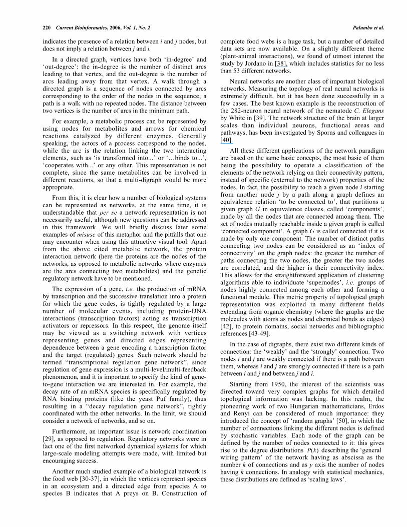
for the possibility to derive, from purely topologicalinformation on the metabolic network of SaccharomycesCerevisiae, the lethal character of genetic mutations.

The metabolic network of microorganisms, at odds withdifferent biological networks like protein-protein interactionnetwork or genetic regulation network, is very wellunderstood and characterized. It corresponds to thoseBoheringer’s ‘Charts of Metabolism’, pinned on the walls ofalmost every biochemistry laboratory in the world, havingenzymatic reactions as edges and metabolites as nodes. Sincean enzymatic reaction is catalyzed by one or more enzymes,an arc can also represent the enzymes involved in thereaction. This opens the way to a straightforward analysis ofthe possibility to derive biologically meaningful featuresfrom network topology: the elimination of an enzyme bymeans of a knock-out experiment implies the eliminationfrom the network of the edge (or edges since the sameenzyme can catalyze several biochemical reactions)corresponding to that particular enzyme. If it is possible topick up a connectivity descriptor able to unequivocallydefine essential enzymes (those enzymes whose lackprovokes the yeast death) we can safely assume thebiological relevance of the metabolism ‘wiring structure’,irrespective of the knowledge of the specific nature of theinvolved enzymes. In other words, this should correspond tothe possibility to define the essentiality of single enzymes forthe yeast life in terms of metabolic network topology. Thisalso implies that the relevance of a specific enzyme can be

Fig. (2). In the graphic representation of the Saccharomyces cerevisiae metabolic network shown here, nodes represent metabolites, and arcs

indicate enzymes involved in the reaction necessary to synthesize a product from a reactant. Yellow bars show where essential enzymes are

positioned in the network. Essential enzymes are those whose lack provokes lethal effects for the yeast. Nodes colored in blue, light blue,

violet and green belong to the strong connected components of the network. These components constitute the cores of the network and all of

the nodes belonging to one of them can reach one another because they are fully connected.

Networks Everywhere Current Bioinformatics, 2006, Vol. 1, No. 2 223

defined not per se, but thanks to the pattern of relations it haswith other elements in the network.

In the considered case of Saccharomyces Cerevisiaenetwork, the analysis of 36 lethal mutations out of the 412relative to enzymes involved in metabolism, reported in theStanford repository (http://www-sequence.stanford.edu/group/yeast_deletion_project/deletions3.html) and inJeong and colleagues [70], allowed us to discover that all ofthe enzymes corresponding to lethal mutations, whendeleted, prevent the connections between the separated nodes[71]. No other path is available to restore the broken arc andthe involved metabolites (nodes) are no more connected byalternative pathways as shown in Fig. 2.

The strict relation between lack of alternative pathwaysreaching a given metabolite and enzyme essentiality impliesthat the crucial elements of the network corresponds toperiphery edges (more central locations being more easilyreachable by alternative paths along the graph): this is in linewith the recently discovered importance of the so called non-hub connectors (elements linking different modules of thenetwork) [72].

The apparent contradiction between the relevance ofperiphery in metabolic networks and the crucial role exertedby the hubs (nodes at the center of the connection pattern) inthe scale-free protein network a-la-Barabasi is solved by theopposite formalization adopted for protein and metabolicnetwork while in protein networks we operate by theelimination of nodes, in metabolic networks, the perturbationis represented by the elimination of edges. The factorsinfluencing the relevance for the general system of theelimination of a node or an edge are exactly the opposite: theentity of the damage we can provoke by the elimination of anode is proportional to the number of relations that the nodewas implied into, in the case of the arc, by definition, wedirectly perturb only one relation (the one corresponding tothe arc), the entity of the damage is in this case proportionalto the number of elements that relied on that arc for beingconnected each other. This is perfectly intuitive if we thinkof the consequences on the traffic of the block of a‘peripherical’ highway constituting the obliged connectionbetween two cities and the consequences of a block of acentral road, which keeps a lot of alternative pathwaysopened.

The possibility to define the essential character of a givenmutation by means of network topological invariants opensthe possibility to consider the metabolic network wiringstructure as a biological entity that, even if immaterial,deeply influences the behavior of the organism.

This consideration is reinforced by the possibility toderive phylogenetic trees by the comparison of metabolicnetwork wiring patterns of different organisms sodemonstrating that metabolic network topology is influencedby evolution process.

1.3. Evolution of Network Topologies

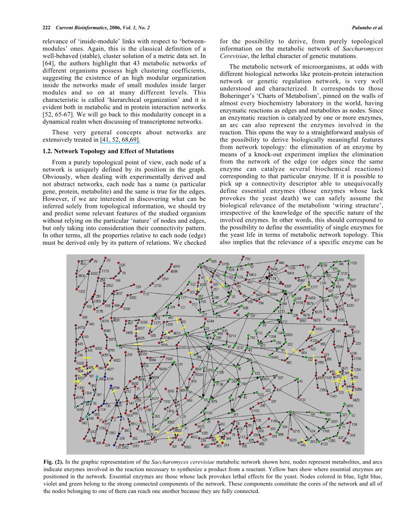
A network of n nodes can be represented as a binarysquare adjacency matrix n n where the entry at (i, j)

position is 1/0 if there is/there is not an edge from vertex I tovertex j (see Fig. 3). In the case of metabolic networks, an

arc can be imagined as an enzyme catalyzing a chemicalreaction transforming a metabolite into the other.

Fig. (3). The network on the left is represented as an adjacency

matrix, in which an element in i,j position is 1/0 if an arc

exists/does not exist connecting node i to j.

The adjacency matrix formalization was very useful indescribing a lot of network structures, and the literatureadopting this notation is particularly rich. The adjacencymatrix allows to the development a straightforward metricsto compare different metabolic networks. The same networkmodule (like glycolysis, purine metabolism, aminoacidbiosynthesis...) gives rise to a peculiar adjacency matrix foreach organism. All these matrices have the same set of rowsand columns corresponding to the maximal coverage of thewhole set of intervening metabolites (it is enough that agiven metabolite is present in a single network to allowinclusion). The distance between each pair of networks willbe simply set to the Hamming distance between the twonetworks, i.e. to the number of discrepancies (1vs.0 or 0vs.1)scored in the corresponding elements of the two networks. Inorder to make the metrics independent of the number ofanalyzed variables (metabolites), we divide the sum of thediscrepancies by the total number of variables (maximalattainable distance) and multiply the ratio by 100. Thus, weobtain a ‘percentage of dissimilarity’ ranging from 0(complete equivalence of the two networks) to 100. Thisoperation, when applied to a set of n different networks willend into a symmetric n n dissimilarity matrix conveying allthe information linked to the pairwise similarities betweenthe correspondent organisms in terms of the metabolicmodule analyzed.

Being the dissimilarity matrix fully quantitative, it can beanalyzed by means of the whole range of multidimensionalstatistical techniques (multidimensional scaling, principalcomponent analysis) as well as to be the basis for theconstruction of similarity trees. These can be considered as‘phylogenetic’ trees analog to those based upon thecomparisons between biological polymers. The idea ofmetabolic pathway comparisons was exploited by manyauthors starting from the pioneering work of Dandekar andcolleagues [73] to the recent [74]. The interest of the topicresides in the fact that the metabolic network topology canbe considered as a ‘holistic’ phenotype of the selectedorganisms and thus ideally suited for genotype/phenotypecorrelations. The method we present here is simpler than theabove mentioned ones, thus allowing for a wider applicationrange.

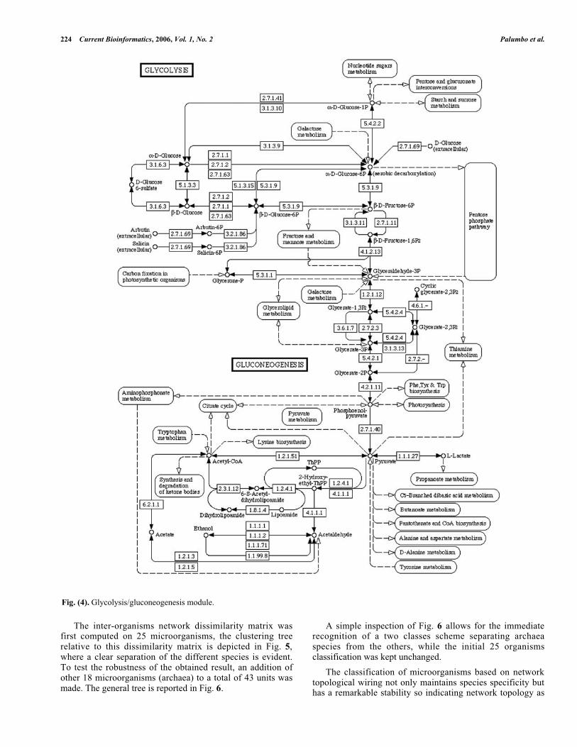
We analyzed the glycolysis/gluconeogenesis module, andthe general scheme of this metabolic network is reported inFig. 4.

224 Current Bioinformatics, 2006, Vol. 1, No. 2 Palumbo et al.

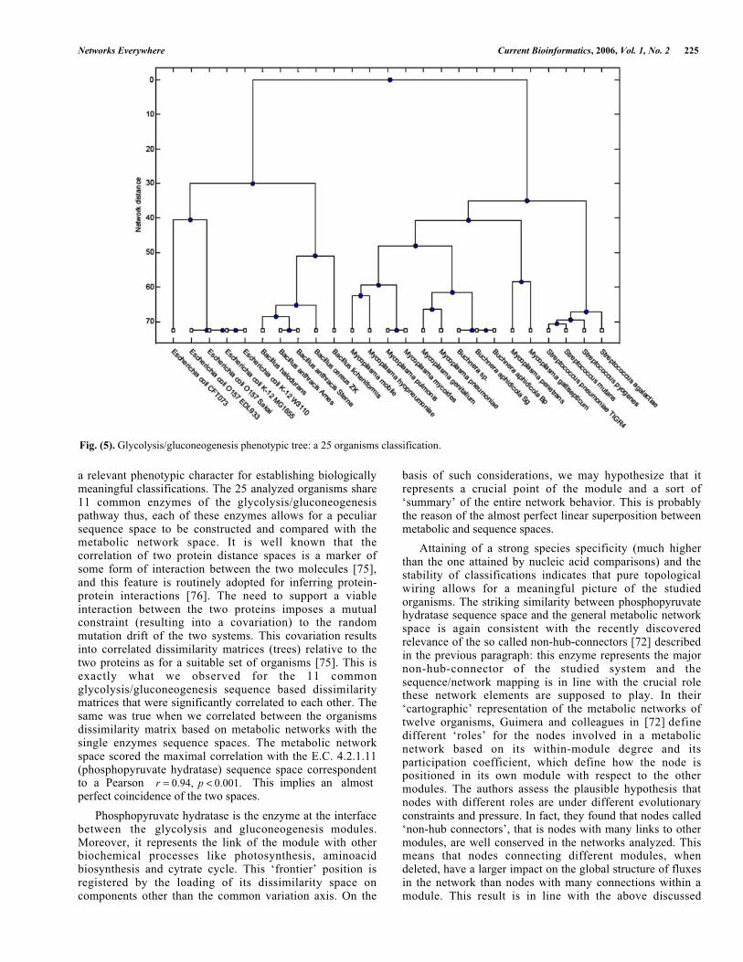
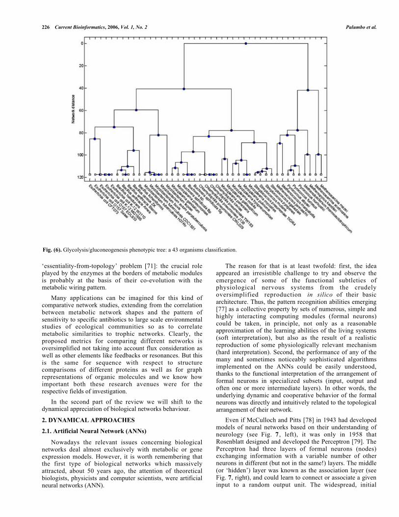
The inter-organisms network dissimilarity matrix wasfirst computed on 25 microorganisms, the clustering treerelative to this dissimilarity matrix is depicted in Fig. 5,where a clear separation of the different species is evident.To test the robustness of the obtained result, an addition ofother 18 microorganisms (archaea) to a total of 43 units wasmade. The general tree is reported in Fig. 6.

A simple inspection of Fig. 6 allows for the immediaterecognition of a two classes scheme separating archaeaspecies from the others, while the initial 25 organismsclassification was kept unchanged.

The classification of microorganisms based on networktopological wiring not only maintains species specificity buthas a remarkable stability so indicating network topology as

Fig. (4). Glycolysis/gluconeogenesis module.

Networks Everywhere Current Bioinformatics, 2006, Vol. 1, No. 2 225

a relevant phenotypic character for establishing biologicallymeaningful classifications. The 25 analyzed organisms share11 common enzymes of the glycolysis/gluconeogenesispathway thus, each of these enzymes allows for a peculiarsequence space to be constructed and compared with themetabolic network space. It is well known that thecorrelation of two protein distance spaces is a marker ofsome form of interaction between the two molecules [75],and this feature is routinely adopted for inferring protein-protein interactions [76]. The need to support a viableinteraction between the two proteins imposes a mutualconstraint (resulting into a covariation) to the randommutation drift of the two systems. This covariation resultsinto correlated dissimilarity matrices (trees) relative to thetwo proteins as for a suitable set of organisms [75]. This isexactly what we observed for the 11 commonglycolysis/gluconeogenesis sequence based dissimilaritymatrices that were significantly correlated to each other. Thesame was true when we correlated between the organismsdissimilarity matrix based on metabolic networks with thesingle enzymes sequence spaces. The metabolic networkspace scored the maximal correlation with the E.C. 4.2.1.11(phosphopyruvate hydratase) sequence space correspondentto a Pearson r = 0.94, p < 0.001. This implies an almostperfect coincidence of the two spaces.

Phosphopyruvate hydratase is the enzyme at the interfacebetween the glycolysis and gluconeogenesis modules.Moreover, it represents the link of the module with otherbiochemical processes like photosynthesis, aminoacidbiosynthesis and cytrate cycle. This ‘frontier’ position isregistered by the loading of its dissimilarity space oncomponents other than the common variation axis. On the

basis of such considerations, we may hypothesize that itrepresents a crucial point of the module and a sort of‘summary’ of the entire network behavior. This is probablythe reason of the almost perfect linear superposition betweenmetabolic and sequence spaces.

Attaining of a strong species specificity (much higherthan the one attained by nucleic acid comparisons) and thestability of classifications indicates that pure topologicalwiring allows for a meaningful picture of the studiedorganisms. The striking similarity between phosphopyruvatehydratase sequence space and the general metabolic networkspace is again consistent with the recently discoveredrelevance of the so called non-hub-connectors [72] describedin the previous paragraph: this enzyme represents the majornon-hub-connector of the studied system and thesequence/network mapping is in line with the crucial rolethese network elements are supposed to play. In their‘cartographic’ representation of the metabolic networks oftwelve organisms, Guimera and colleagues in [72] definedifferent ‘roles’ for the nodes involved in a metabolicnetwork based on its within-module degree and itsparticipation coefficient, which define how the node ispositioned in its own module with respect to the othermodules. The authors assess the plausible hypothesis thatnodes with different roles are under different evolutionaryconstraints and pressure. In fact, they found that nodes called‘non-hub connectors’, that is nodes with many links to othermodules, are well conserved in the networks analyzed. Thismeans that nodes connecting different modules, whendeleted, have a larger impact on the global structure of fluxesin the network than nodes with many connections within amodule. This result is in line with the above discussed

Fig. (5). Glycolysis/gluconeogenesis phenotypic tree: a 25 organisms classification.

226 Current Bioinformatics, 2006, Vol. 1, No. 2 Palumbo et al.

‘essentiality-from-topology’ problem [71]: the crucial roleplayed by the enzymes at the borders of metabolic modulesis probably at the basis of their co-evolution with themetabolic wiring pattern.

Many applications can be imagined for this kind ofcomparative network studies, extending from the correlationbetween metabolic network shapes and the pattern ofsensitivity to specific antibiotics to large scale environmentalstudies of ecological communities so as to correlatemetabolic similarities to trophic networks. Clearly, theproposed metrics for comparing different networks isoversimplified not taking into account flux consideration aswell as other elements like feedbacks or resonances. But thisis the same for sequence with respect to structurecomparisons of different proteins as well as for graphrepresentations of organic molecules and we know howimportant both these research avenues were for therespective fields of investigation.

In the second part of the review we will shift to thedynamical appreciation of biological networks behaviour.

2. DYNAMICAL APPROACHES

2.1. Artificial Neural Network (ANNs)

Nowadays the relevant issues concerning biologicalnetworks deal almost exclusively with metabolic or geneexpression models. However, it is worth remembering thatthe first type of biological networks which massivelyattracted, about 50 years ago, the attention of theoreticalbiologists, physicists and computer scientists, were artificialneural networks (ANN).

The reason for that is at least twofold: first, the ideaappeared an irresistible challenge to try and observe theemergence of some of the functional subtleties ofphysiological nervous systems from the crudelyoversimplified reproduction in silico of their basicarchitecture. Thus, the pattern recognition abilities emerging[77] as a collective property by sets of numerous, simple andhighly interacting computing modules (formal neurons)could be taken, in principle, not only as a reasonableapproximation of the learning abilities of the living systems(soft interpretation), but also as the result of a realisticreproduction of some physiologically relevant mechanism(hard interpretation). Second, the performance of any of themany and sometimes noticeably sophisticated algorithmsimplemented on the ANNs could be easily understood,thanks to the functional interpretation of the arrangement offormal neurons in specialized subsets (input, output andoften one or more intermediate layers). In other words, theunderlying dynamic and cooperative behavior of the formalneurons was directly and intuitively related to the topologicalarrangement of their network.

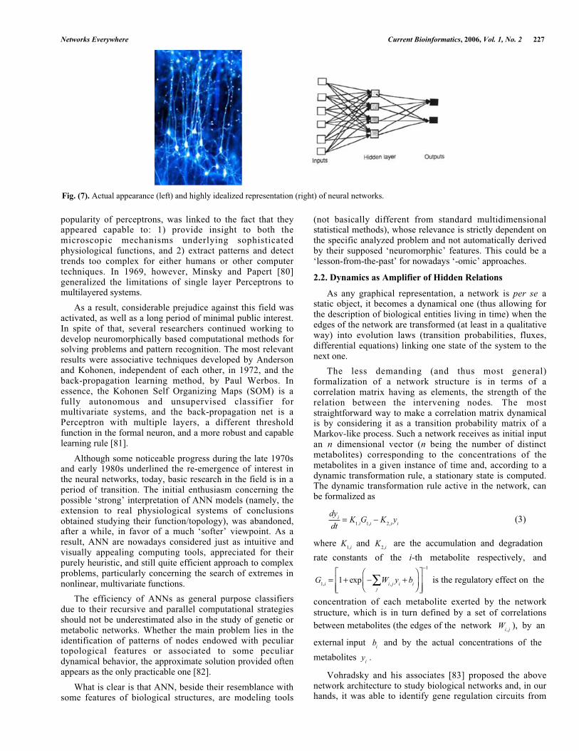
Even if McCulloch and Pitts [78] in 1943 had developedmodels of neural networks based on their understanding ofneurology (see Fig. 7 , left), it was only in 1958 thatRosenblatt designed and developed the Perceptron [79]. ThePerceptron had three layers of formal neurons (nodes)exchanging information with a variable number of otherneurons in different (but not in the same!) layers. The middle(or ‘hidden’) layer was known as the association layer (seeFig. 7, right), and could learn to connect or associate a giveninput to a random output unit. The widespread, initial

Fig. (6). Glycolysis/gluconeogenesis phenotypic tree: a 43 organisms classification.

Networks Everywhere Current Bioinformatics, 2006, Vol. 1, No. 2 227

popularity of perceptrons, was linked to the fact that theyappeared capable to: 1) provide insight to both themicroscopic mechanisms underlying sophisticatedphysiological functions, and 2) extract patterns and detecttrends too complex for either humans or other computertechniques. In 1969, however, Minsky and Papert [80]generalized the limitations of single layer Perceptrons tomultilayered systems.

As a result, considerable prejudice against this field wasactivated, as well as a long period of minimal public interest.In spite of that, several researchers continued working todevelop neuromorphically based computational methods forsolving problems and pattern recognition. The most relevantresults were associative techniques developed by Andersonand Kohonen, independent of each other, in 1972, and theback-propagation learning method, by Paul Werbos. Inessence, the Kohonen Self Organizing Maps (SOM) is afully autonomous and unsupervised classifier formultivariate systems, and the back-propagation net is aPerceptron with multiple layers, a different thresholdfunction in the formal neuron, and a more robust and capablelearning rule [81].

Although some noticeable progress during the late 1970sand early 1980s underlined the re-emergence of interest inthe neural networks, today, basic research in the field is in aperiod of transition. The initial enthusiasm concerning thepossible ‘strong’ interpretation of ANN models (namely, theextension to real physiological systems of conclusionsobtained studying their function/topology), was abandoned,after a while, in favor of a much ‘softer’ viewpoint. As aresult, ANN are nowadays considered just as intuitive andvisually appealing computing tools, appreciated for theirpurely heuristic, and still quite efficient approach to complexproblems, particularly concerning the search of extremes innonlinear, multivariate functions.

The efficiency of ANNs as general purpose classifiersdue to their recursive and parallel computational strategiesshould not be underestimated also in the study of genetic ormetabolic networks. Whether the main problem lies in theidentification of patterns of nodes endowed with peculiartopological features or associated to some peculiardynamical behavior, the approximate solution provided oftenappears as the only practicable one [82].

What is clear is that ANN, beside their resemblance withsome features of biological structures, are modeling tools

(not basically different from standard multidimensionalstatistical methods), whose relevance is strictly dependent onthe specific analyzed problem and not automatically derivedby their supposed ‘neuromorphic’ features. This could be a‘lesson-from-the-past’ for nowadays ‘-omic’ approaches.

2.2. Dynamics as Amplifier of Hidden Relations

As any graphical representation, a network is per se astatic object, it becomes a dynamical one (thus allowing forthe description of biological entities living in time) when theedges of the network are transformed (at least in a qualitativeway) into evolution laws (transition probabilities, fluxes,differential equations) linking one state of the system to thenext one.

The less demanding (and thus most general)formalization of a network structure is in terms of acorrelation matrix having as elements, the strength of therelation between the intervening nodes. The moststraightforward way to make a correlation matrix dynamicalis by considering it as a transition probability matrix of aMarkov-like process. Such a network receives as initial inputan n dimensional vector (n being the number of distinctmetabolites) corresponding to the concentrations of themetabolites in a given instance of time and, according to adynamic transformation rule, a stationary state is computed.The dynamic transformation rule active in the network, canbe formalized as

dyi

dt= K

1.iG

1,iK

2,iy

i(3)

where K1,i

and K2,i

are the accumulation and degradation

rate constants of the i-th metabolite respectively, and

G1,i= 1+ exp W

i, jy

i+ b

ij

1

is the regulatory effect on the

concentration of each metabolite exerted by the network

structure, which is in turn defined by a set of correlations

between metabolites (the edges of the network Wi, j

), by an

external input bi and by the actual concentrations of the

metabolites yi.

Vohradsky and his associates [83] proposed the abovenetwork architecture to study biological networks and, in ourhands, it was able to identify gene regulation circuits from

Fig. (7). Actual appearance (left) and highly idealized representation (right) of neural networks.

228 Current Bioinformatics, 2006, Vol. 1, No. 2 Palumbo et al.

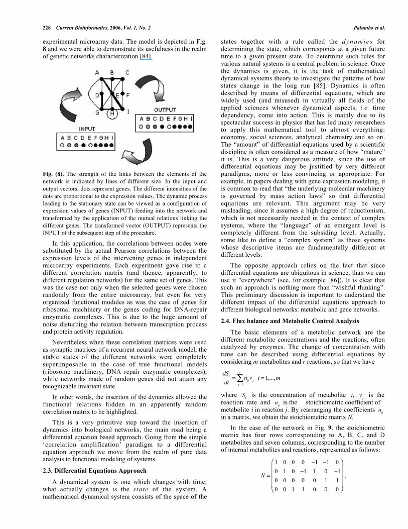
experimental microarray data. The model is depicted in Fig.8 and we were able to demonstrate its usefulness in the realmof genetic networks characterization [84].

Fig. (8). The strength of the links between the elements of the

network is indicated by lines of different size. In the input and

output vectors, dots represent genes. The different intensities of the

dots are proportional to the expression values. The dynamic process

leading to the stationary state can be viewed as a configuration of

expression values of genes (INPUT) feeding into the network and

transformed by the application of the mutual relations linking the

different genes. The transformed vector (OUTPUT) represents the

INPUT of the subsequent step of the procedure.

In this application, the correlations between nodes weresubstituted by the actual Pearson correlations between theexpression levels of the intervening genes in independentmicroarray experiments. Each experiment gave rise to adifferent correlation matrix (and thence, apparently, todifferent regulation networks) for the same set of genes. Thiswas the case not only when the selected genes were chosenrandomly from the entire microarray, but even for veryorganized functional modules as was the case of genes forribosomal machinery or the genes coding for DNA-repairenzymatic complexes. This is due to the huge amount ofnoise disturbing the relation between transcription processand protein activity regulation.

Nevertheless when these correlation matrices were usedas synaptic matrices of a recurrent neural network model, thestable states of the different networks were completelysuperimposable in the case of true functional models(ribosome machinery, DNA repair enzymatic complexes),while networks made of random genes did not attain anyrecognizable invariant state.

In other words, the insertion of the dynamics allowed thefunctional relations hidden in an apparently randomcorrelation matrix to be highlighted.

This is a very primitive step toward the insertion ofdynamics into biological networks, the main road being adifferential equation based approach. Going from the simple‘correlation amplification’ paradigm to a differentialequation approach we move from the realm of pure dataanalysis to functional modeling of systems.

2.3. Differential Equations Approach

A dynamical system is one which changes with time;what actually changes is the state of the system. Amathematical dynamical system consists of the space of the

states together with a rule called the dynamics fordetermining the state, which corresponds at a given futuretime to a given present state. To determine such rules forvarious natural systems is a central problem in science. Oncethe dynamics is given, it is the task of mathematicaldynamical systems theory to investigate the patterns of howstates change in the long run [85]. Dynamics is oftendescribed by means of differential equations, which arewidely used (and misused) in virtually all fields of theapplied sciences whenever dynamical aspects, i.e. timedependency, come into action. This is mainly due to itsspectacular success in physics that has led many researchersto apply this mathematical tool to almost everything:economy, social sciences, analytical chemistry and so on.The “amount” of differential equations used by a scientificdiscipline is often considered as a measure of how “mature”it is. This is a very dangerous attitude, since the use ofdifferential equations may be justified by very differentparadigms, more or less convincing or appropriate. Forexample, in papers dealing with gene expression modeling, itis common to read that “the underlying molecular machineryis governed by mass action laws” so that differentialequations are relevant. This argument may be verymisleading, since it assumes a high degree of reductionism,which is not necessarily needed in the context of complexsystems, where the “language” of an emergent level iscompletely different from the subsiding level. Actually,some like to define a “complex system” as those systemswhose descriptive items are fundamentally different atdifferent levels.

The opposite approach relies on the fact that sincedifferential equations are ubiquitous in science, than we canuse it "everywhere" (see, for example [86]). It is clear thatsuch an approach is nothing more than “wishful thinking”.This preliminary discussion is important to understand thedifferent impact of the differential equations approach todifferent biological networks: metabolic and gene networks.

2.4. Flux balance and Metabolic Control Analysis

The basic elements of a metabolic network are thedifferent metabolite concentrations and the reactions, oftencatalyzed by enzymes. The change of concentration withtime can be described using differential equations byconsidering m metabolites and r reactions, so that we have

dSi

dt= n

ijv

jj=1

r

i = 1,...,m

where Si is the concentration of metabolite i, v

j is the

reaction rate and nij

is the stoichiometric coefficient ofmetabolite i in reaction j. By rearranging the coefficients n

ij

in a matrix, we obtain the stoichiometric matrix N.

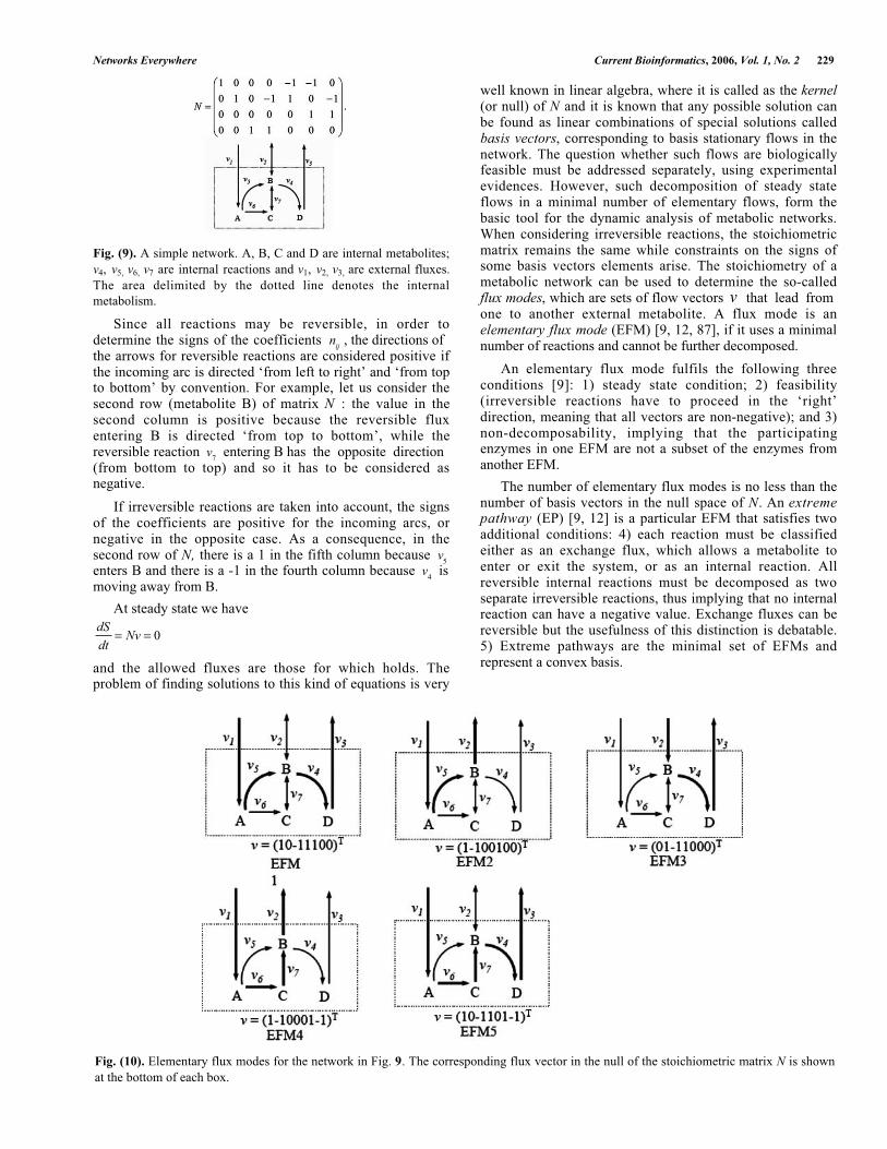
In the case of the network in Fig. 9, the stoichiometricmatrix has four rows corresponding to A, B, C, and Dmetabolites and seven columns, corresponding to the numberof internal metabolites and reactions, represented as follows:

N =

1 0 0 0 1 1 0

0 1 0 1 1 0 1

0 0 0 0 0 1 1

0 0 1 1 0 0 0

.

Networks Everywhere Current Bioinformatics, 2006, Vol. 1, No. 2 229

Fig. (9). A simple network. A, B, C and D are internal metabolites;

v4, v5, v6, v7 are internal reactions and v1, v2, v3, are external fluxes.

The area delimited by the dotted line denotes the internal

metabolism.

Since all reactions may be reversible, in order todetermine the signs of the coefficients n

ij, the directions of

the arrows for reversible reactions are considered positive ifthe incoming arc is directed ‘from left to right’ and ‘from topto bottom’ by convention. For example, let us consider thesecond row (metabolite B) of matrix N : the value in thesecond column is positive because the reversible fluxentering B is directed ‘from top to bottom’, while thereversible reaction v

7 entering B has the opposite direction

(from bottom to top) and so it has to be considered asnegative.

If irreversible reactions are taken into account, the signsof the coefficients are positive for the incoming arcs, ornegative in the opposite case. As a consequence, in thesecond row of N, there is a 1 in the fifth column because v

5

enters B and there is a -1 in the fourth column because v4

ismoving away from B.

At steady state we have

dS

dt= Nv = 0

and the allowed fluxes are those for which holds. Theproblem of finding solutions to this kind of equations is very

well known in linear algebra, where it is called as the kernel(or null) of N and it is known that any possible solution canbe found as linear combinations of special solutions calledbasis vectors, corresponding to basis stationary flows in thenetwork. The question whether such flows are biologicallyfeasible must be addressed separately, using experimentalevidences. However, such decomposition of steady stateflows in a minimal number of elementary flows, form thebasic tool for the dynamic analysis of metabolic networks.When considering irreversible reactions, the stoichiometricmatrix remains the same while constraints on the signs ofsome basis vectors elements arise. The stoichiometry of ametabolic network can be used to determine the so-calledflux modes, which are sets of flow vectors v that lead fromone to another external metabolite. A flux mode is anelementary flux mode (EFM) [9, 12, 87], if it uses a minimalnumber of reactions and cannot be further decomposed.

An elementary flux mode fulfils the following threeconditions [9]: 1) steady state condition; 2) feasibility(irreversible reactions have to proceed in the ‘right’direction, meaning that all vectors are non-negative); and 3)non-decomposability, implying that the participatingenzymes in one EFM are not a subset of the enzymes fromanother EFM.

The number of elementary flux modes is no less than thenumber of basis vectors in the null space of N. An extremepathway (EP) [9, 12] is a particular EFM that satisfies twoadditional conditions: 4) each reaction must be classifiedeither as an exchange flux, which allows a metabolite toenter or exit the system, or as an internal reaction. Allreversible internal reactions must be decomposed as twoseparate irreversible reactions, thus implying that no internalreaction can have a negative value. Exchange fluxes can bereversible but the usefulness of this distinction is debatable.5) Extreme pathways are the minimal set of EFMs andrepresent a convex basis.

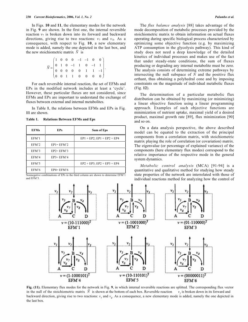
Fig. (10). Elementary flux modes for the network in Fig. 9. The corresponding flux vector in the null of the stoichiometric matrix N is shown

at the bottom of each box.

230 Current Bioinformatics, 2006, Vol. 1, No. 2 Palumbo et al.

In Figs. 10 and 11, the elementary modes for the networkin Fig. 9 are shown. In the first one, the internal reversiblereaction v7 is broken down into its forward and backwarddirections, giving rise to two reactions: v7 and v 8. As aconsequence, with respect to Fig. 10, a new elementarymode is added, namely the one depicted in the last box, andthe new stoichiometric matrix N is

N =

1 0 0 0 1 1 0 0

0 1 0 1 1 0 1 1

0 0 0 0 0 1 1 1

0 0 1 1 0 0 0 0

.

For each reversible internal reaction, the set of EFMs andEPs in the modified network includes at least a ‘cycle’.However, these particular fluxes are not considered, sinceEFMs and EPs are important to understand the exchange offluxes between external and internal metabolites.

In Table 1, the relations between EFMs and EPs in Fig.11 are shown.

Table 1. Relations Between EFMs and Eps

EFMs EPs Sum of Eps

EFM’1 EP1 + EP2; EP1 + EP2 + EP4

EFM’2 EP1= EFM’2

EFM’3 EP2= EFM’3

EFM’4 EP3= EFM’4

EFM’5 EP2 + EP3; EP2 + EP3 + EP4

EFM’6 EP4= EFM’6

Nonnegative combinations of EPs in the third column are shown to determine EFM’1and EFM’5.

The flux balance analysis [88] takes advantage of themode decomposition of metabolic processes provided by thestoichiometric matrix to obtain information on actual fluxesoperating during specific biological process characterized byoptimizing some objective function (e.g. by maximizingATP consumption in the glycolysis pathway). This kind ofstudy does not need a deep knowledge of the detailedkinetics of individual processes and makes use of the factthat under steady-state conditions, the sum of fluxesproducing or degrading any internal metabolite must be zero.The analysis consists of determining extreme pathways byintersecting the null subspace of N and the positive fluxorthant, thus obtaining a polyhedral cone and by imposingconstraints on the magnitude of individual metabolic fluxes(Fig. 12).

The determination of a particular metabolic fluxdistribution can be obtained by maximizing (or minimizing)a linear objective function using a linear programmingapproach. Examples of such objective functions areminimization of nutrient uptake, maximal yield of a desiredproduct, maximal growth rate [89], flux minimization [90]and so on.

On a data analysis perspective, the above describedmodel can be equated to the extraction of the principalcomponents from a correlation matrix, with stoichiometricmatrix playing the role of correlation (or covariation) matrix.The eigenvalue (or percentage of explained variance) of thecomponents (here elementary flux modes) correspond to therelative importance of the respective mode in the generalsystem dynamics.

Metabolic control analysis (MCA) [91-94] is aquantitative and qualitative method for studying how steadystate properties of the network are interrelated with those ofindividual reactions method for analyzing how the control of

Fig. (11). Elementary flux modes for the network in Fig. 9, in which internal reversible reactions are splitted. The corresponding flux vector

in the null of the stoichiometric matrix N is shown at the bottom of each box. Reversible reaction v7 is broken down in its forward and

backward direction, giving rise to two reactions: v7 and v

8. As a consequence, a new elementary mode is added, namely the one depicted in

the last box.

Networks Everywhere Current Bioinformatics, 2006, Vol. 1, No. 2 231

fluxes and intermediate concentrations in a metabolicpathway is distributed among the different enzymes thatconstitute the pathway. One of the most importantapplications of MCA is in biotechnological productionprocesses, since it is important to reveal which enzyme(s)should be activated in order to increase the synthesis rate ofsome given metabolite. The relationship between stationaryflux distribution and kinetic parameters is highly nonlinearand to date, no general method to predict the effects of largeparameter variations is known or proved to be effective. Forthis reason, it is convenient to consider small variations, i.e.assuming a linear relationship, so that precise mathematicalexpression can be derived and metabolic network behaviourquantitatively predicted. In MCA, one studies the relativecontrol exerted by each step (enzyme) on the system’svariables (fluxes and metabolite concentrations). Thiscontrol is measured by applying a perturbation to the stepbeing studied and measuring the effect on the variable ofinterest after the system has settled to a new steady state. Thebasic mathematical tool is the sensitivity coefficient defined,for a generic quantity x depending on a parameter p , asfollows:

Fig. (12). In a three-dimensional flux space, grey arrows

correspond to the extreme pathways. They determine a convex cone

inside the positive orthant. Capacity constraints on each flux limit

the cone region to the polytope determined by the grey arrows and

the light blue area. All possible flux distributions lie within such

polytope. When the cost function is a linear combination of fluxes,

then the optimal solution (red dot) usually lies in a corner of the

polytope or, on occasions, it lies along a whole edge.

cp

x=

p

x

x

px 0

=p

x

x

p=

ln x

ln p

An elasticity coefficient quantifies the sensitivity of areaction rate with respect to a change of concentration or akinetic parameter, while control coefficients refer to thechange of steady state flux and concentration distributionsdue to a change of individual reactions rate. Elasticitycoefficients are local properties regarding individualreactions and can be calculated for any given state whilecontrol coefficients are global properties related to the newsteady state reached after a perturbation.

MCA was used in [95-97] to model the humanerythrocyte and in the specialized literature, there are plentyof applications.

2.5. Gene Network Dynamics

Eukaryotic gene expression is the end result of a largenumber of closely linked biological events at the molecular

level that begins with transcription initiation, elongation andtermination. After release, the mature transcript is exportedinto the cytoplasm where either it is translated into a proteinor it is degraded. Some proteins are able to bind DNA ormRNA and positively or negatively interfering with thetranscription and degradation processes, thus producing ahighly coordinated dynamical expression program.Moreover, there may be additional levels of regulation suchas post-translational protein modifications (such asphosphorylation) and protein transport through subcellularcompartments. Consequently, understanding genetic controlrequires more than merely collecting large amounts ofexperimental data: the network metaphor, often coupled todynamical equations, has been extensively used byresearchers in the attempt to capture the intrinsic dynamicalnature of gene expression. Recently, the so-called “chip-chip” methodology was able to identify in vivo transcriptionfactors thus revealing the “transcriptional gene network” forS. cerevisiae [98]. In this framework, a gene is a node and anarrow originates from a “regulator” (i.e. a gene encoding atranscription factor) and ends into a “target” gene.

In order to understand the dynamic behavior oftranscriptional networks, Uri Alon and co-workers, haveidentified some network motifs, such as the feed-forwardloop motif [99], a three-gene pattern, composed of two inputtranscription factors, one of which regulates the other, bothjointly regulating a target gene. Such motif is over-represented in real gene networks as opposed to randomnetworks. It is also claimed that it acts as sign-sensitiveaccelerators able to speed up gene expression in a specificdirection (from ON to OFF or vice versa). As a consequence,the authors speculate on the possibility that they might beused to understand the network dynamics in terms ofelementary computational building blocks. From thisintriguing perspective, topology and dynamics are inherentlylinked. However, it has been argued [100] that different“design principles” underlying a given biological networkmay lead to the over-representation of a particular networkmotif without the need of any specific biological function forit. The message is clear: one has to take a great care whenmoving from metaphors to reality.

Mathematical modeling of gene expression dynamics is aformidable task and a large number of approaches has beenpresented in the literature. For example, an interesting wayto enforce dynamics into a gene network is the Booleannetworks approach [101]. Such model assumes the state of agene to be ON or OFF and that regulatory control can bedescribed using Boolean functions. For example, the outputof an AND function at time step t +1 is ON provided thatboth input genes are ON at the preceding time step. Thesystem is assumed to be updated synchronously. The discretenature of this model is appropriate to describe situations inwhich well separated “functional steps” are present and infact, not surprisingly, the Boolean networks have beenapplied to embryogenesis. A recent example of Booleanmodeling is the Drosophila segment polarity gene network[102] controlling about 40 genes organized in a hierarchicalcascade to organize the body of the fruit fly in segments.However, the same network has been analyzed using adifferential equations approach [103] showing that it isresistant to variations in the kinetic constants that govern itsbehavior. The obvious advantage of the use of differential

232 Current Bioinformatics, 2006, Vol. 1, No. 2 Palumbo et al.

equations is that it allows for a continuous change of thestate of the system, as observed in many physiologicalprocesses, such as the cell cycle. Nevertheless, its usefulnessis severely limited by the need of large amount of goodquality data, since derivatives are very hard to estimate in thepresence of noise. Small gene networks have beensuccessfully analyzed using steady state data [104], althoughthe use of time series is much more informative.

CONCLUSION

The above analyzed cases allowed us to realize howpowerful the network approach can be and, at the same time,how misleading if we substitute its consideration as amodeling tool with the idea of a ‘real existence’ of networksin the biological systems.

We tried and explain the basic similarities linkingnetwork based approaches to statistical techniques likecluster analysis and principal component analysis whosestatus of analytical tools (and not biologically motivatedrelation structures) is widely recognized. The reference to theANN story was very instructive in this respect. For the samereasons, the search for ‘the definitive network’ of anyorganism is devoid of any sense: the actual shape ofmetabolism (as well as of gene regulation [98, 105] orprotein interaction pattern) changes in time and with respectto the environmental conditions. The possibility to design(and even to profitably study) topological Charts-of-Metabolism must not make scientists forget those chartsreport ‘what in principle could happen’ and not whatnecessarily happens in any situation. The same kind ofrelation holds between the entire genome sequence and theeffective activation of certain genes. The same kind ofrelation but with a basic difference, for metabolic networksthe purely topological, static approach, is much more fruitfuland rich for biological consequences than for DNA.

This takes us to the basic question: how and when thenetwork approach gives the scientist some doubt freeadvantages with respect to other methods?

We think the best criteri0n is embedded in the idea ofwhat a network is: a bunch of nuclei (where matter as well aseventual activities are strongly concentrated) linked to eachother by arcs (streets, mechanical junctions, power cables)passing in a much less dense environment.

In this view, the highways connecting different big citiesconstitute a network, because there is a sharp differencebetween the activity density (crowding, population density,energy expenditure) of the nodes (cities) with respect to thecountry along which the highway passes by. On the otherhand, the intermingled texture of internal city streets is muchless naturally formalized as a network, with the nodes/arcsdistinction much less clear. This is the reason why thenetwork paradigm was very useful to study metabolismwhere organic molecules are immediately evident ‘crucialpoints’ of the entire ‘game’ (the cities), while it is much lessnatural to consider different RNAs transcription levels (likein microarray experiments) as the nodes of the differentialgene expression. Finally, we would like to stress that theanalogies we can find between network approaches and othermathematical modeling tools by no means imply that thenetwork approach has no peculiar features on its own. On thecontrary, the analogies with other methods provide a useful

background over which the widespread potentialities of thenetwork metaphor can be fully and objectively appreciated.

REFERENCES

[1] De Jong H. Modeling and simulation of genetic regulatory systems:A literature review. J Comput Biol 2002; 9: 67-103.

[2] Shen-Orr SS, Milo R, Mangan S, Alon U. Network motifs in thetranscriptional regulation network of Escherichia coli. Nat Genet

2002; 31: 64-8.[3] Smolen P, Baxter DA, Byrne J. Modeling transcriptional control in

gene networks-Methods, recent results, and future directions. BullMath Biol 2000; 62: 247-92.

[4] Wolkenhauer O. Mathematical modelling in the post-genome era:understanding genome expression and regulation – a system

theoretic approach. BioSystems 2002; 65: 1-18.[5] Gardner TS, Faith JJ. Reverse-engineering transcriptional control

networks. Phys Life Rev 2005; 2: 65-88.[6] Chua G, Robinson MD, Morris Q, Hughes TR. Transcriptional

networks: reverse-engineering gene regulation on global scale.Curr Opin Microbiol 2004; 7: 638-46.

[7] Bork P, Jensen LJ, Von Mering C, Ramani AK, Lee I, MarcotteEM. Protein interaction networks from yeast to human. Curr Opin

Struct Biol 2004; 14: 292-99.[8] Nielsen J. Metabolic engineering: techniques of analysis of targets

for genetic manipulations. Biotechnol Bioeng 1998; 58: 125-32.[9] Klamt S, Stelling J. Stoichiometric analysis of metabolic networks.

Tutorial at the 4th International Conference on Systems Biology2003.

[10] Stelling J, Klamt S, Bettenbrock K, Schuster S, Gilles ED.Metabolic network structure determines key aspects of

functionality and regulation. Nature 2002; 420: 190-3.[11] Giersch C. Matematical modelling of metabolism. Curr Opin Plant

Biol 2000; 3: 249-53.[12] Papin JA, Price ND, Wiback SJ, Fell DA, Palsson BO. Metabolic

pathways in the post-genome era. TRENDS Biochem Sci 2003; 28:250-8.

[13] Fiehn O, Weckwerth W. Deciphering metabolic networks. Eur JBiochem 2003; 270: 579-88.

[14] Crampin EJ, Schnell S, McSharry PE. Mathematical andcomputational techniques to deduce complex biochemical reaction

mechanism. Prog Biophys Mol Biol 2004; 86: 77-112.[15] Stephanopoulos G. Metabolic fluxes and metabolic engineering,

Metab Eng 1999; 1: 1-11.[16] Jeong H, Tombor B, Albert R, Oltvai ZN, Barabasi A-L. The large-

scale organization of metabolic networks. Nature 2000; 407: 651-4.[17] Lässig M, Bastolla U, Manrubia SC, Valleriani A. Shape of

Ecological Networks. Phys Rev Lett 2001; 86: 4418-21.[18] Verboom J, Foppen R, Chardon P, Opdam P, Luttikhuizen P.

Introducing the key patch approach for habitat networks withpersistent populations: an example for marshland birds. Biol

Conserv 2001; 100: 89-101.[19] Vos CC, Verboom J, Opdam PFM, Ter Braak CJF. Toward

ecologically scaled landscape indices. The Am Naturalist 2001;183: 24-41.

[20] Opdam P, Assessing the conservation potential of habitat networks,In: Gutzwiller KJ Ed, Concepts and application of landscape

ecology in biological conservation. Springer Verlag, New York,NY 2002; 381–404.

[21] McMahon SM, Miller KH, Drake J. Networking tips fpr socialscientists and ecologists. Science 2001; 293: 1604-5.

[22] Rao F, Caflisch A. The protein folding network. J Mol Biol 2004;342: 299-306.

[23] Scala A, Nunes Amaral LA, Barthélémy M. Small-world networksand the conformation space of a short lattice polymer chain.

Europhys Lett 2001; 55: 594-600.[24] Gomperts BD, Mramer IM, Tatham PER. Signal transduction,

Academic Press, New York, NY 2002.[25] Sauro HM, Kholodenko BN. Quantitative analysis of signaling

networks. Prog Biophys Mol Biol 2004; 86: 5-43.[26] Bhalla US, Iyengar R. Emergent properties of networks of

biological signalling pathways. Nature 1999; 283: 381-7.[27] Zadeh LA, Desoer CA. Linear System Theory-The State Space

Approach, McGraw-Hill Book Co., New York, NY 1963.[28] Klipp E, Herwig R, Kowald A, Wierling C, Lehrach H. Systems

biology in practice. Wiley-VCH, Weinheim 2005.

Networks Everywhere Current Bioinformatics, 2006, Vol. 1, No. 2 233

[29] Mesarovic MD, Sreenath SN, Keene JD. Search for organising

principles: understanding in systems biology. Sys Biol 2004; 1: 19-27.

[30] Williams RJ, Martinez ND, Simple rules yield complex food webs.Nature 2000, 404: 180-3.

[31] Stouffer DB, Camacho J, Guimerà R, Ng CA, Nunes Amaral LA.Quantitative patterns in the structure of model and empirical food

webs. Ecology 2005; 86: 1301-11.[32] Cohen JE, Briand F, Newman CM. Community food webs: data

and theory, Springer-Verlag, Berlin, Germany 1990.[33] Pacual M, Dunne JA. Ecological networks: linking structure to

dynamics in food webs, Oxford University Press, Oxford, UK2005.

[34] May RM, The structure of food webs. Nature 1983; 301: 566-8.[35] Morin PJ, Lawler SP, Food web architecture and population

dynamics: theory and empirical evidence. Annu Rev Ecol System1995; 26: 505-29.

[36] Briand F, Environmental control of food web structure. Ecology1983; 64: 253-63.

[37] De Ruiter P, Volkmar W, Moore J, Dynamic food webs:multispecies assemblages, ecosystem development and

environmental change, Academic Press, 2005 (in press).[38] Jordano P, Bascompte J, Olesen JM. Invariant properties in

coevolutionary networks of plant-animal interactions. EcologyLetters 2003; 6: 69-81.

[39] White JG, Southgate E, Thompson JN, Brenner S. The structure ofthe nervous system of the nematode C. Elegans. Phil Trans R Soc

London 1986; 314: 1–340.[40] Sporns O. Network analysis, complexity, and brain function.

Complexity 2002; 8: 56–60.[41] Newman MEJ. The structure and function of complex networks.

SIAM REVIEW 2003; 45: 167-256.[42] Lukovits I. A compact form of the adjacency matrix. J Chem Inf

Comput Sci 2000; 40: 1147-50.[43] Fararo TJ. Theoretical sociology in the 20th century. JoSS 2001; 2.

[44] Ferrer I Cancho R, Solé RV. The small world of human language.Proc R Soc Lond B 2001; 268: 2261-5.

[45] Freeman LC. The development of social network analysis: a studyin the sociology of science, Booksurge Publishing, Vancouver, CA

2004.[46] Newman MEJ. Scientific collaboration networks. I. Network

construction and fundamental results. Phys Rev E 2001; 64: 0161311-9.

[47] Wasserman S, Faust K. Social network analysis, Cambridgeuniversity press, Cambridge, UK 1994.

[48] Newman MEJ. The structure of scientific collaboration networks.Proc Natl Acad Sci USA 2001; 98: 404-9.

[49] Redner S. How popular is your paper? An empirical study of thecitation distribution. Eur J Phys B 1998; 4: 131-4.

[50] Erdos P, Rényi A. On the evolution of random graphs. Publ MathInst Hung Acad Sci 1960; 17-61.

[51] Barabasi A-L, Albert R. Emergence of scaling in random networks.Science 1999; 286: 509-12.

[52] Barabasi A-L, Oltvai ZN. Network biology: understanding thecell’s functional organization. Nat Rev Genet 2004; 5: 101-13.

[53] Watts DJ, Strogatz SH. Collective dynamics of 'small-world'networks. Nature 1998; 393: 440-2.

[54] Wagner A, Fell DA. The small world inside large metabolicnetworks. Proc R Soc Ser B 2001; 268: 1803-10.

[55] Nunes Amaral LA, Scala A, Barthélémy M, Stanley HE. Classes ofsmall-world networks. Proc Natl Acad Sci USA 2000; 97: 11149-

52.[56] Watts DJ. Small Worlds: the dynamics of networks between order

and randomness, Princeton University Press, Princeton, NewJersey, USA, 2003.

[57] Fell DA, Wagner A. The small world of metabolism. N a tBiotechnol 2000; 18: 1121-2.

[58] Albert R, Jeong H, Barabasi A-L. Error and attack tolerance ofcomplex networks. Nature 2000; 406: 378-82.

[59] Albert R, Jeong H, Barabasi A-L. A correction to: "Error and attacktolerance of complex networks". Nature 2001; 409: 542.

[60] Arita M. The metabolic world of Escherichia Coli is not small.Proc Natl Acad Sci USA 2004; 101: 1543-7.

[61] Tanaka R. Scale-Rich Metabolic Networks. Phys Rev Lett 2005;94: 168101 1-4.

[62] Arima C, Hanay T. Gene Expression Analysis Using Fuzzy k-

means clustering. Genome Informatics 2003; 14: 324-35.[63] Tamayo P, Slonim D, Mesirov J, et al. Interpreting patterns of gene

expression with self-organizing maps: Methods and application tohematopoietic differentiation. Proc Natl Acad Sci USA 1999; 96:

2907-12.[64] Rasvatz E, Somera AL, Mongru DA, Oltvai ZN, Barabasi A-L.

Hierarchical organization of modularity in metabolic networks.Science 2002; 297: 1551-5.

[65] Pereira-Leal JB, Enright AJ, Ouzounis CA. Detection of functionalmodules from protein interaction networks. PROTEINS 2004; 54:

49-57.[66] Przulj N, Wingle DA, Jurisica I. Functional topology in a network

of protein interactions. Bioinformatics 2004; 20: 340-8.[67] Rives AW, Galitski T. Modular organization of cellular networks.

Proc Natl Acad Sci USA 2003; 100: 1128-33.[68] Albert R, Barabasi A-L. Statistical mechanics of complex

networks. Rev Mod Phys 2002; 74: 47-97.[69] Nunes Amaral LA, Ottino JM. Complex networks. Augmenting the

framework for the study of complex systems. Eur Phys J B 2004;38: 147-62.

[70] Jeong H, Oltvai ZN, Barabasi A-L. Prediction of proteinessentiality based on genomic data. ComPlexUs 2003; 1: 19-28.

[71] Palumbo MC, Colosimo A, Giuliani A, Farina L. Functionalessentiality from topology features in metabolic networks: a case

study in yeast. FEBS Lett 2005; 579: 4642-6.[72] Guimera R, Nunes Amaral LA. Functional cartography of complex

metabolic networks. Nature 2005; 433: 895-900.[73] Dandekar T, Schuster S, Snel B, Huynen M, Bork P. Pathway

alignment: application to the comparative analysis of glycolyticenzymes. Biochem J 1999; 343: 115-24.

[74] Zhu D, Qin ZS. Structural comparison of metabolic networks inselected single cell organisms. BMC Bionformatics 2005; 6: 8.

[75] Goh KI, Kahng B, Kim D. Spectra and eigenvectors of scale-freenetworks. Phys Rev E 2001; 64: 051903 1-5.

[76] Legrain P, Wojcik J, Gauthier JM. Protein-protein interactionmaps: a lead towards cellular functions. Trends Genet 2001; 17:

346-52.[77] Hopfield JJ. Neural networks and physical systems with emergent

collective computational abilities. Proc Natl Acad Sci USA 1982;79: 2554-8.

[78] McCulloch WS, Pitts W. A logical calculus of the ideas immanentin nervous activity. Bullet Mathemat Biophys 1943; 5: 115-33.

[79] Rosenblatt F. The perceptron: A probabilistic model forinformation storage and organization in the brain. Psychol Rev

1958; 65: 386-408.[80] Minsky M, Papert SA. Perceptrons: An Introduction to

Computational Geometry, MIT Press, Cambridge, MA 1988(expanded edition 1969).

[81] Hinton G, Sejnowski TJ. Unsupervised Learning and MapFormation: Foundations of Neural Computation, MIT Press,

Cambridge, MA 1999.[82] Duda RO, Hart PE, Stork DG. Pattern classification (2nd edition),

John Wiley & Sons, New York, NY 2001.[83] Vohradsky J, Neural network model of gene expression. FASEB J

2001; 15: 846–54.[84] Blasi MF, Casorelli I, Colosimo A, Blasi FS, Bignami M, Giuliani

A, A recursive network approach can identify constitutiveregulatory circuits in gene expression data. Physica A 2005; 348:

349-70.[85] Hirsh MW, The dynamical systems approach to differential

equations. Bullet Am Mathemat Soc 1984; 11: 1-64.[86] Rinaldi S, Laura, Petrarch. An Intriguing Case of Cyclical Love

Dynamics. SIAM J Appld Math 1998; 58: 1205-21.[87] Schuster S, Dandekar T, Fell DA. Detection of elementary flux

modes in biochemical networks: a promising tool for pathwayanalysis and metabolic engineering. TIBTECH 1999; 17: 53-60.

[88] Varma A, Palsson BO. Metabolic Flux balancing – Basic Concepts,Scientific and practical Use. Bio/Technol 1994; 12: 994-8.

[89] Edwards JS, Ibarra RU, Palsson BO. In silico prediction ofEscherichia Coli metabolic capabilities are consistent with

experimental data. Nat Biotechol 2001; 19: 125-30.[90] Holtzhutter H-G. Analysis of complex metabolic networks on the

basis of optimization principles. Proc conference Complexity in theliving 2004: 122-38.

234 Current Bioinformatics, 2006, Vol. 1, No. 2 Palumbo et al.

[91] Fell DA. Metabolic Control Analysis: a survey of its theoretical

and experimental development. Biochem J 1992; 286: 313-30.[92] Fell DA. Understanding the control of metabolism, Portland Press,

London, UK 1997.[93] Heinrich R, Rapoport TA, A linear steady-state treatment of

enzymatic chains. General properties, control and effector strength.Eur J Biochem 1974; 42: 89-95.

[94] Kacser H, Burns JA. The control of flux. Symp Soc Exp Biol 1973;27: 65-104.

[95] Mulquiney PJ, Bubb WA, Kuchel PW. Model of 2,3-biphosphoglycerate metabolism in the human erythrocyte based on

detailed enzyme kinetic equations: in vivo kinetic characterizationof 2,3-biphosphoglycerate synthase/phosphatase using 13C and 31P

NMR. Biochem J 1999; 342: 567-80.[96] Mulquiney PJ, Kuchel PW. Model of 2,3-biphosphoglycerate

metabolism in the human erythrocyte based on detailed enzymekinetic equations: equations and parameter refinement. Biochem J

1999; 342: 581-96.[97] Mulquiney PJ, Kuchel PW. Model of 2,3-biphosphoglycerate

metabolism in the human erythrocyte based on detailed enzymekinetic equations: computer simulation and Metabolic Control

Analysis. Biochem J 1999; 342: 597-604.

[98] Harbison CT, Gordon DB, Lee TI, et al. Transcriptional regulatory

code of a eukaryotic genome. Nature 2004; 431: 99-104.[99] Mangan S, Alon U. Structure and function of the feed-forward loop

network motif. Proc Natl Acad Sci USA 2003; 100: 11980-5.[100] Artzy-Randrup Y, Fleishman SJ, Ben-Tal N, Stone L. Comment on

“Network Motifs: Simple Building Blocks of Complex Networks”and “Superfamilies of Evolved and Designed Networks”. Science

2004; 305: 1107c.[101] Somogyi R, Sniegoski CA. Modelling the complexity of of genetic

networks: Understanding multigenic and pleiotropic regulation.Complexity 1996; 1: 45-63.

[102] Albert R, Othmer HG. The topology of the regulatory interactionspredict the expression pattern of the segment polarity genes in

Drosophila melanogaster. J Theor Biol 2003; 223: 1-18.[103] Von Dassow G, Meir E, Munro EM, Odell GM. The segment

polarity network is a robust developmental module. Nature 2000;406: 131-2.

[104] Gardner TS, di Bernardo D, Lorenz D, Collins JJ. Inferring geneticnetworks and identifying compound mode of action via expression

profiling. Science 2003; 301: 102-5.[105] Luscombe NM, Babu MM, Yu H, Snyder M, Teichmann SA,

Gerstein M. Genomic analysis of regulatory network dynamicsreveals large topological changes. Nature 2004; 431: 308-12.

Received: August 3, 2005 Revised: October 7, 2005 Accepted: October 18, 2005