Network Simulation for Professional Audio Networks - CORE
345
Network Simulation for Professional Audio Networks Submitted in fulfilment of the requirements of the degree Doctor of Philosophy of Rhodes University Fred Otten June 2014
-
Upload
khangminh22 -
Category
Documents
-
view
2 -
download
0
Transcript of Network Simulation for Professional Audio Networks - CORE

Network Simulation for Professional Audio Networks
Submitted in fulfilment
of the requirements of the degree
Doctor of Philosophy
of Rhodes University
Fred Otten
June 2014

Abstract
Audio Engineers are required to design and deploy large multi-channel sound systems which meeta set of requirements and use networking technologies such as Firewire and Ethernet AVB. Band-width utilisation and parameter groupings are among the factors which need to be considered in thesedesigns. An implementation of an extensible, generic simulation framework would allow audio en-gineers to easily compare protocols and networking technologies and get near real time responseswith regards to bandwidth utilisation. Our hypothesis is that an application-level capability can bedeveloped which uses a network simulation framework to enable this process and enhances the audioengineer’s experience of designing and configuring a network. This thesis presents a new, extensiblesimulation framework which can be utilised to simulate professional audio networks. This frameworkis utilised to develop an application - AudioNetSim - based on the requirements of an audio engineer.The thesis describes the AudioNetSim models and implementations for Ethernet AVB, Firewire andthe AES- 64 control protocol. AudioNetSim enables bandwidth usage determination for any networkconfiguration and connection scenario and is used to compare Firewire and Ethernet AVB bandwidthutilisation. It also applies graph theory to the circular join problem and provides a solution to detectcircular joins.

Acknowledgements
Firstly I would like to thank God “For from him and through him and to him are ALL things” (Ro-mans 11:36 [NIV], Emphasis added). My life is a testimony of his mercy and grace. He has given memy abilities and deserves all the glory.
I would like to thank my beautiful wife - Nicki - for her support and encouragement throughoutthis process. I would also like to thank my family and friends for their support on this journey.
I specially want to thank my supervisor - Prof. Richard Foss - for all his advice and guidance over theyears as I have completed this work. His knowledge and expertise has taught me so much and I reallyappreciate all the time and effort he has put in to help shape this work. I would also like to thank allthe people in the Computer Science Department - particularly my peers Nyasha Chigwamba, PhilipFoulkes and Osedum Igumbor. Thanks for reading through sections of my thesis and for the manygreat times we shared working together in the lab.
I would finally like to thank Telkom SA for allowing me to complete these studies and the AndrewMelon Foundation and DAAD for their generous financial support.
UMAN is acknowledged for the provision of hardware devices and the use of the UNOS Visionsoftware. The sponsors of the Center of Excellence at Rhodes University (Telkom SA, BusinessConnexion, Comverse, Verso Technologies, THRIP, Stortech, Tellabs, Mars Technologies, AmatoleTelecommunication Services, Bright Ideas 39, Open Voice and the National Research Foundation)are also acknowledged.

Contents
1 Introduction 1
1.1 Introduction . . . . . . . . . . . . . . . . . . . . . . . . . . . . . . . . . . . . . . . 1
1.2 Professional Audio Networks . . . . . . . . . . . . . . . . . . . . . . . . . . . . . . 1
1.3 Problem Statement . . . . . . . . . . . . . . . . . . . . . . . . . . . . . . . . . . . 3
1.4 Network Simulation . . . . . . . . . . . . . . . . . . . . . . . . . . . . . . . . . . . 4
1.5 Research Questions . . . . . . . . . . . . . . . . . . . . . . . . . . . . . . . . . . . 4
1.6 Thesis Layout . . . . . . . . . . . . . . . . . . . . . . . . . . . . . . . . . . . . . . 4
1.6.1 Chapter 2 - Introduction to Firewire and AVB Networks . . . . . . . . . . . 4
1.6.2 Chapter 3 - Network Simulation . . . . . . . . . . . . . . . . . . . . . . . . 5
1.6.3 Chapter 4 - Network Design Applications . . . . . . . . . . . . . . . . . . . 5
1.6.4 Chapter 5 - Overview of Sound System Control and AES64 . . . . . . . . . 5
1.6.5 Chapter 6 - Network Simulator Design . . . . . . . . . . . . . . . . . . . . 5
1.6.6 Chapter 7 - Modelling and Analysing Joins . . . . . . . . . . . . . . . . . . 5
1.6.7 Chapter 8 - Bandwidth Calculation for Firewire and AVB Networks . . . . . 5
1.6.8 Chapter 9 - Comparison of Firewire and AVB Networks . . . . . . . . . . . 6
2 Introduction to Firewire and AVB Networks 7
2.1 Introduction . . . . . . . . . . . . . . . . . . . . . . . . . . . . . . . . . . . . . . . 7
2.2 Firewire Networks . . . . . . . . . . . . . . . . . . . . . . . . . . . . . . . . . . . 7
2.2.1 The nature of the Firewire bus . . . . . . . . . . . . . . . . . . . . . . . . . 8
2.2.1.1 CSR Architecture . . . . . . . . . . . . . . . . . . . . . . . . . . 8
2.2.1.2 Firewire Bridges and Routers . . . . . . . . . . . . . . . . . . . . 10
2.2.1.3 Firewire Communications Model . . . . . . . . . . . . . . . . . . 11
2.2.1.4 Operation of a Firewire Network . . . . . . . . . . . . . . . . . . 12
i

CONTENTS ii
2.2.1.5 Physical Layer . . . . . . . . . . . . . . . . . . . . . . . . . . . . 13
2.2.2 Transmission Modes . . . . . . . . . . . . . . . . . . . . . . . . . . . . . . 13
2.2.2.1 Isochronous Transmission . . . . . . . . . . . . . . . . . . . . . . 13
2.2.2.2 Asynchronous Transmission . . . . . . . . . . . . . . . . . . . . . 16
2.2.3 Arbitration . . . . . . . . . . . . . . . . . . . . . . . . . . . . . . . . . . . 17
2.2.3.1 Legacy Arbitration . . . . . . . . . . . . . . . . . . . . . . . . . . 17
2.2.3.2 1394a Enhancements . . . . . . . . . . . . . . . . . . . . . . . . 18
2.2.3.3 BOSS Arbitration . . . . . . . . . . . . . . . . . . . . . . . . . . 19
2.2.4 Configuration . . . . . . . . . . . . . . . . . . . . . . . . . . . . . . . . . . 22
2.2.5 Timing and synchronisation . . . . . . . . . . . . . . . . . . . . . . . . . . 23
2.2.6 IP over 1394 . . . . . . . . . . . . . . . . . . . . . . . . . . . . . . . . . . 24
2.3 Ethernet AVB Networks . . . . . . . . . . . . . . . . . . . . . . . . . . . . . . . . 24
2.3.1 Ethernet AVB . . . . . . . . . . . . . . . . . . . . . . . . . . . . . . . . . . 25
2.3.2 Queues, Priorities and Packet Types . . . . . . . . . . . . . . . . . . . . . . 27
2.3.2.1 Traffic Classes . . . . . . . . . . . . . . . . . . . . . . . . . . . . 27
2.3.2.2 Selection Algorithms . . . . . . . . . . . . . . . . . . . . . . . . 28
2.3.2.3 Queue Types . . . . . . . . . . . . . . . . . . . . . . . . . . . . . 29
2.3.3 Timing and synchronisation . . . . . . . . . . . . . . . . . . . . . . . . . . 29
2.3.4 The Multiple Reservation Protocol (MRP) and its applications . . . . . . . . 30
2.3.4.1 MRP . . . . . . . . . . . . . . . . . . . . . . . . . . . . . . . . . 30
2.3.4.2 MVRP . . . . . . . . . . . . . . . . . . . . . . . . . . . . . . . . 33
2.3.4.3 MSRP . . . . . . . . . . . . . . . . . . . . . . . . . . . . . . . . 33
2.3.5 Transmission of Streaming Data . . . . . . . . . . . . . . . . . . . . . . . . 37
2.4 Conclusion . . . . . . . . . . . . . . . . . . . . . . . . . . . . . . . . . . . . . . . 38
3 Network Simulation 39
3.1 Introduction . . . . . . . . . . . . . . . . . . . . . . . . . . . . . . . . . . . . . . . 39
3.2 Network Simulation . . . . . . . . . . . . . . . . . . . . . . . . . . . . . . . . . . . 39
3.2.1 Definitions and Concepts . . . . . . . . . . . . . . . . . . . . . . . . . . . . 40
3.2.2 Existing Network Simulation . . . . . . . . . . . . . . . . . . . . . . . . . . 41
3.2.3 Network Simulation Requirements . . . . . . . . . . . . . . . . . . . . . . . 42
3.2.4 Tension between Abstraction and Accuracy . . . . . . . . . . . . . . . . . . 42

CONTENTS iii
3.2.5 Concluding Remarks . . . . . . . . . . . . . . . . . . . . . . . . . . . . . . 43
3.3 A Representational approach to modelling Firewire . . . . . . . . . . . . . . . . . . 44
3.3.1 NS-2 . . . . . . . . . . . . . . . . . . . . . . . . . . . . . . . . . . . . . . 44
3.3.2 NS-2 Firewire implementation . . . . . . . . . . . . . . . . . . . . . . . . . 45
3.3.2.1 Tcl code . . . . . . . . . . . . . . . . . . . . . . . . . . . . . . . 46
3.3.2.2 C++ code . . . . . . . . . . . . . . . . . . . . . . . . . . . . . . 49
3.3.3 Evaluation of NS-2 . . . . . . . . . . . . . . . . . . . . . . . . . . . . . . . 55
3.3.3.1 The network animator . . . . . . . . . . . . . . . . . . . . . . . . 56
3.3.3.2 Tracefile output . . . . . . . . . . . . . . . . . . . . . . . . . . . 56
3.3.3.3 Setting up a network scenario . . . . . . . . . . . . . . . . . . . . 58
3.3.3.4 Outputting required information . . . . . . . . . . . . . . . . . . . 59
3.3.4 Concluding Remarks . . . . . . . . . . . . . . . . . . . . . . . . . . . . . . 59
3.4 Conclusion . . . . . . . . . . . . . . . . . . . . . . . . . . . . . . . . . . . . . . . 59
4 Network Design Applications 61
4.1 CobraCAD . . . . . . . . . . . . . . . . . . . . . . . . . . . . . . . . . . . . . . . 61
4.2 mLAN Installation Designer . . . . . . . . . . . . . . . . . . . . . . . . . . . . . . 64
4.3 HiQNet London Architect . . . . . . . . . . . . . . . . . . . . . . . . . . . . . . . 66
4.4 Harman System Architect . . . . . . . . . . . . . . . . . . . . . . . . . . . . . . . . 68
4.5 Comparison of Existing Configuration and Design Programs . . . . . . . . . . . . . 70
4.6 Usability Requirements for Network Simulator Application . . . . . . . . . . . . . . 72
4.7 Conclusion . . . . . . . . . . . . . . . . . . . . . . . . . . . . . . . . . . . . . . . 73
5 Sound System Control Protocols 74
5.1 Introduction . . . . . . . . . . . . . . . . . . . . . . . . . . . . . . . . . . . . . . . 74
5.2 Comparison of Protocols . . . . . . . . . . . . . . . . . . . . . . . . . . . . . . . . 75
5.2.1 Device Model and Parameter Addressing . . . . . . . . . . . . . . . . . . . 75
5.2.2 Transport independence . . . . . . . . . . . . . . . . . . . . . . . . . . . . 77
5.2.3 Monitoring and Control . . . . . . . . . . . . . . . . . . . . . . . . . . . . 77
5.2.4 Device Discovery . . . . . . . . . . . . . . . . . . . . . . . . . . . . . . . . 77
5.2.5 Standardisation . . . . . . . . . . . . . . . . . . . . . . . . . . . . . . . . . 78
5.2.6 Graphical Control Applications . . . . . . . . . . . . . . . . . . . . . . . . 78

CONTENTS iv
5.2.7 Connection Management . . . . . . . . . . . . . . . . . . . . . . . . . . . . 78
5.2.8 Grouping . . . . . . . . . . . . . . . . . . . . . . . . . . . . . . . . . . . . 78
5.2.9 Concluding Remarks . . . . . . . . . . . . . . . . . . . . . . . . . . . . . . 78
5.3 AES64 . . . . . . . . . . . . . . . . . . . . . . . . . . . . . . . . . . . . . . . . . . 79
5.3.1 Protocol Overview . . . . . . . . . . . . . . . . . . . . . . . . . . . . . . . 79
5.3.1.1 7 level structure . . . . . . . . . . . . . . . . . . . . . . . . . . . 80
5.3.1.2 Commands and Responses . . . . . . . . . . . . . . . . . . . . . 81
5.3.1.3 Wildcarding Mechanism . . . . . . . . . . . . . . . . . . . . . . . 81
5.3.1.4 The Universal Snap Group (USG) Mechanism . . . . . . . . . . . 83
5.3.1.5 Desk Items . . . . . . . . . . . . . . . . . . . . . . . . . . . . . . 83
5.3.2 Connection Management . . . . . . . . . . . . . . . . . . . . . . . . . . . . 83
5.3.2.1 IEEE 1394 . . . . . . . . . . . . . . . . . . . . . . . . . . . . . . 83
5.3.2.2 Ethernet AVB . . . . . . . . . . . . . . . . . . . . . . . . . . . . 84
5.3.3 Parameter Control . . . . . . . . . . . . . . . . . . . . . . . . . . . . . . . 85
5.3.3.1 Control Application - UNOS Vision . . . . . . . . . . . . . . . . 86
5.3.4 Parameter Monitoring . . . . . . . . . . . . . . . . . . . . . . . . . . . . . 88
5.3.5 Parameter Grouping . . . . . . . . . . . . . . . . . . . . . . . . . . . . . . 88
5.3.6 Device Discovery . . . . . . . . . . . . . . . . . . . . . . . . . . . . . . . . 88
5.4 Conclusion . . . . . . . . . . . . . . . . . . . . . . . . . . . . . . . . . . . . . . . 88
6 Network Simulator Design and Implementation 90
6.1 Introduction . . . . . . . . . . . . . . . . . . . . . . . . . . . . . . . . . . . . . . . 90
6.2 Modelling the Network . . . . . . . . . . . . . . . . . . . . . . . . . . . . . . . . . 92
6.2.1 A Generic Network Model . . . . . . . . . . . . . . . . . . . . . . . . . . . 93
6.2.2 Firewire Networks . . . . . . . . . . . . . . . . . . . . . . . . . . . . . . . 96
6.2.3 AVB Networks . . . . . . . . . . . . . . . . . . . . . . . . . . . . . . . . . 99
6.2.4 Network Model for AudioNetSim . . . . . . . . . . . . . . . . . . . . . . . 101
6.3 Modelling the Control Protocol . . . . . . . . . . . . . . . . . . . . . . . . . . . . . 101
6.3.1 Modelling AES64 Parameters . . . . . . . . . . . . . . . . . . . . . . . . . 103
6.3.1.1 ParamTree . . . . . . . . . . . . . . . . . . . . . . . . . . . . . . 108
6.3.1.2 ParamTreeNode . . . . . . . . . . . . . . . . . . . . . . . . . . . 108
6.3.1.3 ParamTreeParam . . . . . . . . . . . . . . . . . . . . . . . . . . . 109

CONTENTS v
6.3.1.4 Traversing the Parameter Tree . . . . . . . . . . . . . . . . . . . . 110
6.3.1.5 Getting and Setting Parameters . . . . . . . . . . . . . . . . . . . 110
6.3.2 Additional AES64 Control Protocol Concepts . . . . . . . . . . . . . . . . . 110
6.3.2.1 USG Mechanism . . . . . . . . . . . . . . . . . . . . . . . . . . 111
6.3.2.2 Device Discovery and Enumeration . . . . . . . . . . . . . . . . . 113
6.3.2.3 The Enhanced USG Mechanism . . . . . . . . . . . . . . . . . . 116
6.3.2.4 Modelling the USG Mechanism . . . . . . . . . . . . . . . . . . . 119
6.3.2.5 The USG Push Mechanism . . . . . . . . . . . . . . . . . . . . . 121
6.3.2.6 Modelling the USG Push Mechanism . . . . . . . . . . . . . . . . 123
6.4 Graphical User Interface . . . . . . . . . . . . . . . . . . . . . . . . . . . . . . . . 125
6.4.1 AudioNetSim user interface . . . . . . . . . . . . . . . . . . . . . . . . . . 126
6.4.2 Clouds to group devices . . . . . . . . . . . . . . . . . . . . . . . . . . . . 128
6.4.3 Subnet Status Window . . . . . . . . . . . . . . . . . . . . . . . . . . . . . 129
6.4.4 Device Library . . . . . . . . . . . . . . . . . . . . . . . . . . . . . . . . . 131
6.4.5 Link between graphical user interface component and the network model . . 131
6.4.6 XML Representation of Devices . . . . . . . . . . . . . . . . . . . . . . . . 134
6.4.6.1 XML Schema . . . . . . . . . . . . . . . . . . . . . . . . . . . . 134
6.4.6.2 Example . . . . . . . . . . . . . . . . . . . . . . . . . . . . . . . 135
6.5 Control Application . . . . . . . . . . . . . . . . . . . . . . . . . . . . . . . . . . . 137
6.6 Interface for interaction with the simulated network . . . . . . . . . . . . . . . . . . 138
6.6.1 UNOS Vision Currently . . . . . . . . . . . . . . . . . . . . . . . . . . . . 139
6.6.2 Description of interaction interface design approaches . . . . . . . . . . . . 139
6.6.2.1 API approach . . . . . . . . . . . . . . . . . . . . . . . . . . . . 140
6.6.2.2 IP-level approach . . . . . . . . . . . . . . . . . . . . . . . . . . 141
6.6.3 Selected Approach . . . . . . . . . . . . . . . . . . . . . . . . . . . . . . . 142
6.6.4 Implementation of the API approach . . . . . . . . . . . . . . . . . . . . . . 143
6.7 AudioNetSim . . . . . . . . . . . . . . . . . . . . . . . . . . . . . . . . . . . . . . 143
6.8 Conclusion . . . . . . . . . . . . . . . . . . . . . . . . . . . . . . . . . . . . . . . 147

CONTENTS vi
7 Modelling and Analysing Joins 148
7.1 Introduction . . . . . . . . . . . . . . . . . . . . . . . . . . . . . . . . . . . . . . . 148
7.2 Joins . . . . . . . . . . . . . . . . . . . . . . . . . . . . . . . . . . . . . . . . . . . 148
7.3 Modelling the Join mechanism . . . . . . . . . . . . . . . . . . . . . . . . . . . . . 149
7.4 Circular Joins . . . . . . . . . . . . . . . . . . . . . . . . . . . . . . . . . . . . . . 154
7.5 Example of Preventing Circular Joins . . . . . . . . . . . . . . . . . . . . . . . . . 155
7.5.1 Yamaha O1V . . . . . . . . . . . . . . . . . . . . . . . . . . . . . . . . . . 155
7.6 Proposed Solution . . . . . . . . . . . . . . . . . . . . . . . . . . . . . . . . . . . . 157
7.7 Introduction to Graph Theory . . . . . . . . . . . . . . . . . . . . . . . . . . . . . . 157
7.8 Description of graph theory methods . . . . . . . . . . . . . . . . . . . . . . . . . . 160
7.8.1 Collapsing Peers . . . . . . . . . . . . . . . . . . . . . . . . . . . . . . . . 160
7.8.2 Directed Graph Methods . . . . . . . . . . . . . . . . . . . . . . . . . . . . 162
7.8.2.1 Determine if a graph can linearly ordered . . . . . . . . . . . . . . 162
7.8.2.2 Peel off the leaves of the tree . . . . . . . . . . . . . . . . . . . . 165
7.8.2.3 Perform a depth first search . . . . . . . . . . . . . . . . . . . . . 167
7.8.2.4 Matrix operations . . . . . . . . . . . . . . . . . . . . . . . . . . 169
7.8.3 Directed Graph Method with Collapsing Peers . . . . . . . . . . . . . . . . 172
7.8.4 Tracing Method . . . . . . . . . . . . . . . . . . . . . . . . . . . . . . . . . 172
7.8.5 Hybrid approach . . . . . . . . . . . . . . . . . . . . . . . . . . . . . . . . 173
7.9 Scenarios . . . . . . . . . . . . . . . . . . . . . . . . . . . . . . . . . . . . . . . . 174
7.9.1 Description of Scenarios . . . . . . . . . . . . . . . . . . . . . . . . . . . . 174
7.9.1.1 Recording . . . . . . . . . . . . . . . . . . . . . . . . . . . . . . 175
7.9.1.2 Live Sound . . . . . . . . . . . . . . . . . . . . . . . . . . . . . . 176
7.9.1.3 Installations . . . . . . . . . . . . . . . . . . . . . . . . . . . . . 179
7.9.2 Description of Join Scenarios and their associated graphs . . . . . . . . . . . 181
7.10 Evaluation of methods . . . . . . . . . . . . . . . . . . . . . . . . . . . . . . . . . 187
7.10.1 Tests to evaluate the different methods . . . . . . . . . . . . . . . . . . . . . 187
7.10.2 Test results and evaluation . . . . . . . . . . . . . . . . . . . . . . . . . . . 188
7.10.3 Methods used for implementation . . . . . . . . . . . . . . . . . . . . . . . 192
7.11 Implementation of Path Graph Method within AudioNetSim . . . . . . . . . . . . . 193
7.12 Example of a circular join being created in UNOS Vision . . . . . . . . . . . . . . . 195
7.13 Conclusion . . . . . . . . . . . . . . . . . . . . . . . . . . . . . . . . . . . . . . . 198

CONTENTS vii
8 Bandwidth Calculation for Firewire and AVB Networks 200
8.1 Introduction . . . . . . . . . . . . . . . . . . . . . . . . . . . . . . . . . . . . . . . 200
8.2 Monitoring and Control Data Bandwidth . . . . . . . . . . . . . . . . . . . . . . . . 200
8.2.1 Packet Size Calculation . . . . . . . . . . . . . . . . . . . . . . . . . . . . . 201
8.3 Firewire . . . . . . . . . . . . . . . . . . . . . . . . . . . . . . . . . . . . . . . . . 203
8.3.1 IEEE 1394A . . . . . . . . . . . . . . . . . . . . . . . . . . . . . . . . . . 203
8.3.2 IEEE 1394B . . . . . . . . . . . . . . . . . . . . . . . . . . . . . . . . . . 207
8.3.3 Hybrid Network . . . . . . . . . . . . . . . . . . . . . . . . . . . . . . . . 211
8.3.4 Evaluation of Results . . . . . . . . . . . . . . . . . . . . . . . . . . . . . . 211
8.3.4.1 FireSpy Program . . . . . . . . . . . . . . . . . . . . . . . . . . . 211
8.3.4.2 Results and Evaluation . . . . . . . . . . . . . . . . . . . . . . . 211
8.3.5 Conclusion . . . . . . . . . . . . . . . . . . . . . . . . . . . . . . . . . . . 213
8.4 Ethernet AVB . . . . . . . . . . . . . . . . . . . . . . . . . . . . . . . . . . . . . . 213
8.4.1 Bandwidth Calculation . . . . . . . . . . . . . . . . . . . . . . . . . . . . . 214
8.4.2 Evaluation of Results . . . . . . . . . . . . . . . . . . . . . . . . . . . . . . 215
8.4.2.1 Methodology . . . . . . . . . . . . . . . . . . . . . . . . . . . . . 215
8.4.2.2 Results . . . . . . . . . . . . . . . . . . . . . . . . . . . . . . . . 216
8.4.2.3 Evaluation . . . . . . . . . . . . . . . . . . . . . . . . . . . . . . 218
8.4.3 Conclusion . . . . . . . . . . . . . . . . . . . . . . . . . . . . . . . . . . . 218
8.5 Incorporating Bandwidth Calculation into AudioNetSim . . . . . . . . . . . . . . . 218
8.5.1 Firewire Networks . . . . . . . . . . . . . . . . . . . . . . . . . . . . . . . 219
8.5.2 Ethernet AVB Networks . . . . . . . . . . . . . . . . . . . . . . . . . . . . 220
8.6 Conclusion . . . . . . . . . . . . . . . . . . . . . . . . . . . . . . . . . . . . . . . 221
9 Comparison of Firewire and AVB Networks 222
9.1 Introduction . . . . . . . . . . . . . . . . . . . . . . . . . . . . . . . . . . . . . . . 222
9.2 Comparison of Technologies . . . . . . . . . . . . . . . . . . . . . . . . . . . . . . 222
9.3 Virtual Device Design . . . . . . . . . . . . . . . . . . . . . . . . . . . . . . . . . . 223
9.3.1 Firewire Evaluation Board . . . . . . . . . . . . . . . . . . . . . . . . . . . 223
9.3.2 Linux PC Ethernet AVB Endpoint . . . . . . . . . . . . . . . . . . . . . . . 227
9.3.3 Differences between the AES64 Parameter Tree of the Firewire EvaluationBoard and the AVB Endpoint . . . . . . . . . . . . . . . . . . . . . . . . . 228

CONTENTS viii
9.3.3.1 Differences between Configuration Section Blocks . . . . . . . . . 229
9.3.3.2 Differences between Parameter Blocks . . . . . . . . . . . . . . . 230
9.3.3.3 Differences between Multicore Parameter Blocks . . . . . . . . . 231
9.3.4 AVB Evaluation Board . . . . . . . . . . . . . . . . . . . . . . . . . . . . . 234
9.3.4.1 Updates to the Configuration Section Block . . . . . . . . . . . . 235
9.3.4.2 Updates to the Multicore Parameter Blocks . . . . . . . . . . . . . 235
9.4 Comparative Network Configurations and Testing Methodology . . . . . . . . . . . 236
9.4.1 Firewire Network . . . . . . . . . . . . . . . . . . . . . . . . . . . . . . . . 237
9.4.2 AVB Network . . . . . . . . . . . . . . . . . . . . . . . . . . . . . . . . . . 237
9.4.3 Testing Methodology . . . . . . . . . . . . . . . . . . . . . . . . . . . . . . 238
9.5 Results and Analysis . . . . . . . . . . . . . . . . . . . . . . . . . . . . . . . . . . 239
9.6 Conclusion . . . . . . . . . . . . . . . . . . . . . . . . . . . . . . . . . . . . . . . 242
10 Conclusion 243
10.1 Introduction . . . . . . . . . . . . . . . . . . . . . . . . . . . . . . . . . . . . . . . 243
10.2 Summary of Investigation . . . . . . . . . . . . . . . . . . . . . . . . . . . . . . . . 244
10.3 Answer to Problem Statement . . . . . . . . . . . . . . . . . . . . . . . . . . . . . 245
10.4 Reviewing Research Questions . . . . . . . . . . . . . . . . . . . . . . . . . . . . . 246
10.4.1 What would make it easy for an audio engineer to use a simulated network? . 246
10.4.2 What is missing from the currently available audio network simulation anddesign options? . . . . . . . . . . . . . . . . . . . . . . . . . . . . . . . . . 247
10.4.3 Can a system be created that provides an accurate and usable simulation of anaudio network? . . . . . . . . . . . . . . . . . . . . . . . . . . . . . . . . . 247
10.4.4 Can this system be used to compare network technologies? . . . . . . . . . . 247
10.4.5 What level of abstraction should be employed to provide accurate simulationof an audio network? . . . . . . . . . . . . . . . . . . . . . . . . . . . . . . 248
10.5 Future Work . . . . . . . . . . . . . . . . . . . . . . . . . . . . . . . . . . . . . . . 248
10.5.1 The implementation of additional control protocols . . . . . . . . . . . . . . 249
10.5.2 The implementation of additional network types . . . . . . . . . . . . . . . 249
10.5.3 The creation of devices with multiple control protocols and network types . . 249
10.5.4 An analysis of control latency and system delay . . . . . . . . . . . . . . . . 249
10.5.5 Investigating robustness . . . . . . . . . . . . . . . . . . . . . . . . . . . . 250
10.5.6 Evaluating synchronisation protocols and extending AudioNetSim to use thesemethods for synchronisation . . . . . . . . . . . . . . . . . . . . . . . . . . 250

CONTENTS ix
References 251
A Functions within the XFN API 260
B Additional Firewire Information 265
B.1 Isochronous Packet Structure . . . . . . . . . . . . . . . . . . . . . . . . . . . . . . 265
B.2 Asynchronous Transmission . . . . . . . . . . . . . . . . . . . . . . . . . . . . . . 266
B.3 Process to Identify the Root Node . . . . . . . . . . . . . . . . . . . . . . . . . . . 268
B.4 Self Identification Process . . . . . . . . . . . . . . . . . . . . . . . . . . . . . . . 269
B.5 IP over 1394 . . . . . . . . . . . . . . . . . . . . . . . . . . . . . . . . . . . . . . . 270
B.5.1 IP over 1394 Asynchronous Packet Structure . . . . . . . . . . . . . . . . . 270
B.5.2 1394 ARP . . . . . . . . . . . . . . . . . . . . . . . . . . . . . . . . . . . . 272
C Additional Ethernet AVB Information 273
C.1 BMCA Algorithm . . . . . . . . . . . . . . . . . . . . . . . . . . . . . . . . . . . . 273
D Control Protocols 275
D.1 OSC . . . . . . . . . . . . . . . . . . . . . . . . . . . . . . . . . . . . . . . . . . . 275
D.1.1 Protocol Overview . . . . . . . . . . . . . . . . . . . . . . . . . . . . . . . 275
D.1.2 Connection Management . . . . . . . . . . . . . . . . . . . . . . . . . . . . 276
D.1.3 Parameter Control . . . . . . . . . . . . . . . . . . . . . . . . . . . . . . . 277
D.1.4 Parameter Monitoring . . . . . . . . . . . . . . . . . . . . . . . . . . . . . 278
D.1.5 Parameter Grouping . . . . . . . . . . . . . . . . . . . . . . . . . . . . . . 278
D.1.5.1 Grouping Managed by the Controller . . . . . . . . . . . . . . . . 278
D.1.5.2 Grouping Managed by the Device . . . . . . . . . . . . . . . . . . 279
D.1.6 Device Discovery . . . . . . . . . . . . . . . . . . . . . . . . . . . . . . . . 279
D.2 SNMP . . . . . . . . . . . . . . . . . . . . . . . . . . . . . . . . . . . . . . . . . . 279
D.2.1 Protocol Overview . . . . . . . . . . . . . . . . . . . . . . . . . . . . . . . 280
D.2.2 Connection Management . . . . . . . . . . . . . . . . . . . . . . . . . . . . 281
D.2.3 Parameter Control . . . . . . . . . . . . . . . . . . . . . . . . . . . . . . . 282
D.2.4 Parameter Monitoring . . . . . . . . . . . . . . . . . . . . . . . . . . . . . 282
D.2.5 Parameter Grouping . . . . . . . . . . . . . . . . . . . . . . . . . . . . . . 282
D.2.6 Device Discovery . . . . . . . . . . . . . . . . . . . . . . . . . . . . . . . . 283

CONTENTS x
D.3 IEC 62379 . . . . . . . . . . . . . . . . . . . . . . . . . . . . . . . . . . . . . . . . 283
D.3.1 Protocol Overview . . . . . . . . . . . . . . . . . . . . . . . . . . . . . . . 283
D.3.2 Connection Management . . . . . . . . . . . . . . . . . . . . . . . . . . . . 285
D.3.3 Parameter Control . . . . . . . . . . . . . . . . . . . . . . . . . . . . . . . 286
D.3.4 Parameter Monitoring . . . . . . . . . . . . . . . . . . . . . . . . . . . . . 287
D.3.5 Parameter Grouping . . . . . . . . . . . . . . . . . . . . . . . . . . . . . . 287
D.3.6 Device Discovery and Enumeration . . . . . . . . . . . . . . . . . . . . . . 288
D.4 HiQNet . . . . . . . . . . . . . . . . . . . . . . . . . . . . . . . . . . . . . . . . . 289
D.4.1 Protocol Overview . . . . . . . . . . . . . . . . . . . . . . . . . . . . . . . 289
D.4.2 Connection Management . . . . . . . . . . . . . . . . . . . . . . . . . . . . 291
D.4.3 Parameter Control . . . . . . . . . . . . . . . . . . . . . . . . . . . . . . . 293
D.4.4 Parameter Monitoring . . . . . . . . . . . . . . . . . . . . . . . . . . . . . 295
D.4.5 Parameter Grouping . . . . . . . . . . . . . . . . . . . . . . . . . . . . . . 295
D.4.6 Device Discovery . . . . . . . . . . . . . . . . . . . . . . . . . . . . . . . . 295
D.5 AV/C . . . . . . . . . . . . . . . . . . . . . . . . . . . . . . . . . . . . . . . . . . 296
D.5.1 Protocol Overview . . . . . . . . . . . . . . . . . . . . . . . . . . . . . . . 297
D.5.2 Connection Management . . . . . . . . . . . . . . . . . . . . . . . . . . . . 298
D.5.3 Parameter Control . . . . . . . . . . . . . . . . . . . . . . . . . . . . . . . 299
D.5.4 Parameter Monitoring . . . . . . . . . . . . . . . . . . . . . . . . . . . . . 300
D.5.5 Parameter Grouping . . . . . . . . . . . . . . . . . . . . . . . . . . . . . . 300
D.5.6 Device Discovery . . . . . . . . . . . . . . . . . . . . . . . . . . . . . . . . 301
D.6 OCA . . . . . . . . . . . . . . . . . . . . . . . . . . . . . . . . . . . . . . . . . . . 301
D.6.1 Protocol Overview . . . . . . . . . . . . . . . . . . . . . . . . . . . . . . . 301
D.6.2 Connection Management . . . . . . . . . . . . . . . . . . . . . . . . . . . . 305
D.6.3 Parameter Control . . . . . . . . . . . . . . . . . . . . . . . . . . . . . . . 306
D.6.4 Parameter Monitoring . . . . . . . . . . . . . . . . . . . . . . . . . . . . . 307
D.6.5 Parameter Grouping . . . . . . . . . . . . . . . . . . . . . . . . . . . . . . 307
D.6.6 Device Discovery . . . . . . . . . . . . . . . . . . . . . . . . . . . . . . . . 307
D.7 IEEE 1722.1 . . . . . . . . . . . . . . . . . . . . . . . . . . . . . . . . . . . . . . . 307
D.7.1 Protocol Overview . . . . . . . . . . . . . . . . . . . . . . . . . . . . . . . 308
D.7.2 Connection Management . . . . . . . . . . . . . . . . . . . . . . . . . . . . 312

CONTENTS xi
D.7.3 Parameter Control . . . . . . . . . . . . . . . . . . . . . . . . . . . . . . . 313
D.7.4 Parameter Monitoring . . . . . . . . . . . . . . . . . . . . . . . . . . . . . 313
D.7.5 Parameter Grouping . . . . . . . . . . . . . . . . . . . . . . . . . . . . . . 314
D.7.6 Device Discovery . . . . . . . . . . . . . . . . . . . . . . . . . . . . . . . . 314
E Examples of Professional Audio Networks 315
E.1 Recording Studio . . . . . . . . . . . . . . . . . . . . . . . . . . . . . . . . . . . . 315
E.1.1 M-Studios . . . . . . . . . . . . . . . . . . . . . . . . . . . . . . . . . . . . 315
E.1.2 Sound Pure Studios . . . . . . . . . . . . . . . . . . . . . . . . . . . . . . . 316
E.2 Live Sound . . . . . . . . . . . . . . . . . . . . . . . . . . . . . . . . . . . . . . . 316
E.2.1 Crown Amplifier Example Systems . . . . . . . . . . . . . . . . . . . . . . 316
E.2.2 Yamaha Pro Audio Example System . . . . . . . . . . . . . . . . . . . . . . 318
E.3 Installations . . . . . . . . . . . . . . . . . . . . . . . . . . . . . . . . . . . . . . . 320
E.3.1 The City Center on the Las Vegas Strip . . . . . . . . . . . . . . . . . . . . 320
E.3.2 The Oregon Convention Center . . . . . . . . . . . . . . . . . . . . . . . . 321

List of Figures
2.1 Architecture of devices in a bus following the CSR architecture . . . . . . . . . . . . 8
2.2 Serial Bus Address Space . . . . . . . . . . . . . . . . . . . . . . . . . . . . . . . . 9
2.3 IEEE 1394 Bridge Operation [93] . . . . . . . . . . . . . . . . . . . . . . . . . . . 10
2.4 Protocol Layers . . . . . . . . . . . . . . . . . . . . . . . . . . . . . . . . . . . . . 11
2.5 Isochronous Data Transmission . . . . . . . . . . . . . . . . . . . . . . . . . . . . . 14
2.6 Isochronous period for legacy mode and beta mode . . . . . . . . . . . . . . . . . . 14
2.7 AM824 format . . . . . . . . . . . . . . . . . . . . . . . . . . . . . . . . . . . . . 15
2.8 Blocking and Non-blocking transmission methods . . . . . . . . . . . . . . . . . . . 15
2.9 Legacy Arbitration [112] . . . . . . . . . . . . . . . . . . . . . . . . . . . . . . . . 18
2.10 BOSS Arbitration with Data being sent from the BOSS and requests being sent to theBOSS [112] . . . . . . . . . . . . . . . . . . . . . . . . . . . . . . . . . . . . . . . 20
2.11 BOSS arbitration with 3 nodes [112] . . . . . . . . . . . . . . . . . . . . . . . . . . 21
2.12 Typical Cycle when using Legacy arbitration and BOSS arbitration [112] . . . . . . 22
2.13 Bridged LAN [64] . . . . . . . . . . . . . . . . . . . . . . . . . . . . . . . . . . . . 26
2.14 Ethernet Frame with a VLAN tag [41] . . . . . . . . . . . . . . . . . . . . . . . . . 27
2.15 MRP Architecture [65] . . . . . . . . . . . . . . . . . . . . . . . . . . . . . . . . . 31
2.16 Talker-Listener MSRP example [41] . . . . . . . . . . . . . . . . . . . . . . . . . . 36
2.17 Packet structure used by AVTP transporting IEC 61883-6 audio data . . . . . . . . . 38
3.1 Link between two nodes in NS-2 . . . . . . . . . . . . . . . . . . . . . . . . . . . . 47
3.2 Tree of Nodes which is generated . . . . . . . . . . . . . . . . . . . . . . . . . . . . 49
3.3 NS-2 LAN . . . . . . . . . . . . . . . . . . . . . . . . . . . . . . . . . . . . . . . 49
3.4 link-1394 Class Diagram . . . . . . . . . . . . . . . . . . . . . . . . . . . . . . . . 50
3.5 mac-1394 Class Diagram . . . . . . . . . . . . . . . . . . . . . . . . . . . . . . . . 51
3.6 State Transition Diagram . . . . . . . . . . . . . . . . . . . . . . . . . . . . . . . . 53
xii

LIST OF FIGURES xiii
3.7 agent-1394 Class Diagram . . . . . . . . . . . . . . . . . . . . . . . . . . . . . . . 55
3.8 NS-2 Network Animator . . . . . . . . . . . . . . . . . . . . . . . . . . . . . . . . 56
4.1 CobraCAD User Interface . . . . . . . . . . . . . . . . . . . . . . . . . . . . . . . 62
4.2 Design Check with CobraCAD . . . . . . . . . . . . . . . . . . . . . . . . . . . . . 63
4.3 Configuring Internal Routing of a CobraNet device in CobraCAD . . . . . . . . . . 64
4.4 mLAN Installation Designer User Interface . . . . . . . . . . . . . . . . . . . . . . 65
4.5 HiQNet London Architect’s User Interface . . . . . . . . . . . . . . . . . . . . . . . 67
4.6 Defining the layout of the venue in System Architect . . . . . . . . . . . . . . . . . 68
4.7 Adding Devices in System Architect . . . . . . . . . . . . . . . . . . . . . . . . . . 69
4.8 Command and Control in System Architect . . . . . . . . . . . . . . . . . . . . . . 69
4.9 Custom Control Panel in System Architect . . . . . . . . . . . . . . . . . . . . . . . 71
5.1 Parameters used for connection management in IEEE 1394 . . . . . . . . . . . . . . 84
5.2 Parameters used for connection management in Ethernet AVB . . . . . . . . . . . . 85
5.3 Level Parameter for a Cross Point . . . . . . . . . . . . . . . . . . . . . . . . . . . 86
5.4 UNOS Vision - Devices Tab . . . . . . . . . . . . . . . . . . . . . . . . . . . . . . 86
5.5 UNOS Vision - Connection Manager . . . . . . . . . . . . . . . . . . . . . . . . . . 87
5.6 UNOS Vision - GUI Editor . . . . . . . . . . . . . . . . . . . . . . . . . . . . . . . 87
6.1 Simulation Framework . . . . . . . . . . . . . . . . . . . . . . . . . . . . . . . . . 92
6.2 Class Diagram for a Generic Network . . . . . . . . . . . . . . . . . . . . . . . . . 93
6.3 Class Diagram for a Firewire Network . . . . . . . . . . . . . . . . . . . . . . . . . 97
6.4 Example Firewire Network . . . . . . . . . . . . . . . . . . . . . . . . . . . . . . . 98
6.5 Example Firewire Network Object Model . . . . . . . . . . . . . . . . . . . . . . . 98
6.6 Class Diagram for an AVB Network . . . . . . . . . . . . . . . . . . . . . . . . . . 99
6.7 Example AVB Network . . . . . . . . . . . . . . . . . . . . . . . . . . . . . . . . . 100
6.8 Example AVB Network Object Model . . . . . . . . . . . . . . . . . . . . . . . . . 101
6.9 Firewire and AVB Network classes within the Generic Network Model . . . . . . . . 102
6.10 Parameters in an AES64 device . . . . . . . . . . . . . . . . . . . . . . . . . . . . . 104
6.11 Class diagram for the AES64 Parameter Tree . . . . . . . . . . . . . . . . . . . . . 106
6.12 AES64 Parameter Tree using structures . . . . . . . . . . . . . . . . . . . . . . . . 107
6.13 Simple USG Process . . . . . . . . . . . . . . . . . . . . . . . . . . . . . . . . . . 111

LIST OF FIGURES xiv
6.14 Flowchart for ipDiscoverCallback . . . . . . . . . . . . . . . . . . . . . . . . . . . 115
6.15 Typical use of the Enhanced USG Mechanism . . . . . . . . . . . . . . . . . . . . . 116
6.17 USG Push Mechanism . . . . . . . . . . . . . . . . . . . . . . . . . . . . . . . . . 121
6.16 Fetching parameters using USG mechanism . . . . . . . . . . . . . . . . . . . . . . 122
6.18 Performing a USG push . . . . . . . . . . . . . . . . . . . . . . . . . . . . . . . . . 125
6.19 Graphical User Interface Component . . . . . . . . . . . . . . . . . . . . . . . . . . 126
6.20 AudioNetSim user interface . . . . . . . . . . . . . . . . . . . . . . . . . . . . . . 127
6.21 Graphical User Interface Component . . . . . . . . . . . . . . . . . . . . . . . . . . 128
6.22 A Cloud within the network simulator . . . . . . . . . . . . . . . . . . . . . . . . . 128
6.23 Graphical User Interface Component . . . . . . . . . . . . . . . . . . . . . . . . . . 129
6.24 Subnet Status Window for a Firewire Network . . . . . . . . . . . . . . . . . . . . . 130
6.25 Graphical User Interface Component . . . . . . . . . . . . . . . . . . . . . . . . . . 131
6.26 Links between the graphical user component and the network model . . . . . . . . . 132
6.27 Adding a device to the simulated network . . . . . . . . . . . . . . . . . . . . . . . 133
6.28 Parameter Tree for A-1, B-1 and B-2 . . . . . . . . . . . . . . . . . . . . . . . . . . 135
6.29 UNOS Vision and AudioNetSim . . . . . . . . . . . . . . . . . . . . . . . . . . . . 138
6.30 Current operation of UNOS Vision without Simulator . . . . . . . . . . . . . . . . . 139
6.31 API Approach . . . . . . . . . . . . . . . . . . . . . . . . . . . . . . . . . . . . . . 140
6.32 AES64 API Approach . . . . . . . . . . . . . . . . . . . . . . . . . . . . . . . . . . 140
6.33 IP-level approach . . . . . . . . . . . . . . . . . . . . . . . . . . . . . . . . . . . . 141
6.34 IP-level approach . . . . . . . . . . . . . . . . . . . . . . . . . . . . . . . . . . . . 142
6.35 Setting a parameter from UNOS Vision . . . . . . . . . . . . . . . . . . . . . . . . 145
6.36 Class Diagram for the Network Simulator . . . . . . . . . . . . . . . . . . . . . . . 146
7.1 Single List for each parameter . . . . . . . . . . . . . . . . . . . . . . . . . . . . . 150
7.2 Three lists for each parameter . . . . . . . . . . . . . . . . . . . . . . . . . . . . . . 150
7.3 Object Model for Parameters . . . . . . . . . . . . . . . . . . . . . . . . . . . . . . 151
7.4 Join Lists for P-1 and P-2 before and after a peer-to-peer join . . . . . . . . . . . . . 152
7.5 Join Lists for P-1 and P-2 after a master-slave join . . . . . . . . . . . . . . . . . . . 153
7.6 Adding a master-slave join between two parameters . . . . . . . . . . . . . . . . . . 154
7.7 Example of a Circular Join . . . . . . . . . . . . . . . . . . . . . . . . . . . . . . . 154
7.8 Master-slave parameter relationships across devices . . . . . . . . . . . . . . . . . . 157

LIST OF FIGURES xv
7.9 An Example Graph . . . . . . . . . . . . . . . . . . . . . . . . . . . . . . . . . . . 158
7.10 An Example Graph with a Cycle . . . . . . . . . . . . . . . . . . . . . . . . . . . . 159
7.11 The collapsing of peers into a single node . . . . . . . . . . . . . . . . . . . . . . . 161
7.12 Linear Ordering Algorithm on a graph with no cycles . . . . . . . . . . . . . . . . . 163
7.13 Linear Ordering Algorithm on a graph with a cycle . . . . . . . . . . . . . . . . . . 164
7.14 Peeling Leaves Algorithm on a graph with no cycles . . . . . . . . . . . . . . . . . . 165
7.15 Peeling Leaves Algorithm on a graph with a cycle . . . . . . . . . . . . . . . . . . . 166
7.16 Depth First Search Algorithm on a graph with no cycles . . . . . . . . . . . . . . . . 168
7.17 Depth First Search Algorithm on a graph with a cycle . . . . . . . . . . . . . . . . . 169
7.18 Example Graph . . . . . . . . . . . . . . . . . . . . . . . . . . . . . . . . . . . . . 170
7.19 Graph used for the tracing method . . . . . . . . . . . . . . . . . . . . . . . . . . . 173
7.20 Using the Tracing Approach with and without collapsing peers . . . . . . . . . . . . 174
7.21 Example Network for Recording . . . . . . . . . . . . . . . . . . . . . . . . . . . . 177
7.22 Example Network for Live Sound . . . . . . . . . . . . . . . . . . . . . . . . . . . 179
7.23 Example Network for Installations . . . . . . . . . . . . . . . . . . . . . . . . . . . 181
7.24 Join Graph for Recording (channel 1 for two individuals) . . . . . . . . . . . . . . . 182
7.25 Join Graph for Live Sound (channel 1 for two individuals and two speaker stacks) . . 184
7.26 Join Graph for Installations . . . . . . . . . . . . . . . . . . . . . . . . . . . . . . . 186
7.27 Join Graph and Join Graph with Collapsed Peers . . . . . . . . . . . . . . . . . . . 193
7.28 UNOS Vision Control Window . . . . . . . . . . . . . . . . . . . . . . . . . . . . . 196
7.29 Selecting the type of joins to be created . . . . . . . . . . . . . . . . . . . . . . . . 196
7.30 Creating Master-Slave joins between parameters . . . . . . . . . . . . . . . . . . . . 197
7.31 Creating a Master-Slave join between two parameters . . . . . . . . . . . . . . . . . 197
7.32 Circular Join Dialog box . . . . . . . . . . . . . . . . . . . . . . . . . . . . . . . . 198
8.1 Firewire bus for root and node A over a given time period . . . . . . . . . . . . . . . 204
8.2 3 node Firewire network . . . . . . . . . . . . . . . . . . . . . . . . . . . . . . . . 205
8.3 Packet Format . . . . . . . . . . . . . . . . . . . . . . . . . . . . . . . . . . . . . . 207
8.4 Isochronous Transmission with BOSS Arbitration . . . . . . . . . . . . . . . . . . . 209
8.5 Network Diagram and Audio Sequences being transmitted . . . . . . . . . . . . . . 212
8.6 Network diagram for testing environment . . . . . . . . . . . . . . . . . . . . . . . 216
8.7 Wireshark Capture . . . . . . . . . . . . . . . . . . . . . . . . . . . . . . . . . . . 217

LIST OF FIGURES xvi
9.1 Block Diagram for the Evaluation Board [39] . . . . . . . . . . . . . . . . . . . . . 224
9.2 Matrices used to model the internal routing of the Firewire evaluation board [39] . . 225
9.3 Firewire Network within AudioNetSim . . . . . . . . . . . . . . . . . . . . . . . . 237
9.4 AVB Network within AudioNetSim . . . . . . . . . . . . . . . . . . . . . . . . . . 237
9.5 Bandwidth Utilisation when transmitting minimum number of streams . . . . . . . . 239
9.6 Bandwidth Utilisation when transmitting 32 streams . . . . . . . . . . . . . . . . . . 240
9.7 Amount of data sent each 125µs . . . . . . . . . . . . . . . . . . . . . . . . . . . . 240
B.1 Isochronous Packet Structure . . . . . . . . . . . . . . . . . . . . . . . . . . . . . . 265
B.2 CIP packet format . . . . . . . . . . . . . . . . . . . . . . . . . . . . . . . . . . . . 266
B.3 General Asynchronous Packet Format . . . . . . . . . . . . . . . . . . . . . . . . . 267
B.4 Acknowledgment Packet . . . . . . . . . . . . . . . . . . . . . . . . . . . . . . . . 268
B.5 Encapsulation Header . . . . . . . . . . . . . . . . . . . . . . . . . . . . . . . . . . 270
B.6 Header when there is link fragmentation . . . . . . . . . . . . . . . . . . . . . . . . 271
B.7 1394 ARP Request / Response packets . . . . . . . . . . . . . . . . . . . . . . . . . 272
C.1 master-slave hierarchy of time-aware systems [66] . . . . . . . . . . . . . . . . . . . 273
D.1 OSC Address Structure . . . . . . . . . . . . . . . . . . . . . . . . . . . . . . . . . 276
D.2 Object Hierarchy . . . . . . . . . . . . . . . . . . . . . . . . . . . . . . . . . . . . 280
D.3 A simple two channel mixer [61] . . . . . . . . . . . . . . . . . . . . . . . . . . . . 284
D.4 AVTP multiplexing/demultiplexing . . . . . . . . . . . . . . . . . . . . . . . . . . 286
D.5 HiQNet device architecture [34] . . . . . . . . . . . . . . . . . . . . . . . . . . . . 289
D.6 Channels to Slots Mapping in HiQNet . . . . . . . . . . . . . . . . . . . . . . . . . 292
D.7 Talker and Listener Objects in HiQNet . . . . . . . . . . . . . . . . . . . . . . . . . 293
D.8 System Explorer in System Architect . . . . . . . . . . . . . . . . . . . . . . . . . . 294
D.9 The Usage of FCP registers . . . . . . . . . . . . . . . . . . . . . . . . . . . . . . . 296
D.10 AV/C Unit Structure [71] . . . . . . . . . . . . . . . . . . . . . . . . . . . . . . . . 297
D.11 An Example AV/C Subunit[71] . . . . . . . . . . . . . . . . . . . . . . . . . . . . . 298
D.12 OCA Device Model [3] . . . . . . . . . . . . . . . . . . . . . . . . . . . . . . . . . 302
D.13 OCA Object Hierarchy . . . . . . . . . . . . . . . . . . . . . . . . . . . . . . . . . 303
D.14 OCP protocol stack [4] . . . . . . . . . . . . . . . . . . . . . . . . . . . . . . . . . 304
D.15 OcpDanteManager Class Diagram [4] . . . . . . . . . . . . . . . . . . . . . . . . . 305

LIST OF FIGURES xvii
D.16 OcpGain Class Diagram [2] . . . . . . . . . . . . . . . . . . . . . . . . . . . . . . . 306
D.17 AVDECC Endstation [92] . . . . . . . . . . . . . . . . . . . . . . . . . . . . . . . . 309
D.18 2 mono channel input/output audio entity [92] . . . . . . . . . . . . . . . . . . . . . 311
E.1 Large System using Crown Amplifiers [12] . . . . . . . . . . . . . . . . . . . . . . 317
E.2 Large Networked System using Crown Amplifiers [12] . . . . . . . . . . . . . . . . 319
E.3 Yamaha EtherSound system for a Concert . . . . . . . . . . . . . . . . . . . . . . . 320

List of Tables
1.1 OSI Stack . . . . . . . . . . . . . . . . . . . . . . . . . . . . . . . . . . . . . . . . 2
1.2 IP Stack . . . . . . . . . . . . . . . . . . . . . . . . . . . . . . . . . . . . . . . . . 2
2.1 Maximum data payload . . . . . . . . . . . . . . . . . . . . . . . . . . . . . . . . . 15
2.2 Maximum data payload . . . . . . . . . . . . . . . . . . . . . . . . . . . . . . . . . 17
2.3 The default MRP timer values . . . . . . . . . . . . . . . . . . . . . . . . . . . . . 32
2.4 Declaration type when propagating of listener attributes . . . . . . . . . . . . . . . . 35
2.5 Packet Structure of a Talker attribute . . . . . . . . . . . . . . . . . . . . . . . . . . 36
3.1 Filename, Programming Language and Purpose of file contained in Firewire imple-mentation . . . . . . . . . . . . . . . . . . . . . . . . . . . . . . . . . . . . . . . . 45
3.2 Event functions defined and when they are called . . . . . . . . . . . . . . . . . . . 52
3.3 Packet Types . . . . . . . . . . . . . . . . . . . . . . . . . . . . . . . . . . . . . . 54
4.1 Summary of Applications . . . . . . . . . . . . . . . . . . . . . . . . . . . . . . . . 72
5.1 Comparison of Sound Control Protocols . . . . . . . . . . . . . . . . . . . . . . . . 76
5.2 An Example of a Seven Level Address . . . . . . . . . . . . . . . . . . . . . . . . . 81
5.3 AES64 levels to retrieve all the IP addresses on a given device . . . . . . . . . . . . 82
5.4 Parameters returned by a USG request to a UMAN Evaluation Board . . . . . . . . . 82
6.1 Stack for the network simulator . . . . . . . . . . . . . . . . . . . . . . . . . . . . . 91
6.2 Format of USG lists and responses . . . . . . . . . . . . . . . . . . . . . . . . . . . 112
6.3 Parameters Requested during device discovery . . . . . . . . . . . . . . . . . . . . . 113
6.4 Information discovered and functions called by discoverDeviceInfo . . . . . . . . . 114
6.5 Local Parameter for Meters in UNOS Vision . . . . . . . . . . . . . . . . . . . . . . 124
6.6 Summary of categories for implemented functions . . . . . . . . . . . . . . . . . . . 144
xviii

LIST OF TABLES xix
7.1 Linear Ordering Algorithm Lists . . . . . . . . . . . . . . . . . . . . . . . . . . . . 164
7.2 Linear Ordering Algorithm Lists . . . . . . . . . . . . . . . . . . . . . . . . . . . . 165
7.3 List of nodes peeled off . . . . . . . . . . . . . . . . . . . . . . . . . . . . . . . . . 166
7.4 List of nodes peeled off . . . . . . . . . . . . . . . . . . . . . . . . . . . . . . . . . 167
7.5 Node mapping . . . . . . . . . . . . . . . . . . . . . . . . . . . . . . . . . . . . . . 170
7.6 Timing Results (in seconds) for the five algorithms with and without the use of thecollapsed peers approach . . . . . . . . . . . . . . . . . . . . . . . . . . . . . . . . 189
7.7 Ratio between time taken without the use of collapsing peers and the time take whencollapsing peers . . . . . . . . . . . . . . . . . . . . . . . . . . . . . . . . . . . . . 189
7.8 The effect of collapsed peers on number of nodes and memory utilisation . . . . . . 190
7.9 Time (in seconds) taken for second set of tests . . . . . . . . . . . . . . . . . . . . . 190
7.10 Rank for Algorithms in terms of time for first set of tests . . . . . . . . . . . . . . . 191
7.11 Rank for Algorithms in terms of time for second set of tests . . . . . . . . . . . . . . 191
7.12 Path Graph and Tracing Method to check for cycles . . . . . . . . . . . . . . . . . . 192
7.13 Mapping of Parameters to Node IDs . . . . . . . . . . . . . . . . . . . . . . . . . . 194
7.14 Peer Groups . . . . . . . . . . . . . . . . . . . . . . . . . . . . . . . . . . . . . . . 194
7.15 Node IDs and Peer Group IDs . . . . . . . . . . . . . . . . . . . . . . . . . . . . . 194
7.16 Index of Node Array mapped to Node in Figure 7.27b . . . . . . . . . . . . . . . . . 194
7.17 Path Graph . . . . . . . . . . . . . . . . . . . . . . . . . . . . . . . . . . . . . . . 195
8.1 Packaging of Meter Values . . . . . . . . . . . . . . . . . . . . . . . . . . . . . . . 201
8.2 AES64 Packet Header . . . . . . . . . . . . . . . . . . . . . . . . . . . . . . . . . . 201
8.3 UDP Datagram containing AES64 Message . . . . . . . . . . . . . . . . . . . . . . 202
8.4 Number of blocks of 96 meters which can be sent . . . . . . . . . . . . . . . . . . . 202
8.5 Total overhead for isochronous transmission without subaction gaps or headers . . . 206
8.6 Overhead for an IEEE 1394b network . . . . . . . . . . . . . . . . . . . . . . . . . 210
8.7 Bandwidth calculation between 2 routers . . . . . . . . . . . . . . . . . . . . . . . . 212
8.8 Parameter structure to check if the multicores are started . . . . . . . . . . . . . . . 219
8.9 Parameter structure to determine how many audio pins are sent in a multicore . . . . 219
8.10 Parameter structure for the talker . . . . . . . . . . . . . . . . . . . . . . . . . . . . 220
8.11 Parameter structure for the listener . . . . . . . . . . . . . . . . . . . . . . . . . . . 221
9.1 Parameter types for the multicore parameter block . . . . . . . . . . . . . . . . . . . 233

LIST OF TABLES xx
9.2 Summary of results . . . . . . . . . . . . . . . . . . . . . . . . . . . . . . . . . . . 241
10.1 Summary of Applications . . . . . . . . . . . . . . . . . . . . . . . . . . . . . . . . 247
B.1 Asynchronous Transaction Codes . . . . . . . . . . . . . . . . . . . . . . . . . . . 267
B.2 Values for the EtherType field . . . . . . . . . . . . . . . . . . . . . . . . . . . . . 270
B.3 Values for the lf field . . . . . . . . . . . . . . . . . . . . . . . . . . . . . . . . . . 271
D.1 Example OSC command . . . . . . . . . . . . . . . . . . . . . . . . . . . . . . . . 277
D.2 Block table for example . . . . . . . . . . . . . . . . . . . . . . . . . . . . . . . . . 284
D.3 Connector table for example . . . . . . . . . . . . . . . . . . . . . . . . . . . . . . 284
D.4 aMixerInputLevel table for example . . . . . . . . . . . . . . . . . . . . . . . . . . 287
D.5 Master Relationship Table . . . . . . . . . . . . . . . . . . . . . . . . . . . . . . . 288
D.6 Block Table with Group ID . . . . . . . . . . . . . . . . . . . . . . . . . . . . . . . 288
D.7 Relationship Type . . . . . . . . . . . . . . . . . . . . . . . . . . . . . . . . . . . . 288

Chapter 1
Introduction
1.1 Introduction
The use of digital multimedia networks for the distribution of professional audio and video is in-creasing. The advantages of less cables, dynamic routing and flexible command and control makedigital multimedia networking attractive. This is leading manufacturers to adopt digital networkingtechnologies rather than using analog patch bays and large quantities of cables. The use of digitalnetworks introduces a number of questions such as:
• Is there sufficient bandwidth for all audio streams?
• Can the delivery of audio from a source to a destination be guaranteed?
• Are the grouping relationships between parameters on a network valid?
Audio engineers need to be able to answer these questions before committing to a large and expensiveinstallation. Our hypothesis is that Network simulation can be used to simulate the activity of thenetwork and provide answers to these questions. Furthermore, the use of network simulation canenhance the configuration and design of a professional audio network. This chapter serves as anintroduction to this thesis. It begins by introducing professional audio networks. It then presentsthe problem statement and introduces network simulation. This is followed by an outline of someimportant research questions which we set out to answer and a layout of the rest of this thesis.
1.2 Professional Audio Networks
Professional audio networks are large audio networks which are often used in locations that requiresound distribution, such as convention centers, production studios and stadiums. They consist of anumber of devices, such as amplifiers, mixing desks and routers, which are connected together usingnetworking technologies such as Firewire or Ethernet and use various protocols to provide connection
1

CHAPTER 1. INTRODUCTION 2
management, command and control. There are a number of examples of networked audio solutions.These include: CobraNet [44], Dante [11], Ravenna [53], EtherSound [35], mLAN [26] and therecently standardised AES-67 [100].
Instead of traditional patch bays, workstation applications are used to direct the streams and performconnection management. Connection management, as well as control and monitoring can be per-formed by using a high level protocol. Protocols such as HiQNet [47], OCA [4], IEC 62379 [59],OSC [121], IEEE 1722.1 [92], SNMP [45], AV/C [8] and AES64 [99] can be used. An overview andcomparison of these protocols is given in Chapter 5. This chapter also describes why AES64 is thechosen control protocol for this research.
The Open Systems Interconnection (OSI) model is traditionally used as an abstract model of network-ing. The model is divided into layers, where each layer performs a certain function on the networkeddevice and each layer provides services to the layer above it. The combination of the layers is referredto as the OSI stack. Each layer in the OSI stack has a specific function. For example, the protocoldefined in IEEE 802.3, which is used for media access control (MAC) in Ethernet resides in Layer 2and is therefore referred to as a layer 2 protocol [108].
7 Application Layer
6 Presentation Layer
5 Session Layer
4 Transport Layer
3 Network Layer
2 Data Link Layer
1 Physical Layer
Table 1.1: OSI Stack
Table 1.1 shows the different layers in the OSI stack. The data link layer can be divided into twosublayers - Logical Link Control (LLC) and Media Access Control (MAC). The LLC sublayer isresponsible for error detection and retransmission of packets, while the MAC sublayer provides ad-dressing and access control mechanisms for transmission using the physical layer. The LLC sublayeris usually only used in wireless networks [108]. It is not used in Ethernet networks and Firewirenetworks, hence in this thesis we will refer to the MAC sublayer as the MAC layer. This term will beused synonymously with layer 2. Braden [19] describes a four layer model for the internet. This iscommonly known as the IP stack or IP suite. This is shown in Table 1.2.
4 Application Layer
3 Transport Layer
2 Internet Layer
1 Link Layer
Table 1.2: IP Stack

CHAPTER 1. INTRODUCTION 3
Transport protocols such as IEEE 1722, EtherSound, CobraNet, and the IEEE 1394 Link and Trans-action layers reside within layer 2 of the OSI stack and are referred to as layer 2 transport protocols.IP-based transport protocols such as Ravenna, AES-67 and Dante reside at layer 3 of the IP stack andare referred to as layer 3 transport protocols. Application-based control protocols such as AES64,HiQNet and OCA reside at layer 7 within the OSI stack.
1.3 Problem Statement
The equipment used in professional audio networks is expensive, so these networks need to be care-fully planned by Audio Engineers before deploying them. Audio Engineers need to ensure that thecorrect number of audio channels can be transmitted. There is also a need to be able to pre-configurea network virtually and then deploy this configuration onto a real network. This includes aspects suchas grouping relationships which enhance the control over digital audio networks.
An extensible, generic simulation framework would allow audio engineers to easily compare proto-cols and networking technologies and get near real time responses with regards to bandwidth utilisa-tion.
Our hypothesis is that an application-level capability can be developed which uses network simulationto enable this process and enhance the audio engineer’s experience of designing and configuring anetwork. This requires an application to:
• Employ an accurate model of the network and for it to be designed for an audio engineer.
• Provide an audio engineer with real-time feedback regarding how a change in configuration orcreation of a connection alters the network state.
• Be easy to use and have a Graphical User Interface (GUI) which is suited for an audio engineer.
• Be able to handle large configurations with multiple subnets.
This research will focus on two aspects of an audio network that are of concern to audio engineers:
• Bandwidth utilisation
• Grouping relationships
This research aims to investigate bandwidth utilisation on both Firewire and Ethernet AVB networksand to use the simulation framework to compare them. It also aims to explore graph theory as anapproach to be used to determine whether the grouping relationships are valid. Two other issueswhich are essential for designing audio networks - robustness (what happens if devices or links fail)and system delay - are not addressed in this research, however future work may utilise the simulationframework to investigate these issues.

CHAPTER 1. INTRODUCTION 4
1.4 Network Simulation
Network Simulation is a well researched topic. Large amounts of work have been done modellingprotocols such as TCP [80, 57, 25, 16]. Simulation is essentially the imitation of the operation ofa real-world process or system over time. In the case of network simulation, it is the imitation of agiven network’s activity over time. One of the most important questions in network simulation is howmuch detail is necessary to accurately represent the network and obtain the required information. Asthe level of detail increases, the resource requirements increase, which can lead to scalability issues.This introduces a tension between large-scale simulation and realistic simulation.
Since simulation can occur at many levels, different levels of abstraction can be used. To provide anaccurate simulation, we therefore need to consider only those aspects of the system that affect theproblem under investigation. This is tailored to the requirements of the simulation - i.e. the metricswhich we are interested in. Network Simulation will be discussed further in Chapter 3.
1.5 Research Questions
There are a number of research questions which need to be investigated and answered. This thesissets out to answer the following questions:
• What would make it easy for an audio engineer to use a simulated network?
• What is missing from the currently available audio network simulation and design applications?
• Can a system be created that provides an accurate and usable simulation of an audio network?
• Can this system be used to compare audio network technologies?
• What level of abstraction should be employed to provide accurate simulation of an audio net-work?
1.6 Thesis Layout
1.6.1 Chapter 2 - Introduction to Firewire and AVB Networks
This chapter introduces Firewire and AVB Networks. It provides the context for the rest of the thesisand introduces concepts specific to these networks. These concepts are used throughout the rest ofthe thesis.

CHAPTER 1. INTRODUCTION 5
1.6.2 Chapter 3 - Network Simulation
This chapter takes a closer look at network simulation. It introduces the concepts which are used inthe field of network simulation, discusses the nature of models which can be used and then reviews acurrent network simulation implementation using NS-2, which can be applied to professional audionetworks. It also discusses the various simulation approaches, simulation requirements for the project,and the way forward.
1.6.3 Chapter 4 - Network Design Applications
This chapter takes a look at existing professional audio network design packages. It describes andcompares each of the applications and presents the usability requirements for the network simulatorbased on their current user experience and the features present in these applications.
1.6.4 Chapter 5 - Overview of Sound System Control and AES64
This chapter gives an overview of sound system control in professional audio networks. It discussesa number of different protocols, highlighting briefly how they are used, their capabilities and theirlimitations. It also discusses AES64, highlighting the reasons why it is the chosen control protocol forthis research, as well as providing a detailed overview of the protocol and the stack implementation.
1.6.5 Chapter 6 - Network Simulator Design
Based on the findings in the previous chapters, this chapter discusses the design of a network simulatorwhich meets the requirements of an audio engineer. It discusses how each layer of the network ismodelled and shows how it is a representation of the real network. It also elaborates on the AES64protocol and how this is simulated.
1.6.6 Chapter 7 - Modelling and Analysing Joins
The AES64 protocol allows for the joining of parameters. A network simulation can be a useful toolto evaluate these joins, since circular joins can cause problems such as feedback loops where twoparameters constantly adjust each other’s value. This chapter discusses how the join mechanism ismodelled and methods which can be used to evaluate whether joins are valid.
1.6.7 Chapter 8 - Bandwidth Calculation for Firewire and AVB Networks
In order to provide metrics for an audio engineer, bandwidth utilisation needs to be calculated. Thischapter discusses how bandwidth utilisation is calculated for Firewire and AVB networks. It alsodiscusses how these calculations are used in the network simulator.

CHAPTER 1. INTRODUCTION 6
1.6.8 Chapter 9 - Comparison of Firewire and AVB Networks
This chapter uses the results from our simulation and discusses the differences between Firewireand AVB networks. It takes a look at the capacity and bandwidth utilised by the two networkingtechnologies.

Chapter 2
Introduction to Firewire and AVB Networks
2.1 Introduction
Firewire and Ethernet AVB Networks are the two core networking technologies which are investigatedin this thesis. Both of these networking types are rather different from traditional Ethernet networks.Firewire is a serial bus networking technology which provides support for both real-time streamsand non-real time data with acknowledged delivery. Ethernet AVB is a set of specifications whichaugments traditional Ethernet networks to enable guaranteed quality of service for real-time streams.This chapter provides an introduction to these technologies and highlights the concepts which areused throughout this thesis.
2.2 Firewire Networks
Firewire (otherwise known as IEEE 1394 - these terms will be used interchangeably) is a high speedserial bus which has been standardised by the IEEE. It is based on the ISO/IEC 13213 (ANSI/IEEE1212) specification “Control and status registers (CSR) architecture for microcomputer buses” [102].This specification defines a common set of features which are implemented by a variety of buses.Firewire is essentially a serial bus specific extension to the CSR architecture. Since the developmentof Firewire, there have been a number of improvements. It was standardised by the IEEE as IEEE1394 in 1995 [103]. Subsequent revisions occurred in 2000 (IEEE 1394a) [104], 2002 (IEEE 1394b)[101] and 2006 (IEEE 1394c) [105].
Firewire has been used in a number of professional audio device implementations. Examples includeYamaha devices used in mLAN networks [32] and breakout boxes such as the TerraTec PHASE 24FW [113] which uses the BridgeCo DM-1000 chip.
This section describes Firewire networks. It begins by describing the nature of the Firewire busand the various components of a Firewire bus. It then describes the Asynchronous and Isochronoustransmission modes and the IP over 1394 protocol which can be used to transmit IP datagrams over aFirewire network. This protocol is used to transmit AES64 messages.
7

CHAPTER 2. INTRODUCTION TO FIREWIRE AND AVB NETWORKS 8
2.2.1 The nature of the Firewire bus
2.2.1.1 CSR Architecture
As mentioned, The IEEE 1394 specification is a serial bus extension of the ISO/IEC 13213 specifica-tion. The goals of IEC 13213 are to provide a common specification which buses can follow to reducethe amount of customised software needed to support the bus standard, simplify and improve inter-operability across platforms, support bridging between different types of buses and improve softwaretransparency between different buses [5].
IEC 13213 defines an architecture which is followed by the devices which are attached to the bus.
It defines the following aspects:
Module This is the physical device which is attached to the bus. A module contains one or morenodes. Within this thesis, the term device is used synonymously with this term.
Node A node is a logical entity within a module. A node contains Control and Status Registers andROM entries.
Unit A unit is a functional component of a node - for example processing, memory or I/O function-ality.
Figure 2.1 shows an example from Anderson [5] of a module connected to a serial bus.
Figure 2.1: Architecture of devices in a bus following the CSR architecture
This module consists of three nodes, which in turn consist of a number of units (functional compo-nents). Within our Firewire simulation detailed in Section 6.2.2, we are concerned with modules andnodes. The unit functionality is encapsulated by nodes within our simulation. A bus can contain up

CHAPTER 2. INTRODUCTION TO FIREWIRE AND AVB NETWORKS 9
to 63 nodes. These nodes are logical entities on Firewire devices (which are also termed modules).Each node can in turn contain a number of ports, which can be used to daisy chain devices.
Within a bus, there is an address space defined, which is used by all the nodes. The IEEE 1394specification uses 64-bit fixed addressing for this address space, which means that 16 exabytes canbe addressed. The address space is divided into space for 65536 nodes - that is 64 nodes within 1024possible buses.
Figure 2.2 shows how the address space of a node is divided up.
Figure 2.2: Serial Bus Address Space
Each node has 256 terabytes of address space allocated to it. This is further divided into blocks whichare used by the node for different purposes. There are:
• Initial memory space
• Private space - reserved for a node’s local use
• Register space - standardised locations used for serial bus configuration and management
The register space can be further divided into the initial node space and the initial units space. Theinitial node space contains the following:
• Core control and status registers (CSRs) - Examples of Core registers include the Node ID andClock value
• Serial bus space - The serial bus space includes serial bus dependent registers such as the cycletime, bus time, bandwidth available and channels available registers

CHAPTER 2. INTRODUCTION TO FIREWIRE AND AVB NETWORKS 10
• Configuration ROM space - This can be of one of two formats - minimal (just the vendoridentifier) and general (vendor ID, bus information block, root directory containing informationentries and/or pointers to another directory or to a leaf)
The initial units space then contains other information entries which are specified by the root directoryin the configuration ROM. More information on these can be found in Anderson [5].
The CSR Architecture defines two transaction types - Asynchronous and Isochronous - and a messagebroadcast mechanism to send to all nodes or to units within a node. A broadcast to all nodes will occurwhen sent to node 63. The Asynchronous and Isochronous transaction types are explained in Section2.2.2.2 and Section 2.2.2.1.
2.2.1.2 Firewire Bridges and Routers
Since a Firewire network can only consist of up to 63 Firewire nodes on a single bus, multiple busesare utilised to construct larger networks. These buses are connected using Firewire bridges. Figure2.3 shows a conceptual view of the operation of IEEE 1394 bridges. A bridge consists of two IEEE1394 nodes, which are also known as portals, which are connected to separate buses. Each of thebridge portals forward asynchronous and isochronous packets to the bus on the other portal. Moreinformation can be found within Okai-Tetty [93]
Figure 2.3: IEEE 1394 Bridge Operation [93]
The company Universal Media Access Networks (UMAN) have developed a Firewire router whichutilises these concepts and contains four portals which may have traffic forwarded between them. Thisrouter will be utilised within this research and will be referred to later as a Firewire router. Within theUMAN router, the number of devices which can be daisy chained and connected to a portal is limitedto 16 [94].

CHAPTER 2. INTRODUCTION TO FIREWIRE AND AVB NETWORKS 11
2.2.1.3 Firewire Communications Model
The Firewire communication model consists of four protocol layers - the bus management layer, thetransaction layer, the link layer and the physical layer. Their purpose is as follows:
Bus Management Layer Bus configuration and management
Transaction Layer The request-response protocol used for Asynchronous data (this is described inSection 2.2.2.2)
Link Layer Translation of transaction layer request or response into a packet. This layer providesaddress and channel number decoding for asynchronous and isochronous packets. CRC errorchecking is also performed in this layer.
Physical Layer The electronic hardware mechanism which transmits digital packet data
Figure 2.4 shows the interaction between the four protocol layers.
Figure 2.4: Protocol Layers
The bus management layer consists of four parts - the cycle master, the isochronous resource manager(IRM), the bus manager and the node controller.
• The cycle master is responsible for specifying the 125us interval and marks the beginning of thenext series of isochronous transactions by broadcasting a cycle start packet. The cycle master isusually the root node, unless the root is not cycle master capable. In this case, other nodes arechecked. Once a node is found which is cycle master capable, it becomes the new root node.
CHAPTER 2. INTRODUCTION TO FIREWIRE AND AVB NETWORKS 12
The cycle start packet contains the value of the CYCLE_TIME register and is used for timingand synchronisation.
• The IRM is responsible for managing resources on the network and ensuring that sufficientbandwidth is available for all the nodes to transmit their data. This is done by maintainingthe BANDWIDTH_AVAILABLE and CHANNELS_AVAILABLE registers. When a devicewishes to transmit, it first checks if there is enough bandwidth to transmit. This is done byreading the BANDWIDTH_AVAILABLE register of the IRM, which contains the number ofallocation units which are available (This is discussed further in Section 8.3.1). It requests achannel by performing a lock (compare and swap) operation on the CHANNELS_AVAILABLEregister. This is a 64bit bitmap which indicates which channels are available to use for transmis-sion. It then updates the BANDWIDTH_AVAILABLE register by performing a lock (compareand swap) operation. The IRM, in this way, makes sure that the bandwidth requests do notexceed 80 percent of the available bandwidth and ensures that bandwidth is available beforeallowing a device to transmit isochronous data. The IRM is the Node with the highest PhysicalID that is isochronous resource manager capable.
• The bus manager provides bus management services to the bus. These services include: pub-lishing a topology map and speed map, enabling the cycle master, power management controland optimizing bus traffic.
2.2.1.4 Operation of a Firewire Network
When the network is powered up or a bus reset occurs, a self identification process (Self-ID phase)occurs and each node is assigned a Node ID. During this process, a device node tree is built withineach device and a root node (also called the cycle master) is identified. This node is responsiblefor sending out CYCLE_START packets at regular intervals. A CYCLE_START packet denotesthe start of the isochronous interval during which the transmission of isochronous data occurs. Theisochronous interval is ended by an idle gap which is called a sub-action gap. A sub-action gapoccurs when no devices have transmission requests for this cycle. These idle gaps also occur betweenasynchronous transmissions. The length of these gaps is determined by the GAP_COUNT register,which is a PHY register in a device that indicates the maximum number of cable hops between nodes.As mentioned, certain nodes are assigned management roles within the IEEE 1394 network. Theseare the Bus Manager and the Isochronous Resource Manager (IRM) (these roles can be assigned to asingle node).
To ensure that there are no collisions on the bus, an arbitration mechanism needs to be used. This isof particular interest to bandwidth calculation since it influences the time when the nodes are able totransmit. It also means that additional gaps and communication might be necessary to obtain use ofthe bus.

CHAPTER 2. INTRODUCTION TO FIREWIRE AND AVB NETWORKS 13
2.2.1.5 Physical Layer
IEEE 1394 [103] uses Data Strobe Signalling for data transmission at the Physical layer. This is ahalf-duplex transmission method which transmits the data on one pair and a strobe on another pair toenable synchronisation. This transmission method is constrained to small distances.
IEEE 1394a [104] was created to clarify the initial specification and add additional features and per-formance improvements. IEEE 1394b [101] defines further improvements and uses a new signallingmethod. It introduces beta mode signalling, which uses 8B/10B signalling and provides full duplexdata transmission.
The physical medium and the types of transmission are beyond the scope of this thesis. We only needto consider the limitations which are in place. In IEEE 1394 and IEEE 1394a, the maximum cablelength between two nodes is 4.5m.
With the IEEE 1394b project, the IEEE aimed to overcome the limitations of IEEE 1394a (short cablelength and bandwidth wasted by the use of idle gaps) in order to broaden the scope of IEEE 1394 andmake the interface more valuable to the end user. To enable the use of longer cables, IEEE 1394b usesa form of 8B/10B encoding for signalling [119], which was developed by IBM to enable transmissionover longer distances. The use of this signalling method is termed beta mode signalling. The useof beta mode signalling rather than data strobe signalling also means that full duplex transmission ispossible, since a strobe does not need to be transmitted on the second pair. IEEE 1394b still maintainsthe ability to do data-strobe signalling to ensure legacy compatibility.
2.2.2 Transmission Modes
Firewire supports dual transmission modes - Asynchronous and Isochronous transmission. This al-lows Firewire to support live streaming with guaranteed quality of service and packet transmissionwith acknowledged receipt. This section takes a look at these two transmission modes and detailstheir packet structures.
2.2.2.1 Isochronous Transmission
The isochronous transmission mode allows devices to perform real-time streaming of data by sendingdata every 125µs. Isochronous data can use up to 80 percent of the available bandwidth (100µs).Each device is able to transmit a number of sequences within isochronous streams. The isochronousperiod begins after the transmission of a CYCLE_START packet and ends when a sub action gaphas occurred (in IEEE 1394 [103] and IEEE 1394a [104]) or a token has been transmitted (in IEEE1394b [101]). Each isochronous stream is identified using a channel number. This is obtained fromthe isochronous resource manager, which as mentioned, maintains the CHANNELS_AVAILABLEand BANDWIDTH_AVAILABLE registers. Once a node has successfully reserved bandwidth, it canbegin isochronous transmission. During the isochronous period, after waiting for what is termed an

CHAPTER 2. INTRODUCTION TO FIREWIRE AND AVB NETWORKS 14
isochronous gap, nodes arbitrate for use of the bus to transmit their stream. The arbitration techniqueis described further in Section 2.2.3.
Figure 2.5 shows the transmission of Isochronous Data for IEEE 1394 and IEEE 1394a - legacymode. Figure 2.6 shows the isochronous period for IEEE 1394 or IEEE 1394a (legacy mode) andIEEE 1394b (beta mode). This figure shows how the gaps are eliminated by using BOSS arbitrationrather than legacy arbitration.
Figure 2.5: Isochronous Data Transmission
Figure 2.6: Isochronous period for legacy mode and beta mode
Isochronous packets are used for the transmission of multiple ’sequences’ of audio. The generalpacket format used for the transmission of audio is the common isochronous packet (CIP) format andthe data block within the isochronous packet is formatted using this format. Packets using this formatare known as CIP packets. More details on the structure of these packets can be found in Section B.1of Appendix B which contains diagrams of the packet structures.
The CIP header contains the source identifier (SID), data block size (DBS), count of data blocks(DBC), format (FMT), and the time that the packet should be presented at the receiver (SYT). Morethan one sample must be packaged into the CIP data section before transmission.
The protocol used for the transmission of audio and music data in Firewire networks is specified inIEC 61883-6 - “Audio and Music Data Transmission Protocol” [58]. A format known as AM824 isused to format the audio samples.

CHAPTER 2. INTRODUCTION TO FIREWIRE AND AVB NETWORKS 15
Figure 2.7 shows the AM824 format. The label is used to identify the audio format, while the datasection is used for the sample.
Figure 2.7: AM824 format
These audio samples can be transmitted using either blocking or non-blocking transmission. Whenusing the blocking transmission mode, the device waits until a fixed number of events have arrivedbefore transmitting the CIP packet, whereas with a non-blocking transmission method, if there areone or more events, the CIP packet is transmitted.
Figure 2.8 shows the use of blocking and non-blocking transmission methods for transmitting audiosamples.
Figure 2.8: Blocking and Non-blocking transmission methods
The maximum data payload for isochronous packets is constrained according to the speed at whichthe packets are being transmitted. Table 2.1 shows the maximum payload for isochronous packets foreach of the packet transmission speeds.
Speed Isochronous Data
S100 1024
S200 2048
S400 4096
S800 8192
S1600 16384
S3200 32768
Table 2.1: Maximum data payload

CHAPTER 2. INTRODUCTION TO FIREWIRE AND AVB NETWORKS 16
2.2.2.2 Asynchronous Transmission
The Firewire standard provides a means for a node to read data from and write data to an addresslocation on a different node. These are termed asynchronous transactions. An asynchronous trans-action consists of two parts - a request subaction and a response subaction. The request is initiatedby the requester node, while the response is sent by the targeted node (also termed the respondingnode). The request subaction may be a read, write or lock to an addressed location, while the re-sponse subaction may be an acknowledgment or the content of the requested address location. Inthis manner, asynchronous transactions provide guaranteed delivery. Once the isochronous periodhas concluded (either by the transmission of a token in 1394b or the occurrence of a subaction gapin 1394a), the transmission of asynchronous data may commence. As mentioned, 20 percent of thebandwidth available is reserved for asynchronous transmission.
In order to ensure that every node is able to transmit, the concept of a fairness interval is introduced.Within a fairness interval, each node is able to transmit once. Once a node has transmitted a requestor response, it has to wait until the next fairness interval before it is able to transmit. In 1394a, thefairness intervals are separated by an arbitration reset gap (which is equivalent to two subaction gaps).In 1394b, this is indicated by the transmission of a token. Each asynchronous request or responseis also separated by a subaction gap. To indicate that the packet has been received by a node, anacknowledge packet is sent to the requesting node by the responding node. Before this may be sent,an acknowledgment gap is timed to ensure that there are no collisions. An acknowledgment is sentfor all asynchronous transactions with the exception of broadcast packets such as CYCLE_STARTand asynchronous stream packets which are asynchronous packets used for data streaming whenguaranteed latency is of little concern. More information about asynchronous stream packets can befound in Section B.2 of Appendix B..
One of the asynchronous transaction types is a lock operation. A lock operation is used in cases wherethe memory location is to be only read or changed by one node at a time. The responder ensures thatthis location is not accessed or modified by any other node until the transaction has been completed.A lock request’s payload consists of an argument value followed by a data value. There are manytypes of lock requests. We are particularly interested in the compare and swap lock request since thisis used to update the CHANNEL_AVAILABLE and BANDWIDTH_AVAILABLE registers. For thislock transaction, the argument value is the current value of the register which was read, while the datavalue is the value which the requester wishes to write to the register. The responder checks the valueof the register against the argument value and if it is the same, it writes the data value to the registerand returns a lock response that contains the previous value of the register. If the argument value wasnot the same as the value of the register, the data value is not written to the register and the currentvalue is returned in the response packet. To verify if the compare and swap lock was successful, therequester must check the argument value against the value returned in the lock response packet. If itis the same, then the operation was successful, otherwise it wasn’t.
Before commencing an asynchronous transaction, the node has to arbitrate with the root node or theBOSS for use of the bus. This is discussed further in Section 2.2.3.

CHAPTER 2. INTRODUCTION TO FIREWIRE AND AVB NETWORKS 17
The maximum data payload for asynchronous packets is constrained according to the speed at whichthe packets are being transmitted. Table 2.2 shows the maximum payload for asynchronous packetsfor each of the packet transmission speeds.
Speed Asynchronous Data
S100 512
S200 1024
S400 2048
S800 4096
S1600 8192
S3200 16384
Table 2.2: Maximum data payload
More information about asynchronous transmission - including the details on the packet structures -can be found in Section B.2 of Appendix B.
2.2.3 Arbitration
Arbitration is an important process to consider, since it can effect the amount of bandwidth by in-troducing time gaps onto the bus. This section discusses the processes for legacy arbitration, theimprovements in IEEE 1394a and the improvements for BOSS arbitration.
2.2.3.1 Legacy Arbitration
Figure 2.9 shows the technique used for arbitration in IEEE 1394 and IEEE 1394a networks. Thistechnique is termed Legacy Arbitration. The process is as follows:
• Each node wishing to arbitrate sends a request to its parents. In Part 1 of Figure 2.9, Node #0and Node #2 send arbitration requests.
• The parents forward the request towards the root and send a deny to the other children. Thiscan be seen in Part 2 of Figure 2.9 in which Node #3 (which is the parent of Node #2) sends adeny on its other port (to which Node #1 is connected) and forwards the request to Node #4.
• Eventually the request gets to the root (which is responsible for handling arbitration) - whichcan be seen in Part 2 of Figure 2.9 where Node #4 is the root. Node #4 also receives a requestfrom Node #0 and hence sends a deny to Node #3. This causes Node #3 to withdraw its requestand send a deny to Node #2 (which can be seen in Part 3 of Figure 2.9). Node #3 then sends thedeny to Node #2, which withdraws its request and waits until the next round to arbitrate. Theroot node sends a grant to the node which wins arbitration. The node closest to the root winsarbitration, which, in this case, is Node #0. This can be seen in Part 3 of Figure 2.9.

CHAPTER 2. INTRODUCTION TO FIREWIRE AND AVB NETWORKS 18
Figure 2.9: Legacy Arbitration [112]
• Once the grant reaches the node which made the request, it sends out a DATA_PREFIX packetwhich gets sent to all the nodes. This can be seen in Part 4 and 5 of Figure 2.9.
• Once the all the other nodes see this packet, the nodes are ready to receive the data transmissionfrom Node #0.
• The other nodes (in this case Node #2) who lost arbitration need to then wait for a gap to retry.
This technique is designed for a bus in which bi-directional transmission is only possible using ahalf-duplex implementation. Idle gaps are used in IEEE 1394 to mark the end of the self-ID phase,terminate the isochronous interval and separate asynchronous transmissions.
2.2.3.2 1394a Enhancements
IEEE 1394a [104] was created to clarify the initial specification as well as to add additional featuresand performance improvements.

CHAPTER 2. INTRODUCTION TO FIREWIRE AND AVB NETWORKS 19
A number of arbitration enhancements are included in IEEE 1394a [5]. These are as follows:
• Fly-by concatenation - If the packet being transmitted does not require an acknowledgmentfrom the target node (which restricts it to asynchronous and isochronous packets), a node canconcatenate their packet to a packet which they are forwarding. This is called Fly-by concate-nation. It can only be performed when a packet is moving towards the root.
• ACK accelerated arbitration - If a node has a packet to transmit and is sending an acknowledg-ment packet, it can concatenate its packet to the acknowledgment packet which it is sending.This is termed ACK accelerated arbitration.
• Priority Arbitration - This allows a node to arbitrate more than once within a fairness interval.This was previously used for the root node to ensure that a cycle start packet is transmitted tobegin the isochronous period. The number of times a node can arbitrate during the fairnessinterval is specified in the FAIRNESS_BUDGET register.
These enhancements do not effect the fairness interval, since once the nodes have transmitted, theyare required to wait until the next fairness interval before transmitting additional packets. While theseenhancements do reduce the amount of gaps due to the arbitration techniques, there are still sub actiongaps when using IEEE 1394a and hence there is not optimal use of the available bandwidth.
IEEE 1394b [101] defines further improvements and uses a new signalling method. BOSS Arbitrationis used in IEEE 1394b to take advantage of the full duplex nature of beta mode signalling and removethe possibility of arbitration gaps. This will be discussed in the next section.
2.2.3.3 BOSS Arbitration
IEEE 1394b defines a new arbitration technique which takes advantage of the full duplex nature ofbeta mode signalling. This technique is called Bus Owner/Supervisor/Selector (BOSS) arbitration. InBOSS arbitration, the request signalling is overlapped with data transmission, which removes the needfor idle gaps. By removing these idle gaps, extra bandwidth is made available for data transmission.
In legacy arbitration, each device sends a request to a fixed root, which determines the winner ofarbitration. This means that devices which are further away from the root have to wait longer forarbitration requests to be completed. The last node to transmit is usually in the proximity of the nextnode to transmit, so instead of having a fixed root which determines the winner of arbitration, BOSSarbitration uses a variable node. When a node begins transmission, it becomes the BOSS. It is theonly node in the bus that can be receiving arbitration requests on every active port and is therefore inthe best position to decide which node to issue a grant to. The BOSS is initially the root node.
Figure 2.10 shows an example of requests being sent to the BOSS in one direction while data is sentfrom the BOSS in the other direction.

CHAPTER 2. INTRODUCTION TO FIREWIRE AND AVB NETWORKS 20
Figure 2.10: BOSS Arbitration with Data being sent from the BOSS and requests being sent to theBOSS [112]
When a node begins transmitting a packet then it becomes the BOSS immediately. This means thatthe transmission of an acknowledgment packet or a PHY response packet establishes a node as BOSS.A node can also become BOSS by receiving a grant. There are two different types of grants whichcan be issued: an explicit grant and an implicit grant. An explicit grant occurs when a PHY receivesa packet whose packet end consists of GRANT or GRANT_ISOCH symbols, or when these symbolshave been sent to a node in response to an arbitration request to the BOSS. In this case, the currentBOSS is explicitly granting the node control of the bus and hence this is termed an explicit grant.An implicit grant occurs when a node independently determines that the sub action has concludedand that it is able to become BOSS. In this case it is implied that the node can transmit and henceit becomes BOSS when it begins transmission. After an extended period of inactivity, the root nodeassumes the role of BOSS.
BOSS arbitration also introduces the ability to pipeline requests. This is made possible by introducingthe concept of a phase. Both the isochronous and asynchronous intervals have phases which areindependent of each other. These phases oscillate between EVEN and ODD (in the case of a busreset both phases become EVEN). In this way, the nodes are able to send arbitration requests for thecurrent phase (ISOCH_CURRENT) or the next phase (ISOCH_NEXT_EVEN/ODD). When a nodehas no more requests for the current phase or the next phase, it transmits a “none” request indicatingthe current phase (NONE_EVEN/ODD). This informs the BOSS that the node has no more requestsfor the current phase.
Figure 2.11 shows an example of BOSS arbitration with three nodes (A, B and C). This figure il-lustrates the process described above. It shows the requests being received by the BOSS (1), thedata/tokens being transmitted by the BOSS (2) and the three nodes (node A, B and C) transmittingdata (3). It also shows who is the BOSS at various points (4), the use of pipelining requests (5) and thechange of phase when there are only “none” requests and requests for the next phase being transmitted(6).

CHAPTER 2. INTRODUCTION TO FIREWIRE AND AVB NETWORKS 21
Figure 2.11: BOSS arbitration with 3 nodes [112]
BOSS arbitration uses tokens to communicate with the devices on the bus. These tokens are trans-mitted for the minimum amount of time which ensures that everyone on the bus receives the token.These tokens include: CYCLE_START_EVEN/ODD and ASYNC_EVEN/ODD which are used toindicate the start of the isochronous interval and asynchronous interval respectively. As mentioned, inIEEE 1394a the isochronous interval begins after a cycle start packet and ends when a sub action gapoccurs (at which point asynchronous data can be transmitted). When using beta mode signalling, theisochronous interval begins with a CYCLE_START_EVEN/ODD token and a cycle start packet andends when the BOSS has no more in-phase isochronous requests pending (i.e. only “none” requestsand requests for the next phase). When this is the case, an ASYNC_EVEN/ODD token is transmittedto indicate the start of the asynchronous interval.
Figure 2.12 (a) shows a typical cycle using legacy arbitration, while Figure 2.12 (b) shows the cy-cle structure using BOSS arbitration.This shows the removal of the gaps between sub actions andisochronous packets. Figure 2.12 (b) also shows the use of CYCLE_START_EVEN/ODD tokensand ASYNC_EVEN/ODD tokens to indicate the start of the isochronous interval and asynchronousinterval respectively.

CHAPTER 2. INTRODUCTION TO FIREWIRE AND AVB NETWORKS 22
(a) Legacy Cycle
(b) Beta Cycle
Figure 2.12: Typical Cycle when using Legacy arbitration and BOSS arbitration [112]
2.2.4 Configuration
The configuration of IEEE 1394 devices, regardless of revision, occurs locally on the serial bus be-tween the nodes. The configuration process consists of three procedures:
• Bus reset (also termed bus initialisation)
• Tree identification
• Self identification
A bus reset occurs when a node is added or removed from the IEEE 1394 bus. During a bus reset, allof the nodes are returned to their initial state and all topology information is cleared. The bus resetinitialises the bus and prepares each node for the tree identification process in which the root node isidentified. More information on this process can be found in Section B.3 of Appendix B.
A standard bus reset assumes that the state of the bus is unknown and hence requires time for thelongest transaction to complete, as well as time for the reset procedure. With an arbitrated bus reset(or short bus reset), the node performing the reset first arbitrates for control of the bus before asserting

CHAPTER 2. INTRODUCTION TO FIREWIRE AND AVB NETWORKS 23
a reset. This significantly shortens the time taken for the bus reset, since it gains control of the busand hence doesn’t have to wait for transactions to complete.
Once the root has been identified, each port is identified as being a parent or a child. It is possible toforce a node to become the root node by setting the ’force root’ bit in the PHY register.
During the self identification process, all nodes are assigned addresses and specify their capabilitiesby broadcasting Self ID packets. They are each assigned Physical IDs (also termed node IDs) in thisprocess. More information on this process can be found in Section B.4 of Appendix B.
The Self ID packet contains the following information:
• Current value for the Gap Count (this is defined in Section 2.2.1.4)
• Whether the node is Isochronous Resource Manager Capable (is a contender)
• Power Characteristics
• Port Status
• Whether the node initiated the bus reset
• PHY speed and PHY delay
Nodes which can fulfill the role of bus manager determine the topology map and speed map, usingthe information obtained from the Self ID packets, which are broadcast throughout the network.During the Self ID process, the Isochronous Resource Manager and Bus Manager (optionally) arealso identified.
The node IDs, tree structure and the root node within a configuration are important within the networksimulation, since they affect the distance to the root (which affects arbitration time) and may alter thetransmission order.
2.2.5 Timing and synchronisation
Timing and synchronisation are important in professional audio networks. In an IEEE 1394 bus,each node has a CYCLE_TIME register that is incremented by a clock on the node. This clockhas a frequency of 24.576MHz. The cycle start packet contains the root node’s cycle time registervalue. When a node receives the cycle start packet, it updates its CYCLE_TIME registers to thevalue obtained from the CYCLE_START packet. In this manner, the clock times are synchronisedthroughout the bus.
The CYCLE_TIME register is composed of three fields: a 7 bit second count field, a 13 bit cyclecount field and a 12 bit cycle offset field. The cycle offset field is updated until it reaches a value of3071. At this point it rolls over to zero and the cycle count field is updated by one. The roll overhappens every 125us and is used to trigger the transmission of cycle start packets. Once every 125us,

CHAPTER 2. INTRODUCTION TO FIREWIRE AND AVB NETWORKS 24
the root node broadcasts a cycle start packet onto the bus. The cycle count field is updated until itreaches a value of 7999. At this point it rolls over to zero and the second count field is updated byone. This happens every second. The second count field is updated until it reaches a value of 127. Atthis point it rolls over to a value of zero. The BUS_TIME register contains the number of seconds.
To account for transmission delay and ensure synchronisation, each isochronous packet is time stampedwith a presentation time. This value is a combination of the cycle time register and the transmissionoffset calculated by the transmitter. This offset is known as the TRANSFER_DELAY. The TRANS-FER_DELAY takes into account the maximum delay incurred in the transfer of an isochronous packeton its path from transmitter to receiver. It also takes into account the potential of a short bus resetthat might occur during its transmission. The default value for the TRANSFER_DELAY is 354.17us. The presentation time is contained in the SYT field of the CIP header.
2.2.6 IP over 1394
Command and control packets are sent using IP datagrams. An IP datagram is an internet messagewhich conforms to the format specified by STD 5, RFC 791 [37]. RFC 2734 [74] describes standard-ised methods that can be used to transport Internet Protocol Version 4 (IPv4) datagrams over a serialbus, which conforms to the IEEE 1394 standard [103] and which can be described as IP-capable. Italso specifies the unit directory and textual descriptors which are included in the node (these can befound within the specification and are not mentioned here since they are beyond the scope of thisthesis).
All of the Firewire nodes detailed within this thesis are IP-capable. IP datagrams sent over IEEE 1394are contained within asynchronous write request packets. Some IP datagrams, as well as 1394 ARPrequests and responses, may also be contained within asynchronous stream packets. The IEEE 1394Address Resolution Protocol (1394 ARP) determines the Node ID of an IP node from the IP addressof the node [74]. The Node ID can then be used when transmitting packets to that specific node us-ing asynchronous requests. Asynchronous Stream Packets are utilised for IP broadcast. For this to bepossible, a channel needs to be obtained from the IRM. This channel number is stored in the BROAD-CAST_CHANNEL register of the node. Responses are either transmitted using asynchronous streampackets or as block write requests to the address specified in the request packet. More information onIP over 1394 and 1394 ARP may be found in Section B.5 of Appendix B.
2.3 Ethernet AVB Networks
The IEEE 802.1 Audio Video Bridging Task Group [46] has been developing a set of standards toprovide quality of service at the data link layer (layer 2 in the OSI Stack). These standards arecommonly referred to as Audio Video Bridging (AVB). Ethernet AVB is an extension of currentbridged Ethernet (802.3) networks [48]. Before AVB, there were proprietary Ethernet solutions suchas Dante [11], CobraNet [44] and EtherSound [35] that provide quality of service. Quality of Service

CHAPTER 2. INTRODUCTION TO FIREWIRE AND AVB NETWORKS 25
has also been made possible in Ethernet using higher level protocols such as the Resource ReservationProtocol (RSVP) [38]. In order for quality of service to be provided, there has to be guaranteedresource reservation, as well as timing and synchronisation.
The IEEE 802.1 AVB task group is responsible for developing specifications that will allow for time-synchronised low-latency streaming services to take place through bridged IEEE 802 networks. Thesestandards augment the current bridging standards to provide quality of service. These standards pro-vide a layer 2 method of ensuring that there is sufficient bandwidth within a network. The followingstandards form part of AVB:
• 802.1Qat - resource reservation [67]
• 802.1Qav - forwarding and queueing of time sensitive streams [68]
• 802.1 AS - timing and synchronisation [66]
• 802.1 BA (which is currently still under standardisation) - features, options and configurationsfor AVB systems [69]
This section introduces Ethernet AVB networks and discusses the various protocols which are used toensure that audio will be delivered with Quality of Service (QoS). Foulkes and Foss [42] and Foulkes[41] provide an extensive review of Ethernet AVB and will be referred to extensively in the upcomingsections of this chapter.
2.3.1 Ethernet AVB
AVB Networks are an extension of standard bridged ethernet networks. Ethernet AVB networksprovide the following:
• Precise synchronization
• Traffic shaping and resource allocation to ensure that media streams are delivered and onlyutilise the resources allocated to them
• Admission controls for devices, and the identification of non-participating devices.
These are provided by introducing extra features into the MAC layer.
Ethernet AVB networks are a form of bridged ethernet networks [64]. Bridges are used to connecttogether different LANs which may be using different physical layers or media access control entities.A bridged LAN refers to a number of these LANs which are interconnected using bridges. A bridgein the network can also be referred to as a switch (these terms are used interchangeably within thisthesis). Figure 2.13 shows an example of a bridged LAN taken from [64]. In this example there arefive different LANs that are interconnected using five bridges. Note that the MAC technology of theseLANs does not have to be the same.

CHAPTER 2. INTRODUCTION TO FIREWIRE AND AVB NETWORKS 26
Figure 2.13: Bridged LAN [64]
Ethernet AVB uses Virtual LAN (VLAN) networks. In a VLAN, the end points communicate witheach other as if they are attached to a single broadcast domain regardless of where they are situated onthe network or how many bridges are between them in the bridged LAN. These VLANs are uniquelyidentified by a VLAN identifier (VID). Information about the VLAN is contained in a VLAN tagwhich is inserted into an Ethernet frame. An Ethernet frame with a VLAN tag is shown in Figure2.14.
The use of VLAN tags allows priority information to be carried within the frames. This is done usingthe VLAN tag’s priority code point (PCP) field. These priority values are used to classify traffic intodifferent traffic classes, which makes it possible for transmission requirements to be met. EthernetAVB frames are transmitted on VLANs, with the default value of the VID being 2.
The Ethernet AVB specifications also detail a number of protocols which are used to register streams,manage streams and broadcast their characteristics throughout the network. A protocol called theMultiple Registration Protocol (MRP) is defined in an amendment (802.1ak) to the original 802.1Qspecification [65]. This will be discussed further in Section 2.3.4.1. A number of MRP applications- Multiple Stream Reservation Protocol (MSRP), Multiple VLAN Registration Protocol (MVRP)and Multiple MAC Registration Protocol (MMRP) are used to facilitate the allocation of bandwidthfor realtime streams. MSRP is defined in 802.1Qav [68], while MVRP and MMRP are defined in802.1ak [65]. MSRP and MVRP will be discussed in Section 2.3.4.3 and Section 2.3.4.2. MMRP isnot discussed since it is optional and it is not used in the network simulator.

CHAPTER 2. INTRODUCTION TO FIREWIRE AND AVB NETWORKS 27
Figure 2.14: Ethernet Frame with a VLAN tag [41]
The terms Talker and Listener are used for the endpoint that sends a stream and the endpoint thatreceives a stream, respectively. 802.1QAS [66] defines mechanisms to ensure timing and synchroni-sation of audio across an AVB network.
Using these MRP applications and the timing and synchronisation mechanisms, AVB networks arecapable of transmitting both realtime and non-realtime data, while guaranteeing quality of servicefor streams which are time sensitive. Ethernet AVB limits the amount of bandwidth which can beallocated for realtime streams by default to 75 percent of the total available bandwidth. This ensuresthat bandwidth is still available to transmit other traffic (such as command and control data) on thenetwork.
2.3.2 Queues, Priorities and Packet Types
The PCP field within the VLAN tagged frames is used to place frames into priority queues that supportstream data, whilst non-stream data is placed into other queues. This provides a mechanism formapping the priorities of received frames. A traffic class has a one-to-one association with a specificqueue on an outbound port of a bridge. There is a fixed mapping between the priority associated witheach frame and the traffic class which each frame belongs to.
2.3.2.1 Traffic Classes
A number of traffic classes are defined within an Ethernet AVB network. Each traffic class is associ-ated with a particular queue, which uses a given selection algorithm - credit shaper or strict priority(these will be explained in the next section). These are mapped to a number of priority values (there

CHAPTER 2. INTRODUCTION TO FIREWIRE AND AVB NETWORKS 28
are eight priority values which can be used). For example: if there are four traffic classes, then eachtraffic class will have two of the eight priority values assigned to it. Each traffic class is assigned anamount of bandwidth to ensure Quality of service. Traffic class zero is used for traffic which doesn’trequire Quality of Service, while the non-zero traffic classes are used for traffic which requires Qual-ity of Service. Traffic classes are numbered from 0 to N-1 where there are N queues available on thedevice. The specification defines a fixed mapping between priorities and traffic classes for a givennumber of traffic classes and available selection algorithms.
A special type of traffic class is a Stream Reservation (SR) class. A SR class is a traffic class thatallows bandwidth to be reserved for its stream data. SR classes are denoted using a letter (A-G). EachSR class has a priority associated with it that is used to map frames to the appropriate traffic class.By default, SR classes are numbered using the highest traffic class numbers that are associated witha bridge port’s queues. If, for example, a bridge port implements six traffic classes and two of thosetraffic classes are SR classes, the SR classes will use traffic class four and traffic class five.
2.3.2.2 Selection Algorithms
Two selection algorithms are defined in 802.1Qav [68] - Strict priority and credit-based shaper. Thestrict priority transmission selection algorithm allows a queue with the highest priority and a frameavailable for transmission to transmit its frame.
The credit-based shaper algorithm is more complex than the strict priority selection algorithm and isused to shape the transmission of stream-based traffic in accordance with the bandwidth that has beenreserved on an associated queue. In this algorithm, a credit parameter is defined that represents thetransmission credit (in bits per second) that is available to the queue. The algorithm determines if aframe within a queue can be transmitted by looking at whether the amount of credit associated withthe queue is positive or zero. The credit value starts at zero and is updated according to parametersthat are associated with a particular queue. The parameters are as follows:
Idle slope The value of the idle slope parameter represents the rate of change of the credit parameterwhen a frame is not being transmitted out of the associated queue.
Send slope The value of the send slope parameter represents the rate of change of the credit param-eter when a frame is being transmitted from the associated queue.
When no frame is being transmitted, the credit value increases according to the idle slope and when aframe is being transmitted, the credit value decreases according to the send slope. If at any time thereare no frames in the queue, the value of the credit parameter is set to zero. Transmission may onlybegin when the credit value is positive or zero, so if a traffic class has transmitted a packet at a higherspeed and a different traffic class with the same priority has packets to transmit, the first traffic classwill have to wait until it has resources to transmit the next frame in the queue. In this manner, thecredit-based shaper algorithm ensures that a traffic class is not able to utilise more resources than it isallocated.

CHAPTER 2. INTRODUCTION TO FIREWIRE AND AVB NETWORKS 29
2.3.2.3 Queue Types
There are two different types of queues implemented within an AVB switch - queues which utilisethe strict priority transmission selection algorithm and queues which utilise the credit-based shaperalgorithm.
Any traffic classes that support the credit-based shaper algorithm have a higher priority than thosetraffic classes that support the strict priority (or any other) transmission selection algorithm. Withinan AVB capable switch, at least one traffic class should support the credit-based shaper algorithm,and at least one traffic class should support the strict priority transmission selection algorithm. Theclass that supports the strict priority transmission selection algorithm allows for data that is not partof a reservation to be transmitted (e.g., best-effort traffic).
SR classes are mapped to queues which support the credit-based shaper algorithm.
2.3.3 Timing and synchronisation
The timing and synchronisation techniques used by Ethernet AVB are defined within the 802.1 ASspecification. A protocol called the Generalised Precision Time Protocol (gPTP) is defined to enableend points to all share a common sense of time. This time can be obtained from either an endpoint ora switch.
End stations and bridges are defined as being either time-aware or not time-aware. A time-aware endstation is one which is capable of acting as a source or destination of synchronised time using thegPTP protocol. A time-aware bridge is a bridge that is capable of communicating a synchronisedtime which it has received on one of its ports to the other ports on the bridge using the gPTP protocol.A time-aware system may be either a time-aware end station or a time-aware bridge.
In an Ethernet AVB network, the grandmaster is the device to whom all other devices synchronisetheir clocks.
The gPTP protocol uses an algorithm called the best master clock algorithm (BMCA) to select one ofthe time-aware systems (usually the one with the best clock) as the grandmaster. This is described inmore detail in Section C.1 of Appendix C.
Once the grandmaster has been determined, time synchronisation is performed with the selectedgrandmaster sending its current time (amongst other information) to all of the time-aware systemsdirectly attached to it. Each one of the time-aware systems that receives this information corrects thereceived time by adding the propagation time needed for the information to transit the communicationpath from the grandmaster.
A time-aware bridge will forward the corrected synchronised time information (including additionaldelays in the forwarding process) to all of its attached time-aware systems. For this mechanism towork, two time intervals need to be determined: The time taken to transmit information betweenthe two time-aware systems and the forwarding delay through bridges (called the residence time).

CHAPTER 2. INTRODUCTION TO FIREWIRE AND AVB NETWORKS 30
The measurement of the residence time is local to a bridge and must be less than or equal to 10msaccording to the specification [66].
2.3.4 The Multiple Reservation Protocol (MRP) and its applications
2.3.4.1 MRP
MRP is defined in 802.1ak [65]. It is a distributed, many-to-many generic protocol that allows partic-ipants in an MRP application (for example MSRP) to declare attributes, and to have those attributesregistered within other participants on a bridged LAN. In an AVB network, an end point has a singleMRP participant per MRP application and a switch has one MRP participant per MRP application perport. MRP is the protocol used in Ethernet AVB networks to distribute information about streams,VLANs and multicast MAC addresses. Using MRP, attributes are registered on an endpoint or on aport of a switch. These attributes are used to convey information and may be composed of one ormore fields. An example of an attribute would be the ’talker advertise’ attribute that is used by MSRP(an MRP application described in Section 2.3.4.3). This attribute indicates that a particular endpointis a talker and has a number of streams that can be received by a potential listener. It contains an eightbyte identifier to identify a stream, and fields that defines the maximum frame size and frame rate ofthe stream. These can be used by a potential listener to determine if it is able to receive the stream,given its available resources, and the network between the talker and listener.
An MRP participant consists of three components - an MRP application component, an MRP attributedeclaration (MAD) component, and an MRP attribute propagation (MAP) component (which is onlyutilised in bridges). The application component is responsible for the semantics associated with at-tribute values and attribute registrations. It is responsible for encoding and decoding its attributes. Forexample, the MSRP application is aware of the semantics associated with the registration of ’talkeradvertise’ attributes. The MAD component is responsible for executing the MRP protocol. It keepstrack of attributes, and marks whether each one is declared or registered. It generates MRP messagesfor transmission, and it processes messages it receives from other participants. The MAP componentis used to propagate attributes between MRP participants. Attributes are sent between MRP partic-ipants using MRP Data Units (MRPDU), which contain the attribute type, the attribute value, theattribute events and optionally additional values.
Figure 2.15 shows the MRP architecture. In this figure, each of the components described above isshown.

CHAPTER 2. INTRODUCTION TO FIREWIRE AND AVB NETWORKS 31
Figure 2.15: MRP Architecture [65]
An example can be used to show how these components interact with each other to fulfill the MRPprotocol.
1. When an attribute is created or removed, the MAD component is signalled.
2. The MAD component declares the attribute on the device.
3. The MAP component is utilised to propagate it to the other MRP components.
4. When an attribute cannot be located, it is created and registered on the device.
In the specification, MRP is defined as a number of state machines. They are as follows:
• ’applicant’ - The declaration of an attribute by an MRP participant is done using the ’applicant’state machine.
• ’registrar’ - The registration of an attribute is recorded by its ’registrar’ state machine.
• ’leave all’ - The ’leave all’ state machine is responsible for periodically ensuring that all partic-ipants on a LAN deregister any stale attribute registrations.

CHAPTER 2. INTRODUCTION TO FIREWIRE AND AVB NETWORKS 32
• ’periodic transmission’ - The ’periodic transmission’ state machine periodically causes thestates of its declared attributes to be sent to a LAN to ensure that the attributes are registered onother participants.
For an MRP participant, each attribute (which can be defined as declared, registered or tracked) hasan ’applicant’ and ’registrar’ state machine associated with it. The participant also has a ’leave all’and ’periodic transmission’ state machine associated with it.
Various timers are used to cause actions to take place after a defined period of time:
• The join period timer is used to control the time between transmit opportunities that are grantedto ’applicant’ and ’leave all’ state machines that requested transmit opportunities. There is ajoin period timer per MRP participant.
• The leave period timer is used to control the amount of time that a registrar state machine willwait in the “previously registered, but is now being timed out” state before it transitions to the“not registered” state.
• The ’leave all’ period timer controls the frequency at which the leave all state machine generatesleave all messages. One of these timers exists per MRP participant.
• The periodic transmission timer controls the frequency at which the periodic transmission statemachine indicates to the applicant state machines that its timer has expired. This timer is usedto stimulate periodic transmission and ensure that current attribute declarations are registeredon all participants on a LAN. One of these timers exists on a per-port basis.
Table 2.3 shows the default values for the MRP timers described above. These values are importantwhen creating a simulation because it determines when packets will be sent on the network.
Timer Value (ms)
Join period 200
Leave period 600-1000
Leave all period 10000
Periodic transmission 1000
Table 2.3: The default MRP timer values
Each specific MRP application uses a unique EtherType in order to identify the application protocol(for example MSRP uses an EtherType of 0x22EA).
AVB Networks always use the MSRP application and MVRP application and optionally use theMMRP application. Since MMRP is optional, we do not use it in the network simulator. The nexttwo sections describe MVRP and MSRP.

CHAPTER 2. INTRODUCTION TO FIREWIRE AND AVB NETWORKS 33
2.3.4.2 MVRP
In Section 2.3.1, it was noted that Ethernet AVB networks are a form of bridged networks and that theyuse VLANs. VLANs allow for the construction of a number of separately manageable virtual bridgedLANs to run above bridged LANs. A VLAN is composed of a set of stations that communicate asif they were attached to a single broadcast domain regardless of their location on a bridged LAN.A bridged LAN may contain a number of VLANs which are configured in software. A VLAN isidentified by a VLAN identifier (VID).
The MVRP application allows for dynamic VLANs to be created. It allows end stations to performsource pruning (if an end station has frames to transmit on a particular VLAN, but that VLAN doesnot consist of any members, the frames will not be transmitted onto the LAN). The MVRP applicationallows the user to register and deregister VLAN membership. It configures bridges such that they willforward frames that are part of the requested VLAN. To do this it updates the filtering database on thebridges.
In our simulated network, we use a single VLAN with a VID of 2, and hence it is not necessary tomodel MVRP.
2.3.4.3 MSRP
MSRP is utilised to allocate resources and set up streams on an Ethernet AVB network. This meansthat an understanding of MSRP is critical to be able to determine whether resources are allocated.This is necessary to be able to perform bandwidth calculation. This section will describe the differentMSRP attributes, when they are declared, and will give an example.
IEEE 802.1 Qat [67] defines the multiple stream reservation protocol (MSRP). This is an MRP appli-cation and is the signalling protocol used by Ethernet AVB devices to communicate information aboutstreams and reserve network resources on the network. A talker declares an attribute that providesinformation about the streams which it can transmit. Each stream is uniquely identified by a streamidentifier (stream ID). When such an attribute is declared, it propagates through the network using themechanisms provided by MSRP (MAP and MAD components). This allows end stations and bridges(also referred to as switches) to have information about the streams which the talker can send. Asmentioned, in an AVB network, an end point has a single MRP participant per MRP application anda switch has one MRP participant per MRP application per port. Each endpoint has a single MSRPparticipant which communicates to the MSRP participant for the port on the switch to which the end-point is connected. The MSRP participants within the switch communicate with each other using theswitch’s MAP component and in this manner, attributes are propagated.
There are two types of talker attributes in MSRP:
• Talker advertise - This is sent out initially by a talker to inform other end stations about thestreams which it is able to transmit.

CHAPTER 2. INTRODUCTION TO FIREWIRE AND AVB NETWORKS 34
• Talker failed - A ’talker advertise’ is altered by a switch to a ’talker failed’ attribute and passedon to the attached end point if the outbound port is not able to support a particular stream.
When a talker has a stream to offer, it invokes MSRP’s ’register stream request’ service which requestsits MAD component to declare a ’talker advertise’ attribute.
When a bridge receives the ’talker advertise’ attribute declaration sent by an endpoint, it is registeredby the MSRP participant on the port that receives the attribute declaration. The MSRP MAP functionassesses whether there are sufficient resources on each of the other ports of the bridge for the stream.If it is found that an outbound port is not able to support a particular stream, MSRP’s MAP componentwill change a ’talker advertise’ attribute to a ’talker failed’ attribute before propagating it to the MSRPparticipant on that port.
If an endpoint wishes to receive a stream from a talker, then it invokes MSRP’s ’register stream attach’service, indicating the listener declaration type. This causes its MAD component to declare a listenerattribute to request the reception of the talker’s advertised streams. Transmitted data that conformsto a successful stream reservation will not be discarded by any bridge due to congestion on a LAN.In this manner QoS is guaranteed. There is a single listener attribute which can have one of threedeclaration types:
• Ready - this is declared by the endpoint wishing to receive the stream when all the listenersalong a path from a desired talker to the endpoint have enough resources.
• Asking Failed - this is declared by an endpoint wishing to receive the stream when one or morelisteners are requesting attachment to the same stream, but none of those listeners are able toreceive the stream because of network resource allocation problems.
• Ready Failed - this is declared by an endpoint wishing to receive the stream when two or morelisteners are requesting the same stream and at least one of the listeners has sufficient resourcesalong the path to receive the stream, but there are one or more other listeners that are are unableto receive the stream because of network resource allocation problems.
If the end point receiving the stream has a ’talker ready’ attribute registered for the stream on thelistener’s port, the listener will also request membership to the VLAN using MVRP and then declarea listener attribute with a declaration type of ’ready’ for the stream. If an endpoint has a ’talker failed’attribute registered for the stream, it will declare a listener attribute with a declaration type of ’askingfailed’ for the stream.
When this listener attribute is declared, it will be registered on the port of the switch to which theendpoint is attached. The MAP component will propagate this declaration to the other ports on theswitch using the following rule set:
• If there are no corresponding talker attributes on any of the ports, the listener attribute will notbe propagated.

CHAPTER 2. INTRODUCTION TO FIREWIRE AND AVB NETWORKS 35
• If there is a corresponding talker attribute:
– If the declaration type was ’ready’ or ’ready failed’ and a ’talker failed’ attribute is regis-tered on that port, the declaration type will be modified to ’asking failed’ before propagat-ing the listener attribute to that port.
– If the declaration type was ’ready’ or ’ready failed’ and a ’talker advertise’ attribute isregistered on that port, the declaration type will not be modified and the listener attributewill be propagated to that port as is.
This rule set is summarised in Table 2.4.
None Talker Advertise Talker Failed
Ready None Ready Asking Failed
Ready Failed None Ready Failed Asking Failed
Asking Failed None Asking Failed Asking Failed
Table 2.4: Declaration type when propagating of listener attributes
A bridge’s MSRP MAP function will use the stream ID field of the talker and listener attributes toassociate listener attributes with talker attributes. This allows listener attributes to be forwarded onlyon the ports on which the talker attributes are registered (this is referred to as listener pruning). Ifany bridge along the path from a stream talker to a stream listener does not have sufficient resourcesavailable to support a stream, its MSRP MAP function will change a ’listener ready’ attribute to a’listener asking failed’ attribute. If it is found that there is no talker attribute declaration to associatewith a listener attribute declaration, the listener attribute will not be propagated. If a bridge receivesa listener ready attribute declaration and it associates it with a talker failed attribute declaration, thebridge will transform the listener attribute declaration into a ’listener asking failed’ declaration beforeforwarding it.
When a talker registers a listener attribute, it examines the stream ID and the declaration type of thelistener attribute to determine if it should start transmission of the stream. If the listener attributedeclared on the port matches the stream ID of an advertised stream and the declaration type for thelistener attribute is either ’ready’ or ’ready failed’, then the stream will be transmitted. If the streamis currently being transmitted and the declaration type for the listener attribute with matching streamID is ’asking failed’, then the talker stops transmitting the stream.
Figure 2.16 shows an example of the propagation of talker and listener attributes.

CHAPTER 2. INTRODUCTION TO FIREWIRE AND AVB NETWORKS 36
Figure 2.16: Talker-Listener MSRP example [41]
The talker sends out a ’talker advertise’ attribute, which propagates to the other two end stations andis registered (R:TA). These stations each declare a ’listener’ attribute with the declaration type ’ready’(D:LR) which propagates to the talker through the port and the MAP component of the switch. Oncethe talker receives the ’listener ready’ (R:LR), it is able to transmit its stream. A detailed example ofall of these attributes and their use can be found in Foulkes [41].
Table 2.5 shows the structure of a ’talker advertise’ attribute. The only difference between a ’talkeradvertise’ and a ’talker failed’ attribute is that failure information is added to the structure.
Description
Stream ID This is the unique ID of the stream
Data frame parameters Destination MAC address and VLAN ID
TSpec Traffic specification - contains max frame size, max interval frames
Priority and Rank Priority is used to determine the queue
Accumulated Latency The amount of latency from the talker to this point
Table 2.5: Packet Structure of a Talker attribute
The data frame parameters contain information about the destination MAC address and the VLANID. These parameters are used to configure the filtering database within the bridge, which is used todetermine what traffic is sent to which port of the bridge. The traffic specification and the accumulatedlatency are used by the listener to determine if there are sufficient resources and whether the latency is
CHAPTER 2. INTRODUCTION TO FIREWIRE AND AVB NETWORKS 37
acceptable for the desired level of service. In the case of a transmission failure, the failure informationcontains the bridge and port where the failure occurred, so that the other listeners can be aware ofwhere the problem is in the network.
A listener attribute just contains the Stream ID and the type (’ready’, ’asking failed’ or ’ready failed’).
2.3.5 Transmission of Streaming Data
Ethernet AVB supports the transmission of both streaming and non-streaming data. The streamingdata has bandwidth reserved for it using MSRP. To ensure interoperability between end stations trans-mitting audio on an AVB bridged LAN, the IEEE 1722 specification is used. IEEE 1722 [70] specifiesa protocol, packet formats, and presentation time procedures which can be used on Ethernet AVB net-works. The protocol defined in IEEE 1722 is known as the audio/video transport protocol (AVTP).It allows audio that is transmitted by a talker to be reproduced by a listener. This protocol uses theservices defined in Ethernet AVB (these are discussed in the previous sections). MSRP is used tocommunicate AVTP stream resource requirements to a bridged LAN and to reserve resources for thestreams, while gPTP is used to ensure a common sense of time and convey timing information fromtalkers to listeners.
IEEE 1722 is capable of transmitting many different audio and video formats (including AVTP).AVTP allows for the transportation of a subset of the IEC 61883 family of protocols [70]. Thisresearch is concerned with the transportation of IEC 61883-6 audio data [58]. Figure 2.17 shows thepacket structure used by AVTP when transporting IEC 61883-6 audio data. It shows the commonheader (the CD field is set to zero to indicate that AVTP is transmitting stream data), common streamdata header and CIP header. This is followed by audio samples that are formatted according to AM824(see Section 2.2.2.1) which is the same format that is used by Firewire. The data sent to transmitaudio samples via Firewire does not include the AVTP header but does make use of a CIP header(described in Section 2.2.2.1) and the AM824 format. In Firewire, the CIP header and audio samplesare encapsulated within an isochronous stream packet.

CHAPTER 2. INTRODUCTION TO FIREWIRE AND AVB NETWORKS 38
Figure 2.17: Packet structure used by AVTP transporting IEC 61883-6 audio data
2.4 Conclusion
Firewire and Ethernet AVB Networks are the two core networking technologies that are investigatedin this thesis. Both of these networking types are rather different from traditional Ethernet networks.Firewire is a serial bus networking technology which provides support for both real-time streams andnon-real time data with acknowledged delivery. Ethernet AVB utilises a set of bridging specifications(AVB) to augment traditional Ethernet networks to enable guaranteed quality of service for real-timestreams. This chapter has provided an introduction to these technologies and highlighted the keyconcepts which are used throughout this thesis.

Chapter 3
Network Simulation
3.1 Introduction
A core goal of this study was to produce a configuration and design tool that uses network simulationto provide an audio engineer with information about bandwidth utilisation and grouping relationships.This chapter investigates network simulation and aims to determine the best approach for simulatinga professional audio network. It describes the different types of network simulation and evaluates anexisting Firewire network simulation.
3.2 Network Simulation
The aim of network simulation is to produce an accurate representation of a system’s activity and sta-tus so that inferences can be made about the use of different network designs and the use of differentprotocols in that network. Breslau [20] outlines three themes of network simulation research - choos-ing between different network options, exploring complex behaviour and exploring multiple protocolinteraction. With professional audio networks, we are concerned with choosing between options withdifferent configurations, protocols or network types, and exploring complex behaviour such as groupinteractions and different routings of audio streams.
Either an analytical model can be constructed using a set of equations or a computer-based modelcan be constructed which mimics the activity of the network [25]. When creating a model, differentlevels of abstraction can be used depending on the level of detail and accuracy required and whatinformation the simulation needs to produce [20].
This section begins by introducing the definitions and concepts involved in network simulation. Someof the existing network simulators are then reviewed. This is followed by a discussion of networksimulation requirements and the tension between abstraction and accuracy.
39

CHAPTER 3. NETWORK SIMULATION 40
3.2.1 Definitions and Concepts
Simulation can be defined as the imitation of the operation of a real-world process or system overtime. In the case of network simulation, it is the imitation of a given network’s activity over time.When modelling a network, it is important to consider the system and the boundaries of that system.A system consists of a group of objects which are joined together and interact with each other toaccomplish a purpose. The boundary of a system is determined by the line between the system and itsenvironment [81]. In modeling a system, it is necessary to determine this boundary. This is dependenton the complexity of the model and what is required of the model. A system is often affected bychanges occurring outside the system. Such changes are said to occur in the system environment. Asystem can be viewed as containing a number of components [81]:
Entities - An entity is an object of interest in the system.
Attributes - An attribute is a property of an entity.
Activities - An activity represents a number of actions which occur in a time period of specifiedlength.
System State - The state of a system is defined to be that collection of variables necessary to describethe system at any time.
Events - An event is defined as an instantaneous occurrence that may change the state of the system.
A model is a representation of a system created for the purpose of studying the system. Within asimulation model, usually only those aspects of the system that affect the problem under investigationare considered. This is important when determining the level of abstraction (This will be discussed inSection 3.2.4).
A simulation can be classified according to a number of categories:
Static - the simulation is concerned with a system at a particular point in time
Dynamic - the simulation is concerned with how the system changes over time
Deterministic - the system has no random variables, only known inputs and known outputs
Stochastic - the system has one or more random variables as input
Discrete - attributes of the system change at discrete points in time
Continuous - the attributes of the system change continually and these changes cannot be isolated todiscrete points in time
For professional audio network simulation, we are concerned with a discrete, dynamic system, as weare interested in the system as changes occur over time, at particular points in time, particularly in

CHAPTER 3. NETWORK SIMULATION 41
terms of bandwidth utilisation. The architecture of the network is known, as is the topology and theactivity of the network (the activity is defined by specifications). For example: consider a Firewirenetwork of two nodes sending isochronous streams to each other. This network has a defined topologyand defined activity.The IEEE 1394 specifications describe mechanisms which are used to determinewhich node will transmit as well as the headers which will be attached. Based on the specifications,it is possible to show accurately when each node will transmit and what the resulting traffic will beon the bus. Hence, the system is deterministic.
There are two types of simulation models - analytical and representational. Analytical modelling isalso referred to as mathematical modelling and modelling [55] in literature. Representational mod-elling is also referred to as discrete event [84], computer simulation [25], simulation [55], packet-based or flow-based modelling in the literature. With analytical models, equations are used to modelthe system. The metrics in the network are represented as a set of equations which can be evaluated.With representational models, a virtual model of the network is created. Three different approachesare often used for representational modelling [81]:
Activity-orientated - Activities are set and they start when conditions are satisfied. This is oftenused for simulating physical devices.
Event-orientated - Similar to activity-orientated, however the system is divided into events and rou-tines which are invoked when each kind of event occurs.
Process-orientated - The system is modelled in terms of interacting processes.
The type of approach used is largely the preference of the person implementing the simulator. Anymodel can be used to represent a particular system.
3.2.2 Existing Network Simulation
There are many different types of simulators which exist in both the academic and commercial world.These simulators use different techniques to model networks. These include mathematical techniquessuch as Markov Chains (State transitions), Queueing Theory and Graph Theory, as well as Packet-based or Flow-based (usually for TCP streams) models of the traffic travelling over the wire.
A number of simulation programs have been developed. Academic Examples include: REAL [75];NEST [14]; INSANE (IP over ATM) [86]; NetSim [17] (detailed simulation of ethernet); GlomoSim[122]; PARSEC [79] (which is a C-based language); Maisie [15]); NS-2 [117]; VINT [78]; HarvardSimulator [118]; NIST Network Emulation Tool (NIST Net) [23]; FlowSim [1]; and SSFNet [90].Commercial examples include: OPNET [25] and CSIM [80]. These simulation programs are eitherdesigned as generic simulations (such as NS-2) or specialised network simulators (such as GloMoSimwhich is a simulator for wireless networks and NetSim which is a simulator for ethernet networks).Most network simulation research has been done using ethernet networks [57], wireless networks orthe TCP/IP protocol [16].

CHAPTER 3. NETWORK SIMULATION 42
Broadly these simulators can be broken down into two different types: robust (or generic) networksimulators, which can simulate many different types of networks; and specialised network simulators,which are designed to simulate a specific network. There has been much work done on Ethernetsimulators and there are a number of different simulators which have been created.
3.2.3 Network Simulation Requirements
The Virtual Inter-Network Testbed (VINT) Project is a collaborative project which aims to build anetwork simulator that will allow the study of scale and protocol interaction in the context of currentand future network protocols [78]. While developing this project, a number of key factors wereidentified by which a network simulation can be evaluated. Breslau [20] highlights five key factorswhich need to be considered:
Abstraction - The network protocol of a given system can be studied at many different levels ofdetail. For example, within a TCP/IP network, the system can be studied at the followinglevels:
• Flow level - simulation of the flow between two devices during a TCP session
• Packet level - looking at the IP packets being transferred between the two devices
• Physical level - looking at the zeros and ones being transmitted and considering the physics ofthe transmission medium
Emulation - To introduce additional real world factors which may not be possible to simulate accu-rately (such as noise and network activity for a particular environment), it can be useful for thesimulation to interact with a real network. This is termed emulation.
Scenario Generation - It needs to be easy to generate scenarios, which can be used to comparedifferent protocols.
Visualisation - Once the simulation has been concluded, it is useful to have a visual representationof behavior of the network and of the metrics which the user performing the simulation isinterested in.
Extensibility - The simulation needs to be easy to extend and it needs to be simple to add newfunctionality.
3.2.4 Tension between Abstraction and Accuracy
One of the most important questions in network simulation is how much detail is necessary to ac-curately represent the network and obtain the required information. As the level of detail increases,

CHAPTER 3. NETWORK SIMULATION 43
the resource requirements increase, which can lead to scalability issues. This introduces a tensionbetween large-scale simulation and realistic simulation [20].
Abstraction can be performed by making certain assumptions (for example: the packets are alwaysdelivered or there is a certain percentage of packet loss), and focusing on those aspects related to thepurpose of the simulation. Since simulation can occur at many levels, different levels of abstractioncan be used to provide differing levels of accuracy. To provide an accurate simulation, we thereforeneed to consider only those aspects of the system that affect the problem under investigation. This istailored to the requirements of the simulation - i.e. the metrics which the user is interested in.
Consider creating a network simulation which aims to calculate the bandwidth utilised by a particularprotocol with a defined behavior. Packet-level, representative models would be significantly moredetailed and hence require significantly larger computational overhead than analytical models. Thisis because in a representational model, the entire packet, its contents and the path travelled are con-sidered rather than just the size of the packets and the defined behavior. Memory and processing timecan constrain the number of network objects which can be simulated. Simpler models may requireless memory and processing power and also take less time to perform the simulation, but if they donot consider enough detail, the simulation may not be able to provide accurate results. The essentialquestion is: what level of detail is required to obtain a desired level of accuracy?
For example, consider a wired network. There are many levels of abstraction - from electromagneticpropagation, to bit, packet and flow level simulation [57]. If we are interested in the bandwidth of aflow between two different devices, the system can be modeled using simple queues with a bandwidthlimit and propagation delay [57] rather than modelling the actual physical propagation.
The simulation model is typically a simplification of the system, however the model should be suffi-ciently detailed to permit valid conclusions to be drawn about the real system in order to be useful.It must be noted that while networks in general may consist of a wide mix of traffic and topologies[16], this is not true for audio networks, since usually a given technology and control protocol is usedthroughout the network.
There are three approaches to enabling a simulator to support large networks - optimising the sim-ulation’s implementation, removing unnecessary simulation detail and supporting parallelism in thesimulation [20]. Within this thesis, we use the approach of removing unnecessary detail, since wehave a defined scope, namely audio networks. There are specific protocols and defined metrics whichwe are interested in, namely bandwidth and consistency of parameter groups. By using a higher levelof abstraction and removing detail which is not necessary for our scope, we can enable the simulatorto support large audio networks.
3.2.5 Concluding Remarks
The rest of this chapter focuses on determining the best approach for audio network simulation, eitheran analytical or a representational model, based on the requirements for the network simulator. The

CHAPTER 3. NETWORK SIMULATION 44
following section describes a simulation of Firewire networks. It describes a Firewire implementa-tion created for NS-2, which is a robust network simulator that uses a representational approach tomodelling a network, and presents an evaluation against the requirements for a network simulator, asindicated in Section 1.3.
3.3 A Representational approach to modelling Firewire
Network simulation is often conducted to test protocols which are to be deployed on the internet,where there is a large variety of traffic patterns, topologies and protocols. These simulations havethe disadvantage that they often don’t provide the wide range of topologies and protocols which arefound in real networks such as the internet and hence cannot always be used to accurately determinethe performance of the protocol in real life situations. In Firewire audio networks, however, thevarying traffic patterns can be realistically modeled since the expected traffic is based on parameterswhich can be specified and they don´t have such a wide range of topologies. In this section we takea look at an existing Firewire network simulation to evaluate the effectiveness of a robust networksimulator that uses a representational model to simulate professional audio networks.
Not much work has been done simulating Firewire networks. Holst [54] created a module for NS-2 for simulating Firewire networks to investigate the differences between isochronous and asyn-chronous data transmission. Lee et al. [80] used CSIM to perform a study of TCP performanceon small Firewire networks (which would typically be used in homes to deliver multimedia to differ-ent sources). The next section presents an overview of the NS-2 simulation and discusses whether therepresentational approach to modelling used by NS-2 is appropriate for simulating professional audionetworks based on the requirements of an audio engineer.
3.3.1 NS-2
NS-2 is a robust network simulator which is freely available [117]. It has been widely used in theacademic community to perform research on different protocols. It is a packet-level simulator - i.e.it simulates the actual packets which get transferred and does not abstract them to flows of packets.NS-2 is version 2 of a simulator known as NS which is derived from the REAL (Realistic and Large)network simulator [75], which in turn is a modification of NEST (Network Simulation Testbed) [14].The development of NS-2 was supported by Defense Advanced Research Projects Agency (DARPA)and also includes substantial contributions from leading researchers and companies such as Sun Mi-crosystems.
NS-2 contains a number of modules to perform simulations on wired and wireless networks and cansimulate a number of protocol implementation - including FTP and TCP. It also contains a networkanimator and is able to create trace files showing the activity of the simulated network. It has beenused extensively in research and has been shown to be highly scalable [91, 89].

CHAPTER 3. NETWORK SIMULATION 45
NS-2 uses a split-programming model. It uses both the C++ programming language and the Tclscripting language. C++ is used to implement the simulation kernel but Tcl expresses the definition,configuration and control of a simulation [20]. C++ is used to implement the main simulation compo-nents since it is fast, while Tcl is used to create simple scripts which access the components createdin C++. This combines the power and speed of C++ with the ease of Tcl scripts.
3.3.2 NS-2 Firewire implementation
As noted in the previous section, Holst created an NS-2 module for IEEE1394 to perform a studyof the bandwidth utilization of the asynchronous and isochronous data transmission schemes. Thismodule is not included within the NS-2 source code by default but can be added. Holst created thismodule for version 2.1b8a of NS-2. With a few minor modifications, this NS-2 IEEE1394 modulewas compiled and installed on the latest version of NS-2 at the time of writing (version 2.33). Therest of this section describes the implementation of this module.
Table 3.1 shows the files which are included in the module’s source code, which language they arewritten in (since NS-2 uses a split programming model with both C++ and Tcl code), and what theirpurpose is.
File Language Purpose
agent-1394.{cc,h} C++ This contains the implementation of the Agentswhich are used for Isochronous and
Asynchronous data transmission
link-1394.{cc,h} C++ This contains the implementation of the LinkLayer
mac-1394.{cc,h} C++ This contains the implementation of the MACLayer
packet-1394.{cc,h} C++ This contains the definition of the 1394 packets
Firewire-lan.tcl Tcl This contains procedures to set up the Firewirenetwork
Table 3.1: Filename, Programming Language and Purpose of file contained in Firewire implementa-tion
Holst’s module is based on the LAN implementation contained in NS-2. Firewire-lan.tcl
is the file which is used to conduct the testing of the bandwidth for asynchronous and isochronousstreams. This file contains the code to set up the network and make connections between Firewirenodes. It is done in a similar manner to the addNode and make-lan functions which are containedin vlan.tcl (part of the LAN Implementation in NS-2). Firewire-lan.tcl also contains thedefinitions of the LanNode and LaniFace classes, which are used by this Firewire module. Theseclasses abstract the LAN node and the LAN interface which is used to connect different nodes.
The Firewire module contains code written in C++ for:

CHAPTER 3. NETWORK SIMULATION 46
• The Agents - Async and Isoch (both in agent-1394.{cc,h}) - which are used to create theasynchronous and isochronous data transmission methods
• A link layer (link-1394.{cc,h}) which models the link layer of Firewire.
• A MAC layer (mac-1394.{cc,h}) which models the MAC layer of Firewire
• An IEEE 1394 packet definition (packet-1394.{cc,h}).
The Firewire simulation is implemented by using the NS-2 LAN modules to create nodes and inter-faces and then using the link layer and MAC layer modules, which are Firewire specific. The MAClayer ensures that aspects such as arbitration, timing, gaps etc. are handled correctly. The Agents areused to simulate the two different transmission modes - asynchronous and isochronous. The next twosections expand on the Tcl code and the C++ code respectively.
3.3.2.1 Tcl code
As mentioned, Firewire-lan.tcl contains functions for creating a Firewire network, addingnodes to this Firewire network and connecting the nodes together. The Tcl code creates objects forthe link layer and MAC layer of the Firewire network. These are defined within the vlan.tcl fileof NS-2 using the Link layer and MAC layer which is written in C++ (these are described in Section3.3.2.2). This section examines the Tcl code which is contained in Firewire-lan.tcl - particu-larly the following three important functions: create_ieee1394LanNode; create_ieee1394Node_fromNode;and connect_ieee1394Nodes.
create_ieee1394LanNode
This function creates and returns a LanNode using the IEEE 1394 Link Layer and MAC Layer (dis-cussed in Section 3.3.2.2). The function takes three parameters which specify the bandwidth of thenetwork, the transmission delay and whether or not a trace file is being used to output the results ofthe simulation.
The LanNode which is returned by this function is the node to which all the other nodes are connectedto create a LAN. Consider a link between two nodes (say A and B). In NS-2, this link is divided inhalf and turned into two links, one from Node A to the LAN Node and the other from the LANNode to Node B. This creates a virtual central point, which is used to manage the traffic flow and theconnections between interfaces. The example of a link between two nodes (A and B) is illustrated inFigure 3.1. Figure 3.1 (a) shows what the link looks like logically, while Figure 3.1 (b) shows how itis split in NS-2 with the LanNode in between.

CHAPTER 3. NETWORK SIMULATION 47
(a) Logical Link between two nodes (b) Links between two nodes with LanNode
Figure 3.1: Link between two nodes in NS-2
The LanNode created by this function is used by the other Tcl functions, which are described below.As mentioned, LanNode is part of the NS-2 LAN implementation and is defined in vlan.tcl.
An example of the use of the function is as follows:
set lan [eval create_ieee1394LanNode $bw $delay $trace]
This code associates the variable lan with the LanNode which is created using the bandwidth anddelay parameters in the variables bw and delay. trace is a boolean variable which is set to true whena trace file is being used to output the results of the simulation.
create_ieee1394Node_fromNode
This function creates an IEEE 1394 node and associates it with the LanNode which was created bycreate_ieee1394LanNode. This function takes five parameters which specify the LanNode, the 1394node, the bandwidth for the LAN interface, the link delay and whether or not a trace file is being usedto output the results of the simulation.
This function does the following:
1. Creates a LaniFace (LAN interface) between the 1394 node and the LanNode
2. Sets the link layer delay to the given parameter
3. Sets the bandwidth for the LaniFace (using the Phy object on the interface which represents thephysical layer)
4. Sets the interface for the 1394 Node on the LAN to the LAN interface which has been created
5. Creates two links - one between the 1394 Node and the LanNode and the other LanNode and1394 Node. This enables data transmission in both directions - in and out of the 1394 node.
6. Connects the relevant links to the output and input interfaces of the node
7. Sets the delay of each link to the given delay/2 (since 2 links make the 1 logical link)
An example of the use of this function is as follows:

CHAPTER 3. NETWORK SIMULATION 48
for {set i 0} {$i < $num_nodes} {incr i} {
set iface($i) [eval create_ieee1394Node_fromNode
$lan $node($i) $bw $delay $trace]
}
This code iterates through each node in the array node and performs the procedure discussed above.lan is the LanNode created by create_ieee1394LanNode, bw specifies the bandwidth for the LANinterface, delay specifies the link delay and trace is a boolean variable which is set to true whena trace file is being used to output the results of the simulation. create_ieee1394Node_fromNode
returns the Laniface (LAN interface) associated with that node on the LAN.
connect_ieee1394Nodes
This function creates a physical connection between 2 LaniFaces (LAN interfaces). It takes fourparameters which specify the first interface, the second interface, the bandwidth for the LAN interfaceand the link delay.
connect_ieee1394Nodes uses the NS-2 channel object which is an abstraction of the mediumused to transmit the messages in NS-2. It begins by creating a new channel object, and then does thefollowing for both the parent and child node (where the parent node is closest to the root node):
1. Creates a new wired physical layer (Phy)
2. Creates a HandlerRecv (receive handler) using the MAC layer. This will handle data which isreceived by the MAC layer.
3. Connects the new Phy to the MAC layer
4. Sets bandwidth, channel (to the channel created), node and interfaces for the new Phy
An example of how this function is used is as follows:
set num_children 2
for {set i 1} {$i < $num_nodes} {incr i} {
connect_ieee1394Nodes
$iface([expr int(floor(($i - 1) / $num_children))])
$iface($i) $bw $delay
}
This code connects the interfaces together into a tree structure at the physical layer. It utilises theconnect_ieee1394Nodes function described above. The parameters used are the two interfaces -(floor(($i-1)/$numchildren) and $i) - the bandwidth ($bw) and the delay ($delay).

CHAPTER 3. NETWORK SIMULATION 49
The floor function rounds the result down to the nearest integer - For example: floor(6.9)=6. Figure3.2 shows the tree which is generated by the code above when there are six nodes.
Figure 3.2: Tree of Nodes which is generated
If there were seven nodes, then the tree would also contain node number 7 attached to node number3. If there were eight nodes, then node number 8 would be attached to node number 4. Each node canhave 2 children (specified in num_children) and a new node is attached to the lowest node which hasless than two children. It utilises an array of LaniFace called iface.
3.3.2.2 C++ code
As mentioned, in NS-2, the Tcl code utilises the modules which have been built in C++. In the case ofthe Firewire module, it consists of agent-1394.{cc,h}, link-1394.{cc,h}, mac-1394.{cc,h}and packet-1394.{cc,h}. These files contain code that implements the agents (Isoch andAsync), the link layer, the mac layer and the packets for Firewire.
Figure 3.3 shows the process that occurs when a packet is transmitted on an NS-2 LAN.
Figure 3.3: NS-2 LAN

CHAPTER 3. NETWORK SIMULATION 50
1. It enters a Queue
2. It gets passed to the Link Layer, which in this case is the link layer implemented in link-1394.ccand link-1394.h.
3. It gets passed to the Mac Layer, which in this case is the mac layer implemented in mac-1394.ccand mac-1394.h.
4. It gets passed to the channel which passes it to the classifier. The classifier then sends it back upthe stack. The classifier is a function which receives a packet, examines its destination address,and then maps the values to the outgoing object that is the next recipient of the packet.
The next four sections describe each of the four C++ files in detail.
link-1394
The packet is either passed onto the link layer from the queue or received by the link layer from theMAC layer. In Holst’s implementation, the link layer does not include much functionality. In fact, itsimply passes the packet directly to the MAC layer or the node (depending on whether the packet istravelling up or down the stack).
Figure 3.4 shows a class diagram of all the classes involved in the Link Layer.
Figure 3.4: link-1394 Class Diagram
The IEEE1394 Link Layer Class (ieee1394LL) is defined as an extension of the LL class which inturn inherits from the LinkDelay class. These are classes which are defined in the NS-2 source codeto create link layer objects. ieee1394LL declares sendDown, sendUp, recv and channel functions.The channel function returns the PHY’s channel (downtarget from the MAC layer). The recv functionchecks the direction and then calls either sendUp or sendDown, which schedules the packets to besent to the downtarget (MAC) and uptarget (node) respectively.
mac-1394
The packet is passed from the link layer to the MAC layer and then passed to the channel (in thephysical layer) by the MAC layer. The MAC layer contains most of the implementation for the

CHAPTER 3. NETWORK SIMULATION 51
Figure 3.5: mac-1394 Class Diagram
Firewire simulation. As mentioned, the link layer in Holst’s implementation passes on the packet tothe MAC layer or up to the node depending on whether it is an input or output packet.
Figure 3.5 shows a class diagram of all the classes involved in the MAC Layer.
The mac-1394 code contains three different components, which are represented using three differentclasses. These are:
• The Mac Handler (ieee1394MacHandler)
• The Mac State (ieee1394MacState)
• The ’Main Part’ which co-ordinates (ieee1394Mac).
The ieee1394MacHandler class is extended by five different classes: ieee1394MacHandlerSend;
ieee1394MacHandlerRecv; ieee1394MacHandlerSubactionGapTimer; ieee1394MacHandlerIsochGapTimer;
and ieee1394MacHandlerFairnessGapTimer. These are used to schedule the sending of packets, andhence they are used to simulate the sending and receiving of packets based on the intervals and gapsdefined in IEEE1394.
The main class (ieee1394Mac) extends the Mac class, which is part of the NS-2 source code. The Mac
class is used to simulate media access protocols in NS-2. The ieee1394Mac class adds the mac headerand transmits onto the channel according to the IEEE1394 specification. ieee1394MacHandlerRecv

CHAPTER 3. NETWORK SIMULATION 52
handles the receipt of packets by the MAC layer. It calls the recv function of the link layer whenreceiving from the link layer and recv_from_phys when receiving from the physical layer.
The send method within ieee1394MacHandler uses the MAC protocol txtime() function to calcu-late the transmission time on the physical medium, then Channel::send() sends the packet. Theieee1394MacHandler class resumes activity after transmission time has elapsed.
The 1394MacState class is used to model the states which a Firewire node can be in. There are anumber of different states which are defined in Holst’s implementation. In each state, a response toan event is defined. Within the source code, each state is represented as a new class which inheritsfrom 1394MacState and defines functions for events which occur when in these states. This is shownin the class diagram in Figure 3.5.
Table 3.2 shows a list of the possible event functions and when these events are triggered. When anevent occurs, the corresponding function is called to cause a transition into a different state.
Event Function When it is called
eventBecomeCurrentState() after this instance becomes the current state.
eventRequestSendData(p,h) when the LL wants to send a packet p with handler h.
eventSendCompleted() after a sent packet (any type).
eventSendCanceled() after a sent packet (any type).
eventRecvCompleted() after a recv packet (any type).
eventRecvCanceled() after a recv packet (any type).
eventIncomingData(p,r) when receiving a packet p via interface r.
eventReceivedData(p,r) after receiving a packet p via interface r.
eventIncomingArbReq(p,r) when receiving a packet p via interface r.
eventReceivedArbReq(p,r) after receiving a packet p via interface r.
eventIncomingArbGrant(p,r) when receiving a packet p via interface r.
eventReceivedArbGrant(p,r) after receiving a packet p via interface r.
eventIncomingAck(p,r) when receiving a packet p via interface r.
eventReceivedAck(p,r) after receiving a packet p via interface r.
eventIncomingCycleRestart(p,r) when receiving a packet p via interface r.
eventReceivedCycleRestart(p,r) after receiving a packet p via interface r.
eventSubactionGap() after a gap length for async.
eventFairnessGap() after a gap length for the fairness interval.
eventIsochGap() after a gap length for isoch.
eventTimeToRestartCycle() after cycle length timer expires.
Table 3.2: Event functions defined and when they are called
Figure 3.6 shows the State transition diagram of these states, while the inset table - 3.6a - shows thedescription of the various states represented in this diagram.

CHAPTER 3. NETWORK SIMULATION 53
LETTER DESCRIPTION
B TransactionSendC IdleD WaitReqArbE WaitGrantArbF ArbCompletionG WaitActionCompleteH AsyncSendDataI IsochSendDataJ WaitForAckK CycleRestartSend
(a) State Transition Diagram Key
Figure 3.6: State Transition Diagram

CHAPTER 3. NETWORK SIMULATION 54
The State transition diagram for an IEEE 1394a node as given in the IEEE 1394a specification [104]has seven states:
• Idle (A0)
• Request Test (A1)
• Request Delay (A2)
• Request (A3)
• Grant (A4)
• Receive (A5)
• Transmit (A6)
The model used by Holst is, in fact, not an exact representation of the states given in the IEEE 1394aspecification. The state transition diagram from Holst’s implementation, shown in Figure 3.6, con-tains ten different states. The state machine in Figure 3.6 has states corresponding to WaitRequestArb(A3), WaitGrantArb (A4) and Idle (A0). It also contains a state called Receive (A5). Holst’s imple-mentation contains three states for sending data (TransactionSend, AsyncSendData, IsochSendData,CycleRestartSend) which model the Transmit state (A6) and also contains two states for ’waiting’which return to Idle once done (WaitforAck, WaitActionComplete). These are used to model theRequest Delay (A2) and Request Test (A1) states.
packet-1394
packet-1394 is used to define the packets for Firewire. There are a number of different types ofFirewire packets. The packet types are used in the MAC layer to determine states and transitions.
Table 3.3 shows, for each packet type, its name, a description of the packet type, and the code associ-ated with each packet type.
Name Code Description
ACK 0 Acknowledgment Packet
ASYNC 1 Asynchronous Data Packet
ISOCH 2 Isochronous Data Packet
REQ_ARB 3 Request Arbitration Packet
GRANT_ARB 4 Grant Arbitration Packet
CYCLE_RESTART 5 Cycle Start Packer
Table 3.3: Packet Types

CHAPTER 3. NETWORK SIMULATION 55
agent-1394
In NS-2, Agents are defined to use different protocol types to transmit data. The code in agent-1394 isused to define an Asynchronous Agent and Isochronous Agent, which can be used to send data usingthe particular data mode.
Figure 3.7 shows a class diagram of all the classes associated with Agents.
Figure 3.7: agent-1394 Class Diagram
There are three classes defined in agent-1394: ieee1394agent; ieee1394agentAsync; and ieee1394agentIsoch.ieee1394agent extends the Agent class which is an NS-2 class used to create Agents. The Agents setup the packet sizes and the packet type of the packets to be transmitted. ieee1394agentAsync andieee1394agentIsoch extend the ieee1394agent class.
3.3.3 Evaluation of NS-2
This section has detailed Holst’s module which can be used to simulate a Firewire network usingNS-2. This module is not included in the distribution of NS-2. There are a number of assumptionswhich were made in this implementation. Holst’s aim was to study the effective bandwidth utilizationof different arbitration schemes and determine how they behave under increasing load and varyingtopologies. Holst makes an assumption that the user will not use more than 80% of the bandwidth forIsoch traffic. There is no Isochronous Resource Manager (IRM) and a fixed tree topology is assumed(this can be seen in Section 3.3.2.1). Different speed capabilities are also not taken into considerationso it cannot build a network with different PHY speeds on different nodes.
A great advantage of using NS-2 is that once a module has been created, there is access to a largenumber of protocols which can be run on any given network and also a network animator which canbe used to view the activity on the network. It is a robust network simulator (this is defined in Section3.2.2), which means that it includes modules for other network types and hence the interaction withother networks can be tested using NS-2.
This section evaluates NS-2 as a possible base for a network simulator for audio engineers.

CHAPTER 3. NETWORK SIMULATION 56
3.3.3.1 The network animator
Figure 3.8 shows an example of the network animator in action when using Holst’s Firewire imple-mentation.
Figure 3.8: NS-2 Network Animator
In other network implementations, the network animator displays packets moving along the networkconnections. Since Holst’s implementation uses a LanNode (which is a type of node implementationin NS-2), it displays solid lines, rather than showing moving packets between nodes, as this is howpackets transmitted using a LanNode are displayed by the network animator. The Time intervalbetween packets is rather small and the network animator is only able to slow down to a point ofdisplaying 10 simulated microseconds per real second, which results in 12.5 seconds per isochronouscycle at the slowest speed. Since it cannot be slowed down further and displays solid lines (due to theway the module is implemented), the network animator does not give a good picture of how traffic istravelling on the network and is hence not very useful for an audio engineer as it only displays solidlines.
3.3.3.2 Tracefile output
Given below is an extract from a trace file produced by NS-2 when using the Firewire module andtransmitting isochronous data on a four node network from node 3 to the rest of the nodes. Each linein the trace file contains the following fields:
• Classification - whether the packet is entering the queue, exiting the queue, on its way to anothernode (hop) or being received
• Time - the time of arrival of the packet at the given point in seconds - the timestamp starts at 0at the beginning of the simulation
• Source_Node - the node which is sending the packet
• Destination_Node - the node for which the packet is destined
• Packet_Name - the type of packet (eg. ieee1394)

CHAPTER 3. NETWORK SIMULATION 57
• Packet_Size - the packet size in bytes
• Flags - various NS-2 specific flags (not used in this module)
• Flow_ID - the flow identifier (this is also not used in this module)
• Source - the source address - port and node
• Destination - the destination address - port and node
• Sequence_Number - the sequence number of the packet (not used in this module)
• Packet_ID - a unique identifier for the packet
The Classification is as follows:
h hop
+ Enter queue
- Exit queue
r received
h 0.1 1 0 ieee1394 1024 ------- 0 1.1 2.0 -1 2397
h 0.1 2 0 ieee1394 1024 ------- 0 2.1 3.0 -1 2398
h 0.1 3 0 ieee1394 1024 ------- 0 3.1 4.0 -1 2399
h 0.1 4 0 ieee1394 1024 ------- 0 4.1 1.0 -1 2400
+ 0.1 1 0 ieee1394 1024 ------- 0 1.1 2.0 -1 2397
- 0.1 1 0 ieee1394 1024 ------- 0 1.1 2.0 -1 2397
+ 0.1 2 0 ieee1394 1024 ------- 0 2.1 3.0 -1 2398
- 0.1 2 0 ieee1394 1024 ------- 0 2.1 3.0 -1 2398
+ 0.1 3 0 ieee1394 1024 ------- 0 3.1 4.0 -1 2399
- 0.1 3 0 ieee1394 1024 ------- 0 3.1 4.0 -1 2399
+ 0.1 4 0 ieee1394 1024 ------- 0 4.1 1.0 -1 2400
- 0.1 4 0 ieee1394 1024 ------- 0 4.1 1.0 -1 2400
r 0.100094 0 2 ieee1394 1024 ------- 0 1.1 2.0 -1 2397
r 0.100183 0 4 ieee1394 1024 ------- 0 3.1 4.0 -1 2399
r 0.100272 0 1 ieee1394 1024 ------- 0 4.1 1.0 -1 2400
h 0.12 1 0 ieee1394 1024 ------- 0 1.1 2.0 -1 2887
h 0.12 2 0 ieee1394 1024 ------- 0 2.1 3.0 -1 2888
h 0.12 3 0 ieee1394 1024 ------- 0 3.1 4.0 -1 2889
h 0.12 4 0 ieee1394 1024 ------- 0 4.1 1.0 -1 2890

CHAPTER 3. NETWORK SIMULATION 58
This extract from the trace file shows packets from the four nodes entering and exiting the queue tobe sent (as indicated by the pluses and minuses). The concept of a queue in NS-2 is explained inSection 3.3.2.2. In this example, node 3 is sending packets to nodes 1, 2 and 4. This extract showsthe data being received between 0.100094 and 0.100272 seconds. After that, one can see that thereis bandwidth free between 0.100272 and 0.12 and using this knowledge, the percentage of bandwidthutilised can be calculated by observing when the packet was sent and when it was received. Notethat this shows the packets entering and exiting the queue to complete the process of sending fromthe LanNode to the receiving node. Hence the important part of the packet trace (shown in italics) iswhen the packet was transmitted (the hops from the LanNode to the node) and when it was received bynodes. Since Node 3 is transmitting, it does not receive it. This is handled within the implementation.
3.3.3.3 Setting up a network scenario
An important question for an audio engineer is how easy it is to set up a network scenario and simulateit.
Section 1.3 states that in order for the network simulator to satisfy the requirements of a professionalaudio network simulator, the configuration needs to be created using a GUI, there must be support formultiple subnets and the use of routers, and the simulator must provide information in real-time asconfigurations and streams change.
In NS-2, networks are setup by writing Tcl code, rather than via a GUI. The audio streams withina configuration need to be setup in advance with details of when to start and stop the streams. Thestream setup is specified in terms of Asynchronous and Isochronous packet data, which the audioengineer should not be concerned with. An audio engineer should preferably work at a higher levelof connection management and control.
Once the Tcl script has been written, the simulation needs to be run before any information can beextracted. A GUI can be created which outputs Tcl code and performs the necessary configuration,however this will still not give results in real time. Each time a parameter (such as a a new streamor a connection being made) is changed, the simulation will have to be re-run to return the requiredinformation. This time will depend on the size of the network, the number of packets being sent andthe duration of the simulation. In the example given - sending a single stream in a four node networkwith a simulation duration of 10 seconds - NS-2 took on average 3.495 seconds to run the simulation(this was measured using the Unix time command and averaged over five iterations). Only after thispoint can an analysis be performed to determine the values of the required metrics. An important goalof an audio network simulator is to evaluate the bandwidth associated with a given configuration innear real-time, since the audio engineer will be using this information to edit the configuration andevaluate various options. When using NS-2, this requirement cannot be fulfilled. Another goal is tobe able to evaluate grouping relationships to determine if there are circular joins. Since NS-2 is apacket-based simulator and has no knowledge of parameter grouping, this can not be evaluated usingNS-2.

CHAPTER 3. NETWORK SIMULATION 59
Holst’s NS-2 Firewire simulation is for a single bus. This limits the size of the network. The IEEE1394 specification [103] describes IEEE 1394 bridging and the use of multiple busses. This is de-scribed further in Okai-Tettey [93]. This would enhance the size of the simulated network, howeverHolst’s implementation does not provide support for multiple busses.
3.3.3.4 Outputting required information
A further question is whether NS-2 can be used to output the bandwidth information required by anaudio engineer. A professional audio network simulator is required to give information on the band-width available. As mentioned, the bandwidth available can be calculated using the trace files.Thetime between sending and arriving can be calculated from the trace output.
3.3.4 Concluding Remarks
A representational approach using a packet-based simulator model results in a large amount of detailwhich may be useful for certain applications. For example, if one was interested in packet trafficdistribution or simulating packet latency, a representational approach, using a packet-based simulatormodel may provide a good solution. For the information required by an audio engineer, however,the packet-based approach provided by NS-2 is not viable. It is therefore proposed that an analyt-ical model which uses calculations based on given parameters - such as the network topology andthe number of streams running - and a knowledge of how the system operates, would better suit therequirements of an audio network simulator. Analytical techniques, such as graph theory, could alsobe used to evaluate groups. The design of a network simulator (AudioNetSim) that utilises an analyt-ical approach will be presented in Chapter 6. This design incorporates the graphical construction ofthe networks to be tested and assumes the use of a particular sound control protocol. Chapter 4 willprovide an overview of current graphical network design tools, while Chapter 5 will describe soundcontrol protocols. The analytical approaches for evaluating groups and calculating bandwidth willbe described in Chapter 7 and Chapter 8. These methods produce results in near real-time for largenetworks and are used in the AudioNetSim simulation framework
3.4 Conclusion
A core goal of this project was to produce a configuration and design tool which uses network simula-tion to provide an audio engineer with information about bandwidth utilisation and evaluate groupingrelationships. This chapter has introduced concepts and definitions used in network simulation anddetailed previous work done on Firewire networks using the robust network simulator NS-2. NS-2uses a representational approach to modelling networks. It has detailed the Firewire implementationcreated for the NS-2 by Holst and has presented an evaluation against the requirements for a networksimulator which can be utilised by an audio engineer (which are laid out in Section 1.3). This evalu-ation showed that a robust network simulator that uses a representational approach to modelling the

CHAPTER 3. NETWORK SIMULATION 60
network is not ideal as a platform for creating a professional audio network simulator. A representa-tional approach using a packet-based simulator model results in a large amount of detail which maybe useful for certain applications. For example, if we were interested in packet traffic distributionor simulating packet latency, a representational approach using a packet-based approach may pro-vide a good solution. For the information required by an audio engineer, however, the packet-basedapproach provided by NS-2 is not viable.
Chapter 4
Network Design Applications
A number of programs have been created by various manufacturers to aid the design of audio net-works. These include: CobraCAD, mLAN Installation Designer, Harman System Architect and BSSLondon Architect. In these applications, the Audio Engineer is able to insert devices and create con-nections between them to build a configuration. In order to design a network simulation applicationwhich suits an audio engineer, it is necessary to evaluate existing applications that are used for thedesign of audio networks. This is also necessary to ensure that the application level capability whichthis project aims to produce does not exist within other tools. This chapter takes a look at these fournetwork design applications, discusses their features and limitations, and relates them to our require-ments. Based on the how these applications operate, a list of requirements is also determined whichmakes a network design program ’easy to use’.
4.1 CobraCAD
CobraCAD is a CobraNet Modeling tool[83]. CobraNet is a technology which utilises Ethernet andprovides isochronous data transport and sample clock distribution. SNMP [52] is usually used formonitoring and control [82]. A comparison between mLAN (which uses Firewire) and CobraNet canbe found in [76]. In CobraNet, the isochronous traffic is subdivided into bundles, where each bundlecomprises up to 8 audio channels.
61

CHAPTER 4. NETWORK DESIGN APPLICATIONS 62
Figure 4.1: CobraCAD User Interface
Figure 4.1 shows a screen shot of the CobraCAD user interface. In this figure, an Ethernet device(3Com 3300 12 port switch) and two CobraNet devices (both BSS BLU-32 CobraNet devices with8 analogue inputs and 8 analogue outputs) have been added to the canvas (this is the term used todescribe the area in which the audio network is built).
In CobraCAD, a user can design a network by adding different devices to a configuration, where thedevices are grouped into different categories - Ethernet devices and CobraNet devices. It also allowsthe user to add generic audio devices such as a CD player, headphones or a PC. This can be done byeither selecting the device from the bottom pane in the window, which lists the capabilities, or fromthe “Devices” menu where the devices are ordered according to manufacturer. The devices are addedto the canvas where they can be moved around and connections made between them.
CobraCAD has four different editing modes – Edit, Wire, Zoom and Pan – which can be chosen byeither using a keyboard shortcut, clicking on an icon, or selecting the option from the top menu. Thewire mode is used to insert cables between devices. The application supports zooming in and out, aswell as zooming to fit (in the zoom mode). It also allows the user to save and print the installationdiagram. Multiple pages are possible for large installations with multiple components.
The user can toggle which devices are shown in the canvas. The application allows the user to showall devices, only the CobraNet devices or only the Ethernet devices.

CHAPTER 4. NETWORK DESIGN APPLICATIONS 63
CobraCAD allows the user to check the design in order to see whether it is valid or not and displayinformation such as link utilisation, the devices, the number of different networks and the differentbundles. As mentioned, CobraCAD allows the user to include a number of generic audio deviceswhen designing a system. These are ignored during the design check, but are displayed to give aclearer picture of general system flow. Figure 4.2 shows a design check being performed on thissimple audio network, which consists of two devices and a switch.
Figure 4.2: Design Check with CobraCAD
In this example, the first output bundle on the first device has been connected to the first input bun-dle on the second device. The design check also performs a simple simulation and shows the linkutilisation - as shown in the Figure.
CobraCAD is unable to determine latency and doesn’t take into account control data when calculatinglink utilisation. A further limitation of CobraCAD is that it can’t create a connection from one pageto the next. In order to do this, symbol points need to be inserted on each page and connectedtogether. CobraCAD supports very limited configuration of the devices. It is possible to configure theinternal routing between analogue ports and CobraNet bundles for a device, however no additionalconfiguration is possible. Figure 4.3 shows an example of a window which can be used to configurethe internal routing of the first BLU-32 device.

CHAPTER 4. NETWORK DESIGN APPLICATIONS 64
Figure 4.3: Configuring Internal Routing of a CobraNet device in CobraCAD
CobraCAD does not provide the ability to do offline editing and synchronization with a real network.It does, however support the ability to alter the internal routing of devices by double clicking on thedevice. CobraCAD is limited to designing CobraNet networks.
4.2 mLAN Installation Designer
The mLAN Installation Designer [43] is a tool which can be used to design networks which consist ofmLAN Firewire devices (such as Yamaha MOTIF, O1V, etc.). mLAN (Music Local Area Network)is a network designed by Yamaha for synchronized transmission and management of multi-channeldigital audio and multi-port MIDI. mLAN networks utilise Firewire for transmission of audio andprovide connection management capabilities, while MIDI is used for command and control [26].
Figure 4.4 shows the user interface for the mLAN Installation Designer.

CHAPTER 4. NETWORK DESIGN APPLICATIONS 65
Figure 4.4: mLAN Installation Designer User Interface
In this figure, 2 Yamaha 01V devices have been added to the canvas and are connected to each other.Figure 4.4 also shows the library manager dialog.
The mLAN Installation Designer has a library of components such as mixing consoles and bridges.Devices are inserted by either selecting them from the library or selecting them from a drop downmenu. There are three different types of devices - device, repeater and bridge. These devices aredefined in the Library manager. When inserting a device, it is added to the canvas, where it can bemoved around and cables added.
As in CobraCAD, the mLAN Installation Designer has different editing modes which are used tocreate a configuration. The mLAN Installation Designer has three different modes, which are asfollows:
Selecting - In this mode, devices can be selected, moved and their port positions can be altered.
Adding a device - In this mode, devices can be added to the design canvas.
Cabling - In this mode, cables can be inserted between the various ports of the devices.
When inserting a cable, the Installation Designer checks to see that this connection does not cause acircular connection between the source and target device. This is the only analysis, design check orsimulation which is performed.
Configurations can be saved as mLAN installation documents. An XML representation of the config-uration can also be viewed and exported.

CHAPTER 4. NETWORK DESIGN APPLICATIONS 66
The mLAN Installation Designer allows the user to alter a few aspects of a device, however it doesnot support the ability to configure internal routing. It also does not provide any ability to performoffline editing and synchronization with a real network. It does not provide the facility for the user toperform connection management between the devices. It is only able to check whether the physicalconfiguration is valid.
4.3 HiQNet London Architect
HiQNet London Architect is a program created by BSS [21] to design networks using their devices.These networks use HiQNet as the monitoring and control protocol and are connected together usingEthernet technologies such as Ethernet AVB or CobraNet.
HiQNet is a monitoring and control protocol defined by the Harman group, which uses a MicrosoftUniversal Plug and Play compliant architecture [47]. This control protocol is described further inSection 5.5.
HiQNet London Architect is an enhancement of SoundWeb Designer, which is a network designand control application created by BSS for their ’SoundWeb Original’ series of devices. Accord-ing to BSS, the ’SoundWeb Original’ series was “the first large-scale system to offer a distributed,programmable DSP system with robust capabilities and simple controls on a single Cat 5 cable.” [22]
HiQNet London Architect was built as a design, maintenance and control application for their ’SoundWebLondon’ series of devices, which are an evolution of the ’SoundWeb Original’ series of devices.
Figure 4.5 shows the user interface for HiQNet London Architect. It uses a drag and drop approachto designing the system. The user can select a device from an extensive library of devices - includingrepresentations of Microphones, DSP devices, Amplifiers, Consoles and speakers - and drag it ontothe design canvas. This library includes many devices from the Harman Pro group, such as Crownamplifiers and JBL speakers. The devices are classified according to manufacturer. The device de-scriptions are stored in XML format and the user can create a custom device by creating an XML filefor that device. The user can include switches, wall controllers and serial servers in a network design.

CHAPTER 4. NETWORK DESIGN APPLICATIONS 67
Figure 4.5: HiQNet London Architect’s User Interface
Features of HiQNet London Architect include:
• The ability to group devices into “zones” - this can be used to group devices which would be ina certain area such as a rack room or on stage.
• The user may use different colours to show the different types of connections (such as CobraNetconnections or physical connections).
• The user can give names to the CobraNet bundles and it performs intelligent signal namingthroughout the network.
• Support for primary and secondary CobraNet devices as well as the use of multicast and unicastbundles within the network.
• Support for both CobraNet and Ethernet AVB.
• The user is able to create custom control panels with multiple pages to control a device - in thismanner, HiQNet London Architect allows offline editing of an existing system.
HiQNet London Architect does not include facilities to perform bandwidth calculation or determinethe latency of audio and control data. It is also limited to Ethernet devices which use HiQNet forcommand and control. It provides facilities for managing and controlling a network once it has beendesigned and installed. Since it doesn’t provide feedback such as the bandwidth used and latency ina given configuration, it is not effective for experimenting with different configurations and designsand performing comparisons between them.

CHAPTER 4. NETWORK DESIGN APPLICATIONS 68
4.4 Harman System Architect
Harman System Architect [51] is a system design and configuration program for devices that use theHiQNet protocol for command and control. It uses a design philosophy centered on the proceduresfollowed by an audio engineer when designing a network and uses a diagrammatic representation ofthe installed or live sound venue.
It divides the design process into different stages. It doesn’t start at the device level, but rather startsby letting the user define the layout of the venue. Figure 4.6 shows the user interface for HarmanSystem Architect which allows the user to define the layout of the venue. In this Figure, 3 rooms aredrawn.
Figure 4.6: Defining the layout of the venue in System Architect
The next stage in the design process allows the user to arrange devices by both their physical andlogical placement within the configuration. This is done by firstly adding the devices to their location.A drag and drop approach is used to add devices. The user drags the device from a pane next tothe design canvas into the appropriate location. Devices are grouped according to manufacturer andshown pictorially in a pane next to the design canvas. Figure 4.7 shows three devices (2 BSS BLU-32devices and a Crown Amplifier) which have been added to Room 2. It also shows the devices inthe left pane which can be dragged into a room. Once device arrangement is complete, the user canassociate amplifiers with different channel numbers in the ’associate amplifiers’ section (this can befound in the top left of Figure 4.6 - it is the third option in the design workflow). This facilitates easyconnection management.

CHAPTER 4. NETWORK DESIGN APPLICATIONS 69
Figure 4.7: Adding Devices in System Architect
Harman System Architect allows the user to associate the devices in the system architect design withdevices in a live network. This allows a user to perform offline editing and also allows easy monitoringand control of the designed system when connected to the live network. Figure 4.8 shows an exampleof the command and control capability that System Architect provides.
Figure 4.8: Command and Control in System Architect
This window allows the user to monitor and control the Crown amplifier which was added to thedesign. Custom control panels can be defined for monitoring and controlling multiple devices in asingle window. Figure 4.9 shows the design of a custom control panel (Figure 4.9 (a)) and an instance

CHAPTER 4. NETWORK DESIGN APPLICATIONS 70
of this custom control panel (Figure 4.9 (b)). This particular custom control panel allows the user toalter the level of input channel 1 of the Crown amplifier using the fader. Harman System Architectis able to detect devices in a live network and allows the user to place the devices according to thelayout of the venue, monitor them and control them.
Harman System Architect is very easy to use. The procedure followed when designing an audionetwork is designed specifically for an audio engineer and it automates many tasks, such as the con-nections between the devices. Although the ease of use is advantageous, it can also be a disadvantage.It doesn’t give the user an understanding of how the configuration is physically connected together.Since it automates many tasks, it takes control away from the user. Like HiQNet London Architect,System Architect does not include facilities to perform bandwidth calculation or determine the latencyof audio and control data. It is limited to Ethernet devices which use HiQNet for command and con-trol. System Architect does, however, provide good facilities for managing and controlling a networkonce it has been designed and installed. At the time of analysis, it didn’t provide feedback such asthe bandwidth used and latency in a given configuration, and hence was not considered effective forexperimenting with different configurations and designs, and performing comparisons between them.
4.5 Comparison of Existing Configuration and Design Programs
The previous four sections have investigated the different applications which can be used to designaudio networks and discussed their features and limitations. In this review, a number of capabilitiesof audio network design software have been discussed.
Table 4.1 shows a summary of the four applications discussed. It shows which of the capabilities arepresent in each of the applications.

CHAPTER 4. NETWORK DESIGN APPLICATIONS 71
(a) Designing a Custom Control Panel
(b) The custom control panel
Figure 4.9: Custom Control Panel in System Architect

CHAPTER 4. NETWORK DESIGN APPLICATIONS 72
mLAN
Installation
Designer
CobraCADHiQNet London
Architect
Harman System
Architect
Custom Control Panels N N Y Y
Offline Editing N N Y Y
Configuration Validation Y Y N N
Determine Latency N N N N
Calculate Bandwidth N Y N N
Use HiQNet Protocol N N Y Y
Use AES64 Protocol N N N N
Synchronise with a Real Network N N Y Y
Device Library Available Y Y Y Y
Firewire Networks Y N N N
AVB Networks N N Y Y
CobraNet Networks N Y Y Y
Table 4.1: Summary of Applications
4.6 Usability Requirements for Network Simulator Application
Based on the four applications presented in the previous section, the following usability requirementshave been determined for the configuration and design component of a network simulator application:
• Representation of a large network - The network simulator needs to be able to handle largeconfigurations without creating a cluttered window. Harman System Architect facilitates thisby allowing users to insert devices into particular physical locations and enables zooming intoa location to see the devices. CobraCAD facilitates this by allowing the user to use multiplepages to design their network.
• Canvas with Drag and Drop capabilities - Each of the network design packages presented in thischapter has a design canvas into which devices are inserted. Once the devices are on the canvas,the user is able to drag and drop them into different locations and connect them together.
• Ability to group devices - HiQNet London Architect includes the ability to group devices into“zones”. This can be used to group devices which would be in a certain area such as a rackroom or on stage. This is one method which can be used to aid the representation of a largenetwork.
• Library of Devices - All the applications include a library of devices where a user can view thecapabilities of each device and where the users can browse the available devices.

CHAPTER 4. NETWORK DESIGN APPLICATIONS 73
• Different Modes of Operation - CobraCAD and mLAN Installation designer utilise differentmodes of operation for different capabilities such as cabling (for inserting cables between de-vices) and editing (selecting and moving devices on the design canvas). Harman System Ar-chitect has different modes of operation for each of its design phases - Venue Layout, AddingDevices and Associating Amplifiers.
4.7 Conclusion
Responding to the need for an audio engineer to effectively design networks, a number of programshave been created by various manufacturers to aid the design of audio networks. These include: Co-braCAD, mLAN Installation Designer, Harman System Architect and BSS London Architect. Thischapter has evaluated these applications and compared their features. Based on this evaluation, thischapter has highlighted the usability requirements which need to be taken into account when design-ing the configuration and design component of a network simulator.

Chapter 5
Sound System Control Protocols
5.1 Introduction
For an audio engineer to interact with a simulated audio network, there need to be a graphical userinterface that will allow for connection management and grouping and a control protocol via whichthe user interface can communicate with the simulated network. This chapter briefly reviews andcompares current sound control protocols and then provides a description of the chosen protocolAES64.
The control protocol should have the following characteristics:
• Connection management capabilities - When connections are made, stream transmission can besimulated and bandwidth utilisation determined.
• Ability to control internal routing within a device - Internal connections provide the sources andsinks for the simulated streams and also determine how many audio streams are transmitted.
• Ability to group parameters across devices - This research explores how parameter groups canbe validated within the simulated network.
• Have a device discovery mechanism - Simulated devices have to be discovered.
• Be transport agnostic - This research investigates both Firewire and Ethernet AVB.
• Have accessible implementations, documentation and control applications - The intention wasto incorporate the simulation into a current control application.
The choice of control protocol also needs to take into account the protocol requirements of the controlapplication that hosts the simulation. For this reason, the ability to control and monitor parameters isadded as a required characteristic.
The next section gives a comparison of the following sound system control protocols:
74

CHAPTER 5. SOUND SYSTEM CONTROL PROTOCOLS 75
• Open Sound Control (OSC) (see Section D.1 of Appendix D for more details)
• Simple Network Management Protocol (SNMP) (see Section D.2 of Appendix D for moredetails)
• IEC 62379 (see Section D.3 of Appendix D for more details)
• HiQNet (see Section D.4 of Appendix D for more details)
• Audio/Video Control (AV/C) (see Section D.5 of Appendix D for more details)
• Open Control Architecture (OCA) (see Section D.6 of Appendix D for more details)
• IEEE 1722.1 (see Section D.7 of Appendix D for more details)
• AES64 (See Section 5.3 for more details)
The protocols are compared using the characteristics described above. This chapter highlights whyAES64 is the chosen protocol for this research and concludes by presenting details on the AES64control protocol which will be referred to in this thesis. More details on each of the other protocolscan be found in Appendix D. The relevant section in the appendix presents an overview of the protocoland how it operates, followed by how connection management can be achieved, how parameters arecontrolled and monitored, a description of the grouping capabilities present in the protocol, and finallya description of how device discovery is performed.
5.2 Comparison of Protocols
Table 5.1 shows a summary of each of the control protocols whose details can be found in AppendixD.
As this table shows, most of the protocols meet most of the requirements. This section presents acomparison of the protocols with the required characteristics in mind and explains why AES64 wasthe protocol chosen for this research.
5.2.1 Device Model and Parameter Addressing
All of the protocols use a hierarchical model for the parameters of a device. OSC, SNMP, IEC 62379and AES64 use a tree structure to store parameters. AES64 is the only protocol with a fixed number oflevels, it uses a 7 level hierarchy. OCA utilises an object oriented model with an inheritance structure.HiQNet, AV/C and IEEE 1722.1 use a modular structure to represent devices. IEC 62379, OCA andAES64 provide guidelines for manufacturers to follow when implementing a parameter hierarchy, soas to ensure compatibility between devices. The parameters are accessed in all the protocols by usingan address which points to the position of the parameter within the hierarchy. AES64 provides the

CHAPTER 5. SOUND SYSTEM CONTROL PROTOCOLS 76
OSC
SNM
PIE
C62
379
HiQ
Net
AV/C
OC
AIE
EE
1722
.1A
ES6
4
Dev
ice
Arc
hite
ctur
eTr
eest
ruct
ure
iden
tified
with
stri
ngs
Para
met
erTr
ee
stru
ctur
ede
fined
by
MIB
Para
met
erTr
ee
stru
ctur
e
Mul
ti-tie
red
Para
met
erhi
erar
chy
-Vir
tual
Dev
ices
,
Obj
ects
and
Para
met
ers
Uni
ts,S
ubun
itsan
d
Para
met
ers
Obj
ectO
rien
tate
d,
Inhe
rita
nce
from
defin
edob
ject
s
AE
M7
leve
l,hi
erar
chic
al
para
met
ertr
ee
stru
ctur
e
Ext
ensi
bilit
yV
ery
exte
nsib
leV
ery
exte
nsib
le,
defin
ea
new
MIB
Pred
efine
d,ca
n
defin
ea
MIB
Ver
yex
tens
ible
Ver
yex
tens
ible
Ver
yex
tens
ible
Ver
yex
tens
ible
Ext
ensi
ble,
defin
e
new
stru
ctur
es
Tran
spor
tPro
toco
lU
DP/
IPU
DP/
IPU
DP/
IPU
DP/
IPFi
rew
ire,
The
reis
anAV
/Cov
erIP
impl
emen
tatio
n
TC
P/IP
Eth
erne
tAV
BU
DP/
IP
Mon
itori
ngPo
lling
Polli
ng,P
erio
dic,
Eve
nt-b
ased
,
Cha
nge
Not
ifica
tion
Polli
ng,P
erio
dic,
Cha
nge
Not
ifica
tion
Polli
ng,P
erio
dic,
Cha
nge
Not
ifica
tion
Polli
ng,
Eve
nt-b
ased
,
Cha
nge
Not
ifica
tion
Polli
ng,P
erio
dic,
Eve
nt-b
ased
,
Cha
nge
Not
ifica
tion
Polli
ng,P
erio
dic,
Eve
nt-b
ased
,
Cha
nge
Not
ifica
tion
Polli
ng,P
erio
dic,
Cha
nge
Not
ifica
tion
Con
trol
Yes
Yes
Yes
Yes
Yes
Yes
Yes
Yes
Gro
upin
gC
ontr
olle
rand
App
licat
ion
on
Dev
ice
Con
trol
lera
nd
defin
edin
MIB
Con
trol
lera
nd
Eal
esm
odifi
catio
ns
Con
trol
ler
Con
trol
ler
Con
trol
ler,
Oca
Gro
uper
clas
s
Con
trol
ler
Inte
rnal
toPr
otoc
ol
Con
nect
ion
Man
agem
ent
Defi
ned
exte
rnal
ly
byim
plem
enta
tion
Dep
endi
ngon
MIB
Yes
Exi
sts
but
undo
cum
ente
d
-Y
esY
esY
es
Inte
rnal
Rou
ting
Dep
endi
ngon
Hie
rarc
hyde
finiti
on
Dep
endi
ngon
MIB
Yes
Poss
ible
Yes
Yes
Poss
ible
Yes
Dev
ice
Dis
cove
ryB
onjo
urB
onjo
urB
onjo
urPr
opri
etar
yPr
otoc
ol
over
IP
Bon
jour
Bon
jour
AD
PB
road
cast
Stan
dard
isat
ion
-IE
TF
IEC
-13
94TA
-IE
EE
AE
S
Tabl
e5.
1:C
ompa
riso
nof
Soun
dC
ontr
olPr
otoc
ols

CHAPTER 5. SOUND SYSTEM CONTROL PROTOCOLS 77
ability for a parameter to be accessed by using a parameter index rather than the full address of itsposition in the tree, so that less bandwidth is utilised.
The object oriented nature of OCA allows it to provide upwards compatibility in a unique mannerthrough inheritance. In this manner, it can incorporate non-standard devices in a maximally com-patible manner. OSC, SNMP and HiQNet provide flexible structures, however interoperability issacrificed at the expense of flexibility.
5.2.2 Transport independence
All the protocols are transport independent with the exception of AV/C and IEEE 1722.1, which aredesigned for IEEE 1394 and Ethernet AVB networks specifically. IEEE 1722.1 provides the abilityto transport AV/C messages. IEEE 1722.1 is the only protocol which enables the tunnelling of othercontrol protocol messages. The only criterion is that the device receiving the message is able tounderstand it.
5.2.3 Monitoring and Control
All of the protocols provide the ability to control individual parameters within a device by usingtheir addresses. OSC and AES64 also provide the ability for the audio engineer to control multipleparameters with a single message by using a wildcard mechanism. AES64 provides a mechanismcalled USG to push and pull multiple parameters from a device and a ’Desk Items’ feature whichallows a graphical representation of the controls to be stored on the device.
SNMP is traditionally used for monitoring and controlling bridges and routers, and as a result providesflexible monitoring capabilities. The parameter hierarchy is specified by using user defined MIBs.IEC 62379 is essentially a set of MIBs for SNMP. There are other protocols which use SNMP, suchas the SNMP version of AVBC defined by Gross [45].
In terms of monitoring, SNMP, IEC 62379, HiQNet, OCA, IEEE 1722.1 and AES64 can all provideperiodic status updates of the value of a parameter. The AVBC specification [77] suggests an extensionto OSC which provides a subscription mechanism so that a device can receive periodic updates. InIEEE 1722.1, the value does, however still need to be retrieved by the device as it is simply notifiedwith a list of parameters which have been updated. AV/C, OCA and IEEE 1722.1 provide event basedstatus update mechanisms. All the protocols with the exception of OSC are able to receive immediateupdates when a parameter is modified.
5.2.4 Device Discovery
For device discovery, most of the protocols utilise Bonjour with the exception of AES64, IEEE 1722.1and HiQNet. AES64 utilises an IP broadcast mechanism, while IEEE 1722.1 and HiQNet use theirown device discovery protocols. All of the protocols provide methods for a user to explore the pa-rameters within the device.

CHAPTER 5. SOUND SYSTEM CONTROL PROTOCOLS 78
5.2.5 Standardisation
HiQNet, OSC and OCA are not currently associated with a standards organisation. HiQNet does,however, have a strong industry backing since it is used by devices from the Harman group. AV/Calso has a strong industry backing and has been used in many legacy devices. OSC has a numberof open implementations which makes it an attractive option, however they lack interoperability. Adownside of HiQNet is that the documentation is limited and does not provide clear information aboutimportant processes such as connection management.
5.2.6 Graphical Control Applications
HiQNet has a powerful control and management suite in Harman System Architect which also allowsoffline device capabilities. Only AES64, which has UNOS Vision, has a control application whichcan rival System Architect. OSC and AES64 allow user defined methods to be triggered when aparameter is modified. Multiple callbacks can be registered in AES64.
5.2.7 Connection Management
All the protocols with the exception of AV/C provide connection management capabilities. AV/Cdoes, however, provide the ability to configure internal routing within the device. When using AV/C,the Firewire registers are utilised to perform connection management.
AES64 and HiQNet both allow a user to set a parameter without explicit knowledge of the units beingused. HiQNet provides a facility which uses a percentage, while AES64 parameters can use globalunits which are mapped to the real values using a table.
5.2.8 Grouping
An important aspect which this research is concerned with is the analysis of grouping within a networkand using simulation techniques to determine whether there are circular joins. While it is possible toprovide an application level implementation of joins by using a controller with any of the protocols oran application level solution on the devices in SNMP-based protocols and OSC, none of the protocolshave the grouping capabilities which exist in AES64. AES64 provides flexible grouping capabilitieswhich can be spread over multiple devices.
5.2.9 Concluding Remarks
While all of the protocols meet most of the requirements, AES64 meets all of the requirements. Ithas a powerful control application in UNOS vision which can be modified (only HiQNet has anequivalently powerful control application) and was standardised as part of the AES X-170 project.

CHAPTER 5. SOUND SYSTEM CONTROL PROTOCOLS 79
The Audio Engineering Research group at Rhodes University has been involved in the developmentof the AES64 protocol and hence there is good access to devices, source code, documentation andexpertise, helpful when developing the network simulator. The grouping capabilities allow networksimulation to be used to evaluate the groups and determine if there are circular joins. AES64 can alsobe used by many different network types, since it operates over IP which allows the comparison ofnetwork types. The following section will provide a description of the AES64 sound control protocol.
5.3 AES64
AES64, which is also known as XFN, is an IP-based, transport agnostic, peer-to-peer protocol whichwas standardised within the AES X-170 project. It includes a powerful grouping mechanism as wellas parameter monitoring capabilities. It is independent of any networking architecture and utilisesUDP/IP to transport messages. This section investigates AES64. It begins with an overview of theprotocol, which describes the 7 level hierarchical structure and the message format used. It then de-scribes the connection management, parameter control, parameter monitoring and parameter groupingcapabilities which are present within AES64. It concludes by briefly describing Device Discovery.Since this protocol is used in our simulation (for reasons described in Section 5.2), more detailedexplanations are given later in the text.
5.3.1 Protocol Overview
The AES64 protocol has the following features:
• A 7 level hierarchical structure for parameters, with a wildcard mechanism to address multipleparameters
• Grouping and Joining capabilities (these will be described in Section 7.2)
• Universal Snap Group (USG) mechanism for requesting multiple parameters
• USG Push Mechanism for monitoring and control (this will be described in Section 6.3.2.7)
• Each parameter has an associated parameter index value which may be used to address theparameter
The parameter indexing mechanism lowers bandwidth consumption on the network. The sectionswhich follow will describe the seven level structure, commands and responses, the wildcarding mech-anism and the USG mechanism.

CHAPTER 5. SOUND SYSTEM CONTROL PROTOCOLS 80
5.3.1.1 7 level structure
The AES64 protocol was created after an investigation into the structure of professional audio devicesrevealed that most parameters conformed to a similar hierarchical structure. The device structure canbe viewed as a series of functional groupings with parameters being positioned at the lowest level ofthese groupings. AES64 uses a fixed seven level addressing scheme which reflects the hierarchicalstructure of a device. Each leaf node is also associated with a user supplied callback function whichgets called when the parameter is modified.
The levels are as follows:
• Section Block - A device is viewed as comprising of a number of ’container’ blocks. Forexample an Input Section Block contains inputs into the device, while an Output Section Blockcontains outputs from the device.
• Section Type - This identifies a congruent subsection within the section block. For example,the input section may be composed of an analogue input section type and a digital input sectiontype.
• Section Number - There are a number of instances of each section type. The section numberindicates which one we are dealing with. For example, an analogue input section type may becomposed of ten analogue inputs, so a section number of 2 would indicate that we are dealingwith the second analogue input.
• Parameter Block - There are a number of parameters associated with each section. These pa-rameters may be grouped together into a block. Parameter blocks are used for this purpose. Anexample of this would be an equaliser block.
• Parameter Block Index - Parameter block indexes are used to identify which part of a parameterblock we are dealing with. For example, an equaliser may have low, low-mid, high-mid andhigh bands. The parameter block index would be used to identify which band we are dealingwith.
• Parameter Type - Within each of the identified parameter blocks, there may be a number ofparameter subsections. For example, each equaliser band can have parameters such as Q, fre-quency and gain. The parameter type is used to indicate which parameter we are dealing with.
• Parameter Index - There may be a number of parameters of the same type. The parameterindex is used to identify which of the parameters we are dealing with. For example, if an inputchannel has more than one gain value, then the parameter index can be used to identify whichone we are dealing with.
Each of these levels has standard address level identifiers which can be used when modelling a device.The address level identifiers are defined within the AES64 specification, so that when a manufactureris creating a device hierarchy, they can use standard identifiers to ensure compatibility with other

CHAPTER 5. SOUND SYSTEM CONTROL PROTOCOLS 81
devices using AES64. Some devices might not need all seven levels to model their parameters. In thiscase, a dummy value (usually 1) is placed into the address level in place of a standard level identifier.Table 5.2 shows an example of a seven level address for an equalisation parameter.
Address Level Level Name Example Parameter Address
1 Section Block Input block
2 Section Type Analogue Inputs
3 Section Number Input 1
4 Parameter Block Equaliser
5 Parameter Block Index Band 1
6 Parameter Type Equalisation Parameter
7 Parameter Index Parameter 1
Table 5.2: An Example of a Seven Level Address
5.3.1.2 Commands and Responses
AES64 uses a command and response mechanism to communicate between devices using UDP data-grams. The following message components specify the nature of the command:
• Message Type (Request/Response)
• Command Executive (nature of message - eg. get or set)
• Command Qualifier (directed to a certain attribute of a parameter - eg. value, name and flags)
An example would be a ’set value’ request directed at a certain parameter. The parameters can bespecified by either using a parameter index or the seven level structure which points to the parame-ter. The parameter’s value format is identified by a value format field. The messages may be sent asbroadcast messages or as targeted messages to a specific node. When certain parameters are modi-fied, further action may need to be performed. This is done using a callback function which can beregistered for the parameter.
5.3.1.3 Wildcarding Mechanism
Parameters may be addressed individually using a full seven-level address, or groups of parameterson a device may be addressed by replacing address level values with wildcards. If, for example, acontroller would like to adjust all of the gain parameters of a particular channel, it would send a ’setvalue’ message to the device, addressing the gain parameter, and wildcard the parameter index part ofthe parameter’s address. The device will then cycle through all of the parameter indexes and set thevalue of each parameter (via the callback function). Wildcards may appear at more than one level.If, for example, a controller would like to adjust all of the gain parameters of all of the channels

CHAPTER 5. SOUND SYSTEM CONTROL PROTOCOLS 82
of a device, it could wildcard the section number and the parameter index portions of the seven-levelparameter address. A receiving device will then cycle through each channel, and for each channel willcycle through each gain parameter and set its value. AES64 messages that make use of the wildcardmechanism may be broadcast or multicast. This allows multiple parameters on multiple devices to beaddressed with a single message.
As an example, consider the case where we wish to retrieve all of the IP Addresses on a given device.Wild cards are used at all the levels for which we desire all nodes.
Table 5.3 shows the values for the seven levels which would be used to retrieve all of the IP addresseson a given device.
Level Description
1 XFN_SCT_BLOCK_CONFIG
2 XFN_LEVEL_WILDCARD
3 XFN_LEVEL_WILDCARD
4 XFN_PRM_BLOCK_IP
5 XFN_LEVEL_WILDCARD
6 XFN_PTYPE_IP_ADDRESS
7 XFN_LEVEL_WILDCARD
Table 5.3: AES64 levels to retrieve all the IP addresses on a given device
In this table, we can see that wildcards have been used at levels 2, 3, 5 and 7.
Table 5.4 shows the parameters that will be returned when a USG request is made to a UMAN Eval-uation board using the seven levels shown in table 5.3.
Level
1 XFN_SCT_BLOCK_CONFIG XFN_SCT_BLOCK_CONFIG
2 XFN_SCT_TYPE_1394_INTERFACE_CONFIG XFN_SCT_TYPE_ETHERNET_INTERFACE_CONFIG
3 fw2 et1
4 XFN_PRM_BLOCK_IP XFN_PRM_BLOCK_IP
5 1 1
6 XFN_PTYPE_IP_ADDRESS XFN_PTYPE_IP_ADDRESS
7 IP Address IP Address
Table 5.4: Parameters returned by a USG request to a UMAN Evaluation Board
XFN_SCT_BLOCK_CONFIG also has XFN_SCT_TYPE_GENERAL andXFN_SCT_TYPE_DEVICE, as child nodes, however upon further traversal of the tree neither ofthese nodes have XFN_PRM_BLOCK_IP as a child at level 4, which means that address blocks forthese section blocks are not returned.

CHAPTER 5. SOUND SYSTEM CONTROL PROTOCOLS 83
5.3.1.4 The Universal Snap Group (USG) Mechanism
The USG Mechanism can be used to retrieve multiple parameters from a device in a time efficientmanner. The USG mechanisms are extensions to the AES standard that will be incorporated intothe standard in the future. There are two types of USG mechanisms. The first is the standard USGmechanism (which is used for Device Discovery), while the second is the Enhanced USG mechanismwhich incorporates additional features and has improved performance. These are described in moredetail in Section 6.3.2.1 and Section 6.3.2.3.
5.3.1.5 Desk Items
Desk Items are a graphical representation of a device’s controls which are linked to parameters withinthe stack. They are stored in an XML representation within a device, so a controller can simplyretrieve the XML from the device, create the necessary graphical controls, and thereby enable a userto control the parameter of a device using a Desk Item.
5.3.2 Connection Management
Connection Management within AES64 is achieved by sending messages to connection related pa-rameters in a device. Updating a connection parameter triggers a callback function, which performsthe necessary network connection operations. In this thesis, the term multicore is used to describea network audio stream that comprises one or more audio channels (sometimes referred to as se-quences). Audio pins are used to refer to the channel endpoints within the multicores. This sectionwill describe how connection management is performed in IEEE 1394 networks and Ethernet AVBnetworks.
5.3.2.1 IEEE 1394
Figure 5.1 shows an extract of the parameter tree with the parameters associated with connectionmanagement in IEEE 1394 networks.

CHAPTER 5. SOUND SYSTEM CONTROL PROTOCOLS 84
Figure 5.1: Parameters used for connection management in IEEE 1394
The channel number (XFN_PTYPE_MULTICORE_ISOCH_CHANNEL_NUM) is set on both thetransmitter and receiver to be the same. This is the isochronous channel number used to broadcast thestream.
When the XFN_PTYPE_MULTICORE_START parameter within the hierarchy is set, a callbackfunction is triggered which adjusts the Firewire PCR registers to start the multicore. The channelnumber, running states, and number of active audio pins are all stored within the parameter tree.More detail on Firewire networks can be found in Section 2.2.
5.3.2.2 Ethernet AVB
Work done by Foulkes [41] details how connection management can be applied to Ethernet AVBdevices using the AES64 protocol. Foulkes [41] defines a parameter tree and indicates the necessarynetwork functions which need to be called when the parameters are modified.
Figure 5.2 shows an extract of the parameter tree with the parameters associated with connectionmanagement in Ethernet AVB networks.

CHAPTER 5. SOUND SYSTEM CONTROL PROTOCOLS 85
Figure 5.2: Parameters used for connection management in Ethernet AVB
When a connection is made, the XFN_PTYPE_ADVERTISE parameter is set on the transmitter (ifthis has not already been done). This will cause MSRP to declare a talker advertise attribute whichwill propagate through the network. The XFN_PTYPE_LISTEN parameter on the receiver is setand the XFN_PTYPE_STREAM_ID is set to the value of the Stream ID which it wishes to receive.This will cause MSRP to declare a listener attribute which will propagate through the network to thetransmitter. If there is sufficient resources along the path, the transmitter will start transmitting thestream. The XFN_PTYPE_STREAM_ID identifies the stream using the Ethernet AVB Stream ID.The parameter tree also stores information such as the Ethernet AVB Stream ID, network speed andstream (multicore) name. More information on Ethernet AVB can be found in Section 2.3.1.
5.3.3 Parameter Control
In AES64, parameters are controlled by sending ’get value’ and ’set value’ requests to the seven leveladdress or parameter index of the targeted parameter. Figure 5.3 shows the seven level address for thevolume level of a cross point between bus 1 and bus 2. When a ’set value’ command is sent with thisparameter address, then the level will be adjusted to the new value.

CHAPTER 5. SOUND SYSTEM CONTROL PROTOCOLS 86
Figure 5.3: Level Parameter for a Cross Point
5.3.3.1 Control Application - UNOS Vision
UNOS Vision is a control application that has been created by UMAN [111] to monitor and controldevices which use the AES64 control protocol. It performs device discovery and is able to performconnection management, adjust and monitor the values of parameters using graphical elements calledDesk Items. Figure 5.4 shows a window for UNOS Vision. UNOS Vision has two tabs - Devices(1) and Connection Manager (2). Figure 5.4 shows the Device tab selected. On the left pane (3), thedevices within the selected subnet are shown. In the right pane (4), the subnets are shown. The usermay select the subnet by clicking on the subnet in the right pane.
Figure 5.4: UNOS Vision - Devices Tab
The second tab (Connection Manager) is for performing connection management as well as monitor-ing and control of parameters within devices. Figure 5.5 shows the UNOS Vision window when thistab is selected. In this tab, connections can be made between multicores (1), internal routing withinthe device can be configured (2), parameters may be adjusted using Desk Items (3) and devices canbe monitored using meters (4) within the Desk Item pane. Desk Items from different devices may be

CHAPTER 5. SOUND SYSTEM CONTROL PROTOCOLS 87
dragged on the bottom left hand pane (5) where they may be altered no matter what device is visiblewithin the Desk Item pane.
Figure 5.5: UNOS Vision - Connection Manager
The items within the Desk Items pane can be modified using the GUI editor. In this manner, devicespecific controls can be added and the user may alter the layout and type of controls. Figure 5.6 showthe GUI editor.
Figure 5.6: UNOS Vision - GUI Editor

CHAPTER 5. SOUND SYSTEM CONTROL PROTOCOLS 88
5.3.4 Parameter Monitoring
AES64 includes a push mechanism, which can be used to enable a device to periodically send pa-rameter values to a requesting device. This is included within the protocol, since it is inefficient toconsistently poll for the value of a parameter when its value needs to be read often, for example whenmetering levels of parameters. Via the push mechanism, a requesting device can instruct a seconddevice to tell it whenever one of its parameter values changes. The requesting device does this bysending a ’set push’ command to the second device, which addresses the parameter to be monitored.Updates are then sent to the requesting device when the parameter changes. The mechanism allowsupdates to be sent at regular intervals or only if the parameter’s value has changed by a given amount.The requesting device may instruct the second device to stop informing it of changes by sending a ’setpush off’ message to the parameter. If after a timeout time, a device does not receive notification thata requesting device is still interested in receiving parameter value updates, it will also stop sendingnotifications.
5.3.5 Parameter Grouping
AES64 provides powerful grouping capabilities which enable groups of parameters to be controlledwith a single message. Both master-slave and peer-to-peer relationships can be established betweendifferent parameters, which may reside on the same device or different devices. These relationshipscan be absolute or relative. AES64 includes a standard unit for parameter values, which is called aglobal unit, in order to create the possibility of relationships between unrelated parameters. A globalunit value is mapped to a device’s units (such as db for a meter) using a value table. These capabilitiesare described further in Section 7.2.
AES64 includes a modifier mechanism in which more complex relationships than either relative orabsolute can be established between two parameters. It may be desirable to create a logarithmic,inverse, or other relationship between parameters. Modifiers can be used for this purpose. AES64includes three types of modifiers - value modifiers, level modifiers, and event modifiers. These modifythe values, seven-level address blocks and timing of the message, respectively.
5.3.6 Device Discovery
Device discovery in AES64 is performed by sending out a broadcast message to request values ofparameters such as the IP address, Node ID (in the case of IEEE1394) and name of each interface.This process is described further, and in more detail, in Section 6.3.2.2.
5.4 Conclusion
This chapter has presented a brief overview of current control protocols. More information abouteach of these control protocols can be found in Appendix D. This chapter has compared the protocols

CHAPTER 5. SOUND SYSTEM CONTROL PROTOCOLS 89
against a set of requirements set out at the beginning of the chapter, focussing on the following aspects:
• Device Model and Parameter Addressing
• Transport independence
• Monitoring and Control
• Device Discovery
• Standardisation
• Graphical Control Applications
• Connection Management
• Grouping
This comparison concluded that AES64 is the best protocol to use for this research due to its exten-sive feature set, grouping capabilities and good access to devices, source code, documentation anda powerful control application. It can also be used on multiple network types, which allows it to beused when comparing network types. This chapter also presented an introduction to AES64 and itscontrol application - UNOS Vision.

Chapter 6
Network Simulator Design andImplementation
6.1 Introduction
In professional audio networks, such as the ones we are investigating, control packets may be sentusing a protocol such as AES64, encapsulated in IP datagrams. Communication occurs betweendevices using such a protocol, and parameters can be modified by a control application. Streamingconnections are established and streams are transmitted. In Ethernet AVB, bandwidth is reserved forthe streaming traffic using MSRP and it is transmitted using VLAN tagged frames, while in Firewirebandwidth is reserved via the IRM and the streams are transmitted using isochronous packets duringthe isochronous period. These concepts are explained in more detail in Chapter 2.
Chapter 3 concluded that the most suitable simulation approach to model a professional audio networkis an analytical approach. To simulate the audio network and determine metrics such as bandwidthutilisation analytically, we need to use information such as the network structure (the devices andconnections between them), audio stream information and knowledge about how the protocols usedoperate in given scenarios. This means that our network simulator is required to have a model ofthe network and the protocols used. Such a model is used to provide parameters for the calculationsperformed by the network simulator to determine the metrics analytically.
To ensure ease of use for an audio engineer, a graphical user interface is required which meets therequirements described in Section 4.6. There is also a requirement to interact with the simulatednetwork using a control application and a control protocol. Without such a capability, the audioengineer would not be able to see the effect of changes such as starting and stopping audio streamsand creating joins between devices. This chapter discusses the simulation framework which meetsthese requirements and its implementation.
To ensure extensibility, the simulation framework is divided into five parts which interact with eachother. An object orientated approach is utilised in the design and implementation. The five parts areas follows:
90

CHAPTER 6. NETWORK SIMULATOR DESIGN AND IMPLEMENTATION 91
1. Network Model - to model the structure of the network.
2. Control protocol model - to model protocol parameters and mechanisms.
3. Graphical User Interface (GUI) - to enable graphical configuration of a network
4. Control application - to alter parameters and perform connections
5. Interface for interaction between the control application and the control protocol model - to linkthe control application and the control protocol model
Table 6.1 shows the network stack utilised for the network simulator based on the OSI stack. IEEE1394 has components within both the Physical Layer and the Data Link layer.
Application AES64
Data Link IEEE 1394, IEEE 1722, MSRP
Physical IEEE 1394, Ethernet
Table 6.1: Stack for the network simulator
The network model focusses on the physical layer and the data link layer (since we are modellinglayer 2 transport protocols). The network model abstracts the network into a form which can useanalytical methods to determine metrics useful to an audio engineer.
The control protocol model focuses on the control aspect of the network (the application layer). Thisseparation allows for different control protocols to be used on top of the same network. In order for anaudio engineer to build the network easily, a graphical user interface is required, which can be used tolay out the device configuration and view the bandwidth utilisation. This is considered to be separatefrom the network technology being used and allows a generic configuration to be built. An interfaceis also required so that the audio engineer can use the control protocol to modify parameters, createconnections and perform grouping operations. This allows different control applications to be usedwith the simulated network. The five part framework allows the network simulator to be used in avariety of environments and allows easy implementation of different networks and protocols, due tothis separation of components.
Figure 6.1 shows these five parts and how they fit together.

CHAPTER 6. NETWORK SIMULATOR DESIGN AND IMPLEMENTATION 92
Figure 6.1: Simulation Framework
This chapter discusses each of these components in the following sections:
• Modelling the Network (Section 6.2) - This section begins by presenting a generic model whichcan be used to model the network and then describes how Firewire and Ethernet AVB networksare modelled as an extension of the generic model.
• Modelling the Control Protocol (Section 6.3) - This section describes how the AES64 protocolis modelled.
• Graphical User Interface (Section 6.4) - This section describes the network simulator applica-tion and its graphical user interface - AudioNetSim. It also makes reference to how the networkmodel is incorporated into the application.
• Control Application (Section 6.5) - This section briefly describes the UNOS Vision controlapplication.
• Interface for interaction with the simulated network (Section 6.6) - This section describes thedifferent interfaces which can be used to interact with the network simulator. It focuses on twopossible interfaces and describes in detail the interface used by AudioNetSim to interact withthe UNOS Vision control application.
6.2 Modelling the Network
In order to accurately model the activity of a professional audio network, it is important to have anaccurate model of the structure of the underlying network. The network simulator needs to havestructures which can store the necessary information to perform a simulation. This section begins

CHAPTER 6. NETWORK SIMULATOR DESIGN AND IMPLEMENTATION 93
by briefly looking at the components of a professional audio network and describes a generic net-work model which can be extended to allow for many different network types to be simulated usingAudioNetSim. It then takes a closer look at Firewire and Ethernet AVB networks and describes theobject model which is used for each of these networks as an extension of the generic network model.
6.2.1 A Generic Network Model
In order to provide the capability to simulate a number of different types of networks, a genericnetwork model needs to be defined, which can be extended to provide for additional network types -such as Firewire and AVB networks. A network contains a number of devices, which support one ormore control protocols. A control protocol can be used to communicate with the devices and adjustparameters such as volume and equalisation. The devices are connected together using cables (suchas optical or twisted pair cables) and the cables are plugged into ports.
Figure 6.2 shows a class diagram for the generic network, which is used for modelling the network inthe network simulator.
Figure 6.2: Class Diagram for a Generic Network
The model consists of the following parts:
• GenericNetwork - This is the main object which represents the network. All the other objectsare contained within this object
• GenericDevice - This object is used to model the device
• GenericPort - This object is used to model the ports on the device
• ParamTree - This object is used to model the AES64 Parameter tree. This can be replaced byanother protocol object if the network simulator is being used to model another protocol. Moredetails can be found in Section 6.3.

CHAPTER 6. NETWORK SIMULATOR DESIGN AND IMPLEMENTATION 94
• DeviceThread - This object is a thread which is run when an instance of the device is created.This allows the device to perform device specific functions to simulate device behaviour.
• SubnetInfo - This object contains information about a portion of the network (either an IPsubnet, a subset of devices or a single device). This object is used to update the informationwithin the SubnetStatusWindow GUI object (described in Section 6.4.3).
It is important to note that the term “subnet” may not always refer to the IP subnet on which devicesreside, but rather this term is used here as a partitioning mechanism to divide up the network intocomponents that are relevant to bandwidth calculation. Within Firewire networks, the amount ofbandwidth within a bus is important as streams are broadcast to all nodes on a bus. Within EthernetAVB networks, the amount of bandwidth used by each device is the sum of the bandwidth for streamsthat it is receiving and streams that is sending - hence bandwidth is important on a device level. TheSubnetInfo objects within the network simulator feed information into the SubnetStatusWindow GUIobject (described in Section 6.4.3) to be displayed to the user.
Within this model, a GenericNetwork object contains a number of GenericDevice objects and a num-ber of SubnetInfo objects, which contain information on how the network is divided up - for exampleit may be divided into a number of subnets which each contain a subset of the devices. This wouldbe determined by the type of network that is being modelled. This information is used within theGraphical User Interface to display specific information about a particular subnet or device - such asbandwidth utilisation. This will be described further in the next two sections. Our scope is limited toinvestigating the AES64 control protocol, and hence a device contains a number of AES64 ParameterTrees (for each node in the AES64 stack of that device). If the network simulation contained addi-tional control protocol models, the GenericNetwork object would also contain an object for each ofthe control protocol’s models.
As mentioned, a device may need to be able to perform device specific functions - such as reportinginformation or responding to a change in parameter. To provide this capability, a number of threadsare provided. The GenericDevice object contains a number of DeviceThread objects which can beused to perform device specific functionality such as adjusting parameters when a device enters acertain state or sending out meter values.
All calls related to the network within the network simulator are made via the generic network model- i.e. any object which is outside the network model that updates either the device or network objectsmust make calls to the simulated network via the generic network model. This means that the networkmodel can be separated from the graphical user interface (GUI) component and the same GUI can beused for different network types. For example, in the context of AVB networks, the AVBDevice andAVBEndpoint classes are extensions of the GenericDevice class. AVBNetwork is an extension of theGenericNetwork class and AVBPort is an extension of the GenericPort class. These will be describedin more detail in Section 6.2.3. Regardless of the network type, the graphical user interface makescalls to the GenericNetwork and GenericDevice objects and references GenericPort objects. This isan example of the object orientated concept of polymorphism which is a feature that allows values of

CHAPTER 6. NETWORK SIMULATOR DESIGN AND IMPLEMENTATION 95
different data types to be handled using a uniform interface [106]. This creates a separation betweenthe GUI and the network type. This will be described further in Section 6.4.5.
To enable polymorphism, the classes within the Generic network model define a number of virtualfunctions which need to be implemented in classes that extend the base classes. These functions areused by other components in the framework to interact with the simulated network. The functions areas follows:
GenericNetwork class
• getDeviceByIP - uses the IP address to return the device associated with a particular IP address
• addDevice - this adds a device to the network
• addCable - this adds a cable between two ports
• removeCable - this removes a cable from between 2 ports
• removeDevice - this removes a device from the network
• reCalculateSubnets - this reconfigures the network and re-calculates the IP addresses which areused
GenericDevice class
• createDevice - this creates a device which can then be added to a network
• deleteDevice - this deletes a device
• getNetwork - this returns the network which the device is on
GenericPort class
• onDevice - this returns the device which the port is on
SubnetInfo class
• updateBWU - updates the amount of bandwidth used within a portion of the network
The classes also maintain a number of generic variables which can be used to get information aboutthe network and devices.
GenericNetwork class
• ControllerNode - This identifies the device which is being used by the control application
• networkType - This identifies the type of network so that the application can also include net-work specific calls.

CHAPTER 6. NETWORK SIMULATOR DESIGN AND IMPLEMENTATION 96
• networkDeviceIP - This contains a list of the IP addresses contained within the network
• networkSubnetInfo - This contains information which is used by the graphical user interfacecomponent - particularly the subnets window (described in Section 6.4.3). As mentioned, thismight not necessarily contain information about IP subnets, but rather any number of subsets ofthe devices on the network. It can also contain information about every device in the networkindividually.
GenericDevice class
• assocIPs - A list of the IP addresses associated with a device
• devPorts - A list of the ports on a device
• devThread - The device thread which can be used for a device to perform operations
• devParams - This is used to point to the structure which models the control protocol on a device
• devType - This identifies the type of device. This is optional and specific to the type of networkbeing modelled
• name - This contains the name of the device
SubnetInfo class
• BWU - This is the number of bandwidth units which are utilised in the “subnet”
• numPins - Total number of audio streams which are sent by devices in the “subnet”
• numChannels - Total number of channels of audio which are sent by devices in the “subnet”
• numDev - This contains the number of devices within the “subnet”
6.2.2 Firewire Networks
Figure 6.3 shows a class diagram which can be used to model a Firewire network. The networkcontains a number of devices (FirewireDevice in the class diagram) - such as mixing consoles, routers,amplifiers, etc. To make it possible for activity to occur, each device has a number of threads whichare run during its existence. The threads may be used to alter parameters, respond to changes or sendout information (such as meter values).

CHAPTER 6. NETWORK SIMULATOR DESIGN AND IMPLEMENTATION 97
Figure 6.3: Class Diagram for a Firewire Network
In Firewire, a device contains one or more nodes. In the case of a Firewire router (described in Section2.2.1), the device contains a node for each portal (FirewireNode in the class diagram). These nodescontain a number of ports (FirewirePort in the class diagram) such as optical/electrical ports. Theseports can be connected together using cables (FirewireCable in the class diagram). Since we areusing IP over Firewire for control, each network contains a number of subnets (FirewireSubnet in theclass diagram). Each node is allocated an IP address when it is added to the network. Each subnet,therefore contains a number of nodes, each node being on a given device.
Each device contains a number of AES64 parameter trees (one for each AES64 node in the AES64stack of that device - See Section 5.3.1 for more information about AES64 nodes and the AES64stack) to allow the use of AES64 for command and control. In the class diagram shown in Figure 6.3,there is a single ParamTree class which provides a Firewire device with the ability to interact withmultiple AES64 Nodes and their associated trees. This is described further in Section 5.3.1. Usingthis class diagram, a representation of a Firewire network can be built.
Consider a Firewire network made up of four evaluation boards and a Firewire router (a two portalmini router), connected as shown in Figure 6.4. Note that this shows the connections as made in theAudioNetSim GUI, and that labels have also been added to identify each evaluation board (EV 1,EV 2, EV 3, EV 4). The EV1 Icon within AudioNetSim identifies the device type as used in UNOSVision. This network comprises two subnets, each subnet consisting of two evaluation boards, andone of the portals of the router.

CHAPTER 6. NETWORK SIMULATOR DESIGN AND IMPLEMENTATION 98
Figure 6.4: Example Firewire Network
Figure 6.5 shows an object model of a connection between the second evaluation board (EV 2) and aportal of the router, based on the class diagram presented in Figure 6.3.
Figure 6.5: Example Firewire Network Object Model
The Firewire network consists of five devices. In this figure the following is shown:
• A cable between the second evaluation board and a portal of the router.
• The Firewire node on the second evaluation board and the two portals on the router.

CHAPTER 6. NETWORK SIMULATOR DESIGN AND IMPLEMENTATION 99
• The two subnets which consist of nodes from the devices
The Firewire nodes for each of the Evaluation Boards (EV 1, EV 2, EV 3 and EV 4) are denoted asEVN x for Evaluation Board EV x.
6.2.3 AVB Networks
Figure 6.6 shows a class diagram which can be used to model an AVB network. An AVB Networkconsists of a number of AVB end points and switches, which are connected together. Each end pointhas a single port and each switch contain a number of ports. These ports are connected together usingcables. Each port runs a number of instances of MRP applications such as MSRP (which is used forresource allocation). Each application utilises a number of MRP attributes. In the case of MSRP,during resource allocation, attributes are registered on the port using MRP (more details on MRP andMSRP can be found in Section 2.3.4.1).
Figure 6.6: Class Diagram for an AVB Network
Multiple threads are used for both switches and end points. These may be used to alter parameters,respond to changes or send out information (such as meter values). Each endpoint also implementsa control protocol, which can be used to control the device. In this example, AES64 is used as the

CHAPTER 6. NETWORK SIMULATOR DESIGN AND IMPLEMENTATION 100
control protocol and each endpoint contains a number of AES64 parameter trees (one for each node inthe AES64 stack of that device) to allow the use of AES64 for command and control. One differencebetween Firewire and AVB networks is that all of the devices on an AVB network exist on a single IPsubnet. This means that the subnet class is unnecessary within the class diagram. When applying thegeneric network model, however, it is necessary to represent each AVB end point device within itsown subnet, so that bandwidth information can be passed to the graphical user interface component.This will be discussed further in Section 6.4.5.
Consider an AVB network made up of four AVB endpoints and a four port AVB switch. They areconnected as shown in Figure 6.7. Note that this shows the connections as made in the AudioNetSimGUI and that labels have also been added to identify each evaluation board (EV 1, EV 2, EV 3, EV4). The EV1 Icon within AudioNetSim identifies the device type used in UNOS Vision. This networkwill consist of a single “subnet” for each device but all of the devices will reside on a single IP subnet.
Figure 6.7: Example AVB Network
Figure 6.8 shows how this translates to an object model using the class diagram presented in Figure6.6. The AVB network consists of four AVBEndpoints and one AVBSwitch. In this figure, thefollowing is shown:
• A cable between the second AVB endpoint and the switch
• Each device is contained on a single “subnet”

CHAPTER 6. NETWORK SIMULATOR DESIGN AND IMPLEMENTATION 101
Figure 6.8: Example AVB Network Object Model
6.2.4 Network Model for AudioNetSim
Figure 6.9 (on the next page) shows how the class diagrams for Firewire and AVB networks fit intothe generic network model. This is the class diagram used by AudioNetSim. AVBNetwork andFirewireNetwork extend the GenericNetwork class, while AVBSwitch, FirewireDevice, and AVBEnd-
point are extensions of the GenericDevice class. When the simulator interacts with the network, itcalls the member functions of the GenericNetwork and GenericDevice classes. These were illustratedin Section 6.2.1. These then call member functions which are specific to the network being simu-lated. When a device is controlled using its control protocol, calls are made to member functions ofthe control protocol class (in the case of AES64, the ParamTree class) which is contained within theGenericDevice class. Other classes are introduced to accurately model the particular networks (suchas FirewireNode for Firewire networks and MRP for AVB networks).
By extending the generic network model, many different networks can be modelled and any level ofdetail can be used. The separation from the graphical user interface also allows the network model tobe used for purposes apart from bandwidth and parameter relationship analysis.
6.3 Modelling the Control Protocol
As mentioned in Section 6.1, the control protocol is modelled separately. This section describes theobject model which is used to model the AES64 control protocol. The interface for interaction withthe other components of the network simulator (which is described is Section 6.6) allows the othercomponents to interact with the modelled control protocol. Each protocol which is supported by thenetwork simulator is modelled as a separate class. As indicated in Section 6.2, each device within an

CHAPTER 6. NETWORK SIMULATOR DESIGN AND IMPLEMENTATION 102
Figu
re6.
9:Fi
rew
ire
and
AVB
Net
wor
kcl
asse
sw
ithin
the
Gen
eric
Net
wor
kM
odel

CHAPTER 6. NETWORK SIMULATOR DESIGN AND IMPLEMENTATION 103
audio network has an associated control protocol, which can be used to provide command and controlof that device. Our scope is limited to modelling the AES64 protocol. The sections which follow willdescribe aspects of the AES64 protocol which need to be modelled.
6.3.1 Modelling AES64 Parameters
This section explains how the parameters and the parameter trees in a device which uses AES64 forcommand and control are modelled. First, the AES64 protocol is described and then the structureswhich are used to model the parameters and parameter trees for a parameter stack are discussed. Thissection builds on the concepts presented in Section 5.3.1, which introduces the AES64 protocol, anddescribes how it can be modelled. AES64 uses a seven level hierarchy to represent the parameters ina device. This structure was the result of the observation that any device can be viewed as a series offunctional groupings, and that device parameters are positioned at the lowest level of such a series ofgroupings.
The groupings are as follows:
1. Section Block
2. Section Type
3. Section Number
4. Parameter Block
5. Parameter Block Index
6. Parameter Type
7. Parameter Index
An example of an equalisation parameter is given in Section 5.3.1.1. As mentioned in Section 5.3.1,for each device, a parameter tree is built using the groupings to create a seven level tree. This is showndiagrammatically in Figure 6.10.

CHAPTER 6. NETWORK SIMULATOR DESIGN AND IMPLEMENTATION 104
Figure 6.10: Parameters in an AES64 device
The application makes calls to the AES64 stack to create the level and parameter structures. TheAES64 stack adds this to a hierarchical tree with seven levels. Each parameter will have one ormore callbacks associated with it. A callback is a method which is called when the parameter’svalue is modified. A callback may perform any number of operations based on the value of theparameter. These operations may include updating a graphical slider or modifying an internal deviceconfiguration. Callbacks can be used within the network model to ensure that device and networkspecific information is updated when an associated parameter is modified. For example, if a parameterwhich starts meters is modified, a callback function can be used to set the virtual device in the networkmodel to start sending meter values. Using callbacks that perform operations on the network anddevice models ensures a separation between the network and device models and the control protocol.
As mentioned in Section 5.3.5, AES64 includes a powerful grouping mechanism which allows theuser to perform joins between different parameters, and hence create parameter groups. There aretwo join types which can be used to create parameter groups - peer-to-peer and master-slave. In amaster-slave group, one parameter is master over a number of slave parameters. When the value ofthe master parameter is adjusted, all of the slave parameter’s values are adjusted accordingly. When aslave parameter is adjusted, the master parameter is not adjusted. In a peer-to-peer group, when anyone of the peers’ parameter values are adjusted, then all of its peer’s parameter values are adjusted.A join between two parameters can also be relative or absolute. In a relative join, the parameter isadjusted according to the amount the parameter to which it is joined is changed. In an absolute join,the parameter is adjusted to be the same value as the parameter to which is joined, regardless of thedifference between the two parameters before the adjustment occurs. This is discussed further in

CHAPTER 6. NETWORK SIMULATOR DESIGN AND IMPLEMENTATION 105
Chapter 7 which discusses the modelling and analysis of joins.
The AES64 stack uses two structures to build a hierarchical tree:
• The parameter structure (XFN_PARAM_STRUCT), which is used to represent the parameters
• The level entry structure (XFN_LEVEL_STRUCT), which is used to build the nodes within thehierarchical tree.
The parameter structure is defined as follows within the AES64 stack’s code:
struct XFN_PARAM_STRUCT {
UInt32 paramIndex; // Parameter Index
char * paramName; // Parameter Name
struct XFN_LEVEL_STRUCT *parent; // Parent Node in the Parameter Tree
struct XFN_DEVICE_NODE *XFNNode; // The AES64 Node on the device
UInt8 valft; // Value Format
UInt8 userLevel; // User Level (not used)
struct XFN_PARAM_ACTIONS_STRUCT *actions; // Actions performed when change in value
XFNValueCallback app_ValueCB; // Callback function
PVOID appData; // Application Level Data
struct XFN_GENERIC_QUEUE_STRUCT *ptpNodeList; // Peers list
struct XFN_GENERIC_QUEUE_STRUCT *masterNodeList; // Masters list
struct XFN_GENERIC_QUEUE_STRUCT *slaveNodeList; // Slaves list
struct XFN_GENERIC_QUEUE_STRUCT *deskItemNodeList; // Desk Items list
SInt32 XFNUnitValue; // Value in Global Units
//Push list
struct XFN_GENERIC_QUEUE_STRUCT *pushEntryList;
struct XFN_GENERIC_QUEUE_STRUCT *registeredCallbackList;
//Multi user usg listener update list
struct XFN_GENERIC_QUEUE_STRUCT *valueChangeListenerList;
//Flags
UInt32 flags;
//OSG
UInt32 tempOsgId;
UInt8 tmpUsgAddressType;
struct XFN_MESSAGE_VALFT_HEADER tempOsgValft;
//Alternative value
UInt8* altValueDataPtr;
UInt32 altValueDataLength;
struct XFN_MESSAGE_VALFT_HEADER altValueValft;
};
The structure used to store the levels in the AES64 stack is defined as follows:
struct XFN_LEVEL_STRUCT {
struct XFN_LEVEL_ID_STRUCT level_id; // Level Identifier
UInt8 levelNumber; // Level Number
struct XFN_LEVEL_STRUCT *parent; // Parent Node
struct XFN_GENERIC_QUEUE_STRUCT childNodes; // Child Nodes
struct XFN_DEVICE_NODE *deviceNode; // Device Node
char* levelAlias; // Alias of the Level
};

CHAPTER 6. NETWORK SIMULATOR DESIGN AND IMPLEMENTATION 106
The structures used to build up the parameter tree within the AES64 stack contain a number of el-ements which will not be necessary for the simulation (such as identifiers and flags used within thestack and variables used to send multiple parameters). This section presents a simplified model whichis a good representation of the stack, is able to replicate the functionality of the AES64 protocol andis also able interface with the AES64 API.
In the generic network model described in Section 6.2.1, each device contains a ParamTree class,which is used to represent the trees that are built on that device to house parameters. This class hasmethods which can be called to get/set a parameter based on the seven level addressing scheme. AnAES64 device may have more than one node within it, where each node has its own parameter tree.Each node on an AES64 device is identified with a unique Node ID. The node represents a sub-devicewithin a device. This makes it possible for AES64 to be used to control devices which use otherprotocols such as AV/C, by running an AES64 stack on a proxy device. The proxy device wouldtranslate messages from AV/C to AES64 parameters and vice-versa. Igumbor and Foss [72] givesmore details about this. Each device on the proxy has its own node on the AES64 stack.
Figure 6.11 shows a portion of the class diagram which is used to model the AES64 parametertree. A ParamTree object contains a number of ParamTreeNode objects - one for each AES64node on the device. At every subsequent level in the tree hierarchy, a ParamTreeNode will con-tain ParamTreeNodes of the next level in the hierarchy. The ParamTreeNode object is analogous tothe XFN_LEVEL_STRUCT described earlier. The ParamTreeNode object on the seventh level hasa ParamTreeParam associated with it, which contains the parameter data for the parameter. This isanalogous to the XFN_PARAM_STRUCT described earlier. Lists of ParamJoinNode structures areused to model the three join lists – masters, slaves and peers. This will be discussed in the Chapter 7.An example of how the seven level tree is built using these structures is shown in Figure 6.12.
Figure 6.11: Class diagram for the AES64 Parameter Tree

CHAPTER 6. NETWORK SIMULATOR DESIGN AND IMPLEMENTATION 107
Figure 6.12: AES64 Parameter Tree using structures

CHAPTER 6. NETWORK SIMULATOR DESIGN AND IMPLEMENTATION 108
The next three sections explain these objects in detail and how they are used to build a tree that is areflection of the AES64 parameter tree.
6.3.1.1 ParamTree
The ParamTree object is created within the GenericDevice object. As described in Section 6.2.1, aGenericDevice object represents a device in the network (for example a Firewire Evaluation Boardor a Firewire Router). The ParamTree object is the parent object whose class contains the methodsto get and set parameters in the parameter tree. It contains methods to get or set single parametersusing either a full address or parameter index and a method to get multiple parameters (this is used forgetting data from USG requests which are described further in Section 6.3.2). The ParamTree classcontains the following fields:
vector<ParamTreeNode*> nodes; // The AES64 Nodes
vector<ParamJoinNode*> allmasterslist; // A list of all Masters for each node
vector<ParamJoinNode*> allslaveslist; // A list of all Slaves for each node
vector<ParamJoinNode*> allpeerslist; // A list of all Peers for each node
vector<ParamIdx*> paramindexes; // A list of Parameter indexes for each node
When a ParamTree object is created, a vector of ParamTreeNode objects (nodes) is created, whichrepresent the different AES64 Nodes that are created in the AES64 stack. A number of vectorscontaining ParamJoinNode objects are also created in order to store the various joins which are createdon a device. This is discussed further in Chapter 7. A further vector is created to contain the parameterindexes (see Section 5.3.1 for more details on parameter indexes in AES64) which are linked to theParamTreeNode that contains the parameter.
6.3.1.2 ParamTreeNode
The ParamTreeNode class is used to represent the different nodes in the tree (including AES64 nodesand parameter tree nodes). The fields declared in the ParamTreeNode class are as follows:
string name; // Name of the node
int identifier; // Unique identifier
ParamTreeNode* parent; // Parent node
ParamTree* onTree; // Which parameter tree is this a part of
vector<ParamTreeNode*> subnodes; // Child nodes
ParamTreeParam* param; // Parameter values (NULL if not 7th level)
The name is used to store the alias for the node in a text form, while the identifier stores the ID used forthat node (for example in level 1 of an AES64 stack, the node with the alias XFN_SCT_BLOCK_CONFIGhas an identifier of 225). The subnodes vector contains all the nodes which are directly below thegiven node in the tree. The first ParamTreeNode objects which are declared in the ParamTree ob-ject represent the different AES64 nodes which are created in the AES64 stack. In this case, theidentifier stores the AES64 Node ID. The subnodes vector is used to represent the immediate child

CHAPTER 6. NETWORK SIMULATOR DESIGN AND IMPLEMENTATION 109
nodes for a node at a particular level of the parameter tree. In the case of the level seven nodes, theParamTreeParam object (param) is set to contain the parameter value and joins for that parameter.The ParamTreeParam object is discussed in the next section. An example of how the tree is builtusing ParamTreeNode objects is shown in Figure 6.12.
6.3.1.3 ParamTreeParam
The ParamTreeParam class is used to represent the parameters which are attached to the leaf nodes ofthe tree. The fields declared in the ParamTreeParam class are as follows:
int valft; // Value Format
int paramidx; // Parameter Index
int datalength; // Length of the data for the Parameter Value
unsigned __int8* data; // Pointer to the Data
vector<VTableEntry> valuetable; // Value Table
vector<XFN_CALLBACK_LIST_ENTRY*> callbacks; // Callback functions
vector<void*> cbdata; // Application data for callback functions
ParamTreeNode* onNode; // Node to which the Parameter is attached
vector<ParamJoinNode*> masters; // Masters
vector<ParamJoinNode*> slaves; // Slaves
vector<ParamJoinNode*> peers; // Peers
The variable valft is used to store the format of the parameter value. The paramidx variable isused to store the parameter index which is assigned to the parameter. Parameter indexes are used inAES64 to allow for quick access to a parameter. The ParamTree object (Section 6.3.1.1) keeps a listof the parameter indexes for all the AES64 nodes which are on the simulated device’s stack.
The data pointer and datalength are used to store the value and length of the parameter. Incertain cases, a parameter (such as Sampling Frequency) may also have a parameter value table as-sociated with it, which contains a textual description of the different parameter values (44.1 KHz, 48KHz, etc. in the case of Sampling Frequency). This is modelled using the valuetable vector and isused for graphical display purposes. When a parameter is altered, a number of callback functions canbe registered to be called. The vectors callbacks and cbdata contain pointers to these callbackfunctions and the application data which is expected by the callback functions. The pointer onNodepoints to the ParamTreeNode to which the parameter is attached (i.e. the leaf node of the parametertree).
Joins are stored in AES64 by keeping join lists on the device. A device contains three join lists:
• Masters of this parameter
• Slaves of this parameter
• Peers of this parameter
When the parameter is modified, these lists are used to modify the joined simulated parameters in thesame manner as in a real device.

CHAPTER 6. NETWORK SIMULATOR DESIGN AND IMPLEMENTATION 110
6.3.1.4 Traversing the Parameter Tree
As mentioned and shown in Figure 6.12, the tree is built using ParamTreeNode objects. The ParamTreeN-
ode class provides a subnodeExists method which either returns NULL if the sub node does not existor a pointer to the ParamTreeNode object of the sub node if it exists. This method searches throughthe subnodes vector which contains pointers to the ParamTreeNode objects for the child nodes. Thismethod is utilised to search for a specific sub node. In the case where the level has a wildcard,the subnodes vector may be used to traverse the tree and return all of the matching parameters. AParamTreeNode object also contains pointers to the tree which it is part of and its parent ParamTreeN-
ode. Using these pointers, the subnodeExists function, and the subnodes vector, the Parameter Treecan be traversed.
6.3.1.5 Getting and Setting Parameters
Within the ParamTree class, there are methods to get and set parameters. These methods are used byother parts of the network simulator to make changes and retrieve AES64 parameters using either theaddress block or a parameter index. They are as follows:
• setParameter - sets the value of a parameter with a specified address block to a given value
• setParamValueByIdx - sets the value of a parameter with a specified parameter index to a givenvalue
• getParameter - gets the value of a parameter with a specified address block
• getParamValueByIdx - gets the value of a parameter with a specified parameter index
6.3.2 Additional AES64 Control Protocol Concepts
Apart from the protocol tree containing the parameters, there are a number of additional protocolconcepts which are important to model. They are:
• The USG (Universal Snap Groups) Mechanism - A mechanism which can be used to retrievemultiple parameters from a device using wildcards. The Device Discovery process uses a simpleUSG mechanism.
• Device Discovery - The process by which devices in a network are discovered by a controlapplication.
• The Enhanced USG Mechanism - This is an extended USG mechanism which enables quickerretrieval of multiple parameters. It is used within certain control applications to obtain bulkinformation such as the multicores or matrix mixer cross points.

CHAPTER 6. NETWORK SIMULATOR DESIGN AND IMPLEMENTATION 111
• The USG Push Mechanism - This is used by a device to periodically send parameter values toa controller.
• The grouping capabilities (This is discussed in Chapter 7)
Note that the USG mechanisms are extensions to the AES64 protocol [27]. These are included withinthe simulator’s protocol model since they are used by UNOS Vision. By investigating how these capa-bilities are used within UNOS Vision [116], which is an advanced command and control applicationthat uses the AES64 control protocol, we can make sure that the abstractions used in the networksimulator are compatible with existing control applications. The sections which follow investigateeach of these protocol concepts within UNOS Vision and describes how they are modelled within thesimulator. This section explains how these mechanisms operate based on the author’s investigationinto the source code provided by UMAN. Section 6.3.2.4 and Section 6.3.2.6 describe how thesemechanisms are modelled by the author within the network simulator.
6.3.2.1 USG Mechanism
Universal Snap Groups (USG) is a method for retrieving the values of multiple parameters from adevice with a single request. The wildcard mechanism, which is described in Section 5.3.1.3, can beused to specify multiple parameters.
Figure 6.13 shows the procedure followed by USG when retrieving parameters.
Figure 6.13: Simple USG Process
• The device (Device A) performing the USG request sends a ’select’ command to the devicefrom which it wants to retrieve parameters (Device B). This command contains a list of theparameters whose values it wants to retrieve. The parameters in the list may contain wildcards.By using wild cards, a large number of parameters may be selected. Device B will structurethose parameters into multiples lists.
• Device B returns the number of USG Lists and List IDs to Device A which can be used toretrieve the lists.

CHAPTER 6. NETWORK SIMULATOR DESIGN AND IMPLEMENTATION 112
• Device A requests the parameters in each list from Device B (in most cases there is only onelist)
• Device B returns the data to Device A.
Table 6.2 shows the format of the USG list. Table 6.2 (a) shows the format in which the lists arereturned in the case where there are n responses. The number of responses is indicated, followed byeach response. Table 6.2 (b) shows the format of each of these responses.
Description Size (bytes)
Number of Responses (n) 4
Response 1 ?
Response 2 ?
... ?
Response n ?
(a) USG list
Description Size (bytes)
AES64 Node ID 4
Address Type 1
Address 13 for Full Address Block
Valft 1
Data Length (x bytes) 4
Data x
(b) Format of each response
Table 6.2: Format of USG lists and responses
In the AES64 API, the sendCreateUSGRequest_nonb_fdb and getRemoteUSGList_block_fdb meth-ods are used by the simple USG process. The sendCreateUSGRequest_nonb_fdb creates the USGrequest (“SELECT” in Figure 6.13) and sends it to the device. This method specifies a callback func-tion which is called when the results are returned. The number of lists and buffer ID are returnedto the device and sent to the given callback function (“Num Lists” in Figure 6.13). The buffer IDis used to indicate the ID of the buffer which is utilised by the responding device to store the list ofparameters. getRemoteUSGList_block_fdb retrieves a given USG list (“Get List x” in Figure 6.13)from the device. This method also specifies a callback function which is called when the results arereturned. When the results are returned, the response data is sent to to the callback function (“Listx Data” in Figure 6.13). A more complex procedure is followed by the Enhanced USG mechanism.This is explained in Section 6.3.2.3. The following section will give an example of the use of thesimple USG mechanism.

CHAPTER 6. NETWORK SIMULATOR DESIGN AND IMPLEMENTATION 113
6.3.2.2 Device Discovery and Enumeration
An AES64 application discovers devices by transmitting a broadcast message which requests a num-ber of parameters. This may be a USG request or a request for a given parameter. All the devices inthe network respond to the request and in this manner the application is able to determine the deviceswhich are on the network and then can then acquire further information by transmitting GET requests.If a device has more than one interface, each interface will return a response since each of these in-terfaces may be able to send streams or have parameters associated with them. Most devices have asingle interface. This section describes the process of device discovery and device enumeration usedin UNOS Vision using the example of Firewire (introduced in Section 5.3.3.1) and also illustrateshow the simple USG mechanism is used.
Device Discovery
In UNOS Vision, a USG select request (as described in the previous section) is broadcast specifyingthe parameters shown in Table 6.3.
1 2 3
XFN_SCT_BLOCK_CONFIG XFN_SCT_BLOCK_CONFIG XFN_SCT_BLOCK_CONFIG
XFN_LEVEL_WILDCARD XFN_LEVEL_WILDCARD XFN_LEVEL_WILDCARD
XFN_LEVEL_WILDCARD XFN_LEVEL_WILDCARD XFN_LEVEL_WILDCARD
XFN_PRM_BLOCK_IP XFN_PRM_BLOCK_IP XFN_PRM_BLOCK_IP
XFN_LEVEL_WILDCARD XFN_LEVEL_WILDCARD XFN_LEVEL_WILDCARD
XFN_PTYPE_IP_ADDRESS XFN_PTYPE_SUBNET_MASK XFN_PTYPE_XFN_BOUND
XFN_LEVEL_WILDCARD XFN_LEVEL_WILDCARD XFN_LEVEL_WILDCARD
4 5 6
XFN_SCT_BLOCK_CONFIG XFN_SCT_BLOCK_CONFIG XFN_SCT_BLOCK_CONFIG
XFN_SCT_TYPE_1394_INTERFACE_CONFIG XFN_SCT_TYPE_GENERAL XFN_SCT_TYPE_GENERAL
XFN_LEVEL_WILDCARD 1 1
XFN_PRM_BLOCK_1394 1 XFN_PRM_BLOCK_TEXT
1 1 1
XFN_PTYPE_GUID XFN_PTYPE_DEVICE_TYPE XFN_PTYPE_DEVICE_NAME
XFN_LEVEL_WILDCARD 1 1
Table 6.3: Parameters Requested during device discovery
When a device receives the USG select request, it creates a USG buffer containing a list of the param-eters. It then returns the buffer ID and number of lists (one in this case) to the device which performedthe USG request. When the buffer ID and the number of lists is received by the requesting device, itfetches the USG list from the target device and puts the requested parameters into a local list. Thelocal list is then processed and validated and a list of device network interfaces and nodes for all thedevices on the network is constructed.

CHAPTER 6. NETWORK SIMULATOR DESIGN AND IMPLEMENTATION 114
Enumeration of Device Information for Firewire
Figure 6.14 shows a flowchart which depicts the process used by UNOS Vision to discover deviceinformation on a Firewire network. The device information includes firmware version, serial number,the clock sources, sampling frequencies and multicores. Firstly, the Device Type is set within UNOSVision using the information obtained during the discovery process. If the device already existswithin UNOS Vision, then the GUI in UNOS Vision is updated, otherwise a new Device object ispopulated with information obtained during the discovery process such as the name and the GUID.If the device is on a new bus, then a new bus is created. If the device is a Firewire router, thena request is sent out to retrieve its unique ID. Routers contain a number of portals which are eachregarded as separate interfaces. For each router, a single device object is created in UNOS Visiondespite receiving multiple new AES64 interface notifications. To achieve this, each portal is added toits associated router device. The router device is identified using the unique device ID.
Once the device objects have been updated, UNOS Vision sends out requests to each device to retrievefurther information about the device.
Table 6.4 shows the information which is retrieved for a given device by UNOS Vision.
Description Function called
Multicores discoverMulticores_usg_version
Presets discoverPresets
Device Snapshots getDeviceSnapshots_nonb
1394 Specific Information
Cycle Master Status getCycleMasterStatus
Is it Root getForceRoot_nonb
General Device Information
Firmware Version getDeviceDescriptorString(firmwareVersion)
Serial Number getDeviceDescriptorString(serialNumber)
AES64 Stack Version getDeviceDescriptorString(AES64StackVersion)
Not a Router
Clock Sources discoverClockSources
Sampling Frequencies discoverSamplingFrequencies
Table 6.4: Information discovered and functions called by discoverDeviceInfo
For further reference, it also shows the functions which are called within UNOS Vision to retrieveparameter information. These functions use the relevant seven level addresses to retrieve the informa-tion from the parameter where it is stored on a device. These are done using either single requests ora USG request in the case of the discovery of multicore parameters. The discovery of multicore pa-rameters uses the Enhanced USG Mechanism and will be discussed in the next section. Once UNOSVision has completed retrieving these parameters and updating its data structures, it triggers an updateof the GUI and the new devices are displayed.

CHAPTER 6. NETWORK SIMULATOR DESIGN AND IMPLEMENTATION 115
Figure 6.14: Flowchart for ipDiscoverCallback

CHAPTER 6. NETWORK SIMULATOR DESIGN AND IMPLEMENTATION 116
6.3.2.3 The Enhanced USG Mechanism
The Enhanced USG Mechanism is used to retrieve multiple parameters. This mechanism is usedwithin UNOS Vision for device enumeration and hence it is necessary to simulate it. It is morecomplex than the simple USG method previously described and includes a number of enhancementsto provide speedup for querying a large number of parameters. The enhanced mechanism makesthe assumption that most parameter values are stored in terms of global units. When using the En-hanced USG mechanism, an application simply calls functions exposed by the AES64 API such asXFNUsgApi_selectUSGParams and provides a callback function which processes the returned dataand application data for the callback function. This section begins by describing the Enhanced USGmechanism. This is followed by a description of how it is used by an application.
Description of the Enhanced USG Mechanism
Figure 6.15: Typical use of the Enhanced USG Mechanism
Figure 6.15 shows the typical use of the enhanced USG mechanism by a USG Requestor. The as-sumption made by the enhanced USG mechanism is that most of the parameters being returned useglobal units (Section 5.3.5 describes global units). The value format of each parameter returned canbe identified using a bitmap provided by the target. In this manner, parameters which do not useglobal units can be identified. When parameters do not use global units, an “other unit” table is used

CHAPTER 6. NETWORK SIMULATOR DESIGN AND IMPLEMENTATION 117
to store the value of these parameters and an index to this table is returned to the USG requestor whenthe parameter values are retrieved. The process shown in this figure is as follows:
• The USG Requestor sends a message to the USG Target indicating the parameters that it wishesto retrieve. This takes the form of a list of full address blocks (which may contain wildcards).The USG Target returns the USG Buffer ID, the total number of “address block to parameterindex” lists, the number of fragments and the total number of parameters which will be returned.The USG target also returns the first “address data block to parameter index” list. Each elementof an “address block to parameter index” list contains the full address block of a parameter andits index.
• The USG Requestor sends a message to the USG Target to retrieve each of the remaining“address block to parameter index” lists and the USG Target responds by returning the requestedlist. Each list contains the number of entries, as well as the address block and parameter indexfor each entry.
• The USG Requestor then requests the USG target to send it the bitmap for this USG request.The bitmap contains a representation of the value format of each of the parameters that formpart of the USG group. The USG Target responds by returning the bitmap. This is returned inthe same order as the parameters appear in the “address block to parameter index” list.
• The USG Requestor then requests parameter values for each of the fragments from the USGTarget. The USG Target returns the requested fragment as each is requested. Each fragmentcontains a list of parameter values. This is either the global unit value or an index into the “otherunit” table.
• The USG Requestor then requests the “other unit” table from the USG Target. The USG targetresponds with the number of entries as well as the value format and value of each entry.
• Finally the USG Requestor sends a command to the USG Target to reset the USG buffer thatwas being used. The USG Target responds with a message indicating success or an error.
Using the Enhanced USG Mechanism
To enable ease of use, the enhanced USG mechanism has been integrated into the AES64 stack. Thismeans that an application makes calls to the AES64 API and receives back information which can beprocessed. This section describes the process by taking a look at the retrieval of multicore parameterinformation in UNOS Vision.
To use the Enhanced USG mechanism, an object which is based on the GenericUsgListHandler class(USG List Handler) needs to be defined. This will interpret the results received from the USG request.
The following process is followed to discover multicore parameters using the Enhanced USG Mech-anism:

CHAPTER 6. NETWORK SIMULATOR DESIGN AND IMPLEMENTATION 118
• Create a USG List Handler which will be used to interpret the values that are received.
• Make a call to the AES64 API (XFNUsgApi_selectUSGParams) specifying the following argu-ments:
– IP Address and AES64 Node ID of the USG Target.
– A list of the full address blocks for the multicore parameters.
– A callback function (in this case a generic callback function which sends the returned datato the USG List Handler).
– Application data for the callback function so that the list of values can be processed by theapplication (in this case a pointer to the USG List Handler is provided).
• The generic callback function will be called with aXFN_USG_RESPONSE_ENTRY_STRUCT structure that contains the value entries for the pa-rameters relating to the multicores that were returned.
• The generic callback function passes the results to the USG List Handler which sets the multi-core properties within UNOS Vision and triggers an update to the GUI.
When creating a link between the AES64 API and the simulated object model (this will be discussedfurther in the next section), a knowledge of what is expected by the callback functions and howreturned data is used is important to create a seamless connection between the two.
The Generic callback function described above is declared as follows:
static void XFNAppUSGApi_completedCallback(struct XFNUSGBufferMetaData* XFNUsgBufferMetaData,
UInt32 senderIP, struct XFN_USG_RESPONSE_ENTRY_STRUCT* responseEntries, UInt32 numEntries, void* cbData,
UInt32 errorCode)
The responses entries from the target device are returned using the responseEntries array which is anarray of XFN_USG_RESPONSE_ENTRY_STRUCT objects. This structure is defined as follows:
struct XFN_USG_RESPONSE_ENTRY_STRUCT {
UInt8 db[XFN_FULL_DATABLOCK_HEADER_LENGTH]; // Data Block
UInt32 paramIndex; // Parameter Index
UInt32 callbackID;
UInt8 usesXFNUnits; // Valft XFN Units?
UInt32 XFNUnitOtherIndex;
UInt32 valft; // Value format
UInt32 valftLen; // Length of data
UInt8* dataPtr; // Pointer to data
UInt32 usgXFNUnitOrIndexListNumber;
UInt32 usgXFNUnitOrIndexListEntryPos;
};

CHAPTER 6. NETWORK SIMULATOR DESIGN AND IMPLEMENTATION 119
Within the USG List Handler, appropriate functions interpret the various types of data which is re-turned by the Enhanced USG Mechanism. Only once the data has been retrieved using the USGmechanism and put into the value entries structure within the USG List Handler, the appropriatefunctions are executed to interpret the data for use in the application.
In the case of multicores, the multicore properties are set for the device based on the data received.Multicore objects are created within UNOS Vision and all the parameters are set based on the data.These operations are performed within functions defined within the USG List Handler for Multicores.Note that these can be Firewire multicores or AVB multicores.
6.3.2.4 Modelling the USG Mechanism
In order to model the USG mechanism, the simulated network has to allow multiple parameters to beretrieved when wild cards are used in the address block. It is therefore necessary to be able to traversethe parameter tree and return multiple parameters. A recursive algorithm is used to traverse the treeand return the responses. This algorithm is described below.
Note the following:
• parameter is an array with the seven component levels of a parameter that need to be fetched.This contains the identifier for each level.
• responses is an array to store responses. A single array is used for all responses.
• numresponses is a variable to store the number of responses. It starts at 0.
• The getNodeID function returns the first ParamTreeNode of the AES64 parameter tree with thegiven ID.
• WILDCARD is used to denote the AES64 level wild card parameter value, which is used to retrievemultiple parameters.
• getManyParameters returns true if a one or more parameters matching the array parameter arefound.
• getParameters is the function which is called by an application to retrieve parameters.
boolean getManyParameters(parameter, currentnode, level, response, numresponses)
{
if (level==7)
{
numresponses = numresponses + 1
add parameter value to response
return true

CHAPTER 6. NETWORK SIMULATOR DESIGN AND IMPLEMENTATION 120
}
else
{
if (parameter[level]==WILDCARD)
{
for each subnode in currentnode
{
parameter2 = parameter
parameter2[level]=subnode identifier
return getManyParameters(parameter2, subnode, level+1, response,
numresponses)
}
}
else
{
if subnode exists within current node with identifier of parameter[level]
{
temp = subnode within current node with identifier of parameter[level]
return getManyParameters(parameter, subnode, level+1, response, num)
}
}
}
return false;
}
boolean getParameters(parameterlist)
{
result = false
for each parameter in parameterlist
{
temp = getManyParameters(parameter, getNodeID(ID), 0, responses,
numresponses)
if (temp == TRUE) result = true
}
return result
}
Two getParameters functions are included within the ParamTree object which traverse the tree andbuild a response - one for the Enhanced USG mechanism and another for the simple USG mech-anism. These functions use the same methodology (described above) to traverse the tree, but re-turn the results within different structures. The Enhanced USG mechanism uses a structure called

CHAPTER 6. NETWORK SIMULATOR DESIGN AND IMPLEMENTATION 121
XFN_USG_FULLDB_LEVEL_STRUCT to specify the levels which are to be retrieved by the EnhancedUSG mechanism and its results are returned in a XFN_USG_RESPONSE_ENTRY_STRUCT, which can besent to the callback function within the control application. These structures are therefore used by thenetwork simulator to return results for the Enhanced USG mechanism. For the simple USG mech-anism, the network simulator formats the data according to the format expected by the simple USGmechanism but uses the same method to traverse the tree as is used by the enhanced USG mechanism(described in Section 6.3.2.1). Since the internals of the Enhanced USG mechanism are containedwithin the AES64 stack and the control application makes a call to the AES64 API specifying a call-back function which expects certain data, it is only necessary to return the data in the format that isrequired for the callback function and not necessary to model all of the internals.
Figure 6.16 shows a UML representation of the USG mechanism described above.
6.3.2.5 The USG Push Mechanism
In order to provide real time monitoring of data such as audio level meter data, the USG mechanismwas enhanced to provide an efficient mechanism for event driven single-target or multi-target mes-saging. This is called the USG push mechanism. Figure 6.17 shows how this mechanism operates.
Figure 6.17: USG Push Mechanism
The following steps are followed within the USG push mechanism:
1. Device B sets up a static USG buffer which contains parameters that can be pushed to a deviceusing the USG push mechanism.
2. When Device A wishes to subscribe to particular monitoring parameters on Device B, it requestsinformation about the parameters which can be monitored on Device B.

CHAPTER 6. NETWORK SIMULATOR DESIGN AND IMPLEMENTATION 122
Figure 6.16: Fetching parameters using USG mechanism

CHAPTER 6. NETWORK SIMULATOR DESIGN AND IMPLEMENTATION 123
3. Device A creates a local push handler parameter that will be responsible for updating the rele-vant local parameters.
4. Device A registers its local push handler parameter as a listener for monitoring data on DeviceB. This indicates that Device A is a listener for monitoring data on Device B.
5. An entry that identifies Device A’s push handler parameter is then added to Device B’s pushtargets within the static USG buffer.
6. Within Device B, there is a native AES64 process that periodically updates the values of theparameters being monitored.
7. The updated list of values are sent to all push targets that have registered their push handler.
8. Upon receiving the updated list of values, Device A’s push handler parameter updates its asso-ciated local parameters.
A rate can be specified for updates which largely depends on what is being monitored. An exampleof the use of the USG push mechanism use is metering. Meter values are sent every 25ms to deviceswhich are contained within the push handler parameter list. This mechanism is described in moredetail in Chigwamba [27]. It uses concepts introduced in Chigwamba et al. [28].
6.3.2.6 Modelling the USG Push Mechanism
As noted in the previous section, the parameters of a device which can be monitored by a controller arespecific to a device. The model for the device described in Section 6.2 provides a DeviceThread objectwhich can be used for device specific functionality. This is utilised to model the USG mechanism.
Also shown in the previous section, the updates for monitored parameters are received by a controllerwhen the local push handler parameter on the controller is modified.
Since the lists of parameters which can be monitored are device specific and identified using a USGID, they are modelled within the DeviceThread class using a number of lists of ParamTreeNodes.
These lists represent the parameters within the device that can be retrieved using the push mechanism.At the time of writing, there was only a single list (id=0) implemented within UNOS Vision, whichwas used to retrieve meter values. This list of meter values is sent to to the local parameter shown inTable 6.5.

CHAPTER 6. NETWORK SIMULATOR DESIGN AND IMPLEMENTATION 124
XFN_SCT_BLOCK_GLOBAL
XFN_SCT_TYPE_METER_BLOCK
1
XFN_PRM_BLOCK_All_METERS
1
XFN_PTYPE_METERS_MeterValue
0
Table 6.5: Local Parameter for Meters in UNOS Vision
To model the USG Push Mechanism, the following function was created within the DeviceThread
class:
• addParameters_USG_PUSH_List - This function is called when the network simulator starts toadd the parameters to the USG push lists.
Within DeviceThread, a structure called USG_PUSH is defined which stores information about the pushlists. It is defined as follows:
struct USG_PUSH
{
int id; // USG ID
int destparamidx; // Destination Param Index on ControllerNode
int lastRegisterTime; // Last time registered in ticks
vector<ParamTreeNode*> parameters; // Parameters within the PUSH list
int updatetime; // Amount of ticks between update
};
A concepts of ticks is utilised to indicate when last UNOS Vision registered to receive the meter valuesand how often an update needs to be sent. In AudioNetSim, a tick is defined to be 5 milliseconds.The DeviceThread object contains a list of USG_PUSH structures that each represent a USG push list.At a fixed interval, this thread updates the values of the parameters within a device and pushes thesevalues to the controller.
Figure 6.18 shows a UML representation of the USG push mechanism. It shows a USG push beingperformed by the device thread to all of the destination push parameters. Firstly, a buffer is filledwith the values of all of the parameters that are to be pushed. Once this is completed, the value ofthe parameter index of the local push handler parameter on the controller node (destparamidx)is retrieved from the controller and associated with the buffer. Using this index, the buffer values arepushed to the controller.

CHAPTER 6. NETWORK SIMULATOR DESIGN AND IMPLEMENTATION 125
Figure 6.18: Performing a USG push
6.4 Graphical User Interface
In order to provide a design interface which is familiar to an audio engineer and easy to use, a graph-ical user interface is required to build a configuration. Section 4.6 evaluated other network designpackages and concluded that the following capabilities are necessary:
• Representation of a large network - needs to be able to handle large configurations withoutcreating a cluttered window.
• Canvas with Drag and Drop capabilities - Ability to insert devices on to the canvas, drag anddrop them into different locations and connect them together.
• Ability to group devices - group devices which would be in a certain area such as a rack roomor on stage. This is one method which can be used to aid the representation of a large network.
• Library of Devices - a library of devices where a user can view the capabilities of each deviceand can browse the available devices.
• Different Modes of Operation - e.g. device mode (for adding devices to the canvas), cablingmode (for inserting cables between devices), editing mode (selecting and moving devices onthe design canvas) and deleting mode (for deleting devices and cables).
In addition, to satisfy the requirements of the simulation framework laid out in Section 6.1, the fol-lowing characteristics are necessary:

CHAPTER 6. NETWORK SIMULATOR DESIGN AND IMPLEMENTATION 126
• Separation of the network model component from the graphical user component
• Notification if there are invalid joins (this will be described in Section 7.11)
• Windows to view calculated metrics and notification windows for invalid configurations.
These capabilities will be described in the sections which follow. Figure 6.19 shows a class diagramfor the graphical user interface component of AudioNetSim.
Figure 6.19: Graphical User Interface Component
This will be referred to in each of the sections which follow.
6.4.1 AudioNetSim user interface
Figure 6.20 shows a screenshot of the AudioNetSim user interface. In this figure, a Firewire Net-work is shown. The label EV1 is used within AudioNetSim to show the type of device (in this caseevaluation board) used in UNOS Vision.

CHAPTER 6. NETWORK SIMULATOR DESIGN AND IMPLEMENTATION 127
Figure 6.20: AudioNetSim user interface
It shows a drop down box which can be used to select a device (1). The selected device can be addedby clicking on the ’Add’ button (2). Clouds can be inserted by clicking on the ’Cloud’ button (3).Clouds are used to group devices and are described in the next section. The library (described inSection 6.4.4) can be opened by clicking on the ’Library’ button (4). The delete mode can be enabledby clicking on the ’Delete’ button (5). When this mode is active, any device or cable that is clicked isremoved from the canvas and hence from the configuration. When a device is added, a ’DeviceBox’(6) with ports (7) is added to the canvas. Cables can be inserted by clicking on the ’Cable’ button (8)and selecting two ports.

CHAPTER 6. NETWORK SIMULATOR DESIGN AND IMPLEMENTATION 128
6.4.2 Clouds to group devices
Figure 6.21: Graphical User Interface Component
Figure 6.21 shows the classes within the graphical user interface component class diagram that relateto cloud grouping. The ’CloudBox’ is the graphical representation of the cloud which is displayedon the canvas and can be double clicked to open up the cloud window. ’CloudBoxWindow’ is thewindow for a cloud and displays the contents of the cloud when opened.
Clouds can be used to group devices into a single box so that larger networks can be built. Figure6.22 shows an example of a cloud which contains two evaluation boards.
Figure 6.22: A Cloud within the network simulator

CHAPTER 6. NETWORK SIMULATOR DESIGN AND IMPLEMENTATION 129
When the box representing the cloud is double clicked, a window is opened which contains all thedevices within the cloud. A cloud exposes two ports which can be used to connect to it. In Figure6.22, each of the ports has an evaluation board connected to it. Clouds can be used to build predefinedracks, which can be saved to the Library. Devices and Cables can be added to a cloud in the samemanner as within the main simulation window. Each cloud has two ports which are used to connectthe cloud to other clouds or devices (indicated as A in Figure 6.22). These ports are analogous to theports on the ’CloudBox’. Clouds may also be added within a cloud. The cloud name can be set withinthe cloud window by typing the name in the text box (indicated as B in Figure 6.22) and clicking theUpdate button (indicated as C in Figure 6.22).
The use of clouds in AudioNetSim gives the ability to build large configurations.
6.4.3 Subnet Status Window
Figure 6.23 displays the class within the graphical user interface component concerned with the subnetstatus window.
Figure 6.23: Graphical User Interface Component
The subnet status window is used to depict the bandwidth utilised within the network. This is cal-culated using techniques described in Chapter 8. Section 8.5.1 and Section 8.5.2 detail how thebandwidth calculations for Firewire and Ethernet AVB networks are included into AudioNetSim.
Figure 6.24 shows an example of this window.

CHAPTER 6. NETWORK SIMULATOR DESIGN AND IMPLEMENTATION 130
Figure 6.24: Subnet Status Window for a Firewire Network
The window is divided into four identical panes each with a drop down menu to select the relevantsubnet. Once a subnet is selected, the pane is updated with the bandwidth usage and the number ofstreams for that particular “subnet”. As mentioned in Section 6.2.1, a subnet refers to one or moredevices that contend for bandwidth and may not necessarily be an IP subnet. It is possible for eachdevice to be a subnet. When a user makes a connection in the control application (in our case, UNOSVision), these values are updated. The subnets are obtained from the networkSubnetInfo list, whichis contained in the GenericNetwork class. In AVB Networks all devices exist on a single IP subnet,but the individual devices are all shown in the drop down menu of each pane, so that the user candetermine how much bandwidth is used by each device. In Firewire networks using a UMAN router,however, there are a number of IP subnets which correspond to Firewire buses. All devices on a buscontend for the same bandwidth, and thus the IP subnets are shown in each drop down menu.

CHAPTER 6. NETWORK SIMULATOR DESIGN AND IMPLEMENTATION 131
6.4.4 Device Library
Figure 6.25: Graphical User Interface Component
Figure 6.25 displays the classes within the graphical user interface component concerned with thedevice library. The devices are described using a device template (DeviceTemplate class) which hasthe following attributes:
• Device Type - The type of device e.g. Ethernet AVB Router
• Name - The name of the device e.g. UMAN Evaluation Board
• Number of nodes - This is the number of nodes on the device. This is generally one, howeverit is provided to accommodate devices such as Firewire routers which contain more than onenode.
• Number of ports on each node - This is the number of ports for each node on the device. Theincludes information such as the port type and capabilities
• Parameter Tree - The AES64 parameter tree for the device
For Firewire, the Link Layer and Physical Layer version types (A or B) are also included in the devicelibrary. All the devices for the network type being simulated are shown within the library.
A DeviceTemplate object is utilised when inserting a device into the configuration. Its attributes areused to populate the parameters within the network model and build the AES64 tree for the device.
6.4.5 Link between graphical user interface component and the network model
Figure 6.26 shows all of the links from the graphical user component to the network model. The func-tions and the classes of the graphical user interface are associated with classes in the generic network

CHAPTER 6. NETWORK SIMULATOR DESIGN AND IMPLEMENTATION 132
Figu
re6.
26:L
inks
betw
een
the
grap
hica
luse
rcom
pone
ntan
dth
ene
twor
km
odel

CHAPTER 6. NETWORK SIMULATOR DESIGN AND IMPLEMENTATION 133
model. For example, the DeviceBox class in the graphical user interface component is associated witha GenericDevice, which is part of the generic network model. When a device is added by a user, adevice object is created based on the type of network and type of device and then associated with aDeviceBox object. When a cable is added, the GenericPort class is used to create a connection whichis associated with a connection in the GUI component model. The network model for a specific net-work type is built using the graphical user interface, since the specific network type is an extension ofthe generic network model as indicated in Section 6.2.
Figure 6.27 shows a UML representation of what happens within AudioNetSim when a device isadded to the simulated network using the graphical user interface component. When the device isadded, the device template is retrieved from the device library and, based on the type of device, a newdevice is created. This device is added to the network and a DeviceBox is added to the canvas whichrepresents the new device.
Figure 6.27: Adding a device to the simulated network

CHAPTER 6. NETWORK SIMULATOR DESIGN AND IMPLEMENTATION 134
6.4.6 XML Representation of Devices
The devices contained within the device library, as well as saved clouds, are stored using XML nota-tion. This section describes the XML representation of the devices within AudioNetSim.
6.4.6.1 XML Schema
The following entities and attributes are used within the XML schema
• DEVICE
– name - The device name
– type - Network Model Type - Firewire or AVB currently
– avbtype - For AVB networks - either EndPoint or Switch
– X - X position of the DeviceBox on the canvas
– Y - Y position of the DeviceBox on the canvas
• NODE (For Firewire devices) - Specifies a Firewire node
– LL - Firewire link layer version - A for 1394A, or B for 1394B
– PHY - Firewire physical layer version - A for Data Strobe, or B for beta mode signalling
– PORTS - number of ports on a device
• PORT (For AVB devices)
– num - number of ports
• PARAM
– id - Parameter Identifier
– name - Parameter Alias
• PARAMDATA
– index - Parameter Index
– length - data length
– data - data in hexadecimal
• PARAMVTABLE
– numitems - number of items in the value table (see Section 5.3.5 for more information onvalue tables within AES64)

CHAPTER 6. NETWORK SIMULATOR DESIGN AND IMPLEMENTATION 135
• PARAMVTABLEITEM
– id - identifier for the parameter value table item
– Data is contained within the tag
• CLOUD
– name - name of the cloud
– X - X position of the CloudBox on the canvas
– Y - Y position of the CloudBox on the canvas
6.4.6.2 Example
For simplicity, we will consider a two level parameter tree which contains three parameters (A-1, B-1,B-2) in this example. An AES64 parameter tree would contain seven levels but would be built in thesame manner. The parameter tree used in this example is shown in Figure 6.28.
Figure 6.28: Parameter Tree for A-1, B-1 and B-2
Note that parameter B-1 has a value table containing two items - Item 1 and Item 2
A Firewire device with this parameter tree would have the following XML description:
<DEVICE name=”Example” type=”Firewire”> // Firewire device name=Example
<NODE LL=”B” PHY=”B” PORTS=1 /> // The firewire device node
// has a single port and a
// 1394B Physical layer and link
// layer

CHAPTER 6. NETWORK SIMULATOR DESIGN AND IMPLEMENTATION 136
<PARAM id=1 name=”A”> // The level 1 node for A
// The id can be used to identify
// the level node
<PARAM id=1 name=”1”> // The sub node 1
<PARAMDATA length=4 data=00000000 /> // Data for A-1 (parameter value)
</PARAM>
</PARAM>
<PARAM id=2 name=”B”> // The node B
<PARAM id=1 name=”1”> // The sub node 1
<PARAMDATA length=4 data=00000000 /> // Data for B-1 - id=0 in table
<PARAMVTABLE numitems=2> // Value table to look up data
<PARAMVTABLEITEM id=0>Item 1</PARAMVTABLEITEM> // Value for B-1 = 0
<PARAMVTABLEITEM id=1>Item 2</PARAMVTABLEITEM> // Value for B-1 = 1
</PARAMVTABLE>
</PARAM>
<PARAM id=2 name=”2”> // The sub node 2
<PARAMDATA length=4 data=00000000 /> // Data for B-2
</PARAM>
</PARAM>
</DEVICE>
An AVB device with the same parameter tree would have the following XML description:
<DEVICE name=”Example” type=”AVB” avbtype=”EndPoint”> // AVB Endpoint name=Example
<PORTS num=1 /> // 1 port
<PARAM id=1 name=”A”> // See Firewire example
<PARAM id=1 name=”1”>
<PARAMDATA length=4 data=00000000 />
</PARAM>
</PARAM>
<PARAM id=2 name=”B”> // See Firewire example
<PARAM id=1 name=”1”>
<PARAMDATA length=4 data=00000000 />
<PARAMVTABLE numitems=2>

CHAPTER 6. NETWORK SIMULATOR DESIGN AND IMPLEMENTATION 137
<PARAMVTABLEITEM id=0>Item 1</PARAMVTABLEITEM>
<PARAMVTABLEITEM id=1>Item 2</PARAMVTABLEITEM>
</PARAMVTABLE>
</PARAM>
<PARAM id=2 name=”2”>
<PARAMDATA length=4 data=00000000 />
</PARAM>
</PARAM>
</DEVICE>
Configurations are also saved using this XML format. The above parameter tree is for a single device.A configuration would contain multiple of these devices and parameter tree with the addition of XMLfor a CLOUD entity in the case where devices are grouped into a cloud and the x and y positions forthe DeviceBox and CloudBox in the DEVICE and CLOUD entities.
Consider a cloud which contains two devices at (x,y) positions of (50,50) and (60,60). Assume thatthe cloud box for this cloud as well as a device are contained on a separate canvas at (x,y) positionsof (10,10) and (55,55). The XML would be as follows: (The ellipses can be replaced with deviceconfigurations such as the ones shown above):
<CLOUD x=10 y=10>
<DEVICE x=50 y=50> ... </DEVICE>
<DEVICE x=60 y=60> ... </DEVICE>
</CLOUD>
<DEVICE x=55 y=55> ... </DEVICE>
6.5 Control Application
As mentioned in Chapter 5, the chosen control protocol for this research is AES64. The control proto-col model component of the simulation framework was described in Section 6.3. A control applicationis required to manage connections within the simulated network. The control application interactswith the device using the control protocol and is therefore included within the simulation framework.UNOS Vision, which is described in Section 5.3.3.1, is a powerful application that provides con-nection management, command and control to a network using AES64 as its control protocol. It istherefore used with AudioNetSim to interact with the devices using an AES64 API. The simulationframework was designed in such a manner that it can be used to simulate multiple professional audionetwork types and control protocols. This means that if the simulation framework was being utilisedto model a HiQNet network [34], Harman System Architect could be used as the control application.The following section will describe the interface for interaction with the control application usingUNOS Vision as an example.

CHAPTER 6. NETWORK SIMULATOR DESIGN AND IMPLEMENTATION 138
Figure 6.29 shows the network simulator and AudioNetSim with the Firewire Network describedin Section 6.2.2. In this example, two multicore streams are being transmitted within subnet 1(192.168.1.0), while a single multicore stream is being transmitted from 192.168.2.1 to 192.168.2.2within subnet 2 (192.168.2.0). The devices within subnet 2 are shown within the UNOS Vision win-dow.
Figure 6.29: UNOS Vision and AudioNetSim
The interface for interaction between AudioNetSim and the simulated network that enables the use ofthe control application is described in the following section.
6.6 Interface for interaction with the simulated network
In order to make connections between devices on the simulated network, there is a need for an inter-face for interaction with the simulated network. This provides a seamless method for audio engineersto set up a network, create connections between devices on this network and check the amount ofbandwidth which is being utilised by those connections. This interface provides a link between a givencontrol application and the control protocol used within the simulated network. Two approaches wereidentified that could be used to provide an interface to interact with the simulated network. Thesewere:
1. Create an API which the control application can utilise to interact with the simulated networkand set/get parameters. This should be equivalent to the API utilised to interact with the actualprotocol stack (termed the API approach).

CHAPTER 6. NETWORK SIMULATOR DESIGN AND IMPLEMENTATION 139
2. Do no modifications to the control application and make the simulation program (in whichthe simulated network is contained) interact with the control application via IP-based controlprotocol messages, as if it were a real network (termed the IP level approach).
The choice of which approach to use depends on the requirements and the availability of APIs/sourcecode for the control protocol and control application. This section describes these two approaches,highlights the advantages and disadvantages of each approach, and gives examples of when eachapproach should be used within the simulation framework. This section uses UNOS Vision as anexample for each of the approaches. It concludes by highlighting the selected approach and detailingits implementation.
6.6.1 UNOS Vision Currently
Figure 6.30: Current operation of UNOS Vision without Simulator
Figure 6.30 shows the current operation of UNOS Vision. UNOS Vision uses a class called UMAN-DLL to communicate with XFNDLL (via the AES64 API). XFNDLL is a dynamic linked librarythat incorporates the AES64 stack. The AES64 API is the API which is exposed by XFNDLL.When UMANDLL makes calls to XFNDLL using the AES64 API, it specifies a callback function.XFNDLL transmits an IP message to the network and waits for a response. Once a response is re-ceived, the data which is received is passed to the callback function. The callback function performsappropriate actions with the data received (such as making changes to structures in UNOS Vision).Source code for UNOS Vision was available, so essentially either of the approaches outlined in theprevious section could be utilised to interact with the simulated network. The core of UNOS Visionrefers to classes that make up UNOS Vision as well as UMANDLL which makes calls to XFNDLL.
6.6.2 Description of interaction interface design approaches
It is preferable to perform as few modifications to UNOS Vision as possible, since this is an evolv-ing commercial application which is constantly being adapted to meet new requirements. It is alsopreferable that the complexity of the interface is kept to a minimum. This section evaluates the twoapproaches for interaction, highlighting the advantages and disadvantages of each.

CHAPTER 6. NETWORK SIMULATOR DESIGN AND IMPLEMENTATION 140
6.6.2.1 API approach
A simulated API can be created which the control application can use to interact with the controlprotocol. The control application would call functions within the API to interact with the simulatednetwork. The API can be the same as the API used to interact with a live network which wouldprovide seamless integration. Figure 6.31 shows a diagrammatic representation of this approach.
Figure 6.31: API Approach
Figure 6.32 shows a diagrammatic representation of this approach applied to UNOS Vision.
Figure 6.32: AES64 API Approach
When UMANDLL makes a call to a function in the AES64 API and when simulation mode is enabled,the AES64 API function call requests data from AudioNetSim. When simulation mode is not enabled,the AES64 API function call calls the function in the XFNDLL library rather than requesting the datafrom AudioNetSim.
The AES64 API approach requires very few changes to UNOS Vision and no changes to the core ofUNOS Vision. It involves creating an API which interacts with the simulated network rather than theXFNDLL. UMANDLL would operate as usual, but when it makes calls to the AES64 stack, it wouldcall the simulated AES64 API functions rather than the functions contained in the original AES64API.
This approach provides flexibility for the UNOS Vision and AudioNetSim projects to evolve inde-pendently. Only when there are changes to the AES64 API, would the simulated AES64 API need to

CHAPTER 6. NETWORK SIMULATOR DESIGN AND IMPLEMENTATION 141
be modified. Another advantage of this method is that there is no need to interpret AES64 messagesand provide appropriate responses. When the simulated AES64 API functions are called by UNOSVision then the necessary information can be retrieved from the simulated model. This approach isable to model the network accurately and the devices appear as if they were real devices. Using thismethod, each virtual device would be able to have its own IP address and there would be support fordisplaying multiple subnets and routers in UNOS Vision.
6.6.2.2 IP-level approach
The IP-level approach involves creating and sending control protocol response messages to the controlapplication in response to the requests which are sent by the control application to the simulatednetwork. This can be done by either running a protocol stack for each device or by interpretingmessages which are sent to the IP stack of a workstation running the simulator. Figure 6.33 shows adiagrammatic representation of this approach.
Figure 6.33: IP-level approach
The control application communicates with the network by sending out IP-based control protocolmessages. These messages are sent out on the network and responses are returned by the networksimulator to the control application, which in turn processes these messages as if the simulated de-vices are real devices. This will require the interface of the workstation on which the network sim-ulator is running to be bound to multiple IP addresses (as each of the simulated devices may havedifferent IP addresses). This can be done by using IP aliases on the interface [88, 96]. This is themost flexible approach and can be used with any control protocol but may be subject to resourceconstraints - for example certain versions of the Linux kernel only support up to 256 IP aliases [96].For example, if we implemented the HiQNet protocol [47] within AudioNetSim and wished to usethe Harman System Architect control application and we did not have access to the source code ofSystem Architect or an API to which we could return results from the simulated devices, we wouldneed to interact with System Architect at the IP level. This would involve interpreting the HiQNetprotocol’s IP messages which are sent to multiple IP addresses and returning appropriate responsesfrom the simulated devices. To do this, multiple IP addresses would need to be bound to an interface.
When applying this approach to UNOS Vision, the IP-level approach involves creating and sendingAES64 messages to UNOS Vision in response to requests which are sent by UNOS Vision to thesimulated devices. This can be done by either running an AES64 stack for each of the devices or

CHAPTER 6. NETWORK SIMULATOR DESIGN AND IMPLEMENTATION 142
by interpreting control protocol messages which are sent to the IP stack and binding to multiple IPaddresses. Note that this can be done on a single workstation or on multiple workstations. Figure6.34 shows a diagrammatic representation of this approach applied to UNOS Vision.
Figure 6.34: IP-level approach
The XFNDLL communicates with the network by sending out IP-based control protocol messages.These IP messages are sent out on the network and responses are sent back to the XFNDLL for UNOSVision, which in turn calls the relevant callback function. Requests are interpreted in the same manneras data received from real devices. The network simulator creates virtual devices which run abovetheir own AES64 stack and are each bound to an IP address on an interface in the network.
An IP-level approach will mean that no changes are made to UNOS Vision, but rather IP-based controlprotocol messages will be sent between UNOS Vision and the simulated devices. This can be doneby implementing an IP-layer solution which supports multiple IP addresses and sends/receives therelevant IP messages to/from UNOS Vision. This would be able to accurately model the network andUNOS Vision would operate in the same manner as it would for an equivalent real network. Thismethod is, however, rather complex as it involves developing an application on top of an IP stack withmultiple IP addresses that is able to interpret AES64 messages and provide appropriate responses. Foreach device, the network simulator would need to bind to a port on that device’s IP address, which isdefined as an alias on an interface. When the network simulator receives a message, it would need tointerpret the IP message and respond to the encapsulated AES64 command. It would need to constructa response, taking into account the encapsulation and packetising into IP packets, and send these IPmessages to the network simulator.
6.6.3 Selected Approach
The IP-level approach requires no alterations to UNOS Vision, however it is a more complex approachas it requires the interpretation of AES64 control protocol messages encapsulated within IP packetsfor multiple IP addresses. This makes the interface between AudioNetSim and UNOS Vision complexand difficult to update when there are changes to the packet structure or new messages are introduced.The AES64 API approach requires no alterations to the core of UNOS Vision but acts as a bridgebetween UNOS Vision and AudioNetSim. The AES64 API approach was chosen since it offerssimilar advantages as well as the attraction of working at a higher level (API functions rather than IP

CHAPTER 6. NETWORK SIMULATOR DESIGN AND IMPLEMENTATION 143
packets generated from calls to these functions) without requiring any alteration to the core of UNOSVision. Since we had access to the source code and documentation for UNOS Vision and XFNDLL,this approach was possible.
6.6.4 Implementation of the API approach
The AES64 API contains a number of function calls for functions within the AES64 stack. A names-pace called XFNDLL was created, which mirrors the functions contained within the AES64 API. Aconditional statement is used to determine whether the functions within the network simulator shouldbe called to fulfill the API function, or whether the AES64 stack’s functions are used to transmit amessage to the live network.
Figure 6.35 shows a UML representation of what happens within AudioNetSim when a parameter isset within UNOS Vision. If UNOS Vision is in simulation mode, a call is made to XFNDLL whichthen makes calls to the simulated network to set the relevant parameter. If UNOS Vision is not insimulation mode, a call is made to the AES64 stack which transmits the relevant IP messages overthe network to set the relevant parameter.
Appendix A contains a listing of the functions within the AES64 API which have been implemented.Within the appendix, the functions are grouped into categories containing similar functions. Table 6.6(on the next page) shows a summary of these categories.
The following additional functions are also included within the namespace:
• isSim - returns a boolean value specifying whether or not simulation mode is enabled.
• setSim - sets the boolean value which enables or disables simulation mode. The generic networkis optionally specified.
• getSimNet - returns the generic network object - SimNet
6.7 AudioNetSim
AudioNetSim is the combination of the following components which have been presented in thischapter:
• Generic Network Model - implementations of Firewire and AVB networks (described in Section6.2)
• AES64 Control Protocol Model (described in Section 6.3)
• AudioNetSim Graphical User Interface (described in Section 6.4)
• UNOS Vision Control Application (described in Section 6.5)

CHAPTER 6. NETWORK SIMULATOR DESIGN AND IMPLEMENTATION 144
• Interface to UNOS Vision (described in Section 6.6.4)
Category Description
Functions used for setting upand destroying stack
The functions set up the structures used by theAES64 stack and destroy these structures
Functions used for building aparameter tree
These functions are utilised to create levels, createparameters and build the AES64 parameter tree
Functions to alter Parametervalues
These functions get and set the values of AES64parameters
Grouping functions These functions are utilised to create and removepeer-to-peer and master-slave relationships between
AES64 parameters
USG Mechanism functions These functions are used by the USG mechanism thatis utilised for fetching multiple AES64 parameters
Push Mechanism functions These functions are used when using the USG pushmechanism to send a number of parameters (such as
a meter block) to a device
Parameter Index functions These functions are associated with parameterindexes, including getting a parameter using a
parameter index
Value table functions These functions are utilised to get parameter valuetables that are associated with a particular parameter
Parameter and Levelfunctions
These function are utilised to get further informationabout a parameter level (such as an alias) orparameter (such as value format description)
Data Block functions These functions are utilised to create data blocks thatare used to identify the parameters using levels
Stack information functions These functions are utilised to get information aboutthe AES64 stack such as the version
Table 6.6: Summary of categories for implemented functions
Figure 6.36 shows the class diagram of AudioNetSim with the combination of these components. Thesequence diagrams shown within this chapter illustrate how the objects interact with each other. Thefollowing scenarios have been illustrated:
• Setting a parameter using UNOS Vision (Figure 6.35)
• Adding a simulated device (Figure 6.27)
• Adding a master-slave join between two parameters (Figure 7.6 within the next chapter showsthis)

CHAPTER 6. NETWORK SIMULATOR DESIGN AND IMPLEMENTATION 145
Figu
re6.
35:S
ettin
ga
para
met
erfr
omU
NO
SV
isio
n

CHAPTER 6. NETWORK SIMULATOR DESIGN AND IMPLEMENTATION 146
Figu
re6.
36:C
lass
Dia
gram
fort
heN
etw
ork
Sim
ulat
or

CHAPTER 6. NETWORK SIMULATOR DESIGN AND IMPLEMENTATION 147
• Fetching parameters using the USG mechanism (Figure 6.16)
• Performing a USG push (Figure 6.18)
6.8 Conclusion
This chapter has described a framework which can be used to model a professional audio network.The simulation framework consists of five parts:
1. Network Model - to model the structure of the network.
2. Control protocol model - to model protocol parameters and mechanisms.
3. Graphical User Interface (GUI) - to enable graphical configuration of a network
4. Control application - to alter parameters and perform connections
5. Interface for interaction between the control application and the control protocol model - to linkthe control application and the control protocol model
The network model focusses on the physical, data link and transaction layers and abstracts the net-work into a form which can use analytical methods to determine metrics useful to an audio engineer.The control protocol model focuses on the control aspect of the network. Within the control protocolmodel, the functionality and parameters within the control protocol are modelled. The graphical userinterface component focuses on how the device configuration is laid out by an audio engineer andhow bandwidth utilisation can be viewed. The interface for interaction with the simulator focusses ondifferent approaches which could be used to interact with the simulated network and control protocolmodel using a control application. For proof of concept, a network simulation application - AudioNet-Sim - was developed which includes network models for Firewire and Ethernet AVB networks andan AES64 control protocol model. It is integrated with UNOS Vision to allow for connection man-agement, command and control. This framework was shown to be able to simulate different typesof networks (Firewire and Ethernet AVB). Further extension is possible due to the separation of theframework into five parts.

Chapter 7
Modelling and Analysing Joins
7.1 Introduction
A hallmark of the AES64 protocol is its powerful grouping capabilities. AES64 provides the abilityfor an audio engineer to establish peer-to-peer and master-slave relationships between different pa-rameters. One of the problems with providing capabilities such as master-slave joins is the ease withwhich circular joins can be created. These circular joins can cause the values of parameters to changein an unpredictable manner. The advantage of a simulated environment over a large network is thatone can easily evaluate the relationships between all the parameters (since they all exist within thesimulated object model) and determine if such circular joins occur. This environment can thereforebe used to test different constraint algorithms to determine which would be most effective in a livenetwork.
This chapter discusses a graph theory approach which can be used to determine if there is a circularjoin. It begins by describing joins and how they are modelled. It then describes circular joins andcurrent approaches which are used to prevent circular joins. The chapter then describes some graphtheory methods which can be used to determine if there are circular joins and evaluates which methodis the best to use for the different scenarios which are described, namely recording, live sound andinstallation environments. The chapter concludes by describing an implementation of these methodsin our simulation environment - AudioNetSim.
7.2 Joins
AES64 provides the ability to join parameters into groups. There are two different types of joins:
1. Master-Slave Join
2. Peer-to-peer Join
148

CHAPTER 7. MODELLING AND ANALYSING JOINS 149
In a group that has been constructed from master-slave joins, one parameter is master over a numberof slaves. When the master is adjusted, all of the slaves are adjusted. When a slave is adjusted, themaster is not adjusted. In a group that has been constructed from a peer-to-peer join, when any oneof the peers is adjusted, all the other members of the group are adjusted. Any join can be relativeor absolute. In a relative join, the parameter is adjusted according to the amount the parameter towhich it is joined is adjusted. In an absolute join, the parameter is adjusted to be the same value asthe parameter to which it is joined, regardless of the difference between the two parameters beforethe adjustment occurs. In order to make this method work and for the lists to be consistent, there area number of rules in place.
Consider three parameters - A, B and C where A has a relationship with B and A has a relationshipwith C. From these two relationships, the relationship type between B and C can be determinedaccording to a set of rules provided by the AES64 specification [39].
Rule 1: A related to B relative, A related to C relative, implies B related to C relative
Rule 2: A related to B absolute, A related to C relative, implies B related to C relative
Rule 3: A related to B relative, A related to C absolute, implies B related to C relative
Rule 4: A related to B absolute, A related to C absolute, implies B related to C absolute
Within the device, lists are maintained for each of the join types. The following code is an extractfrom the parameter entry structure for the AES64 stack.
struct XFN_GENERIC_QUEUE_STRUCT *ptpNodeList;
struct XFN_GENERIC_QUEUE_STRUCT *masterNodeList;
struct XFN_GENERIC_QUEUE_STRUCT *slaveNodeList;
This code shows the structures used for each of the join lists - ptpNodeList, masterNodeList, andslaveNodeList. ptpNodeList contains a list of a parameter’s peers, masterNodeList contains a list of aparameter’s masters and slaveNodeList contains a lists of a parameter’s slaves.
7.3 Modelling the Join mechanism
A network consists of a number of devices, which each have a number of parameters within theirrespective parameter trees. Using the AES64 protocol, joins (master-slave or peer-to-peer) can becreated between parameters. It must be noted that these parameters may reside on different devices.Two types of structures can be utilised to model joins at a parameter level. They are as follows:
1. A single list of related parameters for each parameter which notes the type of relationship (i.e.master-slave or peer-to-peer).

CHAPTER 7. MODELLING AND ANALYSING JOINS 150
2. Three lists of related parameters (masters, slaves and peers) for each parameter, as is done on areal device that uses the AES64 control protocol.
Consider the case of six parameters - A, B, C, D, E and F - where there is a master-slave relationshipbetween A and B, a peer-to-peer relationship B and C (i.e. A is also master of C), a peer-to-peerrelationship between E and F and a master-slave relationship between D and E and D and F.
Figure 7.1 and 7.2 show the different data structures which would be used by each of the approachesto modelling joins at a parameter level using this example.
Figure 7.1: Single List for each parameter
Figure 7.2: Three lists for each parameter
In the first approach, each parameter maintains a single list of the joins for that parameter as well asthe type of join (i.e. master-slave or peer-to-peer). This, in effect, joins together the three lists whichwould occur on a real device into a single list. The disadvantage of this method is that operations

CHAPTER 7. MODELLING AND ANALYSING JOINS 151
need to be performed that are particular to either master-slave or peer-to-peer relationships and theparameter lists have to be searched to identify the relationships.
In the second approach, lists are maintained as they are in a real device. Each parameter has three lists(masters, slave and peers) which maintain the join relationships for that parameter. When a parameteris altered, the parameter tree is traversed in order to locate the parameter’s structure, and the valueis altered. Since the three lists are maintained at the parameter level, they can be used to alter thevalues of the parameters to which the parameter is joined. As mentioned, in order to evaluate thejoins and check whether or not they are valid, or whether circular connections have been made, it isnecessary to traverse the tree further or maintain another structure for this purpose. The advantage ofthis approach is that it mirrors the operation of an actual device which is using the AES64 stack.
Since it is an accurate representation of the parameter relationships on a device and enables a moreefficient relationship search, we use the second approach of creating three lists (slaves, masters andpeers) for each of the parameters.
Figure 7.3 shows the class diagram which is used to model parameters.
Figure 7.3: Object Model for Parameters
In this class diagram, it can be seen that a ParamTreeParam class (discussed in the previous chapter)contains a number of ParamJoinNode structures. The previous chapter showed that the ParamTreeParam
structure contains three vectors of ParamJoinNode structures - one for each list (masters, slaves andpeers) - as is the case for the approach shown in Figure 7.2. The ParamJoinNode class contains thefollowing variables:
ParamTreeNode* onDeviceNode // The first node in the join

CHAPTER 7. MODELLING AND ANALYSING JOINS 152
ParamTreeNode* otherNode // The second node in the join
bool Relative // Is it a relative or absolute join?
int offset // Kept for relative joins to assist updates
To show how these classes are used, we will present how a peer-to-peer join and master-slave join arecreated between two parameters.
Peer-to-peer Join
Figure 7.4 shows the join list for two parameters (P-1 and P-2) before and after a peer-to-peer join iscreated between them.
Figure 7.4: Join Lists for P-1 and P-2 before and after a peer-to-peer join
Initially, P-3 has a peer-to-peer relationship with P-2, while P-4 is the master of P-1. Once the join iscreated, P-4 also becomes a master of P-2, since a master of one peer is a master of all the peers inthe peer group and P-4 is a master of P-1. P-2 and P-3 are already peers, so the peer-group becomesP-1, P-2 and P-3. This means that the list of peers for P-1 is P-2 and P-3 and the list of peers for P-2is P-1 and P-3.
In our object model, derived from the class diagram, the parameters are represented by ParamTreeParam
objects and lists of ParamJoinNode objects are used to represent the master, slave and peer lists.
Master-slave Join
Figure 7.5 shows the join list for two parameters (P-1 and P-2) before and after a master-slave join iscreated between them.

CHAPTER 7. MODELLING AND ANALYSING JOINS 153
Figure 7.5: Join Lists for P-1 and P-2 after a master-slave join
Initially, P-3 has a peer-to-peer relationship with P-2, while P-4 is the master of P-1. Once the join iscreated, P-1 becomes a master of P-2 and hence P-1 gets added to the master list of P-2 and P-2 to theslave list of P-1. A peer group exists which consists of P-2 and P-3.
Figure 7.6 shows a UML representation of what happens within AudioNetSim when a master-slavejoin is created between two parameters within UNOS Vision. If UNOS Vision is in simulation mode,a call is made to XFNDLL which then retrieves each of the parameters and adds each parameter tothe relevant list of the other parameters. If UNOS Vision is not in simulation mode, a call is made tothe AES64 stack which transmits the relevant IP messages over the network to create a join betweenthe relevant parameters.

CHAPTER 7. MODELLING AND ANALYSING JOINS 154
Figure 7.6: Adding a master-slave join between two parameters
7.4 Circular Joins
A join between two parameters can potentially cause the values of a number of other parameters tobe altered when one of the parameters is altered. It is possible to create a situation where a parameterbeing altered causes it to alter a number of other parameters, which in turn alter the original parameter.This causes a feedback loop and is the result of a circular join.
Figure 7.7: Example of a Circular Join
Figure 7.7 shows a simple example of a circular join, containing three master-slave relationships,depicted using a join graph. Join graphs will be described further in Section 7.7. In this example,parameter A is master of parameter B which is in turn the master of parameter C. This means that whenparameter A is modified, parameter B is modified and then parameter C is modified. If parameter C ismaster of parameter A (as is the case in this example) then this will cause parameter A to be modified,resulting in a feedback loop. While this case is obvious, in a large audio network such as one used ina large conference center, it might not be obvious. The network will consist of many devices spread

CHAPTER 7. MODELLING AND ANALYSING JOINS 155
out over a large venue, with each device having thousands of parameters. Peer-to-peer and master-slave joins may be established between these parameters and it is easy to create circular relationshipsin such a large network where many relationships have been created. It is for this reason that it isnecessary to explore techniques that put constraints on what joins can be created. In a simulatednetwork, we have structures for all the parameters and joins, and this provides an environment toeasily evaluate joins and determine if they are valid or cause a circular relationship.
7.5 Example of Preventing Circular Joins
7.5.1 Yamaha O1V
The Yamaha O1V is a digital mixing console which has 8 auxiliary sends, 8 buses and 32 inputchannels. It features a number of grouping capabilities. Chigwamba [28] and the O1V user manual[32] give a detailed description of the grouping capabilities of the O1V mixing console and how thevarious relationships can be established.
The following grouping capabilities are available on the O1V:
• Pairing Input Channels and Aux Sends or Buses (Absolute peer-to-peer) - In order to providethe possibility of using stereo effects or stereo inputs/outputs, the O1V provides the user withthe ability to pair odd and even input channels, as well as aux sends or buses, in an absolutepeer-to-peer relationship. This means that, in the case of input channels, when one of the fadersis adjusted, the other fader gets adjusted to the same value and hence means that the left andright channels will have the same gain value.
• Standard Fader Groups (Relative peer-to-peer) - When a fader group is created, the relativeoffset of each fader to the other faders in the group is stored. When a fader in the group isadjusted, the other faders are adjusted so that the relative differences are maintained. Thesegroups are limited to input channels only or output channels only. 8 groups can be defined -these are labelled A-H.
• Master Fader Groups (Relative master-slave) - A group master slider is provided which canadjust the level of all of the faders within a standard fader group while maintaining their relativedifferences.
• Standard Mute Groups (Relative peer-to-peer) - When a mute group is created, the mute status(on or off) for each channel is saved. When one channel in the mute group is muted, the othersare toggled according to their original state when the group was created. Mute groups apply toeither input channels only or output channels only. 8 mute groups can be defined - these arelabelled I-P.

CHAPTER 7. MODELLING AND ANALYSING JOINS 156
• Master Mute Groups (Absolute master-slave) - As with the fader groups, a master switch isprovided which can mute all of the channels within a mute group. The master mute groupfunction takes precedence over the standard mute groups.
• Linking EQ and Compressor Parameters (Absolute peer-to-peer) - All parameters within thegroup share the same value. The settings of the first channel added to the group are applied tomembers which are added after that. There are four groups defined - a, b, c and d.
The manner in which the grouping capabilities are exposed ensures that circular joins are not possible.The following rules are put in place to prevent circular joins and maintain group independence:
• When faders are linked as a stereo pair (absolute peer-to-peer), then when one of the faders isadded to a group such as a fader group, the other is also added to the group. This means thatyou can’t have each member of the stereo pair in different groups thereby allowing a singlefader move to adjust the values of 2 groups.
• The master faders and master mute buttons for the groups cannot have masters themselves. Theyare not physical faders or buttons on the console, but rather parameters which can be altered onthe screen of the O1V. Since they cannot be put into groups, this eliminates the possibility ofone master being a master of another.
• The slave faders cannot have more than one master. If a slave is added to a group, it is removedfrom the group to which it belonged previously. This is limiting since we might wish to have acase where a single fader is part of more than one group. e.g. the fader controlling an acousticguitar could be grouped with the fader controlling the rhythm instruments, such as drums andbass, as well as with the faders controlling the other guitars. However, this means that channelfaders can only be placed in a single group and hence can only have a single master.
• A fader cannot exist in more than one relative peer-to-peer group. If a fader is added to agroup, it is removed from the group to which it belonged previously. This maintains groupindependence so that when a fader is adjusted, only the members of its group are adjusted.
• Input and output channel faders have separate groups and cannot be put into the same group.
Through these mechanisms, it becomes impossible to have a circular relationship between parameterssince parameters cannot be part of two groups and may only have a single master. As mentioned, how-ever, these rules limit the capabilities of the joins. Tiered master-slave relationships are not possiblein the O1V. An example of a tiered master-slave relationships would be the use of multiple controllerswithin a network. This can occur where there is a local master-slave control over a number of gainparameters and a capability to provide remote control over this local master.

CHAPTER 7. MODELLING AND ANALYSING JOINS 157
7.6 Proposed Solution
To solve the problem of circular joins, a number of different methods can be used. Constraints andrules can be put in place to prevent the problem, as noted in the previous section. In the case wherewe do not have multi-tiered master-slave relationships spread across different devices, rules such asthe ones presented in the previous section can provide an effective solution. However, consider thefollowing scenario (depicted using a join graph in Figure 7.8):
• Parameter A is master of 3 parameters (B, C and D), which are peers and on separate devices
• Parameter D is master of parameter E, which is on the same device
• Parameters B and C will alter Parameter D since they are peers, which in turn effects parameterE (since D is master). Parameter B and C are therefore logically masters of parameter E andhence shown in the join graph.
• Parameter E is master of parameter A
In this scenario, involving three devices, a circular relationship is created.
Figure 7.8: Master-slave parameter relationships across devices
In cases such as this, checks needs to be done between devices taking into account the peer relation-ships which are spread across multiple devices. In a simulated environment, mechanisms can be putin place to check whether the join being created is valid across multiple devices. A join graph can bebuilt and when joins are created on the simulated network, they can be evaluated using graph theoryand the result of the join may be returned to the audio engineer. This chapter will describe a numberof different methods which can be used to evaluate whether a join graph has circular joins. It will alsodescribe how the chosen method is implemented within AudioNetSim.
7.7 Introduction to Graph Theory
This brief introduction to graph theory is provided in order to facilitate an understanding of the graphtheory methods used in this chapter. There are a number of different types of graphs and extensionsto graphs. These include directed graphs, trees, hypergraphs, etc. Graphs also have a number ofproperties such as being connected or acyclic [56]. This section defines the concepts which are used

CHAPTER 7. MODELLING AND ANALYSING JOINS 158
in the next section when describing the graph theory methods to determine the presence of circularjoins.
A graph is a collection of nodes which can be connected together using edges. Figure 7.9 shows anexample of a directed graph containing 5 nodes and 4 edges.
Figure 7.9: An Example Graph
In formal notation, a graph is defined as follows:
G = (V,E) where V is a set of vertices (also termed nodes) and E is a set of edges.
An edge is represented as a tuple of 2 nodes. For example, an edge between node A and node Bwould be represented as (A, B). A directed edge is an edge which has a direction associated with it,i.e. an edge between A and B would either be from A to B or from B to A. In a tuple (A, B), thedirected edge would be from node A to node B.
In the example shown in Figure 7.9, G = (V,E) where V = {A, B, C, D, E} andE = {(A, B), (C, B), (A, D), (D, E)}.
A sub-graph is defined as a graph which is created using a subset of the vertices and the associatededges. For example, G′ = (V ′, E ′) where V ′ = {A, B, C} and E ′ = {(A, B), (C, B)} would be asubgraph of G.
A directed graph is a graph which contains directed edges. In a directed graph, nodes can have prede-cessors and ancestors. If a graph contains an edge (A, B) then A would be defined as a predecessorof B and B would be defined as an ancestor of A. In a directed graph, edges can also be defined asincoming edges or outbound edges with respect to a particular node. Consider a node A. An edge(x, A) - where x is an arbitrary node in the graph - is defined as an incoming edge, while an edge(A, x) is defined as an outbound edge. In Figure 7.9, (D, E) is an example of an outgoing edge fromD, while (A, D) is an example of an incoming edge to D.
A path is created by following one or more edges. For example, in Figure 7.9, the edges (A, D) and(D, E) would form a path between nodes A and E. A graph is described as connected if and only ifthere is a path between every pair of vertices.
A cycle in a graph occurs when there is a path between a node and itself. Figure 7.10 shows anexample of a cycle within a graph.

CHAPTER 7. MODELLING AND ANALYSING JOINS 159
Figure 7.10: An Example Graph with a Cycle
The edges (A, D), (D, E), (E, A) form a cycle in this graph. An acyclic graph is defined a graphwhich contains no cycles.
A graph G can be described as a tree if it has one of the following properties [56]:
• G is connected and |E| = |V | − 1 (number of edges = number of vertices - 1)
• G is acyclic and |E| = |V | − 1
• There exists a unique path between every pair of vertices in G
The root node of a tree is the node which has no incoming edges but only outbound edges. The depthof a tree is the longest path from the root to a leaf node.
A graph is described as a forest of trees if it can be divided into a number of graphs which are trees.
A graph can be described by using an adjacency matrix. An adjacency matrix is defined as follows:
A matrix A with elements aij where i is the row and j is the column of the matrix, aij = 1 wherethere is an edge from node i to node j, otherwise aij = 0.
The adjacency matrix of the graph shown in Figure 7.10 would be as follows:
A B C D E
A 0 1 0 1 0B 0 0 0 0 0C 0 1 0 0 0D 0 0 0 0 1E 1 0 0 0 0
We define a join graph as a graph which depicts the master-slave relationships as well as the logicalmaster-slave relationships (cases where a peer alters the master which in turn alters the slave). This isdefined formally as follows:
A graphG = (V, E) in which V is the set of parameters which have master-slave relationships or existwithin a peer group of a parameter which is a master andE is the set of edges such that an edge (A, B)
exists between two parameters A and B when A is master of B or A is within a peer group with Cwhich is a master ofB. Consider the example presented in Section 7.6 which is depicted in Figure 7.8.In this case, V = {A,B,C,D,E} andE = {(A,B), (A,C), (A,D), (B,E), (C,E), (D,E), (E,A))}.

CHAPTER 7. MODELLING AND ANALYSING JOINS 160
(A,B), (A,C), (A,D), (D,E) and (E,A) are edges since they are master-slave relationships, while(B,E) and (C,E) are edges since they are logical master-slave relationships resulting from B, C andD being peers. G is connected if and only if there is a master-slave relationship between a pair ofparameters, by definition. If there are no master-slave relationships, G is an empty graph.
7.8 Description of graph theory methods
Graph theory techniques are often used to deal with problems similar to the circular join problem.Having both peer-to-peer and master-slave joins makes our problem unique. In this section we de-scribe four methods which can be used to detect cyclic dependency:
1. The directed graph approach uses graph theory algorithms to determine whether the graph is atree (termed Directed Graph Method)
2. The directed graph approach can also be used on a graph where nodes in peer-to-peer rela-tionships are collapsed into a single node (termed the Directed Graph Method with CollapsingPeers)
3. A method which deals with the subgraph of nodes related to the nodes which are being joined.This method traces to see whether or not there is an indirect relationship between the two nodeswhich are being joined (termed the Tracing Method).
4. A hybrid method which uses the tracing method on a graph in which the peers have beencollapsed into a single node (termed the Hybrid Method)
First, a description and motivation for collapsing peer nodes into a single node is provided.
7.8.1 Collapsing Peers
Since master-slave relationships are important in the context of cyclic relationships, collapsing peerrelationships into a single node enables a focus on these master-slave relationships and reduces thenumber of nodes in the join graph. This reduces the time required to determine the presence of cyclicrelationships.

CHAPTER 7. MODELLING AND ANALYSING JOINS 161
Figure 7.11: The collapsing of peers into a single node
Figure 7.11 shows the process of collapsing the nodes in a peer to peer relationship into a single node.In the graph, A is the master of B and D is the master of F, while B, C, D and G are peers. This meansthat A is the master of G, B, C and D. G, B, and C are logical masters of F since D is master of F andG, B and C are peers with D.
In the collapsing peers method, the nodes B, C, D and G are collapsed into a single node H and all ofthe edges from and to these nodes are made into edges which are from or to the new node H. So in theexample, the edges from A to G, A to B, A to C and A to D become a single edge from A to H. Thiscreates a new directed graph (as can be seen in Figure 7.11), which has less nodes than the originalgraph. Since there is a rule in place that if a node is master of a single peer within a peer group, itis master of all the peers within the group, the new graph is equivalent to the original graph in termsof master-slave relationships (as each peer has the same masters and slaves). By collapsing the peersand hence reducing the number of nodes, graph theory algorithms are able to be run faster since thegraph has less nodes.
In this example we can see that if we wanted to create a master-slave relationship between F and A(with F being the master), then we would create a cyclic relationship. When we wish to create a newmaster-slave relationship (which may be the result of a new peer-to-peer relationship), we can add theedge to the graph and check to see if, with the addition of this new edge, the graph is still acyclic. Thiscan be checked by using a number of different algorithms, which will be described in the followingsections.
This process of collapsing the peers can be described formally as follows:
1. Create a graph G with nodes x1, x2, ... , xn where n is the number of parameters
2. Create a directed edge between xi and xj if xiis the master of xj . We use the existing relation-ships as well as the new relationship which is to be checked.
3. In the instance where 2 nodes, xi and xj , are in a peer-to-peer relationship, combine them intoa single node y. For all edges (a, b) and (c, a) where a ε {xi, xj}, create new edges (y, b) and(c, y) and remove the edges (a, b) and (c, a) as well as the nodes xiand xj from the graph G.

CHAPTER 7. MODELLING AND ANALYSING JOINS 162
Note that as in the previous step, we use the existing relationships as well as the new relationshipwhich is to be checked.
7.8.2 Directed Graph Methods
In graph theory, a graph is acyclic (contains no cycles) if and only if it can be represented as a tree.So to check if the graph is cyclic we need to show that it can’t be represented as a tree. There are anumber of algorithms which can be used to check if a graph is a tree (or a forest of trees).
A graph is a tree if and only if it satisfies the following criteria: it is connected and acyclic. Since allof our graphs (or their subgraphs) are connected because an edge is put in place if there is a master-slave relationship, a graph is a tree if and only if it is acyclic. This means that we can use algorithmsto determine either whether the graph is acyclic (such as the tracing approach discussed in the nextsection) or whether it is a tree. There are a number of algorithms which exist to check if a graph is atree. This section discusses the different graph theory approaches which can be used to determine ifa graph is a tree (or acyclic). These are termed Directed Graph Methods.
7.8.2.1 Determine if a graph can linearly ordered
In graph theory, a topological sort or topological ordering is a linear ordering of the nodes of a graphin which each node comes before all nodes to which it has outbound edges [56]. This means that ifyou numbered the nodes for a graph based on this ordering, for each edge (a, b), a < b where a and bare the numbers for their respective nodes. A theorem states that the nodes on a graph can be linearlyordered if and only if the graph is acyclic [56]. The following algorithm can be used to perform linearordering of a graph:
Let X be an empty list where we put the sorted nodes
Let Y be the set of all nodes with no incoming edges
while Y is non-empty:
remove a node n from Y
insert n into X
for each node m with an edge e from n to m do
remove edge e from the graph
if m has no other incoming edges then
insert m into Y
Once this algorithm has completed, if the graph still contains edges then the graph has a cycle other-wise X contains a possible linear order for the graph.

CHAPTER 7. MODELLING AND ANALYSING JOINS 163
(a) Initial Graph (Iteration 0)
(b) Iteration 1
(c) Iteration 2
(d) Iterations 3 to 5
Figure 7.12: Linear Ordering Algorithm on a graph with no cycles
Consider the graph shown in Figure 7.12 (a). Figure 7.12 shows the graph as the linear orderingalgorithm progresses, while Table 7.1 shows the lists X and Y as the algorithm progresses.

CHAPTER 7. MODELLING AND ANALYSING JOINS 164
Iteration List Values
0 X -Y A, C
1 X AY C, D
2 X A, CY D, B
3 X A, C, DY B, E
4 X A, C, D, BY E
5 X A, C, D, B, EY -
Table 7.1: Linear Ordering Algorithm Lists
At Iteration 5, List Y is empty and the graph contains no edges. This means that in this graph, atopological sort is possible and hence it contains no cycles.
Consider the graph shown in Figure 7.13 (a). Figure 7.13 shows the graph as the linear orderingalgorithm progresses, while Table 7.2 shows the lists X and Y as the algorithm progresses. At the endof Iteration 1, List Y is empty. The graph, however still contains edges (as can be seen in Figure 7.13(b)), which means that in this graph, a topological sort is not possible and hence it contains one ormore cycles and is not acyclic.
(a) Initial Graph
(b) Iteration 1
Figure 7.13: Linear Ordering Algorithm on a graph with a cycle

CHAPTER 7. MODELLING AND ANALYSING JOINS 165
Iteration List Values
0 X -Y C
1 X CY -
Table 7.2: Linear Ordering Algorithm Lists
7.8.2.2 Peel off the leaves of the tree
If a graph is acyclic then it must have at least one node which is a leaf (has no outbound edges). Sothis algorithm peels off the leaves of the graph until there are either no leaves or our graph is empty.If the graph is empty, then it is acyclic. If it is not empty, then at least one cycle exists. The algorithmcan be implemented by maintaining a list of nodes which have been peeled off. Once the algorithmhas completed, if this list shows that all nodes have been peeled off, then we can conclude that thegraph is acyclic.
(a) Initial Graph
(b) Iteration 1
(c) Iteration 2
Figure 7.14: Peeling Leaves Algorithm on a graph with no cycles
Consider the graph shown in Figure 7.14 (a). Figure 7.14 shows the graph as the algorithm progresses.Once the algorithm has completed, the graph is empty, which means that the graph is acyclic.

CHAPTER 7. MODELLING AND ANALYSING JOINS 166
Index Node Initially Iteration 1 Iteration 2 Iteration 3
0 A 0 0 0 1
1 B 0 1 1 1
2 C 0 0 1 1
3 D 0 0 1 1
4 E 0 1 1 1
Table 7.3: List of nodes peeled off
Table 7.3 shows the list which is used to note which of the nodes have been peeled off as the algorithmprogresses. When the value in the list is a 1, it has been peeled off, and when it is a 0, it has not beenpeeled. Once the algorithm has completed, there are no 0s present in the list, which means that thegraph is empty and hence the graph is acyclic.
Consider the graph shown in Figure 7.15 (a). Figure 7.15 shows the graph as the algorithm progresses.We know that this graph is cyclic. Once the algorithm has completed, we can see in Figure 7.15 (c)that the graph contains no leaves and is not empty. We can therefore conclude that this graph is notacyclic.
(a) Initial Graph
(b) Iteration 1
(c) Iteration 2
Figure 7.15: Peeling Leaves Algorithm on a graph with a cycle
Table 7.4 shows the list which is used to note which of the nodes have been peeled off as the algorithmprogresses. When the value in the list is a 1, it has been peeled off and when it is a 0, it has not beenpeeled off. Once the algorithm has completed, there are still 0s present in the list, which means thatthe graph is not empty and hence the graph is not acyclic.

CHAPTER 7. MODELLING AND ANALYSING JOINS 167
Index Node Initially Iteration 1 Iteration 2
0 A 0 0 0
1 B 0 1 1
2 C 0 0 1
3 D 0 0 0
4 E 0 0 0
Table 7.4: List of nodes peeled off
7.8.2.3 Perform a depth first search
A depth first search is a systematic method for exploring a graph. In this method, the graph is traversedsystematically until a leaf node is found. At this point, the algorithm backtracks to one of the leaf’sother parents and explores any other children. In this manner, every node of the graph will be exploredeventually.
There is a theorem in graph theory which states that a directed graph is acyclic if and only if a depthfirst search reveals no back-edges [56]. A back-edge is an edge in a graph which points from a nodeto one of its ancestors. To determine if there are back-edges, we pick a node with no incoming edgesand traverse all connections according to the direction of the edge - marking that node as travelled.This process is continued with each node being marked as it is traversed. If we travel to a markednode then we have encountered a back-edge and the graph is not acyclic and hence is not a tree. Thisprocess is repeated for each node with no incoming edges.
Consider the graph shown in Figure 7.16 (a). Figure 7.16 shows the graph as the algorithm progresses.As the nodes are traversed, they are marked in the figures. Once the algorithm has completed, we havetraversed all connections and not encountered a marked node. This means that the graph is acyclic.

CHAPTER 7. MODELLING AND ANALYSING JOINS 168
(a) Initial Graph
(b) Iteration 1
(c) Iteration 2
(d) Iteration 3
Figure 7.16: Depth First Search Algorithm on a graph with no cycles
Consider the graph shown in Figure 7.17 (a). Figure 7.17 shows the graph as the algorithm progresses.As the nodes are traversed, they are marked in the figures. While the algorithm in progressing, wetraverse a marked node (Node A), which means that we have encountered a back-edge and hence thegraph is not acyclic. This is shown in Figure 7.17 (d) with the back-edge marked.

CHAPTER 7. MODELLING AND ANALYSING JOINS 169
(a) Initial Graph
(b) Iteration 1
(c) Iteration 2
(d) Iteration 3
Figure 7.17: Depth First Search Algorithm on a graph with a cycle
7.8.2.4 Matrix operations
For any graph, we can map the edges to an adjacency matrix A with elements aij where i is the rowand j is the column of the matrix. In this matrix, aij = 1 where there is an edge from node i to nodej.
Consider the graph shown in Figure 7.18. The mapping of the nodes is shown in Table 7.5.

CHAPTER 7. MODELLING AND ANALYSING JOINS 170
Figure 7.18: Example Graph
1 2 3 4 5
A B C D E
Table 7.5: Node mapping
The adjacency matrix for this graph would be as follows:
A B C D E
A 0 1 0 1 0B 0 0 0 0 0C 0 1 0 0 0D 0 0 0 0 1E 1 0 0 0 0
We can perform matrix operations on the adjacency matrix to determine properties of the graph, suchas whether or not the graph is acyclic. Three approaches were investigated:
1. Using the Determinant of the Matrix
2. Using the Eigenvalues for the Matrix
3. Using a Path Matrix (Creating a Path Graph)
Using the Determinant of the Matrix
Theorem 1 (which follows) is a theorem which has been proved by the author to enable the use ofsome graph theory results based on the determinant value of the adjacency matrix.
Theorem 1: If a join graph is acyclic with an adjacency matrix A, then det(A) = 0
Proof:
Consider the join graph for a graph with n nodes and an adjacency matrix A.
Assuming the graph is acyclic, there needs to be at least one node which does not have any incomingedges. This will result in one of the columns of the adjacency matrix only having zeros. There is a

CHAPTER 7. MODELLING AND ANALYSING JOINS 171
theorem which states that if A has a row of zeros or a column of zeros then det(A) = 0 [6]. Thereforeif the join graph is acyclic with an adjacency matrix A, then det(A) = 0
Using the contrapositive, if det(A) 6= 0 then the join graph is not acyclic. The reverse does not follow.If the graph is not acyclic, it does not imply det(A) 6= 0
Consider the following example:
A =
0 1 0
1 0 0
0 1 0
det(A) = 0(0− 1) + 1(0− 0) = 0
This graph is cyclic and the determinant is 0.
Using the Eigenvalues for the Matrix
From work done by McKay et. al. [87], we know that the number of acyclic directed graphs with nlabelled vertices is equal to the number of nxn matrices whose eigenvalues are real positive numbers.
An eigenvector of a square matrix A is a non-zero vector v which when multiplied by the matrix,yields a constant multiple of v (the multiplier is commonly denoted by λ) - i.e. Av = λv. λ is calledthe eigenvalue of A corresponding to v.
A corollary of Mc Kay et al.’s theorem states that if the eigenvalues of the (0,1) matrix A are positive,then the graph of A is acyclic.
There are a number of methods which can be used to determine the eigenvalues of a matrix. There aremethods such as QR decomposition which creates an upper triangle matrix [6]. These methods relyon the matrix being invertible. In our case, numerical methods such as QR decomposition cannot beused since the eigenvalues only need to be evaluated in the cases where the determinant is 0. Havinga determinant of 0 implies that the matrix does not have an inverse matrix, which means that thesenumerical methods cannot be used. The characteristic equation can be determined and then the rootscalculated using numerical methods. However, these calculations are slower and it would be quickerto just perform one of the previous methods to determine if the graph is cyclic.
Using a Path Matrix (Create a Path Graph)
Another method to determine if the matrix is cyclic is to construct a matrixB fromA in which bij = 1
if there is a path from i to j in the join graph of B. This matrix is termed a path graph. To checkif a new join between node i and node j would cause a circular join, we would just need to check ifbji = 1. If bji = 1 then there is an indirect relationship between node j and node i, which means thatindirectly node j is already master of node i and hence a new join between node i and node j wouldcreate a circular join. This matrix can be maintained in the same manner as A and updated as joinsare created.
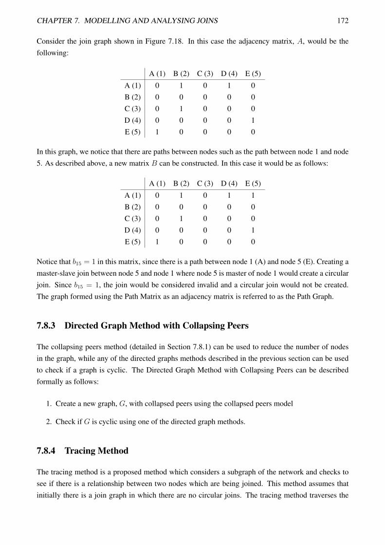
CHAPTER 7. MODELLING AND ANALYSING JOINS 172
Consider the join graph shown in Figure 7.18. In this case the adjacency matrix, A, would be thefollowing:
A (1) B (2) C (3) D (4) E (5)
A (1) 0 1 0 1 0B (2) 0 0 0 0 0C (3) 0 1 0 0 0D (4) 0 0 0 0 1E (5) 1 0 0 0 0
In this graph, we notice that there are paths between nodes such as the path between node 1 and node5. As described above, a new matrix B can be constructed. In this case it would be as follows:
A (1) B (2) C (3) D (4) E (5)
A (1) 0 1 0 1 1B (2) 0 0 0 0 0C (3) 0 1 0 0 0D (4) 0 0 0 0 1E (5) 1 0 0 0 0
Notice that b15 = 1 in this matrix, since there is a path between node 1 (A) and node 5 (E). Creating amaster-slave join between node 5 and node 1 where node 5 is master of node 1 would create a circularjoin. Since b15 = 1, the join would be considered invalid and a circular join would not be created.The graph formed using the Path Matrix as an adjacency matrix is referred to as the Path Graph.
7.8.3 Directed Graph Method with Collapsing Peers
The collapsing peers method (detailed in Section 7.8.1) can be used to reduce the number of nodesin the graph, while any of the directed graphs methods described in the previous section can be usedto check if a graph is cyclic. The Directed Graph Method with Collapsing Peers can be describedformally as follows:
1. Create a new graph, G, with collapsed peers using the collapsed peers model
2. Check if G is cyclic using one of the directed graph methods.
7.8.4 Tracing Method
The tracing method is a proposed method which considers a subgraph of the network and checks tosee if there is a relationship between two nodes which are being joined. This method assumes thatinitially there is a join graph in which there are no circular joins. The tracing method traverses the

CHAPTER 7. MODELLING AND ANALYSING JOINS 173
existing paths from the two nodes which represent the parameters to be joined and checks to seewhether there is already a relationship between them which would cause a circular join.
Figure 7.19 shows the graph used to explain the tracing method.
Figure 7.19: Graph used for the tracing method
In this graph, there is an indirect relationship between A and F. A is master of B (and hence all ofits peers), B is a peer of D, and D is a master of F. This means that a change to parameter A resultsin a change in parameter F. If we were considering creating a master-slave join between parameter Fand parameter A, where F would be master of parameter A, we would trace all the relationships fromparameter A and check if F would be changed if parameter A is changed (which is the case in thisexample). This means traversing all slaves of A and all further slaves. The algorithm for this methodcan be described formally as follows:
Consider a proposed join between node a and node b
1. Let x=b
2. If x==a then the proposed join is not valid
3. For all slaves y of x, Let x=y and go to step 2
Applying this method to the join graph shown in Figure 7.19, let us consider a proposed join betweennode F and node A. We will traverse the slaves of A (B, C, D and G which are peers). Only D has aslave (F) so we will then conclude that the join is invalid since there is a indirect relationship betweenA and F.
7.8.5 Hybrid approach
We can use the tracing method with the graph generated using the collapsing peers method. This istermed the hybrid approach.
Figure 7.20 shows an example graph and the new graph after using the collapsing peers method tocreate a new graph.

CHAPTER 7. MODELLING AND ANALYSING JOINS 174
(a) Without Collapsing Peers (b) With Collapsing Peers
Figure 7.20: Using the Tracing Approach with and without collapsing peers
When a join is created between Parameter G and Parameter A and we are using the tracing methodwithout collapsing the peers on the graph shown in Figure 7.20 (a), at most 6 edges would need tobe traversed (1, 2, 3, 4, 5, 6), whereas when using the hybrid approach (i.e. collapsing the peers andusing the tracing approach), at most 4 edges would need to be traversed (9, 10, 11, 12) (this graph isshown in Figure 7.20 (b)). In this case, a circular relationship would be created with this join. Bothmethods reveal an indirect relationship between Parameter A and Parameter G.
7.9 Scenarios
In order to effectively evaluate the methods described in the previous section, we need to considerreal scenarios which an audio engineer would typically encounter. For each scenario, we need toconsider the audio network and then determine what joins would be created. This can be used tocreate example join graphs, which can be used to test the methods described in the previous section.
We will consider three different real life scenarios and take a look at how the methods would beapplied to each scenario.
In order to develop our scenarios, we refer to the AES R-10 standards document [40] which detailsuse cases for networks in professional audio. This document was compiled by the AES SC-02-12working group with input from industry (including professional audio companies such as Shure, SSLand UMAN). It details three application areas - Recording, Live Sound and Installations. For each ofthese application areas, we review a case study of an existing system and from this, develop a systemwhich we use for a test scenario. This system is based on the use cases presented in AES-R10 andinformation obtained from the case study. Once the scenarios for each application area have beendescribed, this chapter then describes how joins could be used in each of these application areas andgives the join graph which we use for testing purposes.
7.9.1 Description of Scenarios
This section gives a description of each of the three different application areas for professional audioequipment - Recording, Live Sound and Installations. Firewire networks are used in each of these

CHAPTER 7. MODELLING AND ANALYSING JOINS 175
examples. This is followed by a commercial example within each area and then the network which isto be used for testing purposes. In these networks, we are not concerned with the particular equipmentused but rather with the number of input, output, and auxiliary channels which need to be transmittedacross the network, as these determine the number of control parameters. In each application area,unless otherwise specified, we are also only concerned with the largest and most complex use casesince the other use cases can be represented as a subset of the largest use case.
7.9.1.1 Recording
AES R-10 [40] details three different use cases for the recording application area - Portable Record-ing Studio, Desktop Recording Studio and Professional Recording Studio. In this section we shallfocus on the design of a professional recording studio since it is the largest of the three and the mostcomplex.
The requirements for the design of a professional recording studio are specified as follows in the AESR-10 document [40]:
• The capability to scale and easily add or remove new equipment
• Being able to record multiple different channels simultaneously in different configurations.These can range from a single source such as a guitar or microphone to a large orchestra
• Many inputs and outputs
• Support for music to be performed and captured live from many different analogue and digitalsources.
• Multiple sources and destinations and flexible routing between rooms
• Monitoring in each of the studio rooms as well as in the control rooms
• A large-format tactile control surface
• Facilities to record, mix and master
The studio may consist of one or several recording rooms and separate control rooms. In each of theserooms, there would be a number of different inputs, outputs and controls for the different analogueand digital sources, as well as for monitoring and control.
An example network was created based on a case study of two different recording studios - M-Studiosand Sound Pure Studios. These were chosen as examples since they provide comprehensive lists ofequipment on their websites and they are both professional recording studios. The details of the casestudy may be found in Section E.1 of Appendix E.

CHAPTER 7. MODELLING AND ANALYSING JOINS 176
Our Example Network
Our example studio facility will contain a vocal booth, a drum booth, an amp room, a control roomand a ’big’ room. In the vocal booth and amp room there will be 8 input channels, in the drum booth24 input channels, while in the big room, 48 input channels. For monitoring purposes there will be anumber of 16 channel digital mixing consoles in which headphones can be used as well as poweredspeakers. In the control room, there are two sets of monitor speakers as well as 5 speakers and a subfor mixing 5.1 surround sound. The equipment list is therefore as follows:
• 12 x digital mixers and headphones
• 18 x powered speakers, 2 powered subs
• 1 x control surface
• 1 x 24 channel mixing console
• 1 x 48 channel mixing console
• 1 x PC with audio interface for recording
• 11 x analogue to digital converter boxes with 8 input channels
Figure 7.21 shows a diagram of a firewire network using these components. This figure shows the fivedifferent rooms and the components in each of the rooms. It also shows how the devices would beconnected together using firewire routers. This network is used for the join scenario in this applicationarea. Section 7.9.2 describes the scenario and presents the join graph which is used.
7.9.1.2 Live Sound
AES R-10 contains four different use cases for live sound installations - a coffee house, a club, aconcert hall and a festival. The largest of these four is the festival use case in which there are severalbands with one or more stages, possibly appearing over several nights. This is an extension of theconcert hall use case. The important difference between a stage in a festival and that of a concert hallis that a festival contains more devices (particularly amplifiers), since festivals are usually held at anoutside venue and cater for more people than in a typical concert hall. As mentioned, a festival cancontain stages apart from the main stage. These stages are typically isolated and either replicas orsmaller versions of the main stage. It is therefore only necessary to focus on a single stage within afestival.
By investigating the contents of a typical concert hall and a stage within a festival as detailed in AESR-10 [40], we can conclude that a typical single system contains the following equipment:
• A number of loudspeakers - these may either be in the form of stacks or line arrays

CHAPTER 7. MODELLING AND ANALYSING JOINS 177
Figure 7.21: Example Network for Recording
• A number of amplifiers
• Large-scale front of house and monitor mixing consoles (usually between 48 and 96 channels)
• Snakes to carry audio from the stage to the front of house and monitor mixing consoles
• Cube-type monitor speakers and in-ear monitors
• Microphones and Instruments (these can be wired or wireless)
• Instrument Cables, Microphone Cables and Speaker Cables
• Effects racks
In this scenario, the monitor speakers are usually mixed by a separate, dedicated monitor engineerand a multi-track recording of the performance is sometimes captured.

CHAPTER 7. MODELLING AND ANALYSING JOINS 178
Based on a case study of two example live sound systems from different manufacturers - CrownAmplifiers and Yamaha Pro Audio - and the requirements specified in AES R-10 [40], an examplenetwork was created. The details of the case study may be found in Section E.2 of Appendix E.
Example Network
From the description given in AES R-10 [40] and the example systems from Crown Amplifiers andYamaha Pro Audio, we can get a good idea of the components which are required for an examplenetwork for live sound. This section gives the details of the example network which can be used forthe live sound application area. As mentioned, this network is designed to be used for a single stageat a festival. Our example network contains the following professional audio components:
• 2 x 48 channel mixers (using 48 input channels and 32 output channels as in the Yamaha exam-ple)
• 10 x 16 channel mixers for individual monitor mixes
• 1 x PC for recording
• 6 x Monitor amplifiers for cube-type monitor speakers
• 2 x Arrays (Left and right) consisting of 12 speakers and 6 amplifiers
• 1 x Center array containing 4 speakers and 2 amplifiers
• 16 x Bass bins with 8 amplifiers
• 1 x Amplifier for left and right front fill
• 2 x Speakers for left and right front fill
• 2 x Amplifiers (1 speaker and a sub) for left side fill, right side fill as well as drummer monitors
This leads to a total of 2 mixing consoles, 33 amplifiers and a PC which need to be included in thenetwork. Figure 7.22 shows a diagram of a network using these components. This network is usedfor the join scenarios in this application area. Section 7.9.2 describes the scenario and presents thejoin graph which is used.

CHAPTER 7. MODELLING AND ANALYSING JOINS 179
Figure 7.22: Example Network for Live Sound
7.9.1.3 Installations
AES R-10 contains two different use cases for installations - a standard room installation with inter-connections and a large-scale conference system. This section focuses on the large-scale conferencesystem since it is larger and more complex. Such a system can contain many different rooms anddevices spread out over a large venue, with separate control rooms controlling many different devicesthroughout the conference center.
In such a conference center, there also needs to be facilities for translation, and separate audio chan-nels need to be routed to different headphones and speakers according to the conference requirements.
AES R-10 [40] specifies that a conference center may consist of the following:
• A complex central matrix with up to 4000 or more input and output channels
• Analogue microphones at each seat

CHAPTER 7. MODELLING AND ANALYSING JOINS 180
• Auto mixer (this reduces the level to eliminate the possibility of feedback in the case of multiplemicrophones)
• Distributed and delay compensated speaker system
• Facilities for translators and headphone sets for conference participants
Based on a case study of two large installations - the City Center on the Las Vegas Strip and theOregon Convention Center - and the requirements specified in AES R-10 [40], an example networkwas created. The details of the case study may be found in Section E.3 of Appendix E.
Example Network
For our example network we consider a large convention center such as the ones described in SectionE.3 of Appendix E. In these examples, most of the speakers are ceiling speakers. We include facilitiesfor 10 different translators and wireless headsets for translation plus a number of microphones in adiscussion room. We also have a large exhibition space which contains a number of speakers. Theequipment list of our convention center is as follows:
• 200 x Powered ceiling speakers for the exhibition space
• 20 x Digital mixing consoles for possible venues or when meeting rooms are partitioned
• 10 x Digital to analogue converters in the rooms made available for translators
• 100 x Wireless receivers
• 100 x 2-channel input systems
• 20 x Amplifiers which can connect to passive speakers for when meetings rooms are partitioned
• 1 x PC for configuring routing in the system
Figure 7.23 shows a diagram of a network using these components with the components placed intheir respective parts of the venue. Since there are 20 ceiling speaker clusters, 10 translation roomsand 20 breakout rooms, these component types are shown in Figure 7.23 below the conference venue,while within the conference venue’s network diagram each component is depicted as a circle. Thisnetwork is used for the join scenarios in this application area. Section 7.9.2 describes the scenarioand presents the join graph which is used.

CHAPTER 7. MODELLING AND ANALYSING JOINS 181
Figure 7.23: Example Network for Installations
7.9.2 Description of Join Scenarios and their associated graphs
For each of the application areas described in the previous section, a scenario needs to be developedin which joins would be used, so that a join graph can be developed. This section describes such ascenario for each of the application areas and presents a join graph that will be used for testing thealgorithms described in the next section. These three join scenarios are applied specifically to theexample networks described in the previous section.
Recording
Assume that there are a number of instrumentalists who each have their own monitoring requirements.These instrumentalists might be in separate rooms, such as the vocal room or even need monitoringfrom an amp room (such as the case of a guitarist who is using amps located in the amp room).There is also a master mix so that each person can hear the other instruments which are playing theirrespective parts. Different sections (such as strings) may be grouped in such a manner that a masterfader will be able to adjust all of the slaves.

CHAPTER 7. MODELLING AND ANALYSING JOINS 182
For our example network, the following joins will be created:
• Relative master-slave join between a master fader in the control room and each of the channels(16) for the 10 individual monitor mixers.
• Peer-to-peer join between the parameters on the control application running on the PC withinthe control room (such as gain and equalisation parameters) and each of the parameters for theindividual mixes so that the control room and the individual mixes are synchronised.
• Relative master-slave join between the master and individual mixers for the high, mid and lowparameters in the equalizer.
Figure 7.24 shows a depiction of a part of the join graph for this scenario for a single channel beingsent to two individual monitor mixers.
Figure 7.24: Join Graph for Recording (channel 1 for two individuals)
This join graph shows 20 nodes. A master-slave join is created between channel 1 of the main monitormixer and channel 1 on each of the individual monitor mixers. In this scenario, a master-slave join isset up for 4 different parameters related to the channel - gain, high, mid and low. The control roomcontains a PC which runs a control application. In this scenario, peer-to-peer joins are establishedbetween the control room controller parameters and the individual monitor mixer parameters. Thismeans that the monitor mixer is a logical master of the parameters in the control application, andhence included in the join graph.

CHAPTER 7. MODELLING AND ANALYSING JOINS 183
In this scenario, a circular join could be created if a master-slave join was established between oneof the controller application control parameters for a channel and a parameter on the monitor mixerwithin the control room, as shown in Figure 7.24. Additional relationships between the parametersfor different channels would introduce additional possibilities of creating a circular join.
By extending the example presented above to include 10 individuals and 16 channels, a join graphcontaining 1344 nodes is constructed (where each node represents a parameter). The nodes are asfollows:
• 16 master gain controls on the control room monitor mixer, as well as 16 high, mid and lowcontrols on the control room monitor mixer.
• 16 gain controls on each of the 10 individual monitor mixers, 16 high, mid and low controls oneach of the 10 individual monitor mixers.
• 640 control application parameters for the individual monitor mixers.
Live Sound
In a large concert, each instrumentalist will ideally have their own monitor mix. Typically an engineerwill also be present who controls the overall monitor mix, while each instrumentalist will make slighttweaks to their own monitor mix. This is similar to the example presented in the previous section butin this case the monitor engineer controls the mix, not the studio engineer. Master-slave relationshipscan be created between the monitor console and each musician’s individual console. In a live soundscenario, there is also a front of house engineer who is responsible for the sound which is delivered tothe audience. The front of house engineer may wish to link the equalisation parameters for the frontof house console with the equalisation parameters of the monitor console.
Compressors and Reverb are often applied to vocals. The audio engineer may wish to have a mastercontrol to increase the reverb on all of the reverb units. These can be linked using a master-slaverelationship.
In a typical live sound setup there are numerous amplifiers. The audio engineer may wish to adjustthe volume on all of the amplifiers using a master control. This may also be true for each of thecomponent stacks.
For our example network, the following joins will be created:
• Relative master-slave joins between a master fader on the monitor mixing console and each ofthe channels (16) for the 10 individual monitor mixers.
• Peer-to-peer joins between parameters on a control application running on a PC and each of theparameters for the individual mixers.
• Relative master-slave joins between the main monitor mixing console and individual mixers forthe high, mid and low equalization parameters.

CHAPTER 7. MODELLING AND ANALYSING JOINS 184
• Master-slave relationship between the master volume on the front of house mixing console foreach amplifier stack and all the amplifiers in each stack.
• Peer-to-peer joins between the gain parameters of amplifiers within each stack.
Figure 7.25 shows a depiction of a part of the join graph for this scenario for a single channel beingsent to two individual monitor mixers, the front of house (FOH) mixer and two speaker stacks, eachcontaining two amps.
Figure 7.25: Join Graph for Live Sound (channel 1 for two individuals and two speaker stacks)
This join graph shows 26 nodes. A master-slave join is created between channel 1 of the monitormixer and channel 1 on each of the individual mixes. In this scenario, a master-slave join is set up for4 different parameters related to the channel - gain, high, mid and low. The front of house controllerhas a PC which runs a control application. In this scenario, peer-to-peer joins are established betweencontrol application parameters and the individual monitor mixer parameters. This means that themonitor mixer is a logical master of the parameters in the control application, and hence included inthe join graph. The front of house mixing console has parameters to control the gain of the ampswithin each of the speaker stacks. Master-slave joins are created between the gain parameter on thefront of house mixing console for the amp stack with the gain parameter of each of the two amplifiersthat are contained within that stack.
In this scenario, a circular join could be created if a master-slave join was established between the oneof the controller application parameters for a channel of the individual mixer and the corresponding

CHAPTER 7. MODELLING AND ANALYSING JOINS 185
channel on the main monitor mixer. This is shown in Figure 7.25. Additional relationships betweenthe parameters for different channels would introduce additional possibilities of creating a circularjoin.
By extending the example presented above to include 10 individuals and 16 channels for monitors,as well as the six speaker arrays, a join graph containing 1374 nodes (where each node represents aparameter). The nodes are as follows:
• 16 master gain controls on the monitor mixer, 16 high, mid and low controls on the monitormixer.
• 16 gain controls on each of the 10 individual monitor mixers, 16 high, mid and low controls oneach of the 10 individual monitor mixers.
• 640 controller parameters for the individual monitor mixers
• 6 master gain parameters for front of house speaker arrays and front fills
• 6 amp gains for left speaker array
• 6 amp gains for right speaker array
• 2 amp gains for center speaker array
• 1 amp gain for left front fill
• 1 amp gain for right front fill
• 8 amp gains for bass bins
Installations
Within a conference center, many amplifiers are deployed throughout the venue. A control roomwould need to be able to control the volume of signals which are being sent to the different rooms. Inthis case, a master control parameter would adjust all of the volumes of the amplifiers. The conventioncenter may be divided into segments, in which case a master controller would be required for each ofthese segments.
Our example network contained a number of ceiling speaker clusters. Each of these clusters will beconsidered as a segment. For our example network, the following joins will be created:
• Master-slave join between a volume control in the control room and a volume parameter oneach of the amplifiers deployed in the conference center.
• Master-slave join between a volume control in the control room and a volume parameter oneach of the amplifiers deployed in a segment of the conference center. This would be done foreach segment.

CHAPTER 7. MODELLING AND ANALYSING JOINS 186
• Peer-to-peer joins between the amplifiers for each segment to ensure that all of the amplifierswithin the segment have the same volume.
Figure 7.26 shows a depiction of a part of the join graph for this scenario for a single speaker cluster(segment) containing two amplifiers and two partitioned rooms. It also shows the control parameterson the control application which is running within the control room.
Figure 7.26: Join Graph for Installations
This join graph shows 9 nodes. A master-slave join is created between a volume parameter within thecontrol room for each of the amplifiers and the volume parameter on each of the amplifiers. A master-slave join is also created between the volume parameter within the control room for the segment andthe volume parameter of the two amplifiers contained within the speaker cluster.
In this scenario, if a wall controller (WC in Figure 7.26) was installed in partitioned room 1 and apeer-to-peer relationship was established with the amp (which means that the control room parameteris a logical master of the wall controller parameter) a circular join could be created if a master-slavejoin was established between the wall controller and the control parameter in the control room, asshown in Figure 7.26.
By extending the example presented above to include 10 partitioned rooms, 10 translation rooms and20 speaker clusters containing 10 speakers, a join graph containing 480 nodes is constructed (whereeach node represents a parameter). The nodes are as follows:
A join graph for this scenario would contain 480 nodes. They are as follows:
• 20 controller volume parameters in the control room for each of the segments
• 200 volume parameters for the ceiling speaker amplifiers
• 20 volume parameters for the amplifiers in the partitioned rooms
• 10 volume parameters for the amplifiers in the translation rooms
• 230 controller volume parameters in the control room for the amplifiers

CHAPTER 7. MODELLING AND ANALYSING JOINS 187
7.10 Evaluation of methods
This section evaluates the methods presented in Section 7.8 using the scenarios presented in the pre-vious section and determines which is the best method or combination of methods to use in thesimulated environment.
7.10.1 Tests to evaluate the different methods
From the methods discussed in Section 7.8, there are a number of tests which need to be performedin order to determine which is the best method to use to evaluate whether there are circular joins ornot. The methods were as follows:
• Directed Graph Methods (described in Section 7.8.2)
– Check if we can perform a linear ordering of nodes in the graph
– Peel the leaves off the tree
– Perform a Depth First Search
– Perform Matrix Operations
* Create a path graph
• Directed Graph Methods with Collapsing Peers (described in Section 7.8.3)
• The Tracing Method (described in Section 7.8.4)
• The Hybrid Method - which is the Tracing Method with collapsing peers (described in Section7.8.5)
There are essentially two approaches to testing joins - one where tests are performed as the join graphis constructed and one where an entire complete join graph is tested for cycles.
To evaluate the above methods, the methods were implemented as C++ programs which utilise a twodimensional array to store the graph as an adjacency matrix. Timing was performed for each methodusing the Unix ’time’ command. As there are two approaches to testing, two sets of tests had tobe performed on the join graphs (with and without collapsing peers) to evaluate all of the methodseffectively. They are as follows:
1. Checking the entire join graph for circular joins
2. Building up a join graph iteratively and using the methods to check for circular joins at eachiteration before creating the join.
In the first set of tests (Entire Join Graph), the following tests are performed on the two join graphs(with and without collapsed peers) for each scenario, to evaluate checking the entire graph for circularjoins:

CHAPTER 7. MODELLING AND ANALYSING JOINS 188
• Construct a new graph which shows if there are any paths between two nodes (Path Graph) andcheck are any 1s along the diagonal of the matrix (i.e. there is a path from one node to itself)
• Perform a depth first search (Depth first search) on the entire graph
• Perform a Linear Ordering of the nodes (Linear ordering) on the entire graph
• Peel the leaves off the tree (Peel leaves) on the entire graph
• Use the tracing method to check if there is a path between any of the two nodes (TracingMethod)
In the second set of tests, the following tests are performed before each join is created to determine ifthat join causes a circular join:
• Check if there is there is an edge between the two nodes in the Path Graph. Update the pathgraph to include the new join.
• Perform a depth first search (Depth first search) after each join is created
• Perform a Linear Ordering of the nodes (Linear ordering) after each join is created
• Peel the leaves off the tree (Peel leaves) after each join is created
• Use the tracing method to check if there is a path between the two nodes being joined (TracingMethod)
In the second set of tests, we start with an empty join graph and use the methods to evaluate whetheror not the join creates a circular join. If it does not create a circular join, the join is created. As before,the Unix ’time’ command was utilised to perform timing. These tests are also done with and withoutthe collapsing peers method for each scenario. The results of these two sets of tests will be describedin the following section.
7.10.2 Test results and evaluation
The previous section presented the tests to be performed in order to evaluate which algorithm isoptimal for determining whether or not there is a circular join. This section shows the results of thesetests using the join graphs for the three scenarios - live sound, recording and installations - whichwere described in Section 7.9.2. This section seeks to answer the following questions:
• Should we collapse peers?
• Which algorithm is the fastest?
• Which algorithm uses the least amount of memory?
• Which algorithm is the best overall, based on a combination of speed and memory utilisation?

CHAPTER 7. MODELLING AND ANALYSING JOINS 189
Collapsing Peers
The collapsing peers method decreases the number of nodes in the graph, which means that all of thealgorithms will be performed faster. The collapsing of peers occurs whenever a peer-to-peer join iscreated. In terms of time, there are two factors to consider - how long it takes to collapse the peersand how much improvement this leads to in terms of algorithm time. In terms of resources, we alsoneed to consider the memory reduction with the collapsing peers method. In each of the tables, thescenarios are numbered as follows:
1. Live Sound (described in Section 7.9.1.2)
2. Recording (described in Section 7.9.1.1)
3. Installations (described in Section 7.9.1.3)
Table 7.6 show the size of the graph for each of the three scenarios, the time to collapse peers, and thetimes for each of the five algorithms with and without the use of the collapsed peers approach fromthe first set of tests.
Normal Collapsed Peers
Scenario 1 2 3 1 2 3
Nodes in Graph 1374 1344 480 716 704 50
Collapse Peers 1.54 1.28 0.05 - - -
Linearly ordering 0.0979 0.0502 0.004 0.0179 0.0114 0.000044
Depth First Search 0.0138 0.0023 0.00006 0.0017 0.0015 0.000005
Peel Leaves 0.0003 0.0011 0.0003 0.0001 0.0002 0.000004
Create a Path Graph 0.0127 0.0122 0.0015 0.0034 0.0032 0.000016
Tracing Method 5.5 4.7010 0.3080 0.7720 1.0920 0.0005
Table 7.6: Timing Results (in seconds) for the five algorithms with and without the use of the collapsedpeers approach
This table shows how collapsing peers improves the times for all of the algorithms.
Table 7.7 shows the ratio between the time taken without the use of collapsing peers and the timetaken when collapsing the peers.
1 2 3
Linearly ordering 5.4693 4.4035 90.9091
Depth First Search 8.1177 1.5333 12
Peel Leaves 3 5.5 75
Create a Path Graph 3.73530 3.8125 93.75
Tracing Method 7.1244 4.3049 616
Table 7.7: Ratio between time taken without the use of collapsing peers and the time take whencollapsing peers

CHAPTER 7. MODELLING AND ANALYSING JOINS 190
Table 7.7 shows that the time for the algorithms is improved by a factor of between 1.5 and 616.Collapsing Peers, however, does take time and it is questionable as to whether the improvementis worth it, since collapsing the peers takes between 0.05 and 1.54 seconds for each of the threescenarios.
Table 7.8 shows the number of nodes in the graph with and without the use of collapsing peers, aswell as the reduction in the amount of memory (in bytes) required to store the graph.
Normal Collapsed Peers
Scenario 1 2 3 1 2 3
Nodes in Graph 1374 1344 480 716 704 50
Memory Usage 1887876 1806336 230400 512656 495616 2500
Memory Improvement - - - 1375220 1310720 227900
% Improvement - - - 72.84% 72.56% 98.91%
Table 7.8: The effect of collapsed peers on number of nodes and memory utilisation
The reduction in the number of nodes leads to a significant reduction in the amount of memory whichis used to store the graph. This table shows that the memory usage is reduced by between 72.56 and98.91 percent. This also needs to be considered when deciding whether or not to collapse the peersinto a single node.
Multiple nodes can be collapsed into a single node at the same time as the relationships are established.Therefore, a better indication would be to evaluate the amount of time which is required to create allthe joins in the graph and at the same time run the test algorithms. This is done in the second set oftests in which we start with an empty join graph and use the methods to evaluate whether or not thejoin creates a circular join. If it does not create a circular join, the join is created. This is done foreach join until all of the joins are performed.
Table 7.9 shows the time taken for the second set of tests for the three scenarios with and withoutcollapsing peers.
Normal Collapsed Peers
Scenario 1 2 3 1 2 3
Linearly ordering 27.87 25.917 0.842 23.596 25.8 0.065
Depth First Search 4.165 4.043 0.135 3.259 4.322 0.028
Peel Leaves 0.096 0.042 0.049 0.224 0.174 0.019
Path Graph 0.077 0.056 0.004 0.373 0.395 0.033
Tracing Method 0.049 0.045 0.004 0.401 0.517 0.048
Table 7.9: Time (in seconds) taken for second set of tests
This table shows that collapsing peers improves the times for the linear ordering method and thedepth first search. It only improves the speed of peeling leaves for the installation scenario. This

CHAPTER 7. MODELLING AND ANALYSING JOINS 191
table suggests that in terms of algorithm time, it is best to only collapse peers when using the linearordering method or the depth first search method. However, this should be weighed up against theimprovement in memory utilisation.
The question of whether or not to collapse peers is largely case specific. It depends on the number ofnodes, at what point the peers are collapsed and how many peer-to-peer joins are created. The largereduction in the amount of memory utilised and the fact that the peers can be collapsed at the time ofcreating the join are motivating factors for collapsing peers.
Algorithm Timing
Table 7.10 shows the rank of the algorithms in terms of time for the first set of tests for the threescenarios with and without collapsing peers.
Normal Collapsing Peers
1 2 3 Average Rank 1 2 3 Average Rank
Linearly ordering 4 4 4 4 4 4 4 4
Depth First Search 3 2 1 2 2 2 2 2
Peel Leaves 1 1 2 1.33 1 1 1 1
Path Graph 2 3 3 2.67 3 3 3 3
Tracing Method 5 5 5 5 5 5 5 5
Table 7.10: Rank for Algorithms in terms of time for first set of tests
From these results, we can see that the fastest algorithm is the peeling leaves algorithm, while theslowest is using the tracing method followed by performing a linear ordering.
Table 7.11 shows the rank of the algorithms in terms of time for the second set of tests for the threescenarios with and without collapsing peers.
Normal Collapsing Peers
1 2 3 Average Rank 1 2 3 Average Rank
Linearly ordering 5 5 4 4.6667 5 5 5 5
Depth First Search 4 4 3 3.6667 4 4 2 3.3333
Peel Leaves 3 1 2 2 1 1 1 1
Path Graph 2 3 1 2 2 2 3 2.3333
Tracing Method 1 2 1 1.3333 3 3 4 3.3333
Table 7.11: Rank for Algorithms in terms of time for second set of tests
This table shows that the path graph method is in fact faster than the peeling leaves method and thedepth first search in the second set of tests. It also shows that the tracing method is the fastest method.

CHAPTER 7. MODELLING AND ANALYSING JOINS 192
Tracing method versus Path Graph method
From the results shown in Table 7.9, the tracing method is the fastest method in all three scenariosfollowed by the path graph. Both the tracing method and the path graph method perform evaluationsbased on the join being created (i.e. they check for an existing path between two nodes in the joingraph). In the case where a network has been imported from a real network and the presence ofcircular joins needs to be evaluated, both of these algorithms require that checks are done betweeneach of the nodes within the join graph to determine if there is a circular join.
Normal Collapsed Peers
Path Graph Construct Trace Path Graph Construct Trace
Live Sound 0.002 0.0127 5.5 0.0006 0.0034 0.772
Recording 0.0019 0.0122 4.701 0.0006 0.0032 1.092
Installations 0.0003 0.0015 0.308 0.000003 0.000016 0.000521
Table 7.12: Path Graph and Tracing Method to check for cycles
Table 7.12 shows the time taken to check for cycles in an existing graph using the path graph and thetracing method. This table is an enhancement of Table 7.6 to show the time taken to construct the pathgraph. This table shows that the path graph method is significantly faster than the tracing method. Ifwe include the time to construct the path graph, the path graph method is still significantly faster thanthe tracing method.
7.10.3 Methods used for implementation
Since an audio engineer performs the joins in real-time, the cost (in terms of time) of collapsing thepeers is not as high as when it is done once-off. Collapsing peers results in a significant reduction inthe memory required which could be very valuable if an audio engineer is designing a large systemlike the ones presented in the previous section. In the tests conducted in a real-time scenario, the pathgraph method and tracing method were shown to be the fastest for determining whether or not a joincreates a circular join. Since it is a requirement to be able to import an existing system and check ifthere are any circular joins, the path graph algorithm is used rather than the tracing algorithm. Thetracing method was faster than the path graph method for a single join, however when this method isused to trace between each of the nodes to see if there are any circular joins, it is slower than the pathgraph method (in fact it is the second slowest out of all the algorithms tested). It is for this reason thatwe use the path graph method within AudioNetSim.
When using the path graph method, updates to the path graph structures are only done if a join isvalid. When a join is created, the following occurs:
• The new peers are collapsed into a single node.

CHAPTER 7. MODELLING AND ANALYSING JOINS 193
• The old nodes are removed from the path graph and a new (collapsed) node is created for thenew peer group.
• The relationships within the path graph are updated to reflect the new join.
If the new join does not result in a peer group being created or a peer group being altered, only thepath graph is updated with the new relationship as there is no need to collapse any of the graph’snodes into a single node.
The next section will describe the implementation and the data structures used to store the path graphwithin AudioNetSim.
7.11 Implementation of Path Graph Method within AudioNet-Sim
Chapter 6 has described AudioNetSim and Section 7.3 has described how join lists are modelledand how they are a reflection of the implementation of join lists in a real device. In order to enablethe checking of joins which have been created, a two dimensional array is used to contain the joingraph. This is a common method of storing a graph [6]. In addition, a structure is maintained whichidentifies the node IDs. This section uses an example scenario (described below) to illustrate thestructures which are used to implement the path graph method within AudioNetSim.
Consider the following scenario: 6 parameters - A, B, C, D, E and F - where B and C are peers andE and F peers. A is master of B and C, while D is master of E and F. Figure 7.27a shows the joingraph for this scenario, while Figure 7.27b shows the join graph for this scenario when the peers arecollapsed into a single node.
(a) Join Graph (b) Join Graph with Col-lapsed Peers
Figure 7.27: Join Graph and Join Graph with Collapsed Peers
Within AudioNetSim, this scenario is represented using the following structures:
• A list of Peer Group IDs and the Node IDs of the nodes which are contained within that peergroup
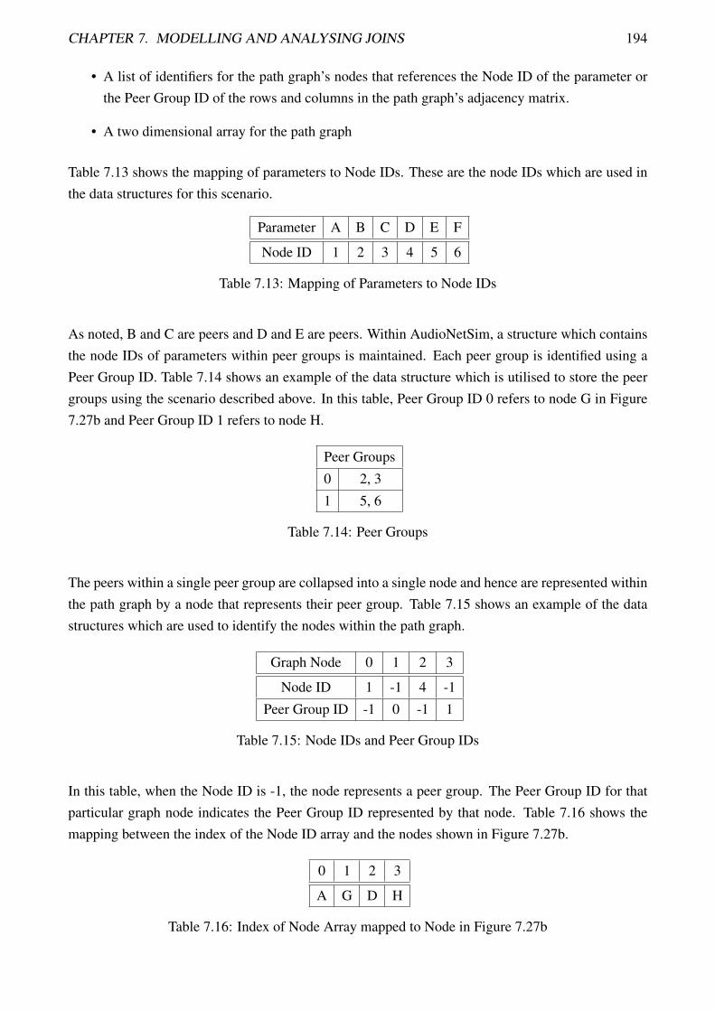
CHAPTER 7. MODELLING AND ANALYSING JOINS 194
• A list of identifiers for the path graph’s nodes that references the Node ID of the parameter orthe Peer Group ID of the rows and columns in the path graph’s adjacency matrix.
• A two dimensional array for the path graph
Table 7.13 shows the mapping of parameters to Node IDs. These are the node IDs which are used inthe data structures for this scenario.
Parameter A B C D E F
Node ID 1 2 3 4 5 6
Table 7.13: Mapping of Parameters to Node IDs
As noted, B and C are peers and D and E are peers. Within AudioNetSim, a structure which containsthe node IDs of parameters within peer groups is maintained. Each peer group is identified using aPeer Group ID. Table 7.14 shows an example of the data structure which is utilised to store the peergroups using the scenario described above. In this table, Peer Group ID 0 refers to node G in Figure7.27b and Peer Group ID 1 refers to node H.
Peer Groups
0 2, 3
1 5, 6
Table 7.14: Peer Groups
The peers within a single peer group are collapsed into a single node and hence are represented withinthe path graph by a node that represents their peer group. Table 7.15 shows an example of the datastructures which are used to identify the nodes within the path graph.
Graph Node 0 1 2 3
Node ID 1 -1 4 -1
Peer Group ID -1 0 -1 1
Table 7.15: Node IDs and Peer Group IDs
In this table, when the Node ID is -1, the node represents a peer group. The Peer Group ID for thatparticular graph node indicates the Peer Group ID represented by that node. Table 7.16 shows themapping between the index of the Node ID array and the nodes shown in Figure 7.27b.
0 1 2 3
A G D H
Table 7.16: Index of Node Array mapped to Node in Figure 7.27b

CHAPTER 7. MODELLING AND ANALYSING JOINS 195
Table 7.17 shows the path graph’s adjacency matrix for this scenario. A two dimensional array is usedto store this matrix.
Graph 0 1 2 3
0 0 1 0 0
1 0 0 0 0
2 0 0 0 1
3 0 0 0 0
Table 7.17: Path Graph
AudioNetSim maintains this two dimensional array (described in Section 7.8.2). This structure isupdated every time a join is created. When a join is created, the two dimensional array is first checkedto see if there is already a relationship present which would cause a circular join. If there is already arelationship present, the join is not performed and an error message is given to the user. If there isn’ta relationship present, the path graph is updated to reflect all new paths that are created by the newjoin.
Consider the example where a user wishes to create a new master-slave relationship between Param-eter F (Node ID of 6) and Parameter D (Node ID of 4). Node ID 6 is contained within the peer groupwith Peer Group ID of 1. These are graph nodes 2 and 3 within the path graph. By checking the pathgraph matrix, we can see that there is already a relationship between graph nodes 2 and 3 and hencethe new relationship would create a circular join.
Consider a further example where a user wishes to create a new master-slave relationship betweenParameter E (Node ID of 5) and Parameter A (Node ID of 1). Node ID 5 is contained within the peergroup with Peer Group ID of 1. These are graph nodes 0 and 3 within the path graph. The path graphmatrix shows that there is currently no relationship between these graph nodes, and hence there is norelationship between the parameters and the new relationship can be created, as it would not create acircular join. When AudioNetSim detects a circular join being created, it will not create the join, butwill rather inform the user that the join being created causes a circular join using a dialog box. Thiswill be shown in the following section.
7.12 Example of a circular join being created in UNOS Vision
As described in Section 6.5, UNOS Vision is used as the control application for the devices withinthe simulated network created by AudioNetSim. UNOS Vision provides the capability to createjoins between parameters. When using a simulated network, the joins would be performed betweenparameters within the simulated network and these would be evaluated using the structures describedin the previous section.
Figure 7.28 shows the connection manager tab in UNOS Vision and the desk items for the simulatedUMAN Evaluation Board.

CHAPTER 7. MODELLING AND ANALYSING JOINS 196
Figure 7.28: UNOS Vision Control Window
The evaluation board contains an 16x18 DICE mixer matrix. The desk items that can be used tocontrol the parameters associated with this mixer matrix are shown within the desk item pane of thewindow. Each pot control controls a single gain parameter within the mixer matrix. To create joinsbetween parameters in UNOS Vision, the user will click on the ’Join’ button. When this button isclicked, the user can then select the join type which they wish to create between parameters. Figure7.29 shows the menu which is opened when the user clicks on the ’Join’ button.
Figure 7.29: Selecting the type of joins to be created
The user may select Peer-to-Peer or Master-Slave - depending on the type of joins they wish to create.For this example, we will look at creating master-slave joins. Once the user selects Master-Slave,buttons will be added next to each of the deskitems. Figure 7.31 shows the resulting buttons whichare added next to each of the pot controllers (which each represent a gain parameter in the mixermatrix).

CHAPTER 7. MODELLING AND ANALYSING JOINS 197
Figure 7.30: Creating Master-Slave joins between parameters
The user can then click on the ’M’ button next to the desk item of the relevant parameter to select it asa master and the ’S’ button to select it as a slave. Once the buttons have been clicked, the selections forthe parameters are highlighted in red. Consider the example of creating a master-slave join between(1,1) and (3,4) in the mixer matrix - with (1,1) being the master. Figure 7.31 shows the UNOS Visionwindow once the relationships for the new join have been selected.
Figure 7.31: Creating a Master-Slave join between two parameters
Once the parameters and types for the new joins have been selected, the user can click on the ’Join’button to complete the joins between the parameters. This results in function calls to XFNDLL (seeSection 6.6 for more details) to create the joins. This results in calls being made to the control protocolmodel of AES64 within AudioNetSim to create the joins between the parameters within the simulatedparameter trees. Before the joins are created, they are evaluated using the structures described in theprevious section to determine whether or not they will introduce a circular join. If a circular join

CHAPTER 7. MODELLING AND ANALYSING JOINS 198
would be created, a dialog box is shown informing the user that the joins being created introduce acircular join and they are not created. If the new joins do not create a circular join, the structureswithin the control protocol model, as well as the path graph matrix are updated.
To illustrate this, we consider creating relationships between three parameters using UNOS Vision.This is shown in Figure 7.32 which shows UNOS Vision with the resulting dialog box and identifiesthe Desk Items of the parameters which this example refers to. In this example, we previously createdmaster-slave joins between parameter 1 and parameter 2 and parameter 2 and parameter 3 usingUNOS Vision. To create a circular join, we tried to create a master-slave join between parameter 3and parameter 1 using UNOS Vision which resulted in the dialog box being shown.
Figure 7.32: Circular Join Dialog box
7.13 Conclusion
A hallmark of the AES64 protocol is its powerful grouping capabilities. AES64 provides the capa-bility for an audio engineer to establish peer-to-peer and master-slave relationships between differentparameters. One of the problems with providing capabilities such as master-slave joins is the easewith which circular joins can be created. These circular joins set up feedback loops and cause thevalues of parameters to be changed in an unpredictable manner.
This chapter has shown how a simulated environment can be used to easily evaluate the relationshipsbetween all the parameters. It has discussed a number of different algorithms which can be usedto evaluate whether or not a join is valid as well as determining if a circular join is present. It has

CHAPTER 7. MODELLING AND ANALYSING JOINS 199
also shown how this approach can be implemented in a simulated environment using the example ofAudioNetSim.

Chapter 8
Bandwidth Calculation for Firewire and AVBNetworks
8.1 Introduction
Chapter 2 provided an introduction to Firewire and Ethernet AVB. These are the transport technolo-gies which are analysed in this thesis. An analytical simulation approach is used to calculate therequired metrics. These are based on the topology of the network and the activity on the network (eg.the audio streams which are being transmitted). In this chapter, the metric we are concerned with isthe bandwidth utilisation within the network.
This chapter discusses bandwidth calculation in Firewire and Ethernet AVB networks. It presentsmethods which can be used to calculate bandwidth in IEEE 1394a, IEEE 1394b and Ethernet AVBnetworks. These methods are evaluated using data obtained from a real network. This chapter alsodescribes how the bandwidth calculations are integrated into AudioNetSim so that the bandwidthutilisation can be viewed in real-time by audio engineers as they create and remove connectionsbetween devices.
8.2 Monitoring and Control Data Bandwidth
With both Firewire and Ethernet AVB, the amount of bandwidth utilised for streaming is constrainedto a certain amount - 80 percent of the total bandwidth for Firewire and 75 percent for Ethernet AVB.The rest of the bandwidth is available for monitoring and control. This section evaluates whether thereis sufficient bandwidth for control and monitoring data and whether it needs to be considered withinthe bandwidth calculation. In this section, we will look at the most bandwidth intensive application -the metering of changing parameters.
AES64 provides a mechanism which allows each device to transmit a block of meters every 25ms.This mechanism is called the PUSH mechanism.
200

CHAPTER 8. BANDWIDTH CALCULATION FOR FIREWIRE AND AVB NETWORKS 201
In this mechanism, a device transmits a SET DATABLOCK request (described in Section 5.3.1) withmultiple parameter values to a target control application, which requested that these parameter valuesbe sent to it. Every 25ms (or another fixed time period), the device will read the values and if atleast one of them is valid (greater than zero), they are packaged into a datablock and sent to the targetcontrol application which alters its local parameters based on this list. This mechanism is typicallyused for meters.
8.2.1 Packet Size Calculation
Consider a device which is sending n meter values to a target control application. They are packagedin the format shown below in Table 8.1.
Number of Values (n) (32 bits)
Meter 1 Parameter Index (32 bits)
Meter 1 Value (32 bits)
...
Meter n Parameter Index (32 bits)
Meter n Value (32 bits)
Table 8.1: Packaging of Meter Values
The number of meters, as well as the parameter index of each meter and its value is sent to the targetcontrol application. This data is packaged into an AES64 packet. Table 8.2 shows the packet headerformat of an AES64 packet, which does not require a response.
Target Device ID (32 bits)
Target AES64 Node ID (32 bits)
Sender Device ID (32 bits)
Sender AES64 Node ID (32 bits)
Sender Parameter ID (32 bits)
User Level (8 bits) Message Type (8 bits)
Command Executive (8 bits) Command Qualifier (8 bits)
Table 8.2: AES64 Packet Header
In the case of the PUSH mechanism, the command executive SET and the command qualifier DATA_BLOCKis used. More information about the different command executives and qualifiers which can be usedin AES64 can be obtained in the AES64 specification [115]. More information on the AES64 protocolcan be found in Section 5.3.1.

CHAPTER 8. BANDWIDTH CALCULATION FOR FIREWIRE AND AVB NETWORKS 202
AES64 messages are sent as UDP datagrams over IP. This means that the headers for IP and UDPalso need to be included in the calculation of the packet size.
Table 8.3 shows the IP header followed by the UDP header and the UDP datagram which contains theAES64 message (header and data). It also shows the total size (in bits) of each of the parts.
IP Header including source and destination IP address (160 bits)
UDP Header including source and destination port (64 bits)
AES64 Header, AES64 Address block (192 bits)
Data (64n+32 bits)
Table 8.3: UDP Datagram containing AES64 Message
A packet containing n meters therefore requires 448+64n bits (56+8n bytes) to be sent every 25ms.This translates to 40 events every second which equates to 2240+320n bytes every second. For a 96channel mixing console with 96 meters, there will be 32960 bytes per second which is 32.1875 KB/s.
When utilising Firewire to transmit UDP datagrams over IP, an IP over 1394 header also needs to beincluded, which is 4 bytes. This would increase the packet size of a packet containing n meters to60+8n bytes, which equates to 2400+320n bytes every second (since 40 events are sent every secondas described earlier). A meter block consisting of 96 meters would therefore be 2400+320(96) =33120 bytes every second. Using a 100Mbps example, Firewire would have 20Mbps (20 percent),while Ethernet AVB would have 25Mbps (25 percent). Based on this, we can calculate an approxi-mation of how many meter blocks it will take to utilise this bandwidth. 20Mbps = 2621440 bytes persecond. This means that approximately 2621440
33120= 79.15 (i.e. 79) sets of 96 meters can be sent every
25ms. For Ethernet AVB, 25Mbps = 3276800 bytes per second, which means that approximately327680032960
= 99.41. (i.e. 99) sets of meters can be sent every 25ms. Table 8.4 shows how many sets of 96meters can be sent every 25ms when the maximum amount of bandwidth has been used for streamingfor Firewire at 100Mbps, 400Mbps and 800Mbps and Ethernet AVB at 100Mbps and 1000Mbps.
Firewire Ethernet AVB
100 400 800 100 1000
Number of 96 Meter Blocks 79 316 633 99 994
Table 8.4: Number of blocks of 96 meters which can be sent
This table shows that there is more than sufficient bandwidth for control and monitoring data, sinceeven on a network which can transmit less than 100 audio streams (such as the 100Mbps networks),7584 metering values can be sent every 25ms. This is 75 times the amount of meters which would needto be sent if monitoring the level for each audio stream. This same argument can be applied to control(and control messages utilise less bandwidth than meter blocks) as many more parameters can beadjusted or read than required. This means that we do not need to consider the control and monitoringdata within the bandwidth calculation, but rather we only need to investigate the percentage of thestreaming data which is used.

CHAPTER 8. BANDWIDTH CALCULATION FOR FIREWIRE AND AVB NETWORKS 203
8.3 Firewire
8.3.1 IEEE 1394A
In order to calculate the amount of bandwidth an IEEE 1394 node is able to use to transmit sequences,the time overhead due to arbitration, the network configuration (cable length and topology) and thepacket headers need to be taken into account. These all affect how the BANDWIDTH_AVAILABLEregister content should be calculated.
As noted in Section 2.2.3.1, idle gaps are used to avoid contention. Isochronous gaps of 2µs are usedbetween isochronous packets, while subaction gaps are to end the isochronous period and start theasynchronous period. These gaps increase the time overhead. Since IEEE 1394A uses half duplextransmission, arbitration is completed before packet transmission and does not occur concurrently.The amount of time taken to arbitrate is dependent on the distance of cable between the nodes and thetopology as these requests need to traverse the entire network. The overhead is therefore completelydependent on the topology of the network, the length of the cables used, and settings such as theGAP_COUNT (which is used to determine the size of the idle gaps - sub-action gap and arbitrationreset gaps). The gap count is typically set to the maximum amount of hops between any two nodes [5].A greater hop count and longer cables increases the time taken to transmit and the length of the idlegaps. More information about the idle gaps can be found in Section 2.2 which gives an introductionto Firewire networks. Anderson [5] gives the following formulae for calculating the sub action gapand arbitration reset gap based on the GAP_COUNT (where g is the GAP_COUNT):
• Sub action Gap: 29+16g98.304
µs
• Arbitration Reset Gap:53+32g98.304
µs .
By minimising the GAP_COUNT, the length of the sub-action gap and arbitration reset gap can beminimised and hence more bandwidth can be made available for the transmission of data.
Yamaha [31] recommend that the root should be forced to be the most central node in the network (thisminimises the total time spent sending data to the root when sending arbitration requests). They alsorecommend that based on the maximum number of hops in the network, the GAP_COUNT shouldbe set to a minimal value for the given network configuration. This ensures that every device in thenetwork will be able to detect the sub-action gaps, while minimising their length.
When transmitting packet data in an IEEE 1394 network, a DATA_PREFIX is first transmitted as apacket transmission signal (this includes an indication of the packet speed). This is followed by thetransmission of the packet data and a DATA_END symbol, which signals that packet transmissionhas completed. Once the packet transmission has completed, the bus enters an idle state. After thebus has been in an idle state for a period of time, termed an isochronous gap (0.04µs), arbitrationbegins. The next node then transmits its packet data in the manner described above. This processcontinues until all the nodes have transmitted. Once this has happened, the bus will be idle for the

CHAPTER 8. BANDWIDTH CALCULATION FOR FIREWIRE AND AVB NETWORKS 204
time of a sub-action gap (between 0.45 µs and 10.71 µs depending on the GAP_COUNT) and thenasynchronous data will be transmitted until the end of the 125 µs cycle.
Figure 8.1 shows the bus of an IEEE 1394a network over time from the point of view of the root andan arbitrary node - node A.
Figure 8.1: Firewire bus for root and node A over a given time period
This figure shows a CYCLE_START packet (CSP), node A arbitrating for use of the bus, node Areceiving a grant from the root and then transmitting an isochronous packet. This shows that, apartfrom the data being sent, there are a number of additional factors which need to be taken into con-sideration when calculating the amount of bandwidth which is available for transmitting isochronousdata. These factors include:
• The arbitration start delay (1)
• The arbitration delay (which takes into account the delay between the root node and node A -Dtr) (2)
• The time taken transmitting the data prefix (3)
• The time taken transmitting the data end (4)
• The delay for the packet to reach the next transmitting node - Dtn (5)
These factors are labeled in Figure 8.1 using the numbers indicated in brackets.
Yamaha [31] take into account these factors and use a method to produce a table and calculate theamount of overhead in the network. The rest of this section describes this method.
According to Yamaha [31], the physical layer (PHY) transmission delay (from the data link layer tothe wire) is 144ns. The arbitration delay and delay to next transmitting node is calculated by addingthis physical layer transmission delay to the cable delay, which according to Yamaha [31] is 5.05ns/m.Yamaha [31] also note that the time for the data prefix and data end to be transmitted are 140ns and260ns respectively. Once the network is analysed and the time overhead is calculated, the overheadis converted to bandwidth units (BWU). A BWU is defined as the time taken to transport 1 quadlet

CHAPTER 8. BANDWIDTH CALCULATION FOR FIREWIRE AND AVB NETWORKS 205
of data at 1600Mbps (the actual speed of 1600Mbps firewire is 1572.86 Mbps [5]), so the time totransmit 1 quadlet = 32
1572.86×106 s = 20.35ns) [31]. There are 8000 cycles of 125 µs within a second,which means that there are 1572.86×106
32×8000 = 6144 (rounded) BWU in a cycle. The maximum amount ofbandwidth which can be used for isochronous transmission in a single cycle is 80% which is 4915.20BWU (80% of 6144 BWU). It is from this value that we need to subtract the overhead due to thefactors described above.
In the Yamaha scheme, each node is assigned an Overhead ID value, where an Overhead ID of 1 isequivalent to 32 BWU. The Overhead ID value is constrained to one byte and is used by Yamahadevices when altering the BANDWIDTH_AVAILABLE register on the IRM.
Since the Overhead ID is an integer, the Overhead ID is rounded up for each node and hence isactually more than the actual bandwidth required. For example, if the overhead BWU value for anode is 48, the Overhead ID would be rounded up to 2. The Overhead ID for a node is adjusted basedon the rest of the node Overhead IDs within the network, so that the sum of the node Overhead IDsin the network is not too much more than the actual overhead bandwidth required (which ensures themaximum amount of bandwidth can be used for stream transmission). If this process was not done,each Overhead ID would be rounded up and the BWU total based on the Sum of the Overhead IDswould be much larger than actual overhead BWU. The node’s Overhead ID is adjusted by observingthe summed values of the Overhead IDs for the nodes which have transmitted and the total amountof overhead at the time the device transmits. By using this method, if the node’s Overhead ID is toohigh, it will be reduced so that the total of all the Overhead IDs is representative of the bandwidthbeing utilised once it has transmitted. When performing a bandwidth calculation, we consider eachnode that is transmitting packets within the isochronous cycle and calculate the Overhead ID for eachof these nodes.
Figure 8.2 shows an example three node network which is used for calculations to show the impact ofthe various time overheads.
Figure 8.2: 3 node Firewire network
Each node has a cable of 4.5m between it and another node (which is the maximum length for acable in an IEEE 1394a network). The root is Node A, so therefore the transmission order is NodeA, then Node B and then Node C (i.e. in order of who is closest to the root). The maximum numberof hops in this network occurs between Node A and Node C (2 hops). This translates to an optimalGAP_COUNT of 2 (the maximum number of hops), which leads to a sub-action gap of 620.52nsusing the equation presented earlier in this section (which is equivalent to 30.49 BWU).
Table 8.5 shows the calculation of the overhead for each node in the network without subaction gapsor headers. This calculation considers each node as it transmits in an isochronous cycle and takesinto account the Overhead ID of the previous nodes that have transmitted, to adjust the Overhead ID

CHAPTER 8. BANDWIDTH CALCULATION FOR FIREWIRE AND AVB NETWORKS 206
for the node transmitting such that the Accumulated Overhead in BWU matches the AccumulatedOverhead ID. In this example, all 3 nodes are transmitting a single isochronous channel.
A B C Total
Arbitration Start Delay 226 226 226 678
Arbitration Delay 0 333.45 666.9 1000.35
Data Prefix 140 140 140 420
Data End 260 260 260 780
Delay to Next 22.73 22.73 22.73 68.18
PHY Delay 144 144 144 432
Total Overhead (ns) 792.73 1126.18 1459.63 3378.53
Total Overhead (BWU) 38.95 55.34 71.73 166.02
Overhead ID 2 2 3 7
Total Overhead ID so far 2 4 6
Accumulated Overhead (BWU) 38.95 94.29 166.02
Accumulated Overhead ID 2 3 6
Adjusted Overhead ID 2 1 3 6
Reserved Overhead (BWU) 64 32 96 192
Table 8.5: Total overhead for isochronous transmission without subaction gaps or headers
• The nodes transmit in the following order: A, B, C.
• The arbitration start delay is 226ns for all the nodes.
• The arbitration delay is the time to the root and back including PHY delay (A-B = 166.73ns soA-B-A = 333.45ns).
• The delay to next node is calculated using the cable length (A-B and B-C are both 4.5m whichequates to 22.73 ns).
• The Total overhead ID so far when Node B transmits is 4 (since the previous AccumulatedOverhead ID is 2 and the Overhead ID for Node B is calculated to be 2). However, the Ac-cumulated Overhead is 94.29 BWU which is equivalent to an Overhead ID of 3. This meansthat the Overhead ID for B must be adjusted and hence the Adjusted Overhead ID is 1 and theAccumulated Overhead ID is 3 after Node B transmits.
• The total overhead is 166.02 BWU, however since Overhead ID are used used, the reservedoverhead is 192 BWU (Overhead ID of 6).
This example shows that although the use of Overhead ID results in more bandwidth being allocatedthan necessary, the Adjusted Overhead ID causes it to be closer to the actual bandwidth overhead. Ifno adjustments were done, the Total of the Overhead IDs would have been 7 which is 224 BWU.

CHAPTER 8. BANDWIDTH CALCULATION FOR FIREWIRE AND AVB NETWORKS 207
In addition to these factors shown in the table, a sub-action gap (before the start of asynchronoustransmission) and the overhead for the headers of the isochronous channels need to be taken intoaccount. The overhead for the sub-action gap is 30.49 BWU (as described previously), while theoverhead for headers is 60 BWU when transmitting at 400 Mbps (3 channels - 1 per device each witha header of 5 quadlets). This leads to a total overhead of 282.49 BWU (192 + 60 + 30.49), whichmeans that 4632.71 BWU out of the 4915.20 BWU are available for isochronous transmission. Thisequates to 4632.71
32= 144.77 (i.e. 144) sequences at a sampling rate of 48 KHz and a transmission speed
of 400 Mbps - each sequence requires 32 BWU (8 quadlets at 400 Mbps).
8.3.2 IEEE 1394B
A beta-only network is a network in which all the nodes use beta mode signalling and BOSS arbitra-tion. When calculating bandwidth in a beta-only network, there is no need to include an arbitrationtime since arbitration is done in parallel with the sending of data. This section takes into accountthese changes and describes how to calculate bandwidth for an IEEE 1394b beta-only network.
When calculating bandwidth, a knowledge of the packet format is essential for determining the over-head. The packet consists of 3 parts - the packet prefix, the packet itself and the packet end.
Figure 8.3 shows a depiction of the IEEE 1394b packet format.
Figure 8.3: Packet Format
The packet prefix incorporates the speed signal followed by a number of DATA_PREFIX tokens. Thespeed signal consists of a number of SPEEDa, SPEEDb and SPEEDc control tokens. These tokensare utilised to indicate the packet speed (relative to the port operating speed) to the receiving node.The use of SPEEDa and SPEEDb tokens also indicates whether the packet format is legacy or beta(which it is in this case). Regardless of which packet speed is being used, the speed signal has aconstant duration. This is described in greater detail in Section 2.3.1.
In IEEE 1394b, the port operating speed remains constant for all packet speeds. The packet speedcannot be faster than the port operating speed. In the case where the packet speed is less than port

CHAPTER 8. BANDWIDTH CALCULATION FOR FIREWIRE AND AVB NETWORKS 208
operating speed, other characters (padding characters or packet delimiters) are transmitted with thepayload characters as indicated in Figure 8.3. These characters are SPEEDc control tokens. Thetokens can also be termed symbols.
Following the speed signal, a number (p) of DATA_PREFIX symbols are transmitted. In a beta-onlynetwork, p is the ratio of the port operating speed to the packet speed (for all packet speeds). Anumber (e) of DATA_PREFIX symbols are also transmitted after the p DATA_PREFIX symbols tocompensate for frequency differences between the clocks on different devices used for transmission.These symbols are called deletable symbols. They are introduced such that the duration of deletablesymbols is at least 2 symbols at the current packet speed (or the duration of 2 symbols at 400 Mbpsfor packet speeds faster than 400 Mbps).
The packet end consists of a stream of packet end symbols. These include:
• ARB_CONTEXT - Arbitration context
• DATA_END - Indicating the end of the data stream
• DATA_PREFIX - Used before data is sent
• DATA_NULL - No data
• GRANT - Inform the recipient that they can send the next packet
• GRANT_ISOCH - Inform the recipient that they can send the next isochronous packet
In a beta-only network, a number (n) of packet end symbols are transmitted at port operating speedwhere n=2*g (g is the ratio of the port operating speed to the operating speed of the port being trans-mitted to) if the port being being transmitted to has a port operating speed less than the transmittingport, otherwise n=2*m (m is the ratio of the transmitting port operating speed to its packet speed).
The transmission duration of the packet prefix and packet end in a beta-only network is less thantheir duration in an IEEE 1394a network. This, along with the lack of idle gaps, are the reasons whythere is more bandwidth available for transmitting data in a beta-only network than in an IEEE 1394anetwork.
Figure 8.4 shows an isochronous interval from the perspective of two devices - The BOSS (NodeA) and the next node to transmit (Node B). In this diagram, Node A transmits a packet followed byNode B. Node B becomes the BOSS after it receives the packet from Node A and then it transmits itspacket.

CHAPTER 8. BANDWIDTH CALCULATION FOR FIREWIRE AND AVB NETWORKS 209
Figure 8.4: Isochronous Transmission with BOSS Arbitration
As in the previous section, there are a number of overhead factors which need to be taken into account.These are as follows:
• The time taken to transmit the Speed signal (1)
• The time taken to transmit the Data Prefix (2)
• The time taken to transmit the Data End (3)
• The delay to next transmitting node (4)
These factors are labeled in Figure 8.4 using the numbers indicated in brackets.
As mentioned, a speed signal is included in the packet prefix. The duration of this speed signal is8000x
ns where x is the packet speed in Mbps [101]. There is no information on the PHY delay in theIEEE 1394b spec. It is, however, shorter than the PHY delay in a IEEE 1394a node, and varies frommanufacturer to manufacturer. For the purposes of this calculation, the same value is used as is usedfor IEEE 1394a (144ns) since we know that the PHY delay for IEEE 1394b is less than or equal tothis value. As mentioned, the packet end consists of a stream of packet end symbols. For the purposesof this calculation, we consider the case where there are a number of nodes transmitting after eachother (as this is the case with isochronous transmission). The packet end, therefore, consists of anISOCH_GRANT, which is sent to the next node to transmit. Using the same methodology as thecalculation presented in Section 8.3.1, we can calculate the overhead in a beta-only network.
Table 8.6 shows the overhead calculated for a beta-only network using a 3 node network equivalent tothe one used in Section 8.3.1 (which is shown in Figure 8.2). This calculation considers each node asit transmits in an isochronous cycle and takes into account the Overhead ID of the previous nodes thathave transmitted to adjust the Overhead ID for the node transmitting such that the Accumulated Over-head in BWU matches the Accumulated Overhead ID. In this example, all 3 nodes are transmitting asingle isochronous channel.

CHAPTER 8. BANDWIDTH CALCULATION FOR FIREWIRE AND AVB NETWORKS 210
A B C Total
Data Prefix 81.05 81.05 81.05 243.15
Data End 40.7 40.7 40.7 122.1
Delay to Next 22.73 22.73 22.73 68.18
PHY Delay 144 144 144 432
Total Overhead (ns) 288.48 288.48 288.48 865.43
Total Overhead (BWU) 14.18 14.18 14.18 42.53
Overhead ID 1 1 1 3
Total Overhead ID so far 1 2 2
Accumulated Overhead (BWU) 14.18 28.36 42.53
Accumulated Overhead ID 1 1 2
Adjusted Overhead ID 1 0 1 2
Reserved Overhead (BWU) 32 0 32 64
Table 8.6: Overhead for an IEEE 1394b network
• The nodes transmit in the following order: A, B, C.
• The port operating speed and packet speed of all nodes is 400 Mbps.
• The data prefix consists of a speed signal (20ns) and 3 Data Prefix symbols transmitted at 400Mbps (61.05ns).
• The packet end consists of two ISOCH_GRANT or DATA_END symbols transmitted at 400Mbps (40.7ns).
• The delay to next are calculated using the cable length (A-B and B-C are both 4.5m whichequates to 22.73 ns).
• The Total overhead ID so far when Node B transmits is 2 (since the previous AccumulatedOverhead ID is 1 and the Overhead ID is calculated to be 1), however the Accumulated Over-head is 28.36 BWU which is equivalent to an Overhead ID of 1. This means that the OverheadID for B must be adjusted and hence the Adjusted Overhead ID is 0 and the AccumulatedOverhead ID is 1 after Node B transmits.
• The total overhead is 42.53 BWU, however since the Overhead ID is used, the reserved over-head is 64 BWU (Total Overhead ID of 2).
This example shows that although the use of Overhead ID results in more bandwidth being allocatedthan necessary, the Adjusted Overhead ID causes it to be closer to the actual bandwidth overhead. Ifno adjustments were done, the Total of the Overhead IDs would have been 3 which is 96 BWU.
There is no sub-action gap to factor in, however there is still the overhead for headers - which is 60BWU (3 channels - 1 per device each with 5 quadlet headers). This leads to a total overhead of 124

CHAPTER 8. BANDWIDTH CALCULATION FOR FIREWIRE AND AVB NETWORKS 211
(64 + 60) BWU, which means that there is more than 150 extra BWU available for the transmission ofaudio relative to IEEE 1394a. 4791.20 BWU out of the 4915.20 BWU are available for isochronoustransmission. This equates to 4791.2
32= 149.73 (i.e. 149) sequences at a sampling rate of 48 KHz and
a transmission speed of 400Mps (which requires 32 BWU per sequence) - which is approximately 5more sequences than when using IEEE 1394a.
8.3.3 Hybrid Network
Within a hybrid network comprising both IEEE 1394a and IEEE 1394b devices, there is a need toobserve gaps so that isochronous traffic can be broadcast throughout the network. This means thatwe need to take into account the worst case scenario. The bandwidth calculation for IEEE 1394a istherefore used, since this assumes gaps between all the nodes.
8.3.4 Evaluation of Results
8.3.4.1 FireSpy Program
To ensure the accuracy of the bandwidth calculations, a program (Bandwidth Allocation Program) wascreated which performed the bandwidth calculation described in the Section 8.3.2. A further program(FireSpy Analysis Program) was created to analyse the output from a Firewire bus analyser knownas a FireSpy [109], and calculate the real bandwidth usage. The Bandwidth Allocation Programcalculates the amount of overhead (in BWU) which is used by a given network. The FireSpy Analysisprogram uses the output from the FireSpy to calculate the amount of bandwidth used for each cycle,based on the time taken and the number of sequences which are sent in that cycle
8.3.4.2 Results and Evaluation
To perform tests, an audio network was created that transmitted 128 sequences between 2 Firewirerouters (Firewire routers are introduced in Section 2.2.1.2), which were both using beta mode sig-nalling. The packets transmitted on the network were captured using the FireSpy. Figure 8.5 shows adiagram of this network and the audio sequences which are being transmitted to the first router. It alsoshows the FireSpy which is connected to the second router on the same portal as the first router. Thesequences were transmitted using 10 isochronous streams spread across 5 devices. 3 devices on thenetwork sent 2 isochronous streams, each containing 16 sequences and 2 devices sent 2 isochronousstreams, each containing 8 sequences. The isochronous streams were sent to the Router A in Figure8.5, which was connected to another router - Router B in Figure 8.5. The 10 isochronous streamswere then transmitted between the routers using beta mode signalling.

CHAPTER 8. BANDWIDTH CALCULATION FOR FIREWIRE AND AVB NETWORKS 212
Figure 8.5: Network Diagram and Audio Sequences being transmitted
Table 8.7 shows the output from the Bandwidth Allocation Program given a network containing 2nodes with a 4 meter cable between them (which is approximately the length of the cable used betweenthe 2 routers when conducting the tests) where only transmission Router A to Router B is considered.
Overhead Items A - B
Data Prefix (ns) 81.05
Data End (ns) 40.7
Delay To Next Tx (ns) 20.2
PHY Delay (ns) 144
Total Overhead (ns) 285.95
Total Overhead (BWU) 14.05
Total Adjusted Overhead (BWU) 32
Table 8.7: Bandwidth calculation between 2 routers
The total BWU used for headers would be 200 BWU (10 isochronous streams with headers of 5quadlets). This means that there is a total overhead of 232 BWU as the adjusted overhead is 32 BWU.This results in 4683.2 BWU being available for isochronous transmission - which equates to 146.35sequences at a sampling rate of 48 KHz and transmission speed of 400 Mbps.
The devices transmitting the isochronous streams in Figure 8.5 used DICE II chips [110]. Thesechips use a blocking method of transmission (See section 2.2) and therefore only send data when theoutput buffer is full (8 data blocks), which leads to 32 BWU (8 quadlets at 400Mbps) being used fortransmitting audio at a sampling rate of 48KHz at 400Mbps. An empty packet is sent once every fourcycles. This is observed in the FireSpy output.
The FireSpy Analysis program uses the data captured by the FireSpy to calculate the number ofsequences which can be transmitted in each cycle. Since the headers have already been transmitted forthe isochronous streams being used, the number of sequences which can be sent in the time remaining

CHAPTER 8. BANDWIDTH CALCULATION FOR FIREWIRE AND AVB NETWORKS 213
needs to be added to the number of sequences which have already been sent in the isochronous cycleto obtain the number of sequences which can be transmitted in each cycle. Transmitting a sequenceat 48KHz requires 32 BWU which is equivalent to 651.2ns (1 BWU = 20.35ns [31]).
The following results are produced by the FireSpy Analysis Program:
There are 5097 cycles
Overall usage - 63.27 percent of isoch
Based on these results 146.40811 sequences can be sent
This output shows a number of results:
• The number of cycles
• The overall usage during the captured period
• The amount of sequences which can be sent.
These results agree with the results given by the calculation presented in the previous section whichcalculated that 146 sequences, with a sampling rate of 48KHz, can be transmitted at 400 Mbps be-tween the two routers. We can therefore conclude that the calculation presented in the previous sectionprovides an accurate representation of the activity on the bus.
8.3.5 Conclusion
To ensure successful transmission of audio between devices, an audio engineer needs to be sure thatthere is sufficient bandwidth available on the network when making connections. Firewire is one tech-nology which is used within professional audio networks. With the creation of IEEE 1394b, supportis provided for longer distances due to a new type of signalling. It also offers full duplex transmission,faster transmission speeds and better use of bandwidth with a new arbitration technique called BOSSarbitration. This section has shown that in a network consisting of three nodes (connected togetherwith two 4.5m cables), five additional sequences (a 3.4 percent increase) can be sent on a bus whenusing beta mode signalling and BOSS arbitration rather than data strobe signalling and legacy arbi-tration. The bandwidth calculation was also shown to be accurate and agrees with results obtainedwhen analysing the output from a FireSpy capture of data transmitted on a real network transmitting128 sequences in 10 isochronous streams.
8.4 Ethernet AVB
This section focusses on bandwidth calculation for Ethernet AVB networks. It discusses how theamount of bandwidth being utilised can be calculated and evaluates the results in comparison to testsdone on a real network.

CHAPTER 8. BANDWIDTH CALCULATION FOR FIREWIRE AND AVB NETWORKS 214
8.4.1 Bandwidth Calculation
The TSpec value within the Talker attribute used in MSRP (see Section 2.3.4.3) contains the trafficspecification for a stream. This consists of the maximum frame size and the maximum frame rate fora given stream. From this, the actual bandwidth required for a stream can be calculated by taking intoaccount the per frame overhead.
The following calculation can be used: Actual bandwidth = (per frame overhead + maximum framesize) × maximum frame rate. The maximum frame size and the maximum frame rate can be deter-mined from the TSpec for the stream, however the per frame overhead needs to be calculated based onthe headers which need to be transmitted. Section 2.3.5 described the transmission of streaming datain Ethernet AVB. Streams are transported using the audio/video transport protocol (AVTP), which isdescribed in IEEE 1722 [70], while audio samples are packaged using IEC 61883-6. Section 2.3.5also described the headers associated with AVTP and IEC 61883-6 (these can be seen in Figure 2.17).
The AVTP packets are encapsulated in Ethernet frames which are VLAN tagged. The overheadassociated with Ethernet VLAN tagged frames is as follows:
• Inter frame gap (IFG): 12 bytes
• Preamble: 8 bytes
• Ethernet header (with VLAN tag): 18 bytes
• Trailer: 4 bytes
This is a total of 42 bytes for Ethernet VLAN related headers. To transmit streams using AVTP, anAVTP Common header and AVTP Common Stream Header needs to be transmitted. The overheadfor these headers is as follows:
• AVTP Common Header: 12 bytes
• AVTP Common Stream Header: 10 bytes
This is a total of 22 bytes for AVTP headers. The audio data is transmitted using IEC 61883-6 whichrequires a CIP header to be transmitted. This introduces an additional overhead of 10 bytes. Thisleads to a grand total overhead of 74 bytes for each stream packet.
The calculation is therefore: Actual bandwidth = (74 + maximum payload) × maximum frame rate
The total packet size would be 74+(x*n), where x refers to the number of events transmitted in aframe at the requested frame rate and n refers to the number of sequences being transmitted in thestream. The maximum payload in this case is (x*n). The frame rate depends on the traffic class whichis being used. In traffic class A, packets are transmitted every 125µs (i.e. a frame rate of 8000 persecond) with a maximum of 7 hops and a maximum latency of 2ms, while in traffic class B, packetsare transmitted every 250µs (i.e. a frame rate of 4000 per second) with a maximum of 9 hops and amaximum latency of 20ms.

CHAPTER 8. BANDWIDTH CALCULATION FOR FIREWIRE AND AVB NETWORKS 215
The transmission of a 48KHz stream using traffic class A translates to 24 bytes (48000/8000 = 6multiplied by 4 bytes) being sent 8000 times every second for each of the two channels. In this case,the actual bandwidth for a stereo stream would be (74 + (24 × 2)) × 8000 = 976000 bytes everysecond. This is equivalent to 0.931 MB/s. Within Ethernet AVB, 75 percent of the total bandwidthcan be reserved for streams, which means that 100.698 (0.75×1000
8= 93.75 MB/s = 93.75
0.931= 100.698
stereo streams) of these stereo 48Khz streams could be sent on a gigabit ethernet link.
The concept of a BWU was introduced earlier in this chapter when dealing with IEEE 1394 (seeSection 8.3.1). Recall that 1 BWU is equivalent to the time taken to transport 1 quadlet of data at1600Mbps (i.e. 20.35ns). Let a be the value of the required bandwidth in bytes per second and s bethe speed in Mbps of the Ethernet network. The required bandwidth can be converted to BWU by firstconverting it to Mbps ( 8a
10242), and dividing it by the speed (s) to give the number of seconds taken to
transmit the payload. This is converted to BWU by dividing by 20.35× 10⁻⁹ seconds (20.35ns). Theformula is therefore as follows:
8a
20.35× 10⁻⁹ × s× 10242=
a
s× 2.66732× 10⁻³
Within AudioNetSim, the number of bytes per second required for stream transmission is convertedto BWU for display. This is because it uses BWU within its generic models to display bandwidth.
8.4.2 Evaluation of Results
8.4.2.1 Methodology
To evaluate the results of the bandwidth calculation presented in the previous section, a 48 KHz monostream was set up between two Ethernet AVB Linux Endpoints and Wireshark [120] (which is apacket capturing program) was run to capture the traffic that was sent on the network. The traffic wasthen filtered to isolate the streaming packets so that the results could be analysed. The results werethen compared to the results from the bandwidth calculation.
The test network consisted of 3 PCs:
• A Windows 7 PC running UNOS Vision (The control application used to create connections)and Wireshark
• Two Linux AVB endpoints developed by Foulkes [41].
These three PCs were connected to a switch and a single mono stream was sent between the two AVBEndpoints.
Figure 8.6 shows a diagram of this network.

CHAPTER 8. BANDWIDTH CALCULATION FOR FIREWIRE AND AVB NETWORKS 216
Figure 8.6: Network diagram for testing environment
It shows the AVB talker and the AVB listener as well as the PC used to run Wireshark and UNOSVision.
8.4.2.2 Results
This section presents the results of the test using the methodology described in the previous section.It firstly shows the results from the Wireshark capture and then shows the results for the bandwidthcalculation.
Wireshark Capture
The wireshark output consisted of a number of packets which contained the following:
• Miscellaneous network traffic
• UDP AES64 traffic
• MSRP packets
• Streaming packets
Figure 8.7 shows a screenshot of part of the Wireshark capture. It shows the streaming packets andthe MSRP packets.
Wireshark maintains a relative timestamp from the beginning of the packet capture. The transmissionof streaming packets begins at 58.04 seconds and ends at 184.19 seconds. During this period, thepacket capture shows 1009382 packets each of size 98 bytes transmitted. This translates to 8001.427packets per second, which is slightly more than 8000.

CHAPTER 8. BANDWIDTH CALCULATION FOR FIREWIRE AND AVB NETWORKS 217
Figu
re8.
7:W
ires
hark
Cap
ture

CHAPTER 8. BANDWIDTH CALCULATION FOR FIREWIRE AND AVB NETWORKS 218
Bandwidth Calculation
The amount of data which is transmitted 8000 times every second is 24 bytes. Ethernet AVB does notuse a blocking method like Firewire but rather transmits when the packets are available and there isavailable credit (see the credit shaper algorithm description in Section 2.3.2.2). In this example, themaximum amount of audio data within each packet is 24 bytes - since we are transmitting a singlemono audio stream at 48 KHz, while the number of frames per seconds is 8000. This yields thefollowing actual bandwidth calculation:
Actual Bandwidth = (74 + 24)× 8000 = 784000 bytes per second.
8.4.2.3 Evaluation
The analysis of the Wireshark output shows that just over 8000 (8001.427 on average every second)packets of size 98 bytes are sent every second. This matches the frame size calculation given inSection 8.4.1 (74+24). The larger amount of packets (more than 8000) results in higher bandwidthutilisation on the real network. This, however, can be explained by the fact that the AVB Endpointdoes not use an 802.1 AS capable interface (due to unavailability of a compatible combination ofdrivers and gPTP software). The unpredictable processing nature of user-space programs running ona general purpose operating system on a general purpose computer result in a timing uncertainty thatis higher than that specified by IEEE 1722.
8.4.3 Conclusion
As mentioned previously, to ensure successful transmission of audio between devices, an audio en-gineer needs to be sure that there is sufficient bandwidth available on the network when makingconnections. Ethernet AVB is an emerging technology which is used within professional audio net-works for deterministic transmission of audio with guaranteed quality of service. This section haspresented a bandwidth calculation which can be used to calculate the bandwidth utilisation within anEthernet AVB network. The bandwidth calculation was shown to be accurate and agrees with resultsobtained from Wireshark when capturing AVB packet data transmitted on a real network.
8.5 Incorporating Bandwidth Calculation into AudioNetSim
Within the generic device class of AudioNetSim, there is a virtual function named UpdateBWU anda variable called BWU. The BWU variable stores the number of bandwidth units that are used bya device. The particular network class - for example FirewireNetwork or AVBNetwork - inheritsfrom the generic class and defines the function to calculate bandwidth. This function calculates thebandwidth using its knowledge of incoming and outgoing streams. To display the bandwidth, thenetwork class contains a list of “subnets” that contain the bandwidth information that is shown in the

CHAPTER 8. BANDWIDTH CALCULATION FOR FIREWIRE AND AVB NETWORKS 219
subnet status windows. A “subnet” refers to a partition of the network and does not necessarily referto an IP subnet. This is explained in Section 6.24. The following sections describe how the bandwidthutilisation is calculated for Firewire networks and AVB networks.
8.5.1 Firewire Networks
Isochronous streams are broadcast on a Firewire network. The bandwidth needs to be calculated foreach device on the network, as is shown in Section 8.3, and then summed together to give the totalbandwidth for the bus. Each device can identify how many streams it is transmitting by checking theMULTICORE_START and ACTIVE_AUDIO_PINS parameter types within the AES64 stack.
Table 8.8 shows the seven level parameter structure for MULTICORE_START (used to check if themulticore is started) and Table 8.9 shows the seven level parameter structure for ACTIVE_AUDIO_PINS(used to check how many active audio pins there are in a multicore).
XFN_SCT_BLOCK_INPUT / XFN_SCT_BLOCK_OUTPUT
XFN_SCT_TYPE_STREAM
Node Number
XFN_PRM_BLOCK_MULTICORE
Multicore Number
XFN_PTYPE_MULTICORE_START
1
Table 8.8: Parameter structure to check if the multicores are started
XFN_SCT_BLOCK_INPUT / XFN_SCT_BLOCK_OUTPUT
XFN_SCT_TYPE_STREAM
Node Number
XFN_PRM_BLOCK_MULTICORE
Multicore Number
XFN_PTYPE_MULTICORE_ACTIVE_AUDIO_PINS
1
Table 8.9: Parameter structure to determine how many audio pins are sent in a multicore
In Firewire networks, we are concerned with the amount of bandwidth available on a bus, so the listof bandwidth information in the Firewire network class contains the total bandwidth for each bus.
Within AudioNetSim, the bandwidth is calculated using the methodology described within this chap-ter. The number of audio pins is identified by reading the value of the ACTIVE_AUDIO_PINS withinthe AES64 parameter tree, while the number of channels is calculated by checking whether each ofthe multicores within the device have been started. A BWU value is then calculated for each device

CHAPTER 8. BANDWIDTH CALCULATION FOR FIREWIRE AND AVB NETWORKS 220
and stored within its FirewireDevice object. The total BWU for each subnet within the simulatednetwork is stored within the SubnetInfo object for each subnet (See Figure 6.3 in Section 6.2.2 for theclass diagram). This is utilised by the SubnetStatusWindow object to show the bandwidth utilisationfor each subnet graphically.
8.5.2 Ethernet AVB Networks
In Ethernet AVB, streaming bandwidth is allocated end-to-end (along the path from talker to listener).The Talker Advertise attribute contains the TSpec which indicates the bandwidth requirements for thestream. This attribute propagates throughout the network. If a node wishes to become a listener, itdeclares a Listener Ready attribute which propagates through the network to the Talker. The TSpeccan be used to calculate the actual bandwidth using the calculation described in Section 8.4. If a nodehas a talker and a listener attribute declared for the same Stream ID, then a stream will be transmittedand this will require bandwidth.
The bandwidth utilised by an AVB Endpoint can be calculated by investigating the parameters re-lated to the streams which are declared in the AES64 stack. When a node is a talker, it has anXFN_PTYPE_ADVERTISE parameter type set for a given multicore, while when a node is a listener,it has an XFN_PTYPE_LISTEN parameter type set for a given multicore. The parameter structurefor a talker is shown in Table 8.10, while the parameter structure for a listener is shown in Table 8.11.The total bandwidth for each end point is the sum of incoming and outgoing streams. In EthernetAVB networks, all the devices reside on a single subnet and streams are not broadcast but rather sentalong a path from talker to listener. In Ethernet AVB networks, we are concerned with the amountof bandwidth used by each Endpoint, so the list of bandwidth information in the AVBNetwork classcontains SubnetInfo objects for each Endpoint (See Figure 6.6 in Section 6.2.3 for the class diagram).
XFN_SCT_BLOCK_OUTPUT
XFN_SCT_TYPE_STREAM
1
XFN_PRM_BLOCK_MULTICORE
Multicore Number
XFN_PTYPE_ADVERTISE
1
Table 8.10: Parameter structure for the talker

CHAPTER 8. BANDWIDTH CALCULATION FOR FIREWIRE AND AVB NETWORKS 221
XFN_SCT_BLOCK_INPUT
XFN_SCT_TYPE_STREAM
1
XFN_PRM_BLOCK_MULTICORE
Multicore Number
XFN_PTYPE_LISTEN
1
Table 8.11: Parameter structure for the listener
Within AudioNetSim, the bandwidth is calculated using the methodology described within this Sec-tion 8.4.1. The number of audio pins is identified by reading the value of the ACTIVE_AUDIO_PINSwithin the AES64 parameter tree of a device, while the number of channels is calculated by check-ing whether an advertise message has been sent out by the device (XFN_PTYPE_ADVERTISE) andwhether the device listening to any talker devices (XFN_PTYPE_LISTEN). A BWU value is thencalculated for each device and stored within its AVBDevice object. This BWU value is stored withina separate SubnetInfo object for each device. The list of SubnetInfo objects is utlilised by the Subnet-
StatusWindow object to show the bandwidth utilisation for each device graphically.
8.6 Conclusion
An audio engineer is concerned with the bandwidth utilisation within a network. This chapter hasdiscussed methods which can be used for bandwidth calculation in Firewire and Ethernet AVB net-works. It presented methods which can be used to calculate bandwidth in IEEE 1394a, IEEE 1394band Ethernet AVB networks. These methods were evaluated using data obtained from a real networkand shown to produce accurate results. This chapter also described how the bandwidth calculationsare integrated into AudioNetSim so that the bandwidth utilisation can be viewed in real-time by audioengineers as they create and remove connections between devices.

Chapter 9
Comparison of Firewire and AVB Networks
9.1 Introduction
AudioNetSim, which was introduced in Chapter 6, can be used to simulate both Firewire and EthernetAVB networks. As shown in Chapter 2, which provides an introduction to Firewire and Ethernet AVBnetworks, these networking technologies are different in many respects and have different overheadswhen transmitting audio packets. AudioNetSim can be used to compare the bandwidth utilisation ofthese two networking technologies. This chapter presents and discusses the results of this comparison.Virtual Firewire and Ethernet AVB devices were created for comparison purposes, and the design ofthese two virtual devices are described.
9.2 Comparison of Technologies
Firewire and Ethernet AVB are quite different networking technologies. Firewire uses arbitrationtechniques to determine if a node can transmit, while ethernet uses Carrier Sense Multiple Access withCollision detection (CSMA/CD) to determine if a node can transmit. Ethernet has transmission speedsof 10Mbps, 100Mbps, 1000Mbps and 10000Mbps, while Firewire supports transmission speeds of100Mbps, 400Mbps and 800Mbps. 1600Mbps and 3200Mbps are described as being supported byFirewire, however there were no implementations at the time of writing.
Firewire uses a blocking transmission scheme and transmits streams every 125µs during a periodtermed the isochronous period. A node transmits when it is granted access to the bus. This is doneusing either BOSS arbitration (described in Section 2.2.3.3) or legacy arbitration (described in Section2.2.3.1). Ethernet AVB puts frames in a queue and uses a credit shaping algorithm (described inSection 2.3.2.2) to determine if the audio streams can be transmitted.
In both technologies, the amount of bandwidth reserved for transmitting streams is constrained. InEthernet AVB, 75 percent of the total bandwidth can be reserved for stream transmission, while inFirewire, 80 percent of the total bandwidth can be reserved for stream transmission using isochronouspackets. Reservation is done in Ethernet AVB by setting MSRP talker and listener attributes which
222

CHAPTER 9. COMPARISON OF FIREWIRE AND AVB NETWORKS 223
propagate throughout the network, while in Firewire reservation is done by performing a compare andswap lock transaction to registers within the IRM. More details about this can be found in Chapter 2.Streams are uniquely identified in Ethernet AVB by using a Stream ID, while in Firewire, streams areallocated a unique channel number. Ethernet AVB allows multiple traffic classes which can transmitat different rates, while in Firewire, a packet is transmitted every 125µs. In Firewire, if there is nodata to transmit in a cycle on a channel that is being utilised, an empty packet is transmitted in thatcycle.
In Ethernet AVB, the MMRP protocol is used to register multicast MAC addresses for a stream.Streams only travel to nodes which have registered as listeners for the stream. This is managed by theAVB switches. In Firewire, streams are broadcast to all the nodes on a bus. The packet overhead forEthernet AVB streaming packets is larger than the packet overhead for Firewire streaming packets.
These differences make for an interesting comparison between Firewire and Ethernet AVB. The sec-tions which follow will use AudioNetSim, which uses the bandwidth calculations outlined in Chapter8, to compare the bandwidth utilisation of the two technologies.
9.3 Virtual Device Design
In order to compare equivalent Firewire and Ethernet AVB networks using AudioNetSim, similarvirtual devices are required. At the time of research, the real Firewire device available for testingpurposes was an Evaluation Board created by UMAN Technologies [111], while the Ethernet AVBdevice available was a Linux PC using the implementation created by Foulkes [41]. The EthernetAVB device is a proof of concept which does not have the same capabilities as the Firewire Evalu-ation board. To enable comparison, it was necessary to create an Ethernet AVB virtual device withcapabilities similar to the Firewire Evaluation board - i.e. an Ethernet AVB Evaluation Board virtualdevice. AudioNetSim uses XML to define virtual devices. These virtual devices are representationsof the real devices. This section describes the design of these virtual devices. It begins by describingcapabilities of the real Firewire evaluation board and its AES64 parameter tree. It then describes theLinux PC Ethernet AVB Endpoint followed by a description of the differences between the AES64parameter trees of the two devices. It concludes with a description of the virtual devices which canbe used within AudioNetSim.
9.3.1 Firewire Evaluation Board
The Firewire evaluation board is able to act as a word clock source and route audio and MIDI streamsbetween a number of ports. It also contains facilities for connection management and contains a basicmixer. It has the following ports which can be utilised by an audio engineer:
• 8 analogue XLR output ports for audio output
• 6 analogue XLR input ports for audio input

CHAPTER 9. COMPARISON OF FIREWIRE AND AVB NETWORKS 224
• Ethernet port
• AES/EBU input and output sockets
• 2 ADAT in and out sockets for audio
• MIDI in and out sockets
• BNC word clock source
The Firewire evaluation board utilises a DICE chip [110] to be able to transmit and receive twoisochronous streams, which can each contain up to 16 audio channels. Figure 9.1 shows a blockdiagram of the Evaluation board. There is a processor within the evaluation board that has controlover the cross bar router and mixer, and that can pick up AES64 control messages from the network.The Mixer Tx block represents outputs from the mixer, while the Mixer Rx block represents inputsto the mixer. The cross bar router enables any of the audio inputs to be routed to any of the audiooutputs.
Figure 9.1: Block Diagram for the Evaluation Board [39]
The evaluation board contains an AES64 stack, which creates a parameter tree with 12475 param-eters. These parameters enable the routing within the device to be set, connection management be

CHAPTER 9. COMPARISON OF FIREWIRE AND AVB NETWORKS 225
performed, and remote control of parameters such as gain. In order to model the internal routing andthe mixer within the device, three matrices are used. They are as follows:
• A cross point matrix that allows connections from audio inputs to audio outputs and bus1 lines
• A mixer matrix that allows connections from bus 1 lines to bus 2 lines
• A cross point matrix that allows connections from bus 2 lines to audio outputs
The structure is shown in Figure 9.2. Each block within Figure 9.2 represents a matrix. The crosspoint matrix is used to indicate which inputs are routed to which outputs, while the mixer matrix alsoincludes a level parameter. More information can be found within the AES64 protocol specification[39].
Figure 9.2: Matrices used to model the internal routing of the Firewire evaluation board [39]
The AES64 parameter tree utilised by the evaluation board contains 8 section blocks which are de-scribed below.
XFN_SCT_BLOCK_CONFIG This section block contains parameters which can be utilised toconfigure the device. This includes the parameters to configure the 1394 interfaces and theethernet interface, as well as general parameters (such as the device name and firmware revi-sion) and device specific parameters (such as turning on an LED).
XFN_SCT_BLOCK_GLOBAL This section block contains parameters with data related to the de-vice (such as desk item parameters) as well as 1394 specific parameters (for example cyclemaster status) and MIDI specific parameters (whether MIDI learning is enabled).

CHAPTER 9. COMPARISON OF FIREWIRE AND AVB NETWORKS 226
XFN_SCT_BLOCK_USER This section block contains user related presets such as MIDI con-troller information.
XFN_SCT_BLOCK_SIGNAL_OUTPUT This section block contains parameters which controlaudio output related aspects such as starting a multicore.
XFN_SCT_BLOCK_SIGNAL_INPUT This section block contains parameters which control au-dio input related aspects such as routing.
XFN_SCT_BLOCK_CLOCK This section block contains parameters which can control aspectsrelated to the clock source for a given interface such as the source itself and the samplingfrequency.
XFN_SCT_BLOCK_BUS1 This section block contains parameters related to bus 1 lines, such as alevel within the mixer matrix.
XFN_SCT_BLOCK_BUS2 This section block contains parameters related to bus 2 lines, such as alevel within the mixer matrix.
The AES64 parameter tree contains parameters which pertain to the following:
• Mixer Matrix - The evaluation board contains a mixer matrix with level parameters. Theseparameters are contained within the XFN_SCT_BLOCK_BUS1and XFN_SCT_BLOCK_BUS2 section blocks.
• Desk Items - As mentioned in Section 5.3.1, Desk Items are graphical elements which can beused within a control application to control parameters. A preset template can be stored on thedevice so that it can loaded by a control application. This template is stored using a number ofparameters within the XFN_SCT_BLOCK_GLOBAL section block.
• Multicores - The AES64 parameter tree can be used to control the multicore audio packetswhich are being sent and received by the Firewire evaluation board. This includes startingand stopping the multicore as well as getting information related to a multicore, such as theisochronous channel number. These parameters are contained within the XFN_SCT_BLOCK_INPUTand XFN_SCT_BLOCK_OUTPUT section blocks.
• Internal Routing Matrix - Within the evaluation board, a routing matrix can be utilised tocontrol the routing of audio between different ports. AES64 parameters can be used to al-ter this matrix. These parameters are contained within the XFN_SCT_BLOCK_INPUT andXFN_SCT_BLOCK_OUTPUT section blocks.
• Interface configuration - The IP addresses and other aspects of the Firewire and ethernet inter-faces can be controlled by using parameters within the AES64 parameter tree. These parametersare contained within the XFN_SCT_BLOCK_CONFIG section block.

CHAPTER 9. COMPARISON OF FIREWIRE AND AVB NETWORKS 227
• Firewire specific - These include aspects such as the cycle master status and the GUID. TheAES64 parameter tree can be utilised to read and alter these parameters. These parametersare contained within the XFN_SCT_BLOCK_CONFIG and XFN_SCT_BLOCK_GLOBALsection blocks.
The device can be identified by using the device type parameter within the general configurationsection (XFN_SCT_BLOCK_CONFIG section block) of the AES64 parameter tree. The device typevalue for the Evaluation board is 8, which identifies it as a “UMAN Firewire Evaluation Board”. Thedevice type is used by control applications (in this case UNOS Vision) to determine the proceduresused to identify the rest of the device parameters, as well as aid further interaction with the device.
9.3.2 Linux PC Ethernet AVB Endpoint
As mentioned, a Linux PC Ethernet AVB Endpoint, which can be controlled by AES64, has beendeveloped by Foulkes [41]. From this point onwards, this will be referred to as the AVB Endpoint.It utilises the Advanced Linux Sound Architecture (ALSA) [97] to retrieve streams from a PC andsend them using Ethernet AVB. ALSA provides audio and MIDI functionality to the Linux operatingsystem. The AVB Endpoint contains an AES64 stack with a parameter tree containing 168 parameters.The parameter tree utilised by the AVB Endpoint contains 3 section blocks, which are describedbelow.
XFN_SCT_BLOCK_CONFIG This section block contains parameters which can be utilised toconfigure the device. This includes the parameters to configure the ethernet interface, as wellas general parameters (such as the device name and firmware revision).
XFN_SCT_BLOCK_SIGNAL_INPUT This section block contains parameters which control au-dio input related aspects, such as sending out a listener ready message to request a stream
XFN_SCT_BLOCK_SIGNAL_OUTPUT This section block contains parameters which controlaudio output related aspects such as sending out a talker advertise message to advertise a stream
The AES64 parameter tree contains parameters which pertain to the following:
• Internal Routing Matrix - Within the evaluation board, a routing matrix can be utilised to controlthe routing of audio. AES64 parameters can be used to alter this matrix. These parameters arecontained within the XFN_SCT_BLOCK_SIGNAL_INPUT andXFN_SCT_BLOCK_SIGNAL_OUTPUT section blocks.
• Multicores - The AES64 parameter tree can be used to control the multicore audio packetswhich are being sent and received using Ethernet AVB. This includes starting and stopping themulticore as well as getting Ethernet AVB specific information such as the Stream ID. Theseparameters are contained within the XFN_SCT_BLOCK_SIGNAL_INPUT andXFN_SCT_BLOCK_SIGNAL_OUTPUT section blocks.

CHAPTER 9. COMPARISON OF FIREWIRE AND AVB NETWORKS 228
• Interface configuration - The IP addresses and other aspects of the ethernet interface can be de-termined by using parameters within the AES64 parameter tree. These parameters are containedwithin the XFN_SCT_BLOCK_CONFIG section block.
The device can be identified by using the device type parameter within the general configurationsection (XFN_SCT_BLOCK_CONFIG section block) of the AES64 parameter tree. The device typevalue for the AVB Endpoint is 3, which identifies it as an “AVB XFN Virtual Device”. This devicetype can be used by the control application (in this case UNOS Vision) to determine the proceduresused to identify the rest of the device parameters and aid further interaction with the device.
9.3.3 Differences between the AES64 Parameter Tree of the Firewire Evalua-tion Board and the AVB Endpoint
There are a number of differences between the parameter trees for the Firewire evaluation board andthe AVB Endpoint. This section analyses the XML representations of the parameter trees utilisedby AudioNetSim to build the parameter trees for each of these devices. The XML representationscontain all of the parameters which are present within the device parameter trees, and have the samelevel hierarchies. The XML format used is described further in Section 6.4.6. This section highlightsthe differences between the parameter trees of the devices. These differences will be utilised in thenext section to create an Ethernet AVB evaluation board virtual device which is equivalent to theFirewire evaluation board.
Section 9.3.1 showed that there are 8 section blocks in the AES64 parameter tree for the FirewireEvaluation Board:
• XFN_SCT_BLOCK_CONFIG (id=225)
• XFN_SCT_BLOCK_GLOBAL (id=241)
• XFN_SCT_BLOCK_USER (id=193)
• XFN_SCT_BLOCK_SIGNAL_OUTPUT (id=17)
• XFN_SCT_BLOCK_SIGNAL_INPUT (id=1)
• XFN_SCT_BLOCK_CLOCK (id=144)
• XFN_PRM_BLOCK_BUS1 (id=186)
• XFN_PRM_BLOCK_BUS2 (id=187)
Section 9.3.2 showed that there are three section blocks in the AES64 parameter tree for the LinuxPC Ethernet AVB Endpoint:
• XFN_SCT_BLOCK_CONFIG (id=225)

CHAPTER 9. COMPARISON OF FIREWIRE AND AVB NETWORKS 229
• XFN_SCT_BLOCK_SIGNAL_INPUT (id=1)
• XFN_SCT_BLOCK_SIGNAL_OUTPUT (id=17)
The AES64 protocol specification [39] details each of these section blocks. More information canalso be found in the previous two sections. The parameter trees for the Firewire Evaluation Board andthe AVB Endpoint contain three common section types:
• XFN_SCT_BLOCK_CONFIG
• XFN_SCT_BLOCK_SIGNAL_INPUT
• XFN_SCT_BLOCK_SIGNAL_OUTPUT
This section will begin by taking a look at differences between the XFN_SCT_BLOCK_CONFIGsection blocks of each device and then it will look at the differences between the multicore parameterblocks within the XFN_SCT_BLOCK_SIGNAL_INPUT andXFN_SCT_BLOCK_SIGNAL_OUTPUT section blocks of each device. This will highlight the dif-ferences between the parameter trees of the two devices.
9.3.3.1 Differences between Configuration Section Blocks
Within XFN_SCT_BLOCK_CONFIG, there are a number of section types. The Firewire EvaluationBoard contains the following section types:
• XFN_SCT_TYPE_1394_INTERFACE_CONFIG (id=4) - This section type contains parameterblocks which relate to the IEEE 1394 interface’s configuration such as the IP parameter block.This is a streaming interface (id=4) which means that it can be used to stream audio.
• XFN_SCT_TYPE_ETHERNET_INTERFACE_CONFIG (id=3) - This section type containsparameter blocks which relate to the ethernet interface’s configuration such as the IP parameterblock. This is a non-streaming interface (id=3) which means that it cannot be used to streamaudio.
• XFN_SCT_TYPE_GENERAL (id=195) - This section type contains parameter blocks withdescriptive parameter types such as Device Name and Device Type.
• XFN_SCT_TYPE_DEVICE (id=214) - This section type contains parameter blocks with pa-rameter types specific to the Firewire Evaluation Board - such as toggling the device LED orrestarting the device.
The AVB Endpoint contains the following section types:
• XFN_SCT_TYPE_STREAM_INTERFACE_CONFIG (id=4) - This section type contains pa-rameter blocks which relate to the configuration of the ethernet streaming interface for the AVBEndpoint such as the IP parameter block.

CHAPTER 9. COMPARISON OF FIREWIRE AND AVB NETWORKS 230
• XFN_SCT_TYPE_GENERAL (id=195) - This section type contains parameter blocks withdescriptive parameter types such as Device Name and Device Type.
The Firewire Evaluation Board contains two types of interfaces - the ethernet interface, which isa non-streaming ethernet interface, and the 1394 interface which is used for streaming. The AVBendpoint contains a single ethernet interface, which is used for streaming. Since the ethernet interfacewithin the Firewire evaluation board is not used for streaming, it has a different section type to theone in the AVB Endpoint (and hence a different id).
9.3.3.2 Differences between Parameter Blocks
The Firewire Evaluation board has two parameter blocks within theXFN_SCT_TYPE_1394_INTERFACE_CONFIG section type:
• XFN_PRM_BLOCK_1394 - the 1394 parameter block which contains parameter types that arespecific to the Firewire interface - such as the force root parameter and the GUID parameter.
• XFN_PRM_BLOCK_IP - the IP parameter block which contains parameters relating to the IPaddress of the interface (such as IP address and subnet mask) as well as whether or not theinterface is XFN bound - i.e. whether this interface will be used for streaming and must bepicked up by the control application.
The Firewire Evaluation Board has two parameter blocks within theXFN_SCT_TYPE_ETHERNET_INTERFACE_CONFIG section type:
• XFN_PRM_BLOCK_ETHERNET - the ethernet parameter which block contains informationspecific to the ethernet interface (MAC address and MTU)
• XFN_PRM_BLOCK_IP - the IP parameter block which contains information about the IP ad-dress of the interface as well as whether or not the interface is XFN bound - i.e. whether thisinterface will be used for streaming and must be picked up by the control application.
Note that the IP parameter block for the ethernet interface has the same structure as the one for theIEEE 1394 interface, however the value for XFN bound parameter on the ethernet interface is 0 ratherthan 1 on the 1394 interface. This is because it is not meant to be picked up by the control application- as it is not a streaming interface.
The AVB Endpoint only has a single parameter block for IP configuration within theXFN_SCT_TYPE_STREAM_INTERFACE_CONFIG section type:
• XFN_PRM_BLOCK_IP - the IP parameter block which contains information about the IP ad-dress of the interface as well as whether or not the interface is XFN bound - i.e. whether thisinterface will be used for streaming and must be picked up by the control application

CHAPTER 9. COMPARISON OF FIREWIRE AND AVB NETWORKS 231
The value for the XFN bound parameter in the IP parameter block of the AVB Endpoint is set as it isa streaming interface and will be picked up by the control application. This parameter block has thesame structure as the IP parameter block for the Firewire Evaluation Board.
9.3.3.3 Differences between Multicore Parameter Blocks
One of the key differences between the AES64 Parameter trees of the AVB Endpoint and the FirewireEvaluation Board lies within the multicore parameter blocks that are contained within the input andoutput section blocks of the parameter trees. Section 5.3.2 describes the connection managementprocedures for Ethernet AVB and Firewire using the AES64 protocol. This provides an introductionto the parameters which are utilised within the two parameter trees for connection management.
The input multicores parameter block (XFN_PRM_BLOCK_MULTICORE) resides within theXFN_SCT_TYPE_STREAM section type, which is contained within theXFN_SCT_BLOCK_SIGNAL_INPUT section block of the Firewire Evaluation Board’s parametertree. It contains five parameter types:
• XFN_PTYPE_MULTICORE_ACTIVE_AUDIO_PINS - Number of active audio pins on aninput socket (IEC-61883-6 specific)
• XFN_PTYPE_MULTICORE_FREEZE - Stop receiving the multicore
• XFN_PTYPE_MULTICORE_NAME - Name of the multicore
• XFN_PTYPE_MULTICORE_RUNNING_STATE - Whether or not a stream is being received
• XFN_PTYPE_MULTICORE_TYPE - The type of multicore (in this case 1 - isochronous stream)
The output multicores parameter block (XFN_PRM_BLOCK_MULTICORE) resides within theXFN_SCT_TYPE_STREAM section type, which is contained within theXFN_SCT_BLOCK_SIGNAL_OUTPUT section block of the Firewire Evaluation Board’s parametertree. It contains eight parameter types:
• XFN_PTYPE_MULTICORE_ACTIVE_AUDIO_PINS - Number of active audio pins on aninput socket (IEC-61883-6 specific)
• XFN_PTYPE_MULTICORE_ACTIVE_MIDI_PINS - Number of active audio pins on an inputsocket (IEC-61883-6 specific)
• XFN_PTYPE_MULTICORE_START - Start sending the multicore
• XFN_PTYPE_MULTICORE_ISOCH_CHANNEL_NUM - The isochronous channel numberthat the stream is being sent on
• XFN_PTYPE_MULTICORE_FREEZE - Stop sending the multicore

CHAPTER 9. COMPARISON OF FIREWIRE AND AVB NETWORKS 232
• XFN_PTYPE_MULTICORE_NAME - Name of the multicore
• XFN_PTYPE_MULTICORE_RUNNING_STATE - Whether or not a stream is being received
• XFN_PTYPE_MULTICORE_TYPE - The type of multicore (in this case 1 - isochronous stream)
The input multicores parameter block (XFN_PRM_BLOCK_MULTICORE) resides within theXFN_SCT_TYPE_STREAM section type, which is contained within theXFN_SCT_BLOCK_SIGNAL_INPUT section block of the AVB Endpoint’s parameter tree. It con-tains seven parameter types:
• XFN_PTYPE_MULTICORE_NETWORK_SPEED - The speed of the network
• XFN_PTYPE_MULTICORE_RUNNING_STATE - Where or not we are receiving a stream
• XFN_PTYPE_MULTICORE_TYPE - The type of multicore (in this case 4 - Ethernet AVBstream)
• XFN_PTYPE_MULTICORE_NAME - Name of the multicore
• XFN_PTYPE_MULTICORE_START - Start receiving the multicore
• XFN_PTYPE_MULTICORE_STREAM_ID - The Ethernet AVB stream ID of the stream whichis being received
• XFN_PTYPE_LISTEN - Indicates whether or not a listener ready message has been sent out
The output multicores parameter block (XFN_PRM_BLOCK_MULTICORE) resides within theXFN_SCT_TYPE_STREAM section type, which is contained within theXFN_SCT_BLOCK_SIGNAL_OUTPUT section block of the AVB Endpoint’s parameter tree. Itcontains seven parameter types
• XFN_PTYPE_MULTICORE_NETWORK_SPEED - The speed of the network
• XFN_PTYPE_MULTICORE_RUNNING_STATE - Whether or not a stream is being transmit-ted
• XFN_PTYPE_MULTICORE_TYPE - The type of multicore (in this case 4 - Ethernet AVBstream)
• XFN_PTYPE_MULTICORE_NAME - Name of the multicore
• XFN_PTYPE_MULTICORE_START - Start sending the multicore
• XFN_PTYPE_MULTICORE_STREAM_ID - The Ethernet AVB stream ID of the stream whichis being sent

CHAPTER 9. COMPARISON OF FIREWIRE AND AVB NETWORKS 233
• XFN_PTYPE_ADVERTISE - Indicates whether or not we have sent out a talker advertise mes-sage
There are a number of differences between the parameter types which are utilised within the FirewireEvaluation Board and the AVB Endpoint within the multicore parameter blocks. Table 9.1 shows asummary of the parameter types for the multicore parameter blocks of the Firewire Evaluation Boardand the AVB Endpoint.
Firewire Evaluation Board
Input Output
ACTIVE_AUDIO_PINS# ACTIVE_AUDIO_PINS#
FREEZE ACTIVE_MIDI_PINS#
NAME START
RUNNING_STATE ISOCH_CHANNEL_NUM*
TYPE FREEZE
NAME
RUNNING_STATE
TYPE
AVB Endpoint
Input Output
NETWORK_SPEED* NETWORK_SPEED*
RUNNING_STATE RUNNING_STATE
TYPE TYPE
NAME NAME
START START
STREAM_ID* STREAM_ID*
LISTEN* ADVERTISE*
* - Firewire/AVB specific# - IEC 61883 specific parameters
Table 9.1: Parameter types for the multicore parameter block
Each of the parameter blocks contain a few Firewire or AVB specific parameter types (such asIsochronous Channel Number for Firewire and Stream ID for Ethernet AVB), while the FirewireEvaluation Board also contains additional IEC 61883-6 specific parameters which enable the possi-bility of sending more than one audio channel within a stream. These are not included within theAVB Endpoint since it only includes a single audio channel for each multicore.

CHAPTER 9. COMPARISON OF FIREWIRE AND AVB NETWORKS 234
9.3.4 AVB Evaluation Board
As mentioned, in order to compare equivalent Firewire and Ethernet AVB networks using AudioNet-Sim, similar virtual devices are required. At the time of research, the Firewire device available fortesting purposes was an evaluation board, while the Ethernet AVB device available was a Linux PCusing the implementation created by Foulkes [41]. The Ethernet AVB device is a proof of conceptwhich does not have the same capabilities as the evaluation board. It was therefore necessary to createan Ethernet AVB virtual device with capabilities similar to the Firewire evaluation board - i.e. an Eth-ernet AVB evaluation board virtual device. As mentioned, AudioNetSim uses virtual devices, whichare defined using an XML format, to build a network. These virtual devices are representations of thereal devices.
Based on the comparison presented in the previous section, a virtual evaluation board was created thatuses Ethernet AVB to transmit audio, but includes all of the features which are present in the FirewireAVB evaluation board. This virtual evaluation board is described in this section. The XML formatused in this section is the same as the one utilised within AudioNetSim to configure the parametertree for a device. This format is described further in Section 6.4.6.
The following fields are required to define a virtual device in AudioNetSim using XML:
• Device Name
• Device Type (Firewire, AVB)
• AVB Type - only for AVB devices (EndPoint or Switch)
• Number of ports
• Nodes - only for Firewire devices
• Link Layer and PHY Version - only for Firewire devices (A or B)
• AES64 Parameter Tree
The first part to be altered was the device information. In this part, the ports are specified as wellas any Firewire or AVB specific information. The XML for the device information of the FirewireEvaluation Board is as follows:
<DEVICE name="Eval Board" type="Firewire">
<NODE LL="B" PHY="B" PORTS=2 />
This XML was replaced by the equivalent for an AVB Endpoint with one ethernet port:
<DEVICE name="AVB Linux EndPoint 1" type="AVB" avbtype="EndPoint">
<PORTS num=1>

CHAPTER 9. COMPARISON OF FIREWIRE AND AVB NETWORKS 235
The second part to be altered was the AES64 parameter tree. The Firewire specific information wasremoved from the new device and replaced with Ethernet AVB specific information. This requiredan update of the configuration section block and the multicore parameter blocks which are containedwithin the input and output section blocks. More details about these differences can be found in theprevious section.
9.3.4.1 Updates to the Configuration Section Block
Within the configuration section block, the device type as well as the interfaces were updated. Thechanges were as follows:
• A streaming ethernet interface is utilised rather than a non-streaming ethernet interface in orderto be able to transmit audio. Within the ethernet interface section type, the value of the ’XFNbound’ parameter was also updated to 1 so that it could be detected by UNOS Vision.
• The value for the device type is set to 3 which identifies it as an ’AVB XFN Virtual Device’to the control application (in this case UNOS Vision). As mentioned in the previous sections,within the general configuration section of the configuration section block, a device type pa-rameter is included which identifies the type of device. Within the AVB Endpoint, the value ofthe parameter is 3 (AVB XFN Virtual Device), while within the Firewire evaluation board, thevalue of the parameter is 8 (UMAN Firewire Evaluation Board). The device type is used by thecontrol application (in this case UNOS Vision) to determine the procedures used to identify therest of the device parameters and aid further interaction with the device.
9.3.4.2 Updates to the Multicore Parameter Blocks
Within the multicore parameter blocks, the parameter types were updated to include AVB specificparameters as well as the IEC 61883-6 specific parameters which are included in the input and outputsection blocks of the Firewire evaluation board. The following updates were done:
• The Firewire specific parameter type - ISOCH_CHANNEL_NUM - was removed and theAVB specific parameter types were added - STREAM_ID, NETWORK_SPEED and LIS-TEN/ADVERTISE.
• Ethernet AVB is able to transmit multiple audio pins on a single multicore (since this is possiblewith IEC 61883-6) and hence the IEC 61883-6 specific parameters were added to allow this.
• The Firewire Evaluation Board has two transmit multicores. The new AVB device was createdso that it can also transmit two multicores.
• The Firewire Evaluation Board has two receive multicores. In Firewire, all nodes receive atransmitted stream, and hence the total bandwidth utilised is the same for all nodes. On anEthernet AVB network, only devices which are registered as listeners will receive a stream.

CHAPTER 9. COMPARISON OF FIREWIRE AND AVB NETWORKS 236
This means that the total bandwidth utilised on a link will be the sum of the bandwidth forthe multicores that it is transmitting and the multicores for which it is registered as a listener,rather than the total bandwidth for all the multicores being transmitted by the nodes in thenetwork. To enable equal comparison between Firewire and AVB, it is necessary to enable thenew AVB device to receive two multicores from 15 devices (i.e. 30 multicores) - since theFirewire configurations used were restricted to 16 nodes. To enable all nodes to be listeners toall of the streams being transmitted, 30 receive multicores were included in the new device.
• A multicore type of 1 is used to identify a 1394 audio multicore, while a multicore type of 4 isused to identify an AVB audio multicore. The new device, therefore, used a multicore type of4.
In summary, the following parameter types are included within the multicore parameter block of theEthernet AVB Evaluation Board:
• ACTIVE_AUDIO_PINS
• ACTIVE_MIDI_PINS
• START
• NAME
• RUNNING_STATE
• TYPE
• NETWORK_SPEED
• STREAM_ID
• LISTEN
• ADVERTISE
9.4 Comparative Network Configurations and Testing Method-ology
This section introduces the networks and the testing methodology that will be used to compareFirewire and Ethernet AVB. These networks are designed in such a manner that they are equivalentand the figures for bandwidth utilisation are comparable. This section begins by describing each ofthe networks and concludes by describing the testing methodology used to obtain the results presentedin the following section.

CHAPTER 9. COMPARISON OF FIREWIRE AND AVB NETWORKS 237
9.4.1 Firewire Network
The maximum number of evaluation board devices which can be daisy-chained in a Firewire networkusing the evaluation boards is limited to 16 devices by the manufacturer [94]. AudioNetSim was usedto construct a Firewire network consisting of 16 daisy-chained virtual Firewire evaluation boards.Figure 9.3 shows the network setup within AudioNetSim.
Figure 9.3: Firewire Network within AudioNetSim
Each of the evaluation boards has the potential to send and receive 2 isochronous streams, each with 16audio channels. These streams would be broadcast across the bus and hence would use up bandwidthon the bus.
9.4.2 AVB Network
To create an equivalent network to the one described above, an AVB Network was constructed using16 Virtual AVB Evaluation Boards (this device is described in Section 9.3.4) and a 16 port switch.Figure 9.4 shows the network set up within AudioNetSim.
Figure 9.4: AVB Network within AudioNetSim

CHAPTER 9. COMPARISON OF FIREWIRE AND AVB NETWORKS 238
Each of these devices is able to send 2 streams, each with 16 audio channels, and receive up to 30streams, each with 16 audio channels.
9.4.3 Testing Methodology
The Virtual AVB Evaluation Board was designed in such a manner that each device can become alistener to all of the streams which are being transmitted (30) and hence simulate the same behavior interms of bandwidth utilisation as a Firewire network. The networks described in the previous sectionsare equivalent and hence the bandwidth on the Firewire bus may be compared to the bandwidth on asingle Ethernet AVB link using AudioNetSim.
Audio streams are routed between devices by connecting multicores (which represent audio streamscontaining a number of channels) using UNOS Vision. UNOS Vision is also used to increase thenumber of audio channels within each stream. For our testing purposes, all audio channels are mono,48KHz audio streams.
The following process was followed to perform bandwidth testing once the network was set up withinAudioNetSim:
1. Start a new output multicore.
2. Connect the multicore to an input (receiving) multicore on one of the devices (Firewire) or allof the devices (AVB).
3. Increase the number of channels being transmitted on the multicore from 1-16.
4. Record the bandwidth utilisation for each iteration.
5. Repeat until either all multicores (32) are transmitting or bandwidth is fully utilised.
Within Firewire networks only, a single multicore connection is made between and output and inputmulticore. This causes a stream to be broadcast over the entire network. Within AVB networks,however, connections are made between an output multicore and an input multicore on every otherdevice. This ensures that the comparison is equivalent, connections are made in such a manner thatit is as if each AVB device is broadcasting to all of the AVB devices in the network - i.e. each AVBdevice becomes a listener of all of the multicores being sent by the other AVB devices.
In the process described above, once the connection is created, the number of audio channels isincreased until the maximum, 16, is reached. At each point, the bandwidth utilisation is recorded andhence a matrix is constructed with the number of streams (1-16), the number of channels (1-512) andthe bandwidth utilisation. These results will be analysed in the next section.

CHAPTER 9. COMPARISON OF FIREWIRE AND AVB NETWORKS 239
9.5 Results and Analysis
This section presents and analyses the Firewire and Ethernet AVB bandwidth utilisation results ob-tained from AudioNetSim using the networks and testing methodology presented in the previoussection.
Figure 9.5 shows the percentage of bandwidth utilised when transmitting a certain number of audiochannels (shown on the x-axis), utilising the minimum number of streams and using each of thetechnologies. Each audio stream can contain up to 16 audio channels, so the minimum number ofstreams is
⌈n16
⌉where n is the number of audio channels being transmitted.
Figure 9.5: Bandwidth Utilisation when transmitting minimum number of streams
Each stream from the evaluation board is able to contain up to 16 audio channels. The inset figureshows a zoomed-in view of the bandwidth utilised when transmitting less than 32 channels. This fig-ure shows that for equivalent speeds (for example at 100 Mbps), Ethernet AVB utilises less bandwidththan Firewire when there are more than 2 audio channels being sent.
Figure 9.6 shows the percentage of bandwidth utilised when transmitting a varying number of audiochannels (shown on the x-axis) utilising 32 streams for each of the technologies. In this example,32 multicore connections were made. The line for AVB100 cannot be seen in this figure since theheaders for 32 streams use more than 100 percent of the available bandwidth.

CHAPTER 9. COMPARISON OF FIREWIRE AND AVB NETWORKS 240
Figure 9.6: Bandwidth Utilisation when transmitting 32 streams
This figure shows that when transmitting few audio channels within a stream and multiple streams,Firewire can utilise less bandwidth than Ethernet AVB. When transmitting 32 streams, Firewire 800utilises less bandwidth than Ethernet AVB running over gigabit ethernet for up to 64 channels of audiotransmission. When transmitting more than 64 channels using 32 streams, however, Ethernet AVButilises less bandwidth than Firewire 800 and is able to transmit more audio channels.
Figure 9.7a shows the amount of data (in bytes including headers and audio samples) transmittedevery 125µs when transmitting a certain number of audio channels utilising Firewire and EthernetAVB and the minimum number of streams.
(a) Transmitting minimum amount of streams (b) Transmitting 32 streams
Figure 9.7: Amount of data sent each 125µs

CHAPTER 9. COMPARISON OF FIREWIRE AND AVB NETWORKS 241
The inset figure shows a zoomed-in view of the data transmitted when transmitting less than 10streams. This figure shows that the amount of data sent by Ethernet AVB is less than the amountof data sent by Firewire when transmitting the minimum number of streams with more than 7 audiochannels.
Figure 9.7b shows the amount of data (in bytes) transmitted every 125µs when transmitting a certainnumber of audio channels utilising Firewire and Ethernet AVB, and 32 streams. This figure showsthat the amount of data sent by Firewire is less than the amount of data sent by Ethernet AVB whenutilising 32 streams with up to 216 audio channels.
The gradient of the lines for Firewire is steeper than the gradient for AVB in both Figure 9.7a andFigure 9.7b. This means that as the number of audio channels increases, the increase in data sent isgreater for Firewire than it is for AVB. This is because the data reserved (i.e. utilised within a cycle)is 32 bytes per audio channel rather than 24 bytes for Ethernet AVB. This is because the Firewireevaluation board utilises a blocking method for transmission, i.e. data is only sent once eight samplesare in the buffer (See Section 2.2.2.1 for more details). The use of the blocking method means thatin some isochronous cycles, data is not sent, however it is reserved and hence considered utilised. InEthernet AVB, traffic class A is utilised, which sends 8000 packets per second. The streams are nottransmitted using a blocking mechanism every 125 µs as in Firewire, but rather as they are available,and if the traffic shaper algorithm has a positive or zero credit.
In terms of overhead per stream, Ethernet AVB has significantly larger packet headers than Firewire(more details about the packet headers can be found in Section 2.2.2.1 and Section 2.3.5). Firewiredoes, however, have additional overhead such as data begin and data end tokens, which encapsulatethe data. This explains why Firewire utilises a smaller percentage of bandwidth than Ethernet AVBwhen multiple streams are being sent with minimal channels of audio per stream.
Table 9.2 shows a summary of the bandwidth utilisation for Firewire and Ethernet AVB.
Firewire Ethernet AVB
100 400 800 100 1000
% 1 stream (16 channels) 47.909 15.348 10.026 34.934 3.493
max. channels < 50% 16 66 133 21 226
max. channels < 100% 34 140 281 45 456
Table 9.2: Summary of results
It shows the maximum number of audio channels that can be transmitted before the bandwidth util-isation exceeds 50 percent and also before it reaches 100 percent. It also shows the percentage ofbandwidth which is utilised when transmitting a single stream with 16 audio channels. This tableshows that Ethernet AVB networks are able to transmit a larger number of audio channels than equiv-alent Firewire networks. Ethernet AVB is able to transmit 11 more channels than Firewire at 100Mbps. The percentage bandwidth utilised for transmitting a single stream at 100 Mbps with 16 chan-nels is 12.975 percent lower for Ethernet AVB.

CHAPTER 9. COMPARISON OF FIREWIRE AND AVB NETWORKS 242
From the results presented, we can conclude that a Firewire network is more efficient when transmit-ting multiple streams with few channels to many devices. This might occur in an audio network fordigital home audio. However, when there is a demand for multi-channel transmission, for example ina live concert scenario, then an Ethernet AVB network will be more bandwidth effective.
9.6 Conclusion
AudioNetSim has been used to simulate both Firewire and Ethernet AVB networks. As shown inChapter 2, which gives an introduction to Firewire and Ethernet AVB networks, these networkingtechnologies are rather different and have different overheads when transmitting audio streams. Au-dioNetSim was used to compare the bandwidth utilisation of these two networking technologies.This chapter showed the design of an Ethernet AVB virtual device equivalent to the Firewire evalu-ation board which was utilised in Chapter 8 to validate the bandwidth calculations. This device wasthen utilised to compare Ethernet AVB to Firewire using AudioNetSim.This chapter showed that, ingeneral, Ethernet AVB is more efficient than Firewire networks for transmitting audio. It also has anumber of advantages, including the directed transmission to connected listeners, which saves band-width for other connections, and the ability to utilise existing ethernet infrastructure. At 100 Mbps,Ethernet AVB is able to transmit 11 additional audio channels. It also uses 12.975 percent less band-width to send a single stream on a 100Mbps network. Firewire is only shown to be more efficient thanEthernet AVB when transmitting multiple streams with few channels to many devices

Chapter 10
Conclusion
10.1 Introduction
The creation of a professional audio network is an expensive undertaking, so these networks needto be carefully planned by audio engineers before deploying them. For any proposed configuration,audio engineers need to ensure that the required number of audio channels can be transmitted. Thereis also a need to be able to pre-configure a network virtually and then deploy this configuration ontoa real network to save time. This includes aspects such as grouping relationships which enhance thecontrol over digital audio networks. There is a need for an extensible, generic simulation frameworkfor audio engineers to use to easily compare protocols and networking technologies and get nearreal time responses with regards to bandwidth utilisation. Our hypothesis is that an application-levelcapability can be developed that uses network simulation to enable this process, thereby enhancingthe audio engineer’s experience of designing and configuring a network.
A number of steps were taken to investigate the feasibility of such an application-level capability.
1. Various network simulation approaches and existing applications were investigated. From thisinvestigation it was determined that an analytical approach was the best approach and that asimulation framework specifically for audio networks needed to be developed. The network ismodelled and the analytical approach applied to the model.
2. The existing audio networking technologies were investigated and analytical calculations forbandwidth utilisation were determined, as well as methods to evaluate grouping relationships.
3. An extensible simulation framework, AudioNetSim, was developed.
Following the investigation, the bandwidth utilisation of Firewire and AVB was compared using thenetwork simulation framework. This chapter presents the conclusions from this research. It begins bypresenting a summary of the work presented. This is followed by an answer to the problem statementand the research questions presented in Chapter 1. It concludes by discussing future work which canbe done based on this research.
243

CHAPTER 10. CONCLUSION 244
10.2 Summary of Investigation
Firewire and Ethernet AVB Networks are the two core networking technologies which are investigatedin this thesis. Both of these networking technologies are rather different from traditional ethernetnetworks. Firewire is a serial bus networking technology which provides support for both real-timestreams and non-real time data with acknowledged delivery. Ethernet AVB is a set of specificationswhich augments traditional Ethernet networks to enable guaranteed quality of service for real-timestreams. Chapter 2 provides an introduction to these technologies and highlights the key conceptswhich are used throughout this thesis.
One of the aims of this project was to produce a configuration and design tool which uses networksimulation to provide an audio engineer with information about bandwidth utilisation and an eval-uation of relationships. Chapter 3 describes the concepts used in network simulation and detailsprevious work done on Firewire networks using the robust network simulator NS2. It describes theFirewire implementation created for the NS2 by Holst and presents an evaluation with regards to therequirements for a network simulator that can be utilised by an audio engineer (which are laid out inSection 1.3). This evaluation shows that robust network simulators are not ideal for creating a profes-sional audio network simulator. The detail provided by a packet-based simulator is much more thanrequired, and an analytical approach based on a model of Firewire is able to provide results whichare sufficient for the given requirements. In addition, the analytical approach provides the opportu-nity for real-time results when changing a configuration. Chapter 4 compares existing design andconfiguration packages and provides a list of requirements for the network simulator.
There are a number of control protocols which can be used in professional audio networks. Chapter 5presents an brief overview of eight of these protocols - describing how these operate, how connectionmanagement can be achieved, how parameters are controlled and monitored, the grouping capabilitiespresent in the protocol, and finally how device discovery is performed. It compares the protocolsagainst a set of requirements which are set out in Section 1.3. Given the requirements, AES64 waschosen as the protocol to use for this research due to its extensive feature set, grouping capabilities anddevice implementations, source code availability, documentation, and a powerful control application.It can also be used on multiple network types, which allows it to be used when comparing networktypes.
Chapter 6 describes a framework which can be used to model a professional audio network. Thisconsists of five parts:
• Graphical User Interface - focuses on how the device configuration is laid out by an audioengineer and how bandwidth utilisation can be viewed
• Network Model - focuses on the physical, data link and transaction layers and abstracts thenetwork into a form which can use analytical methods to determine metrics useful to an audioengineer
• Control protocol model - focuses on the control aspect of the network

CHAPTER 10. CONCLUSION 245
• Interface for Interaction with the simulator - focuses on different approaches which can be usedfor interaction with the network simulator
• Control Application - the control application which interacts with the network simulator
A network simulator called AudioNetSim is described. This includes network models for Firewireand Ethernet AVB networks and the AES64 control protocol. The framework is able to simulate avariety of environments and allows easy implementation of different networks and protocols due tothe separation of parts.
A hallmark of the AES64 protocol is its powerful grouping capabilities. AES64 provides the capa-bility for an audio engineer to establish peer-to-peer and master-slave relationships between differentparameters. One of the problems with providing capabilities such as master-slave joins is the easewith which circular joins can be created. These circular joins can cause the values of parameters tobehave in an unpredictable manner. Chapter 7 shows how a simulated environment can be used toeasily evaluate the relationships between parameters. It discusses a number of different algorithmswhich can be used to evaluate whether or not a join is valid, as well as determining if a circular join ispresent. It also shows how this approach can be implemented within a simulated environment, usingthe example of AudioNetSim.
As mentioned, the simulation application uses an analytical approach, which involves using equationsto determine metrics (such as bandwidth) based on the topology which is described using a networkmodel. Chapter 8 presents methods which can be used to calculate bandwidth in IEEE 1394a, IEEE1394b and Ethernet AVB networks. These methods are evaluated using data obtained from a real net-work and are shown to produce accurate results. Chapter 8 describes how the bandwidth calculationsare integrated into AudioNetSim so that the bandwidth utilisation can be viewed in near real-time byan audio engineer as they create and remove connections between devices.
Finally, Chapter 9 uses AudioNetSim to compare Firewire and Ethernet AVB networks. It presentsthe results of using identical networks to transport multicores containing 16 audio pins. EthernetAVB is shown to be more efficient than Firewire networks, and to have a number of advantages. Oneparticular advantage is the transmission of streams only to interested listeners, which saves bandwidth.On a 100 Mbps network, Ethernet AVB is able to transmit 11 additional audio channels. It also uses12.975 percent less bandwidth to send a single multicore on a 100Mbps network.
10.3 Answer to Problem Statement
This thesis has presented an extensible, generic simulation framework for audio engineers to use toeasily compare protocols and networking technologies and get near real time responses with regardsto bandwidth utilisation. This simulation framework, known as AudioNetSim, proves our hypothesisthat an application-level capability can be developed which uses network simulation to enable anaudio engineer to design and configure a network offline. AudioNetSim uses an accurate model ofthe network and is designed for an audio engineer to use based on existing sound system design

CHAPTER 10. CONCLUSION 246
application which were evaluated. AudioNetSim provides an audio engineer with near real-timefeedback regarding how a change in configuration or creation of a connection alters the network state.The cloud concept (described in Section 6.4.2) enables it to handle large configurations.
This thesis focuses on the two main factors that an audio engineer would be interested in within thenetwork - bandwidth and grouping relationships. Chapter 9 uses AudioNetSim to compare EthernetAVB and Firewire networking technologies, while Chapter 7 discusses a number of graph theorymethods which can be used to determine if grouping relationships are valid. This is implemented intoAudioNetSim using methods described in Section 7.11.
10.4 Reviewing Research Questions
This project set out to answer the following questions:
• What would make it easy for an audio engineer to use a simulated network?
• What is missing from the currently available audio network simulation and design options?
• Can a system be created that provides an accurate and usable simulation of an audio network?
• Can this system be used to compare audio network technologies?
• What level of abstraction should be employed to provide accurate simulation of an audio net-work?
This section gives a summary of the answers to these questions. The answers are elaborated withinthe thesis.
10.4.1 What would make it easy for an audio engineer to use a simulated net-work?
Chapter 4 discussed the various sound system configuration and design applications. Based on this,Section 4.6 highlighted the requirements for a configuration and design application to be easy to use.It showed that the following aspects are important:
• Representation of a large network
• Canvas with Drag and Drop capabilities
• Ability to group devices
• Library of Devices
• Different Modes of Operation
Section 6.7 describes AudioNetSim, which was designed with the intention of satisfying these re-quirements.

CHAPTER 10. CONCLUSION 247
10.4.2 What is missing from the currently available audio network simulationand design options?
Chapter 4 described and compared the existing sound system design and configuration programs.Table 10.1 shows a summary of the capabilities of the existing network design applications.
mLANInstallationDesigner
CobraCADHiQNetLondon
Architect
HarmanSystem
Architect
Custom Control Panels N N Y Y
Offline Editing N N Y Y
Configuration Validation Y Y N N
Determine Latency N N N N
Calculate Bandwidth N Y N N
HiQNet N N Y Y
Synchronise with a Real Network N N Y Y
Device Library Y Y Y Y
Firewire Networks Y N N N
AVB Networks N N Y Y
CobraNet Networks N Y Y Y
Table 10.1: Summary of Applications
The only programs which have simulation capabilities are mLAN Installation Designer, which is ableto check for circular connections, and CobraCAD which can calculate how many bundles are utilisedin a given configuration.
10.4.3 Can a system be created that provides an accurate and usable simula-tion of an audio network?
AudioNetSim provides accurate bandwidth calculations (as shown in Section 8.3 and Section 8.4).It provides an audio engineer with an easy to use interface to design and configure a network. Au-dioNetSim is able to provide near real-time feedback on bandwidth utilisation within a network usinga simple interface. The simulation framework used by AudioNetSim allows further modules to bedeveloped for additional control protocols and network types (as shown in Section 6.2 and Section6.3).
10.4.4 Can this system be used to compare network technologies?
The simulation framework described in Chapter 6 was designed in such a manner that different controlprotocols and network types can be used with any control application if an interface is designed for

CHAPTER 10. CONCLUSION 248
that control protocol. Network models for Firewire and Ethernet AVB are defined in the proof ofconcept application - AudioNetSim. Chapter 9 uses AudioNetSim to compare Firewire and EthernetAVB networking technologies. By using identical configurations of devices and creating equivalentaudio stream connections between devices, AudioNetSim was used to compare Firewire and EthernetAVB networks.
10.4.5 What level of abstraction should be employed to provide accurate sim-ulation of an audio network?
Chapter 6 describes the simulation framework which can be used to develop a simulator for pro-fessional audio networks. The network model and control protocol components allow the simulatordesigner to use whatever level of abstraction is necessary for the proposed simulation. Chapter 6describes the design of AudioNetSim (which uses an analytical approach to calculate metrics basedon a network model) and also describes the levels of abstraction which are used. Within the networkmodel, the physical topology is modelled and this is utilised by AudioNetSim to calculate metrics.The MAC layer utilised is only considered within the bandwidth calculations (described in Chapter8) and is not explicitly included within the device model since this level of detail is not required toprovide input into the bandwidth calculations. The simulation is shown to provide accurate results.When modelling the control protocol, only the parameter tree is modelled and aspects, such as thequeues within the stack, are not modelled. This is because they are not required to provide the re-quired information to the simulation and their exclusion simplifies the implementation of the protocolsimulations. The results for commands issued to the control protocol are determined by traversingthe tree and returning the required results. In this manner, the simulated model provides an accuraterepresentation of the control protocol and mimics its functionality.
10.5 Future Work
The development of the simulation framework and AudioNetSim introduces a number of possibilitiesfor future work. These include incorporating into the simulator:
• The implementation of additional control protocols
• The implementation of additional network types
• Devices with multiple control protocols and network types
Other work which could be performed include:
• An analysis of control latency
• An evaluation of synchronisation protocols and an extension of AudioNetSim to use these meth-ods for synchronisation

CHAPTER 10. CONCLUSION 249
The sections which follow describe these possibilities for future work created by this thesis.
10.5.1 The implementation of additional control protocols
There are many different control protocols which can be used for connection management, commandand control of a professional audio network. Chapter 5 describes eight such protocols, with moredetail on each protocol given in Appendix D. Additional control protocols can be developed forAudioNetSim by defining, for each protocol, a protocol class which can be used to interact withthe generic network model and also by defining an interface to the protocol class from a controlapplication. This thesis showed the development of a protocol class for AES64 (See Section 6.3) andan interface that the UNOS Vision control application could use (See Section 6.6). Future work couldcreate protocol classes for protocols such as OCA, OSC, IEC 62379 and HiQNet, and interfaces fortheir control applications.
10.5.2 The implementation of additional network types
There are a number of network types which are used within professional audio networks. These in-clude CobraNet and EtherSound networks. The simulation framework defines generic network classeswhich can be extended to implement additional network types. This thesis shows the developmentof network classes for Firewire and Ethernet AVB networks. Future work could create new networkclasses for networks such as CobraNet and EtherSound network types.
10.5.3 The creation of devices with multiple control protocols and networktypes
A device in this simulation framework has a single control protocol and a single network type. Igum-bor and Foss [73] have developed a proxy device which allows multiple control protocols to be used.Foulkes and Foss have also done work on creating tunnelling between Firewire and Ethernet AVBnetworks [42]. This opens the possibility of devices which have multiple control protocols and net-work types. Future work could modify the simulation framework to allow for multiple protocols andnetwork types on a single device. For proof of concept, a simulated proxy device and a simulatedtunnelling node can be created.
10.5.4 An analysis of control latency and system delay
This thesis has analysed streaming bandwidth within a network. Another aspect which can be inves-tigated is control latency. By performing tests on protocol stacks and defining an analytical model todetermine latency, this can be incorporated into AudioNetSim. Pauses can also be introduced withinthe control protocol object to allow the audio engineer to get a feel for the real responsiveness of

CHAPTER 10. CONCLUSION 250
a given network. Future work could add this capability to AudioNetSim and analyse the latency ofdifferent control protocols.
10.5.5 Investigating robustness
AudioNetSim can be utilised to build and design the network topology. Models can be incorporatedinto AudioNetSim which perform “what if” scenario analysis that could be used to evaluate the ro-bustness of the network design. Algorithms can also be defined which give an indication of the levelof robustness for a given network topology and identify weak point in the network design.
10.5.6 Evaluating synchronisation protocols and extending AudioNetSim touse these methods for synchronisation
AudioNetSim provides limited capabilities for synchronisation of a simulated system within a realsystem. This includes the ability to get a device schema from a real device, associate a real devicewith a simulated device, retrieve all parameters from a real device and send all the simulated pa-rameters to a real device. There are many protocols - such as rsync [114] - which can be used tosynchronise data such as contacts and files. Future work could investigate these protocols to deter-mine a method of synchronising real networks and simulated networks, and enhancing the capabilitieswithin AudioNetSim to synchronise real and simulated networks.

References
[1] Jong-Suk Ahn, Peter B. Danzig, Deborah Estrin, and Brenda Timmerman. Hybrid techniquefor simulating high bandwidth delay computer networks. In Proceedings of the 1993 ACM
SIGMETRICS conference on Measurement and modeling of computer systems, pages 260–261,New York, NY, USA, 1993. ACM.
[2] OCA Alliance. OCC: Detailed Class Descriptions 1.0 (Revision 1.0), September 2011.
[3] OCA Alliance. OCF: Framework 1.0 (Revision 3), August 2011.
[4] OCA Alliance. OCA - Technology. Available Online: http://www.oca-alliance.com/Technology/index.html (Last Accessed: 15 October 2012), 2012.
[5] Don Anderson. Firewire System Architecture. PC System Architecture Series. Mindshare, 2ndedition edition, October 2000.
[6] Howard Anton and Chris Rorres. Elementary Linear Algebra: Applications Version. JohnWiley & Sons, 2003.
[7] Apple. Bonjour. Availabile Online: http://www.apple.com/support/bonjour (Last Accessed: 1February 2014), February 2014.
[8] 1394 Trade Association. TA Document 1999008: AV/C Audio Subunit Specification 1.0, 2000.
[9] 1394 Trade Association. TA Document 1999025: AV/C Descriptor Mechanism SpecificationVersion 1.0, 2001.
[10] 1394 Trade Association. TA Document 2004007: AV/C Music Subunit Specification 1.1, 2005.
[11] Audinate. Dante - Digital Audio Networking Just Got Easy. Available Online:http://www.audinate.com/images/PDF/Audinate(Last Accessed: 15 October 2012), 2009.
[12] Crown Audio. Live/Tour Sound System Diagrams. Available Online:http://www.crownaudio.com/apps_htm/apps-tour.htm (Last Accessed: 13 July 2011),July 2011.
[13] Harman Pro Audio. Project Profiles - City Center. Available Online:http://www.harmanpro.com/ProjectProfile.aspx?fId=36 (Last Accessed: 16 July 2011),July 2011.
251

REFERENCES 252
[14] David Bacon, Alexander Dupuy, Jed Schwartz, and Yechiam Yemini. NEST: A Network Simu-lation and Prototyping Tool. In Proceedings of the USENIX Winter 1988 Technical Conference,Dallas, Texas, USA, January 1988.
[15] R. L. Bagrodia and Liao W. T. Maisie: A language for the design of effient discrete-eventsimulations. IEEE Transactions on Software Engineering, 20:225–238, April 1994.
[16] Sandeep Bajaj, Lee Breslau, Deborah Estrin, Kevin Fall, Sally Floyd, Padma Haldar, MarkHandley, Ahmed Helmy, John Heidemann, Polly Huang, Satish Kumar, Steven McCanne, RezaRejaie, Puneet Sharma, Kannan Varadhan, Ya Xu, Haobo Yu, and Daniel Zappala. Improvingsimulation for network research. Technical Report 99-702, University of Southern California,March 1999.
[17] Lewis Barnett. NetSim - An Ethernet Simulator. Available Online:http://www.mathcs.richmond.edu/ lbarnett/netsim/Netsim_Readme.html (Last Accessed:25 November 2012), April 2006.
[18] Jeff Berryman. The Open Control Architecture. Audio Engineering Society, 61(4):185–200,April 2013.
[19] R. Braden. RFC 1122: Requirements for Internet Hosts - Communication Layers (Updated byRFC 1349, RFC 4379), October 1989.
[20] Lee Breslau, Deborah Estrin, Kevin Fall, Sally Floyd, John Heidemann, Ahmed Helmy, PollyHuang, Steven McCanne, Kannan Varadhan, Ya Xu, and Haobo Yu. Advances in NetworkSimulation. Computer, 33(5):59–67, May 2000.
[21] BSS. About London Architect. Availiable Online:http://www.bssaudio.co.uk/LA_Features.php (Last Accessed: 10 March 2011).
[22] BSS. About Soundweb London. Available Online:http://www.bssaudio.com/aboutsoundweblondon.php (Last Accessed: 10 March 2011).
[23] Mark Carson and Darrin Santay. NIST Net: a Linux-based network emulation tool. SIGCOMM
Comput. Commun. Rev., 33(3):111–126, July 2003.
[24] J. Case, M. Fedor, M. Schoffstall, and J. Davin. RFC 1157: A Simple Network ManagementProtocol (SNMP), May 1990.
[25] Xinjie Chang. Network simulations with OPNET. In Proceedings of Winter Simulation Con-
ference, volume 1, pages 307–314, Phoenix, Arizona, United States, December 1999. ACMPress.
[26] Jun chi Fujimori and Richard Foss. mLAN: Current Status and Future Directions. In 113th
Audio Engineering Society Convention, Los Angeles, California, USA, October 2002.

REFERENCES 253
[27] Nyasha Chigwamba. An Investigation of Parameter Relationships in a High-Speed Digital
Multimedia Environment. PhD thesis, Rhodes University, 2013.
[28] Nyasha Chigwamba, Richard Foss, Robby Gurdan, and Bradley Klinkradt. Parameter Rela-tionships in High Speed Audio Networks. In Proceedings of 129th Audio Engineering Society
Convention, San Francisco, CA, USA, November 2010. Audio Engineering Society.
[29] CompView. Oregon Conference Center Equipment List. Available Online:http://www.compview.com/pdf/OR_Conv_Ctr_equiplist.pdf (Last Accessed: 16 July 2011),September 2008.
[30] CompView. Project Profile - Oregon Conference Center. Available Online:http://www.compview.com/pdf/OR_Convention_Ctr.pdf (Last Accessed: 16 July 2011),September 2008.
[31] Yamaha Corporation. mLAN Guide for Bandwidth Efficiency, 2002.
[32] Yamaha Corporation. 01V96 Digital Mixing Console (Version 2) Owner’s Manual, 2004.
[33] Yamaha Corporation. Yamaha Digital Audio System De-sign - CobraNet, EtherSound and MADI. Available Online:http://www.yamahaproaudio.com/downloads/brochures/application_guides/digital_audio_system_design.pdf(Last Accessed: 18 July 2011), July 2011.
[34] Harman System Development and Integration Group. HiQnet Third Party Programmer Docu-
mentation - Protocol Specification, December 2010.
[35] Digigram. An Introduction to the ES-100 Technology Rev. 3.0b, August 2006.
[36] Andrew Eales. The Derivation of a Standard Device Model and Associative Memory Control
Protocol Based on a Study of Current Audio Control Protocols. PhD thesis, Rhodes University,2012. Pending Examination.
[37] Jon Postel (Ed). RFC 791: Internet Protocol, September 1981.
[38] R. Braden (Ed.), L. Zhang, S. Berson, S. Herzog, and S. Jamin. RFC 2205: Resource ReSer-Vation Protocol (RSVP), September 1997.
[39] Richard Foss and Robby Gurdan. AES standard for audio applications of networks - IntegratedControl, Monitoring, and Connection Management for digital audio and other media networks.
[40] Richard Foss, Filip Saelen, Scott Peer, Robby Gurdan, and Fred Speckeen. AES standardsproject report - Use cases for networks in professional audio, August 2008.
[41] Philip Foulkes. Audio Video Bridging Networks. PhD thesis, Rhodes University, 2011.

REFERENCES 254
[42] Philip J. Foulkes and Richard J. Foss. Providing Interoperability of, and Control over, Qualityof Service Networks for Real-time Audio and Video Devices. In South African Telecommuni-
cations and Networking Applications Conference, 2009.
[43] Junichi Fujimori, Rob Laubscher, and Richard Foss. An XML-Based Approach to the Gen-eration and Testing of mLAN Sound Installation Configurations. In Proceedings of the 116th
Audio Engineering Society Convention, Berlin, Germany, May 2004.
[44] Kevin Gross. CobraNet Technology Datasheet. Technical report, Peak Audio, April 2001.
[45] Kevin Gross. AVBC via SNMP for 1722.1, April 2010.
[46] Audio/Video Bridging Task Group. IEEE 802.1. Available Online:http://www.ieee802.org/1/pages/avbridges.html (Last Accessed: March 2012), March2012.
[47] Harman Pro Group. About HiQNet. Available Online: http://hiqnet.harmanpro.com/about/(Last Accessed: 10 March 2011).
[48] IEEE 802.3 Ethernet Working Group. IEEE 802.3 Ethernet Working Group. Available Online:www.ieee802.org/3/ (Last Accessed: 20 March 2013), March 2012.
[49] Harman. HiQnet AVB Device Behavior - external. Draft version 0.3, January 2009.
[50] Harman. HiQnet AVB device behavior slides. 2009.
[51] Harman. System Architect. Available Online: http://hiqnet.harmanpro.com/general/system_architect(Last Accessed: 10 November 2010), 2010.
[52] D. Harrington, R. Presuhn, and B. Wijnen. RFC 3411: An Architecture for Describing SimpleNetwork Management Protocol (SNMP) Management Frameworks, December 2002.
[53] Stefan Heinzmann, Ralf Michl, and Andreas Hildebrand. RAVENNNA Operating Principles
Draft 1.0, June 2011.
[54] Glendon Holst. IEEE 1394 and Isochronous Traffic: An ns2 implementation and simulation ofeffective bandwidth usage. 2002.
[55] Polly Huang, Debora Estrin, and John Heidemann. Enabling Large-scale Simulations: Se-lective Abstraction Approach to Study Multicast Protocols. In Proceedings of International
Symposium on Modeling, Analysis and Simulation of Computer and Telecommunications Sys-
tems, Montreal, Canada, July 1998.
[56] James A. Mc Hugh. Algorithmic Graph Theory. Prentice Hall, 1990.
[57] Alefiya Hussain, Aman Kapoor, and John Heidemann. The Effect of Detail on Ethernet Sim-ulation. In Proceedings of Principles of Advanced and Distributed Simulation, pages 97–104,Kufstein, Austria, May 2004. ACM Press.

REFERENCES 255
[58] IEC. IEC 61883-6: Consumer Audio/Video Equipment - Digital Interface - Part 6: Audio andmusic data transmission protocol, 2005.
[59] IEC. IEC 62379-1: Common Control Interface - Part 1: General, June 2007.
[60] IEC. IEC 61883-1: Consumer Audio/Video Equipment - Digital Interface - Part 1: General,2008.
[61] IEC. IEC 62379-2: Common Control Interface - Part 2: Audio, June 2008.
[62] IEC. IEC 62379-5-1: Common control interface for networked digital audio and video products- Part 5-1: Transmission over networks - General, March 2011.
[63] IEC. IEC 62379-5-2: Common control interface for networked digital audio and video products- Part 5-2: Transmission over networks - Signalling, March 2011.
[64] IEEE. 802.1Q: Virtual Bridged Local Area Networks, 2005.
[65] IEEE. IEEE802.1ak - Multiple Registration Protocol, June 2007.
[66] IEEE. 802.1AS: Timing and Synchronisation for Time-Sensitive Applications in Bridged LocalArea Networks, 2009.
[67] IEEE. 802.1Qat: Stream Reservation Protocol, 2009.
[68] IEEE. 802.1Qav: Forwarding and Queueing Enhancements for Time-Sensitive Streams, 2009.
[69] IEEE. 802.1BA: Audio Video Bridging (AVB) Systems, 2010.
[70] IEEE. Draft Standard for Layer 2 Transport Protocol for Time Sensitive Applications in aBridged Local Area Network, 2010.
[71] Osedum Igumbor. A Proxy Approach to Protocol Interoperability within Digital Audio Net-works. Master’s thesis, Rhodes University, September 2009.
[72] Osedum Igumbor and Richard Foss. A Proxy Solution for Networked Audio Device Interop-erability. In Proceedings of South African Telecommunications and Networking Applications
Conference 2009, 2009.
[73] Osedum Igumbor and Richard Foss. A Proxy Approach to Control Interoperability on Eth-ernet AVB Networks. In Proceedings of South African Telecommunications and Networking
Applications Conference 2011, 2011.
[74] P. Johansson. RFC 2734: IPv4 over IEEE 1394, December 1999.
[75] Srinivasan Keshav. REAL: A Network Simulator. Technical Report 88-472, University ofCalifornia - Berkeley, Berkeley, CA, USA, 1988.

REFERENCES 256
[76] Bradley Klinkradt and Richard Foss. A Comparative Study of mLAN and CobraNet Tech-nologies and their use in the Sound Installation Industry. In Proceedings of the 114th Audio
Engineering Society Convention, Amsterdam, The Netherlands, March 2003.
[77] Jeff Koftinoff. AVBC - A Protocol for Connection Management and System Control for AVBv1.3. April 2010.
[78] Satish Kumar. VINT - Virtual InterNetwork Testbed. Available Online:http://www.isi.edu/nsnam/vint/ (Last Accessed: 25 November 2012), October 1997.
[79] UCLA Paralell Computing Laboratory. PARSEC - Parallel Simulation Environment for Com-plex Systems. Available Online: http://pcl.cs.ucla.edu/projects/parsec/ (Last Accessed: 25November 2012), 2012.
[80] Chiewon Lee, Jongwook Jang, E. K. Park, and Sam Makki. A simulation study of TCP per-formance over IEEE 1394 home networks. Computer Communications, 26(7):670–678, May2003.
[81] Ying-Dar Lin. Simulation Notes. Available Online:http://speed.cis.nctu.edu.tw/ ydlin/course/cn/nsd/Simulation.pdf (Last Accessed: 25 Novem-ber 2012), November 2011.
[82] Cirrus Logic. SNMP and CobraNet. SNMP White Paper Rev. 1.0, 2004.
[83] Cirrus Logic. Cobracad 1.10. Available Online: http://www.cobranet.info/downloads/cobracad(Last Accessed: 15 August 2013), 2013.
[84] Gilberto Flores Lucio, Marcos Paredes-Farrera, Emmanuel Jammeh, Martin Fleury, and Mar-tin J. Reed. OPNET modeler and Ns-2 - Comparing the accuracy of network simulators forpacket-level analysis using a network testbed. WSEAS Transactions on Computers, 2(3):700–707, July 2003.
[85] M-Studios. M-Studios: Professional Audio and Video Recording Studio - Equipment List, July2011.
[86] Bruce A. Mah. INSANE - An Internet Simulated ATM Networking Environment. AvailableOnline: http://www.kitchenlab.org/www/bmah/Software/Insane/ (Last Accessed: 25 Novem-ber 2012), November 1998.
[87] B. McKay, F. E. Oggier, G. Royle, N. J. A. Sloane, I. M. Wanless, and H. S. Wilf. AcyclicDigraphs and Eigenvalues of (0,1) Matrices. Journal of Integer Sequences, 7, 2004.
[88] Microsoft. Microsoft Knowledgebase: Adding More than Five IP Addresses to NIC in Win-dows NT. Available Online: http://support.microsoft.com/kb/149426 (Last Accessed: 1 Febru-ary 2014), 2014.

REFERENCES 257
[89] David Nicol. Scalability of Network Simulators Revisited. In Proceedings of the Communi-
cation Networks and Distributed Systems Modeling and Simulation Conference, Orlando, FL,February 2003.
[90] David Nicol, Jason Lui, Michael Liljenstam, and Guanhua Yan. Simulation of Large-scaleNetworks using SSF. In Proceedings of Winter Simulation Conference, December 2003.
[91] David M. Nicol. Comparision of Network Simulators Revisited. Technical report, DarthmouthCollege, May 2002.
[92] Institute of Electrical and Electronics Engineers. IEEE P1722.1TM/D17 Draft Standard forStandard Device Discovery, Connection Management and Control Protocol for IEEE 1722Based Devices, November 2011.
[93] Harold Okai-Tettey. High speed end-to-end connection management in a bridged IEEE 1394
network of professional audio devices. PhD thesis, Rhodes University, December 2005.
[94] Harold Okai-Tettey. Network S400 Mini Router FPGA Design, October 2011.
[95] opensoundcontrol.org. Discovery of OSC Clients and Servers on a Local Network. AvailableOnline: http://opensoundcontrol.org/discovery-osc-clients-and-servers-local-network (LastAccessed: 22 November 2011), 2011.
[96] Harish Pillay. Setting up IP Aliasing on A Linux Machine Mini-HOWTO. AvailableOnline: ftp://213.13.27.82/pub/LDP/HOWTO/pdf/IP-Alias.pdf (Last Accessed: 1 February2014), 2001.
[97] Alsa Project. Alsaproject. Available Online: http://www.alsa-project.org/ (Last Accessed: 15December 2012), 2012.
[98] Audio Engineering Society. AES10: AES Recommended Practice for Digital Audio Engineer-ing - Serial Multichannel Audio Digital Interface (MADI).
[99] Audio Engineering Society. AES64: AES standard for audio applications of networks - Com-mand, control, and connection management for integrated media, January 2012.
[100] Audio Engineering Society. AES67: AES standard for audio applications of networks - High-performance streaming audio-over-IP interoperability, September 2013.
[101] IEEE Society. IEEE Standard for a Higher Peformance Serial Bus - Amendment 2, January2002.
[102] IEEE Computer Society. ISO/IEC 13213 (ANSI/IEEE 1212) - Control and Status Registers(CSR) Architecture for microcomputer buses, October 1994.
[103] IEEE Computer Society. IEEE Standard for a High Peformance Serial Bus - Firewire, January1995.

REFERENCES 258
[104] IEEE Computer Society. IEEE Standard for a High Peformance Serial Bus - Amendment 1,January 2000.
[105] IEEE Computer Society. IEEE Standard for a High Performance Serial Bus - Amendment 3,January 2006.
[106] Bjarne Stroustrup. The C++ Programming Language. Addison-Wesley, 4th edition edition,July 2013.
[107] Sound Pure Studios. Our Studio’s Pro Audio Gear List. Available Online:http://soundpurestudios.com/our-recording-studio/the-gear-list (Last Accessed: 13 July 2011),July 2011.
[108] Andrew S. Tanenbaum. Computer Networks. Pearson Education, 2003.
[109] DAP Technologies. Firespy bus analyzer family. Available Online:http://www.daptechnology.com/index.php?id=73 (Last Accessed: 15 April 2013), 2010.
[110] TC Applied Technologies. Digital Interface Communications Engine (TCD2210/2220) Users
Manual - Revision 0.14, February 2007.
[111] UMAN Technologies. Available Online: http://www.umannet.com (Last Accessed: 10 October2013), 2013.
[112] Michael Johas Teener. Technical Introduction to IEEE 1394. Available On-line: http://www.teener.com/docs/files/NewTechIntroTo1394.pdf (Last Accessed 10 February2009), February 2009.
[113] TerraTec. Description - PHASE 24 FW. Available Online:http://ftp.terratec.net/Producer/PHASE/PHASE24FireWire/ (Last Accessed: 20 October2012), 2004.
[114] Andrew Trigwell. Efficient Algorithms for Sorting and Synchronization. PhD thesis, AustralianNational University, February 1999.
[115] UMAN. XFN Protocol Overview, April 2008.
[116] UMAN. UNOS Vision. Available Online: http://unosnet.com/index.php/unos-vision.html(Last Accessed: 17 November 2012), November 2012.
[117] Unknown. NS-2 Wiki. Available Online:http://nsnam.isi.edu/nsnam/index.php/Main_Page(Last Accessed: 25 November 2012), November 2011.
[118] S.Y. Wang and H.T. Kung. A Simple Methodology for Constructing Extensible and High-Fidelity TCP/IP Network Simulators. In In Proceedings of IEEE INFOCOM’99 (The Confer-
ence on Computer Communications), pages 1134–1143, New York, USA, March 1999.

REFERENCES 259
[119] A. X. Widmer and P.A. Franaszek. A DC-Balanced, Partitioned-Block, 8B/10B TransmissionCode. IBM Journal of Research and Development, 27(5):700–707, May 1983.
[120] Wireshark. Wireshark. Available Online: http://www.wireshark.org/ (Last Access: 15 April2013), 2013.
[121] Matthew Wright and Adrian Freed. Open Sound Control: A New Protocol for Communi-cating with Sound Synthesizers. In Proceedings of the 1997 International Computer Music
Conference, pages 101–104, Thessaloniki, Hellas, Greece, 1997.
[122] Xiang Zeng, Rajive Bagrodia, and Mario Gerla. GloMoSim: a Library for Parallel Simula-tion of Large-scale Wireless Networks. In Proceedings of the 12th Workshop on Parallel and
Distributed Simulations – PADS ’98, Banff, Alberta, Canada, May 1998.

Appendix A
Functions within the XFN API
Functions used for setting up and destroying stack
• XFNInitialiseTasks - initialises the stack on the device
• XFN_Cleanup - destroys the stack and cleans up the memory on the device
Functions used for building a parameter tree
• createXFNLevel - creates a new level for the parameter tree
• addParameterToXFNLevel - adds the given parameter structure as a child below a parent levelstructure
• createXFNParameter - creates a parameter structure
• addChildXFNLevel - adds the given level as a child below a parent level structure
• addParameterToXFNDevNode - adds the given parameter (with its parent level structures) tothe parameter tree on the device
• addXFNDeviceNodeWithID - adds a device node (which represents a parameter tree on thedevice) with a given ID
• removeXFNDeviceNode - removes the device node (which represents a parameter tree on thedevice)
• addLevelToXFNDevNode - adds the given level to the first level of a parameter tree on thedevice
Functions to alter Parameter values
• setRemoteParamValue - sets a given parameter on a remote device
• setParamValue - sets a given local parameter
260

APPENDIX A. FUNCTIONS WITHIN THE XFN API 261
• setRemoteParamValue_block_fdb - sets a given parameter on a remote device with the param-eter being specified with a full datablock and using blocking transmission
• setRemoteParamValue_nonb_fdb - sets a given parameter on a remote device with the parame-ter being specified with a full datablock and using non-blocking transmission
• setRemoteParamValue_block_fdb_delay_retransmit - sets a given parameter on a remote de-vice with the parameter being specified with a full datablock and using blocking transmission,retransmits if response not received within a given time period
• setRemoteParamValue_nonb_fdb_delay_retransmit - sets a given parameter on a remote devicewith the parameter being specified with a full datablock and using non-blocking transmission,retransmits if response not received within a given time period
• getRemoteParamValue_block_fdb - gets a given parameter on a remote device with the param-eter being specified with a full datablock and using blocking transmission
• getRemoteParamValue_block_fdb_delay_retransmit - gets a given parameter on a remote de-vice with the parameter being specified with a full datablock and using non-blocking transmis-sion, retransmits if response not received within a given time period
• getRemoteParamValue_nonb_fdb - gets a given parameter on a remote device with the param-eter being specified with a full datablock and using non-blocking transmission
• getRemoteParamValue_nonb_fdb_delay_retransmit - gets a given parameter on a remote devicewith the parameter being specified with a full datablock and using non-blocking transmission,retransmits if response not received within a given time period
• getRemoteParamValue_nonb_fdb_withLength - gets a given parameter on a remote device withthe parameter being specified with a full datablock and using non-blocking transmission withthe maximum response length specified
• getRemoteParamValue_Broadcast - gets a given parameter from multiple remote devices usinga broadcast
• registerLocalParamCallback - registers a call-back function that will be called when a givenlocal parameter is altered
• unregisterLocalParamCallback - unregisters a call-back function that was called when a givenlocal parameter was altered
• localParamSetValue - sets a given local parameter
Grouping functions
• getPTPGroup_block_fdb - get a peer to peer group list for a parameter

APPENDIX A. FUNCTIONS WITHIN THE XFN API 262
• getMasterGroup_block_fdb - get a master group list for a parameter
• getSlaveGroup_block_fdb - get a slave group list for a parameter
• sendJoinRequest - send a local join request
• unjoinPTPParam - unjoin local peer-to-peer parameters
• sendMasterJoinRequest - create a master-slave join between two local parameters
• sendMasterUnjoinRequest - remove a master-slave join between two local parameters
• sendMasterSlaveJoinRequest - create a master-slave join between two local parameters
• sendDeskItemJoinRequest_fdb - create a join for a desk item using a full data block
• sendDeskItemJoinRequest - create a join for a desk item
• unjoinDeskItemControlParam - unjoin the desk item control parameter
• sendRemoteParamPTPJoinRequest_nonb - create a peer-to-peer join using one or more remoteparameters
• sendRemoteParamPTPUnjoinRequest_nonb - unjoin peers using one or more remote parame-ters
• sendRemoteParamPTPUnjoinRequest_blocking - unjoin peers using one or more remote pa-rameters, use blocking transmission
• sendRemoteParamMasterSlaveJoinRequest_nonb - create a master-slave join using one or moreremote parameters
• sendRemoteParamMasterSlaveUnjoinRequest_nonb - remove a master-slave join using one ormore remote parameters
• localPTPParamUnjoin - unjoin local peer-to-peer parameters
• sendPTPJoinRequest - create a peer-to-peer join between two or more local parameters
USG Mechanism functions
• xfnUsgApi_setUsgPush - set up a USG push
• xfnUsgApi_getSelectUSGParams - get a specific USG buffer
• xfnUsgApi_selectUSGParams - get a number of parameters using the USG mechanism
• initialiseParameterCacheList - initialise the parameter cache list
• initUSGBuffers - initialise the USG buffers within the device

APPENDIX A. FUNCTIONS WITHIN THE XFN API 263
Push Mechanism functions
• sendPushRequest_fdb_blocking - send a push request to retrieve a USG buffer using blockingtransmission
• sendPushRequest_fdb_no_response - send a push request to retrieve a USG buffer
Parameter Index functions
• findParamFromID - get a parameter based on the parameter index
• getParameterIndex - get the parameter index of a parameter
• getParameterIndex_nonb - get the parameter index of a parameter using non-blocking transmis-sion
• addParamIndexTranslationEntry - adds a translation entry between a parameter index on a re-mote device and a parameter index on the local device
Value table functions
• getRemoteParamValueTable - get the value table for a given remote parameter
Parameter and Level functions
• getChildLevelAliases - get the alias of all child levels for a given node
• setXFNLevelAlias - set the alias for a given level
• xfinLevelFromUInt32 - get a level based on an ID
• getValftValueFromString - get the value format
• getValftNumBytesFromValft - get the number of bytes which a value format uses
• getLevelSizeInBits - get the size of a given level in bits
• getChildLevelAliases_nonb - get the alias of all child levels for a given node using non-blockingtransmission
• getLevelAliasFromLevelValue - get the alias of a level based on an ID
Data Block functions
• findLevelFromDatablock - get the level node for a given datablock header
• getLevelNodeCount - get the number of nodes within a level of the parameter tree

APPENDIX A. FUNCTIONS WITHIN THE XFN API 264
• createDatablock - create a datablock given level values
• buildFullDatablockHeader - build the full datablock based on values for the seven levels
• findParamFromDatablock - get a parameter based on a full datablock
Stack information functions
• XFNGetStackVersion - get the version of the XFN stack that is running
• getHostnameFromUInt32 - get a hostname given an IP address
• getUInt32FromHostname - get an IP address given a hostname
• getLocalIPAddress - get the local IP address that the XFN stack is running on

Appendix B
Additional Firewire Information
B.1 Isochronous Packet Structure
Figure B.1: Isochronous Packet Structure
265

APPENDIX B. ADDITIONAL FIREWIRE INFORMATION 266
Figure B.2: CIP packet format
B.2 Asynchronous Transmission
Figure B.3 shows the general asynchronous packet format. Table B.1 shows the possible values forthe tcode (Transaction Code) field.

APPENDIX B. ADDITIONAL FIREWIRE INFORMATION 267
Figure B.3: General Asynchronous Packet Format
Transaction TCode
Write Request For Data Quadlet 0
Write Request For Data Block 1
Write Response 2
Read Request For Data Quadlet 4
Read Request For Data Block 5
Read Response For Data Quadlet 6
Read Response For Data Block 7
Cycle Start 8
Lock Request 9
Asynchronous Streaming Packet A
Lock Response B
Not standardized. Internal Use E
Table B.1: Asynchronous Transaction Codes

APPENDIX B. ADDITIONAL FIREWIRE INFORMATION 268
The packets vary according to the packet type. As can be seen in Table B.1, there are three types ofwrite packets - a write quadlet request packet, a write data block request packet and a write responsepacket. When a write packet is transmitted, a write response packet is returned.
Asynchronous transmission also makes provision for applications to perform data streaming whenguaranteed latency is of little concern. This is done using an Asynchronous Stream Packet, which isequivalent in structure to an isochronous packet (refer to Figure B.1). No acknowledgment packet orresponse will be returned by the targetted node when an asynchronous stream packet is received. Achannel number must be obtained by the node wishing to transmit an Asynchronous Stream Packet.Asynchronous stream packets can be used to broadcast data to all the nodes on the network. Asyn-chronous Stream Packets are used for 1394 ARP in IP over 1394, which will be discussed in SectionB.5.2.
As can be seen in Table B.1, there are four types of read packets - a read data quadlet request packet,read data quadlet response packet, a read data block request packet and a read data block responsepacket.
As mentioned, the beginning of the isochronous period is signalled by the transmission of a cyclestart packet. This is a write quadlet request packet with the quadlet data containing the value of theCYCLE_TIME register of the root node.
Receipt of all asynchronous packets are acknowledged (with the exception of broadcast packets suchas CYCLE_START and Asynchronous stream packets).
Figure B.4 shows the structure of the acknowledgment packet which is sent by the responder to therequester. Acknowledgment packets are sent for all asynchronous transactions.
Figure B.4: Acknowledgment Packet
B.3 Process to Identify the Root Node
The process to identify the root uses parent_notify and child_notify signals. The following rules arein place:
1. Only nodes which have received a parent_notify on all but one port can signal parent_notify,which means that only leaf nodes can signal parent_notify.
2. A node will not signal child_notify to a port in response to a parent_notify until all but one ofits ports have received a parent_notify
After a bus reset, the only nodes which satisfy the first rule are the leaf nodes in the configuration(since they only have one port). To begin, they send parent_notify on their single attached port to the

APPENDIX B. ADDITIONAL FIREWIRE INFORMATION 269
attached node. That node receives the parent_notify and marks that port as a “child” port (i.e. furtherfrom the root). Once it has received parent_notify on all its ports except one, it sends out child_notifyon the marked ports and parent_notify on the last port. When a node receives a child_notify, it marksits port as a “parent” port. Once all the nodes have identified all other attached nodes as either childrenor parents, the Tree ID process is complete. A scenario can arise in which 2 nodes send parent_notifyto each other (this is called contention). This is resolved by each node selecting a random time delay(either fast or slow) before re-signalling. Eventually one will select a fast delay and the other a slowdelay. The one which selects the fast delay will signal parent_notify and become the child.
It is possible to force a node to be the root node by setting the ’force root’ bit in the PHY register.When this occurs, the node delays sending a parent_notify, which means that if every node signalsbefore this delay has been completed, it will become root. If more than one node has this bit set, thencontention results and the process described earlier is used to determine which is the root node.
B.4 Self Identification Process
During the self identification process, all nodes are assigned addresses and specify their capabilitiesby broadcasting Self ID packets. They are each assigned Physical IDs (also termed node IDs) inthis process. To begin this process, the node identified as root in the tree identification process sendsan arbitration grant to its port with the lowest number and a DATA_PREFIX (which is a type ofpacket in IEEE 1394) on its other ports. The grant and DATA_PREFIX are forwarded through thenetwork. When a node receives a grant, it forwards the grant on its lowest port number and sends aDATA_PREFIX on the other ports. This occurs until a leaf node is reached. When this occurs, thenode assigns itself a node ID equivalent to the number of Self-ID packets which it has received (inthis case 0) and broadcasts a Self-ID packet. Its port and its parent port are then marked as identified.Each node increments its Self-ID count when it receives a Self-ID packet. After a delay, the rootnode repeats this process of sending out an arbitration grant to its lowest numbered port that hasn’tbeen marked as identified. This propagates until a node is reached which only has a single port whichhasn’t been marked as identified (the one it is receiving on). This node then assigns itself a node IDequivalent to the number of Self-ID packets it has received (Self-ID count) and broadcasts its Self-IDpacket. Its port and its parent port are then marked as identified. Each node increments its own Self-ID count it they receives a Self_ID packet. After a delay, the root node again repeats this process.This process is repeated until all the ports on the root node have been identified. The root node thensets its node ID to the value of its Self-ID count and broadcasts its Self-ID packet.
The Self-ID packet contains the following information:
• Current value for the Gap Count (this is defined in Section 2.2.1.4)
• Whether the node is Isochronous Resource Manager Capable (is a contender)
• Power Characteristics

APPENDIX B. ADDITIONAL FIREWIRE INFORMATION 270
• Port Status
• Whether it initiated the bus reset
• PHY speed and PHY delay
During the Self ID process, the Isochronous Resource Manager and Bus Manager (optionally) areidentified. The node which has the highest node ID and is a contender becomes the IsochronousResource Manager. The Bus Manager is the first node to update the BUS_MANAGER_ID registeron the IRM (using a compare and swap lock) with its node ID. This value is set to 3Fh if there is noBus Manager.
B.5 IP over 1394
B.5.1 IP over 1394 Asynchronous Packet Structure
The contents of the IP over 1394 packets consist of two parts - the encapsulation header and a linkfragment. The encapsulation header is a structure which precedes all IP data transmitted over 1394.A link fragment is a portion of an IP datagram transmitted within a single 1394 packet. Figure B.5shows the encapsulation header for IP over 1394 datagrams.
Figure B.5: Encapsulation Header
The EtherType field indicated the nature of the IP datagram. Table B.2 shows the values for thedifferent types of IP datagrams which can be transmitted over 1394. We are only concerned with theIPv4 datagrams and the 1394 ARP datagrams since these are used when transmitting AES64 packetsover a Firewire network.
EtherType Datagram
0x0800 IPv4
0x0806 1394 ARP
0x8861 MCAP
Table B.2: Values for the EtherType field
These packets are contained within asynchronous write request packets. Some IP datagrams, as wellas 1394 ARP requests and responses, may also be contained within asynchronous stream packets.

APPENDIX B. ADDITIONAL FIREWIRE INFORMATION 271
Because the format of the asynchronous stream packets utilises the first two quadlets of data forheaders, the maximum data payloads are reduced by 8 octets.
In cases where the length of the datagram exceeds the maximum data payload, the datagram is brokeninto link fragments. This is termed link fragmentation. Figure B.6 (a) shows the encapsulation headerfor the first fragment, while Figure B.6 (b) shows the encapsulation header for subsequent fragments.
(a) First Fragment
(b) Subsequent Fragments
Figure B.6: Header when there is link fragmentation
Table B.3 shows the values for the lf field within these headers.
lf Position
0 Unfragmented
1 First
2 Last
3 Interior
Table B.3: Values for the lf field
The datagram size within the first fragment (see Figure B.6 (a)) is the size of the entire IP datagram(i.e. the sum of the payload for all fragments). The field Fragment Offset is only present in thesecond and subsequent fragments. It specifies the offset of the fragment from the beginning of the IPdatagram. The dlg field is the datagram label field. This indicates the datagram number and is usedtogether with the Source ID to identify the link fragments which need to be reassembled to obtain theIP datagram which was sent by the requester. It is incremented for all subsequent datagrams until itreached 65535 (which is the maximum value). At this point, it is reset to zero and incremented forall subsequent datagrams. This field is necessary since the fragments might not necessarily arrive inorder.

APPENDIX B. ADDITIONAL FIREWIRE INFORMATION 272
B.5.2 1394 ARP
The IEEE 1394 Address Resolution Protocol (1394 ARP) determines the Node ID of an IP nodefrom the IP address of the node. This can then be used when transmitting packets to that specificnode using asynchronous requests. Asynchronous Stream Packets are utilised for IP broadcast. Forthis to be possible, a channel needs to be obtained from the IRM. This channel number is stored inthe BROADCAST_CHANNEL register. Responses are either transmitted using asynchronous streampackets or as block write requests to the Sender Unicast FIFO address specified within the requestpacket. Figure B.7 shows the structure of 1394 ARP request / response packets.
Figure B.7: 1394 ARP Request / Response packets

Appendix C
Additional Ethernet AVB Information
C.1 BMCA Algorithm
Figure C.1: master-slave hierarchy of time-aware systems [66]
BMCA utilises announce messages to exchange information between time-aware systems. Each an-nounce message contains information that identifies a time-aware system as the root of the spanning
273

APPENDIX C. ADDITIONAL ETHERNET AVB INFORMATION 274
tree (this is also the grandmaster if it is grandmaster capable). The information contained within anannounce message includes: a priority value, multiple clock characteristic values, and a clock identityvalue that is used to uniquely identify a time-aware system. Initially, a time-aware system will identifyitself as the root and thus the grandmaster. When the algorithm is run, each time-aware system sendsout an announce message to time-aware systems which are attached to it. A receiving time-awaresystem compares the information contained within this announce message and either announces itssuperiority as a grandmaster or passes on the message. A time-aware bridge will only forward theannounce message of the most superior time-aware system to its other ports (i.e. the one with the bestclock).
In a steady state, the grandmaster transmits an announce message announcing its presence and supe-riority periodically. Time-aware systems keep track of the current grandmaster. If a new time-awaresystem is added, it will receive the announce message and if it has a better clock, it will return an an-nounce message announcing its superiority. This will then propagate through the network and it willbecome the root of the spanning tree and thus the grandmaster. If the time-aware system that is theroot of the spanning tree is removed, then after a timeout period, each time-aware system will send anannounce message announcing its superiority. This will be compared, and eventually the time-awaresystem with the best clock will be identified as grandmaster.
Once the root is determined, its ports have the role of master, while the ports they connect to areslaves. In this manner, a spanning tree can be constructed.
A example of a master-slave hierarchy is shown in Figure C.1. The BMCA algorithm is utilised tocommunicate who the grandmaster is to the other time-aware systems.

Appendix D
Control Protocols
D.1 OSC
OSC is a command and control protocol which was created by the center for new music and audiotechnologies (CNMAT) at the University of California, Berkley. Wright and Freed [121] describethis protocol as “an open, efficient, transport-independent, message-based protocol developed forcommunication among computers, sound synthesizers, and other multimedia devices” . This sectioninvestigates the OSC protocol, focussing on its connection management, control, parameter groupingand device discovery capabilities.
D.1.1 Protocol Overview
There are two types of OSC application - an OSC client which sends packets and an OSC serverwhich receives packets. Messages are transmitted between OSC clients and OSC servers using OSCpackets. A device can act as both a client and a server.
An OSC device creates a tree structure which is called an OSC address space. This consists of threeparts:
• A Root Container
• OSC Containers
• OSC Methods
Figure D.1 shows an example of an extract of an OSC Address structure. The root container containsa number of OSC containers and OSC methods, and is the root node of the tree structure. OSCcontainers are branch nodes within the tree, while OSC methods are leaf nodes. Figure D.1 showsthe first three levels of an OSC Address structure. In this figure, ’channels’ is not a leaf node. ’get’and ’set’, however are leaf nodes. OSC methods are used to control various parameters. Each of the
275

APPENDIX D. CONTROL PROTOCOLS 276
OSC containers and OSC methods have a symbolic name which may consist of any printable ASCIIcharacter except for the following: space # * / ? [ ] { }
Figure D.1: OSC Address Structure
An address for a node in the tree is formed by using the symbolic names along the path from theroot node to the node being addressed, with each node separated by a /. For example, the get nodein Figure D.1 would be addressed by /config/get since the path to the get node traverses theconfig node from the root. This is similar to the URL-notation which is commonly used for webaddresses and referencing directory locations. Multiple nodes can also be addressed by using patternmatching in a similar manner to a regular expression.
An OSC method is called by sending an OSC packet which contains the address for the OSC method’snode. A variable number of arguments can be supplied by the OSC client within an OSC packet, andoptionally their data type may be specified by using what are termed OSC tag strings. An OSCmessage consists of three elements - the OSC address pattern, the OSC tag string (optional) and zeroor more arguments.
Using the example in Figure D.1 a message to perform a call to the set method would consist of theaddress pattern /config/set, a tag string specifying the data type and arguments such as “temp 2”
An OSC packet may contain multiple OSC messages. This is done by using an OSC ’bundle’. AnOSC ’bundle’ consists of an OSC tag time and zero or more bundled elements. A bundled elementmay either be an OSC message or an OSC bundle. The OSC tag time within an OSC bundle is usedto determine when the methods specified within the OSC messages are executed.
D.1.2 Connection Management
Foulkes [41] details the use of the OSC protocol for connection management in AVTP capable AVBnetworks as proposed in the AVBC specification [77]. This specification describes a hierarchy whichcan be used for AVB control. Two of the specified OSC methods are relevant to connection man-agement - /avb/source/create and /avb/sink/create. A number of arguments can bepassed to the /avb/source/create method. These include:
• The name of the stream

APPENDIX D. CONTROL PROTOCOLS 277
• The media format
• The presentation time offset
• The number of channels
• The media source channel code
When this source create method is called, the stream is created and a stream ID and multicast MACaddress are allocated to it. This stream is then advertised using MSRP (See Section 2.3.4.3 for moredetails on MSRP).
A number of arguments can be passed to the /avb/sink/create method. These include:
• The Stream ID
• The Multicast MAC address
• The presentation time offset
• The number of channels
• The media sink source code
When this sink create method is called, the information is used to declare a listener attribute usingMSRP. This will establish streaming between the source and the sink.
When the above methods are called, structures are also created within the hierarchy with informa-tion about the sources and sinks for that node. The source and sink streams are maintained within/avb/source and /avb/sink.
D.1.3 Parameter Control
Parameters are controlled by making calls to OSC methods with the relevant arguments. A methodcall will alter the value of a parameter using the values specified in the argument. An example hierar-chy is given in AVBC [77]. /media/source/[MEDIA_SOURCE_ID]/level is an OSC com-mand defined to alter the volume level of a given media source identified by MEDIA_SOURCE_ID.
Table D.1 shows an example of an OSC command that specifies a float value (noted by the tag stringf) of 96.0 for the level.
OSC Address Tag String Value
/media/source/[MEDIA_SOURCE_ID]/level f 96.0
Table D.1: Example OSC command
This command will set the level parameter to 96 db for the given media source.

APPENDIX D. CONTROL PROTOCOLS 278
D.1.4 Parameter Monitoring
There are no explicit parameter capabilities defined within the OSC protocol. It is however possiblefor a controller to monitor the status of a parameter by polling it at regular time intervals to retrievethe value using standard OSC methods. AVBC specifies a vendor specific container for additionaladdress items to allow for metering. This OSC command is located at the following OSC address:/media/source/[MEDIA_SOURCE_ID]/vendor/[VENDOR_OUI]/meter (where MEDIA_SOURCE_IDidentifies the media source and VENDOR_OUI identifies the vendor). A controller could send a mes-sage with this OSC address at regular intervals to retrieve the value for the meter and in this mannermonitor the value of the meter over time.
In the AVBC specification [77], an extension to OSC is suggested which provides a subscriptionmechanism so that devices can subscribe for periodic updates of a particular parameter. This extensioncan be used for parameter monitoring.
D.1.5 Parameter Grouping
Multiple parameters can be targetted by using pattern matching characters when specifying the OSCaddress. An example would be to use a ’set level’ method to set the level to 0 on multiple channels./media/channels/*/setlevel 0 can be used to address the setlevel methods for allchannels and set the level to 0. This will execute multiple OSC methods with the same argumentsand hence effectively form a group of level parameters. To ensure a permanent grouping relationship,every time one of these parameters is altered, the group would have to be specified with patternmatching.
Apart from this, there is no explicit parameter grouping mechanism defined within the OSC protocol.The protocol is, however, very flexible and hence application-specific implementations of parametergrouping can be developed. Eales [36] proposes two methods which can be used to make parametergrouping possible in OSC - grouping managed by the Controller and Grouping managed by the de-vice. The next two sections describe Eales’s methods and explain how they create groups for OSCparameters.
D.1.5.1 Grouping Managed by the Controller
As mentioned, the parameters within a device are associated with OSC methods, which can be usedto read their values and alter their values. These parameters can be discovered by a controller, whichcan group the parameters. When a parameter value is changed by the controller, the values for theother grouped parameters can be calculated, based on this value change. OSC messages can then besent by the controller to update each of these parameters. If the parameters are on the same device,the messages can be grouped into a single OSC packet by creating an OSC bundle. This method islimited, since if one of the parameters in a particular group is modified, and the controller is unawareof this modification, the rest of the parameters in the group will be unaffected.

APPENDIX D. CONTROL PROTOCOLS 279
D.1.5.2 Grouping Managed by the Device
The second method proposed by Eales [36] manages the groups on the device on which the parameterresides. Eales [36] defines an additional configuration section within the OSC address space, whichis used for grouping. The following OSC methods are defined:
• /config/createMS - Create master-slave groups
• /config/createPTP - Create peer-to-peer groups
• /config/deleteGroup - Delete groups
These methods create and delete groups of parameters within the device. The methods for alteringparameters are also modified, so that when a parameter value is updated, the grouped parametersare also updated. The associated OSC method first checks if the parameter is part of a group whenupdating and if it is part of a group, the group processing is done. This involves retrieving the networkaddress and OSC address of each parameter in the group, calculating the new value for each parameter,and then setting the new value of each of the parameters in the group to the calculated value.
D.1.6 Device Discovery
There is no inherent device discovery mechanism defined within the OSC protocol. OSC devices aremost often discovered using ZeroConf or Bonjour [95].
D.2 SNMP
Simple Network Management Protocol (SNMP) [24] is a protocol which runs over UDP and is tra-ditionally used for remotely monitoring and controlling bridges and routers on IP networks. SNMPhas, however, also been used to control networked audio devices on a CobraNet network [82] and hasbeen proposed as a way to control AVTP capable AVB devices [45]. This section will give:
• A brief overview of SNMP
• An indication of how it has been used for connection management, control and monitoring.
• The grouping capabilities of SNMP
• Device discovery with SNMP.
This section also serves as an introduction for Section D.3, which describes IEC 62379, a protocolwhich uses SNMP.

APPENDIX D. CONTROL PROTOCOLS 280
D.2.1 Protocol Overview
In SNMP, the network elements can be classified as either managers and/or agents, which are definedas follows:
Manager runs software that can handle management tasks for a network
Agent a piece of software that runs on a device that is being monitored or controlled
An entity which can be monitored or controlled by SNMP is called a ’managed object’.
Structure of management information (SMI) mechanisms are used to define how managed objectsare named, and their associated data types. Each managed object has a name, an object identifier(OID), a type, a syntax, and an encoding defined for it. These managed objects are arranged in ahierarchical tree structure. The OID is used to identify the object and it is in the form of a series ofintegers separated by dots. These integers identify nodes in the tree structure. A human readable OIDis a series of names separated by dots. When using the managed objects, the OID has an additionalnumber attached to it. This is used to identify the instance of that managed object.
Figure D.2 shows an example of an object hierarchy for SNMP.
Figure D.2: Object Hierarchy
In this figure, we can see the general and audio parts of IEC 62379. The audio part has an OID of1.0.62379.2 (iso.standard.iec62379.audio in meaningful form).
An SNMP table is defined as an ordered collection of objects consisting of one or more rows. Eachrow contains one of more objects.
A Management Information Base (MIB) is a collection of managed objects that an agent tracks. Anyinformation that can be accessed by a manager is defined in a MIB. An agent may implement manyMIBs. SMI provides mechanisms to define managed objects, while a MIB is the definition of theobjects themselves. SNMP defines management operations in terms of read and writes on a MIB.
The hierarchy has certain predefined elements (such as iso, internet, etc.). It is possible for anyone toimplement their own tree hierarchy for their own needs below the ’enterprises’ branch of the hierarchy(1.3.6.1.4.1). An application can be made to IANA for the assignment of a private enterprise number.

APPENDIX D. CONTROL PROTOCOLS 281
For example Gross [45] shows that Peak Audio has enterprise number 2680 allocated to it. This isused for the parameters of CobraNet devices.
A number of operations are defined for a manager to interact with an agent. They are as follows:
Get This request contains the OID that the requestor is interested in. The agent responds with a ’getresponse’ message, which may contain an error message if the request can not be performed.
Get Next This request is used to retrieve a group of object values from an agent. It traverses aspecified subtree in lexicographical order. When an error is returned, this signifies the end ofthe MIB.
Get Bulk This request is used to retrieve a large section of the table at once.
Set This request is used to change the value of a managed object or create a new row in a table. Amanager can set more that one object at a time. The agent responds with a ’set response’ tospecify whether the command was carried out successfully.
Trap A trap informs a manager when a managed object changes state. A trap message is sent by theagent to a specified trap destination address. This message contains managed objects and theirvalues.
SNMP uses UDP as its transport protocol. UDP is connectionless and unreliable, so SNMP has todeal with lost packets. It does this by retransmiting a request if a response has not been receivedwithin a certain amount of time. The manager is, however, not required to send a response back tothe agent acknowledging receipt of a trap.
D.2.2 Connection Management
An SNMP version of AVBC was proposed by Gross [45] for control over AVTP capable AVB devices[45]. The document proposes to represent AVTP stream sources and sinks with rows in SNMP tables,where each row in a table represents an AVTP stream.
Each row in one of the tables contains properties associated with the stream such as:
• Name
• Stream ID
• MMAC (Multicast MAC address)
• State - State of the stream. This is used to determine whether MSRP successfully reservedresources for the stream.
• Media Format
• Number of Channels

APPENDIX D. CONTROL PROTOCOLS 282
• Map - connection management internal to a device
• Presentation Time offset
The creation of a row in the source table allows an AVTP stream source to be created. In SNMP,this can be achieved by a read-only managed object that indicates the next available row index. Thisresults in the stream being advertised via MSRP. A row can be deleted by setting its state field to avalue indicating that the stream is no longer required. The creation of a row in the sink table allows anAVTP stream sink to be created. This results in the device requesting attachment (via MSRP Listenerattribute) to a stream.
D.2.3 Parameter Control
Parameter Control in SNMP can be performed by issuing a ’set’ command to the specified parameterwith a given value. Gross [45] indicates that audio device attributes can be defined within the MIBdefinition file. This provides the capabilities for attributes such as level/gain/meter to be defined forthe control over the media sources and sinks.
D.2.4 Parameter Monitoring
In order to provide parameter monitoring, Gross [45] proposes that traps are utilised to provide notifi-cation of changes to specified variables related to connection management. Three traps are proposedfor this purpose:
1. Change in device capabilities
2. Successful stream connection – indicates affected sources or sinks by index
3. Loss of stream connection – indicates affected sources or sinks by index
Other traps can also be utilised to notify when there is a change in parameter value and hence providesfor parameter monitoring.
D.2.5 Parameter Grouping
SNMP does not explicitly provide for parameter grouping capabilities, but these can be implementedby a controller. The controller may maintain grouping relationships and make use of SNMP set com-mands to update each of the parameters in a grouped relationship. Consider the example of threeparameters within an SNMP network. These parameters could be mapped to controls on a controller.When a parameter is updated via the graphical representation on the controller, the grouping relation-ships would be applied and the values of the other two parameters updated accordingly. The controllerwould send out ’set’ commands to each of the agents. Traps could also be used to notify the controllerwhen a parameter in the group is changed. The controller could then send commands to the relevantagents to update their parameters accordingly.

APPENDIX D. CONTROL PROTOCOLS 283
D.2.6 Device Discovery
There is no inherent device discovery mechanism specified by Gross [45] for SNMP. Device discoveryprotocols such as ZeroConf and Bonjour can be used for device discovery.
D.3 IEC 62379
IEC 62379 is a set of standards which define a control framework for networked multimedia devices.This set of standards was originally developed for radio broadcast and later extended to be used inother contexts. It provides two types of service - one suitable for media control and one suitable formanagement. IEC 62379 consists of seven parts, which address the following topics:
• Part 1 - General aspects common to all equipment
• Part 2 - Audio specific aspects
• Part 3 - Video specific aspects
• Part 4 - Data specific aspects
• Part 5 - Transmission over networks (issues such as control and management)
• Part 6 - Packet transfer service
• Part 7 - Measurements for Network Performance
Of interest in this section are Part 1 [59] - which specifies aspects common to all types of equipment,Part 2 [61, 61] - which specifies aspects specific to audio equipment, and Part 5 [62, 63] - whichspecifies methods to use for control when performing transmission of various realtime media overnetworking technologies. Subpart 1 of Part 5 [62] details the management of aspects which arecommon to all networking technologies, while subpart 2 [63] describes protocols which can be usedto set up connections between networking equipment.
IEC 62379 uses SNMP (which is described in the previous section) for configuration and monitoringof multimedia devices. The OID of objects defined by IEC 62379 begins with 1.0.62379. IEC 62379defines a MIB which can be used to describe devices.
D.3.1 Protocol Overview
Part 1 of IEC 62379 describes multimedia devices as being composed of multiple interconnectedfunctional blocks. Each device is modelled as a unit, which contains a number of functional elementsknown as blocks. Blocks consist of inputs, outputs and internal functionality. Each block is describedby a group of managed objects which represent the parameters that exist within a functional blockand can be associated with control and status monitoring capabilities.

APPENDIX D. CONTROL PROTOCOLS 284
These blocks are connected together using the inputs and outputs. When the blocks in a unit areconnected together, they form a processing chain. Ports are a special type of block, which are used toenable external connections. These can be either inputs to, or outputs from the multimedia device.
This architecture is described using two tables which are defined for each unit. They are:
Block Table This table consists of the blocks which are contained within a unit.
Connectivity Table This table consists of the connections which have been made between the blockswithin a unit to form the processing chain.
Each of the blocks within a unit is uniquely identified by a block id. The block type is known by aspecified OID which points to an element defined in the MIB.
IEC 62379-2 [61] describes an example of a simple audio device that mixes two inputs and providesa limiter. Figure D.3 shows a block diagram for this example.
Figure D.3: A simple two channel mixer [61]
Table D.2 shows the block table for this example. The block type is identified with the OID of theassociated block within the MIB. There are entries within the block table - one for each block in theaudio device. Table D.3 shows the connector table for this example. This table shows how the blocksare connected together. For example, the first row shows output 1 from block ID 1 connected to input1 from block ID 3. In Figure D.3, this is equivalent to the connection between the first AES/EBUInput block and the Mixer block.
Block ID Block Type
1 1.0.62379.2.1.1 (Audio Port)
2 1.0.62379.2.1.1 (Audio Port)
3 1.0.62379.2.1.2 (Mixer Block)
4 1.0.62379.2.1.5 (Limiter Block)
5 1.0.62379.2.1.1 (Audio Port)
Table D.2: Block table for example
Block ID Block Input Block ID Block Output
3 1 1 1
3 2 2 1
4 1 3 1
5 1 4 1
Table D.3: Connector table for example

APPENDIX D. CONTROL PROTOCOLS 285
Each managed object type within IEC 62379 is defined by the following attributes:
• identifier - name and number
• syntax - abstract data structure representing the value
• index - uniquely identify a row - eg. block ID
• readable - privilege level for read access
• writable - privilege level for write access
• volatile - retained after a hard reset?
• status - level of implementation support for this object - mandatory, optional or deprecated
Tables are also defined to describe aspects of the unit. A modes table is used to list all of the mediaformats which are supported for a block’s output, and a ports table is used to detail all of the portsthat exist on a unit.
D.3.2 Connection Management
Part 5 of IEC 62379 specifies mechanisms which can be used for control over the transmission ofrealtime data over digital networks. Within IEC 62379, the concept of a “call” is used for a connection.This is analogous to a call in an ATM network, which is the type of network for which IEC 62379 wasoriginally developed, and describes the process of connecting two endpoints. A call is set up betweenthe source and the sink to enable the streaming of data. A control application acts as a managementterminal and sends out a command to the unit (which is a model of a device), which in turn requests thenetwork to make a connection. IEEE 1394 and Ethernet AVB offer connection-orientated services.When the network is requested to make a connection, these services can be utilised to create theconnection.
Each device on the network has a unit destination list and a source destination list. These list thestreams being received or transmitted by a device. These streams are stored within tables on thedevice. The entries within the table keep track of the following properties of each stream:
• size of payload
• state of the stream - ready to connect, call proceeding, active
• block identifier of port from or to which the stream is flowing
• input/output port block (e.g. mixer output port)

APPENDIX D. CONTROL PROTOCOLS 286
If a device wants to receive a stream, then it creates a new entry within the unit destination list ofthe device from which it wishes to receive the stream. When the connection is successfully created,a new output is created on the network port block of the device from which it wishes to receive thestream. The output from this is connected to the input of another block within the device creating theconnection. In the case of an Ethernet AVB network, the network port can be connected to the AVTPMultiplexing De-Multiplexing block which splits up the stream and sends it to the relevant parts ofthe device (such as mixers or limiters).
This is illustrated in Figure D.4.
Figure D.4: AVTP multiplexing/demultiplexing
In this Figure, we can see the network port being connected to the AVTP Multiplexing De-multiplexingblock and the AVTP streams flowing in and out of the network port block. The AVTP MultiplexingDe-multiplexing block is connected to inputs to and outputs from the mixer block.
D.3.3 Parameter Control
As with SNMP (described in Section D.2), parameters are controlled by issuing ’set’ commands tospecified parameters. Parameter Control in SNMP is described in Section D.2.3.
IEC 62379 Part 2 describes the MIB which can be used for audio devices. Consider the example ofsetting a level within the mixer block in Figure D.3. The mixer block is addressed by 1.0.62379.2.1.2.It consists of two tables - aMixerBlockTable, addressed by 1.0.62379.2.1.2.1 and aMixerInputTable,addressed by 1.0.62379.2.1.2.2. There is one entry in aMixerBlockTable for each mixer block in aunit and an entry in aMixerInputTable for each input of each mixer. The Mixer Input table sectioncontains a column for aMixerInputLevel which specifies the level for the given fader. In the example,there is only one mixer block, so there would just be a single row in the aMixerBlockTable whichidentifies the Block ID of 3. There are two inputs into the mixer block, so this table will contain tworows. An example of the contents of Block ID and Input Number columns in aMixerInputLevel isshown in Table D.4. This table also contains columns for the input level, input fade to level and mixerinput delay.

APPENDIX D. CONTROL PROTOCOLS 287
Block ID Input Number Input Level Input fade Mixer Input Delay
3 1 1db -1 2ms
3 2 2db -2 1ms
Table D.4: aMixerInputLevel table for example
D.3.4 Parameter Monitoring
IEC 62379 Part 1 specifies a status broadcast mechanism which provides a method for parameterswithin a device to be regularly monitored. A status broadcast is a point-to-multipoint transmissionwhich is sent out periodically to report the values of parameters within a device. These status broad-casts are initiated by a device in response to a message from a controller indicating which statusbroadcast group the controller would like to receive. A status broadcast group is uniquely identifiedby an OID and consists of a number of related status pages.
Status pages are messages containing structured values representing some internal state of a unit.Each page is organized into a fixed format of related information. A unit may define and supportmultiple types of status page. Status pages contain information that relate to the multimedia device asa whole or to particular blocks within a unit.
Part 2 of IEC 62379 defines three status page groups for audio devices - audio ports (1.0.62379.2.3.1),standard ports (1.0.62379.2.3.2) and audio alarms (1.0.62379.2.3.3). Each of these page groups con-tains one or more status pages, for example audio ports contains an audio port page and AES3 ancil-lary data page.
As mentioned, a request is sent to a device to request that the group with a given OID be broadcast.The request contains the following information:
• block id
• page group OID
• rate of transmission
By sending a rate of transmission, the maximum throughput can be limited to ensure that regularlychanging fields such as meters do not utilise excessive bandwidth.
D.3.5 Parameter Grouping
IEC 62379 does not explicitly define any grouping capabilities between parameters or blocks. Eales[36] proposes a number of extensions to IEC 62379 which would allow grouping relationships be-tween blocks. To enable this, an additional column - group identifier - is included in the block table,as shown in Table D.6. Two tables are defined to describe the nature of the relationship. The first

APPENDIX D. CONTROL PROTOCOLS 288
table (example Table D.7) indicates the relationship type, while the second table (example Table D.5)indicates the master block ID. If the master block ID in the latter table is set to zero, it indicates apeer-to-peer group, otherwise the block id of the master is indicated.
Consider an example of four volume control blocks where blocks 1, 2 and 3 are in group 1. The blockID table is shown in Table D.6.
Group Id Master Block Id
1 3
2 0 (peer)
Table D.5: Master Relationship Table
Block Id Block Type Group Id
1 1.0.62379.2.1.10 (Volume) 1
2 1.0.62379.2.1.10 (Volume) 1
3 1.0.62379.2.1.10 (Volume) 1
4 1.0.62379.2.1.10 (Volume) 0 (not in a group)
Table D.6: Block Table with Group ID
Group Id Block Id Block Id Relationship Type
1 3 1 1 (absolute)
1 2 3 2 (relative)
Table D.7: Relationship Type
Table D.5 shows the master block IDs for the groups. For example purposes, a group ID of 2 isincluded to show how a peer-to-peer group would be stored. In this example, block ID 3 is the masterof group 1. The relationship between any two blocks can be defined as absolute or relative. TableD.7 shows an example of a relationship type table where within group 1, block ID 3 has an absolutemaster-slave relationship with block 1 and a relative master-slave relationship with block 2.
D.3.6 Device Discovery and Enumeration
The IP addresses of the devices can be determined by using a device discovery mechanism such asZeroConf or Bonjour [7].
A device enumeration process is defined by IEC 62379 to determine the capabilities and configurationof devices. The management terminal is required to perform the following tasks:
• Determine and create a list of the units on the network.

APPENDIX D. CONTROL PROTOCOLS 289
• Determine and create a list of blocks for each unit.
• Determine the connections between the blocks within a unit in order to better understand itsprocessing chain.
IEC 62379 allows manufacturers to specify new types of blocks in addition to those specified withinthe IEC 62379 standard. These blocks are associated with a MIB table which contains all of thecharacteristics of the blocks.
D.4 HiQNet
The HiQNet [34] protocol defines a common architecture for devices to follow, as well as a messag-ing system that enables communication between devices which have this architecture. The messagingprotocol is designed to be transport independent and hence can be used with many different network-ing technologies. This section describes the HiQNet protocol. It begins by giving an overview of thedevice architecture and the protocol. It then describes the connection management, parameter control,parameter monitoring, parameter grouping and device discovery capabilities which are present in theprotocol.
D.4.1 Protocol Overview
HiQNet takes a multi-tiered approach to modelling devices.
Figure D.5 shows the architecture of a HiQNet device.
Figure D.5: HiQNet device architecture [34]
The device contains one or more virtual devices each of which contains objects and parameters. Anobject may also contain other objects or parameters. These elements are defined as follows:

APPENDIX D. CONTROL PROTOCOLS 290
Device (or Node) This represents the physical device. It contains a number of Virtual Devices
Virtual Device A virtual device contains objects and/or parameters that make up a unit (which is apart of the device). By dividing the physical device into one or more virtual devices, HiQNetoffers designers a method for segmenting a product into logical entities. For example: The dbx4000 (which is an audio processing unit) is split into 2 units - one for all processing objects andone for the global utility section - which each have their own virtual device.
Device Manager (or Node Manager) The device manager is the first virtual device within a device.It contains important attributes such as the class name, name string, flags, serial number andsoftware version. These elements are required.
Object An object may contain other objects or parameters. An object is used to enable a collectionof parameters to be grouped together for convenience. Examples of such objects are: Com-pressor objects, EQ objects and Channel objects. These objects may contain other objects orparameters. For example, a channel object may contain a gain parameter and an EQ object.
Parameter A parameter holds the state of a single controllable variable. HiQNet supports severaldifferent data types for parameters such as unsigned byte, float and string. Each parameter hasa number of attributes including: data type, name string, minimum value, maximum value andcontrol law (this specifies how a control changes the value of the parameter e.g. logarithmic).
Each Virtual Device, Object and Parameter has a unique Class ID and Class Name. All VirtualDevices, Objects and Parameters contain attributes, which are member variables that contain usefuldata about the respective Virtual Devices, Objects or Parameters. These attributes can be one of threetypes:
Static Set by the manufacturer and are the same for all devices which are made by the same manu-facturer
Instance Set by the device each time it is powered up. It cannot be modified after the device hasbeen powered up.
Instance+Dynamic Set when the device is powered up, but can be modified at any stage.
Regardless of whether it is a value for an electronic gain control or a mechanical fader on a mixingconsole, these control values are all viewed as parameters within the model. This means that the samemechanisms for subscription and control can be used.
Parameters are addressed by using an addressing scheme which is divided into four parts: The HiQNetdevice address, the virtual device address, the object address and the parameter index. Each of theseare unique.
Parameters may be modified by using a number of methods. Some examples include:
• Device Level Methods

APPENDIX D. CONTROL PROTOCOLS 291
– GetAttributes - Get a list of the Attributes within a Device
– GetVDList - Get a list of the Virtual Devices within a Device
– Store - Stores local information for a device
– Recall - Recalls stored local information about a device
– Locate - Requests the Device to identify itself. This can be done using a flashing LED.
• MultiParamSet - set the value of the attribute of multiple parameters (will be described furtherin Section D.4.3)
• MultiParamGet - get the value of the attribute of multiple parameters (will be described furtherin Section D.4.3)
• ParamSetPercent - sets the value of a parameter. This function requires no prior knowledge ofthe parameter’s attributes, but sets the parameter based on a percentage value (will be describedfurther in Section D.4.3)
In order to make HiQNet transport agnostic, the protocol includes a routing layer, which performstwo functions - the abstraction of different networking architectures, and the routing of messagesbetween them. The routing of messages should not be confused with routing that occurs within thenetwork layer. The routing layer in the HiQNet protocol is only responsible for routing HiQNetmessages across different network transports (for example between IEEE 1394 and Ethernet AVB).Routing within a particular network transport is the responsibility of the network layer of that networktransport.
The protocol allows for both connectionless datagram services and reliable, connection-orientateddatagram services to be used. The protocol provides for offline capabilities so that audio engineerscan design and control their networks offline using products such as Harman System Architect. AHiQNet address is used rather than a MAC address in design files, so that there is no dependencyon the MAC address, which means that the design can be applied to any network which contains thesame devices connected together in the same manner.
D.4.2 Connection Management
There are limited details on connection management for HiQNet. A brief explanation on AVB Devicebehaviour is given by Harman in a draft document [49] and presentation slides [50].
Channels are arranged into slots which are sent between the Talker and Listener as a Stream. FigureD.6 shows an example of the mapping of channels to slots.

APPENDIX D. CONTROL PROTOCOLS 292
Figure D.6: Channels to Slots Mapping in HiQNet
A Talker Object and a Listener Object are defined within the presentation slides [50]. Figure D.7 (a)shows the Talker object, while Figure D.7 (b) shows the Listener object. Attributes such as Stream IDand Node Address are required for the MSRP mechanism.

APPENDIX D. CONTROL PROTOCOLS 293
PARAMETER DESCRIPTION
Stream ID Talker MAC Address: ID
Stream DA Stream Destination Address - This is usually a multicast address
Talker Presentation Offset Presentation Time offset in nanoseconds
Listener HiQNet Address The HiQNet Address of the Listener
Traffic Class What traffic class is the stream
Ranking What ranking is the stream
Audio/Video Format What is the audio/video format of the stream
MediaClockDomainID What is the ID of the media clock domain
Name Names of the Stream
Slots Slots within the stream
Map Mapping between slots and channels
(a) Talker
PARAMETER DESCRIPTION
Stream ID Talker MAC Address: ID
Stream DA Stream Destination Address - This is usually a multicast address
Talker Address The HiQNet Address of the Talker
Audio/Video Format What is the audio/video format of the stream
MediaClockDomainID What is the ID of the media clock domain
Name Names of the Stream
Slots Slots within the stream
Mapping Mapping between slots and channels
(b) Listener
Figure D.7: Talker and Listener Objects in HiQNet
It is assumed that to perform connection management, parameters are set in the Talker and Listenerobjects. The draft document [49] also gives flow charts indicating the process of a Talker Startupand the Listener startup. This includes using the HiQNet device discovery mechanism to translateHiQNet addresses into Stream IDs and MAC addresses and then using the MSRP mechanism toreserve bandwidth and initiate streaming.
D.4.3 Parameter Control
As mentioned in Section D.4.1, the HiQNet protocol specifies a number of methods, including Mul-
tiParamSet and MultiParamGet. These methods can be used to set and get the values of parameterswithin a HiQNet device. The parameters are each referenced using their HiQNet address, which iden-tifies the Virtual Device, Object and Parameter Index of a parameter. Consider the example of a dbxSC-32 device with a HiQNet address of 1. Figure D.8 shows the System Explorer pane for this devicewithin Harman System Architect. This pane shows device parameters. The analog gain parameter for

APPENDIX D. CONTROL PROTOCOLS 294
the first channel of the analogue input card is highlighted. This parameter’s address would be virtualdevice 70, object 0.0.1, parameter index 9. To adjust the value of this gain, a MultiParamSet messagewould be sent with the parameter’s address and the new value.
Figure D.8: System Explorer in System Architect
HiQNet provides a method for the user to set the value of a parameter without having prior knowledgeof the minimum and maximum values, as well as the control laws associated with the given parameter.ParamSetPercent allows the user to set the value of a parameter using a percentage value. The con-troller then deals with the data type formatting, range limits and control law conversions. Considerperforming a ParamSet on a parameter with a Class ID of ’ClassPeqFreq’. This has the followingattributes:
ParamClass ParamClassPeqFreq
Data_Type ULONG
Max 20000
Min 20
Control Primitive LOG
In other words, the parameter can have a value between 20 and 20000 and is stored using a ULONGdata type. Logarithmic mapping is used between the controller and the parameter. This knowledgewould have to be used when using MultiParamSet to calculate the actual value. With ParamSetPer-cent, however, a percentage value could be sent, which represents the percentage value of the controlon the controller.

APPENDIX D. CONTROL PROTOCOLS 295
D.4.4 Parameter Monitoring
HiQNet provides the ability for a controller to subscribe and unsubscribe to parameters. In this man-ner, parameters can be monitored. To subscribe to a number of parameters, a controller can senda MultiParamSubscribe command to a device. The controller can specify a sensor rate, which is thefastest rate that the controller wishes to receive updates on the requested parameters. Whenever one ormore parameters are changed, the device sends out a MultiParamSet command to the controller withthe changed parameters. A controller can unsubscribe from receiving parameter updates by sendinga MultiParamUnsubscribe command to the device. HiQNet also provides a ParamSubscribePercentmethod which means that parameters are updated using ParamSetPercent rather than MultiParamSet(these methods were explained in the previous section).
D.4.5 Parameter Grouping
HiQNet does not explicitly provide parameter grouping capabilities, but these can be implementedby a controller. The controller may maintain grouping relationships and make use of MultiParamSetcommands to update each of the parameters in the grouping relationship. The controller can also mon-itor the values of a group by subscribing to the parameters using the MultiParamSubscribe command.The existence of the ParamSetPercent and ParamSubscribePercent commands means that unrelatedparameters can be grouped by the controller. The controller does not have to have explicit knowledgeof the parameter’s class information (minimum value, maximum value, data type and control law) toenable grouping.
Consider the example of three parameter controls within a network being controlled by HiQNet. As-sume that parameters are mapped to a control on a controller. When the control is updated by thegraphical representation on the controller, the grouping relationships would be applied and the valuesof the other parameters updated accordingly. The controller would send out the relevant MultiParam-
Set or ParamSetPercent commands. When a parameter is updated by a network device other than thecontroller, the device would send a MultiParamSet or ParamSetPercent command to the controller.The controller would then be able to update the values of the grouped parameters and send out therelevant MultiParamSet or ParamSetPercent commands to the grouped parameters.
D.4.6 Device Discovery
HiQNet provides a device discovery mechanism which is similar to Bonjour and UPnP. This mech-anism utilises ’DiscoInfo’ messages to communicate with the network. There are two types of ’Dis-coInfo’ messages. They are as follows:
DiscoInfoQ DiscoInfoQ is used to send a query. It has two purposes:
1. To find a Device on the network

APPENDIX D. CONTROL PROTOCOLS 296
2. To pass onto the receiving Devices some additional information about the sender.
DiscoInfoI DiscoInfoI is an informative message. This is either sent in reply to DiscoInfoQ or as aninformation message at startup.
A Device will announce its arrival on the network by transmitting 5 DiscoInfoI messages onto thenetwork at regular 2 second intervals. If a device wishes to search for another device on the networkor determine information about the device, it can send a DiscoInfoQ message to the device if its routeis known or otherwise send a broadcast with the device address. The device will then reply with aDiscoInfoI message which contains information about the device.
D.5 AV/C
AV/C is a standards-based protocol that can be used to control audio/video devices on an IEEE 1394bus by using the function control protocol (FCP) command and response mechanism. The FCP com-mand and response mechanism is defined in IEC 61883-1 [60]. The FCP frames are transportedwithin Firewire asynchronous packets. A Firewire device that conforms to the IEC 61883 specifica-tion possesses two FCP registers - FCP_COMMAND and FCP_RESPONSE - which are 512 bytes insize.
Figure D.9 shows the FCP command and response mechanism implemented as writes to the registerswithin the node’s register space.
Figure D.9: The Usage of FCP registers
The controller writes a command to the FCP_COMMAND register of the target node and in responsethis node writes to the FCP_RESPONSE register of the controller node. In this manner, asynchronousmessages can be used to control a device.

APPENDIX D. CONTROL PROTOCOLS 297
D.5.1 Protocol Overview
AV/C devices are modelled as a number of interconnected AV/C units which each contain a numberof AV/C subunits, input plugs and output plugs. The input plugs and output plugs are used to connecttogether the AV/C units within a device. An example would be a professional audio device whichwould contain an audio unit [8]. This audio unit may contain a music subunit [10] which processesisochronous streams and an audio subunit which processes audio signals from unit plugs. There arethree main types of AV/C unit plugs - serial bus isochronous stream plugs, serial bus asychronousstream plugs and external plugs.
• Serial bus isochronous stream plugs are virtual connection end points on the AV/C unit that areused to transmit isochronous data to and from the AV/C unit.
• Serial bus asynchronous stream plugs are virtual connection end points on the AV/C unit thatare used to transmit asynchronous data to and from the unit.
• External plugs are used to transfer data between the AV/C unit and inputs/outputs other thanIEEE 1394.
The AV/C subunit is composed of source plugs, destination plugs and optionally one or more functionblocks. The function blocks process input signals received by the subunit destination plugs, whichare then sent from the subunit via the subunit source plugs.
Figure D.10 shows the structure of an AV/C Unit.
Figure D.10: AV/C Unit Structure [71]
This figure shows the isochronous stream plugs, asynchronous stream plugs and external plugs onthe unit as well as two AV/C subunits. A unit input plug receives signal from the Firewire bus, anon-Firewire signal source or from a unit output plug. A unit output plug receives signal from either asubunit source plug or from a unit input plug. A subunit destination plug receives signal from either a

APPENDIX D. CONTROL PROTOCOLS 298
unit input plug or a subunit source plug. A subunit source plug transmits signal to either a unit outputplug or subunit destination plug.
Figure D.11 shows an example of an AV/C subunit.
Figure D.11: An Example AV/C Subunit[71]
In this figure, we can see the destination and source plugs for the subunit as well as the functionblocks which are connected together. The subunit destination plugs are used for inputting signals intothe subunit, while the subunit source plugs are used for outputting signals from the subunit. Each unitor subunit plug is uniquely identified by its plug ID. The function blocks within subunits also possessfunction block plugs for input and output. These can be seen in Figure D.11.
The FCP frames used for AV/C command and response messages contain a subunit type, a subunit idand an optional number of operands which provide command or response specific metadata. Com-mand frames contain a command type code which identifies the type of command. The followingcommand types are provided by AV/C:
• CONTROL - this is used to perform an operation on the target
• STATUS - this is used to retrieve the current status of a device
• SPECIFIC INQUIRY - this is used to check if a target supports a control with specified numberof operands
• NOTIFY - this is used to request to receive notifications when the state of a device changes
• GENERAL INQUIRY - this is used to check if a target supports a give control command with-out specifying operands
In response the target sends AV/C response frames. Response frames contain a response type codewhich identifies the type of response.
D.5.2 Connection Management
AV/C does not include any inherent commands to perform connection management between devices.Connection management between devices that use AV/C is done by updating IEEE 1394 plugs. The

APPENDIX D. CONTROL PROTOCOLS 299
IEEE 1394 plugs are virtual end points of Firewire isochronous streams. These plugs are accessiblethrough registers on the Firewire device. The IEC 61883-1 specification [60] defines a number ofregisters that correspond to isochronous stream plugs on a Firewire device. An input master plugregister (iMPR) specifies the number of input plugs on a device. Each input plug has an associatedinput plug control register (iPCR) which specifies the isochronous channel number of the streamassociated with that input plug. An output master plug register (oMPR) specifies the number of outputplugs on a device. Each output plug has an associated output plug control register (oPCR), whichspecifies the isochronous channel number that the stream is transmitted on. Connection managementis done by performing asynchronous write transactions on the iPCR and oPCR registers. The iPCRand oPCR registers on the transmitting and receiving device are updated with the channel number onwhich the stream is being transmitted.
AV/C does, however, specify a method for performing connection management within a device (in-ternal routing). The AV/C audio subunit provides a number of function blocks that are audio signalprocessing blocks. It also provides a suite of commands that allow signal routing within audio sub-units. AV/C Music Subunit version 1.0 provides abstractions of input plugs and output plugs knownas music input plugs and music output plugs. AV/C Music Subunit version 1.1 [10] combines theconcept of an input music plug and a output music plugs into a single plug known as a music plug.This plug handles Firewire audio and MIDI signals. Each music plug possesses an input end and anoutput end. The AV/C Music Subunit Specification defines AV/C music subunit commands that canbe used to obtain music plug information and manipulate internal routing within the music subunit.This, however, requires that all of the unit and subunits descriptors and info blocks within the AV/Cdevice are parsed, in order to determine the routing.
D.5.3 Parameter Control
The parameters within an AV/C device can be modified by sending CONTROL commands to a targetdevice. Each command specifies the parameter ID as well as a new parameter value. The target noderesponds with an ACCEPTED response to indicate that the parameter value has been updated. If theparameter update fails, a REJECTED response will be returned to the controller. If the target nodecannot respond within 100 milliseconds, it will send an INTERIM response to the controller beforeresponding with ACCEPTED or REJECTED. If the parameter is not implemented within the targetdevice, a NOT_IMPLEMENTED response will be returned to the controller.
Parameters can be retrieved from an AV/C device by sending STATUS commands to a target de-vice. The target node will respond with an IMPLEMENTED/STABLE response which contains thevalue of the requested parameter. If the parameter is not implemented within the target device, aNOT_IMPLEMENTED response will be returned to the controller. If the device is in a state of tran-sition, an IN_TRANSITION response will be returned to the controller.

APPENDIX D. CONTROL PROTOCOLS 300
D.5.4 Parameter Monitoring
AV/C provides parameter monitoring capabilities using the NOTIFY command and the CHANGEDresponse. To subscribe to a parameter, a controller will send a NOTIFY command with the requestedparameter. The target will respond with an INTERIM response to indicate that subscription wassuccessful and that it will send updates whenever the requested parameter is changed. When theparameter is changed, the target sends a CHANGED response to the controller.
If the target responds to the NOTIFY command with NOT_IMPLEMENTED (indicating that the NO-TIFY command is not implemented) or REJECTED, the controller can perform parameter monitoringby sending a STATUS command periodically to the target node.
D.5.5 Parameter Grouping
No explicit parameter grouping capabilities are defined within the AV/C protocol, however a con-troller is capable of managing groups of parameters and making use of fundamental AV/C commandsto update the target parameters. The following process can be followed by a controller node:
1. Initially, the controller sends a STATUS command to retrieve the values of each of the param-eters within the group. It will receive a STABLE response for each parameter indicating itsvalue. The controller keeps the value of the parameters within a data structure.
2. The controller subscribes to each of the parameters within the group using the NOTIFY com-mand. The controller will then be notified with a CHANGED response whenever the parametervalue is updated.
3. Check whether the parameter value has been updated.
4. If so:
(a) Calculate the new values for each of the parameters based on the grouping informationwithin the controller.
(b) Send CONTROL commands to modify each of the grouped parameters.
(c) Receive ACCEPTED responses for each of the grouped parameters.
If a device does not support the NOTIFY command, Step 2 can be replaced with the following:
1. The controller periodically send a STATUS command to retrieve values of the parameters withinthe group. It receives STABLE responses which contain the values of the parameters within thegroup.

APPENDIX D. CONTROL PROTOCOLS 301
D.5.6 Device Discovery
The number of nodes on a Firewire network are determined by the device at startup, using informa-tion obtained when the Firewire network initialises and Self ID packets are transmitted. Each device’sconfiguration ROM can be accessed to determine whether or not it is an AV/C device. In this manner,a list of AV/C devices can be created. Further device information can be obtained by either sendingSTATUS messages to the device or by parsing the descriptors and information blocks for the device.These descriptors and information blocks are defined in the AV/C Descriptor Mechanism Specifica-tion [9]. Descriptors are structured data interfaces that a device presents to other Firewire devices,and contain information about its internal features and data structures - essentially a blueprint of adevice’s features.
D.6 OCA
Open Control Architecture (OCA) is a system control and monitoring architecture which has beendefined for media networks. The protocol which is defined in OCA is OCP. There are multiple imple-mentations of OCP, with OCP.1 being the TCP/IP version. OCA may be integrated with any streamingprogram transport protocol scheme, as long as the underlying digital network offers TCP/IP connec-tivity for the control and monitoring traffic. It consists of three elements:
• Application Network Model
• Device Model
• Application Protocol
The Application Network model for OCP.1 is based on the use of TCP/IP networks, the device modelis an object orientated model of the device and the application protocol is the protocol used for mes-saging. The architecture is designed in such a manner that interoperability between networks is possi-ble. OCA devices are able to coexist harmlessly with non-OCA devices on a network. The protocol isextensible and new device types and parameters can easily be added. This section begins by giving anoverview of OCA, which describes the device model and application protocol. It then describes howOCA provides parameter control, parameter monitoring, parameter grouping and device discoverycapabilities.
D.6.1 Protocol Overview
OCA uses an object orientated approach to model devices. Devices are described as sets of objects.Each object has a set of data elements and methods which are defined by the object’s class. A classis identified by a unique class identifier. The concept of inheritance is also used in OCA. A class mayinherit from a parent class, override methods and define new methods. This means that the protocol

APPENDIX D. CONTROL PROTOCOLS 302
is expandable and new features can be added in an upwards compatible manner by creating newclasses from old ones. It guarantees that the new classes will support the functions and interfaces oftheir parents. In this manner, OCA provides a well-defined mechanism for the incorporation of non-standard devices in a maximally compatible way. Restrictions are, however, placed on the objects.Each class may have only one parent class (except the base class which has no parent class). Theseclasses are used in the OCA Device Model.
Figure D.12 shows the device model which is used in OCA.
Figure D.12: OCA Device Model [3]
The objects defined in OCA can be divided into worker objects (which are used to model the device’ssignal processing, status control and monitoring elements such as level sensors and gain controls) andmanager objects (which manage fundamental capabilities of the device). Figure D.12 shows 8 of themanager objects which every device usually supports. Dotted lines are used to indicate the optionalelements. The manager objects are as follows:
Device Manager The device manager manages information which is relevant to the entire devicesuch as serial number, MAC address and device name.
Security Manager The security manager manages security keys which are used by the device.
Object List Manager The object list manager manages a list of the object numbers within a deviceand their associated classes. This is used in the discovery process.
Subscription Manager The subscription manager manages the event subscriptions for the device.

APPENDIX D. CONTROL PROTOCOLS 303
Signal Path Manager The signal path manager is an optional object that can be used to return thedevice’s signal path in an encoded form. This is used by controllers that need to discover thedevice’s signal path. This is generally only implemented in devices whose signal processingtopology can be varied.
Firmware Manager The firmware manager is used to manage firmware versions. If the device sup-ports firmware upgrades over the network, then the firmware manager is responsible for thiscapability.
Media Transport Manager The media transport manager is used to control the device’s networkmedia input and output. It is also used for managing routing within the device. The implemen-tation of this manager is specific to the type of media transport mechanism being used by thenetwork (for example Dante, AVB).
Media Routing Manager The media routing manager is a controller specific object that handlessetting up one to one, or one to many signal routes (mono or multi-channel) between devices.
OCA classes are defined as nodes in a tree structure rooted in a single node (the “base class”), andarranged in order by inheritance. Each object within a device is uniquely identified by an objectnumber (oNo).
Figure D.13 shows an example of the object hierarchy.
Figure D.13: OCA Object Hierarchy
The base class is OcpRoot. This is extended by OcpManager (Manager Objects), OcpWorker (WorkerObjects) and OcpUserInterface. OcpWorker is extended by OcpActuator and OcpSensor. An exampleof a class which extends OcpActuator is OcpGain, which represents a gain control. OcpGain isdescribed further in Section D.6.3.
OCA defines an application protocol - Object Control Protocol (OCP) - which can be used to interactwith the device model. OCP.1 is the version of OCP which runs on top of TCP. It is important tonote that implementation of this protocol is not limited to object orientated languages, as long as themessaging model is maintained.
Figure D.14 shows the protocol stack which is used in OCP.

APPENDIX D. CONTROL PROTOCOLS 304
Figure D.14: OCP protocol stack [4]
As mentioned, OCP.1 is built on top of the TCP/IP protocol stack. Bonjour is used for Device andService discovery, while OCP messages are sent using TCP or UDP datagrams. OCP transmissioncan also be secured point-to-point by using TLS on top of TCP. A requirement for OCA is thateach node has a unique IP address. This can be done by using fixed addresses, DHCP, or self-assigned link-local addressing (RFC3927). Once IP addresses and node names are established, thesystem controllers proceed to discover the OCA devices and their contents, in order to confirm thatthe network configuration is as expected or, for self-configuring controllers, to discover what is inneed of controlling. This is discussed further in Section D.6.6.
OCP is a request-response protocol which is used to trigger methods within the OCA device model.This is done by sending messages, which are contained in OCP data units (PDU), between objects. Amessage may be one of the following:
• A method call
• A response packet
• An event announcement
A PDU consists of one or more messages. The source and destination of the messages are objects.The PDUs are transmitted via IP and hence the destination IP address is included to identify thedestination device. The destination of a message is an object within the destination device, whichis identified by an Object Number (ONo). A method call would identify a method within the objectand supply the necessary parameters, while a response packet would contain data in response. Event

APPENDIX D. CONTROL PROTOCOLS 305
announcements are sent to devices which subscribe to a parameter. These are described further inSection D.6.4.
D.6.2 Connection Management
OCA can be used for connection management. The details depend on the media transport schemebeing used (for example AVB, Dante, etc.), however the process within the protocol is the same. Eachdevice contains an object called the media transport manager. The purpose of this object is to providesupport for the setup and teardown of media streams in response to commands issued using the OCPprotocol. OCA does not replace the connection setup process of the transport scheme, but rather isintended to exercise a higher level of control. OCA requests connection setup (and teardown) from thetransport scheme; the transport scheme uses its own protocols and processing to comply with OCA’srequests. An example of this can be found in the detailed class descriptions for OCA [4]. The classOcpDanteManager is a media transport manager for Dante networks (OCA was originally developedby Bosch to operate on Dante networks)
Figure D.15: OcpDanteManager Class Diagram [4]
Figure D.15 shows the class diagram for this class. Of interest are the following methods:
• OcpStatus StartSending(List<UINT8> channelNumbers, string multicastIpAddress);
• OcpStatus StopSending(List<UINT8> channelNumbers);
• OcpStatus StartReceiving(List<OcpDanteRxChannel> rxChannels, UINT32 latency);
• OcpStatus StopReceiving(List<UINT8> channelNumbers);
The list parameter in the methods contains the channel numbers which are requested to be sent orreceived. This is a list of channel numbers or a list of OcpDanteRxChannel objects (which is astructure that contains the IP Address and channel number of a stream). The return value for each

APPENDIX D. CONTROL PROTOCOLS 306
of these methods indicates whether or not the method succeeded. ’multicastIPAddress’ indicates themulticast IP address of the audio stream. ’latency’ indicates the receive latency in microseconds.
To perform connection management between 2 nodes, the following process will occur:
• An OCP message calling the ’StartSending’ method will be sent to the source.
• An ’OcpStatus’ of success will be returned indicating that the source is sending the stream.
• Once the success status has been returned, an OCP message calling the ’StartReceiving’ methodwill be sent to the sink.
• An ’OcpStatus’ of success will be returned, indicating that the sink is receiving the stream andhence the connection has been established.
D.6.3 Parameter Control
As mentioned, device parameters, such as gain and meter level, are modelled using worker objects.These objects can be controlled using OCP. An example would be OcpGain, which models a gainparameter on a device.
Figure D.16: OcpGain Class Diagram [2]
Figure D.16 shows the class diagram of the OcpGain class. This diagram also shows the parent class- OcpActuator - and its parent class - OcpWorker. Two methods are defined within the OcpGainclass - SetLevel and GetLevel. These are used to set and get the gain level respectively. To performparameter control, an OCP message would be sent to a gain object. This message would indicate amethod with a new level value for the parameter.

APPENDIX D. CONTROL PROTOCOLS 307
D.6.4 Parameter Monitoring
OCA provides a subscription mechanism to enable parameter monitoring. The subscription mecha-nism enables devices to request that certain objects transmit property value update messages to otherobjects automatically and repetitively. Two types of subscriptions are provided - periodic (the param-eter value is reported at a fixed frequency) and event-based (the parameter value is reported when agiven condition occurs - typically a value or a value change that exceeds a defined threshold). Periodicreadings are sent using UDP, while TCP is used for event-based readings. Subscriptions are made bycommunicating with the Subscription Object in the OCA Device Model.
D.6.5 Parameter Grouping
The class OcaGrouper within OCA defines objects responsible for aggregating property values. Withthe use of this class, multiple parameters can be controlled by a single parameter. In this manner,groups can be established. More information on parameter grouping within OCA can be found inBerryman [18].
D.6.6 Device Discovery
OCA utilises the Bonjour protocol suite for device discovery [7]. An OCA service is defined wheneach device is initialised. Service discovery using DNS-SD (which is part of the Bonjour protocolsuite) allows an application to find specific services on the network. This means that device discov-ery in OCA is equivalent to performing service discovery for the OCP service. The capabilities ofdevices can then be discovered by using OCP to call methods on objects within the device. The Ob-
jectListManager object within a device manages a list of the object numbers within a device and theirassociated classes. This can be retrieved and parsed. The SignalPathManager object within a devicecan be queried to retrieve information about the signal path within a device.
D.7 IEEE 1722.1
IEEE 1722.1 is a protocol specification which can be used for device discovery, connection man-agement, and command and control, on an AVB Network that uses AVTP for audio/video streaming[92]. This standard enables interoperability between end-stations that stream time-sensitive mediaand data across local area networks, while also providing providing time synchronization and la-tency/bandwidth services.
The protocol defined within IEEE 1722.1 is called Audio/Video Discovery, Enumeration, ConnectionManagement, and Control (AVDECC). If a device utilises the AVCDECC protocol, it is termed anAVDECC device. All AVDECC devices have a single GUID that is unchangeable by the end userand are able to send and receive network layer 2 AVTP control packets. The GUID is used by the

APPENDIX D. CONTROL PROTOCOLS 308
AVDECC Discovery Protocol (ADP) so that entities may discover each other when needed. This willbe discussed further in Section D.7.6.
This section takes a look at the different aspects of the AVDECC protocol. It begins with an overviewof the protocol, followed by sections on how connection management, parameter control, parametermonitoring, parameter grouping and device discovery are achieved when using this protocol.
D.7.1 Protocol Overview
Devices which conform to the IEEE 1722.1 standard for command and control can be classified asone or more of the following:
AVDECC Entity This is a logical entity within an IEEE 1722.1 compliant device which can acceptand respond to AVDECC messages.
AVDECC Controller This is an AVDECC entity which initiates commands to other AVDECC En-tities.
AVDECC Talker This is an AVDECC entity that is a talker (sending audio) on the Ethernet AVBnetwork.
AVDECC Listener This is an AVDECC entity that is a listener (receiving audio) on the EthernetAVB network.
AVDECC Proxy This is an AVDECC controller that can forward AVDECC messages between net-work protocol layer 3 and layer 2. This is included for completeness.
An AVDECC end station is defined as an Ethernet AVB end station with one or more network ports,and which contains one or more AVDECC entities.
Figure D.17 shows the architecture of an AVDECC end station and the various components whichare contained within an AVDECC end station. It shows the components from IEEE 1722 (which isdiscussed in Section 2.3.5) as well as the IEEE 1722.1 entities.
The AVDECC protocol consists of three sub-protocols, which are shown within Figure D.17 as partof the IEEE 1722.1 entities:
• AVDECC connection management protocol (ACMP)
• AVDECC Enumeration and Control Protocol (AECP)
• AVDECC Discovery Protocol (ADP)
As their names suggest, these protocols are used for connection management, enumeration and con-trol, and device discovery respectively. These protocols will be discussed in more detail in Section

APPENDIX D. CONTROL PROTOCOLS 309
Figu
reD
.17:
AVD
EC
CE
ndst
atio
n[9
2]

APPENDIX D. CONTROL PROTOCOLS 310
D.7.2, Section D.7.3 and Section D.7.6. All three of these protocols interact with the AVDECC EntityModel (AEM), which is an abstraction of the internal structure of the IEEE1722.1 compliant device.
The AEM describes the internal structure of the entity as a hierarchy of objects, with each objectproviding information about itself, it’s children and where it is located in the hierarchy.
The top level of the model is the entity object, which describes the configurations of the entity. Aconfiguration describes one operating mode of the entity. It contains all of the streams, units, clocksources, interfaces, ports and entity level controls.
These components can be described as follows:
Stream A stream describes an incoming or outgoing AVB stream.
Unit A unit describes a clock domain for one of the media types. There are units for audio, video,and sensors. A configuration may have any number of each type of unit. A unit contains portsfor connecting streams, jacks and other units, as well as any controls specific to the unit signalpaths.
Jack A jack describes a physical port such as a RCA or a XLR port on a device from which audiocan be input to or output from a device.
Port There are three types of port abstractions in an entity:
Streaming port A streaming port describes an abstraction of a port to which streams are inputand from which streams are output from a device (with specialized types for audio, videoand sensors).
External port An external port describes an abstraction of a port which is used to connect to ajack.
Internal port An internal port describes an abstraction of a port which is used for connectingto other units.
Clock Sources A clock source describes a source of clocking that may be used for sampling orrunning media converters. Clock sources can be derived from internal oscillators, externaljacks, the IEEE 802.1AS grandmaster, or media streams.
Interfaces An interface describes an AVB network interface.
Entity level controls A control describes a set of values related to a specific function, action or item.Controls such as volume and mute along a signal path describe their location along the path byspecifying where their signal is sourced from.
An operating mode of an entity describes limitations when certain settings are applied. For example,an entity which supports 10 channels at 48k and 96k but only 6 channels at 192k would have twoconfigurations, one describing the entity at 48k and 96k and a second describing the entity at 192k.

APPENDIX D. CONTROL PROTOCOLS 311
Figure D.18 shows the example of an entity which contains 2 channel audio input and output.
Figure D.18: 2 mono channel input/output audio entity [92]
In this Figure, the components of the first configuration can be seen. There are AVB streams cominginto, and going out from the device as well as 2 external mono channels coming into, and going outof the device via jacks. The figure shows these jacks as Ext Jack In 0 and Ext Jack In 1 for the inputchannels and Ext Jack Out 0 and Ext Jack Out 1 for the output channels. Stream In 0 and Stream Out0 are the input and output AVB streams.
Audio 0 is a unit which contains abstractions of the external ports (Ext Port In 0, Ext Port In 1, ExtPort Out 0 and Ext Port Out 1) as well as an abstraction for the audio streams (Audio Port 0 andAudio Port 1) coming into and going out of the device. These audio ports contain the audio clusters(Audio Cluster 0, Audio Cluster 1, Audio Cluster 2 and Audio Cluster 3) which are being transmittedusing AVTP. A cluster can be a single channel or multiple channels which are treated a signal as itpasses through the audio unit. Audio 0 contains 4 controls which can be applied to the incoming andoutgoing streams (Control 1 and Control 2 - Mute, Control 3 and Control 4 - Volume).
Audio maps (Audio Map 0, Audio Map 1) are also shown in Figure D.18. These are used to map theclusters to various channel numbers and configure streams to be forwarded to necessary parts of thedevice. For example within Figure D.18, Stream In 0 is sent to an audio map which maps each of thechannels within the stream to the audio clusters within Audio Port In 0.
Figure D.18 shows how the various external ports, abstracted ports and units are interconnected, aswell as the hierarchy which exists within a device.
A 1722.1 device contains a number of AEM Descriptors, which can be retrieved by any controlleror device using the AVDECC protocol. An AEM Descriptor is a fixed field structure followed byvariable length data, which describes an object in the AEM Entity model. More details about thisstructure can be found in the specification [92].
There may be multiple AVDECC Controllers on a single LAN at the same time. In order to ensurethat multiple controllers are able to perform atomic operations on another entity, AVDECC provides

APPENDIX D. CONTROL PROTOCOLS 312
a LOCK_ENTITY command to lock an entity. While an entity is locked, another AVDECC con-troller will not be allowed to perform any modifications on the entity, however it may read values ordescriptors from the AEM.
AVDECC includes a method for devices to discover the media formats which are compatible withthat device. These are stored in what is called an AVDECC profile. The protocol specifies differentAVDECC profiles which in turn specify a list of required media component formats to be supported.A profile may be retrieved by another device.
D.7.2 Connection Management
Connection management can be described as the process of making and breaking connections betweenstream sinks and stream sources. These streams may be between two or more AVDECC entities.Connection management can be performed by using the AVDECC Connection Management Protocol(ACMP) which is described in IEEE 1722.1 [92]. This section describes ACMP is more detail.
ACMP is a subprotocol of AVDECC. ACMP Data Units (ACMPDUs) are utilised to transport mes-sages for this protocol. They are based on the control AVTPDU, which is defined in IEEE 1722 [70].ACMPDUs are transported to a multicast destination MAC - 91-E0-F0-01-00-00. This is one of theaddresses from the reserved multicast MAAP MAC address range specified in IEEE 1722.
Since these are transported best effort, ACMP uses timeouts, sequence IDs and a single retry to pro-vide a reliability mechanism. Commands and responses are matched by looking primarily at the con-troller_guid, sequence_id and message_type fields. The talker_guid, talker_unique_id, listener_guidand listener_unique_id fields can also be used for additional matching.
ACMP defines a number of commands which can be used to make and break connections betweenAVDECC entities. More information on these commands can be found in the specification [92].
IEEE 1722.1 defines four connection modes which use these ACMP commands in a certain mannerand in certain circumstances. They are as follows:
Fast Connect Fast connect is used in rapid boot mode, when the listener entity has a saved stateindicating that it’s input stream sink is connected to a specific entity GUID and unique identifier.It attempts to quickly re-establish the connection by sending a command to the talker entity. Ifthis does not result in a successful connection, the listener entity uses ADP discovery (this isdescribed in Section D.7.6) to listen for the talker entity to appear on the network and will retrythe connection again at that time. On a successful connection attempt, the listener entity sendsout a listener ready MSRP packet and prepares to receive the stream.
Fast Disconnect Fast disconnect mode is used in a listener entity when it is cleanly powering offwith an open input stream connection.
Controller Connect Controller connect mode is the normal mode of operation for setting up a newconnection using ACMP.

APPENDIX D. CONTROL PROTOCOLS 313
Controller Disconnect Controller disconnect mode is the normal mode of operation for tearing downa connection using ACMP.
D.7.3 Parameter Control
AVDECC provides command and control by using the AVDECC Enumeration and Control Proto-col (AECP). Messages for this protocol are transported using AVDECC Enumeration and ControlProtocol Data Units (AECPDU), which are based on the AVTPDUs defined in IEEE 1722 [70]. Allcommand AECPDUs are transmitted unicast to an AVDECC entity, while responses are transmittedunicast back to the AVDECC controller which sent the command to the AVDECC entity. AECPDUsmay contain control messages from a number of protocols which can be used by different applications.A number of message types are supported by AECP. These are described in detail in the specification[70].
These message types allow AECP to send commands and responses between devices in a number offormats including legacy IEEE 1394 AV/C and vendor-specified proprietary formats. They allow anAVDECC entity to expose register-based device models and allow for firmware updates. The onlyrequirement is that the device receiving the commands is able to understand them.
IEEE 1722.1 also specifies controls within the AEM. Using AECP, these control values can be alteredremotely by other AVDECC entities. AEM commands, with a message_type of AEM_COMMAND,are used to send commands to interact with an entity’s model. AEM responses, with a message_typeof AEM_RESPONSE, are responses from the entity, which indicate success or failure and return anyrequested information. Controls are identified by an ID. Some examples of the types of commandsprovided by the AEM include commands to get or set the clock source, stream format or controlvalue. The AEM also includes commands to lock or unlock the entity to ensure atomic access as wellas reading and writing the descriptor. More examples and detailed explanations of commands whichcan be used to interact with the AEM can be found in the specification [70].
D.7.4 Parameter Monitoring
IEEE 1722.1 provides features for parameter monitoring. Notifications are used to inform interestedcontrollers when a state changes within an entity. There are three types of notifications provided:
Identification Notification This is used for entity to controller identification.
State Change Notification This notification is sent out when there is a change in state of the entitymodel, such as an update of the entity name.
Specific Query Notification This notification type can be used to provide updates to a specific query.
State Change Notifications and Specific Query Notifications can be used by controllers to monitorparameters.

APPENDIX D. CONTROL PROTOCOLS 314
State Change Notifications allow a controller to listen for when there is a change in state on a givenentity. When a change in state occurs, a STATE_CHANGE_NOTIFICATION response is broadcastto the network. This provides a list of descriptor types and IDs which have been changed since thelast notification. A controller is then able to query the new value of these parameters using AECPAEM commands. A change in state may occur through actions such as: setting the name, changing acontrol value, or updating dynamic descriptor field values.
Specific Query Notifications allow a controller to execute a specified query repeatedly on an entity.This allows the controller to be specific about what information it desires. Specific query notificationsare then sent unicast to the controller making the query request. Due to the resource overheads ofproviding specific query notifications, an entity may have a limit on the number of queries that canbe performed simultaneously. Specific query notification requests provide both a period betweennotifications and a maximum number of notifications that may be sent.
D.7.5 Parameter Grouping
IEEE 1722.1 does not explicitly provide for parameter grouping capabilities, but these can be imple-mented by a controller. The controller may maintain grouping relationships and make use of AECP(described in Section D.7.3) to update each of the parameters in the grouping relationship. Consideran example of three controls within an IEEE 1722.1 network. These controls are mapped to a con-troller, which monitors the state of each of these controls. When a control is updated by the graphicalrepresentation on the controller, the grouping relationships are applied and the values of the otherparameters are updated accordingly. The controller sends out SET_CONTROL_VALUE messagesto each of the entities concerned. If the value is updated by the entity or another controller, this willtrigger a notification which the controller can use to update the values of the related parameters.
D.7.6 Device Discovery
Device discovery on an IEEE 1722.1 compliant network uses the AVDECC Discovery Protocol(ADP). Messages for this protocol are transported using AVDECC Discovery Protocol Data Units(ADPDU), which are based on AVTPDUs, as defined in IEEE 1722 [70]. ADPDUs are transportedto a multicast destination MAC - 91-E0-F0-01-00-00. This is one of the addresses from the reservedmulticast MAAP MAC address range specified in IEEE 1722. ADP allows AVDECC entities tobe discovered by each other. It provides notifications when AVDECC entities become available orunavailable and also provides features for searching for available AVDECC entities.

Appendix E
Examples of Professional Audio Networks
E.1 Recording Studio
E.1.1 M-Studios
M-Studios is a small professional audio and video recording studio in Illinois. Their studio consistsof a single control room and a large room in which instruments are recorded.
The control room contains the following equipment [85]:
• Console: Yamaha DM2000 V2
• Monitors: JBL 4326P (5), JBL 4312P sub, Mackie 824 (2)
• Computers: Mac Dual 2GHz PPC G5 with dual LCDs and Magma Expansion Chassis, IntelCore Duo 1.83 GHz Imac (2), Intel Core Duo 2.0 GHz MacBook (2)
• Software: Pro Tools HD3 v7, Waves Gold Bundle, Live 6, Reason 3.0, Logic Pro 7, Pro ToolsM-Powered V7, Final Cut Studio 2, Adobe CS3
• Hardware: Digidesign 192 Digital (2), RME ADI-8 AE, Apogee Big Ben, Glyph GT103 harddrive system, Aviom A-16 Pro A-Net Distributor, M-Audio Fast Track Pro (2), M-Audio 1814,M-Audio Oxygen 8v2, Alesis ADAT XT20, Zoom H4 Handyrecorder, Avalon 737sp, Avalon2022, Focusrite Voicemaster, Empirical Labs Distressors with British Mode (2), RSP TubeSaturator, Little Labs PCP Instrument Distro 3.0
The big room (in which instruments and vocals are recorded) contains the following equipment [85]:
• Monitors: M-Audio BX-5a (5), M-Audio BX-8 sub
• Mixers: Aviom A-16II Headphone Mixers (4)
• Instruments and Microphones
315

APPENDIX E. EXAMPLES OF PROFESSIONAL AUDIO NETWORKS 316
E.1.2 Sound Pure Studios
Sound Pure Studios contains two control rooms as well as two studio recording rooms. The firststudio recording room and control room are coupled together and referred to as Studio A, while thesecond studio recording room and control room are coupled together and referred to as Studio B.Their website [107] gives a comprehensive equipment list of all their mic pre-amps, compressors,equalisers and other outboard gear. We focus on the mixing console, computer and monitoring whichis used.
In Studio A, they use a Digidesign 24 Channel D-Command, an Apple Mac Pro 8 Core, DigidesignHD 3 Accel PCIe and the following AD/DA converters:
• Lavry AD10 (2)
• Lavry DA10
• Lynx Aurora 16 AD Converter (2)
For monitoring they use the following:
• Focal Twin 6
• Focal Sub 6
• Ultrasone Headphones 550
• Aviom A-16II Monitoring System
• Dynaudio BM6A
In Studio B they use a Malcom Toft 32 Channel analogue console, Apple Mac Pro 8 Core, DigidesignHD 3 Accel PCIe and a Lynx Aurora 16 AD Converter. For monitoring they use a Hear Back Head-phone System and a Focal Solo 6.
E.2 Live Sound
E.2.1 Crown Amplifier Example Systems
Crown Amplifiers detail a number of example systems on their website [12] which can be used forlive/tour sound. These are a “Small System”, “Medium System”, “Large System” and “Large Net-worked System”. The “Large System” and “Large Networked System” are of particular interest whenconsidering the festival use case.
Figure E.1 shows the “Large System”. It contains a number of microphones and DI boxes (usedto connect instruments) which are connected to a stage splitter. The stage splitter sends the audio

APPENDIX E. EXAMPLES OF PROFESSIONAL AUDIO NETWORKS 317
Figu
reE
.1:L
arge
Syst
emus
ing
Cro
wn
Am
plifi
ers
[12]

APPENDIX E. EXAMPLES OF PROFESSIONAL AUDIO NETWORKS 318
channels to both the monitor mixing console and the front of house mixing console. Outboard gear(such as compressors and effects) can be seen connected to the front of house console. A numberof amplifiers and speakers are connected to the front of house to provide sound to the audience. Onstage, there are a number of monitors and amplifiers, as well as powered monitors for the side fillsand drum fill. These are connected to the monitor mixing console.
Figure E.2 shows the “Large Networked System”. This system uses HiQNet technology. This systemis larger than the “Large System” shown in Figure E.1. As in the “Large System”, there are a numberof microphone and DI boxes connected to a stage splitter which sends the channels to the monitormixing console and the front of house mixing console. The “Large Networked System” uses poweredspeakers rather than passive speakers with amplifiers. These speakers are also configured into three(left, right and center) arrays rather than two arrays (left and right). There are also left and right frontfills connected to the front of house console. The monitors on stage are as described for the “LargeSystem”.
In both of these systems, we can see the components mentioned earlier that are described in AES-R10[40].
E.2.2 Yamaha Pro Audio Example System
Yamaha Pro Audio details a number of example systems in their document on Digital Audio Systemdesign [33]. The document shows three similar solutions which use CobraNet [44], EtherSound[35] and MADI [98] technologies. In this section, we will present an example system for a concertrequiring 48 input channels and 32 output channels using EtherSound. This is the largest of the threepresented in their document and contains details of the main components as can be seen in AES R-10and in Crown Amplifier’s example systems. Their document also later details the use of AVIOMmixers in which each instrumentalist is able to have their own personal monitor mix. This is ofparticular interest when it comes to the join scenarios which are described in Section 7.9.2.

APPENDIX E. EXAMPLES OF PROFESSIONAL AUDIO NETWORKS 319
Figu
reE
.2:L
arge
Net
wor
ked
Syst
emus
ing
Cro
wn
Am
plifi
ers
[12]

APPENDIX E. EXAMPLES OF PROFESSIONAL AUDIO NETWORKS 320
Figure E.3: Yamaha EtherSound system for a Concert
Figure E.3 shows an example system for a concert requiring 48 input channels and 32 output channelsusing EtherSound. In this example, we can see the following components:
• A number of microphones connected to analogue to digital converters, which in turn are con-nected to the network.
• Two mixing consoles - the monitor mixing console and the front of house console. The mixingconsoles are digital mixing consoles and have expansion cards that connect them to the network.
• Power amplifiers for monitors and front of house speakers.
• A PC connected for live recording and a laptop which is running AVS-ESMonitor, which is aconnection management and command and control application for EtherSound networks.
E.3 Installations
E.3.1 The City Center on the Las Vegas Strip
An example of a large project installation is the City Center on the Las Vegas strip. This was ajoint venture between the MGM Mirage and Dubai world. It is a 16,797,000-square-foot (1,560,500

APPENDIX E. EXAMPLES OF PROFESSIONAL AUDIO NETWORKS 321
m2) mixed-use, urban complex built on 76 acres on the Las Vegas strip.The Harman Pro AudioWebsite [13] gives details of what equipment was used in this installation. The installation containsthe following equipment:
Speakers:
• 5224 x Various speakers from the JBL CONTROL series
• 68 x Various speakers from the JBL VERTEC series
• 24 x JBL VP7212/64DP
• 54 x JBL VP7212MDP
Amplifiers:
• 707 x Crown Amplifiers
Signal Processing:
• 1 x BSS LONDON BLUE 160
• 753 x BSS LONDON BLUE 800
This is a total of 5370 speakers, 707 amplifiers and 754 signal processing devices.
E.3.2 The Oregon Convention Center
The Oregon Convention Center (which was an installation done by CompView Audio-Visual SystemIntegration Services) is an example of a large convention center installation. The center has twogrand ballrooms and 50 meeting rooms. It spans 1 million square feet, including 255,000 square feetof exhibit space, and can handle events from 10 to 10,000 people [30]. The equipment which wasused in this project can be found on their website [29]. The audio-related equipment is as follows:
Speakers:
• 140 x JBL Control 24CT 70V Ceiling Speaker
• 48 x JBL Control 322CT 70V Ceiling Speaker
• 192 x Community R.5-66T 70V Ceiling Speaker
Amplifiers:
• 23 x QSC CX204V 70V Four Channel Audio Amplifier

APPENDIX E. EXAMPLES OF PROFESSIONAL AUDIO NETWORKS 322
• 3 x RDL RU-DA4D Audio Distribution Amplifier
Input and Output / Singal Processing:
• 6 x ADC I-24C Audio Passthru
• 23 x ADC PPA3-14MKII26SN 2 By 26 Patchbay
• 1 x Atlas Soundolier MVXA-2008 Rack Audio Monitor
• 18 x Biamp AudiaFLEX CM Audio DSP Chassis with CobraNet
• 20 x Biamp AudiaFLEX CM AudiaFLEX Chassis with Cobranet
• 81 x Biamp IP2 2 Channel Mic/Line Input Card
• 73 x Biamp OP2e 2 Channel Mic/Line Output Card
• 1 x Biamp IP2 2 Channel Mic/Line Input Card
• 72 x Biamp IP2 2 Channel Input Card
• 3 x Biamp OP2e 2 Channel Mic/Line Output Card
• 72 x Biamp OP2e 2 Channel Output Card
• 48 x Biamp Volume 8 Wall Control Panel
Microphones
• 8 x Crown PZM-20RW Pressure Zone Mics
This is a total of 380 speakers, 26 amplifiers, 154 input cards, 148 output cards, audio distributionunits and control panels and 8 microphones.