
Narrowing and Rewriting Logic: from Foundations to Applications
261
Electronic Notes in Theoretical Computer Science (Preliminary Versions) 15th workshop on functional and (constraint) logic programming WFLP’06 Madrid, Spain November 16-17, 2006 Guest Editor: Francisco J. L´ opez Fraguas
Transcript of Narrowing and Rewriting Logic: from Foundations to Applications

Electronic Notes in Theoretical Computer Science(Preliminary Versions)
15th workshop on functional and (constraint)logic programming
WFLP’06
Madrid, Spain
November 16-17, 2006
Guest Editor:
Francisco J. Lopez Fraguas

ii

Contents
Preface v
S. Escobar, J. Meseguer (Invited Speaker) and P. ThatiNarrowing and Rewriting Logic: from Foundations to Applications . . . 1
P. Padawitz (Invited Speaker)Expander2: Program verification between interaction and automation 29
M. HanusReporting Failures in Functional Logic Programs . . . . . . . . . . . . . . . . . . . . . 49
R. Caballero, C. Hermanns and H. KuchenAlgorithmic Debugging of Java Programs . . . . . . . . . . . . . . . . . . . . . . . . . . . . 63
B. BrasselA Framework for Interpreting Traces of Functional Logic Computations 77
P. H. Sadeghi and F. HuchThe Interactive Curry Observation Debugger COOiSY . . . . . . . . . . . . . . . 93
D. Cheda, J. Silva and G. VidalStatic Slicing of Rewrite Systems . . . . . . . . . . . . . . . . . . . . . . . . . . . . . . . . . . . . . 109
C. Ochoa and G. PueblaA Study on the Practicality of Poly-Controlled Partial Evaluation . . . . 123
R. Caballero and Y. GarcıaImplementing Dynamic-Cut in Toy . . . . . . . . . . . . . . . . . . . . . . . . . . . . . . . . . . . 137
R. Berghammer and S. FischerImplementing Relational Specifications in a Constraint Functional LogicLanguage . . . . . . . . . . . . . . . . . . . . . . . . . . . . . . . . . . . . . . . . . . . . . . . . . . . . . . . . . . . . 153
S. FischerLazy Database Access with Persistent Predicates . . . . . . . . . . . . . . . . . . . . . 167
C. M. Segura and C. TorranoUsing Template Haskell for Abstract Interpretation . . . . . . . . . . . . . . . . . . . 183
V. Nogueira and S. AbreuTemporal Contextual Logic Programming . . . . . . . . . . . . . . . . . . . . . . . . . . . . 197
iii

S. Estevez, A. J. Fernandez, T. Hortala, M. Rodrıguez and R.del Vado VırsedaA Fully Sound Goal Solving Calculus for the Cooperation of Solvers inthe CFLP Scheme . . . . . . . . . . . . . . . . . . . . . . . . . . . . . . . . . . . . . . . . . . . . . . . . . . . . 211
R. Gonzalez del Campo and F. SaenzProgrammed Search in a Timetabling Problem over Finite Domains . . 227
E. J. Gallego, J. Marino and J. M. ReyDisequality Constraints in Sloth . . . . . . . . . . . . . . . . . . . . . . . . . . . . . . . . . . . . . . 241
iv

Preface
This volume contains preliminary versions of the papers presented at the 15thWorkshop on Functional and (Constraint) Logic Programming (WFLP’06),which was held in Madrid, Spain, on November 16-17, 2006. The definitiveversion of the Proceedings will appear as an issue of the series Electronic Notesin Theoretical Computer Science (ENTCS, Elsevier, http://www.elsevier.nl/locate/entcs.).
The aim of the workshop is to bring together researchers sharing a commoninterest in functional programming and (constraint) logic programming, as wellas their integration. It promotes a cross-fertilizing exchange of ideas and experi-ences among researchers and students from the different communities interestedin the foundations, applications, and combinations of high-level, declarativeprogramming languages and related areas. Previous WFLP editions have beenorganized in Tallinn (2005), Aachen (2004), Valencia (2003), Grado (2002), Kiel(2001), Benicassim (2000), Grenoble (1999), Bad Honnef (1998), Schwarzenberg(1997, 1995, 1994), Marburg (1996), Rattenberg (1993), and Karlsruhe (1992).
On this occasion 18 papers were submitted to WFLP’06. After a carefulreview process, with at least three reviews for each paper and a subsequentin-depth discussion, the Program Committee selected 14 papers for presenta-tion at the workshop. In addition to regular papers, the scientific program ofWFLP’06 included also two invited talks by Jose Meseguer (University of Illinoisat Urbana) and Peter Padawitz (University of Dortmund).
I would like to thank all the people who contributed to WFLP’06: thecontributing authors; the PC members and the additional reviewers for theirgreat effort in the review process; the invited speakers for their willingness toattend WFLP’06 and to prepare complete versions of their talks; the OrganizingCommittee for their continuous help; and, last but not least, the sponsoringinstitutions for their financial and logistic support.
Next WFLP will be held in Paris. This will be an excellent opportunity forthe WFLP community to meet again and, as Henri IV said some centuries ago,‘Paris vaut bien une messe’.
Madrid, 20 October 2006
Francisco J. Lopez Fraguas
v

Program Committee
Sergio Antoy Portland State University, USARafael Caballero Universidad Complutense de Madrid, SpainAgostino Dovier Universita di Udine, ItalyRachid Echahed Institut IMAG, FranceSantiago Escobar Universidad Politecnica de Valencia, SpainMoreno Falaschi Universita di Siena, ItalyMichael Hanus Christian-Albrechts-Universitat zu Kiel, GermanyFrank Huch Christian-Albrechts-Universitat zu Kiel, GermanyTetsuo Ida University of Tsukuba, JapanHerbert Kuchen Westfalische Wilhelms-Universitat Munster, GermanyFrancisco J. Lopez-Fraguas Universidad Complutense de Madrid, Spain (chair)Wolfgang Lux Westfalische Wilhelms-Universitat Munster, GermanyMircea Marin University of Tsukuba, JapanJulio Marino Universidad Politecnica de Madrid, SpainJuan J. Moreno-Navarro Universidad Politecnica de Madrid, SpainGerman Vidal Universidad Politecnica de Valencia, Spain
Additional reviewers
Marco CominiLars-Ake FredlundEmilio GallegoSebastian FischerEvelina LammaGines MorenoCarla PiazzaGianfranco RossiJosep SilvaAlicia Villanueva
Organizing Committee
Rafael CaballeroSonia EstevezIsabel PitaJuan RodrıguezCarlos RomeroJaime SanchezRafael del Vado
Sponsoring Institutions
Ministerio de Educacion y CienciaGrants TIN2005-09207-C03-03 ‘MERIT-FORMS’ and TIN2006-26891-E
Comunidad de MadridGrant S-0505/TIC/0407 ‘PROMESAS-CAM’
Universidad Complutense de MadridVicerrectorado de InvestigacionFacultad de InformaticaDepartamento de Sistemas Informaticos y Computacion
vi

WFLP 2006
Narrowing and Rewriting Logic: fromFoundations to Applications
Santiago Escobara,1 Jose Meseguerb,2 Prasanna Thatic,3
a Universidad Politecnica de Valencia, Spain.
b University of Illinois at Urbana-Champaign, USA.c Carnegie-Mellon University, USA.
Abstract
Narrowing was originally introduced to solve equational E-unification problems. It has also been recognizedas a key mechanism to unify functional and logic programming. In both cases, narrowing supports equationalreasoning and assumes confluent equations. The main goal of this work is to show that narrowing canbe greatly generalized, so as to support a much wider range of applications, when it is performed withrewrite theories (Σ, E, R), where (Σ, E) is an equational theory, and R is a collection of rewrite ruleswith no restrictions. Such theories axiomatize concurrent systems, whose states are equivalence classesof terms modulo E, and whose transitions are specified by R. In this context, narrowing is generalizedfrom an equational reasoning technique to a symbolic model checking technique for reachability analysisof a, typically infinite, concurrent system. We survey the foundations of this approach, suitable narrowingstrategies, and various applications to security protocol verification, theorem proving, and programminglanguages.
Keywords: Narrowing, Rewriting Logic, Maude, Reachability, Equational Reasoning, Security protocols
1 Introduction
1.1 Why Rewriting Logic
Logic programming is a parametric idea: it is parameterized by the computationallogic one chooses as the basis of one’s programming language [42]. The more ex-pressive the logic, the wider the range of applications one can naturally supportwithout having to corrupt the language’s declarative semantics. This poses the in-teresting challenge of finding more expressive computational logics without losinggood efficiency; that is, without falling into the Turing tar pits of general theoremproving.
Rewriting logic [43] is a computational logic that can be efficiently implementedand that widens quite substantially the range of applications naturally supported by
1 Email:[email protected] Email:[email protected] Email:[email protected]
This paper is electronically published inElectronic Notes in Theoretical Computer Science
URL: www.elsevier.nl/locate/entcs

Escobar, Meseguer, Thati
declarative programming. It generalizes both equational logic and Horn logic, andfurthermore supports a declarative programming style for object-oriented systemsand for general distributed programming [44]. In fact, it is a very general logicaland semantic framework, in which a wide range of logics and models of computationcan be faithfully represented [40].
For the purposes of this paper it may be enough to sketch out two ideas: (i) howrewriting logic combines equational logic and traditional term rewriting; and (ii)what the intuitive meaning of a rewrite theory is all about. A rewrite theory is atriple R = (Σ, E, R) with Σ a signature of function symbols, E a set of Σ-equationsof the form t = t′, and R a set of Σ-rewrite rules 4 of the form l → r. Therefore, thelogic’s atomic sentences are of two kinds: equations, and rewrite rules. Equationaltheories and traditional term rewriting systems then appear as special cases. Anequational theory (Σ, E) can be faithfully represented as the rewrite theory (Σ, E, ∅);and a term rewriting system (Σ, R) can likewise be faithfully represented as therewrite theory (Σ, ∅, R).
Of course, if the equations of an equational theory (Σ, E) are confluent, thereis another useful representation, namely, as the rewrite theory (Σ, ∅, RE), whereΣ = Σ∪{≈, true}, and RE =
−→E ∪{ x ≈ x → true}, where
−→E are the rewrite rules
obtained by orienting the equations E. By confluence we then have the equivalence:
(Σ, E) ` t = t′ ⇔ (Σ, ∅, RE) ` t ≈ t′ →∗ true
Much work in rewriting techniques and in functional logic programming has tradi-tionally centered around this equivalence. But by implicitly suggesting that rewriterules are just an efficient technique for equational reasoning, this equivalence caneasily prevent us from seeing that rewrite rules can have a much more generalnonequational semantics. This is the whole raison d’etre of rewriting logic. Inrewriting logic a rewrite theory has two complementary readings: one computa-tional, and the other logical. Computationally, a rewrite theory R = (Σ, E, R)axiomatizes a concurrent system, whose states are E-equivalence classes, and whoseatomic transitions are specified by the rules R. Logically, R axiomatizes a logicalinference system, whose formulas are Σ-expressions satisfying structural axioms E,and whose inference rules are precisely the rules in R. The inference system ofrewriting logic [43] then allows us to answer the same question in two complemen-tary readings: (i) can we reach state [t′]E from state [t]E? and (ii) can we deriveformula [t′]E from formula [t]E?
1.2 Narrowing as Symbolic Reachability Analysis
Of course, questions (i) and (ii) above are the same question, namely, the reacha-bility question. Rewriting logic gives us a complete inference system [43] to derivefor a given rewrite theory R all valid universally quantified reachability formulas(∀−→x ) t →∗ t′. But an equally important problem is being able to derive all validexistentially quantified reachability formulas (∃−→x ) t →∗ t′. Why is answering suchexistential reachability questions important? Because if we could, we would have
4 In general, rewrite rules can be conditional [43], but we treat here the simpler, unconditional case.
2

Escobar, Meseguer, Thati
a very powerful symbolic model checking technique, not in the limited BDD-basedfinite-state sense, but in the much more general sense of model checking infinitestate systems. Indeed, in the formula (∃−→x ) t →∗ t′, t represents a typically infiniteset of initial states, and t′ represents a typically infinite set of target states. Themodel checking question is then whether from some initial state in t we can reachsome state in t′. For example, t′ may describe a set of attacks on a security protocol;then such attacks exist iff (∃−→x ) t →∗ t′ is valid.
Here is where narrowing comes in. Proposed originally as a method to solveequational goals (∃−→x ) t = t′, [23,33,35], it was soon recognized as a key mechanismto unify functional and logic programming [26,29]. But even in that original settingwe can reinterpret narrowing as a technique to answer reachability questions. Thatis, narrowing allows us to convert the question (∃−→x ) t = t′ in (Σ, E) into thereachability question (∃−→x ) t ≈ t′ →∗ true in the rewrite theory (Σ, ∅, RE). Butthe converse is definitely not true: when we interpret rewrite rules as transitions ina system, reachability questions do not have an equational counterpart: we may beable to reach a state b from a state a, but it may be impossible to return to a fromb. That is, reachability is definitely not symmetric. The whole point of a rewritetheory (Σ, E, R) is to distinguish equality between states by E, and reachabilitybetween states by R as totally different relations.
The goal, then, is to generalize narrowing from an equational solving techniquefor confluent equational theories (Σ, E) to a symbolic reachability analysis tech-nique for arbitrary rewrite theories (Σ, E, R), whose rules R may typically fail tobe confluent, and may often not terminate. In this way, we obtain a useful newtechnique, first suggested in [44,14], to model check infinite state systems. In thissense, narrowing complements other existing techniques for analyzing such systems,including model checking for suitable subclasses, e.g., [7,9,17,24], abstraction tech-niques, e.g., [10,38,28,36,54], tree-automata based reachability analyses, e.g., [25,50],and theorem proving, e.g. [52,51].
Note that narrowing now has to happen modulo the equations E. A particularlynice situation, on which we focus, is when the equations E decompose as a disjointunion E = ∆ ] B, with B having a finitary unification algorithm, and with ∆confluent and terminating modulo B. Under appropriate coherence [60] conditionsdiscussed in Section 3, the theory (Σ, E, R) becomes semantically equivalent to themuch more tractable theory (Σ, B,
−→∆ ∪R).
In the fullest possible generality, narrowing is a sound but not necessarily com-plete method to solve reachability goals (∀−→x ) t →∗ t′. However, in Sections 5 and6 we show that: (i) it is complete in the weaker sense of finding all normalized solu-tions; (ii) it is complete in the strong sense for wide classes of theories of practicalinterest; and (iii) completeness in the solvability sense can be recovered for arbitraryrewrite systems using back-and-forth narrowing.
Efficiency of narrowing by means of clever strategies is another important con-cern. In Section 6.2 we report on two research directions we have been advancingin this area. One the one had, our goal has been to generalize to arbitrary rewrit-ing systems the extension from lazy rewriting strategies [55,4,5] to a lazy narrowingstrategies for functional logic programming provided by Antoy, Echahed, and Hanuswith their needed narrowing [6,5]. This is an optimal demand-driven strategy that
3

Escobar, Meseguer, Thati
lazily narrows only those outermost positions that are strictly necessary while gener-ating also optimal unifiers. Needed narrowing was improved by a more refined notionof demandedness by the natural narrowing strategy proposed by S. Escobar [18,19].However, these lazy narrowing strategies are complete only under certain strongassumptions, such as that the rewrite rules are left-linear and constructor-based.These assumptions, while reasonable in a functional (logic) setting, are quite re-strictive in our more general reachability setting that we are interested in. In recentwork [21], we have proposed a generalization of natural narrowing to a reachabilitysetting where the rewrite rules can be non-left-linear and non-constructor-based.This generalization is strictly more efficient than needed narrowing when special-ized to the functional (logic) setting, and it is complete in the weak sense that itis guaranteed to find all R-normalized solutions. On the other hand, a second,quite different strategy idea, first suggested by C. Meadows [41], centers upon usingterm grammars to drastically cut down the narrowing search space. Although weillustrate this technique in the context of security protocol verification in which itfirst arose, and where we are further extending it in collaboration with Meadows[20], we believe that it will have a much wider applicability in practice to generalnarrowing-based symbolic model checking.
1.3 From Foundations to Applications
As already mentioned, the whole point of having a more general computational logicis to support a wider range of applications. In Section 7 we try to give a flavor forseveral new applications that our proposed generalization of narrowing to rewritetheories make possible, including: (i) new security protocol verification methods;(ii) more efficient theorem proving techniques; and (iii) more expressive and efficientprogramming language techniques.
2 Background
We assume some familiarity with term rewriting and narrowing, see [57,43] formissing definitions. Given a binary relation ⇒⊆ T × T on a set T of elements, wesay that an element a ∈ T is ⇒-irreducible (or is a normal form w.r.t. ⇒) if thereis no element b ∈ T such that a ⇒ b. We denote the transitive closure of ⇒ by⇒+, and the transitive and reflexive closure by ⇒∗. We say that the relation ⇒ isterminating if there is no infinite sequence a1 ⇒ a2 ⇒ · · · ⇒ · · · . We say that ⇒is confluent if whenever a ⇒∗ b and a ⇒∗ c, there exists an element d such thatb ⇒∗ d and c ⇒∗ d. We say that ⇒ is convergent if it is confluent and terminating.
An order-sorted signature Σ is defined by a set of sorts S, a partial order re-lation of subsort inclusion ≤ on S, and an (S∗ × S)-indexed family of operations{Σw,s}(w,s)∈S∗×S. We denote f ∈ Σw,s by f : w → s. We define a relation ≡ on S asthe smallest equivalence relation generated by the subsort inclusion relation ≤. Weassume that each equivalence class of sorts contains a top sort that is a supersortof every other sort in the class. Formally, for each sort s we assume that there is asort 5 [s] such that s ≡ s′ implies s′ ≤ [s]. Furthermore, for each f : s1× . . .× sn → s
5 In the order-sorted specifications discussed in this paper we will sometimes leave this top sort and its
4

Escobar, Meseguer, Thati
we assume that there is also an f : [s1]× . . .× [sn] → [s]. We require the signature Σto be sensible, i.e., whenever we have f : w → s and f : w′ → s′ with w,w′ of equallength, then w ≡ w′ implies s ≡ s′.
A Σ-algebra is defined by an S-indexed family of sets A = {As}s∈S such that s ≤ s′
implies As ⊆ As′ , and for each function f : w → s with w = s1 × . . .× sn a functionfAw,s : As1 × . . .× Asn → As. Further, we require that subsort overloaded operationsagree, i.e., for each f : w → s and (a1, . . . , an) ∈ Aw we require fAw,s(a1, . . . , an) =fA[w],[s](a1, . . . , an), where if w = s1 × . . . × sn, then [w] = [s1] × . . . × [sn]. Weassume a family X = {Xs}s∈S of infinite sets of variables such that s 6= s′ impliesXs ∩ Xs′ = ∅, and all variables in X are different from any constant symbols in Σ.We use uppercase letters X, Y,W, . . . to denote variables in X . We denote the setof ground Σ-terms and Σ-terms of sort s by TΣs and TΣ(X )s, respectively. Moregenerally, we write TΣ for the Σ-algebra of ground terms over Σ, and TΣ(X ) for theΣ-algebra of terms with variables from X . We use lowercase letters t, s, u, v, w, . . .
to denote terms in TΣ(X ). Var(t) denotes the set of variables in t ∈ TΣ(X ). Aterm is linear if each variable in the term occurs at a single position. We denotethe linearized version of a term t by t.
We use a finite sequence of positive integers, called a position, to denote anaccess path in a term. We use lowercase letters p, q to denote positions in a term.For t ∈ TΣ(X ), Pos(t) denotes the set of positions in t, and PosΣ(t) denotes theset of non-variable positions in t. Given a position p and a set P of positions, wedefine p.P = {p.q | q ∈ P} and just write p.q for p.{q}. The root of a term is at theempty position ε. The subterm of t at position p is denoted by t|p and t[s]p is theterm t with the subterm at position p replaced by s.
A substitution is an S-sorted mapping σ : X → TΣ(X ) which maps a variable ofsort s to a term of sort s, and which is different from the identity only for a finitesubset Dom(σ) of X . A substitution σ with Dom(σ) = {X1, . . . , Xn} is usuallydenoted as σ = [t1/X1, . . . , tn/Xn]. The identity substitution is denoted by id, i.e.,Dom(id) = ∅. We denote the homomorphic extension of σ to TΣ(X ) also by σ. Theset of variables introduced by σ is Ran(σ) = ∪X∈Dom(σ)Var(σ(X)). A substitutionσ is called a renaming if it is a bijective mapping of variables to new variablesthat preserves the sorts strictly, i.e., for each X ∈ Xs, σ(X) ∈ (Xs \ Dom(σ))and σ(X) 6= σ(Y ) for any two different variables X, Y ∈ Dom(σ). A term t iscalled a renamed version of another term s if there is a renaming σ such thatt = σ(s). The restriction of a substitution σ to a set of variables V is defined asσ|V (X) = σ(X) if X ∈ V ; and σ|V (X) = X otherwise. For substitutions σ, ρ suchthat Dom(σ)∩Dom(ρ) = ∅ we define their composition as (σ ◦ρ)(X) = ρ(σ(X)) foreach variable X in X . We say that a substitution σ is away from a set of variablesV if Ran(σ) ∩ V = ∅.
A Σ-equation is an expression of the form t = t′, where t, t′ ∈ TΣ(X )s for anappropriate sort s. Order-sorted equational logic has a sound and complete inferencesystem E `Σ (see [45]) inducing a congruence relation =E on terms t, t′ ∈ TΣ(X ):t =E t′ if and only if E `Σ t = t′; where under the assumption that all sorts S in Σare non-empty, i.e., ∀s ∈ S : TΣs 6= ∅, the inference system E `Σ can treat universal
associated operators implicit, in the sense that an order-sorted signature can always be conservativelycompleted to one satisfying our requirements.
5

Escobar, Meseguer, Thati
quantification in an implicit way.The E-subsumption preorder �E holds between t, t′ ∈ TΣ(X ), denoted t �E t′
(meaning that t′ is more general than t), if there is a substitution σ such thatt =E σ(t′); such a substitution σ is said to be an E-match from t to t′. Forsubstitutions σ, ρ and a set of variables V we define σ|V =E ρ|V if σ(x) =E ρ(x) forall x ∈ V , and σ|V �E ρ|V if there is a substitution η such that σ|V =E (ρ ◦ η)|V .We write e � e′ when E is empty, i.e., for e �∅ e′.
An E-unifier for a Σ-equation t = t′ is a substitution σ such that σ(t) =E σ(t′).For Var(t) ∪ Var(t′) ⊆ W , a set of substitutions CSUE(t = t′,W ) is said to bea complete set of unifiers of the equation t =E t′ away from W if: (i) each σ ∈CSUE(t = t′,W ) is an E-unifier of t =E t′; (ii) for any E-unifier ρ of t =E t′ thereis a σ ∈ CSUE(t = t′,W ) such that ρ|V �E σ|V and V = Var(t) ∪Var(t′); (iii) forall σ ∈ CSUE(t = t′,W ), Dom(σ) ⊆ (Var(t) ∪ Var(t′)) and Ran(σ) ∩W = ∅. AnE-unification algorithm is complete if for any equation t = t′ it generates a completeset of E-unifiers. Note that this set needs not be finite. A unification algorithm issaid to be finitary and complete if it always terminates after generating a finite andcomplete set of solutions.
A rewrite rule is an expression of the form l → r, where l, r ∈ TΣ(X )s foran appropriate sort s. The term l (resp. r) is called the left-hand side (resp.right-hand side) of the rule l → r. In this paper we allow extra variables in right-hand sides, i.e., we do not impose the usual condition Var(r) ⊆ Var(l). We willmake explicit when extra variables are not allowed. An (unconditional) order-sortedrewrite theory is a triple R = (Σ, E, R) with Σ an order-sorted signature, E a setof Σ-equations, and R a set of rewrite rules. We write R−1 for the reversed rules ofR, i.e., R−1 = {r → l | l → r ∈ R}. We call R linear (resp. left-linear, right-linear)if for each rule l → r ∈ R, l and r are linear (resp. l is linear, r is linear). GivenR = (Σ, ∅, R), we might assume that Σ is defined as the disjoint union Σ = C ] Dof symbols c ∈ C, called constructors, and symbols f ∈ D, called defined symbols,where D = {root(l) | l → r ∈ R} and C = Σ−D. A pattern is a term f(l1, . . . , lk)where f ∈ D and li ∈ TC(X ), for 1 ≤ i ≤ k. A rewrite system R = (C ] D, ∅, R) isconstructor-based if every left-hand side of a rule in R is a pattern.
We define the one-step rewrite relation →R on TΣ(X ) as follows: tp→R t′ (or
→R if p is not relevant) if there is a position p ∈ PosΣ(t), a (possibly renamed) rulel → r in R such that Var(t)∩ (Var(r)∪Var(l)) = ∅, and a substitution σ such thatt|p = σ(l) and t′ = t[σ(r)]p. Note that during a rewrite step extra variables in theright-hand side of the rewrite rule being used may be automatically instantiatedwith arbitrary substitutions. The relation →R/E for rewriting modulo E is definedas =E ◦ →R ◦ =E , i.e., t →R/E t′ if there are w,w′ ∈ TΣ(X ) such that t =E w,w →R w′, and w′ =E t′. Note that →R/E induces a relation on E-equivalenceclasses, namely, [t]E →R/E [t′]E iff t →R/E t′. We say R = (Σ, E, R) is terminating(resp. confluent, convergent) if the relation →R/E is terminating (resp. confluent,convergent).
For substitutions σ, ρ and a set of variables V we define σ|V →R ρ|V if there isX ∈ V such that σ(X) →R ρ(X) and for all other Y ∈ V we have σ(Y ) = ρ(Y ).The relation →R/E on substitutions is defined as =E ◦ →R ◦ =E . A substitution σ
is called R/E-normalized if σ(X) is →R/E-irreducible for all X.
6

Escobar, Meseguer, Thati
3 Narrowing
Since E-congruence classes can be infinite, →R/E-reducibility is undecidable in gen-eral. Therefore, we “implement” R/E-rewriting by a combination of rewriting usingoriented equations and rules. We assume that E is split into a set of (oriented) equa-tions ∆ and a set of axioms B, i.e., E = ∆ ]B, and is such that:
(i) B is regular, i.e., for each t = t′ in B, we have Var(t) = Var(t′), and sort-preserving, i.e., for each substitution σ, we have σ(t) ∈ TΣ(X )s if and only ifσ(t′) ∈ TΣ(X )s.
(ii) B has a finite and complete unification algorithm and ∆ ∪ B has a complete(but not necessarily finite) unification algorithm.
(iii) For each t = t′ in ∆ we have Var(t′) ⊆ Var(t).
(iv) ∆ is sort-decreasing, i.e., for each t = t′ in ∆, each s ∈ S, and each substitutionσ, σ(t′) ∈ TΣ(X )s implies σ(t) ∈ TΣ(X )s.
(v) The rewrite rules−→∆ obtained by orienting the equations in ∆ are confluent
and terminating modulo B, i.e., the relation →−→∆/B
is convergent modulo B.
Definition 3.1 (R ∪∆, B-rewriting) We define the relation →R,B on TΣ(X ) ast →R,B t′ if there is a p ∈ PosΣ(t), l → r in R such that Var(t)∩(Var(r)∪Var(l)) =∅, and a substitution σ such that t|p =B σ(l) and t′ = t[σ(r)]p. The relation →∆,B
is similarly defined by considering the oriented rewrite rules−→∆ obtained from the
equations in ∆. We define →R∪∆,B as →R,B ∪ →∆,B.
Note that, since B-matching is decidable, →∆,B, →R,B, and →R∪∆,B are decid-able. R ∪ ∆, B-normalized (and similarly R,B or ∆, B-normalized) substitutionsare defined in a straightforward manner.
The idea is to implement →R/E (on terms and goals) using →R∪∆,B. For thisto work, we need the following additional assumptions.
(vi) We assume that→∆,B is coherent with B [35], i.e., ∀t1, t2, t3 we have t1 →+∆,B t2
and t1 =B t3 implies ∃t4, t5 such that t2 →∗∆,B t4, t3 →+
∆,B t5 and t4 =E t5.
(vii) We assume that(a) →R,B is E-consistent with B, i.e. ∀t1, t2, t3 we have that t1 →R,B t2 and
t1 =B t3 imply ∃t4 such that t3 →R,B t4 and t2 =E t4; and(b) →R,B is E-consistent with →∆,B, i.e. ∀t1, t2, t3 we have that t1 →R,B t2
and t1 →∗∆,B t3 imply ∃t4, t5 such that t3 →∗
∆,B t4 and t4 →R,B t5 andt5 =E t2.
The following lemma links →R/E with →∆,B and →R,B.
Lemma 3.2 [47] Let R = (Σ,∆ ∪ B,R) be an order-sorted rewrite theory withproperties (i)–(vii) assumed above. Then t1 →R/E t2 if and only if t1 →∗
∆,B→R,B t3for some t3 =E t2.
Thus t1 →∗R/E t2 if and only if t1 →∗
R∪∆,B t3 for some t3 =E t2.Narrowing generalizes rewriting by performing unification at non-variable po-
sitions instead of the usual matching. The essential idea behind narrowing is tosymbolically represent the transition relation between terms as a narrowing relation
7

Escobar, Meseguer, Thati
between terms. Specifically, narrowing instantiates the variables in a term by aB-unifier that enables a rewrite modulo B with a given rule and a term position.
Definition 3.3 (R ∪∆, B-narrowing) The R∪∆, B-narrowing relation on TΣ(X )is defined as t
σ R∪∆,B t′ (or σ if R ∪ ∆, B is understood) if there is p ∈
PosΣ(t), a rule l → r in R ∪ ∆ such that Var(t) ∩ (Var(l) ∪ Var(r)) = ∅, andσ ∈ CSUB(t|p = l, V ) for a set V of variables containing Var(t), Var(l), and Var(r),such that t′ = σ(t[r]p).
4 Narrowing Reachability Goals
First, we recall the definition of reachability goals provided in [47].
Definition 4.1 (Reachability goal) Given an order-sorted rewrite theory R =(Σ, E, R), we define a reachability goal G as a conjunction of the form t1 →∗ t′1 ∧. . . ∧ tn →∗ t′n, where for 1 ≤ i ≤ n, we have ti, t
′i ∈ TΣ(X )si for appropriate sorts
si. The empty goal is denoted by Λ. We assume that conjunction ∧ is associativeand commutative, so that the order of conjuncts is irrelevant.
We say that the ti are the sources of the goal G, while the t′i are the targets. Wedefine Var(G) =
⋃i(Var(ti) ∪ Var(t′i)). A substitution σ is an R-solution of G (or
just a solution for short, when R is clear from the context) if σ(ti) →∗R/E σ(t′i) for
1 ≤ i ≤ n.
Definition 4.2 (R/E-rewriting on goals) We define the rewrite relation on goalsas follows.
(Reduce) G ∧ t1 →∗ t2 →R/E G ∧ t′1 →∗ t2 if t1 →R/E t′1
(Eliminate) G ∧ t →∗ t →R/E G.
The relations →R∪∆,B, →R,B, and →∆,B are lifted to goals and substitutions in asimilar manner.
Lemma 4.3 [47] σ is a solution of a reachability goal G if and only if σ(G) →∗R/E Λ.
Given an (unconditional) order-sorted rewrite theory R, we are interested infinding a complete set of R-solutions for a given goal G.
Definition 4.4 (Complete set of solutions on goals) A set Γ of substitutionsis said to be a complete set of R-solutions of G if
• Every substitution σ ∈ Γ is an R-solution of G, and• For any R-solution ρ of G there is a substitution σ ∈ Γ such that σ|Var(G) �E
ρ|Var(G).
The narrowing relation on terms is extended to reachability goals by narrowingonly the left-hand sides of the goals, while the right-hand sides only accumulatesubstitutions. The idea is to repeatedly narrow the left-hand sides until each left-hand side unifies with the corresponding right-hand side. The composition of theunifier with all the substitutions generated (in the reverse order) gives us a solutionof the goal.
Definition 4.5 (R ∪∆, B-narrowing on goals) We define the narrowing rela-
8

Escobar, Meseguer, Thati
tion on goals as follows.
(Narrow) G ∧ t1 →∗ t2σ R∪∆,B σ(G) ∧ t′1 →∗ σ(t2) if t1
σ R∪∆,B t′1
(Unify) G ∧ t1 →∗ t2σ R∪∆,B σ(G) if σ∈CSU∆∪B(t1 = t2,Var(G)).
We write Gσ
∗R G′ if there is a sequence of derivations G
σ1 R . . .σn R G′ such that
σ = σn ◦σn−1 ◦ . . .◦σ1. Similarly, ∆, B-narrowing and R∪∆, B-narrowing relationsare defined on terms and goals, as expected.
5 Soundness and Weak Completeness
Let us recall that ∆, B-narrowing is known to give a sound and complete proce-dure for ∆ ∪ B-unification [35]. Soundness of narrowing as a solving reachabilityprocedure is easy from [35].
Theorem 5.1 (Soundness) [47] If Gσ
∗R∪∆,B Λ, then σ is a solution of G.
The completeness of narrowing as a procedure for solving equational goals crit-ically depends on the assumption that the equations are confluent, an assumptionthat is no longer reasonable in our more general reachability setting, where themeaning of a rewrite is changed from an oriented equality to a transition or aninference, so that we can specify and program with rewrite theories concurrentsystems and logical inference systems. In this general setting, confluence and ter-mination are not reasonable assumptions, and are therefore dropped. As a result ofthis, narrowing is no longer a complete procedure for solving reachability goals, inthat it may fail to find certain solutions.
The idea behind proving weak completeness is to associate with each R ∪∆, B-rewriting derivation an R∪∆, B-narrowing derivation. It is possible to establish sucha correspondence only for R/E-normalized substitutions, and hence the weaknessin completeness.
Theorem 5.2 (Weak completeness) [47] Let R be a set of rewrite rules withno extra-variables in the right-hand side, ρ be an R/E-normalized solution of areachability goal G, and let V be a finite set of variables containing Var(G). Thenthere is σ such that G
σ
∗R∪∆,B Λ and σ|V �E ρ|V .
Narrowing is complete only with respect to R/E-normalized solutions, as shown bythe following example.
Example 5.3 Consider R = (Σ, ∅, R), where Σ has a single sort, and constantsa, b, c, d, and a binary function symbol f , and R has the following three rules:
a → b a → c f(b, c) → d
The reachability goal G : f(x, x) →∗ d has σ = {a/x} as a solution. But G hasneither a trivial solution nor a narrowing derivation starting from it.
We can provide a general procedure which builds a narrowing tree starting fromG to find all R/E-normalized solutions.
9

Escobar, Meseguer, Thati
Theorem 5.4 [47] Let R be a set of rewrite rules with no extra-variables in theright-hand side. For a reachability goal G, let V be a finite set of variables containingVar(G), and Γ be the set of all substitutions σ, where G
σ
∗R∪∆,B Λ. Then Γ is a
complete set of solutions of G with respect to R/E-normalized solutions.
Nodes in this tree correspond to goals, while edges correspond to one-step R∪∆, B-narrowing derivations. There are two issues to be addressed here:
(i) Since there can be infinitely long narrowing derivations, the tree has to betraversed in a fair manner to cover all possible narrowing derivations.
(ii) The ∆ ∪B-unification algorithm invoked at each node of a tree for R/E canin general return an infinite set of unifiers. By assumption (ii) in Section 4,∆∪B-unification has a complete but not necessarily finite unification algorithm.However, the narrowing steps themselves of the general procedure above useonly B-unification, which is finite, and thus the enumeration of ∆∪B-unifiersshould be interleaved in a fair manner with the expansion of the narrowingtree. If the rhs’s of G are strongly →∆,B-irreducible, i.e., all their instances by→∆,B-normalized substitutions are →∆,B-irreducible, then ∆ ∪ B-unificationcan be replaced by B-unification.
While this general procedure gives us weak completeness, for it to be useful inpractice we need effective narrowing strategies that drastically cut down the searchspace by expanding only relevant (or necessary) parts of the narrowing tree. Wediscuss this topic in Section 6.2.
6 Completeness and Computational Efficiency Issues
6.1 Completeness
The crucial reason for losing completeness is that, by definition, narrowing can beperformed only at non-variable positions, and therefore cannot account for rewritesthat occur within the solution (i.e. under variable positions) 6 . Such “under-the-feet” rewrites can have non-trivial effects if the rewrite rules or the reachability goalare non-linear, and the rules are not confluent.
A natural question to ask is whether the simple narrowing procedure describedabove is complete for specific classes of rewrite theories. In [47] we have identifiedseveral useful classes of rewrite theories for which the naive narrowing procedurecan find all solutions, and have applied these results to verify safety propertiesof cryptographic protocols. One such class is that of so-called “topmost” rewritetheories, that includes: (i) most object-oriented systems; (ii) a wide range of Petrinet models; and (iii) many reflective distributed systems [46]. Another such class isone where the rewrite rules are right linear and the reachability goal is linear.
In [58], we establish a completeness result of a much broader scope by gener-alizing narrowing to back-and-forth-narrowing for solving reachability goals. Back-and-forth narrowing is complete in the solvability sense, i.e., it is guaranteed to
6 One could of course generalize the definition of narrowing to allow narrowing steps at variable positions.But that would make the narrowing procedure very inefficient since, in general, we would have to performarbitrary instantiations of variables.
10

Escobar, Meseguer, Thati
find a solution when there is one. The back-and-forth procedure is very general,in the sense that there are absolutely no assumptions on the given rewrite systemR = (Σ, ∅, R). In particular, the rewrite rules in R need not be left or right linear,or confluent, or terminating, and can also have extra variables in the right-handside.
In back-and-forth narrowing, we:
• generalize the basic narrowing step through linearization of the term being nar-rowed, and
• use a combination of forward and backward narrowing with this generalized rela-tion.
Specifically, we account for under-the-feet rewrites by defining an extended nar-rowing step that is capable of “skipping” several such rewrites and capturing thefirst rewrite that occurs at a non-variable position. This is achieved by linearizing aterm before narrowing it with a rule. The intermediate under-the-feet rewrites thathave thus been skipped will be accounted for by extending the reachability goal withappropriate subgoals. For example, consider the reachability goal ∃x. f(x, x) →∗ d
in Example 5.3 again. We: (i) linearize the term f(x, x) to, say, f(x1, x2), (ii) nar-row the linearized term with the rule f(b, c) → d and the unifier {b/x1, c/x2}, and(iii) extend the reachability goal with subgoals x →∗ b and x →∗ c. This gives usthe new reachability goal ∃x. d →∗ d ∧ x →∗ b ∧ x →∗ c.
However, linearization alone is not enough, in general, to regain completeness:we also need to use the “back-and-forth” idea. For example, consider a goal ∃−→x .t →∗
t′, where the solution σ is such that any rewrite sequence σ(t) →∗ σ(t′) is such thatnone of the rewrites occur at non-variable positions of t. But observe that if at leastone of these rewrites occurs at a non-variable position in t′, then we can narrow theright side t′ in the backward direction, i.e. using R−1, to obtain a simpler goal. Forinstance, in the goal ∃x. d →∗ d∧x →∗ b∧x →∗ c above, backward narrowing givesus the goal ∃x. d →∗ d ∧ x →∗ a ∧ x →∗ a, which has the unifier (solution) {a/x}.
In general, backward narrowing might in turn enable forward narrowing stepsusing R on the left-hand side, and so on, until we reach a point where all therewrites occur under variable positions of both the left-hand and right-hand sides.In this case, however, the left-hand and right-hand sides are unifiable, and we aretherefore done. For the simple example considered above, however, note that justbackward narrowing with R−1, even without any linearization, gives us the solutionas follows: d id f(b, c) id id f(a, a). But in [58] we present examples showingthat a combination of forward and backward narrowing is indeed necessary, in thatneither direction is complete by itself.
6.2 Narrowing Strategies
An important problem for narrowing to be effective in practice is to devise strate-gies that improve its efficiency. Otherwise, one could quickly face a combinatorialexplosion in the number of possible narrowing sequences. When several narrowingderivations are possible for the same solution, the question is whether there is apreferred strategy and whether a standardization result is possible.
11

Escobar, Meseguer, Thati
We have been working on two strategy approaches to explore the search space ina smart manner: (i) the natural narrowing strategy [21]; and (ii) the grammar-basednarrowing strategy for cryptographic protocol verification [20].
6.2.1 Natural narrowingIn a recent work [21], we have proposed a narrowing strategy, called natural nar-rowing, which allows rewrite theories R = (Σ, ∅, R) that can be non-left-linear, non-constructor-based, non-terminating, and non-confluent. This strategy improves allthe previous state-of-the-art narrowing strategies within the functional logic setting,and it is complete in the weak sense that it is guaranteed to find all R-normalizedsolutions. We give the reader an intuitive feeling for how natural narrowing works.
Example 6.1 [21] Consider the following rewrite system for proving equality (≈)of arithmetic expressions built using modulus or remainder (%), subtraction (−),and minimum (min) operations on natural numbers.
(1) M % s(N) → (M−s(N)) % s(N) (5) min(0, N) → 0
(2) (0 − s(M)) % s(N) → N − M (6) min(s(N),0) → 0
(3) M − 0 → M (7) min(s(N),s(M)) → s(min(M,N))
(4) s(M) − s(N) → M−N (8) X ≈ X → true
Note that this rewrite system is not left-linear because of rule (8), and it is notconstructor-based because of rule (2). Furthermore, note that it is neither termi-nating nor confluent due to rule (1).
Consider the term 7 t = ∞% min(X,X−0) ≈ ∞% 0 and the following two nar-rowing sequences. Only these two are relevant, while evaluation of subterm ∞ mayrun into problems. First, the following sequence leading to true, that starts byunifying subterm t|1.2 with left-hand side (lhs) (5):∞% min(X,X−0) ≈ ∞% 0 [X 7→0] ∞% 0 ≈ ∞% 0 id true
Second, the following sequence not leading to true, that starts by reducing subtermt|1.2.2 with lhs (3) and that early instantiates variable X:∞% min(X,X−0) ≈ ∞% 0 [X 7→s(X’)] ∞% min(s(X’),s(X’)) ≈ ∞% 0
id ∞% s(min(X’,X’)) ≈ ∞% 0
The key points to achieve these optimal evaluations are:
(i) (Demanded positions). This notion is relative to a left-hand side (lhs) l anddetermines which positions in a term t should be narrowed in order to be ableto match l at a root position. For the term ∞% min(X,X−0) ≈ ∞% 0 andlhs X ≈ X, only subterm min(X,X−0) is demanded.
(ii) (Failing term). This notion is relative to a lhs l and stops further wasteful nar-rowing steps. Specifically, the last term ∞% s(min(X’,X’)) ≈ ∞% 0 of thesecond former sequence fails w.r.t. lhs (8), since the subterm s(min(X’,X’))is demanded by (8) but there is a clash between symbols s and 0.
(iii) (Most frequently demanded positions). This notion determines those demandedpositions w.r.t. non-failing lhs’s that are demanded by the maximum numberof rules and that cover all such non-failing lhs’s. It provides the optimality
7 The subterm ∞ represents an expression that has a remarkably high computational cost.
12

Escobar, Meseguer, Thati
properties. If we look closely at lhs’s (5), (6), and (7) defining min, we cansee that the first argument is demanded by the three rules, whereas the secondargument is demanded only by (6) and (7). Thus, subterm X at the firstargument of min in term ∞% min(X,X−0) ≈ ∞% 0 is the most frequentlydemanded position. Note that this subterm is a variable; this motivates thelast point.
(iv) (Lazy instantiation). This notion relates to an incremental construction ofunifiers without the explicit use of a unification algorithm. This is necessaryin the previous example, since subterm min(X,X−0) does not unify with lhs’sl6 and l7. However, we can deduce that narrowing at subterm X−0 is onlynecessary when substitution [X 7→ s(X’)], inferred from l6 and l7, has beenapplied. Thus, we early construct the appropriate substitutions [X 7→ 0] and[X 7→ s(X’)] in order to reduce the search space.
6.2.2 A Grammar-based Strategy for Protocol VerificationIn work of Escobar, Meadows, and Meseguer [20], the grammar techniques used byMeadows in her NRL Protocol Analyzer (NPA) [41] have been placed within thegeneral narrowing setting proposed in this paper and have been implemented inMaude, in what we call the Maude-NPA tool. For narrowing to be a practical toolfor such protocol analysis we need efficient strategies that drastically cut down thesearch space, since protocols have typically an infinite search space and are highlynon-deterministic.
The NRL Protocol Analyzer [41] is a tool for the formal specification and analysisof cryptographic protocols that has been used with great effect on a number ofcomplex real-life protocols. One of the most interesting of its features is that itcan be used, not only to prove or disprove authentication and secrecy propertiesusing the standard Dolev-Yao model [16], but also to reason about security in faceof attempted attacks on low-level algebraic properties of the functions used in aprotocol. Maude-NPA’s ability to reason well about these low-level functionalitiesis based on its combination of symbolic reachability analysis using narrowing moduloalgebraic axioms E, together with its grammar-based techniques for reducing thesize of the search space. On one hand, unification modulo algebraic properties (e.g.,encryption and decryption, concatenation and deconcatenation) as narrowing usinga finite convergent (i.e., confluent and terminating) set of rewrite rules where theright-hand side of each rule is either a subterm of the left-hand side or a groundterm [15] allows the tool to represent behavior which is not captured by the usualDolev-Yao free algebra model. On the other hand, techniques for reducing thesize of the search space by using inductively defined co-invariants describing statesunreachable to an intruder allow us to start with an infinite search space, and reduceit in many cases to a finite one, thus freeing us from the requirement to put any apriori limits on the number of sessions.
Example 6.2 Consider a protocol with only two operations, encryption, repre-sented by e(K, X), and decryption, represented by d(K, X), where K is the keyand X is the message. Suppose that each time an honest principal A receives amessage X, it outputs d(k, X), where k is a constant standing for a key shared by
13

Escobar, Meseguer, Thati
all honest principals. We can denote this by a protocol rule X → d(k, X) in R.Encryption and decryption usually satisfy the following cancellation properties E:d(K, e(K, X)) = X and e(K, d(K, X)) = X. In order to keep the example simple,we assume that the intruder does not perform operations, so no extra intruder rulesare added to R. Suppose now that we want to find out how an intruder can learna term m that does not know initially. The NPA uses backwards search, so weask what rules could produce m, and how. According to the honest principal ruleX → d(k, X) and the property d(K, e(K, X)) = X, we have that the intruder canlearn m only if previously knows e(k, m). That is, we consider the rule applicatione(k, m) → d(k, e(k, m)), where d(k, e(k, m)) =E m. We then ask the Maude-NPAhow the intruder can learn e(k, m), and we find that this can only happen if theintruder previously knows e(k, e(k, m)). We see a pattern emerging, which suggestsa set of terms belonging to the following formal tree language L:
L 7→ m
L 7→ e(k, L)
We can verify the co-invariant stating that intruder knowledge of any member ofL implies previous knowledge of some member of L, therefore being impossible foran intruder to learn any member of L from an initial state in which does not knowany messages.
This defines a backwards narrowing strategy where we discard any protocol statein which the intruder has to learn some term in the grammar L, since this wouldlead to a useless backwards search path. For more details see [20] and Section 7.1.
7 Applications
In this section we show how narrowing can be used as a unified mechanism forprogramming and proving. We consider the following scenarios:
(i) The use of narrowing reachability analysis in security protocol verification (Sec-tion 7.1).
(ii) Various uses of narrowing in theorem proving, e.g., for improving equationalunification, for inductive theorem proving, and for automatic, inductionlessinduction theorem proving (Section 7.2).
(iii) Within functional logic programming, the use of narrowing in broader classesof programs not supported by current functional logic programming languages,e.g., narrowing modulo AC axioms, removing left-linearity or constructor-based requirements, nonconfluent systems, etc. (Section 7.3).
(iv) Many formal techniques use some form of narrowing. For example, induction-less induction and partial evaluation do so. These techniques can yield betterresults when more efficient narrowing strategies are used (Sections 7.2.3 and7.3.1).
The grammar-based strategy of Section 6.2.2 supports scenario (i), whereas thenatural narrowing strategy of Section 6.2.1 supports scenarios (ii), (iii), and (iv).
14

Escobar, Meseguer, Thati
7.1 Security Protocol Verification
Verification of many security protocol properties can be formulated as solving reach-ability problems. For instance, verifying the secrecy property of a protocol amountsto checking whether the protocol can reach a state where an intruder has discov-ered a data item that was meant to be a secret. In this section we show how thestrong completeness of narrowing for topmost rewrite theories, together with thegrammar-based strategy explained in Section 6.2.2, can be exploited to get a genericand complete procedure for the analysis of such security properties modulo algebraicproperties of the cryptographic functions.
Example 7.1 Consider the well-known Needham-Schroeder protocol [48] that usespublic keys to achieve authentication between two parties, Alice and Bob. Theprotocol is specified in Maude 8 according to the framework described in [20]:fmod PROTOCOL-SYMBOLS is
--- Importing Auxiliary Sorts: Msg, Fresh, Strands, ...protecting DEFINITION-PROTOCOL-RULES .
--- Sort Informationsorts Name Nonce Key Enc .subsort Name Nonce Enc Key < Msg .subsort Name < Key .
--- Encoding operators for public/private encryptionop pk : Key Msg -> Enc .op sk : Key Msg -> Enc .
--- Nonce operatorop n : Name Fresh -> Nonce .
--- Intruder’s nameop i : -> Name .
--- Associativity operatorop _;_ : Msg Msg -> Msg .
*** Encryption/Decryption Cancellation Algebraic Propertieseq pk(Ke:Key,sk(Ke:Key,Z:Msg)) = Z:Msg .eq sk(Ke:Key,pk(Ke:Key,Z:Msg)) = Z:Msg .
endfm
mod PROTOCOL-STRANDS-RULES isprotecting PROTOCOL-SYMBOLS .
var SS : StrandSet .var K : IntruderKnowledge .vars L ML L1 L2 : SMsgList .vars M M1 M2 : Msg .vars A B : Name .var Ke : Key .var r : Fresh .var N : Nonce .
*** General rule: Accept input messagerl [ L1 | -(M), L2 ] & SS & {M inI, K} => [ L1, -(M) | L2 ] & SS & {M inI, K} .
*** General rule: Accept output messagerl [ L1 | +(M), L2 ] & SS & {M !inI, K} => [ L1, +(M) | L2 ] & SS {M inI, K} .
*** General rule: Accept output messagerl [ L1 | (+(M), L2) ]) & SS & K => [ L1, +(M) | L2 ] & SS & K .
*** Dolev-Yao Intruder Rules
8 The Maude syntax is so close to the corresponding mathematical notation for defining rewrite theoriesas to be almost self-explanatory. The general point to keep in mind is that each item: a sort, a subsort,an operation, an equation, a rule, etc., is declared with an obvious keyword: sort, subsort, op, eq (or ceqfor conditional equations), rl (or crl for conditional rules), etc., with each declaration ended by a spaceand a period. Indeed, a rewrite theory R = (Σ, ∆ ∪ B, R) is defined with the signature Σ using keywordop, equations in ∆ using keyword eq, axioms in B using keywords assoc, comm and id:, and rules in Rusing keyword rl. Another important point is the use of “mix-fix” user-definable syntax, with the argumentpositions specified by underbars; for example: if then else fi.
15

Escobar, Meseguer, Thati
rl ([ -(M1)), -(M2) | +(M1 ; M2) ] & SS & {(M1 ; M2) !inI, K} => SS & {(M1 ; M2) inI, K} .
rl ([ -(M1 ; M2) | +(M1) , +(M2) ] & SS & {M1 !inI, K} => SS & {M1 inI, K} .
rl ([ -(M1 ; M2) | +(M2) , +(M1) ] & SS & {M2 !inI, K} => SS & {M2 inI, K} .
rl ([ -(M) | +(sk(i, M)) ] & SS & {sk(i, M) !inI, K} => SS & {sk(i, M) inI, K} .
rl ([ -(M) | +(pk(Ke, M)) ] & SS & {pk(Ke, M) !inI, K} => SS & {pk(Ke, M) inI, K} .
rl ([ nil | +(A) ] & SS & {A !inI, K} => SS & {A inI, K} .
*** Initiatorrl [ nil | +(pk(B, A ; n(A, r))), -(pk(A, n(A, r) ; N)), +(pk(B, N)) ] & SS
& {pk(B, A ; n(A, r)) !inI, K}=> SS & {pk(B, A ; n(A, r)) inI, K} .
rl [ +(pk(B, A ; n(A, r))), -(pk(A, n(A, r) ; N)) | +(pk(B, N)) ] & SS & {pk(B,N) !inI, K}=> SS & {(B,N) inI, K} .
*** Responderrl [ -(pk(B,A ; N)) | +(pk(A,N ; n(B,r))), -(pk(B,n(B,r))) ] & SS
& {pk(A,N ; n(B,r)) !inI, K}=> SS & {pk(A,N ; n(B,r)) inI, K} .
endm
In this Maude specification, a nonce, i.e., a random number sent by one prin-cipal to another to ensure confidentially, is denoted by n(A,r), where A is thename of the principal and r is the randomly generated number. Concatenationof two messages is denoted by the operator ; , e.g., n(A,r);n(B,r’). Encryp-tion of a message M with the public key of principal A is denoted by pk(A,M),e.g., pk(A,n(S,r);S). Encryption of a message with a private key is denoted bysk(A,M), e.g., sk(A,n(S,r);S). The name of the intruder is fixed and denoted byconstant i. The only secret key operation the intruder can perform is sk(i,m) fora known message m.
The protocol is described using strands [22]. A state of the protocol is a set ofstrands (with & the associative and commutativity union operator) and the intruderknowledge at that point, which is enclosed within curly brackets and contains twokinds of facts: positive knowledge facts, denoted by (m inI), and negative knowl-edge facts, denoted by (m !inI). A strand denotes the sequence of input messages(denoted by −(M) or M−) and output messages (denoted by +(M) or M+) thata principal performs. Different sessions of the same protocol can be run in paralleljust by having different strands in the set of strands. The protocol is described asthe following set of strands [20]:
(i) [pk(B,A;n(A, r))+, pk(A,n(A, r);Z)−, pk(B,Z)+]This strand represents principal A initiating the protocol by sending his/hername and a nonce, both encrypted with B’s public key, to B in the firstmessage. Then A receives B’s response and sends a final message consistingof the rest of the message received from B.
(ii) [pk(B,A;W )−, pk(A,W ;n(B, r′))+, pk(B,n(B, r′))−]This strand represents principal B receiving A’s first message, checking thatit is the public key encryption of A’s name concatenated with some value W ,and then sending to A the concatenation of that value W with B’s own nonce,encrypted with A’s public key. Then, B receives the final message from A
and verifies that the final message that it receives has B’s nonce encryptedwith B’s public key.
together with the intruder capabilities to concatenate, deconcatenate, encrypt and
16

Escobar, Meseguer, Thati
decrypt messages according to the Dolev-Yao attacker’s capabilities [16]:
(iii) [M−1 ,M−
2 , (M1;M2)+] Concatenation of two messages into a message.(iv) [(M1;M2)−,M+
1 ,M+2 ] Extraction of two concatenated messages.
(v) [M−, pk(Y, M)+] Encryption of a message with a public key.(vi) [M−, sk(i, M)+] Encryption of a message with the intruder’s secret key.
All these strands give rise to backwards rewrite rules describing their effect on theintruder’s knowledge as shown in the above Maude specification. There are alsothree general rules for accepting input and output messages. As explained in [20],we then perform a backwards narrowing reachability analysis, i.e., we provide areachability goal from a final state pattern describing an attack, like
· · · & [m1, m2, . . . , mk | nil] & · · · & {(m′1 inI), . . . , (m′
n inI)}
to an initial state pattern of the form· · · & [nil | m1, m2, . . . , mk] & · · · & {(m′
1 !inI), . . . , (m′n !inI), . . . , (m′
n+j !inI)}
where the initial state may contain more strands and more terms m′ to be knownin the future (m′ !inI) in the intruder knowledge than the final state, since theymay have been added during the backwards narrowing process.
Consider, for example, the following final attack state pattern (where Z is avariable of sort Msg, and A,B are variables of sort Name):
[ pk(B, A; Z)−, pk(A, Z; n(B, r′))+, pk(B, n(B, r′))− | nil ] & { (n(B, r′) inI) }
which represents a situation where B has completed the expected communicationwith someone (i.e., A) and the intruder has learned B’s nonce. For this insecuregoal state, the reachability analysis returns several possible solutions, including thefollowing initial state corresponding to Lowe’s attack [39] (note the new strands andthe new terms in the intruder knowledge):
[ nil | pk(i, A; n(A, r))+, pk(A, n(A, r); n(B, r′))−, pk(i, n(B, r′))+ ] &
[ nil | pk(i, A; n(A, r))−, (A; n(A, r))+ ] &
[ nil | (A; n(A, r))−, pk(B, (A; n(A, r))+ ] &
[ nil | pk(B, A; n(A, r))−, pk(A, n(A, r); n(B, r′))+, pk(B, n(B, r′))− ] &
[ nil | pk(i, n(B, r′))−, n(B, r′)+ ] &
[ nil | n(B, r′)−, pk(B, n(B, r′))+ ] &
{ (n(B, r′) !inI), (pk(i, n(B, r′)) !inI), (pk(A, n(A, r); n(B, r′)) !inI),
(pk(i, A; n(A, r)) !inI), ((A; n(A, r)) !inI), (pk(B, (A; n(A, r)) !inI),
(pk(B, n(B, r′)) !inI) }
Note that, in order to define an effective mechanism to find the previous attack,we have to detect and avoid many irrelevant paths (usually infinite in depth). Forinstance, we should avoid the following infinite backwards narrowing sequence gen-erated by the Dolev-Yao strand for deconcatenation shown above,
[. . . , m− | . . .]
[. . . | m−, . . .] & [(M1; m)− | m+, M+1 ]
[. . . | m−, . . .] & [nil | (M1; m)−, m+, M+1 ] & [(M2; (M1; m))− | (M1; m)+, M+
2 ]
[. . . | m−, . . .] & [nil | (M1; m)−, m+, M+1 ] & [nil | (M2; (M1; m))−, (M1; m)+, M+
2 ]
& [(M3; (M2; (M1; m)))− | (M2; (M1; m))+, M+3 ]
· · ·
which shows that the intruder learnt a message m1; · · · ;mn;m in a previous statethat he/she is decomposing to learn m. Indeed, this useless search and many similar
17

Escobar, Meseguer, Thati
ones are avoided using a grammar-based strategy (see Section 6.2.2). Furthermore,for many protocols backwards narrowing with a grammar-based strategy terminates,allowing full verification of security properties.
7.2 Theorem Proving
We consider three aspects related to theorem proving where narrowing reachabilityanalysis using a convergent equational theory E is relevant:
• equational unification problems, i.e., solving (∃−→x ) t(−→x ) = t′(−→x ),• inductive theorem proving, i.e., solving E `ind (∃−→x ) t = t′, and• automatic proof by inductionless induction of goals E `ind (∀−→x ) t = t′.
7.2.1 Equational unificationNarrowing was originally introduced as a complete method for generating all solu-tions of an equational unification problem, i.e., for goals F of the form
(∃−→x ) t1(−→x ) = t′1(−→x ) ∧ . . . ∧ tn(−→x ) = t′n(−→x )
in free algebras modulo a set E of convergent equations [23,33,35]. As alreadypointed out in the Introduction, solving E-unification problems such as the goal F
above, is equivalent to solving by narrowing the reachability goal G = (∃−→x ) t1 ≈t′1 →∗ true ∧ . . . ∧ tn ≈ t′n →∗ true in the rewrite theory RE = (Σ, ∅, RE), whereΣ = Σ ∪ {≈, true} and RE =
−→E ∪ { x ≈ x → true}, with
−→E the rules obtained
orienting the equations E. Even in this traditional setting, our techniques canbe useful. For example, many convergent equational theories fail to satisfy theleft-linearity and constructor-based requirements; but no such restrictions apply tonatural narrowing.
7.2.2 Inductive theorem provingThe just-described reduction of existential equality goals to reachability goals hasimportant applications to inductive theorem proving. Specifically, it is useful inproving existentially quantified inductive theorems like E `ind (∃−→x ) t = t′ in theinitial model, i.e., in the minimal Herbrand model of E satisfies (∃−→x ) t = t′. As itis well-known (see, e.g., [27])
E ` (∃−→x ) t = t′ ⇔ E `ind (∃−→x ) t = t′
therefore, narrowing is an inductive inference method. An effective narrowing strat-egy, such as natural narrowing, can provide a very effective semidecision procedurefor proving such inductive goals, because it will detect failures to unify, stopping witha counterexample instead of blindly expanding the narrowing tree. In particular,an effective narrowing strategy can be added to inductive provers such as Maude’sITP [11]. In cases when equational narrowing is ensured to terminate (see [49]), aneffective narrowing strategy can also be used to prove universal inductive goals ofthe form E `ind (∀−→x ) C ⇒ t = t′, with C a conjunction of equations, because wecan reduce proving such a goal to first solving E `ind (∃−→x ) C by narrowing, andthen proving E `ind (∀−→x ) σ(t) = σ(t′) for each of the solutions σ found for C.
18

Escobar, Meseguer, Thati
7.2.3 Inductionless InductionAn effective narrowing strategy can also be useful in proving universal inductivetheorems of the form E `ind (∀−→x ) t = t′, even in the case where equational nar-rowing is not guaranteed to terminate. Specifically, an effective narrowing strategycan be fruitfully integrated in automatic techniques that use narrowing for provingor refuting such goals, such as inductionless induction [12].
Inductionless induction aims at automatically proving universal inductive theo-rems without using an explicit induction scheme, as in implicit induction techniquessuch as [8,53]. It simplifies the task by using classical first-order theorem proverswhich are refutation-complete and saturation-based, and a dedicated technique toensure (in-)consistency. Given a set C of equations that are to be proved or refuted(also understood as conjectures) in the initial model for a set of equations E, thetechnique considers a (first-order) axiomatization A of the initial model that repre-sents the “negative” information about inequalities in the model. The key fact thatis exploited is that the conjectures C are inductive theorems if and only if C∪A∪E
is consistent. This consistency check is in turn performed in two stages 9 : (i) firstthe logical consequences of C using E are computed, and (ii) the consistency of eachsuch consequence with A is checked using a refutationally complete theorem-prover.The conjectures are true if and only if there are no logical consequences that areinconsistent with A.
The relevant point in this inductionless induction technique is that deductions ofC are computed by a (not very restricted) version of narrowing called superposition,with some additional tactics to eliminate redundant (or irrelevant) consequences.Specifically, the conjectures in C are narrowed using oriented equations E to obtainthe logical consequences. The consistency of each such non-redundant consequencewith A is checked as before, until the superposition does not return any more non-redundant consequences. The point is that a narrowing strategy can be used insteadof superposition (under some restrictions not discussed here) to compute a smallerset of deductions, which can increase the chances of termination of the procedureabove, without loss of soundness.
We briefly recall a few more details about the inductionless induction method(see [12] for additional details). We assume below that � is a reduction order-ing which is total on ground terms, i.e. a relation � which is irreflexive, transitive,well-founded, total, monotonic, and stable under substitutions. A well-known re-duction ordering is the recursive path ordering, based on a total ordering �Σ (calledprecedence) on Σ. The following is the inference rule defining the superpositionstrategy (note that l = r is symmetric).
Superpositionl = r c[s]p
σ(c[r]p)
if σ = mgu(l, s), s is not a variable,σ(r) 6� σ(l), l = r ∈ E, c[s]p ∈ C.
Given a ground equation c, C≺c is the set of ground instances of equations in C
that are strictly smaller than c in this ordering. A ground conjecture c is redundantin a set of conjectures C if E ∪A∪C≺c ` c. A non-ground conjecture is redundant
9 Under suitable assumptions about E and A (see [12]).
19

Escobar, Meseguer, Thati
if all its ground instances are. An inference is redundant if one of its premises or itsconclusion are redundant in C.
Example 7.2 Consider the problem of coding the rather simple inequality x+ y +z + w 6 h for natural numbers x, y, z, w, h, borrowed from [18], which is specifiedin the following Maude module.mod SOLVE is
sort Nat .op 0 : -> Nat .op s : Nat -> Nat .
vars X Y Z W H : Nat .
op _+_ : Nat Nat -> Nat .rl X + 0 => X .rl X + s(Y) => s(X) + Y .
op _<+>_<+>_<+>_<=_ : Nat Nat Nat Nat Nat -> Bool .rl X <+> s(Y) <+> s(Z) <+> W <= s(H) => X <+> Y <+> s(Z) <+> W <= H .rl X <+> 0 <+> s(Z) <+> W <= s(H) => X <+> 0 <+> Z <+> W <= H .rl s(X) <+> Y <+> 0 <+> W <= s(H) => X <+> Y <+> 0 <+> W <= H .rl 0 <+> s(Y) <+> 0 <+> W <= s(H) => 0 <+> Y <+> 0 <+> W <= H .rl 0 <+> 0 <+> 0 <+> s(W) <= s(H) => 0 <+> 0 <+> 0 <+> W <= H .rl 0 <+> 0 <+> 0 <+> 0 <= H => true .rl 0 <+> 0 <+> 0 <+> s(W) <= 0 => false .rl s(X) <+> Y <+> 0 <+> 0 <= 0 => false .rl X <+> 0 <+> s(Z) <+> W <= 0 => false .rl 0 <+> s(Y) <+> Z <+> 0 <= 0 => false .rl 0 <+> s(Y) <+> 0 <+> s(W) <= 0 => false .rl s(X) <+> s(Y) <+> s(Z) <+> 0 <= 0 => false .
endm
Consider also the following conjecture to be proved
(c1)∀X, Y, Z : (0 <+> Z <+> 1 <+> (X + Y) <= Z) = (0 <+> Z <+> 1 <+> (Y + X) <= Z)
Inductionless induction with superposition cannot prove this conjecture, because itgoes into a loop by generating infinitely many non-redundant logical consequencesof the conjecture. These consequences are generated when the subterms Y + X andX + Y are narrowed by such not very restricted narrowing. However, the naturalnarrowing strategy never narrows the above subterms, resulting in only finitelymany non-redundant consequences. In this way, inductionless induction can provethe conjecture.
The rules (which in this context are understood as equations and have to beoriented) are correctly oriented using the recursive path ordering and the precedence(_<+>_<+>_<+>_<=_) �Σ + �Σ s �Σ 0 �Σ false �Σ true. This means that forevery rule l → r ∈ R and every substitution σ, σ(l) � σ(r). Note also that the rulesare confluent, terminating, and sufficiently complete, which are conditions necessaryfor the inductionless induction technique. Consider the following axiomatizationA of the initial model for the equations under consideration, also necessary forrefutation in the inductionless induction technique:
true 6= false s(X) 6= 0 s(X) = s(Y) ⇒ X = Y
Now, we try to prove the conjecture. We have the following consequences if weperform superposition starting from the conjecture c1:
(c2) false = (0 <+> Z <+> 1 <+> (Y + X) <= 0) at position ε in the left side with [Z 7→ 0]
(c3) (0 <+> Z <+> 1 <+> (X + Y) <= 0) = false at position ε in the left side with [Z 7→ 0]
20

Escobar, Meseguer, Thati
(c4) (0 <+> Z’ <+> 1 <+> (X + Y) <= Z’) = (0 <+> s(Z’) <+> 1 <+> (Y + X) <= s(Z’))
at position ε in the left side with [Z 7→ s(Z’)]
(c5) (0 <+> s(Z’) <+> 1 <+> (X + Y) <= s(Z’)) = (0 <+> Z’ <+> 1 <+> (Y + X) <= Z’)
at position ε in the left side with [Z 7→ s(Z’)]
(c6)(0 <+> Z <+> 1 <+> X <= Z) = (0 <+> Z <+> 1 <+> (0 + X) <= Z)
at position 4 in the left side with [Y 7→ 0]
(c7)(0 <+> Z <+> 1 <+> (s(X) + Y’) <= Z) = (0 <+> Z <+> 1 <+> (s(Y’) + X) <= Z)
at position 4 in the left side with [Y 7→ s(Y’)]
(c8)(0 <+> Z <+> 1 <+> (0 + Y) <= Z) = (0 <+> Z <+> 1 <+> Y <= Z)
at position 4 in the right side with [X 7→ 0]
(c9)(0 <+> Z <+> 1 <+> (s(X’) + Y) <= Z) = (0 <+> Z <+> 1 <+> (s(Y) + X’) <= Z)
at position 4 in the right side with [X 7→ s(X’)]
Now, the conjectures c2, c3, c4, c5 are redundant, since they can be simplified to aterm of the form t = t by using the (oriented) equations and (oriented) conjecturec1. Conjectures c6, c7, c8, c9 are not redundant but consistent w.r.t. A. Narrowingthe conjectures c6, c7, c8, c9 by instantiating the variable Z with 0 and s(Z’), willgive us redundant consequences that are similar to c2, c3, c4, c5. Apart from theseredundant consequences, we have the following consequences for c6:
(c10)(0 <+> Z <+> 1 <+> 0 <= Z) = (0 <+> Z <+> 1 <+> 0 <= Z)
at position 4 in the right side with [X 7→ 0]
(c11)(0 <+> Z <+> 1 <+> s(X’) <= Z) = (0 <+> Z <+> 1 <+> (s(0) + X’) <= Z)
at position 4 in the right side with [X 7→ s(X’)]
where c10 is a trivial conjecture, and thus redundant. Furthermore, we have thefollowing consequences for c7:
(c12)(0 <+> Z <+> 1 <+> s(X) <= Z) = (0 <+> Z <+> 1 <+> (s(0) + X) <= Z)
at position 4 in the left side with [Y’ 7→ 0]
(c13)(0 <+> Z <+> 1 <+> (s(s(X)) + Y’’) <= Z) = (0 <+> Z <+> 1 <+> (s(s(Y’’)) + X) <= Z)
at position 4 in the left side with [Y’ 7→ s(Y’’)]
(c14)(0 <+> Z <+> 1 <+> (s(0) + Y’) <= Z) = (0 <+> Z <+> 1 <+> s(Y’) <= Z)
at position 4 in the right side with [X 7→ 0]
(c15)(0 <+> Z <+> 1 <+> (s(s(X’)) + Y’) <= Z) = (0 <+> Z <+> 1 <+> (s(s(Y’)) + X’) <= Z)
at position 4 in the right side with [X 7→ s(X’)]
where c12 is identical to c11 and c13 is identical to c15, up to renaming of variables.We have similar consequences for c8 and c9, which have not been shown here forsimplicity. At this point, the reader can realize that the inductionless inductionprocess will loop forever producing the non-redundant conjectures:
(0 <+> Z <+> 1 <+> sk(X) <= Z) = (0 <+> Z <+> 1 <+> (sk(0) + X) <= Z)
(0 <+> Z <+> 1 <+> (sk(0) + X) <= Z) = (0 <+> Z <+> 1 <+> sk(Y) <= Z)
(0 <+> Z <+> 1 <+> (sk(X) + Y) <= Z) = (0 <+> Z <+> 1 <+> (sk(Y) + X) <= Z)
However, natural narrowing produces only the consequences c2, c3, c4, c5, since itfirst lazily instantiates the most frequently demanded variable Z with 0 and s(Z’),and after either of these instantiations the conjecture c1 fails with respect to therules that demand the subterms Y + X and X + Y. Since all of the conjecturesc2, c3, c4, c5 are redundant, the inductionless induction procedure terminates, thusproving the conjecture c1.
21

Escobar, Meseguer, Thati
Another relevant point is the observation that an effective narrowing strategycan be used as the basis of a much simpler inductionless induction procedure, whereno inconsistency checks and no use of a first-order theorem prover based on satura-tion are needed, and only some tactics on top of narrowing to eliminate redundantdeductions are necessary. The point is that logical consequences obtained by satura-tion and the inconsistency check with A can be implicitly performed by an effectivenarrowing strategy: for example, with the rule X ≈ X → true added to the setof equations E, inconsistency can be detected as failure of an effective narrowingstrategy to further narrow a conjecture of the form t ≈ t′, as shown in the follow-ing example. Such an inductionless induction procedure would be applicable to avery broad class of equational theories, namely to theories that are terminating,confluent, and sufficiently complete with respect to constructor symbols C.
Example 7.3 Consider again the rewrite theory of Example 7.2, but now with theconjecture s(X + Y) = Y. If we add the rule X ≈ X → true to the rewrite theoryand execute the expression s(X + Y) ≈ Y with the natural narrowing strategy, thefollowing sequence s(X + Y) ≈ Y [Y 7→0] s(X) ≈ 0 ending in a (failing) expres-sion different from true is obtained by the strategy, hence refuting the conjecture.
7.3 Programming Languages
Effective rewriting and narrowing strategies are useful in functional programminglanguages based on rewriting, such as Haskell [31], and functional logic programminglanguages based on narrowing, such as Curry [30]. Programs in these languages arecommonly represented as left-linear constructor-based rewrite theories.
One of the main issues of concern in all previous approaches [6,5,4,32,55,18,19]has been to extend the class of rewrite theories where the known rewriting andnarrowing strategies are applicable. This is crucial in a programming language set-ting, because the situations to which the basic strategy of the language is applicabledetermine the range of applications where the programming language can be effec-tively used. This is one of the main contributions of our work to the programminglanguages area, since supporting general classes of rewriting theories without left-linearity and constructor-based restrictions or modulo equational properties such asassociativity-commutativity (AC) is highly desirable. Programs in equational pro-gramming languages such as OBJ, CafeOBJ, ASF+SDF, Maude, and ELAN usuallyfit into this larger class of rewrite theories. For instance, the program of Example7.1 cannot be encoded into a programming language such as Curry, since it does notobey the left-linearity and constructor-based restrictions, and furthermore requiresthe use of equational properties such as AC axioms.
In what follows we focus on one particular technique in programming languagesthat can benefit from our work: partial evaluation.
7.3.1 Partial EvaluationVarious techniques in programming languages, such as partial evaluation, use someform of narrowing. These techniques can yield better results when a naive, unre-stricted narrowing strategy is replaced by a more efficient version of narrowing.
Partial evaluation (PE) is a semantics-based program transformation which spe-
22

Escobar, Meseguer, Thati
cializes a program with respect to known parts of its input [34]. PE has been widelyapplied in the fields of functional programming [34,56], logic programming [13], andfunctional logic programming [2,37,1]. The various PE techniques in all these con-texts share the common idea of narrowing sequences. Indeed, “partially evaluating”a functional term for which only some of its inputs are known, while the others “un-knowns” are represented by logical variables, is essentially the same as narrowingsuch a term with some added stopping criterion. This is sometimes implicit in theusual PE and supercompilation terminology, where such kind of narrowing is oftendescribed by other names such as driving [59]. However, the use of narrowing hasalready been explicitly considered as a unifying framework for PE in [2].
The core of PE is that a finite narrowing tree is produced from the input term t
by using a narrowing strategy and an unfolding rule (also understood as a stoppingcriterion) [2]. Then, the specialized program is obtained from the leaves of thisnarrowing tree, i.e., informally speaking, we apply the computed substitutions tothe initial term, which gives us the left-hand sides of the specialized rules, and takethe leaves as the corresponding right-hand sides. Hence, the success of the partialevaluation lies in having a good narrowing strategy and a good unfolding rule. Anaive (and not very interesting) version would be to consider unrestricted narrowingand an unfolding rule such as “stop constructing the narrowing tree when it reachesdepth k”.
We briefly recall the partial evaluation technique of [2]. Given a narrowingsequence t ∗
σ s, we call σ(t) → s its resultant. A narrowing tree for a term t ina rewrite theory R is a tree such that the root node is t, and for each term s inthe tree we have t ∗
σ s. Given a narrowing tree for a term t in which no termwith a constructor symbol at top is narrowed in any of the narrowing sequences,the set of resultants associated to the narrowing sequences of the tree is called apre-evaluation of t in R. A pre-evaluation can already be seen as the specializedversion of the program for input term t. However, the partial evaluation techniquealso uses a notion of S-closedness of a term t w.r.t. a set of terms S, to ensurethat any possible instance of the term t is covered by S. Specifically, for a set S
of terms, we say that a term t is S-closed if any subterm t|p that is rooted by adefined symbol is an instance of a term s ∈ S, i.e. ∃σ : σ(s) = t|p, and all termsσ(x) for x ∈ X are also S-closed. We say that a pre-evaluation is S-closed if forall resultants ti → si in the pre-evaluation, si is S-closed. Partial evaluation of aprogram R w.r.t. a set of terms S consists of producing an S-closed pre-evaluationof each term s ∈ S and obtaining the specialized program from all the resultants.Finally, the specialized program is obtained from the resultants using a mappingfrom terms to terms in order to simplify the resulting program (see [2] for details).
Our work can be quite useful for PE applications for several reasons. First,efficient narrowing strategies such as natural narrowing can avoid combinatorialexplosions while constructing the narrowing tree, which is the main danger in PEalgorithms. Second, it can be applied, much more generally than previous PEtechniques, to rewrite theories having non-functional semantics, an area where,to the best of our knowledge, PE techniques have not yet been applied. Third,as illustrated by the PE example below, it can result in smaller, more effectivespecialized programs than those obtained using other narrowing strategies.
23

Escobar, Meseguer, Thati
We show below how partially evaluating programs using more effective narrow-ing strategies can result in smaller and more effective specialized programs. Thiswas recently illustrated in [3] using the needed narrowing strategy [6]. That is,any narrowing strategy performing better than others can give better specializedprograms (under some restrictions not discussed here), as shown in the followingexample.
Example 7.4 Consider the rewrite theory of Example 7.2. Such program is left-linear and constructor-based. Indeed, it is also orthogonal but many rewriting andnarrowing strategies behave badly and cannot provide a unique normal form. Now,consider the input t = (X + Y) <+> 0 <+> 3 <+> W <= 2 for which the programabove is to be specialized. Clearly, the specialized program should always evaluateto false, regardless of what the rest of the input is. Furthermore, t can be rewrittento false without ever instantiating the variables X, Y and W, as follows:
(X + Y) <+> 0 <+> 3 <+> W <= 2
→ (X + Y) <+> 0 <+> 2 <+> W <= 1 → (X + Y) <+> 0 <+> 1 <+> W <= 0 → false
Natural narrowing is able to provide this optimal computation, whereas weaklyneeded narrowing [5] yields an unnecessarily bigger narrowing tree. That is, when weconsider the weakly needed narrowing strategy [5], we have the following narrowingsequences from t:
(X + Y) <+> 0 <+> 3 <+> W <= 2
id (X + Y) <+> 0 <+> 2 <+> W <= 1 id (X + Y) <+> 0 <+> 1 <+> W <= 0 id false
(X + Y) <+> 0 <+> 3 <+> W <= 2
[Y 7→0] X <+> 0 <+> 3 <+> W <= 2
id X <+> 0 <+> 2 <+> W <= 1 id X <+> 0 <+> 1 <+> W <= 0 id false
(X + Y) <+> 0 <+> 3 <+> W <= 2
[Y 7→s(Y’)] (s(X) + Y’) <+> 0 <+> 3 <+> W <= 2
Instead, natural narrowing returns only the first narrowing sequence, correspondingto the optimal one shown above. Hence, the specialized program that we obtainusing natural narrowing in the partial evaluation framework of [2] would be (afterthe usual renaming stage)
solve(X,Y,W) → false
which is simpler than the one obtained by using weakly needed narrowing [5]:solve’(X,Y,W) → false
solve’(X,0,W) → false
solve’(X,s(Y’),W) → solve’(s(X),Y’,W)
8 Conclusions and Future Work
We have explained how narrowing can be generalized from its original equationalsetting to the much wider setting of rewriting logic. Of course, the equational andfunctional logic programming worlds are faithfully preserved; but now they canfruitfully interact with a much richer range of new applications.
Much work remains ahead in three main directions: foundations, implementa-tions, and applications. At the foundational level, several natural generalizationsseem highly desirable. For example, extending our results to conditional rewritetheories, and generalizing the order-sorted equational setting to membership equa-tional logic [45]. Work on strategies should also be advanced. For example, we
24

Escobar, Meseguer, Thati
should generalize natural narrowing to work modulo equational axioms such as as-sociativity and commutativity; and extend grammar-based strategies to a muchwider range of theories. At the implementation level, our future work will focuson adding narrowing capabilities to the Maude rewriting logic language and onadvancing the Maude-NPA tool. At the applications level, besides continuing ourown work on protocol verification, model checking, and automated deduction, wehope that other researchers will become actively engaged with these ideas and willdevelop new application areas.
Acknowledgments. We cordially thank Catherine Meadows for her fundamen-tal contributions to the security protocol verification ideas that we have summa-rized as one of the important applications of this work. We thank Marıa Alpuente,Salvador Lucas, and German Vidal for their comments about partial evaluation.S. Escobar has been partially supported by the EU (FEDER) and Spanish MECTIN-2004-7943-C04-02 project, the Generalitat Valenciana under grant GV06/285,and the ICT for EU-India Cross-Cultural Dissemination ALA/95/23/2003/077-054project. J. Meseguer’s research has been supported in part by ONR Grant N00014-02-1-0715.
References
[1] Albert, E. and G. Vidal, The Narrowing-driven Approach to Functional Logic Program Specialization,New Generation Computing 20(1) (2001), pp. 3–26.
[2] Alpuente, M., M. Falaschi and G. Vidal, Partial Evaluation of Functional Logic Programs, ACMTransactions on Programming Languages and Systems 20 (1998), pp. 768–844.
[3] Alpuente, M., S. Lucas, M. Hanus and G. Vidal, Specialization of functional logic programs based onneeded narrowing., Theory and Practice of Logic Programming 5 (2005), pp. 273–303.
[4] Antoy, S., Definitional trees, in: Proc. of the 3rd International Conference on Algebraic and LogicProgramming ALP’92, Lecture Notes in Computer Science 632 (1992), pp. 143–157.
[5] Antoy, S., R. Echahed and M. Hanus, Parallel evaluation strategies for functional logic languages,in: Proc. of the Fourteenth International Conference on Logic Programming (ICLP’97) (1997), pp.138–152.
[6] Antoy, S., R. Echahed and M. Hanus, A needed narrowing strategy, Journal of the ACM 47(4) (2000),pp. 776–822.
[7] Bouajjani, A. and R. Mayr, Model checking lossy vector addition systems, in: C. Meinel and S. Tison,editors, 16th Annual Symposium on Theoretical Aspects of Computer Science, Lecture Notes inComputer Science 1563, 1999, pp. 323–333.
[8] Bouhoula, A. and M. Rusinowitch, Implicit induction in conditional theories, Journal of AutomatedReasoning 14 (1995), pp. 189–235.
[9] Burkart, O., D. Caucal, F. Moller and B. Steffen, Verification over Infinite States, in: J. Bergstra,A.Ponse and S. Smolka, editors, Handbook of Process Algebra, Elsevier Publishing, 2001 pp. 545–623.
[10] Clarke, E. M., O. Grumberg and D. E. Long, Model checking and abstraction, ACM Transactions onProgramming Languages and Systems 16 (1994), pp. 1512–1542.
[11] Clavel, M., F. Duran, S. Eker and J. Meseguer, Building equational proving tools by reflection inrewriting logic, in: K. Futatsugi, A. T. Nakagawa and T. Tamai, editors, Cafe: An Industrial-StrengthAlgebraic Formal Method, Elsevier, 2000 pp. 1–31, http://maude.csl.sri.com/papers.
[12] Comon, H. and R. Nieuwenhuis, Induction = I-Axiomatization + First-Order Consistency, Informationand Computation 159 (2000), pp. 151–186.
[13] De Schreye, D., R. Gluck, J. Jørgensen, M. Leuschel, B. Martens and M. Sørensen, Conjunctive PartialDeduction: Foundations, Control, Algorithms, and Experiments, Journal of Logic Programming 41(1999), pp. 231–277.
25

Escobar, Meseguer, Thati
[14] Denker, G., J. Meseguer and C. L. Talcott, Protocol specification and analysis in Maude, in: N. Heintzeand J. Wing, editors, Proceedings of Workshop on Formal Methods and Security Protocols, June 25,1998, Indianapolis, Indiana, 1998, http://www.cs.bell-labs.com/who/nch/fmsp/index.html.
[15] Dershowitz, N., S. Mitra and G. Sivakumar, Decidable matching for convergent systems (preliminaryversion)., in: D. Kapur, editor, 11th International Conference on Automated Deduction (CADE-11),Lecture Notes in Computer Science 607 (1992), pp. 589–602.
[16] Dolev, D. and A. Yao, On the security of public key protocols, IEEE Transaction on Information Theory29 (1983), pp. 198–208.
[17] Emerson, A. and K. Namjoshi, On model checking for nondeterministic infinite state systems, in: 13th
IEEE Symposium on Logic in Computer Science, 1998, pp. 70–80.
[18] Escobar, S., Refining weakly outermost-needed rewriting and narrowing, in: D. Miller, editor, Proc. of5th International ACM SIGPLAN Conference on Principles and Practice of Declarative Programming,PPDP’03 (2003), pp. 113–123.
[19] Escobar, S., Implementing natural rewriting and narrowing efficiently, in: Y. Kameyama and P. J.Stuckey, editors, 7th International Symposium on Functional and Logic Programming (FLOPS 2004),Lecture Notes in Computer Science 2998 (2004), pp. 147–162.
[20] Escobar, S., C. Meadows and J. Meseguer, A rewriting-based inference system for the NRL ProtocolAnalyzer and its meta-logical properties, Theoretical Computer Science (2006), to appear.
[21] Escobar, S., J. Meseguer and P. Thati, Natural narrowing for general term rewriting systems, in:J. Giesl, editor, 16th International Conference on Rewriting Techniques and Applications, Lecturenotes in computer science 3467 (2005), pp. 279–293.
[22] Fabrega, F. J. T., J. C. Herzog and J. Guttman, Strand spaces: Proving security protocols correct,Journal of Computer Security 7 (1999), pp. 191–230.
[23] Fay, M., First order unification in equational theories, in: W. Bibel and R. Kowalski, editors, 4th
Conference on Automated Deduction, Lecture Notes in Computer Science 87 (1979), pp. 161–167.
[24] Finkel, A. and P. Schnoebelen, Well-structured transition systems everywhere!, Theoretical ComputerScience 256 (2001), pp. 63–92.
[25] Genet, T. and V. V. T. Tong, Reachability analysis of term rewriting systems with Timbuk, in: 8th
International Conference on Logic for Programming, Lecture Notes in Computer Science 2250, 2001.
[26] Goguen, J. and J. Meseguer, Equality, types, modules and (why not?) generics for logic programming,Journal of Logic Programming 1 (1984), pp. 179–210.
[27] Goguen, J. and J. Meseguer, Models and Equality for Logical Programming, in: G. L. H. Ehrig,R. Kowalski and U. Montanari, editors, Proc. of TAPSOFT’87, Lecture Notes in Computer Science250 (1987), pp. 1–22.
[28] Graf, S. and H. Saidi, Construction of abstract state graphs with PVS, in: O. Grumberg, editor,Computer Aided Verification. 9th International Conference, CAV’97, Haifa, Israel, June 22-25, 1997,Proceedings, Lecture Notes in Computer Science 1254, 1997, pp. 72–83.
[29] Hanus, M., The integration of functions into logic programming: From theory to practice, Journal ofLogic Programming 19&20 (1994), pp. 583–628.
[30] Hanus, M., S. Antoy, H. Kuchen, F. Lopez-Fraguas, W. Lux, J. Moreno Navarro andF. Steiner, Curry: An Integrated Functional Logic Language (version 0.8), Available at:http://www.informatik.uni-kiel.de/~curry (2003).
[31] Hudak, P., P. L. Wadeler, Arvind, B. Boutel, J. Fairbairn, J. Fasel, K. Hammond, J. Hughes,T. Johnsson, R. Kieburtz, R. S. Nikhil, S. L. Peyton-Jones, M. Reeve, D. Wise and J. Young, Reporton the functional programming language haskell, Technical report, Department of Computer Science,Glasgow University (1990).
[32] Huet, G. and J.-J. Levy, Computations in Orthogonal Term Rewriting Systems, Part I + II, in:Computational logic: Essays in honour of J. Alan Robinson (1992), pp. 395–414 and 415–443.
[33] Hullot, J., Canonical forms and unification, in: W. Bibel and R. Kowalski, editors, 5th Conference onAutomated Deduction, Lecture Notes in Computer Science 87 (1980), pp. 318–334.
[34] Jones, N., C. Gomard and P. Sestoft, “Partial Evaluation and Automatic Program Generation,”Prentice-Hall, Englewood Cliffs, NJ, 1993.
[35] Jouannaud, J.-P., C. Kirchner and H. Kirchner, Incremental construction of unification algorithmsin equational theories, in: 10th International Colloquium on Automata, Languages and Programming,Lecture Notes in Computer Science 154 (1983), pp. 361–373.
26

Escobar, Meseguer, Thati
[36] Kesten, Y. and A. Pnueli, Control and data abstraction: The cornerstones of practical formalverification, International Journal on Software Tools for Technology Transfer 4 (2000), pp. 328–342.
[37] Lafave, L. and J. Gallagher, Constraint-based Partial Evaluation of Rewriting-based FunctionalLogic Programs, in: Proc. of 7th International Workshop on Logic-based Program Synthesis andTransformation, LOPSTR’97, Lecture Notes in Computer Science 1463 (1997), pp. 168–188.
[38] Loiseaux, C., S. Graf, J. Sifakis, A. Bouajjani and S. Bensalem, Property preserving abstractions forthe verification of concurrent systems, Formal Methods in System Design 6 (1995), pp. 1–36.
[39] Lowe, G., Breaking and fixing the Needham-Schroeder public-key protocol using fdr, in: Tools andalgorithms for construction and analysis of systems (TACAS ’96), Lecture Notes in Computer Science1055 (1996), pp. 147–166.
[40] Martı-Oliet, N. and J. Meseguer, Rewriting logic as a logical and semantic framework, in: D. Gabbayand F. Guenthner, editors, Handbook of Philosophical Logic, 2nd. Edition, Kluwer Academic Publishers,2002 pp. 1–87, first published as SRI Tech. Report SRI-CSL-93-05, August 1993.
[41] Meadows, C., The NRL Protocol Analyzer: An overview, The Journal of Logic Programming 26 (1996),pp. 113–131.
[42] Meseguer, J., General logics, in: H.-D. E. et al., editor, Logic Colloquium’87 (1989), pp. 275–329.
[43] Meseguer, J., Conditional rewriting logic as a unified model of concurrency, Theoretical ComputerScience 96 (1992), pp. 73–155.
[44] Meseguer, J., Multiparadigm logic programming, in: H. Kirchner and G. Levi, editors, Proc. 3rd Intl.Conf. on Algebraic and Logic Programming (1992), pp. 158–200.
[45] Meseguer, J., Membership algebra as a logical framework for equational specification, in: F. Parisi-Presicce, editor, Proc. WADT’97 (1998), pp. 18–61.
[46] Meseguer, J. and C. Talcott, Semantic models for distributed object reflection, in: Proceedings ofECOOP’02, Malaga, Spain, June 2002 (2002).
[47] Meseguer, J. and P. Thati, Symbolic reachability analysis using narrowing and its application toverification of cryptographic protocols, High-Order Symbolic Computation (2006), to appear.
[48] Needham, R. and M. Schroeder, Using encryption for authentication in large networks of computers,Communications of the ACM 21 (1978), pp. 993–999.
[49] Nieuwenhuis, R., Basic paramodulation and decidable theories, in: Proceedings of the Eleventh AnnualIEEE Symposium On Logic In Computer Science (LICS’96) (1996), pp. 473–483.
[50] Ohsaki, H., H. Seki and T. Takai, Recognizing boolean closed A-tree languages with membershipconditional mechanism, in: 14th International Conference on Rewriting Techniques and Applications,Lecture notes in computer science 2706 (2003), pp. 483–498.
[51] Owre, S., N. Shankar, J. Rushby and D. Stringer-Calvert, “PVS system guide, PVS language reference,and PVS prover guide version 2.4,” Computer Science Laboratory, SRI International (2001).
[52] Paulson, L., “Isabelle: A Generic Theorem Prover,” Lecture Notes in Computer Science 828, SpringerVerlag, 1994.
[53] Reddy, U., Term rewriting induction, in: M. E. Stickel, editor, Proceedings of the 10th InternationalConference on Automated Deduction, Lecture Notes in Computer Science 449 (1990), pp. 162–177.
[54] Saıdi, H. and N. Shankar, Abstract and model check while you prove, in: N. Halbwachs and D. Peled,editors, Computer Aided Verification. 11th International Conference, CAV’99, Trento, Italy, July 6-10,1999, Proceedings, Lecture Notes in Computer Science 1633, 1999, pp. 443–454.
[55] Sekar, R. and I. Ramakrishnan, Programming in equational logic: Beyond strong sequentiality,Information and Computation 104 (1993), pp. 78–109.
[56] Sørensen, M. H., R. Gluck and N. D. Jones, A positive supercompiler, Journal of FunctionalProgramming 6 (1996), pp. 811–838.
[57] TeReSe, editor, “Term Rewriting Systems,” Cambridge University Press, Cambridge, 2003.
[58] Thati, P. and J. Meseguer, Complete symbolic reachability analysis using back-and-forth narrowing,Theoretical Computer Science (2006), to appear.
[59] Turchin, V. F., Program Transformation by Supercompilation, in: H. Ganzinger and N.D. Jones, editors,Proceedings of Programs as Data Objects, Lecture Notes in Computer Science 217 (1986), pp. 257–281.
[60] Viry, P., Equational rules for rewriting logic, Theoretical Computer Science 285 (2002), pp. 487–517.
27

28

WFLP 2006
Expander2: Program verification betweeninteraction and automation
Peter Padawitz1
Informatik 1University of Dortmund
Germany
Abstract
Expander2 is a flexible multi-purpose workbench for interactive rewriting, verification, constraint solving,flow graph analysis and other procedures that build up proofs or computation sequences. Moreover, tailor-made interpreters display terms as two-dimensional structures ranging from trees and rooted graphs to avariety of pictorial representations that include tables, matrices, alignments, partitions, fractals and turtlesystems. Proofs and computations performed with Expander2 follow the rules and the semantics of swingingtypes. Swinging types are based on many-sorted predicate logic and combine visible constructor-based typeswith hidden state-based types. The former come as initial term models, the latter as final models consistingof context interpretations. Relation symbols are interpreted as least or greatest solutions of their respectiveaxioms. This paper presents an overview of Expander2 with particular emphasis on the system’s provercapabilities. It is an adaptation of [20] to the latest version of Expander2. In particular, proof rules tailor-made for transition rule specifications have been added to the system and are discussed and exemplifiedhere for the first time.
Keywords: algebraic specification, program verification, theorem proving, constraint solving, rewriting,transition systems
1 Introduction
The following design goals distinguish Expander2 from many other proof editors ortools using formal methods:
• Expander2 provides several representations of formal expressions and allowsthe user to switch between linear, tree-like and pictorial ones when executinga proof or computation on formulas or terms.
• Proof and computation steps take place at three levels of interaction: the sim-plifier automates routine steps, axiom-triggered computations are performedby narrowing and rewriting, analytical rules like induction and coinduction areapplied locally and stepwise.
• The underlying logic is general enough to cover a wide range of applicationsand to admit the easy integration of special structures or methods by adding or
1 Email: [email protected]
This paper is electronically published inElectronic Notes in Theoretical Computer Science
URL: www.elsevier.nl/locate/entcs

Padawitz
exchanging signatures, axioms, theorems or inference rules including built-insimplifications.
• Expander2 has an intelligent GUI that interprets user entries in dependence ofthe current values of certain global variables. This frees the user from enteringinput that can be deduced from the context in which the system actually works.
Proofs and computations performed with the system are correct with respectto the semantics of swinging types [16,17,18]. A swinging type is a functional-logic specification consisting of a many-sorted signature and a set of (generalized)Horn or co-Horn axioms (see section 3) that define relation symbols as least orgreatest fixpoints and function symbols in accordance with the initial resp. finalmodel induced by the specification.
Sortedness is only implicit because otherwise the proof and computation pro-cesses would become unnecessarily complicated. If used as a specification envi-ronment, the main purpose of Expander2 is proof editing and not type checking.Therefore, the syntax of signatures is kept as minimal as possible. The only ex-plicit distinction between different types is the one between constants on the onehand and functions and relations on the other hand, expressed by the distinctionbetween first-order variables (fovars) and higher-order variables (hovars). Proofsor computations that depend on a finer sort distinction can always be performedby introducing and using suitable membership predicates.
The prover features of Expander2 do not aim at the complete automation ofproof processes. Instead, they support natural derivations, which humans can com-prehend and thus control easily. Natural deduction avoids skolemization and otherextensive normalizations that make formulas unreadable and thus inappropriatefor interactive proving. For instance, the simplifier (see Section 5), which turnsformulas into equivalent “simplified” ones, prefers implication to negation.
Of course, many conjectures can be proved both comprehensibly and efficientlywithout any human intervention into the proof process. Such proofs often followparticular schemas and thus may be candidates for derived inference rules. However,proofs of program correctness usually do not fall into this category, especially ifinduction or coinduction is involved and the original conjecture must be generalizedin a particular way.
In fact, the simplifier of Expander2 performs certain normalizations. But theyare in compliance with natural deduction and deviate from classical normalizationsinsofar as, for instance, implications and quantifiers are not eliminated by intro-ducing negations and new signature symbols, respectively. On the contrary, thesimplifier eliminates negation symbols by moving them to literal positions and thenare removed completely by transforming negated (co)predicates into their comple-ments. Axioms for relations and their complements can be constructed from eachother: If P is a predicate specified by Horn axioms, then these axioms can be trans-formed systematically into co-Horn axioms for the copredicate not P, and vice versa.This follows from the fact that relation symbols are interpreted by the least resp.greatest solutions of their axioms provided that these are negation-free and thusinduce monotonic consequence operators [16,17].
Expander2 has been written in O’Haskell [12], an extension of Haskell [8] withobject-oriented features for reactive programming and a typed interface to Tcl/Tk
30

Padawitz
for developing GUIs. Besides providing a comfortable GUI the overall design goalsof Expander2 were to integrate testing, proving and visualizing deductive methods,to admit several degrees of interaction and to keep the system open for extensionsor adaptations of individual components to changing demands.
2 System components
The main components of Expander2 are two copies of a solver, a painter, a sim-plifier an enumerator and a recorder that saves proofs and other computationsequences as well as executable proof terms. The components work together viaseveral interfaces. For instance, the painter is used for drawing normal forms orsolutions produced by the solver.
The solver is accessed via a window for editing and displaying a list of treesthat represents a disjunction or conjunction of logical formulas or a sum of algebraicterms. By moving the slider below the canvas of the solver window one selects thesummand/factor to be shown on the canvas. If the parse text resp. parse treebutton is pushed, the linear representation of a term or formula in the solver’s textfield is translated into an equivalent tree representation on the canvas and viceversa. Both representations are editable. As a linear representation is edited byselecting substrings, the tree representation is edited by selecting subtrees or nodesor redirecting edges.
The painter consists of several widget interpreters from which one is selectedand applied to the current trees or parts of them. The resulting pictorial represen-tations are displayed in a painter window. Pictures can be edited in the painterwindow and completed to widget graphs. Widgets are built up of path, polygon andturtle action constructors that admit the definition of a variety of pictorial represen-tations ranging from tables and matrices via string alignments, piles and partitionsto complex fractals generated by turtle systems [23]. The latter define pictures interms of sequence of basic actions that a turtle would perform when it draws thepicture while moving over the canvas of a window. The turtle works recursively intwo ways: it maintains a stack of positions and orientations where it may return to,and it may create trees whose pictorial representations are displayed at its currentposition.
The solver and its associated painter are fully synchronized: the selection ofa tree in the solver window is automatically followed by a selection of the tree’spictorial representation in the painter window and vice versa. Hence rewriting,narrowing and simplification steps can be carried out from either window.
The enumerator provides algorithms that enumerate trees or graphs and passtheir results both to the solver and the painter. Currently, two algorithms areavailable: a generator of all sequence alignments [5,19] satisfying constraints thatare partly given by axioms, and a generator of all nested partitions of a list with agiven length and satisfying constraints given by particular predicates. The painterdisplays an alignment in the way DNA sequences are usually visualized. A nestedpartition is displayed as a rectangular dissection of a square where different levelsare colored differently.
The user of Expander2 operates on specifications (consisting of signatures and
31

Padawitz
axioms), theorems, substitutions, trees (representing algebraic terms, logical formu-las or transition systems to be evaluated, solved, proved, or executed, respectively)via commands selected from the solver’s menus (see Fig. ??). Sliders control thelayout of a tree. With the slider in the middle of a solver window, one browsesamong several trees. All these actions yield input for the solver and may modifyits state variables. Hence the solver can be regarded as a finite automaton whoseactions are triggered not only by user input, but also by the actual system state.Here are the main state variables:
The current signature consists of symbols denoting basic specifications consist-ing of signatures, axioms, theorems and/or conjectures, predicates interpreted asthe least solutions of their (Horn) axioms, copredicates interpreted as the great-est solutions of their (co-Horn) axioms, constructors for building up data, definedfunctions specified by (Horn) axioms or implemented as Haskell functions calledby the simplifier, first-order variables that may be instantiated by terms or formu-las, and higher-order variables that may be instantiated by functions or relations.Most built-in signature symbols have the same syntax and semantics as synonymousHaskell functions (see [19]).
The current axioms and theorems are applied to conjectures and build upthe high- or medium-level steps of a computation or proof. Axioms and theoremsare applied by narrowing or rewriting. A narrowing/rewriting step starts with uni-fying/matching a subtree (the redex) with/against an axiom. Narrowing applies(guarded) Horn or co-Horn clauses, rewriting applies only unconditional, but possi-bly guarded equations. The guard of an axiom is a subformula to be solved beforethe axiom is applied.
The widget interpreter pictEval recognizes paintable terms or formulas andtransforms them into their pictorial representations (see above).
The current proof records the sequence of derivation steps performed since thelast initialization of the list of current trees. Each element of the current proofconsists of a description of a rule application, the resulting list of current trees andthe resulting values of state variables.
The current proof term represents the current proof as an executable expressionfor the purpose of later proof checking. It is built up automatically when a derivationis carried out and can be saved to a user-defined file. A saved proof term is loadedby writing its name into the entry field and pushing check proof term from file. Thisaction overwrites the current proof term. The proof represented by the loaded proofis carried out stepwise (and thus checked) on the displayed tree by pushing only the---> button. Each click triggers a proof step.
treeMode indicates whether the list trees of current trees (or other rootedgraphs) is a singleton or represents a disjunction or conjunction of formulas or asum (= disjoint union) of terms. True, False and () are the respective zero elements.The slider between the canvas and the text field of a solver window allows one tobrowse among the current trees and to select the one to be displayed on the canvas.
The list treePoss consists of the positions of selected subtrees of the actuallydisplayed tree. Subtrees are selected (and moved) by pushing the left mouse buttonwhile placing the cursor over their roots.
varCounter maps a variable x to the maximal index i such that xi occurs in
32

Padawitz
the current proof. varCounter is updated when new variables are needed.Expander2 allows the user to control proofs and computations at three levels of
interaction. At the high level, analytic and synthetic inference rules and other syn-tactic transformations are applied individually and locally to selected subtrees. Therules cover single axiom applications, substitution or unification steps, Noetherian,Hoare, subgoal or fixpoint induction and coinduction. Derivations are correct if, inthe case of trees representing terms, their sum is equivalent to the sum of their suc-cessors or, in the case of trees representing formulas, their disjunction/conjunctionis implied by the disjunction/conjunction of their successors. The underlying mod-els are determined by built-in data types and the least/greatest interpretation ofHorn/co-Horn axioms. Incorrect deduction steps are recognized and cause a warn-ing. All proper tree transformations are recorded, be they correct proofs or othertransformations.
At the medium level, rewriting and narrowing realize the iterated and exhaus-tive application of all axioms for the defined functions, predicates and copredicatesof the current signature. Rewriting terminates with normal forms, i.e. terms con-sisting of constructors and variables. Terminating narrowing sequences end up withthe formula True, False or solved formulas that represent solutions of the initialformula (see section 3). Since the axioms are functional-logic programs in abstractlogical syntax, rewriting and narrowing agree with program execution. Hence themedium level allows one to test such programs, while the inference rules of the highlevel provide a ”tool box” for program verification. In the case of finite data sets,rewriting and narrowing is often sufficient even for program verification. Besidesclassical relations or deterministic functions, non-deterministic functions (e.g. statetransition systems) and ”distributed” transition systems like Maude programs [10]or algebraic nets [25] may also be axiomatized and verified by Expander2. Thelatter are executed by applying associative-commutative rewriting or narrowing onbag terms, i.e. multisets of terms (see section 3).
At the low level, built-in Haskell functions simplify or (partially) evaluate termsand formulas and thereby hide most routine steps of proofs and computations. Thefunctions comprise arithmetic, list, bag and set operations, term equivalence andinequivalence and logical simplifications that turn formulas into nested Gentzenclauses (see section 5). Evaluating a function f at the medium level means narrow-ing upon the axioms for f , Evaluating f at the low level means running a built-inHaskell implementation of f . This allows one to test and debug algorithms andvisualize their results. For instance, translators between different representationsof Boolean functions were integrated into Expander2 in this way. In addition, anexecution of an iterative algorithm can be split into its loop traversals such thatintermediate results become visible. Currently, the computation steps of Gaussianequation solving, automata minimization, OBDD optimization, LR parsing, dataflow analysis and global model checking can be carried out and displayed.
Section 3 presents the syntax of the axioms and theorems that can be handledby Expander2 and describes how they are applied to terms or formulas and how theapplications build up proofs. Section 4 shows how axiom applications are combinedto narrowing or rewriting steps. Section 5 goes into the logical details of the sim-plifier and lists the simplification rules for formulas. Section 6 provides induction,
33

Padawitz
coinduction and other rules that Expander2 offers at the high level of interaction.The correctness of the rules presented in Sections 4, 5 and 6 follows almost imme-diately from corresponding soundness results given in [15,16,17]. The concludingsection 7 focuses on future work.
3 Axioms, theorems, and derivations
Axioms and theorems to be applied in derivations are Horn clauses ((1)-(7)),co-Horn clauses ((8)-(12)) or tautologies ((13) and (14)):
(1) {guard⇒} (f(~t) = u {⇐= prem})(2) {guard⇒} (t1 ∧ . . . ∧tk
∧!∧tk+1∧ . . . ∧tn → u {⇐= prem})
(3) {guard⇒} (p(~t) {⇐= prem})(4) t = u {⇐= prem}(5) q(~t) {⇐= prem}(6) at1 ∧ . . . ∧ atn {⇐= prem}(7) at1 ∨ . . . ∨ atn {⇐= prem}(8) {guard⇒} (q(~t) =⇒ conc)(9) t = u =⇒ conc
(10) p(~t) =⇒ conc(11) at1 ∧ . . . ∧ atn =⇒ conc(12) at1 ∨ . . . ∨ atn =⇒ conc(13) True =⇒ conc(14) False ⇐= prem
Curly brackets enclose optional parts. f , p and q denote a defined function, apredicate and a copredicate, respectively, of the current signature. In the case of ahigher-order symbol f , p or q, (~t) may denote a “curried” tuple (~t1) . . . (~tn). Usually,at1, . . . , atn are atoms, but may also be more complex formulas (see section 6).
The underlined terms or atoms are called anchors. Each application of a clauseto a redex, i.e. a subterm or subformula of the current tree, starts with the searchfor a most general unifier of the redex and the anchor of the clause. If the unificationis successful and the unifier satisfies the guard, then the redex is replaced by thereduct, i.e. the instance of prem, u or conc, respectively, by the unifier. Moreover,the reduct is augmented with equations that represent the restriction of the unifierto the redex variables (see section 4). If the current trees are terms, then the reductsmust be terms and thus only premise-free, but possibly guarded clauses of the form(1) or (2) can be applied.
A guarded clause is applied only if the instance of the guard by the unifier issolvable. The derived (most general) solution extends the unifier. Guarded axiomsare needed for efficiently evaluating ground, i.e. variable-free, formulas. Axioms ortheorems used as lemmas in proofs, however, should be unguarded. Otherwise thesearch for a solution of the guard may block the proof process.
Axioms represent functional-logic programs and thus are of the form (1), (2),(3) or (8). Axioms determine the least/greatest fixpoint model of a specification(see section 1). Theorems are supposed to be valid in this model. Narrowing andrewriting consist of automatic axiom applications (see section 4). Applications ofindividual axioms are restricted to the high level of interaction (see section 6).
34

Padawitz
Axiom (2) can be applied to a bag term t = u1∧ . . . ∧um if the list [t1, . . . , tn]
unifies with a list [ui1 , . . . , uin ] of elements of t such that 1 ≤ i1 ≤ . . . ≤ in ≤ m,the unifier satisfies the guard and t is the left-hand side of a transitional atomt→ t′. This atom is then replaced by the formula
uσ∧uk1σ∧ . . . ∧ukm−nσ = t′σ {∧ premσ}
where {k1, . . . , km−n} = {1, . . . ,m} \ {i1, . . . , in}. If the application of (2) to t fails,the elements of t are permuted. If after 100 permutations (2) is still inapplicable,the last permutation of a will be returned as result - and yield a new starting pointfor further attempts to apply (2).
For applying a clause of type (1)-(5) or (8)-10), a term/atom at′ with posi-tive/negative polarity must be selected in the displayed tree such that the leadingterm/atom at is unifiable with at′. at′ is replaced by the corresponding instance ofprem/conc.
For applying a clause of type (6), (7), (11) or (12), n subformulas at′1, . . . , at′n
must be selected in a disjunction/conjunction ϕ with positive/negative polarityof the displayed tree such that for all 1 ≤ i ≤ n, ati is unifiable with at′i. Thesummands/factors of ϕ where at′1, . . . , at
′n are selected from must not contain
universal/existential quantifiers or negation or implication symbols. at′1, . . . , at′n
are replaced by the corresponding instance of prem/conc. The resulting sum-mands/factors are combined conjunctively in the case of a Horn clause and dis-junctively in the case of a co-Horn clause (see section 6).
For applying a tautology, select a subformula ϕ in the displayed tree. In case(13), ϕ is replaced by the conjunction ∀~zconc ⇒ ϕ. In case (14), ϕ is replacedby ¬ϕ ⇒ ∃~zprem where ~z consists of the free variables of conc resp. prem. Thereplacement is usually followed by a substitution of ~z by terms ~t of ϕ, i.e. ∀~zconc⇒ ϕ
and ¬ϕ ⇒ ∃~zprem are turned into the goals conc[~t/~z] ⇒ ϕ and ¬ϕ ⇒ prem[~t/~z],respectively.
Example 1 We specify finite lists with a defined function flatten for flatteninglists of lists and a predicate part for generating list partitions:constructs: [] :defuncts: flattenpreds: partfovars: x y s s’ paxioms: part([x],[[x]]) &
(part(x:y:s,[x]:p) <=== part(y:s,p)) &(part(x:y:s,(x:s’):p) <=== part(y:s,s’:p)) &flatten[] = [] &flatten(s:p) = s++flatten(p)
Example 2 We specify streams (infinite lists) with defined functions head, tailand eq, a constant stream blink and, given a Boolean function f , a predicate exists(f)and a copredicate fair(f) that check whether f holds true for some element resp.infinitely many elements of the stream argument: 2
specs: NAT BOOLconstructs: [] :defuncts: head tail eq blinkpreds: existscopreds: fairfovars: x y shovars: faxioms: head(x:s) = x &
tail(x:s) = s &
2 & and | denote conjunction and disjunction, respectively.
35

Padawitz
head(blink) = 0 &tail(blink) = 1:blink &eq(x)(x) = true &(x =/= y ==> eq(x)(y) = false) &(f(head(s)) = true ==> exists(f)(s)) &(f(head(s)) = false ==> (exists(f)(s) <=== exists(f)(tail(s)))) &
(fair(f)(s) ===> exists(f)(s) & fair(f)(tail(s)))
Example 3 We specify modal-logic formulas in terms of first- or second-orderstate predicates (for least fixpoints) and copredicates (for greatest fixpoints). Thebinary predicate → denotes the underlying LTS:constructs: a bpreds: P true OD Y ->copreds: false OB Xfovars: x st st’hovars: Paxioms: true(st) &
(false(st) ===> False) &(OD(x)(P)(st) <=== (st,x) -> st’ & P(st’)) &(OB(x)(P)(st) ===> ((st,x) -> st’ ==> P(st’))) &
(X(st) ===> Y(st)) &(X(st) ===> OB(b)(X)(st)) &(Y(st) <=== OD(a)(true)(st)) &(Y(st) <=== OD(b)(Y)(st)) &
(2,b) -> 1 & (2,b) -> 3 & (3,b) -> 3 & (3,a) -> 4 & (4,b) -> 3
A derivation with Expander2 is a sequence of successive values of the statevariable trees (see Section 2). It is stored in the state variables proof and proofterm. All three variables are initialized when the contents of the text field is parsedand the resulting tree t is displayed on the canvas. Then the state variable trees isset to the singleton [t].
A derivation is correct if the derived disjunction/conjunction (resp. sum) ofthe current trees implies (resp. is a possible result of) the original one. The under-lying semantics is described in section 1. Built-in symbols are interpreted by thesimplifier. Expander2 checks the correctness of each derivation step and delivers awarning if the step may be incorrect.
A correct derivation that ends up with the formula True or False is a proof resp.refutation of the original formula ϕ. Further possible results are solved formulas,which are conjunctions of existentially quantified equations or universally quantifiedinequations that represent a substitution of the free variables of ϕ by normal forms(see section 2). The substitution is a solution of ϕ if the derivation of the solvedformula is correct.
The correctness of a derivation step depends on the polarity of the redex withrespect to its position within the current trees. The polarity is positive if the numberof preceding negation symbols or premise positions is even. Otherwise it is negative.A rule is analytical or expanding if the reduct implies the redex. Here theredex must have positive polarity if the derivation step shall be correct. A ruleis synthetical or contracting if the redex implies the reduct. Here the redexmust have negative polarity if the derivation step shall be correct. Expander2checks these applicability conditions automatically. Of course, both analytical andsynthetical rules transform a redex into an equivalent formula and thus may beapplied regardless of the polarity.
36

Padawitz
4 Narrowing and rewriting
The narrowing procedure of Expander2 applies axioms and simplification rules re-peatedly from top to bottom and from left to right, first to the currently displayedtree and then to other current trees. Usually, all applicable axioms for the anchor ofa redex are applied simultaneously. Hence narrowing steps within a proof providecase distinctions.
Applying all applicable (Horn) axioms for a predicate or defined function simul-taneously results in the replacement of the redex by the disjunction of their premisestogether with equations representing the computed unifiers (see Section 3). Apply-ing all applicable (co-Horn) axioms for a copredicate simultaneously results in thereplacement of the redex by the conjunction of their conclusions. The narrowingrules read as follows:
narrowing upon a predicate p 6=→p(t)∨k
i=1 ∃Zi : (ϕiσi ∧ ~x = ~xσi)
where γ1 ⇒ (p(t1) ⇐= ϕ1), . . . , γn ⇒ (p(tn) ⇐= ϕn) are the axioms for p,
(∗) ~x is a list of the variables of t,for all 1 ≤ i ≤ k, tσi = tiσi, γiσi ` True 3 and Zi = var(ti, ϕi),for all k < i ≤ n, t is not unifiable with ti.
narrowing upon a copredicate p
p(t)∧ki=1 ∀Zi : (~x = ~xσi ⇒ ϕiσi)
where γ1 ⇒ (p(t1) =⇒ ϕ1), . . . , γn ⇒ (p(tn) =⇒ ϕn) are the axioms for p and (∗)holds true.
narrowing upon a defined function f
r(. . . , f(t), . . .)∨ki=1 ∃Zi : (r(. . . , ui, . . .)σi ∧ ϕiσi ∧ ~x = ~xσi) ∨∨l
i=k+1(r(. . . , f(t), . . .)σi ∧ ~x = ~xσi)
where r is a predicate or copredicate,γ1 ⇒ (f(t1) = u1 ⇐= ϕ1), . . . , γn ⇒ (f(tn) = un ⇐= ϕn) are the axioms for f ,
(∗∗) ~x is a list of the variables of t,for all 1 ≤ i ≤ k, tσi = tiσi, γiσi ` True and Zi = var(ti, ϕi),for all k < i ≤ l, σi is a partial unifier of t and ti,for all l < i ≤ n, t is not partially unifiable with ti.
t ∧v → t′∨ki=1 ∃Zi : ((ui
∧v)σi = t′σi ∧ ϕiσi ∧ ~x = ~xσi) ∨∨li=k+1((t
∧v)σi → t′σi ∧ ~x = ~xσi)
where γ1 ⇒ (t1 → u1 ⇐= ϕ1), . . . , γn ⇒ (tn → un ⇐= ϕn) are the axioms for →,(∗∗) holds true and σi is a unifier modulo associativity and commutativity of ∧
3 Hence σi solves the guard γi. Expander2 tries to solve γi by applying at most 100 narrowing steps.
37

Padawitz
elimination of non-narrowable atoms and termsp(t)False
q(t)True
r(. . . , f(t), . . .)r(. . . , (), . . .)
t→ t′
() → t′
where p 6=→ is a predicate, q is a copredicate, r is a predicate or copredicate, fis a defined function, t is a normal form and for all axioms γ ⇒ (p(u) ⇐= ϕ),γ ⇒ (q(u) =⇒ ϕ), γ ⇒ (f(u) = v ⇐= ϕ) and γ ⇒ (u → v ⇐= ϕ), t and u are notunifiable.
u1, . . . , un may be tuples of terms. In the case of narrowing upon a definedfunction, the unification of t with ui may fail because at some position, the rootsymbols of t and ui are different and one of them is a defined function f . Sincethe unification may succeed later, when subsequent narrowing steps have replacedf by a constructor or a variable, we save the already obtained partial unifier σi
and construct a reduct that consists of the σi-instance of the redex and equationsthat represent σi. This version of the narrowing rule has been derived from theneeded narrowing strategy [1,15]. If the underlying specification is functional,the strategy of applying these narrowing rules iteratively from top to bottom toa formula ϕ leads to a set S of solutions of ϕ such that each solution of ϕ is aninstance of some s ∈ S [16,17]. Hence, in the context of this strategy, the narrowingrules are equivalence transformations.
If the current trees are terms, only rewriting steps can be applied. Rewriting isthe special case of narrowing upon defined functions where the unifiers σi do notinstantiate redex variables:
rewriting upon a defined function f
c(f(t))c(u1σ1)<+> . . .<+>c(ukσk)
where γ1 ⇒ f(t1) = u1, . . . , γ1 ⇒ f(tn) = un are the axioms for f and
(∗) for all 1 ≤ i ≤ k, t = tiσi and γiσi ` True,for all k < i ≤ n, t does not match ti.
rewriting upon the predicate →c(t)
c(u1σ1)<+> . . .<+>c(ukσk)where γ1 ⇒ t1 → u1, . . . , γ1 ⇒ tn → un are the axioms for → and (∗) holds true.
elimination of non-rewritable termsf(t)()
where f is a defined function, t is a normal form and for all axioms γ ⇒ f(u) = v
and γ ⇒ u→ v, t and u are not unifiable.
5 Simplification
Narrowing removes predicates, copredicates and defined functions from the currenttrees. The simplifier does the same with logical operators, constructors and symbolsof the built-in signature. Simplifications realize the highest degree of automationand the lowest level of interaction (see section 2). The reducts of rewriting ornarrowing steps are simplified automatically.
38

Padawitz
The evaluation rules used by the simplifier are equivalence transformations. Be-sides the partial evaluation of built-in predicates and functions, the following rulesare applied: 4
Elimination of zeros and ones
ϕ ∧ Trueϕ
ϕ ∨ Falseϕ
ϕ ∧ FalseFalse
ϕ ∨ TrueTrue
() → t
Falset <+> ()
t
Flattening
ϕ ∧ (ψ1 ∧ . . . ∧ ψn)ϕ ∧ ψ1 ∧ . . . ∧ ψn
ϕ ∨ (ψ1 ∨ . . . ∨ ψn)ϕ ∨ ψ1 ∨ . . . ∨ ψn
Disjunctive normal form Let f be a function and p be a (co)predicate.
f(. . . , t1 <+> . . . <+> tn, . . .)f(. . . , t1, . . .) <+> . . . <+> f(. . . , tn, . . .)
p(. . . , t1 <+> . . . <+> tn, . . .)p(. . . , t1, . . .) ∨ . . . ∨ p(. . . , tn, . . .)
ϕ ∧ ∀~x(ψ1 ∨ . . . ∨ ψn)∀~x((ϕ ∧ ψ1) ∨ . . . ∨ (ϕ ∧ ψn))
if no x ∈ ~x occurs freely ϕ
Term decomposition Let c and d be different constructors.
c(t1, . . . , tn) = c(u1, . . . , un)t1 = u1 ∧ . . . ∧ tn = un
c(t1, . . . , tn) = d(u1, . . . , un)False
c(t1, . . . , tn) 6= c(u1, . . . , un)t1 6= u1 ∨ . . . ∨ tn 6= un
c(t1, . . . , tn) 6= d(u1, . . . , un)True
Quantifier distribution
∀~x(ϕ1 ∧ . . . ∧ ϕn)∀~xϕ1 ∧ . . . ∧ ∀~xϕn
∃~x(ϕ1 ∨ . . . ∨ ϕn)∃~xϕ1 ∨ . . . ∨ ∃~xϕn
∃~x(ϕ⇒ ψ)∀~xϕ⇒ ∃~xψ
∃~x(ϕ1 ∧ . . . ∧ ϕn)∃ ~x1ϕ1 ∧ . . . ∧ ∃ ~xnϕn
∀~x(ϕ1 ∨ . . . ∨ ϕn)∀ ~x1ϕ1 ∨ . . . ∨ ∀ ~xnϕn
if ~x = ~x1 ∪ . . .∪ ~xn and for all 1 ≤ i ≤ n, no variable of ~xi occurs freely in some ϕj ,1 ≤ j ≤ n, j 6= i.
Removal of negation. Negation symbols are moved to literal positionswhere they are replaced by complement predicates: ¬P (t) is reduced to not P (t),¬not P (t) is reduced to P (t). Co-Horn/Horn axioms for not P can be generatedautomatically from Horn/Co-Horn axioms for P .
Removal of quantifiers. Unused bounded variables are removed. Successivequantifiers are merged.
Subsumption
ϕ⇒ ψ
Trueϕ ∧ ψϕ
ϕ ∨ ψψ
ϕ ∧ (ψ ⇒ θ)ϕ ∧ θ
if ϕ subsumes ψ
Subsumption is the least binary relation on terms and formulas that satisfies thefollowing implications: Let ∼ be the syntactic equality of formulas modulo the re-
4 The binding-priority ordering of logical operators is given by {¬, ∀, ∃} > ∧ > ∨ > ⇒.
39

Padawitz
arrangement of arguments of permutative operators and the renaming of variables.ϕ or ψ subsumes ϑ =⇒ ϕ subsumes ψ ⇒ ϑϕ′ subsumes ϕ, ϕ subsumes ψ and ψ subsumes ψ′
=⇒ ϕ⇒ ψ subsumes ϕ′ ⇒ ψ′
ψ subsumes ϕ =⇒ ¬ϕ subsumes ¬ψ∃ 1 ≤ i ≤ n : ϕ subsumes ψi =⇒ ϕ subsumes ψ1 ∨ . . . ∨ ψn∀ 1 ≤ i ≤ n : ϕ subsumes ψi =⇒ ϕ subsumes ψ1 ∧ . . . ∧ ψn∀ 1 ≤ i ≤ n : ϕi subsumes ψ =⇒ ϕ1 ∨ . . . ∨ ϕn subsumes ψ∃ 1 ≤ i ≤ n : ϕi subsumes ψ =⇒ ϕ1 ∧ . . . ∧ ϕn subsumes ψϕ(~x) subsumes ψ(~x) =⇒ ∃~xϕ(~x) subsumes ∃~yψ(~y)ϕ(~x) subsumes ψ(~x) =⇒ ∀~xϕ(~x) subsumes ∀~yψ(~y)∃ ~t : ϕ ∼ ψ(~t) =⇒ ϕ subsumes ∃~xψ(~x)∃ ~t : ψ ∼ ϕ(~t) =⇒ ∀~xϕ(~x) subsumes ψ
Elimination of equations and inequations. Let x ∈ ~x \ var(t).∃~x(x = t ∧ ϕ)∃~xϕ[t/x]
∀~x(x 6= t ∨ ϕ)∀~xϕ[t/x]
∀~x(x = t ∧ ϕ⇒ ψ)∀~x(ϕ⇒ ψ)[t/x]
∀~x(ϕ⇒ x 6= t ∨ ψ)∀~x(ϕ⇒ ψ)[t/x]
Substitution by normal forms. Let x ∈ ~x \ var(t) and t be a normal form.∃~x(x = t ∧ ϕ)
∃~x(x = t ∧ ϕ[t/x])∀~x(x 6= t ∨ ϕ)
∀~x(x 6= t ∨ ϕ[t/x])
∀~x(x = t ∧ ϕ⇒ ψ)∀~x(x = t ∧ ϕ[t/x] ⇒ ψ[t/x])
∀~x(ϕ⇒ x 6= t ∨ ψ)∀~x(ϕ[t/x] ⇒ x 6= t ∨ ψ[t/x])
Universal quantification of implications∃~xϕ⇒ ψ
∀~x(ϕ⇒ ψ)ψ ⇒ ∀~xϕ∀~x(ψ ⇒ ϕ)
if no variable of ~x occurs freely in ψ
Implication splitting∀~x(ϕ1 ∨ . . . ∨ ϕn ⇒ ψ)
∀~x(ϕ1 ⇒ ψ) ∧ . . . ∧ ∀~x(ϕn ⇒ ψ)∀~x(ϕ⇒ ψ1 ∧ . . . ∧ ψn)
∀~x(ϕ⇒ ψ1) ∧ . . . ∧ ∀~x(ϕ⇒ ψn)Uncurrying
ϕ⇒ (θ ⇒ ψ1) ∨ ψ2
ϕ ∧ θ ⇒ ψ1 ∨ ψ2
Besides being an essential part of proof processes, simplification in Expander2may be used for testing algorithms, especially iterative ones, which change valuesof state terms during loop traversals [19]. Several such algorithms have beenintegrated into the simplifier by translating a loop traversal into a simplificationstep. Consequently, intermediate results can be visualized in a painter window (seeSection 2). The respective state terms are created by applying particular equationalaxioms.
Similarly to narrowing and rewriting, the simplifier pursues a top-down strategythat ensures termination and the eventual application of all applicable rules. Thisis necessary because it usually works in the background. For instance, narrowingreducts are simplified automatically before they are submitted to further narrowingsteps.
The notion of simplification differs from prover to prover. For instance, Isabelle[13] subsumes rewriting upon equational axioms under simplification.
40

Padawitz
6 Rules at the high level of interaction
Narrowing steps and simplifications are both analytical and synthetical and thusturn formulas into semantically equivalent ones. Instances of the rules that areaccessible via the solver’s subtrees menu (see Fig. ??), however, may be strictlyanalytical or strictly synthetical. Hence they can be applied only individually andonly to subtrees with positive resp. negative polarity (see Section 3). We describethe main rules in terms of the actions to be taken by the user in order to applythem.
Instantiation. Select an existentially/universally quantified variable x. If thescope of x has positive/negative polarity, then all occurrences of x in the scope arereplaced by the term in the solver’s entry field. Alternatively, the replacing term t
may be taken from the dispalyed tree and moved to a position of x in the scope.Again, all occurrences of x in the scope are replaced by t.
Generalization. Select a subformula ϕ and enter a formula ψ into the solver’sentry field. If ϕ has positive/negative polarity, then ϕ is combined conjunc-tively/disjunctively with ψ.
Unification. Select two factors of a conjunction ϕ = ∃~x(ϕ1 ∧ . . . ∧ ϕn) or twosummands of a disjunction ψ = ∀~x(ϕ1 ∨ . . . ∨ ϕn). If they are unifiable and theunifier instantiates only variables of ~x, then one of them is removed and the unifieris applied to the remaining conjunction/disjunction. The transformation is correctif ϕ/ψ has positive/negative polarity.
Copy. Select a subtree ϕ. A copy of ϕ is added to the children of the subtree’sparent node. The transformation is correct if the parent node holds a conjunctionor disjunction symbol.
Removal. Select subtrees φ1, . . . , φn. φ1, . . . , φn are removed from the displayedtree. The transformation is correct if φ1, . . . , φn are summands/factors of the samedisjunction/conjunction with positive/negative polarity.
Reversal. The list of selected subtrees is reversed. The transformation is correctif all subtrees are arguments of the same occurrence of a permutative operator.Currently, the permutative operators are:
&, |,=,= / =,∼,∼/∼,+, ∗, ∧, {}.
Atom decomposition.f(t1, . . . , tn) = f(u1, . . . , un)t1 = u1 ∧ . . . ∧ tn = un
⇑ f(t1, . . . , tn) 6= f(u1, . . . , un)t1 6= u1 ∨ . . . ∨ tn 6= un
⇓
Replacement by other sides.t = u ∧ ϕ(t)t = u ∧ ϕ(u)
m t 6= u ∨ ϕ(t)t 6= u ∨ ϕ(u)
m
t = u ∧ ϕ(t) ⇒ ψ(t)t = u ∧ ϕ(u) ⇒ ψ(u)
m ϕ(t) ⇒ t 6= u ∨ ψ(t)ϕ(u) ⇒ t 6= u ∨ ψ(u)
m
Transitivity. Select an atom tRt′ with positive polarity or n− 1 factors
t1Rt2, t2Rt3, . . . , tn−1Rtn
of a conjunction with negative polarity such that R is among <,≤, >,≥,=,∼ . Theselected atoms are decomposed resp. composed in accordance with the assumption
41

Padawitz
that R is transitive.Constrained narrowing. Select subtrees φ1, . . . , φn and write axioms into
the text field or a signature symbol f into the solver’s entry field. Then narrow-ing/rewriting steps upon the axioms in the text field or the axioms for f , respec-tively, are applied to φ1, . . . , φn.
Axiom/theorem application. Select subtrees φ1, . . . , φn and write thenumber of an axiom or theorem into the solver’s entry field. The selected axiom ortheorem ψ is applied from left to right or from right to left to φ1, . . . , φn. Left/rightrefers to t resp. u if ψ has the form tRu⇐= prem where R is symmetric and to theformula left/right of ⇐= resp. =⇒ in all other cases. The transformation is correctif the conclusion/premise of ψ has positive/negative polarity.
A clause of type (6), (7), (11) or (12) is applied to atoms at′1, . . . , at′n each
of which is part of a conjunction or disjunction: Let ~z consist of the free variablesof prem resp. conc that do not occur in at1, . . . , atn.
application of (6)ϕ1(at′1) ∧ . . . ∧ ϕn(at′n)
(∧n
i=1 ϕi(∃~z(premσ ∧∧
x∈dom(σ) x ≡ xσ)))⇑
where for all 1 ≤ i ≤ n, at′iσ = atiσ and ϕi does not contain existential quantifiersor negation or implication symbols.
application of (7)ϕ1(at′1) ∨ . . . ∨ ϕn(at′n)
(∧n
i=1 ϕi(∃~z(premσ ∧∧
x∈dom(σ) x ≡ xσ)))⇑
where for all 1 ≤ i ≤ n, at′iσ = atiσ and ϕi does not contain universal quantifiersor negation or implication symbols.
application of (11)ϕ1(at′1) ∧ . . . ∧ ϕn(at′n)
(∨n
i=1 ϕi(∀~z(∧
x∈dom(σ) x ≡ xσ ⇒ concσ)))⇓
where for all 1 ≤ i ≤ n, at′iσ = atiσ and ϕi does not contain existential quantifiersor negation or implication symbols.
application of (12)ϕ1(at′1) ∨ . . . ∨ ϕn(at′n)
(∨n
i=1 ϕi(∀~z(∧
x∈dom(σ) x ≡ xσ ⇒ concσ)))⇓
where for all 1 ≤ i ≤ n, at′iσ = atiσ and ϕi does not contain universal quantifiersor negation or implication symbols.
Noetherian induction. Select a list of free or universal induction variablesx1, . . . , xn in the displayed tree. If ϕ = (prem⇒ conc), then the induction hypothe-ses
conc′ ⇐= (x1, . . . , xn) � (x′1, . . . , x′n) ∧ prem′
prem′ =⇒ ((x1, . . . , xn) � (x′1, . . . , x′n) ⇒ conc′)
are added to the current theorems. If ϕ is not an implication, then
conc′ ⇐= (x1, . . . , xn) � (x′1, . . . , x′n)
is added. Primed formulas are obtained from unprimed ones by priming the oc-currences of x1, . . . , xn. � denotes the induction ordering. Each left-to right ap-plication of an added theorem corresponds to an induction step and introduces anoccurrence of �. After axioms for � have been added to the current axioms,narrowing steps upon � should remove the occurrences of � because the transfor-mation is correct only if ϕ can be derived to True [14,15].
42

Padawitz
Factor shift. Select an implication ϕ = (prem1 ∧ . . . ∧ premn ⇒ conc) andpremise indices i1, . . . , ik. ϕ is turned into the equivalent implication
premj1 ∧ . . . ∧ premjr ⇒ (premi1 ∧ . . . ∧ premik ⇒ conc′)
where j1, . . . , jr = {1, . . . , n} \ i1, . . . , ik. This transformation may be necessary forsubmitting ϕ to a proof by fixpoint induction.
Summand shift. Select an implication ϕ = (prem⇒ conc1 ∨ . . . ∨ concn) andconclusion indices i1, . . . , ik. ϕ is turned into the equivalent implication
prem ∧ ¬conci1 ∧ . . . ∧ ¬concik ⇒ concj1 ∨ . . . ∨ concjr
where j1, . . . , jr = {1, . . . , n} \ i1, . . . , ik. This transformation may be necessary forsubmitting ϕ to a proof by coinduction.
The following rules are correct if the selected subformulas have positive polarity.For each predicate, copredicate or function p, let AXp be the set of axioms for p.
Coinduction on a copredicate p. Select subformulas
{prem1 ⇒} p(~t1)∧ . . . (A)∧ {premk ⇒} p(~tk)
such that p does not depend on any predicate or function occurring in premi.(A) is turned into
p(~x) ⇐= {prem1 ∧} ~x = ~t1∧ . . . (A’)∧ {premk ∧} ~x = ~tk
where ~x is a list of variables. Moreover, a new predicate p′ is added to the currentsignature and
p′(~x) ⇐= {prem1 ∧} ~x = ~t1∧ . . . (*)∧ {premk ∧} ~x = ~tk
becomes the axiom for p′. (*) is applied to AXp[p′/p]. The conjunction of theresulting clauses replaces the original conjecture (A).
Fixpoint induction on a predicate p. Select subformulas
p(~t1) ⇒ conc1∧ . . . (B)∧ p(~tk) ⇒ conck
such that p does not depend on any predicate or function occurring in conci.(B) is turned into
p(~x) =⇒ (~x = ~t1 ⇒ conc1)∧ . . . (B’)∧ (~x = ~tk ⇒ conck)
where ~x is a list of variables. Morever, a new predicate p′ is added to the currentsignature and
p′(~x) =⇒ (~x = ~t1 ⇒ conc1)∧ . . . (*)∧ (~x = ~tk ⇒ conck)
becomes the axiom for p′. (*) is applied to AXp[p′/p]. The conjunction of theresulting clauses replaces the original conjecture (B).
43

Padawitz
Fixpoint induction on a function f . Select subformulas
f(~t1) = u1 ⇒ conc1∧ . . . (C)∧ f(~tk) = uk ⇒ conck
orf(~t1) = u1 {∧ conc1}
∧ . . . (D)∧ f(~tk) = uk {∧ conck}
such that f does not depend on any predicate or function occurring in ui or conci.(C) is turned into
f(~x) = z =⇒ (~x = ~t1 ∧ z = u1 ⇒ conc1)∧ . . . (C’)∧ (~x = ~tk ∧ z = uk ⇒ conck),
(D) is turned into
f(~x) = z =⇒ (~x = ~t1 ⇒ z = u1{∧ conc1})∧ . . . (D’)∧ (~x = ~tk ⇒ z = uk{∧ conck})
where ~x is a list of variables and z is a variable. Moreover, a new predicate f ′ isadded to the current signature and
f ′(~x, z) =⇒ ((~x = ~t1 ∧ z = t1) ⇒ conc1)∧ . . . (*)∧ ((~x = ~tk ∧ z = tk) ⇒ conck)
resp.
f ′(~x, z) =⇒ (~x = ~t1 ⇒ (z = t1{∧ conc1}))∧ . . . (*)∧ (~x = ~tk ⇒ (z = tk{∧ conck}))
becomes the axiom for f ′. (*) is applied to flat(AXf )[f ′/(f( ) ≡ )]. The conjunc-tion of the resulting clauses replaces the original conjecture (C)/(D).
Hoare induction. Select a subformula of the form (C) or (D) such that k = 1and f has a single axiom of the form f(~x) = loop(~v). (C)/(D) is turned into(C’)/(D’) and then transformed into the following conjectures, which characterizeINV as a Hoare invariant:
INV (~x,~v) (INV 1)loop(~y) = z ∧ INV (~x, ~y) ⇒ conc1 (INV 2)
Subgoal induction. Same as Hoare induction except that the following con-jectures are created, which characterize INV as a subgoal invariant:
INV (~v, z) ⇒ conc1 (INV 1)loop(~y) = z ⇒ INV (~y, z) (INV 2)
Example 1 (continued) An Expander2 proof by fixpoint induction is pre-sented. The conjecture says that part returns only partitions of the given list. 5 .part(s,p) ==> s = flatten(p)
Applying fixpoint induction w.r.t.
part([x],[[x]])& (part(x:(y:s),[x]:p) <=== part(y:s,p))& (part(x:(y:s),(x:s’):p) <=== part(y:s,s’:p))
5 All and Any denote universal and existential quantification, respectively
44

Padawitz
at position [] of the preceding formula leads to a single formula, which is given by
All x y s p s’:( [x] = flatten[[x]]& (x:(y:s) = flatten([x]:p) <=== y:s = flatten(p))& (x:(y:s) = flatten((x:s’):p) <=== y:s = flatten(s’:p)))
Simplifying the preceding formula (5 steps) leads to
All x:([x] = flatten[[x]])& All x y s p:(y:s = flatten(p) ==> x:(y:s) = flatten([x]:p))& All x y s p s’:(y:s = flatten(s’:p) ==> x:(y:s) = flatten((x:s’):p))
Narrowing at position [0] of the preceding formula (2 steps) leads to
True& All x y s p:(y:s = flatten(p) ==> x:(y:s) = flatten([x]:p))& All x y s p s’:(y:s = flatten(s’:p) ==> x:(y:s) = flatten((x:s’):p))
Simplifying the preceding formula leads to
All x y s p:(y:s = flatten(p) ==> x:(y:s) = flatten([x]:p))& All x y s p s’:(y:s = flatten(s’:p) ==> x:(y:s) = flatten((x:s’):p))
Applying the axioms
flatten(s13:p10) = s13++flatten(p10)& flatten(s11:p8) = s11++flatten(p8)
at positions [1,0,1],[0,0,1] of the preceding formula leads to
All x y s p:(y:s = flatten(p) ==> x:(y:s) = [x]++flatten(p))& All x y s p s’:(y:s = flatten(s’:p) ==> x:(y:s) = (x:s’)++flatten(p))
Simplifying the preceding formula (21 steps) leads to
All y s p s’:(y:s = flatten(s’:p) ==> y:s = s’++flatten(p))
Applying the axiom
flatten(s15:p12) = s15++flatten(p12)
at position [0,0] of the preceding formula leads to
All y s p s’:(y:s = s’++flatten(p) ==> y:s = s’++flatten(p))
Simplifying the preceding formula (2 steps) leads to
True
A proof by Noetherian induction of the same conjecture is less straightforwardand more than twice as long as the one above (see [19], Examples, PARTproof2).
Example 2 (continued) An Expander2 proof by coinduction is presented. Theconjecture says that blink and 1:blink contain infinitely many zeros.fair(eq(0))(blink) & fair(eq(0))(1:blink)
Applying coinduction w.r.t.
fair(f)(s) ===> exists(f)(s) & fair(f)(tail(s))
at position [] of the preceding formula leads to the formula
All f s:( f = eq(0) & s = blink | f = eq(0) & s = 1:blink===> exists(f)(s)
& (f = eq(0) & tail(s) = blink | f = eq(0) & tail(s) = 1:blink))
Simplifying the preceding formula (44 steps) leads to
exists(eq(0))(1:blink) & tail(blink) = 1:blink & exists(eq(0))(blink)| exists(eq(0))(1:blink) & tail(blink) = blink & exists(eq(0))(blink)
Narrowing the preceding formula leads to
exists(eq(0))(tail(1:blink)) & tail(blink) = 1:blink & exists(eq(0))(blink)| exists(eq(0))(1:blink) & tail(blink) = blink & exists(eq(0))(blink)
Narrowing the preceding formula leads to
True & tail(blink) = 1:blink & exists(eq(0))(blink)
45

Padawitz
| exists(eq(0))(1:blink) & tail(blink) = blink & exists(eq(0))(blink)
Simplifying the preceding formula leads to
tail(blink) = 1:blink & exists(eq(0))(blink)| exists(eq(0))(1:blink) & tail(blink) = blink & exists(eq(0))(blink)
Narrowing the preceding formula leads to
1:blink = 1:blink & exists(eq(0))(blink)| exists(eq(0))(1:blink) & tail(blink) = blink & exists(eq(0))(blink)
Simplifying the preceding formula (3 steps) leads to
exists(eq(0))(blink)
Narrowing the preceding formula leads to
True
Example 3 (continued) An Expander2 proof by coinduction is presented. Theconjecture says that states 3 and 4 satisfy the predicate X.X(3) & X(4)
Applying coinduction w.r.t.
(X(st) ===> Y(st))& (X(st) ===> OB(b)(X)(st))
at position [] of the preceding formula leads to
All st:( (st = 3 | st = 4 ===> Y(st))& (st = 3 | st = 4 ===> OB(b)(X0)(st)))
Simplifying the preceding formula (14 steps) leads to
Y(3) & Y(4) & OB(b)(X0)(3) & OB(b)(X0)(4)
The rest of the proof is a sequence of formulas each of wich is derived from itspredecessor by a narrowing step:
OD(a)(true)(3) & Y(4) & OB(b)(X0)(3) & OB(b)(X0)(4)| OD(b)(Y)(3) & Y(4) & OB(b)(X0)(3) & OB(b)(X0)(4)
Any st’0:((3,a) -> st’0 & true(st’0)) & Y(4) & OB(b)(X0)(3) & OB(b)(X0)(4)| OD(b)(Y)(3) & Y(4) & OB(b)(X0)(3) & OB(b)(X0)(4)
true(4) & Y(4) & OB(b)(X0)(3) & OB(b)(X0)(4)| OD(b)(Y)(3) & Y(4) & OB(b)(X0)(3) & OB(b)(X0)(4)
Y(4) & OB(b)(X0)(3) & OB(b)(X0)(4)
OD(a)(true)(4) & OB(b)(X0)(3) & OB(b)(X0)(4)| OD(b)(Y)(4) & OB(b)(X0)(3) & OB(b)(X0)(4)
Any st’1:((4,a) -> st’1 & true(st’1)) & OB(b)(X0)(3) & OB(b)(X0)(4)| OD(b)(Y)(4) & OB(b)(X0)(3) & OB(b)(X0)(4)
OD(b)(Y)(4) & OB(b)(X0)(3) & OB(b)(X0)(4)
Any st’2:((4,b) -> st’2 & Y(st’2)) & OB(b)(X0)(3) & OB(b)(X0)(4)
Y(3) & OB(b)(X0)(3) & OB(b)(X0)(4)
OD(a)(true)(3) & OB(b)(X0)(3) & OB(b)(X0)(4)| OD(b)(Y)(3) & OB(b)(X0)(3) & OB(b)(X0)(4)
Any st’3:((3,a) -> st’3 & true(st’3)) & OB(b)(X0)(3) & OB(b)(X0)(4)| OD(b)(Y)(3) & OB(b)(X0)(3) & OB(b)(X0)(4)
true(4) & OB(b)(X0)(3) & OB(b)(X0)(4)| OD(b)(Y)(3) & OB(b)(X0)(3) & OB(b)(X0)(4)
OB(b)(X0)(3) & OB(b)(X0)(4)
All st’4:((3,b) -> st’4 ==> X0(st’4)) & OB(b)(X0)(4)
X0(3) & OB(b)(X0)(4)
46

Padawitz
OB(b)(X0)(4)
All st’5:((4,b) -> st’5 ==> X0(st’5))
X0(3)
True
7 Conclusion
We have given an overview of Expander2 with special focus on the system’s provercapabilities. Other features, such as the generation, editing and combination ofpictorial term representations or the use of state terms by the simplifier are describedin detail in [19]. Future work on Expander2 and on the underlying Swinging Typesapproach will concentrate on the following:
â Representation of coalgebraic data types in terms of coinductively definedfunctions and of corresponding subtypes defined in terms of co-Horn clauses formembership predicates or coequalities. First steps towards this extension can befound in [18]. Coalgebraic specifications are also dealt with in, e.g., [6,22,9,11].O’Haskell records [12] may be suitable for embedding standard coalgebraic datatypes into the simplifier.
â Compilers that translate functional or relational programs written in, e.g.,Haskell, Maude [10], Prolog or Curry [7] into simplification rules. This might involvethe combination of particular programming language constructs and their semanticswith the pure algebraic-logic semantics of Expander2 specifications. Related workhas been done by combining the algebraic specification language CASL [3] withHaskell [24].
â A compiler of UML class diagrams and OCL constraints into Expander2specifications has been developed in a students’ project. This yields a basis forproving invariants, reachabilities and other safety or liveness properties of object-oriented specifications within Expander2.
â Commands for the automatic generation of particular axioms, theorems orsimplification rules. Such commands are already available for specifying complementpredicates, deriving “generic” lemmas from the least/greatest fixpoint semantics ofrelations and for turning co-Horn axioms into equivalent Horn axioms (see [19],Axioms menu).
â Simplification rules that cooperate with other theorem provers [2,21,26,27,28]or constraint solvers [4] via tailor-made interfaces.
â Narrowing and fixpoint (co)induction complement each other with respect tothe direction axioms are combined with conjectures: In the first case, axioms areapplied to conjectures, and the proof proceeds by transforming the modified conjec-tures. In the second case, conjectures are applied to axioms and the proof proceedsby transforming the modified axioms. Moreover, narrowing on a predicate p is, atfirst, a computation rule, i.e. a rule for evaluating p, while fixpoint induction on p
is a proof rule, i.e. a rule for proving something about p. Strinkingly, the situationturns upside down for copredicates: narrowing on a copredicate q is rather a proofrule, whereas coinduction on q is used as a computation rule. This observationmakes it worthwhile to look for a uniform proof/computation strategy that usesfixpoint (co)induction already at the medium level of interaction.
47

Padawitz
References
[1] S. Antoy, R. Echahed, M. Hanus, A Needed Narrowing Strategy, Journal of the ACM 47 (2000) 776-822
[2] Automated Reasoning Systems, www-formal.stanford.edu/clt/ARS/systems.html
[3] M. Bidoit, P.D. Mosses, CASL User Manual, Springer LNCS 2900 (2004)
[4] Th. Fruhwirth, S. Abdennadher, Essentials of Constraint Programming, Springer 2003
[5] R. Giegerich, A Systematic Approach to Dynamic Programming in Bioinformatics. Parts 1 and 2:Sequence Comparison and RNA Folding, Report 99-05, Technical Department, University of Bielefeld1999
[6] J. Goguen, G. Malcolm, A Hidden Agenda, Theoretical Computer Science 245 (2000) 55-101
[7] M. Hanus, ed., Curry: A Truly Integrated Functional Logic Language,www.informatik.uni-kiel.de/∼curry
[8] Haskell: A Purely Functional Language, haskell.org
[9] B. Jacobs, J. Rutten, A Tutorial on (Co)Algebras and (Co)Induction, EATCS Bulletin 62 (1997) 222-259
[10] The Maude System, maude.cs.uiuc.edu
[11] Till Mossakowski, Horst Reichel, Markus Roggenbach, Lutz Schroder, Algebraic-coalgebraic specificationin CoCASL, Proc. WADT 2002, Springer LNCS 2755 (2003) 376-392
[12] J. Nordlander, ed., The O’Haskell homepage, www.cs.chalmers.se/∼nordland/ohaskell
[13] T. Nipkow, L.C.Paulson, M. Wenzel, Isabelle/HOL, Springer LNCS 2283 (2002)
[14] P. Padawitz, Deduction and Declarative Programming, Cambridge University Press 1992
[15] P. Padawitz, Inductive Theorem Proving for Design Specifications, J. Symbolic Computation 21 (1996)41-99
[16] P. Padawitz, Proof in Flat Specifications, in: E. Astesiano, H.-J. Kreowski, B. Krieg-Bruckner, eds.,Algebraic Foundations of Systems Specification, IFIP State-of-the-Art Report, Springer (1999) 321-384
[17] P. Padawitz, Swinging Types = Functions + Relations + Transition Systems, Theoretical ComputerScience 243 (2000) 93-165
[18] P. Padawitz, Dialgebraic Specification and Modeling, fldit-www.cs.uni-dortmund.de/∼peter/Dialg.pdf
[19] P. Padawitz, Expander2: A Formal Methods Presenter and Animator,fldit-www.cs.uni-dortmund.de/∼peter/Expander2.html
[20] P. Padawitz, Expander2: Towards a Workbench for Interactive Formal Reasoning, in: H.-J. Kreowski,U. Montanari, F. Orejas, G. Rozenberg, G. Taentzer, eds., Formal Methods in Software and SystemsModeling, Springer LNCS 3393 (2005) 236-258
[21] The QPQ Database of Deductive Software Components, www.qpq.org
[22] H. Reichel, An Approach to Object Semantics based on Terminal Coalgebras, Math. Structures in Comp.Sci. 5 (1995) 129-152
[23] G. Rozenberg, A. Salomaa, eds., Handbook of Formal Languages, Vol. 3: Beyond Words, Springer 1997
[24] L. Schroder, T. Mossakowski, Monad-Independent Dynamic Logic in HasCASL, Proc. WADT 2002,Springer LNCS 2755 (2003) 425-441
[25] M.-O. Stehr, J. Meseguer, P.C. Olveczky, Rewriting Logic as a Unifying Framework for Petri Nets, in:H. Ehrig et al., eds., Unifying Petri Nets, Springer LNCS 2128 (2001)
[26] G. Sutcliffe, Problem Library for Automated Theorem Proving, www.cs.miami.edu/∼tptp
[27] F. Wiedijk, ed., The Digital Math Database, www.cs.kun.nl/∼freek/digimath
[28] The Yahoda Verification Tools Database, anna.fi.muni.cz/yahoda
48

WFLP 2006
Reporting Failures in Functional LogicPrograms 1
Michael Hanus2
Institut fur InformatikChristian-Albrechts-Universitat Kiel
D-24098 Kiel, Germany
Abstract
Computing with failures is a typical programming technique in functional logic programs. However, thereare also situations where a program should not fail (e.g., in a deterministic top-level computation) but theevaluation fails accidentally, e.g., due to missing pattern combinations in an operation defined by patternmatching. In this case, the program developer is interested in the context of the failed program point in orderto analyze the reason of the failure. Therefore, this paper discusses techniques for reporting failures andproposes a new one that has been integrated in a Prolog-based compiler for the declarative multi-paradigmlanguage Curry. Our new technique supports separate compilation of modules, i.e., the compilation ofmodules has not taken into account whether failures should be reported or not. The failure reporting isonly considered in some linking code for modules. In contrast to previous approaches, the execution ofprograms in the failure reporting mode causes only a small overhead so that it can be also used in largerapplications.
Keywords: Functional logic programming, debugging, implementation
1 Motivation
Functional logic languages (see [17] for a survey) integrate the most importantfeatures of functional and logic languages to provide a variety of programming con-cepts to the programmer. For instance, the concepts of demand-driven evaluation,higher-order functions, and polymorphic typing from functional programming arecombined with logic programming features like computing with partial information(logic variables), constraint solving, and nondeterministic search for solutions. Thiscombination, supported by optimal evaluation strategies [3] and new design pat-terns [5], leads to better abstractions in application programs such as implementinggraphical user interfaces [20] or programming dynamic web pages [21,22].
Since functional logic languages, like Curry [19,27] or Toy [30], support bothfunctional and logic programming styles, functional logic programs often containparts that are evaluated in a purely deterministic manner and other parts where
1 This work has been partially supported by the German Research Council (DFG) under grant Ha 2457/5-1.2 Email: [email protected]
This paper is electronically published inElectronic Notes in Theoretical Computer Science
URL: www.elsevier.nl/locate/entcs

Hanus
search for solutions is involved. These parts are sometimes combined by encapsu-lating search [10,26] so that the search results are processed by a deterministic partof the program. Thus, computing with failure is a typical programming techniquein nondeterministic computations whereas a failure in the deterministic parts is aprogramming error in most cases. In the latter situation, the programmer is inter-ested to see the failed function call as well as the context of the failure in order toanalyze its reason.
For instance, consider the Curry program defining functions to compute thehead, tail and the length of a list, and to select an element in a list at a particularposition (nth) or at the end (last):
head (x:_) = x
tail (_:xs) = xs
length [] = 0length (_:xs) = 1 + length xs
nth xs n = if n==0 then head xselse nth (tail xs) (n-1)
last xs = nth xs (length xs)
If we evaluate the expression “last [1,2]” w.r.t. these definitions, we do not geta value: for instance, the PAKCS programming environment for Curry [23] prints“No more solutions” instead of a value. Since this is a purely deterministic com-putation without any logic variables or nondeterministic operations involved, theresult is not intended so that some function call accidentally fails. In a deterministiccomputation, this must be the last function call in the sequence of reductions. Inthis example, it is the function call “head []”. Although this is the only failingfunction call in the evaluation of the initial expression, the partial definition of thefunction head is obviously not the reason of this failure. Therefore, one is interestedto see the context of this failure in order to understand why head is applied to theempty list. One possibility is to show the sequence of unevaluated calls from theinitial expression to the failed function call. This corresponds to the call stack andis shown by the tool presented in this paper as follows:
5: last [1,2]4: nth [1,2] (length [1,2])3: nth (tail [1,2]) (2-1)2: nth (tail (tail [1,2])) (1-1)1: head (tail (tail [1,2]))head: failed for argument: []
Now one can see that the reason of this failure is not the definition of head butone superfluous application of tail which can be avoided by the following correctdefinition of last:
last xs = nth xs (length xs - 1)
Note that the call stack contains only those function calls from the initial expressionto the failed call that are not yet evaluated at the moment when the failure occurs.
50

Hanus
In particular, intermediate calls, like “if length [1,2]==0 then...else...” or“length [1,2]==0” are not shown since they have already been evaluated.
Although one can discuss whether the visualization of such a call sequence oranother representation of the context of the failure is better to spot the reason ofthe failure, it is clear that information about the failed call and its context is quiteuseful for debugging.
Unfortunately, most publications related to the implementation of functionallogic languages concentrate on the efficient implementation of successful implemen-tations rather than reporting failures (see, for instance, the survey in [17] or morerecent works like [4,6,7,12,25,30,31]). Approaches to report failures can be foundin the context of debugging declarative languages. For instance, Gill [16] proposedthe debugger Hood for Haskell that is based on the idea that the user annotates ex-pressions in the source program where the evaluation of those expressions is shownafter the entire execution of a program. This idea has been extended to Curry withthe COOSy tool [8]. Since these observation debuggers require the annotation of“relevant” expressions by the programmer before the program’s execution, it is notvery helpful in order to spot failures at some unknown position in the program.
Alternative approaches are tracers that record complete information about theevaluation steps during the execution and present them to the programmer withbrowsing facilities after the execution (e.g., see [15] for Haskell or [11] for Curry).Although these tools could be quite useful, since they present the evaluation in adifferent and better comprehensible order, they have also a disadvantage from apractical point of view. Since the complete trace, containing all reduction steps,variable bindings etc., must be stored, the amount of data to be stored can be hugeso that these tracers have problems to deal with larger applications. Although thereare approaches to improve their efficiency (e.g., [9]), the current implementationsare not mature enough to be applied for larger applications. Therefore, we proposein this paper a simpler approach that can be implemented in a much more efficientway but still provides useful information to the programmer. Moreover, we show theintegration of this approach in a Prolog-based compiler for Curry that supports aseparate compilation of modules: no specific compilation is required when modulesare executed such that failures are reported (e.g., in contrast to [9,11,15]). Thelatter property is important for the usability of this debugging method.
In the next section, we review the general structure of Curry programs in orderto understand the subsequent development. A standard scheme to compile Curryprograms into Prolog programs is reviewed in Section 3. Section 4 discusses existingapproaches to report failures and proposes our new approach that enables a moreefficient implementation. Finally, Section 5 contains our conclusions.
2 Curry Programs
We review in this section some aspects of Curry programs that are necessary tounderstand the contents of this paper. More details about Curry’s computationmodel and a complete description of all language features can be found in [1,19,27].
Curry is a declarative multi-paradigm language combining in a seamlessway features from functional, logic, and concurrent programming and supports
51

Hanus
programming-in-the-large with specific features (types, modules, encapsulatedsearch). From a syntactic point of view, a Curry program is a functional pro-gram extended by the possible inclusion of free (logic) variables in conditions andright-hand sides of defining rules. Curry has a Haskell-like syntax [32], i.e., (type)variables and function names usually start with lowercase letters and the names oftype and data constructors start with an uppercase letter. The application of afunction f to an argument e is denoted by juxtaposition (“f e”).
A Curry program consists of the definition of functions and the data types onwhich the functions operate. Functions are defined by conditional equations withconstraints in the conditions. They are evaluated lazily and can be called with par-tially instantiated arguments. Function calls with free variables are evaluated bya possibly nondeterministic instantiation of demanded arguments (i.e., argumentswhose values are necessary to decide the applicability of a rule) to the requiredvalues in order to apply a rule (this evaluation mechanism is often called “narrow-ing”). In order to support concurrent programming (in a style that is also knownas “residuation”), there is a primitive to define general “suspension” combinatorsfor concurrent programming: the predefined operation ensureNotFree returns itsargument evaluated to head normal form but suspends as long as the result is a freevariable.
Example 2.1 The following program defines the types of Boolean values and poly-morphic lists and functions to concatenate lists and to compute the last element ofa list in a logic programming style:
data Bool = True | Falsedata List a = [] | a : List a
conc :: [a] -> [a] -> [a]conc [] ys = ysconc (x:xs) ys = x : conc xs ys
last :: [a] -> alast xs | conc ys [x] =:= xs = x where x,ys free
The data type declarations define True and False as the Boolean constants and[] (empty list) and : (non-empty list) as the constructors for polymorphic lists (ais a type variable ranging over all types and the type “List a” is usually writtenas [a] for conformity with Haskell). The (optional) type declaration (“::”) of thefunction conc specifies that conc takes two lists as input and produces an outputlist, where all list elements are of the same (unspecified) type. 3
In general, functions are defined by (conditional) rules of the form
f t1 . . . tn | c = e where vs free
with f being a function, t1, . . . , tn patterns (i.e., expressions without defined func-tions) without multiple occurrences of a variable, the condition c is a constraint, e isa well-formed expression which may also contain function calls, lambda abstractions
3 Curry uses curried function types where α->β denotes the type of all functions mapping elements of typeα into elements of type β.
52

Hanus
etc, and vs is the list of free variables that occur in c and e but not in t1, . . . , tn. 4
The condition and the where parts can be omitted if c and vs are empty, respec-tively. The where part can also contain further local function definitions whichare only visible in this rule. A conditional rule can be applied if its left-hand sidematches the current call and its condition is satisfiable.
A constraint is any expression of the built-in type Success. For instance, thetrivial constraint success is an expression of type Success that denotes the alwayssatisfiable constraint. “c1 & c2” denotes the concurrent conjunction of the constraintsc1 and c2, i.e., this expression is evaluated by proving both argument constraintsconcurrently. Each Curry system provides at least equational constraints of theform e1 =:= e2 which are satisfiable if both sides e1 and e2 are reducible to unifiablepatterns. However, specific Curry systems also support more powerful constraintstructures, like arithmetic constraints on real numbers, Boolean constraints, or finitedomain constraints, as in the PAKCS implementation [24].
The operational semantics of Curry [1,19] is based on an optimal evaluationstrategy [3] for functional logic evaluations. It is a conservative extension of lazyfunctional programming (if no free variables occur in the program or the initialgoal) and (concurrent) logic programming. Due to its demand-driven behavior, itprovides optimal evaluation (e.g., shortest derivation sequences, minimal solutionsets) on well-defined classes of programs (see [3] for details). Curry also offers thestandard features of functional languages, like higher-order functions or monadicI/O [34].
3 Compilation into Prolog
In this section we discuss standard high-level implementation techniques of func-tional logic languages by compilation into Prolog. This is the basis of our proposalto integrate failure reporting presented in the subsequent section.
The main extensions of functional logic languages compared to purely functionallanguages are the coverage of logic variables and nondeterministic search. Sincethese features are directly supported in Prolog [33], it is a natural idea to translatefunctional logic programs into Prolog programs in order to exploit the implemen-tation technology available for Prolog. Actually, there are various approaches toimplement functional logic languages with demand-driven evaluation strategies inProlog (e.g., [2,4,14,18,28,29]). Since modern functional logic languages are basedon the non-strict lazy evaluation of functions [1], the main challenge of Prolog-based implementations are efficient techniques to obtain this behavior. Since thecomputation to a head normal form (i.e., a constructor-rooted term or a variable)is the central task of lazy evaluation, a common idea of such implementations is thetranslation of source operations into predicates that compute only the head normalform of a call to this operation. Thus, an n-ary operation could be translated intoa predicate with n + 1 arguments where the last argument contains the head nor-mal form of the evaluated call. For instance, the list concatenation conc defined in
4 The explicit declaration of free variables is sometimes redundant (it is not redundant in case of nestedscopes introduced by lambda abstractions or local definitions) but still useful to provide some consistencychecks by the compiler.
53

Hanus
Example 2.1 and the function head defined in Section 1 can be translated into thefollowing Prolog predicates:
conc(Xs,Ys,H) :- hnf(Xs,HXs), conc_1(HXs,Ys,H).
conc_1([],Ys,H) :- hnf(Ys,H).conc_1([X|Xs],Ys,[X|conc(Xs,Ys)]).
head(Xs,H) :- hnf(Xs,HXs), head_1(HXs,H).head_1([X|Xs],H) :- hnf(X,H).
Since conc is defined by a case distinction on the first argument, the value is neededand, hence, computed by the predicate hnf before it is passed to conc_1 implement-ing the pattern matching on the first argument. Since the right-hand side of thesecond rule of conc is already in head normal form, no further evaluation is neces-sary. In the first rule of conc_1, it is unknown at compile time whether the secondargument Ys is already in head normal form. Therefore, the evaluation to headnormal form is enforced by the predicate hnf. The goal hnf(t,h) evaluates anyterm t to its head normal form h. Some of the clauses defining hnf are:
hnf(V,V) :- var(V), !.hnf([],[]).hnf([X|Xs],[X|Xs])....hnf(conc(Xs,Ys),H) :- conc(Xs,Ys,H).hnf(head(Xs),H) :- head(Xs,H)....
Variables and constructor-rooted terms are already in head normal form (first threeclauses). For each call to a defined function, there is a clause that calls the corre-sponding predicate implementing the evaluation of this function. Using this scheme,there is a straightforward transformation of Curry programs into Prolog. Further-more, the predefined equational constraint “=:=” can be implemented by a predicateconstrEq which computes the head normal form of its arguments and performs avariable binding if one of the arguments is a variable (following the scheme presentedin [29]):
constrEq(A,B,H) :- hnf(A,HA), hnf(B,HB), constrEqHnf(HA,HB,H).
constrEqHnf(A,B,H) :- var(A), !, bind(A,B,H).constrEqHnf(A,B,H) :- var(B), !, bind(B,A,H).constrEqHnf(A,B,success) :- number(A), !, A=B.constrEqHnf(c(X1,...,Xn),c(Y1,...,Yn),H) :- !,
hnf((X1=:=Y1)&...&(Xn=:=Yn),H). % ∀n-ary constructors c
bind(X,Y,success) :- var(Y), !, X=Y.bind(X,Y,success) :- number(Y), !, X=Y.bind(X,c(Y1,...,Yn),H) :- !, % ∀n-ary constructors c
occursNot(X,Y1),..., occursNot(X,Yn), X=c(X1,...,Xn),hnf(Y1,HY1), bind(X1,HY1,H),...hnf(Yn,HYn), bind(Xn,HYn,H).
54

Hanus
Due to the lazy semantics of the language, the binding is performed incrementally.We use an auxiliary predicate, bind, which performs an occur check (implementedby occursNot) followed by an incremental binding of the goal variable and thebinding of the arguments.
Note that the scheme presented so far does not implement sharing (where it isrequired that each function call should be evaluated at most once) or residuation(i.e., the suspension of operations where arguments are required to be bound to anon-variable value). Both features can be covered by extending this scheme: shar-ing can be supported by introducing “share structures” for arguments with multipleoccurrences in the right-hand side of rules, and residuation can be supported by ad-ditional arguments in each predicate to control the potential suspension of functioncalls and exploiting coroutining facilities of Prolog implementations (see [4] for de-tails). Since these extensions complicates the presentation and are independent ofthe design of our approach to report failures, we omit the implementation of sharingand residuation in the following.
4 Prolog-based Failure Reporting
Before we present our new proposal to report failures, we discuss existing approacheswith a similar objective.
4.1 Report Failures by Backtracking
A failure occurring in a Curry program compiled into Prolog with the approachsketched in the previous section causes a failure of the corresponding Prolog pro-gram. Thus, standard Prolog implementations just report “no” which is clearly notvery helpful to locate a bug. Therefore, Prolog implementations usually supportsource-level tracing of the Prolog program under execution following Byrd’s boxmodel [13]. However, tracing the compiled Curry program on the level of Prologis also not helpful since basic reduction steps are implemented by a sequence ofpredicate calls and the Curry programmer should not know the compilation modelin order to find a bug in his program. Thus, it is better to hide the implementationlevel of Prolog to the programmer but add features that report the failures on thelevel of the source language Curry.
It is a well known technique in logic programming to enhance meta-interpreterswith features for tracing or debugging [33]. Similar techniques can also be usedwhen compiling other languages into Prolog. For instance, to report a failure in afunction call, one can modify the generation of clauses for the predicate hnf so thateach evaluation of the corresponding predicate has an alternative goal that reportsthe failure:
...hnf(conc(Xs,Ys),H) :- conc(Xs,Ys,H) ; failprint(cons(Xs,Ys)).hnf(head(Xs),H) :- head(Xs,H) ; failprint(head(Xs))....
For instance, in case of a call to head, the goal failprint(head(Xs)) is executedonly if the evaluation of the goal head(Xs,H) failed. In this case, failprint just
55

Hanus
prints its argument (in the Curry syntax format) and also fails:
failprint(Exp) :-write(’Failure due to irreducible expression: ’),writeCurry(Exp), nl,!, fail.
Since failures are printed for each failed function call, this implementation reportsall failures up to the main expression. Due to its striking simplicity, this techniquehas been integrated for a long time in the PAKCS programming environment [23].
Although this approach is easy to implement and reports the complete context ofa failure, it has also a serious drawback that makes it impractical for larger programs.For each function call, a choice point is created in order to report the potential failureby failprint. Thus, as long as the computation proceeds without a failure, a hugenumber of choice points is created without ever discarding them. Since the creationof choice points is one of the most expensive operation in Prolog implementationsand requires a considerable amount of memory [35], larger computations are oftenterminated due to insufficient memory before reaching the failure point which wewant to analyze. This demands for another implementation technique that causesexecution costs only in the case of a failed computation. Our solution to this problemwill be described next.
4.2 Report Failures without Backtracking
The main idea of our approach is to treat a failing computation not as a failedcomputation in the Prolog program but as a computation that returns a specificvalue containing some information about the source of the failure. For this pur-pose, we assume a predefined function failure that wraps its argument into thedistinguished constructor FAIL that is not accessible to standard Curry programs.Although this function is predefined (since it is not typable w.r.t. the standard typesystem of Curry), for the moment we assume the following definition of failure:
failure x = FAIL [x]
Thus, failure puts its argument into a list which will later be stepwise extended tothe list of all failed function calls from the main expression to the innermost failedcall. The function failure is explicitly used whenever some function call mightfail due to missing pattern combinations. 5 For instance, the operation head is notdefined on empty lists. Therefore, we complete the definition of head with a callto failure in case of an empty list as argument so that we obtain the followingextended definition of the predicate head_1:
head_1([X|Xs],H) :- hnf(X,H).head_1([],H) :- hnf(failure(head([])),H).
Note that all predicates implementing pattern matching in source programs can beautomatically completed in this way due to the typed nature of the source languageCurry. 6 However, this code contains a slight problem. Since Curry is a functional
5 failure is also used whenever a call to the equational constraint “=:=” fails, see Section 4.3.6 The completion of functions with many missing patterns could be optimized if the implementation sup-ports some sort of “default cases.” In our case, the definition of predicates with a complete set of patterns
56

Hanus
logic language, head can be also called with a logic variable as argument. In thenew implementation, the logic variable can be bound to [X|Xs] as well as to []. Inthe latter case, failure is called to report a failure although this was not presentin the original program.
In order to avoid such unintended instantiations of logic variables, we introducein front of the new failure clauses a single clause which tries to bind the argumentto a new constructor (here: varcut) that does not occur in regular computations.If this binding is successful, we know that the argument must be a free variable sothat we can safely ignore the remaining clauses by a cut/fail combination:
head_1([X|Xs],H) :- hnf(X,H).head_1(varcut,H) :- !, fail. % ignore further clauseshead_1([],H) :- hnf(failure(head([])),H).
Note that we could have also implemented the second varcut clause by a call tothe Prolog meta-predicate var in order to check the freeness of the argument:
head_1(X,H) :- var(X), !, fail. % ignore further clauses
However, this would destroy the standard Prolog indexing scheme on the first ar-gument and creates additional choice points. Our proposed translation scheme has(almost) no influence on the execution time but only extends the program size alittle bit (around 10% in our larger examples).
As mentioned above, FAIL is a new constructor to pass the information aboutfailing computations. Therefore, it is a new value that must be considered in allpattern matchings, i.e., if the actual argument is a FAIL value, it is directly returnedto the caller. Thus, we obtain the following final code that implements the patternmatching of head:
head_1([X|Xs],H) :- hnf(X,H).head_1(varcut,H) :- !, fail. % ignore further clauseshead_1([],H) :- hnf(failure(head([])),H).head_1(’FAIL’(A),’FAIL’(A)).
Note that all pattern matching predicates must be extended by a FAIL clause. How-ever, the varcut clause needs only be inserted in case of partially defined functions.Our extended translation of pattern matching for failure reporting causes only aslight increase in the code size but has no negative influence on the execution ofthese predicates. Thus, we can compile all Curry modules in this extended wayindependent of the fact whether we want to report failures or not. This propertyis important to support separate compilation, e.g., usually system libraries cannotbe recompiled by individual users of an installed Curry system. All the logic aboutthe treatment of FAIL values is contained in the implementation of the predefinedoperation failure and hnf clauses which we discuss next.
Translated Curry programs can be executed in a standard mode or a “failurereporting” mode. The mode can be selected in the PAKCS environment which storesit in the predicate reportFailure. The Prolog implementation of the primitivefailure is as follows:
is more efficient due to Prolog’s specific support for argument indexing.
57

Hanus
failure(_,_) :- reportFailure(no), !, fail. % no reporting requiredfailure(FailedCall,’FAIL’([FailedCall]). % return FAIL value
Hence, if the user do not want to see the failed calls, failure just fails (first clause)so that the behavior is identical to the standard execution. Otherwise, the FAILvalue containing the failed call is returned (second clause).
In order to extend FAIL values with outermost function calls up to the mainexpression, we modify the definition of the predicate hnf. Note that, due to separatecompilation implemented in PAKCS, the definition of the predicate hnf is generatedfor each program loaded into PAKCS: since hnf transfers the evaluation of eachfunction call to the predicate implementing this function, it can be considered as the“linking code” that glues the separately compiled modules. Therefore, generatinga new definition of hnf is a minor task compared to the compilation of a module(usually performed in a few milliseconds) so that this is usually not recognized bythe PAKCS user when he switches to the failure reporting mode.
The definition of hnf for failure reporting adds a goal to check for FAIL valuesafter each predicate call so that it has the following structure:
hnf(V,V) :- var(V), !.hnf([],[]).hnf([X|Xs],[X|Xs])....hnf(conc(Xs,Ys),H) :- conc(Xs,Ys,HF),
checkFailValue(conc(Xs,Ys),HF,H).hnf(head(Xs),H) :- head(Xs,HF), checkFailValue(head(Xs),HF,H)....
Note that this change causes only a small overhead due to the call tocheckFailValue but does not introduce new choice points. Hence, this scheme iscompatible with the execution of large applications. The predicate checkFailValuechecks whether its second argument is a FAIL value. If this is the case, it extendsthe argument by the current function call which is passed as the first argument,otherwise it just returns the second argument:
checkFailValue(Call,Value,Result) :-(nonvar(Value), Value=’FAIL’(FailStack))-> Result=’FAIL’([Call|FailStack]); Result=Value.
Due to this implementation scheme, a failed computation returns the completecall stack from the outermost main function call to the innermost failed call in alist structure. This list structure can be processed in the PAKCS environment indifferent ways according to the current settings:
• Show only the innermost failed function call or the list of all failed calls (as shownin Section 1).
• Enter an interactive mode for failure tracing. This mode is useful if the completetrace is too large to show it on a screen. In this mode the programmer canexplore different regions of the complete trace, show calls with arguments up tosome depth (useful for large argument terms) etc.
58

Hanus
• Write the list of all failed calls into some file. This is useful to explore failuresoccurring in non-interactive applications like dynamic web pages executed by anHTTP server [21,22].
Our implementation scheme causes only a small overhead in case of non-failingcomputations and has a behavior substantially different from the standard executiononly if a failure occurs. Although the returned structure can be large if considered asa term, it fits well into main memory even for larger applications since most parts ofthe structure (in particular, the arguments of the function calls) are already createdin the heap when the failure occurs. Thus, our implementation is a viable andmore generally applicable alternative than failure reporting based on backtracking(Section 4.2) or tracing the complete execution [9,11,15].
4.3 Failures in Equational Constraints
In functional logic languages, failures cannot only occur in user-defined operationsbut also in equational constraints due to non-unifiable terms. For instance, theconstraints “True =:= False” and “x =:= 1:x” are not solvable (the former due toincompatible constructors and the latter due to the occur check) and, thus, fail.Since equational constraints are predefined with a specific implementation (see Sec-tion 3), one cannot use the implementation scheme to report failures in user-definedfunctions as presented in the previous section. Thus, in order to report failures inequational constraints, we extend the definition of constrEqHnf and bind in theimplementation scheme for “=:=” presented in Section 3 as follows:
constrEqHnf(A,B,H) :- var(A), !, bind(A,B,H).constrEqHnf(A,B,H) :- var(B), !, bind(B,A,H).constrEqHnf(’FAIL’(A),B,’FAIL’(A)) :- !.constrEqHnf(A,’FAIL’(B),’FAIL’(B)) :- !.constrEqHnf(A,B,H) :- number(A), !,
(A=B -> H=success ; hnf(failure(A=:=B),H)).constrEqHnf(c(X1,...,Xn),c(Y1,...,Yn),H) :- !,
hnf((X1=:=Y1)&...&(Xn=:=Yn),H). % ∀n-ary constructors c
constrEqHnf(A,B,H) :- hnf(failure(A=:=B),H).
bind(X,Y,success) :- var(Y), !, X=Y.bind(X,Y,success) :- number(Y), !, X=Y.bind(X,’FAIL’(Y),’FAIL’(Y)) :- !.bind(X,c(Y1,...,Yn),H) :- % ∀n-ary constructors c
occursNot(X,Y1),..., occursNot(X,Yn), !, X=c(X1,...,Xn),hnf(Y1,HY1), bind(X1,HY1,H1),((nonvar(H1), H1=’FAIL’(S)) -> H=H1 ;
...hnf(Yn,HYn), bind(Xn,HYn,H)...).
bind(X,Y,H) :- hnf(failure(X=:=Y),H).
The additional third and fourth clause of constrEqHnf and the additional thirdclause of bind passes a FAIL value of an argument evaluation. The new final clausesof constrEqHnf and bind report failures due to incompatible constructors and occur
59

Hanus
check, respectively. Similarly, the constrEqHnf clause for numbers must be slightlymodified to report failures in case of incompatible numbers.
4.4 Failures in Encapsulated Search
As mentioned at the beginning, computing with failures is a typical programmingtechnique in functional logic programs. However, in practical applications one hasto restrict the search for solutions in order to avoid a nondeterministic behavior ofthe entire program in I/O operations (such a behavior is considered as a run-timeerror in Curry). Thus, the programmer usually encapsulate nondeterministic searchby specific search operators that return the solutions to some constraint [10,26].Since reporting failures is usually not intended in these parts of the programs,failure reporting is disabled during encapsulated search (which is controlled by asimple flag in the run-time system), i.e., the predicate failure always fails insidean encapsulated search. If the programmer is still interested to see failures in theseparts of the program, he can just execute these parts at the top-level of PAKCSwithout the search operators.
5 Conclusions
We have presented a new scheme to compile functional logic programs into Prologthat supports the report of failed computations. The scheme is based on the idea torepresent failed computations by a specific failure value containing the sequence offailed function calls at the end of a failed computation. For this purpose, the missingpatterns of each partially defined function are completed with calls to a distinguishedfailure function that returns a failure value. Furthermore, all functions need to beextended in order to pass failure values as arguments. We have designed this schemesuch that the additional clauses for the predicates implementing each function donot cause an execution overhead for standard executions. Thus, the new scheme canbe used to compile Curry programs. A specific compilation to report failures is onlynecessary for the definition of the global predicates to compute the head normal formof any expression and to prove equational constraints. These predicates establishthe linking code between the different modules so that their definition is generatedbefore loading each program. Altogether, the proposed scheme can be efficientlyimplemented and does not cause a substantial execution overhead in contrast toother approaches based on backtracking or storing the complete execution trace.Thus, our scheme can also be used to get information about the context of a failurein larger application programs.
Although we have implemented our approach in a Prolog-based implementationof Curry and carefully designed it in order to exploit the efficiency of current Pro-log implementations, it can be also applied to implementations of functional logiclanguages based on other target languages than Prolog. However, our implementa-tion technique might not be relevant for lower level languages where one has directaccess to the call stack and other run-time structures.
For future work, it might be interesting to explore whether it is possible togenerate more structural information in case of errors. Since the structure of thecall stack is oriented towards the lazy evaluation of expressions, the order of calls
60

Hanus
might not be the best one for presentation to the programmer. Further practicalexperience is necessary to develop appropriate presentation structures.
The implementation described in this paper is freely available with the latestdistribution of PAKCS [23].
References
[1] E. Albert, M. Hanus, F. Huch, J. Oliver, and G. Vidal. Operational Semantics for Declarative Multi-Paradigm Languages. Journal of Symbolic Computation, Vol. 40, No. 1, pp. 795–829, 2005.
[2] S. Antoy. Non-Determinism and Lazy Evaluation in Logic Programming. In Proc. Int. Workshopon Logic Program Synthesis and Transformation (LOPSTR’91), pp. 318–331. Springer Workshops inComputing, 1991.
[3] S. Antoy, R. Echahed, and M. Hanus. A Needed Narrowing Strategy. Journal of the ACM, Vol. 47,No. 4, pp. 776–822, 2000.
[4] S. Antoy and M. Hanus. Compiling Multi-Paradigm Declarative Programs into Prolog. In Proc.International Workshop on Frontiers of Combining Systems (FroCoS’2000), pp. 171–185. SpringerLNCS 1794, 2000.
[5] S. Antoy and M. Hanus. Functional Logic Design Patterns. In Proc. of the 6th International Symposiumon Functional and Logic Programming (FLOPS 2002), pp. 67–87. Springer LNCS 2441, 2002.
[6] S. Antoy, M. Hanus, J. Liu, and A. Tolmach. A Virtual Machine for Functional Logic Computations. InProc. of the 16th International Workshop on Implementation and Application of Functional Languages(IFL 2004), pp. 108–125. Springer LNCS 3474, 2005.
[7] S. Antoy, M. Hanus, B. Massey, and F. Steiner. An Implementation of Narrowing Strategies. InProc. of the 3rd International ACM SIGPLAN Conference on Principles and Practice of DeclarativeProgramming (PPDP 2001), pp. 207–217. ACM Press, 2001.
[8] B. Braßel, O. Chitil, M. Hanus, and F. Huch. Observing Functional Logic Computations. In Proc.of the Sixth International Symposium on Practical Aspects of Declarative Languages (PADL’04), pp.193–208. Springer LNCS 3057, 2004.
[9] B. Brassel, S. Fischer, and F. Huch. A Program Transformation for Tracing Functional LogicComputations. In Pre-Proceedings of the International Symposium on Logic-based Program Synthesisand Transformation (LOPSTR’06), pp. 141–157. Technical Report CS-2006-5, Universita ca’ Foscaridi Venezia, 2006.
[10] B. Braßel, M. Hanus, and F. Huch. Encapsulating Non-Determinism in Functional Logic Computations.Journal of Functional and Logic Programming, Vol. 2004, No. 6, 2004.
[11] B. Braßel, M. Hanus, F. Huch, and G. Vidal. A Semantics for Tracing Declarative Multi-ParadigmPrograms. In Proceedings of the 6th ACM SIGPLAN International Conference on Principles andPractice of Declarative Programming (PPDP’04), pp. 179–190. ACM Press, 2004.
[12] B. Braßel and F. Huch. Translating Curry to Haskell. In Proc. of the ACM SIGPLAN 2005 Workshopon Curry and Functional Logic Programming (WCFLP 2005), pp. 60–65. ACM Press, 2005.
[13] L. Byrd. Understanding the Control Flow of Prolog Programs. In Proc. of the Workshop on LogicProgramming, Debrecen, 1980.
[14] P.H. Cheong and L. Fribourg. Implementation of Narrowing: The Prolog-Based Approach. In K.R. Apt,J.W. de Bakker, and J.J.M.M. Rutten, editors, Logic programming languages: constraints, functions,and objects, pp. 1–20. MIT Press, 1993.
[15] O. Chitil, C. Runciman, and M. Wallace. Freja, Hat and Hood – A Comparative Evaluation of ThreeSystems for Tracing and Debugging Lazy Functional Programs. In Proc. of the 12th InternationalWorkshop on Implementation of Functional Languages (IFL 2000), pp. 176–193. Springer LNCS 2011,2001.
[16] A. Gill. Debugging Haskell by Observing Intermediate Data Structures. Electr. Notes Theor. Comput.Sci., Vol. 41, No. 1, 2000.
[17] M. Hanus. The Integration of Functions into Logic Programming: From Theory to Practice. Journalof Logic Programming, Vol. 19&20, pp. 583–628, 1994.
[18] M. Hanus. Efficient Translation of Lazy Functional Logic Programs into Prolog. In Proc. FifthInternational Workshop on Logic Program Synthesis and Transformation, pp. 252–266. Springer LNCS1048, 1995.
61

Hanus
[19] M. Hanus. A Unified Computation Model for Functional and Logic Programming. In Proc. of the 24thACM Symposium on Principles of Programming Languages (Paris), pp. 80–93, 1997.
[20] M. Hanus. A Functional Logic Programming Approach to Graphical User Interfaces. In InternationalWorkshop on Practical Aspects of Declarative Languages (PADL’00), pp. 47–62. Springer LNCS 1753,2000.
[21] M. Hanus. High-Level Server Side Web Scripting in Curry. In Proc. of the Third InternationalSymposium on Practical Aspects of Declarative Languages (PADL’01), pp. 76–92. Springer LNCS1990, 2001.
[22] M. Hanus. Type-Oriented Construction of Web User Interfaces. In Proceedings of the 8thACM SIGPLAN International Conference on Principles and Practice of Declarative Programming(PPDP’06), pp. 27–38. ACM Press, 2006.
[23] M. Hanus, S. Antoy, B. Braßel, M. Engelke, K. Hoppner, J. Koj, P. Niederau, R. Sadre,and F. Steiner. PAKCS: The Portland Aachen Kiel Curry System. Available athttp://www.informatik.uni-kiel.de/~pakcs/, 2006.
[24] M. Hanus, S. Antoy, M. Engelke, K. Hoppner, J. Koj, P. Niederau, R. Sadre, and F. Steiner. PAKCS:The Portland Aachen Kiel Curry System. Available at http://www.informatik.uni-kiel.de/~pakcs/,2005.
[25] M. Hanus and R. Sadre. An Abstract Machine for Curry and its Concurrent Implementation in Java.Journal of Functional and Logic Programming, Vol. 1999, No. 6, 1999.
[26] M. Hanus and F. Steiner. Controlling Search in Declarative Programs. In Principles of DeclarativeProgramming (Proc. Joint International Symposium PLILP/ALP’98), pp. 374–390. Springer LNCS1490, 1998.
[27] M. Hanus (ed.). Curry: An Integrated Functional Logic Language (Vers. 0.8.2). Available athttp://www.informatik.uni-kiel.de/~curry, 2006.
[28] J.A. Jimenez-Martin, J. Marino-Carballo, and J.J. Moreno-Navarro. Efficient Compilation of LazyNarrowing into Prolog. In Proc. Int. Workshop on Logic Program Synthesis and Transformation(LOPSTR’92), pp. 253–270. Springer Workshops in Computing Series, 1992.
[29] R. Loogen, F. Lopez Fraguas, and M. Rodrıguez Artalejo. A Demand Driven Computation Strategyfor Lazy Narrowing. In Proc. of the 5th International Symposium on Programming LanguageImplementation and Logic Programming, pp. 184–200. Springer LNCS 714, 1993.
[30] F. Lopez-Fraguas and J. Sanchez-Hernandez. TOY: A Multiparadigm Declarative System. In Proc. ofRTA’99, pp. 244–247. Springer LNCS 1631, 1999.
[31] W. Lux. Implementing Encapsulated Search for a Lazy Functional Logic Language. In Proc. 4th FujiInternational Symposium on Functional and Logic Programming (FLOPS’99), pp. 100–113. SpringerLNCS 1722, 1999.
[32] S. Peyton Jones, editor. Haskell 98 Language and Libraries—The Revised Report. CambridgeUniversity Press, 2003.
[33] L. Sterling and E. Shapiro. The Art of Prolog. MIT Press, Cambridge, Massachusetts, 2nd edition,1994.
[34] P. Wadler. How to Declare an Imperative. ACM Computing Surveys, Vol. 29, No. 3, pp. 240–263, 1997.
[35] D.H.D. Warren. An Abstract Prolog Instruction Set. Technical Note 309, SRI International, Stanford,1983.
62

WFLP 2006
Algorithmic Debugging of Java Programs
R. Caballero1,2
Facultad de InformaticaUniversidad Complutense de Madrid
Madrid, Spain
C. Hermanns 3
Institut fur WirtschaftsinformatikUniversitat MunsterMunster, Germany
H. Kuchen1,4
Institut fur WirtschaftsinformatikUniversitat MunsterMunster, Germany
Abstract
In this paper we propose applying the ideas of declarative debugging to the object-oriented language Javaas an alternative to traditional trace debuggers used in imperative languages. The declarative debuggerbuilds a suitable computation tree containing information about method invocations occurred during awrong computation. The tree is then navigated, asking the user questions in order to compare the intendedsemantics of each method with its actual behavior until a wrong method is found out. The technique hasbeen implemented in an available prototype. We comment the several new issues that arise when using thisdebugging technique, traditionally applied to declarative languages, to a completely different paradigm andpropose several possible improvements and lines of future work.
Keywords: Declarative Debugging, Object-Oriented Languages.
1 Introduction
Nowadays the concept of encapsulation has become a key idea of the software de-velopment process. Applications are seen as the assembly of different encapsulatedsoftware components, where each component can in turn be composed of other sim-pler components. The encapsulation here means that the programmer only needsto know what each component does (the semantics), without worrying about how
1 This author has been funded by the projects TIN2005-09207-C03-03 and S-0505/TIC/0407.2 Email: [email protected] Email: [email protected] Email: [email protected]
This paper is electronically published inElectronic Notes in Theoretical Computer Science
URL: www.elsevier.nl/locate/entcs

Caballero, Hermanns, and Kuchen
this is done (the implementation). Object oriented languages such as Java [16] arebased on this concept, allowing the definition of flexible, extensible, and reusablesoftware components, thus saving time and avoiding errors in the final program.
While this view of the software as an assembly of components has been successfuland it is widely used during the phases of design and implementation, it has hadlittle influence on later phases of the software development cycle such as testingand debugging. Indeed, the debuggers usually included in the modern IDEs oflanguages such as Java, are sophisticated tracers, and they do not take advantageof the component relationships.
Declarative debugging, also known as algorithmic debugging, was introduced byE. Y. Shapiro in [14] as an alternative to trace debuggers for the Logic Programmingparadigm, where the complex execution mechanism makes traditional debuggingless suitable. The idea was afterwards employed in other declarative programmingparadigms such as functional [11] and functional-logic [3] programming.
A declarative debugger starts when the user finds out some unexpected behaviorwhile testing a program, i.e. an initial symptom. Then the debugger builds a treecorresponding to the computation that produced the initial symptom. Each nodeof this tree corresponds to the result of some subcomputation, and has a fragmentof program code associated, namely the fragment of code needed for producing theresult. The children of a node correspond to the results of those subcomputationsthat were necessary to obtain the parent result. In particular the root of the treecorresponds to the result of the main computation. The user navigates the treelooking for a node containing a non-valid result but whose children produced validresults. Such a node is considered a buggy node and its associated fragment of codeis pointed out as erroneous because it has produced a wrong output result from thecorrect input results of its children.
In this paper we apply the idea of declarative debugging to the object orientedlanguage Java. Starting from some erroneous computation, our debugger locates awrong method in the debugged program. The task of the user during a debuggingsession is reduced to checking the validity of the results produced by some methodcalls occurring during the computation. Thus, our tool abstracts away the details ofthe implementation of each method, deducing the wrong method from the intendedsemantics of the methods and the structure of the program.
In order to improve the efficiency of the tool we propose using a test-case gen-erator such as GlassTT [8,9,10]. This tool divides the possible input values of eachmethod into equivalence classes using some coverage criteria. The correct/incorrectbehavior of a method call for any representative of an equivalence class will entailthe validity/non-validity of the method for the other members of the class. There-fore the debugger can use this information in order to infer the state of several nodesfrom a single user answer. Although still in the early stages of study, we think thatthis improvement can dramatically reduce the number of nodes considered duringa debugging session.
The idea of using declarative debugging out of declarative programming is notnew. In 1989 N. Shahmehri and P. Fritzson presented in [13] a first proposal, furtherdeveloped by the same authors in [5]. In this works a declarative debugger for theimperative language Pascal was presented. The main drawback of the proposal was
64

Caballero, Hermanns, and Kuchen
that the computation tree was obtained by using a program transformation, whichlimited the efficiency of the debugger. The differences of our approach w.r.t. theseearlier proposals are:
• Java is a language much more complex than Pascal. The declarative debugging ofprograms including objects and therefore object states introduces new difficultiesthat had not been studied up to now and that we tackle in this paper.
• Modern languages such as Java offer new possibilities for implementing the declar-ative debugger. In our case we have based the implementation of our prototypeon the Java Platform Debugging Architecture (JPDA) [7]. JPDA has an event-based architecture and uses the method-entry and method-exit events in order toproduce the computation tree. The result is a much more efficient tool.
A more recent related work [6] presents a declarative debugger for Java that keepsinformation about most of the relevant events occurred during a Java computation,storing them in a deductive database. The database can be queried afterwards bythe user in order to know the state of the program (variables, threads, etc.) indifferent moments of the execution in order to infer where the bug is located. Themain difference between both proposals is that our debugger concentrates only onthe logic of method calls, storing them in a structured way (the computation tree)which allows the debugger to deduce the wrong method from the user answers.
In the next section we present the application of the ideas of declarative debug-ging to the case of Java programs. Section 3 introduces the idea of using a test-casegenerator in order to reduce the number of questions that the user must answerbefore finding the bug. In Section 4, we discuss the limitations of our prototype.Finally the work ends presenting some conclusions and future work.
2 Declarative Debugging
In this section we present the ideas of declarative debugging applied to the object-oriented language Java, and its prototype implementation.
2.1 Computation Trees
We start by defining the structure of the computation trees used by our debugger.Since the aim of the tool is detecting wrong methods in Java programs, each nodeof the tree will contain information about some method call occurred during thecomputation being analyzed. Let N be a node in the computation tree containingthe information of a method call for some method f . Then the children nodes of N
will correspond to the method calls occurring in the definition of f that have beenexecuted during the computation of the result stored at N . For example, considera method f defined as:
public int f(int a) { if (a>0) return g(a); else return h(a); }
Then any node associated to a method call for f will have exactly one child node,that will correspond to either a method call to g (if the parameter is positive) or toh (otherwise). Thus, as we will see in the example of the next subsection, a methodcall occurring inside a loop statement can produce several children nodes.
65

Caballero, Hermanns, and Kuchen
01 public class Heapsort {
02 protected int[ ] h;
03 public void sink(int l, int r){04 int i = l;
05 int j = 2*l+1;
06 int x = h[l];
07 if (j<r && h[j+1]>h[j]) j++;
08 while (j <= r && h[j]>x){09 h[i] = h[j];
10 i = j;
11 j = 2*j+1;
12 if (j < r && h[j+1]>h[j]) j++;}13 h[i] = x;}
14 public void buildHeap(){15 for(int i = h.length/2-1; i>=0; i--)
16 sink(i,h.length-1);}
17 public int getMax(int r){18 int max = h[0];
19 h[0] = h[r-1];
20 sink(0,r-1);
21 return max;}
22 public void sort(int[] a){23 h = a;
24 buildHeap();
25 for(int r = h.length-1; r>0; r--)
26 h[r] = getMax(r);}27 }
01 public class TestHeapSort {
02 public static void main(String[] args){03 System.out.println(”Result: ”+testSort()); }
04 public static boolean testSort(){05 boolean test = true;
06 int sortedArray[] = {4,5,12,17,29,42,89,93};07 int testArray[] = {89,5,93,12,29,4,42,17};08 Heapsort alg = new Heapsort();
09 alg.sort(testArray);
10 for (int i=0; test && i<testArray.length; i++)
11 test = test&&(sortedArray[i]==testArray[i]);
12 return test; }13 }
Fig. 1. Heapsort example.
This structure of the computation tree guarantees that a buggy node, i.e. a non-valid node with valid children, will correspond to a wrong method and that thereforethe proposed debugging technique is correct. However checking the validity of a nodein a Java computation tree is far more complex than for instance in a functionallanguage. This is because apart of returning results, methods in object-orientedlanguages can change both the caller object and the parameters states. All thisinformation must be available to the user at the moment of the debugging sessionin order to detect the validity of the nodes. Hence the information stored at eachnode of our computation trees will be:
• The full qualified name of the method corresponding to the call.• The input values in the parameters and, in case of objects and arrays, the output
values if they have been modified by the method.• The returned value.• The state (i.e. the attributes) of the caller object which contains the method. As
in the case of the parameters both the input and the output states are needed inorder to check the validity of the node.
66

Caballero, Hermanns, and Kuchen
In order to simplify the debugging, the debugger marks in a different color thenames of the parameters and attributes changed during the method execution. Theobject inspector of the debugger allows the user to check the state changes in detail.
The next subsection presents an example of a debugging session using our declar-ative debugger prototype which will show these ideas in practice.
Fig. 2. Screen shot of the declarative debugger.
2.2 A Debugging Session Example
Figure 1 shows a program for ordering an array using the well-known Heapsortalgorithm [4], which we will use as a running example. Heapsort first transformsan array to the well-known heap data structure (see below) and then successivelypicks the maximal element from it, while preserving the heap structure.
The intended semantics of each method in class Heapsort is the following:
• sort(a): sorts the elements of array a in ascending order. The result is stored inthe attribute h.
• buildHeap(): rearranges the elements of array a in such a way that they form aheap h, i.e. h(i) ≥ h(2i + 1) for 0 ≤ i ≤ h.length/2 − 1 and h(i) ≥ h(2i + 2) for0 ≤ i ≤ h.length/2− 2.
• sink(int l, int r): starting from i=l element h(i) is successively interchanged withthe maximum of h(2i + 1) and h(2i + 2), until this maximum is not larger thanh(i) or the end of array h is reached.
• getMax(int r): picks the maximum at the root h(0) of the remaining heaph(0),. . . ,h(r) and maintains the heap structure of the remaining elements.
Method getMax includes an error in line 19 which should be h[0] = h[r];. Wewill use the declarative debugger for locating the error. The example also includesa class TestHeapSort for testing the class Heapsort. The class contains a methodtestSort which checks if the sort method of the Heapsort class orders a particulararray correctly. The debugging session starts when the user runs the programobtaining an unexpected result false as outcome of the test. The debugger thenrepeats the computation producing a computation tree with 23 nodes. The rootcorresponds to the initial method call for main. Its only child corresponds to the
67

Caballero, Hermanns, and Kuchen
method call to testSort, which returns the unexpected value false. The user thenright-clicks over the node or uses the icons of the toolbar to mark this node asnon-valid, as can be seen in Fig. 2.
From this starting point the user can select the option of automatic navigation,and the debugger will choose the nodes to be checked. These are the nodes involvedin the debugging session of our example:
• The node Heapsort.Init(), which corresponds to the constructor of class Heapsort,is easily detected as valid. The navigation proceeds by the next sibling.
• The next node contains a call to the method Heapsort.sort(). Expanding the node(see Figure 3), the user checks the value of the argument testArray, which containsthe initial value [89,5,93,12,29,4,42,17] . Then we click over the caller object alg,which is displayed in yellow to show that its state has changed after the methodcall:
Fig. 3. Screen shot of the declarative debugger.
The object inspector (see Fig. 3, right hand side) shows that the attributeh has changed from the value null to [4,4,5,17,29,42,89,93]. The node is non-valid because it should contain the same elements as the input parameter butin ascending order. However, the value 12 is missing while 4 occurs twice. Thenavigation proceeds asking about the validity of the first child of this node.
• The next node contains a call to Heapsort.buildHeap(). The user checks that it isvalid and the navigation proceeds by the next sibling.
• For the subsequent call to Heapsort.getMax(7), we check the value of attribute hin the object inspector (see Fig. 4).
• In Fig. 4 we see that h contained [93,29,89,17,5,4,42,12] at the moment of themethod call, and that the values 93 and 89 where replaced by 89 and 42, re-spectively, after the method call. Thus the value of the attribute h at the endof the method is [89,29,42,17,5,4,42,12]. From the intended interpretation of themethod we have that after a call to getMax(7) the attribute h should contain inits 7 first elements the resulting heap after eliminating its first element. The first7 elements of h after the method call are [89,29,42,17,5,4,42], and the repetitionof 42 means that the call is non-valid, because the value 42 was not repeated in
68

Caballero, Hermanns, and Kuchen
Fig. 4. Screen shot of the declarative debugger.
[93,29,89,17,5,4,42,12].• In a similar way the debugger proceeds asking about the validity of the only child
of the previous node, which corresponds to a call to sink. After examining theattribute h, the user determines that this node is valid.
At this moment the debugger points to the method getMax as buggy, ending thedebugging session. The user must then check the method and correct the error.
As we have seen, some of the questions that occur during a debugging sessioncan be very complex. Notice however that the same questions will occur implicitlyduring a debugging session using a normal trace debugger. Moreover, the use ofthe declarative debugger facilitates the debugging process by allowing the user tocompare the input and output values of each attribute and parameter modified in amethod call. The directed navigation also helps by reducing the number of questionsto those nodes with a non-valid node (5 questions out of 23 nodes in the example).Two additional features of the tool can be used to further reduce the number ofnodes that the user needs to check before finding the erroneous method:
• Before the debugging process the user can exclude some packages and classeswhich can be trusted. This reduces the size of the tree and therefore the numberof questions.
• At any moment during the navigation the user can mark the method associatedto any node as trusted which means that all the associated method calls areautomatically valid.
In spite of this features, the number of questions performed by the debugger canstill be large. The next section presents a proposal that can be very helpful in thissense.
69

Caballero, Hermanns, and Kuchen
3 Reducing the Number of Questions
Without any further improvements our declarative debugger will ask a lot of ques-tions such that debugging is still tedious and time consuming. An obvious improve-ment is that we make sure that no question is asked several times. Unfortunately,it rarely occurs in practical applications that exactly the same questions would beasked. Thus, we are interested in a generalization of this idea. We could try to avoidequivalent questions. This leaves us with the need to find an appropriate notion ofequivalence which ensures that answers to equivalent questions will be the same, atleast with high probability.
When looking for an appropriate notion of equivalence, we came across theapproaches for glass-box testing [12]. Here the idea is to generate a system of testcases (i.e. pairs of inputs and corresponding outputs of a component which is beingtested) which in some sense covers the possible control and/or data flows of thatcomponent. Note that it is usually impossible to test all possible control and/ordata flows, since there are too many and often infinitely many of them. Thus, oneis usually content with some reasonable coverage. Typical goals are the coverageof all nodes and edges of the control-flow graph (see Fig. 5 for an example) or thecoverage of all so-called def-use chains [1].
A def-use chain is a pair of a statement, where the value of some variable iscomputed, and a statement, where this value is used. Moreover, the value of thevariable must not be changed between the definition and the use. In our example inFig. 1, the assignment in line 06 and the assignment in line 13 constitute a def-usechain for variable x, denoted by (x,06,13) for short. Other examples of def-use chainsare (j,11,08) and (j,11,11). These examples demonstrate that a definition needs notbe textually above a use, in particular in the presence of loops. On the other hand,(j,05,12) is not a def-use chain, since the value of j is modified on every path from05 to 12, in this case in line 11.
i=j;h[i] = h[j];
j= 2*j+1;
h[i]=x;
int i = l;
int j = 2*l+1;int x = h[l]
h[j] > x
j < r
h[j+1]>h[j]
j < r
h[j+1]>h[j]
j <= r
j++;
j++;
y
y
y
y
y
y
n
n
n
n
n
n
0
1
2
4
6
7
9
11
12
14
35
8
10
17
1315
16
Fig. 5. Control-flow graph of method sink in the Heapsort example. The blue edge numbers correspond tothose in Figure 7 b).
Testers assume that a component is correct, if all test cases pass without indi-cating an error. Each test case is a representative of a class of equivalent test casescausing an equivalent behavior, i.e. they produce the same coverage. We would liketo pick up this notion of equivalence. If a question concerning the soundness of amethod call m(a1,. . . ,an) shall be asked by the debugger and if there was a previous
70

Caballero, Hermanns, and Kuchen
question corresponding to some method call m(b1,. . . ,bn), where m(a1,. . . ,an) andm(b1,. . . ,bn) are equivalent w.r.t. to the corresponding coverage of the control ordata flow, the second question will not be asked but the result of the first questionwill be re-used.
a)
01 public static int percent(int x, int y){02 result = x/y; // should be: x/y*100;03 return result;04 }
b)
result = x/y;
return result; throw ArithmeticException();
implicit!
Fig. 6. Erroneous method percent and corresponding control-flow graph.
Unfortunately, the mentioned coverage criteria cannot guarantee the absence oferrors. It is well-known that a program may still contain errors, although all testcases constructed according to the criterion have passed. For instance, the erroneousmethod percent in Figure 6 contains the three def-use chains (x,01,02),(y,01,02), and(result,02,03). All of them are covered by the test case with input parameters x=0and y=1 and expected output 0 without exposing the error. If we add a test casewith input parameters x=0 and y=0 and with an ArithmeticException as expectedoutput, then also all edges (and nodes) of the control-flow graph (see Figure 6 b) )are covered, again without exposing the error. This would require another test case,e.g. with input x=1 and y=1 and expected output 100.
Since most but not all errors can be detected based on a coverage criterion, nomatter which of them we select, we will allow the user to switch off the coverage-based inference of answers. The general approach will work as follows. In thebeginning the user enables the elimination of equivalent questions. Just as the cov-erage criteria allow to find most errors in a software component, this configurationwill allow the user to perform most of the debugging quickly and easily by answeringas few questions as possible. As soon as no further errors can be found this way,the debugger is switched into a mode where it does ask equivalent questions w.r.t.the coverage criterion. Only identical questions and questions, where the answercan surely be inferred from previous answers, will be eliminated.
Now it remains to find a way to check method calls for equivalence. We intend todo this based on the test-case generator GlassTT [8,9,10]. This tool automaticallygenerates a system of test cases which guarantees a selected coverage criterion to bemet. Each test case generated corresponds to a solution of a system of constraintswhich describes the respective equivalent class.
GlassTT is based on a symbolic Java virtual machine (SJVM) and a system ofconstraint solvers. The SJVM executes the Java byte code symbolically. The inputparameters are understood as a kind of logic variables whose values are not yetknown and which will be described by constraints which appear during the symboliccomputation when a branching instruction is encountered. In this case the SJVMwill check with the help of a system of constraint solvers which alternatives remainvalid. These alternatives will be tried one by one using a backtracking mechanism.
The SJVM contains in addition to the heap and frame stack of the usual Java
71

Caballero, Hermanns, and Kuchen
virtual machine some components which are known from abstract machines for logicprogramming languages such as the Warren Abstract Machine (WAM) for Prolog[2,17]. In particular, it provides a choice point stack and a trail. These componentsenable the mentioned backtracking.
One way for checking the equivalence of method calls is to check whether theycorrespond both to solutions of the same set of constraints. Another way wouldbe just to compare the sets of covered def-use chains or edges and nodes of thecontrol-flow graph. We could even go one step further and combine the informationgathered from several previous answers given by the user. We could compute theunion of the corresponding coverage sets and check whether the coverage caused bythe considered method call is subsumed by this union. We need more experience inorder to tell whether this generalization is helpful in practice or not.
a) sort([89,5,93,12,29,4,42,17])buildHeap()
sink(3,7)sink(2,7)sink(1,7) (+)sink(0,7)
getMax(7)sink(0,6) (*,+)
getMax(6)sink(0,5) (+)
getMax(5)sink(0,4)
getMax(4)sink(0,3) (*,+)
getMax(3)sink(0,2) (*,+)
getMax(2)sink(0,1) (*,+)
getMax(1)sink(0,0) (*,+)
b) sink(3,7):D ={(l,03,04),(l,03,05),(l,03,06),
(r,03,07),(r,03,08),(r,03,12),(h,03,06),(h,03,08),(h,03,9.2),(i,04,09),(i,10,13),(x,06,08),(x,06,13)(j,05,07),(j,05,08),(j,05,08.2),(j,05,09),(j,05,10),(j,05,11),(j,11,12),(j,11,12),(j,11,08)}
E = {0,1,2,3,5,7,8,9,11,13,17}
sink(2,7):D ={(l,03,04),(l,03,05),(l,03,06),
(r,03,07),(r,03,08),(h,03,06),(h,03,07),(h,03,07.2),(h,03,08),(i,04,13),(x,06,08),(x,06,13),(j,05,07),(j,05,07.2),(j,05,07.3),(j,05,07.4),(j,7.4,08),(j,7.4,08.2)}
E = {0,1,2,4,6,7,10,14,17}
sink(1,7):D ={(l,03,04),(l,03,05),(l,03,06),
(r,03,07),(r,03,08),(r,03,12),(h,03,06),(h,03,07),(h,03,07.2),(h,03,08),(h,03,9.2)(i,04,09),(i,10,13),(x,06,08),(x,06,13),(j,05,07),(j,05,07.2),(j,05,07.3),(j,05,07.4),(j,7.4,08),(j,7.4,08.2),(j,7.4,09),(j,7.4,10),(j,7.4,11),(j,11,12),(j,11,08)}
E = {0,1,2,4,6,7,8,9,11,13,17}
sink(0,7) and sink(0,6):D ={(l,03,04),(l,03,05),(l,03,06),
(r,03,07),(r,03,08),(r,03,12),(h,03,06),(h,03,07),(h,03,07.2),(h,03,08),(h,03,9.2),(h,09,12),(h,09,12.2),(i,04,09),(i,10,13),(x,06,08),(x,06,13),(j,05,07),(j,05,07.2),(j,05,07.3),(j,05,07.4),(j,7.4,08),(j,7.4,08.2),(j,7.4,09),(j,7.4,10),(j,7.4,11.2),(j,11,12),(j,11,12.2),(j,11,12.3),(j,11,12.4),(j,12.4,08),(j,12.4,08.2)}
E = {0,1,2,4,6,7,9,10,11,12,14,15,16,17}
Fig. 7. a) Hierarchy of method calls in the Heapsort example. For calls marked with (*) the answer can beinferred from the previous answers based on def-use chain coverage. For calls marked with (+) the answercan be inferred from the previous answers based on edge coverage of the control-flow graph in Figure 5.b) Sets D of def-use chains and sets E of edges in the control-flow graph (see Figure 5) covered by callsto sink. If there are several occurrences of a considered variable in some line XX, XX.j refers to the j-thoccurrence of that variable (j = 2, . . .).
Figure 7 a) shows the hierarchy of method calls in our running example. Aspointed out already the tester has indicated that buildHeap() worked properly. SincebuildHeap() causes several calls to sink, they have also worked correctly. Since thesecalls cover all def-use chains covered by the call sink(0,6), the corresponding questionin the body of getMax is redundant and the result can be inferred from the previouslycollected information. In fact, the sets of def-use chains for sink(0,6) and sink(0,7)are the same. Thus, already the (implicit) answer to the question, whether sink(0,7)works properly, can be used to infer that sink(0,6) works properly, too. If we useedge coverage in the control-flow graph rather the def-use chain coverage, we also
72

Caballero, Hermanns, and Kuchen
observe that the sets of edges covered by sink(0,6) and sink(0,7) are the same (seeFigure 7 b) ). Thus, for both coverage criteria the debugger can directly concludein our example that a question corresponding to the call sink(0,6) can be omittedand the error is located within the body of getMax.
If we would have been interested in also investigating the rest of the computationtree, all the questions corresponding to calls marked with (*) would also have beenomitted, since there answers could also have been inferred based on def-use chaincoverage. With edge coverage of the control-flow graph questions related to thecalls marked with (+) could have been omitted. Figure 7 b) shows all the def-usechains and edges covered by the calls to sink. 5
Let D1,. . . , Dn be the sets of def-use chains corresponding to the previous n
calls of the considered method, and let D be the set of def-use chains covered by theconsidered call to that method. Analogously, let E1,. . . , En be the sets of edges ofthe control-flow graph covered by the previous n calls of the considered method, andlet E be the set of edges covered by the considered call to that method. These piecesof information give us a couple of options, how to combine them. Depending onhow conservative we want to be, we can infer that a considered call works properly,if
(i) ∃ 1 ≤ i ≤ n D ⊂ Di
(ii) ∃ 1 ≤ i ≤ n E ⊂ Ei
(iii) ∃ 1 ≤ i ≤ n D ⊂ Di ∨ E ⊂ Ei
(iv) ∃ 1 ≤ i ≤ n D ⊂ Di ∧ E ⊂ Ei
(v) D ⊂n⋃
i=1Di
(vi) E ⊂n⋃
i=1Ei
(vii) D ⊂n⋃
i=1Di ∨ E ⊂
n⋃i=1
Ei
(viii) D ⊂n⋃
i=1Di ∧ E ⊂
n⋃i=1
Ei
(ix) . . .
The tester can select one of these strategies by modifying a configuration optionof the tool. Moreover, it is possible to change this option while testing. Thus, it isrecommendable to start with a “generous” strategy (e.g. (vii)) in order to eliminatemost errors quickly and easily and then switch to a more conservative one (e.g.(iv)), as soon as no more errors can be found with the selected option. At the end,all these options will be switched off and only identical questions and questionsrelated to trusted methods will be omitted.
In our running example, all eight strategies would allow us to omit the questionrelated to the call sink(0,6).
When combining negative information (i.e. the call was not working properly),
5 Note that we have here attributed definitions and uses to the whole array h. This could be refined byattributing them to individual elements.
73

Caballero, Hermanns, and Kuchen
we have to take ⊃ instead of ⊂ in (i) - (iv). The other strategies make no sense inthis case.
4 Limitations
Our present prototype does not yet support threads. We do not think that itwould be difficult to support them, we just have not done it. In contrast to aconventional debugger, the declarative debugger would even have the advantagethat the computation tree records one fixed run of the program and this run canbe investigated as long and as often as the user likes. We don’t have the problemto repeat an error when debugging. Thus, we get techniques such as instant replay[15] for free.
Another limitation of our prototype is that it only indicates a wrong methodrather than the buggy statement in that method. We could switch to a tracedebugging mode for finding the error more precisely. However, a well-designedprogram should not contain long methods. Thus, it should not be a problem to findthe erroneous line in the indicated method.
Moreover, there are some difficulties when debugging event-driven computations.Methods such as actionPerformed are not called directly from main or some otherown method but implicitly from the event-processing mechanism. We can onlyrecord and process the computation tree below the call to such a call-back method.
Surprisingly, our prototype is useful for debugging non-terminating computa-tions, too. Here, the user must abort the program and the debugger will show thepartially constructed tree. Some of the nodes will not contain a result, but otherswill and they can be used for debugging. Something similar happens, if the programends with a non-captured exception.
Another problem is the debugging of very large programs or programs workingwith large data structures, which will require a lot of computer memory to keepthe whole computation tree. In the future we plan to overcome this difficulty bystoring the computation tree in a database. Since only part of the tree is displayedat each moment on the screen this will not affect the navigation phase. Notice how-ever that from the point of view of the effort required from the user to find a bugour declarative debugger is not worse than a trace debugger. On the contrary, thehigher-level of abstraction can dramatically reduce the amount of material the userhas to investigate, especially with the improvements discussed in the last section.Moreover, we strongly suggest to take the test cases produced by GlassTT also fordebugging. They have not only the advantage that they cover the code systemat-ically, but they are also very small w.r.t. the data structures used as parameters.Among all equivalent test cases leading to the same coverage, GlassTT tries to gen-erate that test case with the smallest possible data structures as parameters. Thus,the generated test cases are the smallest ones that enable to detect an error causedby a particular coverage. Experiments show that usually very small data structureswith very few elements (mostly less than five) are sufficient. Thus, there is typicallylittle need to handle arrays of thousands of elements when debugging.
74

Caballero, Hermanns, and Kuchen
5 Conclusions and Future Work
We have shown that the concept of declarative debugging known from declarativeprogramming can be applied to imperative and object oriented programming, too.In particular, we have developed and presented a tool which enables the declarativedebugging of Java programs. A major difference to the situation found in declarativelanguages is that Java enables side effects. Thus, it is not sufficient to show justthe parameters and result of some method call to the tester. It is also necessary toshow the attributes and possibly also local variables. This requires a well-designeduser interface, which does not overstrain the tester with too much information, butallows to expand the required pieces of the state space on demand and to fold themagain later on. It also has to allow the demand driven navigation of the objectgraphs which are accessible from the variables and attributes
The major advantage of declarative debugging compared to conventional de-bugging is that it works on a higher level of abstraction. Rather than inspectingthe state space after each instruction starting from some break point, the testeris asked a sequence of questions related to method calls. This gives us semanticalinformation, which can be used to avoid identical or equivalent questions and henceto reduce the search space enormously.
A particular novelty of our approach is the idea to use classical code-coveragecriteria such as def-use chain coverage or coverage of the edges and nodes of thecontrol-flow graph as basis for defining the equivalence of method calls and a meansfor reducing the amount of questions. In order to check the equivalence of methodcalls we have resorted to our test-case generator GlassTT, which automaticallygenerates a system of test-cases guaranteeing a selected coverage criterion.
In a couple of experiments, our declarative debugger has behaved quite nicelyand we could find errors rather quickly.
As future work we intend to supply empirical evidence for the advantage of ourapproach. We plan to let groups of students search for errors using conventionaland declarative debugging and to investigate the differences based on some exampleapplications of different sizes.
Acknowledgement
We thank Francisco Gonzalez-Blanch Rodrıguez, Reyes de Miguel Roses and SusanaSerrano Soria for their work in the implementation of the prototype.
References
[1] A.V. Aho, R. Sethi, J.D. Ullman: Compilers: Principles, Techniques and Tools. Addison Wesley, 186.
[2] H. Aıt-Kaci: Warren’s Abstract Machine: A Tutorial Reconstruction, MIT Press, 1991.
[3] R. Caballero and M. Rodrıguez-Artalejo. A Declarative Debugging System for Lazy Functional LogicPrograms. Electronic Notes in Theoretical Computer Science, 64, 2002.
[4] T.H. Cormen, C.E. Leiserson, R.L. Rivest: Introduction to Algorithms, section 7, MIT Press, 1990.
[5] P. Fritzson, N. Shahmehri, M. Kamkar and T. Gyimothy. Generalized algorithmic debugging and testingACM Letters on Programming Languages and Systems (LOPLAS) archive Volume 1 , Issue 4 (December1992), pp. 303 - 322, 1992.
75

Caballero, Hermanns, and Kuchen
[6] H. Z. Girgis and B. Jayaraman: JavaDD: a Declarative Debugger for Java. Tech. Report 2006-7,Department of Computer Science and Engineering, University at Buffalo, 2006.
[7] JPDA: http://java.sun.com/j2se/1.5.0/docs/guide/jpda.
[8] C. Lembeck, R. Caballero, R. Muller, H. Kuchen: Constraint Solving for Generating Glass-Box TestCases, Proceedings of International Workshop on Functional and (Constraint) Logic Programming(WFLP), 19-32, Aachen, 2004.
[9] R. Muller, C. Lembeck, H. Kuchen: A Symbolic Java Virtual Machine for Test-Case Generation,Proceedings IASTED, 2004.
[10] R. Muller, C. Lembeck, H. Kuchen: GlassTT - a Symbolic Java Virtual Machine Using ConstraintSolving Techniques for Glass-Box Test Case Generation, Technical Report 102, University of Munster,Department of Information Systems, 2003.
[11] H. Nilsson: How to look busy while being lazy as ever: The implementation of a lazy functional debugger.Journal of Functional Programming 11(6), pages 629–671, 2001.
[12] R.S. Pressman: Software Engineering – A Practitioner’s Approach, McGraw-Hill, 1982.
[13] N. Shahmehri and P. Fritzson. Algorithmic debugging for imperative programs with side-effects. Res.Rep. LiTH-IDA-R-89-49. Dept. of Computer and Information Science, Linkoping Univ. Sweden. 1989.
[14] E.Y. Shapiro: Algorithmic Program Debugging. The MIT Press, 1982.
[15] K.Shen, S. Gregory: Instant Replay debugging of concurrent logic programs, New GenerationComputing,volume 14 (1): 79–107, 1996.
[16] Sun Microsystems: Java 2 Platform, 2006. http://java.sun.com/javase/.
[17] D.H.D. Warren: An Abstract Prolog Instruction Set, Technical Note 309, SRI International, MenloPark, CA, October 1983.
76

WFLP 2006
A Framework for Interpreting Traces ofFunctional Logic Computations
Bernd Braßel1 ,2
Institute of Computer ScienceChristian-Albrechts-University of Kiel
Germany
Abstract
This paper is part of a comprehensive approach to debugging for functional logic languages. The basicidea of the whole project is to trace the execution of functional logic programs by side effects and thengive different views on the recorded data. In this way well known debugging techniques like declarativedebugging, expression observation, redex trailing but also step-by-step debuggers and cost center orientedsymbolic profiling can be implemented as special views on the recorded data. In addition, creating newviews for special debugging purposes should be easy to implement. This is where the contribution of thiswork sets in. We describe how the recorded data is interpreted and preprocessed in order to yield anextremely simple yet versatile interface to base the different views on. Using this interface, formulating thebasic functionality of declarative debugging, for example, is a matter of a few lines.
Keywords: debugging, functional logic programming
1 Introduction
1.1 The Problem
It is the basic credo of declarative programming that abstracting from certain as-pects of program executions greatly improves the quality of the written code: Typ-ical sources of errors are principally omitted, like issues of memory management,type errors and multiple allocation of variables. The program is much nearer to thelogic of the implemented algorithm than to its execution. This makes code muchmore readable, comprehensive and maintainable.
There seems to be at first glance, however, a great drawback to these techniques:As there is such a far abstraction from the actual program execution, the executedprogram becomes a black box. Where an imperative programmer is able to stepthrough his program’s execution and recognize parts of his programs, the declarative
1 This work has been partially supported by the DFG under grant Ha 2457/5-1.2 Email:[email protected]
This paper is electronically published inElectronic Notes in Theoretical Computer Science
URL: www.elsevier.nl/locate/entcs

Braßel
programmer is usually not able to draw any such connections. This is of course anespecially severe problem for debugging.
1.2 Related Work
There are many approaches in the literature to close this gap between the sourcecode and its execution. Among the many techniques proposed so far we can onlyname a few and give a broad categorization:
Visualization of Computation A straightforward approach to search bugs is torepresent the actual program execution in a human readable form and to pro-vide tools to comfortably browse this representation. Such tools, beginning withstep-by-step debuggers, have been developed for many languages, imperative anddeclarative alike. These tools normally depend on a specific backend of the sup-ported language and seldom aim at portability. Some very elaborated examplesfor declarative languages include ViMer [11] for the logic language Mercury [28],Ozcar [21] for the Mozart system 3 , a backend for the language Oz [27] and TeaBag[3] for the FLVM implementation [2] of the functional logic language Curry [18].
Value Oriented Debugging approaches based on analyzing what values have beencomputed by evaluating a given expression within the program are for instancedeclarative debugging (cf. [26] for logic, [22,23] for functional, [10] for functionallogic programming), observations for lazy languages (cf. [15] for functional [5,19]for functional logic languages 4 ), backward stepping and redex trailing (for func-tional languages only, cf. [4] resp. [29]).
Performance Oriented Sometimes the bug is not in the computed values but inits failing efficiency. The general approach to analyze the frequency and dura-tion of function calls is mostly known as “profiling”. Profilers measuring actualrun times are naturally dependent on a specific backend. Traditional profilingmethods do not readily translate to lazy languages. A solution to this problem –attributing execution costs to user defined cost centers – was proposed in [25] forthe GHC 5 for the functional language Haskell [24] and ported for PAKCS [17], animplementation of the functional logic language Curry, in [8]. In adition to run-time profiling, both approaches feature a more abstract and therefore much moreportable approach to profiling which is called “symbolic profiling”. Such abstractmeasurements are not only more portable but also accessible to verification.
Special Purpose Tools Under this catch-all category we would like to mentionsome approaches which give backend depending information about special fea-tures of the program execution. Among many existing systems are stack inspec-tion for the GHC [14], a statistic overview of the search space available in theOz debugger [21], the graphical representation of profiling data for the GHC [24]and GHood, an animated graphical viewer of observations [15].
The tools and categories above can only give a remote hint to the magnitude of toolsgiving information about the execution of declarative programs. As is often the case
3 http://www.mozart-oz.org4 [19] is part of this volume.5 http://www.haskell.org/ghc/
78

Braßel
with such a multi-faceted research field: the same problems are solved many timesand many basic approaches have to be reinvented time and again. How to cope withlarge applications? How to obtain information if no direct access to the back end isgiven? Is the represented data correct and is it complete or do we miss something?Wouldn’t it be nice to have the same tool they got for that other backend for ourlanguage? The first approach that gave the basic idea that these problems mightbe solvable after all was the further development of redex trailing as proposed in[12]. There the authors observed that the data collected for redex trailing wasalso sufficient to provide declarative debugging as in the systems Freja [23] andobservations like in Hood [15]. The approach of [12] is also more portable thanFreja and a more powerful implementation of Hood. Freja was implemented asa special Haskell compiler available only for the Solaris operation system, and themore powerful version of Hood had to be integrated in the Haskell interpreter Hugs 6
in order to achieve some additional features. The key idea to obtain this portabilitywas to transform the given program and collect the information by side effects ratherthan relying on a specific backend.
1.3 Our Approach
In [6,9], we have extended the basic ideas of [12] in several ways. First, our approachsupports the additional features available in functional logic languages, i.e., freevariables and non-deterministic functions. In addition, we have based our approachon a core language which features the main concepts of functional logic languages.This language, called “Flat Curry”, is described in detail in [1] and cannot be fullydeveloped here.
Functional logic languages like Toy [20] or Curry can be translated to this corelanguage (and actually are in some implementations of Curry). On one hand this isone step away from the original source program but on the other hand this approachhas some important advantages:
Portability At least conceptually, our approach is open to be ported to all declar-ative languages which can be translated to Flat Curry, including lazy functionallanguages. The program transformation, cf. [6], maps a valid Flat Curry pro-gram to another valid Flat Curry program. The only features the backend has tosupport in order to execute the transformed program are some basic functionalityto create side effects like “unsafePerformIO”.
Verifiability A considerable part of the formal foundation of functional logic lan-guages has been developed with respect to Flat Curry, cf. [1]. 7 Therefore, wewere able to give proves about correctness and completeness of the collected datain [9] which was not yet possible for the approach of [12] 8
In addition to the points above, we also extended the approach of [12] by record-ing information about the actual pattern matching performed while executing the
6 http://www.haskell.org/hugs/7 The other main thread of formal reasoning about functional logic languages is based on [16]. It is still adesideratum to give the missing prove link between the CLN calculus of [16] or one of its further developedsuccessors with the big-step semantics of [1]. A good place to start might be the DN calculus of [13].8 According to personal communication with O. Chitil, formal reasoning for the approach of [12] is forth-coming.
79

Braßel
program. This information turns out to be crucial when integrating more of thetools described in Section 1.2. The HAT system of [12] was able to emulate, amongothers, redex trailing, observations and declarative debugging because these are allvalue oriented techniques. These techniques are concerned with the denotationalmapping between expressions and their values. The other tools mentioned in Sec-tion 1.2 are concerned with operational aspects of the program execution. As itis not possible to reconstruct the state transformation induced by executing theprogram from the data recorded by HAT, it is not possible to integrate such moreoperational tools. In our approach, in contrast, the operational behavior of theprogram can be reconstructed and, thus, at least conceptually, the whole range oftools mentioned can be emulated as special views on the recorded data.
1.4 Contribution of this Work
Up to now we have described the comprehensive approach of the overall project.Naturally, this article can only make a partial contribution to this project.
The present paper is concerned with how to provide a simple yet versatile inter-face to the traces of program executions in the functional logic language Curry. Itdescribes on one hand how the traced data is represented in Curry (Section 2) andproposes a much simpler data structure to represent general computations (Sec-tion 3.1). In addition, techniques of how to elegantly obtain and process this datastructure are described (Section 3.2). Using this structure it should be easy to im-plement tools like the ones mentioned in Section 1.2, at least as far as the access torun-time data about program executions is concerned.
The basic idea is that representing computations in the framework of functionallogic languages can be as simple as categorizing computation steps into a) singlestep b) subcomputation c) branching. A single step might be further distinguishedto be an unfolding, the binding of a variable, the suspending of a computation orperhaps some representation of a side effect. Value oriented techniques are thencharacterized by subcomputation to the most evaluated form whereas operationoriented tools feature subcomputations to head normal form only. These differentkinds of subcomputations can be seen as interpreting the program trace in thelight of different evaluation strategies. Computing the most evaluated form is likeemploying a strict strategy while stopping at head normal form is lazy evaluation.
This paper represents work in progress in several respects: 1) It is meantas a proposal of a simple yet versatile interface. So far, declarative debugging,step by step debuggers and visualization as proof trees have been implemented assimple views. A more sophisticated view allows the user to interactively browsethe program’s interpretation, enabling him to open and close subderivations andnon-deterministic choices at will. Whether or not he uses these views with avalue oriented or operation oriented interpretation of the execution trace is upto the user. 2) The implementation is unstable but will be available soon underhttp://www-ps.informatik.uni-kiel.de/~bbr/. 3) For the overall project oftracing functional logic programs some work is still to be done in order to cope withlarge applications.
80

Braßel
2 Tracing and its Results
As mentioned above, this paper is based on two preliminary works. In [9], wehave extended a semantics for functional logic languages by the construction of atrace graph. In [7] we have presented a program transformation which writes by sideeffects information into a file from which a graph in the sense of [9] can be produced.[9] includes a proof that the computed graph correctly represents relevant aspectsof the program executions. Therefore we can omit deeper details here and simplypresent an example of how the computed graphs look like.
Example 2.1
data Nat = Z | S Natadd Z y = yadd (S x) y = S (add x y)eq Z Z = Trueeq (S x) (S y) = eq x ymain = eq (add x x) Z where x free
Before discussing the trace graph corresponding to the evaluation of main, we give aversion of functions add and eq with explicit pattern matching. This will be usefulwhen comprehending the graph.
add x y = fcase x of {Z -> y; S x’ -> S (add x’ y)}eq x y = fcase x of {Z -> fcase y of {Z -> True};
S x’ -> fcase y of {S y’ -> eq x’ y’}}
main eq fcase
2:Z
1:Z
add
2:fcase
1:fcase
2:Failed
1:True
fcase
_5
2:S
1:Z
2:S
Fig. 1. Trace Graph of Example 2.1
The trace graph resulting from the evaluation of main is depicted in Figure 1. Note,that there are some differences to the graphs as defined in [9] which will be discussedbelow. In Figure 1 you can see three kinds of arrows:
• Successor arrows have a normal shape and represent a reduction. For instance,there is a successor arrow between the node labeled main and the node with labeleq. This corresponds to the fact that the function main directly reduces to a call
81

Braßel
to function eq.• Parent arrows are in dashed style. There are two basic cases in which parent
arrows appear: 1) If node A is successor of node B then B is the parent of A. Inthe example, the node labeled main is the parent of the node labeled eq. 2) if theevaluation of an expression was demanded by pattern matching (represented bycase nodes, cf. below) then the parent of the node representing this expression isa node representing the pattern matching. In the example, the node labeled 1:Zat the bottom line represents the Z in the call (eq (add x x) Z) in the example.This Z was evaluated by the pattern matching of the first rule of function eq andits parent is therefore a node labeled fcase.
• Argument arrows have a dot at their origin. A node referred to by an argumentarrow represents an expression which was an argument of the function representedby the node from whence the arrow came. In the example, the node labeled add isthe origin of two argument arrows both pointing to the node _5, which representsa free variable. This corresponds to the expression (add x x) of the exampleprogram.
The description of the arrows suggests that there are also different kinds of nodesin the trace graph:
• There are application nodes like the ones labeled with main, add or True. Thesenodes represent the unfolding of the function (resp. application of a constructor)corresponding to the label. Each application node has one position for eachargument of the corresponding function (or constructor).
• Case nodes represent pattern matching and are either labeled case or fcase.This corresponds to the distinction between residuation (case) and narrowing(also called flexible matching and therefore written fcase). Each case node hasone argument position, where the expression is referred to which is evaluatedto head normal form in order to match with a given pattern. In the examplethe fcase node which is the successor of the node labeled eq represents thepattern matching on eq’s first argument. To match the pattern, the expression(add x x) has to be evaluated and therefore the corresponding node is referencedby the argument arrow of that fcase.
• Variable nodes are labeled with _ and a number for identification. Each variablehas one argument position in which the binding(s) of the variable are referenced.In the example, _5 represents a free variable, which is bound to S _ and Z re-spectively. Note that the argument of S _ was never evaluated in this exampleand is therefore not represented in the graph.
• Failure nodes, labeled with Failed represent an unsuccessful pattern matching.In the example, the matching (fcase Z of {S y’ -> eq x’ y’}) (part of eval-uating function eq in the program) is responsible for the only Failed node in thegraph.
There is only one detail of Figure 1 left to explain. Some node labels are headedby numbers like 1:Z or 2:Failed. These numbers denote the so called path of acomputation. (For convenience, in Figure 1 nodes with the same path also have thesame color. The only exception are failure nodes, which are always red.) Each com-
82

Braßel
putation has a path starting with the empty path for main. This path is extendedwhenever a non-deterministic branching occurs. Each branch gets a different num-ber and thus, different paths mean that the nodes belong to different branches ofthe computation. The original tracing semantics [9] non-deterministically computestwo graphs for the above example, as shown in Figure 2. It can be seen immediately
main eq fcase
Z
add
fcase True
fcase
_5 Z
main eq fcase
Z
add
fcase Failed
fcase
_5
S
S
Fig. 2. The two Graphs of Example 2.1 produced by the Semantics of [9]
that it is much more economic to produce a single graph, which is an overlay of allthe graphs produced by the original semantics. The connection between the graphscan be seen immediately when considering the paths. We call a path p equal orsmaller than a path q, with the usual notation p ≤ q, if p is a prefix of q. Whenwe take the set of all paths attached to nodes in the overlay graph, each path ofthis set which is maximal with respect to ≤ corresponds to a graph produced bythe original semantics. For each maximal element m of this set, the correspondinggraph can be obtained by taking only those nodes, whose attached path q satisfiesq ≤ m. An example can be obtained by comparing Figures 1 and 2.
In [7] we described how to transform a given Flat Curry program such that duringits execution a file is written by sideeffects. The generated file contains a codifiedversion of the graphs introduced above. This codified version has to be rehashedinto a more declarative structure, which is described in the next subsections.
2.1 Representation of Trace Graphs
In lazy functional (logic) languages there are possibilities to construct graphs inan elegant way. First, sharing already introduces directed acyclic graphs. For in-stance, both arguments of the tuple introduced by (let x=e in (x,x)) physicallyrefer to the same memory address at run time. But also cyclic graphs can beconstructed where recursive let expressions are allowed. For instance, the expres-sion (let ones=1:ones in ones) introduces at run time a structure with a cyclicreference in the heap. Representing graphs in this way has some advantages:
83

Braßel
• Following edges in the graph is an operation with a constant cost.• Programming by pattern matching is possible.• Unreferenced parts of the graph can be detected by garbage collection.
Therefore, we can represent trace graphs with the simple structure:
type Path = [Int]data TraceGraph = Nil Path
| Node Int Path TraceGraph [TraceGraph] TraceInfo
The graph consists of nodes (Node) and leafs (Nil). Leafs represent subexpressionswhich were not evaluated during program execution. Each node of the graph has areference of type Int (to allow node identification) and a path which is representedby a list of integers (cf. the discussion above). Note, that leafs also have paths inorder to support language implementations which do not feature sharing of evalua-tions across non-deterministic branches. In such an implementation, subexpressionsmight be evaluated in one branch but stay unevaluated in another and, thus, a leafmight belong to a special path only. In addition to reference and path, nodes alsohave a parent node and a list of successor nodes. (There is always a single parentbut there may be more than one successors, cf. Figure 1 above.) In addition, eachnode has some special information which represents what kind of node it is:
data CaseMode = Flex | Rigiddata TraceInfo = App String [[TraceGraph]] | Or| Case CaseMode TraceGraph | Free Int [TraceGraph] | Failed
Note that application nodes (App) contain a list of lists of trace graphs. This isbecause in different computation branches the arguments of an application nodemight point to different expressions. 9 For example, the node labeled eq in Figure 1has two different pointers in its second argument. This eq node is represented as
Node 1 [] (Node 0 [] (Nil []) (App "main" []))(App "eq" [[Node 3 [] (Node 2 ... (Case Flex (Node 3 ...))) (App "add" [...])],
[Node 9 [1] (Node 8 ...) (App "Z" []),Node 14 [2] (Node 13 ...) (App "Z" [])]])
The “...” are not only to shorten the example. Because of the cycles in thestructure it is impossible to give a complete term representation. For instance, in therun-time heap, the argument node of the flexible case (Case Flex (Node 3 ...))is identical with the first argument of eq, (Node 3 ...) as you can see in Figure 1.
2.2 Implementation of Trace Graph Building
During the execution of the transformed program a file is generated, in which allparts of the graph are codified by numbers, called references. There are two separatespaces of references, one for the successor and parent relation and one for argumentpointers. Such a trace is a sequence of pieces of information of the three kinds:
data TraceItem = Successor Int Int| RedirectArg Int Path Int| TNode Int Path Int ItemInfo
9 This also happens only if there is no sharing of evaluations across non-deterministic branches.
84

Braßel
type Trace = [TraceItem]
Successor i j The node with reference j is successor of the node with reference i.
RedirectArg p ar nr Each application node with argument reference ar belong-ing to the computation of path p should be replaced by a reference to the nodewith number nr.
TNode r p par info The node with number r belongs to the computation of pathp and has the node with number par as parent. The kind of the node (application,failure, free variable or case, cf. above) is then given in the info part which willnot be considered in the following.
If we assume a data structure to associate integer keys with data elements like asearch tree, hash table, array or similar, with the following interface:
data Mapping a = ...lookup :: Mapping a -> Int -> ainsert :: Int -> a -> Mapping a -> Mapping aempty :: Mapping a
Then the building of the graph as a cyclic data structure can be implemented as afunction manipulating three of these search structures: 1) a mapping of node refer-ences to the list of their successor references 2) a mapping of argument referencesto the list of their corresponding node references and their paths 3) one mappingof node references to trace nodes. (The Structure of trace nodes was defined inSection 2.1).
type Maps = (Mapping [Int],Mapping [(Int,Path)],Mapping TraceGraph)
traceToCycGraph :: Trace -> TraceGraphtraceToCycGraph tr = let (_,_,ns) = cycle tr (empty,empty,empty) inlookup ns mainReference
cycle :: Trace -> Maps -> Mapscycle [] maps = mapscycle (Successor x y:xs) (sMap,aMap,nMap) =cycle xs (insert x y sMap,aMap,nMap)
cycle (RedirectArg v p ref:xs) (sMap,aMap,nMap) =cycle xs (sMap,insert v (ref,p) aMap,nMap)
cycle (TNode ref path par info:xs) (sMap,aMap,nMap) =let maps = cycle xs (sMap,aMap,insert ref node nMap)
(sMap2,aMap2,nMap2) = mapssucs = map (lookup nMap2) (lookup sMap2 ref)node = TraceNode ref path (lookup nMap2 par) sucs
(buildInfo maps info)in maps
The rules for Successor and RedirectArg only add information to the maps. Thelast rule contains the recursive let which adds the information of the current tracenode to the node map. The elements of these trace nodes depend on the call tocycle on the thus updated map. This ties the loop and makes sure that the result
85

Braßel
of cycle is a cyclic structure in the heap which directly resembles the trace graph.An elegant definition in this way is only possible in lazy languages.
There are, however, drawbacks to this technique: This definition can only workefficiently if the whole trace fits into memory. This is not to be expected for allapplications we would like to be able to debug. Therefore there is an alternative im-plementation to build the trace graph. This alternative implementation representsthe graph as a potentially infinite term. Each node is upon demand retrieved fromthe trace file by side effects. This is comparable to lazy file access by the Currystandard function readFile. The access to the parents, successors or arguments isnot possible in constant time as it involves some kind of binary search on the file foreach access. But as there are no cycles in the graph, the degree of heap referencingis much lower and therefore trace nodes can become garbage much more often. Thisensures that the program will only have parts of the trace graph in memory at eachmoment.
Advantages and disadvantages of the two alternative implementations can besummarized as follows:
Cyclic Graph Infinite Graph
Access to successor in constant time in logarithmic time
Access to value in constant time linear in chain length
Processed nodes not always garbage always garbage
application normal traces huge traces
It remains to be evaluated where the border between “normal” and “huge” is.
3 A Framework for Interpreting Trace Graphs
The basic idea of providing a simple yet versatile interface to program views on thetraced program executions is to represent the trace as a sequence of computationsteps. These steps are categorized into a) single step b) subcomputation c) branch-ing. A single step might be further distinguished to be an unfolding, the bindingof a variable, the suspending of a computation or perhaps some representation of aside effect. Value oriented techniques are then characterized by subcomputation tothe most evaluated form whereas operation oriented tools feature subcomputationsto head normal form only. These different kinds of subcomputations can be seen asinterpreting the program trace in the light of different evaluation strategies. Com-puting the most evaluated form is like employing a strict strategy while stopping athead normal form is lazy evaluation. For debugging, the main idea is that it is mucheasier to understand the execution of a program, if it is evaluated with a simplestrategy. It is therefore better to understand a strict evaluation of the program thana lazy one. This is just another way of saying that value oriented approaches (cf.Section 1.2) try to show the results as if they were evaluated strictly.
Of course, evaluating the given expression in a fully strict manner is not goingto work, as the expression might contain potentially infinite structures. Therefore,strict evaluation is generalized to what we call strict evaluation with oracle. Beside
86

Braßel
the unusual name, the basic idea should be familiar from denotational semantics.The semantics of a potentially infinite structure like the one denoted by (repeat 1)for the definition
repeat x = x : repeat x
is a set of values whose least upper border is the infinite value rather than thatinfinite value itself:
Jrepeat 1K = {⊥, 1 : ⊥, 1 : 1 : ⊥, . . .}A “strict semantics with oracle” can be understood as a non-deterministic choiceof one element of the set as result of the evaluation of (repeat 1). For debuggingwe choose exactly that element that corresponds to how far the expression wasevaluated during the traced program execution. If, for instance, we have traced
main = take 2 (repeat 1)
we choose 1 : 1 : ⊥ as the semantics of (repeat 1). This means in particular thatwe can have different choices, should (repeat 1) be called in different contextsduring the program’s execution.
3.1 Representation of Computations
As metinoed above, computations are categorized into three basic kinds of steps,as shown in Figure 3. Simple steps denote for instance a function unfolding or the
Fig. 3. The three kinds of Steps
binding of a free variable, forks denote the non-deterministic branchings inducedby logic search and short cuts embed subcomputations, i.e. reductions inside thegiven term. Each computation is terminated when it produces a value. For reasonsdeveloped in the next subsection, we also need to represent invalid computationsand to augment each value with a computation state. Thus, we have:
data Computation step state = Deadend| Goal state| Step step (Computation step state)| Fork [Computation step state]| Sub (Computation step ()) (Computation step state)
There is good reason to have the content of a single step as a type variable. Manyviews can be formulated without any knowledge of what these steps consist of, aslong as there is a way to represent them. Therefore we can have different definitionsof a step depending on the strategy we want to represent and the detail level wewould like to include. As an example of what a single step consists of, we might
87

Braßel
define:
type Narrowing state = Computation NarrowingStep statedata NarrowingStep = Unfold Term | Bind Int Term | Faildata Term = Term String [Term] | Var Int Term | Unevaluated
This is enough for value oriented tools, whereas operational oriented tools mightneed to include more information like suspending goals.
Example 3.1 The evaluation of main in example 2.1 can be represented as follows,where the value Unevaluated is abbreviated as _:
Step (Unfold (Term "main" [])) (Step (Unfold (Term "eq" [Term "add" [Var 1 _,Var 1 _],Term "Z" []])) (Sub (Step (Unfold (Term "add" [Var 1 _,Var 1 _]))Fork [Step (Bind 1 (Term "Z" []) (
Step (Unfold (Term "add" [Term "Z" [],Term "Z" []])) (Step (Unfold (Term "Z" [])) (Goal ())))),Step (Bind 1 (Term "S" [_])) (Step (Unfold (Term "add" [Term "S" [_], (Term "Z" [])])) (Step (Unfold (Term "S" [_])) (Goal ())))]
Fork [Step (Unfold (Term "eq" [Term "Z" [],Term "Z" []])) (Step (Unfold (Term "True" [])) (Goal ())),Step (Unfold (Term "eq" [Term "S" [_],Term "Z" []])) (Step Fail (Goal ()))])))
which can be shown to the user in different ways, for instance in form of twoindependent proof trees, cf. also Figure 2:
maineq (add _A _A) Z/add _A _A|_A\Z|add Z Z\Zeq Z ZTrue
maineq (add _A _A) Z/add _A _A|_A\S _|add (S _) (S _)\S _eq (S _) ZFAIL
3.2 Generating Computations
The definition of computations above allows to generate, combine and process com-putations in a monadic programming style. Computations are a combination oflist and state monads. As is well known, list monads are very expressive for non-determinism and a state monad is useful to abstract from information which has tobe updated regularly during computations. In our case, this information includesfor instance the path for which a given subgraph has to be interpreted. (Cf. thediscussion of the path concept above.)
The introduction of dead ends has the purpose of making interpretations satisfythe additional axioms of plus on monads, see below. This is also very helpful whenimplementing interpretations. When dead ends are added, we have to exchange theoriginal constructors Step, Fork and Sub with constructing functions step, fork,sub, which make sure that dead ends eliminate a whole subway up to a next fork:
step :: a -> Computation a b -> Computation a bstep x w = if noDeadend w then Step x w else Deadendsub :: Computation a () -> Computation a b -> Computation a bsub x w = if noDeadend x && noDeadend w then Sub x w else Deadend
88

Braßel
The function to construct forks makes sure that each fork has at least two subways:
fork :: [Computation a b] -> Computation a bfork ws = mkFork (filter noDeadend ws)where mkFork [] = Deadend
mkFork [x] = xmkFork (x:y:xs) = Fork (x:y:xs)
Relative to these constructing functions, the following functions on ways satisfy themonadic axioms:
return = Goal(Step x w) >>= b = step x (w >>= b)(Fork ws) >>= b = fork (map (>>= b) ws)(Sub d w) >>= b = sub d (w >>= b)Deadend >>= _ = DeadendGoal o >>= b = b o
Computations also satisfy the additional axioms of monad plus:
mzero = Deadendmplus Deadend w = wmplus (Goal o) w = if noDeadend w then w else Goal omplus (Step x w1) w2 = step x (mplus w1 w2)mplus (Fork ws) w2 = fork (map (flip mplus w2) ws)mplus (Sub d w1) w2 = sub d (mplus w1 w2)
It is straightforward to ensure that the monadic laws for these definitions indeedhold with respect to the constructing functions.
The huge advantage of this technique lies in the way it allows to abstract fromthe details of both the non-determinism and the manipulation of the state. Forinstance, if we interpret a given node of the trace graph, we can proceed like this:
interpretNodes :: [TraceGraph] -> State -> Narrowing StateinterpretNodes [Node _ _ _ successors info] =interpretInfo info >>= interpretNodes successors
We do not have to care about whether the interpretation of the successors yields adeterministic sequence of steps or if there will be forks in the result. The operator(>>=) automatically makes sure that the interpretation of the successor is added toall branches when necessary.
Likewise, if we wish to make sure that the node we interpret is compatible withthe current path (which is part of the state), we can define like this:
interpretNodes :: [TraceGraph] -> State -> Narrowing StateinterpretNodes [Node _ p _ successors info] =ensurePath p >>= interpretInfo info >>= interpretNodes successors
ensurePath :: Path -> State -> Narrowing StateensurePath p st = if p <= path st then return st else Deadend
This basic framework to implement interpretations makes it very convenient (if not
89

Braßel
possible in the first place) to define interpretations.
4 Summary
We have given an account of the current state of the project to unify differentapproaches to debugging into a single methodology. The flexibility needed to realizedifferent aspects of debugging within a single framework comes from dividing theprocess into several steps:
(i) Trace the execution of the program to collect the relevant data for all differentapproaches.
(ii) Interpret and preprocess the recorded data to provide a simple yet versatileinterface to the run-time information.
(iii) Based on the interface it is easy to create views on the recorded data, such thatmany of the tools successfully employed in debugging can be quickly integratedinto the setting.
This paper was concerned with step (ii) of the above. We have described how thedata recorded by program tracing is made available for libraries in the functionallogic language Curry. We have then presented a proposal for a simple interface tothis data. The main idea was that it suffices to represent the executed programas a sequence of computation steps, categorizing the steps into a) simple steps b)subcomputations and c) non-deterministic branchings. The different interpretationsneeded to cover value oriented techniques like declarative debugging as well as op-erational oriented techniques like symbolic profiling is only a question of how thecomputation is broken into subcomputations.
After describing the representation of computations we gave an account of howthese representations can easily be generated and processed in a monadic program-ming style. Overall we have shown how different advanced features of Curry can beused to lift the low level information contained in the execution trace to a higherabstraction. Advanced programming techniques work together in order to create aframework in which interpretation for traces can elegantly be formulated. Futurework includes giving an overview of the different strategies and views we realizedusing this framework.
References
[1] Albert, E., M. Hanus, F. Huch, J. Oliver and G. Vidal, Operational semantics for declarative multi-paradigm languages, Journal of Symbolic Computation 40 (2005), pp. 795–829.
[2] Antoy, S., M. Hanus, J. Liu and A. Tolmach, A virtual machine for functional logic computations, in:Proc. of the 16th International Workshop on Implementation and Application of Functional Languages(IFL 2004) (2004), pp. 169–184.
[3] Antoy, S. and S. Johnson, Teabag: A functional logic language debugger, in: Proc. 13th InternationalWorkshop on Functional and (Constraint) Logic Programming (WFLP 2004) (2004), pp. 4–18.
[4] Booth, S. P. and S. B. Jones, Walk backwards to happiness - debugging by time travel, in: Proceedingsof the Third International Workshop on Automatic Debugging (AADEBUG), 1997, pp. 171–183.
[5] Braßel, B., O. Chitil, M. Hanus and F. Huch, Observing functional logic computations, in: Proc. of theSixth International Symposium on Practical Aspects of Declarative Languages (PADL’04) (2004), pp.193–208.
90

Braßel
[6] Brassel, B., S. Fischer and F. Huch, A program transformation for tracing functional logiccomputations, in: Pre-Proceedings of the International Symposium on Logic-based Program Synthesisand Transformation (LOPSTR’06) (2006), pp. 141–157.
[7] Braßel, B., S. Fischer and F. Huch, A program transformation for tracing functional logiccomputations, in: Pre-Proceedings of the International Symposium on Logic-based Program Synthesisand Transformation (LOPSTR’06) (2006), pp. 141–157.
[8] Braßel, B., M. Hanus, F. Huch, J. Silva and G. Vidal, Run-time profiling of functional logic programs,in: Proceedings of the International Symposium on Logic-based Program Synthesis and Transformation(LOPSTR’04) (2005), pp. 182–197.
[9] Braßel, B., M. Hanus, F. Huch and G. Vidal, A semantics for tracing declarative multi-paradigmprograms, in: Proceedings of the 6th ACM SIGPLAN International Conference on Principles andPractice of Declarative Programming (PPDP’04) (2004), pp. 179–190.
[10] Caballero, R. and M. Rodrıguez-Artalejo, Ddt: a declarative debugging tool for functional-logiclanguages, in: Proceedings of the 7th International Symposium on Functional and Logic Programming(FLOPS 2004) (2004), pp. 70–84.
[11] Cameron, M., M. Garcıa de la Banda, K. Marriott and P. Moulder, Vimer: A visual debugger formercury, in: Proceedings of the 8th ACM SIGPLAN International Conference on Principles andPractice of Declarative Programming (PPDP’03) (2003), pp. 56–66.
[12] Chitil, O., C. Runciman and M. Wallace, Freja, hat and hood – a comparative evaluation of three systemsfor tracing and debugging lazy functional programs, in: Proc. of the 12th International Workshop onImplementation of Functional Languages (IFL 2000) (2001), pp. 176–193.
[13] del Vado Virseda, R., A demand-driven narrowing calculus with overlapping definitional trees, in:Proceedings of the 8th ACM SIGPLAN International Conference on Principles and Practice ofDeclarative Programming (PPDP’03) (2003), pp. 253–263.
[14] Ennals, R. and S. Peyton Jones, Hsdebug : Debugging lazy programs by not being lazy (2003).
[15] Gill, A., Debugging Haskell by observing intermediate datastructures, Electronic Notes in TheoreticalComputer Science 41 (2001).
[16] Gonzalez-Moreno, J., M. Hortala-Gonzalez, F. Lopez-Fraguas and M. Rodrıguez-Artalejo, An approachto declarative programming based on a rewriting logic, Journal of Logic Programming 40 (1999), pp. 47–87.
[17] Hanus, M., S. Antoy, B. Braßel, M. Engelke, K. Hoppner, J. Koj, P. Niederau, R. Sadre and F. Steiner,PAKCS: The Portland Aachen Kiel Curry System, http://www.informatik.uni-kiel.de/~pakcs/(2006).
[18] Hanus (ed.), M., Curry: An integrated functional logic language (vers. 0.8.2), Available athttp://www.informatik.uni-kiel.de/~curry (2006).
[19] Huch, F. and P. H. Sadeghi, The interactive Curry observation debugger COOiSY, in: Proceedings ofthe 15th Workshop on Functional and (Constraint) Logic Programming (WFLP 2006) (2006).
[20] Lopez-Fraguas, F. and J. Sanchez-Hernandez, TOY: A multiparadigm declarative system, in: Proc. ofRTA’99 (1999), pp. 244–247.
[21] Lorenz, B., “Ein Debugger fur Oz,” Master’s thesis, Fachbereich Informatik, Universitat des Saarlandes(1999).
[22] Nilsson, H. and P. Fritzson, Algorithmic debugging for lazy functional languages, Journal of FunctionalProgramming 4 (1994), pp. 337–370.
[23] Nilsson, H. and J. Sparud, The Evaluation Dependence Tree as a Basis for Lazy Functional Debugging,Automated Software Engineering 4 (1997), pp. 121–150.
[24] Peyton Jones, S., editor, “Haskell 98 Language and Libraries—The Revised Report,” CambridgeUniversity Press, 2003.
[25] Sansom, P. and S. Peyton Jones, Formally based profiling for higher-order functional languages, ACMTransactions on Programming Languages and Systems 19 (1997), pp. 334–385.
[26] Shapiro, E., “Algorithmic Program Debugging,” MIT Press, Cambridge, Massachusetts, 1983.
[27] Smolka, G., The oz programming model, in: J. van Leeuwen, editor, Computer Science Today: RecentTrends and Developments (1995), pp. 324–343.
[28] Somogyi, Z. and F. Henderson, The design and implementation of mercury, Slides of a tutorial atJICSLP’96 (1996).
[29] Sparud, J. and C. Runciman, Tracing Lazy Functional Computations Using Redex Trails, in: Proc. ofthe 9th Int’l Symp. on Programming Languages, Implementations, Logics and Programs (PLILP’97)(1997), pp. 291–308.
91

92

WFLP 2006
The Interactive Curry Observation DebuggerCOOiSY 1
Parissa H. Sadeghi and Frank Huch
{phsa,fhu}@informatik.uni-kiel.deInstitute of Computer Science
University of KielOlshausenstr. 40, 24098 Kiel, Germany
Abstract
Debugging by observing the evaluation of expressions and functions is a useful approach for finding bugsin lazy functional and functional logic programs. However, adding and removing observation annotationsto a program is an effort making the use of this debugging technique in practice uncomfortable. Havingtool support for managing observations is desirable. We developed a tool that provides this ability forprogrammers. Without annotating expressions in a program, the evaluation of functions, data structuresand arbitrary subexpressions can be observed by selecting them from a tree-structure representing the wholeprogram. Furthermore, the tool provides a step by step performing of observations where each observationis shown in a separated viewer. Beside searching bugs, the tool can be used to assist beginners in learningthe non-deterministic behavior of lazy functional logic programs. To find a surrounding area that containsthe failure, the tool can furthermore show the executed part of the program by marking the expressionsthat are activated during program execution.
Keywords: Curry, debugging, functional logic languages, observation, tool
1 Introduction
One of the original problems of programming is locating bugs in programs. Thisis especially true for declarative programming languages which make it difficultto predict the evaluation order. There is a variety of methods for locating bugsin a program (related approaches are discussed in Section 7). Although the toolsimplementing these methods do usually not remove the bugs, they are often calleddebuggers. The Curry Object Observation SYstem (COOSY) is one of them [1].This debugger is a tool to observe data structures and functions of a program writtenin the declarative multi-paradigm language Curry [7]. COOSY extends Gill’s idea[4] of observing expressions in lazy functional programs to the lazy functional logicsetting.
In COOSY, a programmer annotates expressions in her/his program to observethe evaluation of the program execution in the desired position. However, in practice
1 This work has been partially supported by the German Research Council (DFG) under grant Ha 2457/5-1.
This paper is electronically published inElectronic Notes in Theoretical Computer Science
URL: www.elsevier.nl/locate/entcs

Sadeghi and Huch
adding and removing observations to/from the program is some kind of effort whichkeeps people away from using tools like COOSY. Instead, people prefer printingdata structures using trace, which influences the evaluation behavior and does notprovide the power of observing functions. Another problem exists for beginners stillfighting the type system, currying, and lazy evaluation: understanding COOSYwould mean another burden to them (especially since Curry does not provide typeclasses and observations have to be annotated with special observers related to thetype of the observed values).
Our solution to this problem is a convenient graphical interactive tool calledCOOiSY (Curry Object Observation Interactive System) which supports debuggingby observations with the following features:
• marking expressions representing the executed part of the program to locate asurrounding area which contains the failure.
• representing the whole program as a tree-structure with the selection ability oneach expression or function in a graphical user interface.
• showing the observation steps of each desired part of the program in separatedviewers, with the backward and forward stepping ability on the steps.
• automatic generation of observers for all user defined data types.
All source code modifications are performed automatically before executing thecode. A step by step presentation of the evaluation of selected data structures orfunctions in a separate window can help beginners to understand the lazy executionsemantics of Curry. This presentation provides another advantage: all views areimplemented by independent system processes which may even be distributed onmultiple computers to avoid a slow-down or shortage of memory of observed exe-cutions. Finally, observation sessions can be saved and reloaded when debuggingis necessary again. The tool is implemented in Curry using libraries for GUI pro-gramming [5,9] and meta programming which are available for the Curry systemPAKCS [3].
2 A Review on Observations in COOSY
COOSY [1] is based on the idea to observe data structures and functions duringprogram execution. The programmer can import the module Observe into her/hisprogram and annotate expressions with applications of the function observe:
observe :: Observer a -> String -> a -> a
The function observe behaves as an identity on its third argument. Additionally,it generates, as a hidden side effect, a trail file representing the evaluated part ofthe observed data. To distinguish different observations from each other, observetakes a label as its second argument. After program termination (including run-time errors and aborts), all observations are presented to the user, with respect totheir different labels. Finally, observe demands an observer as its first argumentwhich defines the special observation behavior for the type of the value observeis applied to. For each predefined type τ such an observer is defined as oτ . Forexample, for expressions of type Int the observer oInt should be used and for [Int]the observer oList oInt. Note, that observers for polymorphic type constructors
94

Sadeghi and Huch
(e.g., []) are functions taking as many arguments as the type constructor.The explicit annotation of the observer for each type is necessary, since Curry,
in contrast to Haskell, does not provide type classes which hide these observers fromthe user in HOOD. However, there is also a benefit of these explicit annotations.It is possible to use different observers for the same type which allows selectivemasking of substructures in large observed data structures, e.g. by the predefinedobserver oOpaque [1] which presents every data structure by the symbol #.
As a small example, we consider a function which computes all sublists of agiven list (here with elements of type Int):
sublists :: [Int] -> [[Int]]sublists xs = let (ready,extend) = sublists’ xs in ready++extend
sublists’ :: [Int] -> ([[Int]],[[Int]])sublists’ [] = ([[]],[[]])sublists’ (x:xs) = let (ready,extend) = sublists’ xs in
(ready++extend,[x]:map (x:) extend)
The idea is to distinguish lists which are already closed sublists and lists whichmay be extended with the actual list element x. Unfortunately, this program con-tains a little bug. sublists [1,2,3] yields:
[[],[],[3],[3],[2],[2,3],[2,3],[1],[1,2],[1,2,3],[1,2,3]]
Some elements occur twice in the result. To find this bug, we first observe thetwo results of sublists’ in sublists and obtain:
sublists xs =let (ready,extend) = observe (oPair (oList (oList oInt))
(oList (oList oInt)))"result" (sublists’ xs) in
ready++extend
result------([[],[],[3],[3],[2],[2,3],[2,3]],[[1],[1,2],[1,2,3],[1,2,3]])
The bug seems to result from the first pair component because the replicationappears here. Hence, we observe this component within the right-hand side ofsublists’ and obtain:
sublists’ (x:xs) =let (ready,extend) = sublists’ xs in
(observe (oList (oList oInt)) "first component" (ready++extend),[x]:map (x:) extend)
first component---------------[[],[]][[],[],[3],[3]][[],[],[3],[3],[2],[2,3],[2,3]]
95

Sadeghi and Huch
This observation still shows the bug, but does not help to locate it, since wecannot distinguish the values of ready and extend. A better observation pointwould have been the result of sublists’ during recursion. Hence, we again changethe source code and add an observer to another place:
sublists’ (x:xs) =let (ready,extend) =
observe (oPair (oList (oList oInt)) (oList (oList oInt)))"sublists’" (sublists’ xs) in
(ready++extend, [x]:map (x:) extend)
sublists’---------([[]],[[]])([[],[]],[[3],[3]])([[],[],[3],[3]],[[2],[2,3],[2,3]])
In the second line of this observation, we see that the bug is located in thesecond pair component. Thinking about this observation, we see that the expression[x]:map (x:) extend adds the list [3] twice, since the empty list is contained inextend. The bug is located in the base case which should be corrected to:
sublists’ [] = ([[]],[])
Observing data structures can help finding a bug. However, a program consistsof functions and it is more interesting to observe functions which COOSY providesas well. Observers for functions can be constructed by means of the right associativeoperator:
(~>) :: Observer a -> Observer b -> Observer (a -> b)
In our example, we could have used a functional observer to observe the recursivecalls of sublists’:
sublists’ (x:xs) =let (ready,extend) =
observe (oList oInt ~> oPair (oList (oList oInt))(oList (oList oInt)))
"sublists’" sublists’ xs in(ready++extend, [x]:map (x:) extend)
sublists’---------[] -> ([[]],[[]])[3] -> ([[],[]],[[3],[3]])[2,3] -> ([[],[],[3],[3]],[[2],[2,3],[2,3]])
In this observation, it is also possible to detect the bug and in practice it is ofteneasier to find bugs by observing functions. However, in larger programs it is still aniteration of adding and removing observers to find the location of a bug, similar tothe debugging session sketch for the sublists example. A tool which supports the
96

Sadeghi and Huch
Fig. 1. A tree of all program expressions in the main window
programmer in adding and removing observers is desired.
3 Tree Presentation of a Program
COOiSY is a small portable Curry program that provides a graphical interfacedebugger for the Curry programs. It uses the meta-programming library of Curry [3]and presents the whole program as a tree which contains functions, data structuresand all defined subexpressions of the program which may be necessary to be observedfor finding bugs. By means of Curry’s Tcl/Tk library [5,9] we provide convenientaccess to this tree. By default all functions of a program (module) are available. Onselection of a corresponding rule the user can access the right-hand side of a functiondefinition and descend into the tree representing all its subexpression. On the otherhand, for a concise presentation, initially local definitions and all subexpressionsare hidden and can be opened on demand by the user. She/he can also select anddeselect arbitrary expressions for being observed.
Let us consider the following simple program that offers the reverse presentationof a list:
reverse :: [Int] -> [Int]reverse [] = []reverse (x:xs) = reverse xs ++ [x]
The function reverse is defined by two rules which we present as reverse(1) andreverse(2) to the user. Each of these rules can be selected for observation. All
97

Sadeghi and Huch
expressions within each of these rules have to be presented in the tree. In the right-hand side of the first rule the only expression is the empty list. In other words, onlythe expression [] is presented to the user. The second rule contains three functioncalls: (++), reverse and (:). Each function takes two expressions as parameters.Furthermore, every function call itself and all partial applications are represented(see Figure 1).
Now by the selection of the expression that is done by only a mouse-click on theexpressions, COOiSY automatically adds necessary observe function to the sourcecode as described in the following section and loads the changed program auto-matically in a new PAKCS-Shell which is provided for the programmer to performrequest to the program. Advance can be triggered automatically in separate viewerswhich are distinguished by different labels they belong to.
4 Automatic Observations in COOiSY
In this section we show how COOiSY helps programmers during debugging byautomatically adding the necessary observers to selected expressions and functions.
4.1 Observing Functions
The most important feature of a convenient observation tool, is the observationof top-level functions. In Curry, these functions can be defined by one or morerules and may behave non-deterministically. The idea of observing such a functionshould be that every call to this function is observed. The easiest way to realize thisbehavior is to add a wrapper function which adds the observation to the originalfunction. In our example from Section 2, an observation of all calls to sublists’can be obtained as follows:
sublists’ = observe (oList oInt ~> oPair (oList (oList oInt))(oList (oList oInt)))
"sublists’"helpSublists’
wherehelpSublists’ [] = ([[]],[[]])helpSublists’ (x:xs) =
let (ready,extend) = sublists’ xs in(ready++extend,[x]:map (x:) extend)
Note, that we reuse the original function name for the wrapper function. By leav-ing the recursive calls in the right hand sides of the original function definitionunchanged, we guarantee that COOiSY observes each application of sublists’.This technique can also be applied to locally defined functions and is provided byour tool.
4.2 Observing Data Types
The most problematic part of using COOSY (especially for beginners) is the defini-tion of observers for newly introduced data types, although COOSY provides useful
98

Sadeghi and Huch
abstractions for this task. For every user defined data type, corresponding observershave to be defined to observe values of this type. Our tool provides an automaticderivation of these observers, not only for defined data types in the program, butalso for data types which are imported from other modules. We sketch the idea bymeans of an example. Consider the data type for natural numbers:
data Nat = O | S Nat
It defines two constructors, the constructor O :: Nat with arity 0 and the con-structor S :: Nat -> Nat with arity 1. The observer for each type τ (e.g., Int)should be available as function oτ (e.g., oInt). Hence, we define an observer oNat.COOSY already provides generic observers o1, o2, o3,. . . by which the observeroNat can easily be defined as follows:
oNat :: Observer NatoNat O = o0 "O" OoNat (S x) = o1 oNat "S" S x
For polymorphic data types an observer needs observers for the polymorphicarguments as well, like oList. The construction should become clear from thefollowing example:
data Tree a b = Branch a b [Tree a b] [Tree a b]
oTree :: Observer x1 -> Observer x2 -> Observer (Tree x1 x2)oTree oa ob (Branch x1 x2 x3 x4) =
o4 oa ob (oList (oTree oa ob)) (oList (oTree oa ob)) "Branch"Branch x1 x2 x3 x4
In this way, generic observers for all data structures defined in the program aregenerated and added automatically to the program. These observers are used forobservations of functions and expressions over values of this type. This method isapplied to the imported data types, so that for all imported modules the data typesobservers can be generated and automatically imported to the program.
However, polymorphism brings up a problem. How can polymorphic functionsbe observed? The function can be used in different type instantiations. Hence, theonly type we can assign to its polymorphic arguments is oOpaque.
4.3 Observing Expressions
Sometimes it is not sufficient to observe functions defined in a program. Observa-tions of subexpressions in the right-hand sides of rules can become necessary to finda bug. A user can also select (sub-)expressions from right-hand sides of functiondefinitions. For this purpose COOiSY provides a tree representation of the wholeprogram, in which the user can select arbitrary (sub-)expressions of the program tobe observed. Corresponding calls of observe are automatically added as presentedin Section 2. The type of each selected expression is inferred and a correspondingobserver is generated.
COOiSY also automatically generates labels for the observers which helps theprogrammer to later identify the observations. Top-level functions are simply la-
99

Sadeghi and Huch
beled with their name. Local functions are labeled with a colon-separated list offunction names leading to the declaration of the observed function. Finally, expres-sions are labeled with the corresponding function name and a String representationof the selected expression.
4.4 Observing Imported Modules
COOiSY supports adding observations to different modules of a project. When theuser selects functions or expressions of a module to be observed a new module isgenerated which contains the observer calls. Since observer calls in (even indirectly)imported modules must also be executed, COOiSY can check for each importedmodule whether an observer version is available and uses this for execution.
5 Design of COOiSY
With the advance of modern computer technology, distributed programming is be-coming more and more popular. Instead of storing huge amounts of data redun-dantly in many places, we use a client/server architecture, and typically, we havemany clients connected to many servers. For the communication between a clientand a server in Curry, TCP communication can be used. In this section we brieflyreview the client/server architecture of COOiSY for showing the observation stepsin separate viewing tools.
5.1 Architecture
Originally in COOSY, each time the computation made progress the informationabout observed values was recorded in a separate trace file as events. There are twokinds of events to distinguish unevaluated expressions from failed or non-terminatedcomputations: Demand and Value. A demand event shows that a value is neededfor the computation. A value event shows that the computation of a value hassucceeded [1]. These events were shown with a textual visualization in the viewerof COOSY.
Instead, in COOiSY, we use a Socket establishing a connection between themain window of the tool and the observed application (PAKCS-System). All eventsof the observed application are sent to COOiSY’s main window. Each event containsthe label of the observation it belongs to. Using this architecture we can also
Main Window
Client ServerSocket
(label,event)
"next step?"PAKCS−System
of COOiSY
Fig. 2. A Socket to connect the observe applications and the main window
present observations in a single-step mode which helps beginners to understand theevaluation order of a computation. By pressing the forward button in this mode,the user can delay the client for an acknowledging message from the server beforethe computation continues and the next message is sent to the server (see Figure 2).The received messages in the server are forwarded to the trace windows, for showing
100

Sadeghi and Huch
all observations of a special label. When started, each trace window generates asocket and waits to receive the events from the main window, see Figure 3.
Main Window
........... ...........
Client
Trace
Trace
Window 2
Servers
Window 1
Sockets
events
events
of COOiSY
Fig. 3. Sockets to connect the main window and the trace windows
In Section 2 we have seen that for each observed function/expression a label isneeded to match the observed values with the observed expressions. These labelsgroup the progress of the execution for each observed expression in separate tracewindows. Each of these windows which is named with the corresponding labelreceives messages from the main window through a socket.
Now, by sending events, the observed values are shown to the programmer witha textual visualization in the related trace window. The programmer may conve-niently arrange these windows on her/his screen and even close observations she/heis not interested in anymore.
5.2 Surfing Observation
Originally in COOSY, the information about the observed expression was recordedas a list of events in a trace file which was considered to be shown after the programexecution. That means the programmer could observe the evaluation of selectedexpressions only when the execution was terminated. Our aim in the new version(COOiSY) is the ability to also show intermediate steps of the evaluation withthe possibility of forward and backward stepping. For this purpose we use TCPcommunication and change the list data-structure to a tree structure which is storedin a dynamic predicate [6]. Dynamic predicates are similar to external functions,whose code is not contained in the program, but is dynamically computed/extended,like the meta predicates assert and retract in Prolog.
In COOSY the generation of the observations for each observation label con-tained in the trace file works in a bottom-up manner. For a continuous updateof observed data terms this algorithm is of no use, since in each step the wholeobserved data structure has to be re-constructed. We need a top-down algorithmwhich allows extensions in all possible leaf positions of the presented data structure.For instance, during the computation non-evaluated arguments (represented by un-derscores) may flip into values, but values within a data structure will not changeanymore. However, we must consider the non-determinism within Curry by whichvalues may later be related to different non-deterministic computations. Our newrepresentation of events is stored in the following dynamic predicate:
101

Sadeghi and Huch
TreesTable :: [([Index],EvalTree)] -> DynamicTreesTable = dynamic
data EvalTree = Open Int| Value Arity String Index [EvalTree]| Demand ArgNr Index [EvalTree]| Fun Index [EvalTree]| LogVar Index [EvalTree]
type Index = Inttype ArgNr = Inttype Arity = Int
The dynamic predicate TreesTable is a kind of global state accessible and mod-ifiable within the whole program. The indices represent all nodes occuring in thecorresponding evaluation tree (EvalTree) with respect to the order in which theywere added. This is necessary since the evaluation order is not statically fixed.
In Section 5 we have seen that events are sent via a socket connection from themain window of COOiSY to each trace window. Each event contains a logical parentshowing in which order values are constructed. Hence, within one non-deterministicbranching the index list [Index] is extended in its head position whenever theevaluation tree is extended, usually in an Open leaf.
If part of a value is used in more than one non-deterministic computation, thenthe logical parent indicates which part of an evaluation tree is shared within twonon-deterministic computations. We only consider the subtree consisting of nodesfrom the index list up to the logical parent of the new event. This subtree withthe corresponding indices is copied as an additional evaluation tree to the globalTreesTable.
As an example we consider the following simple program that performs a non-deterministic computation:
add :: Int -> Int -> Intadd x y = x + ymain = add (0?1) 1
The expression (0?1) either yields 0 or 1. That means the function main offers twodifferent results 0+1 and 1+1.
For the first result after selecting the function add to be observed, ten events aresent from the observe application to the main window. The first event is a Demandthat is stored in the above defined dynamic tree with the index 0 as:
[([0], Demand 0 0 [(Open 1)])]
The second received message is a Fun event with the logical parent 0 that shouldbe substituted in the open-subtree of its parent:
[([1,0], Demand 0 0 [Fun 1 [(Open 1),(Open 2)]])]
This Fun event is stored as a node with two subtrees presenting the argument andthe result of the corresponding function. Functions are represented in curried form,
102

Sadeghi and Huch
i.e. the result of a function with arity two is again a function.After adding the remaining eight events to the evaluation tree we obtain
[([9,8,7,6,5,4,3,2,1,0] , Demand0)]|Fun1/ \
Demand5 Demand2| |
Value6 Fun3| / \"0" Demand7 Demand4
| |Value8 Value9
| |"1" "1"
which is shown to the user as {\0 1 -> 1}.The next incoming event is a value event with the logical parent 5. This index
does not occur in the head position of the index list. Hence, we detect a non-deterministic computation. The observed value of this computation shares the nodeswith indices 0 to 5 with the first tree. Hence we copy this part and extend it withthe new event 10, which means the same function is called with another argument(1) in this non-deterministic branch. After adding three further events we obtain
([13,12,11,10,5,4,3,2,1,0] , Demand0)|Fun1/ \
Demand5 Demand2| |
Value10 Fun3| / \"1" Demand11 Demand4
| |Value12 Value13
| |"1" "2"
which is shown to the user as {\0 1 -> 1}.This method helps us to provide fast pretty printing for each intermediate step
of observations in the trace windows. Furthermore, we can present shared partsof the evaluation trees in the second presentation by a lighter color, which helpsto understand non-deterministic computations. Figure 4 shows the last four stepsof the example. While, the underscore represents a non-evaluated expression, theexclamation mark stands for an initiated but not jet finished computation.
By storing the number of incoming events in a list we can also perform backwardand forward stepping through the observations presented in one observation windowby filtering the TreesTable with respect to a subsets of considered indices.
103

Sadeghi and Huch
Fig. 4. A trace window
For removing the evaluated trees from the TreesTable we have defined a clear-button in each trace window. Furthermore when the observed program is restartedthe TreesTable is cleared automatically.
6 Executed Parts of the Program
In some cases programmers prefer to follow the order of program execution insteadof observing functions to see the program behavior during the execution. Further-more, knowing which parts of the program have been executed is an interestinginformation for the programmer, because this restricts the possible locations ofa bug to the executed parts. Observers should only be added to executed code.COOiSY provides such a feature which can also be useful for testing small separatefunctions of a program and focus on a small environment of the program for beingobserved.
Another nice feature of constantly showing the executed parts of a program isthat in case of the program yielding No more solutions, the last marked expressionusually shows where the computation finally failed. In many cases, the last markedexpression determines the reason for an unexpected program failure or run-timeerror. To keep the result view of our tool small (c.f. Figure 5), we take the followingartificial program as an example:
test :: [Int] -> [Int]test xs = bug xs ++ okay xs
bug :: [Int] -> [Int]bug [] = []
okay :: [Int] -> [Int]okay xs = xs
The function bug represents a failing computation which might be much more com-plex in a real application. COOiSY’s presentation of the execution of test [1] isshown in Figure 5. The program is again represented as a tree (Section 3), in whichexecuted parts are marked green and the last executed expression is marked red.We can see that the function okay is never applied. The bug may either be locatedin the application of bug to xs or within the function bug. Furthermore, we can see
104

Sadeghi and Huch
that the program finally failed when the function bug was applied to xs.
Fig. 5. Marking the executed part of the program
The viewer also shows how many times the executed functions are called. Fora non-terminating computation, this information can be helpful to find the non-terminating recursion.
For marking expressions, COOiSY adds calls to the function markLineNumberapplied to the position of the actual expression in a flat-tree of the curry program:
markLineNumber :: String -> Int -> a -> a
To distinguish the expressions of imported modules from the main module, thefunction takes the name of the actual module as its first argument. The secondargument is the position of the actual expression in a flat-tree representing thewhole program and the third argument is the executed expression that the functionmarkLineNumber behaves as an identity function on. Executing this function, thefirst and second argument are sent as a message from the executed application tothe main window of COOiSY (Section 5). In the main window process, the mes-sage initiates a marking of the corresponding position of the actual expression inthe viewer beside showing the observation steps with the ability of backward andforward stepping on the marked expressions. This technique is a light-weight imple-mentation of program slicing as defined in [8]. Furthermore, it will be interesting toinvestigate how this kind of slicing can be used for improving debugging like donein [2].
7 Related Work
COOiSY is an observational debugger for the functional logic language Curry whichextends Gill’s idea (HOOD) [4] to observe data structures of program expressions.It is an improvement of COOSY that covers all aspects of modern functional logiclanguages such as lazy evaluation, higher order functions, non-deterministic search,logical variables, concurrency and constraints.
COOiSY offers a comfortable graphical user interface that helps the user toconveniently and automatically observe the evaluation of arbitrary program ex-pression. It displays the observation steps as a comprehensive summary, based onpretty-printing.
105

Sadeghi and Huch
The graphical visualization of HOOD (GHOOD) [10] also uses Gill’s idea toobserve the expressions of a program. In contrast to HOODs comprehensive sum-mary as a textual visualization, GHOOD offers a graphical visualization, based ona tree-layout algorithm which displays the structure of the selected expression of aprogram as a tree. However, also in GHOOD observers have to be added manuallywhich still means more effort than using COOiSY.
For having a suitable overview of large programs, GHOOD offers a graphicalvisualization instead of textual information. This is nice for educational purposes.However, for real application the textual representation seems more appropriateand we decided to keep COOSY’s textual representation within COOiSY. As animprovement we present the trace for each selected expression in a separate windowwhich the user can conveniently move or even close within his graphical environment.
Also related to debugging lazy languages is the Haskell tracer Hat [11]. It isbased on tracing the whole execution of a program, combined with different viewingtools supporting users to conveniently analyze the recorded trace. Although Hatis a powerful debugging tool, there are also some disadvantage of Hat compared toobservation based debugging:
• Hat is restricted to a subset of Haskell. Extension of Haskell can not be coveredeasily and Hat cannot be used at all to analyze programs using such extensions.
• During the execution, large trace files are generated which may slow down usingthe tracer for debugging real applications a lot.
These disadvantages do not hold for COOiSY which is still light-weight andworks independently of Curry extension (at least for that parts of a program notusing the extension). On the other hand, having the whole program as a datastructure in COOiSY, some more global information like in Hat can be computed(like the line information discussed in Section 6). However, COOiSY is supposed tostay a light-weight and easy to use debugger.
8 Conclusion
Sometimes it is hard to figure out what caused an unexpected output or programfailure. A well implemented, easy to use debugger is needed to help the programmerin finding the position of the error in the program quickly and easily.
We have extended the Curry Object Observation System [1] in a new version toprovide a comfortable graphical interface as Curry Object Observation InteractiveSystem. It helps the programmer to observe data structure or functions of arbitraryexpressions of her/his program to find bugs. Using COOiSY is very simple andshould be accessible to beginners which we want to investigate in our next lecturesabout declarative programming.
Distributed programming helps us to send the information about the observedexpressions through a socket and to show each computed expression in a trace win-dow in parallel. The trace windows separate the display of observation steps forselected expressions and offer an understandable result for programmers. The infor-mation about observed expressions/functions is collected in each trace window andthe ability of going forward and backward on the collected information is provided
106

Sadeghi and Huch
for the programmer.The programmer does not need to add annotations to her/his program to observe
the desired expressions. These annotations are added automatically by COOiSY.A tree containing all program expressions (i.e. global and local functions, patterns,variables and all subexpressions) is provided for the programmer. Each selection inthis tree activates COOiSY to write the annotations in an extra file automatically,without changing the original program. Also larger projects consisting of differentmodules are supported.
For future work, we want to improve observations of polymorphic functions bygenerating specialized versions for each usage of observed polymorphic functions.Furthermore, we plan to investigate, how our tool can also be used as a platform forother development tools for Curry, like refactoring, test environment and programanalysis. Another possible future work could result from the fact that our toolholds a lot of meta information about debugged programs. Hence, it could bepossible to add observations to every/many program functions automatically andderive information about the connection between different observations which mayimprove debugging.
References
[1] B. Braßel, O. Chitil, M. Hanus, and F. Huch. Observing functional logic computations. In Proc. ofthe Sixth International Symposium on Practical Aspects of Declarative Languages (PADL’04), pages193–208. Springer LNCS 3057, 2004.
[2] Olaf Chitil. Source-based trace exploration. In Clemens Grelck, Frank Huch, Greg J. Michaelson, andPhil Trinder, editors, Implementation and Application of Functional Languages, 16th InternationalWorkshop, IFL 2004, LNCS 3474, pages 126–141. Springer, March 2005.
[3] M.Hanus et. al. Pakcs: The portland aachen kiel curry system, 2004.
[4] Andy Gill. Debugging haskell by observing intermediate data structures. Electr. Notes Theor. Comput.Sci., 41(1), 2000.
[5] M. Hanus. A functional logic programming approach to graphical user interfaces. In PADL ’00:Proceedings of the Second International Workshop on Practical Aspects of Declarative Languages,pages 47–62, London, UK, 2000. Springer-Verlag.
[6] M. Hanus. Dynamic predicates in functional logic programs. In Journal of Functional and LogicProgramming, volume 5. EAPLS, 2004.
[7] M. Hanus. Curry: An integrated functional logic language, 2006.
[8] C. Ochoa, J. Silva, and G. Vidal. Lightweight Program Specialization via Dynamic Slicing. In Proc. ofthe Workshop on Curry and Functional Logic Programming (WCFLP 2005), pages 1–7. ACM Press,2005.
[9] John K. Ousterhout. Tcl and the Tk Toolkit. Addison Wesley Longman,Inc., 1998.
[10] Claus Reinke. GHood – Graphical Visualisation and Animation of Haskell Object Observations. InRalf Hinze, editor, ACM SIGPLAN Haskell Workshop, Firenze, Italy, volume 59 of Electronic Notesin Theoretical Computer Science, page 29. Elsevier Science, September 2001. Preliminary Proceedingshave appeared as Technical Report UU-CS-2001-23, Institute of Information and Computing Sciences,Utrecht University. Final proceedings to appear in ENTCS.
[11] Malcolm Wallace, Olaf Chitil, Thorsten Brehm, and Colin Runciman. Multiple-view tracing for Haskell:a new Hat. In Ralf Hinze, editor, Preliminary Proceedings of the 2001 ACM SIGPLAN HaskellWorkshop, pages 151–170, Firenze, Italy, September 2001. Universiteit Utrecht UU-CS-2001-23. Finalproceedings to appear in ENTCS 59(2).
107

108

WFLP 2006
Static Slicing of Rewrite Systems 1
Diego Cheda2 Josep Silva2 German Vidal2
DSIC, Technical University of ValenciaCamino de Vera S/N, 46022 Valencia, Spain
Abstract
Program slicing is a method for decomposing programs by analyzing their data and control flow. Slicing-based techniques have many applications in the field of software engineering (like program debugging,testing, code reuse, maintenance, etc). Slicing has been widely studied within the imperative programmingparadigm, where it is often based on the so called program dependence graph, a data structure that makesexplicit both the data and control dependences for each operation in a program. Unfortunately, the notionof “dependence” cannot be easily adapted to a functional context. In this work, we define a novel approachto static slicing (i.e., independent of a particular input data) for first-order functional programs whichare represented by means of rewrite systems. For this purpose, we introduce an appropriate notion ofdependence that can be used for computing program slices. Also, since the notion of static slice is generallyundecidable, we introduce a complete approximation for computing static slices which is based on theconstruction of a term dependence graph, the counterpart of program dependence graphs.
Keywords: Program slicing, rewrite systems
1 Introduction
Program slicing [13] is a method for decomposing programs by analyzing their dataand control flow. Roughly speaking, a program slice consists of those program state-ments which are (potentially) related with the values computed at some programpoint and/or variable, referred to as a slicing criterion. In imperative programming,slicing criteria are usually given by a pair (program line, variable).
Example 1.1 Consider the program in Figure 1 to compute the number of charac-ters and lines of a text. A slice of this program w.r.t. the slicing criterion (12, chars)would contain the black sentences (while the gray sentences are discarded). This slicecontains all those parts of the program which are necessary to compute the value ofvariable chars at line 12.
1 This work has been partially supported by the EU (FEDER) and the Spanish MEC under grant TIN2005-09207-C03-02, by the ICT for EU-India Cross-Cultural Dissemination Project ALA/95/23/2003/077-054,by LERNet AML/19.0902/97/0666/II-0472-FA and by the Vicerrectorado de Innovacion y Desarrollo dela UPV under project TAMAT ref. 5771.2 Email: {dcheda,jsilva,gvidal}@dsic.upv.es
This paper is electronically published inElectronic Notes in Theoretical Computer Science
URL: www.elsevier.nl/locate/entcs

Cheda, Silva, Vidal
(1) lineCharCount(str)(2) i:=1;(3) lines:=0;(4) chars:=0;(5) while (i<length(str)) do(6) if (str[i] == CR)(7) then lines := lines + 1;(8) chars := chars + 1;(9) else chars := chars + 1;(10) i = i + 1;(11) return lines;(12) return chars;
Fig. 1. Example program lineCharCount
Start (1) (2) (3) (4) (5)
(6)
(11)
(7)
(9)
(8) (10)
(12) Stop
Fig. 2. Control flow graph of lineCharCount
In order to extract a slice from a program, the dependences between its statementsmust be computed first. The control flow graph (CFG) is a data structure whichmakes the control dependences for each operation in a program explicit. For in-stance, the CFG of the program in Fig. 1 is depicted in Fig. 2.
However, the CFG does not generally suffice for computing program slices be-cause it only stores control dependences and, for many applications (such as debug-ging), data dependences are also necessary. For this reason, in imperative program-ming, program slices are usually computed from a program dependence graph (PDG)[4,6] that makes explicit both the data and control dependences for each operationin a program. A PDG is an oriented graph where the nodes represent statementsin the source code and the edges represent data and control dependences. As anexample, the PDG of the program in Fig. 1 is depicted in Fig. 3 where solid arrowsrepresent control dependences and dotted arrows represent data dependences.
Program dependences can be traversed backwards or forwards (from the slicingcriterion), which is known as backward or forward slicing, respectively. Additionally,slices can be dynamic or static, depending on whether a concrete program’s inputis provided or not. A complete survey on slicing can be found, e.g., in [12].
While PDGs are good to represent the data and control flow behavior of imper-ative programs, their level of granularity (i.e., considering all function bodies as awhole) is not appropriate for representing dependences in functional programming.
In this work, we present a new notion of dependence in term rewriting thatcan be used to give an appropriate definition of static slicing. Unfortunately, thecomputation of static slices is generally undecidable—since one should consider allpossible computations for a given program—and, thus, we also introduce a complete
110

Cheda, Silva, Vidal
(1)
(2) (3) (4) (5) (11) (12)
(10)
(7) (8) (9)
(6)
Fig. 3. Program dependence graph of lineCharCount
algorithm to compute static slices which is based on the construction of term depen-dence graphs, a new formalism to represent both data and control flow dependencesof first-order functional programs denoted by term rewriting systems.
The rest of the paper is organized as follows. In the next section, we recallsome notions on term rewriting that will be used throughout the paper. Then, inSection 3, we present our approach to static slicing within a functional context.Section 4 introduces a new data structure, called term dependence graph, than canbe used to compute static slices. Finally, Section 5 discusses some related work andconcludes.
2 Preliminaries
For completeness, here we recall some basic notions of term rewriting. We refer thereader to [3] for details.
A set of rewrite rules (or oriented equations) l → r such that l is a nonvariableterm and r is a term whose variables appear in l is called a term rewriting system(TRS for short); terms l and r are called the left-hand side and the right-hand sideof the rule, respectively. We assume in the following that all rules are numbereduniquely. Given a TRS R over a signature F , the defined symbols D are the rootsymbols of the left-hand sides of the rules and the constructors are C = F \ D. Werestrict ourselves to finite signatures and TRSs. We denote the domain of termsand constructor terms by T (F ,V) and T (C,V), respectively, where V is a set ofvariables with F ∩ V = ∅.
A TRS R is constructor-based if the left-hand side of its rules have the formf(s1, . . . , sn) where si are constructor terms, i.e., si ∈ T (C,V), for all i = 1, . . . , n.The root symbol of a term t is denoted by root(t). A term t is operation-rooted(resp. constructor-rooted) if root(t) ∈ D (resp. root(t) ∈ C). The set of variablesappearing in a term t is denoted by Var(t). A term t is linear if every variableof V occurs at most once in t. R is left-linear (resp. right-linear) if l (resp. r) islinear for all rules l → r ∈ R. In this paper, we restrict ourselves to left-linearconstructor-based TRSs, which we often call programs.
As it is common practice, a position p in a term t is represented by a sequence ofnatural numbers, where Λ denotes the root position. Positions are used to addressthe nodes of a term viewed as a tree: t|p denotes the subterm of t at position p
111

Cheda, Silva, Vidal
and t[s]p denotes the result of replacing the subterm t|p by the term s. A term t isground if Var(t) = ∅. A substitution σ is a mapping from variables to terms suchthat its domain Dom(σ) = {x ∈ V | x 6= σ(x)} is finite. The identity substitutionis denoted by id. Term t′ is an instance of term t if there is a substitution σ witht′ = σ(t). A unifier of two terms s and t is a substitution σ with σ(s) = σ(t). Inthe following, we write on for the sequence of objects o1, . . . , on.
A rewrite step is an application of a rewrite rule to a term, i.e., t →p,R s ifthere exists a position p in t, a rewrite rule R = (l → r) and a substitution σ witht|p = σ(l), s = t[σ(r)]p (p and R will often be omitted in the notation of a reductionstep). The instantiated left-hand side σ(l) is called a redex. A term t is calledirreducible or in normal form if there is no term s with t → s. We denote by →+
the transitive closure of → and by →∗ its reflexive and transitive closure. Given aTRS R and a term t, we say that t evaluates to s iff t →∗ s and s is in normal form.
3 Static Slicing of Rewrite Systems
In this section, we introduce our notion of dependence in term rewriting, which isthen used to give an appropriate definition of static slicing. First, we define theprogram position of a term, which uniquely determines its location in the program.
Definition 3.1 (position, program position) Positions are represented by a se-quence of natural numbers, where Λ denotes the empty sequence (i.e., the root po-sition). They are used to address subterms of a term viewed as a tree:
t|Λ = t for all term t ∈ T (F ,V) d(tn)|i.w = ti|w if i ∈ {1, . . . , n}, d/n ∈ F
A program position is a pair (k,w) that addresses the (possibly variable) subtermr|w in the right-hand side r of the k-th rule l → r of P. Given a program P, Pos(P)denotes the set of all program positions of the terms in the right-hand sides of P.
Definition 3.2 (labeled term) Given a program P , a labeled term is a term inwhich each (constructor or defined) function or variable symbol is labeled with a setof program positions from Pos(P). The domain of labeled terms can be inductivelydefined as follows:
• aP is a labeled term, with a ∈ F ∪ V and P ⊆ Pos(P);• if d/n ∈ F , P ⊆ Pos(P) and t1, . . . , tn are labeled terms, then dP (t1, . . . , tn) is
also a labeled term.
In the remainder of this paper, we assume the following considerations:
• The right-hand sides of program rules are labeled.• Labels do not interfere with the standard definitions of pattern matching, in-
stance, substitution, rewrite step, derivation, etc (i.e., labels are ignored).• The application of a (labeled) substitution σ to a term t is redefined so that,
for each binding x 7→ dP0(tP11 , . . . , tPn
n ) of σ, if variable xP occurs in t, then it isreplaced by dP∪P0(tP1
1 , . . . , tPnn ) in σ(t).
The next example shows why we need to associate a set of program positions withevery term and not just a single position:
112

Cheda, Silva, Vidal
Example 3.3 Consider the following labeled program: 3
(R1) main → g{(R1,Λ)}(f{(R1,1)}(Z{(R1,1.1)}))
(R2) g(x) → x{(R2,Λ)}
(R3) f(x) → x{(R3,Λ)}
together with the derivation:
main{} →Λ,R1 g{(R1,Λ)}(f{(R1,1)}(Z{(R1,1.1)}))
→1,R3 g{(R1,Λ)}(Z{(R3,Λ),(R1,1.1)})
→Λ,R2 Z{(R2,Λ),(R3,Λ),(R1,1.1)}
Here, one may argue that the list of program positions of Z in the final term ofthe derivation should only contain the pair (R1, 1.1) (i.e., the only occurrence of Zin the right-hand side of the first rule). However, for program slicing, it is alsorelevant to know that Z has been propagated through the variable x that appears inthe right-hand sides of both the second and third rules.
Observe that main is labeled with an empty set of program positions since it doesnot appear in the right-hand side of any program rule.
Before introducing our notion of “dependence”, we need the following definition. 4
Here, we let “•” be a fresh constructor symbol not occurring in F (which is notlabeled). We use this symbol to denote a missing subterm.
Definition 3.4 (subreduction) Let D : t0 →p1,R1 . . . →pn,Rn tn be a derivationfor t0 in a program P, with tn ∈ T (C,V). We say that D′ : t′0 →p′
1,R′1
. . . →p′m,R′
mt′m,
m ≤ n, is a subreduction of D if the following conditions hold:
(i) t′0 = t0[•]p for some position p,
(ii) t′m is a normal form, and
(iii) all the elements in the sequence (p′1, R′1), . . . , (p
′m, R′
m) also appear in the se-quence (p1, R1), . . . , (pn, Rn) and in the same order.
Roughly, we say that a derivation is a subreduction of another derivation if
• the initial terms are equal except possibly for some missing subterm,• both derivations end with a normal form (i.e., an irreducible term), and• the same steps, and in the same order, are performed in both derivations except
for some steps that cannot be performed because of the missing subterm in theinitial term (and its descendants).
Example 3.5 Consider the following labeled program:
(R1) main → C{(R1,Λ)}(f{(R1,1)}(A{(R1,1.1)}), g{(R1,2)}(B{(R1,2.1)}))
(R2) f(A) → D{(R2,Λ)}
(R3) g(x) → x{(R3,Λ)}
3 In the examples, data constructor symbols start with uppercase letters while defined functions and vari-ables start with lowercase letters. Furthermore, we underline the selected redex at each reduction step.4 A similar, though more general, notion of subreduction can be found in [5].
113

Cheda, Silva, Vidal
together with the derivation
D : C{(R1,Λ)}(f{(R1,1)}(A{(R1,1.1)}), g{(R1,2)}(B{(R1,2.1)}))
→1,R2 C{(R1,Λ)}(D{(R2,Λ)}, g{(R1,2)}(B{(R1,2.1)}))
→2,R3 C{(R1,Λ)}(D{(R2,Λ)}, B{(R3,Λ),(R1,2.1)})
Then, for instance, the following derivations:
D1 : C{(R1,Λ)}(f{(R1,1)}(A{(R1,1.1)}), g{(R1,2)}(•))
→1,R2 C{(R1,Λ)}(D{(R2,Λ)}, g{(R1,2)}(•))
→2,R3 C{(R1,Λ)}(D{(R2,Λ)}, •)
D2 : C{(R1,Λ)}(f{(R1,1)}(A{(R1,1.1)}), •)
→1,R2 C{(R1,Λ)}(D{(R2,Λ)}, •)
D3 : C{(R1,Λ)}(f{(R1,1)}(•), g{(R1,2)}(B{(R1,2.1)}))
→2,R3 C{(R1,Λ)}(f{(R1,1)}(•), B{(R3,Λ),(R1,2.1)})
are subreductions of D.
Now, we can introduce our notion of dependence in term rewriting. Informallyspeaking, given a function call f(vn) that evaluates to a constructor term v, we saythat a subterm of v, say s2, depends on a term s1 (that appears in the program) if
• there exists a derivation of the form f(vn) →∗ t →∗ v where s1 is a subterm of t
and• if s1 is replaced in t by the fresh symbol •, then the root symbol of s2 is not
computed anymore in the considered value v.
Definition 3.6 (dependence) Given a program P , a constructor term s2 dependson the term s1 w.r.t. function f of P , in symbols s1 f s2, iff there exists aderivation of the form f(vn) →∗ t →∗ v, where vn and v are constructor terms,t|p = s1 and v|q = s2 for some positions p and q, and there is a subreductiont′ →∗ v′ of a suffix t →∗ v of the derivation f(vn) →∗ t →∗ v with t′ = t[•]p suchthat root(v′|q) 6= root(s2).
Example 3.7 Consider again the program of Example 3.5. Here, A main D becausewe have a derivation
main→D︷ ︸︸ ︷
C(f(A), g(B)) → C(D, g(B)) → C(D, B)
with C(D, B)|1 = D, C(f(A), g(B))|1.1 = A, and in the following subreduction of D:
C(f(•), g(B)) → C(f(•), B)
we have root(C(f(•), B)|1) = f 6= D.
Note that we are not fixing any particular strategy in the definition of dependence.Our aim is to produce static slices which are independent of any evaluation strategy.Now, we introduce the basic concepts of our approach to static slicing.
114

Cheda, Silva, Vidal
For the definition of slicing criterion, we recall the notion of slicing patterns:
Definition 3.8 (slicing pattern [8]) The domain Pat of slicing patterns is de-fined as follows:
π ∈ Pat ::= ⊥ | > | c(πk)
where c/k ∈ C is a constructor symbol of arity k ≥ 0, ⊥ denotes a subexpression ofthe value whose computation is not relevant and > a subexpression which is relevant.
Slicing patterns are similar to the liveness patterns which are used to perform deadcode elimination in [7]. Basically, they are abstract terms that can be used to denotethe shape of a constructor term by ignoring part of its term structure. For instance,given the constructor term C(A, B), we can use (among others) the following slicingpatterns >, ⊥, C(>,>), C(>,⊥), C(⊥,>), C(⊥,⊥), C(A,>), C(A,⊥), C(>, B), C(⊥, B),C(A, B), depending on the available information and the relevant fragments of C(A, B).
Given a slicing pattern π, the concretization of an abstract term is formal-ized by means of function γ, so that γ(π) returns the set of terms that can beobtained from π by replacing all occurrences of both > and ⊥ by any construc-tor term. This usually leads to an infinite set, e.g., γ(C(A,>)) = γ(C(A,⊥)) ={C(A, A), C(A, B), C(A, D), C(A, C(A, A)), C(A, C(A, B)), . . .}.
Definition 3.9 (slicing criterion) Given a program P, a slicing criterion for Pis a pair (f, π) where f is a function symbol and π is a slicing pattern.
Now, we introduce our notion of static slice. Basically, given a slicing criterion(f, π), a program slice is given by the set of program positions of those terms in theprogram that affect the computation of the relevant parts—according to π—of thepossible values of function f . Formally,
Definition 3.10 (slice) Let P be a program and (f, π) a slicing criterion for P.Let Pπ be the set of positions of π which do not address a symbol ⊥. Then, the sliceof P w.r.t. (f, π) is given by the following set of program positions:
⋃{(k, w) | (k, w) ∈ P, tP f v|q, v ∈ γ(π) and q ∈ Pπ}
Observe that a slice is a subset of the program positions of the original programthat uniquely identifies the program (sub)terms that belong to the slice.
Example 3.11 Consider again the program of Example 3.5 and the slicing pattern(main, C(>,⊥)).
• The concretizations of C(>,⊥) are γ(C(>,⊥)) = {C(A, A), C(A, B), C(A, D), C(B, A),C(B, B), C(B, D), C(D, A), C(D, B), C(D, D), . . .}.
• The set of positions of C(>,⊥) which do not address a symbol ⊥ are Pπ = {Λ, 1}.• Clearly, only the value C(D, B) ∈ γ(C(>,⊥)) is computable from main.• Therefore, we are interested in the program positions of those terms such that
either C(D, B) (i.e., C(D, B)|Λ) or D (i.e., C(D, B)|1) depend on them.• The only computations from main to a concretization of C(>,⊥) (i.e., to a term
115

Cheda, Silva, Vidal
from γ(C(>,⊥))) are thus the following:
D1 : main{} →Λ,R1 C{(R1,Λ)}(f{(R1,1)}(A{(R1,1.1)}), g{(R1,2)}(B{(R1,2.1)}))
→1,R2 C{(R1,Λ)}(D{(R2,Λ)}, g{(R1,2)}(B{(R1,2.1)}))
→2,R3 C{(R1,Λ)}(D{(R2,Λ)}, B{(R3,Λ),(R1,2.1)})
D2 : main{} →Λ,R1 C{(R1,Λ)}(f{(R1,1)}(A{(R1,1.1)}), g{(R1,2)}(B{(R1,2.1)}))
→2,R3 C{(R1,Λ)}(f{(R1,1)}(A{(R1,1.1)}), B{(R3,Λ),(R1,2.1)})
→1,R2 C{(R1,Λ)}(D{(R2,Λ)}, B{(R3,Λ),(R1,2.1)})
In this example, it suffices to consider only one of them, e.g., the first one. Now,in order to compute the existing dependences, we show the possible suffixes ofD1 together with their associated subreductions (here, for clarity, we ignore theprogram positions):
Suffix : C(f(A), g(B)) →1,R2 C(D, g(B)) →2,R3 C(D, B)
Subreductions : •
C(f(•), g(B)) →2,R3 C(f(•), B)
C(•, g(B)) →2,R3 C(•, B)
C(f(A), g(•)) →1,R2 C(D, g(•)) →2,R3 C(D, •)
C(f(A), •) →1,R2 C(D, •)
Suffix : C(D, g(B)) →2,R3 C(D, B)
Subreductions : •
C(•, g(B)) →2,R3 C(•, B)
C(D, g(•)) →2,R3 C(D, •)
C(D, •)
Suffix : C(D, B)
Subreductions : •
C(•, B)
C(D, •)
Therefore, we have the following dependences (we only show the program posi-tions of the root symbols, since these are the only relevant program positions for
116

Cheda, Silva, Vidal
f
C
A B
f
C g
A B B B
Fig. 4. Tree terms of f(C(A, B)) and f(C(A, B), g(B, B))
computing the slice):· From the first suffix and its subreductions:
C{(R1,Λ)}(f(A), g(B)) main C(D, B)
A{(R1,1.1)} main D
f{(R1,1)}(A) main D
· From the second suffix and its subreductions:
C{(R1,Λ)}(D, g(B)) main C(D, B)
D{(R2,Λ)} main D
· From the third suffix and its subreductions:
C{(R1,Λ)}(D, B) main C(D, B)
D{(R2,Λ)} main D
Therefore, the slice of the program w.r.t. (main, C(>,⊥)) returns the following setof program positions {(R1,Λ), (R1, 1), (R1, 1.1), (R2,Λ)}.
Clearly, the computation of all terms that depend on a given constructor term isundecidable. In the next section, we present a decidable approximation based onthe construction of a graph that approximates the computations of a program.
4 Term Dependence Graphs
In this section, we sketch a new method for approximating the dependences of a pro-gram which is based on the construction of a data structure called term dependencegraph. We first introduce some auxiliary definitions.
Definition 4.1 (Tree term) We consider that terms are represented by trees inthe usual way. Formally, the tree term T of a term t is a tree with nodes labeledwith the symbols of t and directed edges from each symbol to the root symbols of itsarguments (if any).
For instance, the tree terms of the terms f(C(A, B)) and f(C(A, B), g(B, B)) are de-picted in Fig. 4.
We introduce two useful functions that manipulate tree terms. First, functionTerm from nodes to terms is used to extract the term associated to the subtree
117

Cheda, Silva, Vidal
C
f
A B
g
main g
x
f
A
xD
(R1,2)
(R1,2.1)(R1,1.1)
(R1,1)
(R1,/\) (R2,/\) (R3,/\)
Fig. 5. Term dependence graph of the program in Example 3.5
whose root is the given node of a tree term:
Term(T, n) =
n if n has no children in T
n(Term(T, nk)) if n has k children nk in T
Now, function Termabs is analogous to function Term but replaces inner operation-rooted subterms by fresh variables:
Termabs(T, n) =
n if n has no children in T
n(Term ′abs(T, nk)) if n has k children nk in T
Term ′abs(T, n) =
x if n is a function symbol,
where x is a fresh variable
Termabs(T, n) otherwise
Now, we can finally introduce the main definition of this section.
Definition 4.2 (Term dependence graph) Let P be a program. A term depen-dence graph for P is built as follows:
(i) the tree terms of all left- and right-hand sides of P belong to the term depen-dence graph, where edges in these trees are labeled with S (for Structural);
(ii) we add an edge, labeled with C (for Control), from the root symbol of everyleft-hand side to the root symbol of the corresponding right-hand side;
(iii) finally, we add an edge, labeled with C, from every node n of the tree term Tr
of the right-hand side of a rule to the node m of the tree term Tl of a left-handside of a rule whenever Termabs(Tr, n) and Term(Tl,m) unify.
Intuitively speaking, the term dependence graph stores a path for each possiblecomputation in the program. A similar data structure is introduced in [1], whereit is called graph of functional dependencies and is used to detect unsatisfiablecomputations by narrowing [11].
Example 4.3 The term dependence graph of the program of Example 3.5 is shownin Fig. 5. 5 Here, we depict C arrows as solid arrows and S arrows as dotted arrows.Observe that only the symbols in the right-hand sides of the rules are labeled withprogram positions.
5 For simplicity, we make no distinction between a node and the label of this node.
118

Cheda, Silva, Vidal
Clearly, the interest in term dependence graphs is that we can compute a completeprogram slice from the term dependence graph of the program. Usually, the slice willnot be correct since the graph is an approximation of the program computationsand, thus, some paths in the graph would not have a counterpart in the actualcomputations of the program.
Algorithm 1 Given a program P and a slicing criterion (f, π), a slice of P w.r.t.(f, π) is computed as follows:
(i) First, the term dependence graph of P is computed according to Def. 4.2.
For instance, we start with the term dependence graph of Fig. 5 for the programof Example 3.5.
(ii) Then, we identify in the graph the nodes N that correspond to the program po-sitions Pπ of π which do not address the symbol ⊥; for this purpose, we shouldfollow the path from f to its possible outputs in the graph.
For instance, given the slicing criterion (main, C(>,⊥)) and the term depen-dence graph of Fig. 5, the nodes N that correspond to the program positions ofC(>,⊥) which do not address the symbol ⊥ are shown with a bold box in Fig. 6.
(iii) Finally, we collect• the program positions of the nodes (associated with the right-hand side of a
program rule) in every C-path—i.e., a path made of C arrows—that ends ina node of N ,
• the program positions of the descendants M of the above nodes (i.e., all nodeswhich are reachable following the S arrows) excluding the nodes of N , and
• the program positions of the nodes which are reachable from M following theC arrows, and its descendants.
Therefore, in the example above, the slice will contain the following programpositions:• the program positions (R1,Λ), (R1, 1), (R2,Λ) associated with the paths that
end in a node with a bold box;• the program positions of their descendants, i.e., (R1, 1.1);• and no more program positions, since there is no node reachable from the
node labeled with A.
Trivially, this algorithm always terminates. The completeness of the algorithm (i.e.,that all the program positions of the slice according to Definition 3.10 are collected)can be proved by showing that all possible computations can be traced using theterm dependence graph.
However, the above algorithm for computing static slices is not correct sincethere may be C-paths in the term dependence graph that have no counterpart inthe computations of the original program. The following example illustrates thispoint.
119

Cheda, Silva, Vidal
C
f
A B
g
main g
x
f
A
xD
(R1,1)
(R1,1.1)
(R1,2)
(R1,2.1)
(R1,/\) (R2,/\) (R3,/\)
Fig. 6. Slice of the program in Example 3.5
main g g
B
A
f
A
f A
B
Fig. 7. Term dependence graph of the program in Example 4.4
Example 4.4 Consider the following program:
(R1) main → g(f(A))
(R2) g(B) → B
(R3) f(A) → A
The associated term dependence graph is shown in Fig. 7. From this term depen-dence graph, we would infer that there is a computation from main to B while thisis not true.
5 Related Work and Discussion
The first attempt to adapt PDGs to the functional paradigm has been recentlyintroduced by Rodrigues and Barbosa [10]. They have defined the functional de-pendence graphs (FDG), which represent control relations in functional programs.However, the original aim of FDGs was the component identification in functionalprograms and thus they only consider high level functional program entities (i.e.,the lowest level of granularity they consider are functions).
In a FDG, a single node often represents a complex term (indeed a completefunction definition) and, hence, the information about control dependences of itssubterms is not stored in the graph. Our definition of term dependence graph solvesthis problem by representing terms as trees and thus considering a lower level ofgranularity for control dependences between subterms.
As mentioned before, our term dependence graph shares many similarities withthe loop checks of [1]. Roughly speaking, [1] defines a directed graph of functionaldependencies as follows: for every rule l → r, there is an R-arrow from l to everysubterm of r (where inner arguments are replaced by fresh variables); also, u-arrows
120

Cheda, Silva, Vidal
are added from every term in the right-hand side of an R-arrow to every term inthe left-hand side of an R-arrow with which it unifies. In this way, every possiblecomputation path can be followed in the directed graph of functional dependencies.Later, [2] introduced the computation of similar relations (the so called dependencypairs) to analyze the termination of term rewriting systems.
As for future work, we plan to formally prove the completeness of the slicescomputed by Algorithm 1. We also want to identify and define more dependencerelations in the term dependence graph in order to augment its precision w.r.t. Def-inition 3.6. Then, we want to extend the framework to cover higher-order features.Finally, we plan to implement the slicing algorithm and integrate it in a Curry slicer[9] to perform static slicing of functional and functional logic programs.
References
[1] M. Alpuente, M. Falaschi, M.J. Ramis, and G. Vidal. Narrowing Approximations as an Optimizationfor Equational Logic Programs. In J. Penjam and M. Bruynooghe, editors, Proc. of PLILP’93, Tallinn(Estonia), pages 391–409. Springer LNCS 714, 1993.
[2] T. Arts and J. Giesl. Termination of term rewriting using dependency pairs. Theoretical ComputerScience, 236(1-2):133–178, 2000.
[3] F. Baader and T. Nipkow. Term Rewriting and All That. Cambridge University Press, 1998.
[4] J. Ferrante, K.J. Ottenstein, and J.D. Warren. The Program Dependence Graph and Its Use inOptimization. ACM Transactions on Programming Languages and Systems, 9(3):319–349, 1987.
[5] J. Field and F. Tip. Dynamic Dependence in Term Rewriting Systems and its Application to ProgramSlicing. Information and Software Technology, 40(11-12):609–634, 1998.
[6] D.J. Kuck, R.H. Kuhn, D.A. Padua, B. Leasure, and M. Wolfe. Dependence Graphs and CompilerOptimization. In Proc. of the 8th Symp. on the Principles of Programming Languages (POPL’81),SIGPLAN Notices, pages 207–218, 1981.
[7] Y.A. Liu and S.D. Stoller. Eliminating Dead Code on Recursive Data. Science of ComputerProgramming, 47:221–242, 2003.
[8] C. Ochoa, J. Silva, and G. Vidal. Dynamic Slicing Based on Redex Trails. In Proc. of the ACMSIGPLAN 2004 Symposium on Partial Evaluation and Program Manipulation (PEPM’04), pages 123–134. ACM Press, 2004.
[9] C. Ochoa, J. Silva, and G. Vidal. Lighweight Program Specialization via Dynamic Slicing. In Workshopon Curry and Functional Logic Programming (WCFLP 2005), pages 1–7. ACM Press, 2005.
[10] N. Rodrigues and L.S. Barbosa. Component Identification Through Program Slicing. In Proc. ofFormal Aspects of Component Software (FACS 2005). Elsevier ENTCS, 2005.
[11] J.R. Slagle. Automated Theorem-Proving for Theories with Simplifiers, Commutativity andAssociativity. Journal of the ACM, 21(4):622–642, 1974.
[12] F. Tip. A Survey of Program Slicing Techniques. Journal of Programming Languages, 3:121–189, 1995.
[13] M.D. Weiser. Program Slicing. IEEE Transactions on Software Engineering, 10(4):352–357, 1984.
121

122

WFLP 2006
A Study on the Practicality ofPoly-Controlled Partial Evaluation
Claudio Ochoa and German PueblaSchool of Computer Science
Technical University of MadridMadrid, Spain
{claudio,german}@fi.upm.es
Abstract
Poly-controlled partial evaluation (PCPE) is a flexible approach for specializing logic programs, which hasbeen recently proposed. It takes into account repertoires of global control and local control rules insteadof a single, predetermined, combination. Thus, different global and local control rules can be assigned todifferent call patterns, obtaining results that are hybrid in the sense that they cannot be obtained using asingle combination of control rules, as traditional partial evaluation does. PCPE can be implemented as asearch-based algorithm, producing sets of candidate specialized programs (many of them hybrid), instead ofa single one. The quality of each of these programs is assessed through the use of different fitness functions,which can be resource aware, taking into account multiple factors such as run-time, memory consumption,and code size of the specialized programs, among others. Although PCPE is an appealing approach, itsuffers from an inherent blowup of its search space when implemented as a search-based algorithm. Thus,in order to be used in practice, and to deal with realistic programs, we must be able to prune its searchspace without losing the interesting solutions. The contribution of this work is two-fold. On one hand weperform an experimental study on the heterogeneity of solutions obtained by search-based PCPE, showingthat the solutions provided behave very differently when compared using a fitness function. Note that thisis important since otherwise the cost of producing a large number of candidate specializations would notbe justified. The second contribution of this work is the introduction of a technique for pruning the searchspace of this approach. The proposed technique is easy to apply and produces a considerable reductionof the size of the search space, allowing PCPE to deal with a reasonable number of benchmark programs.Although pruning is done in a heuristic way, our experimental results suggest that our heuristic behaveswell in practice, since the fitness value of the solutions obtained using pruning coincide with the fitnessvalue of the solution obtained when no pruning is applied.
Keywords: Partial Evaluation, Control Strategies, Resource Awareness, Program Optimization, PruningTechniques
1 Introduction
The aim of partial evaluation (PE ) is to specialize a program w.r.t. part of itsinput, which is known as the static data[11]. The quality of the code generatedby partial evaluation greatly depends on the control strategy used. Unfortunately,the existence of sophisticated control rules which behave (almost) optimally for allprograms is still far from reality. Poly-controlled partial evaluation [15] (PCPE )attempts to cope with this problem by employing a set of global and local controlrules instead of a predetermined combination (as done in traditional partial eval-uation algorithms). This allows using different global and local control rules for
This paper is electronically published inElectronic Notes in Theoretical Computer Science
URL: www.elsevier.nl/locate/entcs

Ochoa and Puebla
different call patterns (atoms). Thus, PCPE can produce specialized programs thatare not achievable by traditional partial evaluation using any of the considered localand global control rules in isolation.
In [15], two algorithms for implementing PCPE were introduced. One of themuses a function called pick to decide a priori which (global and local) control strate-gies are to be applied to every atom. The second one applies a number of pre-selectedcontrol rules to every atom, generating several candidate specializations, and de-cides a posteriori which specialization is the best one by empirically comparingthe final configurations (candidate specializations) using a fitness function, possiblytaking into account factors such as size of the specialized program and time- andmemory-efficiency of such a specialized program. Since choosing a good Pick func-tion can be a very hard task, and in the need of a proof of concept of the idea ofPCPE, we have implemented the second algorithm (leaving the first one for futurework), although this algorithm is less efficient in terms of size of the search space.
Among the main advantages of PCPE we can mention:
It can obtain better solutions than traditional PE: In [15], preliminary ex-periments showed that PCPE produced hybrid solutions with better fitness valuethan any of the solutions achievable by traditional PE, for a number of differentresource-aware fitness functions. Hybrid solutions are not achievable by tradi-tional partial evaluation, since different global and local control rules are appliedto different call patterns.
It is a resource-aware approach: in traditional PE, existing control rules focuson time-efficiency by trying to reduce the number of resolution steps which areperformed in the residual program. Other factors such as the size of the compiledspecialized program, and the memory required to run the residual program aremost often neglected—some relevant exceptions being the works in [4],[3]—. Inaddition to potentially generating larger programs, it is well known that partialevaluation can slow-down programs due to lower level issues such as clause in-dexing, cache sizes, etc. PCPE, on the other hand, makes use of resource awarefitness functions to choose the best solution from a set of candidate solutions.
It is more user-friendly: existing partial evaluators usually provide several globaland local control strategies, as well as many other parameters (global trees, com-putation rules, etc.) directly affecting the quality of the obtained solution. For anovice user, it is extremely hard to find the right combination of parameters inorder to achieve the desired results (reduction of size of compiled code, reductionof execution time, etc.). Even for an experienced user, it is rather difficult topredict the behavior of partial evaluation, especially in terms of space-efficiency(size of the residual program). PCPE allows the user to simultaneously experi-ment with different combinations of parameters in order to achieve a specializedprogram with the desired characteristics.
It performs online partial evaluation: as opposed to other approaches (e.g.[3]), PCPE performs online partial evaluation, and thus it can take advantage ofthe great body of work available for online partial evaluation of logic programs.
Unfortunately, PCPE is not the panacea, and it has a number of disadvantages.The main drawback of this approach is that, when implemented as a search-based
124

Ochoa and Puebla
algorithm, its search space suffers from an inherent exponential blowup since givena configuration, the number of successors can be as high as the number of combi-nations of local and global control rules considered. As a direct consequence, thespecialization time of PCPE is higher than its PE counterpart.
After getting acquainted for the first time with the basic idea of poly-controlledpartial evaluation, probably two questions come up immediately to our mind:
(i) does PCPE provides a wide range of solutions? I.e., is the set of obtainedsolutions heterogeneous enough to offer us a wide set of candidate solutions tochoose from?
(ii) is PCPE feasible in practice? I.e., since there is an exponential blowup ofthe search space, is it possible to perform some pruning in order to deal withrealistic programs without losing the interesting solutions?
Throughout this work we address these two questions, providing some experi-mental results to help us justify our allegations.
2 Background
We assume some basic knowledge on the terminology of logic programming. See forexample [12] for details.
Very briefly, an atom A is a syntactic construction of the form p(t1, . . . , tn),where p/n, with n ≥ 0, is a predicate symbol and t1, . . . , tn are terms. The functionpred applied to atom A, i.e., pred(A), returns the predicate symbol p/n for A.A clause is of the form H ← B where its head H is an atom and its body B is aconjunction of atoms. A definite program is a finite set of clauses. A goal (or query)is a conjunction of atoms.
Two terms t and t′ are variants, denoted t ≈ t′, if there exists a renaming ρ
such that tρ = t′. We denote by {X1 7→ t1, . . . , Xn 7→ tn} the substitution σ withσ(Xi) = ti for all i = 1, . . . , n (with Xi 6= Xj if i 6= j) and σ(X) = X for any othervariable X, where ti are terms. A unifier for a finite set S of simple expressions is asubstitution θ if Sθ is a singleton. A unifier θ is called most general unifier (mgu)for S, if for each unifier σ of S, there exists a substitution γ such that σ = θγ.
2.1 Basics of Partial Evaluation in LP
Partial evaluation of LP is traditionally presented in terms of SLD semantics. Webriefly recall the terminology here. The concept of computation rule is used to selectan atom within a goal for its evaluation.
Definition 2.1 A computation rule is a function R from goals to atoms. Let G bea goal of the form ← A1, . . . , AR, . . . , Ak, k ≥ 1. If R(G) =AR we say that AR isthe selected atom in G.
The operational semantics of definite programs is based on derivations [12].
Definition 2.2 [derivation step] Let G be ← A1, . . . , AR, . . . , Ak. Let R be acomputation rule and let R(G) =AR. Let C = H ← B1, . . . , Bm be a renamed
125

Ochoa and Puebla
apart clause in P . Then G′ is derived from G and C viaR if the following conditionshold:
θ = mgu(AR,H)G′ is the goal ← θ(A1, . . . , AR−1, B1, . . . , Bm, AR+1, . . . , Ak)
As customary, given a program P and a goal G, an SLD derivation for P ∪{G}consists of a possibly infinite sequence G = G0, G1, G2, . . . of goals, a sequenceC1, C2, . . . of properly renamed apart clauses of P , and a sequence θ1, θ2, . . . ofmgus such that each Gi+1 is derived from Gi and Ci+1 using θi+1.
A derivation step can be non-deterministic when AR unifies with several clausesin P , giving rise to several possible SLD derivations for a given goal. Such SLDderivations can be organized in SLD trees. A finite derivation G = G0, G1, G2, . . . , Gn
is called successful if Gn is empty. In that case θ = θ1θ2 . . . θn is called the computedanswer for goal G. Such a derivation is called failed if it is not possible to performa derivation step with Gn.
In partial evaluation, SLD semantics is extended in order to also allow incompletederivations which are finite derivations of the form G = G0, G1, G2, . . . , Gn andwhere no atom is selected in Gn for further resolution. This is needed in order toavoid (local) non-termination of the specialization process. Also, the substitutionθ = θ1θ2 . . . θn is called the computed answer substitution for goal G. An incompleteSLD tree possibly contains incomplete derivations.
In order to compute a partial evaluation (PE) [11], given an input program and aset of atoms (goals), the first step consists in applying an unfolding rule to computefinite incomplete SLD trees for these atoms. Then, a set of resultants or residualrules are systematically extracted from the SLD trees.
Definition 2.3 [unfolding rule] Given an atom A, an unfolding rule computes a setof finite SLD derivations D1, . . . , Dn (i.e., a possibly incomplete SLD tree) of theform Di = A, . . . , Gi with computer answer substitution θi for i = 1, . . . , n whoseassociated resultants are θi(A)← Gi.
Therefore, this step returns the set of resultants, i.e., a program, associated tothe root-to-leaf derivations of these trees. The set of resultants for the computedSLD tree is called a partial evaluation for the initial goal (query). The partialevaluation for a set of goals is defined as the union of the partial evaluations foreach goal in the set. We refer to [8] for details.
In order to ensure the local termination of the PE algorithm while producinguseful specializations, the unfolding rule must incorporate some non-trivial mech-anism to stop the construction of SLD trees. Nowadays, well-founded orderings(wfo) [2,13] and well-quasi orderings (wqo) [16,9] are broadly used in the context ofon-line partial evaluation techniques (see, e.g., [6,10,16]).
In addition to local termination, an abstraction operator is applied to properlyadd the atoms in the right-hand sides of resultants to the set of atoms to be partiallyevaluated. This abstraction operator performs the global control and is in chargeof guaranteeing that the number of atoms which are generated remains finite. Thisis done by replacing atoms by more general ones, i.e., by losing precision in orderto guarantee termination. The abstraction phase yields a new set of atoms, some
126

Ochoa and Puebla
of which may in turn need further evaluation and, thus, the process is iterativelyrepeated while new atoms are introduced.
3 Poly-Controlled Partial Evaluation
Traditional algorithms for partial evaluation (PE) of logic programs (LP) are para-metric w.r.t. the global control and local control rules 1 . In these algorithms, oncea specialization strategy has been selected, it is applied to all call patterns in theresidual program. However, it is well known that several control strategies existwhich can be of interest in different circumstances. It is indeed a rather difficultendeavor to find a specialization strategy which behaves well in all settings. Thus,rather than considering a single specialization strategy, at least in principle one canbe interested in applying different specialization strategies to different atoms (callpatterns). Unfortunately, this is something which existing algorithms for PE do notcater for. Poly-controlled partial evaluation (PCPE) [15] fills this gap by allowingthe use of a set of specialization strategies instead of a predetermined one.
3.1 A Search-Based Poly-Controlled Partial Evaluation Algorithm
Algorithm 1 shows a search-based poly-controlled partial evaluation algorithm. Inthis algorithm, a configuration Confi is a pair 〈Si,Hi〉 s.t. Si is the set of atomsyet to be handled by the algorithm and Hi is the set of atoms already handled bythe algorithm. Indeed, in Hi not only we store atoms Ai but also the result A′
i ofapplying global control to such atoms and the unfolding rule Unfold which has beenused to unfold Ai, i.e., members of Hi are tuples of the form 〈Ai, A
′i, Unfold〉. We
store Unfold in order to use exactly such unfolding rule during the code generationphase. Correctness of the algorithm requires that each A′
i is an abstraction of Ai, i.e.,Ai = A′
iθ. Algorithm 1 employs two auxiliary data structures. One is Confs, whichcontains the configurations which are currently being explored. The other one isSols, which stores the set of solutions currently found by the algorithm. As it is wellknown, the use of different data structures for Confs provides different traversals ofthe search space. In our implementation of this algorithm in CiaoPP [7], we haveused both a stack and a queue, traversing the search space in a depth-first and abreadth-first fashion, respectively.
Given a set of atoms S which describe the potential queries to the program,the initial configuration is of the form 〈S, ∅〉. In each iteration of the algorithm,a configuration 〈Si,Hi〉 is popped from Confs (line 6), and an atom Ai from Si
is selected (line 7). Then, several combinations of global control (Abstract ∈ G)and local control (Unfold ∈ U) rules, respectively, are applied (lines 11 and 12).Each application builds an SLD-tree for A′
i, a generalization of Ai as determinedby Abstract, using the corresponding unfolding rule Unfold. Once the SLD-tree τi
is computed, the leaves in its resultants, i.e., the atoms in the residual code forA′
i are collected by the function leaves (line 14). Those atoms in leaves(τi) whichare not a variant of an atom handled in previous iterations of the algorithm areadded to the set of atoms to be considered (Si+1) and pushed on Confs. We use
1 From now on, we call any combination of global and local control rules a specialization strategy.
127

Ochoa and Puebla
Algorithm 1 Search-Based Poly-Controlled Partial Evaluation AlgorithmInput: Program P
Input: Set of atoms of interest S
Input: Set of unfolding rules UInput: Set of generalization functions GOutput: Set of partial evaluations Sols
1: H0 = ∅2: S0 = S
3: create(Confs); Confs = push(〈S0,H0〉, Confs)4: Sols = ∅5: repeat6: 〈Si,Hi〉 = pop(Confs)7: Ai = Select(Si)8: Candidates = {〈Abstract,Unfold〉 | Abstract ∈ G,Unfold ∈ U}9: repeat
10: Candidates = Candidates− {〈Abstract,Unfold〉}11: A′
i = Abstract(Hi, Ai)12: τi = Unfold(P,A′
i)13: Hi+1 = Hi ∪ {〈Ai, A
′i,Unfold〉}
14: Si+1 = (Si − {Ai}) ∪ {A ∈ leaves(τi) | ∀ 〈B, , 〉 ∈ Hi+1 . B 6≡ A}15: if Si+1=∅ then16: Sols = Sols ∪ {Hi+1}17: else18: push(〈Si+1,Hi+1〉,Confs)19: end if20: until Candidates = ∅21: i = i + 122: until empty stack(Confs)
B ≡ A to denote that B and A are variants, i.e., they are equal modulo variablerenaming. The process terminates when the stack of configurations to handle isempty, i.e. all final configurations have been reached. The specialized program cor-responds to
⋃〈A,A′,Unfold〉∈Hn
resultants(A′, Unfold), where the function resultantsis parametric w.r.t. the unfolding rule.
Note that in this algorithm, once an atom Ai is abstracted into A′i, code for A′
i
will be generated, and it will not be abstracted any further no matter which otheratoms are handled in later iterations of the algorithm. As a result, the set of atomsfor which code is generated are not guaranteed to be independent. Two atoms areindependent when they have no common instance. However, the pairs in H uniquelydetermine the version used at each program point. Since code generation producesa new predicate name per entry in H, independence is guaranteed, and thus thespecialized program will not produce more solutions than the original one.
As mentioned in [15], one could think of a similar algorithm deciding a priori acontrol strategy to be applied to each atom. This algorithm would be more similarto the traditional PE algorithm, employing possibly different control rules for differ-
128

Ochoa and Puebla
:- module(_,[rev /2] ,[]).:- entry rev([_,_|L],R).
rev ([] ,[]).rev([H|L],R) :-
rev(L,Tmp),app(Tmp ,[H],R).
app([],L,L).app([X|Xs],Y,[X|Zs]) :-
app(Xs ,Y,Zs).
(a)
Input query #solutions
rev(L,R) 6
rev([ |L],R) 48
rev([ , |L],R) 117
rev([ , , |L],R) 186
rev([ , , , |L],R) 255
rev([1|L],R) 129
rev([1,2|L],R) 480
(b)
Fig. 1. The nrev example and the number of solution generated by PCPE
ent atoms. Unfortunately, it is not clear how this decision can be made, so insteadAlgorithm 1 generates several candidate partial evaluations and then decides a pos-teriori which specialized program to use. Clearly, generating all possible candidatespecialized programs is more costly than computing just one. However, selectingthe best candidate a posteriori allows to make much more informed decisions thanselecting it a priori.
3.2 Exponential Blowup of the Search Space
Given that Algorithm 1 allows different combinations of specialization strategies,given a configuration, there are several successor configurations. This can be in-terpreted as, given G={A1, . . . , Aj} and U={U1, . . . , Ui}, there is a set of trans-formation operators TA1
U1, . . . , TA1
Ui, . . . , T
Aj
Ui. Thus, in the worst case, given a set
of unfolding rules U = {Unfold1, . . . ,Unfoldi}, and a set of abstraction functionsG = {Abstract1, . . . , Abstractj}, there are i × j possible combinations. As alreadymentioned, this represents an inherent exponential blowup in the size of the searchspace, and it makes the algorithm impractical for dealing with realistic programs.
Of course, several optimizations can be done to the base algorithm shown above,in order to deal with this problem. A first obvious optimization is to eliminateequivalent configurations which are descendants of the same node in the search tree.I.e., it is often the case that given a configuration Conf there are more than one TA
U
and TA′U ′ with (A,U) 6= (A′, U ′) s.t. TA
U (Conf) = TA′U ′ (Conf). This optimization is
easy to implement, not very costly to execute, and reduces search space significantly.However, even with this optimization, a simple experiment shows the magnitude
of this problem. Let us consider the program in Listing 1(a), which implements anaive reverse algorithm.
In this experiment, let us choose the set of global control rules G={dynamic,
hom emb}. The hom emb global control rule is based on homeomorphic embed-ding [8,9] and flags atoms as potentially dangerous (and are thus generalized) whenthey homeomorphically embed any of the previously visited atoms at the global con-trol level. Then, dynamic is the most abstract possible global control rule, whichabstracts away the value of all arguments of the atom and replaces them withdistinct variables. Also, let us choose the set of local control rules U={one step,df hom emb as}. The rule one step is the simplest possible unfolding rule whichalways performs just one unfolding step for any atom. Finally, df hom emb as is an
129

Ochoa and Puebla
unfolding rule based on homeomorphic embedding. More details on this unfoldingrule can be found in [14]. It can handle external predicates safely and can performnon-leftmost unfolding as long as unfolding is safe (see [1]) and local (see [14]).
In CiaoPP [7], the description of initial queries (i.e., the set of atoms of interestS in Algorithm 1 ) is obtained by taking into account the set of predicates exportedby the module, in this case rev/2, possibly qualified by means of entry declarations.For example, the entry declaration in Listing 1(a) is used to specialize the naivereverse procedure for lists containing at least two elements.
Table (b) of Figure 1 shows the number of candidate solutions generated byAlgorithm 1 (eliminating equivalent configurations in the search tree), for severalentry declarations. As can be observed in the table, as the length of the list pro-vided as entry grows, the number of candidate solutions computed quickly grows.Furthermore, if the elements of the input list are static, then the number of candi-dates grows even faster, as can be seen in the last two rows in Table 1, where weprovide the first elements of the list. From this small example, it is clear that, inorder to be able to cope with realistic Prolog programs, it is mandatory to reducethe search space. In Section 5 we propose a technique to do so.
4 Heterogeneity of PCPE Hybrid Solutions
As mentioned before, Algorithm 1 produces a set of candidate solutions. Of these,a few of them are pure, in the sense that they can be obtained via traditional PE(i.e., they apply the same control strategy to all atoms in the residual program), andthe rest are hybrid, in the sense that they apply different specialization strategiesto different atoms. In this section, we try to determine how heterogeneous are thefitness values of the different solutions obtained by PCPE.
4.1 Choosing Adequate Sets of Global and Local Control Rules
The question of whether the solutions obtained by PCPE are heterogeneous w.r.t.their fitness values depends, in a great deal, on the particular choice of specializa-tion strategies to be used, as well as on the arity of the sets G and U of controlrules. We can expect that by choosing control rules different enough, the candidatesolutions will be also very different, and viceversa. To see this, think for a momentthat we choose U = {det, lookahead} where both det and lookahead are purelydeterminate [6,5]—i.e., they select atoms matching a single clause head—, the dif-ference being that lookahead uses a ”look-ahead” of a finite number of computationsteps to detect further cases of determinacy [6]. Given that both rules are basedon determinate unfolding, and this is considered a very conservative technique, it ishighly probable that this particular choice of local control rules will not contributeto finding heterogeneous solutions. A better idea will be then to choose one un-folding rule that is conservative, and another one that is aggressive. An exampleof an aggressive local control rule would be one performing non-leftmost unfolding.The same reasoning can be done when selecting the global control rules, we couldselect one rule that is very precise—while guaranteeing termination—, and a veryimprecise global control rule.
130

Ochoa and Puebla
Benchmark Input Queryspeedup
Vers Fitness Mean St Dev Diam
example pcpe main( , ,2, ) 27 1.56 0.87 0.21 0.99
permute permute([1,2,3,4,5,6],L) 70 1.31 1.15 0.48 1.16
nrev rev([ , , , |L],R) 255 1.09 0.66 0.15 0.51
advisor what to do today( , , ) 14 1.68 1.31 0.67 0.97
relative relative(john,X) 61 18.01 3.45 4.84 16.37
ssuply ssupply( , , ) 31 5.15 1.84 1.82 4.72
transpose transpose([[ , , , , , , , , ], , ], ) 154 2.62 0.87 0.30 2.13
overall 87.4 4.49 1.45 1.21 3.83
Table 1PCPE statistics over different benchmarks (speedup)
4.2 Heterogeneity of the Fitness of PCPE Solutions
Once we select an appropriate set of control rules for PCPE, we need to deter-mine whether the fitness of the solutions we obtain are heterogeneous. With thispurpose, we have ran some experiments over a set of benchmarks and different fit-ness functions, in order to collect statistical facts such as Standard Deviation andDiameter that can help us to determine how different are the obtained solutions.In our experiments, as mentioned in Section 3, we have used a set of global con-trol rules G={dynamic, hom emb} and a set of local control rules U={one step,df hom emb as}. Besides, we used different fitness functions already introduced in[15]. For reasons of space, we will show some of the results obtained when using thefollowing fitness functions:
speedup compares programs based on their time-efficiency, measuring run-timespeedup w.r.t. the original program. When using this fitness function, the userneeds to provide a set of run-time queries with which to time the execution ofthe program. Such queries should be representative of the real executions of theprogram 2 . This fitness function is computed as
speedup=Torig/Tspec,where Tspec is the execution time taken by the specialized program to run thegiven run-time queries, and Torig the time taken by the original program.
reduction compares programs based on their space-efficiency, measuring reductionof size of compiled bytecode w.r.t. the original program. It is computed as
reduction=(Sorig − Sempty)/ (Sspec − Sempty),where Sspec is the size of the compiled bytecode of the specialized program, Sorig
is the size of the compiled bytecode of the original program, and Sempty is thesize of the compiled bytecode of an empty program.
In Table 1 we can observe, for a number of benchmarks, the collected statisticswhen using speedup [15] as a fitness function. As mentioned before, the numberof versions obtained is tightly related to several factors, such as the number andkind of control rules used, as well as the initial input queries used to specialize eachprogram. For this particular experiment, PCPE generated a mean of 87 candidatesolutions per benchmark. In most cases we can observe that both the fitness of the
2 Though the issue of finding representative run-time queries is an interesting research topic in its ownright, it is out of the scope of this paper to automate such process.
131

Ochoa and Puebla
best solution and the mean fitness are over 1, meaning that a speedup is achievedwhen comparing the obtained solutions w.r.t. the original program. In some cases,the mean speedup is below 1, indicating that many of the solutions are bad and geta slowdown w.r.t. the original program. Let us take transpose, for example. In thisparticular benchmark, we can see that most of the 154 final solutions are slowerthan the original program, meaning that it is easy to specialize this program withdifferent control strategies and obtain a solution that runs slower than the originalprogram. Note however, that the best solution obtained by PCPE is 2.62 fasterthan the original program.
In order to answer our initial question, i.e., whether does PCPE provide a widerange of solutions, the columns we are interested in looking at are St Dev andDiameter. St Dev stands for standard deviation, and measures how spread out thevalues in a data set are. Diameter measures the difference of fitness among (anyof) the best solution(s) when compared to (any of) the worst solution(s). Note thatmany of the solutions found by PCPE can have the same fitness value. Values closerto 0 in St Dev would indicate that most solutions are similar and their fitness valueis similar to the mean fitness value. However, the mean St Dev is 1.21, showing thatin general solutions are spread out, i.e., they are different when compared againsteach other, even though very little static information is provided to the PCPEalgorithm (as shown in the column Input Query of Table 1). This fact is evidentwhen we look at the fitness of the different solutions in a graphical way. In Fig. 2we can observe, for the nrev benchmark, as defined in Listing 1(a), how the fitnessof all solutions are quite distributed across the mean value. We have chosen thisbenchmark because it is the one with the lowest Standard Deviation value, and withthe highest number of versions obtained. Also, we can see that many solutions sharethe same fitness value, and that in some way they are grouped together, indicatingthat it should be possible to find ways to collapse those solutions into one, pruningin this way the search space. Regarding the Diameter column, we can observe thatthe mean diameter is 3.83, indicating that there is an important difference betweenthe worst and the best solutions.
These preliminary results are encouraging, showing that PCPE is capable ofobtaining several heterogeneous solutions, most of them not being achievable bytraditional partial evaluation. Similar results have been obtained for other fitnessfunctions (not shown here due to lack of space). Though it is clear we need to prunethe search space in order to make this approach practical, we should do it with care,in order to not to prune the good solutions.
5 Pruning the Search Space: SPRS Heuristic
In spite of the possibility of eliminating redundant configurations and non-promisingbranches, it is worthwhile to explore in practice the use of poly-controlled partialdeduction with more restrictive capabilities in order to reduce the cost of exploringthe search space. For instance, rather than allowing all possible combinations ofspecialization strategies for different atoms in a configuration, we can restrict our-selves to configurations which always use the same specialization strategy for allatoms which correspond to the same predicate. This restriction will often signifi-
132

Ochoa and Puebla
0.4
0.5
0.6
0.7
0.8
0.9
1
1.1
0 50 100 150 200 250 300
solution0.64
Fig. 2. PCPE solutions for nrev
cantly reduce the branching factor of our algorithm since, handling of an atom Ai
will become deterministic as soon as we have previously considered an atom for thesame predicate in any configuration which is an ancestor of the current one in thesearch space, i.e., it is compulsory to use exactly the same specialization strategyas before. We call this approach SPSR, standing for Same Predicate, Same Rules.We will refer to configurations which satisfy this restriction as consistent, and asinconsistent to those which do not. Though this simplification may look too restric-tive at first sight, it is often the case in practice that there exists a specializationstrategy which behaves well for all atoms which correspond to the same predicate,in the context of a given program.
We will modify Algorithm 1 in such a way that only consistent configurations arefurther processed. For this we need to store for every atom in every configurationthe global control rule used to generalize such an atom. We now provide a formaldefinition of consistent configurations w.r.t. to the SPSR heuristic.
Definition 5.1 [consistent configuration] given a configuration Conf = 〈S, H〉,we say that Conf is consistent iff ∀〈A1, A
′1, G1, U1〉 ∈ H, ∀〈A2, A
′2, G2, U2〉 ∈
H, pred(A1) = pred(A2)⇒ (G1 = G2 ∧ U1 = U2)
Note that the definition of consistent configuration can be applied to interme-diate configurations (not only to final ones). Thus, if a given configuration Conf isinconsistent, it will be pruned, i.e., it will not be pushed on Confs. By doing thiswe are pruning not only this configuration, but also all the successor configurationsthat would have been generated from it. This means that early pruning will achievesignificant reductions of the search space.
133

Ochoa and Puebla
Benchmark Heur VersionsFitness
MeanStDev
DiameterPCPE CS PE
example pcpeorig 27 1.56
hd 1.370.87 0.21 0.99
spsr 27 1.60 0.86 0.23 1.11
permuteorig 70 1.31
hd 1.060.91 0.48 1.16
spsr 9 1.29 1.02 1.01 1.01
nrevorig 255 1.03
hd 1.030.64 0.15 0.51
spsr 9 1.06 0.71 0.19 0.55
advisororig 14 1.68
hd 1.551.21 0.67 0.97
spsr 8 1.66 1.49 0.86 1.06
relativeorig 61 18.01
hd 15.303.45 4.84 16.37
spsr 11 17.96 8.00 9.36 16.95
ssuplyorig 31 5.15
hd 5.151.52 1.82 4.72
spsr 31 5.13 1.53 1.82 4.51
transposeorig 154 2.62
hd 2.600.87 0.30 2.13
spsr 6 2.54 1.08 0.57 1.60
overallorig 87.4 4.49
4.011.35 1.21 3.83
spsr 14.4 4.44 2.09 2.01 3.82
Table 2Comparison of search-pruning alternatives(speedup)
6 Experimental Results
Since the SPSR heuristic prunes the search space in a blind way, i.e., without makingany evaluation of the candidates being pruned, there is a possibility of pruning theoptimal solutions. In order to determine if this is the case, we have extended theexperiments shown in Sec. 4, adding the results obtained when applying the SPSRheuristic to the example programs.
In Table 2, we show the number of versions obtained by PCPE, the fitness valueof both the optimal solution(s) obtained by PCPE, and the best solution obtained bytraditional PE (together with the control strategy CS used to obtain such value 3 ),the mean value of all solutions, their standard deviation and their diameter, whenusing speedup as a fitness function. We compare in all cases the values obtainedby the original PCPE approach (in row orig under colum Heur) versus the valuesobtained by PCPE when pruning its search space by means of the SPSR heuristics(in row spsr).
As shown in the table, the search space is significantly reduced when applyingSPSR, and the mean number of versions is reduced from 87 candidate solutions toonly 14. However, there are some benchmarks for which no pruning of the searchspace is achieved, as is the case of example pcpe and ssupply. This is due to thefact that these programs contain very few atoms in their candidate specializations,and all of such configurations are consistent, satisfying the SPSR restriction.
In our experiments, when pruning is done, the St Dev grows, indicating that weare pruning solutions sharing the same fitness value. By looking at the fitness values,we can presume that the best solution is preserved, in spite of performing a blindpruning (the slight difference between fitness values of orig and spsr is probablydue to noise when measuring time). Note that, in most cases, PCPE outperforms
3 We use the following notation for denoting pairs of control rules: ho={hom emb,one step},hd={hom emb,df hom emb as}, do={dynamic,one step}, dd={dynamic,df hom emb as}
134

Ochoa and Puebla
Benchmark Heur Versions SolsFitness
MeanStDev
DiameterPCPE CS PE
example pcpeorig 27 1 1.22
hd 1.150.82 0.19 0.82
spsr 27 1 1.22 0.82 0.19 0.82
permuteorig 70 6 1.15
do 0.980.61 0.27 1.15
spsr 9 1 1.15 0.63 0.34 1.15
nrevorig 255 3 0.98
do 0.980.32 0.15 0.79
spsr 9 1 0.98 0.55 0.25 0.71
advisororig 14 1 1.69
hd 1.681.03 0.34 1.41
spsr 8 1 1.69 0.94 0.38 1.41
relativeorig 61 2 1.17
do 0.980.67 0.25 1.04
spsr 11 1 1.17 0.80 0.28 1.04
ssuplyorig 31 1 11.26
hd 11.261.61 1.79 10.32
spsr 31 1 11.26 1.61 1.79 10.32
transposeorig 154 5 0.98
do 0.980.39 0.19 0.75
spsr 6 1 0.98 0.63 0.26 0.70
overallorig 87.4 2.71 2.63
2.570.77 0.45 2.32
spsr 14.4 1.00 2.63 0.85 0.49 2.30
Table 3Comparison of search-pruning alternatives(reduction)
traditional PE. Interestingly, it is clear that for these benchmarks the best strategyfor PE is hd. We can observe also that the mean fitness is higher when pruning isperformed, which could indicate that bad solutions are pruned away.
In Table 3 we show the same information as above, but for the reduction fitnessfunction. We have also added an extra column Sols showing the number of bestsolutions found by PCPE (note that this column does not make any sense whentime-efficiency is measured, because this measurement is subject to noise). Bylooking at the fitness value, we can see that the best solution is preserved, in spiteof performing a blind pruning. But according to the Sols column, we are pruningaway the redundant best solutions, and leaving only one of them. Clearly, thenumber of versions pruned by SPSR does not depend on the fitness function used,since the fitness function is used after generating all solutions in order to determinewhich candidates are the best ones.
With regard to the fitness value, it is interesting to note that the strategy do,i.e., dynamic as a global control and one step as a local control, produces a pro-gram that is very similar to the original one (probably having some variable andpredicate renaming). This means that in situations where the original program hasfew predicates, it is difficult to obtain a residual program smaller than the origi-nal program. This is reflected in the benchmarks permute, nrev, relative andtranspose, where the best control strategy is do and the fitness value is close to 1.However, note that PCPE still obtains better solutions in the cases of permute andrelative, clearly through a hybrid solution.
It is also interesting to see that the diameter is preserved most of times, indi-cating that both the best and worst solutions are preserved. However, in nrev andtranspose the diameter decreases a bit, and since the best solution is preserved,this means we are pruning the worst solutions in these cases.
In summary, SPSR seems to be a very interesting pruning technique, since itsignificantly reduces the search space of PCPE, it seems to preserve the best solu-
135

Ochoa and Puebla
tions (at least for the tested benchmarks), and can allow us to use PCPE in orderto attack more interesting benchmarks, and also to provide more static informationto the algorithm. It remains as future work to develop other techniques for pruningthe search space in PCPE, that can ensure that the optimal solution is preserved.
Acknowledgments.
This work was funded in part by the Information Society Technologies programof the European Commission, Future and Emerging Technologies under the IST-15905 MOBIUS project, by the Spanish Ministry of Education under the TIN-2005-09207 MERIT project, and by the Madrid Regional Government under theS-0505/TIC/0407 PROMESAS project.
References
[1] E. Albert, G. Puebla, and J. Gallagher. Non-Leftmost Unfolding in Partial Evaluation of LogicPrograms with Impure Predicates. In 14th International Symposium on Logic-based Program Synthesisand Transformation (LOPSTR’05), number 3901 in LNCS. Springer-Verlag, April 2006.
[2] M. Bruynooghe, D. De Schreye, and B. Martens. A General Criterion for Avoiding Infinite Unfoldingduring Partial Deduction. New Generation Computing, 1(11):47–79, 1992.
[3] Stephen-John Craig and Michael Leuschel. Self-tuning resource aware specialisation for Prolog. InPPDP ’05: Proceedings of the 7th ACM SIGPLAN international conference on Principles and practiceof declarative programming, pages 23–34, New York, NY, USA, 2005. ACM Press.
[4] Saumya K. Debray. Resource-Bounded Partial Evaluation. In Proceedings of PEPM’97, the ACMSigplan Symposium on Partial Evaluation and Semantics-Based Program Manipulation, pages 179–192. ACM Press, 1997.
[5] J. Gallagher and M. Bruynooghe. The derivation of an algorithm for program specialisation. NewGeneration Computing, 9(1991):305–333, 1991.
[6] J.P. Gallagher. Tutorial on specialisation of logic programs. In Proceedings of PEPM’93, the ACMSigplan Symposium on Partial Evaluation and Semantics-Based Program Manipulation, pages 88–98.ACM Press, 1993.
[7] Manuel V. Hermenegildo, German Puebla, Francisco Bueno, and Pedro Lopez-Garcıa. IntegratedProgram Debugging, Verification, and Optimization Using Abstract Interpretation (and The CiaoSystem Preprocessor). Science of Computer Programming, 58(1–2):115–140, October 2005.
[8] M. Leuschel and M. Bruynooghe. Logic program specialisation through partial deduction: Controlissues. Theory and Practice of Logic Programming, 2(4 & 5):461–515, July & September 2002.
[9] Michael Leuschel. On the power of homeomorphic embedding for online termination. In Giorgio Levi,editor, Static Analysis. Proceedings of SAS’98, LNCS 1503, pages 230–245, Pisa, Italy, September 1998.Springer-Verlag.
[10] Michael Leuschel, Bern Martens, and Danny De Schreye. Controlling generalisation and polyvariancein partial deduction of normal logic programs. ACM Transactions on Programming Languages andSystems, 20(1):208–258, January 1998.
[11] J. W. Lloyd and J. C. Shepherdson. Partial evaluation in logic programming. The Journal of LogicProgramming, 11:217–242, 1991.
[12] J.W. Lloyd. Foundations of Logic Programming. Springer, second, extended edition, 1987.
[13] B. Martens and D. De Schreye. Automatic finite unfolding using well-founded measures. Journal ofLogic Programming, 28(2):89–146, 1996. To Appear, abridged and revised version of Technical ReportCW180, Departement Computerwetenschappen, K.U.Leuven, October 1993.
[14] G. Puebla, E. Albert, and M. Hermenegildo. Efficient Local Unfolding with Ancestor Stacks forFull Prolog. In 14th International Symposium on Logic-based Program Synthesis and Transformation(LOPSTR’04), number 3573 in LNCS, pages 149–165. Springer-Verlag, 2005.
[15] G. Puebla and C. Ochoa. Poly-Controlled Partial Evaluation. In Proc. of 8th ACM-SIGPLANInternational Symposium on Principles and Practice of Declarative Programming (PPDP’06). ACMPress, July 2006.
[16] M.H. Sørensen and R. Gluck. An Algorithm of Generalization in Positive Supercompilation. In Proc.of ILPS’95, pages 465–479. The MIT Press, 1995.
136

WFLP 2006
Implementing Dynamic-Cut in T OY 1
R. Caballero2 Y. Garcıa-Ruiz3
Departamento de Sistemas Informaticos y ProgramacionUniversidad Complutense de Madrid
Madrid, Spain
Abstract
This paper presents the integration of the optimization known as dynamic cut within the functional-logicsystem T OY . The implementation automatically detects deterministic functions at compile time, andincludes in the generated code the test for detecting at run-time the computations that can actually bepruned. The outcome is a much better performance when executing deterministic functions including eitheror-branches in their definitional trees or extra variables in their conditions, with no serious overhead inthe rest of the computations. The paper also proves the correctness of the criterion used for detectingdeterministic functions w.r.t. the semantic calculus CRWL.
Keywords: determinism, functional-logic Programming, program analysis, programming languageimplementation.
1 Introduction
Nondeterminism is one of the characteristic features of Logic Programming sharedby Functional-Logic Programming. It allows elegant algorithm definitions, increas-ing the expressiveness of programs. However, this benefit has an associated draw-back, namely the lack of efficiency of the computations. There are two main reasonsfor this:
- The complexity of the search engine required by nondeterministic programs,which slows down the execution mechanism.
- The possible occurrence of redundant subcomputations during a computation.
In the Logic Programming language Prolog, the second point is partially solvedby introducing a non-declarative mechanism, the so-called cut. Programs using cutsare much more efficient, but at the price of becoming less declarative.
In the case of Functional-Logic Programming the situation is somehow alleviatedby the demand driven strategy [2,8], which is based on the use of definitional trees
1 This work has been funded by the projects TIN2005-09207-C03-03 and S-0505/TIC/0407.2 Email: [email protected] Email: [email protected]
This paper is electronically published inElectronic Notes in Theoretical Computer Science
URL: www.elsevier.nl/locate/entcs

Caballero, Garcıa-Ruiz
[1,8]. Given any particular program function, the strategy uses the structure of theleft-hand sides of the program rules in order to reduce the number of redundantsubcomputations. The implementation of modern Functional-Logic languages suchas T OY [9] or Curry [6] is based on this strategy. Our proposal also relies onthe demand driven strategy, but introduces a safe and declarative optimization tofurther improve the efficiency of deterministic computations. This optimization isthe dynamic cut, first proposed by Rita Loogen and Stephan Winkler in [10]. In[4,3] the same ideas were adapted to a setting including non-deterministic functionsand a demand driven strategy, showing by means of examples the efficiency of theoptimization.
However, in spite of being well-known and accepted as an interesting opti-mization, the dynamic cut had not been implemented in any real system up tonow. In this paper we present this implementation in the functional-logic systemT OY (available at http://toy.sourceforge.net).
The dynamic cut considers two special fragments of code:
(i) Rules with existential variables in the conditions.
(ii) Sets of overlapping rules occurring in deterministic functions.
As we will explain in section 3, computations involving these fragments of code canbe safely pruned if certain dynamic conditions are fullfilled.
A key point of the optimization is detecting deterministic functions. The infor-mation about deterministic functions is required not only at compile time but alsoat run-time, when it is used for checking dynamically if the cut must take place ina particular computation. As previous works [10,4,3] have shown, this dynamic testis necessary for ensuring the correctness of the cut, i.e. that the optimization doesnot affect the set of solutions of any goal.
The determinism analysis performed by the system follows the well-known cri-terion of non-ambiguity already introduced in [10]. From the theoretical point ofview, the novelty of this paper w.r.t. previous work is that we have proved formallythe correctness of such a criterion w.r.t. the semantic calculus CRWL, proposed assuitable logic foundation for Functional-Logic Programming in [5]. Of course, com-pleteness cannot be established because determinism is an undecidable property[13]. For that reason we also allow the user to annotate explicitly some functionsas deterministic.
The paper is organized as follows. The next section introduces the non-ambiguitycriterion for detecting deterministic functions and the correctness theorem. Section3 shows by means of examples the cases where the optimization will be applied.Section 4 presents the steps followed during the implementation of the dynamic cutin T OY, and Section 5 finalizes presenting some conclusions.
2 Detecting Deterministic Functions in Functional-Logic Programs
This section proves the correctness of the non-ambiguity condition used for detectingdeterministic functions w.r.t. the semantic calculus CRWL [5].
138

Caballero, Garcıa-Ruiz
2.1 The CRWL calculus
CRWL is an inference system consisting of six inference rules:
BT Bottom:e → ⊥
RF Reflexivity:X → X
DC Decompositione1 → t1 . . . em → tm
c e1 . . . em → c t1 . . . tmc ∈ CDn ∪ FSn+1, m ≤ n, ti ∈ CTerm⊥
FA Function Application:e1 → t1 . . . , en → tn C r → a a a1 . . . ak → t
f e1 . . . en a1 . . . ak → t(k ≥ 0)
if t 6= ⊥, (f t1 . . . tn → r ⇐ C) ∈ [R]⊥
JN Join:e1 → t e2 → t
e1 == e2t ∈ CTerm
The notation [R]⊥ in rule FA represents the set of all the possible instances of pro-gram rules, where each particular instance is obtained from some function definingrule in R, by some substitution of (possibly partial) terms in place of variables. See[5] for a detailed description of this and related calculi.
2.2 Deterministic Functional-Logic Functions
Before defining and characterizing deterministic functions we need to establishbriefly some basic notions and terminology. We refer to [5] for more detailed defi-nitions. We assume a signature Σ = 〈DC, FS〉, where DC and FS are ranked setsof constructor symbols resp. function symbols. Given a countably infinite set Vof variables, we build CTerms (using only variables and constructors) and Terms(using variables, constructors and function symbols). We extend Σ with a specialnullary constructor ⊥ (0-arity constructor) obtaining a new signature Σ⊥ and wewill write Term⊥ and CTerm⊥ (partial terms) for the corresponding sets of termsin this extended signature.
A T OY program P is composed of data type declarations, type alias, infix op-erators, function type declarations and a set of defining rules for functions symbols.Each defining rule for a function f ∈ FS has a left-hand side, a right-hand side anda optional condition: f t1 . . . tn| {z }
left-hand side
→ r|{z}right-hand side
⇐ C|{z}condition
where t1 . . . tn must be linear Cterms and C must consist of finitely many (possiblyzero) joinability statements e1 == e2 with e1, e2 ∈ Term. A natural approximationordering v for partial terms can be defined as the least partial ordering over Term⊥satisfying the following properties:
• ⊥ v t, for all t ∈ Term⊥
• X v X, for all variable X
• if t1 v s1, ..., tn v sn, then c t1 . . . tn v c s1 . . . sn, for all c ∈ DCn and ti, si ∈CTerm⊥.
A partially ordered set (poset in short) with bottom is a set S equipped with a partialorder v and a least element ⊥ (w.r.t. v). D ⊆ S is a directed set iff for all x, y ∈ D
there exists z ∈ D such that x v z, y v z. A subset A ⊆ S is a cone, iff ⊥ ∈ A
and for all x ∈ A, y ∈ S y v x ⇒ y ∈ A. An ideal I ⊆ S is a directed cone.The program semantics is defined by the semantic calculus CRWL presented in
139

Caballero, Garcıa-Ruiz
[5]. CRWL (Constructor Based ReWriting Logic) is a theoretical framework forthe lazy functional logic programming paradigm. Given any program P , CRWLproves statements of the form e → t with e ∈ Term⊥ and t ∈ CTerm⊥. We denoteby P `CRWL e → t that the statement e → t can be proved in CRWL w.r.t. P .The intuitive idea is that t is a valid approximation of e in P. The denotation ofany e ∈ Term⊥, written [[e]], is defined as: [[e]] = {t ∈ CTerm⊥ | P `CRWL e → t}.
Now we are ready for presenting the formal definition of deterministic functionin our setting.
Definition 2.1 (Deterministic Functions)Let f be a function defined in a program P. We say that f is a deterministic functioniff [[f tn]] is an ideal for every tn s.t. ti is a CTerm⊥ for all i = 1 . . . n.
We call a function non-deterministic, if it does not fulfill the previous definition.The intuitive idea behind a deterministic function is that it returns at most one re-sult for any arbitrary ground parameters [7]. In addition, in a lazy setting whenevera function returns some value t, it is expected to return all the less defined termss v t as well. The previous definition of deterministic function takes this idea intoaccount. Consider for instance the following small program:
data pair = pair int int f 1 = pair 1 2 g 1 = 1 g 1 = 2
Using CRWL it can be proved that [[f 1]] = {⊥, pair ⊥ ⊥, pair 1 ⊥, pair ⊥ 2,
pair 1 2}, [[f t]] = {⊥} if t 6= 1, [[g 1]] = {⊥, 1, 2}, [[g t]] = {⊥} if t 6= 1. Then g isa non-deterministic function because for the parameter 1 the set {⊥, 1, 2} is not anideal, in particular because it is not directed: taking x = 1, y = 2 it is not possibleto find z ∈ {⊥, 1, 2} s.t. x v z, z v 2. On the other hand, it is easy to check thatf is a deterministic function.
2.3 Non-ambiguous functions
The definition 2.1 is only a formal definition and cannot be used in practice. In[4] an adaptation of the non-ambiguity condition of [11] is presented, which we willuse as an easy mechanism for the effective recognition of deterministic functions.Although not all the deterministic functions are non-ambiguous, the non-ambiguitycriterion will be enough for detecting several interesting deterministic functions.
Definition 2.2 (Non-ambiguous functions)Let P be a program defining a set of functions G. We say that F ⊆ G is a set ofnon-ambiguous functions if every f ∈ F verifies:
(i) If f tn = e ⇐ C is a defining rule for f , then var(e) ⊆ var(t) and all functionsymbols in e belong to F .
(ii) For any pair of variants of defining rules for f , f tn = e ⇐ C, f t′n = e′ ⇐ C ′,one of the following two possibilities holds:(a) Left-hand sides do not overlap, that is, the terms (f tn) and (f t′n) are not
unifiable.(b) If θ is the m.g.u. of f tn and f t′n, then eθ ≡ e′θ.
In [3,4] the inclusion of the set on non-ambiguous functions in the set of deterministic
140

Caballero, Garcıa-Ruiz
functions was claimed. Here, and thank to the previous formal definition, we willbe able to prove the result.
Before that we need some auxiliar lemmata. The proofs of these results aretedious but straightforward using induction on the structure of the CRWL-proofsand are not included for the sake of the space. The first two lemmata establishsubstitution properties that will play an important role in the proof. The lemmatause the symbol CSubst for the set of all the c-substitutions, which are mappings θ :V → CTerm, and the notation CSubst⊥ for the set of all the partial c-substitutionsθ : V → CTerm⊥ defined analogously. We note as tθ the result of applying thesubstitution θ to the term t.
Lemma 2.3 Let t ∈ CTerm, s ∈ CTerm⊥ be such that t v s. There there existsa substitution θ ∈ CSubst⊥ verifying tθ = s.
Lemma 2.4 Let t, t′ ∈ CTerm be such that: 1) t, t′ are linear, 2) var(t)∩var(t′) =∅ and 3) There exists γ = m.g.u.(t,t’). Let s ∈ Cterm⊥ be a term and θ, θ′ ∈CSubst⊥ such that tθ v s, t′θ′ v s. Then there exists a substitution θ′′ s.t. tγθ′′ =t′γθ′′ = s.
Lemma 2.5 Let P be aprogram and e ∈ Term⊥. Then:
i) Let t, t′ ∈ CTerm⊥ be such that P `CRWL e → t and t′ v t. Then P `CRWL
e → t′.
ii) Let P be a program and e ∈ Term⊥ and θ ∈ CSubst⊥ be s.t. P `CRWL eθ → t.Then P `CRWL eθ′ → t for all θ′ s.t. θ v θ′.
iii) Let en s.t. ei ∈ Term⊥ for all i = 1 . . . n, and s.t. P `CRWL e en → t, anda ∈ Term⊥ such that e v a. Then P `CRWL a en → t.
iv) [[e]] is a cone.
Now we are ready to prove that non-ambiguous functions are deterministic.
Theorem 2.6 . Let P be a program and f be a non-ambiguous function defined inP. Then f is deterministic.
Proof. In order to check that f is a deterministic function, we must prove that[[f tn]] is an ideal, i.e.:- [[f tn]] is a cone by lemma 2.5 item iv).- [[f tn]] is a directed set. We prove a more general result: Consider e ∈ Term⊥ andsuppose that all the function symbols occurring in e are correspond to non-ambiguousfunctions. Then, [[e]] is a directed set.
Let be. t, t′ ∈ Cterm⊥ verifying (R1) : P `CRWL e → t and (R2) : P `CRWL e → t′.We prove that exists s ∈ Cterm⊥ s.t.: a) t v s, b) t′ v s and c) P `CRWL e → s byinduction on the depth l of a CRWL -proof for e → t:l = 0. Three possible CWRL-inference rules:
• BT. Then t = ⊥ and defining s = t′ we have: a) ⊥ v s, b) t′ v s and c)P `CRWL e → s (by (R2)).
• RF. Then the proof for (R1) must be of the form X → X, and hence e = X
and t = X. Then t′ only can be X or ⊥ (otherwise no CRWL inference could
141

Caballero, Garcıa-Ruiz
be applied and (R2) would not hold). We define s as X and then: a) t v X b)t′ v X c) P `CRWL e → s by (R1).
• DC. Then e = c, t = c, with c ∈ DC0. Then t′ must be either c or ⊥. In anycase defining s as c the result holds.
l > 0 There are three possible inference rules applied at the first step of the proof:• DC. Then e = c e1 . . . em, t = c t1 . . . tm with c ∈ DCn ∪ FSn+1, m ≤ n.
Analogously t′ = c t1 . . . tm and the first inference rules of any proof for (R1) y(R2) must be of the form:
(R1) :e1 → t1 . . . em → tm
c e1 . . . em → c t1 . . . tm(R2) :
e1 → t′1 . . . em → t′mc e1 . . . em → c t′1 . . . t′m
The proofs for P `CRWL ei → ti and P `CRWL ei → t′i have a maximum depth ofl− 1. Therefore by induction hypotheses exists si ∈ Cterm⊥ satisfying ti, t
′i v si,
and P `CRWL ei → si for all 1 ≤ i ≤ m. Then defining s = c s1 . . . sm, t v s,t′ v s hold and P `CRWL e → s with a proof starting with a DC inference.
• JN. Very similar to the previous case.• AF. Then e is of the form f en with ei ∈ CTerm⊥ for i = 1 . . . n. Moreover n is
greater of equal to the program arity of f . Hence an AF inference must have beenapplied at the first step of any proof of (R2). In each case a suitable instance(I1) y (I2) must have been used. We call θ and θ′ to the substitutions associatedto the first and to the second instance respectively, θ, θ′ ∈ CSubst⊥.The first inference step of each proof will be of the following form:
(1) :e1 → t1θ, . . . , ek → tkθ, Cθ, rθ → a, a ek+1 . . . en → t
f e1 . . . ek ek+1 . . . en → t
(2) :e1 → t′1θ′, . . . , ek → t′kθ′, C′θ′, r′θ′ → a′, a′ ek+1 . . . en → t′
f e1 . . . ek ek+1 . . . en → t′
with (k > 0), t, t′ 6= ⊥ and the rule instances:
I1: (f t1 . . . tk → r ⇐ C)θ ∈ [R]⊥ I2: (f t′1 . . . t′k → r′ ⇐ C ′)θ′ ∈ [R]⊥Now we consider separately two cases: a) I1 e I2 correspond to the same programrule, and b) each instance correspond to a different program rule. The first caseis easy to check and does not rely on the non-ambiguity criterion. For the sakeof the space we only include the proof of the case b).
Assume that I1, I2 are instances of two different program rules. By thenon-ambiguity criterion there exists γ=m.g.u. (f tk, f t′k), i.e. tiγ = t′iγ fori = 1 . . . k and rγ = r′γ. Calling ui to tiγ = t′iγ, the rule instances can be seenas: (f u1 . . . uk → r′′ ⇐ Cγ) and (f u1 . . . uk → r′′ ⇐ C ′γ). Now we must lookfor some s ∈ CTerm⊥ such that: a) t v s, b) t′ v s and c) P `CRWL fen → s
for some substitution θ′′. The proof of c) can be of one of these two forms
(4) :e1 → u1θ′′, . . . , ek → ukθ′′, Cγθ′′, r′′θ′′ → a′′, a′′ ek+1 . . . en → s
f e1 . . . ek ek+1 . . . en → s
(5) :e1 → u1θ′′, . . . , ek → ukθ′′, C′γθ′′, r′′θ′′ → a′′, a′′ ek+1 . . . en → s
f e1 . . . ek ek+1 . . . en → s
We observe that γ unifies the heads and fusions the right-hand sides, but itdoesn’t relation C y C ′. We consider the form (4) (the (5) is analogous). From
142

Caballero, Garcıa-Ruiz
the premises of (1) y (2) we know that P `CRWL ei → tiθ and P `CRWL ei → t′iθ′
for i = 1 . . . k. By induction hypotheses exists si ∈ CTerm⊥ s.t.: a)tiθ v si, b)t′iθ
′ v si, and c) P `CRWL ei → si. Since ti, t′i are unified by γ, we can apply
the Lemma 2.4. Then there exist substitutions θi which we can restrict to thevariables in ui s.t. uiθi = si. (u1, . . . , uk) is a linear tuple because (t1, . . . , tk)and (t′1, . . . , t
′k) are both linear. Then we can define a substitution θ′′ as:
θ′′(X) =
(θi(X) if X ∈ var(ti, t
′i) for some i, 1 ≤ i ≤ k
θ(X) otherwise
ensuring that there exist CRWL -proofs of ei → uiθ′′ for all i = {1, . . . , k} in (4)
(this is because uiθi = uiθ′′).
Checking that rest of the premises of (4) also have CRWL -proof requires similararguments.
2
The non-ambiguity condition characterizes a set of functions F as deterministic.This is because the value of a function may depend on other functions, and ingeneral this dependence can be mutual. In practice the implementation starts withan empty set F of non-ambiguous functions, adding at each step to F those functionsthat satisfy the definition and that only depend on functions already in F . This isdone until a fix-point for F is reached.
Although most of the deterministic functions that occur in a program are non-ambiguous as well, there are some functions which are not detected. This happensfor instance in the function f of following example: f 1 = 1 f 1 = g 1 g 1 = 1.It would be useful to use additional determinism criteria, such as those based onabstract interpretation proposed in [12], but the detection of deterministic functionwill be still incomplete. For that reason the system allows the programmer todistinguish deterministic functions annotating them by using --> instead of =, asin the following example: f 1 --> 1 f 1 --> g 1 g 1 = 1,which indicates that f is deterministic. The non-annotated functions like g will beanalyzed following the non-ambiguity criterion.
3 Pruning Deterministic Computations
In this section we present briefly the two different situations where the dynamic cutcan be introduced.
3.1 Deterministic Functions Defined through Overlapping Program Rules
Sometimes deterministic functions can be defined in a natural way by using over-lapping rules. Consider for instance the two programs of Figure 1. Both programscontain functions for computing arithmetic using Peano’s representation. The func-tion toNat is used for easily converting positive numbers of type int to their Peanorepresentation. The only difference between P1 and P2 is the method for multiply-ing numbers. The function multi at P2, which we have called ’classical’ reduces thefirst argument before each recursive call until it becomes zero. The method multiof P1, which we have called ’parallel’, reduces both arguments before the recursivecall. Observe that the first two rules of multi in P1 are overlapping. However it iseasy to check that it is a non-ambiguous and hence a deterministic function.
143

Caballero, Garcıa-Ruiz
% P1: ’Parallel’ multiplication
data nat = zero | s nat
add zero Y = Y
add (s X) Y = s (add X Y)
multi zero = zero
multi zero = zero
multi (s X) (s Y) = s (add X (add Y (multi X Y) ))
power N zero = s zero
power N (s M) = multi N (power N M)
odd zero = false
odd (s zero) = true
odd (s (s N)) = odd N
toNat N = if (N==0) then zero
else s (toNat (N-1))
% P2: ’Classical’ multiplication
data nat = zero | s nat
add zero Y = Y
add (s X) Y = s (add X Y)
multi zero = zero
multi (s X) Y = add Y (add X Y)
power N zero = s zero
power N (s M) = multi N (power N M)
odd zero = false
odd (s zero) = true
odd (s (s N)) = odd N
toNat N = if (N==0) then zero
else s (toNat (N-1))
Fig. 1. Two methods for multiplying
X Y P1 P2
0 100000 0 0
0 50000 0 0
100 1000 2.7 2.7
400 400 4.1 4.1
1000 100 4.9
50000 0 0 3.5
100000 0 0
multi (toNat X) (toNat Y)
N P1 P2
104 0.7 0
105 6.1 0
106 60.0 0
107 0
odd (power zero (toNat N))
without dynamic cut
N P1 P2
104 0 0
105 0 0
106 0 0
107 0 0
odd (power zero (toNat N))
with dynamic cut
Fig. 2. Comparative tables
The first table at Figure 2 shows the time 4 required for computing the firstanswer for goals of the form multi (toNat X) (toNat Y) == R in both programs.
The symbol means that the system has run out of memory for the goal. Fromthis data it is clear that the parallel multi of P1 behaves better than its classicalcounterpart of P2. The reason is that in P1 the computation of multi reduces thetwo arguments simultaneously saving both time and space. However this kind of’parallel’ definition is not used very often in Functional-Logic Programming becauseprogrammers know that overlapping rules can produce unexpected behaviors due tothe backtracking mechanism. Indeed using P1 a goal like multi zero zero == R hastwo solutions, both giving R the value zero, instead of only one as expected (andas the program P2 does). Such redundant computations can affect the efficiency ofother computations. The central table of Figure 2 contains the time required byboth programs for checking if the N-th power of zero is odd without the dynamiccut optimization. The goal returns no in both cases as expected, but we observethat now P1 behaves rather worse than P2, even running out of memory for largeenough numbers. This is because the subgoal power zero (toInt N) needs to computeN multiplications, and in P1 this means N redundant computations. Thus using P1
without dynamic cut the goal odd (power zero (toInt N)) will check N times if zero
4 All the results displayed in seconds, obtained on a computer at 2.13 GHz with 1 Gb of RAM
144

Caballero, Garcıa-Ruiz
data nucleotides = adenine | guanine | cytosine | thymine
compatible adenine thymine = true
compatible thymine adenine = true
compatible guanine cytosine = true
compatible cytosine guanine = true
dna [ ] [ ] = true
dna [N1|R1] [N2|R2] = true ⇐= compatible N1 N2, (dna R1 R2)
dnaPart S1 S2 L = true ⇐= part P1 S1 L , part P2 S2 L, dna P1 P2
part X Y L = true ⇐= (U ++ X) ++ V == Y, length X == L
Fig. 3. Detecting DNA strands
is odd, while in P2 this is done only once. The dynamic cut solves this situation,detecting that multi in P1 is a deterministic function and cutting the possibilityof using the second rule of multi if the first one has succeeded producing a result(and satisfying some conditions explained below). The third table, at the right ofFigure 2 has been obtained after activating the dynamic cut. The problem of theredundant computations has been solved. It is worth pointing out that the data ofthe first table do not change after activating the optimization, because all the goalsconsidered produce only one answer, and the dynamic cut optimization only haseffect on the second and posteriors answers.
3.2 Existential variables in conditions
Consider now the program of Figure 3. It includes a simple representation of DNAmolecules, which are build by two chains of nucleotides. The nucleotides of the twostrands are connected in compatible pairs, defined in the program through functioncompatible. The function dna detects if its two input parameters represent twostrands that can be combined in a DNA molecule. Function dnaPart checks if thetwo input sequences S1 and S2 contain some subsequences P1 and P2 of length Lthat can occur associated in a DNA molecule. This function relies in function partwhich checks if the parameter X is a sublist of length L of the list Y. The functions++ and length, represent respectively the concatenation of lists and the number ofelements in a list. Consider the following session in the system T OY :
Toy> dnaPart (repeat 1000 adenine) (repeat 1000 thymine) 5
yes. Elapsed time: 844 ms.
more solutions? y
yes. Elapsed time: 40390 ms.
The goal dnaPart (repeat 1000 adenine) (repeat 1000 thymine) 5 asks if in two strandsof 1000 nucleotides of adenine and thymine respectively it is possible to find twosubsequences of 5 nucleotides, one from each strand, which can occur associated ina DNA molecule. The answer given by the system after 0.8 seconds is yes (actuallyall the subsequences of n elements of the first strand are compatible with all thesubsequences of n elements of the second strand). If the user asks for a secondanswer, the same redundant answer yes is obtained after more than 40 seconds. Thesecond answer is useless because it doesn’t provide new information, and greatlyaffects the efficiency. It can be argued that there is no point in asking for a second
145

Caballero, Garcıa-Ruiz
answer after the first, but this situation can occur as subcomputations of a biggercomputation and cannot be avoided in general.
Examining the code we find out easily the source of the redundant computation:the condition of function part includes two existential variables U and V. When theuser asks for more solutions the backtracking mechanism looks for new values ofthe variables satisfying the conditions. But this is unnecessary because the rulealready has returned true and cannot return any new value. The dynamic cut willavoid this redundant computation. Here is the same goal running after activatingthe dynamic cut optimization in T OY :
Toy>dnaPart (repeat 1000 adenine) (repeat 1000 thymine) 5
yes. Elapsed time: 844 ms.
more solutions ? y
no. Elapsed time: 0 ms.
Now the system detects automatically that there are no more possible solutionsafter the first one, reducing the 40 seconds to 0. The interested reader can find in [4]more experimental results. The experiments in that paper were tested introducingmanually the code for the dynamic cut before the optimization was part of thesystem. However the results have been confirmed by the current implementation.
3.3 Dynamic conditions for the cut
From the previous examples one could consider that the cut can be introduced safelyin the code of functions multi and part without taking into account any run-timetest. But the cut also depends on dynamic conditions. There are two situationsthat must be taken into account before applying the cut:
i) Variable bindings.Consider the goal: multi X zero == R, with X a logical variable. Using the programP1 of Figure 1 this goal produces two answers: { X7→zero, R7→zero } and { R7→zero}. The first answer is obtained using the first rule for multi and the second answerthrough the second rule. Introducing a cut after the first answer would be unsafe;the second answer is not redundant, but gives new information w.r.t. the first one.As it includes no binding for X it can be interpreted as ’for every X, the equalitymulti X zero == zero holds’, and therefore subsumes the first answer.
ii) Non deterministic functions computed.Suppose we include a new function zeroOrOne in the program P1 of Figure 1 definedas: zeroOrOne = zero zeroOrOne = s zero
Then a goal like multi zeroOrOne (s zero) == R will return two answers: { R 7→zero } and { R 7→ s zero }. Introducing the cut after the first answer would beagain unsafe. But in this case it is not because it prevents the use of the secondrule, but because it would avoid the backtracking of the non-deterministic functionzeroOrOne that leads to the application of the third rule of multi, yielding the secondanswer.
Therefore the cut must not take place if after obtaining the first result of the de-terministic function any of the variables in the input arguments has been bound or anon-deterministic function has been computed. As we will see in the following para-graph the implementation generates a dynamic test for checking these conditions
146

Caballero, Garcıa-Ruiz
before introducing the cut.
4 Implementing the Dynamic Cut
4.1 Compiling programs into Prolog
The T OY compiler transforms T OY programs into Prolog programs following ideasdescribed in [8]. A main component of the operational mechanism is the compu-tation of head normal forms (hnf) for expressions. The translation scheme can bedivided into three phases:
1) Higher order T OY programs are translated into programs in first order syntax.
2) Function calls f(e1, . . . , en) occurring in the first order T OY program rules arereplaced by Prolog terms of the form susp(f(e1, . . . , en), R, S) called suspensions.The logical variable S is a flag which is bound to a concrete value, say hnf, once thesuspension is evaluated. R contains the result of evaluating the function call. Itsvalue is meaningful only if S==hnf holds.
3) Finally the Prolog clauses are generated, adding code for strict equality and hnf(to compute head normal forms). Each n-ary function f is translated into a Prologpredicate f(X1, . . . , Xn,H). When computing a hnf for an unevaluated suspensionsusp(f(X1,. . . ,Xn),R,S), a call f(X1,. . . ,Xn,H) will occur in order to obtain in H thedesired head normal form.
We are particularly interested in the third phase (code generation), since it will beaffected by the introduction of dynamic cuts. Before looking more closely at thisphase we need to introduce briefly our notation for definitional trees.
4.2 Definitional Trees in T OY
Before generating the code for any function the compiler builds its associated def-initional tree. In our setting the definitional tree dt of a function f , can be of oneof the following three forms:
• dt(f) = f(tn) → case X of 〈c1(Xm1) : dt1; . . . ; ck(Xmk) : dtk〉, where X is the
variable at position u in f(tn) and c1 . . . ck are constructor symbols, with dti adefinitional tree for i = 1 . . . k.
• dt(f) = f(tn) → or 〈dt1 | . . . | dtk〉, with dti a definitional tree for i = 1 . . . k.• dt(f) = f(tn) → try (r ⇐ C), with f tn = r ⇐ C corresponding to an instance
of a program rule for f .
In each case we say that the tree has a case/or/try node at the root, respectively.A more precise definition together with the algorithm that produces a definitionaltree from a function definition can be found in [8]. The only difference is that we donot allow ’multiple tries’, i.e. try nodes including several program rules, replacingthem by or nodes with multiple try child nodes, one for each rule included in theinitial multiple try. The tree obtained by this modification is obviously equivalentand will be more suitable for our purposes. As an example of a definitional tree,consider again the definition of function multi in the program P1 of Figure 1.
147

Caballero, Garcıa-Ruiz
Its definitional tree, denoted as dt(multi), is defined in T OY as:
dt(multi) = multi(A,B)→ or 〈multi(A,B)→ case A of
〈 zero : multi (zero, B) → try (zero) % 1st rule
; s(X) : multi (s(X),B) → case B of
〈 s(Y) : multi (s(X), s(Y)) → try (s (add X (add Y (multi(X,Y))))) 〉 % 3rd rule
| multi(A,B)→ case B of 〈 zero: multi (A,zero) → try (zero) 〉 % 2nd rule
4.3 Definitional trees with cut
From the definitional tree dt of each function the T OY system generates a defi-nitional tree with cut, dtc. Definitional trees with cut have the same structure asusual definitional trees. The only difference is that they rename some or and trynodes as orCut and tryCut, respectively. We define a function Γ transforming a def-initional tree dt into its corresponding definitional tree with cut straightforwardlyby distinguishing cases depending on the root node of dt:
• Γ( f(tn) → case X of 〈c1(Xm1) : dt1; . . . ; ck(Xmk) : dtk〉 ) =
f(tn) → case X of 〈c1(Xm1) : Γ(dt1); . . . ; ck(Xmk) : Γ(dtk)〉
• Γ( f(tn) → or〈dt1 | . . . | dtk〉 ) =f(tn) → orCut 〈Γ(dt1) | . . . | Γ(dtk)〉, if f is deterministic.
• Γ( f(tn) → or〈dt1 | . . . | dtk〉 ) =f(tn) → or 〈Γ(dt1) | . . . | Γ(dtk)〉, if f is non-deterministic.
• Γ (f(tn) → try (r ⇐ C) = f(tn) → tryCut (r ⇐ C) if some existential variableoccurs in C (i.e. some variable occurs in C but not in the rest of program rule).
• Γ (f(tn) → try (r ⇐ C) = f(tn) → try (r ⇐ C) if no existential variable occursin C.
For instance the dt of function multi displayed above is transformed into thefollowing definitional tree with cut dct (denoted dtc(multi)):
dtc(multi) = multi(A,B)→ orCut 〈multi(A,B)→ case A of
〈 zero : multi (zero, B) → try (zero) % 1st rule
; s(X) : multi (s(X),B) → case B of
〈 s(Y) : multi (s(X), s(Y)) → try (s (add C (add D (multi(C,D))))) 〉 % 3rd rule
| multi(A,B)→ case B of 〈 zero: multi (A,zero) → try (zero) 〉 % 2nd rule
Notice that the only difference corresponds to the root, which has been transformedinto a orCut node because multi is a deterministic function.
4.4 Generating the code
Now we can describe the function prolog(f, dtc) which generates the code for afunction f from its definitional tree with cut dtc. The function definition dependson the node found at the root of dtc. There are five possibilities:Case 1. dtc = f(s) → case X of 〈c1(Xm1) : dtc1; . . . ; cm(Xmk
) : dtcm〉. Then:
148

Caballero, Garcıa-Ruiz
prolog(g, dtc) = {g(s, H) : − hnf(X, HX), g′(sσ,H).} ∪
prolog(g′, dtc1) ∪ . . . ∪ prolog(g′, dtcm)where σ = X/HX and g′ is a new function symbol. The first call to hnf ensuresthat the position indicated by X is already in head normal form, and therefore canbe used in order to distinguish the different alternatives.
Case 2. dtc = f(s) → or〈dtc1 | . . . | dtcm〉. Then:
prolog(g, dtc) = {g(s, H) : − g1(s, H).} ∪ . . . ∪ {g(s, H) : − gm(s, H).} ∪
prolog(g1, dtc1) ∪ . . . ∪ prolog(gm, dtcm)
where g1, . . . , gm are new function symbols. In this case each new function symbolrepresents one of the non-deterministic choices.
Case 3. dtc = f(s) → orCut〈dtc1 | . . . | dtcm〉. Then
prolog(g, dtc) = {g(s, H) :−varlist(s, Vs), g′(s, H),
(checkvarlist(Vs), ! ; true). } ∪
{g′(s, H) : −{g1(s, H).} ∪ . . . ∪ {g′(s, H) : − gm(s, H).} ∪
prolog(g1, dtc1) ∪ . . . ∪ prolog(gm, dtcm)
where g′, g1, . . . , gm are new function symbols. Observe the differences with thecase 2:
• A new function g′ is used as an intermediate auxiliary function between g andthe non-deterministic choices.
• g starts calling a predicate varlist. This predicate, whose definition is tedious butstraightforward, returns in its second parameter Vs a list containing all the logicalvariables in the input parameters, including those used as flags for detecting theevaluation of suspensions of non-deterministic functions.
• After g′ succeeds, i.e. after an or-branch has produced a result, the test forthe dynamic cut is performed. This test, represented by predicate checkvarlist,checks if any of the variables in the list produced by varlist has been bound.This will mean that either an input logical variable has been bound or a non-deterministic function has been evaluated. In any of these cases the cut is avoided.Otherwise the dynamic cut, which is implemented as an ordinary Prolog cut, issafely performed. The definition of checkvarlist is simple:
checkVarList([ ]).
checkVarList([X|Xs]):- var(X), \+varInList(X,Xs), checkVarList(Xs).
The literal \+varInList(X,Xs), checks if the variable X occurs twice in the list,detecting bindings among variables of the list.
Case 4. dtc = try (e ⇐ l1 == r1, . . . , ln == rn). Then
prolog(g, dtc) = { g(s, H) : − equal(l1, r1), . . . , equal(ln, rn), hnf(e,H). }If all equalities in the conditions are satisfied the program rule returns the head
149

Caballero, Garcıa-Ruiz
normal form of its right-hand side e.
Case 5. dtc = tryCut (e ⇐ l1 == r1, . . . , ln == rn). Then
prolog(g, dtc) = {g(s, H) :−varlist((s, e), Vs),
equal(l1, r1), . . . , equal(ln, rn),
(checkvarlist(Vs), ! ; true),
hnf(e,H).}
This case is similar to the case of the orCut. The main difference is that in thiscase we also collect the possible new variables of the right-hand side, because if thecondition binds any of them the cut must be discarded.
4.5 Examples
Now we show the Prolog code generated by T OY for some of the function examplespresented through the paper:
• Prolog code for function part of Figure 3:part(A, B, C, true):- varList( [A, B, C ], Vs ),
equal(susp( ++, [ susp(++, [D,A]),J]),B),equal(susp(length, [A]), C),(checkVarList(Vs), !; true).
This corresponds to the implementation of a tryCut node. In this examplevarList only looks for variables and non-deterministic functions in the parametersA, B and C, because the right-hand side of this rule is the ground term true.
• Prolog code for function multi of Figure 1multi(A, B, H):- varList([A,B], Vs),
multi’(A, B, H),(checkVarList(Vs), ! ; true ).
multi’(A, B, H):- hnf(A, F),multi’_1(F, B, H).
multi’(A, B, zero):- hnf(B, zero).
multi’_1(zero, B, zero).multi’_1(s(X), B,s(susp(add,[X,susp(add,[Y,susp(multi,[X,Y])])]))):- hnf(B, s(Y)).
The code of this example corresponds to the implementation of an orCut node.The two branches are represented here by the two clauses for multi′ (correspond-ing to function g′ in the case 3 of the previous subsection). The cut is introducedif the first alternative, which corresponds to a case node with two possibilities,succeeds.
5 Conclusions
In this paper we have presented the implementation of the dynamic cut optimizationin the Functional-Logic system T OY . The optimization improves dramatically theefficiency of the computations in the situations explained in the paper. Moreover,we claim that in practice it allows the use of some elegant and expressive functiondefinitions that were disregarded due to their inefficiency up to now.
The cut is introduced automatically by the system following the next steps:
150

Caballero, Garcıa-Ruiz
(i) The deterministic functions of the program are detected using the non-ambiguity criterion. The correctness of the criterion is ensured by theorem2.6. Also the user can indicate explicitly that any function is deterministic.
(ii) The definitional tree associated to each program function is examined. Theor nodes occurring in deterministic functions are labeled during this processas or-cut nodes. Also the try nodes corresponding to program rules includingexistential variables in the conditions are labeled as try-cut nodes.
(iii) During the code generation the system will generate the dynamic cut codefor or-cut and try-cut nodes. However the cut only will be performed if thedynamic conditions explained in subsection 3.3 are fulfilled.
We think that a similar scheme might also be used for incorporating the dynamiccut to the Prolog-based implementations of the Curry language [6].
Currently the dynamic cut must be turned on in T OY by typing the command /cutat the prompt. However, we have checked that the optimization produces almostno overhead in the cases where it cannot be applied, and we plan to provide itactivated by default in the future versions of the system.
References
[1] Antoy, S., Definitional trees, in: Int. Conf. on Algebraic Logic Programming (ALP’92), number 632 inLNCS (1992), pp. 143–157.
[2] Antoy, S., R.Echahed and M. Hanus, A needed narrowing strategy, Journal of the ACM 47 (2000),pp. 776–822.
[3] Caballero, R. and F. Lopez-Fraguas, Dynamic-cut with definitional trees, in: Proceedings of the 6thInternational Symposium on Functional and Logic Programming, FLOPS 2002, number 2441 in LNCS(2002), pp. 245–258.
[4] Caballero, R. and F. Lopez-Fraguas, Improving deterministic computations in lazy functional logiclanguages, Journal of Functional and Logic Programming 2003 (2003).
[5] Gonzalez-Moreno, J., M. Hortala-Gonzalez, F. Lopez-Fraguas and M. Rodrıguez-Artalejo, An approachto declarative programming based on a rewriting logic, The Journal of Logic Programming 40 (1999),pp. 47–87.
[6] Hanus, M., Curry: An Integrated Functional Logic Language (version 0.8.2. march 28, 2006), Availableat: http://www.informatik.uni-kiel.de/ curry/papers/report.pdf (2006).
[7] Henderson, F., Z. Somogyi and T. Conway, Determinism analysis in the mercury compiler (1996).URL citeseer.ist.psu.edu/henderson96determinism.html
[8] Loogen, R., F. Lopez-Fraguas and M. Rodrıguez-Artalejo, A demand driven computation strategy forlazy narrowing, in: Int. Symp. on Programming Language Implementation and Logic Programming(PLILP’93), number 714 in LNCS (1993), pp. 184–200.
[9] F. Lopez-Fraguas and J. Sanchez-Hernandez, Toy: a multiparadigm declarative system, in: Int. Symp.RTA’99, number 1631 in LNCS (1999), pp. 244–247.
[10] Loogen, R. and S. Winkler, Dynamic detection of determinism in functional-logic languages, in: Int.Symp. on Programming Language Implementation and Logic Programming (PLILP’91), number 528in LNCS (1991), pp. 335–346.
[11] Loogen, R. and S. Winkler, Dynamic detection of determinism in functional logic languages,in: J. Maluszynski and M. Wirsing, editors, Programming Language Implementation and LogicProgramming: Proc. of the 3rd International Symposium PLILP’91, Passau, Springer, Berlin,Heidelberg, 1991 pp. 335–346.
[12] Pena, R. and C. Segura, Non-determinism analyses in a parallel-functional language, Journal of LogicProgramming 2004 (2005), pp. 67–100.
[13] Sawamura, H. and T. Takeshima, Recursive Unsolvability of Determinacy, Solvable Cases ofDeterminacy and Their Applications to Prolog Optimization, in: Proceedings of the Symposium onLogic Programming, 1985, pp. 200–207.
151

152

WFLP 2006
Implementing Relational Specifications in aConstraint Functional Logic Language
Rudolf Berghammer and Sebastian Fischer1
Institut fur InformatikUniversitat Kiel
Olshausenstraße 40, 24098 Kiel, Germany
Abstract
We show how the algebra of (finite, binary) relations and the features of the integrated functional logicprogramming language Curry can be employed to solve problems on relational structures (like orders,graphs, and Petri nets) in a very high-level declarative style. The functional features of Curry are used toimplement relation algebra and the logic features of the language are combined with BDD-based solving ofboolean constraints to obtain a fairly efficient implementation of a solver for relational specifications.
Keywords: Functional programming, constraint solving, Curry, relation algebra, relational specifications
1 Introduction
For many years, relation algebra has widely been used by mathematicians and com-puter scientists as a convenient means for problem solving. Its use in ComputerScience is mainly due to the fact that many datatypes and structures (like graphs,hyper-graphs, orders, lattices, Petri nets, and data bases) can be modeled via rela-tions, problems on them can be specified naturally by relation-algebraic expressionsand formulae, and problem solutions can benefit from relation-algebraic reasoningand computations. A lot of examples and references to relevant literature can befound, e.g., in [17,4,6,13].
In fortunate cases a relational specification is executable as it stands, i.e., is anexpression that describes an algorithm for computing the specified object. Thenwe have the typical situation where a tool like RelView [2] for mechanizing re-lational algebra is directly applicable. But in large part relational specificationsare non-algorithmic as they implicitly specify the object to be computed by a setof properties. Here the standard approach is to intertwine a certain program de-velopment method with relation-algebraic calculations to obtain an algorithm (a
1 Email: {rub,sebf}@informatik.uni-kiel.de
This paper is electronically published inElectronic Notes in Theoretical Computer Science
URL: www.elsevier.nl/locate/entcs

Berghammer and Fischer
relational program) that implements a relational specification (see [15,1] for sometypical examples). Rapid prototyping at the specification level is not applied. Asa consequence, specification errors usually are discovered at later stages of the pro-gram development.
To avoid this drawback, we propose an alternative approach to deal with rela-tional specifications (and programs). We formulate them by means of the functionallogic programming language Curry [8]. Concretely, this means that we use the op-erational features of this language for implementing relation algebra. On that scoreour approach is similar to [16,11], the only implementations of relation algebra ina functional language we are aware of. But, exceeding [16,11], we use the logicalproblem-solving capabilities of Curry for formulating relational specifications andnondeterministically searching for solutions. As we will demonstrate, this allows toprototype a lot of implicit relational specifications. To enhance efficiency, we employa boolean constraint solver that is integrated into the Curry language. The inte-gration of constraint solving over finite domains and real numbers into functionallogic languages has been explored in [12,7]. We are not aware of other approachesthat integrate boolean constraints into a functional logic language or combine themwith relation algebra to express constraints over relations. The implementationof relation algebra in Curry enables to formulate relational programs within thislanguage. In respect thereof, we even can do more than RelView since Curry is ageneral purpose language in contrast to the rather restricted language of RelView.
The remainder of this paper is organized as follows. Sections 2 and 3 pro-vide some preliminaries concerning relation algebra and the programming languageCurry. In Section 4 we show how the functional features of Curry can be employedfor elegantly implementing the constants and operations of relation algebra and,based on this, the logical features of the language can be employed for directlyexpressing relational problem specifications. Some examples for our approach arepresented in Section 5, where we also report on results of practical experiments.Section 6 contains concluding remarks.
2 Relation-algebraic Preliminaries
In the following, we first introduce the basics of relation algebra. Then we showhow specific relations, viz. vectors and points, can be used to model sets. For moredetails concerning relations, see, e.g., [17,4].
2.1 Relation Algebra
We write R : X↔Y if R is a relation with domain X and range Y , i.e., a subsetof X × Y . If the sets X and Y of R’s type X↔Y are finite and of size m and n,respectively, we may consider R as a boolean m×n matrix. Since a boolean matrixinterpretation is well suited for many purposes, in the following we often use matrixterminology and notation. Especially we speak about rows and columns and writeRx,y instead of 〈x, y〉 ∈ R or xR y. We assume the reader to be familiar with thebasic operations on relations, viz. RT (inversion, transposition), R (complement ,negation), R ∪ S (union, join), R ∩ S (intersection, meet), and RS (composition,multiplication, denoted by juxtaposition), the predicate R ⊆ S (inclusion), and the
154

Berghammer and Fischer
special relations O (empty relation), L (universal relation), and I (identity relation).
2.2 Modeling of Sets
There are some relation-algebraic possibilities to model sets. In this paper we willuse (row) vectors, which are relations v with v = Lv. Since for a vector the domainis irrelevant, we consider in the following mostly vectors v : 1↔X with a specificsingleton set 1 := {⊥} as domain and omit in such cases the first subscript, i.e.,write vx instead of v⊥,x. Such a vector can be considered as a boolean matrix withexactly one row, i.e., as a boolean row vector or a (linear) list of truth values, andrepresents the subset {x ∈ X | vx} of X.
A non-empty vector v is said to be a point if vTv ⊆ I, i.e., v is a non-emptyfunctional relation. This means that it represents a singleton subset of its domainor an element from it if we identify a singleton set with the only element it contains.Hence, in the boolean matrix model a point v : 1↔X is a boolean row vector inwhich exactly one component is true.
3 Functional Logic Programming with Curry
The functional logic programming language Curry [8,10] aims at integrating differentdeclarative programming paradigms into a single programming language. It can beseen as a syntactic extension of Haskell [14] with partial data structures and adifferent evaluation strategy. The operational semantics of Curry is based on lazyevaluation combined with a possible instantiation of free variables. On ground termsthe operational model is similar to lazy functional programming, while free variablesare nondeterministically instantiated like in logic languages. Nested expressions areevaluated lazily, i.e., the leftmost outermost function call is selected for reductionin a computation step. If in a reduction step an argument value is a free variableand demanded by an argument position of the left-hand side of some rule, it iseither instantiated to the demanded values nondeterministically or the functioncall suspends until the argument is bound by another concurrent computation.Binding free variables is called narrowing ; suspending calls on free variables is calledresiduation. Curry supports both strategies because which of them is right dependson the intended meaning of the called function.
3.1 Datatypes and Function Declarations
Curry supports algebraic datatypes that can be defined by the keyword data fol-lowed by a list of constructor declarations separated by the symbol “|”. For exam-ple, the following two declarations introduce the predefined datatypes for booleanvalues and polymorphic lists, respectively, where the latter usually is written as [a]:
data Bool = True | Falsedata List a = [] | a : List a
Later we will also use the following two functions on lists:
any :: (a -> Bool) -> [a] -> Boolnull :: [a] -> Bool
155

Berghammer and Fischer
The first function returns True if its second argument contains an element thatsatisfies the given predicate and the second function checks whether the given listis empty.
Type synonyms can be declared with the keyword type. For example, thefollowing definition introduces matrices with entries from a type a as lists of lists:
type Matrix a = [[a]]
Curry functions can be written in prefix or infix notation and are defined by rulesthat are evaluated nondeterministically. The four declarations
not :: Bool -> Boolnot True = Falsenot False = True
(&&), (||) :: Bool -> Bool -> BoolTrue && b = bFalse && _ = False
True || _ = TrueFalse || b = b
(++) :: [a] -> [a] -> [a][] ++ ys = ys(x:xs) ++ ys = x : (xs++ys)
introduce three well-known boolean combinators (conjunction and disjunction asinfix operations) and list concatenation (also as infix operation).
3.2 Nondeterministic Search
The logic features of Curry can be employed to nondeterministically search for so-lutions of constraints. Constraints are represented in Curry as values of the specifictype Success. The always satisfied constraint is denoted by success and two con-straints can be combined into a new one with the following concurrent conjunctionoperator:
(&) :: Success -> Success -> Success
To constrain a boolean expression to be satisfied one can use the following functionthat maps the boolean constant True to success and is undefined for the booleanconstant False:
satisfied :: Bool -> Successsatisfied True = success
Based on this function, the following function takes a predicate and nondetermin-istically computes a solution for the predicate using narrowing:
find :: (a -> Bool) -> afind p | satisfied (p x) = x where x free
156

Berghammer and Fischer
Here the part of the rule between the two symbols “|” and “=” is called a guard andmust be satisfied to apply the rule. Furthermore, the local declaration where x freedeclares x to be an unknown value. Based on this, the function find can be usedto solve boolean formulae. For example, given the definition
one :: (Bool,Bool) -> Boolone (x,y) = x && not y || not x && y
for the boolean formula (x ∧ ¬y) ∨ (¬x ∧ y), the call (find one) evaluates to(True,False) or (False,True). This means that the formula holds iff x is assignedto the truth value true and y is assigned to the truth value false or x is assigned tofalse and y is assigned to true.
3.3 Boolean Constraint Solving
Boolean formulae can be solved more efficiently using binary decision diagrams [5].Therefore, the PAKCS [9] implementation of Curry contains a specific library CLPBthat provides Constraint Logic Programming over Booleans based on BDDs. In thislibrary, boolean constraints are represented as values of type Boolean. There aretwo constants, viz. the always satisfied constraint and the never satisfied constraint:
true :: Booleanfalse :: Boolean
Besides these constants, the library CLPB exports a lot of functions on booleanconstraints. For example, there are the following nine functions corresponding tothe boolean lattice structure of Boolean, where the meaning of the function negand the operations (.&&), (.||), (.==), and (./=) is obvious and the remainingoperations denote the comparison relations on Boolean with the constant falsebeing defined strictly smaller than the constant true:
neg :: Boolean -> Boolean
(.&&), (.||), (.==), (./=), (.<), (.<=), (.>), (.>=):: Boolean -> Boolean -> Boolean
Decisive for the applications we will discuss later is the CLPB-function
satisfied :: Boolean -> Success
that nondeterministically yields a solution if the argument is a satisfiable booleanconstraint by possibly instantiating free variables in the constraint. This functionis far more efficient than the narrowing-based version presented in Section 3.2.
4 Implementation of Relation Algebra
In this section we sketch an implementation of relation algebra over finite, binary,relations in the Curry language. We will represent relations as boolean matrices.This allows to employ the higher-order features of Curry for an elegant formulationof the relation-algebraic operations, predicates, and constants. As we will also
157

Berghammer and Fischer
demonstrate, relational constraints can be integrated seamlessly into Curry becausewe can use free variables to represent unknown parts of a relation. Based on this, thenondeterministic features of Curry permit us to formulate the search for unknownrelations that satisfy a given predicate in a natural way.
4.1 Functional Combinators
The functional features of Curry serve well to implement relation algebra. Relationscan be easily modeled as algebraic datatype and relational operations, predicates,and constants can be defined as Curry-functions over this datatype. We only con-sider relations with finite domain and range. As already mentioned in Section 2.1,such a relation can be represented as boolean matrix. Guided by the type of ma-trices introduced in Section 3.1, we define the following type for relations:
type Rel = [[Boolean]]
Note that we use the type Boolean instead of Bool for the matrix elements. Thisallows to apply the more efficient constraint solver satisfied of Section 3.3 forsolving relational problems. Furthermore, note that in our implementation a vectorcorresponds to a list which contains exactly one list.
The dimension (i.e., the number of rows and columns, respectively) of a relationcan be computed using the function
dim :: Rel -> (Int,Int)
and an empty relation, universal relation, and identity relation of a certain dimen-sion can be specified by the functions
O, L :: (Int,Int) -> RelI :: Int -> Rel.
The definitions of these three functions are straightforward and, therefore, omitted.Next, we consider the inverse of a relation. In the matrix model of relation algebrait can be computed by transposing the corresponding matrix, and in Curry thistransposition looks as follows:
inv :: Rel -> Relinv xs | any null xs = []
| otherwise = map head xs : inv (map tail xs)
Here the predefined function map :: (a -> b) -> [a] -> [b] maps a functionover the elements of a list and the predefined functions head and tail compute thehead and the tail of a non-empty list, respectively.
The complement of a relation can be easily computed by negating the matrixentries. In Curry this can be expressed by the following declaration, where thefunction map has to be used twice since we have to map over a matrix which is alist of lists:
comp :: Rel -> Relcomp = map (map neg)
158

Berghammer and Fischer
Union and intersection are implemented using boolean functions that combine thematrices element-wise using disjunction and conjunction, respectively:
(.|.), (.&.) :: Rel -> Rel -> Rel(.|.) = elemWise (.||)(.&.) = elemWise (.&&)
Here the function elemWise is defined as
elemWise :: (a -> b -> c) -> [[a]] -> [[b]] -> [[c]]elemWise = zipWith . zipWith
using the predefined functions
(.) :: (b -> c) -> (a -> b) -> (a -> c)zipWith :: (a -> b -> c) -> [a] -> [b] -> [c]
for function composition and list combination, respectively. Finally, relational com-position can be implemented as multiplication of boolean matrices. A correspondingCurry function looks as follows:
(.*.) :: Rel -> Rel -> Relxs .*. ys = [ [ foldr1 (.||) (zipWith (.&&) xrow ycol)
| ycol <- inv ys ]| xrow <- xs ]
Here we employ list comprehensions to enhance readability. Furthermore, we usethe predefined function foldr1 :: (a -> a -> a) -> [a] -> a that combines allelements of the given list (second argument) with the specified binary operator (firstargument).
4.2 Relational Constraints
In Section 2.1 we introduced one more basic combinator on relations, namely re-lational inclusion. It differs from the other constructions because it does not com-pute a new relation but yields a truth value. For the applications we have inmind, we understand relational inclusion as a boolean constraint over relations,i.e., a function that takes two relations of the same dimension and yields a valueof type Boolean. Its Curry implementation is rather straightforward by combin-ing the already used functions foldr1 and elemWise with the predefined functionconcat :: [[a]] -> [a] that concatenates a list of lists into a single list.
(.<=.) :: Rel -> Rel -> Booleanxs .<=. ys = foldr1 (.&&) (concat (elemWise (.<=) xs ys))
Replacing the operation (.<=) (the implication on constraints) in this declarationby the equivalence test (.==) on constraints immediately leads to the followingfunction for testing equality of relations:
(.==.) :: Rel -> Rel -> Booleanxs .==. ys = foldr1 (.&&) (concat (elemWise (.==) xs ys))
159

Berghammer and Fischer
This definition is slightly more efficient than using (.<=.) twice to express equality.Hence, we prefer it over the following simpler definition:
(.==.) :: Rel -> Rel -> Booleanxs .==. ys = xs .<=. ys .&& ys .<=. xs
To automatically solve relational constraints we, finally, provide the following func-tion that relies on the function satisfied provided by the constraint solver and afunction freeRel that computes an unknown relation with the specified dimensions:
find :: (Int,Int) -> (Rel -> Boolean) -> Relfind d p | satisfied (p rel) = rel where rel = freeRel d
freeRel :: (Int,Int) -> RelfreeRel (m,n) = map (map freeVar) (replicate m (replicate n ()))where freeVar () = let x free in x
The predefined function replicate :: Int -> a -> [a] computes a list of givenlength that contains only the specified element. The function find is the key tomany solutions of relational problems using Curry since it takes a predicate overa relation and nondeterministically computes solutions for the predicate. A gener-alization of find to predicates over more than one relation is obvious, but for theproblems we will consider in this paper this simple version suffices.
5 Applications and Results
Now, we present some example applications. We also report on the results of ourpractical experiments with the PAKCS implementation of Curry on a PowerPCG4 processor running at 1.33 GHz with 768 MB DDR SDRAM main memory.Unfortunately, the current PAKCS system is not able to use more than 256 MB ofmain memory which turned out to be a limitation for some examples.
5.1 Least Elements
In the following first example we present an application of our library that does notrely on the logic features of Curry. We implement the relational specification of aleast element of a set with regard to an ordering relation. This specification is notgiven as a predicate but as a relation-algebraic expression.
Let R : X↔X be an ordering relation on the set X and v : 1↔X be a vectorthat represents a subset V of X. Then the vector v∩ v RT : 1↔X is either emptyor a point. In the latter case it represents the least element of V with regard to R
since the equivalence
(v ∩ v RT )x ⇐⇒ vx ∧ ¬∃ y : vy ∧ RTy,x
⇐⇒ vx ∧ ∀ y : vy → Rx,y
⇐⇒ x ∈ V ∧ ∀ y : y ∈ V → Rx,y
160

Berghammer and Fischer
holds for all x ∈ X. Based on the relational specification v ∩ v RT , in Curry theleast element of a set/vector v with regard to an ordering relation R can be computedby the following function:
leastElement :: Rel -> Rel -> RelleastElement R v = v .&. comp (v .*. comp (inv R))
The body of this function is a direct translation of the relational specification intothe syntax of Curry.
5.2 Linear Extensions
As an example for a relational specification given as a predicate, we consider linearextensions of an ordering relation. A relation R : X↔X is an ordering relation onX if it is reflexive, transitive, and antisymmetric. It is well-known how to expressthese properties relation-algebraically. Reflexivity is described by I ⊆ R, transitivityby RR ⊆ R, and antisymmetry by R ∩ RT ⊆ I. Hence, we immediately obtain theCurry-predicate
ordering :: Rel -> Booleanordering R = refl R .&& trans R .&& antisym Rwhererefl r = I (fst (dim r)) .<=. rtrans r = r .*. r .<=. rantisym r = r .&. inv r .<=. I (fst (dim r))
for testing relations to be ordering relations, where the predefined function fstselects the first element of a pair.
A linear extension of an ordering relation R : X ↔ X is an ordering relationR′ : X ↔ X that includes R and is linear, i.e., R′
x,y or R′y,x holds for all x, y ∈ X.
The latter means that R ∪RT = L. Hence, in Curry a linear extension R’ of R canbe specified by the following predicate:
linext :: Rel -> Rel -> Booleanlinext R R’ = R .<=. R’ .&& ordering R’ .&& linear R’wherelinear r = r .|. inv r .==. L (dim r)
To compute a linear extension of an ordering relation, we directly can employ thefunction find introduced in Section 4.2. The result is the following function thattakes an ordering relation as argument and nondeterministically returns a linearextension of the given relation.
linearExtension :: Rel -> RellinearExtension R = find (dim R) (linext R)
Using encapsulated search [3], the function linearExtension can be employed toenumerate all linear extensions of an ordering relation. We do not need to specifysets of linear extensions relation algebraically to compute them. The nondeterminis-tic features of Curry permit us to use a simple specification for one linear extension
161

Berghammer and Fischer
Fig. 1. Dependency structure of a set of tasks
to compute all of them. Enumerating linear extensions is of great interest to com-puter scientists because of its relationship to sorting and scheduling problems. Forexample, the NP-hard problem of computing a possible scheduling for a distributedsystem with dependencies given as ordering relation R obviously can be solved bycomputing all linear extensions of R and picking a best linear extension.
Since the relational constraint solving facilities are implemented as a Currylibrary, they can be used within functional logic programs to solve specific subprob-lems that can be elegantly expressed using relation algebra. Especially, one cancombine solving of relational constraints and encapsulated search with a functionalprogram that computes optimal schedulings. Similar to an example presented in[12], we consider a set of tasks with dependencies depicted as a directed graph inFigure 1. Based on linearExtension, a function that computes all linear exten-sions of an ordering relation R can be easily defined as follows:
allLinearExtensions :: Rel -> [Rel]allLinearExtensions R = findall (=:=linearExtension R)
Here (=:=) :: a -> a -> Success is the built-in constraint equality and partiallyapplied to get a predicate on relations and findall :: (a -> Success) -> [a]encapsulates the search and returns a list of all values that satisfy the given pred-icate. We use it despite its deficiencies discussed in [3] because it suffices for ourpurposes.
If the given ordering relation represents the dependencies of tasks in a distributedsystem, each linear extension represents a possible scheduling expressed as relationof type Rel. To rate a scheduling with regard to some quality factor, it wouldbe more convenient to represent it as an ordered list of tasks. The conversionis accomplished by the following function that relies on the predefined functionsortBy :: (a -> a -> Bool) -> [a] -> [a] that sorts a list according to anordering predicate. The function evaluate :: Boolean -> Bool converts betweenboolean constraints and values of type Bool and (xs !! n) selects the n-th elementof the list xs.
linearOrderToList :: Rel -> [Int]linearOrderToList R = sortBy leq (take (length R) [1..])where leq x y = evaluate (R !! (x-1) !! (y-1))
162

Berghammer and Fischer
narrowing
sec k = 3 k = 4 k = 5 k = 6 k = 7
n = 2 0.04 0.1 0.15 0.37 0.96
n = 3 0.1 0.19 0.49 1.36 3.59
n = 4 0.22 0.39 1.19 3.32 8.85
constraint solving
sec k = 5 k = 10 k = 20 k = 30 k = 40
n = 2 0.05 0.09 0.3 0.64 1.16
n = 3 0.07 0.12 0.48 1.1 1.96
n = 4 0.13 0.22 0.87 1.97 3.62
Fig. 2. Narrowing vs. constraint solving
For the example depicted in Figure 1 there are 16 possible schedulings. We can ratea schedule by the time tasks have to wait for others by accumulating for each taskthe run times of all tasks that are scheduled before and computing the sum of allthese delays. If we assign a run time of 2 time units to tasks 2 and 4 and a run timeof 1 time unit to all other tasks, the list [1,3,2,5,4,6,7] represents an optimalscheduling.
5.3 Maximal Cliques
As another example for a relational specification given as predicate, we considerspecific sets of nodes of a graph. The adjacency matrix of a graph g is a relationR : X↔X on the set X of nodes of g. For our example we restrict us to undirectedgraphs, i.e., we assume the relation R to be irreflexive (R ⊆ I ) and symmetric(R = RT). A subset C of X is called a clique, if for all x, y ∈ C from x 6= y itfollows Rx,y. If x 6= y and Rx,y are even equivalent for all x, y ∈ C, then C is amaximal clique.
Similar to the simple calculation in Section 5.1 we can show that a vector v :X↔X represents a maximal clique of the undirected graph g iff v R ∪ I = v .Hence, a maximal clique of an undirected graph can be specified in Curry as follows,which exactly reflects the relational specification:
maxclique :: Rel -> Rel -> Booleanmaxclique R v = v .*. comp (R .|. I (fst (dim R))) .==. comp v
As a consequence, a single maximal clique or even the set of all maximal cliques ofan undirected graph can be computed via
maximalClique :: Rel -> RelmaximalClique R = find (1, fst (dim R)) (maxclique R)
using the function find similar to Section 5.2.
163

Berghammer and Fischer
0 20 40 60 80 100 120 1400
2
4
6
8
n = 2n = 3n = 4n = 2n = 3n = 4
sec
nodes
Fig. 3. Computing maximal cliques
5.4 Discussion
Of course, with regard to efficiency, our approach to execute relational specifica-tions cannot compete with specific algorithms for the problems we have considered.It should be pointed out that our intention is not to support the implementationof highly efficient algorithms. We rather strive for automatic evaluation of rela-tional specifications with minimal programming effort and reasonable performancefor small problem instances. Therefore, we compared our approach to a narrowing-based implementation, that does not rely on a constraint solver but uses the hand-coded function satisfied introduced in Section 3.2. The results of our experimentsshow that using a constraint solver significantly increases the performance while itpreserves the declarative formulation of programs.
To compare the constraint-based implementation with the narrowing-based onewe especially used the last example and computed maximal cliques in undirectedgraphs of different size. Problem instances that are published in the Web andgenerally used to benchmark specific algorithms for computing cliques could not besolved by our approach with reasonable effort. Therefore, for our benchmarks wegenerated our own problem instances as the disjoint union of n complete (loopless)graphs with k nodes each, and searched for all maximal cliques in these specificgraphs. The run times of our benchmarks for different values of k and n are givenin the two tables depicted in Figure 2. To check correctness was easy since in eachcase a maximal clique consists of the set of k nodes of a copy of the complete graphswe started with and there are exactly n maximal cliques.
The run time of the constraint-based implementation increases moderately com-pared to the narrowing based implementation. To visualize this difference moreclearly, the results of the tables are depicted graphically in Figure 3. We could notcompute cliques in larger graphs because the constraint solver turned out to be very
164

Berghammer and Fischer
memory consuming and fails with a resource error for larger problem instances. Theinstances that can be solved are solved reasonably fast – the maximal cliques of agraph with 160 nodes are computed in less than 4 seconds. Note that, conceptually,the huge number 2160 = 1461501637330902918203684832716283019655932542976 ofsets of nodes has to be checked in a graph with 160 nodes.
6 Conclusion
In this paper we have demonstrated how the functional logic programming languageCurry can be used to implement relation algebra and to prototype relational speci-fications. We have used the functional features of Curry for elegantly implementingrelations and the most important operations on them. Then the execution of ex-plicit specifications corresponds to the evaluation of expressions. For the executionof implicit specifications we employed a boolean constraint solver available in thePAKCS system which proved to be head and shoulders above a narrowing-basedapproach. Without presenting an example, it should be clear that our approachalso allows the formulation of general relational algorithms (like the computation ofthe transitive closure R+ of R as limit of the chain O ⊆ fR(O) ⊆ fR(fR(O)) ⊆ . . .,where fR(X) = R ∪XX) as Curry-programs.
By implementing a solver for relational specifications using Curry, we describedan application of the integration of different programming paradigms. The involvedparadigms are the following:
• Relation algebra – to formulate specifications.• Functional programming – to express relations as algebraic datatype and rela-
tional combinators as functions over this datatype.• Constraint solving – to efficiently solve constraints over relations.• Free variables and built-in nondeterminism – to express unknown relations and
different instantiations in a natural way.
Using our library, relational specifications can be checked in a high-level declara-tive style with minimal programming effort. We have demonstrated that differentprogramming paradigms can benefit from each other. Functional programming canbe made more efficient using constraint solving facilities and constraint program-ming can be made more readable by abstraction mechanisms provided by functionalprogramming languages. Especially, higher-order functions and algebraic datatypesserve well to implement constraint generation on a high level of abstraction. Func-tional logic languages allow for a seamless integration of functional constraint gen-eration and possibly nondeterministic constraint solving with instantiation of un-known values.
Since the underlying constraint solver uses BDDs to represent boolean formulae,constraints over relations are also represented as BDDs. Unlike RelView we do notrepresent relations as BDDs but use a matrix representation. For future work weplan to investigate, whether the ideas behind the BDD representation of relationsemployed in RelView can be combined with the BDD representation of relationalconstrains. Such a combination could result in a more efficient implementation fortwo reasons: Firstly, applications that use our library to implement relational al-
165

Berghammer and Fischer
gorithms where many relational expressions need to be evaluated benefit becauseoperations on relations can be implemented more efficiently on BDDs than on ma-trices. Secondly, even in applications were a specification only has to be evaluatedonce before it is instantiated by the constraint solver, we can benefit if the BDD-based representation of relations uses less memory than the matrix representation.As another topic for future work, we plan to consider a slightly different interfaceto our library that hides the dimensions of relations. Specifying dimensions of rela-tions is tedious and error prone. They could be handled explicitly in the datatypefor relations and propagated by the different relational combinators. The challengewill be to ensure correct guessing of unknown relations without extra specificationsby the programmer.
References
[1] Berghammer, R. and T. Hoffmann, Relational depth-first-search with applications, Information Sciences139 (2001), pp. 167–186.
[2] Berghammer, R. and F. Neumann, RelView – An OBBD-based Computer Algebra system for relations,in: Proc. Int. Workshop on Computer Algebra in Scientific Computing (2005), pp. 40–51.
[3] Braßel, B., M. Hanus and F. Huch, Encapsulating non-determinism in functional logic computations,Journal of Functional and Logic Programming 2004 (2004).
[4] Brink, C., W. Kahl and G. Schmidt, editors, “Relational Methods in Computer Science,” Advances inComputing, Springer, 1997.
[5] Bryant, R., Graph-based algorithms for boolean function manipulation, IEEE Transactions onComputers C35 (1986), pp. 677–691.
[6] de Swart, H., E. Orlowska, G. Schmidt and M. Roubens, editors, “Theory and Applications of RelationalStructures as Knowledge Instruments,” Lecture Notes in Computer Science 2929, Springer, 2003.
[7] Fernandez, A., M. Hortala-Gonzalez and F. Saenz-Perez, Solving combinatorial problems with aconstraint functional logic language, in: Proc. 5th Int. Symposium on Practical Aspects of DeclarativeLanguages (PADL 2003) (2003), pp. 320–338.
[8] Hanus, M., The integration of functions into logic programming: From theory to practice, Journal ofLogic Programming 19&20 (1994), pp. 583–628.
[9] Hanus, M. et al., PAKCS: The Portland Aachen Kiel Curry System (version 1.7.1), Available at URLhttp://www.informatik.uni-kiel.de/~pakcs/ (2003).
[10] Hanus, M. et al., Curry: An integrated functional logic language (version 0.8.2), Available at URLhttp://www.informatik.uni-kiel.de/~curry (2006).
[11] Kahl, W., Semigroupoid interfaces for relation-algebraic programming in Haskell, in: R. A. Schmidt,editor, Relations and Kleene Algebra in Computer Science, Lecture Notes in Computer Science 4136,2006, pp. 235–250.
[12] Lux, W., Adding linear constraints over real numbers to Curry, in: Proc. 5th Int. Symposium onFunctional and Logic Programming (FLOPS 2001) (2001), pp. 185–200.
[13] MacCaull, W., M. Winter and I. Duntsch, editors, “Proc. Int. Seminar on Relational Methods inComputer Science,” Lecture Notes in Computer Science 3929, Springer, 2006.
[14] Peyton Jones, S., editor, “Haskell 98 Language and Libraries—The Revised Report,” CambridgeUniversity Press, 2003.
[15] Ravelo, J., Two graph-algorithms derived, Acta Informatica 36 (1999), pp. 489–510.
[16] Schmidt, G., A proposal for a multilevel relational reference language, Journal of Relational Methodsin Computer Science 1 (2004), pp. 314–338.
[17] Schmidt, G. and T. Strohlein, “Relations and Graphs – Discrete Mathematics for Computer Scientists,”Springer, 1993.
166

WFLP 2006
Lazy Database Access withPersistent Predicates ?
Sebastian Fischer
Institut fur InformatikUniversitat Kiel
Olshausenstraße 40, 24098 Kiel, Germany
Abstract
Programmers need mechanisms to store application specific data that persists multiple program runs. To ac-complish this task, they usually have to deal with storage specific code to access files or relational databases.Functional logic programming provides a natural framework to transparent persistent storage through per-sistent predicates, i.e., predicates with externally stored facts.We extend previous work on persistent predicates for Curry by lazy database access. Results of a databasequery are only read as much as they are demanded by the application program. We also present a type-oriented approach to convert between database and Curry values which is used to implement lazy access topersistent predicates based on a low level lazy database interface.
Keywords: Curry, database access, dynamic predicates, laziness, persistence
1 Introduction
Programming languages need mechanisms to store data that persists among pro-gram executions. Internal data needs to be saved and recovered, and external datahas to be represented and manipulated by an application. For instance, web appli-cations often read data stored on a database server and present it to the user in astructured way.
Relational databases are typically used to efficiently access a large amount ofstored data. In a relational database, data is stored in tables that can be dividedinto rows and columns. From the logic programming point of view, a databasetable can be seen as specification of a predicate, storing the predicate’s facts in itsrows. In previous work [7,5,4], we developed an approach to database access inCurry where database tables are seen as dynamic specification of special predicates.The specification is dynamic because it may change at run time. Hence, suchpredicates are called dynamic predicates. Dynamic predicates whose facts are storedpersistently, e.g., in a database, are called persistent predicates.
? This work has been partially supported by the DFG under grant Ha 2457/5-1.
This paper is electronically published inElectronic Notes in Theoretical Computer Science
URL: www.elsevier.nl/locate/entcs

Fischer
A first attempt of a prototypical implementation of our approach turned outto be inefficient for large result sets because these were parsed completely when aquery was executed. Therefore, we developed a lazy implementation that does notread unused results. This implementation consists of two parts:
• we develop a low level lazy database interface and• we implement lazy access to persistent predicates based on this interface.
The most interesting point of the second part is concerned with data conversion. Wepresent a type-oriented approach to convert between the values stored in a databaseand Curry data terms. This paper mainly describes practical work. Although weslightly modify the interface of our library, we do not introduce conceptual novelties.Nevertheless, it is remarkable that we could employ high-level declarative techniquesto achieve quite technical goals. As a result, we get a concise and both portableand maintainable implementation.
The remainder of this paper is structured as follows: in Section 1.1 we motivatepersistent predicates by reflecting related work on database access in declarativeprogramming languages. In Section 2 we present the interface of our databaselibrary. We discuss a low level implementation of lazy database access in Section 3.We sketch a type-oriented approach to conversion between database and Curryvalues in Section 4 that is used to implement lazy access to persistent predicatesbased on the low level interface. Finally, Section 5 contains concluding remarks.
1.1 Related Work
The notion of persistent predicates is introduced in [3] where a database and a filebased Prolog implementation are provided. Persistent predicates enable the pro-grammer to store data that persists from one execution to the next and is storedtransparently, i.e., the program’s source code need not be changed with the storagemechanism. However the implementation presented in [3] has two major drawbacks:firstly, access to persistent predicates is implemented using side effects. This is aproblem, because in this approach the behavior of a program with calls to persistentpredicates depends on the order of evaluation. Another drawback of [3] is that it,secondly, does not support transactions. Databases are often used in the contextof web applications where potentially a lot of processes access the database concur-rently. Therefore, transactions are a key feature for a practical implementation ofa database library.
Both problems are solved in [7] where database access is only possible inside theIO monad [11] and a transaction concept is provided. Eliminating side effects isespecially essential in the context of functional logic programming languages whichare based on sophisticated evaluation strategies [1]. [4] extends the library presentedin [7] by a database implementation of persistent predicates. We improve thisimplementation by means of lazy database access and slightly simplify its interface.Section 2 recapitulates the interface to our library and mentions differences to theversion presented in [4].
A combinator library for Haskell, which is used to construct database querieswith relational algebra, is provided by [9]. It allows for a syntactically correct andtype safe implementation of database access. The authors provide a general ap-
168

Fischer
proach to embed domain specific languages into higher-order typed languages andapply it to relational algebra to access relational databases. While [9] syntacti-cally integrates a domain specific language into the Haskell programming language,persistent predicates transparently integrate database access into a familiar pro-gramming paradigm.
2 The Database Library
In our approach, persistent predicates are defined by the keyword persistent,since their definition is not part of the program but externally stored. The onlyinformation given by the programmer is a type signature and a string argumentto persistent identifying the storage location. The predicate defined below stores(finitely many) prime numbers in the table primes in the database currydb:
prime :: Int -> Dynamicprime persistent "db:currydb.primes"
The storage location is prefixed with "db:" to indicate that it is a database table.After the colon, the database and the table are given divided by a period.
The result type of persistent predicates is Dynamic which is conceptually similarto Success (the result type of constraints and ordinary predicates in Curry.) Dy-namic predicates are distinguished from other predicates to ensure that the functionsprovided to access them are only used for dynamic predicates, and not for ordinaryones. Conceptually, the type Dynamic should be understood as a datatype with asingle value – just like Success is a datatype with the single value success. Inter-nally, the datatype stores information on how to access the externally stored facts.This information is introduced by the predicate specifications and the combinatorspresented in Section 2.2.
2.1 Basic Operations
The basic operations for persistent predicates stored in a database are assertionto insert new facts, retraction to delete and query to retrieve them. Because thedefinition of persistent predicates changes over time, their access is only possibleinside the IO monad to provide an explicit order of evaluation. To manipulate thefacts of a persistent predicate, the operations
assert :: Dynamic -> IO ()retract :: Dynamic -> IO ()
are provided. Conceptually, these functions modify a global knowledge base as aside effect: assert inserts new facts into the knowledge base and retract removesthem. The arguments of assert and retract must not contain free variables, andthus, only assertion and retraction of ground facts are allowed. If the arguments ofa database predicate are not ground, a call to assert or retract suspends untilthey are. Note that, currently, Curry only supports concurrency of constraints viathe concurrent conjunction operator
(&) :: Success -> Success -> Success
169

Fischer
An extension of Curry similar to Concurrent Haskell [10] that supports concur-rent i/o actions could make use of this feature for synchronization. We coulddefine an alternative version of retract that does not suspend on partially in-stantiated arguments but deletes all matching facts from the database withoutpropagating the resulting bindings to the program. These bindings would thenbe encapsulated in the call to retract. However, this behavior can be achievedusing getDynamicSolutions defined below and, more importantly, the implemen-tation of retract would become inefficient, if the encapsulation would be doneinternally for all calls to retract, i.e., also for those that do not involve free vari-ables. Moreover, a similar alternative does not seem to exist for the implementationof assert. Representing unknown parts as null -values seems to be appropriate atfirst glance. However, the information about which variables are identical is lost, ifall free variables are represented as null -values, thus, suspension or failure seem tobe more practical for retract and the only reasonable options for assert. We chosesuspension to support possible extensions of Curry concerned with concurrency.
A query to a persistent predicate can have multiple solutions computed non-deterministically. To encapsulate search, the function
getDynamicSolutions :: (a -> Dynamic) -> IO [a]
takes a dynamic predicate abstraction and returns a list of all values satisfying theabstraction similar to getAllSolutions for predicates with result type Success.The function
getDynamicSolution :: (a -> Dynamic) -> IO (Maybe a)
can be used to query only one solution. Note that this function would not benecessary if getDynamicSolutions were lazy. But with a strict implementation allsolutions are computed in advance even if the program demands only the head of theresult list. Unfortunately not all Curry implementations support lazy encapsulatedsearch and we can provide it only for predicates that are stored in a database. Alsonote that only encapsulated access to a dynamic predicate is provided. Dynamicpredicates cannot be used in guards like ordinary predicates and, thus, cannot causenondeterministic behavior of the program.
2.2 Combining Persistent Predicates
Often information needs to be queried from more than one persistent predicate atonce, or a query has to be restricted with a boolean condition. To combine severalpersistent predicates, we provide two different forms of conjunction. One combinestwo values of type Dynamic similarly to the function (&) for ordinary constraints.The other one combines a Dynamic predicate with a boolean condition:
(<>) :: Dynamic -> Dynamic -> Dynamic(|>) :: Dynamic -> Bool -> Dynamic
These combinators can be employed to construct Dynamic abstractions that resem-ble typical database queries. For example, the abstraction
170

Fischer
\(x,y) ->prime x <> prime y|> x+2 == y
resembles the SQL query
SELECT tab1.prime, tab2.primeFROM primes AS tab1, primes AS tab2WHERE tab1.prime + 2 = tab2.prime
The translation into SQL relies on very few primitive features present in SQL.Simple select-statements with a where-clause suffice to query facts of a persistentpredicate – also if it involves complex conjunctions. Since there are no combinatorsto define predicates with aggregating arguments – like the sum, average, minimumor maximum of another argument – we do not need such features of SQL. Also,nested queries and having- or order-by-clauses are not generated by our implemen-tation. We do not provide aggregation features because it is unclear how to performassert on a predicate with aggregating arguments. Aggregation is only reasonablefor queries and thus has to be coded explicitly. Null-values can be accessed asNothing if the corresponding argument is of a Maybe type. If it is not, null-valuesare represented as free variables. A detailed transformation scheme including amechanism to transform boolean conditions attached to persistent predicates intoefficient SQL queries is discussed in [5,4].
2.3 Transactions
Since changes made to the definition of persistent predicates are instantly visible toother programs employing the same predicates, transactions are required to declareatomic operations. As database systems usually support transactions, the providedfunctions rely on the databases transaction support:
transaction :: IO a -> IO (Maybe a)abortTransaction :: IO a
The function transaction is used to start transactions. The given i/o action isperformed atomically and Nothing is returned, if the i/o action fails or is explicitlyaborted with abortTransaction. Nested transactions are not supported and leadto a run-time error. We simplified the interface of [4] by eliminating the functiontransactionDB that takes a database name to perform the transaction in. Now,transactions are specified with the function transaction regardless whether theyemploy database predicates or not and the transaction is performed in all databasesknown to the current process. Whether this is a performance penalty depends onthe implementation of transactions in the involved database systems. Usually, atransaction that does not touch any tables, does not block other processes that ac-cess the database. Actually, one process will typically not access different databasesystems, so the simplified interface will rarely cause any performance overhead.
171

Fischer
3 Lazy Database Access
Although complex restrictions can be expressed using the conjunction combinators(<>) and (|>) presented in the previous section, database queries may still havelarge result sets. If the programmer accesses only parts of the results, it is anunnecessary overhead to retrieve all results from the database.
The implementation presented in [4] communicates with the database via stan-dard i/o and always parses the complete result set before providing it to the applica-tion program. This turned out to be inefficient for large result sets. Thus, we devel-oped an alternative implementation. The implementation presented in this paperdoes not query the complete results when getDynamicSolutions is called. Instead,it only retrieves a handle which is used to query the results when they are demanded.The advantage of this approach is obvious: a call to getDynamicSolutions causesonly a negligible delay because it only retrieves a handle instead of the whole resultset from the database. Moreover, results that are not demanded by the applicationare not queried from the database. Thus, a delay is only caused for reading resultsthat are consumed by the program – no results are queried in advance. If resultsare read on demand, it is important that they are independent of when they aredemanded. Especially, results must not be affected by table updates that happenbetween the query and the consumption of the results. This property is ensured bythe database system. Conceptually, a snapshot of the database is created when thequery yields a handle and all results correspond to this snapshot. Hence, the factthat a query is read lazily does not affect the corresponding set of results.
Relational database systems allow us to retrieve result sets of queries incremen-tally via an API. In this section we show how we access this API from a Curryprogram. One possibility to access the database API is to use external functions.However, implementing them is a complex task and more importantly external func-tions need to be re-coded for every Curry implementation, so it is a good idea toavoid them wherever possible.
3.1 Curry Ports
Java supports a variety of database systems. Curry supports distributed program-ming using ports [6] and it is possible to port this concept to Java and write dis-tributed applications that involve both Curry and Java programs. So we can accessall database systems supported by Java in Curry if we can communicate with a Javaprogram using Curry.
We implemented database access using ports to get a high-level, maintainable,and portable Curry implementation that benefits from the extensive support for dif-ferent database systems in Java. We will not discuss how ports and database accessare implemented in Java, but focus on the Curry part of our implementation. Wewill concentrate on ports and how we use them to model a lazy database interface.
A port is a multiset of messages which is constrained to hold exactly the elementsof a specified list. There is a predicate
openPort :: Port a -> [a] -> Success
that creates a port for messages of type a. Usually, openPort is called with free
172

Fischer
variables as arguments and the second argument is instantiated by sending messagesto the first argument. A client can send a message to a port using
send :: a -> Port a -> Success
Since the message may contain free variables that can be bound by the server, thereis no need for a receive function on ports: if the client needs to receive an answerfrom the server, it can include a free variable in his request and wait for the serverto bind this variable.
To share a port between different programs, it can be registered under a globalname accessible over the network. The i/o action
openNamedPort :: String -> IO [a]
opens a globally accessible port and returns the list of messages that are sent to theport. The i/o action
connectPort :: String -> IO (Port a)
returns the port that is registered under the given name.The last two functions destroy type-safety of port communication because their
return values are polymorphic. The predicates openPort and send ensure that onlytype correct messages are sent to or received from a port. With openNamedPortand connectPort, however, it is possible to send type-incorrect messages to a port.The function openNamedPort creates a stream of messages of unspecified type andthe type of messages that can be sent to a port created by connectPort is alsounspecified. If ports are used for communication over a network, this communicationis no longer type-safe. Therefore, we have to carefully establish type-correct messageexchange ourselves. The user of our library is not concerned with these issuesbecause the ports-based interface is not exported.
3.2 Lazy Interface to the Database
In this section we describe the messages that are used to communicate with theJava program that implements database access and the functions that use thesemessages to implement a lazy database interface. This interface is not intended forapplication programs but only used internally for our implementation of persistentpredicates. For the communication with the Java program we need a datatype forthe messages that are sent via ports and a datatype for the values that are storedin a database table. A Curry process must be able to open and close databaseconnections and send insert-, delete-, or commit-statements. However the mostinteresting messages with regard to lazy database access are those concerned withqueries and result retrieval. As mentioned earlier, a handle must be returned asresult of a query. Furthermore, it must be possible to check, whether there aremore results corresponding to a handle and if so to query another row of the resultset. Hence, we define the following datatypes:
173

Fischer
data DBMessage= Open String DBHandle| Update DBHandle String| Query DBHandle String ResultHandle| EndOfResults DBHandle ResultHandle Bool| NextRow DBHandle ResultHandle [DBValue]| Close DBHandle
type DBHandle = Inttype ResultHandle = Int
data DBValue= NULL | BOOLEAN Bool | INT Int| FLOAT Float | CLOB String | TIME ClockTime
type Connection = (Port DBMessage, DBHandle)
A connection consists of a port of type (Port DBMessage) and an integer of typeDBHandle. The datatype DBValue wraps values of different SQL column types.SQL supports a variety of different column types and we chose a reasonable smallrepresentation as algebraic datatype. To obtain a small representation, we representvalues of different SQL types as values of the same Curry type. For example, valuesof type DOUBLE, FLOAT, REAL, . . . are all represented as wrapped Float values inCurry. SQL supports the special datatypes DATE, TIME and DATETIME for date andtime values that are represented as wrapped value of type ClockTime – the standarddatatype for representing time values in Curry. Although subsuming column typesis an abstraction, it is detailed enough for transparent database access in Curry.
A central part of our implementation is the definition of the datatype DBMessage.The defined messages serve the following purpose:
• (Open spec db) opens a new connection to the specified database and db is in-stantiated with an integer representing the connection.
• (Update db sql) performs an SQL statement sql in the database represented bydb without returning a result.
• (Query db sql result) is used for queries that return a result. Note that onlyan integer that represents the result set is returned.
• (EndOfResults db result empty) checks whether the result set is empty,• (NextRow db result row) queries one row from a non-empty result set and• (Close db) closes the specified connection.
As a simple example for the communication with a database server over ports usingthis datatype consider the following definition:
endOfResults :: Connection -> ResultHandle -> BoolendOfResults (p,db) r| send (EndOfResults db r empty) p = ensureNotFree emptywhere empty free
174

Fischer
The call to ensureNotFree suspends until its argument is bound and is used towait for the answer returned from the server. The function endOfResults and theNextRow-message can be employed to define a function
query :: Connection -> String -> [[DBValue]]
that performs an SQL query and returns a list of all rows in the result set lazily.The key idea is to delay the query for the actual rows until they are demandedby the program. The function lazyResults that takes a connection and a resulthandle and lazily returns a list of rows is implemented as follows:
lazyResults :: Connection -> ResultHandle -> [[DBValue]]lazyResults (p,db) r| endOfResults (p,db) r = []| otherwise = send (NextRow db r row) &>
(ensureNotFree row : lazyResults (p,db) r)where row free
Each row is queried on demand by sending a NextRow message and the result set isempty if endOfResults returns True. Note that we demand the contents of eachrow, when the corresponding constructor (:) of the result list is demanded. Sinceevery call to endOfResults advances the result pointer to the next row, we maynot be able to demand the contents of previous rows later.
Finally, the function query can be implemented using the Query-message andthe function lazyResults:
query :: Connection -> String -> [[DBValue]]query (p,db) sql| send (Query db sql resultHandle) p= lazyResults (p,db) (ensureNotFree resultHandle)where resultHandle free
Note that the presented functions are not i/o actions. Although i/o is performed bythe Java application we communicate with, the communication itself is done withsend-constraints outside the IO monad. Therefore, the presented functions can beconsidered unsafe and need to be used with care. Demand driven database accesscannot be implemented without this kind of unsafe features. Recall that it is, e.g.,not possible to implement a lazy readFile operation without unsafe features in theIO monad.
Note that the presented functions are not part of our database library. They areonly used internally in the implementation of persistent predicates. The functionquery can be used to define a lazy version of getDynamicSolutions to retrieve allsolutions of a persistent predicate abstraction on demand. Its implementation has toconsider predicates that are combined from heterogeneous parts. Predicates storedin a database can be freely combined with others stored in files or those with factsheld in main memory. The details are out of the scope of this paper. However, aninteresting aspect of these details is how to convert between the datatype DBValueand Curry values automatically. An approach to this problem that employs type-oriented database specifications is discussed in Section 4. Beforehand, we consider
175

Fischer
an example that demonstrates lazy database access with persistent predicates:
main = doassert (foldr1 (<>) (map prime [3,5,7]))(p:ps) <- getDynamicSolutions primeprint pretract (prime 5)print (head ps)
The output of this program is:
35
The first line inserts three prime numbers into the database. In the next line theseprime numbers are queried from the database – at least conceptually. In fact, onlythe first prime is read from the database because it is demanded by the pattern(p:ps). The next line prints the demanded prime on the screen. Then, the value5 is deleted from the database. This does not affect the results that are not yetdemanded because the database maintains a consistent snapshot of each result set.So in the next line, when the next prime is demanded and queried from the database,the value 5 is still an element of the result set that was queried before 5 was deleted.The value 7 is not queried from the database because it is not demanded by theprogram.
The communication performed by a call to main looks as follows: messagesthat are sent to the database server are aligned to the left and variable bindingsthat denote the response of the server are aligned to the right. Free variables arerepresented as terms (VAR n) during communication where n is an integer thatidentifies the variable.
Open "jdbc:mysql://localhost/currydb" (VAR 0) (VAR 0) bound to 0Update 0 "INSERT INTO primes VALUES (3),(5),(7)"Query 0 "SELECT prime FROM primes" (VAR 0) (VAR 0) bound to 0EndOfResults 0 0 (VAR 0) (VAR 0) bound to FalseNextRow 0 0 (VAR 0) (VAR 0) bound to [INT 3]Update 0 "DELETE FROM primes WHERE prime = 5"EndOfResults 0 0 (VAR 0) (VAR 0) bound to FalseNextRow 0 0 (VAR 0) (VAR 0) bound to [INT 5]
SQL statements that do not return results are sent to the database in an Update-message. The Open- and the Query-message contain a free variable that is boundto a database- and a result-handle respectively. In this example both handles areequal to 0. The EndOfResults-message is sent twice in the examples and alsocontains a free variable which is bound to False both times because the programdoes not demand all results. The free variable in the NextRow-message is bound tothe list that represents the currently demanded prime each time the message is sent.Lazy access plays well together with transactions as the following slightly modified
176

Fischer
example demonstrates:
main’ = doJust ps’ <- transaction (doassert (foldr1 (<>) (map prime [3,5,7]))(p:ps) <- getDynamicSolutions primeprint pretract (prime 5)return ps)
print (head ps’)
Here the modifications of the prime predicate are done inside a transaction and thesecond prime is demanded after the transaction has been committed. The outputof the modified program is identical to the output of the original program, i.e., thevalue 5 is still queried from the database, although its retraction has been committedbefore it is demanded. We need to explicitly return the tail of the prime lists asresult ps’ of the transaction to be able to demand further primes. The variable psis not visible outside the transaction. If the transaction was aborted, we could notdemand further primes because the tail of the prime list would not be available.In case of an abortion Nothing would be the result of the transaction instead ofJust ps’. The communication performed by a call to main’ looks as follows:
Open "jdbc:mysql://localhost/currydb" (VAR 0) (VAR 0) bound to 0Update 0 "START TRANSACTION"Update 0 "INSERT INTO primes VALUES (3),(5),(7)"Query 0 "SELECT prime FROM primes" (VAR 0) (VAR 0) bound to 0EndOfResults 0 0 (VAR 0) (VAR 0) bound to FalseNextRow 0 0 (VAR 0) (VAR 0) bound to [INT 3]Update 0 "DELETE FROM primes WHERE prime = 5"Update 0 "COMMIT"EndOfResults 0 0 (VAR 0) (VAR 0) bound to FalseNextRow 0 0 (VAR 0) (VAR 0) bound to [INT 5]
The interaction of lazy access with transaction management is handled by thedatabase server. We do not have to take special precautions within our imple-mentation. Especially, we do not explicitly store a consistent snapshot when wereturn the handle to the results of a query. We rather rely on the database sys-tem to return only results that are consistent with the point in time of the query.The Java program we communicate with merely defines wrapper functions for somedatabase operations provided by the Java database interface (JDBC) and managesthe different connections created by Curry programs. JDBC supports three differ-ent ways to query the results of a database query. All of them employ the notion ofa cursor that navigates over the rows of a result set. The first only allows to retrievethe results subsequently one after the other, i.e., the cursor may only move forwardstep by step. The others support so called scrollable result sets where the cursor isallowed to move multiple steps at once forward and backward. The scrollable resultsets differ in whether changes to the database that are made while the result handleis open are made visible or not. Insensitive result sets do not show such changes –
177

Fischer
sensitive result sets do. Generally, scrollable result sets are less efficient than theone that supports only sequential access to the results. Therefore, we employ anon-scrollable result set in our implementation. We experienced this type of resultset to be insensitive, which is crucial for lazy access. However, this may vary amongdifferent database servers. Hence, it may be necessary to use a scrollable, insensitiveresult set with other database systems. We believe that even an implementationthat uses scrollable result sets will perform better than our original approach [4,5]based on parsing a string representation of the complete result set.
4 Type-Oriented Database Specifications
To implement the operations to access persistent predicates we need to convertbetween Curry values and values of type DBValue. Especially, to implement en-capsulated search with the function getDynamicSolutions, we need to parse therows of type [DBValue] that are returned by the function query introduced in Sec-tion 3.2. In this section we describe an approach to this problem using type-orienteddatabase specifications. A similar technique has been employed in [8] to constructweb user interfaces.
The special syntax to declare persistent predicates using the keyword persistentintroduced in Section 2 is transformed into a call to a special function persistentn,where n is the arity of the declared predicate. Instead of prime numbers, we considera slightly more complex example for a persistent predicate that stores informationabout persons:
data Name = Name String Stringtype YearOfBirth = Int
person :: Name -> YearOfBirth -> Dynamicperson persistent "db:currydb.persons"
A person has a name that consist of a first and a last name and the year of birthis stored to be able to compute the persons age. We use the given type signatureand additional information (about the database driver) available to the run-timesystem to transform persistent predicate declarations when the program is loaded.The declaration of the persistent predicate person is internally transformed into
person :: Name -> YearOfBirth -> Dynamicperson = persistent2
"jdbc:mysql://localhost/currydb persons"(cons2 Name (string "last") (string "first"))(int "born")
This declaration states that person is a persistent predicate with 2 arguments storedit the database currydb in a MySQL database on the local machine in the tablepersons. The table persons has 3 columns. The first two columns – last andfirst – store the name of a person, i.e., the first argument of person. The thirdcolumn – born – stores the year of birth, i.e., the second argument of person. Thespecifications
178

Fischer
cons2 Name (string "last") (string "first")int "born"
resemble the structure of the argument types of person. The first resembles aconstructor with two string arguments and the second represents an integer. Thestring arguments to the primitive specifications string and int denote the columnnames where the corresponding values are stored. Declarations like the one shownabove are generated automatically from the provided type information. However,less intuitive column names would be selected by this automatic transformation.
The presented specifications serve different purposes. Firstly, they store infor-mation about the corresponding column names and SQL column types. Secondly,they store functions to convert between database and Curry values. We define adatatype DBSpec for these specifications as follows:
data DBSpec a = DBSpec [String] [String] (ReadDB a) (ShowDB a)type ReadDB a = [DBValue] -> (a,[DBValue])type ShowDB a = a -> [DBValue] -> [DBValue]
In fact, these types are a bit more complicated in the actual implementation. How-ever, the presented types are sufficient for this description. The first two componentsof a DBSpec store the column names and types. A function of type (ReadDB a) is aparser that takes a list of database values and returns a value of type a along withthe remaining unparsed database values. A function of type (ShowDB a) takes avalue of type a and a list of database values and extends this list with the represen-tation of the given value as database values. We can define the primitive combinatorint presented above as follows:
int :: String -> DBSpec Intint name = DBSpec [name] ["INT"] rd shwhererd (NULL : xs) = (let x free in x, xs)rd (INT n : xs) = (n, xs)
sh n xs = (INT (ensureNotFree n) : xs)
The parser for integers reads one column from the list of database values and returnsa free variable if it is a null -value. The show function extends the given databasevalues with an integer value and suspends on free variables. Database specificationsfor other primitive types, viz. string, float, bool and time, can be definedsimilarly.
Complex datatypes can be represented by more than one column. Recall thespecification for the name of a person introduced above:
cons2 Name (string "last") (string "first")
179

Fischer
The combinator cons2 can be defined as follows:
cons2 :: (a -> b -> c) -> DBSpec a -> DBSpec b -> DBSpec ccons2 cons (DBSpec nsa tsa rda sha) (DBSpec nsb tsb rdb shb)= DBSpec (nsa++nsb) (tsa++tsb) rd shwhereCons a b = cons a brd = rda />= \a -> rdb />= \b -> ret (Cons a b)sh (Cons a b) = sha a . shb b
This combinator takes a binary constructor cons as first argument. The subsequentarguments are database specifications corresponding to the argument types of theprovided constructor. The name and type informations of the provided specifica-tions are merged into the new specification, i.e., the arguments of the constructorare stored in subsequent columns of a database table. Finally, the read and showfunctions are constructed from the read and show-functions for the arguments. Weuse the predefined function composition (.) :: (b->c) -> (a->b) -> (a->c) todefine the show function and monadic parser combinators for the read function:
(/>=) :: ReadDB a -> (a -> ReadDB b) -> ReadDB brda />= f = uncurry f . rda
ret :: a -> ReadDB aret a xs = (a,xs)
The function uncurry :: (a->b->c) -> (a,b) -> c transforms a binary functioninto a function on pairs.
The definition of the show function may be confusing at first glance: it matchesa value (Cons a b) where Cons is a locally defined function equal to the constructorcons provided as first argument. Apart from constructors, in Curry also definedfunction symbols can be used in pattern declarations [2]. This allows us to definetype-based combinators for arbitrary datatypes instead of only for specific ones. Weprovide similar combinators cons1, cons3, cons4, . . . for constructors of differentarity.
The presented combinators allow for a concise declaration of database specifica-tions that are used to convert between database and Curry values. The declarationsare introduced automatically when a program is loaded. However, the programmercan also introduce them himself if he wants to control the column names, e.g., if hewants to access existing database tables. The generated converters are used inter-nally to implement lazy access to persistent predicates based on the low level lazydatabase interface presented in Section 3.2.
The idea of type-oriented combinators seems to be applicable in a variety ofapplications. They bring the flavor of generic programming to a language withoutspecific generic programming features. We plan to explore this connection in moredetail in the future.
180

Fischer
5 Conclusions
We described a lazy implementation of a functional logic database library for Curry.The library is based on persistent predicates which allow for transparent access toexternally stored data, i.e., without storage specific code. We extend [4] with animplementation of lazy database access and simplified the declaration of transactionsby discarding the function transactionDB.
We present an implementation of lazy database access that is both portable andmaintainable because it is implemented in Curry using the concepts of ports [6] andnot integrated into the run-time system using external functions. Moreover, ourimplementation supports a variety of database systems because it benefits from theextensive support for different database systems in Java. Using the ports-based lazydatabase interface, we implemented a low level lazy database interface for Curry.Based on this, we developed type-oriented converter specifications to implementa lazy version of getDynamicSolutions that encapsulates results of a Dynamicabstraction lazily. Values that are not demanded by the application program arenot queried from the database in advance.
Although we do not introduce conceptual novelties concerning our database li-brary, we demonstrate that quite technical implementation goals – viz. laziness,i.e., efficiency – can be achieved using high-level programming techniques. Func-tional logic programming is powerful enough to transparently and efficiently inte-grate database programming into its programming paradigm using functional logicprogramming techniques.
References
[1] Antoy, S., R. Echahed and M. Hanus, A needed narrowing strategy, Journal of the ACM 47 (2000),pp. 776–822.
[2] Antoy, S. and M. Hanus, Declarative programming with function patterns, in: Proceedings of theInternational Symposium on Logic-based Program Synthesis and Transformation (LOPSTR’05) (2005),pp. 6–22.
[3] Correas, J., J. Gomez, M. Carro, D. Cabeza and M. Hermenegildo, A generic persistence model for(C)LP systems (and two useful implementations), in: Proc. of the Sixth International Symposium onPractical Aspects of Declarative Languages (PADL’04) (2004), pp. 104–119.
[4] Fischer, S., A functional logic database library, in: WCFLP ’05: Proceedings of the 2005 ACMSIGPLAN Workshop on Curry and Functional Logic Programming (2005), pp. 54–59.
[5] Fischer, S., “Functional Logic Programming with Databases,” Master’s thesis, Kiel University (2005),available at: http://www.informatik.uni-kiel.de/~mh/lehre/diplom.html.
[6] Hanus, M., Distributed programming in a multi-paradigm declarative language, in: Proc. of theInternational Conference on Principles and Practice of Declarative Programming (PPDP’99) (1999),pp. 376–395.
[7] Hanus, M., Dynamic predicates in functional logic programs, Journal of Functional and LogicProgramming 2004 (2004).
[8] Hanus, M., Type-oriented construction of web user interfaces, in: Proc. of the 8th International ACMSIGPLAN Conference on Principle and Practice of Declarative Programming (PPDP’06) (2006), pp.27–38.
[9] Leijen, D. and E. Meijer, Domain specific embedded compilers, in: Proceedings of the 2nd Conferenceon Domain-Specific Languages (DSL’99) (1999), pp. 109–122.
[10] Peyton Jones, S., A. Gordon and S. Finne, Concurrent Haskell, in: Proc. 23rd ACM Symposium onPrinciples of Programming Languages (POPL’96) (1996), pp. 295–308.
[11] Wadler, P., How to declare an imperative, ACM Computing Surveys 29 (1997), pp. 240–263.
181

182

WFLP 2006
Using Template Haskell for AbstractInterpretation
Clara Segura1,2
Departamento de Sistemas Informaticos y ProgramacionUniversidad Complutense de Madrid
Madrid, Spain
Carmen Torrano3
Departamento de Sistemas Informaticos y ProgramacionUniversidad Complutense de Madrid
Madrid, Spain
Abstract
Metaprogramming consists of writing programs that generate or manipulate other programs. TemplateHaskell is a recent extension of Haskell, currently implemented in the Glasgow Haskell Compiler, givingsupport to metaprogramming at compile time. Our aim is to apply these facilities in order to staticallyanalyse programs and transform them at compile time. In this paper we use Template Haskell to implementan abstract interpretation based strictness analysis and a let-to-case transformation that uses the resultsof the analysis. This work shows the advantages and disadvantages of the tool in order to incorporate newanalyses and transformations into the compiler without modifying it.
Keywords: Meta-programming, Template Haskell, abstract interpretation, strictness analysis.
1 Introduction
Metaprogramming consists of writing programs that generate or manipulate otherprograms. Template Haskell [17,18] is a recent extension of Haskell, currently im-plemented in the Glasgow Haskell Compiler [12] (GHC 6.4.1), giving support tometaprogramming at compile time. Its functionality is obtained from the librarypackage Language.Haskell.TH. It has been shown to be a useful tool for differentpurposes [6], like program transformations [7] or the definition of an interface forHaskell with external libraries (http://www.haskell.org/greencard/). Specially in-teresting is the implementation of a compiler for the parallel functional languageEden [15] without modifying GHC.
1 Work partially supported by the Spanish project TIN2004-07943-C04.2 Email: [email protected] Email: [email protected]
This paper is electronically published inElectronic Notes in Theoretical Computer Science
URL: www.elsevier.nl/locate/entcs

Segura, TorranoSegura, Torrano
Haskell Code Abstract Syntax Core SyntaxDesugarer CoreToStg
SimplifierNew Pass
Fig. 1. GHC compilation process with new analyses and transformations
Using such an extension, a program written by a programmer can be inspectedand/or modified at compile time before proceeding with the rest of the compilationprocess. Our aim is to apply these metaprogramming facilities in order to staticallyanalyse programs and transform them at compile time. This will allow us on the onehand to quickly implement new analyses defined for functional languages and on theother hand to incorporate these analyses into the compiler without modifying it. InFigure 1 we show a scheme of GHC compilation process. Haskell code is desugaredinto a simpler functional language called Core. Analyses and transformations inGHC take place at Core syntax level, which are summarized as a simplifier phase.In order to add new analyses and transformations it would be necessary to modifythe compiler. However, by using Template Haskell these can be incorporated at thelevel of Haskell syntax without modifying GHC. In Figure 1 this is added as a newpass at the level of the abstract syntax tree.
In particular, languages like Eden [5] can benefit from these facilities. Eden isa parallel extension of Haskell whose compiler is implemented on GHC [3]. Severalanalyses have been theoretically defined for this language [14,11,4] but they havenot been incorporated to the compiler because this involves the modification ofGHC, once for each new analysis we could define, which seems unreasonable. UsingTemplate Haskell new analyses and/or transformations could be first prototypedand then incorporated to the compilation process without directly modifying theinternals of the compiler.
In this paper we explore the usefulness of Template Haskell for these purposesby implementing an abstract interpretation based strictness analysis and a let-to-case transformation that uses the results of the analysis. These are well-known andalready solved problems, which allows us to concentrate on the problems arisingfrom the tool. In Section 2 we describe those features of Template Haskell usedin later sections. In Section 3 we give an introduction to abstract interpretation,and describe the strictness analysis and the let-to-case transformation. Section 4describes their implementation using Template Haskell and shows some examples.Finally, in Section 5 we conclude and discuss the improvements to the tool thatcould make it more useful.
2 Template Haskell
Template Haskell is a recent extension of Haskell for compile-time meta-progra-mming. This extension allows the programmer to observe the structure of the codeof a program and either transform that code, generate new code from it, or analyseits properties. In this section we summarize the facilities o!ered by the extension.
The code of a Haskell expression is represented by an algebraic data type Exp,and similarly are represented each of the syntatic categories of a Haskell program,like declarations (Dec) or patterns (Pat). In Figure 2 we show parts of the definitionsof these data types, which we will use later in Section 4.
2
Fig. 1. GHC compilation process with new analyses and transformations
Using such an extension, a program written by a programmer can be inspectedand/or modified at compile time before proceeding with the rest of the compilationprocess. Our aim is to apply these metaprogramming facilities in order to staticallyanalyse programs and transform them at compile time. This will allow us on the onehand to quickly implement new analyses defined for functional languages and on theother hand to incorporate these analyses into the compiler without modifying it. InFigure 1 we show a scheme of GHC compilation process. Haskell code is desugaredinto a simpler functional language called Core. Analyses and transformations inGHC take place at Core syntax level, which are summarized as a simplifier phase.In order to add new analyses and transformations it would be necessary to modifythe compiler. However, by using Template Haskell these can be incorporated at thelevel of Haskell syntax without modifying GHC. In Figure 1 this is added as a newpass at the level of the abstract syntax tree.
In particular, languages like Eden [5] can benefit from these facilities. Eden isa parallel extension of Haskell whose compiler is implemented on GHC [3]. Severalanalyses have been theoretically defined for this language [14,11,4] but they havenot been incorporated to the compiler because this involves the modification ofGHC, once for each new analysis we could define, which seems unreasonable. UsingTemplate Haskell new analyses and/or transformations could be first prototypedand then incorporated to the compilation process without directly modifying theinternals of the compiler.
In this paper we explore the usefulness of Template Haskell for these purposesby implementing an abstract interpretation based strictness analysis and a let-to-case transformation that uses the results of the analysis. These are well-known andalready solved problems, which allows us to concentrate on the problems arisingfrom the tool. In Section 2 we describe those features of Template Haskell usedin later sections. In Section 3 we give an introduction to abstract interpretation,and describe the strictness analysis and the let-to-case transformation. Section 4describes their implementation using Template Haskell and shows some examples.Finally, in Section 5 we conclude and discuss the improvements to the tool thatcould make it more useful.
2 Template Haskell
Template Haskell is a recent extension of Haskell for compile-time meta-progra-mming. This extension allows the programmer to observe the structure of the codeof a program and either transform that code, generate new code from it, or analyseits properties. In this section we summarize the facilities offered by the extension.
The code of a Haskell expression is represented by an algebraic data type Exp,and similarly are represented each of the syntatic categories of a Haskell program,
184

Segura, Torrano
data Exp =LitE Lit -- literalVarE Name -- variableConE Name -- constructorLamE [Pat] Exp -- lambda abstractionAppE Exp Exp -- applicationCondE Exp Exp Exp -- conditionalLetE [Dec] Exp -- let expressionCaseE Exp [Match] -- case expressionInfixE (Maybe Exp) Exp (Maybe Exp) -- primitive op.. . .
data Match =Match Pat Body [Dec] -- pat -> body where decs
data Pat =VarP Name -- variableConP Name [Pat] -- constructor. . .
data Body =NormalB Exp -- just an expression. . .
data Dec =ValD Pat Body [Dec] -- v = e where decsFunD Name [Clause [Pat] Body [Dec]] -- f p1 ... pn = e
-- where decs
Fig. 2. Data types representing Haskell syntax
like declarations (Dec) or patterns (Pat). In Figure 2 we show parts of the definitionsof these data types, which we will use later in Section 4.
A quasi-quotation mechanism allows one to represent templates, i.e. Haskellprograms at compile time. Quasi-quotations are constructed by placing brackets,[| and |], around concrete Haskell syntax fragments, e.g. [|\x->x|].
This mechanism is built on top of a monadic library. The quotation monad Qencapsulates meta-programming features as fresh name generation. It is an exten-sion of the IO monad. The usual monadic operators bind, return and fail areavailable, as well as the do-notation [19]. The function runQ makes the abstractsyntax tree inside the Q monad available to the IO monad, for example for printing.This is everything we need to know about the quotation monad for our purposes.
The translation of quoted Haskell code makes available its abstract syntax treeas a value of type ExpQ, where type ExpQ = Q Exp; e.g. [|\x->x|]::ExpQ.
Library Language.Haskell.TH makes available syntax construction functionsbuilt on top of the quotation monad. Their names are similar to the constructors ofthe algebraic data types, e.g. lamE :: [PatQ] -> ExpQ -> ExpQ. For example, wecan build the expression [|\x->x|] also by writing lamE [varP (mkName "x")](varE (mkName "x")), where mkName:: String -> Name.
Evaluation can happen at compile time by means of the splice notation $. Itevaluates its content (of type ExpQ) at compile-time, converts the resulting abstractsyntax tree into Haskell code and inserts it in the program at the location of its invo-cation. As an example, [|\x->$qe|] evaluates qe at compile time and the resultof the evaluation, a Haskell expression qe’, is spliced into the lambda abstractiongiving [|\x->qe’|].
We will use in Section 4 the quasi-quotation mechanism in order to analyseand transform Haskell programs, and the splicing notation in order to do this atcompile time. A pretty printing library Language.Haskell.TH.PprLib will beuseful in order to visualize the results of our examples.
There are other features of Template Haskell we are not using here; the interested
185

Segura, Torrano
reader may look at [17,18] for more details.
3 Strictness Analysis and let-to-case transformation
3.1 Motivation
Practical implementations of functional languages like Haskell use a call-by-needparameter passing mechanism. A parameter is evaluated only if it is used in thebody of the function; once it has been evaluated to weak-head normal form, it isupdated with the new value so that subsequent accesses to that parameter do notevaluate it from scratch. The implementation of this mechanism builds a closure orsuspension for the actual argument, which is updated when evaluated. The samehappens with a variable bound by a let expression: A closure is built and it isevaluated and subsequently updated when the main expression demands its value.
Strictness analysis [9,1,20,2] detects parameters that will be evaluated by thebody of a function. In that case the closure construction can be avoided and itsevaluation can be done immediately. This means that call-by-need is replaced bycall-by-value.
The same analysis can be used to detect those variables bound by a let expressionthat will be evaluated by the main expression of the let. Such variables can beimmediately evaluated, so that the let expression can be transformed into a caseexpression without modifying the expression semantics [16]. This is known as let-to-case transformation:
let x = e in e′ ⇒ case e of x → e′
Notice that this transformation assumes a strict semantics for the case expression.Core case expression is strict in the discriminant, but Haskell case with a uniquevariable pattern alternative is lazy. As our analysis and transformation happenat Haskell level we would not obtain the desired effect with the previous transfor-mation. Additionally it can even be incorrect from the point of view of the typesbecause let-bound variables are polymorphic while case-bound ones are monomor-phic. For example, the expression let x = [ ] in case x of [ ] → (1 : x,′ a′ : x) istype correct as x has a polymorphic type [a], which means that the types of the twooccurrences of x in the tuple may be different instances of it, i.e. [Int] and [Char].However its transformed version is not type correct, because x is monomorphic, andthe types of the two occurrences are not unifiable.
However we can use Haskell’s polymorphic function seq::a->b->b to obtainthe desired effect maintaining the types. It evaluates its first argument to weakhead normal form and then returns as result its second argument. Consequently,our transformation is the following: let x = e in e′ ⇒ let x = e in x ‘seq‘ e′
3.2 Strictness Analysis by Abstract Interpretation
Strictness analysis can be done by using abstract interpretation [10]. This techniquecan be considered as a non-standard semantics in which the domain of values isreplaced by a domain of value descriptions, and where each syntactic operator isgiven a non-standard interpretation allowing to approximate at compile time the
186

Segura, Torrano
e → c { constant }
| v { variable }
| e1 op e2 { primitive operator }
| if e1 then e2 then e3 { conditional}
| λb.e { first-order lambda }
| C e1 . . . en {constructor application }
| e1 e2 { function application }
| let v1 = e1 . . . vn = en in e { let expression }
| case e of alt1 . . . altn { case expression }
alt → C b1 . . . bn → e
| b → e
Fig. 3. A first-order subset of Haskell
run-time behavior with respect to the property being studied.Mycroft [9] gave for the first time an abstract interpretation based strictness
analysis for a first-order functional language. Later, Burn et al. [1] extended itto higher order programs and Wadler [20] introduced the analysis of data types.Peyton Jones and Partain [13] described how to use signatures in order to makeabstract interpretation more efficient.
We show here an abstract interpretation based strictness analysis for expressionsof a first-order subset of Haskell with data types, whose syntax is shown in Figure 3.For the moment, this analysis is enough for our purposes. In Section 5 we discussthe extension of the analysis to higher order and in general to full Haskell.
Notice that for flexibility reasons we allow lambda abstractions as expressions,but we restrict them to be first-order lambda abstractions, i.e. the parameter is avariable b that can only be bound to a zeroth order expression.
As the language is first-order the only places where lambda abstractions areallowed are function applications and right hand sides of let bindings. Function andconstructor applications must be saturated. Let bindings may be recursive. Noticethat if we lift the previously mentioned restrictions we have a higher-order subsetof Haskell. This is the reason for our definition.
Case expressions may have at most one default alternative (b → e).The basic abstract values are ⊥ and >, respectively representing strictness and
”don’t know” values, where ⊥ ≤ >. Operators u and t are respectively the greatestlower bound and the least upper bound. In order to represent the strictness of afunction in its different arguments we use abstract functions over basic abstractvalues a. For example λa1.λa2.a1 u a2 represents that the function is strict in botharguments, and λa1.λa2.a1 represents that it is strict in its first argument but thatwe do not know anything about the second one.
In Figure 4 we show the interpretation of each of the language expressions, whereρ represents an abstract environment assigning abstract values to variables. Theenvironment ρ+[v → av] either extends environment ρ if variable v had no assigned
187

Segura, Torrano
[[c]] ρ = >
[[v]] ρ = ρ(v)
[[e1 op e2]] ρ = [[e1]] ρ u [[e2]] ρ
[[if e1 then e2 then e3]] ρ = [[e1]] ρ u ([[e2]] ρ t [[e3]] ρ)
[[λb.e]] ρ = λa.[[e]] (ρ + [b → a])
[[C e1 . . . en]] ρ = >
[[e1 e2]] ρ = [[e1]] ρ [[e2]] ρ
[[let v1 = e1 . . . vn = en in e]] ρ = [[e]] ρ′
where ρ′ = fix f
f = λρ.ρ + [v1 → [[e1]] ρ, . . . vn → [[en]] ρ]
[[case e of b → e′]] ρ = [[e′]] (ρ + [b → a])
where a = [[e]] ρ
[[case e of alt1 . . . altn]] ρ = a u (a1 t . . . t an) (n > 1)
where a = [[e]] ρ
ai = [[alti]] ρ a
[[C b1 . . . bn → e]] ρ a = [[e]] (ρ + [b1 → a, . . . bn → a])
[[b → e]] ρ a = [[e]] (ρ + [b → a])
Fig. 4. A strictness analysis by abstract interpretation
abstract value, or updates the abstract value of v if it had. The interpretation isstandard so we only give some details.
Primitive binary operators, like + or ∗, are strict in both arguments so we use uoperator. The abstract value of a constructor application is > because constructorsare lazy. This means for example, that function λx.x : [ ] is not considered strict inits first argument. Notice that in the lists abstract domain we have safely collapsedthe four-valued abstract domain of Wadler [20] into a two-valued domain, where forexample ⊥ : ⊥, [1,⊥, 2] and [1, 2, 3] are abstracted to >, and only ⊥ is abstractedto ⊥. In the three examples it is safe to evaluate the list to weak head normal form.
In a case expression the variables bound by the case alternatives inherit theabstract value of the discriminant. When there is only a default alternative case islazy, otherwise it is strict in the discriminant.
As we have used first-order abstract functions as abstract values, function ap-plication can be easily interpreted as abstract function application. To interpret alet expression we need a standard fixpoint calculation as it may be recursive.
3.3 Signatures
Abstract interpretation based analyses of higher order functions is expensive. Sig-natures [13] can be used in order to improve their efficiency although they implylosing some precision in the analysis. We use them in our implementation as we
188

Segura, Torrano
are interested in analyses for full Haskell. Strictness basic signatures are ⊥ and>. Signatures for functions of n arguments are n-tuples of signatures (s1, . . . , sn)indicating whether the function is strict in each of its arguments. For example,(⊥,>,⊥) is the signature of a function with three arguments that is strict is thefirst and the third arguments.
The strictness signature of a function is obtained by probing it with n combi-nations of arguments. Component si is calculated by applying the function to thecombination in which the ith argument is given the value ⊥ and the rest of them aregiven the value >. For example, the signature of function λx.λy.λz.x+y, (⊥,⊥,>),is obtained by applying the function to (⊥,>,>), (>,⊥,>) and (>,>,⊥).
When considering higher order, functions must be probed with signatures of theappropriate functional types. For example in λf.λx.f 3 + x, the first argument is afunction, so it has to be probed with ((⊥,⊥),>) and ((>,>),⊥) giving (⊥,⊥), asexpected. In Section 5 we will discuss about the problems encountered in this case,when trying to extend the analysis.
4 Implementation using Template Haskell
In this section we describe the implementation of the strictness analysis and thecorresponding transformation using Template Haskell. Given a Haskell expressione the programmer wants to evaluate, this is the module he/she has to write:
module Main whereimport Strictimport System.IOimport Language.Haskell.TH
main = putStr (show $(transfm [| e |]))
Module Strict contains the transformation function and the strictness analysis.First we quote the Haskell expression in order to be able to inspect the abstractsyntax tree; then we modify such tree using function transfm, defined below. Weuse $ to execute the transformation at compile time.
These small modifications could be even completely transparent to the program-mer if we generate them automatically. If we want the new pass to do more thingswe just have to modify function transfm.
4.1 Strictness Analysis Implementation
The analysis is carried out by function strict :: Exp -> Env -> AbsVal whichgiven a expression and a strictness environment returns the abstract value of theexpression. Abstract values are represented using a data type AbsVal:
data StrictAnnot = Bot | Top deriving (Show,Eq)data AbsVal = B StrictAnnot | F [StrictAnnot] | FB Int
The basic annotations are B Bot, to represent strictness, and B Top to representthe ”don’t know” value. The abstract value of a function with n arguments isapproximated through a signature of the form F [b1, b2, ..., bn] where each
189

Segura, Torrano
strict :: Exp -> Env -> AbsValstrict (VarE s) rho = getEnv s rhostrict (LitE l) rho = B Topstrict (InfixE (Just e1) e (Just e2)) rho =
if (isCon e) then (B Top)else inf (strict e1 rho) (strict e2 rho)
strict (CondE e1 e2 e3) rho =inf (strict e1 rho)
(sup (strict e2 rho) (strict e3 rho))
Fig. 5. Strictness Analysis Implementation-Basic Cases
strict (LamE ((VarP s):[]) e) rho =let B b = strictaux e (addEnv (s,0,B Bot) rho) incase (strict e (addEnv (s,B Top) rho)) of
B b1 -> F (b:[])F bs -> F (b:bs)
strictaux::Exp -> Env -> AbsValstrictaux (LamE ((VarP s):[]) e) rho =
strictaux e (addEnv (s,B Top) rho)strictaux e rho = strict e rho
Fig. 6. Strictness Analysis Implementation-Lambda Expressions
bi indicates whether the function is strict in the ith argument. The special FB nvalue is the abstract value of a completely undefined function with n arguments,that is, the bottom of the functional abstract domain, which is useful in severalplaces.
The transformation function calls this function, but if we want to prove theprototype with examples we can write the following:
main = putStr (show $(strict2 [| e |] empty))
where e is a closed expression we want to analyse, empty represents the emptystrictness environment, and function strict2 is defined as follows:
strict2 :: ExpQ -> Env -> ExpQstrict2 eq rho = do {e <- eq ;
return (toExp(strict e rho))}
where function toExp :: AbsVal -> Exp just converts an abstract value intoan expression. Notice that the analysis is carried out at compile time and that wehave defined strict2 as a transformation from a expression to another expressionrepresenting its abstract value. This is because the compile time computationshappen inside the quotation monad, so both the argument and the result of strict2must be of type ExpQ. We use the do-notation in order to encapsulate strict intothe monadic world.
Function strict is the actual strictness analysis defined by case distinction overthe abstract syntax tree, we need to remember the Exp data type definition (shownin Figure 2) and the restrictions of our language (explained in the previous section).
In Figure 5 we show the interpretation of constants, primitive operators, vari-ables and conditional expressions, as shown in the previous section. We have tobe careful with infix operators because some constructors like lists : are infix. Wedistinguish them using function isCon, which we do not show here. Operator infcalculates the greatest lower bound and sup the least upper bound, and getEnvgets from the environment the abstract value of a variable.
In Figure 6 we show the interpretation of a lambda abstraction. Its value is asignature F [b1, ..., bn], being n the number of arguments, obtained by probing
190

Segura, Torrano
strict (ConE cons) rho = B Topstrict (AppE (ConE cons) e) rho = B Topstrict (AppE e1 e2) rho =
if (isCon e1) then B Topelse absapply (strict e1 rho) (strict e2 rho)
absapply::AbsVal -> AbsVal -> AbsValabsapply (FB n) a
| n==1 = B Bot| n > 1 = FB (n-1)
absapply (F (h:tl)) (B b)| null tl = B x| x == Top = F tl| otherwise = FB (length tl)where x = sups h b
Fig. 7. Strictness Analysis Implementation-Applications
the function with several combination of arguments, as we explained in Section 3.3.We start probing the function with the first argument. First, we give it the valueB Bot and the auxiliary function strictaux gives the rest of the arguments thevalue B Top. Then we give it the value B Top and recursively probe with the restof the arguments. In such a way we obtain all the combinations we wish.
In Figure 7 we show the interpretation of both constructor and function applica-tions. From the point of view of the language they are the same kind of expression,so we use again function isCon to distinguish them.
If it is a function application, absapply carries out the abstract function appli-cation. The abstract value FB n represents the completely undefined function soit returns B Bot when completely applied and FB (n-1) when there are remainingarguments to be applied to.
When a signature F [b1, ..., bn] is applied to an abstract value B b we needto know whether it is the last argument. If that is the case we can return a basicvalue, otherwise we have to return a functional value. The resulting abstract valuedepends on both b1 and b.
If b1 is Top the function is not necessarily strict in its first argument, so indepen-dently of the value of b we can return B Top if it was the last argument or continueapplying the function to the rest of the arguments by returning the rest of the list.
The same happens if b is Top as head xs was obtained by giving the first ar-gument the value Bot: we have lost information and the only thing we can say is”we don’t know” and consequently either return B Top or continue applying thefunction.
If neither b1 nor b is Top (i.e. when the least upper bound sups returns Bot)then the function is strict in its first argument, which is undefined, so we can returnB Bot independently of the rest of the arguments. However if there are argumentsleft we return the completely undefined function FB (n-1).
In Figure 8 we show the interpretation of a let expression. Auxiliary functionstrictdecs carries out the fixpoint calculation. Function splitDecs splits the lefthand sides (i.e. the bound variables) and the right hand sides of the declarations.The initial environment init is built by extending the environment with the newvariables bound to an undefined abstract value of the appropriate type, done byextendEnv. Function combines updates the environment with the new abstractvalues in each fixpoint step; it also returns a boolean value False when the envi-ronment does not change and consequently the fixpoint has been reached.
Finally, in Figure 9 we show the interpretation of a case expression. Function
191

Segura, Torrano
strict (LetE ds e) rho = strict e (strictdecs ds rho)
strictdecs:: [Dec] -> Env -> Envstrictdecs [ ] rho = rhostrictdecs ds rho =let
(varns,es) = splitDecs dsinit = extendEnv rho varnsf = \ rho’ ->let
aes = map (flip strict rho’) estriples = zipWith triple varns aes
incombines rho’ triples
fix g (env,True) = fix g (g env)fix g (env,False) = env
infix f (init,True)
Fig. 8. Strictness Analysis Implementation-Let Expressions
strict (CaseE e ms) rho =let
se = strict e rhol = caseaux ms se rho
sl = suplist lin
if (nostrict ms) then slelse (inf se sl)
caseaux :: [Match] -> AbsVal -> Env -> [AbsVal]caseaux ms se rho = map (casealt se rho) ms
casealt :: AbsVal -> Env -> Match -> AbsValcasealt abs rho m =
case m ofMatch (InfixP (VarP h) con (VarP tl)) (NormalB e) [] ->
let rho’ = addEnvPat abs [VarP h, VarP tl] rhoin strict e rho’
Match (ConP con ps) (NormalB e) []->let rho’ = addEnvPat abs ps rhoin strict e rho’
Match (VarP x)(NormalB e)[] ->let rho’ = addEnvPat abs ((VarP x):[]) rhoin strict e rho’
Fig. 9. Strictness Analysis Implementation-Case Expressions
nostrict returns true if it is a lazy case expression. The first two branches ofcasealt correspond to constructor pattern matches (either infix or prefix) and thethird one to the variable alternative. Function suplist calculates the least upperbound of the alternatives, and casealt interprets each of the alternatives. The vari-ables bound by the case alternatives inherit the abstract value of the discriminant,which is done by function addEnvPat.
Example 4.1 Given the expression \ x -> \ y -> 3 * x , the analysis returnsF [Bot, Top], as expected; i.e. the function is strict in the first argument.
Example 4.2 Another example with a case expression is the following one:
\ x -> \ z-> case 1:[] of [] -> xy:ys -> x + z
The result is F [Bot, Top] as expected, telling us that the function is strict inthe first argument but maybe not in the second one, although we know it is. Noticethe loss of precision. This is because the analysis is static, but not because of theimplementation.
Example 4.3 The use of signatures in the implementation implies a loss of preci-sion with respect to the analysis shown in Section 3. For example, function
192

Segura, Torrano
transf :: Exp -> Env -> Exptransf (LetE ds e) rho =if (isRecorFun ds) then
let(vs,es) = splitDecs dsrho’ = foldr addEnvtop rho vses’ = map (flip transf rho’) esds’ = zipWith makeDec ds es’te’ = transf e rho’
in LetE ds’ te’else
case (head ds) ofValD (VarP x) (NormalB e’) [] ->lette’ = transf e’ rhote = transf e (addEnv (x,B Top) rho)ds’ = ValD (VarP x) (NormalB te’) []:[]lambda = LamE ((VarP x):[]) teF bs = strict lambda rho
in if (head bs) == Bot thenLetE ds’ (InfixE (Just (VarE x))
(VarE (mkName "Prelude:\’u"))(Just te))
else LetE ds’ te
Fig. 10. Transformation of a let expression
\ x -> \ y -> \ z -> if z then x else y
has abstract value λa1.λa2.λa3.a3u(a1ta2) but the implementation would assign itsignature F [Top, Top, Bot] which is undistinguishable from the abstract valueλa1.λa2.λa3.a3. Function \ x -> \ y -> \ z -> z has the same signature.
4.2 Transformation implementation
The let-to-case transformation has been developed in a similar way. We wantthe transformation function to be applied not only to the main expression attop level but also, when possible, to all its subexpressions. For example, func-tion \ x -> let z = 3 in x + z can be transformed to \ x -> let z = 3 inz ‘seq‘ (x + z). But then, even when the main expression is closed, subex-
pressions may have free variables. Consequently, we need a strictness environment,initially empty, carrying the abstract values of the free variables:
transfm e = transf2 e emptytransf2 :: ExpQ -> Env -> ExpQtransf2 eq rho = do {e <- eq;
return (transf e rho)}
In this case, if we want to view the result of the transformation instead ofthe evaluation of the transformed expression, we can use the function runQ of themonad, which allows us to extract the transformed expression before proceedingwith the rest of the compilation. Then we print it with function ppr from thelibrary Language.Haskell.TH.PprLib:
main = do {e <- runQ (transf2 q empty) ;putStr (show (ppr e))}
The function doing all the important work is transf. We show in Figure 10 onlythe most interesting case, the let expression. We are assuming that several defini-tions appearing in a let expression are mutually recursive. The compiler partitionsthese definitions into strongly connected components in order to benefit of poly-morphism as much as possible. The content of all quasi-quoted code is typechecked
193

Segura, Torrano
[8] so it seems a reasonable assumption.So when the let expression defines a function or is a set of recursive definitions
(told by function isRecorFun) we do not apply the transformation at top level butwe can apply it in the right hand sides of the declarations and in the main expressionof the let. When transforming these expressions, the abstract values of the boundvariables are irrelevant so we give them the top abstract value. This is done byaddEnvtop.
When there is only a non-recursive binding let x = e in e′ we build a lambdaabstraction λx.e′ and analyse it in order to see if the body of the let is strict in thebound variable. If that is the case, the transformation is done. At the same timethe right hand side of the binding and the body may also be transformed.
Example 4.4 The following expression
let a = 1 in let b = 2 in a + b
is transformed to:
let a_0 = 1in a_0 Prelude:seq (let b_1 = 2
in b_1 Prelude:seq (a_0 GHC.Num.+ b_1))
Example 4.5 In the following example it is possible to see that the transformationmay happen not only at the top level but also in any subexpression of the mainexpression. Function
\ x -> (let a = 1 in a + 3) * (let y = 2 in y + x )
is transformed to:
\ x_0 -> (let a_1 = 1 in a_1 Prelude:seq (a_1 GHC.Num.+ 3))GHC.Num.*(let y_2 = 2 in y_2 Prelude:seq (y_2 GHC.Num.+ x_0))
5 Conclusions and Future Work
In this paper we have studied how to use Template Haskell in order to incorporatenew analyses and transformations to the compiler without modifying it. We havepresented the implementation of a strictness analysis and a subsequent let-to-casetransformation. The source code can be found at http://dalila.sip.ucm.es/miem-bros/clara/publications.html. These are well-known problems, which has allowedus to concentrate on the difficulties and limitations of using Template Haskell forour purposes, see the discussion below. As far as we know, this is the first time thatTemplate Haskell has been used for developing static analyses.
There are some compiling tools available for GHC (see http://www.haskell.org/li-braries/#compilation) which are useful to write analyses prototypes, but our aimis to use the results of the analyses and to continue with the GHC’s compilationprocess.
Analyses and transformations are usually done over a simplified language wherethe syntactic sugar has disappeared: Core in GHC. Currently, those researchersinterested in writing just a new simplifier pass, can only do it by linking their
194

Segura, Torrano
code into the GHC executable, which is not trivial. In http://www.haskell.org/-ghc/docs/latest/html/users guide/ext-core.html a (draft) formal definition for Coreis provided with the aim of making Core fully usable as a bi-directional communi-cation format. At the moment it is only possible to dump to a file the Core codeobtained after the simplifier phase in such external format.
The analysis has been developed for a first-order subset of Haskell. This hasbeen relatively easy to define. The only difficulty here is the absence of a properlycommented documentation of the library. The analysis could be extended to higher-order programs. We have not done this for the moment for the following reason.When analysing higher order functions, it is necessary to probe functions withfunctional signatures, which we have to generate, as we explained in Section 3.3. Inorder to generate such signatures we need to know how many arguments the functionhas, which in the first order case was trivial (we just counted the lambdas) but notin the higher order case due to partial applications. If we had types available in thesyntax tree, it would be trivial again. In this analysis the probing signatures arequite simple; if the argument function has n arguments then the probing signature isFB n. But in other analyses, like non-determinism analysis [14], probing signaturesare more complex and types are fundamental to generate them properly.
Although there is a typing algorithm for Template Haskell [8], the type infor-mation is not kept in the syntax tree. We could of course develop our own typingalgorithm but it would be of no help for other users if it is not integrated in thetool. This would be very useful also to do type-based analyses, which we plan toinvestigate.
Using Template Haskell for analyses and transformations has several disadvan-tages. First, the analysis and transformation must be defined for full Haskell. Defin-ing the analysis for Core would make sense if it were possible to control in whichphase of the compiler we want to access the abstract syntax tree, and for the mo-ment this is not the case. If the analysis is defined for a subset of Haskell, like ours,it would be necessary to study the transformations done by GHC’s desugarer inorder to determine how to analyse the sugared expressions. An analysis at the verybeginning of the compilation process is still useful when we want to give informationto the user about the results of the analysis. In that case we want to reference theoriginal variables written by him/her, which are usually lost in further phases of thecompiler. Notice that in our examples variables are indexed but they still maintainthe original string name. The desugarer however generates fresh variables unknownfor the programmer.
Second, we can profit only of those analyses whose results are used by a subse-quent transformation. The results of the analysis cannot be propagated to furtherphases of the compiler, which would be affected by them. Examples of this situa-tion is the non-determinism analysis [14] whose results are used to deactivate sometransformations done by the simplifier, or the usage analysis which affects to theSTG code generated by the compiler [21].
However it is useful for developing abstract interpretation based analyses whoseresults can be used to transform Haskell code, and incorporate easily such transfor-mation to the compilation process.
195

Segura, Torrano
References
[1] G. L. Burn, C. L. Hankin, and S. Abramsky. The Theory of Strictness Analysis for Higher OrderFunctions. In Programs as Data Objects, volume 217 of LNCS, pages 42–62. Springer-Verlag, October1986.
[2] T. P. Jensen. Strictness Analysis in Logical Form. In R. J. M. Hughes, editor, Functional ProgrammingLanguages and Computer Architecture, volume 523 of LNCS, pages 352–366. Springer-Verlag, NewYork, 1991.
[3] U. Klusik, Y. Ortega-Mallen, and R. Pena. Implementing Eden - or: Dreams Become Reality. InSelected Papers of the 10th International Workshop on Implementation of Functional Languages,IFL’98, volume 1595 of LNCS, pages 103–119. Springer-Verlag, 1999.
[4] U. Klusik, R. Pena, and C. Segura. Bypassing of Channels in Eden. In P. Trinder, G. Michaelson, andH.-W. Loidl, editors, Trends in Functional Programming. Selected Papers of the 1st Scottish FunctionalProgramming Workshop, SFP’99, pages 2–10. Intellect, 2000.
[5] R. Loogen, Y. Ortega-Malln, R. Pena, S. Priebe, and F. Rubio. Patterns and Skeletons for Paralleland Distributed Computing. F. Rabhi and S. Gorlatch (eds.), chapter Parallelism Abstractions in Eden,pages 95–128. Springer-Verlag, 2002.
[6] I. Lynagh. Template Haskell: A report from the field. (http://web.comlab.ox.ac.uk/oucl/work/ian.lynagh/papers/), 2003.
[7] I. Lynagh. Unrolling and Simplifying Expressions with Template Haskell. (http://web.comlab.ox.ac.uk/oucl/work/ian.lynagh/papers/), 2003.
[8] I. Lynagh. Typing Template Haskell: Soft Types. (http://web.comlab.ox.ac.uk/oucl/work/ian.lynagh/papers/), 2004.
[9] A. Mycroft. Abstract Interpretation and Optimising Transformations for Applicative Programs. Phd.thesis, technical report cst-15-81, Dept Computer Science, University of Edinburgh, December 1981.
[10] F. Nielson, H. R. Nielson, and C. Hankin. Principles of Program Analysis. Springer-Verlag, 1999.
[11] R. Pena and C. Segura. Sized Types for Typing Eden Skeletons. In T. Arts and M. Mohnen, editors,Selected papers of the 13th International Workshop on Implementation of Functional Languages,IFL’01, volume 2312 of LNCS, pages 1–17. Springer-Verlag, 2002.
[12] S. L. Peyton Jones, C. V. Hall, K. Hammond, W. D. Partain, and P. L. Wadler. The Glasgow HaskellCompiler: A Technical Overview. In Joint Framework for Inf. Technology, Keele, DTI/SERC, pages249–257, 1993.
[13] S. L. Peyton Jones and W. Partain. Measuring the Effectiveness of a Simple Strictness Analyser.In Glasgow Workshop on Functional Programming 1993, Workshops in Computing, pages 201–220.Springer-Verlag, 1993.
[14] R. Pea and C. Segura. Non-determinism Analyses in a Parallel-Functional Language. Journal ofFunctional Programming, 15(1):67–100, 2005.
[15] S. Priebe. Preprocessing Eden with Template Haskell. In Generative Programming and ComponentEngineering: 4th International Conference, GPCE 2005, volume 3676 of LNCS, pages 357–372.Springer-Verlag, 2005.
[16] A. L. M. Santos. Compilation by Transformation in Non-Strict Functional Languages. PhD thesis,Glasgow University, Dept. of Computing Science, 1995.
[17] T. Sheard and S. Peyton Jones. Template meta-programming for Haskell. SIGPLAN Notices,37(12):60–75, 2002.
[18] S. Peyton Jones T. Sheard. Notes on Template Haskell Version 2. (http://research.microsoft.com/˜simonpj/tmp/notes2.ps), 2003.
[19] P. Wadler. Monads for functional programming. In J. Jeuring and E. Meijer, editors, AdvancedFunctional Programming. LNCS 925. Springer-Verlag, 1995.
[20] P. L. Wadler and R. J. M. Hughes. Projections for Strictness Analysis. In G. Kahn, editor, Proceedingsof Conference Functional Programming Languages and Computer Architecture, FPCA’87, volume 274of LNCS, pages 385–407. Springer-Verlag, 1987.
[21] K. Wansbrough and S. L. Peyton Jones. Once Upon a Polymorphic Type. In Conference Record ofPOPL ’99: The 26th ACM SIGPLAN-SIGACT Symposium on Principles of Programming Languages,pages 15–28, San Antonio, Texas, January 1999. ACM Press.
196

WFLP 2006
Temporal Contextual Logic Programming
Vitor Nogueira1
Universidade de Evora and CENTRIA FCT/UNLPortugal
Salvador Abreu2
Universidade de Evora and CENTRIA FCT/UNLPortugal
Abstract
The importance of temporal representation and reasoning is well known not only in the database communitybut also in the artificial intelligence one. Contextual Logic Programming [17] (CxLP) is a simple andpowerful language that extends logic programming with mechanisms for modularity. Recent work not onlypresented a revised specification of CxLP together with a new implementation for it but also explained howthis language could be seen as a shift into the Object-Oriented Programming paradigm [2]. In this paperwe propose a temporal extension of such language called Temporal Contextual Logic Programming. Suchextension follows a reified approach to the temporal qualification, that besides the acknowledge increasedexpressiveness of reification allows us to capture the notion of time of the context. Together with thesyntax of this language we also present its operational semantics and an application to the management ofworkflows.
Keywords: Temporal, logic, contexts, modular.
1 Introduction and Motivation
Contextual Logic Programming [17] (CxLP) is a simple and powerful language thatextends logic programming with mechanisms for modularity. Recent work not onlypresented a revised specification of CxLP together with a new implementation forit but also explained how this language could be seen as a shift into the Object-Oriented Programming paradigm [2]. Finally, CxLP was shown to be a powerfullanguage in which to design and implement Organizational Information Systems [3].
Temporal representation and reasoning is a central part of many Artificial Intelli-gence areas such as planning, scheduling and natural language understanding. Alsoin the database community we can see that this is a growing field of research [12,9].Although both communities have several proposals for working with time, it still
1 Email: [email protected] Email: [email protected]
This paper is electronically published inElectronic Notes in Theoretical Computer Science
URL: www.elsevier.nl/locate/entcs

Nogueira and Abreu
remains as challenging problem. For instance, there is no standard for temporalSQL or commercial DBMS that goes far beyond the traditional implementation oftime.
To characterize a temporal reasoning system we can consider besides the ontol-ogy and theory of time, the ”pure” temporal forms along with the logical forms.Although the first two issues are out of the scope of this paper, they were not ne-glected since they have been the subject of previous work [19,16], where we proposeda theory of time based on an ontology that considers points as the primitive unitsof time and the structure for the temporal domain was discrete and linear. Never-theless, also intervals and durations were easily represented because the paradigmused to represent the temporal forms was Constraint Logic Programming. The lastissue, the logical form of the reasoning system, is the subject of this work.
Adding a temporal dimension to CxLP results in a language that besides hav-ing all the expressiveness acknowledged to logic programming, allow us easily toestablish connections to common sense notions because of its contextual structure.In this article we will introduce the language Temporal Contextual Logic Program-ming (TCxLP) along its operational semantics and discuss the application to thecase workflow management systems.
The remainder of this article is structured as follows. In Sects. 2 and 3 we brieflyoverview Contextual Logic Programming and Many–Sorted First–Order Logic, re-spectively. Section 4 discusses some temporal reasoning options followed and Sect. 5presents the syntax and operational semantics of the proposed language, TemporalContextual Logic Programming. Its application to the management of workflows isshown in Sect. 6. In Sect. 7 we establish some comparisons with similar formalisms.Conclusions and proposals for future work follow.
2 An Overview of Contextual Logic Programming
For this overview we assume that the reader is familiar with the basic notions ofLogic Programming. Contextual Logic Programming (CxLP) [17] is a simple yetpowerful language that extends logic programming with mechanisms for modular-ity. In CxLP a finite set of Horn clauses with a given name is designated by unit.The vocabulary of Contextual Logic Programming contains sets of variables, con-stants, function symbols and predicate symbols, from which terms and atoms areconstructed as usual. Also part of the vocabulary is a set of unit names.
More formally, we have that each unit name is associated to a unit described bya pair 〈Lu, Cu〉 consisting of a label Lu and clauses Cu. The unit label Lu is a termu(v1, . . . , vn), n ≥ 0, where u is the unit name and v1, . . . , vn are distinct variablesdenominated unit’s parameters. We define a unit designator as any instance of aunit label.
In [2] we presented a new specification for CxLP, which emphasizes the OOPaspects by means of a stateful model, allowed by the introduction of unit arguments.Using the syntax of GNU Prolog/CX, consider a unit named employee to representsome basic facts about University employees:
Example 2.1 CxLP unit employee
198

Nogueira and Abreu
:-unit(employee(NAME, POSITION)).
name(NAME).position(POSITION).
item :- employee(NAME, POSITION).employee(bill, teachingAssistant).employee(joe, associateProfessor).
The main difference between the code of example 2.1 and a regular logic pro-gram is the first line that declares the unit name (employee) along with two unitarguments (NAME, POSITION). Unit arguments help avoid the annoying prolifera-tion of predicate arguments, which occur whenever a global structure needs to bepassed around. A unit argument can be interpreted as a “unit global” variable,i.e. one which is shared by all clauses defined in the unit. Therefore, as soon as aunit argument gets instantiated, all the occurrences of that variable in the unit arereplaced accordingly. For instance if the variable NAME gets instantiated with billwe can consider that the following changes occur:
:-unit(employee(bill, POSITION)).name(bill).item :- employee(bill, POSITION).
Consider another unit baseSalary that besides some facts has a rule to calcu-late the employees base salary: multiply an index by a factor that depends of theemployee position. For instance, if the position is teaching assistant, then the basesalary is 10(index) ∗ 200(factor) = 2000.
Example 2.2 CxLP unit baseSalary
:-unit(baseSalary(S)).
item :- position(P),position_factor(P, F),index(I),S is I*F.
position_factor(teachingAssistant, 200).position_factor(associateProfessor, 400).
index(10).
We can see that there is no clause for predicate position/1 in this unit. Althoughit will be explained in detail below, for now we can consider that the definition forthis predicate will be obtained from the context.
A set of units is designated as a contextual logic program. With the units abovewe can build the program:
P = {employee, baseSalary}.
Since in the same program we could have two or more units with the same name
199

Nogueira and Abreu
but different arities, to be more precise besides the unit name we should also referits arity i.e. the number of arguments. Nevertheless, most of the times when thereis no ambiguity, we omit the arity of the units.
If we consider that employee and baseSalary designate sets of clauses, then theresulting program is given by the union of these sets.
For a given CxLP program, we can impose an order on its units, leading tothe notion of context. Contexts are implemented as lists of unit designators andeach computation has a notion of its current context. The program denoted bya particular context is the union of the predicates that are defined in each unit.Moreover, we resort to the override semantics to deal with multiple occurrences ofa given predicate: only the topmost definition is visible.
To construct contexts, we have the context extension operation given by theoperator :> . The goal U :> G extends the current context with unit U and resolvesgoal G in the new context. For instance to obtain the employees information we coulddo:
| ?- employee(N, P) :> item.
N = bill P = teachingAssistant ? ;N = joe P = associateProfessor
In this query we extend the initial empty context [] 3 with unit employeeobtaining context [employee(N, P)] and then resolve query item. This leads tothe two solutions above.
Units can be stacked on top of a context; as an illustration consider the followingquery:
| ?- employee(bill, _) :> (item,baseSalary(S) :> item).
In this goal we start by adding the unit employee/2 to the empty context result-ing in context [employee(bill, )]. The first call to item matches the definitionin unit employee/2 and instantiates the remaining unit argument. The contextthen becomes
[employee(bill,teachingAssistant)].
After baseSalary/1 being added, we are left with the context [baseSalary(S),employee(bill,teachingAssistant)]. The second item/0 goal is evaluated andthe first matching definition is found in unit baseSalary. In the body of the rulefor item we find position(P) and since there is no rule for this goal in the currentunit (baseSalary), a search in the context is performed. Since employee is thetopmost unit that has a rule for position(P), this goal is resolved in the (reduced)context [employee(bill, teachingAssistant)]).
In an informal way, we can say that we ask the context for the positionfor which we want to calculate the base salary. Variable P is instantiated toteachingAssistant and computation of goal position factor(teaching-
3 In the GNU Prolog/CX implementation the empty context contains all the standard Prolog predicatessuch as =/2.
200

Nogueira and Abreu
Assistant, F), index(I), S is F*I is executed in context [baseSalary(S),employee(bill, teachingAssistant)]. Using the clauses of unitbaseSalary we get the final context [baseSalary(2000), employee(bill,teachingAssistant)] and the answer S = 2000.
3 Many–Sorted First–Order Logic
For self–containment reasons in this section we will briefly present Many–SortedFirst–Order Logic (MSFOL). For a more detailed discussion see for instance [14].
Many–Sorted First-Order Logic can be regarded as a ’typed version’ of First–Order Logic (FOL), that results from adding to the FOL the notion of sort. Al-though MSFOL is a flexible and convenient logic, it still preserves the properties ofFOL.
In MSFOL besides predicate and function symbols, there exists sort symbolsA,B, C. Each function f has an associated sort sort(f) of the form A1 × . . . ×Aarity(f) → A and each predicate symbol P has an associated sort sort(P ) of theform A1 × . . . × Aarity(P ). Likewise, each variable has an associated sort. Thesesorts have to be respected in order to build only well–formed formulas.
An MSFOL interpretationM consists of:
• a domain DA for each sort A
• for each function symbol f a function I(f) : DA1×. . .×DAarity(f)→ DA, matching
the sort of f
• for each predicate symbol P a function I(P ) : DA1×. . .×DAarity(P )→ B, matching
the sort of P .
The satisfiability for MSFOL interpretations is defined as expect, i.e. the quan-tification variables in clauses becomes sort–dependent.
4 Temporal Reasoning Issues
In this section we discuss several temporal reasoning options that we followed inour approach. Namely, the temporal qualification and temporal ontology.
4.1 The Model of Time
To define the model of time we need to define not only the time ontology but alsothe time topology. By time ontology we mean the class or classes of objects time ismade of (instants, intervals, durations, . . . ) and the time topology is related to theproperties of sets of the objects defined, namely:
• discrete, dense or continuous• bounded or unbounded• linear, branching, circular or with a different structure• are all individuals comparable by the order relation (connectedness)• are all individuals equal (homogeneity)• is it the same to look at one side or to the other (symmetry)
201

Nogueira and Abreu
4.2 Temporal Qualification
Temporal qualification is by itself a very prolific field of research. For an overview onthis subject see for instance [18]. Besides modal logic proposals, from a first–orderpoint of view we can consider the following methods for temporal qualification:temporal arguments, token arguments, temporal reification and temporal tokenreification. Although no method is clearly superior to the others, we decided tofollow a temporal reification to units designators. Because besides assigning a specialstatus to time, temporal reification has the advantage of allowing to quantify overpropositions. The major critics made to reification is that such approach requires asort structure to distinguish between terms that denote real objects of the domain(terms of the original object language) and terms that denote propositional objects(propositions of the original object language).
One major issue in every temporal theory is deciding what sort of informationis subject to change. In the case of Contextual Logic Programming the temporalqualification could be performed at the level of clauses, units or even contexts. Inorder to be as general as possible we decided to qualify units, more specifically,units designators. This way we can also qualify:
• clauses: by considering units with just one clause;• contexts: by considering contexts containing a single unit.
Moreover, this way temporal qualification is twofolded: it is static when we areconsidering units and it is dynamic when those units are part of a context.
4.3 Temporal Ontology
From an ontological point of view we can classify the temporal relations into anumber of classes such as fluents, events, etc. Normally, each of these classes hasassociated a theory of temporal incidence. For instance the occurrence of an eventover an interval is solid (if it holds over a interval it does not hold on any intervalthat overlaps it) whereas fluents hold in a homogeneous way (if it holds in an intervalthen it holds in each part of the interval). Our theory of temporal incidence will beencoded by means of conditions in the operational semantics and to be as expressiveas possible unit designators can be considered as events or as fluents according tothe context, i.e. the current context will specify if they must hold in a solid orhomogeneous way (see inference rule Reduction of page 206).
5 Temporal Contextual Logic Programming
In this section we present our temporal extension of CxLP, called Temporal Con-textual Logic Programming (TCxLP). We start by providing the syntax of this lan-guage that can be regarded as a two–sorted CxLP where one of sort is for temporalelements and the other for non–temporal elements. Then we give the operationalsemantics by means of a set of inference rules which specify computations.
202

Nogueira and Abreu
5.1 Syntax
Temporal Contextual Logic Programming is a two–sorted CxLP with the sorts Tand NT , where the former sort stands for temporal sort and the later for non–temporal sort. It is convenient to move to many–sorted logics since it naturallyallows to distinguish between time and non–time individuals. There is a constantnow of the temporal sort that stands for the current time and one new operator(::) to obtain the time of the context.
In Temporal Contextual Logic Programming each unit is described by a triple〈Lu, Cu, Tu〉 where the element Tu is the temporal qualification. The unit temporalqualification Tu is a set of holds(ud, t) where ud is a unit designator for u and t aterm of the temporal sort.
To illustrate the concepts above, consider the table taken from [5] that representsinformation about Eastern Europe history, modeling the independence of variouscountries (to simplify we presented just the excerpt related to Poland) where eachrow represents an independent nation and its capital:
Year Timeslice
1025 { indep(Poland, Gniezno) }
. . .
1039 { indep(Poland, Gniezno) }
1040 { indep(Poland, Cracow) }
. . .
Table 1Eastern European history: abstract temporal database
For this example we can consider the unit indep where the label is:
:- unit(indep(Country, Capital)).
the temporal qualification is:
holds(indep(poland, gniezno), time(1025, 1039)). holds(indep(poland,cracow), time(1040, 1595)).
and the clauses are:
country(Country). capital(Capital). item :- holds( indep(Country,Capital) ).
A temporal context is any sequence of the following elements:
• unit designator,• term of the sort T .
With the unit above we can build temporal contexts like:
time(1400, 1600) :> indep(poland, C) :> item.
In this context C stands for name of all the capitals of (independent) Poland
203

Nogueira and Abreu
between 1400 and 1600.In this section we are going to use λ to denote the empty context, t for a term of
the temporal sort, ud for unit designator, u to represent the set of predicate symbolsthat are defined in unit u and C to denote contexts. Moreover, we may specify acontext as C = e.C ′ where e is the topmost element and C ′ is the remaining context(C ′ is the supercontext of C).
5.2 Operational Semantics
As usual in logic programming, we present the operational semantics by means ofderivations. For self–containment reasons, we explain briefly what is a derivation.Such explanation follows closely the one in [15].
Derivations are defined in a a declarative style, by considering a derivation rela-tion and introducing a set of inference rules for it. A tuple in the derivation relationis written as
U , C ` G[θ]
where U is a set of units, C a temporal context, G a goal and θ a substitution. Sincethe set of units remains the same for a derivation, we will omit U in the definitionof the inference rules. Each inference rule has the following structure:
Antecedents
Consequent{Conditions
The Consequent is a derivation tuple, the Antecedents are zero, one or twoderivation tuples and Conditions are a set of arbitrary conditions. The inferencerules can be interpreted in a declarative or operational way. In the declarativereading we say that the Consequent holds if the Conditions are true and theAntecedents hold. From a operational reading we get that if the Conditions aretrue, to obtain the Consequent we must establish the Antecedents. A derivationis a tree such that:
(i) any node is a derivation tuple
(ii) in all leaves the goal is null
(iii) the relation between any node and its children is that between the consequentand the antecedents of an instance of an inference rule
(iv) all clause variants mentioned in these rule instances introduce new variablesdifferent from each other and from those in the root.
The operation of the temporal contextual logic system is as follows: given acontext C and a goal G the system will try to construct a derivation whose root isC ` G [θ], giving θ as the result substitution, if it succeeds. The substitution θ iscalled the computed answer substitution.
We may now enumerate the inference rules which specify computations. We willpresent just the rules for the basic operators since the remaining can be obtainedfrom these ones: for instance, the extension U :> G can be obtained by combiningthe inquiry with the switch as in :> C, [U|C] :< G. Together with each rule wewill also present its name and a corresponding number. Moreover, the paragraphafter each rule gives an informal explanation of how it works.
204

Nogueira and Abreu
Null goal
C ` ∅[ε](1)
The null goal is derivable in any context, with the empty substitution ε asresult.
Conjunction of goals
C ` G1[θ] Cθ ` G2θ[σ]C ` G1, G2[θσdvars(G1, G2)]
(2)
To derive the conjunction derive one conjunct first, and then the other in thesame context with the given substitutions. The notation δdV stands for therestriction of the substitution δ to the variables in V .
Since C may contain variables in unit designators or temporal terms that maybe bound by the substitution θ obtained from the derivation of G1, we have thatθ must also be applied to C in order to obtain the updated context in which toderive G2θ.
Context inquiry
C ` :> X[θ]
{θ = mgu(X, C)(3)
In order to make the context switch operation (4) useful, there needs to be anoperation which fetches the context. This rule recovers the current context C
as a term and unifies it with term X, so that it may be used elsewhere in theprogram.
Context switch
C ′ ` G[θ]C ` C ′ :< G[θ]
(4)
The purpose of this rule is to allow execution of a goal in an arbitrary context,independently of the current context. This rule causes goal G to be executed incontext C ′.
Time inquiry: empty context
λ ` :: now[ε](5)
Time inquiry: temporal element
tC ` :: t′[θ]
sort(t) = T
sort(t′) = T
θ = mgu(t, t′)
(6)
The two rules above state that the time of a context is now if the contextis empty (5) or is given by the first element of the context, if such element isof the temporal sort (6). From the combination of these rules with the one for
205

Nogueira and Abreu
the context traversal (8) we get that the time of a context is represented by the”first” or topmost temporal element of such context (or now if there is no explicitmention of time). Therefore, also for the time enquiry operator we resort to anoverriding semantics.
Reduction
uCθ ` (G1, G2 · · ·Gn)θ[σ]uC ` G[θσdvars(G)]
H ← G1, G2 · · ·Gn ∈ u
θ = mgu(G, H)
holds(uϕ, t′) ∈ Tu
uC ` :: t
uC ` intersects(t, t′)
(7)
The clauses of topmost unit (u) can be applied in a context (uC) if there is atleast one unit designator (uϕ) that holds (holds(uϕ, t′)) at the time of the context(uC ` :: t and uC ` intersects(t, t′)). In a informal way we can say that whena goal has a definition in the topmost unit in the context (first two conditions)and such unit (instantiation) can be applied in the time of the context (last threeconditions), then it will be replaced by the body of the matching clause, afterunification.
The reader might have noticed that not only the time (t) is obtained fromthe context but also the definition of predicate intersects/2. This way wecan have not only different temporal elements (points, intervals, etc) but alsodifferent ontologies. For instance, if t and t’ are time points and the definitionof intersects in the context is a synonym for equal then we can consider unitdesignators as events. On the other hand if t and t’ are intervals and thedefinition of intersects in the context is a synonym for intervals overlappingthen we can consider unit designators as fluents. Finally, we can also have acombination of both (events and fluents) approaches.
Context traversal:
C ` G[θ]eC ` G[θ]
(8)
When none of the previous rules applies, remove the top element of the context,i.e. resolve goal G in the supercontext.
5.2.1 Application of the rulesIt is rather straightforward to check that the inference rules are mutually exclusive,leading to the fact that given a derivation tuple C ` G[θ] only one rule can beapplied.
6 Application: Management of Workflow Systems
Workflow management systems (WfMS) are software systems that support the au-tomatic execution of workflows. Although time is an important resource for them,
206

Nogueira and Abreu
Fig. 1. The Student Enrolment process model: initial proposal (left) and refinement (right)
the time management offered by most of these systems must be handled explicitlyand is rather limited. Therefore, automatic management of temporal aspects ofinformation is an important and growing field of research [8,6,7,13]. Such manage-ment can defined not only at the conceptual level (for instance changes defined overa schema) but also at run time (for instance workload balancing among agents).
The example used to illustrate the application of our language to workflows isbased on the one given in [7]. The reason to use an existing example is two folded:not only we consider that such example is an excellent illustration of the temporalaspects in a WfMS but also will allow us to give a more precise comparison to theapproach of those authors. For that consider the process of enrollment of graduatestudents applying for PhD candidate positions. In the first proposal of the processmodel, from September 1st, 2003, any received application leads to an interviewof the applicant (see workflow on the left of Fig. 1). After September 30th, 2003,the process model was refined and the applicants CVs must be analyzed first: onlyapplicants with an acceptable CV will be interviewed (see workflow on the right ofFig 1).
One process of the above workflow is selecting the successor(s) of a completedtask. Since for the example given there is a refinement of the workflow process, suchselection must depend of the time. For instance, if the completed task is “ReceiveApplication” and the current date is the 4th of September of 2003 then the next taskmust be “Interview”. But if the current date is after September 30th, 2003, then thenext task must be “AnalyzeCV”. To represent such process consider the followingunit next. Please notice that besides the unit label and clauses, now we have thetemporal qualification of the units designators. The first temporal qualificationstates that for the student enrolment the next task after receiving and applicationis doing an interview, but this is only valid between ’03-09-01’ and ’03-09-30’.
% L_next: label:- unit(next(SchemaName, TaskName, NextTask)).
% C_next: clausesitem :- holds(next(SchemaName, TaskName, NextTask), _).
207

Nogueira and Abreu
% T_next: temporal qualificationholds(next(studentEnrollment, receiveApplication, interview),
time(’03-09-01’, ’03-09-30’)).holds(next(studentEnrollment, interview, r1),
time(’03-09-01’, inf)).holds(next(studentEnrollment, rejectApplication, end_flow),
time(’03-09-01’, inf)).holds(next(studentEnrollment, acceptApplication, end_flow),
time(’03-09-01’, inf)).holds(next(studentEnrollment, rejectAndThank, end_flow),
time(’03-10-01’, inf)).holds(next(studentEnrollment, receiveApplication, analyzeCV),
time(’03-10-01’, inf)).holds(next(studentEnrollment, analyzeCV, r2),
time(’03-10-01’, inf)).
With the unit above and assuming an homogeneous approach (see 4.3), considerthe goal:
?- time(’03-09-04’) :> next(studentEnrollment, receiveApplication,N) :> item. N = interview
I.e., at September 4th, 2003, the next task after receiving an application is aninterview. The same query could be done without the explicit time:
?- next(studentEnrollment, receiveApplication, N) :> item. N =analyzeCV
Remembering that if nothing is said about the time then we assume we are inthe present time (after September 30th, 2003) and according to the refined workflow,the next task must be to analyze the CV.
In the goals above our main focus was on the temporal aspects of the problem,leaving aside the modular aspects. Nevertheless we can consider a slightly moreelaborated version of the problem where we have another temporally qualified unitcalled worktask with the name of the tasks and the role required by the agent forthe execution: unit( worktask(SchemaName, TaskName, Role). A variant of thequery above that besides the next task (N) would also find out a (valid) role for anagent to perform such task, could be stated as:
?- next(studentEnrollment, receiveApplication, N) :> (item,worktask(studentEnrollment, N, R) :> item).
N = analyzeCV R = comitteeMember
7 Comparison With Other Approaches
One language that has some similarities with ours is Temporal Prolog of Hrycej [11].Although such language provided a very interesting temporal extension of Prolog,it was restricted to Allen’s temporal constraint model [4] for reasoning about timeintervals and their relationships. Moreover, the predicate space was flat, i.e. it had
208

Nogueira and Abreu
no solution to the problem of modularity.Its not a novelty the use of many–sorted logic to represent time (along other
concepts). For instance to represent and reason about policies in [10] we find sortsfor principals, actions and time. Moreover, there is an interesting notion of environ-ment that can be regarded as a counterpart for context. Nevertheless since handlingpolicies is the main focus, time is treated in a rather vague way.
Combi and Pozzi [8,6,7] have a very interesting framework for temporal workflowmanagement systems. Their proposal is more “database oriented” and thereforepresents the advantages and disadvantages known towards logical approaches. Forinstance, their queries are far more verbose (see trigger findSuccessor), not onlybecause we use logical variables but also because contexts allow us to make somefacts implicit or in the context.
8 Conclusions and Future Work
In this paper we presented a temporal extension of CxLP that can be regarded asa two–sorted CxLP. Although we aimed that such extension could be as minimalas possible we also wanted to be as expressive as possible, leading to the notion ofunits whose applicability depends of the time of the context, i.e. temporally qualifiedunits. Although we presented the operational semantics we consider that to obtaina more solid foundation there is still need for declarative approach together with itssoundness and completeness proof.
To our understanding the best way to prove the usefulness of this language is bymeans of application, and for that purpose we chose the management of workflowsystems. Besides this example, we are currently applying this language to thelegislation field, namely to represent and reason about the evolution of laws. Asmentioned in Sect. 7, using TCxLP as a language for specifying policies seems asfruitfully area of research.
Finally, it is our goal to show that this language can act as the backbone forconstruction and maintenance of temporal information systems. Therefore, theevolution of this language or its integration with others such as ISCO [1] is one ofthe current lines of research.
References
[1] Salvador Abreu. Isco: A practical language for heterogeneous information system construction. InProceedings of INAP’01, Tokyo, Japan, October 2001. INAP.
[2] Salvador Abreu and Daniel Diaz. Objective: In minimum context. In Catuscia Palamidessi, editor,ICLP, volume 2916 of Lecture Notes in Computer Science, pages 128–147. Springer, 2003.
[3] Salvador Abreu, Daniel Diaz, and Vitor Nogueira. Organizational information systems design andimplementation with contextual constraint logic programming. In IT Innovation in a Changing World– The 10th International Conference of European University Information Systems, Ljubljana, Slovenia,June 2004.
[4] J .F. Allen. Maintaining knowledge about temporal intervals. cacm, 26(11):832–843, nov 1983.
[5] M. H. Boehlen, J. Chomicki, R. T. Snodgrass, and D. Toman. Querying TSQL2 databases with temporallogic. Lecture Notes in Computer Science, 1057:325–341, 1996.
[6] Carlo Combi and Giuseppe Pozzi. Temporal conceptual modelling of workflows. In Il-Yeol Song,Stephen W. Liddle, Tok Wang Ling, and Peter Scheuermann, editors, ER, volume 2813 of LectureNotes in Computer Science, pages 59–76. Springer, 2003.
209

Nogueira and Abreu
[7] Carlo Combi and Giuseppe Pozzi. Architectures for a temporal workflow management system. In SAC’04: Proceedings of the 2004 ACM symposium on Applied computing, pages 659–666, New York, NY,USA, 2004. ACM Press. arquivos/p659-combi.pdf.
[8] Carlo Combi and Giuseppe Pozzi. Task scheduling for a temporalworkflow management system.Thirteenth International Symposium on Temporal Representation and Reasoning (TIME’06), 0:61–68, 2006.
[9] Chris Date and Hugn Darwen. Temporal Data and the Relational Model. Morgan Kaufmann PublishersInc., San Francisco, CA, USA, 2002.
[10] Joseph Y. Halpern and Vicky Weissman. Using first-order logic to reason about policies. In 16th IEEEComputer Security Foundations Workshop (CSFW-16 2003), 30 June - 2 July 2003, Pacific Grove,CA, USA, pages 187–201. IEEE Computer Society, 2003.
[11] Tomas Hrycej. A temporal extension of prolog. J. Log. Program., 15(1-2):113–145, 1993.
[12] Gad Ariav Ilsoo Ahn, Don Batory, James Clifford, Curtis E. Dyreson, Ramez Elmasri, Fabio Grandi,Christian S. Jensen, Wolfgang Kafer, Nick Kline, Krishna Kulkarni, T. Y. Cliff Leung, Nikos Lorentzos,John F. Roddick, Arie Segev, Michael D. Soo, and Suryanarayana M. Sripada. The TSQL2 TemporalQuery Language. Kluwer Academic Publishers, 1995.
[13] Elisabetta De Maria, Angelo Montanari, and Marco Zantoni. Checking workflow schemas with timeconstraints using timed automata. In Robert Meersman, Zahir Tari, Pilar Herrero, Gonzalo Mendez,Lawrence Cavedon, David Martin, Annika Hinze, George Buchanan, Marıa S. Perez, Vıctor Robles, JanHumble, Antonia Albani, Jan L. G. Dietz, Herve Panetto, Monica Scannapieco, Terry A. Halpin, PeterSpyns, Johannes Maria Zaha, Esteban Zimanyi, Emmanuel Stefanakis, Tharam S. Dillon, Ling Feng,Mustafa Jarrar, Jos Lehmann, Aldo de Moor, Erik Duval, and Lora Aroyo, editors, OTM Workshops,volume 3762 of Lecture Notes in Computer Science, pages 1–2. Springer, 2005.
[14] K. Meinke and J. V. Tucker, editors. Many-sorted logic and its applications. John Wiley & Sons, Inc.,New York, NY, USA, 1993.
[15] Luıs Monteiro and Antonio Porto. A Language for Contextual Logic Programming. In K.R. Apt, J.W.de Bakker, and J.J.M.M. Rutten, editors, Logic Programming Languages: Constraints, Functions andObjects, pages 115–147. MIT Press, 1993.
[16] Vitor Beires Nogueira, Salvador Abreu, and Gabriel David. Towards temporal reasoning inconstraint contextual logic programming. In Proceedings of the 3rd International Workshop onMultiparadigm Constraint Programming Languages MultiCPL’04 associated to ICLP’04, Saint–Malo,France, September 2004.
[17] Antonio Porto and Luıs Monteiro. Contextual logic programming. In Giorgio Levi and MaurizioMartelli, editors, Proceedings 6th Intl. Conference on Logic Programming, Lisbon, Portugal , 19–23June 1989, pages 284–299. The MIT Press, Cambridge, MA, 1989.
[18] H. Reichgelt and L. Vila. Handbook of Temporal Reasoning in Artificial Intelligence, chapter TemporalQualification in Artificial Intelligence. Foundations of Artificial Intelligence, 1. Elsevier Science, 2005.
[19] Vitor Nogueira. A Temporal Programming Language for Heterogeneous Information Systems. InG. Gupta M. Gabbrielli, editor, Proceedings of the 21st Intl.Conf. on Logic Programming (ICLP’05),number 3668 in LNCS, pages 444–445, Sitges, Spain, October 2005. Springer.
210

WFLP 2006
A Fully Sound Goal Solving Calculus for theCooperation of Solvers in the CFLP Scheme
S. Estevez Martına,1 A. J. Fernandezb,2
M.T. Hortala Gonzaleza,1 M. Rodrıguez Artalejoa,1
R. del Vado Vırsedaa,1
a Departamento de Sistemas Informaticos y ComputacionUniversidad Complutense de Madrid
b Departamento de Lenguajes y Ciencias de la ComputacionUniversidad de Malaga
Abstract
The CFLP scheme for Constraint Functional Logic Programming has instances CFLP (D) correspondingto different constraint domains D. In this paper, we propose an amalgamated sum construction for buildingcoordination domains C, suitable to represent the cooperation among several constraint domains D1, . . . ,Dnvia a mediatorial domain M. Moreover, we present a cooperative goal solving calculus for CFLP (C), basedon lazy narrowing, invocation of solvers for the different domains Di involved in the coordination domainC, and projection operations for converting Di constraints into Dj constraints with the aid of mediatorialconstraints (so-called bridges) supplied by M. Under natural correctness assumptions for the projectionoperations, the cooperative goal solving calculus can be proved fully sound w.r.t. the declarative semantics ofCFLP (C). As a relevant concrete instance of our proposal, we consider the cooperation between Herbrand,real arithmetic and finite domain constraints.
Keywords: Cooperative Goal Solving, Constraints, Functional-Logic Programming, Lazy Narrowing.
1 Introduction
The scheme CFLP for Constraint Functional Logic Programming, recently pro-posed in [11], continues a long history of attempts to combine the expressive powerof functional and logic programming with the improvements in performance pro-vided by domain specific constraint solvers. As the well-known CLP scheme [9],CFLP has many possible instances CFLP (D) corresponding to different specificconstraint domainsD given as parameters. In spite of the generality of the approach,the use of one fixed domain D is an important limitation, since many practical pro-blems involve more than one domain.
1 Author partially supported by projects TIN2005-09207-C03-03 and S-0505/TIC0407.2 Author partially supported by projects TIN2004-7943-C04-01 and TIN2005-08818-C04-01.
This paper is electronically published inElectronic Notes in Theoretical Computer Science
URL: www.elsevier.nl/locate/entcs

Estevez, Fernandez, Hortala, R. Artalejo, del Vado
A solution to this practical problem in the CLP context can be found in the conceptof solver cooperation [5], an issue that is raising an increasing interest in the cons-traint community. In general, solver cooperation aims at overcoming two problems:a lack of declarativity of the solutions (i.e., the interaction among solvers makes iteasier to express compound problems) and a poor performance of the systems (i.e.,the communication among solvers can improve the efficiency of the solving process).
This paper presents a proposal for coordinated programming in the CFLP
scheme as described in [11]. We introduce coordination domains as amalgamatedsums of the various domains to be coordinated, along with a mediatorial domainwhich supplies special communication constraints, called bridges, used to imposeequivalences among values of different base types. Building upon previous works[2,10,15], we also describe a coordinated goal solving calculus which combines lazynarrowing with the invocation of the cooperating solvers and two kinds of communi-cation operations, namely the creation of bridges and the projection of constraintsbetween different constraint stores. Projection operations are guided by existingbridges. Using the declarative semantics of CFLP , we have proved a semantic re-sult called full soundness, ensuring soundness and local completeness of the goalsolving calculus.
In order to place our proposal for solver cooperation in context, we briefly dis-cuss main differences and similarities with a limited selection of related proposalsexisting in the literature. E. Monfroy [14] proposed the system BALI (Binding Archi-tecture for Solver Integration) that facilitates the specification of solver cooperationas well as integration of heterogeneous solvers via a number of cooperations primi-tives. Monfroy’s approach assumes that all the solvers work over a common store,while our present proposal requires communication among different stores. Also,Mircea Marin [12] developed a CFLP scheme that combines Monfroy’s approachto solver cooperation with a higher-order lazy narrowing calculus somewhat simi-lar to [10,15] and the goal solving calculus presented in this paper. In contrastto our proposal, Marin’s approach allows for higher-order unification, which leadsboth to greater expressivity and to less efficient implementations. Moreover, theinstance of CFLP implemented by Marin and others [13] combines four solversover a constraint domain for algebraic symbolic computation, while the instancewe are currently implementing deals with the cooperation among Herbrand, finitedomain and real arithmetic constraints. Recently, P. Hofstedt [7,8] proposed ageneral approach for the combination of various constraint systems and declarativelanguages into an integrated system of cooperating solvers. In Hofstedt’s proposal,the goal solving procedure of a declarative language is viewed also as a solver, andcooperation of solvers is achieved by two mechanisms: constraint propagation, thatsubmits a constraint belonging to some domain D to its constraint store, say SD;and projection of constraint stores, that consults the contents of a given store SDand deduces constraints for another domain. Projection, as used in this paper,differs from Hofstedt’s projection in the creation and use of bridges; since Hofs-tedt’s propagation corresponds to our goal solving rules for placing constraints instores and invoking constraint solvers. Hofstedt also proposes the construction ofcombined computation domains, similar to our coordination domains. The lackof bridges in Hofstedt’s approach corresponds to the lack of mediatorial domains
212

Estevez, Fernandez, Hortala, R. Artalejo, del Vado
within her combined domains. In different places along the paper we will includecomparisons to Hofstedt’s approach; see especially Table 5 in Section 5.
The structure of the paper is as follows: Section 2 introduces the basic notions ofconstraint domains and solvers underlying the CFLP scheme. Section 3 describesthe constructions needed for coordination in our setting, namely coordination do-mains, bridges and projections. Programs, goals, the lazy narrowing calculus forcooperative goal solving (with a typical example), and the full soundness result aredescribed in Section 4. Section 5 summarizes conclusions and future work.
2 Constraint Domains and Solvers in the CFLP Scheme
In this section, we recall the essentials of the CFLP (D) scheme [11], which serves asa logical and semantic framework for lazy Constraint Functional Logic Programming(briefly CFLP ) over a parametrically given constraint domain D. The proper choiceof D for modeling the coordination of several constraint domains will be discussedin Section 3. As a main novelty w.r.t. [11], the current presentation of CFLP (D)includes now an explicit treatment of a Milner-like polymorphic type system in theline of previous work in Functional Logic Programming [4].
2.1 Signatures and Constraint Domains
We assume a universal signature Σ = 〈TC, DC, DF 〉, where TC =⋃
n∈N TCn,DC =
⋃n∈NDCn and DF =
⋃n∈NDFn are families of countably infinite and
mutually disjoint sets of type constructor, data constructor and defined functionsymbols, respectively. We also assume a countable set TVar of type variables.
Types τ ∈ TypeΣ have the syntax τ ::= α | C τ1 . . . τn | (τ1, . . . , τn) | τ → τ ′,where α ∈ TVar and C ∈ TCn. By convention, C τn abbreviates C τ1 . . . τn, “→”associates to the right, τn → τ abbreviates τ1 → · · · → τn → τ , and the set oftype variables occurring in τ is written TVar(τ). A type τ is called monomorphiciff TVar(τ) = ∅, and polymorphic otherwise. Types C τn, (τ1, . . . , τn) and τ → τ ′
are used to represent constructed values, tuples and functions, respectively. A typewithout any occurrence of “→” is called a datatype. Each n-ary c ∈ DCn comeswith a principal type declaration c :: τn → C αk, where n, k ≥ 0, α1, . . . , αk arepairwise different, τi are datatypes, and TVar(τi) ⊆ {α1,. . . , αk} for all 1 ≤ i ≤ n.Also, each n-ary f ∈ DFn comes with a principal type declaration f :: τn → τ ,where τi, τ are arbitrary types. For the sake of semantic considerations, we assumea special data constructor (⊥ :: α) ∈ DC0, intended to represent an undefineddata value that belongs to every type. 3
Intuitively, a constraint domain provides specific data elements, along with cer-tain primitive functions operating upon them. Following this idea, and extendingthe formal approach of [11] with a type system, we consider domain specific sig-natures Γ=〈BT, PF 〉 disjoint from Σ, where BT is a family of base types (suchas int for integer numbers or real for real numbers) and PF is a family of primi-tive function symbols, each one with an associated principal type declaration p ::
3 In concrete programming languages such as T OY [1] and Curry [6], data constructors and their principaltypes are introduced by datatype declarations, the principal types of defined functions can be either declaredor inferred, and ⊥ does not textually occur in programs.
213

Estevez, Fernandez, Hortala, R. Artalejo, del Vado
τ1→. . .→τn→τ (shortly, p :: τn→τ), where τ1, . . ., τn and τ are datatypes. Thenumber n is called arity of p, and the set of n-ary symbols in PF is noted as PFn.
A constraint domain over a specific signature Γ (in short, Γ-domain) is a struc-ture D=〈{UDd }d∈BT , {pD}p∈PF 〉, where each d ∈ BT is interpreted as a non-emptyset UDd of base elements of type d, as e.g. Z=UDint or R=UDreal; and interpretationspD of primitive function symbols behave as explained in Subsection 2.3 below.
2.2 Extended Types, Expressions, Patterns and Substitutions over a Domain DGiven a Γ-domain D, extended types τ ∈ TypeΣ,Γ over Γ have the syntax τ ::= α |d | C τ1 . . . τn | τ → τ ′ | (τ1, . . . , τn) where d ∈ BTΓ. Obviously, TypeΣ ⊆ TypeΣ,Γ.
Given a countable infinite set Var of data variables disjoint from TVar, Σ and Γ,expressions over D e ∈ ExpD, have the syntax e ::= X | u | h | (e e1), where X ∈ Var,u ∈ UD =def
⋃d∈BTΓ
UDd , and h ∈ DCΣ ∪DFΣ ∪ PFΓ. Note that (e e1) - not to beconfused with the pair (e, e1) - stands for the application operation which applies thefunction denoted by e to the argument denoted by e1. Following usual conventions,we assume that application associates to the left, and we abbreviate (e e1 . . . en) as(e en). Expressions without repeated variable occurrences are called linear, variable-free expressions are called ground and expressions without any occurrence of ⊥ arecalled total. Patterns over D are special expressions t ∈ PatD whose syntax isdefined as t::=X | u | (c tm) | (f tm) | (p tm), where X∈Var, u∈UD, c∈DCn
Σ withm≤n, f∈DFn
Σ with m<n, and p∈PFnΓ with m<n. The set of all ground patterns
over D is noted GPatD. The following classification of expressions is also useful:(X em), with X∈Var and m≥0, is called a flexible expression, while u∈UD and (h em)with h∈DCΣ∪DFΣ∪PFΓ are called rigid expressions. Moreover, a rigid expression(h em) is called active iff h ∈ DFn
Σ ∪ PFnΓ and m ≥ n, and passive otherwise.
We also consider substitutions σ, θ ∈ SubsD over D as mappings from variablesto patterns, and by convention, we write ε for the identity substitution, eσ insteadof σ(e) for any e ∈ ExpD, and σθ for the composition of σ and θ. A substitutionσ such that σσ = σ is called idempotent. The domain Vdom(σ) ⊆ Var and variablerange Vran(σ) ⊆ Var of σ are defined as usual. For any set of variables χ ⊆ Var wedefine the restriction σ ¹X as the substitution σ′ such that Vdom(σ′) = χ and σ′(X)= σ(X) for all X ∈ χ. We use the notation σ =X θ to indicate that σ ¹X = θ ¹Xgiven χ ⊆ Var, and we abbreviate σ =V\X θ as σ =\X θ. Type substitutions mappingtype variables to types can be defined analogously. Monomorphic instances τ ′ of agiven type τ can be obtained by applying type substitutions to τ .
Finally, we define the information ordering vD as the least partial ordering overExpD such that ⊥ vD e for all e ∈ ExpD and (e e1) vD (e′ e′1) whenever e vD e′
and e1 vD e′1. The information ordering is useful for semantic considerations.
2.3 Interpreting Primitive Function Symbols
Assume a specific signature Γ = 〈BT, PF 〉 and a Γ-domain D. We define the carrierset DD of D as the set GPatD of all the ground patterns over D. For each p∈PFn
whose declared principal type in Γ is p::τn→τ , the interpretation of p must be aset of tuples pD⊆Dn+1
D . By convention, we write pDtn→t to indicate (tn, t)∈pD.Moreover, pD is required to satisfy three conditions:
214

Estevez, Fernandez, Hortala, R. Artalejo, del Vado
(i) Polarity: For all tn, t′n, t, t′∈DD, if pD tn→t,tnvDt′n and twDt′ then pDt′n→t′
(i.e., monotonicity w.r.t. arguments and antimonotonicity w.r.t. result).
(ii) Radicality: For all tn, t∈DD, if pDtn→t then t = ⊥ or else there is some totalt′∈DD such that t′wDt, and pDtn→t′.
(iii) Well-Typedness: For all monomorphic τ ′n, τ ′∈TypeΣ,Γ and all tn, t∈DD, ifτ ′n→τ ′ is a monomorphic instance of τn→τ , D `MT tn::τ ′n and pDtn→t thenD`MT t::τ ′ (where D`MT tn::τ ′n abbreviates D`MT t1::τ ′1,. . . ,D`MT tn::τ ′n).
Type judgements of the form D`MT t::τ ′ as used in item (iii) above mean that τ ′ isa monomorphic instance of e’s principal type, and can be derived by well-knowntype inference rules, see e.g. [4].
2.4 Constraint Solutions and Constraint Solvers
Constraints over a given Γ-domain D are logical statements built from atomic cons-traints by means of logical conjunction ∧ and existential quantification ∃. Atomicconstraints can have the form ♦ (standing for truth), ¨ (standing for falsity), orp en→!t with p∈PFn
Γ , en∈ExpD and t∈PatD total. Atomic primitive constraintshave the form ♦, ¨ or p tn→!t with tn∈PatD. In the sequel, the set of all primitiveconstraints (resp. atomic primitive constraints) over D is noted PCon(D), (resp.APCon(D)). Three concrete constraint domains considered in this paper are:
• The Herbrand domain H, with no specific base type, which supports syntacticequality and disequality constraints seq e1e2→!t (abbreviated as e1==e2 ande1/=e2 when t is true resp. false) over elements of any type. See [11] for details.
• FD, with specific base type int, which supports finite domain constraints overUFDint =Z and the primitive functions described in [3] and summarized in Table 1.
• R, with specific base type real, which supports real arithmetic constraints overURreal=R and the primitive functions described in[11] and summarized in Table 2.
Ground substitutions η over D are called valuations. The set of all valuationsover D is denoted V alD. For any π ∈ PCon(D), SolD(π) = {η ∈ V alD|η satisfies π}can be defined in a natural way; see [11] for details. Moreover, the set of solutions ofΠ ⊆ PCon(D) is defined as SolD(Π) =
⋂π∈Π SolD(π). Therefore, sets of constraints
are interpreted as conjunctions. A variable X ∈ var(Π) such that η(X) 6= ⊥ for allη ∈ SolD(Π) is said to be demanded by Π.
For any constraint domain D we postulate a constraint solver given as a functionsolveD such that for any finite Π ⊆ APCon(D), solveD(Π) returns a finite disjunc-tion
∨kj=1 ∃Y j . (Πj 2 σj) fulfilling the following correctness conditions:
• For all 1≤j≤k: Y j are new variables, Πj ⊆ APCon(D) finite, σj idempotentsubstitution such that Vdom(σj)⊆var(Πj), Vran(σj)⊆Y j , and solveD(Πj)=Πj2ε.• SolD(Π) =
⋃kj=1 SolD(∃Y j . (Πj 2 σj)) (where 2 is interpreted as conjunction).
Π is called a solved form iff solveD(Π) = Π 2 ε. In the sequel, we will use thefollowing notations:• Π ` solveD ∃Y ′. (Π′ 2 σ′) to indicate that ∃Y ′. (Π′ 2 σ′) is ∃Y j . (Πj 2 σj) forsome 1 ≤ j ≤ k (successful solving step).• Π ` solveD ¨ to indicate that k = 0 (failing solving step; in this case, SolD(Π)=∅).A solving step Π ` solveD ∃Y ′. (Π′ 2 σ′) is called admissible w.r.t. a set of variables
215

Estevez, Fernandez, Hortala, R. Artalejo, del Vado
U iff the two following conditions hold:• Uσ′ is a set of pairwise variable-disjoint linear patterns.• Either U ∩ var(Π′) = ∅ or else some variable in U is demanded by Π′.This notion will be used in the goal solving calculus presented in Section 4.
3 Coordination of Domains in the CFLP Scheme
In this section, we describe the construction of the coordination domain C built fromvarious domains Di, intended to cooperate, and a mediatorial domain M, whichsupplies special communication constraints called bridges. Instances CFLP (C),where C is a coordination domain, provide a declarative semantic framework forcooperative CFLP programming and goal solving.
3.1 Mediatorial and Coordination Domains
Assume a Γ-domain D and a Γ′-domain D′ with specific signatures Γ=〈BT,PF 〉and Γ′=〈BT ′, PF ′〉. D and D′ are called joinable iff PF∩PF ′=∅ and UDd =UD′d forall d∈BT∩BT ′. The amalgamated sum D ⊕ D′ of two joinable domains D andD′ is a new domain with specific signature Γ′′=〈BT ′′, PF ′′〉 where BT ′′=BT∪BT ′,PF ′′=PF∪PF ′, and is constructed as follows:• For all d∈BT , UD′′d =UDd , and for all d∈BT ′, UD′′d =UD′d .• For all p∈PF and all tn, t∈DD′′ : pD′′tn→t⇔def either tn∈DD, t∈DD and pDtn→t,or else t=⊥.• For all p∈PF ′ and all tn, t∈DD′′ : pD′′tn→t ⇔def either tn∈DD′ , t∈DD′ andpD′tn→t, or else t=⊥.The amalgamated sum of n pairwise joinable domains can be defined analogously.
Assume n pairwise joinable domains Di with specific signatures Γi = 〈BTi, PFi〉(1 ≤ i ≤ n) and another domain M with specific signature Γ0 = 〈BT0, PF0〉. M iscalled a mediatorial domain for D1, . . . ,Dn iff• BT0 ⊆
⋃ni=1BTi, and for all 1≤i≤n: PF0 ∩ PFi = ∅.
• For each p ∈ PF0 there exists 1≤i, j≤n, di ∈ BTi and dj ∈ BTj such that p is anequivalence primitive equivdi,dj
:: di → dj → bool and there is an injective partial
mapping injdi,dj :: UDidi−→ UDj
djsuch that, for all t1, t2, t ∈ DM: equivMdi,dj
t1 t2 → t
⇔def t1 ∈ dom(injdi,dj ), t2 = injdi,dj (t1) and true wM t, or else t1 ∈ dom(injdi,dj ),
t2 ∈ UDj
dj, t2 6= injdi,dj (t1) and false wM t, or else t = ⊥.
We note that, for fixed i, j, 1≤i, j≤n:• If d ∈ BTi ∩ BTj , an equivalence primitive equivd,d :: d → d → bool can be definedif wished, whose interpretation equivMd,d is based on the identity function injd,d =
id : UDid → UDj
d (UDid = UDj
d due to the joinability requirements). The primitiveequivd,d may be useful for communication purposes in case that Di and Dj havedifferent primitives involving the common base type d.• There can be none, one, or more than one possibilities of choosing base types di
∈ BTi, dj ∈ BTj such that an equivalence primitive equivdi,dj :: di → dj → bool isavailable in the mediatorial domain M. We assume that M provides at most onesuch primitive for one and the same di, dj . If equivdi,dj is available in M for somedi ∈ BTi, dj ∈ BTj , we say that Di is comparable to Dj .
We assume now n given pairwise joinable domains D1, . . . , Dn with specific
216

Estevez, Fernandez, Hortala, R. Artalejo, del Vado
signatures Γ1, . . . , Γn and a mediatorial domain M for D1, . . . ,Dn. Then, the n+1domains M,D1, . . . ,Dn are pairwise joinable, and the amalgamated sum C = M ⊕D1 ⊕ . . . ⊕ Dn can be built. In the sequel, we assume that the Herbrand domain His taken as one of the Di, and thus C = M⊕ H ⊕ D1 ⊕ . . . ⊕ Dn. Such a C is calleda coordination domain, because CFLP (C) supports coordinated CFLP program-ming, using bridge constraints of the form e1#==di,dje2 =def equivdi,dje1e2→!true
for communication between Di and Dj (this will work for all the equivalence primi-tives available in the mediatorial domain M).
The instance CRWL(C) of the Constraint ReWriting Logic CRWL presented in[11] provides a declarative semantics for CFLP (C) programming, whose usefulnessfor correctness results will be seen in Subsection 4.4.
3.2 Bridges and Projections for Cooperative Goal Solving
The cooperative goal solving calculus for CFLP (C) described in Section 4 belowstores bridge constraints in a special store M and uses them for enabling coope-ration between different solvers. More precisely, bridge constraints of the forme1#==di,dj
e2 can be used either for binding or projection purposes. Binding simplyinstantiates a variable occurring at one end of a bridge whenever the other endof the bridge becomes a primitive value. Projection is a more complex operationwhich infers constraints to be placed in Dj ’s store from the constraints available inDi’s store and the relevant bridges available in M . This enables each solver to takeadvantage of the computations performed by other solvers. For every pair i, j suchthat Di is comparable to Dj , we postulate a projection function projectionsDi→Dj
such that for any π ∈ APCon(Di) and any finite set M of bridges constraints,projectionsDi→Dj (π,M) return a finite disjunction
∨lk=1∃Y k. Π′k fulfilling the follo-
wing correctness conditions:• For all 1 ≤ k ≤ l: Y k are new variables, and Π′k ⊆ APCon(Dj) is finite.• SolC(π ∧ M) ⊆ ⋃l
k=1 SolC(∃Y k. (π ∧ Π′k ∧ M)) (where M and Π′k are interpretedas conjunctions).In the sequel, we use the notation (π, M) `
projectionsDi→Dj ∃Y ′. Π′ to indicate that∃Y ′. Π′ is ∃Y k. Π′k for some 1 ≤ k ≤ l (successful projection step). Our projectionsare inspired by those of [7,8], but our proposal of bridge constraints is a novelty. 4
Following the terminology of [8], we say that a projection returning k alternativesis strong if k > 1 and weak otherwise.
In order to maximize the opportunities for projection, we postulate for each pairi, j such that Di is comparable to Dj a function bridgesDi→Dj such that for any π ∈APCon(Di) and any finite set M of bridge constraints, bridgesDi→Dj (π, M) returna finite set M ′ of new bridge constraints involving new variables V , so that thefollowing correctness condition holds: SolC(π ∧ M) ⊆ SolC(∃V . (π ∧ M ∧ M ′))(where M and M ′ are interpreted as conjunctions).
As a concrete example, Table 1 and Table 2 show a partial description of thefunctions bridges and projections between the comparable domains FD and R,where bridges constraints written as u#==v are based on an equivalence primitiveequiv :: int → real → bool.4 Projections in [8] depend on the set of variables common to the stores of Di and Dj . In our CFLPframework, well-typing usually prevents the occurrence of one and the same variable in two different stores.
217

Estevez, Fernandez, Hortala, R. Artalejo, del Vado
π ∈ APCon(FD) bridgesFD→R(π, M) projectionsFD→R(π, M)
domain[X1,...,Xn] a b {Xi#==RXi | 1≤i≤n, Xi has no
bridge in M , RXi new}{a ≤ RXi, RXi ≤ b | 1≤i≤n, (Xi#==
RXi) ∈ M}
belongs X [a1,..., an] {X#==RX |X has no bridge in M ,
RX new}{min(a1,..,an)≤RX, RX≤max(a1, ., an)
| 1≤i≤n, (X#==RX) ∈ M}
t1#<t2 (analogously
#<=,#>,#=>,#=)
{Xi#==RXi | 1≤i≤2, ti is a varia-
ble Xi with no bridge in M , RXi
new}
{tR1 < tR2 | For 1≤i≤2: either ti is an
integer constant n and tRi is n, or else
ti is a variable Xi, (Xi#==RXi) ∈ M ,
and tRi is RXi}
t1#+t2 →!t3 (analo-
gously #−, #∗){Xi#==RXi|1≤i≤3,ti is a variable
Xi with no bridge in M ,RXi new}{tR1 + tR2 →! tR3 | For 1≤i≤3: tRi is
determined as in the previous case}
Table 1Bridge Constraints and Projections from FD to R
π ∈ APCon(R) bridgesR→FD(π, M) projectionsR→FD(π, M)
RX<= RY ∅ (no bridges are created) {X#<=Y |(X#==RX),(Y #==RY )∈M}
RX<= a ∅ (no bridges are created) {X#<=bac | a∈R, (X#==RX)∈M}
t1 + t2 →! t3 (ana-
logously for −, ∗){X#==RX | t3 is a variable RX
with no bridge in M , X new, for
1≤i≤2, ti is either an integer cons-
tant or a variable RXi with bridge
(Xi#==RXi) ∈ M}
{tFD1 #+ tFD2 →! tFD3 | For 1≤i≤3: tFDi
is determined as in the previous case}
Table 2Bridge Constraints and Projections from R to FD
4 Coordinated CFLP Programming
In this section, we discuss the syntax of CFLP (C)-programs and admissible goalsfor programs, in order to set the basis for coordinated programming in the CFLP
scheme using lazy narrowing with cooperation of constraint solvers.
4.1 Structure of Program Rules and Goals
CFLP (C)-programs are sets of constrained rewriting rules that define the beha-vior of possible higher-order and/or non-deterministic lazy functions over C, calledprogram rules. More precisely, a program rule for a defined function symbol f ∈DFn
Σ with principal type τn → τ has the form f tn = r ⇐ C, where f ∈ DFnΣ ,
tn is a linear sequence of patterns, r is an expression and C is a finite conjunctionδ1, . . . , δm of atomic constraints δi for each 1 ≤ i ≤ m, possibly including occurrencesof defined function symbols. Program rules are required to be well-typed. 5
As an example for the rest of the paper, we consider the following program
5 The notion of well-typed CFLP program can be formalized by an easy extension of [4].
218

Estevez, Fernandez, Hortala, R. Artalejo, del Vado
fragment adapted from [8] and written in T OY syntax [1]. Function rc computesthe capacity of circuits built from a set of resistors with given capacities by means ofsequential and parallel composition. The program rules involve typical constraintsover the domains FD and R, as well as cooperation via communication bridgesX #== C with X :: int and C :: real.
data resistor = res real | seq resistor resistor | par resistor resistortype capacity :: real
rc :: resistor -> capacityrc (res C) = C <== X #== C, belongs X [300,600,900,...,2700,3000]rc (seq R1 R2) = rc R1 + rc R2rc (par R1 R2) = 1/((1/rc R1) + (1/rc R2))
In the sequel, we consider CFLP (C)-goals in the general form G ≡ ∃U. P 2 C
2 M 2 H 2 S1 2 . . . 2 Sn, in order to represent a generic state of the computationwith cooperation of solvers over the coordination domain C = M ⊕ H ⊕ D1 ⊕ . . .
⊕ Dn. The symbol 2 is interpreted as conjunction and,
• U is a finite set of so-called existential variables, intended to represent local varia-bles in the computation.
• P is a set of so-called productions of the form e1 → t1, . . . , em → tm, where ei ∈ExpD and ti ∈ PatD for all 1 ≤ i ≤ m. 6 The set of produced variables of G isdefined as the set pvar(P ) of variables occurring in t1 . . . tm.
• C is a finite set of constraints to be solved, possibly including active occurrencesof defined functions symbols.
• M is the so-called mediatorial store including bridge constraints of one of the fourfollowing forms: X#==di,djX
′ or u#==di,djX′ or X#==di,dju
′ or u#==di,dju′,
where 1 ≤ i, j ≤ n are such that Di is comparable to Dj , X,X ′ are variables, u
∈ UDidi
and u′ ∈ UDj
dj.
• H is the so-called Herbrand store, including a finite set Π of atomic primitiveH-constraints and an answer substitution θ with variable bindings. We use thenotation (Π 2 θ) to represent the store H.
• Si (1 ≤ i ≤ n) is a Di constraint store associated to the domain Di, includinga finite set Πi ⊆ PCon(Di) of atomic primitive Di-constraints and an answersubstitution θi with variable bindings. We use the notation (Πi 2 θi) to representthe structure of the store Si.
We work with admissible goals G satisfying the goal invariants given in [10,15] andsuch that no variable has more than one bridge in M for communication between oneand the same pair of constraint domains. We also write ¥ to denote an inconsistentgoal. Moreover, we say that a variable X is a demanded variable in a goal G iff X
is demanded by some of the constraint stores occurring in G in the sense explainedin Subsection 2.4. For example, X is demanded by the FD constraint X #=> 3,but not demanded by the H constraint sucX /= zero, where suc and zero areconstructor symbols.
Two special kinds of admissible goals are useful. Initial goals, consisting just of afinite conjunction C of constraints and without any existential variables; and solved
6 A production ei → ti can be viewed as a suspension. It is solved by evaluating ei by lazy narrowing andunifying the result with ti.
219

Estevez, Fernandez, Hortala, R. Artalejo, del Vado
goals (also called solved forms), consisting of a conjunction of constraint stores insolved form (H, M and Si, for each 1 ≤ i ≤ n) and empty P and C parts, possiblywith existential variables.
DC Decomposition
∃U. h em→h tm, P 2C2M2H2 S12. . .2Sn ` DC ∃U. em → tm, P 2C2M2H2S12. . .2 Sn
CF Conflict Failure ∃U. e → t, P 2 C 2 M 2 H 2 S1 2 . . . 2 Sn ` CF ¥
if e is rigid and passive, t /∈ Var, e and t have conflicting roots.
SP Simple Production
∃U. s → t, P 2 C 2 M 2 H 2 S1 2 . . . 2 Sn ` SP ∃U ′. (P 2 C 2 M 2 H 2 S1 2 . . . 2 Sn)@Hσ
if s ≡ X ∈ Var, t /∈ Var, σ = {X 7→ t} or s ∈ PatD, t ≡ X ∈ Var, σ = {X 7→ s}; U ′ ≡ U \ {X}.
IM Imitation
∃X, U. h em→X, P 2C2M2H2S12. . .2Sn2 ` IM ∃Xn, U.(em → Xm, P 2C2M2H 2S12. . .2Sn)σ
if h em /∈ PatD is passive, X is a demanded variable and σ = {X 7→ h Xm}.
EL Elimination ∃X, U.e → X, P2C2M2H2S12. . .2Sn` EL∃U.P2C2M2H2S12. . .2Sn
if X does not occur in the rest of the goal.
DF Defined Function
∃U. f enak → t, P 2 C 2 M 2 H 2 S1 2 . . . 2 Sn ` DF
∃X, Y , U. en → tn, r → X, X ak → t, P 2 C′, C 2 M 2 H 2 S1 2 . . . 2 Sn
if f ∈ DF nΣ (k ≥ 0), t /∈ Var or t is a demanded variable and R : f tn = r ⇐ C′ is a fresh variant of a
rule in P, with Y = var(R) and X are new variables (if k = 0 we can omit X).
PC Place Constraint
∃U. p en→t, P2C2M2H 2 S12. . .2Sn ` PC ∃U.P2p en→!t, C2M2H2S12. . .2Sn
if p ∈ PF nΓ , t /∈ Var or t is a demanded variable.
FC Flatten Constraint
∃U. P 2 p en →! t, C 2 M 2 H 2 S1 2 . . . 2 Sn ` FC
∃V m, U. am → Vm, P 2 p tn →! t, C 2 M 2 H 2 S1 2 . . . 2 Sn
if some ei /∈ PatD, am are those ei which are not patterns, V m are new variables, p tn is obtained from
p en by replacing each ei which is not a pattern by Vi.
SC Submit Constraints
∃U.P2p tn →! t, C2M2H2S12. . .2Si2. . .Sn ` SC ∃U.P2C2M ′2H′2S12. . .2S′i2. . .2 Sn
If SB cannot be used to set new bridges, and one of the following cases applies:
• If p tn →! t is a bridge t1 #== t2 then M ′ ≡ (t1 #== t2 ∧M), H′ ≡ H, and S′i ≡ Si.
• If p tn →! t is seq t1 t2 →! t then M ′ ≡ M , H′ ≡ (seq t1 t2 →! t ∧Π 2 θ), and S′i ≡ Si.
• If p tn →! t is a primitive constraint π ∈ PCon(Di) then M ′ ≡ M , H′ ≡ H, and S′i ≡ (π ∧Πi 2 θi).
Table 3Rules for Constrained Lazy Narrowing
In the sequel, we use the following notations in order to indicate the transforma-tion of a goal by applying a substitution σ and also adding σ to the correspondingstore H or Si (1 ≤ i ≤ n):
220

Estevez, Fernandez, Hortala, R. Artalejo, del Vado
• (P2C2M2H2S1 2 . . . 2 Sn)@Hσ=def (Pσ2Cσ2Mσ2 H ¹ σ 2S1σ2 . . . 2Snσ),where H ¹ σ ≡ (Π 2 θ) ¹ σ =def Πσ 2 θσ.• (P2C2M2H2S12. . .2Si2. . .2Sn)@Siσ=def (Pσ2Cσ2Mσ2Hσ2S1σ2. . .2Si ¹σ2. . .2Snσ), where Si ¹ σ ≡ (Πi 2 θi) ¹ σ =def Πiσ 2 θiσ.
4.2 A Lazy Narrowing Calculus for Cooperative Goal Solving
The Cooperative Constrained Lazy Narrowing Calculus CCLNC(C) presented inthis section generalizes [2] to cooperative goal solving in CFLP (C) for any coordi-nation domain C and has been proved fully sound w.r.t. CRWL(C) semantics, asshown in Subsection 4.4. Moreover, projections (as understood in this paper and[8]) can operate over the constraints included in the constraint stores of the currentgoal, while the propagations used in [2] can only operate over constraints in the C
part of the current goal, that are not yet placed in any particular store. Due tothis difference, projections are computationally more powerful and more difficult toimplement than propagations.
As in the case of related calculi, CCLNC(C) is based on goal transformationrules intended to transform a given initial goal into solved form. The presentationbelow distinguishes two kinds of goal transformation rules: rules for constrained lazynarrowing with sharing, relying on the productions (these rules are easily adaptedfrom [10,15]; see Table 3), and new rules for cooperative constraint solving, relyingon bridges and projections. The following two rules describe the creation of newbridge constraints stored in M with the aim of enabling projections, and the actualprojection of constraints via bridges between any pair of constraint stores Si andSj (1 ≤ i, j ≤ n) corresponding to comparable domains Di and Dj .
SB Set Bridges∃U. P 2 π, C 2 M 2 H 2 S1 2 . . . 2 Sn ` SB
∃V , U. P 2 π, C 2 M ′, M 2 H 2 S1 2 . . . 2 Sn
If π ∈ APCon(Di), M ′ ≡ bridgesDi→Dj (π, M) 6= ∅, and V = var(M ′)\ var(M) arenew variables occurring in the new bridge constraints.
PR Projection∃U. P 2 C 2 M 2 H 2 S1 2 . . . 2 Si 2 . . . 2 Sj 2 . . . 2 Sn ` PR
∃Y ′, U. P 2 C 2 M 2 H 2 S1 2 . . . 2 Si 2 . . . 2 S′j 2 . . . 2 Sn
Where Si ≡ (π ∧ Πi 2 θi) is the Di-store, Sj ≡ (Πj 2 θj) is the Dj-store, and(π,M) `
projectionsDi→Dj ∃Y ′. Π′, with S′j ≡ (Π′ ∧ Πj 2 θj).
The four rules in Table 4 describe the process of constraint solving by means ofthe application of a constraint solver over the corresponding stores (M , H or Si).Note that the constraint solving rules impose certain technical conditions to thevariable bindings produced by solvers. These conditions are needed for ensuringthe admissibility of goals (see [10,15] for more details).
4.3 An Example of Cooperative Goal Solving
In order to illustrate the behavior of CCLNC(C), let us discuss a goal solvingexample inspired by [8] and involving cooperation among the domains H, FD andR. We compute all the solved forms from the constraint rc (par RA RB) == 200
221

Estevez, Fernandez, Hortala, R. Artalejo, del Vado
MS M-Solver
• ∃U.P2C2 X #==di,dju′, M2H2S12. . .2Sn ` MS1
∃U ′.(P2C2M2H2S12. . .2Sn)@Siσ
If X /∈pvar(P ), u′∈UDj
dj, σ = {X 7→u} with u∈UDi
disuch that equivMdi,dj
u u′→true and U ′ = U if X /∈ U
and U ′ = U \ {X} otherwise.
• ∃U.P2C2 u #==di,djX, M 2H2S12. . .2Sn ` MS2
∃U ′.(P2C2M2H2S12. . .2Sn)@Sjσ
If X /∈pvar(P ), u∈UDidi
, σ = {X 7→u′} with u′∈UDj
djsuch that equivMdi,dj
u u′→true and U ′ = U if X /∈ U
and U ′ = U \ {X} otherwise.
• ∃U.P2C2u #==di,dju′, M 2H2S12. . .2Sn ` MS3
∃U. P2C2M2H2S12. . .2Sn
If u∈UDidi
, u′∈UDj
dj, and equivMdi,dj
u u′→true .
• ∃U. P 2 C 2 u #==di,dju′, M 2 H 2 S1 2 . . . 2 Sn ` MS4 ¥
If u∈UDidi
, u′∈UDj
dj, and equivMdi,dj
u u′→false .
HS H-Solver ∃U.P2C2M2H2S12. . .2Sn ` HS ∃Y ′, U.(P2C2M2(Π′2σ)2S1 2. . .2Sn)@Hσ′
If H = (Π2σ), and the H-solving step Π ` solveH ∃Y ′. (Π′2σ′) is admissible w.r.t. pvar(P ).
SiS Si-Solver
∃U.P2C2M2H2S12. . . 2Si2. . .2Sn ` SiS ∃Y ′, U.(P2C2M2H2S12. . . 2(Π′i2σi)2. . .2Sn)@Siσ′i
If Si = (Πi2σi), and the Di-solving step Πi ` solveDi ∃Y ′. (Π′i2σ′i) is admissible w.r.t. pvar(P ).
SF Solving Failure ∃U. P 2 C 2 M 2 H 2 S1 2 . . . 2 Si 2 . . . 2 Sn ` SF ¥
If K` solveD¨, where D is the constraint domain H or Di (1≤i≤n) and K is the set of constraints
included in D′s store.
Table 4Rules for Constraint Solving
and the program rules given in Subsection 4.1. At each goal transformation step,we underline which subgoal is selected. For the sake of readability, we omit explicitquantification of existential variables. See Section 5 for a comparison between thecomputations below and those sketched in [8].
rc(par RA RB)==200 ` FC rc(par RA RB)→C C==200 ` PC
rc(par RA RB)→C C==200 ` HS rc(par RA RB)→200 ` DFrc.3,DC,SP2
1/(1/rc(RA)+1/rc(RB))→200 ` PC 1/(1/rc(RA)+1/rc(RB))→!200 ` FC
1/rc(RA)+1/rc(RB)→C1 1/C1→!200 ` PC,SC
1/rc(RA)+1/rc(RB)→!C1 1/C1→!200 ` FC,PC2,SC
1/rc(RA)→!C2, 1/rc(RB)→!C3 C2+C3→!C1, 1/C1→!200 ` FC2,SC2
rc(RA)→C4,rc(RB)→C5 1/C4→!C2,1/C5→!C3,C2+C3→!C1,1/C1→!200` RS
rc(RA)→C4, rc(RB)→C5 (1/C4)+(1/C5)==1/200 ` DFrc.1RA→res C6, C6→C4, rc(RB)→C5 X6#==C6,
belongs X6 [300,600,900,1200,2700,3000] (1/C4)+(1/C5)==1/200` 2SP
rc(RB)→C5 X6#==C6,belongs X6 [300,..,3000] RA7→res C6 (1/C6)+(1/C5)==1/200` 2SC
rc(RB)→C5 X6#==C6 RA 7→res C6 belongs X6 [300,..,3000] (1/C6)+(1/C5)==1/200` ∗DFrc.1X7#==C7,X6#==C6 RB 7→res C7,RA7→res C6 belongs X7[300,..,3000],
belongs X6[300,..,3000] (1/C6)+(1/C7)==1/200` 2PRF→R
X7#==C7,X6#==C6 RB 7→res C7,RA7→res C6 belongs X7 [300,..,3000],belongs X6 [300,..,3000] 300≤C7,C7≤3000,300≤C6,C6≤3000, (1/C6)+(1/C7)==1/200` RS
X7#==C7,X6#==C6 RB 7→res C7,RA7→res C6 belongs X7 [300,..,3000],
belongs X6 [300,..,3000] 300≤C7,C7≤600,300≤C6,C6≤600,(1/C6)+(1/C7)==1/200` 4PRR→F
X7#==C7,X6#==C6 RB 7→res C7, RA 7→res C6 300#≤X7, X7#≤600, 300#≤X6,X6#≤600,belongs X7 [300,..,3000], belongs X6 [300,..,3000]
222

Estevez, Fernandez, Hortala, R. Artalejo, del Vado
300≤C7, C7≤600, 300≤C6, C6≤600, (1/C6)+(1/C7)==1/200 ` FS
At this point there are four possible continuations of the computation:G1 ≡ 300#==C7,300#==C6 RB 7→res C7,RA7→res C6 X7 7→300,X67→300 300≤C7,C7≤600,
300≤C6,C6≤ 600,(1/C6)+(1/C7)==1/200 ` 2MS RB7→res 300,RA7→res 300 300≤300,
300≤600,300≤300,300≤600,(1/300)+(1/300)==1/200` RS ¥G2 ≡ 300#==C7,600#==C6 RB 7→res C7,RA7→res C6 X7 7→300,X67→600 300≤C7,C7≤600,300≤C6,
C6≤ 600,(1/C6)+(1/C7)==1/200 ` 2MS RB 7→res 300,RA7→res 600 300≤300,300≤600,
300≤600,600≤600,(1/600)+(1/300)==1/200 ` RS RB 7→res 300,RA7→res 600
G3 ≡ 600#==C7,300#==C6 RB 7→res C7,RA7→res C6 X7 7→600,X67→300 300≤C7,C7≤600,300≤C6,C6≤600,(1/C6)+(1/C7)==1/200 ` MS2,RS RB7→res 600, RA7→res 300
G4 ≡ 600#==C7,600#==C6 RB 7→res C7,RA7→res C6 X7 7→600,X67→600 300≤C7,C7≤600,300≤C6,C6≤600,(1/C6)+(1/C7)==1/200 ` MS2,RS ¥
4.4 Full Soundness of the Cooperative Goal Solving Calculus
This section presents the main semantic result of the paper, namely full soundness ofthe cooperative goal solving calculus w.r.t. the declarative semantics of CFLP (C),formalized by means of the constraint rewriting logic CRWL(C). We define thenotion of solution for an admissible goal G ≡ ∃U. P 2 C 2 M 2 H 2 S1 2 . . .
2 Sn and a given CFLP (C)-program P as a valuation µ ∈ V al(C) such that thereexists some other valuation µ′ =\U µ fulfilling the following two conditions: µ′ is asolution of (P 2 C) (which means by definition P `CRWL(C) (P 2 C)µ′ 7 ) and µ′
∈ SolC(M 2 H 2 S1 2 . . . 2Sn) (which can be proved equivalent to µ′ ∈ SolM(M)∩ SolH(H) ∩ SolD1(S1) ∩ . . . ∩ SolDn(Sn)). We write SolP(G) for the set of allsolutions for G. It is easy to check that SolP(S) = SolC(S) for any solved goal S.
The following theorem proves that the goal transformation rules preserve thesolutions of admissible goals and fail only in case of inconsistent goals.
Theorem 4.1 (Full Soundness) Assume an admissible goal G not in solved formand a given CFLP (C)-program P. For any CCLNC(C)-rule RL applicable to G,there exist l admissible goals Gk such that G ` RL,P Gk for each 1 ≤ k ≤ l andSolP(G) =
⋃lk=1 SolP(Gk). Moreover, the transformation steps fail only in case of
inconsistent goals (i.e., if G ` RL,P ¥ then SolP(G) = ∅).
The soundness of the calculus follows easily from Theorem 4.1. It ensures thatthe solved forms obtained as computed answers for an initial goal using the rules ofthe cooperative goal solving calculus are indeed semantically valid answers of G.
Corollary 4.2 (Soundness) Let G an initial admissible goal and P a CFLP (C)-program such that G ` ∗
P S, where S is a solved goal. Then, SolC(S) ⊆ SolP(G).
Proof. As an obvious consequence of Theorem 4.1, one gets SolP(G′) ⊆ SolP(G)for any G′ such that G ` P G′. From this, an easy induction shows that SolP(S) ⊆SolP(G) holds for each solved form S such that G ` ∗
P S. Since SolP(S) = SolC(S),the corollary is proved. 2
7 See [11] for more details about deductions in the CRWL(D) constrained rewriting logic, which works inparticular when D is a coordination domain C.
223

Estevez, Fernandez, Hortala, R. Artalejo, del Vado
5 Conclusions and Future Work
This paper contributes to the investigation of cooperation among solvers in declara-tive programming languages. A small survey of related work has been presented inthe introduction. We have focused on coordinated goal solving techniques suitablefor constraint functional logic languages such as T OY and Curry. Extending theparticular proposal given in [2] to a quite general setting, we have presented coordi-nation domains C and a cooperative goal solving calculus CCLNC(C), thus showingthat the CFLP (C) instances of the CFLP scheme [11] provide a fully sound formalframework for functional logic programming with cooperating solvers over variousconstraint domains. The computation model embodied in CCLNC(C) combineslazy narrowing with the coordinated action of various domain specific solvers.
CFLP (C) Petra Hofstedt′s Approach
Polymorphic types Monomorphic types (sorts)
Coordination domain C (with mediatorial do-
main)
Combined computation domain (without media-
torial domain)
Projections guided by bridge constraints (pro-
vided by a mediatorial domain)
Projections guided by common variables
H within C ”The FLP Store”
Placing and solving constraints as independient
actions
Placing and solving constraints as simultaneous
actions (function tell)
Resistors example: Weak projections suffice
(solvers can generate alternatives)
Resistors example: Strong projections claimed
to be necessary
Declarative programming systems as goal sol-
ving calculi on top of solvers for primitive cons-
traints (Motivation: obtaining precise descrip-
tion of goal solving procedures and strong se-
mantic results)
Declarative programming systems viewed as
solvers (Motivation: modeling the combination
of programming languages as combination of
solvers)
Table 5Comparison to Petra Hofstedt’s Approach
Inspired by [7,8], we have used projection operations for communication amongdifferent solvers. As a novelty w.r.t. Hofstedt’s work, projections in our setting areguided by so-called bridge constraints, provided by a mediatorial domain, whichcan be used to express equivalences between values of different base types. A com-parison between the CCLNC(C) computations for the resistors example shown inSubsection 4.3 above and the computations for the same example given in Section3.1 of [8] reveals some differences between Hofstedt’s work and our approach, assummarized in Table 5. In particular, note that the CCLNC(C) computations cansolve the resistors problem without resorting to the strong projections used for thesame example in [8]. In our opinion, weak projections suffice for the cooperationbetween FD and R, since the generation of alternatives can be handled (at least inthis particular but typical example) by the solvers.
224

Estevez, Fernandez, Hortala, R. Artalejo, del Vado
As future work, we plan to implement cooperative goal solving with bridges andprojections for CFLP (H ⊕ FD ⊕ R) in the T OY system, by extending the im-plementation reported in [2]. As mentioned in Subsection 4.2, this implementationalready supports bridges and a particular kind of projections, called propagations.On the other hand, we also plan to investigate completeness results for CCLNC(C).Obviously, the full soundness theorem 4.1 implies completeness under the additionalhypothesis of a finite search space. We aim at stronger completeness results thathold under less restrictive hypotheses, like those found in [10,15] and other relatedpapers. Finally, we plan to investigate the behavior of iterated goal solving andprojection operations under different strategies, which should be useful both forimplemented systems and as a guide for completeness proofs.
References
[1] P. Arenas, F.J. Lopez-Fraguas, M. Rodrıguez-Artalejo. T OY. A Multiparadigm Declarative Language.Version 2.2.2 (2006), R. Caballero and J. Sanchez (Eds.), Available at http://toy.sourceforge.net.
[2] S. Estevez Martın, A.J. Fernandez, M.T. Hortala-Gonzalez, M. Rodrıguez-Artalejo, F. Saenz-Perezand R. del Vado-Vırseda. A Proposal for the Cooperation of Solvers in Constraint Functional LogicProgramming. To appear in the Proceedings of PROLE’2006.
[3] A.J. Fernandez, M.T. Hortala-Gonzalez, F. Saenz-Perez and R. del Vado-Vırseda. Constraint functionallogic programming over finite domains. To appear in the Journal of Theory and Practice of LogicProgramming, volume 7(3), 2006. Available on-line in http://arXiv.org/abs/cs/0601071.
[4] J.C. Gonzalez-Moreno, M.T. Hortala-Gonzalez and M. Rodrıguez-Artalejo. Polymorphic Types inFunctional Logic Programming. FLOPS’99 special issue of the Journal of Functional and LogicProgramming, (2001). http://danae.uni-muenster.de/lehre/kuchen/JFLP.
[5] L. Granvilliers, E. Monfroy, and F. Benhamou. Cooperative solvers in constraint programming: a shortintroduction. ALP Newsletter, 14(2), May 2001.
[6] M. Hanus. Curry: an Integrated Functional Logic Language, Version 0.8.2, March 28, (2006).http://www-i2.informatik.uni-kiel.de/∼curry/.
[7] P. Hofstedt. Cooperation and Coordination of Constraint Solvers. Ph.D. thesis, Shaker Verlag, Aachen,2001.
[8] P. Hofstedt and P. Pepper. Integration of Declarative and Constraint Programming. Theory andPractice of Logic Programming, 2006.
[9] J. Jaffar and M. Maher. Constraint logic programming: a survey. The Journal of Logic Programming,19-20:503–581, 1994.
[10] F.J. Lopez-Fraguas, M. Rodrıguez-Artalejo and R. del Vado-Vırseda. A Lazy Narrowing Calculus forDeclarative Constraint Programming. In Proc. ACM SIGPLAN of Int. Conf. on Principles and Practiceof Declarative Programming (PPDP’04), ACM Press, pp. 43–54, 2004.
[11] F.J. Lopez-Fraguas, M. Rodrıguez-Artalejo and R. del Vado-Vırseda. A New Generic Scheme forFunctional Logic Programming with Constraints. To appear in the Journal of Higher-Order andSymbolic Computation, volume 20(1/2), 2006.
[12] M. Marin. Functional Logic Programming with Distributed Constraint Solving. PhD thesis, JohannesKepler Universitat Linz, 2000.
[13] M. Marin, T. Ida, and W. Schreiner. CFLP: a Mathematica Implementation of a Distributed ConstraintSolving System. In Third International Mathematica Symposium (IMS’99), Hagenberg, Austria, August23–25 1999. Computational Mechanics Publications, WIT Press, Southampton, UK.
[14] E. Monfroy. Solver collaboration for constraint logic programming. PhD thesis, Centre de Rechercheen Informatique de Nancy, INRIA-Lorraine, November 1996.
[15] R. del Vado Vırseda. Declarative Constraint Programming with Definitional Trees. In Proc. of the 5thInternational Conference on Frontiers of Combining Systems (FroCoS’05), volume 3717 of LNCS, pages184-199, Springer, 2005.
225

226

WFLP 2006
Programmed Search in a TimetablingProblem over Finite Domains 1
R. Gonzalez-del-Campo2 F. Saenz-Perez3
Departamento de Sistemas Informaticos y ProgramacionUniversidad Complutense de Madrid
Madrid, Spain
Abstract
Labeling is crucial in the performance of solving timetabling problems with constraint programming. Tradi-tionally, labeling strategies are based on static and dynamic information about variables and their domains,and selecting variables and values to assign. However, the size of combinatorial problems tractable by thesetechniques is limited. In this paper, we present a real problem solved with constraint programming usingprogrammed search based on the knowledge about the solution structure as a starting point for classicalpropagation and labeling techniques to find a feasible solution. For those problems in which solutions areclose to the seed because of its structure, propagation and labeling can reach a first solution within asmall response time. We apply our approach to a real timetabling problem, and we tackle its implementa-tion with two different languages, OPL and T OY, using the constraint programming paradigm over finitedomains. While OPL is a commercial, algebraic, and specific-purpose constraint programming language,T OY is a prototype of a general-purpose constraint functional logic programming language. We presentthe specification of the problem, its implementation with both languages, and a comparative performanceanalysis.
Keywords: Finite Domains, Search, Applications, Timetabling
1 Introduction
In the last years, the number of applications of timetabling has grown spectacularly.Timetabling [6] refers to the allocation, subject to constraints, of given resources toobjects being placed in space-time, in such a way as to satisfy as nearly as possible aset of desirable objectives (also known as the cost function). Timetabling problemsare NP-complete and, therefore, these problems have been usually tackled with fourtechniques: evolutionary computing [25,15], integer programming [13], constraintprogramming [18], and constraint logic programming [19]. Evolutionary computingis based on rules simulating natural evolution and solutions are stochastically lookedfor, reaching reasonable solutions but, in general, not optimal w.r.t. a cost function[28]. In addition, problem formulation lacks of a clear reading. See, for instance,
1 This work has been funded by the projects TIN2005-09207-C03-03 and S-0505/TIC/0407.2 Email: [email protected] Email: [email protected]
This paper is electronically published inElectronic Notes in Theoretical Computer Science
URL: www.elsevier.nl/locate/entcs

Gonzalez-del-Campo and Saenz-Perez
the works [27,26,9,10] that apply this technique to timetabling. Both integer [33]and constraint programming [23] applied to timetabling problems in particular canreach optimal solutions w.r.t a cost function, and problem formulation becomes al-gebraic, which is a very abstract programming paradigm, but they lack the benefitsof a general purpose programming language. OPL [30] is an outstanding example ofa (commercial) constraint programming language with a quite effective state-of-the-art constraint solver. These timetabling problems have also been formulated underthe constraint logic programming paradigm [1,21], and the advantages coming outfrom both its declarative nature and general purpose approach makes them moreamenable for problem solving. In addition, optimal solutions can be found in thisparadigm (as well as in constraint programming) because, besides they enjoy effi-cient solution space cutting due to concurrent propagators, a complete enumerationprocedure can be applied.
Another step beyond declarative languages has been raised with the integra-tion of higher order functions, lazy evaluation, types and partial applications intoconstraint logic programming, giving as a result the constraint functional logic pro-gramming paradigm [22]. Examples of this paradigm are T OY [12] and Curry [16],which are equipped, in particular, with finite domain solvers adequated for the for-mulation of timetabling problems. We can see an example of applications of theconstraint functional logic programming paradigm in timetabling problems in [2].
Finite domain constraint solvers usually found in constraint languages (bothalgebraic or general purpose languages) include labeling strategies for enumeratingthe search space. These strategies are based on static and dynamic informationabout variables and their domains, and the selection of variables and values toassign. Because of their enumeration nature, the size of the combinatorial problemswhich can be tackled with such an approach is limited. In order to overcome thissituation, incomplete enumeration strategies are proposed [31,32], trying to findfeasible (but no necessarily optimal) solutions. In many cases, this is a suitableapproach since one is interested in quickly finding a reasonable solution. However,one can also be interested on being able to find all the feasible solutions, althoughinsisting on a quick approximation to the optimum. An example of this applicationis the finding of timetables for a company staff.
In this paper, we perform a programmed search based on the knowledge aboutthe solution structure. It amounts to generate a seed [24], as a case of local searchspace pruning [5,29,4,7]. This search consists of a fast generation of a seed whichwill be used as a starting point for the classical propagation and labeling techniquespresent in constraint solving (see also [20,8]). In contrast to other approaches,as stochastical (such as evolutionary computing and simulated annealing), we willbe able to quickly find a first solution but retaining the ability of searching thewhole solution space by using the efficient constraint solving classical techniques(i.e., propagation and labeling). We can apply this technique for those problemsin which solutions are close to the seed because of the problem structure itself.Incidentally, this is the case of real problems with a regular solution structure, aswe have found in a particular company staff timetabling. In this problem, solutionsoccur close in the search space in the sense that, in general, few variables need tobe assigned to distinct values for subsequent solutions, and we conjecture that our
228

Gonzalez-del-Campo and Saenz-Perez
approach could be applied to other problems showing the same property.In addition, we apply our approach to this real case using two constraint sys-
tems: OPL, a commercial, algebraic, and specific-purpose constraint programminglanguage, and T OY, a prototype of a general-purpose declarative constraint pro-gramming language. We test and compare the performance of both programmingsystems solving this problem over finite domain constraints 4 .
This paper is organised as follows. Section 2 presents the specification of thetimetabling problem in the concrete real case we faced. In Section 3, we describeour approach to the programmed search. Section 4 and 5 introduce, respectively, anoutline of the implementation with both OPL 3.7 and T OY 2.1.0 systems. Section6 resumes the performance results during a calendar up to one year, comparing andanalysing the results from both systems. Finally, in Section 7, we summarise someconclusions and propose future work.
2 A Real-Case Problem
We were faced to this problem during our professional service in the data processingdepartment of a big national company (for which we omit its name and concretedata for the problem because of confidential issues), in which the problem of findingfeasible assignments for workers in the working calendar revealed as a complex task.This company offers a continuous service in a given department to fulfill an annualagenda. There are thirteen workers which are organised by four teams of threeworkers with skills enough to provide the service. There is also an extra worker(a joker) for coping with incidents, which may be because of holidays or otherabsences (sick leaves, maternity leaves, and so on). These workers present differentqualification levels and, therefore, an adequate assignment is needed for a team orpart of a team in order to have enough abilities to fulfill their duties. In addition,there are some possible time slots that workers can be assigned to, that tightlydepend on the needs of the company. In particular, we can find the following timeslots:
• T1: 8:00 to 8:00 (24 working hours)• T2: 8:00 to 22:00 (14 working hours)• T3: 18:00 to 8:00 (14 working hours)• T4: 15:00 to 8:00 (17 working hours)• T5: 8:00 to 21:00 (13 working hours)• T6: 8:00 to 14:00 (6 working hours)
Each worker works during a time slot. With respect to worker qualification, wefind two levels: workers with level 1 are experienced and can be workers in chargeon all time slots. Workers with level 2 are apprentices and cannot be in charge ofa team. In every team there is a worker with qualification level 2 and two workerswith qualification level 1. A worker which has been working during a night mustrest during the next two working days, at the least. The number of working hours
4 For a comparative analysis of several finite domain constraint programming systems, see [12].
229

Gonzalez-del-Campo and Saenz-Perez
during a year is established by a working calendar, and there are maximum andminimum limits, both monthly and annual, over working hours which cannot beviolated. In every team, only one worker can simultaneously enjoy holidays.
Workers have to be assigned to time slots during the working calendar, whichusually extends to one year, although plannings can observe shorter time intervals.Usually, a team works every four days. In a working day, there should be threeworkers available. Every worker has to be assigned to a different time slot (T1, T2or T3). The joker has assigned the time slot T6 in absence of incidents. Saturdaysand holidays feature two workers available with time slot T1 and the extra workerdoes not work. Time slots rotate for the workers in a team each time they completea time slot. December 24th and 31st are special days without continuous service inwhich there must be two workers available, every one gets the time slot T5, andat least one worker must have a qualification level 1. When an incident happensbecause a worker is absent, and if the joker is available, then the joker replaces theabsent. Otherwise, only two workers will cover the absence with time slots T1 orT4.
3 Seed Generation and Programmed Search
As stated in the introduction, in order to gain performance in the search-for-solutions process, we quickly generate a seed which is not expected to fulfill allthe constraints imposed by the problem, and then we apply classical propagationand labeling techniques. The idea is to generate an assignment for the decision vari-ables present in the implementation of the problem such that the solution structureis observed. This means for our particular problem that we assign rotating timeslots to each member of all the teams each four days in a consistent way with theworking calendar, and ignoring some other constraints. Although this seed maynot meet all the constraints, such as the limits imposed on the maximum numberof working hours during the planning, it behaves as a good starting point for theclassical constraint solving techniques to find a first solution.
The procedure to develop the seed is to assign the time slots T1, T2 and T3 toworkers for working days, and T1 to two workers of the same team if either the dayis Saturday or there is a known incident. Time slots rotate next days. Then, weassign incidents to workers. In such a way, the number of working hours of eachworker is uniform along the planned calendar. If there are few incidents, we havefound that the seed is close to a feasible solution because the labeling strategy findsa solution by processing a few nodes in the search tree.
Once this first assignment is done, a feasible solution will be hopefully close toa solution. If so, the process of labeling will have few failures and the first solutionwill be met within a small running time, which is the case of our problem, as wewill see in Section 6. After the initial assignment of the seed has been applied andthe first solution found, we develop a search based on the remaining variables inthe corresponding domains in an ordered way, i.e., observing the problem structureand imposing disequality constraints on values found to be a solution so far.
230

Gonzalez-del-Campo and Saenz-Perez
4 Implementing with OPL
OPL [17] is a commercial and specific-purpose programming language, which wasmotivated by modeling languages such as AMPL [14] and GAMS [3] that providecomputer equivalents to the traditional algebraic notation. It provides similar sup-port for modeling linear, integer, and constrained programs. OPL adds support forconstraint programming and complex structures of data: arrays, records, variablesover enumerated sets, and variables and expressions as indices. In addition, OPLprovides predefined search procedures as well as constructs for defining user-definedsearch strategies.
OPL programs must conform with a sectioned arrangement in which severalsections are included: data initialisation, decision variable and constraint declara-tions, and search procedures. In the section intended for data initialisation, alldata parameters needed for posing the constraints are declared and initialised.For example, the declaration int+ totalHours below is the number of hours ina timetable with the exact working hours. int+ variation= ...; is the variationallowed in the number of hours of each worker, where dots (...) indicate thatvariables are assingned from a data file. int+ stands for the type of positive inte-gers. timeSlotDuration[timeSlots] is an array with duration of time slots. Theenumeration workersRange represents all the workers, and daysRange, the workingcalendar. timeSlots is an integer range that represents time slots. Time slots andteams are represented by subranges of integers.
int+ totalHours = ...;int+ variation = ...;range durationRange 0..24;durationRange timeSlotDuration[timeSlots] = ...;
timeSlots new [workersRange, daysRange];
In the declaration section, we specify decision variables and constraints. Forinstance, the timetable is represented by the two-dimensional array timetable withelements of type timeSlots, which ranges over the subrange of integers 1 to 6,denoting the possible time slots. The prefix var indicates that timetable is adecision variable.
var timeSlots timetable [workersRange, daysRange];
We then impose constraints over this two-dimensional decision array, and show,as an example, how the constraint about the variation limit on working hours isposed.
forall (t in workersRange) {abs (sum (d in daysRange)
timeSlotDuration[timetable[t,d]] - totalHours)<=variation;};
which is intended to be equivalent to the following algebraic expression:
231

Gonzalez-del-Campo and Saenz-Perez
∀t∈workersRange
|Σd∈daysRange(timeSlotDuration[timetable[t, d]])− totalHours|≤ variation
Observe that, in this OPL formulation for this constraint, we have used decisionvariables as array indexes.
The seed is generated in an auxiliary two-dimensional array new of the same typeand size as timetable, which will hold all the assigments for decision variables.
The next code fragment shows how the searching is implemented in the OPLsection devoted to user-defined search procedures. It features some (reflection)functions as dsize(v), which returns the size of the domain of v. bound(v) is trueif the domain of v is a singleton. dmin returns the minimum value in the domainof v. let m = expression assigns to m the value computed for expression. tryv = value 1 | v = value 2 assigns to v the value 1 and adds this assignment tothe constraint store together with a choice point. On backtracking, v is assigned tothe value 2 and the choice point is removed.
The search procedure listed below includes these sentences and reflection func-tions, and it implements the building of the whole search tree.
search {forall (t in workersRange)forall (d in daysRange)if dsize(timetable[t,d]) > 1 thentry timetable[t,d] = new[t,d] |
{timetable[t,d] <> new[t,d];while not bound(timetable[t,d]) dolet m = dmin(timetable[t,d]) intry timetable[t,d] = m |
timetable[t,d] <> mendtry;}
endtryendif;
};
The OPL program implementing the problem specification has 615 code lines.
5 Implementing with TOY
T OY is an implementation of a constraint functional logic language which enjoys,in particular, finite domain constraints. This language adds the power of con-straint programming over finite domains to the characteristics of functional logicprogramming. T OY increases the expressiveness and power of constraint logic pro-gramming over finite domains (CLP(FD)) by combining functional and relationalnotation, curried expressions, higher order functions, patterns, partial applications,non-determinism, constraint composition, lazy evaluation, logical variables, types,domain variables, constraints, and constraint propagators. T OY combines boththe efficiency and expressiveness of CLP(FD) with new features not existing in
232

Gonzalez-del-Campo and Saenz-Perez
CLP(FD) that contribute to increase the expressiveness of constraint declarativelanguages. Its basic data structure is the list, which is specified as in Prolog, andits elements can only be sequentially accessed. T OY programs include data typedeclarations and defined functions, but do not present a sectioned arrangements asOPL programs.
A timetable is represented by a list of lists of decision variables, each one of typet timeSlot. The type for the timetable (t planificacion) is then declared as:
type t_timetable = [t_worker]type t_worker = [t_timeSlot]type t_timeSlot = int
[T] denotes a list with elements of type T, and each decision variable (a cell inthe timetable that represents an assignment for a given worker and day) is of typeinteger, as the above declaration states, instead of a proper subrange. This subrangeis limited by constraining each domain variable, a task that needs to be performedby sequential access to the list of lists, in contrast to OPL, which allows a directaccess to each decision variable. However, as constraints are posted sequentially inour problem, the timetable does not need a random access.
The seed is generated again in an auxiliary list of lists of parameters, instead ofan array as before, with the same type and size as timetable (a list of lists of decisionvariables), which will hold all the assigments. Note that neither a timetable nor itsseed is declared as a data structure for the decision variables, but it is created atrun-time during narrowing as an argument of the main function which implementsthe timetabling procedure. Again, this is in contrast to OPL, in which a staticmemory assignment is performed.
As an example of implementing constraints over the list of lists of decision vari-ables, we return to the limitation about working hours during the calendar. As theexample in the previous section, we want this number of hours to be inside a giveninterval. In the following code fragment, workerHours D is applied over a vectorwhich is the list of the time slots for all the days in the working calendar, and re-turns an integer which is the total sum of hours worked by the worker. This functionuses another one, duration D, which returns the hours corresponding to a giventime slot D. The function yearHours posts constraints about the limits of exceededworking hours. It takes the timetable as a first argument, M as an input parameterrepresenting the number of working hours in the calendar, and R as also an inputparameter representing the allowed variation in the number of worked hours alongthe calendar.
workerHours :: t_worker -> int workerHours W = foldl (#+) 0 (mapduration W)
yearHours :: t_timetable -> int -> int -> bool yearHours [] M R =true yearHours [T|Ts] M R = true
<== workerHours T #> (M-R), workerHours T #< (M+R),yearHours Ts M R
Durations for each time slot are represented by the function duration, instead ofthe array timeSlotDuration[timeSlots] indexed by constraint variables as used
233

Gonzalez-del-Campo and Saenz-Perez
in OPL. In addition, we implement two versions of this function for comparing itsreadability and performance in order to analyse the trade-off between such factors.The first implementation is shown below and uses arithmetical constraint operators:
duration:: int -> int duration T = m0_0 T #+ m1_24 T #+ m2_14 T #+m3_14 T#+
m4_17 T #+ m5_13 T #+ m6_6 T #+ m7_6 T #+ m8_0 T
We show a case of the functions involved in duration, which are intended tocompute the duration of a given time slot:
m4_17:: int -> int m4_17 T = 17#*T#*(T #- 1)#*(T #- 2)#*(T #-3)#*(5#- T)#*
(6 #- T)#*(7 #- T)#*(8 #- T)#/576
The second implementation involves two non-existing propositional constraintoperators in T OY version 2.1.0, namely implication (#=>) and disjunction (#\/),so that we have implemented them into the system.
duration:: int -> int duration T = D <== (((((T #= 1) #=> (D #= 24))#\/
((T #= 2) #=> (D#= 14))) #\/(((T #= 3) #=> (D #= 14)) #\/((T #= 4) #=> (D #= 17)))) #\/
((((T #= 5) #=> (D #= 13)) #\/((T #= 6) #=> (D #= 6))) #\/(((T #= 7) #=> (D #= 6)) #\/((T #= 8) #=> (D #= 0))))) #\/((T #= 0) #=> (D #= 0))
The generation of the seed in T OY is similar to OPL, but we make the elementsof the list [V|Vs] to be assigned to suitable values. The list [X|Xs] of lists of finitedomains variables is assigned to the seed list.
In the following code fragment, remove V List removes V from its second ar-gument (List). fromXuntilY V W generates a list with all values between V andW. The reflection function fd min V returns the minimum value in the domain ofV, whereas fd max V returns the maximum. rest V W removes the value W fromthe domain of the decision variable V. generate list X V generates a list of valuesincluding the value V and all the values in the domain variable X, assumed thatmaybe V is not a feasible assignment for X. The first element of the generated listis the value of the seed for X. try V [W|Ws] tries, by backtracking, to label thedecision variable V with every value W of its second argument. my search [X|Xs][V|Vs] tries to assign each value V in the list, which is in its first argument, to eachcorresponding decision variable X, which is in its second argument. ++ is the listconcatenation operator.
rest :: int -> int -> [int] rest X V = remove V (fromXuntilY(fd_minX) (fd_max X))
234
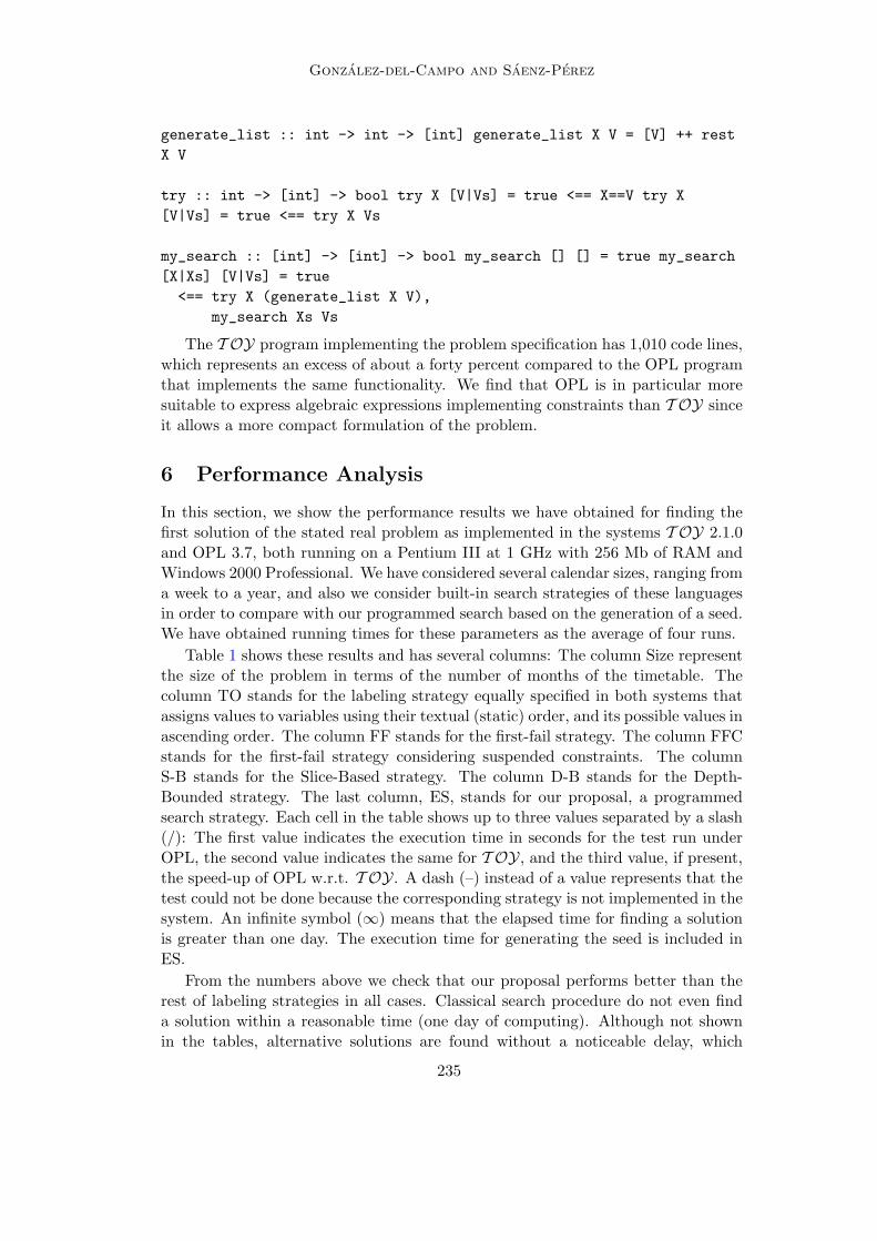
Gonzalez-del-Campo and Saenz-Perez
generate_list :: int -> int -> [int] generate_list X V = [V] ++ restX V
try :: int -> [int] -> bool try X [V|Vs] = true <== X==V try X[V|Vs] = true <== try X Vs
my_search :: [int] -> [int] -> bool my_search [] [] = true my_search[X|Xs] [V|Vs] = true
<== try X (generate_list X V),my_search Xs Vs
The T OY program implementing the problem specification has 1,010 code lines,which represents an excess of about a forty percent compared to the OPL programthat implements the same functionality. We find that OPL is in particular moresuitable to express algebraic expressions implementing constraints than T OY sinceit allows a more compact formulation of the problem.
6 Performance Analysis
In this section, we show the performance results we have obtained for finding thefirst solution of the stated real problem as implemented in the systems T OY 2.1.0and OPL 3.7, both running on a Pentium III at 1 GHz with 256 Mb of RAM andWindows 2000 Professional. We have considered several calendar sizes, ranging froma week to a year, and also we consider built-in search strategies of these languagesin order to compare with our programmed search based on the generation of a seed.We have obtained running times for these parameters as the average of four runs.
Table 1 shows these results and has several columns: The column Size representthe size of the problem in terms of the number of months of the timetable. Thecolumn TO stands for the labeling strategy equally specified in both systems thatassigns values to variables using their textual (static) order, and its possible values inascending order. The column FF stands for the first-fail strategy. The column FFCstands for the first-fail strategy considering suspended constraints. The columnS-B stands for the Slice-Based strategy. The column D-B stands for the Depth-Bounded strategy. The last column, ES, stands for our proposal, a programmedsearch strategy. Each cell in the table shows up to three values separated by a slash(/): The first value indicates the execution time in seconds for the test run underOPL, the second value indicates the same for T OY, and the third value, if present,the speed-up of OPL w.r.t. T OY. A dash (–) instead of a value represents that thetest could not be done because the corresponding strategy is not implemented in thesystem. An infinite symbol (∞) means that the elapsed time for finding a solutionis greater than one day. The execution time for generating the seed is included inES.
From the numbers above we check that our proposal performs better than therest of labeling strategies in all cases. Classical search procedure do not even finda solution within a reasonable time (one day of computing). Although not shownin the tables, alternative solutions are found without a noticeable delay, which
235

Gonzalez-del-Campo and Saenz-Perez
Size TO FF FFC S-B D-B ES
1/4 0.04/0.54/12.2 –/0.52 –/0.55 0.04/– 0.04/– 0.05/0.76/15.2
1/2 0.07/1.09/14.7 –/1.11 –/1.06 0.07/– 0.07/– 0.09/1.41/15.6
1 0.87/13.77/15.9 –/18.85 –/3.84 0.91/– 0.90 /– 0.19 /2.78/14.6
2 12.15 / 209.99/17.2 –/309.62 –/27.23 12.68/– 12.52/– 0.31/5.86/18.9
3 ∞ / ∞ –/∞ –/∞ ∞ /– ∞ /– 0.41/10.00/24.4
4 ∞ / ∞ –/∞ –/∞ ∞ /– ∞ /– 0.53 /14.89/28.1
5 ∞ / ∞ –/∞ –/∞ ∞ /– ∞ /– 0.65 /20.84/32.1
6 ∞ / ∞ –/∞ –/∞ ∞/– ∞ /– 0.77 /27.43/35.6
8 ∞ / ∞ –/∞ –/∞ ∞ /– ∞ /– 0.98 /43.52/44.4
10 ∞ / ∞ –/∞ –/∞ ∞ /– ∞ /– 1.25 /63.56/50.9
12 ∞ / ∞ –/∞ –/∞ ∞ /– ∞ /– 1.69 /86.58/51.2
Table 1Programmed Search vs. Classical Constraint Solving for OPL and T OY
indicates the locality of solutions. However, for small problem sizes (less than onemonth), classical strategies are slightly better than explicit search.
If, on the other hand, we compare the execution times for OPL and T OY, wefind that programmed search in OPL behaves better than in T OY because OPL hasseveral features which are not present is T OY and makes it more appropriate forperformance. For instance, OPL has conditional and disjunction constraint opera-tors, static decision and data variables with direct memory access, and arrays. Toovercome the drawbacks derived from the absence of such features, the T OY pro-gram has to rely on building structures (lists of lists, in particular) with sequentialaccess by means of recursive functions.
In order to identify in more detail the factors intervening in the total goal solvingtime for both systems, we have accounted for the ones shown in Table 2. Thecolumn ”Size” stands for the size of the problem, as before. Next column, ”DataStructure”, stands for the time involved in computing the data structures. Thecolumn labeled with ”Seed” stands for the time employed in building the seed.The columns ”Posting and Propagation” and ”Labeling” show the time for theseprocesses, whereas the last column shows the total time. The cells in the tablefollow the same data format as Table 1. Note that there are times shown as 0.00,which means that the time measure is less than 0.01 seconds.
Size Data Structure Seed Posting and Labeling Total
Propagation
1/4 0.00/0.13/– 0.00/0.16/– 0.05/0.47/9.44 0.00/0.00/– 0.05/0.76/15.2
1/2 0.00/0.22/– 0.00/0.23/– 0.09/0.89/9.89 0.00/0.07/– 0.09/1.41/15.6
1 0.00/0.30/– 0.01/0.48/48.4 0.18/1.87/10.4 0.00/0.13/– 0.19 /2.78/14.6
2 0.00/0.46/– 0.02/1.11/55.5 0.29/3.93/13.6 0.00/0.36/– 0.31/5.86/18.9
3 0.00/0.63/– 0.05/2.07/41.3 0.37/6.85/19.0 0.00 /0.46/– 0.41/10.00/24.4
4 0.00/0.77/– 0.06/3.23/53.8 0.46/10.20/22.7 0.02/0.69/34.5 0.53 /14.89/28.1
5 0.00/0.86/– 0.08/4.89/61.1 0.53/14.40/27.2 0.04/0.70/19.3 0.65 /20.84/32.1
6 0.00/1.06/– 0.11/6.57/59.7 0.62/18.77/30.3 0.04/1.05/26.3 0.77 /27.43/35.6
8 0.00/1.37/– 0.16/10.98/68.6 0.81/29.81/39.7 0.07/1.36/19.4 0.98 /43.52/44.4
10 0.00/1.66/– 0.22/16.38/74.4 1.11/43.03/46.8 0.11/2.50/22.7 1.25 /63.56/50.9
12 0.00/1.93/– 0.28/22.98/82.1 1.27/58.98/46.4 0.14/2.70/19.3 1.69 /86.58/51.2
Table 2Factors involved in Goal Solving for OPL and T OY
236

Gonzalez-del-Campo and Saenz-Perez
Building structures in OPL is negligible, whereas T OY takes as much as almost2 seconds. In this last system, seed generation quickly grows with problem size,more than the former, which means that the specific-purpose algorithms in OPL tobuild structures behave better than the general-purpose computation performed inT OY. Posting and propagating constraints also grow, but the gain of OPL w.r.t.T OY is less than before. The gain of the labeling is, in the average, about 23.5,with small deviations. The last column shows the same data as Table 1 and is keptfor reference.
Next, Table 3 shows the impact of propagation alone over the total computationtime for both systems. This table highlights the power of the underlying constraintsolver. In particular, the second column shows a maintained gain of about 10.3 inthe average, showing that the growing gain of OPL w.r.t. T OY noticed in formertables is not due to propagation, but for the nature of the declarative languageinvolving less efficient data structures and the lazy narrowing mechanism inherentto the system. This table also contains the number of constraints (which is thesame for the former tables) and this number is about 22 in the average.
Finally, in Table 4 we compare the two implementations of the function durationin T OY, measuring the timings for several factors: posting and propagation, prop-agation, and propagation for the function vs. total propagation. In this table, theformat of timing cells changes as follows. There are three values separated by aslash (/): The first value indicates the execution time in seconds for the first imple-mentation of duration with arithmetical operators, the second value indicates thesame for its implementation with propositional constraint operators, and the thirdvalue, the speed-up of the first implementation w.r.t. the second one.
We note that the first implementation behaves better than the second in about 19percent of total time. Also, posting and propagating constraints is about 28 percentbetter. Propagation time grows up to almost 5 percent. The ratio of propagationtime of the constraints due to duration w.r.t. total propagation time is constant.In the first case it is 0.38, whereas in the second case is 0.67. There is about a 10percent more constraints in the second case. The ratio of the number of constraintsdue to duration w.r.t. total number of constraints is constant. In the first caseis 0.93, whereas in the second case is 0.94. Although the second implementationbehaves worse than the first one, the additional costs may be accepted in favour of
Size Propagation Rest of Program Number of Constraints Propagation/Total
1/4 0.03/0.25/8.33 0.02/0.51/25.5 585/10,638/18.18 0.60/0.34
1/2 0.06/0.56/9.33 0.03/0.85/28.33 1,047/22,741/21.72 0.67/0.41
1 0.14/1.02/7.29 0.05/1.77/35.40 2,163/46,948/21.71 0.73/0.38
2 0.22/1.95/8.86 0.09/3.91/43.44 4,011/89,278/22.26 0.71/0.37
3 0.25/2.80/11.2 0.16/7.20/45.00 6,057/136,138/22.48 0.61/0.33
4 0.31/3.81/12.29 0.22/11.09/50.41 8,037/181,428/22.57 0.58/0.30
5 0.37/4.90/13.24 0.28/ 15.95/56.96 10,083/228,360/22.65 0.57/0.28
6 0.46/5.16/11.21 0.31/22.27/71.84 12,063/273,686/22.69 0.60/0.25
8 0.57/6.35/11.14 0.41/37.17/90.65 16,155/367,424/22.74 0.58/0.22
10 0.74/8.41/11.36 0.51/55.15/108.14 20,181/459,646/22.78 0.59/0.21
12 1.05/9.12/8.69 0.64/77.47/121.05 24,207/551,850/22.80 0.62/0.19
Table 3Propagation vs. Goal Solving for OPL and T OY
237

Gonzalez-del-Campo and Saenz-Perez
Propagation
Posting for duration Number
Size Total and Propagation / of
Propagation Total Constraints
Propagation
1/4 0.76/0.88/1.16 0.47/0.59/1.25 0.25/0.52/2.08 0.51/0.78 10,638/11,824/1.11
1/2 1.41/1.68/1.19 0.89/1.16/1.30 0.56/1.08/1.95 0.48/0.73 22,741/25,488/1.12
1 2.78/3.44/1.24 1.87/2.53/1.35 1.02/2.21/2.17 0.31/0.75 46,948/51,656/1.10
2 5.86/7.15/1.22 3.93/5.23/1.32 1.95/4.42/2.26 0.31/0.74 89,278/98,322/1.10
3 9.99/11.96/1.20 6.85/8.81/1.28 2.80/6.92/2.47 0.35/0.69 136,138/150,046/1.10
4 14.89/17.52/1.18 10.20/12.83/1.26 3.81/9.76/2.56 0.32/0.67 181,428/200,064/1.10
5 20.84/24.24/1.16 14.40/17.80/1.24 4.89/13.08/2.67 0.34/0.62 228,360/251,560/1.10
6 27.43/31.67/1.15 18.77/23.01/1.23 5.16/16.09/3.12 0.36/0.63 273,686/301,878/1.10
8 43.52/54.53/1.25 29.81/40.82/1.37 6.35/28.51/4.49 0.37/0.65 367,424/407,841/1.11
10 63.56/76.01/1.20 43.03/54.47/1.27 8.41/37.40/4.45 0.42/0.59 459,646/505,611/1.10
12 86.58/100.77/1.16 58.98/73.17/1.24 9.12/43.90/4.82 0.45/0.54 551,850/612,554/1.11
Table 4Comparing both Implementations of the Function duration in T OY
a more readable implementation.
7 Conclusions and Future Work
Traditionally, labeling strategies are based on static and dynamic information aboutvariables and their domains, and selecting variables and values to assign. However,this information is not sufficient for many hard problems to be tractable. Labelingproduces many fails during searching for solutions and the response time growsexponentially with problem size. With a programmed search based on the knowledgeabout the program structure, a seed close to a solution can be found in a reasonabletime, which means than the enumeration strategy produces few fails. The keyquestion is whether one can find close solutions in the problem, which stronglydepends on the solution structure, a point that should be eventually addressed.
In this work, two of the best state-of-the-art constraint programming systems(in their corresponding settings) have been taken into account for implementing thespecification of a real problem. From the performance results we have found thatthe average time for finding the first solution is low compared to classical techniquesin the field of constraint solving, even if the seed is not a solution. It is therefore notnecessary to specify a first solution to depart from in our searching proposal. Theexecution time becomes moderate with few different values in variable domains.OPL gives responses faster than T OY because T OY version 2.1.0 did not enjoykey features present in OPL as arrays indexed by decision variables. Implicationand disjunction constraints were also not included, and we have implemented them,showing that their use augments program readability and introducing a reasonableburden.
Although OPL behaves clearly better than T OY, this system enjoys a morehomogeneous syntax for solving problems in the sense that the same program con-structs are used to generate the seed, post constraints, and specify the search strat-egy. That is, there is no the impedance mismatch that can be found in OPL when
238

Gonzalez-del-Campo and Saenz-Perez
used from a host language. OPL, in turn, has three sections in a program with iso-lated syntaxes: initialisation of data, decision variable and constraint declarations,and search procedures section (among others such as database handling). We havefound that the implementation of the problem is easier in a language as T OY sinceit seamlessly embodies constraints into a very expressive general purpose languagebecause of its declarative nature. In addition, the propagation solver for the T OYunderlying system behaves reasonable fine w.r.t. the solver of OPL. Finally, whileOPL is a commercial system, T OY is for free.
Some lines we emphasise as being amenable to explore as future work are: First,the inclusion of the array data structure with direct access on its elements, along thepossibility to index such an array by means of decision variables. Second, a memoryusage analysis (including garbage collection) in the context of a complex operatingsystem. Finally, an algebraic component should be added to the language in orderto be able to compactly declare constraints and decision variables. The algebraicnotation would allow more compact programs, whereas (static) decision variabledeclarations would do for faster memory allocations.
References
[1] Azevedo, F. and P. Barahona, Timetabling in Constraint Logic Programming, in: Proceedings of 2ndWorld Congress on Expert Systems, Estoril, Portugal, 1994.
[2] Brauner, N., R. Echahed, G. Finke, H. Gregor and F. Prost, Specializing narrowing for timetablegeneration: A case study., in: PADL, 2005, pp. 22–36.
[3] Brooke, A., D. Kendrick and A. Meeraus, GAMS: A User’s Guide (1992).
[4] Burke, E. and J. Landa Silva, The design of memetic algorithms for scheduling and timetablingproblems, in: S. J. Krasnogor N., Hart W., editor, Recent Advances in Memetic Algorithms, 2004,pp. 289–312.
[5] Burke, E. and S. Petrovic, Recent Research Directions in Automated Timetabling, European Journalof Operational Research 140 (2002), pp. 266–280.
[6] Burke, E. K., K. Jackson, J. H. Kingston and R. F. Weare, Automated University Timetabling: TheState of the Art, Comput. J. 40 (1997), pp. 565–571.
[7] Burke, E. K., J. P. Newall and R. F. Weare, A Memetic Algorithm for University Exam Timetabling, in:Practice and Theory of Automated Timetabling. Volume 1153 of Lecture Notes in Computer Science,Lecture Notes in Computer Science 1153 (1995), pp. 241–250.
[8] Castro, C., M. Moossen and M. Riff, A Cooperative Framework Based on Local Search and ConstraintProgramming for Solving Discrete Global Optimisation, in: Advances in Artificial Intelligence SBIA2004 (2004), pp. 93–102.
[9] Corne, D., P. Ross and H.-L. Fang, Evolutionary Timetabling: Practice, Prospects and work in Progress,in: Proceedings of the UK Planning and Scheduling SIG Workshop Strathclyde, 1994.
[10] Corne, D., P. Ross and H.-L. Fang, Fast Practical Evolutionary Timetabling, in: Lecture Notes inComputer Science, vol 865 (Evolutionary Computing AISB Workshop, Leeds, UK, April 1994) (1994),pp. 251–263.
[11] Dıaz, A., “Optimizacion Heurıstica y Redes Neuronales,” Editorial Paraninfo, 1996.
[12] Fernandez, A. J., T. Hortala-Gonzalez, F. Saenz-Perez and R. del Vado, Constraint functional logicprogramming over finite domains, Theory and Practice of Logic Programming (2006), in Press.
[13] Garfinkel, R. and G. Nemhauser, “Integer Programming,” John Wiley & Sons, New York, 1972.
[14] Gay, D. M., Symbolic-Algebraic Computations in a Modeling Language for Mathematical Programming.
[15] Goldberg, D. E., “Genetic Algorithms in Search, Optimization and Machine Learning,” Addison-WesleyLongman Publishing Co., Inc., Boston, MA, USA, 1989.
239

Gonzalez-del-Campo and Saenz-Perez
[16] Hanus, M., Curry: a Truly Integrated Functional Logic Language (1999), http://www.informatik.uni-kiel.de/∼curry/.
[17] Hentenryck, P. V., L. Michel, L. Perron and J.-C. Regin, Constraint Programming in OPL, in:G. Nadathur, editor, Proceedings of the International Conference on Principles and Practice ofDeclarative Programming (PPDP’99), Lecture Notes in Computer Science 1702, 1999, pp. 98–116.
[18] Hentenryck, P. V. and V. Saraswat, Strategic Directions in Constraint Programming, ACM Comput.Surv. 28 (1996), pp. 701–726.
[19] Jaffar, J. and J. Lassez, Constraint Logic Programming, in: 14th ACM Symposium on Principles ofProgramming Languages (POPL’87) (1987), pp. 111–119.
[20] Khemmoudj, M., M. Porcheron and H. Bennceur, Using Constraint Programming and Local Search forScheduling of Electricite de France Nuclear Power Plant Outages (1998).
[21] Lajos, G., Complete University Modular Timetabling using Constraint Logic Programming, in: Selectedpapers from the First International Conference on Practice and Theory of Automated Timetabling(1996), pp. 146–161.
[22] Lopez-Fraguas, F. J., A General Scheme for Constraint Functional Logic Programming, in: Proceedingsof the Third International Conference on Algebraic and Logic Programming (1992), pp. 213–227.
[23] Marte, M., “Models and Algorithms for School Timetabling - A Constraint-Programming Approach,”Dissertation/Ph.D. thesis, Institute of Computer Science, LMU, Munich (2003).
[24] Merlot, L. T. G., N. Boland, B. D. Hughes and P. J. Stuckey, A Hybrid Algorithm for the ExaminationTimetabling Problem, in: Proceedings of the 4th International Conference on the Practice and Theoryof Automated Timetabling. Volume 2740 of Lecture Notes in Computer Science, Lecture Notes inComputer Science 2740 (2002), pp. 207–231.
[25] Michalewicz, Z., “Genetic Algorithms + Data Structures = Evolution Programs (3rd ed.),” Springer-Verlag, London, UK, 1996.
[26] Ross, P., D. Corne and H.-L. Fang, Improving Evolutionary Timetabling with Delta Evaluation andDirected Mutation, in: Y. Davidor, H.-P. Schwefel and R. Manner, editors, Parallel Problem Solvingfrom Nature – PPSN III (1994), pp. 556–565.
[27] Ross, P., D. Corne and H.-L. Fang, Successful Lecture Timetabling with Evolutionary Algorithms, in:A. E. Eiben, B. Manderick and Z. Ruttkay, editors, Applied Genetic and other Evolutionary Algorithms:Proceedings of the ECAI’94 Workshop, Springer, Berlin, 1995 .
[28] Ross, P., E. Hart and D. Corne, Some Observations about GA-Based Exam Timetabling, in: PATAT’97: Selected papers from the Second International Conference on Practice and Theory of AutomatedTimetabling II (1998), pp. 115–129.
[29] Rossi-Doria O., P. B., A memetic algorithm for university course timetabling, in: CombinatorialOptimisation 2004 Book of Abstracts, Lancaster, UK, Lancaster University, 2004.
[30] Van Hentenryck, P., “The OPL Optimization Programming Language,” The MIT Press, Cambridge,MA, 1999.
[31] Walsh, T., Depth-bounded Discrepancy Search, in: Proceedings of the International Joint Conferenceon Artificial Intelligence IJCAI, 1997, pp. 1388–1395.
[32] William D. Harvey, M. L. G., Limited Discrepancy Search, in: C. S. Mellish, editor, Proceedings of theFourteenth International Joint Conference on Artificial Intelligence (IJCAI-95); Vol. 1 (1995), pp.607–615.
[33] Winston, W., “Operations Research: Applications and Algorithms,” International Thomson Publishing,Boston, Massachusetts, 1991.
240

WFLP 2006
A Proposal for Disequality Constraints inCurry
Emilio Jesus Gallego Ariasa,1,2 Julio Marino Carballoa,1,3
Jose Marıa Rey Pozab,4
a Babel Research GroupUniversidad Politecnica de Madrid
Madrid, Spainhttps: // babel. ls. fi. upm. es
b Telefonica I+D
Abstract
We describe the introduction of disequality constraints over algebraic data terms in the functional logiclanguage Curry, and their implementation of them in Sloth, our Curry compiler. This addition extendsthe standard definition of Curry in several ways. On one hand, we provide a disequality counterpart tothe constraint equality operator (=:=). Secondly, boolean equality operators are also redefined to copewith constructive disequality information, which leads to a more symmetric design w.r.t. the existing one.Semantically speaking, our implementation is very similar to previous proposals, although there are somenovel aspects. One of them is that the implementation is partly based on an existing finite domain constraintsolver, which provides a more efficient execution in some examples. There are also some issues regardingthe interaction of our extension with the type and module systems that deserve some discussion. Somebenchmarks, an operational semantics minimally extending the one in the Curry draft, and a moderatelydetailed description of the implementation complete the paper.
Keywords: Curry, Sloth, Disequality, Constraints, Implementation.
1 Introduction
This paper describes an extension that allows programming with disequality con-straints over data terms in Sloth. Proposals of this kind [5,1] can be dated backto the pre-Curry ages (one of them is for the Babel language) and are alreadyincluded in other FLP languages (T OY). However, although the possibility ofextending Curry with disequality constraints is explicitly mentioned in the Currydraft, they have not been included so far, perhaps because equality is too close tothe core of the language (unification). Also, equality operators are closely related
1 Authors partly supported by Spanish grants MCYT TIC 2002-0055 and CAM S-0505/TIC/04072 Email: [email protected] Email: [email protected] Email: [email protected]
This paper is electronically published inElectronic Notes in Theoretical Computer Science
URL: www.elsevier.nl/locate/entcs

Gallego, Marino, Rey
to some aspects of Curry that are likely to suffer changes in the near future — typeclasses, standard classes analogous to Eq, etc.
For these reasons, having experimental versions of this kind of features is a goodstarting point, possibly at the cost of inconsistencies with other features alreadypresent in the draft. Although not completely polished, the proposal described inthis paper is already available in our Sloth system (https://babel.ls.fi.upm.es/research/Sloth) 5 including the examples presented below.
Sloth [6,2] is a compiler that translates Curry [3] programs into Prolog, con-tinuing our group’s previous experience that started with the translation of Babelprograms into Prolog. Currently, Sloth generates Ciao Prolog[4] code and the sys-tem implements most of the 0.8 version of the Curry draft.
The main motivation for developing and maintaining a not-so-efficient implemen-tation of Curry is the need of keeping up to date with a rapidly evolving language,easily introducing changes that would take longer in an abstract machine basedimplementation. Nevertheless, while slower than Prolog, Sloth is perfectly usableas a first contact with Curry.
These changes can be additions to the Curry standard or, perhaps, experimentalfeatures that need some testing preceding the mandatory discussion needed in orderto include them in later versions of the standard.
Integration with the Ciao platform has a number of advantages consideringits advanced features like: the realistic set of libraries – including, among other,constraint programming, concurrency, foreign language interface; the static analysisframework; meta-programming constructs, etc.
Improving the support of constraint programming in Curry is one of the maingoals of Sloth, as many of the outstanding features of Ciao are constraint librariesthemselves or libraries which provide support for programming new constraint ex-tensions — although often in a nondeclarative manner. In fact, experimental sup-port for constraint programming over rationals and finite domains is already avail-able in the latest stable version of Sloth.
An example
The following example, taken from [5] – although adapted to our language – shouldserve to motivate the behavior expected from our extension:
Example 1.1 The size of a list is defined as the number of distinct elements itcontains. 6
module Size where
member x [] = False member x (h:ts) = x == h || member x ts
data Nat = Zero | Succ Nat
size :: [a] → Int size [] = 0 size (h:ts) = if member h tsthen size tselse 1+( size ts)
Consider a goal
5 Use the “Development versions” link when in there.6 The == operator used here is a flexible one with disequality support.
242

Gallego, Marino, Rey
let x, y, z free in size [(x, Zero), (y, z)]
The size of that list can be 1 or 2, depending on the actual values for x, y and z.The answers returned by our system are: 7
1 :: Int {z =:= Zero} Try more (y/n)? y 2 :: Int {x =/= y} Try more(y/n)? y 2 :: Int {z =:= Succ _} Try more (y/n)? y no solutions
Overview of the paper
Next section presents the current state of (equality) constraints in Curry and in-troduces our proposal for a new set of operators, allowing disequality constraints.An operational semantics dealing with the new operators is described in Sec. 3. Itis intended to be as similar as possible to the one present in the Curry Report.Implementation details are not trivial, mainly due to interactions between the con-straint operators and the type system and the choice to offload part of the constraintsolving to a finite domains constraint solver. All of them are described in depth insection 4. Some benchmarks are shown in Sec. 5 and Sec. 6 discusses the results,shortcomings and point directions for future progress.
2 A proposal for equality and disequality operators
The core of the constraint system present in Curry is the =:= operator, which standsfor constrained equality. This operator is overloaded so it can deal with Integerdata types and the likes. Resolving such overloading problems is a different topicitself, so from now onwards we will restrict ourselves to allow only algebraic datatypes in Curry expressions.
The absence of disequality constraints in Curry has influenced the current choiceof equality operators. As the report itself says in page 11:
“However, the evaluation of [x]=:=[0] does not deliver a Boolean value True orFalse, since the latter value would require a binding of x to all values differentfrom 0 (which could be expressed if a richer constraint system than substitutions,e.g., disequality constraints, is used)...”
So far, the solution adopted has been to limit the LP features of equality oper-ators, i.e. we have to chose between losing the disequality information or having itonly for ground instances of queries — which may lead to incompleteness.
The current set of equality operators is shown in table 1. Roughly speaking, theycan be classified in two groups: operators returning Bool and operators returningSuccess. The operators returning Bool use residuation as their operational modelwhile operators returning Success use narrowing.
Flexible operators (i.e. those using narrowing) are very interesting when a searchis needed and to construct non-deterministic functions. On the other hand, residua-tion-based operators (the ones returning Bool) are the right choice when a deter-ministic function or predicate is required.
Further, operators returning Bool can be used to find positive as well as negative
7 the output has been slightly beautified to easy the reading.
243

Gallego, Marino, Rey
op. name type flexible?
== a → a → Bool no
/= a → a → Bool no
=:= a → a → Success yes
Table 1Existing equality operators in Curry.
answers (i.e. answers making the goal True and False respectively) while operatorsreturning Success find positive answers only, pruning the others (this is becauseSuccess is a one-point domain). The operator to choose depends on what theprogrammer wants to obtain from the program.
However, when dealing when disequalities, negative answers are often requiredas a result out from searches. In this case, one would like to have flexible operatorsreturning Bool. There are none of these in current versions of Curry. The followingexample illustrates the problem:
Example 2.1 We want to search for the elements of a list:elem :: a → [a] → Bool elem _ [] = False elem x (y:ys) = x ==y || elem x ys
> let x free in elem x [1,2,3] =:= True> Suspended
If == had a flexible implementation we would get only one result, because of theabsence of negative answers:> let x free in elem x [1,2,3] =:= True> success {x 7→ 1}> Try more (y/n)? y> no solutions
The intended behavior would be more on the line of:> let x free in elem x [1,2,3] =:= True> success {x 7→ 1}> Try more (y/n)? y> success {x 7→ 2}> Try more (y/n)? y> success {x 7→ 3}> no solutions
In order to overcome this and trying to reach a more orthogonal operator set weare proposing a new set that can be seen in table 2. With our proposal we have:
• Two rigid operators on Bool. These operators already exist in Curry althoughwe have renamed them.
• The flexible version of the two previous operators. Those operators are new.• Finally, the operators returning Success. The disequality operator is new in
Curry and is the key element in this work.
244

Gallego, Marino, Rey
op. name type flexible? notes
== a → a → Bool yes
/= a → a → Bool yes defined as not.(==)
=:= a → a → Success yes no changes
=/= a → a → Success yes the new operator
=== a → a → Bool no old rigid equality
/== a → a → Bool no the negation of previous one
Table 2Our proposal for equality operators in Curry.
Computation step for a single expression:
Eval[[ei]] ⇒ D
Eval[[e1&e2]] ⇒ replace(e1&e2, i, D)i ∈ {1, 2}
Eval[[ei]] ⇒ D
Eval[[c(e1, . . . , en)]] ⇒ replace(c(e1, . . . , en), i, D)i ∈ {1, . . . , n}
Eval[[f(e1, . . . , en)]]T ⇒ D
Eval[[f(e1, . . . , en)]] ⇒ Dif T is a definitional tree for f with fresh variables
Computation step for an operation-rooted expression e:
Eval[[e]]rule(l=r) ⇒ {ε; id []σ(r)}if σ is a substitution with σ(l) = e
Eval[[e]]T1 ⇒ D1 Eval[[e]]T2 ⇒ D2
Eval[[e]]or(T1, T2) ⇒ D1 ∪D2
Eval[[e]]branch(π, p, r, T1, . . . , Tk) ⇒8>><>>:D if e|p = c(e1, . . . , en), pat(Ti)|p = c(x1, . . . , xn) and Eval[[e]]Ti ⇒ D∅ if e|p = c(. . . ) and pat(Ti) 6= c(. . . ), i = 1, . . . , kSk
i=1{ε; σi[]σi(e)} if e|p = x, r = flex , and σi = {x 7→ pat(Ti)|p}replace(e, p, D) if e|p = f(e1, . . . , en) and Eval[[e|p]] ⇒ D
Derivation step for a disjunctive expression:
Eval[[e]] ⇒ {γ1; σ1[]e1, . . . , γn; σn[]en}{γ; σ[]e} ∪D ⇒ clean({γ1 ∧ σ1(γ); σ1 ◦ σ[]e1, . . . , γn ∧ σn(γ); σn ◦ σ[] en}) ∪D
Fig. 1: Operational semantics of Curry
3 Operational semantics
In this section we present an operational semantics that allows computing withdisequality constraints. The presentation tries to be a minimal extension to thatpresent in the Curry draft. This way, changes can be easily located. Essentially,there are two changes. First, the mechanism for accumulating answers is enhancedto include constraints in solved form in addition to answer substitutions. This ex-tension is generic, i.e. largely independent of the constraint system in use. Secondly,specific rules for simplifying disequality constraints are included.
The main execution cycle is described by the rules in Fig. 1, that introduces thederivability relation D1 ⇒ D2 on pairs of disjunctive expressions.
245

Gallego, Marino, Rey
Eval[[ei]] ⇒ D
Eval[[e1=:=e2]] ⇒ replace(e1=:=e2, i, D)if ei = f(t1, . . . , tn), i ∈ {1, 2}
Eval[[c(e1, . . . , en)=:=c(e′1, . . . , e′
n)]] ⇒ {ε; id []e1=:=e′1& . . . &en=:=e′
n}
Eval[[c(e1, . . . , en)=:=d(e′1, . . . , e′
m)]] ⇒ ∅if c 6= d or n 6= m
Eval[[x=:=e]] ⇒ D
Eval[[e=:=x]] ⇒ Dif e is not a variable
Eval[[x=:=y]] ⇒ {ε; {x 7→ y}[]success}
Eval[[x=:=c(e1, . . . , en)]] ⇒ {ε; σ[]y1=:=σ(e1)& . . . &yn=:=σ(en)}
if x /∈ cv(e1, . . . , en),
σ = {x 7→ c(y1, . . . , yn)},y1, . . . , yn fresh variables
Eval[[x=:=c(e1, . . . , en)]] ⇒ ∅if x ∈ cv(c(e1, . . . , en))
Fig. 2: Solving equational constraints
Disjunctive expressions represent (fragments of) the fringe of a search tree. For-mally, they are multisets of answer expressions of the form γ;σ[]e, where γ is aconstraint, 8 σ a substitution and e a Curry expression. An answer expressionγ;σ[]e is solved when e is a data term and γ is solved and consistent. We will use ε
to denote a trivial constraint.The computation of an expression e suspends if there is no D such that Eval[[e]] ⇒
D. A constraint expression is solvable if it can be reduced to success. As can beseen in Fig. 1, reduction of terms rooted by user-defined function symbols is guidedby an overloaded version of Eval[[]] that takes a Curry expression and a definitionaltree as arguments. For details on these, and other aspects of the semantics which arelargely orthogonal to the questions discussed here – conditional rules, higher-orderfeatures, freezing, etc – the reader is referred to [3].
The disjunctive behavior of disjunctive expressions is partly captured by thelast rule in Fig. 1, which expresses how answers are accumulated. Observe thatthe combination of answers – both substitutions and new constraints – with theaccumulated constraint might introduce inconsistency or perhaps constraints notin solved form. This is why a call to the auxiliary function clean is needed. Itsdefinition depends on the actual constraint system and will be presented later forthe disequality case.
The other half of this disjunctive behavior is captured by the auxiliary functionreplace, that inserts a disjunctive expression into a position in a term, giving anotherdisjunctive expression as result:
replace(e, p, {γ1;σ1[]e1, . . . , γn;σn[]en}) = {γ1;σ1[]σ1(e)[e1]p, . . . , γn;σn[]σn(e)[en]p}
Figure 2 shows the rules for solving equational constraints. These are practically
8 Here, the word constraint refers to formal constraints i.e. internal representations of constraint formulae,opposed to Curry constraint expressions.
246

Gallego, Marino, Rey
Eval[[ei]] ⇒ D
Eval[[e1=/=e2]] ⇒ replace(e1=/=e2, i, D)if ei = f(t1, . . . , tn), i ∈ {1, 2}
Eval[[c(e1, . . . , en)=/=c(e′1, . . . , e′
n)]] ⇒ {ε; id []e1=/=e′1, . . . , ε; id []en=/=e′
n}
Eval[[c(e1, . . . , en)=/=d(e′1, . . . , e′
m)]] ⇒ successif c 6= d or n 6= m
Eval[[x=/=e]] ⇒ D
Eval[[e=/=x]] ⇒ Dif e is not a variable
Eval[[x=/=y]] ⇒ {x 6= y; id []success}if range(x) is infinite
Eval[[x=/=y]] ⇒ {x 6= y ∧ x ∈ range(x) ∧ y ∈ range(y); id []success}if range(x) is finite
Eval[[x=/=cj(e1, . . . , en)]] ⇒ {ε; σ1[]success, . . . , ε; σj []σj(x)=/=cj(e1, . . . , en), . . . , ε; σk[]success}
if x /∈ cv(e1, . . . , en), σi = {x 7→ ci(yi1, . . . , yi ar(ci))}, yuv fresh variables
Eval[[x=/=c(e1, . . . , en)]] ⇒ successif x ∈ cv(c(e1, . . . , en))
Fig. 3: Solving disequality constraints
identical to those in the Curry draft and are included here mainly to reveal thesymmetries and dualities w.r.t. the rules for solving disequality constraints, shownin Fig. 3. Observe that the auxiliary function cv , such that cv(e) collects thevariables in e not inside a function call is used to implement an occurs check.
Although the theory of disequality constraints is well established, the actualchoice of solved forms may vary with regard to implementation considerations. Fol-lowing [5], we have chosen to avoid explicit disjunctive constraints and instead wecarry those alternatives over the search tree of the Curry semantics, i.e. disjunctiveconstraints are distributed over disjunctive expressions.
This way, solved disequality constraints – those appearing in the left hand ofanswer expressions – amount to conjunctions of disequations between distinct vari-ables, in the case where those variables range over infinite sets of values. When thevariables can only take a finite set of values, solved forms are extended with thecorresponding constraints for domain consistency.
As we have said before, accumulating answers may corrupt the constraint storeeither by making it inconsistent or not solved. The task of tidying everything up –perhaps moving part of the constraint information back to the expression store – isthe responsibility of function clean:
clean(∅) = ∅
clean({γ;σ[]e} ∪D) = clean(D) if γ inconsistent
clean({e1 6= e2 ∧ γ;σ[]e} ∪D) = clean({γ;σ[]e1=/=e2&>e} ∪D) if e1 or e2 nonvars
clean({γ;σ[]e} ∪D) = {γ;σ[]e} ∪ clean(D) otherwise
247

Gallego, Marino, Rey
4 Implementation details
We will consider two cases:
Implementation for infinite types.In types with an infinite number of instances handling disequality is easier as wecan guarantee that a disequality between an instance – likely partial – of such atype and a new free variable is always satisfiable. Support for constraints amongvariables of infinite types is already present in T OY and in the Munster CurryCompiler.
Extending our implementation to correctly handle finite types.In finite types, testing consistency of constraints is harder, as there are disequalitychains where one runs out of possible instances for variables.
The implementation has been done using Ciao Prolog and its attributed variableslibrary. Regarding Sloth, it is a new library which plugs into the current modulesystem supplying the =/= operator.
4.1 Implementation for infinite types
The basic technique used is to attach to each disequality constrained variable anattribute, which contains the set of disallowed instantiations for that variable:
DiseqAttribute = ’$de_store ’(Var , List))
where List containts all the terms that Var should be different from.The system can just assume that each constrained variable must have its cor-
respoding attribute, so the implementation should hook into the compiler in twoways:
• The disequality operator itself.• Unification of constrained variables, both with terms or with other constrained
variables.
which nicely maps to the semantics of attributed variables.
Attaching attributesDisequality constraints are added when the execution path tries to reduce an expres-sion whose head is the =/= operator to HNF. The implementation of this operatoris fully native – we mean fully written in Prolog – using the standard hooks presentin Sloth for external libraries.
The first action to be performed by the operator is to evaluate its arguments toHNF, then select the applicable case: both arguments are variables, only one is avariable or neither are.
In addition, we will use a predicate for adding constraints to the variables’ store:add_to_store(Var , L) :-
( get_attribute(Var , ’$de_store ’(Var , List)) →append(List , L, LNew),update_attribute(Var , ’$de_store ’(Var , LNew))
;attach_attribute(Var , ’$de_store ’(Var , L))
).
248

Gallego, Marino, Rey
Then, given the structure of our store, the case when both arguments are variablesbecomes trivial:diseq_vars(A, B) :-
add_to_store(A, [B]),add_to_store(B, [A]).
as is the one for a variable and an instantiated term:%% Term is in HNF.diseq_one_var(Var , Term) :-
add_to_store(Var , [Term]).
The final case is when both arguments are not variables, so we need to check theirparameters, if they have any:diseq_spine(Term1 , Term2) :-
Term1 =.. [C1|L1],Term2 =.. [C2|L2],( \+ C1 = C2 →
true;
C1 = C2 ,diseq_or(L1, L2)
).diseq_or ([A|AL],[B|BL]) :-
( diseq(A, B);
diseq_or(AL, BL)).
In the code above we profit from our representation of Curry data constructors asProlog terms.
Unification hooksUnification of constrained variables has two different cases:
• The variable is being unified with a term instantiated to at least HNF form.• The variable is being unified with another constrained variable.
Ciao Prolog provides the multifile predicates verify_attribute/2 for the firstitem and combine_attributes/2 for the second.
Unification with a term Unification with a term just checks that the set of accu-mulated disequality constraints in our constraint store holds, and then proceedsto unify the var with the term:verify_attribute(’$de_store ’(Var , List), Term) :-
diseq_and(Term , List),detach_attribute(Var),Var = Term.
The instantiation of Var will also instantiate all copies of the variable present inother constraint stores. This non-trivial detail is possible thanks to Ciao Prologimplementation of attributed variables, which allows us to store the real variablesin the attributes.diseq_and will just verify – by calling the main diseq predicate – that all the
elements in the list are different from the term to unify with.This has a very important effect, as it will create the new needed disequality
constraints in the case Term would be partially instantiated, or our constraintstore contained partially instantiated constraints.
249

Gallego, Marino, Rey
Unification between variables When dealing with disequality between two al-ready constrained variables, our new constraint store will be the union of theirrespective constraint stores, if there doesn’t exist a previous disequality betweenthe unifying variables:combine_attributes(’$de_store ’(V1 , L1), ’$de_store ’(V2 , L2)) :-
\+ contains_ro(V1, L2), % doesn ’t instantiate varsunion(L1 , L2 , NewL),detach_attribute(V1), detach_attribute(V2),V1 = V2 ,attach_attribute(V1 , ’$de_store ’(V1, NewL).
It should be noted that like in the previous case, the union/3 predicate will unifythe non-instantiated terms present in the constraint stores. This is precisely whatwe are looking for, as any constraint attached to such terms will be combined.
The behavior of backtracking is solved as Ciao Prolog fully supports backtrackingattributed variables, so it is not an issue, indeed it greatly helps our implementation,as when unification of a constrained variable needs to be undone, all the operationswill be rolled back, including reattaching the previous attributes.
4.2 Implementation for finite types
As mentioned in the operational semantics, when the terms to be constrained dobelong to a finite data type, the number of available instantiations for a variableis bound. This way, when dealing with the disequality case we must be proactivechecking the constraint store consistency.
The following example> let a,b,c free in a=/=b & b=/=c & c=/=a & a=:= True
would give a wrong answer under the previous implementation, given that it isassumed we have an infinite number of instantiations for variables, but in this caseis not true, as the variables a, b, c can be only be instantiated to two differentvalues, thus making the above constraint unsatisfiable.
At the implementation level, our view is to handle this situation as a FD prob-lem, getting an important leverage from mature FD solvers. So our constraint storeis extended with a FD variable:DiseqAttribute = ’$de_store ’(Var , Fd , List))
being Fd the FD variable associated to Var.For this scheme to work, we assume the existence of the following two predicates
for obtaining type meta-information:type(Term , Type , Range)
which returns the type and the range of any arbitrary translated Curry term, in-cluding variables.index(Term , IndexList)
which returns the index i of Term, i ⊆ range(type(Term)) as a list. How thismetainformation is obtained will be discussed in section 4.5.
250

Gallego, Marino, Rey
The modified constraint solverWe will detail here only the parts of the solver affected by this extension, startingwith the store handling operation:add_to_store(Var , Fd, L) :-
( get_attribute(Var , ’$de_store ’(Var , FdOld , List)) →append(List , L, LNew),Fd = FdOld ,consistent(Fd), % Needed only in some FD solversupdate_attribute(Var , ’$de_store ’(Var , Fd, LNew))
;attach_attribute(Var , ’$de_store ’(Var , Fd, L))
).
For the two variables case, we have to correctly constrain their associated FDvariables:diseq_vars(A, B) :-
( type(A, flat , Range) →get_fd_var(A, FdA), % Will return a fresh var if A has no FD varget_fd_var(B, FdB),FdA in 1..Range ,FdB in 1..Range ,FdA .<>. FdB
;true % A is non -flat
),add_to_store(A, FdA , [B]),add_to_store(B, FdB , [A]).
Constraining a variable to be different from a term is achieved in this case byconstraining its associated FD var:%% Term is in HNF.diseq_one_var(Var , Term) :-
( type(Term , flat , _) →get_fd_var(A, FdA),index(Term , TIndex),constraint_fd_list(FdA , TIndex)
;true
),add_to_store(Var , FdA , Term).
where constraint_fd_list(Fd, List) forces Fd to be different from all the ele-ments in List.
When both arguments are instantiated, we don’t need to change the behaviorof the solver.The unification is sightly modified to care about the new FD variablesin the store:
Unification with a term The new case introduced by the flat terms is taken careof by the remap_term/2 predicate, which checks that the term is in the variabledomain and maps any residual constraint into the possible subterms.verify_attribute(’$de_store ’(Var , Fd , List), Term) :-
( type(Term , flat , Range) →remap_term(Term , Fd)
;diseq_and(Term , List),
),detach_attribute(Var),Var = Term.
Unification between variables The new added case is very simple, we only haveto constraint our FD variables to be equal.combine_attributes(’$de_store ’(V1 , Fd1 , L1), ’$de_store ’(V2, Fd2 ,
251

Gallego, Marino, Rey
L2)) :-( type(Term , flat , Range) →
Fd1 .=. Fd2;
\+ contains_ro(V1, L2), % doesn ’t instantiate varsunion(L1 , L2 , NewL)
),update_attribute(V1 , ’$de_store ’(V1, NewL).
4.3 The FD solver
As the reader can see, the use of the FD solving library is fairly limited, as we onlyuse the disequality (.<>.) predicate. This means that maybe using a full-featuredFD solver is overkill for this application, but our hope is to profit from advancedarc-consistency algorithm found in this kind of constraint libraries so a considerablespeedup can happen.
4.4 A combined approach example
To illustrate some of the gains from this mixed approach, we will showcase anexample using both strategies. Let’s use the query:> let x free in [x] =/= [True] & [x] =/= [False]
Then our execution trace will look like:> (x:[]) =/= (True :[]) & . . . { spine case }> success & (x:[]) =/= (False :[]) { x =/= True }> (x:[]) =/= (False :[]) { x =/= True ∧ x =/= False }> fail { inconsistent FD store }
The execution first uses the normal method for non-flat types – in this case the listtype – but when it finds a flat variable can use that information to always returncorrect answers.
4.5 Type meta-data handling
An obvious problem of this approach is that it needs knowledge about term andvariable types at runtime. The first step is to perform static analysis on the typesso we can determine which types are flat and what others not.
Definition 4.1 [Type Graph] A type graph G for a type T is informally defined asthe directed graph with types as nodes and edges from T1 to T2 when T1 containsT2. Type variables have the special type Pol.
Definition 4.2 [Finite types] A type T is finite when its associated graph G hasno cycles and no leaf node is in Pol. Then we define range of T as Πt∈N |TC(t)|.
Definition 4.3 [Polymorphic types] A type T is polymorphic when its associatedgraph G has a leaf with in Pol and has no cycles. We call the set of all leaves inPol PLevel(T ).
Definition 4.4 [Infinite types] A type T is infinite when its associated graph G
has one or more cycles.
Once this analysis is performed, we attach to each term e a finiteness annotationwhich will be:
252

Gallego, Marino, Rey
• fixed(r) if type(e) is finite, where r = range(type(v)).• poly(P ) if type(e) is polymorphic, where P = PLevel(T ).• infinite if type(e) is infinite.
With this information attached, we can easily determine the information neededfor the predicate type/3, which is emitted at compile time.
The last step is to obtain the information given by the index/2 predicate. Thenaive approach currently used is to instantiate all possible terms and assign to eachone a numerical index. However, it should be noted that more sensible approachesdo exist.
Meta-data implementation in SlothThere are different approaches to try when implementing this kind of runtime typ-ing. In Sloth, we have opted for the simplest one, that is to convert every term ina tuple (t, a), where t was the original term and a is its finiteness annotation.
This approach allows to propagate finiteness annotations in the same momentterms are unified, so it comes handy avoiding function specialization for flat types.
We are undertaking a complete redesign of this area, obviously to lower theoverhead caused for the double unification that we currently use. Given the factthat terms instantiated to some degree already carry their type information 9 , theonly difficult case would be the variables’ one, and using attributed variables tosolve this problem seems sensible.
5 Experimental results
We present some preliminary experimental results just as a sample of what oursystem can do. We also have written more tests for the disequality implementation,which can be found in the compiler distribution.
The chosen problem is the coloring of a square map, where each cell has 4neighbors and a cell cannot have the same color as any of them. The correspondingCurry program can be seen in figure 4. The disequality operator to use has beenabstracted as an argument, so we can use the same code for all the tests.
The first test has been performed using the old == operator and narrowing,which implies that we have to instantiate the map first, the second one allowingresiduation whereas the third one uses the new disequality constraint operator.
Our motivation for benchmarking is not proving big performance enhancements,but to check that there is no major slowdown going on with the new disequalitysystem. This seems to be true and indeed the disequality library used here lacksfine tuning and we are also planning to use a much more improved FD solver.
Anyways, comparing a system with disequality to a equality-only one is not easy,as the main advantage that disequality supports brings us is a far more expressivelanguage. The results for a random map which has a proportion of 90% free variablesamong its elements are shown in table 3. As a matter of reference, we present the
9 This is a property of our name handling in the compiler
253

Gallego, Marino, Rey
data Color = Red | Green | Yellow | Blue
diff x y = (x==y) =:= False diff_c x y = x =/= y
color Red = success color Yellow = success color Green = successcolor Blue = success
foldr_c l = foldr (&) success l
coloring :: (Color → Color → Success) → [[ Color ]] → Successcoloring _ [] = success coloring f (l:ls) = c_lists f l ls &map_c_list f (l:ls)
c_lists :: (Color → Color → Success) → [Color] → [[ Color ]] →Success c_lists _ _ [] = success c_lists f l (x:xs) = foldr_c(map (uncurry f) (zip x l)) & c_lists f x xs
map_c_list :: (Color → Color → Success) → [[ Color ]] → Successmap_c_list f l = foldr_c (map (c_list f) l)
c_list :: (Color → Color → Success) → [Color] → Success c_list f[x] = success c_list f (x1:x2:xxs) = f x1 x2 & c_list f(x2:xxs)
p_naive map = constraint map & coloring diff map p_reseq map =coloring diff map & constraint map p_diseq map = coloring diff_c map& constraint map
constraint l = foldr_c (map (\ll → foldr_c (map color ll)) l)
Fig. 4: The map coloring problem.
System Problem timenormal timeres timediseq
Sloth Coloring > 100 sec. 20 ms. 24 ms.
T OY Coloring > 100 sec. n.a. 20 ms.
Table 3Benchmark results for the coloring problem with a 5x5 map
results for the same algorithm using T OY 10 , although direct comparison of twosystems is meaningless, as they use different Prolog compilers, etc. . .
6 Conclusions and future work
We have extended Curry’s operational semantics to allow disequality constraintsin a similar spirit to the one presented in[5]. A first implementation in the Slothsystem has been described and is already available from our download site. So far,we believe that implementation results are promising, and we hope that practicewith our prototype can help in improving the support for constraints in the Currystandard.
There are some specific aspects of our implementation that probably need somepolishing, namely the interaction with the underlying finite domain solver and thestatic analyses needed to detect finite types and for tagging all variables with theirtypes.
Another issue to consider in the near future, among others, is the interactionwith the type classes extension. It would be desirable to restrict the types for whichequality/disequality operators can be applied, analogously to the Eq standard type
10The code used for T OY can be found in the compiler tarball.
254

Gallego, Marino, Rey
class in Haskell. At the time of writing this version (July 2006) type classes supportfor Curry lives in a different development branch, although a merge will happenshortly.
References
[1] Puri Arenas-Sanchez, Ana Gil-Luezas, and Francisco Javier Lopez-Fraguas. Combining lazy narrowingwith disequality constraints. In PLILP, pages 385–399, 1994.
[2] Emilio Jesus Gallego Arias and Julio Marino. An overview of the Sloth2005 Curry System: SystemDescription. In WCFLP ’05: Proceedings of the 2005 ACM SIGPLAN workshop on Curry and functionallogic programming, pages 66–69, New York, NY, USA, 2005. ACM Press.
[3] Michael Hanus, Sergio Antoy, Herbert Kuchen, Francisco J. Lopez-Fraguas, Wolfgang Lux, Juan JoseMoreno-Navarro, and Frank Steiner. Curry: An Integrated Functional Logic Language, 0.8.2 edition,April 2006. Editor: Michael Hanus.
[4] M. Hermenegildo, F. Bueno, M. Garcıa de la Banda, and G. Puebla. The CIAO multi-dialect compilerand system: An experimentation workbench for future (C)LP systems. In Proceedings of the ILPS’95Workshop on Visions for the Future of Logic Programming, Portland, Oregon, USA, december 1995.Available from http://www.clip.dia.fi.upm.es/.
[5] Herbert Kuchen, Francisco Javier Lopez-Fraguas, Juan Jose Moreno-Navarro, and Mario Rodrıguez-Artalejo. Implementing a lazy functional logic language with disequality constraints. In JICSLP, pages207–221, 1992.
[6] Julio Marino and Jose Marıa Rey. The implementation of Curry via its translation into Prolog. InKuchen, editor, 7th Workshop on Functional and Logic Programming (WFLP98), number 63 in WorkingPapers. Westfalische Wilhelms-Universitat Munster, 1998.
255