Multivariate analysis of the impacts of the turbine fuel JP-4 in a microcosm toxicity test with...

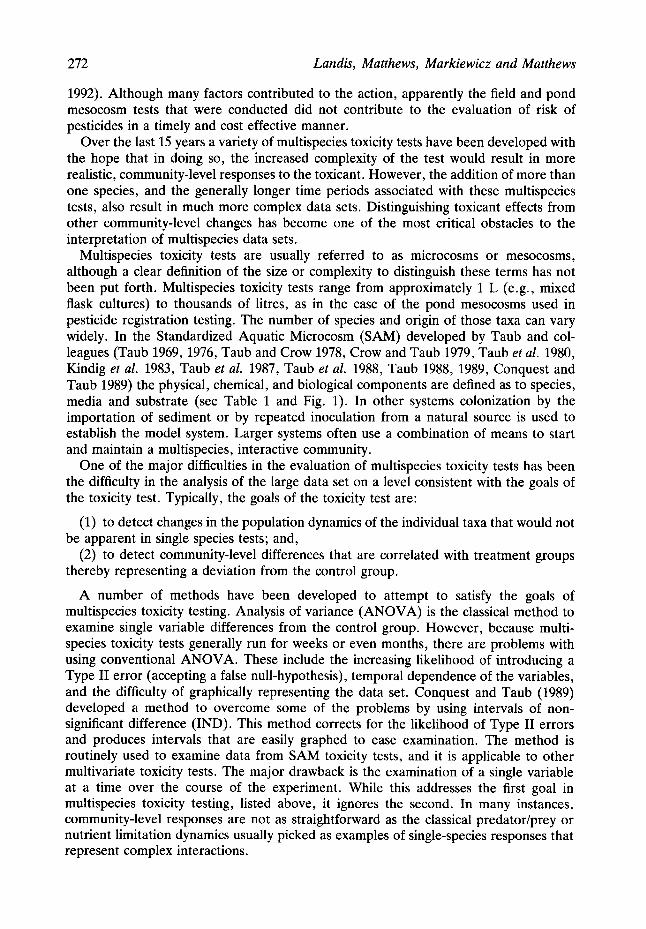
Ecotoxicology 2, 271-300 (1993)

Multivariate analysis of the impacts of the turbine fuel JP-4 in a microcosm toxicity test with implications for the evaluation of ecosystem dynamics and risk assessment W A Y N E G. L A N D I S 1. , R O B I N A. M A T T H E W S 1, A P R I L J. M A R K I E W I C Z 1 and G E O F F R E Y B. M A T T H E W S 2

1Institute of Environmental Toxicology and Chemistry, Huxley College of Environmental Studies, Western Washington University, Bellingham, WA 98225 USA 2Computer Science Department, Western Washington University, Bellingham, WA 98225 USA

Received 7 April 1993; revised and accepted 22 July 1993

Turbine fuels are often the only aviation fuel available in most of the world. Turbine fuels consist of numerous constituents with varying water solubilities, volatilities and toxicities. This study investigates the toxicity of the water soluble fraction (WSF) of JP-4 using the Standard Aquatic Microcosm (SAM). Multivariate analysis of the complex data, including the relatively new method of nonmetric clustering, was used and compared to more traditional analyses. Particular emphasis is placed on ecosystem dynamics in multivariate space.

The WSF is prepared by vigorously mixing the fuel and the SAM microcosm media in a separatory funnel. The water phase, which contains the water-soluble fraction of JP-4 is then collected. The SAM experiment was conducted using concentrations of 0.0, 1.5 and 15% WSF. The WSF is added on day 7 of the experiments by removing 450 ml from each microcosm including the controls, then adding the appropriate amount of toxicant solution and finally bringing the final volume to 3 L with microcosm media. Analysis of the WSF was performed by purge and trap gas chromatography. The organic constituents of the WSF were not recoverable from the water column within several days of the addition of the toxicant. However, the impact of the WSF on the microcosm was apparent. In the highest initial concentration treatment group an algal bloom ensued, generated by the apparent toxicity of the WSF of JP-4 to the daphnids. As the daphnid populations recovered the algal populations decreased to control values. Multivariate methods clearly demonstrated this initial impact along with an additional oscillation seperating the four treatment groups in the latter segment of the experiment. Apparent recovery may be an artifact of the projections used to describe the multivariate data. The variables that were most important in distinguishing the four groups shifted during the course of the 63 day experiment. Even this simple microcosm exhibited a variety of dynamics, with implications for biomonitoring schemes and ecological risk assessments.

Keywords: jet fuel; microcosm; multivariate statistics; nonmetric clustering; risk assessment.

Introduction

As this is written, the United States Environmental Protection Agency has suspended the requi rement for conducting ecosystem level studies for pesticide registration (Fisher

*To whom correspondence should be addressed.

0963-9292 (~ 1993 Chapman & Hall

272 Landis, Matthews, Markiewicz and Matthews

1992). Although many factors contributed to the action, apparently the field and pond mesocosm tests that were conducted did not contribute to the evaluation of risk of pesticides in a timely and cost effective manner.

Over the last 15 years a variety of multispecies toxicity tests have been developed with the hope that in doing so, the increased complexity of the test would result in more realistic, community-level responses to the toxicant. However, the addition of more than one species, and the generally longer time periods associated with these multispecies tests, also result in much more complex data sets. Distinguishing toxicant effects from other community-level changes has become one of the most critical obstacles to the interpretation of multispecies data sets.

Multispecies toxicity tests are usually referred to as microcosms or mesocosms, although a clear definition of the size or complexity to distinguish these terms has not been put forth. Multispecies toxicity tests range from approximately 1 L (e.g., mixed flask cultures) to thousands of litres, as in the case of the pond mesocosms used in pesticide registration testing. The number of species and origin of those taxa can vary widely. In the Standardized Aquatic Microcosm (SAM) developed by Taub and col- leagues (Taub 1969, 1976, Taub and Crow 1978, Crow and Taub 1979, Taub et al. 1980, Kindig et al. 1983, Taub et al. 1987, Taub et al. 1988, Taub 1988, 1989, Conquest and Taub 1989) the physical, chemical, and biological components are defined as to species, media and substrate (see Table 1 and Fig. 1). In other systems colonization by the importation of sediment or by repeated inoculation from a natural source is used to establish the model system. Larger systems often use a combination of means to start and maintain a multispecies, interactive community.

One of the major difficulties in the evaluation of multispecies toxicity tests has been the difficulty in the analysis of the large data set on a level consistent with the goals of the toxicity test. Typically, the goals of the toxicity test are:

(1) to detect changes in the population dynamics of the individual taxa that would not be apparent in single species tests; and,

(2) to detect community-level differences that are correlated with treatment groups thereby representing a deviation from the control group.

A number of methods have been developed to attempt to satisfy the goals of multispecies toxicity testing. Analysis of variance (ANOVA) is the classical method to examine single variable differences from the control group. However, because multispecies toxicity tests generally run for weeks or even months, there are problems with using conventional ANOVA. These include the increasing likelihood of introducing a Type II error (accepting a false null-hypothesis), temporal dependence of the variables, and the difficulty of graphically representing the data set. Conquest and Taub (1989) developed a method to overcome some of the problems by using intervals of non- significant difference (IND). This method corrects for the likelihood of Type II errors and produces intervals that are easily graphed to ease examination. The method is routinely used to examine data from SAM toxicity tests, and it is applicable to other multivariate toxicity tests. The major drawback is the examination of a single variable at a time over the course of the experiment. While this addresses the first goal in multispecies toxicity testing, listed above, it ignores the second. In many instances, community-level responses are not as straightforward as the classical predator/prey or nutrient limitation dynamics usually picked as examples of single-species responses that represent complex interactions.

Multivariate analyses o f JP-4 toxicity 273

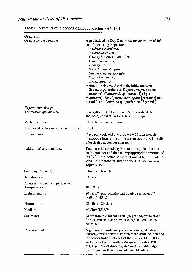
Table 1. Summary of test conditions for conducting SAM JP-4

Organisms Organisms per chamber:

Experimental design Test vessel type and size:

Medium volume:

Number of replicates x concentrations:

Reinoculation:

Addition of test materials:

Sampling frequency:

Test duration:

Physical and chemical parameters Temperature:

Light intensity:

Photoperiod:

Medium:

Sediment:

Measurements:

Algae (added on Day O at initial concentration of 103 cells for each algae species:

Anabaena cylindrica, Ankistrodesmus sp., Chlamydomonas reinhardi 90, Chlorella vulgaris, L yngbya sp., Scenedesmus obliquus, Selenastrum capricornutum , Stigeoclonium sp., and Ulothrix sp.

Animals (added on Day 4 at the initial numbers indicated in parentheses): Daphnia magna (16 per microcosm), Cypridopsis sp. (ostracod) (6 per microcosm), Tetrahymena thermophila [protozoa] (0.1 per mL), and Philodina sp. (rotifer) (0.03 per mL)

One-gallon (3.8 L) glass jars 16.0 cm wide at the shoulder, 25 cm tall with 10.6 cm openings

3 L added to each container

6 × 4

Once per week add one drop (ca 0.05 mL) to each microcosm from a mix of the ten species = 5 x 102 cells of each alga added per microcosm

Test material added day 7 by removing 450 mL from each container and then adding appropriate amounts of the WSF to produce concentrations of 0, 1, 5 and 15% WSF. After toxicant addition the final volume was adjusted to 3 L.

2 times each week

63 days

20 to 25 °C

80 ~tE m-Z photosynthetically active radiation s-1 (850 to 1000 fc)

12 h light/12 h dark

Medium T82MV

Composed of silica sand (200 g), ground, crude chitin (0.5 g), and cellulose powder (0.5 g) added to each container

Algal, invertebrate and protozoa counts, pH, dissolved oxygen, optical density, Parameters calculated included the concentrations of each of thespecies, DO, DO gain and loss, net photosynthesis/respiration ratio (P/R), pH, algal species diversity, daphnid fecundity, algal biovolume, and biovolume of available algae.


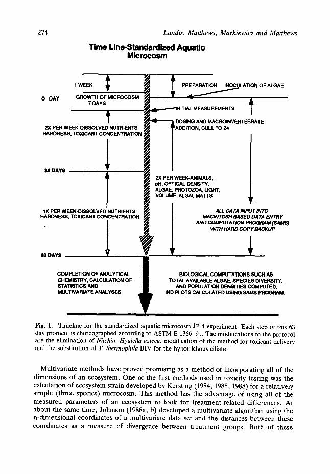
Time Line-Standardized Aquatic Microcosm

0 DAY

1 WEEK "~

GROWTH OF MICROCOSM 7 DAYS

2X PER WEEK-DISSOLVED NUTRIENTS, HARDNESS, TOXICANT CONCENTRATION

35 DAYS

1X PER WEEK-DISSOLVED NUTRIENTS, HARDNESS, TOXICANT CONCENTRATION

63 DAYS

Fig. 1.

PREPARATION INOCULATION OF ALGAE

~ID MAC, ROINVERTEBRATE CULL TO 24

2X PER WEEK-ANIMALS, pH, OPTICAL DENSITY, ALGAE, PROTOZOA, UG~"IT, VOLUME, ALGAL MATTS

i ! ALL DATA INPUT INTO

M4CINTOSH BASED DATA ENTRY

WITH HARD COPY BACKUP

COMPLETION OF ANALYTICAL CHEMISTRY, CALCULATION OF STATISTICS AND MULTIVARIATE ANALYSES

Timeline for the standardized aquatic microcosm JP-4 experiment. Each step of this 63 day protocol is choreographed according to ASTM E 1366-91. The modifications to the protocol are the elimination of Nitchia, Hyalella azteca, modification of the method for toxicant delivery and the substitution of T. thermophila BIV for the hypotrichous ciliate.

Multivariate methods have proved promising as a method of incorporating all of the dimensions of an ecosystem. One of the first methods used in toxicity testing was the calculation of ecosystem strain developed by Kersting (1984, 1985, 1988) for a relatively simple (three species) microcosm. This method has the advantage of using all of the measured parameters of an ecosystem to look for treatment-related differences. At about the same time, Johnson (1988a, b) developed a multivariate algorithm using the n-dimensional coordinates of a multivariate data set and the distances between these coordinates as a measure of divergence between treatment groups. Both of these


methods have the advantage of examining the ecosystem as a whole rather than by single variables, and can track such processes as succession, recovery and the deviation of a system due to an anthropogenic input.

However, a major disadvantage of both these methods, and of many conventional multivariate methods, is that all of the data are often incorporated without regard to the units of measurement or the appropriateness of including all variables in the analysis. It can be difficult to combine variables such as pH, with units ranging from 0-14, with the numbers of bacterial cells per ml, where low numbers are in the 10 6 range, to say nothing of the conceptual difficulties of adding pH units to counts. Similarly, random variables (i.e., variables with no treatment-related response) indiscriminately incorporated into the analysis may contribute so much noise that they overshadow variables that do show treatment-related effects.

Ideally, a multivariate statistical test used for evaluating complex data sets will have the following characteristics:

(1) It will not combine counts from dissimilar taxa by means of sums of squares, or other ad hoc mathematical techniques, as in the Euclidean and cosine distance measures.

(2) It will not require transformations of the data, such as normalizing the variance. (3) It will work without modification on incomplete data sets. (4) It will work without further assumptions on different data types (e.g., species

counts or presence/absence data). (5) Significance of a taxon to the analysis will not be dependent on the absolute size

of its count, so that taxa having a small total variance, such as rare taxa, can compete in importance with common taxa, and taxa with a large, random variance will not automatically be selected, to the exclusion of others.

(6) It will provide an integral measure of 'how good' the analysis is, i.e. whether the data set differs from a random collection of points.

(7) It will, in some cases, identify a subset of the taxa that serve as reliable indicators of the physical environment.

Recently developed for the analysis of ecological data, nonmetric clustering is a multivariate derivative of artificial intelligence research that satisfies all these criteria, and has the potential of circumventing many of the problems of conventional multivariate analysis.

In this paper, we use ANOVA and intervals of non-significant difference, and three multivariate techniques to search for meaningful patterns in the data set from a SAM toxicity test using Jet-A turbine fuel. The multivariate techniques include two conventional tests based on the ratio of multivariate metric distances (Euclidean distance and cosine of the vector distance), and one relatively new program, RIFFLE, which employs nonmetric clustering and association analysis (Matthews and Hearne 1991). All three of the multivariate techniques have proven useful in analysing complex ecological data sets (Matthews et al. 1991a, b). Of the three, only nonmetric clustering meets all of the criteria listed above (Matthews and Matthews 1991). The major disadvantage of the RIFFLE program is that, in order to find a clustering of the data points with the desirable qualities listed above, a massive search through thousands of potential clustering candidates is made before settling on the 'right' one. Even after this search, there is no guarantee that RIFFLE finds an optimal clustering. However, in our experience, RIFFLE does find an excellent clustering in reasonable time.


Jet fuels or perhaps more accurately, turbine fuels, are one of the primary fuels for internal combustion engines worldwide and certainly are the most widely available aviation fuel. Over the last 15 years virtually all of the commercial airline operations and charter operations have converted to a turbine engine because of the inherent low operating cost of the power plant, its reliability, and in part to the availability of fuel even in underdeveloped areas. In the US military there has been a progressive replace- ment of conventional piston engine vehicles with turbine equivalents. Standardization on a single type of turbine fuel to relieve logistical demands is also underway. Given the overwhelming predominance of turbine fuel, a fuel spill or accidental release of aviation fuel will probably be one of the prevalent turbine fuels: Jet-A, used for commercial and general aviation; JP-4, the standard fuel of the US Air Force and Army Aviation; and JP-5, the naval equivalent of JP-4, JP-8 is a new fuel proposed as the standard for all military vehicles using turbine engines.

Along with the environmental considerations, turbine fuels also offer advantages as model complex toxicants for toxicological research. Because of their use as aviation fuel, turbine fuels are produced to stringent specifications designed to ensure the safety of flight. Therefore, the overall general properties of these materials are tightly controlled. In addition, standard archived samples of the military fuels are maintained for toxicological studies at Wright Patterson, AFB. Jet fuels also tend to be less explosive and less volatile than gasoline, making the materials easier and safer to use. These properties make jet fuels an ideal material for the investigation of the effects of complex mixtures upon community dynamics. Like all petroleum products, however, the exact identity of the constituents varies according to the original crude and the refining process.

This paper reports the effects of low concentration of the water soluble fraction of JP-4 on the community incorporated in the SAM. The effects of the WSF on the microcosm communities were subtle. An early increase in algal density was apparent in the treatment groups containing the highest concentrations of the WSF and was matched by a decrease in daphnid populations. Multivariate analysis proved to be more powerful and efficient in highlighting important variables and processes than ANOVA. The variables that were most important were those distinguishing where treatment-related effects shifted during the course of the experiment. The multivariate analysis also detected oscillations in the similarity of the control and dosed groups that were not apparent using conventional univariate tests. The oscillations may be due to the inherent perturbations in community dynamics and interactions, or the effects upon the segments of the community not directly measured, the bacterial detritivores. We also discuss the implications of this research with regards to the use of indices and the conduct of environmental risk assessments.

Materials and methods

Reagents All chemicals used in the culture of the organisms and in the formulation of the microcosm media were reagent grade or as specified by the ASTM method.

JP-4 was supplied by the US Air Force Toxicology Laboratory at Wright Patterson, AFB, Ohio.

Multivariate analyses of JP-4 toxicity 277

Water soluble fraction (WSF) The WSF of JP-4 was prepared in glassware washed in nonphosphate soap, rinsed, then soaked in 2N HC1 for at least lh, rinsed ten times with distilled water, dried and finally autoclaved for 30 min. Microcosm medium, T82MV, acted as the diluent for the water fraction of the WSF.

Twenty five ml of JP-4 is added to the 1 I separatory funnel containing 1 I of T82MV, and is agitated as follows: (1) Shake separatory funnel for 5 rain, releasing built up pressure as necessary, (2) allow funnel contents to remain undisturbed for 15 min, (3) shake contents for 5 rain, allow to stand 15 rain, (4) continue same pattern for a total time of 1 h, and finally (5) allow separatory funnel contents to remain undisturbed for 8 h. At the end of this procedure the mixture was allowed to stand overnight. The next day all but 100 ml of T82MV/WSF of j et fuel mixture from the separatory funnel (leaving the lighter, insoluble fuel mixture in the flask) was drained into a cleaned, sterile 1 1 amber glass bottle and capped with a Teflon-lined screw cap. The WSF was used within 24 h or stored at 4 °C for no longer than 48 h before use as toxicant mixture.

Gas chromatography of WSF This protocol utilizes a Tekmar LSC 2000 Purge and Trap (P&T) concentrator system in tandem with a Hewlett Packard 5890A Gas Chromatograph with a Flame Ionization Detector (FID) (ASTM D3710 1988: ASTM D2887 1988: Westendorf 1986). Instrument blanks and deionized distilled water blanks are used to verify the cleanliness of the P&T and GC columns prior to analysis of samples. A 5 ml sample is injected into a 5 ml sparger, purged with pre-purified nitrogen gas for 11 min and dry purged for 4 rain. Volatile hydrocarbons, purged from the sample and collected on the Tenax/Silica Gel column, are desorbed at 180 °C directly onto the gas chromatograph SPB-5, 30 m x 0.53 mm ID 1.5 ~tm film, fused silica capillary column. The column, at 35 °C, is held at that temperature for 2 min, increased to 225 °C at 12 °C rain -a and held at that temperature for 5 min. A Spectra-Physics 4290 Integrator records the FID signal output of the volatile hydrocarbons that have been separated and eluted from the column by molecular weight.

Identification and quantification of GC fractions Qualitative identification of some components in the WSF of the JP-4 fuel used as the toxicant in the microcosm test, were determined using a Simulated Distillation (SIMDIS) Calibration Mixture. The ASTM Method D3710 Qualitative Calibration Mixture is the standard test method for determining the Boiling Range Distribution of Gasoline and Gasoline Fractions by Gas Chromatography. This mixture was used as a calibration standard to determine the retention times for each known component in the mixture against which unknown components, in the WSF of the Jet fuel mixture, were compared and identified.

Quantitative estimates of some components of the WSF were made by comparing sample chromatographs to certified n-paraffin and n-naphtha chromatograph standards, prepared and analysed under the same P&T/GC conditions.


Algal toxicity tests In order to estimate the relative toxicities of the JP-4 mixture and to set the concentrations for the microcosm, a series of short-term toxicity tests were performed (ASTM E 1218 1991). Algal growth inhibition tests were performed using Ankistrodesmus falcatus and Selenastrum capricornutum strains identical to those used in the SAM toxicity tests.

Test algae were grown in a semi-flow through culture apparatus on the microcosm media T82MV and taken during log phase growth for inoculation into the test flasks. Erlenmeyer flasks (250 ml) were used as test chambers, with serial dilutions of the WSF at concentrations of 0.0, 6.25, 12.5, 25, 50 and 100% placed in the flasks. The test organisms were added at a concentration of approximately 3.0 × 10 4 cells m1-1. Total volume was 100 ml with two replicates of controls and the test concentrations used. Test mixtures were incubated at 20.0 °C + 1.0°C with a 12:12 h light/dark cycle. Using a Newbauer Counting Chamber, cell densities were determined every 24 h for the 96 h duration of the test.

The cell numbers were then plotted against the concentrations. If possible, a least square regression line was drawn and the LCs0 (the concentration at which algal growth is inhibited to 50% of the control) determined. ANOVA was then run on the replicates to determine if any of the groups are significantly different.

SAM protocol

The 64-day SAM protocol has been described previously (ASTM E 1366-91 1991). Table 1 describes the organisms, conditions and modifications of ASTM E1366-91 for this particular experiment. Briefly, the microcosms were prepared by the introduction of ten algal, four invertebrate, and one bacterial species into 3 1 of sterile defined medium. Test containers were 4 1 glass jars. An autoclaved sediment consisting of 200 g silica sand and 0.5 g of ground chitin is autoclaved in the experimental jar immersed in a water bath to a point above the sand and chitin level during sterilization. This procedure helps prevent breakage of the jars and subsequent loss of replicates.

Numbers of organisms, dissolved oxygen (DO) and pH were determined twice weekly. Room temperature was 20 °C + 2 °. Illumination was 79.2 IxEm -2 photosynthetically active radiation s -1 with a range of 78.6-80.4 and a 16.8 day/night cycle.

Two major modifications were made to the SAM protocol. The first was the means of toxicant delivery. Test material was added on day 7 by stirring each microcosm, removing 450 ml from each container and then adding appropriate amounts of the WSF to produce concentrations of 0, 1, 5 and 15 % WSF. After toxicant addition the final volume was adjusted to 31. No attempt was made to filter and retain the organisms withdrawn during the removal of the 450 ml prior to toxicant addition. All graphs and statistical analysis start with the first sampling day, day 11.

The second modification was the substitution of Tetrahymena thermophila BIV for the hypotrichous ciliate used in past experiments. The hypotrichous ciliate was becoming increasingly difficult to culture, probably due to the age of the clone. T. thermophila has routinely been used in biochemical research and in detoxification studies of organophos- phates (Landis et al. 1985, 1987, 1991). Using SAM controls, constructed prior to this experiment, it was demonstrated that the T. thermophila populations were able to exist within the system. T. thermophila are maintained steriley in a 3% proteous peptone distilled water media at 20 °C with routine biweekly transfers to perpetuate the stocks.


The results presented below demonstrate the suitability of the Tetrahymena for inclusion in the protocol.

Data analysis

All data were recorded onto standard computer entry forms and checked for accuracy. The data was then keyed into the SAMS data analysis program and checked for accuracy. Parameters calculated included the concentrations of each of the species, DO, DO gain and loss, net photosynthesis/respiration ratio (P/R), pH, algal species diversity, algal biovolume, and biovolume of available algae. The statistical significance of these parameters compared to the controls was also computed for each sampling day using the Interval of Non-significant Difference (IND) plots developed by Conquest. Note that algal biovolume, algal species diversity and available algae are all derived variables based on the algal counts. The net photosynthesis/respiration ratio is not derived using 14C methods but by comparing oxygen concentrations before lights on, at the end of the photosynthetic period, and then at the next morning, as specified in the standard protocol. Photosynthesis/respiration ratio was the variable used during the analysis to incorporate these measurements.

The multivariate methods used in the analysis include cosine and vector distances and nonmetric clustering. All of these methods have been previously described (Matthews et al. 1991, Landis et al. 1993a, b) and are reviewed in Appendix A. Table 2 lists the variables used in the clustering process.

Results

Algal toxicity results

The WSF of JP-4 was not very toxic on a percentage (v/v) of the total culture media. Effects were compared by computing the area underneath the growth curve for both the 96 h experiments. As determined by graphical analysis, since 100% inhibition compared to controls was not achieved, the IC50 for Ankistrodesmus was 57% WSF and for Selenastrum 95% WSF.

Persistence of the JP-4 WSF

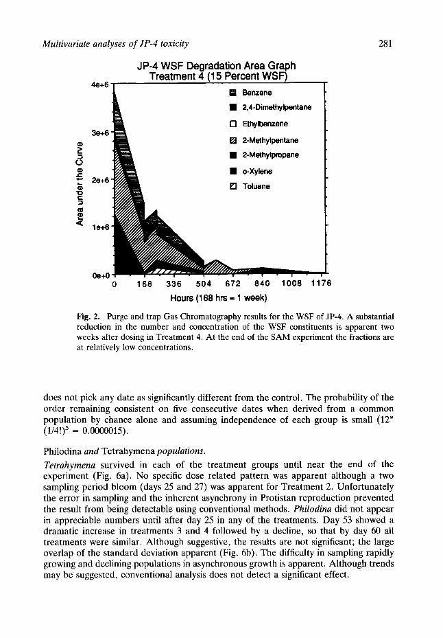
Seven compounds, benzene, 2,4 dimthylpentane, ethylbenzene, 2-methylpentane, 2- methylpropane, o-xylene and toluene, were tracked using GC analysis during the course of the SAM experiment. Figure 2 is an area graph that presents both the concentrations of the individual components along with the totals of these seven materials in microcosms of Treatment 4. As can be readily seen, 504 h after dosing, the relative concentrations of these materials have rapidly disappeared. After week three, only 2-methylpentane and 2-methylpropane are detectable. Since only the 2-methylpropane is present 672 h after dosing, this material may be the final biodegradative product of the absorbed fraction of the WSF, and is being investigated in more detail.

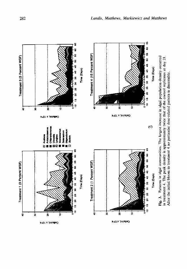
Patterns in algal communities

The largest increase in algal population density occurred in treatment 4 (Fig. 3). The peak density is approximately twice that of the control replicates at day 21. After the initial bloom in treatment 4, no particular dose-related pattern is discernible. Lyngbya makes up a substantial portion of the algal community in each treatment group, which


Table 2. Biotic parameters used in the multivariate statistical tests. Biotic variables such as diversity, available biovolume, and total algal biovolume are not used since they are derived from the variables listed below. Including derived variables weights some parameters more than others since some like Anabaena can be used alone and again in the calculation of total algal biovolume

Biotic parameter

Anabaena Ankistrodesmus Chlamydomonas Chlorella Daphnia Ephipia

Small Daphnia Medium Daphnia Large Daphnia

Tetrahymena Lyngbya Miscellaneous sp. Ostracod ( Cyprinotus) Philodina (Rotifer) Scenedesmus Selanastrum Stigeoclonium Ulothrix

is historically unusual. The number of algal species, as enumerated by the counting technique, also generally declines in each of the treatment groups, but in a general sense not related to dose.

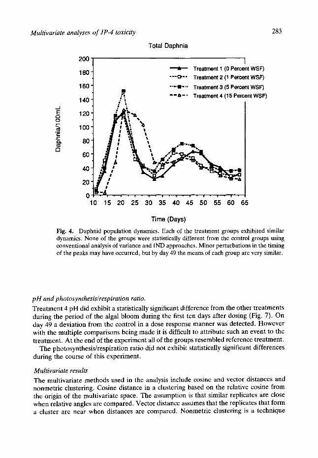
Daphnid populations.

Each of the treatment groups exhibited similar dynamics (Fig. 4). None of the groups were statistically different from the control groups using conventional analysis of variance approaches. Minor perturbations in the timing of the peaks may have occurred, but by day 50 the means of each group were very similar.

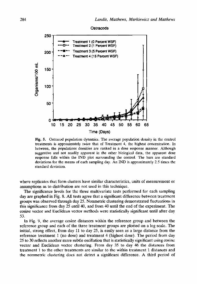
Ostracod populations.

At the end of the experiment, the average population density in the control treatments is approximately twice that of treatment 4, the highest toxicant concentration (Fig. 5). Population density in the two treatment groups with the highest toxicant concentrations, decline below the no dose treatment and the lowest treatment densities. This pattern is apparent graphically from day 53 onward. Conventional analysis such as the IND plot


t -

" 0 r -

<

JP-4 WSF Degradation Area Graph Treatment 4 (15 Percent WSF)

4e+6 [] Benzene

• 2,4-Dimethylpentane

I-I Ethylbenzene 3 e + 6 ' m

[ ] 2-Methylpentane

• 2-Methylpropane

• o-Xylene 2e+6'

[ ] Toluene

le+6'

Oe+O 0 168 336 504 672 840 1008 1176

Hours (168 hrs = 1 week)

Fig. 2. Purge and trap Gas Chromatography results for the WSF of JP-4. A substantial reduction in the number and concentration of the WSF constituents is apparent two weeks after dosing in Treatment 4. At the end of the SAM experiment the fractions are at relatively low concentrations.

does not pick any date as significantly different from the control. The probability of the order remaining consistent on five consecutive dates when derived from a common population by chance alone and assuming independence of each group is small (12" (1/4!) 5 = 0.0000015) .

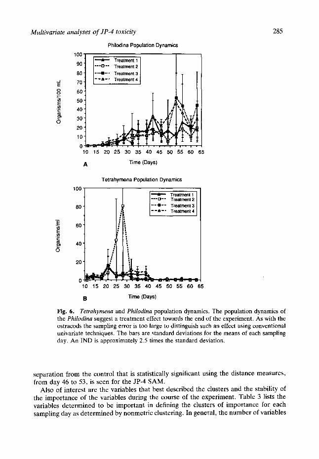
Philodina and Tetrahymena populations. Tetrahymena survived in each of the treatment groups until near the end of the experiment (Fig. 6a). No specific dose related pattern was apparent although a two sampling period bloom (days 25 and 27) was apparent for Treatment 2. Unfortunately the error in sampling and the inherent asynchrony in Protistan reproduction prevented the result from being detectable using conventional methods. Philodina did not appear in appreciable numbers until after day 25 in any of the treatments. Day 53 showed a dramatic increase in treatments 3 and 4 followed by a decline, so that by day 60 all treatments were similar. Although suggestive, the results are not significant; the large overlap of the standard deviation apparent (Fig. 6b). The difficulty in sampling rapidly growing and declining populations in asynchronous growth is apparent. Although trends may be suggested, conventional analysis does not detect a significant effect.

40

30

20

10

Trea

tmen

t 1

(0 P

erce

nt W

SF)

0 10

15

20

25

30

35

40

45

50

55

60

65

Tim

e (

Day

s)

[]

/mab

ena

• A

nk

ara

•

c~

../.

,,.~

. r~

Chk

arda

[]

Ly

r~ym

•

,S~e

nede

~r, us

D U~lhdx

40

'

30

10' 10

Trea

tmen

t 3

(5 P

erce

nt W

SF)

lS

20

2S

30

35

40

4

5

50

55

Tim

e (

Da

ys)

60

65

b~

b~

Trea

tmen

t 2

(1 P

erce

nt W

SF)

"t 30 40

30

20'

x 20

_.

t E

10

10

Trea

tmen

t 4

(15

Perc

ent

WS

F)

O

0 10

15

20

25

30

35

40

4

5

50

55

60

65

t0

15

20

25

30

35

40

4

5

50

55

Tim

e (D

ays)

""

T

ime

(D

ays

)

Fig.

3.

Pat

tern

s in

alg

al c

omm

unit

ies.

The

lar

gest

inc

reas

e in

alg

al p

opul

atio

n de

nsit

y oc

curr

ed

in t

reat

men

t 4.

The

pea

k de

nsit

y is

app

roxi

mat

ely

twic

e th

at o

f th

e co

ntro

l re

plic

ates

at

day

21.

Aft

er t

he i

niti

al b

loom

in

trea

tmen

t 4

no p

arti

cula

r do

se-r

elat

ed p

atte

rn i

s di

scer

nibl

e.

60

65

N


Total Daphnia

_..I E

O O

"F ¢- Q .

CI

200 I ~, Treatment 1 (0 Percent WSF)

180 " " ~ ' " Treatment 2 (1 Percent WSF)

160 • . . . . • " " Treatment 3 (5 Percent WSF) ;'~ - - a - - Treatment 4 (15 Percent WSF)

120 t ~.

1 O0

401

0, 10 15 20 25 30 35 40 45 50 55 60 65

Time (Days)

Fig. 4. Daphnid population dynamics. Each of the treatment groups exhibited similar dynamics. None of the groups were statistically different from the control groups using conventional analysis of variance and IND approaches. Minor perturbations in the timing of the peaks may have occurred, but by day 49 the means of each group are very similar.

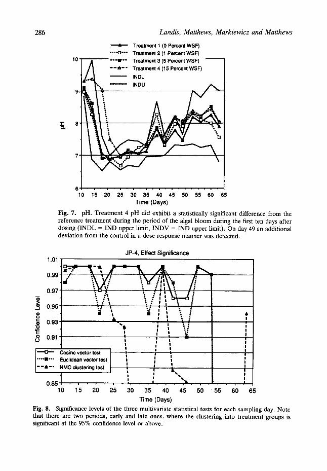
pH and photosynthesis~respiration ratio. Treatment 4 pH did exhibit a statistically significant difference from the other treatments during the period of the algal bloom during the first ten days after dosing (Fig. 7). On day 49 a deviation from the control in a dose response manner was detected. However with the multiple comparisons being made it is difficult to attribute such an event to the treatment. At the end of the experiment all of the groups resembled reference treatment.

The photosynthesis/respiration ratio did not exhibit statistically significant differences during the course of this experiment.

Multivariate results The multivariate methods used in the analysis include cosine and vector distances and nonmetric clustering. Cosine distance in a clustering based on the relative cosine from the origin of the multivariate space. The assumption is that similar replicates are close when relative angles are compared. Vector distance assumes that the replicates that form a cluster are near when distances are compared. Nonmetric clustering is a technique


Ostracods

._1 E

o o T"

E t - ¢1

O

250

200'

150'

100'

,1. =re=D==

=ImaD==m

m ~ m m

5 0

0 ~.~. - , 10 15

Treatment 1 (0 Percent WSF) Treatment 2 (1 Percent WSF) Treatment 3 (5 Percent WSF) Treatment 4 (15 Percent WSF)

¢

)},:

20 25 30 35 40 45 50 55 60 65

"13me (Days)

Fig. 5. Ostracod population dynamics. The average population density in the control treatments is approximately twice that of Treatment 4, the highest concentration. In between, the populations densities are ranked in a dose response manner. Although suggestive and not readily apparent in the other biological data, the apparent dose response falls within the IND plot surrounding the control. The bars are standard deviations for the means of each sampling day. An IND is approximately 2.5 times the standard deviation.

where replicates that form clusters have similar characteristics, units of measurement or assumptions as to distribution are not used in this technique.

The significance levels for the three multivariate tests performed for each sampling day are graphed in Fig. 8. All tests agree that a significant difference between treatment groups was observed through day 25. Nonmetric clustering demonstrated fluctuations in this significance from day 25 until 40, and from 40 until the end of the experiment. The cosine vector and Euclidean vector methods were statistically significant until after day 53.

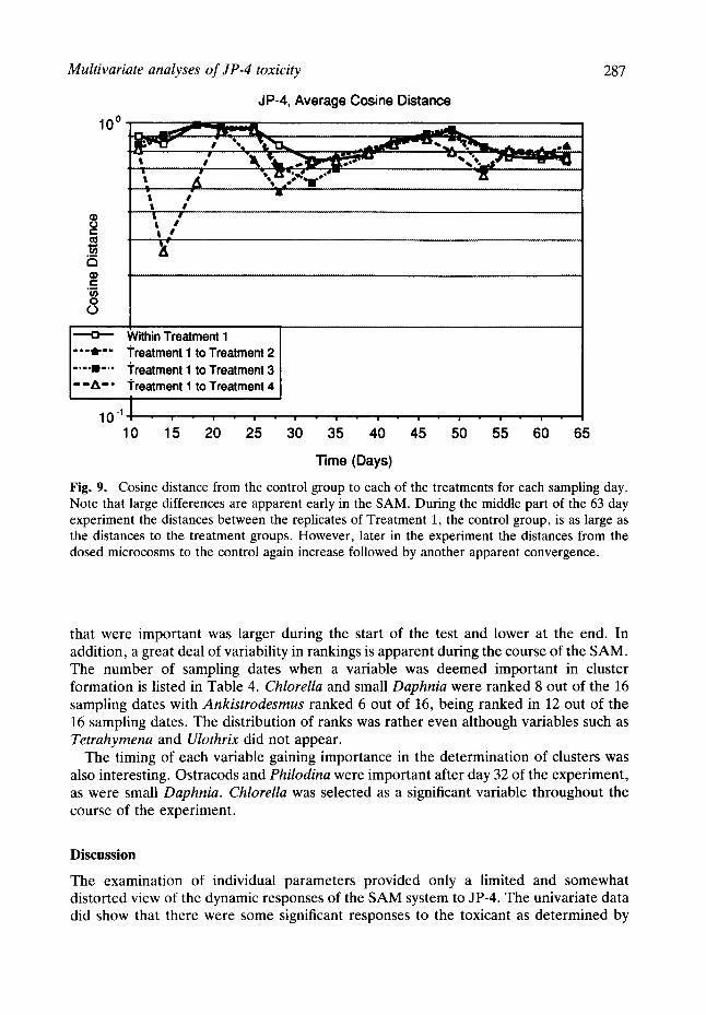
In Fig. 9, the average cosine distances within the reference group and between the reference group and each of the three treatment groups are plotted on a log scale. The initial, strong effect, from day 11 to day 25, is easily seen as a large distance from the reference treatment 1 (no dose) and treatment 4 (highest dose). The period from day 25 to 30 reflects another more subtle oscillation that is statistically significant using cosine vector and Euclidean vector clustering. From day 35 to day 46 the distances from treatment 1 to the other treatments are similar to the within treatment 1 distances and the nonmetric clustering does not detect a significant difference. A third period of


...J

E O O

E o0 "E- ¢O

O

100

90"

80

70-

Philodina Population Dynamics

]i:i ii tr.,m., Treatment 2 Treatment 3 Treatment 4

60 50" I.

I '; " i 30 k, t , t ":'..,

1 0

10 15 20 25 30 35 40 45 50 55 60 65

A Time (Days)

100'

8 0

-~ 60 E u )

.w ¢ -

40' O

Tetrahymena Population Dynamics

20 ¸

0

10

Treatment 1 ] ---0,-- Treatment 2 [

i l [ i .... • " - Treatment 3 [ - -~ ' - " Treatn'mnt 4 J

1 |

15 20 25 30 35 40 45 50 55 60 65

B Time (Days)

Fig. 6. Tetrahymena and Philodina population dynamics. The population dynamics of the Philodina suggest a treatment effect towards the end of the experiment. As with the ostracods the sampling error is too large to distinguish such an effect using conventional univariate techniques. The bars are ~tandard deviations for the means of each sampling day. An IND is approximately 2.5 times the standard deviation.

separation from the control that is statistically significant using the distance measures, from day 46 to 53, is seen for the JP-4 SAM.

Also of interest are the variables that best described the clusters and the stability of the importance of the variables during the course of the experiment. Table 3 lists the variables determined to be important in defining the clusters of importance for each sampling day as determined by nonmetric clustering. In general, the number of variables


Jl. Treatment 1 (0 Percent WSF)

• . . -o - . . Treatment 2 (1 Percent WSF) A - - - I . - - Treatment 3 (5 Percent WSF)

! . . . . ~ ' " " Treatment 4 (15 Percent WSF)

' oo;

6 1 - , - , - , - , - , - , - , - , - , - , - I

10 15 20 25 30 35 40 45 50 55 60 65 T ime (Days)

Fig. 7. pH. Treatment 4 pH did exhibit a statistically significant difference from the reference treatment during the period of the algal bloom during the first ten days after dosing ( INDL = IND upper limit, INDV = IND upper limit). On day 49 an additional deviation from the control in a dose response manner was detected•

1.01 JP-4, Effect Signi f icance

. . 0 , , ," /: • • - . , l ~ I . : 0.97 ?, ~. : i ~ ~ . 1:" "

S ; : . i : :

0.93 ; , t : .',2_ "E o 0.91 O

-.--O--- Cosine vector t es t

. . . . i t - - . Euclidean vector t es t

- - J ' - " NMC clustering t es t

~ I I I I

I I I m I m I I I I I I I I I I

I I • I I ~%

0.85 . , - . . . . . , . m ~ .

10 15 20 25 30 35 40 45 50 5 5

t : I I I I I |

60

I I

I I I I I I ! ! ! ! |

65

Time (Days)

Fig. 8. Significance levels of the three multivariate statistical tests for each sampling day. Note that there are two periods, early and late ones, where the clustering into treatment groups is significant at the 95% confidence level or above.

Multivariate analyses of JP-4 toxicity

JP-4, Average Cosine Distance

10° .Jr',,.._ -""~"-,,,, , . ; - ' : - -Z~ ; . . , .....

o e-.

C

o 0

t # t • ....... ~ ......... ~ ,,

. : / g

287

Within Treatment 1 - - - t - - treatment I to Treatment 2 . . . . m-,- "i'reatment I to Treatment 3 - - L t - - treatment 1 to Treatment 4

I

I 0 I I , , , 10 15 20 25

i | • | - i - i i i

30 35 40 45 50 55 60 65

Time (Days)

Fig. 9. Cosine distance from the control group to each of the treatments for each sampling day. Note that large differences are apparent early in the SAM. During the middle part of the 63 day experiment the distances between the replicates of Treatment 1, the control group, is as large as the distances to the treatment groups. However, later in the experiment the distances from the dosed microcosms to the control again increase followed by another apparent convergence.

that were important was larger during the start of the test and lower at the end. In addition, a great deal of variability in rankings is apparent during the course of the SAM. The number of sampling dates when a variable was deemed important in cluster formation is listed in Table 4. Chlorella and small Daphnia were ranked 8 out of the 16 sampling dates with Ankistrodesmus ranked 6 out of 16, being ranked in 12 out of the 16 sampling dates. The distribution of ranks was rather even although variables such as Tetrahymena and Ulothrix did not appear.

The timing of each variable gaining importance in the determination of clusters was also interesting. Ostracods and Philodina were important after day 32 of the experiment, as were small Daphnia. Chlorella was selected as a significant variable throughout the course of the experiment.

Discussion

The examination of individual parameters provided only a limited and somewhat distorted view of the dynamic responses of the SAM system to JP-4. The univariate data did show that there were some significant responses to the toxicant as determined by


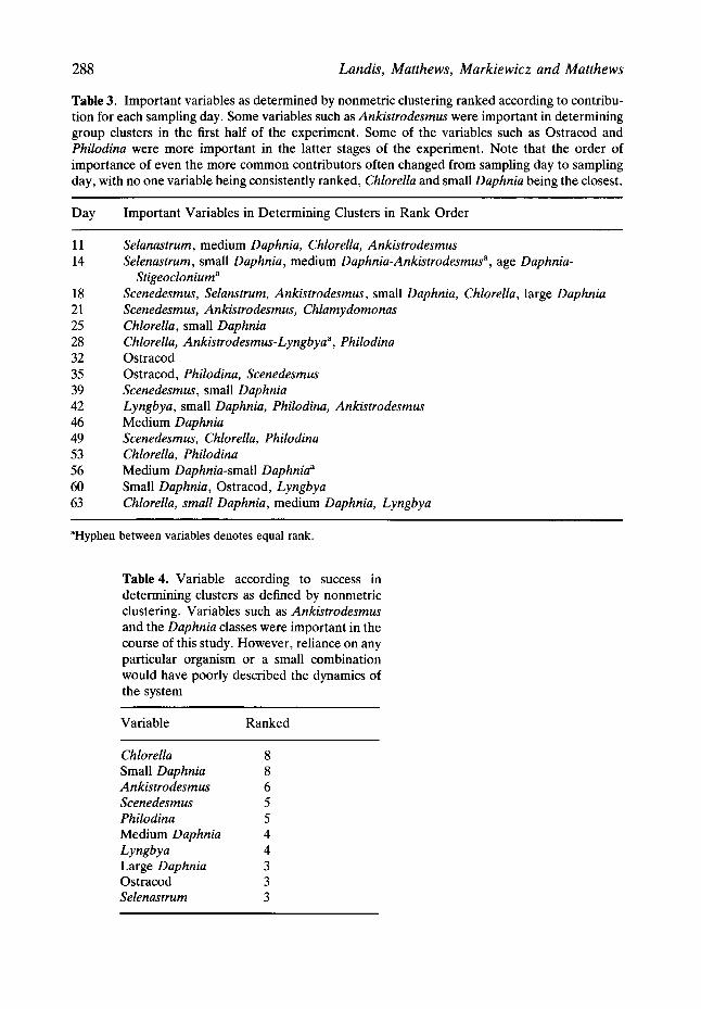
Table 3. Important variables as determined by nonmetric clustering ranked according to contribu- tion for each sampling day. Some variables such as Ankistrodesmus were important in determining group clusters in the first half of the experiment. Some of the variables such as Ostracod and Philodina were more important in the latter stages of the experiment. Note that the order of importance of even the more common contributors often changed from sampling day to sampling day, with no one variable being consistently ranked, Chlorella and small Daphnia being the closest.

Day Important Variables in Determining Clusters in Rank Order

11 14

18 21 25 28 32 35 39 42 46 49 53 56 60 63

Selanastrum, medium Daphnia, ChloreUa, Ankistrodesmus Selenastrum, small Daphnia, medium Daphnia-Ankistrodesmus a, age Daphnia-

Stigeoclonium a Scenedesmus, Selanstrum, Ankistrodesmus, small Daphnia, Chlorella, large Daphnia Scenedesmus, Ankistrodesmus, Chlamydomonas Chlorella, small Daphnia Chlorella, Ankistrodesmus-L yngbya a, Philodina Ostracod Ostracod, Philodina, Scenedesmus Scenedesmus, small Daphnia Lyngbya, small Daphnia, Philodina, Ankistrodesmus Medium Daphnia Scenedesmus, Chlorella, Philodina Chlorella, Philodina Medium Daphnia-small Daphnia a Small Daphnia, Ostracod, Lyngbya Chlorella, small Daphnia, medium Daphnia, Lyngbya

aHyphen between variables denotes equal rank.

Table 4. Variable according to success in determining clusters as defined by nonmetric clustering. Variables such as Ankistrodesmus and the Daphnia classes were important in the course of this study. However, reliance on any particular organism or a small combination would have poorly described the dynamics of the system

Variable Ranked

Chlorella 8 Small Daphnia 8 Ankistrodesmus 6 Scenedesmus 5 Philodina 5 Medium Daphnia 4 Lyngbya 4 Large Daphnia 3 Ostracod 3 Selenastrum 3


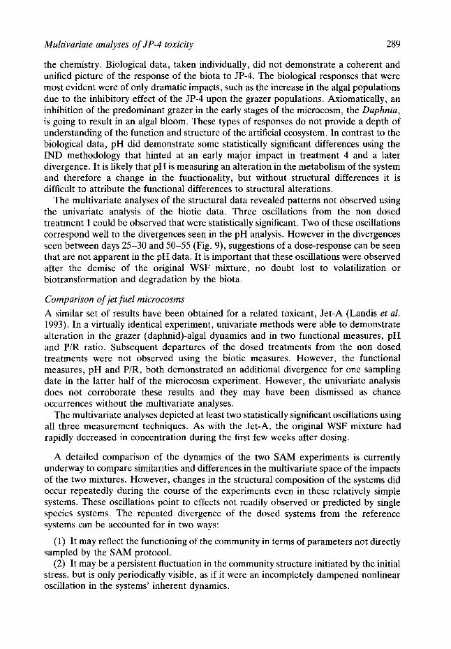
the chemistry. Biological data, taken individually, did not demonstrate a coherent and unified picture of the response of the biota to JP-4. The biological responses that were most evident were of only dramatic impacts, such as the increase in the algal populations due to the inhibitory effect of the JP-4 upon the grazer populations. Axiomatically, an inhibition of the predominant grazer in the early stages of the microcosm, the Daphnia, is going to result in an algal bloom. These types of responses do not provide a depth of understanding of the function and structure of the artificial ecosystem. In contrast to the biological data, pH did demonstrate some statistically significant differences using the IND methodology that hinted at an early major impact in treatment 4 and a later divergence. It is likely that pH is measuring an alteration in the metabolism of the system and therefore a change in the functionality, but without structural differences it is difficult to attribute the functional differences to structural alterations.

The multivariate analyses of the structural data revealed patterns not observed using the univariate analysis of the biotic data. Three oscillations from the non dosed treatment 1 could be observed that were statistically significant. Two of these oscillations correspond well to the divergences seen in the pH analysis. However in the divergences seen between days 25-30 and 50-55 (Fig. 9), suggestions of a dose-response can be seen that are not apparent in the pH data. It is important that these oscillations were observed after the demise of the original WSF mixture, no doubt lost to volatilization or biotransformation and degradation by the biota.

Comparison of jet fuel microcosms A similar set of results have been obtained for a related toxicant, Jet-A (Landis et al. 1993). In a virtually identical experiment, univariate methods were able to demonstrate alteration in the grazer (daphnid)-algal dynamics and in two functional measures, pH and P/R ratio. Subsequent departures of the dosed treatments from the non dosed treatments were not observed using the biotic measures. However, the functional measures, pH and P/R, both demonstrated an additional divergence for one sampling date in the latter half of the microcosm experiment. However, the univariate analysis does not corroborate these results and they may have been dismissed as chance occurrences without the multivariate analyses.

The multivariate analyses depicted at least two statistically significant oscillations using all three measurement techniques. As with the Jet-A, the original WSF mixture had rapidly decreased in concentration during the first few weeks after dosing.

A detailed comparison of the dynamics of the two SAM experiments is currently underway to compare similarities and differences in the multivariate space of the impacts of the two mixtures. However, changes in the structural composition of the systems did occur repeatedly during the course of the experiments even in these relatively simple systems. These oscillations point to effects not readily observed or predicted by single species systems. The repeated divergence of the dosed systems from the reference systems can be accounted for in two ways:

(1) It may reflect the functioning of the community in terms of parameters not directly sampled by the SAM protocol.

(2) It may be a persistent fluctuation in the community structure initiated by the initial stress, but is only periodically visible, as if it were an incompletely dampened nonlinear oscillation in the systems' inherent dynamics.


Examination of individual parameters provides only a limited, and somewhat distorted view of the SAM microcosm response to the WSF of each fuel. The univariate data analysis did indeed show that there were some significant responses to the toxicant by individual taxa and chemistry; however, the responses were scattered over time, and did not present a logical, coherent pattern. Furthermore, the individual responses detected were typified by wild swings in the population density of a taxon over time.

If you kill or restrict the reproduction of most of the Daphnia, the next microcosm response is probably an algal bloom. This result could easily have been predicted by the short term toxicity tests and was expected. However, recent modelling efforts by Taub et al. (submitted) suggest that the dynamics of these interactions and the resulting magnitudes of the algal blooms are highly dependent upon the timing of the toxic insult. Measuring these types of gross responses to the toxicant do not provide much more insight into impact of the toxicant in the ecosystem than do the short-term single-species tests. The absolute magnitude of the disturbance and the period of recovery can be obtained from the microcosm experiment, in the sense of a classical predator prey interaction. However, the multivariate analysis reveals a more interesting dynamic.

The multivariate patterns suggest a much more complex pattern of multiple divergences and convergences in the similarities between treatment groups. Much as an ecosystem could be expected to display the rise and fall of species assemblages, the SAM microcosms appear to indicate that the first divergence is only the beginning of a series of responses.

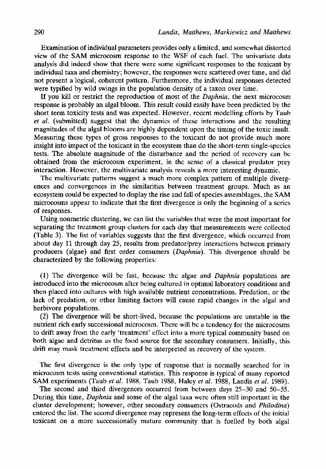
Using nonmetric clustering, we can list the variables that were the most important for separating the treatment group clusters for each day that measurements were collected (Table 3). The list of variables suggests that the first divergence, which occurred from about day 11 through day 25, results from predator/prey interactions between primary producers (algae) and first order consumers (Daphnia). This divergence should be characterized by the following properties:

(1) The divergence will be fast, because the algae and Daphnia populations are introduced into the microcosm after being cultured in optimal laboratory conditions and then placed into cultures with high available nutrient concentrations. Predation, or the lack of predation, or other limiting factors will cause rapid changes in the algal and herbivore populations.

(2) The divergence will be short-lived, because the populations are unstable in the nutrient rich early successional microcosm. There will be a tendency for the microcosms to drift away from the early 'treatment' effect into a more typical community based on both algae and detritus as the food source for the secondary consumers. Initially, this drift may mask treatment effects and be interpreted as recovery of the system.

The first divergence is the only type of response that is normally searched for in microcosm tests using conventional statistics. This response is typical of many reported SAM experiments (Taub et al. 1988, Taub 1988, Haley et al. 1988, Landis et al. 1989).

The second and third divergences occurred from between days 25-30 and 50-55. During this time, Daphnia and some of the algal taxa were often still important in the cluster development; however, other secondary consumers (Ostracods and Philodina) entered the list. The second divergence may represent the long-term effects of the initial toxicant on a more successionally mature community that is fuelled by both algal


productivity and detritus. If so, the resulting divergences should have the following characteristics:

(1) It should be strongly influenced by detritus quality. Detritus is conditioned by bacteria and fungi, which are highly sensitive to toxicants but are unmeasured in the microcosm. Also, detritus that has passed through the gut of a consumer (e.g., consumed algae) is different from detritus that originates directly from dead algae (unconsumed). Therefore, the quality of the detritus may be highly affected by the treatment, but none of the factors influencing the effects will be measured directly.

(2) Secondary consumers of detritus and bacteria are no less affected by the quality of their food source than algal consumers, so the treatment-related alterations of the quality of detritus and bacteria will cause differences in the secondary consumer populations.

Therefore, the series of divergences following the initial algal-daphnid interaction may still represent a direct response to the initial treatment effects, but because it occurs late in the microcosm experiment, it is easily misinterpreted as noisy or the effects of a degradation product. An inclusion of measures of detritus quality and microbial metabolism may answer these questions and such studies are currently being incorporated into our series of microcosm experiments.

Invoking unseen properties of an ecosystem or other mechanistic explanations may not be needed to explain the occurrence of oscillations and divergences from a non- dosed reference system. An alternative and complimentary explanation is available that perhaps describes the dynamics of multispecies systems at a more fundamental level.

Ecosystem dynamics and the illusion of recovery The return of a system to its pre-existing state, cally, is a classical definition of recovery. There govern the composition of an ecosystem after from colonizing sources, genetic variability of

structurally, metabolically and dynami- are many biotic and abiotic factors that a stress event; substrate type, distance the resident population are but a few.

Since each of the initial conditions are likely to be different from those that lead to the original system, it is unlikely that the subsequent system will be identical. Similarity, however, does not mean the same. In fact, similarity at the structural level may lead to an illusion of recovery.

First, the apparent recovery or movement of the dosed systems towards the reference or treatment 1 case may be an artifact of our measurement systems that allow the n-dimensional data to be represented in a two dimensional system. In an n-dimensional sense, the systems may be moving in opposite directions and simply pass by similar coordinates during certain time intervals. Positions may be similar, but the n- dimensional vectors describing the movements of the systems can be very different.

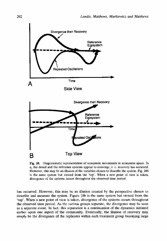
The apparent recoveries and divergences may also be artifacts of our attempt to choose the best means of collapsing and representing n-dimensional data into a two or three dimensional representation. In order to represent such data, it is necessary to project n-dimensional data into three or fewer dimensions. As information is lost when the shadow of a cube is projected upon a two dimensional screen, a similar loss of information can occur in our attempt to represent n-dimensional data. The possible illusion of recovery based on this type of projection is diagramatically represented in Fig. 10. In Fig. 10a the dosed and the reference systems appear to converge, i.e. recovery


Divergence then Recovery

m m m m m m

Reference

A

Repeated Oscillations

Time

Side View

k

Divergence then Recovery

l l | | l m ] ] l ' | l | |

Reference E~system

B Top View

Fig. 10. Diagrammatic representation of ecosystem movements in ecosystem space. In a, the dosed and the reference systems appear to converge, i. e. recovery has occurred. However, this may be an illusion of the variables chosen to describe the system. Fig. 10b is the same system but viewed from the 'top'. When a new point of view is taken, divergence of the systems occurs throughout the observed time period.

has occurred. However , this may be an illusion created by the perspective chosen to describe and measure the system. Figure 10b is the same system but viewed from the ' top' . When a new point of view is taken, divergence of the systems occurs throughout the observed time period. As the various groups separate, the divergence may be seen as a separate event. In fact, this separation is a continuation of the dynamics initiated earlier upon one aspect of the community. Eventually, the illusion of recovery may simply be the divergence of the replicates within each treatment group becoming large


enough, with enough inherent variation, so that even the multivariate analysis can not distinguish treatment group similarities. Not every divergence from the control treatment may have a causal effect related to it in time: differentiating these events from those due to degradation products or other perturbations is challenging.

Complexity in nonlinear ecological systems

Not only may system recovery often be an illusion but strong theoretical reasons indicate that recovery to a reference system may be impossible or at least unlikely. In fact, systems that differ only marginally in their initial conditions and at levels probably impossible to measure are likely to diverge in unpredictable manners. May and Oster (1978) in a particularly seminal paper investigated the likelihood that many of the dynamics seen in ecosystems, generally attributed to chance or stochastic events, are in fact deterministic. In fact simple deterministic models of population can give rise to complicated behaviours. Using equations resembling those used in population biology, bifurcations occur resulting with several distinct outcomes. Eventually, given the proper parameters, the system appears chaotic in nature although the underlying mechanisms are completely deterministic. Obviously, biological systems have limits, extinction being perhaps the most obvious and best recorded. Another ramification is that the noise in ecosystems and in sampling may not be the result of a stochastic process but the result of underlying deterministic, chaotic relationships.

These principles also apply to spatial distributions of populations as recently reported by Hassell et al. (1991). In a study using host-parasite interactions as the model, a variety of spatial patterns were developed using the Nicholson-Bailey model. Host-parasite interactions demonstrated patterns ranging through static 'crystal lattice' patterns, spiral waves, chaotic variation or extinction with the appropriate variation of only three parameters within the same set of equations. The deterministic patterns could be extremely complex and not distinguishable from stochastic environmental changes.

Given the perhaps chaotic nature of populations it may not be possible to predict accurately species presence, population interactions, or structural and functional attri- butes. Katz et al. (1987) examined the spatial and temporal variability in zooplankton data from a series of five lakes in North America. Much of the analysis was based on limnological data collected by Brige and Juday from 1925 to 1942. Copepods and cladocera, except Bosmina, exhibited larger variability between lakes than between years in the same lake. Some taxa showed consistent patterns among the study lakes. They concluded that the controlling factors for these taxa operated uniformly in each of the study sites. However, in regards to the depth of maximal abundance for calanoid copepods and Bosmina, the data obtained from one lake had little predictive power for application to other lakes. Part of this uncertainty was attributed to the intrinsic rate of increase of the invertebrates with variability increasing with a corresponding increase in rma x. A high rmax should enable the populations to accurately track changes in the environment. Katz et al. suggest that these taxa be used to track changes in the environment. Unfortunately, in the context of environmental toxicology, the inability to use one lake to predict the non-dosed population dynamics of these organisms in another, reduces the sensitivity of methods that use comparisons of two systems as measures of anthropogenic impacts.

A better strategy may be to let the data and a clustering protocol identify the important parameters in determining the dynamics of and impacts to ecological systems.


This approach has been recently suggested independently by Dickson et al. (1992) and Matthews and Matthews (1991). This approach is in direct contrast to the more usual means of assessing anthropogenic impacts. One classical approach is to use the presence or absence of so called indicator species. This assumes that the tolerance to a variety of toxicants is known and that chaotic or stochastic influences are minimized. A second approach is to use hypothesis testing to differentiate metrics from the systems in question. This second approach assumes that the investigators know a priori the important parameters. Given that the important parameters in differentiating non-dosed from dosed systems change from sampling period to sampling period, this assumption can not be made. Classification approaches such as nonmetric clustering or the canonical correlation methodology developed by Dickson et al. eliminate these assumptions.

Implications for monitoring and risk assessment

The results presented in this report combined with the others cited above and the implications of chaotic dynamics suggest that reliance upon any one variable or an index of variables is an operational convenience that may provide a misleading representation of pollutant effects and the associated risks. The use of indices such as diversity and the Index of Biological Integrity have the effect of collapsing the dimensions of the descriptive hypervolume in a relatively arbitrary fashion. Indices, since they are compo- sited variables, are not true endpoints. The collapse of the dimensions that are compo- sited tends to eliminate crucial information, such as the inherent variability, and its importance in describing these variables. The mere presence or absence and the frequency of these events can be analysed using techniques such as nonmetric clustering that preserve the nature of the dataset. A useful function was certainly served by the application of indices, but the new methods of data compilation, analysis and representation derived from the Artificial Intelligence tradition can now replace these approaches and illuminate the underlying structure and dynamic nature of ecological systems. In the next 12 months RISC (reduced instruction set computer) based personal computers will make these approaches widely available and rapidly run at the desktop.

The implications are important. Currently, only small sections of ecosystems are monitored or a heavy reliance is placed upon so-called indicator species. Our data suggest that this is dangerous, potentially producing misleading interpretations and resulting in costly error in management and regulatory judgments. Much larger toxicological test systems are currently analysed using conventional statistical methods on the limit of acceptable statistical power. Interpretation of the results has proven to be difficult.

The dynamics observed in our experiments and in the research discussed above should make obvious that a metaphor such as ecosystem health is inappropriate and misleading. In a recent critical evaluation, Suter (1993) dismissed ecosystem health as a misrepresen- tation of ecological science. Ecosystems are not organisms with the patterns of homeos- tasis determined by a central genetic core. Since ecosystems are not organismal in nature, health is a property that can not describe the state of such a system. The urge to represent such a state as health has lead to the compilation of variables with different metrics, characteristics and relationships. Suter suggests a better alternative would be to evaluate the array of ecosystem processes of interest, with an underlying understanding that the fundamental nature of these systems is quite different from those of organisms.

One of the ongoing debates in environmental toxicology has been the suitability of


the extrapolation and realism of the various multispecies toxicity tests that have been developed over the last 15 years. One of the major criticisms of small scale systems is that the low diversity of the system is not representative of natural systems in dynamic complexity (Sugiura 1992). Given the above discussion and the conclusions derived from it much of this debate may have been misdirected. The small scale systems used in our study have been demonstrated to express complex dynamics. Kersting and Van Wun- gaarden (1992) found that even the three compartment microecosystem, as developed by Kersting (1984, 1985, 1988), expresses indirect effects as measured by pH changes after dosing with chloropyrifos. Since even full scale systems can not serve as reliable predictors of the dynamics of other full scale systems, it is impossible to suggest that any artificially created system can provide a generic representation of any full scale system. Debate should probably revert to more productive areas such as improvements in culture, sampling and measurement techniques or other characteristics of these systems. A more worthwhile goal is probably the understanding of the scaling factors, in a full n-dimensional representation, that should enable the accurate representation of specific ecosystem characteristics. Certain aspects of a community may be included in one system to answer specific questions that in another system would be entirely inappropriate. If questions as to detritus quality are important then the system should include that particular component. In other words, the system should attempt to answer the particular scientific question.

Several questions are now the goals of future research. The dynamics of the loss of jet fuels from the SAM systems is currently being investigated in greater depth. Additional data should indicate the persistence of the constituents and help aid in the determination of initial toxicity, including further information from literature searches or using quantitative structure activity relationship models. Additional testing of related materials is being conducted. Finally, questions as to the effects of size and community structure abound. The SAM system is relatively simple. Data sets incorporating more diverse species assemblages and of varying sizes are being investigated for comparison.

Conclusion

Effects are seen in the microcosm after the degradation of the toxicant to very low levels in an oscillating pattern of divergence from the non-dosed treatment, apparent recovery, which is then followed by another divergence.

Multivariate analysis is crucial in observing effects with typically noisy datasets and points to the dynamic nature of the variables important in distinguishing the four treatment groups. Univariate methods would have discounted the contributions of variables such as Philodina and Ostracod, since the dosed treatments could not be demonstrated as being statistically different using conventional methods. However, the nonmetric clustering and association analysis demonstrated the importance of these two variables and allows the generation of a new hypothesis, the switch of the system to a detritus base and the resultant differences in system dynamics as indirect effects of the toxicant addition.

Two general hypotheses are proposed to account for the observed dynamics of the system. The oscillations may be the result of structural and functional components not measured, such as detrital processing and quality. The second and not exclusive hypothesis is that the oscillations are due to the inherent nonlinear nature of ecosystems and


may propagate in an inherently unpredictable but not unbounded fashion over time. Nonlinear or chaotic dynamics do not imply random behaviour. In fact, chaotic equations are perfectly deterministic. However, small changes in initial conditions give rise over time to different outcomes. The possibly nonlinear nature of ecosystems does place a time constraint over which, given an initial accuracy of initial conditions, the dynamics of the system can be predicted. Predictions are perhaps better represented as forecasts over specified periods of time.

The implications of these results is that reliance upon indices that condense data or upon indicator species may be misleading in determining effects of stressors upon biological communities. A strategy providing better resolution in determining ecosystem impacts may be the sampling of a broader set of variables, accepting the variability inherent in sampling. Given the difficulty of accurately determining initial conditions, and therefore the dynamics of the system, it may be impracticable or impossible to accurately predict relevant measurements at specific times. If it is inherently impossible to predict the relevant parameters at a specified time, only an examination of a compendium of data from the system is likely to reliably measure effects. A focus on only a few assessments and their corresponding measurement endpoints will probably miss important changes in ecosystem structure and function that create the illusion of sameness, but important differences in the dynamics of structural changes may go undetected.

If multiple undampened oscillations and even chaotic dynamics characterize ecosystems then concepts such as ecosystem health and ecosystem recovery should be eliminated or redefined. Nonlinear or complex systems bordering on the chaotic are unlikely to exhibit characteristics that correspond to health at the organismal level. Similarly, recovery of a system to a preexisting state, both in location and dynamics, may be impossible or highly unlikely.

Appendix A. Multivariate Techniques-Nonmetric Clustering

In the research described above, three multivariate significance tests were used. Two of them were based on the ratio of multivariate metric distances within treatment groups versus between treatment groups. One of these is calculated using Euclidean distance and the other with cosine of vectors distance (Good 1982; Smith et al. 1990). The third test used nonmetric clustering and association analysis (Matthews et al. 1990). In the microcosm tests there were four treatment groups with six replicates, giving a total of 24. This example is used to illustrate the applications in the derivations that follow.

Treating a sample on a given day as a vector of values, ~ = )xl . . . xn-, with one value for each of the measured biotic parameters, allows multivariate distance functions to be computed. Euclidean distance between two sample points ~ and y is computed as

(1) ~ Z ( X i _ yi) 2 i

The cosine of the vector distance between the points ~ and ~ is computed as


(2) 1 - ~_,i xy i

~ / Z i x 2 Z y 2

Subtracting the cosine from one yields a distance measure, rather than a similarity measure, with the measure increasing as the points get farther from each other.

The within-between ratio test used a complete matrix of point-to-point distance (either Eucli- dean or cosine) values. For each sampling date, one sample point ~ was obtained from each of six replicates in the four treatment groups, giving a 24 x 24 matrix of distances. After the distances were computed, the ratio of the average within group metric (W) to the average between group metric (B) was computed (W/B). If the points in a given treatment group are closer to each other, on average, than they are to points in a different treatment group, then this ratio will be small. The significance of the ratio is estimated with an approximate randomization test. This test is based on the fact that, under the null hypothesis, assignment of points to treatment groups is random, the treatment having no effect. The test, accordingly, randomly assigns each of the replicate points to groups, and recomputes the W/B ratio, a large number of times (500 in our tests). If the null hypothesis is false, this randomly derived ratio will (probably) be larger than the W/B ratio obtained from the actual treatment groups. By taking a large number of random reassignments, a valid estimate of the probability under the null hypothesis is obtained as (n + 1)/(500 + 1) where n is the number of times a ratio less than or equal to the actual ratio was obtained (Noreen 1989).

In the clustering association test, the data are first clustered independently of the treatment group, using nonmetric clustering and the computer program RIFFLE (Matthews and Hearne 1991). Because the RIFFLE analysis is naive to treatment group, the clusters may, or may not correspond to treatment effects. To evaluate whether the clusters were related to treatment groups, whenever the clustering procedure produced four clusters for the sample points, the association between clusters and treatment groups was measured in a 4 x 4 contingency table, each point in treatment group i and cluster j being counted as a point in frequency cell ij. Significance of the association in the table was then measured with Pearson's X 2 test, defined as

(3) 7,,2 = ~ (N i j - n i # 2 ~

ij nq

where N//is the actual cell count and nij is the expected cell frequency, obtained from the row and column marginal totals N+j and N~+ as

N+jNi+ (4) nq -

N

where N = 24 is the total cell count, and a standard procedure for computing the significance (probability) of X 2 taken from Press (1990).

Acknowledgements

We would like to thank the suppor t staff of the Insti tute of Env i ronmenta l Toxicology and Chemis t ry , no tab ly L. Keel, R. Sahakian and N. Shough. L. Holmquis t and T. Litwiller con t r ibu ted to the editing and p roduc t ion of this document . This research is suppor ted by U S A F O S R Gran t No. AFOSR-91-0291 D E F .


References

ASTM D3710 (1988) Standard Test Method for Boiling Range Distribution of Gasoline and Gasoline Fractions by Gas Chromatography. 1988 Annual Book of ASTM Standards, Vol. 5.03, pp. 78-88. Philadelphia: American Society for Testing and Materials.

ASTM D2887 (1988) Standard Test Method for Boiling Range Distribution of Petroleum Fractions by Gas Chromatography. 1988 Annual Book of ASTM Standards, Vol. 5.02, pp. 506-13. Philadelphia: American Society for Testing and Materials.

ASTM E 1218 (1991) Conducting Static 96-h Toxicity Tests with Microalgae. 1991 Annual Book of ASTM Standards, Vol. 11.04, pp. 845-56. Philadelphia: American Society for Testing and Materials.

ASTM E 1366-91 (1991) Standard Practice for the standardized aquatic microcosm: fresh water, 1991 Annual Book of ASTM Standards, Vol 11.04. pp. 1017-51. Philadelphia: American Society for Testing and Materials.

Conquest, L.L. and Taub, F.B. (1989) Repeatability and reproducibility of the Standard Aquatic Microcosm: Statistical properties. In Cowgill, U.M. and Williams, L.R. eds. Aquatic Toxico- logy and Hazard Assessment, 12th Volume, ASTM STP 1027, pp. 159-77. Philadelphia, PA: American Society for Testing and Materials.

Crow, M.E. and Taub, F.B. (1979) Designing a microcosm bioassay to detect ecosystem level effects. Intern. J. Environmental Studies 13, 141-7.

Dickson, K.L., Waller, W.T., Kennedy, J.H. and Ammann, L.P. (1992) Assessing the relationship between ambient toxicity and instream biological response. Env. Tox. Chem. 11, 1307-22.

Fisher, L. (1992) Memorandum: Decisions on the Ecological, Fate and Effects Task Force. Office of Pesticides and Toxic Substances, US Environmental Protection Agency.

Good, I.J. (1982) An index of separateness of clusters and a permutation test for its significance. J. Statist. Comp. Simul. 15, 81-4.

Haley, M.V., Johnson, D.W. and Landis, W.G. (1988) The aquatic toxicity of brass dust. In Adams, W., Chapman, G. and Landis, W.G., eds. Aquatic Toxicology and Environmental Fate; lOth Volume ASTM STP -971, pp. 468-79. Philadelphia: American Society for Testing and Materials.

Hassell, M.P.H., Comins, N. and May, R.M. (1991) Spatial structure and chaos in insect population dynamics. Nature 353, 255-8.

Johnson, A.R. (1988a) Evaluating ecosystem response to toxicant stress: a state space approach. In Adams, W.J., Chapman, G.A. and Landis, W.G., eds, Aquatic Toxicology and Hazard Assessment: lOth Volume, ASTM STP 971, pp. 275-85. Philadelphia: American Society for Testing and Materials.

Johnson, A.R. (1988b) Diagnostic variables as predictors of ecological risk. Environmental Management 12, 515-23.

Katz, T.K., Frost, T.M. and Magnuson, J.J. (1987) Inferences from spatial and temporal variability in ecosystems: Long-term zooplankton data from lakes. Amer. Nat. 129, 830-46.

Kersting, K. (1984) Development and use of an aquatic micro-ecosystem as a test system for toxic substances. Properties of an aquatic micro-ecosystem IV. Int. Revue ges. Hydrobiol. 69, 567-607.

Kersting, K. (1985) Properties of an aquatic micro-ecosystem V. Ten years of observations of the prototype. Verh. Internat. Verein. Limnol. 22, 3040-5.

Kersting, K. (1988) Normalized ecosystem strain in micro-ecosystems using different sets of state variables. Verh. Internat. Verein. Limnol. 23, 1641-6.

Kersting, K. and van Wungaarden, R. (1992) Effects of Chlorpyifos on a microecosystem. Env. Tox, Chem. l l , 365-72.

Kindig, A.C., Loveday, L.C. and Taub, F.B. (1983) Differental sensitivity of new versus mature


synthetic microcosms to streptomycin sulfate treatment. In Bishop, W.E., Cardwell, R.D. and Heidolph, B.B. eds. Aquatic Toxicology and Hazard Assessment. 6th Volume, ASTM STP-802, pp. 192-203. Philadelphia: American Society for Testing and Materials.

Landis, W.G., Savage, R.E. Jr. and Hoskin, F.C.G. (1985) An organofluorophosphate- hydrolyzing activity in Tetrahymena thermophila. J. Protozool. 32, pp. 517-9.

Landis, W.G., Haley, D.M., Haley, M.V., Johnson, D.W., Durst, H.D. and Savage, R.E. Jr. (1987) Discovery of multiple organofluorophosphate hydrolyzing activities in the protozoan Tetrahymena thermophila. J. of Appl. Toxicol. 7, 35-41.

Landis, W.G., Chester, N.A., Haley, M.V., Johnson, D.W., Muse, W.T. Jr., and Tauber, R.M. (1989) The utility of the standard aquatic microcosm as a standard method for ecotoxicological evaluation. In Suter, G. and Adams, M., eds. Aquatic Toxicology and Environmental Fate, 11th Volume ASTM STP-IO07, pp. 353-67. Philadelphia: American Society for Testing and Materials.

Landis, W.G. (1991) Distribution and nature of the aquatic organophosphorus acid anhydrases: enzymes for organophosphate detoxification. Rev. in Aquat. Sci. 5, 267-85.

Landis, W.G., Haley, M.V. and Chester, N.A. (1993a) The use of the standardized aquatic microcosm in the evaluation of degradative bacteria in reducing impacts to aquatic ecosystems. In Landis, W.G., Hughes, J. and Lewis, M., eds. Environmental Toxicology and Risk Assessment, 1st Volume, ASTM STP -1179, Philadelphia: American Society for Testing and Materials. (in press).

Landis, W.G., Matthews. R.A., Markiewicz, A.J., Shough, N.J. and Matthews, G.B. (1993b) Multivariate analysis of the impacts of turbine fuel using a standard aquatic microscosm toxicity test. J. Env. Sci. (In press).

Matthews, G.B., Matthews, R.A. and Landis, W.G. (1990) Applications of nonmetric clustering (NMC) to pattern analysis in aquatic toxicology. Proceedings of the 11th Annual Society of Environmental Toxicology and Chemistry Meeting, Arlington, V.A., 1990.

Matthews, G.B. and Hearne, J. (1991) Clustering without a metric. IEEE Transactions on Pattern Analysis and Machine Intelligence, 13, 175-84.

Matthews, G.B. and Matthews, R.A. (1991) A model for describing community change. In Pesticides in Natural Systems: How Can Their Effects Be Monitored? Proceeding of the Conference, Corvallis, O.R.: Environmental Research Laboratory/ORD, EPA 9109/9-91/ 011.

Matthews, G.B., Matthews, R.A. and Hachmoller, B. (1991a) Mathematical analysis of temporal and spatial trends in the benthic macroinvertebrate communities of a small stream. Can. J. Fish. Aq. Sci. 48, 2184-90.

Matthews, R.A., Matthews, G.B. and Ehinger, W.J. (1991b) Classification and ordination of limnological data: a comparison of analytical tools. Ecological Modeling 53, 167-87.

May, R.M. and Oster, G.F. (1978) Bifurcations and dynamical complexity in simple ecological models. Amer. Nat. 110, 573-99.

Noreen, E.W. (1989) Computer Intensive Methods for Testing Hypotheses. New York, N.Y., Wiley-Interscience.

Press, W.H., Flannery, B.P., Teukolsky, A.A. and Vetterline, W.T. (1990) Numerical Recipes in C, the Art of Scientific Computing. New York, NY: Cambridge University Press.

Smith, E.P., Pontasch, K.W. and Cairns, J.Jr., (1990) Community similarity and the analysis of multispecies environmental data: a unified statistical approach. Water Res. 24, 507-14.

Sugiura, K. (1992) A multispecies laboratory microcosm for screening ecotoxicological impacts of chemicals. Env. Tox. Chem. 11, 1217-26.

Suter, G. (1993) A critique of ecosystem health: Concepts and indices. Environ Tox. Chem. (In press).

Taub, F.B. (1969) Gnotobiotic models of freshwater communities. Verh Internat. Verein. Limnol. 17, 485-96.


Taub F.B. (1976) Demonstration of pollution effects in aquatic microcosms. Intern. J. Environ- mental Studies 10, 23-3.

Taub, F.B. (1988) Standardized aquatic microcosm - development and testing. In A. Boudou and F. Ribeyre, ed., Aquatic Ecotoxicology II.

Taub, F.B. (1989) Standardized aquatic microcosms. Environm. Sci. Technol. 23, 1064-6. Taub, F.B. and Crow, M.E. (1978) Loss of a critical species in a model (laboratory) ecosystem.

Verh. Internat. Verein. Limnol. 20, 1270-6. Taub, F.B., Crow, M.E. and Hartmann, H.J. (1980) Responses of aquatic microcosms to acute

mortality. In Giesy, J.P. Jr., Microcosms in Ecological Research, Washington, D.C.: Techni- cal Information Center, US Department of Energy. pp. 513-35.

Taub, F.B., Kindig, A.C. and Conquest, L.L. (1987) Interlaboratory testing of a standardized aquatic microcosm. In Adams, pp. 385-405. W.J., Chapman, G.A. and Landis, W.G., eds. Aquatic Toxicology and Hazard Assessment," lOth Volume, ASTM STP-971, Philadelphia, P.A.: American Society for Testing and Materials.

Taub, F.B., Kindig, A.C., Conquest, L.L. and Meador, J.P. (1988) Results of the interlaboratory testing of the Standardized Aquatic Microcosm protocol. In Suter, G. and Lewis, M., eds. Aquatic Toxicology and Hazard Assessment; 11th Volume, ASTM pp. 368-394. Philadelphia, PA: American Society for Testing and Materials.

Taub, F.B., Rose, K.A., Swartzman, G.L. and Taub, J.H. (submitted) Translating population toxicity to community effects. Env. Tox. Chem.

Westendorf, R.G. (1986) Performance aspects of volatile organics analysis by purge and trap capillary column gas chromatography with flame ionization detectors. Tekmar Technical Papers. Cincinnati, Ohio: Tekmar Company.

Multivariate analysis of the impacts of the turbine fuel JP-4 in a microcosm toxicity test with...

Documents

Transcript of Multivariate analysis of the impacts of the turbine fuel JP-4 in a microcosm toxicity test with...