ORIGINAL ARTICLE

Structure optimization of neural network for dynamic systemmodeling using multi-objective genetic algorithm

Sayed Mohammad Reza Loghmanian •

Hishamuddin Jamaluddin • Robiah Ahmad •

Rubiyah Yusof • Marzuki Khalid

Received: 9 September 2010 / Accepted: 7 February 2011 / Published online: 1 March 2011

� Springer-Verlag London Limited 2011

Abstract The problem of constructing an adequate and

parsimonious neural network topology for modeling non-

linear dynamic system is studied and investigated. Neural

networks have been shown to perform function approxima-

tion and represent dynamic systems. The network structures

are usually guessed or selected in accordance with the

designer’s prior knowledge. However, the multiplicity of the

model parameters makes it troublesome to get an optimum

structure. In this paper, an alternative algorithm based on a

multi-objective optimization algorithm is proposed. The

developed neural network model should fulfil two criteria or

objectives namely good predictive accuracy and minimum

model structure. The result shows that the proposed algo-

rithm is able to identify simulated examples correctly, and

identifies the adequate model for real process data based on a

set of solutions called the Pareto optimal set, from which the

best network can be selected.

Keywords Artificial neural network � Multi-objective

genetic algorithm � NSGA-II � System identification �Model structure selection

1 Introduction

The field of non-linear system identification has been studied

for many years and yet still an active research area. Many

techniques have been proposed for non-linear system iden-

tification, which are mostly based on parameterized

non-linear models such as artificial neural networks (ANNs)

[1–3], Volterra series, Wiener and Hammerstein models [4]

and wavelet networks. Artificial neural network requires

establishing the structure in terms of number of layers,

number of nodes in the layers and connections between them.

A network with more complicated structure than necessary

over fits the training data [5] i.e., it performs well on data

included in the training set but may perform poorly on testing

set. On the other hand, a network having a simpler structure

than necessary will not give good performance even for

training set, thus structural optimization is important. Trial

and error method is one of the methods of artificial neural

network structural optimization [6], but this approach is

laborious and may not arrive to an optimum structure. In

addition, if a large number of initial values such as learning

rate, weight, and threshold and so forth are to be defined, then

these methods become impractical for ANNs. Network

growing techniques such as cascade-correlation learning and

network pruning have also been successfully used for

structural optimization [7]. However, all these methods still

suffer from slow convergence. In addition, these are based on

gradient techniques and can easily stick at a local minimum.

Genetic algorithms (GAs) have been proposed to optimize

the structure and identification of parameters in non-linear

S. M. R. Loghmanian (&) � R. Yusof � M. Khalid

Centre for Artificial Intelligence and Robotics (CAIRO),

Universiti Teknologi Malaysia, 54100 Jalan Semarak, Kuala

Lumpur, Malaysia

e-mail: mLoghmanian@ic.utm.my

R. Yusof

e-mail: rubiyah@ic.utm.my

M. Khalid

e-mail: marzuki@utm.my

H. Jamaluddin � R. Ahmad

Department of Applied Mechanics, Faculty of Mechanical

Engineering, Universiti Teknologi Malaysia, 81310 Johor,

Malaysia

e-mail: hishamj@fkm.utm.my

R. Ahmad

e-mail: robiah@fkm.utm.my

123

Neural Comput & Applic (2012) 21:1281–1295

DOI 10.1007/s00521-011-0560-3

system identification [8–10]. In the field of the neural net-

work, GAs have been employed to optimize weights, layers,

number of input–output nodes, neurons and derive optimal

ANN structures [9, 11].

A reliable automated technique for structure optimiza-

tion is needed. Considering the requirements and the nature

of modeling is to obtain a good predictive accuracy and

optimum model structure, two objective functions namely

the minimization of mean square error of the model pre-

diction and model complexity are proposed. This leads to

the proposed multi-objective function optimization. To

obtain an optimal structure, the two objectives must be

minimized simultaneously. In contrast with classical

methods such as the weighted sum, e-constrain, weighted

metric and Benson’s method, which uses a single initial

point and strongly requires some prior knowledge about the

problem, there exist evolutionary algorithms with multi-

objective optimization methods [12]. Since classical search

and optimization methods use a point by point approach,

where one solution in each iteration is modified to a dif-

ferent solution, the outcome of using a classical optimi-

zation method is a single optimized solution. The field of

search and optimization has changed by the introduction of

a number of non-classical, unconventional and stochastic

search, and optimization algorithms. The main difference

between classical search and evolutionary algorithms

(EAs) is the use of population of solutions in each iteration.

Schaffer [13] performed the first multi-objective GA,

vector evaluated genetic algorithm (VEGA), to find a set of

non-dominated solutions. This algorithm is based on

dividing a population of GA to the number of objective

functions used (M) randomly. Each subpopulation is

assigned a fitness based on a different objective function. In

this approach, no solution is tested for other (M-1) objec-

tive functions. Another method for multi-objective evolu-

tionary algorithms is the multiple objective genetic

algorithms (MOGAs). To maintain diversity, user must

define the sharing parameter. So, the algorithm needs prior

knowledge about the problem [14].

Non-dominated sorting genetic algorithm (NSGA) [15]

implements sharing operation to maintain population

diversity, but it is too sensitive to the selection of sharing

parameters. Besides, the lack of elitism is also a motivation

for the modification of NSGA to NSGA-II [12]. Elitist non-

dominated sorting genetic algorithm (NSGA-II) has been

proposed to optimize neural network as a multi-objective

optimization algorithm. Unlike other methods, NSGA-II

uses an elite-preservation strategy and an explicit diversity-

preserving mechanism simultaneously. These mechanisms

do not allow an already found Pareto optimal solution to be

deleted [12]. Some studies on multi-objective optimization

of ANN design have been presented. For example, Field-

send and Singh [16] optimized the structure of a four

hidden layers ANN for stock data prediction and used risk

and profit as objectives. Abbass [17] implemented a me-

metic or a hybrid method to minimize the number of hid-

den units and approximation error of ANN and showed that

it is faster than traditional back propagation. Sexton et al.

[18] investigated the simultaneous optimization of struc-

ture and effectiveness of multi-layer perceptron (MLP),

with ANN simultaneous optimization algorithm. However,

this method needs assignment of penalty value. Gonzalez

et al. [19] applied multiple objective genetic algorithms

(MOGAs) to optimize error and number of basis functions

for radial basis function neural network. Palmes [20] and

Koza and Rice [11] employed multi-objective optimization

for structure and initial weights for ANN and Mandal et al.

[21] adopted NSGA-II to get the best structure of ANN for

optimizing two parameters of electrical discharge

machining. However, the methods that have been proposed

for modeling dynamic system using neural network have

considered only one objective function based on error to

optimize hidden nodes and layers [22].

In this study, two objective functions are proposed, the

first one is complexity based on assignment of input nodes

and variable as well as hidden node, while the second

objective function is based on the mean square error.

This study starts by using simulated data generated from

dynamic models represented by known defined neural

network structures. Since their structures are known, the

final models can be validated in terms of the model

structure identified by the algorithm and the respective

values of the weights and thresholds as well. A multi-

objective optimization method was employed. After prov-

ing the effectiveness of the algorithm using simulated

models, a real process data available from literature was

used for further study. Model validity tests were performed

to test the adequacy of the developed model.

2 Dynamic system modeling

System identification is a general process of developing a

model of a system based on measured or given input–

output data. The general construction of the model [23]

involves acquiring the process input and output data sets,

defining a class of the model to be used, parameter esti-

mation, and model validation.

2.1 Neural network for dynamic system modeling

The neural networks have been successfully applied in

many research areas such as speech processing, pattern

recognition, and non-linear system identification. Extensive

works on non-linear identification using the neural network

have been reported [2, 24] covering various applications

1282 Neural Comput & Applic (2012) 21:1281–1295

123

and received significant interest. It offers many advantages

such as adaptation without having a prior knowledge, speed

and efficiency in providing solutions, and their ability to

handle non-numeric data, and generalization. For a given

set of data, a multi-layer perceptron network can provide a

good non-linear relationship. Theoretical works have pro-

ven that a feedforward multi-layer perceptron even with

only one hidden layer can uniformly approximate any

continuous function [25]. Thus, a feedforward MLP is an

attractive approach for researchers [26].

Non-linear counterparts to the linear model structures

are given by

yðtÞ ¼ G½uðt; hÞ; h� þ eðtÞ; ð1Þ

or on predictor form

yðtjhÞ ¼ G½uðt; hÞ; h�: ð2Þ

where u(t, h) is the regression vector, while h is the vector

containing the adjustable parameters in the neural network

known as weights, the function G is realized by the neural

network and it is assumed to have a feedforward structure.

Depending on the regression vector, different non-linear

model structures can be obtained. If the regression vector is

selected as in ARX model, the model structure is called

NNARX as the acronym for neural network ARX. Likewise,

there exist NNFIR, NNARMAX, NNOE, and NNSSIF [26].

2.2 Multi-objective evolutionary algorithms

A number of stochastic optimization techniques such as

simulated annealing, tabu search, and ant colony optimi-

zation could be used to generate Pareto set [22]. Due to the

working procedure of these algorithms, the solutions

attempt to obtain a good approximation, but they do not

guarantee to identify optimal trade-offs [27]. Evolutionary

algorithms are characterized by a population of solution

candidates, and the reproduction process enables the

combination of existing solutions to generate new solu-

tions. This enables finding several members of Pareto

optimal set in a single run instead of performing a series of

separate runs, which is the case for some of the conven-

tional stochastic processes. Finally, natural selection

determines which individuals of the current population

participate in the new population.

Some of the other advantages of having evolutionary

algorithms is that they require very little knowledge about

the problem being solved, less susceptible to the shape or

continuity of the Pareto front, easy to implement, robust,

and could be implemented in a parallel environment [12].

Srinivas and Deb [15] presented the non-dominated

sorting GA (NSGA) as Pareto-based approach. The main

advantage of the algorithm is the assignment of fitness

according to non-dominated sets. Nevertheless, the

performance is sensitive to the sharing parameter. To

overcome the disadvantage, the elitist non-dominated

sorting genetic algorithm (NSGA-II) has been proposed

[12]. In this paper, NSGA-II is applied to the modeling

dynamic system. Two objective functions in this study can

be formulated mathematically as follows:

Predictive error; min: MSE ¼ 1

Ns

XNs

i�1

yiðtÞ � yiðtÞð Þ2

Complexity; min: CX ¼ nu þ ny þ nd

ð3Þ

where Ns is the number of samples, y(t) and yðtÞ are the

desired and predicted system output, respectively and nu, ny

and nd are the number of input, output lags, and hidden

nodes, respectively.

2.3 Elitist non-dominated sorting genetic algorithm

Deb [12] presented the elitist non-dominated sorting

genetic algorithm (NSGA-II). This method uses an explicit

diversity-preserving mechanism. For a multi-objective

optimization problem, any two solutions a and b can have

one of the two possibilities: one dominates the other or

none dominates the other. In a minimization problem,

without loss of generality, a solution a dominates b if the

following two conditions are satisfied:

8m fmðaÞ� fmðbÞ m ¼ 1; 2; . . .; g a; b 2 Rn

9m fmðaÞ\fmðbÞ m ¼ 1; 2; . . .; g a; b 2 Rn

If any of the above conditions are not violated, solution

a dominates solution b. If there is not a solution like a, which

dominates solution b, then b is called the non-dominated

solution. The solutions that are non-dominated within the

entire search space are denoted as Pareto optimal and con-

stitute the Pareto optimal set or Pareto optimal front.

After creation of new population Q by using parent P of

size N, two populations are combined together and a new

population R of size 2 N is constructed. Then the process of

finding the non-dominated solution sorts the population in

R. After non-dominated sorting, the new population is

constructed by a new non-dominated front. It starts with the

best front (rank one or first front) and continues with the

second non-dominated front and so forth. Since the size of

R is 2 N and the new population needs N individuals, in the

case of equality in their front level they will be selected

according to crowding distance. The crowding distance is

used by NSGA-II to maintain the diversity among solutions

in a front. The crowding distance for an individual is cal-

culated using hypercube [12].

For selection between the two solutions with the same

rank, the method chooses the one with a larger distance.

The advantages of NSGA-II are that an elite-preservation

strategy and an explicit diversity-preserving mechanism

Neural Comput & Applic (2012) 21:1281–1295 1283

123

are used simultaneously. These mechanisms do not allow

an already found Pareto optimal solution to be deleted and

keep the diversity of solution. The implementation steps of

NSGA-II can be summarized as follows.

Step 1. Generate binary initial population P0 of size

N according to the number and length of the decision

variables.

Step 2. Calculate the objective functions for each

chromosome (individual).

Step 3. Assign number of ranks as the fitness function to

each chromosome by the non-dominated sorting proce-

dure and classify them into distinct Pareto fronts.

Step 4. Create offspring population Pt (start with t = 1)

from initial population P0 by GA operators namely

selection, crossover, and mutation.

Step 5. Compute the objective functions for each

chromosome in Pt.

Step 6. Create a combine population of size 2 N consist-

ing of parent and off-spring populations, Rt = Pt [ Pt-1.

Step 7. Perform non-dominated sorting and compute

crowding distance for all chromosomes.

Step 8. Select lower ranked solutions and put them in the

new population, Pt?1 of size N.

Step 9. In the case of equality of the front number among

the solutions, choose the chromosomes with a higher

crowding distance.

Step 10. A new population is ready, Pt?1, go to step 4

and repeat until Pareto optimal front is obtained.

It is important to note again that the concept of Pareto

front indicates a set of solutions that are non-dominated to

each other, but they are better than the rest of the solutions.

Consequently, it is impossible to find the best single

solution and there is always a group of possible solution in

the first front (rank one) in the last generation.

3 Model validation

In most reported works in modeling non-linear systems

using neural networks, one-step-ahead prediction has been

used to verify the models. However, this is not a sufficient

indicator of model performance because at each step the

past input, outputs, and residuals are available and used to

predict just one increment forward. The one-step-ahead

prediction is given by:

yOSAðtÞ ¼ F½ðyðt � 1Þ; . . .; yðt � nyÞ; uðt � 1Þ; . . .; uðt� nuÞÞ� ð4Þ

where F is an estimate of the non-linear function.

Model validation such as the correlation test is another

validation technique that can detect deficiency using the

prediction errors or residuals, which give biased result in

parameter estimation. If a model of a system is adequate

then the residual or predictive error e(t) should be

unpredictable from all linear and non-linear combinations

of past inputs and outputs. The derivation of simple tests

which can detect these conditions is complex, but it

can be shown that [28] the following conditions should

hold:

UeeðsÞ ¼E½eðtÞeðt � sÞ�

E½e2ðtÞ� ¼ dðsÞ s ¼ 0

UueðsÞ ¼E½uðsÞeðt � sÞ�ffiffiffiffiffiffiffiffiffiffiffiffiffiffiffiffiffiffiffiffiffiffiffiffiffi

E½u2ðsÞe2ðtÞ�p ¼ 0 8s

UeðeuÞðsÞ ¼E½eðtÞeðt � 1� sÞuðt � 1� sÞ�ffiffiffiffiffiffiffiffiffiffiffiffiffiffiffiffiffiffiffiffiffiffiffiffiffiffiffiffiffiffiffiffiffiffiffiffiffiffiffi

E½e2ðtÞ�E½e2ðtÞu2ðtÞ�p ¼ 0; s� 0

Uu2eðsÞ ¼E½ðu2ðtÞ � �u2Þeðt � sÞ�ffiffiffiffiffiffiffiffiffiffiffiffiffiffiffiffiffiffiffiffiffiffiffiffiffiffiffiffiffiffiffiffiffiffiffiffiffiffiffiffiffiffiffiffiffiffiE½ðu2ðtÞ � �u2Þ2�E½e2ðtÞ�

q ¼ 0; 8s

Uu2e2ðsÞ ¼ E½ðu2ðtÞ � �u2Þe2ðt � sÞ�ffiffiffiffiffiffiffiffiffiffiffiffiffiffiffiffiffiffiffiffiffiffiffiffiffiffiffiffiffiffiffiffiffiffiffiffiffiffiffiffiffiffiffiffiffiffiE½ðu2ðtÞ � �u2Þ2�E½e4ðtÞ�

q ¼ 0; 8s ð5Þ

where U represents the standard correlation function, E[.]

is the expectation operator, dðsÞ is an impulse function and

e(t) represents the prediction errors or residual,

e ¼ y� y ð6Þ

where y is the predicted output, and

�u2 ¼ 1

Np

XNp

t¼1

u2ðtÞ: ð7Þ

These tests are able to indicate the adequacy of the fitted

model. Generally, if the correlation functions are within the

95% confidence interval, i.e., �1:96=ffiffiffiffiffiffiNp

p, the model is

regarded as adequate, where Np is the number of data

points.

4 Results

4.1 Case studies

To show the effectiveness of the proposed algorithm, first

three simulated systems referred as S1, S2, and S3 were

used. They were chosen because of their ability to repre-

sent one hidden layer perceptron networks exactly.

S1 : yðtÞ ¼ 0:6

1þ e�ð0:1uðt�2Þ�0:5uðt�3Þ�0:2yðt�1Þ�0:7yðt�5Þþ0:3Þ

1284 Neural Comput & Applic (2012) 21:1281–1295

123

S2 :

yðtÞ ¼ 0:6

1þ e�ð0:1uðt�2Þ�0:5uðt�3Þ�0:2yðt�1Þ�0:7yðt�5Þþ0:3Þ

þ �0:2

1þ e�ð�0:44uðt�2Þ�0:67uðt�3Þþ0:23yðt�1Þ�0:17yðt�5Þ�0:1Þ

System S1 can represent a network with one hidden node

and four input nodes with variables u(t - 2), u(t - 3),

y(t - 1), and y(t - 5). Solution S2 expresses a two hidden

nodes network with four input nodes u(t - 2), u(t - 3),

y(t - 1), and y(t - 5) and S3 represents a four hidden nodes

neural network with eight input nodes u(t - 1), u(t - 2),

u(t - 3), u(t - 5), y(t - 1), y(t - 2), y(t - 4), and y(t -

5). All corresponding weights and thresholds are tabulated in

Table 1. Thus, the expected results are at least one among the

final solutions of Pareto optimal front equivalent to the

neural network structure of S1, S2, and S3 as shown in

Table 1.

To show the application of the proposed algorithm on

real process dataset, the Box–Jenkins gas furnace data (S4)

available in the literature [29] is used.

4.2 Implementation procedure

To implement multi-objective optimization of neural net-

work structure, some initial settings need to be defined. The

initial parameters and values are divided into two sets. The

first set is associated with the neural network and system

identification. These are the number of epochs, activation

function, weights and thresholds, learning rate and number

of training, and testing data. The second set deals with the

multi-objective genetic algorithm, such as population size,

number of generations and crossover and mutation proba-

bilities. After setting these parameters, the algorithm gen-

erates the initial population. The length of the chromosome is

according to the maximum number of input lag, nu, and

output lag, ny, and number of hidden nodes, nd, and the limits

are

1� nu� 5

1� ny� 5

1� nd � 8

8><

>:ð8Þ

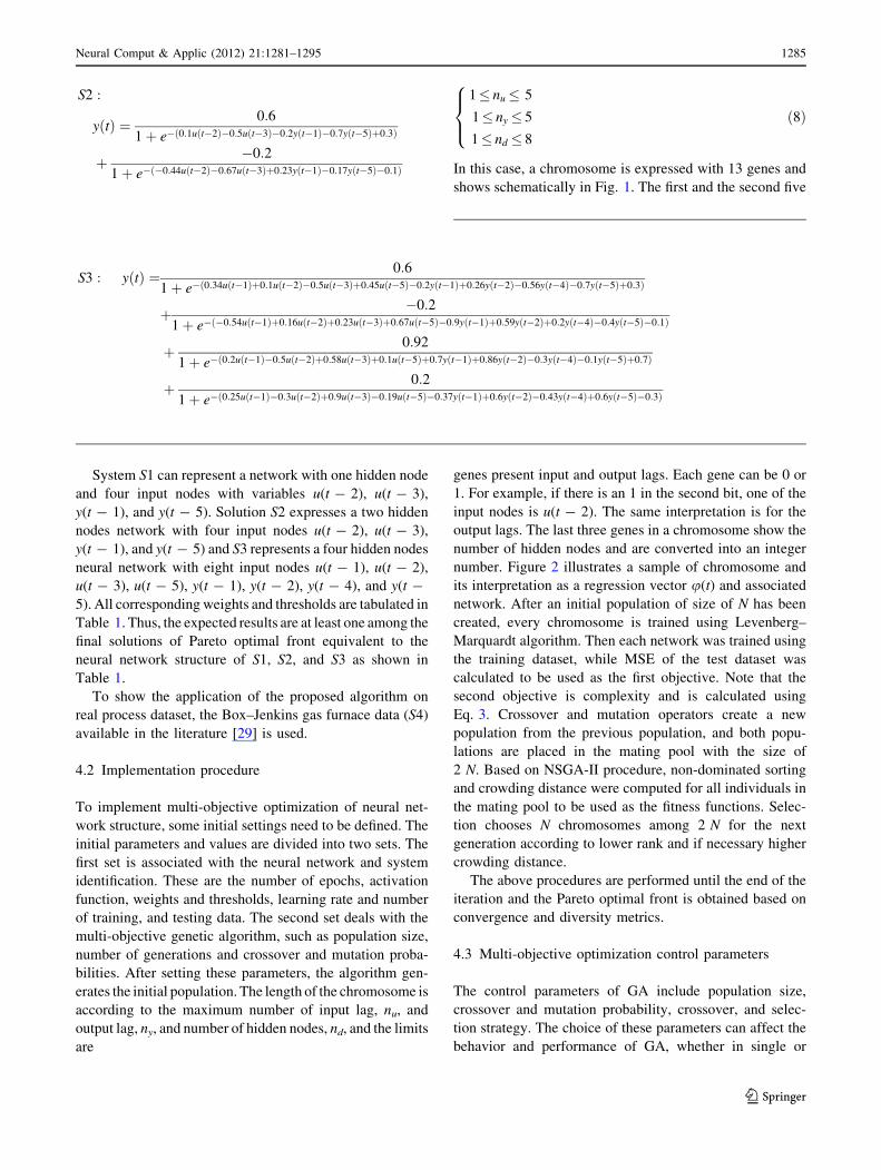
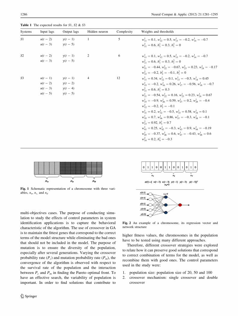
In this case, a chromosome is expressed with 13 genes and

shows schematically in Fig. 1. The first and the second five

genes present input and output lags. Each gene can be 0 or

1. For example, if there is an 1 in the second bit, one of the

input nodes is u(t - 2). The same interpretation is for the

output lags. The last three genes in a chromosome show the

number of hidden nodes and are converted into an integer

number. Figure 2 illustrates a sample of chromosome and

its interpretation as a regression vector u(t) and associated

network. After an initial population of size of N has been

created, every chromosome is trained using Levenberg–

Marquardt algorithm. Then each network was trained using

the training dataset, while MSE of the test dataset was

calculated to be used as the first objective. Note that the

second objective is complexity and is calculated using

Eq. 3. Crossover and mutation operators create a new

population from the previous population, and both popu-

lations are placed in the mating pool with the size of

2 N. Based on NSGA-II procedure, non-dominated sorting

and crowding distance were computed for all individuals in

the mating pool to be used as the fitness functions. Selec-

tion chooses N chromosomes among 2 N for the next

generation according to lower rank and if necessary higher

crowding distance.

The above procedures are performed until the end of the

iteration and the Pareto optimal front is obtained based on

convergence and diversity metrics.

4.3 Multi-objective optimization control parameters

The control parameters of GA include population size,

crossover and mutation probability, crossover, and selec-

tion strategy. The choice of these parameters can affect the

behavior and performance of GA, whether in single or

S3 : yðtÞ ¼ 0:6

1þ e�ð0:34uðt�1Þþ0:1uðt�2Þ�0:5uðt�3Þþ0:45uðt�5Þ�0:2yðt�1Þþ0:26yðt�2Þ�0:56yðt�4Þ�0:7yðt�5Þþ0:3Þ

þ �0:2

1þ e�ð�0:54uðt�1Þþ0:16uðt�2Þþ0:23uðt�3Þþ0:67uðt�5Þ�0:9yðt�1Þþ0:59yðt�2Þþ0:2yðt�4Þ�0:4yðt�5Þ�0:1Þ

þ 0:92

1þ e�ð0:2uðt�1Þ�0:5uðt�2Þþ0:58uðt�3Þþ0:1uðt�5Þþ0:7yðt�1Þþ0:86yðt�2Þ�0:3yðt�4Þ�0:1yðt�5Þþ0:7Þ

þ 0:2

1þ e�ð0:25uðt�1Þ�0:3uðt�2Þþ0:9uðt�3Þ�0:19uðt�5Þ�0:37yðt�1Þþ0:6yðt�2Þ�0:43yðt�4Þþ0:6yðt�5Þ�0:3Þ

Neural Comput & Applic (2012) 21:1281–1295 1285

123

multi-objectives cases. The purpose of conducting simu-

lation to study the effects of control parameters in system

identification applications is to capture the behavioral

characteristic of the algorithm. The use of crossover in GA

is to maintain the fittest genes that correspond to the correct

terms of the model structure while eliminating the bad ones

that should not be included in the model. The purpose of

mutation is to ensure the diversity of the population,

especially after several generations. Varying the crossover

probability rate (Pc) and mutation probability rate (Pm), the

convergence of the algorithm is observed with respect to

the survival rate of the population and the interaction

between Pc and Pm in finding the Pareto optimal front. To

have an effective search, the variability of population is

important. In order to find solutions that contribute to

higher fitness values, the chromosomes in the population

have to be tested using many different approaches.

Therefore, different crossover strategies were explored

to relate how it can preserve good solutions that correspond

to correct combination of terms for the model, as well as

recombine them with good ones. The control parameters

used in the study were:

1. population size: population size of 20, 50 and 100

2. crossover mechanism: single crossover and double

crossover

Table 1 The expected results for S1, S2 & S3

Systems Input lags Output lags Hidden neuron Complexity Weights and thresholds

S1 u(t - 2)

u(t - 3)

y(t - 1)

y(t - 5)

1 5 w111 ¼ 0:1; w1

12 ¼ 0:5; w113 ¼ �0:2; w1

14 ¼ �0:7

w211 ¼ 0:6; b1

1 ¼ 0:3; b21 ¼ 0

S2 u(t - 2)

u(t - 3)

y(t - 1)

y(t - 5)

2 6 w111 ¼ 0:1; w1

12 ¼ 0:5; w113 ¼ �0:2; w1

14 ¼ �0:7

w211 ¼ 0:6; b1

1 ¼ 0:3; b21 ¼ 0

w121 ¼ �0:44; w1

22 ¼ �0:67; w123 ¼ 0:23; w1

24 ¼ �0:17

w212 ¼ �0:2; b1

2 ¼ �0:1; b21 ¼ 0

S3 u(t - 1)

u(t - 2)

u(t - 3)

u(t - 5)

y(t - 1)

y(t - 2)

y(t - 4)

y(t - 5)

4 12 w111 ¼ 0:34; w1

12 ¼ 0:1; w113 ¼ �0:5; w1

14 ¼ 0:45

w115 ¼ �0:2; w1

16 ¼ 0:26; w117 ¼ �0:56; w1

18 ¼ �0:7

w211 ¼ 0:6; b1

1 ¼ 0:3

w121 ¼ �0:54; w1

22 ¼ 0:16; w123 ¼ 0:23; w1

24 ¼ 0:67

w115 ¼ �0:9; w1

26 ¼ 0:59; w127 ¼ 0:2; w1

28 ¼ �0:4

w212 ¼ �0:2; b1

2 ¼ �0:1

w131 ¼ 0:2; w1

32 ¼ �0:5; w133 ¼ 0:58; w1

34 ¼ 0:1

w135 ¼ 0:7; w1

36 ¼ 0:86; w137 ¼ �0:3; w1

38 ¼ �0:1

w213 ¼ 0:92; b1

3 ¼ 0:7

w141 ¼ 0:25; w1

42 ¼ �0:3; w143 ¼ 0:9; w1

44 ¼ �0:19

w145 ¼ �0:37; w1

46 ¼ 0:6; w147 ¼ �0:43; w1

48 ¼ 0:6

w214 ¼ 0:2; b1

4 ¼ �0:3

Fig. 1 Schematic representation of a chromosome with three vari-

ables, nu, ny, and nd

Fig. 2 An example of a chromosome, its regression vector and

network structure

1286 Neural Comput & Applic (2012) 21:1281–1295

123

3. crossover probabilities: probabilities of 0.05, 0.3, 0.6,

0.9

4. mutation probabilities: probabilities of 0.001, 0.01,

0.1.

4.3.1 Population size

To study the effect of varying population size, the other

control parameters were fixed with the number of genera-

tions 50, Pc was 0.6 and Pm was 0.01. System S3 was

studied (because it is more complex) and after 50 itera-

tions, the metrics of convergence and diversity for 20, 50

and 100 population sizes are shown in Figs. 3 and 4. The

convergence for 20 population size is faster than the others,

but the diversity metrics for all populations converged. For

a small number of populations, most of the highly superior

individuals dominate the population towards the later

generation giving them the chance of being selected for the

next generation. The disadvantage is that there will be a

chance of not selecting the better solution within the whole

population thus resulting in a poor exploration. For further

investigation, the algorithm was applied 50 times for all

three population sizes and the solutions in the last gener-

ations were investigated. The results show that, in some

attempts for population size of 20, the expected solution

was not among the non-dominated solutions. While for

sizes of 50 and 100 in all attempts, the expected solutions

(mentioned in Table 1) existed. Thus, it seems that the

population size of 50 is the best choice for this study and

increasing to 100 is not necessary.

4.3.2 Crossover and mutation

By varying the crossover probability rate, Pc, and mutation

probability rate, Pm, the performance of the algorithm was

observed. The population size was set to 50 and the number

of generations was set to 50. The effect of different

crossover strategies was also investigated. The metrics to

evaluate the results are the convergence and diversity

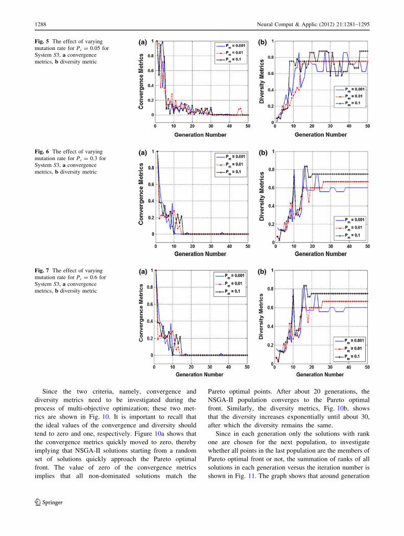
preservation. Figure 5 shows the metrics for various Pm

with crossover probability of 0.05. The convergence occurs

around generation 30 for all Pm, but the diversity for

Pm = 0.01 is more stable than the other cases.

Increasing Pc to 0.3 indicates better results in both

metrics (Fig. 6). The convergence to zero is faster and the

diversity metrics are more stable. Figure 7 shows the

results for Pc = 0.6. The figure clearly shows the reduction

in diversities of Pareto optimal front for different mutation

probabilities.

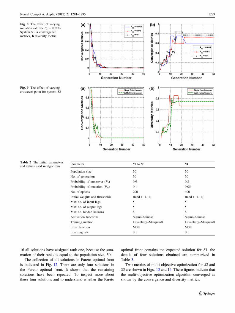
Finally, after increasing Pc to 0.9, there are similarities

in convergences for different mutation probabilities as

shown in Fig. 8a. The second metric in Fig. 8b indicates

that in all cases convergence have occurred. However,

none of them has converged to the ideal value of one like

the previous cases.

The above results indicate that there are no specific rules

for values Pc and Pm and these values have to be chosen by

trial and error. However, Pm = 0.1 produced a better result

among the others. Although, the crossover probability of

0.3 and 0.9 has shown acceptable performances, but

Fig. 8b shows more reliable convergence for all mutation

probability values than Fig. 6b.

To investigate the effect of varying crossover strategy,

single and double point crossovers were considered. Using

the above results, Pc and Pm were chosen 0.9 and 0.1,

respectively. Figure 9 shows the convergence (a) and

diversity metrics (b) for the multi-objective optimization of

neural network structure using NSGA-II with these two

crossover strategies. The result shows that a double cross-

over strategy slightly gives better diversity preservation.

The above tests were applied to all three simulated

systems and real process data of case studies and the results

are summarized in Table 2.

4.4 Case studies of S1, S2, and S3

To model the data generated by S1 until S3 and optimi-

zation of the model structure, the initial parameters as

summarized in Table 2 were used.

Fig. 3 The effect of varied population size on convergence, S3

Fig. 4 The effect of varied population size on diversity, S3

Neural Comput & Applic (2012) 21:1281–1295 1287

123

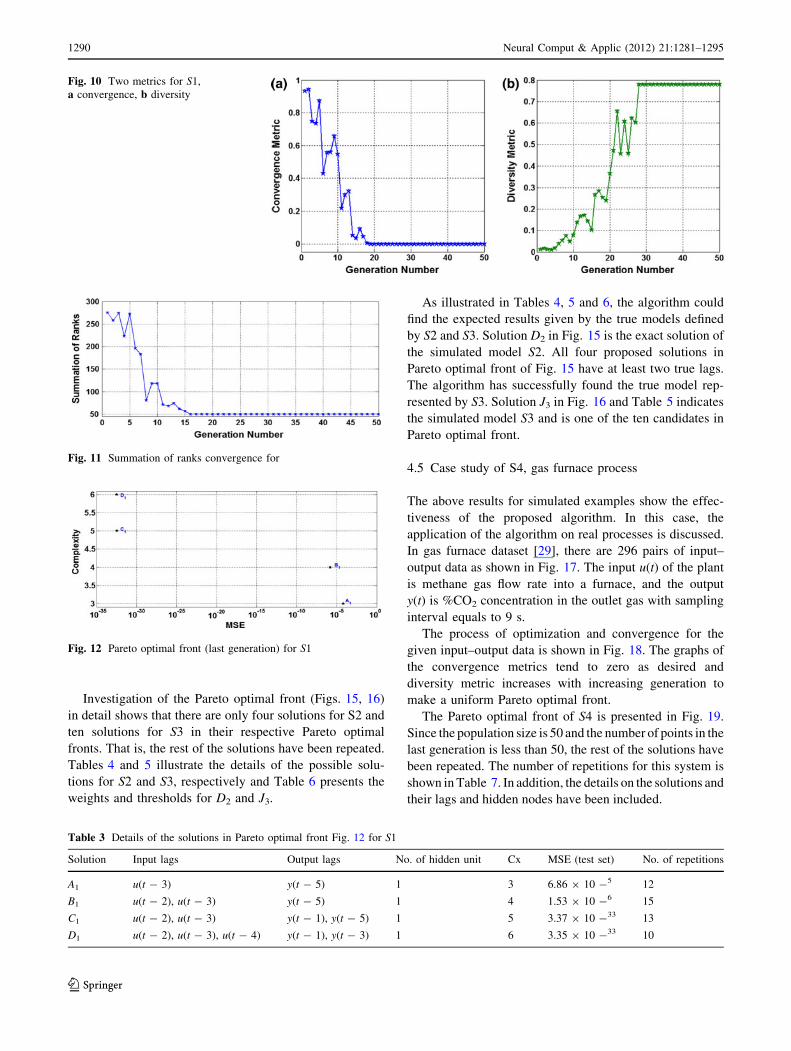
Since the two criteria, namely, convergence and

diversity metrics need to be investigated during the

process of multi-objective optimization; these two met-

rics are shown in Fig. 10. It is important to recall that

the ideal values of the convergence and diversity should

tend to zero and one, respectively. Figure 10a shows that

the convergence metrics quickly moved to zero, thereby

implying that NSGA-II solutions starting from a random

set of solutions quickly approach the Pareto optimal

front. The value of zero of the convergence metrics

implies that all non-dominated solutions match the

Pareto optimal points. After about 20 generations, the

NSGA-II population converges to the Pareto optimal

front. Similarly, the diversity metrics, Fig. 10b, shows

that the diversity increases exponentially until about 30,

after which the diversity remains the same.

Since in each generation only the solutions with rank

one are chosen for the next population, to investigate

whether all points in the last population are the members of

Pareto optimal front or not, the summation of ranks of all

solutions in each generation versus the iteration number is

shown in Fig. 11. The graph shows that around generation

Fig. 5 The effect of varying

mutation rate for Pc = 0.05 for

System S3, a convergence

metrics, b diversity metric

Fig. 6 The effect of varying

mutation rate for Pc = 0.3 for

System S3, a convergence

metrics, b diversity metric

Fig. 7 The effect of varying

mutation rate for Pc = 0.6 for

System S3, a convergence

metrics, b diversity metric

1288 Neural Comput & Applic (2012) 21:1281–1295

123

16 all solutions have assigned rank one, because the sum-

mation of their ranks is equal to the population size, 50.

The collection of all solutions in Pareto optimal front

is indicated in Fig. 12. There are only four solutions in

the Pareto optimal front. It shows that the remaining

solutions have been repeated. To inspect more about

these four solutions and to understand whether the Pareto

optimal front contains the expected solution for S1, the

details of four solutions obtained are summarized in

Table 3.

Two metrics of multi-objective optimization for S2 and

S3 are shown in Figs. 13 and 14. These figures indicate that

the multi-objective optimization algorithm converged as

shown by the convergence and diversity metrics.

Fig. 8 The effect of varying

mutation rate for Pc = 0.9 for

System S3, a convergence

metrics, b diversity metric

Fig. 9 The effect of varying

crossover point for system S3

Table 2 The initial parameters

and values used in algorithmParameter S1 to S3 S4

Population size 50 50

No. of generation 50 50

Probability of crossover (Pc) 0.9 0.8

Probability of mutation (Pm) 0.1 0.05

No. of epochs 200 400

Initial weights and thresholds Rand (-1, 1) Rand (-1, 1)

Max no. of input lags 5 5

Max no. of output lags 5 5

Max no. hidden neurons 8 8

Activation functions Sigmoid-linear Sigmoid-linear

Training method Levenberg–Marquardt Levenberg–Marquardt

Error function MSE MSE

Learning rate 0.1 0.1

Neural Comput & Applic (2012) 21:1281–1295 1289

123

Investigation of the Pareto optimal front (Figs. 15, 16)

in detail shows that there are only four solutions for S2 and

ten solutions for S3 in their respective Pareto optimal

fronts. That is, the rest of the solutions have been repeated.

Tables 4 and 5 illustrate the details of the possible solu-

tions for S2 and S3, respectively and Table 6 presents the

weights and thresholds for D2 and J3.

As illustrated in Tables 4, 5 and 6, the algorithm could

find the expected results given by the true models defined

by S2 and S3. Solution D2 in Fig. 15 is the exact solution of

the simulated model S2. All four proposed solutions in

Pareto optimal front of Fig. 15 have at least two true lags.

The algorithm has successfully found the true model rep-

resented by S3. Solution J3 in Fig. 16 and Table 5 indicates

the simulated model S3 and is one of the ten candidates in

Pareto optimal front.

4.5 Case study of S4, gas furnace process

The above results for simulated examples show the effec-

tiveness of the proposed algorithm. In this case, the

application of the algorithm on real processes is discussed.

In gas furnace dataset [29], there are 296 pairs of input–

output data as shown in Fig. 17. The input u(t) of the plant

is methane gas flow rate into a furnace, and the output

y(t) is %CO2 concentration in the outlet gas with sampling

interval equals to 9 s.

The process of optimization and convergence for the

given input–output data is shown in Fig. 18. The graphs of

the convergence metrics tend to zero as desired and

diversity metric increases with increasing generation to

make a uniform Pareto optimal front.

The Pareto optimal front of S4 is presented in Fig. 19.

Since the population size is 50 and the number of points in the

last generation is less than 50, the rest of the solutions have

been repeated. The number of repetitions for this system is

shown in Table 7. In addition, the details on the solutions and

their lags and hidden nodes have been included.

Fig. 10 Two metrics for S1,

a convergence, b diversity

Fig. 11 Summation of ranks convergence for

Fig. 12 Pareto optimal front (last generation) for S1

Table 3 Details of the solutions in Pareto optimal front Fig. 12 for S1

Solution Input lags Output lags No. of hidden unit Cx MSE (test set) No. of repetitions

A1 u(t - 3) y(t - 5) 1 3 6.86 9 10 -5 12

B1 u(t - 2), u(t - 3) y(t - 5) 1 4 1.53 9 10 -6 15

C1 u(t - 2), u(t - 3) y(t - 1), y(t - 5) 1 5 3.37 9 10 -33 13

D1 u(t - 2), u(t - 3), u(t - 4) y(t - 1), y(t - 3) 1 6 3.35 9 10 -33 10

1290 Neural Comput & Applic (2012) 21:1281–1295

123

4.5.1 Trade-off

It is important to note that A4, B4, C4, D4, and E4 are not

superior or inferior to each other. For instance, B4 is better

than A4 in the first objective, MSE, but is worse in the second

objective (complexity). One trade-off among the solutions

A4, B4, C4, D4, and E4 in Table 7 is that point A4 and B4 have

large errors compared with the others. Although, E4 has the

smallest error among C4, D4, and E4, but the difference is not

too much (0.002 between D4 and E4 and 0.005 between C4

and E4), while it has more complexity compare with D4 and

C4. Thus, the selection should be done between C4 and D4.

Model validity test such as the correlation tests may helps us

to find the better solution between C4 and D4. Figures 20 and

21 show the correlation tests for solution C4 and D4,

respectively. Figure 20 indicates that all correlation func-

tions fall within the confidence bands except uee for C4, while

all the correlation tests were satisfied for D4 as shown in

Fig. 21. Thus, it seems that D4 could be an adequate model

for the gas furnace data.

4.6 Summary and discussion

The proposed algorithm has been applied on the data,

generated by three simulated system. There were several

points in the Pareto optimal front of each system. Since

these simulated systems represent the multi-layer percep-

tron network exactly, at least one of the non-dominated

solutions in the Pareto optimal front is exactly the same as

the simulated model with the same weights, thresholds,

input and output lags, and hidden nodes. Thus, in S1, S2

and S3 the results showed the effectiveness of the proposed

algorithm.

Fig. 13 Two metrics for S2,

a convergence, b diversity

Fig. 14 Two metrics for S3,

a convergence, b diversity

Fig. 15 Pareto optimal front (last generation) for S2

Fig. 16 Pareto optimal front (last generation) for S3

Neural Comput & Applic (2012) 21:1281–1295 1291

123

Gas furnace dataset was chosen from literature to show

the application of the algorithm. There was no prior

knowledge about the number of lags to help designers to

make a final decision. The correlation of MSE and com-

plexity and correlation test can be the basis to choose the

final solution.

In this study, only one hidden layer has been considered.

A more complex neural network structure with more than

one hidden layers will require re-definition of the chro-

mosomes in the algorithm and more extensive computation

would be involved. The procedure remains the same and

similar modeling results are expected as the optimization

Table 4 Details of the solutions in Pareto optimal front Fig. 15, S2

Solution Input lags Output lags No. of hidden unit Cx MSE (test set) No. of repetitions

A2 u(t - 2) y(t - 1) 1 3 4.00 9 10-4 16

B2 u(t - 2), u(t - 3) y(t - 5) 1 4 1.30 9 10-6 16

C2 u(t - 2), u(t - 3) y(t - 1), y(t - 5) 1 5 2.61 9 10-7 16

D2 u(t - 2), u(t - 3) y(t - 1), y(t - 3) 2 6 7.48 9 10-27 2

Table 5 Details of the solutions in Pareto optimal front Fig. 16, S3

Solution Input lags Output lags No. of hidden unit Cx MSE (test set) No. of

repetitions

A3 u(t - 1) y(t - 2) 1 3 1.46 9 10-3 10

B3 u(t - 1), u(t - 2) y(t - 2) 1 4 3.57 9 10-4 11

C3 u(t - 1), u(t - 2), u(t - 3) y(t - 2) 1 5 1.50 9 10-4 14

D3 u(t - 1), u(t - 2), u(t - 3) y(t - 1) 2 6 1.00 9 10-4 2

E3 u(t - 1), u(t - 2), u(t - 3), u(t - 5) y(t - 2) 2 7 4.82 9 10-5 2

F3 u(t - 1), u(t - 2), u(t - 3), u(t - 5) y(t - 2) 3 8 2.99 9 10-5 3

G3 u(t - 1), u(t - 2), u(t - 3), u(t - 5) y(t - 2), y(t - 4) 3 9 2.41 9 10-5 3

H3 u(t - 1), u(t - 2), u(t - 3), u(t - 5) y(t - 2), y(t - 4), y(t - 5) 3 10 5.00 9 10-6 2

I3 u(t - 1), u(t - 2), u(t - 3), u(t - 5) y(t - 1), y(t - 2), y(t - 4), y(t - 5) 3 11 1.44 9 10-6 1

J3 u(t - 1), u(t - 2), u(t - 3), u(t - 5) y(t - 1), y(t - 2), y(t - 4), y(t - 5) 4 12 6.91 9 10-25 2

Table 6 Connection values for D2 and J3

Solution Weights Thresholds

D2 w111 ¼ 0:1; w1

12 ¼ �0:5; w113 ¼ �0:2; w1

14 ¼ �0:7

w211 ¼ 0:6; b1

1 ¼ 0:3; b12 ¼ 0

w121 ¼ �0:44; w1

22 ¼ �0:67; w123 ¼ 0:23; w1

24 ¼ �0:17

w121 ¼ �0:2; b1

2 ¼ �0:1; b21 ¼ 0

b11 ¼ 0:3; b1

2 ¼ 0:1

b21 ¼ 0:2

J3 w111 ¼ 0:34; w1

12 ¼ 0:1; w113 ¼ �0:5; w1

14 ¼ 0:45; w115 ¼ �0:2; w1

16 ¼ 0:26; w117 ¼ �0:56; w1

18 ¼ �0:7

w111 ¼ 0:6

w121 ¼ �0:54; w1

22 ¼ 0:16; w123 ¼ 0:23; w1

24 ¼ 0:67; w115 ¼ �0:9; w1

26 ¼ 0:59; w127 ¼ 0:2; w1

28 ¼ �0:4

w212 ¼ �0:2

w131 ¼ 0:2; w1

32 ¼ �0:5; w133 ¼ 0:58; w1

34 ¼ 0:1; w135 ¼ 0:7; w1

36 ¼ 0:86; w137 ¼ �0:3; w1

38 ¼ �0:1

w213 ¼ 0:92

w141 ¼ �0:25; w1

42 ¼ 0:3; w143 ¼ �0:9; w1

44 ¼ 0:19; w145 ¼ 0:37; w1

46 ¼ �0:6; w147 ¼ 0:43; w1

48 ¼ �0:6

w214 ¼ �0:2

b11 ¼ 0:3

b12 ¼ �0:1

b13 ¼ 0:7

b14 ¼ 0:3

b21 ¼ 0:2

1292 Neural Comput & Applic (2012) 21:1281–1295

123

procedures are still the same, but performance such as

convergence rate might be affected.

5 Conclusion

A multi-objective genetic algorithm method, the elitist non-

dominated sorting genetic algorithm (NSGA-II), has been

proposed and investigated to optimize the neural network

structure for modeling dynamic systems. The objective

functions used are the complexity of the neural network

Fig. 17 Input and output data

for S4

Fig. 18 Two metrics for S4,

a convergence, b diversity

Fig. 19 Pareto optimal front (last generation) for S4, gas furnace data

Table 7 Details of the solutions in Pareto optimal front Fig. 19, S4

Solution Input lags Output lags No. of hidden unit Cx MSE (test set) No. of repetitions

A4 u(t - 3) y(t - 1) 1 3 4.12 9 10-1 8

B4 u(t - 2) y(t - 1), y(t - 2) 1 4 1.63 9 10-1 12

C4 u(t - 2) y(t - 1), y(t - 2), y(t - 4) 1 5 1.41 9 10-1 9

D4 u(t - 2) y(t - 1), y(t - 2), y(t - 4) 2 6 1.38 9 10-1 11

E4 u(t - 2) y(t - 1), y(t - 2), y(t - 4) 3 7 1.36 9 10-1 10

Neural Comput & Applic (2012) 21:1281–1295 1293

123

architecture and mean square error of the test set which are

minimized simultaneously. The proposed method has been

shown to be effective in identifying the correct structure of

the system using two objective functions for three neural

network simulated systems. Then the algorithm was applied

to a real process data. There is more than one possible

solution in multi-objective optimization problems. Trade-off

among the possible solutions in Pareto optimal and correla-

tion tests can help designers to select the final solution.

References

1. Hagan MT, Demuth MT, Beale MH (1996) Neural network

design. PWS Publishing, Boston

2. Billings SA, Jamaluddin H, Chen S (1992) Properties of neural

networks with applications to modeling non-linear dynamical

systems. Int J Control 55(1):193–224

3. Chen S, Billings SA, Grant PM (1990) Non-linear system iden-

tification using neural networks. Int J Control 51(6):1191–1214

4. Xua KJ, Zhang J, Wang XF, Teng Q, Tan J (2008) Improvements

of nonlinear dynamic modeling of hot-film MAF sensor. Sens

Actuators A 147:34–40

5. Caruana R, Lawrence S, Giles CL (2001) Overfitting in neural

networks: backpropagation, conjugate gradient, and early stop-

ping. Adv Neural Inf Process Syst 13:402–408

6. Bebis G, Georgiopoulos M (1994) Feed-forward neural networks:

why network size is so important. IEEE Potentials 13(4):27–31

7. Sietsma J, Dow RJF (1988) Neural net pruning—why and how.

In: Proceedings of the IEEE international conference on neural

networks, San Diego, pp 325–333

8. Ahmad R, Jamaluddin H, Hussain MA (2004) Model structure

selection for discrete-time nonlinear systems using genetic

algorithm. J Syst Control Eng 218(12):85–98

Fig. 20 Correlation test for

solution C4 of S4

Fig. 21 Correlation test for

solution D4 of S4

1294 Neural Comput & Applic (2012) 21:1281–1295

123

9. SK Oh, Pedrycz W (2006) Genetic optimization driven multi

layer hybrid fuzzy neural networks. Simul Model Pract Theory

14:597–613

10. Park KJ, Pedrycz W, Oh SK (2007) A genetic approach to

modeling fuzzy systems based on information granulation and

successive generation-based evolution method. Simul Model

Pract Theory 15:1128–1145

11. Koza YJR, Rice JP (1991) Genetic generation of both the weights

and architecture for a neural network. In: IEEE international joint

conference on neural networks, vol 2. IEEE Press, Seattle,

pp 397–404

12. Deb K (2001) Multi-objective optimization using evolutionary

algorithms. Wiley, Chichester

13. Schaffer JD (2011) Some experiments in machine learning using

vector evaluated genetic algorithm. Ph.D Thesis, Vanderbilt

University, Nashville, TN

14. Fonseca CM, Fleming PJ (1993) Genetic algorithms for multi-

objective optimization: formulation, discussion and generalisa-

tion. In: Proceedings of the fifth international conference on

genetic algorithms, Morgan Kaufman, San Mateo, pp 416–423

15. Srinivas N, Deb K (1994) Multi-objective optimization using

non-dominated sorting in genetic algorithms. Evol Comput

2(3):221–248

16. Fieldsend JE, Singh S (2005) Pareto evolutionary neural net-

works. IEEE Trans Neural Netw 16(2):338–354

17. Abbass HA (2003) Speeding up backpropagation using multi-

objective evolutionary algorithms. Neural Comput 15(11):2705–

2726

18. Sexton RS, Dorsey RE, Sikander NA (2004) Simultaneous opti-

mization of neural network function and architecture algorithm.

Decis Support Syst 36:283–296

19. Gonzalez J, Rojas I, Ortega J, Pomares H, Fernandez J, Diaz A

(2003) Multi-objective evolutionary optimization of the size,

shape, and position parameters of radial basis function networks

for function approximation. IEEE Trans Neural Netw

14(1):1478–1495

20. Palmes S (2005) Robustness, evolvability and optimality in

evolutionary neural networks. Biosystems 82(2):168–188

21. Mandal D, Pal SK, Sah P (2007) Modeling of electrical discharge

machining process using back propagation neural network and

multi-objective optimization using non-dominating sorting

genetic algorithm-II. J Mater Process Technol 186:154–162

22. Sexton RS, Dorsey RE, Johnson JD (1999) Optimization of

neural networks: a comparative analysis of the genetic algorithm

and simulated annealing. Eur J Oper Res 114:589–601

23. Ljung L (1999) System identification, theory for the user, 2nd

edn. Prentice-Hall, Englewood Cliffs

24. Ibnkahla M (2003) Nonlinear system identification using neural

networks trained with natural gradient descent. EURASIP J Appl

Signal Process 12:1229–1237

25. Funahashi K (1989) On the approximate realization of continuous

mappings by neural networks. Neural Netw 2:183–192

26. Norgaard MRO, Poulsen NK, Hansen LK (2000) Neural net-

works for modeling and control of dynamic systems. A practi-

tioner’s handbook. Springer, London

27. Zitzler E, Deb K, Thiele L (2000) Comparison of multi-objective

evolutionary algorithm: empirical results. Evol Comput

8:173–195

28. Billings SA, Voon WSF (1986) Correlation based model validity

tests for non-linear models. Int J Control 44(1):235–244

29. Box GEP, Jenkins GM, Reinsel GC (1994) Time series analysis

forecasting and control. Prentice-Hall Inc, Englewood Cliffs

Neural Comput & Applic (2012) 21:1281–1295 1295

123