Technical ReportNumber 571

Computer Laboratory

UCAM-CL-TR-571ISSN 1476-2986

Multi-layer network monitoring andanalysis

James Hall

July 2003

15 JJ Thomson AvenueCambridge CB3 0FDUnited Kingdomphone +44 1223 763500

http://www.cl.cam.ac.uk/

c© 2003 James Hall

This technical report is based on a dissertation submitted April2003 by the author for the degree of Doctor of Philosophy to theUniversity of Cambridge, King’s College.

Some figures in this document are best viewed in colour. If youreceived a black-and-white copy, please consult the online versionif necessary.

Technical reports published by the University of CambridgeComputer Laboratory are freely available via the Internet:

http://www.cl.cam.ac.uk/TechReports/

Series editor: Markus Kuhn

ISSN 1476-2986

AbstractPassive network monitoring offers the possibility of gathering a wealth of data about the traffictraversing the network and the communicating processes generating that traffic. Significantadvantages include the non-intrusive nature of data capture and the range and diversity of thetraffic and driving applications which may be observed. Conversely there are also associatedpractical difficulties which have restricted the usefulness of the technique: increasing networkbandwidths can challenge the capacity of monitors to keep pace with passing traffic withoutdata loss, and the bulk of data recorded may become unmanageable.

Much research based upon passive monitoring has in consequence been limited to that usinga sub-set of the data potentially available, typically TCP/IP packet headers gathered usingTcpdump or similar monitoring tools. The bulk of data collected is thereby minimised, andwith the possible exception of packet filtering, the monitor’s available processing power isavailable for the task of collection and storage. As the data available for analysis is drawnfrom only a small section of the network protocol stack, detailed study is largely confined tothe associated functionality and dynamics in isolation from activity at other levels. Such lackof context severely restricts examination of the interaction between protocols which may inturn lead to inaccurate or erroneous conclusions.

The work described in this dissertation attempts to address some of these limitations. Anew passive monitoring architecture — Nprobe — is presented, based upon ‘off the shelf’components and which, by using clusters of probes, is scalable to keep pace with current highbandwidth networks without data loss. Monitored packets are fully captured, but are subjectto the minimum processing in real time needed to identify and associate data of interest acrossthe target set of protocols. Only this data is extracted and stored. The data reduction ratiothus achieved allows examination of a wider range of encapsulated protocols without strainingthe probe’s storage capacity.

Full analysis of the data harvested from the network is performed off-line. The activity ofinterest within each protocol is examined and is integrated across the range of protocols,allowing their interaction to be studied. The activity at higher levels informs study of thelower levels, and that at lower levels infers detail of the higher. A technique for dynamicallymodelling TCP connections is presented, which, by using data from both the transport andhigher levels of the protocol stack, differentiates between the effects of network and end-process activity.

The balance of the dissertation presents a study of Web traffic using Nprobe. Data collectedfrom the IP, TCP, HTTP and HTML levels of the stack is integrated to identify the patternsof network activity involved in downloading whole Web pages: by using the links containedin HTML documents observed by the monitor, together with data extracted from the HTMLheaders of downloaded contained objects, the set of TCP connections used, and the way inwhich browsers use them, are studied as a whole. An analysis of the degree and distributionof delay is presented and contributes to the understanding of performance as perceived by theuser. The effects of packet loss on whole page download times are examined, particularly thoselosses occurring early in the lifetime of connections before reliable estimations of round triptimes are established. The implications of such early packet losses for pages downloads usingpersistent connections are also examined by simulations using the detailed data available.

5

Acknowledgements

I must firstly acknowledge the very great contribution made by Micromuse Ltd., withoutwhose financial support for three years it would not have been possible for me to undertakethe research leading to this dissertation, and to the Computer Laboratory whose furthersupport allowed me to complete it.

Considerable thanks is due to my supervisor, Ian Leslie, for procuring my funding, for hisadvice and encouragement, his reading and re-reading of the many following chapters, hissuggestions for improvement and, perhaps above all, his gift for identifying central issues onthe occasions when I have become bogged down in the minutiae. Thanks also to Ian Prattwho is responsible for many of the concepts underlying the Nprobe monitor, and who hasbeen an invaluable source of day-to–day and practical advice and guidance.

Although the work described here has been largely an individual undertaking, it could nothave proceeded satisfactorily without the background of expertise, discussion, imaginativeideas and support provided by my past and present colleagues in the Systems Research Group.Special mention must be made of Derek McAuley who initially employed me, of Simon Cosby,who encouraged me to make the transition from research assistant to PhD student, and ofJames Bulpin for his ever-willing help in the area of system administration: to them, to SteveHand, Tim Harris, Keir Fraser, Jon Crowcroft, Dickon Reed, Andrew Moore, and to all theothers, I am greatly indebted.

Many others in the wider community of the Computer Laboratory and University ComputingService have also made a valuable contribution: to Margaret Levitt for her encouragementover the years, to Chris Cheney and Phil Cross for their assistance in providing monitoringfacilities, to Martyn Johnson and Piete Brookes for accommodating unusual demands uponthe Laboratory’s systems, and to many others, I offer my thanks.

Thank you to those who have rendered assistance in proof-reading the final draft of thisdissertation: to Anna Hamilton, and to some of those mentioned above — you know who youare.

Very special love and thanks goes to my wife, Jenny, whose continual encouragement andsupport has underpinned all of my efforts. She has taken on a vastly disproportionate shareof our domestic and child-care tasks, despite her own work, and has endured much undeservedneglect to allow me to concentrate on my work. My love and a big thank-you also go to Charlieand Sam who have seen very much less of their daddy than they have deserved, and to Joand Luke, ‘my boys’, with whom I have recently sunk fewer pints than I should.

Finally, the role of an unlikely player deserves note. In the early 1980’s I was unwillinglyconscripted into the ranks of Maggie’s army — the hundreds of thousands made unemployedin one of the cruelest and most regressive pieces of social engineering ever to be inflicted uponthis country. For many it spelled unemployment for the remainder of their working lives.With time on my hands I embarked upon an Open University degree, the first step on a pathwhich lead to the Computer Laboratory, the Diploma in Computer Science, and eventuallyto the writing of this dissertation — I was one of the fortunate ones.

7

Table of Contents

1 Introduction 21

2 Background and Related Work 31

3 The Nprobe Architecture 45

4 Post-Collection Analysis of Nprobe Traces 79

5 Modelling and Simulating TCP Connections 111

6 Non-Intrusive Estimation of Web Server Delays Using Nprobe 141

7 Observation and Reconstruction of World Wide Web Page Downloads 159

8 Page Download Times and Delay 175

9 Conclusions and Scope for Future Work 193

A Class Generation with SWIG 201

B An Example of Trace File Data Retrieval 205

C Inter-Arrival Times Observed During Web Server Latency Tests 213

Bibliography 219

9

Contents

Table of Contents 7

List of Figures 14

List of Tables 16

List of Code Fragments and Examples 17

List of Acronyms 18

1 Introduction 21

1.1 Introduction . . . . . . . . . . . . . . . . . . . . . . . . . . . . . . . . . . . . . 21

1.2 Motivation . . . . . . . . . . . . . . . . . . . . . . . . . . . . . . . . . . . . . 22

1.2.1 The Value of Network Monitoring . . . . . . . . . . . . . . . . . . . . 22

1.2.2 Passive and Active Monitoring . . . . . . . . . . . . . . . . . . . . . . 22

1.2.3 Challenges in Passive Monitoring . . . . . . . . . . . . . . . . . . . . . 23

1.3 Multi-Protocol Monitoring and Analysis . . . . . . . . . . . . . . . . . . . . . 26

1.3.1 Interrelationship and Interaction of Protocols . . . . . . . . . . . . . . 26

1.3.2 Widening the Definition of a Flow . . . . . . . . . . . . . . . . . . . . 27

1.4 Towards a More Capable Monitor . . . . . . . . . . . . . . . . . . . . . . . . . 27

1.5 Aims . . . . . . . . . . . . . . . . . . . . . . . . . . . . . . . . . . . . . . . . . 29

1.6 Structure of the Dissertation . . . . . . . . . . . . . . . . . . . . . . . . . . . 29

2 Background and Related Work 31

2.1 Data Collection Tools and Probes . . . . . . . . . . . . . . . . . . . . . . . . . 31

2.2 Wide-Deployment Systems . . . . . . . . . . . . . . . . . . . . . . . . . . . . . 33

2.3 System Management and Data Repositories . . . . . . . . . . . . . . . . . . . 34

2.4 Monitoring at Ten Gigabits per Second and Faster . . . . . . . . . . . . . . . 34

2.5 Integrated and Multi-Protocol Approaches . . . . . . . . . . . . . . . . . . . . 35

2.6 Flows to Unknown Ports . . . . . . . . . . . . . . . . . . . . . . . . . . . . . . 38

2.7 Measurement Accuracy . . . . . . . . . . . . . . . . . . . . . . . . . . . . . . 39

2.8 Studies Based upon Passively Monitored Data . . . . . . . . . . . . . . . . . . 39

2.8.1 A Brief Mention of some Seminal Studies . . . . . . . . . . . . . . . . 39

2.8.2 Studies of World Wide Web Traffic and Performance . . . . . . . . . . 40

2.9 Summary . . . . . . . . . . . . . . . . . . . . . . . . . . . . . . . . . . . . . . 42

10 Contents

3 The Nprobe Architecture 453.1 Design Goals . . . . . . . . . . . . . . . . . . . . . . . . . . . . . . . . . . . . 453.2 Design Overview . . . . . . . . . . . . . . . . . . . . . . . . . . . . . . . . . . 46

3.2.1 Principal Components . . . . . . . . . . . . . . . . . . . . . . . . . . . 463.2.2 Rationale . . . . . . . . . . . . . . . . . . . . . . . . . . . . . . . . . . 48

3.3 Implementation . . . . . . . . . . . . . . . . . . . . . . . . . . . . . . . . . . . 513.3.1 Packet Capture . . . . . . . . . . . . . . . . . . . . . . . . . . . . . . . 513.3.2 Scalability . . . . . . . . . . . . . . . . . . . . . . . . . . . . . . . . . . 543.3.3 On-Line Packet Processing and Data Extraction . . . . . . . . . . . . 543.3.4 Data Output . . . . . . . . . . . . . . . . . . . . . . . . . . . . . . . . 683.3.5 Protocol Compliance and Robustness . . . . . . . . . . . . . . . . . . 693.3.6 Error Handling, Identification of Phenomena of Interest and Feedback

into the Design . . . . . . . . . . . . . . . . . . . . . . . . . . . . . . . 723.4 Trace and Monitoring Process Metadata . . . . . . . . . . . . . . . . . . . . . 733.5 Hardware and Deployment . . . . . . . . . . . . . . . . . . . . . . . . . . . . . 743.6 Probe Performance . . . . . . . . . . . . . . . . . . . . . . . . . . . . . . . . . 753.7 Security and Privacy . . . . . . . . . . . . . . . . . . . . . . . . . . . . . . . . 763.8 Summary . . . . . . . . . . . . . . . . . . . . . . . . . . . . . . . . . . . . . . 77

4 Post-Collection Analysis of Nprobe Traces 794.1 A Generic Framework for Post-Collection Data Analysis . . . . . . . . . . . . 79

4.1.1 Modularity and Task-Driven Design . . . . . . . . . . . . . . . . . . . 804.1.2 The Framework Components . . . . . . . . . . . . . . . . . . . . . . . 82

4.2 The Data Retrieval Interface . . . . . . . . . . . . . . . . . . . . . . . . . . . 844.2.1 Data Retrieval Components . . . . . . . . . . . . . . . . . . . . . . . . 844.2.2 Data Retrieval . . . . . . . . . . . . . . . . . . . . . . . . . . . . . . . 87

4.3 Data Analysis . . . . . . . . . . . . . . . . . . . . . . . . . . . . . . . . . . . . 874.3.1 Protocol Analysis Classes . . . . . . . . . . . . . . . . . . . . . . . . . 874.3.2 Discrete Protocol Analysis . . . . . . . . . . . . . . . . . . . . . . . . . 884.3.3 Protocol-Spanning Analysis — Associative Analysis Classes . . . . . . 884.3.4 Analysis Classes as Toolkit Components . . . . . . . . . . . . . . . . . 894.3.5 Accumulation of Analysis Results . . . . . . . . . . . . . . . . . . . . . 894.3.6 Memory Constraints . . . . . . . . . . . . . . . . . . . . . . . . . . . . 90

4.4 Analysis Logs, Results and Presentation . . . . . . . . . . . . . . . . . . . . . 914.4.1 An Analysis Summary Tool . . . . . . . . . . . . . . . . . . . . . . . . 924.4.2 Summaries of Analysis Results . . . . . . . . . . . . . . . . . . . . . . 92

4.5 Visualisation . . . . . . . . . . . . . . . . . . . . . . . . . . . . . . . . . . . . 934.5.1 The Data Plotter . . . . . . . . . . . . . . . . . . . . . . . . . . . . . . 934.5.2 TCP Connection and Browser Activity Visualisation . . . . . . . . . . 934.5.3 Visualisation as an Analysis Design Tool . . . . . . . . . . . . . . . . . 98

4.6 Assembling the Components . . . . . . . . . . . . . . . . . . . . . . . . . . . . 1004.7 Issues of Data Bulk, Complexity and Confidence . . . . . . . . . . . . . . . . 101

4.7.1 Data Bulk — The Anatomy of a Small Trace and Its Analysis . . . . 1014.7.2 Data and Analysis Complexity . . . . . . . . . . . . . . . . . . . . . . 1034.7.3 Determinants of Validity . . . . . . . . . . . . . . . . . . . . . . . . . . 1034.7.4 Indicators of Validity and Confidence in the Absence of Formal Proof 1044.7.5 Visualisation as an Informal Indicator of Confidence . . . . . . . . . . 105

Contents 11

4.8 An Assessment of Python as the Analysis Coding Language . . . . . . . . . . 106

4.8.1 Python and Object Orientation . . . . . . . . . . . . . . . . . . . . . . 106

4.8.2 Difficulties Associated with the Use of Python . . . . . . . . . . . . . 106

4.9 Summary . . . . . . . . . . . . . . . . . . . . . . . . . . . . . . . . . . . . . . 108

5 Modelling and Simulating TCP Connections 111

5.1 Analytical Models . . . . . . . . . . . . . . . . . . . . . . . . . . . . . . . . . 111

5.2 The Limitations of Steady State Modelling . . . . . . . . . . . . . . . . . . . 112

5.3 Characterisation of TCP Implementations and Behaviour . . . . . . . . . . . 114

5.4 Analysis of Individual TCP Connections . . . . . . . . . . . . . . . . . . . . . 116

5.5 Modelling the Activity of Individual TCP Connections . . . . . . . . . . . . . 117

5.5.1 The Model as an Event Driven Progress . . . . . . . . . . . . . . . . . 117

5.5.2 Packet Transmission and Causality . . . . . . . . . . . . . . . . . . . . 117

5.5.3 Monitor Position and Interpretation of Packet Timings . . . . . . . . . 120

5.5.4 Unidirectional and Bidirectional Data Flows . . . . . . . . . . . . . . . 122

5.5.5 Identifying and Incorporating Packet Loss . . . . . . . . . . . . . . . . 123

5.5.6 Packet Re-Ordering and Duplication . . . . . . . . . . . . . . . . . . . 125

5.5.7 Slow Start and Congestion Avoidance . . . . . . . . . . . . . . . . . . 126

5.5.8 Construction of the Activity Model . . . . . . . . . . . . . . . . . . . . 126

5.5.9 Enhancement of the Basic Data-Liberation Model . . . . . . . . . . . 130

5.5.10 The Model Output . . . . . . . . . . . . . . . . . . . . . . . . . . . . . 133

5.6 Simulation of Individual TCP Connections . . . . . . . . . . . . . . . . . . . . 133

5.6.1 Assessment of the Impact of Packet Loss . . . . . . . . . . . . . . . . . 134

5.6.2 Construction of the Simulation . . . . . . . . . . . . . . . . . . . . . . 134

5.6.3 Simulation Output . . . . . . . . . . . . . . . . . . . . . . . . . . . . . 137

5.7 Visualisation . . . . . . . . . . . . . . . . . . . . . . . . . . . . . . . . . . . . 137

5.8 Validation of Activity Models and Simulations . . . . . . . . . . . . . . . . . 137

5.9 Summary and Discussion . . . . . . . . . . . . . . . . . . . . . . . . . . . . . 138

6 Non-Intrusive Estimation of Web Server Delays Using Nprobe 141

6.1 Motivation and Experimental Method . . . . . . . . . . . . . . . . . . . . . . 141

6.2 Use of the Activity Model . . . . . . . . . . . . . . . . . . . . . . . . . . . . . 142

6.3 Assessment Using an Artificially Loaded Server . . . . . . . . . . . . . . . . . 142

6.3.1 Client and Local Server with Small Round Trip Times . . . . . . . . . 145

6.3.2 Client and Remote Server with Larger Round Trip Times . . . . . . . 147

6.3.3 HTTP/1.1 Persistent Connections . . . . . . . . . . . . . . . . . . . . 149

6.3.4 Discussion of the Experimental Results . . . . . . . . . . . . . . . . . 154

6.4 Observation of Real Web Traffic to a Single Site . . . . . . . . . . . . . . . . 154

6.5 Summary . . . . . . . . . . . . . . . . . . . . . . . . . . . . . . . . . . . . . . 156

7 Observation and Reconstruction of World Wide Web Page Downloads 159

7.1 The Desirability of Reconstructing Page Downloads . . . . . . . . . . . . . . 159

7.2 The Anatomy of a Page Download . . . . . . . . . . . . . . . . . . . . . . . . 160

7.3 Reconstruction of Page Download Activity . . . . . . . . . . . . . . . . . . . . 161

7.3.1 Limitations of Packet-Header Traces . . . . . . . . . . . . . . . . . . . 162

7.3.2 Reconstruction Using Data from Multiple Protocol Levels . . . . . . . 162

7.4 Constructing the Reference Tree . . . . . . . . . . . . . . . . . . . . . . . . . 163

12 Contents

7.4.1 Referrers, Links and Redirection . . . . . . . . . . . . . . . . . . . . . 163

7.4.2 Multiple Links, Repeated Downloads and Browser Caching . . . . . . 168

7.4.3 Aborted Downloads . . . . . . . . . . . . . . . . . . . . . . . . . . . . 168

7.4.4 Relative References, Reference Scopes and Name Caching . . . . . . . 169

7.4.5 Self-Refreshing Objects . . . . . . . . . . . . . . . . . . . . . . . . . . 169

7.4.6 Unresolved Connections and Transactions . . . . . . . . . . . . . . . . 169

7.4.7 Multiple Browser Instances and Web Cache Requests . . . . . . . . . 171

7.4.8 Timing Data . . . . . . . . . . . . . . . . . . . . . . . . . . . . . . . . 172

7.5 Integration with Name Service Requests . . . . . . . . . . . . . . . . . . . . . 172

7.6 Visualisation . . . . . . . . . . . . . . . . . . . . . . . . . . . . . . . . . . . . 173

7.7 Web Traffic Characterisation . . . . . . . . . . . . . . . . . . . . . . . . . . . 173

7.8 Summary . . . . . . . . . . . . . . . . . . . . . . . . . . . . . . . . . . . . . . 173

8 Page Download Times and Delay 175

8.1 Factors Contributing to Overall Download Times . . . . . . . . . . . . . . . . 175

8.2 The Contribution of Object Delay to Whole Page Download Times . . . . . . 176

8.2.1 Differentiating Single Object and Page Delays . . . . . . . . . . . . . . 176

8.2.2 Assessing the Degree of Delay . . . . . . . . . . . . . . . . . . . . . . . 178

8.2.3 The Distribution of Object Delay within a Page Download . . . . . . 179

8.3 The Effect of Early Packet Loss on Page Download Time . . . . . . . . . . . 180

8.4 Delay in Downloading from a Site with Massive Early Packet Loss . . . . . . 181

8.5 Comparison with a General Traffic Sample . . . . . . . . . . . . . . . . . . . . 185

8.6 Implications of Early Packet Loss for Persistent Connections . . . . . . . . . 185

8.7 Summary . . . . . . . . . . . . . . . . . . . . . . . . . . . . . . . . . . . . . . 189

9 Conclusions and Scope for Future Work 193

9.1 Summary . . . . . . . . . . . . . . . . . . . . . . . . . . . . . . . . . . . . . . 193

9.2 Assessment . . . . . . . . . . . . . . . . . . . . . . . . . . . . . . . . . . . . . 195

9.2.1 Conclusion . . . . . . . . . . . . . . . . . . . . . . . . . . . . . . . . . 196

9.2.2 The Original Contribution of this Dissertation . . . . . . . . . . . . . 197

9.3 Scope for Future Work . . . . . . . . . . . . . . . . . . . . . . . . . . . . . . . 199

9.3.1 Further Analysis of Web Activity . . . . . . . . . . . . . . . . . . . . . 199

9.3.2 Nprobe Development . . . . . . . . . . . . . . . . . . . . . . . . . . . . 200

A Class Generation with SWIG 201

A.1 Interface Definition . . . . . . . . . . . . . . . . . . . . . . . . . . . . . . . . . 201

A.2 Tailoring Data Representation in the Interface . . . . . . . . . . . . . . . . . 202

B An Example of Trace File Data Retrieval 205

B.1 A Typical Data-Reading Function . . . . . . . . . . . . . . . . . . . . . . . . 205

B.2 Use of Retrieval Interface Classes . . . . . . . . . . . . . . . . . . . . . . . . . 207

B.3 Using the FileRec Class to Minimize Memory Use . . . . . . . . . . . . . . . 209

C Inter-Arrival Times Observed During Web Server Latency Tests 213

C.1 Interpretation of Request and Response Inter-Arrival Times . . . . . . . . . . 213

C.2 Inter-Arrival Times for Client and Local Server with Small Round Trip Times 214

C.3 Inter-Arrival Times for Client and Distant Server with Larger Round Trip Times216

Contents 13

C.3.1 Using Non-Persistent Connections . . . . . . . . . . . . . . . . . . . . 216C.3.2 Using Persistent Pipelined Connections . . . . . . . . . . . . . . . . . 216

Bibliography 219

14

List of Figures

2.1 The Windmill probe architecture . . . . . . . . . . . . . . . . . . . . . . . . . 36

2.2 Control flow of the BLT tool HTTP header extraction software . . . . . . . . . 37

3.1 The principal components of Nprobe . . . . . . . . . . . . . . . . . . . . . . . 47

3.2 Nprobe scalability . . . . . . . . . . . . . . . . . . . . . . . . . . . . . . . . . 55

3.3 Generalised state storage unit arrangement. . . . . . . . . . . . . . . . . . . . 59

3.4 Nprobe data dump format . . . . . . . . . . . . . . . . . . . . . . . . . . . . . 70

4.1 Nprobe data analysis . . . . . . . . . . . . . . . . . . . . . . . . . . . . . . . . 81

4.2 Data retrieval from Nprobe trace file records . . . . . . . . . . . . . . . . . . . 86

4.3 TCP connection visualisation . . . . . . . . . . . . . . . . . . . . . . . . . . . 95

4.4 Web browser activity visualisation . . . . . . . . . . . . . . . . . . . . . . . . 97

5.1 Distribution of HTTP object sizes and number of delivery segments . . . . . . 113

5.2 Distribution of server return codes . . . . . . . . . . . . . . . . . . . . . . . . 114

5.3 Data liberations, ACK obligations, flights and rounds . . . . . . . . . . . . . . 118

5.4 Causative packet associations, lags, application-level delays and partial roundtrip times . . . . . . . . . . . . . . . . . . . . . . . . . . . . . . . . . . . . . . 121

5.5 Base, state and application-level models . . . . . . . . . . . . . . . . . . . . . 128

5.6 The effect of receiver acknowledgement strategies . . . . . . . . . . . . . . . . 131

5.7 Calculation of bottleneck bandwidths . . . . . . . . . . . . . . . . . . . . . . . 133

5.8 Growth in rounds as a result of packet loss . . . . . . . . . . . . . . . . . . . 135

6.1 Local server: load, calculated server latency and pRTT, and delay function . . 145

6.2 Local server: detail of individual server delays . . . . . . . . . . . . . . . . . . 146

6.3 Distant server: load, calculated server latency and pRTT, and delay function . 148

6.4 Distant server with pipelined requests on a persistent connection: load, calcu-lated server latency and pRTT, and delay function . . . . . . . . . . . . . . . 150

6.5 Activity on a pipelined persistent connection . . . . . . . . . . . . . . . . . . 151

6.6 Details of pipelined connection activity . . . . . . . . . . . . . . . . . . . . . . 152

6.7 News server: calculated latency and pRTT . . . . . . . . . . . . . . . . . . . 155

6.8 News server: measurement context . . . . . . . . . . . . . . . . . . . . . . . . 155

7.1 Detail of a typical page download . . . . . . . . . . . . . . . . . . . . . . . . . 164

7.2 Close detail of Figure 7.1 . . . . . . . . . . . . . . . . . . . . . . . . . . . . . 165

7.3 The complete page download . . . . . . . . . . . . . . . . . . . . . . . . . . . 166

7.4 Detail of download redirection . . . . . . . . . . . . . . . . . . . . . . . . . . . 167

7.5 A self-refreshing object . . . . . . . . . . . . . . . . . . . . . . . . . . . . . . . 170

List of Figures 15

8.1 The contribution of single object delays to overall page download time . . . . 1778.2 News server: whole page download times . . . . . . . . . . . . . . . . . . . . . 1828.3 News server: server latency and pRTTs . . . . . . . . . . . . . . . . . . . . . 1848.4 News server: components of early-loss delay . . . . . . . . . . . . . . . . . . . 1848.5 The contribution of early delay to page downloads using persistent connections 1868.6 Page download times for the pages downloaded from the news site using sim-

ulated persistent connections . . . . . . . . . . . . . . . . . . . . . . . . . . . 188

A.1 SWIG Trace file interface generation . . . . . . . . . . . . . . . . . . . . . . . 202

C.1 Local server: inter-arrival times . . . . . . . . . . . . . . . . . . . . . . . . . . 215C.2 Distant server: inter-arrival times . . . . . . . . . . . . . . . . . . . . . . . . . 217

16

List of Tables

3.1 Serialization delays for a range of packet payload sizes . . . . . . . . . . . . . 53

4.1 The anatomy of a small trace . . . . . . . . . . . . . . . . . . . . . . . . . . . 102

5.1 Principal distinctions between tcpanaly and the activity model . . . . . . . 138

6.1 Calculation of additional latency in pipelined request bursts . . . . . . . . . . 153

8.1 Summary of delays and cumulative object delays . . . . . . . . . . . . . . . . 1808.2 News site: summary of page download times . . . . . . . . . . . . . . . . . . . 1838.3 Traces 2 – 4: summary of page download times . . . . . . . . . . . . . . . . . 1898.4 News site: summary of trace and delays . . . . . . . . . . . . . . . . . . . . . 1918.5 Summary of trace and delays: Traces 2 – 4 (general Web traffic) . . . . . . . 192

17

List of Code Fragments andExamples

3.1 Encapsulation of extracted data . . . . . . . . . . . . . . . . . . . . . . . . . . 583.2 Recording variable-length data . . . . . . . . . . . . . . . . . . . . . . . . . . 603.3 Stepping through pipelined HTTP connections . . . . . . . . . . . . . . . . . . 653.4 HTML links buffer and management structures. . . . . . . . . . . . . . . . . . 67

5.1 Grouping packets into flights . . . . . . . . . . . . . . . . . . . . . . . . . . . 127

B.1 Trace file data retrieval . . . . . . . . . . . . . . . . . . . . . . . . . . . . . . 205B.2 Instantiation and reuse of retrieval interface classes . . . . . . . . . . . . . . . 207B.3 Minimizing memory use by storing record locations . . . . . . . . . . . . . . . 209

18

List of Acronyms

AMP Active Measurement Project (NLANR)

ATM Asynchronous Transfer Mode

BGP Border Gateway Protocol

BLT Bi-Layer Tracing

vBNS Very High Performance Backbone Network Service

BPF Berkeley Packet Filter

C The C Programming Language

CAIDA Cooperative Association for Internet Data Analysis

CDN Content Distribution Network

CGI Common Gateway Interface

CPA Critical Path Analysis

CPU Central Processing Unit

CWND Congestion WiNDow (TCP)

DAG Directed Acyclic Graph

DAU Data Association Unit (Nprobe)

DNS Domain Name Service

DRR Data Reduction Ratio

ECN Explicit Congestion Notification

FDDI Fiber Distributed Data Interface

FTP File Transfer Protocol

Gbps Gigabits per second

GPS Global Positioning System

List of Acronyms 19

HPC High Performance Connection (Networks)

HTML Hypertext Markup Language

HTTP Hypertext Transfer Protocol

IAB Instantaneous ACK Bandwidth (TCP)

ICMP Internet Control Message Protocol

IGMP Internet Group Management Protocol

I/O Input/Output

IP Internet Protocol

IPMON IP MONitoring Project (Sprintlabs)

IPSE Internet Protocol Scanning Engine

ISP Internet Service Provider

IW Initial Window (TCP)

SuperJANET United Kingdom Joint Academic NETwork

LAN Local Area Network

LLC Logical Link Control

MAC Media Access Control

MBps Megabytes per second

Mbps Megabits per second

MIB Management Information Base

MSS Maximum Segment Size (TCP)

NAI Network Analysis Infrastructure

NDA Non Disclosure Agreement

NFS Network Filing System

NIC Network Interface Card

NIMI National Internet Measurement Infrastructure (NLANR)

NLANR National Laboratory for Applied Network Research

OCx Optical Carrier level x

PC Personal Computer

PCI Peripheral Component Interconnect

20 List of Acronyms

PDT Payload Delivery Time (TCP)

PMA Passive Measurement and Analysis (NLANR)

POP Point of Presence

QOS Quality of Service

RAID Redundant Array of Inexpensive Disks

RFC Request for Comment

RLP Radio Link Protocol

RTSP Real Time Streaming Protocol

RTT Round Trip Time

pRTT partial Round Trip Time

SACK Selective ACKnowledgement (TCP)

SMTP Simple Mail Transfer Protocol

SNMP Simple Network Management Protocol

SONET Synchronous Optical NETwork

SSTHRESH Slow-Start THRESHold (TCP)

SSU State Storage Unit (Nprobe)

SWIG Simplified Wrapper and Interface Generator

TCP Transmission Control Protocol

UCCS University of Cambridge Computing Service

UDP User Datagram Protocol

URI Uniform Resource Indicator

URL Uniform Resource Locator

WAN Wide Area Network

WAWM Wide Area Web Measurement Project

WWW World Wide Web

Chapter 1

Introduction

Computer networks in general, whether serving the local, medium or wide area, and in partic-ular, the globally spanning aggregation known as the Internet (henceforth referred to simplyas the network) remain in a period of unprecedented and exponential growth. This growth isnot only in terms of the number of communicating hosts, links and switching or routing nodes;but also encompasses new technologies and modes of use, new demands and expectations byusers, and new protocols to support and integrate the functioning of the whole.

Heavy demands are made by new overlaying technologies (e.g. streamed audio and video)which carry with them additional requirements for timely delivery and guaranteed loss rates— the concept of Quality of Service (QOS) becomes significant; the growth of distributedcomputing makes new demands in terms of reliability. Sheer growth in the size of the net-work and volume of traffic carried places strain on the existing infrastructure and drives newphysical technologies, routing paradigms and management mechanisms.

Within this context the ability to observe the dynamic functioning of the network becomescritical. The complexity of interlocking components at both physical and abstract levels hasoutstripped our capacity to properly understand how they inter-operate, or to exactly predictthe outcome of changes to existing, or the introduction of new, components.

1.1 Introduction

The thesis of this dissertation may be summarised thus: observation of the network and thestudy of its functioning have relied upon tools which, largely for practical reasons, are oflimited capability. Research relying upon these tools may in consequence be restricted inits scope or accuracy, or even determined, by the bounded set of data which they can makeavailable. New tools and techniques are needed which, by providing a richer set of data, willcontribute to enhanced understanding of application performance and the system as a whole,its constituent components, and in particular the interaction of the sub-systems representedby the network protocol stack.

22 Introduction

The hypothesis follows that such improved tools are feasible, and is tested by the design andimplementation of a new monitoring architecture — Nprobe — which is then used in two casestudies which would not have been possible without such a tool.

1.2 Motivation

This section outlines the motivation underlying passive network monitoring and the devel-opment of more capable tools by which it can be carried out. The following sections (1.3and 1.4) introduce the desirability of monitoring a wider range of protocols and suggest theattributes desirable in a monitor which would have this capability.

1.2.1 The Value of Network Monitoring

The term network monitoring describes a range of techniques by which it is sought to ob-serve and quantify exactly what is happening in the network, both on the microcosmic andmacrocosmic time scales. Data gathered using these techniques provides an essential inputtowards:

• Performance tuning: identifying and reducing bottlenecks, balancing resource use, im-proving QOS and optimising global performance.

• Troubleshooting: identifying, diagnosing and rectifying faults.

• Planning: predicting the scale and nature of necessary additional resources.

• Development and design of new technologies: Understanding of current operations andtrends motivates and directs the development of new technologies.

• Characterisation of activity to provide data for modelling and simulation in design andresearch.

• Understanding and controlling complexity: to understand the interaction between com-ponents of the network and to confirm that functioning, innovation, and new technolo-gies perform as predicted and required. The introduction of persistent HTTP connec-tions, for instance, was found in some cases to reduce overall performance [Heidemann97a].

• Identification and correction of pathological behaviour.

1.2.2 Passive and Active Monitoring

The mechanisms employed to gather data from the network are classified as passive or active,although both may be used in conjunction.

1.2 Motivation 23

1.2.2.1 Passive Monitoring

Passively monitored data is collected from some element of a network in a non-intrusivemanner. Data may be directly gathered from links — on-line monitoring — using probes1

(e.g. tcpdump) to observe passing traffic, or from attached hosts (usually routers/switchesor servers, e.g. netflow [Cisco-Netflow], Hypertext Transfer Protocol (HTTP) server logs).In the first case the data may be collected in raw form (i.e. the unmodified total or partcontent of passing packets) or may be summarised (e.g. as protocol packet headers). Allor a statistical sample of the traffic may be monitored. In the second case the data is mostcommonly a summary of some aspect of the network traffic seen, or server activity (e.g. trafficflows [netflow], Web objects served, or proportion of cache hits).

Data thus collected is typically stored for later analysis, but may be the subject of real-timeanalysis, or forwarded to collection/analysis servers for further processing.

The strength of passive monitoring is that no intrusion is made into the traffic/events beingmonitored, and further — in the case of on-line monitoring by probes attached to a networkattached directly to network links — that the entire set of data concerning the network’s trafficand functioning is potentially available. The weakness, particularly as network bandwidthsand the volume of traffic carried increase, is that it becomes difficult to keep up with thepassing traffic (in the processing power required both to collect the data and to carry out anycontemporaneous processing) and that the volume of data collected becomes unmanageable.

1.2.2.2 Active Monitoring

Active network monitoring, on the other hand, is usually concerned with investigating someaspect of the network’s performance or functioning by means of observing the effects ofinjecting traffic into the network. Injected traffic takes the form appropriate to the subjectof investigation (e.g. Internet Control Message Protocol (ICMP) ping packets to establishreachability, HTTP requests to monitor server response times).

The data gathered is largely pertinent only to the subject of investigation, and may bediscarded at the time of collection, or may be stored for global analysis. Specificity of injectedtraffic and results may limit the further usefulness of the data gathered. There is always therisk that the injected traffic, being obtrusive, may in itself colour results or that incorrect orinappropriate framing may produce misleading data.

1.2.3 Challenges in Passive Monitoring

When considering passive monitoring, issues of maximising potential information yield andminimising data loss arise.

1Here and elsewhere in this dissertation the term probe is used to describe a data capture software system,and the computer on which it runs, connected to a network for monitoring purposes.

24 Introduction

1.2.3.1 How and Where to Monitor

As the majority of data pertinent to a network’s functioning and instantaneous state originatefrom, and are as a result of, the traffic traversing the network, it follows that the traffic itselfis the richest source of data — and from that data, information of interest. At best dataobtained from sources such as server logs or Management Information Bases (MIBs) can onlybe summaries; of events internal to a particular machine, of network events or traffic visibleto the machine, or of events or state communicated by others. Such summaries are likelyto be specific to a particular purpose, or of a limited subset of the data originally available.It follows that there are cogent arguments for conducting passive monitoring on-line (i.e. byusing a probe machine to observe and examine all packets traversing the network(s) to whichit is attached; the technique usually referred to as packet monitoring) rather than by observingor collecting state held by others.

This is, of course, exactly the way in which hosts such as routers build repositories of data(e.g. NetFlow), but there are crucial differences. Modern routers or switches are specialisedmachines, often able to handle high bandwidths by carrying out critical functions in hardware,and optimised for this purpose. Those core functions, moreover, are likely to be concernedprimarily (or totally) with processing packets at a specific level in the protocol stack. Therange of data collected by these machines is therefore generally limited, relatively inflexible intype and scope, and largely (although not always exclusively) specific to the protocol level ofthe machine’s core function. The potential richness of information contained in the availabledata is largely lost.

Care must be taken when deciding the placement of on-line network probes, and the effectsof placement upon the data gathered given due weight. Ideally probes should be attached tolinks where the greatest and widest sample of traffic is carried, where packets travelling in bothdirections between servers and clients are visible, and where routeing variations have minimalimpact. A great deal may be learned, however, through selective placement (e.g. attachmentto links accessing specific sites can illustrate the usage patterns of particular communities,attachment adjacent to modem banks or server farms may produce informative comparisons).

1.2.3.2 Avoiding Data Loss

As previously mentioned, constantly increasing bandwidths and traffic volumes make consid-erable demands of the mechanisms designed to collect, process and store monitored traffic.Leland and Wilson [Leland91] describe a relatively complex mechanism2 employed at thestart of the last decade to collect packet arrival times and lengths on a 10 Megabits per sec-ond (Mbps) ethernet segment, and which provided the data upon which at least two seminalpapers were based [Leland94] [Paxson95]. In the intervening 13 years network link band-widths have increased by up to three orders of magnitude; the increase in processor speeds,memory and storage capacities has tended to lag behind.

The core functionality of any on-line monitoring probe is to passively capture the trafficarriving at its interface to the monitored network, and to process and store data contained

2See Section 2.8.1 on page 39.

1.2 Motivation 25

in or derived from that traffic. The utility of the monitoring is constrained by the processingpower of the probe and its ability to store the desired data; if arrivals from the networkover-run either capacity packets will be dropped and data lost. To process data arriving atrates of tens or hundreds of Mbps (or, increasingly, Gigabits per second (Gbps)) consumesconsiderable computational resources. To store the traffic traversing a fully utilised 10 Gbps

link in one direction verbatim would, for instance, generate over 4.5 Terabytes of data perhour requiring an on-disc bandwidth in excess of 1,250 Megabytes per second (MBps).

It is useful to establish some terminology at this point, where data refers to the data whichit is desired to capture from the network, and which may be a verbatim copy of all or part ofpacket contents, or may be an abstract of the partial content of interest:

Data drop: arbitrary data lost in an uncontrolled manner because the probe has beenoverwhelmed by arrivals (e.g. packet loss due to network input buffer over-run) orexhaustion of probe storage capacity

Data loss: failure to fully capture and store required data

Data discard: selective data rejection, either because it is not required or in order tolimit the demands on the probe and hence avoid data drop (but not necessarily dataloss)

Data extraction: identification, capture and storage of the required sub-set of the totaldata; implies data discard

Data abstraction: data extraction of a summary or semantic element from some partof the whole data as opposed to a verbatim copy of packet content

Data association: the aggregation of all data forming a logically associated sub-setwithin and across protocol and packet boundaries

Data reduction: reduction of the total volume of data to be stored through a processof data extraction

Data reduction ratio: the ratio of the volume of stored data to observed traffic volumeafter data reduction

In designing mechanisms for passive network monitoring the optimal degree of data reductionmust be sought: too little and storage requirements become excessive both in volume andbandwidth, too much and the computational cost of data extraction may make it impossibleto keep up with the monitored traffic.

Traditional monitoring tools (e.g. tcpdump3) impose a coarse-grained data extraction policy.Discard based upon packet filtering to select a desired sub-set of traffic operates at the resolu-tion of whole packets, while further data selection is limited to capture of the first N octets ofall accepted packets — hence potentially storing a considerable amount of unwanted content.There is no mechanism for abstraction of required data from packet content. The availableprocessor resources are largely consumed in making two copies of the data between kernel

3Unless otherwise stated reference to tcpdump is to its use as a data-capture system rather than in its roleas a packet content summary tool.

26 Introduction

and user memory, one to read packet contents from the packet filter, and one for output todisc.

The consequence of such limited data extraction capability is that data capture has beenlargely restricted to the opening octets (e.g. Media Access Control (MAC), Internet Protocol(IP) and Transmission Control Protocol (TCP) headers) of a limited range packets representinga traffic class of interest. It follows that research based purely upon on-line monitoring hasalso been largely restricted to that which can be carried out using this sub-set of the data.

1.3 Multi-Protocol Monitoring and Analysis

Almost all passive on-line monitoring systems, and the research based upon the data whichthey collect, take as a minimum data set the IP and TCP headers contained in the capturedpackets. However, in the context of this dissertation the term multi-protocol monitoring isreserved for systems which harvest data from a wider span of the network protocol stack,particularly from levels at and above the transport level.

1.3.1 Interrelationship and Interaction of Protocols

The design of the network protocol stack seeks to achieve independence of each level of thestack from those above and below it, and to allow multiplexing of protocols at any level on toone or more protocols at the lower level. However functional and dynamic independence is nota reality — the demands made upon lower level protocols by those above will vary according tothe purpose and behaviour of the user protocol or application. Contrast the differing demandsmade upon the infrastructure by TCP and the User Datagram Protocol (UDP); while bothmay seek to maximise throughput, TCP is adaptive to congestion, UDP is not. Both FileTransfer Protocol (FTP) and HTTP traffic use TCP as a transport layer protocol, but makewidely differing demands of it (and hence the underlying network); one attempts to maximisethroughput in (usually) one continuous burst, the other will more often produce many burstsof activity as the Web browser opens pages containing graphic images — typically by openingmultiple TCP connections to fetch those objects.

If network monitoring is to help us achieve a true understanding of the phenomena observed,analysis of behaviour at all levels and the interaction between them is desirable. The contentof a Web object, for instance, may do much to illustrate the traffic following it across thenetwork. For the reasons explained above past work has tended to concentrate data collectionand analysis within a small set of protocols in isolation, albeit in a specific context. It isnecessary to broaden this approach so that a greater range of data from multiple protocollevels is gathered and integrated, with obvious implications for data extraction and reductionwhich may now demand that a certain amount of the integration is performed on the fly.

New protocols, supporting existing or (more commonly) new traffic types (e.g. streamed me-dia), are supported at lower levels by existing protocols whose original design never envisagedthe demands now made of them. In such a circumstance it may be difficult to predict the pos-

1.4 Towards a More Capable Monitor 27

sible interaction of protocols, which may be sufficiently complex that undesirable side effectsare introduced, or the required functionality is not fully achieved. Monitoring methods mustbe developed which are capable of observing and correctly interpreting such phenomena.

1.3.2 Widening the Definition of a Flow

Much work has been done on the analysis of flows across the Internet; most commonly de-fined as all traffic passing between two host/port pairs without becoming quiescent for morethan some specified time-out period. A richer understanding may perhaps be achieved bywidening this definition into a hierarchy of flows, with all traffic flowing in the network at itshead. Sub-flows (which need not necessarily be disjunct) may then be more flexibly defined(e.g. traffic between two networks, traffic providing a particular service, traffic carrying aparticular payload type, traffic from a single host to a particular network flowing across aparticular link, and so on).

While flow data collected in terms of host/port/protocol may be used to identify flows definedupon some subset of the tuple (e.g. network/network flows or flows of a particular service type)the flows so defined are themselves necessarily super-sets of those flows which can be definedby those tuples. Hence if certain aspects of network behaviour, or traffic types are to bestudied in terms of flows, through the mechanism of monitoring, it may again be necessaryto gather a more comprehensive data set as the traffic is observed. This also implies thatpacket contents beyond the network and transport protocol level headers must be examined.The transmission of real-time video and audio presents an example: streamed traffic maypass between end points on two hosts where the ports used are not well-known addresses,subsequent to negotiation during a set-up phase which uses a connection established usinga known address. Without observing and interpreting the higher level protocol content ofpackets during the set-up period the existence of such a flow may be observed, but at bestits nature can only be (perhaps incorrectly) inferred. Similarly the dynamics of passingIP multicast traffic may be better understood if data can be gathered from the relevantInternet Group Management Protocol (IGMP) packets; and of World Wide Web traffic ifcausal contents contained in earlier Web objects are identified. Many flows may only be fullyidentifiable and understandable if information is gathered from a range of relevant protocols.

1.4 Towards a More Capable Monitor

Section 1.2 has discussed factors motivating packet monitoring, some of the practical diffi-culties which may limit the usefulness of the technique, and the shortcomings of traditionalpacket monitoring software. Section 1.3 presents an argument for extending the capabilitiesof packet monitoring systems, particularly in order to capture a wider set of data across thespan of the protocol stack.

It is unlikely, despite constant increases in the power of available processors, that probesbased upon the prevailing current model of data capture will be able to provide the requiredfunctionality. A new generation of packet monitoring probe is therefore called for, in which

28 Introduction

the following attributes are desirable:

Optimal Data Reduction Ratio: Data storage requirements should be minimised by achiev-ing the highest Data Reduction Ratio (DRR) compatible with the avoidance of infor-mation loss.

Efficiency: Processor cycles expended in housekeeping tasks such as packet and data copyingshould be minimised in order to free computational resources as far as possible for dataextraction. Any memory copies should be of the reduced data.

Scalability: Emerging network bandwidths are likely to fatally challenge the capabilitiesof even costly purpose designed probes, and it is, in any case, desirable that probesshould be based upon relatively inexpensive commodity hardware so that the widestrange of placements and most representative data samples are available. Neverthelessit is desirable that monitoring facilities should be capable of keeping pace with highbandwidth links without data loss — probes should be scalable to meet bandwidthdemands.

Fine-grained data extraction: To minimise storage requirements without data loss.

Data abstraction: To further minimise storage requirements where core data is less bulkythan the corresponding packet content (e.g. textual HTTP header field contents mayoften be recorded more concisely as numeric codes).

Coarse-grained data discard: While fine-grained data extraction or abstraction are nec-essary (and imply a fine-grained data discard) they may be computationally expensive;the probe should also be capable of coarse-grained discard of unwanted data.

Statefulness: Simple data extraction, for instance of IP addresses or UDP/TCP port num-bers, can be carried out on a per-packet basis with each packet treated as a discreteentity. At higher levels of the protocol stack, data extraction may require knowledgeof previous packet contents; data of interest may span packet boundaries or may besemantically indeterminable without earlier context, and stream-oriented data may re-quire reassembly or re-ordering (e.g. TCP re-transmissions). Data association may alsobe determined by earlier context. The probe must maintain sufficient state for the dura-tion of a defined flow or logical data unit to enable accurate extraction and associationof data in such circumstances.

Accurate time-stamping: Individual packets should ideally be associated with a timestamp which is attached as they arrive at the probe in order to avoid inaccuracies.Time stamps should be both as accurate as possible, and of an appropriate resolutionwhich, as a minimum, reflects the serialisation time of packets at the bandwidth of thenetwork(s) monitored.

Dynamic flow identification: Identification of flows based upon static 5-tuples of end-point IP addresses, TCP/UDP port numbers and transport level protocol is likely tobe inadequate as an increasing number of services are sourced at dynamically assignedserver ports or hosts. Probes used to capture data from such flows will require thecapability to understand and track dynamic allocations.

1.5 Aims 29

Flexibility and modularity: A simple packet monitor exercising data capture through ver-batim copying of packet content requires little or no knowledge of the arrangement,syntax or semantics of the data captured (although the user may need such knowledge,in order to define the packet octet range of interest). Capabilities such as fine-graineddata extraction and statefulness imply that the probe must possess such knowledge andwill in consequence be very much more complex. Such capabilities also imply that func-tionality will be closely tied to specific monitoring tasks and the data requirements ofthe particular study being undertaken — the one-size-fits-all probe model is no longerappropriate. It would be impractical to design a new and complex system for eachnew task; specificity must be accomplished through a degree of flexibility which allowsfunctionality to be tailored as necessary. A design is suggested which provides an infras-tructure of basic functionality, but which facilitates the addition of task-specific dataextraction modules.

1.5 Aims

The work described in this dissertation concerns the development of a generic framework fordata collection and analysis which can be tailored to specific research tasks. The aim was thedesign and implementation of a packet monitor possessing the desirable attributes describedin Section 1.4 and which addresses the challenges posed in Sections 1.2.3.2 and 1.3.

The harvesting of data from the network is, of course, only the first step in a process whichmust proceed to a later analysis of the gathered data. Although study and content-specificanalysis will be similar, however the data was collected, the logged data itself will reflect thetask-specific tailoring of the collection process, and will be more complex in structure than theverbatim packet copy of a simple probe due to the intervening processes of data extractionand abstraction. The attributes of flexibility and modularity in the probe, as discussed inSection 1.4, must be reflected in the analysis software. In order to avoid the undesirable taskof writing all parts of the analysis code from scratch for each individual study, an additionalstage must be introduced into the post-collection processing of the data which understands thetask-specific logging format and presents data in a canonical form. A second aim of the workhas therefore been to develop a further generic framework for the retrieval and presentationof data from monitor logs.

The scope for research based upon use of such a powerful new monitoring system is enormous;a third and final aim of the work has been to conduct two studies as examples illustratingthe potential of the new tools, but which would not have been possible without them.

1.6 Structure of the Dissertation

The following chapter of this dissertation describes the historical background to this work,and places it in the context of related research.

The remainder of the body of the dissertation falls broadly into two parts. In the first part

30 Introduction

Chapter 3 describes the design and implementation of the Nprobe architecture and Chapter 4introduces the framework for post-collection analysis of the logs collected. Chapter 5 goeson to describe a technique for modelling TCP connection activity based upon the protocol-spanning data provided.

The second part presents two studies based upon data collected using Nprobe. Chapter 6describes the estimation of Web server latencies, Chapter 7 introduces the observation andreconstruction of Web page downloads, and in Chapter 8 this foundation is extended toexamine causes of download delay with particular emphasis on delays originating from packetloss during the early stages of a TCP connection’s lifetime.

Finally Chapter 9 reviews the work contained in previous chapters and draws a number ofconclusions. The original contribution of the dissertation is assessed and areas for furtherwork suggested.

Chapter 2

Background and Related Work

A considerable body of research based upon network monitoring has been established andto present a comprehensive review would be impracticable. This chapter therefore describesonly some historically significant contributions and current work particularly related to theresearch described in this dissertation.

It is convenient to divide the work described into approximately functional (although notnecessarily disjoint) categories:

2.1 Data Collection Tools and Probes

No survey of passive network monitoring tools would be complete without mention of theubiquitous tcpdump [Jacobson89] which, with its variants, remains the staple collection toolfor much post-collection analysis based research. Despite its high copy overheads and inabilityto keep pace with high arrival rates, its packet filtering capacity and familiarity are attractiveto many projects. This familiarity also makes tcpdump a useful base-line to which othersystems can be compared.

Packet capture is provided by the libpcap [McCanne89] library which also provides routinesfor verbatim binary dumping of packet contents to file1, for reading back dumped files, anda platform-independent interface to a packet filter.

A coarse-grained data discard facility is provided by the packet filter — normally the BerkeleyPacket Filter (BPF) [McCanne93] which incorporates a highly efficient and flexible stack-basedcontent-matching capability allowing packets to be accepted on the basis of a very wide rangeof criteria. The packet filter may be implemented in user space, but is more often incorporatedinto the kernel for reasons of efficiency. Both the BPF and libpcap are widely used in otherdata capture tools.

1A defined ‘capture length’ of the first N bytes is usually dumped rather than the entire packet content;each packet is prepended with a short header record containing a time stamp, details of packet length, etc.

32 Background and Related Work

Tcpdump provides facilities for both packet capture and the textual summarization of packets.The latter role implies some syntactic and semantic understanding of the range of protocolshandled, and hence a degree of data extraction — this is limited, however, to content pre-sentation and no data reduction (other than partial packet capture) is applied to dumpedcontent. Although both facilities may be used simultaneously the computational cost of pre-sentation — not to mention the limitations of the human eye and brain — makes use inthis way infeasible in monitoring all but the most sparse traffic. Tcpdump is therefore mostcommonly used as a data capture tool, the logs generated being interpreted and analysed byother software, or in presenting the content of previously gathered logs2.

The AT&T Packetscope [Anerousis97] has provided the packet capture facility for a numberof research projects. Built upon hardware consisting of dedicated DEC Alpha workstationsequipped with raid discs and tape robots it is capable of collecting very large traces. Softwareis based upon tcpdump but with the kernel enhancements to optimise the network interface/-packet filter data path suggested by Mogul and Ramakrishnan [Mogul97b]. The ability tokeep pace with 45 Mbps T3 and 100 Mbps Fiber Distributed Data Interface (FDDI) linkswith packet loss levels of less than 0.3%, while collecting contents up to and including HTTP

protocol headers, has been reported by Feldmann [Feldmann00].

Further traces of HTTP request and response header fields collected using the PacketScopehave been used to drive simulations [Caceres98] demonstrating the deleterious effects of cook-ies and aborted connections on cache performance.

The Cooperative Association for Internet Data Analysis (CAIDA) are responsible for con-tinuing development of one of the most ambitious families of data collection tools — OCx-Mon [Apisdorf96]. OC3Mon, OC12Mon and OC48Mon probes, designed to keep pacewith OC-3, OC-123 and OC-48 fibre-carried traffic at bit arrival rates of 155Mbps, 622Mbps

and 2.5Gbps respectively, collected via a passive optical tap, have been widely deployed. ‘Offthe shelf’ components are used in this Personal Computer (PC)-based architecture which usesprecise arrival time-stamping provided by the network interface card, and custom firmwaredriving the card’s on-board processor. Initially only the first cell of each AAL5-based IP

datagram was passed by the interface (allowing for collection of IP headers and — in theabsence of any IP option fields — TCP or UDP headers). No data extraction or associationis carried out and no data reduction beyond selection of the leading proportion of packets tobe collected.

The OCxMon family of probes have now been subsumed into the CAIDA Coral Reef [Keys01]project. Coral Reef provides a package of libraries, device drivers, and applications for thecollection and analysis of network data. Packet capture is provided through the OCxMonfamily or more conventional Network Interface Cards (NICs) via libpcap; packet filtering(e.g. the BPF) may be incorporated.

The IP MONitoring Project (IPMON) monitor [Fraleigh01a], developed by Sprint ATL,

2Some analysis software uses tcpdump to extract data (possibly selected by a user-level invocation of thepacket filter) and uses the textual output thus generated as its own input (e.g. TCP-Reduce [TCP-Reduce]).

3OC3Mon and OC12Mon were originally designed for the capture of Asynchronous Transfer Mode (ATM)traffic, but the range of network interfaces now employed has extended to additional technologies (e.g. 100 Mbps

and 1 Gbps Ethernet).

2.2 Wide-Deployment Systems 33

is designed to keep pace with line speeds on up to OC-48 links. Only the first 48 bytes ofeach packet are stored, on a verbatim basis. The system is distinguished particularly by itsuse of Global Positioning System (GPS) receivers to very accurately synchronise time-stampsamongst distributed probes, and data taps from the network links using optical splitters andDAG Synchronous Optical NETwork (SONET) Network Interface Cards [DAG-Over].

2.2 Wide-Deployment Systems

Several projects deploy sets of probes monitoring traffic at selected points and whose outputcan be integrated in order to capture a more comprehensive picture of network traffic thancan be obtained from a single monitoring point.

The National Laboratory for Applied Network Research (NLANR) Network Analysis Infras-tructure (NAI) [NLANR98] project seeks to ‘gather more insight and knowledge of the innerworkings of the Internet’ through the Passive Measurement and Analysis (PMA) [NLANR02]and Active Measurement Project (AMP) [NLANR] projects. Monitoring points are scatteredamongst the High Performance Connection (HPC), Very High Performance Backbone NetworkService (vBNS), and Internet2/Abilene high performance networks. Results, as raw traces, orat various levels of integration and abstraction, are publicly available.

The PMA project relies on a set of over 21 OC3 and OC12-based probes to passively monitortraffic passing over the target networks. The traces collected are post-processed, anonymizedand collected in a central data repository. A set of trace selection and analysis tools areprovided.

The AMP project uses over 100 active monitors which periodically inject traffic into thenetwork to measure Round Trip Time (RTT), packet loss, topology, and throughput acrossall monitored sites.

Sprint ATL deploy 32 IPMON monitors at Point of Presences (POPs) and public peeringpoints on their IP backbone networks. The very large data samples collected are used primarilyfor workload and link-utilisation characterisation, construction of traffic matrices, and TCP

performance and delay studies [Fraleigh01b].

Possibly the most widely deployed passive monitoring system is to be found in Cisco routersand switches, which are equipped with a flow data collection mechanism, Netflow

[Cisco-Netflow], which collects network and transport protocol layer data for each packethandled, together with routing information and first and last packet time stamps for eachidentified flow. Expired flow data is exported for storage/analysis by UDP datagram to en-abled hosts running Cisco’s own FlowCollector [Cisco-Netflow] software or other systemssuch as CAIDA’s cflowd Traffic Flow Analysis Tool [CAIDA-cflowd]. Much work has beendone using data collected by Netflow but is limited in its scope by the data set.

Netflow-collected information formed part of the input data for a study by Feldmann et al.[Feldmann01] which derived a model of traffic demands in support of traffic engineering anddebugging.

34 Background and Related Work

While Netflow is a powerful and voluminous source of data, the limited data set providedseverely restricts the scope of studies using it; its employment may also detract from routerperformance and, in conditions of high load, the proportion of data loss can be extremelyhigh. It is noted in [Feldmann01] that up to 90% of collected data was lost due to limitedbandwidth to the collection server.

Mention should also be made of the Simple Network Management Protocol (SNMP)[Stallings98], the most widely used network management protocol. Routers maintain a MIB

of data pertinent to each link interface (e.g. packets and bytes received and transmitted ordropped, and transmission errors) collected by an agent. Most routers support SNMP andimplement both public and vendor-specific MIBs. Data is retrieved by management stationsvia UDP.

2.3 System Management and Data Repositories

The employment of multiple probes capturing common or complementary data implies thattechniques and systems must be developed for the transfer, storage and management of po-tentially very large volumes of data; and for secure remote management of remote probes4.Data repositories or warehouses are required which provide selection and retrieval facilitiesand implement data audit trails.

Several systems have been proposed and implemented. The data repository and managementsystems employed by Sprint ATL are described in [Fraleigh01b] and [Moon01]. Research atAT&T makes use of the facilities provided by the WorldNet Data Warehouse.

The NLANR National Internet Measurement Infrastructure (NIMI) project [Paxson00][Paxson98], based upon Paxson’s Network Probe Daemon [Paxson97b], uses servers de-ployed throughout the Internet to generate active probes which compute metrics such asbandwidth, packet delay and loss. This sophisticated and comprehensive framework is inde-pendent of the actual measuring tools used by the probes and will use the services of as manyprobes as are required for the metric measured and the desired level of accuracy. In commonwith all active techniques it suffers from the problem of capacity to generate only a smallnumber of metrics at a time.

2.4 Monitoring at Ten Gigabits per Second and Faster

Advances in network technology dictate the need to monitor at continually higher line speeds.Probes keeping pace with OC-3 and OC-12 carried traffic are now commonplace and thosecapable of monitoring at OC-48 arrival rates are being deployed (e.g. Coral Reef and IPMON).The design of probes capable of monitoring higher speed networks is the subject of continuingresearch and development and becomes more feasible with increases in input/output busbandwidths and the availability of the corresponding NICs. As NICs become more capable,

4Even single probes are usually, of course, likely to require remote management.

2.5 Integrated and Multi-Protocol Approaches 35

additional functionality can be incorporated to the advantage of monitoring systems: higherbandwidths dictate the need for more accurate and finer-grained time-stamps attached topackets at arrival times and many NICs now provide this functionality; some NICs supportedby the OCxMon family, for instance, are migrating a sub-set of the packet filter into the card’sfirmware.

The current challenge is the development of probes with the capacity to pace network band-widths of an order of 10 Gbps (e.g. OC-192 and 10 Gigabit Ethernet technologies). The NLANR

OC192Mon project [OC192Mon] (with support from Sprint ATL) is currently testing a mon-itor capable of collecting IP header traces at such arrival rates.

Monitoring requirements, especially as distributed probe systems are deployed, and the band-widths monitored increase, may call for functionality not normally found in NICs, and hencepurpose designed cards. The University of Waikato (New Zealand) Dag research group havedeveloped the DAG series of NICs [DAG-Cards] which incorporate accurate time-stamps syn-chronised using GPS receivers and can interface with OC-x or Ethernet carried traffic. Thecards are equipped with large field-programmable gate arrays and ARM processors whichallow for on-board processing (e.g. packet filtering or data compression). DAG3 Cards aredesigned to keep pace with OC-3 and OC-12 line speeds, and DAG4 cards with OC-48; bothare used in PMA, IPMON and Coral Reef. DAG6 Cards, designed to match OC-192 and10 Gigabit Ethernet speeds form the packet capture element of the OC192Mon project.

An approach to keeping pace with higher bandwidth networks by using monitoring clusters isdescribed by Mao et al. [Mao01]. In contrast to the Nprobe method of striping packets acrossmultiple processors/monitors (described in Section 3.3.2 on page 54) the authors describea system in which a switch is used to direct packets to clustered monitors. Algorithms formonitor allocation and probe failure recovery are discussed.

Iannaccone et al. [Iannaccone01] describe some of the issues raised in monitoring very highspeed links; some of the proposed techniques (e.g. flow-based header compression flow termi-nation) had already at the time been incorporated in the Nprobe design.

2.5 Integrated and Multi-Protocol Approaches

This section describes work employing a multi-protocol or stateful approach to probe design.

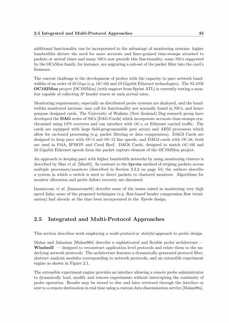
Malan and Jahanian [Malan98b] describe a sophisticated and flexible probe architecture —Windmill — designed to reconstruct application level protocols and relate them to the un-derlying network protocols. The architecture features a dynamically generated protocol filter,abstract analysis modules corresponding to network protocols, and an extensible experimentengine as shown in Figure 2.1.

The extensible experiment engine provides an interface allowing a remote probe administratorto dynamically load, modify and remove experiments without interrupting the continuity ofprobe operation. Results may be stored to disc and later retrieved through the interface orsent to a remote destination in real time using a custom data dissemination service [Malan98a].

36 Background and Related Work

The Windmill Packet Filter runs in the kernel for efficiency and is dynamically recompiledas experiments are added or removed. The packet filter passes packets identified by theexperiments’ subscriptions to a dispatcher which in turn passes them to the appropriatesubscribing experiment(s). An experiment draws on the services of one or more abstractprotocol modules to extract data specific to the protocol. The modules maintain and manageany state associated with the target protocol and also ensure that processing is not duplicatedby overlapping experiments. A per-packet reference count is maintained which allows eachpacket to be freed once seen by all interested experiments.

Experiments have been carried out to investigate the correlation between network utilisationand routeing instability noted by Labovitz [Labovitz98], and to demonstrate real-time datareduction by collecting user-level statistics for traffic originating in the Upper AtmosphericResearch Collaboratory, a data access system to over 40 instruments. The latter study alsoillustrated Windmill’s ability to trigger external active measurements defined by the experi-ments in progress.

IP

TCPHTTP

UDP

Packet Despatcher

Experiment 1

Experiment n

Protocol Filter

Device Driver

User Space

Kernel Space

Network

Abstract Protocol Modules Extensible Experiment Engine

Note: Reproduced from An Extensible Probe Architecture for Network Protocol Performance Measure-ment [Malan98b] pp. 217 c©1998 ACM, Inc. Included here by permission.

Figure 2.1: The Windmill probe architecture

At lower levels of the protocol stack Ludwig et al. [Ludwig99] have conducted a study ofthe interaction between TCP and the Radio Link Protocol (RLP) [ETSI95] using tcpdump tocollect TCP headers and their own rlpdump tool to extract data from an instrumented RLP

2.5 Integrated and Multi-Protocol Approaches 37

protocol implementation. The two sets of data were associated during post-processing usingthe purpose designed multitracer tool.

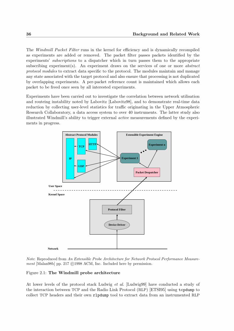
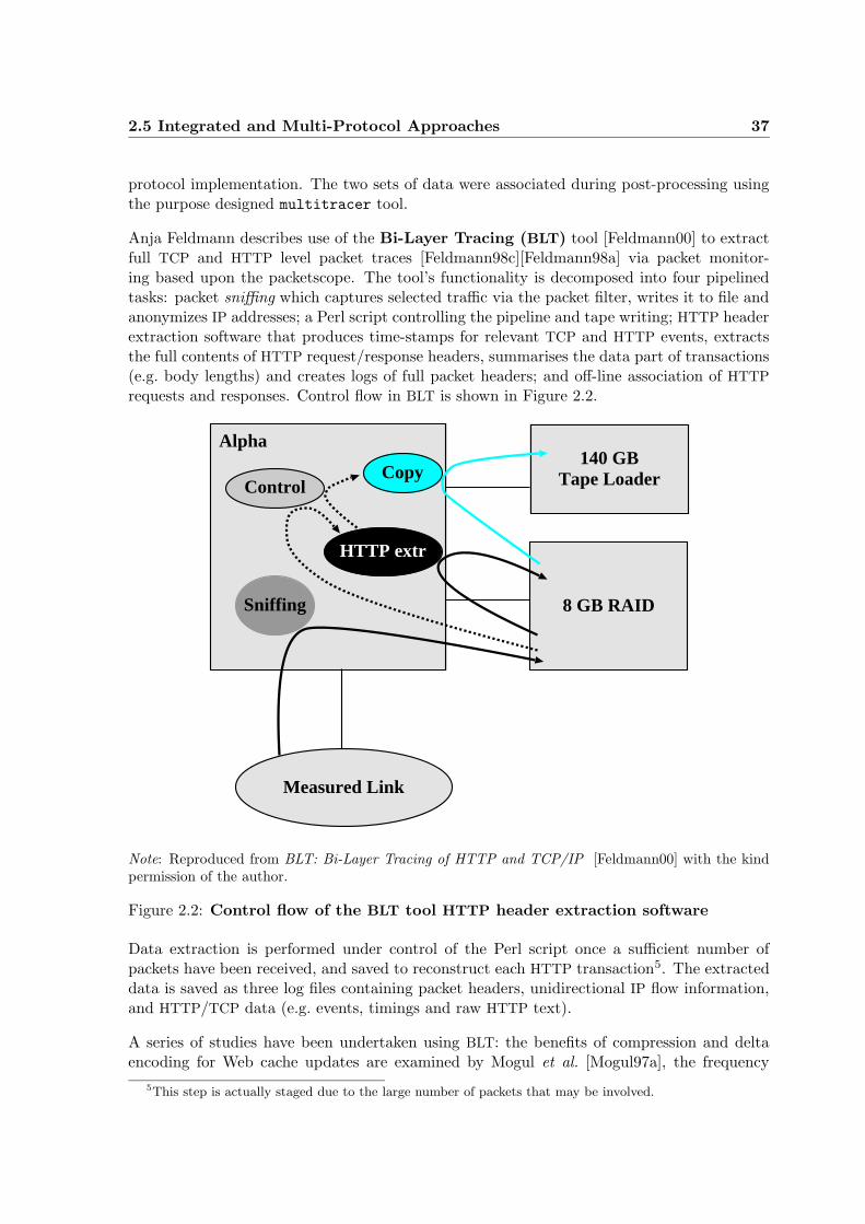
Anja Feldmann describes use of the Bi-Layer Tracing (BLT) tool [Feldmann00] to extractfull TCP and HTTP level packet traces [Feldmann98c][Feldmann98a] via packet monitor-ing based upon the packetscope. The tool’s functionality is decomposed into four pipelinedtasks: packet sniffing which captures selected traffic via the packet filter, writes it to file andanonymizes IP addresses; a Perl script controlling the pipeline and tape writing; HTTP headerextraction software that produces time-stamps for relevant TCP and HTTP events, extractsthe full contents of HTTP request/response headers, summarises the data part of transactions(e.g. body lengths) and creates logs of full packet headers; and off-line association of HTTP

requests and responses. Control flow in BLT is shown in Figure 2.2.

Measured Link

Sniffing

Copy

HTTP extr

Control

Alpha

8 GB RAID

140 GBTape Loader

Note: Reproduced from BLT: Bi-Layer Tracing of HTTP and TCP/IP [Feldmann00] with the kindpermission of the author.

Figure 2.2: Control flow of the BLT tool HTTP header extraction software

Data extraction is performed under control of the Perl script once a sufficient number ofpackets have been received, and saved to reconstruct each HTTP transaction5. The extracteddata is saved as three log files containing packet headers, unidirectional IP flow information,and HTTP/TCP data (e.g. events, timings and raw HTTP text).

A series of studies have been undertaken using BLT: the benefits of compression and deltaencoding for Web cache updates are examined by Mogul et al. [Mogul97a], the frequency

5This step is actually staged due to the large number of packets that may be involved.

38 Background and Related Work

of resource requests, their distribution and how often they change are investigated by thesame authors in [Douglis97]; the processor and switch overheads for transferring HTTP trafficthrough flow-switched networks are assessed by Feldmann, Rexford and Caceres in a furtherstudy [Feldmann98d]. BLT-produced data sets were used by Feldmann et al. [Feldmann98b]to reason about traffic invariants in scaling phenomena. Other work includes that on theperformance of Web proxy caching [Feldmann99][Krishnamurthy97].

One of the earliest architectures designed with a capability for ‘on the fly’ data extraction isthe Internet Protocol Scanning Engine (IPSE) [Internet Security96] developed by the InternetSecurity, Applications, Authentication and Cryptography Group, Computer Science Division,at the University of California, Berkeley. This packet-filter based architecture incorporateda set of protocol specific modules which processed incoming packets at the protocol level(e.g. TCP stream reassembly) before passing them upwards to experiment-specific modules.An HTTP specific module was used by Gribble and Brewer [Gribble97] to extract and recordIP, TCP and HTTP header data in a client-side study of Web users on the Berkeley Home IPService.

This section closes with mention of another probe design, HTTPDUMP [Wooster96] which,although extracting data only from the HTTP contents of packets into the common log for-mat [Consortium95], is stateful in order to associate per-transaction data. Packets are ex-tracted from the network via a packet filter into a FIFO queue from which a user-level threadreads and stores content in a cell-based array. Data is extracted, under the control of a dis-patcher thread, on a thread per transaction basis on to disc. The designers themselves weredisappointed with performance.

2.6 Flows to Unknown Ports

Identifying traffic within flows of interest will usually be based upon the well-known portat the server. In the case of some traffic types, the server will not communicate via such awell-known port, and port allocation may be dynamic; the Real Time Streaming Protocol(RTSP) [Schulzrinne98], the dominant control protocol for streaming content on the Internet,for example, defines a negotiation between client and server during which the characteristics ofthe streamed content, including server port, are determined. In such cases a probe is requiredto extract pertinent information (i.e. server port number) seen during the negotiation phaseand to capture packets accordingly.

The mmdump monitor [van der Merwe00] is designed to have this capacity. Based upon tcpdump

this system passes RTSP protocol packet contents to a parsing module which extracts the portnumbers to be used for the streamed content, the packet filter then being dynamically modifiedto accept the flow so defined. Modules understanding the set-up phase used by the SessionInitiation Protocol (SIP) [Handley99] and the H.323 conferencing control protocol [ITU-T96]are also incorporated into the tool. While monitoring, the probe initially accepts traffic onthe well-known ports used by the monitored protocols. As set-up traffic is parsed (and saved)and streams added to the packet filter set, the streaming packets are also dumped to file.Further data extraction and association is performed during a second, off-line, pass of thesaved data through mmdump.

2.7 Measurement Accuracy 39

2.7 Measurement Accuracy

Issues of accuracy in measurement are discussed by Cleary et al. [Cleary00] and Belenki andTafvelin [Belenki00] with particular emphasis on time-stamp accuracy and precision. Theemphasis of the first of these works is on the use of purpose-designed NICs for monitoringuse (the DAG cards described in Section 2.4), while the second describes techniques for theanalytical removal of error.

Pasztor and Veitch [Pasztor02] describe a software solution to providing timestamps with 1 nsresolution and low access overheads for PC-based monitoring applications.

2.8 Studies Based upon Passively Monitored Data

As an introduction to this section the comment in the preamble to this chapter, concerningthe sheer bulk of research and publication in the network monitoring field, is reiterated.

Much past work has centred upon characterisation of network traffic, usually based upon oneparticular, or a combination of, protocols. Currently the greatest volume identified by protocolis World Wide Web (WWW) traffic transferred using the HTTP protocol [Fielding99]. Withthe growth in individual connections to the Internet there is little reason to think that thiswill change in the foreseeable future, and consequently this area receives particular attention.

2.8.1 A Brief Mention of some Seminal Studies

Perhaps the best known early bulk data collection was made by Leland and Wilson [Leland91]at Bellcore in 1989. A single board computer (SBC) with on-board Ethernet interface capturedand time-stamped packets, the first 60 bytes of which were then stored in a dedicated buffer.The SBC was in turn connected to the internal bus of a Sun workstation which, when thebuffer was full, copied its contents to disc. A lower-priority process then spooled the collecteddata from disc to tape. An interval timer board, also interfaced to the workstation’s bus,provided accurate relative time stamps. Three seminal papers were based upon the traces ofLocal Area Network (LAN) and Wide Area Network (WAN) traffic gathered: on the natureand time-scale of network congestion [Fowler91]; and on the properties of self-similarity foundin the traces [Leland94] and [Paxson95]6. The self-similar nature of network traffic is a topicwhich has preoccupied many researchers ever since.

Another early bulk data collection was made by Crowcroft and Wakeman [Wakeman92] whomonitored all traffic between University College London and the Unites States for a periodof five hours. Data from IP and TCP/UDP headers were saved using tcpdump and a setof detailed traffic characterisations produced by analysing the (ASCII) traces using AWKscripts. The statistics generated included packet size, connection duration, and number ofpackets per connection distributions — both global and broken down by protocol; Domain

6Data from a wider selection of traces was also used in this study.

40 Background and Related Work

Name Service (DNS) response latencies; inter-packet delays and inter-packet gaps (in packetsand time). It is interesting to note that, at the time (March 1991), the authors report thatFTP and Simple Mail Transfer Protocol (SMTP) accounted for 79% of all traffic seen.

In 1990 the growing power of workstations prompted Jeffrey Mogul to present a paper[Mogul90] describing their use as passive monitors as an alternative to dedicated hardware.The principles of using workstations for this purpose, underlying issues, and some principlesof post-collection analysis were discussed. The same author investigated the phenomenonof TCP ACK compression in TCP connections in [Mogul92]. It was shown, using passivelycollected traces of TCP/IP headers, that ACK compression could be automatically identifiedusing techniques to compute instantaneous ACK bandwidths, and that a correlation existedbetween ACK compression and packet loss.

Vern Paxson is another investigator who has based several well known studies on passively-collected traces, of which three are mentioned here. In [Paxson94] 2.5 million TCP connectionsfrom 14 traces of wide-area traffic are used to derive analytic models describing the randomvariables associated with common application protocols and a methodology presented forcomparing the effectiveness of the models with empirical models such as tcplib [Danzig91].

A study described in [Paxson99] used data derived from passive measurement of 20,000 TCP

bulk transfers to observe and characterise a range of network pathologies and TCP behaviours.Measurements were taken using the NPD measurement framework [Paxson97b] at both end-points in recognition of asymmetry between forward and return Internet paths. The samedata was used in a further study with Mark Allman [Allman99b] which evaluated the ef-fectiveness of a number of retransmission timeout estimation algorithms and investigated animproved receiver-side bandwidth estimation algorithm.

2.8.2 Studies of World Wide Web Traffic and Performance

Improvements to overcome the shortcomings in HTTP/1.0 were suggested by Mogul and Pad-manabhan [Padmanabhan95] and the initial design of HTTP/1.1 persistent connections in-formed by simulation studies driven by data sets derived from Web server logs [Mogul95]7.

Traffic to and from the official Web server of the 1996 Atlanta Olympic Games was observedby Balakrishnan et al. [Balakrishnan98] who took TCP header traces from the FDDI ringfeeding the servers, which were additionally instrumented to notify the tracing machine ofretransmitted packets. The traces were post-analysed to examine the dynamics of the con-nections used, and to suggest improvements that might be made to transport-level protocols.Deficiencies were found in the existing TCP loss recovery techniques (almost 50% of losses re-quiring a coarse timeout for recovery), receivers’ advertised windows were found to contributea bottleneck, and the correlation between ACK compression and packet loss was confirmed. Itwas discovered that multiple parallel HTTP connections were more aggressive users of the net-work than single connections, current use of Selective ACKnowledgements (SACKs) avoidedonly a small proportion of timeouts, and parallel connections with small outstanding windowssuffered a disproportionate share of loss. Proposed improvements to single connections’ loss

7This work is described more fully in Section 7.2 on page 160.

2.8 Studies Based upon Passively Monitored Data 41

recovery mechanism using right edge recovery (prompting duplicate ACKS by sending a seg-ment with a high sequence number), and to multiple connections’ loss recovery by integratingcongestion control/recovery across the set of connections, were simulated and found to bebeneficial.

Bruce Mah determined a set of several Web retrieval characteristics using solely tcpdump-collected traces of TCP/IP headers in order to establish an empirical model of HTTP networktraffic for further use in simulation studies [Mah97]. Grouping of individual components intoWeb pages depended upon a set of heuristics. Factors such as request/reply lengths, documentsize, consecutive document retrievals and server popularity were quantified.

Mark Allman [Allman00] used a combination of passively-collected header traces and Webserver logs to characterise downloads from a single server over a period of one and a halfyears, and to extend this work to investigate the TCP-level activity of the connections used.The findings note increasing use of the TCP SACK option, the detrimental effects of smalladvertised windows, that larger values of Congestion WiNDow (CWND) would be beneficialand that the use of persistent TCP/HTTP connections appeared to be declining.

An investigation of Web traffic by Donelson Smith et al. [Smith01] using OC3Mon andOC12Mon-gathered traces of TCP/IP headers from a campus network, and further similartraces from the NLANR repository, established a number of characterisations of the trafficand the patterns of TCP usage by HTTP.

The Wide Area Web Measurement Project (WAWM) [Barford99a][Barford99b] com-bines the collection and analysis of packet traces with active measurement techniques to studythe effects of varying load on Web servers. A server, established for the purpose of the exper-iments, was subject to a variable load generated by the Scalable URL Reference Generator(SURGE) [Barford01] on both local and distant clients.

A similar, but extended, combination of active and passive components was used to drivea further study [Barford00] using varying loads, but employing critical path analysis (CPA)techniques to identify and quantify the time elements constituting object download times.

Web object download times were deconstructed into server address resolution, TCP connectionestablishment, server latency and object download times by Habib and Abrahams [Habib00]using the keynote measurement tools [Keynote98] and artificially generated loads. Olshefskiet al. [Olshefski02] describe Certes (CliEnt response Time Estimated by the Server), a server-based mechanism which combines connection drop, acceptance and completion rates withpacket-level measurements to measure response times experienced by the client. The effectsof combining Certes with web server control mechanisms and listen queue management toimprove quality of service are discussed.

Several studies based upon combined TCP and HTTP data gathered using the Packetscope(BLT) have been referred to in Section 2.5.

42 Background and Related Work

2.9 Summary

This chapter has attempted to distill a ‘snapshot’ of the current state of passive monitordesign together with some historical background and indication of how trends towards themonitoring of higher network bandwidths are to be accommodated. It will be noted thatfew of the probe architectures presently implemented possess all, or even a majority of, thedesirable attributes described in Section 1.4.

A broad division exists between architectures intended to keep pace with high bandwidths(OCxMon, IPMON), which essentially only capture a verbatim copy of packet headers up tothe TCP level and are not stateful, and those with more capable data extraction features(Windmill, IPSE and Packetscope (as BLT)). HTTPDUMP suffers from poor performanceand is, essentially, only a single-protocol monitor, while mmdump, which supports dynamicflow identification does not (except in this limited sense) implement data extraction.

The Packetscope (BLT) is built upon a complex data flow and control structure, with frag-mented logging, which is likely to inhibit its generality in terms of multi-protocol monitoringof a range of higher level protocols. The majority part of data association is postponed untilthe post-processing stage, hence rendering trace logs less concise than might otherwise be thecase8. Data extraction is largely coarse-grained, HTTP headers, for instance, being copiedverbatim. Although it is reported as keeping pace with FDDI link speeds of 100Mbps it is sur-mised that the complexity of the architecture may inhibit its use to monitor at substantiallyhigher network bandwidths.

Both Windmill and IPSE implement finer-grained data extraction, but both designs predatecurrently common bandwidths, and it is not known how well they would perform, or howeasily the designs might be adapted, in the present context.

Some relevant research using data obtained through passive monitoring are briefly describedin Section 2.8.2. These studies may be characterised into those observing real traffic [Mah97],([Balakrishnan98], and [Smith01]); and those based upon artificially generated traffic([Barford99a], [Barford00], and [Habib00]).

In the context of Chapters 7 and 8 of this dissertation there is a critical distinction be-tween those studies based solely upon data garnered from the traffic’s TCP and IP headers([Balakrishnan98], [Mah97], [Allman00], [Smith01], and [Habib00]); and those where the basedata contained elements drawn from activity at the HTTP level ([Allman00], [Barford99a],[Barford00], and [Feldmann00]). In the case of the latter category, the studies based uponBLT-gathered data are unique in that the HTTP-level data was extracted from monitoredpackets — in all other cases the higher-level protocol information originated from server logs(Allman) or from specially instrumented servers.

All of the work mentioned relates TCP and HTTP-level activity with the exception of that byMah [Mah97] and to a greater-or-lesser extent derives some characterisation of Web traffic.With the, again, notable exception of the BLT studies, associations between TCP and HTTP-

8The BLT architecture is designed as in part to deliberately disassociate stored data in order to addressconcerns of privacy and security.

2.9 Summary 43

level activity have to be largely9 inferred from the lower-level protocol activity using knowledgeof the operational semantics of HTTP; thus a data-carrying TCP segment transmitted by abrowser client can be assumed to carry a HTTP request, and the following data-carryingsegments from the server to carry a reply; a pause in activity may imply that an entire pagehas been downloaded and further activity following this ‘think-time’ that a fresh page hasbeen requested10. The extent to which such reliance upon inference may affect the accuracyof results is discussed further in Section 7.3.1 on page 162.

9In the case of studies collecting only TCP and IP header data, of course, entirely.10Mah [Mah97] demonstrates the effect of differing assumed think-times.

Chapter 3

The Nprobe Architecture

The increasing power of relatively inexpensive PCs in terms of processor frequency, bus band-width, memory, and disc capacity makes feasible the design of a relatively inexpensive yet morecapable on-line monitoring system than currently available; one utilizing standard hardware,device drivers, and operating systems, but sufficiently nimble to keep up with the potentialbandwidth usage of contemporary network link technologies.

Such a system should be capable of capturing all packets traversing the network(s) to which itis attached with minimal or no loss. It should be sufficiently powerful to process and analyseprotocol header fields at all levels together with some simple examination of packet content— the capacity for data reduction at a speed matching its input from the network, and shouldhave attached storage media with access bandwidth and capacity sufficient to store generateddata without loss and for trace periods of a macrocosmic scale.

This chapter describes the implementation of the Nprobe monitoring system and the on-linepacket processing performed in order to extract and store data of interest. The later off-lineprocessing of the stored data is described in Chapter 4.

3.1 Design Goals

The design and implementation of the Nprobe monitor have been based upon a set of generalrequirements which dictate that it should:

• possess the desirable characteristics introduced in Section 1.4 on page 27.

• be based upon an off the shelf PC machine architecture with sufficient expansion slotsto accommodate several network interface cards

• incorporate multiple processors of the highest commonly available frequency for maxi-mum processing power

46 The Nprobe Architecture

• run the Linux operating system — although it is desirable to use standard operatingsystem components and device drivers, the availability of the Linux source code makessome relatively minor but necessary modifications possible

• be equipped with high capacity Redundant Array of Inexpensive Disks (RAID) storage

• minimize the overhead of copies to and from user and kernel space while performingInput/Output (I/O) by using the kernel’s memory mapping facility

• be non-invasive of the attached network(s)

• collect packets arriving at network interface(s) but not process them in the devicedrivers, minimizing modification to the drivers

• perform all packet processing in user-level processes, hence maintaining flexibility

• employ a modular architecture for user-level packet processing software

3.2 Design Overview

Figure 3.1 illustrates the principal components and arrangement of the Nprobe architecture.

3.2.1 Principal Components

Nprobe functionality encompasses three stages: packet capture, packet processing, and datastorage. Buffering between the stages accommodates burstiness in packet arrivals, and varia-tions in packet processing and data storage rates.

Packets arriving from the network are presented to a simple filter implemented in the NIC’sfirmware; those passing the filter are time-stamped and transferred into a kernel memoryreceive buffer pool without any further processing.

A probe will have one or more receive buffer pools, each associated with one user-level Nprobeprocess and mapped into its address space. Nprobe processes present packets held in thereceive buffer pool to a series of protocol-based modules which extract the required datafrom each packet in place; each packet is processed in turn in its entirety (except as noted inSection 3.3.3.4 on page 59), and its containing buffer marked as free for re-use by the networkinterface driver. Data extraction will normally be dependent on the context provided by theprocessing of preceding packets; this context is held as state which is attached to each packetas it is processed. Extracted data is temporarily stored as part of the attached state.

When the last packet of an associated series has been processed all of the extracted dataheld in state is copied into an output log buffer from where, once sufficient data has beenaccumulated, it is written to a trace file on disc.

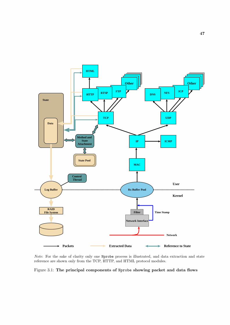
47

OtherOther

Log Buffer

State

Data

Method and State

AttachmentICMP

UDP

MAC

IP

TCP

HTML

Rx Buffer Pool

FTPRTSPHTTPICPNFSDNS

Filter

Network Interface

Time Stamp

User

Kernel

State Pool

Packets Extracted Data Reference to State

RAIDFile System

Network

Control Thread

Note: For the sake of clarity only one Nprobe process is illustrated, and data extraction and statereference are shown only from the TCP, HTTP, and HTML protocol modules.

Figure 3.1: The principal components of Nprobe showing packet and data flows

48 The Nprobe Architecture

3.2.2 Rationale

The Nprobe design rationale is presented in Section 3.2.2.1 and develops the two intimatelyrelated themes of data flow through the system and control; a third, and equally significanttheme — that of state emerges as a consequence.

Several monitoring architectures are briefly described in Chapter 2; in Section 3.2.2.2 onpage 50 the Nprobe design rationale is developed further by comparison with the most similarsystems described in Section 2.5 on page 35.

3.2.2.1 Data Flow and Control

The central task of a passive on-line monitoring system is to transform an afferent flowof data contained in packets captured from the network into stored output consisting ofonly the required data. This task will be partitioned into functional components whichmust be coordinated. In a sophisticated system which performs data extraction, reduction,and association, the control of interaction between these components may become complex.Subject only to physical constraints of bus and I/O bandwidth, the system’s capacity tokeep pace with packet arrivals will depend upon the maximum possible proportion of CentralProcessing Unit (CPU) resources being available to the system’s central task, and to this taskbeing executed as efficiently as possible. Any control function should therefore absorb theminimum possible number of CPU cycles and should not introduce inefficiency into packetprocessing; separate control processes requiring frequent context switches are, for instance,undesirable.

In the Nprobe design control is as far as possible data driven (e.g. packets are passed fromone protocol processing module to another according to their content): the packet processingloop is driven by the presence of packets in the receive buffer pool, data copy from state to logbuffer is triggered by the processing of the final packet of an associated sequence). No controlprocesses are introduced (with one exception — the infrequently called file management threaddescribed in Section 3.3.4 on page 68) and control derives from data processing, hence addingonly a minimal overhead.

Any monitoring system must accommodate the bursty nature of packet arrivals, the widelyvarying workload involved in the processing of individual packets, and the variable rate atwhich saved data is generated — at the very least buffering will be required between thesethree fundamental stages in the flow of data through the system. The desirability of packetprocessing in user-level processes to maximize flexibility, and of avoiding such processing indevice drivers so as to minimize modification, has been stated as a design goal; to thesecan now be added the desirability of minimizing any packet processing as part of networkinterrupt handling — such processing may compromise the buffering of bursty arrivals andcontribute to the risk of packet loss at the network interface. Arriving packets are thereforesimply placed in a receive buffer pool by the interface; the pool is as large as is possiblewith regard to overall memory size in order to accommodate bursty arrival rates and variableprocessing demands.

3.2 Design Overview 49

Monitors based upon the tcpdump model incur a considerable data copy overhead as arrivingpackets placed in the kernel’s receive buffers must be copied into user memory space forprocessing. Nprobe avoids this penalty by using the kernel’s memory-mapping facility to mapthe receive buffer pool directly into the user-level packet processing process(es)’ address space.All data extraction and other processing is carried out on the packets in place.

At the very high arrival rates to be expected when monitoring contemporary networks, evena relatively large receive buffer pool would be exhausted if required to hold incoming packetsfor any more than a minimal period. The Nprobe design therefore calls for all packets tobe processed, as far as is possible, in their entirety as soon as possible after arrival and thebuffer so freed returned to the pool of buffers available to receive new incoming packets.This principle is, of course, violated by the necessity to hold out of order packets whenreconstructing stream oriented flows (e.g. as explained in Section 3.3.3.4 on page 59). Thatsome packets must inevitably be held strengthens, rather than negates, the necessity that theremainder be dealt with promptly.

The immediate processing of packets has two important implications. Firstly, while the datacontained within packets which is pertinent to lower level protocols (e.g. TCP and IP headers)forms discrete, per-packet, quanta and may be extracted as such, higher-level protocol datamay well conform to both syntactic and semantic units which span packets; the processing ofdiscrete packets must therefore be carried out in the context of the additional state neededto ‘bridge’ processing across packet boundaries, and the processing itself is made rather morecomplex. Secondly, however, control flow is simplified. Packets are simply passed upwards bythe processing modules representing the ascending levels of the protocol stack as determinedby the packet type and contents and the data requirements of the study being conducted.

The desirability of statefulness was introduced in Section 1.2 in the context of enabling packet-spanning data extraction and association from contents at higher protocol levels, and rein-forced earlier in this section in the context of bridging packet boundaries during processing.Even when the data collected requires no context external to the containing packet (e.g. TCP

or IP headers), there are good reasons for maintaining data association across logical flowsas, for example, explained in Section 3.3.3.4. The existence of state requires a determinationof the granularity with which it is held, which in turn follows from an identification of themost efficient Data Association Unit (DAU)1. A larger DAU may assist in achieving a highdata reduction ratio (as less data is required to be stored solely to later associate data), butmay make unacceptable demands on memory, or be unfeasibly expensive to compute on thefly. A smaller unit may be cheaper to compute, make less demand on available memory (as itis likely to be completed and dumped to disc after fewer packets have been seen, its lifetimewill be shorter and less units of state will therefore be concurrently held), but may be moreexpensive to maintain and to save (e.g. several smaller units would be more expensive toinitialize or to transfer into output buffers than fewer, larger, ones).

In the case of the Nprobe design this decision was informed by two, happily complementary,factors: it was anticipated that most studies would be based upon particular traffic types(i.e. services as identified by TCP or UDP port numbers), and that the association of packets

1A DAU is defined as the sequence or set of packets from which logically or semantically associated data isaggregated.

50 The Nprobe Architecture

(and hence of the data extracted from them) by the five-tuple of the two host IP addresses,port numbers and the IP header protocol field is a relatively cheap operation. The normalDAU was therefore chosen to coincide with the naturally self-suggesting unit of the TCP orUDP connection; and it is at this granularity that state is initialized and associated with thepackets processed; and data associated, stored, and dumped to disc. The choice of DAU alsodetermines the point at which packets are associated with the state providing the contextwithin which they are processed, and it will be consequently seen in Figure 3.1 on page 47that attachment of state to packets is carried out at the level of the transport level protocolprocessing modules. Once state has been attached to a packet, additional, protocol-specificstate, may be further attached to the basic unit as the packet is passed to higher-level modules.Throughout the remainder of this dissertation the set of packets contributing to a DAU arereferred to as a flow.

As data is extracted from packets, it is stored as part of the associated state and upontermination of the flow is copied into a log buffer in memory. The log buffer is configured asa memory mapped file, hence is written asynchronously to disc by the operating system —the only data copy required therefore is that of the reduced data from state to buffer.

3.2.2.2 Comparison with other probe architectures

The maximum duration of an Nprobe monitoring run is determined by the available disccapacity — both the Packetscope (BLT) and Windmill are designed to collect very long,continuous, traces: BLT through utilizing tape storage and Windmill by exporting dataduring collection. The first of these solutions to the problem presented by finite and limiteddisc capacity when collecting very long traces, was not considered for incorporation into theNprobe design on grounds of expense, and because the overheads associated with copyingto tape would violate the underlying aim of producing a ‘lean and mean’ design where themaximum possible resources are devoted to packet capture and data extraction. The optionof exporting data while the monitor was live was also similarly discounted on grounds ofavoiding additional CPU and I/O bandwidth overhead, and because, in the anticipation thatprobe placements would normally be such as to preclude the provision of dedicated datadownload links, downloading large volumes of data while monitoring would carry the riskof perturbing the monitored traffic. The provision of dedicated links would, alternatively,limit probe deployment options. It is thought that the provision of disc capacity sufficient torecord 24 hour traces (and hence any diurnal traffic cycles) is likely to cater adequately forthe majority of studies; only a very few connections remain alive beyond this time scale, andlonger periodic variations in traffic can be catered for by repeated traces.

Nprobe, Windmill and BLT all incorporate a packet filter in some form, although differingin purpose and implementation. Both Windmill and BLT implement coarse-grained datadiscard through packet filtering: the former accepting only HTTP traffic selected by portnumber and the latter the selection of traffic dynamically subscribed to by the currentlyrunning experiments. In both cases, the packet filter operates on packets which have beenaccepted from the attached link and placed into the probe’s receive buffers. The Nprobe

filter is relatively simple and serves a different purpose — to support scalability as describedin Section 3.3.2 on page 54; it is implemented in the NIC’s firmware with the result that

3.3 Implementation 51

unwanted packets are rejected without being transferred into receive buffers, hence avoidingunnecessary load on the probe’s Peripheral Component Interconnect (PCI) bus.

The BLT control flow, shown diagrammatically in Figure 2.2 on page 37, implements pipeliningbetween the packet sniffing, data extraction, and (two stage) writing to log through themechanism of files used as buffers between the stages of the pipeline. HTTP data extractionis only carried out after a set number of packets have been accumulated. Computationaloverhead is introduced by the number of data copies introduced into the long data pathand by the need to manage the stages of the pipeline; the accumulation of packets prior todata extraction would incur a considerable memory penalty if they were not buffered on disc,but this in itself must introduce a bottleneck and tend to slow operation. This mechanismcontrasts significantly with the minimal control overhead, buffering arrangements and fastpacket turnover of the Nprobe design.

Flexibility and the capacity to load and unload different experiments while continuously mon-itoring also lead to a relatively complex data and control flow in the Windmill architecture,as shown in Figure 2.1 on page 36. This represents a very different approach to the tailoringof the probe to suit the data requirements of varying studies than that employed in Nprobe.The Windmill packet filter accepts the super-set of all packets required by subscribing exper-iments, which are then submitted to the experiment(s) by a packet dispatcher. The variousexperiments draw upon the services of a series of abstract protocol modules which are calledrecursively to extract the required data from each packet. The protocol modules maintainany state that must be maintained across packet boundaries. Because Nprobe is not designedfor continuous operation, flexibility can be achieved through the addition or modificationand recompilation of the various user-level processing modules, and it is suggested that thisapproach can lead to an equal or greater functionality (as described in Section 3.3.3.1 onpage 55) without the additional complexity of the Windmill design. The ability to gatherdata concurrently for a range of experiments is provided by provision of a suite of appropriateprocessing methods which form part of state, control flow thereby being determined by packetcontent rather than external mechanisms.

3.3 Implementation

Nprobe remains under continuing development but at the time of writing (April 2003) themajor infrastructure has been implemented together with modules processing common link-level (MAC), IP, TCP, UDP, DNS, HTTP and Hypertext Markup Language (HTML) protocols.Embryonic modules relevant to ICMP, FTP, RTSP, and NFS have also been partially developed.The Nprobe implementation is coded entirely in the C language.

3.3.1 Packet Capture

The receiving interface places incoming packets into a receive buffer pool in the normal way,this pool is considerably larger, however, than that normally employed in order to bufferbetween bursty arrivals and variable packet processing demands at higher levels. All packet

52 The Nprobe Architecture

processing is carried out by user-level processes, to which the buffer pool is made visible bymapping the buffer pool memory into the processes’ memory space using the standard kernelmemory mapping mechanism. In this way no copy overhead is incurred in making packetcontents available to the analysis processes. Packet handling as part of interrupt processingthus remains minimal and is primarily concerned with buffer management and with standarddevice control functions.

3.3.1.1 Network connection

Nprobe connection to the target physical network will depend upon the technology of thenetwork: in the case of shared media types (e.g. 10 Mbps Ethernet, FDDI) it is sufficient toconnect in the normal way and to operate the interface in promiscuous mode; in the caseof non-shared media it is necessary to tap directly into links or to make use of the portmonitoring facility provided by switches — although care must be taken to select links orswitches which will maximize the visibility of traffic. In some instances it may be necessaryto employ multiple taps drawing traffic from several links into a range of interfaces.

Nprobe machines have to date monitored fibre-optic carried ATM traffic via a passive opticalsplitter placed into the link(s) of interest2 and 1 Gbps ethernet networks via port monitoring.

3.3.1.2 Operating System and Driver Modifications3

Nprobe runs over the Gnu Linux operating system with minimal modification, principally tocircumvent minor shortcomings in the memory management and mapping code. Other smallpatches have been required to improve the behaviour of the asynchronous msync() systemcall used in writing data log files to disc (see Section 3.3.4 on page 68).

Minor modifications are required to the standard interface drivers — the mechanism by whichbuffers are marked as containing valid data by the driver during interrupt processing, and thenfreed by the receiving process for re-use must now encompass interaction between kernel anduser space processes. The firmware of the most commonly used NICs has also been modifiedto provide the high-resolution time stamps described in Section 3.3.1.3 and packet filteringfunctionality described in Section 3.3.2 on page 54.

3.3.1.3 Packet arrival time-stamping

The modified NIC firmware prepends each accepted packet with an accurate arrival timestamp generated by a clock on the card. In this way inaccuracies due to latency between

2Care must be taken when using optical splitters because of the signal attenuation caused by the splitter;it is envisaged that suitable links will be identified as those between switches within switching centres, ratherthan long haul links, so this should not be found to be a problem in practice.

3The work described in this Section (3.3.1.2) has been carried out by Dr. Ian Pratt and Dr Steven Hand ofthe Computer Laboratory Systems Research Group. Dr. Pratt is responsible for modifications to the networkinterface drivers and NIC firmware and Dr. Hand has contributed the file system patches.

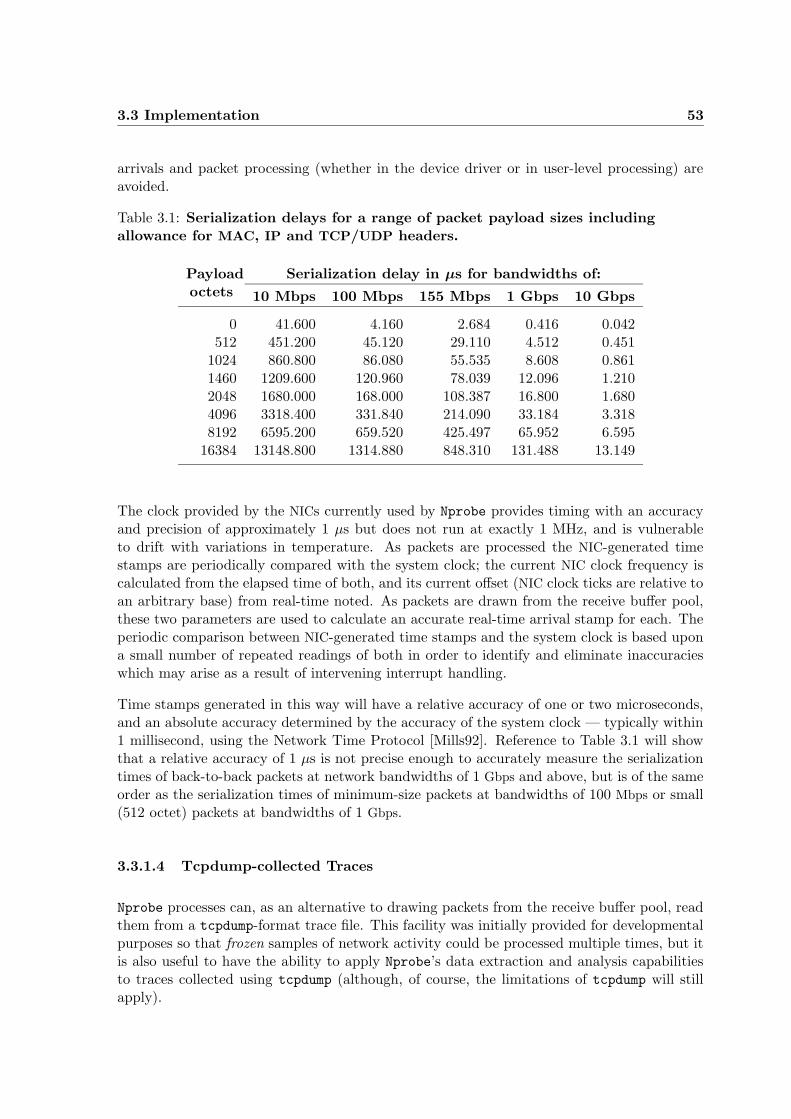
3.3 Implementation 53

arrivals and packet processing (whether in the device driver or in user-level processing) areavoided.

Table 3.1: Serialization delays for a range of packet payload sizes includingallowance for MAC, IP and TCP/UDP headers.

Payloadoctets

Serialization delay in µs for bandwidths of:

10 Mbps 100 Mbps 155 Mbps 1 Gbps 10 Gbps

0 41.600 4.160 2.684 0.416 0.042512 451.200 45.120 29.110 4.512 0.451

1024 860.800 86.080 55.535 8.608 0.8611460 1209.600 120.960 78.039 12.096 1.2102048 1680.000 168.000 108.387 16.800 1.6804096 3318.400 331.840 214.090 33.184 3.3188192 6595.200 659.520 425.497 65.952 6.595

16384 13148.800 1314.880 848.310 131.488 13.149

The clock provided by the NICs currently used by Nprobe provides timing with an accuracyand precision of approximately 1 µs but does not run at exactly 1 MHz, and is vulnerableto drift with variations in temperature. As packets are processed the NIC-generated timestamps are periodically compared with the system clock; the current NIC clock frequency iscalculated from the elapsed time of both, and its current offset (NIC clock ticks are relative toan arbitrary base) from real-time noted. As packets are drawn from the receive buffer pool,these two parameters are used to calculate an accurate real-time arrival stamp for each. Theperiodic comparison between NIC-generated time stamps and the system clock is based upona small number of repeated readings of both in order to identify and eliminate inaccuracieswhich may arise as a result of intervening interrupt handling.

Time stamps generated in this way will have a relative accuracy of one or two microseconds,and an absolute accuracy determined by the accuracy of the system clock — typically within1 millisecond, using the Network Time Protocol [Mills92]. Reference to Table 3.1 will showthat a relative accuracy of 1 µs is not precise enough to accurately measure the serializationtimes of back-to-back packets at network bandwidths of 1 Gbps and above, but is of the sameorder as the serialization times of minimum-size packets at bandwidths of 100 Mbps or small(512 octet) packets at bandwidths of 1 Gbps.

3.3.1.4 Tcpdump-collected Traces

Nprobe processes can, as an alternative to drawing packets from the receive buffer pool, readthem from a tcpdump-format trace file. This facility was initially provided for developmentalpurposes so that frozen samples of network activity could be processed multiple times, but itis also useful to have the ability to apply Nprobe’s data extraction and analysis capabilitiesto traces collected using tcpdump (although, of course, the limitations of tcpdump will stillapply).

54 The Nprobe Architecture

The ability to read packets from tcpdump-style traces is also used in investigating data pro-cessing failures as explained in Section 3.3.6 on page 72.

3.3.2 Scalability

It must be recognised that a probe’s ability to keep pace with packet arrivals will be over-runat some point as the need arises to monitor higher bandwidth links or link utilisation increases;however efficiently the probe’s software processes incoming packets, the available processorcycles are finite and physical limitations exist in terms of memory access time and I/O orbus bandwidth and contention. Even costly and dedicated purpose-designed hardware willeventually hit hard limits, but these will be lower in the case of probes built upon commodityPCs.

Nprobe’s scalability is based upon the striping of packets across multiple Nprobe processes,possibly running on multiple probes; although the capacity of individual PC-based probesmay be less than that of purpose hardware, their relatively low cost makes the employmentof monitoring clusters an attractive proposition. Striping may, alternatively, be used as aform of coarse-grained data discard in order to collect a sample of the total network trafficby simply discarding a sub-set of the total stripes.

A simple filter, shown in Figure 3.2 on the facing page, is implemented in the firmware of eachof the probe’s NICs; accepted packets are transferred into the receive buffer pool associatedwith an individual Nprobe process, rejected packets are simply dropped, hence not placingload on the probe’s PCI bus. The filter employs an N -valued hash based upon packets’ XOR’dsource and destination IP addresses — hence distributing traffic amongst N processes, eachdealing with a specific aggregated bi-directional sub-set of the total. The number of processesemployed will be determined by the power of the probe machines and the arrival bandwidth;if the number of processes required exceeds that available on a single machine then multipleprobes, forming a monitoring cluster will be deployed. Where multi-processor probe machinesare employed, one Nprobe process is run per processor (hence exploiting processor affinity— to exceed one process per processor would simply unnecessarily waste cycles in contextswitching).

3.3.3 On-Line Packet Processing and Data Extraction

Packets collected by Nprobe are processed on the fly by user-level nprobe processes whichextract the required data from the contained protocol headers and payloads and save it forpost-collection analysis. Each incoming packet is dealt with in its entirety and the containingbuffer immediately returned for re-use by the input driver unless temporarily retained for TCPsequence ordering. Because data extraction also requires a partial analysis of packet contentin order to associate data, on-line processing is henceforth referred to as packet analysis; toavoid confusion the later off-line analysis of collected data is referred to as data analysis.

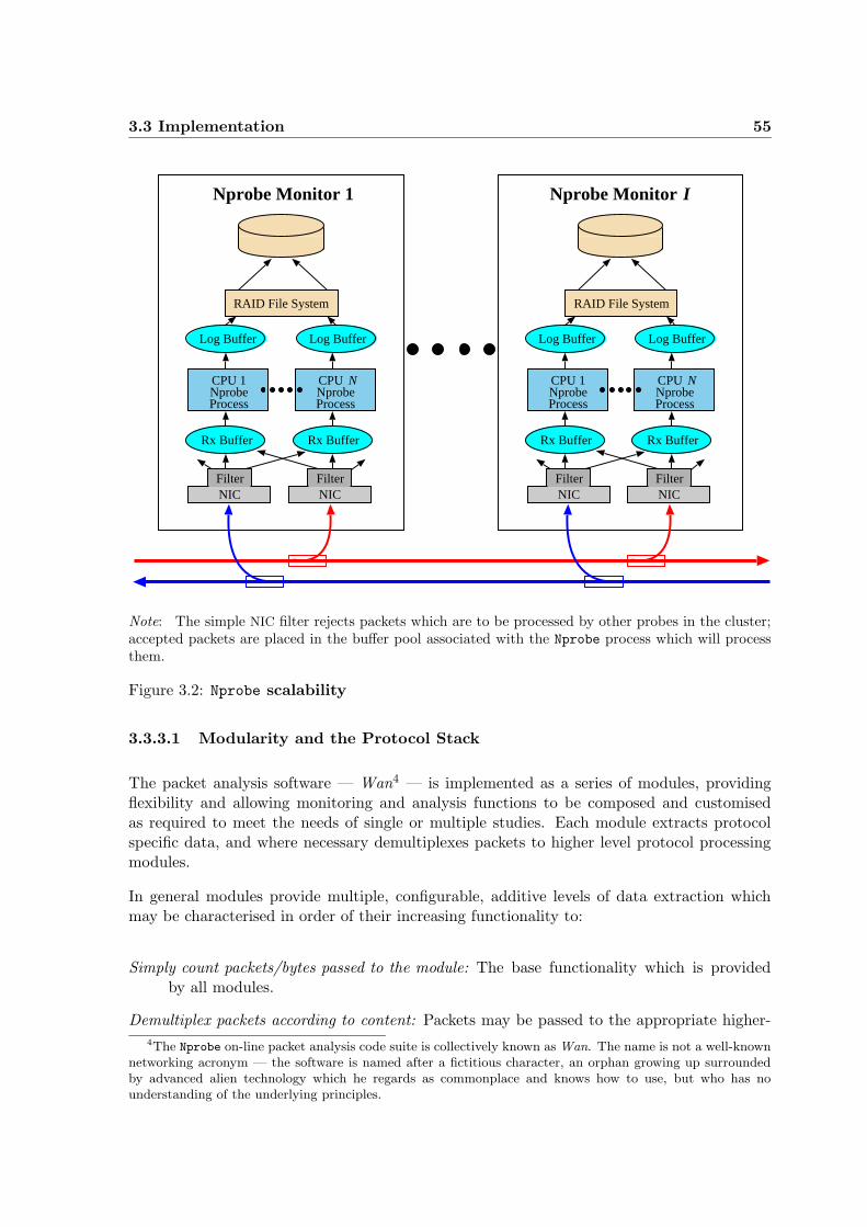
3.3 Implementation 55

CPU 1NprobeProcess

CPU NprobeProcess

Log Buffer Log Buffer

Rx Buffer Rx Buffer

RAID File System

NICFilter

NICFilter

N

Nprobe Monitor 1

CPU 1NprobeProcess

CPU NprobeProcess

Log Buffer Log Buffer

Rx Buffer Rx Buffer

RAID File System

NICFilter

NICFilter

N

Nprobe Monitor I

Note: The simple NIC filter rejects packets which are to be processed by other probes in the cluster;accepted packets are placed in the buffer pool associated with the Nprobe process which will processthem.

Figure 3.2: Nprobe scalability

3.3.3.1 Modularity and the Protocol Stack

The packet analysis software — Wan4 — is implemented as a series of modules, providingflexibility and allowing monitoring and analysis functions to be composed and customisedas required to meet the needs of single or multiple studies. Each module extracts protocolspecific data, and where necessary demultiplexes packets to higher level protocol processingmodules.

In general modules provide multiple, configurable, additive levels of data extraction whichmay be characterised in order of their increasing functionality to:

Simply count packets/bytes passed to the module: The base functionality which is providedby all modules.

Demultiplex packets according to content: Packets may be passed to the appropriate higher-

4The Nprobe on-line packet analysis code suite is collectively known as Wan. The name is not a well-knownnetworking acronym — the software is named after a fictitious character, an orphan growing up surroundedby advanced alien technology which he regards as commonplace and knows how to use, but who has nounderstanding of the underlying principles.

56 The Nprobe Architecture

level protocol module or not processed further.

Process data for presentation to higher-level protocol modules: Strip protocol headers and per-form a minimal correctness check; more complex processing may be required — in thecase of a TCP processing module, for instance, higher level protocol handling modulesmay require a properly reconstructed and ordered byte-stream.

Extract data specific to the protocol: The degree and nature of the data extracted may itselfbe configurable, or alternative modules supplied which are tailored to the exact needsof a particular study.

As explained in Sections 3.2.2.2 and 3.3.2 the NIC-based packet filter provides scalabilityrather than a coarse-grained packet discard function — the latter is distributed amongstthe processing modules. Because the Nprobe architecture does not copy packets from kernelto user space, there is no longer a need to concentrate discard in a kernel-based filter toavoid copying packets which will later be discarded. By distributing packet discard amongstprocessing modules, where discard decisions can be based upon packet contents, considerableflexibility can be achieved, and both accepted and discarded packets can be accounted for.Whatever the specific study-based data being currently collected by Nprobe it is desirablethat this is placed in the context of the traffic mix traversing the monitored network. Byappropriately configuring modules the desired level of detail can be obtained; at each protocolstack level demultiplexing may either pass packets to the appropriate higher-level modulewhere they will be accounted for (and possibly processed further) or alternatively simplyaccount for them as the default ‘other’ type.

3.3.3.2 State and Data Management and Format

The concept of a data association unit (DAU ) was introduced in Section 3.2.2.1 and may bedefined as a sequence of packets having semantic or functional continuity at one or more levelsof the protocol stack, and from which data is extracted, aggregated and associated. For thereasons described in Section 3.2.2.1 the DAU normally employed is that of the TCP or UDP5

connection. It is clear that both the state necessary to extract and associate data acrosspacket boundaries, and the extracted data itself, will refer to the same DAU and that thetwo can therefore be stored and managed together, extracted data forming part of the stateassociated with a DAU during its lifetime. The storage allocation unit for state is henceforthreferred to as a State Storage Unit (SSU). Each current DAU will have a corresponding StateStorage Unit (SSU) held in the probe’s memory.

Lines 1 – 9 of Fragment 3.1 show the (partial) C structure forming the repository of basicTCP or UDP connection data. Lines 11 – 18 define the state associating the packets of theseDAUs and illustrate how the data is encapsulated within the outer SSU structure at Line 15.In this way state and data are identified for attachment to packets, initialised and managed asa single unit, and data can be transferred efficiently as a single continuous block of memory.Complex data and state associations may require several levels of nested structures.

5UDP is, of course, not connection oriented as is TCP , but a UDP connection can now be defined as the

sequence of packets which together form a DAU .

3.3 Implementation 57

The continual birth and death of DAUs gives rise to a very high turnover of associated SSUs.Rather than constantly allocate and free memory it is more efficient6 to create a pool of thevarious SSU structures when the monitor is activated, and for SSUs to be drawn from it asrequired. The pool is organised as a stack so as to maximise locality of reference.

Flexibility in the degree and type of data collected from packets, tailored to the specificrequirements of a particular study (or set thereof), is reflected in the requirement for asimilar degree of flexibility in the content and format of the SSUs employed. State anddata vary with studies’ requirements within a specific protocol and the composition of dataextraction functions as packets are passed from one module to another will determine aparallel composition of SSU components. Additionally, even for the same composition of dataextraction functions/SSU components, the nature and extent of data may vary significantly(e.g. an HTTP/TCP connection may carry one or many HTTP transactions, the HTTP headerfields present in each may vary, and the types of object returned for each may vary).

The choice of TCP or UDP connection as the normal DAU determines that an SSU is associatedwith a packet as it is passed to the corresponding transport-level protocol processing module.As new DAUs are encountered a new SSU is drawn from the pool and entered into a hashlist based upon IP addresses and port numbers7; as succeeding packets are processed theappropriate SSU can therefore be efficiently located.

The content and format of a SSU for each Wan module are defined by the module itself andreflect the data that will be extracted by it; by linking module-level SSUs these become sub-components of the SSU corresponding to a specific DAU and the composition of module-levelextraction functions can be accommodated; repetitive data extraction (e.g. multiple HTTP

transactions over one TCP connection) is accommodated by chaining the SSUs associatedwith a particular module. Figure 3.3 on page 59 illustrates the arrangement of a generalisedSSU . Because the monitor may see traffic travelling in only one direction, state and data aredivided into meta state/data applying to the DAU as a whole and two directional sub-units,each pertaining to a unidirectional flow. The directional sub-units need not be symmetrical.

The size of data fields within an SSU may be statically or dynamically determined. Numericor abstracted data will be stored in numerical data types of known size, but a mechanismfor the storage of variable-sized data (normally alphanumeric strings or sequences, e.g. thealphanumeric Uniform Resource Locator (URL) field of an HTTP request header) is alsorequired. The demands of efficient packet processing preclude an exact memory allocationfor each data instance and a trade-off therefore has to be made between allocating sufficientspace to accommodate unusually large requirements and making unduly heavy demands uponthe available memory. In the case of such data a count of length is kept and used to ensurethat only the data (as opposed to the size of statically allocated buffers) is logged.

Code Fragment 3.2 illustrates the way in which variable-length data is stored. The http trans

structure forms the top-level SSU for HTTP transactions, and the nested http trans cinf

structure is the request data repository. The URL length field reqlen at Line 5 forms part of

6Profiling of the Wan code during early development showed that up to 40% of processor cycles were beingconsumed in allocation and deallocation of memory for SSUs.

7The hashing strategy used is actually two-stage, based first upon IP addresses and then port numbers.The option to associate multiple connections as a single flow is thereby provided.

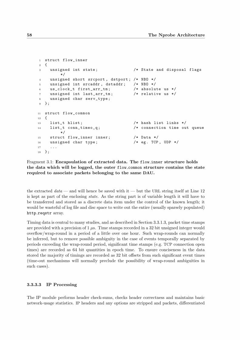
58 The Nprobe Architecture

1 struct flow_inner

2 {

3 unsigned int state; /* State and disposal flags

*/

4 unsigned short srcport , dstport ; /* NBO */

5 unsigned int srcaddr , dstaddr ; /* NBO */

6 us_clock_t first_arr_tm ; /* absolute us */

7 unsigned int last_arr_tm ; /* relative us */

8 unsigned char serv_type;

9 };

11 struct flow_common

12 {

13 list_t hlist; /* hash list links */

14 list_t conn_timeo_q ; /* connection time out queue

*/

15 struct flow_inner inner; /* Data */

16 unsigned char type; /* eg. TCP , UDP */

17 ...

18 };

Fragment 3.1: Encapsulation of extracted data. The flow inner structure holdsthe data which will be logged, the outer flow common structure contains the staterequired to associate packets belonging to the same DAU.

the extracted data — and will hence be saved with it — but the URL string itself at Line 12is kept as part of the enclosing state. As the string part is of variable length it will have tobe transferred and stored as a discrete data item under the control of the known length; itwould be wasteful of log file and disc space to write out the entire (usually sparsely populated)http reqstr array.

Timing data is central to many studies, and as described in Section 3.3.1.3, packet time stampsare provided with a precision of 1 µs. Time stamps recorded in a 32 bit unsigned integer wouldoverflow/wrap-round in a period of a little over one hour. Such wrap-rounds can normallybe inferred, but to remove possible ambiguity in the case of events temporally separated byperiods exceeding the wrap-round period, significant time stamps (e.g. TCP connection opentimes) are recorded as 64 bit quantities in epoch time. To ensure conciseness in the datastored the majority of timings are recorded as 32 bit offsets from such significant event times(time-out mechanisms will normally preclude the possibility of wrap-round ambiguities insuch cases).

3.3.3.3 IP Processing

The IP module performs header check-sums, checks header correctness and maintains basicnetwork-usage statistics. IP headers and any options are stripped and packets, differentiated

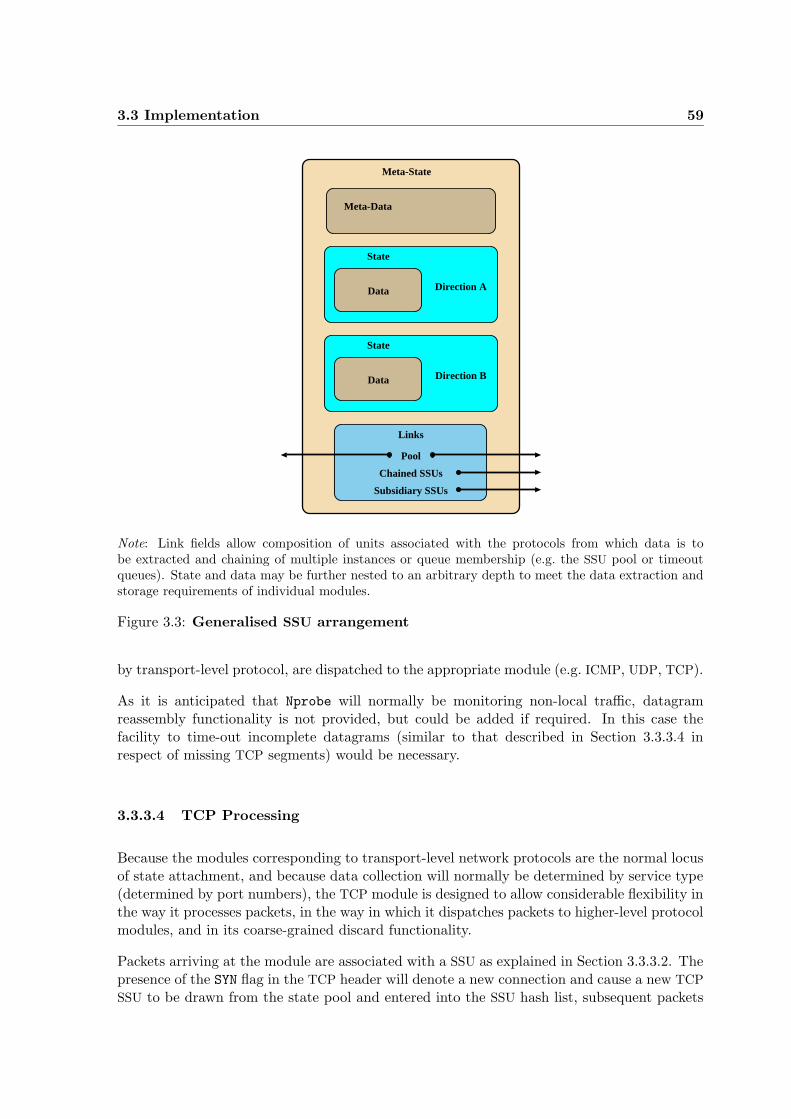
3.3 Implementation 59

Meta-State

Direction A

State

Data

Direction B

State

Data

Links

Pool

Chained SSUs

Subsidiary SSUs

Meta-Data

Note: Link fields allow composition of units associated with the protocols from which data is tobe extracted and chaining of multiple instances or queue membership (e.g. the SSU pool or timeoutqueues). State and data may be further nested to an arbitrary depth to meet the data extraction andstorage requirements of individual modules.

Figure 3.3: Generalised SSU arrangement

by transport-level protocol, are dispatched to the appropriate module (e.g. ICMP, UDP, TCP).

As it is anticipated that Nprobe will normally be monitoring non-local traffic, datagramreassembly functionality is not provided, but could be added if required. In this case thefacility to time-out incomplete datagrams (similar to that described in Section 3.3.3.4 inrespect of missing TCP segments) would be necessary.

3.3.3.4 TCP Processing

Because the modules corresponding to transport-level network protocols are the normal locusof state attachment, and because data collection will normally be determined by service type(determined by port numbers), the TCP module is designed to allow considerable flexibility inthe way it processes packets, in the way in which it dispatches packets to higher-level protocolmodules, and in its coarse-grained discard functionality.

Packets arriving at the module are associated with a SSU as explained in Section 3.3.3.2. Thepresence of the SYN flag in the TCP header will denote a new connection and cause a new TCP

SSU to be drawn from the state pool and entered into the SSU hash list, subsequent packets

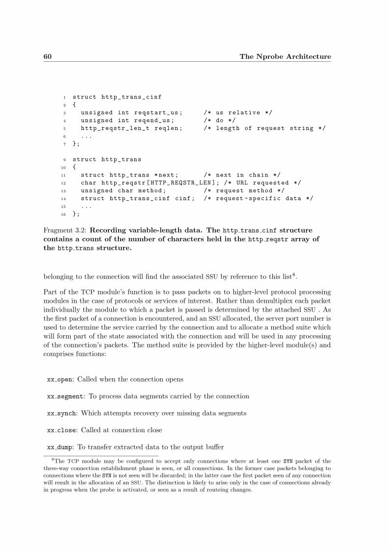
60 The Nprobe Architecture

1 struct http_trans_cinf

2 {

3 unsigned int reqstart_us ; /* us relative */

4 unsigned int reqend_us ; /* do */

5 http_reqstr_len_t reqlen ; /* length of request string */

6 ...

7 };

9 struct http_trans

10 {

11 struct http_trans *next; /* next in chain */

12 char http_reqstr[HTTP_REQSTR_LEN ]; /* URL requested */

13 unsigned char method ; /* request method */

14 struct http_trans_cinf cinf; /* request -specific data */

15 ...

16 };

Fragment 3.2: Recording variable-length data. The http trans cinf structurecontains a count of the number of characters held in the http reqstr array ofthe http trans structure.

belonging to the connection will find the associated SSU by reference to this list8.

Part of the TCP module’s function is to pass packets on to higher-level protocol processingmodules in the case of protocols or services of interest. Rather than demultiplex each packetindividually the module to which a packet is passed is determined by the attached SSU . Asthe first packet of a connection is encountered, and an SSU allocated, the server port number isused to determine the service carried by the connection and to allocate a method suite whichwill form part of the state associated with the connection and will be used in any processingof the connection’s packets. The method suite is provided by the higher-level module(s) andcomprises functions:

xx open: Called when the connection opens

xx segment: To process data segments carried by the connection

xx synch: Which attempts recovery over missing data segments

xx close: Called at connection close

xx dump: To transfer extracted data to the output buffer

8The TCP module may be configured to accept only connections where at least one SYN packet of thethree-way connection establishment phase is seen, or all connections. In the former case packets belonging toconnections where the SYN is not seen will be discarded; in the latter case the first packet seen of any connectionwill result in the allocation of an SSU. The distinction is likely to arise only in the case of connections alreadyin progress when the probe is activated, or seen as a result of routeing changes.

3.3 Implementation 61

Method suites are accompanied by a flag-set, also provided by the appropriate higher-levelmodule, which controls the packet processing carried out at the TCP level, primarily whetherthe delivery of a coherent, ordered, byte stream is required, whether packets should be check-summed and whether packet header information should be recorded.

Two alternative default method suites are provided by the TCP module: the first simplyaccounts for all connections and packets not providing a service of interest as an aggregate of‘other’ packets and octets, the second maintains similar counts but on a per-connection basisfor each connection seen.

If TCP-level activity is of interest the significant header fields (e.g. sequence and acknowl-edgement numbers, segment size, window advertisement, and flags) of each packet are logged.Flow-based compression is used; because packets are associated repeated fields such as ad-dresses and port numbers do not need to be saved for each. As connections are opened eachis assigned a unique 32 bit identifier and this, the addresses, port numbers, and time logged.Any further data associated with this connection, for instance the main dump of extracteddata, is identified by reference to this unique identifier. Per-packet header data is accumulatedas part of the connection’s data and dumped to log with it on the close of the connection.Because each connection may comprise a potentially very large number of packets it would beinfeasible to pre-allocate sufficient memory to meet all cases; the normal TCP SSU thereforebuffers data pertaining only to 32 packet headers. In the case of longer connections, theheader data is periodically written to the output buffer in blocks of this size, identified by theconnection identifier. For conciseness each block of header data carries a 32 bit time offsetfrom the connection opening, and each packet records a further time offset from this.

Data collected for every connection processed will include a set of significant event timings(e.g. that of SYNs, FINs or RSTs, first and last data segments in each direction); a count of TCP

and payload octets, and of total and data segments; a count of missing, duplicated and outof order packets and octets; and connection Maximum Segment Size (MSS) and window-scaleoptions.

Packets from which higher-level data is to be extracted will normally be subject to IP checksum verification before being passed for further processing. Malformed or corrupted packetsmay break processing code or incorrect data may be extracted; it is assumed that such packetswill also be rejected by the receiving host and therefore retransmitted and seen again by theprobe.

The TCP headers of incoming packets presented to the module are checked for correctness, andstripped from packets being passed to other modules. Any TCP option fields are examined andMSS notifications and window scale factor options extracted. Other options are not currentlyrecorded as data, but may be noted as points of interest as explained in Section 3.3.6 onpage 72. The flags field of each header is examined, and the current connection status heldin state; a greatly simplified TCP state machine detects connection closure either through thenormal 4-way handshake or the presence of the RST flag.

Care must be taken that SSUs associated with the inevitably arising unclosed connectionsdo not exhaust the probe’s memory; such connections may result from FIN or RST seg-ments unseen due to packet loss, routing changes, or crashing or misbehaving hosts. A

62 The Nprobe Architecture

timeout mechanism is employed to detect and deactivate quiescent connections. The ques-tion of whether a static or adaptive timeout should be used is discussed by Christophe Diotet al. [Iannaccone01], based upon work by K.C.Claffy et al. [Claffy93][Claffy95], who concludethat a 60 second timeout will correctly determine the termination of an adequate proportionof flows. A slightly different approach is employed in the Nprobe implementation: the mem-ory allocation available for the storage of TCP SSUs is bounded and there is consequently noreason why connections should be timed out until all available SSUs have been utilised (i.e. itis the finite amount of available memory which determines how many currently live flows canbe accommodated by the system, and hence dictates that timeouts must occur as a conse-quence of new flows arriving). In this way timeout periods are not static, but are dynamicallydetermined by the level of network and probe activity, and may be made as long as possibleso as to accommodate the maximum possible period of connection quiescence before forcingclosure. A minimum timeout period now needs to be determined so as to detect over-earlytimeouts due to the capacity of the probe being over run. In practice, subject to a shortertimeout period determined by SSU availability, an upper timeout bound is imposed — as datais logged at connection closure an over-generous timeout period would lead to it appearing inthe saved traces later than it should, with possibly unfortunate results when analysing partialtraces.

All live TCP SSUs are placed upon a timeout queue; as each packet is processed its arrivaltime is noted and its SSU is moved to the tail of the queue which is consequently time orderedwith the least recently active connection at the head. The last arrival time of the queue headis periodically examined to ascertain whether connection(s) should be timed out. The queuehead SSU is recycled and the associated connection timed out if the pool of free TCP SSUsbecomes exhausted.

All packets (other than those aggregated and accounted for as ‘other’) are examined in thecontext of the connection’s sequence space and counts maintained of out-of-order, duplicatedor missing segments9. In the normal case of connections providing services of interest, wherepackets are passed to further modules, those modules expect to receive a complete and orderedbyte stream corresponding to that delivered to a higher-level protocol in the receiving machine.The TCP module therefore performs the necessary reordering and coalescing required todeliver a coherent byte stream. In-sequence segments are delivered immediately using thesegment processing function provided by the method suite associated with the connection,segments already seen are discarded or trimmed, and any segments preceded by a gap in thesequence space are held pending reordering and delivery — note that this is the one exceptionto the general rule of immediate packet processing and buffer return.

Each TCP SSU provides for a sequence-ordered priority queue in which any held segments areplaced; as the great majority of segments placed into the queue will be received in order, andhence be appended at the rear, the cost of insertion is normally trivial. If packets are heldon the queue any newly arriving in-sequence packets are checked against the sequence of thequeue head; if the sequence void is filled all queued packets up to any further sequence gapare immediately removed from the queue, passed on for processing and the containing buffers

9These may not be the same as seen by endpoint hosts due to Nprobe’s placement at an arbitrary pointbetween the two; segments can, for instance, be lost ‘downstream’ of the probe or routes changed and packetsrouted around it.

3.3 Implementation 63

returned to the receive pool.

A timeout mechanism is also required for out of order segments held awaiting the arrival ofmissing segments (which may not be seen, in the same way as packets signifying connectionclosure can be lost to the probe). A more aggressive timeout policy is required however —each live connection only consumes one SSU but may require multiple out of order segments(and hence receive buffers) to be held — exhaustion of the receive buffer pool would result indisastrous packet drop and data loss. The segment at the head of a connection’s held queueis therefore timed out if any of the following conditions apply:

• More than a set proportion of the entire receive buffer pool is consumed by held segments— in practice a proportion of 50% of the total number of buffers has been found to givesatisfactory operation.

• An acknowledgement for any sequence number beyond the missing segment(s) is seenhence indicating that a retransmission is unlikely to be encountered.

• The number of segments held by the connection reaches a predetermined threshold — toguard against the possibility of long connections absorbing a disproportionate numberof buffers.

• The connection as a whole is timed out.

When a timeout occurs the held segment(s) are presented to the appropriate method suite’ssynch function which may attempt to resynchronize its data extraction with the interruptedbyte stream (e.g. the HTTP module’s resynchronization function might look for byte sequencesindicating the start of a fresh transaction, or simply jump a certain number of bytes if thesequence gap falls within the length of a known-size object). All subsequent held segmentsare then processed in the same way as if an arriving segment had filled the sequence void. Inthe case of timeouts due to overall connection timeout the synchronisation function may berepeatedly called if multiple sequence voids exist, until all segments have been processed. Itshould be noted that the arrival of a RST, or the FIN segments representing a full connectionclose do not trigger a timeout (which could then precede the arrival of retransmitted packets).

3.3.3.5 UDP Processing

The configuration and operation of the UDP module are very similar to those of the TCP

module with the significant and obvious exception that connection-oriented functionality —the tracking of connection set-up and tear-down phases and byte-stream ordering — is notrequired.

Because there is no UDP mechanism corresponding to the closure of a TCP connection thereis not the same convenient signification of when a flow has reached completion and datacan be dumped, and state torn down. The timeout mechanism will ensure that all flows areeventually terminated from the probe’s viewpoint, but this may lead to an undue consumptionof UDP SSUs associated with flows completed, but awaiting timeout. It is expected that UDP

64 The Nprobe Architecture

flows of interest (i.e. those where state is attached, rather than those simply accounted foras ‘other’) will normally also be processed by higher-level protocol modules which will detecttermination as determined by the protocol semantics (e.g. trivially, a DNS flow is terminatedby the receipt of a response datagram).

3.3.3.6 HTTP Processing

The main function of the HTTP processing module is to parse HTTP request and responsemessages and to extract data from the lines and header fields of interest. The following areidentified and processed:

Request-Lines: Method, requested URL and HTTP version are extracted.

Response status lines: Numeric response code and server HTTP version are extracted.

Header Fields: Currently recognised fields include:

• Connection (persistent or non-persistent connections are identified and persis-tence negotiations tracked.)

• Content-Type and Content-Length

• Referer (sic)

• Transfer-Encoding

• TE and Trailer (are trailer header fields acceptable, and if so are any present tobe parsed?)

• Host

• User-Agent

• Via

• Location

• Refresh

• Server

The header field identification and data extraction infrastructure is implemented through aseries of C macros in such a way that additional fields can be trivially added. It is planned toextend the current set of fields to include those pertaining to cache control, object freshnessand lifetime and conditional requests.

The timing of significant events (e.g. the start and finish of request and response headers andbodies) is recorded.

Although the great majority of HTTP headers are usually wholly contained in a single TCP

segment the possibility of fragmentation across several segments must be catered for wherethe sender implements a particularly aggressive transmission policy. Rather than construct aparsing mechanism which is able to recommence after the interruption represented by segment

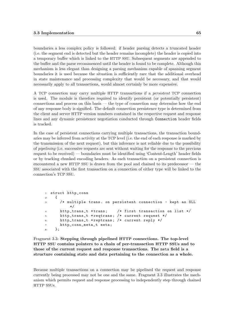
3.3 Implementation 65

boundaries a less complex policy is followed: if header parsing detects a truncated header(i.e. the segment end is detected but the header remains incomplete) the header is copied intoa temporary buffer which is linked to the HTTP SSU. Subsequent segments are appended tothe buffer and the parse recommenced until the header is found to be complete. Although thismechanism is less elegant than designing a parsing mechanism capable of spanning segmentboundaries it is used because the situation is sufficiently rare that the additional overheadin state maintenance and processing complexity that would be necessary, and that wouldnecessarily apply to all transactions, would almost certainly be more expensive.

A TCP connection may carry multiple HTTP transactions if a persistent TCP connectionis used. The module is therefore required to identify persistent (or potentially persistent)connections and process on this basis — the type of connection may determine how the endof any response body is signified. The default connection persistence type is determined fromthe client and server HTTP version numbers contained in the respective request and responselines and any dynamic persistence negotiation conducted through Connection header fieldsis tracked.

In the case of persistent connections carrying multiple transactions, the transaction bound-aries may be inferred from activity at the TCP level (i.e. the end of each response is marked bythe transmission of the next request), but this inference is not reliable due to the possibilityof pipelining (i.e. successive requests are sent without waiting for the response to the previousrequest to be received) — boundaries must be identified using ‘Content-Length’ header fieldsor by tracking chunked encoding headers. As each transaction on a persistent connection isencountered a new HTTP SSU is drawn from the pool and chained to its predecessor — theSSU associated with the first transaction on a connection of either type will be linked to theconnection’s TCP SSU.

1 struct http_conn

2 {

3 /* multiple trans . on persistent connection - kept as SLL

*/

4 http_trans_t *trans ; /* first transaction on list */

5 http_trans_t * reqtrans ; /* current request */

6 http_trans_t * reptrans ; /* current reply */

7 http_conn_meta_t meta;

8 };

Fragment 3.3: Stepping through pipelined HTTP connections. The top-levelHTTP SSU contains pointers to a chain of per-transaction HTTP SSUs and tothose of the current request and response transactions. The meta field is astructure containing state and data pertaining to the connection as a whole.

Because multiple transactions on a connection may be pipelined the request and responsecurrently being processed may not be one and the same. Fragment 3.3 illustrates the mech-anism which permits request and response processing to independently step through chainedHTTP SSUs.

66 The Nprobe Architecture

The combination of HTTP header parsing and location of the HTTP body end serve to delimitthe message entity. Header and body lengths are recorded. In all cases a crc-based hash isused to fingerprint the entity; the fingerprint is stored and may be used in later analysis toidentify the resource or to detect changes in its composition. No further processing is carriedout on entity bodies, except in the case of HTML documents, which are passed to the HTML

processing module.

3.3.3.7 HTML Processing

The primary function of the HTML module is to parse HTML documents and to extract andrecord any contained links — this data may be used during data analysis to aggregate themultiple transactions used to fetch a complete page. Reference links (i.e. those followed underuser control) are distinguished from in-line links (i.e. those referencing document images,frames, style sheets etc.).

If pages are to be successfully reconstructed both links and additional information are re-quired; the parser therefore passes through both the head and the body of the document andrecognises:

Elements/Tags: Which may contain attributes with absolute or relative URL values. A non-exhaustive list includes:

ANCHOR AREA BODY

FRAME IMG IFRAME

LINK MAP STYLE

The attributes themselves: Which may take URL values, including:

HREF BACKGROUND ACTION

USEMAP SRC CODE

CODEBASE OBJECT ARCHIVE

DATA

Base Elements/Tags: Which may define the base of relative or relocated URLs (e.g. BASE)and the end of such base scopes.

META tags: Particularly HTTP-EQUIV elements and REFRESH directives together with the as-sociated CONTENT and URL attributes. Such directives may cause repeated or periodicdownloads of the same or other documents, or may be used as a redirection mechanism.

There is a significant probability that HTML documents will span several TCP segments, andthe simple mechanism employed to parse fragmented HTTP headers is therefore inappropri-ate. Instead a ‘simple’ parser has been implemented which is capable of resuming a parseinterrupted by segment boundaries. This mechanism implies both that the state of the inter-rupted parse must be recorded and that a linear, rather than a recursive, method be employed— a series of templates are provided which specify the tags and elements of interest and the

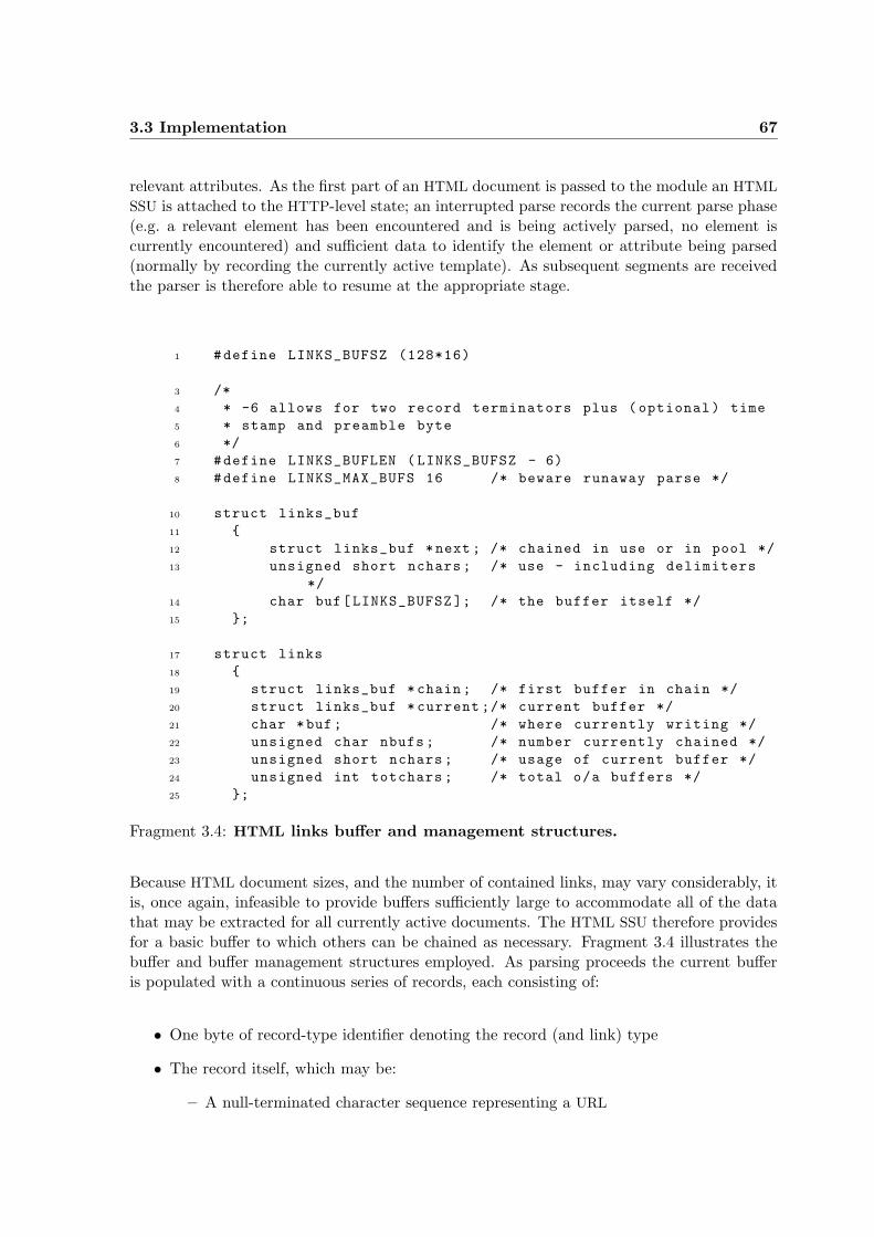
3.3 Implementation 67

relevant attributes. As the first part of an HTML document is passed to the module an HTML

SSU is attached to the HTTP-level state; an interrupted parse records the current parse phase(e.g. a relevant element has been encountered and is being actively parsed, no element iscurrently encountered) and sufficient data to identify the element or attribute being parsed(normally by recording the currently active template). As subsequent segments are receivedthe parser is therefore able to resume at the appropriate stage.

1 #define LINKS_BUFSZ (128*16)

3 /*

4 * -6 allows for two record terminators plus ( optional) time

5 * stamp and preamble byte

6 */

7 #define LINKS_BUFLEN ( LINKS_BUFSZ - 6)

8 #define LINKS_MAX_BUFS 16 /* beware runaway parse */

10 struct links_buf

11 {

12 struct links_buf *next ; /* chained in use or in pool */

13 unsigned short nchars ; /* use - including delimiters

*/

14 char buf[LINKS_BUFSZ ]; /* the buffer itself */

15 };

17 struct links

18 {

19 struct links_buf *chain ; /* first buffer in chain */

20 struct links_buf * current ;/* current buffer */

21 char *buf; /* where currently writing */

22 unsigned char nbufs; /* number currently chained */

23 unsigned short nchars ; /* usage of current buffer */

24 unsigned int totchars ; /* total o/a buffers */

25 };

Fragment 3.4: HTML links buffer and management structures.

Because HTML document sizes, and the number of contained links, may vary considerably, itis, once again, infeasible to provide buffers sufficiently large to accommodate all of the datathat may be extracted for all currently active documents. The HTML SSU therefore providesfor a basic buffer to which others can be chained as necessary. Fragment 3.4 illustrates thebuffer and buffer management structures employed. As parsing proceeds the current bufferis populated with a continuous series of records, each consisting of:

• One byte of record-type identifier denoting the record (and link) type

• The record itself, which may be:

– A null-terminated character sequence representing a URL

68 The Nprobe Architecture

– A null-terminated character sequence representing a base URL (used in relativeURL resolution)

– An end of base scope marker

– A four byte sequence representing a relative time stamp giving the arrival time ofthe segment containing the link (the time stamp applies to all following links untilthe next time stamp is encountered.)

When the end of the flow is reached and data dumped, the chained buffers are coalesced andprepended with a count of content length.

3.3.3.8 Dynamic Flow Recognition

Identifying traffic within flows of interest will usually be based upon the well-known port atthe server as described in Section 3.3.3.4. However in the case of some services the serverwill not communicate via such a well-known port, or port allocation may be dynamic; theRTSP [Schulzrinne98] protocol, for example, defines a negotiation between client and serverduring which the server port is determined.

Services using a known port outside the well-known range are trivially catered for — theport number can simply be coded into the table of significant port numbers of interest inthe normal way. Where services using negotiated port numbers are to be investigated it isanticipated that a module with knowledge of the syntax of the negotiation protocol (whichwill be directed to a known port) will be deployed and will identify the port to be used. Thisport can then be entered into the table of ports of interest, and a suitable SSU inserted intothe SSU hash table — as the base SSU will be a TCP or UDP SSU it will also discriminatepackets based upon IP addresses so will not accept other, unrelated, traffic which may alsobe using the same port number.

3.3.4 Data Output

Sections 3.2.1 and 3.2.2.1 introduce the need for buffering between the extraction of data andits storage on disc. The data generation rate will be variable due to bursty packet arrivalsand variations in the computational expense of data extraction, and it is desirable to committo disc efficiently in multiples of the block size. The relationship between stored data andoutput buffering is illustrated in Figure 3.1 on page 47.

As flows terminate, extracted data, held in state, is dumped into a log output buffer as aseries of continuous records in the format to which they will be written to disc. The formatmust reflect the variable nature and format of the data collected and must therefore be self-specifying. Each record opens with a header containing a record type10 identifier and aninteger record length count: the type identifier is used, when retrieving data from disc, to

10Output record types are not confined to those recording extracted data — others may record interestingphenomena or probe-centric data as explained in Sections 3.3.6 on page 72 and 3.4 on page 73.

3.3 Implementation 69

identify the data type and format of the DAU meta data block following the header; the lengthfield is used during retrieval to step over unwanted records.

Dumping is triggered by the close function of the method suite provided by service-levelprotocol modules, which will invoke the services of the corresponding dump method. WhereSSUs are linked, dump invocations will be chained to save all data from the various SSU sub-components of the overall SSU. At least one chained dump call will normally be made — tothe appropriate transport-level SSU associated with the service. Data dumping functionalitymust reside with the protocol processing modules as it is they who define and understandthe protocol specific data storage format and any state denoting the nature and degree ofthe data extracted. The data held as part of any top-level SSU will contain a flags fielddenoting which data constituents have been extracted and consequently which nested datastructures are to be dumped. In the case of the TCP module, for instance, connection metadata (shown in Figure 3.3 on page 59) will always be dumped and contains flags indicatingwhich directional traffic has been seen; one or both directional sub-SSU state repositories willbe dumped accordingly. When data is retrieved from trace files the same meta data fieldswill be used to indicate the format and presence of the saved data. Figure 3.4 illustrates howthe dump format is controlled by the contents of state.

The output buffer is configured as a memory mapped file and is therefore written out todisc by the operating system’s piod thread as blocks of data accumulate. The only memorycopy involved in data output is therefore that of dumping data to the buffer. This copy isunavoidable as the unpredictable nature and extent of the data as it is extracted denies thepossibility of formatting or reserving buffer space until the termination of each flow.

Even with the high data reduction ratio achieved by Nprobe very large trace files will begathered which may exceed the maximum file size allowed by the system. Output is thereforedivided amongst a succession of trace files, a file cycle being signalled when a predeterminednumber of bytes have been dumped. Although the memory mapped output file is configuredfor asynchronous operation, the unmapping of a completed file (which will cause it to be closedand the file cache buffers to be flushed) can cause the unmapping process to block for a shortperiod. Because continuous processing of incoming packets is critical to avoid receive bufferpool exhaustion, each Nprobe process spawns a file management thread at probe start-upwhich manages file cycle operations. As this thread is called upon infrequently, the contextswitch overhead is acceptable.

3.3.5 Protocol Compliance and Robustness

When processing very large numbers of packets and flows it is inevitable that some will beencountered giving rise to maverick conditions:

Pathological conditions: Which may arise from poor protocol implementations, misbehavingor poorly configured hosts, malformed packets or protocol headers, corruption of packetcontents, or other errors.

Protocol specification infringements due to erroneous implementations: Some Web browsers

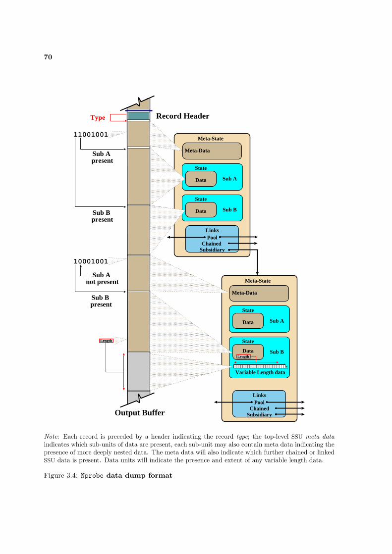
70

Meta-State

Sub A

State

Data

Sub B

State

Data

LinksPool

Chained Subsidiary

Meta-Data

11001001

Sub A present

Sub B present

10001001

Sub A not present

Sub B present

Length

Output Buffer

Record HeaderType

Meta-State

Sub A

State

Data

Sub B

State

Data

Meta-Data

LinksPool

ChainedSubsidiary

Variable Length data

Length

Note: Each record is preceded by a header indicating the record type; the top-level SSU meta dataindicates which sub-units of data are present, each sub-unit may also contain meta data indicating thepresence of more deeply nested data. The meta data will also indicate which further chained or linkedSSU data is present. Data units will indicate the presence and extent of any variable length data.

Figure 3.4: Nprobe data dump format

3.3 Implementation 71

and Servers, as an example, terminate HTML header lines with a lone <NL> rather thanthe specified <CR><NL> sequence.

Flow interruptions: Missing packets which have been lost in the network or due to routeingchanges).

Intentional protocol infringements: One family of Web browsers, for instance, does not con-form to the standard TCP four-way handshake after receiving an HTTP object on anon-persistent connection — it simply transmits a RST segment. The TCP module mustbe capable of differentiating such behaviour from RST segments indicating pathologicalconnection conditions.

Inconsistencies due to probe placement: Because the probe may be placed in an arbitraryposition at any point between communicating hosts, normal protocol semantics maynot fully apply. Multiple concurrent TCP connections, for instance, may appear toexist between the same two hosts and same two port numbers — a RST segment, forexample, may be sent by one host followed by a SYN segment opening a new connectionbetween the same two ports. Traffic belonging to the first connection may still be seenarriving from the other host. Such a case is compounded by hosts which do not correctlyimplement the selection of TCP Initial Sequence Numbers and reuse the sequence spaceof the original connection.

Content or behaviour which is correct but which is not understood by processing modules: Thecomplexity inherent in network and end system dynamics, and component interactions,will give rise to situations that the probe is unable to dispose of correctly — to foreseeevery circumstance that will arise is infeasible.

In the case of a simple probe which copies packet content verbatim, the problems posed bysuch mavericks are deferred until post collection analysis of traces, but a data-extracting probemust be capable of handling any condition without interrupting normal operation, corruptingcollected data, extracting erroneous data, or itself entering a pathological state — it must berobust in the face of whatever arrives11 on the network.

Maverick conditions arising from pathological states or protocol compliance failures will nor-mally be detected during packet processing as checksum failures, malformed packets or proto-col headers, or breaches of protocol syntax or semantics. A distinction must be made betweenincorrect and misleading semantics: the former (e.g. pathological errors in TCP sequence num-bering, contradictory HTML header fields) are detectable and action can be taken; the latter(e.g. incorrect HTML Last-Modified header fields, inaccurate HTML content) are not. TheNprobe implementation, in attempting to identify such conditions, is guided by considerationof how problematic packets or content would impact upon the receiving host or application;thus the former category may generate an error condition, the latter would probably alsoremain undetected by the recipient.

Detectable errors will result in one of the following outcomes:

11Or, conversely, sometimes, what does not arrive.

72 The Nprobe Architecture

The condition is regarded as pathological: An error condition is generated and processing ofthe packet is dropped — detailed processing will not be carried out on any subsequentpackets of the DAU.

The condition is not pathological, but further full processing of the DAU packets is impossible:For example a missing TCP segment over which a higher-level protocol module cannotresynchronize with the byte stream or an HTML header parse failure.

The error is fatal only to processing of the individual packet: If recovery is possible normalprocessing may resume with subsequent packets.

Disambiguation or toleration of probe position inconsistencies: Apparently concurrent TCP

connections between the same host/port pairs, for instance, can largely be resolvedby maintaining SSUs for each connection and assigning packets to a particular flow onthe basis of sequence space feasibility; delays between seeing the final packet of an HTTP

response and the first packet of a subsequent request on a persistent connection maymake it impossible for the probe to tell whether or not pipelining is taking place —processing must proceed correctly without this knowledge.

The condition would probably be accepted by the receiving host: The probe must attempt toaccommodate it (e.g. minor syntactic errors; the HTTP module can, for instance, parseheader lines missing the <CR> part of the delimiter).

In all cases the SSU and corresponding data will be marked and the type of error recorded.

Considerable ingenuity has been invested in attempts to ensure that maverick conditions aredetected and the correct action taken, particularly in the case of minor or recoverable errors.The law of diminishing returns, however, applies: some problems will be too computationallyexpensive to detect or recover from, and others will be too rare to reasonably accommodate.Where to set the cut-off point is subject to arbitrary decision, but the Nprobe implemen-tation sets a target of successfully processing 99% of all incoming packets. Some semanticirregularities or inconsistencies may be detectable, and corrective action possible, during dataprocessing when the absence of time constraints allows greater computational resources to beemployed, and when data can be integrated and compared across DAU boundaries.

3.3.6 Error Handling, Identification of Phenomena of Interest and Feed-back into the Design

In addition to the main trace files Nprobe outputs an error log to which offending packets arewritten in their entirety when error conditions are generated. This log file is formatted as atcpdump trace file, but with the MAC/LLC header overwritten with an error code and some(error dependent) bytes of additional information; the interface type field of the tcpdump fileheader identifies the file as generated by Nprobe.

The tcpdump format was chosen as it allows examination of the error log files using tcpdump12,

12A slightly modified tcpdump is used which is capable of interpreting and printing the data over-writing theLLC/MAC header.

3.4 Trace and Monitoring Process Metadata 73

and in particular because the packet filter can then be used to select packets for display orextraction by error type (possibly in combination with other criteria). As Nprobe can takepacket input from tcpdump trace files (see Section 3.3.1.4), offending packets can be re-offeredto the analysis process multiple times as an aid to module development or improvement. Theerror log output is managed by the file management thread and file cycling is synchronisedwith that of the trace files.

When error conditions arise resulting in the situation where further data extraction is notpossible for the remainder of a flow it is still, nevertheless, desirable to track, and accountfor, any subsequent packet arrivals (e.g. the HTTP module provides for two types of dummytransaction SSU; these accumulate a count of packets and octets arriving after error conditionsor sequence voids).

Conditions, or phenomena, of interest may arise during probe operation which it is desirableto record, but which do not form part of the data normally extracted: it may, as an example,be wished to count occurrences so as to determine whether extraction code should be enlargedto handle certain conditions, to identify unusual correlations between data, or to note minorsyntax infringements. A C macro, which can be placed anywhere in a processing module,identifies the desired condition and causes a record of type interesting to be written tothe normal log buffer; the record is textual and therefore provides a very flexible means ofrecording all associated data of interest.

A similar, macro-based, mechanism which parallels distributed coarse-grained data discardcan also be placed anywhere in the processing modules to dump entire packets to the error logwhen interesting, as opposed to error, conditions are encountered. Traffic samples conformingto a flexible specification can thereby be gathered.

The mechanisms in this section provide both a means of examining and categorising thecause of error conditions, which can be utilised in the iterative design process, and a meansof gathering sample data over a range of granularities for the development of new processingmodules.

3.4 Trace and Monitoring Process Metadata

An operating probe will not only generate data extracted from the packets observed — datapertinent to traffic as a whole, and to the probe’s own operation must be recorded; such traceand monitoring process meta data is gathered and dumped on a periodic13 basis as a numberof output record types which record for each period:

Operational error conditions: Principally the number of packets dropped due to receive bufferpool exhaustion or by the network interface14

13The period employed is arbitrary, involving a balance between computational/storage cost and granularity,but two seconds is currently employed. A summary of major data items is also presented at the console witha rather greater period.

14Nprobe is intended to operate with nil packet loss but rather than shut down the system if loss occurs it is

74 The Nprobe Architecture

CPU and system usage: CPU cycles accounted to the Nprobe process, interrupts taken, con-text switches, page faults, I/O blocks, memory Resident Set Size, and number of pageswaps as retrieved from the /proc pseudo-filesystem

Process receive buffer and SSU pool usage accounts: The number of buffers withdrawn and re-turned to the receive pool and the maximum number concurrently held, together withsimilar data pertaining to the SSU pool

Timeout accounting: The number and type of connection and reassembly timeouts, and theminimum timeout period necessitated by SSU pool availability

Traffic statistics: A count of total packets and octets received with categorisation of typeand sub type(s) at the granularity and level of detail provided by the various protocolprocessing modules; the arrival bandwidths of major traffic classes

Output file usage: The total number of bytes and records or packets written to the trace andlog files respectively, both overall and in respect of the current file cycle

Operational meta data: Which is saved at each file cycle and includes the file start and endtimes, Wan software version and configuration, hardware version and operational param-eters of the monitoring run

Disposal summary: Saved on a per file basis giving a summarised total of the periodic data,the number and type of error conditions encountered and successful flow terminations,maximum and minimum values for the number of concurrent active flows of each type,and maximum and minimum arrival rates for the major traffic types

New probe deployments and shifting traffic patterns dictate that overall operating parameters(e.g. the relative proportions of the various SSU types held in the pool) have to be tuned; theavailability of suitable meta data informs this process.

3.5 Hardware and Deployment

Nprobe was initially developed on a DEC Alpha 3100 workstation equipped with a four GBhard disc and network interface provided by a TurboChannel FDDI NIC fed from an opticaltap in the University of Cambridge Computing Service (UCCS) internal FDDI ring.

Further development was carried out using the probes which have been deployed to date:dual Intel 500 MHz Pentium III machines with 64 GB software RAID discs. These probeshave been fitted with Fore 200LE ATM and Alteon ACEnic 1 Gbps NIC cards and deployed tomonitor traffic traversing the link between the UCCS and the United Kingdom Joint AcademicNETwork (SuperJANET) and in the switching centre of a large commercial Internet ServiceProvider (ISP).

preferable to record loss rates periodically. Traces with unacceptable loss can be rejected. SSU pool exhaustionis regarded as a fatal error condition as it may result in massive data loss. The shutdown condition would berecorded.

3.6 Probe Performance 75

A new generation of more powerful probe machines are being acquired (April 2003) basedupon dual Intel Xeon 2.4 GHz processors with 4 GB of DDR EEC memory, each equipped withthirteen 200 GB RAID discs. A range of deployments across institutional and ISP locationsis planned.

3.6 Probe Performance

Deployments to date have not strained the probe’s capabilities — traffic rates of approxi-mately 120 Mbps with HTTP content of 95 Mbps have been monitored continuously withoutpacket loss, with the consumption of less than 20% of available processor cycles on a 500 MHzdevelopment machine, and achieving a data-reduction ratio of approximately 12:1. Calcula-tion of capacity based upon off-line data extraction (i.e. running the monitoring softwarewith input from tcpdump trace files) suggest that the software itself will keep pace with band-widths of approximately 780 Mbps, using a single 2.4 GHz processor, when a small number15

of concurrent connections are monitored.

Benchmarking tests have been carried out16 using traffic generated by clusters of machinesand concentrated via a common switch. The test load has encompassed a range of trafficmixes, packet sizes, and numbers of concurrent connections, and has also included the replayof real traffic multiplexed to the desired line rate by modifying host IP addresses. The results,described in [Moore03], suggest that any one of several factors may limit monitoring capacity.

The performance of the available Gigabit Ethernet cards varies, and unfortunately, theircapacity to perform at nominal ratings over single packets does not, in general, extend to asustained ability to deal with trains of small packets. The appropriate combination of NIC

and motherboard are necessary to achieve optimal performance, as underlined in a studyby Hughes-Jones et. al. [Hughes-Jones93]. PCI bus bandwidth can prove a bottleneck, andat high arrival rates interrupt handling becomes problematic. A high number of concurrentconnections, and hence high state memory requirement, can cause the extraction software tobecome a limiting factor due to frequent processor cache misses. As other components of thesystem are tuned and optimised trace bandwidth onto disc will eventually become a furtherbottleneck.

Initial tests based upon a single data extraction process running on a 2.4 GHz processor sug-gested that live traffic loads of approximately 790 Mbps could be accommodated over a limitednumber of concurrent flows, the rate dropping to 280 Mbps when using replays of real trafficmixes. When all non-HTTP traffic was removed from these traces a sustainable monitoringrate of 189 Mbps was achieved. It should be noted, however, that these results were obtainedusing standard interface drivers and un-optimised extraction code with full debugging and‘safety’ features enabled. Since they were performed, considerable improvements to capturerates have already been made, and there is confidence that full capture approaching 1 Gbps

using a single probe will shortly be achieved — and will be exceeded using the emerging faster

15A small number of connections, in this context, meaning those whose state can be accommodated in theprocessor’s L2 cache.

16The benchmarking work has been carried out by Euan Harris, Christian Kreibich and Dr. Andrew Mooreof the Computer Laboratory Systems Research Group.

76 The Nprobe Architecture

PCI bus technologies.

3.7 Security and Privacy

Because on-line monitoring can potentially examine and record the entire content of networktraffic, regard must be paid to issues of the privacy of users and the security of content; tothese should, perhaps, also be added the protection of researchers — consider the position ofan investigator who unintentionally discovers illegal activity.

The accepted practice in addressing these issues is to anonymize IP addresses and to limitdata capture to the lower, and essentially content free, levels of the protocol stack. The first ofthese mechanisms, it is argued, may provide an illusory security and may place considerablepractical limitations on the useful information content of captured data; the second is, ofcourse, in contradiction to one of the basic rationales underlying the Nprobe design.

It must be remembered that research based upon monitoring is only one of a growing numberof legitimate activities which may potentially compromise security and privacy. Most networkservice providers, whether ISPs, private or public institutions, or other organisations, carryout some form of monitoring — for network or personnel management purposes. In theUnited Kingdom it has been proposed that ISPs should keep comprehensive records of users’e-mails and Web accesses which will be available, on demand and without legal scrutiny, toa wide range of central and local government agencies. The level of security, and respect forprivacy, required in monitoring must be placed in the context of the many potential sourcesof ‘leakage’.

Address anonymization may be classified by method into techniques which render the orig-inal address recoverable (i.e. employing symmetrical cryptosystems) or not (using one-waycryptographic functions), and further into those which are prefix-preserving (i.e. anonymizedaddresses based within the same network or sub-net will still be identifiable as such) or not.There are powerful arguments for both recoverable and prefix-preserving schemes: the pro-posed research may well require identification or aggregation of the original addresses (e.g. allof an ISP’s dial-up customers, all traffic to a certain service); original IP addresses may be re-quired in data analysis (e.g. reconstruction of Web page download activity may require DNS

look-ups of addresses as explained in Section 7.5 on page 172). Whichever anonymizationscheme is employed the level of security offered may be partially illusory: an IP address of32 bits represents a relatively small search space, and with relatively little traffic analysis (ifany is actually required at all) is very vulnerable to a known text style of attack. Althoughthe designers of prefix-preserving schemes (e.g. Xu et al. [Xu01]) claim security comparablewith non prefix-preserving methods it is inescapable that the discovery of one address willcompromise others. If recoverable schemes are employed, security rests inevitably with thegroup in possession of the essential key.

Data gathered from higher protocol levels may similarly be anonymized through encryption,but will almost certainly have to be recoverable to be usable, and may be equally vulnerableto known text attack (consider commonly known and popular Web sites). Higher and lower-level data may also be combined to compromise security: the IP address of a Web server may,

3.8 Summary 77

for instance, be anonymized but will possibly appear as a textual Host field in HTTP headers— if one is to be anonymized both must be, and also the requested URL — hence addingconsiderable, and perhaps unacceptable, computational overhead to data extraction. AnjaFeldmann describes the BLT exercise [Feldmann00] as separating the data files containinganonymized IP addresses from those containing HTTP header fields, yet the two must becapable of combination, hence security rests, in effect, in the secure storage of data ratherthan the mechanism employed.

The essence of the matter rests with access; it is argued that any probe-gathered data,anonymized and encrypted or not, is to some extent vulnerable and security must rest pri-marily in restricting access to it. It is certainly to be hoped that researchers are possessedof no less integrity than others (ISP employees, for instance) with access to sensitive userinformation, and that their data storage facilities will be at least as secure. Technical secu-rity mechanisms must be considered as an adjunct to, rather than as a substitute for, theappropriate use of measures such as Non Disclosure Agreements (NDAs) and data securityenforcement.

It may be that, when seeking probe placements, or permission to monitor, researchers feelthe need to engage in a certain degree of technological over-kill in order to reassure providersand managers that the issues have been addressed, or to conform to the expectations of theirpeers. The experience of finding potential deployments for Nprobe monitors suggests stronglythat the majority of service providers are happy to give access subject only to the appropriateNDAs.

Nprobe therefore relies upon access restriction as its primary mechanism ensuring privacy andsecurity. The probes can only be activated by a very restricted group of root users, and datastored at the probe or elsewhere can only be accessed by a similarly restricted group. Accessto remote probes is only possible using secure means (e.g. ssh) and data is downloaded inencrypted form using similar mechanisms (e.g. scp). Address and data anonymization (of, forinstance, URLs) can be applied as data is collected if required, using recoverable techniqueswhich may, additionally, provide for prefix preservation.

Addresses are anonymized in the case of traces made available in the public domain or inpublished results.

3.8 Summary

A unique passive on-line network monitoring architecture has been proposed, which embodiesthe desirable attributes introduced in Section 1.4 on page 27 of Chapter 1, and is subjectto the design goals described in Section 3.1 on page 45. The design rationale employed isdescribed in Section 3.2.2 on page 48 and developed with reference to the themes of data flow,control and state. The monitor would provide a more powerful and flexible tool than hithertoavailable for harvesting data from the network and would, consequently, enable studies whichhad previously not been possible.

The main body of this chapter describes the more detailed design and implementation of the

78 The Nprobe Architecture

monitor — Nprobe. The major infrastructure and protocol processing modules have beencompleted, and although design and development of the probe continue — it is part of theunderlying design philosophy that it should be extensible — probes have been deployed andhave operated satisfactorily. Traces have been gathered, some of which form the basis of thestudies presented in Chapters 6 and 8 which demonstrate the utility of the system.

The success of the design and implementation of Nprobe, and the extent to which it has livedup to its ambitious goals may be judged, following the operation of prototype probes, by theforthcoming purchase of a series of more powerful and capable hardware platforms and theplanning of their wider deployment.

Chapter 4

Post-Collection Analysis of NprobeTraces

Chapter 3 has described the implementation of the Nprobe monitor and the generation oftrace files containing data extracted from packets traversing the network. During data col-lection, packet contents are only analysed sufficiently to allow the correct interpretation ofcontent during data extraction or abstraction, to aggregate data at the granularity of a DataAssociation Unit (DAU), and to allow flow-based compression. The transformation from datato information will require, at the very least, the retrieval of data from the format in whichit is stored in the trace files and, in almost all cases its further post-collection association andanalysis.

This chapter describes the mechanism of post-collection data analysis and a framework for itsdesign and execution which reflects the unique nature of the traces gathered by Nprobe. Theframework is introduced in Section 4.1; Sections 4.2 – 4.5 describe its components and theanalysis process itself, and Section 4.6 illustrates how the toolkit that it provides is used toconstruct complex analysis processes. Section 4.7 considers how confidence may be attachedto the results obtained, and in section 4.8 implementation issues arising from the use ofPython are discussed.

4.1 A Generic Framework for Post-Collection Data Analysis

Analysis of Nprobe-gathered data presents challenges which differ both in scale and naturefrom those inherent in the analysis of more conventional probe traces. The format of thetrace files is more complex and is likely to be extended or amended. The data itself is richerand more complex, and consequently the information which can be distilled from it will alsobe both more sophisticated and diverse. As a result a wider range of analysis tasks, or formsof analysis, may be called for to fully realise the information potential of the data.

The design of a data gathering system such as Nprobe must, therefore, be accompanied byan analysis framework which addresses these issues. Such a framework should recognise the

80 Post-Collection Analysis of Nprobe Traces

differing demands of two broad phases in the analysis process:

• Analysis development: calling for an analysis development environment supporting fastassembly of analysis software from existing components, reasoning about the meaningand relationships of data items, iterative analysis algorithm design, comprehensive trac-ing during analysis execution, detailed examination of preliminary results, and a highlevel of code re-use

• Generation of results: where mature analysis code is run on complete traces and theemphasis is on summarising, selection, and the presentation of results

The principal components of the Nprobe data analysis framework and their relationship toeach other are shown in simplified form in Figure 4.1.

The analysis framework and analysis tasks related to specific studies are implemented inPython [Python01][Lutz96]: its late binding, powerful high-level data types, object orienta-tion, modular structure, and suitability for quick prototyping make it attractive for use incomplex analysis tasks where there may be a considerable degree of code re-use. Section 4.8.1on page 106 enlarges upon the suitability of an object-oriented language for writing dataanalysis software, and some of the difficulties inherent in the use of Python are discussed inSection 4.8.2.

4.1.1 Modularity and Task-Driven Design

Analysis design will be motivated in three ways:

• Identified tasks: where directed research requires specific, predefined, information.

• Suggested tasks: arising where analysis results indicate that additional information maybe available, or that further phenomena of interest may be investigated. The scope ofthe data gathered by Nprobe makes it likely that, even when data has been gatheredtailored specifically to the needs of an identified task, further, suggested, tasks will begenerated during analysis, or that additional identified tasks may be based upon thesame data set.

• Exploratory analysis: because Nprobe-gathered data is so rich, it will often containvalues or correlations not envisaged when identifying the data to be collected, andwhich do not fall within the scope of suggested analysis tasks. Exploratory analysismay be particularly suggested when:

– Traces contain speculative data (i.e. not identified in advance as required for aparticular research goal, but gathered for the sake of completeness or its potentialinformational content).

– Archival traces are gathered (e.g. for purposes of future research or time basedcomparison). Patterson et al. [Patterson01] identify the need to collect such traceswhich are, by their nature, entirely speculative.

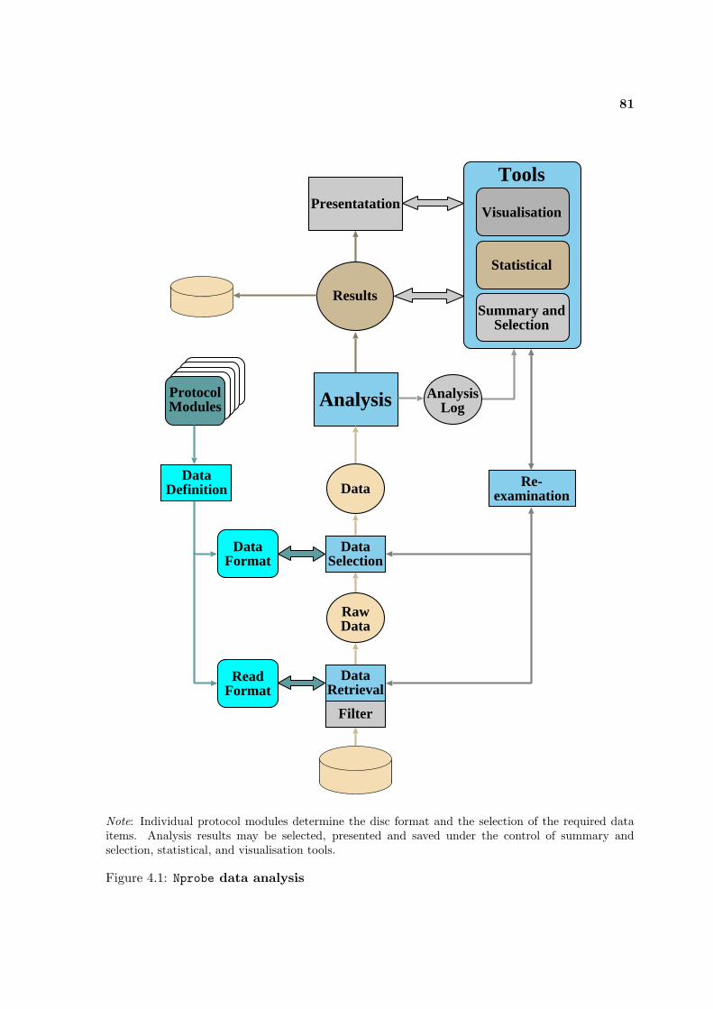
81

ProtocolModules

Presentatation

Results

Analysis AnalysisLog

Summary andSelection

Statistical

Visualisation

Tools

DataDefinition Data

RawData

ReadFormat

DataRetrieval

Filter

Re-examination

DataSelection

DataFormat

Note: Individual protocol modules determine the disc format and the selection of the required dataitems. Analysis results may be selected, presented and saved under the control of summary andselection, statistical, and visualisation tools.

Figure 4.1: Nprobe data analysis

82 Post-Collection Analysis of Nprobe Traces

Even disparate analysis tasks will share some common functionality (e.g. the manipulation oftrace files, selection and retrieval of data from trace files, the aggregation and presentation ofresults, and other utility functions), but rising to a very high degree in the case of suggestedor additionally identified tasks. The decomposition of any analysis task will, in other words,identify many sub-components (both utility and analytic) which are shared with other tasks.A series of modules, or components, are required which can be reused and composed asnecessary to meet the requirements of the current analysis task, new modules being addedwhen necessary and enlarging the existing pool of components. Top-down analysis design willtherefore become a matter of recursively decomposing a task until sub-tasks can be met fromthe set of standard or existing modules and any new components identified and implemented.

The analysis framework may therefore be regarded as providing a toolkit of utility and analysiscomponents, which can be combined as required to meet the requirements of specific tasks withthe minimum duplication of functionality and expenditure of time spent in the developmentof analysis software. The toolkit also contributes the analysis development environment.

Analysis framework or toolkit components may consist of Python modules, module-level func-tions, classes, or class methods, as determined by the functionality provided and the way thatthey will be used in conjunction with other components. At the highest level, analysis willbe driven by a Python script, which will import and call upon the services of the requiredcomponents. Simple analysis tasks may be implemented in a very few lines of code using onlybasic data retrieval components, but even comparatively complex tasks can be executed bya relatively short script which imports and uses the more sophisticated higher-level analysisand utility classes.

4.1.2 The Framework Components

The components of the data analysis framework fall into four categories:

A consistent data retrieval interface: Traces gathered using a monitoring system such astcpdump consist of a series of verbatim extracts of packet content, each prependedwith a header containing data such as arrival time stamp, packet length and capturelength. Successive headers are read from the trace file, identifying the length of thefollowing (possibly partial) packet to be read. Post collection analysis is presented withpertinent data from the header (e.g. time stamp and packet length) and as much ofthe verbatim packet contents as were captured. Before any analysis can proceed therequired data must be extracted from packet contents.

In contrast, Nprobe-gathered traces contain data already extracted from packet contentsduring collection, but due to the variable degree, nature, and format of the data, retrievalfrom trace files is more complex, and the required subset of the total recorded datamust be selected. Section 3.3.4 on page 68 explains how Nprobe trace files consist of aseries of records with a self specifying format, and Figure 3.4 on page 70 illustrates themechanism diagrammatically.

Differing studies may require the retrieval of a varying set of trace records from tracefiles, and of varying sets of data selected from those records. Because Nprobe is intended

4.1 A Generic Framework for Post-Collection Data Analysis 83

to be extensible, and to be flexible in its collection of data, new protocol modules maybe added, or existing modules amended or extended. In order to avoid the need to re-write analysis code from scratch in each case it is necessary to provide a uniform dataretrieval interface for the recovery of data from trace files, and its selection in canonicalform. The interface should, furthermore, as far as possible, be transparent to changesin trace file format, and allow the simple addition of new data record types.

The data retrieval interface is described in detail in Section 4.2 on the next page.

Data analysis components: The very simplest analysis may be implemented by the appropri-ate code contained within a script, but as explained in Section 4.1.1 and Section 4.8.1on page 106 it will normally be preferable to implement analysis components as themethods of dedicated analysis classes. Sections 4.3.1 on page 87 and 4.3.2 on page 88introduce protocol analysis classes providing analysis methods applicable to individualinstances of protocol use and Section 4.3.3 on page 88 explains how associative anal-ysis classes are used to aggregate and analyse data pertinent to several instances of aprotocol’s use and where data spans protocols.

As new analysis tasks are encountered new classes will be written, new methods addedto existing classes, or existing classes will be sub-typed to modify their functionality.By implementing analysis functionality in this way the repertoire of components madeavailable to the toolkit is continually enlarged.

Data conversion, analysis support, and general utilities: There are many low-level and util-ity functions shared by a range of components, together with functionality required tosupport analysis tasks independent of the nature of the task itself. Section 4.8.2 onpage 106, for instance, describes how data conversion or manipulation is required in thecase of some C data types not supported by Python, Section 4.3.5 on page 89 intro-duces the common support required to accumulate analysis results, and Section 4.3.6on page 90 explains a method of storing data locations to enable partitioning of analysistasks. It is convenient to make these and similar functionalities available as a set ofutility components.

Tools for summarising, examining, selecting, and presenting results: The toolkit provides toolsfor summarising, examining, selecting, and presenting results. These tools, which aredescribed in more detail in Section 4.4 on page 91, will be used primarily for the man-agement of results when running mature analysis code, but when used during analysisdevelopment contribute primarily to the analysis development environment.

Tools for visualising trace file data and analysis results: The bulk and scope of trace file datacall for tools which render the data and the relationships that it contains in a compactand readily comprehensible form. Visualisation provides a powerful aid to understandingand reasoning and is supported by the tools described in Section 4.5 on page 93.

Framework components are used to construct a trace file reader, which although not part ofthe framework is an essential accompanying utility. A Python script uses the data retrievalinterface and textual presentation methods contributed by Nprobe’s protocol modules to reada trace file and present its contents in human-readable form. Multiple trace files, representingthe whole, or part of a monitoring run, may be specified as input, in which case the trace

84 Post-Collection Analysis of Nprobe Traces

meta-data is aggregated appropriately. The reader permits rudimentary file navigation byapplying a set of input filters, specified in the command line, which determine the record(s)to be displayed using one or more of the criteria: record type(s) or identifier; originatinghost(s); protocol(s), or connection identifier.

4.2 The Data Retrieval Interface

Nprobe trace files contain binary data as records in the self-specifying format described inSection 3.3.4 on page 68 and consist, in essence, of a series of dumped C structures. Thecontent and format of these structures is, in turn, determined by the type definitions ofthe various Nprobe infrastructure and protocol-specific packet processing modules. An in-terface is required, therefore, between trace files and analysis code which performs not onlythe retrieval of data from disc, but its conversion to a form suitable for use in the Pythonanalysis code. It would be possible to hand craft such a data retrieval interface, but thiswould be a time consuming task, and would not meet the requirement that the interfacebe transparent to minor changes or additions to the underlying C structures — even minorchanges would require laborious re-writing of parts, or all, of the interface. The core of therequired interface is therefore generated automatically by the Simplified Wrapper and Inter-face Generator (SWIG) [Beazley96], the operation of which is described in greater detail inAppendix A.

4.2.1 Data Retrieval Components

Data retrieval from trace files draws upon services provided by several Python modules:

A trace file manipulation module: Which exports a get files function taking as its argu-ment a list of one or more trace files1, or a directory containing trace files, orders thefiles and checks for continuity, and aggregates monitoring and traffic meta-data. Themeta-data and a list of open file objects are returned.

A flexible filter module: Containing an infrastructure which constructs a filter allowing se-lection of DAUs for analysis based upon arbitrarily complex predicates which may becomposed and may span multiple protocols. Predicates are selected as an analysisprocess command line argument.

The SWIG-generated file interface module: Which defines the principal classes based upon therequired Nprobe infrastructure and protocol module C data structure definitions:

A TraceFile class: Which provides trace file navigation methods (e.g. analogues of fseekand ftell file-positioning functions, step over the current record), record selectionmethods (e.g. to position the file pointer to read the next record encountered of

1It is explained in Section 3.3.4 on page 68 that, for all but the shortest monitoring runs, a series of tracefiles will be generated. Analysis may be based upon a single file of the series, all files, or a subset selected byappropriate use of shell wild-cards.

4.2 The Data Retrieval Interface 85

a specified type or group of types), file reporting methods (e.g. to provide tex-tual summaries of file contents or monitor meta-data), record retrieval methodswhich build upon the record selection methods and DAU classes to return objectsof those classes populated with data, and various other utility methods relating tomanipulation of trace files as a whole.

Data retrieval classes: Whose primary purpose is to provide a mechanism for readingformatted data from trace files and fast accessor functions to individual data fields.

Utility classes: In some instances data manipulation is required which is not readilyaccommodated as a method of one of the existing classes. In other cases classesneeded for analysis purposes perform the majority of their data manipulation uponthe C based structures underlying the basic retrieval classes. In these situations it isadvantageous to define utility classes as a set of C structures and functions for whichSWIG will generate a Python interface — access to data is hence more efficient, andmanipulation can be carried out with minimal crossing of the C/Python interface.The list of links, for instance, contained in an HTML Web object are recordedin a buffer of type char, as explained in Section 3.3.3.7 on page 66, in whichheader type fields, textual strings and multi-byte integer values are serialised. Thereconstruction of Web page downloads described in Chapter 7 makes use of a Linkclass; in order to populate objects of this class the buffer must be parsed andvalues of the correct type extracted — a trivial task to implement using C pointermanipulation and type coercion, but which would be complex, and less efficient inPython.

Module-level utility functions: Many utility functions required during analysis are Nprobespecific, are not provided by standard Python modules, are more efficiently invokedfrom C, or (where provided by Python) may be more conveniently accessed fromthe interface module. Such functions are provided as SWIG-generated module levelPython functions by inclusion of the appropriate C prototypes and implementa-tion code (which may be hooks into functions provided by standard libraries orelsewhere in the Nprobe code) in the SWIG interface definition file. Examples ofsuch functions include byte-ordering utilities, textual representations of abstractedor coded data values, or name/address translations.

Class utility modules: It is convenient to provide utility modules which provide functions as-sociating high and low level or related protocol-based classes, or instantiate and populatesets of classes. A http util module, for instance, exports a function get conn and trans

which, given a file positioned at the start of a file record containing data appertainingto a TCP connection carrying HTTP transactions, will instantiate the appropriate TCP

and HTTP transaction DAU retrieval classes, populate them with data from the tracefile record and return the TCP object together with a list of the transaction objects.

As data retrieval from trace files involves a series of highly iterative operations, as much aspossible of the data retrieval functionality is implemented in C. The data retrieval interfaceis illustrated in Figure 4.2.

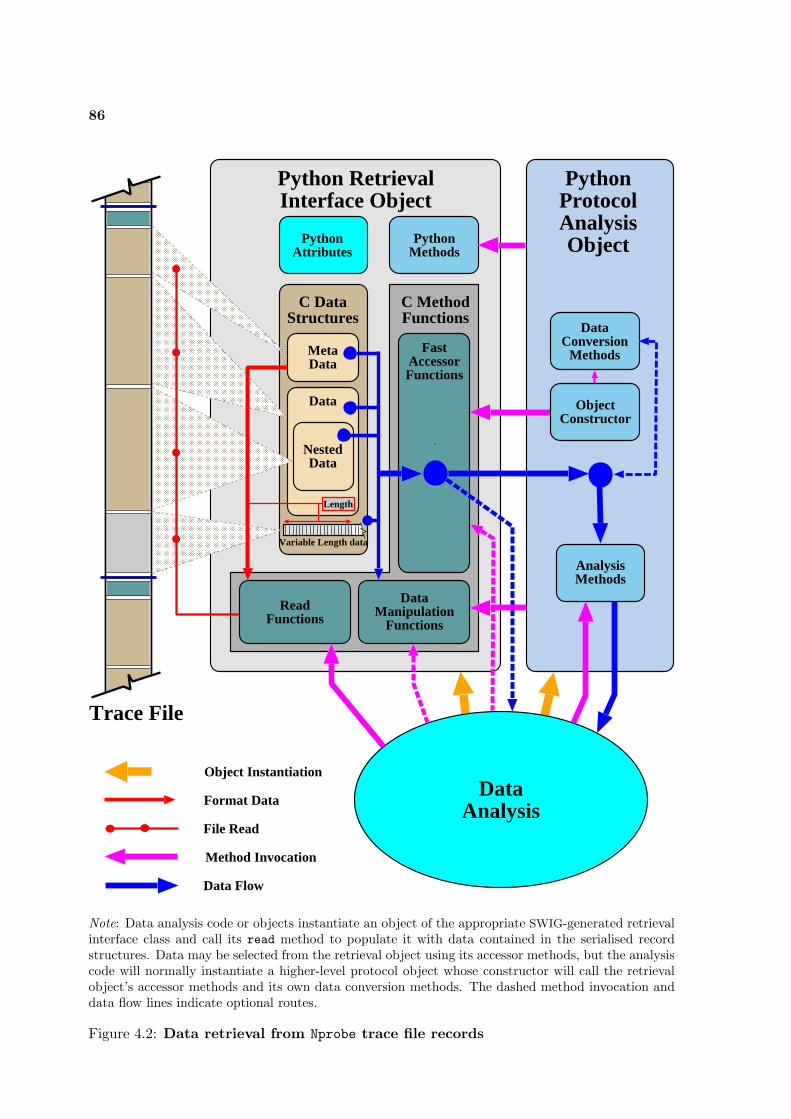
86

PythonProtocolAnalysisObject

DataAnalysis

Python RetrievalInterface Object

C DataStructures

Data

Variable Length data

Length

MetaData

NestedData

PythonAttributes

C MethodFunctions

FastAccessorFunctions

PythonMethods

ReadFunctions

DataManipulation

Functions

Trace File

Data Flow

Format Data

File Read

Object Instantiation

Method Invocation

DataConversion

Methods

ObjectConstructor

AnalysisMethods

Note: Data analysis code or objects instantiate an object of the appropriate SWIG-generated retrievalinterface class and call its read method to populate it with data contained in the serialised recordstructures. Data may be selected from the retrieval object using its accessor methods, but the analysiscode will normally instantiate a higher-level protocol object whose constructor will call the retrievalobject’s accessor methods and its own data conversion methods. The dashed method invocation anddata flow lines indicate optional routes.

Figure 4.2: Data retrieval from Nprobe trace file records

4.3 Data Analysis 87

4.2.2 Data Retrieval

The classes generated by SWIG do not store the values of data attributes in the normalPython internal representation, but in the defined C structures as part of the underlyingC implementation of the class. The read functions provided by the Nprobe modules cantherefore populate retrieval class objects with data from trace files simply and efficiently byreading a block of data from file into the corresponding structure. It is the function ofthe accessor methods to select individual data items from the C structures and return theirPython representation.

Trace file objects’ get next rec method provides the mechanism to sequentially locate tracefile records of the required type(s). The records’ header fields indicate the precise record typeand hence the data retrieval class providing the appropriate read method. The first data tobe read will be meta-data, part of which specifies which structures are present in the serialisedrecord. Where nested or chained data is present, the process continues recursively until theentire record is read, and the retrieval class instance(s) fully populated with the data present.

Appendix B provides an example of the use of the data retrieval infrastructure to read Nprobe

trace files during the analysis process. Code Example B.1 on page 205 demonstrates how theuse of retrieval classes and standard utility functions enables analysis functions or scriptsto retrieve data in a very few lines of code; Code Example B.2 on page 207 illustrates thefunction of retrieval classes in greater detail.

4.3 Data Analysis

Data analysis processes will call upon a range of components provided by the analysis frame-work, but as explained in Section 4.1.2 analysis functionality is provided primarily by acollection of analysis classes.

4.3.1 Protocol Analysis Classes

Although analysis code can access data using the retrieval classes’ accessor functions, this is,in most cases, not the optimal mechanism:

• The same data item may be referenced several times, each occurrence requiring trans-lation at the C/Python interface.

• Many data fields are of types not directly supported by Python (e.g. unsigned or longlong integers as explained in Section 4.8.2 on page 106) and would require mapping onto a supported type for every reference.

• The majority of time stamps are relative; to adjust them to a common base on everyreference would be inefficient.

88 Post-Collection Analysis of Nprobe Traces

These difficulties could, of course, be overcome by a single recovery of each data value usingan accessor function, and its storage in the retrieval class as a Python data attribute afterany necessary type or base conversions; the retrieval class would have to be equipped with aset of methods to provide the necessary conversions. This solution is not ideal: Section 4.8.2on page 106 explains that memory capacity can be a problem when using Python to analyselarge data sets, and this difficulty would be exacerbated by, in effect, storing each data itemtwice. Instead, a higher-level protocol analysis class analogous to each protocol specific StateStorage Unit (SSU) of the DAU-based retrieval-level classes is defined in which the data valuesare stored after any conversion. Data retrieval can now be based upon the use of a singleobject of each retrieval class whose read method is repeatedly called for each new record; theobject is passed as an argument to the protocol class constructor and its accessor functionsinvoked to select the required data during instantiation of the new object. All type andbase conversions are now carried out in the higher-level class’ constructor method, possiblycalling other, dedicated, class methods. The reuse of a single retrieval object of each classcarries additional benefits: repetitious creation of new objects is avoided, and the objectsthemselves can be instantiated fully equipped with all chained and linked subsidiary SSUs,storage, buffers for variable length data, and optional components (e.g. buffers for TCP packetheader data, HTML links buffers, multiple HTTP transaction chains) rather than inefficientlyand repeatedly allocate them on a per-record demand basis.

During simple data analysis where few data values are required, where repeated accesses tothose values are few, or where the data requires no conversion, the use of higher-level objectsis not required and data selection can simply use the retrieval class objects’ accessor methodsdirectly.

4.3.2 Discrete Protocol Analysis

Data analysis may be concerned with activity occurring at a single protocol level, or whenrelating activity at multiple protocol levels may still contain components drawn from a singlelevel. Analysis of discrete protocols is carried out by analysis methods of the protocol analysisclasses, each analysis task being implemented by a dedicated class method and operating onthe class object’s data attribute values.

As explained in Section 4.2.2 the protocol class objects are populated with data by invoca-tion of the appropriate retrieval class’ accessor methods, and at this initialisation stage anynecessary type conversions are carried out. The semantic integrity of the data is also checkedat this stage.

4.3.3 Protocol-Spanning Analysis — Associative Analysis Classes

Analysis will usually draw from data relating to activity at several levels of the protocol stack.Multi-protocol trace file data is already associated at the granularity of a DAU, and this willbe reflected in the grouping of protocol class objects containing the retrieved data. Therewill also, however, be analysis tasks for which further integration or association of data isrequired (e.g. all of the TCP connections and transactions involved in the download of a Web

4.3 Data Analysis 89

page and DNS requests associated with the TCP connections to a Web server).

Such complex analysis requires mechanisms both to gather and integrate the more widelyassociated data, and to perform analysis on the large data composites which are collected.Analysis of this sort can be carried out by execution of an appropriately coded script, but it islikely that multiple forms of analysis will be carried out on the data composites, and either aspecific script for each purpose, or a single and unduly complex script would be required. It istherefore preferable to define a further set of yet higher-level associative analysis classes whichcan be instantiated by a relatively simple script, which act as the aggregation locus for the setof protocol analysis objects of interest, and provide methods for each of the various analysistasks. Where components of the analysis relate only to one protocol level, the associativeanalysis objects’ methods can invoke the discrete protocol analysis methods of the protocolanalysis class objects which they have gathered. Chapter 7 demonstrates how a WebHostanalysis object gathers together all of the TCP-connection protocol objects relating to asingle client with the the HTTP transactions that they carry, and how it provides methodswhich, for instance, reconstruct Web page downloads, identify causes of delay, and relate thepages downloaded to each other.

4.3.4 Analysis Classes as Toolkit Components

Analysis classes, by forming a locus in which data and analysis methods are associated,contribute analytical components to the toolkit which can be readily selected, combined, ormodified. Specific analysis functionality is made available simply by instantiating an analysisobject of the appropriate class and calling the class method required, encapsulation ensuringthat objects may call upon each other’s services without risk of undesirable side effects.

Where new analytical methods are required new classes may be called for, but existing classeswill often provide the needed functionality by the addition of new methods or by the modi-fication of their behaviour by sub-classing. The ease with which existing components can bemodified ensures that a wide range of tasks can be constructed based upon a relatively smallnumber of basic components.

4.3.5 Accumulation of Analysis Results

Data analysis will generate two categories of output: the analysis results, usually in statisticalform, and a record of the analysis process itself; both require accumulation and collation asanalysis proceeds through its input data. In accordance with the aim of establishing a genericanalysis framework a further utility is provided — the StatsCollector class.

Different analysis tasks will generate results with widely varying characteristics and content,which will require similarly differing collation. There are, however, many items of functionalitywhich will be common to all analysis, and the StatsCollector class is designed to make thesereadily available. The following, for example, are provided:

Logging methods: Used to create and manipulate logs of analysis activity. Entries in analysis

90 Post-Collection Analysis of Nprobe Traces

logs might include trace statements recording activity, summaries of the input data or re-sults, notes of data which are not amenable to interpretation by the analysis algorithms,or records of particular conditions or combinations found in the data.

Recording methods: A consistent syntax and format for log entries is provided by a set ofrecording methods.

Interface methods: Which provide a common interface to tools which summarise, select, orpresent results.

A consistent analysis control interface: Analysis tasks may proceed differently according tothe task in hand; the way in which activity logs are collected may, for instance, varybetween analysis intended purely to generate results and that being carried out in ananalysis design environment.

The results collection and collation functionality specific to each analysis task are providedby using the mechanisms of sub-typing and inheritance to define task specific collector sub-classes. Such sub-classes may be defined with the required collection and collation methods,or may act as ‘results repositories’ for similar methods provided by analysis classes.

In their most sophisticated form objects of StatsCollector sub-classes control the analy-sis to be performed by calling the analysis methods of the protocol and associative analysisobjects of interest to generate the data which they accumulate. At the completion of analy-sis the StatsCollector’s termination method will invoke a Summary object (described inSection 4.4.1 on page 92) to summarise analysis activity and results.

4.3.6 Memory Constraints

Any analysis of large data sets may encounter difficulties due to the memory requirementsof the analysis program exceeding the physical memory capacity of the machine upon whichit is being executed; this problem is particularly evident when using Python as describedin Section 4.8.2 on page 106. As analysis proceeds working space is needed which remainsconstant, but there will be an additional memory requirement proportionate to the size ofthe trace file being analysed due to:

• Accumulation of results

• Accumulation of data pending association or aggregation

• Retention of data which may be needed for further examination

Various strategies can be used to circumvent these difficulties, the analysis task usually de-termining which will be employed:

Partition of the analysis: The process of analysis may be partitioned in order to reduce mem-ory demands. Transverse partitioning (i.e. analysing sub sets of a series of trace files

4.4 Analysis Logs, Results and Presentation 91

or only partial files) is effective, but may be inappropriate where long-term trends orphenomena feature in the analysis. Longitudinal partitioning is often the technique ofchoice, but may suffer from the disadvantage of additional complexity, the introductionof additional passes through the data, or the need to accumulate data in order to controlor identify the partitions.

Accumulation of results in temporary data files: The nature of the data collected by Nprobe

will normally encourage analysis generating rich and voluminous results (consider com-plete data concerning the timing, causes and magnitude of packet loss delays for allof the Web page downloads and millions of supporting TCP connections contained ina large trace), and the results of several analysis tasks may be generated concurrentlyas described in Section 4.8.2 on page 106. The data which will be accumulated duringanalysis may therefore become very bulky, and will advantageously be stored in tem-porary files. In this case a further analysis pass, or a separate subordinate analysisprogram will be required to correlate and accumulate such intermediate results.

Concise representation of data held for association, aggregation, or further examination: Datawill frequently be held for purposes of association or aggregation but not analysed fur-ther until that process is complete (e.g. associating all of the TCP connections andHTTP transactions originating from a particular client). As the data is not immediatelyrequired the analysis process need only collate it and store a reference to its locationduring a preliminary pass and proceed to full analysis during a second pass once as-sociation is complete — in effect producing a fine grained longitudinal partition of thedata. A further utility class — FileRec — makes this possible. The class stores refer-ences to the data as a list of open file/offset pairs indicating where the data is to befound together with a type code indicating the type of analysis class relevant to furtheranalysis. The FileRec class exports one primary method — reconstruct — whichinstantiates an analysis object of the appropriate type and uses the necessary retrievalclasses to populate it with data. Code Example B.3 on page 209 illustrates the use ofthe FileRec class.

Strategies may also be determined by whether analysis is being conducted in its final form orin the analysis development environment. In the former case it is likely that full traces willbe analysed, and greater use will be made of longitudinal partitions and the accumulation ofresults and analysis logs in temporary files. During analysis development shorter traces, orexcerpts, will probably be processed, but the ready availability of results and the facility tore-examine the analysis of individual record are, by comparison, more desirable; greater usewill therefore be made of FileRec objects.

4.4 Analysis Logs, Results and Presentation

Analysis processes produce a log summarising their activity and noting any points of interestencountered which the analysis designer wishes to be recorded. Processes will also generateresults which may consist of many sets and subsets of data, which may be large and complex,and which may require examination and management. An interactive analysis summary toolpresents log contents and results in a convenient form.

92 Post-Collection Analysis of Nprobe Traces

4.4.1 An Analysis Summary Tool

The analysis of large trace files will generate large logs recording and summarising analysisactivity. Log entries are generated at the discretion of the analysis designer but at a minimumare likely to include data relevant to the analysis process (e.g. the count of file records pro-cessed, the number of DAUs encountered) and to record points of note arising during analysis(e.g. situations where analysis could not satisfactorily resolve the data presented or had touse heuristic rather than deterministic rules to interpret it, error conditions, or phenomena ofparticular interest). During analysis design many additional entries may be made identifyingand quantifying situations or values requiring further attention.

The size of log files, and the wide variety of entries, would make it very difficult to identifyand collate the information that they contain; support is therefore provided by the analysissummary tool. The tool collates, sorts, and summarises log entries; the summary is presentedas a pane containing top-level summary entries which can be interactively selected and recur-sively expanded in detail, hence allowing for fast and comprehensive navigation of the log.Collation may be selected by entry (e.g. TCP connections with multiple SYN packets) or byid (e.g. by connection identifier, Web client address).

As explained in Section 4.3.5 the summary tool is normally invoked from the analysis pro-cess’s StatsCollector object, which is also responsible, during invocation, for providing thetool with a callback function; log entries may be accompanied by tags identifying the datagenerating the entry, and which are passed by the tool as an argument to the callback. Thecallback will identify the type of entry and will re-analyse the data which generated it withfull tracing enabled, possibly also invoking the appropriate visualisation tool2. Hence an audittrail is established allowing the originating raw data and its analysis to be examined in closedetail.

The summary tool may also be used in ‘stand alone’ mode for the retrieval and examinationof logs generated by past analysis processes. When used in this way the facility to examinethe origin of entries is, of course, absent.

4.4.2 Summaries of Analysis Results

The analysis process’s StatsCollector object may generate summaries of the analysis resultsand references to data sets which are appended to the log. The summary tool also collates,summarises and presents these entries in the same manner as normal log entries.

In the case of results entries, the callback functions provided by the StatsCollector willnormally present data sets by invoking the data plotter tool or other visualisation tools ap-propriate to the granularity of the summary items. Because the callback is provided by theStatsCollector, the system allows for very flexible selection of the data or its subsets whichare to be examined.

2Visualisation tools are described in Section 4.5 on the facing page .

4.5 Visualisation 93

4.5 Visualisation

Visualisation tools constitute an important element of the toolkit and provide support in thedesign and mature phases of analysis. They contribute significantly to the design environment,as described in Section 4.5.3, and in assessing informal indicators of confidence as describedin Section 4.7.5.

4.5.1 The Data Plotter

The data plotter tool may be used as a stand-alone data plotter but is normally invoked fromthe summary tool in order to display selected data sets from analysis results. The tool isdesigned to make the manipulation, examination and comparison of data sets possible withoutreloading; and provides interactive support for raising, lowering, or blanking out individualsets and a zoom facility. Plotting styles can be varied as desired, and the data re-plotted asscatter plots, histograms, probability and cumulative density functions as appropriate to itstype. Basic smoothing methods are also available.

The plotter acts as the principal data management tool allowing selected data sets (or sub sets)or their derivatives (e.g. distribution functions) to be saved or printed. The most significantdifference between the plotter and other plotting programs is, however, its facility allowingthe user to examine the derivation of data points. A callback and tag mechanism similarto that employed by the summary tool allows the user to select a set of data points and toexamine the underlying raw data and the process of its (re-)analysis in close detail.

4.5.2 TCP Connection and Browser Activity Visualisation

The raw trace file data contributing to each datum generated during analysis are likely to becomplex and bulky and to have complex relationships (consider the data associated with eachpacket of a TCP connection, the number of packets that may be sent on a single connection,the complications due to packet loss, and the number of connections that may be involved ina Web page download). The raw data, furthermore will be sparsely distributed amongst theother file contents. Although the trace file reader mentioned in Section 4.1.2 presents tracerecords in a convenient form, and provides rudimentary facilities for selecting associated data,it would be time consuming, and (in the case of large data associations) virtually impossible tofully assimilate and comprehend all items without assistance. The appropriate visualisationtools will present data in a compact and comprehensible way which assists in identifying therelationships that it represents.

Trace file data analysis is, however, concerned with the distillation of information from theraw data. Visualisation should, therefore, not only present the raw data but also, insofar as ispossible the information generated by analysis and the relationships upon which it is based.The analysis framework visualisation tools are designed to meet this requirement.

94 Post-Collection Analysis of Nprobe Traces

4.5.2.1 The TCP Visualisation Tool

The TCP visualisation tool, illustrated in Figure 4.3, plots sequence numbers against time in astyle similar to Tcptrace [Ostermann]. Data segments are shown as vertical arrows scaled tothe data length carried, acknowledgements as points, the ACK high water drawn, and segmentsare annotated with any flags set. Other salient data (e.g. window advertisements) may alsobe shown.

The tool, however, has considerably greater functionality: Chapter 5 explains a technique forexamining the dynamics of TCP connections, relating them to activity at higher levels of thestack and identifying application behaviour and connection characteristics. Where connec-tions have been subject to this technique its inferences are also displayed: the relationshipbetween TCP and application activity, causal relationships between packets, and congestionwindows are, for instance shown; secondary plots of the number of packets in flight, inferrednetwork round trip times, and application delays are also presented.

Figure 4.3 shows the tool’s primary window displaying, as an example, the activity of a non-persistent TCP/HTTP connection. Although the figure contains a great deal of interestingdetail comment on a few features illustrates the power of the visualisation:

A The solid purple line to the left of the segment arrows represents the server’s conges-tion window as predicted by the connection model — the number of segments in eachsubsequent flight increasing as the window opens.

B Packet #13 is retransmitted (packet #18 — shown as a red arrow) at approximate time540 ms.

C The server’s congestion window shrinks following the retransmission, resulting in a flightof only two segments immediately afterwards. The retransmission also causes the con-nection to enter congestion avoidance — shown by the broken congestion window line.

D Horizontal dashed lines indicate causal relationships between packets. Here packet #25from the server triggers an acknowledgement — packet #26 — from the client

E The last line of the legend at the top of the main pane indicates that the modelling processhas explained the behaviour the server’s TCP implementations based upon a generalisedbase model of behaviour with an Initial Window of two segments; the client’s behaviouris explained by a similar model, but the IW is unknown as less than one MSS of data hasbeen sent. The term ‘SSTG=1’ denotes that the implementations enter the congestionavoidance phase when the congestion window exceeds3 the slow start threshhold.

To ascertain the patterns of TCP activity involved in even the relatively short and uncom-plicated connection visualised in Figure 4.3 would require the close examination of 38 packetheaders, a time consuming task which might, even then, fail to identify all of the featurespresent. To fully comprehend the activity of a substantial connection, or one with complex

3This is the default for the base TCP model — TCP implementations may optionally enter congestionavoidance when the congestion window reaches the threshold [Allman99a].

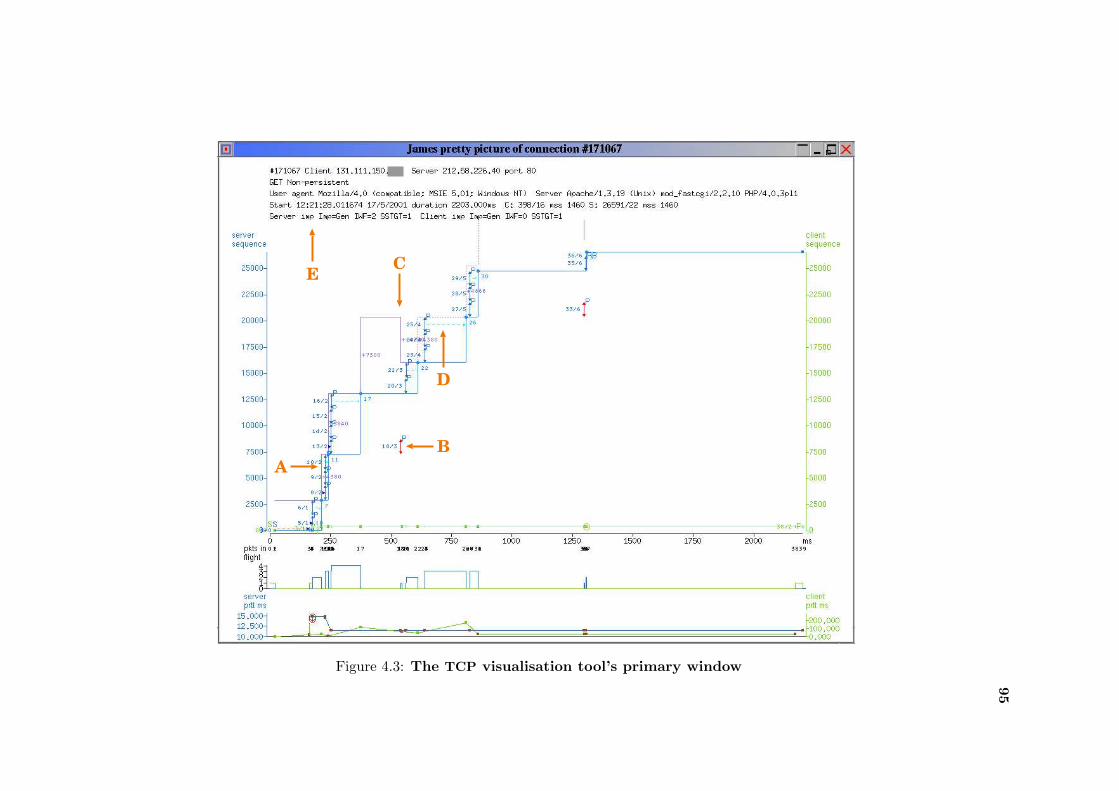
95

BA

D

CE

Figure 4.3: The TCP visualisation tool’s primary window

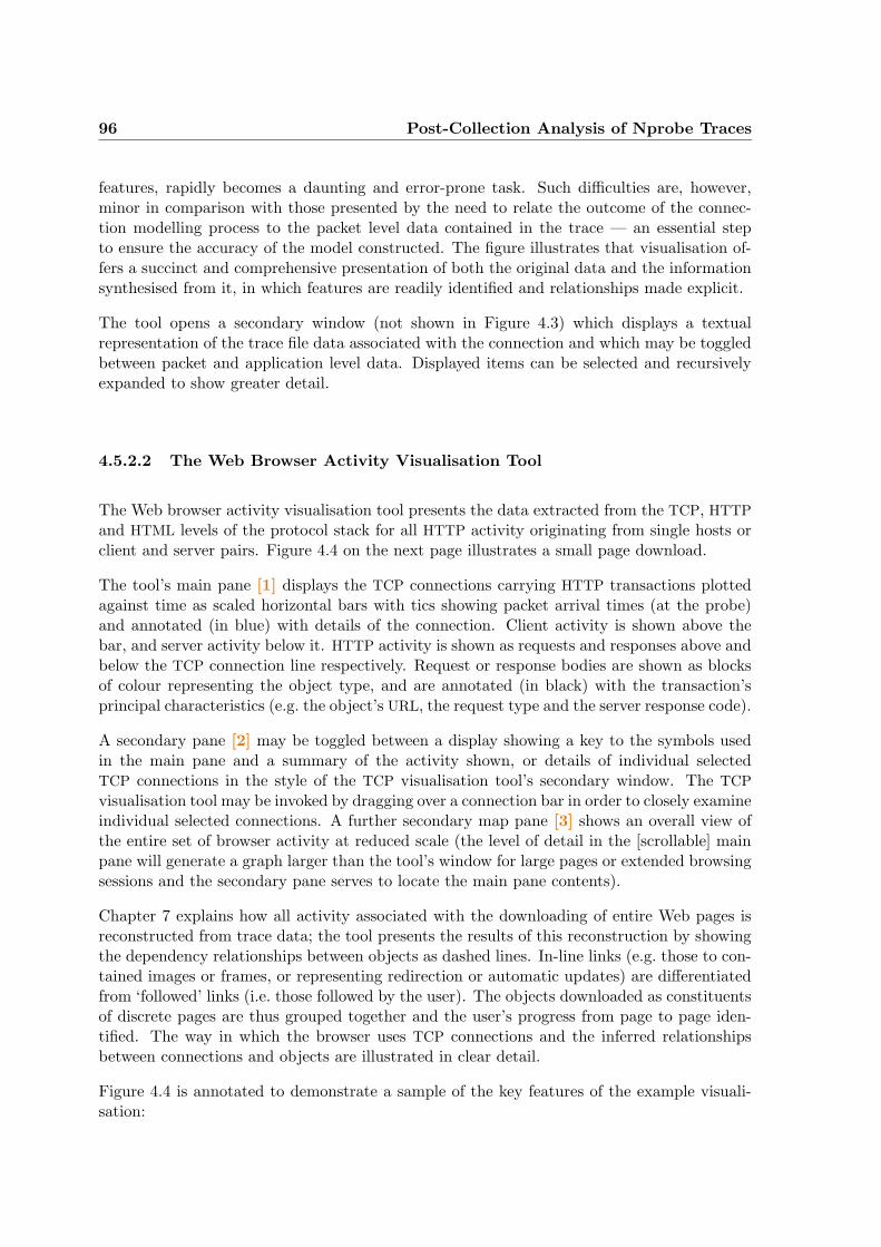
96 Post-Collection Analysis of Nprobe Traces

features, rapidly becomes a daunting and error-prone task. Such difficulties are, however,minor in comparison with those presented by the need to relate the outcome of the connec-tion modelling process to the packet level data contained in the trace — an essential stepto ensure the accuracy of the model constructed. The figure illustrates that visualisation of-fers a succinct and comprehensive presentation of both the original data and the informationsynthesised from it, in which features are readily identified and relationships made explicit.

The tool opens a secondary window (not shown in Figure 4.3) which displays a textualrepresentation of the trace file data associated with the connection and which may be toggledbetween packet and application level data. Displayed items can be selected and recursivelyexpanded to show greater detail.

4.5.2.2 The Web Browser Activity Visualisation Tool

The Web browser activity visualisation tool presents the data extracted from the TCP, HTTP

and HTML levels of the protocol stack for all HTTP activity originating from single hosts orclient and server pairs. Figure 4.4 on the next page illustrates a small page download.

The tool’s main pane [1] displays the TCP connections carrying HTTP transactions plottedagainst time as scaled horizontal bars with tics showing packet arrival times (at the probe)and annotated (in blue) with details of the connection. Client activity is shown above thebar, and server activity below it. HTTP activity is shown as requests and responses above andbelow the TCP connection line respectively. Request or response bodies are shown as blocksof colour representing the object type, and are annotated (in black) with the transaction’sprincipal characteristics (e.g. the object’s URL, the request type and the server response code).

A secondary pane [2] may be toggled between a display showing a key to the symbols usedin the main pane and a summary of the activity shown, or details of individual selectedTCP connections in the style of the TCP visualisation tool’s secondary window. The TCP

visualisation tool may be invoked by dragging over a connection bar in order to closely examineindividual selected connections. A further secondary map pane [3] shows an overall view ofthe entire set of browser activity at reduced scale (the level of detail in the [scrollable] mainpane will generate a graph larger than the tool’s window for large pages or extended browsingsessions and the secondary pane serves to locate the main pane contents).

Chapter 7 explains how all activity associated with the downloading of entire Web pages isreconstructed from trace data; the tool presents the results of this reconstruction by showingthe dependency relationships between objects as dashed lines. In-line links (e.g. those to con-tained images or frames, or representing redirection or automatic updates) are differentiatedfrom ‘followed’ links (i.e. those followed by the user). The objects downloaded as constituentsof discrete pages are thus grouped together and the user’s progress from page to page iden-tified. The way in which the browser uses TCP connections and the inferred relationshipsbetween connections and objects are illustrated in clear detail.

Figure 4.4 is annotated to demonstrate a sample of the key features of the example visuali-sation:

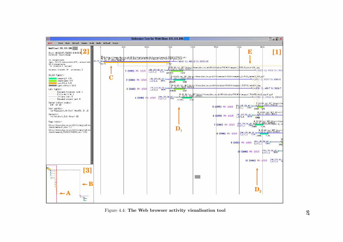
97

[2]

[3]

[1]

AB

C

D2

E

D1

Figure 4.4: The Web browser activity visualisation tool

98 Post-Collection Analysis of Nprobe Traces

A The red box in the map pane [3] identifies the section of the entire reference tree shownin the main pane [1] which can be scrolled by either dragging the box or the main paneitself.

B The map pane shows that the user goes on to visit another page following that currentlyoccupying the main pane.

C The page’s root HTML document identifies its referrer, not seen by the trace, which isrepresented by the small black box immediately above it.

D1 and D2 The browser is configured to download subsidiary objects using four concurrentlyopen TCP connections.

D1 Connections #1 – #4 are used to download the first four in-line images in the page. Eachrequest occupied a single packet shown as a large tic above the connection bar (colouredgrey for ‘type unknown’ as there is no object associated with the GET requests); dottedlines above the request tics connect them to the referring object (C) at the packetcarrying the portion of the parent document containing the links. Although the linkswere seen in a packet at approximate time 450 ms the browser did not open connectionsupon which to request the objects until approximate time 1400 ms — hence introducinga delay of nearly a second into the page download.

E Although delivery of the first four image objects was completed by approximate time1950 ms the browser does not close the relevant connections until approximate time3300 ms, hence inhibiting the opening of the subsequent set of four connections, andintroducing a further overall delay of about 1.3 seconds.

To manually identify and associate the activity involved in downloading the first page shownin Figure 4.4 would require the examination of 12 trace file records containing details of anequal number of transactions, and of 159 TCP packets — a complex and tedious task. Toidentify the links contained in the parent document would additionally involve the scanningof 8,658 bytes of HTML spread over 17 packets. If traditional tcpdump style traces had beencollected the exercise would involve the manual examination of all 159 packets, their TCP andHTTP headers. The page illustrated is atypically small — pages with container documentsmeasured in tens of kilobytes containing tens or hundreds of in-lined images are not unusual— it would be infeasible to manually examine the data describing activity in such cases, andto correctly interpret its internal relationships and meaning. The utility of the tool is amplydemonstrated in the figure which presents all of the relevant data and the inferences drawnduring analysis in an immediately accessible form. The overall pattern of activity is plainlydiscernible and features of interest clearly identifiable.

The tool’s contribution to analysis design is discussed in Section 4.5.3, and its role in assessingthe confidence invested in the veracity of analysis results in Section 4.7.5 on page 105.

4.5.3 Visualisation as an Analysis Design Tool

Although visualisation tools may be invoked to examine features of analysis results in detail,their main role is in the analysis development environment. The presentation of raw data

4.5 Visualisation 99

in comprehensible and compact form assists in identifying relationships within the data andreasoning about those relationships when designing analysis algorithms.

Sections 4.5.2.1 and 4.5.2.2 illustrate the power of the visualisation tools and comment uponthe difficulty of comprehending and interpreting large masses of associated data without amechanism for its succinct presentation — an essential precursor to analysis design. Fig-ures 4.3 and 4.4 demonstrate the way in which visualisation identifies and clarifies relation-ships, features and patterns of activity within the data — also essential to the design process.Both sections illustrate the volume and scope of trace data which may contribute to a singleanalysis result datum (e.g. the download time of a single Web page) and, by implication, thecomplexity of the analysis involved in its calculation.

The presentation of analysis output in conjunction with the data upon which it is basedallows the relationships between raw data and analysis output to be examined and verifiedin detail, and the facility to repeat the analysis underlying selected results supports the closeexamination of the analysis process. Iterative design is supported by the facility to reloadand re-execute analysis software on selected sets of data. Both visualisation tools may beinstructed to redraw their displays: all analysis modules are re-imported, the underlying rawdata is re-read from the trace file and re-analysed with full tracing enabled, and the displayredrawn. Analysis code can therefore be modified during the analysis process and immediatelyre-run, and the modified analysis process examined in detail.

Although both of the tools described are specific to particular protocol sets they are con-structed in such a way as to contribute to a generic framework. Functionality is dividedbetween protocol-specific and display management classes (i.e. one set of classes provides andmanages canvases and interactive features, another — given a set of raw data and results— knows how to draw them into the display provided). In some cases entirely new drawingclasses may be required, but in general sub-typing will provide the appropriate functionality:the TCP tool’s drawing class could be trivially sub-typed (with much removed functional-ity) to display the activity of UDP flows and the browser visualisation tool’s drawing classessub-typed to accommodate other higher level protocol activity.

The summary tool provides a convenient mechanism for recording and identifying items ofinterest within the data and any correlations which may require particular attention duringanalysis design, and to then closely examine and modify analysis algorithms. The facility toquickly select and examine data sets generated by analysis, and to then examine the derivationof multiple or individual data items supports similar design processes at a larger scale.

The tight integration between analysis code, summary tool, and visualisation tools, and theway in which their invocation can be cascaded, provides a rich and productive design envi-ronment. The support for examination of the analysis process during design also facilitatesvalidation of the analysis methods employed, and hence underpins confidence in the resultsobtained. The part played by the tools in assessing confidence is further explored in sec-tion 4.7.5 on page 105.

100 Post-Collection Analysis of Nprobe Traces

4.6 Assembling the Components

The previous Sections of this Chapter have described the components provided by the analysisframework; an overview of how they may typically be combined to build a complex analysisprocess can now be presented — a Python script will:

1. Use the file manipulation module to return TraceFile objects representing the trace filesto be analysed and the accompanying accumulated meta data.

2. Instantiate data retrieval class objects appropriate to the file record types to be read(e.g. TCP/HTTP connections).

3. Instantiate a Filter class object if further selection of records (e.g. by host, HTTP-1.0

persistent connections).

4. Instantiate an appropriately sub-classed StatsCollector object to invoke the requiredanalysis methods of analysis classes and accumulate the results generated.

5. Call upon the file objects’ NextRec record selection methods to step through the tracefile(s) and:

(a) Use the retrieval class objects’ read methods to recover data from file.

(b) Instantiate the required analysis class or subtype object and call the requiredanalysis method(s).

6. At analysis completion:

(a) The StatsCollector object will instantiate a Summary object, the user may:

i. Examine results data by invoking the Plotter tool.

ii. Examine the analysis log.

iii. Invoke visualisation objects to re-analyse selected data under close observation.

iv. Modify code, re-import and repeat Step 6(a)iii.

(b) The data generated, or its subsets or derivatives can be saved.

The example above illustrates a non, or transversely, partitioned analysis operating on datacontained within discrete DAUs. If further association of data, or a longitudinal partition ofthe analysis, is required step 5 might be replaced by a two-pass analysis using the FileRec

class:

5a. First pass — call upon the file objects’ NextRec record selection methods to step throughthe trace file(s) and:

(a) Use the data retrieval object’s read method to establish the record’s collation key(e.g. host address).

4.7 Issues of Data Bulk, Complexity and Confidence 101

(b) Add the record’s location to an existing FileRec object containing associatedrecords, or at the first instance of the collation key instantiate a FileRec of theappropriate type.

5b. Further collate and partition the collected FileRec objects if required

5c. Second pass — for each partition:

(a) Call the FileRec(s) reconstruct method to instantiate and populate the appropri-ate analysis class object.

(b) Call the required analysis method(s).

Note that the above example does not represent a prescriptive formula for analysis processes,but rather an example of the way in which framework components may be easily and flex-ibly assembled to meet the requirements of analysis tasks. Standard components are usedthroughout, only the StatsCollector and analysis classes requiring modification through sub-typing or the addition of further analytical methods. As the existing component collectiongrows through the addition of analytical methods and sub-types, it will be increasingly thecase that analysis requirements will be met entirely from existing methods used in new com-binations, or that only minimal modifications will be required in order to achieve the requiredbehaviour.

As data extraction from additional protocols is added to Nprobe’s repertoire, new retrievalclasses will be automatically generated, the only manual effort required being to contributeappropriate trace file reading functions. Steps 6(a)i – 6(a)iv of the process described abovewill support fast development of new protocol analysis classes or the modification of thosealready existing.

4.7 Issues of Data Bulk, Complexity and Confidence

The Nprobe design reflects the expectation that it will be used to collect relatively longtraces comprising many gigabytes, if not terabytes, of data, and that this data will be bothcomprehensive, and span activity at multiple levels of the protocol stack. Analysis of thecollected data will generate commensurately rich and bulky results and explore and identifycomplex relationships within the data (e.g. interactions between protocols, complex behaviourwithin individual protocol levels). Consideration must therefore be given to the validity ofthe results and measures of confidence that can be attached to them.

4.7.1 Data Bulk — The Anatomy of a Small Trace and Its Analysis

Sections 4.5.2.1 and 4.5.2.2 on pages 94 and 96 comment upon the mass of associated datawhich may require integration during analysis to produce a single result datum. Table 4.1 onthe next page, on the larger scale, indicates the magnitude of the data input to the analysis

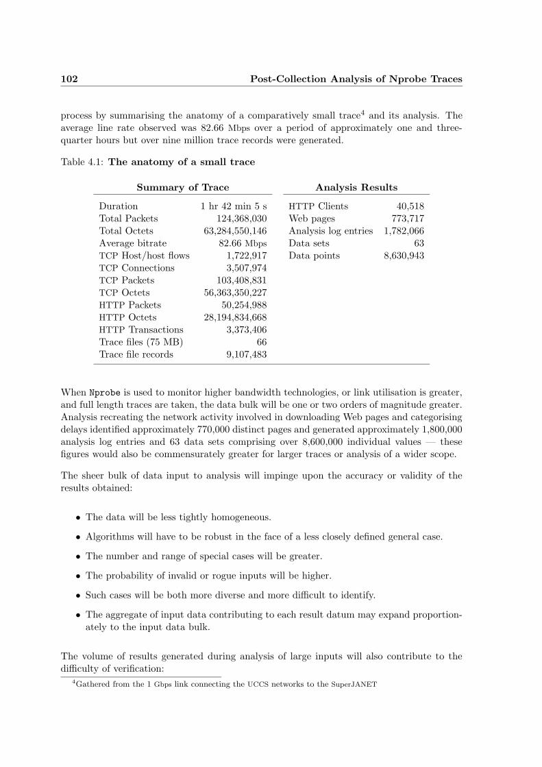
102 Post-Collection Analysis of Nprobe Traces

process by summarising the anatomy of a comparatively small trace4 and its analysis. Theaverage line rate observed was 82.66 Mbps over a period of approximately one and three-quarter hours but over nine million trace records were generated.

Table 4.1: The anatomy of a small trace

Summary of Trace Analysis Results

Duration 1 hr 42 min 5 s HTTP Clients 40,518Total Packets 124,368,030 Web pages 773,717Total Octets 63,284,550,146 Analysis log entries 1,782,066Average bitrate 82.66 Mbps Data sets 63TCP Host/host flows 1,722,917 Data points 8,630,943TCP Connections 3,507,974TCP Packets 103,408,831TCP Octets 56,363,350,227HTTP Packets 50,254,988HTTP Octets 28,194,834,668HTTP Transactions 3,373,406Trace files (75 MB) 66Trace file records 9,107,483

When Nprobe is used to monitor higher bandwidth technologies, or link utilisation is greater,and full length traces are taken, the data bulk will be one or two orders of magnitude greater.Analysis recreating the network activity involved in downloading Web pages and categorisingdelays identified approximately 770,000 distinct pages and generated approximately 1,800,000analysis log entries and 63 data sets comprising over 8,600,000 individual values — thesefigures would also be commensurately greater for larger traces or analysis of a wider scope.

The sheer bulk of data input to analysis will impinge upon the accuracy or validity of theresults obtained:

• The data will be less tightly homogeneous.

• Algorithms will have to be robust in the face of a less closely defined general case.

• The number and range of special cases will be greater.

• The probability of invalid or rogue inputs will be higher.

• Such cases will be both more diverse and more difficult to identify.

• The aggregate of input data contributing to each result datum may expand proportion-ately to the input data bulk.

The volume of results generated during analysis of large inputs will also contribute to thedifficulty of verification:

4Gathered from the 1 Gbps link connecting the UCCS networks to the SuperJANET

4.7 Issues of Data Bulk, Complexity and Confidence 103

• Verification by inspection becomes less feasible.

• Invalid results are less readily identified in large data sets, particularly those with dis-persed or long tailed distributions.

• Mappings between input data and results are more difficult to identify and to navigate.

4.7.2 Data and Analysis Complexity

Because the data gathered by Nprobe may be collected from multiple layers of the proto-col stack, and because the data collected from each layer may be very comprehensive, therelationships between data items will be both complex and sometimes subtle, reflecting thecomplex dynamics and interactions of the network and application activities observed. As thenumber of individual data contributing to each output datum increases the complexity of theirpotential relationships will grow exponentially; this growth will be limited by transitivity, butthis, in itself, carries the risk that analysis errors will be propagated.

The complex nature of the phenomena studied dictates that elements of analysis will dependupon a degree of inference and may be based upon heuristic rules. Complex data encompassingequally complex relationships, inference, and a widely ranging set of possible input conditionsall determine that there is considerable scope for error in the design and implementation ofanalysis processes, and the reasoning that underpins them. The audit trail between inputdata and the information extracted or synthesised from it will, additionally, become morecomplex and commensurately difficult to follow.

Sections 4.5 and 4.6 explain how complexity in analysis design is supported by the use ofvisualisation tools and the composition of mature analysis components provided by the toolkit.Sections 4.7.3 – 4.7.5 now go on to discuss the establishment of confidence in the informationgenerated by analysis.

4.7.3 Determinants of Validity

The validity of analysis results will depend upon a range of factors the most significant being:

The veracity and accuracy of the raw data (i.e. rubbish in — rubbish out): As explained inSections 3.3.3.3 to 3.3.3.7 on pages 58–66 the process of data extraction at the pro-tocol level both implies a check on the semantic integrity of that data and may involvespecific semantic tests. Section 3.3.5 on page 69 describes the situations which mayarise where semantic constraints are broken by the contents of packets arriving at theprobe, and the disposal of such situations: in effect a DAU is marked as terminatingin an error condition if any of the associated data is semantically inconsistent as itappears to the probe. The section also introduces the distinction between incorrect andmisleading data semantics — the former will generate an error condition, and data willbe rejected during analysis, but the latter must be detected during the analysis processor by its contribution to anomalous results.

104 Post-Collection Analysis of Nprobe Traces

The design and robustness of the analysis algorithms employed: The truism that analysis al-gorithms must correctly interpret the data presented to them should not obscure con-sideration of the extent to which such algorithms must be robust in the face of unan-ticipated or unusual data. Section 3.3.5 points out that it is infeasible to provide dataextraction software which will dispose correctly of every possible combination of networkor application behaviour, or packet content — the number of possible permutations issimply too great, even in the absence of pathological conditions, incorrect behaviour,or incorrect protocol implementations. The same is, of course, true in the case of anal-ysis software: there will, inevitably, be combinations of activity in the sometimes verycomplex operations observed and interrelationships between protocols which will not beanticipated during algorithm design.

Appropriate identification and interpretation of the relationships between data items: Analysisresults will be incorrect if the algorithms employed do not correctly identify and interpretthe relationships between the data items recorded in Nprobe trace files, even though thealgorithms themselves may be technically correct. In this context confidence dependsupon the validity of the knowledge and reasoning bought to bear upon the analysisdesign process. There is, unfortunately, no formalism, or system of proof, applicable tothis critical factor.

In the absence of an appropriate formalism an assessment of validity, and hence of confidence,must depend upon informal, or heuristic, indicators.

4.7.4 Indicators of Validity and Confidence in the Absence of Formal Proof

Indicators of validity may be pertinent to either the raw data, intermediate, or final resultsand may serve to suggest overall measures of confidence, or to identify dubious results. Suchindicators will include:

Protocol and Application Semantics: During analysis more sophisticated checks can be car-ried out on data to identify incorrect or unusual values arising from misleading protocolsemantics than are possible during data collection.

Cross Protocol Semantics: The semantics of individual protocols will often bear upon thoseof the protocols with which they interact and may generate similar indicators. TheHTTP response header lengths and the size of the objects delivered should sum, forinstance, to the number of data octets carried from the server by the TCP connectiontransporting them.

Data self consistency: Both data and results can be checked for self consistency, often inconjunction with semantic checks.

Consistency with other known data or results: Unless there are known reasons why identifi-able differences should exist, data and results should be consistent with other knownvalues, although care must be taken that consistency is not the result of common er-rors. Ideally such consistency checks should be based upon data sets arrived at byindependent and unrelated methods.

4.7 Issues of Data Bulk, Complexity and Confidence 105

Independent verification: Verification may be sought through comparison with known ac-curate data (using consistency checks) or through data gathered specifically for thepurpose, possibly using active methods. The round trip times calculated in Chapter 6were, as an example, checked for feasibility using measurements obtained by the ping

programme; the reconstruction of Web page downloads described in Chapter 7 can beverified by independently downloading a sample of pages and manually examining theHTML page source and tcpdump traces collected on the client machine.

Statistical Indicators: Statistical indicators may apply at both microcosmic and macrocosmicscales. Examination of results data may reveal distributions informally suggesting thatanalysis results are feasible, or may, conversely, suggest that the derivation of resultsshould be examined more closely (e.g. if unexpected or inexplicable features are present).Checks that results match a particular statistical distribution will usually be too precise— indeed it may be part of the research goal to identify distribution characteristics.Small scale features of distributions (e.g. outlying points) may suggest errors in theanalysis and that further examination is required.

Examination of samples from results : The derivation of individual data items contained inresults can be examined for accuracy. The individual items may be a sample of thewhole, a sample of a subset of the whole (e.g. those based upon TCP connections whereloss has occurred), or be suggested by statistical indicators or analysis logs (e.g. outlyingpoints or those derived in an unusual or particularly complex context).

The application of indicators runs across a spectrum from those which suggest specific tests ap-plied automatically during analysis (e.g. those based upon semantics or data self-consistency)to those, more applicable to results, which require user intervention and reasoning (e.g. in-dependent verification or the examination of statistical indicators). Which indicators areemployed will also depend upon the stage of analysis development reached: the examinationof individual values and their derivation will be more common early in the cycle and macro-cosmic statistical indicators will assume a more significant role when using mature analysisprocesses.

4.7.5 Visualisation as an Informal Indicator of Confidence

Section 4.5.3 explains how the visualisation tools contribute to an analysis design environmentsupporting the development of robust code which produces valid results and hence engendersconfidence. The tools also provide convenient access to a set of indicators of confidence.

The summary and plotter tools support the examination of statistical indicators at the macro-cosmic scale. The facility to examine the derivation of individual data contained in the resultsthrough re-analysis and visualisation make scrutiny at the microcosmic scale convenient. Fastand comprehensive navigation of analysis logs facilitates the identification and examinationof analysis in the case of dubious results or analysis failures, and allows for the examinationof samples from analysis results.

106 Post-Collection Analysis of Nprobe Traces

4.8 An Assessment of Python as the Analysis Coding Lan-guage

This section assesses the contribution of the Python language’s features to implementation ofthe analysis framework and code, and some of the difficulties arising from its use.

4.8.1 Python and Object Orientation

It is proposed that data analysis is an environment to which the object-oriented paradigmis eminently suited: sets of data items are grouped in hierarchies and aggregations of dif-fering granularities, and at each hierarchical level a distinct set of analytical operations isrequired. Although Python does not enforce strict data hiding its class structure implies fullencapsulation of data sets and the operations to be performed on them.

The very rich nature of the data gathered by Nprobe suggests that data analysis will becomplex, and that it will be the subject of a potentially wide range of analytic tasks, eachof which will draw from a different set of operations at each level of the data hierarchy.Section 4.2.2 shows how automatically generated retrieval classes contribute to a generic dataretrieval interface and Section 4.3 explains how analysis and utility classes form a locus foranalysis functionality which, by appropriate design and choice of analysis methods and theinheritance mechanism, provide a flexible and powerful analysis infrastructure with a highdegree of code reuse.

The implementation of the summary and visualisation tools introduced in Section 4.5 asclasses, which may be invoked from anywhere in the analysis code, in cascades, and recursively,allows a degree of integration contributing a flexible and productive development environment.The facility to re-import modules and to re-run code also makes a significant contribution tofast design.

4.8.2 Difficulties Associated with the Use of Python

Although the choice of Python as the language in which the data analysis code and environ-ment have been written has proved itself in practice, there are, nevertheless, some disadvan-tages which must be noted:

Python lacks some low-level data types useful in the context of trace file analysis: Python pro-vides two signed integer types: plain integers and long integers5. There is, therefore nodirect Python representation of some integer types frequently occurring in Nprobe tracefiles:

32 bit unsigned integers: Which are heavily used in numeric data items to obtain max-imum capacity in a 32 bit quantity and in protocol (e.g. TCP ) header fields. The

5Python plain integers are based upon C long integers and hence provide at least 32 bit precision; Pythonlong integers give unlimited precision.

4.8 An Assessment of Python as the Analysis Coding Language 107

manipulation of TCP sequence numbers also relies heavily upon the properties ofunsigned integer arithmetic.

64 bit integers (i.e. C long long integers): Which are used by Nprobe for full time stamps.

The lack of these types does not present insuperable difficulties — all of these C typescan be represented as Python long integers, but a conversion overhead is introduced,especially as conversion must be carried out at the Python, rather than the C level, inthe data retrieval interface. SWIG-generated retrieval classes treat unsigned integers assigned, and accessor functions therefore return unsigned integers as (incorrectly valued)signed plain integers. A utility module — np longutils — provides a set of functionsemploying bit-level manipulations to convert such items to correctly valued long integers.Conditional inclusion in a type-defining header file, part of the SWIG input, ensuresthat 64 bit integers are seen by SWIG as a class containing two unsigned 32 bit integers;similar functions can then be employed to convert these values to a Python long integerrepresentation. A further utility module — np seq — provides a set of functions which,applied to Python long integers, mimic the results of unsigned integer arithmetic for themanipulation of sequence numbers. All type conversion of this nature is normally carriedout during the data population of protocol analysis classes as explained in Section 4.2.2.

The execution of Python code is slower than of C: Python, an interpreted language, runs moreslowly than would the equivalent C program. This disadvantage is minor in the case ofmature analysis code: although complex analysis of a large trace file may take severalhours it is expected that traces will normally require once-only analysis, and the use ofanalysis classes equipped with a rich range of functionality as described in Section 4.8.1makes the concurrent execution of multiple analysis tasks during a single run feasible.The drawback of relatively slow execution is more apparent during the iterative design ofanalysis algorithms and code, but must be balanced against the ease and speed of codegeneration in an interpreted high-level language, and the tools described in Section 4.5are designed, in part, to alleviate this problem.

Python can be memory hungry: The memory overheads associated with object instantiationand Python’s internal data representation result in a substantially higher memory us-age per data item than would be the case if analysis code were written in C, and thiscan produce difficulties due to shortage of physical memory when analysing large tracefiles6. Because Python does not provide direct control over memory allocation it is,additionally, not possible to exploit locality of reference in the case of programs wherevirtual memory requirements exceed physical capacity. Careful partitioning of the anal-ysis process may be required, together with other mechanisms such as the FileReferenceclass described in Section 4.3.6.

Garbage collection contributes an unwelcome overhead: Python objects are reference counted,being destroyed and their memory deallocated when the count decrements to zero. Amore sophisticated garbage-collection mechanism detects reference cycles creating refer-ence counts which would never reach zero and would result in objects which are neverdestroyed. In such cases the reference cycles must be explicitly broken, or the Python

6Memory constraints will, of course, be felt whatever the language used and similar mechanisms employedto circumvent the consequent difficulties — the problem is simply exaggerated by the use of Python.

108 Post-Collection Analysis of Nprobe Traces

garbage collector must be relied upon to detect those cycles which are no longer reach-able (i.e. encompass objects none of which are referenced from objects external to thecycle) and to destroy them. It is inevitable that complex analysis tasks will createmany reference cycles, and that it will be difficult, or infeasible, to manually identifyand break them — one disadvantage of the analysis infrastructure model is that it is notpossible to tell in advance exactly how standard classes will be used in future analysistasks, and it may therefore be inappropriate to build in the explicit breaking of cycles.As analysis will normally involve a high degree of iteration, any cycles created will recurvery frequently and garbage collection will therefore become correspondingly expensive.The Python garbage collector is, fortunately, tunable, and the frequency with which itis invoked can be controlled — the correct balance must be found between too frequentinvocation (in which case the overhead becomes unacceptable) and infrequent invoca-tion, in which case objects persist unnecessarily long with consequent effects on totalmemory usage.

4.9 Summary

The gathering of data by a network monitoring probe is only the first stage of a process whichmust later progress to an analysis of the data gathered. Nprobe trace files are distinguishedfrom those gathered by more conventional means by their complex format and the scope andvariability of the data that they record. The complex data format and variable content callfor a uniform interface to data retrieval from trace files; the scope of the data implies thatanalytical tasks will be more complex than normally encountered, that multiple similar taskswill be called for or that trawling for information in speculatively gathered traces will bedesirable. These factors determine that the monitor design cannot be regarded as completewithout the provision of an appropriate framework within which analysis can be designed andexecuted — Nprobe data collection and analysis are complementary components of a commonsystem.

This chapter has described the implementation of a suitable analysis framework. Section 4.1introduces the need for a framework in the context of Nprobe-gathered data, and in particularthe requirement for an analysis development environment which readily supports the evolutionand design of a range of analysis tasks. The development environment is based upon a toolkitwhich provides a consistent data retrieval interface, data analysis, analysis support and utilitycomponents, and tools for manipulating and navigating analysis results. Visualisation toolswhich present analysis input data and results in a succinct form are also provided.

The aim of the toolkit is to provide a set of building blocks which can be combined as re-quired to support fast analysis development, and tools to support the design of new analysiscomponents. Some components (e.g. the data retrieval interface, data conversion and supportutilities, and results manipulation tools) provide an infrastructure common to all analysis,but others (e.g. data analysis and results-gathering components) will be selected and com-posed for the needs of specific analysis tasks. As new analysis components are designed andimplemented they add to the existing stock.

The analysis framework is implemented in Python, whose rich high-level data types support

4.9 Summary 109

the writing of complex analysis code, and whose modularity and object-oriented structuresupports the composition and tight integration of the toolkit components. Section 4.2 in-troduces the data retrieval interface responsible for extracting the required data from thecomplex formatting of trace files and presenting it it in canonical form to analysis processes.Because the trace file format is dictated by the Nprobe data extraction modules, data retrievalclasses are automatically generated from the Nprobe modules’ data format specification, henceavoiding a complex and tedious manual chore, accommodating changes in file formats withoutrequiring modification of analysis code, and reflecting additions to the range of protocol datacollected.

The mechanism of data analysis is described in Section 4.3 which explains how analysis func-tionality resides in a series of protocol analysis classes in which data is associated, and whichprovide methods specific to analysis within that protocol. Where analysis spans protocols, orwhere multiple protocol instances are associated, associative analysis classes act as the dataaggregation locus, provide appropriate analysis methods, or call upon the analysis methodsof the associated protocol classes. By instantiating the appropriate analysis classes and usingselected methods, complex analysis processes can be quickly constructed using existing com-ponents. New analysis components can be safely added by providing new methods to existingclasses, and behaviour modified, if required, by using sub-typing.

The analysis of large trace files may require large amounts of memory, and the section con-cludes by introducing techniques for circumventing the difficulties which arise from memoryconstraints: analysis may be partitioned, or references to data locations in the trace file(s)stored rather than the data itself.

Analysis may also generate long and comprehensive logs of its execution, together with largeand varied sets of results data. Section 4.4 introduces an analysis summary tool which sup-ports the navigation of log files and the examination and manipulation of analysis results.The summary tool is integrated with the visualisation tools and allows the close examinationof the input data and analysis process underlying selected results.

Section 4.5 introduces and briefly describes the visualisation tools, currently comprising a dataplotter, TCP visualisation tool, and Web browser activity visualisation tool. The data plotterallows results and their derivatives to be examined from within the analysis process, and itsintegration with the other tools allows examination of the derivation of results in a mannersimilar to the analysis summary tool. The power of the visualisation tools is demonstratedby illustrations of their use and the way in which they present input and results data, andclarify the relationship between them. The role of the tools in analysis design is explainedwith emphasis on their support of iterative design, reasoning about relationships within thedata, and close examination of the analysis process.

The use of the toolkit is illustrated in Section 4.6 which draws the preceding sections togetherwith an explanation of how an analysis task might be constructed from individual components.Examples of a partitioned and non-partitioned analysis are given, and demonstrate the utilityand flexibility of the system.

The potentially very large trace files analysed, the complexity of the analysis itself, and thevolume and variety of results which may be generated, call for an assessment of the validity

110 Post-Collection Analysis of Nprobe Traces

of the analysis and the confidence with which results can be viewed. Section 4.7 considersdeterminants of validity, how indicators of confidence may be identified, and the role ofvisualisation tools as indicators.

The chapter concludes with an appraisal of Python as the coding language for the analysisframework. The strengths of object orientation in the context of data analysis are discussed,together with some of the problems arising from the use of Python and how they are accom-modated.

The toolkit has been used for the development of the analysis software used in the studiespresented in the later chapters of this dissertation, and has confirmed both the rationale forits development and the utility of its implementation. In conclusion it is noted that otheranalysis of Nprobe traces has been carried out in support of Web traffic characterisationspresented in a recently submitted paper [Moore02]. The principal researcher and author,who was previously unacquainted with the Nprobe system, designed and implemented thenecessary analysis in a few hours and reports in the paper:

“It is worth noting that the whole task of off-line processing of the data wasconstructed in 10’s of lines of Python code.”

Chapter 5

Modelling and Simulating TCPConnections

TCP activity does not take place in isolation: connections are opened and data transfersoriginated by processes higher in the protocol stack, the underlying IP and physical networklayers determine crucial factors such as latency (e.g. Round Trip Times (RTTs) and serialisa-tion delays), packet loss and bandwidths. Packet-trace based studies normally force inferenceof network properties from the activity observed at the transport level, and the limitationsof most traditionally-collected traces (i.e. containing only IP/TCP headers) similarly confineobservation of activity at higher, or application, levels to that of inference.

The traces collected by Nprobe do not contain any additional information about the net-work and physical layers but, because they may contain details of higher-level activity, allowTCP connections to be interpreted in context and, conversely, allow the higher levels to bestudied in the light of the TCP connection activity which underlies them. One of the primemotivations for the development of Nprobe was to provide data for the detailed study of theinteraction between the transport layer and higher-level protocols; in order to do this it isnecessary to distinguish activity determined by the network, the transport mechanism andhigher levels. This chapter describes a technique which allows such distinctions to be made bymodelling the activity of individual TCP connections. Because the technique precisely definesthe characteristics of the TCP connections studied and the behaviour of the applications usingthem, the output of the models constructed can be used as the input to accurate trace-drivensimulations of the same connections in order to examine their performance with varying inputparameters.

5.1 Analytical Models

Analytical models of TCP have been developed by many researchers. Mathis et al. [Mathis97]proposed a performance model predicting effective bandwidths under conditions of light tomoderate loss, and which accommodates connections using SACKs. Padhye et al. [Padhye98]

112 Modelling and Simulating TCP Connections

[Padhye00] construct an analytic characterisation of TCP throughput which incorporatestimeout-based and fast retransmissions, and the effects of small receiver-side windows.

Both these and other similar models are based upon an assumption of steady state (i.e. a bulkdata transfer over an established and unending connection in which the sender maintainsa full transmit buffer). The models are verified through a combination of simulation andmeasurement of real traffic.

5.2 The Limitations of Steady State Modelling

The great weakness of steady state models is that they do not reflect the reality of the majorityof TCP connections: Brownlee and Claffy [Brownlee02] report, in a study of traffic observedon the campus OC12 link at UC San Diego, that 87% of Web streams were under 1 kB inlength, 8% between 1 and 10 kB, and 4.8% between 10 and 100 kB. For non-Web traffic theproportions were 89%, 7%, and 1.5% respectively. The same authors, with others, reportin [Brownlee01] that 75% of TCP flows were of less than ten packets and of length less than2 kB. Although the small proportion of large-transfer connections may represent a majorityof the bytes transferred, the preponderance of small transfers is of critical importance. Theuser will often be aware of large transfers and anticipate some delay; the characteristics ofsmall connections, however, will frequently be cumulative (e.g. in the download of multipleWeb-page components) and will effect perceived utility disproportionately to the number ofbytes actually carried.

Figure 5.1, based upon an analysis of responses to HTTP GET requests in a one and three-quarter hour trace of the University of Cambridge’s external link, shows approximately similarresults. Figure 5.1(a) shows the distribution of delivered object sizes: approximately 39% ofobjects were less than 1 kB in size, 43% between 1 and 10 kB, and 17% between 10 and100 kB. Figure 5.1(b) shows the distribution of the number of TCP segments required todeliver HTTP responses to the requests made over non-persistent connections: just over 60%of all responses are carried in a single segment, 90% in eight segments or less, and 92% in tenor less.

Much of the apparent discrepancy between Figures 5.1(a) and 5.1(b) (and between theseand those of the studies cited) can be explained by reference to Figure 5.2 which shows thedistribution of status codes accompanying server responses to these requests. Approximately38% of the responses (304 — ‘Not Modified’ and 302 — ‘Moved Temporarily’) do not returnan object; the HTTP response header itself — typically of a few hundred bytes — beingtransmitted in a single packet.

Steady state models characterise TCP connections primarily in terms of their RTTs, MaximumSegment Sizes (MSSs), and loss rates. The dominant feature of short1 connections are thoseof latency: connection establishment, in the originator’s response to establishment, and in theother party’s response; and of slow start. Although steady state models normally incorporate

1In this context ‘short’ should be interpreted as meaning a connection carrying a small number of datasegments, rather than ‘short-lived’. Such connections are by definition ‘mice’, they are only probably ‘dragon-flies’.

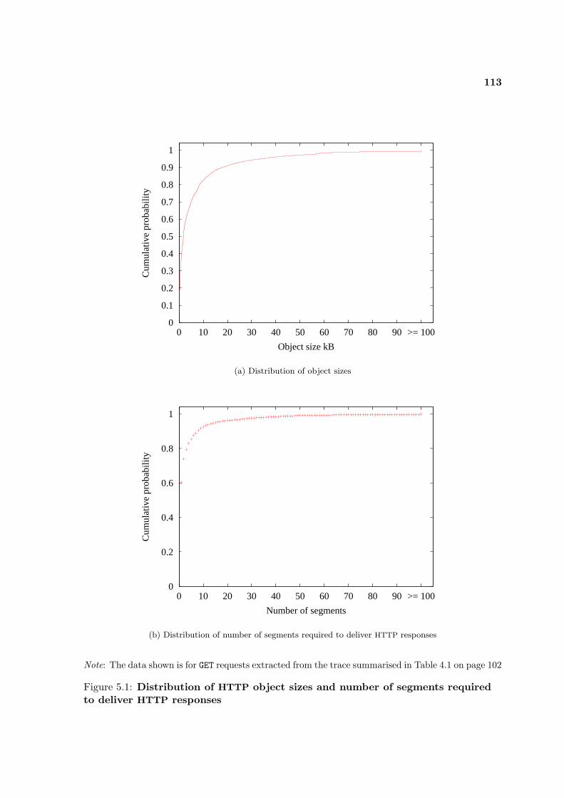
113

0

0.1

0.2

0.3

0.4

0.5

0.6

0.7

0.8

0.9

1

0 10 20 30 40 50 60 70 80 90 >= 100

Cum

ulat

ive

prob

abili

ty

Object size kB

(a) Distribution of object sizes

0

0.2

0.4

0.6

0.8

1

0 10 20 30 40 50 60 70 80 90 >= 100

Cum

ulat

ive

prob

abili

ty

Number of segments

(b) Distribution of number of segments required to deliver HTTP responses

Note: The data shown is for GET requests extracted from the trace summarised in Table 4.1 on page 102

Figure 5.1: Distribution of HTTP object sizes and number of segments requiredto deliver HTTP responses

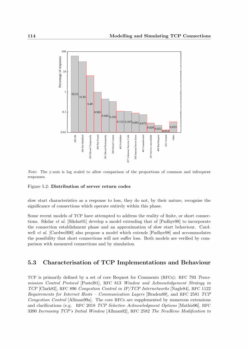
114 Modelling and Simulating TCP Connections

59.5331.85

6.40

0.9650.442 0.332

0.112 0.107 0.091 0.0750.029 0.022

0.0130.033

0.01

0.1

1

10

100

Perc

enta

ge o

f re

spon

ses

200

OK

304

Not

Mod

ifie

d

302

Mov

ed T

empo

rari

ly

404

Not

Fou

nd

301

Mov

ed P

erm

anen

tly

206

Part

ial C

onte

nt

403

Forb

idde

n

207

Unk

now

n Su

cces

s C

ode

500

Inte

rnal

Ser

ver

Err

or

401

Una

utho

rise

d

503

Serv

ice

unav

aila

ble

400

Bad

Req

uest

201

Cre

ated

Oth

er

Note: The y-axis is log scaled to allow comparison of the proportions of common and infrequentresponses.

Figure 5.2: Distribution of server return codes

slow start characteristics as a response to loss, they do not, by their nature, recognise thesignificance of connections which operate entirely within this phase.

Some recent models of TCP have attempted to address the reality of finite, or short connec-tions. Sikdar et al. [Sikdar01] develop a model extending that of [Padhye98] to incorporatethe connection establishment phase and an approximation of slow start behaviour. Card-well et al. [Cardwell00] also propose a model which extends [Padhye98] and accommodatesthe possibility that short connections will not suffer loss. Both models are verified by com-parison with measured connections and by simulation.

5.3 Characterisation of TCP Implementations and Behaviour

TCP is primarily defined by a set of core Request for Comments (RFCs): RFC 793 Trans-mission Control Protocol [Postel81], RFC 813 Window and Acknowledgement Strategy inTCP [Clark82], RFC 896 Congestion Control in IP/TCP Internetworks [Nagle84], RFC 1122Requirements for Internet Hosts – Communication Layers [Braden89], and RFC 2581 TCPCongestion Control [Allman99a]. The core RFCs are supplemented by numerous extensionsand clarifications (e.g. RFC 2018 TCP Selective Acknowledgment Options [Mathis96], RFC

3390 Increasing TCP’s Initial Window [Allman02], RFC 2582 The NewReno Modification to

5.3 Characterisation of TCP Implementations and Behaviour 115

TCP’s Fast Recovery Algorithm [Floyd99], and RFC 2988 Computing TCP’s RetransmissionTimer).

The status of RFCs varies (e.g. ‘STANDARD’, ‘PROPOSED STANDARD’, ‘INFORMA-TIONAL’) as does the degree of prescription in their recommendations (e.g. ‘MUST’,‘SHOULD’); the recommendations are, moreover, for minimal standards of behaviour or func-tionality, rather than exact definitions or implementation directives. There are many TCP

implementations, although often based upon a smaller number of core implementations andtheir variations; not all behave as intended and some (particularly in early manifestations)contain bugs or are not entirely RFC compliant. All TCP implementations, moreover, definea number of user-configurable parameters which may be expected to take a range of values.

As a consequence it is impossible to predict the behaviour of individual TCP connectionswith absolute confidence in the face of widely varying network conditions, higher-level pro-tocol behaviours, peer implementations, and connection histories; even when the generalcharacteristics of a particular known implementation are relatively well understood, nothingis absolutely guaranteed.

Several studies have characterised the behaviour of specific implementations, or of TCP con-nections in the round. The majority of these works have employed active techniques, normallyconstructing sequences of segments designed to elicit responses from the target implementa-tion illustrative of its behaviour in a range of specific circumstances.

Comer and Lin [Comer94] used this technique to investigate retransmission timer, keep aliveand zero window probing behaviours of a range of implementations without access to thesource code. A similar study was performed by Dawson et al. [Dawson97], who used an instru-mented kernel and fault injection techniques to investigate a range of commercially availableimplementations. Brakmo and Peterson [Brakmo95] used simulation, together with examina-tion and modification of the source, to investigate performance problems in the BSD4.4 TCP

implementation. A rather different approach was taken by Padhye and Floyd who describea tool — TBIT [Pahdye01] — which probes Web servers2 to investigate Initial Window val-ues; congestion control algorithms; responses to SACKs, time wait durations, and responseto Explicit Congestion Notification (ECN), of a wide range of servers. Rather than targeta known set of implementations the NMAP tool [Fyodor97] is used to identify the targetimplementation.

All of these studies confirmed the differing behaviours to be found between and within imple-mentations. In addition all identified flaws or bugs in the implementations and areas of RFC

non-compliance.

A contrasting study by Paxson [Paxson99] used passive measurement of 20,000 TCP bulktransfers to observe and characterise a range of network pathologies and TCP behaviours.Measurements were taken using the NPD measurement framework [Paxson97b] at both end-points in recognition of asymmetry between forward and return Internet paths.

2Web servers are chosen because of the predominance of HTTP traffic on the Internet — the techniquecan be generalised to any service reachable through a well-known address which can therefore be expected torespond.

116 Modelling and Simulating TCP Connections

5.4 Analysis of Individual TCP Connections

It is axiomatic that analytical models of TCP are generalised, and many are, additionally,essentially stochastic in nature. The shortcomings of models based upon steady state as-sumptions are discussed briefly in Section 5.2, but even those based upon the more realisticrecognition of finite and short connections, such as [Sikdar01] and [Cardwell00], will not re-liably describe the detailed behaviour of individual connections at the packet level: not allfeatures, implementation variations, optional features, or network parameters can be gen-eralised, and such models do not take into account behaviour of application-level processes(e.g. client or server latency, use of multiple serial or concurrent connections) or of human users(e.g. human browsing patterns). Although the steady state model is isolated from application-level behaviour (explicitly by assumptions, for instance, of constantly full transmit buffers),this is a weakness of finite-connection models as currently developed.

The characterisations described in Section 5.3, which are based upon active probing, arealso limited in their prediction of the overall behaviour of individual connections: with theexception of [Pahdye01], they are limited to specific implementations, but more fundamentally,although probing is carried out on individual connections, they all describe specific behaviourassessed in the context of sets of carefully contrived conditions.

The work described in [Paxson99], being based upon passive measurements, does not subjectthe end implementations to predefined conditions and observes a wider range of characteristicTCP behaviour. Although the emphasis is upon the use of TCP connections to observe and in-fer network dynamics, the study is particularly relevant to the work in this chapter: analysis ofthe individual connections observed necessarily involved differentiating between TCP and net-work behaviour and relies heavily for this reason upon Paxson’s tcpanaly tool [Paxson97a].

Tcpanaly was developed to automate the analysis of individual connections and, by isolatingTCP behaviour, to identify idiosyncrasies, bugs, and RFC non-compliance in TCP implemen-tations. The original hope that analysis could be carried out on the fly proved unrealistic,but off-line analysis demonstrated the effectiveness of the tool, which successfully identifieda range of implementations and their shortcomings. Input to tcpanaly consists of TCP/IP

headers collected by a packet filter based monitor. The underlying analytic mechanism isbased upon modelling the state of the TCP implementation at each end point, the change instate arising from packet arrivals, and the packet transmission behaviour of each implemen-tation as a result of the state modification. This mechanism is similar to that used by themodelling technique described in Section 5.5 of this chapter; although there are significantdifferences, the concepts of causality, data liberation and ACK generation are central to both.

A different approach to the analysis of individual connections was taken by Barford andCrovella [Barford00]. Their tcpeval tool also relies upon the identification of data liberationsand ACK generation, but with the emphasis on Critical Path Analysis (CPA) of the TCP

connections carrying HTTP transactions.

5.5 Modelling the Activity of Individual TCP Connections 117

5.5 Modelling the Activity of Individual TCP Connections

Because Nprobe traces will normally contain details of activity at levels above the transportlayer of the protocol stack, it is possible to construct models of individual TCP connectionactivity which incorporate this knowledge and can more accurately distinguish between net-work, transport, and higher levels than the studies in [Paxson97a] and [Barford00]. Whiletcpanaly and tcpeval make this distinction in order to isolate and describe activity partic-ularly at the network and transport levels respectively, the modelling technique described inthis chapter can also provide information pertinent to higher-level activity and, significantly,describe how activity at lower levels is seen by the application and consequently the user.

This section describes an activity model of individual TCP connections which reconstructsconnection dynamics on a packet by packet basis by identifying the cause and effect relation-ships between segments in the context of models of TCP end-point state. A parallel model ofapplication-level activity both informs the TCP model and is informed by it.

5.5.1 The Model as an Event Driven Progress

The timing of primary events observed when monitoring a TCP connection (i.e. the transmis-sion of data segments and/or acknowledgements) will be determined by a variety of causes,which are themselves events occurring over a range of levels in the protocol stack. The seriesof segments, for instance, whose payload is an HTTP response comprising a Web object, isinitiated by the receipt of the corresponding HTTP request. The exact transmission time ofeach individual segment or acknowledgement will, however, be determined by one or more ofa number of preceding events and the current state associated with the connection — thesein turn are determined by the events that precede them and the connection state at the time.

From the viewpoint of the monitor, the packets observed reliably represent transmission eventsand possibly the higher-level events represented by packet contents. The observed packetsdo not represent receipt events as packets may be lost between the monitoring point andreceiving host. Receipt events can only be inferred from the observation of the transmissionevents which they trigger. A further category — hidden events — also identified only byinference include transmission events not seen because of packet loss, timer driven events(e.g. retransmission timeouts, delayed ACKs), or transmission buffer exhaustion.

5.5.2 Packet Transmission and Causality

The modelling technique described in this section is based upon the proposition that theobserved activity can only be fully understood by the correct association of cause and effect— an HTTP response occurs because a request is received, but it is not possible to quantifythe server’s delay in responding simply by measuring the time between seeing request andresponse — why the corresponding data segments are transmitted at a certain time must beunderstood. The precipitating event may be the arrival of the request, a received acknowl-edgement advancing the sender’s transmission window or enlarging its congestion window,

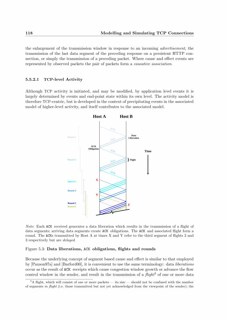
118 Modelling and Simulating TCP Connections

the enlargement of the transmission window in response to an incoming advertisement, thetransmission of the last data segment of the preceding response on a persistent HTTP con-nection, or simply the transmission of a preceding packet. Where cause and effect events arerepresented by observed packets the pair of packets form a causative association.

5.5.2.1 TCP-level Activity

Although TCP activity is initiated, and may be modified, by application level events it islargely determined by events and end-point state within its own level. The activity model istherefore TCP-centric, but is developed in the context of precipitating events in the associatedmodel of higher-level activity, and itself contributes to the associated model.

Host A Host B

Data

ACK

Data

ACK

ACK

DataLiberation

} Flight

Time

Y

X

ACKObligation

Round 1

Round 2

Round 3

Round 4

Round 5

Round 6Z

Note: Each ACK received generates a data liberation which results in the transmission of a flight ofdata segments; arriving data segments create ACK obligations. The ACK and associated flight form around. The ACKs transmitted by Host A at times X and Y refer to the third segment of flights 2 and3 respectively but are delayed.

Figure 5.3: Data liberations, ACK obligations, flights and rounds

Because the underlying concept of segment based cause and effect is similar to that employedby [Paxson97a] and [Barford00], it is convenient to use the same terminology: data liberationsoccur as the result of ACK receipts which cause congestion window growth or advance the flowcontrol window in the sender, and result in the transmission of a flight3 of one or more data

3A flight, which will consist of one or more packets — its size — should not be confused with the numberof segments in flight (i.e. those transmitted but not yet acknowledged from the viewpoint of the sender); the

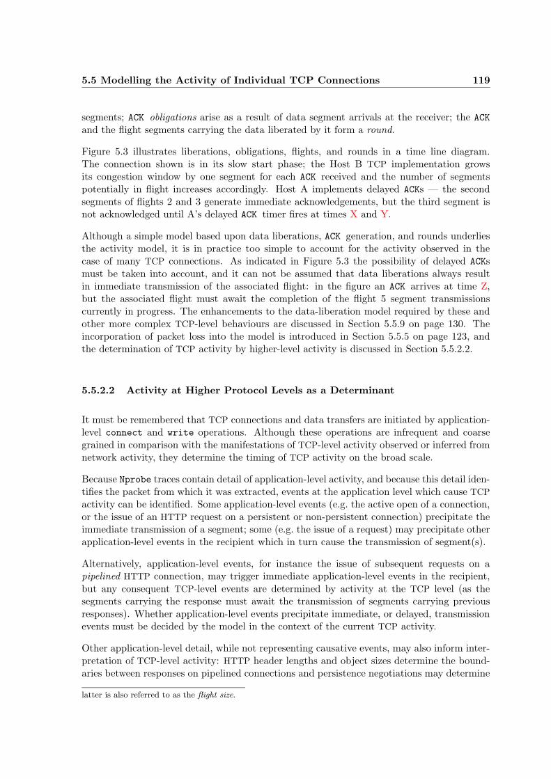
5.5 Modelling the Activity of Individual TCP Connections 119

segments; ACK obligations arise as a result of data segment arrivals at the receiver; the ACK

and the flight segments carrying the data liberated by it form a round.

Figure 5.3 illustrates liberations, obligations, flights, and rounds in a time line diagram.The connection shown is in its slow start phase; the Host B TCP implementation growsits congestion window by one segment for each ACK received and the number of segmentspotentially in flight increases accordingly. Host A implements delayed ACKs — the secondsegments of flights 2 and 3 generate immediate acknowledgements, but the third segment isnot acknowledged until A’s delayed ACK timer fires at times X and Y.

Although a simple model based upon data liberations, ACK generation, and rounds underliesthe activity model, it is in practice too simple to account for the activity observed in thecase of many TCP connections. As indicated in Figure 5.3 the possibility of delayed ACKsmust be taken into account, and it can not be assumed that data liberations always resultin immediate transmission of the associated flight: in the figure an ACK arrives at time Z,but the associated flight must await the completion of the flight 5 segment transmissionscurrently in progress. The enhancements to the data-liberation model required by these andother more complex TCP-level behaviours are discussed in Section 5.5.9 on page 130. Theincorporation of packet loss into the model is introduced in Section 5.5.5 on page 123, andthe determination of TCP activity by higher-level activity is discussed in Section 5.5.2.2.

5.5.2.2 Activity at Higher Protocol Levels as a Determinant

It must be remembered that TCP connections and data transfers are initiated by application-level connect and write operations. Although these operations are infrequent and coarsegrained in comparison with the manifestations of TCP-level activity observed or inferred fromnetwork activity, they determine the timing of TCP activity on the broad scale.

Because Nprobe traces contain detail of application-level activity, and because this detail iden-tifies the packet from which it was extracted, events at the application level which cause TCP

activity can be identified. Some application-level events (e.g. the active open of a connection,or the issue of an HTTP request on a persistent or non-persistent connection) precipitate theimmediate transmission of a segment; some (e.g. the issue of a request) may precipitate otherapplication-level events in the recipient which in turn cause the transmission of segment(s).

Alternatively, application-level events, for instance the issue of subsequent requests on apipelined HTTP connection, may trigger immediate application-level events in the recipient,but any consequent TCP-level events are determined by activity at the TCP level (as thesegments carrying the response must await the transmission of segments carrying previousresponses). Whether application-level events precipitate immediate, or delayed, transmissionevents must be decided by the model in the context of the current TCP activity.

Other application-level detail, while not representing causative events, may also inform inter-pretation of TCP-level activity: HTTP header lengths and object sizes determine the bound-aries between responses on pipelined connections and persistence negotiations may determine

latter is also referred to as the flight size.

120 Modelling and Simulating TCP Connections

which party initiates a connection close. TCP activity can, conversely, imply application-levelevents (e.g. a FIN segment on a non-persistent HTTP connection denotes an completion ofobject event).

5.5.2.3 Interaction Between TCP and Higher-Level Protocols

As noted in Section 5.2, analytic TCP models have largely been based upon steady stateassumptions, a simplification which isolates TCP activity from that at higher levels. Studiesbased upon the analysis of individual connections have also simplified the models upon whichthey are based to minimise the impact of higher-level events: tcpanaly operates on traces ofsingle bulk data transfers of 100 Kilobytes, hence limiting application-level activity to openingthe connection and a single write operation; tcpeval isolates the connection set up andHTTP request/response phases from the main liberation-based model. These simplificationsare not only convenient, but are also necessary in the absence of comprehensive knowledge ofapplication activity.

Higher-level activity which overtly precipitates TCP activity has been discussed in Sec-tion 5.5.2.2, but more subtle interactions are also possible. The rate at which the receiverconsumes data will affect the sender’s transmission rate through the window advertisementmechanism. TCP transmission will cease if the sender does not maintain adequate data inthe transmit buffer. In the former case, the effect is explicit through the observed windowadvertisements and is trivially incorporated into the liberation based model; transmit bufferexhaustion must be inferred from the sender’s failure to transmit data at the expected time.

The amount of data to be transmitted can also modify TCP behaviour: Heidemann[Heidemann97a] notes how persistent HTTP performance can be compromised by delays intransmitting partial segments due to the operation of Nagle’s algorithm [Nagle84]. Followingthe publication of Heidemann’s findings, most Web servers operate with Nagle’s algorithmdisabled, but the activity model must be able to incorporate the behaviour of TCP connec-tions where this is not the case: there is no guarantee that Nagle’s algorithm will be disabledby all Web servers, and it will not be in many other applications. Because the model knowsdata transfer sizes Nagle effects can be identified and incorporated.

5.5.3 Monitor Position and Interpretation of Packet Timings

The monitoring point from which data is gathered may be anywhere between the commu-nicating endpoints and it is therefore inappropriate to interpret packet arrivals in terms ofconventional RTTs. RTTs, moreover, measure the total time taken by rounds and comprisenetwork transit times, delays introduced by TCP itself and application delays — the moti-vation behind the development of the activity model is partly to distinguish between thesecomponents.

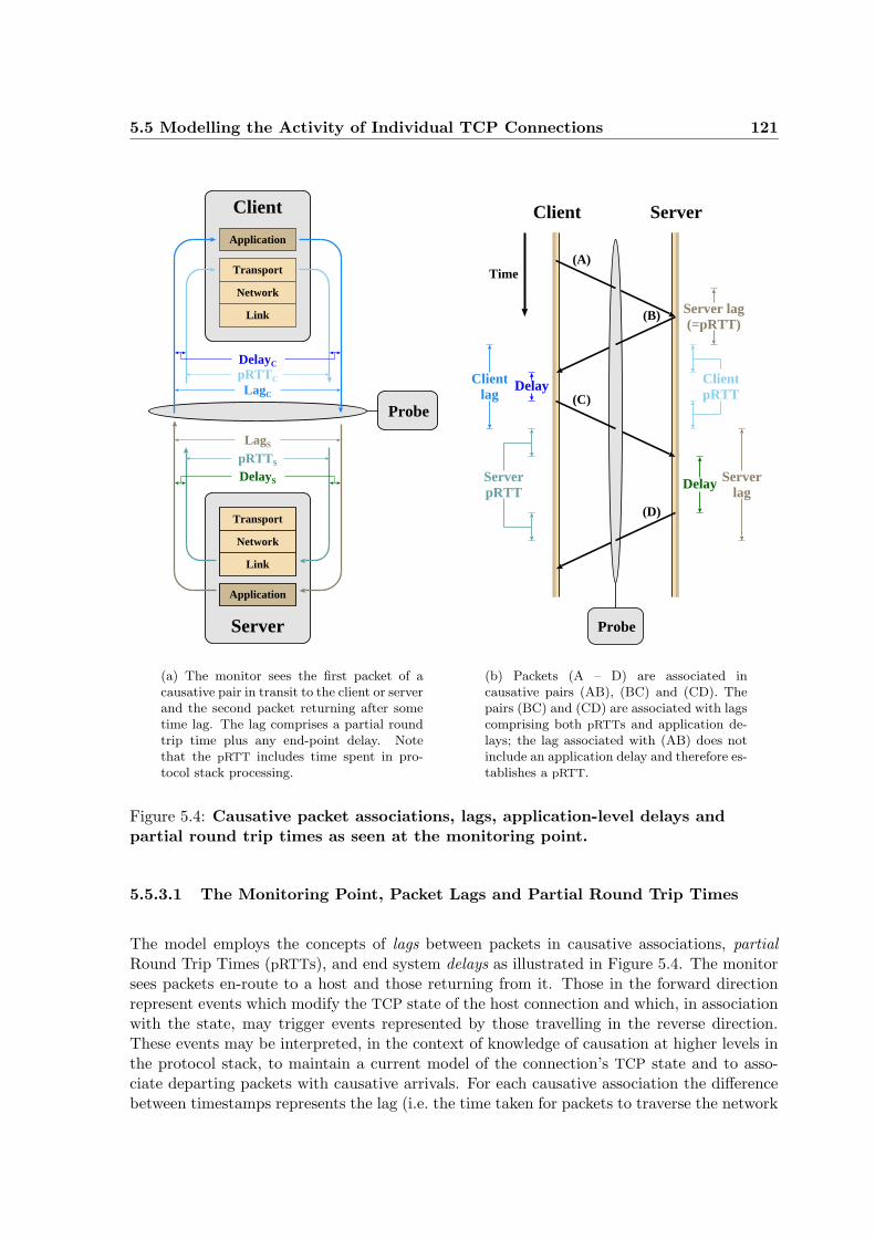
5.5 Modelling the Activity of Individual TCP Connections 121

Link

Network

Transport

Application

Client

Server

Link

Network

Transport

Application

Probe

DelayC

pRTTC

LagC

LagS

pRTTS

DelayS

(a) The monitor sees the first packet of acausative pair in transit to the client or serverand the second packet returning after sometime lag. The lag comprises a partial roundtrip time plus any end-point delay. Notethat the pRTT includes time spent in pro-tocol stack processing.

ServerpRTT

Probe

Client Server

(C)DelayClient

lag

(A)

(B)

Serverlag

Delay

(D)

Time

Server lag(=pRTT)

ClientpRTT

(b) Packets (A – D) are associated incausative pairs (AB), (BC) and (CD). Thepairs (BC) and (CD) are associated with lagscomprising both pRTTs and application de-lays; the lag associated with (AB) does notinclude an application delay and therefore es-tablishes a pRTT.

Figure 5.4: Causative packet associations, lags, application-level delays andpartial round trip times as seen at the monitoring point.

5.5.3.1 The Monitoring Point, Packet Lags and Partial Round Trip Times

The model employs the concepts of lags between packets in causative associations, partialRound Trip Times (pRTTs), and end system delays as illustrated in Figure 5.4. The monitorsees packets en-route to a host and those returning from it. Those in the forward directionrepresent events which modify the TCP state of the host connection and which, in associationwith the state, may trigger events represented by those travelling in the reverse direction.These events may be interpreted, in the context of knowledge of causation at higher levels inthe protocol stack, to maintain a current model of the connection’s TCP state and to asso-ciate departing packets with causative arrivals. For each causative association the differencebetween timestamps represents the lag (i.e. the time taken for packets to traverse the network

122 Modelling and Simulating TCP Connections

from the monitoring point to a communicating host, any delay at the host, and for returningpackets to traverse the reverse path). A conventional RTT4 is thus analogous to a pair of lagsfrom the client and server sides of the monitor.

If any delay at the host is deducted from the relevant lag the residual time represents thenetwork transit time or partial Round Trip Time (pRTT) of packets from monitor to host andback; a pair of pRTTs therefore represents the total network transit time between the twohosts. Figure 5.4(a) illustrates the relationship between lags, pRTTs and end-point delays.

5.5.3.2 Differentiation of Network and End System Times

The activity model discriminates the returning packets of causative pairs into those trans-mitted immediately on receipt of an incoming packet — in which case the lag time of theassociation is equal to, and establishes, a pRTT — and those transmitted after some delay.Figure 5.4(b) shows a time line diagram of causative associations with and without delay.End-point delays may be categorised as those due to:

• TCP implementation mechanisms (e.g. delayed ACKs , Nagle effects)

• Application delays (e.g. HTTP request processing and response generation)

• Serialisation delays (e.g. transmission awaiting that of previously queued packets)

• Combinations of two or more of the above

Because the activity model maintains models of the current TCP end-point state and appli-cation activity, it is able to both identify causative associations where lags include a delayand to categorise the delay. The majority of delays are identifiable as due to a single factor,but where more than one cause is possible the delay is taken to be due to the cause for whichthe model calculates the maximum notional lag magnitude.

For each identified delay the current pRTT is calculated by interpolation from nearby knownpRTTs and deducted from the lag time to calculate the magnitude. It is axiomatic that alag containing a delay does not yield an immediate pRTT and it has to be accepted that, inorder to calculate delay magnitudes, some inaccuracy arising from interpolation of pRTTs isinevitable. The accuracy obtained by this technique will, however, normally be far better thanthat obtained by those where network transit times and end-point delays are not differentiated.

5.5.4 Unidirectional and Bidirectional Data Flows

The activity model is described for simplicity in terms of a unidirectional data flow. SuchTCP flows are comparatively rare (the data transfer connections used by the File Transfer

4A similar technique is reported by Jiang and Dovrolis [Jiang02] who base RTT estimations on rounds —the activity model can achieve the same end, by combining pairs of pRTTs , but the differentiation of clientand server pRTTs allows the calculation of delay magnitudes.

5.5 Modelling the Activity of Individual TCP Connections 123

Protocol representing a significant exception) — even protocols such as HTTP , where themajority data transfer is unidirectional, normally include some bidirectional element (e.g. thetransmission of the client request).

The model is, however, able to accommodate bidirectional flows without significant additionalcomplexity. Where bidirectional flows do not take place concurrently, connection activity canbe regarded in effect as two distinct unidirectional flows bounded by application-level activity;where the two flows occur concurrently causative associations are not invalidated, but caremust be taken to differentiate ACKs piggy-backed on data segments from those whose timingis determined by normal ACK generation alone.

5.5.5 Identifying and Incorporating Packet Loss

Because the Nprobe monitor may be positioned at any point between communicating hostspacket loss presents particular difficulties. Packets may be lost:

Between the monitor and the receiver: The monitor sees the lost packet, but receiver statemust not be modified to erroneously reflect its arrival.

Between the sender and the monitor: The monitor does not see the lost packet, but the lossmust be detected by the model in order to adjust transmitter state appropriately.

In the first case, loss of data segments is trivially identified as the monitor will see a duplicate(retransmission) of the lost segment. An initial pass through the trace packet records marksthe lost segment; when encountered the model adjusts the transmitter state but not that ofthe receiver.

In the second case the transmission of the sent, but unseen, segment must be inferred. In themajority of cases the loss will be suggested by a sequence gap in the segments seen by themonitor — also detected during an initial pass through the packets — during which a dummypacket can be inserted into the packet records to ensure that transmitter state is adjustedat the correct point. If the missing segment is part of a flight, the time that it would havebeen seen by the monitor can be estimated with reasonable accuracy from the timings of theaccompanying segments.

In both cases loss will also usually be indicated by the generation of duplicate ACKs generatedby the receiver. The possibility of individual segment loss can also be eliminated by theassumption that all acknowledged segments have been received5.

There is more difficulty in identifying data segments lost between the sender and monitorwhere, at the time of loss, no subsequent segments are transmitted and hence no sequencegap is identified. In this case the model must rely upon either a subsequent data liberationmanifesting the sequence gap or its own expectation that an unseen segment should have beentransmitted. In the former instance the preliminary pass will identify the lost packet in the

5This assumption is regarded as safe — a TCP receiving an ACK for an unsent sequence would reset theconnection and the model would be rejected as invalid.

124 Modelling and Simulating TCP Connections

normal way, in the second there is the possibility of ambiguity: the expected packet mayhave been lost, its transmission may have been subject to an application delay6 or both delayand loss may be present. A heuristic solution is employed based upon the model’s currentestimation of the sender’s retransmission timeout, application-level activity and the data sizeof the eventually transmitted segment.

When data segment loss is detected, the model must reflect the consequent effects upon TCP

state and subsequent events, and must differentiate between timeout triggered retransmis-sions and fast retransmits [Allman99a]7. The possibility of a fast retransmit will have beenflagged by the observation of three or more duplicate ACKs , and the timing of the retransmis-sion will normally indicate which has occurred. The model must incorporate the connection(re)entering a slow-start or fast recovery phase and adjust the value of its congestion windowand slow-start threshold accordingly; the notional retransmission timer value must also beadjusted.

The loss of ACK segments presents rather more difficulty than that of data segments as theclue provided by retransmission is absent; it is primarily for this reason that the detectionof lost data segments does not place reliance on the absence of the relevant observed ACK.Conversely, because ACK obligations result only from activity at the TCP level no possibilityof confusion between lost ACKs and application-level delays arises.

It is useful, at this point, to introduce more of Paxson’s terminology [Paxson97a]: ACK obli-gations may be optional — TCP may acknowledge a data arrival (e.g. when new in-sequencedata arrives) or mandatory — an ACK must be generated (e.g. when out of sequence dataarrives, for at least every second full sized segment, and at the upper bound of ACK delays[500 ms]). ACKs arising from in-sequence data may be normal (i.e. those for two full sizedsegments), delayed (i.e. for single segments) or stretch (i.e. for more than two full-sized seg-ments). The activity model adds the term sequence acknowledgement for those generated bythe arrival of out of sequence data.

ACK loss occurring between sender and monitoring point may be indicated by the failure toobserve expected ACKs (either normal, or delayed after an appropriate period); unfortunatelystretch ACKs are not uncommon8 which renders the expectation of mandatory ACKs for everysecond segment unreliable as an indicator of loss on connections where they are found. Theloss of stretch ACKs themselves can be detected because they inevitably acknowledge sequenceswithin the same flight.

The cumulative nature of ACKs means that any failure to update the sender’s state in thecase of losses before the monitoring point is healed by subsequent ACKs. Similarly, ACKs lostbetween the monitor and the receiver are indicated by the release of an unexpectedly largeflight following the receipt of a subsequent ACK — the flight size also distinguishes this casefrom that of data segment loss before the monitor. When flight sizes are determined by the

6TCP mechanism delays are disqualified — the model would anticipate such delays and a segment trans-

mission would not be expected.7The ‘NewReno’ modification to the fast retransmit algorithm [Floyd99] is not yet incorporated into the

model — SACKs are not yet collected by Nprobe or modelled.8With the exception of a maximum ACK delay of 500 ms, RFC 1122 [Braden89] couches its recommendations

for ACK generation in terms of ‘SHOULD’ rather than ‘MUST’.

5.5 Modelling the Activity of Individual TCP Connections 125

congestion, rather than the flow, window, the corresponding indicator is a failure of expectedwindow growth.

Fortunately the case critical to the accuracy of the model is that where ACK loss (whereverit occurs) results in retransmission, for which identification mechanisms are comparativelyrobust, and the retransmitting host’s state can thus be corrected accordingly. The removalof possible ambiguities in detecting loss is also made easier because expectations can usuallybe expressed both in terms of sequence, and of observation time.

It may appear that a modelling process which depends upon both inferring loss and delaythrough observed activity is analogous to lifting one’s self by the boot straps. The set-up phase of the connection, however, provides a reliable foundation for any following time-based heuristics. Application-level delays are absent from this phase, default retransmissiontimeouts (initially three seconds) are sufficiently large to be unambiguously identifiable, andan approximate magnitude for the connection’s pRTTs is established.

5.5.6 Packet Re-Ordering and Duplication

Although, with the exception of retransmissions, it is assumed that data segments are trans-mitted strictly in order, the activity model must recognise that packets may be re-ordered bythe network. As with packet loss, re-ordering may occur both upstream and downstream ofthe monitoring point. In general re-ordering may be distinguished from the case of packetslost before reaching the monitor and their retransmission, following intervening packets, be-cause re-ordering inevitably occurs within the same flight9, and because insufficient time willhave elapsed for a retransmission to have taken place.

Upstream data re-ordering is trivially detected during the initial pass through packet records,and the relevant packets so marked to avoid confusion with sequence gaps denoting lostpackets; downstream occurrences can only be inferred through subsequent connection activity.Because re-ordering does not effect the sender, and because, once the re-ordered sequence hasbeen delivered, the receiver state is identical to that had not re-ordering taken place, themodel is faced with little difficulty subject to the proviso that:

• Re-ordering is not confused with retransmission

• Any sequence ACKs generated are not taken as indicators of packet loss (the distinctionis drawn by a closely subsequent normal or delay ACK)

• Fast retransmits due to multiple sequence ACKs are recognised10

ACK segment re-ordering has a lower incidence than that of data segments: Paxson reports9This observation is supported by Bellardo and Savage who conducted a survey of packet re-

ordering [Bellardo02] using active techniques which exploited characteristic TCP behaviour. They reportfinding the incidence of re-ordering of minimum-sized TCP packets to be less than 2 per cent when separatedby more than 50 µs , tending to zero at 250 µs.

10This will occur only in the case of a re-ordering distance greater than three segments — no such distanceshave yet been observed.

126 Modelling and Simulating TCP Connections

a ratio of approximately 1:3 [Paxson99] for bulk transfers where a high proportion of ACKsmight be expected to cluster due to large flights of data segments. For the majority of short-lived connections the findings reported in [Bellardo02] (see Footnote 5.9) suggest that ACK

re-ordering will be extremely rare. Where ACKs are reordered, their impact on both receiverand model are minimal (due to their cumulative nature), although the model should ensurethat the ACK following the delayed ACK is not confused with a stretch ACK .

Packets may also be duplicated by the network. Where data duplications are seen by themonitor, they can normally be distinguished from duplication due to retransmission by theirarrival time. Duplications are detected during the initial pass through the packet records,marked, and subsequently rejected by the model, as they would be by the receiver. DuplicatedACKs can be ignored by the model; they will introduce inaccuracy only in the unlikely eventthat three duplications trigger a fast retransmission.

5.5.7 Slow Start and Congestion Avoidance

Congestion window growth must be tracked by the model during slow-start and congestion-avoidance phases of the connection. Accurate identification of flight sizes (Section 5.5.8 andCode Fragment 5.1 on the facing page) is necessary to enable the model’s predictive element(Section 5.5.8.2) to verify that window-growth behaviour is accurately understood.

TCP implementations may enter congestion avoidance either when CWND is equal to theSlow-Start THRESHold (SSTHRESH), or when it becomes larger. The model notes the pointat which CWND = SSTHRESH and determines the implementation’s behaviour on the basisof CWND growth thereafter.

5.5.8 Construction of the Activity Model

The core of the activity model is a representation of the TCP state at the communicatingend points; packet events (as represented by the header records collected by Nprobe ) arepresented in order to the model and state modified — the exact interpretation of eventsand their impact upon state are dependent upon the state at the time of the event. Therepresentation of state identifies cause and effect relationships between packet events, andthese and the state itself. A model of higher-level activity is incorporated and provides thecontext for the TCP-level activity observed; this model is typically relatively simple, activityconsisting of request/response events and data transfer sizes. Other relevant information(e.g. the course of HTTP persistence negotiations, or whether pipelining is employed) is alsorecorded.

The model makes a preliminary pass through the packet records in order to group datasegments into flights, and to mark any retransmitted, re-ordered, or duplicated packets iden-tifiable at this stage. The simple, but reliable, algorithm used to identify flights is reproducedin Code Fragment 5.1.

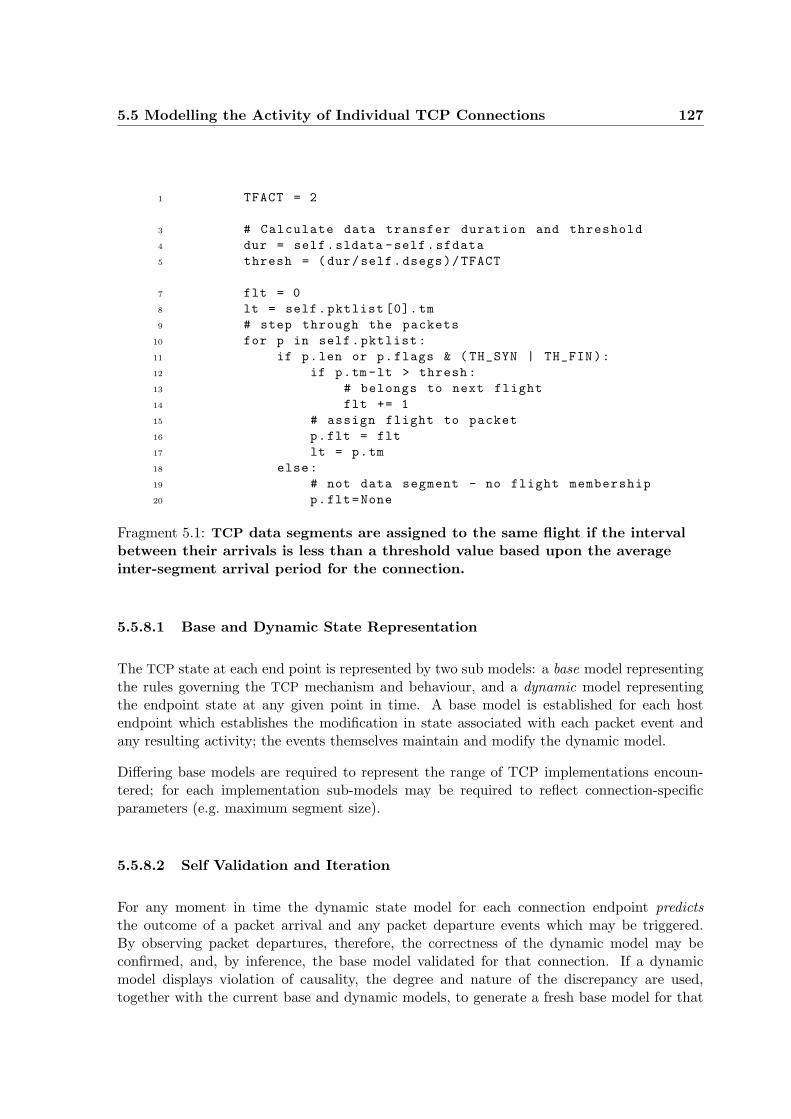
5.5 Modelling the Activity of Individual TCP Connections 127

1 TFACT = 2

3 # Calculate data transfer duration and threshold

4 dur = self.sldata -self.sfdata

5 thresh = ( dur/self.dsegs)/TFACT

7 flt = 0

8 lt = self.pktlist [0].tm

9 # step through the packets

10 for p in self.pktlist:

11 if p.len or p.flags & ( TH_SYN | TH_FIN):

12 if p.tm-lt > thresh:

13 # belongs to next flight

14 flt += 1

15 # assign flight to packet

16 p.flt = flt

17 lt = p.tm

18 else:

19 # not data segment - no flight membership

20 p.flt=None

Fragment 5.1: TCP data segments are assigned to the same flight if the intervalbetween their arrivals is less than a threshold value based upon the averageinter-segment arrival period for the connection.

5.5.8.1 Base and Dynamic State Representation

The TCP state at each end point is represented by two sub models: a base model representingthe rules governing the TCP mechanism and behaviour, and a dynamic model representingthe endpoint state at any given point in time. A base model is established for each hostendpoint which establishes the modification in state associated with each packet event andany resulting activity; the events themselves maintain and modify the dynamic model.

Differing base models are required to represent the range of TCP implementations encoun-tered; for each implementation sub-models may be required to reflect connection-specificparameters (e.g. maximum segment size).

5.5.8.2 Self Validation and Iteration

For any moment in time the dynamic state model for each connection endpoint predictsthe outcome of a packet arrival and any packet departure events which may be triggered.By observing packet departures, therefore, the correctness of the dynamic model may beconfirmed, and, by inference, the base model validated for that connection. If a dynamicmodel displays violation of causality, the degree and nature of the discrepancy are used,together with the current base and dynamic models, to generate a fresh base model for that

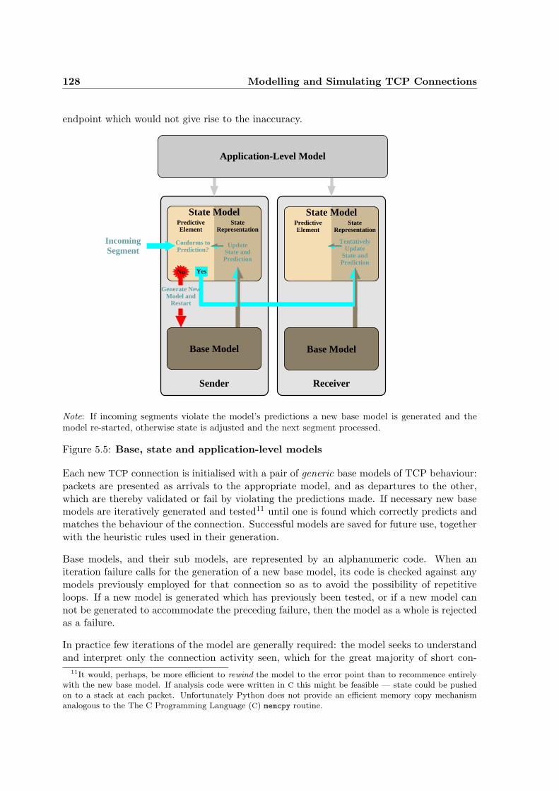
128 Modelling and Simulating TCP Connections

endpoint which would not give rise to the inaccuracy.

ReceiverSender

IncomingSegment

State ModelPredictiveElement

StateRepresentation

TentativelyUpdate

State andPrediction

Conforms toPrediction?

State ModelPredictiveElement

StateRepresentation

Yes

UpdateState andPrediction

No

Generate NewModel and

Restart

Application-Level Model

Base Model Base Model

Note: If incoming segments violate the model’s predictions a new base model is generated and themodel re-started, otherwise state is adjusted and the next segment processed.

Figure 5.5: Base, state and application-level models

Each new TCP connection is initialised with a pair of generic base models of TCP behaviour:packets are presented as arrivals to the appropriate model, and as departures to the other,which are thereby validated or fail by violating the predictions made. If necessary new basemodels are iteratively generated and tested11 until one is found which correctly predicts andmatches the behaviour of the connection. Successful models are saved for future use, togetherwith the heuristic rules used in their generation.

Base models, and their sub models, are represented by an alphanumeric code. When aniteration failure calls for the generation of a new base model, its code is checked against anymodels previously employed for that connection so as to avoid the possibility of repetitiveloops. If a new model is generated which has previously been tested, or if a new model cannot be generated to accommodate the preceding failure, then the model as a whole is rejectedas a failure.

In practice few iterations of the model are generally required: the model seeks to understandand interpret only the connection activity seen, which for the great majority of short con-

11It would, perhaps, be more efficient to rewind the model to the error point than to recommence entirelywith the new base model. If analysis code were written in C this might be feasible — state could be pushedon to a stack at each packet. Unfortunately Python does not provide an efficient memory copy mechanismanalogous to the The C Programming Language (C) memcpy routine.

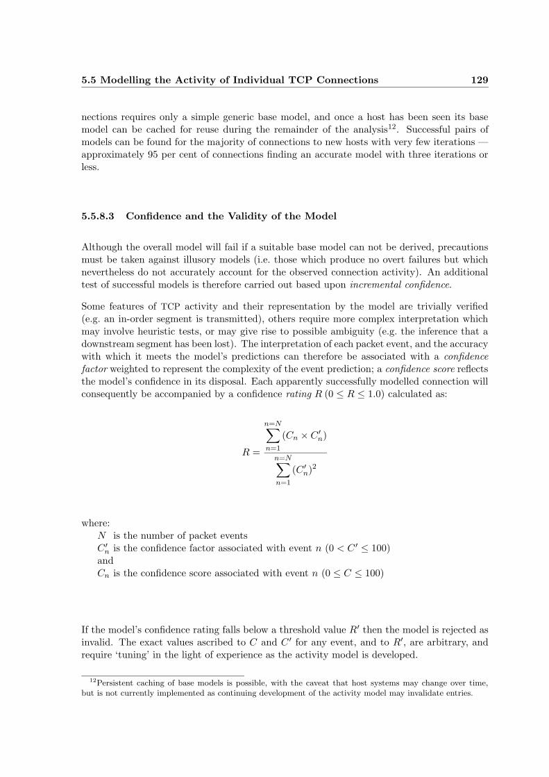
5.5 Modelling the Activity of Individual TCP Connections 129

nections requires only a simple generic base model, and once a host has been seen its basemodel can be cached for reuse during the remainder of the analysis12. Successful pairs ofmodels can be found for the majority of connections to new hosts with very few iterations —approximately 95 per cent of connections finding an accurate model with three iterations orless.

5.5.8.3 Confidence and the Validity of the Model

Although the overall model will fail if a suitable base model can not be derived, precautionsmust be taken against illusory models (i.e. those which produce no overt failures but whichnevertheless do not accurately account for the observed connection activity). An additionaltest of successful models is therefore carried out based upon incremental confidence.

Some features of TCP activity and their representation by the model are trivially verified(e.g. an in-order segment is transmitted), others require more complex interpretation whichmay involve heuristic tests, or may give rise to possible ambiguity (e.g. the inference that adownstream segment has been lost). The interpretation of each packet event, and the accuracywith which it meets the model’s predictions can therefore be associated with a confidencefactor weighted to represent the complexity of the event prediction; a confidence score reflectsthe model’s confidence in its disposal. Each apparently successfully modelled connection willconsequently be accompanied by a confidence rating R (0 ≤ R ≤ 1.0) calculated as:

R =

n=N∑

n=1

(Cn × C ′

n)

n=N∑

n=1

(C ′

n)2

where:N is the number of packet eventsC ′

n is the confidence factor associated with event n (0 < C ′ ≤ 100)andCn is the confidence score associated with event n (0 ≤ C ≤ 100)

If the model’s confidence rating falls below a threshold value R′ then the model is rejected asinvalid. The exact values ascribed to C and C ′ for any event, and to R′, are arbitrary, andrequire ‘tuning’ in the light of experience as the activity model is developed.

12Persistent caching of base models is possible, with the caveat that host systems may change over time,but is not currently implemented as continuing development of the activity model may invalidate entries.

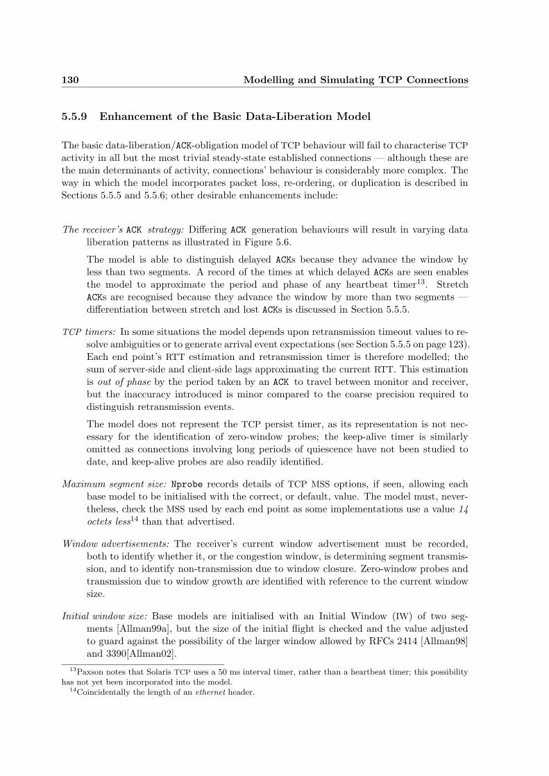
130 Modelling and Simulating TCP Connections

5.5.9 Enhancement of the Basic Data-Liberation Model

The basic data-liberation/ACK-obligation model of TCP behaviour will fail to characterise TCP

activity in all but the most trivial steady-state established connections — although these arethe main determinants of activity, connections’ behaviour is considerably more complex. Theway in which the model incorporates packet loss, re-ordering, or duplication is described inSections 5.5.5 and 5.5.6; other desirable enhancements include:

The receiver’s ACK strategy: Differing ACK generation behaviours will result in varying dataliberation patterns as illustrated in Figure 5.6.

The model is able to distinguish delayed ACKs because they advance the window byless than two segments. A record of the times at which delayed ACKs are seen enablesthe model to approximate the period and phase of any heartbeat timer13. StretchACKs are recognised because they advance the window by more than two segments —differentiation between stretch and lost ACKs is discussed in Section 5.5.5.

TCP timers: In some situations the model depends upon retransmission timeout values to re-solve ambiguities or to generate arrival event expectations (see Section 5.5.5 on page 123).Each end point’s RTT estimation and retransmission timer is therefore modelled; thesum of server-side and client-side lags approximating the current RTT. This estimationis out of phase by the period taken by an ACK to travel between monitor and receiver,but the inaccuracy introduced is minor compared to the coarse precision required todistinguish retransmission events.

The model does not represent the TCP persist timer, as its representation is not nec-essary for the identification of zero-window probes; the keep-alive timer is similarlyomitted as connections involving long periods of quiescence have not been studied todate, and keep-alive probes are also readily identified.

Maximum segment size: Nprobe records details of TCP MSS options, if seen, allowing eachbase model to be initialised with the correct, or default, value. The model must, never-theless, check the MSS used by each end point as some implementations use a value 14octets less14 than that advertised.

Window advertisements: The receiver’s current window advertisement must be recorded,both to identify whether it, or the congestion window, is determining segment transmis-sion, and to identify non-transmission due to window closure. Zero-window probes andtransmission due to window growth are identified with reference to the current windowsize.

Initial window size: Base models are initialised with an Initial Window (IW) of two seg-ments [Allman99a], but the size of the initial flight is checked and the value adjustedto guard against the possibility of the larger window allowed by RFCs 2414 [Allman98]and 3390[Allman02].

13Paxson notes that Solaris TCP uses a 50 ms interval timer, rather than a heartbeat timer; this possibilityhas not yet been incorporated into the model.

14Coincidentally the length of an ethernet header.

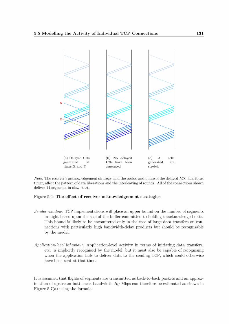
5.5 Modelling the Activity of Individual TCP Connections 131

X

Y

(a) Delayed ACKsgenerated attimes X and Y

(b) No delayedACKs have beengenerated

(c) All acksgenerated arestretch

Note: The receiver’s acknowledgement strategy, and the period and phase of the delayed-ACK heartbeattimer, affect the pattern of data liberations and the interleaving of rounds. All of the connections showndeliver 14 segments in slow-start.

Figure 5.6: The effect of receiver acknowledgement strategies

Sender window: TCP implementations will place an upper bound on the number of segmentsin-flight based upon the size of the buffer committed to holding unacknowledged data.This bound is likely to be encountered only in the case of large data transfers on con-nections with particularly high bandwidth-delay products but should be recognisableby the model.

Application-level behaviour: Application-level activity in terms of initiating data transfers,etc. is implicitly recognised by the model, but it must also be capable of recognisingwhen the application fails to deliver data to the sending TCP, which could otherwisehave been sent at that time.

It is assumed that flights of segments are transmitted as back-to-back packets and an approx-imation of upstream bottleneck bandwidth BU Mbps can therefore be estimated as shown inFigure 5.7(a) using the formula:

132 Modelling and Simulating TCP Connections

BU =(s + ((n − 1) × OP )) × 8

t

where:n is the size of the flightOP is the per-segment packet overhead in octetsSi is the initial sequence number of segment i of the flights = Sn − S0

Ti is the arrival time of segment i of the flightandt = Tn − T0 in microseconds

Downstream bottleneck bandwidths are less accessible, but an estimation can be based uponthe rate of returning ACKs using the technique of Instantaneous ACK Bandwidths (IABs) usedby Mogul [Mogul92] and shown in Figure 5.7(b), and explained here, in simplified form. TheIAB of two ACKs — BI Mbps — is calculated as:

BI =s

tA

where:s = (sA + (nA × OP )) × 8sA is the number of octets acknowledgednA is the number of segments acknowledgedOP is the per-segment packet overhead in octetsandtA is the time interval between the acknowledgements in microseconds

Figure 5.7(b) on the facing page shows the ACKs which might be generated by the segmentsshown in Figure 5.7(a) on the next page. IABs will indicate the downstream bottleneckbandwidth if the packets upon which they are based maintain queueing at the bottleneck:s1/t1 and s3/t3 will yield meaningful results if it is assumed that packets in the first andsecond flights queue; the value given by s2/t2 will probably not, as the buffer at the bottleneckmay have drained between the two flights. Mogul demonstrates that a frequency analysis ofthe IABs generated by a connection produces a median value representing the connection’sbottleneck bandwidth; values below the median represent segments which have not queued,and those above it represent ACK compression on the return path15. If the upstream bottleneckpasses a lower bandwidth than that downstream then no information about the downstreambandwidth is available.

15Mogul’s study is an investigation of ACK compression and its effect on TCP’s self-clocking mechanism. TheIAB technique itself is originally owed to Shepard [Shepard91].

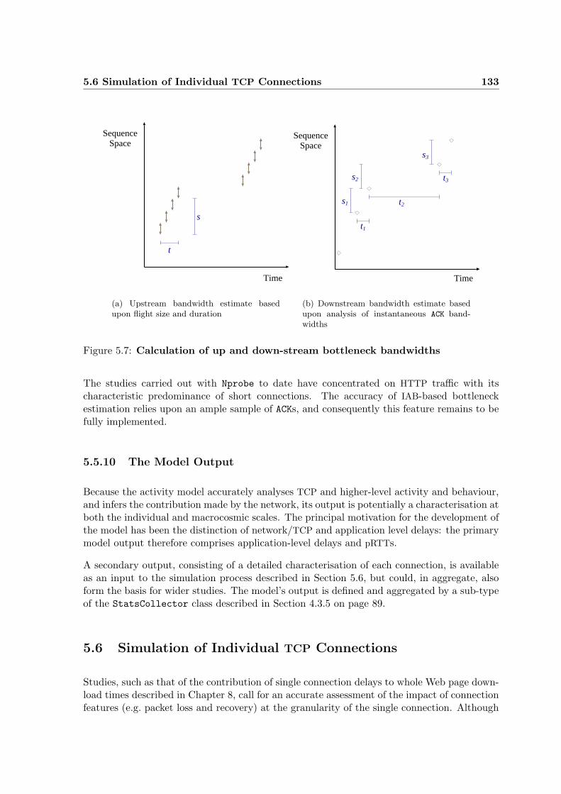
5.6 Simulation of Individual TCP Connections 133

Time

SequenceSpace

t

s

(a) Upstream bandwidth estimate basedupon flight size and duration

Time

s1

t1

SequenceSpace

t2

s2

s3

t3

(b) Downstream bandwidth estimate basedupon analysis of instantaneous ACK band-widths

Figure 5.7: Calculation of up and down-stream bottleneck bandwidths

The studies carried out with Nprobe to date have concentrated on HTTP traffic with itscharacteristic predominance of short connections. The accuracy of IAB-based bottleneckestimation relies upon an ample sample of ACKs, and consequently this feature remains to befully implemented.

5.5.10 The Model Output

Because the activity model accurately analyses TCP and higher-level activity and behaviour,and infers the contribution made by the network, its output is potentially a characterisation atboth the individual and macrocosmic scales. The principal motivation for the development ofthe model has been the distinction of network/TCP and application level delays: the primarymodel output therefore comprises application-level delays and pRTTs.

A secondary output, consisting of a detailed characterisation of each connection, is availableas an input to the simulation process described in Section 5.6, but could, in aggregate, alsoform the basis for wider studies. The model’s output is defined and aggregated by a sub-typeof the StatsCollector class described in Section 4.3.5 on page 89.

5.6 Simulation of Individual TCP Connections

Studies, such as that of the contribution of single connection delays to whole Web page down-load times described in Chapter 8, call for an accurate assessment of the impact of connectionfeatures (e.g. packet loss and recovery) at the granularity of the single connection. Although

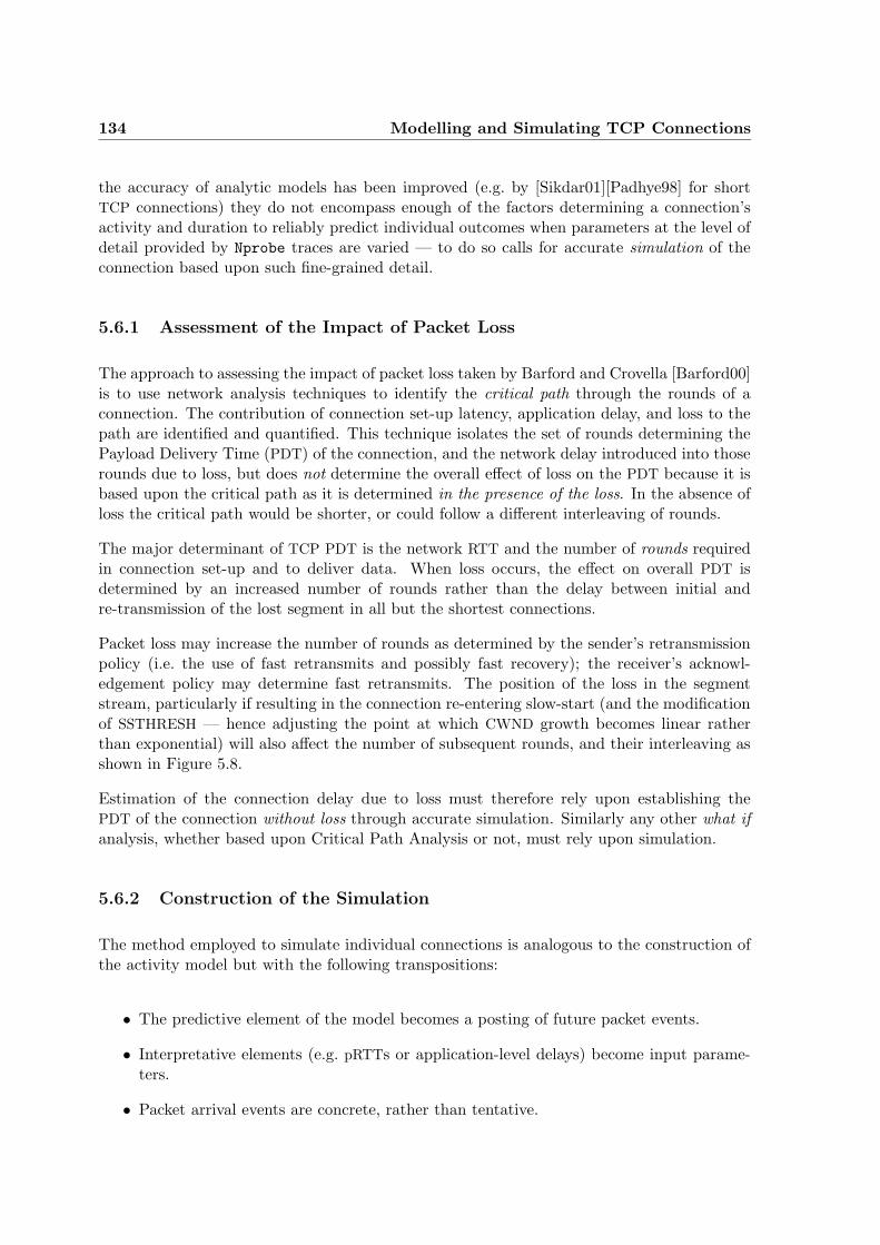
134 Modelling and Simulating TCP Connections

the accuracy of analytic models has been improved (e.g. by [Sikdar01][Padhye98] for shortTCP connections) they do not encompass enough of the factors determining a connection’sactivity and duration to reliably predict individual outcomes when parameters at the level ofdetail provided by Nprobe traces are varied — to do so calls for accurate simulation of theconnection based upon such fine-grained detail.

5.6.1 Assessment of the Impact of Packet Loss

The approach to assessing the impact of packet loss taken by Barford and Crovella [Barford00]is to use network analysis techniques to identify the critical path through the rounds of aconnection. The contribution of connection set-up latency, application delay, and loss to thepath are identified and quantified. This technique isolates the set of rounds determining thePayload Delivery Time (PDT) of the connection, and the network delay introduced into thoserounds due to loss, but does not determine the overall effect of loss on the PDT because it isbased upon the critical path as it is determined in the presence of the loss. In the absence ofloss the critical path would be shorter, or could follow a different interleaving of rounds.

The major determinant of TCP PDT is the network RTT and the number of rounds requiredin connection set-up and to deliver data. When loss occurs, the effect on overall PDT isdetermined by an increased number of rounds rather than the delay between initial andre-transmission of the lost segment in all but the shortest connections.

Packet loss may increase the number of rounds as determined by the sender’s retransmissionpolicy (i.e. the use of fast retransmits and possibly fast recovery); the receiver’s acknowl-edgement policy may determine fast retransmits. The position of the loss in the segmentstream, particularly if resulting in the connection re-entering slow-start (and the modificationof SSTHRESH — hence adjusting the point at which CWND growth becomes linear ratherthan exponential) will also affect the number of subsequent rounds, and their interleaving asshown in Figure 5.8.

Estimation of the connection delay due to loss must therefore rely upon establishing thePDT of the connection without loss through accurate simulation. Similarly any other what ifanalysis, whether based upon Critical Path Analysis or not, must rely upon simulation.

5.6.2 Construction of the Simulation

The method employed to simulate individual connections is analogous to the construction ofthe activity model but with the following transpositions:

• The predictive element of the model becomes a posting of future packet events.

• Interpretative elements (e.g. pRTTs or application-level delays) become input parame-ters.

• Packet arrival events are concrete, rather than tentative.

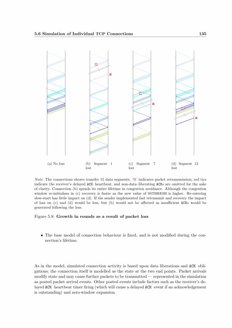
5.6 Simulation of Individual TCP Connections 135

(a) No loss

R

(b) Segment 1lost

R

(c) Segment 7lost

R

(d) Segment 12lost

Note: The connections shown transfer 15 data segments. ‘R’ indicates packet retransmission, red ticsindicate the receiver’s delayed ACK heartbeat, and non-data–liberating ACKs are omitted for the sakeof clarity. Connection (b) spends its entire lifetime in congestion avoidance. Although the congestionwindow re-initialises in (c) recovery is faster as the new value of SSTHRESH is higher. Re-enteringslow-start has little impact on (d). If the sender implemented fast retransmit and recovery the impactof loss on (c) and (d) would be less, but (b) would not be affected as insufficient ACKs would begenerated following the loss.

Figure 5.8: Growth in rounds as a result of packet loss

• The base model of connection behaviour is fixed, and is not modified during the con-nection’s lifetime.

As in the model, simulated connection activity is based upon data liberations and ACK obli-gations; the connection itself is modelled as the state at the two end points. Packet arrivalsmodify state and may cause further packets to be transmitted — represented in the simulationas posted packet arrival events. Other posted events include factors such as the receiver’s de-layed ACK heartbeat timer firing (which will cause a delayed ACK event if an acknowledgementis outstanding) and zero-window expansion.

136 Modelling and Simulating TCP Connections

5.6.2.1 The Simulation Viewpoint

Because the simulation is based upon data collected at Nprobe’s arbitrary monitoring pointbetween hosts, it, in common with the activity model, must recreate connection activityin terms of time delays between packet events as seen at the monitoring point. pRTTs,application-level, and other delays are recombined to create lags between causative packetassociations.

The unmodified simulation will be short by the total time taken for the first SYN segment totravel from the originating host to the monitor, and the final segment to travel from monitorto host. One-half of the relevant pRTT is added in compensation, but will introduce possibleinaccuracy due to path asymmetries.

5.6.2.2 Input to the Simulation

Input to the simulation comprises its basic parameters and the detailed characterisation of theend-point TCP behaviours and application-level activity determined by the activity model:

The base model: determining the connections behaviour and parameters, such as initial con-gestion window size and delayed ACK period and phase. The default base model is oneof generic TCP behaviour based upon RFCs 793, 813, 1122, and 2581, without fast re-transmission and recovery. If the activity model has identified behaviour modifying thegeneric base model then the modified base model is passed to the simulation.

A list of data transfers: incorporating details of request/response delays at client and serverand whether transfers are pipelined.

A list of application-induced features (e.g. window-advertisement adjustments and any zero-window periods, and transmit buffer starvation).

A list of (numbered) segments to be dropped: dropped segments modify the sender’s state,but are not scheduled as arrival events. The simulation models the connection’s re-transmission timers in accordance with RFC 2988 and uses the appropriate values topost retransmission events if fast retransmits are not being used, or are not triggered.

The construction of a simulation with unmodified input parameters should produce a notionalconnection essentially identical to the observed connection upon which it is based. Any of theinput parameters may be adjusted as required to investigate the desired what if scenarios.

5.6.2.3 Underlying Assumptions

The assumptions upon which any simulation is based are reduced as the level of input detailrises. The fine-grained characterisation of behaviour and activity produced by the activitymodel minimises the number of assumptions that must be made when generating the simu-lations described, although with the caveat that simulation may give rise to states with an

5.7 Visualisation 137

outcome not assessed by the informing model. Such cases are minimised because many con-nections are often seen from a specific host, and characterisations of its TCP implementationbehaviour can therefore be aggregate-based; where they do arise accuracy must depend uponappropriate generalisation of default behaviour.

A further, and inescapable, class of assumption is that other factors remain invariant whenone or more input parameters are modified (e.g. changes in data transmission patterns do notaffect the end points’ ability to source or sink data, RTTs, or packet loss). Simulation resultsshould be interpreted in the context of such assumptions.

5.6.3 Simulation Output

The primary simulation output is a list of the packets generated and Payload Delivery Times.Unmodified input parameters are already known and do not require duplication.

When a detailed analysis of simulation output is required, the output can be input to theactivity model and the desired data extracted and aggregated as for observed connections.Care must be taken that any shortcomings in the original model are not perpetuated throughthe simulation and remodelling processes.

5.7 Visualisation

The results of activity-model analysis are incorporated into the TCP connection visualisationintroduced in Section 4.5.2.1 on page 94. Causal relationships are presented, together withthe model’s congestion and flow-control window predictions, pRTT, and application delayestimations.

Support for analysis model and simulation development are provided by the visualisationtool. The Python TCP base model class interacts with the visualisation tool to present amenu allowing the results of activity modelling of each connection with a variety of bases tobe assessed, and features such as the congestion window, and ACK high-water, indicators canbe interactively slid to investigate their fit to observed data. The tool also allows simulationsto be generated and the results modelled and displayed in order to present the effects ofparameter modification.

5.8 Validation of Activity Models and Simulations

The activity model conducts the internal assessment of validity and confidence described inSection 5.5.8.3. The confidence which can be associated with analysis results in general,discussed in Section 4.7, is also pertinent to results obtained from the model and simulations.In the latter case, however, an additional difficulty arises because the results obtained containa notional element which can not be traced back to known data.

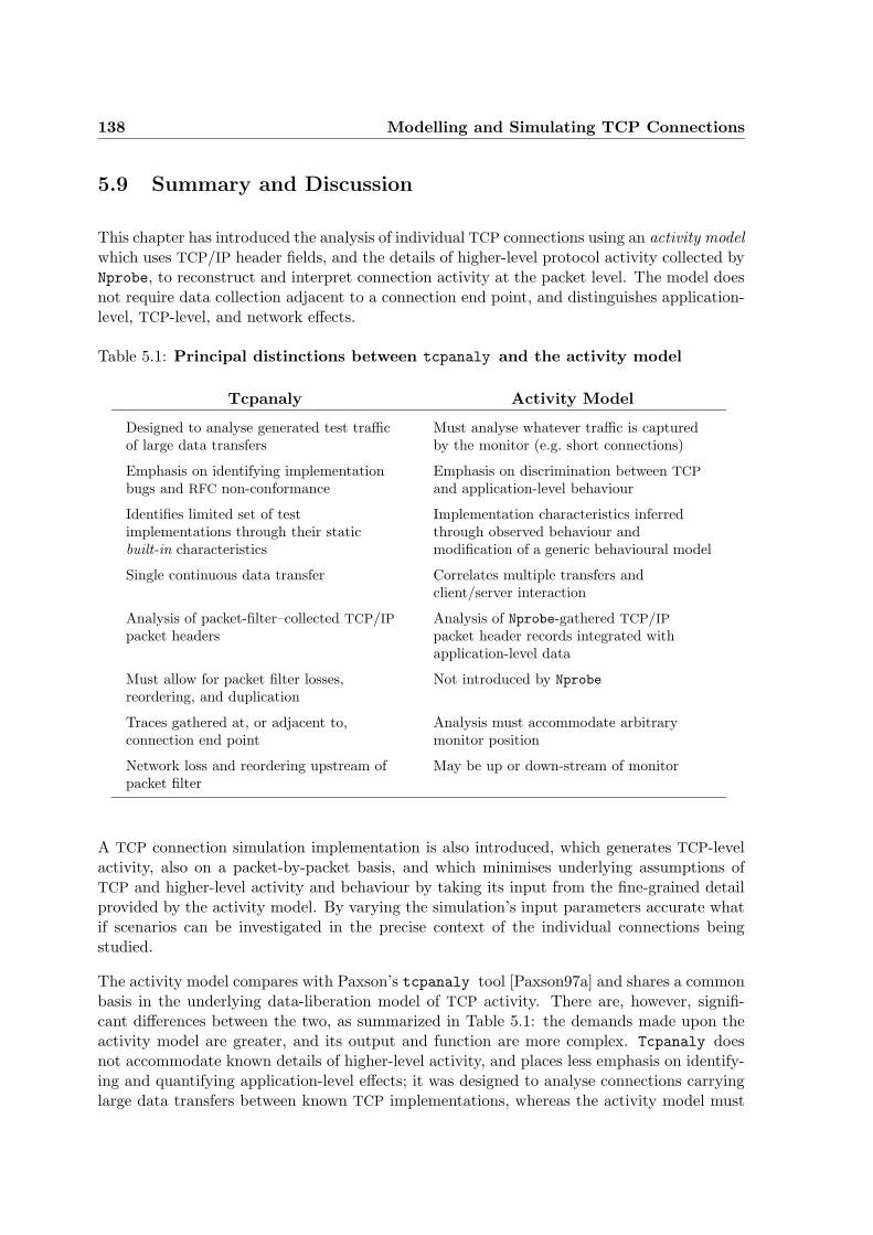
138 Modelling and Simulating TCP Connections

5.9 Summary and Discussion

This chapter has introduced the analysis of individual TCP connections using an activity modelwhich uses TCP/IP header fields, and the details of higher-level protocol activity collected byNprobe, to reconstruct and interpret connection activity at the packet level. The model doesnot require data collection adjacent to a connection end point, and distinguishes application-level, TCP-level, and network effects.

Table 5.1: Principal distinctions between tcpanaly and the activity model

Tcpanaly Activity Model

Designed to analyse generated test trafficof large data transfers

Must analyse whatever traffic is capturedby the monitor (e.g. short connections)

Emphasis on identifying implementationbugs and RFC non-conformance

Emphasis on discrimination between TCP

and application-level behaviour

Identifies limited set of testimplementations through their staticbuilt-in characteristics

Implementation characteristics inferredthrough observed behaviour andmodification of a generic behavioural model

Single continuous data transfer Correlates multiple transfers andclient/server interaction

Analysis of packet-filter–collected TCP/IP

packet headersAnalysis of Nprobe-gathered TCP/IP

packet header records integrated withapplication-level data

Must allow for packet filter losses,reordering, and duplication

Not introduced by Nprobe

Traces gathered at, or adjacent to,connection end point

Analysis must accommodate arbitrarymonitor position

Network loss and reordering upstream ofpacket filter

May be up or down-stream of monitor

A TCP connection simulation implementation is also introduced, which generates TCP-levelactivity, also on a packet-by-packet basis, and which minimises underlying assumptions ofTCP and higher-level activity and behaviour by taking its input from the fine-grained detailprovided by the activity model. By varying the simulation’s input parameters accurate whatif scenarios can be investigated in the precise context of the individual connections beingstudied.

The activity model compares with Paxson’s tcpanaly tool [Paxson97a] and shares a commonbasis in the underlying data-liberation model of TCP activity. There are, however, signifi-cant differences between the two, as summarized in Table 5.1: the demands made upon theactivity model are greater, and its output and function are more complex. Tcpanaly doesnot accommodate known details of higher-level activity, and places less emphasis on identify-ing and quantifying application-level effects; it was designed to analyse connections carryinglarge data transfers between known TCP implementations, whereas the activity model must

5.9 Summary and Discussion 139

deal with connections of arbitrary length, and between whichever implementations are en-countered. Both recognise that analysis of connection activity can not be based upon a fullygeneric model of TCP behaviour: the tcpanaly solution is to equip the tool with the knowncharacteristics of the test implementations used; the activity model uses a generic base modelwhich is modified to reflect the implementation-specific behaviour observed.

The activity model is not intended to uniquely identify the end-point host TCP implementa-tions, the majority case of short connections without packet loss provides insufficient data,but to accurately interpret the observed activity sufficiently to discriminate the contribu-tions of network, TCP, and higher-level protocols. Implementations are therefore categorisedby behaviour rather than marque, and the reservation arises that there may, therefore, beno cross check of the model’s interpretation against TCP implementation. It is, however,possible to confirm that the model consistently identifies the same model of behaviour onall connections from the same host with the same level of activity complexity — a correlationwhich can be investigated with base-model caching disabled. A further indication is provided,when analysing TCP/HTTP connections, by examining the HTTP User-Agent and Server

header fields. Although these fields only yield a low level of implementation detail, a goodcorrelation between operating system/version and the model’s interpretation across all hostsis established.

Development of the activity model is continuing to ensure robust interpretation of increasinglycomplex connection activity, but in its present state effectively all connections without lossare correctly interpreted, and better than 90 per cent of those with loss. Chapter 6 describesa series of tests designed to assess the model’s ability to discriminate and quantify Web serverlatency, concluding with a study of latency at a popular server. Chapter 8 describes theuse of the activity model and simulation to investigate delay in Web page downloads. Thetechnique provides a new and valuable facility to distinguish between the factors contributingto connection and application performance.

Chapter 6

Non-Intrusive Estimation of WebServer Delays Using Nprobe

The study described in this chapter was undertaken in order to assess the development ofthe activity model described in Chapter 5. It is not a demonstration of the full scope of datacollection, or study complexity that Nprobe was designed to meet.

6.1 Motivation and Experimental Method

The performance of Web servers is a matter of considerable importance to the Internet Com-munity, one metric of interest being response times to the requests received. Whilst thesecan be measured using both existing active and passive techniques, such measurements arelikely to be inaccurate. At the worst TCP connection latency may be included (confirmed bythe WAWM project [Barford99a] to make a major contribution to the time taken by HTTP

transactions); at the best, even when the interval solely between request and response ismeasured, the contribution of server latency and network RTT to the observed delay are notdifferentiated.

Web content is increasingly generated dynamically, and often tailored on-the-fly to the useraccessing the site. This places a considerable burden on the server through the execution ofserver-side programs accessed through mechanisms such as the Common Gateway Interface(CGI), and the use of scripting languages such as DHTML, ASP or PERL. Back-end processinginvolving database accesses is also often involved. Thus, servers may be expected to becomemore vulnerable to high or over-load conditions, and the potential requirement to monitortheir performance and response latencies will become more acute.

A series of Nprobe traces of Web object downloads were analysed using the activity model todiscriminate and quantify server latencies and partial Round Trip Times (pRTTs). Althoughthe study emphasises initial server delays (i.e. from complete receipt of a request until the firstsegment of the response is dispatched), the analysis could equally well be used to identify allcomponents of delay whether contributed by the server, browser, network, or TCP behaviour.

142 Non-Intrusive Estimation of Web Server Delays Using Nprobe

Three sets of experimental tests, based upon artificially generated traffic and described inSection 6.3, were conducted to assess the techniques used. In the study described in Section 6.4on page 154 the techniques were then applied to real-world traffic. The target servers in theinitial tests were set up specifically for the purpose, and were free of other, unknown, loads.

6.2 Use of the Activity Model

Sections 5.5.2 and 5.5.3 on pages 117 and 120 of Chapter 5 describe causal relationships be-tween packets observed by the monitor, and how network, TCP, and application-level timecomponents can be differentiated by the activity model. Section 5.5.3.2, in particular, de-scribes how application-level delays are calculated.

In the experiments described in this chapter the calculation of server latency is based uponthe measured delay between observing the final request packet from the client, and the firstpacket of the matching response from the server. This delay forms the lag from which apRTT , interpolated from those established by non-delayed packets (i.e. those triggering animmediate return transmission by the receiver), can be deducted to calculate the componentcontributed by the application level. The activity model must thus correctly identify theappropriate causative associations in activity at both TCP and application levels.

In the case of the tests conducted using pipelined persistent connections described in Sec-tion 6.3.3, the model was required to establish valid causation in a more complex contextwhere transaction boundaries are less evident, and where the timing of responses might bedetermined by activity at either the TCP or application levels, queueing behind precedingresponses, or packet serialisation delays.

All connections carrying the transactions of the observed server load were presented to theactivity model, which was used to identify instances of server latency and to differentiatethe associated pRTTs. The model output, in this instance, comprised a list of latencies andpRTTs indexed by time. The latencies calculated for pipelined transactions were furtherdistinguished by type as explained in Section 6.3.3.

6.3 Assessment Using an Artificially Loaded Server

The first set of tests, described in Section 6.3.1, observed traffic between a server and loadingclients which were all connected to the same Cisco LX3500 100 Mbps Ethernet switch. Thenetwork RTTs were therefore considerably smaller than the expected server delays. In thesecond set of tests (Section 6.3.2) a more remote server, situated in the Computer ScienceDepartment of the University of Glasgow, was used and loaded by the same set of machinesin the Cambridge Laboratory. This yielded an observation of transactions with RTTs andserver delays of approximately the same order of magnitude.

Both servers ran the Apache 1.3.9 Web Server over Linux: on an Intel Pentium III 500MHzbased PC in Cambridge and, in Glasgow, an Intel Pentium 200MHz based PC. The objects

6.3 Assessment Using an Artificially Loaded Server 143

requested consisted of static objects — files of random bytes of varying sizes.

Two patterns of artificially generated load were produced:

• One or more background loads generated by Httperf [Mosberger98] consisting of re-peated single requests at specified rates.

• An observed load generated by Httperf comprising repetitions of a single GET requestfor a 1024 byte document followed, on completion, by a series of ten concurrent requestsfor a 512 byte object. The estimated server delays are based upon observation of thisload as the background load was varied with time.

The set of objects forming the background and observed loads was chosen to ensure that allrequests could be satisfied from the server’s cache, hence avoiding random delays due to diskreads. The cache was primed by a set of requests made before each test commenced.

A low priority idle loop process was run on each server for the duration of the tests, whichsimply recorded the number of times it was able to increment a counter during each 100 msperiod — hence providing an indication of spare CPU capacity at any time during the experi-ment. The process was launched and terminated via CGI requests, enabling its operation andresults to be synchronised with those derived by monitoring the network.

In each test the idle loop was first launched, followed by the observed load at time 10 s.Background loads were progressively added, and later removed, at further 10 s intervals.The client and server machines, load characteristics, load generating program, etc. for eachtest were defined by a simple configuration file providing the input to a script running on amaster machine which controlled the various components of the experiment. The master wasresponsible for starting slave scripts on each of the loading clients, instructing them of theload to be generated and issuing commands to start and stop load generation at the timesdefined in the configuration file.

In the three experiments described in this section it was expected that server latency wouldrise with load, that the pRTT between monitor and server might rise as network throughputincreased, and (trivially) that the number of free CPU cycles would fall. The results are shownin Figures 6.1 – 6.4: in each, Sub-figure (a) shows the total number of objects delivered persecond and serves to confirm that the specified loads were actually presented to the server;Sub-figures (b) and (c) present the server latencies and pRTTs discriminated and calculatedby the activity model; and (d) demonstrates the correlation between server delay and CPU

usage.

In each Sub-figure (d) server delays averaged over successive correlation intervals are plottedagainst an average CPU load factor for the same interval. The tests were not intended tosaturate the server, and even at the highest background loading spare cycles are available.

The CPU load factor φ (0 ≤ φ ≤ 1.0) expressed as the ratio of CPU cycles absorbed byservicing the current load to those available at zero load is calculated as:

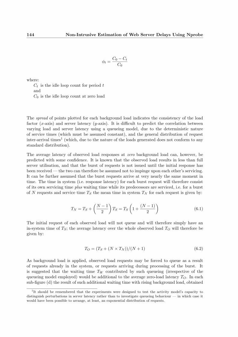
144 Non-Intrusive Estimation of Web Server Delays Using Nprobe

φt =C0 − Ct

C0

where:Ct is the idle loop count for period tandC0 is the idle loop count at zero load

The spread of points plotted for each background load indicates the consistency of the loadfactor (x-axis) and server latency (y-axis). It is difficult to predict the correlation betweenvarying load and server latency using a queueing model, due to the deterministic natureof service times (which must be assumed constant), and the general distribution of requestinter-arrival times1 (which, due to the nature of the loads generated does not conform to anystandard distribution).

The average latency of observed load responses at zero background load can, however, bepredicted with some confidence. It is known that the observed load results in less than fullserver utilisation, and that the burst of requests is not issued until the initial response hasbeen received — the two can therefore be assumed not to impinge upon each other’s servicing.It can be further assumed that the burst requests arrive at very nearly the same moment intime. The time in system (i.e. response latency) for each burst request will therefore consistof its own servicing time plus waiting time while its predecessors are serviced, i.e. for a burstof N requests and service time TS the mean time in system TN for each request is given by:

TN = TS +

(

N − 1

2

)

TS = TS

(

1 +(N − 1)

2

)

(6.1)

The initial request of each observed load will not queue and will therefore simply have anin-system time of TS ; the average latency over the whole observed load TO will therefore begiven by:

TO = (TS + (N × TN ))/(N + 1) (6.2)

As background load is applied, observed load requests may be forced to queue as a resultof requests already in the system, or requests arriving during processing of the burst. Itis suggested that the waiting time TW contributed by such queueing (irrespective of thequeueing model employed) would be additional to the average zero-load latency TO. In eachsub-figure (d) the result of such additional waiting time with rising background load, obtained

1It should be remembered that the experiments were designed to test the activity model’s capacity todistinguish perturbations in server latency rather than to investigate queueing behaviour — in which case itwould have been possible to arrange, at least, an exponential distribution of requests.

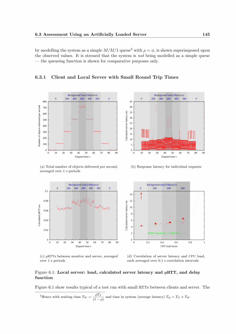
6.3 Assessment Using an Artificially Loaded Server 145

by modelling the system as a simple M/M/1 queue2 with ρ = φ, is shown superimposed uponthe observed values. It is stressed that the system is not being modelled as a simple queue— the queueing function is shown for comparative purposes only.

6.3.1 Client and Local Server with Small Round Trip Times

Background load (Objects/s)

0

100

200

300

400

500

600

700

800

0 10 20 30 40 50 60 70 80 90

Num

ber

of o

bjec

ts d

eliv

ered

per

sec

ond

Elapsed time s

0 200 400 600 400 200 0

(a) Total number of objects delivered per second,averaged over 1 s periods

Background load (Objects/s)

0

5

10

15

20

25

30

35

40

45

0 10 20 30 40 50 60 70 80 90

Cal

cula

ted

serv

er la

tenc

y m

s

Elapsed time s

0 200 400 600 400 200 0

(b) Response latency for individual requests

Background load (Objects/s)

0

0.02

0.04

0.06

0.08

0.1

0 10 20 30 40 50 60 70 80 90

Cal

cula

ted

pRT

T m

s

Elapsed time s

0 200 400 600 400 200 0

(c) pRTTs between monitor and server, averagedover 1 s periods

6004002000

0

2

4

6

8

10

12

14

0 0.2 0.4 0.6 0.8 1

Cal

cula

ted

serv

er la

tenc

y m

s

CPU load factor

Background load (Objects/s)

M/M/1 Queue (TS = 0.836 ms)

(d) Correlation of server latency and CPU load,each averaged over 0.1 s correlation intervals

Figure 6.1: Local server: load, calculated server latency and pRTT, and delayfunction

Figure 6.1 show results typical of a test run with small RTTs between clients and server. The

2Hence with waiting time TW =ρTS

(1 − ρ)and time in system (average latency) TQ = TO + TW

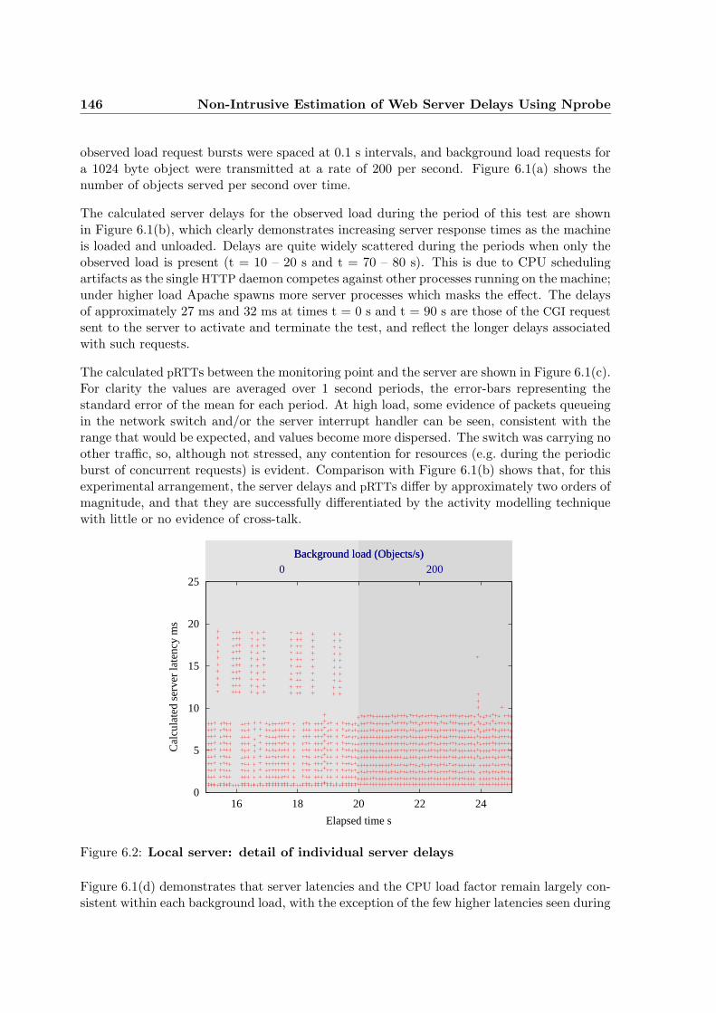
146 Non-Intrusive Estimation of Web Server Delays Using Nprobe

observed load request bursts were spaced at 0.1 s intervals, and background load requests fora 1024 byte object were transmitted at a rate of 200 per second. Figure 6.1(a) shows thenumber of objects served per second over time.

The calculated server delays for the observed load during the period of this test are shownin Figure 6.1(b), which clearly demonstrates increasing server response times as the machineis loaded and unloaded. Delays are quite widely scattered during the periods when only theobserved load is present (t = 10 – 20 s and t = 70 – 80 s). This is due to CPU schedulingartifacts as the single HTTP daemon competes against other processes running on the machine;under higher load Apache spawns more server processes which masks the effect. The delaysof approximately 27 ms and 32 ms at times t = 0 s and t = 90 s are those of the CGI requestsent to the server to activate and terminate the test, and reflect the longer delays associatedwith such requests.

The calculated pRTTs between the monitoring point and the server are shown in Figure 6.1(c).For clarity the values are averaged over 1 second periods, the error-bars representing thestandard error of the mean for each period. At high load, some evidence of packets queueingin the network switch and/or the server interrupt handler can be seen, consistent with therange that would be expected, and values become more dispersed. The switch was carrying noother traffic, so, although not stressed, any contention for resources (e.g. during the periodicburst of concurrent requests) is evident. Comparison with Figure 6.1(b) shows that, for thisexperimental arrangement, the server delays and pRTTs differ by approximately two orders ofmagnitude, and that they are successfully differentiated by the activity modelling techniquewith little or no evidence of cross-talk.

Background load (Objects/s)Background load (Objects/s)0 200

0

5

10

15

20

25

16 18 20 22 24

Cal

cula

ted

serv

er la

tenc

y m

s

Elapsed time s

Figure 6.2: Local server: detail of individual server delays

Figure 6.1(d) demonstrates that server latencies and the CPU load factor remain largely con-sistent within each background load, with the exception of the few higher latencies seen during

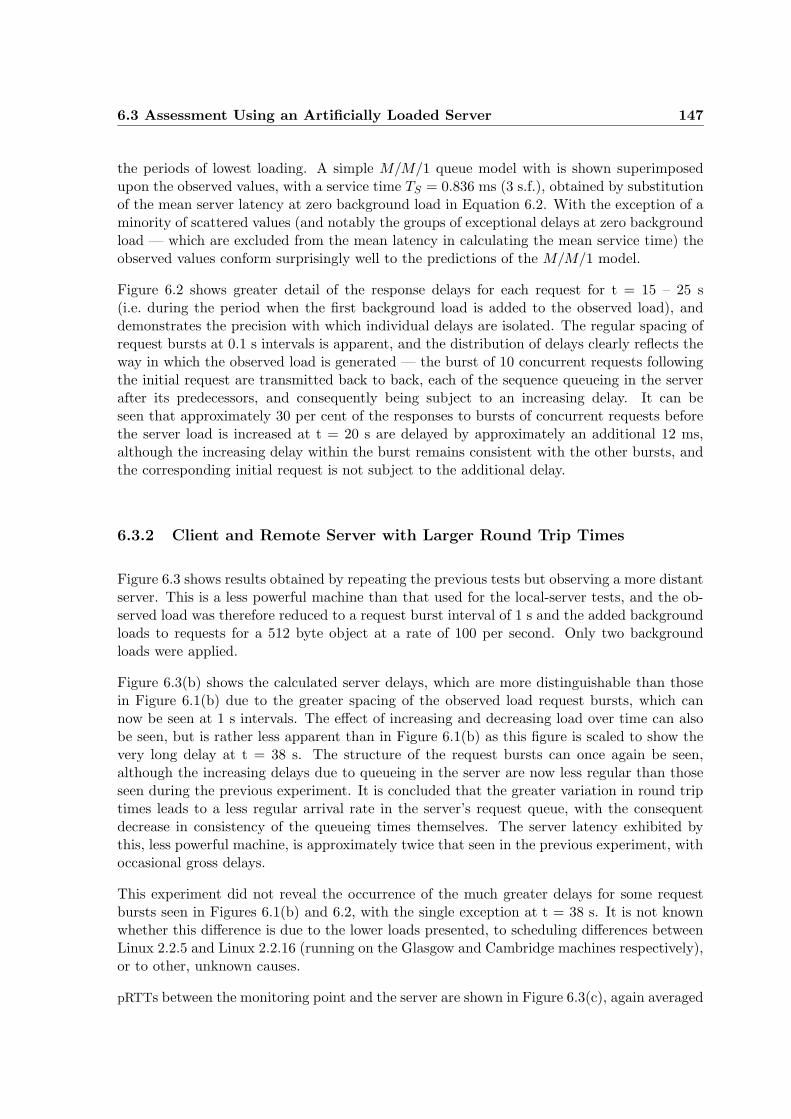
6.3 Assessment Using an Artificially Loaded Server 147

the periods of lowest loading. A simple M/M/1 queue model with is shown superimposedupon the observed values, with a service time TS = 0.836 ms (3 s.f.), obtained by substitutionof the mean server latency at zero background load in Equation 6.2. With the exception of aminority of scattered values (and notably the groups of exceptional delays at zero backgroundload — which are excluded from the mean latency in calculating the mean service time) theobserved values conform surprisingly well to the predictions of the M/M/1 model.

Figure 6.2 shows greater detail of the response delays for each request for t = 15 – 25 s(i.e. during the period when the first background load is added to the observed load), anddemonstrates the precision with which individual delays are isolated. The regular spacing ofrequest bursts at 0.1 s intervals is apparent, and the distribution of delays clearly reflects theway in which the observed load is generated — the burst of 10 concurrent requests followingthe initial request are transmitted back to back, each of the sequence queueing in the serverafter its predecessors, and consequently being subject to an increasing delay. It can beseen that approximately 30 per cent of the responses to bursts of concurrent requests beforethe server load is increased at t = 20 s are delayed by approximately an additional 12 ms,although the increasing delay within the burst remains consistent with the other bursts, andthe corresponding initial request is not subject to the additional delay.

6.3.2 Client and Remote Server with Larger Round Trip Times

Figure 6.3 shows results obtained by repeating the previous tests but observing a more distantserver. This is a less powerful machine than that used for the local-server tests, and the ob-served load was therefore reduced to a request burst interval of 1 s and the added backgroundloads to requests for a 512 byte object at a rate of 100 per second. Only two backgroundloads were applied.

Figure 6.3(b) shows the calculated server delays, which are more distinguishable than thosein Figure 6.1(b) due to the greater spacing of the observed load request bursts, which cannow be seen at 1 s intervals. The effect of increasing and decreasing load over time can alsobe seen, but is rather less apparent than in Figure 6.1(b) as this figure is scaled to show thevery long delay at t = 38 s. The structure of the request bursts can once again be seen,although the increasing delays due to queueing in the server are now less regular than thoseseen during the previous experiment. It is concluded that the greater variation in round triptimes leads to a less regular arrival rate in the server’s request queue, with the consequentdecrease in consistency of the queueing times themselves. The server latency exhibited bythis, less powerful machine, is approximately twice that seen in the previous experiment, withoccasional gross delays.

This experiment did not reveal the occurrence of the much greater delays for some requestbursts seen in Figures 6.1(b) and 6.2, with the single exception at t = 38 s. It is not knownwhether this difference is due to the lower loads presented, to scheduling differences betweenLinux 2.2.5 and Linux 2.2.16 (running on the Glasgow and Cambridge machines respectively),or to other, unknown causes.

pRTTs between the monitoring point and the server are shown in Figure 6.3(c), again averaged

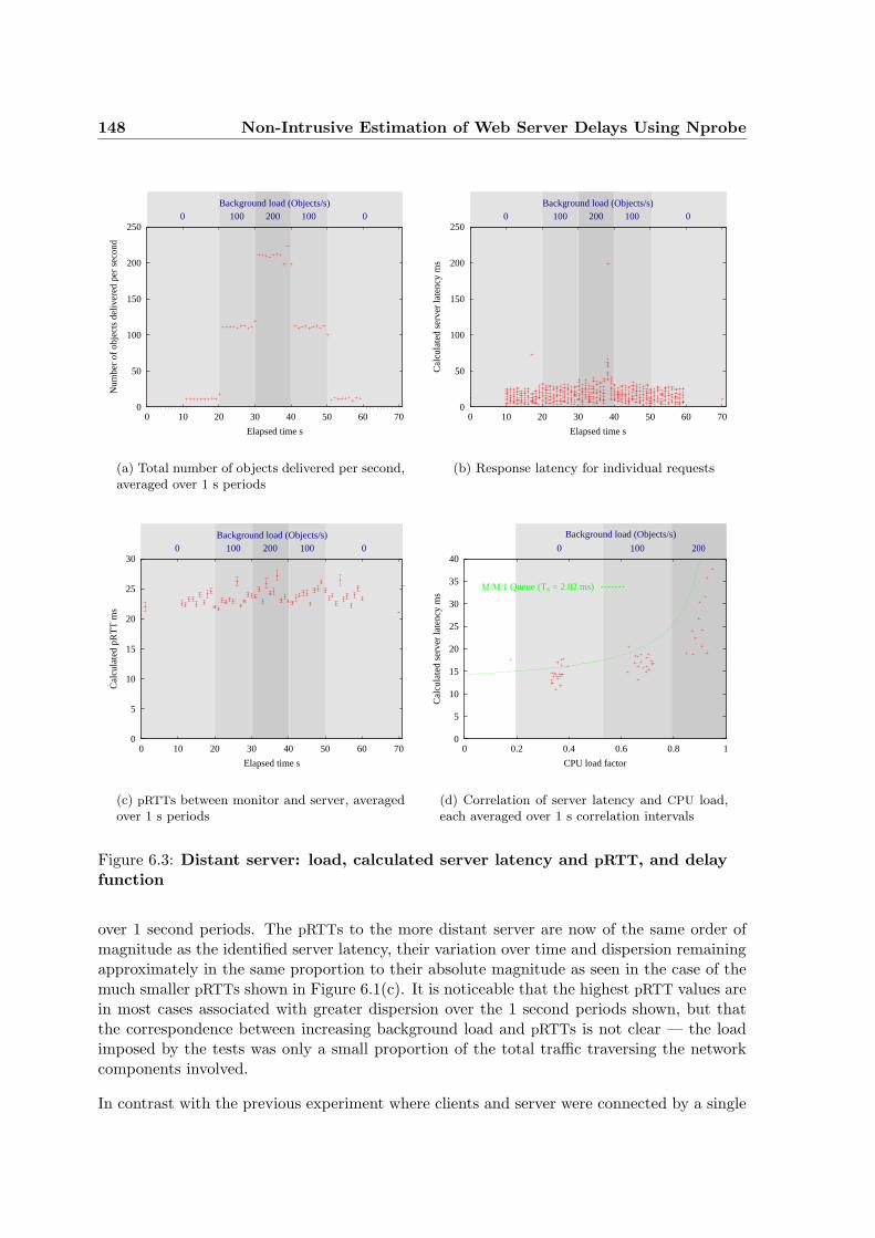
148 Non-Intrusive Estimation of Web Server Delays Using Nprobe

Background load (Objects/s)

0

50

100

150

200

250

0 10 20 30 40 50 60 70

Num

ber

of o

bjec

ts d

eliv

ered

per

sec

ond

Elapsed time s

0 100 200 100 0

(a) Total number of objects delivered per second,averaged over 1 s periods

Background load (Objects/s)0 100 200 100 0

0

50

100

150

200

250

0 10 20 30 40 50 60 70

Cal

cula

ted

serv

er la

tenc

y m

sElapsed time s

(b) Response latency for individual requests

Background load (Objects/s)0 100 200 100 0

0

5

10

15

20

25

30

0 10 20 30 40 50 60 70

Cal

cula

ted

pRT

T m

s

Elapsed time s

(c) pRTTs between monitor and server, averagedover 1 s periods

1000 200

0

5

10

15

20

25

30

35

40

0 0.2 0.4 0.6 0.8 1

Cal

cula

ted

serv

er la

tenc

y m

s

CPU load factor

Background load (Objects/s)

M/M/1 Queue (TS = 2.82 ms)

(d) Correlation of server latency and CPU load,each averaged over 1 s correlation intervals

Figure 6.3: Distant server: load, calculated server latency and pRTT, and delayfunction

over 1 second periods. The pRTTs to the more distant server are now of the same order ofmagnitude as the identified server latency, their variation over time and dispersion remainingapproximately in the same proportion to their absolute magnitude as seen in the case of themuch smaller pRTTs shown in Figure 6.1(c). It is noticeable that the highest pRTT values arein most cases associated with greater dispersion over the 1 second periods shown, but thatthe correspondence between increasing background load and pRTTs is not clear — the loadimposed by the tests was only a small proportion of the total traffic traversing the networkcomponents involved.

In contrast with the previous experiment where clients and server were connected by a single

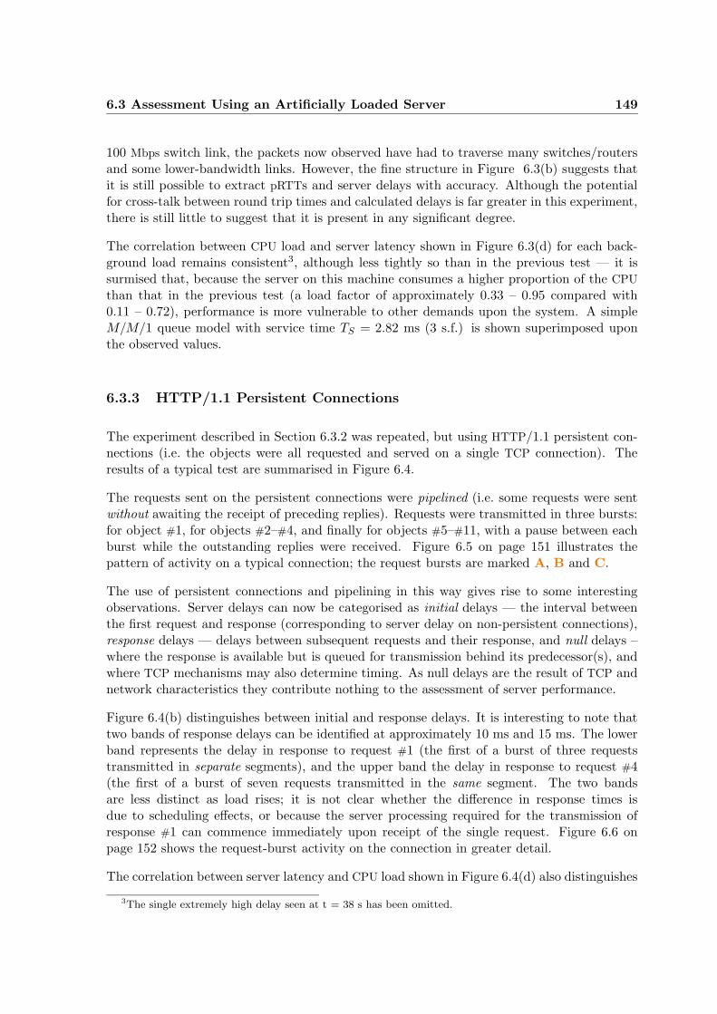
6.3 Assessment Using an Artificially Loaded Server 149

100 Mbps switch link, the packets now observed have had to traverse many switches/routersand some lower-bandwidth links. However, the fine structure in Figure 6.3(b) suggests thatit is still possible to extract pRTTs and server delays with accuracy. Although the potentialfor cross-talk between round trip times and calculated delays is far greater in this experiment,there is still little to suggest that it is present in any significant degree.

The correlation between CPU load and server latency shown in Figure 6.3(d) for each back-ground load remains consistent3, although less tightly so than in the previous test — it issurmised that, because the server on this machine consumes a higher proportion of the CPU

than that in the previous test (a load factor of approximately 0.33 – 0.95 compared with0.11 – 0.72), performance is more vulnerable to other demands upon the system. A simpleM/M/1 queue model with service time TS = 2.82 ms (3 s.f.) is shown superimposed uponthe observed values.

6.3.3 HTTP/1.1 Persistent Connections

The experiment described in Section 6.3.2 was repeated, but using HTTP/1.1 persistent con-nections (i.e. the objects were all requested and served on a single TCP connection). Theresults of a typical test are summarised in Figure 6.4.

The requests sent on the persistent connections were pipelined (i.e. some requests were sentwithout awaiting the receipt of preceding replies). Requests were transmitted in three bursts:for object #1, for objects #2–#4, and finally for objects #5–#11, with a pause between eachburst while the outstanding replies were received. Figure 6.5 on page 151 illustrates thepattern of activity on a typical connection; the request bursts are marked A, B and C.

The use of persistent connections and pipelining in this way gives rise to some interestingobservations. Server delays can now be categorised as initial delays — the interval betweenthe first request and response (corresponding to server delay on non-persistent connections),response delays — delays between subsequent requests and their response, and null delays –where the response is available but is queued for transmission behind its predecessor(s), andwhere TCP mechanisms may also determine timing. As null delays are the result of TCP andnetwork characteristics they contribute nothing to the assessment of server performance.

Figure 6.4(b) distinguishes between initial and response delays. It is interesting to note thattwo bands of response delays can be identified at approximately 10 ms and 15 ms. The lowerband represents the delay in response to request #1 (the first of a burst of three requeststransmitted in separate segments), and the upper band the delay in response to request #4(the first of a burst of seven requests transmitted in the same segment. The two bandsare less distinct as load rises; it is not clear whether the difference in response times isdue to scheduling effects, or because the server processing required for the transmission ofresponse #1 can commence immediately upon receipt of the single request. Figure 6.6 onpage 152 shows the request-burst activity on the connection in greater detail.

The correlation between server latency and CPU load shown in Figure 6.4(d) also distinguishes

3The single extremely high delay seen at t = 38 s has been omitted.

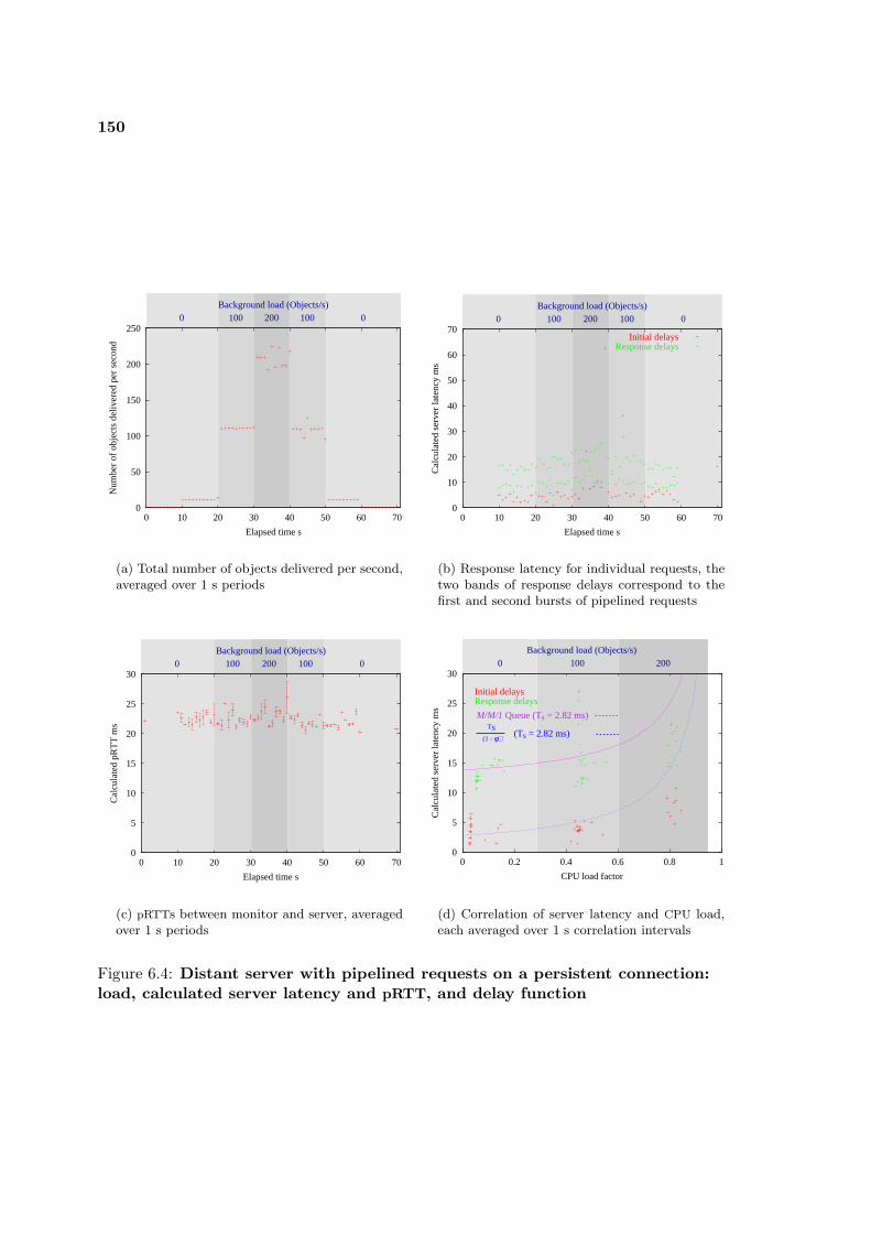
150

Background load (Objects/s)0 100 200 100 0

0

50

100

150

200

250

0 10 20 30 40 50 60 70

Num

ber

of o

bjec

ts d

eliv

ered

per

sec

ond

Elapsed time s

(a) Total number of objects delivered per second,averaged over 1 s periods

Background load (Objects/s)

0

10

20

30

40

50

60

70

0 10 20 30 40 50 60 70

Cal

cula

ted

serv

er la

tenc

y m

s

Elapsed time s

Initial delaysResponse delays

0 100 200 100 0

(b) Response latency for individual requests, thetwo bands of response delays correspond to thefirst and second bursts of pipelined requests

Background load (Objects/s)0 100 200 100 0

0

5

10

15

20

25

30

0 10 20 30 40 50 60 70

Cal

cula

ted

pRT

T m

s

Elapsed time s

(c) pRTTs between monitor and server, averagedover 1 s periods

100 2000

0

5

10

15

20

25

30

0 0.2 0.4 0.6 0.8 1

Cal

cula

ted

serv

er la

tenc

y m

s

CPU load factor

Initial delaysResponse delays

Background load (Objects/s)

M/M/1 Queue (TS = 2.82 ms) TS

(1 - φ) (TS = 2.82 ms)

(d) Correlation of server latency and CPU load,each averaged over 1 s correlation intervals

Figure 6.4: Distant server with pipelined requests on a persistent connection:load, calculated server latency and pRTT, and delay function

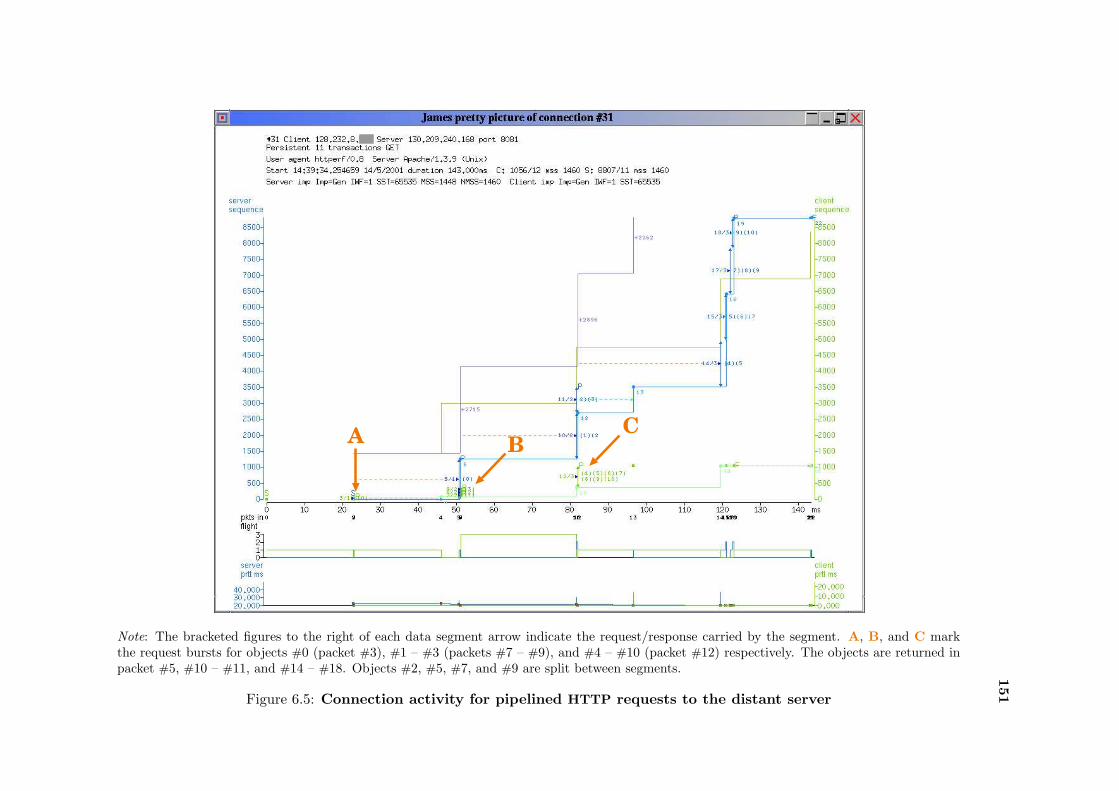
151

A CB

Note: The bracketed figures to the right of each data segment arrow indicate the request/response carried by the segment. A, B, and C markthe request bursts for objects #0 (packet #3), #1 – #3 (packets #7 – #9), and #4 – #10 (packet #12) respectively. The objects are returned inpacket #5, #10 – #11, and #14 – #18. Objects #2, #5, #7, and #9 are split between segments.

Figure 6.5: Connection activity for pipelined HTTP requests to the distant server

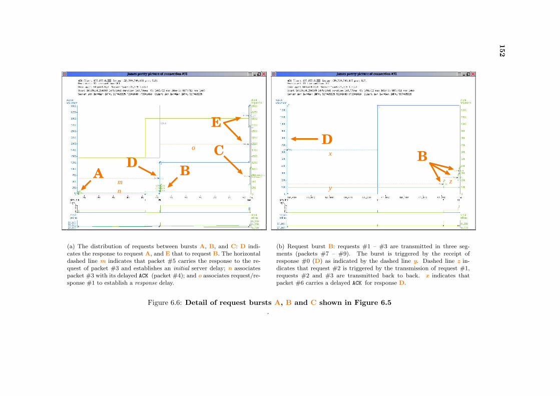
152

CD

E

A Bmn

o

(a) The distribution of requests between bursts A, B, and C: D indi-cates the response to request A, and E that to request B. The horizontaldashed line m indicates that packet #5 carries the response to the re-quest of packet #3 and establishes an initial server delay; n associatespacket #3 with its delayed ACK (packet #4); and o associates request/re-sponse #1 to establish a response delay.

DBx

yz

(b) Request burst B: requests #1 – #3 are transmitted in three seg-ments (packets #7 – #9). The burst is triggered by the receipt ofresponse #0 (D) as indicated by the dashed line y. Dashed line z in-dicates that request #2 is triggered by the transmission of request #1,requests #2 and #3 are transmitted back to back. x indicates thatpacket #6 carries a delayed ACK for response D.

Figure 6.6: Detail of request bursts A, B and C shown in Figure 6.5.

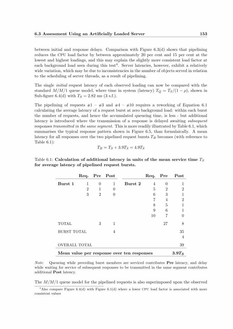
6.3 Assessment Using an Artificially Loaded Server 153

between initial and response delays. Comparison with Figure 6.3(d) shows that pipeliningreduces the CPU load factor by between approximately 20 per cent and 15 per cent at thelowest and highest loadings, and this may explain the slightly more consistent load factor ateach background load seen during this test4. Server latencies, however, exhibit a relativelywide variation, which may be due to inconsistencies in the number of objects served in relationto the scheduling of server threads, as a result of pipelining.

The single initial request latency of each observed loading can now be compared with thestandard M/M/1 queue model, where time in system (latency) TQ = TS/(1 − ρ), shown inSub-figure 6.4(d) with TS = 2.82 ms (3 s.f.).

The pipelining of requests #1 – #3 and #4 – #10 requires a reworking of Equation 6.1calculating the average latency of a request burst at zero background load: within each burstthe number of requests, and hence the accumulated queueing time, is less - but additionallatency is introduced where the transmission of a response is delayed awaiting subsequentresponses transmitted in the same segment. This is more readily illustrated by Table 6.1, whichsummarises the typical response pattern shown in Figure 6.5, than formulaically. A meanlatency for all responses over the two pipelined request bursts TB becomes (with reference toTable 6.1):

TB = TS + 3.9TS = 4.9TS

Table 6.1: Calculation of additional latency in units of the mean service time TS

for average latency of pipelined request bursts.

Req. Pre Post Req. Pre Post

Burst 1 1 0 1 Burst 2 4 0 12 1 0 5 2 23 2 0 6 3 1

7 4 28 5 19 6 1

10 7 0

TOTAL 3 1 27 8

BURST TOTAL 4 354

OVERALL TOTAL 39

Mean value per response over ten responses 3.9TS

Note: Queueing while preceding burst members are serviced contributes Pre latency, and delaywhile waiting for service of subsequent responses to be transmitted in the same segment contributesadditional Post latency.

The M/M/1 queue model for the pipelined requests is also superimposed upon the observed

4Also compare Figure 6.4(d) with Figure 6.1(d) where a lower CPU load factor is associated with moreconsistent values

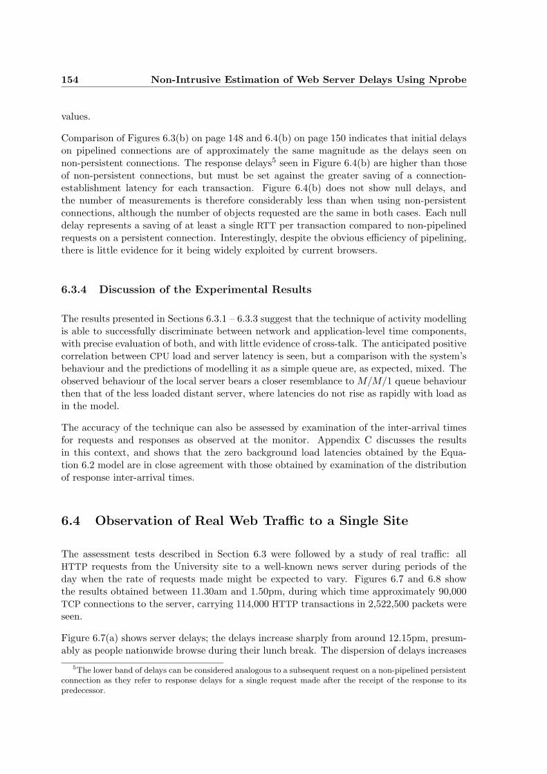
154 Non-Intrusive Estimation of Web Server Delays Using Nprobe

values.

Comparison of Figures 6.3(b) on page 148 and 6.4(b) on page 150 indicates that initial delayson pipelined connections are of approximately the same magnitude as the delays seen onnon-persistent connections. The response delays5 seen in Figure 6.4(b) are higher than thoseof non-persistent connections, but must be set against the greater saving of a connection-establishment latency for each transaction. Figure 6.4(b) does not show null delays, andthe number of measurements is therefore considerably less than when using non-persistentconnections, although the number of objects requested are the same in both cases. Each nulldelay represents a saving of at least a single RTT per transaction compared to non-pipelinedrequests on a persistent connection. Interestingly, despite the obvious efficiency of pipelining,there is little evidence for it being widely exploited by current browsers.

6.3.4 Discussion of the Experimental Results

The results presented in Sections 6.3.1 – 6.3.3 suggest that the technique of activity modellingis able to successfully discriminate between network and application-level time components,with precise evaluation of both, and with little evidence of cross-talk. The anticipated positivecorrelation between CPU load and server latency is seen, but a comparison with the system’sbehaviour and the predictions of modelling it as a simple queue are, as expected, mixed. Theobserved behaviour of the local server bears a closer resemblance to M/M/1 queue behaviourthen that of the less loaded distant server, where latencies do not rise as rapidly with load asin the model.

The accuracy of the technique can also be assessed by examination of the inter-arrival timesfor requests and responses as observed at the monitor. Appendix C discusses the resultsin this context, and shows that the zero background load latencies obtained by the Equa-tion 6.2 model are in close agreement with those obtained by examination of the distributionof response inter-arrival times.

6.4 Observation of Real Web Traffic to a Single Site

The assessment tests described in Section 6.3 were followed by a study of real traffic: allHTTP requests from the University site to a well-known news server during periods of theday when the rate of requests made might be expected to vary. Figures 6.7 and 6.8 showthe results obtained between 11.30am and 1.50pm, during which time approximately 90,000TCP connections to the server, carrying 114,000 HTTP transactions in 2,522,500 packets wereseen.

Figure 6.7(a) shows server delays; the delays increase sharply from around 12.15pm, presum-ably as people nationwide browse during their lunch break. The dispersion of delays increases

5The lower band of delays can be considered analogous to a subsequent request on a non-pipelined persistentconnection as they refer to response delays for a single request made after the receipt of the response to itspredecessor.

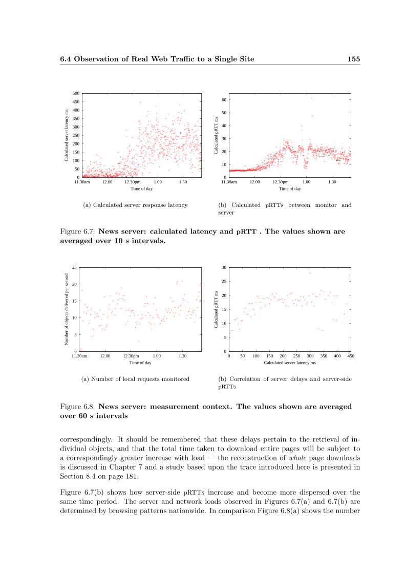
6.4 Observation of Real Web Traffic to a Single Site 155

0

50

100

150

200

250

300

350

400

450

500

11.30am 12.00 12.30pm 1.00 1.30

Cal

cula

ted

serv

er la

tenc

y m

s

Time of day

(a) Calculated server response latency

0

10

20

30

40

50

60

11.30am 12.00 12.30pm 1.00 1.30

Cal

cula

ted

pRT

T m

s

Time of day

(b) Calculated pRTTs between monitor andserver

Figure 6.7: News server: calculated latency and pRTT . The values shown areaveraged over 10 s intervals.

0

5

10

15

20

25

11.30am 12.00 12.30pm 1.00 1.30

Num

ber

of o

bjec

ts d

eliv

ered

per

sec

ond

Time of day

(a) Number of local requests monitored

0

5

10

15

20

25

30

0 50 100 150 200 250 300 350 400 450

Cal

cula

ted

pRT

T m

s

Calculated server latency ms

(b) Correlation of server delays and server-sidepRTTs

Figure 6.8: News server: measurement context. The values shown are averagedover 60 s intervals

correspondingly. It should be remembered that these delays pertain to the retrieval of in-dividual objects, and that the total time taken to download entire pages will be subject toa correspondingly greater increase with load — the reconstruction of whole page downloadsis discussed in Chapter 7 and a study based upon the trace introduced here is presented inSection 8.4 on page 181.

Figure 6.7(b) shows how server-side pRTTs increase and become more dispersed over thesame time period. The server and network loads observed in Figures 6.7(a) and 6.7(b) aredetermined by browsing patterns nationwide. In comparison Figure 6.8(a) shows the number

156 Non-Intrusive Estimation of Web Server Delays Using Nprobe

of requests per second originating from the University site (i.e. the traffic which was monitoredin order to calculate the delays and pRTTs shown). It can be seen that although an increasein delays and pRTTs is detected, reflecting national usage trends, this is independent of therate of traffic monitored, which remains approximately constant throughout the experiment,and indicates that the results obtained are not effected by local load conditions.

The relationship between the calculated server delays and pRTTs for the observed periodis shown in Figure 6.8(b). It can be seen that, while there is a strong correlation betweenpRTTs and increasing delays up to a value of approximately 150 ms, the network transittime remains approximately constant for higher delays. The implication is that (for thelinks involved) network performance is more robust than server performance in the face ofincreasing load.

6.5 Summary

The activity model described in Chapter 5 has been developed to differentiate and quantifythe activity and time components contributing to a TCP connection’s life time and behaviourby the network, TCP, and application-levels. This chapter has described the use of the modelto analyse the TCP connections carrying Web traffic, with emphasis on isolating and assessingserver latency.

Section 6.3 describes experiments in which Nprobe observed artificial HTTP traffic to andfrom a dedicated server to assess the accuracy of the activity model and its ability to cor-rectly discriminate between TCP and application-level phenomena. A series of tests presentedvarying loads to the server to promote small differences in response latency, and were repeatedwith both geographically close and distant servers to vary the ratio of RTT to server latency.In all tests the model successfully isolated and measured latency and RTT, producing preciseand accurate results.

A final, and more demanding, series of tests were based upon the observation of persistentHTTP connections with pipelined requests and are described in Section 6.3.3. The modelwas able to accurately associate transactions and the TCP segments carrying them usinginformation collected from HTTP headers, and to distinguish characteristics of server latencyarising from connections of this type which have been hitherto inaccessible without end-systeminstrumentation.

The accurate assessment of application-level delays is desirable, but previous techniques basedupon passive monitoring risk introducing inaccuracy because the contribution of networkRTTs can not be precisely evaluated and removed. Conversely RTT estimations will be in-accurate when application-level effects are included in the apparent network transit timesmeasured. Section 6.4 describes a study of Web traffic between the University site and a pop-ular news server. The growth in server latency experienced as the site becomes busy duringthe lunch break is clearly defined, and the trends in RTT, although an order of magnitudeless than latency, successfully discriminated. The behaviour of a busy server as it reachesdemand saturation is identified.

6.5 Summary 157

The utility and accuracy of the activity model has been demonstrated, and results not pre-viously accessible using passive techniques have been obtained. An accurate measure ofapplication performance has been demonstrated — although the HTTP traffic monitored con-forms to a relatively simple model of client/server interaction, the techniques underlying theresults obtained are applicable to a wide range of protocols and applications.

Chapter 7

Observation and Reconstruction ofWorld Wide Web Page Downloads

World Wide Web (WWW) traffic forms by far the largest single category carried by thecurrent Internet. As such, its study motivates a considerable and wide body of research. Atthe largest scale, characterisation informs network planning and traffic engineering, and atthe smaller scale its underlying mechanisms, their interactions, and performance continue toattract attention as their dynamics are studied and performance improvements sought. Thischapter describes how the data contained in Nprobe traces is used to reconstruct the activityinvolved in the download of whole Web pages, in contrast to more usual research based uponexamination of the TCP connections used to download individual objects.

7.1 The Desirability of Reconstructing Page Downloads

Although the underlying Hypertext Transfer Protocol (HTTP) has wide applicability and isfrequently used for single document, or object, transfers, its primary employment is to requestand download Web pages comprising multiple objects. Detailed study of the dynamics of pagedownloads must encompass not only network, TCP, and HTTP activity, but also the behaviourof browser and server; accuracy also demands that the set of objects involved — the page’scomponents — must be correctly identified.

A great deal has been learned from the examination of individual TCP/HTTP connections,but as explained later in Section 8.2 on page 176 such examination may fail to answer evensuch fundamental questions as how delay in downloading a page’s constituent objects affectsthe download time of the whole page. Although the interaction of the protocols involved canbe studied at the granularity of a single TCP connection, this runs the risk common in anyconcentration upon a system component in isolation — that the system as a whole, and theinterplay of its parts, are not fully understood. By using trace data pertinent to the full rangeof protocols involved in Web activity, not only can the set of individual objects concerned beproperly identified, but the interrelationships and interactions of the activities by which they

160 Observation and Reconstruction of World Wide Web Page Downloads

are retrieved, and the behaviour of the entities concerned, can be analysed in the context ofthe whole.

7.2 The Anatomy of a Page Download

The typical Web page consists of a container document, normally written in HypertextMarkup Language (HTML), which may stand alone for simple documents, but normally con-tains in-line links to other subsidiary page components (e.g. images) which are automaticallydownloaded. More complex documents may contain further, subsidiary, container documents— frames — also downloaded via in-line links. Pages may also contain a scripted element:executable scripts run at page download or close time, or under user control. Scripts maybe embedded in the container document or independently downloaded, and may themselvesdownload further components, or fresh pages, either automatically or upon user demand.The layout and style of the page may be internally defined, or may be specified by one ormore automatically downloaded Cascading Style Sheet components. The page itself, or oneor more components (e.g. tickers), may, additionally, be automatically refreshed either onceor periodically. Pages usually contain external, or reference, links (to other discrete pages),which are normally followed by the user and do not contribute to the current page download.Components of whatever type are habitually referred to as objects.

Container and subsidiary components usually reside upon the same (origin) server, but insome cases (e.g. central repositories of advertising material, Content Distribution Networks(CDNs)) sub-sets of components may be fetched from secondary servers. Because browserscan maintain caches of previously downloaded objects, not every link encountered results ina new request for the target object; requests may be conditional upon the freshness of thecached object and do not necessarily receive the object as a response.

Objects are normally retrieved via HTTP GET requests, but may also sometimes be returnedas the response to other request types (e.g. POST). The request for a page will result in thereturn of the container document followed by a burst of requests for in-line objects whichmay be cascaded if those objects include frames or script elements. The identification of allobjects is by Uniform Resource Indicator (URI) [Berners-Lee98], but the close coupling ofidentity and location inherent in object retrieval is reflected in the inevitable use of the URL

subset [Berners-Lee94][Fielding95].

HTTP uses TCP as its transport mechanism. Early browsers opened a separate connectionfor each transaction, each download thus being subject to connection establishment latency,and commencing in the slow start phase. Additional load was placed upon the network, andservers had to maintain and service an unnecessarily large number of connections. Improve-ments to this strategy were suggested by Mogul and Padmanabhan [Padmanabhan95]. Ofparticular relevance were persistent HTTP connections — multiple requests carried over a sin-gle connection, and pipelining — requests transmitted without waiting for the response to theirpredecessor. Experimental data supported their recommendations and showed a significantreduction in overall download latency. A following paper by Mogul [Mogul95] demonstratedthe reduction in latency that could be achieved, and presented the results of extensive simu-lations which also showed the reduction in server resources under TCP TIME-WAIT states of

7.3 Reconstruction of Page Download Activity 161

various durations. HTTP/1.1 [Fielding97], published in January 1997, incorporated persistentHTTP connections and pipelining, together with a protocol allowing connection persistenceto be negotiated between HTTP/1.0 and HTTP/1.1 clients and servers.

Nielson et al. [Nielsen97] evaluated the performance of persistent HTTP connections andpipelining, concluding that significant improvements required the use of both techniques butwere less noticeable when data was carried over low-bandwidth links. This observation wasreinforced by Heidemann et al. [Heidemann97b] who conclude, as a result of the analysis oftraffic models, that lowest link bandwidths in excess of 200 Kbps are required in order torealise a subjective improvement in performance seen by the user. The models used werevalidated in another paper [Heidemann97a] by comparison with real traffic. This paper alsoidentifies areas of TCP/HTTP interaction where persistence introduces delay due to the effectsof Nagle’s algorithm [Nagle84].

The most common pattern of TCP activity seen during a page download is the opening of asingle connection used to download the container document, followed, as the browser encoun-ters in-line links, by the opening of one or more connections for the retrieval of subsidiarycomponents. The number of following connections concurrently open is typically limited totwo in order to limit undue bursts of demand on both network and server. If persistent connec-tions are being used, all subsidiary components are normally downloaded on two connections,otherwise one connection is opened for each. Observation of very many downloads by Nprobe

to date suggests that, despite potential performance improvements, persistent connectionsare used only in a minority of downloads (approximately 10%) and pipelining in hardly any1.

7.3 Reconstruction of Page Download Activity

Page downloads must be examined in terms of the objects downloaded (HTTP transactions),the TCP connections used and their dynamics, and client and server activity. In order toquantify the contribution of these elements, each must be identified, but the interactionsbetween them can only be fully understood in the additional context of:

(a) The arrival time of each in-line link at the browser2.

(b) The full set of objects and their dependency structure (i.e. how do the objects relate toeach other, which objects contain links causing others to be downloaded).

1This may be explained by many popular browsers being configured to use non-persistent connections bydefault. User-configurable browser properties vary greatly between browser marques, and between versions ofthe same browser. The option to employ pipelining is offered by very few, and is pointless in many cases asfew servers support it

2Analysed in terms of lags and delays, as explained in Section 5.5.3 on page 120, because of the monitor’sposition independence. The term arrival time is used hereonwards for convenience and is valid in the contextof observed causative associations where the delay between components is of interest (e.g. browser-contributedlatency in opening a connection may be inferred from the difference between the time when the packet carryingan HTML link is seen by the monitor and that of the the corresponding SYN segment — a correction for theappropriate pRTT must be made).

162 Observation and Reconstruction of World Wide Web Page Downloads

The dependency structure within a page can be represented by a sparse Directed AcyclicGraph (DAG) with objects as nodes and links as edges — it is convenient to refer to thisstructure as a reference tree. Because pages may be arbitrarily linked to one another, thereference structure of multiple pages does not necessarily form an acyclic graph, but againmay be represented as such if the progress through a cycle is regarded as a return to annode visited earlier (to do so reflects the reality of re-using cached documents and pagecomponents). Because components (e.g. page decorations) are often shared between sets ofpages the overall reference structure forms a set of DAGs with a number of shared nodes.

7.3.1 Limitations of Packet-Header Traces

Traditional traces, based upon TCP/IP headers do not provide the context described: thedata required to satisfy (a) are absent, and (b) must rely upon inference which may bemisleading. A burst of connections carrying HTTP traffic between two hosts may implythat a page is being downloaded, but will fail to recognise concurrent page downloads, orassociate components from multiple servers. Analysis of the individual connection activitymay recognise the boundaries between transactions on persistent connections (e.g. a datapacket from the client [request] followed by one or more from the server [response]), but willfail in the presence of pipelining. The nature of the server’s responses is unknown, henceretrieval of small objects may be indistinguishable from non-delivery responses (e.g. not

modified to conditional requests). Nothing can be inferred concerning the structure of thepage (e.g. the presence of frames), and phenomena such as redirection, or automatic reloads,will not be recognised.

Studies of web performance using traditional traces have often concentrated upon singleTCP connections but, as explained in Section 8.2.1 on page 176, there is often no directrelationship between single-connection performance and overall page download times. Wheremultiple connections have been considered, the inferential element may introduce considerableinaccuracy. The full set of data required to accurately reconstruct page downloads can,uniquely, be captured in Nprobe traces because of the monitor’s capacity to extract datafrom the full range of relevant protocols. Data extraction from the IP, TCP, HTTP andHTML levels of the protocol stack is described in Sections 3.3.3.3 to 3.3.3.4 on pages 58–63and 3.3.3.6 to 3.3.3.7 on pages 64–68.

7.3.2 Reconstruction Using Data from Multiple Protocol Levels

Page downloads are reconstructed and analysed using objects of the WebHost associativeanalysis class described in Section 4.3.3 on page 88. TCP connections are assigned to eachobject by client IP address; the structure of Nprobe trace files immediately associates eachHTTP transaction with the TCP connection carrying it.

The relationship between objects is established by construction of the page reference tree(s),as described in Section 7.4, using HTML link and HTTP header data. The reference tree deter-mines the relationships between transactions, the connections carrying them, the connectionsthemselves, and hence any interactions of interest between protocols — the DAG representing

7.4 Constructing the Reference Tree 163

the reference tree also represents an analogous graph in which the nodes are TCP connections,and which establishes the relationship between connections.

Figure 7.1 on the next page shows the relationships between the container document and in-line image objects for the early part of a typical page download. Analysis and deconstructionof the connection, using the activity model, identify time components derived from connectionactivity using TCP/IP header and HTML-level data. Thus LReq and LResp indicate the lagsfrom which browser request (SYN-ACK → request) and server response (request → first packetof response) latencies are calculated for the download of transaction #3.

The notation ‘PO: N/N/N’ (A) denotes the number of connections presently open as each newconnection is opened, calculated by the three criteria (initial SYN → final FIN-ACK), (server’sSYN-ACK → final FIN-ACK), and (server’s SYN-ACK → first FIN) respectively — observation ofmany downloads suggests that all of these tests are applied by various browsers in decidingwhen a subsequent connection may be opened. For the connection shown the browser ismaintaining four concurrently-open connections using the first criterion, hence connection #4opens as a result of the full close of connection #0, and #5 follows #2.

The delay between the browser ‘seeing’ an in-line link and initiating a transaction to fetchthe relevant object contributes browser connection latency, quantified using HTML link andTCP connection data, and shown as LConn in the enlarged detail of Figure 7.2. Whereconnection open time is dependent upon the close of an earlier connection LConn is determinedby connection timings as shown in Figure 7.1.

Connection ordering is normally determined by the ordering of the transactions carried, butit is interesting to note that this is not the case for the first three secondary connections (#1– #3) shown. It is surmised that the browser has opened these connections speculatively astheir request latencies are larger than those of following connections, which are ordered asexpected. Figures 7.1 and 7.2 show detail of a page download with the visualisation toolin detail mode: the ordering of events is maintained but time periods in which no eventstake place are ‘sliced out’ in order to allow detail to be shown — the horizontal time scaleis therefore non-linear. In contrast, Figure 7.3 on page 166 shows the entire page downloadin time mode; horizontal scaling is now linear, and the relationship in time between events isclear.

7.4 Constructing the Reference Tree

Construction of the reference tree depends upon data from two sources: HTTP request head-ers, which contribute ‘Host’ and ‘Referer’ fields; and the HTML content of container docu-ments, which contribute the list of contained links extracted by Nprobe .

7.4.1 Referrers, Links and Redirection

For each container document identified during data collection, an associated list of link records(described in Section 3.3.3.7 on page 66) is attached to its Data Association Unit (DAU) trace

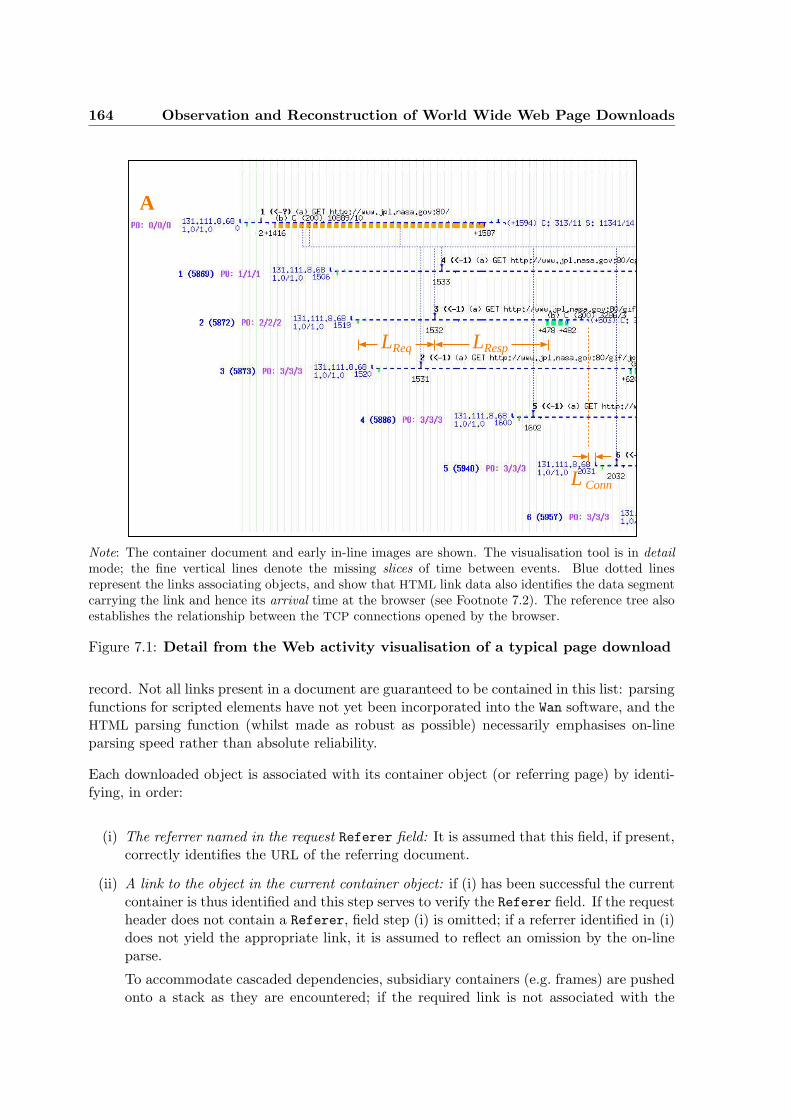
164 Observation and Reconstruction of World Wide Web Page Downloads

LReq LResp

A

L Conn

Note: The container document and early in-line images are shown. The visualisation tool is in detailmode; the fine vertical lines denote the missing slices of time between events. Blue dotted linesrepresent the links associating objects, and show that HTML link data also identifies the data segmentcarrying the link and hence its arrival time at the browser (see Footnote 7.2). The reference tree alsoestablishes the relationship between the TCP connections opened by the browser.

Figure 7.1: Detail from the Web activity visualisation of a typical page download

record. Not all links present in a document are guaranteed to be contained in this list: parsingfunctions for scripted elements have not yet been incorporated into the Wan software, and theHTML parsing function (whilst made as robust as possible) necessarily emphasises on-lineparsing speed rather than absolute reliability.

Each downloaded object is associated with its container object (or referring page) by identi-fying, in order:

(i) The referrer named in the request Referer field: It is assumed that this field, if present,correctly identifies the URL of the referring document.

(ii) A link to the object in the current container object: if (i) has been successful the currentcontainer is thus identified and this step serves to verify the Referer field. If the requestheader does not contain a Referer, field step (i) is omitted; if a referrer identified in (i)does not yield the appropriate link, it is assumed to reflect an omission by the on-lineparse.

To accommodate cascaded dependencies, subsidiary containers (e.g. frames) are pushedonto a stack as they are encountered; if the required link is not associated with the

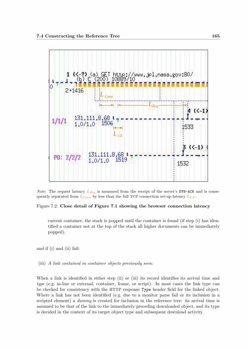
7.4 Constructing the Reference Tree 165

L Conn

LReq

L CE

Note: The request latency LReq is measured from the receipt of the server’s SYN-ACK and is conse-quently separated from LConn by less than the full TCP connection set-up latency LCE .

Figure 7.2: Close detail of Figure 7.1 showing the browser connection latency

current container, the stack is popped until the container is found (if step (i) has iden-tified a container not at the top of the stack all higher documents can be immediatelypopped).

and if (i) and (ii) fail:

(iii) A link contained in container objects previously seen:

When a link is identified in either step (ii) or (iii) its record identifies its arrival time andtype (e.g. in-line or external, container, frame, or script). In most cases the link type canbe checked for consistency with the HTTP response Type header field for the linked object.Where a link has not been identified (e.g. due to a monitor parse fail or its inclusion in ascripted element) a dummy is created for inclusion in the reference tree: its arrival time isassumed to be that of the link to the immediately preceding downloaded object, and its typeis decided in the context of its target object type and subsequent download activity.

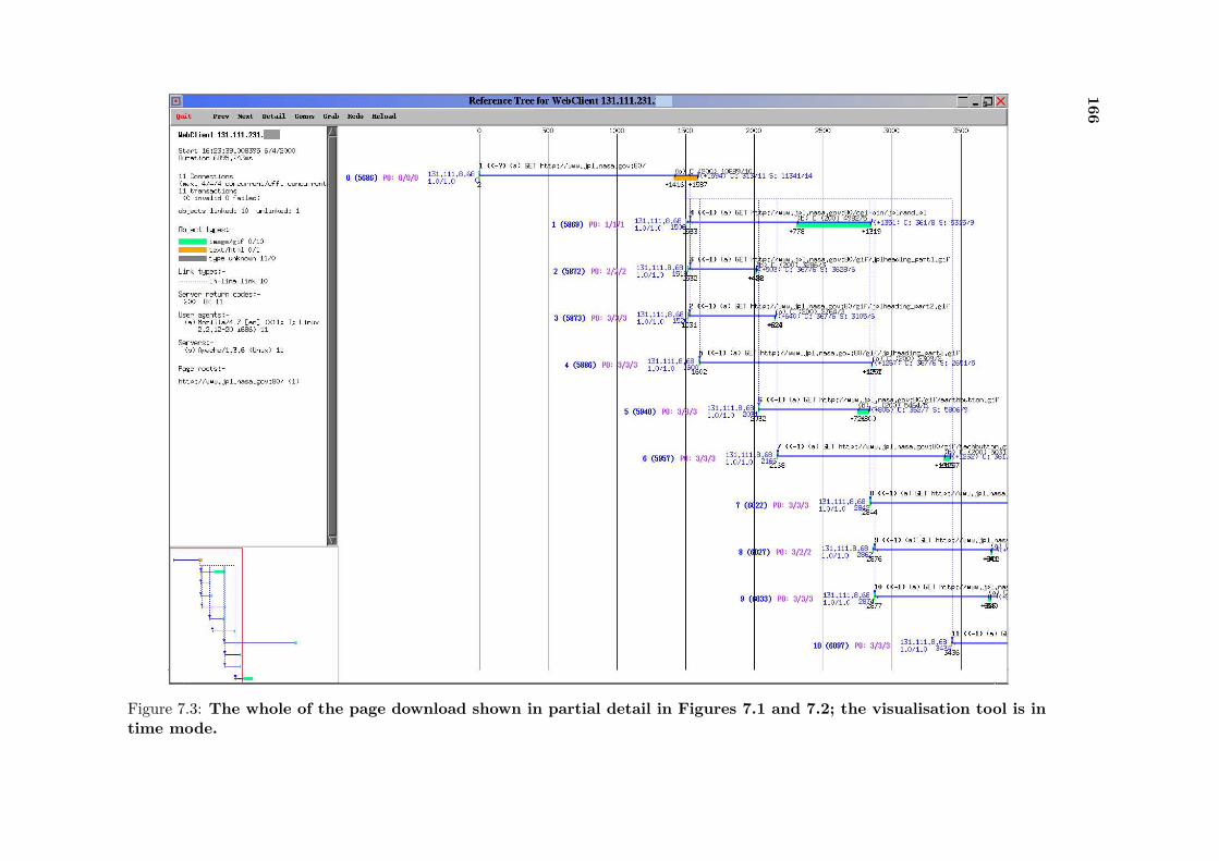
166

Figure 7.3: The whole of the page download shown in partial detail in Figures 7.1 and 7.2; the visualisation tool is intime mode.

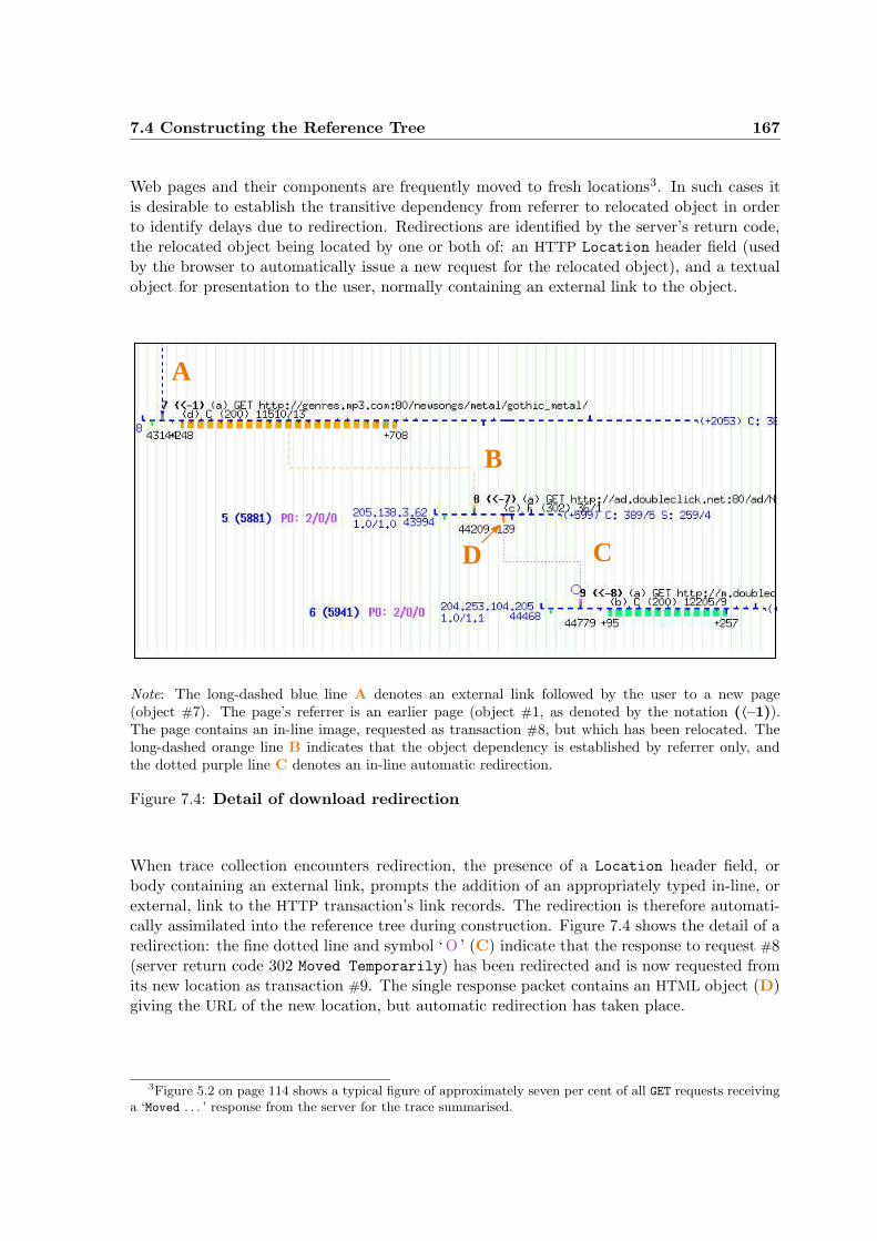
7.4 Constructing the Reference Tree 167

Web pages and their components are frequently moved to fresh locations3. In such cases itis desirable to establish the transitive dependency from referrer to relocated object in orderto identify delays due to redirection. Redirections are identified by the server’s return code,the relocated object being located by one or both of: an HTTP Location header field (usedby the browser to automatically issue a new request for the relocated object), and a textualobject for presentation to the user, normally containing an external link to the object.

A

B

CD

Note: The long-dashed blue line A denotes an external link followed by the user to a new page(object #7). The page’s referrer is an earlier page (object #1, as denoted by the notation (〈–1)).The page contains an in-line image, requested as transaction #8, but which has been relocated. Thelong-dashed orange line B indicates that the object dependency is established by referrer only, andthe dotted purple line C denotes an in-line automatic redirection.

Figure 7.4: Detail of download redirection

When trace collection encounters redirection, the presence of a Location header field, orbody containing an external link, prompts the addition of an appropriately typed in-line, orexternal, link to the HTTP transaction’s link records. The redirection is therefore automati-cally assimilated into the reference tree during construction. Figure 7.4 shows the detail of aredirection: the fine dotted line and symbol ‘o ’ (C) indicate that the response to request #8(server return code 302 Moved Temporarily) has been redirected and is now requested fromits new location as transaction #9. The single response packet contains an HTML object (D)giving the URL of the new location, but automatic redirection has taken place.

3Figure 5.2 on page 114 shows a typical figure of approximately seven per cent of all GET requests receivinga ‘Moved . . . ’ response from the server for the trace summarised.

168 Observation and Reconstruction of World Wide Web Page Downloads

7.4.2 Multiple Links, Repeated Downloads and Browser Caching

The same link is frequently included multiple times in a container document (e.g. to smallpage decorations), and in multiple pages. Browser caching will normally result in a singlerequest for the target object; in which case the object download is assumed to be triggeredby the first occurrence of the link in the current container document (it is assumed that anydownload of the object in response to links in earlier containers will already have been made).Objects are sometimes requested multiple times (the browser may not be caching the object,may be faulty, or the object may have a nil lifetime) in which case the multiple requests areassociated with link occurrences in order.

A difficulty may arise when the user returns to a previously visited page (either throughuse of the ‘back button’ or by following a cyclic link. If the container object has beencached, but other components are requested, then the delimiter of the fresh container requestis absent, and the component requests may appear to be much-delayed multiple requestsoriginating from the original page. This situation can normally be identified due to interveningpage downloads, but can cause confusion if components are shared. The converse case (thecontainer is re-fetched but components are satisfied from the browser cache) is not problematicas the reference tree simply omits the cached objects, as it would in the case of fresh pagedownloads where components are cached. When components requests are observed which donot form part of the current page download (identified as such because they have a differentreferrer, the relevant links are absent from the container, and an arbitrary threshold periodhas been exceeded), a revisit is assumed and a dummy link inserted into the reference tree.

7.4.3 Aborted Downloads

Users may abort page downloads — usually as a result of delay — either by using the browser’s‘stop’ button, or by recommencing the download using the ‘refresh’ button. These cases cannot be identified by a failure to download all components, which may result from caching.

Recommenced downloads may be indicated by the abort of one or more currently activeconnections, followed by a continuation of normal download activity (and possibly one or morerepeated requests for objects already seen). Aborted connections are themselves indicatedby premature termination (a lone SYN or a connection reset). Care must be taken overapparently reset connections, as browsers from the Internet Explorer stable tend to respondto the server’s FIN segment on non-persistent connections with a RST segment, rather thancomplete the normal full four-way connection close. Such RSTs can normally be identified, asthe transaction is complete, and there is no indication of inconsistent TCP state. A similarcessation of activity will be seen in the case of total aborts, but without the recommencementof the download.

Aborted downloads are a matter of considerable interest, particularly their correlation withthe user’s subjective experience of delay. Future Nprobe development will include furtherempirical assessment of activity in this situation and will aim to make its identification asrobust as possible.

7.4 Constructing the Reference Tree 169

7.4.4 Relative References, Reference Scopes and Name Caching

Because a textual match is required to associate link, referrer, and request URLs , and becausethese are frequently given in abbreviated or relative form, all occurrences are converted intocanonical form before contributing to construction of the reference tree. Although deprecated,URLs may sometimes include dotted decimal IP addresses rather than machine names.

Relative URLs are resolved in the context of the current relative base, normally that ofthe container document, but HTML provides mechanisms for defining alternative, defined,bases and their scope. The on-line HTML parse identifies such base elements and scopedelimiters, and includes appropriate records in the list of extracted links. During referencetree reconstruction relative URLs are therefore resolved in the correct context.

HTTP requires that all requests contain a (textual) Host header field identifying the originserver for the requested object. The given host name is used to resolve abbreviated URLs(e.g. of the form “/”), and also to check the host part of URLs for consistency. A problem canarise when dotted decimal addresses are used in request URLs and the Host field is omitted.In such cases the canonical URL is established by reference to the analysis process’s own cacheof name bindings described in Section 7.5 on page 172.

7.4.5 Self-Refreshing Objects

HTML documents may contain ‘HTTP-EQUIV = REFRESH’ META tags which cause the browserto reload the same, or another, object after a defined period, and which may result in repeateddownloads if the refreshed object also contains the same directive. The mechanism may beused to redirect requests (in which case it is identified by the Wan code and accommodatedin a manner similar to normal redirection as described in Section 7.4.1) or, more usually, toimplement features such as tickers.

The mechanism is, for tree reconstruction, equivalent to the inclusion of an in-line link (asit results in an automatic download). Refreshes must be identified and excluded from theassessment of page-download times.

Figure 7.5 illustrates a self-refreshing object repeatedly downloaded to drive a ticker: theperiodic refresh can be seen in the map window. The activity shown is extracted from a longtrace, in which the object is refreshed at 31 s periods for over 40 minutes. The user continuesto browse — transaction #2 is part of another page download (the root is not seen in this9.4 s excerpt and is therefore represented by a dummy object). The transaction is abortedby a browser RST (indicated by a red packet tic) before completion, but not before an in-linetext object is downloaded (transaction #4) - this connection is terminated by a server RST.

7.4.6 Unresolved Connections and Transactions

It may not be possible to immediately associate some transactions with a referring object:the Referer field may be absent, and no matching link found. In the case of container

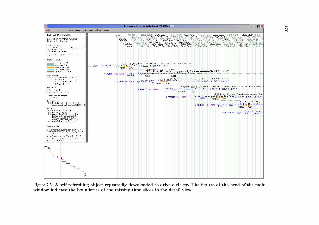
170

Figure 7.5: A self-refreshing object repeatedly downloaded to drive a ticker. The figures at the head of the mainwindow indicate the boundaries of the missing time slices in the detail view.

7.4 Constructing the Reference Tree 171

documents it is assumed that the referrer has not been seen because its download fell outsidethe monitoring period, or because the request originates from a bookmark or user-providedURL . Such transactions become the roots of discrete reference trees.

In the case of subsidiary page components a simple heuristic is employed — if the transactionfalls within a group of others known to originate from the current container, then that con-tainer is taken as the referrer. A dummy link is created similar to that in the case of resolvedtransactions with no identified link.

Aborted connections upon which a request has been issued can be integrated into the referencetree in the normal way, but where connection attempts have been unsuccessful, or connectionsare aborted before a request is made, no transaction request exists with which to integratethe connection into the reference tree — it is desirable to do so because such connectionsmay indicate aborted or recommenced downloads (Section 7.4.3 on page 168). It is normallypossible to resolve such connections using a similar heuristic to that employed in the case ofunresolved transactions.

7.4.7 Multiple Browser Instances and Web Cache Requests

Multiple concurrent page downloads can occur when a single user instantiates more than onebrowser, or in the case of multi-user hosts. This may cause confusion in the constructionof reference trees, if identical pages, or those with common components, are concurrentlydownloaded. Although transactions are associated with a browser using the client IP addressof the connections carrying them, such potential confusion can be minimised by using thefiner-grained association provided by the browser employed — this information is providedby the HTTP User-Agent header field. It is suggested that multiple concurrent downloads ofthe same page, to the same host, using the same browser marque and version are relativelyrare, and where they do arise inaccuracies are likely to be, to some extent, self-cancelling.

Where the requesting entity is a Web cache, it is expected that a smaller set of page compo-nents will be requested, the majority of objects being satisfied from the cache, and the pos-sibility of multiple concurrent requests for identical objects being filtered out by the cachingoperation. The reference trees constructed will be sparse, and massively interleaved, but areof less significance than those in respect of studies based upon browsers — the focus of interestis likely to be on cache performance.

Any future study of cache performance using Nprobe (it would, for instance, be informativeto position monitors both up and down stream of caches) will add impetus towards theextraction of data pertaining to object freshness and lifetime, and caching directives, fromHTTP header fields. An analytic methodology to associate and compare such traces remainsto be developed.

172 Observation and Reconstruction of World Wide Web Page Downloads

7.4.8 Timing Data

The transaction data recorded by Nprobe includes the timing of significant events (e.g. startand end of requests, responses and objects, link arrivals). TCP data includes significantconnection timings (e.g. open, close, SYN, FIN and packet arrivals). All major components ofpage downloads can therefore be analysed correctly in the time domain.

The timings provided by Nprobe are attached to events after any packet delivery reorderingnecessitated by loss in order to reflect, as accurately as possible, when content would havebeen delivered to the application. This mechanism can account only for losses and delayeddelivery where the monitor is aware of retransmission (i.e. where loss has occurred upstreamof the monitor). Where traces are known to have been collected immediately adjacent to aclient this may be adequate, but where there is the possibility that significant down-streamloss may have occurred, connections must be filtered through the activity model to attachthe effective application delivery time to each packet and associated events.

7.5 Integration with Name Service Requests

Domain Name Service (DNS) requests made prior to connection opening have been shown byHabib [Habib00] to contribute to download latency. When an Nprobe monitor is positionedso as to observe DNS requests from the client they are incorporated into the page-downloadreconstruction.

Where the construction of canonical URLs demands a name binding between a dotted-decimalIP address in a requested URL, and the requester’s HTTP Host header field is missing, thebinding is supplied from a cache maintained by the analysis process. The cache is populatedfrom three sources:

• Bindings contributed where the Host field is present

• DNS requests observed by the monitor

• A persistent cache maintained by all analysis processes

Bindings are not obtained by correlating server addresses and Host fields as they would beincorrect in the case of requests made to caches.

Persistent caches are maintained on both a global basis, and specific to individual traces (asname bindings may change over time, and between traces). Where a mapping cannot beobtained from the trace-specific cache, it is located, if possible, from the global cache. Thename binding module provided as part of the analysis tool kit provides a stand-alone methodfor extracting the server addresses from traces and building caches by issuing the appropriateDNS requests.

7.6 Visualisation 173

7.6 Visualisation

The Web activity visualisation tool graphically reproduces the relationships between objectsand connections as represented by the reference tree. Relationships in time between com-ponents are also illustrated. The alternative detail and time modes allow for inspection ofdetail, or scaled relationships in time, and the selectable secondary pane contents provide de-tailed inspection of the underlying trace data. A draggable cursor accurately indicates timeintervals, even in the non-linearly–scaled detail mode, and hence supports evaluation of timebased relationships.

The tool presents the structure and context of page downloads in readily comprehensible form,and aids the identification of relationships between transactions, connections, and betweenthe two. It is particularly valuable in the development of analysis of page downloads, and inrecognising both typical, and dysfunctional, patterns of behaviour.

7.7 Web Traffic Characterisation

Because Nprobe is unique in collecting a range of transaction data from the HTTP headercontent of the observed traffic, the potential exists for characterisation based upon data notpreviously available, or available only in limited, or partial form, from server logs, content, orusing active techniques. Such characterisations could include, for instance, the proportions ofrequests eliciting particular server responses, conditional requests, characterisation of objectlifetimes, and so on; the possible range is wide.

The ability, also unique, to accurately recreate page structures also makes possible moreaccurate characterisations of metrics such as the number of component objects, overall datatransfer sizes, or the proportions of different component types. There remains a further, andmost significant, area of characterisation which has hitherto been impossible — that of wholepage download times; without the facility to accurately associate all components of a page,no measure of overall time has been possible. The matter of page download times, and theimpact of individual connection delays, is discussed more fully in Chapter 8.

7.8 Summary

Commonly available passive monitoring tools, because normally limiting data collection toTCP/IP headers, restrict the study of Web downloads to that of single connection activity.Inference, based upon host addresses and patterns of activity over multiple connections, maysuggest the grouping of individual objects into pages, but inferential methods are likely to beinaccurate because of factors such as concurrent downloads, frames, redirection and multiply-hosted pages.

It is suggested in this chapter that Web page downloads must be examined as a whole ifthe contribution of the various components of the download system and their interactions

174 Observation and Reconstruction of World Wide Web Page Downloads

are to be identified. A full understanding can be achieved only by investigating the full setof page objects, the connections used to download them, and activity at all of the protocollevels involved. In Chapter 8 it will be seen, for instance, that the contribution of individualobject delays to whole page download times can only be assessed in the context of the wholedownload set.

The protocol-spanning data collected by Nprobe, and its level of detail, allow page down-loads to be accurately reconstructed during post-collection analysis, and hence examined asa whole. This chapter has introduced the technique used, and has shown how integration ofthe available data makes explicit the relationships between system components, and detailaccessible at both coarse and fine granularities.

The ability to accurately reconstruct whole page downloads will present new opportunities topresent Web traffic characterisations based upon this unit. The explanation of the analysisand reconstruction techniques that have been developed show that the comprehension andcorrect interpretation of the complex and diverse data are, once again, assisted and madefeasible by the tools provided in the post-analysis toolkit.

Chapter 8

Page Download Times and Delay

No one who has used a browser to access pages from the World Wide Web has escaped theexperience of over-long download times. While times in the order of seconds are acceptable,those exceeding even a few tens of seconds become increasingly annoying.

Identification of the various elements contributing to the download time of Web objects hasbeen the subject of much research. It is, however, the download time of a set of objectscomprising an entire page which is of critical importance to the user — particularly in thepresence of delay leading to subjectively long waits. In this chapter the contribution of delaysin downloading individual objects is related to the effect on the download time of whole pages,and techniques are introduced for assessing both the degree and the distribution of delay. Thepotentially disastrous effects of packet loss early in the lifetime of the TCP connections usedis considered, and is assessed in a case study of downloads from a popular site. The effectof such early loss is examined in the context of a trace-driven simulation of the same set ofpages downloaded using exclusively persistent connections.

8.1 Factors Contributing to Overall Download Times

Overall page download times are determined by a number of factors:

The number and size of the constituent objects: How many objects must be downloaded, howmany are cached by the browser and how many may be satisfied by conditional requests

The composition of the page: Is delay introduced by redirection, and can sub sets of objectsonly be requested after the receipt of subsidiary container documents (e.g. frames)

Server latency (i.e. the period between receipt of the complete request and the start of re-sponse transmission)

Browser latency (i.e. the period between the browser receiving a segment of the responsecontaining an in-line link to a subsidiary object and the transmission of a request forthat object)

176 Page Download Times and Delay

TCP connection latency (i.e. the time taken to establish a TCP connection)

Network RTTs

Available bandwidth

Packet loss: What proportion of packets are lost, when in the connection’s lifetime, and theTCP implementations’ recovery strategy

The browser’s use of TCP connections: Are persistent connections used, and if so are re-quests pipelined, how many concurrently open connections are maintained, and doesthe browser open and close connections in a timely manner

While it is axiomatic that packet loss causes delay, disproportionate or avoidably high con-tributions by any of these factors may also be considered delays. Whereas some factors (e.g.the number of constituent objects or the use of persistent connections) have a direct effect onpage download time, others’ immediate effect is on the download time of individual objects,and only indirectly influences the whole page.

8.2 The Contribution of Object Delay to Whole Page Down-

load Times

Because browsers typically use parallel TCP connections to download the set of objects, andbecause they may not use these connections in a timely manner, overall page download timesare not simply the sum of the individual object download times, and delays at the page scaleare similarly not the sum of delays suffered by individual objects. To fully analyse the timecomponents of page downloads it is therefore necessary to consider the full set of constituentobject deliveries, the connections used, and their interrelationships over the total downloadperiod. The download of a Web page must be distinguished from that of its componentobjects.

8.2.1 Differentiating Single Object and Page Delays

The point is illustrated by Figure 8.1 on the next page, which shows three simple cases of pagedownloads and the effects that delayed objects might have on overall times. In Sub-figure (a)Object B is delayed, but with no effect on overall page download time. Objects D – J aredelayed as only a single connection is available, but not by the magnitude of the Object Bdelay; this will be noticeable in a browser which renders objects as they are received.

In Sub-figure 8.1(b) Object B is delayed beyond the download time of the container document,and hence adds to the overall page download time. Objects C – I are delayed as in Sub-figure 8.1(a). Object J is also delayed, but adds nothing to the delay in overall time alreadycontributed by Object B. Although the overall page download time has been extended, it isonly the rendering of two objects which is significantly delayed.

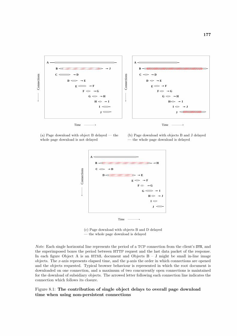
177

A

B

C

D

E

F

G

H

I

Time

Con

nect

ions

E

D

F

H

I

G

J

J

(a) Page download with object B delayed — thewhole page download is not delayed

A

B

C

D

E

F

G

H

I

J

TimeC

onne

ctio

ns D

E

F

G

H

I

J

(b) Page download with objects B and J delayed— the whole page download is delayed

A

B

C

D

J

Time

Con

nect

ions

G

D

E F

F G

H J

I

E

H

I

(c) Page download with objects B and D delayed— the whole page download is delayed

Note: Each single horizontal line represents the period of a TCP connection from the client’s SYN, andthe superimposed boxes the period between HTTP request and the last data packet of the response.In each figure Object A is an HTML document and Objects B – J might be small in-line imageobjects. The x-axis represents elapsed time, and the y-axis the order in which connections are openedand the objects requested. Typical browser behaviour is represented in which the root document isdownloaded on one connection, and a maximum of two concurrently open connections is maintainedfor the download of subsidiary objects. The arrowed letter following each connection line indicates theconnection which follows its closure.

Figure 8.1: The contribution of single object delays to overall page downloadtime when using non-persistent connections

178 Page Download Times and Delay

Sub-figure 8.1(c) also shows a download in which two objects are delayed. In this case thedownloads of six of the remaining objects are also significantly delayed resulting in late receiptof eight of the nine images contained in the page.

It will be appreciated that the typical Web page will probably contain many more objectsthan in the simple examples shown, and that, while individual object delays of the generalpattern shown in Sub-figures 8.1(a) and 8.1(b) may serve only to introduce minor delaysin the presentation of a whole page, there is also the possibility that delays occurring inpatterns similar to that shown in Sub-figure 8.1(c) may result in very a significant cumulativedegradation in performance.

8.2.2 Assessing the Degree of Delay

Whole page delay may be defined as the difference between the time when delivery of thelast object of a page completes and the corresponding time had there been no delays in thedelivery of individual objects. Calculation of this delay therefore depends upon establishingthe notional download time without delay.

In order to calculate the duration of the delay-free page download three steps are required:

Establishment of an accurate model: A model of the set of TCP connections and HTTP trans-actions involved is derived using the reconstruction techniques described in Section 7.3.

Calculation of object PDTs in the absence of delay: The delay-free PDT for each individualobject is calculated using the accurate connection simulations described in Section 5.6on page 133. Because the technique draws upon fine-grained detail of TCP, application,and network-level activity provided by the activity model, downloads can be simulatedin the total absence of loss, or as a set of what if scenarios (e.g. with only a certaincategory of packet loss1, with a differing probability of loss, with modified browser/serverlatencies, or if persistent connections or pipelining were used).

Reconstruction of the page download based upon the modified constituent download times:The original download will be traversed by a critical path through its constituent con-current connections and transactions. Reconstruction of the download may make theoriginal critical path obsolete, but it is not necessary to use network analysis techniquesto identify or calculate the duration of either the original, or the new, path — both areinherent in the reconstruction of the download.

Even with the relatively rich set of data provided by Nprobe traces it is not entirely simpleto derive a model of an equivalent, non-delayed, set of downloads for a page. It can bedifficult to ascertain the target number of concurrently open TCP connections: browsers areoften inconsistent — even within a single page, the point of connection closure recognised bybrowsers may also vary (the completion of the full TCP 4-way close, the transmission of the

1In some cases where timings are to be calculated with the removal of an easily identified and quantifiedcategory of loss (e.g. SYN loss) it is possible to do so without traversing a simulation.

8.2 The Contribution of Object Delay to Whole Page Download Times 179

browser’s FIN packet, the receipt of the server’s FIN packet on a non-persistent connection,etc.), the opening of new connections may be delayed by the browser, and account must betaken of the delay between causative and consequent events as seen by the probe.

A frequency analysis of the number of connections currently open, as each fresh connectionopens, is calculated on the basis of the various possible criteria which a browser may use.This gives an indication of the criterion used by the browser and its concurrency target.

The whole page download is reconstructed by taking the set of connections used, discardingany which did not establish a full connection or succeed in obtaining a server response, andadjusting the PDTs of the remainder using the desired scenario. The modified open and ‘close’times can then be calculated for each successive connection on the basis of the timings of thepreceding connections, and the browser’s concurrency criterion and target. It is assumedthat any inconsistencies in the browser’s observed pattern of connection concurrency wouldalso apply to the recalculated set of download connections2, and in calculating when eachconnection would open, the number of currently open connections at the point of openingare used in order to maintain any such inconsistencies. It is also assumed that any delays inthe server remain constant despite changes in the pattern of requests over time, and similarlythat any browser-introduced delays remain constant. Because the relationship between thelinks contained in the root document and object downloads is known, it can be ensured thatmodified connection timings do not cause an object to be requested before the browser wouldhave seen the corresponding link.

Chapter 6 describes the techniques used to estimate server and client delays together withthe pRTTs between probe/host/probe which establish the time lag between causative andconsequent events, but for the purposes of this calculation such techniques are not consid-ered necessary if it is assumed that client/server delays and network transit times remainunchanged (and unless these are modified as part of a what if scenario). These assumptionsare considered reasonable, as the new model of the set of downloads without delays does notin general produce major changes to either patterns of network or server activity. Any vari-ations which break these assumptions are also likely to be at least two orders of magnitudesmaller than the phenomena of interest.

8.2.3 The Distribution of Object Delay within a Page Download

From the subjective perspective of the user it is not just the overall page download time whichis important, but also the distribution of any object delays within the download period. Thedelays shown in Figure 8.1(c) would probably be perceived as more annoying than thoseshown in Figure 8.1(b), although both pages may be completed in the same times. It isassumed that, in the general case, in-line objects are fetched in the order that the browser’sHTML parser encounters the relevant links, and that this order reflects the significance andrendering order of the objects.

In the current analysis the distribution of individual object delays is characterised using asimple metric — a cumulative object delay (cod) for a page of N objects calculated as follows:

2There appears to be no correlation between unsuccessful or delayed connections and such inconsistencies.

180 Page Download Times and Delay

cod =

(

n=N∑

n=1

(Dn − Un)

)

×1

N

where:N is the number of objects in the page,Dn is the delivery completion time of object nandUn is the notional delivery completion time of

object n in the absence of delay

As an illustration of the effect of object delays and distribution on the cod, Table 8.1 sum-marises the downloads shown in Figure 8.1, giving the cod for each case, assuming the con-tainer document downloads in 100 time units and that each image object would download in10 time units if not delayed. It is stressed that the cod represents a measure of the distribu-tion of delay; while it is intuitive that delay early in the download of a page is subjectivelyless acceptable than delay affecting only the later components, assessment of user dissatis-faction is not within this field of study. This metric, however, together with the accuratecalculation of overall download time and delay, would provide a constructive basis for anysuch investigation.

Table 8.1: Summary of delays and cumulative object delays for the pagedownloads illustrated in Figure 8.1.

Fig.Individual object delays Cumulative

delayPage Download Time

codObject Delay Object Delay Delayed Undelayed

(a) B 50 - - 100 100 100 10(b) B 130 J 90 310 180 100 31(c) B 130 D 60 670 150 100 67

Note: Although the total individual object delays, and the overall page download time, are higherin (b) than in (c), the distribution of object delays results in a higher cod for (c).

8.3 The Effect of Early Packet Loss on Page Download Time

In the initial stages of a TCP connection neither client nor server has seen enough packets toestablish a usable round trip time estimation. In the case of packet loss, retransmission willtherefore take place only after a default timeout period (typically in the order of 3 seconds,increasing exponentially for each repeat). Packet losses during this period are henceforthreferred to as early packet loss. Such delays in individual connections have been noted by theWAWM Project [Barford99a].

8.4 Delay in Downloading from a Site with Massive Early Packet Loss 181

This context gives rise to a serious implication for the use of many short-lived TCP connectionsdelivering single objects. While long delays may be introduced by early packet loss on anyconnection, the page downloads using non-persistent connections are particularly vulnerable— most or all activity taking place in conditions of potential early packet loss. From hereonwards in this chapter ‘delay’ will refer to delay arising as a result of early packet loss unlessotherwise stated.

Whereas the delay contribution to page download times due to connection setup latency, orto packet loss on an established connection, are likely to comprise a small number of RTTs— in the order of some tens or hundreds of milliseconds — those due to early packet losscontribute delays in the order of seconds, and which, when occurring in patterns similar tothat illustrated in Figure 8.1(c) may cumulatively reach the order of tens or even hundredsof seconds. It is also inherent in this stage of a connection’s lifetime that fast-retransmitmechanisms will not be operative. It is worth noting that in the context of many short-livedconnections, default retransmission values based upon shared routing metrics are also unlikelyto be available to individual connections.

On an individual connection early packet losses will manifest themselves as:

• Loss of client’s SYN packets(s) causing one or more SYN retransmissions.

• Loss of server’s SYN-ACK causing one or more SYN retransmissions.

• Loss of client’s request causing one or more retransmissions.

• Loss of server’s ACK to the request causing one or more retransmissions.

• Loss of server’s response.

Such losses may occur on both persistent and non-persistent connections, but in the persistentcase losses of requests/responses after the first will normally cause retransmits based uponestablished RTT values or fast-retransmit mechanisms. The case where a client’s first requestis lost can be distinguished from that where the server merely exhibits a long delay beforeresponding by the receipt of an ACK for the segment carrying the request.

8.4 Delay in Downloading from a Site with Massive EarlyPacket Loss

Users of a popular British news Web site frequently experience long and frustrating delaysin downloading pages. Traffic between this site and the UCCS network was monitored for aperiod of 24 hours to obtain the trace first introduced in Section 6.4. Analysis of the tracerevealed that downloads from the site suffered a high incidence of exactly the delays due toearly packet loss discussed in Section 8.3, and that the delivery of many pages was therebyconsiderably delayed.

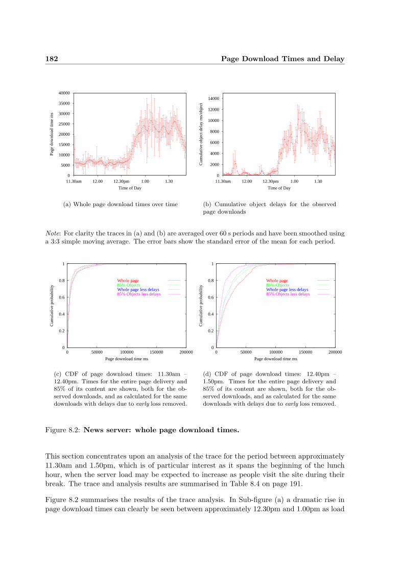
182 Page Download Times and Delay

0

5000

10000

15000

20000

25000

30000

35000

40000

11.30am 12.00 12.30pm 1.00 1.30

Page

dow

nloa

d tim

e m

s

Time of Day

(a) Whole page download times over time

0

2000

4000

6000

8000

10000

12000

14000

11.30am 12.00 12.30pm 1.00 1.30

Cum

ulat

ive

obje

ct d

elay

ms/

obje

ct

Time of Day

(b) Cumulative object delays for the observedpage downloads

Note: For clarity the traces in (a) and (b) are averaged over 60 s periods and have been smoothed usinga 3:3 simple moving average. The error bars show the standard error of the mean for each period.

0

0.2

0.4

0.6

0.8

1

0 50000 100000 150000 200000

Cum

ulat

ive

prob

abili

ty

Page download time ms

Whole page85% ObjectsWhole page less delays85% Objects less delays

(c) CDF of page download times: 11.30am –12.40pm. Times for the entire page delivery and85% of its content are shown, both for the ob-served downloads, and as calculated for the samedownloads with delays due to early loss removed.

0

0.2

0.4

0.6

0.8

1

0 50000 100000 150000 200000

Cum

ulat

ive

prob

abili

ty

Page download time ms

Whole page85% ObjectsWhole page less delays85% Objects less delays

(d) CDF of page download times: 12.40pm –1.50pm. Times for the entire page delivery and85% of its content are shown, both for the ob-served downloads, and as calculated for the samedownloads with delays due to early loss removed.

Figure 8.2: News server: whole page download times.

This section concentrates upon an analysis of the trace for the period between approximately11.30am and 1.50pm, which is of particular interest as it spans the beginning of the lunchhour, when the server load may be expected to increase as people visit the site during theirbreak. The trace and analysis results are summarised in Table 8.4 on page 191.

Figure 8.2 summarises the results of the trace analysis. In Sub-figure (a) a dramatic rise inpage download times can clearly be seen between approximately 12.30pm and 1.00pm as load

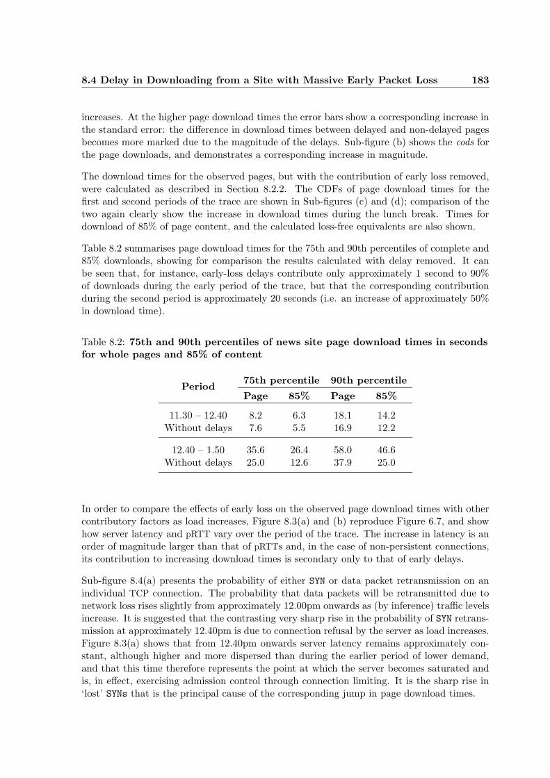
8.4 Delay in Downloading from a Site with Massive Early Packet Loss 183

increases. At the higher page download times the error bars show a corresponding increase inthe standard error: the difference in download times between delayed and non-delayed pagesbecomes more marked due to the magnitude of the delays. Sub-figure (b) shows the cods forthe page downloads, and demonstrates a corresponding increase in magnitude.

The download times for the observed pages, but with the contribution of early loss removed,were calculated as described in Section 8.2.2. The CDFs of page download times for thefirst and second periods of the trace are shown in Sub-figures (c) and (d); comparison of thetwo again clearly show the increase in download times during the lunch break. Times fordownload of 85% of page content, and the calculated loss-free equivalents are also shown.

Table 8.2 summarises page download times for the 75th and 90th percentiles of complete and85% downloads, showing for comparison the results calculated with delay removed. It canbe seen that, for instance, early-loss delays contribute only approximately 1 second to 90%of downloads during the early period of the trace, but that the corresponding contributionduring the second period is approximately 20 seconds (i.e. an increase of approximately 50%in download time).

Table 8.2: 75th and 90th percentiles of news site page download times in secondsfor whole pages and 85% of content

Period75th percentile 90th percentile

Page 85% Page 85%

11.30 – 12.40 8.2 6.3 18.1 14.2Without delays 7.6 5.5 16.9 12.2

12.40 – 1.50 35.6 26.4 58.0 46.6Without delays 25.0 12.6 37.9 25.0

In order to compare the effects of early loss on the observed page download times with othercontributory factors as load increases, Figure 8.3(a) and (b) reproduce Figure 6.7, and showhow server latency and pRTT vary over the period of the trace. The increase in latency is anorder of magnitude larger than that of pRTTs and, in the case of non-persistent connections,its contribution to increasing download times is secondary only to that of early delays.

Sub-figure 8.4(a) presents the probability of either SYN or data packet retransmission on anindividual TCP connection. The probability that data packets will be retransmitted due tonetwork loss rises slightly from approximately 12.00pm onwards as (by inference) traffic levelsincrease. It is suggested that the contrasting very sharp rise in the probability of SYN retrans-mission at approximately 12.40pm is due to connection refusal by the server as load increases.Figure 8.3(a) shows that from 12.40pm onwards server latency remains approximately con-stant, although higher and more dispersed than during the earlier period of lower demand,and that this time therefore represents the point at which the server becomes saturated andis, in effect, exercising admission control through connection limiting. It is the sharp rise in‘lost’ SYNs that is the principal cause of the corresponding jump in page download times.

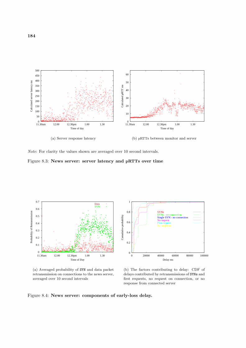
184

0

50

100

150

200

250

300

350

400

450

500

11.30am 12.00 12.30pm 1.00 1.30

Cal

cula

ted

serv

er la

tenc

y m

s

Time of day

(a) Server response latency

0

10

20

30

40

50

60

11.30am 12.00 12.30pm 1.00 1.30C

alcu

late

d pR

TT

ms

Time of day

(b) pRTTs between monitor and server

Note: For clarity the values shown are averaged over 10 second intervals.

Figure 8.3: News server: server latency and pRTTs over time

0

0.1

0.2

0.3

0.4

0.5

0.6

0.7

11.30am 12.00 12.30pm 1.00 1.30

Prob

abili

ty o

f R

etra

nsm

issi

on

Time of Day

DataSYN

(a) Averaged probability of SYN and data packetretransmission on connections to the news server,averaged over 10 second intervals

0

0.2

0.4

0.6

0.8

1

0 20000 40000 60000 80000 100000

Cum

ulat

ive

prob

abili

ty

Delay ms

SYNsSYNs - no connectionSingle SYN - no connectionNo requestFirst requestNo response

(b) The factors contributing to delay: CDF ofdelays contributed by retransmissions of SYNs andfirst requests, no request on connection, or noresponse from connected server

Figure 8.4: News server: components of early-loss delay.

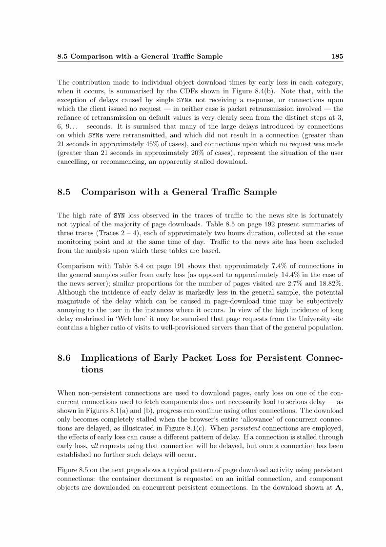
8.5 Comparison with a General Traffic Sample 185

The contribution made to individual object download times by early loss in each category,when it occurs, is summarised by the CDFs shown in Figure 8.4(b). Note that, with theexception of delays caused by single SYNs not receiving a response, or connections uponwhich the client issued no request — in neither case is packet retransmission involved — thereliance of retransmission on default values is very clearly seen from the distinct steps at 3,6, 9. . . seconds. It is surmised that many of the large delays introduced by connectionson which SYNs were retransmitted, and which did not result in a connection (greater than21 seconds in approximately 45% of cases), and connections upon which no request was made(greater than 21 seconds in approximately 20% of cases), represent the situation of the usercancelling, or recommencing, an apparently stalled download.

8.5 Comparison with a General Traffic Sample

The high rate of SYN loss observed in the traces of traffic to the news site is fortunatelynot typical of the majority of page downloads. Table 8.5 on page 192 present summaries ofthree traces (Traces 2 – 4), each of approximately two hours duration, collected at the samemonitoring point and at the same time of day. Traffic to the news site has been excludedfrom the analysis upon which these tables are based.

Comparison with Table 8.4 on page 191 shows that approximately 7.4% of connections inthe general samples suffer from early loss (as opposed to approximately 14.4% in the case ofthe news server); similar proportions for the number of pages visited are 2.7% and 18.82%.Although the incidence of early delay is markedly less in the general sample, the potentialmagnitude of the delay which can be caused in page-download time may be subjectivelyannoying to the user in the instances where it occurs. In view of the high incidence of longdelay enshrined in ‘Web lore’ it may be surmised that page requests from the University sitecontains a higher ratio of visits to well-provisioned servers than that of the general population.

8.6 Implications of Early Packet Loss for Persistent Connec-

tions

When non-persistent connections are used to download pages, early loss on one of the con-current connections used to fetch components does not necessarily lead to serious delay — asshown in Figures 8.1(a) and (b), progress can continue using other connections. The downloadonly becomes completely stalled when the browser’s entire ‘allowance’ of concurrent connec-tions are delayed, as illustrated in Figure 8.1(c). When persistent connections are employed,the effects of early loss can cause a different pattern of delay. If a connection is stalled throughearly loss, all requests using that connection will be delayed, but once a connection has beenestablished no further such delays will occur.

Figure 8.5 on the next page shows a typical pattern of page download activity using persistentconnections: the container document is requested on an initial connection, and componentobjects are downloaded on concurrent persistent connections. In the download shown at A,

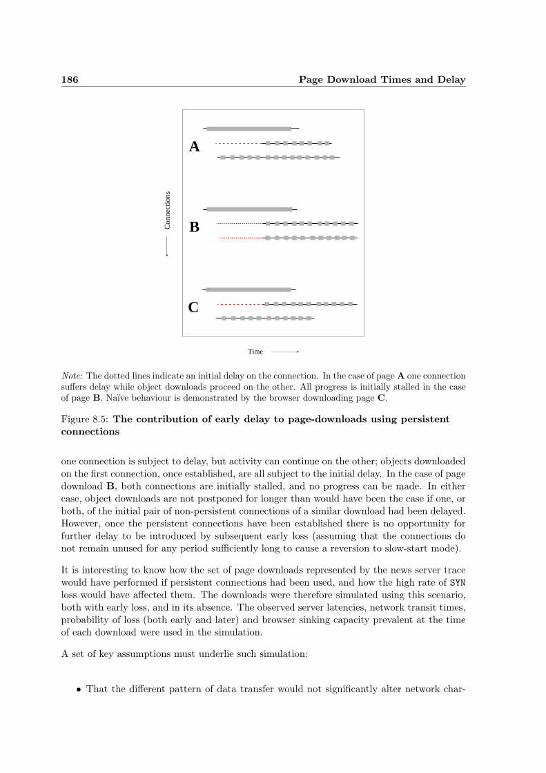
186 Page Download Times and Delay

A

Time

Con

nect

ions

B

C

Note: The dotted lines indicate an initial delay on the connection. In the case of page A one connectionsuffers delay while object downloads proceed on the other. All progress is initially stalled in the caseof page B. Naıve behaviour is demonstrated by the browser downloading page C.

Figure 8.5: The contribution of early delay to page-downloads using persistentconnections

one connection is subject to delay, but activity can continue on the other; objects downloadedon the first connection, once established, are all subject to the initial delay. In the case of pagedownload B, both connections are initially stalled, and no progress can be made. In eithercase, object downloads are not postponed for longer than would have been the case if one, orboth, of the initial pair of non-persistent connections of a similar download had been delayed.However, once the persistent connections have been established there is no opportunity forfurther delay to be introduced by subsequent early loss (assuming that the connections donot remain unused for any period sufficiently long to cause a reversion to slow-start mode).

It is interesting to know how the set of page downloads represented by the news server tracewould have performed if persistent connections had been used, and how the high rate of SYNloss would have affected them. The downloads were therefore simulated using this scenario,both with early loss, and in its absence. The observed server latencies, network transit times,probability of loss (both early and later) and browser sinking capacity prevalent at the timeof each download were used in the simulation.

A set of key assumptions must underlie such simulation:

• That the different pattern of data transfer would not significantly alter network char-

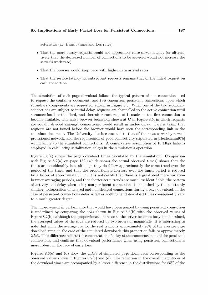
8.6 Implications of Early Packet Loss for Persistent Connections 187

acteristics (i.e. transit times and loss rates)

• That the more bursty requests would not appreciably raise server latency (or alterna-tively that the decreased number of connections to be serviced would not increase theserver’s work rate)

• That the browser would keep pace with higher data arrival rates

• That the service latency for subsequent requests remains that of the initial request oneach connection

The simulation of each page download follows the typical pattern of one connection usedto request the container document, and two concurrent persistent connections upon whichsubsidiary components are requested, shown in Figure 8.5. When one of the two secondaryconnections are subject to initial delay, requests are channelled to the active connection untila connection is established, and thereafter each request is made on the first connection tobecome available. The naıve browser behaviour shown at C in Figure 8.5, in which requestsare equally divided amongst connections, would result in undue delay. Care is taken thatrequests are not issued before the browser would have seen the corresponding link in thecontainer document. The University site is connected to that of the news server by a well-provisioned network, and the requirement of good connectivity stipulated in [Heidemann97b]would apply to the simulated connections. A conservative assumption of 10 Mbps links isemployed in calculating serialization delays in the simulation’s operation.

Figure 8.6(a) shows the page download times calculated by the simulation. Comparisonwith Figure 8.2(a) on page 182 (which shows the actual observed times) shows that thetimes are considerably less, although they do follow approximately the same trend over theperiod of the trace, and that the proportionate increase over the lunch period is reducedby a factor of approximately 1.7. It is noticeable that there is a great deal more variationbetween averaging periods, and that shorter-term trends are much less identifiable; the patternof activity and delay when using non-persistent connections is smoothed by the constantlyshifting juxtaposition of delayed and non-delayed connections during a page download, in thecase of persistent connections delay is ‘all or nothing’ and download times consequently varyto a much greater degree.

The improvement in performance that would have been gained by using persistent connectionis underlined by comparing the cods shown in Figure 8.6(b) with the observed values ofFigure 8.2(b): although the proportionate increase as the server becomes busy is maintained,the averaged values of the cods are reduced by two orders of magnitude. It is interesting tonote that while the average cod for the real traffic is approximately 25% of the average pagedownload time, in the case of the simulated downloads this proportion falls to approximately2.5%. This difference reflects the concentration of delay at the commencement of the persistentconnections, and confirms that download performance when using persistent connections ismore robust in the face of early loss.

Figures 8.6(c) and (d) show the CDFs of simulated page downloads corresponding to theobserved values shown in Figures 8.2(c) and (d). The reduction in the overall magnitudes ofthe download times are accompanied by a lesser difference in the distributions for 85% of the

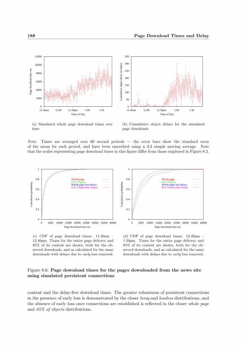
188 Page Download Times and Delay

0

2000

4000

6000

8000

10000

12000

11.30am 12.00 12.30pm 1.00 1.30

Page

dow

nloa

d tim

e m

s

Time of Day

(a) Simulated whole page download times overtime

0

50

100

150

200

250

300

350

11.30am 12.00 12.30pm 1.00 1.30

Cum

ulat

ive

obje

ct d

elay

ms/

obje

ct

Time of Day

(b) Cumulative object delays for the simulatedpage downloads

Note: Times are averaged over 60 second periods — the error bars show the standard errorof the mean for each period, and have been smoothed using a 3:3 simple moving average. Notethat the scales representing page download times in this figure differ from those employed in Figure 8.2.

0

0.2

0.4

0.6

0.8

1

0 5000 10000 15000 20000 25000 30000 35000 40000

Cum

ulat

ive

prob

abili

ty

Page download time ms

Whole page85% ObjectsWhole page less delays85% Objects less delays

(c) CDF of page download times: 11.30am –12.40pm. Times for the entire page delivery and85% of its content are shown, both for the ob-served downloads, and as calculated for the samedownloads with delays due to early loss removed.

0

0.2

0.4

0.6

0.8

1

0 5000 10000 15000 20000 25000 30000 35000 40000

Cum

ulat

ive

prob

abili

ty

Page download time ms

Whole page85% ObjectsWhole page less delays85% Objects less delays

(d) CDF of page download times: 12.40pm –1.50pm. Times for the entire page delivery and85% of its content are shown, both for the ob-served downloads, and as calculated for the samedownloads with delays due to early loss removed.

Figure 8.6: Page download times for the pages downloaded from the news siteusing simulated persistent connections

content and the delay-free download times. The greater robustness of persistent connectionsin the presence of early loss is demonstrated by the closer lossy and lossless distributions, andthe absence of early loss once connections are established is reflected in the closer whole pageand 85% of objects distributions.

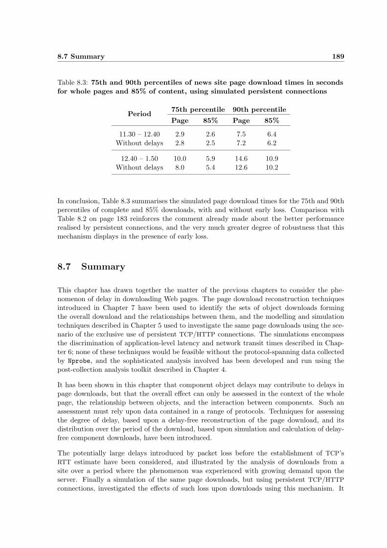
8.7 Summary 189

Table 8.3: 75th and 90th percentiles of news site page download times in secondsfor whole pages and 85% of content, using simulated persistent connections

Period75th percentile 90th percentile

Page 85% Page 85%

11.30 – 12.40 2.9 2.6 7.5 6.4Without delays 2.8 2.5 7.2 6.2

12.40 – 1.50 10.0 5.9 14.6 10.9Without delays 8.0 5.4 12.6 10.2

In conclusion, Table 8.3 summarises the simulated page download times for the 75th and 90thpercentiles of complete and 85% downloads, with and without early loss. Comparison withTable 8.2 on page 183 reinforces the comment already made about the better performancerealised by persistent connections, and the very much greater degree of robustness that thismechanism displays in the presence of early loss.

8.7 Summary

This chapter has drawn together the matter of the previous chapters to consider the phe-nomenon of delay in downloading Web pages. The page download reconstruction techniquesintroduced in Chapter 7 have been used to identify the sets of object downloads formingthe overall download and the relationships between them, and the modelling and simulationtechniques described in Chapter 5 used to investigate the same page downloads using the sce-nario of the exclusive use of persistent TCP/HTTP connections. The simulations encompassthe discrimination of application-level latency and network transit times described in Chap-ter 6; none of these techniques would be feasible without the protocol-spanning data collectedby Nprobe, and the sophisticated analysis involved has been developed and run using thepost-collection analysis toolkit described in Chapter 4.

It has been shown in this chapter that component object delays may contribute to delays inpage downloads, but that the overall effect can only be assessed in the context of the wholepage, the relationship between objects, and the interaction between components. Such anassessment must rely upon data contained in a range of protocols. Techniques for assessingthe degree of delay, based upon a delay-free reconstruction of the page download, and itsdistribution over the period of the download, based upon simulation and calculation of delay-free component downloads, have been introduced.

The potentially large delays introduced by packet loss before the establishment of TCP’sRTT estimate have been considered, and illustrated by the analysis of downloads from asite over a period where the phenomenon was experienced with growing demand upon theserver. Finally a simulation of the same page downloads, but using persistent TCP/HTTP

connections, investigated the effects of such loss upon downloads using this mechanism. It

190 Page Download Times and Delay

is demonstrated that the use of persistent connections is not only more robust in the face ofearly loss, but that the distribution of delay is considerably more favourable. The trace-drivensimulations used, and the page download reconstructions based upon them, would, again, nothave been possible without the powerful analytic tools provided by the Nprobe monitoringand analysis systems.

Web browsing is probably the most common computer-based activity currently experienced bythe non-specialist, and certainly their most common interaction with the Internet. Downloaddelays are a common, and subjectively irritating experience, yet their investigation has beenhampered by the restriction of research to the investigation of single-object delays, due to thelimitations of the prevalent data collection and analysis technologies. By making the study ofwhole-page downloads possible, based upon more powerful and comprehensive data collectionand analysis techniques, the work described in this chapter has made a new and significantcontribution to this important area of research.

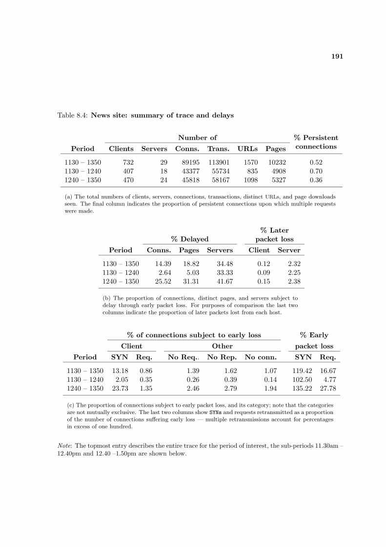
191

Table 8.4: News site: summary of trace and delays

Number of % PersistentconnectionsPeriod Clients Servers Conns. Trans. URLs Pages

1130 – 1350 732 29 89195 113901 1570 10232 0.521130 – 1240 407 18 43377 55734 835 4908 0.701240 – 1350 470 24 45818 58167 1098 5327 0.36

(a) The total numbers of clients, servers, connections, transactions, distinct URLs, and page downloadsseen. The final column indicates the proportion of persistent connections upon which multiple requestswere made.

% Later% Delayed packet loss

Period Conns. Pages Servers Client Server

1130 – 1350 14.39 18.82 34.48 0.12 2.321130 – 1240 2.64 5.03 33.33 0.09 2.251240 – 1350 25.52 31.31 41.67 0.15 2.38

(b) The proportion of connections, distinct pages, and servers subject todelay through early packet loss. For purposes of comparison the last twocolumns indicate the proportion of later packets lost from each host.

% of connections subject to early loss % Early

Client Other packet loss

Period SYN Req. No Req.. No Rep. No conn. SYN Req.

1130 – 1350 13.18 0.86 1.39 1.62 1.07 119.42 16.671130 – 1240 2.05 0.35 0.26 0.39 0.14 102.50 4.771240 – 1350 23.73 1.35 2.46 2.79 1.94 135.22 27.78

(c) The proportion of connections subject to early packet loss, and its category; note that the categoriesare not mutually exclusive. The last two columns show SYNs and requests retransmitted as a proportionof the number of connections suffering early loss — multiple retransmissions account for percentagesin excess of one hundred.

Note: The topmost entry describes the entire trace for the period of interest, the sub-periods 11.30am –12.40pm and 12.40 –1.50pm are shown below.

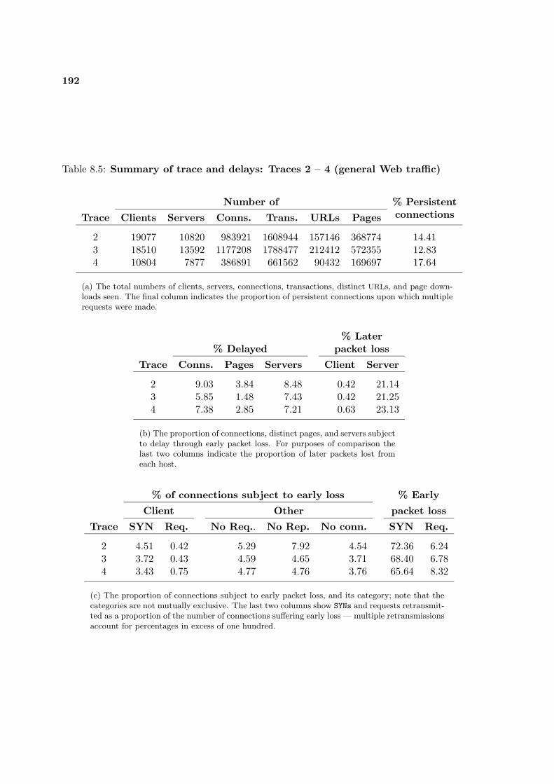
192

Table 8.5: Summary of trace and delays: Traces 2 – 4 (general Web traffic)

Number of % PersistentconnectionsTrace Clients Servers Conns. Trans. URLs Pages

2 19077 10820 983921 1608944 157146 368774 14.413 18510 13592 1177208 1788477 212412 572355 12.834 10804 7877 386891 661562 90432 169697 17.64

(a) The total numbers of clients, servers, connections, transactions, distinct URLs, and page down-loads seen. The final column indicates the proportion of persistent connections upon which multiplerequests were made.

% Later% Delayed packet loss

Trace Conns. Pages Servers Client Server

2 9.03 3.84 8.48 0.42 21.143 5.85 1.48 7.43 0.42 21.254 7.38 2.85 7.21 0.63 23.13

(b) The proportion of connections, distinct pages, and servers subjectto delay through early packet loss. For purposes of comparison thelast two columns indicate the proportion of later packets lost fromeach host.

% of connections subject to early loss % Early

Client Other packet loss

Trace SYN Req. No Req.. No Rep. No conn. SYN Req.

2 4.51 0.42 5.29 7.92 4.54 72.36 6.243 3.72 0.43 4.59 4.65 3.71 68.40 6.784 3.43 0.75 4.77 4.76 3.76 65.64 8.32

(c) The proportion of connections subject to early packet loss, and its category; note that thecategories are not mutually exclusive. The last two columns show SYNs and requests retransmit-ted as a proportion of the number of connections suffering early loss — multiple retransmissionsaccount for percentages in excess of one hundred.

Chapter 9

Conclusions and Scope for FutureWork

This final chapter of the dissertation summarises the work upon which it is based and assessesthe original contribution of the work. The closing section describes continuing developmentof the Nprobe monitor and post-collection analysis, and indicates the scope for future work.

9.1 Summary

As the volume of traffic carried by networks continues to increase, and the bandwidths em-ployed rise, passive monitoring is faced with a dual challenge: to keep pace with the observedtraffic, and to store and manage the potentially very large volume of data collected. Althoughthere is a body of research dedicated to monitoring ever-faster network technologies, the com-mon approach to these challenges is to limit capture to TCP/IP headers — hence boundingboth computational expense and volume, or to sub-sample. Packet capture continues to relyprincipally on packet-filter–based mechanisms which may also be used selectively, but whichimpose a coarse-grained data discard policy.

Such an approach has the great disadvantage that activity at higher levels of the protocolstack cannot be directly observed, and, crucially, that the facility to examine the interactionbetween higher and lower level protocols is severely limited. As a consequence, research basedupon passive monitoring has often been shaped by the limitations of the available tools.

Chapter 1 introduces the concept of a monitor designed to keep pace with higher bandwidthsand which captures data simultaneously from the whole of a range of protocols of interest,and discusses the attributes desirable in pursuit of this goal. In particular, it is suggested thatthe design should minimise data bulk through extraction, abstraction, and storage of only thedata of interest — leading in turn to integration of data over disparate protocol data units andthe need to maintain state. The design should be scalable: by striping packets across multipleprocessors, possibly in a cluster of monitoring machines, to accommodate high traffic volume;and through modularity, to allow the addition and tailoring of data collection mechanisms

194 Conclusions and Scope for Future Work

to varying experimental demands. Such a monitor should also be efficient, minimising datacopying and control overheads.

A considerable body of research has been founded upon passive network monitoring andChapter 2 outlines a selection of the most relevant work. It is seen that the two themes —of monitoring higher bandwidths, and of monitoring a wider range of protocols — have notsignificantly come together in any single project or wide deployment of monitoring effort. Thefew projects which have extended the range of protocols monitored (e.g. Windmill [Malan98b],IPSE [Internet Security96], BLT [Feldmann00]) have either not been designed to monitor highbandwidths (Windmill, IPSE) or have been designed only to study an integrated but limitedrange of protocols (BLT). Other studies which integrate data from higher protocol levelshave relied upon a combination of TCP/IP-level traces augmented by server instrumentation(Balakrishnan et al. [Balakrishnan98]), server logs (Allman [Allman00]), or data gatheredusing active techniques (WAWM [Barford99a][Barford99b]).

Chapter 3 describes the design and implementation of a unique monitor — Nprobe — whichconstitutes the major single item of work described in this dissertation. The probe infras-tructure, common to all protocols monitored, is described, together with the protocol-specificdata extraction modules implemented to date.

Traces collected with existing monitoring tools are likely to consist of verbatim copies ofwhole or partial packets; the required data can be extracted using knowledge of the containedprotocols’ syntax and semantics — trivially in the case of those protocols (e.g. TCP, IP,RPC, or NFS) where the verbatim copy mirrors defined C language structures. Nprobe-collected traces, on the other hand, contain data which is not only already extracted butmay be abstracted or coded, and which is variable in nature and format as determined byexperimental requirements; a common interface for data retrieval is required. The relativelyrich and complex data contained in Nprobe traces, moreover, will be collected for the purposeof, and subject to, commensurately more complex and sophisticated post-collection analysis.An early decision was therefore made that the Nprobe design would be incomplete withoutan accompanying post-collection analysis infrastructure.

Chapter 4 describes the post-collection analysis of Nprobe traces based upon an analysistoolkit which provides a data-retrieval interface generated automatically from the data struc-ture definitions contained in the Nprobe data extraction modules, a library of standard ana-lytical methods for the protocols so far incorporated, and an analysis development environ-ment. Visualisation tools are also provided to present trace data in a summarized and readilycomprehensible form, and to assist in identifying and reasoning about the interrelationshipsbetween the activities represented by it. An analysis definition and control infrastructuredefines the analysis to be carried out and accumulates the data generated, while an analysissummary tool presents the, possibly high, volume of results and an analysis log. The datagenerated may be examined using the toolkit’s own plotting tool, which, together with thesummary tool, is integrated with the analysis modules to allow the derivation of any resultto be re-run and examined in detail. Analysis code may also be modified and re-run underclose scrutiny during the analysis process, hence supporting iterative design. The potentiallylarge volumes of trace data to be analysed dictate that mechanisms should also be providedto allow partitioning of analysis, and that confidence in results should be supported by thefacility to follow an audit trail based upon the data’s derivation.

9.2 Assessment 195

The possession of data from multiple protocols allows analysis to examine activity at anyprotocol level with an accurate knowledge of events at other levels. Chapter 5 presents anactivity model of TCP behaviour which differentiates and quantifies the effects of the network,TCP itself, and application-level processes. The detailed information provided by the modelmay, in turn, be used as the basis for trace-driven simulations which, by varying the knownparameters of the observed connections, can be used to investigate what if scenarios and, forinstance, to assess the exact effects of loss, RTT variation, or changes in server latencies.

Use of the activity model is illustrated in Chapter 6 in a case study of Web server latency.Traffic carrying artificial server loads is observed to assess the accuracy of the modellingtechnique, and the changing latency of a busy server examined as load increases.

The investigation of Web page downloads based upon passive monitoring has, because of thelimited data gathered by existing tools, been largely confined to the study of the downloadof individual page components. Chapter 7 explains how the comprehensive data collectedby Nprobe can be used to accurately reconstruct the total activity involved in the downloadof whole pages, hence allowing the relationships between HTTP transactions and the TCP

connections carrying them to be examined in full context, and the download to be analysedas a complete system of activity.

Finally, Chapter 8 draws together the work described in earlier chapters in a case study ofdelay in Web page downloads. It is demonstrated that whole page delays are not simply thesum of component delays; the technique of page download reconstruction is used to assess thedownload times of pages observed in traffic to a popular news site, with particular emphasison major delays caused by packet loss occurring before the establishment of TCP RTTs . Theconnection modelling and simulation techniques introduced in Chapter 5 are then used toexamine the implications of early packet loss on the observed page downloads had persistentHTTP connections been exclusively used.

9.2 Assessment

This section of the dissertation measures the work described in the previous chapters againstthe thesis and hypothesis stated in Chapter 1, and assesses its original contribution to thefield of passive network monitoring.

“The thesis of this dissertation may be summarised thus: observation of thenetwork and the study of its functioning have relied upon tools which, largely forpractical reasons, are of limited capability. Research relying upon these tools mayin consequence be restricted in its scope or accuracy, or even determined, by thebounded set of data which they can make available. New tools and techniques areneeded which, by providing a richer set of data, will contribute to enhanced un-derstanding of application performance and the system as a whole, its constituentcomponents, and in particular the interaction of the sub-systems represented bythe network protocol stack.

The hypothesis follows that such improved tools are feasible, and is tested by

196 Conclusions and Scope for Future Work

the design and implementation of a new monitoring architecture — Nprobe whichis then used in two case studies which would not have been possible without sucha tool.”

9.2.1 Conclusion

Chapter 2 draws attention to the paucity of research based upon examination of activity at alllevels of the network protocol stack, and shows that when such research has been conducted,it has rarely drawn all of its data from passive monitoring of the network. A small bodyof research has been based upon data gathered from levels above TCP/IP, but has beenbased upon monitoring systems designed for a single protocol set, or has not addressed theparallel challenge of keeping pace with contemporary network bandwidths. Current work inmonitoring high-speed network technologies has, conversely, limited itself to the traditionalcollection of a verbatim copy of a limited set of lower-level protocol headers.

It is axiomatic that any research based upon gathered data must be shaped by the scope ofthat data. All inter-computer communications are based upon complex systems of interrelatedand interacting components and protocols, yet current tools fail to exploit the breadth andscope of the data available through passive monitoring, and as a consequence, research islargely limited to investigation of sub-systems of the whole. The limitation is manifest in twoways: at the granularity of a single connection only a subset of the protocols are studied, andat the larger granularities often implicit in application activity, the set of connections usedmay not be accurately identified and associated with that activity. In both cases the study ofapplication-level activity is inhibited, and the interactions between system components maynot be manifest, identifiable, or quantifiable.

A passive network monitor has been designed and implemented which successfully circum-vents the limitations of existing tools of the genre. By extracting only the data of interest frompassing traffic the bulk to be stored is reduced, and data from the whole range of contributingprotocols can be captured. Careful attention to efficiency of operation, and to achieving adata-reduction ratio which balances computational expense against storage volume, enablesthe design to keep pace with relatively high bandwidths. Extensibility in terms of the pro-tocols studied is ensured by the provision of a common infrastructure and protocol-centricdata extraction modules, which also provide the capacity to tailor data collection to specificneeds. The extensibility required to keep pace with higher traffic bandwidths is providedby partitioning data processing between multiple processors, possibly located in clusters ofmonitoring machines.

A more comprehensive set of gathered data suggests the potential for post-collection analysisemploying a variety of more sophisticated techniques, particularly as the interplay of activityinherent in examination of a greater range of subsystems is captured. The richer nature of thedata, moreover, also suggests that, for any data set, the range of analysis that can be carriedout is wider and more varied. There is consequently a danger that the full informationalpotential of the data gathered will not be realised if analysis tasks are designed in an ad-hocmanner: an environment is called for where analysis tasks can be designed and executed withminimal time expenditure; which supports a common data retrieval interface, reuse of analysis

9.2 Assessment 197

components, and investigative analysis design; and reflects the bulk and complexity of thedata. The analysis infrastructure and toolkit accompanying the Nprobe monitor meet thisrequirement, and represent a foundation upon which the new analysis techniques presentedin this dissertation are constructed.

New and powerful analysis techniques — the TCP activity model, Web server latency mea-surement, Web page download reconstruction and delay assessment, the investigation of earlypacket loss effects, both as observed and as assessed using accurate trace-driven simulation —demonstrate the greater understanding of application-level behaviour and system componentinteractions which can be contributed by gathering a more complete set of data from thenetwork, and which would not be possible without it. Some of these analysis techniques aregeneral, others are directed towards specific protocols or tasks, but all can be generalised.

In summary — a new and more powerful passive monitoring design has been implementedand used to gather a considerable amount of data from a range of network protocols. Newanalysis techniques have been developed which exploit the comprehensive contents of thedata and have demonstrated the ability to investigate and understand behaviour at network,transport and application levels of the protocol stack. The utility of the monitor, and of theenhanced analysis of the gathered data have thus been demonstrated.

9.2.2 The Original Contribution of this Dissertation

The proposition that passively monitored data would contribute to more comprehensive re-search if the data were to be gathered from a wider range of network protocols is hardlynew. The requirement for probes to keep pace with increases in network bandwidths is wellrecognised and such probes are the subject of ongoing development. It is then, perhaps,rather surprising that so few probes have been designed to gather data from protocols be-yond TCP/IP1, and that no probe has yet been developed for use by the network researchcommunity which directly addresses both needs.

The Nprobe design, therefore, makes a new and powerful contribution to the field of computernetwork research based upon passively monitored and gathered data. For the first time thethree requirements of multi-protocol data capture, capacity to monitor high bandwidths, andgeneral applicability (i.e. the capacity to extend and tailor data gathering to the requirementsof a specific study) have been addressed in a single probe implementation. The probe istherefore not only capable, but highly flexible.

The implications for future research based upon such a tool are considerable: application-levelactivity can not only be observed directly, but can be related to lower-level activity; eventshitherto studied at the granularity of a single connection can be aggregated into the multiplesassociated with higher-level activity; and the interactions of components at all levels andgranularities can be studied. Probe placements are not (as) limited to low-volume (and hencepossibly unrepresentative) links, and data reduction allows for longer traces to be gathered

1Probes based upon the packet filter and its variants can, of course, do so, simply by capturing a greaterpacket length, but are largely discounted because of the data copy overheads and the infeasibly high volumeof the resulting capture.

198 Conclusions and Scope for Future Work

for any set traffic volume and mix.

Neither is the association of data collection and analysis into a single system entirely new:Coral Reef [Keys01], netflow [Cisco-Netflow], and NIMI [Paxson98][Paxson00], for instance,all provide standard analysis and report mechanisms. These mechanisms are, however, essen-tially static: set measurements are performed and subject to one or more standard analyses.Nprobe breaks new ground in providing an analysis toolkit and environment designed tosupport not only the execution of post-collection analysis tasks, but their fast design anddevelopment; the richness and complexity of the data gathered must be matched by equallysophisticated analysis methods.

The variable and extensible nature of the data collected has required the development of aunique, automatically generated, data retrieval interface which can be used by any analysistask. The principle is extended into an innovative framework of standard analysis control,data collection, and analysis summary tools accompanied by a library of reusable analysisclasses. Full advantage is taken of the object-oriented software model to ensure that theinfrastructure and analysis classes can be rapidly modified through sub-typing and composedto meet the requirements of specific tasks. Two new visualisation techniques also introducenovel features: a TCP connection visualisation tool, and a Web download visualisation tool,present not only a summary of trace data but also the results of the analysis carried out onit. The relationships within the data are made more easily identifiable, and confidence ispromoted by the explicit connection between original and generated data which is displayed.The design and testing of complex analysis would be very much more difficult without suchtools.

The provision of a fully integrated and extensible analysis toolkit also enables the incorpo-ration of other novel features: both the analysis summary tool and a dedicated data plotteremploy callback mechanisms which allow the derivation of individual or multiple results tobe examined in detail and the appropriate visualisations instantiated. Thus development andconfidence are both supported.

The TCP activity model represents a new technique for the examination of individual TCP

connections and the discrimination of activity determined by the separate components atnetwork, TCP and application-levels. The model is also innovative in its independence ofprobe position and ability to interpret TCP-level activity without a priori knowledge of theparticipating implementations.

Another new and far reaching technique that has been introduced is that of Web page down-load reconstruction, enabling downloads to be studied as a whole, and the contribution andinteraction of all components assessed. Such a technique is particularly valuable as it rep-resents the ability to accurately investigate communications involving multiple connections,where previously they would have to be studied individually, and their relationships inferred.

The two case studies which have been presented, investigations into Web server latenciesand Web page download times, represent original and unique research into Web activity.This area was chosen to demonstrate Nprobe capabilities because, although the protocolsand principles involved are relatively well understood, it is also a field where the accurateinvestigation of certain fundamental phenomena — those involved in whole page downloads

9.3 Scope for Future Work 199

— have been beyond reach without the range of data gathered by Nprobe and the analysistechniques which depend upon it. The study presented in Chapter 8, in particular, representsunique work in its assessment of individual transactions’ contribution to overall page downloadtimes, the investigation of early loss, and the accuracy of the simulations used in assessing analternative download scenario.

Although the case studies are included primarily as examples of the power of the Nprobe

monitor, and the analysis techniques which it makes possible, they stand as original researchin their own right. It is important to note that the underlying analysis makes use of thecommon analysis infrastructure and TCP analysis classes, which could contribute equally tothe investigation of other protocol sets. The elements of analysis specific to HTTP and HTML

would contribute equally to wider analysis of these protocols, but, more importantly, establishprinciples and techniques which can be generalised to the study of further protocols.

The potential of the monitor, and the breadth of new research which it makes feasible, arerecognised by the establishment of two new projects which are based upon it. The ComputerLaboratory’s Gridprobe project will build upon the work described here to continue Nprobe

development, with the aim of increasing capture rates and extending the range of protocolsand tools. The Intel Cambridge Laboratory’s Scope project [Hamilton03] will collaborativelypursue the same aims.

9.3 Scope for Future Work

It is convenient to present discussion of the scope for future work under the heads of furtherinvestigation into Web traffic and continuing Nprobe development.

9.3.1 Further Analysis of Web Activity

Although the exemplary studies presented here have concentrated upon the assessment ofdelay due to early packet loss, it will be little more than a triviality to extend the workto assess the impact of download delay due to all causes, and the contributions made byboth server and browser. In particular, initial investigations indicate that browsers maysometimes behave in a less than optimal manner, and this may prove a fruitful field forfurther investigation. It is hoped that future probe placements will present the opportunityto observe a more representative sample of traffic than that so far encountered, and that thismay be used to establish up to date traffic characterisations, which will be more valuablethan those hitherto available because they will be page, rather than object, based.

It is remarked that the Web traffic gathered to date provides almost an embarrassment ofinformation that might be extracted by widening existing analysis methods, but that furtherexamples of possible research include extension of the HTTP data extraction module to gatherobject lifetime, freshness, and caching data to study cache behaviour and effectiveness. Itis also noted, for instance, that a high proportion of GET requests are conditional, and thatof these a very high proportion receive not modified responses; it may be that those re-

200 Conclusions and Scope for Future Work

sponsible are unduly pessimistic about object lifetimes, and that considerable unnecessarytraffic is therefore generated. Informal observation suggests that the number of individualpages drawing content from multiple servers appears to be growing, particularly where partialcontent (e.g. that from ad-servers or CDNs) is independent of the main content. It would beinteresting to know whether such multiple sourcing has deleterious effects upon performance.

In some cases analysis of the collected data reveals that full understanding of the phenomenaseen can only be achieved through further observation, or data gathering by other means.Section 7.4.3, for example, refers to aborts of apparently healthy TCP connections as indicatorsof aborted page downloads. While this situation can be inferred from currently gathered data,accurate identification of aborted or recommenced downloads, and their correlation withdelay, must depend upon the dependable recognition of user behaviour based upon patternsestablished using mechanisms such as instrumented browsers, or the observation of browsingsessions set up for the purpose.

9.3.2 Nprobe Development

Current work is concentrating on benchmarking Nprobe performance — no probe placementhas so far provided traffic volumes sufficient to test its capabilities — and increasing potentialcapture rates. The capabilities of the available NICs are being investigated, together withimprovements to their drivers to allow higher degrees of interrupt coalescence. The use ofmore powerful NICs, such as the DAG cards, may also be investigated. Work is also requiredto optimise the way in which workload is shared across multiple processors, particularly dualcore architectures.

Because Nprobe is designed to allow the simple addition of further protocol-based data extrac-tion modules, the scope for further work using it is very wide — the existence and availabilityof a more powerful tool leads to further research, and ease of analysis development encouragesinnovative studies. There are currently plans to add a Border Gateway Protocol (BGP) mod-ule to investigate routing convergence and stability, and further modules designed to observestreamed media traffic. Future work may include investigations of real and user-perceivedQuality of Service, denial-of–service attack detection, traffic engineering issues, and extensioninto observation of new Grid traffic types.

The use of Nprobe is not, of course, limited to the observation of established protocols andapplication activity: its unique capabilities may make it a valuable tool in the developmentof new protocols, and of distributed systems.

Appendix A

Class Generation with SWIG

Figure A.1 on the following page illustrates the generation of the data retrieval interface bySWIG. Input, in the form of the relevant C header files, is converted into a Python mod-ule — the data retrieval interface — defining a series of Python classes, each analogous toone of the C structures in which data is stored and dumped by Nprobe, and having dataattributes corresponding to the fields of the C structure. SWIG output consists of the Pythonmodule containing the class definitions, a C file containing the class implementations, andan (optional) documentation file. The class definitions include initialization and destructormethods for the class, together with a set of accessor methods for the data attributes. TheC implementation file is compiled into a library which is imported into the Python interfacemodule.

A.1 Interface Definition

SWIG operation and module generation are specified in an interface definition file which liststhe header files upon which class generation is to be based, and also those which must beincluded in the C interface implementation file. Any changes in the header files are incorpo-rated into the interface by regenerating it under the control of the normal make dependencyhierarchy.

The SWIG interface definition file allows considerable flexibility in the generation of the desiredmodule. Additional C structures may be defined, generating further classes for inclusion in themodule, and C function prototypes may be included which will generate module-level functionsimplemented by C code, also included in the interface file, and which is copied verbatiminto the C interface implementation file. Such C code may be specified as implementingfurther methods (helper functions) for each of the classes generated. Defining methods for theinterface classes in this way can lead to efficiency gains in certain circumstances: automaticallygenerated accessor methods for nested classes (structures) will call an accessor method foreach level of nesting whereas a helper function can return the desired value in a single method(function) call, and where manipulation of the underlying C structure is required, this can beimplemented directly by helper functions.

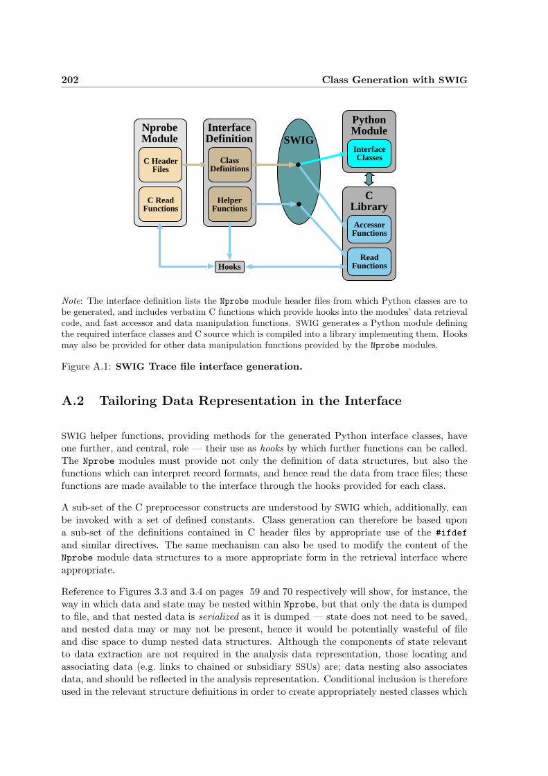
202 Class Generation with SWIG

PythonModule

InterfaceClasses

CLibrary

AccessorFunctions

ReadFunctionsHooks

SWIGNprobeModule

C HeaderFiles

C ReadFunctions

InterfaceDefinition

ClassDefinitions

HelperFunctions

Note: The interface definition lists the Nprobe module header files from which Python classes are tobe generated, and includes verbatim C functions which provide hooks into the modules’ data retrievalcode, and fast accessor and data manipulation functions. SWIG generates a Python module definingthe required interface classes and C source which is compiled into a library implementing them. Hooksmay also be provided for other data manipulation functions provided by the Nprobe modules.

Figure A.1: SWIG Trace file interface generation.

A.2 Tailoring Data Representation in the Interface

SWIG helper functions, providing methods for the generated Python interface classes, haveone further, and central, role — their use as hooks by which further functions can be called.The Nprobe modules must provide not only the definition of data structures, but also thefunctions which can interpret record formats, and hence read the data from trace files; thesefunctions are made available to the interface through the hooks provided for each class.

A sub-set of the C preprocessor constructs are understood by SWIG which, additionally, canbe invoked with a set of defined constants. Class generation can therefore be based upona sub-set of the definitions contained in C header files by appropriate use of the #ifdef

and similar directives. The same mechanism can also be used to modify the content of theNprobe module data structures to a more appropriate form in the retrieval interface whereappropriate.

Reference to Figures 3.3 and 3.4 on pages 59 and 70 respectively will show, for instance, theway in which data and state may be nested within Nprobe, but that only the data is dumpedto file, and that nested data is serialized as it is dumped — state does not need to be saved,and nested data may or may not be present, hence it would be potentially wasteful of fileand disc space to dump nested data structures. Although the components of state relevantto data extraction are not required in the analysis data representation, those locating andassociating data (e.g. links to chained or subsidiary SSUs) are; data nesting also associatesdata, and should be reflected in the analysis representation. Conditional inclusion is thereforeused in the relevant structure definitions in order to create appropriately nested classes which

A.2 Tailoring Data Representation in the Interface 203

include only the state fields required to associate and link SSUs and recreate data nesting.Serialized data structures are retrieved into the original nested form.

Appendix B

An Example of Trace File DataRetrieval

Section 4.2.2 on page 87 explains the role of automatically generated Python retrieval classesand utility module functions, provided by the analysis infrastructure, when reading trace filedata. The examples in this Appendix demonstrate the use of the infrastructure during theanalysis process.

B.1 A Typical Data-Reading Function

The Code Example in this section shows how a get data function1 retrieves selected datafrom an Nprobe trace file.

2 #

3 # Retrieve TCP connection and HTTP transaction data

4 # from Nprobe trace files:

5 # - argument file_list is list of trace files

6 # - returns data as list of connection/transaction list tuples

7 #

9 from np_file_util import get_files , EOF

10 from np_http_util import allocate_http_reusable_objects

11 from np_http_util import get_http_rec_and_trans

12 from np_TCPConn import TCPConn

13 from np_HTTPTrans import HTTPTrans

14 from nprobe import REC_TCP_HTTP

16 def get_data(file_list):

1The example shows a function called by a data analysis script, but it could equally well be a method of ananalysis object. Whether to drive analysis through function calls made by a script, or method invocations ofan analysis object will depend upon which is the more appropriate for the analysis task in hand.

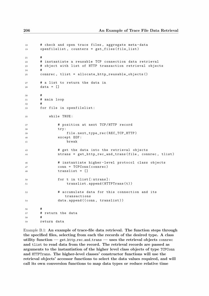
206 An Example of Trace File Data Retrieval

18 # check and open trace files , aggregate meta -data

19 openfilelist , counters = get_files(file_list)

21 #

22 # instantiate a reusable TCP connection data retrieval

23 # object with list of HTTP transaction retrieval objects

24 #

25 connrec , tlist = allocate_http_reusable_objects ()

27 # a list to return the data in

28 data = []

30 #

31 # main loop

32 #

33 for file in openfilelist:

35 while TRUE:

37 # position at next TCP/HTTP record

38 try:

39 file.next_type_rec(REC_TCP_HTTP)

40 except EOF:

41 break

43 # get the data into the retrieval objects

44 ntrans = get_http_rec_and_trans (file , connrec , tlist)

46 # instantiate higher -level protocol class objects

47 conn = TCPConn(connrec)

48 translist = []

50 for t in tlist [: ntrans ]:

51 translist.append(HTTPTrans(t))

53 # accumulate data for this connection and its

transactions

54 data.append ((conn , translist))

56 #

57 # return the data

58 #

59 return data

Example B.1: An example of trace-file data retrieval. The function steps throughthe specified files, selecting from each the records of the desired type. A classutility function — get http rec and trans — uses the retrieval objects connrec

and tlist to read data from the record. The retrieval records are passed asarguments to the instantiation of the higher level class objects of type TCPConn

and HTTPTrans. The higher-level classes’ constructor functions will use theretrieval objects’ accessor functions to select the data values required, and willcall its own conversion functions to map data types or reduce relative time

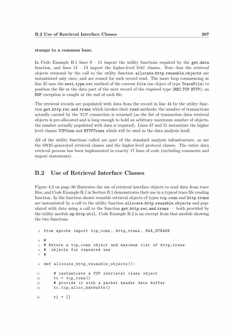
B.2 Use of Retrieval Interface Classes 207

stamps to a common base.

In Code Example B.1 lines 9 – 11 import the utility functions required by the get data

function, and lines 12 – 13 import the higher-level DAU classes. Note that the retrievalobjects returned by the call to the utility function allocate http reusable objects areinstantiated only once, and are reused for each record read. The inner loop commencing atline 35 uses the next type rec method of the current file (an object of type TraceFile) toposition the file at the data part of the next record of the required type (REC TCP HTTP); anEOF exception is caught at the end of each file.

The retrieval records are populated with data from the record in line 44 by the utility func-tion get http rec and trans which invokes their read methods; the number of transactionsactually carried by the TCP connection is returned (as the list of transaction data retrievalobjects is pre-allocated and is long enough to hold an arbitrary maximum number of objects,the number actually populated with data is required). Lines 47 and 51 instantiate the higherlevel classes TCPConn and HTTPTrans which will be used in the data analysis itself.

All of the utility functions called are part of the standard analysis infrastructure, as arethe SWIG-generated retrieval classes and the higher-level protocol classes. The entire dataretrieval process has been implemented in exactly 17 lines of code (excluding comments andimport statements).

B.2 Use of Retrieval Interface Classes

Figure 4.2 on page 86 illustrates the use of retrieval interface objects to read data from tracefiles, and Code Example B.1 in Section B.1 demonstrates their use in a typical trace file readingfunction. In the function shown reusable retrieval objects of types tcp conn and http trans

are instantiated by a call to the utility function allocate http reusable objects and pop-ulated with data using a call to the function get http rec and trans — both provided bythe utility module np http util. Code Example B.2 is an excerpt from that module showingthe two functions.

2 from nprobe import tcp_conn , http_trans , MAX_NTRANS

4 #

5 # Return a tcp_conn object and maximum list of http_trans

6 # objects for repeated use

7 #

9 def allocate_http_reusable_objects ():

11 # instantiate a TCP retrieval class object

12 tc = tcp_conn ()

13 # provide it with a packet header data buffer

14 tc.tcp_alloc_hdrbuffs ()

16 tl = []

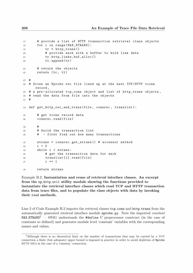
208 An Example of Trace File Data Retrieval

17 # provide a list of HTTP transaction retrieval class objects

18 for i in range(MAX_NTRANS):

19 tr = http_trans ()

20 # provide each with a buffer to hold link data

21 tr.http_links_buf_alloc ()

22 tl.append(tr)

24 # return the objects

25 return (tc , tl)

27 #

28 # Given an Nprobe rec file lined up at the next TCP/HTTP tconn

record ,

29 # a pre -allocated tcp_conn object and list of http_trans objects ,

30 # read the data from file into the objects

31 #

33 def get_http_rec_and_trans (file , connrec , translist):

35 # get tconn record data

36 connrec.read(file)

38 #

39 # build the transaction list

40 # - first find out how many transactions

42 ntrans = connrec.get_ntrans () # accessor method

43 i = 0

44 while i < ntrans :

45 # get the transaction data for each

46 translist[i].read(file)

47 i += 1

49 return ntrans

Example B.2: Instantiation and reuse of retrieval interface classes. An excerptfrom the np http util utility module showing the functions provided toinstantiate the retrieval interface classes which read TCP and HTTP transactiondata from trace files, and to populate the class objects with data by invokingtheir read methods.

Line 2 of Code Example B.2 imports the retrieval classes tcp conn and http trans from theautomatically generated retrieval interface module nprobe.py. Note the imported constantMAX NTRANS2 — SWIG understands the #define C preprocessor construct (in the case ofconstants so defined) and generates module level ‘constant’ variables with the correspondingnames and values.

2Although there is no theoretical limit on the number of transactions that may be carried by a TCP

connection a finite (but adequate) upper bound is imposed in practice in order to avoid depletion of NprobeHTTP SSUs in the case of a ‘runaway’ connection.

B.3 Using the FileRec Class to Minimize Memory Use 209

The function get http rec and trans at line 9 instantiates a single tcp conn object and alist of MAX NTRANS http trans objects. Lines 14 and 21 equip the objects with buffers intowhich they can read TCP packet header and HTML links data respectively — as the retrievalobjects are to be re-used it would be inefficient to allocate these buffers on the fly as requiredby individual record instances.

get http rec and trans at line 33 is called as each record is encountered in order to pop-ulate the retrieval classes with data from the trace file, taking as its arguments the currentTraceFile object (positioned to read the record data) and the retrieval objects. The read

method of the tcp conn object is invoked at line 36 and its get ntrans() accessor methodat line 42 in order to establish the number of transactions present. The loop at line 44 readsthe required number of transaction records serially from the file, each being populated by theread method of the corresponding http trans in the list.

B.3 Using the FileRec Class to Minimize Memory Use

Data association during analysis may exceed the available memory capacity if all data isstored. The FileRec class is used to store the location of the associated trace file recordsduring a preliminary pass through the file(s) and then, during full analysis of the associateddata, to retrieve data from file and instantiate an analysis object of the appropriate type.Code Example B.3 illustrates the association of data using FileRec objects.

3 from np_file_util import get_files , EOF from nprobe import

tcp_conn ,

4 REC_TCP_HTTP from np_filerec import FileRec , WEBCLIENT

6 #

7 # Use an initial pass through the trace to associate TCP/HTTP data

8 # on a per -client basis using the FileRec class

9 #

11 def first_pass(file_list):

13 # check and open trace files , aggregate meta -data

14 openfilelist , counters = get_files(file_list)

16 #

17 # instantiate a reusable TCP connection data retrieval object

18 #

19 connrec = tcp_conn ()

21 # a dictionary in which to store the associated data (as

FileRecs)

22 clients = {}

24 #

25 # main loop

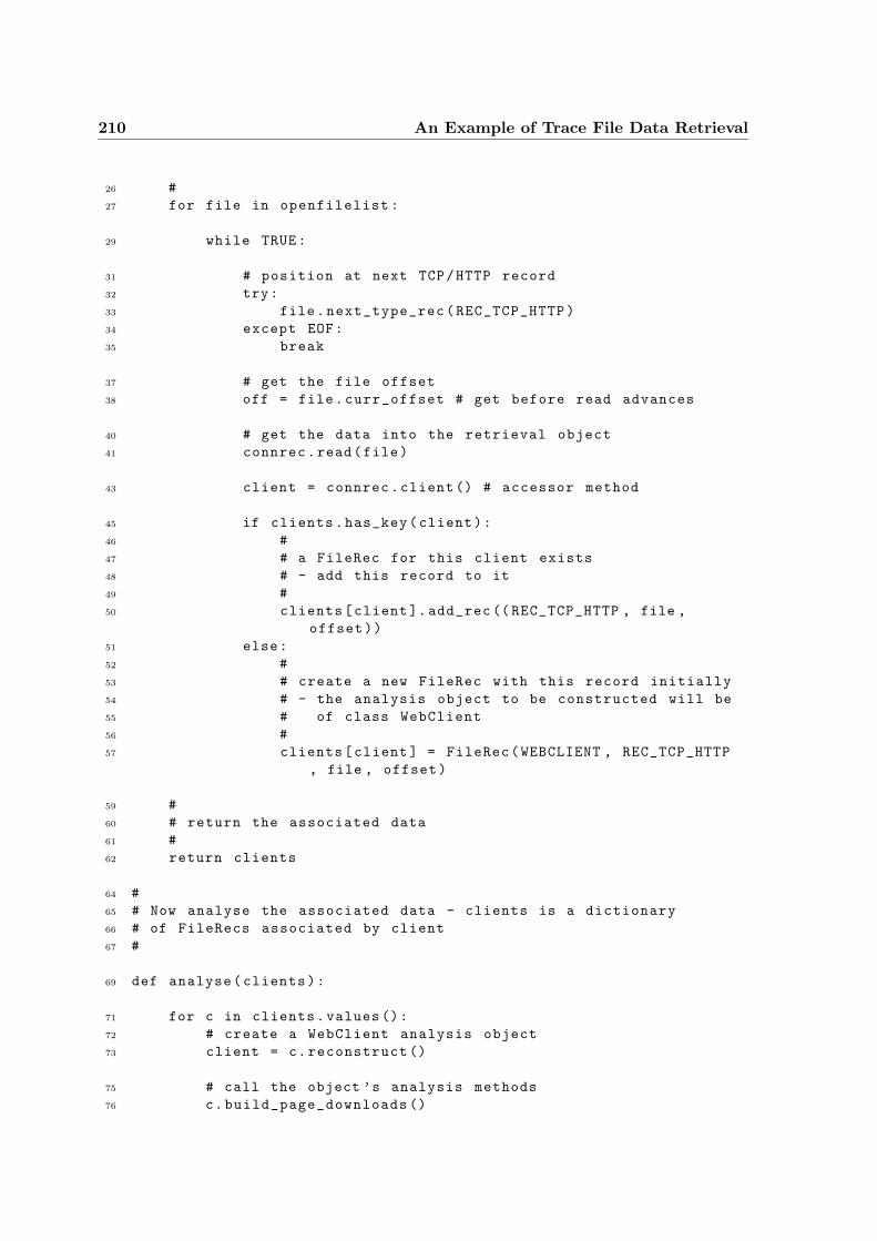
210 An Example of Trace File Data Retrieval

26 #

27 for file in openfilelist :

29 while TRUE:

31 # position at next TCP/HTTP record

32 try:

33 file.next_type_rec(REC_TCP_HTTP)

34 except EOF:

35 break

37 # get the file offset

38 off = file.curr_offset # get before read advances

40 # get the data into the retrieval object

41 connrec.read(file)

43 client = connrec.client () # accessor method

45 if clients.has_key(client):

46 #

47 # a FileRec for this client exists

48 # - add this record to it

49 #

50 clients[client ]. add_rec (( REC_TCP_HTTP , file ,

offset))

51 else:

52 #

53 # create a new FileRec with this record initially

54 # - the analysis object to be constructed will be

55 # of class WebClient

56 #

57 clients[client ] = FileRec(WEBCLIENT , REC_TCP_HTTP

, file , offset)

59 #

60 # return the associated data

61 #

62 return clients

64 #

65 # Now analyse the associated data - clients is a dictionary

66 # of FileRecs associated by client

67 #

69 def analyse(clients):

71 for c in clients.values ():

72 # create a WebClient analysis object

73 client = c.reconstruct ()

75 # call the object ’s analysis methods

76 c.build_page_downloads ()

B.3 Using the FileRec Class to Minimize Memory Use 211

77 c.first_analysis_task ()

79 .

80 .

81 .

83 return

Example B.3: Minimizing memory use by storing record locations. TCP/HTTP

data pertaining to individual clients is associated by client during an initial passthrough the trace. The data itself is not stored — objects of the FileRec classaccumulate a list of the relevant record locations. During full analysis objects ofthe WebClient class are instantiated and populated using the FileRec objects’reconstruct method.

Data association (in this case the activity associated with individual Web clients) is carriedout during the first pass through the trace file(s) by the function first pass at line 11. Theopening of the listed files at line 14 and the main loop at line 27 are substantially equivalentto the similar operations shown in Code Example B.1, but in this case protocol class objectsare not instantiated. A re-used data retrieval object reads the record from file at line 41, theonly data accessed being the address of the TCP connection client. If the client has alreadybeen encountered (the if statement at line 45) the record’s type and location are added tothe client’s existing FileRec object’s list of records at line 45. Otherwise a new FileRec

object is created, initially populated with the location of this first record encountered, andentered into the clients dictionary at line 57.

Analysis of the associated data is carried out in the analyse function at line 69 which stepsthrough the entries in the clients dictionary instantiating WebClient analysis objects atline 73 by invoking the reconstruct method of the FileRec object forming the data part ofeach dictionary client entry. The WebClient’s analysis methods are then called from line 76onwards.

Appendix C

Inter-Arrival Times ObservedDuring Web Server Latency Tests

Chapter 6 describes a technique, based upon the activity model of TCP connections, whichcan be used to distinguish and quantify network and application-level time components ofTCP connections. Sections 6.3.1 – 6.3.3 describe a series of experiments conducted to evaluatethe technique and present the results in Figures 6.1 to 6.4 on pages 145–150. This Appendixexamines the results of these experiments in the context of the request and response inter-arrival times observed at the monitor.

C.1 Interpretation of Request and Response Inter-Arrival Times

Figures C.1 and C.2 show the distribution of inter-arrival times for requests and responsesin each of the typical experiments. As the monitoring point was immediately adjacent tothe clients the request distribution shown is known to be minimally effected by variations innetwork transit times and therefore reliably represents intervals at the client.

The distribution of response inter-arrival times may assume a different shape to that ofrequests due to one or more of three factors:

• Variations in the processing time of individual requests

• Request queueing at the server

• Variations in network pRTTs between monitor and server

As care was taken to ensure that all requests could be satisfied from the server cache, andbecause demands upon the server were constant during each loading interval, variations in theprocessing time of individual requests should not materially effect the distribution of responseinter-arrival times. In the case of the local server pRTTs are typically less than 0.05 per cent

214 Inter-Arrival Times Observed During Web Server Latency Tests

of the minimum inter-arrival periods observed, and therefore can not materially effect theirdistribution.

Although pRTTs were of the same order of magnitude as inter-arrival periods in the experi-ments conducted with a distant server, examination of Figures 6.3(c) and 6.4(c) on pages 148and 150 shows that variations in pRTT are less than the significant inter-arrival periods andthat (for each averaging period) the standard error of the mean is generally less than 1 ms.It is unlikely, therefore, that pRTT variations contribute significantly to the distributions ob-served in these experiments. Reference to Figures C.2 (a) – (b) and (d) – (e) additionallyshows that response inter-arrival periods remain consistent for the proportion of responsesexpected to occur regularly, and also suggests that pRTT variation does not materially affectthe distributions seen.

It is concluded, therefore, that differences seen between the distributions for requests and re-sponses accurately reflects queueing behaviour at the server. Where a section of the responseinter-arrival time distribution is displaced from the corresponding section of the request dis-tribution, and both refer to the same set of requests/responses, the offset represents either aminimum possible server response time or the delay due to queueing.

C.2 Inter-Arrival Times for Client and Local Server with Small

Round Trip Times

Figure C.1 shows the distribution of inter-arrival times for the typical experiment using alocal server, and with small RTTs, for the range of four background loads employed (0, 200,400 and 600 objects per second, Sub-figures (a) and (c) – (e)). In all cases the proportion ofinter-arrival times attributable to each part of the observed and background loads is clearlyidentifiable, and is annotated appropriately. As background loads are added, shown in (c) –(e), the features due solely to the observed load, shown in (a) become less significant, andcontribute a correspondingly lower probability to the distribution.

Figure C.1(b) presents a detail of the small inter-arrival time distribution at zero backgroundload showing the contribution of the burst of back-to-back requests which forms part of theobserved load. It is clear that the server has a maximum service rate, represented by aminimum latency of 0.8 ms (i.e. service time TS), which is present at all background loads,and which will contribute an accumulative queueing delay of this magnitude to each responseto requests arriving back-to-back. It is exactly this accumulative delay which is seen inFigure 6.1(b) on page 145, and confirms the figures calculated by the activity model; it alsoconforms reasonably to the service time of 0.836 ms predicted by the zero-background–loadmodel of server activity.

Sub figures (c) – (e) show that, at background loads of 200 and 400 requests per second theserver response is sufficiently fast to avoid queueing for the majority of the requests, but ata background load of 600 requests per second all requests are queued. The distinct stepsintroduced into the distribution by the successively added background loads suggest that therequests generated by the loading machines were (as might be expected) neither in phase,

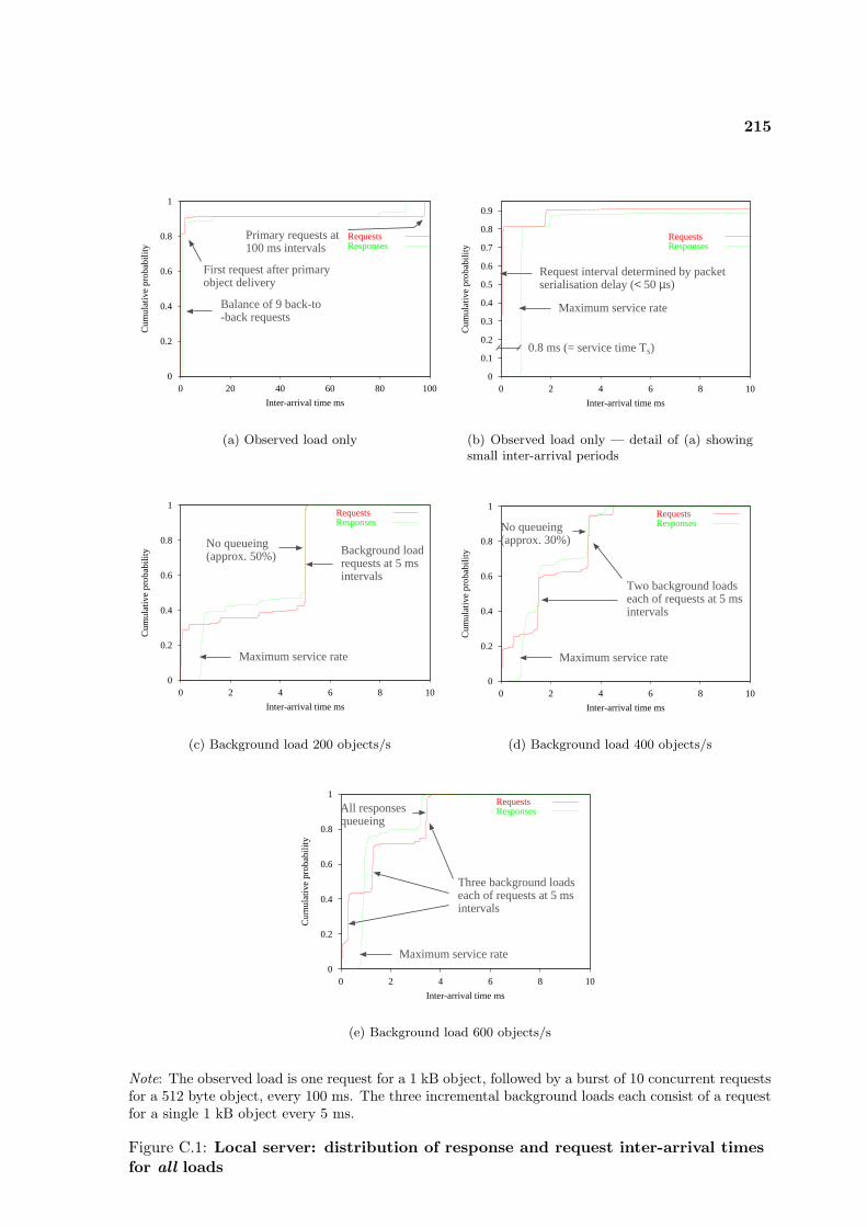
215

0

0.2

0.4

0.6

0.8

1

0 20 40 60 80 100

Cum

ulat

ive

prob

abili

ty

Inter-arrival time ms

RequestsResponses

Primary requests at100 ms intervals

First request after primaryobject delivery

Balance of 9 back-to-back requests

(a) Observed load only

0

0.1

0.2

0.3

0.4

0.5

0.6

0.7

0.8

0.9

0 2 4 6 8 10

Cum

ulat

ive

prob

abili

ty

Inter-arrival time ms

RequestsResponses

Maximum service rate

Request interval determined by packetserialisation delay (< 50 µs)

0.8 ms (= service time TS)

(b) Observed load only — detail of (a) showingsmall inter-arrival periods

0

0.2

0.4

0.6

0.8

1

0 2 4 6 8 10

Cum

ulat

ive

prob

abili

ty

Inter-arrival time ms

RequestsResponses

Maximum service rate

No queueing(approx. 50%) Background load

requests at 5 msintervals

(c) Background load 200 objects/s

0

0.2

0.4

0.6

0.8

1

0 2 4 6 8 10

Cum

ulat

ive

prob

abili

ty

Inter-arrival time ms

RequestsResponses

Maximum service rate

No queueing(approx. 30%)

Two background loadseach of requests at 5 msintervals

(d) Background load 400 objects/s

0

0.2

0.4

0.6

0.8

1

0 2 4 6 8 10

Cum

ulat

ive

prob

abili

ty

Inter-arrival time ms

RequestsResponses

Maximum service rate

All responsesqueueing

Three background loadseach of requests at 5 msintervals

(e) Background load 600 objects/s

Note: The observed load is one request for a 1 kB object, followed by a burst of 10 concurrent requestsfor a 512 byte object, every 100 ms. The three incremental background loads each consist of a requestfor a single 1 kB object every 5 ms.

Figure C.1: Local server: distribution of response and request inter-arrival timesfor all loads

216 Inter-Arrival Times Observed During Web Server Latency Tests

nor were their phases evenly distributed — although the average request arrival interval(approximately 1.4 ms at the highest load) is never less than the server’s minimum responselatency the phasing of the requests makes it inevitable that some queueing will result.

C.3 Inter-Arrival Times for Client and Distant Server with

Larger Round Trip Times

Figure C.2 shows the distribution of inter-arrival times for the typical experiments using a localserver with small RTTs on non-persistent and persistent pipelined connections, for the rangeof four background loads employed (0, 100 and 200 objects per second, sub figures (a) – (c)and (d) – (f)). Sub figures (b) and (e) show detail of the small inter-arrival time distributionat zero background load.

C.3.1 Using Non-Persistent Connections

The features of the zero-load inter-arrival times for the larger RTTs encountered in these tests,when using non-persistent connections (Figure C.2 (a) – (c)), are similar (although slightlyless well defined) to those of the tests utilising a server with small round trip times. The lesspowerful server used reflects in a lower maximum service based upon a minimum latency of2.5 ms, clearly seen in sub figure (b). This degree of latency again agrees closely with theaccumulative queueing delays calculated by the activity model for this test, and which areshown in Figure 6.3(b) on page 148, and compares with a service time of 2.82 ms derivedfrom the zero-background–load model.

The zero-load distribution features are not as well preserved by comparison, however, whenbackground loads are added (sub figure (c)), and this probably reflects the higher proportion-ate load placed upon the machine’s processor (compare Figures 6.1(d) and 6.3(d) on pages 145and 148). The distribution of background load request inter-arrival times differs dramaticallyfrom the cleanly stepped distribution seen in the case of the local server. It is suggested thatHttperf’s request-scheduling policy underlies this difference: when called upon to gener-ate a high request rate, Httperf schedules its activity by spinning between requests, henceachieving precise timings; at lower rates the select system call is used to schedule requests.The median values of background load request inter-arrival times are approximately 5 and10 ms, as expected for loads of 100 and 200 requests per second, with a mean dispersion ofapproximately 2.5 ms — a typical, and expected, degree of precision when using the select

mechanism.

C.3.2 Using Persistent Pipelined Connections

Zero-load inter-arrival time distributions for a typical test using persistent connections withpipelined requests are shown in Figure C.2 (d) and (e). Sub figure (d) demonstrates thedivision of request intervals into those between primary requests (approximately 9.1% of the

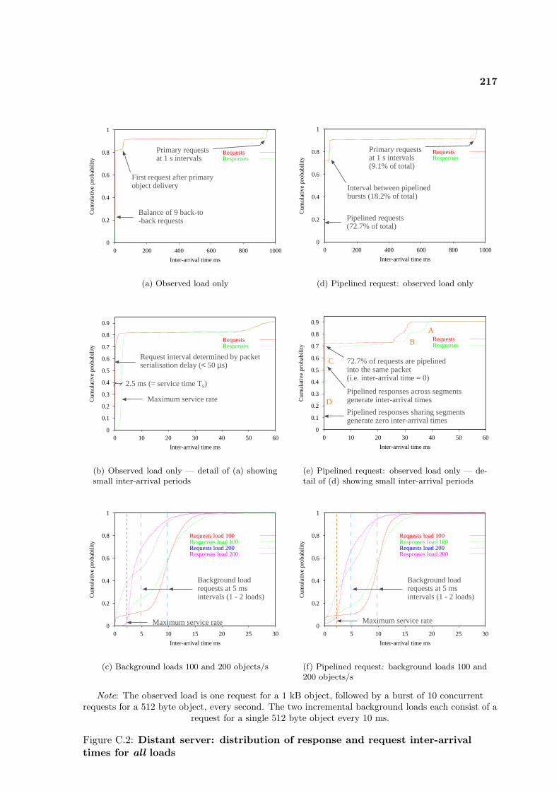
217

0

0.2

0.4

0.6

0.8

1

0 200 400 600 800 1000

Cum

ulat

ive

prob

abili

ty

Inter-arrival time ms

RequestsResponses

Primary requestsat 1 s intervals

First request after primaryobject delivery

Balance of 9 back-to-back requests

(a) Observed load only

0

0.2

0.4

0.6

0.8

1

0 200 400 600 800 1000

Cum

ulat

ive

prob

abili

ty

Inter-arrival time ms

RequestsResponses

Primary requestsat 1 s intervals(9.1% of total)

Interval between pipelinedbursts (18.2% of total)

Pipelined requests(72.7% of total)

(d) Pipelined request: observed load only

0

0.1

0.2

0.3

0.4

0.5

0.6

0.7

0.8

0.9

0 10 20 30 40 50 60

Cum

ulat

ive

prob

abili

ty

Inter-arrival time ms

RequestsResponses

Maximum service rate

Request interval determined by packetserialisation delay (< 50 µs)

2.5 ms (= service time TS)

(b) Observed load only — detail of (a) showingsmall inter-arrival periods

0

0.1

0.2

0.3

0.4

0.5

0.6

0.7

0.8

0.9

0 10 20 30 40 50 60

Cum

ulat

ive

prob

abili

ty

Inter-arrival time ms

RequestsResponses

Pipelined responses sharing segmentsgenerate zero inter-arrival times

72.7% of requests are pipelinedinto the same packet(i.e. inter-arrival time = 0)

Pipelined responses across segmentsgenerate inter-arrival times

A

B

C

D

(e) Pipelined request: observed load only — de-tail of (d) showing small inter-arrival periods

0

0.2

0.4

0.6

0.8

1

0 5 10 15 20 25 30

Cum

ulat

ive

prob

abili

ty

Inter-arrival time ms

Requests load 100Responses load 100Requests load 200Responses load 200

Maximum service rate

Background loadrequests at 5 msintervals (1 - 2 loads)

(c) Background loads 100 and 200 objects/s

0

0.2

0.4

0.6

0.8

1

0 5 10 15 20 25 30

Cum

ulat

ive

prob

abili

ty

Inter-arrival time ms

Requests load 100Responses load 100Requests load 200Responses load 200

Maximum service rate

Background loadrequests at 5 msintervals (1 - 2 loads)

(f) Pipelined request: background loads 100 and200 objects/s

Note: The observed load is one request for a 1 kB object, followed by a burst of 10 concurrentrequests for a 512 byte object, every second. The two incremental background loads each consist of a

request for a single 512 byte object every 10 ms.

Figure C.2: Distant server: distribution of response and request inter-arrivaltimes for all loads

218 Inter-Arrival Times Observed During Web Server Latency Tests

total), between two bursts of pipelined requests (18.2%) and pipelined requests (72.7%). It issuggested, therefore, that the principal features exhibited by the distribution are determinedby the pipelining behaviour of the requesting agent.

Sub-figure (e) shows the detail of (d) and is clarified by reference to Figure 6.5 on page 151,which shows the pattern of pipelining for request bursts and responses. The differing intervalbetween the transmission of the primary response and the first response burst (approximately32 ms) and the first and second response bursts (approximately 38 ms) are seen at B andA. The 45% of all responses whose initial octets share a segment with those of the precedingresponse result in zero inter-arrival times seen at D; 27 per cent of pipelined responses whoseinitial octets are carried in a subsequent segment are seen at C. It is clear that the principalfeatures of the response inter-arrival time distribution are also determined largely by thepattern of pipelining. It is interesting to note, however, that the segments carrying responses#4 –#10 are not transmitted back to back1, but are separated by approximately 1.5 ms (C).It may be that this interval represents a maximum service rate for pipelined responses, whichis feasible compared with the 2.5 ms minimum latency exhibited for non-persistent and non-pipelined responses, where each involves the additional computational expense of creatingand scheduling a separate server thread — the zero-background–load model of the server,however, does not support this supposition. The lower workload in the persistent/pipelinedcase is reflected in the lower CPU load factor seen in Figure 6.4(d).

The predominant features of the distributions with the addition of background load (Sub-figure C.2(f)) are dictated by the additional loadings, and are essentially similar to those inthe case of non persistent connections shown in sub figure C.2(c). The different pattern ofobserved load is, however, reflected in the lower left-hand part of the two plots.

1The activity model assumes that these segments are transmitted back to back, and that the responsesthat they carry are, therefore, subject to null delays (see Section 6.3.3 on page 149). This will not introduceinaccuracy, but the model should be enhanced to recognise such delays between pipelined responses.

Bibliography

[Allman98] M. Allman, S. Floyd, and C. Partridge. RFC 2414: Increasing TCP’sInitial Window, September 1998. Status: INFORMATIONAL. (p 130)

[Allman99a] M. Allman, V. Paxson, and W. Stevens. RFC 2581: TCP CongestionControl, April 1999. (pp 94, 114, 124, 130)

[Allman99b] Mark Allman and Vern Paxson. On Estimating End-to-End NetworkPath Properties. In SIGCOMM, pages 263–274, 1999. (p 40)

[Allman00] Mark Allman. A Web Server’s View of the Transport Layer. ACM SIG-COMM Computer Communication Review, 30(5):10–20, 2000. (pp 41,

42, 194)

[Allman02] M. Allman, S. Floyd, and C. Partridge. RFC 3390: Increasing TCP’sInitial Window, October 2002. Status: PROPOSED STANDARD.(pp 114, 130)

[Anerousis97] N. Anerousis, R. Caceres, N. Duffield, A. Feldmann, A. Greenberg,C. Kalmanek, P. Mishra, K.K. Ramakrishnan, and J. Rexford. Usingthe AT&T Labs PacketScope for Internet Measurements, Design, andPerformance Analysis. AT&T Services and Infrastructure PerformanceSymposium, November 1997. (p 32)

[Apisdorf96] J. Apisdorf, K. Claffy, K. Thompson, and Rick Wilder. OC3MON: flexi-ble, affordable, high performance statistics collection. Technical Report,National Laboratory for Applied Network Research., 1996. An overviewis available at http://www.nlanr.net/NA/Oc3mon/. (p 32)

[Balakrishnan98] Hari Balakrishnan, Venkata N. Padmanabhan, Srinivasan Seshan, MarkStemm, and Randy H. Katz. TCP Behavior of a Busy Internet Server:Analysis and Improvements. In INFOCOM (1), pages 252–262, 1998.(pp 40, 42, 194)

[Barford99a] Paul Barford and Mark Crovella. Measuring Web Performance in theWide Area. Technical Report 1999-004, CS Department, Boston Uni-versity, April 1999. (pp 41, 42, 141, 180, 194)

[Barford99b] Paul Barford and Mark Crovella. A Performance Evaluation of HyperText Transfer Protocols. In Proceedings of the International Conference

220 Bibliography

on Measurement and Modeling of Computer Systems, pages 188–197.ACM Press, 1999. (pp 41, 194)

[Barford00] Paul Barford and Mark Crovella. Critical Path Analysis of TCP Trans-actions. In SIGCOMM, pages 127–138, 2000. (pp 41, 42, 116, 117, 118,

134)

[Barford01] Paul Robert Barford. Modeling, Measurement And Performance OfWorld Wide Web Transactions. Ph.D. Dissertation, University ofIllinois, 2001. Available on-line at http://www.cs.wisc.edu/~pb/

pbthesis.ps.gz. (p 41)

[Beazley96] David M. Beazley. SWIG: An Easy to Use Tool for Integrating ScriptingLanguages with C and C++. 4th Annual Tcl/Tk Workshop, Monterey,CA., July 1996. Extensive SWIG documentation can be found at http://www.swig.org/. (p 84)

[Belenki00] Stanislav Belenki and Sven Tafvelin. Analysis of Errors in Network LoadMeasurements. ACM SIGCOMM Computer Communication Review,30(1):5–14, 2000. (p 39)

[Bellardo02] John Bellardo and Stefan Savage. Measuring Packet Reordering. In Pro-ceedings of the Second ACM SIGCOMM Workshop on Internet Mea-surement, November 2002. Available online at http://www.icir.org/vern/imw-2002/imw2002-papers/204.ps.gz. (pp 125, 126)

[Berners-Lee94] T. Berners-Lee, L. Masinter, and M. McCahill. RFC 1738: UniformResource Locators (URL), December 1994. Status: PROPOSED STAN-DARD. (p 160)

[Berners-Lee98] T. Berners-Lee, R. Fielding, U.C. Irvine, and L. Masinter. RFC 2396:Uniform Resource Identifiers (URI): Generic Syntax, August 1998. Sta-tus: DRAFT STANDARD. (p 160)

[Braden89] R. T. Braden. RFC 1122: Requirements for Internet hosts — commu-nication layers, October 1989. Status: STANDARD. (pp 114, 124)

[Brakmo95] Lawrence S. Brakmo and Larry L. Peterson. Performance Problems inBSD4.4 TCP. ACM SIGCOMM Computer Communication Review,25(5):69–86, 1995. (p 115)

[Brownlee01] Nevil Brownlee, K C Claffy, Margaret Murray, and Evi Nemeth.Methodology for Passive Analysis of a Commodity Internet Link. InPAM2001, April 2001. Available online at http://www.ripe.net/

pam2001/Papers/talk_13.ps.gz. (p 112)

[Brownlee02] Nevil Brownlee and Kimberly C. Claffy. Internet Stream Size Distri-butions. In Proceedings of the 2002 ACM SIGMETRICS InternationalConference on Measurement and Modeling of Computer Systems, pages282–283. ACM Press, 2002. (p 112)

Bibliography 221

[Caceres98] R. Caceres, F. Douglis, A. Feldmann, G. Glass, and M. Rabinovich. WebProxy Caching: the Devil is in the Details. In Workshop on InternetServer Performance, Madison, Wisconsin USA., June 1998. (p 32)

[CAIDA-cflowd] Cooperative Association for Internet Data Analysis. cflowd: TrafficFlow Analysis Tool. Details available on-line at http://www.caida.

org/tools/measurement/cflowd/. (p 33)

[Cardwell00] Neal Cardwell, Stefan Savage, and Thomas Anderson. Modeling TCPLatency. In Proceedings of the 2000 IEEE Computer and Communica-tions Societies Conference on Computer Communications (INFOCOM-00), pages 1742–1751. IEEE, March 26–30 2000. (pp 114, 116)

[Cisco-Netflow] Cisco Product Documentation. Flow Collector Overview. Avail-able on-line at http://www.cisco.com/warp/public/732/Tech/nmp/

netflow/index.shtml. (pp 23, 33, 198)

[Claffy93] Kimberly C. Claffy, George C. Polyzos, and Hans-Werner Braun. Appli-cation of Sampling Methodologies to Network Traffic Characterization.ACM SIGCOMM Computer Communication Review, 23(4):194–203,1993. (p 62)

[Claffy95] Kimberly C. Claffy, Hans-Werner Braun, and George C. Polyzos. AParameterizable Methodology for Internet Traffic Flow Profiling. IEEEJournal of Selected Areas in Communications, 13(8):1481–1494, 1995.(p 62)

[Clark82] David D. Clark. RFC 813: Window and acknowledgement strategy inTCP, July 1982. Status: STANDARD. (p 114)

[Cleary00] John Cleary, Stephen Donnelly, Ian Graham, Anthony McGregor, andMurray Pearson. Design Principles for Accurate Passive Measurement.In Proceedings of PAM2000: The First Passive and Active MeasurementWorkshop, pages 1 – 7, Hamilton, New Zealand, April 2000. (p 39)

[Comer94] Douglas Comer and John C. Lin. Probing TCP Implementations. InUSENIX Summer, pages 245–255, 1994. (p 115)

[Consortium95] W3C World Wide Web Consortium. Logging Control In W3C httpd.Web Page, July 1995. At http://www.w3.org/Daemon/User/Config/

Logging.html. (p 38)

[DAG-Cards] DAG Project. Home Page. At http://dag.cs.waikato.ac.nz/.(p 35)

[DAG-Over] DAG documentation and support. Overview. On-line at http://dag.

cs.waikato.ac.nz/dag/dag-docs.html. (p 33)

[Danzig91] Peter B. Danzig and Sugih Jamin. tcplib: A Library of TCP/IP TrafficCharacteristics. USC Networking and Distributed Systems LaboratoryTR CS-SYS-91-01, October 1991. (p 40)

222 Bibliography

[Dawson97] Scott Dawson, Farnam Jahanian, and Todd Mitton. Experiments onSix Commercial TCP Implementations Using a Software Fault Injec-tion Tool. Software Practice and Experience, 27(12):1385–1410, 1997.(p 115)

[Douglis97] Fred Douglis, Anja Feldmann, Balachander Krishnamurthy, and Jef-frey C. Mogul. Rate of Change and Other Metrics: a Live Study of theWorld Wide Web. In USENIX Symposium on Internet Technologiesand Systems, 1997. (p 38)

[ETSI95] ETSI. Radio Link Protocol for Data and Telematic Services on theMobile Station – Base Station System (MS-BSS) Interface and the BaseStation System – Mobile Switching Center (BSS-MSC) Interface, GSMSpecification 04.22, Version 5.0.0, December 1995. (p 36)

[Feldmann98a] A. Feldmann. Usage of HTTP Header Fields. Available on-line at http://www.research.att.com/~anja/w3c_webchar/http_

header.html, 1998. (p 37)

[Feldmann98b] A. Feldmann, A. C. Gilbert, W. Willinger, and T. G. Kurtz. The Chang-ing Nature of Network Traffic: Scaling Phenomena. ACM SIGCOMMComputer Communication Review, 28(2):5–29, 1998. (p 38)

[Feldmann98c] Anja Feldmann. Continuous Online Extraction of HTTP Tracesfrom Packet Traces. Position paper for the W3C Web Char-acterization Group Workshop, November 1998. Available on-lineat http://www.research.att.com/~anja/feldmann/papers/w3c98_

httptrace.ps. (p 37)

[Feldmann98d] Anja Feldmann, Jennifer Rexford, and Ramon Caceres. Reducing Over-head in Flow-Switched Networks: An Empirical Study of Web Traffic.In INFOCOM (3), pages 1205–1213, 1998. (p 38)

[Feldmann99] Anja Feldmann, Ramon Caceres, Fred Douglis, Gideon Glass, andMichael Rabinovich. Performance of Web Proxy Caching in Hetero-geneous Bandwidth Environments. In INFOCOM (1), pages 107–116,1999. (p 38)

[Feldmann00] Anja Feldmann. BLT: Bi-layer Tracing of HTTP and TCP/IP. In Pro-ceedings of the 9th International World Wide Web Conference on Com-puter Networks : The International Journal of Computer and Telecom-munications Networking, pages 321–335. North-Holland Publishing Co.,2000. (pp 32, 37, 42, 77, 194)

[Feldmann01] Anja Feldmann, Albert Greenberg, Carsten Lund, Nick Reingold, Jen-nifer Rexford, and Fred True. Deriving Traffic Demands for OperationalIP Networks: Methodology and Experience. IEEE/ACM Transactionson Networking (TON), 9(3):265–280, 2001. (pp 33, 34)

[Fielding95] R. Fielding. RFC 1808: Relative Uniform Resource Locators, June 1995.Status: PROPOSED STANDARD. (p 160)

Bibliography 223

[Fielding97] R. Fielding, J. Gettys, J. Mogul, H. Frystyk, and T. Berners-Lee. RFC2068: Hypertext Transfer Protocol — HTTP/1.1, January 1997. Status:PROPOSED STANDARD (OBSOLETED by RFC 2616). (p 161)

[Fielding99] R. Fielding, J. Gettys, J. Mogul, H. Frystyk, L. Masinter, P. Leach, andT. Berners-Lee. RFC 2616: Hypertext Transfer Protocol – HTTP/1.1,June 1999. Status: STANDARD. (p 39)

[Floyd99] S. Floyd and T. Henderson. RFC 2582: The NewReno Modificationto TCP’s Fast Recovery Algorithm, April 1999. Status: PROPOSEDSTANDARD. (pp 115, 124)

[Fowler91] Henry J. Fowler and Will E. Leland. Local Area Network Traffic Charac-teristics, with Implications for Broadband Network Congestion Manage-ment. IEEE Journal of Selected Areas in Communications, 9(7):1139–1149, 1991. (p 39)

[Fraleigh01a] C. Fraleigh, C. Diot, B. Lyles, S. Moon, P. Owezarski, D. Papagiannaki,and F. Tobagi. Design and Deployment of a Passive Monitoring Infras-tructure. Lecture Notes in Computer Science, 2170:556–568, 2001. alsoat PAM2001. (p 32)

[Fraleigh01b] C. Fraleigh, S. Moon, C. Diot, B. Lyles, and F. Tobagi. Packet-Level Traffic Measurements from a Tier-1 IP Backbone. TechnicalReport TR01-ATL-110101, Sprint ATL, Burlingame, CA, November2001. Available on-line at http://www.sprintlabs.com/PUB/sbmoon/TR01-ATL-110101.ps.gz. (pp 33, 34)

[Fyodor97] Fyodor. Remote OS Detection via TCP/IP Stack FingerPrinting.Phrack Magazine, 7(51), September 1997. Available on-line at http:

//www.insecure.org/nmap/nmap-fingerprinting-article.html.(p 115)

[Gribble97] Steven D. Gribble and Eric A. Brewer. System Design Issues for In-ternet Middleware Services: Deductions from a Large Client Trace. InProceedings of the 1997 Usenix Symposium on Internet Technologiesand Systems (USITS-97), Monterey, CA, 1997. (p 38)

[Habib00] M. Habib and M. Abrams. Analysis of Sources of Latency in Down-loading Web Pages. In Proceedings of WebNet 2000, San Antonio,Texas, October 2000. Also available on-line as Virginia Tech. TechnicalReport TR-99-4 at http://research.cs.vt.edu/nrg/papers/tr994.pdf. (pp 41, 42, 172)

[Hamilton03] Scott Hamilton. Intel Research Expands Moore’s Law. Computer,36(1):31 – 40, January 2003. (p 199)

[Handley99] M. Handley, H. Schulzrinne, E. Schooler, and A. Rosenberg. RFC2543: Session Initiation Protocol, March 1999. Status: STANDARDSTRACK. (p 38)

224 Bibliography

[Heidemann97a] J. Heidemann. Performance Interactions between P-HTTP and TCPImplementations. ACM Computer Communication Review, 27(2):65–73, April 1997. (pp 22, 120, 161)

[Heidemann97b] John Heidemann, Katia Obraczka, and Joe Touch. Modeling the Perfor-mance of HTTP over Several Transport Protocols. IEEE/ACM Trans-actions on Networking (TON), 5(5):616–630, 1997. (pp 161, 187)

[Hughes-Jones93] R. Hughes-Jones, S. Dallison, and G. Fairey. Performance Measure-ments on Gigabit Ethernet NICs and Server Quality Motherboards. InFirst International Workshop on Protocols for Fast Long-Distance Net-works, CERN, Geneva, Switzerland, February 1993. Available onlinethrough the PFLDnet Home page at http://datatag.web.cern.ch/

datatag/pfldnet2003/index.html. (p 75)

[Iannaccone01] Gianluca Iannaccone, Christophe Diot, Ian Graham, and Nick McKe-own. Monitoring Very High Speed Links. In Proceedings of the FirstACM SIGCOMM Workshop on Internet Measurement, pages 267–271.ACM Press, 2001. (pp 35, 62)

[Internet Security96] Authentication Internet Security, Applications and Berkeley Cryptogra-phy Group, Computer Science Division at the University of California.Internet Protocol Scanning Engine, 1996. Scant details are availableat http://www.cs.berkeley.edu/~iang/isaac/ipse.html. (pp 38,

194)

[ITU-T96] ITU-T. Recommendation H.323: Visual Telephone Systems and Equip-ment for Local Area Networks which Provide a Non-guaranteed Qualityof Service, 1996. (p 38)

[Jacobson89] V. Jacobson, C. Leres, and S. McCanne. Tcpdump, 1989. Available viaanonymous ftp to ftp.ee.lbl.gov. (p 31)

[Jiang02] Hao Jiang and Constantinos Dovrolis. Passive Estimation of TCPRound-Trip Times. ACM SIGCOMM Computer Communication Re-view, 32(3):75–88, 2002. (p 122)

[Keynote98] Keynote Systems Inc. Home Page, 1998. URL: http://www.keynote.com/. (p 41)

[Keys01] Ken Keys, David Moore, Ryan Koga, Edouard Lagache, MichaelTesch, and K. Claffy. The Architecture of CoralReef: an Inter-net Traffic Monitoring Software Suite. In PAM2001 — A work-shop on Passive and Active Measurements. CAIDA, RIPE NCC,April 2001. Available on-line from http://www.caida.org/outreach/

papers/2001/CoralArch/. An overview of Coral Reef can be found athttp://www.caida.org/tools/measurement/coralreef/. (pp 32,

198)

Bibliography 225

[Krishnamurthy97] Balachander Krishnamurthy and Craig E. Wills. Study of PiggybackCache Validation for Proxy Caches in the World Wide Web. In USENIXSymposium on Internet Technologies and Systems, 1997. (p 38)

[Labovitz98] Labovitz, Malan, and Jahanian. Internet Routing Instability. IEEET-NWKG: IEEE/ACM Transactions on Networking IEEE Communica-tions Society, IEEE Computer Society and the ACM with its SpecialInterest Group on Data Communication (SIGCOMM), ACM Press, 6,1998. (p 36)

[Leland91] Will E. Leland and Daniel V. Wilson. High Time-Resolution Measure-ment and Analysis of LAN Traffic: Implications for LAN Interconnec-tion. In INFOCOM (3), pages 1360–1366, 1991. (pp 24, 39)

[Leland94] Will E. Leland, Murad S. Taqqu, Walter Willinger, and Daniel V. Wil-son. On the Self-Similar Nature of Ethernet Traffic (Extended Ver-sion). IEEE/ACM Transactions on Networking (TON), 2(1):1–15, 1994.(pp 24, 39)

[Ludwig99] Reiner Ludwig, Bela Rathonyi, Almudena Konrad, Kimberly Oden, andAnthony Joseph. Multi-Layer Tracing of TCP over a Reliable WirelessLink. In Proceedings of the International Conference on Measurementand Modeling of Computer Systems, pages 144–154. ACM Press, 1999.(p 36)

[Lutz96] Mark Lutz. Programming Python. O’Reilly & Associates, 1st edition,October 1996. (p 80)

[Mah97] Bruce A. Mah. An Empirical Model of HTTP Network Traffic. InINFOCOM (2), pages 592–600, 1997. (pp 41, 42, 43)

[Malan98a] G. Robert Malan, F. Jahanian, and S. Subramanian. Salamander: APush-Subscribe Distribution Substrate for Internet Applications. In Pro-ceedings of the USENIX Symposium on Internet Technologies and Sys-tems, pages 171 – 181, Monterey, USA, December 1998. (p 35)

[Malan98b] G. Robert Malan and Farnam Jahanian. An Extensible Probe Architec-ture for Network Protocol Performance Measurement. In Proceedingsof the ACM SIGCOMM ’98 Conference on Applications, Technologies,Architectures, and Protocols for Computer Communication, pages 215–227. ACM Press, 1998. (pp 35, 36, 194)

[Mao01] Yun Mao, Kang Chen, Dongsheng Wang, and Weimin Zheng. Cluster-Based Online Monitoring System of Web Traffic. In Proceedings of theThird International Workshop on Web Information and Data Manage-ment, pages 47–53. ACM Press, 2001. (p 35)

[Mathis96] M. Mathis, J. Mahdavi, S. Floyd, and A. Romanow. RFC 2018: TCPSelective Acknowledgment Options, October 1996. Status: PROPOSEDSTANDARD. (p 114)

226 Bibliography

[Mathis97] Matthew Mathis, Jeffrey Semke, and Jamshid Mahdavi. The Macro-scopic Behavior of the TCP Congestion Avoidance Algorithm. ACMSIGCOMM Computer Communication Review, 27(3):67–82, 1997.(p 111)

[McCanne89] S. McCanne, C. Leres, and V. Jacobson. Libpcap, June 1989. Availablevia anonymous ftp to ftp.ee.lbl.gov. (p 31)

[McCanne93] Steven McCanne and Van Jacobson. The BSD Packet Filter: A NewArchitecture for User-level Packet Capture. In USENIX Winter, pages259–270, 1993. (p 31)

[Mills92] David L. Mills. RFC 1305: Network Time Protocol (Version 3), March1992. Status: STANDARD. (p 53)

[Mogul90] J. Mogul. Efficient Use of Workstations for Passive Monitoring of LocalArea Networks. In Proceedings of the ACM Symposium on Communi-cations Architectures & Protocols, pages 253–263. ACM Press, 1990.(p 40)

[Mogul92] Jeffrey C. Mogul. Observing TCP Dynamics in Real Networks. In Con-ference Proceedings on Communications Architectures and Protocols,pages 305–317. ACM Press, 1992. (pp 40, 132)

[Mogul95] Jeffrey C. Mogul. The Case for Persistent-Connection HTTP. InProceedings of the Conference on Applications, Technologies, Archi-tectures, and Protocols for Computer Communication, pages 299–313.ACM Press, 1995. (pp 40, 160)

[Mogul97a] Jeffrey C. Mogul, Fred Douglis, Anja Feldmann, and Balachander Krish-namurthy. Potential Benefits of Delta Encoding and Data Compressionfor HTTP. In Proceedings of the ACM SIGCOMM ’97 Conference onApplications, Technologies, Architectures, and Protocols for ComputerCommunication, pages 181–194. ACM Press, 1997. (p 37)

[Mogul97b] Jeffrey C. Mogul and K. K. Ramakrishnan. Eliminating Receive Live-lock in an Interrupt-Driven Kernel. ACM Transactions on ComputerSystems, 15(3):217–252, 1997. (p 32)

[Moon01] S. Moon and T. Roscoe. Metadata Management of Terabyte Datasetsfrom an IP Backbone Network: Experience and Challenges. In Proceed-ings of ACM SIGMOD Workshop on Network-Related Data Manage-ment, Santa Barbara, California, May 2001. (p 34)

[Moore02] Andrew W. Moore, Rolf Neugebauer, James Hall, and Ian Pratt. Net-work Monitoring with Nprobe, May 2002. Unpublished submission tothe ACM SIGCOMM Internet Measurement Workshop 2002. (p 110)

[Moore03] Andrew Moore, James Hall, Christian Kreibich, Euan Harris, and IanPratt. Architecture of a Network Monitor. In Passive & Active Mea-surement Workshop 2003 (PAM2003), April 2003. (p 75)

Bibliography 227

[Mosberger98] David Mosberger and Tai Jin. httperf: A Tool for Measuring Web ServerPerformance. In First Workshop on Internet Server Performance, pages59—67. ACM, June 1998. (p 143)

[Nagle84] J. Nagle. RFC 896: Congestion control in IP/TCP internetworks, Jan-uary 1984. Status: INFORMATIONAL. (pp 114, 120, 161)

[Nielsen97] Henrik Frystyk Nielsen, James Gettys, Anselm Baird-Smith, EricPrud’hommeaux, Hkon Wium Lie, and Chris Lilley. Network Perfor-mance Effects of HTTP/1.1, CSS1, and PNG. In Proceedings of theACM SIGCOMM ’97 Conference on Applications, Technologies, Archi-tectures, and Protocols for Computer Communication, pages 155–166.ACM Press, 1997. (p 161)

[NLANR] NLANR. Active Measurement Project. Overview. Available at http:

//watt.nlanr.net//. (p 33)

[NLANR98] NLANR. Towards a Systemic Understanding of the Internet Organ-ism: a Framework for the Creation of a Network Analysis Infrastruc-ture. Overview, May 1998. Available at http://moat.nlanr.net/NAI/.(p 33)

[NLANR02] NLANR. Network Analysis Times. Vol. 3(2) Published on-line,March 2002. Available at http://moat.nlanr.net/NATimes/NAT.3.

1.pdf. An overview of PMA is available on-line at http://pma.nlanr.net/PMA/ and tools at http://moat.nlanr.net/NEW/PMAtools.html.(p 33)

[OC192Mon] The OC192mon Project Overview. Overview to be found on-line athttp://moat.nlanr.net/NEW/OC192.html. (p 35)

[Olshefski02] David P. Olshefski, Jason Nieh, and Dakshi Agrawal. Inferring ClientResponse Time at the Web Server. In Proceedings of the InternationalConference on Measurement and Modeling of Computer Systems, pages160–171. ACM Press, 2002. (p 41)

[Ostermann] Shawn Ostermann. Tcptrace. Details are available from the Tcp-trace home page at http://irg.cs.ohiou.edu/software/tcptrace/

index.html. (p 94)

[Padhye98] Jitendra Padhye, Victor Firoiu, Don Towsley, and Jim Kurose. Model-ing TCP Throughput: a Simple Model and its Empirical Validation. InProceedings of the ACM SIGCOMM ’98 Conference on Applications,Technologies, Architectures, and Protocols for Computer Communica-tion, pages 303–314. ACM Press, 1998. (pp 111, 114, 134)

[Padhye00] Jitendra Padhye, Victor Firoiu, Donald F. Towsley, and James F.Kurose. Modeling TCP Reno Performance: a Simple Model and itsEmpirical Validation. IEEE/ACM Transactions on Networking (TON),8(2):133–145, 2000. (p 112)

228 Bibliography

[Padmanabhan95] V. N. Padmanabhan and J. Mogul. Improving HTTP Latency. Com-puter Networks and ISDN Systems, 28(1 – 2):25 – 35, 1995. (pp 40,

160)

[Pahdye01] Jitendra Pahdye and Sally Floyd. On Inferring TCP Behavior. In Pro-ceedings of the 2001 Conference on Applications, Technologies, Archi-tectures, and Protocols for Computer Communications, pages 287–298.ACM Press, 2001. (pp 115, 116)

[Pasztor02] Attila Pasztor and Darryl Veitch. PC Based Precision Timing withoutGPS. In Proceedings of the 2002 ACM SIGMETRICS InternationalConference on Measurement and Modeling of Computer Systems, pages1–10. ACM Press, 2002. (p 39)

[Patterson01] D. Patterson, D. Clark, A. Karlin, J. Kurose, E.Lazowska, D. Lid-dle, D. Mcauley, V. Paxson, S. Savage, and E. Zegura. Look-ing Over the Fence at Networks: A Neighbor’s View of NetworkingResearch. Committee on Research Horizons in Networking, Com-puter Science and Telecommunications Board, Division of Engineer-ing and Physical Sciences, National Research Council, 2001. Avail-able on-line from http://www7.nationalacademies.org/cstb/pub_

lookingover.html. (p 80)

[Paxson94] Vern Paxson. Empirically Derived Analytic Models of Wide-AreaTCP Connections. IEEE/ACM Transactions on Networking (TON),2(4):316–336, 1994. (p 40)

[Paxson95] Vern Paxson and Sally Floyd. Wide Area Traffic: the Failure of PoissonModeling. IEEE/ACM Transactions on Networking (TON), 3(3):226–244, 1995. (pp 24, 39)

[Paxson97a] Vern Paxson. Automated Packet Trace Analysis of TCP Implementa-tions. In Proceedings of the ACM SIGCOMM Conference : Applica-tions, Technologies, Architectures, and Protocols for Computer Com-munication (SIGCOMM-97), volume 27,4 of Computer CommunicationReview, pages 167–180, New York, September 14–18 1997. ACM Press.(pp 116, 117, 118, 124, 138)

[Paxson97b] Vern Paxson. End-to-End Routing Behavior in the Internet.IEEE/ACM Transactions on Networking (TON), 5(5):601–615, 1997.(pp 34, 40, 115)

[Paxson98] V. Paxson, J. Mahdavi, A. Adams, and M. Mathis. An Architecture forLarge-Scale Internet Measurement. IEEE Communications, 36(8):48–54, August 1998. A collectionn of papers and other information is avail-able on-line at http://www.ncne.nlanr.net/nimi/. (pp 34, 198)

[Paxson99] Vern Paxson. End-to-End Internet Packet Dynamics. IEEE/ACMTransactions on Networking (TON), 7(3):277–292, 1999. (pp 40, 115,

116, 126)

Bibliography 229

[Paxson00] V. Paxson, A. Adams, and M. Mathis. Experiences with NIMI. InPAM2000 — A workshop on Passive and Active Measurements. CAIDA,RIPE NCC, 2000. (pp 34, 198)

[Postel81] J. Postel. RFC 793: Transmission Control Protocol, September 1981.Status: STANDARD. (p 114)

[Python01] Guido van Rossum. Python Reference Manual. iUniverse, 2001. Com-prehensive documentation is available at http://www.python.org/.(p 80)

[Schulzrinne98] H. Schulzrinne, A. Rao, and R. Lanphier. RFC 2326: Real Time Stream-ing Protocol, April 1998. Status: STANDARDS TRACK. (pp 38, 68)

[Shepard91] T. J. Shepard. TCP Packet Trace Analysis. Technical ReportMIT/LCS/TR-494, Laboratory for Computer Science, MassachusettsInstitute of Technology, February 1991. (p 132)

[Sikdar01] Biplab Sikdar, Shivkumar Kalyanaraman, and Kenneth S. Vastola. AnIntegrated Model for the Latency and Steady-State Throughput of TCPConnections. Performance Evaluation, 46(2-3):139–154, 2001. (pp 114,

116, 134)

[Smith01] F. Donelson Smith, Felix Hernandez-Campos, Kevin Jeffay, and DavidOtt. What TCP/IP Protocol Headers Can Tell Us about the Web. InSIGMETRICS/Performance, pages 245–256, 2001. (pp 41, 42)

[Stallings98] William Stallings. SNMP, SNMPv2, SNMPv3, and RMON 1 and 2(3rd Edition)SNMP, SNMPv2, SNMPv3, and RMON 1 and 2. Addison-Wesley, 3rd edition, December 1998. (p 34)

[TCP-Reduce] TCP-Reduce. Internet Traffic Archive Tools. Details of TCP-Reducecan be found at http://ita.ee.lbl.gov/html/contrib/tcp-reduce.html. (p 32)

[van der Merwe00] Jacobus van der Merwe, Ramon Caceres, Yang hua Chu, and CormacSreenan. mmdump: a Tool for Monitoring Internet Multimedia Traf-fic. ACM SIGCOMM Computer Communication Review, 30(5):48–59,2000. (p 38)

[Wakeman92] I. Wakeman, D. Lewis, and J. Crowcroft. Traffic Analysis of Trans-Atlantic Traffic. In Proceedings of INET ’92, pages 417 – 430, Kyoto,Japan, June 1992. (p 39)

[Wooster96] R. Wooster, S. Williams, and P. Brooks. HTTPDUMP: a NetworkHTTP Packet Snooper, 1996. Available on-line at http://ei.cs.vt.

edu/~succeed/96httpdump/. (p 38)

[Xu01] Jun Xu, Jinliang Fan, Mostafa Ammar, and Sue B. Moon. On the De-sign and Performance of Prefix-Preserving IP Traffic Trace Anonymiza-tion. In Proceedings of the First ACM SIGCOMM Workshop on Inter-net Measurement, pages 263–266. ACM Press, 2001. (p 76)