Lab Manual

M.Sc. Second Semester (PHY555a)

General Experiments

Central Department of Physics Tribhuvan University, Kirtipur

Feb 2018

LIST OF EXPERIMENTS

EXPERIMENT – 1 Study the absorption of -particle by using (a) Alumnium and (b)

Copper absorber and estimate the end-point energy of the given -source.

EXPERIMENT 2

-241 and (b) Ra-226 source and end-window counter.

EXPERIMENT 3

Study the resistance versus Temperature curve of the given thermistor material. Also design and study its use as a sensor.

EXPERIMENT 4

Study the Hall coefficient of given n- & p-type materials and obtain the charge carrier density in each case and study the Hall mobility. (b) Also design and study use of n- & p- type materials to apply as

fluxmeter probe.

EXPERIMENT 5 Study the magnetic susceptibility of given diamagnetic and

paramagnetic substances

EXPERIMENT 6 Lattice Dynamics: (a) Study the monoatomic lattice vibration. Hence

obtain the cut-off frequency of the given materials. (b) Study the diatomic lattice vibrations and determine the optical band gap

EXPERIMENT 7

Study the heat capacity of given materials (use 0.1o

C sensitivity)

EXPERIMENT 8 Study the hysteresis loss of the given materials and compare them.

EXPERIMENT 9

Study the photocell and verify inverse square law. Hence determine Planck’s constant and use it as a detector.

EXPERIMENT – 1 Study the absorption of -particle by using (a) Alumnium and (b)

Copper absorber and estimate the end-point energy of the given -source.

DESCRIPTION

Strontium-90 is a commonly used beta emitter used in industrial sources. It is also used as a

thermal power source in radioisotope thermoelectric generator power packs. These use heat

produced by radioactive decay of strontium-90 to generate heat, which can be converted to

electricity using a thermocouple. Strontium-90 has a shorter half-life, produces less power, and

requires more shielding than Plutonium-238, but is cheaper as it is a fission product and is present

in a high concentration in nuclear waste and can be relatively easily chemically extracted.

Strontium-90 based RTGs have been used to power remote lighthouses.

Strontium-89 is a short lived beta emitter which has been used as a treatment for bone tumors,

this is used in palliative care in terminal cancer cases. Both strontium-89 and strontium-90 are

fission products.

In the radioactive decay of nuclides emitting beta particles, all beta particle energies are possible

from zero to a maximum called the endpoint energy. The endpoint energy in beta decay

corresponds to the mass difference between the parent and daughter nuclides. The average

energy of the beta particles is less than one half of the endpoint energy. The remaining energy is

carried away by the anti-neutrino (in the case of beta- decay) or the neutrino (in the case of beta+

decay).

WORKING FORMULA

The -decay is a random process. Though it can be studied using laws of radioactivity, which is

based on the laws of probability. The intensity of -particle after passing the thickness ‘x’ of any

absorber material having -absorption coefficient is given by, = −𝜇 (1)

Here I0 is the intensity of -particle at x = 0. The value of I is proportional to the number of -

particles in the beam which in turn proportional to the number of counts of -particle per second

given by GM counter. If N0 and N are the number of counts corresponding to I0 and I, then = −𝜇

Taking log, we get = − 𝜇 (2)

If we make a plot between lnN versus distance, the negative slope of the line gives the absorption coefficient.

The maximum range R of the -particle is determined by extrapolation of absorption curve for zero counting (or up to the level of background). The maximum range is related to the maximum particle energy E by this empirical formula, = 𝑅+ .. (3)

Where R is measured in gm/cm2 (thickness x density) and E is in MeV.

EXPERIMENTAL SET-UP Go to C. L. Arora or any other B.Sc. Laboratory work book for the detail procedure. Your teacher

will describe the method. [Note: The distance between source and the absorber material should

be less than that of the distance between GM tube and the absorber material]

Figure 1: Experimental Set up

OBSERVATION (a) For operating voltage of GM Tube (do NOT put any source for calibrating GM tube)

S.N. Voltage (Volts)

Count rate per 30 seconds (at least 10 readings)

Average count/30 sec

1 300

2 325

3 350

4 375

5 400

6 425

7 450

8 475

The platue curve of GM tube describe its rosponce towards the decays, shown below:

Figure 3: Platue Curve to calculate operating voltage of GM counter (do NOT use any radioactive source!)

300 350 400 450

0

20

40

60

V2

V1

Cou

nt R

ate

(per

30

secs

)

Voltage (volts)

From the graph, V1 = ............................. volt

V2 = ............................. volt

Operating voltage is,

V = V1 + (V2-V1)/3 = ............................. volt

The background count at the operating voltage (= ...................... volt):

The average background count per 30 sec is ..........................................

The background count (B) per second is ..............................................

(b) Absorption by the Al absorber

Beta Source: .........................................

Distance between b-source and the window of GM tube = ..................................

(this distance should be less than 2 cm)

S.N. Thickness of Al absorber (mm)

Count Rate / 30Seconds (N)

Average (N)

Background Subtracted

(N-B)

1

2

3

4

5

6

7

8

9

10

11

12

BEST FIT CALCULATION

Let y = ln(C) and x is the thickness of the Alumunium absorber, then = + (4)

represents the best fitted line (shown in Figure 5), where m is the slope and c the intercept.

Taking sum, equation (4) takes this form: 𝚺 = 𝚺 + (5)

Multiplying (4) by x, 𝚺 = 𝚺 + 𝚺 (6)

Multiplying (5) by x and (6) by n and solving these expression for the slope (m), we get,

= 𝚺 −𝚺 𝚺𝚺 − 𝚺 (7)

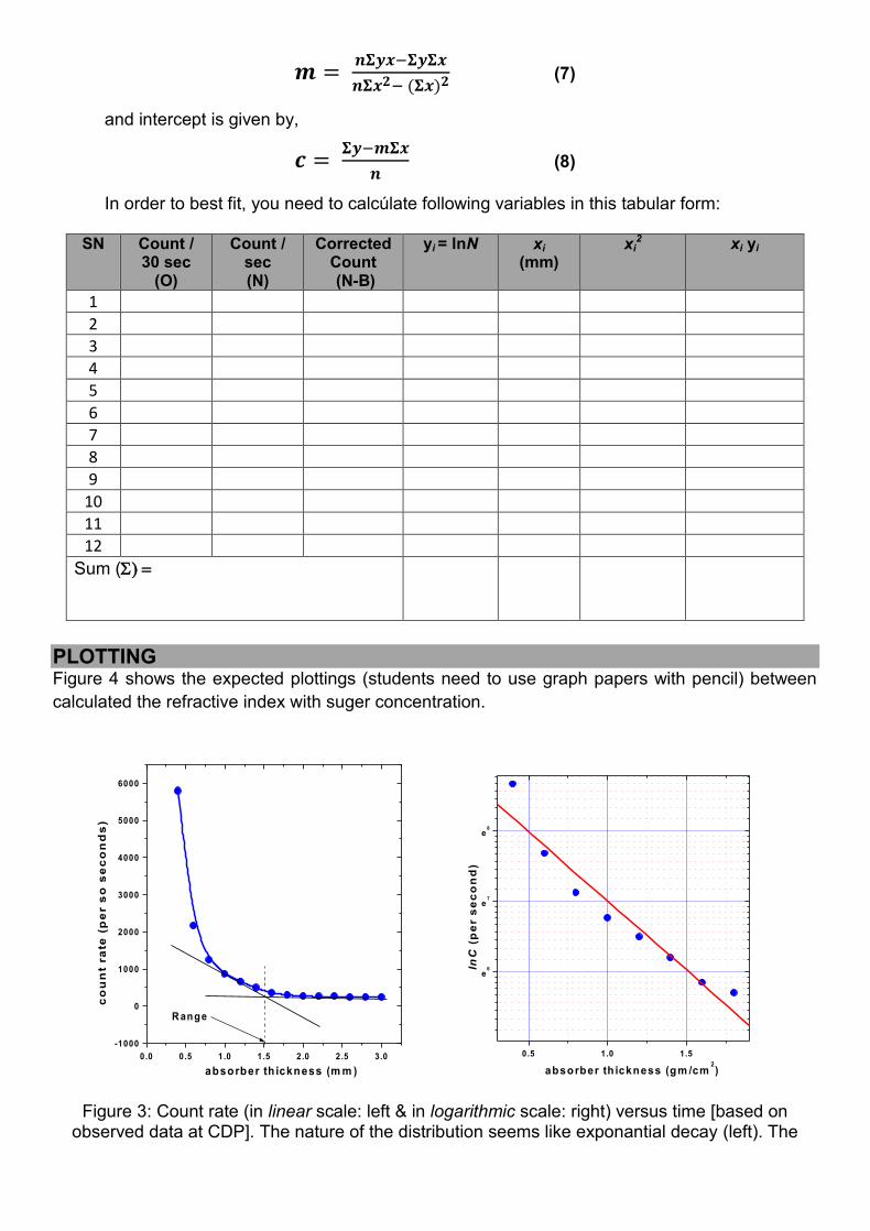
and intercept is given by, = 𝚺 − 𝚺 (8)

In order to best fit, you need to calcúlate following variables in this tabular form:

SN Count / 30 sec

(O)

Count / sec (N)

Corrected Count (N-B)

yi = lnN xi

(mm) xi

2 xi yi

1

2

3

4

5

6

7

8

9

10

11

12

Sum (

PLOTTING Figure 4 shows the expected plottings (students need to use graph papers with pencil) between

calculated the refractive index with suger concentration.

Figure 3: Count rate (in linear scale: left & in logarithmic scale: right) versus time [based on

observed data at CDP]. The nature of the distribution seems like exponantial decay (left). The

0.0 0.5 1.0 1.5 2.0 2.5 3.0

-1000

0

1000

2000

3000

4000

5000

6000

R ange

co

un

t ra

te (

pe

r s

o s

ec

on

ds

)

absorber th ickness (m m )

0.5 1.0 1.5

e6

e7

e8

lnC

(p

er s

ec

on

d)

absorber th ickness (gm /cm2)

nature of the distribution fits the laws of radioactivity, lnC is proportional to absorber thickness (b). You need to fit your observed data using (7) and (8).

We get = = and intercept = = We use the value of slope to find the value of half life of the prepared liquid source. absorption coefficient 𝜇 = − = …………… .………… . cm /gm To find the end point energy of given beam of b-particles, the range R (Figure 3) can be used. = 𝑅+ .. = = ⋯……… . . MeV

ERROR ANALYSIS

SN yi = lnN xi

(mm) −

1

2

3

4

5

6

7

8

9

10

11

12

=

The error in the slope is Δ = [ Σ 𝑖− ] / = = Here = Σ − and = Σ 𝑖 − Σ 𝑖 −

Note: Repeat the whole process for Copper absorber.

RESULT

(1) It is found that the absorption coefficient -particles emitted from the given

source in the almunium absorber of is …………………………………. ±

………………………….... The end point energy of b-particle is found to be

…………………. MeV.

(2) It is found that the absorption coefficient -particles emitted from the given

source in the Copper absorber of is …………………………………. ± ………………………….... The end point energy of b-particle is found to be

…………………. MeV.

INTERPRETATION OF YOUR RESULT You need to interpret your result yourself.

PRECAUTION Write down precaution that you faced or experienced during the experiment.

EXPERIMENT 2

Study the absorption of particle in the air using (a) Am-241 and (b) Ra-226 source and end-window counter.

Objectives of the Experiment

(a) Study the radioactivity of given -emitters.

(b) Study the -absorption in the air using end-window counter. Find its absorption coefficient.

(c) Find the number of -nuclei present in your source using given activity. What will be the number after 1 year, 10 years?

(d) Study the wave properties of -particles by verifying inverse square law.

(e) Study the ionization energy of -particles.

Absorption of-particles in the gases

Interaction of heavy charged particles with matter In nuclear physics, the term “heavy particles” is

applied to particles with mass that is much larger than electron mass. Examples of heavy

particles are the proton (e.g., He nucleus, which is com posed of two protons and two neutrons).

When radiation is composed of charged particles, the main quantity characterizing interaction of

radiation with matter is the average decrease of particle kinetic energy per unit path length. This

quantity is called the stopping power of the medium and is denoted S. The main mechanism of the

energy loss of heavy charged particles (and electrons with energies of the order of a few MeV or

less) is ionization or excitation of the atoms of matter (excitation is the process when internal

energy of the atom increases, but it does not lose any electrons). All such energy losses are

collectively called ionization energy losses (this term is applied to energy losses due to excitation,

too). Atoms that are excited or ionized due to interaction with a fast charged particle lie close to

the trajectory of the incident particle (at a distance of a few nanometers from it). The nature of the

interaction that causes ionization or excitation of atoms is the so-called Coulomb force which acts

between the incident particles and electrons of the matter.

Americium-241

Americium-241 is made in nuclear reactors, and is a decay product of plutonium-241. The element

americium (atomic number 95) was discovered in 1945 during the Manhattan Project in USA.

Figure 1: Decay Scheme of Am-241

The first sample of americium was produced by bombarding plutonium with neutrons in a nuclear

reactor at the University of Chicagoa. Americium-241, with a half-life of 432 years, was the first

americium isotope to be isolated, and is the one used today in most domestic smoke detectors.

Am-241 decays by emitting alpha particles and gamma radiation to become neptunium-237. The

most common application of americium is of the Am-241 isotope as an ionization source in smoke

detectors, and most of the several kilograms of americium recovered each year is used in this way

at present.

Ra-226 The nuclide Ra 226 is an isotope of the element radium (atomic number 88, chemical symbol Ra).

There are 226 nucleons in the nucleus consisting of 88 protons and 138 neutrons. Ra 226 is

radioactive with a half-life of 1600 years. It decays through alpha emission. The alpha particle

energy with the highest emission probability is at 4.7843 MeV followed by 4.601 MeV. Additional

alpha particles are also observed – indicated by the dots. In contrast to beta emission (where only

two beta energies are given – the most probable and the highest energy respectively), the alpha

particle energies are listed according to decreasing emission probability.

Figure 2: Decay Scheme of Ra-226

Laws of Radioactivity Activity of radioactive substance A(t) is at any time t proportional to number of radioactive particles N(t),

(1) The number of radioisotope present at time t, decays exponentially with time, i.e.,

(2)

In terms of mass absorption coefficient, we express t = mx. One can calculate mass absorption coefficient using above expression. These ionizing radiation shows wave properties and hence satisfies inverse square law, i.e., N(t) is inversely proportional to the square of the distance between the GM tube and the source.

Ionization Energy of a-particles The quantum mechanical calculation of the stopping power due to ionization energy losses is given by

(3)

where v is the particle velocity, z is its charge in terms of elementary charge e (“elementary

charge” e is the absolute value of electron charge), n is the electron concentration in the material,

me is electron mass, ε0 is the electric constant (ε0 = 8.854 x 10-12 F/m), is the ratio of particle velocity and velocity of light c (i. e. ≡ v / c), and the parameter I is the mean excitation energy of

the atomic electrons (i. e., the mean value of energies needed to cause all possible types of

excitation and ionization of the atom). This formula is applicable when v exceeds 107 m/s (this

corresponds to alpha particle energy of 2 MeV).

Smoke Detectors

Americium-241 emits alpha particles and low energy gamma rays. The alpha particles emitted by

the Am-241 collide with the oxygen and nitrogen in air in the detector's ionisation chamber to

produce charged particles (ions). A low-level electric voltage applied across the chamber is used

to collect these ions, causing a steady small electric current to flow between two electrodes. When

smoke enters the space between the electrodes, the smoke particles attach to the charged ions,

neutralizing them. This causes the number of ions present – and therefore the electric current – to

fall, which sets off an alarm. The radiation dose to the occupants of a house from a domestic

smoke detector is essentially zero, and in any case very much less than that from natural

background radiation. The alpha particles are absorbed within the detector, while most of the

gamma rays escape harmlessly. The small amount of radioactive material that is used in these

detectors is not a health hazard and individual units can be disposed of in normal household

waste. Even swallowing the radioactive material from a smoke detector would not lead to

significant internal absorption of Am-241. Americium dioxide is insoluble, so will pass through the

digestive tract without delivering a significant radiation dose. (Americium-241 is however a

potentially dangerous isotope if it is taken into the body in soluble form. It decays by both alpha

activity and gamma emissions and it would concentrate in the skeleton).

Instrumentation

(a) End-window counter with cable for α, , and X-rays

‘

Figure 3: End-window tube and counter

Self-quenching Geiger-Müller counter tube, in a plastic housing, with a very thin mica end-window which also allows the registration of soft radiation. With a permanently attached cable. Complete with a protective cap for the mica window. Technical Data

Gas filling: neon, argon, halogen Dead time: approx. 100 µs

Mean operating voltage: 450 V Service life: > 1010 pulses

Connection: screened cable, 55 cm long, with coaxial plug

Background in plateau: approx. 0.2 pulses/s

Plateau length: 200 V Responsivity to radiation: approx. 1% Relative plateau slope: < 0.05%/V End-window: 9 mm diam.

(b) Counter S

For counting of counter tube pulses, pulse rates or other electrical pulses as well as for frequency

and time measurement. Especially suitable for student work. With 5-digit LED display, internal

loudspeaker and special counter tube input with internal high-voltage supply, 2 photoelectric

barrier inputs, operation via built-in keys. Plug-in power supply unit included.

Technical Data

Measuring ranges: Frequency: 0 ... 99999 Hz Time: 0 ... 99999 s, 0 ... 99.999 ms

Pulse input and output: 4 mm safety sockets

Gate times for counter tube: fixed 10s, 60s, 100s,

Sensitivity: TTL-compatible

manual up to 9999 s Display: 5-digit LED display

Photoelectric barrier inputs: 6-pole DIN-sockets

Integrated counter tube voltage : 500 V Inputs and outputs

Power supply: 12 V AC/DC via plug-in power supply(included)

Counter tube input: coaxial socket Dimensions: 20.7 cm x 13 cm x 4.5 cm

Procedure

(1) You do not need to find out operating voltage of the GM tube. It is a very special GM

tube names as ‘end window counter’ with halogen gases capable of detecting not only

-rays (strong penetrating power). The

operating voltage of this tube is 450 V and it is supplied through 12 V AC/DC via plug-in

power supply.

(2) You need to connect the cable of end window counter and the GM Counter S in a gentle

way. Adjust knobs to GM manual at first. Do not place the radioactive sources nearby

the set-up. Take readings for about 5 minutes. This will discharge the effect of previous

measurements.

(3) Now observe background counts by adjusting knob at 60 seconds. Take at least 20

observations for the background. Find the mean, standard deviation and standard error

of background counts.

(4) Now place Am-241 at 5 cm far from the window of end-window counter. Take at least

20 readings for the interval of 60 seconds.

Figure 4: Experimental set-up for the measurement of -absorption in the air. A fixed scale with a

hard board and fixed end-window tube and fixed source in a wooden box is preferred.

(5) Now decrease the distance by 0.50 cm carefully (if needed set the distance yourself) and observe the reading (see Figure 3). For each position, take at least 20 observations.

(6) Using the standard value of half life of Am-226 and the given value of the activity, you can calculate disintegration constant and hence the mass absorption coefficient.

(7) Since you have the accurate values of distances between the source and the detector, you can verify inverse square law.

(8) Try to calculate the number of radioactive atom present in your source. Similarly velocity -particles can be calculated by using its energy. Using these values one can

calculate stopping power.

(9) You need to show best fitted graphs for the calculation of mass absorption coefficient and the inverse square law (Figure 4).

Figure 5: Count rate versus absorption of alpha particles by air.

(10) Since you know the standard error of your all sets of data, you will be able to put error bars in your plot.

(11) Repeat the whole process for Ra-226 and compare their results. Discussion Interpret your plots and calculated values in the context of alpha interaction with the air in the

laboratory.

EXPERIMENT 3 Study the resistance versus Temperature curve of the given

thermistor material. Also design and study its use as a sensor.

DESCRIPTION

The termistor is a semiconductor device which consists of a bead or disc of various oxides

manganese, Nickel, cobalt, iron or other metals. A word termistor is derived from termal resistor. A

termistor is a device whose resistance varies quite makedly with temperatura depending upon

their composition. The termistor can have either positive temperatura coefficient or a negative

temperatura coefficient. The neagative temperatura coefficient type consists of a mixture of oxides

of iron, nickel and cobalt. The positive temperatura coefficient type is base don Barium titanate

and shows a temperatura increase of 50 to 200 times for a temperatura rise of few degrees.

These are used in temperatura controlled switch.

WORKING FORMULA

A semiconductor material is characterized by the property that its conductivity increases sharply

with rise in temperature. This is because the number of charge carrier is increased in an

exponential manner as characterized by the factor exp-Eg/KT. The resistance (R) of

semiconductor material is given by

𝑅 = 𝑅 − 𝐸𝑔𝐾𝑇 (1)

Here R0 is the resistance at highest temperature. Taking log both sides we get,

log 𝑅 = log 𝑅 − 𝐸𝑔𝐾𝑇 (2)

The slope of the plot between log(1/R) and (1/T) is - (Eg/K). Thus, band gap of the given

semiconductor material can be calculated if we linearly fit our observations, according to equation

(2). The value of resistance can be measured with the balanced condition of Wheatstone Bridge,

i.e., null deflection in the Galvanometer. Under Balancing condition:

𝑅𝑅 = 𝑅𝑅 (3)

Since R3 = R4, thus R1 = R2. Here R1 is the resistance of thermistor and R2 in the resistance of

bridge. The temperature is measured with the help of thermometer. The slope of straight line gives

the band gap Eg of given semiconductor material.

EXPERIMENTAL SET-UP Go to C. L. Arora or any other B.Sc. Laboratory work book for the detail procedure.

Figure 1: Experimental Set up

OBSERVATION

(a) For variation of resistance (Note: Students need to keep 2 degree centigrade difference

while taking observation. In addition, observation should be taken by increasing and

decreasing temperature)

S.N. Temperature (oC) Resistance (Ω) Increasing (I) Decreasing (d) Value (for I) Value (for d)

1 30 92

2 32 90

3 34 88

4 36 86

5 38 84

6 40 82

7 42 80

8 44 78

9 46 76

10 48 74

11 50 72

12 52 70

13 54 68

14 56 66

15 58 64

16 60 62

17 62 60

18 64 58

19 66 56

20 68 54

21 70 52

22 72 50

23 74 48

24 76 46

25 78 44

25 80 42

27 82 40

28 84 38

29 86 36

30 88 34

31 90 32

32 92 30

The variation of resistance with temperature is shown in Figure 2 (below).

Figure 2: Variation of resistance with increasing temperature [students need to perform similar workout (observation, plotting and calculation) with decreasing temperature]

BEST FIT CALCULATION

Let y = log(1/R) and x = 1/T, then the working formula can be written in this form = + (4)

which represents the best fitted line (shown in Figure), where m is the slope and c the intercept.

Taking sum, equation (4) takes this form: 𝚺 = 𝚺 + (5)

Multiplying (4) by x, 𝚺 = 𝚺 + 𝚺 (6)

Multiplying (5) by x and (6) by n and solving these expression for the slope (m), we get,

= 𝚺 −𝚺 𝚺𝚺 − 𝚺 (7)

and intercept is given by,

30 40 50 60 70 80 90

0

200

400

600

800

increasing T

Re

sis

tan

ce

(O

hm

)

Tem perature (oC )

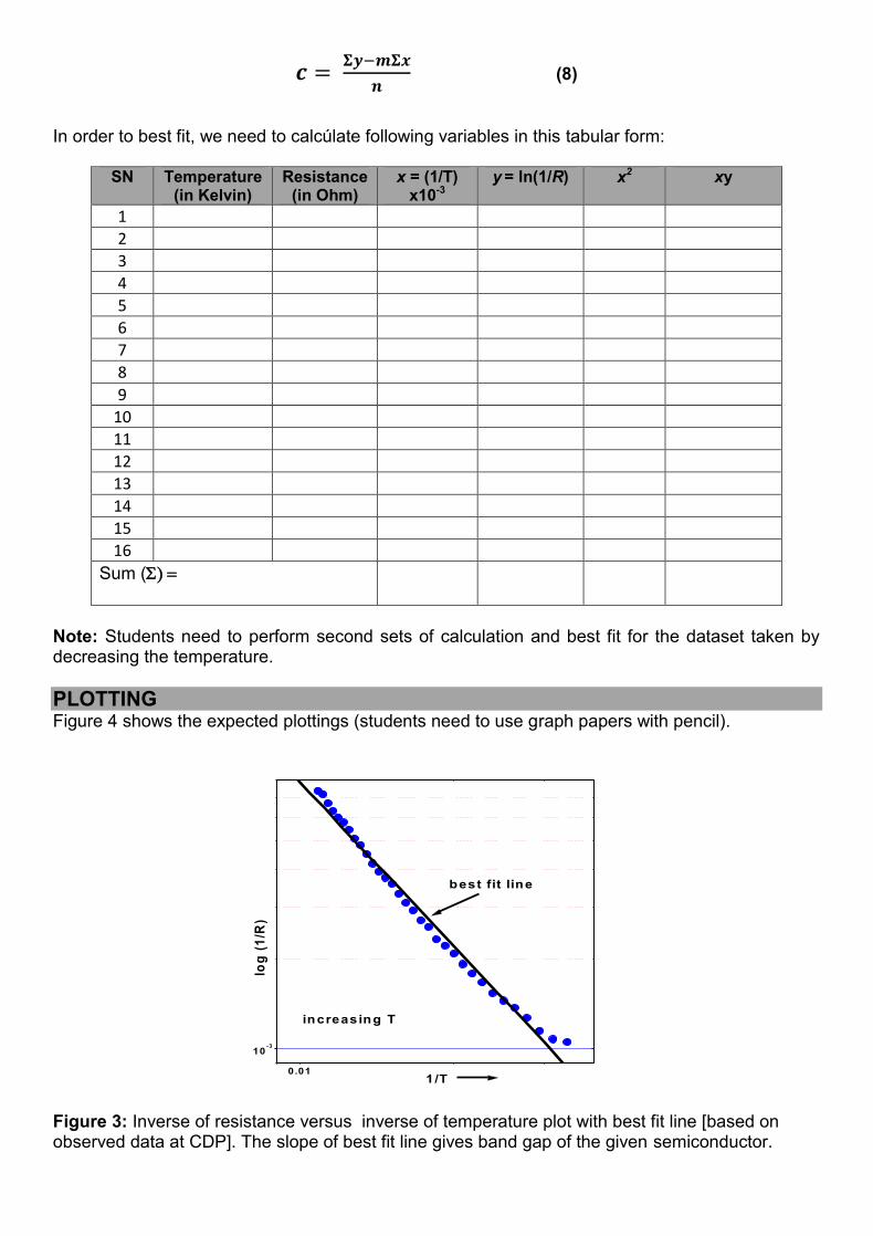
= 𝚺 − 𝚺 (8)

In order to best fit, we need to calcúlate following variables in this tabular form:

SN Temperature (in Kelvin)

Resistance (in Ohm)

x = (1/T) x10-3

y = ln(1/R) x2 xy

1

2

3

4

5

6

7

8

9

10

11

12

13

14

15

16

Sum (

Note: Students need to perform second sets of calculation and best fit for the dataset taken by decreasing the temperature.

PLOTTING Figure 4 shows the expected plottings (students need to use graph papers with pencil).

Figure 3: Inverse of resistance versus inverse of temperature plot with best fit line [based on observed data at CDP]. The slope of best fit line gives band gap of the given semiconductor.

0.01

10-3

best fit line

increasing T

log

(1

/R)

1/T

We get = = and intercept = =

We use the value of slope to find the value band gap in the given semiconductor. = = Thus,

= × = ⋯………… .… . . 𝐉 = ……………………… . 𝐞𝐕

Note: You will get two band gaps after taking first and second set of observations. These values can be average out.

Different Uses for Thermistors A thermistor is a specific type of resistor that uses sensors to help regulate cold and heat. They

can do more then simply regulate temperature. They are also used for voltage regulation, volume

control, time delays, and circuit protection. These products are made up of ceramic and metal

oxides, but it also contains circuits and wires. These resistors have many practical applications

both in terms of manufacturing and personal products. Below, we will be going over some of the

different uses and applications for thermistors throughout multiple industries.

Microwave

For those who have used a microwave, you have used a thermistor. They are used in these

machines to determine and maintain internal temperature. Without the resistor in the microwave,

there is a possibility of overheating in the unit. This could lead to potential fires.

Circuit Protector

If you have a power supply or surge protector in your home or office then you are also using a

thermistor. Without a thermistor in this product, surges of energy would be uncontrolled. This

could lead to overheating or too much electricity being pushed to whatever is plugged in. This

could lead to some of your electronics shorting out.

Automotive

Cars, trucks, and buses all use thermistors. They are used to determine the temperature of oil and

coolants. This is how you are able to know if your car is overheating or not. The thermistors are

connected to indicators on the dashboard of the vehicle. Thermistors in cars do not prevent or

regulate. Instead, they are used to gather information. This allows a driver to fix their car or truck

before something serious happens.

Digital Thermometers

Have you ever wondered how digital thermometers are able to accurately gauge someone’s

temperature? This is possible because of thermistors. Just like with cars, these devicesused to

gather information rather than helping to maintain temperature.

Rechargeable Batteries

The ability to recharge a battery is only possible because of the help it gets. When you start

charging batteries, there is a tendency for things to get hot. The low resistance of the thermistor

allows it to stop the charging if things are getting too hot.

Thermistors are used in everyday life, and they are used in so many different ways.

PLAN A WORK USING THERMISTORS

You need a make a sketch regarding the use of the termistor that you have in your laboratory.

Plan it as a sensor in your design. Discuss with your colleague.

RESULT

It is found that the resistance of given thermister increases with the decrease in the temperature.

In addition, we found that the band gap in the given semiconductor is …….…………………eV.

INTERPRETATION OF YOUR RESULT You need to interpret your result yourself.

PRECAUTION Write down precaution that you faced or experienced during the experiment.

EXPERIMENT 4

Study the Hall coefficient of given n- & p-type materials and obtain the charge carrier density in each case and study the Hall mobility. (b) Also design and study use of n- & p- type materials to apply as

fluxmeter probe.

AIM OF THE EXPERIMENT

After conducting this experiment students will understand

1. measurement the Hall voltage developed across the sample material.

2. measurement the Hall coefficient and the carrier concentration of the sample material

APPARATUS REQUIRED:

1. Electromagnets

2. Power Supply Unit for Electromagnets

3. Gauss Meter for Measuring Magnetic field

4. Power Supply Unit for Crystal

5. p or n semiconductor slice

THEORY:

When a magnetic field is applied perpendicular to current carrying conductors a voltage is

developed across it in the direction perpendicular to both current and magnetic field. This

phenomenon is called Hall Effect and voltage itself is known as Hall voltage.

Fig. 1: Schematic representation of Hall Effect

If the current passes in X-direction in the conductor a magnetic field is applied in Z-direction,

then Hall Voltage is developed in Y-direction. The sign of Hall Voltage depends on the nature of

charge carriers.Experimentally it has found that Hall voltage

∝ , ∝ 𝑗 & ∝

Where 𝑗 current density and b iswidth of the specimen across which Hall Voltage is developed

So ∝ 𝑗 ⇒ = 𝑗 , is constant for the given conductor and is known as Hall

Coefficient

𝑗 = × = × ×

It can be shown that = 𝑉𝐻 𝐵

Slope = = 𝑅𝐻𝐵

Thus from the graph

EXPLANATION: Consider a semiconductor in which holes are assumed to move in the X-direction representing a

current density 𝑗 = ×

When magnetic field (0, 0, B) is applied. The holes experience magnetic force = (𝑣 × )q

directed towards the upper force and creation these a surface of possible charges negative

=

= ×

charges at the lower surface. Thus electric field directed in (-y) direction is developed inside the

conductor and equilibrium is reached when the electric field force on the charges balances the

magnetic force.

Thus at equilibrium = 𝑣 = ⇒ = 𝑣 = 𝒆 ×

𝑉𝐻 = 𝑣 , ⇒ 𝑉𝐻 = 𝑥 × 𝐵×

&

PROCEDURE

1. Calibrated the magnetic field against magnetizing current by using a Hall probe and digital

Gauss meter.

2. Measure the magnetic field, B with a gauss meter.

3. Connect the p or n semiconductor slice to constant power supply unit for crystal in their

respective Sockets.

4. Measure Hall Voltage for both the directions of current and magnetic field(i.e. four

observations for a particular value of current and magnetic field).

5. Change the value of in steps and note corresponding value of and , Then plot a

graph between and . It will be straight line whose slope will be given by𝑉𝐻𝑥 .

OBSERVATION

Table 1: Observation of Magnetic Field

No.

of obs.

Current Magnetic Field

In Gauss In Tesla

VH = ne Ix Bt RH = ne

Table 2: Different applied magnetic field (We get different set of current and Hall voltage)

No.

of obs.

(mA)

𝑩 = .....

(0V)

𝑩 = ….. (30V)

𝑩 = ….. (60V)

𝑩 = ….. (90V)

𝑩 = ….. (120V)

(mV)

(mV)

(mV)

(mV)

(mV)

1

2

3

4

5

6

7

8

9

10

PLOTS:

(you need to make plots for all voltajes (0V, 30V, 60V, 90V and 120 V) and fild slopes (m)

from their best fits)

3 6 9 12-1

-2

-3

-4

-5

H = m I + c

0 V

Hall V

olt

ag

e (

mV

)

Current (mA)3 6 9 12

-10

-20

-30

-40

-50

H = m I + c

30 V

Hall V

olt

ag

e (

mV

)

Current (mA)

Figure 3: Hall voltage versus current plot. The error bar respresents the standard error. (This

data is taken from the set up at CDP, TU, Kirtipur)

CALCULATION:

By using the relation = × 𝐵 & =

Here slope should be calculated from best fit plot (given below)

= ……………

n = …………………..

ERROR ANALYSIS:

RESULT:

DISCUSSION:

SECOND PART Design and study use of n- & p- type materials to apply as fluxmeter probe. Discuss with your group to make it and finally consult your teacher.

Reference:

1. Kittel C. – Introduction to solid state physics, 8th ed., John wiley& Sons (2005).

EXPERIMENT 5 Study the magnetic susceptibility of given diamagnetic and

paramagnetic substances AIM OF THE EXPERIMENT

After performing this experiment students will understand

1. Magnetic susceptibility 𝜒 of a given paramagnetic (e.g., FeCl3) and diamagnetic solution

(e.g., water) for a specific Concentration.

2. Meaning and importance of mass susceptibility

APPARATUS REQUIRED:

1. Electromagnet

2. Quincke’s tube or (U- shape

tube)

3. Fluxmeter

4. Search Coil

5. Travelling Microscope

6. Hall Probe

7. Ferric Chloride Solution

THEORETICAL BACKGROUND

When a substance is placed within a magnetic field, it is magnetized. Most materials can be

classified as diamagnetic, paramagnetic or ferromagnetic according to their behavior in external

magnetic. Diamagnetic substances are magnetized feebly in opposite to the magnetizing field and

soSusceptibility is small and negative. Paramagnetic substances are magnetized feebly in the

direction of magnetizing field. Susceptibility is small and positive. Ferromagnetic substances are

magnetized strongly in the direction of magnetizing field and so Susceptibility is large and positive.

Quincke’s devised a simple method to determine the magnetic susceptibility (𝜒), of a

paramagneticsolution by observing how the liquid rises up between the two pole pieces of an

electromagnet. In this experiment an aqueous solution of Ferric Chloride Solution (FeCl3) is kept

in the narrower part of a Quincke’stube. The narrower part is placed in a nearly uniform magnetic

field while the wider part is far removed from the field. On activating the field with current the

meniscus in the narrower part will rise if the solution paramagnetic and will fall if it is diamagnetic.

A Hall probe determines the relationship between the current and the applied field. The magnetic

susceptibility is given by 𝜒 =

where M is magnetization and H is the magnetic field and it is a dimensionless quantity and is

positive for the Paramagnetic substances.

Energy of magnetic field in the absence of substance = 𝜇 ∫ dv

Energy of magnetic field in the presence of substance = ∫ 𝜇 𝜇 dv

𝜇 = + 𝜒 and 𝜒 is susceptibility. Gain in energy when the substance is placed in magnetic

field

(U) = − = = 𝜇 ∫ 𝜇 − dv

= 𝜇 ∫𝜒 dv

Fig. 1: Sketch of the experimental set up

Considering the magnetic field H along y-direction, its gradient along z-direction and supposing

the filed to be uniform along x-y plane = , = and so F = = − 𝜇 ∫𝜒 𝜕𝜕 dv 𝜕𝜕 dv = 𝜕𝜕 Adz =

Therefore, F = = − 𝜇 𝜒 ∫ = 𝜇 𝜒

Under the action of forceFthe liquid is raised inside the tube until it’sbalanced by the weight of the

liquid itself. If h is the height of the liquid raised an is the density.

So F= = ℎ

At equilibrium, =

𝜇 χ = ℎ

χ = 𝝆𝝁

Mass susceptibility (𝜒 = 𝑖 𝑖 𝑖 =

𝜒𝑚𝜌

Therefore, 𝝌 = 𝝌 = 𝝁 = 𝝁𝑩

Instead of Quinck’s tube, U-shaped tube is used the height is replaced by 2h, 𝜒 = 𝑔𝜇 ℎ𝐵

𝝌 𝒓 = 𝝌 × 𝒆 𝒓 𝒆

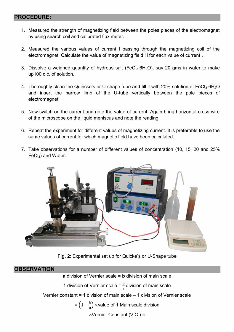
PROCEDURE:

1. Measured the strength of magnetizing field between the poles pieces of the electromagnet

by using search coil and calibrated flux meter.

2. Measured the various values of current I passing through the magnetizing coil of the

electromagnet. Calculate the value of magnetizing field H for each value of current .

3. Dissolve a weighed quantity of hydrous salt (FeCl3.6H2O), say 20 gms in water to make

up100 c.c. of solution.

4. Thoroughly clean the Quincke’s or U-shape tube and fill it with 20% solution of FeCl3.6H2O

and insert the narrow limb of the U-tube vertically between the pole pieces of

electromagnet.

5. Now switch on the current and note the value of current. Again bring horizontal cross wire

of the microscope on the liquid meniscus and note the reading.

6. Repeat the experiment for different values of magnetizing current. It is preferable to use the

same values of current for which magnetic field have been calculated.

7. Take observations for a number of different values of concentration (10, 15, 20 and 25%

FeCl3) and Water.

Fig. 2: Experimental set up for Quicke’s or U-Shape tube

OBSERVATION

a division of Vernier scale = b division of main scale

1 division of Vernier scale = division of main scale

Vernier constant = 1 division of main scale – 1 division of Vernier scale

= − ×value of 1 Main scale division ∴Vernier Constant (V.C.) =

Table 1: Measurement of Magnetic Field

Table 2: For 10% concentration of FeCl3

𝜒 = 𝑔𝜇 ℎ𝐵 = ………….m kg⁄

Table 3: For 15% concentration of FeCl3

𝜒 = 𝑔𝜇 ℎ𝐵 = ………….m kg⁄

Table 4: For 20% concentration of FeCl3

No. of obs

Current (Ampere)

Magnetic field

In Gauss In Tesla

1

2

3

4

5

No. of

obs

Current (Ampere)

Initial Reading Final Reading h = − (cm)

M.S V.S×V.C Total( ) M.S V.S×V.C Total( )

1

2

3

4

5

6

No. of

obs

Current (Ampere)

Initial Reading Final Reading h = − (cm)

M.S V.S×V.C Total( ) M.S V.S×V.C Total( )

1

2

3

4

5

6

No. of

obs

Current (Ampere)

Initial Reading Final Reading h = − (cm)

M.S V.S×V.C Total( ) M.S V.S×V.C Total( )

1

2

3

4

5

6

𝜒 = 𝑔𝜇 ℎ𝐵 = ………….m kg⁄

Table 5: For 25% concentration of FeCl3

𝜒 = 𝑔𝜇 ℎ𝐵 = ………….m kg⁄

Table 6: For Water

𝜒 = 𝑔𝜇 ℎ𝐵 = ………….m kg⁄

EXPECTED PLOTS:

(make plots for each concentrations and best fit these plots for the slope)

0.00

0.02

0.04

0.06

0.08

0.10

h = m H2 + c

10% Concentration of FeCl3

heig

ht

(cm

)

H2 (in 10

-8T)

0.000

-0.005

-0.010

-0.015

-0.020

h = m H2 + c

water

heig

ht

(cm

)

H2 (in 10

-8T)

Figure 3: Height versus H2 plot. The error bar respresents the standard error. (This data is taken

from the set up at CDP, TU, Kirtipur)

ERROR ANALYSIS:

No. of

obs

Current (Ampere)

Initial Reading Final Reading h = − (cm)

M.S V.S×V.C Total( ) M.S V.S×V.C Total( )

1

2

3

4

5

6

No. of

obs

Current (Ampere)

Initial Reading Final Reading h = − (cm)

M.S V.S×V.C Total( ) M.S V.S×V.C Total( )

1

2

3

4

5

6

We have, 𝜒 = 𝑔𝜇 ℎ𝐵 ∆𝜒 = 𝜒 [ ∆ℎℎ + ∆𝐵𝐵 ]

= …………. m kg⁄

RESULT:

DISCUSSION:

References:

1. Arora C.L. B.Sc. Practical Physics, S. Chand and Company Ltd. (2010).

EXPERIMENT 6 Lattice Dynamics: (a) Study the monoatomic lattice vibration. Hence

obtain the cut-off frequency of the given materials. (b) Study the diatomic lattice vibrations and determine the optical band gap

Aim of the Experiment

The following experiments may be performed with the help of this setup:

1. Study of the dispersion relation for the mono-atomic lattice-Comparison with theory.

2. Determination of the cut-off frequency of the mono-atomic lattice.

3. Study of the dispersion relation for the di-atomic lattice – ‘acoustical mode’ and ‘optical

mode’ energy gap. Comparison with theory.

Theory:

Lattice dynamics is an essential component of any postgraduate course in Physics, Engineering

Physics, Electronic Engineering and Material Science. In particular it is essential for understanding

the interaction of electromagnetic waves and crystalline solids. In present setup, mono-atomic and

diatomic lattices are stimulated using the transmission line having ten identical sections of LC

resonant circuit. The dispersion relation for electrical analogue of the mono-atomic lattice is

and dispersion relation for electrical analogue of diatomic lattice is

With the help of the simple and user friendly setup the phase difference between the input and

output wave is measured at different frequencies and tabulated.

Then a graph of the experimental value and the theoretical value is plotted and compared.

Lattice Dynamics Kit

Lattice Dynamics Kit consists of the following parts:

It consists of an Audio oscillator with amplitude control and facility to vary the frequency from 0.9

KHz to 90 KHz. It has built in power-supply and output stage to match the impedance of simulated

lattice. Another part of Lattice Dynamic Kit consists of transmission line, which simulates one-

dimensional mono-atomic and di-atomic lattices. The only additional equipment needed is a

General purpose C.R.O. Figure 1 shows the kit.

OBSERVATION & CALCULATION

In the Lattice dynamics Kit, we have L = ................................H and C = ......................... mF. So

for theoretically, for electrical analog circuit, = √ 4 = ⋯

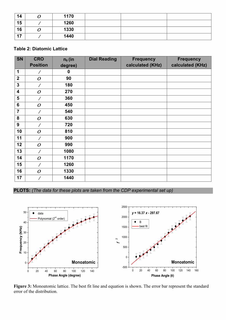
Table 1: Monoatomic Lattice

SN CRO

Position

n(in

degree)

Dial Reading Frequency

calculated

Frequency

calculated

1 0

2 90

3 180

4 270

5 360

6 450

7 540

8 630

9 720

10 810

11 900

12 990

13 1080

14 1170

15 1260

16 1330

17 1440

Table 2: Diatomic Lattice

SN CRO

Position

n(in

degree)

Dial Reading Frequency

calculated (KHz)

Frequency

calculated (KHz)

1 0

2 90

3 180

4 270

5 360

6 450

7 540

8 630

9 720

10 810

11 900

12 990

13 1080

14 1170

15 1260

16 1330

17 1440

PLOTS: (The data for these plots are taken from the CDP experimental set up)

0 20 40 60 80 100 120 140

0

10

20

30

40

50

Monoatomic

data

Polynomial (2nd

order)

Fre

qu

en

cy (

kH

z)

Phase Angle (degree)

0 20 40 60 80 100 120 140 160-500

0

500

1000

1500

2000

2500

Monoatomic

y = 16.37 x - 297.67

B

best fit

f 2

Phase Angle ()

Figure 3: Monoatomic lattice. The best fit line and equation is shown. The error bar represent the standard

error of the distribution.

0 20 40 60 80 100 120 1400

5

10

15

20

25

30

35

40

Band Gap

Diatomic

Optical Branch

Acoustical Mode

Fre

qu

en

cy (

kH

z)

Phase Angle ()

Figure 3: Diatomic lattice. The error bar represent the standard error of the distribution.

ERROR ANALYSIS Estimate chi-square distribution by taking calculated and observed values frequencies for both

mono and diatomic cases. You need to calculate chi-square value and chi-square probability and

interpret your result.

RESULT Summarize your result

DISCUSSION Discuss your result