DOT/FAA/TC-13/33 Federal Aviation Administration William J. Hughes Technical Center Aviation Research Division Atlantic City International Airport New Jersey 08405

Development of a Process-Monitoring Strategy for Drilling and Broaching Operations in Critical Aircraft Engine Components September 2017 Final Report This document is available to the U.S. public through the National Technical Information Services (NTIS), Springfield, Virginia 22161. This document is also available from the Federal Aviation Administration William J. Hughes Technical Center at actlibrary.tc.faa.gov.

U.S. Department of Transportation Federal Aviation Administration

NOTICE

This document is disseminated under the sponsorship of the U.S. Department of Transportation in the interest of information exchange. The U.S. Government assumes no liability for the contents or use thereof. The U.S. Government does not endorse products or manufacturers. Trade or manufacturers’ names appear herein solely because they are considered essential to the objective of this report. The findings and conclusions in this report are those of the author(s) and do not necessarily represent the views of the funding agency. This document does not constitute FAA policy. Consult the FAA sponsoring organization listed on the Technical Documentation page as to its use. This report is available at the Federal Aviation Administration William J. Hughes Technical Center’s Full-Text Technical Reports page: actlibrary.tc.faa.gov in Adobe Acrobat portable document format (PDF).

Technical Report Documentation Page 1. Report No. DOT/FAA/TC-13/33

2. Government Accession No. 3. Recipient's Catalog No.

4. Title and Subtitle DEVELOPMENT OF A PROCESS MONITORING STRATEGY FOR DRILLING AND BROACHING OPERATIONS IN CRITICAL AIRCRAFT ENGINE COMPONENTS

5. Report Date September 2017

6. Performing Organization Code

7. Author(s) Dr.-Ing. Drazen Veselovac

8. Performing Organization Report No.

9. Performing Organization Name and Address WZL—Laboratory for Machine Tools and Production Engineering

10. Work Unit No. (TRAIS)

RWTH Aachen—Aachen University of Technology Steinbachsraβe 19 52074 Aachen Germany

11. Contract or Grant No.

12. Sponsoring Agency Name and Address FAA New England Regional Office 12 New England Executive Park Burlington, MA 01803

13. Type of Report and Period Covered Final Report

14. Sponsoring Agency Code ANE-180

15. Supplementary Notes The FAA William J. Hughes Technical Center Aviation Research Division Technical Monitors were Cu Nguyen (retired) and Dave Galella. 16. Abstract The manufacture of turbine engine critical parts, such as discs and spacers, demands a very high level of process reliability and safety. Damages or anomalies that can be induced by the machining process have to be recognized and documented early in the manufacturing process. This study investigated the strategies to monitor broaching and hole-making, which are operations performed near the end of the turbine disc manufacture. Usually such parts have a significant value at the hole-making and broaching operations stage. Process-monitoring systems and signal analysis strategies, which are able to detect anomalies and induced part damages, should be able to minimize high-value scrap in production and increase part reliability. 17. Key Words Process monitoring, Hole-making, Broaching, Special-cause events

18. Distribution Statement This document is available to the U.S. public through the National Technical Information Service (NTIS), Springfield, Virginia 22161. This document is also available from the Federal Aviation Administration William J. Hughes Technical Center at actlibrary.tc.faa.gov.

19. Security Classif. (of this report) Unclassified

20. Security Classif. (of this page) Unclassified

21. No. of Pages 146

22. Price

Form DOT F 1700.7 (8-72) Reproduction of completed page authorized

iii

ACKNOWLEDGEMENTS

The Laboratory for Machine Tools at the University of Aachen in Germany would like to acknowledge the cooperation of engine manufacturers in the U.S. and Europe for their contributions to this project. This effort was possible thanks to test material, machine time in production, data from production, and the experiences in process monitoring provided by Avio S.p.A, GE-Aviation, Honeywell International, Inc., MTU Aero Engines, Pratt & Whitney, Rolls-Royce, Safran, and Volvo Aero.

iv

TABLE OF CONTENTS

Page

EXECUTIVE SUMMARY xiii

1. INTRODUCTION 1

1.1 Scope 1 1.2 Objectives 2

2. STATE OF THE ART AND BACKGROUND IN PM 2

2.1 Review of PM Techniques and Sensor Specification 4

2.1.1 Sensor Specifications 4 2.1.2 The PM Strategies 10

2.2 Review of Monitoring Techniques from Manhirp 12

2.2.1 The PM of the Drilling Processes 12 2.2.2 The PM of the Broaching Processes 16

2.3 Review of latest publication in PM for drilling and broaching 22 2.4 Data analysis in time and frequency domain 25

2.4.1 Preprocessing 25 2.4.2 Statistical Values 26 2.4.3 Correlation and Spectral Analysis 27 2.4.4 Models 27

2.5 Literature Study on Data/Signal Mining for PM Applications 28

2.5.1 Neural Networks 30 2.5.2 The NN Applications in PM 31 2.5.3 Fuzzy Logic 32 2.5.4 Hydrid Systems: NNs and Fuzzy Logic 33 2.5.5 Hierarchical Algorithm 34 2.5.6 Genetic Algorithms 35 2.5.7 Decision Trees 35

2.6 Literature Study of Physical Models Describing Measures 35

3. CURRENT PRACTICES AND GENERAL REVIEW OF EXPERIENCESWITH PM IN PRODUCTION 39

3.1 Current PM Used in Production 39

v

3.1.1 Drilling 39 3.1.2 Broaching 39

3.2 Review of Testing 42

3.2.1 Review of Quality Aspects 42 3.2.2 Review of Production Aspects 43 3.2.3 Review of Safety Aspects 44 3.2.4 Review of Human Factors 44

4. IDENTIFICATION OF PM TECHNIQUES 46

4.1 Drilling 46

4.1.1 Signal Characteristics in TD 47 4.1.2 Signal Characteristics in the Frequency Domain 49 4.1.3 Tool Wear 51 4.1.4 Tool Breakage 52 4.1.5 Chip Block 53 4.1.6 Failure at the Cutting Edge 54 4.1.7 Coolant Failure 55 4.1.8 Long-Chip Formation 56

4.2 Broaching 57

4.2.1 Signal Characteristics in TD 58 4.2.2 Signal Characteristics in Frequency Domain 62 4.2.3 Tool Wear 64 4.2.4 Cutting-Edge Failure 66 4.2.5 Surface Macroanomalies 67 4.2.6 Other Considerations 69

4.3 Qualification summary of sensor systems 73

5. THE PM SYSTEMS DATABASE 76

5.1 Designs of PM Systems 76

5.1.1 Machine Cabinet Systems 77 5.1.2 Software Systems 80 5.1.3 The PCI Card Systems 81 5.1.4 Front-End Systems 82

5.2 Sensor Connection and Output Interfaces 84 5.3 The PM Strategies 87

6. SOFTWARE DEVELOPMENT 89

vi

6.1 Software Basic Structure 90

6.1.1 Software Input Parameters 90 6.1.2 Communication and Interfaces 91 6.1.3 Software Outputs 91

6.2 Automated Computer-Based Feature Extraction 91

6.2.1 The GUI 93 6.2.2 Signal Preprocessing 95

6.3 Development of Database Architecture 97

7. REACTION STRATEGIES 97

7.1 The PM with Machine Interface 98 7.2 Warning Signals 99 7.3 New PM Strategies 100 7.4 Methodology for the Qualification of Machining Processes 100 7.5 Other Strategies 101

8. SUMMARY AND CONCLUSIONS 101

9. RECOMMENDATIONS FOR FUTURE WORK 103

10. BIBLIOGRAPHY 104

APPENDICES

A—JOINT TIME FREQUENCY MAP CHARACTERISTICS FOR DRILLING B—TOOL ENGAGEMENT IN BROACHING C—EXAMPLE DATA MINING PROCEDURE IN DRILLING D—EXAMPLE DATA MINING PROCEDURE IN BROACHING E—MODEL TO EXPERIMENTAL FORCE COMPARISON F—CONSIDERATION FOR PROCESS MODELING IN BROACHING G—SURFACE AND SIGNALS RELATION IN BROACHING H—SURVEY RESULTS SUMMARY I—PREPROCESSING ALGORITHM FOR OFFLINE ANALYSIS

vii

LIST OF FIGURES

Figure Page 1 Sensor and Mounting Location Selection 3

2 Multicomponent Dynamometer 5

3 Channel Charge Amplifier 5

4 Accelerometer 6

5 Channel Charge Amplifier 6

6 Acoustic Emission Sensor 7

7 The AE Coupler 8

8 Pressure Transducer 8

9 Strain Piezoelectric Sensor 9

10 Comparison Current to Effective Power Measurement 9

11 Effective Power Measurement 10

12 Nordmann WLM-3 10

13 Overview of PM Strategies 11

14 The AE Signal During the Drilling Operation 13

15 Characterization of Burr Length With Feed Force 13

16 Visual Inspection of Drilled Holes in Inconel 718 14

17 Feed Force Signals at Different Wear States of a Drilling Tool 14

18 Force Drop During Tool Chipping in Drilling TiA16V4 15

19 Force Drop During Tool Chipping When Drilling Inconel 718 15

20 Overview of the Sensor Effectiveness for Tool Condition Monitoring 16

21 Spectra of Fy (a) and Fz (b) 17

22 The Ay Spectra for the Weakened Tooth (a) and the Last Tooth (b) 17

23 Techniques to Identify a Burr Formation 18

24 The Cutting Force Signals (a) Without Burr and (b) With Burr (The length of the burr (c) can be calculated from the time delay between the Fx and Fy/Fz signals.) 19

25 The AE Signal for Plucking 21

26 The AE Signal for Redeposited Material 22

27 Time-Series Analysis Strategies 25

28 Overview of the Steps That Compose the DM Process [FAYY96] 28

29 The DM Methods 29

viii

30 Neural Network 31

31 The NN Implemented in Tool Condition Recognition System [AXIN06] 32

32 Membership Functions of Fuzzy Logic 33

33 Process Flow Implementing FN for the Monitoring of Surface Roughness [KIRB07] 33

34 Multisensor System for Tool Wear Estimation [KUO99] 34

35 Distribution of the Effective Work During the Cutting Process [KLOC08] 36

36 Cutting Variables in Drilling [ZAH07] 37

37 Cutting Variables in Broaching [ZAH07] 38

38 Connection of a ToolScope© to a Machine Tool [BRIN11] 41

39 Integrated 3x-Force Measurement System 42

40 Postmachining Operations of European OEMs [Source: ACCENT Project] 43

41 Influence of Human Characteristics on the Manufacturing Process [Source: RoMan, Federal Aviation Administration] 45

42 Available Sensor Systems for Process Monitoring in Machining 46

43 Sensor Specifications for Sensor Evaluation 47

44 Comparison of the Power Calculated From Torque Signal and the Effective Power Measured 47

45 Idle Power vs. RPM for Machining Center 48

46 Typical Signals in TD for Drilling 48

47 Spindle Power During Tool Change 49

48 Idle Spindle Power Characteristic Frequency 50

49 Torque and Power Spectrum for Drilling Process With 600 RPM 50

50 Steps for Spectral Analysis of Drilling Signals 51

51 Sensor Signals for Sharp and Worn Tool 52

52 Tool Breakage Caused by an Excessive Feed Rate 52

53 Signal Characteristics for Recognition of Chip Blockage 54

54 Cutting Edge Failure Due to Damage at the Edge of the Rim 54

55 Failure at the Edge of the Drill Head Point 55

56 Frequency Domain Power Signals for the Identification of Cutting-Edge Failure 55

57 Sudden Coolant Supply Loss 56

58 Obstruction of One Hole for the Tool’s Internal Cooling 56

59 Identification of Long-Chip Formation 57

60 Long-Chip Formation in Drilling and Reaming 57

ix

61 Sensor Specification for Machining Trials 58

62 Force and Power Distribution for the Whole Tool Set 59

63 Details of Idle, Cutting Power, and Force 60

64 Lapointe Broaching Machine PM Signals 60

65 The AE and Vibration (A) in the Broaching Process 61

66 Hammer Test Results to Verify Frequency Range 62

67 Influence of Mounting Type on Frequency Range and Sensitivity 62

68 Hammer Test on Machine Table With Built-In Piezoelectric Load Cells 63

69 Broaching Forces and Vibration in the Frequency Domain 63

70 Calculated Force Acquired With ToolScope 64

71 Tool Wear Identification With ToolScope System 65

72 Force Spectrum for Worn and Sharp Tool Details 65

73 Acceleration Signal in Time and Frequency Domain for Worn Tools 66

74 AERMS Signal for Sharp and Worn Tools 66

75 Power, Force, and Vibration Signals for Tooth Damages 67

76 Acceleration in Time and Frequency Domain 67

77 Chatter Marks on Broached Surface 68

78 Burr Formation 68

79 Detail of Form Finishers Force Signals 69

80 Process Energy for Form Finishers 69

81 Broaching Cutting Energy for Different Tool Details 70

82 Finishing Broaching Detail Forces for Different Process Conditions 70

83 Process Energy (a) and Residual Stress (b) 71

84 The PM Capabilities 74

85 Cabinet Systems 78

86 Cabinet System Compatibility With Machine Controls 79

87 Communication Structure of the Artis CTM V5 82

88 Front-End Systems 83

89 Sensor Connections and Inputs 85

90 Output Interfaces 86

91 Process-Monitoring Strategies 88

92 Software Structure 89

x

93 Interaction Between Automated Computer-Based Feature Extraction Software Modules 92

94 Software Tool User Interface 93

95 Exemplar SF for the Identification of Process State 95

96 Software Tool Preprocessing Flow Chart 96

97 Monitoring Alarms 99

xi

LIST OF TABLES

Table Page 1 Summary of Reference Data 23

2 Lasest Publications in PM 12/2 24

3 State-of-the-Art Summary for DM Applications in PM 30

4 Signal Features Representing Abnormal Modes 71

5 Sensor System Qualification for Hole-Making 75

6 Sensor System Qualification for Broaching 76

7 Designs Offered by Various Manufacturers 77

8 Software Systems and Compatibility to Machine Control 80

9 Compatibility of PCI Cards 81

10 List of Front-End Systems 84

xii

LIST OF ACRONYMS

AC Alternating current AE Acoustic emission AERMS Acoustic emission root mean square DAQ Data acquisition DC Direct current DFT Discrete Fourier Transform DM Data mining FFT Fast Fourier Transform FN fuzzy nets Fx Axial force Fxmax Maximal axial force Fy Push-off force Fz Cutting force Fzmax Maximal cutting force GA Genetic algorithms GUI Graphical user interface HMI Human machine interface JTF Joint Time Frequency kW Kilowatts LCF Low-cycle fatigue Mc Cutting torque MANHIRP Manufacturing to Produce High-Integrity Rotating Parts Mz Torque NC Numeric control NCU Numeric control unit NI National Instruments NN Neural networks OEM Original Equipment Manufacturer PDF Probability density function PM Process monitoring PNN Probabilistic neural networks RMS Root mean square RoMan Rotor Manufacturing Project Team RPM Revolution per minute SAW Surface acoustic wave SF Signal features TD Time Domain TSA Time series analysis v Velocity V Voltage VB Land wear VI Virtual instrument WZL Werkzeugmaschinenlabor - Laboratory for Machine Tools, Aachen, Germany

xiii

EXECUTIVE SUMMARY

The results for this research project are presented in this report. A detailed review of the state of the art in process monitoring (PM) was conducted. This research concentrated on the former Manufacturing to Produce High-Integrity Rotating Parts project, which was a European-funded project dealing with monitoring issues for the manufacture of critical rotating parts. Sensors installed on the machine showed changes in process and product quality. Sometimes, the use of these sensors is limited to the laboratory environment and, therefore, application has not been implemented in the industry. Alternatively, engine manufacturers have already implemented PM as a requirement. The experiences in PM from the production point of view were examined. In this area, standards are already established for hole-making monitoring. Depending on the workpiece, monitoring the spindle power, coolant flow rate, and other variables is required. In broaching, the use of load cells for uni- or multiaxial force measurement is used by some engine manufacturers as means to improve and gain better process understanding. In many cases, other processes are also monitored based on internal engine manufacturer’s guidelines and experiences. To expand and support the already acquired PM knowledge, a multiple-sensor system was tested for hole-making and broaching to establish its suitability to recognize process disturbances. Production constraints were considered during the evaluation. To find suitable sensors and sensing principles, the process conditions (e.g., tools, cutting conditions, process parameter, possible disturbances, and physical processes) were defined. Monitoring of tool chipping and breakage, wear behavior, coolant failure, and other conditions were considered to be of major interest for the detection of machining anomalies. After the definition of the distinct physical quantities, suitable sensing principles and sensors were chosen. Piezoelectric dynamometers, effective power measurement modules, accelerometers, acoustic emissions, flow, and pressure sensors were tested. Some results for internal machine signals were also indicated. In hole-making, power monitoring offers information about most special-cause events. This measurement was compared to the torque and feed force measurement acquired through a dynamometer. It was found that the spindle power provided very accurate results; however, the feed power was able to detect process anomalies, but its measurement was not comparable to the feed force, and the distribution could change from one to another. Coolant flow and pressure provided the complementary information to the spindle power. In broaching, the main drive power and machine table vibrations offered corresponding information to low- and high-frequency process events. A database with the PM systems available on the market was provided. This served as a reference for engine manufacturers to learn the capabilities of different systems and to make selections according to the requirements. As part of the project, a software tool for the acquisition and storage of PM signals was developed. This tool allowed the buildup of a signals database to increase process knowledge and reliability. Furthermore, a routine for automated extraction of signal features (SF) in hole-making was also implemented. The saved SF for each part served as the product’s signature.

xiv

In conclusion, the recommended strategies included in this report are currently used or preferred in industry. Warning signals and the automatic shutdown of the process still have the most acceptances. The yellow and red limits to other signals and the SF will have to be determined for each application.

1

1. INTRODUCTION

The manufacture of critical turbine engines parts, such as discs and spacers, demands a very high level of process reliability and safety. Damages or anomalies that can be induced by the machining process of critical turbine engine parts have to be recognized and documented early in the manufacturing process. With this focus, the two machining processes that are the most interesting to monitor during the manufacturing process are broaching and drilling, which are performed on turbine discs to finalize the geometry. Apart from shot peening or similar processes, this operation is one of the last machining operations. However, of these three, the most critical and sensitive process is the hole-making operation because of its difficult cutting tip engagement, complicated chip flow, and unfavorable heat dissemination. Therefore, the monitoring of hole-making processes is the main subject of the investigation in this project. Furthermore, broaching operations in critical rotating aircraft engine components are very problematic because of their difficult one-stroke nature. This is strongly supported by the Rotor Manufacturing Project Team (RoMan) group and their lessons-learned database, which refers exactly to the subject machining operations. Process monitoring (PM) is identified as the most effective technique to recognize special-cause events in the manufacturing process. Therefore, the evaluation performed in this project is in response to the needs expressed in the industry to characterize PM signals. The PM systems and signal analysis strategies that are able to detect manufacturing-induced anomalies and part damages will increase process reliability and minimize high-value scrap during production. 1.1 SCOPE

Manufacturing-induced anomalies in rotating components may cause engine failure. Therefore, it is imperative to detect them as early as possible. Engine component manufacturing processes use fixed parameters that have been approved. However, various unexpected events can be present during the components’ machining. The identification of these events can be done through the implementation of sensor systems in the machining tool that provide process-related information during machining. This program focused on understanding the basics and physics of the process that can be recognized in the PM signals. Therefore, the detection of manufacturing-induced anomalies and part damage is possible. Special focus was given to PM systems that can be implemented in the production machines without modifying the process conditions and can deliver reliable information. Anomalies produced by pushing the limits of process parameters were not investigated. The program was developed in four main stages: • Stage 1—Research state-of-the-art PM and data and signal mining, with discussions on

PM experience in the industry. • Stage 2—Evaluate sensors to identify process anomalies and define the PM system that

can be implemented in production and provide information about special-cause events.

2

• Stage 3—Perform machining trials on machines in the industry to test sensors on-site at the engine manufacturers.

• Stage 4—Software development: automate extraction of signal features (SF) for process

characterization. Discuss possible reaction strategies with the industry. Implement warning signals in the software. This is the most accepted action taken when a special-cause event is identified.

The main objective of this program was achieved; however, further work is expected in stages 3 and 4. Additional tests in the industry are required for the optimization of the software tool. 1.2 OBJECTIVES

The primary objective of this program was to correlate anomalies and process special-cause events to patters in the monitoring signals and to list them in a database. Another objective was to develop a software tool for data acquisition (DAQ) of the PM signals and the extraction of the features to provide information about process anomalies. A database of monitoring systems on the market and scientific research in this area were performed as a reference by the engine manufacturers. 2. STATE OF THE ART AND BACKGROUND IN PM

Detection of irregularities in the cutting process and obtaining information from the process condition for optimization are major tasks, which should be attained with a monitoring system. All cutting processes are subject to malfunctions, which lead to the production of substandard parts or even make it difficult to continue the process. Major problems can be related to the condition of the tool. Most critical conditions are tool breakage and chipping of cutting edges. When these problems occur, the process should be immediately interrupted to change the tool. In the case of machining, critical parts (such as turbine discs and spacers and microchipping of a tool) are also critical because of a possible anomaly in the machined surface. A very small anomaly during the cutting process should be detected, even if it is no reason to immediately change the tool. An intensive nondestructive inspection (NDI) of the area where the problem occurs should be performed. Therefore, the breakage and chipping, even microchipping of the cutting tool, will be monitored and detected with high reliability. However, failures of cutting tools made of hard and brittle materials are stochastic processes and, therefore, difficult to predict. The next important task is to detect the wear behavior of the tool. It can cause deterioration of the surface quality of the machined parts and increase the cutting forces and heat generation during the process, resulting in an increase in machining errors. The tool wear is again a random process and, hence, the tool life can show significant scatter. In industrial practice, cutting tools are changed after a predetermined cutting time or number of machined parts, which often wastes cutting capacity. Formation of a built-up edge on the tool face, which is considered as adhesion of the workpiece material, is another serious problem in cutting processes because it also deteriorates the surface quality of the machined parts. The occurrence of this phenomenon depends on the combination

3

of the tool and workpiece material and the cutting conditions. In addition, it is affected by the supply of cutting fluids and the tool wear state. Furthermore, chatter vibrations might also occur, which can be distinguished as two types (i.e., forced and self-excited vibrations). Both types of vibrations will generate undesirable chatter marks on the machined surface and could even cause tool breakage. The prediction of these effects, based on theoretical analysis, is still difficult and, thus, a technique to detect any kind of chatter vibration is desirable. Other problems to mention are chip tangling and collision due to numeric control (NC) errors or operator failures. The extraction procedure to find suitable sensors and sensing principles is shown in figure 1.

Figure 1. Sensor and Mounting Location Selection

Based on the information about the process conditions (such as used tools, cutting conditions, process parameters, and possible disturbances during a certain machining operation), physical processes and disturbance quantities were defined and characterized. This kind of information about the anomalies, which might occur during a machining operation, were investigated in initial trials to find the best-suited sensing principle for a monitoring solution. Generally, within the process-sensing description, the following signal types are used to obtain information about the cutting process. • Torque • Forces (strain) • Acoustic emission • Vibration and acceleration • Temperature These physical quantities can be measured by different principles, some of which may be used for several quantities. Forces and torque, for example, can be detected by using either the piezoelectric, magnetostrictive, or (indirectly by measuring strain) the resistive effect. All

4

sensing devices can be specified according to their characteristic features, some for certain sensors of certain principles and some generally needed for sensor description. The frequency range, for example, is needed to describe a sensor and the amount of data given by a sensor signal, and the natural frequency is needed for dynamic measurement. The detailed description of the input interface is very important (i.e., the description of how a sensor can be implemented in the machine tool structure for a specific application). This also incorporates the provision of restrictions that are given either by the sensing principle or the sensor design. One example for this is the signal transmission from the sensor to the preprocessing or processing unit. If a wireless transmission is not possible, the application of a sensor to a moving or rotating workpiece, table, or pallet is difficult or even impossible within the production environment. 2.1 REVIEW OF PM TECHNIQUES AND SENSOR SPECIFICATION

The Manufacturing to Produce High-Integrity Rotating Parts (MANHIRP) project is required to monitor disturbances that cause signal changes within a low-frequency range (i.e., forces, acceleration, and power) and to monitor slight changes of the cutting process that occur in very high-frequency ranges (i.e., AE) and other sources that generate sound within a machining operation. Generally, machining operations with defined cutting edges have certain characteristics during chip formation. The starting point of all process disturbances and signals is the cutting area, where the tool is interacting with the workpiece. Various sensors and sensor types may be used on a machine to monitor the above-mentioned conditions that occur during the machining operation. The variety of possible sensors and sensing devices was reduced for the trials within the MANHIRP project to a limited number of sensors that covered the range of sensing principles required. Sensors were used that did not have to be implemented into the machine tools structure and were very easy to mount as external sensors on the used machine tools. These sensors are discussed in sections 2.1.1.1 through 2.1.1.6. 2.1.1 Sensor Specifications

2.1.1.1 Cutting Force Sensor

There are many force transducers that can be used with various instrumentations. Kistler’s three-component force dynamometer piezoelectric transducers (shown in figure 2) are used in many applications. The multicomponent dynamometer provides dynamic and quasistatic measurements of the three orthogonal components of force (axial (Fx), push-off (Fy), and cutting (Fz)) acting from any direction onto the top plate. The dynamometer has high rigidity and, therefore, high natural frequency. The high resolution enables very small dynamic changes to be measured in large forces. The dynamometer measures the active cutting force regardless of its application point. Both the average value of the force and the increase in dynamic force can be measured. The force to be measured is introduced through a top plate and distributed between four three-component force sensors arranged between the base and top plates. Each sensor has three pairs of quartz plates; one sensitive to pressure in the z-direction and the other two to shear in the x- and y-directions, respectively. The force components are measured practically without displacement. In these four force sensors, the force introduced is broken down into three components. The dynamometer is rustproof and protected against the entrance of water and

5

coolant. This type of dynamometer is a dependable instrument requiring virtually no maintenance.

Three-Component Dynamometer • Type: Kistler 9255B • Fx max, Fy max: 20 kN • Fz max: 40 kN • Natural frequency: 3 kHz

Figure 2. Multicomponent Dynamometer

Besides the dynamometer, a three-component measuring system also needs three charge amplifiers, which convert the dynamometer charge signals into output voltages proportional to the forces sustained. The amplifiers used are one-channel Kistler 5011 charge amplifiers, as shown in figure 3. The main microprocessor-controlled one-channel amplifier converts the electrical charge, yielded by piezoelectric sensors, into proportional voltage quantities, e.g., pressure, force, or acceleration. Its main features are its continuous measuring range adjustment facility from ±10 to ±999,000 pC, and convenient adjustment of the parameters with a two-line liquid crystal display. The values entered are retained if there is an interruption in the power supply.

One-Channel Charge Amplifier • Type: Kistler 5011 • Low-pass filter • Time constant adjustable

Figure 3. Channel Charge Amplifier

2.1.1.2 Acceleration Sensor

Piezoelectric triaxial accelerometers simultaneously measure vibration in three mutually perpendicular axes (x, y, and z). The sensors feature high-sensitivity and low-impedance voltage output. The lightweight accelerometer reduces mass loading on thin-walled structures. The accelerometer used for the tests was a Kistler piezoelectric triaxial 8692C10M1, shown in figure 4. The accelerometer, with an integral four-pin connector, is designed for simplified and versatile installation. The sensor is directly mounted on the test structure with a screw. This solution is possible if drilling holes are available or if holes could be drilled into the test structure. The 8692C series features a wide-frequency response with outstanding thermal stability and phase response.

6

Three-Dimensional Accelerometer • Type: Kistler 8692C10M1 • Fixture: screws • Resonant frequency: 22 kHz • Frequency response: 0.5-5 kHz

Figure 4. Accelerometer

The sensor is operated from a Kistler Piezotron™ power supply coupler, type 5134A1, as shown in figure 5. The low-impedance voltage output allows for the use of low-cost cables and offers immunity to electrical noise. Magnetic mounts allow for the best mounting location on a structure of a machine tool to fix the sensor on a ferromagnetic surface. The high mass is a disadvantage when using a magnetic mount for acceleration measurement compared to the sensor itself. Higher-mass magnetics are recommended only for measurements of vibrations with frequencies up to 1000 kHz. In addition, the added mass may affect the measurement of very light structures because of mass loading.

Four-Channel Coupler • Type: Kistler 5134A1 • Selectable gains: 1 to 100 • Low pass filters: 100 Hz-30 kHz • Natural frequency: 3 kHz

Figure 5. Channel Charge Amplifier

The microprocessor-controlled coupler provides power and signal processing to four channels of the accelerometer. A display and keyboard allows easy selection of gain and filters for each channel individually. The unit’s very low-noise level makes it particularly useful for general laboratory use with a triaxial accelerometer. The coupler can also be used in combination with an external impedance converter and a high-impedance sensor. 2.1.1.3 Acoustic Emission Sensor

AE involves a phenomenon in which short, acoustic pulses are emitted as a result of deformation processes or crack propagation in the material. The signal intensity in the AE range of 50 kHz up to 1 MHz is usually very low and diminished with increasing distance from the source. In low-frequency range, these signals are mostly covered by machine vibrations and interferences from the environment; therefore, a significant analysis is very difficult below 50 kHz. Piezoelectric sensors are particularly suited for measuring AE. Figure 6 shows the Kistler Piezotron 815B121 AE sensor used in the tests. The AE sensor with built-in impedance converter is for measuring AE above 50 kHz in machine structures. Such AE result from plastic deformation of materials, crack formation and growth, fracturing, or friction. With its small size, it mounts easily near the source of emission and optimally captures the signal. The small sensor

7

may be easily mounted nearly anywhere on the machine. Because of the rugged construction and the tightly welded housing, it can operate under severe environmental conditions. The AE sensor consists of the sensor case, the piezoelectric measuring element, and the integral impedance converter. The measuring element of piezoelectric ceramic is mounted on a thin-steel diaphragm. Its structure determines the sensitivity and frequency response of the sensor. The diaphragm welded into the case has a slightly protruding coupling surface, allowing it to be pressed with an accurately defined force during mounting. This ensures constant and reproducible coupling for the AE transmission. The measuring element is largely acoustically insulated by the specific design of the sensor case and, thus, well protected against external interference. The AE sensors feature a very high sensitivity for surface and longitudinal waves over a broad frequency range. It covers 50- to 400-kHz range.

AE sensor: • Type: Kistler 8152B121 • Frequency range: 50-400 kHz • Case material: stainless steel • Natural frequency: 3 kHz

Figure 6. Acoustic Emission Sensor

A miniature impedance converter is built into the AE sensor, giving a low-impedance voltage signal at the output. The AE coupler, Kistler 5125B2 (shown in figure 7) is used for power and signal processing. The coupler processes the high-frequency output signals from the AE sensor. Gains, filters, and integration time constant of the built-in root mean square (RMS) converter are designed as plug-in modules, which allows, in situ, the best possible adaptation to the particular monitoring function concerned. The unit is also designed for industrial applications. The coupler with a built-in RMS converter and a limit switch is specially designed for the processing of high-frequency sound emission signals from the AE sensors. The gain can be set with a jumper (x1) either to tenfold or (x10) to hundredfold. The amplifier has two series-connected filters of the second order designed as plug-in elements. The type of filter (high-pass or low-pass) as well as the frequency limit is freely selectable. A bandpass filter is obtained by the series connection of one high-pass and one low-pass filter. The integration time constant of the RMS converter can be freely selected. The limit switch is set with a potentiometer. The switching threshold can be monitored at the limit output. The output of the limit switch is electrically isolated by an optocoupler. The AE sensor is connected directly to the terminals in the coupler. The coupler supplies the sensor and processes the sound emission signal. High-frequency AE signals can be greatly attenuated by the length and number of joints within the transmission path between the AE source and the mounting location of the sensor. The AE sensor should therefore be mounted as close as possible to the AE source.

8

Coupler: • Type: Kistler 5125B2 • Frequency range: 15-1000 kHz • Selectable gains: 1x, 10x • Standard filters: low/high

Figure 7. The AE Coupler

2.1.1.4 Cylinder Pressure Sensor

The pressure transducer is designed to provide a high level of performance, coupled with a robust mechanical package ensuring trouble-free operation under extreme environmental conditions. The transducer uses GEMS Sensors 2200, as shown in figure 8, chemical vapor deposition technology to manufacture inherently stable sensing elements. This sensing element is laser-welded to a stainless steel force-summing diaphragm, which, in turn, is vacuum-brazed to a pressure port to guarantee mechanical integrity. Comprehensive pressure and temperature calibration is completed on every unit and compensation is performed where necessary. After compensation, the transducer can be fitted with a variety of pressure and electrical connectors to suit most applications at an affordable price in a short lead time. The transducer uses molecularly bonded, high-output strain gauges to provide 100-millivolt output for full range pressure.

Pressure Transducer: • Type: Gems Transinstruments 2200 • Range: 0-100 bar • Output voltage: 0-5 V

Figure 8. Pressure Transducer

2.1.1.5 Strain Piezoelectric Sensor

The strain sensor, Kistler 9232A, as show in figure 9, is for measuring dynamic and quasistatic forces on stationary and nonstationary machinery. The high sensitivity and acceleration-compensated design of the sensor allows PM on fast-running process machinery. The strain of the basic material acts via two contact surfaces on the sensor as a change in distance. The sensor enclosure serves as an elastic transmission element and converts the change in distance into a force. The piezoelectric elements subjected to shear strain produce an electric charge proportional to this force. The design allows it to be used in industrial environments. It measures the dynamic and quasistatic stress in machinery. The main area of use is in indirect force measurement. It is mounted at a position on the machine where its mechanical stress is sufficiently large in proportion to the measurement required and where it is as free as possible from additional disturbing influences. Calibration of the measuring arrangement is performed by a comparative measurement in situ. The advantages compared with the wire strain gauge are the

9

high sensitivity, large overload resistance, and practically unlimited life, even under fluctuating loads. The sensor is attached to a machined surface using only one fastening screw, and aligned in the direction of the largest anticipated strain.

Strain Piezoelectric Sensor: • Type: Kistler 9232A • Measuring range: ±600 µε • Sensitivity (strain): -80 pC/µε • Natural frequency: ≥12 kHz

Figure 9. Strain Piezoelectric Sensor

2.1.1.6 Hall Current Transducers for the Measurement of Effective Power

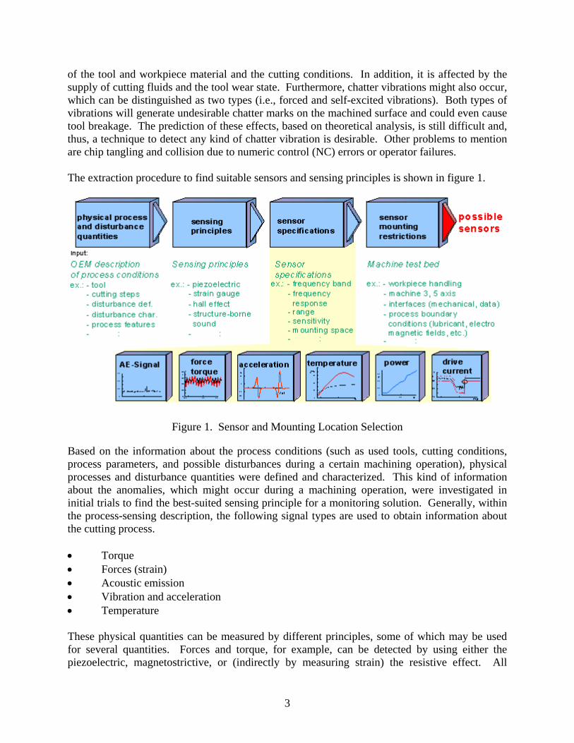
Power modules measure the active power input of spindle or feed drives. There are modules for motors operated by direct current (DC) or alternating current (AC). The modules are characterized by high accuracy. The power input of the motor, which has to be monitored, will be determined by the measurement of current (intensity (I) and voltage (V)), as shown in figure 10. In AC motors, the power factor or phase angle will be determined also, and the actual power will be calculated internally in the module (equation 1). The result is available as an analogue output signal proportional to the effective power. cosP I V= − − ϕ (1)

Figure 10. Comparison Current to Effective Power Measurement

Power measurement is used specifically for the detection of tool breakages, missing tools, and tool wear monitoring. Effective power sensors (as shown in figures 11 and 12) are well-suited for industrial monitoring applications because of robust construction, selectable measuring ranges, and the fact that no devices are necessary in the machine’s workroom.

10

Effective Power Module: • Type: Nordmann WLM-3 • Measuring range: according to Hall

sensor up to 120 kW • Sensitivity: according to equation

Figure 11. Effective Power Measurement

Figure 12. Nordmann WLM-3

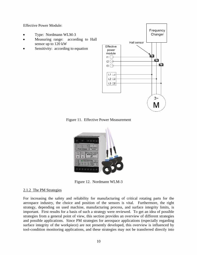
2.1.2 The PM Strategies

For increasing the safety and reliability for manufacturing of critical rotating parts for the aerospace industry, the choice and position of the sensors is vital. Furthermore, the right strategy, depending on used machine, manufacturing process, and surface integrity limits, is important. First results for a basis of such a strategy were reviewed. To get an idea of possible strategies from a general point of view, this section provides an overview of different strategies and possible applications. Since PM strategies for aerospace applications (especially regarding surface integrity of the workpiece) are not presently developed, this overview is influenced by tool-condition monitoring applications, and these strategies may not be transferred directly into

11

this project. Nevertheless, the knowledge of the state of the art for PM strategies is a sufficient basis for developing new strategies for the future. Some representative limit descriptions are listed in the following. An overview is shown in figure 13.

Missing Underload

Work Under

Overload Contact

Rising Through/FallingThroughWork Over

Dynamic Limits

PM Strategies

Figure 13. Overview of PM Strategies [Source: Prometec GmbH, Germany]

2.1.2.1 Overload and Underload

Static limits are applicable if the cutting conditions stay almost constant over the process. Overload- and underload-type limits set an alarm when the signal remains at least below an amount over a preset limit for a defined response time. These types of limits can detect tool breakages and incorrect workpiece dimensions. 2.1.2.2 Work Over and Work Under

The work-over and work-under limit type sets an alarm when the work value remains over an amount below a preset limit up to the end of the cycle. This limit type is also capable of detecting tool breakage and incorrect workpiece dimensions. 2.1.2.3 Contact and Missing

The contact and missing alarm sends out an output message as soon as the limit is exceeded. The message is reset when the signal remains at least below the limit for a preset response time. The contact alarm detects contact between tool and workpiece and can be used to minimize machining times in-air (GAP-reduction). The missing alarm can detect missing tools or broken-off tools, respectively.

12

2.1.2.4 Rising Through and Falling Through

Rising alarm types are set when a defined time limit is passed, but the signal does not pass through the limit in rising or falling mode. Time-displaced signals occur for broken or shortened tools; missing tools or workpieces; and incorrect tools or workpieces. This alarm type represents a specific monitoring of the start and end of the cut with tolerance of the full cut. Chip jamming or other major changes in the monitoring signal do not result in false alarms. 2.1.2.5 Dynamic Limits

Dynamic limits above and below a distinct monitoring signal follow the monitoring signal continuously to every load level with a limited adaption speed. They may not to be confused with signal pattern or signal tube. In the case of an extremely fast crossing, one of the two dynamic limits are frozen (rendered static), and such factors as breakage, chipping, workpiece cavity, and hard cut interruption are distinguished from each other via visual comparison with the monitor signal. Sudden load changes are due to total tool breakage or chipping. 2.2 REVIEW OF MONITORING TECHNIQUES FROM MANHIRP

2.2.1 The PM of the Drilling Processes

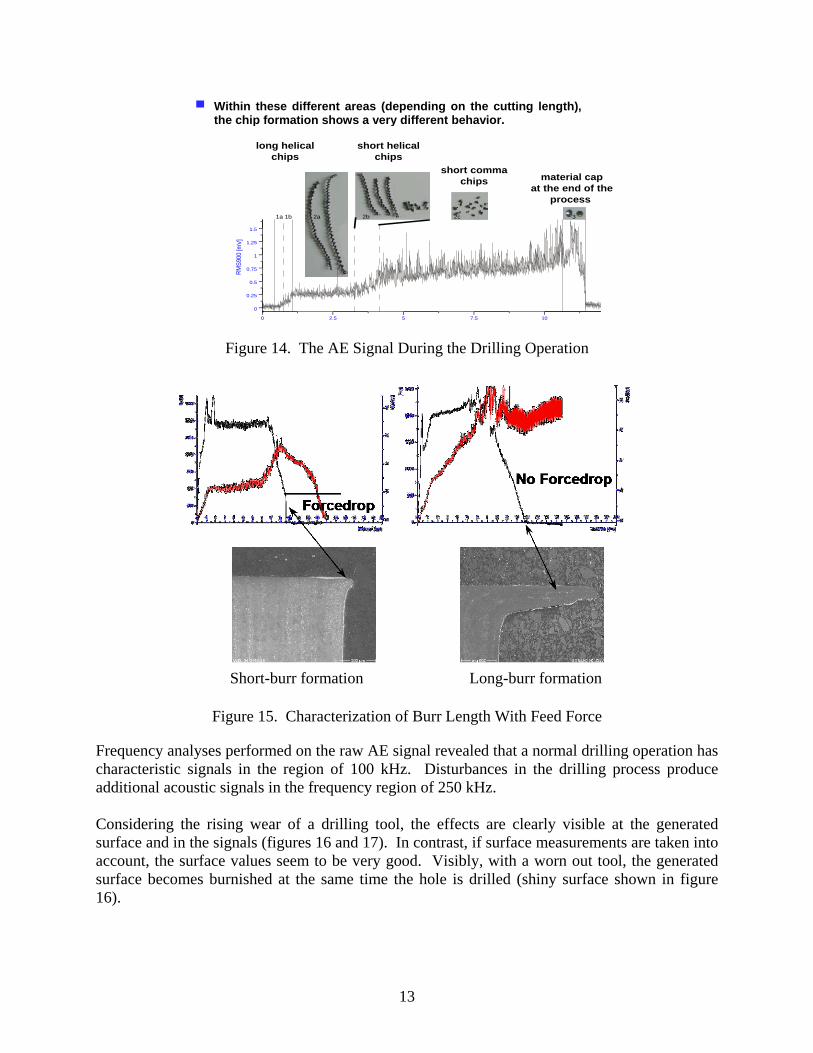
During the MANHIRP Project, PM trials were conducted at Werkzeugmaschinenlabor (WZL) (laboratory for machine tools) and the participating original equipment manufacturer (OEM) machine shops. For all trials, signal analysis and interpretation were conducted. Examples of these analyses and the first connections to the nondestructive inspection and material analysis results were drawn. The drilling process results of TiAl6V4 showed similar physical effects as Inconel 718 (nickel-based alloy). The monitored anomalies and process disturbances, which were transferable from TiAl6V4 to Inconel 718, are described below. Three phases of the drilling process were characterized by AE monitoring and feed force. Studies with artificially worn tools have identified a relationship between wear level and feed force. Different types of chip formation occurred in the three different phases of drilling, which can be related to the AE signals (see figure 14). During drilling, tool chipping was detected by a sudden drop in the feed force. The drop in feed force is proportional to the area of chip. In drilling, the characteristics in the behavior of the cutting force can be directly related to burr formation. An extensive burr can be associated with material deformation at the exit, which may not be totally removed by burr formation (see figure 15).

13

0 2.5 5 7.5 10

0

0.25

0.5

0.75

1

1.25

1.5

RMS9

00 [m

V ]

1a 1b 2a 2b 2c 3

Within these different areas (depending on the cutting lenght), the chip formation shows a very different behaviour.

long helicalchips

short helicalchips

short commachips material cap

at the end of theprocess

Figure 14. The AE Signal During the Drilling Operation

Figure 15. Characterization of Burr Length With Feed Force

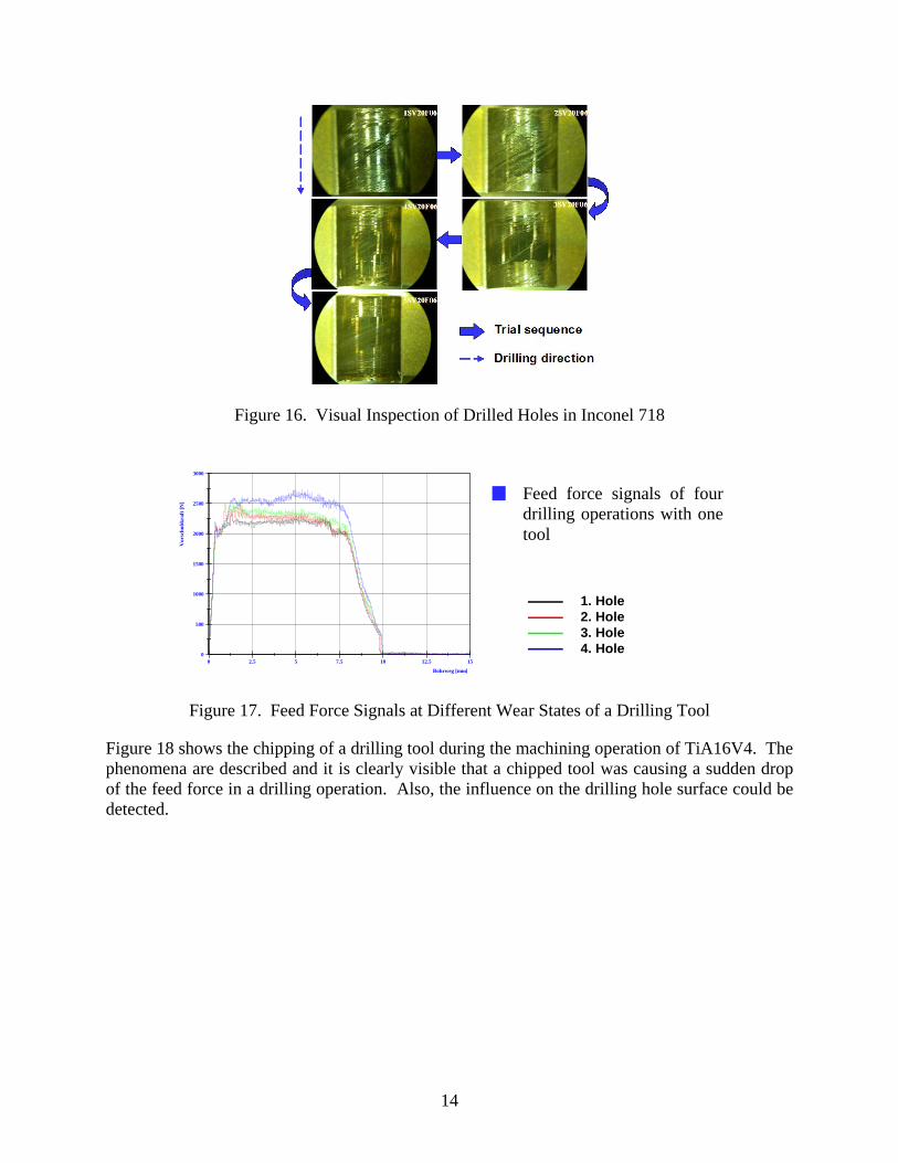
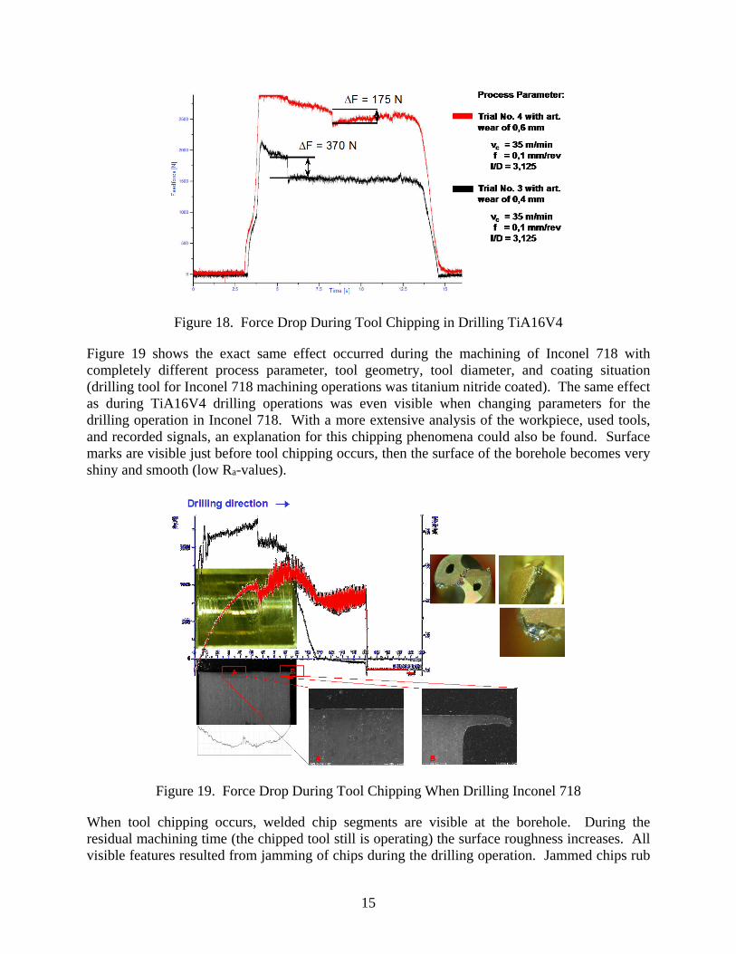
Frequency analyses performed on the raw AE signal revealed that a normal drilling operation has characteristic signals in the region of 100 kHz. Disturbances in the drilling process produce additional acoustic signals in the frequency region of 250 kHz. Considering the rising wear of a drilling tool, the effects are clearly visible at the generated surface and in the signals (figures 16 and 17). In contrast, if surface measurements are taken into account, the surface values seem to be very good. Visibly, with a worn out tool, the generated surface becomes burnished at the same time the hole is drilled (shiny surface shown in figure 16).

Short-burr formation Long-burr formation

Within these different areas (depending on the cutting length), the chip formation shows a very different behavior.

14

Figure 16. Visual Inspection of Drilled Holes in Inconel 718

0 2.5 5 7.5 10 12.5 15

Bohrweg [mm]

0

500

1000

1500

2000

2500

3000

Vor

schu

bkra

ft [N

]

Feed force signals of 4 drilling operations with one tool

1. Hole2. Hole 3. Hole 4. Hole

Figure 17. Feed Force Signals at Different Wear States of a Drilling Tool

Figure 18 shows the chipping of a drilling tool during the machining operation of TiA16V4. The phenomena are described and it is clearly visible that a chipped tool was causing a sudden drop of the feed force in a drilling operation. Also, the influence on the drilling hole surface could be detected.

Feed force signals of four drilling operations with one tool

15

Figure 18. Force Drop During Tool Chipping in Drilling TiA16V4

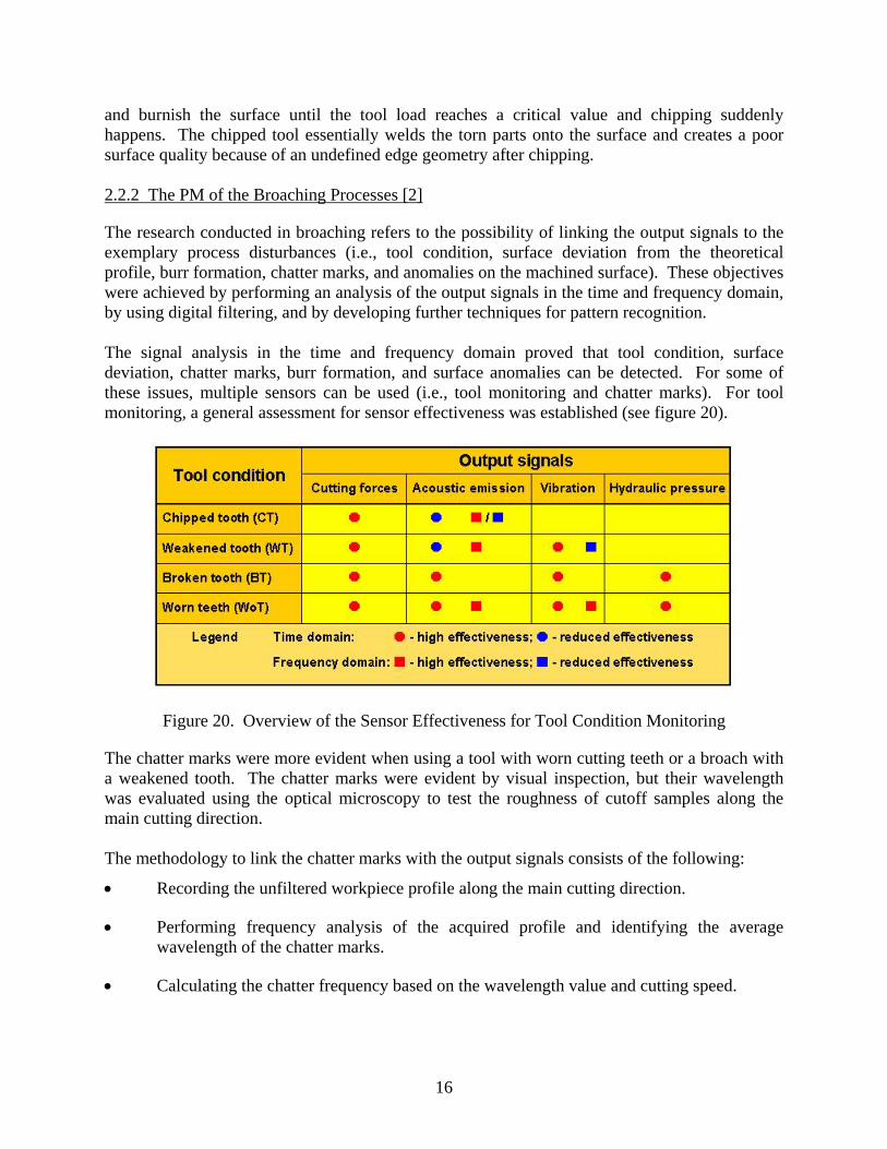
Figure 19 shows the exact same effect occurred during the machining of Inconel 718 with completely different process parameter, tool geometry, tool diameter, and coating situation (drilling tool for Inconel 718 machining operations was titanium nitride coated). The same effect as during TiA16V4 drilling operations was even visible when changing parameters for the drilling operation in Inconel 718. With a more extensive analysis of the workpiece, used tools, and recorded signals, an explanation for this chipping phenomena could also be found. Surface marks are visible just before tool chipping occurs, then the surface of the borehole becomes very shiny and smooth (low Ra-values).

Figure 19. Force Drop During Tool Chipping When Drilling Inconel 718

When tool chipping occurs, welded chip segments are visible at the borehole. During the residual machining time (the chipped tool still is operating) the surface roughness increases. All visible features resulted from jamming of chips during the drilling operation. Jammed chips rub

16

and burnish the surface until the tool load reaches a critical value and chipping suddenly happens. The chipped tool essentially welds the torn parts onto the surface and creates a poor surface quality because of an undefined edge geometry after chipping. 2.2.2 The PM of the Broaching Processes [2]

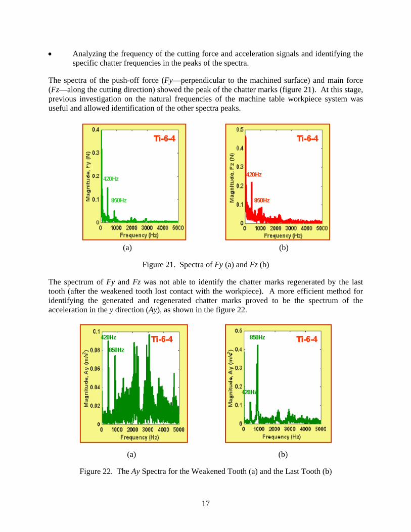
The research conducted in broaching refers to the possibility of linking the output signals to the exemplary process disturbances (i.e., tool condition, surface deviation from the theoretical profile, burr formation, chatter marks, and anomalies on the machined surface). These objectives were achieved by performing an analysis of the output signals in the time and frequency domain, by using digital filtering, and by developing further techniques for pattern recognition. The signal analysis in the time and frequency domain proved that tool condition, surface deviation, chatter marks, burr formation, and surface anomalies can be detected. For some of these issues, multiple sensors can be used (i.e., tool monitoring and chatter marks). For tool monitoring, a general assessment for sensor effectiveness was established (see figure 20).

Figure 20. Overview of the Sensor Effectiveness for Tool Condition Monitoring

The chatter marks were more evident when using a tool with worn cutting teeth or a broach with a weakened tooth. The chatter marks were evident by visual inspection, but their wavelength was evaluated using the optical microscopy to test the roughness of cutoff samples along the main cutting direction. The methodology to link the chatter marks with the output signals consists of the following:

• Recording the unfiltered workpiece profile along the main cutting direction.

• Performing frequency analysis of the acquired profile and identifying the average wavelength of the chatter marks.

• Calculating the chatter frequency based on the wavelength value and cutting speed.

17

• Analyzing the frequency of the cutting force and acceleration signals and identifying the specific chatter frequencies in the peaks of the spectra.

The spectra of the push-off force (Fy—perpendicular to the machined surface) and main force (Fz—along the cutting direction) showed the peak of the chatter marks (figure 21). At this stage, previous investigation on the natural frequencies of the machine table workpiece system was useful and allowed identification of the other spectra peaks.

(a) (b)

Figure 21. Spectra of Fy (a) and Fz (b)

The spectrum of Fy and Fz was not able to identify the chatter marks regenerated by the last tooth (after the weakened tooth lost contact with the workpiece). A more efficient method for identifying the generated and regenerated chatter marks proved to be the spectrum of the acceleration in the y direction (Ay), as shown in the figure 22.

(a) (b)

Figure 22. The Ay Spectra for the Weakened Tooth (a) and the Last Tooth (b)

18

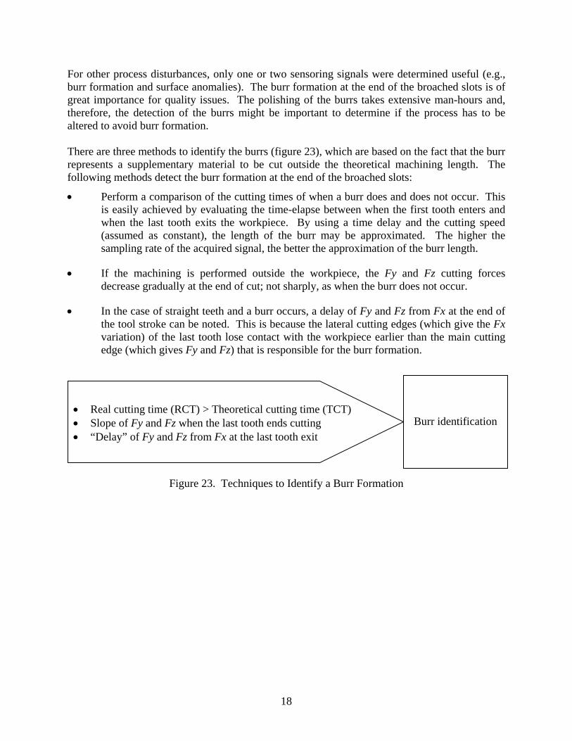
For other process disturbances, only one or two sensoring signals were determined useful (e.g., burr formation and surface anomalies). The burr formation at the end of the broached slots is of great importance for quality issues. The polishing of the burrs takes extensive man-hours and, therefore, the detection of the burrs might be important to determine if the process has to be altered to avoid burr formation. There are three methods to identify the burrs (figure 23), which are based on the fact that the burr represents a supplementary material to be cut outside the theoretical machining length. The following methods detect the burr formation at the end of the broached slots:

• Perform a comparison of the cutting times of when a burr does and does not occur. This is easily achieved by evaluating the time-elapse between when the first tooth enters and when the last tooth exits the workpiece. By using a time delay and the cutting speed (assumed as constant), the length of the burr may be approximated. The higher the sampling rate of the acquired signal, the better the approximation of the burr length.

• If the machining is performed outside the workpiece, the Fy and Fz cutting forces decrease gradually at the end of cut; not sharply, as when the burr does not occur.

• In the case of straight teeth and a burr occurs, a delay of Fy and Fz from Fx at the end of the tool stroke can be noted. This is because the lateral cutting edges (which give the Fx variation) of the last tooth lose contact with the workpiece earlier than the main cutting edge (which gives Fy and Fz) that is responsible for the burr formation.

Figure 23. Techniques to Identify a Burr Formation

• Real cutting time (RCT) > Theoretical cutting time (TCT) • Slope of Fy and Fz when the last tooth ends cutting • “Delay” of Fy and Fz from Fx at the last tooth exit

Burr identification

19

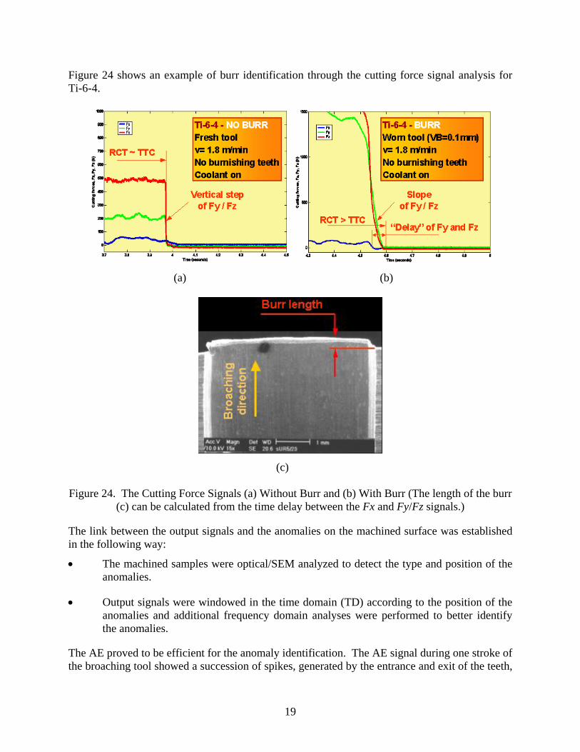
Figure 24 shows an example of burr identification through the cutting force signal analysis for Ti-6-4.

(a) (b)

(c) Figure 24. The Cutting Force Signals (a) Without Burr and (b) With Burr (The length of the burr

(c) can be calculated from the time delay between the Fx and Fy/Fz signals.)

The link between the output signals and the anomalies on the machined surface was established in the following way:

• The machined samples were optical/SEM analyzed to detect the type and position of the anomalies.

• Output signals were windowed in the time domain (TD) according to the position of the anomalies and additional frequency domain analyses were performed to better identify the anomalies.

The AE proved to be efficient for the anomaly identification. The AE signal during one stroke of the broaching tool showed a succession of spikes, generated by the entrance and exit of the teeth,

20

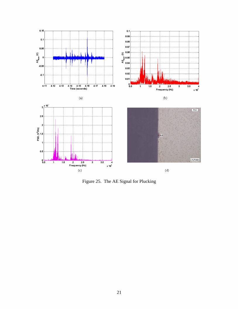
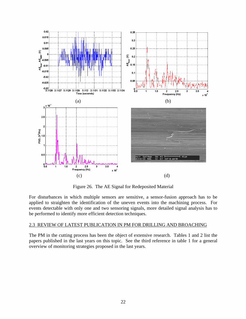
with low-signal amplitude in between. If an uneven event happens between entrance and exit spikes, a local increase of the AE amplitude should happen. This assumption proved to be correct, and it helped create a TD identification of the anomalies. Care should be taken when the AE signal is analyzed using this method because, in broaching, at least two teeth are simultaneously in contact with the workpiece. Therefore, the AE sensor acquires uneven events that happen at the level of each tooth in contact with the workpiece at a certain moment. Note that the last tooth is primarily responsible for the final surface quality of the machined surface. The AE signal analysis for anomaly identification is easier when only the last tooth is in contact with the workpiece (the end part of the machined slot equal with the pitch of the broaching tool) and no uneven disturbances are possible from the other teeth. Therefore, it is important to distinguish between the uneven events generated at the level of the last tooth, which may generate the anomalies on the final machined surface, and those generated by the other teeth simultaneously in contact with the workpiece. For this purpose, a methodology was investigated based on the fact that even the teeth are identical (e.g., edge preparation). Differences can be noted from the burst signals when cutting starts and ends. This may have been due to different teeth loading, intimate differences in edge preparation, or wear land. These differences were able to be detected in the frequency domain and used to link the final surface anomalies with the AE signal generated by the last tooth of the broaching tool. Figures 25 and 26 show examples of anomaly identification using the AE signal when machining Inconel 718. Figure 25 shows (a) an example of the AE signal feature in TD and frequency domain ((b) magnitude, and (c) power spectrum density for a plucking obtained after broaching. The parameters were cutting speed 1.8 m/min, coolant on, worn teeth at VB = 0.25 mm, and without burnishing teeth. Figure 26 shows (a) an example of the AE signal feature in TD and frequency domain ((b) magnitude, and (c) power spectrum density for redeposited material obtained after broaching with 2.7 m/min, coolant off, worn teeth at VB = 0.25 mm, and burnishing teeth. The signal analysis shows that the techniques developed are efficient in detecting the anomalies on the machined surface, but, up until now, the distinction between different anomalies is difficult to make. Techniques for signal processing to address this issue are investigated in this report.

21

Figure 25. The AE Signal for Plucking

22

(a) (b)

(c) (d)

Figure 26. The AE Signal for Redeposited Material

For disturbances in which multiple sensors are sensitive, a sensor-fusion approach has to be applied to straighten the identification of the uneven events into the machining process. For events detectable with only one and two sensoring signals, more detailed signal analysis has to be performed to identify more efficient detection techniques. 2.3 REVIEW OF LATEST PUBLICATION IN PM FOR DRILLING AND BROACHING

The PM in the cutting process has been the object of extensive research. Tables 1 and 2 list the papers published in the last years on this topic. See the third reference in table 1 for a general overview of monitoring strategies proposed in the last years.

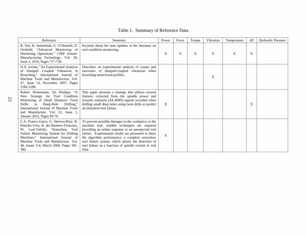
Table 1. Summary of Reference Data

Reference Summary Power Force Torque Vibration Temperature AE Hydraulic Pressure R. Teti, K. Jemielniak, G. O’Donnell, D. Ornfield, “Advanced Monitoring of Machining Operations,” CIRP Annals-Manufacturing Technology, Vol. 59, Issue 2, 2010, Pages 717-739.

Keynote about the lasts updates of the literature on tool-condition monitoring.

X X X X X X

D.A. Axinte, “An Experimental Analysis of Damped Coupled Vibrations in Broaching,” International Journal of Machine Tools and Manufacture, Vol. 47, Issue 14, November 2007, Pages 2182-2188.

Describes an experimental analysis of causes and outcomes of damped-coupled vibrations when broaching semiclosed profiles. X

Robert Heinemann, Sri Hinduja, “A New Strategy for Tool Condition Monitoring of Small Diameter Twist Drills in Deep-Hole Drilling,” International Journal of Machine Tools and Manufacture, Vol. 52, Issue 1, January 2012, Pages 69-76.

This paper presents a strategy that utilizes several features extracted from the spindle power and acoustic emission (AE-RMS) signals recorded when drilling small deep holes using twist drills to predict an imminent tool failure.

X X

L.A. Franco-Gasca, G. Herrera-Ruiz, R. Peniche-Vera, R. deJ.Romero-Troncoso, W. Leal-Tafolla, “Sensorless Tool Failure Monitoring System for Drilling Machines,” International Journal of Machine Tools and Manufacture, Vol. 46, Issues 3-4, March 2006, Pages 381-386.

To prevent possible damages to the workpiece or the machine tool, reliable techniques are required providing an online response to an unexpected tool failure. Experimental results are presented to show the algorithm performance, a complete sensorless tool failure system, which allows the detection of tool failure as a function of spindle current in real time.

X

23

Table 2. Lasest Publications in PM 12/2

Publication Summary Power Force Torque Vibration Temperature AE Hydraulic Pressure G. Byrne, G.E. O’Donnell, “An Integrated Force Sensor Solution for Process Monitoring of Drilling Operations,” CIRP Annals-Manufacturing Technology, Vol. 56, Issue 1, Pages 89-92.

Two piezoelectric force sensor rings were developed and integrated into a direct-driven motor spindle for online process monitoring or matching processes. Performance comparisons are made between the integrated force sensors and traditional monitoring sensors, such as motor power and acoustic emission.

X

Duck whan Kim, Young Soo Lee, Min Soo Park, Chong Nam Chu, “Tool Life Improvement by Peck Drilling and Thrust Force Monitoring During Deep-Micro-Hole Drilling of Steel,” International Journal of Machine Tools and Manufacture, Vol. 49, Issues 3-4, March 2009, Pages 246-255.

An unstable drilling process results from the insufficient supply of cutting fluid and bad chip removal as machining depth increases. Peck drilling, which utilizes an intermittent feed, is widely used in drilling deep holes. This paper proposes the peek drilling method using thrust force signal monitoring.

X

F. Bound, N.N.Z. Gindy, “Application of Multi-Sensor Signals for Monitoring Tool/Work Piece Condition in Broaching,” International Journal of Computer Integrated Manufacturing, Archive Vol. 21, Issue 6, September 2008.

Identification of appropriate techniques for monitoring tool condition and surface anomalies in broaching. Presents results of the output signals obtained from multiple sensors, such as acoustic emission, cutting forces, vibration, hydraulic pressure, and table displacement.

X X X X

Axinte D.A., Gindy N., “Tool Condition Monitoring in Broaching,” Wear, Volume 254, Number 3, February 2003, pp. 370-382(13)

The paper reports on research that attempts to correlate the conditions of broaching tools to the output signals obtained from multiple sensors, namely acoustic emission (AE), vibration, cutting forces, and hydraulic pressure, which are connected to a hydraulic broaching machine.

X X X X

24

25

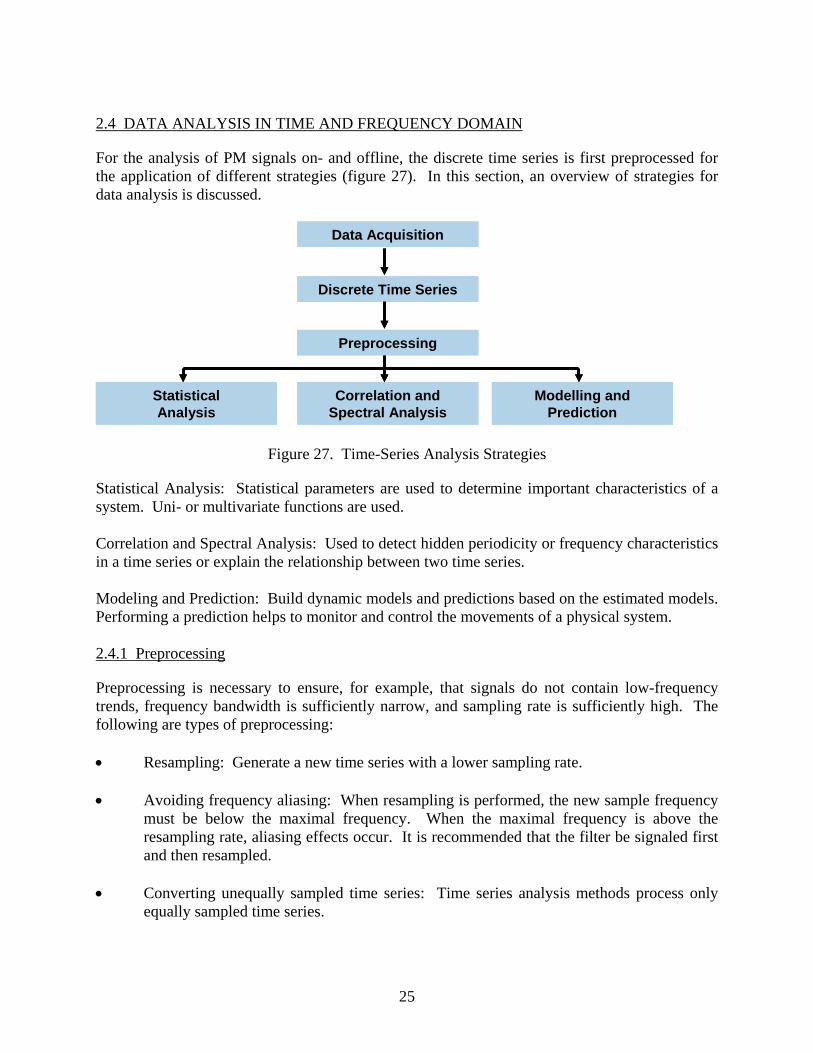
2.4 DATA ANALYSIS IN TIME AND FREQUENCY DOMAIN

For the analysis of PM signals on- and offline, the discrete time series is first preprocessed for the application of different strategies (figure 27). In this section, an overview of strategies for data analysis is discussed.

Data Acquisition

Discrete Time Series

Preprocessing

Correlation and Spectral Analysis

StatisticalAnalysis

Modelling and Prediction

Data Acquisition

Discrete Time Series

Preprocessing

Correlation and Spectral Analysis

StatisticalAnalysis

Modelling and Prediction

Figure 27. Time-Series Analysis Strategies

Statistical Analysis: Statistical parameters are used to determine important characteristics of a system. Uni- or multivariate functions are used. Correlation and Spectral Analysis: Used to detect hidden periodicity or frequency characteristics in a time series or explain the relationship between two time series. Modeling and Prediction: Build dynamic models and predictions based on the estimated models. Performing a prediction helps to monitor and control the movements of a physical system. 2.4.1 Preprocessing

Preprocessing is necessary to ensure, for example, that signals do not contain low-frequency trends, frequency bandwidth is sufficiently narrow, and sampling rate is sufficiently high. The following are types of preprocessing: • Resampling: Generate a new time series with a lower sampling rate. • Avoiding frequency aliasing: When resampling is performed, the new sample frequency

must be below the maximal frequency. When the maximal frequency is above the resampling rate, aliasing effects occur. It is recommended that the filter be signaled first and then resampled.

• Converting unequally sampled time series: Time series analysis methods process only

equally sampled time series.

26

• Smoothing: There are different schemes for smoothing. The time series analysis (TSA) moving average compensates for the phase shift of the smoothed signal. A TSA exponential average was performed smoothly according to the characteristics of the time series. To correct signals, an additive or multiplicative scheme can be used.

• Detrending: The normal function adjusts only constant offset components. The

component mean value is subtracted from the signal. 2.4.2 Statistical Values

Nonstationary data, as obtained from PM signals, is characterized in many cases by the negative statement that specifies the lack of stationary properties, rather than defining the precise nature of the nonstationary [BEND66]. Statistical values are used for this purpose and for the characterization of stable cutting conditions. Arithmetic mean is the arithmetic average of a set of values or distribution. For skewed distributions, the mean is not necessarily the same as the middle value (median):

1

1 n

ii

x xn =

= ⋅∑ (2)

Variance is a measure of how far a set of numbers is spread out. It is one of several descriptors of a probability distribution, describing how far the numbers lie from the mean (expected value). If a random variable X has the expected value (mean) μ = E[X], then the variance of X is given by: ( ) ( )2Var X E X = − µ (3)

The expectation of this random variable X is defined as: [ ] 1 1 2 2 ... k kE X x p x p x p= + + + (4) when the random variable X can take value x1 with probability p1, value x2 with probability p2, and so on, up to value xk with probability pk. Skewness indicates the symmetry of the probability density function (PDF). Kurtosis measures the peakedness of the PDF. • 3: Gaussian distribution • >3 : sharp peak • <3 : flat peak

Confidence limits are user-specified probability bounds for the range of statistical parameters.

27

2.4.3 Correlation and Spectral Analysis

One application of time series analysis is detecting hidden periodicities or frequency characteristics in a time series at specific frequencies. For this purpose, time series virtual instruments (VI) are used. The correlation analysis finds periodic patterns at a specific frequency in one or more-time series. This function is used to identify or extract other features, such as phase. Fast Fourier Transform (FFT) is an efficient algorithm to compute the discrete Fourier transform (DFT). A DFT decomposes a sequence of values into components of different frequencies. Joint Time Frequency (JTF) is a Fourier-related transform used to determine the sinusoidal frequency and phase content of local sections of a signal as it changes over time. It has the advantage of providing both frequency and time information represented on a graph in the x and y axes. The z axis, which shows the amplitude of the frequency peaks, can be represented in colors. Signals usually contain both low- and high-frequency components: • Low frequency varies slowly with time and requires fine frequency resolution, but coarse

time resolution.

• High frequency varies quickly with time and requires fine-time resolution, but coarse frequency resolution.

Analytic Wavelet Transform provides both magnitude and phase information of signals in time-scale or time-frequency domain. The magnitude information describes the envelope of the signals. The phase information encodes the time-related characteristics. Autocorrelation captures periodic components in one signal. The autocorrelation preserves frequency and amplitude, but not the phase. 2.4.4 Models

Autoregressive models predict the current value based on the past values plus a prediction error. Many real-world linear systems can be modelled accurately with autoregressive models. Therefore, this function is a good choice for parametric modeling. Other models: Autoregressive moving average models, modal-parametric models, and stochastic state-space models. Besides these models, which in many cases may be machine-dependant and, therefore, not transferable, the use of physical models related to the measured signals is desired. Given the complexity of the process and machine dynamics, physical models do not exist for all signals and, in some cases, data mining (DM) methods are applied. The DM methods and models are summarized in section 2.5.

28

2.5 LITERATURE STUDY ON DATA/SIGNAL MINING FOR PM APPLICATIONS

The integration of multiple sensors, as well as the used of high sampling rates, yields large databases from which the important data has to be identified and transformed into relevant information. For these purposes, different DM strategies were applied in PM to identify specific process conditions (e.g., tools wear status) and implement actions. The DM is an analytic process that explores data and searches for consistent patterns and systematic relationships between variables, which are validated with new data. The DM combines computer power and statistical-learning algorithms to automatically or semiautomatically extract previously unknown and potentially useful knowledge and patterns from large databases. However, to implement the DM process, as shown in figure 28, the following steps are required:

1. Task definition 2. Data integration and selection 3. Data preprocessing 4. Data transformation 5. Selection of the DM method 6. Interpretation and evaluation of mine patterns, models 7. Identification and implementation of actions according to results from the model

Action

Data

Preprocessed Data

Transformed Data

Model

Knowledge

PatternsPreprocessing

Transformation

Data Mining

Interpretation/Evaluation

Action

Data

Preprocessed Data

Transformed Data

ModelModel

Knowledge

Patterns

KnowledgeKnowledge

PatternsPreprocessing

Transformation

Data Mining

Interpretation/Evaluation

Figure 28. Overview of the Steps That Compose the DM Process [FAYY96]

The extraction of knowledge or useful information from data is an interactive and iterative process, involving numerous steps with many decisions made by the user. Before the actual implementation of a DM method, two important and time-demanding steps have to be performed: data preprocessing and transformation. These are very important for the successful implementation of a reliable system.

29

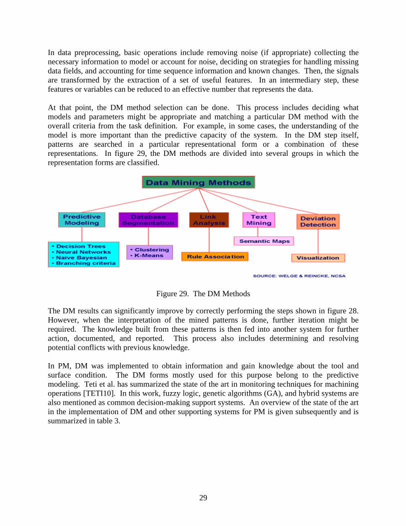
In data preprocessing, basic operations include removing noise (if appropriate) collecting the necessary information to model or account for noise, deciding on strategies for handling missing data fields, and accounting for time sequence information and known changes. Then, the signals are transformed by the extraction of a set of useful features. In an intermediary step, these features or variables can be reduced to an effective number that represents the data. At that point, the DM method selection can be done. This process includes deciding what models and parameters might be appropriate and matching a particular DM method with the overall criteria from the task definition. For example, in some cases, the understanding of the model is more important than the predictive capacity of the system. In the DM step itself, patterns are searched in a particular representational form or a combination of these representations. In figure 29, the DM methods are divided into several groups in which the representation forms are classified.

Figure 29. The DM Methods

The DM results can significantly improve by correctly performing the steps shown in figure 28. However, when the interpretation of the mined patterns is done, further iteration might be required. The knowledge built from these patterns is then fed into another system for further action, documented, and reported. This process also includes determining and resolving potential conflicts with previous knowledge. In PM, DM was implemented to obtain information and gain knowledge about the tool and surface condition. The DM forms mostly used for this purpose belong to the predictive modeling. Teti et al. has summarized the state of the art in monitoring techniques for machining operations [TETI10]. In this work, fuzzy logic, genetic algorithms (GA), and hybrid systems are also mentioned as common decision-making support systems. An overview of the state of the art in the implementation of DM and other supporting systems for PM is given subsequently and is summarized in table 3.

30

Table 3. State-of-the-Art Summary for DM Applications in PM

Drilling/Boring Broaching Milling Turning

Tool

Condition Surface Integrity

Tool Condition

Surface Integrity

Tool Condition

Surface Integrity

Tool Condition

Surface Integrity

Flank wear Roughness 4 states Roughness Flank wear Roughness NN Static/

dynamic [SANJ05] [AXIN06] [GIRI06]

[HABE03] [BENA02] [CHRY92]

[SCHE04] [BURK92] [SICK02] [KILU10]

RBF [TSAO08] [KUO00] [KUO99] [KUO98] [KUO97]

Fuzzy [JANT00] [MOHA09] [KUO00] [KUO99] [KUO98] [KUO97]

[KIRB07]

Genetic algorithms

[BREZ04] [SCHE04] [KIRB06]

Fuzzy logic [JANT06] [XIAO98]

[ACHI02] [XIAO98]

Hierarchical algorithms

[JANT00] [JEMI08] [DAS03] [ACHI02]

Regression analysis

[SANJ05] [JANT06] [JANT03]

[CHRY92]

Process model [CHRY92] [SAHI04] Decision tree [JIAA98]

[KILU10]

Bayesian method

[KILU10] [ELAN10] [ABEL07]

[ABEL07]

Further studies have been conducted in this area. However, as shown in table 1, most of the research focused on the turning operation because of its quasi-stationary characteristics, which make this process easier to define. 2.5.1 Neural Networks

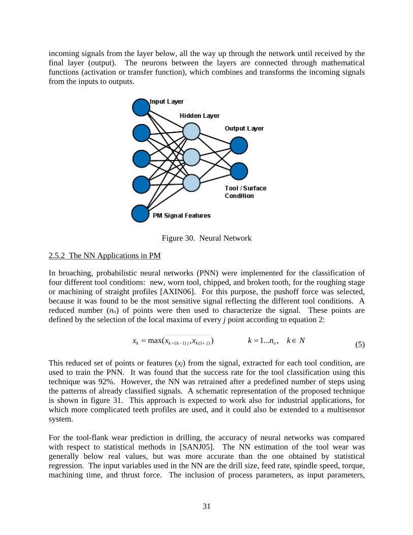
A neural network (NN) is the series of interconnected biological neurons in the human brain. This model has been implemented in the artificial NN, where the single processing elements, called neurons or nodes, are organized in layers and interconnected to produce an output. The NN can be used as mapping devices, pattern classifiers, or pattern completers. The NN has to be trained in either a supervised or unsupervised mode with some initial data to predict the desire output. An example of a simple three-layer NN is shown in figure 30. The neurons from the input layer are the features that were extracted from the PM signals and had a correlation to the desired output. The hidden layers are arrays of neurons that receive, transform, and transmit the

31

incoming signals from the layer below, all the way up through the network until received by the final layer (output). The neurons between the layers are connected through mathematical functions (activation or transfer function), which combines and transforms the incoming signals from the inputs to outputs.

Figure 30. Neural Network

2.5.2 The NN Applications in PM

In broaching, probabilistic neural networks (PNN) were implemented for the classification of four different tool conditions: new, worn tool, chipped, and broken tooth, for the roughing stage or machining of straight profiles [AXIN06]. For this purpose, the pushoff force was selected, because it was found to be the most sensitive signal reflecting the different tool conditions. A reduced number (no) of points were then used to characterize the signal. These points are defined by the selection of the local maxima of every j point according to equation 2:

(5)

This reduced set of points or features (xj) from the signal, extracted for each tool condition, are used to train the PNN. It was found that the success rate for the tool classification using this technique was 92%. However, the NN was retrained after a predefined number of steps using the patterns of already classified signals. A schematic representation of the proposed technique is shown in figure 31. This approach is expected to work also for industrial applications, for which more complicated teeth profiles are used, and it could also be extended to a multisensor system. For the tool-flank wear prediction in drilling, the accuracy of neural networks was compared with respect to statistical methods in [SANJ05]. The NN estimation of the tool wear was generally below real values, but was more accurate than the one obtained by statistical regression. The input variables used in the NN are the drill size, feed rate, spindle speed, torque, machining time, and thrust force. The inclusion of process parameters, as input parameters,

N k n k x x x o j k j k k k ∈ = = + − + , ... 1 ) , max( ) 1 ( ) 1 (

32

should allow the system to be used for different drills; however, it is important to keep in mind that, in this work, only one tool diameter was actually used.

Figure 31. The NN Implemented in Tool Condition Recognition System [AXIN06]

Given that tool wear is a dynamic process and does not follow the same geometry and growth rate, a dynamic modeling approach was suggested in [SCHE04]. In that work, NNs were implemented in two loops to monitor the tool condition in interrupted turning. The offline, static network was trained to model the known feature values of tool wear and cutting conditions. The online, dynamic network attempted to predict the current wear by using the previous predictions of tool wear as input. The training goal of the dynamic network was to minimize the error between online measurements and the output of the static networks. 2.5.3 Fuzzy Logic

Fuzzy logic is a mathematical technique for dealing with imprecise data and problems that have many solutions. This approach computes a result based on degrees of truth rather than the usual true or false (1 or 0) Boolean logic in which the modern computer was based. Software based on the application of fuzzy logic allows computers to mimic human reasoning more closely, so decisions can be made with incomplete or uncertain data. Fuzzy logic was used for solving problems with expert systems and real-time systems that must react to an imperfect environment of highly variable, volatile, or unpredictable conditions. The concept was conceived in 1964 by Lotfi Zadeh, former chairman of the electrical engineering and computer science department at the University of California at Berkeley. Membership functions were used to convert the output of the neuro-fuzzy algorithm from quantitative to linguistic values. An example is shown in figure 32. Because the uncertainties involved made it difficult to define certain boundaries between different tool conditions, trapezoidal membership functions were chosen. As a result, the tool condition could be defined

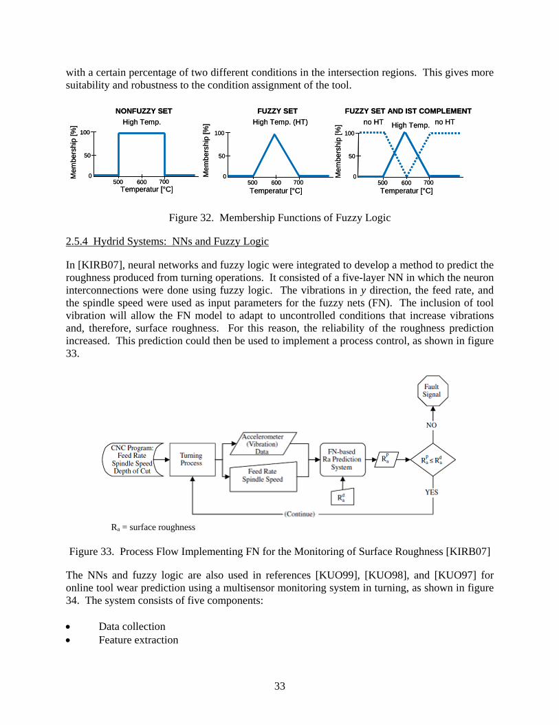
33

with a certain percentage of two different conditions in the intersection regions. This gives more suitability and robustness to the condition assignment of the tool.

0

50

100

Temperatur [°C]500 600 700

High Temp.NONFUZZY SET

Mem

bers

hip

[%]

0

50

100

500 600 700

High Temp. (HT)FUZZY SET

0

50

100

500 600 700

High Temp.

FUZZY SET AND IST COMPLEMENT no HT no HT

Temperatur [°C]

Mem

bers

hip

[%]

Temperatur [°C]

Mem

bers

hip

[%]

0

50

100

Temperatur [°C]500 600 700

High Temp.NONFUZZY SET

Mem

bers

hip

[%]

0

50

100

500 600 700

High Temp. (HT)FUZZY SET

0

50

100

500 600 700

High Temp.

FUZZY SET AND IST COMPLEMENT no HT no HT

Temperatur [°C]

Mem

bers

hip

[%]

Temperatur [°C]

Mem

bers

hip

[%]

Figure 32. Membership Functions of Fuzzy Logic

2.5.4 Hydrid Systems: NNs and Fuzzy Logic

In [KIRB07], neural networks and fuzzy logic were integrated to develop a method to predict the roughness produced from turning operations. It consisted of a five-layer NN in which the neuron interconnections were done using fuzzy logic. The vibrations in y direction, the feed rate, and the spindle speed were used as input parameters for the fuzzy nets (FN). The inclusion of tool vibration will allow the FN model to adapt to uncontrolled conditions that increase vibrations and, therefore, surface roughness. For this reason, the reliability of the roughness prediction increased. This prediction could then be used to implement a process control, as shown in figure 33.

Ra = surface roughness

Figure 33. Process Flow Implementing FN for the Monitoring of Surface Roughness [KIRB07]

The NNs and fuzzy logic are also used in references [KUO99], [KUO98], and [KUO97] for online tool wear prediction using a multisensor monitoring system in turning, as shown in figure 34. The system consists of five components: • Data collection • Feature extraction

34

• Pattern recognition • Multisensor integration • Tool/work distance compensation for tool flank wear For each sensor, a radial basis function network was used to predict the tool wear from the extracted features. The fuzzy NN was then used to integrate the decisions obtained from the multisensor system and provide a more accurate estimation. Furthermore, the use of fuzzy NN reduced the training time.

Figure 34. Multisensor System for Tool Wear Estimation [KUO99]

2.5.5 Hierarchical Algorithm

In [JEMI08], a tool-condition monitoring method using multiple PM signals (force and AE), based on hierarchical algorithms, was developed for micromilling. In this case, the tool condition was not regarded as the tool flank wear, but the used-up portion (∆T) from the total tool life (T) was considered:

TtT =∆ (6)

where t: cutting time Several statistical values were extracted from the signals to be used as SF that correlate to ∆T. The SF that best describes the tool condition are found by approximating the function for SF

35

versus ∆T with a second-degree polynomial. Then, the SF with an RMS error lower than 0.2 in this approximation are selected. The subsequent main steps for the tool condition estimation are as follows:

1. The functions ∆T = f (SF) are divided into arrays of 120 elements Sn (every 1% of ∆T up to 120%).

2. The Sn array is searched to find the SFn closest to the measured value (starts with the value obtained in the previous run).

3. ∆Ts estimations from each SF are averaged, taking into consideration that values that differ more than 3σ from mean value are not considered.

The method proposed in [JEMI08] is not very complex and the use of several features from a multisensor system provides a higher reliability in the tool condition prediction. However, given the changes that could be present in tool life, the training step should be performed with more than one tool. 2.5.6 Genetic Algorithms

A GA is a search algorithm that is based on the biological principles of selection, reproduction, and mutation. Unlike other search strategies, the GA operates on a population of potential solutions called chromosomes. The chromosome is composed of a string of numbers and represents the encoding of the solution. A GA follows an analogy of processes that occurs in living nature within the evolution of live organisms. This method has been successfully used in optimization problems, unlike the traditional gradient optimization methods. 2.5.7 Decision Trees

A decision tree is one of the most systematic tools of decision-making theory and practice. Decision trees are particularly helpful in situations of complex multistage decision problems. For example, when you need to plan and organize a sequence of decisions, taking into account the choices made at earlier stages, the outcomes of possible external events will determine the types of decisions and events at later stages of that sequence. A decision-making tree is essentially a diagram that represents, in a specially organized way, the decisions and the main external or other events that introduce uncertainty, as well as possible outcomes of all those decisions and events. 2.6 LITERATURE STUDY OF PHYSICAL MODELS DESCRIBING MEASURES

The use of a physical model for PM was also considered by several researchers. However, in most cases, the signal response can be very difficult to model and the use of reference signals or DM methods is required.

36

For the force in the cutting processes, an empirical model was developed. Equation 4 considers the force as a function of the cross-sectional area being cut and can be used for the estimation of the process forces (Fi) (cutting force (Fc), passive force (Fp), and feed force (Ff)). The constant values have to be determined experimentally for each workpiece and tool material combination. The specific cutting force ki1.1 is determined for a cut cross section with a 1-millimeter chip thickness (h) and a 1-millimeter chip width (b):

)1(

1.1cm

ii hbkF −⋅⋅= (7)

The energy used for the cutting process is obtained according to Deutsche Industrie Nom 6584 by multiplying the distance traveled times the force actuating in this direction. Correspondingly, the power is calculated by multiplying the cutting speed with the force in its direction. The cutting power (equation 5) and feed power (equation 6) are shown below. c c cP F v= ⋅ (8) f f fP F v= ⋅ (9) The total effective power is the addition of the cutting and feed power. e c fP F v= ⋅ (10) Figure 35 shows the distribution of the effective work during the cutting process. The percentage that goes into each part depends on the chip thickness. However, it was found that, in general, most of the mechanical work is transformed into heat [KLOC08]. This consideration is very important because the surface is highly influenced by this factor.

Figure 35. Distribution of the Effective Work During the Cutting Process [KLOC08]

In PM, the Kienzle force model can be used to establish limits for the force and, therefore, for the power. Further details for the use of this model for hole making and broaching are given below. The cutting parameters and different correction factors that can be considered are specified in reference [ZAH07]. Other considerations can be found in appendices F and G.

shear work cutting work

friction at flank friction at face

Latent energy

and heat

Effective work We

We=Fc*Lc+Ff*Lf

Deformation work

Friction work

shear work cutting work

friction at flank friction at face

Latent energy

and heat

Effective work We

We=Fc*Lc+Ff*Lf

Deformation work

Friction work

shear work cutting work

friction at flank friction at face

shear work cutting work

friction at flank friction at face

Latent energy

and heat

Latent energy

and heat

Effective work We

We=Fc*Lc+Ff*Lf Effective work We

We=Fc*Lc+Ff*Lf

Deformation work

Deformation work

Friction work

Friction work

37

Figure 36 shows the Kienzle force model application for drilling.

4mD+dr = 2cm mV r n= ⋅ ⋅ ⋅π

f zV n f z= ⋅ ⋅ 2p

D da −=

sinp

r

ab =

κ

sinz rh f= ⋅ κ

pA b h a f= ⋅ = ⋅ ( )2 214 fQ D d= π⋅ − ⋅ υ

11 1mc

cz c g verF b h k f k−= ⋅ ⋅ ⋅ ⋅ ⋅ c cz mM z F r= − ⋅

2c cP M n= ⋅ π⋅

Figure 36: Cutting Variables in Drilling [ZAH07]

A = Chip cross section Mc = Cutting torque ap = Cutting width mc = Tangent of angle of elevation b = Width of chip n = Tool revolution per minute (RPM) D = External diameter rm = Mean radius of chip cross section d = Internal diameter Pc = Cutting power fB = Process factor of drilling Q = Material removal rate fz = Feed rate per tooth vcm = Mean cutting speed Fcz = Cutting force per tooth fυ = Feed rate h = Chip thickness mm z = Number of tool flutes kc1.1 = Specific cutting force δ = Point angle Kver = Wear correction factor κr = Tool entering angle

38

Figure 37 shows the Kienzle force model application for broaching.

09rκ = sin

p

r

ab =

κ

sinz rh f= ⋅ κ ie

wzt

=

ie z p cQ z f a v= ⋅ ⋅ ⋅ 11.1

imcz c R ye vrF b h k f K K−= ⋅ ⋅ ⋅ ⋅ ⋅

c ie czF Z F= − c c cP F v= ⋅

Figure 37. Cutting Variables in Broaching [ZAH07]

ap = Cutting width b = Width of chip fR = Process factor for broaching fz = Rise per tooth Fc = Cutting force Fcz = Cutting force per tooth

Pc = Cutting power Q = Material removal rate t(min) = Minimum pitch vc = Cutting speed w = Broaching length zie = Tooth in contact

39

h = Chip thickness mm kc1.1 = Specific cutting force Kvr = Wear correction factor Ky0 = Chip angle correction mc = Tangent of angle of elevation

α = Clearance angle γ = Hook angle κr = Tool angle setting λS = Tooth tilt angle

3. CURRENT PRACTICES AND GENERAL REVIEW OF EXPERIENCES WITH PM IN PRODUCTION

A review of the current industry practices is summarized in this section. This should serve as the basis for good practices to be implemented and taken into account in production. 3.1 CURRENT PM USED IN PRODUCTION

The PM has been the object of intensive research in the industry. Various strategies and systems are already used in production for both online PM and offline process analysis. Power and flow-rate sensors find the most application for online monitoring. Of concern to the industry is the online identification of process anomalies. In addition, a better understanding of the process, forces, torque, and vibration monitoring investigated. New applications, like the use of the internal machine signals, is also receiving good acceptance. Other signals monitored are spindle speed and coolant pressure. 3.1.1 Drilling

Online PM of hole-making is a standard and, in some cases, a required practice in industry. It is required by application specification to part drawings for the hole-making process in rotor and forged static High Pressure Compressor (HPC) parts. Komet® Brinkhaus GmbH, Caron Engineering, Artis, and Omative offer systems that cover these requirements. The system’s capabilities and requirements are based on the following six features: ´ • Power and coolant monitoring with tool retract on alarm • Spindle speed check • Baseline set • Coolant check • Coolant monitoring • Monitored data upload The different functions are activated through the use of M-functions coming from the NC. 3.1.2 Broaching

Given the complexity of broaching, process analysis through the implementation of three-axial force monitoring is used. For online monitoring, uniaxial force measurement systems are installed at several companies. Coolant flow sensors are used to determine sudden loss of coolant and vibration to define excessive wear and regrind condition.

40

3.1.2.1 Uniaxial Force Measurement

The cutting force is acquired through load cells installed under the machine table or built-in sensors on the machine. Pharos Broach Technical Services (B.T.S. Limited) This system provides information about broach-cutting loads through piezo-quartz cells installed underneath the machine table or fixture. An amplifier, which resets before each cut, transmits the signal to the computer. An encoder is attached to the tool slide and is used to indicate the cutting position. Therefore, the load can be monitored in relation to the displacement. The tolerance limits are established based on a reference or signature signal characteristic for each tool and workpiece setup. Signature data are saved in a database to be used every time the same setup is machined. 3.1.2.2 Power Monitoring

The power monitoring required for the broaching process can be done through both the internal machine signals (not available at all types of numerical control units) or external effective power modules. This signal provides information about flank wear and chipping. ToolScope The ToolScope© from Brinkhaus GmbH, Germany consists of a computer, which is linked to the Numerical Control Unit (NCU) from Siemens. All signals come from this unit to the ToolScope via a PROFIBUS (purple line in figure 38). The addition of external sensors, like accelerometer or AE sensors, is possible through analog ports linked to the ToolScope (yellow line). The DAQ capability is up to 10 kHz. The ToolScope manages all the signals and records them so that they can be transferred onto a laptop for later analysis.

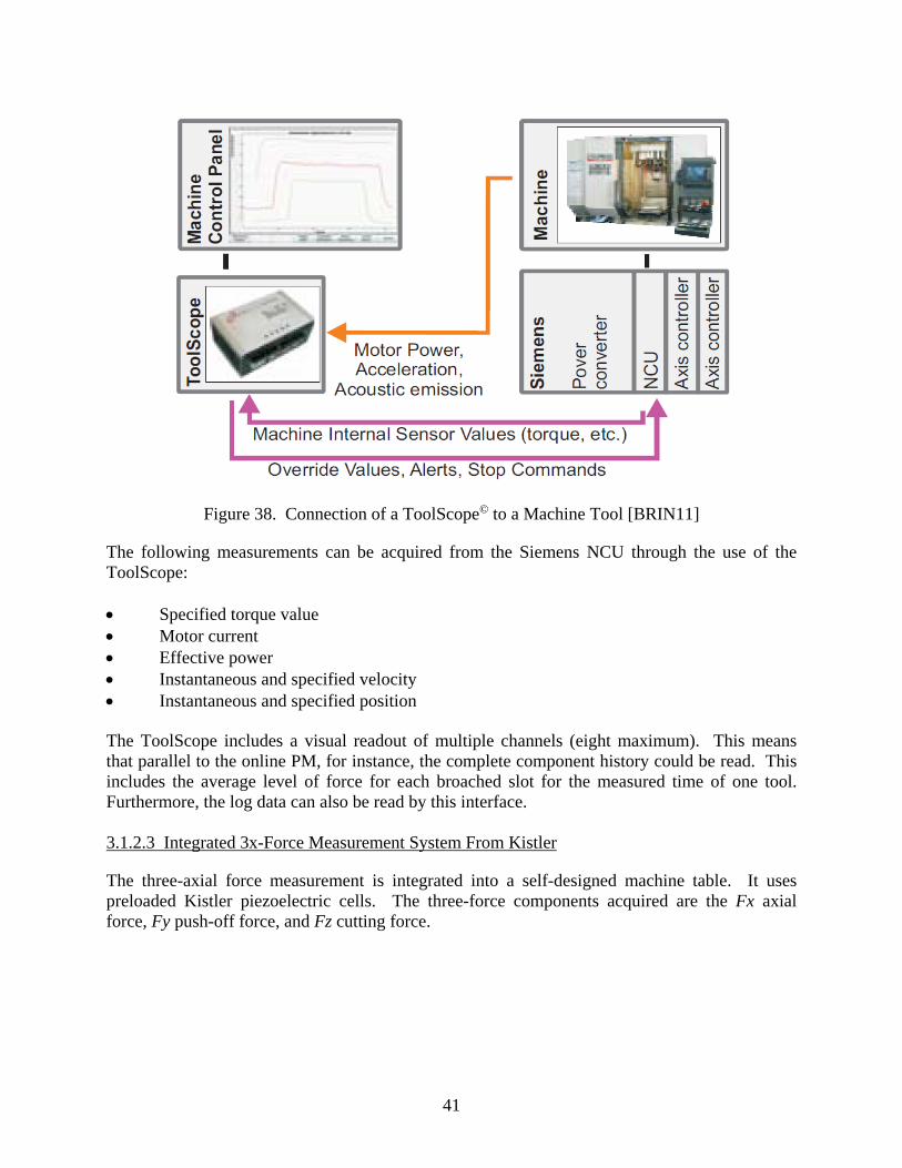
41

Figure 38. Connection of a ToolScope© to a Machine Tool [BRIN11]

The following measurements can be acquired from the Siemens NCU through the use of the ToolScope: • Specified torque value • Motor current • Effective power • Instantaneous and specified velocity • Instantaneous and specified position The ToolScope includes a visual readout of multiple channels (eight maximum). This means that parallel to the online PM, for instance, the complete component history could be read. This includes the average level of force for each broached slot for the measured time of one tool. Furthermore, the log data can also be read by this interface. 3.1.2.3 Integrated 3x-Force Measurement System From Kistler

The three-axial force measurement is integrated into a self-designed machine table. It uses preloaded Kistler piezoelectric cells. The three-force components acquired are the Fx axial force, Fy push-off force, and Fz cutting force.

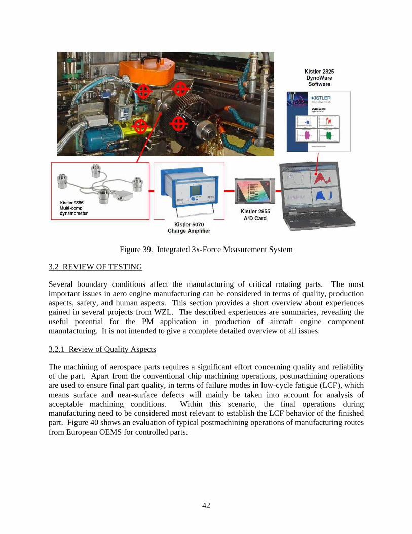
42

Figure 39. Integrated 3x-Force Measurement System

3.2 REVIEW OF TESTING

Several boundary conditions affect the manufacturing of critical rotating parts. The most important issues in aero engine manufacturing can be considered in terms of quality, production aspects, safety, and human aspects. This section provides a short overview about experiences gained in several projects from WZL. The described experiences are summaries, revealing the useful potential for the PM application in production of aircraft engine component manufacturing. It is not intended to give a complete detailed overview of all issues. 3.2.1 Review of Quality Aspects

The machining of aerospace parts requires a significant effort concerning quality and reliability of the part. Apart from the conventional chip machining operations, postmachining operations are used to ensure final part quality, in terms of failure modes in low-cycle fatigue (LCF), which means surface and near-surface defects will mainly be taken into account for analysis of acceptable machining conditions. Within this scenario, the final operations during manufacturing need to be considered most relevant to establish the LCF behavior of the finished part. Figure 40 shows an evaluation of typical postmachining operations of manufacturing routes from European OEMS for controlled parts.

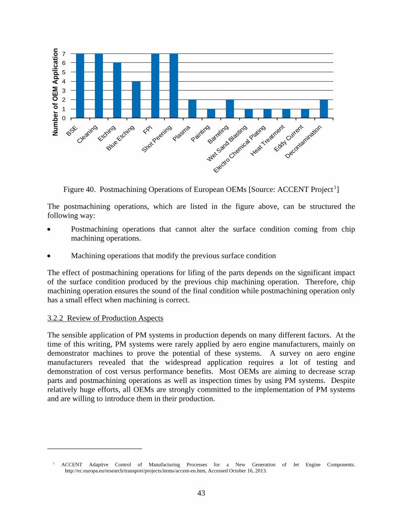
43

01234567

BSE

Cleaning

Etching

Blue Etch

ing FPI

Shot P

eening

Plasma

Paintin

g

Barreli

ng

Wet San

d Blas

ting

Electro C

hemica

l Plat

ing

Heat T

reatmen

t

Eddy C

urrent

Decon

taminatio

n

Num

ber o

f OEM

App

licat

ion

Figure 40. Postmachining Operations of European OEMs [Source: ACCENT Project1]

The postmachining operations, which are listed in the figure above, can be structured the following way:

• Postmachining operations that cannot alter the surface condition coming from chip machining operations.

• Machining operations that modify the previous surface condition

The effect of postmachining operations for lifing of the parts depends on the significant impact of the surface condition produced by the previous chip machining operation. Therefore, chip machining operation ensures the sound of the final condition while postmachining operation only has a small effect when machining is correct. 3.2.2 Review of Production Aspects

The sensible application of PM systems in production depends on many different factors. At the time of this writing, PM systems were rarely applied by aero engine manufacturers, mainly on demonstrator machines to prove the potential of these systems. A survey on aero engine manufacturers revealed that the widespread application requires a lot of testing and demonstration of cost versus performance benefits. Most OEMs are aiming to decrease scrap parts and postmachining operations as well as inspection times by using PM systems. Despite relatively huge efforts, all OEMs are strongly committed to the implementation of PM systems and are willing to introduce them in their production.

1 ACCENT Adaptive Control of Manufacturing Processes for a New Generation of Jet Engine Components. http://ec.europa.eu/research/transport/projects/items/accent-en.htm, Accessed October 16, 2013.

44

3.2.3 Review of Safety Aspects

Safety for aircraft engine components is mainly connected to lifing. Lifing processes for controlled parts performed for OEMs are based on experimental testing and lifing analysis from the data obtained from the tests. These tests are mainly rig tests or specific feature tests of representative parts, including the surface condition, since the same manufacturing route is required for the specimens. Lifing methods include the manufacturing route in the tests. However, because the tests are performed in very small samples, usually on one part in the case of a full-scale rig, it is necessary to demonstrate that this part is representative of all the population. That is the reason all the manufacturing relevant variables are frozen. A machining anomaly was not studied unless the damaged was intentionally included in the testing, which was not recommended because the predicted life for the part would be drastically reduced. Therefore, life calculations also incorporate probabilistic studies regarding the predicted probability of burst because of a nondetectable anomaly (tolerance damage) based on a minimum nondetectable initial crack. Control of manufacturing by means of monitoring could be used in two ways: • Reducing the predicted probability of burst because of the manufacturing control • As an additional nondestructive technique with its associated POD Monitoring improves the current quality standards and increases the predicted safe life, reducing the scatter of the probabilistic calculations. 3.2.4 Review of Human Factors

For the control of manufacturing processes, the manufacturing process and human factors should be considered. The application of suitable sensor and PM equipment can help attain oversight and a robust control of the manufacturing processes, but it is not possible to replace the human being in the process. Machine operators, material handlers, engineers, and others play an important role by representing the link between the process and the detection of anomalies in the process. Every observation of an anomaly, even with an enabled PM system, must be reviewed and documented. Training and motivation of the human beings involved in every stage of the manufacture of critical aircraft engine parts is very important (figure 41).

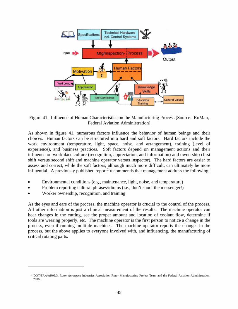
45

Figure 41. Influence of Human Characteristics on the Manufacturing Process [Source: RoMan, Federal Aviation Administration]

As shown in figure 41, numerous factors influence the behavior of human beings and their choices. Human factors can be structured into hard and soft factors. Hard factors include the work environment (temperature, light, space, noise, and arrangement), training (level of experience), and business practices. Soft factors depend on management actions and their influence on workplace culture (recognition, appreciation, and information) and ownership (first shift versus second shift and machine operator versus inspector). The hard factors are easier to assess and correct, while the soft factors, although much more difficult, can ultimately be more influential. A previously published report2 recommends that management address the following: • Environmental conditions (e.g., maintenance, light, noise, and temperature) • Problem reporting cultural phrases/idioms (i.e., don’t shoot the messenger!) • Worker ownership, recognition, and training As the eyes and ears of the process, the machine operator is crucial to the control of the process. All other information is just a clinical measurement of the results. The machine operator can hear changes in the cutting, see the proper amount and location of coolant flow, determine if tools are wearing properly, etc. The machine operator is the first person to notice a change in the process, even if running multiple machines. The machine operator reports the changes in the process, but the above applies to everyone involved with, and influencing, the manufacturing of critical rotating parts.

2 DOT/FAA/AR06/3, Rotor Aerospace Industries Association Rotor Manufacturing Project Team and the Federal Aviation Administration, 2006.

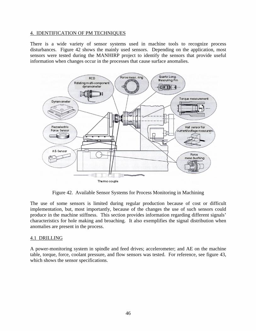
46

4. IDENTIFICATION OF PM TECHNIQUES

There is a wide variety of sensor systems used in machine tools to recognize process disturbances. Figure 42 shows the mainly used sensors. Depending on the application, most sensors were tested during the MANHIRP project to identify the sensors that provide useful information when changes occur in the processes that cause surface anomalies.

Figure 42. Available Sensor Systems for Process Monitoring in Machining

The use of some sensors is limited during regular production because of cost or difficult implementation, but, most importantly, because of the changes the use of such sensors could produce in the machine stiffness. This section provides information regarding different signals’ characteristics for hole making and broaching. It also exemplifies the signal distribution when anomalies are present in the process. 4.1 DRILLING

A power-monitoring system in spindle and feed drives; accelerometer; and AE on the machine table, torque, force, coolant pressure, and flow sensors was tested. For reference, see figure 43, which shows the sensor specifications.

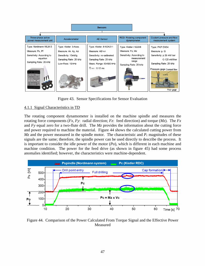
47

Figure 43. Sensor Specifications for Sensor Evaluation

4.1.1 Signal Characteristics in TD

The rotating component dynamometer is installed on the machine spindle and measures the rotating force components (Fx, Fy: radial direction; Fz: feed direction) and torque (Mz). The Fx and Fy equal zero for a two-flute drill. The Mz provides the information about the cutting force and power required to machine the material. Figure 44 shows the calculated cutting power from Mz and the power measured in the spindle motor. The characteristic and Pc magnitudes of these signals are the same; therefore, the spindle power can be used directly to describe the process. It is important to consider the idle power of the motor (Po), which is different in each machine and machine condition. The power for the feed drive (as shown in figure 45) had some process anomalies identified; however, the characteristics were machine-dependent.

Figure 44. Comparison of the Power Calculated From Torque Signal and the Effective Power Measured

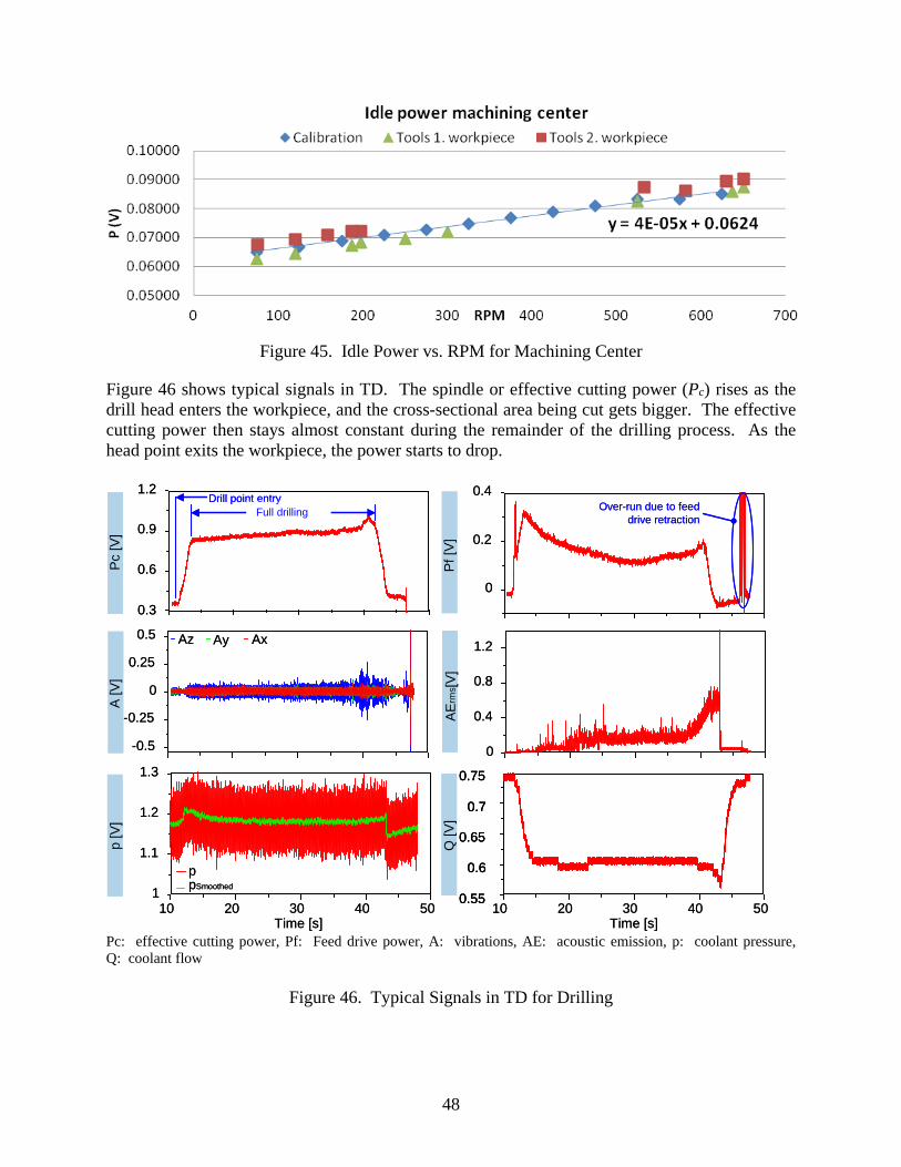
48

Figure 45. Idle Power vs. RPM for Machining Center

Figure 46 shows typical signals in TD. The spindle or effective cutting power (Pc) rises as the drill head enters the workpiece, and the cross-sectional area being cut gets bigger. The effective cutting power then stays almost constant during the remainder of the drilling process. As the head point exits the workpiece, the power starts to drop.

-0.5

-0.25

0

0.25

0.5

A [V

]

Az Ay Ax

0

0.4

0.8

1.2

AErm

s[V]

0.3

0.6

0.9

1.2

Pc[V

]

0

0.2

0.4

Pf [V

]

Time [s]

Q [V

]

10 20 30 40 5010 20 30 40 50Time [s]

1

1.1

1.2

1.3

p [V

]

ppSmoothed

Over-run due to feeddrive retraction

0.75

0.7

0.65

0.6

0.55

Full drillingDrill point entry

-0.5

-0.25

0

0.25

0.5

A [V

]

Az Ay Ax

0

0.4

0.8

1.2

AErm

s[V]

0.3

0.6

0.9

1.2

Pc[V

]

0

0.2

0.4

Pf [V

]

Time [s]

Q [V

]

10 20 30 40 5010 20 30 40 50Time [s]

1

1.1

1.2

1.3

p [V

]

ppSmoothed

Over-run due to feeddrive retraction

0.75

0.7

0.65

0.6

0.55

0.75

0.7

0.65

0.6

0.55

Full drillingDrill point entry

Pc: effective cutting power, Pf: Feed drive power, A: vibrations, AE: acoustic emission, p: coolant pressure, Q: coolant flow

Figure 46. Typical Signals in TD for Drilling

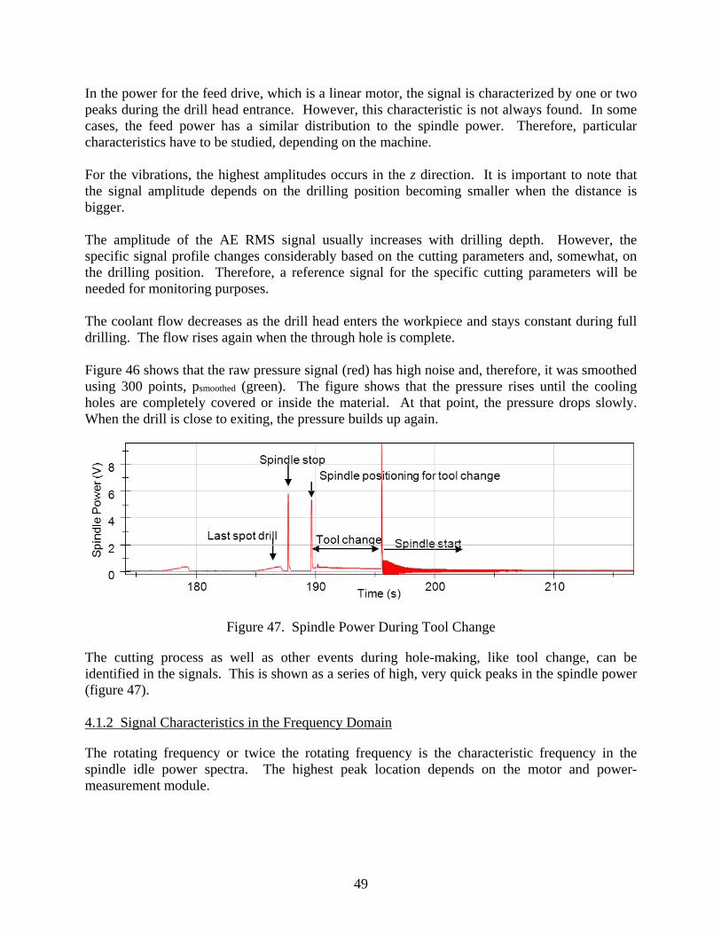
49

In the power for the feed drive, which is a linear motor, the signal is characterized by one or two peaks during the drill head entrance. However, this characteristic is not always found. In some cases, the feed power has a similar distribution to the spindle power. Therefore, particular characteristics have to be studied, depending on the machine. For the vibrations, the highest amplitudes occurs in the z direction. It is important to note that the signal amplitude depends on the drilling position becoming smaller when the distance is bigger. The amplitude of the AE RMS signal usually increases with drilling depth. However, the specific signal profile changes considerably based on the cutting parameters and, somewhat, on the drilling position. Therefore, a reference signal for the specific cutting parameters will be needed for monitoring purposes. The coolant flow decreases as the drill head enters the workpiece and stays constant during full drilling. The flow rises again when the through hole is complete. Figure 46 shows that the raw pressure signal (red) has high noise and, therefore, it was smoothed using 300 points, psmoothed (green). The figure shows that the pressure rises until the cooling holes are completely covered or inside the material. At that point, the pressure drops slowly. When the drill is close to exiting, the pressure builds up again.

Figure 47. Spindle Power During Tool Change

The cutting process as well as other events during hole-making, like tool change, can be identified in the signals. This is shown as a series of high, very quick peaks in the spindle power (figure 47). 4.1.2 Signal Characteristics in the Frequency Domain

The rotating frequency or twice the rotating frequency is the characteristic frequency in the spindle idle power spectra. The highest peak location depends on the motor and power-measurement module.

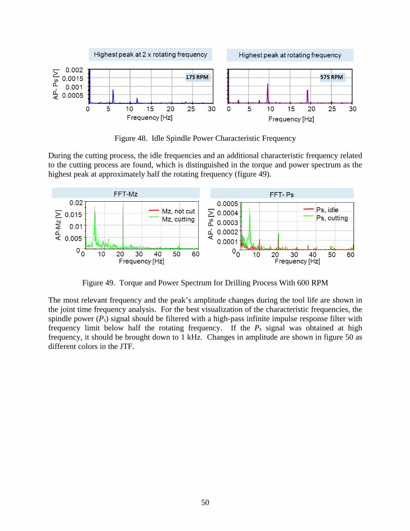
50

Figure 48. Idle Spindle Power Characteristic Frequency

During the cutting process, the idle frequencies and an additional characteristic frequency related to the cutting process are found, which is distinguished in the torque and power spectrum as the highest peak at approximately half the rotating frequency (figure 49).

Figure 49. Torque and Power Spectrum for Drilling Process With 600 RPM

The most relevant frequency and the peak’s amplitude changes during the tool life are shown in the joint time frequency analysis. For the best visualization of the characteristic frequencies, the spindle power (Ps) signal should be filtered with a high-pass infinite impulse response filter with frequency limit below half the rotating frequency. If the Ps signal was obtained at high frequency, it should be brought down to 1 kHz. Changes in amplitude are shown in figure 50 as different colors in the JTF.

51

Tim

e

Joint Time Frequency

Tim

e

Ps, filtered signal

Ps: Spindle effec. Power

Pf: Feed effec. power

Ax,y,z: Machine vibrations

AE: Acoustic Emission

Sample Freq. fs= 20 KHz

Data Acquisition Discrete Time Series Preprocessing Spectral Analysis

Tim

e

Ps (Spindle power)

Preprocessing

Time series analysis.

Ps and Pf selected as most relevant signals.

3 Hz Highpass IIR-FilterSignal downsampled 1 kHz

Joint Time Frequency (JTF) though whole tool life in order to

identify critical amplitudes

Tim

e

Joint Time Frequency

Tim

e

Ps, filtered signal

Ps: Spindle effec. Power

Pf: Feed effec. power

Ax,y,z: Machine vibrations

AE: Acoustic Emission

Sample Freq. fs= 20 KHz

Data Acquisition Discrete Time Series Preprocessing Spectral Analysis

Tim

e

Ps (Spindle power)

Preprocessing

Time series analysis.

Ps and Pf selected as most relevant signals.

3 Hz Highpass IIR-FilterSignal downsampled 1 kHz

Joint Time Frequency (JTF) though whole tool life in order to

identify critical amplitudes

Figure 50. Steps for Spectral Analysis of Drilling Signals

4.1.3 Tool Wear

One of the most often used practices is spindle power monitoring for the detection of tool wear. A static upper limit is set to this signal allowing an increase in the power requirement up to a certain level consistent with previously measured tool wear. Figure 51 shows other sensor signals for a new (sharp) and a worn tool. The Ps and Pf increase as the tools wear. For Ps, this increase is constant during the entire cutting process, while in Pf, the power rises especially at the beginning and exit of the hole. Also, there is a rise in the AE and vibrations signal at the beginning of the cutting process. It is important to keep in mind that the signals from these sensors have a strong dependency on the sensors’ position. Ideally, the sensors are located very close to the process and this position is kept constant during the machining of the entire workpiece. However, drilling with these conditions cannot be met in real production.

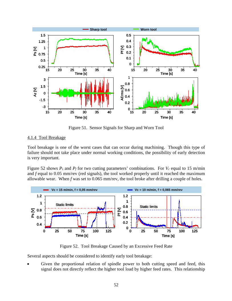
52

15 20 25 30 35 40Time [s]

0.25

0.5

0.75

1

1.25

1.5Ps

[V]

15 20 25 30 35 40Time [s]

0

0.1

0.2

0.3

0.4

0.5

Pf [V

]

15 20 25 30 35 40Time [s]

-3

-1.5

0

1.5

3

Az

[V]

15 20 25 30 35 40Time [s]

0

0.2

0.4

0.6

0.8

1

AErm

s[V

]

Sharp tool Worn tool

15 20 25 30 35 40Time [s]

0.25

0.5

0.75

1

1.25

1.5Ps

[V]

15 20 25 30 35 40Time [s]

0

0.1

0.2

0.3

0.4

0.5

Pf [V

]

15 20 25 30 35 40Time [s]

-3

-1.5

0

1.5

3

Az

[V]

15 20 25 30 35 40Time [s]

0

0.2

0.4

0.6

0.8

1

AErm

s[V

]

15 20 25 30 35 40Time [s]

0.25

0.5

0.75

1

1.25

1.5Ps

[V]

15 20 25 30 35 40Time [s]

0

0.1

0.2

0.3

0.4

0.5

Pf [V

]

15 20 25 30 35 40Time [s]

-3

-1.5

0

1.5

3

Az

[V]

15 20 25 30 35 40Time [s]

0

0.2

0.4

0.6

0.8

1

AErm

s[V

]

Sharp tool Worn tool

Figure 51. Sensor Signals for Sharp and Worn Tool

4.1.4 Tool Breakage

Tool breakage is one of the worst cases that can occur during machining. Though this type of failure should not take place under normal working conditions, the possibility of early detection is very important. Figure 52 shows Ps and Pf for two cutting parameters’ combinations. For Vc equal to 15 m/min and f equal to 0.05 mm/rev (red signals), the tool worked properly until it reached the maximum allowable wear. When f was set to 0.065 mm/rev, the tool broke after drilling a couple of holes.

0 25 50 75 100 125Time [s]

0.4

0.6

0.8

1

1.2

Ps[V

]

0 25 50 75 100 125Time [s]

00.20.40.60.8

11.2

Pf [V

]

Vc = 15 m/min, f = 0,05 mm/rev Vc = 10 m/min, f = 0,065 mm/rev

Static limits Static limits

0 25 50 75 100 125Time [s]

0.4

0.6

0.8

1

1.2

Ps[V

]

0 25 50 75 100 125Time [s]

00.20.40.60.8

11.2

Pf [V

]

Vc = 15 m/min, f = 0,05 mm/rev Vc = 10 m/min, f = 0,065 mm/rev

Static limits Static limits

0 25 50 75 100 125Time [s]

0.4

0.6

0.8

1

1.2

Ps[V

]

0 25 50 75 100 125Time [s]

00.20.40.60.8

11.2

Pf [V

]

0 25 50 75 100 125Time [s]

0.4

0.6

0.8

1

1.2

Ps[V

]

0 25 50 75 100 125Time [s]

00.20.40.60.8

11.2

Pf [V

]

Vc = 15 m/min, f = 0,05 mm/rev Vc = 10 m/min, f = 0,065 mm/rev

Static limits Static limits

Figure 52. Tool Breakage Caused by an Excessive Feed Rate

Several aspects should be considered to identify early tool breakage:

• Given the proportional relation of spindle power to both cutting speed and feed, this signal does not directly reflect the higher tool load by higher feed rates. This relationship

53

is shown in equation 8 for the power consumption according to Sandvic (the trials’ tool manufacturer).

• For the feed power, the cutting speed has a linear relationship, while the feed relationship is quadratic, as shown in equation 9. For this reason, the higher tool load is easier to identify in this signal, as shown in figure 52, when a Pf is higher for f equal to 0.065 mm/rev at the beginning of the process.

• If static limits are used knowing that a tool breakage will cause an overload, the Pf signal will detect the failure earlier, as seen in figure 52.

fVcKVckDfVcFcP c

s ⋅⋅=⋅⋅

⋅⋅=⋅= 1310240 (11)

(12)

4.1.5 Chip Block

Generally, chip blockage occurs when the drilling length-to-diameter ratio is quite high (greater than 3) and no internal cooling is provided. In that case, the chip transport becomes difficult and, in the worst case, stays in the drill helix or inside the hole. The chips that stay in the hole could damage the surface or even cause tool breakage. Figure 53 shows the signals for the normal drilling process and with chip blockage. The blue lines show the signal changes. The same signal characteristics or features are identified for minor and substantial chip blockages. When chip blockage occurs, the signal fluctuates around the reference line. In addition, some peaks can be recognized in the spindle power and especially in the feed power. The vibrations do not show any considerable change.

2 2

1000 2

sin 5 , 0 f Vc K D

Vc f f D k V F P c f f f ⋅ ⋅ =

⋅ ⋅ ⋅

⋅

⋅ ⋅ ⋅ ⋅

= ⋅ = π

κ

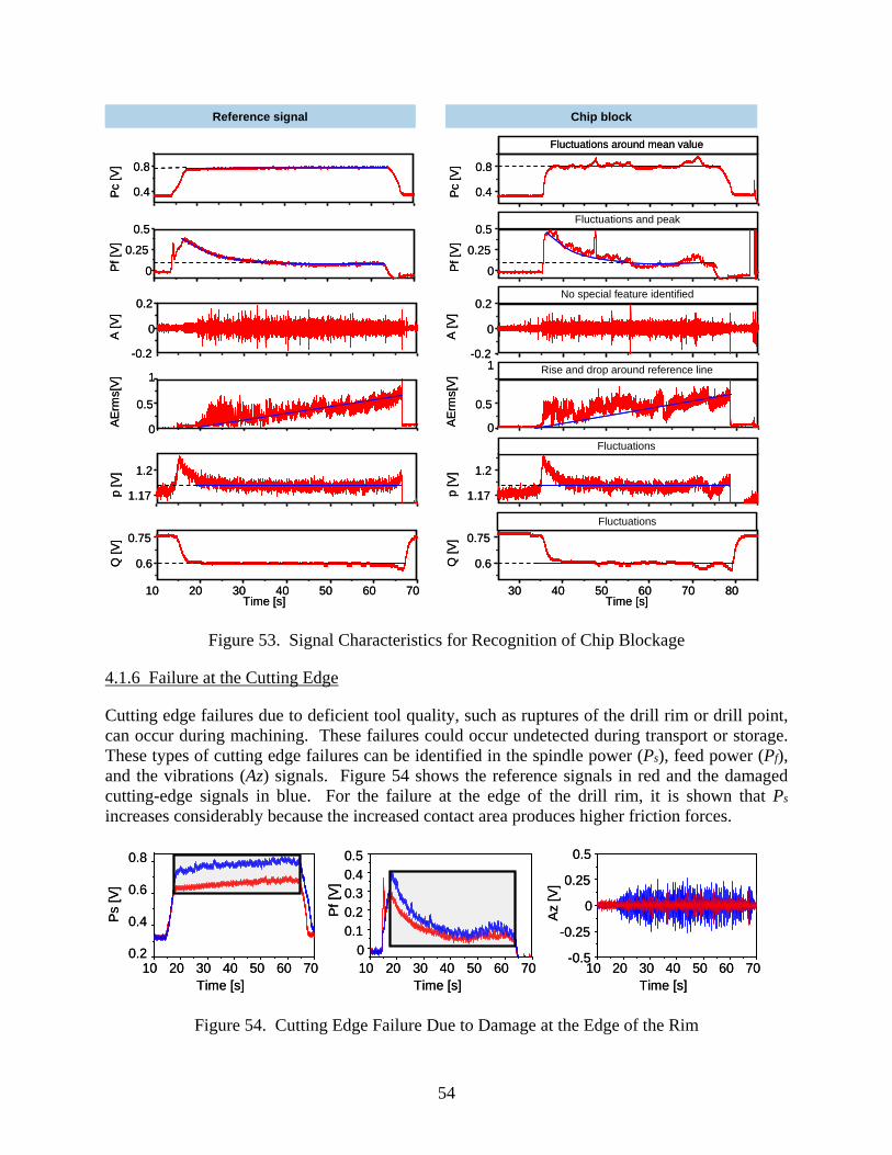
54

-0.2

0

0.2

A [V

]

0

0.5

1

AErm

s[V]

0.4

0.8

Pc [V

]

0

0.25

0.5

Pf [V

]

10 20 30 40 50 60 70Time [s]

0.6

0.75

Q [V

]

1.17

1.2

p [V

]

-0.2

0

0.2

A [V

]

0

0.5

1

AErm

s[V]

0.4

0.8

Pc [V

]

0

0.25

0.5

Pf [V

]

30 40 50 60 70 80Time [s]

0.6

0.75

Q [V

]

1.17

1.2p

[V]

Reference signal Chip block

Fluctuations around mean value

Fluctuations and peak

No special feature identified

Rise and drop around reference line

Fluctuations

Fluctuations

-0.2

0

0.2

A [V

]

0

0.5

1

AErm

s[V]

0.4

0.8

Pc [V

]

0

0.25

0.5

Pf [V

]

10 20 30 40 50 60 70Time [s]

0.6

0.75

Q [V

]

1.17

1.2

p [V

]

-0.2

0

0.2

A [V

]

0

0.5

1

AErm

s[V]

0.4

0.8

Pc [V

]

0

0.25

0.5

Pf [V

]

30 40 50 60 70 80Time [s]

0.6

0.75

Q [V

]

1.17

1.2p

[V]

Reference signal Chip block

Fluctuations around mean value

Fluctuations and peak

No special feature identified

Rise and drop around reference line

Fluctuations

Fluctuations

Figure 53. Signal Characteristics for Recognition of Chip Blockage

4.1.6 Failure at the Cutting Edge

Cutting edge failures due to deficient tool quality, such as ruptures of the drill rim or drill point, can occur during machining. These failures could occur undetected during transport or storage. These types of cutting edge failures can be identified in the spindle power (Ps), feed power (Pf), and the vibrations (Az) signals. Figure 54 shows the reference signals in red and the damaged cutting-edge signals in blue. For the failure at the edge of the drill rim, it is shown that Ps increases considerably because the increased contact area produces higher friction forces.

10 20 30 40 50 60 70Time [s]

0.2

0.4

0.6

0.8

Ps

[V]

10 20 30 40 50 60 70Time [s]

00.10.20.30.40.5

Pf [

V]

10 20 30 40 50 60 70Time [s]

-0.5

-0.25

0

0.25

0.5

Az

[V]

10 20 30 40 50 60 70Time [s]

0.2

0.4

0.6

0.8

Ps

[V]

10 20 30 40 50 60 70Time [s]

00.10.20.30.40.5

Pf [

V]

10 20 30 40 50 60 70Time [s]

-0.5

-0.25

0

0.25

0.5

Az

[V]

Figure 54. Cutting Edge Failure Due to Damage at the Edge of the Rim

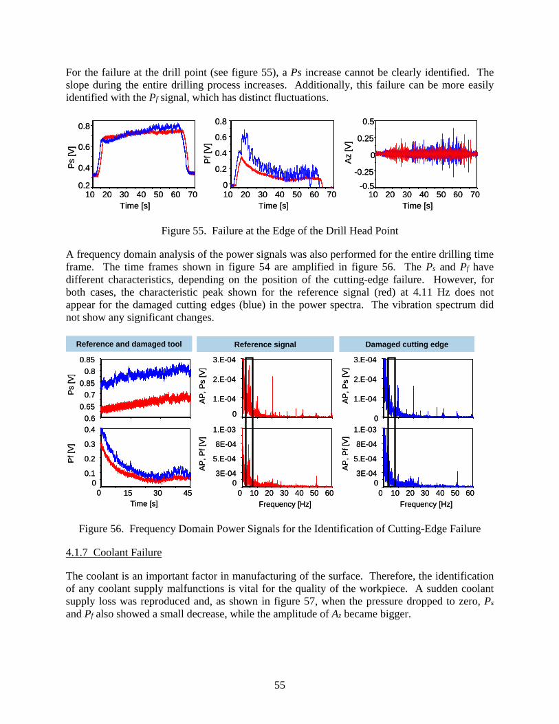
55

For the failure at the drill point (see figure 55), a Ps increase cannot be clearly identified. The slope during the entire drilling process increases. Additionally, this failure can be more easily identified with the Pf signal, which has distinct fluctuations.

10 20 30 40 50 60 70Time [s]

0.2

0.4

0.6

0.8

Ps[V

]

10 20 30 40 50 60 70Time [s]

0

0.2

0.4

0.6

0.8

Pf [V

]10 20 30 40 50 60 70

Time [s]

-0.5

-0.25

0

0.25

0.5

Az

[V]

10 20 30 40 50 60 70Time [s]

0.2

0.4

0.6

0.8

Ps[V

]

10 20 30 40 50 60 70Time [s]

0

0.2

0.4

0.6

0.8

Pf [V

]10 20 30 40 50 60 70

Time [s]

-0.5

-0.25

0

0.25

0.5

Az

[V]

Figure 55. Failure at the Edge of the Drill Head Point

A frequency domain analysis of the power signals was also performed for the entire drilling time frame. The time frames shown in figure 54 are amplified in figure 56. The Ps and Pf have different characteristics, depending on the position of the cutting-edge failure. However, for both cases, the characteristic peak shown for the reference signal (red) at 4.11 Hz does not appear for the damaged cutting edges (blue) in the power spectra. The vibration spectrum did not show any significant changes.

0

1.E-04

2.E-04

3.E-04

AP

, Ps

[V]

0 10 20 30 40 50 60Frequency [Hz]

03E-04

5.E-04

8E-04

1.E-03

AP

, Pf [

V]

0

1.E-04

2.E-04

3.E-04

AP

, Ps

[V]

0 10 20 30 40 50 60Frequency [Hz]

03E-04

5.E-04

8E-04

1.E-03

AP

, Pf [

V]

0.60.65

0.70.85

0.80.85

Ps

[V]

0 15 30 45Time [s]

00.1

0.2

0.3

0.4

Pf [

V]

Reference signal Damaged cutting edgeReference and damaged tool

0

1.E-04

2.E-04

3.E-04

AP

, Ps

[V]

0 10 20 30 40 50 60Frequency [Hz]

03E-04

5.E-04

8E-04

1.E-03

AP

, Pf [

V]

0

1.E-04

2.E-04

3.E-04

AP

, Ps

[V]

0 10 20 30 40 50 60Frequency [Hz]

03E-04

5.E-04

8E-04

1.E-03

AP

, Pf [

V]

0.60.65

0.70.85

0.80.85

Ps

[V]

0 15 30 45Time [s]

00.1

0.2

0.3

0.4

Pf [

V]

Reference signal Damaged cutting edgeReference and damaged tool

Figure 56. Frequency Domain Power Signals for the Identification of Cutting-Edge Failure

4.1.7 Coolant Failure

The coolant is an important factor in manufacturing of the surface. Therefore, the identification of any coolant supply malfunctions is vital for the quality of the workpiece. A sudden coolant supply loss was reproduced and, as shown in figure 57, when the pressure dropped to zero, Ps and Pf also showed a small decrease, while the amplitude of Az became bigger.

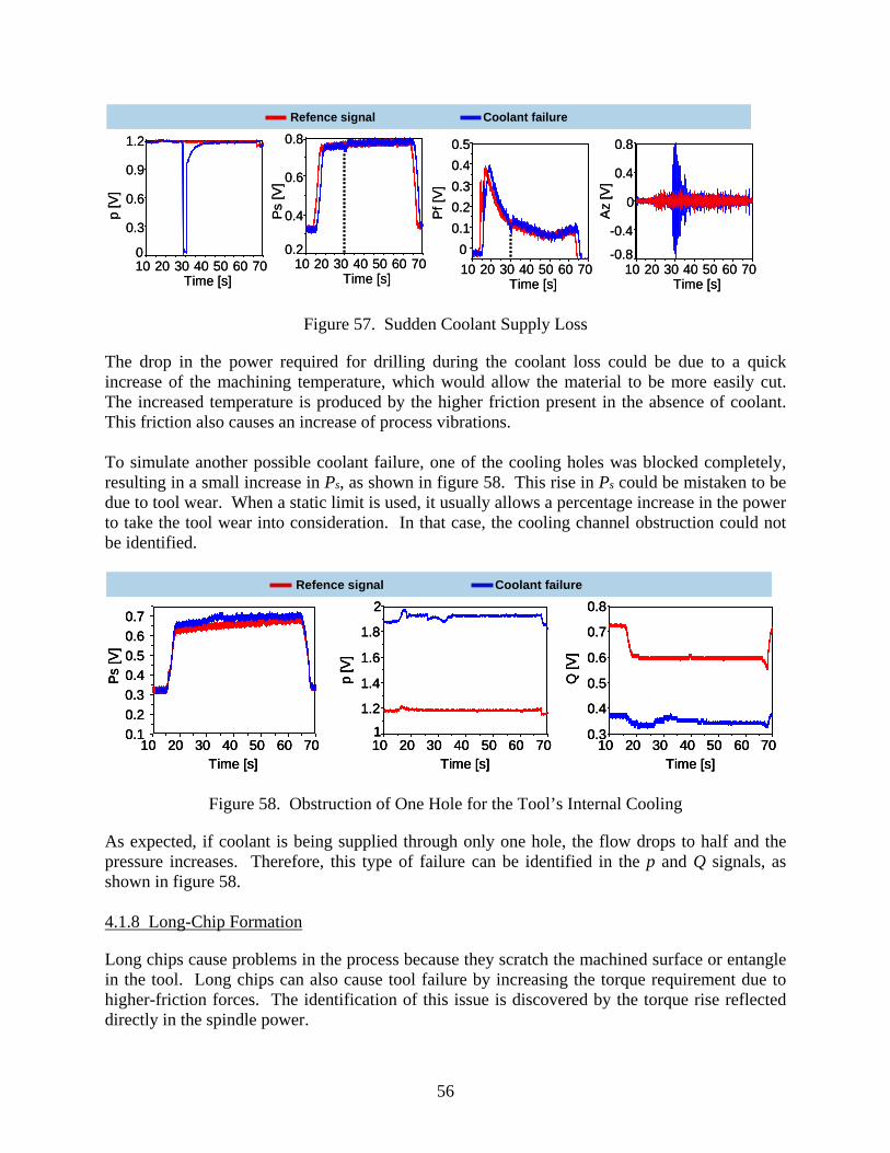
56

0.8

10 20 30 40 50 60 70Time [s]

0.2

0.4

0.6

Ps

[V]

10 20 30 40 50 60 70Time [s]

0

0.3

0.6

0.9

1.2

p [V

]

10 20 30 40 50 60 70Time [s]

00.10.20.30.40.5

Pf [

V]

10 20 30 40 50 60 70Time [s]

-0.8

-0.4

0

0.4

0.8

Az

[V]

Refence signal Coolant failure

0.8

10 20 30 40 50 60 70Time [s]

0.2

0.4

0.6

Ps

[V]

10 20 30 40 50 60 70Time [s]

0

0.3

0.6

0.9

1.2

p [V

]

10 20 30 40 50 60 70Time [s]

00.10.20.30.40.5

Pf [

V]

10 20 30 40 50 60 70Time [s]

-0.8

-0.4

0

0.4

0.8

Az

[V]

Refence signal Coolant failure

Figure 57. Sudden Coolant Supply Loss

The drop in the power required for drilling during the coolant loss could be due to a quick increase of the machining temperature, which would allow the material to be more easily cut. The increased temperature is produced by the higher friction present in the absence of coolant. This friction also causes an increase of process vibrations. To simulate another possible coolant failure, one of the cooling holes was blocked completely, resulting in a small increase in Ps, as shown in figure 58. This rise in Ps could be mistaken to be due to tool wear. When a static limit is used, it usually allows a percentage increase in the power to take the tool wear into consideration. In that case, the cooling channel obstruction could not be identified.

10 20 30 40 50 60 70Time [s]

0.10.20.30.40.50.60.7

Ps [V

]

10 20 30 40 50 60 70Time [s]

1

1.2

1.4

1.6

1.8

2

p [V

]

10 20 30 40 50 60 70Time [s]

0.3

0.4

0.5

0.6

0.7

0.8

Q [V

]Refence signal Coolant failure

10 20 30 40 50 60 70Time [s]

0.10.20.30.40.50.60.7

Ps [V

]

10 20 30 40 50 60 70Time [s]

1

1.2

1.4

1.6

1.8

2

p [V

]

10 20 30 40 50 60 70Time [s]

0.3

0.4

0.5

0.6

0.7

0.8

Q [V

]

10 20 30 40 50 60 70Time [s]

0.10.20.30.40.50.60.7

Ps [V

]

10 20 30 40 50 60 70Time [s]

1

1.2

1.4

1.6

1.8

2

p [V

]

10 20 30 40 50 60 70Time [s]

0.3

0.4

0.5

0.6

0.7

0.8

Q [V

]Refence signal Coolant failure

Figure 58. Obstruction of One Hole for the Tool’s Internal Cooling

As expected, if coolant is being supplied through only one hole, the flow drops to half and the pressure increases. Therefore, this type of failure can be identified in the p and Q signals, as shown in figure 58. 4.1.8 Long-Chip Formation

Long chips cause problems in the process because they scratch the machined surface or entangle in the tool. Long chips can also cause tool failure by increasing the torque requirement due to higher-friction forces. The identification of this issue is discovered by the torque rise reflected directly in the spindle power.

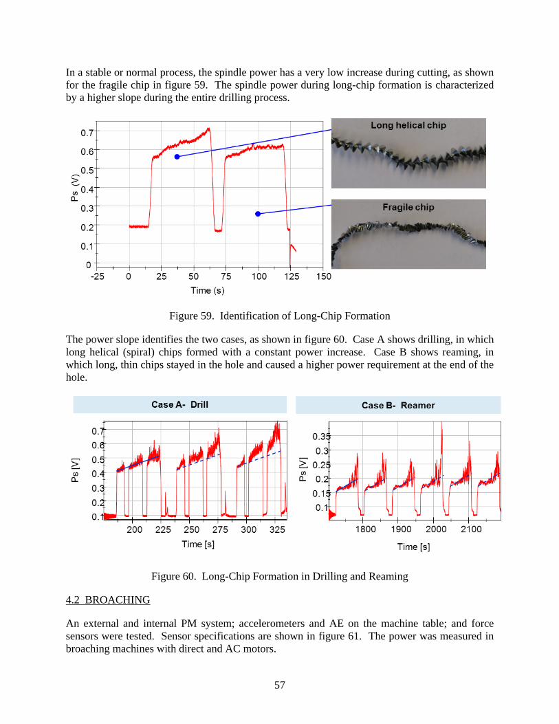
57

In a stable or normal process, the spindle power has a very low increase during cutting, as shown for the fragile chip in figure 59. The spindle power during long-chip formation is characterized by a higher slope during the entire drilling process.

Figure 59. Identification of Long-Chip Formation

The power slope identifies the two cases, as shown in figure 60. Case A shows drilling, in which long helical (spiral) chips formed with a constant power increase. Case B shows reaming, in which long, thin chips stayed in the hole and caused a higher power requirement at the end of the hole.

Figure 60. Long-Chip Formation in Drilling and Reaming

4.2 BROACHING

An external and internal PM system; accelerometers and AE on the machine table; and force sensors were tested. Sensor specifications are shown in figure 61. The power was measured in broaching machines with direct and AC motors.

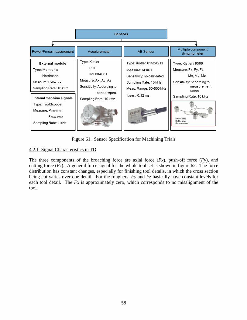
58

Figure 61. Sensor Specification for Machining Trials

4.2.1 Signal Characteristics in TD

The three components of the broaching force are axial force (Fx), push-off force (Fy), and cutting force (Fz). A general force signal for the whole tool set is shown in figure 62. The force distribution has constant changes, especially for finishing tool details, in which the cross section being cut varies over one detail. For the roughers, Fy and Fz basically have constant levels for each tool detail. The Fx is approximately zero, which corresponds to no misalignment of the tool.

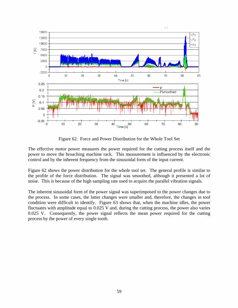
59

Figure 62. Force and Power Distribution for the Whole Tool Set

The effective motor power measures the power required for the cutting process itself and the power to move the broaching machine rack. This measurement is influenced by the electronic control and by the inherent frequency from the sinusoidal form of the input current. Figure 62 shows the power distribution for the whole tool set. The general profile is similar to the profile of the force distribution. The signal was smoothed, although it presented a lot of noise. This is because of the high sampling rate used to acquire the parallel vibration signals. The inherent sinusoidal form of the power signal was superimposed to the power changes due to the process. In some cases, the latter changes were smaller and, therefore, the changes in tool condition were difficult to identify. Figure 63 shows that, when the machine idles, the power fluctuates with amplitude equal to 0.025 V and, during the cutting process, the power also varies 0.025 V. Consequently, the power signal reflects the mean power required for the cutting process by the power of every single tooth.

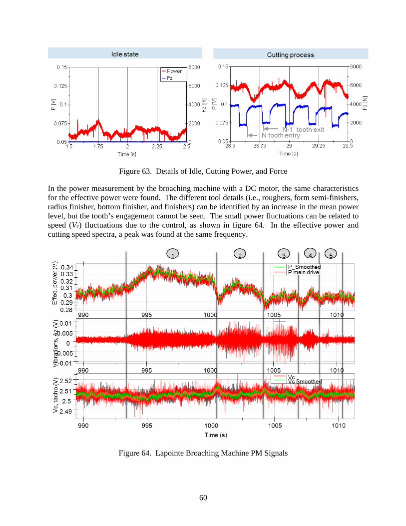
60

Figure 63. Details of Idle, Cutting Power, and Force

In the power measurement by the broaching machine with a DC motor, the same characteristics for the effective power were found. The different tool details (i.e., roughers, form semi-finishers, radius finisher, bottom finisher, and finishers) can be identified by an increase in the mean power level, but the tooth’s engagement cannot be seen. The small power fluctuations can be related to speed (Vc) fluctuations due to the control, as shown in figure 64. In the effective power and cutting speed spectra, a peak was found at the same frequency.

Figure 64. Lapointe Broaching Machine PM Signals

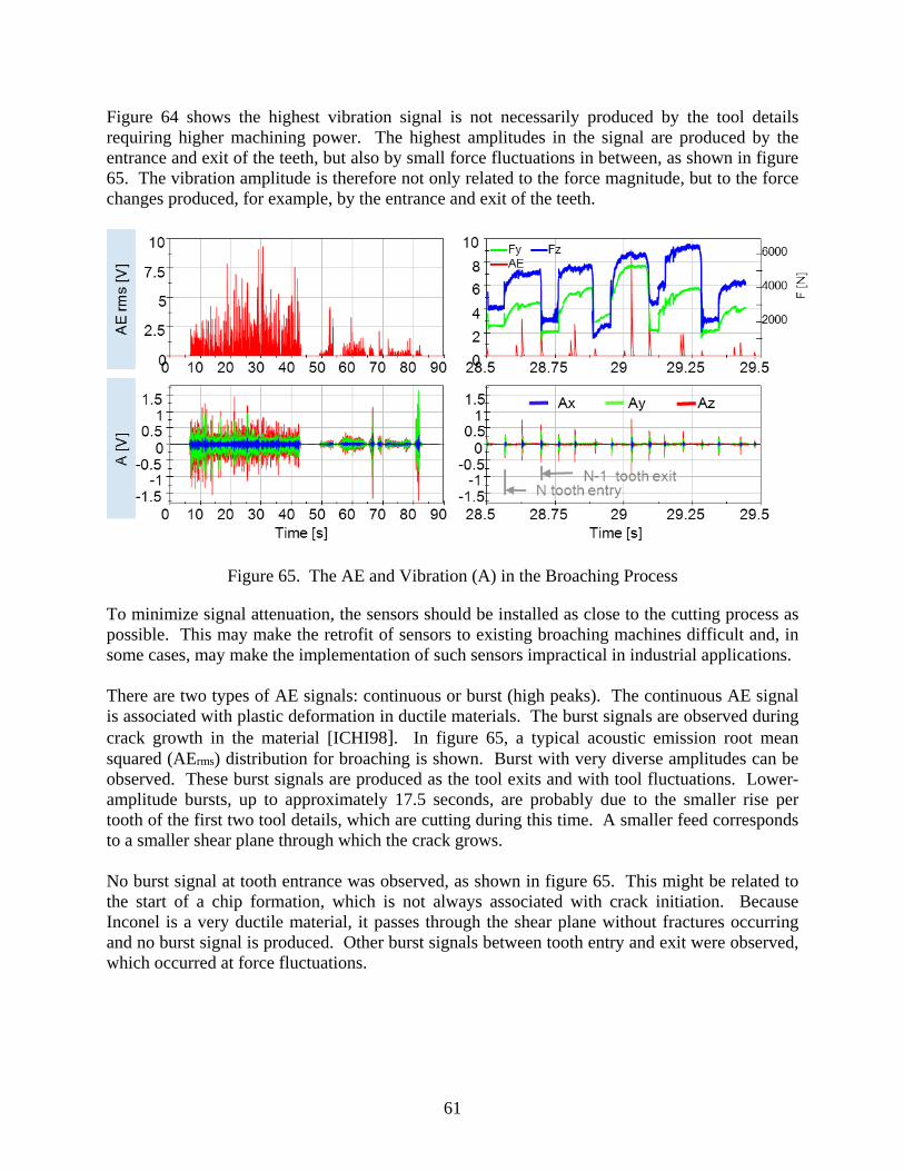
61

Figure 64 shows the highest vibration signal is not necessarily produced by the tool details requiring higher machining power. The highest amplitudes in the signal are produced by the entrance and exit of the teeth, but also by small force fluctuations in between, as shown in figure 65. The vibration amplitude is therefore not only related to the force magnitude, but to the force changes produced, for example, by the entrance and exit of the teeth.

Figure 65. The AE and Vibration (A) in the Broaching Process

To minimize signal attenuation, the sensors should be installed as close to the cutting process as possible. This may make the retrofit of sensors to existing broaching machines difficult and, in some cases, may make the implementation of such sensors impractical in industrial applications. There are two types of AE signals: continuous or burst (high peaks). The continuous AE signal is associated with plastic deformation in ductile materials. The burst signals are observed during crack growth in the material [ICHI98]. In figure 65, a typical acoustic emission root mean squared (AErms) distribution for broaching is shown. Burst with very diverse amplitudes can be observed. These burst signals are produced as the tool exits and with tool fluctuations. Lower-amplitude bursts, up to approximately 17.5 seconds, are probably due to the smaller rise per tooth of the first two tool details, which are cutting during this time. A smaller feed corresponds to a smaller shear plane through which the crack grows. No burst signal at tooth entrance was observed, as shown in figure 65. This might be related to the start of a chip formation, which is not always associated with crack initiation. Because Inconel is a very ductile material, it passes through the shear plane without fractures occurring and no burst signal is produced. Other burst signals between tooth entry and exit were observed, which occurred at force fluctuations.

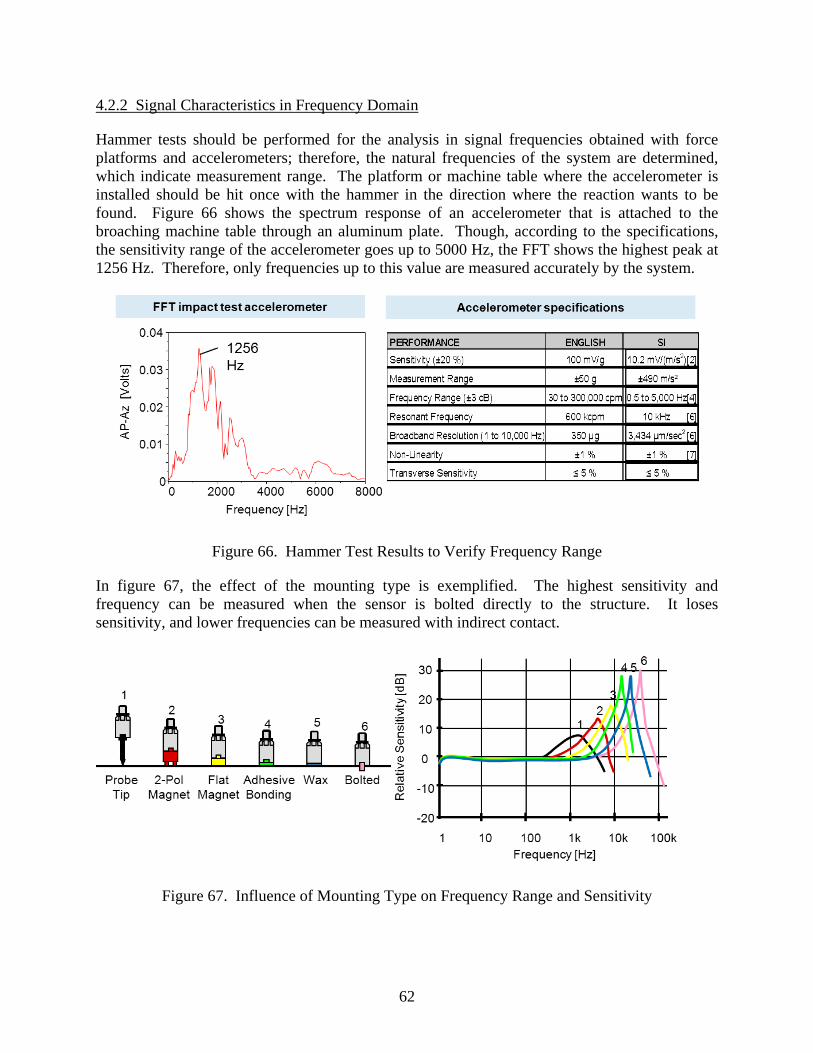
62

4.2.2 Signal Characteristics in Frequency Domain

Hammer tests should be performed for the analysis in signal frequencies obtained with force platforms and accelerometers; therefore, the natural frequencies of the system are determined, which indicate measurement range. The platform or machine table where the accelerometer is installed should be hit once with the hammer in the direction where the reaction wants to be found. Figure 66 shows the spectrum response of an accelerometer that is attached to the broaching machine table through an aluminum plate. Though, according to the specifications, the sensitivity range of the accelerometer goes up to 5000 Hz, the FFT shows the highest peak at 1256 Hz. Therefore, only frequencies up to this value are measured accurately by the system.

Figure 66. Hammer Test Results to Verify Frequency Range

In figure 67, the effect of the mounting type is exemplified. The highest sensitivity and frequency can be measured when the sensor is bolted directly to the structure. It loses sensitivity, and lower frequencies can be measured with indirect contact.

Figure 67. Influence of Mounting Type on Frequency Range and Sensitivity

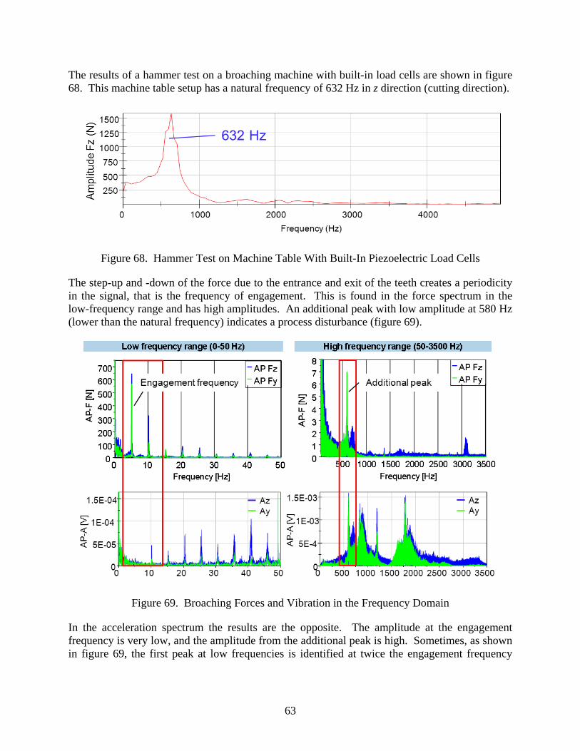
63

The results of a hammer test on a broaching machine with built-in load cells are shown in figure 68. This machine table setup has a natural frequency of 632 Hz in z direction (cutting direction).

Figure 68. Hammer Test on Machine Table With Built-In Piezoelectric Load Cells

The step-up and -down of the force due to the entrance and exit of the teeth creates a periodicity in the signal, that is the frequency of engagement. This is found in the force spectrum in the low-frequency range and has high amplitudes. An additional peak with low amplitude at 580 Hz (lower than the natural frequency) indicates a process disturbance (figure 69).

Figure 69. Broaching Forces and Vibration in the Frequency Domain

In the acceleration spectrum the results are the opposite. The amplitude at the engagement frequency is very low, and the amplitude from the additional peak is high. Sometimes, as shown in figure 69, the first peak at low frequencies is identified at twice the engagement frequency

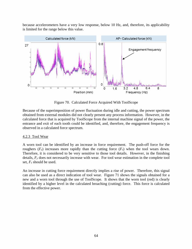
64

because accelerometers have a very low response, below 10 Hz, and, therefore, its applicability is limited for the range below this value.

Figure 70. Calculated Force Acquired With ToolScope

Because of the superimposition of power fluctuation during idle and cutting, the power spectrum obtained from external modules did not clearly present any process information. However, in the calculated force that is acquired by ToolScope from the internal machine signal of the power, the entrance and exit of each tooth could be identified, and, therefore, the engagement frequency is observed in a calculated force spectrum. 4.2.3 Tool Wear

A worn tool can be identified by an increase in force requirement. The push-off force for the roughers (Fy) increases more rapidly than the cutting force (Fz) when the tool wears down. Therefore, it is considered to be very sensitive to those tool details. However, in the finishing details, Fy does not necessarily increase with wear. For tool wear estimation in the complete tool set, Fz should be used. An increase in cutting force requirement directly implies a rise of power. Therefore, this signal can also be used as a direct indication of tool wear. Figure 71 shows the signals obtained for a new and a worn tool through the use of ToolScope. It shows that the worn tool (red) is clearly identified by a higher level in the calculated broaching (cutting) force. This force is calculated from the effective power.

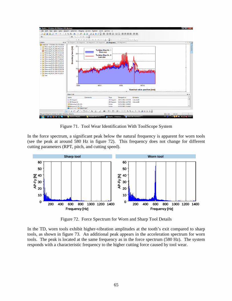
65

Figure 71. Tool Wear Identification With ToolScope System

In the force spectrum, a significant peak below the natural frequency is apparent for worn tools (see the peak at around 580 Hz in figure 72). This frequency does not change for different cutting parameters (RPT, pitch, and cutting speed).

200 400 600 800 1000 1200 1400Frequency [Hz]

0

10

20

30

40

50

60

AP-F

y[N

]

200 400 600 800 1000 1200 1400Frequency [Hz]

0

10

20

30

40

50

60

AP-F

y[N

]

Worn toolSharp tool

200 400 600 800 1000 1200 1400Frequency [Hz]

0

10

20

30

40

50

60

AP-F

y[N

]

200 400 600 800 1000 1200 1400Frequency [Hz]

0

10

20

30

40

50

60

AP-F

y[N

]

200 400 600 800 1000 1200 1400Frequency [Hz]

0

10

20

30

40

50

60

AP-F

y[N

]

200 400 600 800 1000 1200 1400Frequency [Hz]

0

10

20

30

40

50

60

AP-F

y[N

]

Worn toolSharp tool

Figure 72. Force Spectrum for Worn and Sharp Tool Details

In the TD, worn tools exhibit higher-vibration amplitudes at the tooth’s exit compared to sharp tools, as shown in figure 73. An additional peak appears in the acceleration spectrum for worn tools. The peak is located at the same frequency as in the force spectrum (580 Hz). The system responds with a characteristic frequency to the higher cutting force caused by tool wear.

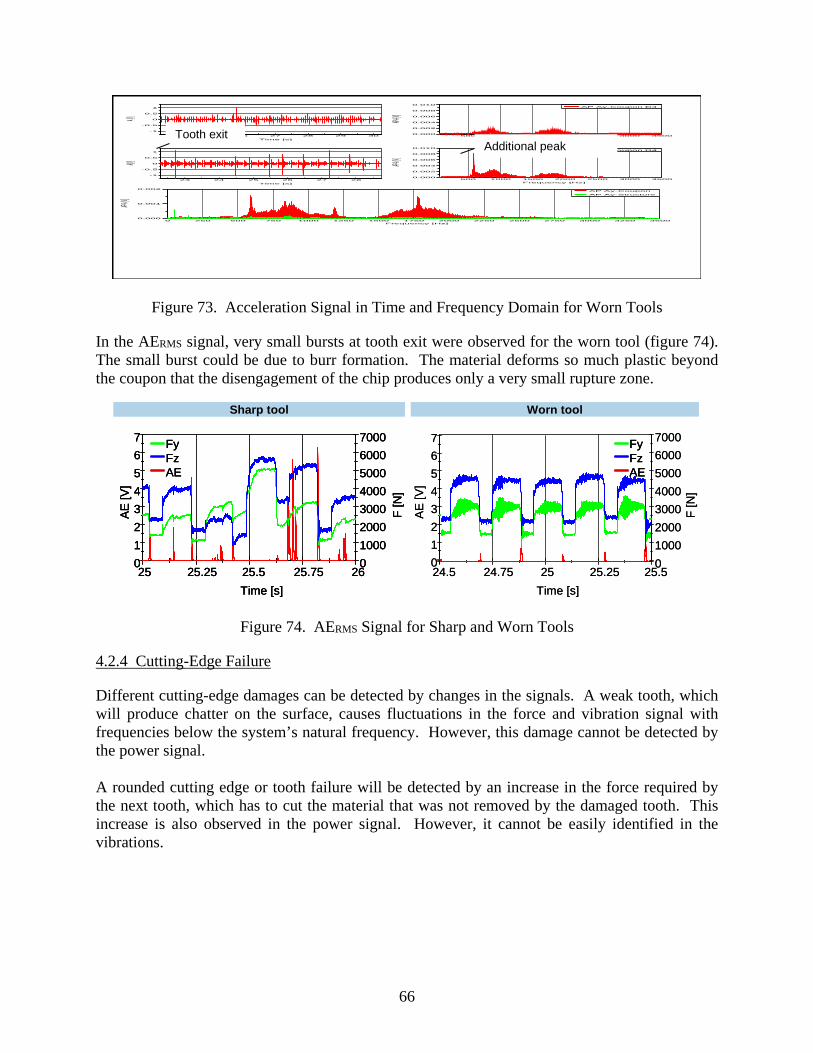
66

24 25 26 27 28 29 30

Time [s]

-1

-0.5

0

0.5

1

A [V]500 1000 1500 2000 2500 3000 3500

Frequency [Hz]

0.000

0.002

0.004

0.006

0.008

0.010

AP-A [V]

AP Ay-Coupon D4

23 24 25 26 27 28

Time [s]

-1

-0.5

0

0.5

1

A [V]

0 250 500 750 1000 1250 1500 1750 2000 2250 2500 2750 3000 3250 3500Frequency [Hz]

0.000

0.001

0.002

AP-A [V]

AP Ay-Coupon

AP Ay-Structure

500 1000 1500 2000 2500 3000 3500

Frequency [Hz]

0.000

0.002

0.004

0.006

0.008

0.010

AP-A [V]

AP Ay-Coupon D4

Figure 73. Acceleration Signal in Time and Frequency Domain for Worn Tools

In the AERMS signal, very small bursts at tooth exit were observed for the worn tool (figure 74). The small burst could be due to burr formation. The material deforms so much plastic beyond the coupon that the disengagement of the chip produces only a very small rupture zone.

24.5 24.75 25 25.25 25.5Time [s]

AE [V

]

01000200030004000500060007000

F [N

]

01234567

Worn tool

25 25.25 25.5 25.75 26Time [s]

01234567

AE [V

]

01000200030004000500060007000

F [N

]Sharp tool

FyFzAE

FyFzAE

24.5 24.75 25 25.25 25.5Time [s]

AE [V

]

01000200030004000500060007000

F [N

]

01234567

Worn tool

25 25.25 25.5 25.75 26Time [s]

01234567

AE [V

]

01000200030004000500060007000

F [N

]Sharp tool

25 25.25 25.5 25.75 26Time [s]

01234567

AE [V

]

01000200030004000500060007000

F [N

]Sharp tool

FyFzAE

FyFzAE

FyFzAE

FyFzAE

Figure 74. AERMS Signal for Sharp and Worn Tools

4.2.4 Cutting-Edge Failure

Different cutting-edge damages can be detected by changes in the signals. A weak tooth, which will produce chatter on the surface, causes fluctuations in the force and vibration signal with frequencies below the system’s natural frequency. However, this damage cannot be detected by the power signal. A rounded cutting edge or tooth failure will be detected by an increase in the force required by the next tooth, which has to cut the material that was not removed by the damaged tooth. This increase is also observed in the power signal. However, it cannot be easily identified in the vibrations.

Additional peak Tooth exit

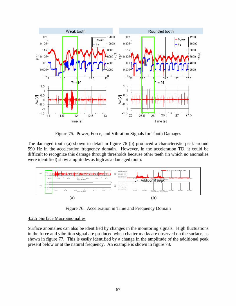
67

Figure 75. Power, Force, and Vibration Signals for Tooth Damages

The damaged tooth (a) shown in detail in figure 76 (b) produced a characteristic peak around 590 Hz in the acceleration frequency domain. However, in the acceleration TD, it could be difficult to recognize this damage through thresholds because other teeth (in which no anomalies were identified) show amplitudes as high as a damaged tooth.

11 12 13 14 15 16 17

Time [s]

-1

-0.5

0

0.5

1

A [V]

500 1000 1500 2000 2500 3000 3500

Frequency [Hz]

0.0000

0.0020

0.0040

0.0060

0.0080

0.0100

AP-A [V]

AP Ay-Kistler D2

23 24 25 26 27 28

Time [s]

-1

-0.5

0

0.5

1

A [V]

500 1000 1500 2000 2500 3000 3500

Frequency [Hz]

0.0000

0.0025

0.0050

0.0075

0.0100

AP-A [V]

(a) (b)

Figure 76. Acceleration in Time and Frequency Domain

4.2.5 Surface Macroanomalies

Surface anomalies can also be identified by changes in the monitoring signals. High fluctuations in the force and vibration signal are produced when chatter marks are observed on the surface, as shown in figure 77. This is easily identified by a change in the amplitude of the additional peak present below or at the natural frequency. An example is shown in figure 78.

Additional peak

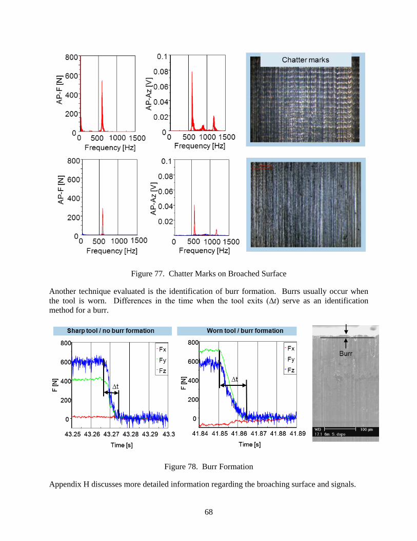
68

Figure 77. Chatter Marks on Broached Surface

Another technique evaluated is the identification of burr formation. Burrs usually occur when the tool is worn. Differences in the time when the tool exits (∆t) serve as an identification method for a burr.

Figure 78. Burr Formation

Appendix H discusses more detailed information regarding the broaching surface and signals.

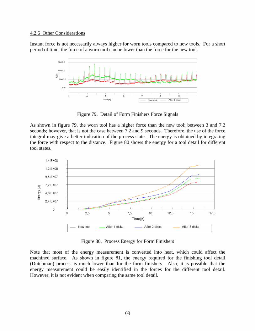
69

4.2.6 Other Considerations

Instant force is not necessarily always higher for worn tools compared to new tools. For a short period of time, the force of a worn tool can be lower than the force for the new tool.

Figure 79. Detail of Form Finishers Force Signals

As shown in figure 79, the worn tool has a higher force than the new tool; between 3 and 7.2 seconds; however, that is not the case between 7.2 and 9 seconds. Therefore, the use of the force integral may give a better indication of the process state. The energy is obtained by integrating the force with respect to the distance. Figure 80 shows the energy for a tool detail for different tool states.

Figure 80. Process Energy for Form Finishers

Note that most of the energy measurement is converted into heat, which could affect the machined surface. As shown in figure 81, the energy required for the finishing tool detail (Dutchman) process is much lower than for the form finishers. Also, it is possible that the energy measurement could be easily identified in the forces for the different tool detail. However, it is not evident when comparing the same tool detail.

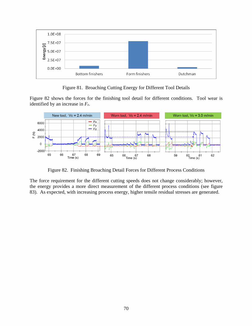
70

Figure 81. Broaching Cutting Energy for Different Tool Details

Figure 82 shows the forces for the finishing tool detail for different conditions. Tool wear is identified by an increase in Fz.

Figure 82. Finishing Broaching Detail Forces for Different Process Conditions

The force requirement for the different cutting speeds does not change considerably; however, the energy provides a more direct measurement of the different process conditions (see figure 83). As expected, with increasing process energy, higher tensile residual stresses are generated.

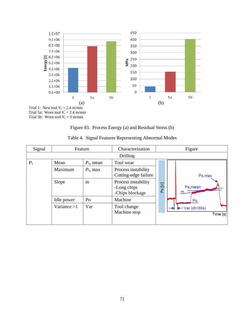
71

(a) (b) Trial 1: New tool Vc = 2.4 m/min Trial 5a: Worn tool Vc = 2.4 m/min Trial 5b: Worn tool Vc = 3 m/min

Figure 83. Process Energy (a) and Residual Stress (b)

Table 4. Signal Features Representing Abnormal Modes

Signal Feature Characterization Figure Drilling

Ps Mean Ps, mean Tool wear

Maximum Ps, max Process instability Cutting-edge failure

Slope m Process instability -Long chips -Chips blockage

Idle power Po Machine Variance >1 Var Tool change

Machine stop

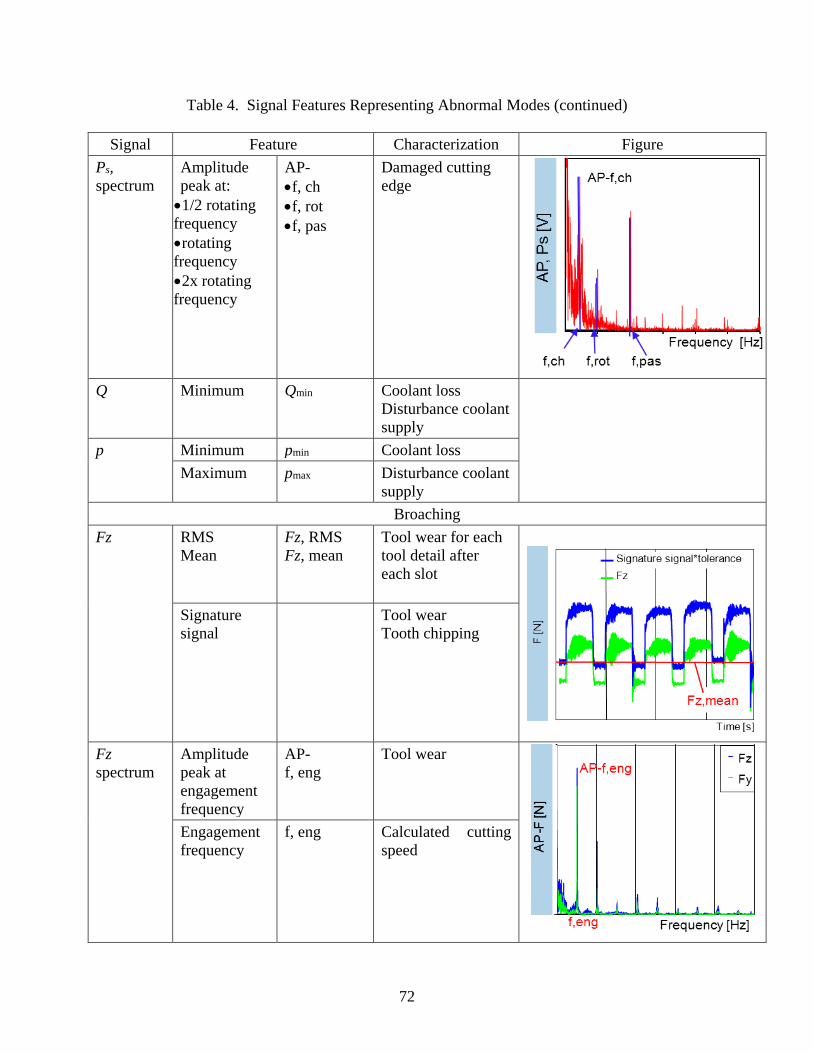
72

Table 4. Signal Features Representing Abnormal Modes (continued)

Signal Feature Characterization Figure Ps, spectrum

Amplitude peak at:

•1/2 rotating frequency •rotating frequency •2x rotating frequency

AP- •f, ch •f, rot •f, pas

Damaged cutting edge

Q Minimum Qmin Coolant loss

Disturbance coolant supply

p Minimum pmin Coolant loss Maximum pmax Disturbance coolant

supply Broaching

Fz RMS Mean

Fz, RMS Fz, mean

Tool wear for each tool detail after each slot

Signature signal

Tool wear Tooth chipping

Fz spectrum

Amplitude peak at engagement frequency

AP- f, eng

Tool wear

Engagement frequency

f, eng Calculated cutting speed

73

Table 4. Signal Features Representing Abnormal Modes (continued)

Signal Feature Characterization Figure P Signature

signal Tool wear

Tooth chipping

Model Tool wear

Tooth chipping

Az Envelope signature signal

Az, envelope

Tool wear Tooth chipping

Tolerance range

Az, range Damage tooth

Az, spectrum

Amplitude peak at natural frequency

AP- f, nat

Weak cutting edge Chatter

Additional peak

f, char Weak cutting edge Chatter

4.3 QUALIFICATION SUMMARY OF SENSOR SYSTEMS

The sensor system qualification is determined based on laboratory trials and industry experience. Some monitoring systems are currently used in the industry as a common application during production and others remain as science topics. Figure 84 and table 5 show the results for special-cause events.

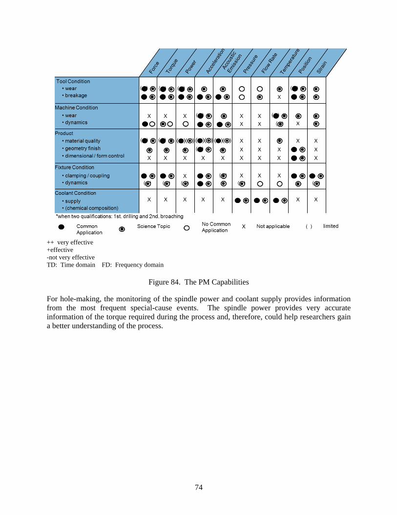
74

++ very effective +effective - not very effective TD: Time domain FD: Frequency domain

Figure 84. The PM Capabilities

For hole-making, the monitoring of the spindle power and coolant supply provides information from the most frequent special-cause events. The spindle power provides very accurate information of the torque required during the process and, therefore, could help researchers gain a better understanding of the process.

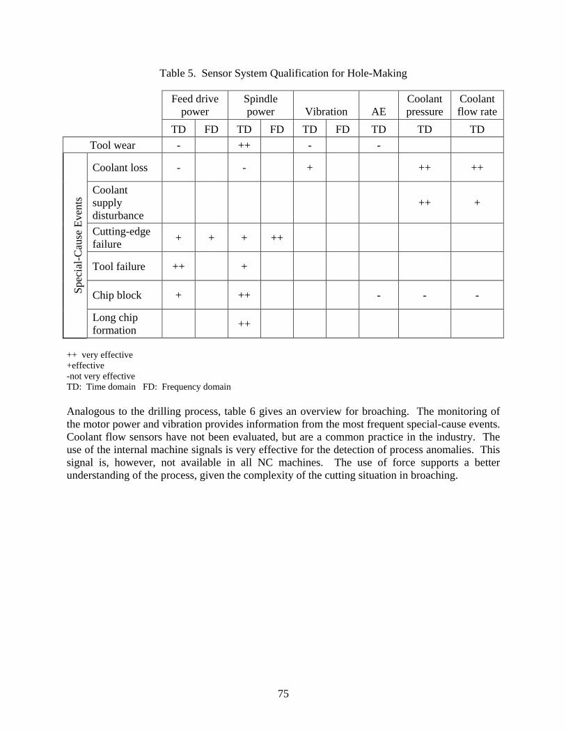
75

Table 5. Sensor System Qualification for Hole-Making

Feed drive power

Spindle power Vibration AE

Coolant pressure

Coolant flow rate

TD FD TD FD TD FD TD TD TD Tool wear - ++ - -

Spec

ial-C

ause

Eve

nts

Coolant loss - - + ++ ++

Coolant supply disturbance

++ +

Cutting-edge failure + + + ++

Tool failure ++ +

Chip block + ++ - - -

Long chip formation ++

++ very effective +effective - not very effective TD: Time domain FD: Frequency domain Analogous to the drilling process, table 6 gives an overview for broaching. The monitoring of the motor power and vibration provides information from the most frequent special-cause events. Coolant flow sensors have not been evaluated, but are a common practice in the industry. The use of the internal machine signals is very effective for the detection of process anomalies. This signal is, however, not available in all NC machines. The use of force supports a better understanding of the process, given the complexity of the cutting situation in broaching.

76

Table 6. Sensor System Qualification for Broaching

Motor power

Forces (dynamometer)

Calculated force (internal signal) Vibration AE

TD TD FD TD FD TD FD TD Tool wear ++ ++ + ++ + + -

Spec

ial-C

ause

Eve

nts

Rounded/broken tooth ++ ++ + -

Chipped tooth + + + -

Weak cutting edge + ++ + ++

Wrong speed + +

Tool failure + + +

5. THE PM SYSTEMS DATABASE

This section serves as guide for different PM systems and describes individual features and distinguishing criteria. 5.1 DESIGNS OF PM SYSTEMS

Monitoring systems can be distinguished according to their design. Table 7 shows the designs offered by various manufacturers.

77

Table 7. Designs Offered by Various Manufacturers

Manufacturer (1) (2) (3) (4) (5) Aradex - ● - - - Argotech - - - ● - Artis ● ● ● ● ● Brankamp - - - ● - Brinkhaus ● - - - - Caron Engineering ● - - - -

Comara - ● - - - Digital Way ● - - - - Dittel ● - - - ● Nordmann ● - - ● ● MCU ● - - - ● Montronix ● - ● ● - Omative Systems ● ● - - -

Prometec ● ● - - ● Schwer + Kopka - - - ● - Techna-Tool - - ● ● - Dr. Zinngrebe ● - - - ●

1. Machine cabinet systems 2. Software systems 3 3. PCI card systems 4. Front-end systems 5. Separate displays with input options

5.1.1 Machine Cabinet Systems

Cabinet systems are usually independent computing units mounted on rails in the machine cabinet. Some examples are shown in figure 85.

3 Software system with an independent monitoring system software for PM that runs on the HMI or the NC core. It is not a software module to monitor and visualize external hardware.

78

(Quelle: www.zinngrebe.de) (Quelle: www.nordmann.eu)

Figure 85. Cabinet Systems

These systems do not have their own display or parameterization; therefore, external means are required by which the parameterization and visualization can be performed. Depending on the manufacturer, the cabinet systems can be connected to the following interface: • An external personal computer • A human machine interface (HMI) • A separate programmable or display module Figure 86 lists the cabinet systems and their parameterization with the machine controls.

Source: www.zinngrebe.de Source: www.nordmann.eu

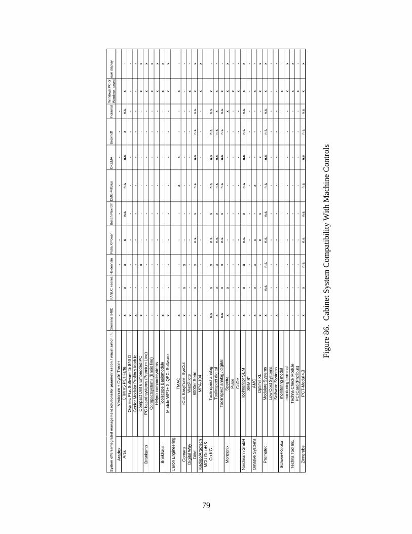
79

Sie

men

s 84

0DFA

NU

C i-

serie

sH

eide

nhai

nFi

dia

X-P

ower

Bos

ch R

exro

thD

MG

-Mill

plus

OK

UM

AB

eckh

off

Indr

amat

Win

dow

s P

C o

r W

indo

ws

base

dow

n di

spla

y

Ara

dex

Vec

tonu

m +

Cyc

le T

race

r -

--

--

--

--

Arti

sC

TM V

5 P

CI K

arte

xx

xx

n.s.

n.s.

n.s.

xn.

s.x

-O

rant

ec P

lus

Sof

twar

e fü

r 840

Dx

--

--

--

--

--

Gen

ior M

odul

ar P

rofib

us M

odul

ex

--

--

--

--

--

Com

pact

Uni

t 6 E

mbe

dded

PC

x-

x-

--

--

-x

xB

rank

amp

PC

bas

ed s

yste

ms

(Pre

miu

m L

ine)

--

--

--

--

-x

xC

ompa

ctsy

stem

s (B

asis

line

)-

--

--

--

--

xx

Hel

pro

com

pact

syst

ems

--

--

--

--

-x

xB

rinkh

aus

Tool

scop

e B

asis

mod

ule

x-

--

--

--

-x

xM

odul

e W

P1+

X, Q

PC

, Sof

twar

ex

--

--

--

--

xx

Car

on E

ngin

eerin

gTM

AC

x-

--

-x

x-

-x

-C

omar

aiC

ut, E

asyT

une,

Sys

Cut

xx

x-

--

--

--

-D

igita

l Way

Wat

tPilo

te-

--

--

--

--

x-

Ditt

el60

00er

Ser

iex

xx

n.s.

xn.

s.n.

s.n.

s.n.

s.x

xK

adig

o/A

rgot

ech

MP

A-1

04-

--

--

--

--

xx

MC

U G

mbH

&

Co.

KG

Tool

insp

ect a

nalo

gn.

s.x

xn.

s.x

n.s.

n.s.

n.s.

n.s.

x-

Tool

insp

ect d

igita

lx

xx

n.s.

xn.

s.n.

s.n.

s.x

x-

Tool

insp

ect a

nalo

g / d

igita

ln.

s.x

xn.

s.x

n.s.

n.s.

n.s.

n.s.

x-

Mon

troni

xS

pect

rax

x-

--

--

-x

xx

Pul

se-

--

--

--

--

x-

CoD

e-

--

--

--

--

x-

Nor

dman

n G

mbH

Tool

mon

itor S

EM

xx

xn.

s.x

n.s.

n.s.

n.s.

n.s.

xx

SE

M B

“-

--

--

--

--

--

Om

ativ

e S

yste

ms

AM

C

xx

xx

-x

--

-x

-O

ptim

ill X

Lx

--

xx

-x

--

xx

Pro

met

ecM

odul

are

Sys

tem

sx

n.s.

n.s.

n.s.

n.s.

n.s.

n.s.

n.s.

n.s.

xx

Low

Cos

t Sys

tem

s-

--

--

--

--

--

Sof

twar

e S

yste

ms

x-

--

--

--

--

-S

chw

er+K

opka

mon

itorin

g m

odul

--

--

--

--

-x

-m

onito

ring

term

inal

--

--

--

--

-x

xTe

chna

Too

l Inc.

Tech

na C

heck

Mod

ule

--

--

--

--

-x

xP

CI C

ard

(Pro

fibus

)-

--

--

--

--

x-

Zinn

greb

eP

CT-

Mod

ul 4

.3x

xn.

s.n.

s.n.

s.n.

s.n.

s.n.

s.n.

s.x

x

Syst

em o

ffers

inte

grat

ed m

anag

emen

t sol

utio

ns fo

r par

amet

rizat

ion

/ vis

ualiz

atio

n in

:

Figu

re 8

6. C

abin

et S

yste

m C

ompa

tibili

ty W

ith M

achi

ne C

ontro

ls

80

5.1.2 Software Systems

Software systems are independent monitoring systems that run on the HMI or the NC core. The systems for visualization and parameterization of external sensors systems are not included in this group. Table 8 shows identified monitoring software solutions and their compatibility to controllers. Since the software systems are very different, no direct comparison of all systems is reported.

Table 8. Software Systems and Compatibility to Machine Control

Software Siemens

840D Fanuc

i-Series Heidenhain Fidia

X-Power DMG

Millplus Aradex

Vectonum Arardex Vecto IDM - - - - - ●

Artis Orantec Plus ● - - - - - Comara iCut ● ● ● - - - Comara EasyTune ● - - - - - Omative AMC ● ● ● ● ● - Prometec ACfeed ● - - - - - Prosin Prometec ● ● - - - -

The Artis Orantec plus software is designed to be used with Sinumeric 840D control. It evaluates the data from the drive controller. The monitoring tasks are limited to the evaluation of tool breakage and missing tool analysis. The Prosine Prometec has the module Prosine plus for Sinumeric 840D controls and Prosine F for Fanuc i-series controllers. The software is used to monitor overload situations and tool monitoring by reading out the drive controller data. Tool-monitoring tasks are the identification of tool breakage, missing tools, and blunt tools. The Comara EasyTune is monitoring software that also offers overload-, tool breakage-, and missing tool-monitoring functions. The software is extended to the function of process analysis that gives recommendations for the adjustment of feed rates for individual NC lines. The OMATIVE AMC software system consists of different modules, which cover the areas of adaptive control and tool monitoring. The software generally runs in the computer numerical control (CNC) and is used for its operation of the HMI control. The monitoring functions are overload, wear, and tool breakage detection. The adaptive control can be used for feed optimization and feed adjustment according to tool wear. The Comara iCut and the Prometec AC feed software systems are also among the adaptive control systems. These evaluate the internal control signals (e.g., the spindle or feed power) and regulate the feed rate corresponding to a nominal value of power consumption. When the spindle power exceeds the present limit despite the adjustment, an emergency stop is triggered in

81

the machine. Furthermore, when the power signal is not present, the tool breaks or the missing tool is determined. 5.1.3 The PCI Card Systems

PCI card systems are offered by Artis, Montronix, and Techna Tool. The cards can be installed in PCI slots of the controller or personal computers, see table 9.

Table 9. Compatibility of PCI Cards

Product Siemens

840D Fanuc

i-Series Heiden-Hain Fidia

X-Power Beckhoff Indramat

Windows -PC or -Based Control

Artis CTM V5 PCI Karte ● ● ● ● ● - ●

Montronix Spectra Card ● ● - - - ● ●

Techna-Tool Techna-Check PCI - - - - - - ●

The Artis CTM V5 PCI card offers the greatest compatibility with the controls and is usually mounted directly to the operational panel of the controller. Therefore, the PCI card’s parameters are set and the results are displayed. In addition, the PCI card is connected via Profibus directly to the CNC machine and can communicate independently from the control panel directly to the CNC (e.g., to read data from the driving system or to return or reset values in the controller). For the connection of external sensors, the PCI card has an Artis sensor bus terminal. Figure 87 shows the communication structure of the Artis CTM V5.

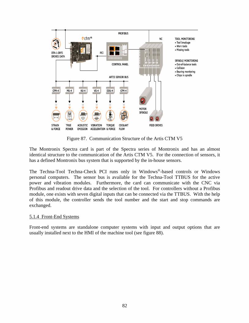
82

Figure 87. Communication Structure of the Artis CTM V5

The Montronix Spectra card is part of the Spectra series of Montronix and has an almost identical structure to the communication of the Artis CTM V5. For the connection of sensors, it has a defined Montronix bus system that is supported by the in-house sensors. The Techna-Tool Techna-Check PCI runs only in Windows®-based controls or Windows personal computers. The sensor bus is available for the Techna-Tool TTBUS for the active power and vibration modules. Furthermore, the card can communicate with the CNC via Profibus and readout drive data and the selection of the tool. For controllers without a Profibus module, one exists with seven digital inputs that can be connected via the TTBUS. With the help of this module, the controller sends the tool number and the start and stop commands are exchanged. 5.1.4 Front-End Systems

Front-end systems are standalone computer systems with input and output options that are usually installed next to the HMI of the machine tool (see figure 88).

83

(Quelle: www.brankamp.com)(Quelle: www.sk-gmbh.de)

Figure 88. Front-End Systems

The complete monitoring system software works independently; therefore, these devices can practically be applied to all controls. The communication between the control and the monitoring unit is used mostly for only transmission of start and stop commands and can be done via digital inputs and outputs or bus systems, such as Profibus. With the communication via Profibus, some systems can also read the data from the drive controller. For the connection of external sensors, these systems have many suitable analog inputs. Table 10 lists the front-end systems from various manufacturers.

Source: www.sk-gmbh.de Source: www.brankamp.com

84

Table 10. List of Front-End Systems

Manufacturer Systems

Argotech (Kadigo) MPA 104, PA-2, and PA-4

Artis Compact Unit 6 Embedded PC—Front-end implementation

Brankamp Premium Line, wie z. B. X7, PK 6000, PK 4U, and PK4000

Basis Line: e.g., B15, ECO 500, ECO 200, C 100, B 100, CMS, and CMS-GT

Helpro-Kompaktsysteme UP, MP, and LC

Montronix Spectra Vision

Nordmann Toolmonitor SEM, cabinet, and table units

SEM B

Schwer & Kopka SK 200, SK 300, SK 500, SK 600, SK 800, SK 6, and SK 8

Techna Tool Techna-Check 6400, Techna-Check 3200, and Techna-Check 101 5.2 SENSOR CONNECTION AND OUTPUT INTERFACES

This section discusses the sensor connectivity and output interfaces. A distinction is made between systems with integrated sensors, systems that take sensors from third-party manufacturers, and systems with machine control data readout capability. The following figures show a summary regarding the physical measures taken, sensor inputs, and output interfaces (see figures 89 and 90).

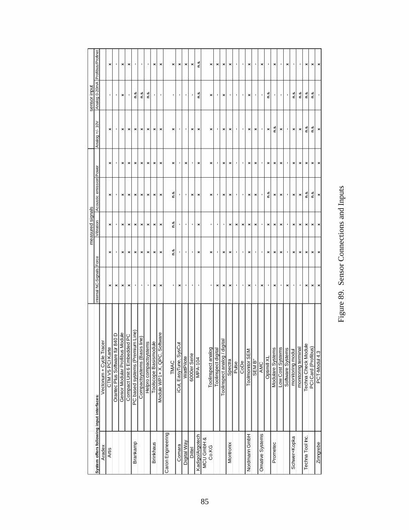
85

Sys

tem

offe

rs fo

llow

ing

inpu

t int

erfa

ces:

inte

rnal

NC

-Sig

nals

Forc

eV

ibra

tion

Aco

ustic

em

issi

onP

ower

Ana

log

+/- 1

0VA

nalo

g 0-

20m

AP

rofib

us/P

rofin

etA

rade

xV

ecto

num

+ C

ycle

Tra

cer

Arti

sC

TM V

5 P

CI K

arte

xx

xx

xx

-x

Ora

ntec

Plu

s S

oftw

are

für 8

40 D

x-

--

--

--

Gen

ior M

odul

ar P

rofib

us M

odul

ex

xx

xx

xx

xC

ompa

ct U

nit 6

Em

bedd

ed P

Cx

xx

xx

x-

xB

rank

amp

PC

bas

ed s

yste

ms

(Pre

miu

m L

ine)

-x

xx

xx

n.s.

-C

ompa

ctsy

stem

s (B

asis

line

)-

xx

xx

xn.

s.-

Hel

pro

com

pact

syst

ems

-x

xx

xx

n.s.

-B

rinkh

aus

Tool

scop

e B

asis

mod

ule

xx

xx

xx

-x

Mod

ule

WP

1+ X

, QP

C, S

oftw

are

xx

xx

xx

-x

Car

on E

ngin

eerin

gTM

AC

-n.

s.n.

s.n.

s.x

x-

xC

omar

aiC

ut, E

asyT

une,

Sys

Cut

x-

--

--

-x

Dig

ital W

ayW

attP

ilote

--

--

x-

-x

Ditt

el60

00er

Ser

ie-

--

x-

x-

xK

adig

o/A

rgot

ech

MP

A-1

04-

xx

xx

xn.

s.n.

s.M

CU

Gm

bH &

C

o.K

GTo

olin

spec

t ana

log

-x

-x

xx

xx

Tool

insp

ect d

igita

lx

--

--

--

xTo

olin

spec

t ana

log

/ dig

ital

xx

-x

xx

xx

Mon

troni

xS

pect

rax

xx

xx

x-

xP

ulse

--

x-

--

--

CoD

e-

-x

--

--

-N

ordm

ann

Gm

bHTo

olm

onito

r SE

Mx

xx

xx

xx

xS

EM

B“

--

xx

xx

--

Om

ativ

e S

yste

ms

AM

C

x-

--

--

-x

Opt

imill

XL

-x

xn.

s.x

xn.

s.-

Pro

met

ecM

odul

are

Sys

tem

sx

xx

xx

n.s.

-x

Low

Cos

t Sys

tem

s-

xx

xx

x-

-S

oftw

are

Sys

tem

sx

--

--

--

xS

chw

er+K

opka

mon

itorin

g m

odul

-x

xx

xx

n.s.

-m

onito

ring

term

inal

-x

xx

xx

n.s.

-Te

chna

Too

l Inc.

Tech

na C

heck

Mod

ule

xx

xn.

s.x

n.s.

n.s.

xP

CI C

ard

(Pro

fibus

)x

xx

n.s.

xn.

s.n.

s.x

Zinn

greb

eP

CT-

Mod

ul 4

.3x

xx

xx

x-

x

mea

sure

d si

gnal

sse

nsor

inpu

t

Figu

re 8

9. S

enso

r Con

nect

ions

and

Inpu

ts

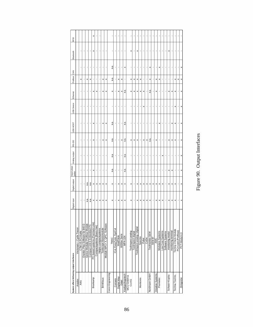
86

Dig

ital i

nput

Dig

ital o

utpu

tH

and

whe

el

puls

eA

nalo

g ou

tput

RS

-232

US

B H

OS

TU

SB

Dev

ice

Eth

erne

tP

rofib

usC

AN

Blu

etoo

thR

FID

Ara

dex

Vec

tonu

m +

Cyc

le T

race

r A

rtis

CTM

V5

PC

I Kar

te-

--

--

--

-x

--

Ora

ntec

Plu

s S

oftw

are

für 8

40 D

--

--

--

--

--

-G

enio

r Mod

ular

Pro

fibus

Mod

ule

n.s.

n.s.

--

--

--

x-

-C

ompa

ct U

nit 6

Em

bedd

ed P

Cn.

s.n.

s.-

--

--

-x

--

Bra

nkam

pP

C b

ased

sys

tem

s (P

rem

ium

Lin

e)x

xx

-x

x-

x-

-x

xC

ompa

ctsy

stem

s (B

asis

line

)x

x-

--

--

x-

--

-H

elpr

o co

mpa

ctsy

stem

sx

x-

--

--

--

--

-B

rinkh

aus

Tool

scop

e B

asis

mod

ule

xx

--

xx

-x

x-

-M

odul

e W

P1+

X, Q

PC

, Sof

twar

ex

x-

-x

x-

xx

--

Car

on E

ngin

eerin

gTM

AC

xx

n.s.

n.s.

n.s.

n.s.

-x

n.s.

n.s.

--

Com

ara

iCut

, Eas

yTun

e, S

ysC

ut-

--

--

--

--

--

-D

igita

l Way

Wat

tPilo

tex

x-

--

--

xx

--

-D

ittel

6000

er S

erie

xx

--

x-

-x

x-

--

Kad

igo/

Arg

otec

hM

PA

-104

xx

n.s.

n.s.

n.s.

n.s.

-n.

s.-

x-

-M

CU

Gm

bH &

C

o.K

GTo

olin

spec

t ana

log

xx

--

x-

-x

x-

x-

Tool

insp

ect d

igita

l-

--

-x

--

xx

--

-To

olin

spec

t ana

log

/ dig

ital

xx

--

x-

-x

x-

x-

Mon

troni

xS

pect

rax

x-

--

--

xx

--

-P

ulse

xx

--

x-

xx

--

--

CoD

ex

x-

-x

--

--

--

-N

ordm

ann

Gm

bHTo

olm

onito

r SE

Mx

x-

-n.

s.-

-n.

s.x

x-

-S

EM

B“

-x

--

--

--

--

--

Om

ativ

e S

yste

ms

AM

C

xx

--

x-

-x

x-

--

Pro

met

ecM

odul

are

Sys

tem

sx

x-

--

x-

-x

x-

-Lo

w C

ost S

yste

ms

xx

-x

--

--

--

--

Sof

twar

e S

yste

ms

--

--

--

--

--

--

Sch

wer

+Kop

kam

onito

ring

mod

ulx

xx

-x

--

x-

-x

-m

onito

ring

term

inal

xx

x-

xx

-x

--

--

Tech

na T

ool In

c.Te

chna

Che

ck M

odul

ex

x-

-x

xx

xx

--

-P

CI C

ard

(Pro

fibus

)-

--

--

--

-x

--

-Zi

nngr

ebe

PC

T-M

odul

4.3

xx

xx

xx

xx

xx

--

Sys

tem

offe

rs fo

llow

ing

outp

ut in

terf

aces

:

Figu

re 9

0. O

utpu

t Int

erfa

ces

87

5.3 THE PM STRATEGIES

Monitoring strategies are chosen depending on the monitoring task. The individual monitoring systems mostly have data-processing algorithms already specified by the manufacturer that perform the monitoring task. Because different priorities exist in the development of monitoring strategies, monitoring systems have significantly different characteristics in data processing. The algorithms from each manufacturer differ from the programming point of view; however, the exact differences cannot be specified because of the lack of algorithm knowledge. The monitoring strategies used by different manufacturers are shown in figure 91.

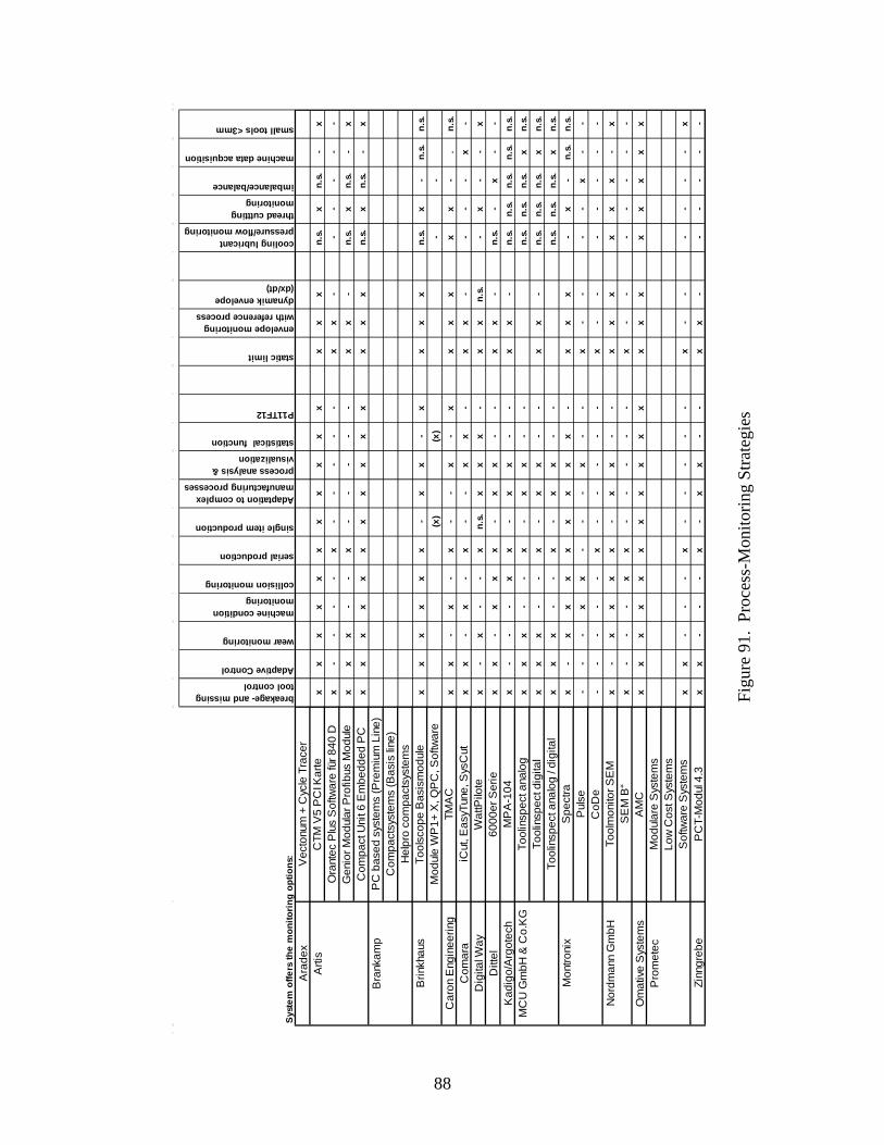
88

Sys

tem

offe

rs th

e m

onito

ring

opt

ions

:

breakage- and missing tool control

Adaptive Control

wear monitoring

machine condition monitoring

collision monitoring

serial production

single item production

Adaptation to complex manufacturing processes

process analysis & visualization

statistical function

P11TF12

static limit

envelope monitoring with reference process

dynamik envelope (dx/dt)

cooling lubricant pressure/flow monitoring

thread cuttting monitoring

imbalance/balance

machine data acquisition

small tools <3mm

Ara

dex

Vec

tonu

m +

Cyc

le T

race

r A

rtis

CTM

V5

PC

I Kar

tex

xx

xx

xx

xx

xx

xx

xn.

s.x

n.s.

-x

Ora

ntec

Plu

s S

oftw

are

für 8

40 D

x-

--

-x

--

--

-x

x-

--

--

-G

enio

r Mod

ular

Pro

fibus

Mod

ule

xx

x-

-x

--

--

-x

x-

n.s.

xn.

s.-

xC

ompa

ct U

nit 6

Em

bedd

ed P

Cx

xx

xx

xx

xx

xx

xx

xn.

s.x

n.s.

-x

Bra

nkam

pP

C b

ased

sys

tem

s (P

rem

ium

Lin

e)C

ompa

ctsy

stem

s (B

asis

line

)H

elpr

o co

mpa

ctsy

stem

sB

rinkh

aus

Tool

scop

e B

asis

mod

ule

xx

xx

xx

-x

x-

xx

xx

n.s.

x-

n.s.

n.s.

Mod

ule

WP

1+ X

, QP

C, S

oftw

are

(x)

(x)

--

Car

on E

ngin

eerin

gTM

AC

xx

-x

-x

--

x-

xx

xx

xx

-.

n.s.

Com

ara

iCut

, Eas

yTun

e, S

ysC

utx

x-

x-

x-

-x

x-

xx

--

--

x-

Dig

ital W

ayW

attP

ilote

x-

x-

-x

n.s.

xx

x-

xx

n.s.

-x

--

xD

ittel

6000

er S

erie

xx

-x

xx

-x

x-

-x

x-

n.s.

-x

--

Kad

igo/

Arg

otec

hM

PA

-104

x-

--

xx

-x

x-

-x

x-

n.s.

n.s.

n.s.

n.s.

n.s.

MC

U G

mbH

& C

o.K

GTo

olin

spec

t ana

log

xx

x-

-x

-x

x-

-n.

s.n.

s.n.

s.x

n.s.

Tool

insp

ect d

igita

lx

xx

--

x-

xx

--

xx

-n.

s.n.

s.n.

s.x

n.s.

Tool

insp

ect a

nalo

g / d

igita

lx

xx

--

x-

xx

--

n.s.

n.s.

n.s.

xn.

s.M

ontro

nix

Spe

ctra

x-

xx

xx

xx

xx

-x

xx

-x

-n.

s.n.

s.P

ulse

--

-x

x-

--

x-

-x

--

--

x-

-C

oDe

--

--

-x

--

--

-x

--

--

--

-N

ordm

ann

Gm

bHTo

olm

onito

r SE

Mx

-x

xx

x-

xx

--

xx

xx

xx

-x

SE

M B

“x

--

-x

x-

--

--

x-

--

--

--

Om

ativ

e S

yste

ms

AM

C

xx

xx

xx

xx

xx

xx

xx

xx

xx

xP

rom

etec

Mod

ular

e S

yste

ms

Low

Cos

t Sys

tem

sS

oftw

are

Sys

tem

sx

x-

--

x-

--

--

x-

--

--

-x

Zinn

greb

eP

CT-

Mod

ul 4

.3x

x-

--

x-

xx

--

xx

--

--

--

Figu

re 9

1. P

roce

ss-M

onito

ring

Stra

tegi

es

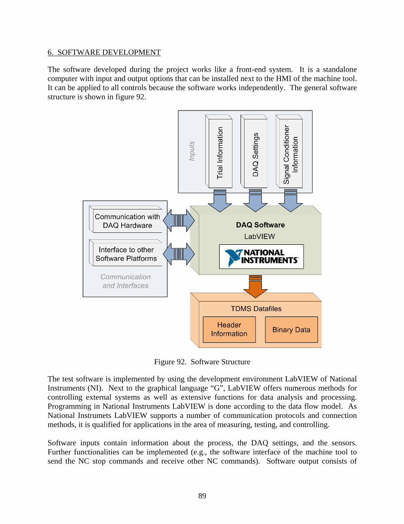
89

6. SOFTWARE DEVELOPMENT

The software developed during the project works like a front-end system. It is a standalone computer with input and output options that can be installed next to the HMI of the machine tool. It can be applied to all controls because the software works independently. The general software structure is shown in figure 92.

Figure 92. Software Structure

The test software is implemented by using the development environment LabVIEW of National Instruments (NI). Next to the graphical language “G”, LabVIEW offers numerous methods for controlling external systems as well as extensive functions for data analysis and processing. Programming in National Instruments LabVIEW is done according to the data flow model. As National Instrumets LabVIEW supports a number of communication protocols and connection methods, it is qualified for applications in the area of measuring, testing, and controlling. Software inputs contain information about the process, the DAQ settings, and the sensors. Further functionalities can be implemented (e.g., the software interface of the machine tool to send the NC stop commands and receive other NC commands). Software output consists of

90

binary Technical Data Management Streaming (TDMS)–data files that provide the input information in the header. 6.1 SOFTWARE BASIC STRUCTURE

The basic structure of the DAQ software can be used independently from the monitored process. Raw data are acquired and stored for offline analysis. Exact testing or cutting conditions are saved as part of the signal data file. 6.1.1 Software Input Parameters

6.1.1.1 Cutting Process (Trial) Information

All the process parameters per workpiece are input into a parameter sheet. These are: • Machine number • Part number • Tool specification • Date • Time • Hole/slot number • Cutting parameters 6.1.1.2 The DAQ and Signal Conditioner Settings

To guarantee exchangeability among different machines and facilities, DAQ information has to be standardized regarding its features as well as the order of sequence for all monitoring systems within one partner. DAQ settings example: • Channel 1: Spindle Power

- Type: ARTIS MU4 - Sample Rate: 25 kHz - Range: +/-10 Volt

• … • Channel 3: Acoustic Emission • Type: Kistler • Sample Rate: 25 kHz • Range: +/- 5 Volt Signal conditioner settings example: • Channel 1: Spindle Power

91

- Type: ARTIS M U4 - Number of Coils: 2 - Smoothing Factor: 3

• Channel 2: 3-Comp. Force Dynamometer

- Type: KISTLER Charge Amplifier - Amplification Level: 2

• Channel 3: Acoustic Emission

- Low-Pass: 500 kHz - High-Pass: 50 kHz - Tao_RMS: 0.012 ms

• … 6.1.2 Communication and Interfaces

There is a user interface and communication to the PM system. Measured signals that overpass the limits will be observed as warning or stop signals on the user interface, but not transferred to the machine. The implementation of the machine interface can be performed as an upgrading function in the software. This function for the automatic machine shutdown is regarded as important to ensure timely reaction when a special-cause event occurs. The software is based on NI LabVIEW and can be included in other platforms capable of dealing with dll (dynamic-link libraries). In case new data processing algorithms had to be edited using other software solutions, the programmed SubVIs could run within a dll-supporting software, such as MatLab. 6.1.3 Software Outputs

The standard files created by LabVIEW are in TDMS format, which provides the opportunity to create binary files. The advantages of binary files are the small size and the fact that the data files contain two parts of information: • Header: all input information • Data: the measurement data If needed, the data can easily be converted into American Standard Code for Information Interchange code. 6.2 AUTOMATED COMPUTER-BASED FEATURE EXTRACTION

A computer-based feature extraction software was developed for drilling. An overview of the software structure is given in figure 93. The user interface is presented in figure 94. As already specified, there is no interaction between the machine and the PM system. Identification of the process start and end points is performed by signal characteristics and the SF for each hole

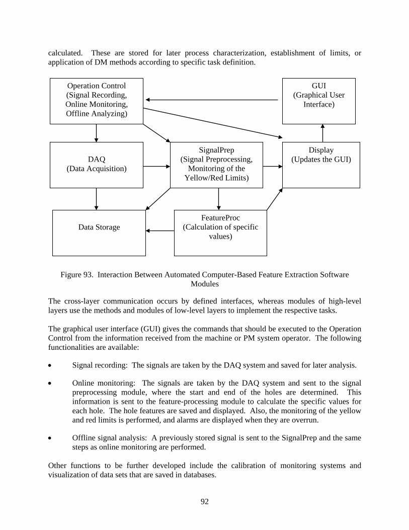
92

calculated. These are stored for later process characterization, establishment of limits, or application of DM methods according to specific task definition.

Figure 93. Interaction Between Automated Computer-Based Feature Extraction Software

Modules

The cross-layer communication occurs by defined interfaces, whereas modules of high-level layers use the methods and modules of low-level layers to implement the respective tasks. The graphical user interface (GUI) gives the commands that should be executed to the Operation Control from the information received from the machine or PM system operator. The following functionalities are available:

• Signal recording: The signals are taken by the DAQ system and saved for later analysis.

• Online monitoring: The signals are taken by the DAQ system and sent to the signal preprocessing module, where the start and end of the holes are determined. This information is sent to the feature-processing module to calculate the specific values for each hole. The hole features are saved and displayed. Also, the monitoring of the yellow and red limits is performed, and alarms are displayed when they are overrun.

• Offline signal analysis: A previously stored signal is sent to the SignalPrep and the same steps as online monitoring are performed.

Other functions to be further developed include the calibration of monitoring systems and visualization of data sets that are saved in databases.

Operation Control (Signal Recording, Online Monitoring, Offline Analyzing)

DAQ

(Data Acquisition)

Data Storage

SignalPrep (Signal Preprocessing,

Monitoring of the Yellow/Red Limits)

FeatureProc (Calculation of specific

values)

Display (Updates the GUI)

GUI (Graphical User

Interface)

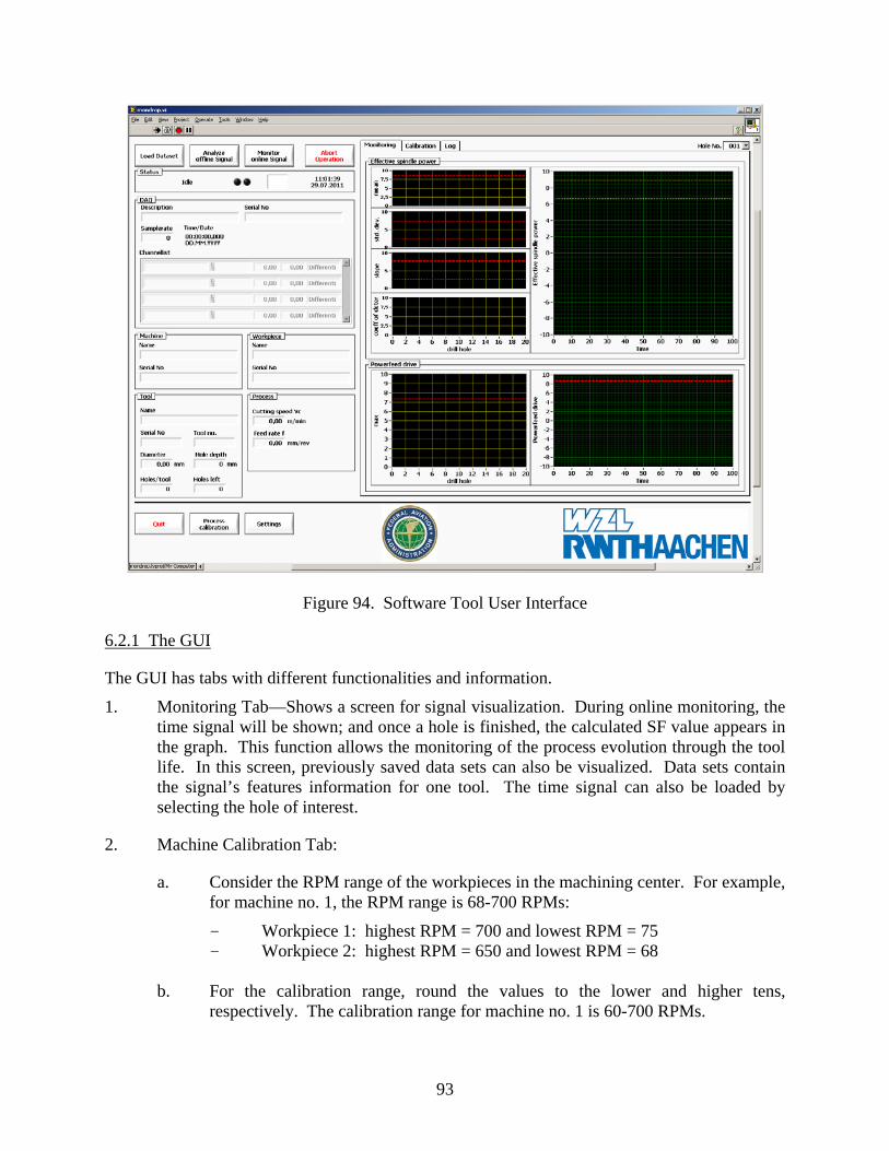
93

Figure 94. Software Tool User Interface

6.2.1 The GUI

The GUI has tabs with different functionalities and information.

1. Monitoring Tab—Shows a screen for signal visualization. During online monitoring, the time signal will be shown; and once a hole is finished, the calculated SF value appears in the graph. This function allows the monitoring of the process evolution through the tool life. In this screen, previously saved data sets can also be visualized. Data sets contain the signal’s features information for one tool. The time signal can also be loaded by selecting the hole of interest.

2. Machine Calibration Tab:

a. Consider the RPM range of the workpieces in the machining center. For example, for machine no. 1, the RPM range is 68-700 RPMs:

- Workpiece 1: highest RPM = 700 and lowest RPM = 75 - Workpiece 2: highest RPM = 650 and lowest RPM = 68

b. For the calibration range, round the values to the lower and higher tens,

respectively. The calibration range for machine no. 1 is 60-700 RPMs.

94

c. Run the spindle from the lowest to the highest range value in 50-RPM steps. This can be done manually by letting the spindle run in the air at least 30 seconds for each step.

d. Take the average of the measured signal for each step and represent it against the

RPM. e. Find the linear regression for the effective power versus RPMs

= ⋅ +P m RPM b f. Use the slope and y intercept for machine tool characterization in the software.

3. Log Tab—Shows the possible special-cause events that might have taken place during the process or when an SF is outside its limit values.

4. Configuration Tab—Shows the machine, workpiece, process parameters, and tool information from the data set being taken or loaded. This information is required and saved at the moment an online monitoring or offline analysis is started.

Steps 2d through 2f could be performed automatically by the software as an additional functionality. An Input parameter sheet for hole-making has to be completed before doing online or offline analyses. It contains the part number and the machine used. Correct specification of the machine and the machining steps is indispensable for accurate signal processing. The following is a list of required parameters: • Tool sequence • Cutting tool number • Tool type

- Spot drill - Drill - Reamer - Radius tool

• Tool diameter • Cutting speed (spindle RPM) • Tool feed rate • Depth of hole • Tool change point • Holes per workpiece/slots • The limits for each machining step

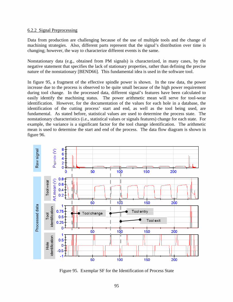
95

6.2.2 Signal Preprocessing

Data from production are challenging because of the use of multiple tools and the change of machining strategies. Also, different parts represent that the signal’s distribution over time is changing; however, the way to characterize different events is the same. Nonstationary data (e.g., obtained from PM signals) is characterized, in many cases, by the negative statement that specifies the lack of stationary properties, rather than defining the precise nature of the nonstationary [BEND66]. This fundamental idea is used in the software tool. In figure 95, a fragment of the effective spindle power is shown. In the raw data, the power increase due to the process is observed to be quite small because of the high power requirement during tool change. In the processed data, different signal’s features have been calculated to easily identify the machining status. The power arithmetic mean will serve for tool-wear identification. However, for the documentation of the values for each hole in a database, the identification of the cutting process’ start and end, as well as the tool being used, are fundamental. As stated before, statistical values are used to determine the process state. The nonstationary characteristics (i.e., statistical values or signals features) change for each state. For example, the variance is a significant factor for the tool change identification. The arithmetic mean is used to determine the start and end of the process. The data flow diagram is shown in figure 96.

Figure 95. Exemplar SF for the Identification of Process State

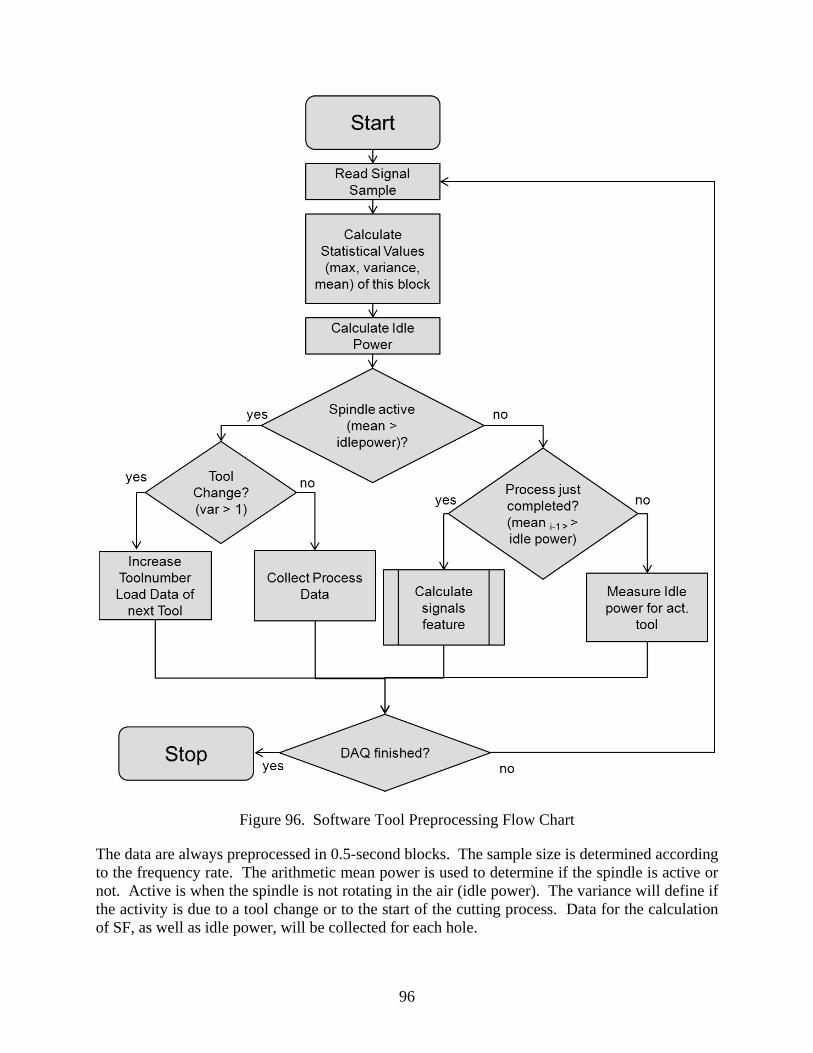
96

Figure 96. Software Tool Preprocessing Flow Chart

The data are always preprocessed in 0.5-second blocks. The sample size is determined according to the frequency rate. The arithmetic mean power is used to determine if the spindle is active or not. Active is when the spindle is not rotating in the air (idle power). The variance will define if the activity is due to a tool change or to the start of the cutting process. Data for the calculation of SF, as well as idle power, will be collected for each hole.

97

For a better understanding of the algorithms for the signal preprocessing, a script for the offline process of the signals in NI DIAdem is included in appendix J. The SF will be saved to build up the database. Limits for different SF can be established once historical data are available. Raw data are also collected for verification of results. This can be deactivated according to the needs. 6.3 DEVELOPMENT OF DATABASE ARCHITECTURE

The following steps should be followed to develop a set of specifications, rules, and processes on how data should be stored so it can be accessed by other components of the system.

• A naming convention should be established and strictly followed.

- The base names must be unique within each object type, but should not be too long (preferably less than 50 characters).

- Date, Time, Machine No., Part No., Tool, Slot/Hole No. information should be included in the DB (file/table) name.

• Normalization—Form parent/child relationships between the tables. The many goals of data normalization include ensuring data integrity and avoiding redundancy.

• Relationships—A hierarchy for the tables or folders in which the data will be stored. For each relationship between two tables, one is the parent and the other is the child. For example, Machine No. is the parent and Part No. is the child.

• Primary key—The field in a table in which the value uniquely identifies each record. It must not contain any duplicate values and the values must not change. For the best performance, it should also be compact. These characteristics are difficult to find in naturally occurring data. A surrogate primary key field contains artificially derived values that have no intrinsic meaning. The sole purpose for the values is to uniquely identify each record.

• Foreign keys—The field in a table that refers to parent records in another table. The references are represented by the primary key values of the corresponding parent records.

• Concurrency—Any multiuser database application has to have some method of dealing with concurrent access to data.

7. REACTION STRATEGIES

The PM was found to have the highest implementation in hole-making within the industry; however, this process is still a concern within the industry, where it has been established that the hazardous processes should be monitored. A process can be regarded as hazardous if the number of engaged cutting edges is two or more and the involved sector is greater than 180°.

98

The strategies used most when detecting special-cause events are power and flow-rate monitoring. However, monitoring systems still lack an integral solution. The industry performs system implementation to comply with the specifications given by the OEMs or to follow internal guidelines. New strategies are also developed. Complete results of the benchmarking survey are presented in appendix I. The yellow and red limits (i.e., a warning signal or stop of the machine) are the strategies that find the most acceptance within the industry. Recommendations of tool change and modification of the cutting parameters are also considered. However, the use of these strategies (e.g., for the process and tool life optimization) is not possible because the process is frozen. Taking into consideration the approved parameter ranges, further investigations is needed in the area of cutting parameters adaption. There is also a need for additional PM system capability to have automatic serial part-specific data storage of monitored parameters. A database of the signal characteristics will not only serve to see component-specific information, but also will allow monitoring of the production history and build up the process knowledge. Furthermore, as stated in a previous report4, PM systems should interface with the machine numerical control to provide automatic machine shutdown when a process special-cause event occurs. 7.1 THE PM WITH MACHINE INTERFACE

For a monitoring system with machine interface to be implemented, the basic strategy to follow is: • The NC-PLC sends commands to the PM-Programmic Logic Cobtributor. The NC file is

responsible for process traceability. • The set values (yellow and red process limits) are sent from the NC to the PM once per

hole. This ensures that the correct limit is applied for the current operation and that no false alarms occur if there is a restart or if an action is blocked.

• The maximum power is the set value not to be exceeded. An overrun of this value will

cause either an alarm or a stop if the yellow and red limits are overrun respectively. • The maximum time limit accepted for an overrun of the set values without causing an

alarm is 1000 ms. • Only the power required for the process is to be considered. The idle power before each

hole has to be measured at approximately 10 seconds and subtracted from the total power at least once after tool change.

4 DOT/FAA/AR06/3, Rotor Aerospace Industries Association Rotor Manufacturing Project Team and the Federal Aviation Administration, 2006.

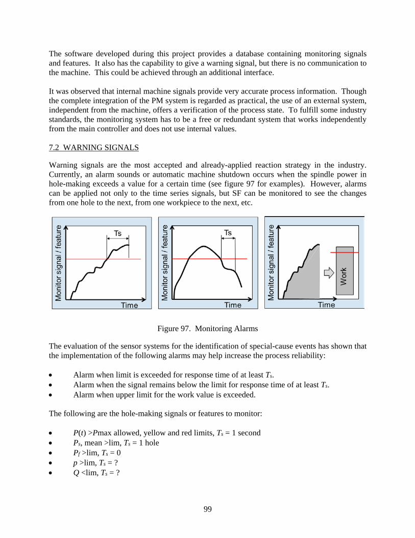
99

The software developed during this project provides a database containing monitoring signals and features. It also has the capability to give a warning signal, but there is no communication to the machine. This could be achieved through an additional interface. It was observed that internal machine signals provide very accurate process information. Though the complete integration of the PM system is regarded as practical, the use of an external system, independent from the machine, offers a verification of the process state. To fulfill some industry standards, the monitoring system has to be a free or redundant system that works independently from the main controller and does not use internal values. 7.2 WARNING SIGNALS

Warning signals are the most accepted and already-applied reaction strategy in the industry. Currently, an alarm sounds or automatic machine shutdown occurs when the spindle power in hole-making exceeds a value for a certain time (see figure 97 for examples). However, alarms can be applied not only to the time series signals, but SF can be monitored to see the changes from one hole to the next, from one workpiece to the next, etc.

Figure 97. Monitoring Alarms

The evaluation of the sensor systems for the identification of special-cause events has shown that the implementation of the following alarms may help increase the process reliability: • Alarm when limit is exceeded for response time of at least Ts. • Alarm when the signal remains below the limit for response time of at least Ts. • Alarm when upper limit for the work value is exceeded. The following are the hole-making signals or features to monitor: • P(t) >Pmax allowed, yellow and red limits, Ts = 1 second • Ps, mean >lim, Ts = 1 hole • Pf >lim, Ts = 0 • p >lim, Ts = ? • Q <lim, Ts = ?

100

The industry has expressed interest in further research to determine how long Ts coolant could be absent during the reaming process without damaging the surface. The signals or features to monitor in broaching are: • F or P >signature signal/model • Work or energy Estimation can be used to establish limits for a broaching model that uses the cross-sectional area for the power. 7.3 NEW PM STRATEGIES

Engine manufacturers established that investigation of wireless and miniature sensors could contribute to advances in PM and that surface acoustic wave (SAW) sensors should be implemented. The SAW sensors transform kinetic energy into electric energy and allow remote interrogation of the sensor by wireless network. They are an intelligent, autonomous sensor low-cost solution. The SAW sensor principle is well developed regarding specialized temperature measurement applications and is a common technology in tire-pressure sensing on the latest automotive applications. Wireless SAW sensor systems are based on the principle of surface waves. The detection mechanism is a mechanical acoustic wave. As the acoustic wave propagates through or on the surface of the material, any changes to the characteristics of the propagation path affect the velocity and/or amplitude of the wave. Using radar signals, the response of a sensor’s signal towards a request signal can be interrelated to physical changes like the deformation or elongation of a part’s length. The SAW sensors are passive (no power required), wireless, low cost, rugged, extremely small, and lightweight, making them well suited for measuring moving objects, such as tools. These characteristics offer advantages over such technologies as capacitive and piezo-resistive sensors, which require operating power and are not wireless. The SAW sensors are not as common as applications to identify disturbances of a manufacturing process. Nevertheless, their functionality and characteristics are up and coming and will enable future adaptive control systems; therefore, an evaluation of their usability is necessary to determine their potential role for the development of PM strategies. 7.4 METHODOLOGY FOR THE QUALIFICATION OF MACHINING PROCESSES

For the implementation of new manufacturing strategies or materials, the processes have to be validated to ensure the integrity of the machined part. As stated in the RoMan project, PM could also be used to find the optimal machining parameters and to optimize validated processes. The PM signals, especially those acquired very close to the process or in the direct load flow, balance very accurate information about the machining conditions, such as thermal and mechanical loads on the tool’s cutting edge and the workpiece surface. Therefore, the use of PM

101

systems (e.g., for temperature and force measurement during the qualification process) provides information that enables a faster qualification of the process. The specific methodology will depend on the goals to be achieved (e.g., higher productivity, better surface finish). Signal and process features databases should facilitate the decision-making process when new machining processes are implemented, assuming that the past and actual process conditions are known. The knowledge gained during time through PM signals allows rapid actions. 7.5 OTHER STRATEGIES

Other strategies (e.g., the adaption of cutting parameters to increase productivity) are not currently of major interest to the industry. This strategy can be better investigated once a database of the process condition is available. This will be possible through the PM signals acquired and saved over time. 8. SUMMARY AND CONCLUSIONS

Under laboratory conditions, the force and torque signals have proven to provide very accurate process information because their measurements are done very close to the cutting location and piezoelectric sensors are very sensitive (e.g. >10mN in a range of 5 kN) and highly linear. However, these types of sensors find limited application in the industry given their costs and the fact that machine conditions might be changed with their installation. Other piezoelectric sensors, such as accelerometers and acoustic emission sensors, have also been demonstrated to deliver information related to process disturbances. These sensors can be installed on the machine without causing any stiffness changes and their signals have specific characteristics for each process. However, the dependency of signal amplitude to the cutting location, mounting conditions, and different machine masses can make their characterization difficult. For the previously mentioned reasons, the measurement of the effective power (current transducers) and of the coolant flow and pressure have found the most acceptance in production. These are easy to implement and provide information about two very important factors influencing the surface quality: tool wear and cooling. Many companies already have a standard for monitoring hole-making, using limits to these two measurements. When the yellow and red limits are overpassed, a warning or stop signal is sent. In the broaching process, similar limits are obtained from a signature signal (uniaxial force, power, internal signals). However, in both cases, no information about the possible process disturbance is delivered. Therefore, laboratory trials for the characterization of signals for special cause events were performed. Before the characterization of special cause events, the spindle and feed drive power was compared to the torque and feed force acquired through a dynamometer. It was found that the spindle power measured by the effective power module provided comparably accurate information to the torque. Also, small changes were seen in the torque signal. Conversely, the power of the feed drive was not comparable to the feed force. This signal was, however, also sensitive to process changes. One important factor to be taken into account is the idle power. This value changes for different machines and with time; therefore, it has to be subtracted from the measurement during the process to consider only the cutting power, which is independent from the machine. Because the spindle power provides very accurate information of the torque

102

required during the process, it was established that this signal can help to gain better understanding of the process. From the laboratory trials, in which the most frequent special cause events were simulated, it is concluded that these can be identified in the spindle power, coolant pressure, and flow signals. Other signals could be used for validation of results obtained from these two signals. • Tool wear—Directly related to mean spindle power

• Tool chipping—Higher spindle power and change in characteristic frequency in power

spectrum

• Tool failure—Very quick increase and decrease in spindle power

• Chip block/jams—Higher amplitude fluctuation and steep increase in spindle power during cutting

• Long chip formation—Steep increase in spindle power during cutting

• Coolant loss—Quick drop in coolant flow

• Coolant supply disturbance—Higher pressure and lower flow

In broaching, it was found that the power does not provide one-to-one information about the process forces in all cases. From the external effective power module, the single entrance and exit of each tooth are not identified in the power as in the force signal because power fluctuations, intrinsic from the motor, superimpose the steps due to tooth entry and exit. The signal presents the mean power required for the cutting process, but not the power required by every single tooth. On the other hand, the force can be calculated from the internal measurement. It is to be taken into account that a motor model may be required when the machine has two drive motors. For broaching, monitoring the motor power and vibration provides information from the most frequent special cause events. Coolant flow sensors have not been evaluated, but a common practice in the industry and highly recommended given the high influence of cooling on surface integrity. The use of the internal machine signals is also very effective for the detection of process anomalies. However, this signal is not available in all numerical controls of the machine tool. The use of force measurements is suggested to support a better understanding of the process given the complexity of the cutting situation in broaching. Special cause events in production can be identified in the following ways: • Tool wear—Higher power, higher cutting force, additional peak in the force and

acceleration spectrum

• Rounded/broken tooth—Higher power and cutting force for subsequent tooth

103

• Tooth chipping—Increase in power and force

• Weak cutting edge—Higher amplitude vibrations, higher force and additional peak in force and vibration spectrum

• Wrong speed—Change in characteristic frequency

There are many process monitoring (PM) systems available in the market. For a robust PM, it will be recommended to use a software system with compatibility to the machine control. Some manufacturers offer standard solutions to fulfill aerospace requirements for holemaking and broaching. The software developed during this project allows the storage of monitoring signals and features in order to build a database. It also has the capability of giving a warn signal, but there is no communication to the machine. This could be achieved through an additional interface. The software can be applied to both hole-making and broaching for the acquisition of PM signals from multiple sensors. These signals are saved with a standard name structure so that they can be easily found for each part, tool, or machine. Furthermore, the files contain all configuration information and can be loaded for visualization. The automatic feature extraction function is only implemented for hole-making. In the feature extraction function, the entire signal for the hole-making process is analyzed. With a tool-cutting parameter protocol (inputted by the user) and the signal processing, the specific cutting process and the features are calculated and stored only for drilling and reaming. Currently, the signals analyzed are the spindle and feed drive power. The features extracted for the spindle power are the mean, maximal, and slope during cutting, which represent tool wear, tool chipping or failure, and chip jams or long chip formation, respectively. Also, the maximal value for the feed force is monitored because this value provides quicker information of tool failure. Other signal features could be considered in the future. As already mentioned, static limits are the most accepted and already implemented strategies when process disturbances are identified through the PM signals. Yellow and red are established in hole-making from the maximal spindle power in wear tests and for broaching from a signature signal in time. An overrun of these limits will cause a warn signal and an immediate stop. The industry will also consider recommendations for tool change and modification of the cutting parameters. Further research in process control will be necessary because the use of frozen parameters is one way to assure quality. 9. RECOMMENDATIONS FOR FUTURE WORK

To large extent, PM has been applied in the manufacturing of critical aero engine components. Each of the eight manufacturers that provided feedback in the benchmarking survey used PM strategies in production or as support for better process understanding and assistance in the process qualification. However, these strategies are not common to all of them and, in many cases, the basic knowledge is built by each company independently. Therefore, further academia research projects in collaboration with the industry can provide a faster startup and further

104

developments by the integration of the laboratory and production work in PM. Work in the following areas can be conducted in the future: • Sensor systems—Engine manufacturers have manifested that investigation of wireless

and miniature sensors could contribute in advances for PM and surface acoustic wave sensors (SAWs) should be implemented.

• PM strategy—Establishment of dynamic limits, determination of response time that a limit can be overpassed without causing surface damage (very important in cooling), use of multivariable charts.

• Automated features extraction software—Optimization and implementation in the industry; development of interface to the machine tool.

• Strategy for process qualification.

• Adaptive machining.

10. BIBLIOGRAPHY

[AXIN04] D.A. Axinte, European Project MANHIRP Report, 2004 [AXIN06] D.A. Axinte, Approach Into the use of Probabilistic Neural Networks for

Automated Classification of Tool Malfunction in Broaching, International Journal of Machine Tools and Manufacture, Vol. 46, 2006, pp. 1445-1448.

[ABEL07] José Vcte Abellán Nebot, Rubén Morales-Menéndez, Antonio J Vallejo Guevara, and Ciro A. Rodríguez, “Surface Roughness and Cutting Tool-Wear Diagnosis Based on Bayesian Networks,” Fault Detection, Supervision and Safety of Technical Processes 2006, 2007, pp. 408-413.

[ACHI02] Sofiane Achiche, Marek Balazinski, Luc Baron, and Krzysztof Jemielniak, “Tool Wear Monitoring Using Genetically-Generated Fuzzy Knowledge Bases Original Research Article,” Engineering Applications of Artificial Intelligence, Vol. 15, Issues 3-4, June-August 2002, pp. 303-314.

[BENA02] P.G. Benardos, G.C. Vosniakos, “Prediction of Surface Roughness in CNC Face Milling Using Neural Networks and Taguchi’s Design of Experiments,” Robotics and Computer Integrated Manufacturing, Vol. 18, 2002, pp. 343-354.

[BEND66] Bendat J. and Pierson A., Measurement and Analysis of Random Data, 1966 [BURK92] L.I. Burke, “Competitive Learning Based Approaches to Tool-Wear

Identification,” IEEE Transactions on Systems, Man, and Cybernetics, Vol. 22, Issue 3, May and June 1992, pp. 559-563.

[BREZ04] M. Brezocnik, M. Kovacic, and M. Ficko, “Prediction of Surface Roughness With Genetic Programming,” Journal of Materials Processing Technology Vol. 157-158, 2004, pp. 28-36.

[BRIN09] Brinkhaus, J., “Statistische Verfahren zur selbstlernenden Überwachung spanender Bearbeitungen in Werkzeugmaschinen, ” Dissertation University of Hannover, 2009.

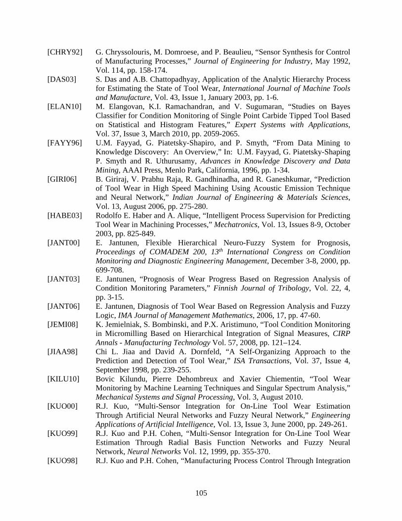
105

[CHRY92] G. Chryssolouris, M. Domroese, and P. Beaulieu, “Sensor Synthesis for Control of Manufacturing Processes,” Journal of Engineering for Industry, May 1992, Vol. 114, pp. 158-174.

[DAS03] S. Das and A.B. Chattopadhyay, Application of the Analytic Hierarchy Process for Estimating the State of Tool Wear, International Journal of Machine Tools and Manufacture, Vol. 43, Issue 1, January 2003, pp. 1-6.

[ELAN10] M. Elangovan, K.I. Ramachandran, and V. Sugumaran, “Studies on Bayes Classifier for Condition Monitoring of Single Point Carbide Tipped Tool Based on Statistical and Histogram Features,” Expert Systems with Applications, Vol. 37, Issue 3, March 2010, pp. 2059-2065.

[FAYY96] U.M. Fayyad, G. Piatetsky-Shapiro, and P. Smyth, “From Data Mining to Knowledge Discovery: An Overview,” In: U.M. Fayyad, G. Piatetsky-Shaping P. Smyth and R. Uthurusamy, Advances in Knowledge Discovery and Data Mining, AAAI Press, Menlo Park, California, 1996, pp. 1-34.

[GIRI06] B. Giriraj, V. Prabhu Raja, R. Gandhinadha, and R. Ganeshkumar, “Prediction of Tool Wear in High Speed Machining Using Acoustic Emission Technique and Neural Network,” Indian Journal of Engineering & Materials Sciences, Vol. 13, August 2006, pp. 275-280.

[HABE03]

Rodolfo E. Haber and A. Alique, “Intelligent Process Supervision for Predicting Tool Wear in Machining Processes,” Mechatronics, Vol. 13, Issues 8-9, October 2003, pp. 825-849.

[JANT00] E. Jantunen, Flexible Hierarchical Neuro-Fuzzy System for Prognosis, Proceedings of COMADEM 200, 13th International Congress on Condition Monitoring and Diagnostic Engineering Management, December 3-8, 2000, pp. 699-708.

[JANT03] E. Jantunen, “Prognosis of Wear Progress Based on Regression Analysis of Condition Monitoring Parameters,” Finnish Journal of Tribology, Vol. 22, 4, pp. 3-15.

[JANT06] E. Jantunen, Diagnosis of Tool Wear Based on Regression Analysis and Fuzzy Logic, IMA Journal of Management Mathematics, 2006, 17, pp. 47-60.

[JEMI08] K. Jemielniak, S. Bombinski, and P.X. Aristimuno, “Tool Condition Monitoring in Micromilling Based on Hierarchical Integration of Signal Measures, CIRP Annals - Manufacturing Technology Vol. 57, 2008, pp. 121–124.

[JIAA98] Chi L. Jiaa and David A. Dornfeld, “A Self-Organizing Approach to the Prediction and Detection of Tool Wear,” ISA Transactions, Vol. 37, Issue 4, September 1998, pp. 239-255.

[KILU10] Bovic Kilundu, Pierre Dehombreux and Xavier Chiementin, “Tool Wear Monitoring by Machine Learning Techniques and Singular Spectrum Analysis,” Mechanical Systems and Signal Processing, Vol. 3, August 2010.

[KUO00] R.J. Kuo, “Multi-Sensor Integration for On-Line Tool Wear Estimation Through Artificial Neural Networks and Fuzzy Neural Network,” Engineering Applications of Artificial Intelligence, Vol. 13, Issue 3, June 2000, pp. 249-261.

[KUO99] R.J. Kuo and P.H. Cohen, “Multi-Sensor Integration for On-Line Tool Wear Estimation Through Radial Basis Function Networks and Fuzzy Neural Network, Neural Networks Vol. 12, 1999, pp. 355-370.

[KUO98] R.J. Kuo and P.H. Cohen, “Manufacturing Process Control Through Integration

106

of Neural Networks and Fuzzy Model,” Fuzzy Sets and Systems Vol. 98, 1998, pp. 15-31.

[KUO98] R.J. Kuo and P.H. Cohen, “Intelligent Tool Wear Estimation System Through Artificial Neural Networks and Fuzzy Modelling,” PII:SO954-1810(97)00027-7.

[KUO97] R.J. Kuo and P.H. Cohen, “Intelligent Tool Wear Estimation System Through Artificial Neural Networks and Fuzzy Modelling,” PII:SO954-1810(97)00027-7.

[KIRB07] E. Daniel Kirby and Joseph C. Chen, “Development of a Fuzzy-Nets-Based Surface Roughness Prediction System in Turning Operations,” Computers & Industrial Engineering Vol. 53, 2007, pp. 30-42.

[KIRB06] E. Daniel Kirby, Joseph C. Chen, and Julie Z. Zhang, “Development of a Fuzzy-Nets-Based in-Process Surface Roughness Adaptive Control System in Turning Operations,” Expert Systems With Applications, Vol. 30, Issue 4, May 2006, pp. 592-604.

[MOHA09] M. Malekiana, S. Parka, and M.B.G. Jun, “Tool Wear Monitoring of Micro-Milling Operations,” Journal of Materials Processing Technology Vol. 209, 2009, pp. 4903-4914.

[SAHI04] Y. Sahin and A.R. Motorcu, Surface Roughness Prediction Model in Machining of Carbon Steel by PVC Coated Cutting Tools, American Journal of Applied Sciences, Vol. 1, 2004, pp. 12-17.

[SANJ05] C. Sanjay, M.L. Neema, and C.W. Chin, “Modelling of Tool Wear in Drilling by Statistical Analysis and Artificial Neural Network,” Journal of Materials Processing Technology, 2005, Vol. 170, pp. 494-500.

[SICK02] B. Sick, “On-Line and Indirect Tool Wear Monitoring in Turning With Artificial Neural Networks: A Review of More Than a Decade of Research,” Mechanical Systems and Signal Processing, Vol. 16, Issue 4, 2002, pp. 487-546.

[SCHE04] C. Scheffer and P.S. Heyns, “An Industrial Tool Wear Monitoring System for Interrupted Turning,” Mechanical Systems and Signal Processing Vol. 18, 2004, pp. 1219-1242.

[TÖNS05] H.K. Tönshoff, C. Hollmann and Hochgeschwindigkeitsspanen, WILEY-VCH, ISBN 3-527-31256-0, Weinheim, 2005.

[TSAO08] C.C. Tsao and H. Hocheng, Evaluation of Thrust Force and Surface Roughness in Drilling Composite Material Using Taguchi Analysis and Neural Network, Journal of Material Processing Technology, Vol. 203, 2008, pp. 342-348.

[XIAO98] L. Xiaoli and Y. Zhejun, “Tool Wear Monitoring With Wavelet Transform-Fuzzy Clustering Method,” Wear Vol. 219, 1998, pp. 145-154.

[ZAH07] M. Zäh and G. Reinhart, Formelsammlung Spanende Fertigungsverfahren Institut für Werkzeugmaschinen und Betriebswissenschaften, Munich Technical University, 2007.

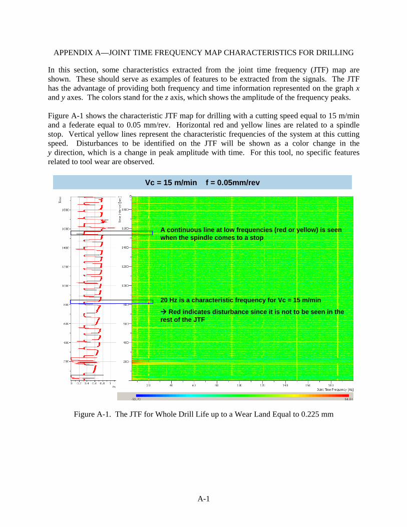
A-1

APPENDIX A—JOINT TIME FREQUENCY MAP CHARACTERISTICS FOR DRILLING

In this section, some characteristics extracted from the joint time frequency (JTF) map are shown. These should serve as examples of features to be extracted from the signals. The JTF has the advantage of providing both frequency and time information represented on the graph x and y axes. The colors stand for the z axis, which shows the amplitude of the frequency peaks. Figure A-1 shows the characteristic JTF map for drilling with a cutting speed equal to 15 m/min and a federate equal to 0.05 mm/rev. Horizontal red and yellow lines are related to a spindle stop. Vertical yellow lines represent the characteristic frequencies of the system at this cutting speed. Disturbances to be identified on the JTF will be shown as a color change in the y direction, which is a change in peak amplitude with time. For this tool, no specific features related to tool wear are observed.

Vc = 15 m/min f = 0.05mm/rev

A continuous line at low frequencies (red or yellow) is seen when the spindle comes to a stop

20 Hz is a characteristic frequency for Vc = 15 m/min

Red indicates disturbance since it is not to be seen in the rest of the JTF

Vc = 15 m/min f = 0.05mm/rev

A continuous line at low frequencies (red or yellow) is seen when the spindle comes to a stop

20 Hz is a characteristic frequency for Vc = 15 m/min

Red indicates disturbance since it is not to be seen in the rest of the JTF

Figure A-1. The JTF for Whole Drill Life up to a Wear Land Equal to 0.225 mm

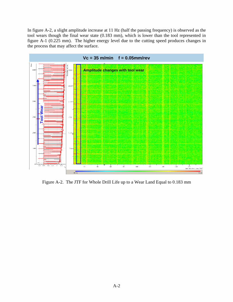
A-2

In figure A-2, a slight amplitude increase at 11 Hz (half the passing frequency) is observed as the tool wears though the final wear state (0.183 mm), which is lower than the tool represented in figure A-1 (0.225 mm). The higher energy level due to the cutting speed produces changes in the process that may affect the surface.

Vc = 35 m/min f = 0.05mm/rev

Amplitude changes with tool wear

Tool

Wea

r

Vc = 35 m/min f = 0.05mm/rev

Amplitude changes with tool wear

Tool

Wea

r

Figure A-2. The JTF for Whole Drill Life up to a Wear Land Equal to 0.183 mm

B-1

APPENDIX B—TOOL ENGAGEMENT IN BROACHING

The tooth entrance and exit can easily be identified in the force distribution. The first tooth, in an orthogonal cut, shows an almost stepwise increase of the force Fz, which remains constant until the second tooth enters the material. The force then increases by the same magnitude as for the first tooth. The force continues increasing with any successive tooth entrance until the whole workpiece has been cut by the first tooth. As soon as this tooth exits the workpiece, Fz decreases in magnitude for one cutting edge. For the cutting parameters and the coupon used in the trials, only two teeth are engaged at the same time. The magnitude of Fz for the first tooth (1) could not be equal to the increase when the second tooth (2) engages the workpiece. This could be due to the alignment in feed direction. Depending on this alignment, the first tooth cuts less material or more than one tooth can be cutting only air. An uneven force distribution can also be noticed in some tool details. This could be due to different feeds obtained after the resharpening process. Given the characteristics of the force mentioned above, the time while a tooth is engaged can be determined. Figure B-1 shows the tool engagement with its characteristic lengths. From the force distribution for the 4-m/min setup speed, also shown in figure B-1, the time to travel these distances is obtained.

Vcset-up= 4 m/s

30.3 30.4 30.5 30.6 30.7 30.8

Time [s]

0

1000

2000

3000

4000

F [N]

Fz

0 10 20 30 40 50 60 70 80 90Time [s]

-2500

0

2500

5000

7500

10000

12500

15000

F [N]

Fx

Fy

Fz

30 31 32 33 34 35 36 37

Time [s]

0

1000

2000

3000

4000

F [N]

Length (mm) Time (s)

1 Tooth engagement 16 0,33

2 Tooth entry 9,525 0,2

3 Only one tooth engaged 3,050 0,13

4 Two teeth engaged 6.475 0,07

Figure B-1. Tooth Engagement Length and Time

Additionally, the actual cutting speed can be calculated using the determined length and time, as shown in equation B-1.

1

2

4 3

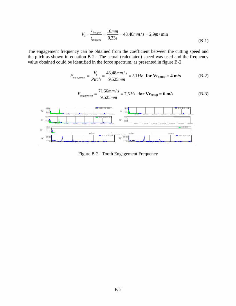
B-2

min/9,2/48,48

33,016 msmm

smm

tL

Vengaged

couponc ====

(B-1)

The engagement frequency can be obtained from the coefficient between the cutting speed and the pitch as shown in equation B-2. The actual (calculated) speed was used and the frequency value obtained could be identified in the force spectrum, as presented in figure B-2.

Hz

mmsmm

PitchVF c

engagement 1,5525,9

/48,48===

for Vcsetup = 4 m/s (B-2)

Hz

mmsmmFengagement 5,7

525,9/66,71

== for Vcsetup = 6 m/s (B-3)

1000 2000 3000Frequency [Hz]

0

100

200

300

400

500

600

700

AP F [N]

AP Fz

AP Fy

0 5 10 15 20 25 30

Frequency [Hz]

0

200

400

600

800

1000

AP-F [N]

AP Fz D4

500 1000 1500 2000 2500 3000 3500

Frequency [Hz]

0

10

20

30

40

50

AP-F [N]

AP Fz D2

AP Fy D2

500 1000 1500 2000 2500 3000 3500

Frequency [Hz]

0

10

20

30

40

50

AP-F [N]

AP Fz D3

AP Fy D3

500 1000 1500 2000 2500 3000 3500

Frequency [Hz]

0

10

20

30

40

50

AP-F [N]

AP Fz D2

AP Fy D2

500 1000 1500 2000 2500 3000 3500

Frequency [Hz]

0

10

20

30

40

50

AP-F [N]

0 5 10 15 20 25 30

Frequency [Hz]

0

200

400

600

800

1000

AP-F [N]

AP Fz D4

Figure B-2. Tooth Engagement Frequency

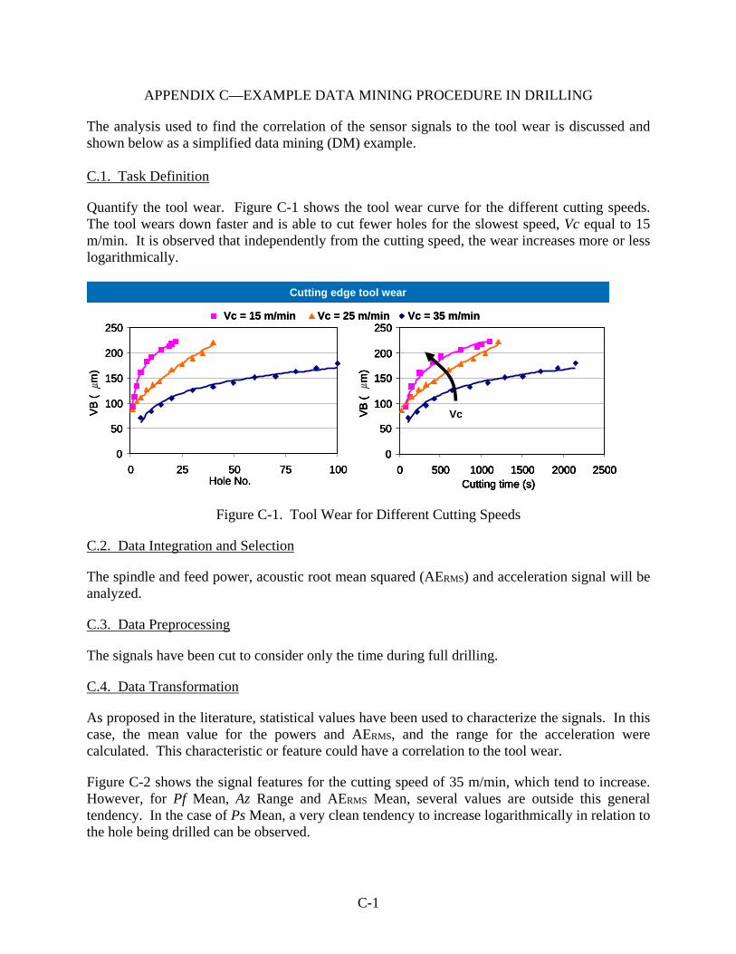
C-1

APPENDIX C—EXAMPLE DATA MINING PROCEDURE IN DRILLING

The analysis used to find the correlation of the sensor signals to the tool wear is discussed and shown below as a simplified data mining (DM) example. C.1. Task Definition

Quantify the tool wear. Figure C-1 shows the tool wear curve for the different cutting speeds. The tool wears down faster and is able to cut fewer holes for the slowest speed, Vc equal to 15 m/min. It is observed that independently from the cutting speed, the wear increases more or less logarithmically.

Vc = 15 m/min Vc = 25 m/min Vc = 35 m/min

Cutting edge tool wear

0

50

100

150

200

250

0 25 50 75 100Hole No.

VB (

m)

0

50

100

150

200

250

0 500 1000 1500 2000 2500Cutting time (s)

VB (

m)

Vc

Vc = 15 m/min Vc = 25 m/min Vc = 35 m/min

Cutting edge tool wear

0

50

100

150

200

250

0 25 50 75 100Hole No.

VB (

m)

0

50

100

150

200

250

0 500 1000 1500 2000 2500Cutting time (s)

VB (

m)

0

50

100

150

200

250

0 25 50 75 100Hole No.

VB (

m)

0

50

100

150

200

250

0 500 1000 1500 2000 2500Cutting time (s)

VB (

m)

0

50

100

150

200

250

0 500 1000 1500 2000 2500Cutting time (s)

VB (

m)

Vc

Figure C-1. Tool Wear for Different Cutting Speeds

C.2. Data Integration and Selection

The spindle and feed power, acoustic root mean squared (AERMS) and acceleration signal will be analyzed.

C.3. Data Preprocessing

The signals have been cut to consider only the time during full drilling.

C.4. Data Transformation

As proposed in the literature, statistical values have been used to characterize the signals. In this case, the mean value for the powers and AERMS, and the range for the acceleration were calculated. This characteristic or feature could have a correlation to the tool wear.

Figure C-2 shows the signal features for the cutting speed of 35 m/min, which tend to increase. However, for Pf Mean, Az Range and AERMS Mean, several values are outside this general tendency. In the case of Ps Mean, a very clean tendency to increase logarithmically in relation to the hole being drilled can be observed.

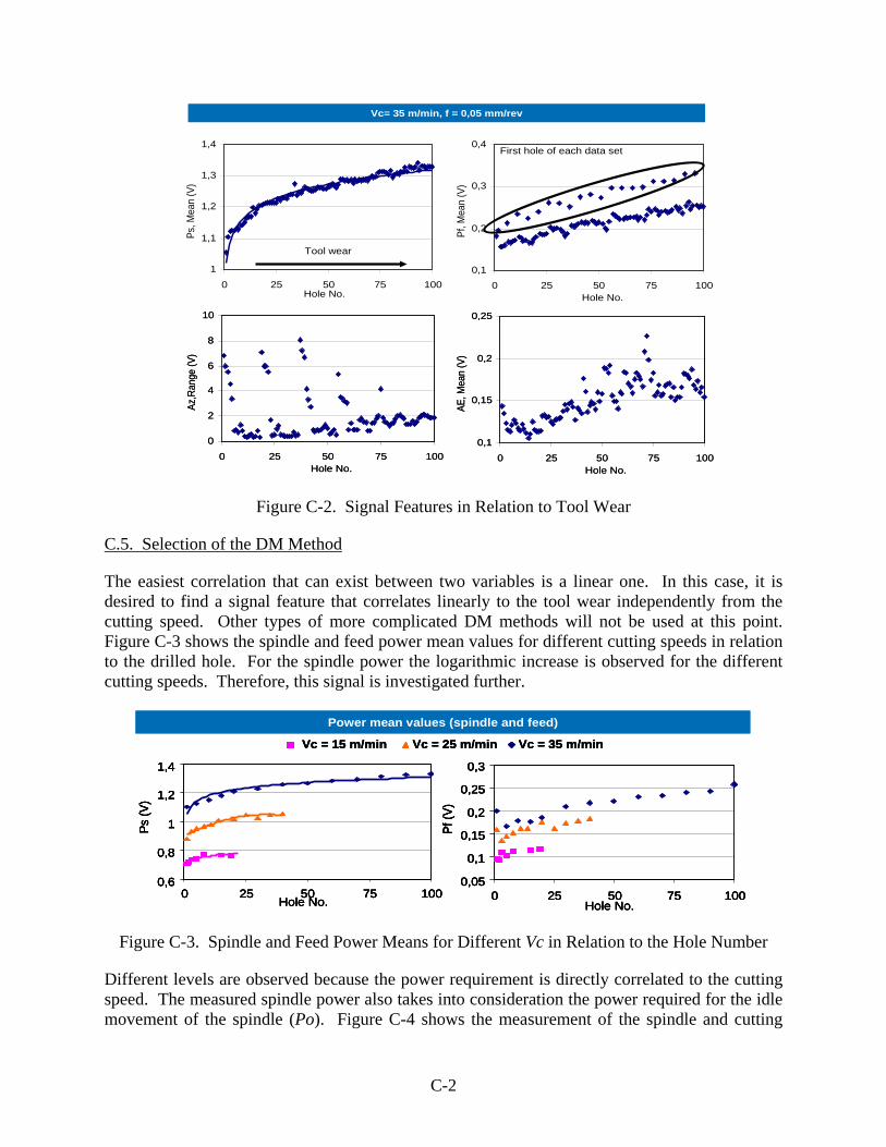
C-2

1

1,1

1,2

1,3

1,4

0 25 50 75 100Hole No.

Ps, M

ean

(V)

0,1

0,2

0,3

0,4

0 25 50 75 100Hole No.

Pf, M

ean

(V)

0

2

4

6

8

10

0 25 50 75 100Hole No.

Az,R

ange

(V)

0,1

0,15

0,2

0,25

0 25 50 75 100Hole No.

AE, M

ean

(V)

Vc= 35 m/min, f = 0,05 mm/rev

Tool wear

First hole of each data set

1

1,1

1,2

1,3

1,4

0 25 50 75 100Hole No.

Ps, M

ean

(V)

0,1

0,2

0,3

0,4

0 25 50 75 100Hole No.

Pf, M

ean

(V)

0

2

4

6

8

10

0 25 50 75 100Hole No.

Az,R

ange

(V)

0,1

0,15

0,2

0,25

0 25 50 75 100Hole No.

AE, M

ean

(V)

Vc= 35 m/min, f = 0,05 mm/rev

Tool wear

First hole of each data set

Figure C-2. Signal Features in Relation to Tool Wear

C.5. Selection of the DM Method

The easiest correlation that can exist between two variables is a linear one. In this case, it is desired to find a signal feature that correlates linearly to the tool wear independently from the cutting speed. Other types of more complicated DM methods will not be used at this point. Figure C-3 shows the spindle and feed power mean values for different cutting speeds in relation to the drilled hole. For the spindle power the logarithmic increase is observed for the different cutting speeds. Therefore, this signal is investigated further.

0,6

0,8

1

1,2

1,4

0 25 50 75 100Hole No.

Ps(V

)

0,05

0,1

0,15

0,2

0,25

0,3

0 25 50 75 100Hole No.

Pf (V

)

Power mean values (spindle and feed)

Vc = 15 m/min Vc = 25 m/min Vc = 35 m/min

0,6

0,8

1

1,2

1,4

0 25 50 75 100Hole No.

Ps(V

)

0,05

0,1

0,15

0,2

0,25

0,3

0 25 50 75 100Hole No.

Pf (V

)

0,6

0,8

1

1,2

1,4

0 25 50 75 100Hole No.

Ps(V

)

0,6

0,8

1

1,2

1,4

0 25 50 75 100Hole No.

Ps(V

)

0,05

0,1

0,15

0,2

0,25

0,3

0 25 50 75 100Hole No.

Pf (V

)

0,05

0,1

0,15

0,2

0,25

0,3

0 25 50 75 100Hole No.

Pf (V

)

Power mean values (spindle and feed)

Vc = 15 m/min Vc = 25 m/min Vc = 35 m/minVc = 15 m/min Vc = 25 m/min Vc = 35 m/min

Figure C-3. Spindle and Feed Power Means for Different Vc in Relation to the Hole Number

Different levels are observed because the power requirement is directly correlated to the cutting speed. The measured spindle power also takes into consideration the power required for the idle movement of the spindle (Po). Figure C-4 shows the measurement of the spindle and cutting

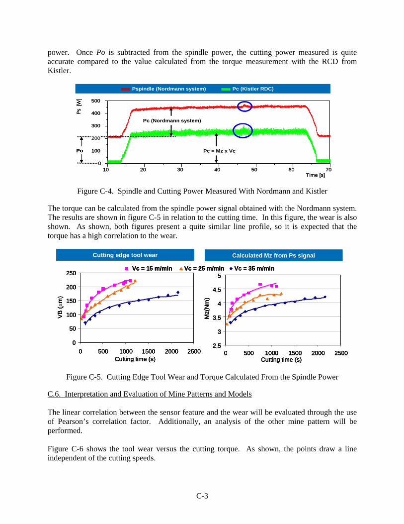
C-3

power. Once Po is subtracted from the spindle power, the cutting power measured is quite accurate compared to the value calculated from the torque measurement with the RCD from Kistler.

10 20 30 40 50 60 70Time [s]

0

100

300

400Ps[W

] 500

Pc = Mz x VcPo

Pc (Nordmann system)

200

Pspindle (Nordmann system) Pc (Kistler RDC)

10 20 30 40 50 60 70Time [s]

0

100

300

400Ps[W

] 500

Pc = Mz x VcPo

Pc (Nordmann system)

200

Pspindle (Nordmann system) Pc (Kistler RDC)

Figure C-4. Spindle and Cutting Power Measured With Nordmann and Kistler

The torque can be calculated from the spindle power signal obtained with the Nordmann system. The results are shown in figure C-5 in relation to the cutting time. In this figure, the wear is also shown. As shown, both figures present a quite similar line profile, so it is expected that the torque has a high correlation to the wear.

Cutting edge tool wear Calculated Mz from Ps signal

0

50

100

150

200

250

0 500 1000 1500 2000 2500Cutting time (s)

VB (

m)

2,5

3

3,5

4

4,5

5

0 500 1000 1500 2000 2500Cutting time (s)

Mz(

Nm

)

Vc = 15 m/min Vc = 25 m/min Vc = 35 m/min

Cutting edge tool wear Calculated Mz from Ps signal

0

50

100

150

200

250

0 500 1000 1500 2000 2500Cutting time (s)

VB (

m)

2,5

3

3,5

4

4,5

5

0 500 1000 1500 2000 2500Cutting time (s)

Mz(

Nm

)

0

50

100

150

200

250

0 500 1000 1500 2000 2500Cutting time (s)

VB (

m)

0

50

100

150

200

250

0 500 1000 1500 2000 2500Cutting time (s)

VB (

m)

2,5

3

3,5

4

4,5

5

0 500 1000 1500 2000 2500Cutting time (s)

Mz(

Nm

)

2,5

3

3,5

4

4,5

5

0 500 1000 1500 2000 2500Cutting time (s)

Mz(

Nm

)

Vc = 15 m/min Vc = 25 m/min Vc = 35 m/minVc = 15 m/min Vc = 25 m/min Vc = 35 m/min

Figure C-5. Cutting Edge Tool Wear and Torque Calculated From the Spindle Power

C.6. Interpretation and Evaluation of Mine Patterns and Models The linear correlation between the sensor feature and the wear will be evaluated through the use of Pearson’s correlation factor. Additionally, an analysis of the other mine pattern will be performed. Figure C-6 shows the tool wear versus the cutting torque. As shown, the points draw a line independent of the cutting speeds.

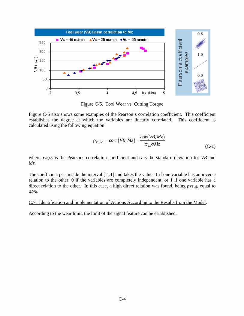
C-4

Figure C-6. Tool Wear vs. Cutting Torque

Figure C-5 also shows some examples of the Pearson’s correlation coefficient. This coefficient establishes the degree at which the variables are linearly correlated. This coefficient is calculated using the following equation:

( ) ( )

,

,,ρ = =

σ σVB MzVB

cov VB Mzcorr VB Mz

Mz (C-1) where ρVB,Mz is the Pearsons correlation coefficient and σ is the standard deviation for VB and Mz. The coefficient ρ is inside the interval [-1.1] and takes the value -1 if one variable has an inverse relation to the other, 0 if the variables are completely independent, or 1 if one variable has a direct relation to the other. In this case, a high direct relation was found, being ρVB,Mz equal to 0.96. C.7. Identification and Implementation of Actions According to the Results from the Model. According to the wear limit, the limit of the signal feature can be established.

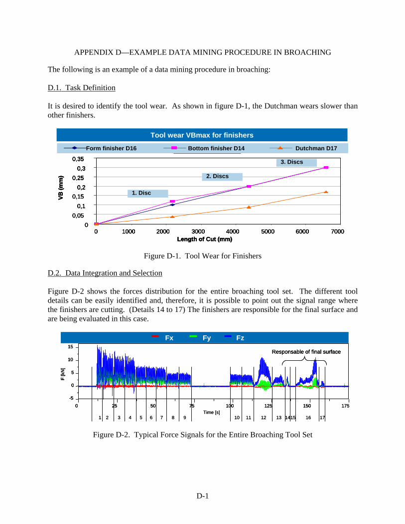
D-1

APPENDIX D—EXAMPLE DATA MINING PROCEDURE IN BROACHING

The following is an example of a data mining procedure in broaching: D.1. Task Definition It is desired to identify the tool wear. As shown in figure D-1, the Dutchman wears slower than other finishers.

Tool wear VBmax for finishers

00,05

0,10,15

0,20,25

0,30,35

0 1000 2000 3000 4000 5000 6000 7000Length of Cut (mm)

VB (m

m)

1. Disc

2. Discs

3. Discs

Form finisher D16 Bottom finisher D14 Dutchman D17

Tool wear VBmax for finishers

00,05

0,10,15

0,20,25

0,30,35

0 1000 2000 3000 4000 5000 6000 7000Length of Cut (mm)

VB (m

m)

1. Disc

2. Discs

3. Discs

00,05

0,10,15

0,20,25

0,30,35

0 1000 2000 3000 4000 5000 6000 7000Length of Cut (mm)

VB (m

m)

00,05

0,10,15

0,20,25

0,30,35

0 1000 2000 3000 4000 5000 6000 7000Length of Cut (mm)

VB (m

m)

1. Disc

2. Discs

3. Discs

Form finisher D16 Bottom finisher D14 Dutchman D17Form finisher D16 Bottom finisher D14 Dutchman D17

Figure D-1. Tool Wear for Finishers

D.2. Data Integration and Selection Figure D-2 shows the forces distribution for the entire broaching tool set. The different tool details can be easily identified and, therefore, it is possible to point out the signal range where the finishers are cutting. (Details 14 to 17) The finishers are responsible for the final surface and are being evaluated in this case.

1 2 3 4 5 6 7 8 9 10 11 12 13 1415 16 17Time [s]

Fx Fy Fz

0 25 50 75 100 125 150 175

-5

0

5

10

15

F [k

N]

Responsable of final surface

1 2 3 4 5 6 7 8 9 10 11 12 13 1415 16 17Time [s]

Fx Fy Fz

0 25 50 75 100 125 150 175

-5

0

5

10

15

F [k

N]

Responsable of final surface

0 25 50 75 100 125 150 175

-5

0

5

10

15

F [k

N]

Responsable of final surface

Figure D-2. Typical Force Signals for the Entire Broaching Tool Set

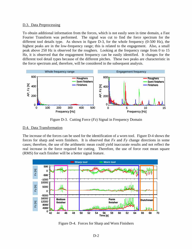
D-2

D.3. Data Preprocessing

To obtain additional information from the forces, which is not easily seen in time domain, a Fast Fourier Transform was performed. The signal was cut to find the force spectrum for the different tool details type. As shown in figure D-3, for the whole frequency (0-500 Hz), the highest peaks are in the low-frequency range; this is related to the engagement. Also, a small peak above 250 Hz is observed for the roughers. Looking at the frequency range from 0 to 15 Hz, it is observed that the engagement frequency can be easily identified. It changes for the different tool detail types because of the different pitches. These two peaks are characteristic in the force spectrum and, therefore, will be considered in the subsequent analysis.

RoughersSemi finishersFinishers

0 100 200 300 400 500Frequency [Hz]

0

200

400

600

AP

, Fz

[N]

0 5 10 15Frequency [Hz]

0

200

400

600

AP

, Fz

[N]

RoughersSemi finishersFinishers

Whole frequency range Engagement frequency

RoughersRoughersSemi finishersSemi finishersFinishersFinishers

0 100 200 300 400 500Frequency [Hz]

0

200

400

600

AP

, Fz

[N]

0 5 10 15Frequency [Hz]

0

200

400

600

AP

, Fz

[N]

RoughersRoughersSemi finishersSemi finishersFinishersFinishers

Whole frequency range Engagement frequency

Figure D-3. Cutting Force (Fz) Signal in Frequency Domain

D.4. Data Transformation

The increase of the forces can be used for the identification of a worn tool. Figure D-4 shows the forces for sharp and worn finishers. It is observed that Fx and Fy change directions in some cases; therefore, the use of the arithmetic mean could yield inaccurate results and not reflect the real increase in the force required for cutting. Therefore, the use of force root mean square (RMS) for each finisher will be a better signal feature.

-5000

0

5000

10000

Fy[N

]

-1000

-500

0

500

Fx[N

]

42 44 46 48 50 52 54 56 58 60 62 64 66 68 70Time [s]

040008000

1200016000

Fz[N

]

Sharp tool Worn tool

Bottomfinisher

Form finisher

Dutchman

-5000

0

5000

10000

Fy[N

]

-1000

-500

0

500

Fx[N

]

42 44 46 48 50 52 54 56 58 60 62 64 66 68 70Time [s]

040008000

1200016000

Fz[N

]

Sharp tool Worn tool

-5000

0

5000

10000

Fy[N

]

-1000

-500

0

500

Fx[N

]

42 44 46 48 50 52 54 56 58 60 62 64 66 68 70Time [s]

040008000

1200016000

Fz[N

]

Sharp tool Worn tool

Bottomfinisher

Form finisher

Dutchman

Figure D-4. Forces for Sharp and Worn Finishers

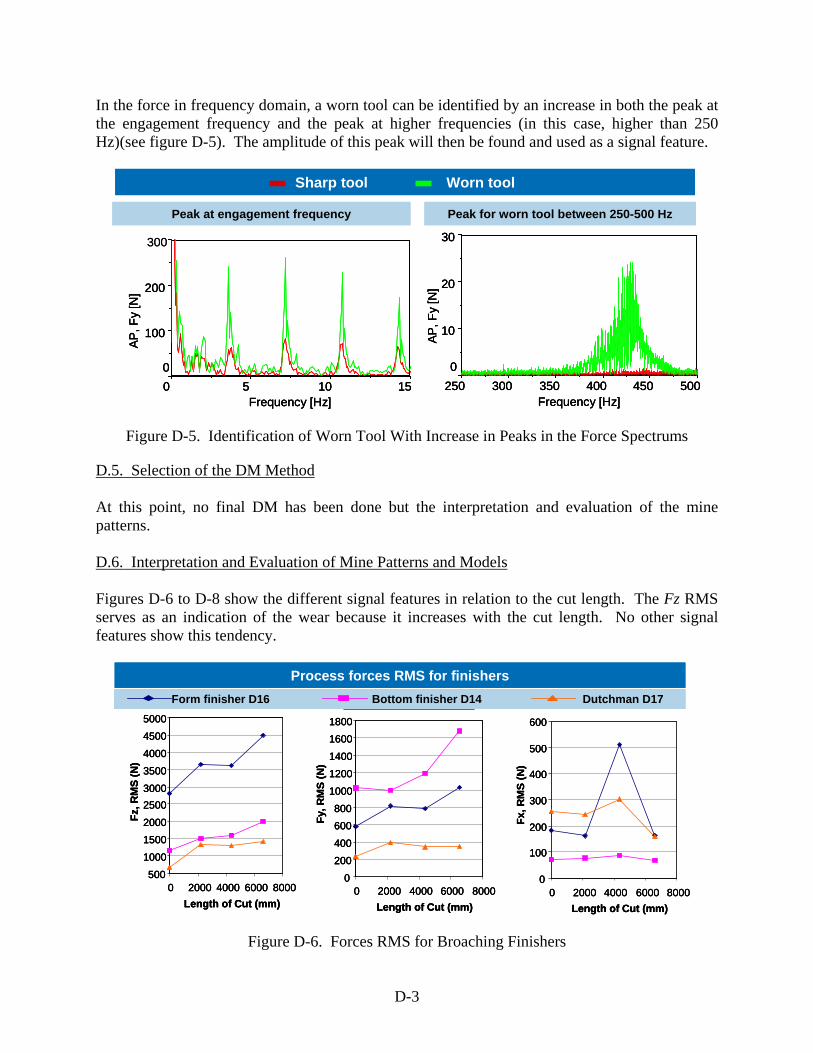
D-3

In the force in frequency domain, a worn tool can be identified by an increase in both the peak at the engagement frequency and the peak at higher frequencies (in this case, higher than 250 Hz)(see figure D-5). The amplitude of this peak will then be found and used as a signal feature.

300

0 5 10 15Frequency [Hz]

0

100

200

AP, F

y[N

]

250 300 350 400 450 500Frequency [Hz]

0

10

20

30

AP, F

y[N

]

Peak at engagement frequency Peak for worn tool between 250-500 Hz

Sharp tool Worn tool

300

0 5 10 15Frequency [Hz]

0

100

200

AP, F

y[N

]

0 5 10 15Frequency [Hz]

0

100

200

AP, F

y[N

]

250 300 350 400 450 500Frequency [Hz]

0

10

20

30

AP, F

y[N

]

250 300 350 400 450 500Frequency [Hz]

0

10

20

30

AP, F

y[N

]

Peak at engagement frequency Peak for worn tool between 250-500 Hz

Sharp tool Worn tool

Figure D-5. Identification of Worn Tool With Increase in Peaks in the Force Spectrums

D.5. Selection of the DM Method At this point, no final DM has been done but the interpretation and evaluation of the mine patterns. D.6. Interpretation and Evaluation of Mine Patterns and Models Figures D-6 to D-8 show the different signal features in relation to the cut length. The Fz RMS serves as an indication of the wear because it increases with the cut length. No other signal features show this tendency.

500100015002000250030003500400045005000

0 2000 4000 6000 8000Length of Cut (mm)

Fz, R

MS

(N)

0200400600800

10001200140016001800

0 2000 4000 6000 8000Length of Cut (mm)

Fy, R

MS

(N)

0

100

200

300

400

500

600

0 2000 4000 6000 8000Length of Cut (mm)

Fx, R

MS

(N)

Process forces RMS for finishersForm finisher D16 Bottom finisher D14 Dutchman D17

500100015002000250030003500400045005000

0 2000 4000 6000 8000Length of Cut (mm)

Fz, R

MS

(N)

0200400600800

10001200140016001800

0 2000 4000 6000 8000Length of Cut (mm)

Fy, R

MS

(N)

0

100

200

300

400

500

600

0 2000 4000 6000 8000Length of Cut (mm)

Fx, R

MS

(N)

500100015002000250030003500400045005000

0 2000 4000 6000 8000Length of Cut (mm)

Fz, R

MS

(N)

0200400600800

10001200140016001800

0 2000 4000 6000 8000Length of Cut (mm)

Fy, R

MS

(N)

0

100

200

300

400

500

600

0 2000 4000 6000 8000Length of Cut (mm)

Fx, R

MS

(N)

Process forces RMS for finishersForm finisher D16 Bottom finisher D14 Dutchman D17Form finisher D16 Bottom finisher D14 Dutchman D17

Figure D-6. Forces RMS for Broaching Finishers

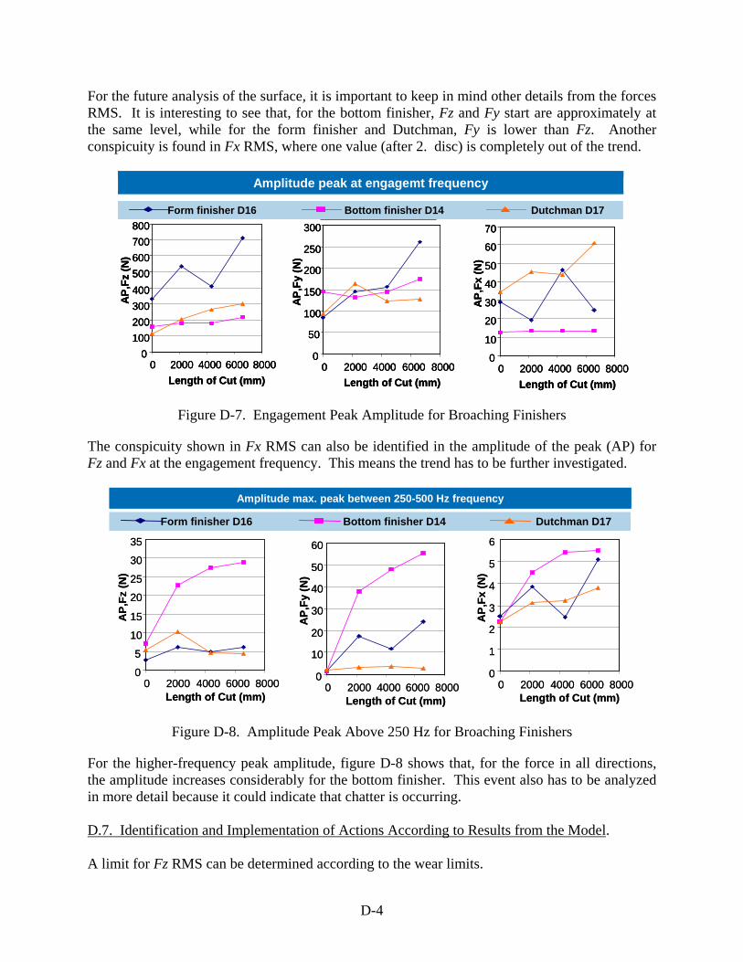
D-4

For the future analysis of the surface, it is important to keep in mind other details from the forces RMS. It is interesting to see that, for the bottom finisher, Fz and Fy start are approximately at the same level, while for the form finisher and Dutchman, Fy is lower than Fz. Another conspicuity is found in Fx RMS, where one value (after 2. disc) is completely out of the trend.

Amplitude peak at engagemt frequency

0100200300400500600700800

0 2000 4000 6000 8000

AP,

Fz(N

)

0

50

100

150

200

250

300

0 2000 4000 6000 8000

AP,

Fy(N

)

0

10

20

30

40

50

60

70

0 2000 4000 6000 8000

AP,

Fx(N

)

Length of Cut (mm) Length of Cut (mm) Length of Cut (mm)

Form finisher D16 Bottom finisher D14 Dutchman D17

Amplitude peak at engagemt frequency

0100200300400500600700800

0 2000 4000 6000 8000

AP,

Fz(N

)

0

50

100

150

200

250

300

0 2000 4000 6000 8000

AP,

Fy(N

)

0

10

20

30

40

50

60

70

0 2000 4000 6000 8000

AP,

Fx(N

)

Length of Cut (mm) Length of Cut (mm) Length of Cut (mm)

0100200300400500600700800

0 2000 4000 6000 8000

AP,

Fz(N

)

0

50

100

150

200

250

300

0 2000 4000 6000 8000

AP,

Fy(N

)

0

10

20

30

40

50

60

70

0 2000 4000 6000 8000

AP,

Fx(N

)

Length of Cut (mm) Length of Cut (mm) Length of Cut (mm)

Form finisher D16 Bottom finisher D14 Dutchman D17Form finisher D16 Bottom finisher D14 Dutchman D17

Figure D-7. Engagement Peak Amplitude for Broaching Finishers

The conspicuity shown in Fx RMS can also be identified in the amplitude of the peak (AP) for Fz and Fx at the engagement frequency. This means the trend has to be further investigated.

Amplitude max. peak between 250-500 Hz frequency

0

5

10

15

20

25

30

35

0 2000 4000 6000 8000Length of Cut (mm)

AP,

Fz(N

)

0

10

20

30

40

50

60

0 2000 4000 6000 8000Length of Cut (mm)

AP,

Fy(N

)

0

1

2

3

4

5

6

0 2000 4000 6000 8000Length of Cut (mm)

AP,

Fx(N

)

Form finisher D16 Bottom finisher D14 Dutchman D17

Amplitude max. peak between 250-500 Hz frequency

0

5

10

15

20

25

30

35

0 2000 4000 6000 8000Length of Cut (mm)

AP,

Fz(N

)

0

10

20

30

40

50

60

0 2000 4000 6000 8000Length of Cut (mm)

AP,

Fy(N

)

0

1

2

3

4

5

6

0 2000 4000 6000 8000Length of Cut (mm)

AP,

Fx(N

)

Form finisher D16 Bottom finisher D14 Dutchman D17

Figure D-8. Amplitude Peak Above 250 Hz for Broaching Finishers

For the higher-frequency peak amplitude, figure D-8 shows that, for the force in all directions, the amplitude increases considerably for the bottom finisher. This event also has to be analyzed in more detail because it could indicate that chatter is occurring. D.7. Identification and Implementation of Actions According to Results from the Model. A limit for Fz RMS can be determined according to the wear limits.

E-1

APPENDIX E—MODEL TO EXPERIMENTAL FORCE COMPARISON

The information provided by Sandvic [E-1], (the drill manufacturer used for the trials) has been used for the model evaluation. Figure E-1 shows that the cutting parameters for the force calculation are represented on the drill. The specific cutting force values are also shown in the figure.

ISO Material Specific cutting force kc1 (N/mm2)

mc

Nickel base

Annealed or solution treated

Aged or solution treated and aged

Cast or cast and aged

2650

2900

3000

0.25

0.25

0.25

S

Drilling variables Coro-Drill specifications and force constants [SANDVIC]

ISO Material Specific cutting force kc1 (N/mm2)

mc

Nickel base

Annealed or solution treated

Aged or solution treated and aged

Cast or cast and aged

2650

2900

3000

0.25

0.25

0.25

S

ISO Material Specific cutting force kc1 (N/mm2)

mc

Nickel base

Annealed or solution treated

Aged or solution treated and aged

Cast or cast and aged

2650

2900

3000

2650

2900

3000

0.25

0.25

0.25

0.25

0.25

0.25

S

Drilling variables Coro-Drill specifications and force constants [SANDVIC]

Figure E-1. Drilling Variables and Constant Values for Force Calculation [reference E-1]

The equation for the cutting power calculation given by Sandvic is:

310240 ⋅⋅⋅⋅

= cccnc

kDVfP (E-1)

Where kc is calculated with the following equation and kc1 is found in Figure 111:

( ) 0

1 sin 1100

mcc c z rk k f − γ = ⋅ ⋅ κ ⋅ −

(E-2)

The torque is obtained from the power by the equation:

330 10⋅ ⋅=

π⋅c

cPM

n (E-3)

The feed force is calculated as follows:

0.5 sin

2= ⋅ ⋅ ⋅ κc

f c n rDF k f

(E-4)

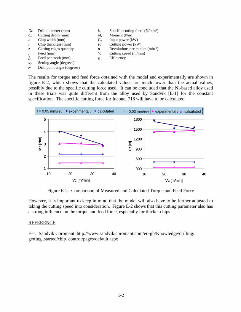
E-2

Dc Drill diameter (mm) kc Specific cutting force (N/mm2) ap Cutting depth (mm) Mc Moment (Nm) b Chip width (mm) Pa Input power (kW) h Chip thickness (mm) Pc Cutting power (kW) z Cutting edges quantity n Revolutions per minute (min-1) f Feed (mm) Vc Cutting speed (m/min) fz Feed per tooth (mm) η Efficiency κr Setting angle (degrees) σ Drill point angle (degrees)

The results for torque and feed force obtained with the model and experimentally are shown in figure E-2, which shows that the calculated values are much lower than the actual values, possibly due to the specific cutting force used. It can be concluded that the Ni-based alloy used in these trials was quite different from the alloy used by Sandvik [E-1] for the constant specification. The specific cutting force for Inconel 718 will have to be calculated.

1

2

3

4

5

10 20 30 40

Vc [m/min]

Mz

[Nm

]

300

600

900

1200

1500

1800

10 20 30 40

Vc [m/min]

Fz[N

]

calculatedf = 0.05 mm/rev experimental / calculatedf = 0.03 mm/rev experimental /

1

2

3

4

5

10 20 30 40

Vc [m/min]

Mz

[Nm

]

300

600

900

1200

1500

1800

10 20 30 40

Vc [m/min]

Fz[N

]

calculatedf = 0.05 mm/rev experimental / calculatedf = 0.03 mm/rev experimental /calculatedf = 0.05 mm/rev experimental / calculatedf = 0.03 mm/rev experimental /

Figure E-2. Comparison of Measured and Calculated Torque and Feed Force

However, it is important to keep in mind that the model will also have to be further adjusted to taking the cutting speed into consideration. Figure E-2 shows that this cutting parameter also has a strong influence on the torque and feed force, especially for thicker chips. REFERENCE. E-1. Sandvik Coromant. http://www.sandvik.coromant.com/en-gb/Knowledge/drilling/ getting_started/chip_control/pages/default.aspx

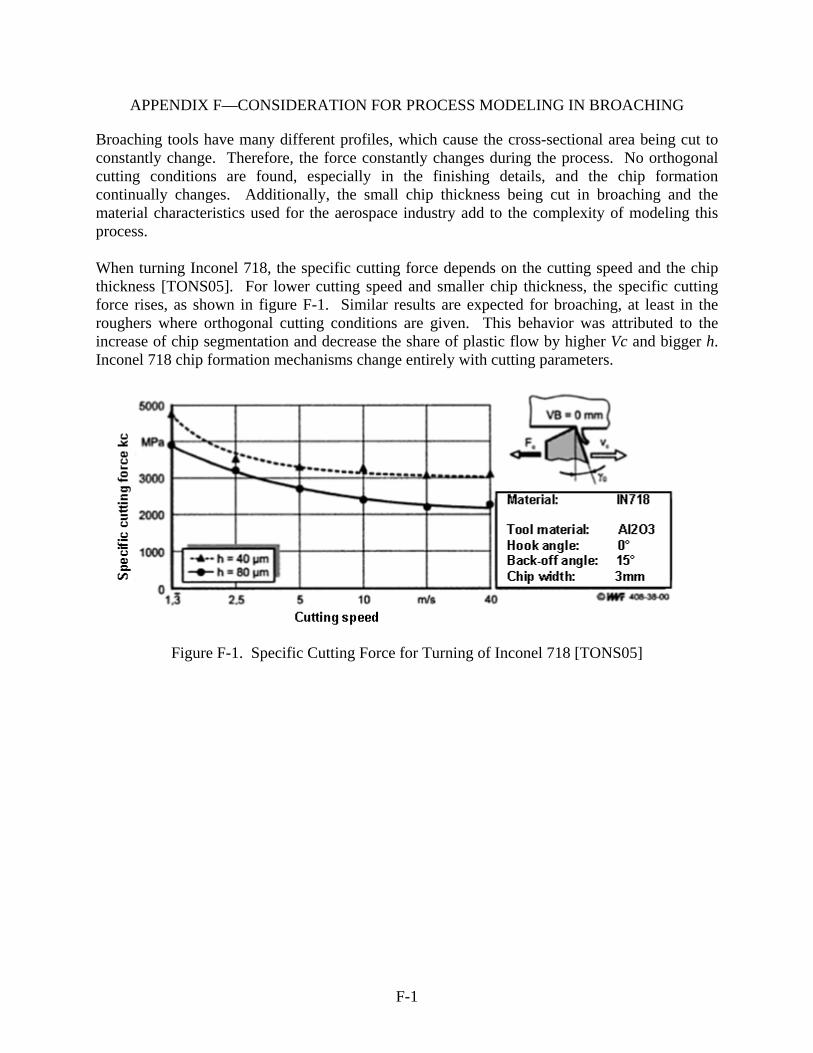
F-1

APPENDIX F—CONSIDERATION FOR PROCESS MODELING IN BROACHING

Broaching tools have many different profiles, which cause the cross-sectional area being cut to constantly change. Therefore, the force constantly changes during the process. No orthogonal cutting conditions are found, especially in the finishing details, and the chip formation continually changes. Additionally, the small chip thickness being cut in broaching and the material characteristics used for the aerospace industry add to the complexity of modeling this process. When turning Inconel 718, the specific cutting force depends on the cutting speed and the chip thickness [TONS05]. For lower cutting speed and smaller chip thickness, the specific cutting force rises, as shown in figure F-1. Similar results are expected for broaching, at least in the roughers where orthogonal cutting conditions are given. This behavior was attributed to the increase of chip segmentation and decrease the share of plastic flow by higher Vc and bigger h. Inconel 718 chip formation mechanisms change entirely with cutting parameters.

Figure F-1. Specific Cutting Force for Turning of Inconel 718 [TONS05]

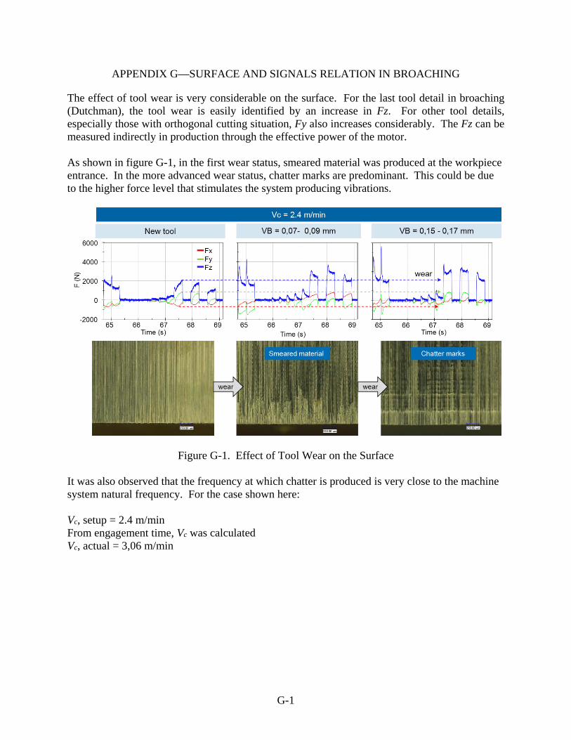
G-1

APPENDIX G—SURFACE AND SIGNALS RELATION IN BROACHING

The effect of tool wear is very considerable on the surface. For the last tool detail in broaching (Dutchman), the tool wear is easily identified by an increase in Fz. For other tool details, especially those with orthogonal cutting situation, Fy also increases considerably. The Fz can be measured indirectly in production through the effective power of the motor. As shown in figure G-1, in the first wear status, smeared material was produced at the workpiece entrance. In the more advanced wear status, chatter marks are predominant. This could be due to the higher force level that stimulates the system producing vibrations.

Figure G-1. Effect of Tool Wear on the Surface It was also observed that the frequency at which chatter is produced is very close to the machine system natural frequency. For the case shown here: Vc, setup = 2.4 m/min From engagement time, Vc was calculated Vc, actual = 3,06 m/min

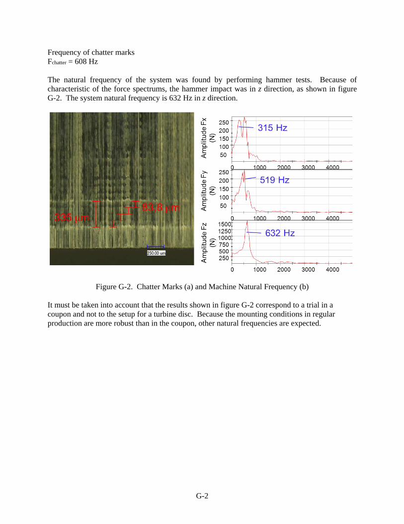
G-2

Frequency of chatter marks Fchatter = 608 Hz The natural frequency of the system was found by performing hammer tests. Because of characteristic of the force spectrums, the hammer impact was in z direction, as shown in figure G-2. The system natural frequency is 632 Hz in z direction.

Figure G-2. Chatter Marks (a) and Machine Natural Frequency (b) It must be taken into account that the results shown in figure G-2 correspond to a trial in a coupon and not to the setup for a turbine disc. Because the mounting conditions in regular production are more robust than in the coupon, other natural frequencies are expected.

H-1

APPENDIX H—SURVEY RESULTS SUMMARY

No. of Partners Qualification Most critical process Broaching 5

Drilling 3 Major known process anomalies

Cutting edge failure/chipped 8 35 Improper tool grinds 5 17 Coolant failure 5 17 Chip blockage 5 13 Excessive tool wear 3 11 Tool failure 2 7 Weak cutting edges 2 6 Wrong feed and/or speed 1 2

Major known surface anomalies

**Surface topography: Smearing 6 19 Scratches 2 9 Scores 2 7 Chatter 2 7 Roughness 1 4 Cracks 1 4 Surface deviation 1 2 Foreign material inclusion 1 1 **Microstructural changes: Distorted layer 7 30 White amorphous layer 5 17 Abnormal residual stresses 2 4

Use of PM Drilling 6 Broaching 5 Turning 1

Specification of PM system OEM's and Internal Specs PM sensors used Power sensors and systems 6

Flow rate 5 Load/Forces 4 Pressure 3 Vibration 2 Torque 1 Spindle speed 1 Internal machine signals 1

H-2

Reaction strategies desired Warning signal when special-cause event occurs 8 29

Immediate stop with tool retraction when special-cause event occurs 8 22

Warn signal indicating when the tool should be changed/ inspected 6 18

Cutting parameters modification/control 5 12

Automatic, serial part-specific data storage of monitored parameters 3

I-1

APPENDIX I—PREPROCESSING ALGORITHM FOR OFFLINE ANALYSIS

_______________________________________________________________________ 'INPUT PARAMETERS '----------------------------------------------------------------------- SampleRate = 5000 'RPM for different tools RPM1 = 525 RPM2 = 650 RPM3 = 637 RPM4 = 198 RPM5 = 187 RPM6 = 300 RPM7 = 250 RPM8 = 120 RPM9 = 75 '-------------------------------------------------------------------------- Interval = 0.5 'duration of the time interval to be considered PacketSize = SampleRate*Interval 'Specifies start values ToolNo = 0 HoleNo = 0 L1=1 'point number for starting the analysis L2= L1 + PacketSize '-------------------------------------------------------------------------- for j = 1 to 6000 'Total of packets to be analyzed....only for offline analysis. 5000 = time in seconds * 2 (each packet = 0.5 seconds) '_______________________________________________________________________ 'CALCULATES STATISTICAL VALUES '----------------------------------------------------------------------- For i = 1 To 23 StatSel(i) = "No" Next StatSel(5) = "Yes" 'Maximum StatSel(6) = "Yes" 'Arith. mean StatSel(15) = "Yes" 'Variance Call StatBlockCalc("Channel",""&L1&"-"&L2,"[6]/Spindle_pwr") L6 = ChnLength ("[7]/ArithmeticMean") L7 = L6 + 1 Call DataBlCopy("'[8]/Maximum'",1,1,"'[7]/Maximum'",L7) Call DataBlCopy("'[8]/ArithmeticMean'",1,1,"'[7]/ArithmeticMean'",L7)

I-2

Call DataBlCopy("'[8]/Variance'",1,1,"'[7]/Variance'",L7) Call Data.Root.ChannelGroups(8).Channels.Remove("ArithmeticMean") Call Data.Root.ChannelGroups(8).Channels.Remove("Maximum") Call Data.Root.ChannelGroups(8).Channels.Remove("Variance") '_______________________________________________________________________ 'DETERMINES IF A NEW TOOL IS USED '----------------------------------------------------------------------- Variance1 = CHD (j, "[7]/Variance") if Variance1 > 1 then y = 1 else y = 0 end if Call DataBlInsertVal("'[7]/New tool'", j, 1, y) '_______________________________________________________________________ 'TOOL NUMBER SPECIFICATION '----------------------------------------------------------------------- if j >= 16 then Var = CHD (j, "[7]/Variance") 'variance at the "presently measured" interval 'Variance from the past time intervals Var1 = CHD (j-1, "[7]/Variance") Var2 = CHD (j-2, "[7]/Variance") Var3 = CHD (j-3, "[7]/Variance") Var4 = CHD (j-4, "[7]/Variance") Var5 = CHD (j-5, "[7]/Variance") Var6 = CHD (j-6, "[7]/Variance") Var7 = CHD (j-7, "[7]/Variance") Var8 = CHD (j-8, "[7]/Variance") Var9 = CHD (j-9, "[7]/Variance") Var10 = CHD (j-10, "[7]/Variance") Var11 = CHD (j-11, "[7]/Variance") Var12 = CHD (j-12, "[7]/Variance") Var13 = CHD (j-13, "[7]/Variance") Var14 = CHD (j-14, "[7]/Variance") Var15 = CHD (j-15, "[7]/Variance") HoleNo10 = CHD (j-10, "[6]/Hole No. 2 option") if Var > 1 and HoleNo10<>0 and Var1<1 and Var2<1 and Var3<1 and Var4<1 and Var5<1 and Var6<1 and Var7<1 and Var8<1 and Var9<1 and Var10<1 and Var11<1 and Var12<1 and Var13<1 and Var14<1 and Var15<1 then

I-3

ToolNo = ToolNo +1 else ToolNo = ToolNo end if end if Call DataBlInsertVal("'[6]/Tool No.'", j, 1, ToolNo) '_______________________________________________________________________ 'IDLE POWER CALCULATION AND DETERMINATION OF CUTTING OR NOT CUTTING SITUATION '----------------------------------------------------------------------- ArithmeticMean = CHD (j, "[7]/ArithmeticMean") toolNo = CHD (j, "[6]/Tool No.") Max = CHD (j, "[7]/Maximum") ' RPM taken from the list of the tools if toolNo = 1 then RPM = RPM1 elseif toolNo = 2 then RPM = RPM2 elseif toolNo = 3 then RPM = RPM3 elseif toolNo = 4 then RPM = RPM4 elseif toolNo = 5 then RPM = RPM5 elseif toolNo = 6 then RPM = RPM6 elseif toolNo = 7 then RPM = RPM7 elseif toolNo = 8 then RPM = RPM8 elseif toolNo = 9 then RPM = RPM9 else RPM = 0 end if relmaxtomean = Max / ArithmeticMean idlepower = 4E-05*RPM + 0.0624 'idle power calculated from the RPM. This has to be found for each machine!!!! if ArithmeticMean > idlepower*1.35 then z = 1 else z = 0 end if Call DataBlInsertVal("'[7]/new hole 2 option'", j, 1, z) '_______________________________________________________________________ 'HOLE NUMBER SPECIFICATION '-----------------------------------------------------------------------

I-4

if j >= 8 then newho = CHD (j-6, "[7]/new hole 2 option") 'new hole 2 option at the "presently measured" interval 'New hole value from the past time interval newho1 = CHD (j-7, "[7]/new hole 2 option") Var_1 = CHD (j-7, "[7]/Variance") Var = CHD (j-6, "[7]/Variance") Var1 = CHD (j-5, "[7]/Variance") Var2 = CHD (j-4, "[7]/Variance") Var3 = CHD (j-3, "[7]/Variance") Var4 = CHD (j-2, "[7]/Variance") Var5 = CHD (j-1, "[7]/Variance") Var6 = CHD (j, "[7]/Variance") if newho = 1 and Var_1>1 or Var > 1 or Var1 > 1 or Var2 > 1 or Var3 > 1 or Var4 > 1 or Var5 > 1 or Var6 > 1 then HoleNo = 0 elseif newho = 1 and newho1=0 then HoleNo = HoleNo + 1 elseif newho = 1 and newho1=1 then HoleNo = HoleNo else HoleNo = HoleNo end if Call DataBlInsertVal("'[6]/Hole No. 2 option'", j-6, 1, HoleNo) end if L1= L2+1 L2= L1 +PacketSize next