Monetizing Mobile Data via Data RewardsHaoran Yu, Member, IEEE, Ermin Wei, Member, IEEE, and Randall A. Berry, Fellow, IEEE

Abstract—Most mobile network operators generate revenuesby directly charging users for data plan subscriptions. Someoperators now also offer users data rewards to incentivize themto watch mobile ads, which enables the operators to collectpayments from advertisers and create new revenue streams.In this work, we analyze and compare two data rewardingschemes: a Subscription-Aware Rewarding (SAR) scheme and aSubscription-Unaware Rewarding (SUR) scheme. Under the SARscheme, only the subscribers of the operators’ data plans areeligible for the rewards; under the SUR scheme, all users areeligible for the rewards (e.g., the users who do not subscribe tothe data plans can still get SIM cards and receive data rewardsby watching ads). We model the interactions among an operator,users, and advertisers by a two-stage Stackelberg game, andcharacterize their equilibrium strategies under both the SARand SUR schemes. We show that the SAR scheme can lead tomore subscriptions and a higher operator revenue from the datamarket, while the SUR scheme can lead to better ad viewershipand a higher operator revenue from the ad market. We furthershow that the operator’s optimal choice between the two schemesis sensitive to the users’ data consumption utility function and theoperator’s network capacity. We provide some counter-intuitiveinsights. For example, when each user has a logarithmic utilityfunction, the operator should apply the SUR scheme (i.e., rewardboth subscribers and non-subscribers) if and only if it has a smallnetwork capacity.

Index Terms—Stackelberg game, network economics, mobiledata rewards, business model.

I. INTRODUCTION

Despite the rapid growth of global mobile traffic, severalleading analyst firms estimate that global mobile servicerevenue has nearly reached a saturation point. For example,Strategy Analytics forecasts that the global mobile servicerevenue will only increase by 3% between 2018 and 2021[2]. As suggested in [3], one promising approach for themobile network operators to create new revenue streams isto offer mobile data rewards: the network operators rewardusers with free mobile data every time the users watch mobileads delivered by the operators, and the operators are paid bythe corresponding advertisers.

The data rewarding paradigm leads to a “win-win-win”outcome [3]. First, the operators monetize their services basedon the mobile advertising, the global revenue of which wasestimated to reach $80 billion at the end of 2017 [3]. Second,the advertisers gain incentivized advertising, where the rewardsincentivize the users to better engage with ads and the advertis-ers allow the users to have more control over their experiences

Manuscript received September 1, 2019; accepted November 9, 2019. Thisresearch was supported by the NSF grants AST-1343381, AST-1547328 andCNS-1701921. Some results in the paper were presented at IEEE INFOCOM,Paris, France, April 2019 [1]. (Corresponding author: Haoran Yu.)

The authors are with the Department of Electrical and Computer En-gineering, Northwestern University, Evanston, IL 60208, USA (email:yhrhawk@gmail.com; {ermin.wei, rberry}@northwestern.edu).

(e.g., whether and when to watch ads). According to surveysconducted by Forrester Consulting, IPG Media Lab, and Kiip,most mobile app users prefer to watch ads with rewards thanto watch targeted ads [4]. Third, the users earn free mobiledata to satisfy their growing data demand.

There has been an increasing number of businesses enteringthis space. Aquto and Unlockd are two leading companiesthat provide technical support for data rewarding (e.g., theydevelop mobile apps that display ads and track the amountof rewarded data). Aquto has collaborated with operators,such as Verizon and Telefonica [5]. Unlockd has collaboratedwith Tesco Mobile (in the United Kingdom), Boost Mobile(in the United States), Lebara Mobile (in Australia), andAXIS (in Indonesia) [6]. Other examples of operators thathave offered data rewards include DOCOMO, Optus, andChungHwa Telecom [7], [8]. Furthermore, AT&T recently ac-quired AppNexus (a leading online advertising company) andwill make a significant investment in the advertising business[9]. Offering mobile data rewards could become a natural andeffective approach to further monetize an operator’s mobileservice.

We use an example in Table I to show that offering datarewards might lead to a significant revenue improvement foran operator. Suppose that an operator rewards 0.5MB of dataper image ad.1 If a user watches 40 image ads every day,2 itcan get 600MB of data after 30 days. When the CPM (costper thousand impressions, also called cost per mille) is $8.2[12], the operator’s corresponding ad revenue is $9.84. In otherwords, the operator gets $9.84 by rewarding 600MB of datato the user. As a comparison, the conventional data pricingis less profitable to the operator. As shown in [13], operatorsonly charge a user an extra $4 when the user switches from a1GB data plan to a 2GB data plan.

Based on the eligibility of receiving rewards, there are twobasic types of data rewarding schemes. In the Subscription-Aware Rewarding (SAR) scheme, the operators only allow theusers who subscribe to the operators’ existing data plans (withmonthly fees) to watch ads for rewards.3 In the Subscription-Unaware Rewarding (SUR) scheme, the operators rewardall users for watching ads, regardless of whether the users

1To ensure that users carefully watch the ads, the operator can ask ad-relatedquestions before giving the rewards [10].

2According to [11], a mobile user unlocks its phone 80 times per day onaverage. Then, watching 40 image ads per day is similar to watching an imagead every two times the user unlocks its phone.

3Some operators, such as AT&T and Verizon, offer unlimited data plans[14]. However, when the actual data usage of an unlimited data plan’s sub-scriber exceeds a threshold, the subscriber’s network speed will be throttled.Hence, the unlimited data plans’ subscribers may also earn free high-speeddata by watching ads.

arX

iv:1

911.

1202

3v1

[cs

.GT

] 2

7 N

ov 2

019

2

TABLE I: Example of Data Rewards

Rewarding Plan A User’s Views and Reward (Per Month) Calculation of Operator’s Ad RevenueViews Reward CPM Views/1000×CPM=Ad Revenue

0.5MB per image ad 1200 image ads 600MB $8.2 1200/1000×$8.2=$9.84

!!

!"#$%& !"#$%' !"#$%( !"#$%)

*+,#$-."#$"

*+"

! "!/"0$./#%-1%+*-*%23*4

5*-06%*+"

4#-51$7%12#$*-1$

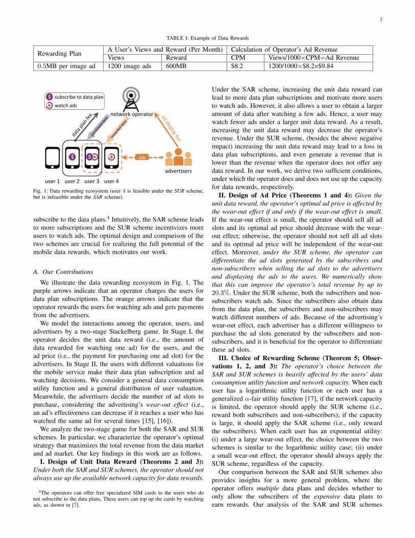
Fig. 1: Data rewarding ecosystem (user 4 is feasible under the SUR scheme,but is infeasible under the SAR scheme).

subscribe to the data plans.4 Intuitively, the SAR scheme leadsto more subscriptions and the SUR scheme incentivizes moreusers to watch ads. The optimal design and comparison of thetwo schemes are crucial for realizing the full potential of themobile data rewards, which motivates our work.

A. Our Contributions

We illustrate the data rewarding ecosystem in Fig. 1. Thepurple arrows indicate that an operator charges the users fordata plan subscriptions. The orange arrows indicate that theoperator rewards the users for watching ads and gets paymentsfrom the advertisers.

We model the interactions among the operator, users, andadvertisers by a two-stage Stackelberg game. In Stage I, theoperator decides the unit data reward (i.e., the amount ofdata rewarded for watching one ad) for the users, and thead price (i.e., the payment for purchasing one ad slot) for theadvertisers. In Stage II, the users with different valuations forthe mobile service make their data plan subscription and adwatching decisions. We consider a general data consumptionutility function and a general distribution of user valuation.Meanwhile, the advertisers decide the number of ad slots topurchase, considering the advertising’s wear-out effect (i.e.,an ad’s effectiveness can decrease if it reaches a user who haswatched the same ad for several times [15], [16]).

We analyze the two-stage game for both the SAR and SURschemes. In particular, we characterize the operator’s optimalstrategy that maximizes the total revenue from the data marketand ad market. Our key findings in this work are as follows.

I. Design of Unit Data Reward (Theorems 2 and 3):Under both the SAR and SUR schemes, the operator should notalways use up the available network capacity for data rewards.

4The operators can offer free specialized SIM cards to the users who donot subscribe to the data plans. These users can top up the cards by watchingads, as shown in [7].

Under the SAR scheme, increasing the unit data reward canlead to more data plan subscriptions and motivate more usersto watch ads. However, it also allows a user to obtain a largeramount of data after watching a few ads. Hence, a user maywatch fewer ads under a larger unit data reward. As a result,increasing the unit data reward may decrease the operator’srevenue. Under the SUR scheme, (besides the above negativeimpact) increasing the unit data reward may lead to a loss indata plan subscriptions, and even generate a revenue that islower than the revenue when the operator does not offer anydata reward. In our work, we derive two sufficient conditions,under which the operator does and does not use up the capacityfor data rewards, respectively.

II. Design of Ad Price (Theorems 1 and 4): Given theunit data reward, the operator’s optimal ad price is affected bythe wear-out effect if and only if the wear-out effect is small.If the wear-out effect is small, the operator should sell all adslots and its optimal ad price should decrease with the wear-out effect; otherwise, the operator should not sell all ad slotsand its optimal ad price will be independent of the wear-outeffect. Moreover, under the SUR scheme, the operator candifferentiate the ad slots generated by the subscribers andnon-subscribers when selling the ad slots to the advertisersand displaying the ads to the users. We numerically showthat this can improve the operator’s total revenue by up to20.3%. Under the SUR scheme, both the subscribers and non-subscribers watch ads. Since the subscribers also obtain datafrom the data plan, the subscribers and non-subscribers maywatch different numbers of ads. Because of the advertising’swear-out effect, each advertiser has a different willingness topurchase the ad slots generated by the subscribers and non-subscribers, and it is beneficial for the operator to differentiatethese ad slots.

III. Choice of Rewarding Scheme (Theorem 5; Obser-vations 1, 2, and 3): The operator’s choice between theSAR and SUR schemes is heavily affected by the users’ dataconsumption utility function and network capacity. When eachuser has a logarithmic utility function or each user has ageneralized α-fair utility function [17], if the network capacityis limited, the operator should apply the SUR scheme (i.e.,reward both subscribers and non-subscribers); if the capacityis large, it should apply the SAR scheme (i.e., only rewardthe subscribers). When each user has an exponential utility:(i) under a large wear-out effect, the choice between the twoschemes is similar to the logarithmic utility case; (ii) undera small wear-out effect, the operator should always apply theSUR scheme, regardless of the capacity.

Our comparison between the SAR and SUR schemes alsoprovides insights for a more general problem, where theoperator offers multiple data plans and decides whether toonly allow the subscribers of the expensive data plans toearn rewards. Our analysis of the SAR and SUR schemes

3

captures the key considerations of choosing these schemes(e.g., whether to motivate more subscriptions to the expensivedata plans or incentivize more ad watching).

B. Related Work

1) Provision of Fee-Based and Ad-Based Services: Therehas been some work studying markets where providers offerboth a fee-based service and an ad-based free service. Forexample, Riggins in [18] studied an online publisher that offersboth the fee-based and ad-based versions of its website. In[19], a Wi-Fi network provider allows users to either directlypay or watch ads to access the Wi-Fi network. In [20], anapp developer offers virtual items, and each app user willeither pay or watch ads to obtain them in the equilibrium. Inthese studies, the fee-based and ad-based services are alwayssubstitutes, and each user chooses between these two options.In our work, their relation is more complicated, since a usermay subscribe to the data plan and meanwhile watch ads formore data. Under the SAR scheme, increasing the rewardfor watching ads can increase the number of subscribers,which shows the complementary relation between the subscrip-tion and data rewards. Therefore, our work studies a novelstructure, and derives new insights for the joint provisionof fee-based and ad-based services. Furthermore, our workconsiders the operator’s capacity for providing the service andthe advertising’s wear-out effect, which were not consideredin [19] and [20].

2) Sponsored Mobile Data: As studied in [17], [21]–[23],sponsored data provides another way for operators to createnew revenue streams: content providers sponsor the data usageof their content, and users can access the content free ofcharge. There are several key differences between sponsoreddata and data rewards as studied here. First, the users canconsume sponsored data only for the content specified by thecontent providers, while they can use reward data to accessany online content. Second, with sponsored data, the contentproviders benefit from the users’ data consumption on thecorresponding content. With data rewards, the advertisers aimto deliver ads effectively, and do not benefit from the users’data consumption.

3) Other Related References: Other related work includes[24]–[26]. Bangera et al. in [24] conducted a survey, whichshows that 76% of the respondents are interested in watchingads in exchange for mobile data. Sen et al. in [25] conductedan experiment to study the effectiveness of monetary rewardsin increasing ads’ viewership. Both [24] and [25] did notanalyze the equilibrium strategies of the entities, such asoperators, advertisers, and users. Harishankar et al. in [26]studied monetizing the operator’s idle network capacity byproviding users with supplemental discount offers, which arenot related to advertising.

II. MODEL

In this section, we model the strategies of the operator,users, and advertisers, and introduce the two-stage game. Weuse capital letters to denote parameters, and lower-case lettersto denote decision variables or random variables.

A. Network Operator

We consider a monopolistic operator, who offers a predeter-mined (monthly) flat-rate data plan (F,Q) to users. ParameterF > 0 denotes the subscription fee, and Q > 0 denotes thedata amount associated with a subscription.5 To derive insightsinto the data reward design, we focus on a single-operator,single-data plan scenario, which has been widely consideredin literature (e.g., [17], [23]).

The operator decides two variables: (i) a unit data rewardω ∈ [0,∞), which is the amount of data that a user receivesfor watching one ad; (ii) an ad price p ∈ (0,∞), which is theprice that the operator charges the advertisers for buying onead slot. Here, we consider a price-based mechanism, wherethe operator sells the ad slots in advance at a fixed price.6

B. Users

We consider a continuum of users, and denote the mass ofusers by N . Let θ denote a user’s type, which parameterizes itsvaluation for mobile service. We assume that θ is a continuousrandom variable drawn from [0, θmax], and its probabilitydensity function g (θ) satisfies g (θ) > 0 for all θ ∈ [0, θmax].

Let r ∈ {0, 1} denote a user’s data plan subscriptiondecision, and x ∈ [0,∞) denote the number of ads that a userchooses to watch (during one month). We allow x and theadvertisers’ purchasing decisions to be fractional [19], [28].The amount of data that a user obtains from its subscriptionand ad watching is Qr+ωx. We use θu (Qr + ωx) to capturea type-θ user’s utility of using the mobile service. Here,u (z) , z ≥ 0, is the same for all users, and can be any strictlyincreasing, strictly concave, and twice differentiable functionthat satisfies u (0) = 0 and limz→∞ u′ (z) = 0. The concavityof u (z) captures the diminishing marginal return with respectto the data amount. Unless otherwise specified, our results arederived under a general u (z) that satisfies these properties. Tostudy the impact of u (z)’s shape, we will also consider threeconcrete choices of u (z) used in the literature:• Logarithmic function [29], [30]: u (z) = ln (1 + z);• Generalized α-fair function [17]: u (z) = (z+µ)1−α

1−α −µ1−α

1−α , 0 < α < 1, µ ≥ 0;• Exponential function [31]: u (z) = 1− e−γz, γ > 0.

One reason for considering these is that the logarithmicfunction and generalized α-fair function are not upper boundedfor z ≥ 0, while the exponential function is upper bounded.This difference will affect the optimal choice between the SARand SUR schemes. For ease of exposition, we call u (·) a user’sutility function (although the actual utility is θu (·)).

5Compared with designing data rewards, the operator has less flexibility toadjust its data plan (e.g., subscribers may sign long-term contracts with theoperator). Hence, we study the operator’s reward design, given its existing dataplan. In our future work, we plan to extend our analysis by jointly optimizingthe data plan and reward.

6The operator and advertisers usually have large-scale collaborations, e.g.,an advertiser’s ads are displayed around 300,000 times per promotion activity.In this case, the price-based mechanism facilitates the customization andcommunication process [27]. The operator can also sell the slots via the real-time auction, especially when it has some user profiles and the advertisers wantto target different user categories [27]. We leave the study of heterogeneousadvertisers and real-time auctions to future work.

4

A type-θ user’s payoff is

Πuser (θ, r, x, ω) = θu (Qr + ωx)− Fr − Φx, (1)

where F is the subscription fee, and Φ > 0 denotes a user’saverage disutility (e.g., inconvenience) of watching one ad.We assume that the total disutility of watching ads linearlyincreases with the number of watched ads [20], [32].

In Sections III-A and IV-A, we will analyze the users’optimal decisions r∗ (θ, ω) and x∗ (θ, ω). Next, we introducetwo notations to capture the total number of ad slots created byusers. Let Nad (ω) denote the mass of users with x∗ (θ, ω) > 0(i.e., who watch ads), and let y be the value of x∗ (θ, ω) chosenby one of these Nad (ω) users. Because these Nad (ω) usersmay have different types θ, they may have different values ofx∗ (θ, ω), i.e., watch different numbers of ads. Therefore, y isa random variable. The distribution of y gives the distributionof the number of ads watched by a user given that the userwatches ads.7 The expected total number of created ad slots issimply the expected total number of ads watched by the users,given by E [y]Nad (ω).

C. Advertisers

We consider K homogeneous advertisers. When Nad (ω) >0, we assume that to display the ads to a user, the operatorrandomly draws ads from all the E [y]Nad (ω) ad slots withoutreplacement.

Suppose an advertiser purchases m ∈ [0,∞) ad slots fromthe operator (in Sections III-C and IV-C, the operator willchoose its ad price p to ensure that the total number of soldad slots does not exceed E [y]Nad (ω)). If a user watchesy ads, on average, my

E[y]Nad(ω)ads among the y watched ads

belong to this advertiser. We let ψ (m, y, ω) denote the overalleffectiveness of the advertiser’s advertising on the user (e.g., alarge ψ (m, y, ω) implies that the user has a good impressionof the advertiser’s product). We model ψ (m, y, ω) by

ψ (m, y, ω) = Bmy

E [y]Nad (ω)−A

(my

E [y]Nad (ω)

)2

, (2)

where B > 0 and A ≥ 0 are parameters. Eq. (2) meansthat ψ (m, y, ω) is quadratic in my

E[y]Nad(ω). This reflects the

advertising’s wear-out effect: the advertising’s effectivenessmay first increase and then decrease with the number of adsdelivered by this advertiser to the user. This is because toomuch repetition may lead the user to have a bad impressionof the product. The wear-out effect has been widely observedin the literature [15], [16]. Some studies, such as [33] and[34], explicitly considered a quadratic relation between the adrepetition and the advertising’s effectiveness, which is similarto (2). Note that a larger A in (2) reflects a stronger degree ofwear-out effect.8

7In Example 1 in Section III-B, we will compute the concrete distributionof y given the assumption of θ. Moreover, the distribution of y depends onthe operator’s decision ω. For the simplicity of presentation, we omit thisdependence in the notation.

8When advertising its product, the advertiser can make several differentversions of ads, and fill the m purchased ad slots with them. This can reduceA, as it mitigates the feeling of repetition from the perspective of the users.

We define an advertiser’s utility as the expected total valueof its advertising’s effectiveness on all users. If a user doesnot see the advertiser’s ads, the advertising’s effectivenesson the user is zero. Therefore, an advertiser’s utility issimply Ey [ψ (m, y, ω)]Nad (ω). Considering the advertiser’spayment for purchasing m ad slots, the advertiser’s payoff is

Πad (m,ω, p) = Ey [ψ (m, y, ω)]Nad (ω)−mp

(a)= Ey

[Bmy

E [y]Nad (ω)− Am2y2

(E [y]Nad (ω))2

]Nad (ω)−mp

= (B − p)m−AE[y2]

(E [y])2Nad (ω)

m2. (3)

Note that E [y]Nad (ω) and(E [y]Nad (ω)

)2in the denomi-

nators on the right-hand side of equality (a) are deterministic.When Nad (ω) = 0, we simply define Πad (m,ω, p) ,−mp, and it is easy to see that the advertiser will not purchaseany ad slot in this case.

D. Two-Stage Stackelberg Game

We model the interactions among the operator, users, andadvertisers by a two-stage Stackelberg game. In Stage I, theoperator decides the unit data reward ω and ad price p. InStage II, each type-θ user chooses the subscription decision rand the number of watched ads x, and each advertiser decidesthe number of purchased ad slots m.9

We assume that the users’ maximum valuation θmax satisfiesθmax > u′(0)F

u′(Q)u(Q) . Similar assumptions about the range ofusers’ attributes have been made in [35]–[37]. As shown inSections III and IV, this assumption implies that the high-valuation users may both subscribe to the data plan and watchads under a small reward ω. In fact, we can easily see that theuser equilibrium under θmax ≤ u′(0)F

u′(Q)u(Q) will be a special case

of that under θmax >u′(0)F

u′(Q)u(Q) . We summarize our paper’skey notations in Appendix A.

III. SUBSCRIPTION-AWARE REWARDING

In this section, we analyze the two-stage game under theSAR scheme, i.e., the operator only allows the subscribers ofthe data plan to watch ads for rewards. Note that we do notstudy the scheme which only rewards the non-subscribers forwatching ads. This scheme is less reasonable in practice, i.e.,the subscribers should not have a lower priority of using theservice than the non-subscribers.

A. Users’ Decisions in Stage II

Given ω, a type-θ user solves the following problem:

maxr∈{0,1}, x∈[0,∞)

Πuser (θ, r, x, ω) , s.t. x = xr, (4)

where Πuser (θ, r, x, ω) is given in (1), and x = xr implies thata user can watch ads (x > 0) only if it subscribes (r = 1).

9If we break Stage II into two stages and consider the sequential decisionmaking of the advertisers and users, the game’s outcome will not change.This is because given the operator’s unit data reward, the users’ decisions arenot directly affected by the advertisers’ decisions. Hence, the advertisers cananticipate the users’ decisions, regardless of their decision sequence.

5

!" !#

!"

!$%&

'!'

!$%&

'!'

(%)%*+,-$*.%)/0123*%(4*

15657*8*&9:!78;

!$%&

'

<%46*=

<%46*>

<%46*<

!'

(%)%*+,-$*(%)%*?@%2**

15657*A*,9:!78;

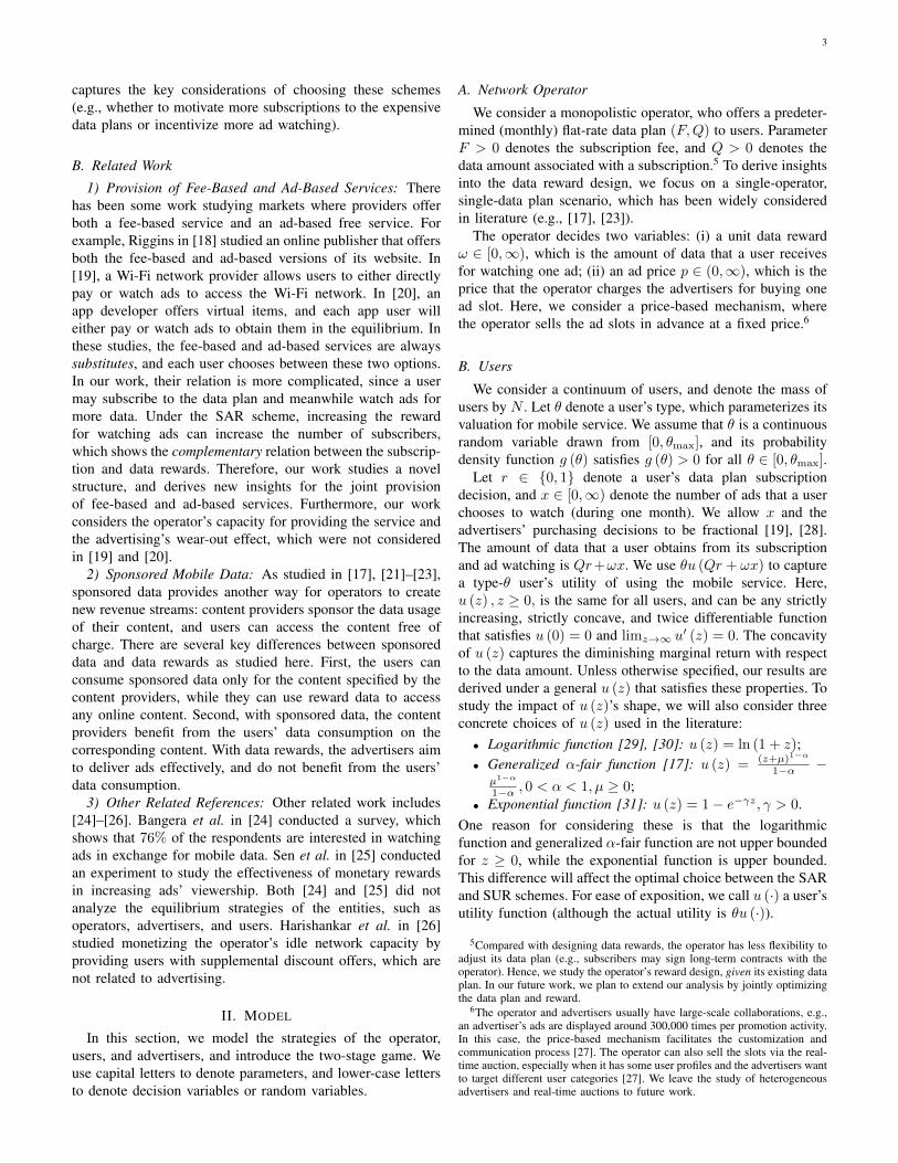
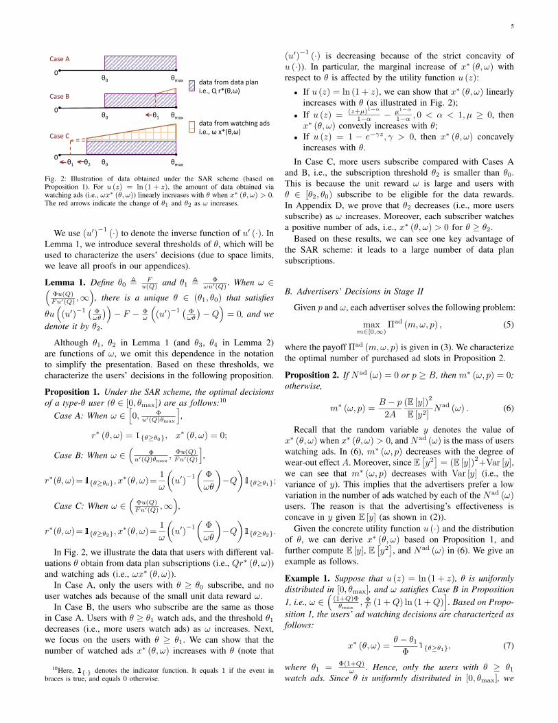
Fig. 2: Illustration of data obtained under the SAR scheme (based onProposition 1). For u (z) = ln (1 + z), the amount of data obtained viawatching ads (i.e., ωx∗ (θ, ω)) linearly increases with θ when x∗ (θ, ω) > 0.The red arrows indicate the change of θ1 and θ2 as ω increases.

We use (u′)−1

(·) to denote the inverse function of u′ (·). InLemma 1, we introduce several thresholds of θ, which will beused to characterize the users’ decisions (due to space limits,we leave all proofs in our appendices).

Lemma 1. Define θ0 , Fu(Q) and θ1 , Φ

ωu′(Q) . When ω ∈(Φu(Q)Fu′(Q) ,∞

), there is a unique θ ∈ (θ1, θ0) that satisfies

θu(

(u′)−1 ( Φ

ωθ

))− F − Φ

ω

((u′)

−1 ( Φωθ

)−Q

)= 0, and we

denote it by θ2.

Although θ1, θ2 in Lemma 1 (and θ3, θ4 in Lemma 2)are functions of ω, we omit this dependence in the notationto simplify the presentation. Based on these thresholds, wecharacterize the users’ decisions in the following proposition.

Proposition 1. Under the SAR scheme, the optimal decisionsof a type-θ user (θ ∈ [0, θmax]) are as follows:10

Case A: When ω ∈[0, Φ

u′(Q)θmax

],

r∗ (θ, ω) = 1{θ≥θ0}, x∗ (θ, ω) = 0;

Case B: When ω ∈(

Φu′(Q)θmax

, Φu(Q)Fu′(Q)

],

r∗(θ, ω)=1{θ≥θ0}, x∗(θ, ω)=

1

ω

((u′)

−1(

Φ

ωθ

)−Q

)1{θ≥θ1};

Case C: When ω ∈(

Φu(Q)Fu′(Q) ,∞

),

r∗(θ, ω)=1{θ≥θ2}, x∗(θ, ω)=

1

ω

((u′)

−1(

Φ

ωθ

)−Q

)1{θ≥θ2}.

In Fig. 2, we illustrate the data that users with different val-uations θ obtain from data plan subscriptions (i.e., Qr∗ (θ, ω))and watching ads (i.e., ωx∗ (θ, ω)).

In Case A, only the users with θ ≥ θ0 subscribe, and nouser watches ads because of the small unit data reward ω.

In Case B, the users who subscribe are the same as thosein Case A. Users with θ ≥ θ1 watch ads, and the threshold θ1

decreases (i.e., more users watch ads) as ω increases. Next,we focus on the users with θ ≥ θ1. We can show that thenumber of watched ads x∗ (θ, ω) increases with θ (note that

10Here, 1{·} denotes the indicator function. It equals 1 if the event inbraces is true, and equals 0 otherwise.

(u′)−1

(·) is decreasing because of the strict concavity ofu (·)). In particular, the marginal increase of x∗ (θ, ω) withrespect to θ is affected by the utility function u (z):

• If u (z) = ln (1 + z), we can show that x∗ (θ, ω) linearlyincreases with θ (as illustrated in Fig. 2);

• If u (z) = (z+µ)1−α

1−α − µ1−α

1−α , 0 < α < 1, µ ≥ 0, thenx∗ (θ, ω) convexly increases with θ;

• If u (z) = 1 − e−γz, γ > 0, then x∗ (θ, ω) concavelyincreases with θ.

In Case C, more users subscribe compared with Cases Aand B, i.e., the subscription threshold θ2 is smaller than θ0.This is because the unit reward ω is large and users withθ ∈ [θ2, θ0) subscribe to be eligible for the data rewards.In Appendix D, we prove that θ2 decreases (i.e., more userssubscribe) as ω increases. Moreover, each subscriber watchesa positive number of ads, i.e., x∗ (θ, ω) > 0 for θ ≥ θ2.

Based on these results, we can see one key advantage ofthe SAR scheme: it leads to a large number of data plansubscriptions.

B. Advertisers’ Decisions in Stage II

Given p and ω, each advertiser solves the following problem:

maxm∈[0,∞)

Πad (m,ω, p) , (5)

where the payoff Πad (m,ω, p) is given in (3). We characterizethe optimal number of purchased ad slots in Proposition 2.

Proposition 2. If Nad (ω) = 0 or p ≥ B, then m∗ (ω, p) = 0;otherwise,

m∗ (ω, p) =B − p

2A

(E [y])2

E [y2]Nad (ω) . (6)

Recall that the random variable y denotes the value ofx∗ (θ, ω) when x∗ (θ, ω) > 0, and Nad (ω) is the mass of userswatching ads. In (6), m∗ (ω, p) decreases with the degree ofwear-out effect A. Moreover, since E

[y2]

= (E [y])2+Var [y],

we can see that m∗ (ω, p) decreases with Var [y] (i.e., thevariance of y). This implies that the advertisers prefer a lowvariation in the number of ads watched by each of the Nad (ω)users. The reason is that the advertising’s effectiveness isconcave in y given E [y] (as shown in (2)).

Given the concrete utility function u (·) and the distributionof θ, we can derive x∗ (θ, ω) based on Proposition 1, andfurther compute E [y], E

[y2], and Nad (ω) in (6). We give an

example as follows.

Example 1. Suppose that u (z) = ln (1 + z), θ is uniformlydistributed in [0, θmax], and ω satisfies Case B in Proposition1, i.e., ω ∈

((1+Q)Φθmax

, ΦF (1 +Q) ln (1 +Q)

]. Based on Propo-

sition 1, the users’ ad watching decisions are characterized asfollows:

x∗ (θ, ω) =θ − θ1

Φ1{θ≥θ1}, (7)

where θ1 = Φ(1+Q)ω . Hence, only the users with θ ≥ θ1

watch ads. Since θ is uniformly distributed in [0, θmax], we

6

can further compute Nad (ω) as follows:

Nad (ω) =θmax − θ1

θmaxN. (8)

According to (7) and the fact that θ ∼ U [0, θmax], the numberof ads watched by one of the Nad (ω) users is uniformlydistributed in

[0, θmax−θ1

Φ

]. This implies that y is uniformly

distributed in[0, θmax−θ1

Φ

].11 Then, we can compute E [y] and

E[y2]

as follows:

E [y] =1

2

θmax − θ1

Φ,E[y2]

=1

3

(θmax − θ1

Φ

)2

. (9)

Based on Proposition 2, we can derive m∗ (ω, p) as follows:

m∗ (ω, p) =3

8

max {B − p, 0}A

θmax − θ1

θmaxN. (10)

In Appendix F, we compute m∗ (ω, p) for other values ofω (i.e., ω that satisfies Cases A or C) under the logarithmicutility function and uniformly distributed user types.

C. Operator’s Decisions in Stage I

The operator obtains revenue from both the mobile datamarket and ad market. In the mobile data market, each userwho subscribes to the data plan should pay F to the operator.The operator’s corresponding revenue is

Rdata (ω) = NF

∫ θmax

0

r∗ (θ, ω) g (θ) dθ. (11)

In the ad market, each advertiser pays p for each purchasedad slot. The operator’s corresponding revenue is

Rad (ω, p) = Km∗ (ω, p) p. (12)

Let D (ω) denote the total data demand, i.e., the totalamount of mobile data that users request (by subscription andwatching ads) under reward ω. We can compute D (ω) as

D (ω) = N

∫ θmax

0

(Qr∗ (θ, ω) + ωx∗ (θ, ω)) g (θ) dθ, (13)

where Qr∗ (θ, ω) and ωx∗ (θ, ω) are illustrated in Fig. 2.Based on Rdata (ω), Rad (ω, p), and D (ω), we formulate

the operator’s problem as follows:

maxω≥0,p>0

Rtotal (ω, p) , Rdata (ω) +Rad (ω, p) (14)

s.t. D (ω) ≤ C, (15)

Km∗ (ω, p) ≤ E [y]Nad (ω) . (16)

Here, Rtotal (ω, p) is the operator’s total revenue. Constraint(15) implies that the total data demand D (ω) cannot exceed acapacity C [17], [23]. To ensure that choosing ω = 0 (i.e., nodata reward) is feasible to the problem, we assume that C ≥D (0). Here, D (0) is the data demand when the operator only

11Strictly speaking, x∗ (θ1, ω) = 0 and hence only the users withθ > θ1 will watch ads. As a result, y should be uniformly distributed in(

0, θmax−θ1Φ

]. However, the probability that θ = θ1 is zero due to the

continuous distribution of θ. Therefore, we can consider users with θ ≥ θ1when counting Nad (ω) and treat y as a variable uniformly distributed in[0, θmax−θ1

Φ

]without affecting our analysis.

offers the data plan without any data reward. Constraint (16)implies that the total number of sold ad slots (i.e., Km∗ (ω, p))should not exceed the number of available ad slots. When theoperator does not sell all ad slots, it can fill the unsold slotswith content like public news and pictures to guarantee thefairness among the users choosing to watch ads (e.g., Optusdisplayed wallpapers to users when there were unsold ad slots[38]).

To solve (14)-(16), we first analyze p∗ (ω), which is theoptimal ad price under a given ω. Then, we substitute p =p∗ (ω) into Rtotal (ω, p), and analyze the optimal unit datareward ω∗. We characterize p∗ (ω) in the following theorem.

Theorem 1. If ω ∈[0, Φ

u′(Q)θmax

], any positive price is

optimal; if ω ∈(

Φu′(Q)θmax

,∞)

,

p∗ (ω) = max

{B

2, B −

2AE[y2]

KE [y]

}. (17)

Note that the random variable y is the value of x∗ (θ, ω)whenx∗ (θ, ω)>0. Hence, both E

[y2]

and E [y] depend on ω.

If ω ∈[0, Φ

u′(Q)θmax

], no user watches ads (based on Propo-

sition 1). In this case, the advertisers do not purchase ad slots,regardless of the ad price p. If ω ∈

(Φ

u′(Q)θmax,∞)

, Eq. (17)implies that p∗ (ω) decreases with A (the degree of wear-outeffect) when A is small, but does not change with A when A islarge. When A < BKE[y]

4E[y2] , the wear-out effect is small, and theadvertisers have high willingness to purchase ad slots. Hence,

the operator chooses p∗ (ω) = B − 2AE[y2]KE[y] to sell all the

ad slots (which leads to Km∗ (ω, p∗ (ω)) = E [y]Nad (ω)).When A ≥ BKE[y]

4E[y2] , the large wear-out effect decreases theadvertisers’ willingness to purchase slots. The operator willnot sell all slots, and will choose p∗ (ω) = B

2 , which isindependent of A.

Next, we analyze ω∗, which maximizes Rtotal (ω, p∗ (ω)),subject to D (ω) ≤ C. We first introduce Proposition 3.Proposition 3. Given C ≥ D (0), there is a unique ω ∈[

Φu′(Q)θmax

,∞)

such that D (ω) = C. We denote this ω byD−1 (C). Moreover, D−1 (C) strictly increases with C.

Based on Proposition 3, we can rewrite D (ω) ≤ C as ω ≤D−1 (C). From numerical experiments, Rtotal (ω, p∗ (ω)) iseither always increasing or unimodal in ω ∈ [0,∞). Hence,we can easily search for ω∗ in the interval

[0, D−1 (C)

](e.g.,

when Rtotal (ω, p∗ (ω)) is unimodal, we can apply the GoldenSection method [39]). Next, we study when the operator willchoose ω to be D−1 (C), i.e., use up the network capacity fordata rewards. In Theorem 2, we show a sufficient conditionunder which ω∗ = D−1 (C).

Theorem 2. Under the SAR scheme, if both (E[y])2

E[y2] Nad (ω)

and E [y]Nad (ω) increase with ω for ω ∈(

Φu′(Q)θmax

,∞)

,the operator’s optimal unit data reward is given by ω∗ =D−1 (C).

We explain this sufficient condition by discussing the unitdata reward ω’s influence on Rdata (ω) and Rad (ω, p∗ (ω)).

7

First, increasing ω can increase Rdata (ω), because more userssubscribe. Second, increasing ω has the following impactson Rad (ω, p∗ (ω)): (i) (positive impact) It increases Nad (ω),i.e., more users watch ads; (ii) (negative impact) It maydecrease E [y]. Under a larger ω, a user can obtain a largeramount of data after watching a few ads. Then, the user’swillingness to watch more ads may decrease because of theconcavity of the utility function; (iii) (negative impact) It mayincrease Var [y]. Under a larger ω, more users with differentvaluations θ watch ads, which can increase the variance of y.As discussed in Section III-B, increasing Var [y] decreasesthe advertisers’ willingness to purchase ad slots. Under ageneral utility function u (·) and a general distribution ofθ, it is challenging to analyze the net effect of the aboveimpacts. Theorem 2 implies that when both (E[y])2

E[y2] Nad (ω) and

E [y]Nad (ω) increase with ω, the positive impact dominatesthe negative impacts. In this case, the operator should set ωas large as possible without violating the capacity constraint(15) under the SAR scheme.

A widely considered setting is that each user has a log-arithmic utility function (e.g., [29], [30]) and a uniformlydistributed type (e.g., [19], [36]). We can verify that this settingsatisfies the sufficient condition in Theorem 2, and hence wehave the following proposition.

Proposition 4. When u (z) = ln (1 + z) and θ ∼ U [0, θmax],the operator’s optimal unit data reward is given by ω∗ =D−1 (C).

When each user has an exponential utility function (i.e.,u (z) = 1−e−γz), E [y]Nad (ω) may decrease with ω and ω∗

can be smaller than D−1 (C) (i.e., the operator does not use upthe capacity for rewards). We show an example in AppendixK.

IV. SUBSCRIPTION-UNAWARE REWARDING

In this section, we consider the SUR scheme, i.e., both thesubscribers and non-subscribers can watch ads for rewards.

A. Users’ Decisions in Stage II

Since the users can watch ads without subscription, eachtype-θ user simply chooses r and x to maximize its payoffwithout the constraint x = xr, as in (4) in Section III-A.

In Lemma 2, we introduce two new thresholds of θ.

Lemma 2. Define θ3 , Φωu′(0) . When ω ∈

(Φu(Q)Fu′(0) ,

ΦQF

),

there is a unique θ ∈ (θ3, θ1) that satisfies θu(

(u′)−1 ( Φ

ωθ

))−

Φω (u′)

−1 ( Φωθ

)= θu (Q)− F , and we denote it by θ4.

Recall that (u′)−1

(·) denotes the inverse function of u′ (·).Based on the thresholds introduced in Lemmas 1 and 2, wecharacterize the users’ decisions in the following proposition(we use symbol ˆ to indicate that the results are obtained underthe SUR scheme).

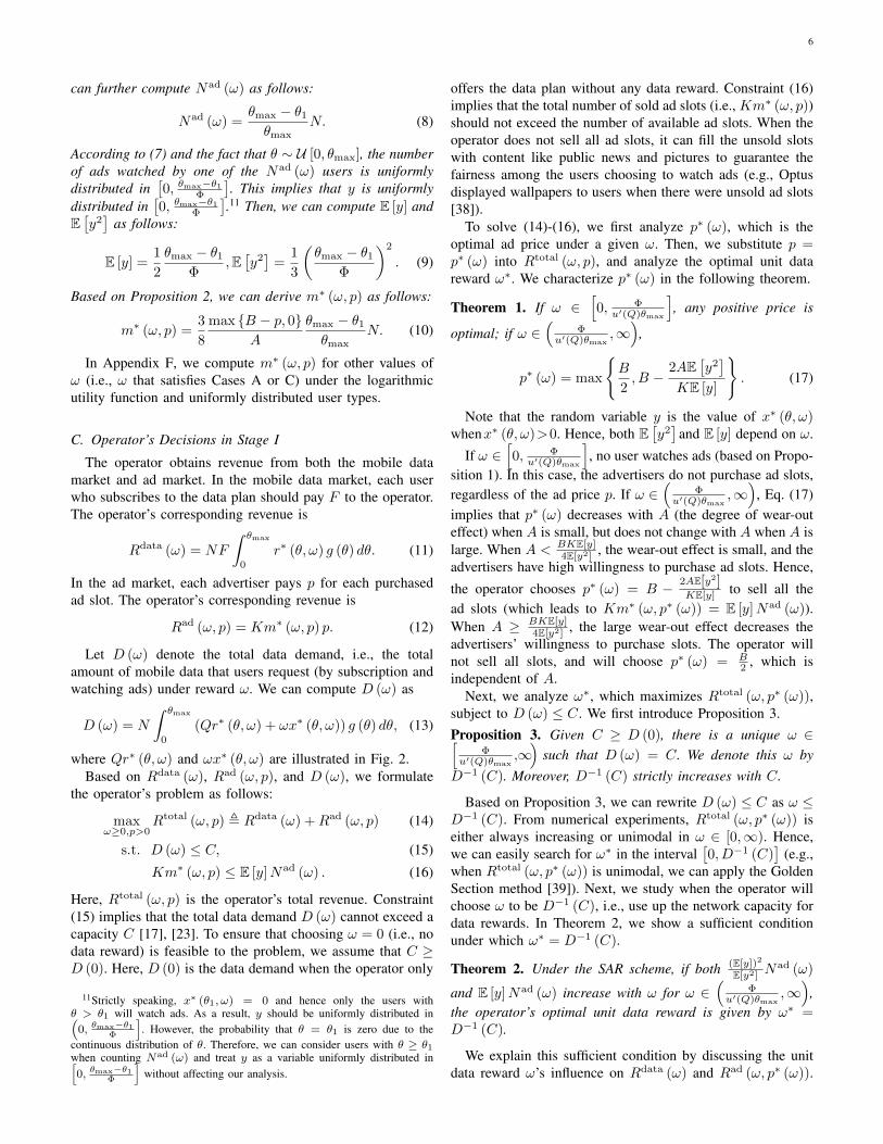
Proposition 5. Under the SUR scheme, the optimal decisionsof a type-θ user (θ ∈ [0, θmax]) are as follows:

!" !#$%

&!'

($)*+(,

!-

!#$%

&

($)*+.,

!-

/$0$+123#+/$0$+45$6++

78*89+:+2;<!9=>,

/$0$+123#+?$0@A76B+$/)+

78*89+=+%;<!9=>,

!&

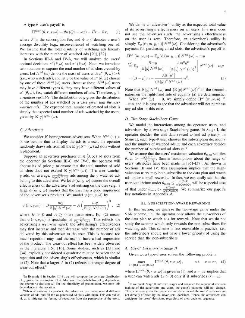
Fig. 3: Illustration of data obtained under the SUR scheme (based onProposition 5). For u (z) = ln (1 + z), the amount of data obtained viawatching ads (i.e., ωx∗ (θ, ω)) linearly increases with θ when x∗ (θ, ω) > 0.The red arrows indicate the change of θ1, θ3, and θ4 as ω increases.

Case A: When ω ∈[0, Φ

u′(Q)θmax

],

r∗ (θ, ω) = 1{θ≥θ0}, x∗ (θ, ω) = 0;

Case B: When ω ∈(

Φu′(Q)θmax

, Φu(Q)Fu′(0)

],

r∗(θ, ω)=1{θ≥θ0},x∗(θ, ω)=

1

ω

((u′)

−1(

Φ

ωθ

)−Q)1{θ≥θ1};

Case C: When ω ∈(

Φu(Q)Fu′(0) ,

ΦQF

),

r∗(θ,ω)=1{θ≥θ4},

x∗(θ,ω)=1

ω(u′)

−1(

Φ

ωθ

)1{θ3≤θ<θ4}+

1

ω

((u′)

−1(

Φ

ωθ

)−Q)1{θ≥θ1};

Case D: When ω ∈[

ΦQF ,∞

),

r∗ (θ, ω) = 0, x∗ (θ, ω) =1

ω(u′)

−1(

Φ

ωθ

)1{θ≥θ3}.

The users’ optimal decisions in Cases A and B are the sameas those in Cases A and B (under the SAR scheme), respec-tively. Hence, in Fig. 3, we only illustrate the data obtainedby users via subscription (i.e., Qr∗ (θ, ω)) and watching ads(i.e., ωx∗ (θ, ω)) in Cases C and D.

In Case C, two segments of users watch ads: users withvaluations θ ≥ θ1 watch ads and subscribe; users withvaluations θ3 ≤ θ < θ4 watch ads without subscription. Wecharacterize the properties of θ4 in the following lemma.

Lemma 3. When ω ∈(

Φu(Q)Fu′(0) ,

ΦQF

)(i.e., Case C), (i) θ4 is

greater than θ0, and (ii) θ4 increases with ω.

In Case B, the subscription threshold is θ0. Hence, result(i) of Lemma 3 implies that some low-valuation users whosubscribe in Case B become non-subscribers in Case C.This is because these low-valuation users’ marginal benefit ofconsuming data decreases after earning the data rewards, andit is no longer beneficial for them to subscribe to the data planin Case C. Result (ii) of Lemma 3 shows that more subscribersbecome non-subscribers as the unit reward increases.

In Case D, since ω is large, all users simply watch ads toearn the rewards, without paying for the subscription.

8

0.012 0.014 0.016 0.018 0.02 0.022 0.024

107

1.96

1.97

1.98

1.99

2

2.01

2.02

2.03

2.04

2.05

2.06

(a) Function D (ω).

0.012 0.014 0.016 0.018 0.02 0.022 0.024

108

3.8

4

4.2

4.4

4.6

4.8

5

5.2

0.0239 0.0240 0.024 0.0240 0.0241 0.0241 0.0242 0.0242

108

3.924

3.9245

3.925

3.9255

3.926

3.9265

3.927

3.9275

3.928

3.9285

3.929

(b) Function Rtotal (ω, p∗ (ω)).

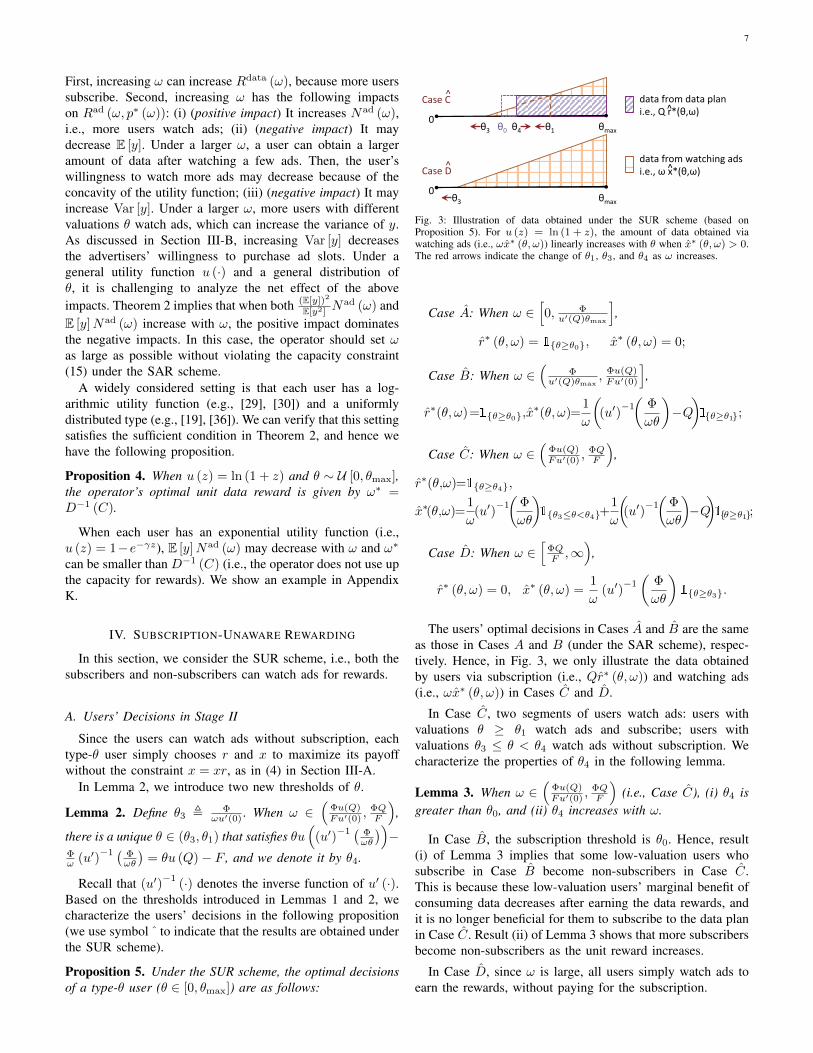
Fig. 4: Examples of D (ω) and Rtotal (ω, p∗ (ω)): We assume that u (z) = 1− e−0.7z and obtain the distribution of θ by truncating the normal distributionN (125, 30) to interval [0, 250]. We choose N = 107, F = 42, Q = 2, Φ = 0.5, K = 13, A = 1, B = 5, and C = 2.015× 107.

B. Advertisers’ Decisions in Stage II

Compared with the SAR scheme, the SUR scheme changeseach advertiser’s optimal decision through changing the massof users watching ads and the distribution of the number ofads watched by each of these users.

Given r∗ (θ, ω) and x∗ (θ, ω) in Proposition 5, we cancompute Nad (ω) (i.e., the mass of users watching ads) and thedistribution of y (i.e., x∗ (θ, ω)’s value when x∗ (θ, ω) > 0).To compute m∗ (ω, p), we can simply replace Nad (ω), E [y],and E

[y2]

in Proposition 2 by Nad (ω), E [y], and E[y2].

C. Operator’s Decisions in Stage I

Based on r∗ (θ, ω), x∗ (θ, ω), and m∗ (ω, p), we can com-pute Rdata (ω), Rad (ω, p), and D (ω) in a similar manner asin (11)-(13). The operator’s problem in Stage I is then givenby:

maxω≥0,p>0

Rtotal (ω, p) , Rdata (ω) + Rad (ω, p) (18)

s.t. D (ω) ≤ C, Km∗ (ω, p) ≤ Nad (ω)E [y] , (19)

which is similar to problem (14)-(16).To solve (18)-(19), we first compute p∗ (ω), i.e., the optimal

ad price under a given ω. The analysis of p∗ (ω) is similar tothat of p∗ (ω) in Theorem 1 under the SAR scheme. We canprove that if ω ∈

[0, Φ

u′(Q)θmax

], no user watches ads and

hence any positive ad price is optimal; otherwise, we have

p∗ (ω) = max

{B2 , B −

2AE[y2]KE[y]

}.

Then, we compute ω∗ by maximizing Rtotal (ω, p∗ (ω)),subject to D (ω) ≤ C. The computation of ω∗ is differ-ent from that of ω∗ under the SAR scheme, because (i)D (ω) can be decreasing in ω ∈

(Φu(Q)Fu′(0) ,

ΦQF

), and (ii)

Rtotal (ω, p∗ (ω)) is discontinuous at ω = ΦQF . Specifically,

when ω ∈(

Φu(Q)Fu′(0) ,

ΦQF

), increasing ω reduces the number

of data plan subscribers, which may decrease D (ω). More-over, when ω increases to ΦQ

F , all data plan subscribers quit

their subscriptions and the distribution of users’ ad watch-ing times also changes. This leads to the discontinuity ofRtotal (ω, p∗ (ω)) at ω = ΦQ

F . We illustrate examples of D (ω)

and Rtotal (ω, p∗ (ω)) in Fig. 4(a) and Fig. 4(b), respectively.We can compute ω∗ as follows. First, we search for ω’s

feasible region, where D (ω) ≤ C. We can numerically showthat ω’s feasible region consists of at most three intervals.Then, we can show that Rtotal (ω, p∗ (ω)) is either monotoneor unimodal in each interval.12 Hence, we can determine ω∗

by comparing the local optimal unit data rewards found inthese intervals.

Under the SAR scheme, the operator always uses up thecapacity for rewards if u (z) = ln (1 + z) and θ ∼ U [0, θmax].Under the SUR scheme, this does not hold, and a large ω mayeven generate a total revenue that is lower than the revenuewhen the operator does not offer any reward. This is becausea large ω may reduce the number of subscribers (as shown inCase C) and hence decrease Rdata (ω). Next, we characterizea sufficient condition under which the network capacity is notused up for rewards (given general u (z) and g (θ)).

Theorem 3. Under the SUR scheme, when the networkcapacity C > N (u′)

−1(

FθmaxQ

)and the degree of wear-out

effect A > B2K

8F∫ θmaxθ0

g(θ)dθ, we have D (ω∗) < C.

When the operator has a large capacity and the wear-out effect is large, using up the capacity for rewards willsignificantly decrease Rdata (ω) and will not significantlyincrease Rad (ω, p∗ (ω)). Hence, we have D (ω∗) < C in thissituation. We can show that both thresholds N (u′)

−1(

FθmaxQ

)and B2K

8F∫ θmaxθ0

g(θ)dθdecrease with F (i.e., the subscription fee).

Intuitively, if the data plan is expensive, the operator shouldnot use up the capacity for rewards under the SUR scheme.

12For example, in Fig. 4(a), ω’s feasible region consists of the yellow,blue, and purple intervals (denoted by intervals (1), (2), and (3)). In Fig. 4(b),Rtotal (ω, p∗ (ω)) is increasing when ω is in the yellow or purple intervals,and is decreasing when ω is in the blue interval.

9

D. Extension: Differentiation of Ad Slots

In the above analysis, we assume that the operator does notdifferentiate the ad slots generated by the users. It sells allad slots to the advertisers at the same price, and randomlydraws ads from all ad slots when a user watches ads. Underthe SUR scheme, the ad slots can be generated by both thesubscribers and non-subscribers. In this section, we considerthe differentiation of these two types of ad slots,13 whichaffects both the pricing and ad display rule. The operator cansell these two types of ad slots at different prices. When asubscriber or non-subscriber watches ads, the operator drawsads only from the corresponding type of ad slots (e.g., ifan advertiser only purchases the ad slots generated by thesubscribers, its ads will only be seen by the subscribers).

Given ω, we use NadI (ω) and Nad

II (ω) to denote the numberof the subscribers that watch ads and the number of the non-subscribers that watch ads, respectively. Let random variablesyI and yII denote the numbers of ads watched by one of thesesubscribers and one of these non-subscribers, respectively.Similar to Proposition 2, we have the following results:• For the ad slots generated by the subscribers, the operator

can set a price pI > 0. If NadI (ω) > 0, the number of

these slots purchased by each advertiser is m∗I (ω, pI) =max{B−pI,0}

2A(E[yI])

2

E[y2I ]Nad

I (ω); otherwise, m∗I (ω, pI) = 0;• For the slots generated by the non-subscribers, the op-

erator can set pII > 0. If NadII (ω) > 0, the number of

these slots purchased by each advertiser is m∗II (ω, pII) =max{B−pII,0}

2A(E[yII])

2

E[y2II]Nad

II (ω); otherwise, m∗II (ω, pII)= 0.

The operator’s problem with differentiation is given by:

maxω≥0,pI,pII>0

Rdata(ω)+Km∗I (ω, pI) pI+Km∗II(ω, pII) pII (20)

s.t. D (ω) ≤ C, (21)

Km∗I (ω, pI) ≤ E [yI] NadI (ω) , (22)

Km∗II (ω, pII) ≤ E [yII] NadII (ω) . (23)

Constraint (22) means that the total number of sold ad slotsthat correspond to the subscribers should not exceed the num-ber of ad slots generated by the subscribers. Constraint (23)can be explained similarly for the non-subscribers. In fact, onlywhen ω satisfies Case C in Proposition 5, both the subscribersand non-subscribers watch ads (i.e., Nad

I (ω) , NadII (ω) > 0),

and problem (20)-(23) is different from problem (18)-(19) (i.e.,the problem without differentiation). In the remaining cases,problem (20)-(23) reduces to problem (18)-(19).

We define ΠSUR , Rtotal (ω∗, p∗ (ω∗)), which is theoptimal objective value of problem (18)-(19). Let ΠSURD

denote the optimal objective value of problem (20)-(23), i.e.,ΠSURD is the operator’s optimal total revenue under the SURscheme with differentiation. We compare ΠSUR and ΠSURD

in the following theorem.

Theorem 4. We always have ΠSURD ≥ ΠSUR.

13Besides the subscription decision r, a user decides x, e.g., the number ofads to watch within a month. Different from r, the operator does not preciselyknow the user’s decision of x until the end of the month. If the operator canestimate x’s range based on the user’s historical behavior, it can classify usersinto different categories and differentiate the corresponding ad slots similarly.

Hence, differentiation does not decrease the operator’s op-timal total revenue (given general u (z) and g (θ)). In general,it is easy to show that allowing a seller to sell items atdifferent prices does not decrease its revenue. However, thedifferentiation here affects the ad display rule as well as thepricing, so it is non-trivial to prove Theorem 4. For example,one conjecture is that given any (ω, p) which is feasibleto (18)-(19), the operator can choose the same ω and setpI = pII = p in (20)-(23) to ensure that the value of objective(20) is no smaller than that of (18). In fact, the conjecture doesnot hold, because (ω, pI, pII) may be infeasible for (20)-(23).

Intuitively, if the optimal unit data reward satisfies Case Cand the distributions of yI and yII are significantly different,the gap between ΠSURD and ΠSUR will be large. In the nextsection, we will show this gap numerically.

V. COMPARISON BETWEEN REWARDING SCHEMES

We define ΠSAR , Rtotal (ω∗, p∗ (ω∗)), which is theoperator’s optimal total revenue under the SAR scheme. Inthis section, we compare ΠSAR, ΠSUR, and ΠSURD. Sincethe comparison is challenging under a general user typedistribution and a general utility function, we focus on specificuser type distributions and utility functions. In Sections V-Aand V-B, we consider uniformly distributed user types andtruncated normally distributed user types, respectively.

A. Uniformly Distributed User Types

In this section, we assume that each user’s type θ followsa uniform distribution. We will consider logarithmic utility,generalized α-fair utility, and exponential utility.

1) Logarithmic Utility Function: We assume that u (z) =ln (1 + z). Theorem 5 characterizes the analytical comparisonbetween different schemes as C →∞.

Theorem 5. When θ ∼ U [0, θmax] and u (z) = ln (1 + z), ifnetwork capacity C →∞, then ΠSAR > ΠSURD ≥ ΠSUR.

Theorem 5 implies that if the operator has sufficiently largenetwork capacity, it should only reward the subscribers forwatching ads. Intuitively, this allows the operator to motivateall users to subscribe and watch ads via high data rewards. Itmaximizes the operator’s revenue from both the data marketand the ad market.

Under a finite network capacity C, none of ΠSAR, ΠSUR, orΠSURD has a closed-form expression, and their analytical com-parison is challenging. Next, we compare them numerically.In the numerical experiment, we choose N = 107, F = 30,Q = 0.8, θ ∼ U [0, 155], Φ = 0.3, K = 23, A = 0.6, andB = 5. Here, we consider an area with 10 million users. InAppendix R, we consider different parameter settings (e.g.,different values of N ), and the key observations summarizedin this section still hold under those settings.

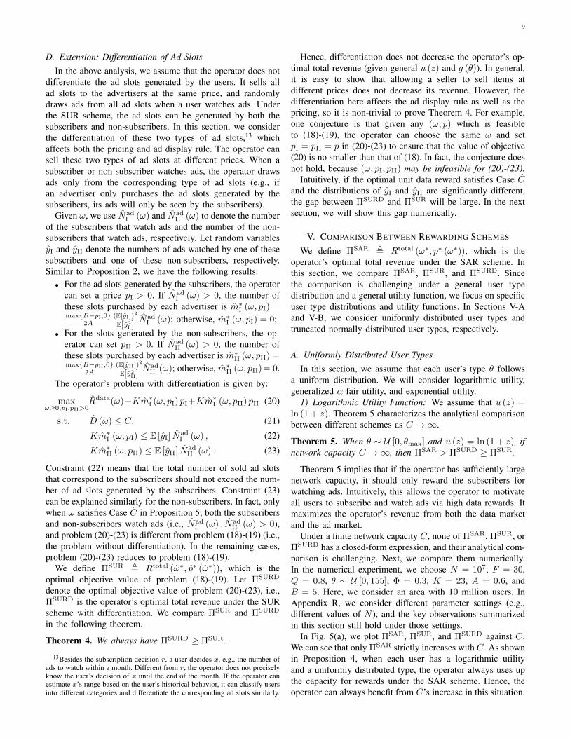
In Fig. 5(a), we plot ΠSAR, ΠSUR, and ΠSURD against C.We can see that only ΠSAR strictly increases with C. As shownin Proposition 4, when each user has a logarithmic utilityand a uniformly distributed type, the operator always uses upthe capacity for rewards under the SAR scheme. Hence, theoperator can always benefit from C’s increase in this situation.

10

107

1 1.5 2 2.5 3 3.5

108

6

6.5

7

7.5

8

8.5

9

9.5

(a) Logarithmic Utility.

107

1.5 2 2.5 3 3.5 4 4.5

108

7

7.5

8

8.5

9

9.5

(b) Generalized α-Fair Utility.

107

1.6 1.7 1.8 1.9 2 2.1 2.2 2.3 2.4 2.5

108

3.5

4

4.5

5

5.5

6

6.5

7

7.5

8

8.5

(c) Exponential Utility (Large A).

107

2 2.5 3 3.5

109

0.5

1

1.5

2

2.5

3

(d) Exponential Utility (Small A).

Fig. 5: ΠSAR, ΠSUR, and ΠSURD Under Different Network Capacity (Uniformly Distributed θ).

First, we compare ΠSAR and ΠSUR. When C is closeto D (0), ΠSAR and ΠSUR are equal. In this situation, theoperator can only choose a very small unit reward ω. As shownin Case B in Proposition 1 and Case B in Proposition 5, theusers’ optimal decisions under the two schemes are the same,which leads to the same operator’s revenue. When C is from0.84 × 107 to 1.54 × 107, ΠSAR is smaller than ΠSUR. Thisis because the SUR scheme can motivate two segments ofusers to watch ads (by setting ω ∈

(Φu(Q)Fu′(0) ,

ΦQF

), as shown in

Case C in Proposition 5), which generates a higher ad revenuethan the SAR scheme. When C is greater than 1.54 × 107,ΠSAR is greater than ΠSUR. The operator will fully utilizethe large network capacity under the SAR scheme, and set alarge ω to motivate more users to both subscribe and watchads. This is consistent with Theorem 5 (i.e., if C →∞, thenΠSAR > ΠSUR). We summarize the results in Observation 1(the comparison between ΠSAR and ΠSURD is similar to thecomparison between ΠSAR and ΠSUR).

Observation 1. When u (z) = ln (1 + z), if C is small, theSUR scheme achieves a higher operator’s revenue; otherwise,the SAR scheme achieves a higher operator’s revenue.

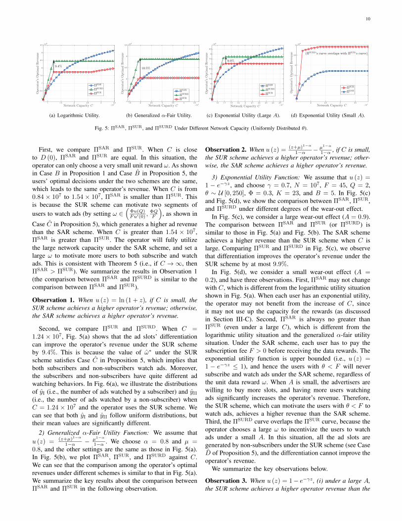
Second, we compare ΠSUR and ΠSURD. When C =1.24 × 107, Fig. 5(a) shows that the ad slots’ differentiationcan improve the operator’s revenue under the SUR schemeby 9.4%. This is because the value of ω∗ under the SURscheme satisfies Case C in Proposition 5, which implies thatboth subscribers and non-subscribers watch ads. Moreover,the subscribers and non-subscribers have quite different adwatching behaviors. In Fig. 6(a), we illustrate the distributionsof yI (i.e., the number of ads watched by a subscriber) and yII

(i.e., the number of ads watched by a non-subscriber) whenC = 1.24 × 107 and the operator uses the SUR scheme. Wecan see that both yI and yII follow uniform distributions, buttheir mean values are significantly different.

2) Generalized α-Fair Utility Function: We assume thatu (z) = (z+µ)1−α

1−α − µ1−α

1−α . We choose α = 0.8 and µ =0.8, and the other settings are the same as those in Fig. 5(a).In Fig. 5(b), we plot ΠSAR, ΠSUR, and ΠSURD against C.We can see that the comparison among the operator’s optimalrevenues under different schemes is similar to that in Fig. 5(a).We summarize the key results about the comparison betweenΠSAR and ΠSUR in the following observation.

Observation 2. When u (z) = (z+µ)1−α

1−α − µ1−α

1−α , if C is small,the SUR scheme achieves a higher operator’s revenue; other-wise, the SAR scheme achieves a higher operator’s revenue.

3) Exponential Utility Function: We assume that u (z) =1 − e−γz , and choose γ = 0.7, N = 107, F = 45, Q = 2,θ ∼ U [0, 250], Φ = 0.3, K = 23, and B = 5. In Fig. 5(c)and Fig. 5(d), we show the comparison between ΠSAR, ΠSUR,and ΠSURD under different degrees of the wear-out effect.

In Fig. 5(c), we consider a large wear-out effect (A = 0.9).The comparison between ΠSAR and ΠSUR (or ΠSURD) issimilar to those in Fig. 5(a) and Fig. 5(b). The SAR schemeachieves a higher revenue than the SUR scheme when C islarge. Comparing ΠSUR and ΠSURD in Fig. 5(c), we observethat differentiation improves the operator’s revenue under theSUR scheme by at most 9.9%.

In Fig. 5(d), we consider a small wear-out effect (A =0.2), and have three observations. First, ΠSAR may not changewith C, which is different from the logarithmic utility situationshown in Fig. 5(a). When each user has an exponential utility,the operator may not benefit from the increase of C, sinceit may not use up the capacity for the rewards (as discussedin Section III-C). Second, ΠSAR is always no greater thanΠSUR (even under a large C), which is different from thelogarithmic utility situation and the generalized α-fair utilitysituation. Under the SAR scheme, each user has to pay thesubscription fee F > 0 before receiving the data rewards. Theexponential utility function is upper bounded (i.e., u (z) =1 − e−γz ≤ 1), and hence the users with θ < F will neversubscribe and watch ads under the SAR scheme, regardless ofthe unit data reward ω. When A is small, the advertisers arewilling to buy more slots, and having more users watchingads significantly increases the operator’s revenue. Therefore,the SUR scheme, which can motivate the users with θ < F towatch ads, achieves a higher revenue than the SAR scheme.Third, the ΠSURD curve overlaps the ΠSUR curve, because theoperator chooses a large ω to incentivize the users to watchads under a small A. In this situation, all the ad slots aregenerated by non-subscribers under the SUR scheme (see CaseD of Proposition 5), and the differentiation cannot improve theoperator’s revenue.

We summarize the key observations below.

Observation 3. When u (z) = 1− e−γz , (i) under a large A,the SUR scheme achieves a higher operator revenue than the

11

0 50 100 150 200 250 300 3500

0.002

0.004

0.006

0.008

0.01

0.012

(a) Logarithmic Utility and Uniformly Distributed θ.

0 10 20 30 40 50 60 70 80 900

0.01

0.02

0.03

0.04

0.05

0.06

0.07

0.08

(b) Exponential Utility and Truncated Normally Distributed θ.

Fig. 6: Probability Distribution Function of yI and yII.

107

3 3.5 4 4.5 5 5.5 6

109

1.3

1.35

1.4

1.45

1.5

1.55

1.6

1.65

1.7

(a) Logarithmic Utility.

107

4 5 6 7 8 9 10

109

1.3

1.35

1.4

1.45

1.5

1.55

1.6

1.65

1.7

1.75

(b) Generalized α-Fair Utility.

107

2 2.05 2.1 2.15 2.2 2.25 2.3 2.35

108

4

4.5

5

5.5

6

6.5

7

7.5

(c) Exponential Utility (Large A).

107

2 2.5 3 3.5 4

109

0.4

0.6

0.8

1

1.2

1.4

1.6

1.8

2

2.2

2.4

2.6

(d) Exponential Utility (Small A).

Fig. 7: ΠSAR, ΠSUR, and ΠSURD Under Different Network Capacity (Truncated Normally Distributed θ).

SAR scheme if and only if C is below a finite threshold; (ii)under a small A, the SUR scheme always achieves a higheroperator revenue than the SAR scheme.

B. Truncated Normally Distributed User Types

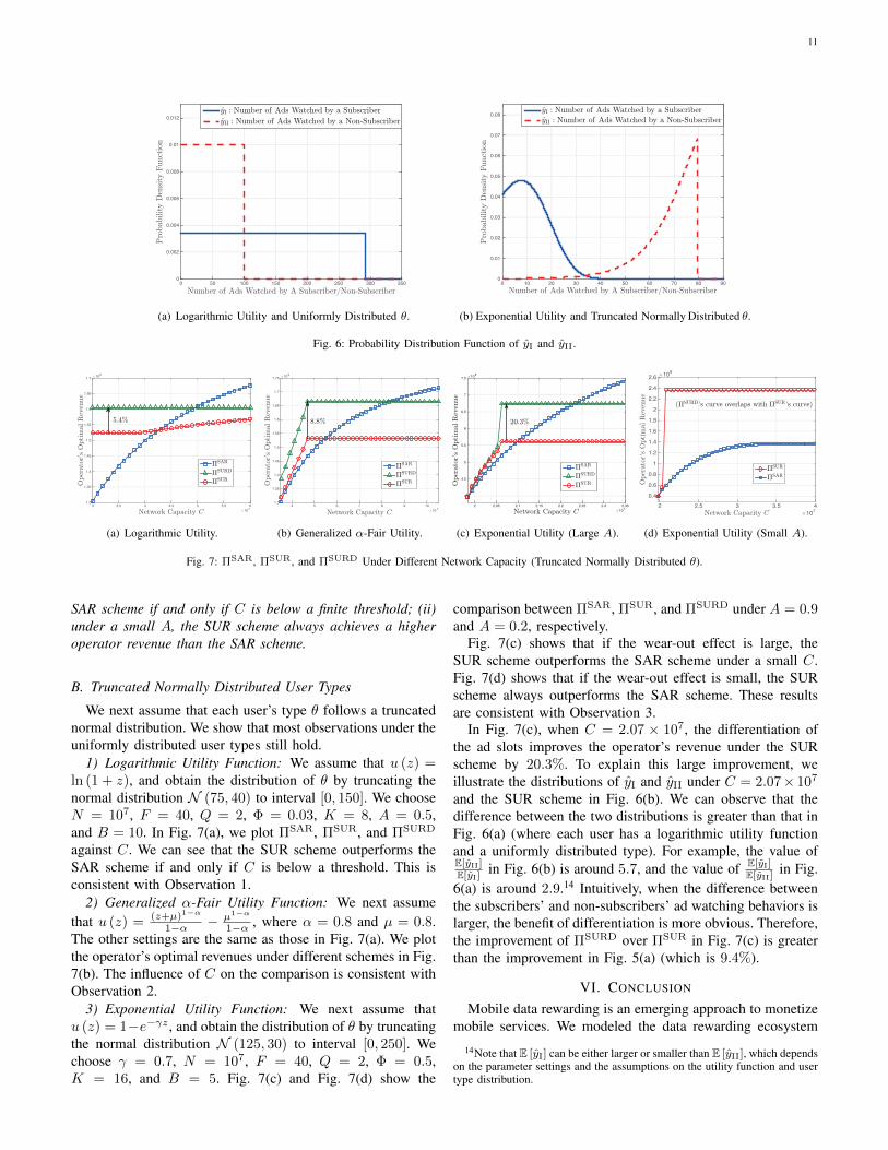
We next assume that each user’s type θ follows a truncatednormal distribution. We show that most observations under theuniformly distributed user types still hold.

1) Logarithmic Utility Function: We assume that u (z) =ln (1 + z), and obtain the distribution of θ by truncating thenormal distribution N (75, 40) to interval [0, 150]. We chooseN = 107, F = 40, Q = 2, Φ = 0.03, K = 8, A = 0.5,and B = 10. In Fig. 7(a), we plot ΠSAR, ΠSUR, and ΠSURD

against C. We can see that the SUR scheme outperforms theSAR scheme if and only if C is below a threshold. This isconsistent with Observation 1.

2) Generalized α-Fair Utility Function: We next assumethat u (z) = (z+µ)1−α

1−α − µ1−α

1−α , where α = 0.8 and µ = 0.8.The other settings are the same as those in Fig. 7(a). We plotthe operator’s optimal revenues under different schemes in Fig.7(b). The influence of C on the comparison is consistent withObservation 2.

3) Exponential Utility Function: We next assume thatu (z) = 1−e−γz , and obtain the distribution of θ by truncatingthe normal distribution N (125, 30) to interval [0, 250]. Wechoose γ = 0.7, N = 107, F = 40, Q = 2, Φ = 0.5,K = 16, and B = 5. Fig. 7(c) and Fig. 7(d) show the

comparison between ΠSAR, ΠSUR, and ΠSURD under A = 0.9and A = 0.2, respectively.

Fig. 7(c) shows that if the wear-out effect is large, theSUR scheme outperforms the SAR scheme under a small C.Fig. 7(d) shows that if the wear-out effect is small, the SURscheme always outperforms the SAR scheme. These resultsare consistent with Observation 3.

In Fig. 7(c), when C = 2.07 × 107, the differentiation ofthe ad slots improves the operator’s revenue under the SURscheme by 20.3%. To explain this large improvement, weillustrate the distributions of yI and yII under C = 2.07× 107

and the SUR scheme in Fig. 6(b). We can observe that thedifference between the two distributions is greater than that inFig. 6(a) (where each user has a logarithmic utility functionand a uniformly distributed type). For example, the value ofE[yII]E[yI]

in Fig. 6(b) is around 5.7, and the value of E[yI]E[yII]

in Fig.6(a) is around 2.9.14 Intuitively, when the difference betweenthe subscribers’ and non-subscribers’ ad watching behaviors islarger, the benefit of differentiation is more obvious. Therefore,the improvement of ΠSURD over ΠSUR in Fig. 7(c) is greaterthan the improvement in Fig. 5(a) (which is 9.4%).

VI. CONCLUSION

Mobile data rewarding is an emerging approach to monetizemobile services. We modeled the data rewarding ecosystem

14Note that E [yI] can be either larger or smaller than E [yII], which dependson the parameter settings and the assumptions on the utility function and usertype distribution.

12

and analyzed an operator’s rewarding scheme. Our resultsreveal that: (i) increasing the unit data reward may decreasethe number of ads watched by the users, and the operatormay not use up its network capacity to reward the users; (ii)under the SUR scheme, the operator can improve its revenueby differentiating the ad slots generated by the subscribers andnon-subscribers; (iii) the operator’s optimal choice between theSAR and SUR schemes is sensitive to the user utility function,network capacity, and advertising’s wear-out effect.

In future work, we plan to first study the operator’s jointoptimization of the data plan and the data rewards. Under theSAR scheme, the operator can reduce the subscription fee tomotivate more users to subscribe and watch ads. Under theSUR scheme, the operator may increase the subscription fee,which (i) extracts more revenue from the users with high θ and(ii) pushes more users with low θ to become non-subscribersand watch ads. Second, we are interested in relaxing theassumptions of a monopolistic operator and homogeneousadvertisers. For example, when there are multiple operators,they will compete for users as well as advertisers, which mayincrease the unit data rewards and reduce the ad prices. Third,we can study a general data rewarding scheme where theoperator can set different unit data rewards for the subscribersand non-subscribers. The SAR and SUR schemes can betreated as two special cases of this general scheme.

REFERENCES

[1] H. Yu, E. Wei, and R. A. Berry, “A business model analysis of mobiledata rewards,” in Proc. of IEEE INFOCOM, Paris, France, 2019, pp.2098–2106.

[2] S. Analytics, “Worldwide cellular user forecasts 2018-2023,” Tech. Rep.,2018.

[3] ——, “Can operator collaboration on sponsored data lead to success?”Tech. Rep., 2018.

[4] eMarketer, https://www.emarketer.com/Article/Want-App-Users-Interact-with-Your-Ads-Reward-Them/1010966, accessed on Nov. 27,2019.

[5] Aquto, http://www.aquto.com/, accessed on Nov. 27, 2019.[6] N. Summers, https://www.engadget.com/2016/06/09/tesco-mobile-

unlockd-lock-screen-ads/, accessed on Nov. 27, 2019.[7] DOCOMO, https://www.nttdocomo.co.jp/english/info/media center/pr/

2017/1225 00.html, accessed on Nov. 27, 2019.[8] R. Johnston, https://www.gizmodo.com.au/2016/11/optus-wants-you-to-

watch-ads-in-return-for-data/, accessed on Nov. 27, 2019.[9] AT&T, https://about.att.com/story/2018/att appnexus.html, accessed on

Nov. 27, 2019.[10] S. Dewing, https://tech.co/news/adwallet-future-advertising-app-2017-

08, accessed on Nov. 27, 2019.[11] J. Naftulin, https://www.businessinsider.com/dscout-research-people-

touch-cell-phones-2617-times-a-day-2016-7, accessed on Nov. 27, 2019.[12] AdStage, “Q3 2018 paid search and paid social benchmark report,” Tech.

Rep., 2018.[13] Ultra Mobile, https://www.ultramobile.com/monthly-plans/, accessed on

Nov. 27, 2019.[14] T. Haselton, https://www.cnbc.com/2018/07/13/unlimited-data-plan-

caps-verizon-att-tmobile-sprint.html, accessed on Nov. 27, 2019.[15] C. Pechmann and D. W. Stewart, “Advertising repetition: A critical re-

view of wearin and wearout,” Current issues and research in advertising,vol. 11, no. 1-2, pp. 285–329, 1988.

[16] A. Kirmani, “Advertising repetition as a signal of quality: If it’sadvertised so much, something must be wrong,” Journal of advertising,vol. 26, no. 3, pp. 77–86, 1997.

[17] C. Joe-Wong, S. Sen, and S. Ha, “Sponsoring mobile data: Analyzingthe impact on internet stakeholders,” IEEE/ACM Transactions on Net-working, vol. 26, no. 3, pp. 1179–1192, 2018.

[18] F. J. Riggins, “Market segmentation and information development costsin a two-tiered fee-based and sponsorship-based web site,” Journal ofManagement Information Systems, vol. 19, no. 3, pp. 69–86, 2002.

[19] H. Yu, M. H. Cheung, L. Gao, and J. Huang, “Public Wi-Fi monetizationvia advertising,” IEEE/ACM Transactions on Networking, vol. 25, no. 4,pp. 2110–2121, 2017.

[20] H. Guo, X. Zhao, L. Hao, and D. Liu, “Economic analysis of rewardadvertising,” Working Paper, 2017.

[21] M. Andrews, U. Ozen, M. I. Reiman, and Q. Wang, “Economic modelsof sponsored content in wireless networks with uncertain demand,” inProc. of IEEE INFOCOM Workshops, Turin, Italy, 2013, pp. 345–350.

[22] M. H. Lotfi, K. Sundaresan, S. Sarkar, and M. A. Khojastepour, “Eco-nomics of quality sponsored data in non-neutral networks,” IEEE/ACMTransactions on Networking, vol. 25, no. 4, pp. 2068–2081, 2017.

[23] L. Zhang, W. Wu, and D. Wang, “Sponsored data plan: A two-class ser-vice model in wireless data networks,” in Proc. of ACM SIGMETRICS,Portland, OR, USA, 2015.

[24] P. Bangera, S. Hasan, and S. Gorinsky, “An advertising revenue modelfor access ISPs,” in Proc. of IEEE ISCC, Heraklion, Greece, 2017.

[25] S. Sen, G. Burtch, A. Gupta, and R. Rill, “Incentive design for ad-sponsored content: Results from a randomized trial,” in Proc. of IEEEINFOCOM Workshops, Atlanta, GA, USA, 2017, pp. 826–831.

[26] M. Harishankar, N. Srinivasan, C. Joe-Wong, and P. Tague, “To acceptor not to accept: The question of supplemental discount offers in mobiledata plans,” in Proc. of IEEE INFOCOM, Honolulu, HI, USA, 2018.

[27] H. Choi, C. Mela, S. Balseiro, and A. Leary, “Online display advertisingmarkets: A literature review and future directions,” Working Paper, 2017.

[28] D. Bergemann and A. Bonatti, “Targeting in advertising markets:implications for offline versus online media,” The RAND Journal ofEconomics, vol. 42, no. 3, pp. 417–443, 2011.

[29] L. Duan, J. Huang, and B. Shou, “Pricing for local and global Wi-Fimarkets,” IEEE Transactions on Mobile Computing, vol. 14, no. 5, pp.1056–1070, 2015.

[30] D. A. Schmidt, C. Shi, R. A. Berry, M. L. Honig, and W. Utschick,“Minimum mean squared error interference alignment,” in Proc. of IEEEACSSC, Pacific Grove, CA, USA, 2009, pp. 1106–1110.

[31] C. Zhou, M. L. Honig, and S. Jordan, “Utility-based power controlfor a two-cell CDMA data network,” IEEE Transactions on WirelessCommunications, vol. 4, no. 6, pp. 2764–2776, 2005.

[32] S. P. Anderson and B. Jullien, “The advertising-financed business modelin two-sided media markets,” in Handbook of media economics, 2015,vol. 1, pp. 41–90.

[33] B. N. Anand and R. Shachar, “Advertising, the matchmaker,” The RANDJournal of Economics, vol. 42, no. 2, pp. 205–245, 2011.

[34] M. C. Campbell and K. L. Keller, “Brand familiarity and advertisingrepetition effects,” Journal of consumer research, vol. 30, no. 2, pp.292–304, 2003.

[35] R. Dewenter, J. Haucap, and T. Wenzel, “On file sharing with indirectnetwork effects between concert ticket sales and music recordings,”Journal of Media Economics, vol. 25, no. 3, pp. 168–178, 2012.

[36] A. Rasch and T. Wenzel, “Piracy in a two-sided software market,”Journal of Economic Behavior & Organization, vol. 88, pp. 78–89, 2013.

[37] H. Yu, G. Iosifidis, B. Shou, and J. Huang, “Pricing for collaborationbetween online apps and offline venues,” IEEE Transactions on MobileComputing, 2019.

[38] Optus, https://www.optus.com.au/shop/mobile/apps/optusxtra, accessedon Nov. 27, 2019.

[39] D. P. Bertsekas, Nonlinear programming. Belmont, MA, USA: AthenaScientific, 1999.

Haoran Yu (S’14-M’17) received the Ph.D. degreefrom the Chinese University of Hong Kong in 2016.During 2015-2016, he was a Visiting Student inthe Yale Institute for Network Science and theDepartment of Electrical Engineering at Yale Uni-versity. During 2018-2019, he was a Post-DoctoralFellow in the Department of Electrical and ComputerEngineering at Northwestern University. His recentresearch interests lie in the field of mechanismdesign for networks. His paper in IEEE INFOCOM2016 was selected as a Best Paper Award finalist and

one of top 5 papers from over 1600 submissions.

13

Ermin Wei is currently an Assistant Professor atthe ECE Dept. of Northwestern University. Shecompleted her PhD studies in Electrical Engineeringand Computer Science at MIT in 2014, advisedby Professor Asu Ozdaglar, where she also ob-tained her M.S.. She received her undergraduatetriple degree in Computer Engineering, Finance andMathematics with a minor in German, from Univer-sity of Maryland, College Park. Wei has receivedmany awards, including the Graduate Women ofExcellence Award, second place prize in Ernst A.

Guillemen Thesis Award and Alpha Lambda Delta National Academic HonorSociety Betty Jo Budson Fellowship. Wei’s research interests include dis-tributed optimization methods, convex optimization and analysis, smart grid,communication systems and energy networks and market economic analysis.

Randall A. Berry (S’93-M’00-SM’12-F’14) re-ceived the Ph.D. degree from the MassachusettsInstitute of Technology in 2000 and joined North-western University, where he is currently the JohnA. Dever Professor and Chair of Electrical andComputer Engineering. Dr. Berry’s research interestsspan topics in network economics, wireless com-munication, computer networking, and informationtheory. He was a recipient of the 2003 CAREERAward from the National Science Foundation. Heserved as an Editor for the IEEE TRANSACTIONS

ON WIRELESS COMMUNICATIONS from 2006 to 2009 and the IEEETRANSACTIONS ON INFORMATION THEORY from 2008 to 2012, aswell as a Guest Editor for special issues of the IEEE JOURNAL ONSELECTED AREAS IN COMMUNICATIONS in 2017, the IEEE JOURNALON SELECTED TOPICS IN SIGNAL PROCESSING in 2008, and the IEEETRANSACTIONS ON INFORMATION THEORY in 2007. He has alsoserved on the program and organizing committees of numerous conferences,including serving as the Co-Chair for the 2012 IEEE Communication TheoryWorkshop and 2010 IEEE ICC Wireless Networking Symposium and the TPCCo-Chair for the 2018 ACM MobiHoc conference.

OutlineAppendix A: Notation Table.Appendix B: Proof of Lemma 1.Appendix C: Proof of Proposition 1.Appendix D: θ2’s Monotonicity with Respect to ω.Appendix E: Proof of Proposition 2.Appendix F: Example of Computing m∗ (ω, p).Appendix G: Proof of Theorem 1.Appendix H: Proof of Proposition 3.Appendix I: Proof of Theorem 2.Appendix J: Proof of Proposition 4.Appendix K: Example WhereE[y]Nad(ω)Decreases with ω.Appendix L: Proof of Lemma 2.Appendix M: Proof of Proposition 5.Appendix N: Proof of Lemma 3.Appendix O: Proof of Theorem 3.Appendix P: Proof of Theorem 4.Appendix Q: Proof of Theorem 5.Appendix R: Numerical Results Under Different Settings.

APPENDIX ANOTATION TABLE

We summarize the key notations in Table II.

APPENDIX BPROOF OF LEMMA 1

Proof. We define function h (θ) as

h (θ) , θu

((u′)

−1(

Φ

ωθ

))− F − Φ

ω

((u′)

−1(

Φ

ωθ

)−Q

).

(24)

First, we compute its derivative. Note that we haveu′(

(u′)−1 ( Φ

ωθ

))= Φ

ωθ . Next, we apply the chain rule to

compute dh(θ)dθ . After the cancellation of the same terms, we

get the following result:

dh (θ)

dθ= u

((u′)

−1(

Φ

ωθ

)). (25)

Note that function u (·) is strictly concave andlimz→∞ u′ (z) = 0. This implies that u′ (·) is a strictlydecreasing function. As a result, (u′)

−1(·), which is

the inverse function of u′ (·), is also a strictly decreasingfunction. Based on this result and the fact that u (·) is a strictlyincreasing function, we can see that dh(θ)

dθ is strictly increasingin θ. Furthermore, when θ = θ1 = Φ

ωu′(Q) , the value ofdh(θ)dθ is given by dh(θ)

dθ = u(

(u′)−1

(u′ (Q)))

= u (Q).Since u (0) = 0, Q > 0, and u (·) is strictly increasing, wecan conclude that dh(θ)

dθ |θ=θ1 > 0. Hence, dh(θ)dθ > 0 for

θ ≥ θ1 = Φωu′(Q) .

Second, we compute h (θ1). By substituting θ1 = Φωu′(Q)

into h (θ), we have

h (θ1) =Φ

ωu′ (Q)u (Q)− F. (26)

14

TABLE II: Key Notations.

ParametersF > 0 Subscription fee of data planQ > 0 Amount of data included in data planN > 0 Mass of usersΦ > 0 A user’s disutility of watching one adK > 0 Number of advertisersA ≥ 0, B > 0 Coefficients in (2) capturing advertis-

ing’s effectiveness. A is the degree ofwear-out effect.

C ≥ D (0) Network capacityDecision Variables

ω ∈ [0,∞) Operator’s unit data rewardp ∈ (0,∞) Operator’s ad pricer ∈ {0, 1} A user’s subscription decisionx ∈ [0,∞) Number of ads that a user watchesm ∈ [0,∞) Number of ad slots that an advertiser

purchasesRandom Variables

θ ∈ [0, θmax] A user’s valuation for mobile servicey Number of ads watched by a user who

chooses to watch ads (i.e., x∗(θ, ω)>0)Functions

g (θ) Probability density function of θu (·) A user’s utility functionΠuser (θ, r, x, ω) A type-θ user’s payoff functionNad (ω) Mass of users who watch ads (i.e., with

x∗ (θ, ω) > 0)Πad (m,ω, p) An advertiser’s payoff functionRdata (ω) Operator’s revenue from data marketRad (ω, p) Operator’s ad revenueRtotal (ω, p) Operator’s total revenueD (ω) Total data demand

Other NotationsΠSAR Operator’s optimal total revenue under

SAR schemeΠSUR, ΠSURD Operator’s optimal total revenues under

SUR scheme. ΠSUR: no ad slot differ-entiation; ΠSURD: with ad slot differen-tiation.

When ω > Φu(Q)Fu′(Q) , we can see that h (θ1) < 0.

Third, we compute h (θ0). By substituting θ0 = Fu(Q) into

h (θ), we have

h (θ0) =F

u (Q)u

((u′)

−1(

Φu (Q)

ωF

))− F

− Φ

ω

((u′)

−1(

Φu (Q)

ωF

)−Q

). (27)

Next, we compare h (θ0) with 0. We define a new function

∆ (F ) as follows:

∆ (F ) =F

u (Q)u

((u′)

−1(

Φu (Q)

ωF

))− F

− Φ

ω

((u′)

−1(

Φu (Q)

ωF

)−Q

). (28)

We can compute ∆(

Φu(Q)ωu′(Q)

)= ∆ (F ) |

F=Φu(Q)

ωu′(Q)

as

∆

(Φu (Q)

ωu′ (Q)

)=

Φ

ωu′ (Q)u(

(u′)−1

(u′ (Q)))

− Φu (Q)

ωu′ (Q)− Φ

ω

((u′)

−1(u′ (Q))−Q

)=

Φu (Q)

ωu′ (Q)− Φu (Q)

ωu′ (Q)= 0. (29)

Then, we analyze d∆(F )dF . We compute d∆(F )

dF as follows:

d∆ (F )

dF=

1

u (Q)u

((u′)

−1(

Φu (Q)

ωF

))− 1. (30)

Recall that u (·) is strictly increasing and (u′)−1

(·) is strictlydecreasing. Hence, d∆(F )

dF is strictly increasing in F . More-over, we can compute d∆(F )

dF |F=Φu(Q)

ωu′(Q)

as d∆(F )dF |F=

Φu(Q)

ωu′(Q)

=

1u(Q)u

((u′)

−1(u′ (Q))

)− 1 = 0. Therefore, we can see

that d∆(F )dF is zero when F = Φu(Q)

ωu′(Q) and is positive when

F > Φu(Q)ωu′(Q) . Combining this result and ∆ (F ) |

F=Φu(Q)

ωu′(Q)

= 0

in (29), we can conclude that ∆ (F ) > 0 for F > Φu(Q)ωu′(Q) .

Because ∆ (F ) equals h (θ0), we have h (θ0) > 0 whenω > Φu(Q)

Fu′(Q) .

When ω > Φu(Q)Fu′(Q) , we have proved that dh(θ)

dθ > 0 forθ ≥ θ1, h (θ1) < 0, and h (θ0) > 0. Hence, there exists aunique θ2 ∈ (θ1, θ0) satisfying h (θ2) = 0.

APPENDIX CPROOF OF PROPOSITION 1

Proof. Step 1: We analyze Case A, i.e., ω ∈[0, Φ

u′(Q)θmax

].

Suppose a type-θ user subscribes to the data plan, i.e., r = 1.Its payoff is Πuser (θ, 1, x, ω) = θu (Q+ ωx)− F − Φx. Wecan see that

∂Πuser (θ, 1, x, ω)

∂x= θωu′ (Q+ ωx)− Φ

≤ u′ (Q+ ωx) θ

u′ (Q) θmaxΦ− Φ. (31)

Since u′ (·) is a strictly decreasing function, we haveu′ (Q+ ωx) < u′ (Q) for x > 0. Hence, ∂Πuser(θ,1,x,ω)

∂x < 0for x > 0. This implies that if a user subscribes to the dataplan, it will not watch any ad for rewards. In this case, theuser’s payoff is θu (Q)− F .

Suppose a type-θ user does not subscribe, i.e., r = 0. Underthe SAR scheme, the user cannot watch ads for the rewards.Hence, its payoff is 0.

Comparing θu (Q) − F and 0, we can see that a usersubscribes if and only if θ ≥ θ0 = F

u(Q) . Moreover, a user

15

with any θ ∈ [0, θmax] will not watch ads. That is to say, wehave

r∗ (θ, ω) = 1{θ≥θ0}, x∗ (θ, ω) = 0, θ ∈ [0, θmax] . (32)

Step 2: We analyze Case B, i.e., ω ∈(

Φu′(Q)θmax

, Φu(Q)Fu′(Q)

].

Suppose a type-θ user subscribes to the data plan, i.e., r = 1.Its payoff is Πuser (θ, 1, x, ω) = θu (Q+ ωx) − F − Φx. Bychecking ∂Πuser(θ,1,x,ω)

∂x , we can see the following result:

(i) If θ ∈[0, Φ

ωu′(Q)

), the user will not watch ads (i.e.,

x = 0), and its payoff will be θu (Q)− F ;

(ii) If θ ∈[

Φωu′(Q) , θmax

], the user will choose x =

1ω

((u′)

−1 ( Φωθ

)−Q

). Since θ ≥ Φ

ωu′(Q) , the value of1ω

((u′)

−1 ( Φωθ

)−Q

)is non-negative. Then, we can see that

the user’s payoff satisfies

Πuser

(θ, 1,

1

ω

((u′)

−1(

Φ

ωθ

)−Q

), ω

)≥Πuser (θ, 1, 0, ω)

=θu (Q)− F.(33)

Since ω ≤ Φu(Q)Fu′(Q) , we have Φ

ωu′(Q) ≥F

u(Q) . Hence, fora user with θ ≥ Φ

ωu′(Q) , its payoff under r = 1 and x =

1ω

((u′)

−1 ( Φωθ

)−Q

)is non-negative.

Suppose a type-θ user does not subscribe, i.e., r = 0. Underthe SAR scheme, the user cannot watch ads for the rewardsand its payoff is 0.

Next, we can compare the choices of r = 1 and r = 0. Re-call that Φ

ωu′(Q) ≥F

u(Q) . We discuss the choices of users with

θ ∈[0, F

u(Q)

), θ ∈

[F

u(Q) ,Φ

ωu′(Q)

), and θ ∈

[Φ

ωu′(Q) , θmax

),

separately. If θ ∈[0, F

u(Q)

), the user has a higher payoff

under r = 0. As discussed above, it cannot watch ads. Ifθ ∈

[F

u(Q) ,Φ

ωu′(Q)

), the user has a higher payoff under

r = 1, and it will not watch ads. If θ ∈[

Φωu′(Q) , θmax

),

the user has a higher payoff under r = 1, and it will choosex = 1

ω

((u′)

−1 ( Φωθ

)−Q

). Recall that we define θ0 = F

u(Q)

and θ1 = Φωu′(Q) . We can conclude that the following result

holds for θ ∈ [0, θmax]:

r∗ (θ, ω)=1{θ≥θ0}, x∗(θ, ω)=

1

ω

((u′)

−1(

Φ

ωθ

)−Q

)1{θ≥θ1}.

(34)

Step 3: We analyze Case C, i.e., ω ∈(

Φu(Q)Fu′(Q) ,∞

).

Suppose a type-θ user subscribes to the data plan, i.e., r = 1.Its payoff is Πuser (θ, 1, x, ω) = θu (Q+ ωx) − F − Φx. Bychecking ∂Πuser(θ,1,x,ω)

∂x , we can see the following result:

(i) If θ ∈[0, Φ

ωu′(Q)

), the user will not watch ads (i.e.,

x = 0), and its payoff will be θu (Q)− F ;

(ii) If θ ∈[

Φωu′(Q) , θmax

], the user will choose x =

1ω

((u′)

−1 ( Φωθ

)−Q

). Since θ ≥ Φ

ωu′(Q) , the value of1ω

((u′)

−1 ( Φωθ

)−Q

)is non-negative. The user’s correspond-

ing payoff is given by

Πuser (θ, 1, x, ω) =θu

((u′)

−1(

Φ

ωθ

))− F

− Φ

ω

((u′)

−1(

Φ

ωθ

)−Q

)(35)

Suppose a type-θ user does not subscribe, i.e., r = 0. Underthe SAR scheme, the user cannot watch ads for the rewardsand its payoff is 0.

Next, we can compare the choices of r = 1 and r = 0. Sinceω > Φu(Q)

Fu′(Q) , we have Φωu′(Q) <

Fu(Q) . If θ ∈

[0, Φ

ωu′(Q)

), the

user has a higher payoff under r = 0, and it cannot watch ads.If θ ∈

[Φ

ωu′(Q) , θ2

), we can see the following relation based

on our proof in Appendix B:

θu

((u′)

−1(

Φ

ωθ

))− F − Φ

ω

((u′)

−1(

Φ

ωθ

)−Q

)< 0.

(36)

The left side is the value of Πuser (θ, 1, x, ω) in (35). Theinequality implies that the user has a higher payoff under r =0. In this case, it cannot watch ads.

If θ ∈ [θ2, θmax], we can see the following relation basedon our proof in Appendix B:

θu

((u′)

−1(

Φ

ωθ

))− F − Φ

ω

((u′)

−1(

Φ

ωθ

)−Q

)≥ 0.

(37)

This implies that the user has a higher payoff under r = 1.In this case, it chooses x = 1

ω

((u′)

−1 ( Φωθ

)−Q

). We can

conclude that the following result holds for θ ∈ [0, θmax]:

r∗(θ, ω)=1{θ≥θ2}, x∗(θ, ω)=

1

ω

((u′)

−1(

Φ

ωθ

)−Q

)1{θ≥θ2}.

(38)

Hence, we have proved r∗ (θ, ω) and x∗ (θ, ω) for Case A,Case B, and Case C.

APPENDIX Dθ2’S MONOTONICITY WITH RESPECT TO ω

We prove that in Case C, θ2 decreases as ω increases.

Proof. Based on θ2’s definition, we have

θ2u

((u′)

−1(

Φ

ωθ2

))− F − Φ

ω

((u′)

−1(

Φ

ωθ2

)−Q

)= 0.

(40)

For both sides of the equation, we take their derivatives withrespect to ω, and get equation (39). After rearrangement, wehave the following equation:

dθ2

dωu

((u′)

−1(

Φ

ωθ2

))+

Φ

ω2

((u′)

−1(

Φ

ωθ2

)−Q

)= 0.

(41)

16

dθ2

dωu

((u′)

−1(

Φ

ωθ2

))+θ2u

′(

(u′)−1(

Φ

ωθ2

)) d(

(u′)−1(

Φωθ2

))dω

+Φ

ω2

((u′)

−1(

Φ

ωθ2

)−Q

)−Φ

ω

d(

(u′)−1(

Φωθ2

))dω

= 0.

(39)

Hence, we can get the expression of dθ2dω as follows:

dθ2

dω=

Φω2

(Q− (u′)

−1(

Φωθ2

))u(

(u′)−1(

Φωθ2

)) . (42)

Based on θ2’s definition, we have θ2 > θ1 = Φωu′(Q) .

Recall that (u′)−1

(·) is strictly decreasing. We can see that(u′)

−1(

Φωθ2

)> (u′)

−1(

Φωθ1

)= Q. As a result, the value

of Φω2

(Q− (u′)

−1(

Φωθ2

))is negative, and the value of

u(

(u′)−1(

Φωθ2

))is positive. Therefore, we can conclude that

dθ2dω < 0.

APPENDIX EPROOF OF PROPOSITION 2

Proof. First, we consider the case where Nad (ω) = 0, i.e.,the mass of users watching ads is zero. Based on the advertiserpayoff’s definition, Πad (m,ω, p) = −mp. Since p > 0, noneof the advertisers will purchase the ad slots, i.e., m∗ (ω, p) =0.

Second, we consider the case where Nad (ω) > 0. Anadvertiser’s payoff is

Πad (m,ω, p) =

Ey

[B

my

E [y]Nad (ω)−A

(my

E [y]Nad (ω)

)2]Nad (ω)−mp.

(43)

After rearrangement, we have

Πad (m,ω, p) = − A

Nad (ω)

E[y2]

(E [y])2m

2 + (B − p)m, (44)

which is a quadratic function of m ≥ 0. We can easily seethat

m∗ (ω, p) = max

{(B − p)Nad (ω) (E [y])

2

2AE [y2], 0

}. (45)

Combining the analysis for Nad (ω) = 0 and Nad (ω) > 0,we can see the following result: If Nad (ω) = 0 or p ≥ B, thenm∗ (ω, p) = 0; otherwise, m∗ (ω, p) = B−p

2A(E[y])2

E[y2] Nad (ω).

APPENDIX FEXAMPLE OF COMPUTING m∗ (ω, p)

In this section, we assume that each user has a logarithmicutility function, i.e., u (z) = ln (1 + z), and a uniformlydistributed type, i.e., θ ∼ U [0, θmax]. We compute the value ofNad (ω), the distribution of y, and the expression of m∗ (ω, p)when ω satisfies Case A, Case B, and Case C.

Step 1: We consider Case A. Since u (z) = ln (1 + z), thecondition of ω in Case A becomes ω ∈

[0, (1+Q)Φ

θmax

]. In this

case, there is no user watching ads. Hence, Nad (ω) = 0. FromProposition 2, we have m∗ (ω, p) = 0.

Step 2: We consider Case B. Since u (z) =ln (1 + z), the condition of ω in Case B becomesω ∈

((1+Q)Φθmax

, ΦF (1 +Q) ln (1 +Q)

]. Based on Proposition

1, the users’ ad watching decisions in Case B are characterizedby the following equation:

x∗ (θ, ω) =1

ω

((u′)

−1(

Φ

ωθ

)−Q

)1{θ≥θ1}

(a)=

1

ω

(θω

Φ− 1−Q

)1{θ≥θ1}

(b)=θ − θ1

Φ1{θ≥θ1}. (46)

Here, equality (a) is due to u (z) = ln (1 + z), and equality (b)is due to θ1 = Φ(1+Q)

ω in Case B. Hence, only the users withθ ≥ θ1 watch ads. Because θ ∼ U [0, θmax], we can computeNad (ω) as follows:

Nad (ω) =θmax − θ1

θmaxN. (47)

Moreover, according to (46) and the fact that θ ∼ U [0, θmax],we can see that the number of ads watched by one of theNad (ω) users is uniformly distributed in

[0, θmax−θ1

Φ

]. This

implies that y is uniformly distributed in[0, θmax−θ1

Φ

]. Then,

we can compute E [y] and E[y2]

as follows:

E [y] =1

2

θmax − θ1

Φ,E[y2]

=1

3

(θmax − θ1

Φ

)2

. (48)

Based on Proposition 2, we can derive m∗ (ω, p)’s expressionas

m∗ (ω, p) =3

8

max {B − p, 0}A

θmax − θ1

θmaxN. (49)

Step 3: We consider Case C. Since u (z) =ln (1 + z), the condition of ω in Case C becomesω ∈

(ΦF (1 +Q) ln (1 +Q) ,∞

). Based on Proposition 1, the

users’ ad watching decisions in Case C are characterized bythe following equation:

x∗ (θ, ω) =1

ω

((u′)

−1(

Φ

ωθ

)−Q

)1{θ≥θ2}

=θ − θ1

Φ1{θ≥θ2}. (50)

Hence, only the users with θ ≥ θ2 watch ads. Because θ ∼U [0, θmax], we can compute Nad (ω) as follows:

Nad (ω) =θmax − θ2

θmaxN. (51)

17

Moreover, according to (50) and the fact that θ ∼ U [0, θmax],we can see that the number of ads watched by one of theNad (ω) users is uniformly distributed in

[θ2−θ1

Φ , θmax−θ1Φ

].

This means that y is uniformly distributed in[θ2−θ1

Φ , θmax−θ1Φ

].

Then, we can compute E [y] and E[y2]

as follows:

E [y] =θ2 − θ1 + θmax − θ1

2Φ, (52)

E[y2]

=

(θ2 − θ1 + θmax − θ1

2Φ

)2

+

(θmax−θ1−(θ2−θ1)

Φ

)2

12.

(53)

To simplify the presentation, we let λa , θ2 − θ1 and λb ,θmax − θ1. We can further have the following result:

(E [y])2

E [y2]=

(λa+λb

2Φ

)2(λa+λb

2Φ

)2+ 1

12

(λb−λa

Φ

)2=

3 (λa + λb)2

3 (λa + λb)2

+ (λb − λa)2 . (54)

Based on Proposition 2, we can derive m∗ (ω, p)’s expressionas

m∗ (ω, p)

=max {B − p, 0}

2A

3 (λa + λb)2

3 (λa + λb)2

+ (λb − λa)2

θmax − θ2

θmaxN

=max {B − p, 0}

2A

3 (λa + λb)2

4λ2a + 4λ2

b + 4λaλb

λb − λaθmax

N

=3 max {B − p, 0}

8A

N

θmax

(λa + λb)2

λ2a + λ2

b + λaλb

(λb − λa)2

λb − λa

=3 max {B − p, 0}

8A

N

θmax

(λ2b − λ2

a

)2λ3b − λ3

a

=3

8

max {B − p, 0}A

N

θmax

((θmax − θ1)

2 − (θ2 − θ1)2)2

(θmax − θ1)3 − (θ2 − θ1)

3 .

(55)

This completes our analysis of m∗ (ω, p) under three caseswhen u (z) = ln (1 + z) and θ ∼ U [0, θmax].

APPENDIX GPROOF OF THEOREM 1

Proof. First, we consider the case where ω ∈[0, Φ

u′(Q)θmax

].

According to Proposition 1, no user watches ads, i.e.,Nad (ω) = 0. From Proposition 2, we can see that m∗ (ω, p) =0 for any p > 0. This means that the operator’s ad revenueRad (ω, p) is zero, regardless of the ad price. Hence, allpositive prices lead to the same ad revenue, and any positiveprice is optimal.

Second, we consider the case where ω ∈(

Φu′(Q)θmax

,∞)

.From Proposition 1, the number of users watching ads ispositive, i.e., Nad (ω) > 0. If p ≥ B, the value of m∗ (ω, p)is zero based on Proposition 2. In this situation, the valueof Rad (ω, p) is also zero. If p < B, we have m∗ (ω, p) =B−p2A

(E[y])2

E[y2] Nad (ω). Then, when ω is given, the operator’s

problem of deciding p can be rewritten as follows:

maxp>0

KB − p

2A

(E [y])2

E [y2]Nad (ω) p (56)

s.t. KB − p

2A

(E [y])2

E [y2]Nad (ω) ≤ E [y]Nad (ω) . (57)

After rearrangement, the problem becomes:

maxp>0

KB − p

2A

(E [y])2

E [y2]Nad (ω) p (58)

s.t. p ≥ B −2AE

[y2]

KE [y]. (59)

The objective function is quadratic in p and achieves themaximum value at p = B

2 . Hence, we can see that the optimalprice under a given ω is given by

p∗ (ω) = max

{B

2, B −

2AE[y2]

KE [y]

}. (60)

APPENDIX HPROOF OF PROPOSITION 3

Proof. Step 1: We analyze the monotonicity of D (ω) in threecases.

First, when ω ∈[0, Φ

u′(Q)θmax

], the value of D (ω) is given

by

D (ω) = NQ

∫ θmax

θ0

g (θ) dθ = NQ

∫ θmax

Fu(Q)

g (θ) dθ, (61)

which is independent of ω.Second, when ω ∈

(Φ

u′(Q)θmax, Φu(Q)Fu′(Q)

], the expression of

D (ω) is given by

D (ω) =NQ

∫ θmax

Fu(Q)

g (θ) dθ

+N

∫ θmax

Φωu′(Q)

((u′)

−1(

Φ

ωθ

)−Q

)g (θ) dθ. (62)

Based on Leibniz’s rule, we can further compute dD(ω)dω as

follows:

dD (ω)

dω= N

∫ θmax

Φωu′(Q)

d(

(u′)−1 ( Φ

ωθ

))dω

g (θ) dθ

−Nd(

Φωu′(Q)

)dω

((u′)

−1

(Φ

ω Φωu′(Q)

)−Q

)g

(Φ

ωu′ (Q)

)

= N

∫ θmax

Φωu′(Q)

d(

(u′)−1 ( Φ

ωθ

))dω

g (θ) dθ. (63)

From our proof in Lemma 1, function (u′)−1

(·) is strictly

decreasing. Hence,d((u′)

−1( Φωθ )

)dω is positive. This implies that

dD(ω)dω is positive.

18

Third, when ω ∈(

Φu(Q)Fu′(Q) ,∞

), the expression of D (ω) is

given by

D (ω) =NQ

∫ θmax

θ2

g (θ) dθ

+N

∫ θmax

θ2

((u′)

−1(

Φ

ωθ

)−Q

)g (θ) dθ. (64)

We can further compute dD(ω)dω as follows:

dD (ω)

dω=−NQg (θ2)

dθ2

dω+N

∫ θmax

θ2

d(

(u′)−1 ( Φ

ωθ

))dω

g (θ)dθ

−N(

(u′)−1(

Φ

ωθ2

)−Q

)g (θ2)

dθ2

dω. (65)

From our proof in Appendix D, we have dθ2dω < 0. Hence, the

first term in the right side of (65) is positive. Since function

(u′)−1

(·) is strictly decreasing, we haved((u′)

−1( Φωθ )

)dω > 0.

Hence, the second term in the right side of (65) is positive.Furthermore, from the definition of θ2, we have θ2 > θ1 =

Φωu′(Q) . As a result, the value of (u′)

−1(

Φωθ2

)−Q is positive.

Considering that dθ2dω < 0, the third term in the right side of

(65) is positive. Based on the above analysis, we can see thatdD(ω)dω > 0.Step 2: We analyze the continuity of D (ω). Since u (·)

is twice differentiable, we can see that D (ω) is continuousfor ω ∈

[0, Φ

u′(Q)θmax

), ω ∈

(Φ

u′(Q)θmax, Φu(Q)Fu′(Q)

), and ω ∈(

Φu(Q)Fu′(Q) ,∞

), based on (61), (62), and (64). Next, we analyze

the continuity of D (ω) at ω = Φu′(Q)θmax

and ω = Φu(Q)Fu′(Q) .

When ω = Φu′(Q)θmax

, the value of Φωu′(Q) equals θmax.

Based on (62), we can compute limω↘ Φu′(Q)θmax

D (ω) as

limω↘ Φ

u′(Q)θmax

D (ω) = NQ

∫ θmax

Fu(Q)

g (θ) dθ.

From (61), we can see that this equals D (ω) |ω= Φu′(Q)θmax

.Based on (61), we can also see that limω↗ Φ

u′(Q)θmax

D (ω) =

D (ω) |ω= Φu′(Q)θmax

. Hence, D (ω) is continuous at ω =Φ

u′(Q)θmax.

Then, we analyze the continuity of D (ω) at ω = Φu(Q)Fu′(Q) .

Recall that θ0 = Fu(Q) and θ1 = Φ

ωu′(Q) . We can see thatlim

ω↘ Φu(Q)

Fu′(Q)

θ1 = θ0. According to the definition of θ2,

we have θ2 ∈ (θ1, θ0). Hence, we have the relation thatlim

ω↘ Φu(Q)

Fu′(Q)

θ2 = limω↘ Φu(Q)

Fu′(Q)

θ1 = θ0. Based on thisrelation, (62), and (64), we can derive the following equation:

limω↘ Φu(Q)

Fu′(Q)

D (ω) = D (ω) |ω=

Φu(Q)

Fu′(Q)

. (66)

From (62), we can also see that limω↗ Φu(Q)

Fu′(Q)

D (ω) =

D (ω) |ω=

Φu(Q)

Fu′(Q)

. Therefore, D (ω) is continuous at ω =

Φu(Q)Fu′(Q) .

The above analysis shows that D (ω) is continuous for ω ≥0.

Step 3: We prove that limω→∞D (ω) =∞.First, we analyze limω→∞ (u′)

−1 ( Φωθ

). Recall that u (·) is

strictly concave and limz→∞ u′ (z) = 0. We can see that as zincreases from 0 to ∞, the value of u′ (z) strictly decreasesfrom u′ (0) to 0. Hence, as z increases from 0 to u′ (0), thevalue of (u′)

−1(z) strictly decreases from ∞ to 0. Hence,

we have limz→0 (u′)−1

(z) = ∞. This implies the followingrelation:

limω→∞

(u′)−1(

Φ

ωθ

)=∞. (67)

When ω > Φu(Q)Fu′(Q) , we can derive the following inequality

from (64):

D (ω) > N

∫ θmax

θ0

((u′)

−1(

Φ

ωθ

)−Q

)g (θ) dθ.

Recall that θ0 = Fu(Q) , which is independent of ω. From

(67), we can see that when ω → ∞, the right side of (68)approaches infinity. Therefore, we have limω→∞D (ω) =∞.

So far, we have shown that (i) D (ω) is continuousin ω ∈ [0,∞); (ii) D (ω) does not change with ω forω ∈

[0, Φ

u′(Q)θmax

], and strictly increases with ω for ω ∈(

Φu′(Q)θmax

,∞)

; (iii) when ω approaches infinity, D (ω)

approaches infinity. Therefore, we can conclude that givenC ≥ D (0), there is a unique ω ∈

[Φ

u′(Q)θmax,∞)

such thatD (ω) = C. Furthermore, this ω strictly increases with C.

APPENDIX IPROOF OF THEOREM 2

Proof. Step 1: We analyze the case where C = D (0). Fromconstraint D (ω) ≤ C, we can see that ω needs to satisfy0 ≤ ω ≤ Φ

u′(Q)θmax. Based on Proposition 1, no user watches

ads in this case. As a result, the value of Nad (ω) is zero. FromProposition 2, the value of m∗ (ω, p) is also zero. Based on(14)-(16), we can easily see that the operator’s problem ofdeciding ω becomes:

maxω∈[0, Φu′(Q)θmax

]Rdata (ω) , (68)

where Rdata (ω) equals NF∫ θmax

Fu(Q)

g (θ) dθ and is indepen-dent of ω. Therefore, when C = D (0), any ω from set[0, Φ

u′(Q)θmax

]is optimal.

Next, we show that when C = D (0), the value of D−1 (C)

is in the set[0, Φ

u′(Q)θmax

]. According to the definition of

D−1 (C) in Proposition 3, D−1 (C) takes the value from set[Φ

u′(Q)θmax,∞)

. Since D (0) = D(

Φu′(Q)θmax

), when C =

D (0), the value of D−1 (C) is Φu′(Q)θmax

. Therefore, the value

of D−1 (C) is in the set[0, Φ

u′(Q)θmax

], and ω = D−1 (C) is

one optimal solution to the operator’s problem.Step 2: We analyze the case where C > D (0). First, we

prove that ω∗ should lie in the interval(

Φu′(Q)θmax

, D−1 (C)].

If ω ∈[0, Φ

u′(Q)θmax

], no user watches ads (from our analysis

in Step 1). The operator’s revenue only consists of the revenue

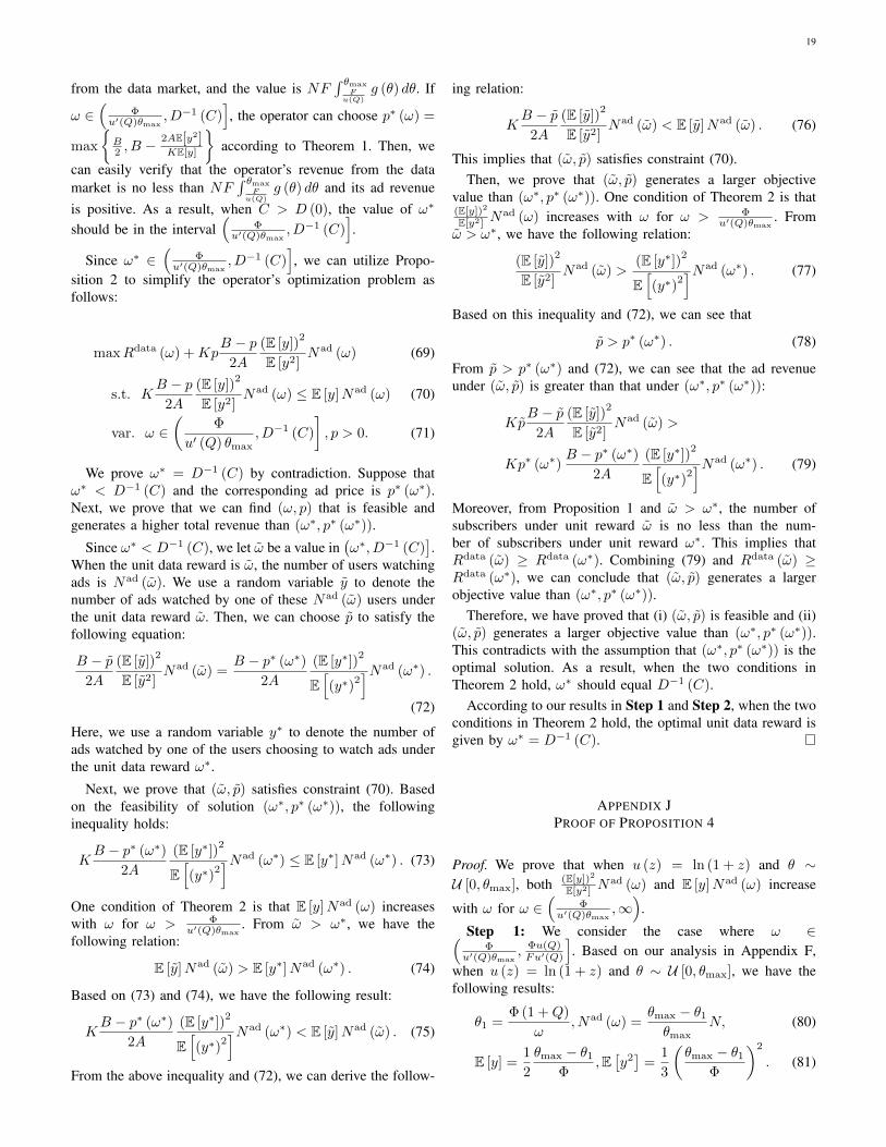
19

from the data market, and the value is NF∫ θmax

Fu(Q)

g (θ) dθ. If

ω ∈(

Φu′(Q)θmax

, D−1 (C)], the operator can choose p∗ (ω) =

max

{B2 , B −

2AE[y2]KE[y]

}according to Theorem 1. Then, we

can easily verify that the operator’s revenue from the datamarket is no less than NF

∫ θmaxF

u(Q)g (θ) dθ and its ad revenue

is positive. As a result, when C > D (0), the value of ω∗

should be in the interval(

Φu′(Q)θmax

, D−1 (C)].

Since ω∗ ∈(

Φu′(Q)θmax

, D−1 (C)], we can utilize Propo-

sition 2 to simplify the operator’s optimization problem asfollows:

maxRdata (ω) +KpB − p

2A

(E [y])2

E [y2]Nad (ω) (69)

s.t. KB − p

2A

(E [y])2

E [y2]Nad (ω) ≤ E [y]Nad (ω) (70)

var. ω ∈(

Φ

u′ (Q) θmax, D−1 (C)

], p > 0. (71)

We prove ω∗ = D−1 (C) by contradiction. Suppose thatω∗ < D−1 (C) and the corresponding ad price is p∗ (ω∗).Next, we prove that we can find (ω, p) that is feasible andgenerates a higher total revenue than (ω∗, p∗ (ω∗)).

Since ω∗ < D−1 (C), we let ω be a value in(ω∗, D−1 (C)

].

When the unit data reward is ω, the number of users watchingads is Nad (ω). We use a random variable y to denote thenumber of ads watched by one of these Nad (ω) users underthe unit data reward ω. Then, we can choose p to satisfy thefollowing equation:

B − p2A

(E [y])2

E [y2]Nad (ω) =

B − p∗ (ω∗)

2A

(E [y∗])2

E[(y∗)

2]Nad (ω∗) .

(72)

Here, we use a random variable y∗ to denote the number ofads watched by one of the users choosing to watch ads underthe unit data reward ω∗.

Next, we prove that (ω, p) satisfies constraint (70). Basedon the feasibility of solution (ω∗, p∗ (ω∗)), the followinginequality holds:

KB − p∗ (ω∗)

2A

(E [y∗])2

E[(y∗)

2]Nad (ω∗) ≤ E [y∗]Nad (ω∗) . (73)

One condition of Theorem 2 is that E [y]Nad (ω) increaseswith ω for ω > Φ

u′(Q)θmax. From ω > ω∗, we have the

following relation:

E [y]Nad (ω) > E [y∗]Nad (ω∗) . (74)

Based on (73) and (74), we have the following result:

KB − p∗ (ω∗)

2A

(E [y∗])2

E[(y∗)

2]Nad (ω∗) < E [y]Nad (ω) . (75)

From the above inequality and (72), we can derive the follow-

ing relation:

KB − p

2A

(E [y])2

E [y2]Nad (ω) < E [y]Nad (ω) . (76)

This implies that (ω, p) satisfies constraint (70).Then, we prove that (ω, p) generates a larger objective

value than (ω∗, p∗ (ω∗)). One condition of Theorem 2 is that(E[y])2

E[y2] Nad (ω) increases with ω for ω > Φ

u′(Q)θmax. From

ω > ω∗, we have the following relation:

(E [y])2

E [y2]Nad (ω) >

(E [y∗])2

E[(y∗)

2]Nad (ω∗) . (77)

Based on this inequality and (72), we can see that

p > p∗ (ω∗) . (78)

From p > p∗ (ω∗) and (72), we can see that the ad revenueunder (ω, p) is greater than that under (ω∗, p∗ (ω∗)):

KpB − p

2A

(E [y])2

E [y2]Nad (ω) >

Kp∗ (ω∗)B − p∗ (ω∗)

2A

(E [y∗])2

E[(y∗)

2]Nad (ω∗) . (79)

Moreover, from Proposition 1 and ω > ω∗, the number ofsubscribers under unit reward ω is no less than the num-ber of subscribers under unit reward ω∗. This implies thatRdata (ω) ≥ Rdata (ω∗). Combining (79) and Rdata (ω) ≥Rdata (ω∗), we can conclude that (ω, p) generates a largerobjective value than (ω∗, p∗ (ω∗)).

Therefore, we have proved that (i) (ω, p) is feasible and (ii)(ω, p) generates a larger objective value than (ω∗, p∗ (ω∗)).This contradicts with the assumption that (ω∗, p∗ (ω∗)) is theoptimal solution. As a result, when the two conditions inTheorem 2 hold, ω∗ should equal D−1 (C).

According to our results in Step 1 and Step 2, when the twoconditions in Theorem 2 hold, the optimal unit data reward isgiven by ω∗ = D−1 (C).

APPENDIX JPROOF OF PROPOSITION 4

Proof. We prove that when u (z) = ln (1 + z) and θ ∼U [0, θmax], both (E[y])2

E[y2] Nad (ω) and E [y]Nad (ω) increase

with ω for ω ∈(

Φu′(Q)θmax

,∞)

.

Step 1: We consider the case where ω ∈(Φ

u′(Q)θmax, Φu(Q)Fu′(Q)

]. Based on our analysis in Appendix F,

when u (z) = ln (1 + z) and θ ∼ U [0, θmax], we have thefollowing results:

θ1 =Φ (1 +Q)

ω,Nad (ω) =

θmax − θ1

θmaxN, (80)

E [y] =1

2

θmax − θ1

Φ,E[y2]

=1

3

(θmax − θ1

Φ

)2

. (81)

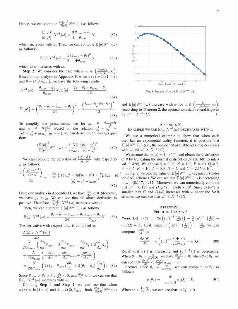
20

Hence, we can compute (E[y])2

E[y2] Nad (ω) as follows:

(E [y])2

E [y2]Nad (ω) =

3

4

θmax − θ1

θmaxN, (82)

which increases with ω. Then, we can compute E [y]Nad (ω)as follows:

E [y]Nad (ω) =1

2

(θmax − θ1)2

ΦθmaxN, (83)

which also increases with ω.Step 2: We consider the case where ω ∈

(Φu(Q)Fu′(Q) ,∞

).

Based on our analysis in Appendix F, when u (z) = ln (1 + z)and θ ∼ U [0, θmax], we have the following results:

Nad (ω) =θmax − θ2

θmaxN,E [y] =

θ2 − θ1 + θmax − θ1

2Φ,

(84)

E[y2]

=

(θ2 − θ1 + θmax − θ1

2Φ

)2

+

(θmax−θ1−(θ2−θ1)

Φ

)2

12.

(85)

To simplify the presentation, we let yh , θmax−θ1Φ

and yl , θ2−θ1Φ . Based on the relation y3

h − y3l =(

y2l + y2

h + ylyh)

(yh − yl), we can derive the following equa-tion:

(E [y])2

E [y2]Nad (ω) =

3

4

NΦ

θmax

(y2h − y2

l

)2y3h − y3

l

. (86)

We can compute the derivative of (y2h−y

2l )

2

y3h−y

3l

with respect toω as follows:

d

((y2h−y

2l )

2

y3h−y

3l

)dω

=−dθ2dω

1Φ

(yhy

2l + 4y2

hyl + y3l

)+ θ1

ωΦ (yh − yl)3

(y2h + y2

l + yhyl)2 .

(87)

From our analysis in Appendix D, we have dθ2dω < 0. Moreover,

we have yh > yl. We can see that the above derivative ispositive. Therefore, (E[y])2

E[y2] Nad (ω) increases with ω.

Then, we can compute E [y]Nad (ω) as follows:

E [y]Nad (ω) =θ2 − θ1 + θmax − θ1

2Φ

θmax − θ2

θmaxN. (88)

The derivative with respect to ω is computed as

d(E [y]Nad (ω)

)dω

=

N

2Φθmax

(dθ2

dωθmax − 2

dθ1

dωθmax −

dθ2

dωθ2 + 2

dθ1

dωθ2

)+

N

2Φθmax

(−dθ2

dωθ2 −

dθ2

dωθmax + 2

dθ2

dωθ1

)=

N

2Φθmax

(2 (θ2 − θmax)

dθ1

dω+ 2 (θ1 − θ2)

dθ2

dω

). (89)

Since θmax > θ2 > θ1, dθ1dω < 0, and dθ2dω < 0, we can see that

E [y]Nad (ω) increases with ω.Combing Step 1 and Step 2, we can see that when

u (z) = ln (1 + z) and θ ∼ U [0, θmax], both (E[y])2

E[y2] Nad (ω)

0.1 0.12 0.14 0.16 0.18 0.2

107

4.5

4.6

4.7

4.8

4.9

5

5.1

5.2

5.3

Fig. 8: Impact of ω on E [y]Nad (ω).

and E [y]Nad (ω) increase with ω for ω ∈(

Φu′(Q)θmax

,∞)

.According to Theorem 2, the optimal unit data reward is givenby ω∗ = D−1 (C).

APPENDIX KEXAMPLE WHERE E [y]Nad (ω) DECREASES WITH ω

We use a numerical example to show that when eachuser has an exponential utility function, it is possible thatE [y]Nad (ω) (i.e., the number of available ad slots) decreaseswith ω and ω∗ < D−1 (C).

We assume that u (z) = 1−e−γz , and obtain the distributionof θ by truncating the normal distribution N (30, 60) to inter-val [0, 320]. We choose γ = 0.95, N = 107, F = 40, Q = 2,Φ = 0.5, K = 16, A = 0.9, B = 5, and C = 2.15× 107.

In Fig. 8, we plot the value of E [y]Nad (ω) against ω (underthe SAR scheme). We can see that E [y]Nad (ω) is decreasingin ω ∈ [0.117, 0.217]. Moreover, we can numerically computethat ω∗ = 0.137 and D (ω∗) = 1.846× 107. Since D (ω∗) issmaller than C and D (ω) increases with ω under the SARscheme, we can see that ω∗ < D−1 (C).

APPENDIX LPROOF OF LEMMA 2

Proof. Let v (θ) = θu(

(u′)−1 ( Φ

ωθ

))− Φ

ω (u′)−1 ( Φ

ωθ

)−

θu (Q) + F . First, since u′(

(u′)−1 ( Φ

ωθ

))= Φ

ωθ , we can

compute dv(θ)dθ as

dv (θ)

dθ= u

((u′)

−1(

Φ

ωθ

))− u (Q) . (90)

Recall that u (·) is increasing and (u′)−1

(·) is decreasing.When θ = θ1 = Φ

ωu′(Q) , we have dv(θ)dθ = 0; when θ < θ1, we

can see that dv(θ)dθ < dv(θ)

dθ |θ=θ1 = 0.Second, since θ3 = Φ

ωu′(0) , we can compute v (θ3) asfollows:

v (θ3) = − Φ

ωu′ (0)u (Q) + F. (91)

When ω > Φu(Q)Fu′(0) , we can see that v (θ3) > 0.

21

Third, we compute v (θ1) as follows:

v (θ1) = −Φ

ωQ+ F. (92)

When ω < ΦQF , we can see that v (θ1) < 0.

Hence, when ω ∈(

Φu(Q)Fu′(0) ,

ΦQF

), we have dv(θ)

dθ < 0 forθ < θ1, v (θ3) > 0, and v (θ1) < 0. Moreover, we havedv(θ)dθ |θ=θ1 = 0. We can conclude that there exists a uniqueθ4 ∈ (θ3, θ1) satisfying v (θ4) = 0.

APPENDIX MPROOF OF PROPOSITION 5

Proof. Step 1: We analyze Case A, i.e., ω ∈[0, Φ

u′(Q)θmax

].

Suppose a type-θ user subscribes to the data plan, i.e., r = 1.Its payoff is Πuser (θ, 1, x, ω) = θu (Q+ ωx)− F − Φx. Wecan see that

∂Πuser (θ, 1, x, ω)

∂x= θωu′ (Q+ ωx)− Φ

≤ u′ (Q+ ωx) θ

u′ (Q) θmaxΦ− Φ. (93)

Since u′ (·) is a strictly decreasing function, we haveu′ (Q+ ωx) < u′ (Q) for x > 0. Hence, ∂Πuser(θ,1,x,ω)

∂x < 0for x > 0. This implies that if a user subscribes to the dataplan, it will not watch any ad for rewards. In this case, theuser’s payoff is θu (Q)− F .

Suppose a type-θ user does not subscribe, i.e., r = 0. Itspayoff is Πuser (θ, 0, x, ω) = θu (ωx)− Φx. We can see that

∂Πuser (θ, 0, x, ω)

∂x= ωθu′ (ωx)− Φ.

Hence, if θ ∈[

Φωu′(0) , θmax

], the user will watch ads with

x = 1ω (u′)

−1 ( Φωθ

), and its payoff will be θu

((u′)

−1 ( Φωθ

))−

Φω (u′)

−1 ( Φωθ

); otherwise, the user will not watch ads, and its

payoff will be zero.Next, we compare the choices of r = 1 and r = 0. Recall

that we assume θmax > u′(0)Fu′(Q)u(Q) in Section II-D. Hence,

when ω ≤ Φu′(Q)θmax

, we have

Φ

ωu′ (0)≥ u′ (Q) θmax

u′ (0)>

F

u (Q). (94)

Consider a user with θ ∈[0, F

u(Q)

). As we discussed above,

if it subscribes, it will not watch ads and its payoff will beθu (Q)−F . Since θ < F

u(Q) , this payoff is negative. If it doesnot subscribe, since θ < F

u(Q) <Φ

ωu′(0) , it will not watch adsand its payoff will be zero. Comparing r = 0 and r = 1, thisuser will not subscribe or watch ads, i.e., r∗ (θ, ω) = 0 andx∗ (θ, ω) = 0.

Consider a user with θ ∈[

Fu(Q) ,

Φωu′(0)

). As we discussed

above, if it subscribes, it will not watch ads and its payoff willbe θu (Q)−F . Since θ ≥ F

u(Q) , this payoff is non-negative. Ifit does not subscribe, since θ < Φ

ωu′(0) , it will not watch adsand its payoff will be zero. Comparing r = 0 and r = 1, thisuser will subscribe without watching any ad, i.e., r∗ (θ, ω) = 1and x∗ (θ, ω) = 0.

Consider a user with θ ∈[

Φωu′(0) , θmax

]. As we discussed

above, if it subscribes, it will not watch ads and its payoff willbe θu (Q)−F . If it does not subscribe, it will watch ads andits payoff will be θu

((u′)

−1 ( Φωθ

))− Φ

ω (u′)−1 ( Φ

ωθ

). Next,

we compare these two payoffs. We define

s (θ) , θu (Q)− F − θu(

(u′)−1(

Φ

ωθ

))+

Φ

ω(u′)

−1(

Φ

ωθ

).

(95)

From u′(

(u′)−1 ( Φ

ωθ

))= Φ

ωθ , we can compute the derivativeof s (θ) as follows:

ds (θ)

dθ= u (Q)− u

((u′)

−1(

Φ

ωθ

)). (96)

Since (u′)−1

(·) is decreasing and ω ≤ Φu′(Q)θmax

≤ Φu′(Q)θ ,

we can see that ds(θ)dθ ≥ 0. Moreover, we can compute

s(

Φωu′(0)

)as follows:

s

(Φ

ωu′ (0)

)=

Φ

ωu′ (0)u (Q)− F. (97)

When ω ≤ Φu′(Q)θmax

, the value of s(

Φωu′(0)

)is no less than

u′(Q)θmax

u′(0) u (Q)− F . Based on θmax >u′(0)F

u′(Q)u(Q) , we further

have the relation that s(

Φωu′(0)

)> u′(Q)

u′(0) u (Q) u′(0)Fu′(Q)u(Q) −

F = 0. From ds(θ)dθ ≥ 0 and s

(Φ

ωu′(0)

)> 0, we can see that

when θ ≥ Φωu′(0) , the value of s (θ) is positive. This implies

that the user should subscribe as it achieves a higher payoff.Hence, we have r∗ (θ, ω) = 1 and x∗ (θ, ω) = 0.

Combining the above three regions of θ, we can concludethat (note that θ0 = F

u(Q) )

r∗ (θ, ω) = 1{θ≥θ0}, x∗ (θ, ω) = 0, θ ∈ [0, θmax] . (98)

Step 2: We analyze Case B, i.e., ω ∈(

Φu′(Q)θmax

, Φu(Q)Fu′(0)

].

Suppose a type-θ user subscribes to the data plan, i.e., r = 1.Its payoff is Πuser (θ, 1, x, ω) = θu (Q+ ωx)− F − Φx. Wecan see that

∂Πuser (θ, 1, x, ω)

∂x= θωu′ (Q+ ωx)− Φ. (99)

(i) If θ ∈[0, Φ

ωu′(Q)

), the user will not watch ads (i.e.,

x = 0), and its payoff will be θu (Q)− F ;

(ii) If θ ∈[

Φωu′(Q) , θmax

], the user will choose x =

1ω (u′)

−1 ( Φωθ

)− Q

ω ≥ 0. Then, we can see that the user’spayoff is

Πuser

(θ, 1,

1

ω(u′)

−1(

Φ

ωθ

)− Q

ω,ω

)=

θu

((u′)

−1(

Φ

ωθ

))− F − Φ

(1

ω(u′)

−1(

Φ

ωθ

)− Q

ω

).

(100)

Suppose a type-θ user does not subscribe, i.e., r = 0. Its

22

payoff is Πuser (θ, 0, x, ω) = θu (ωx)− Φx. We can see that

∂Πuser (θ, 0, x, ω)

∂x= ωθu′ (ωx)− Φ.

Hence, if θ ∈[

Φωu′(0) , θmax

], the user will watch ads with

x = 1ω (u′)

−1 ( Φωθ

), and its payoff will be θu

((u′)

−1 ( Φωθ

))−

Φω (u′)

−1 ( Φωθ

); otherwise, the user will not watch ads, and its

payoff will be zero.Next, we compare the choices of r = 1 and r = 0.

From the concavity of u (·) and limz→∞ u′ (z) = 0, we haveu′ (0) > u′ (Q) > 0. Hence, when ω ≤ Φu(Q)

Fu′(0) , we haveF

u(Q) ≤Φ

ωu′(0) <Φ

ωu′(Q) .

Consider a user with θ ∈[0, F

u(Q)

). If this user chooses r =

1, it will not watch ads and its payoff will be θu (Q)−F , whichis negative. If this user chooses r = 0, it will not watch adsand its payoff will be zero. Hence, the user will not subscribeor watch ads, i.e., r∗ (θ, ω) = 0 and x∗ (θ, ω) = 0.

Consider a user with θ ∈[

Fu(Q) ,

Φωu′(0)

). If this user

chooses r = 1, it will not watch ads and its payoff will beθu (Q)−F , which is non-negative. If this user chooses r = 0,it will not watch ads and its payoff will be zero. Hence, theuser will subscribe without watching ads, i.e., r∗ (θ, ω) = 1and x∗ (θ, ω) = 0.

Consider a user with θ ∈[

Φωu′(0) ,

Φωu′(Q)

). If this user

chooses r = 1, it will not watch ads and its payoff will beθu (Q)−F , which is non-negative. If this user chooses r = 0,it will watch ads and its payoff will be θu

((u′)

−1 ( Φωθ

))−

Φω (u′)

−1 ( Φωθ

). Next we compare these two payoffs. We can

see that the difference between these two payoffs is capturedby s (θ) defined in (95). Based on our analysis in Step 1,we can see that when θ < Φ

ωu′(Q) , we have ds(θ)dθ > 0 and

s(

Φωu′(0)

)= Φ

ωu′(0)u (Q) − F . Because ω ≤ Φu(Q)Fu′(0) in Case

B, we can see that s(

Φωu′(0)

)≥ 0. Therefore, s (θ) is non-

negative for θ ∈[

Φωu′(0) ,

Φωu′(Q)

). This implies that the user

should subscribe without watching ads, i.e., r∗ (θ, ω) = 1 andx∗ (θ, ω) = 0.

Consider a user with θ ∈[

Φωu′(Q) , θmax

]. If this user

chooses r = 1, it will watch ads and its payoff will beθu(

(u′)−1 ( Φ

ωθ

))−F −Φ

(1ω (u′)

−1 ( Φωθ

)− Q

ω

). If this user

chooses r = 0, it will watch ads and its payoff will beθu(

(u′)−1 ( Φ

ωθ

))− Φ

ω (u′)−1 ( Φ

ωθ

). Next we compare this

two payoffs. We can see that the difference between thesetwo payoffs is −F + ΦQ

ω . We first analyze the value ofu (Q)−u′ (0)Q. We can easily see that the following equationholds:

u (Q)− u′ (0)Q = u (0) +

∫ Q

0

u′ (q) dq −∫ Q

0

u′ (0) dq.

(101)

From u (0) = 0 and the strict concavity of u (·), we haveu (Q)− u′ (0)Q < 0. Then, since ω ≤ Φu(Q)

Fu′(0) in Case B, wehave ω < ΦQ

F . Recall that the difference in the two payoffs is

ΦQω − F . We can see that the user can get a higher payoff

by subscription and watching ads, i.e., r∗ (θ, ω) = 1 andx∗ (θ, ω) = 1

ω (u′)−1 ( Φ

ωθ

)− Q

ω .Combining the above four regions of θ, we can conclude

that the following result holds for θ ∈ [0, θmax] (recall thatθ0 = F

u(Q) and θ1 = Φωu′(Q) ):

r∗(θ, ω)=1{θ≥θ0},x∗(θ, ω)=

1

ω

((u′)

−1(

Φ

ωθ

)−Q)1{θ≥θ1}.

(102)

Step 3: We analyze Case C, i.e., ω ∈(

Φu(Q)Fu′(0) ,

ΦQF

).

Suppose a type-θ user subscribes to the data plan, i.e., r = 1.Based on our prior analysis in Step 2, we have the followingresults:

(i) If θ ∈[0, Φ

ωu′(Q)

), the user will not watch ads (i.e.,

x = 0), and its payoff will be θu (Q)− F ;(ii) If θ ∈

[Φ

ωu′(Q) , θmax

], the user will choose x =

1ω (u′)

−1 ( Φωθ

)−Qω , and its payoff will be θu

((u′)

−1 ( Φωθ

))−

F − Φ(

1ω (u′)

−1 ( Φωθ

)− Q

ω

).

Suppose a type-θ user does not subscribe, i.e., r = 0. Basedon our prior analysis in Step 2, we have the following results:

(i) If θ ∈[0, Φ

ωu′(0)

), the user will not watch ads, and its

payoff will be zero.(ii) If θ ∈

[Φ

ωu′(0) , θmax

], the user will watch ads with

x = 1ω (u′)

−1 ( Φωθ

), and its payoff will be θu

((u′)

−1 ( Φωθ

))−

Φω (u′)

−1 ( Φωθ

).

Next, we compare the choices of r = 1 and r = 0. Sinceω > Φu(Q)

Fu′(0) , we have Φωu′(0) <

Fu(Q) . Based on our analysis

in Appendix L, when ω ∈(

Φu(Q)Fu′(0) ,

ΦQF

), there is a unique

θ4 ∈(

Φωu′(0) ,

Φωu′(Q)

)satisfying θ4u

((u′)

−1(

Φωθ4

))−

Φω (u′)

−1(

Φωθ4

)− θ4u (Q) + F = 0.

Consider a user with θ ∈[0, Φ

ωu′(0)

). If this user chooses

r = 1, it will not watch ads and its payoff will be θu (Q)−F ,which is negative due to θ < Φ

ωu′(0) < Fu(Q) . If this user

chooses r = 0, it will not watch ads and its payoff will bezero. Hence, the user will not subscribe or watch ads, i.e.,r∗ (θ, ω) = 0 and x∗ (θ, ω) = 0.

Consider a user with θ ∈[

Φωu′(0) , θ4

). If this user chooses

r = 1, it will not watch ads (due to θ4 <Φ

ωu′(Q) ) and its payoffwill be θu (Q)− F . If this user chooses r = 0, it will watchads and its payoff will be θu

((u′)

−1 ( Φωθ

))− Φω (u′)

−1 ( Φωθ

).

Next, we compare these two payoffs. In Appendix L, wehave proved that function v (θ) = θu

((u′)

−1 ( Φωθ

))−

Φω (u′)

−1 ( Φωθ

)− θu (Q) + F is decreasing for θ < Φ

ωu′(Q)and its value is zero when θ = θ4. Therefore, whenθ < θ4, we have v (θ) > 0. After rearrangement, we haveθu(

(u′)−1 ( Φ

ωθ

))− Φ

ω (u′)−1 ( Φ

ωθ

)> θu (Q) − F . This

implies that the user will not subscribe but it will watch ads,i.e., r∗ (θ, ω) = 0 and x∗ (θ, ω) = 1

ω (u′)−1 ( Φ

ωθ

).

Consider a user with θ ∈[θ4,

Φωu′(Q)

). Compared with

23

the user with θ ∈[

Φωu′(Q) , θ4

), the only difference here is

the comparison between θu(

(u′)−1 ( Φ

ωθ

))− Φ

ω (u′)−1 ( Φ

ωθ

)and θu (Q)− F . Based on our analysis of v (θ) in AppendixL, we can see that v (θ) ≤ 0 for θ ≥ θ4. Hence, wehave θu

((u′)

−1 ( Φωθ

))− Φ

ω (u′)−1 ( Φ

ωθ

)≤ θu (Q)− F . This

implies that the user will subscribe without watching ads, i.e.,r∗ (θ, ω) = 1 and x∗ (θ, ω) = 0.

Consider a user with θ ∈[

Φωu′(Q) , θmax

]. If this user

chooses r = 1, it will watch ads and its payoff will beθu(

(u′)−1 ( Φ

ωθ

))−F −Φ

(1ω (u′)

−1 ( Φωθ

)− Q

ω

). If this user

chooses r = 0, it will watch ads and its payoff will beθu(

(u′)−1 ( Φ

ωθ

))− Φ

ω (u′)−1 ( Φ

ωθ

). When ω < ΦQ

F , theformer payoff is greater. That is to say, the user shouldsubscribe and watch ads, i.e., r∗ (θ, ω) = 1 and x∗ (θ, ω) =1ω (u′)

−1 ( Φωθ

)− Q

ω .Combining the above four regions of θ, we can conclude

the following result. For θ ∈ [0, θmax], we have (recall thatθ3 = Φ

ωu′(0) and θ1 = Φωu′(Q) )

r∗(θ,ω)=1{θ≥θ4}, (103)

x∗(θ,ω)=1

ω(u′)

−1(

Φ

ωθ

)1{θ3≤θ<θ4}+

1

ω

((u′)

−1(

Φ

ωθ

)−Q)1{θ≥θ1}.

Step 4: We analyze Case D, i.e., ω ≥ ΦQF .

Note that the cost of getting a unit data by subscription isFQ , and the “cost” of getting a unit data by watching ads is Φ

ω(i.e., the disutility of watching one ad over the correspondingdata reward). When ω ≥ ΦQ

F , we have FQ ≥

Φω . This implies

that a user should never consider the subscription, since theuser can always watch ads to win the same amount of databut incur a total cost that is no greater than that under thesubscription. Hence, we have r∗ (θ, ω) = 0 for θ ∈ [0, θmax].

Now we can write a type-θ user’s payoff asΠuser (θ, 0, x, ω) = θu (ωx)− Φx. We can see that

∂Πuser (θ, 0, x, ω)

∂x= θωu′ (ωx)− Φ.

Hence, if θ ∈[0, Φ

ωu′(0)

), the user will not watch ads;

otherwise, it will watch ads with x = 1ω (u′)

−1 ( Φωθ

). That is

to say, we have the following result for θ ∈ [0, θmax] (recallthat θ3 = Φ

ωu′(0) ):

r∗ (θ, ω) = 0, x∗ (θ, ω) =1

ω(u′)

−1(

Φ

ωθ

)1{θ≥θ3}. (104)

Hence, we have proved r∗ (θ, ω) and x∗ (θ, ω) for Case A,Case B, Case C, and Case D.

APPENDIX NPROOF OF LEMMA 3

Proof. Step 1: We first prove that when ω ∈(

Φu(Q)Fu′(0) ,

ΦQF

),

the relation that θ4 > θ0 holds.Based on our analysis in Appendix L, if we let v (θ) =

θu(

(u′)−1 ( Φ

ωθ

))− Φ

ω (u′)−1 ( Φ

ωθ

)− θu (Q) + F , then v (θ)

is decreasing when θ < θ1 = Φωu′(Q) . Moreover, θ4 satisfies

θ3 < θ4 < θ1 and v (θ4) = 0.

Now we check the value of v (θ0). We can see that

v (θ0)=F

u (Q)u

((u′)

−1(

Φu (Q)

ωF

))−Φ

ω(u′)

−1(

Φu (Q)

ωF

).

(105)

Let ρ (ω) , Fu(Q)u

((u′)

−1(

Φu(Q)ωF

))−Φω (u′)

−1(

Φu(Q)ωF

).

From u′(

(u′)−1(

Φu(Q)ωF

))= Φu(Q)

ωF , we can compute dρ(ω)dω

asdρ (ω)

dω=

Φ

ω2(u′)

−1(

Φu (Q)

ωF

). (106)

When ω = Φu(Q)Fu′(0) , the value of (u′)

−1(

Φu(Q)ωF

)is zero. When

ω > Φu(Q)Fu′(0) , the value of (u′)

−1(

Φu(Q)ωF

)is greater than zero.

Therefore, when ω = Φu(Q)Fu′(0) , we have dρ(ω)

dω = 0; when

ω > Φu(Q)Fu′(0) , we have dρ(ω)

dω > 0. Moreover, by substituting

ω = Φu(Q)Fu′(0) into the expression of ρ (ω), we can see that

ρ(

Φu(Q)Fu′(0)

)= 0. Then, we can conclude that when ω > Φu(Q)

Fu′(0) ,we have ρ (ω) > 0. Because ρ (ω) has the same expression asv (θ0). When ω > Φu(Q)

Fu′(0) , the value of v (θ0) is positive.Next, we compare θ0 = F

u(Q) with θ1 = Φωu′(Q) . We can

compute θ0θ1

as θ0θ1

= Fωu′(Q)u(Q)Φ . When ω < ΦQ

F , we have θ0θ1<

Qu′(Q)u(Q) . We can rewrite Qu′(Q)

u(Q) as follows:

Qu′ (Q)

u (Q)=

∫ Q0u′ (Q) dq

u (0) +∫ Q

0u′ (q) dq

. (107)

From u (0) = 0 and the strict concavity of u (·), we haveQu′(Q)u(Q) < 1. The value of θ0

θ1is less than 1, i.e., θ0 is smaller

than θ1.So far, we have shown the following results. First, both θ0

and θ4 are smaller than θ1. Second, v (θ) is decreasing forθ < θ1. Third, v (θ0) > 0 and v (θ4) = 0. It is easy to see thatθ0 < θ4.

Step 2: We prove that in Case C, θ4 increases as ωincreases.

Based on θ4’s definition, we have

θ4u

((u′)

−1(

Φ

ωθ4

))− Φ

ω(u′)

−1(

Φ

ωθ4

)− θ4u (Q) + F = 0.

(108)

For both sides of the equation, we take their derivatives withrespect to ω. Since u′

((u′)

−1(

Φωθ4

))= Φ

ωθ4, we can get

dθ4

dωu

((u′)

−1(

Φ

ωθ4

))+

Φ

ω2(u′)

−1(

Φ

ωθ4

)− dθ4

dωu (Q) = 0.

(109)

After rearrangement, we can see that

dθ4

dω=

Φω2 (u′)

−1(

Φωθ4

)u (Q)− u

((u′)

−1(

Φωθ4

)) . (110)

Since θ4 > θ3 = Φωu′(0) , we have (u′)

−1(

Φωθ4

)> 0. More-

over, since θ4 < θ1 = Φωu′(Q) , we have u

((u′)

−1(

Φωθ4

))<

24

u (Q). Hence, dθ4dω > 0.

APPENDIX OPROOF OF THEOREM 3

Proof. Step 1: We prove that when C > N (u′)−1(

FθmaxQ

),

we have D (ω) < C for all ω ∈[0, ΦQ

F

).

First, since (u′)−1

(·) is a decreasing function and θmax >u′(0)F

u′(Q)u(Q) (our assumption in Section II-D), we can derive thefollowing inequality:

N (u′)−1(

F

θmaxQ

)> N (u′)

−1(u′ (Q)u (Q)

u′ (0)Q

). (111)

Then, we analyze the value of u(Q)u′(0)Q . The fraction can be

rewritten as follows:

u (Q)

u′ (0)Q=u (0) +

∫ Q0u′ (q) dq∫ Q

0u′ (0) dq

. (112)

Since u (0) = 0 and u (·) is a strict increasing and concavefunction, we can see that u(Q)

u′(0)Q < 1. Based on this inequalityand (111), we have the following result:

N (u′)−1(

F

θmaxQ

)> N (u′)

−1(u′ (Q)) = NQ. (113)

Therefore, when C > N (u′)−1(

FθmaxQ

), we also have C >

NQ.

Next, we analyze the values of D (ω) in Case A, Case B,and Case C. When ω ∈

[0, Φ

u′(Q)θmax

], we can compute D (ω)

as follows:

D (ω) = NQ

∫ θmax

θ0

g (θ) dθ. (114)

Since∫ θmax

θ0g (θ) dθ < 1 and C > NQ, the value of D (ω) is

smaller than C when ω ∈[0, Φ

u′(Q)θmax

].

When ω ∈(

Φu′(Q)θmax

, Φu(Q)Fu′(0)

], we can compute D (ω) as

follows:

D (ω) = NQ

∫ θmax

θ0

g (θ) dθ

+N

∫ θmax

θ1

((u′)

−1(

Φ

ωθ

)−Q

)g (θ) dθ

= NQ

∫ θ1

θ0

g (θ) dθ +N

∫ θmax

θ1

(u′)−1(

Φ

ωθ

)g (θ) dθ.

(115)

As proved above, we have u(Q)u′(0)Q < 1. Since ω ≤ Φu(Q)

Fu′(0) ,we can see that ω < ΦQ

F . Moreover, (u′)−1

(·) is decreasingand θ ≤ θmax. We can get the relation that (u′)

−1 ( Φωθ

)<

(u′)−1(

FQθmax

). Based on this relation and (115), we can

derive the following inequality:

D (ω)<NQ

∫ θ1

θ0

g (θ) dθ+N (u′)−1(

F

Qθmax

)∫ θmax

θ1

g (θ) dθ

(a)< N (u′)

−1(

F

Qθmax

)(∫ θ1

θ0

g (θ) dθ +

∫ θmax

θ1

g (θ) dθ

)

< N (u′)−1(

F

Qθmax

)< C. (116)

Here, inequality (a) is due to (113). Hence, we have shownthat the value of D (ω) is smaller than C when ω ∈(

Φu′(Q)θmax

, Φu(Q)Fu′(0)

].

When ω ∈(

Φu(Q)Fu′(0) ,

ΦQF

), we can compute D (ω) as

follows:

D (ω) =NQ

∫ θmax

θ4

g (θ) dθ +N

∫ θ4

θ3

(u′)−1(

Φ

ωθ

)g (θ) dθ

+N

∫ θmax

θ1

((u′)

−1(

Φ

ωθ

)−Q

)g (θ) dθ

=NQ

∫ θ1

θ4

g (θ) dθ +N

∫ θ4

θ3

(u′)−1(

Φ

ωθ

)g (θ) dθ

+N

∫ θmax

θ1

(u′)−1(

Φ

ωθ

)g (θ) dθ. (117)

Based on a similar discussion as that after (115), we canprove that (u′)

−1 ( Φωθ

)< (u′)

−1(

FQθmax

). Then, we have

the following result:

D (ω) < NQ

∫ θ1

θ4

g (θ) dθ

+N (u′)−1(

F

Qθmax

)(∫ θ4

θ3

g (θ) dθ+

∫ θmax

θ1

g (θ) dθ

).

(118)

From this inequality, (113), and C > N (u′)−1(

FθmaxQ

), we

can see that the value of D (ω) is smaller than C.Combing our analysis for the cases where ω ∈[

0, Φu′(Q)θmax

], ω ∈

(Φ

u′(Q)θmax, Φu(Q)Fu′(0)

], and ω ∈(

Φu(Q)Fu′(0) ,

ΦQF

), we can conclude that D (ω) < C for all

ω ∈[0, ΦQ

F

).

Step 2: We prove that when A > B2K

8F∫ θmaxθ0

g(θ)dθ, the value

of ω∗ lies in interval[0, ΦQ

F

).

When ω ∈[

ΦQF ,∞

), all users watch ads without subscrip-

tion. In this case, the operator’s revenue only consists of the adrevenue. We can compute the operator’s revenue as follows:

Rtotal (ω, p∗ (ω)) = Rad (ω, p∗ (ω))

= Km∗ (ω, p∗ (ω)) p∗ (ω)

= K(E [y])

2

E [y2]Nad (ω)

B − p∗ (ω)

2Ap∗ (ω) .

(119)

Note that (E[y])2

E[y2] = (E[y])2

(E[y])2+Var[y]≤ 1, where Var [y] is the

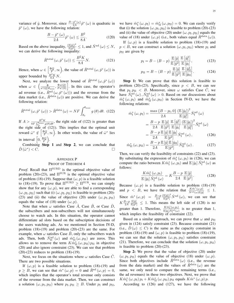
25

variance of y. Moreover, since B−p∗(ω)2A p∗ (ω) is quadratic in

p∗ (ω), we have the following relation:

B − p∗ (ω)

2Ap∗ (ω) ≤ B2

8A. (120)

Based on the above inequality, (E[y])2

E[y2] ≤ 1, and Nad (ω) ≤ N ,we can derive the following inequality:

Rtotal (ω, p∗ (ω)) ≤ B2K

8AN. (121)

Hence, when ω ∈[

ΦQF ,∞

), the value of Rtotal (ω, p∗ (ω)) is

upper bounded by B2K8A N .

Next, we analyze the lower bound of Rtotal (ω, p∗ (ω))

when ω ∈(

Φu′(Q)θmax

, Φu(Q)Fu′(0)

]. In this case, the operator’s

ad revenue (i.e., Rad (ω, p∗ (ω))) and the revenue from thedata market (i.e., Rdata (ω)) are positive. We can derive thefollowing relation:

Rtotal (ω, p∗ (ω)) > Rdata (ω) = NF

∫ θmax

θ0

g (θ) dθ. (122)

If A > B2K

8F∫ θmaxθ0

g(θ)dθ, the right side of (122) is greater than

the right side of (121). This implies that the optimal unitreward ω∗ /∈

[ΦQF ,∞

). In other words, the value of ω∗ lies

in interval[0, ΦQ

F

).

Combining Step 1 and Step 2, we can conclude thatD (ω∗) < C.

APPENDIX PPROOF OF THEOREM 4

Proof. Recall that ΠSURD is the optimal objective value ofproblem (20)-(23), and ΠSUR is the optimal objective valueof problem (18)-(19). Suppose that (ω, p) is a feasible solutionto (18)-(19). To prove that ΠSURD ≥ ΠSUR, we can simplyshow that for any (ω, p), we are able to find a corresponding(ω, pI, pII) such that (i) (ω, pI, pII) is feasible to problem (20)-(23) and (ii) the value of objective (20) under (ω, pI, pII)equals the value of (18) under (ω, p).

Note that when ω satisfies Case A, Case B, or Case D,the subscribers and non-subscribers will not simultaneouslychoose to watch ads. In this situation, the operator cannotdifferentiate ad slots based on the subscription decisions ofthe users watching ads. As we mentioned in Section IV-D,problem (18)-(19) and problem (20)-(23) are the same. Forexample, when ω satisfies Case B, only the subscribers watchads. Then, both Nad

II (ω) and m∗II (ω, pII) are zeros. Thisallows us to remove the term Km∗II (ω, pII) pII in objective(20) and also ignore constraint (23). We can see that problem(20)-(23) reduces to problem (18)-(19).

Next, we focus on the situations where ω satisfies Case C.There are two possible situations.

If (ω, p) is a feasible solution to problem (18)-(19) andp ≥ B, we can see that m∗ (ω, p) = 0 and Rad (ω, p) = 0,which implies that the operator’s total revenue only consistsof the revenue from the data market. Then, we can constructa solution (ω, pI, pII) where pI, pII ≥ B. Under pI and pII,

we have m∗I (ω, pI) = m∗II (ω, pII) = 0. We can easily verifythat (i) the solution (ω, pI, pII) is feasible to problem (20)-(23)and (ii) the value of objective (20) under (ω, pI, pII) equals thevalue of (18) under (ω, p) (i.e., both values equal Rdata (ω)).

If (ω, p) is a feasible solution to problem (18)-(19) andp < B, we can construct a solution (ω, pI, pII) where pI andpII are given by

pI = B − (B − p) E [y]

E [y2]

E[y2

I

]E [yI]

, (123)

pII = B − (B − p) E [y]

E [y2]

E[y2

II

]E [yII]

. (124)

Step 1: We can prove that this solution is feasible toproblem (20)-(23). Specifically, since p < B, we can seethat pI, pII < B. Moreover, since ω satisfies Case C, wehave Nad

I (ω) , NadII (ω) > 0. Based on our discussions about

m∗I (ω, pI) and m∗II (ω, pII) in Section IV-D, we have thefollowing relations:

m∗I (ω, pI) =max {B − pI, 0}

2A

(E [yI])2

E [y2I ]

NadI (ω)

=B − p

2A

E [y]

E [y2]

E[y2

I

]E [yI]

(E [yI])2

E [y2I ]

NadI (ω)

=B − p

2A

E [y]E [yI]

E [y2]Nad

I (ω) , (126)

m∗II (ω, pII) =B − p

2A

E [y]E [yII]

E [y2]Nad

II (ω) . (127)

Then, we can verify the feasibility of constraints (22) and (23).By substituting the expression of m∗I (ω, pI) in (126), we cancompute the ratio between Km∗I (ω, pI) and E [yI] N

adI (ω) as

follows:Km∗I (ω, pI)

E [yI] NadI (ω)

= KB − p

2A

E [y]

E [y2]. (128)

Because (ω, p) is a feasible solution to problem (18)-(19)and p < B, we have the relation that Km∗(ω,p)

Nad(ω)E[y]≤ 1.

Since m∗ (ω, p) = B−p2A

(E[y])2

E[y2] Nad (ω), we can see that

K B−p2A

E[y]E[y2] ≤ 1. This means the left side of (128) is no

greater than 1. Therefore, Km∗I (ω,pI)

E[yI]NadI (ω)

is no greater than 1,which implies the feasibility of constraint (22).

Based on a similar approach, we can prove that ω and pII

given in (124) satisfy constraint (23). Because constraint (21)(i.e., D (ω) ≤ C) is the same as the capacity constraint inproblem (18)-(19) and (ω, p) is feasible to problem (18)-(19),we can see that the solution (ω, pI, pII) satisfies constraint(21). Therefore, we can conclude that the solution (ω, pI, pII)is feasible to problem (20)-(23).

Step 2: We prove that the value of objective (20) under(ω, pI, pII) equals the value of objective (18) under (ω, p).Since both objectives include Rdata (ω) (i.e., the revenuefrom the data market) and the values of Rdata (ω) are thesame, we only need to compare the remaining terms (i.e.,the ad revenues) in these two objectives. Next, we prove thatKm∗I (ω, pI) pI +Km∗II (ω, pII) pII equals Km∗ (ω, p) p.

According to (126) and (127), we have the following

26

NadI (ω)E [yI] pI + Nad

II (ω)E [yII] pII

=NadI (ω)E [yI]

(B − (B − p) E [y]

E [y2]

E[y2

I

]E [yI]

)+ Nad

II (ω)E [yII]

(B − (B − p) E [y]

E [y2]

E[y2

II

]E [yII]

)

=B(Nad

I (ω)E [yI] + NadII (ω)E [yII]

)− (B − p) E [y]

E [y2]

(Nad

I (ω)E[y2

I

]+ Nad

II (ω)E[y2

II

])(a)=B

(Nad (ω)

∫ θmax

θ1g (θ)dθ∫ θmax

θ1g (θ)dθ +

∫ θ4θ3g (θ)dθ

∫ θmax

θ1

x∗ (θ, ω)g (θ)∫ θmax

θ1g (θ)dθ

dθ+Nad (ω)

∫ θ4θ3g (θ)dθ∫ θmax

θ1g (θ)dθ +

∫ θ4θ3g (θ)dθ

∫ θ4

θ3

x∗ (θ, ω)g (θ)∫ θ4

θ3g (θ)dθ

dθ

)

− (B−p) E [y]

E [y2]

(Nad (ω)

∫ θmax

θ1g (θ)dθ∫ θmax

θ1g (θ)dθ +

∫ θ4θ3g (θ)dθ

∫ θmax

θ1

(x∗ (θ, ω))2g (θ)∫ θmax

θ1g (θ)dθ

dθ+Nad (ω)

∫ θ4θ3g (θ)dθ∫ θmax

θ1g (θ)dθ +

∫ θ4θ3g (θ)dθ

∫ θ4

θ3

(x∗ (θ, ω))2g (θ)∫ θ4

θ3g (θ)dθ

dθ

)

=BNad (ω)∫ θmax

θ1g (θ) dθ +

∫ θ4θ3g (θ) dθ

(∫ θmax

θ1

x∗ (θ, ω) g (θ) dθ +

∫ θ4

θ3

x∗ (θ, ω) g (θ)dθ

)

− (B − p) E [y]

E [y2]

Nad (ω)∫ θmax

θ1g (θ) dθ +

∫ θ4θ3g (θ) dθ

(∫ θmax

θ1

(x∗ (θ, ω))2g (θ) dθ +

∫ θ4

θ3

(x∗ (θ, ω))2g (θ)dθ

)(b)=BNad (ω)E [y]− (B − p) E [y]

E [y2]Nad (ω)E

[y2]

=BNad (ω)E [y]− (B − p) Nad (ω)E [y] = pNad (ω)E [y] . (125)

relation:

Km∗I (ω, pI) pI +Km∗II (ω, pII) pII

=KB − p

2A

E [y]

E [y2]

(Nad

I (ω)E [yI] pI + NadII (ω)E [yII] pII

).

(129)

Then, we substitute the expressions of pI and pII in (123) and(124) and compute Nad

I (ω)E [yI] pI + NadII (ω)E [yII] pII in

(125). Note that in step (a) and step (b) of (125), we haveexpanded the expressions of some terms as follows:

NadI (ω) =

Nad (ω)∫ θmax

θ1g (θ) dθ∫ θmax

θ1g (θ) dθ +

∫ θ4θ3g (θ) dθ

, (130)

NadII (ω) =

Nad (ω)∫ θ4θ3g (θ) dθ∫ θmax

θ1g (θ) dθ +

∫ θ4θ3g (θ) dθ

, (131)

E [yI] =

∫ θmax

θ1

x∗ (θ, ω)g (θ)∫ θmax

θ1g (θ) dθ

dθ, (132)

E [yII] =

∫ θ4

θ3

x∗ (θ, ω)g (θ)∫ θ4

θ3g (θ) dθ

dθ, (133)

E [y] =

∫ θmax

θ1x∗ (θ, ω) g (θ) dθ +

∫ θ4θ3x∗ (θ, ω) g (θ)dθ∫ θmax

θ1g (θ) dθ +

∫ θ4θ3g (θ) dθ

,

(134)

E[y2

I

]=

∫ θmax

θ1

(x∗ (θ, ω))2 g (θ)∫ θmax

θ1g (θ) dθ

dθ, (135)

E[y2

II

]=

∫ θ4

θ3

(x∗ (θ, ω))2 g (θ)∫ θ4

θ3g (θ) dθ

dθ, (136)

E[y2]

=

∫ θmax

θ1(x∗ (θ, ω))

2g (θ) dθ+

∫ θ4θ3

(x∗ (θ, ω))2g (θ)dθ∫ θmax

θ1g (θ) dθ +

∫ θ4θ3g (θ) dθ

.

(137)

These equations can be derived based on the definitionsof these terms and Proposition 5. Specifically, as studiedin Proposition 5, users with θ ∈ [θ1, θmax] subscribe andwatch ads, and users with θ ∈ [θ3, θ4) watch ads withoutsubscription.

According to (129) and (125), we can derive the followingrelation:

Km∗I (ω, pI) pI +Km∗II (ω, pII) pII

=KB − p

2A

E [y]

E [y2]pNad (ω)E [y]

=Km∗ (ω, p) p. (138)

Then, we can see that the value of objective (20) under(ω, pI, pII) equals the value of objective (18) under (ω, p).

Combining Step 1 and Step 2, we can conclude that theoptimal objective value of problem (20)-(23) is no less than theoptimal objective value of problem (18)-(19). In other words,we have ΠSURD ≥ ΠSUR.

APPENDIX QPROOF OF THEOREM 5

Proof. Step 1: We derive the operator’s optimal total revenueunder the SAR scheme when C approaches infinity.

Based on Proposition 4, under the SAR scheme, the op-erator’s optimal unit reward ω∗ = D−1 (C). According toour analysis in Appendix H, when ω ∈

(Φu(Q)Fu′(Q) ,∞

), the

27

expression of D (ω) is given by

D (ω) =NQ

∫ θmax

θ2

g (θ) dθ

+N

∫ θmax

θ2

((u′)

−1(

Φ

ωθ

)−Q

)g (θ) dθ

=NQθmax − θ2

θmax+

N

θmax

∫ θmax

θ2

(ωθ

Φ− 1−Q

)dθ.

(139)

We can see that limω→∞D (ω) =∞. Hence, when C →∞,we have ω∗ →∞.

Next, we prove that when ω →∞, the corresponding θ2 →0. According to the defitition of θ2, the value of θ2 is upperbounded by θ0 and is lower bounded by 0. In Appendix D,we have proved that dθ2

dω < 0 for any given ω. Hence, whenω → ∞, the limit of θ2 exists. Let ζ ∈ [0, θ0] denote thislimit. From θ2’s definition, when u (z) = ln (1 + z) and θ ∼U [0, θmax], θ2 satisfies the following equation:

θ2 ln

(θ2ω

Φ

)− F − θ2 +

(1 +Q) Φ

ω= 0. (140)

When we take ω →∞ on both sides of the equation, we cansee that the equality holds only when ζ = 0. That is to say,when ω →∞, the corresponding θ2 → 0.

Based on our analysis in Step 2 of Appendix J,when ω ∈

(Φu(Q)Fu′(Q) ,∞

), the operator’s revenue function

Rtotal (ω, p∗ (ω)) is as follows:

Rtotal (ω, p∗ (ω)) =θmax − θ2

θmaxNF

+ p∗ (ω) (B − p∗ (ω))3KΦ

8Aθmax

(y2h − y2

l

)2y3h − y3

l

N, (141)

where yh = θmax−θ1Φ , yl = θ2−θ1

Φ , and p∗ (ω) =

max{B − 4A

3Ky3h−y

3l

y2h−y

2l, B2

}. When ω →∞, we can verify that

θ1 → 0, yh → θmax

Φ , and yl → 0. Then, we can derive thelimit of the revenue function under ω →∞ as follows:

limω→∞

Rtotal (ω, p∗ (ω)) = NF

+max

{B− 4A

3K

θmax

Φ,B

2

}(B−max

{B− 4A

3K

θmax

Φ,B

2

})3K

8AN.

(142)

When C → ∞, ω∗ → ∞. Hence, the operator’s optimalrevenue under the SAR scheme for C → ∞ is characterizedin (142).

Step 2: We discuss the maximum possible value of theoperator’s total revenue under the SUR scheme.

(i) When ω ∈[0, (1+Q)Φ

θmax

], no user watches ads. When ω ∈(

(1+Q)Φθmax

, Φ ln(1+Q)F

], the value of y is uniformly distributed in[

0, θmax−θ1Φ

]. Hence, when ω ∈

[0, Φ ln(1+Q)

F

], we can derive

the upper bound for the operator’s total revenue as follows:

Rtotal (ω, p∗ (ω)) ≤θmax − θ0

θmaxNF

+ p∗ (ω) (B − p∗ (ω))3K

8A

θmax − θ1

θmaxN,

(143)

where p∗ (ω) = max{B − 4A

3Kθmax−θ1

Φ , B2}

. We compare theright-hand side of the above inequality with the right-handside of (142). We can see that the right-hand side of (142) isalways larger.

(ii) When ω ∈(

Φ ln(1+Q)F , ΦQ

F

), we have the following

relation:

Rtotal (ω, p∗ (ω)) =θmax − θ4

θmaxNF

+p∗(ω)(B−p∗ (ω))3K

8A

(1+η2

)2(1+η) (1+η3)

θmax−θ1+θ4−θ3

θmaxN,

(144)

where η , min{θmax−θ1,θ4−θ3}max{θmax−θ1,θ4−θ3} , ymax , max{θmax−θ1,θ4−θ3}

Φ ,

and p∗ (ω) = max{B − 4A

3K1+η3

1+η2 ymax,B2

}. Based on 0 ≤

η ≤ 1, we can easily show that (1+η2)2

(1+η)(1+η3) ≤ 1. Moreover,we have θmax > θ1 and θ4 > θ3. Therefore, the followingrelation holds:

Rtotal (ω, p∗ (ω))<θmax−θ4

θmaxNF+p∗ (ω) (B−p∗ (ω))

3K

8AN.

(145)

Next, we compare θmax

Φ and 1+η3

1+η2 ymax. Since 0 ≤ η ≤ 1,

we have 1+η3

1+η2 = 1 − 1−η1+η2 η

2 ≤ 1. Moreover, ymax =max{θmax−θ1,θ4−θ3}

Φ < max{θmax,θ4}Φ ≤ θmax

Φ . Hence, we cansee that θmax

Φ > 1+η3

1+η2 ymax. Based on this relation, we canverify that the following relation holds:

max

{B− 4A

3K

θmax

Φ,B

2

}(B−max

{B− 4A

3K

θmax

Φ,B

2

})≥

max

{B− 4A

3K

1+η3

1+η2ymax,

B

2

}(B−max

{B− 4A

3K

1+η3

1+η2ymax,

B

2

}).

(146)

Therefore, we can see that the right-hand side of (145) issmaller than (142).

(iii) When ω ∈[

ΦQF ,∞

), we have the following relation:

Rtotal (ω, p∗ (ω)) = p∗ (ω) (B − p∗ (ω))3K

8A

θmax − θ3

θmaxN,

(147)

where p∗ (ω) = max{B − 4A

3Kθmax−θ3

Φ , B2}

. Since θ3 = Φω

decreases with ω, we can easily prove that Rtotal (ω, p∗ (ω))increases with ω. We can compute the limit of this revenue

28

107

1 1.5 2 2.5 3 3.5

108

4.2

4.4

4.6

4.8

5

5.2

5.4

5.6

5.8

6

(a) Example A.

105

0.6 0.8 1 1.2 1.4 1.6 1.8

106

3.2

3.4

3.6

3.8

4

4.2

4.4

4.6

4.8

5

5.2

(b) Example B.

104

0.5 1 1.5 2

105

2.8

3

3.2

3.4

3.6

3.8

4

4.2

4.4

4.6

(c) Example C.

Fig. 9: ΠSAR, ΠSUR, and ΠSURD Under Different Network Capacity (Uniformly Distributed θ and Logarithmic Utility).

function under ω →∞ as follows:

limω→∞

Rtotal (ω, p∗ (ω)) =

max

{B− 4A

3K

θmax

Φ,B

2

}(B−max

{B− 4A

3K

θmax

Φ,B

2

})3K

8AN.

(148)

We compare the right-hand side of the above equation withthe right-hand side of (142). We can see that the right-handside of (142) is always larger.

Combining the above analysis for all cases of ω (includingthe case where ω → ∞), we can see that the operator’smaximum possible total revenue under the SUR scheme isalways smaller than the value of the right-hand side of (142).Because the right-hand side of (142) is the operator’s optimaltotal revenue under the SAR when C →∞, we complete theproof.

APPENDIX RNUMERICAL RESULTS UNDER DIFFERENT SETTINGS

In this section, we show the numerical comparison amongΠSAR, ΠSUR, and ΠSURD under more parameter settings.Similar to Fig. 5(a), we assume that each user’s type θfollows a uniform distribution and u (z) = ln (1 + z). We runexperiments under three different parameter settings.

First, we choose N = 107, F = 25, Q = 0.7, θ ∼U [0, 155], Φ = 0.2, K = 30, A = 0.5, and B = 3. Weplot ΠSAR, ΠSUR, and ΠSURD against C in Fig. 9(a).

Second, we choose N = 105, F = 32, Q = 0.6, θ ∼U [0, 170], Φ = 0.3, K = 18, A = 0.6, and B = 4. We plotΠSAR, ΠSUR, and ΠSURD against C in Fig. 9(b).

Third, we choose N = 104, F = 28, Q = 0.6, θ ∼U [0, 150], Φ = 0.2, K = 18, A = 0.4, and B = 3. Weplot ΠSAR, ΠSUR, and ΠSURD against C in Fig. 9(c).

We can see that our key observations in Fig. 5(a) also holdin Fig. 9(a), 9(b), and 9(c). For example, if C is small, theSUR scheme achieves a higher operator’s revenue; otherwise,the SAR scheme achieves a higher operator’s revenue. The adslots’ differentiation can improve the operator’s revenue underthe SUR scheme.