Moment-SOS hierarchy for large scale set approximation ...
231
HAL Id: tel-03296221 https://hal.laas.fr/tel-03296221v1 Submitted on 22 Jul 2021 (v1), last revised 1 Apr 2022 (v2) HAL is a multi-disciplinary open access archive for the deposit and dissemination of sci- entific research documents, whether they are pub- lished or not. The documents may come from teaching and research institutions in France or abroad, or from public or private research centers. L’archive ouverte pluridisciplinaire HAL, est destinée au dépôt et à la diffusion de documents scientifiques de niveau recherche, publiés ou non, émanant des établissements d’enseignement et de recherche français ou étrangers, des laboratoires publics ou privés. Moment-SOS hierarchy for large scale set approximation. Application to power systems transient stability analysis Matteo Tacchi To cite this version: Matteo Tacchi. Moment-SOS hierarchy for large scale set approximation. Application to power systems transient stability analysis. Automatic Control Engineering. INSA Toulouse, 2021. English. tel-03296221v1
-
Upload
khangminh22 -
Category
Documents
-
view
0 -
download
0
Transcript of Moment-SOS hierarchy for large scale set approximation ...

HAL Id: tel-03296221https://hal.laas.fr/tel-03296221v1
Submitted on 22 Jul 2021 (v1), last revised 1 Apr 2022 (v2)
HAL is a multi-disciplinary open accessarchive for the deposit and dissemination of sci-entific research documents, whether they are pub-lished or not. The documents may come fromteaching and research institutions in France orabroad, or from public or private research centers.
L’archive ouverte pluridisciplinaire HAL, estdestinée au dépôt et à la diffusion de documentsscientifiques de niveau recherche, publiés ou non,émanant des établissements d’enseignement et derecherche français ou étrangers, des laboratoirespublics ou privés.
Moment-SOS hierarchy for large scale setapproximation. Application to power systems transient
stability analysisMatteo Tacchi
To cite this version:Matteo Tacchi. Moment-SOS hierarchy for large scale set approximation. Application to powersystems transient stability analysis. Automatic Control Engineering. INSA Toulouse, 2021. English.tel-03296221v1

THÈSETHÈSEEn vue de l’obtention du
DOCTORAT DE L’UNIVERSITÉ DETOULOUSE
Délivré par :l’Institut National des Sciences Appliquées de Toulouse (INSA de Toulouse)
Présentée et soutenue le 29 Juin 2021 par :Matteo TACCHI
Moment-SOS hierarchy for large scale set approximation.Application to power systems transient stability analysis.
JURYLeo LIBERTI DR LIX-CNRS Président, RapporteurSorin OLARU Pr. CentraleSupélec RapporteurCarmen CARDOZO Ph.D. Ingénieur RTE ExaminatriceColin N. JONES Assoc. Pr. EPFL ExaminateurMonique LAURENT Pr. CWI Amsterdam ExaminatriceLine ROALD Asst. Pr. UW-Madison ExaminatriceDidier HENRION DR LAAS-CNRS Directeur de Thèse
École doctorale et spécialité :EDSYS : Automatique 4200046
Unité de Recherche :Equipe MAC, LAAS-CNRS (UPR 8001)
Directeur de Thèse :Didier HENRION
Rapporteurs :Leo LIBERTI et Sorin OLARU


i
À Isaac, petit miracle dans notre quotidien.À Giuseppe Pino (1933 – 2021), mémoire éternelle.À Tatiana, coéquipière de choc en toutes circonstances.
“La vie est une ceriseLa mort est un noyauL’amour un cerisier.”Jacques Prévert, Chanson du Mois de Mai.


Remerciements
“La gratitude est le secret de la vie. L’essentiel est de remercierpour tout. Celui qui a appris cela sait ce que vivre signifie. Il apénétré le profond mystère de la vie.”Albert Schweitzer - médecin, philosophe et théologien alsacien.
C’est paradoxalement au début de mon manuscrit de thèse que je fais le bilan,sinon scientifique, au moins personnel, de cette longue période qui touche à sa fin.Regarder ainsi en arrière donne quelque peu le vertige... Il est sans aucun doutede bon aloi de tenter d’exprimer la profonde gratitude que j’éprouve à l’égard despersonnes qui ont contribué, de près ou de loin, à l’aboutissement de ce long travail.
En premier lieu bien sûr, je pense à l’équipe qui a encadré mes recherches :Didier Henrion, mon directeur de thèse, Jean Bernard Lasserre, co-encadrant régulierde mes travaux, Carmen Cardozo, ma référente entreprise, et Patrick Panciatici,conseiller scientifique RTE.
Didier, nous n’aurons finalement jamais eu cette grave discussion à la biblio-thèque... Et pour cause ! Tu m’as apporté un encadrement bienveillant et respec-tueux de mon autonomie, tout en me donnant de précieux conseils, tant sur le fondet la forme de nos travaux que sur leur direction. Ta pédagogie et tes suggestionsde lecture m’ont permis de m’approprier rapidement les concepts difficiles qui sous-tendent la thèse. Enfin, tu as toujours été accessible en dehors du laboratoire, fût-cepour m’aider à gérer des galères ou des conflits, ou simplement pour boire un verre.Je garde un souvenir mémorable de nos missions ensemble, à Prague et à Zürich,expériences fantastiques que j’ai été heureux de partager avec toi. J’espère qu’onpourra continuer ce partage, tant scientifique qu’amical, longtemps après la fin decette thèse.
Jean, tu as été un pilier de nos innovations scientifiques, toujours là pour suggérerune nouvelle piste de réflexion ou proposer une idée que personne n’avait eue, sanspour autant brimer ma propre créativité, et toujours avec une admirable facilité àfaire abstraction du superflu pour te plonger dans l’essentiel scientifique. Avec lerecul, j’ai le sentiment qu’une vraie synergie s’est mise en place, qui a permis desdéveloppements dont je suis fier. Mais aussi, tu as partagé avec moi des trésorsinsoupçonnés, comme la fameuse recette de l’omelette sans œufs, la localisation dudernier type qui t’a mal parlé ou encore l’énigme de Gibraltar. Nos sorties au Bikini,au Filochard et à la Mécanique des Fluides vont me manquer...
Carmen, c’est à toi que je dois d’avoir pu envisager cette thèse. Je n’oublieraijamais ton rôle déterminant dans l’élaboration de ce projet d’encadrement au LAAS,ni comment tu as su transformer le stagiaire timide que j’étais en un doctorantépanoui. Ton expertise technique des systèmes électriques a été d’une aide précieuse,et c’est toi qui m’as permis de réaliser ce rêve que j’avais d’utiliser des connaissancesthéoriques pour m’attaquer à des problèmes appliqués. Ta patience, ta pédagogieet ta rigueur ont été la clef du réalisme de mes contributions les plus techniques.Je n’oublie pas non plus mes séjours au siège de RTE où tu m’as accueilli avecbeaucoup de bienveillance. Pour tout cela, merci à toi.
iii

iv
Pour son suivi assidu de mes travaux et l’initiative de ce projet collaboratif entreRTE et le LAAS, je veux rendre un hommage tout particulier à Patrick Panciatici,dont la vision scientifique extrêmement large, couvrant à la fois les problématiquesindustrielles liées à la gestion des réseaux de transport d’électricité, et les méthodesthéoriques ayant le potentiel pour contribuer à l’innovation dans ce domaine, apermis la rencontre entre les hiérarchies moment-SOS et l’analyse de stabilité dessystèmes électriques. Ta curiosité et ton ouverture d’esprit m’ont fait forte impres-sion, et je sais que c’est aussi grâce à elles que cette thèse a pu avoir lieu. Je meréjouis que notre collaboration se poursuive au-delà de la thèse.
I would also like to deeply thank the members of my defense committee. I amparticularly grateful to Leo Liberti and Sorin Olaru for their very careful review ofthe present manuscript. Your comments and suggestions helped a lot improving theoverall quality of this work, including the PhD defense. Also, thank you Leo for ac-cepting the additional responsibility of presiding over the committee, that was reallyappreciated. Many thanks also to the whole committee: Leo Liberti, Sorin Olaru,Carmen Cardozo, Colin Jones, Monique Laurent, Line Roald and Didier Henrion,for their benevolent compliments on my work, as well as their very interesting andrelevant questions after my talk. Thanks to you all, my defense was a pricelessreward for all the work of the past years.
Then, I am also grateful to all my collaborators. Our stimulating interactionsallowed me to quickly enlarge my scientific horizon to a point that I would havetaken much more than 3 years to reach without you.
Immédiatement après celles et ceux qui ont contribué au lancement, à l’accom-pagnement et à la conclusion de ce marathon scientifique, je tiens à mentionner uncertain nombre d’amis chers à mon coeur : ce dernier volet de mes études a apporté,outre la bénéfique expérience dans le métier de la recherche, son lot d’épreuves etde rencontres, celles-ci ayant été déterminantes pour surmonter celles-là.
Swann, je te le dis tout de go : tu me dois un nugget. Initialement je voulaisentamer ce paragraphe avec une série de private jokes à base de langoustin et de“c’est où Zouane ?”, mais en me relisant j’ai trouvé ça bancal alors je change monfusil d’épaule. On a été co-bureaux pendant 2 ans au bas mot, ce qui fait que tupartages la plupart des souvenirs que j’évoquerai dans les prochains paragraphes. Ilfaut donc que je sois original ici. Il y a un truc unique et je dois dire assez sidérantavec toi, c’est que cette complicité entre nous, qui est si vite devenue centrale dansmon horizon relationnel, continue à se développer même à distance. Je me rappelleles lectures de mails au bureau, les soirées “gaufres” en ville, le Kraken (sacréehistoire) ; mon EVG organisé par tes soins, les voyages ensemble en France et àl’étranger, les Utopiales ; notre goût commun pour l’absurde et la science fiction...Mais en fait je crois que ce qui compte le plus pour moi, c’est ta disponibilité pourparler à coeur ouvert, de visu ou à distance. Merci pour cette amitié profonde,extrêmement précieuse. Et merci pour l’exemple et l’espoir que tu me donnes, parton admirable développement scientifique et professionnel.
Matteo (a.k.a. MDR, a.k.a Jean-Michel Pizza le slovène), merci de porter un sibeau prénom (il te va bien). Merci aussi pour l’excellence de ton humour poétique,

v
pour les sous-problèmes du capitalisme, les descentes de police, la polémique, laretraite à l’italienne... Merci enfin pour tes paroles et tes gestes d’affection toujourstrès touchants. Ti ringrazio per tutto questo e spero di vederti presto!!!
Tillmann, j’ai été très heureux de partager ton bureau pendant presque un an,merci de m’avoir enseigné les ficelles pour être un bon doctorant, merci pour toutesnos conversations, scientifiques ou non, au bureau, au Filochard, à la Méca, auBiergarten, au Père Peinard, au Concorde... merci aussi pour ta présence au mariage.Et merci pour le magnifique concert avant ton départ ! Guten tag!
Victor, sacré Magron, merci à toi d’avoir si souvent volé à mon secours (ton aidelogistique pour ma soutenance a été déterminante), de m’avoir rassuré quand maconfiance en moi déclinait, de m’avoir appris à chercher sur internet. Merci aussipour les sorties à Toulouse, Autrans, Bilbao, Nice, Nantes, Guidel... J’espère qu’onaura encore beaucoup de bons moments à partager ! Mes amitiés à toute la famille.
Flavien, très cher collègue daron au sang chaud, merci pour toute la complicitéqu’on a pu avoir, pour ta solidité aux 50 ans du LAAS, pour ta générosité à l’EVG(déguisements, rafraîchissements et cascades inclus), pour ta camaraderie au week-end ski, pour ton ton expertise en randonnées, pour tes biscottos si bien taillés, pourta solidarité jusque dans la paternité (félicitations à vous trois)... On se reverra !
Alex, merci pour ton accessibilité amicale, j’ai un souvenir impérissable de nossorties au Melting Pot, au Senso et à la Dynamo ! Tu as fait tomber le mur ima-ginaire qui me séparait des chercheurs permanents. Merci aussi pour ton soutienpsychologique dans la dernière ligne droite avant la soutenance, sans lequel j’auraisbien pu perdre les pédales ! À très bientôt j’espère.
Lucie, qui as partagé avec moi la couronne de la galette deux années d’affilée, quit’es mariée la même année que moi (et que Jean), merci pour ton infinie gentillesse,ta précieuse amitié, tes conseils avisés, ton soutien moral... Merci de nous avoir prêtéton époux le temps d’une soirée jeu, et d’avoir accueilli mon pot de thèse dans tonmagnifique jardin. Pense à nous à ton prochain passage en Suisse !
Comme l’ambiance de travail est primordiale pour la créativité scientifique, jeveux aussi remercier ceux de mes collègues de bureau que je n’ai pas encore eu l’oc-casion de citer : Clément, pour les gazzinades et pour le cours de sabre japonais ;Yohei, pour nous avoir suivis très très loin, Swann et moi (belly check) ; Mathias,pour les sympathiques discussions entre deux lignes de code (faut surtout pas s’éner-ver) ; Marianne, pour la profonde gentillesse que j’ai trouvée derrière ta discrétionréservée ; Corbi, pour ta bonne humeur permanente et contagieuse, et pour ta bellemoustache.
Évidemment, je n’oublie pas non plus les camarades doctorants, post-docs etstagiaires dont j’ai pu croiser le chemin, notamment Matthieu, toujours avenant,pour ton sourire et pour les nombreux moments de convivialité partagés (bises àHarmony et Léo) ; Antoine, pour la forte émulation scientifique que j’ai ressentieà ton contact lors de ton stage chez RTE ; Florent, pour ton précieux cocktail decompétence, de modestie et de sympathie ; Hoang, pour tes retours sur certains demes articles ; Roxana, pour ta soutenance tenue le jour de mon arrivée et pour tonplaid dont j’ai hérité ; Alessandra, pour les sorties avec les copains et pour la salsa ;Constantinos, pour la culture orthodoxe, de Grèce, de Russie ou d’ailleurs ; Quentin,

vi
pour la cordialitay et les soirées jeux (bisous à Blanche et KP) ; Larbi, on s’est àpeine croisés mais j’ai beaucoup apprécié nos échanges ; et enfin Yoni et Mathieu,pour votre engagement dans la “vie estudiantine” des doctorants MAC, à travers leséminaire doc, les ateliers oenologie, les gâteaux, et les surprises que vous organisezà l’occasion des soutenances (vous êtes géniaux)... Merci à vous tous, que votre nomsoit écrit ci-dessus ou non (confinement aidant, je ne vous connais malheureusementpas tous personnellement...), chacun de vous contribue à sa manière à faire vivre legroupe des “éphémères” MAC !
Et enfin, puisqu’on parle des “éphémères”, merci aussi à ceux qui ne le sont pas,et qui voient les stagiaires, doctorants et post-doc arriver dans l’équipe, grandir ets’en aller... Après avoir assisté au départ de tous mes prédécesseurs, je crois que jecomprends ce que ressentent les permanents lorsqu’un doctorant qu’ils ont côtoyépendant trois ans soutient finalement sa thèse et part vers de nouveaux horizons.Merci Milan pour t’être joint à nous dans nos soirées festives ; Dmitry, pour m’avoirpartagé ton expérience dans tous les domaines imaginables ; Sophie, pour ces plai-santeries qui vont me manquer (j’adore ce que tu fais !) ; Isabelle, pour les discussionsdans le couloir ou en salle café ; Aneel, pour tes questions toujours stimulantes etpour ton sens de l’humour ; Luca, pour tes précieux conseils de présentation ; Fred,pour avoir partagé avec moi tes astuces d’enseignement ; Mateusz, pour t’être ami-calement joint à nous en pleine crise sanitaire.
Maintenant que j’ai cité les membres du LAAS que j’ai fréquentés régulièrement,je veux aussi exprimer ma gratitude envers des personnes que je n’ai que très rare-ment (voire jamais) croisées, mais sans qui mes recherches (ainsi que la recherche engénéral au LAAS) n’auraient pas pu se faire dans d’aussi bonnes conditions. Mal-heureusement trop souvent oubliés lorsque vient le temps des remerciements, cescollègues fournissent un travail colossal pour nous permettre à nous, enseignants etchercheurs, de nous focaliser sur notre travail scientifique et nos diverses respon-sabilités organisationnelles. Merci, donc, au personnel du restaurant, de permettrechaque jour à des hordes d’employés affamés de venir recharger leurs batteries à lacantine ; à l’équipe de Sysadmin, pour m’avoir installé (et réparé quand c’était né-cessaire) l’ordinateur sur lequel cette thèse a été rédigée, et pour m’avoir aidé à fairefonctionner la visioconférence et la diffusion vidéo de ma soutenance sur les canauxdédiés ; à l’équipe administrative, pour avoir piloté la mise en place de mon contratd’encadrement avec RTE, pris en charge la logistique de mes diverses missions, etsans aucun doute effectué bien d’autres tâches dont j’ignore jusqu’à l’existence même(mention spéciale à Amandine qui a dû gérer ma mobilité à Zürich) ; aux membresdu service documentation pour avoir suivi et enregistré toutes mes publications, ycompris ce manuscrit de thèse ; au personnel de la reprographie, pour m’avoir régu-lièrement imprimé des documents reliés que je garde précieusement, et pour avoirédité le présent ouvrage ; à toute l’équipe d’entretien et de nettoyage, grâce à quimon bureau et toutes les installations que j’ai pu utiliser étaient toujours nickel ;aux employées du standard, pour leurs salutations avenantes le matin (et pour avoirretrouvé ma gourde après ma soutenance) ; enfin, à Éric et Corine du magasin, sansqui j’aurais bien vite manqué de papier, crayons et marqueurs.

vii
Et comme il n’y a pas eu que le LAAS dans ma thèse, il me faut étendre encoremes remerciements à des zones géographiques plus exotiques. Dans un autre bureau,loin, très loin à La Défense (et avant cela à Versailles), j’ai eu le plaisir de faire laconnaissance d’Emeline, Thibault, Guillaume, Philippe, Gilles, Manuel et Jean, deséquipes INT et optimisation chez RTE. Merci pour votre accueil chaleureux, pourvotre curiosité envers mes travaux, et pour avoir fait de mes séjours à Paris desexpériences enrichissantes non seulement scientifiquement mais aussi humainement ;grâce à vous je n’ai jamais eu le mal du pays.
Merci également à mes trois camarades de perdition à l’IRCCyN, Kossi, Jérémyet Yankaï, on sait tous les quatre quelles épreuves on a eues à surmonter, et sansvous peut-être n’aurais-je pas pris les bonnes décisions aux bons moments. Mercipour le temps passé ensemble à Nantes et pour votre solidarité en béton armé !
And I cannot forget those who welcomed me during my mobility in Zürich:Florian, for being my local advisor, and as such patiently and benevolently teachingme so many things (I have not forgotten our ongoing project and I have great hopesin it); Sabrina, for organizing everything for my arrival at IfA; Daniele and Liviu,for sharing your office with me; Irina, for explaining so many things about powerconverter control; Ali, for sharing your knowledge and your codes with me; Michael,for your enthusiastic curiosity about my work; Verena, for joining our power sys-tems stabiltiy group; Lukas, for welcoming me in the team and adding me to theRiot network; Marcello, for your valuable insights on optimization for power systemcontrol.
Mes pensées vont ensuite à toute ma famille, dont le soutien moral et les encoura-gements m’ont indubitablement aidé à surmonter les épreuves qui se sont présentéesà moi.
Claude, Jacky, vous rendre fiers de votre petit-fils a toujours été une importantesource de motivation pour moi, et je me réjouis du soutien affectueux que vousm’apportez sans cesse.
Frédérique, Pascal, votre attention, vos encouragements et votre capacité à tou-jours me consoler dans les moments de cafard n’ont jamais cessé de me donner laforce dont j’avais besoin.
Nicolas, ta fierté, ton enseignement martial et mental, ainsi que nos moments dedétente père-fils, nourrissent continuellement mon développement personnel.
Gaetano, avoir un petit frère aussi brillant que toi (même si tu refuses de l’ad-mettre) a suscité en moi cette fierté qui donne envie de se donner à fond pour être auniveau. Courage pour ta suite d’études, tu feras un médecin admirable. Et n’oubliejamais : Banach, Bourbaki, Alaoglu.
Néo, Angelo, mes chers jeunes petits frères, je suis d’ores et déjà fier de vousdeux. Les bons moments partagés dans notre petite tribu m’apportent ce qu’il fautde bonne humeur pour me plonger sereinement dans mon travail.
Edith, Giuseppe, je n’oublie pas vos conseils, vos félicitations et votre attention àmon égard, notamment au sujet de cette thèse dont nous avons longuement discuté.
Valérie, Jean-Luc, Lisa, Rémi, merci de nous avoir tant reçus (le plus souventà l’improviste) pendant ces trois années où nous fûmes voisins et où nous refîmesle monde ensemble, et merci également pour vos visites chez nous. Ces contacts

viii
réguliers étaient un vrai rayon de soleil.Marianne, Christophe, Florence, je vous remercie tous les trois d’avoir partagé
avec moi votre expérience de docteurs ès sciences ; vos conseils, vos témoignages etvos argumentaires pendants nos débats ont nourri ma réflexion sur ma thèse et lemonde de l’enseignement-recherche en général.
Louise, Alice, Juliette, merci pour les conversations au téléphone, les soirées jeuxà Noël et en été, et tous ces bons moments que nous partageons et qui ont rechargémes batteries à bloc quand je devais affronter mes systèmes électriques.
Enfin, Danièle, Alain, François, Sabine, merci pour vos appels et messages d’en-couragements, aux moments cruciaux, qui renforçaient en moi le sentiment de nejamais être seul face à une difficulté.
Avant de terminer ce chapitre, il y a quelques amis de longue date qui, je pense,méritent aussi que je leur signifie ma reconnaissance, pour avoir été là depuis unbon moment déjà, et avoir donc contribué à me nourrir scientifiquement et émotion-nellement.
Thieum, merci à toi, pour tellement de choses ! Pour m’avoir filé de gros coupsde pouce sur certains problèmes de maths que nos profs s’amusaient à nous poser àLyon, pour ta fabuleuse musique, pour ton accueil à Nantes quand je cherchais untoit... Pour toutes nos discussions politiques, philosophiques et littéraires, qui ontprofondément changé ma vision de beaucoup de choses et qui m’ont énormément aidéà grandir, notamment l’impressionnant préambule de ta thèse [28], qui m’a donnéune véritable leçon d’autocritique. Merci aussi pour l’ossau iraty, le paprika, lesyouhouuu et les wololooo, sans doute plus bas de plafond mais non moins importantspour l’épanouissement émotionnel.
Idriss, quand il est question de discussions, scientifiques, littéraires ou politiquesentre doctorants, ton nom me vient naturellement à l’esprit. Merci pour ton accueilà Jussieu, et pour ton passage à Toulouse, on s’est bien amusés ! Merci aussi dem’avoir rafraîchi les idées sur certains concepts mathématiques qui m’échappaientencore, mon chapitre 4 devrait te rappeler des choses... Et puis, merci pour tonhumour piquant : “Adieu rasta blanc, bonjour mocassins à glands !”.
Juliane, tu as beau détester les maths, il fallait bien que je mette ton nomquelque part dans ce chapitre : même à distance, on a partagé pas mal de choses cesdernières années ! Merci pour l’EVG à Toulouse, pour ton témoignage à Burey, pourta présence à Daru, pour les quelques fois où on a réussi à se voir à Nancy, pour tesséjours à Toulouse, pour m’avoir reproché mes annonces par messages, pour avoirpensé à mon anniversaire, pour le temps passé au téléphone... On continue sur cettelancée !
Un petit mot amical aux camarades Troyens, spécialistes en organisation devacances de rêve, des montagnes du Vercors aux plages vendéennes, en passant parles hospices bourguignons. Ma dernière soirée enquête avec vous commence à dater,il va falloir remettre ça prochainement ! Merci Lisa, Laeti, Thibault, Zoé, Patricia,Simon, Olivier, Julia, Mathilde, Marie, Cécile, Max, Merveille et Péleg, vous êtesun peu comme une deuxième famille : vos petits messages maintiennent le moral etaident à bien bosser. Courage aux doctorant·e·s (Olivier, ces points médians sontpour toi), force aux profs (mes héros) et plein de bonnes choses à tous les autres !

ix
Merci enfin à Solène, pour t’acquitter à merveille de tes rôles de marraine et dedisciple en Hapkido, et pour la relation unique qui en résulte. Ton année en poste àToulouse, alors que j’y étais moi-même établi, a été une excellente surprise (mêmesi c’était beaucoup trop court...) ! Les entraînements ensemble au Shaolin étaient laparfaite excuse pour se voir toutes les semaines. Merci aussi pour les dîners chez toi,et enfin merci pour l’invitation à ton mariage, c’était un sacré événement ! Bisous àAlex et Béatrice...
Je ne pourrais conclure ce chapitre de remerciements autrement qu’en exprimantmon infinie gratitude envers la personne qui a sans doute joué le rôle le plus im-portant dans l’accomplissement quotidien de mon travail, en rendant possible moninstallation à Toulouse malgré les difficultés pratiques qui en ont résulté, et surtouten m’apportant un soutien moral continu et sans faille, ainsi qu’un épanouissementpersonnel total qui a décuplé ma motivation : Tatiana, ma chère et tendre épouse.J’ai longtemps cherché un moyen de te remercier pour tout ce que tu fais et toutce que tu es pour moi, mais les mots me manquent pour exprimer réellement mareconnaissance envers toi. Je me refuse à te remercier de me supporter, car il y aune facilité toute patriarcale à se complaire dans un rôle de boulet et à se félici-ter d’avoir une épouse aimante et patiente pour nous “supporter” quand on rentrefourbu du travail. Pour autant, je veux souligner à quel point le soutien actif quetu m’as apporté a été précieux. J’espère être moi aussi un solide appui pour tonpropre accomplissement. Étant toi aussi en thèse, tu m’as également offert une ému-lation intellectuelle particulièrement stimulante, et nos discussions sur tes propresrecherches ont été autant de motivations pour faire avancer moi aussi l’état desconnaissances dans mon domaine. Et par dessus tout, au plan strictement person-nel, tu m’as comblé de bonheur, d’abord en m’accordant ta main (au premier moisde ma thèse), puis en donnant naissance à notre fils Isaac (au dernier mois de mathèse, amusante coïncidence...). Merci à toi d’être qui tu es. teb lbl.

Abstract
This thesis deals with approximating sets using Lasserre’s moment-SOS hierarchy.The motivation is the increasing need for efficient methods to approximate setsof secure operating conditions for electrical power systems. Indeed, recent andongoing changes in the European power network, such as the increase in renewableenergy sources interfaced by power electronic devices, are bringing up new challengesin terms of power grid security assessment. The aim of the present thesis is toinvestigate the suitability of the moment-SOS hierarchy as a tool for large scalestability assessment.
In this regard, the very scheme of moment-SOS hierarchies is analysed in-depth,and general results regarding the convergence and accuracy of the framework arestated, along with specific computational methods inspired from differential geo-metry and partial differential equations theory, in order to improve the convergenceof the numerical scheme.
From the computational viewpoint, the core of this thesis is the exploitationof problem structure to alleviate the computational burden of high dimensional,large scale industrial problems. The structure of power grids leads us to considergeneral sparsity patterns and design methods which distribute our computationsaccordingly, drastically reducing computational costs in implementation.
In addition to stability analysis, a special interest is put on the theoretical prob-lem of volume computation, whose applications rather concern the field of integralcalculus and probability evaluation, as understanding this problem turns out to bea prerequisite for approximating stability regions of differential systems, such asregions of attraction or positively invariant sets, with the moment-SOS hierarchy.Indeed, the moment-SOS approach to volume computation is the core of moment-SOS stability analysis.
Keywords: Power systems transient stability – infinite dimensional optimization– moments – polynomial sums of squares – set approximation – direct methods forstability analysis – sparsity – semidefinite relaxations.
xi


Résumé
Cette thèse a pour objet l’approximation d’ensembles au moyen de la hiérarchiemoment-sommes-de-carrés (abrégée moment-SOS) de Lasserre. Elle est motivée parle besoin croissant de méthodes efficaces pour approcher des ensembles de pointsde fonctionnement stables dans le domaine des réseaux électriques. En effet, les ré-cents développements et les changements en cours au sein du système électriqueeuropéen, comme l’augmentation de la part des énergies renouvelables dans la géné-ration d’électricité, et leur raccordement au réseau par des interfaces d’électroniquede puissance, soulèvent de nouveaux défis en termes d’évaluation de la sécurité desréseaux électriques. L’objectif de cette thèse est d’étudier la pertinence de la hiérar-chie moment-SOS dans les études de stabilité à grande échelle.
Dans cette optique, le schéma numérique que constituent les hiérarchies moment-SOS est étudié en détails, et des résultats généraux sur la convergence et la précisionde cet outil sont formulés, et accompagnés de méthodes de calcul spécifiques, inspi-rées de notions de géométrie différentielle et de théorie des équations aux dérivéespartielles, visant à améliorer la convergence du schéma numérique.
Du point de vue purement calculatoire, l’élément central de cette thèse est l’ex-ploitation de la structure des problèmes, en vue d’alléger le coût des calculs liésaux problèmes industriels à grande échelle, modellisés en très grande dimension.La structure en réseau des systèmes électriques nous conduit à nous intéresser auxconfigurations dites parcimonieuses, et à concevoir des méthodes distribuant les cal-culs suivant ces configurations, permettant ainsi de réduire drastiquement le coûten calcul de nos implémentations.
Enfin, en plus de l’analyse de stabilité, un intérêt particulier est accordé au pro-blème théorique du calcul de volumes, dont les applications se situent plutôt dansle domaine du calcul intégral et de l’évaluation probabiliste, la compréhension de ceproblème étant un prérequis pour l’approximation de régions de stabilité pour lessystèmes différentiels, comme par exemple les régions d’attractions ou les ensemblespositivement invariants, au moyen des hiérarchies moment-SOS. En effet, l’approchedu calcul de volumes par les hiérarchies moment-SOS est à l’origine de l’analyse destabilité par ces mêmes hiérarchies.
Titre en français : Hiérarchie moments-SOS pour approximation ensembliste àgrande échelle. Application à l’analyse de stabilité transitoire des systèmes élec-triques.
Mots clés : Analyse de la stabilité transitoire des systèmes électriques – optimi-sation en dimension infinie – moments – polynômes sommes de carrés – approxi-mations ensemblistes – méthodes directes pour l’analyse de stabilité – parcimonie –relaxations semidéfinie.
xiii


Contents
Notation xxiii
1 Introduction 11.1 Context and motivation of the thesis . . . . . . . . . . . . . . . . . . 11.2 Power system stability analysis . . . . . . . . . . . . . . . . . . . . . 3
1.2.1 Definition on a classical example . . . . . . . . . . . . . . . . 31.2.2 Overview of some existing TSA approaches . . . . . . . . . . . 61.2.3 Our approach: Direct methods for stability regions . . . . . . 8
1.3 The moment-SOS approach . . . . . . . . . . . . . . . . . . . . . . . 111.3.1 Introduction to measures . . . . . . . . . . . . . . . . . . . . . 111.3.2 A brief history . . . . . . . . . . . . . . . . . . . . . . . . . . 131.3.3 Moment-SOS hierarchies and power systems . . . . . . . . . . 15
1.4 Publications and outline . . . . . . . . . . . . . . . . . . . . . . . . . 161.4.1 Thesis organization . . . . . . . . . . . . . . . . . . . . . . . . 161.4.2 List of publications . . . . . . . . . . . . . . . . . . . . . . . . 17
2 Numerical analysis of moment problems 192.1 The generalized moment problem . . . . . . . . . . . . . . . . . . . . 20
2.1.1 Global polynomial optimization . . . . . . . . . . . . . . . . . 202.1.2 The K-moment problem . . . . . . . . . . . . . . . . . . . . . 222.1.3 Generalizations . . . . . . . . . . . . . . . . . . . . . . . . . . 252.1.4 Infinite dimensional duality ? . . . . . . . . . . . . . . . . . . 28
2.2 The moment-SOS hierarchy . . . . . . . . . . . . . . . . . . . . . . . 332.2.1 Moments . . . . . . . . . . . . . . . . . . . . . . . . . . . . . . 332.2.2 Sums of squares . . . . . . . . . . . . . . . . . . . . . . . . . . 372.2.3 Duality in the hierarchy ? . . . . . . . . . . . . . . . . . . . . 40
3 Transient stability of power systems 473.1 A moment-SOS based approach . . . . . . . . . . . . . . . . . . . . . 48
3.1.1 Occupation measures . . . . . . . . . . . . . . . . . . . . . . . 483.1.2 Outer ROA approximation for polynomial systems . . . . . . . 543.1.3 Finite time ROA estimation for a 3 machines model . . . . . . 57
3.2 An SOS, Lyapunov-based approach . . . . . . . . . . . . . . . . . . . 633.2.1 The single machine - infinite bus system . . . . . . . . . . . . 633.2.2 Lyapunov-based inner ROA approximation . . . . . . . . . . . 683.2.3 Computing an SOS Lyapunov function . . . . . . . . . . . . . 713.2.4 ROA estimation of the SMIB model . . . . . . . . . . . . . . . 78
4 Volume computation and Stokes theorem 854.1 Existing Stokes-based heuristics . . . . . . . . . . . . . . . . . . . . . 88
4.1.1 Linear reformulation of the volume problem . . . . . . . . . . 884.1.2 Stokes’ Theorem and its variants . . . . . . . . . . . . . . . . 904.1.3 Original Stokes constraints . . . . . . . . . . . . . . . . . . . . 90
4.2 Contribution to Stokes constraints heuristics . . . . . . . . . . . . . . 91
xv

xvi CONTENTS
4.2.1 Infinite-dimensional Stokes constraints . . . . . . . . . . . . . 914.2.2 New Stokes constraints and main result . . . . . . . . . . . . . 92
4.3 Solving a PDE to attain an optimum . . . . . . . . . . . . . . . . . . 944.3.1 Equivalence to a Poisson PDE . . . . . . . . . . . . . . . . . . 954.3.2 Poisson PDE on a connected domain . . . . . . . . . . . . . . 964.3.3 General Poisson PDE with boundary regularity . . . . . . . . 1004.3.4 Explicit optimum for Stokes-enhanced hierarchy . . . . . . . . 101
4.4 Numerical experiments and general heuristics . . . . . . . . . . . . . 1024.4.1 Practical implementation . . . . . . . . . . . . . . . . . . . . . 1024.4.2 Bivariate disk . . . . . . . . . . . . . . . . . . . . . . . . . . . 1034.4.3 Higher dimensions . . . . . . . . . . . . . . . . . . . . . . . . 1034.4.4 General heuristics . . . . . . . . . . . . . . . . . . . . . . . . . 105
5 Exploiting sparsity for volume computation 1095.1 The importance of sparsity . . . . . . . . . . . . . . . . . . . . . . . . 110
5.1.1 Motivation . . . . . . . . . . . . . . . . . . . . . . . . . . . . . 1105.1.2 Contribution . . . . . . . . . . . . . . . . . . . . . . . . . . . 1105.1.3 A motivating example . . . . . . . . . . . . . . . . . . . . . . 1115.1.4 The correlative sparsity pattern and its graph representation . 1125.1.5 An illustrative example: the bicylinder . . . . . . . . . . . . . 115
5.2 Exploiting path decomposition sparsity . . . . . . . . . . . . . . . . . 1185.2.1 Path computation theorem . . . . . . . . . . . . . . . . . . . . 1185.2.2 General sparse Stokes constraints . . . . . . . . . . . . . . . . 1225.2.3 Path computation examples . . . . . . . . . . . . . . . . . . . 124
5.3 Exploiting correlative sparsity . . . . . . . . . . . . . . . . . . . . . . 1305.3.1 General correlative sparsity pattern . . . . . . . . . . . . . . . 1305.3.2 Distributed computation theorem . . . . . . . . . . . . . . . . 1335.3.3 Distributed computation examples . . . . . . . . . . . . . . . 1365.3.4 The disjoint intersection hypothesis . . . . . . . . . . . . . . . 143
6 Theoretical contributions to stability analysis 1536.1 Inner approximation of maximal positively invariant sets . . . . . . . 154
6.1.1 MPI set . . . . . . . . . . . . . . . . . . . . . . . . . . . . . . 1556.1.2 Primal approximation problem and its value . . . . . . . . . . 1586.1.3 Dual approximation problem and its value . . . . . . . . . . . 1626.1.4 Numerical implementation and its convergence . . . . . . . . . 164
6.2 Sparsity-based approximation for finite time ROA . . . . . . . . . . . 1696.2.1 A path decomposition sparsity pattern . . . . . . . . . . . . . 1706.2.2 A sparse infinite dimensional formulation . . . . . . . . . . . . 1726.2.3 Sparsity of the actual finite time ROA . . . . . . . . . . . . . 1756.2.4 Computing sparse ROA approximations . . . . . . . . . . . . 177
7 Conclusions and perspectives 1837.1 General conclusions . . . . . . . . . . . . . . . . . . . . . . . . . . . . 1837.2 Perspectives . . . . . . . . . . . . . . . . . . . . . . . . . . . . . . . . 185
7.2.1 Exploiting time sparsity . . . . . . . . . . . . . . . . . . . . . 185

CONTENTS xvii
7.2.2 Combining Stokes & Christoffel-Darboux . . . . . . . . . . . . 1867.2.3 Studying sparsity for general lift-and-project methods . . . . . 1877.2.4 Studying Active electricity Distribution Networks . . . . . . . 188


List of Figures
1.1 Power systems stability classification. . . . . . . . . . . . . . . . . . . 51.2 Power-angle characteristic of a synchronous machine. . . . . . . . . . 61.3 Representation of classical measures. . . . . . . . . . . . . . . . . . . 12
2.1 An example of global polynomial optimization problem. . . . . . . . . 202.2 A possible aspect of Lagrangian for univariate optimization. . . . . . 292.3 SOS hierarchy for the length of [−0.5, 0.5]. . . . . . . . . . . . . . . . 392.4 Illustration of the moment-SOS hierarchy. . . . . . . . . . . . . . . . 45
3.1 Illustration of occupation measures. . . . . . . . . . . . . . . . . . . . 523.2 The three machines cycle. . . . . . . . . . . . . . . . . . . . . . . . . 583.3 Plot of the graph of vd(0, ·), d = 5. . . . . . . . . . . . . . . . . . . . 613.4 Outer ROA approximation of degree d = 5. . . . . . . . . . . . . . . . 613.5 Inner ROA approximation of degree d = 3. . . . . . . . . . . . . . . . 623.6 Synchronous machine connected to an infinite bus (SMIB). . . . . . . 643.7 The equivalent simplified SMIB model. . . . . . . . . . . . . . . . . . 663.8 The short-circuited system. . . . . . . . . . . . . . . . . . . . . . . . 683.9 The expanding interior algorithm. . . . . . . . . . . . . . . . . . . . . 773.10 Projected graph of the Lyapunov function. . . . . . . . . . . . . . . . 803.11 Comparison between ROA estimate and simulation built ROA. . . . . 81
4.1 Illustration of the Gibbs phenomenon. . . . . . . . . . . . . . . . . . 894.2 Polynomials obtained with and without Stokes constraints. . . . . . . 103
5.1 Graph associated to the sparse set (5.1). . . . . . . . . . . . . . . . . 1145.2 Linear clique tree associated to the sparse set (5.1). . . . . . . . . . . 1145.3 Graph associated to the sparse set (5.2). . . . . . . . . . . . . . . . . 1155.4 Branched clique tree associated to the sparse set (5.2). . . . . . . . . 1155.5 A representation of the bicylinder. . . . . . . . . . . . . . . . . . . . . 1165.6 Graph with linear clique tree for the nonconvex set. . . . . . . . . . . 1265.7 Performance for the nonconvex set. . . . . . . . . . . . . . . . . . . . 1265.8 Performance for the high dimensional polytope. . . . . . . . . . . . . 1275.9 Sparse rescaling performance for the high dimensional polytope. . . . 1285.10 Chordal graph (left) with its clique tree (right). . . . . . . . . . . . . 1325.11 Two possible branched clique trees for the 6D polytope. . . . . . . . . 1375.12 Performance for the 6D polytope. . . . . . . . . . . . . . . . . . . . . 1395.13 Two possible clique trees for the 4D polytope. . . . . . . . . . . . . . 1415.14 Performance for the 4D polytope. . . . . . . . . . . . . . . . . . . . . 1435.15 A correlation graph that violates Assumption 5.12. . . . . . . . . . . 1445.16 A way to fix our counterexample. . . . . . . . . . . . . . . . . . . . . 144
6.1 Outer and inner MPI set approximations. . . . . . . . . . . . . . . . . 1686.2 Illustration of the studied sparsity pattern. . . . . . . . . . . . . . . . 1716.3 A stable trajectory x1(t|x0). . . . . . . . . . . . . . . . . . . . . . . . 1766.4 Two unstable trajectories x1(t|x0). . . . . . . . . . . . . . . . . . . . . 177
xix

xx LIST OF FIGURES
6.5 Comparing the sparse and dense ROA approximation schemes. . . . . 1786.6 2D representations of finite time ROA approximations. . . . . . . . . 180

List of Tables
3.1 Parameter values for the SMIB model (p.u.). . . . . . . . . . . . . . . 673.2 Comparison between Lyapunov and occupation measures for TSA. . . 83
4.1 Stokes constraints performances for increasing relaxation degrees. . . 1044.2 Stokes constraints performances for increasing problem dimensions. . 104
5.1 Performance of sparse computation of the bicylinder’s volume. . . . . 1255.2 Performances on a nonconvex high dimensional set. . . . . . . . . . . 131
6.1 Comparison between ROA, finite time ROA & MPI set schemes. . . . 1696.2 Performances of the sparse ROA approximation scheme. . . . . . . . 178
xxi

xxii LIST OF TABLES

Notation
This section provides the notations used all along the thesis.
Usual sets• N: set of natural integers,
• N? := N \ 0: set of positive integers,
• N?N := 1, . . . , N: set of N first consecutive positive integers,
• R: set of real numbers,
• R+ := x ∈ R : x ≥ 0: set of nonnegative real numbers,
• R++ := x ∈ R : x > 0: set of positive real numbers,
• I := [x−, x+], x− < x+ ∈ R: a real interval.
Linear algebra• Rn×m: space of matrices with n rows and m columns with coefficients in R,
• mi,j: for M ∈ Rn×m, refers to the coefficient on the ith row and jth column,
• In ∈ Rn×n: identity matrix, I := I2, J :=(
0 −1
1 0
)∈ R2×2,
• Tr M := ∑1≤i≤nmi,i: trace of a square matrix M,
• M>: transposition of a matrix M,
• Sn: space of real symmetric matrices with n rows (M> = M),
• Sn+: cone of symmetric positive semi-definite matrices, M ∈ Sn+ ⇔ M 0,
• Sn++: open cone of symmetric positive definite matrices, M ∈ Sn++ ⇔ M 0,
• M 0⇔ −M 0, M ≺ 0⇔ −M 0 and M N⇔ N−M 0.
Euclidean geometry• x := (x1, . . . , xn)> ∈ Rn: a real vector with n rows,
• 0: zero finite dimensional vector, x ≥ 0⇔ xi ≥ 0, i ∈ N?n,
• x · y := x>y: inner product of two finite dimensional real vectors,
• |x| := ‖x‖2 =√
x · x: euclidean norm of a real vector x ∈ Rn,
• Bn := x ∈ Rn : |x| ≤ 1: the unit ball of Rn,
xxiii

xxiv Notations
• Sn−1 := x ∈ Rn : |x| = 1: the unit sphere of Rn,
• BR := R Bn and SR := R Sn−1: the ball and sphere of radius R > 0,
• πX : Rn → X: orthogonal projection on the vector subspace X ⊂ Rn,
• X⊥ := kerπX = y ∈ Rn : ∀x ∈ X,x · y = 0: vector space orthogonal to X.
Differential analysisLet Ω ⊂ Rn be an open or compact set, k ∈ N?.
• x := dxdt : derivative of the vector function t 7→ x(t),
• ∂x: partial differentiation operator with respect to the variable x,
• ∂kxi1 ,...,xik := ∂xi1 · · · ∂xik : kth partial differentiation operator w.r.t. xi1 , . . . , xik ,
• ∂ f := (∂xjfi)(i,j)∈N?m×N?n : jacobian matrix of function f : Rn → Rm,
• grad f := (∂ f)> = (∂x1f, . . . , ∂xnf)>: gradient of function f : Rn → R,
• div f := Tr(∂ f): divergence of function f : Rn → Rn,
• ∂ 2f := ∂ (grad f) = (∂2xi,xj
f)i,j∈N?n : hessian matrix of function f : Rn → R,
• ∆f := Tr(∂ 2f) = div(grad f): laplacian of function f : Rn → R,
• C0(Ω) = C(Ω): space of continuous functions on Ω,
• Ck(Ω) :=f ∈ C(Ω) : grad f ∈ Ck−1(Ω)n
, C∞(Ω) := ⋂
l∈NCl(Ω).
IntegrationLet A ⊂ Ω be a Borel set (countable intersection & union of closed & open sets).
•∫
Af(x) dx: Riemann integral of f ∈ C(Ω) on A.
• Cc(Ω): space of continuous functions on Ω vanishing outside a compact.
• M(Ω): space of signed measures, i.e. continuous linear forms on Cc(Ω).
•∫f dµ := 〈f, µ〉: duality or Lebesgue integral of f ∈ Cc(Ω) w.r.t. µ ∈M(Ω).
•∫
Af dµ :=
∫1A f dµ: integral of f ∈ Cc(Ω) w.r.t. µ ∈M(Ω) on A.
• λ: Lebesgue measure s.t. ∀f ∈ Cc(Ω),∫f dλ =
∫Ωf(x) dx.
• λA := 1A λ: restriction of λ to A s.t. ∀f ∈ Cc(Ω),∫f dλA =
∫Af dλ.

Notations xxv
Algebraic geometry• k := (k1, . . . , kn) ∈ Nn: a multi-index made of n integers,
• 1i := (0, . . . , 0, 1, 0, . . . , 0): multi-index with ith coordinate equal to 1, allothers being 0,
• |k| := ‖k‖1 = k1 + . . .+ kn: range of k ∈ Nn,
• Nnd := k ∈ Nn : |k| ≤ d: index set with bounded range,
• xk := xk11 · · ·xknn : kth power of a vector x = (x1, . . . , xn)> ∈ Rn,
• fk := x 7→ f(x)k: kth power of a vector function f = (f1, . . . , fn)> : Rm → Rn,
• R[x] := p(x) = ∑|k|≤d ak xk : d ∈ N ∧ ak ∈ R: space of polynomials in x,
• dp := max|k| : ak 6= 0: degree of p ∈ R[x],
• Σ[x] := s = p21 + · · · + p2
k : k ∈ N? ∧ p1, . . . , pk ∈ R[x]: cone of sums ofsquares of polynomials,
• Rd[x] := p ∈ R[x] : dp ≤ d: space of polynomials of degree at most d,
• Σd[x] := Σ[x] ∩R2d[x]: cone of SOS polynomials of degree at most 2d.


1Introduction
In this introductory chapter, we provide an overview of the concepts and problemsthat we will study in this thesis. Section 1.1 presents the general context of thethesis, namely the need for new tools to assess the stability of industrial powersystems. Section 1.2 briefly reviews some of the different existing approaches topower systems stability analysis. In Section 1.3 we discuss in more details themoment-SOS hierarchical approach, which is the method of interest in this thesis.The chapter ends with Section 1.4, listing the contributions of the thesis and outlinesthe structure of this manuscript.
Contents1.1 Context and motivation of the thesis . . . . . . . . . . . . 11.2 Power system stability analysis . . . . . . . . . . . . . . . 3
1.2.1 Definition on a classical example . . . . . . . . . . . . . . 31.2.2 Overview of some existing TSA approaches . . . . . . . . 61.2.3 Our approach: Direct methods for stability regions . . . . 8
1.3 The moment-SOS approach . . . . . . . . . . . . . . . . . 111.3.1 Introduction to measures . . . . . . . . . . . . . . . . . . 111.3.2 A brief history . . . . . . . . . . . . . . . . . . . . . . . . 131.3.3 Moment-SOS hierarchies and power systems . . . . . . . . 15
1.4 Publications and outline . . . . . . . . . . . . . . . . . . . 161.4.1 Thesis organization . . . . . . . . . . . . . . . . . . . . . . 161.4.2 List of publications . . . . . . . . . . . . . . . . . . . . . . 17
1.1 Context and motivation of the thesisIn the wake of the energy transition, large scale electrical power systems are evolvingfaster and faster, with increasing complexity and stochastic behaviors, mostly dueto the massive introduction of partially uncontrollable renewable energy sourcesas well as corresponding new technologies, especially in power electronics. Amongsuch devices, one can cite High Voltage Direct Current (HVDC) lines [18] as well aspower converters [38]. In order to guarantee the functioning of these sophisticated
1

2 CHAPTER 1. INTRODUCTION
systems, it is necessary to consider new methods for analysing them, see e.g. [49].In particular, the stability analysis of nonlinear systems subject to large perturba-tions has always been an extremely difficult problem, and it is going to complexifyeven more with the upcoming evolutions. Estimating the largest perturbation thatthe system can endure without impacting consumers and industrial loads remainsa key strategy for large scale electrical power systems management. To that end,the “bruteforce” method would consist of running a large number of simulationsof the system’s behavior, corresponding to a sample of all possible perturbations,and determining which ones would present a serious threat for system security, andwhich ones would automatically be subsided by the system controls. Of course,such an approach is not compatible with large scale systems, for which the numberof variables and possible perturbations is way too large to be tractable on a com-puter. Then, new approaches are needed, which should satisfy a certain number ofrequirements listed below:
Be compatible with nonlinearities: Electrical power systems include nonlin-earities brought upon by the presence of alternative current modelled with trigo-nometric functions, as well as power controls involving bilinearities, and eventuallymore sophisticated technologies, such as saturations. Since the aim is to assess thesystem’s behavior subject to large perturbations, linearization around equilibrium,which is the classical method for small signal stability, is not an option here, hencethe need for nonlinear computational methods.
Avoid false negatives: Given a scenario, we want to decide whether it will leadto an instability or, on the contrary, if it will pose no threat to the grid security. Inthat case, supposing that only approximate solutions can be given, so that an erroris possible, it is crucial to control such error: misclassifying a scenario as “secure”while it actually endangers the power network (i.e. a false negative) is forbiddenhere, as it could have catastrophic consequences. On the contrary, any scenarioclassified as “unstable” would be subject to further analysis, which would reveal theeventual false positives. In other words, some certifications should be given alongwith the stability analysis.
Provide accuracy guarantees: Although false positives can be allowed, it is im-portant to control their occurrences. Indeed, a false positive would require additionalwork to be detected, potentially increasing too much the computational burden ofthe analysis. For this reason, any guarantees that the probability of false posit-ive ultimately vanishes, would be highly appreciated. Most often such requirementtranslates into convergence of the analysing algorithm.
Be (at least potentially) scalable: For low-dimensional systems such as localgrids, some methods already exist that will be presented in more details in Section1.2. The central challenge of this thesis is to pave the way for large scale stabilityanalysis, which supposes that we find a way to tackle hundreds (ideally tens ofthousands) of variables in a reasonable amout of time. As we will expose in Section

1.2. POWER SYSTEM STABILITY ANALYSIS 3
1.3, the network structure has the potential to allow for distributed computations,which would drastically reduce the computational burden of our task.
Be perturbation-independent: Another factor that would increase the compu-tational burden of a stability assessment method is the dependence to the analysedperturbation. Indeed, as the number of possible perturbations increases, the num-ber of required computations would also grow very quickly, eventually leading toan intractability. Consequently, a method free from such a dependence, such asgeometric stability characterizations, would be much more efficient and suitable.
In this thesis, we will focus on set approximation schemes, mostly based onLasserre’s moments-sums-of-squares (moment-SOS) hierarchy as well as semidefiniteprogramming (SDP). However, several other approaches to power systems stabilityanalysis have been proposed in the past, that we are now going to review.
1.2 Power system stability analysis
1.2.1 Definition on a classical exampleFor the purpose of illustration let us first focus on the simplest representation of asynchronous machine electromechanical dynamic: the rotating mass or swing equa-tion, see e.g. [90, 21, 6].
Consider a power system composed of N synchronous generators with respectivevoltages v1, . . . ,vN . We assume, as it is common in the literature, that the voltagemagnitudes |v1|, . . . , |vN | are fixed after the fault is cleared, while the phase anglesvector θ := (θ1, . . . , θN) is variable (expressed in a rotating frame) with respectiveangular speed ω := (ω1, . . . , ωN). In addition, the loads in the network are con-sidered to be constant and passive impedances. In normal operation conditions, thephases will satisfy the following set of differential equations (with physical variablesexpressed in SI units here):
θ = ω, (1.1a)Mk ωk = −Dkωk +
(Pmeck − P elec
k (θ)), k ∈ N?N (1.1b)
where Pmeck is the (fixed) mechanical power input at bus k and P elec
k (θ) is the elec-trical power output of each generator k with value given by
P eleck (θ) = Gkk|vk|2 +
∑l 6=k|vk| |vl| Bkl sin(θk − θl) +Gkl cos(θk − θl) . (1.2)
The quantities Bkl and Gkl denote the line susceptances and conductances, andMk refers to the generator inertia constant Hk (Mk = 2Hk). The constant Dk
denotes the damping coefficient of each generator. Equation (1.1) is called theswing equation and models the electromechanical conversion characteristic of thesynchronous machine.
We assume that there exists an equilibrium θ := (θ1, . . . , θN) to these equations,that satisfies

4 CHAPTER 1. INTRODUCTION
Pmeck = P elec
k (θ), k ∈ N?N . (1.3)
In other words, θ corresponds to a steady-state operating point of an AC trans-mission system. As phases are defined up to a reference value, we choose one bus,denoted by subscript “ref”, to serve as the reference bus, with θref = θref = 0 (oftenreferred to as slack bus). Indeed, the equations are invariant up to a phase shift.
We first introduce working notations that we will use all along the thesis. Con-sider a vector field f ∈ C1(Rn)n with equilibrium point x ∈ Rn such that f(x) = 0,along with the differential system
x = f(x). (1.4)
According to the Cauchy-Lipschitz theorem [105, 77], (1.4) admits a continuouslydifferentiable solution map R ×Rn −→ Rn
(t,x0) 7−→ x(t|x0)
such that x(0|x0) = x0 (initial condition) and ∂tx(t|x0) = f(x(t|x0)) (dynamics).Moreover, if x(t|x0) = x holds for one value of t, then it holds for all t ∈ R (inparticular, x0 = x).
Then, transients are defined as follows:Definition 1.1: Transients
Consider a power system (P) described by differential equation (1.4). Supposethat at t = tp a perturbation occurs that drastically modifies the differentialequation, into x = f(x), f ∈ C1(Rn)n. Its trajectory is x(t− tp|x0), t ≥ tp.At t = tcl > tp, the perturbation is cleared and (P) goes back to nominalequation (1.4). We define the clearing state xcl := x(tcl − tp|x) and post-perturbation trajectory x(t− tcl|xcl). The behaviour of (P) for t ≥ tp is calledtransient.
In particular, we want to assess the system’s transient stability, which is definedas follows:
Definition 1.2: Transient stability
In this thesis, we call transient stability of a power system (P) its ability to goback to an operating equilibrium point x from a post-disturbance state xcl farfrom x, with the state variables staying in a secure zone of the state space.
This general definition rules out any linearization-based local stability analysis:we are bound to carry out a sharp, nonlinear transient stability analysis (TSA).
Remark 1.1 (Power system transient stability)In terms of power systems, transient stability more specifically denotes a fea-
ture of the so-called rotor angle stability, based on the functioning of synchronous

1.2. POWER SYSTEM STABILITY ANALYSIS 5
machines described by (1.1) (see figure 1.1). However, from the mathematical meth-odological viewpoint, the specificity of transient stability boils down to the notion oflarge disturbances and the impossibility of linearization. Thus, the works presentedin this thesis apply to all stability analyses related to large disturbances, for examplein voltage stability. As a result, we included all such stability properties in ourdefinition of transient stability.
Figure 1.1 – Power systems stability classification.
Image source – [41]; this classification is an upgrade of the one found in [65].
When a perturbation occurs, the dynamics of the system are modified, so thatthe state leaves its former equilibrium point x and goes into large excursion. For agiven perturbation, the longer the perturbation, the further from x the clearing statexcl. Then, after a certain time, the system state will be too far from equilibrium tobe able to go back to equilibrium, even if the perturbation is cleared, and the rotorangles will quickly go to infinity. We call such time the critical clearing time tcc.
Definition 1.3: Critical Clearing Time (CCT)
tcc := max∆t
∆t
s.t. xcl := x(∆t|x) is stable in the sense of Definition 1.2.
Critical clearing time is a very useful metric to assess transient stability of apower system under a given perturbation. The CCT depends on the studied per-turbation and initial state x0, so that what we are interested in is the whole function(perturbation, x0) 7→ CCT.
Definition 1.4: Critical Clearing State (CCS)
CCT is accompanied with the notion of critical clearing state (CCS), whichwill also be of interest:
xcc := x(tcc|x).

6 CHAPTER 1. INTRODUCTION
In the context of time-invariant systems (1.4), CCS has the advantage to beindependent from the perturbation and the on-fault behavior. It only defines a limitwhich, if it is passed, compromises the transient stability of the system.
1.2.2 Overview of some existing TSA approachesIn this section we present some of the considered methods for transient stabilityanalysis, based on [90, 117].
Currently used methods
Figure 1.2 – Power-angle characteristic of a synchronous machine.
Corresponding to system (1.1) (N = 1) subject to a short-circuit. The plottedcurve is the electrical power that the machine should inject into the grid in normalfunctioning conditions.
Image source – https://www.electrical4u.com/equal-area-criterion/
A first basic method for TSA, called the Equal Area Criterion, consists of plottingthe graph of P elec(θ), denoted Pc(δ) in Figure 1.2. Then, one can identify the criticalclearing angle δc, such that areas A1 and A2 are equal, and tcc is the time at whichδc is attained. Indeed, on the figure δ0 represents normal functioning conditions (i.e.equilibrium), in which the machine injects exactly as much electrical power in thegrid as it receives mechanical power: Pc(δ0) = Pm so that the system (1.1) is atsteady-state. However, during the fault (here a short-circuit), the electrical powerdelivered by the machine to the grid vanishes, so that all mechanical power inputPm is stored in the rotor as kinetic energy (represented by area A1 on the figure),making δ sharply increase. Then, it can be returned only after fault clearing, underthe form of electrical energy, resulting in at most area A2. Thus, if A1 ≤ A2 allstored mechanical power can be returned to the grid before synchronism is lost, i.e.before δ exceeds π, after which δ decreases back to δ0. On the contrary, if A1 > A2,

1.2. POWER SYSTEM STABILITY ANALYSIS 7
then the machine will lose synchronism before all stored energy is returned, resultingin transient instability.
In addition to the intuition that this criterion gives of transient behaviours, ithas been extended and studied deeply by power engineers in the past decades, underthe name of Extended Equal Area Criterion (EEAC, see [140]), although the presentthesis does not focus on this TSA method.
As stated before, the general method used to assess transient stability of generalpower systems consists of numerical time-domain simulations: if one knows a prioriwhat the perturbation will be and how long it will last, then one only has to simulatethe trajectory of the system for t ≥ tp and see whether or not it goes back toequilibrium after tcl. To that end, equation (1.1) or more generally (1.4) is discretizedover time, after which the discretized system is numerically integrated to computethe trajectory of the system. Then, one can directly observe transient stability orinstability by checking the result of the time-domain simulation.
However, transmission system operators (TSO) are actually interested not only indeciding the stability of a system but also in assessing stability margins. Indeed, theactual clearing time tcl is fixed, determined by the speed of the involved protectiondevices. Thus, studying the transient stability of a system boils down to computingtcc and comparing it to the fixed tcl. Then, tcc < tcl means by definition that thesystem will be unstable. However, uncertainties on the model and behaviour of theactual system leads TSOs to look for some kind of robustness propeties for stablesituations, under the form of stability margins, i.e. lower bounds on the value oftcc − tcl. For this reason, TSOs are interested in computing the actual CCT fora given perturbation, and not only assessing stability through a single simulationof the whole transients. However, such computation is very costly, as the moststraightforward method consists of a bisection that would involve a time-domainsimulation at each step.
In order to lighten this computational burden, one can look for randomized solu-tions, such as the classical Monte-Carlo methods, which consist of sampling thepossible scenarios according to their probability, and only computing CCTs associ-ated with the chosen sample. Then, instead of obtaining CCTs for all perturbations,one only has access to an estimation of the probability that the CCT is within agiven interval (see [5, 66]). While such a method would surely decrease the computa-tional cost of the TSA, it poses the problem of forecasting rare transient events withsevere consequences. Indeed, especially in power grids that have been functioning24/7, for decades, even very unlikely events have already occurred, and the possibil-ity for randomized approaches to ignore a part of the potential perturbations posesan issue for conservative transient stability analyses. However, such methods havebeen studied for a long time and paved the way to data-analysis related methods[102].
AI methods
The current times have seen artificial intelligence progressively gain momentum, upto a point where it competes with most of the existing state-of-the art methods.Here we briefly mention different AI-related approaches that have been proposed to

8 CHAPTER 1. INTRODUCTION
carry out transient stability analyses.
• Clustering: A possibility is to train an algorithm to identify classes of per-turbations which will lead to similar behaviors, after which one can studythe details of a small number of representing events and deduce the variousoutcomes of a large number of perturbations. Compared to classical random-ization, this allows for taking outliers into account as specific clusters. Severalcontributions were made in this domain, including [37, 19, 98, 55]. Depend-ing on authors, different classification methods were used, such as k-nearestneighbours, bayesian classification or hierarchical clustering (see [40, 146] fordetails on these classification methods).
• Artificial Neural Networks (ANN): Bio-inspired by the functioning ofhuman brain, ANNs consist of automatically splitting a complex task intosimpler ones that are ditributed along a pre-determined network of “neurones”(basically boolean classifiers), whose historical ancestor was the Perceptronalgorithm. The definition of the subtask is called “training” the ANN andconsists of tuning the neurones in a way that minimizes the error rate of thewhole, when analysing a “training set” of known perturbations. Such methodswere applied in [31, 59, 144, 97].
• Support Vector Machine (SVM): Generalizing linear classification, SVMbelongs to the category of lift-and-project methods; the idea consists of em-bedding the space in which the TSA problem is considered into a vector spacein which discriminating between stable and unstable scenarios is reduced tochecking the sign of a linear form one has to determine. Such a method canbe combined with classical clustering as was done in [94, 142] or with variousoptimization methods such as [133, 141].
While AI-based method bear a great potential for power systems TSA, in thisthesis we decided to study methods capable of both competing with machine learningapproaches and giving a deeper understanding of the physics involved in the transientphenomena. Such methods, called direct methods as they do not require any time-domain simulation at all, have been around for a long time and are based on thephysical notion of energy.
1.2.3 Our approach: Direct methods for stability regions
Direct methods can be seen as dual to time-domain simulations, in the sense thatinstead of computing the successive states of the system, one looks for an observablethat takes the state as input, and outputs a real value on which the stability analysisis based. This duality will be explained more in details in Chapters 2 and 3. Suchdirect methods are based on general differential system stability theory [81, 67] andwere specifically applied to power systems stability analysis in [6, 21, 22, 53, 99].

1.2. POWER SYSTEM STABILITY ANALYSIS 9
Transient stability regions
A promising alternative to the previously reviewed methods consists in determininga priori an approximation of a transient stability region for system (1.4), i.e. aregion A of the state space for which one can guarantee that if the clearing statexcl ∈ A then the system will go back to equilbrium within a given time horizon.We now define a natural candidate for a transient stability region. Indeed, we arelooking for a geometric criterion for convergence of the post-perturbation system,which leads us to define the region of attraction of a set.
Definition 1.5: Region of Attraction (ROA)
Let M ⊂ X ⊂ Rn, T ∈ (0,+∞]. We define the time T region of attraction(ROA) of M (with state constraint X) as:
AXT (M) :=
x0 ∈ Rn :∀t ∈ [0, T ),x(t|x0) ∈ X
dist(x(t|x0),M) −→t→T
0
. (1.5)
where dist(x,Y) := infy∈Y |x − y| is the euclidean distance between a pointx ∈ Rn and a set Y ⊂ Rn. If X = Rn then we only write AT (M) := ARn
T (M).
This definition allows us to state a transient stability analysis problem:
Problem 1: Direct transient stability analysis
Compute an approximating subset A of some well-chosen ROA AXT (M), so
that xcl ∈ A =⇒ xcl can be attained without compromising stability.
Remark 1.2 (False negatives and conservativeness)In Problem 1, we already allow ourselves to compute an approximation of
some ROA. Indeed, in most of the general cases, the exact AXT (M) is out of reach
for standard computational methods, hence the resort to approximation.However, we stated at the beginning of this Chapter that a good TSA should avoid
false negatives. In terms of ROA approximation, this means that we want to computeinner ROA approximations, so that we can miss stable scenarios (AX
T (M) \ A 6= ∅is allowed), but we cannot miss instability issues (A \AX
T (M) 6= ∅ is forbidden).
Remark 1.3 (Access to CCT)Given a solution to Problem 1, one only has access to potential critical clearing
states. Relating such result to critical clearing times requires some kind of time-domain simulation of the faulted system. In other words, direct methods mostlyallow their user to get rid of the post-fault trajectory simulations. For this reason,ideally, the boundary of the computed transient stability region should be close to aset of critical clearing states. Other ways to access CCT are not reviewed in thepresent thesis.

10 CHAPTER 1. INTRODUCTION
Stability oracle functions
What we call stability oracle functions is a most general class of functions whosevalue at state xcl gives insight on the stability of the trajectory x(t|xcl). Suchinformation can in turn be used to assess the transient stability of the studiedsystem. Here we only give the most general definition, as several more specificstability oracles will be studied in the rest of the thesis.
Definition 1.6: Stability Oracle Functions (SOFs)
Let D ⊂ Rn. A stability oracle function (SOF) is a v : Rn → R non-increasingalong trajectories x(t|x0) in D, which is characterized by
∀x ∈ D, f(x) · grad v(x) ≤ 0. (1.6)
Remark 1.4 (Positively invariant sublevel sets)A direct consequence of equation (1.6) is that any sublevel set
Ω := x ∈ Rn : v(x) ≤ l
with l ∈ R such that Ω ⊂ D, is positively invariant for system (1.4).
Example 1.5
• Lyapunov functions, whose definition will be recalled in Section 3.2, are aninstance of SOF, related to infinite time ROA.
• Energy functions [22] are an instance of SOF, related to infinite time ROA.
• Dual decision variables of [42] are an instance of SOF that we will study inSection 3.1, related to finite time ROA.
• Control barrier functions [4] are an instance of SOF, related to positivelyinvariant sets.
Lyapunov arguments are based on the fact that a stable equilibrium point of aphysical system (such as a power network) is characterized as a local minimum of itsenergy. As transient stability requires that the system converges to an equilibriumafter the perturbation is cleared, TSA then reduces to deciding whether the energyof a system in post-fault state xcl will decrease to a minimum or not. As it iswell known, set Ω from Remark 1.4, when considering a specific kind of Lyapunovfunction, is a subset of the Lyapunov ROA A∞(x) of Definition 1.5. Of course,depending on the considered SOF, set Ω will have different properties. Findingrelevant SOF for power systems TSA is part of this work, more specifically addressedin Chapters 3 and 6.
Then, the crucial question remains: how does one compute such functions? Dueto the physical inspiration of direct methods, the first studied oracles were energyfunctions, followed by Lyapunov functions, and most of the time they were de-termined out of physical reasonings or after some analytical computations [22, 131].However, starting in the early 2000s, some algorithmic methods were developped to:

1.3. THE MOMENT-SOS APPROACH 11
• Systematize the computation of SOFs,
• Optimize over SOFs to obtain the “best” transient stability region estimates.
We now introduce some mathematical concepts that will be instrumental in ourcomputations of transient stability region estimates.
1.3 The moment-SOS approach
1.3.1 Introduction to measuresThis section is addressed to a reader unfamiliar with the mathematical notion ofmeasure. It is an intent to give an intuition on the concept of measure, withoutintroducing the sophisticated set theory elements that are necessary for a rigorousdefinition. In contrast, here we build only on the knowledge of normed vector spaces,linear forms and continuity. Given a real vector space X equipped with a norm ‖ ·‖,we recall that:
• A linear form on X is a function φ : X → R s.t. ∀ψ, ψ′ ∈ X , s ∈ R,φ(ψ + s ψ′) = φ(ψ) + s φ(ψ′); we denote 〈ψ, φ〉 := φ(ψ).
• A continuous function on X is a function f : X → R s.t.
‖ψ − ψk‖ −→k→∞
0 =⇒ |f(ψ)− f(ψk)| −→k→∞
0.
• X ′ is the set of continuous linear forms on X , also called dual space1.
Consider the set Cc(Rn) of continuous functions on Rn that vanish outside a ball.This is an infinite dimensional real vector space, equipped with the uniform norm
‖f‖∞ := supx∈Rn
|f(x)|.
We define the dual spaceM(Rn) := Cc(Rn)′, and call it the space of signed measures.For µ ∈M(Rn) and f ∈ Cc(Rn) we define the integral of f w.r.t. µ as∫
f dµ := 〈f, µ〉.
Then, we define the set of nonnegative functions
Cc(Rn)+ := f ∈ Cc(Rn) : ∀x ∈ Rn, f(x) ≥ 0
as well as its dual M(Rn)+ := µ ∈ M(Rn) : ∀f ∈ Cc(Rn)+,∫f dµ ≥ 0. Those
are cones in the sense that they are invariant through multiplication by a positive1If X has finite dimension, then all linear forms are continuous, and the Riesz representation
theorem states that X ′ can be identified with X ; however, it is not the case for infinite dimensionalvector spaces.

12 CHAPTER 1. INTRODUCTION
0.5 1 1.5 x
0.5
1
µ
0(a) Dirac measure in x = 1.
0.5 1 1.5 x
0.5
1
µ
0(b) Lebesgue measure on[0.5, 1.5].
0.5 1 1.5 x
0.5
1
µ
0(c) Gaussian law with mean 1and standard deviation 0.3.
Figure 1.3 – Representation of classical measures.
number. M(Rn)+ is the cone of measures on Rn. Eventually, for X ⊂ Rn, we definethe sets
M(X) :=µ ∈M(Rn) : if f ∈ C(Rn) vanishes on X then
∫f dµ = 0
,
M(X)+ :=µ ∈M(Rn)+ : if f ∈ C(Rn) vanishes on X then
∫f dµ = 0
,
which correspond to measures supported on X.From a physical viewpoint, measures represent mass distributions, or superpos-
itions of points. As a result, they can encode many things, from probability laws(taking a random variable X of law µ,
∫f dµ = E[f(X)]) to superpositions of
trajectories of a dynamical system, including distributions of solutions to a givenoptimization problem.
Example 1.6
• The Dirac distribution δx represents a unitary mass concentrated in x ∈ Rn,so that
∫f dδx = f(x) (Fig. 1.3a).
• The Lebesgue measure λ[a,b] represents a uniform mass distribution on the seg-ment [a, b] ⊂ R, so that
∫f dλ[a,b] =
∫ ba f(x) dx (Fig. 1.3b).
• The Gaussian measure with mean m and standard deviation s represents anormal probability distribution µ such that (see Fig. 1.3c)
∫f dµ = 1
s√
2π
∫ +∞
−∞e−
(x−m)2
2s2 f(x) dx.
Some measures, such as the Gaussian measure, are absolutely continuous w.r.t.the Lebesgue measure, meaning that they correspond to actual functions onRn: theyrepresent densities of mass. Others are not absolutely continuous: for example, theDirac measure does not represent a density of mass, but rather a singularity withmass 1.
In short, measures have two major characteristics:

1.3. THE MOMENT-SOS APPROACH 13
• They are the mathematical formalization of point distributions, and henceappear in a large variety of domains, from probability theory to fluid mechanicsand statistical physics; in particular, trajectories of a differential system canbe encoded under the form of a measure [143, 111, 112, 130, 76];
• They are in duality with functions (such as polynomials as well as stabilityoracle functions) through Lebesgue’s integration theory: indeed, the integralof a function is always computed with respect to a measure (in the case of thestandard integral, the involved measure is the Lebesgue measure).
Remark 1.7 (Link between measures and stability analysis)In particular, measures are the mathematical concept that explains the relation-
ship between time-domain simulations and direct methods for stability analysis. In-deed, on the one hand, as a formalization of point distributions, measures can beused to represent trajectories, that are nothing more than time-state point distribu-tions. On the other hand, Lebesgue integration theory allows for integrating SOFswith respect to such trajectory representing measures, introducing a duality betweentrajectories and SOFs.
As polynomials are continuous functions,∫p dµ represents a particular duality
between p ∈ R[x] and µ ∈M(Rn). Such a duality is instrumental for implementingthe moment-SOS hierarchy. Indeed, historically, moment-SOS hierarchies were madepossible by new theorems on polynomials, that exploited their duality with measures.
1.3.2 A brief historyThe moment-SOS or Lasserre hierarchies are the fundamental tools that we will bestudying and using all along this thesis (except in Section 3.2). They are an elegantframework that brings together real algebraic geometry as well as functional analysis,to define a plug-and-play scheme for solving a very large variety of problems.
The famous 17th Hilbert problem [46] (solved by Emil Artin in [8]) is at the rootof the moment-SOS approach:
“Can a nonnegative rational function be written as a sum of squares of rationalfunctions?”
More precisely, Hilbert had proved that the statement is false if one considerspolynomials instead of rational functions [45], which Motzkin complemented with acounterexample [93], nonnegative but not sum of squares:
pM(x, y) := x4y2 + x2y4 − 3x2y2 + 1.However, the question of identifying polynomials asked to be positive only on
a subset of Rn still remained to be studied, and motivated numerous works in realalgebraic geometry, leading to the so-called Positivstellensätze [60, 119, 115, 107].A P-satz reduces the question of positivity of a polynomial over a given subset ofRn to finding P-satz certificates, involving sums of squares of polynomials (SOS,see Chapter 2 for details). In parallel, equivalence between SOS characterization

14 CHAPTER 1. INTRODUCTION
and spectral analysis of symmetric matrices was also established [70], allowing fornumerical characterization of positivity over subsets of Rn.
These results were put together, along with fundamental functional analysis argu-ments, in 2001 to solve the polynomial optimization problem (POP) using Putinar’sP-satz [68]: Lasserre’s moment-SOS hierarchy was born. The moment-SOS hier-archy is presented in depth in Chapter 2, along with some original contributions ofthis thesis.
Briefly, it consists in modelling a difficult problem using Borel measures suchthat, if the analysis is carried out properly, the initial difficult problem is rephrasedas a linear problem on measures. Then, a series of arguments (which we detail inChapter 2) based on Putinar’s P-satz, makes possible to approximate this infinitedimensional linear problem with a sequence of finite dimensional relaxed problems,that can individually be solved numerically by a computer.
Remark 1.8 (Moment-SOS hierarchies and AI)It is possible to categorize the moment-SOS hierarchy as a lift-and-project method
(similar to previously discussed SVM). The lift part consists of the infinite dimen-sional modelling with Borel measures, and the project part is the formulation andsolution of the finite dimensional relaxed problems.
For now, the crucial point is that the high level of abstraction at which themoment-SOS hierarchy is formulated allowed to apply it in a large number of verydifferent domains:
• After contributing to the POP, the moment-SOS hierarchy was used to solvethe optimal control problem in [72] in 2008. Indeed, from optimizing over astatic point of Rn, a natural extension was optimization over trajectories of acontrol system with values in Rn. This work was a combination of measuremodelling of trajectories with moment-SOS hierarchies, and a duality wasproved between the involved measures and solutions to the Hamilton-Jacobi-Bellman equation [95].
• After that, the problem of computing the volume of a semialgebraic set Kwas addressed in [44]. This time, the formulation as an optimization problemwas only a heuristic to get the volume as optimal solution. An interestingbyproduct of this framework was its duality with functions whose unit sub-level set approximated K; we call this feature the set approximation property.Due to this property, the present thesis also focused on this seminal set ap-proximation problem.
• Eventually, combining trajectory-measure modelling from [72] with the set ap-proximation property stated in [44] allowed to make a decisive contributionin the field of direct methods for stability analysis of polynomial control sys-tems, with references [42, 58, 57], in which inner and outer approximations arecomputed for various instances of the constrained region of attraction.
Comprehensive details on the polynomial optimization problem, as well as the threeaforementioned problems, will be given throughout this thesis.

1.3. THE MOMENT-SOS APPROACH 15
1.3.3 Moment-SOS hierarchies and power systems
In this section we highlight the very general applicability of the moment-SOS hier-archies to power systems, through a fundamental example. The first application ofmoment-SOS hierarchies to the study of power systems was not related to transientstability considerations, but to the so-called Optimal Power Flow (OPF) problem.
Consider a power network with several power sources as well as loads, mod-elled as an AC power system. The AC-OPF problem consists of matching powerconsumption and production while minimizing the energy loss in the process.
The optimal power flow can be written as
OPF? = minvd,vq
f(vd,vq)
s.t. pmin ≤ p(vd,vq) ≤ pmax
qmin ≤ q(vd,vq) ≤ qmax
vminmag ≤ vmag(vd,vq) ≤ vmax
mag
smag(vd,vq) ≤ smaxmag
where f is a convex quadratic cost function, the decision variables vd and vq rep-resent the direct and quadratic coordinates of the voltage at each node of the grid,p, q and vmag are vectors of nonconvex, degree 2 polynomial functions representingrespectively active power, reactive power and voltage magnitude at each node ofthe power grid, and smag is a vector of nonconvex, degree 2 polynomial functionsrepresenting apparent-power line-flows through each line of the power grid (see e.g.[92] and the comprehensive monography [91]).
This is a particular instance of the polynomial optimization problem, with convexpolynomial objective f and nonconvex feasible set, making the OPF problem hardto solve in general. Within the literature, one can cite a variety of works that arereferenced in surveys [48, 101, 35, 148]. Most recent contributions consist of relaxingthe problem to make it more tractable in practice, see e.g. [75, 79, 80]. Among thoseworks, we highlight the use of the moment-SOS hierarchy to formulate a hierarchy ofconvex semidefinite relaxations of the AC-OPF problem, that are studied in [92, 39].In these papers, the authors study in depth the potential that the moment-SOShierarchy bears for solving exactly the AC-OPF problem.
Also, building upon [69, 132], the sparse structure of large scale power systemswas related to mathematical sparsity patterns such as correlative sparsity, allowingfor approximate numerical solution of AC-OPF instances with ∼ 10000 variables in[52]. In a similar direction, it is worth mentioning [1, Chapter 5] for the use of graphdecomposition for Lyapunov stability analysis.
The aim of this thesis is to contribute to the application of moment-SOS hier-archies to real-life power system transient stability analysis problems. It has beenan opportunity for several contributions in various domains, from generic, theoret-ical questions on the convergence of the moment-SOS schemes, to pratical stabilityanalysis of differential systems, and including considerations on the problem of com-puting the volume of a semialgebraic set.

16 CHAPTER 1. INTRODUCTION
1.4 Publications and outline
1.4.1 Thesis organizationThe thesis is organized as follows:• We conclude this introductory chapter with a list of submitted, accepted and
published contributions.
• Chapter 2 progressively introduces the concept of moment-SOS hierarchy inmore detail. We first focus on the general method of infinite dimensional,measure-based modelling in Section 2.1, with two introductory examples (POP,K-moment problem) followed by a general formulation of the problem andsome general contributions on the structure of such problems. Then, we in-troduce the actual moment-SOS hierarchy, which consists of two dual approx-imating hierarchies (moment relaxations and sum-of-squares strengthenings),and we state all the results that we will build upon in the rest of the thesis.Most of the contributions in this chapter were only formulated in particu-lar cases such as polynomial optimization or volume approximation, but forthe first time we give systematic proofs of the classical theorems concerningthe general moment-SOS hierarchy. The contributions of this chapter wereaccepted for publication in [122].
• Chapter 3 then proceeds to the problem of interest here, namely the problemof hierarchical power systems transient stability analysis. While both hier-archical stability analysis and power system TSA have been studied for years,contributions that bring together both fields are scarce. Actually, apart fromthe contributions in the present thesis, it seems that [6] was the first attempt insuch direction, drawing upon SOS programming for Lyapunov stability ana-lysis of power system (1.1). In Section 3.1 (based on publication [53]), weintroduce the moment-SOS based method that was developed in [42] and ad-apt it to the study of the non-polynomial system (1.1) in a similar fashion asin [6], after what Section 3.2 (published in [125]) pushes the method of [6] toits computational limits, by enhancing the considered model with voltage andmechanical power regulations.
• In Chapter 4, we switch to a more theoretical question, namely the volumeapproximation problem. The link between this problem and hierarchical TSAlies in what we call the “set approximation property”, a feature of the hierarch-ical volume approximation method hilghlighted in [44], and which inspired theworks of [42]. More precisely, this chapter is dedicated to enhancing the conver-gence properties of the moment-SOS hierarchy by improving it with additionalconstraints deduced from differential geometry arguments. Interestingly, thedemonstration of the convergence improvement involves basic results on par-tial differential equations. The contributions of this chapter were submittedfor publication as [124].
• Then, Chapter 5 introduces the notion of sparsity, again in the particular con-text of volume approximation, which is simpler than stability analysis. A new

1.4. PUBLICATIONS AND OUTLINE 17
scheme is designed to exploit correlative sparsity patterns in the descriptionof the set whose volume we intend to approximate. This scheme allows us topartially parallelize the computations and organize them along a tree, witha transfer of information from the leaves to the root of the tree, at which asolution to the original problem is computed. A first, very simple path de-composition structure is studied with examples in dimension up to 100, afterwhich we formulate a global scheme for generic correlative sparsity patterns,illustrated on some relevant examples. The corresponding paper [126] wasrecently accepted for publication.
• Eventually, most contributions of the previous chapters are used as an in-spiration for Chapter 6. Section 6.1 focuses on the inner approximation ofMaximal Positively Invariant sets that was published in [100], and the prop-erties of the corresponding moment-SOS hierarchy are directly deduced fromresults of Chapter 2. Then, Section 6.2 (published as [123]) consists of a firstintent to generalize the results of Chapter 5 on sparsity-exploiting volume com-putation, to the problem of transient stability region approximation. In thisfirst attempt the sparsity pattern of interest is again a path decompositionstructure that paves the way for general correlative sparsity structures.
1.4.2 List of publicationsPublished in peer-reviewed international journals
[100] A. Oustry, M. Tacchi and D. Henrion. Inner approximations of themaximal positively invariant set for polynomial dynamical systems. IEEEControl System Letters, 3(3):733–738, 2019.
[126] M. Tacchi, T. Weisser, J. B. Lasserre and D. Henrion. Exploitingsparsity in semi-algebraic set volume computation. Journal of Foundations ofComputational Mathematics. Published online in Feb. 2021. arXiv: 1902.02976.
[122] M. Tacchi. Convergence of Lasserre’s hierarchy: the general case. Op-timization Letters. Published online in June 2021. arXiv: 2011.08139
Published in peer-reviewed international conferences
[125] M. Tacchi, B. Marinescu, M. Anghel, S. Kundu, S. Benahmed. Powersystem transient stability analysis using sum-of-squares programming. In Pro-ceedings of the Power Systems Computation Conference. IEEE, 2018.
[53] C. Josz, D. K. Molzahn, M. Tacchi and S. Sojoudi. Transient stabilityanalysis of power systems via occupation measures. In Proceedings of the 10thAnnual Innovative Smart Grid Technologies Conference. IEEE, 2019.
[123] M. Tacchi, C. Cardozo, D. Henrion and J. B. Lasserre. Approximatingregions of attraction of a sparse polynomial differential system. In Proceedingsof the 21st IFAC World Congress, 2020.

18 CHAPTER 1. INTRODUCTION
Submitted to peer-reviewed international journals
[124] M. Tacchi, J. B. Lasserre and D. Henrion. Stokes, Gibbs and volumecomputation of semialgebraic sets. Submitted in Sept. 2020. arXiv: 2009.12139

2Numerical analysis of moment problems
This preliminary chapter is an intent to summarize the mathematical tools thatwill be used all along this thesis. Briefly, most of the present work is based on thefollowing methodology:
1) Formulating mathematical questions that correspond to the engineering chal-lenge we want to address,
2) Modelling these mathematical questions under the particular form of the gen-eralized moment problem (GMP),
3) Deploying the moment-SOS technology to design schemes that will give ap-proximate solutions to the GMP.
Step 3) in this methodology does not depend on the engineering and mathematicalquestions that arise in the process (these questions will be the subject of the nextchapters). For this reason, we give in the present chapter all the theoretical toolsthat will be needed to implement this last step in practice: Section 2.1 introducesthe generic problem that our numerical schemes will approximate, along with twoillustrating examples (polynomial optimization and K-moment problem), while Sec-tion 2.2 details the hierarchical approximation method that we use. Each sectionends with a technical subsection, marked with a ?.
The original results contained in this chapter were submitted for publication in[122].
Contents2.1 The generalized moment problem . . . . . . . . . . . . . 20
2.1.1 Global polynomial optimization . . . . . . . . . . . . . . . 202.1.2 The K-moment problem . . . . . . . . . . . . . . . . . . . 222.1.3 Generalizations . . . . . . . . . . . . . . . . . . . . . . . . 252.1.4 Infinite dimensional duality ? . . . . . . . . . . . . . . . . 28
2.2 The moment-SOS hierarchy . . . . . . . . . . . . . . . . . 332.2.1 Moments . . . . . . . . . . . . . . . . . . . . . . . . . . . 332.2.2 Sums of squares . . . . . . . . . . . . . . . . . . . . . . . 372.2.3 Duality in the hierarchy ? . . . . . . . . . . . . . . . . . . 40
19

20 CHAPTER 2. NUMERICAL ANALYSIS OF MOMENT PROBLEMS
Figure 2.1 – An example of global polynomial optimization problem.
Here n = 1 and K = [xL, xU ] corresponds to m = 1 and g(x) = (xU − x)(x− xL). Asa continuous function on the compact K, f is bounded and attains its bounds.Image source – Freiburg university, lecture on real optimization, from the computational economics program.
2.1 The generalized moment problemThis section intends to introduce step by step the concept of generalized momentproblem (GMP). We first present two particular instances of GMP: first the polyno-mial optimization problem (POP), which is related to pratical computations involvedin engineering and decision making, and then the K-moment problem, being at theroot of moment-based numerical analysis. We then proceed to give a most generalformulation of the GMP, and we end this section with a synthetic theorem that willbe a fundamental tool for all the numerical analyses presented in this thesis. Mostof the notions and results presented in this section can be found in a detailed fashionin [70].
2.1.1 Global polynomial optimizationA very common instance of the GMP is the global polynomial optimization problem,which consists in looking for a system configuration (represented by a vector of Rn)that minimizes a given (polynomial) cost function under some given (polynomial)state constraints.
Problem 2: Global polynomial optimization (POP)
Let f ∈ R[x] and g ∈ R[x]m such that K := x ∈ Rn : g(x) ≥ 0 is compactand nonempty. We consider the problem of minimizing f over K:
f ? := infxf(x) (2.1)
s.t. x ∈ K.
This problem is known as the global polynomial optimization problem (POP).

2.1. THE GENERALIZED MOMENT PROBLEM 21
Problem 2 has many practical applications among which one can cite the OptimalPower Flow (OPF) problem (see [48, 101, 35, 148, 39] and references therein), butis difficult to solve in practice since neither f nor K are assumed to be convex (for adetailed overview of the approaches to the particular OPF problem, see [91]). Thismakes it challenging in the field of optimization.
A classical approach to global POP consists in using the definition of the infimumf ? as the greatest lower bound of f on K to reformulate problem (2.1) as:
f ? = d?f := max`
` (2.2)
s.t. ∀x ∈ K, f(x) ≥ `
` ∈ R.
Note that problem (2.2) is the definition of the inf operation, so it is litteraly equi-valent to (2.1). We end up faced to a question that is known to be difficult: decidingwhether a polynomial is nonnegative on a whole set. However, compared to (2.1),(2.2) has the advantage to be linear in ` and always admit a unique minimizer`? = f ?.
Another approach to problem 2 relies on randomization: given a random variableX ∈ K with probability law P ∈M(K)+, one intends to minimize the expected valueE[f(X)] of f(X), where the decision variable is the probability distribution P of X.Such a problem is formulated as follows:
f ? = p?f := minP
E[f(X)] (2.3)
s.t. X ∼ P
P ∈ P(K),
where P(K) := P ∈M(K)+ : P(K) = 1 is the set of probability measures on K.The obvious optimal solution to (2.3) would be a deterministic X constantly
equal to a minimizer of f on K: noting argminKf := x ∈ K : f(x) = f ?,if x? ∈ argminKf , then the Dirac probability distribution P = δx? yields X = x?almost surely, so that E[f(X)] = f(x?) = f ?.More generally, any P? ∈ P(argminKf)is a minimizer for problem (2.3).
The striking fact about formulations (2.2) and (2.3) of problem 2, is that theyare two sides of the same coin. Indeed, both of them can be rewritten under theform of semi-infinite linear programming problems that are dual to one another:
p?f = minµ
∫f dµ (2.4a)
s.t. µ ∈M(K)+
µ(K) = 1
d?f = max`
` (2.4b)
s.t. f − ` ∈ C(K)+
` ∈ R
where we recall that M(K)+ is the cone of nonnegative measures on K andC(K)+ is the cone of nonnegative continuous functions on K.
Here the decision variable ` is the Lagrange multiplier corresponding to the(scalar) linear constraint that µ is a probability measure, and conversely the decisionvariable µ is the Lagrange multiplier corresponding to the (infinite dimensional)conic constraint that f − ` is a nonnegative continuous function on K.

22 CHAPTER 2. NUMERICAL ANALYSIS OF MOMENT PROBLEMS
Remark 2.1 (Retrieving minimizers)Both of these problem formulations not only give access to the optimal value
f ?, but also to the minimizers. Indeed, if µ? and `? are minimizers for problems(2.4a) and (2.4b) respectively, then argminK f is exactly the set of roots of f −`? and contains the support of µ?. In particular, the uniform probability measureon argminKf is an optimal solution for (2.4a) that gives access to the whole setargminKf as its support.
In this section we have shown that p?f = f ? = d?f , which means that there is noduality gap between problems (2.4a) and (2.4b).
Historically, POP was the motivation for the design of the Lasserre, moment-sum-of-squares hierarchy that we will present in details later on. The duality prop-erties mentioned in the above are a recurrent, fundamental feature of moment-SOShierarchies, as we will show. For now, we proceed to our second illustrating exampleof the GMP.
2.1.2 The K-moment problemWe consider a more theoretical problem that is a key for measure-based numericalanalysis, namely the K-moment problem. It is formulated as follows:
Problem 3: K-moment problem
Given nonempty sets K ⊂ Rn, Γ ⊂ Nn and a real sequence z := (zk)k∈Γ ∈ RΓ,is there a measure µ ∈M(K)+ satisfying
∀k ∈ Γ,∫
Kxk dµ(x) = zk, (2.5)
where xk := xk11 · · ·xknn .
This problem has found a variety of solutions during the latest century, includingtwo interesting theorems that we will present here. We first need to introduce theconcept of Riesz functional.
Definition 2.1: Riesz functional
Let z := (zk)k∈Nn ∈ RNn be a real sequence. For p(x) := ∑pk xk ∈ R[x], we
defineLz(p) :=
∑pk zk.
The linear form Lz : p 7→ Lz(p) is called the Riesz functional of z. Note thatthe map z 7→ Lz is itself linear.
Example 2.2 Let us focus on univariate polynomials (n = 1): z = (zk)k∈N.Let p(x) := x2, q(x) := 1− x, g(x) := 1− x2. Then,
• Lz(p) = z2 ; Lz(q) = z0 − z1 ; Lz(g) = z0 − z2,
• Lz(p q) = Lz(x2 − x3) = z2 − z3,

2.1. THE GENERALIZED MOMENT PROBLEM 23
• Lz(g p q) = Lz(x2 − x3 − x4 + x5) = z2 − z3 − z4 + z5.
If n = 2, z = (zij)i,j∈N and p(x, y) = (x − y)2 = x2 − 2xy + y2 for instance, thenLz(p) = z20 − 2z11 + z02.
Remark 2.3 (Link between Lz and integrals)If µ ∈M(K)+ is a solution to Problem 3 with Γ = Nn, then by definition for all
p ∈ R[x] ∫p dµ = Lz(p).
Note that Problem 3 only asks for existence of a suitable measure µ here. Thequestion of its uniqueness is a distinct problem, to which a major contribution wasgiven in the case where K is compact, Γ = Nn and µ is asked to have finite totalvariation and be interior-regular (it is then called a Radon measure, see e.g. [110,Section 21.3]): indeed, in this compact K setting, the Riesz-Markov theorem [110,Section 21.4] ensures that a signed Radon measure µ is uniquely represented bythe integrals
∫f dµ of continuous functions f ∈ C(K), and the Stone-Weierstraß
theorem [110, Section 12.3] states that any continuous function f ∈ C(K) can beapproximated uniformly with polynomials (pε)ε>0, so that∫
f dµ = limε→0
∫pε dµ = lim
ε→0Lz(pε)
is uniquely determined by the data zk =∫
xk dµ for all k ∈ Nn.The notion of Riesz functional is instrumental in the formulation of a funda-
mental theorem (see [70, Theorem 3.1]) for solving Problem 3:Theorem 2.2: Riesz-Haviland
Suppose that the set K is closed and that Γ = Nn. Then, Problem 3 has asolution iff
Lz(p) ≥ 0
for all p ∈ R[x] that is nonnegative on K.
Theorem 2.2 provides us with a first criterion to decide the feasibility of Problem3. However, we are again faced with the difficult problem of discriminating polyno-mials with respect to their sign over a set K. With additional assumptions on K, itis however possible to formulate a decisive feasibility theorem for Problem 3, at theprice of the notion of basic semi-algebraic set:
Definition 2.3: Basic semialgebraic sets
K ⊂ Rn is said to be basic semialgebraic if there exists m ∈ N? as well asg := (g1, . . . , gm) ∈ R[x]m s.t.
K = x ∈ Rn : g(x) ≥ 0,
where g(x) ≥ 0 means that for all i ∈ N?m, gi(x) ≥ 0. We call K a simplesemialgebraic set if m = 1, semialgebraic set if it is a finite union of basicsemialgebraic sets.

24 CHAPTER 2. NUMERICAL ANALYSIS OF MOMENT PROBLEMS
Example 2.4
• The half space Hn := x ∈ Rn : xn ≥ 0 is simple semialgebraic.
• The positive orthant Rn+ := x ∈ Rn : ∀i ∈ N?n, xi ≥ 0 is basic semialgebraic.
• The unit ball of Rn, Bn := x ∈ Rn : 1 − |x|2 ≥ 0 is a compact, simplesemialgebraic set.
• The hypercube [−1, 1]n = x ∈ Rn : ∀i ∈ N?n, 1 − x2i ≥ 0 is a compact, basic
semialgebraic set.
Such notions lead to the formulation of Putinar’s P-satz [107, Lemma 3.2], thatis at the root of the moment-SOS hierarchy:
Theorem 2.4: Putinar’s (primal) Positivstellensatz (P-satz)
Suppose that Γ = Nn and that there exists g ∈ R[x]m, R > 0 such that
K = x ∈ Rn : g(x) ≥ 0 ∧ |x|2 ≤ R2.
Then, Problem 3 has a unique solution µ ∈M(K)+ iff for all p ∈ R[x]:
• Lz(p2) ≥ 0,
• Lz((R2 − |x|2) p2) ≥ 0,
• ∀i ∈ N?m,Lz(gi p2) ≥ 0.
Theorem 2.4 makes it possible to replace the difficult positivity constraint on p ofTheorem 2.2 with much more easily checked constraints on squares of polynomialsand, by linearity, sums of squares of polynomials, which is at the origin of the namemoment-sum-of-squares or moment-SOS: the hierarchy relies on the link drawn byPutinar’s P-satz between moments of measures and sums of squares of polynomials.
Remark 2.5 (Ball constraint)Let g ∈ R[x]m and K := x ∈ Rn : g(x) ≥ 0 be a generic compact basic
semialgebraic set. For R > 0, define
KR := x ∈ Rn : g(x) ≥ 0 ∧ |x|2 ≤ R2 = K ∩BR,
where BR := x ∈ Rn : |x| ≤ R is the euclidean ball of radius R. In such setting, ifK is compact then it is bounded, so that there exists R0 > 0 s.t. ∀R ≥ R0, K ⊂ BR,and thus K = KR. This shows that if K is compact, it is always possible to add aredundant ball constraint so that Putinar’s P-satz 2.4 holds for KR. For this reason,we will omit the technical ball constraint in most of this thesis.

2.1. THE GENERALIZED MOMENT PROBLEM 25
2.1.3 GeneralizationsProblems 2 and 3 are actually both particular instances of a more general problempresented in details in [70, Chapter 1].
Let: • K ⊂ X ⊂ Rn, • I,J be sets of indices,
• ϕi ∈ C(X), i ∈ I, • ψj ∈ C(K), j ∈ J,
• ri ∈ R, i ∈ I, • zj ∈ R, j ∈ J, • c ∈ C(K).
The generalized moment problem is the most general linear optimization problemwith measures as decision variables and generalized moment (i.e. integral) objectivefunction and constraints.
Problem 4: Original generalized moment problem (GMP)
p?GM := supµ
∫c dµ (2.6)
s.t. µ ∈M(K)+∫ϕi dµ ≤ ri i ∈ I∫ψj dµ = zj j ∈ J.
Problems 2 and 3 are both instances of Problem 4. Indeed, on the one hand,taking c = f , I = ∅, J = 0, ψ0(x) = 1, z0 = 1, and minimizing instead ofmaximizing, one obtains exactly the formulation (2.3) of Problem 2.
On the other hand, taking c = 0, I = ∅, J = Γ ⊂ Nn, ψj(x) = xj, one ends upwith a feasibility problem formulation that exactly matches Problem 3.
In addition to including both Problems 2 and 3 (as well as a variety of othermoment problems) as particular instances, Problem 4 allows for more general formu-lations that include inequality constraints on some moments of the decision variableµ.
Example 2.6 The volume computation problem is an instance of the GMP (2.6):
p?K := supµ
∫1 dµ
s.t. µ ∈M(K)+∫ϕ dµ ≤
∫Xϕ(x) dx ∀ϕ ∈ C(X)+
where K ⊂ X ⊂ Rn, X being compact. We shall prove later on that p?K = vol K.
One can compute the dual of the GMP, simply by defining the Lagrange multi-pliers wi ∈ R+, i ∈ I (corresponding to the inequality constraints) and vj ∈ R, j ∈ J
(corresponding to the equality constraints) and performing the standard Lagrangedualization process, leading to the following problem:

26 CHAPTER 2. NUMERICAL ANALYSIS OF MOMENT PROBLEMS
d?GM := inf(wi)i∈I(vj)j∈J
∑i∈Iwi ri +
∑j∈J
vj zj
s.t.∑i∈Iwi ϕi +
∑j∈J
vj ψj − c ∈ C(K)+
wi ∈ R+ i ∈ I
vj ∈ R j ∈ J.
However, this dual formulation is somehow more difficult to interpret, with sumsover possibly infinite or even uncountable index sets I and J. Thus, we first workon a rephrazing of Problem 4 allowing for more synthetic dualization: by linearityof the integration operation, we can consider without loss of generality that theelements of ϕ := (ϕi)i∈I and ψ := (ψj)j∈J are linearly independent. Thus, we define:
• Y ′I := span ϕ ⊂ C(X) (resp. Y ′J := span ψ ⊂ C(K)) the vector space spannedby the basis ϕ (resp. ψ),
• Y ′I+ := span+ϕ :=∑K
k=1wk ϕik : K ∈ N? ∧ ∀k ∈ N?K , (wk ≥ 0 ∧ ik ∈ I)the
convex cone spanned by inequality constraints ϕ,
• YI := (Y ′I)′ & YJ := (Y ′J)′ where X ′ := φ ∈ C(X ) : φ is linear denotes thetopological dual of the vector space X , and 〈χ, φ〉X := φ(χ) for φ ∈ X ′, χ ∈ X ,
• YI+ := (Y ′I+)′ = φ ∈ YI : ∀ϕ ∈ Y ′I+, 〈ϕ, φ〉YI ≥ 0 the dual cone of Y ′I+,
• Φ :=
M(K) −→ YI
µ 7−→ [ϕi 7→∫ϕi dµ]
the inequality constraint linear map,
• Ψ :=
M(K) −→ YJ
µ 7−→ [ψj 7→∫ψj dµ]
the equality constraint linear map,
• ρ := [ϕi 7→ ri] ∈ YI & ζ := [ψj 7→ zj] ∈ YJ synthetic optimization paramet-ers.
This allows us to give a synthetic formulation of (2.6) and its dual.Problem 5: Synthetic GMP
p?GM := supµ
∫c dµ (2.7a)
s.t. µ ∈M(K)+
ρ− Φµ ∈ YI+
ζ −Ψµ = 0YJ
d?GM := infv,w〈w, ρ〉YI + 〈v, ζ〉YJ (2.7b)
s.t. Φ′w + Ψ′v − c ∈ C(K)+
w ∈ Y ′I+v ∈ Y ′J
where Φ′ (resp. Ψ′) is the adjoint of Φ (resp. Ψ), defined by

2.1. THE GENERALIZED MOMENT PROBLEM 27
∫(Φ′w) dµ = 〈w,Φµ〉YI (resp.
∫(Ψ′v) dµ = 〈v,Ψµ〉YJ).
Problems (2.6) and (2.7a) are equivalent, and so are their duals.Indeed, ∑iwi ϕi, wi ∈ R+, and
∑j vj ψj, vj ∈ R, can be approximated with w ∈ Y ′I+
and v ∈ Y ′J respectively.
Example 2.7 The volume problem of Example 2.6 can be reformulated as an in-stance of (2.7) with no equality constraints, which allows for easy dual formulation(see [44]):
p?K = supµ
∫1 dµ (2.8a)
s.t. µ ∈M(K)+
λ− µ ∈M(X)+
d?K := infw
∫w dλ (2.8b)
s.t. w − 1 ∈ C(K)+
w ∈ C(X)+
where λ is the Lebesgue measure on X . Now we show that p?K = vol K = d?K:On the primal side: µ? := λK := 1K λ is clearly feasible (since 1K ≤ 1) and for
any feasible µ ∈M(K)+, µ?− µ ∈M(K)+, thus µ? is optimal and p?K =∫
1 dµ? =λ(K) = vol K.
On the dual side: constraints on w can be synthesized as w ≥ 1K; then, bydensity of C(X) in the space L1(X) of Lebesgue-integrable functions, any minimizingsequence (wε)ε is such that
∫wε dλ −→
ε→∞
∫1K dλ = λ(K) = vol K.
The volume problem will serve as an illustrative example in the rest of thischapter. It will also be at the center of Chapters 4 and 5.
However, some already existing applications of the moment-SOS hierarchy to dy-namical and control systems rely on GMP formulations involving multiple measures.For this reason, we eventually propose the following generalization, where insteadof considering a single measure µ ∈M(K)+, one takes:
• µ1 ∈M(X1)+, . . ., µN ∈M(XN)+, where Xk ⊂ Yk ⊂ Rnk ,
• corresponding costs and parameters c1 ∈ C(X1), . . ., cN ∈ C(XN),
• inequality constraint parameters ϕ1 ∈ C(Y1)I, . . . , ϕN ∈ C(YN)I
• equality constraint parameters ψ1 ∈ C(X1)J, . . ., ψN ∈ C(XN)J,
and define the multi-measure integral∫
c · dµ :=N∑k=1
∫ck dµk,
together with the standard operator notation:
• X :=M(X1)× . . .×M(XN) , X+ :=M(X1)+ × . . .×M(XN)+
• X ′ := C(X1)× . . .× C(XN) 3 c , X ′+ := C(X1)+ × . . .× C(XN)+,
• Y := YI × YJ , Y+ := YI+ × 0YJ , b := (ρ, ζ) ∈ Y ,

28 CHAPTER 2. NUMERICAL ANALYSIS OF MOMENT PROBLEMS
• Y ′ := Y ′I × Y ′J , Y ′+ := Y ′I+ × Y ′J , Aµ := (Φµ,Ψµ) ∈ Y ,
• ∀` := (w,v) ∈ Y ′, 〈`,b〉Y := 〈w,ρ〉YI + 〈v, ζ〉YJ
• ∀` := (w,v) ∈ Y ′, A ′` := Φ′w + Ψ′v so that
〈w,Φµ〉YI + 〈v,Ψµ〉YJ = 〈`,Aµ〉Y =∫
(A ′`) · dµ =∫
(Φ′w + Ψ′v) · dµ,
which allows us to write the following abstract rephrazing of the GMP and its dual:Problem 6: Abstract multivariate GMP
p?GM := supµ
∫c · dµ (2.9a)
s.t. µ ∈ X+
b−Aµ ∈ Y+
d?GM := inf`〈`,b〉Y (2.9b)
s.t. A ′`− c ∈ X ′+` ∈ Y ′+
By construction, Problems 4 and 5 are particular instances of Problem 6. Infact, all the infinite dimensional optimization problems that we will consider in thisthesis are instances of this general Problem 6.
Example 2.8 The finite time region of attraction (ROA) problem is another par-ticular instance of the GMP (2.9), see [42]:
p?ROA := supµ,ν,ξ
∫1 dµ
s.t. µ ∈M(X)+
ν ∈M(I×X)+
ξ ∈M(K)+
λ− µ ∈M(X)+
∂tν + div(ν f) = δ0 µ− δT ξ
d?ROA := infv,w
∫w dλ
s.t. w − v(0, ·)− 1 ∈ C(X)+
− ∂tv − f · grad v ∈ C(I×X)+
v(T, ·) ∈ C(K)+
w ∈ C(X)+
v ∈ C1(I×X)
where I := [0, T ], T > 0 and K ⊂ X ⊂ Rn, X being compact. Here c = (1, 0, 0),Φ(µ, ν, ξ) = µ, Ψ(µ, ν, ξ) = ∂tν + div(ν f) + δT ξ − δ0 µ, ρ = (λ, 0, 0), ζ = (0, 0, 0).Then, Φ′w = (w, 0, 0) and Ψ′v = (−v(0, ·),−∂tv − f · grad v, v(T, ·)).
We will have the opportunity to give more detailed explanations on this problemin Chapters 3 and 6.
2.1.4 Infinite dimensional duality ?
This section only aims at stating a technical theorem that we will use all along thisthesis to prove strong duality in our GMP instances.
Lagrangian duality is a rich notion that makes it possible to consider two view-points when faced to an optimization problem. We first introduced it in Section2.1.1 where we gave a primal probabilistic viewpoint (2.4a) as well as a dual ana-lytic viewpoint (2.4b) to the POP (2.1). Then we introduced generic duality in theGMP with formulations (2.7) and (2.9).

2.1. THE GENERALIZED MOMENT PROBLEM 29
Figure 2.2 – A possible aspect of Lagrangian for univariate optimization.
The primal problem maximizes the Lagrangian while staying on the concave curve,and the dual problem minimizes the Lagrangian while staying on the convex curve.Image source – “A saddle point”, Intro to optimization in deep learning: Gradient Descent, Ayoosh Kathuria.
Let us first go back to the dual formulation. Starting from (2.9a), the dual (2.9b)is obtained by rephrazing the problem in terms of Lagrangian:
p?GM = supµ∈X+
inf`∈Y ′+L(µ, `) (2.10a) −→ d?GM := inf
`∈Y ′+supµ∈X+
L(µ, `) (2.10b)
where the Lagrangian functional is defined by
L(µ, `) :=∫
c · dµ+ 〈`,b−Aµ〉Y =∫
(c−A ′`) · dµ+ 〈`,b〉Y ,
both expressions being equivalent by definition of the adjoint operator A ′.Indeed, by definition of the dual cone Y ′+, for any µ ∈ X+,
inf`∈Y ′+
L(µ, `) =
∫
c · dµ if b−Aµ ∈ Y+
−∞ else.
Then, since −∞ <∫
c · dµ, (2.10a) is actually equivalent to (2.9a). Eventually,to formulate the dual problem, one only needs to switch the sup and inf operators,and do the reverse reasoning to show that (2.10b) is equivalent to (2.9b).
No matter the subject, considering several viewpoints for a given problem helpsunderstanding it, and each viewpoint has its special features that allow for elegantproofs or convenient practical implementations. However, in order to be able tofreely switch between primal and dual formulations of a given problem, one needsan essential property: the optimum should not depend on the viewpoint, meaningthat one has to ensure that p?GM = d?GM. This is the strong duality property.
In general, strong duality is not guaranteed, and one only has:Proposition 2.5: Weak duality
It always holds that p?GM ≤ d?GM.

30 CHAPTER 2. NUMERICAL ANALYSIS OF MOMENT PROBLEMS
Proof : Let µ ∈ X+, ` ∈ Y ′+. It is clear that infm∈Y ′+
L(µ,m) ≤ L(µ, `).
Then, one can take the supremum over all µ ∈ X+ to get that p?GM ≤ supµ∈X+
L(µ, `).
Eventually, taking the infimum over all ` ∈ Y ′+ yields p?GM ≤ d?GM. ♦
For the GMP, one can prove an elegant theorem to easily guarantee strong dualityin practice.
Theorem 2.6: Strong duality in the GMP
Suppose that there exists C > 0 s.t. if µ = (µ1, . . . , µN) ∈ X+ is such thatb −Aµ ∈ Y+, then for all k ∈ N?N , µk(Xk) ≤ C . Suppose that there existssuch µ. In that case,
p?GM = d?GM.
Moreover, (2.9a) has an optimal solution µ? ∈ X+ s.t.
b−Aµ? ∈ Y+ &∫
c · dµ? = p?GM.
Proof : We rely on [11, Theorem (7.2), Lemma (7.3)]. Consider the cone
K :=(Aµ,
∫c · dµ
): µ ∈ X+
⊂ Y ×R.
According to [11, Theorem (7.2)] we only have to prove that p?GM < ∞ and K isclosed. Clearly,
p?GM ≤ ‖c‖∞ ‖µ‖TV ≤ ‖c‖∞ N C <∞,where ‖c‖∞ := maxk supxk∈Xk
ck(xk) is finite and ‖µ‖TV := ∑k µk(Xk) ≤ N C.
Besides, [11, Lemma (7.3)] states that for K to be closed, it is sufficient to provethat X+ has a weak-∗ compact, convex base, and that
∀µ ∈ X+,(Aµ,
∫c · dµ
)= (0Y , 0) =⇒ µ = 0X . (∗)
We first exhibit a weak-∗ compact convex base for X+ =M(X1)+× . . .×M(XN)+.Let
P :=φ ∈ X+ :
∫1 · dφ = 1
,
where 1 = (x1 7→ 1, . . . ,xN 7→ 1) ∈ C(X1) × . . . C(XN). P is a base of X+ in thesense that X+ \ 0X is isomorphic to R++ × P through the bijective applicationχ : (t,φ) 7→ t φ. Indeed, any µ ∈ X+ \ 0X has a unique antecedent by χ, givenby
µ = t φ with: t :=∫
1 · dµ =N∑k=1
µk(Xk) > 0 & φ := 1tµ.
P is convex since X+ is convex and for any t ∈ [0, 1], φ1,φ2 ∈ P , φ := tφ1+(1−t)φ2,∫1 · dφ = t
∫1 · dφ1 + (1− t)
∫1 · dφ2 = t+ 1− t = 1.

2.1. THE GENERALIZED MOMENT PROBLEM 31
P is weak-∗ closed as the intersection between the level-1 set of the weak-∗ continuousfunctional µ 7→
∫1 · dµ and the weak-∗ closed cone X+.
Eventually, P ⊂ X≤1 := ν = (ν1, . . . , νN) ∈ X : ∀k ∈ N?N , ‖νk‖TV ≤ 1, where‖ν‖TV := sup
∫ϕ dν : |ϕ| ≤ 1 is the total variation norm. The Banach-Alaoglu
theorem [15, Theorem 3.16] ensures that X≤1 is weak-∗ compact, yielding that Pis a weak-∗ closed subset of a weak-∗ compact set and thus a weak-∗ compact setitself.
It remains to prove (∗). Let µ⊥ ∈ X+ s.t. Aµ⊥ = 0Y and∫
c · dµ⊥ = 0. Wewant to prove that µ⊥ = 0X so that (∗) holds.
Let µ(0) ∈ X+ s.t. b − Aµ(0) ∈ Y+. Define for t ≥ 0 µ(t) := µ(0) + t µ⊥.Let t ≥ 0. Since X+ is a convex cone, µ(t) ∈ X+; in addition, by constructionb − Aµ(t) = b − Aµ(0) is in Y+, so that our assumption ensures that for anyk ∈ N?N , µ
(t)k (Xk) ≤ C. However, µ(t)
k (Xk) = µ(0)k (Xk) + t µ⊥k (Xk) ≥ t µ⊥k (Xk).
This yields that for all t ≥ 0, k ∈ N?N ,
0 ≤ t µ⊥k (Xk) ≤ C,
which is only possible if µ⊥k (Xk) = 0 ∀k ∈ N?N , i.e. if µ⊥ = 0X . ♦
Example 2.9 Consider the global POP:
p?f = minµ
∫f dµ (2.4a)
s.t. µ ∈M(K)+
µ(K) = 1
d?f = max`
` (2.4b)
s.t. f − ` ∈ C(K)+
` ∈ R
We already know that optimal values are attained and that p?f = d?f = f ?. How-ever, this fact can also be proved using Theorem 2.6: any µ ∈M(K)+ s.t. µ(K) = 1satisfies µ(K) ≤ C as long as C ≥ 1, and the set of probability measures overnonempty K is nonempty. Thus, p?f is attained and strong duality holds: p?f = d?f .
Example 2.10 Consider the volume problem:
p?K = supµ
∫1 dµ
s.t. µ ∈M(K)+
λ− µ ∈M(X)+
d?K := infw
∫w dλ
s.t. w − 1 ∈ C(K)+
w ∈ C(X)+
We already know that primal optimum is attained and that p?K = d?K = vol K.However, this fact can also be proved using Theorem 2.6: any µ ∈ M(K)+ s.t.λ − µ ∈ M(X)+ satisfies µ(K) ≤ λ(K) =: C, and the set of such measures isnonempty (for instance, it contains the null measure 0). Thus, p?K is attained andstrong duality holds: p?K = d?K.
Example 2.11 In Chapter 3 we will use Theorem 2.6 to prove strong duality forthe finite time region of attraction problem of Example 2.8.

32 CHAPTER 2. NUMERICAL ANALYSIS OF MOMENT PROBLEMS
Remark 2.12 (Motivation for strong duality results)As stated at the beginning of this section, strong duality first allows tapping into
both versions of the same problem, depending on which property one intends to use,without changing the optimal value of the problem.
However, it is not the only interest for proving strong duality: as we will showlater on, strong duality in the GMP is a first sign that the derived finite dimensionalapproximation problems should be well behaved when numerically addressed throughoptimization algorithms.

2.2. THE MOMENT-SOS HIERARCHY 33
2.2 The moment-SOS hierarchy
After giving an insight on the generalized moment problem and infinite dimensionallinear programming in Section 2.1, we now proceed to detail a method to computeapproximate solutions of such problems, namely Lasserre’s moment-SOS hierarchy.We first introduce the primal, moment hierarchy, that directly exploits previouslyintroduced results to give a finite dimensional counterpart to the moment problem(2.9a). Then, we detail the dual, SOS hierarchy for problem (2.9b), manipulatingsimpler objects such as functions and polynomials instead of measures and moments.Eventually, as in the previous section, we state a strong duality theorem for themoment-SOS hierarchy, as well as some useful additional results.
2.2.1 Moments
We first focus on the primal (2.9a) on measures, as the moment hierarchy is quicklystated using theorem 2.4. For the sake of clarity and without loss of generality, wework with the particular instance of the volume problem:
p?K = supµ
∫1 dµ (2.8a)
s.t. µ ∈M(K)+
λ− µ ∈M(X)+,
with K ⊂ X ⊂ Rn compact sets. The moment hierarchy consists in replacing thedecision variable µ ∈ M(K)+ with the sequence of its moments zk =
∫xk dµ.
To ensure that this does not change the problem, we invoke Putinar’s P-satz 2.4 toguarantee that we really work with moment sequences corresponding to actual meas-ures, and not generic multi-index sequences. However, using Theorem 2.4 requiresan additional assumption on K and X.
Assumption 2.7: Compact basic semialgebraic sets
∃ mK,mX ∈ N, RK, RX ∈ R++, gK ∈ R[x]mK , gX ∈ R[x]mX s.t.
gK,mK(x) = R2K − |x|2, gX,mX(x) = R2
X − |x|2,
K = x ∈ Rn : gK(x) ≥ 0, X = x ∈ Rn : gX(x) ≥ 0.
In words, K and X are basic semialgebraic sets with a ball constraint in theirdescription. According to Remark 2.5, up to adding a redundant ball constraint,this is equivalent to assuming K and X to be compact basic semialgebraic sets.
Assumption 2.7 allows us to use Theorem 2.4 and reformulate the volume prob-

34 CHAPTER 2. NUMERICAL ANALYSIS OF MOMENT PROBLEMS
lem (2.8a):
p?K = supzz0
s.t. z = (zk)k∈Nn ∈ RNn
∀p ∈ R[x] 0 ≤ Lz(p2) ≤∫
Xp(x)2 dx
∀p ∈ R[x] Lz(gK,i p2) ≥ 0 i ∈ N?mK
∀p ∈ R[x] Lz(gX,i p2) ≤
∫XgX,i(x) p(x)2 dx i ∈ N?mX
.
Here, according to Putinar’s P-satz 2.4, we ensure that z is the moment sequence ofa measure µ ∈M(K)+ by enforcing Lz(p2) ≥ 0 and Lz(gK,i p
2) ≥ 0 for all p ∈ R[x]and i ∈ N?mK
. Similarly, the upper bounding constraints on the Riesz functionalsensure that the measure λ − µ, whose moment sequence is (
∫X xk dx − zk)k∈Nn , is
nonnegative on X.Then, Lasserre’s moment hierarchy only consists in relaxing the moment con-
straints by replacing the infinite dimensional test space R[x] with the dimensionDdn :=
(n+dn
)test space Rd[x] of degree at most d polynomials, reducing the search
to finite pseudo-moment sequences:
pdK := supzz0 (2.11)
s.t. z = (zk)|k|≤2d ∈ RNn2d
∀p ∈ Rd[x] 0 ≤ Lz(p2) ≤∫
Xp(x)2 dx
∀p ∈ Rd−dK,i [x] Lz(gK,i p2) ≥ 0 i ∈ N?mK
∀p ∈ Rd−dX,i [x] Lz(gX,i p2) ≤
∫XgX,i(x) p(x)2 dx i ∈ N?mX
,
where |k| = k1 + · · · + kn, Nn2d := k ∈ Nn : |k| ≤ 2d, dK,i := ddgK,i/2e anddX,i := ddgX,i/2e so that the moment constraints only involve the zk for |k| ≤ 2d.
The fundamental difference between problems (2.8a) and (2.11) is that the formeris an infinite dimensional linear cone programming problem, while the latter is afinite dimensional semidefinite programming problem whose constraints can be re-formulated as Linear Matrix Inequalities (LMI), through the following definition.
Definition 2.8: Localizing & moment matrices
Let d, dg ∈ N, g ∈ Rdg [x]. Let ed(x) := (ei(x))i≤Ddn be a basis of Rd[x].Let z = (zk)|k|≤2d+dg ∈ R
Nn2d+dg , where we recall that |Nnd | = Ddn =
(n+dn
).
• The degree d localizing matrix Md(g z) of z in g is defined as the size Ddn
matrix representation in basis ed(x) of the bilinear application
(p, q) ∈ Rd[x]2 7−→ Lz(g p q).
• The degree d moment matrix of z is defined as Md(z) := Md(1 z).

2.2. THE MOMENT-SOS HIERARCHY 35
The localizing matrix is defined so that if p(x) = p · ed(x) and q(x) = q · ed(x),p,q ∈ RDdn , then
Lz(g p q) = p>Md(g z) q & Lz(g p2) = p>Md(g z) p.
Example 2.13 Let us focus on univariate polynomials (n = 1): z = (zk)1≤k≤2d+dg .Let d = 2, g(x) := 1− x2, e2(x) := (1, x, x2). Then, z = (z1, z2, z3, z4, z5, z6) and
• M2(z) =
z0 z1 z2
z1 z2 z3
z2 z3 z4
• M2(g z) =
z0 − z2 z1 − z3 z2 − z4
z1 − z3 z2 − z4 z3 − z5
z2 − z4 z3 − z5 z4 − z6
Now let n = 2, d = 1, g(x, y) = 1 + x− y, e1(x, y) := (1, x, y).Then, z = (z00, z10, z01, z20, z11, z02, z30, z21, z12, z03) and
• M1(z) =(z00 z10 z01
z10 z20 z11
z01 z11 z02
)• M1(g z) =
(z00 + z10 − z01 z10 + z20 − z11 z01 + z11 − z02
z10 + z20 − z11 z20 + z30 − z21 z11 + z21 − z12
z01 + z11 − z02 z11 + z21 − z12 z02 + z12 − z03
)
Remark 2.14 (Localizing matrix computation)One can observe the general property that if Md(z) = (mij)ij is represented by its
coefficients, and ed(x) = (xki)i is a basis of monomials, then mij = mji = zki+kj ,so that the moment matrix computation is straightforward.
Also, always taking a basis of monomials (xki)i as ed(x), if g(x) = ∑k gk xk and
Sk0 := (zk)k 7→ (zk+k0)k is the shift operator, then Md(g z) = ∑k gk Md(Sk z), so
that the localizing matrix is quickly deduced from the moment matrix.For this reason, we define the shift map z 7→ g z := ∑
k gk Sk z.Eventually, if zk =
∫xk dµ for some nonnegative measure µ, then one has the
following relation between µ and Md(z):
Md(z) =∫
ed(x) ed(x)> dµ(x) 0,
where for a symmetric M ∈ Sn, M 0 means that M is positive semidefinite i.e.M ∈ Sn+.
In the rest of this thesis, we work with a basis of monomials ed(x) = (xki)i. Theinterest of Definition 2.8 is that it characterizes nonnegativity of p 7→ Lz(g p2) aspositive semidefiniteness of Md(g z), allowing us to reformulate problem (2.11) as:
Problem 7: Moment relaxation hierarchy
For d ∈ N? large enough, compute
pdK := supzz0 (2.12)
s.t. z = (zk)|k|≤2d ∈ RNn2d
0 Md(z) Md(l)Md−dK,i(gK,i z) 0 i ∈ N?mK
Md−dX,i(gX,i (l− z)) 0 i ∈ N?mX,

36 CHAPTER 2. NUMERICAL ANALYSIS OF MOMENT PROBLEMS
where l := (∫X xk dx)|k|≤2d is the truncated moment sequence of the Lebesgue
measure on X and M N means that N−M 0. Here we are faced with a finitedimensional optimization problem whose constraints are written under the form ofsize Dd
n LMIs, so that it can be tackled by semidefinite programming solvers, atleast for small values of Dd
n.In order to formulate the moment hierarchy, we relaxed the infinite dimensional
constraint that a sequence should represent a measure, into less restrictive finite di-mensional semidefinite positivity constraints on localizing matrices. In other words,the feasible set for (2.12) is larger than the feasible set for (2.8a), in the sense thatif z represents a feasible measure µ for (2.8a), then it is feasible for the (2.12). Forthese reasons, the moment hierarchy is said to be a hierarchy of relaxations, andp?K ≤ pdK.
The same reasoning allows us to define pdGM ≥ p?GM as long as c and the ϕkand ψk can be chosen as families of polynomials, which is the case if Y ′ is dualto a space of Ck functions with compact supports, allowing the use of the Stone-Weierstraß theorem to reformulate all constraints into moment constraints.
We end this section with a quite useful result .Lemma 2.9: Pseudo moment sequences boundedness
Let d ∈ N?, R > 0, z ∈ RNn s.t. Md(z) 0 & Md−1((R2− | · |2) z) 0. Then,
max|k|≤2d
|zk| ≤ z0 max(1, R2d).
In words, asking for the moment matrix and the ball-localizing matrix tobe positive semidefinite ensures uniform boundedness of the pseudo-momentsequence.
Proof : Md(z) 0 is equivalent to
∀p ∈ Rd[x],Lz(p2) ≥ 0, (a)
while Md−1((R2 − | · |2) z) 0 means that
∀p ∈ Rd−1[x],Lz((R2 − | · |2) p2) ≥ 0. (b)
(a) with p(x) = xk, |k| ≤ d yields z2k ≥ 0.(b) with p(x) = 1 yields R2z0 ≥
∑|k|=1 z2k, since |x|2 = ∑n
j=1 x2j = ∑
|k|=1 x2k.Hence, since the z2k are nonnegative, one has |k| = 1⇒ z2k ≤ R2z0.
Going forward, if |k| = 1, (b) with p(x) = xk yields R2z2k ≥∑|k′|=1 z2(k+k′) with
z2(k+k′) ≥ 0 by (a), so that R4z0 ≥ R2zk ≥ z2(k+k′) as long as |k| = |k′| = 1, andthus, if |k| = 2, R4z0 ≥ z2k. By induction, one has for k ∈ Nnd that
0 ≤ z2k ≤ R2|k|z0 ≤ z0 max(1, R2d). (c)
Let k,k′ ∈ Nnd . Then, (a) with p(x) = xk±xk′ yields 0 ≤ Lz(p2) = z2k±2zk+k′+z2k′
so that|zk+k′ | ≤
z2k + z2k′
2 ≤ max(z2k, z2k′)(c)≤ z0 max(1, R2d). (d)

2.2. THE MOMENT-SOS HIERARCHY 37
Eventually, any k ∈ Nn2d can be written k = k′ + k′′ with k′,k′′ ∈ Nnd , so that itsatisfies (d), and |zk| ≤ z0 max(1, R2d).
♦This lemma proves several important things, among which any nonzero feasiblevector z for (2.11) satisfies z0 > 0, and if RX ≤ 1 in Assumption 2.7 and z0 ≤ Cis enforced, then for all d ∈ N, z feasible for (2.11) satisfies |zk| ≤ C ∀k. Thesefeatures of pseudo-moment sequences will be useful to state important results inSection 2.2.3.
2.2.2 Sums of squares
We then proceed with the dual (2.9b) on continuous functions, that are more com-monly used than measures in the field of automatics. For the sake of clarity andwithout loss of generality, we keep working with the particular instance of the volumeproblem:
d?K = infw
∫w dλ (2.8b)
s.t. w − 1 ∈ C(K)+
w ∈ C(X)+,
with K ⊂ X ⊂ Rn compact sets. First, the Stone-Weierstraß theorem allows ap-proximating the function w with polynomials without changing the value of theproblem, yielding:
d?K = infw
∫w dλ
s.t. w − 1 ∈ R(K)+
w ∈ R(X)+,
where R(X)+ := R[x] ∩ C(X)+ is the cone of polynomials that are nonnegativeon X. Here the problem of deciding whether a polynomial is nonnegative on a setappears once again. However, we now give a theorem to tackle this difficulty whenX and K are compact basic semialgebraic sets.
To state our theorem, we introduce the notion of quadratic module:Definition 2.10: Quadratic module
Let m ∈ N?, g ∈ R[x]m. We define:
• The cone Σ[x] := p21 + . . . + p2
K : K ∈ N ∧ p1, . . . , pK ∈ R[x] ofpolynomial sums of squares (SOS)
• The quadratic module (cone) Σ(g) := s0 +s ·g : s0 ∈ Σ[x]∧s ∈ Σ[x]m.
The notion of quadratic module is instrumental in the statement of a dual versionof Theorem 2.4, that is also called Putinar’s Positivstellensatz.

38 CHAPTER 2. NUMERICAL ANALYSIS OF MOMENT PROBLEMS
Theorem 2.11: Putinar’s (dual) Positivstellensatz (P-satz)
Let g ∈ R[x]m, R > 0, K := x ∈ Rn : g(x) ≥ 0 ∧ |x|2 ≤ R2. Then,
R(K)++ ⊂ Σ(g, R2 − | · |2
),
where R(X)++ := p ∈ R[x] : ∀x ∈ X, p(x) > 0.
In words, any polynomial q ∈ R[x] that is positive on K can be written
q(x) = s0(x) + s(x) · g(x) + sR(x) (R2 − |x|2)
with (s0, s, sR) ∈ Σ[x]m+2.Theorem 2.11 is the actual formulation [107, Theorem 1.3] Putinar presented as
the Positivstellensatz in his paper, while its primal formulation 2.4 is a lemma hestated to prove it. In [107], Putinar proved that these two different formulations areequivalent. In terms of duality: positivity of q is dual to existence of the measureµ, s0 is dual to Lz(p2) ≥ 0, s is dual to the Lz(gi p2) ≥ 0, and sR is dual toLz((R2 − |x|2) p2) ≥ 0.
Thus, under Assumption 2.7, Theorem 2.11 ensures that any nonnegative poly-nomial p ∈ R(K)+ (resp. R(X)+) can be approximated with positive polynomialsp+ ε ∈ Σ(gK) (resp. Σ(gX)), ε > 0, so that (2.8b) can be reformulated as
d?K = infw
∫Xw(x) dx
s.t. w − 1 ∈ Σ(gK)w ∈ Σ(gX).
Then, the Lasserre SOS hierarchy simply consists in restricting the feasible setto given finite degree d ∈ N. To write such a rephrazing in a synthetic way, weintroduce a notion of finite dimensional quadratic module.
Definition 2.12: Bounded degree quadratic module
Let g ∈ R[x]m, d ∈ N. For i ∈ N?m, define di := ddgi/2e the half degree ofthe i-th component of g. We define:
• The cone Σd[x] := Σ[x]∩R2d[x] of SOS polynomials of degree 2d or less
• The degree 2d quadratic module
Σd(g) := s0 + s · g : s0 ∈ Σd[x] ∧ ∀i ∈ N?m, si ∈ Σd−di [x] ⊂ R2d[x].
This last definition allows us to formulate a new finite degree optimization prob-lem:

2.2. THE MOMENT-SOS HIERARCHY 39
Figure 2.3 – SOS hierarchy for the length of [−0.5, 0.5].
The SOS hierarchy yields a polynomial wd represented in red, whose integral ap-proximates by above the area below the blue curve.
Problem 8: Sums-of-squares strengthening hierarchy
For d ∈ N? large enough, compute
ddK := infw
∫Xw(x) dx (2.13)
s.t. w − 1 ∈ Σd(gK)w ∈ Σd(gX).
The fundamental difference between problems (2.8b) and (2.13) is that the formeris an infinite dimensional linear cone programming problem, while the latter is afinite dimensional semidefinite programming problem. Indeed, the following resultholds (see [70, Proposition 2.1.]):
Proposition 2.13: SOS programming
Let s ∈ R2d[x] be a degree 2d polynomial, d ∈ N. Let ed(x) be a basis ofRd[x].Then, s ∈ Σd[x] iff there exists a positive semidefinite real matrix S ∈ S
Ddn+
s.t.s(x) = ed(x)> S ed(x).
In words, deciding whether s is SOS reduces to a sizeDdn Linear Matrix Inequality
(LMI) feasibility problem, tractable on a computer for small values of Ddn.
In order to formulate the SOS hierarchy, we strengthened the infinite dimensionalnonnegativity constraints into more restrictive finite dimensional SOS constraints.In other words, the feasible set for (2.13) is smaller than the feasible set for (2.8b), inthe sense that feasibility for the former is sufficient to ensure feasibility for the latter.For these reasons, the SOS hierarchy is said to be a hierarchy of strengthenings, and

40 CHAPTER 2. NUMERICAL ANALYSIS OF MOMENT PROBLEMS
d?K ≤ ddK (see Figure 2.3).The same reasoning allows us to define ddGM ≥ d?GM as long as c and the ϕk
and ψk can be chosen as families of polynomials, which is the case if Y ′ is dualto a space of Ck functions with compact supports, allowing the use of the Stone-Weierstraß theorem to reformulate all constraints into moment constraints.
The approximation power of the SOS hierarchy comes from the following the-orem:
Theorem 2.14: Convergence of the SOS hierarchy
Under Assumption 2.7, (ddGM)d converges monotonically towards d?GM:
ddGM d→∞
d?GM.
Proof : Monotonicity of (ddGM)d is a direct consequence of the fact that we aredealing with a hierarchy of strengthenings: increasing d is equivalent to relaxingconstraints, making it possible to go further in the minimization problem, so thatdd+1
GM ≤ ddGM.Convergence comes from the way we formulated the hierarchy, so that it is suf-
ficient to prove it for the volume problem (2.8b): let ε > 0. Since
d?K = infw
∫Xw(x) dx
s.t. w − 1 ∈ Σ(gK)w ∈ Σ(gX),
there exists wε ∈ Σ(gX) such that wε − 1 ∈ Σ(gK) and d?K ≤∫wε(x) dx ≤ d?K + ε.
Since wε is a (finite degree) polynomial, there exists d1, d2 ∈ N s.t. wε−1 ∈ Σd1(gK)and wε ∈ Σd2(gX). Thus, taking d = d0 := max(d1, d2), wε is feasible for problem(2.13), which yields that
d?K ≤ d(d0)K ≤
∫wε(x) dx ≤ d?K + ε.
Monotonicity finally ensures that for all d ≥ d0, d?K ≤ ddK ≤ d?K + ε, which is thedefinition of convergence of (ddK)d to d?K. ♦
2.2.3 Duality in the hierarchy ?
As in the infinite dimensional case of section 2.1, we study the duality properties ofthe moment-SOS hierarchy.
Skipping the details, duality between the P-satz formulations 2.4 and 2.11 aswell as the Lagrangian function
L(z, w) := z0 +∫
Xw(x) dx− Lz(w),

2.2. THE MOMENT-SOS HIERARCHY 41
where z = (zk)|k|≤2d ∈ RNn2d has positive semidefinite moment and gK localizationmatrices and w ∈ Σd(gX), can be used to prove that the semidefinite programmingproblems (2.12) and (2.13) are dual w.r.t. each other.
A direct consequence of this fact is that the weak duality property of Proposition2.5 also holds for the moment-SOS hierarchy: pdK ≤ ddK, and more generally
pdGM ≤ ddGM,
as the moment and SOS hierarchies are always dual w.r.t. each other.The weak duality property allows us to prove convergence of the moment hier-
archy.Theorem 2.15: Convergence of the moment hierarchy
Suppose that strong duality holds for the GMP: p?GM = d?GM. Then, underAssumption 2.7, (pdGM)d converges monotonically towards p?GM:
pdGM d→∞
p?GM.
Proof : Monotonicity of (pdGM)d is a direct consequence of the fact that weare dealing with a hierarchy of relaxations: decreasing d is equivalent to relaxingconstraints, making it possible to go further in the maximization problem, so thatpd−1
GM ≥ pdGM.Then, one has, for d ∈ N,
d?GMstrong duality
= p?GMrelaxation≤ pdGM
weak duality≤ ddGM,
so that one easily concludes using Theorem 2.14 and the sandwich rule. ♦
Remark 2.15 (Application of strong duality in the GMP)Theorem 2.16 is a good example of the relevance of Theorem 2.6. Indeed, for
Theorem 2.16 to hold, i.e. for the moment hierarchy to actually approximate theGMP, one needs strong duality in the GMP. More generally, strong duality in theGMP is a necessary condition for the moment-SOS hierarchy to work at its fullpotential.
Of course, the strong duality Theorem 2.6 has a hierarchy counterpart that weare now going to state. For the sake of simplicity, in the rest of this section wesuppose that N = 1 in Problem 6. All the following results still hold with severalmeasures as decision variable, at the price of less readable proofs.
Theorem 2.16: Strong duality in the hierarchy
Suppose that there exists C > 0 s.t. if z ∈ RNn2d is feasible for the degree drelaxation of (2.9a), then z0 ≤ C. Suppose that there exists such z. In thatcase, under Assumption 2.7,
pdGM = ddGM.
Moreover, the degree d relaxation of (2.9a) has an optimal solution zd ∈ RNn2d .
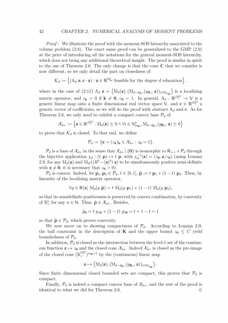
42 CHAPTER 2. NUMERICAL ANALYSIS OF MOMENT PROBLEMS
Proof : We illustrate the proof with the moment-SOS hierarchy associated to thevolume problem (2.8). The exact same proof can be generalized to the GMP (2.9)at the price of introducing all the notations for the general moment-SOS hierarchy,which does not bring any additional theoretical insight. The proof is similar in spiritto the one of Theorem 2.6. The only change is that the cone K that we consider isnow different, so we only detail the part on closedness of
Kd :=
(Ad z, c · z) : z ∈ RNn2d feasible for the degree d relaxation,
where in the case of (2.11) Ad z =(Md(z), (Md−dX,i(gX,i z))i∈N?mX
)is a localizing
matrix operator, and ck = 0 if k 6= 0, c0 = 1. In general, Ad : RD2dn → V is a
generic linear map onto a finite dimensional real vector space V , and c ∈ RD2dn a
generic vector of coefficients, so we will do the proof with abstract Ad and c. As forTheorem 2.6, we only need to exhibit a compact convex base Pd of
Xd+ :=z ∈ RD2d
n : Md(z) 0 ∧ ∀i ∈ N?mK,Md−dK,i(gK,i z) 0
to prove that Kd is closed. To that end, we define
Pd := z = (zk)k ∈ Xd+ : z0 = 1.
Pd is a base of Xd+ in the sense that Xd+\0 is isomorphic to R++×Pd throughthe bijective application χd : (t,p) 7→ t p, with χ−1
d (z) = (z0, z/z0) (using Lemma2.9, for any Md(z) and Md′((R2−|x|2) z) to be simultaneously positive semi-definitewith z 6= 0, it is necessary that z0 > 0).Pd is convex. Indeed, let p1,p2 ∈ Pd, t ∈ [0, 1], p := t p1 + (1− t) p2. Then, by
linearity of the localizing matrix operator,
∀g ∈ R[x] Md(g p) = t Md(g p1) + (1− t) Md(g p2),
so that its semidefinite positiveness is preserved by convex combination, by convexityof Sn+ for any n ∈ N. Thus, p ∈ Xd+. Besides,
p0 = t p10 + (1− t) p20 = t+ 1− t = 1
so that p ∈ Pd, which proves convexity.We now move on to showing compactness of Pd. According to Lemma 2.9,
the ball constraint in the description of K and the upper bound z0 ≤ C yieldboundedness of Pd.
In addition, Pd is closed as the intersection between the level-1 set of the continu-ous function z 7→ z0 and the closed cone Xd+. Indeed Xd+ is closed as the pre-imageof the closed cone (SD
2dn
+ )mK+1 by the (continuous) linear map
z 7→(Md(z), (Md−dK,i(gK,i z))i∈N?mK
).
Since finite dimensional closed bounded sets are compact, this proves that Pd iscompact.
Finally, Pd is indeed a compact convex base of Xd+, and the rest of the proof isidentical to what we did for Theorem 2.6. ♦
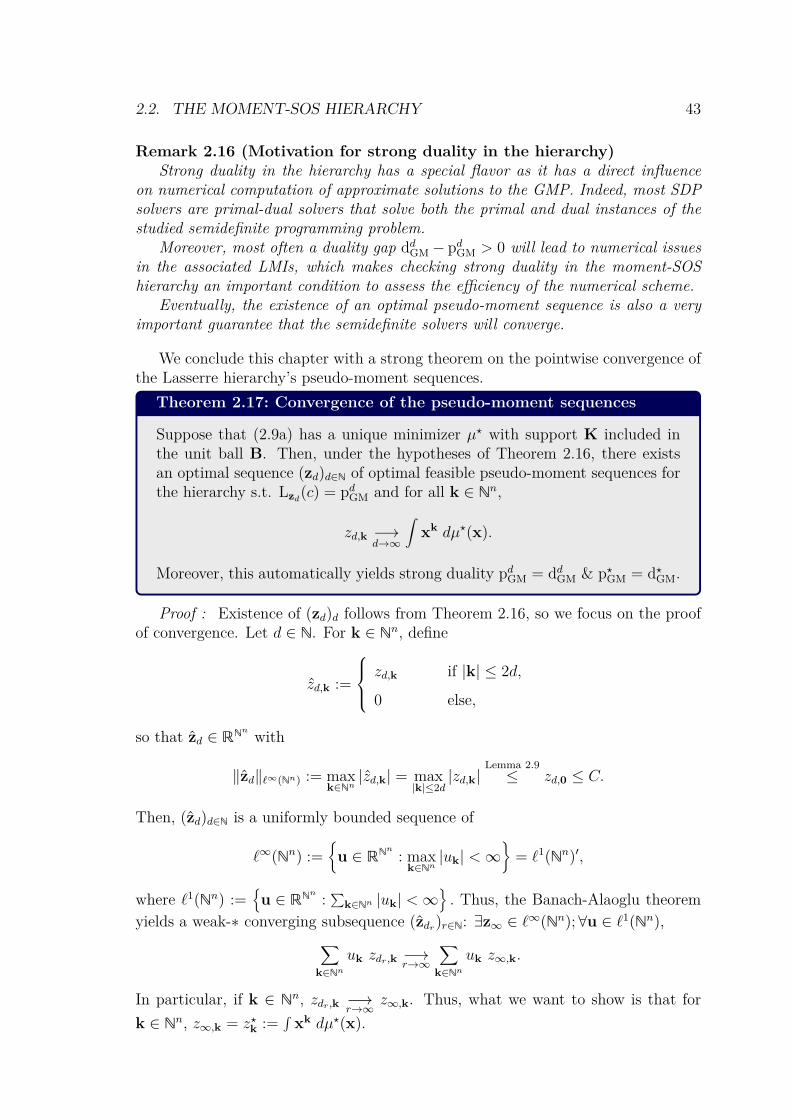
2.2. THE MOMENT-SOS HIERARCHY 43
Remark 2.16 (Motivation for strong duality in the hierarchy)Strong duality in the hierarchy has a special flavor as it has a direct influence
on numerical computation of approximate solutions to the GMP. Indeed, most SDPsolvers are primal-dual solvers that solve both the primal and dual instances of thestudied semidefinite programming problem.
Moreover, most often a duality gap ddGM− pdGM > 0 will lead to numerical issuesin the associated LMIs, which makes checking strong duality in the moment-SOShierarchy an important condition to assess the efficiency of the numerical scheme.
Eventually, the existence of an optimal pseudo-moment sequence is also a veryimportant guarantee that the semidefinite solvers will converge.
We conclude this chapter with a strong theorem on the pointwise convergence ofthe Lasserre hierarchy’s pseudo-moment sequences.
Theorem 2.17: Convergence of the pseudo-moment sequences
Suppose that (2.9a) has a unique minimizer µ? with support K included inthe unit ball B. Then, under the hypotheses of Theorem 2.16, there existsan optimal sequence (zd)d∈N of optimal feasible pseudo-moment sequences forthe hierarchy s.t. Lzd(c) = pdGM and for all k ∈ Nn,
zd,k −→d→∞
∫xk dµ?(x).
Moreover, this automatically yields strong duality pdGM = ddGM & p?GM = d?GM.
Proof : Existence of (zd)d follows from Theorem 2.16, so we focus on the proofof convergence. Let d ∈ N. For k ∈ Nn, define
zd,k :=
zd,k if |k| ≤ 2d,
0 else,
so that zd ∈ RNn with
‖zd‖`∞(Nn) := maxk∈Nn|zd,k| = max
|k|≤2d|zd,k|
Lemma 2.9≤ zd,0 ≤ C.
Then, (zd)d∈N is a uniformly bounded sequence of
`∞(Nn) :=u ∈ RNn : max
k∈Nn|uk| <∞
= `1(Nn)′,
where `1(Nn) :=u ∈ RNn : ∑k∈Nn |uk| <∞
. Thus, the Banach-Alaoglu theorem
yields a weak-∗ converging subsequence (zdr)r∈N: ∃z∞ ∈ `∞(Nn);∀u ∈ `1(Nn),∑k∈Nn
uk zdr,k −→r→∞∑
k∈Nnuk z∞,k.
In particular, if k ∈ Nn, zdr,k −→r→∞ z∞,k. Thus, what we want to show is that fork ∈ Nn, z∞,k = z?k :=
∫xk dµ?(x).

44 CHAPTER 2. NUMERICAL ANALYSIS OF MOMENT PROBLEMS
Without loss of generality we focus on the relaxations of problem (2.8a).Let l := (
∫X xk dx)k∈Nn be the moment sequence of the Lebesgue measure on X.
Let p ∈ R[x]. Then, for all r ∈ N big enough, by feasibility of zdr for therelaxation of degree dr, one has• [0,Ll(p2)] 3 Lzdr (p
2) = Lzdr (p2) −→
r→∞Lz∞(p2)
• 0 ≤ Lzdr (gK,i p2) = Lzdr (gX,i p
2) −→r→∞
Lz∞(gK,i p2)
• 0 ≤ Ll−zdr (gX,i p2) = Ll−zdr (gX,i p
2) −→r→∞
Ll−z∞(gX,i p2)
so that according to Putinar’s P-satz 2.4, z∞ is the actual moment sequence ofa measure µ∞ that is feasible for problem (2.8a). Then, one directly has
p?K ≥∫
1 dµ∞ = z∞,0 = limr→∞
zdr,0 = limr→∞
pdrK ≥ p?K
since for any d ∈ N pdK ≥ p?K. Hence,∫
1 dµ∞ = p?K, i.e. µ∞ is optimal for problem(2.8a). By our uniqueness assumption, this yields µ∞ = µ?, i.e. z∞ = z?. Thus,(zd)d has a unique weak-∗ accumulation point z?, which means that for any k ∈ Nn,
zd,k −→d→∞
z?k =∫
xk dµ?(x).
Eventually, Theorem 2.16 ensures strong duality pdGM = ddGM, so that putting to-gether weak GMP duality and the strenghtening property, one has
p?GMweak duality≤ d?GM
strenghtening≤ ddGM
strong duality= pdGM
convergence−→d→∞
p?GM
and the sandwich rule again yields strong GMP duality. ♦
Remark 2.17 (An “all inclusive” theorem)Theorem 2.17 shows that the hypotheses of Theorem 2.16 for strong duality in the
hierarchy are almost sufficient for the pseudo-moment sequences of the relaxationsto converge pointwise to the moments of the optimal solution of the GMP (2.9a) andfor full strong duality to hold.
In practice we will design instances of the GMP such that Theorem 2.17 holds,so that we automatically obtain strong duality in the GMP and the correspondinghierarchy as well as pointwise convergence of the moment sequence.
In particular, up to rescaling, K ⊂ B can always be enforced.
Synthesis of sections 2.1 & 2.2In this Chapter, the fundamental tools that will be used in this thesis were intro-duced. Section 2.1 focused on infinite dimensional optimization, introducing theGMP and its strong modelling power, as well as a useful strong duality theorem forthe analysis of such problem. Then, Section 2.2 derived the Lasserre, moment-SOShierarchy that allows numerically approximating solutions of the GMP, along with avariety of duality and convergence properties. Those two aspects (modelling infinite

2.2. THE MOMENT-SOS HIERARCHY 45
dimension and approximate finite dimension) of the moment-SOS hierarchy pavethe way for the smooth demonstration of approximating properties for the schemesthat will be presented in the rest of this thesis. As a result, they will be instrumentalin all the remaining chapters. We recall in Figure 2.4 the successive steps of themoment-SOS hierarchy scheme.
Figure 2.4 – Illustration of the moment-SOS hierarchy.
The GMP is used to model a variety of difficult, nonconvex problems, after what adual to the GMP is computed, and the moment and SOS hierarchies are formulatedin parallel, and solved as SDP problems with LMI constraints.


3Transient stability of power systems
The aim of this thesis is to contribute to the application of semidefinite programming(SDP) methods in power systems transient stability analysis (TSA). A natural firststep is thus to give original applications of existing SDP methods to low-dimensionalpower systems. Currently, two schools have issued promising results in the field ofSDP-based direct stability analysis:
• the French school draws on the developments presented in Chapter 2 andmoment-SOS hierarchy-based schemes to approximate various stability regionsof differential systems [42, 58, 57] and its first contribution to power systemsrather focused on the static optimization AC-OPF problem [52]. Section 3.1gives a first application of such methods to power systems stability analysis,based on publication [53].
• the US school focuses on SOS programming for Lyapunov methods [51] and itstarted contibuting to the particular problem of power systems in 2013 [6]. Thesecond section of this chapter is an intent to test the computational limits ofsuch methods on a more sophisticated system model, that was first publishedin [125].
Contents3.1 A moment-SOS based approach . . . . . . . . . . . . . . . 48
3.1.1 Occupation measures . . . . . . . . . . . . . . . . . . . . . 48
3.1.2 Outer ROA approximation for polynomial systems . . . . 54
3.1.3 Finite time ROA estimation for a 3 machines model . . . 57
3.2 An SOS, Lyapunov-based approach . . . . . . . . . . . . 63
3.2.1 The single machine - infinite bus system . . . . . . . . . . 63
3.2.2 Lyapunov-based inner ROA approximation . . . . . . . . 68
3.2.3 Computing an SOS Lyapunov function . . . . . . . . . . . 71
3.2.4 ROA estimation of the SMIB model . . . . . . . . . . . . 78
47

48 CHAPTER 3. POWER SYSTEMS TRANSIENT STABILITY
3.1 A moment-SOS based approachIn this section, we show that the problem of TSA in power systems can be addressedusing the moment-SOS hierarchy that we presented in Chapter 2. TSA considers thebehavior of a power system following a major disturbance. Following considerationsfrom Chapter 1, we focus on direct methods, which consist in computing stabilityoracle functions (SOF) parameterizing approximations of well-chosen regions of at-traction (ROA). We recall that according to Remark 1.2, inner approximations arepreferred to outer ones, as they prevent false negatives; however, we allow ourselvesto also consider outer approximations, if it helps the simplicity of exposition. Inthis section, we focus on uncontrolled dynamics as a first step towards certifiedestimations of the ROA around a given operating point.
From a theoretical viewpoint, the idea is to use the moment-SOS hierarchy tocompute approximated solutions of the finite time ROA problem presented in Ex-ample 2.8 (the interest of finite time will be exposed below). This section is organizedas follows. Section 3.1.1 introduces the notion of occupation measure, which willbe instrumental to deriving the finite time ROA problem in a way that will allowfor moment-SOS hierarchy implementation in Section 3.1.2. Section 3.1.3 describesnumerical experiments conducted to show the practical relevance of the proposedmethod and gives future research directions regarding computational tractability.
3.1.1 Occupation measuresIt turns out that there exist numerical tools inspired from Chapter 2 on the GMP,which give some methods to compute approximations of constrained regions of at-traction. While these numerical tools were initially designed only for polynomialdifferential systems, the following sections will introduce their conceptual basis, andhow they can be applied to some nonpolynomial differential systems, without re-sorting to polynomial approximations of the vector fields.
As shown in [42, 58], the moment-SOS hierarchy makes it possible to numeric-ally approximate AX
T (M) for well-chosen T and M. We recall here how the methodworks. The key idea of the authors is to elegantly combine the set approximatingproperty of the volume problem (see Example 2.6 and the corresponding reference[44]) with the notion of occupation-measure-based moment-SOS hierarchy intro-duced in [72]. More precisely, their method consists of grouping all the necessarytime-domain simulations into the resolution of a single, linear partial differentialequation (PDE). It can be compared to a Monte-Carlo algorithm, but offers theadvantage of giving strong inclusion guarantees on the approximation that the com-putation yields.
Here we introduce the key element to design the ROA problem, following thecontributions in [72]. Suppose that instead of having one deterministic initial condi-tion x0 for the system (1.4), one is given a random variable x0 with probability lawP0 ∈ P(Rn). This means that for a given Borel set Y ⊂ Rn, P(x0 ∈ Y) = P0(Y).Instead of considering a sample for the law P0 and running time-domain simulationsfor its realizations, as a Monte-Carlo algorithm would do, we directly work on theprobability P0. Indeed, if x0 is a random variable that follows the probability P0,

3.1. A MOMENT-SOS BASED APPROACH 49
then for any t ≥ 0, x(t|x0) is also a random variable, so that we call Pt ∈ P(Rn)its probability law1. It is actually pretty easy to deduce Pt from P0, through thenotion of transfer operator:
Definition 3.1: Ruelle’s transfer operator
Let E,F be finite dimensional open or compact sets, ϕ : E → F continuous.Ruelle’s transfer operator [113, 89] ϕ# :M(E)+ →M(F)+ maps a measure µonto its pushforward through ϕ, denoted ϕ#µ and defined, for any Borel setY ⊂ F, by
ϕ#µ(Y) := µ(ϕ−1(Y)) = µx ∈ E : ϕ(x) ∈ Y.
Proposition 3.2: Probability transfer
For all t ≥ 0, Pt is deduced from P0 through the transfer operator x(t|·)# asfollows: Pt = x(t|·)#P0, i.e. for any Borel set Y ⊂ Rn,
Pt(Y) = P0(x(t|·)−1(Y)
)= P0x0 ∈ Rn : x(t|x0) ∈ Y.
Remark 3.1 (Transfer and composition)From a duality perspective, the adjoint to the Ruelle transfer operator µ 7→ ϕ#µ
is the Koopman composition operator v 7→ vϕ. Indeed, besides the above definition,for ϕ : Rm → Rn, v ∈ Cc(Rn) and µ ∈M(Rm)+ one has
∫v d(ϕ#µ) =
∫(v ϕ) dµ.
The Ruelle operator is also called Perron-Frobenius operator, after the Perron-Frobenius theorem whose infinite dimensional extension (named Krein-Rutman the-orem) allows to prove that its eigenvectors are nonnegative measures. However, thePerron-Frobenius theorem has many other applications.
Conversely, knowing P0 and Pt gives an information on x(t|·), without havingto perform any simulation. Moreover, the data Pt for all t ≥ 0 defines a function
ψ :
R+ −→ P(Rn)
t 7−→ ψ(t) := Pt.
Then, a theorem due to Joseph Liouville ensures that ψ is subject to the continuityequation [129, Theorem 5.34]:
1Such time-dependent measure is called a Young measure, after Laurence Chisholm Young, whoinvented them to account for randomized control laws [143].

50 CHAPTER 3. POWER SYSTEMS TRANSIENT STABILITY
Theorem 3.3: Liouville
If f is Lipschitz, then ψ is the unique solution with initial condition ψ(0) = P0of the following infinite dimensional, linear ODE:
ψ = −div(ψ f), (3.1)
where the derivative is defined w.r.t. the weak-∗ topology on P(Rn).In particular, if there exists a density function ρ : R+ × Rn → R such thatPt = ρ(t, ·) λ, then an integration by part yields the classical PDE form
∂tρ+ div(ρ f) = 0. (3.1′)
Remark 3.2 (Divergence of a vector measure)In Theorem 3.3, we introduce the term −div(ψ f), which is defined as follows:
− div(ψ f)(t) :=[v ∈ C1
c (Rn) 7→∫
f · grad v dψ(t)], (3.2)
where C1c (Ω) is the subset of C1(Ω) of functions that vanish outside a compact set.
Notice that ψ is an univariate function (of t), with value in a functionalspace (in x), so that equation (3.1) is indeed a linear ODE ψ = A ψ while (3.1′) isa linear PDE in the multivariate unknown function ρ (of t and x).
Thus, Problem 1 can be rewritten in terms of Young measures, if one restrictsto a finite time horizon T ∈ (0,+∞):
Problem 9: Stable initial measure
Find the maximal support for P0 such that (3.1) holds and:
• For all t ∈ I := [0, T ], ψ(t) is supported in X,
• ψ(T ) is supported in M
so that sptP0def= AX
T (M).
Remark 3.3 (Finite VS infinite time horizon)Historically, stability analysis was first considered in astrophysics, with scientists
concerned about the long term stability of the planet orbits in the solar system. Forthis reason, the most common notion of ROA is the unconstrained, infinite timeROA A∞(M).
However, in the context of power system TSA, all events occur within a finite,narrow time horizon, due to the speed of electro-mechanical dynamics. For thisreason, it is only natural that we consider finite time ROAs here. Moreover, we willsee in this chapter that finite time horizons are more convenient for computationsthat infinite time horizons.
Nevertheless, infinite time horizons can also be considered, as we will show inSections 3.2 and 6.1.

3.1. A MOMENT-SOS BASED APPROACH 51
Now, instead of considering only probability measures P0 ∈ P(Rn) that repres-ent a random initial condition x0, we propose to consider a superposition of initialconditions, which is represented by a measure µ ∈ M(Rn)+ s.t. µ(Rn) < ∞. Onecan easily switch from the probabilistic viewpoint to this statistical physics view-point by the following operations: µ = C P0 for a given C > 0, or P0 = 1
µ(Rn) µ. Bylinearity of the continuity equation, Theorem 3.3 still holds for ψ := t 7→ x(t|·)#µwith initial condition ψ(0) = µ in equation (3.1). It can even be extended to thenotion of occupation measure.
Definition 3.4: Occupation measure
For a given initial measure µ ∈ M(Rn)+ and time horizon T > 0, we definethe occupation measure νµ ∈M(I×Rn)+, for a < b ∈ I and Y ⊂ Rn:
νµ([a, b]×Y) :=∫ b
a
(∫Rn1Y(x(t|x0)) dµ(x0)
)dt =
∫ b
aψ(t)(Y) dt.
In particular, if µ = P0 ∈ P(Rn), then νµ([a, b]×Y) =∫ ba Pt(Y) dt is the average
time that the random trajectory x(t|x0) spends in Y between times a and b.
Remark 3.4 (Alternative definition of occupation measures)Using the Riesz-Markov theorem, one can define the occupation measure ν through
its action on C1 functions instead of its action on Borel sets: for v ∈ C1c (I×Rn),∫
v dνµ :=∫ T
0
(∫Rnv(t,x(t|x0)) dµ(x0)
)dt =
∫ T
0〈v(t, ·), ψ(t)〉 dt.
Remark 3.5 (Relevance of occupation measures)While Young measures such as ψ(t) are measure-valued functions of time, occu-
pation measures are actually standard measures, and as such they can be representedon compact sets by their moments, allowing for a GMP rephrazing and thus the im-plementation of the Moment-SOS hierarchy, as we will show in the next section.
Liouville’s theorem also holds for occupation measures, under a slightly differentform.
Theorem 3.5: Transport of occupation measures
Let µ ∈M(Rn)+, T > 0, νµ ∈M(I×Rn) as in Definition 3.4.Let ξµ := ψ(T ) = x(T |·)#µ (if µ = P0 ∈ P(Rn) then ξµ = PT ).If f is C1, then, (νµ, ξµ) is the unique solution of the following linear PDE withunknown (ν, ξ) ∈M(I×Rn)×M(Rn):
∂tν + div(ν f) + δT ξ = δ0 µ, (3.3)
with parameters f , µ, δ0, δT , where δt = [Y 7→ 1Y(t)] ∈ P(R) is the Diracmeasure in t ∈ R.
Proof :
• (νµ, ξµ) is solution to (3.3):

52 CHAPTER 3. POWER SYSTEMS TRANSIENT STABILITY
Figure 3.1 – Illustration of occupation measures.
Here the red trajectory is initialized at x0r and the green one at x0g, so that one canassign probabilities to both trajectories:
pr := P(red traj.) = P(x0 = x0r) = µ(x0r),pg := P(green traj.) = P(x0 = x0g) = µ(x0g).
Then, the time spent by the red trajectory in Y is Tr = d− c + b− a, and the timespent by the green trajectory in Y is Tg = f− e, so that
νµ([0, 1]× Y) def= µ(x0r)(d− c + b− a) + µ(x0g)(f− e) = prTr + pgTg
is the average of the times spent by the red and green trajectories in Y.
Let v ∈ C1c (I × Rn), φµ := ∂tνµ + div(νµ f) ∈ C1(I × Rn)′. Then by definition one
has
〈v, φµ〉 = −∫
(∂tv(t,x) + f(x) · grad v(t,x)) dνµ(t,x)
= −∫ T
0
∫Rn
(∂tv(t,x(t|x0)) + f(x(t|x0)) · grad v(t,x(t|x0))) dµ(x0) dt
= −∫ T
0
∫Rn
ddt[v(t,x(t|x0))
]dµ(x0) dt
(∗)= −∫Rn
∫ T
0
ddt[v(t,x(t|x0))
]dt dµ(x0)

3.1. A MOMENT-SOS BASED APPROACH 53
= −∫ [
v(t,x(t|x0))]T
0dµ(x0)
=∫v(0,x0) dµ(x0)−
∫v(T,x(T |x0)) dµ(x0)
= 〈v, δ0 µ− δT ξµ〉,
where (∗) is obtained using Fubini’s theorem [36, pages 243–249].By our definition of measures, this proves that φµ = δ0 µ−δT ξµ, which is exactly
equation (3.3).
• Such solution is unique:
Let (ν, ξ) be a solution to (3.3) with µ = 0. By linearity of equation (3.3), showing(ν, ξ) = (0, 0) will prove uniqueness for the generic µ ∈M(Rn)+. Let v ∈ C1
c (I×Rn)and define for (t,x0) ∈ I×Rn
ϕ(t,x0) := −∫ T
tv(s,x(s− t|x0)) ds.
Then, since f is C1, for all t ∈ I one has x(t|·) ∈ C1(Rn), and thus ϕ ∈ C1c (I×Rn)
and for any (t,x0) ∈ I×Rn one has
∂tϕ(t,x(t|x0)) + f(x(t|x0)) · gradϕ(t,x(t|x0)) = ∂t (ϕ(t,x(t|x0)))
= ∂t
(−∫ T
tv(s,x(s− t|x(t|x0))) ds
)
= ∂t
(−∫ T
tv(s,x(s|x0)) ds
)= v(t,x(t|x0))
so that taking x0 = x(−t|x1) for all x1 ∈ Rn one has
∂tϕ(t,x1) + f(x1) · gradϕ(t,x1) = v(t,x1).
Moreover, it is clear that ϕ(T, ·) ≡ 0 so that one also has
0 =∫ϕ(T, ·) dξ
(3.3)= −〈ϕ, ∂tν + div(ν f)〉
=∫∂tϕ+ f · gradϕ dν
=∫v dν.
This last equality holding for all v ∈ C1c (I×Rn), this proves that ν = 0, after which
ξ = 0 is deduced from (3.3). ♦
Remark 3.6 (Regularity of f)For the use of Theorem 3.5, so far we only ask f to be C1 so that the flow x(t|·)
of f exists at all t ∈ I, is unique, and is a C1- diffeomorphism.

54 CHAPTER 3. POWER SYSTEMS TRANSIENT STABILITY
3.1.2 Outer ROA approximation for polynomial systemsAs stated in the introduction, this thesis aims at applying direct methods to assesstransient stability of a power system. Such method resorts to determining as ac-curately as possible a transient stability region, by computing some stability oraclefunction. In this section, we put the focus on solving Problem 9, which is associatedto a finite time horizon. In contrast, Section 3.2 deals with infinite time horizons.
We now give the numerical scheme to approximate the finite time ROA of apolynomial differential system. Such scheme resorts to the aforementioned notionof occupation measure, combined with the set approximation property.
The set approximation property
We consider again the volume problem from [44], which we described in Chapter 2:
p?K = supµ
∫1 dµ (2.8a)
s.t. µ ∈M(K)+
λ− µ ∈M(X)+
d?K := infw
∫w dλ (2.8b)
s.t. w − 1 ∈ C(K)+
w ∈ C(X)+,
with compact sets K ⊂ X ⊂ Rn. Here one can see that the inequality constraintsof the dual problem (2.8b) can be rephrased into
w ≥ 1K on X. (3.5)
Moreover, the convergence properties proved in Chapter 2 yield existence of a min-imizing sequence (wd)d∈N such that∫
(wd − 1K) dλ −→d→∞
0. (3.6)
Then, defining Kd := x ∈ X : wd(x) ≥ 1, (3.5) yields that K ⊂ Kd, and (3.6)ensures a vanishing volume approximation error:
vol(Kd \K
)≤∫
(wd − 1K) dλ −→d→∞
0.
In other words, sequentially solving the SOS hierarchy corresponding to the dualvolume problem (2.8b) yields a converging outer approximation (Kd)d of K. Inthe context of volume approximation, where K is already known, such a byproductis useless. However, it paves the way for general set approximation, and one canmodify problem (2.8) to approximate unknown sets, including some specific regionsof attraction.
From the volume problem to the ROA problem
The ROA problem is then obtained by combining the notion of occupation measureand Liouville equation (3.3) with the set approximation property, through addingthe Liouville equation to the volume problem (2.8a):
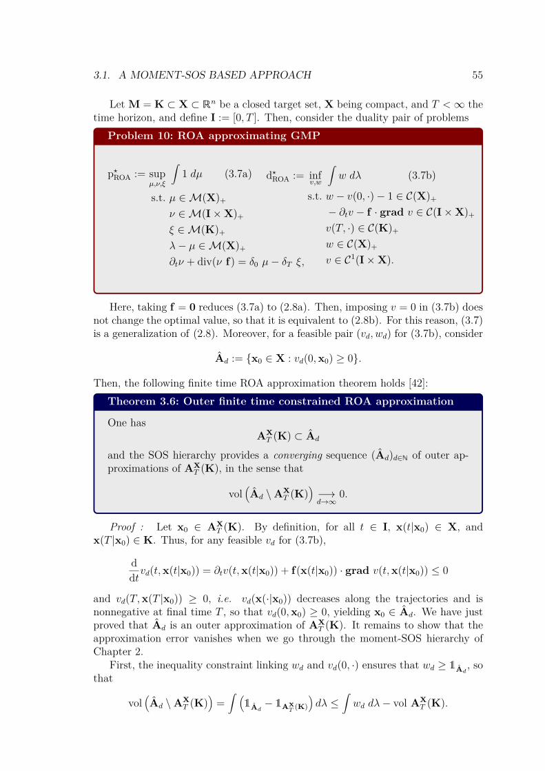
3.1. A MOMENT-SOS BASED APPROACH 55
Let M = K ⊂ X ⊂ Rn be a closed target set, X being compact, and T <∞ thetime horizon, and define I := [0, T ]. Then, consider the duality pair of problems
Problem 10: ROA approximating GMP
p?ROA := supµ,ν,ξ
∫1 dµ (3.7a)
s.t. µ ∈M(X)+
ν ∈M(I×X)+
ξ ∈M(K)+
λ− µ ∈M(X)+
∂tν + div(ν f) = δ0 µ− δT ξ,
d?ROA := infv,w
∫w dλ (3.7b)
s.t. w − v(0, ·)− 1 ∈ C(X)+
− ∂tv − f · grad v ∈ C(I×X)+
v(T, ·) ∈ C(K)+
w ∈ C(X)+
v ∈ C1(I×X).
Here, taking f = 0 reduces (3.7a) to (2.8a). Then, imposing v = 0 in (3.7b) doesnot change the optimal value, so that it is equivalent to (2.8b). For this reason, (3.7)is a generalization of (2.8). Moreover, for a feasible pair (vd, wd) for (3.7b), consider
Ad := x0 ∈ X : vd(0,x0) ≥ 0.
Then, the following finite time ROA approximation theorem holds [42]:Theorem 3.6: Outer finite time constrained ROA approximation
One hasAXT (K) ⊂ Ad
and the SOS hierarchy provides a converging sequence (Ad)d∈N of outer ap-proximations of AX
T (K), in the sense that
vol(Ad \AX
T (K))−→d→∞
0.
Proof : Let x0 ∈ AXT (K). By definition, for all t ∈ I, x(t|x0) ∈ X, and
x(T |x0) ∈ K. Thus, for any feasible vd for (3.7b),
ddtvd(t,x(t|x0)) = ∂tv(t,x(t|x0)) + f(x(t|x0)) · grad v(t,x(t|x0)) ≤ 0
and vd(T,x(T |x0)) ≥ 0, i.e. vd(x(·|x0)) decreases along the trajectories and isnonnegative at final time T , so that vd(0,x0) ≥ 0, yielding x0 ∈ Ad. We have justproved that Ad is an outer approximation of AX
T (K). It remains to show that theapproximation error vanishes when we go through the moment-SOS hierarchy ofChapter 2.
First, the inequality constraint linking wd and vd(0, ·) ensures that wd ≥ 1Ad, so
that
vol(Ad \AX
T (K))
=∫ (
1Ad− 1AX
T (K)
)dλ ≤
∫wd dλ− vol AX
T (K).

56 CHAPTER 3. POWER SYSTEMS TRANSIENT STABILITY
Second, the choice of compact sets for K,X, I ensures that Assumption 2.7 holds,up to Remark 2.5, allowing for the use of Theorem 2.14: the SOS hierarchy givesaccess to minimizing sequences for problem (3.7b), i.e. ∀d ∈ N, ∃vd ∈ R2d[t,x], wd ∈R2d[x] feasible for (3.7b) and such that∫
wd dλ −→d→∞
d?ROA.
Then, we go back to Example 2.8, to prove strong duality: d?ROA = p?ROA. Let usshow that Theorem 2.6 holds. The existence of feasible (µ, ν, ξ) is trivial: (µ, ν, ξ) =(0, 0, 0) is feasible. It only remains to prove that all feasible occupation measuresare uniformly bounded in mass:
• As for the volume (2.8), λ−µ ∈M(X)+ yields that µ(X) ≤ vol X =: Cµ <∞.
• Testing (3.3) against (t,x) 7→ 1 yields ξ(K) = µ(X) ≤ Cµ =: Cξ <∞.
• Testing (3.3) against (t,x) 7→ t yields
ν(I×X) = 〈t, ∂tν + div(ν f)〉 = 〈t, δ0 µ− δT ξ〉 = Tξ(K) ≤ T Cξ =: Cν <∞.
Then, Theorem 2.6 ensures that strong duality holds, and thus∫wd dλ −→
d→∞p?ROA.
Eventually, we show that p?ROA = vol AXT (K). Theorem 3.5 together with the
definition of the pushforward ensure that ξ ∈ M(K)+ ⇒ µ ∈ M(AXT (K))+, so
that µ = 1AXT (K) µ. Together with constraint λ − µ ∈ M(X)+, this yields that
1AXT (K) λ− µ ∈M(X)+, and then p?ROA ≤
∫1AX
T (K) dλ = vol AXT (K).
Moreover, µ = 1AXT (K) λ ∈ M(X)+ is such that ξ = x(T |·)#µ ∈ M(K)+,
so that Theorem 3.5 ensures that 1AXT (K) λ is a feasible value for µ, for which∫
1 dµ = vol AXT (K). Then, taking the supremum, one obtains p?ROA ≥ vol AX
T (K),and by double inequality, p?ROA = vol AX
T (K), so that∫wd dλ −→
d→∞vol AX
T (K).
In conclusion, the approximation error indeed vanishes when d tends to infinity:
vol(Ad \AX
T (K))≤∫wd dλ− vol AX
T (K) −→d→∞
0.
♦
Remark 3.7 (Contribution with respect to [42])Though Theorem 3.6 was already proved in [42], the systematic reduction of the
proof to checking boundedness of the feasible measures, using the original resultsfrom Chapter 2, is new.

3.1. A MOMENT-SOS BASED APPROACH 57
Remark 3.8 (Extension of [42])It is also possible to prove Theorem 3.6 using Theorem 2.17. In such a case, in
addition to the aforementioned results, one also obtains a convergence proof for thepseudo-moment sequences of the moment hierarhy. This, combined with Christoffel-Darboux kernel methods from [87], paves the way for completely new approaches formoment-hierarchy-based set approximations.
Remark 3.9 (Relevance of the constrained finite time ROA)The proof of Theorem 3.6 heavily relies on the finite time horizon T and state
constraint sets X and K. Indeed, this choice of parameters is required for I, Kand X to be compact, which is instrumental in the proof. In other words, stateconstraints and a finite time horizon are the price for the convergence of the ROAapproximation.
However, such constraints are quite relevant for TSA: as pointed in Remark 3.3,a finite time horizon is suitable in this context. Moreover, operational TSA does notonly expect that the system quickly converges to equilibrium, but also that the traject-ory remains secure during all the transients; this involves additional state constraintsecurity specifications (e.g. current, voltage and power boundedness), which can beencoded in X.
Thus, even though the notion of constrained finite time ROA is less usual thanthe notion of free infinite time ROA, it is particularly relevant in the context of thisthesis. As a result, it will be the first TSA approach to which we will apply structuredecomposition to facilitate computations (see Section 6.2).
3.1.3 Finite time ROA estimation for a 3 machines modelApart from rephrazing the proof for the ROA approximation, an important contri-bution of this section is the extension of the framework to non-polynomial equationsof power systems, with numerical application to the three machine model. In termsof numerical application, we are interested in analysing the transient behaviour ofsystem (1.1)–(1.3). More precisely, to numerically illustrate the TSA problem, weuse the three-bus numerical example from Chiang et al. [21], which is composed ofthree synchronous machines connected in a meshed grid. The third bus is arbitrarilychosen as the reference angle (i.e., θ3 = 0), so that one only needs two phase anglevariables, θ1, θ2, and two rotor speed variables, ω1, ω2, to describe the dynamics.[21] neglected conductances Gkl and attributed numerical values to Mk, Dk, Pmec
k ,|vk| and Bkl, obtaining:
θk = ωk, k = 1, 2,ω1 = − sin(θ1)− 0.5 sin(θ1 − θ2)− 0.4 ω2,
ω2 = −0.5 sin(θ2)− 0.5 sin(θ2 − θ1)− 0.5 ω2 + 0.05,
where the ωk are expressed in rad/s and the θk are in rad. A stable equilibrium isgiven by θ = (0.02, 0.06).
This very basic example will serve as a numerical test case for our moment-SOSTSA method.

58 CHAPTER 3. POWER SYSTEMS TRANSIENT STABILITY
M1 M2
M3
G12 + jB12G
13+
jB13
G23 +
jB23
v1 v2
v3
Figure 3.2 – The three machines cycle.
Tackling trigonometric dynamics
Following [6], the coordinates can be shifted so that (θ1, θ2) = (0.00, 0.00) is a stableequilibrium. This dynamical system can in turn be formulated as a polynomialdifferential algebraic system, as suggested in [6]. To that end, we introduce auxiliaryvariables
sk := sin(θk) and ck := 1− cos(θk), k = 1, 2 (3.8)and define ω := (ω1, ω2), s := (s1, s2), c := (c1, c2) as well as x := (ω, s, c) ∈ R6.One then obtains the following differential algebraic equation system (DAEs)
ω1 = 0.4996s2 − 0.4ω1 − 1.4994s1 − 0.02c2 +0.02s1s2
+0.4996s1c2 − 0.4996c1s2 + 0.02c1c2,
ω2 = 0.4996s1 + 0.02c1 − 09986s2 + 0.05c2−0.5ω2
−0.02s1s2 − 0.4996s1c2 + 0.4996c1s2−0.02c1c2,
sk = (1− ck)ωk k = 1, 2,
ck = skωk k = 1, 2,
0 = s2k + c2
k − 2ck k = 1, 2,
We will show later on that one can actually avoid increasing the number of variablesand immediately obtain a polynomial differential system of equations in complex-valued quantities.
A particularity of the occupation measure approach is that the state set X shouldhave an interior point such that the computed volumes are non-zero. Hence, con-straints 0 = h(x) := (s2
k + c2k − 2ck)k=1,2 in the dynamics derived from our change

3.1. A MOMENT-SOS BASED APPROACH 59
of variable may be troublesome, since the manifold M := x ∈ R6 : h(x) = 0 is ahyper-surface with no interior point. A simple method to address this issue consistsof ignoring the equality constraints when computing the ROA approximation Ad,and then consider Ad ∩M as the desired ROA estimation. Such an exact methoddoes not work with any arbitrary equality constraints. However, in the case of con-straints derived from a change of variable, this approach is valid due to the fact thatthe reformulated vector field f then satisfies (grad h)·f ≡ 0. Thus, the dynamics aretangent to M, yielding that any trajectory starting in M will remain in M, which isexactly the constraint h(x(t|x0)) = 0, ∀ t ∈ [0, T ]. For equality constraints that arenot derived from changes of variables, this does not hold anymore; in such case, onecould think of replacing the classical Lebesgue measure λ with a Hausdorff measuresupported on M, and computed using Stokes theorem if M is the boundary of afull-dimensional set [73].
To the best of our knowledge, this is the first time that algebraic equality con-straints derived from a change of variable are addressed within the occupation meas-ure approach. This facilitates the novel application of occupation measures theoryto non-polynomial systems. The general non-polynomial dynamics framework thatcan be tackled with this method will be discussed in details in Section 3.2.3.
Case study
For our numerical experiments, we use MATLAB R2015b, YALMIP [78], SeDuMi 1.3[120], and the “ROA” code of [42] to apply occupation measure theory to the three-bus example from [21] that is described above.
We define the finite time ROA parameters as follows:
• X := [−π, π]2 × [−1, 1]2 × [0, 2]2= x ∈ R6 : (ω2
1,2 ≤ π2) ∧ (s21,2 ≤ 1) ∧ (0 ≤ c1,2 ≤ 2)
• K := Bε = x ∈ R6 : |x|2 ≤ ε2, ε = 0.1, T = 8 s.
Following the developments in Chapter 2, problem (3.7b) admits a SOS strenght-ening that can be expressed as follows:
ddROA := infw
w · l (3.9)
s.t. w(x)− v(0,x)− 1 ∈ Σd(g(x))− ∂tv(t,x)− f(x) · grad v(t,x) ∈ Σd(g(t,x))v(T,x) ∈ Σd(0.01− |x|2)w(x) ∈ Σd(g(x))v(t,x) ∈ R2d[t,x],
where:
• l is the vector of moments of the Lebesgue measure λ on X in a moment basis,
• w is the vector of coefficients of w in the corresponding monomial basis,
• g(x) = (π2 − ω21,2, 1− s2
1,2, (2− c1,2)c1,2, 30− |x|2) describes the state set X,

60 CHAPTER 3. POWER SYSTEMS TRANSIENT STABILITY
• f(x) = (ω, s, c) describes the polynomial dynamics and
• g(t,x) = ((T − t)t, π2 − ω21,2, 1− s2
1,2, (2− c1,2)c1,2, 100− t2 − |x|2).
Again, there is no duality gap between these truncated problems and the corres-ponding moment relaxations of (3.7a), at every order of the hierarchy, thanks toTheorem 2.16 (the proof is identical to the strong duality proof for Theorem 3.6).Though we already have proved the convergence of the outer approximation, thecomputational burden increases sharply as the order d increases.
We complement this explanation by briefly discussing the approach for comput-ing inner approximations. The machinery for inner ROA approximations is verysimilar to the outer approximation approach discussed above. The key distinction isthat the inner approximations consider an outer approximation to the complementof the ROA, AX
T (K)c := X \AXT (K), inducing additional technicalities. See [58] for
further details.We note that practical power system analyses require the ability to address
significantly larger problems than the test case considered in this section. How-ever, constructing certified approximations for the ROA leads to difficult computa-tional challenges, see e.g. Section 3.2. Similar to the demonstrations of previousalgorithms [6],[50], this section focuses on a small system as an initial step towardspractical applications. Future work that exploits network sparsity and other prob-lem structures will be crucial for scalability. Decomposition approaches may alsoprove to be valuable [61, 62, 63].
With final time T = 8 and radius ε = 0.1, we find the following polynomial,v5(0, x), at fifth-order relaxation (d = 5):
v5(0, x) = 1.8707− 4.9538x1 + 0.0017x2
− 4.7856x3 + 0.0018x4 − 0.0037x5
− 4.8546x6 − 0.0131x21 + 10.9412x1x2
− 0.0356x1x3 + 13.9529x1x4 + 0.0208x1x5
+ 0.0142x1x6 + 16.4121x22 + 0.0609x2x3
− 0.2755x55x
56 + 0.0017x4
5x66 + 0.0170x3
5x76
− 0.0002x25x
86 − 0.0021x5x
96 − 0.0003x10
6 .
The zero super-level set A5 := x ∈ R6 : v5(0,x) ≥ 0 provides an outerapproximation to the ROA. We illustrate the polynomial v5(0, ·) in Fig. 3.3 as afunction of the original state variables (θ1, θ2). We consider (ω1, ω2) = (0, 0) inorder to visualize the ROA, but this is not a necessary restriction. We illustrate theouter approximation to the ROA in Fig. 3.4.
Likewise, with T = 8 and ε = 0.1, we find at the third-order relaxation (d = 3)the inner approximation to the ROA presented in Fig. 3.5 (again with ω = (0, 0)used only for representation purposes).
We next show how one could use Hermitian SOS to obtain better numericalresults. For optimal power flow problems, applying Hermitian SOS yields compu-tational advantages while preserving convergence guarantees [54]. The idea is toexploit the structure that comes from alternating current physics in order to reducethe computational burden. We consider the transient dynamics of a system after

3.1. A MOMENT-SOS BASED APPROACH 61
Figure 3.3 – Plot of the graph of vd(0, ·), d = 5.
The polynomial for the three-bus system whose zero super-level set, which is in-dicated by the back region, provides an outer approximation to the ROA. Theprojection shown is for ω = (0, 0).
Figure 3.4 – Outer ROA approximation of degree d = 5.
An outer approximation of the ROA is indicated by the back region. The projectionshown is for (ω1, ω2) = (0, 0).
the fault has disappeared and we assume that there is no voltage instability. In thatcase, it is reasonable to assume that the magnitudes |vk| of the complex voltagesare fixed such that only the phase angles θk are variables. This allows us to definevk := exp(j θk) (up to proper rescaling), such that vk = j θk exp(j θk), where j2 = −1.The dynamics can thus immediately be written as a polynomial differential systemof equations (with physical variables now expressed in perunits, s.t. the voltageshave magnitude 1):

62 CHAPTER 3. POWER SYSTEMS TRANSIENT STABILITY
Figure 3.5 – Inner ROA approximation of degree d = 3.
An inner approximation of the ROA is indicated by the back region. The projectionshown is for (ω1, ω2) = (0, 0).
vk= j ωkvk,
ωk=−DkMkωk + 1
Mk
(Pk − 1
2∑l 6=k−Gkl|vk|2 − Y klvkvl − Yklvlvk
),
0 = |vk|2 − 1,
(3.10)
where Ykl denotes the mutual admittance of the line connecting buses k and l.It is straightforward to adapt the theory of occupation measures to complex
states by leveraging recent results in complex algebraic geometry [27]. A futurework would consist of implementing a complex version of the hierarchy proposedin [42] in order to reduce the computational burden at a given relaxation order.
In conclusion, in the context of the transient stability analysis of power systems,this section demonstrates the potential for using the theory of occupation measures(along with convex optimization techniques) to compute inner and outer approxim-ations to the region of attraction for a stable equilibrium point. To the best of ourknowledge, this is the first time that occupation measure theory has been appliedto analyze transient stability problems for electric power systems. The resultingapproximations have the potential to provide analytically rigorous guarantees thatcan reduce the need for computationally expensive time-domain simulations. Withcomputational tractability remaining an important challenge, the next chapters willinvestigate how to exploit sparsity for set approximation, in particular when usingoccupation measures.

3.2. AN SOS, LYAPUNOV-BASED APPROACH 63
3.2 An SOS, Lyapunov-based approachIn this section, we investigate an alternative SOS method for ROA approximation,which is based on Lyapunov theory rather than occupation measures. We recallhere that, as our variable v in Section 3.1, Lyapunov functions are an instance ofSOF (historically, they even are the archetype of SOF, since the first direct methodsfor stability analysis resorted to what we now call Lyapunov functions) as listed inExample 1.5. The Lyapunov approach was used in [6] for transient stability analysisof a power system. However, the generators were modeled only by their swing equa-tions. As the voltage and frequency regulators have an important impact on stabilityanalysis, in the present section this approach is extended by considering a generatorwith voltage dynamics and both voltage and frequency regulations. This also pavesthe way to taking into account high penetration of power electronics elements in thegrid due to the integration of renewable energies and HVDC transmission lines, thushaving an important impact on the transient stability of the system. SOS methodgives an analytical solution for the construction of Lypunov functions in order toestimate the infinite time ROA for a locally asymptotically stable equilibrium pointof the system.
The section is organized as follows: the problem is formulated and modelled inSection 3.2.1 for a Single Machine-Infinite Bus (SMIB) system. Section 3.2.2 sumsup the elements of Lyapunov theory that are at stake. SOS formalism and algorithmsare briefly recalled in Section 3.2.3, along with a necessary change of variables (i.e.,reformulating the model of the system with trigonometric non linearities into aset of polynomial differential algebraic equations). The reformulating procedure isproved to be a Lie-Bäcklund transformation, which means that the transformedsystem has equivalent trajectories and stability properties [34]. Next, in Section3.2.4 we relax Lyapunov’s conditions for stability and model constraint equationsto suitable SOS conditions using theorems from real algebraic geometry in order toformulate the problem as an optimization one. Hence, a Lyapunov function for theasymptotically stable equilibrium point is constructed using the expanding interioralgorithm developed in [51, 6]. An estimate of the ROA is given by a level set ofthe Lyapunov function. We finally test the ROA estimation error by numericallycomputing the real one in all state directions via full nonlinear simulations. Thecodes are implemented in MATLAB using SOSTOOLS [106] which is a free, third-party MATLAB toolbox that models SOS problems.
3.2.1 The single machine - infinite bus systemWe consider a synchronous machine connected to a power grid through two trans-mission lines in parallel (see Figure 3.6). The power grid is modelled as an infinitebus. The infinite bus imposes a nominal voltage of amplitude Vg and frequency ωg atnode B. Each transmission line is a series of two impedance matrices Zt := RtI+XtJ(or equivalently one synthetic impedance matrix Zeq = 2Zt), where Rt, Xt ∈ R+ and
I =(
1 0
0 1
), J =
(0 −1
1 0
).

64 CHAPTER 3. POWER SYSTEMS TRANSIENT STABILITY
The synchronous machine has two rotating axes d (direct) and q (quadratic), whichsupport the currents id and iq (we use the notation is := (id, iq)>), generating avoltage vs := (vd, vq)> at the machine’s terminal.
The synchronous machine is characterized by an internal resistance Ri and equi-valent reactance matrices Xi := J diag(xd, xq) and X′i := J diag(x′d, xq), withxd, xq, x
′d ∈ R+. It receives a mechanical power Pm and rotates at frequency ω,
generating a field voltage with magnitude Ef orthogonal to the rotor axis, and thusproviding an e.m.f e ∈ R2. Let θ be the phase between the machine internal voltageand the grid voltage and H the machine’s mechanic inertia constant.
Synchronous Machine
AE M
S
B
Zt Zt
Zeq
RiX′i is
ui ut
vme vs vg
∞
Figure 3.6 – Synchronous machine connected to an infinite bus (SMIB).
The equations describing the dynamics of this system are given in [114, p. 105].In this section we give some details on how these equations can be derived as a5th order model. First, we take as a starting point the swing equation that modelsthe synchronous machine, but we do not assume its voltage magnitude |vs| to beconstant anymore. Thus, we enrich the model with the dynamics of the e.m.f. e,obtaining a 3rd order model. Then, we proceed to modelling the outer control loopson the voltage magnitude |vs| and frequency ω, that appear in the dynamics of thefield voltage Ef and mechanical power input Pm respectively, leading to a 5th ordermodel.
Synchronous machine dynamics
As stated above, we write the equations of the system in a rotating frame whosedirect axis is aligned with the rotor’s axis, and whose quadratic axis is aligned withthe field voltage. In such system, the synchronous machine’s dynamics write:
θ = 100π(ω − ωg) (3.11a)2H ω = Pm − (vm · is) (3.11b)
T0 e = Ef
(0
1
)− e− (Xi − X′i) is, (3.11c)
where θ is expressed in rad, and all other variables are expressed in p.u.Notice that equation (3.11c), which models how the field voltage Ef generates
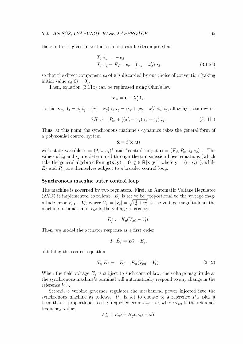
3.2. AN SOS, LYAPUNOV-BASED APPROACH 65
the e.m.f e, is given in vector form and can be decomposed as
T0 ed = − edT0 eq = Ef − eq − (xd − x′d) id (3.11c′)
so that the direct component ed of e is discarded by our choice of convention (takinginitial value ed(0) = 0).
Then, equation (3.11b) can be rephrased using Ohm’s law
vm = e− X′i is,
so that vm · is = eq iq − (x′d− xq) id iq = (eq + (xq − x′d) id) iq, allowing us to rewrite
2H ω = Pm + ((x′d − xq) id − eq) iq. (3.11b′)
Thus, at this point the synchronous machine’s dynamics takes the general form ofa polynomial control system
x = f(x,u)
with state variable x = (θ, ω, eq)> and “control” input u = (Ef , Pm, id, iq)>. Thevalues of id and iq are determined through the transmission lines’ equations (whichtake the general algebraic form g(x,y) = 0, g ∈ R[x,y]m where y = (id, iq)>), whileEf and Pm are themselves subject to a broader control loop.
Synchronous machine outer control loop
The machine is governed by two regulators. First, an Automatic Voltage Regulator(AVR) is implemented as follows. Ef is set to be proportional to the voltage mag-nitude error Vref − Vt, where Vt := |vs| =
√v2d + v2
q is the voltage magnitude at themachine terminal, and Vref is the voltage reference:
E?f := Ka(Vref − Vt).
Then, we model the actuator response as a first order
Ta Ef = E?f − Ef ,
obtaining the control equation
Ta Ef = −Ef +Ka(Vref − Vt). (3.12)
When the field voltage Ef is subject to such control law, the voltage magnitude atthe synchronous machine’s terminal will automatically respond to any change in thereference Vref .
Second, a turbine governor regulates the mechanical power injected into thesynchronous machine as follows. Pm is set to equate to a reference Pref plus aterm that is proportional to the frequency error ωref − ω, where ωref is the referencefrequency value:
P ?m = Pref +Kg(ωref − ω).

66 CHAPTER 3. POWER SYSTEMS TRANSIENT STABILITY
Again, we model the actuator response as a first order
Tg Pm = P ?m − Pm,
obtaining the control equation
Tg Pm = Pref − Pm +Kg(ωref − ω). (3.13)
Now considering the system composed with equations (3.11a), (3.11b′), (3.11c′),(3.12), (3.13), one is seemingly faced to a new polynomial control system x = f(x,u)with state x = (θ, ω, eq, Ef , Pm)> and input u = (id, iq, Vt, Vref , Pref , ωref)>. However,id, iq and Vt are not properly speaking “control inputs”, but rather algebraic vari-ables: as stated before, they are determined by the transmission line equations, thatwe will now derive. Thus, the actual control input is u = (Vref , Pref , ωref)>, and it issupposed to be fixed in the rest of this section.
Transmission lines equations
The circuit represented in Figure 3.6 is equivalent to the much simpler one that wedisplay in Figure 3.7.
AZt is B
ut
vs vg
∞
Figure 3.7 – The equivalent simplified SMIB model.
By construction of our state variable θ as the angle from the grid to the machine,by definition of the infinite bus, and since phases are defined up to an additiveconstant, one has
vg = Vg
(cos(θ0 − θ)
sin(θ0 − θ)
)So that choosing the phase reference as θ0 = π
2 yields
vg = Vg
(sin θ
cos θ
).
On another hand, Ohm’s laws yield that
vs − vg = ut = Zt is (Fig. 3.7) & e− vs = ui = (Ri I + X′i) is (Fig. 3.6)
so that vs = vg + Zt is and e − vg = (Zt + Ri I + X′i) is, and the SMIB model isnow turned into a semi-explicit polynomial differential algebraic system of equations(DAEs) x = f(x,y)
g(x,y) = 0

3.2. AN SOS, LYAPUNOV-BASED APPROACH 67
T0 = 9.67 xd = 2.38 x′d = 0.336 xq = 1.21
H = 3 Ri = 0.002 ωg = ωref = 1 Rt = 0.01
Xt = 1.185 Vg = 1 Ta = 1 Ka = 70
Vref = 1 Tg = 0.4 Kg = 0.5 Pref = 0.7
Table 3.1 – Parameter values for the SMIB model (p.u.).
with f ,g polynomial maps, state variable x = (θ, ω, eq, Ef , Pm)> and algebraic vari-able y = (id, iq, Vt). Eventually, this DAEs has index 1: for all x ∈ R5, the mapy 7→ g(x,y) is invertible, with
is = (Zt +Ri I + X′i)−1(e− vg) & Vt = |vg + Zt is|.
After some elementary computations and simplifications, one obtains the closedformulae
iq = (Xt + x′d)Vg sin θ + (Rt +Ri)(eq − Vg cos θ)(Rt +Ri)2 + (Xt + x′d)(Xt + xq)
(3.14a)
id = Xt + xqRt +Ri
iq −1
Rt +Ri
Vg sin θ (3.14b)
vd = xqiq −Riid (3.14c)vq = Rtiq +Xtid + Vg cos θ (3.14d)
Introducing transients
We next introduce a temporary short-circuit at node S, according to the followingprotocol:
• At a time tsc a short-circuit occurs and we switch from the nominal system(Figure 3.6) to a new short-circuited system (Figure 3.8), and thus we are nolonger at an equilibrium point.
• During the short-circuit, the system leaves the equilibrium point of the nominalmodel and follows the short-circuit equations for the duration ∆t, until theshort-circuit is eliminated.
• At a time tcl = tsc+∆t, we switch back to the nominal topology and equations:the problem is to know whether the system will converge to an equilibriumpoint or not.
The short-circuit equations are computed as follows using the representation ofFigure 3.8: Kirchhoff laws now yield that
vs = vg + ut & is = ia + ib,

68 CHAPTER 3. POWER SYSTEMS TRANSIENT STABILITY
A is
SZt ib
Zt
2 Zt ia
B
ut
vs vg
∞
Figure 3.8 – The short-circuited system.
and according to Ohm’s laws
ut = 2 Zt ia & vs = Zt ib,
so that 3 vs = vg + 2 Zt ia︸ ︷︷ ︸vs
+ 2 Zt ib︸ ︷︷ ︸vs
= vg + 2 Zt is, and eventually
vs = 13vg + 2
3Zt is
that one can compare with the nominal equation vs = vg + Zt is. Since theshort-circuit only affects the transmission line equation, we conclude that the short-circuited system’s equations are the same as (3.11)–(3.14), but with Rt (resp. Xt)replaced by 2
3Rt (resp. 23Xt) and Vg replaced by 1
3Vg. Thus, equations (3.11)–(3.13)are not affected by the short-circuit.
In order to decide if, after the short-circuit is cleared at time tcl, the trajectoryof nominal system (3.11)–(3.14) will return to its stable operating point, we useSOS programming tools and Lyapunov function arguments to compute a numericalapproximation of its region of attraction.
3.2.2 Lyapunov-based inner ROA approximation
The approach that we use in this section is based on Lyapunov stability theory, andmore precisely on a specific definition of stability. We again focus on the differentialsystem
x = f(x), (1.4)
with equilibrium point x ∈ Rn, i.e. f(x) = 0.We are interested in the stability properties of (1.4). There exist several notions
of stability, so we now detail only the one that interests us in this section.

3.2. AN SOS, LYAPUNOV-BASED APPROACH 69
Definition 3.7: Local Asymptotic Stability
The equilibrium point x of ODE (1.4) is said to be:
• Lyapunov-stable (L-S) if
∀ ε > 0,∃ η > 0; |x0 − x| < η =⇒ ∀ t ≥ 0, |x(t|x0)− x| < ε
i.e. if trajectories initialized close enough to x do not go too far from it.
• locally asymptotically stable (LAS) if it is L-S and
∃ R > 0; |x0 − x| < R =⇒ x(t|x0) −→t→∞
x
i.e. if x attracts all trajectories initialized close enough to it.
Remark 3.10 (Alternative characterization of LAS points)Using Definition 1.5, the equilibrium point x is LAS iff A∞(x) contains a ball
of positive radius R > 0.
Several stability estimation theorems are due to Alexandr Mikhailovich Lya-punov and his use of observable functions that are named after him [81]. In partic-ular, the following result holds.
Theorem 3.8: Lyapunov-Persidsky
Suppose that the equilibrium of (1.4) is x = 0. Then 0 is L-S iff there existsan open domain D ⊂ Rn and a C1 “Lyapunov function” V : D→ R such that:
(i) 0 ∈ D and V (0) = 0,
(ii) ∀x ∈ D \ 0, V (x) > 0 (positive definiteness),
(iii) ∀x ∈ D, V (x) := f(x) · grad V (x) ≤ 0 (negative semi-definiteness).
The if part is due to Lyapunov in [81], while the only if comes from Persidsky[104].
At this point, it is worth recalling that the question we want to answer is thefollowing: after given transients, is our SMIB system (3.11)–(3.14) still able toconverge to stable operating point? One can prove that such stable operating pointis actually a LAS equilibrium, which means that if the post-fault state is closeenough to equilibrium, then it will indeed converge.
Definition 1.5 allows us to mathematically formulate the transient stability prob-lem that we presented in Section 3.2.1 for an infinite time horizon.

70 CHAPTER 3. POWER SYSTEMS TRANSIENT STABILITY
Problem 11: Convergence to operating point
Consider the system (3.11)–(3.14), along with a post-fault condition xcl anda LAS equilibrium point x. Determine whether
xcl ∈ A∞(x).
When T = +∞, Definition 1.5 is accompanied with the Krasovsky-LaSalle prin-ciple, which was proved approximately at the same time by Nikolai NikolaievichKrasovsky [10] and Joseph Pierre LaSalle [67, Theorem 2].
Theorem 3.9: Krasovsky-LaSalle
Let V ∈ C1(Rn) and l ∈ R such that Ω := x ∈ Rn : V (x) ≤ l is boundedand ∀ x ∈ Ω, V (x) ≤ 0. Let
M := x0 ∈ Ω : ∀ t ∈ R, V (x(t|x0)) = 0.
Then, Ω is a positively invariant subset of A∞(M).
From Theorems 3.8 and 3.9, one can elegantly deduce a characterization for localasymptotic stability, due to Lyapunov [81] (if) and Massera [88] (only if).
Theorem 3.10: Lyapunov-Massera
Suppose that the equilibrium of (1.4) is x = 0. Then 0 is LAS iff there existsan open domain D ⊂ Rn and a C1 function V : D→ R such that:
• Conditions (i) and (ii) of Theorem 3.8 hold,
• ∀x ∈ D \ 0, V (x) < 0.
Then, for any l ∈ R such that Ω = x ∈ Rn : V (x) ≤ l ⊂ D, one has thatΩ is a positively invariant subset of A∞(0).
Proof : For the considered V , M = 0 in Theorem 3.9. The proof then directlyfollows from application of Theorem 3.8. Note that the original proof of Lyapunovand Massera is more sophisticated since they did not have access to Theorem 3.9,which is actually posterior to Theorem 3.10 but facilitates its demonstration. ♦
This gives a first answer to Problem 11, up to translation on the state space suchthat x = 0: if there exist D, V and l as in Theorem 3.10 such that xcl ∈ Ω, thenxcl ∈ A∞(0). Thus, what remains to do is find such D, V and l.
However, we want to be able to answer Problem 11 for all possible values of xcl.In other words, we are looking for the exact ROA, and not only a subset of it. Suchproblem is a very difficult open question in general, but it is still possible to lookfor inner approximations of the ROA. For example, the Krasovsky-LaSalle principleallows us to strenghten our problem into a more tractable question:

3.2. AN SOS, LYAPUNOV-BASED APPROACH 71
Problem 12: Inner ROA approximation
Numerically approximate the solution to problem
q?ROA = supD,V,l
size(Ω) (3.15)
s.t. D ⊂ Rn, V ∈ C1(D), l ∈ R
0 ∈ D & V (0) = 0∀ x ∈ D \ 0, V (x) > 0 & V (x) < 0Ω = x ∈ Rn : V (x) ≤ lΩ ⊂ D.
for an appropriate “size” function.
Remark 3.11 (Convergence of the inner approximation)Strenghtening Problem 11 into 12 may introduce a strenghtening gap, i.e. one
might always only have Ω A∞(0). Up to this day, to the best of our knowledge, theproblem of knowing if, for a given maximizing sequence Dk, Vk, lk and correspondingΩk, one has
Ωk −→k→∞
A∞(0)
for at least one Hausdorff2 topology on sets, is still an open question.
Remark 3.12 (Relevance of the approach)While the infinite time horizon is not a must, this approach has the advantage
to rely on Lyapunov’s well-known stability theory, making it easy to understand.Moreover, this approach natuarlly favors inner approximations of the ROA, whichwe identified in Remark 1.2 as a crucial feature for TSA.
3.2.3 Computing an SOS Lyapunov functionIn [103], an SOS programming based method was given for certifying whether a poly-nomial map is a Lyapunov function or not. In this section, we display a numericalscheme, based on this method, which was designed in [51] to compute approximatesolutions to Problem 12 for polynomial dynamics f ∈ R[x]n, and extended to aninstance of nonpolynomial dynamics in [6]. Our contribution here is to systematizesuch extension to a class of dynamics that we name algebraic dynamics (not to beconfused with differential algebraic systems).
From algebraic to polynomial dynamics
As highlighted in Chapter 2, reformulating an optimization problem under the formof a SOS programming problem can only be done if all the data of the initial problemare polynomial. However, in our case, equations (3.11)–(3.14) include trigonometric
2i.e. a topology that separates sets A and B when A 6= B.

72 CHAPTER 3. POWER SYSTEMS TRANSIENT STABILITY
functions and non-squared euclidean norms. In addition, Lyapunov functions needthe considered equilibrium point to be 0.
Those two difficulties lead us to perform a change of variables, as described in[6, 53]. Let x := (θ, ω, eq, Ef , Pm)> be the LAS equilibrium point for (3.11)–(3.14),which we summarize under the form x = f(x) with state x = (θ, ω, eq, Ef , Pm)> andnonpolynomial vector field f ∈ C1(R5)5, and let V t be the corresponding value forVt. We define:
φ1(x) := sin(θ − θ)φ2(x) := 1− cos(θ − θ)φ3(x) := ω − ωφ4(x) := eq − eqφ5(x) := Ef − Ef
φ6(x) := Pm − Pm
φ7(x) := Vt − V t
φ8(x) := 1Vt− 1V t
.
along with the change of variable:
y := Φ(x)
and the equality constraints:0 = h1(y) := y2
1 + (1− y2)2 − 1
0 = h2(y) := (y7 + V t)2 − Vt(y)2
0 = h3(y) := (y7 + V t)(y8 + 1
V t
)− 1,
where equation (3.14) ensures that Vt(y)2 is a degree 2 polynomial in y. We thendefine X := R5 as well as the algebraic set:
Y :=y ∈ R8 : h(y) = 0
.
By construction of h, Φ : X −→ Y is a diffeomorphism with smooth inverse Ψdefined by ψ1(y) = θ+ sign(y1) arccos(1−y2) and ψi(y) = yi+1 +xi for i = 2, 3, 4, 5.
Remark 3.13 (Validity of the change of variables)To prove that Φ : X→ Y is well defined, we also need ∀y ∈ Y Vt(y) 6= 0. In fact,
the physics ensure that ∀t Vt 6= 0 because we do not consider short-circuits inside thesynchronous machine. So we already know that starting from any physically relevantpoint, the system will not reach the set x ∈ X : Vt(x) = 0, which is sufficient here.
According to [34], Φ is a particular case of endogenous transformation betweensystems
x = f(x), x ∈ X (1.4)y = ∂Φ(Ψ(y)) f(Ψ(y)), y ∈ Y. (1.4′)
As such it preserves the stability properties as well as all trajectory properties ofsystem (3.11)–(3.14) summarized as (1.4), and thus studying the stability of y isequivalent to studying the stability of x.
Moreover, by construction of Φ it now holds that y = ∂Φ(Ψ(y)) f(Ψ(y)) ∈ R[y]and 0 = Φ(x) is the LAS equilibrium point of interest in the reformulated system(1.4′), which corresponds to the general context in which the following scheme (aswell as the hierarchy presented in Section 3.1) can be applied. Before going to the

3.2. AN SOS, LYAPUNOV-BASED APPROACH 73
next step of the method, we give the extended framework to which SOS programmingschemes can be applied.
Definition 3.11: Algebraic dynamics
Let X := Rn. f ∈ C∞(X)n is said to represent algebraic dynamics iff:
1. there exists h ∈ R[y]q with y ∈ Rm, that define the basic semialgebraicset
Y := y ∈ Rm : h(y) = 0
2. there exists a smooth diffeomorphism Φ : X −→ Y with smooth inverseΨ such that (∂Φ Ψ) (f Ψ) ∈ R[y]m.
Remark 3.14 (Application to occupation measures)Algebraic dynamics always have the property that (∂Φ Ψ) (f Ψ) is tangent to
Y, allowing for systematic use of the heuristic described in Section 3.1.3.
The algorithm that we present hereafter applies to any differential system withLAS equilibrium point x ∈ X and algebraic dynamics such that Φ(x) = 0.
Another Positivstellensatz
Similarly to Chapter 2, we are now faced with an optimization problem (3.15). How-ever, this problem is much more complex than those we discussed earlier, and cannotbe directly tackled using the standard moment-SOS hierarchy. Indeed, Problem 12not only includes semialgebraic set inequality constraints, but also non-nullity con-straints, which require a generalization of the notion of semialgebraic set.
Definition 3.12: General polynomially constrained set
Let g ∈ R[x]p, h ∈ R[x]q, ` ∈ R[x]r, p, q, r ∈ N?. Then, we define
U(g,h, `) :=
x ∈ Rn
∣∣∣∣∣∣∣∣∣∣∣g1(x) ≥ 0, . . . , gp(x) ≥ 0
h1(x) = 0, . . . , hq(x) = 0
`1(x) 6= 0, . . . , `r(x) 6= 0
.
Then, real algebraic geometry provides us with results that allow for more gen-erality than Putinar’s P-satz 2.11, at the price of new computational technicalitiesthat we are going to explain now.
We first introduce general algebraic structures that will be at the center of an-other Positivstellensatz. Let g := (g1, . . . , gm) ∈ R[x]m, m ∈ N?.
Definition 3.13: Multiplicative monoid
We define the multiplicative monoid generated by g as
(g)? :=gk : k ∈ Nm
.

74 CHAPTER 3. POWER SYSTEMS TRANSIENT STABILITY
Definition 3.14: SOS cone
We define the SOS cone generated by g as
Σ[x][g] :=
N∑i=1
si αi : N ∈ N ∧ ∀i ∈ N?N , (αi ∈ (g)? ∧ si ∈ Σ[x]).
Definition 3.15: Ideal
We define the ideal generated by g as
〈g〉 := p · g : p ∈ R[x]m .
With these definitions we can now state the following fundamental theorem [70,Theorem 2.11].
Theorem 3.16: Krivine-Stengle weak Positivstellensatz (P-satz)
Let g ∈ R[x]p, h ∈ R[x]q, ` ∈ R[x]r, p, q, r ∈ N?. Then, the following areequivalent:
1. U(g,h, `) = ∅.
2. There exist g ∈ Σ[x][g], h ∈ 〈h〉 and ` ∈ (`)? such that
g + h+ `2 = 0, (3.16)
The LMI based tests for SOS polynomials provided by Proposition 2.13 canbe used to prove that the set emptiness condition from Theorem 3.16 holds, byfinding specific g, h and k such that g+ h+ `2 = 0. g, h and `2 are known as P-satzcertificates or P-satz refutations, since they certify emptiness of U(g,h, `) and refuteits nonemptiness. The search for bounded degree P-satz certificates can be doneusing semidefinite programming (SDP). If the degree bound is chosen large enoughthe SDP will be feasible and give the refutation certificates. As for the moment-SOShierarchy, by putting an upper bound on the P-satz certificates degrees and checkingwhether (3.16) has a solution within these bounds, one can create a series of testsfor the emptiness of U(g,h, `). Each of these tests requires the construction of someSOS and polynomial multipliers, resulting in a SOS program that can be modelledas an SDP using SOSTOOLS.
The expanding interior algorithm
In the case of problem 12 with reformulated polynomial dynamics (1.4′) and LASequilibrium point at 0, two algorithms making this research possible are discussedin [51]: the expanding D algorithm and the expanding interior (EI) algorithm. Sincethe latter is more efficient than the former in practice, we only implemented the EIalgorithm.
The EI algorithm consists of using a positive definiteW ∈ Σ[y] and an expansion

3.2. AN SOS, LYAPUNOV-BASED APPROACH 75
parameter b > 0 in order to define a variable sized region,
Pb := y ∈ Y : W (y) ≤ b,
included in the sublevel set Ω := y ∈ Y : V (y) ≤ 1 of a yet unknown Lyapunovfunction V , which we choose to be positive on the whole Y\0, so that its domainD satisfies
D = 0 ∪ y ∈ Y : V (y) < 0.
The optimization problem is to expand b as long as we can find a V such thatPb ⊂ Ω. The level set Ω corresponding to the largest b is our best approximationof the ROA. In order to enforce Ω ⊂ D, we must have
y ∈ Y : V (y) ≤ 1 \ 0 ⊆ y ∈ Y : V (y) < 0.
Positive definiteness of V on Y \ 0, Pb ⊂ Ω and Ω ⊂ D are then respectivelyrephrased as
y ∈ Y \ 0 : V (x) ≤ 0 = ∅ & Pb ∩Ωc = ∅ & Ω ∩Dc = ∅.
Consequently, the EI algorithm optimization problem can be formulated using setemptiness constraints as:
Problem 13: Expanding interior optimization problem
b?W := maxb,V
b (3.17)
s.t. b ∈ R, V ∈ R[y], V (0) = 0∅ = y ∈ Rm : (V (y) ≤ 0) ∧ (h(y) = 0) ∧ (y 6= 0)∅ = y ∈ Rm : (W (y) ≤ b) ∧ (h(y) = 0) ∧ (V (y) > 1)∅ = y ∈ Rm : (V (y) ≤ 1) ∧ (h(y) = 0) ∧ (V (y) ≥ 0) ∧ (y 6= 0).
It is worth noting that the particular choice of the EI algorithm is a way tostrenghten (3.15) into (3.17).
Then, taking positive definite `1, `2 ∈ Σ[y] (e.g. `i(y) = αi |y|2) to reformulatethe constraint y 6= 0 as a low dimensional polynomial constraint, we can rephraze(3.17) in terms of emptiness of some well chosen U(g,h, `) sets:
b?W = maxb,V
b (3.18)
s.t. b ∈ R, V ∈ R[y], V (0) = 0∅ = U(−V,h, `1)∅ = U((b−W,V − 1),h, V − 1)∅ = U((1− V, V ),h, `2).
By applying the P-satz Theorem 3.16, (3.18) can in turn be formulated as thefollowing SOS programming problem:

76 CHAPTER 3. POWER SYSTEMS TRANSIENT STABILITY
b?W = maxb,V,(gi)i
(hi)i,(ki)i
b
s.t. b ∈ R, V ∈ R[y], V (0) = 0k1, k2, k3 ∈ N, h1, h2, h3 ∈ 〈h〉g1 ∈ Σ[y][−V ]; 0 = g1 + h1 + `2k1
1
g2 ∈ Σ[y][b−W,V − 1]; 0 = g2 + h2 + (V − 1)2k2
g3 ∈ Σ[y][1− V, V ]; 0 = g3 + h3 + `2k32 .
At this stage, our problem could still include an infinite number of SOS con-straints, due to the structure of Σ[y][g] that gives the possibility to multiply anynumber of powers of g with SOS coefficients. Thus, a first strenghtening can beimplemented by replacing Σ[y][g] in equation (3.16) with
Σ[y][g] :=
N∑i=1
si gki : N ∈ N ∧ ∀i ∈ N?N , si ∈ Σ[y] ∧ ∀j ∈ N?p, kij ∈ 0, 1
which does not remove too much information when one is looking for small degreecertificates. Then, one obtains the following SOS programming problem:
b?W := maxb,V,(ki)i
(pi)i,(sj)j
b
s.t. b ∈ R, V ∈ R[y], V (0) = 0k1, k2, k3 ∈ N,p1,p2,p3 ∈ R[x]q, s1, . . . , s10 ∈ Σ[y]0 = s1 − s2V + p1 · h + `2k1
1
0 = s3 + s4(b−W ) + s5(V − 1) + s6(b−W )(V − 1)+ p2 · h + (V − 1)2k2
0 = s7 + s8(1− V ) + s9V + s10(1− V )V + p3 · h + `2k32 .
In order to limit the size of the SOS problem that we will solve numerically,we restrict ourselves to k1 = k2 = k3 = 1 and we simplify the first constraint byenforcing s2 = `1 and factoring `1 out of s1 and p1. Since the second constraintcontains quadratic terms in the coefficients of V , we select s3 = s4 = 0, and factorV − 1 out of all the terms. Finally, we select s10 = 0 in the third constraint in orderto eliminate the quadratic terms in V and factor `2 out. Thus, after renumbering theremaining SOS polynomials and bounding their degree, we reduce the SOS problemto:
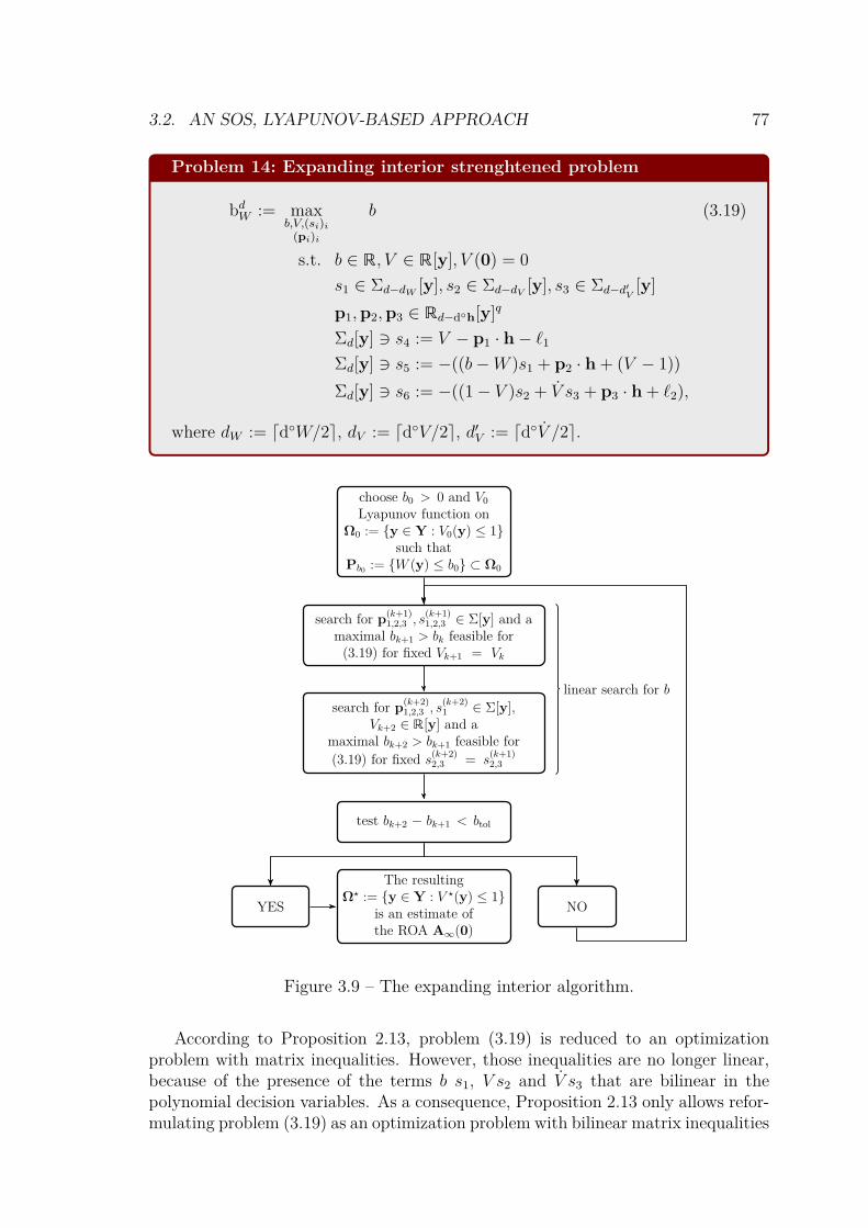
3.2. AN SOS, LYAPUNOV-BASED APPROACH 77
Problem 14: Expanding interior strenghtened problem
bdW := maxb,V,(si)i
(pi)i
b (3.19)
s.t. b ∈ R, V ∈ R[y], V (0) = 0s1 ∈ Σd−dW [y], s2 ∈ Σd−dV [y], s3 ∈ Σd−d′V [y]p1,p2,p3 ∈ Rd−dh[y]q
Σd[y] 3 s4 := V − p1 · h− `1
Σd[y] 3 s5 := −((b−W )s1 + p2 · h + (V − 1))Σd[y] 3 s6 := −((1− V )s2 + V s3 + p3 · h + `2),
where dW := ddW/2e, dV := ddV/2e, d′V := ddV /2e.
choose b0 > 0 and V0Lyapunov function on
Ω0 := y ∈ Y : V0(y) ≤ 1such that
Pb0 := W (y) ≤ b0 ⊂ Ω0
search for p(k+1)1,2,3 , s
(k+1)1,2,3 ∈ Σ[y] and a
maximal bk+1 > bk feasible for(3.19) for fixed Vk+1 = Vk
search for p(k+2)1,2,3 , s
(k+2)1 ∈ Σ[y],
Vk+2 ∈ R[y] and amaximal bk+2 > bk+1 feasible for(3.19) for fixed s(k+2)
2,3 = s(k+1)2,3
test bk+2 − bk+1 < btol
The resultingΩ? := y ∈ Y : V ?(y) ≤ 1
is an estimate ofthe ROA A∞(0)
YES NO
linear search for b
Figure 3.9 – The expanding interior algorithm.
According to Proposition 2.13, problem (3.19) is reduced to an optimizationproblem with matrix inequalities. However, those inequalities are no longer linear,because of the presence of the terms b s1, V s2 and V s3 that are bilinear in thepolynomial decision variables. As a consequence, Proposition 2.13 only allows refor-mulating problem (3.19) as an optimization problem with bilinear matrix inequalities

78 CHAPTER 3. POWER SYSTEMS TRANSIENT STABILITY
(BMI). Such an issue makes problem (3.19) nonconvex and thus more difficult tosolve than the convex problems introduced in Chapter 2. Moreover, Lagrange dual-ity theory does not apply anymore so our convergence proofs cannot be used in thiscontext. Nevertheless, problem (3.19) can still be numerically approximated withinan iterative algorithm that resorts to a bisection search and alternately optimizesover the variables b,p1,p2,p3, s1, s2, s3 on the one hand, and b,p1,p2,p3, s1, V onthe other hand (e.g., [120], [96]), see Figure 3.9.
Remark 3.15 (Dealing with bilinearities)Fixing some polynomials while optimizing over the others helps dealing with poly-
nomial bilinearities V s2 and V s3. On the other hand, the bilinearity b s1 cannot betackled this way, because fixing b would fix the objective function and thus there wouldbe no optimization problem left. Instead, since b is a scalar decision variable, it ispossible to perform a bisection algorithm to optimize over both b and s1 at the sametime.
Remark 3.16 (Outer iterations)In [6], the authors improved the EI algorithm by adding an “outer iteration” loop.
The idea is as follows: once the EI algorithm has stopped and given an optimal pair(b?, V ?), one can restart the whole process with V ? instead of W in the description ofPb := y ∈ Y : V ?(y) ≤ b. This makes the algorithm depend less on the arbitraryinitial choice of W .
Remark 3.17 (Convergence of the EI algorithm)Contrary to the moment-SOS hierarchy, the EI algorithm solves a nonconvex
optimization problem, which makes any proof of convergence much more difficult.However, simultaneously to the first publication [125] of the present work, [50] pro-posed an improved version of the EI algorithm with a proof of convergence to a localoptimum (V ?, b?).
Some features of SOSTOOLS include the setting of polynomial optimizationproblems and the search for a polynomial Lyapunov function after expressing theSOS problem as an SDP problem. In [6], SOSTOOLS is used to implement theexpanding interior algorithm for a dynamic model without regulation.
3.2.4 ROA estimation of the SMIB modelWe finally introduce the second contribution of this section, which is the applicationof the EI algorithm to the SMIB model of Section 3.2.1. Briefly, the improvementthat we bring with respect to [6] is that we tackle a much more complex differentialsystem, which is more computationally challenging than the 2nd order model thatwas then used as a proof of concept. Then, since the additional control loops helpstabilizing the system, one expects to obtain larger inner ROA approximation thanin the case of [6].
In fact, the 8 dimensional problem one ends up with after reformulating theSMIB dynamics already exceeds the computational power of a standard laptop. Forthis reason, we could not directly solve problem (3.19) for system (1.4′). Thus,

3.2. AN SOS, LYAPUNOV-BASED APPROACH 79
we propose to slightly modify the AVR equation (3.12), and transform the voltagedroop into a quadratic droop, yielding
TadEfdt = −Ef +Ka(V 2
ref − V 2t ). (3.12′)
This small change makes the AVR dynamics polynomial, by getting rid of the squareroot operator in the euclidean norm definition. Thus, we no longer need to introducey7 and y8 in the reformulated system which then consists of only the first 6 equationsof (1.4′), with y2
1 + (1− y2)2 = 1 as the only remaining polynomial constraint.From a physical point of view, instead of comparing the magnitude (or modu-
lus) of the voltage (phasor) over the synchronous machine to a reference, we arecomparing its squared magnitude to the square of the reference.
Then, using an expanding domain Pb = y ∈ R6 : W (y) := |y|2 ≤ b, thealgorithm in Figure 3.9 builds an increasing sequence of inner approximations tothe ROA which, when the iterations stop for b? = 0.08544, returns the followingLyapunov function,
V ?(y) = 2.010 y21 + 0.07823 y1y2 + 3.1961 y1y3
−2.244 y1y4 − 0.02231 y1y5 + 0.2172 y1y6
+0.9483 y22 + 3.422 y2y3 − 2.246 y2y4
−0.003099 y2y5 + 0.1913 y2y6 + 22.92 y23 (3.20)
−0.07196 y3y4 − 0.07616 y3y5 + 2.998 y3y6
+4.058 y24 − 0.0003899 y4y5 − 0.1467 y4y6
+0.004611 y25 + 0.008518 y5y6 + 0.2425 y2
6 ,
whose 1-sublevel set Ω? := y ∈ R6 : V ?(y) ≤ 1 provides the largest estimation ofthe ROA.
Two-dimensional projections of the resulting ROA in original coordinates areplotted in Figures 3.10 and 3.11 in red lines. While these estimations are quitelarge, a comparison to the exact (numerically estimated) ROA, thick blue lines inFigure 3.11, shows that further improvements are possible, for example by increasingthe degrees of the polynomials in the SOS program, or by going through more outeriteration loops.
We aim to validate the estimate of the ROA found by the SOS approach, bytesting, in simulation, the limits of stability of the system in all the state-spacedirections. For this, the system is systematically initialized at a starting point farfrom the considered equilibrium point, and we check by simulation if it goes backto equilibrium or not.
Since the system has 5 state variables which means a huge number of combin-ations and because θ and ω are the most important state variables for transientstability analysis, we decide to make the test in a projection of the state space onthe planes (θ, ω), (eq, Ef ), and (Pm, ω).
Figure 3.11 shows that the estimated ROA (red lines) is inside the real one(thick blue line, computed numerically by simulation) and this validates the previousresults. The arrows in the plots show that the real ROA is larger in the direction ofthe arrows.

80 CHAPTER 3. POWER SYSTEMS TRANSIENT STABILITY
(a) (b)
(c)
Figure 3.10 – Projected graph of the Lyapunov function.
On the plots are displayed 2D projections of the estimated ROA (red line) andexpanding domain Pb? (blue line), and 3D views of the LF in the coordinate pairs:(a) (θ, ω), (b) (eq, Ef ), and (c) (Pm, ω).
The same figure shows that the trajectories of the system initialized in severalpoints inside the numerically computed ROA converge asymptotically to the con-sidered equilibrium point.
In conclusion, SOS approaches and tools have been successfully used to quantifytransient stability of a SMIB system for which the generator has been modeled inmore detail than in previous studies. Indeed, voltage dynamics and voltage andfrequency regulations were taken into account in this formalism. First, this providesmore accuracy in estimation of the stability margin in terms of the ROA. Indeed,the estimated ROA is large enough compared to the exact ROA computed by simu-lation. Next, the Lyapunov approach is well suited for the control synthesis and thisquantification can be further exploited to build/tune regulators in order to maxim-ize ROA. As a matter of fact, in the SOS optimization one can next include theregulators’ parameters as decision variables. Future work could focus on
• estimation with the full model (without the approximation (3.12′)),
• inclusion of the non linearities of the machine related to saturations of the

3.2. AN SOS, LYAPUNOV-BASED APPROACH 81
(a) (b)
(c)
Figure 3.11 – Comparison between ROA estimate and simulation built ROA.
We represented 2D projections of the real ROA (thick blue line), the SOS estimate(thin red line), and expanding domain Pβmax (thin blue line) on the coordinatesubspaces: (a) (e′q, Efd). (b) (Pm, ω), and (c) (δ, ω). Trajectories of the systeminitialized in several points (stars) inside the numerically computed ROA convergeasymptotically to the considered equilibrium point.
actuating variables,
• application to larger grids using structure-related model reductions,
• extension to the tuning of regulators’ parameters.
Synthesis of sections 3.1 & 3.2This Chapter has been dedicated to proposing new power-systems applications ofexisting SOS methods for transient stability analysis. The 2nd order model to whichoccupation measures were applied in section 3.1 had already been studied in [6]using the Lyapunov framework, in which the generality of the Krivine-Stengle P-satzallowed for direct integration of equality constraints; in this matter, our contributionmainly consisted of adapting the more specific Putinar-based occupation measure

82 CHAPTER 3. POWER SYSTEMS TRANSIENT STABILITY
method to variable-change equality constraints, making possible the study of non-polynomial algebraic dynamics. Section 3.1 was also a first occasion to apply theresults of Chapter 2 to an instance of the moment-SOS hierarchy, highlighting thesystematic convergence proof allowed by these theoretical results. Section 3.2 thentook SOS methods to the next level of complexity, by considering a 5th order model,within the Lyapunov framework. This gives us an opportunity to compare Lyapunovand occupation measure methods in terms of potential applications. We sum up ourcomparisons in table 3.2.
Both approaches rely on the approximation of the system’s ROA with levelsets of polynomials. A first important feature of such methods is that a degreed polynomial in N variables is defined by Dd
N :=(N+dd
)= (N+d)!
N !d! coefficients, sothat the space of decision variables has dimension Dd
N . One can notice (using theasymptotic equivalent notation f(x)∼
x→ag(x) ↔ f(x)/g(x) −→
x→a1) that Dd
N∼d→∞
dN
N !grows polynomially in d with exponent N . As a result, one wants N to be assmall as possible when implementing those algorithms. For the Lyapunov method,N = n is the number of state variables, while the occupation measure methodinvolves N = n+ 1 variables, due to the inclusion of time as a variable for functionv. Thus, the Lyapunov method is slightly less costly than the occupation measuremethod, even though both methods hardly scale when n grows as one tackles morerealistic models. This highlights the crucial importance of using problem structureto formulate problems with smaller N .
Then, the main difference between the two approaches is that the moment-SOShierarchy presented in Section 3.1 reduces to semidefinite programming, while the ex-panding interior algorithm of Section 3.2 resorts to BMI constraints. Consequently,the Lyapunov method loses all the convexity and duality properties that allowedfor the strong convergence proof of the occupation measures approach. On anothernote, a weaker convergence was recently proved for the EI algorithm in [50], in thesense that the EI algorithm terminates, yielding a local optimum for the optimiza-tion criterion b. Whether such local optimum corresponds to a tight approximationof the infinite time ROA remains an open question to this day.
However, convergence of the moment-SOS hierarchy comes with a price to pay:the global optimum strongly depends on the parameters X,K and T . Depend-ence on X is actually good, since it allows taking into account industrial securitystate constraints in the stability analysis, ruling out stable trajectories that wouldstill damage the power system (such dependence can also be taken into accountin the Lyapunov approach, as a constraint in the Krivine-Stengle P-satz). On thecontrary, dependence on the target set K and time horizon should be consideredcarefully: even though such dependence is also motivated by the TSA specificationsof Definition 1.2, the sensitivity to such parameters makes it necessary to preciselydetermine K and T in advance, using solid power engineering arguments. An in-teresting perspective would be to use a Lyapunov-based infinite time ROA innerapproximation Ω? ⊂ AX
∞(x) as a target set for a finite time ROA inner approxima-tion hierarchy. One would then obtain a sequence of sets Ad,T ⊂ AX
T (Ω?) ⊂ AX∞(x).
Then, intuitively, one would have[limd→∞
vol(AX∞(x) \ Ad,T
)]−→T→∞
0.

3.2. AN SOS, LYAPUNOV-BASED APPROACH 83
Lyapunov Occupation measures
Nb of variables n (state) n+ 1 (state & time)
Constraints BMI LMI
Convexity no yes
Scheme convergence local global
Parameters none X,K, T
Time horizon infinite finite
Target equilibrium eq. neighbourhood
Table 3.2 – Comparison between Lyapunov and occupation measures for TSA.


4Volume computation and Stokes theorem
As suggested in Section 3.1.2, the hierarchy-based ROA approximation method re-lies on the set approximation property that appears in the volume computationproblem (2.8). Then, one “only” has to include occupation measures constrainedby Liouville’s PDE (3.3) to go from approximating a given semialgebraic set to es-timating an unknown ROA. In other words, the volume computation problem isthe simplest set approximation problem one could think of. As a result, it can beuseful to look for ways to enhance the volume problem tractability, so that it can beapplied to other set approximation problems such as estimating the ROA of a powersystem. The two following chapters introduce our contributions in this direction,that one can find in [124, 126].
Contents4.1 Existing Stokes-based heuristics . . . . . . . . . . . . . . . 88
4.1.1 Linear reformulation of the volume problem . . . . . . . . 88
4.1.2 Stokes’ Theorem and its variants . . . . . . . . . . . . . . 90
4.1.3 Original Stokes constraints . . . . . . . . . . . . . . . . . 90
4.2 Contribution to Stokes constraints heuristics . . . . . . . 91
4.2.1 Infinite-dimensional Stokes constraints . . . . . . . . . . . 91
4.2.2 New Stokes constraints and main result . . . . . . . . . . 92
4.3 Solving a PDE to attain an optimum . . . . . . . . . . . 94
4.3.1 Equivalence to a Poisson PDE . . . . . . . . . . . . . . . 95
4.3.2 Poisson PDE on a connected domain . . . . . . . . . . . . 96
4.3.3 General Poisson PDE with boundary regularity . . . . . . 100
4.3.4 Explicit optimum for Stokes-enhanced hierarchy . . . . . 101
4.4 Numerical experiments and general heuristics . . . . . . 102
4.4.1 Practical implementation . . . . . . . . . . . . . . . . . . 102
4.4.2 Bivariate disk . . . . . . . . . . . . . . . . . . . . . . . . . 103
4.4.3 Higher dimensions . . . . . . . . . . . . . . . . . . . . . . 103
4.4.4 General heuristics . . . . . . . . . . . . . . . . . . . . . . 105
85

86 CHAPTER 4. VOLUME COMPUTATION & STOKES THEOREM
Consider the problem of computing the Lebesgue volume of a compact basic semi-algebraic set K ⊂ Rn. For simplicity of exposition we will restrict to the case whereK is a smooth, simple semialgebraic set, i.e. the super-level set x : g(x) ≥ 0 ⊂ Rn
of a single polynomial g.Computing or even approximating the volume of a convex body is already hard
theoretically and in practice as well. Even if K is a convex polytope, exact com-putation of its volume or integration over K is a difficult challenge. Computationalcomplexity of these problems is discussed in, e.g. [14, 29, 32]. In particular, anydeterministic algorithm with polynomial-time complexity that would compute anupper bound and a lower bound on the volume cannot yield an estimate on thebound ratio better than polynomial in the dimension n. For more detail, the inter-ested reader is referred to the discussion in [44] and to [16] for a comparison. Evenapproximating λ(K) by deterministic methods is still a hard problem as explainedin [25] and references therein.
If one accepts randomized algorithms that fail with small probability, then thesituation is more favorable. Indeed, the probabilistic approximation algorithm of [30]computes the volume to fixed arbitrary relative precision ε > 0 in time polynomialin 1/ε. The algorithm uses approximation schemes based on rapidly mixing Markovchains and isoperimetric inequalities; see also hit-and-run algorithms described ine.g. [17, 116, 145]. So far, it seems that the recent works [24, 25] have provided thebest algorithm of this type.
In full generality with no specific assumption on K such as convexity, the onlygeneral method available is Monte-Carlo, that is, one samples N points according toLebesgue measure λ normalized on a simple set X (e.g. a hypercube or an ellipsoid)that contains K. If PN is the proportion of points that fall into K then the randomvariable PN λ(X) provides a good estimator of λ(K) with convergence guarantees asN increases. However this estimator is non deterministic and fails to provide loweror upper bounds on λ(K).
When K and X are compact basic semi-algebraic sets, a deterministic numericalscheme described in [44] provides a sequence ddKd∈N ⊂ R of upper bounds thatconverges to λ(K) as d increases. Briefly, we recall as stated in Chapter 2
λ(K) = d?K = infw∈R[x]
∫w dλ : w ≥ 1K on X
(4.1)
ddK = infw∈R2d[x]
∫w dλ : w ≥ 1K on X
. (4.2)
One can notice that minimizing sequences for (4.1) and (4.2) also minimize theL1(X, λ)-norm ‖w − 1K‖L1(X) :=
∫|w − 1K| dλ (with convergence to 0 in the case
(4.1)). As the upper bound ddK > λ(K) is obtained by restricting the search in(4.2) to polynomials of degree at most 2d, the infimum is attained and an optimalsolution can be obtained by solving a semidefinite program. Of course, the size ofthe resulting semidefinite program increases with the degree d; for more details theinterested reader is referred to [44].
Then clearly, a Gibbs phenomenon1 takes place as one tries to approximate, on1The Gibbs phenomenon appears at a jump discontinuity when one numerically approximates a

87
X and from above, the discontinuous function 1K by a polynomial of degree at mostd. This makes the convergence of the upper bounds ddK very slow (even for modestdimension problems). A trick was used in [44] to accelerate this convergence but atthe price of loosing monotonicity of the resulting sequence.
In fact (4.1) is a dual of the following infinite-dimensional Linear Program (LP)on measures
p?K = supµ∈M(K)+
µ(K) : λ− µ ∈M(K)+ (4.3)
(where M(K)+ is the space of finite Borel measures on K). Its optimal value isalso λ(K) and is attained at the unique optimal solution µ? := λK = 1K λ (therestriction of λ to K).
A simple but key observation. As one knows the unique optimal solutionµ? = λK of (4.3), any constraint satisfied by µ? (in particular, linear constraints)can be included as a constraint on µ in (4.3) without changing the optimal valueand the optimal solution. While these constraints provide additional restrictions in(4.3), they translate into additional degrees of freedom in the dual (hence a relaxedversion of (4.1)), and therefore better approximations when passing to the finite-dimensional strengthened version of (4.2). A first set of such linear constraints,experimented in [71] and later in [139, 73], resulted in drastic improvements butwith no clear rationale behind such improvements.
Contribution. This chapter is based on [124], whose main message and res-ult is that there is an appropriate set of additional linear constraints on µ in (4.3)such that the resulting dual (a relaxed version of (4.1)) has an explicit continuousoptimal solution with value λ(K). These additional linear contraints (called Stokesconstraints) come from an appropriate modelling of Stokes’ theorem for integrationover K, a refined version of that in [71]. Therefore the optimal continuous solu-tion can be approximated efficiently by polynomials with no Gibbs phenomenon,by the hierarchy of semidefinite relaxations defined in [44] (adapted to these newlinear constraints). Interestingly, the technique of proof and the construction of theoptimal solution invoke classical results from the field of elliptic partial differentialequations (PDE), namely the Lax-Milgram and Poincaré-Wirtinger inequalities aswell as regularity theorems for solutions to elliptic PDEs.
Outline. In Section 4.1 we recall the primal-dual linear formulation of thevolume problem, explain why the dual value is not attained, resulting in a Gibbsphenomenon, and present the existing Stokes-based heuristics to tackle this issue. InSection 4.2 we revisit the acceleration strategy based on Stokes’ theorem, with theaim of introducing a more general acceleration strategy and a new primal-dual linearformulation of the volume problem. Our main result, attainment of the dual valuein this new formulation, is stated and proved as Theorem 4.5 in Section 4.3. Thedrastic improvement in the convergence to λ(K) is illustrated on a simple exampleof the Euclidean ball in Section 4.4.
piecewise C1 function with a polynomial function, e.g. by its Fourier series; see e.g. [128, Chapter9].

88 CHAPTER 4. VOLUME COMPUTATION & STOKES THEOREM
4.1 Existing Stokes-based heuristicsConsider a compact simple semi-algebraic set
K := x ∈ Rn : g(x) ≥ 0
with g ∈ R[x]. We suppose that K ⊂ X where X is a compact basic semi-algebraicset for which we know the moments
∫X xk dx of the Lebesgue measure λX, where
xk := xk11 x
k22 · · ·xknn denotes a multivariate monomial of degree k ∈ Nn. We assume
thatΩ := x ∈ Rn : g(x) > 0
is a nonempty open set with closure
Ω = K,
and that its boundary∂Ω = ∂K = K \Ω
is C1 in the sense that it is locally the graph of a continuously differentiable function.We want to compute the Lebesgue volume of K, i.e., the mass of the Lebesguemeasure λK:
λ(K) :=∫
Kdx =
∫1 dλK(x).
4.1.1 Linear reformulation of the volume problemIf X ⊂ Rn is a compact set, denote by M(X) the space of signed Borel measureson X, which identifies with the topological dual of C(X), the space of continuousfunctions on X. Denote byM(X)+ the convex cone of non-negative Borel measureson X, and by C(X)+ the convex cone of non-negative continuous functions on X.
In [44] a sequence of upper bounds converging to λ(K) is obtained by applying themoment-SOS hierarchy to approximate, as closely as desired, the (primal) infinite-dimensional LP on measures:
p?K = maxµ
∫1 dµ (2.8a)
s.t. µ ∈M(K)+
λ− µ ∈M(X)+
whose optimal value is λ(K), attained for µ? := λK (see Section 2.1.3). The LP(2.8a) has an infinite-dimensional LP dual on continuous functions, which reads:
d?K = infw
∫w dλ (2.8b)
s.t. w − 1 ∈ C(K)+.
w ∈ C(X)+
Observe that (2.8b) consists in approximating the discontinuous indicator function1K (equal to one on K and zero elsewhere) from above by continuous functions w,
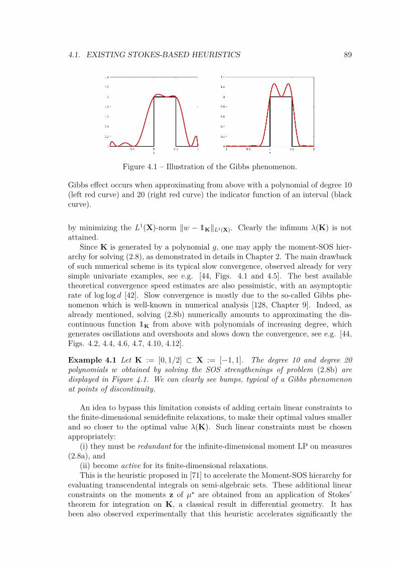
4.1. EXISTING STOKES-BASED HEURISTICS 89
Figure 4.1 – Illustration of the Gibbs phenomenon.
Gibbs effect occurs when approximating from above with a polynomial of degree 10(left red curve) and 20 (right red curve) the indicator function of an interval (blackcurve).
by minimizing the L1(X)-norm ‖w − 1K‖L1(X). Clearly the infimum λ(K) is notattained.
Since K is generated by a polynomial g, one may apply the moment-SOS hier-archy for solving (2.8), as demonstrated in details in Chapter 2. The main drawbackof such numerical scheme is its typical slow convergence, observed already for verysimple univariate examples, see e.g. [44, Figs. 4.1 and 4.5]. The best availabletheoretical convergence speed estimates are also pessimistic, with an asymptopticrate of log log d [42]. Slow convergence is mostly due to the so-called Gibbs phe-nomenon which is well-known in numerical analysis [128, Chapter 9]. Indeed, asalready mentioned, solving (2.8b) numerically amounts to approximating the dis-continuous function 1K from above with polynomials of increasing degree, whichgenerates oscillations and overshoots and slows down the convergence, see e.g. [44,Figs. 4.2, 4.4, 4.6, 4.7, 4.10, 4.12].
Example 4.1 Let K := [0, 1/2] ⊂ X := [−1, 1]. The degree 10 and degree 20polynomials w obtained by solving the SOS strengthenings of problem (2.8b) aredisplayed in Figure 4.1. We can clearly see bumps, typical of a Gibbs phenomenonat points of discontinuity.
An idea to bypass this limitation consists of adding certain linear constraints tothe finite-dimensional semidefinite relaxations, to make their optimal values smallerand so closer to the optimal value λ(K). Such linear constraints must be chosenappropriately:
(i) they must be redundant for the infinite-dimensional moment LP on measures(2.8a), and
(ii) become active for its finite-dimensional relaxations.This is the heuristic proposed in [71] to accelerate the Moment-SOS hierarchy for
evaluating transcendental integrals on semi-algebraic sets. These additional linearconstraints on the moments z of µ? are obtained from an application of Stokes’theorem for integration on K, a classical result in differential geometry. It hasbeen also observed experimentally that this heuristic accelerates significantly the

90 CHAPTER 4. VOLUME COMPUTATION & STOKES THEOREM
convergence of the hierarchy in other applied contexts, e.g. in chance-constrainedoptimization problems [137].
4.1.2 Stokes’ Theorem and its variantsWe then explain the heuristic introduced in [44] to accelerate convergence of theMoment-SOS hierarchy by adding linear constraints on the moments of µ?. Theselinear constraints are obtained from a certain application of Stokes’ theorem forintegration on K.
Theorem 4.1: Stokes
Let Ω ⊂ Rn be a piecewise C1 open set. For any (n − 1)-differential form ωon Ω, one has ∫
∂Ωω =
∫Ωdω.
.
Corollary 4.2: Gauss formula
In particular, for u ∈ C1(Ω)n and ω(x) = u(x) · n(x) dσ(x), where the dot isthe inner product, σ is the surface or Hausdorff measure on ∂Ω and n is theoutward pointing normal to ∂Ω, we obtain the Gauss formula∫
∂Ωu · n dσ =
∫Ω
div u(x) dx. (4.4)
Corollary 4.3: Dual Gauss formula
With the choice u(x) := u(x) ei where u ∈ C1(Ω) and ei is the vector of Rn
with one at entry i and zeros elsewhere, for i = 1, . . . , n, we obtain the dualGauss formula ∫
∂Ωu n dσ =
∫Ω
grad u(x) dx. (4.5)
Proof : These are all particular cases of [47, Theorem 6.10.2]. ♦
4.1.3 Original Stokes constraintsAssociated to a sequence z = (zk)k∈Nn ∈ RNn of moments, introduce the Riesz linearfunctional Lz : R[x]→ R as in Definition 2.1. Thus, if z is the sequence of momentsof λK, i.e. if for all k ∈ Nn, zk :=
∫K xk dx, then Lz(p) =
∫K p(x) dx and by (4.5)
with u(x) := xkg(x):
Lz(grad(xkg(x))) =∫
Kgrad(xkg(x)) dx
=∫∂K
xkg(x) nK(x) dσ(x) = 0,

4.2. CONTRIBUTION TO STOKES CONSTRAINTS HEURISTICS 91
since by construction g vanishes on ∂K. Thus while in the infinite-dimensional LP(2.8a) one may add the linear constraints∫
Kgrad(xkg(x)) dµ(x) = 0 ∀k ∈ Nn,
without changing its optimal value p?K = λ(K), on the other hand inclusion of thelinear moment constraints
Lz(grad(xkg(x))) = 0 , |k| ≤ 2d+ 1− deg(g) (4.6)
in the moment relaxation with pseudo-moments z of degree at most d, will decreasethe optimal value of the initial relaxation.
In practice, it was observed that adding constraints (4.6) dramatically speedsup the convergence of the moment-SOS hierarchy, see e.g. [71, 137]. One maingoal of this section is to provide a qualitative mathematical rationale behind thisphenomenon.
4.2 Contribution to Stokes constraints heuristics
4.2.1 Infinite-dimensional Stokes constraintsIn [126], we formulated Stokes constraints in the infinite-dimensional setting, and adual formulation was obtained in the context of the volume problem. Using (4.4)with u = g v (which vanishes on ∂K) and v ∈ C1(K)n arbitrary, yields:∫
K(grad g(x) · v(x) + g(x) div v(x)) dx =
∫∂Kg v · n dσ = 0 ,
which can be written equivalently (in the sense of distributions) as
(grad g)λK − grad(gλK) = 0 .
This allows us to rewrite problem (2.8a) as
p?K = maxµ
∫1 dµ (2.8a′)
s.t. µ ∈M(K)+
λ− µ ∈M(X)+
(grad g)µ− grad(gµ) = 0
without changing its optimal value p?K = λ(K) attained at µ? = λK.Using the infinite-dimensional convex duality method described in Section 2.1.4,
the dual of LP (2.8a′) reads
d′K := infv,w
∫w dλ (2.8b′)
s.t. w − div(gv)− 1 ∈ C(K)+
w ∈ C(X)+
v ∈ C1(K)n.

92 CHAPTER 4. VOLUME COMPUTATION & STOKES THEOREM
A direct application of Theorem 2.6 yields that d′K = p?K = d?K (we already verifiedthat the theorem’s working assumptions hold in such case, see Example 2.10).
Crucial observation. Notice that w in (2.8b′) is not required to approximate1K from above anymore. Instead, it should approximate 1 + div(gv) on K and 0outside K. Hence, provided that 1 + div(gv) = 0 on ∂K, w might be a continuousfunction for some well-chosen v ∈ C1(K)n, and therefore an optimal solution of(2.8b′) (i.e., the infimum is a minimum). As a result, the Gibbs phenomenon woulddisappear and convergence would be faster.
The issue is then to determine whether the infimum in (2.8b′) is attained or not.And if not, are there other special features of problem (2.8b′) that can be exploitedto yield more efficient semidefinite relaxations ?
4.2.2 New Stokes constraints and main resultIn the previous paragraph, the Stokes constraint∫
(v · grad g + g div v) dµ = 0
or equivalently (in the sense of distributions)
(grad g)µ− grad(gµ) = 0 (4.7)
(with µ ∈M(K)+ being the Lebesgue measure on K) was obtained as a particularcase of Stokes’ theorem with u = g v in (4.4). Instead, we can use a more generalversion with u not in factored form, and also use the fact that
∀x ∈ ∂K,0 6= grad g(x) = −|grad g(x)| nK(x),
to obtain ∫div u dµ = −
∫u · grad g dν ,
or equivalently (in the sense of distributions)
grad µ = (grad g)ν , (4.8)
with µ ∈ M(K)+ being the Lebesgue measure on K and ν ∈ M(∂K)+ beingthe measure having density 1/|grad g(x)| with respect to the (n − 1)-dimensionalHaussdorff measure σ on ∂K. The same linear equation was used in [73] to computemoments of the Hausdorff measure. In fact, equation (4.8) is a generalization ofequation (4.7) in the following sense.
Lemma 4.4: Stokes constraints generalization
If ν ∈M(∂K)+ is s.t. µ ∈M(K)+ satisfies (4.8), then µ also satisfies (4.7).
Proof : Equation (4.8) means that∫div u dµ+
∫u · grad g dν = 0

4.2. CONTRIBUTION TO STOKES CONSTRAINTS HEURISTICS 93
for all u ∈ C1(K)n. In particular if u = g v for some v ∈ C1(K)n then (4.8) reads
∫(v · grad g + g div v) dµ = 0 ,
which is precisely (4.7). ♦
Hence we can incorporate linear constraints (4.8) on µ and ν, to rewrite problem(2.8a) as
p?K = maxµ,ν
∫1 dµ (2.8a′′)
s.t. µ ∈M(K)+
ν ∈M(∂K)+
λ− µ ∈M(X)+
(grad g)ν − grad µ = 0
without changing its optimal value p?K = λ(K) attained at µ? = λK and ν? =σ/|grad g|. Notice that LP (2.8a′′) involves two measures µ and ν whereas LP(2.8a′) involves only one measure µ.
Next, by convex duality, the dual of (2.8a′′) reads
Problem 15: Stokes dual GMP
Find a minimizer for
d′′K = infu,w
∫w dλ (2.8b′′)
s.t. w − div u− 1 ∈ C(K)+
− (u · grad g) ∈ C(∂K)+
w ∈ C(X)+
u ∈ C1(K)n.
Our main result states that the optimal value of the dual (2.8b′′) is attained atsome continuous function (w?,u?) ∈ C(X)+ × C1(K)n. Therefore, in contrast withproblem (2.8b), there is no Gibbs phenomenon at an optimal solution of the (finite-dimensional) semidefinite strengthening associated with (2.8b′′). On the contrary,existence of a regular optimum yields at least one sequence of polynomials thatconverge uniformly to a global optimizer, due to the Stone-Weierßtrass theorem.
Let Ωi, i = 1, . . . , N denote the connected components of Ω, and let
mΩi(g) := 1
λ(Ωi)
∫Ωi
g(x) dx
be the mean of g on Ωi.

94 CHAPTER 4. VOLUME COMPUTATION & STOKES THEOREM
Theorem 4.5: Optimum for dual Stokes volume problem
In dual LP (2.8b′′) the infimum is a minimum, attained at
w?(x) := g(x)N∑i=1
1Ωi(x)
mΩi(g) , x ∈ X ,
andu?(x) := grad u(x) ,
where u solves the Poisson PDE −∆u(x) = 1− w?(x), x ∈ Ω
∂nu(x) = 0, x ∈ ∂Ω.
Remark 4.2 (Computing lower bounds for the volume)The moment-SOS hierarchy associated to LPs (2.8a′′) and (2.8b′′) yields upper
bounds for the volume. Theorem 4.5 is designed for these LPs but it has a straight-forward counterpart for lower bound volume computation, obtained by replacing Kwith X \Ω in the previous developments, i.e. computing upper bounds of λ(X \Ω).However, two additional technicalities should then be considered:
• This work only deals with semi-algebraic sets defined by a single polynomial; ac-tually, it immediately generalizes to finite intersections of such semi-algebraicsets, as long as their boundaries do not intersect (i.e. here K should be in-cluded in the interior of X): the constraints on boundaries should just besplitted between the boundaries of the intersected sets.
• This work heavily relies on the fact that the boundary of the considered setshould be smooth; for this reason, computing lower bounds of the volume im-plies that one chooses a smooth bounding box X (typically a euclidean ball,ellipsoid or `p ball), which rules out simple sets like the hypercube [−1, 1]n.
Upon taking into account these technicalities, Theorem 4.5 still holds, allowingto deterministically compute upper and lower bounds for the volume, with arbitraryprecision. Of course in practice, one is limited by the performance of state-of-artSDP solvers.
4.3 Solving a PDE to attain an optimumTheorem 4.5 is proved in several steps as follows:• we show that solutions to a Poisson PDE are optimal for (2.8b′′);
• we study the Poisson PDE on a connected domain;
• we study the Poisson PDE on a union of connected domains;
• we construct an explicit optimum for problem (2.8b′′).

4.3. SOLVING A PDE TO ATTAIN AN OPTIMUM 95
4.3.1 Equivalence to a Poisson PDELemma 4.6: Optimality condition
Problem (2.8b′′) has an optimal solution iff there exist u ∈ C1(Ω)n, w ∈ C(Ω)+solving
− div u = 1− w in Ω, (4.9a)u · n = 0 on ∂Ω, (4.9b)w = 0 on ∂Ω. (4.9c)
Proof : Let (u, w) solve (4.9). Using (4.9c), one can define
w(x) =
w(x) if x ∈ Ω
0 if x ∈ X \Ω.
Then (u, w) is feasible for (2.8b′′) and one has∫w dλ =
∫w dλ
(4.9a)=∫
Ω(1 + div u) dλ
(4.4)= λ(Ω) +∫∂Ω
u · n dσ
(4.9b)= λ(Ω)
so that (u, w) is optimal.Conversely, let (u, w) be an optimal solution of problem (2.8b′′). We know that
(µ?, ν?) = (λK, σ/|grad g|) is optimal for problem (2.8a′′). Then, duality theoryensures complementarity: ∫
(w − div u− 1) dλK = 0, (4.10a)∫u · grad g
|grad g|dσ = 0. (4.10b)
Since w− div u− 1 is nonnegative on K, (4.10a) yields (4.9a) with w := w|Ω. Like-wise, since −(u ·grad g) is nonnegative on ∂Ω, (4.10b) yields (4.9b) and thus, using(4.4), one has
∫Ω div u dλ = 0. Eventually, (4.10a) yields
∫Ωw dλ = λ(Ω) =
∫w dλ
by optimality of w, so that∫X\Ωw dλ = 0 and, since w is nonnegative, w|X\Ω ≡ 0.
Continuity of w finally allows us to conclude that w = 0 on ∂Ω, which is exactly(4.9c). ♦
From Lemma 4.6, existence of an optimum for (2.8b′′) is then equivalent toexistence of a solution to (4.9), which we rephrase as follows, defining f := 1 − wand u = grad u with u ∈ C2(Ω), and where ∆u := div grad u is the Laplacian ofu, and ∂nu := grad u · n.

96 CHAPTER 4. VOLUME COMPUTATION & STOKES THEOREM
Lemma 4.7: Optimum as solution to Poisson’s PDE
If there exist u ∈ C2(Ω)n and f ∈ C(Ω) solving
−∆u = f in Ω, (4.11a)∂nu = 0 on ∂Ω, (4.11b)f ≤ 1 in Ω, (4.11c)f = 1 on ∂Ω, (4.11d)
then problem (2.8b′′) has an optimal solution.
This rephrazing is a Poisson PDE (4.11a) with Neumann boundary condition(4.11b), whose source term f is a parameter subject to constraints (4.11c) and(4.11d).
Remark 4.3 (Loss of generality)Looking for u under the form u = grad u makes us loose the equivalence. Indeed,
while (2.8b′′) and (4.9) are equivalent, existence of a solution to (4.11) is only asufficient condition for existence of an optimum for (2.8b′′), since (4.9) might haveonly solutions u that are not gradients.
Remark 4.4 (Invariant set for gradient flow)From a dynamical systems point of view, constraint (4.11b) means that we are
looking for a velocity field or control u in the form of the gradient of a potential usuch that Ω is an invariant set for the solutions t ∈ R 7→ x(t) ∈ Rn of the Cauchyproblem
x(t) = −grad u(x(t)), x(0) ∈ X
after what we just have to define w := 1 + ∆u on Ω and enforce constraints (4.11a),(4.11c), (4.11d).
4.3.2 Poisson PDE on a connected domainIt remains to prove existence of solutions to problem (4.11). First, notice thatPDE (4.11a) together with its boundary condition (4.11b) enforces an importantconstraint on the source term f , namely its mean must vanish:∫
Ωf dλ = 0. (4.12)
Indeed, if (f, u) solves (4.11), then∫f dλ
(4.11a)= −∫
∆u dλ(4.4)= −
∫grad u · n dσ
= −∫∂nu dσ
(4.11b)= 0 .
Moreover, the following holds.

4.3. SOLVING A PDE TO ATTAIN AN OPTIMUM 97
Lemma 4.8: Existence on a connected domain
Suppose that Ω is connected. Let the source term f ∈ L2(Ω) ∩ C∞(Ω) havezero mean on Ω, where Lp(Ω) := f ∈ RΩ :
∫|f |p dλ < ∞. Then there
exists u ∈ C∞(Ω) satisfying (4.11a) and (4.11b).
Proof : We first recall some basic definitions:
• for p ∈ R++ and f ∈ Lp(Ω) the Lp norm is defined by
‖f‖Lp(Ω) :=(∫
Ω|f |p dλ
) 1p
.
• The L2 norm is a Hilbert norm with associated inner product
〈u|v〉L2(Ω) :=∫
Ωu v dλ,
such that ‖u‖L2(Ω) =√〈u|u〉L2(Ω).
• The Sobolev Hilbert spaces are defined by
H1(Ω) := u ∈ L2(Ω) : grad u ∈ L2(Ω)n
and by induction on k > 1,
Hk(Ω) := u ∈ L2(Ω) : grad u ∈ Hk−1(Ω)n.
• The Sobolev inner product defines a Hilbert norm:
〈u|v〉H1(Ω) := 〈u|v〉L2(Ω)+〈grad u|grad v〉L2(Ω)n & ‖u‖H1(Ω) :=√〈u|u〉H1(Ω).
Now, let us rephrase the Poisson PDE with Neumann boundary condition under avariational form:
Problem 16: Variational form for (4.11a)-(4.11b)
Find u ∈ H1(Ω) such that for any v ∈ H1(Ω) one has∫Ω
grad u · grad v dλ =∫
Ωf v dλ. (4.13)
Then, for such u, since f ∈ L2(Ω), the interior H2-regularity theorem (see [33,Theorem 1 in Section 6.3.1]) ensures that u ∈ H2
loc(Ω) := ∩YbΩH2(Y) (b standing
for compact inclusion), and Green’s “integration by part” theorem writes, for allv ∈ H1(Ω):∫
∂Ωv ∂nu dσ =
∫Ωv∆u dλ+
∫Ω
grad u · grad v dλ =∫
Ω(∆u+ f) v dλ.
Especially, for v ∈ C∞c (Ω) ⊂ H1(Ω) the left hand side is zero, and by density ofC∞c (Ω) in L2(Ω), we deduce that −∆u = f for the L2(Ω) Hilbert topology and thus

98 CHAPTER 4. VOLUME COMPUTATION & STOKES THEOREM
almost everywhere in Ω. The left hand side is then zero for any v ∈ H1(Ω) andespecially for any v ∈ C∞(Ω) ⊂ H1(Ω), so that, again by density of C∞(∂Ω) inL2(Ω), one has ∂nu = 0 in L2(∂Ω) and then almost everywhere on ∂Ω.
Eventually, the interior C∞-regularity theorem (see [33, Theorem 3 in section6.3.1]) ensures that since f ∈ C∞(Ω), u ∈ C∞(Ω) and we obtain the announcedresult: u is a smooth strong solution of the Poisson PDE.
Next we invoke Lax-Milgram’s theorem which provides existence and uniquenessof a solution to a given PDE (see e.g. [33, Section 6.2.1]). In our context the goal isto solve (4.13) for which it is clear that if u is a solution then any u := u+C, C ∈ R
is also solution, which makes it impossible to obtain uniqueness of the solution inH1(Ω). We thus restrict ourselves to the hyperplane of zero-mean functions
H :=u ∈ H1(Ω) :
∫Ωu dλ = 0
which is closed by continuity of the Lebesgue integral, so that H is a Hilbert spacefor the scalar product
〈u|v〉H := 〈u|v〉H1(Ω) =∫
Ω(uv + grad u · grad v) dλ.
We then define the applications
A :
H −→ R
v 7−→∫
Ωf v dλ.
and
B :
H×H −→ R
(u, v) 7−→∫
Ωgrad u · grad v dλ
The Lax-Milgram theorem then states that if A and B are continuous and if B ismoreover coercive, then there is a unique u ∈ H so that A = B (u, ·), which is theannounced equality (4.13). Let us show that these hypotheses are met.
• Continuity of A . Since A is a linear operator, it is sufficient to show that itis bounded. Let v ∈ H. Then, Hölder’s inequality yields
|A (v)| =∣∣∣∣∫
Ωf v dλ
∣∣∣∣≤ ‖f‖L2(Ω)‖v‖L2(Ω)
≤ ‖f‖L2(Ω)‖v‖H
because ‖v‖H =√‖v‖2
L2(Ω) + ‖grad v‖2L2(Ω) ≥ ‖v‖L2(Ω). Thus,A is a bounded
operator and |||A ||| = ‖f‖L2(Ω) (equality is obtained by taking v = f ∈ H,made possible by (4.12)).

4.3. SOLVING A PDE TO ATTAIN AN OPTIMUM 99
• Continuity of B . Since B is a bilinear operator, it is sufficient to show that itis bounded. Let u, v ∈ H. Again, Hölder’s inequality yields
|B (u, v)| =∣∣∣∣∫
Ωgrad u · grad v dλ
∣∣∣∣≤ ‖grad u‖L2(Ω)‖grad v‖L2(Ω)
≤ ‖grad u‖H‖grad v‖H
because ‖v‖H =√‖v‖2
L2(Ω) + ‖grad v‖2L2(Ω) ≥ ‖grad v‖L2(Ω). Then, B is a
bounded bilinear operator.
• Coercivity of B . First, let us recall the following classical result, proved e.g.in [33, Theorem 1 in Section 5.8.1].
Lemma 4.9: Poincaré-Wirtinger inequality
Let Ω ⊂ Rn be a bounded, connected, C1 open set. There is a constantCΩ ≥ 0 such that for any u ∈ H1(Ω):
‖u−mΩ(u)‖L2(Ω) ≤ CΩ‖grad u‖L2(Ω)n
where mΩ(u) := 1λ(Ω)
∫Ω u dλ.
Now let us look for a coercivity constant C ∈ R such that ‖u‖H ≤ C B (u, u).Let u ∈ H. Then, since ∂Ω is C1, we can use Lemma 4.9:
‖grad u‖L2(Ω)n + ‖u−mΩ(u)‖L2(Ω) ≤ (1 + CΩ)‖grad u‖L2(Ω)n
and thus
B (u, u) =∫
Ω|grad u|2 dλ
= ‖grad u‖2L2(Ω)n
≥‖grad u‖2
L2(Ω)n + ‖u−mΩ(u)‖2L2(Ω)
1 + C2Ω
= ‖u‖2H
1 + C2Ω
since u ∈ H implies that mΩ(u) := 1λ(Ω)
∫Ω u dλ = 0.
Thus, the conditions of the Lax-Milgram theorem are satisfied, which gives us aunique u ∈ H such that for all v ∈ H, equation (4.13) holds. To conclude, we stillneed to extend this property to functions v that have nonzero mean. Let v ∈ H1(Ω),not necessary in H. We define v := v−mΩ(v), so that v ∈ H and grad v = grad v.

100 CHAPTER 4. VOLUME COMPUTATION & STOKES THEOREM
Then, ∫Ωf v dλ =
∫Ωf v dλ+mΩ(v)
∫Ωf dλ
(4.12)=∫
Ωf v dλ
(4.13)=∫
Ωgrad u · grad v dλ
=∫
Ωgrad u · grad v dλ,
which concludes the solution of the variational formulation and the proof of Lemma4.8. ♦
4.3.3 General Poisson PDE with boundary regularityIn Lemma 4.8, we assumed that Ω is connected, so that we could apply the Poincaré-Wirtinger inequality to use the Lax-Milgram theorem, obtaining both existence anduniqueness of a solution in a well-chosen space. However, we are not interested inthe uniqueness property, and we would like to tackle non-connected sets. Since Ωis a semi-algebraic set, it has a finite number of connected components Ω1, . . . ,ΩN .
Corollary 4.10: Existence on a disconnected domain
Let the source term f ∈ L2(Ω) ∩ C∞(Ω) have zero mean on each connectedcomponent of Ω. Then there exists u ∈ C∞(Ω) solving (4.11a) and(4.11b).
Proof : Let i = 1, . . . , N . Since∫Ωif dλ = 0, we can apply the result of Lemma
4.8 replacing Ω with Ωi to obtain ui ∈ C∞(Ωi) such that −∆ui = f in Ωi and∂nui = 0 on ∂Ωi.
Then, we notice that since ∂Ω is C1, the Ωi cannot be mutually tangent, so that∂Ω = ⊔N
i=1 ∂Ωi. Thus, for any x ∈ Ω, the following sum has exactly one non-zeroterm:
u :=N∑i=1
1Ωiui.
By definition of the Ωi as the connected components of Ω, u ∈ C∞(Ω).Let x ∈ Ω. There is an i such that x ∈ Ωi, so that u = ui on a neighbourhood
of x. Thus, −∆u(x) = −∆ui(x) = f(x).Let x ∈ ∂Ω. There is an i such that x ∈ ∂Ωi, so that u = ui on a neighbourhood
of x in Ω. Thus, ∂nu(x) = ∂nui(x) = 0. ♦
In the previous paragraph we have proved that under suitable conditions on thesource term f , equations (4.11a) and (4.11b) have a solution u ∈ C∞(Ω). However,the existence of an optimum for problem (2.8b′′) requires u to be in C1(K): we needto establish regularity at the boundary. For this, an additional assumption on Ω isneeded to state the following corollary to Lemma 4.8.

4.3. SOLVING A PDE TO ATTAIN AN OPTIMUM 101
Lemma 4.11: Regularity on the boundary
Let the source term f ∈ C∞(Ω) have zero mean on each connected componentof Ω. Suppose that ∂Ω is C∞. Then, there exists u ∈ C∞(Ω) solving (4.11a)and (4.11b).
Proof : First, since C∞(Ω) ⊂ L2(Ω) ∩ C∞(Ω), we can use Lemma 4.10 to get asuitable u ∈ C∞(Ω). The only thing that remains to be proved is the regularity ofu on ∂Ω. For this, we use the boundary C∞-regularity theorem [33, Theorem 6 inSection 6.3.2]: since f ∈ C∞(Ω) and ∂Ω is C∞, we conclude that u ∈ C∞(Ω). ♦
Remark 4.5 (Regularity of Ω)Assuming that ∂Ω is C∞ instead of C1 is actually without loss of generality since
Ω is a semi-algebraic set: as soon as ∂Ω is locally the graph of a C1 function, it issmooth.
4.3.4 Explicit optimum for Stokes-enhanced hierarchyOur optimization problem does not feature only the Poisson PDE with Neumanncondition: it also includes constraints (4.11c) and (4.11d) on the source term. Con-sequently, a function f ∈ C∞(Ω) with zero integral over any connected componentof Ω and satisfying (4.11c) and (4.11d) remains to be constructed. We keep thenotations of Lemma 4.10 and suggest as candidate
x 7→ f(x) := 1− g(x)N∑i=1
1Ωi(x)
mΩi(g) . (4.14)
By definition, g = 0 on ∂Ω, so that (4.11d) automatically holds. Moreover, both gand 1Ωi
are nonnegative on Ω, so that (4.11c) also holds.In terms of regularity, f is polynomial on each connected component of Ω and
since g smoothly vanishes on ∂Ω, f ∈ C∞(K).Eventually, let i ∈ 1, . . . , N so that Ωi is a connected component of Ω. Then,
by definition, ∂Ωi ⊂ ∂Ω, and one has
∫Ωi
f dλ =∫
Ωi
1− g(x)N∑j=1
1Ωj(x)
mΩj(g)
dx
= λ(Ωi)−1
mΩi(g)
∫Ωi
g(x) dx = 0,
since by definition mΩi(g) = 1
λ(Ωi)∫Ωig(x) dx.
We finally obtain our couple (u, f) solution to problem (4.11) with f defined in(4.14) and u given by Lemma 4.11. Then we retrieve the couple (u, w) solution toproblem (4.9) by defining u := grad u and for all x ∈ Ω:
w(x) := 1− f(x) = g(x)N∑i=1
1Ωi(x)
mΩi(g) .
102 CHAPTER 4. VOLUME COMPUTATION & STOKES THEOREM
Eventually, the optimization problem (2.8b′′) has a (global) minimizer (u, w) with,for all x ∈ X,
w(x) = g(x)N∑i=1
1Ωi(x)
mΩi(g) .
Indeed, one can check that∫w dλ =
N∑i=1
1mΩi
(g)
∫Ωi
g dλ
=N∑i=1
λ(Ωi) = λ(Ω) = λ(K) ,
which concludes the proof of Theorem 4.5.
4.4 Numerical experiments and general heuristicsTo illustrate how efficient can be the introduction of Stokes constraints for volumecomputation, we consider the simple setting where K is a Euclidean ball included inX = B the unit Euclidean ball. Indeed drastic improvements on the convergence areobserved. All numerical examples were processed on a standard laptop computerunder the Matlab environment with the SOS parser of YALMIP [78], the momentparser GloptiPoly [43] and the semidefinite programming solver of MOSEK [26].
4.4.1 Practical implementationFollowing the Moment-SOS hierarchy methodology for volume computation as de-scribed in [44], in the (finite-dimensional) degree d semidefinite strengthening ofdual problem (2.8b′′):
• w ∈ Rd[x] and u ∈ Rd[x]n are polynomials of degree at most d;
• the positivity constraint w ∈ C0(B)+ is replaced with a Putinar certificate ofpositivity on B, that is:
w(x) = s10(x) + s11(x)(1− |x|2) , ∀x ∈ Rn ,
where s10 (resp. s11) is an SOS polynomial of degree at most 2d (resp. 2d−2);
• the positivity constraint w − divu − 1 ∈ C0(K)+ is replaced with a Putinarcertificate of positivity on K, that is:
w(x)− div u(x)− 1 = s20(x) + s21(x) g(x) , ∀x ∈ Rn ,
where s20 (resp. s21) is an SOS polynomial of degree at most 2d (resp. 2d−dg);
• the positivity constraint u · gradg ∈ C0(∂K)+ is replaced with a Putinarcertificate of positivity on ∂K, that is:
−u(x) · gradg(x) = s30(x) + s31(x) g(x) , ∀x ∈ Rn ,
where s30 (resp. s31) is an SOS polynomial of degree at most 2d (resp. 2d−dg);

4.4. NUMERICAL EXPERIMENTS AND GENERAL HEURISTICS 103
Figure 4.2 – Polynomials obtained with and without Stokes constraints.
Here are represented the degree 16 polynomial approximations obtained withoutStokes constraints (left) and with Stokes constraints (right).
• the linear criterion∫Bwdλ translates into linear criterion on the vector of
coefficients of w, as∫B xα dλ is available in closed-form.
The above identities define linear constraints on the coefficients of all the uknownpolynomials. Next, stating that some of these polynomials must be SOS translateinto semidefinite constraints on their respective unknown Gram matrices. The res-ulting optimization problem is a semidefinite program; for more details the interestedreader is referred to e.g. [44].
4.4.2 Bivariate diskLet us first illustrate Theorem 4.5 for computing the area of the disk K := x ∈R2 : g(x) = 1/4 − (x1 − 1/2)2 − x2
2 ≥ 0 included in the unit disk B := x ∈ R2 :1− x2
1 − x22 ≥ 0.
The degree d = 16 polynomial approximation w obtained by solving the SOSrelaxation of linear problem (2.8b) is represented at the left of Figure 4.2. Wecan see bumps and ripples typical of a Gibbs phenomenon, since the polynomialshould approximate from above the discontinuous indicator function 1K as closelyas possible. A rather loose upper bound of 1.1626 is obtained on the volume λ(K) =π4 ≈ 0.7854.
In comparison, the degree d = 16 polynomial approximation w obtained bysolving the SOS relaxation of linear problem (2.8b′′) is represented at the rightof Figure 4.2. As expected from the proof of Theorem 4.5, the poynomial shouldapproximate from above the continuous function g1K λ(K)/(
∫gλK). The resulting
polynomial approximation is smoother and yields a much improved upper bound of0.7870.
4.4.3 Higher dimensionsIn Table 4.1 we report on the dramatic acceleration brought by Stokes constraintsin the case of the Euclidean ball K := x ∈ R3 : g(x) = (3/4)2 − |x|2 ≥ 0

104 CHAPTER 4. VOLUME COMPUTATION & STOKES THEOREM
n d without Stokes with Stokes
3 4 88% (0.03s) 18% (0.04s)
3 8 57% (0.16s) 1.0% (0.44s)
3 12 47% (1.97s) 0.0% (4.63s)
3 16 43% (23.9s) 0.0% (30.1s)
3 20 41% (142s) 0.0% (206s)
Table 4.1 – Stokes constraints performances for increasing relaxation degrees.
Relative errors (%) and computational times (in brackets in seconds) for solvingmoment relaxations of increasing degrees d approximating the volume of ball ofdimension n = 3.
n d without Stokes with Stokes
1 10 17% (0.05s) 0.0% (0.03s)
2 10 35% (0.09s) 0.2% (0.25s)
3 10 56% (0.52s) 0.3% (1.19s)
4 10 72% (9.74s) 0.4% (22.8s)
5 10 79% (150s) 0.6% (669s)
n d without Stokes with Stokes
6 4 190% (0.25s) 45.1% (1.03s)
7 4 203% (0.32s) 60.0% (4.88s)
8 4 221% (0.42s) 78.6% (8.45s)
9 4 245% (1.15s) 102% (45.1s)
10 4 278% (3.10s) 131% (176s)
Table 4.2 – Stokes constraints performances for increasing problem dimensions.
Relative errors (%) and computational times (in brackets in seconds) for solvingthe degree d = 10 (left) and d = 4 (right) moment relaxation approximating thevolume of a ball of increasing dimensions n.
of dimension n = 3 included in the unit ball B. We specify the relative errorson the bounds obtained by solving moment relaxations with and without Stokesconstraints, together with the computational times (in seconds), for a relaxationdegree d ranging from 4 to 20. We observe that tight bounds are obtained alreadyat low degrees with Stokes constraints, sharply contrasting with the loose boundsobtained without Stokes constraints. However, we see also that the inclusion ofStokes constraints has a computational price.
In Table 4.2 we report the relative errors on the bounds obtained with andwithout Stokes constraints, together with the computational times (in seconds), fora relaxation degree equal to d = 10 (left) resp. d = 4 (right) and for dimension nranging from 1 to 5 (left) resp. from 6 to 10 (right). When d = 10 and n = 5 thesemidefinite relaxation features 6006 pseudo-moments without Stokes constraints,and 12194 pseudo-moments with Stokes constraints. We see that introducing Stokesconstraints incurs a computational cost, to be compromised with the expected qual-ity of the bounds.

4.4. NUMERICAL EXPERIMENTS AND GENERAL HEURISTICS 105
Higher dimensional problems can be addressed only if the problem descriptionhas some sparsity structure, as explained in the next chapter. Also, depending on thegeometry of the problem, and for larger values of the relaxation degree, alternativepolynomial bases may be preferable numerically than the monomial basis which isused by default in Moment and SOS parsers.
4.4.4 General heuristicsAs stated in Section 4.2.2, Problem (2.8a′′) is a generalization of (2.8a′) in the senseof Lemma 4.4. However, such generalization is only valid when K is a smooth simplesemialgebraic set K = x ∈ Rn : g(x) ≥ 0, such that −grad g/|grad g| is welldefined on ∂K and coincides with nK. In this section we propose some heuristicsfor the case of general compact basic semialgebraic sets:
K = x ∈ Rn : g(x) ≥ 0
with g ∈ R[x]m, m > 1. In such case, ∂K is only piecewise smooth:
∂K = K ∩(m⋃i=1x ∈ Rn : gi(x) = 0
)= K ∩ x ∈ Rn : h(x) = 0
where h(x) := g1(x) · · · gm(x). In such case, it is straightforward to state a formu-lation similar to (2.8a′)-(2.8b′):
p?K = maxµ
∫1 dµ
s.t. µ ∈M(K)+
λ− µ ∈M(X)+
(grad h)µ− grad(hµ) = 0,
d′K := infv,w
∫w dλ (4.15)
s.t. w − div(hv)− 1 ∈ C(K)+
w ∈ C(X)+
v ∈ C1(K)n,
since h = 0 on ∂K, using the same reasoning as in Section 4.2.1. In practice,this general formulation with h is the one that has always been used for compactbasic semialgebraic sets. Implementation of this problem drastically improved theconvergence of the corresponding moment-SOS hierarchies. However, Theorem 4.5does not hold for this formulation. At this stage, two possibilities exist for futurework:
• Extending Theorem 4.5 to formulation (2.8b′),
• Extending formulation 2.8b′′ to general basic semialgebraic sets and extendingTheorem 4.5 to the obtained generalization.
If one focuses on the first possibility, then the problem can be seen as the lookingfor w ∈ C(Ω)+, v ∈ C1(Ω)n such that:
− div(hv) = 1− w in Ω,w = 0 on ∂Ω,

106 CHAPTER 4. VOLUME COMPUTATION & STOKES THEOREM
i.e. studying a degenerate linear PDE. While this PDE seems quite simple, so farwe could not produce an analysis similar to the one presented in this chapter.
If one focuses on the second possibility, a key argument might be to keep theseparation of ∂K as a union of basic semialgebraic sets
∂K =m⋃i=1
Ki , Ki := K ∩ x ∈ Rn : gi(x) = 0
and to define a boundary measure νi for each one of them:
p?K = max∫
1 dµ
s.t. µ ∈M(K)+
νi ∈M(Ki)+, i ∈ N?m
λ− µ ∈M(X)+m∑i=1
(grad gi)νi − grad µ = 0,
d′′K = inf∫w dλ (4.16)
s.t. w − div u− 1 ∈ C(K)+
− (u · grad gi) ∈ C(Ki)+, i ∈ N?m
w ∈ C(X)+
u ∈ C1(K)n.
Then, extending Theorem 4.5 reduces to studying the Poisson PDE with Neumannboundary conditions on a non-smooth domain.
ConclusionsIn this chapter we proposed a new primal-dual infinite-dimensional linear formula-tion of the problem of computing the volume of a smooth semi-algebraic set gener-ated by a single polynomial, generalizing the approach of [44] while still allowing forthe application of the moment-SOS hierarchy. The new dual formulation containsredundant linear constraints arising from Stokes’ Theorem, generalizing the heur-istic of [71]. A striking property of this new formulation is that the dual value isattained, contrary to the original formulation. As a consequence, the correspondingdual SOS hierarchy does not suffer from the Gibbs phenomenon, thereby acceleratingthe convergence.
Numerical experiments (not reported here) reveal that the values obtained withthe new Stokes constraints (with a general vector field) are closely matching thevalues obtained with the original Stokes constraints of [71] (with the generatingpolynomial factoring the vector field). It may be then expected that the originaland new Stokes constraints are equivalent, at least in some cases. However atthis stage we have not been able to prove such equivalence. The crucial differencebetween Stokes formulations (2.8a′) and (4.7) is that the former, while allowing fora proof that the dual inf is attained, restricts to simple semialgebraic sets (definedby a single polynomial g ∈ R[x]), while the latter can be applied to general basicsemialgebraic sets, but still lacks a proof of dual optimality attainment. Futureworks could focus on the extension of our proof to standard Stokes constraints (4.7)and (4.15), or to the most general Stokes constraints (4.16).
Eventually, the proof of dual attainment builds upon very classical tools fromlinear PDE analysis, thereby building up a new bridge between infinite-dimensionalconvex duality and PDE theory, in the context of the moment-SOS hierarchy. We

4.4. NUMERICAL EXPERIMENTS AND GENERAL HEURISTICS 107
expect that these ideas can be exploited to prove regularity properties of linearreformulations of other problems in data science, beyond volume approximation. Forexample, it would be desirable to design Stokes constraints tailored to the infinite-dimensional linear reformulation of the region of attraction problem [42] or its sparseversion [123].


5Exploiting sparsity for volume
computation
This chapter is based on contribution [126] which proposes a scheme to adaptthe volume approximating moment-SOS hierarchy to a class of problem structuresnamed sparsity patterns. Such sparsity patterns and their importance are presentedin detail in Section 5.1, with two examples that illustrate both the stake of sparsityexploitation and the intuition that underlies our contribution. Then, Section 5.2 fo-cuses on the simplest sparsity pattern we exploited to make the volume computationmoment-SOS hierarchy more tractable, i.e. the path decomposition, with a varietyof numerical examples, including high dimensional volume problems. This sectionis followed by a generalization in Section 5.3, which gives a computation scheme forgeneral correlative sparsity patterns accompanied by another selection of numericalexamples.
Contents5.1 The importance of sparsity . . . . . . . . . . . . . . . . . . 110
5.1.1 Motivation . . . . . . . . . . . . . . . . . . . . . . . . . . 110
5.1.2 Contribution . . . . . . . . . . . . . . . . . . . . . . . . . 110
5.1.3 A motivating example . . . . . . . . . . . . . . . . . . . . 111
5.1.4 The correlative sparsity pattern and its graph representation112
5.1.5 An illustrative example: the bicylinder . . . . . . . . . . . 115
5.2 Exploiting path decomposition sparsity . . . . . . . . . . 118
5.2.1 Path computation theorem . . . . . . . . . . . . . . . . . 118
5.2.2 General sparse Stokes constraints . . . . . . . . . . . . . . 122
5.2.3 Path computation examples . . . . . . . . . . . . . . . . . 124
5.3 Exploiting correlative sparsity . . . . . . . . . . . . . . . . 130
5.3.1 General correlative sparsity pattern . . . . . . . . . . . . 130
5.3.2 Distributed computation theorem . . . . . . . . . . . . . . 133
5.3.3 Distributed computation examples . . . . . . . . . . . . . 136
5.3.4 The disjoint intersection hypothesis . . . . . . . . . . . . 143
109

110 CHAPTER 5. VOLUME COMPUTATION & SPARSITY
5.1 The importance of sparsity
5.1.1 MotivationAs stated in Section 3.1.2, the measure approach for the volume computation prob-lem (2.8) is intimately linked to the use (3.7) of occupation measures, in dynamicalsystems theory, for computing the ROA of a given target set. Indeed, in [42], theproblem of estimating the ROA is formulated as a GMP very similar to the volumecomputation problem. The idea is to maximize the volume of a set of initial condi-tions that yield trajectories ending in the target set after a given time.
This problem of estimating the ROA of a target set is crucial in power systemssafety assessment, since the power grids must have good stability properties. Theconservative, geometric characterization of the region of attraction as formulated in[42] is a very promising approach for this domain of application, see Section 3.1 andthe results therein.
In both ROA estimation and volume computation, the main limitation of themoment-SOS method is that only problems of modest dimension can be handled bycurrent solvers. Exploiting sparsity seems to be the best approach to allow scalabilityboth in volume computation and ROA estimation. Since volume estimation is asimpler instance of the GMP than ROA estimation, we decided to address first theformer problem.
In addition, volume computation with respect to a measure satisfying some con-ditions (e.g. compactly supported or Gaussian measure) also has applications inthe fields of geometry and probability computation, which is the reason why manyalgorithms were already proposed for volume computation of convex polytopes andconvex bodies in general.
5.1.2 ContributionWe design deterministic methods that provide approximations with strong asymp-totic guarantees of convergence to the volume of K. The methodology that wepropose is similar in spirit to the one initially developed in [44] as described aboveand its extension to non-compact sets and Gaussian measures of [71]. However itis not a straightforward or direct extension of [44] or [71], and it has the followingimportant distinguishing features:
(i) It can handle sets K ⊂ Rn of potentially large dimension n provided that somesparsity pattern (namely: correlative sparsity, see section 5.1.4 as well as [132, 23]for details) is present in the description of K. This is in sharp contrast with [44].
(ii) The computation of upper and lower bounds can be decomposed into smallerindependent problems of the same type, and depending on the sparsity pattern, someof the computations can even be done in parallel. This fact alone is remarkable andunexpected.
To the best of our knowledge, this is the first deterministic method for volumecomputation that takes benefit from a correlative sparsity pattern in the descriptionof K in the two directions of (a) decomposition into problems of smaller size and(b) parallel computation. Of course this sharp improvement is performed at some

5.1. THE IMPORTANCE OF SPARSITY 111
price: our framework only works on semi-algebraic sets that present the appropriatecorrelative sparsity pattern (see Assumption 5.12 as well as Section 5.3.4 for detaileddiscussion on its applicability).
The key idea is to provide a new and very specific sparse formulation of theoriginal problem in which one defines a set of marginal measures whose (small di-mensional) support is in accordance with the correlative sparsity pattern presentin the description of the set K. However, those marginal measures are not similarto the ones used in the sparse formulation [69] of polynomial optimization prob-lems over the same set K. Indeed they are not expected to satisfy the consistencycondition of [69]1.
Finally, in principle, our floating point volume computation in large dimensionn is faced with a crucial numerical issue. Indeed as in Monte-Carlo methods, upto rescaling, one has to include the set K into a box X of unit volume. Thereforethe volume of K is of the order εn for some ε ∈ (0, 1) and thus far beyond machineprecision as soon as n is large. To handle this critical issue we develop a sparsity-adapted rescaling which allows us to compute very small volumes in potentially veryhigh dimension with good precision.
5.1.3 A motivating exampleConsider the following set
K := x ∈ [0, 1]100 : ∀i ∈ N?99, xixi+1 ≤ 1/2.
This is a high-dimensional non-convex sparse semi-algebraic set. The precisedefinition of a sparse semi-algebraic set will be given later on, but so far notice thatin the description of K each constraint involves only 2 variables out of 100. Thevolume of K is hard to compute, but thanks to the structured description of the setwe are able to prove numerically that its volume is smaller than 2 · 10−5 in less than2 minutes on a standard computer.
For this we have implemented a specific version of the moment-SOS hierarchyof SDP relaxations to solve the GMP, in which we exploit the correlative sparsitypattern of the set K. The basic idea is to replace the original GMP that involvesan unknown measure on R100 (whose SDP relaxations are hence untractable) witha GMP involving 99 measures on R2 (hence tractable). In addition, this new GMPcan be solved either in one shot (with the 99 unknown measures) or by solvingsequentially 99 GMPs involving (i) one measure on R2 and (ii) some data obtainedfrom the GMP solved at previous step. Our approach can be sketched as follows.
First, we rescale the problem so that the set K is included in the unit boxX := [0, 1]n on which the moments of the Lebesgue measure are easily computed.
Next, we describe the volume problem on K as a chain of volume subproblemson the subspaces Im(πi) where πi(x1, . . . , x100) = (xi, xi+1), with a link between thei-th and (i+ 1)-th sub-problems.
1If two measures share some variables then the consistency condition requires that their re-spective marginals coincide.

112 CHAPTER 5. VOLUME COMPUTATION & SPARSITY
Finally, in this example, as n = 100 and K ⊂ X, the volume of K is very smalland far below standard floating point machine precision. To handle this numericalissue, we have implemented a sparsity-adapted strategy which consists of rescalingeach subproblem defined on the projections of K to obtain intermediate values allwith the same order of magnitude. Once all computations (involving quantities ofthe same order of magnitude) have been performed, the correct value of the volumeis obtained by a reverse scaling.
The sparse formulation stems from considering some measure marginals appro-priately defined according to the correlative sparsity pattern present in the descrip-tion of K. It leads to a variety of algorithms to compute the volume of sparsesemi-algebraic sets.
In this section we describe the method in the prototype case of linear cliquetrees. The more general case of branched clique trees is treated later on.
5.1.4 The correlative sparsity pattern and its graph repres-entation
This work heavily relies on a specific notion of sparsity defined as follows.
Specific notation: Given a Euclidean space X and a subspace Y ⊂ X, the ortho-gonal projection map from X to Y is denoted by πY . Let 1j denote the j-th vectorof the canonical basis of Rn such that if x = (x1, . . . , xn) then xj = x · 1j. TheN -dimensional subspace spanned by vectors 1i1 , . . . ,1iN is denoted 〈xi1 , . . . , xiN 〉 or〈xij〉1≤j≤N . Given a measure µ ∈ M(X), its marginal with respect to Y is denotedby µY ∈ M(Y ). It is equal to the image or push-forward measure of µ through themap πY .
Definition 5.1: Sparse polynomials
A scalar polynomial p ∈ R[x] is said to be sparse when its vector of coefficientsp (such that p(x) = p·e(x) where e(x) = (xk)|k|≤dp) is sparse. In other words,p is a linear combination of a small number of monomials.
Definition 5.2: Correlative sparsity
A family of polynomial vectors (g1, . . . ,gN) is said to be correlatively sparsewhenever its correlative sparsity pattern matrix R := (Rij)1≤i,j≤n, defined by
Rij := δij +N∑k=1
∥∥∥∥∥ ∂
∂xigk∥∥∥∥∥∥∥∥∥∥ ∂
∂xjgk∥∥∥∥∥
(where δij = 1 if i = j and 0 otherwise, and ‖ · ‖ is any norm on polynomialvectors), is sparse. In other words, for many pairs of indices i 6= j, the variablesxi and xj do not appear simultaneously in any element of g1, . . . ,gN.

5.1. THE IMPORTANCE OF SPARSITY 113
Definition 5.3: Correlation graph
The correlation graph G = (V,E) of (g1, . . . ,gN) is defined by vertices V = N?nand edges E = (i, j) ∈ V2 : i 6= j ∧ Rij 6= 0.The correlative sparsity CS of (g1, . . . ,gN) is the treewidth of its correlationgrapha.
aIntuitively, the treewidth quantifies how “far” a graph is from being a tree. A properdefinition is given in Section 5.3.4.
This chapter proposes a method to reduce the size of the degree d volume com-putation SDP to
(CS+d+1
d
)instead of
(n+dd
), under appropriate assumptions. To give
an idea of the gain in computational complexity, we illustrate it on our motivatingexample of section 5.1.3, where n = 100 while CS = 1.
Definition 5.4: Support of a polynomial
The support of gi is the set I(gi) :=j ∈ N?n : ∂
∂xjgi 6= 0
.
The support subspace of gi is the set Xi := 〈xj〉j∈I(gi), whose dimension issmaller than n. Since by definition gi = gi πXi , we use both notationswith the same meaning. Then X := ∑N
i=1 Xi is called the coordinate subspacedecomposition associated to (g1, . . . ,gN).
Without loss of generality, we can suppose that X = Rn (otherwise, there wouldbe variables that appear in none of the gis).
Definition 5.5: Sparse semialgebraic set
A sparse basic semi-algebraic set has a description
K := x ∈ X : ∀i ∈ N?N , gi(πXi(x)) ≥ 0
where (gi)1≤i≤N is a correlatively sparse family of polynomial vectors (in-equalities are meant entrywise) and X = ∑N
i=1 Xi is the coordinate subspacedecomposition associated to (gi)1≤i≤N (and, by extension, to K).A sparse semi-algebraic set is a finite union of sparse basic semi-algebraic setsthat share the same coordinate subspace decomposition.
A simple example of a sparse basic semi-algebraic set is
K := x ∈ R4 : (g1(x1, x2) ≥ 0) ∧ (g2(x2, x3) ≥ 0) ∧ (g3(x3, x4) ≥ 0) (5.1)
for X = R4, X1 = 〈x1, x2〉, X2 = 〈x2, x3〉, X3 = 〈x3, x4〉 and the projection maps areπX1(x) = (x1, x2), πX2(x) = (x2, x3), πX3(x) = (x3, x4).
Our methodology is based on the classical theory of clique trees. Up to a chordalextension (which is equivalent to slightly weakening the correlative sparsity pattern),we suppose that the correlation graph G = (V,E) is chordal (i.e. every cycle oflength greater than 3 has a chord, that is, an edge linking two nonconsecutivevertices). Then we construct the maximal cliques of the graph (a clique C is a subsetof V such that every vertex of C is connected to all the other vertices of C or, in

114 CHAPTER 5. VOLUME COMPUTATION & SPARSITY
other words, such that C2 ⊂ E; a clique is maximal when its cardinal is maximal).Most of the time, up to concatenation of some of the gi, the maximal cliques of achordal correlation graph are exactly the supports of the gi: Ci = I(gi), so in thefollowing we will consider only such case2. Figure 5.1 illustrates this constuctionfor the sparse set (5.1), the vertices are denoted by xi and our maximal cliques aredenoted by Cj.
x2x1 x3
C1
x4
C2 C3
Figure 5.1 – Graph associated to the sparse set (5.1).
Then, we construct a clique tree which is instrumental to the computer imple-mentation. It is proved in [13] that if the graph is chordal, then its maximal cliquescan be organized within a tree satisfying the clique intersection property: for twomaximal cliques C and C′ the intersection C ∩ C′ is contained in every maximalclique on the path from C to C′. Figure 5.2 represents the clique tree associated tothe sparse set (5.1).
C1 C2 C3
Figure 5.2 – Linear clique tree associated to the sparse set (5.1).
For a slightly more sophisticated illustration, consider the sparse set
K := x ∈ R6 : g1(x1, x2),g2(x2, x3, x4),g3(x3, x5),g4(x4, x6) ≥ 0 (5.2)
whose correlation graph is represented on Figure 5.3 and whose clique tree is rep-resented on Figure 5.4. The clique tree of Figure 5.2 is called linear because allmaximal cliques form a single chain (i.e. they are in a sequence) with no branching.In contrast, the clique tree of Figure 5.4 is called branched.
Our method consists of conveniently rooting the clique tree and splitting thevolume computation problem into lower-dimensional subproblems that are in cor-respondence with the maximal cliques of the graph. The subproblem associated witha maximal clique C takes as only input the solutions of the subproblems associatedwith the children of C in the clique tree. This way, one can compute in parallel thesolutions of all the subproblems of a given generation, and then use their results tosolve the subproblems of the parent generation. This is the meaning of the arrows inFigures 5.2 and 5.4. The volume of K is the optimal value of the (last) sub-problemassociated with the root C1 of the tree.
2The only exception would be cliques forming a triangle and is tackled in detail in section 5.3.4.

5.1. THE IMPORTANCE OF SPARSITY 115
x2
x3
x4
C2
x5
x6
C3
C4
x1
C1
Figure 5.3 – Graph associated to the sparse set (5.2).
C1
C3
C4
C2
Figure 5.4 – Branched clique tree associated to the sparse set (5.2).
5.1.5 An illustrative example: the bicylinderA sparse moment-SOS hierarchy
Before describing the methodology in the general case, we briefly explain the generalunderlying idea on a simple illustrative example. Consider the sparse semi-algebraicset
K :=
x ∈ R3 :g1(x1, x2) := 1− x2
1 − x22 ≥ 0
g2(x2, x3) := 1− x22 − x2
3 ≥ 0
⊂ X := [−1, 1]3 (5.3)
modelling the intersection of two cylinders U1 := x ∈ R3 : x21 + x2
2 ≤ 1 andU2 := x ∈ R3 : x2
2 +x23 ≤ 1, see Figure 5.5. The subspaces are X1 = 〈x1, x2〉 and
X2 = 〈x2, x3〉 and the projection maps are πX1(x) = (x1, x2) and πX2(x) = (x2, x3).Let Ki := πXi(Ui) and Xi := πXi(X) = [−1, 1]2 for i = 1, 2.
Following [44], computing vol K is equivalent to solving the infinite-dimensional
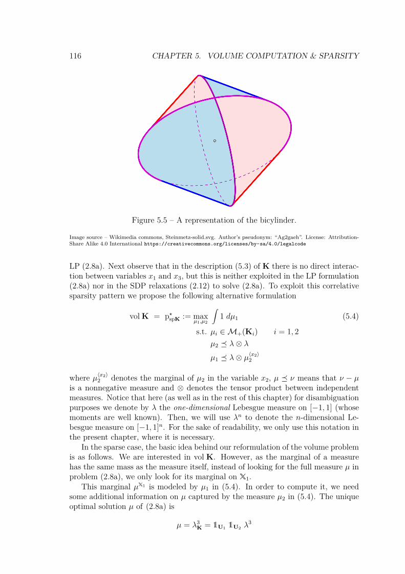
116 CHAPTER 5. VOLUME COMPUTATION & SPARSITY
Figure 5.5 – A representation of the bicylinder.
Image source – Wikimedia commons, Steinmetz-solid.svg. Author’s pseudonym: “Ag2gaeh”. License: Attribution-Share Alike 4.0 International https://creativecommons.org/licenses/by-sa/4.0/legalcode
LP (2.8a). Next observe that in the description (5.3) of K there is no direct interac-tion between variables x1 and x3, but this is neither exploited in the LP formulation(2.8a) nor in the SDP relaxations (2.12) to solve (2.8a). To exploit this correlativesparsity pattern we propose the following alternative formulation
vol K = p?spK := maxµ1,µ2
∫1 dµ1 (5.4)
s.t. µi ∈M+(Ki) i = 1, 2µ2 λ⊗ λµ1 λ⊗ µ〈x2〉
2
where µ〈x2〉2 denotes the marginal of µ2 in the variable x2, µ ν means that ν − µ
is a nonnegative measure and ⊗ denotes the tensor product between independentmeasures. Notice that here (as well as in the rest of this chapter) for disambiguationpurposes we denote by λ the one-dimensional Lebesgue measure on [−1, 1] (whosemoments are well known). Then, we will use λn to denote the n-dimensional Le-besgue measure on [−1, 1]n. For the sake of readability, we only use this notation inthe present chapter, where it is necessary.
In the sparse case, the basic idea behind our reformulation of the volume problemis as follows. We are interested in vol K. However, as the marginal of a measurehas the same mass as the measure itself, instead of looking for the full measure µ inproblem (2.8a), we only look for its marginal on X1.
This marginal µX1 is modeled by µ1 in (5.4). In order to compute it, we needsome additional information on µ captured by the measure µ2 in (5.4). The uniqueoptimal solution µ of (2.8a) is
µ = λ3K = 1U1 1U2 λ
3

5.1. THE IMPORTANCE OF SPARSITY 117
and therefore its marginal µ1 := µX1 in (x1, x2) is given by
dµ1(x1, x2) =∫ 1
0dµ(x1, x2, x3)
= 1K1(x1, x2) dx1
(∫ 1
01K2(x2, x3) dx3
)dx2︸ ︷︷ ︸
dµ〈x2〉2 (x2)
(5.5)
whereµ2 = λ2
K2 . (5.6)
What is the gain in solving (5.4) when compared to solving (2.8a) ? Observethat in (5.4) we have two unknown measures µ1 and µ2 on R2, instead of a singlemeasure µ on R3 in (2.8a). In the resulting SDP relaxations associated with (5.4)this translates into SDP constraints of potentially much smaller size. For instance,and to fix ideas, for the same relaxation degree d:
• The SDP relaxation pdK corresponding to (2.8a) contains a moment matrix(associated with µ in (2.8a)) of size
(3+dd
);
• The SDP relaxation pdspK corresponding to (5.4) contains two moment matrices,one associated with µ1 of size
(2+dd
), and one associated with µ2 of size
(2+dd
),
where µ1 and µ2 are as in (5.4).
As the size of those matrices is the crucial limiting parameter for all SDP solvers,one can immediately appreciate the computational gain that can be expected fromthe formulation (5.4) versus the formulation (2.8a) when the dimension is high orthe relaxation order increases. Next it is not difficult to extrapolate that the gaincan be even more impressive in the case where the correlative sparsity pattern is ofthe form
K = (x0, . . .xN) ∈ X : ∀i ∈ N?N , gi(xi−1,xi) ≥ 0 , (5.7)
with xi ∈ Rni and ni n for i = 0, . . . , N . In fact, it is straightforward to defineexamples of sets K of the form (5.7) where the first SDP relaxation associated withthe original dense LP formulation (2.8a) cannot be even implemented on state-of-the-art computers, whereas the SDP relaxations associated with a generalization ofthe sparse LP formulation (5.4) can be easily implemented, at least for reasonablevalues of d.
Sparse Stokes constraints: the bicylinder
In Section 4.4.4 we designed efficient general Stokes constraints for the dense for-mulation of problem (2.8a), at the price of introducing a polynomial h vanishingon the boundary of K to obtain problem (4.15). However, in the sparse case (5.4),the polynomial h would destroy the sparsity structure, as it is the product of all

118 CHAPTER 5. VOLUME COMPUTATION & SPARSITY
polynomials defining K and as such it depends on all components of x. Thus, wemust adapt our strategy to introduce sparse Stokes constraints3.
In this section, to keep the notations simple, we illustrate the ideas on ourintroductive bicylinder example of Section 5.1.5. Considering the optimal measuresµ1 and µ2 defined in (5.5),(5.6), we can apply Stokes constraints derived from theGauss formula (4.4), in the directions in which they are Lebesgue: for µ1 in the x1direction and for µ2 in the remaining directions. To see this, define
h1(x1, x2) = g1(x1, x2) e1,
h2(x2, x3) = g2(x2, x3) e2,
h3(x2, x3) = g2(x2, x3) e3
where gi(xi, xi+1) = 1−x2i −x2
i+1, such that h1 ·nK1 vanishes on the boundary of K1and h2 · nK2 and h3 · nK2 vanish on the boundary of K2, where nKi
is the outwardpoint vector orthogonal to the boundary of Ki. For i, j, k ∈ N, the Gauss formula(4.4) yields
∫K1
∂
∂x1(g1(x1, x2)xi1x
j2) dµ1 = 0,∫
K2
∂
∂x2(g2(x2, x3)xj2xk3) dµ2 = 0,∫
K2
∂
∂x3(g2(x2, x3)xj2xk3) dµ2 = 0.
Hence, adding these constraints does not change the optimal value of the LP problem(5.4).
5.2 Exploiting path decomposition sparsity
5.2.1 Path computation theoremWe consider a sparse basic semialgebraic set
K := x ∈ X : ∀i ∈ N?N ,gi(πXi(x)) ≥ 0
with gi ∈ R[xi]mi and its coordinate subspace decomposition Rn =: X = ∑Ni=1 Xi.
Let Ui := x ∈ X : gi(πXi(x)) ≥ 0 so that our sparse semi-algebraic set can bewritten
K =N⋂i=1
Ui.
3Actually, Stokes formulation (4.16) can be made sparse more directly, by enforcing the factthat the boundary measure νi only depends on the variables of the polynomial gi. However, duringthe PhD, we tackled sparse volume computation before working on problem (4.16). As a result, inthis chapter we only use Stokes constraints under the form of (4.15).

5.2. EXPLOITING PATH DECOMPOSITION SPARSITY 119
Up to translation and rescaling, we suppose that K ⊂ X := [0, 1]n. Moreover, let
Ki := xi ∈ Xi : gi(xi) ≥ 0 = πXi(Ui) ; Xi := πXi(X)
and letYi := Xi ∩X⊥i+1 = 〈xj〉j∈Ci∩Cc
i+1
be a subspace of dimension ni := |Ci ∩ Cci+1| for i ∈ N?N−1 with YN = XN . The
superscript ⊥ denotes the orthogonal complement. We work under the followingassumptions.
Assumption 5.6: Connected correlation graph
For all i ∈ 2, . . . , N one has Xi ∩i−1∑j=1
Xj 6= 0.
Assumption 5.7: Path decomposition
For all i ∈ 2, . . . , N one has Xi ∩i−1∑j=1
Xj ⊂ Xi−1.
If Assumption 5.6 is violated then K can be decomposed as a Cartesian product,and one should just apply our methodology to each one of its factors. Assumption5.7 ensures that the associated clique tree is a path decomposition as in Figure 5.2,i.e. that it does not contain branchings.
Theorem 5.8: Path computation
If Assumptions 5.6 and 5.7 hold, then
vol K = p?spK := max(µi)i
∫1 dµ1
s.t. µi ∈M(Ki)+ i ∈ N?N (5.8a)µi µ
Xi∩Xi+1i+1 ⊗ λni i ∈ N?N−1 (5.8b)
µN λnN . (5.8c)
Proof : Let us first prove that pspK ≥ volK. For i ∈ N?N , letWi := X⊥i ∩N∑
j=i+1Xj
so thatN∑j=i
Xj = Xi⊕Wi. Our working assumptions ensure that Wi is never reduced
to 0. For xi ∈ Xi define
dµi(xi) := 1Ki(xi)
∫Wi
N∏j=i+1
1Kj πXj(xi + wi) dwi
dxi. (5.9)
By construction µi ∈M+(Ki) and constraints (5.8a) are enforced. In addition, one

120 CHAPTER 5. VOLUME COMPUTATION & SPARSITY
can check that, if xi,i+1 ∈ Xi ∩Xi+1, then
dµXi∩Xi+1i+1 (xi,i+1) def=
∫yi,i+1∈X⊥i ∩Xi+1
dµi+1(xi,i+1 + yi,i+1)
(5.9)=(∫
X⊥i ∩Xi+11Ki+1(xi,i+1 + yi,i+1) . . .
. . .
∫Wi+1
N∏j=i+2
1Kj πXj(xi,i+1 + yi,i+1 + wi+1) dwi+1
dyi,i+1
dxi,i+1
=∫
Wi
N∏j=i+1
1Kj πXj(xi,i+1 + wi) dwi
dxi,i+1
since by construction of the Wj, (X⊥i ∩Xi+1)⊕Wi+1 = Wi.Thus, comparing this to (5.9), one can see that constraints (5.8b) are satisfied.
Moreover, they are saturated on Ki. Eventually, one has
X = X1 ⊕W1
and thus ∫1 dµ1 =
∫X11K1(x1)
∫W1
N∏j=2
1Uj(x1 + w1) dw1
dx1
=∫X
N∏j=1
1Uj(x)
dx
=∫X1K(x) dx
= vol K,
that is, we have just proved that p?spK ≥ vol K.To prove the converse inequality, observe that our previous choice µ1, . . . , µN
saturates the constraints (5.8b) while enforcing the constraints (5.8a). Any otherfeasible solution µ1, . . . , µN directly satisfies the inequality µi µi. In particular,µ1 µ1 and thus ∫
1 dµ1 ≤∫
1 dµ1 = vol K.
Taking the maximum over all feasible (µi)i∈N?N yields that p?spK ≤ vol K. ♦
Remark 5.1 (Duality in the sparse scheme)The dual of the LP problem of Theorem 5.8 is the LP problem
d?spK := inf(wi)i
∫wN dλnN (5.10)
s.t. w1(x1) ≥ 1 x1 ∈ K1
wi+1(xi+1) ≥∫Yi
wi(yi + πXi(xi+1)) dyi xi+1 ∈ Ki+1 i ∈ N?N−1
wi ∈ C(Xi)+ i ∈ N?N .

5.2. EXPLOITING PATH DECOMPOSITION SPARSITY 121
It is straightforward to prove that if µ1, . . . , µN is feasible for problem (5.8), then forany i ∈ N?N , one has
∫1 dµi ≤
∫1 dµN ≤ C := vol XN = 1, so that Theorem 2.6
holds, and there is no duality gap, i.e. d?spK = p?spK = vol K. For example, in thecase of the bicylinder treated in Section 5.1.5, the dual of (5.4) reads:
d?spK = infw1,w2
∫X2w2(x2, x3) dx2dx3
s.t. w1(x1, x2) ≥ 1 (x1, x2) ∈ K1
w2(x2, x3) ≥∫ 1
−1w1(x1, x2) dx1 (x2, x3) ∈ K2
wi ∈ C(Xi)+ i ∈ N?N .
Thus, if (w(d)1 , w
(d)2 )k∈N is a minimizing sequence for this dual LP, then the sets
Kd :=
(x1, x2, x3) ∈ [0, 1]3 : (w(d)1 (x1, x2) ≥ 1) ∧
(w
(d)2 (x2, x3) ≥
∫ 1
0w
(d)1 (x1, x2) dx1
)
are outer approximations of the set K and the sequences (vol Kd)k and (∫w
(d)2 dλ2)
decrease to vol K. Similar statements can be made for the general dual problem.
Corollary 5.9: Convergence of the path computation scheme
Under Assumption 2.7 on the Ki and Xi = πXi([−1, 1]n), i ∈ N?N , the Moment-SOS hierarchy corresponding to problem (5.8) converges to vol K.
Proof : Since strong duality p?spK = d?spK holds, this is a direct consequence ofTheorems 5.8, 2.14 and 2.15. ♦
Remark 5.2 (Sequential Moment-SOS hierarchy)The LP (5.8) is formulated as a single problem on N unknown measures. How-
ever, it is possible to split it in small chained subproblems to be solved in sequence.Each subproblem is associated with a maximal clique (in the linear clique tree) andit takes as input the results of the subproblem associated with its parent clique. Thisway, the sparse volume computation is split into N linked low-dimension problemsand solved sequentially. This may prove useful when N is large because when solvingthe SDP relaxations associated with the single LP (5.8), the SDP solver may en-counter difficulties in handling a high number of measures simultaneously. It shouldbe easier to sequentially solve a high number of low-dimensional problems with onlyone unknown measure. Both formulations being strictly equivalent, this would notchange the convergence properties of the sparse scheme.
As explained in Chapter 2, the hierarchy of SDP relaxations associated with ourinfinite-dimensional LP provides us with a sequence of upper bounds on vol K. Onemay also be interested in computing lower bounds on vol K. In principle it sufficesto apply the same methodology and approximate from above the volume of X \Ksince K is included in the unit box X. However, it is unclear whether X \K has

122 CHAPTER 5. VOLUME COMPUTATION & SPARSITY
also a sparse description. We show that this is actually the case and so one mayexploit correlative sparsity to compute lower bounds although it is more technical.The following result is a consequence of Theorem 5.8:
Corollary 5.10: Lower bounds sparse computation
If K is sparse, then K := X \K is sparse as well, and vol K is the value ofthe LP problem
p?spK := max(µi,j)i,j
N∑j=1
∫1 dµ1,j
s.t. µj,j ∈M(cl Kj)+ 1 ≤ j ≤ N
µi,j ∈M(Ki)+ 1 ≤ i < j ≤ N
µj,j λpj 1 ≤ j ≤ N
µi,j µXi∩Xi+1i+1,j ⊗ λni 1 ≤ i < j ≤ N
where pj := dimXj, ni := dimX⊥i+1 ∩Xi, Kj := [0, 1]pj \Kj is open and cl Kj
denotes its closurea.aThis is necessary to ensure that our measures are defined on compact sets so that all
representation theorems hold.
Proof : The following description
K =N⊔j=1
j−1⋂i=1
Ui ∩ Uj
,where ⊔ stands for disjoint union and Uj := x ∈ Rn : πXj(x) ∈ Kj, is sparse.Indeed the description of the basic semi-algebraic set
Lj :=j−1⋂i=1
Ui ∩ Uj
is sparse. In addition, by σ-additivity of the Lebesgue measure, one has
vol K =N∑j=1
vol Lj.
Finally, by using Theorem 5.8 we conclude that vol Lj is the value of LP consistingof maximizing
∫Xjdµ1,j subject to the same constraints as in the above LP problem.
Summing up yields the correct value. ♦
5.2.2 General sparse Stokes constraintsConsider the sequential decomposition of problem (5.8) in Theorem 5.8:

5.2. EXPLOITING PATH DECOMPOSITION SPARSITY 123
p?spK,i := maxµi
∫1 dµi
s.t. µi ∈M(Ki)+
µi µ?Xi∩Xi+1i+1 ⊗ λni
for i ∈ N?N−1, and
p?spK,N := maxµN
∫1 dµN
s.t. µN ∈M(KN)+
µN λnN
Our algorithm consists of sequentially solving these problems, starting with de-termining µN , then µN−1, and so on until µ1, whose mass will be vol(K). Weimplement Stokes constraints on each one of these problems. For the problem inµN , we implement regular Stokes constraints as in Section 4.4.4:
p?spK,N := maxµN
∫1 dµN
s.t. µN ∈M(KN)+
µN λnN
(grad hN)µN − (grad hN µN) = 0
where hN is a polynomial vanishing on ∂KN , for example hN = gN,1 · · · gN,mN .Then, let i ∈ N?N−1 and suppose that µi+1 is known, such that determining µi
is reduced to solving the LP problem of computing p?spK,i. From the arguments ofSection 5.2.1, we know that the optimal measure µi is supported on Ki and thaton this set it is the product measure between µXi∩Xi+1
i+1 and the uniform measure onYi = 〈xj〉j∈Ci∩Cc
i+1. Since Stokes’ theorem is only valid for uniform measures, it will
only apply to µYii .
Let J ⊂ N?n. For f ∈ C1(Rn) we define
gradJf :=(∂f
∂xj
)j∈J
such that gradN?nf = gradf and gradjf = ∂f
∂xjfor example. This notation allows
us to define Stokes constraints exactly in the directions we are interested in and toformulate the general sparse Stokes constraints:
p?spK,i := maxµi
∫1 dµi
s.t. µi ∈M(Ki)+
µi µ?Xi∩Xi+1i+1 ⊗ λni
(gradCi∩Cci+1hi)µi − gradCi∩Cc
i+1(hi µi) = 0
where hi is a polynomial vanishing on ∂Ki, for example hi = gi,1 · · · gi,mi .

124 CHAPTER 5. VOLUME COMPUTATION & SPARSITY
Remark 5.3 (Refining Stokes constraints)In some cases, in both dense and sparse contexts, these Stokes constraints can
be slightly improved by choosing a different polynomial h(i,)j for each basis vector ejwhen applying the Gauss formula (4.4) to u = hj ej, such that hj can be taken withthe lowest possible degree, allowing for a better implementation of the hierarchy. Forexample, if one is looking for the volume of K := [0, 1]2, the polynomial vanishingon ∂K with the lowest degree is h(x1, x2) := x1(1 − x1)x2(1 − x2), but one canformulate Stokes constraints by applying the Gauss formula (4.4) to x1(1 − x1) e1and x2(1 − x2) e2, instead of h(x1, x2) e1 and h(x1, x2) e2. By doing so, one wouldreplace the constraint (grad h) µ− grad(h µ) = 0 with
(∂hj∂xj
)µ− ∂
∂xj(hj µ) = 0 for
every possible j. This is what we actually implemented in our numerical examples,but we presented the Stokes constraints in the restrictive case of hj = h for all j forthe sake of readability.
5.2.3 Path computation examplesBicylinder revisited
We refer to (2.8a) as the dense problem and to (5.4) as the sparse problem. Forboth problems, we consider instances with and without additional Stokes constraints.Note that for the bicylinder example of Section 5.1.5 the optimal value for both thedense and the sparse problem is
vol K = 163 ≈ 5.3333
since adding Stokes constraints does not change the optimal value.We solve the SDP relaxations with Mosek on a standard laptop, for various
relaxation orders and we report the bounds and the computation times in Table 5.1.We observe a slow convergence for the dense and the sparse versions without Stokesconstraints, and a much faster convergence with Stokes constraints. We also observesignificantly smaller computation times when using the sparse formulation.
A nonconvex set
Let X := R5, X1 = 〈x1, x2〉, X2 = 〈x1, x3〉, X3 = 〈x1, x4〉, X4 = 〈x1, x5〉 and fori = 1, 2, 3, 4
• gi(x1, xi+1) := (2x21 − x2
1+i − 1 , x1 (1− x1) , xi+1 (1− xi+1)),
• Ki := g−1i ((R+)3) = (x1, xi+1) ∈ [0, 1]2 : 2x2
1 − x2i+1 ≥ 1.
Let us approximate the volume of the sparse set
K :=
(x1, x2, x3, x4, x5) ∈ [0, 1]5 : ∀i ∈ N?4, 2x21 − x2
i+1 ≥ 1
=4⋂i=1
π−1Xi
(Ki) .
Here the coordinates x2, x3, x4 and x5 do not interact: they are only linked withthe coordinate x1. The proper way to apply our linear computation Theorem 5.8 isto define a linear clique tree as shown in Figure 5.6.

5.2. EXPLOITING PATH DECOMPOSITION SPARSITY 125
full sparse
d without Stokes with Stokes without Stokes with Stokes
2 7.8232 (1.0s) 5,828 (1.1s) 7,7424 (1.1s) 5,4984 (1.1s)
3 7.2368 (0.9s) 5,4200 (1.3s) 7,1920 (0.9s) 5,3488 (1.1s)
4 7.0496 (1.4s) 5,3520 (2.2s) 7,0040 (1.2s) 5,3376 (1.2s)
5 6,8136 (3.1s) 5,3400 (4.4s) 6,7944 (1.8s) 5,3352 (1.8s)
6 6,7376 (7.2s) 5,3376 (8.2s) 6,6960 (2.1s) 5,3344 (2.3s)
7 6,6336 (12.8s) 5,3360 (18.3s) 6,6168 (2.6s) 5,3344 (3.2s)
Table 5.1 – Performance of sparse computation of the bicylinder’s volume.
Bounds on the volume (and computation times in seconds) vs relaxation order forthe bicylinder.
One can verify that such organization of the cliques satisfies Assumptions 5.6& 5.7, allowing for the application of Theorem 5.8 and the implementation of theMoment hierarchy corresponding to problem (5.8) with sparse Stokes constraints.
This yields the following formulation
vol K = p?spK = max(µi)i
∫1 dµ1 (5.11)
s.t. µi ∈M(Ki)+ i = 1, 2, 3, 4dµ1(x1, x2) dµ
〈x1〉2 (x1) dx2
dµ2(x1, x3) dµ〈x1〉3 (x1) dx3
dµ3(x1, x4) dµ〈x1〉4 (x1) dx4
dµ4(x1, x5) dx1 dx5
with Stokes constraints∂
∂x2
[(2x2
1 − x22 − 1) x2 (1− x2)
]dµ1(x1, x2) = ∂
∂x2
[(2x2
1 − x22 − 1) x2 (1− x2) dµ1(x1, x2)
]∂
∂x3
[(2x2
1 − x23 − 1) x3 (1− x3)
]dµ2(x1, x3) = ∂
∂x3
[(2x2
1 − x23 − 1) x3 (1− x3) dµ2(x1, x3)
]∂
∂x4
[(2x2
1 − x24 − 1) x4 (1− x4)
]dµ3(x1, x4) = ∂
∂x4
[(2x2
1 − x24 − 1) x4 (1− x4) dµ3(x1, x4)
]∂
∂x5
[(2x2
1 − x25 − 1) x5 (1− x5)
]dµ4(x1, x5) = ∂
∂x5
[(2x2
1 − x25 − 1) x5 (1− x5) dµ4(x1, x5)
]∂
∂x1
[(2x2
1 − x25 − 1) x1 (1− x1)
]dµ4(x1, x5) = ∂
∂x1
[(2x2
1 − x25 − 1) x1 (1− x1) dµ4(x1, x5)
].
We can compute analytically
vol K = 115(7− 4
√2)' 0.0895.

126 CHAPTER 5. VOLUME COMPUTATION & SPARSITY
x1
x3
x4
C2
C3
x2
x5
C1
C4
(a) Variable graph.
C1 C2
C3C4
(b) Clique tree.
Figure 5.6 – Graph with linear clique tree for the nonconvex set.
On Figure 5.7 we show results from solving several relaxations via the denseand the sparse approach, with and without Stokes constraints. While solving withMosek the degree 12 dense relaxation took about 1000 seconds, solving the degree12 sparse relaxation took less than 10 seconds. With the sparse relaxations it waspossible to go much higher in the hierarchy. Figure 5.7b shows convincingly howStokes constraints accelerate the convergence of the hierarchy. We can also observethat the nonconvexity of K poses no special difficulty for the volume computation.
2 3 4 5 6 7
relaxation order
10 -1
10 0
10 1
10 2
10 3
tim
es (
se
co
nd
s)
Full Stokes
Full
Sparse Stokes
Sparse
(a) Computation time vs relaxation order.
2 3 4 5 6 7
relaxation order
0.1
0.15
0.2
0.25
0.3
0.35
0.4
bo
un
ds o
n v
olu
me
Full Stokes
Full
Sparse Stokes
Sparse
Analytic
(b) Bounds on the volume vs relaxation order.
Figure 5.7 – Performance for the nonconvex set.
A high dimensional polytope
ConsiderK(n) := x ∈ [0, 1]n : ∀i ∈ N?n−1, xi + xi+1 ≤ 1.

5.2. EXPLOITING PATH DECOMPOSITION SPARSITY 127
According to [118], for any θ ∈ (−π2 ,
π2 ), one has the elegant formula :
tan θ + sec θ = 1 +∞∑n=1
vol K(n) θn
which gives access to the volume of K(n) for n arbitrarily large. For example whenn = 20 we obtain
vol K(20) = 1481484752950197316080327065600 ≈ 1.522 · 10−4.
From the SDP viewpoint, vol K(n) is computed by solving relaxations of the LPproblem given in Theorem 5.8 where N = n − 1, Xi = 〈xi, xi+1〉 and gi(xi, xi+1) =(xi, xi+1, 1− xi − xi+1), i = 1, . . . , n− 1.
We implemented the volume computation algorithm for n = 20, with Stokescontraints. This cannot be achieved without resorting to sparse computation as thedimension is too high for regular SDP solvers. With the sparse formulation howeverwe could solve relaxations up to degree 28 in less than 100 seconds, see Figure 5.8.Note however, that the analytic volume is of the order of 10−4. In consequence weobserve a non monotonicity of the relaxation values which contradicts the theory.This issue is surprising as the Mosek SDP solver terminates without reporting issues.This indicates that computing small volumes in large dimension can be numericallysensitive.
2 4 6 8 10 12 14
relaxation order
1.5
2
2.5
bounds o
n v
olu
me
10 -4
Sparse Stokes
Analytic
Figure 5.8 – Performance for the high dimensional polytope.
We represent the obtained bounds on the volume vs relaxation order.
In order to fix the monotonicity issue, we added a sparse rescaling to our problem.The idea is the following: at each step of the algorithm, the mass of the measure µiis less than the mass of the reference measure
ρi := µXi∩Xi+1i+1 ⊗ λni .
Definingεi := |µi|
|ρi|∈ (0, 1),

128 CHAPTER 5. VOLUME COMPUTATION & SPARSITY
3 4 5 6 7 8 9 10
relaxation order
1.55
1.6
1.65
1.7
1.75
bo
un
ds o
n v
olu
me
10 -4
Mosek
SeDuMi
Analytic
(a) Without rescaling.
3 4 5 6 7 8 9 10
relaxation order
1.55
1.6
1.65
1.7
1.75
bo
un
ds o
n v
olu
me
10 -4
Mosek
SeDuMi
Analytic
(b) With rescaling.
Figure 5.9 – Sparse rescaling performance for the high dimensional polytope.
we obtain that
vol K =N∏i=1
εi
as a telescoping product, since |ρN | = vol XN = 1 (recall that X = [0, 1]n &XN = [0, 1]nN ). As a result, if N is large and the εi are small, one can expect thevolume to be very small, which explains why the SDP solver encounters difficulties.Thus, a solution is to multiply each domination constraint by a well-chosen rescalingfactor ε such that the mass of µi does not decrease too much. As a result, one obtainsvol K = εN−1p? εspK, where
p? εspK := max(µi)i
∫1 dµ1 (5.12)
s.t. µi ∈M(Ki)+ i ∈ N?N
ε µi µXi∩Xi+1i+1 ⊗ λni i ∈ N?N−1
µN λnN .
Figure 5.9 gives a comparison between the results obtained with and without sparserescaling, using the SDP Solvers SeDuMi and Mosek, for the choice ε = 1
2 .First, one can see that without rescaling (Figure 5.9a), both SeDuMi and Mosek
have accuracy issues that make them lose monotonicity, while the rescaling (Figure5.9b) allows recovering monotonicity at least when using SeDuMi (which is slowerbut more accurate than Mosek to our general experience). Second, it is clear that therelative approximation error is much smaller with scaling. This, combined to the factthat the error is relative (after rescaling, the error is much smaller), demonstratesthe power of our rescaling method.

5.2. EXPLOITING PATH DECOMPOSITION SPARSITY 129
A nonconvex high dimensional set
Finally, we consider the set already mentioned in Section 5.1.3, which is both non-convex and high dimensional. Let
K(n) :=x ∈ [0, 1]n : ∀i ∈ N?n−1, xi+1 xi ≤ 1/2
whose analytic volume is a function of the dimension n. For n = 3 the analyticvolume is 0.75, for n = 4 it is 0.6566, approximately. In higher dimensions we donot have an analytic expression for the volume. However, in order to get a feelingfor its value for bigger n, we ran a Monte Carlo simulation with one million samplesfor n = 10, 20, 50, and 100.
Remark 5.4 (On Monte Carlo simulations)We describe the very basic Monte Carlo approach used here. Let X1, . . . ,XN be
i.i.d. samples from some law µ. In our case µ is the uniform distribution on [0, 1]n.Further let f be a function from the probability space into 0, 1. Again, in our case,f would return 1 if the sample Xi is in the set K(n), and 0 else. By the strong lawof large numbers
FN := 1N
N∑i=1
f(Xi) −→N→∞
∫f dµ = vol K(n).
This makes FN a reasonable guess if N is large. However, FN is still a guess, andit might happen that FN is actually far away from the approximated quantity.
As a consequence of the Central Limit Theorem, the difference FN −∫f dµ
behaves (almost) like a normal distributed random variable with zero mean and vari-ance σ2/N where σ2 =
∫(f −
∫fd µ)2 dµ. Note that the variance σ2 can also be
estimated based on the i.i.d. samples X1, . . . ,XN :
S2N := 1
N − 1
N∑i=1
(Xi − FN)2.
This allows one to define a confidence interval for the approximated volume. Indeed,say we are interested in a 99%-confidence interval. Then for G a standard normaldistributed random variable, we have P(|G| < 2.58) ≈ 0.99 and consequently,
P
FN −2.58SN√
N≤∫fdµ ≤ FN + 2.58SN√
N
≈ 0.99.
Remark 5.5 (Moment-SOS hierarchy VS Monte-Carlo)Before we go on, let us emphasize that the method proposed in this chapter is
not in competition with the Monte Carlo approach. While the Monte Carlo methodgives a probabilistic estimate of the volume, our method provides a guaranteed upperbound. Nonetheless, it would be disconcerting if the computed upper bound weremuch smaller than the lower bound of the confidence interval, and we consider ourapproximation valid, when it returns something in the order of the Monte Carloapproximation. The results for different dimensions n and solved with the MosekSDP solver are summarized in Table 5.2.

130 CHAPTER 5. VOLUME COMPUTATION & SPARSITY
As in the previous section we experience accuracy issues for the relaxations of or-der 14 and n = 20, 100, as well as for order 16 and n = 50. Otherwise, the ap-proximations provide better upper bounds for increased relaxation orders as expec-ted. For n = 3, 4 the approximation is reasonably close to the analytic value. Forn = 10, 20, 50 our scheme provides an upper bound in the same order of magnitudeas the 99%-confidence interval of the Monte Carlo simulation. We interpret this asa validation for both the Monte Carlo approach and our own approach. For n = 100we could not derive a meaningful confidence interval. Indeed, as our approximationshows, the volume for n = 100 is less than 9 · 10−6. In order to get an accuracyof ε = 10−6 one would have to draw approximately N = 1
ε2 = 1012 samples. Withour non-sophisticated implementation, the Monte Carlo simulation for one millionpoints took about 5 seconds. Extending this linearly to a simulation with 1012
samples would therefore take a little less than 2 months (5 · 106 s ' 1389 h ' 58 d).With more sophisticated methods, this time could certainly be reduced dramatic-ally. However, it sets the 44 minutes it took to solve relaxation order 16 for n = 100into perspective.
5.3 Exploiting correlative sparsity
5.3.1 General correlative sparsity patternLet us describe a general method to compute the volume of
K :=N⋂i=1
Ui
where Ui = x ∈ X : gi(x) ≥ 0 and (g1, . . . ,gN) is a correlatively sparse family ofpolynomial vectors with associated coordinate subspace decompositionX = ∑N
i=1 Xi.For this we construct the correlation graph G = (V,E) as follows:
• V = 1 . . . , n represents the canonical basis e1, . . . , en of X = Rn;
• E = (i, j) ∈ 1, . . . , n2 : i 6= j & ei, ej ∈ Xk for some k ∈ N?N .
As stated in Section 5.1.4, we suppose that the correlation graph of (gi)1≤i≤N hasexactly N maximal cliques (see Section 5.3.4 for discussions when it is not the case)that are in correspondence with the Xi.
Let K be the set of maximal cliques of G. We will use the following property ofgraphs:
Definition 5.11: Clique Intersection Property (CIP)
The graph G = (V,E) is said to satisfy the clique intersection property (CIP)iff there is a clique tree T = (K, E), E ⊂ K2, such that for all C,C′ ∈ K,C ∩C′ ⊂ C′′ for any C′′ on the path connecting C and C′ in the tree T .

5.3. EXPLOITING CORRELATIVE SPARSITY 131
n=3 n = 4 n=10
d value time (s) value time (s) value time (s)
4 7.86E-01 0.95 7.09E-01 0.61 3.93E-01 1.24
5 7.73E-01 2.87 6.90E-01 0.78 3.57E-01 1.84
6 7.69E-01 2.74 6.84E-01 0.86 3.45E-01 4.21
7 7.66E-01 4.58 6.79E-01 1.83 3.38E-01 4.55
8 7.63E-01 5.00 6.77E-01 2.29 3.34E-01 5.97
9 7.63E-01 6.11 6.74E-01 3.33 3.30E-01 11.56
10 7.62E-01 9.83 6.73E-01 6.86 3.26E-01 18.21
11 7.61E-01 18.16 6.72E-01 8.57 3.26E-01 22.24
12 7.60E-01 19.45 6.71E-01 10.43 3.23E-01 33.78
13 7.60E-01 22.49 6.70E-01 17.89 3.22E-01 74.00
14 7.60E-01 27.02 6.69E-01 26.84 3.21E-01 79.68
15 7.59E-01 32.90 6.69E-01 39.25 3.20E-01 119.7
16 7.58E-01 78.20 6.68E-01 61.32 3.19E-01 176.6
ana/mc 7.50E-01 - 6.57E-01 - [2.99e-01, 3.03e-01]
n = 20 n=50 n = 100
d value time (s) value time (s) value time (s)
4 1.47E-01 5.11 7.68E-03 10.64 9.49E-05 15.19
5 1.20E-01 3.58 4.78E-03 15.10 4.80E-05 26.87
6 1.11E-01 8.13 3.86E-03 21.75 2.84E-05 49.89
7 1.07E-01 11.06 3.42E-03 48.31 2.27E-05 77.07
8 1.03E-01 17.93 3.20E-03 72.78 1.91E-05 135.08
9 1.00E-01 33.31 2.99E-03 120.49 1.63E-05 202.12
10 9.81E-02 41.02 2.99E-03 103.61 1.44E-05 299.44
11 9.70E-02 85.83 2.89E-03 165.56 1.22E-05 441.67
12 9.59E-02 117.08 2.77E-03 220.84 1.19E-05 623.24
13 9.51E-02 138.38 2.67E-03 314.00 1.08E-05 850.92
14 9.57E-02 156.32 2.60E-03 457.92 1.10E-05 1175.02
15 9.39E-02 249.82 2.54E-03 685.64 9.86E-06 1589.49
16 9.36E-02 357.87 2.56E-03 859.60 9.46E-06 2623.02
ana/mc [8.09e-02, 8.24e-02] [1.48e-03, 1.68e-03] -
Table 5.2 – Performances on a nonconvex high dimensional set.
ana/mc refers to the analytic value and the 99%-confidence interval, respectively.

132 CHAPTER 5. VOLUME COMPUTATION & SPARSITY
Such a property is equivalent to the fact that G is chordal4, see [13]. We thenreplace Assumption 5.7 with the following strong correlative sparsity assumption:
Assumption 5.12: Disjoint Intersection Property (DIP)
We suppose that there is a clique tree T = (K, E), rooted in some C1, thatsimultaneously satisfies the CIP and the following disjoint intersection prop-erty (DIP): ∀C,C′,C′′ ∈ K, if (C,C′) ∈ E and (C,C′′) ∈ E then C′ = C′′ orC′ ∩C′′ = ∅.
In words, each clique has an empty intersection with all its siblings. See Section5.3.4 for details on how to check this assumption and construct such a tree whenit exists, as well as possible solutions when Assumption 5.12 does not hold. Figure5.10 illustrates the meaning of this assumption for n = 12 and N = 8. One cancheck that Assumptions 5.6 and 5.12 hold.
Remark 5.6 (On Assumption 5.12)With these assumptions, the only possible clique trees for applying our method to
the nonconvex example illustrated in Figure 5.6 are linear clique trees. Indeed, anybranched clique tree would imply sibling cliques containing x1.
x2
x3
x4
C2
x5
x6
x7
x8
C3
C4
x9
x10
x11
x12
C5
C6
C7
C8
x1
C1
C1
C5
C6
C7
C8
C2
C3
C4
Figure 5.10 – Chordal graph (left) with its clique tree (right).
4Thus the CIP always holds, up to a chordal extension. In particular, cyclic graphs can behandled with empty interactions between well-chosen variables.

5.3. EXPLOITING CORRELATIVE SPARSITY 133
5.3.2 Distributed computation theoremOne can formulate a simple generalization of the sequential implementation of The-orem 5.8 to our general correlative sparsity pattern.
Theorem 5.13: Distributed computation
Let Assumptions 5.6 and 5.12 hold. Let T = (K, E) be a clique tree as inAssumption 5.12. Then vol K =
∫1 dµ?1 where for i ∈ N?N , µ?i is an optimal
solution to the following GMP:
p?spK,i := maxµi
∫1 dµi
s.t. µi ∈M(Ki)+ (5.13a)
µi
⊗(Ci,Cj)∈E
µ?Xi∩Xjj
⊗ λni (5.13b)
and ni = dim Xi ∩( ∑
(Ci,Cj)∈EXj
)⊥=∣∣∣∣∣Ci ∩
( ⋃(Ci,Cj)∈E
Cj
)c∣∣∣∣∣.Proof : We define, for i ∈ N?N ,
Yi := Xi ∩
∑(Ci,Cj)∈E
Xj
⊥ = 〈xk〉k∈Ci ; (Ci,Cj)∈E⇒k/∈Cj
and we observe that, according to Assumption 5.12, for any i ∈ N?N
Xi = ⊕
(Ci,Cj)∈EXi ∩Xj
⊕ Yi.
Thus, constraint (5.13b) is well-posed.For i ∈ N?N , let D(i) := j > i : ∃ an oriented path from Ci to Cj in T
be the set of descendants of Ci, as well as Wi := ∑j∈D(i)
Xj = 〈xk〉k∈Cj ; j∈D(i) and
ri := dimWi =∣∣∣∣∣ ⋃j∈D(i)
Cj
∣∣∣∣∣.We are going to show by induction that for i ∈ N?N ,
µ?i = 1Ki
∏j∈D(i)
1Kj πXj λri
Xi∩Wi
⊗ λni .
Our base cases are the leaves of T , i.e. the i such that D(i) = ∅. Then, problem(5.13) is reduced to the classical problem of computing the volume of Ki, whoseoptimal solution is exactly µ?i = λKi
= 1Kiλni (because D(i) = ∅⇒ ni = dimXi),
which is the expected result.

134 CHAPTER 5. VOLUME COMPUTATION & SPARSITY
Then we can proceed to the induction: let i be a node of T that is not a leaf:D(i) 6= ∅; and suppose that for j ∈ D(i) such that (Ci,Cj) ∈ E ,
µ?j = 1Kj
∏k∈D(j)
1Kk πXk λqj
Xj∩Wj
⊗ λnj .
Then, constraint (5.13b) can be rewritten as
µi
⊗(Ci,Cj)∈E
1Kj
∏k∈D(j)
1Kk πXk λqj
Xj∩Wj
⊗ λnj
Xi∩Xj⊗ λniwhich in turn is simplified into
µi
⊗(Ci,Cj)∈E
1Kj
∏k∈D(j)
1Kk πXk
λnj+qj
Xi∩Wj⊗ λni
since the CIP ensures that Xi∩Xj∩Wj = Xi∩Wj: indeed Cj is on the path betweenCi and any Ck with k ∈ D(j), so that Ci∩Ck ⊂ Cj and thus Xi∩Xk ⊂ Xj, yieldingXi ∩Wj ⊂ Xj. At this point one can notice that nj + qj = dim(Xj + Wj).
Then, using the DIP, we know that if (Ci,Cj), (Ci,Ck) ∈ E with j 6= k thenCj ∩ Ck = ∅ and with the CIP Cj ∩ Cl = ∅ for any l ∈ D(k). This yields that(Xj + Wj) ∩ (Xk + Wk) = 0 and thus Wi = ⊕
(Ci,Cj)∈E(Xj + Wj), allowing us to
rewrite constraint (5.13b) as
µi
⊗(Ci,Cj)∈E
1Kj
∏k∈D(j)
1Kk πXk
λnj+qj
Xi∩Wi
⊗ λni ,
which simplifies into
µi
∏j∈D(i)
1Kj πXj λri
Xi∩Wi
⊗ λni .
Eventually, we are again faced to a classical instance of the dense volume problem
for Ki, with( ∏j∈D(i)
1Kj πXj λri
)Xi∩Wi
⊗ λni instead of only the uniform Lebesgue
measure, and we know that the optimal solution is obtained by multiplying thisnon-negative dominating measure with the indicator of Ki, yielding
µ?i = 1Ki
∏j∈D(i)
1Kj πXj λri
Xi∩Wi
⊗ λni
which is the announced result.

5.3. EXPLOITING CORRELATIVE SPARSITY 135
We conclude by using the fact that D(1) = 2, . . . , N and Rn = X1 + W1 =X1 ⊕ (X⊥1 ∩W1) to compute the value:
∫1 dµ?1 =
∫1K1
N∏j=2
1Kj πXj λq1
X1∩W1
dλn1
=∫X11K1(x1)
∫X⊥1 ∩W1
N∏j=2
1Uj(x1 + w1) dw1
dx1
=∫Rn
(N∏i=1
1Ui(x)
)dx
=∫Rn1K(x) dx
= vol K.
♦
Therefore one obtains a sequence of infinite dimensional LPs on measures thatcan be algorithmically addressed using the usual SDP relaxations. The computationsstart from the leaves of the clique tree and proceed down to the root. It is worthnoting that all the maximal cliques of the same generation in the tree are totallyindependent, which allows treating them simultaneously, i.e. to partially parallelizethe computations. Let d ∈ N. We consider the solutions z(d)
i to the degree d momentrelaxations corresponding to problems (5.13), for i ∈ N?N , as well as the relaxationvalues pdspK,i. We are going to study the convergence of the sequence pdspK,1 to vol K.
Theorem 5.14: Convergence of the branched Moment-SOS hier-archy
Suppose that Assumption 2.7 holds for the Ki and the Xi. Let Ci ∈ Ksuch that for Cj ∈ K satisfying (Ci,Cj) ∈ E , we have a converging se-quence of pseudo-moment vectors (z(d)
j )d: for any appropriate multi-indexk, z(d)
j,k−→d→∞
∫Xj
xkj dµ
?j(xj).
In this setting, if each relaxation of the i-th LP problem (5.13) has at leastone feasible solution, then the corresponding Moment hierarchy converges: forany appropriate multi-index k, z(d)
i,k−→d→∞
∫xki dµ
?i (xi).
Thus, by induction, if at all nodes of T the moment relaxations remain feasibleat all degrees of relaxation, then the branched Moment hierarchy converges,namely pdspK,1 −→
d→∞p?spK,1 = vol K.
Proof : The feasibility assumption ensures that the z(d)i are properly defined at all
degrees d. Then, pointwise convergence of the (z(d)j )d yields that it is bounded for the
weak-∗ topology on R[x]′. The moment relaxation of constraint (5.13b) combinedwith Lemma 2.9 then yield that (z(d)
i )d is bounded for the weak-∗ topology on R[x]′,which means, according to the Banach-Alaoglu theorem, that it has an accumulationpoint. Finally, by uniqueness of the solution to the infinite dimensional LP problem

136 CHAPTER 5. VOLUME COMPUTATION & SPARSITY
(5.13), the convergence of (z(d)j )d to the moment sequence of µ?j ensures that this
accumulation point is none other than the moment sequence of µ?i . This provesexistence and uniqueness of the accumulation point of (z(d)
i )d. Then, we get for anyappropriate multi-index k
z(d)i,k −→
d→∞
∫xk dµ?i (x).
To conclude for the global convergence of the sparse scheme, we just need to check thebase case of this induction. Here again the base case is the leaves of the tree at whichwe are faced to standard instances of the volume problem, whose associated Moment-SOS hierarchy is already proved to converge. Thus, our convergence assumption issatisfied, which means that as long as all the relaxations are feasible, their solutionsconverge weakly-∗ to the infinite dimensional optimal measures, and in particular
pdspK,1 −→d→∞
p?spK,1 = vol K.
♦
Remark 5.7 Stokes constraints can be implemented similarly to the linear case.
5.3.3 Distributed computation examples6D polytope
Let X := R6 and X1 = 〈x1, x2〉, X2 = 〈x2, x3, x4〉, X3 = 〈x3, x5〉, X4 = 〈x4, x6〉. Fori = 1, 3, 4 let gi(x, y) := (x, y, 1− x− y) and
Ki := g−1i
(R2
+
)= (u, v) ∈ [0, 1]2 : u+ v ≤ 1.
Let g2(x, y, z) := (x, y, z, 1− x− y − z) and
K2 := g−12
(R3
+
)= (x, y, z) ∈ [0, 1]3 : x+ y + z ≤ 1.
Let us approximate the volume of the 6D polytope
K :=
x ∈ R6
+ :
x1 + x2 ≤ 1
x2 + x3 + x4 ≤ 1
x3 + x5 ≤ 1
x4 + x6 ≤ 1
=
4⋂i=1
π−1Xi
(Ki) .
No linear clique tree is associated to this problem through Proposition 5.12. Theonly possible clique trees for applying our method are the two branched clique treesof Figure 5.11.
Let us compare the performance of the algorithms derived from the two possibleclique tree configurations and with the dense problem. For that, we first write the

5.3. EXPLOITING CORRELATIVE SPARSITY 137
x2
x3
x4
C2
x5
x6
C3
C4
x1
C1
C1
C3
C4
C2
(a) 3 step clique tree.
x2
x3
x4
C1
x5
x6
C3
C4
x1
C2
C3
C2
C4
C1
(b) 2 step clique tree.
Figure 5.11 – Two possible branched clique trees for the 6D polytope.
problem associated with the 3 step clique tree configuration of the top of Figure5.11:
vol K =∫
1 dµ?1 (5.14)

138 CHAPTER 5. VOLUME COMPUTATION & SPARSITY
where
µ?1 = argmaxµ1
∫1 dµ1
s.t. µ1 ∈M(K1)+
dµ1(x1, x2) dx1 dµ?〈x2〉2 (x2)
µ?2 = argmaxµ2
∫1 dµ2
s.t. µ2 ∈M(K2)+
dµ2(x2, x3, x4) dx2 dµ?〈x3〉3 (x3) dµ?〈x4〉
4 (x4)
µ?i = argmaxµ3
∫1 dµi, i = 3, 4
s.t. µi ∈M(Ki)+
µi λ2.
This problem can be complemented with the following Stokes constraints:∂
∂x1
[x1 (1− x1 − x2)
]dµ1(x1, x2) = ∂
∂x1[x1 (1− x1 − x2) dµ1(x1, x2)]
∂
∂x2
[x2 (1− x2 − x3 − x4)
]dµ2(x2, x3, x4) = ∂
∂x2[x2 (1− x2 − x3 − x4) dµ2(x2, x3, x4)]
∂
∂xi
[xi (1− xi − xi+2)
]dµi(xi, xi+2) = ∂
∂xi[xi (1− xi − xi+2) dµi(xi, xi+2)]
∂
∂xi+2
[xi+2 (1− xi − xi+2)
]dµi(xi, xi+2) = ∂
∂xi+2[xi+2 (1− xi − xi+2) dµi(xi, xi+2)] i = 3, 4.
The 2 step clique tree of the bottom of Figure 5.11 yields the following formulation
vol K =∫
1 dµ?2 (5.15)
where
µ?2 = argmaxµ2
∫1 dµ2
s.t. µ2 ∈M(K2)+
dµ2(x2, x3, x4) dµ?〈x2〉1 (x2) dµ?〈x3〉
3 (x3) dµ?〈x4〉4 (x4)
µ?i = argmaxµi
∫1 dµi, i = 1, 3, 4
s.t. µi ∈M(Ki)+
µi λ2,
with Stokes constraints
∂
∂xi
[xi (1− xi − xj)
]dµi(xi, xj) = ∂
∂xi[xi (1− xi − xj) dµi(xi, xj)]
∂
∂xj
[xj (1− xi − xj)
]dµi(xi, xj) = ∂
∂xj[xj (1− xi − xj) dµi(xi, xj)]

5.3. EXPLOITING CORRELATIVE SPARSITY 139
for (i, j) = (1, 2), (3, 5), (4, 6). However, no Stokes constraints can be applied forthe computation of µ2 (there is no Lebesgue measure in the domination constraint,so the optimal measure is not uniform). For this reason one can expect a slowerconvergence than in the linear configuration.
We implement the hierarchies associated to the 2 and 3 step sparse formulations,as well as the dense problem hierarchy, and compare their performance in Figure5.12. We can compute analytically
vol K = 118 ' 0.0556.
2 3 4 5 6 7 8
relaxation order
10 0
10 1
10 2
tim
es (
se
co
nd
s)
Full Stokes
2 step Stokes
3 step Stokes
(a) Computation time vs relaxation order.
2 3 4 5 6 7 8
relaxation order
0.05
0.06
0.07
0.08
0.09
0.1
0.11
0.12
0.13
bo
un
ds o
n v
olu
me
Full Stokes
2 step Stokes
3 step Stokes
Analytic
(b) Bounds on the volume vs relaxation order.
Figure 5.12 – Performance for the 6D polytope.
Both sparse formulations outperform the dense one in terms of computationaltime needed to solve the corresponding SDPs (Figure 5.12a). On the accuracy sidehowever (Figure 5.12b), we observe that the 2 step formulation seems to be less effi-cient than the 3 step formulation. In particular when considering the accuracy/timeeffort relation at order 3 the dense formulation provides a better value in almost thesame time.
We believe that this can be explained by the way Stokes constraints are addedto the program. Indeed, at a given clique, Stokes constraints can only be imple-mented in the variables that are not shared with the input measure. In the fully(2 step) branched configuration, the last step of the optimization program cannotbe accelerated by Stokes constraints at all, while in the 3 step configuration, step 1includes Stokes constraints in x3, x4, x5, x6, step 2 includes Stokes constraints in x2and step 3 includes Stokes constraints on x1, which explains the gap between theoptimal values of these two configurations.
Moreover, it seems that even the least branched (3 step) configuration stillpresents a gap between its optimal value and the analytic solution. This might alsohappen with a non-sparse instance of the Moment-SOS hierarchy (which convergestheoretically) and it is likely due to the choice of the monomial basis to represent

140 CHAPTER 5. VOLUME COMPUTATION & SPARSITY
polynomials. Indeed, most of the Moment-SOS parsers generate SDP problems withthe basis of monomials, while sometimes other bases (e.g. Chebyshev or Legendrepolynomials) are more appropriate. However, in this precise case, it might also belinked again with the sparse Stokes constraints implementation. Indeed, in step 2of the scheme, the unknown measure measures x2, x3 and x4 but Stokes constraintsare implemented only in x2, leaving a possible Gibbs effect in x3, x4. Unlike most ofour numerical examples, this one still includes an optimization step in which mostof the variables are not controlled through Stokes constraints. The gap between theoptimal value and the analytic value for the 3 step branched formulation in Figure5.12b could be explained by a Gibbs effect in the second optimization step.
As a consequence, in the following, one should avoid the branched hierarchiesthat cannot be accelerated at each step at least partially by Stokes constraints. Sucha hierarchy appears when the root of the chosen clique tree shares all its verticeswith its children cliques. It can be proved that such a configuration can always beavoided while implementing sparse volume computation, by choosing a leaf as thenew root of the tree.
4D polytope
Let X := R4, X1 := 〈x1, x2〉, X2 := 〈x2, x3〉, X3 := 〈x3, x4〉, gi(a, b) := (a, b, 1−a−b),i = 1, 2, 3 and Ki := g−1
i
(R3
+
)= (u, v) ∈ [0, 1]2 : u+ v ≤ 1. Let us approximate
the volume of the 4D polytope
K :=
(x1, x2, x3, x4) ∈ R4
+ :x1 + x2 ≤ 1
x2 + x3 ≤ 1
x3 + x4 ≤ 1
=
3⋂i=1
π−1Xi
(Ki) .
In such a case, there are two possible configurations for the associated clique treeof Proposition 5.12, see Figure 5.13. Accordingly, we can compute vol K in twodifferent ways. The first way
vol K = max(µi)i
∫1 dµ1 (5.16)
s.t. µi ∈M(Ki)+
dµ1(x1, x2) dx1 dµ〈x2〉2 (x2)
dµ2(x2, x3) dx2 dµ〈x3〉3 (x2)
dµ3(x3, x4) dx3 dx4
is the linear formulation given by Corollary 5.8, which is under the form of a non-parallelizable single linear problem. The following additional Stokes constraints can

5.3. EXPLOITING CORRELATIVE SPARSITY 141
x2x1 x3
C1
x4
C2 C3
C1 C2 C3
(a) linear clique tree.
x2x1 x3
C2
x4
C1 C3
C1
C2
C3
(b) branched clique tree.
Figure 5.13 – Two possible clique trees for the 4D polytope.
be added:
∂
∂x1
[x1 (1− x1 − x2)
]dµ1(x1, x2) = ∂
∂x1[x1 (1− x1 − x2) dµ1(x1, x2)]
∂
∂x2
[x2 (1− x2 − x3)
]dµ2(x2, x3) = ∂
∂x2[x2 (1− x2 − x3) dµ2(x2, x3)]
∂
∂x3
[x3 (1− x3 − x4)
]dµ3(x3, x4) = ∂
∂x3[x3 (1− x3 − x4) dµ3(x3, x4)]
∂
∂x4
[x4 (1− x3 − x4)
]dµ3(x3, x4) = ∂
∂x4[x4 (1− x3 − x4) dµ3(x3, x4)] .
On the other hand, if one associates the maximal clique C1 to the subspace X2 andthe maximal clique C2 to the subspace X1, one also has
vol K =∫
1 dµ?2 (5.17)

142 CHAPTER 5. VOLUME COMPUTATION & SPARSITY
where
µ?2 = argmaxµ2
∫1 dµ2
s.t. µ2 ∈M(K2)+
dµ2(x2, x3) µ?〈x2〉1 (dx2) dµ?〈x3〉
3 (x3)
µ?1 = argmaxµ1
∫1 dµ1
s.t. µ1 ∈M(K1)+
dµ1(x1, x2) dx1 dx2
µ?3 = argmaxµ3
∫1 dµ3
s.t. µ3 ∈M(K3)+
dµ3(x3, x4) dx3 dx4
which is the branched formulation associated to Theorem 5.13. Here one can see thatµ?1 and µ?3 can be computed independently in parallel, and then re-injected in theproblem to which µ?2 is the solution. One can add the following Stokes constraints:
∂
∂x1
[x1 (1− x1 − x2)
]dµ1(x1, x2) = ∂
∂x1[x1 (1− x1 − x2) dµ1(x1, x2)]
∂
∂x2
[x2 (1− x1 − x2)
]dµ1(x1, x2) = ∂
∂x2[x2 (1− x1 − x2) dµ1(x1, x2)]
∂
∂x3
[x3 (1− x3 − x4)
]dµ3(x3, x4) = ∂
∂x3[x3 (1− x3 − x4) dµ3(x3, x4)]
∂
∂x4
[x4 (1− x3 − x4)
]dµ3(x3, x4) = ∂
∂x4[x4 (1− x3 − x4) dµ3(x3, x4)] .
We can compute analytically
vol K = 524 ' 0.2083.
In Figure 5.14 we compare the two sparse formulations with and without Stokesconstraints. Surprisingly the linear formulation is faster than the branched onefor small relaxation degrees, most probably because at this level of precision thebranching costs more in terms of constructing and parsing the LMIs than it savesin computational time. When going deeper in the hierarchy we see the advantageof the branched formulation where more computations are done in parallel. As ob-served in the previous example however, the branched formulation seems to haveproblems to converge to the optimal value on an early relaxation. While the val-ues of both formulations without Stokes constraints almost coincide, the values ofthe linear formulation with Stokes are strictly better than the ones of the acceler-ated branched formulation. This further supports our conjecture that formulationswhere Stokes constraints can be added at every step of the optimization programare to be preferred: the fact that both configurations behave equally without Stokesconstraints and that the branched configuration keeps a relaxation gap when im-plementing Stokes constraints suggests that these Stokes constraints behave better

5.3. EXPLOITING CORRELATIVE SPARSITY 143
in linear configurations than in branched configurations. For this reason, in the 6Dcase where all possible configurations are branched, we could not completely elim-inate the relaxation gap, while in this case where there is a linear configuration, therelaxation gap vanishes.
2 4 6 8 10 12 14
relaxation order
10 -1
10 0
10 1
tim
es (
seconds)
Linear Stokes
Linear
Branched Stokes
Branched
(a) Computation time vs relaxation order.
2 4 6 8 10 12 14
relaxation order
0.2
0.25
0.3
0.35
0.4
0.45
0.5
0.55
0.6
bo
un
ds o
n v
olu
me
Linear Stokes
Linear
Branched Stokes
Branched
Analytic
(b) Bounds on the volume vs relaxation order.
Figure 5.14 – Performance for the 4D polytope.
5.3.4 The disjoint intersection hypothesisIt may happen that Assumption 5.12 does not hold, in which case all the aboveresults would not apply. For example one could think of the following set:
K :=x ∈ R6 : x2
1 + x22 + x2
3 ≤ 1 ∧ ∀i ∈ 2, 3, x2i + x2
i+2 + x2i+3 ≤ 1
whose correlative graph is represented on Figure 5.15. Here the DIP and CIP cannotbe simultaneously enforced: the CIP would only be satisfied by a branched cliquetree, but since all the cliques share common vertices, in such a branched tree therewould automatically be sibling cliques with nonempty intersection. Also, one cannotice that in this case (and, as far as we know, only in similar configurations whereAssumption 5.12 is violated), the clique C2 does not correspond to a polynomialappearing in the description of K.
First, we would like to emphasize that the core of this chapter is the linear com-putation theorem, for which the working assumption always holds. The branchedgeneralizations are only consequences of this linear computation theorem.
Second, the fact that Assumption 5.12 does not hold is not a dead-end for usingour scheme. In fact, even the simpler CIP might not hold, in which case one wouldneed to perform a chordal extension, which consists of adding virtual links betweenvariables to construct a chordal graph. Basically, a chordal extension would makethe graph chordal at the price of slightly weakening the correlative sparsity pattern.In general, the same can be performed to enforce Assumption 5.12: one could addvirtual links between variables to enforce the assumption to hold. For example, if

144 CHAPTER 5. VOLUME COMPUTATION & SPARSITY
x2
x3
x1
C1 C2x5
x4
x6
C3
C4
Figure 5.15 – A correlation graph that violates Assumption 5.12.
one artificially links variables x3 and x4 in the correlation graph of K, one obtains anew correlation graph, with an associated clique tree satisfying all our working as-sumptions (see Figure 5.16). This manipulation results in increasing the correlativesparsity CS from 3 to 4, which is a weakening of the correlative sparsity pattern.However, our framework still allows reducing the dimensionality of the problem from6 to 4.
x2
x3
x1
C1x5
x4
x6
C3
C2C1 C2 C3
Figure 5.16 – A way to fix our counterexample.
Remark 5.8 (Alternative to graph extension)There might exist examples for which the DIP would only be obtained by com-
pletely destroying the sparsity pattern one wants to exploit. However, this couldalso happen with the more common CIP. In either case, an option might be to

5.3. EXPLOITING CORRELATIVE SPARSITY 145
consider the standard dual volume computation problem (2.8b) as a way to findminimizing sequences (wd)d that approximate 1K, and to apply it to each one of theKi := xi ∈ Xi : gi(xi) ≥ 0 to obtain a sequence
(w
(d)1 , . . . , w
(d)N
)dsuch that
(w
(d)i
)d
approximates 1Ki. Then, one would still have to prove that the convergence of the
hierarchy is stable by product (which is nontrivial) to conclude that∫ N∏
i=1w
(d)i πXi(x) dx
converges to vol K. The major drawback of this solution is that in order for (wd)dto approximate 1K, we cannot implement Stokes constraints, as they would modifyproblem (2.8b) (see Chapter 4) in a way that makes us lose the convergence to anindicator (this is precisely the point of Stokes constraints: they allow their userto obtain the volume without trying to approximate discontinuous functions withpolynomials). However, we know that the volume approximation hierarchy has a badconvergence rate without Stokes constraints. In general, we should not expect anymethod that approximates indicators with polynomials to yield satisfactory results interms of volume computation. Such a method should be considered only as a lastresort if any trial to apply the above scheme fails. Finally, this option represents aframework that would be completely independent from the above and thus it remainsout of the scope of this chapter.
We now move on to proposing a detailed method to enforce Assumption 5.12. Todo so, we first introduce a more detailed glossary for graph theory. Let G = (V,E)be a graph with vertices set V and edges set E ⊂ V2. The following definitions canbe found in e.g. [13]:
• The degree deg v of v ∈ V is the cardial of the set v′ ∈ V : (v, v′) ∈ E i.e.the number of vertices connected to v.
• A clique of G is a subset of vertices C ⊂ V such that v, v′ ∈ C implies(v, v′) ∈ E.
• A graph G is chordal if every cycle of length greater than 3 has a chord, i.e.an edge connecting two nonconsecutive vertices on the cycle.
• A tree T = (K, E) is a graph without cycle.
• The treewidth of a chordal graph is the size of its biggest clique minus 1. Thusthe treewidth of a tree is 1 and the treewidth of a complete graph (E = V2)of size n is n− 1.
• A rooted tree is a tree in which one vertex has been designated the root.
• In a rooted tree, the parent of a vertex v is the vertex v connected to it onthe path to the root; v is then called a child of v; two vertices that have thesame parent are called siblings; a descendant of a vertex v is any vertex whichis either the child of v or is (recursively) the descendant of any of the childrenof v; v is then called an ancestor of itself and any of its descendants.

146 CHAPTER 5. VOLUME COMPUTATION & SPARSITY
• The vertices of a rooted tree can be partitioned between the root, the leaves(the vertices that have parents but no children) and the branches (that havechildren and parents).
• Let K be the set of maximal cliques of G. A clique tree T = (K, E) of G is atree whose vertices are the maximal cliques of G.
• A clique tree satisfies the clique intersection property (CIP) if for every pairof distinct cliques C,C′ ∈ K, the set C ∩ C′ is contained in every clique onthe path connecting C and C′ in the tree. We denote by T ct the set of cliquetrees of G that satisfy the CIP.
• The ordering K = C1, . . . ,CN satisfies the Running Intersection Property(RIP) if ∀i ∈ 2, . . . , N, ∃ ki ∈ 1, . . . , i− 1 such that Ci ∩
i−1⋃j=1
Cj ⊂ Cki .
• Let A ⊂ V. Then, the subgraph of G generated by A is given by
〈A〉G := (A,E ∩A2).
Theorem 5.15: Chordality & RIP
A connected graph G is chordal if and only if T ct 6= ∅ if and only if K admitsan ordering that satisfies the RIP.
Definition 5.16: Disjoint Intersection Property
Let G = (V,E) be chordal and connected. Let T = (K, E) ∈ T ct be a cliquetree rooted in C1 ∈ K. T satisfies the Disjoint Intersection Property (DIP) if∀C,C′,C′′ ∈ K, if (C,C′) ∈ E and (C,C′′) ∈ E then C′ = C′′ or C′∩C′′ = ∅.In words, each clique has an empty intersection with all its siblings.
We are now going to give a systematic way to enforce Assumption 5.12 andgenerate the associated clique trees. Let (g1, . . . ,gN) be a correlatively sparse familyof polynomial vectors with a connected chordal correlation graph G = (V,E). LetK be the set of maximal cliques of G. We construct the clique graph GK = (K,F)such that (C,C′) ∈ F iff C ∩C′ 6= ∅. One can in turn define cliques (called meta-cliques) for this new graph, and its correlative sparsity CSK is the size of its biggestmaximal meta-clique minus 1. One can note that any clique tree is a subtree of GKincluding all its vertices.
Remark 5.9 If GK itself is a tree (as in section 5.3.3), then it trivially satisfies theDIP and CIP, and Assumption 5.12 automatically holds.

5.3. EXPLOITING CORRELATIVE SPARSITY 147
Lemma 5.17: Genealogy
Let T = (K, E) be a clique tree satisfying Assumption 5.12.
1) Let C,C′ ∈ K such that C 6= C′ and C∩C′ 6= ∅. Then, up to permutingthem, C is a descendant of C′.
2) Let Q be a meta-clique. Then, 〈Q〉T is an oriented path of T : theelements of Q are ancestor to one another and each C ∈ Q has itsparent in Q except one of them.
Proof :
1) Let C′′ be the last common ancestor of C and C′, meaning that C′′ is anancestor of both C and C′ but any child of C′′ is the ancestor of at most oneof them. Such ancestor exists since the root C1 is a common ancestor to Cand C′. Then, C′′ is on the path between C and C′. Since C 6= C′, up topermuting them, we can suppose that C 6= C′′.By contradiction, we suppose that C′ 6= C′′. Then, let C be the child of C′′that is also the ancestor of C, and C the child of C′′ that is also the ancestorof C′. Both exist since C′′ is an ancestor of C and C′ and C 6= C′ 6= C′′. C′′being the latest common ancestor of C and C′, we deduce that C 6= C so thatC and C are siblings. Then, the DIP ensures that C ∩ C = ∅. However, Cand C are on the path between C and C′, so according to the CIP they bothcontain C ∩C′ which is nonempty. This is a contradiction.
2) According to point 1), all elements of Q are descendants of one another, sothat they are all on the same path in T . We only have to show that any Cbetween two elements C′,C′′ of Q on this path is also an element of Q. Indeed,let C′′′ ∈ Q. Then, up to a permutation on C′,C′′,C′′′ we can suppose thatthe unoriented path includes in this order: (C′,C,C′′,C′′′). Then, C is on thepath between C′ and C′′′, so the CIP implies that C ⊃ C′ ∩C′′′ is nonempty(since C′ and C′′′ belong to the same clique Q), and then C has a nonemptyintersection with C′′′. This shows that C has a nonempty intersection withany element of Q, which by maximality of Q is the definition of C ∈ Q.
♦
Corollary 5.18: Path decomposition
If GK is a complete graph (all pairs of maximal cliques have nonempty in-tersection as in section 5.3.3), then the only candidates for our clique treeare linear clique trees (i.e. path decompositions). In such case, Assumption5.12 is equivalent to the existence of a reordering of (g1, . . . ,gN) such thatAssumption 5.7 holds.

148 CHAPTER 5. VOLUME COMPUTATION & SPARSITY
We now give an alogrithm to generate a clique tree T = (K, E) that satisfiesthe DIP and the CIP. In case Assumption 5.12 does not hold, this algorithm auto-matically adds edges to E until it finds an appropriate clique tree (see Algorithm1).
Remark 5.10 (Explanation of Algorithm 1) • Minimizing deg C1 is a wayto ensure Stokes constraints will be fully implementable, in contrast to the 2step implementation in section 5.3.3.
• Index i denotes a clique that has already been added to the tree; the algorithmadds to the tree every clique that shares vertices with Ci, and then incrementsi.
• Index j denotes the meta-clique in which we are working; according to Lemma5.17, in such meta-clique the cliques should be added in line.
• Index k denotes the number of elements that have already been added to thetree; when k is equal to the number of cliques, our clique tree is complete.
• Index l denotes the lates clique of the meta-clique Qj that has been added tothe tree; according to Lemma 5.17, Cl should then be the parent of Ck+1.
• At line 1 we maximize |Qj| to favor linear configurations as they are the mostcompatible with Stokes constraints.
• The if loop at line 1 checks whether it is possible to add the remaining cliquesof Qj to our tree without destroying the CIP.
• The if loop at line 1 checks whether the clique we want to add destroys the DIPor not.
• At line 1 we maximize |Ck+1∩Cl| so that it is less likely to pose problems withCIP and DIP in the future iterations.
• The if loops at lines 1 and 1 are meant to minimize the correlative sparsity ofthe new graph G = (V,E), since it is the limiting factor for the tractability ofour algorithm.
Theorem 5.19: Convergence of Algorithm 1
Any clique tree returned by Algorithm 1 satisfies the DIP and the CIP.
Proof : We are going to show by induction that at any step k, the graphTk := (Pk, Ek) is a tree that satisfies the CIP and the DIP. First, it is trivial thatT1 = (C1,∅) is a tree and satisfies the CIP and the DIP. Next, we supposethat we have constructed a tree Tk satisfying CIP and DIP through iterations of ouralgorithm, and that the next iteration leads us to define a Tk+1 := (Pk∪Ck+1, Ek∪(Cl,Ck+1). Since the only edge we added connected Cl to a new vertex that wasnot in Tk, it did not introduce any cycle, thus Tk+1 is still a tree. We are now goingto check the CIP and DIP.

5.3. EXPLOITING CORRELATIVE SPARSITY 149
Algorithm 1: How to build an appropriate clique treeData: G = (V,E) and its clique graph GK = (K,F).Result: T = (K, E) satisfying CIP & DIP if Assumption 5.12 holds,
G = (V,E) with additional edges else.Initialization: Choose C1 ∈ K with minimal degree in GK;
Initialize i = j = k = 1, P1 := C1, E1 := ∅;while k < |K| do
while Mik := Q maximal meta-clique : Q∩ Pck 6= ∅,Ci ∈ Q 6= ∅ doChoose Qj ∈ argmax
Q∈Mik|Q|;
while Qj ∩ Pck 6= ∅ dol := maxr ≤ k : Cr ∈ Qj;if∃(C,C′) ∈ argmax|C∩Cl| : (C, C) ∈ Pk×Qj∩Pck, C∩C * Clthenif |Cl ∪C| > |Cl ∪C′| then
foreach v ∈ C′, v′ ∈ Cl do E← E ∪ (v, v′), (v′, v);return G = (V,E) ;
elseforeach v ∈ C, v′ ∈ Cl do E← E ∪ (v, v′), (v′, v);return G = (V,E) ;
endelse
Choose Ck+1 ∈ argmaxC∈Qj∩Pck
|C ∩Cl|
endif ∃C ∈ Pk s.t. (Cl,C) ∈ Ek & C ∩Ck+1 6= ∅ then
if |C ∪Ck+1 < |Cl ∪Ck+1| ∧ |Cl ∪C| thenforeach v ∈ C, v′ ∈ Ck+1 do E← E ∪ (v, v′), (v′, v);return G = (V,E) ;
else if |Cl ∪C| > |Cl ∪Ck+1| thenforeach v ∈ Ck+1, v′ ∈ Cl do E← E ∪ (v, v′), (v′, v);return G = (V,E) ;
elseforeach v ∈ C, v′ ∈ Cl do E← E ∪ (v, v′), (v′, v);return G = (V,E) ;
endelsePk+1 := Pk ∪ Ck+1;Ek+1 := Ek ∪ (Cl,Ck+1);k ← k + 1 ;
endendj ← j + 1 ;
endi← i+ 1 ;
endreturn T := (P|K|, E|K|);

150 CHAPTER 5. VOLUME COMPUTATION & SPARSITY
• Let C,C′′ ∈ Pk+1; C ∩C′′ 6= ∅. Let C′ ∈ Pk be on the path between C andC′′ in Tk+1 (C′ 6= Ck+1 because Ck+1 is on no path in Tk+1).
– If C,C′′ ∈ Pk then by our induction hypothesis C ∩C′′ ⊂ C′.– Else, without loss of generality we have C′′ = Ck+1 and C ∈ Pk.∗ Since we successfully passed through the if loop of line 1, we have
C ∩Ck+1 ⊂ Cl.∗ By our induction assumption (Tk satisfies the CIP), we have C∩Cl ⊂
C′ (because either C′ = Cl or C′ is on the path between C and Cl,the parent of Ck+1).
This yields C′ ⊃ C ∩Cl ⊃ C ∩ (C ∩Ck+1) = C ∩Ck+1 = C ∩C′′.
Then, Tk+1 satisfies the CIP.
• Let C ∈ Pk,C′,C′′ ∈ Pk+1 such that (C,C′), (C,C′′) ∈ Ek+1.
– If C′,C′′ ∈ Pk then by our induction hypothesis C′ ∩C′′ = ∅.– Else, without loss of generality we have C′′ = Ck+1,C = Cl, and since
we successfully passed through the if loop of line 1, we have C′ ∩ C′′ =C′ ∩Ck+1 = ∅.
Then, Tk+1 satisfies the DIP.
♦
Finally, we conjecture that if Assumption 5.12 holds, then Algorithm 1 willdirectly return a clique tree satisfying the CIP and the DIP without adding anyedge to G.
Conclusion
Our resultsIn this chapter we addressed the problem of approximating the volume of sparsesemi-algebraic sets with the Moment-SOS hierarchy of SDP relaxations. As illus-trated by our examples, our sparse formulation allows one to dramatically decreasethe computational time for each relaxation, and to tackle high dimensional volumecomputation problems that are not tractable with the usual SDP methods. Bysplitting the problems into low dimensional subproblems, one drastically reducesthe dimension of each relaxation, without loss of precision. This reduction of com-plexity is due to the correspondance between the structure of our algorithm and thecorrelative sparsity pattern in the description of the semi-algebraic set.
We also showed that additional Stokes constraints have a huge effect on con-vergence and precision for volume computation, and that they can successfully beadapted to our sparse formulations. This yields a much better rate of convergence forthe corresponding hierarchy. However, implementing these Stokes constraints leads

5.3. EXPLOITING CORRELATIVE SPARSITY 151
to subtle constraints that have to be enforced if one wants to efficiently compute thevolume:
• First, one should always prefer the linear formulation of Theorem 5.8 wheneverpossible, since this ensures that Stokes constraints can always be efficientlyimplemented.
• Then, in the more general case of Theorem 5.13, one should always avoid for-mulations in which the root of the computation tree has no Stokes constraint;fortunately, such configurations can always be avoided by chosing a leaf as theroot of the clique tree.
Furthermore, in the branched case, one should be aware of the fact that eachstep of the algorithm introduces an approximation error, and the errors accumulateuntil the root is reached. Consequently, a formulation in which the clique tree hastoo many generations will lead to a larger global error than a formulation with lessgenerations. For this reason, one should minimize the number of generations in theclique tree, which is equivalent to parallelizing as much as possible. In additionto that, when the problem has many dimensions and branches, parallelization canobviously drastically increase the speed of the computations.
Applications and future workTo the best of our knowledge, this sparse method for solving volume problems isnew and full of promises for future applications. For instance, the problem of com-puting the mass of any compactly supported measure absolutely continuous (withrespect to the Lebesgue measure) can be adressed using this sparsity method. Also,measures that are not compactly supported but have some decay properties (e.g.Gaussian measures) can also be handled by our method, which may prove useful incomputations for probability and statistics. Also, specific constraints could prob-ably be used in addition to Stokes constraints when the semi-algebraic set presentsa specific structure (e.g. a polytope, a convex body).
Furthermore, the framework of exploiting correlative sparsity can be applied toany method that relies on computations on measures, whether these measures arerepresented by their moments (as it is done in this chapter), or by samples (as inthe stochastic volume computation methods). In particular, we believe that thisformalism could easily be extended to Monte-Carlo-based volume computations.
Finally, we also believe that this method can be adapted to the computation ofregions of attraction, through the formalism developed in [42], for high dimensionaldifferential-algebraic systems that present a network structure, such as power grids,distribution networks in general and possibly other problems. The main difficultyresides in taking sparsity into account when formulating the Liouville equation, andkeeping uniqueness of the solution as in the non-controlled non-sparse framework.


6Theoretical contributions to stability
analysis
This final chapter gathers original contributions to the particular problem of differ-ential systems stability analysis, which is the goal of this thesis. While Chapter 3merely was an extension of existing frameworks to power systems TSA, this chapterdraws on most previously presented results to build two new frameworks for stabilityanalysis of differential systems.
Section 6.1, which is based on the work [100], uses the results of Chapter 2 toextend the existing frameworks presented in Chapter 3, to the inner approximation ofthe Maximal Positively Invariant (MPI) set of a differential system, whose relevancefor power systems security and slightly reduced computational complexity will bediscussed hereafter.
Section 6.2, published as [123], then extends the results from Chapters 3 and 5to approximating regions of attraction of large scale, sparsely coupled, differentialsystems, in a first attempt to fill the gap between stability regions approximationtheory and its application to large scale power grids.
Contents6.1 Inner approximation of maximal positively invariant sets154
6.1.1 MPI set . . . . . . . . . . . . . . . . . . . . . . . . . . . . 155
6.1.2 Primal approximation problem and its value . . . . . . . 158
6.1.3 Dual approximation problem and its value . . . . . . . . . 162
6.1.4 Numerical implementation and its convergence . . . . . . 164
6.2 Sparsity-based approximation for finite time ROA . . . 169
6.2.1 A path decomposition sparsity pattern . . . . . . . . . . . 170
6.2.2 A sparse infinite dimensional formulation . . . . . . . . . 172
6.2.3 Sparsity of the actual finite time ROA . . . . . . . . . . . 175
6.2.4 Computing sparse ROA approximations . . . . . . . . . . 177
153

154 CHAPTER 6. THEORETICAL STABILITY ANALYSIS
6.1 Inner approximation of maximal positively in-variant sets
This section is an effort along a research line initiated in [42] for developing convexoptimization techniques to approximate sets relevant to non-linear control systemssubject to non-linear constraints, with rigorous proofs of convergence in volume.The approximations are obtained by numerically solving a hierarchy of semidefiniteprogramming or linear matrix inequality (LMI) relaxations, as proposed originallyby Lasserre in the context of polynomial optimization [70]. Convergence proofs areachieved by exploiting duality between non-negative continuous functions and Borelmeasures, approximated respectively with sums of squares (SOS) of polynomialsand moments, justifying the terminology moment-SOS or Lasserre hierarchy. In thecontext of control systems, the primal moment formulation builds upon the notionof occupation measures [72] and the dual SOS formulation can be classified underHamilton-Jacobi techniques [9].
Previous works along this line include inner approximations of the region ofattraction [58], outer approximations of the MPI set [57], as well as outer approx-imations of the reachability set [83]. Besides their use for power systems stabilityanalysis (see Section 3.1), these techniques were applied e.g. in robotics [86] andbiological systems [109]. In [42, 58] the regions of attraction are defined for a fi-nite time horizon, which is a technical convenient framework since the occupationmeasures have then finite mass. To cope with an infinite time horizon and MPIsets, a discount factor was added in [57] so that the mass of the occupation meas-ure decreases fast enough when time increases. In [83], the mass was controlled byenforcing a growth condition on the volume of complement sets. This condition,difficult to check a priori, can be validated a posteriori using duality theory.
It must be emphasized here that, in general, the infinite time horizon setupis more convenient for the classical Lyapunov framework and asymptotic stability,see e.g. [20] and references therein, whereas the finite time horizon setup is moreconvenient for approaches based on occupation measures. In the current section, wemake efforts to adapt the occupation measure framework to an infinite time horizonsetup, at the price of technical difficulties similar to the ones already encountered in[83]. Contrary to the outer approximations derived in [57], we have not been able touse discounted occupation measures for constructing inner approximations. Instead,the technical device on which we relied is a growth condition on the average exittime of trajectories.
The main contributions of this section are:
1. A moment-SOS hierarchy for constructing inner approximations of the MPIset for a polynomial dynamical system with semialgebraic constraints;
2. A detailed, self-contained, rigorous proof of convergence of the hierarchy, underan assumption on the average exit time of trajectories.

6.1. INNER APPROXIMATION OF MAXIMAL POSITIVELY INVARIANT SETS155
Section 6.1.1 presents the problem statement. In section 6.1.2 we introducea modified version of occupation measures which allow for a new GMP formula-tion. Section 6.1.3 describes the MPI set inner approximation method with proofof convergence under appropriate assumptions. Numerical results are analyzed inSection 6.1.4.
6.1.1 MPI setConsider the autonomous system
x(t) = f(x), x ∈ Ω ⊂ Rn, t ∈ [0,+∞) (6.1)
with a given polynomial vector field f ∈ R[x]n of degree d0. The state trajectoryx(.) is constrained to the interior Ω of a nonempty compact basic semi-algebraic set
X := x ∈ Rn : ∀i ∈ N?mX, gi(x) ≥ 0
where the gi are given polynomials of degree di. We define ∂X := X \Ω.The vector field f is polynomial and therefore Lipschitz on the compact set X. As
a result, for any x0 ∈ Ω, there exists a unique maximal solution x(·|x0) to ordinarydifferential equation (6.1) with initial condition x(0|x0) = x0. The time interval onwhich this solution is defined contains the time interval on which x(·|x0) ∈ Ω.
For any T ∈ [0,+∞], we define the following set.Definition 6.1: Time T secure initializing set
XT := x0 ∈ Ω : ∀t ∈ [0, T ], x(t|x0) ∈ Ω
is the set of all initial states generating trajectories staying in Ω between timet = 0 and t = T .
Remark 6.1 (Meaning of the name “secure initializing set”)If one considers the set X as a set of polynomial security constraints that should
be enforced (e.g. in the field of power systems: bound specifications for current andvoltage magnitudes as well as active and reactive power or phase shifting), thenXT is the set of initial conditions generating trajectories that satisfy these securityconstraints between time t = 0 and t = T , hence the name of time T “secure”initializing set.
Remark 6.2 (Link with constrained regions of attraction)Using the notation of Definition 1.5, one has
XTdef= AΩ
T (Ω).
To avoid heavy notations, we use the simpler XT naming.
On another hand, the maximal positively invariant set included in Ω is definedas follows

156 CHAPTER 6. THEORETICAL STABILITY ANALYSIS
Definition 6.2: Maximal Positively Invariant (MPI) set
Let P ⊂ Rn. P is said to be positively invariant (PI) for the system (6.1) iff
∀x0 ∈ P,∀t ≥ 0,x(t|x0) ∈ P.
Then, the maximal positively invariant set included in X is defined as its namesuggests:
MPIX :=⋃
P⊂XP PI
P.
Remark 6.3 (Positive invariance and boundary)Defining as in Chapter 4, for any x ∈ ∂P, the outward pointing normal vector
n(x), one immediately has that P is PI for (6.1) iff
∀x ∈ ∂P, f(x) · n(x) ≤ 0.
It is then straightforward to draw a link between the MPI set and infinite timesecure initializing sets, under the form of the following lemma.
Lemma 6.3: MPI set characterization
The infinite time secure initializing set is the MPI set included in Ω:
X∞ = MPIX.
Proof : Let x0 ∈ X∞, t, t′ ∈ [0,∞). Then
x(t′|x(t|x0)) = x(t+ t′|x0) ∈ Ω,
so that x(t|x0) ∈ X∞: X∞ is PI, and thus X∞ ⊂ MPIX.Let x0 ∈ MPIX, t ≥ 0. By definition, x(t|x0) ∈ MPIX ⊂ X, and thus x0 ∈ X∞,
which yields MPIX ⊂ X∞. ♦
Remark 6.4 (Relevance of the MPI set)In terms of stability analysis, computing the infinite time secure initializing set
is very interesting. Indeed, this set is defined as the set of initial (or post-fault)conditions for which the system is bound to “eternally” satisfy all specified securityconstraints that define the set X. In other words, a trajectory initialized in X∞ issure not to lose synchronism, and the values of the current, voltage and power areprevented from reaching dangerous heights.
We make the following assumption implying that X∞ has non-empty interior:Assumption 6.4: Lyapunov stability
Ω contains a Lyapunov-stable equilibrium point x for f .

6.1. INNER APPROXIMATION OF MAXIMAL POSITIVELY INVARIANT SETS157
Indeed in such case if ε > 0 is such that Bε(x) ⊂ Ω, then Definition 3.7 providesus with a η > 0 such that Bη(x) ⊂ X∞, where BR(x) = y ∈ Rn : |x − y| ≤ R isthe radius R euclidean ball around x.
The complementary set XcT := Ω \XT is the set of initial conditions generating
trajectories reaching the target set ∂X at any time before T : this is the region ofattraction of ∂X with free final time lower than T
XcT =
⋃τ∈[0,T )
AΩτ (∂X). (6.2a)
The complementary set Xc∞ is the region of attraction of ∂X with free and unboun-
ded final timeXc∞ =
⋃τ≥0
AΩτ (∂X). (6.2b)
In this section we want to approximate the MPI set X∞ from inside as closelyas possible.
The next section presents a new instance for the GMP, which is as usual ac-companied with a hierarchy of convex linear matrix inequality (LMI) relaxationsyielding a converging sequence (in the sense of the Lebesgue measure) of inner ap-proximations of the MPI set.
However, due to the infinite time horizon, such a strong result is available onlyunder some assumptions, based on the notion of exit time.
Definition 6.5: Exit time
For a given x0 ∈ X, we define the exit time as the smallest time at which thetrajectory initialized in x0 hits the boundary ∂X:
τ(x0) := inft ≥ 0 : x(t|x0) /∈ Ω.
Definition 6.5 allows for straightforward characterizations of the previously in-troduced sets of interest: for T ≥ 0,
XT = x ∈ Ω : τ(x) > T, XcT = x ∈ Ω : τ(x) ≤ T
X∞ = x ∈ Ω : τ(x) =∞, Xc∞ = x ∈ Ω : τ(x) <∞.
In the rest of this section we make the assumption that the average exit time oftrajectories leaving Ω is finite:
Assumption 6.6: Exit time integrability
τ := 1λ(X)
∫Xc∞
τ(x) dx < +∞.
Remark 6.5 (Motivation for Assumption 6.6) This assumption is necessaryfor the rigorous proof of convergence of the sequence of approximations of X∞. It isdifficult to check a priori. We will show however that, independently of this assump-tion, the validity of our approximations can be checked numerically a posteriori.

158 CHAPTER 6. THEORETICAL STABILITY ANALYSIS
6.1.2 Primal approximation problem and its valueAs seen in the literature, the standard set approximation hierarchies are designedfor outer approximations: see Section 3.1.2, [42], [57]. Then, inner approximationsof a set K are obtained as a byproduct of the complementary outer approximationof Kc: see Corollary 5.10 and [58]. In the present case, we thus aim at outerapproximations of Xc
∞. We take our inspiration in the concept of reachable set.Consider the continuous time dynamical system (6.1) as well as the discrete timedynamical system
xk+1 = f(xk) (6.3)so that xk = fk(x0) for any k ∈ N, x0 ∈ X, where fk = f f . . . f︸ ︷︷ ︸
k times
.
Definition 6.7: Reachable sets
Let K0 ⊂ X and inductively define Kr+1 := f(Kr) ∩X.
• The (forward) reachable set (RS) of K0 for system (6.1) is defined as
RXK0 := x(T |x0) : (T ≥ 0) ∧ x0 ∈ K0 s.t. ∀t ∈ [0, T ],x(t|x0) ∈ X
• The (forward) reachable set (RS) of K0 for system (6.3) is defined as
RXK0 :=
fK(x0) : K ∈ N ∧ x0 ∈ K0 s.t. ∀k ∈ N?K , fk(x0) ∈ X
=∞⋃r=0
Kr
• The backward reachable set (BRS) of K0 for a discrete (resp. continuous)time system is the RS if the discrete (resp. continuous) time system withf replaced with −f (i.e. time flowing backwards).
On the one hand, in [83], the authors dealt with the problem of approximating byoutside the forward reachable set for a given initializing set, in the setting of discretetime dynamical systems (6.3). On the other hand, Xc
∞ can be seen as the continuoustime, backward reachable set of the boundary ∂X: indeed, it is constituted of allthe initial conditions generating trajectories that hit the boundary ∂X. Thus, ourcontribution here mostly consists of a (nontrivial) adaptation of the work found in[83] to continuous time systems.
Again, such a method resorts to occupation measures, in a slightly adapted form:instead of working with the occupation measure νµ = I×A 7→
∫X∫I 1A(x(t|x0)) dt dµ
(see Section 3.1.1), consider its time average counterpart
νµ := A 7→∫
X
(∫ τ(x0)
01A(x(t|x0)) dt
)dµ.
Also, we replace the terminal measure ξµ ∈M(K)+ with a boundary measure γµ ∈M(∂X)+ which will measure where the trajectories leave X. Then, if µ ∈M(Xc
∞)+,the Liouville equation (3.3) can be integrated with respect to time to yield
div(νµ f) + γµ = µ, (3.3′)

6.1. INNER APPROXIMATION OF MAXIMAL POSITIVELY INVARIANT SETS159
which we incorporate into our traditional set approximation problem. Eventually, weenforce “by hand” an upper bound on the mass of our average occupation measure.
Problem 17: Primal inner MPI approximation LP
For a given τ+ ∈ R+, we define the following instance of the GMP
p?MPI(τ+) := supµ,ν,γ
∫1 dµ
s.t. µ ∈M(X)+
ν ∈M(X)+
γ ∈M(∂X)+
µ λ (6.4a)div(ν f) + γ − µ = 0 (6.4b)∫
1 dν ≤ τ+ λ(X) (6.4c)
Remark 6.6 (Loss of uniqueness)While the classical Liouville equation (3.3) has a unique solution (ν, ξ) = (νµ, ξµ),
it is not the case anymore with its integral counterpart: there can be several couples(ν, γ), different from the expected (νµ, γµ) and satisfying (3.3′). For example, ifµ = 0, then any (ν, γ) = (t δx, 0) is a solution to (3.3′), where x is the L-S equilibriumpoint for f and t ∈ R. Thus, Theorem 3.5 for the finite time ROA does not have anMPI counterpart, making the analysis of Problem 17 harder to carry out.
Remark 6.7 (Strong duality condition)Here, τ+ is introduced to ensure that all the feasible measures have a finite mass.
Otherwise, the strong duality Theorem 2.6 would not hold. We give more details onthis subject in Section 6.1.3.
Note that problem (6.4) is linear in the decision variables which are the threemeasures µ, ν, γ. The two following lemmata link the infinite-dimensional LP (6.4)and the MPI set X∞.
Lemma 6.8: Upper bound on p?MPI
Assuming that τ+ ≥ τ , we have p?MPI(τ+) ≥ λ(Xc∞).
Proof :
• µ? := λXc∞
• ν? := A 7→∫Xc∞
∫ τ(x0)0 1A(x(t|x0)) dt dx0
• γ? := A 7→∫Xc∞1A(x(τ(x0)|x0)) dx0
define a feasible triplet. Indeed, constraint (6.4a) is automatically satisfied and onehas :

160 CHAPTER 6. THEORETICAL STABILITY ANALYSIS
•∫
1 dν? =∫
Xc∞
(∫ τ(x0)
0dt)
dx0 = τ λ(X) ≤ τ+λ(X) so that (6.4c) holds
• constraint (6.4b) is satisfied, since ∀v ∈ C1(X),
〈div(ν? f), v〉 = −∫
Xc∞
∫ τ(x0)
0grad v(x(t|x0)) · f(x(t|x0)) dt dx0
= −∫
Xc∞
(v(x(τ(x0)|x0))− v(x0)) dx0
= 〈µ? − γ?, v〉.
then, p?MPI(τ+) ≥∫
1 dµ? =∫
1 dλXc∞ = λ(Xc
∞). ♦
Lemma 6.9: Lower bound for p?MPI
For any triplet (µ, ν, γ) feasible in (6.4), µ is supported on Xc∞, i.e.∫
1X∞ dµ = 0.
The proof of this lemma uses the following assumption on the MPI set:Assumption 6.10: Choice of X
∀x ∈ ∂X∞ ∩ ∂X, f(x) · n(x) < 0. In words, at all points where ∂X∞ istangent to ∂X, the trajectories strictly enter X. Up to the choice of X, thisassumption is reasonable for any physical system.
Proof : Let (µ, ν, γ) be a feasible triplet for (6.4). Let χ := div(ν f) (6.4b)= µ− γ.For x ∈ Rn, let
ϕ(x) :=
K exp(− 1
1−|x|2)
if |x| < 10 else
where K > 0 is such that∫ϕ dλ = 1. Then, for ε > 0 and x ∈ Rn, let:
• ϕε(x) := 1εϕ(
xε
)≥ 0
• νε(x) :=∫
Xϕε(y− x) dµ(y) ≥ 0
• χε(x) := div(νε f)(x) = grad νε(x) · f(x) + νε(x) div f(x).
According to the theory of mollifiers (see [15, Section 4.4]), ϕ, ϕε, νε and χε aresmooth compactly supported functions, and for any w ∈ C0
c (Rn),∫Rnw(x) νε(x) dx −→
ε→0
∫Xw(x) dµ(x)

6.1. INNER APPROXIMATION OF MAXIMAL POSITIVELY INVARIANT SETS161
from which it directly follows that for v ∈ C1c (Rn)∫
Rnv(x)χε(x) dx =
∫Rnv(x) div(νε f)(x) dx
= −∫Rn
grad v(x) · f(x) νε(x) dx
−→ε→0−∫Rn
grad v(x) · f(x) dµ(x)
=∫Rnv(x) dχ(x).
By density of C1c (Rn) in C0
c (R) with respect to the supremum norm ‖.‖L∞(Rn) , thisimplies that χε λ weak-∗ converges (in the sense of measures) to χ.
For a given η > 0 consider the set
Xη∞ :=
x ∈ X∞ : inf
y∈∂X|x− y| > η
.
By definition, Xη∞ ∩ ∂X = ∅, and then for any Borel set A ⊂ Xη
∞, one has χ(A) =µ(A). In particular, χ(∂Xη
∞) = µ(∂Xη∞) = 0 since µ λ. Then, we can apply
the Portemanteau theorem (equality marked with a ∗, see [56, Theorem 13.16]) toχ(Xη
∞):
µ(Xη∞) = χ(Xη
∞)∗= limε→0
∫Xη∞χε(x) dx
def= limε→0
∫Xη∞div(νε f)(x) dx
= limε→0
∫∂Xη∞
f(x) · nη(x) νε(x) dσ(x) (6.5)
where nη stands for the unit normal vector to ∂Xη∞ pointing towards Xηc
∞, accordingto the Gauss formula (4.4). Now, let R+ be the function
R+ :
∂X∞ ∩ ∂X −→ R
x 7−→ sup
R > 0 : ∀η ∈ (0, R),∀y ∈ ∂Xη∞
|x− y| < R =⇒ f(y) · nη(y) ≤ 0
.In words, R+(x) is the largest range around x in which the f · nη are non-positive.According to Assumption 6.10, f being continuous, R+ takes only positive values.Moreover, due to the regularity of f , X and X∞, R+ is continuous on the compactset ∂X∞ ∩ ∂X, therefore it attains a minimum R?
+ > 0.Let η ∈ (0,R?
+), x ∈ ∂Xη∞. Then, there are two possibilities:
• either x ∈ ∂X∞, and then by positive invariance of X∞, f(x) · nη(x) ≤ 0;
• or infy∈∂X
|x− y| = η < R?+, and by definition of R?
+, f(x) · nη(x) ≤ 0.

162 CHAPTER 6. THEORETICAL STABILITY ANALYSIS
It follows that for any x ∈ ∂Xη∞, f(x) · nη(x) ≤ 0. Thus, one obtains
∫∂Xη∞
f(x) · nη(x) νε(x) dx ≤ 0
and after letting ε tend to 0, using equation (6.5), we have µ(Xη∞) ≤ 0, which means,
by non-negativity of µ, that µ(Xη∞) = 0.
Eventually, since Xη∞ ⊂ X∞ and µ λ, one has
µ(X∞) = µ(X∞)− µ(Xη∞)
= µ(X∞ \Xη∞)
≤ λ(X∞ \Xη∞)
= λ(
x ∈ X∞ ; infy∈∂X
|x− y| ≤ η)
−→η→0
λ(X∞ ∩ ∂X) = 0
which leads to the conclusion that µ(X∞) = 0. ♦
Theorem 6.11: Value of Problem 17
Assuming that τ+ ≥ τ , the infinite-dimensional LP (6.4) has a valuep?MPI(τ+) = λ(Xc
∞). Moreover the supremum is attained, and the µ? com-ponent of any solution is necessarily the measure λXc
∞ .
Proof : This is a straightforward consequence of Lemmata 6.8 and 6.9. ♦
6.1.3 Dual approximation problem and its value
According to the developments in Section 2.1, the dual LP of problem (6.4) readsas follows.
Problem 18: Primal inner MPI approximation LP
For a given τ+ ∈ R+, we define the following infinite-dimensional LP
d?MPI(τ+) := infu,v,w
∫X
(w(x) + τ+ u) dx
s.t. w − v − 1 ∈ C(X)+ (6.6a)u− f · grad v ∈ C(X)+ (6.6b)v ∈ C(∂X)+ (6.6c)w ∈ C(X)+
v ∈ C1(X)u ∈ R+.

6.1. INNER APPROXIMATION OF MAXIMAL POSITIVELY INVARIANT SETS163
Lemma 6.12: Positive invariance
Let (0, v, w) be a feasible triplet for problem (6.6).Then, the set X∞ := x ∈ Ω : v(x) < 0 is a PI subset of X∞.
Proof : Since X∞ is the MPI set included in X and X∞ ⊂ X by definition, it issufficient to prove that X∞ is positively invariant.
Let x0 ∈ X∞. Then, for any t > 0, one has
v(x(t|x0)) = v(x0) +∫ t
0∇v · f(x(s|x0)) ds ≤ v(x0) < 0
using constraint (6.6b).We still have to show that x(t|x0) remains in Ω at all times t ≥ 0. If not, then
there exists a t∂ > 0 such that x(t∂|x0) ∈ ∂X according to the intermediate valuetheorem, the trajectory being of course continuous in time. However, by feasibilityof (0, v, w), one then has v(x(t∂|x0)) ≥ 0, which is in contradiction with the factthat v(x(t|x0)) < 0 for all t > 0 which we just proved.
Thus, we obtain that for all t > 0, x(t|x0) ∈ Ω and v(x(t|x0)) < 0, i.e. x(t|x0) ∈X∞. ♦
Remark 6.8 (Inner MPI approximation)For a feasible triplet (u, v, w), if u 6= 0, then there is no guarantee that the
solution of (6.6) yields an inner approximation of X∞. However, it still gives accessto inner approximations of the XT , T ∈ R+, and we will show that under Assumption6.6, these approximations converge to X∞.
Lemma 6.13: Inner approximation of XT
For any triplet (u, v, w) feasible in (6.6), for any T > 0,
XT := x0 ∈ Ω : v(x0) + uT < 0 ⊂ XT .
Proof : Let (u, v, w) be a feasible triplet in (6.6) and let x0 be an element of XcT
for a given T > 0.By definition of XT we know that T ≥ τ(x0), where τ is the exit time, and
that for any t ∈ [0, τ(x0)],x(t|x0) ∈ X. Thanks to constraint (6.6b), we cantherefore say that for any t ∈ [0, τ(x0)], (∇v · f)(x(t|x0)) ≤ u. Hence for anyt ∈ [0, τ(x0)], v(x(t|x0)) ≤ v(x0) + u t. In particular, we deduce that
v(x(τ(x0)|x0)) ≤ v(x0) + uτ(x0) ≤ v(x0) + uT.
As x(τ(x0)|x0) ∈ ∂X, (6.6c) yields that v(x(τ(x0)|x0)) ≥ 0 and thus v(x0) ≥ −uT .This proves that
XcT ⊂ x0 ∈ Ω : v(x0) ≥ −uT
hence XT ⊂ XT . ♦

164 CHAPTER 6. THEORETICAL STABILITY ANALYSIS
Theorem 6.14: Strong duality
There is no duality gap between primal LP problem (6.4) on measures anddual LP problem (6.6) on functions in the sense that p?MPI(τ+) = d?MPI(τ+).
Proof : This is a direct consequence of Theorem 2.6: the only thing that wehave to prove is the boundedness of the masses of µ, ν and γ. Boundedness of µand ν respectively follow from constraints (6.4a) and (6.4c). Then,∫
1 dγ (6.4b)=∫
1 dµ
so that the mass of γ admits the same bound as the mass of µ. ♦
Remark 6.9 (The importance of τ+)Taking τ+ to infinity or, equivalently, removing constraint (6.4c) boils down to
imposing u = 0 in the dual problem (6.6). Although this would indeed ensure that ourapproximating set X∞ is included in the actual MPI set X∞, it would also destroyour proof of strong duality.
But looking in detail leads to understand that things are even worse: withoutconstraint (6.4c), any feasible ν generates an infinity of feasible candidates νt :=ν + t δx, where x is the L-S equilibrium point of system (6.1) and δx is the Diracmeasure in x. Actually, this δx would be a nontrivial element of the kernel of (A , c)(using the notations of Chapter 2), i.e. a counterexample to equation (∗) whichis asked to hold in the proof of Theorem 2.6. In other words, constraint (6.4c) isabsolutely necessary to enforce strong duality.
Without this constraint, the results in Section 6.1.2 would still hold, yielding thatp?MPI(τ+) = vol Xc
∞, but one would only have d?MPI(τ+) ≥ p?MPI(τ+). From a “Slater”viewpoint (see [70][pp. 8,128,313] or [11][p. 171]) problem (6.6) might not admitany interior point. Finding a way to bypass the artificial use of constraint (6.4c) isactually an open question for inner MPI computation.
6.1.4 Numerical implementation and its convergenceFollowing the developments of Section 2.2.2, problem (6.6) admits a SOS tighteningwhich can be written as follows:
ddMPI(τ+) := infu,v,w,p(sij)i,j
w · l + u τ+ l0
s.t. w − v − 1 = s10 + s1 · g (6.7a)u− f · grad v = s20 + s2 · g (6.7b)v = s30 + s3 · g + p h (6.7c)w = s40 + s4 · gv, w ∈ R2d[x]u ∈ R+

6.1. INNER APPROXIMATION OF MAXIMAL POSITIVELY INVARIANT SETS165
s10, s10, s10, s10 ∈ Σd[x]s1i, s1i, s1i, s1i ∈ Σd−ddi/2e[x]p ∈ R2d−
∑idi
[x],
where h = g1 · · · gmX . Vector l denotes the Lebesgue moments over X indexed inthe same basis in which the polynomial w with vector of coefficients w is expressed.
SOS problem (6.7) is a tightening of problem (6.6) in the sense that any feasiblesolution in (6.7) gives a triplet (u, v, w) feasible in (6.6).
Theorem 6.15: Inner MPI approximation
Problem (6.7) is an LMI problem and any feasible solution (ud, vd, wd) givesinner approximations Xd
t := x ∈ Ω : vd(x) + ukt < 0 of the XT s. Inparticular, if ud = 0, Xd
∞ := x ∈ Ω : vd(x) < 0 is an inner approximationof X∞.
Proof : This is a direct consequence of Proposition 2.13 as well as Lemmata6.12 and 6.13. ♦
This SOS tightening is a finite dimension convex optimization, and as such itadmits a primal formulation derived from Lagrangian theory, which can be seen asan LMI relaxation of infinite dimensional LP (6.4) (see Section 2.2 for details).
Theorem 6.16: Convergence of the hierarchy
Let τ+ > τ . Then, under Assumption 2.7 for X,
1. The sequence (ddMPI(τ+)) is monotonically decreasing and converging toλ(Xc
∞)
For every d ≥ dmin := 1/2∑i di, let ψd := (ud, vd, wd) denote a 1d-optimal
solution of the dual tightening of order d. One has then :
2. ud −→d→∞
0,
3. wdL1(X)−→d→∞
1Xc∞ .
Proof :
1. is a direct consequence of Theorems 2.14 and 6.14.
2. We define φ? := (µ?, ν?, γ?) feasible for (6.4) as in the proof of Lemma 6.8.Then,
ud
∫1 dν? =
∫ud dν
?
(6.6b)≥
∫f · grad vd dν?
(6.4b)=∫vd dγ
? −∫vd dµ
?

166 CHAPTER 6. THEORETICAL STABILITY ANALYSIS
(6.6c)≥ −
∫vd dµ
?
(6.6a)≥
∫(1− wd) dµ?
def= λ(Xc∞)−
∫wd dµ
?
(6.4a)≥ λ(Xc
∞)−∫
Xwd(x) dx (6.8)
so that
0(6.4c)≤ (τ+ λ(X)− ν?(X))ud
(6.8)≤
∫X
(wd(x) + τ+ ud) dx− λ(Xc∞)
1d-optim.≤ ddMPI(τ+) + 1
d− λ(Xc
∞)1.−→
d→∞0.
Since by assumption τ+ > τ = ν?(X)λ(X) , this means that ud −→
d→∞0.
3. Let ε > 0. Let T > 0 such that λ(XT \X∞) ≤ ε. Let d ≥ dmin such that forall d ≥ d one has that ‖ud T‖L1(X) ≤ ε and |
∫Xwd(x) dx− λ(Xc
∞)| ≤ ε. Suchan integer exists from points 1 and 2. Using the triangle inequality and thefact that ‖ud T‖L1(X) ≤ ε one has
‖wd − 1Xc∞‖L1(X) ≤ ‖wd + ud T − 1Xc
∞‖L1(X) + ε. (6.9)
With the notation A = ‖wd + ud T − 1Xc∞‖L1(X), one has
A =∫
XcT
|wd(x) + ud T − 1Xc∞(x)| dx +
∫XT
|wd(x) + ud T − 1Xc∞(x)| dx.
We denote by B and C these two terms, respectively. Since XcT ⊂ Xc
∞, onecan replace 1Xc
∞ with 1 in B. Then, constraint (6.6a) along with Theorem6.15 allow us to remove the absolute value to obtain
B =∫
XcT
(wd(x) + ud T − 1) dx =∫
XcT
wd(x) dx− λ(XcT ) + λ(Xc
T )ud T
and since λ(XcT )ud T ≤ ‖ud T‖L1(X) ≤ ε,
B ≤∫
XcT
wd(x) dx− λ(XcT ) + ε. (6.10)
Moreover, we have that C ≤∫XT
(|wd(x)|+|ud T |+|1Xc∞(x)|) dx and therefore,
using the nonnegativity of wd and the fact that ‖ud T‖L1(X) ≤ ε, one hasC ≤
∫XT
wd(x) dx +ε+λ(XT \X∞). Since we have λ(XT \X∞) ≤ ε by choice

6.1. INNER APPROXIMATION OF MAXIMAL POSITIVELY INVARIANT SETS167
of T , we deduce that C ≤∫XT
wd(x)dx + 2ε. Combining this inequality with(6.10), we have :
A = B + C ≤∫
Xwd(x) dx− λ(Xc
T ) + 3ε
from which we deduce that A ≤ 5ε, using that |∫Xwd(x) dx − λ(Xc
∞)| ≤ εand λ(Xc
∞ \XcT ) ≤ ε. Combining this with (6.9), we have that
‖wd − 1Xc∞‖L1(X) ≤ 6ε.
♦
Remark 6.10 (No free lunch rule) Despite this convergence result, one shouldbe aware of the fact that the computational burden increases sharply with the di-mension of the state space and the degree of the relaxations. Indeed, the involvedpolynomials have D2d
n =(n+2dn
)coefficients. Consequently, high values of n and d
might be intractable. A possible way to handle this consists in exploiting the struc-ture of the considered problems, such as sparsity. The key is to split the state spaceinto low dimensional subspaces and distribute the problem over the obtained parti-tioning (see Chapter 5 as a first example of what can be done in practice for volumecomputation).
For this section, we chose to focus on the simple example of the Van der Poloscillator, as was done in [42]:x1 = −2 x2
x2 = 0.8 x1 + 10 (1.022x21 − 0.2) x2.
(6.11)
Let X = x ∈ R2 : x21 + x2
2 ≤ 1 and τ+ = 100π.
We implemented the hierarchy of SOS problems (6.7) in MATLAB, using thetoolbox YALMIP interfaced with the SDP solver MOSEK. For d = 6 and 7 (SOSdegrees 12 and 14 respectively), we compared the obtained regions to the outerapproximations computed using the framework presented in [57], see Figure 6.1. Inthis implementation, we checked at each relaxation whether u was near to zero:for d = 6, we had u ∼ 10−7, and for d = 7 we obtained u ∼ 10−6, which issatisfactory. Moreover, we also ran the hierarchy with constraint ud = 0 (to enforceinner approximations) and obtained the same results.
However, we observed some difficulties:
• For low degrees, the only solution v found by the solver is very close to thezero polynomial: the coefficients are of the order 10−5, therefore the plotsare irrelevant; one loses conservativeness and several constraints are violated(namely the positivity constraint on v on ∂X).
• For higher degrees, the basis of monomials is not adapted since for example indimension 1 xα is close to the indicator of −1, 1n. As a result, the coefficientsare of the order 105 or more, and again the plots make little sense.

168 CHAPTER 6. THEORETICAL STABILITY ANALYSIS
-1 -0.5 0 0.5 1
x2
-1
-0.5
0
0.5
1
x1
Outer with k=6
Inner with k=6
Outer with k=7
Inner with k=7
Figure 6.1 – Outer and inner MPI set approximations.
Carried out for the Van der Pol oscillator with the unit disk as the admissible stateset X. The reported k are the relaxation orders (named d in the rest of thesection).
One can also find numerical applications of this method to actual electrical engin-eering problems in [99] with very promising results.
Our original motivation is the study of transient phenomena in large-scale elec-trical power systems, see Section 3.1 and references therein. Our objective is todesign a hierarchy of approximations of the MPI set for large-scale systems de-scribed by non-linear differential equations. A first step towards non-polynomialdynamics can be found in [99]. Since the initial work [42] relied on the mathem-atical technology behind the approximation of the volume of semi-algebraic sets,we already studied in Chapter 5 the problem of approximating the volume of alarge-scale sparse semi-algebraic set. We are now investigating extensions of thetechniques for approximating the MPI set of large-scale sparse dynamical systems,and the current section contributes to a better understanding of its inner approx-imations, in the small-scale non-sparse case. Our next step consists of combiningthe ideas of Chapter 5 with those of the current section, so as to design a Lasserrehierarchy of inner approximations of the MPI set in the large-scale case, and applyit to electrical power system models.
As it was done at the end of Chapter 3 we display an updated comparison tableof the various approaches to stability analysis, depending on the set one intends toapproximate. The need for parameter τ+ is the main drawback of this method, fortwo reasons:
• It should be greater than the average exit time τ of the studied system, whichmost of the time is completely unknown;

6.2. SPARSITY-BASED APPROXIMATION FOR FINITE TIME ROA 169
• When τ+ is too big, numerical issues arise in the hierarchy, mostly because theintegral w · l in the objective of the dual (6.7) becomes negligible with respectto τ+ u l0.
However, the advantages of approximating the MPI set are multiple:
• The approximating scheme presents the classical convexity and convergenceproperties of the Lasserre hierarchy, as for the finite time ROA approximationschemes
• The involved measures and polynomials do not depend on time, so that e.g.for d = 10 and in state dimension 5 (which is a reasonable setting in practice),the LMI size is D10
5 = 3003 instead of D106 = 8008;
• From the power systems stability viewpoint, it is very interesting since itexactly computes the set of post-fault conditions that will not lead to violationof the given security constraints that make up X.
Lyapunov ROA finite time ROA MPI set
Nb of variables n (x) n+ 1 (t,x) n (x)
Constraints BMI LMI LMI
Convexity no yes yes
Scheme convergence local global global
Parameters none X,K, T X, τ+
Time horizon infinite finite infinite
Target x K X
Table 6.1 – Comparison between ROA, finite time ROA & MPI set schemes.
6.2 Sparsity-based approximation for finite timeROA
This section describes a computational technique for generating outer approxima-tions of finite time ROA of sparse polynomial ODEs, with the purpose of assessingthe stability of large scale power systems in the future. These outer approximationscontain all initial conditions for which the dynamical systems can operate safely. In-deed, power networks are usually modeled by an interconnection of weakly couplednodes, while the dynamic behaviour of the system is mainly driven by generators,which are modeled by (closed-loop controlled) ordinary differential equations.

170 CHAPTER 6. THEORETICAL STABILITY ANALYSIS
Most of the technical literature on stability analysis for power networks focuseson the construction of Lyapunov functions computed by nonconvex optimization,and more specifically a bilinear variant of polynomial SOS optimization, as in e.g.[6, 50] and Section 3.2. An inner approximation of the infinite time ROA is thenmodeled as a sublevel set of the Lyapunov function, and various heuristics are usedto enlarge this sublevel set as much as possible, see e.g. [20] and references therein.It can be enforced that the Lyapunov functions have the same sparsity structure asthe system to be analyzed, see e.g. [147] and references therein, but to our knowldge,it was never applied to ROA approximation. Regardless of the application, someefforts have been made to improve the scalability of the costly SOS programmingtechniques (see [2, 3, 85] and the references therein), at the price of accuracy of thecomputed solutions. The work of [63, 64] is a first step towards the application ofLyapunov techniques to ROA estimation for interconnected systems. Another wayof exploiting the system’s structure is to rely on sparsity in terms of time scalesinstead of sparsity in terms of variables, see e.g. [121].
The main contribution of the current section is to identify a sparsity structurethat allows us to apply the moment-SOS hierarchy for sparse ROA approximation.We construct a hierarchy of outer approximations of increasing degree, though thesparsity is introduced at the price of the convergence proof that no longer holds.For this, we rely heavily on Chapter 5 which focused on the approximation of thevolume of a sparse semi-algebraic set.
In the context of differential systems stability analysis, our work can be seenan extension to large-scale systems of results of Sections 3.1 and 6.1 as well as[99]. It can be interpreted as well as a finite time dual approach to the standardLyapunov approach of Section 3.2 and [20, 6, 64, 147]. We prefer however to see theLyapunov approach as a dual to an infinite time occupation measure approach, inthe sense that Lyapunov functions are obtained as a (dual Lagrangian) certificate ofa property (stability) of the system’s trajectories (modeled by occupation measuresin a primal problem). The advantage of considering finite time ROA instead ofstandard Lyapunov ROA is the linearity of its characterization (which leads tosolving convex LMIs instead of nonconvex bilinear matrix inequalities as in theLyapunov framework), as well as the proof of convergence in volume (in the non-sparse case).
6.2.1 A path decomposition sparsity patternLet N ∈ N. We consider the following system of sparsely coupled polynomial ODEs:
xi = fi(xi,xi+1) xi ∈ Xi i ∈ N?N−1 (6.12a)xN = fN(xN−1,xN) xN ∈ XN (6.12b)
where for all i ∈ N?N , Xi := xi ∈ Rni : gXi(xi) ≥ 0, are finite dimensional compact
basic semialgebraic sets and fi ∈ R[xi,xi+1]ni , i ∈ N?N−1, fN ∈ R[xN−1,xN ]nN arepolynomial maps. We define Xi := Rni , X := X1 × . . .×XN , X := X1 × . . .×XN ,f := (f1, . . . , fN) and n := n1 + . . .+nN . Note that X is also a compact semialgebraicset described by the polynomial vector gX := (gX1 πX1 , . . . ,gXN
πXN ).

6.2. SPARSITY-BASED APPROXIMATION FOR FINITE TIME ROA 171
Given a finite time horizon T > 0 and compact basic semialgebraic target setsKi = xi ∈ Xi : gKi
(xi) ≥ 0 ⊂ Xi, K := K1 × . . . ×KN , we aim at computingouter approximations of the finite time ROA, defined as
AXT (K) :=
x0 ∈ Rn :∀t ∈ [0, T ],x(t|x0) ∈ X
x(T |x0) ∈ K
. (6.13)
Remark 6.11 (Link with Chapter 5)This is the path decomposition special case of correlative sparsity that we studied
in Section 5.2. The only difference here is that instead of appearing in the descriptionof the set K we indended to measure, the sparsity pattern is found in the dynamicsof the differential system x = f(x).
Here there are N − 1 cliques Ci = I(gXi)∪I(gXi+1), i ∈ N?N−1 (using the notations
of Section 5.1.4), see Figure 6.2.
... xN−2 xN−1x3x2x1 xN
C1 C2 CN−2 CN−1
Figure 6.2 – Illustration of the studied sparsity pattern.
Remark 6.12 (Information transfer)A way to look at this sparse differential system consists of building the exact
same clique tree as in Chapter 5 (in the present context, we call it the clique path),and then look at the clique CN−1, which is the leaf of the tree. Indeed, the dynamicsof this clique do not depend on any exogenous variable, and it can be viewed as asubsystem of the form
xN−1 = fN−1(xN−1,xN)
xN = fN(xN−1,xN).
Then, solving this system provides us with trajectories xN−1(t|x0), xN(t|x0), andone can consider uN−2(t) := xN−1(t|x0) as a control law for the dynamics of xN−1:
xN−2 = fN−2(xN−2,uN−2).
Eventually, iterating until one reaches the root of the clique path yields the totaltrajectory. However, this is only the problem of finding a trajectory given someinitial condition x0 ∈ X, while our interest is in the inverse problem of fightingsuitable initial conditions AX
T (K) such that the trajectory hits the target set K attime T .

172 CHAPTER 6. THEORETICAL STABILITY ANALYSIS
Remark 6.13 (Specificity of set approximation)Contrary to the volume problem where our interest is only in the volume of a
given set, i.e. the mass (or first moment) of a measure, in set approximation weare interested in determining the set, i.e. computing the support of a measure. Thereason why classical schemes for sparse polynomial optimization (see e.g. [132, 69])do not directly apply to volume computation is precisely that they are rather adaptedto retrieving the support of a measure (i.e. determining minimizers of a polynomial),but if implemented for the volume computation problem, they do not converge tothe volume of the considered set, hence the necessity for the original contributionin Chapter 5. However, again the scheme developed in Chapter 5 is specificallyadapted for volume computation, which is not relevant for approximating regions ofattraction. In the next sections we develop a new method, inspired from the existingones, specifically designed for the study of dynamical systems.
With the future application to electrical power systems in mind, we focus onexploiting the network-like structure in our computations. A power network modelhas the particularity that not all the variables directly interact in the equations.Especially, nodes that are geographically far from each other are not connectedtogether in the dynamics of the system. This corresponds to a sparse structure,which motivates this work.
6.2.2 A sparse infinite dimensional formulationFollowing the inspiration given by both Chapter 5 and [147], we derive an LP prob-lem that can be split into small dimensional subproblems, and thus is a lot morescalable than the dense formulation (3.7). To that end, we introduce the numberof cliques K := N − 1 as well as the sets X′i := Xi × Xi+1, X′i := Xi × Xi+1,K′i := Ki × Ki+1, states x′i := (xi,xi+1), maps f ′i := (fi, fi+1) and dimensionsn′i := dim X′i = ni + ni+1, i ∈ N?K .
We recall that the dense formulation for the finite time ROA outer approximation(3.7) reads:
p?ROA := supµ,ν,ξ
∫1 dµ (3.7a)
s.t. µ ∈M(X)+
ν ∈M(I×X)+
ξ ∈M(K)+
λ− µ ∈M(X)+
∂tν + div(ν f) = δ0 µ− δT ξ,
d?ROA := infv,w
∫w dλ (3.7b)
s.t. w − v(0, ·)− 1 ∈ C(X)+
− ∂tv − f · grad v ∈ C(I×X)+
v(T, ·) ∈ C(K)+
w ∈ C(X)+
v ∈ C1(I×X).
Now, as in Chapter 5 the idea is to split the measures along the cliques dis-tribution. However, as we are not looking for a volume, we do not need any ofthe resulting measures to be marginals of the original ones, which gives us moreslack. The main difficulty lies in the Liouville equation (3.3). Indeed, if we split ourmeasures µ, ν, ξ into µi, νi, ξi, then the following happens in the Liouville equation

6.2. SPARSITY-BASED APPROXIMATION FOR FINITE TIME ROA 173
applied to µ1, ν1, ξ1(extending derivative notation of Section 5.2.2) :
∂tν1 + divx1(ν1 f ′1) + divx2(ν1 f2) = δ0 µ1 − δT ξ1,
which makes no sense if the measures µ1, ν1, ξ1 only depend on states x1,x2, as f2depends on x2 and x3. Enlarging the number of states modelled in a measure isnot an option, since one would always have to deal with the term divxj(ν1 fj), fjdepending on both xj and xj+1. For this reason and to preserve sparsity, we extendν1 with a measure φ1 ∈M(I×X′2)+ and introduce a consistency condition (see [69])between them:
ν〈t,x2〉1 = φ
〈t,x2〉1
so that ν1 and φ1 can be seen as the two marginals of an occupation measure, subjectto a hybrid “Liouville consistency” constraint:
(δ0 µ1 − δT ξ1 − ∂tν1)〈t,x1〉 = divx1(ν1 f1)〈t,x1〉
(δ0 µ1 − δT ξ1 − ∂tν1)〈t,x2〉 = divx2(φ1 f2)〈t,x2〉.
Then, one can write the following GMP:Problem 19: Primal sparse ROA approximation
p?spROA := sup(µi)i,(ξi)i(νi)i,(φi)i
K∑i=1
∫1 dµi (6.15)
s.t. µi ∈M(X′i)+ i ∈ N?K
φi ∈M(I×X′i+1)+ i ∈ N?K−1
νi ∈M(I×X′i)+ i ∈ N?K
ξi ∈M(K′i)+ i ∈ N?K
λn′i − µi ∈M(X′i)+ i ∈ N?K
(δ0 µi − δT ξi − ∂tνi)〈t,x1〉 = divxi(νi fi)〈t,xi〉 i ∈ N?K−1
(δ0 µi − δT ξi − ∂tνi)〈t,xi+1〉 = divxi+1(φi fi+1)〈t,xi+1〉 i ∈ N?K−1
∂tνK + div(νK f ′K) = δ0 µK − δT ξKν〈t,xi+1〉i = φ
〈t,xi+1〉i i ∈ N?K−1
whose dual writes
d?spROA := inf(ui)i,(wi)i(vij)i,j ,vK
K∑i=1
∫wi(xi,xi+1) dxi dxi+1 (6.16a)
s.t. wi(xi,xi+1)− vi1(0,xi)− vi2(0,xi+1) ≥ 1 (6.16b)(xi,xi+1) ∈ X′i, i ∈ N?K−1
wK(xK ,xN)− vK(0,xK ,xN) ≥ 1 (6.16c)

174 CHAPTER 6. THEORETICAL STABILITY ANALYSIS
(xK ,xN) ∈ X′Kfi+1(xi+1,xi+2) · grad vi2(t,xi+1) ≤ −u(t,xi+1) (6.16d)
(t,xi+1,xi+2) ∈ I×X′i+1, i ∈ N?K−1
∂tvi1(t,xi) + ∂tvi2(t,xi+1) + fi(xi,xi+1) · grad vi1(t,xi) ≤ u(t,xi+1) (6.16e)(t,xi,xi+1) ∈ I×X′i, i ∈ N?K−1
∂tvK(t,xK ,xN) + f ′K(xK ,xN) · grad vK(t,xK ,xN) ≤ 0 (6.16f)(xK ,xN) ∈ X′K
vi1(T,xi) + vi2(T,xi+1) ≥ 0 (6.16g)(xi,xi+1) ∈ K′i i ∈ N?K−1
vK(T,xK ,xN) ≥ 0 (6.16h)(xK ,xN) ∈ X′K
wi ∈ C(X′i)+, i ∈ N?K
vi1 ∈ C1(I×Xi), i ∈ N?K−1
vi2 ∈ C1(I×Xi+1), i ∈ N?K−1
vK ∈ C1(I×X′K)ui ∈ C(I×Xi+1), i ∈ N?K−1
Here the idea is to split the decision variables v and w of problem (3.7b) anddistribute them along the components of our sparse system. The decision variablesui are added to take into account the interconnection between the components:summing (6.16d) and (6.16e) yields a regular Lyapunov-like inequality on vi =vi1 + vi2. Thus, we do not simply compute an uncertified intersection of regions ofattraction of smaller subsystems, but rather a sparsely defined outer approximationof the global region of attraction. By doing so, we end up with inequality constraintsinvolving only the variables of one of the considered subsystems at a time, whichdrastically reduces the dimension of the decision space in the SOS hierarchy.
Our main result is the numerical certification that can be stated as follows:
Theorem 6.17: Sparse outer ROA approximation
Let (u,v,w) be feasible for problem (6.16), and consider the set
Av :=
x ∈ Rn :∀i ∈ N?K−1, vi1(0, πXi(x)) + vi2(0, πXi+1(x)) ≥ 0
vK(0, πX′K (x)) ≥ 0
. (6.17)
Then, one has AXT (K) ⊂ Av.
Proof : Let x0 ∈ AXT (K). Then, by definition, x(T |x0) ∈ K, and according to
constraint (6.16g) one has for i ∈ N?K−1
vi1(T, πXi(x(T |x0))) + vi2(T, πXi+1(xi+1(T |x0))) ≥ 0. (6.18)

6.2. SPARSITY-BASED APPROXIMATION FOR FINITE TIME ROA 175
Moreover we know that
vi1(T, πXi(x(T |x0)))− vi1(0, πXi(x0)) =∫ T
0
ddt(vi1(t, πXi(x(t|x0)))) dt
=∫ T
0∂tvi1(t, πXi(x(t|x0)))+
fi(πX′i(x)) · grad vi1(t, πXi(x(t|x0))) dt(6.16e)≤
∫ T
0ui(t, πXi+1(x(t|x0)))− ∂tvi2(t, πXi+1(x(t|x0))) dt.
The same reasoning on vi2 yields
vi2(T, πXi+1(x(T |x0)))− vi2(0, πXi+1(x0))(6.16d)≤∫ T
0∂tvi2(t, πXi+1(x(t|x0)))− ui(t, πXi+1(x(t|x0))) dt.
Finally, adding both inequalities, one obtains
0(6.18)≤ vi1(T, πXi(x(T |x0))) + vi2(T, πXi+1(x(T |x0)))≤ vi1(0, πXi(x0)) + vi2(0, πXi+1(x0)).
Since vK is nonnegative at time T in KK in virtue of (6.16h), and decreasingalong trajectories in virtue of (6.16f), the last required inequality is also satisfied.Thus, x0 ∈ Av. ♦
With this formulation, we design a method to compute sparse outer approxim-ations of the ROA, using only convex semidefinite programming, while all existingmethods resort only to nonconvex optimization, namely bilinear matrix inequalit-ies. However, the constraint that the approximation should be sparse is a significantrestriction that prevents us from proving convergence to the actual ROA. Indeed,with the following elementary exemple we show that in the case of sparse dynamicsand target set, the ROA has no reason to be sparse.
6.2.3 Sparsity of the actual finite time ROAConsider the simple case where N = 3 and the dynamics are:
x1 = (x21 + x2
2 − 0.25)x1 (6.19a)x2 = (x2
2 + x23 − 0.25)x2 (6.19b)
x3 = (x22 + x2
3 − 0.25)x3. (6.19c)
Here, it is clear that the bicylinder C := x ∈ R3 : x21+x2
2 ≤ 0.25, x22+x2
3 ≤ 0.25is contained in the infinite time ROA of the equilibrium point 0.
However, this ROA is strictly larger than our sparsely defined C, and it intricatesall variables, which means that it cannot be sparsely described.

176 CHAPTER 6. THEORETICAL STABILITY ANALYSIS
Figure 6.3 – A stable trajectory x1(t|x0).
Here the initial conditions are x01 = 0.46, x02 = x03 = 0.25.
To illustrate this fact, we plotted the evolution of x1(t|x0) with different initialconditions x0 = (x01, x02, x03) outside C (see Figures 6.3 and 6.4). In the threecases, (x02, x03) is in the disk of radius 0.5 such that x2(t|x0) and x3(t|x0) go to 0quickly.
However, depending on both x02 and x03, the trajectory of x1(t|x0) is eitherstable (with quick convergence to 0) or unstable (with finite time explosion).
This example highlights the non-sparsity of the infinite time ROA. The sameobservation carries over for any finite time ROA (say for T = 100, K = [−0.1, 0.1]3)which is very close to the infinite time ROA.
From this we can deduce that exploiting sparsity prevents from directly provingthe convergence of our ROA estimations towards the actual ROA, the former beingsparsely defined while the latter is not. However, we can still obtain good outerapproximations of the ROA using this technique. The advantages that one gainswhile giving up convergence are twofold :
• The computational time is drastically reduced for systems that were tractableusing the converging dense framework;
• This framework allows one to handle systems that are intractable with thestandard dense framework, as shown experimentally below.
Besides, two possibilities exist that might allow improving this contribution intoa converging scheme:
• First, the fact that the exact ROA itself is not sparse does not mean that itcannot be approximated with sparsely defined sets; thus, looking into sparseapproximation of dense sets, especially emphasizing the sparse structure of thedynamics, might be an interesting option;

6.2. SPARSITY-BASED APPROXIMATION FOR FINITE TIME ROA 177
Figure 6.4 – Two unstable trajectories x1(t|x0).
Here the initial conditions are x01 = 0.46, x02 = 0.26, x03 = 0.25 (left) and x01 =0.46, x02 = 0.25, x03 = 0.3 (right).
• Second, looking for sparse polynomials does not mean that our ROA approx-imations have to be correlatively sparse; for example, one could also look atthe set Av := x ∈ Rn : v(x) := vK(0, πX′K (x)) + ∑K−1
i=1 vi(0, πXi(x)) ≥ 0,whose description is not correlatively sparse as v depends on all variables;however it is obvious that AX
T (K) ⊂ Av ⊂ Av so that the sparse approx-imation is tighter; nevertheless, other non-sparse ROA approximations withsparse schemes could also be investigated.
6.2.4 Computing sparse ROA approximationsWe tested our formulation (6.16) on two numerical examples: the first one is theexample that we mentioned in section 6.2.3, and the second one is a dimension 20chain constituted by 10 interconnected Van der Pol oscillators.
Reducing computational time: a toy example
To check that our sparse method is relevant, we implemented it on system (6.19)and compared its performances to those of the dense formulation of [42], with SOSpolynomials of degrees 8 (Figure 6.5a) and 10 (Figure 6.5b), with state constraintset X = [−1, 1]3, time horizon T = 100 and target set K = [−0.1, 0.1]3.
On these figures we also plot the bicylinder (that should be inside the infinitetime ROA and the finite time ROA AX
T (K) for T large enough and K small enough).We gathered the computational times in Table 6.2.The first thing one can note is the important gain in computational time: our
sparse formulation is by far less costly than the standard dense formulation, and the

178 CHAPTER 6. THEORETICAL STABILITY ANALYSIS
degree dense sparse
4 4 4
6 24 10
8 334 83
10 5542 440
12 - 1865
Table 6.2 – Performances of the sparse ROA approximation scheme.
We report and compare the computation times (in seconds) for the dense and sparseformulations.
gap increases with the degree (at degree 10 the sparse formulation is more than 10times faster).
(a) Degree 8. (b) Degree 10.
Figure 6.5 – Comparing the sparse and dense ROA approximation schemes.We compare the sparse (red) and dense (green) ROA approximations and the bicyl-inder (brown).
Second, one can see that while at degree 8 the dense approximation is tighter thanthe sparse one, at degree 10 this does not hold anymore: the sparse approximationis actually tighter around x = 0 (resulting in the blue-green spot on the side of thesurface), and more generally both approximations are close one to another.

6.2. SPARSITY-BASED APPROXIMATION FOR FINITE TIME ROA 179
High dimension: a chain of Van der Pol oscillators
To test our method on large scale systems, we take the same example as in [63], butadapted to our first sparsity pattern: we consider a chain of Van der Pol oscillatorslinked with random couplings. The general framework is as follows:
yi = −2zi (6.20a)zj = 0.8yj + 10(1.22y2
j − 0.21)zj + εjzj+1yj (6.20b)zN = 0.8yN + 10(1.22y2
N − 0.21)zN (6.20c)
with i ∈ N?N and j ∈ N?K , K = N − 1. This corresponds to our sparse polynomialODE (6.12) with ni = 2 and xi = (yi, zi) for i = 1, . . . , N (thus n = 2N). Onecan notice that the sparse structure is even more specific than stated in our generalframework since
fj(xj,xj+1) =(
fj1(zj)fj2(xj ,zj+1)
)for j = 1, . . . , K.
Here εj is a random variable that follows the uniform law on [−0.5, 0.5], modellinga weak interaction between the oscillators. For reporting our results, we let N = 10,X = [−1, 1]20, T = 30 and K = [−0.1, 0.1]20 and we use a particular sample ε. Wereport on degree 12 certificates, which takes approximately 23’, among which 11’35”for declaring the decision variables with the YALMIP interface, 10’46” for solvingthe SDP problem with MOSEK and 41” for plotting the results with Matlab.
For j = 1, . . . , K we plot the sets
Aj := xj ∈ Xj : vj1(0,xj) ≥ 0
which correspond to T = 30, Kj = [−0.1, 0.1]2 for the j-th Van der Pol oscillatorwith perturbation εjzj+1yj where zj+1 is a trajectory from the (j + 1)-th Van derPol oscillator, starting in 0 at t = 0, as well as
AN := xN ∈ XN : vN(0,xN) ≥ 0
which corresponds to T = 30, KK = [−0.1, 0.1]2 for the N -th (non perturbed) Vander Pol oscillator see Figure 6.6.
As expected considering the low magnitude of the interactions, on Figure 6.6 onecan identify shapes similar to the ROA of a standard Van der Pol oscillator. How-ever, the shapes are perturbed: their respective sizes differ slightly. The standardframework of [42] cannot be used here, due to the high dimension of the state space.It is also important to note that an important part of the computational time wasspent for modelling the SDP problem, while the SDP solver was quite fast, once thedecision variables were properly declared. We believe that these results are quiteencouraging for future works on sparse ROA approximation.
Further comments
This work is a first step towards convex computation of large scale stability regionsfor sparse systems. Like Lyapunov-based methods, this framework gives no conver-gence guarantee for the polynomial approximations when the degree tends to infinity,

180 CHAPTER 6. THEORETICAL STABILITY ANALYSIS
-1 -0.5 0 0.5 1
-1
-0.8
-0.6
-0.4
-0.2
0
0.2
0.4
0.6
0.8
1
-1 -0.5 0 0.5 1
-1
-0.8
-0.6
-0.4
-0.2
0
0.2
0.4
0.6
0.8
1
-1 -0.5 0 0.5 1
-1
-0.8
-0.6
-0.4
-0.2
0
0.2
0.4
0.6
0.8
1
-1 -0.5 0 0.5 1
-1
-0.8
-0.6
-0.4
-0.2
0
0.2
0.4
0.6
0.8
1
-1 -0.5 0 0.5 1
-1
-0.8
-0.6
-0.4
-0.2
0
0.2
0.4
0.6
0.8
1
-1 -0.5 0 0.5 1
-1
-0.8
-0.6
-0.4
-0.2
0
0.2
0.4
0.6
0.8
1
-1 -0.5 0 0.5 1
-1
-0.8
-0.6
-0.4
-0.2
0
0.2
0.4
0.6
0.8
1
-1 -0.5 0 0.5 1
-1
-0.8
-0.6
-0.4
-0.2
0
0.2
0.4
0.6
0.8
1
-1 -0.5 0 0.5 1
-1
-0.8
-0.6
-0.4
-0.2
0
0.2
0.4
0.6
0.8
1
-1 -0.5 0 0.5 1
-1
-0.8
-0.6
-0.4
-0.2
0
0.2
0.4
0.6
0.8
1
Figure 6.6 – 2D representations of finite time ROA approximations.We represented A1 to A10 (from left to right and top to bottom). These are notactual projections of the ROA approximations but can be visually compared withan actual Van der Pol oscillator ROA (due to the small magnitude of the randomcoupling ε).
due to the strong sparsity constraints imposed to the SOS certificates. However, wehave been able to reduce the problem of assessing stability of a large scale sparsesystem into a tractable convex problem. In our opinion this is a complete novelty,since previous works resulted into nonconvex bilinear problems.
This framework is valid for any chain of coupled ODEs, and it can readily beextended to other sparsity patterns, as highlighted in [126]. The presentation ofthe results is however more complicated, which is the reason why we only presentedchained ODEs in this chapter.
For now, we applied it only for outer approximations of the finite time ROA, whileinner approximations of the finite time ROA and maximal positively invariant setsremain to be studied. Future work will also include the transient stability assessmentof a meshed multi-machine system as in [6, 53], and the stability analysis of differentconverter grid-forming controls as in [7, 127].
The present contribution seems to outperform the direct application of [69, 132,147] on example (6.19), although it seems very similar to them. At this point, wedo not have a theoretical explanation of why this heuristic works better in practicethan previously established works on sparsity. Similarly, we expect our frameworkto be more accurate than DSOS and SDSOS approaches such as [84] (where similarscales are tackled) as sparsity keeping full semidefinite constraints usually is.
Synthesis of sections 6.1 & 6.2In this chapter we developed two new GMP instances for power systems stabilityanalysis. The MPI set had already been studied in [57] where an outer approx-imation scheme was given. However, inner approximations required a significantimprovement of the method, through a non-trivial extension of the results proposedin [83], which was the object of Section 6.1. Such a contribution yields a very inter-esting tradeoff between the time-independent Lyapunov formulation of Section 3.2and the convex Lasserre hierarchy strong convergence guarantees associated to Sec-

6.2. SPARSITY-BASED APPROXIMATION FOR FINITE TIME ROA 181
tion 3.1. Then, an original, general heuristic was developed in Section 6.2 in order toexploit correlative sparsity patterns that may appear in the dynamics of power grids,due to their network structure. Exploiting network topology for moment-SOS ROAapproximation is a new feature, since so far sparsity was mostly used for polynomialoptimization and Lyapunov function computation only.
Naturally, while the scheme is proposed and illustrated for the finite time ROAouter approximation, it can as well be applied to inner ROA approximation as wellas inner and outer MPI set approximation. We chose to use the finite time ROAouter approximation framework to illustrate this heuristic, as it is historically thefirst ever application of moment-SOS hierarchies to stability analysis. Combiningthe schemes of sections 6.1 and 6.2 means combining the advantages of the twomethods: in particular, the size of each clique decreases by 1, as time disappearsfrom the problem. This combination, which we postponed to future developments,might yield very interesting results.
Eventually, we want to highlight the fact that both our MPI approximationframework and our correlatively sparse scheme also have the potential to combinewith other sparsity methods, such as sparse BSOS [138], term sparsity [108, 134, 135,136] or time sparsity as it is exploited in the case of grid-forming power convertersin [121]. Especially, we have an ongoing collaboration with the authors of this lastpromising paper, which might lead to time sparsity exploiting, inner MPI set ap-proximation schemes, and thus allow for improved stability analyses of grid-formingpower converters, combining the benefits of these approaches.

7Conclusions and perspectives
7.1 General conclusionsAlthough the motivation for this thesis is the industrial need for innovative methodsin the field of large scale stability analysis, it was the occasion for several contribu-tions in various domains. Indeed, a particular focus was put on methods resortingto set approximating moment-SOS hierarchies, and more precisely on the expectedcomputational gain that exploiting network sparsity structures can yield. This ledto a variety of related problems, that can be listed in chronological order:
1. Since moment-SOS hierarchies take only polynomials as input, is it possibleto apply them to AC power systems, which feature non-polynomial functionssuch as sine, cosine, modulus and saturations? Based on the existing work [6],the answer was yes, but a systematic proof was missing.
2. While sparsity had already been used for polynomial optimization (see [132,69, 54]), its extension to set approximating hierarchies was nontrivial. Theproblem of formulating a sparse scheme for the simplest set approximatinghierarchies (i.e. volume computation) then naturally arose.
3. A side problem to this was the question of theoretical and practical convergenceof the moment-SOS hierarchies, especially for set approximation, which led usto look for systematic proofs of theoretical convergence as well as techniques tospeed up practical convergence, and to investigate more in depth the connexionbetween volume computation and set approximation.
4. Eventually, in parallel to solving all these problem, the fundamental questionof designing new moment-SOS hierarchies, allowing for a fast, tractable stabil-ity analysis in the case of high dimensional, network-like differential systems,needed to be addressed.
Each of these subproblems was then addressed within one or several chapters ofthis thesis, whose technical contributions are listed in what follows:
• Although Chapter 2 was mainly dedicated to formally introducing Lasserre’smoment-SOS hierarchies that are at the core of the thesis, it represented anopportunity for several original contributions regarding general features of theGMP and its numerical solution using moment-SOS hierarchies. Indeed, in
183

184 CHAPTER 7. CONCLUSIONS AND PERSPECTIVES
most previous works on the subject, the features of the involved hierarchieshad to be studied “from scratch”, while always invoking the same set of math-ematical theorems. For the first time, in this Chapter we formulated generalresults independent from the specific problem at hand: Theorem 2.6 statesexplicit conditions for strong duality to hold in any instance of the GMP,Lemma 2.9 gives a new bound on pseudo moment sequences magnitudes, The-orem 2.16 is a finite dimensional version of Theorem 2.6 for strong duality ingeneral moment-SOS hierarchies, and Theorem 2.17 is an “all inclusive” the-orem which proposes standard conditions one can check to ensure convergenceof the moment-hierarchy in terms of pseudo-moment sequences, which is oneof the strongest possible convergence properties.
• In Chapter 3 we continued to introduce key concepts for moment-SOS sta-bility analysis, such as occupation measures, Liouville PDEs and set approx-imating properties, as well as mentioning classical stability notions such aslocal asymptotic stability and Lyapunov functions. However, these standardobjects were again accompanied with some contributions w.r.t. their applica-tion: Section 3.1 studied the application of moment-SOS hierarchies to non-polynomial differential systems, through the use of changes of variables andthe corresponding equality constraints. The core contribution was the obser-vation that these equality constraints do not have to be implemented in themoment-SOS hierarchy (which would require the use of Hausdorff measuresand Stokes theorem), but can instead be added after solving the correspondingSDP relaxations. This was the first application of moment-SOS hierarchies tothe problem of power systems stability analysis. Then, Section 3.2 extendedthese results to a Lyapunov-based hierarchy of SOS programming problems,identifying exactly the class of dynamics that could be studied through polyno-mial optimization (which we named algebraic dynamics), and pushing standardsolvers to their limits in terms of problem dimension (n = 6).
• Chapter 4 can be seen as a practical follow up to Chapter 2 in the sensethat, after studying theoretical convergence of general moment-SOS hierarch-ies, we focused on practical convergence of the volume computation hierarch-ies through the use of so-called Stokes constraints. Classical results fromthe theory of PDEs could be invoked to prove the existence of optimal solu-tions to both primal and dual infinite dimensional GMP instances (main The-orem 4.5), so that the dual optimal solution could be uniformly approximatedwith polynomials, which is the most favorable setting for hierarchical poly-nomial optimization, and in practice drastically improves the convergence ofthe volume computation hierarchy. However, we also observed that this con-vergence improvement mostly concerns the scalar value that approximates theactual volume of the considered set, and that it destroys the set approxima-tion property of the volume computing problem, which is a crucial property forstability analysis (as our strategy consists of applying the set approximationproperty to stability sets such as regions of attraction). This is a fundamentaldifference between the original volume computation problem and the derivedstability analysis problems.

7.2. PERSPECTIVES 185
• In Chapter 5 we started studying the possibility of exploiting sparsity in setapproximating moment-SOS hierarchies. Focusing on the fundamental volumeproblem, we designed two original distributed computation schemes (summedup in Theorems 5.8 and 5.13) that exploit correlative sparsity patterns tosolve previously intractable high-dimensional volume computation problems.Additional graph theory assumptions were required in contrast to sparsityin polynomial optimization [69], so that a computation propagating strategycould be implemented, based on the notion of marginal measures, allowing forpartial parallelization, distributed rescaling and again Stokes-based conver-gence acceleration. This original scheme allowed for unprecedented numericalcomputation of volumes in dimension 100, outperforming by far the stand-ard moment-SOS hierarchy and even competing with non-certified randomizedmethods. However, we later found out that as for sparse polynomial optim-ization schemes, this strategy is very specific to volume computation wherethe target is the scalar value of the volume, approximated with marginals ofmeasures, and does not directly extends to stability analysis, for which anothersparsity exploiting strategy is required.
• Eventually, Chapter 6 groups two original contributions to the domain ofhierarchical stability analysis: Section 6.1 is a contribution on the inner ap-proximation of maximal positively invariant sets, which can be understood asthe biggest secure sets regarding security conditions formulated as polynomialconstraints of type g(x) ≥ 0. Strongly relying on the results of Chapter 2, anew moment-SOS hierarchy is proposed to inner-approximate MPI sets, withconvergence guarantees. Then, Section 6.2 is a first attempt to formulate asparsity exploiting moment-SOS hierarchy for the problem of stability analysis.Here we focused on outer, finite time ROA approximation, and highlighted thefact that even sparse dynamics do not ensure sparsity of the description of theactual ROA. However, we were still able to compute quite accurate outer ap-proximations in settings where the state space dimension exceeded by far whatwe used to be able to tackle with non-sparse moment-SOS hierarchies.
To conclude, in this thesis, we studied a variety of aspects of moment-SOS hier-archies, from theoretical general scheme convergence properties to pratical applica-tion to power systems, including various subtleties around original set approximatinghierarchy formulations. The possible routes for next research works are detailed inthe following section.
7.2 PerspectivesIn this section we give our view of possible future works related to the contributionsthat we presented in this thesis.
7.2.1 Exploiting time sparsityAs a follow-up to the work in Section 6.2, a collaboration was starded at ETH Zürichwith Florian Dörfler and Irina Subotić, on the exploitation of time sparsity, based

186 CHAPTER 7. CONCLUSIONS AND PERSPECTIVES
on [121]. The aim of this project is twofold.
• Apply moment-SOS related methods to the stability analysis of grid formingpower converters, which interface renewable energy sources to global AC powergrids, and using the results to compare different grid forming control strategies,such as droop control, distributed virtual oscillator control, matching control,and more. See [127] for details on these control strategies.
• Combine the heuristics developed in [121], that allow looking for sparse Lya-punov functions in the setting of nested differential systems with multiple timescale, with the sparsity exploiting methods developed in this thesis, mostly inChapter 6, to be able to tackle accurate power converter models, which scaleat a minimum of 12 state variables.
Briefly, the focus is on a system of the form:
x1 = f1(x1,x2) = p(x1) + M(x1)(P x1 + Q x2) (7.1a)
xi = fi(x1, . . . ,xi+1) =i+1∑j=1
Aij xj 2 ≤ i ≤ N − 1 (7.1b)
xN = fN(x1, . . . ,xN) =N∑j=1
ANj xj (7.1c)
where x1 ∈ Rn1 , . . . ,xN ∈ RnN are ordered from slower to faster convergence towardssteady-state, p ∈ R[x1]n1 is a polynomial vector field, M : Rn1 → Rn1×m (withm ∈ N?) is a linear map, P ∈ Rm×n1 , Q ∈ Rm×n3 and Aij ∈ Rni×nj are matrices.Intuitively, each state variable’s dynamics linearly depend on all the slower variablesas well as the first faster variable (except for x1).
In such setting, and under some additional technical assumptions, [121] proposesto look for Lyapunov functions under the form
V (x1, . . . ,xN) =N∑i=1
Vi(yi), (7.2)
where yi = xi − xsi is the difference between xi and its steady-state map xsi . Thus,reproducing their developments, it is possible to adapt the moment-SOS hierarchiescorresponding to finite time ROA and MPI set approximation schemes, and look fordual variables under the same form, drastically reducing the computational time, asthe sparse schemes presented in this thesis allowed to do.
Theoretical developments are near to complete, and mostly the numerical exper-iments remain to be carried out, with challenging model complexity and parametertunings.
7.2.2 Combining Stokes & Christoffel-DarbouxThe issue with Stokes constraints presented in Chapter 4 is that while they addressthe Gibbs phenomenon, they also lead to losing the set approximating property,

7.2. PERSPECTIVES 187
which is crucial to deduce any stability region from the super-level set of a polyno-mial, as was done in Sections 3.1, 6.1 and 6.2. However, Stokes constraints consistof adding linear constraints on the involved measures, that are redundant in theGMP formulation but become active in its moment relaxations. Thus, even thoughour contribution focused on the dual side of Stokes constraints, strong duality inthe hierarchy implies that they also have a positive impact on the convergence ofthe pseudo moment sequences corresponding to the SDP relaxations. Then, insteadof looking for a description of the approximated set in terms of super-level set ofa function from the SOS hierarchy, one could directly use methods to deduce setdescriptions from moments, such as the Christoffel-Darboux polynomial method.
Definition 7.1: Christoffel Darboux (CD) polynomial
Let µ ∈ M(X)+, and let zk :=∫
xk dµ define its moment sequence z. Letd ∈ N and define a basis ed(x) of Rd[x] as in Definition 2.8. We recall that µthen has a moment matrix
Mµ,d := Md(z) =∫
ed(x) · ed(x) dµ(x)
which represents the bilinear functional (p, q) 7→∫p q dµ.
Assuming that the support of µ contains a ball B, for all p := p ·ed(x) ∈ Rd[x]with p ∈ RDdn \ 0, one has
p>Mµ,d p =∫p2 dµ ≥
∫Bp2 dµ > 0,
and Mµ,d is positive definite. In such setting (Mµ,d 0), the Christoffel-Darboux (CD) polynomial is defined by
qµ,d(x) := ed(x)>M−1µ,d ed(x).
The work in [74] shows how sublevel sets of qµ,d can be used to recover thesupport of µ for large d, and its extension [87] gives a method to do the same whenthe support of µ has an empty interior. Our hope is that Stokes constraints canimprove the accuracy of the CD semialgebraic set approximations, and we believethat it would be very interesting to compare the results obtained using the setapproximation property highlighted in this thesis with those obtained using theStokes-augmented, CD approximation. The question of conservativeness, which isguaranteed by the set approximation property but does not hold in general in theCD framework, should be studied with care.
7.2.3 Studying sparsity for general lift-and-project methodsAs highlighted in Remark 5.5, although our sparsity exploiting schemes were de-signed to be applied with moment-SOS hierarchies, they are compatible with othercomputational methods, such as Monte-Carlo schemes. Also, moment-SOS hier-archies can be seen as lift-and-project methods, which consist in taking a difficultproblem, lifting into a higher dimensional linear problem, and solving projections

188 CHAPTER 7. CONCLUSIONS AND PERSPECTIVES
of the obtained high dimensional linear problem. Indeed, in the context of powersystems moment-SOS stability analysis, one is looking for a stability region for afinite dimensional differential system x = f(x), which one represents using occupa-tion measures and the Liouville equation (lift), and then one solves a hierarchy ofcorresponding finite dimensional, SDP relaxations (project).
However, other lift-and-project methods exist, among which one can cite theframework of Reproducing Kernel Hilbert Spaces (RKHS).
Definition 7.2: Reproducing Kernel Hilbert Spaces
If X is a set and H ⊂ RX is a Hilbert space of functions on X , define theevaluation functional
Lx :
H −→ R
f 7−→ f(x)
• H is called a Reproducing Kernel Hilbert Space (RKHS) if ∀x ∈ X ,operator Lx is continuous: ∃Cx > 0 s.t. |Lx(f)| = |f(x)| ≤ Cx ‖f‖H.
• Then the Riesz representation theorem ensures the existence of κx ∈ Hs.t. Lx = 〈·, κx〉H, which allows us to define the reproducing kernel
κ : (x, y) 7→ 〈κx, κy〉H, so that Lx = f 7→ 〈f, κ(x, ·)〉H.
Remark 7.1 (Christoffel-Darboux kernel)Using the notations of Definition 7.2.2, let
κµ,d(x,y) := ed(x)>M−1µ,d ed(y)
(note that one then has qµ,d(x) = κµ,d(x,x), and the vector of coefficients of κµ,d(x, ·)in the basis ed(y) is exactly M−1
µ,d ed(x)). Consider the set X = Rn as well as theHilbert space H := L2(µ) = f ∈ RX :
∫f 2 dµ < ∞ and let p(y) := p · ed(y) ∈
Rd[y]. One then has, by construction of Mµ,d:
〈p, κµ,d(x, ·)〉H =∫p(y)κµ,d(x,y) dµ(y) = p>Mµ,d
(M−1µ,d ed(x)
)= p ·ed(x) = p(x),
so that κµ,d is a reproducing kernel for the Hilbert space Rd[x] ⊂ H.
Then, moment-SOS hierarchies and RKHS intersect in approximating Mµ,d. Al-though RKHS have their own sparsity exploiting heuristics, it could be interestingto compare both fields and see whether moment-SOS sparse schemes could be trans-posed to RKHS, or conversely if RKHS sparse schemes could have applications inmoment-SOS hierarchies.
7.2.4 Studying Active electricity Distribution NetworksThere exists different types of power grids, such as high voltage electricity trans-mission networks that exist at the national / continental scale and are operated by

7.2. PERSPECTIVES 189
transmission system operators (TSO) such as Réseau de Transport d’Électricité inFrance. At a more local scale, power supply is managed through active distribu-tion networks (ADN) that are at the interface between the high voltage networkand most power generators and consumers. Such networks have a tree structurevery similar to the clique tree structures exploited in Chapter 5, which gives us theintuition that sparse schemes should be quite compatible with the study of ADNs.
Thus, from the power systems point of view, all previously mentioned theoreticaloptions could be implemented for the study of ADNs. The idea, from the TSOviewpoint, is that having access to stability regions of ADNs makes it possible toadd stability constraints at the interface between the transmission grid and theADN, and these constraints can be taken into account by the TSO when planningthe next operations, e.g. as additional constraints in the ACOPF problem.
In addition to the possibilities mentioned in the previous sections, new ap-proaches can also be considered for ADN (as well as power systems in general)stability analysis, such as data-driven control barrier functions, that are a generaliz-ation of the dual variables v and w in (3.7). For example, the contributions found in[12] could prove to be useful; indeed, in this paper, an uncertainty set and a controlpolicy are designed to fit an error bound on the trajectory of a linear discrete timesystem, and these outputs (uncertainty set and control policy) might be integratedas constraints or additional information for the transmission grid side OPF prob-lem. Here one could aim at extending from discrete time to continuous time or fromlinear dynamics to polynomial dynamics if electrical powers are involved.
Back to RKHS, recent developments make possible to combine data-driven ana-lysis and robust computation (see e.g. [82], which computes deterministic errorbounds on the predictions provided by RKHS methods), allowing for robust kernel-based control and certified data-driven stability assessment. Here the idea would beto see whether it is possible to obtain certified (conservative) approximations of theADN stability regions at a lower cost than the hierarchy’s relaxations.
All these possible approaches pave the way for new computational methods inthe field of power systems stability analysis and control, in the continuation of thisthesis: with appropriate effort and investment, one of them might be tomorrow’sindustrial standard.


Bibliography
[1] Amir A. Ahmadi. Algebraic Relaxations and Hardness Results in PolynomialOptimization and Lyapunov Analysis. PhD thesis, Massachusetts Institute ofTechnology, 2011.
[2] Amir A. Ahmadi, Georgina Hall, Antonis Papachristodoulou, James Saunder-son, and Yang Zheng. Improving efficiency and scalability of sum of squaresoptimization: recent advances and limitations. In Proceedings of the 56th IEEEConference on Decision and Control, 2017.
[3] Amir A. Ahmadi and Pablo A. Parrilo. Some recent directions in algebraicmethods for optimization and Lyapunov analysis. In Jean-Paul Laumond,Nicolas Mansard, and Jean B. Lasserre, editors, Geometric and NumericalFoundations of Movements. Springer Tracts in Advanced Robotics, volume117, pages 89–112. Springer, Cham, 2017.
[4] Aaron D. Ames, Samuel Coogan, Magnus Egerstedt, Gennaro Notomista,Sreenath Koushil, and Paulo Tabuada. Control barrier functions: theory andapplications. In Proceedings of the 18th IEEE European Control Conference,2019.
[5] George J. Anders. Probability concepts in electric power systems. Wiley, 1989.
[6] Marian Anghel, Federico Milano, and Antonis Papachristodoulou. Algorithmicconstruction of Lyapunov functions for power system stability analysis. IEEETransactions on Circuits and Systems I: Regular Papers, 60(9):2533–2546,2013.
[7] Catalin Arghir, Taouba Jouini, and Florian Dörfler. Grid-forming control forpower converters based on matching of synchronous machines. Automatica,95:273–282, 2018.
[8] Emil Artin. Über die Zerlegung definiter Funktionene in Qadrate. Abhandlun-gen aus dem Mathematischen Seminar des Universität Hamburg, 5:100–115,1927.
[9] Somil Bansal, Mo Chen, Sylvia Herbert, and Clair J. Tomlin. Hamilton-jacobireachability: A brief overview and recent advances. In Proceedings of the 56thIEEE Conference on Decision and Control, 2017.
[10] Evgeny A. Barbashin and Nikolai N. Krasovsky. On the stability of motion asa whole. Doklady Akademii Nauk SSSR, 86:453–456, 1952.
[11] Alexander Barvinok. A Course in Convexity, volume 54 of Graduate Studiesin Mathematics. American Mathematical Society, 2002.
[12] Atlug Bitlisoglu, Thomasz T. Gorecki, and Colin N. Jones. Robust track-ing commitment. IEEE Transactions on Automatic Control, 62(9):4451–4466,2017.
191

192 BIBLIOGRAPHY
[13] Jean R. S. Blair and Barry Peyton. An introduction to chordal graphs andclique trees. In Alan George, John R. Gilbert, and Joseph W.H. Liu, editors,Graph Theory and Sparse Matrix Computation, pages 1–29. Springer, 1993.Part of the IMA Volumes in Mathematics and its Applicationd book series(IMA, volume 56).
[14] Béla Bollobás. Volume estimates and rapid mixing. In Flavors of geometry(MSRI Publications 31), pages 151–180. Cambridge University Press, 1997.
[15] Haim Brezis. Functional Analysis, Sobolev Spaces and Partial DifferentialEquations. Springer, 2011.
[16] Benno Büeler, Andreas Enge, and Komei Fukuda. Exact volume computationfor polytopes: A practical study. In Gil Kalai and Günter M. Ziegler, editors,Polytopes - Combinatorics and Computation (DMV Seminar:29), pages 131–154. Birhäuser, 2000.
[17] Claude Bélisle. Slow hit-and-run sampling. Statistics & Probability Letters,47:33–43, 2000.
[18] C. Cardozo, A. Diaz Garcia, G. Giannuzzi, G. Torresan, F. Xavier, A. Cordón,L. Coronado, R. Zaottini, and C. Pisani. Small signal stability analyis ofthe angle difference control on a HVDC interconnection embedded in the CEsynchronous power system. Preprint (ResearchGate), 2019.
[19] C.S. Chang. Online transient stability evaluation of interconnected powersystems using pattern recognition strategy. IEE Proceedings C (Generation,Transmission and Distribution), 140(2):115–122, 1993.
[20] Graziano Chesi. Domain of Attraction. Analysis and Control via SOS Pro-gramming, volume 415 of Notes in Control and Information Sciences. Springer,2011.
[21] Hsiao-Dong Chiang. Direct Methods for Stability Analysis of Electric PowerSystems. Wiley, 2011.
[22] Hsiao-Dong Chiang, Chia-Chi Chu, and G. Cauley. Direct stability analysisof electric power systems using energy functions: theory, applications, andperspective. Proceedings of the IEEE, 83(11):1497–1529, 1995.
[23] Diego Cifuentes and Pablo A. Parrilo. Exploiting chordal structure in poly-nomial ideals: A Gröbner bases approach. SIAM Journal on Discrete Math-ematics, 30(3):1534–1570, 2016.
[24] Ben Cousins and Santosh Vempala. A practical volume algorithm. Mathem-atical Programming Computation, 8:133–160, 2016.
[25] Daniel Dadush and Santosh S. Vempala. Near-optimal deterministic al-gorithms for volume computation via m-ellipsoids. Proceedings of the NationalAcademy of Sciences, 110(48):19237–19245, 2013.

BIBLIOGRAPHY 193
[26] Joachim Dahl. Semidefinite optimization using MOSEK. In Proceedings of the21st International Symposium on Mathematical Programming, Berlin, 2012.
[27] John P. D’Angelo and Mihai Putinar. Polynomial Optimization on Odd-Dimensional Spheres. In Emerging Applications of Algebraic Geometry.Springer, 2008.
[28] Matthieu Dussaule. Pour une recherche kropotkinienne. In Propriétés asymp-totiques des marches aléatoires dans les groupes relativement hyperboliques.2020.
[29] Martin E. Dyer and M. Frieze Alan. On the complexity of computing thevolume of a polyhedron. SIAM Journal on Computing, 17:967–974, 1988.
[30] Martin E. Dyer, M. Frieze Alan, and Ravi Kannan. A random polynomial-time algorithm for approximating the volume of convex bodies. Journal of theAssociation for Computing Machinery, 38:1–17, 1991.
[31] Mohamed A. El-Sharkawi, Robert J. Marks, and Siri Weerasooriya. Neuralnetworks and their application to power engineering. Control and DynamicSystems, 41:359–461, 1991.
[32] G. Elekes. A geometric inequality and the complexity of measuring the volume.Discrete and Computational Geometry, 1:289–292, 1986.
[33] Lawrence C. Evans. Partial Differential Equations (2nd edition). AmericanMathematical Society, 2010.
[34] Michel Fliess, Jean Levine, Philippe Martin, and Pierre Rouchon. A lie-bäcklund approach to equivalence and flatness of nonlinear systems. IEEETransactions on Automatic Control, 44(5):922–937, 1999.
[35] Stephen Frank, Irina Steponavice, and Steffen Rebennack. Optimal powerflow: a bibliographic survey II. Energy Systems, 3:259–289, 2012.
[36] Guido Fubini. Opere scelte, volume 2. Cremonese, 1958.
[37] G. Garcia, J. Bernussou, and M. Berbiche. Pattern recognition applied totransient stability analysis of power systems with modelling including voltageand speed regulation. IEE Proceedings B (Electric Power Applications),139(4):321–335, 1992.
[38] Francisco M. Gonzalez-Longatt, Martha N. Acosta, Harold R. Chamorro, andJosé Luis Rueda Torres. Power converter dominated power systems. In Fran-cisco M. Gonzalez-Longatt and José Luis Rueda Torres, editors, Modelling andsimulation of power electronic converter dominated power systems in Power-Factory, pages 1–35. Springer, 2020.
[39] S. Gopinath, Hassan L. Hijazi, Tillmann Weisser, Harsha Nagarajan, MertcanYetkin, Kaarthik Sundar, and Russel W. Bent. Proving global optimality ofACOPF solutions. Preprint; arXiv: 1910.03716 [math.OC], 2020.

194 BIBLIOGRAPHY
[40] Trevor Hastie, Robert Tibshirani, and J.H. Friedman. The elements of stat-istical learning: data mining, inference, and prediction. Springer, 2001.
[41] Nikos D. Hatziargyriou, Jovica V. Milanović, Claudia Rahmann, Venkatara-mana Ajjarapu, Claudio Cañizares, István Erlich, Dustin Hill, Ian Hiskens,Innocent Kamwa, Bikash Pal, Pouyan Pourbeik, Juan J. Sanchez-Gasca,Aleksandar M. Stanković, Thierry Van Custem, Vijay Vittal, and ConstantineVournas. Definition and classification of power system stability – revisited &extended. IEEE Transactions on Power Systems. To appear after editing.
[42] Didier Henrion and Milan Korda. Convex computation of the region of attrac-tion of polynomial control systems. IEEE Transactions on Automatic Control,59(2):297–312, 2014.
[43] Didier Henrion, Jean B. Lasserre, and Johan Löfberg. Gloptipoly 3: moments,optimization and semidefinite programming. Optimization Methods and Soft-ware, 24(4-5):761–779, 2009.
[44] Didier Henrion, Jean B. Lasserre, and Carlo Savorgnan. Approximate volumeand integration for basic semialgebraic sets. SIAM Review, 51:722–743, 2009.
[45] David Hilbert. Über die Darstellung definiter Formen als Summe von Formen-quadraten. Mathematische Annalen, 32(3):342–350, 1888.
[46] David Hilbert. Mathematical problems. Bulletin of the American Mathemat-ical Society, 8(10):437–479, 1901.
[47] John H. Hubbard and Barbara Burke Hubbard. Vector Calculus, Linear Al-gebra and Differential Forms (A Unified Approach), 3rd edition. Pearson,2007.
[48] M. Huneault and Francisco D. Galiana. A survey of the optimal power flowliterature. IEEE Transactions on Power Systems, 6(2):762–770, 1991.
[49] Semich Impram, Secil Varbak Nese, and Bülent Oral. Challenges of renewableenergy penetration on power system flexibility: A survey. Energy StrategyReviews, 31:100539, 2020.
[50] Shinsaku Izumi, Hiroki Somekawa, Xin Xin, and Taiga Yamasaki. Estimatingregions of attraction of power systems by using sum of squares programming.Electrical Engineering, 100:2205–2216, 2018.
[51] Zachary W. Jarvis-Wloszek. Lyapunov based analysis and controller synthesisfor polynomial systems using sum-of-squares optimization. PhD thesis, Uni-versity of California, Berkeley, CA, 2003.
[52] Cédric Josz. Application of Polynomial Optimization to Electricity Transmis-sion Networks. PhD thesis, Université Pierre et Maris Curie, 2016.

BIBLIOGRAPHY 195
[53] Cédric Josz, Daniel K. Molzahn, Matteo Tacchi, and Soumayeh Sojoudi. Tran-sient stability analysis of power systems via occupation measures. In Proceed-ings of the 10th IEEE Innovative Smart Grid Technologies Conference, 2019.
[54] Cédric Josz and Daniel K. Molzahn. Lasserre Hierarchy for Large-Scale Poly-nomial Optimization in Real and Complex Variables. SIAM Journal on Op-timization, 28(2):1017–1048, 2018.
[55] I. Kamwa, S. R. Samantaray, and Geza Joos. Development of rule-basedclassifiers for rapid stability assessment of wide-area post-disturbance records.IEEE Transactions on Power Systems, 24(1):258–270, 2009.
[56] Alchim Klenke. Probability Theory. Springer-Verlag, 2 edition, 2014.
[57] Milan Korda, Didier Henrion, and Colin Jones. Convex computation of themaximum controlled invariant set for polynomial control systems. SIAMJournal on Control and Optimization, 52(5):2944–2969, 2014.
[58] Milan Korda, Didier Henrion, and Colin N. Jones. Inner approximations ofthe region of attraction for polynomial dynamical systems. In Proceedings ofthe IFAC Symposium on Nonlinear Control Systems, Toulouse, France, 2013.
[59] Soorya Krishna and K. R. Padiyar. Transient stability assessment using ar-tificial neural networks. In Proceedings of the IEEE International Conferenceon Industrial Technology, pages 627–632, 2000.
[60] Jean-Louis Krivine. Anneaux préordonnés. Journal d’Analyse Mathématique,12:307–326, 1964.
[61] Soumya Kundu and Marian Anghel. Computation of Linear Comparison Equa-tions for Stability Analysis of Interconnected Systems. In Proceedings of the54th IEEE Conference on Decision and Control, 2015.
[62] Soumya Kundu and Marian Anghel. Stability and Control of Power Systemsusing Vector Lyapunov Functions and Sum-of-Squares Methods. In Proceed-ings of the European Control Conference, 2015.
[63] Soumya Kundu and Marian Anghel. A sum-of-squares approach to the sta-bility and control of interconnected systems using vector Lyapunov functions.In Proceedings of the American Control Conference, 2015.
[64] Soumya Kundu and Marian Anghel. A multiple-comparison-systems methodfor distributed stability analysis of large-scale nonlinear systems. Automatica,78:25–33, 2017.
[65] Prabha Kundur, John Paserba, Venkat Ajjarapu, Göran Andersson, AnjanBose, Claudio Canizares, Nikos Hatziargyriou, David Hill, Alex Stankivoc,Carson Taylor, and Thierry Van Custem. Definition and classification ofpower system stability. IEEE Transactions on Power Systems, 19(3):1387–1401, 2004.

196 BIBLIOGRAPHY
[66] P.R.S. Kuruganty and Roy Billinton. A probabilistic assessment of transi-ent stability. International Journal of Electrical Power & Energy Systems,2(2):115–119, 1980.
[67] Joseph Pierre LaSalle. Some extensions of Liapunov’s second method. IRETransactions on Circuit Theory, 7:520–527, 1960.
[68] Jean B. Lasserre. Global optimization with polynomials and the problem ofmoments. SIAM Journal on Optimization, 11(3):796–817, 2001.
[69] Jean B. Lasserre. Convergent SDP relaxations in polynomial optimizationwith sparsity. SIAM Journal on Optimization, 17:822–843, 2006.
[70] Jean B. Lasserre. Moments, Positive Polynomials and Their Applications.Imperial College Press, 2010.
[71] Jean B. Lasserre. Computing Gaussian and exponential measures of semi-algebraic sets. Advances in Applied Mathematics, 91:137–163, 2017.
[72] Jean B. Lasserre, Didier Henrion, Christophe Prieur, and Emmanuel Trélat.Nonlinear optimal control via occupation measures and LMI-relaxations.SIAM Journal on Control and Optimization, 47(4):1643–1666, 2008.
[73] Jean B. Lasserre and Victor Magron. Computing the Hausdorff boundarymeasure of semi-algebraic sets. SIAM Journal on Applied Algebra and Geo-metry, 4(3):441–469, 2020.
[74] Jean B. Lasserre and Édouard Pauwels. The empirical Christoffel functionwith applications in data analysis. Advances in Computational Mathematics,45:1439–1468, 2020.
[75] Javad Lavaei and Steven H. Low. Zero duality gap in optimal power flowproblem. IEEE Transactions on Power Systems, 27(1):92–107, 2012.
[76] Richard M. Lewis and Richard B. Vinter. Relaxation of optimal control prob-lems to equivalent convex programs. Journal of Mathematical Analysis andApplications, 74(2):475–493, 1980.
[77] Ernest Lindelöf. Sur l’application de la méthode des approximations success-ives aux équations différentielles ordinaires du premier ordre. Comptes rendushebdomadaires des séances de l’Académie des Sciences, 118:454–457, 1894.
[78] J. Löfberg. YALMIP: A Toolbox for Modeling and Optimization in MATLAB.In Proceedings of the IEEE International Symposium on Computer Aided Con-trol System Design, 2004.
[79] Steven H. Low. Convex relaxation of Optimal Power Flow – Part I: Formu-lations and equivalence. IEEE Transactions on Control of Network Systems,1(1):15–27, 2014.
BIBLIOGRAPHY 197
[80] Steven H. Low. Convex relaxation of Optimal Power Flow – Part II: Exactness.IEEE Transactions on Control of Network Systems, 1(2):177–189, 2014.
[81] Alexandr M. Lyapunov. The general problem of stability of motion. PhDthesis, University of Kharkov, Kharkov Mathematical Society, 1892.
[82] Emilio T. Maddalena, Paul Scharnhorst, and Colin N. Jones. Deterministicerror bounds for kernel-based learning techniques under bounded noise. Pre-print; arXiv: 2008.04005 [eess.SY], 2020.
[83] Victor Magron, Pierre-Loïc Garoche, Didier Henrion, and Xavier Thirioux.Semidefinite approximations of reachable sets for discrete-time polynomial sys-tems. SIAM Journal on Control and Optimization, 57(4):2799–2820, 2019.
[84] Anirudha Majumdar, Amir A. Ahmadi, and Russ Tedrake. Control and veri-fication of high-dimensional systems with DSOS and SDSOS programming.In Proceedings of the 53rd IEEE Conference on Decision and Control, pages394–401, 2014.
[85] Anirudha Majumdar, Georgine Hall, and Amir A. Ahmadi. Recent scalab-ility improvements for semidefinite programming with applications in ma-chine learning, control and robotics. Annual Review of Control, Robotics andAutonomous Systems, 3:331–360, 2020.
[86] Anirudha Majumdar, Ram Vasudevan, Mark M. Tobenkin, and Russ Tedrake.Convex optimization of nonlinear feedback controllers via occupation meas-ures. International Journal on Robotics Research, 33(9):1209–1230, 2014.
[87] Swann Marx, Édouard Pauwels, Tillmann Weisser, Didier Henrion, andJean B. Lasserre. Semi-algebraic approximation using Christoffel-Darbouxkernel. To appear in Constructive Approximations, 2021. arXiv: 1904.01833[math.OC].
[88] José Luis Massera. On Liapounoff’s conditions of stability. Annals of Math-ematics, 50(2):705–721, 1949.
[89] Dieter H. Mayer. The Ruelle-Araki transfer operator in classical statisticalmechanics. Springer-Verlag, 1978.
[90] M. Moechtar, T.C. Cheng, and L. Hu. Transient stability of power system –a survey. In Proceedings of IEEE WESCON’95, 1995.
[91] Daniel K. Molzahn and Ian A. Hiskens. A survey of relaxations and approx-imations of the power flow equations. Foundations and Trends R© in ElectricEnergy Systems, 4(1–2):1–221, 2019.
[92] Daniel K. Molzahn, Cédric Josz, Ian Hiskens, and Patrick Panciatici. Solutionof optimal power flow problems using moment relaxations augmented withobjective function penalization. In Proceedings of the 54th IEEE Conferenceon Decision and Control, 2015.

198 BIBLIOGRAPHY
[93] T.S. Motzkin. The arithmetic-geometric inequality. In Oved Shisha, editor,Inequalities, pages 205–224. Academic Press, 1967.
[94] L. S. Moulin, A. P. A. da Silva, Mohamed A. El-Sharkawi, and Robert J.Marks. Support vector machines for transient stability analysis of large-scalepower systems. IEEE Transactions on Power Systems, 19(2):818–825, 2004.
[95] D. Subbaram Naidu. The Hamilton-Jacobi-Bellman Equation. In OptimalControl Systems, pages 277–283. Taylor & Francis, 2003.
[96] Yurii Nesterov and Arkadii Nemirovskii. Interior-Point Polynomial Algorithmsin Convex Programming. SIAM, 1994.
[97] P. K. Olulope, K. A. Folly, and S. P. Chowdhury. Transient stability assessmentusing artificial neural network considering fault location. In Proceedings of the1st IEEE International Conference on Energy, Power and Control, 2010.
[98] Dejan R. Ostojic and G. Thomas Heydt. Transient stability assessment bypattern recognition in the frequency domain. IEEE Transactions on PowerSystems, 6(1):231–237, 1991.
[99] Antoine Oustry, Carmen Cardozo, Patrick Panciatici, and Didier Henrion.Maximal positively invariant set determination for transient stability assess-ment in power systems. In Proceedings of the 58th IEEE Conference on De-cision and Control, 2019.
[100] Antoine Oustry, Matteo Tacchi, and Didier Henrion. Inner approximations ofthe maximal positively invariant set for polynomial dynamical systems. IEEEControl System Letters, 3(3):733–738, 2019.
[101] Kartik Pandya and Satish K. Joshi. A survey of optimal power flow meth-ods. Journal of Theoretical and Applied Information Technology, 4(5):450–458,2008.
[102] Panagiotis Papadopoulos and Jovica V. Milanović. Probabilistic frameworkfor transient stability assessment of power systems with high penetration ofrenewable generation. IEEE Transactions on Power Systems, 32(4):3078–3088, 2017.
[103] Pablo A. Parrilo. Structured Semidefinite Programs and Semialgebraic Geo-metry Methods in Robustness and Optimization. PhD thesis, California Insti-tute of Technology, 2000.
[104] K.P. Persidsky. On the theory of stability of solutions of differential equations.Uspekhi Matematicheskikh Nauk, 1(5-6 / 15-16):250–255, 1946.
[105] Émile Picard. Sur l’application des méthodes d’approximations successivesà l’étude de certaines équations différentielles ordinaires. Journal de math-ématiques pures et appliquées, 4(9):217–272, 1893.

BIBLIOGRAPHY 199
[106] Stephen Prajna, Antonis Papachristodoulou, and Pablo A. Parrilo.SOSTOOLS: Sum of squares optimization toolbox for Matlab, 2002.http://www.cds.caltech.edu/sostools.
[107] Mihai Putinar. Positive polynomials on compact semi-algebraic sets. IndianaUniversity Mathematics Journal, 42(3):969–984, 1993.
[108] Bruce Reznick. Extremal PSD forms with few terms. Duke MathematicalJournal, 45(2):363–374, 1978.
[109] Alexandre Rocca, Marcelo Forets, Victor Magron, Eric Fanchon, and ThaoDang. Occupation measure methods for modelling and analysis of biologicalhybrid systems. In Proceedings of the IFAC Conference on Analysis and Designof Hybrid Systems, Oxford, UK, 2018.
[110] Halsey L. Royden and Patrick M. Fitzpatrick. Real Analysis. Pearson, fourthedition, 2010.
[111] J.E. Rubio. Generalized curves and extremal points. SIAM Journal on Control,13(1):28–47, 1975.
[112] J.E. Rubio. Extremal points and optimal control theory. Annali di MatematicaPura ed Applicata, 109(1):165–176, 1976.
[113] David Ruelle. Thermodynamic formalism: the mathematical structures of clas-sical equilibrium statistical mechanics. Addison-Wesley, 1978.
[114] Peter W. Sauer and M.A. Pai. Power System Dynamics and Stability. PrenticeHall, 1998.
[115] Konrad Schmüdgen. The K-moment problem for compact semi-algebraic sets.Mathematische Annalen, 289(1):203–206, 1991.
[116] Robert L. Smith. The hit-and-run sampler: A globally reaching Markov chainsampler for generating arbitrary multivariate distribution. In J. M. Charnes,D. J. Morrice, D. T. Brunner, and J. J Swain, editors, Proceedings of theWinter Simulation Conference, pages 260–264, 1996.
[117] Jyoti Sohoni and S. K. Joshi. A survey on transient stability studies forelectrical power systems. In Proceedings of the Clemson University PowerSystems Conference, 2018.
[118] Richard P. Stanley, Ian G. Macdonald, and Roger B. Nelsen. Solution ofelementary problem e2701. The American Mathematical Monthly, 86(5):396,1979.
[119] Gilbert Stengle. A Nullstellensatz and a Positivstellensatz in semialgebraicgeometry. Mathematische Annalen, 207(2):87–97, 1974.
[120] Jos F. Sturm. Using Sedumi 1.02, a Matlab toolbox for optimizaton oversymmetric cones. Optimization Methods and Software, 11(1–4):625–653, 1999.

200 BIBLIOGRAPHY
[121] Irina Subotić, Dominic Groß, Marcello Colombino, and Florian Dörfler. A Lya-punov framework for nested dynamical systems on multiple time scales withapplication to converter-based power systems. To appear in IEEE Transac-tions on Automatic Control, 2021. arXiv:1911.08945 [math.OC].
[122] Matteo Tacchi. Convergence of Lasserre’s hierarchy: the general case. Toappear in Optimization Letters, 2021. arXiv: 2011.08139 [math.OC].
[123] Matteo Tacchi, Carmen Cardozo, Didier Henrion, and Jean B. Lasserre. Ap-proximating regions of attraction of a sparse polynomial differential system.In Proceedings of the 21st IFAC World Congress, 2020.
[124] Matteo Tacchi, Jean B. Lasserre, and Didier Henrion. Stokes, Gibbs andvolume computation of semialgebraic sets. Preprint; arXiv: 2009.12139[math.OC], 2020.
[125] Matteo Tacchi, Bogdan Marinescu, Marian Anghel, Soumya Kundu, and Sif-fedine Benahmed. Power system transient stability analysis using sum-of-squares programming. In Proceedings of the IEEE Power Systems Computa-tion Conference, 2018.
[126] Matteo Tacchi, Tillmann Weisser, Jean B. Lasserre, and Didier Henrion.Exploiting sparsity in semialgebraic set volume computation. To appearin Foundations of Computational Mathematics, 2021. arXiv: 1902.02976[math.OC].
[127] Ali Tayyebi, Dominic Groß, Adolfo Anta, Friederich Kupzog, and Florian Dör-fler. Interactions of grid-forming power converters and synchronous machines.To appear in IEEE Transactions on Power Systems, 2021. arXiv:1902.10750[math.OC].
[128] Lloyd N. Trefethen. Approximation Theory and Approximation Practice.SIAM, 2013.
[129] Cédric Villani. Topics in Optimal Transportation. American MathematicalSociety, 2003.
[130] Richard B. Vinter and Richard M. Lewis. The equivalence of strong and weakformulations for certain problems in optimal control. SIAM Journal on Controland Optimization, 16(4):546–570, 1978.
[131] V. Vittal, A.N. Michel, and A.A. Fouad. Power system transient stabilityanalysis: formulation as nearly hamiltonian systems. Circuits System SignalProcess, 3(1):105–122, 1984.
[132] Hayato Waki, Sunyoung Kim, Masakazu Kojima, and Masakazu Muramatsu.Sums of squares and semidefinite program relaxations for polynomial optim-ization problems with structured sparsity. SIAM Journal on Optimization,17(1):218–242, 2006.

BIBLIOGRAPHY 201
[133] Bo Wang, Biwu Fang, Yajun Wang, Hesen Liu, and Yilu Liu. Power systemtransient stability assessment based on big data and the core vector machine.IEEE Transactions on Smart Grid, 7(5):2561–2570, 2016.
[134] Jie Wang, Victor Magron, and Jean B. Lasserre. TSSOS: a moment-SOS hier-archy that exploits term sparsity. SIAM Journal on Optimization, 31(1):30–58,2021.
[135] Jie Wang, Victor Magron, Jean B. Lasserre, and N. Hoang A. Mai. CS–TSSOS: Correlative and term sparsity for large-scale polynomial optimization.Preprint; arXiv: 2005.02828 [math.OC], 2020.
[136] Jie Wang, Victor Magron, and Martina Maggio. SparseJSR: a fast algorithmto compute joint spectral radius via sparse SOS decompositions. In Proceedingsof the Americal Control Conference, 2021.
[137] TillmannWeisser. Computing Approximations and Generalized Solutions usingMoments and Positive Polynomials. PhD thesis, University of Toulouse, 2018.
[138] Tillmann Weisser, Jean B. Lasserre, and Kim-Chuan Toh. Sparse-BSOS: abounded degree SOS hierarchy for large scale polynomial optimization withsparsity. Mathematical Programming Computation, 10:1–32, 2018.
[139] Tillmann Weisser, Line A. Roald, and Sidhant Misra. Chance-constrained op-timization for non-linear network flow problems. Preprint; arXiv: 1803.02696,2018.
[140] Yusheng Xue, Louis Wehenkel, Régine Belhomme, Patricia Rousseaux, ManiaPavella, Éric Euxibie, Bertrand Heilbronn, and Jean-François Lesigne. Ex-tended equal area criterion revisited. IEEE Transactions on Power Systems,7(3):1012–1022, 1992.
[141] Shengyong Ye, Xin Li, Xiaoru Wang, and Qingquan Qian. Power systemtransient stability assessment based on Adaboost and support vector machines.In Proceedings of the IEEE Asia-Pacific and Energy Engineering Conference,2012.
[142] Dahai You, Ke Wang, Lei Ye, Junchun Wu, and Ruoyin Huang. Transientstability assessment of power system using support vector machine with gen-erator combinatorial trajectories inputs. International Journal of ElectricalPower & Energy Systems, 44(1):318–325, 2013.
[143] Laurence C. Young. Lectures on the Calculus of Variations and Optimal Con-trol Theory. W.B. Saunders Co., 1969.
[144] James J. Q. Yu, David J. Hill, Albert Y. S. Lam, Jiatao Gu, and Victor O. K.Li. Intelligent time-adaptive transient stability assessment system. IEEETransactions on Power Systems, 33(1):1049–1058, 2018.

202 BIBLIOGRAPHY
[145] Zelda B. Zabinsky and Robert L. Smith. Hit-and-run methods. In S.I. Gassand M.C. Fu, editors, Encyclopedia of Operations Research and ManagementScience. Springer, 2013.
[146] Harry Zhang. The optimality of naive Bayes. In Proceedings of the 17th
International Florida Artificial Intelligence Research Society Conference, 2004.
[147] Yang Zheng. Chordal sparsity in control and optimization of large-scale sys-tems. PhD thesis, Oxford University, 2019.
[148] Fariba Zohrizadeh, Cédric Josz, Ming Jin, Ramtin Madani, Javad Lavaei,and Somayeh Sojoudi. A survey on conic relaxations of optimal power flowproblem. European Journal of Operational Research, 287(2):391–409, 2020.