Modelling multinational telecommunications demand with limited data

International Journal of Forecasting 18 (2002) 605–624www.elsevier.com/ locate/ ijforecast

M odelling multinational telecommunications demand with limiteddata

a b c ,*Towhidul Islam , Denzil G. Fiebig , Nigel MeadeaDepartment of Consumer Studies, University of Guelph, Guelph, Ontari, N1G 2W1, Canada

bThe School of Economics, The University of New South Wales, NSW 2052, AustraliacThe Management School, Imperial College, University of London, Exhibition Road, London SW7 2PG, UK

Abstract

Forecasting the diffusion of innovations in the telecommunications sector is a constantly recurring problem for nationalproviders. The problem is characterised by short data series making the estimation of model parameters unreliable. However,the same innovation will be diffusing simultaneously in other national markets, although with a different start date. The useof this cross-sectional data in constructing innovation diffusion models is investigated here. Four models for pooling thecross-sectional data are described and two diffusion models are discussed although only one, the Gompertz model is usedthroughout. Three innovation data sets are used in the evaluation of the models: digital cellular telephones, ISDNconnections and fax connections. The pooled diffusion forecasts proved to be more accurate in several comparisons relative

¨to a naıve benchmark and to individual forecasts when available. 2002 International Institute of Forecasters. Published by Elsevier Science B.V. All rights reserved.

Keywords: Diffusion; Cross-sectional data; Telecommunications; Gompertz; Bass

1 . Introduction able in 1980 in Japan, USA and Germany butwere not available in Greece until 1986 or in

In the telecommunications sector, there is a Romania until 1990. As with any new service, itlong history of innovation. Typically, individual is necessary to forecast the development of itsinnovations appear at different times in different market for capacity planning purposes, planningcountries. For example, digital cellular tele- numbering schemes and for financial planning.phones were introduced in Germany by July According to Porter (2000), advanced phys-1992 but were not available in Austria until ical infrastructures such as telephone, facsimileApril 1994. Facsimile connections were avail- and availability of cellular phones are leading

indicators for per capita income, rather than viceversa. Porter found exponential relationships*Corresponding author. Tel.:144-207-594-9116; fax:between facsimile and availability of cellular144-207-823-7685.

E-mail address: [email protected](N. Meade). telephones and GDP per capita. Therefore, in

0169-2070/02/$ – see front matter 2002 International Institute of Forecasters. Published by Elsevier Science B.V. All rights reserved.PI I : S0169-2070( 02 )00073-0

mailto:[email protected]

606 T. Islam et al. / International Journal of Forecasting 18 (2002) 605–624

addition to company planning purposes, demand the different pooling models is evaluated. Aforecasts are useful in predicting per capita deterministic trend model is used to provide a

¨national income. naıve benchmark for forecasting accuracy.Within a single country, there is the problem Using median absolute percent error as an

of very short data series making data-based accuracy measure, deterministic trend is secondforecasting difficult. Heeler and Hustad (1980) only to Holt’s damped trend for the M competi-were early to note the difficulties in applying tion series, see Meade (2000). Section 5 sum-Bass-type models in fitting international diffu- marises the evidence for the choice of a poolingsion data. Schmittlein and Mahajan (1982) model and examines the effect of data availabil-suggested that diffusion models typically re- ity on accuracy and revisits the suitability ofquire 10 or more observations to generate individual model forecasts. Conclusions arereasonable parameter estimates or the data must provided in Section 6.cover the inflexion point. Gatignon, Eliashbergand Robertson (1989) reported implausible dif-fusion model parameter estimates in 30% of 2 . Pooling data and linearised modelscases using international data series with 15degrees of freedom each. Dekimpe, Parker and The models for pooling the data from severalSarvary (1998) have reported implausible re- countries will be discussed first. This will besults (wrong signs and insignificant estimates of followed by a description of the diffusiondiffusion model parameters) in 95% of cases for models used.57 international telecommunication data series In these applications, the diffusion of anestimated with 3 to 13 years data. Mahajan, innovation is occurring simultaneously in sever-Muller and Bass (1990) in their review have al countries. The diffusion has started at differ-noted that by the time sufficient observations ent times, but the dynamics of the diffusionhave been developed for reliable estimates, it is process are assumed to be similar. Differenttoo late to use them for practical forecasting assumptions about the definition of the similari-purposes. However, the innovation is diffusing ty between the processes lead to differentsimultaneously in other national markets al- pooling models.though from a different starting date. The use ofthis international information for making coun- 2 .1. The fixed effect modeltry-based forecasts of market development is thetopic explored here. The diffusions of three The dependent variable,y , is a measure ofitinnovations are examined: digital cellular tele- the diffusion of the innovation in countryiphones, Integrated Digital Service Network during periodt(ISDN) connections and facsimile connections.

KFive sections follow. In Section 2, the modelsy 5a 1O b x 1´ (1)it i k ikt itused for pooling the international data and the

k51

diffusion models are discussed in detail. Thedata sets used are described in Section 3. Thewherex is an observation of thekth explanat-ikt

analysis of the data is given in Section 4. Due to ory variable and´ is an error term. In thisit

the volume of results, only the digital cellular model, the intercept term,a , varies betweeni

telephones case is examined in detail, the countries but the slope coefficients,b , arek

analyses of the other data sets are summarised.assumed to be fixed and the same for eachThe comparative accuracy of the forecasts from country. Note that, if the slope coefficients are

https://www.researchgate.net/publication/227444972_Problems_in_Predicting_New_Product_Growth_for_Consumer_Durables?el=1_x_8&enrichId=rgreq-5465b17f-958a-48d3-b200-b658d130407f&enrichSource=Y292ZXJQYWdlOzIyMjI1MjA4MTtBUzoxMDMyNDA1OTUxNDg4MDVAMTQwMTYyNTg4NDI5Ng==

T. Islam et al. / International Journal of Forecasting 18 (2002) 605–624 607

assumed to be fixed and different for each treated as a slope coefficient for an explanatorycountry, then there is no pooling. variable set to unity. This model was proposed

by Swamy (1970) and is similar to the Bayesian2 .2. The random effect model hyper-parameter model of Lindley and Smith

(1972). An important empirical question isHere the intercept term is assumed to be an whether the assumption of random variation in

observation of a random variable. Thus the the coefficients is valid or not. Swamy (1970)interest focuses on the mean value of the proposes a homogeneity statistic that, under theintercept,a, and its variance, rather than in- null hypothesis:dividual coefficient estimates. The model of the

H : d 50 for all i andk,0 ikdependent variable becomes:2

K has an asymptoticx distribution. In the analy-y 5a 1Ob x 1 j 1´ (2) sis, the realisations of the coefficients,b , ares dit k ikt i it ik

k51 estimated using a method suggested byKadiyala and Oberhelman (1979).wherej is the random variation of the intercepti

for country i about the mean value. As Greene2 .4. Coefficients as functions of exogenous(1997, p. 632) points out, the choice between avariablesfixed and random effect model is not always

obvious. The fixed effect model uses dummyThis model will be referred to as the cross-variables to distinguish countries and potentially

sectionally varying, CSV, model for con-uses up a large number of degrees of freedom.venience. In this model, the slope coefficientsThe random effects model is more parsimoniousare assumed to be dependent on exogenousbut assumes the individual effects are uncorre-variables whose function it is to describe thelated with other variables. If this assumption iscountries considered. The exogenous variablesfalse, then the treatment of effects as randommay vary by country or by time. Since in theseleads to inconsistent parameter estimates. Haus-applications, there are many countries and fewman’s test will be used to choose between fixedobservations over time, variation by countryand random effects in the analysis. It uses a

2 only will be consideredstatistic that is asymptoticallyx under the nullK Khypothesis of random effects (for details see 1 2

Greene, 1997). y 5O b x 1O b x 1´ . (4)it 1k 1ikt 2ik 2ikt itk51 k51

2 .3. The random coefficient model The set of explanatory variables is divided intotwo, x and x . The coefficientsb are1ikt 2ikt 1ikAn extension to the random effect model is tofixed constants and the coefficientsb are2ikconsider both the intercepts and slope coeffi-given bycients for each country as random variables. The

Jmodel of the dependent variable becomes:b 5O g z 1h (5)K 2ik jk ijk ik

j51y 5O b x 1´ (3)it ik ikt it

k50 where z are known constants describing theijk]countries (the exogenous variables),g is awhere b 5b 1d and d is the random jkik k ik ik

coefficient andh is an unknown constant.variation of the coefficient for countryi about ik]Combining Eqs. (4) and (5) gives:the mean value,b . Note that the intercept isk


K K K1 2 J 2 models are incorporated into the pooling equa-y 5O b x 1O O g w 1O h x tions in an obvious manner. For the pooledit 1k 1ikt jk ijkt ik 2ikt

k51 k51 j51 k51 Gompertz, the dependent variabley in Eqs.it

1´ (6) (1)–(6) is ln Y 2 ln Y and an independents d s dit t t21

variablex is ln Y , both for countryi. Thes dit t21wherew 5 z x .ijkt ijk 2ikt growth parameter,f, is assumed constant acrossThis modelling approach has been used bycross-sections, the saturation level will varyGatignon et al. (1989) for modelling the diffu-between cross-sections.sion of innovations over several countries.

The model proposed by Bass (1969) has beenused widely, see for example, Dodds (1973),2 .5. Innovation diffusion modelsHeeler and Hustad (1980), Sultan, Farley andLehman (1990), Parker (1993), Joo and JunThere are many precedents for the use of(1996) and Van den Bulte and Lilien (1997).diffusion models in the analysis and forecastingGatignon et al. (1989) and Mahajan and Mullerof telecommunication markets. Examples in-(1994) compare Bass model parameters forclude Chaddha and Chitgopekar (1971), Defrisseveral household appliances across a set ofand Fiebig (1984), Bewley and Fiebig (1988),European countries. Takada and Jain (1991)Lee, Lu and Hong (1992), Meade and Islamused the Bass model for a cross-sectional analy-(1995) and Islam and Meade (1996).sis of the diffusion of durable goods in fourAccording to Meade and Islam (1998), 17Pacific Rim countries. They used the estimateddifferent underlying growth curves have beencoefficients to test hypotheses on country-spe-used in the literature as diffusion models. Incific effects and on lead–lag time effects on theaddition, it is often possible to consider differentdiffusion rates. The linear form given in Bassformulations of the same growth curve, for(1969) is:example, a non-linear curve, a linearised version

or an autoregressive version. Here the choice of q 2]Y 2Y 5 pm 1 q 2 p Y 1 Y 1´s dt t21 t21 t21 tformulation is constrained to linearised versions m

because of the need to pool data across coun- (9)tries. Only the Gompertz and Bass models will

where p is the coefficient of innovation orbe discussed here because of the tractability ofexternal influence, usually interpreted as thetheir linear forms.effect of mass media communications, govern-Illustrative applications of the Gompertzment agencies and sales efforts;q is the coeffi-model in a diffusion context include those ofcient of imitation or internal influence, it isChow (1967), Hendry (1972), Harrison andusually interpreted as measuring the effect ofPearce (1972), Martino (1983) and Young andword of mouth and peer pressure.Ord (1990). The non-linear version is

For the pooled Bass model, the dependentY 5m exp 2 exp 2 a 1 bt 1 e (7)s s dds dt t variable y in Eqs. (1)–(6) isY 2Y andit t t21

2whereY is the cumulative number of adopters independent variables areY and Y , all fort t21 t21

at time t, the saturation level ism and a and b country i. To follow the same procedure as theare constant coefficients,e is an error term. The Gompertz, the estimates ofp and q will bet

linearised version of (7) is given below: pooled across cross-sections and the estimatesof m will vary between cross-sections (i.e.m ).iln Y 2 ln Y 5f ln m 2 ln Y 1´ (8)s d s d s dt t21 t21 t For the fixed effects model, comparing (9) and

wheref is a growth parameter. The linearised (1), this means thatpm is estimated bya ,i i

https://www.researchgate.net/publication/240176516_The_three-parameter_approach_to_long_range_forecasting?el=1_x_8&enrichId=rgreq-5465b17f-958a-48d3-b200-b658d130407f&enrichSource=Y292ZXJQYWdlOzIyMjI1MjA4MTtBUzoxMDMyNDA1OTUxNDg4MDVAMTQwMTYyNTg4NDI5Ng==


q 2 p is estimated byb and (q /m )is esti- obtained from British Telecom, France Tele-s d 1 i

mated by b . However, becauseb does not com, and Deutsche Telecom. Digital cellular2 2

vary between cross-sections and (q /m ) does, it technology became available in 1992 or later.i

is not possible to estimatem using the fixed or The distinguishing feature of this technology,i

random effects models. The same argument compared to previous mobile radio systems, isapplies to CSV model. Thus the Bass model can its use of many base stations with relativelyonly be conventionally interpreted using the small coverage radii (10 km or less compared torandom coefficients model. 50 to 100 km for the earlier mobile systems).

Frequency reuse is the crucial innovation thatallows a much higher subscriber density in agiven spectrum. The recent development of low3 . Description of datarate digital speech coding techniques has made

Three telecommunications data sets are mod- this technology viable. An advantage of a digitalelled and forecast, they are listed in Table 1. cellular system is that an analogue frequency

The data for digital cellular subscribers were channel can be used simultaneously by several

Table 1Data sets and the dependent variable

Data set, frequency and dependent variable Estimation/forecast

Country Start Country Start Country Start Country Start regionsStart date to

Digital cellular subscribers for 16 countries, (quarterly to 95Q2, annually 95Q4 to 98Q4)Number of individuals adoptingAustria 94Q2 France 92Q4 Ireland 93Q3 Sweden 92Q4 94Q4/Belgium 94Q1 Germany 92Q3 Italy 93Q1 Switzerland 93Q2 95Q1, 95Q2,Denmark 92Q4 Greece 93Q3 Norway 93Q2 Turkey 94Q1 95Q4 annuallyFinland 92Q4 Hungary 94Q2 Portugal 92Q4 UK 92Q4 to 98Q4

Integrated Services Digital Network (ISDN) connections,Annual for 16 countries, number of individuals adoptingAustria 93 France 89 Korea 90 Spain 92 1996/1997Belgium 89 Germany 89 Netherlands 91 Switzerland 91Denmark 92 Italy 93 Norway 92 UK 90Finland 93 Japan 88 Singapore 90 USA 88

Facsimile connections,Annual for 38 countries, number of individuals adoptingAlgeria 90 Finland 81 Japan 81 Spain 83 1995/1996 andArgentina 90 France 83 Malaysia 86 Sweden 80 1997Austria 84 Germany 80 Netherlands 86 Switzerland 80Bahrain 86 Greece 86 Oman 86 Thailand 84Belgium 83 Hong Kong 83 Peru 89 Tunisia 90Brazil 87 Hungary 87 Poland 86 Turkey 86Burma 87 India 85 Portugal 86 UAE 86Chile 89 Indonesia 87 Romania 90 UK 84Colombia 88 Israel 89 Saudi Arabia 86Denmark 86 Italy 83 Singapore 80


mobile telephones in a given cell. This further coefficient for the single independent variable,increases the cell subscriber densities. The high lnY is f. Thus, the growth parameter isi,t21

rates of diffusion of this technology in the 16 assumed constant across all countries but theEuropean countries considered are shown in saturation levels are assumed to differ. For aFig. 1. forecast origin of 1994Q3, the Hausman test

ISDN (integrated services digital network) is statistic is 6.78, (P value 0.009). Thus thea completely digital telephone/ telecommunica- evidence indicates a fixed effects model. Thistions network which carries voice, data, image result is repeated for later forecast origins. Theand video over the existing telephone network parameter estimates for the fixed effects modelinfrastructure. The data includes connections for are shown in Table 2. The four estimates ofboth basic rate and primary rate subscribers. each parameter relate to an estimation regionThese connections became available in 1988 or that increases in steps of a quarter from 1994Q3later and their customer base is mainly business to 1995Q2. The fixed effect model can berather than residential. Facsimile connections estimated if there is just one observation for abecame available in 1980 or later and although country, but the random coefficients modeltheir customer base was originally business, requires two observations for the Gompertzthere is an increasing residential market. All model. In order to allow comparison, a mini-three data sets are available fromhttp: / / mum of two observations for each country ismscmga.ms.ic.ac.uk/ info.html. used. For example, Austria and Hungary each

Throughout the analysis, it is implicitly as- have two observations initially. In general, thesumed that the diffusion processes modelled evolving parameter values are stable, even forrepresent first purchases by members of a countries with few observations. If the standardhomogeneous population. This assumption is deviation of the parameter estimates is used as ajustifiable for digital cellular telephones and less measure of stability, then Hungary is leastso for ISDN lines where the adoption decision stable, but Austria is more stable than Greece oris more likely to be made at a company rather Germany, both of which have more developedthan individual level. The relationship between markets.diffusion level and size of decision making unit For the random coefficient model, Swamy’sis addressed in Meade (1989). test statistic is 235.5, convincingly rejecting the

hypothesis of homogeneous coefficients. Themean values of the coefficients are shown inTable 3 below the estimated values for each4 . Modelling and forecasting the datacountry. In this case the estimates correspond totwo estimation periods ending in 1994Q4 and4 .1. Digital cellular telephones1995Q2. The changes in coefficient estimates

The results for the analysis of the digital over time are noticeably more volatile than forcellular telephones using the Gompertz diffu- the fixed effect model. The estimated value ofsion model will be discussed in some detail to both coefficients for Ireland (random coeffi-show the process. The results for the other data cients model) had wrong signs for the firstsets will be summarised. estimation period and have non-significant co-

The first analysis is a comparison between the efficient estimates for the second period, thisfixed and random effects models, (1) and (2). may be due to the very low penetration inFrom (8), it can be seen that the intercept for Ireland. Over all countries, the parameter esti-each country isa 5f ln m and the slope mates from both models are broadly similar.i i

http://mscmga.ms.ic.ac.uk/info.html







Fig

.1.

The

diffu

sion

ofD

igita

lC

ellu

lar

Tel

epho

nes

(DC

T).


Fig

.1.

(con

tinu

ed)


Table 2Parameter estimates for the fixed effects model for digital cellular telephones using the Gompertz diffusion model

Country Minimum a 5f ln m estimated with data up toi i

number ofobservations 94Q3 94 Q4 95Q1 95Q2used forestimation

Austria 2 2.324 2.255 2.224 2.169Belgium 3 2.161 1.998 2.043 1.996Denmark 8 2.327 2.201 2.191 2.121Finland 8 2.108 2.030 2.069 2.035France 8 2.492 2.370 2.371 2.303Germany 9 2.530 2.385 2.407 2.334Greece 5 2.381 2.233 2.217 2.136Hungary 2 2.767 2.355 2.301 2.197Ireland 5 1.324 1.355 1.505 1.497Italy 7 2.049 1.937 1.967 1.924Norway 6 2.209 2.172 2.181 2.169Portugal 8 2.129 2.012 2.036 1.980Sweden 8 2.306 2.250 2.277 2.235Switzerland 6 1.937 1.857 1.865 1.845Turkey 3 2.349 2.222 2.215 2.163UK 8 2.514 2.438 2.441 2.379

Growth parameterf 20.168 20.157 20.159 20.153aMean sample size 5 6 7 8

a Total panel sample quarters divided by number of countries, in this case 16. All parameters are significant at 1%.

For the CSV model, the exogenous variables However, the empirical evidence is mixed.controlling the coefficients need to be identified. Ganesh and Kumar (1996) and Ganesh, KumarFour variables were chosen: the GDP of the and Subramaniam (1997) observed a positivecountry is used as a measure of national wealth; relationship between the time of introduction ofconnection charge and call charge per minute a product in a country and diffusion rate for aare used as measures of running costs, possibly set of European countries using the extendeda barrier to adoption; the number of total Bass learning model framework proposed bysubscribers in the rest of Europe when the Peterson and Mahajan (1978). Kumar, Ganeshservice was first offered in the country. The last and Echambadi (1998) found a positive effectvariable was constructed because it was noticed for four products but an insignificant effect forthat the growth rate tended to be higher for later one. Helsen, Jedidi and DeSarbo (1993) re-entrants into the market. Intuition suggests that ported a negative relationship between time lagthe later introduction of a technological innova- to introduction and the diffusion rate.tion to a country results in faster diffusion. This Using the notation of Eqs. (4), (5) and (6):is because the consumers in the lagging marketK 5 1 and b 5 2f, the growth parameter;1 11

have had an opportunity to learn about the new K 5 1 and J 55, this includes a constant term2

product from the consumers of the leading with the four exogenous variables identifiedmarket, and the manufacturer has time to above. The coefficientb 5f ln m deter-2i1 i

modify the products or standardise the service. mines the saturation level in each country. The


Table 3Parameter estimates for the random coefficients model for digital cellular telephones using the Gompertz diffusion model

Country Minimum Estimated with data up to 1994 Q4 Estimated with data up to 1995 Q2number ofobs. used b P-value b P-value b P-value b P-valuei1 i2 i1 i2

forestimation

Austria 3 2.075 0.000 20.134 0.000 2.539 0.000 20.195 0.000Belgium 4 5.060 0.000 20.450 0.000 2.416 0.001 20.191 0.003Denmark 9 2.440 0.000 20.179 0.003 2.546 0.000 20.192 0.000Finland 9 1.941 0.009 20.142 0.009 1.779 0.002 20.124 0.023France 9 3.237 0.000 20.239 0.000 3.075 0.000 20.225 0.000Germany 10 2.888 0.000 20.195 0.000 2.769 0.000 20.186 0.000Greece 6 3.445 0.000 20.271 0.000 3.539 0.000 20.280 0.000Hungary 3 7.708 0.000 20.685 0.000 4.100 0.000 20.333 0.000Ireland 6 WS WS 0.265 0.450 0.022 0.536Italy 8 1.955 0.000 20.153 0.007 1.836 0.000 20.139 0.001Norway 7 1.645 0.051 20.099 0.251 1.739 0.004 20.111 0.055Portugal 9 2.723 0.000 20.222 0.000 2.372 0.000 20.188 0.000Sweden 9 1.430 0.001 20.077 0.049 1.574 0.000 20.093 0.002Switzerland 7 0.888 0.138 20.048 0.453 1.086 0.020 20.071 0.135Turkey 4 3.906 0.000 20.322 0.000 2.902 0.000 20.222 0.000UK 9 2.116 0.001 20.129 0.035 2.250 0.000 20.149 0.001] ]]b. 5f ln m 2.689 0.000 2.300 0.0001] ]b. 5f 20.202 0.000 20.167 0.0002

Mean sample size 6 8

WS, wrong sign.

estimates of the coefficients,g are given in cient estimates do change noticeably over time.j1

Table 4, these estimates are based on the same The coefficients of call and connection chargesperiods as the fixed effects models. The coeffi- change sign between 1994Q3 and 1994Q4 but

Table 4Digital cellular telephones: pooling using the CSV model, estimated values of the coefficientsg in (6)j1

j exogenous variable Estimated with data up to

94Q3 95Q4 95Q1 95Q2

g P-value g P-value g P-value g P-valuej1 j1 j1 j1

1 Constant 1.365 0.000 1.536 0.000 1.758 0.000 1.220 0.0002 GDP 0.112 0.000 0.134 0.000 0.109 0.000 0.078 0.0003 Connection charge 0.027 0.015 20.038 0.000 20.031 0.000 20.076 0.0004 Call charge 0.059 0.003 20.026 0.129 20.017 0.265 20.003 0.8265 Market size at 0.012 0.004 0.002 0.608 0.006 0.018 0.008 0.003introductionGrowth parameter 0.159 0.000 0.153 0.000 0.155 0.000 0.096 0.000Mean sample size 5 6 7 8


they both eventually appear to have negative model would have looked least plausible ineffects on growth, although call charges become 1995Q2. Its estimates for Ireland are omittedinsignificant as the forecast origin advances. due to their incorrect sign, its estimate forThe coefficient of market size at the time of Sweden at 2.7 telephones per person is exces-introduction is positive throughout and is sig- sive. Twelve of its saturation estimates werenificant for three out of four origins. exceeded within 3.5 years. The fixed effect

As mentioned, only the random coefficient model produces low estimates compared to themodel can be estimated using the original penetration of main telephones but the estimatesinterpretation of the Bass model parameters. An would have appeared feasible but pessimistic inanalysis of the cellular telephone data shows 1995Q2. However, 3.5 years later, 15 of the 16that the model parameters are both significant estimates were exceeded. The model usingand with expected signs for only four cross- exogenous variables to give additional infor-sections (out of 16). The main reason for the mation about the countries produces the mostpoor random coefficient estimates is the short- plausible estimates; they are of similar mag-ness of the data set. The Bass model has been nitude to the main telephone penetration. Thesuccessfully applied to a number of internation- 1995Q2 saturation estimates were later ex-al data sets as outlined previously. However, in ceeded by actual (1998Q4) penetration in Ger-these previous applications, the sample sizes many and Portugal.used for estimation varied from 10 to 20 Forecasting accuracy is measured by absoluteobservations. These sample sizes are not very percentage error,ape, which for a forecast forsmall in the context of diffusion modelling, but countryi made at timeT with a horizon ofLthe sample sizes here are as low as two data time periods is defined as:points for a particular country. The random

y 2E y uy , . . . ,ys di,T1L i,T1L iT i1coefficient response predictions are the weight-]]]]]]]]]100 .U Uyed average of OLS estimates of individual i,T1L

country estimates and the grand mean estimate.In order to judge the value of the accuracyThe difficulty lies with individual country OLS

achieved by the models described, forecastsmodel estimates of three Bass parameters withfrom a deterministic trend model are used as aas few as two data points, the minimum data

¨naıve benchmark. The deterministic trend modelrequirement for the random coefficient model.uses an average of previous differences toThe problem is less obvious with the Gompertzestimate a global linear trend. TheL periodmodel where only two parameters are estimated.ahead forecast at timeT is:As a result of this experience, it was decided to

ˆuse only the Gompertz diffusion model. E y uy , . . . ,y 5 y 1 Lus dT1L T 1 T 0In order to compare the different implications

whereof the pooling models, the saturation levelsTestimated by each model for each country are 1ˆ ]]u 5 O y 2 y .s dcompared. To put the figures on the same scale, 0 i i21T 2 1 i52the saturation estimates are calculated as tele-

phones per 100 people. These estimates are The forecasting accuracy over horizons up tocompared with achieved penetration 3.5 years 16 quarters for the three models is given inafter the end of the estimation region and the Table 6. The CSV model produces the majoritypenetration of main telephones (those based onof best forecasts for all horizons up to 11landlines) in Table 5. The random coefficients quarters and gives the lowest median errors for


Table 5A comparison of estimated saturation levels with current digital cellular telephone penetration and main telephonepresentation

aEstimated saturation level in cell phones/100 people

Population Main Cell Fixed Random Coefficients as(million) telephones/ phones/100 effect coefficient function of

100 people people in model model exogenousDec. 1998 variables

Austria 8.02 46.90 22.82 17.53 5.78 44.11Belgium 10.10 46.50 17.31 4.52 3.08 24.70Denmark 5.22 61.80 33.85 19.76 11.06 91.11Finland 5.09 54.90 51.08 11.54 34.12 106.57France 57.90 56.40 19.04 5.82 1.53 26.17Germany 81.42 53.80 16.64 5.06 3.74 11.92Greece 10.42 50.90 19.74 10.90 2.93 25.85Hungary 10.25 26.10 9.53 16.52 2.21 28.64Ireland 3.58 39.50 21.42 0.49 WS 46.30Italy 57.03 44.00 29.68 0.50 0.97 84.08Norway 4.33 55.50 41.48 32.51 140.34 72.87Portugal 9.90 37.50 31.05 4.16 2.97 22.54Sweden 8.77 68.20 41.11 24.67 269.84 76.01Switzerland 6.99 64.00 23.33 2.44 65.45 32.27Turkey 60.57 22.40 5.58 2.23 0.77 42.85UK 58.40 56.80 23.23 9.50 6.54 34.61

WS, wrong sign.a Model estimated with data up to 1995Q2.

seven out of these nine horizons. The median Two exogenous variables were used here, GDPmape (across the countries considered) increases and market size at introduction. Wildly varyingfrom 10% for one quarter ahead to 70%, 16 saturation estimates resulted from all threequarters ahead. These results support the hy- models. A comparison of the saturation levelspothesis that the saturation levels in each coun- estimated in 1995 and 1997 with achievedtry are to some extent determined by national penetration in 1998 is given in Table 7. Thewealth and cellular telephone connection rapid increase in the number of lines installed ischarges. However, after|3 years, the benefits evident from the comparison of penetration inof the extra information provided by the ex- 1995 and 1998, an average increase of 270%.ogenous variables appear to be eroded and The random coefficients model gave wrongforecasts over longer horizons have similar signs for some countries in 1995, but hadaccuracy to those of the fixed effect model. become more stable by 1997. All models give

saturation levels around 20 times 1998 penetra-tion, although there is wide variation between4 .2. ISDN linescountries for each pooling model.

Forecasts made from origins of 1995, 1996The previous modelling exercise was repli-and 1997 are made with horizons of 1, 2 and 3cated using the ISDN data and, as before, theyears. The mape and percentage best for theseHausman test favoured the fixed effect model.


Table 6The forecasting accuracy of the three pooling models using a Gompertz diffusion model for digital cellular telephones for upto 16 quarters ahead, measured by mean absolute percent error

Quarter Fixed effect Random Coeff. as Deterministicahead coefficient function of trendforecast exogenous

variables

1 Median (mape) 12.15 11.82 9.89 13.80% Best 18.75 25.00 31.25 25.00

2 Median (mape) 20.55 23.60 13.59 26.53% Best 18.75 18.75 50.00 12.50

3 Median (mape) 22.02 29.44 13.25 40.56% Best 18.75 25.00 56.25 0.00

4 Median (mape) 27.49 39.93 22.20 46.35% Best 31.25 12.50 56.25 0.00

6 Median (mape) 35.81 46.96 14.17 52.63% Best 37.50 6.25 56.25 0.00

7 Median (mape) 35.93 61.02 36.97 59.32% Best 37.50 12.50 43.75 6.25

8 Median (mape) 52.54 71.58 40.88 62.76% Best 31.25 12.50 43.75 12.50

10 Median (mape) 54.76 69.41 26.80 71.11% Best 31.25 0.00 68.75 0.00

11 Median (mape) 56.01 75.67 58.22 74.75% Best 31.25 18.75 37.50 12.50

12 Median (mape) 51.96 87.22 57.07 77.29% Best 37.50 18.75 31.25 12.50

14 Median (mape) 69.33 84.14 35.24 81.73% Best 12.50 6.25 81.25 0.00

15 Median (mape) 71.61 85.27 73.34 85.09% Best 37.50 18.75 37.50 6.25

16 Median (mape) 71.30 92.69 73.59 87.18% Best 50.00 12.50 31.25 6.25

Since the data are available quarterly until 1995Q2 and subsequently for 1995Q4, 1996Q4, 1997Q4 and 1998Q4, theaccuracy of a forecast with origin 1994Q4 can be measured up to 16 quarters ahead. In addition, the accuracy of the forecastcan be measured for horizons of 1, 2, 4, 8, and 12 quarters. Similarly, the accuracy of the forecasts with origin 1995Q1 canbe measured for horizons of 1, 3, 7, 11 and 15 quarters and the accuracy of the forecasts with origin 1995Q2 can bemeasured for horizons of 2, 6, 10 and 14 quarters. Thus the mape for horizons of one and two quarters are based on forecastsfrom two origins, for all other horizons the mape is based on forecasts from one origin. There are no mapes for horizons of5, 9 and 13 quarters. The bestmedian mape is shown in bold.

three horizons are shown in Table 8. The fixed 4 .3. Fax connectionseffects model has a lower median error for allthree horizons, the CSV model gives the better This data set is broader than the others, withforecast slightly more often for 3 years ahead. 38 countries and up to 19 years for estimationThe random coefficient model is little better and validation. The random effect model wasthan the deterministic trend. again rejected in favour of the fixed effect


Table 7ISDN lines: a comparison of estimated saturation levels with actual penetration 3 years and 1 year later, from three poolingmodels using a Gompertz diffusion model

Country Actual penetration Saturation level estimated at timeT

(as multiple of actual 1998 penetration)

1995 1998

T 51995 T 51997

Fixed Random Coeff. as Fixed Random Coeff. as

effect coeff. function of effect coeff. function of

exogenous exogenous

variables variables

Austria 16,310 92,077 91.73 WS 11.06 26.36 6.13 15.07

Belgium 28,070 110,411 2.07 WS 3.16 3.01 56.88 4.16

Denmark 14,082 62,891 7.82 WS 8.82 7.91 11.37 12.16

Finland 6416 61,584 24.60 0.40 8.26 26.12 14.27 11.53

France 284,000 468,000 7.02 3.05 8.39 4.46 1.96 10.13

Germany 961,600 3,300,800 5.88 1.02 1.88 5.71 2.48 2.23

Italy 49,061 396,200 28.43 561.87 34.21 20.45 8.37 42.55

Japan 530,053 2,847,900 2.34 0.44 0.59 3.55 2.50 0.66

Korea 5788 21,205 2.21 13.50 107.85 3.13 51.16 136.41

Netherlands 23,700 301,660 1.32 WS 4.93 5.60 29.73 6.44

Norway 12,310 170,818 2.00 WS 2.96 8.83 25.34 4.09

Singapore 2750 9764 0.96 WS 15.16 1.89 207.42 21.11

Spain 10,810 88,006 214.04 1.57 57.21 64.47 7.59 73.01

Switzerland 69,460 236,767 10.35 WS 2.66 7.73 9.74 3.58

UK 117,000 289,000 5.70 3.83 21.94 4.78 3.48 26.77

USA 510,652 1,340,261 4.12 1.78 4.42 3.96 2.22 4.73

Mean sample size 5.4 7.4

WS, wrong sign.

Table 8ISDN lines: a comparison of forecasting performance, from three pooling models using a Gompertz diffusion model

Model One year ahead Two years ahead Three years ahead(from three forecasts) (from two forecasts) (from one forecast)

Median % Best Median % Best Median % Best(mape) (mape) (mape)

Fixed effect 27.61 37.50 35.11 31.25 37.07 31.25Random coefficient 42.76 25.00 55.92 25.00 69.57 25.00Coefficients as 38.91 6.25 44.19 31.25 43.26 37.50function ofexogenous variablesDeterministic trend 31.00 31.25 50.33 12.5 62.24 6.25

Best median mape and percentage best forecasts are shown in bold.


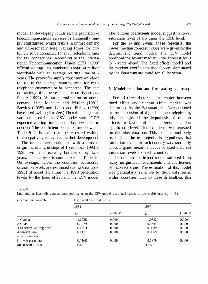
model. In developing countries, the provision of The random coefficients model suggests a lowertelecommunications services is frequently sup- saturation level of 1.5 times the 1998 level.ply constrained, which results in unmet demand For the 1- and 2-year ahead forecasts, theand unreasonably long waiting times for cus- lowest median forecastmapes were given by thetomers to be connected for main telephone lines deterministic trend model. The CSV modelfor fax connections. According to the Interna- produced the lowest medianmape forecast for 3tional Telecommunication Union (ITU, 1999) to 6 years ahead. The fixed effects model andofficial waiting lists numbered about 50 million the random coefficients model were dominatedworldwide with an average waiting time of 2 by the deterministic trend for all horizons.years. The proxy for supply constraint we choseto use is the average waiting time for maintelephone customers to be connected. The data5 . Model selection and forecasting accuracyon waiting time were taken from Islam andFiebig (1999). (As an approximation for unmet For all three data sets, the choice betweendemand Jain, Mahajan and Muller (1991), fixed effect and random effect models wasBowles (1995) and Islam and Fiebig (1999) determined by the Hausman test. As mentionedhave used waiting list size.) Thus the exogenous in the discussion of digital cellular telephones,variables used in the CSV model were: GDP, this test rejected the hypothesis of randomexpected waiting time and market size at intro- effects in favour of fixed effects at a 5%duction. The coefficient estimates are shown in significance level. This experience was repeatedTable 9. It is clear that the expected waiting for the other data sets. This result is intuitivelytime negatively influences market development. reasonable; the test rejects the hypothesis that

The models were estimated with a forecast saturation levels for each country vary randomlyorigin increasing in steps of 1 year from 1993 to about a grand mean in favour of fixed different1998, with a forecasting horizon of up to 6 saturation levels for each country.years. The analysis is summarised in Table 10. The random coefficient model suffered fromOn average, across the countries considered, many insignificant coefficients and coefficientssaturation levels are estimated (using data up to of incorrect signs. The estimation of this model1993) at about 3.5 times the 1998 penetration was particularly sensitive to short data serieslevels by the fixed effect and the CSV model. within countries. Due to these difficulties, this

Table 9International facsimile connections: pooling using the CSV model, estimated values of the coefficientsg in (6)j1

j exogenous variable Estimated with data up to

1991 1997

g P-value g P-valuej1 j1

1 Constant 1.0538 0.000 1.0792 0.0002 GDP 0.1279 0.000 0.1664 0.0003 Expected waiting time 20.0359 0.000 20.0339 0.0004 Market size 0.012 0.000 0.0069 0.000at introductionGrowth parameter 0.1168 0.000 0.1379 0.000Mean sample size 5.6 11.6


Table 10International facsimile connections. A summary of the size of estimated saturation levels and forecasting accuracy

Fixed effect Random CSV Deterministicmodel coefficient trend

model

Median (saturation level / 3.73 1.51 3.421998 connections)1 year ahead Median mape 10.18 10.62 9.55 7.10(six forecasts) % Best 18.42 18.42 21.05 42.102 years ahead Median mape 16.64 16.48 14.35 11.38(five forecasts) % Best 18.42 21.05 26.32 34.213 years ahead Median mape 22.02 26.82 15.15 16.65(four forecasts) % Best 21.05 15.79 36.84 26.324 years ahead Median mape 25.29 37.84 17.50 20.07(three forecasts) % Best 18.42 21.05 36.84 23.685 years ahead Median mape 28.40 41.31 18.25 20.51(two forecasts) % Best 15.79 21.05 39.47 23.686 years ahead Median mape 33.39 35.22 18.38 19.22(one forecast) % Best 21.05 7.90 39.47 31.58

model is not recommended for this type of for the three data sets used are shown in Tableapplication. 11. SIC favours the choice of the CSV model in

In order to choose between the two remaining all three cases, AIC differs in that it favours themodels, choices based on information criteria fixed effect model for cellular telephones.can be used. The fixed effects model is nested Again, intuition would suggest that the modelwithin the CSV model. This is because ifK 5 that uses extra information, via the exogenous2

1, g 5 0 and x ;1 in (6) then the model variables, about the different markets should bejk 211t

reduces to (2) withh 5a . Since the models preferred. Intuition would be undermined if thei1 i

are nested, information criteria can be used to exogenous variables were incorrectly identified.choose between them. The values for Akaike’s Similarly, the fixed effects model might forecast(AIC) and Schwartz’s (SIC) information criteria better if there was a shift in the exogenous

Table 11The choice between the fixed effects model and the function of exogenous variable model using Akaike’s and Schwartz’sinformation criteria

Data set Origin n K K SIC AIC1 2

CSV FE CSV FE

Digital cellular telephones 1995Q2 128 6 17 2287.8 2272.1 2302.9 2318.61994Q4 96 6 17 2183.0 2172.7 2196.3 2214.3

ISDN lines 1997 118 4 17 2172.8 2136.1 2181.9 2181.21994 70 4 17 285.9 243.2 292.9 279.4

Facsimile connections 1997 481 5 39 21221.5 21069.3 21240.4 21230.11991 253 5 39 2514.3 2345.3 2530.0 2481.1

Note:n is the number of observations,K is the parameters estimated using CSV model andK is the number of estimated1 2

parameters using fixed effect (FE) model.


variables between the estimation and forecast parameter estimation has converged. The extentperiod. In this situation, the use of forecast of successful estimation is shown in the last rowvalues of the exogenous variables does not of Table 12. The general picture is similar fornecessarily lead to better forecasts than the fixed each model. Forecast accuracy deteriorates aseffect model (see Islam & Meade, 1996, for an the horizon increases, with the sharpest deterio-example). ration occurring between horizons of 1 and 2

Table 12 shows the effect of sample size on years. The benefit of greater data availability isthe forecasting accuracy of four models (three apparent in the decreasing values of the medianpooling models and one individual linear Gom- ape for a given horizon. Over the forecastpertz model) for the international fax data. (This origins, 1991 to 1997, the 1-year ahead medianuninterrupted data set is more convenient for ape is|86% of its value for the origin 1 yearthis purpose than digital cellular telephones.) before.Please note that individual linear Gompertz We have revisited the suitability of individualforecasts are based on a subset of cases where model estimates for all three data sets. As in the

Table 12Forecasting accuracy for the international facsimile connections data, measured inmedian ape compared to the size of thesample used for estimation

Models Years Forecast origin /mean sample sizeahead

1991 1992 1993 1994 1995 1996 19975.6 6.6 7.6 8.6 9.6 10.6 11.6

Fixed 1 16.60 18.51 12.21 7.71 8.54 6.85 5.61effects 2 40.28 32.33 17.11 18.36 15.31 11.40

3 49.25 39.65 29.74 22.46 19.834 54.40 45.74 34.17 30.035 63.83 57.03 41.136 72.00 66.78

Random 1 17.02 12.04 7.03 7.68 3.69 5.73coeff. 2 29.76 21.91 14.90 12.99 7.73model 3 39.01 34.19 18.11 20.06

4 56.20 46.89 30.055 64.85 52.24

CSV 1 16.75 13.34 8.92 10.26 10.41 8.53 7.232 27.82 21.80 15.10 15.37 17.99 10.073 38.71 22.78 19.69 14.09 18.534 39.33 30.75 21.85 17.695 38.81 33.72 29.456 41.98 38.76

Linear 1 17.60 15.80 16.20 12.70 11.50 10.50 8.30Gompertz, 2 20.90 20.05 18.80 17.70 16.10 12.50individual 3 30.03 29.15 34.50 23.50 17.50estimation 4 50.30 42.10 42.40 24.10

5 54.50 47.90 47.606 57.30 57.60

% of successful 31.6% 39.5% 47.4% 55.3% 65.8% 65.8% 68.4%estimations forlinear Gompertz


Table 13Comparison of the accuracy of the CSV pooling method and individual linear Gompertz for international facsimileconnections in terms of absolute percentage error (APE)

Horizon Median (APE of CSV GM (APE of CSV Percent CSV poolingpooling/APE of linear pooling/APE of linear method APE betterGompertz individual Gompertz individual than APE linearmodel) model) Gompertz

1 0.795 0.742 552 0.860 0.938 603 0.808 0.802 584 0.837 0.809 625 0.810 0.764 656 0.863 0.889 54

Note: the forecasts are computed for origins 1991 to 1997 and to exclude outliers, ratios less than 0.05 and greater than 20have been excluded.

case of facsimile, the proportion of successful with individual univariate Gompertz modelsparameter estimates are relatively low ranging showed that pooling was advantageous for twofrom 18.8% in 1995 to 33.3% in 1997 for ISDN reasons. Firstly, for short series, only poolingand 31.3% in 1994Q4 to 56.3% in 1995Q2 for produced useful forecasts. Secondly, if forecastsdigital cellular. The comparison of forecasting were available from the pooling model and theperformance of the CSV pooling method (the univariate model, the former was generallyone preferred by the SIC and AIC criteria) and more accurate.individual linear Gompertz using facsimile data The CSV pooling model works well for theis shown in Table 13. Comparisons are only fast developing and cost conscious digital cel-based on the cases where linear Gompertz have lular telephone market. The estimates of satura-produced significant parameter estimates. Even tion levels are plausible and the forecasts arein these favorable cases there are significant most accurate according to the median absolutegains from pooling relative to separate models. error and percentage better measures used. ThisThus, if data series are too short or sensible pooling model also offered the highest percentestimates from separate models are unavailable, better forecasts for ISDN connections for 2 andthere is no choice but to use forecasts derived 3 year horizons.from pooled models. In the minority of cases The estimation of the random coefficientswhere there was a choice, forecasts from pooled pooling model was not always possible for amodels were generally more accurate than those subset of countries. Thus the model does notgenerated from separate models. offer sufficient reliability to be used for multina-

tional forecasts. The fixed effect model gave alower median ape for ISDN connections.

The joint use of a pooling model with the6 . ConclusionGompertz diffusion model is shown to be

Four models have been used to pool cross- effective. The evidence for the choice of thesectional data for three telecommunications data CSV pooling model is most persuasive. Ansets using the Gompertz diffusion model. In all intuitively attractive argument in favour of thiscases, except one, the best pooling model was model is its use of relevant individual market

¨more accurate than the naıve deterministic trend information via the exogenous variables. Thismodel. A comparison of the CSV pooling model argument is empirically supported by the


Greene, W. H. (1997). In 3rd ed,Econometric analysis.Schwartz information criterion for the threeNew Jersey: Prentice-Hall.diffusion data sets. In addition, for these sets,

Harrison, P. J., & Pearce, S. F. (1972). The use of trendthe forecasts of the CSV model were either most curves as an aid to market forecasting.Industrialaccurate or second most accurate. Marketing Management, 2, 149–170.

Heeler, R. M., & Hustad, T. P. (1980). Problems inpredicting new product growth for consumer durables.

A cknowledgements Management Science, 26, 1007–1020.Helsen, K., Jedidi, K., & DeSarbo, W. S. (1993). A new

approach to country segmentation utilizing multinationalIslam gratefully acknowledges The Universi-diffusion pattern. Journal of Marketing, 57, 60–71,ty of Sydney U2000 research fellowship.October.

Hendry, I. C. (1972). The three parameter approach to longrange forecasting.Long Range Planning, 5, 40–45.

R eferences Islam, T., & Fiebig, D. G. (1999). Modelling supplyrestricted telecommunications market. Paper presented

Bass, F. M. (1969). A new product growth model for at the 19th international symposium on forecasting,consumer durables.Management Science, 15, 215–227. June 27–30, Washington DC.

Bewley, R., & Fiebig, D. G. (1988). Flexible logistic Islam, T., & Meade, N. (1996). Forecasting the develop-growth model with applications in telecommunications. ment of the market for business telephones in the UK.International Journal of Forecasting, 4, 177–192. Journal of the Operational Research Society, 47, 906–

Bowles, D. (1995). Telephone penetration: industrial coun- 918.tries vs. LDCs. In Lamberton, D. (Ed.),Beyond competi- ITU (1999).Financing network investment. Geneva: Inter-tion: the future of telecommunications. North-Holland, national Telecommunications Union, Chapter XIV.pp. 299–314. Jain, D., Mahajan, V., & Muller, E. (1991). Innovation

Chaddha, R. L., & Chitgopekar, S. S. (1971). A ‘generali- diffusion in the presence of supply restrictions.Market-sation’ of the logistic curve and long range forecasts ing Science, 10, 83–90.(1966–1981) of residence telephones.The Bell Journal Joo, Y. J., & Jun, D. B. (1996). Growth-cycle decomposi-of Economics and Management Science, 2, 542–560. tion diffusion model.Marketing Letters, 7, 207–214.

Chow, G. C. (1967). Technological change and the Kadiyala, K. R., & Oberhelman, D. (1979). Responsedemand for computers.American Economic Review, 57, predictions in regressions on panel data.Proceedings of1117–1130. the Business and Economic Statistics Section, The

Defris, L. V., & Fiebig, D. G. (1984). Forecasting new American Statistical Association, Reprint no. 776, Apriltelecommunications services with limited data. Pre- 1980.sented at 5th international futures and forecasting Kumar, V., Ganesh, J., & Echambadi, R. (1998). Cross-conference. national diffusion research: what do we know and how

Dekimpe, M. G., Parker, P. M., & Sarvary, M. (1998). certain are we?Journal of Product Innovation Manage-Staged estimation of international diffusion models: an ment, 15, 255–268.application to global cellular telephone adoption.Tech- Lee, J. C., Lu, K. W., & Hong, S. C. (1992). Technologicalnological Forecasting and Social Change, 57, 105–132. forecasting with non-linear models.Journal of Fore-

Dodds, W. (1973). An application of the Bass model in casting, 11, 195–206.long term new product forecasting.Journal of Market- Lindley, D. V., & Smith, A. F. M. (1972). Bayes estimatesing Research, 10, 308–311. for the linear model and discussion.Journal of the

Ganesh, J., & Kumar, V. (1996). Capturing the cross- Royal Statistical Society, Series B, 34, 1–41.national learning effect: an analysis of an industrial Mahajan,V., & Muller, E. (1994). Innovation diffusion in atechnology diffusion.Journal of the Academy of Mar- borderless global market: will the 1992 unification ofketing Science, 24, 328–337, Fall. the European Community accelerate diffusion of new

Ganesh, J., Kumar, V., & Subramaniam, V. (1997). Cross- ideas, products and technologies?Technological Fore-national learning effects in global diffusion patterns: an casting and Social Change, 45, 221–237, March.exploratory investigation.Journal of the Academy of Mahajan, V., Muller, E., & Bass, F. M. (1990). NewMarketing Science, 25, 214–228, Summer. product diffusion models in marketing: a review and

Gatignon, H., Eliashberg, J., & Robertson, S. T. (1989). directions for research.Journal of Marketing, 54, 1–26.Modeling multinational diffusion patterns: an efficient Martino, J. P. (1983). In 2nd ed,Technological forecastingmethodology.Marketing Science, 8, 231–247. for decision making. New York: North Holland.





https://www.researchgate.net/publication/271802211_A_New_Approach_to_Country_Segmentation_Utilizing_Multinational_Diffusion_Patterns?el=1_x_8&enrichId=rgreq-5465b17f-958a-48d3-b200-b658d130407f&enrichSource=Y292ZXJQYWdlOzIyMjI1MjA4MTtBUzoxMDMyNDA1OTUxNDg4MDVAMTQwMTYyNTg4NDI5Ng==







Meade, N. (1989). Technological substitution: a frame- University of Guelph, Ontario, Canada. He has an M.Sc. inwork of stochastic models.Technological Forecasting Telecommunications Engineering, an MBA from Dhakaand Social Change, 36, 389–400. University, a DIC (Diploma of Imperial College), and a

Ph.D. in Management Science (1996) from ImperialMeade, N. (2000). Evidence for the selection of forecast-College, University of London. He previously held re-ing methods.Journal of Forecasting, 19, 515–535.search and teaching positions at University of Sydney,Meade, N., & Islam, T. (1995). Forecasting with growthAustralia, Dalhousie University of Northern Britishcurves: an empirical comparison.International JournalColumbia, Canada. His current research is on diffusion ofof Forecasting, 11, 199–215.innovations and behavioral issues in household level trialMeade, N., & Islam, T. (1998). Technological forecast-and repeat purchases. He has published inManagementing—model selection, model stability and combiningScience, European Journal of Operational Research,models.Management Science, 44(8), 1115–1130.Journal of Forecasting, International Journal of Forecast-Parker, P. M. (1993). Choosing among diffusion models:ing, Journal of the Operational Research Society, andsome empirical evidence.Marketing Letters, 4, 81–94.Technological Forecasting and Social Science.Peterson, R., & Mahajan, V. (1978). In Sheth, J. (Ed.),

Multiproduct growth models in research in marketing.Greenwich, CT: JAI, pp. 201–231. Denzil G. FIEBIG completed a Ph.D. from the Universi-

Porter, M. E. (2000). The current competitiveness index: ty of Southern California under the supervision of Profes-measuring the microeconomic foundations of prosperity. sor Henri Theil. He joined the Department of Econo-In Global competitiveness report 2000. Oxford Uni- metrics at the University of Sydney in 1983 and served asversity Press, pp. 40–58. its Head from 1992 to 1999. Denzil was appointed to his

Schmittlein, D. C., & Mahajan, V. (1982). Maximum current position of Professor of Economics in the Schoollikelihood estimation for an innovation diffusion model of Economics at the University of NSW in 2001. He hasof new product acceptance.Marketing Science, 1, 57– been a visiting scholar at the University of Florida,78. University of Southern California, Victoria University of

Sultan, F., Farley, J. U., & Lehman, D. R. (1990). A Wellington and CentER at Tilburg University. Currentmeta-analysis of applications of diffusion models.Jour- research interests are in applied econometrics with em-nal of Marketing Research, 27, 70–77. phasis on the areas of energy, telecommunications and

Swamy, P. A. V. B. (1970). Efficient inference in random health. Denzil has published extensively in major interna-coefficient regression model.Econometrica, 38, 311– tional and Australian journals includingJournal of Econo-323. metrics, Journal of Business and Economic Statistics,

Takada, H., & Jain, D. (1991). Cross-national analysis of International Journal of Forecasting, Journal of Forecast-diffusion of consumer durable goods in pacific rim ing, Economic Record, Journal of Industrial Economicscountries.Journal of Marketing, 55, 48–54. and Energy Journal and has written several monographs.

Van den Bulte, C., & Lilien, G. L. (1997). Bias andsystematic change in the parameter estimates of macro- Nigel MEADE is Professor of Quantitative Finance atlevel diffusion models.Marketing Science, 16, 338– the Management School, Imperial College, University of353. London. His research interests are statistical model build-

Young, P., & Ord, K. (1990). Model selection and estima- ing in general and applied time series analysis andtion for technological growth curves.International forecasting in particular. He is an associate editor of theJournal of Forecasting, 5, 501–513. International Journal of Forecasting.

Biographies: Towhidul ISLAM is Assistant Professorof Marketing at the Department of Consumer Studies,

Modelling multinational telecommunications demand with limited data

Documents

Transcript of Modelling multinational telecommunications demand with limited data