Modeling of Electric Power Supply Chain Networks with Fuel Suppliers

via

Variational Inequalities

Dmytro Matsypura1, Anna Nagurney1,2, and Zugang Liu1

1Department of Finance and Operations Management

Isenberg School of Management

University of Massachusetts

Amherst, Massachusetts 01003

2 Radcliffe Institute for Advanced Study

34 Concord Avenue

Harvard University

Cambridge, Massachusetts 02138

July 2006; updated January 1, 2007

Appears in International Journal of Emerging Electric Power Systems (2007), vol. 8, iss. 1, Article 5.

Abstract: The electric power industry in the United States and in other countries is undergoing

profound regulatory and operational changes. The underlying rationale behind these transforma-

tions is to move once highly monopolized vertically-integrated industry from a centralized operation

approach to a competitive one. The emerging competitive markets and an increase in the number

of market participants have, in turn, fundamentally changed not only electricity trading patterns

but also the structure of the electric power supply chains. This new framework requires new math-

ematical and engineering models and associated algorithmic tools. Moreover, the availability of

fuels for electric power generation is a topic of both economic importance and national security.

This paper uses the model developed by Nagurney and Matsypura (2004, 2006) as the foundation

for the introduction of explicit fuel suppliers, in the case of nonrenewable and/or renewable fuels,

and their optimizing behavior, into a general electric power supply chain network model along with

‘direct-supply’ generation. We derive the optimality conditions for the various decision-makers,

including fuel suppliers, power generators, suppliers, as well as the transmission service providers

and the consumers at the demand markets. We establish that the governing equilibrium conditions

satisfy a finite-dimensional variational inequality problem. We provide qualitative properties of

the equilibrium flow pattern; in particular, existence of a solution and uniqueness under suitable

assumptions. Finally, we discuss how the equilibrium fuel supply and electric power flow pattern

can be computed.

1

1. Introduction

Electric power and its availability play an essential role in modern society. Electric power is a

fundamental resource for heating, cooling, as well as for the powering of computers and machinery

that underpin our manufacturing processes, communication, and transportation. Globally, in 2002,

16.1 trillion kilowatt hours of electric power were generated, with United States being the largest

producer and consumer of electric energy (see Gale Research Inc. (2006)). The US electrical

industry possesses more than half a trillion dollars of net assets, generates $220 billion in annual

sales, and consumes almost 40% of domestic primary energy (coal, natural gas, uranium, and oil),

or approximately 40 quadrillion BTU (British Thermal Units). Specifically, in 2004, over one billion

tons of coal, two hundred million barrels of petroleum, and more than six billion Mcfs (thousand

cubic feet) of natural gas were used in producing electric power, which accounted for almost 70%

of the total electric power production. The other 30% of electric power was generated from nuclear

power and renewable energy with the former comprising 20% and the latter 10% (see Edison Electric

Institute (2000), US Energy Information Administration (2002, 2005)).

The US electric power industry is undergoing a profound transformation in the way it delivers

electricity to millions of residential and commercial customers. Electricity production was once

dominated by vertically integrated investor-owned utilities who owned many of the generation ca-

pacity, transmission, and distribution facilities. However, electricity deregulation has opened up this

monopoly system to competition, and has made the electric power industry today characterized by

many new companies that produce and market wholesale and retail electric power. By February

1, 2005, 1200 companies were registered to sell wholesale power at market-based rates in the US

(statistics available at http://www.eia.doe.gov).

The dramatic increase in the number of market participants and the emerging competitive mar-

kets have fundamentally changed the electricity trading patterns as well as the structure of the

electric power supply chains. These changes, in turn, have stimulated research activity in the area

of electric power supply systems modeling and analysis. For example, models and algowithms have

been developed for the study of more decentralized electric power markets (see, e.g., Schweppe

(1988), Hogan (1992), Chao and Peck (1996), Wu et al. (1996), Conejo and Prieto (2001), Con-

treras, Klusch, and Krawczyk (2004), and Nagurney (2006) and the references therein). Several

simulation models have also been proposed to model the interaction of competing generation firms

who strategically make pricing decisions (see Kahn (1998) and Hobbs et al. (2000)). Day et al.

(2002) simulated the exercising of market power on linearized dc networks based on a flexible rep-

resentation of interactions of competing generating firms.

Nagurney and Matsypura (2004) presented an electric power supply chain network model for elec-

2

tric power generation, transmission, and consumption, which captured the decentralized decision-

making behaviors of the various players involved (for an expanded presentation and discussion, see

Nagurney and Matsypura (2006)). That research formulated the multitiered network equilibrium

problem as a finite-dimensional variational inequality problem (cf. Nagurney (1999)) and provided

a computational algorithm which was applied to solve a number of numerical examples. Wu et al.

(2006) proposed significant extensions to the electric power supply chain network model originally

proposed by Nagurney and Matsypura (2004) in order to capture the behavior of power generators

faced with a portfolio of power plant options and subject to pollution taxes (see also Nagurney et

al. (2006b)).

Nagurney et al. (2006a), in turn, established the equivalence between a static electric power

supply chain network equilibrium model with known demands and a transportation network equi-

librium model with fixed demands over an appropriately constructed supernetwork. This equivalence

yielded a new interpretation of electric power supply chain network equilibria in path flows. They

then proposed a dynamic electric power supply chain network model with time-varying demands and

formulated it as an evolutionary (time-dependent) variational inequality. Both Wu et al. (2006)

and Nagurney et al. (2006a) demonstrated, as hypothesized fifty years ago in Beckmann et al.

(1956), that electric power generation and distribution networks could be reformulated and solved

as transportation network equilibrium problems. For the foundations of supply chain network prob-

lems and their relationships to transportation problems, along with applications, see the book by

Nagurney (2006). McGuire (1997, 1999) also emphasized the relationships between electric power

and transportation networks and the need to capture decentralized decion-making from the electric

power producers through the consumers. For additional background on electric power systems and

associated mathematical modeling methodologies, see also the books by Zaccour (1998) and Singh

(1999).

This paper uses the model proposed by Nagurney and Matsypura (2004, 2006) as the foundation

for the introduction of explicit fuel suppliers and their optimizing behavior into a general electric

power supply chain framework. The model developed in this paper differs from that model as well

as from the model proposed by Wu et al. (2006) (but without taxes) in the following ways. First,

we include another layer into the supply chain, namely, the fuel suppliers, and we allow for distinct

fuels as flows on the network with the transformation into electric power taking place at the various

power plants that handle nonrenewable fuels. Such an extension is especially important since fuels

may come from different locations and there will be costs associated with their transportation

as well as with the production of electric power using different fuels and even fuel combinations.

For example, recently (cf. BNSF Today (2006)) the American Association of Railroads has urged

the Federal Energy Regulatory Commissin (FERC) to conduct a study as to the reliability of the

3

energy supply chain with a focus on electric power and the transportation of coal. Furthermore, as

occurred in the winter of 2006 (cf. The Boston Globe (2006)) the impacts of natural gas cutoffs in

Russia were felt as far as Western Europe. Consumers in the New England region of the US, which

relies primarily on natural gas and oil for electric power generation, is being urged by the head of

Independent System Operator (ISO) New England (Van Welie (2006)) to reduce its demand, in lieu

of diminishing supplies of energy sources for electric power generation.

Moreover, the availability of fuel for electricity generation is a topic of not only economic im-

portance but one that also affects national security as well as environmental quality. In addition,

we consider not only nonrenewable fuels in the supply chain but also renewable fuels, with the as-

sociated electricity production being captured in the model in distinct ways. Second, we explicitly

model ‘direct-supply’ generation, that is, we assume that part of the output of any power generating

plant can be used to directly supply a certain demand market. Finally, we assume fixed demands

and, hence, that consumers are not price-sensitive in the case of electric power. Such an assumption

was also made in Nagurney et al. (2006a).

This paper is organized as follows. In Section 2, we develop the electric power supply chain

network equilibrium model with explicit fuel suppliers and distinct fuels. We describe the behavior of

the various decision-makers, state the equilibrium conditions, and formulate the multitiered network

equilibrium problem as a variational inequality problem. In Section 3, we study the qualitative

properties of the equilibrium pattern, establish existence and uniqueness results, and propose an

algorithm. Section 4 summarizes our results and presents suggestions for future research.

4

1 · · · K

1 · · · S

11 · · · 1n · · · 1N · · · G1 · · · Gn · · · GN 11 · · · gm · · · GM

A1 · · · AI

11 · · · 1I · · · H1 · · · HI

· · · · · ·· · · · · ·

1 T

1 T 1 T

1 T

Demand Markets

TransmissionService Providers

Power Suppliers

CombinationsPower Plant

Power Generator/

Alternative Uses

Combinations

Fuel Supplier/Fuel Type

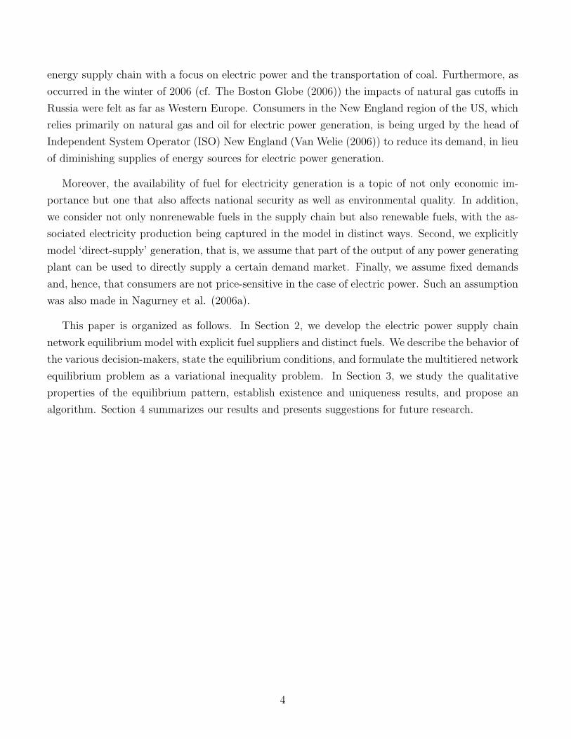
Figure 1: The Structure of the Electric Power Supply Chain Network with Fuel Suppliers

2. The Electric Power Supply Chain Model with Fuel Suppliers

In this Section, we develop the electric power supply chain network model in which the decision-

makers operate in a decentralized manner and in which the behavior of the fuel suppliers is made

explicit. We consider an electric power network economy in which goods and services are limited

to electric power. We assume that there are H fuel suppliers, with a typical supplier denoted by

h; G power generators, with a typical generator denoted by g; S power suppliers (including power

marketers, traders, and brokers), with a typical supplier denoted by s, and T transmission service

providers, with a typical provider denoted by t. There are K demand markets, or end users, with a

typical demand market denoted by k. We assume that there are I nonrenewable fuels that the fuel

suppliers can provide, where i = 1, . . . , I. In addition, we denote a typical power generating plant

or unit using nonrenewable fuels for power generation by n and one using renewable fuels by m

where n = 1, . . . , N and m = 1, . . . , M . A depiction of the supply chain network for electric power

with fuel suppliers is given in Figure 1.

5

The top tier of nodes in Figure 1 represents the fuel supplier/fuel type combinations. Fuel

suppliers are those decision-makers who sell fuel to power generators (or gencos). Because we allow

for distinct fuels for power generation, without loss of generality, we assume that each of the fuel

suppliers can provide every type of fuel. Thus, each node hi; h = 1, . . . , H; i = 1, . . . , I in the top

tier in Figure 1 represents a fuel supplier/fuel type combination. In practice, it may be the case

that fuel supplier h does not deal with all types of fuel, in which case, the extraneous nodes and

links can be eliminated and the notation adjusted accordingly.

The second category of decision-makers in our model is that of the power-generating companies

or gencos. Gencos are those decision-makers who own and operate electricity generating facilities or

power plants. They produce electric power, which is then sold to the power suppliers or directly, as

we discuss subsequently, to the demand markets. We assume that each genco can own and operate

more than one power generating plant, which, in turn, can use different types of fuel. Without

loss of generality, we assume that each genco g owns N plants that use nonrenewable sources of

energy and M plants that use renewable energy sources. Hence, the second tier of nodes in Figure

1 represents power generator/power plant combinations, where node gn represents generator g with

power plant n that uses nonrenewable fuels, with g = 1, . . . , G and n = 1, . . . , N . Similarly, node

gm represents power plant m that uses renewable energy sources and belongs to genco g, where

g = 1, . . . , G and m = 1, . . . , M .

Power suppliers, in turn, bear a function of an intermediary. They buy electric power from power

generators and sell to the consumers at different demand markets. Suppliers are represented by the

third tier of nodes in the supply chain network in Figure 1.

Note that there is a link from each power generating plant to each supplier in the network in

Figure 1 which represents that a supplier can obtain electric power from any generator on the

wholesale market (equivalently, a generator can sell to any/all the suppliers). Note also that the

links between the second tier and the third tier of nodes do not represent the physical connectivity

of two particular nodes. Power suppliers do not physically possess electric power at any stage of

the supplying process; they only hold the rights for the electric power. Hence, the link connecting

a pair of such nodes in the supply chain is a decision-making connectivity link between that pair of

nodes.

In order for electricity to be transmitted from a power plant of a generator to the point of

consumption a transmission service may be required unless there is direct supply. Transmission

service providers are those entities that own and operate the electric transmission and distribution

systems. These are the companies that distribute electricity from generators via suppliers to demand

markets (homes and businesses). Because transmission service providers do not make decisions as to

6

where the electric power will be acquired and to whom it will be delivered, we do not include them in

the model explicitly as nodes. Instead, their presence in the market is modeled as different modes of

transaction (transmission modes) corresponding to distinct links connecting a given supplier node

to a given demand market node in Figure 1 (see also, e.g., Nagurney and Matsypura (2004, 2006)).

We assume that power suppliers cover the direct cost of the physical transaction of electric power

from power generators to the demand markets and, therefore, have to make a decision as to from

where to acquire the transmission services (and at what level).

Finally, the last type of decision-maker in the model consists of the consumers or demand markets.

They are depicted as the bottom tier nodes in Figure 1. The consumers generate the demand that

drives the generation and supply of the electric power in the entire system. We assume a competitive

electric power market, meaning that the demand markets can select among the different electric

power suppliers (power marketers, brokers, etc.).

We also assume that a given power supplier negotiates with the transmission service providers and

makes sure that the necessary electric power is delivered. These assumptions fit well into the main

idea of the restructuring of the electric power industry that is now being performed in the US, the Eu-

ropean Union, and many other countries (see http://www.ferc.gov and http://www.europarl.eu.int).

For the sake of generality, we assume that each power supplier can transact with every demand

market using any of the transmission service providers or any combination of them. Therefore,

there are T links joining every node in the third tier of the network with every node at the bottom

tier (see Figure 1).

Clearly, in some situations, some of the links in the electric power supply chain network in Figure

1 may not exist (due to, for example, various restrictions, regulations, etc.). This can be handled

within our framework by eliminating the corresponding link for the supply chain network or (see

further discussion below) assigning an appropriately high transaction cost associated with that link.

We now turn to the discussion of the behavior of each type of decision-maker and derive the

optimality conditions.

2.1 Fuel Suppliers

As noted earlier, we consider two categories of energy sources that can be used for electric power

generation: renewable fuels (e.g., hydro, geothermal, solar, wind, biomass, municipal solid waste,

etc.) and nonrenewable fuels (such as fossil fuels, notably coal and natural gas, and nuclear energy).

The renewable fuels are ‘free’ and, therefore, do not require regular purchasing. This argument holds

true, for example, for wind, geothermal, and solar sources. In the case of biomass or municipal waste,

7

however, the actual fuel may not be exactly free as it requires certain processing before it can be

used, but the final cost is relatively small so that it may be embedded in the generation cost function

of a particular unit that uses this fuel.

In the case of nonrenewable fuels, we assume that the amount of fuel i held by fuel supplier h

is fixed and is denoted by Uhi for i = 1, . . . , I and h = 1, . . . , H. Clearly, not all available fuels

need be used for power generation and, hence, we introduce nodes Ai; i = 1, . . . , I, which represent

alternative usage of fuel i. Hence, the amount of flow between nodes hi and Ai (on the associated

links) represents the amount of fuel i that supplier h uses for other purposes. The conservation of

flow constraint for node hi takes on the following form:

G∑

g=1

N∑

n=1

qgnhi ≤ Uhi, ∀h, i, (1)

where qgnhi denotes the amount of fuel i that is traded between supplier h and generating plant n

of genco g. We group all the fuel transactions qgnhi ; h = 1, . . . , H; i = 1, . . . , I; g = 1, . . . , G, and

n = 1, . . . , N into the column vector Q0 ∈ RHIGN+ . Also, for convenience, we group the transactions

qgnhi for g = 1, . . . , G; n = 1, . . . , N into the column vector qhi for each h = 1, . . . , H and i = 1, . . . , I.

Let ρgn0hi denote the price of fuel i associated with the transaction between fuel supplier h and

power generating plant n of genco g and let ρgn∗0hi denote the price actually charged. The total

amount of revenue fuel supplier h obtains from his transactions can mathematically be expressed

as:I∑

i=1

G∑

g=1

N∑

n=1

ρgn∗0hi q

gnhi . (2)

In addition to the revenue denoted by expression (2), each fuel supplier h faces certain costs

associated with each transaction and with his operations in general. Let cgnhi denote the transaction

cost associated with fuel supplier h transacting fuel i with the power generating plant n of genco

g. Similarly, let chi denote the operating cost function. Note that fuel must be transported and,

hence, these transaction costs include the cost of fuel transportation from the particular supplier

to the particular power plant of a genco. We assume that the transaction costs and the operating

costs of the suppliers are of the following forms, respectively,

cgnhi = cgn

hi (qgnhi ), ∀h, i, g, n, (3)

chi = chi(qhi), ∀h, i, (4)

where qhi ≡ (q11hi , . . . , q

GNhi ), ∀h, i. The functions in (3) and (4) are assumed to be convex and

continuously differentiable.

8

We assume that each supplier is a profit-maximizer. Each fuel supplier h is faced with an

optimization problem of the following structure:

MaximizeI∑

i=1

G∑

g=1

N∑

n=1

ρgn∗0hi q

gnhi − chi(qhi) −

G∑

g=1

N∑

n=1

cgnhi (q

gnhi )

(5)

subject to:G∑

g=1

N∑

n=1

qgnhi ≤ Uhi, ∀i, (6)

qgnhi ≥ 0, ∀i, g, n.

Assuming that the transaction cost functions are continuously differentiable and convex for all

fuel suppliers h = 1, . . . , H, and fuels i = 1, . . . , I, the optimality conditions for all fuel suppliers

simultaneously can be expressed as the following variational inequality (see Bazaraa et al. (1993)):

determine Q0∗ ∈ K1 satisfying

H∑

h=1

I∑

i=1

G∑

g=1

N∑

n=1

[∂chi(q

∗hi)

∂qgnhi

+∂cgn

hi (qqn∗hi )

∂qgnhi

− ρgn∗0hi

]× [qgn

hi − qgn∗hi ] ≥ 0, ∀Q0 ∈ K1, (7)

where

K1 ≡ {Q0|Q0 ∈ RHIGN+ and (6) is satisfied ∀h}.

2.2 Power Generators

Recall that, as mentioned earlier, power generating plants (cf. Figure 1) are divided into two

categories: those that use nonrenewable fuels and those that use renewable fuels.

A power generating plant can sell power to any of the power suppliers on the market and/or

can also sell directly to the demand markets as a ‘direct-supply.’ According to Manur (2003), 53%

to 59% of electric power generated and consumed in the PJM market (Pennsylvania, New Jersey,

Maryland) is ‘direct-supply.’ There are, hence, links between the second and the third tier, and

between the second and the fourth tier of the electric power supply chain network in Figure 1.

Let αgnhi denote the nonnegative conversion rate of fuel i acquired from supplier h by generating

plant n of genco g, where h = 1, . . . , H; i = 1, . . . , I; g = 1, . . . , G, and n = 1, . . . , N . Let qgns and

qgnk denote the amount of electric power from generator g’s power plant n transacted with supplier

s and demand market k, respectively. Then, for plant n of genco g the following relationship must

hold:S∑

s=1

qgns +K∑

k=1

qgnk =H∑

h=1

I∑

i=1

αgnhi q

gnhi , g = 1, . . . , G; n = 1, . . . , N. (8)

9

Let fgn denote the operating cost function of plant n of genco g, which incorporates all the costs

other than the cost of fuel and the transaction costs:

fgn = fgn(qgn), ∀g, n, (9)

where qgn ≡ (qgn11 , . . . , qgn

hi , . . . , qgnHI). Note that in our framework, as the production output reaches

the capacity of a given generator we can expect that the production cost to become very large (and,

perhaps, even infinite).

We group all transactions qgns into a column vector Q1 ∈ RGNS+ and all transactions qgnk into a

column vector Q3 ∈ RGNK+ .

Let cgns and cgnk denote, respectively, the transaction cost functions of power plant n of genco

g that represent the cost of transacting with supplier s and demand market k, such that:

cgns = cgns(qgns), ∀g, n, s, (10)

cgnk = cgnk(qgnk), ∀g, n, k. (11)

Let ρ∗1gns denote the per unit price of electricity associated with plant n of genco g and power

supplier s and let ρ∗1gnk denote the actual price that plant n of genco g charges demand market k

for direct supply.

The second category of generating plant in the model consists of those that use renewable sources

of energy. Their behavior is similar to that of the first category in the sense that they can sell their

output either to suppliers or directly to the demand markets. The major difference is that the cost

of fuel, if there is such a cost, is incorporated into a generating cost function and there are no links

connecting fuel suppliers and generating plants of the second category. In some cases the cost of

fuel can be considered equal to zero, as in the case of wind and solar generating plants.

Let qgms and qgmk denote the amount of electric power transacted, respectively, between plant

m of genco g and power supplier s, and plant m of genco g and demand market k. We group all

the transactions qgms into a column vector Q4 ∈ RGMS+ and all the transactions qgmk into a column

vector Q5 ∈ RGMK+ .

Let fgm (cf. (9)) denote the operating cost function of plant m of genco g, which incorporates

all the costs other than the transaction costs and depends on the amount of electricity generated:

fgm = fgm(qgm), ∀g, m, (12)

where qgm ≡ (qgms; s = 1, . . . , S; qgmk; k = 1, . . . , K).

10

Let ρ∗1gms denote the price of electric power associated with power plant m of genco g and power

supplier s and let ρ∗1gmk denote the price associated with power plant n of genco g and demand

market k for direct supply.

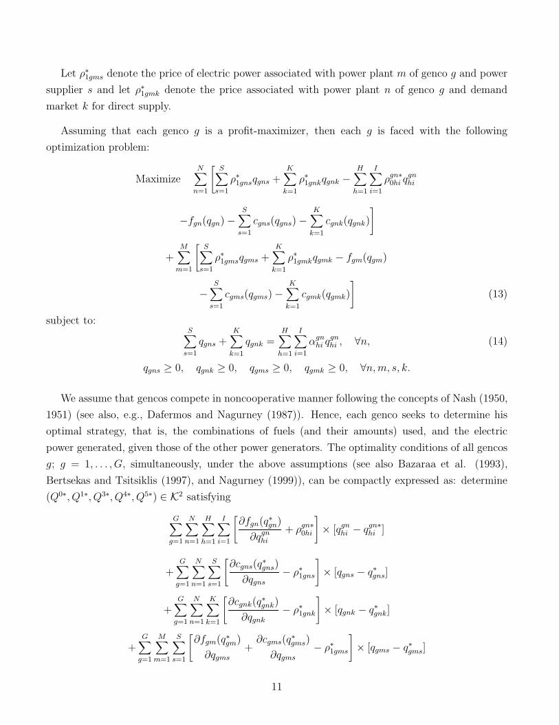
Assuming that each genco g is a profit-maximizer, then each g is faced with the following

optimization problem:

MaximizeN∑

n=1

[S∑

s=1

ρ∗1gnsqgns +

K∑

k=1

ρ∗1gnkqgnk −

H∑

h=1

I∑

i=1

ρgn∗0hi q

gnhi

−fgn(qgn) −S∑

s=1

cgns(qgns) −K∑

k=1

cgnk(qgnk)

]

+M∑

m=1

[S∑

s=1

ρ∗1gmsqgms +

K∑

k=1

ρ∗1gmkqgmk − fgm(qgm)

−S∑

s=1

cgms(qgms) −K∑

k=1

cgmk(qgmk)

](13)

subject to:S∑

s=1

qgns +K∑

k=1

qgnk =H∑

h=1

I∑

i=1

αgnhi q

gnhi , ∀n, (14)

qgns ≥ 0, qgnk ≥ 0, qgms ≥ 0, qgmk ≥ 0, ∀n, m, s, k.

We assume that gencos compete in noncooperative manner following the concepts of Nash (1950,

1951) (see also, e.g., Dafermos and Nagurney (1987)). Hence, each genco seeks to determine his

optimal strategy, that is, the combinations of fuels (and their amounts) used, and the electric

power generated, given those of the other power generators. The optimality conditions of all gencos

g; g = 1, . . . , G, simultaneously, under the above assumptions (see also Bazaraa et al. (1993),

Bertsekas and Tsitsiklis (1997), and Nagurney (1999)), can be compactly expressed as: determine

(Q0∗, Q1∗, Q3∗, Q4∗, Q5∗) ∈ K2 satisfying

G∑

g=1

N∑

n=1

H∑

h=1

I∑

i=1

[∂fgn(q∗gn)

∂qgnhi

+ ρgn∗0hi

]× [qgn

hi − qgn∗hi ]

+G∑

g=1

N∑

n=1

S∑

s=1

[∂cgns(q

∗gns)

∂qgns− ρ∗

1gns

]× [qgns − q∗gns]

+G∑

g=1

N∑

n=1

K∑

k=1

[∂cgnk(q

∗gnk)

∂qgnk− ρ∗

1gnk

]× [qgnk − q∗gnk]

+G∑

g=1

M∑

m=1

S∑

s=1

[∂fgm(q∗gm)

∂qgms+

∂cgms(q∗gms)

∂qgms− ρ∗

1gms

]× [qgms − q∗gms]

11

+G∑

g=1

M∑

m=1

K∑

k=1

[∂fgm(q∗gm)

∂qgmk+

∂cgmk(q∗gmk)

∂qgmk− ρ∗

1gmk

]× [qgmk − q∗gmk] ≥ 0,

∀(Q0, Q1, Q3, Q4, Q5) ∈ K2, (15)

where

K2 ≡ {(Q0, Q1, Q3, Q4, Q5)|(Q0, Q1, Q3, Q4, Q5) ∈ RGN(HI+S+K)+GM(S+K)+

and (14) is satisfied ∀g}.

2.3 Power Suppliers

The behavior of a typical power supplier (or power trader) is assumed here to be very similar to

that described in Nagurney and Matsypura (2004, 2006).

A power supplier s is faced with certain expenses, which may include, for example, the cost of

licensing and the costs of maintenance. We refer collectively to such costs as an operating cost and

denote it by cs. Let qtsk denote the amount of electricity being transacted between power supplier

s and demand market k via the link corresponding to the transmission service provider t. Group

all transactions associated with power supplier s and demand market k into the column vector

qsk ∈ RT+. Then further group all such vectors associated with all the power suppliers into a column

vector Q2 ∈ RSKT+ . Without loss of generality, we can assume that

cs = cs(Q1, Q2, Q4), ∀s. (16)

Each power supplier is involved in transacting with both power generators through their power

plants and with the demand markets through transmission service providers. Therefore, there will

be costs associated with each such transaction. Let cgms denote the transaction cost associated with

power supplier s acquiring electric power from power plant m of genco g and let cgns denote the

transaction cost associated with power supplier s acquiring electric power from power plant n of

genco g, where:

cgms = cgms(qgms), ∀g, m, s, (17)

cgns = cgns(qgns), ∀g, n, s. (18)

Also, let ctsk denote the transaction cost associated with power supplier s transmitting electric power

to demand market k via transmission service provider t, where:

ctsk = ct

sk(qtsk), ∀s, k, t. (19)

We assume that all the above transaction cost functions are convex and continuously differentiable.

12

Let ρt∗2sk denote the price associated with the transaction from power supplier s to demand market

k via transmission service provider t. The total amount of revenue a typical power supplier s obtains

from his transactions can mathematically be expressed as follows:

K∑

k=1

T∑

t=1

ρt∗2skq

tsk. (20)

Prior to formulating the optimization problem of a typical power supplier, let us look closer at

the transmission service providers and their role in the electric power supply chain network system.

2.3.1 Transmission Service Providers

Transmission service providers are those entities that own and operate the electric transmission

and distribution systems. Assume that the price of transmission service depends on how far the

electricity has to be transmitted; in other words, it can be different for different destinations (demand

markets or consumers). Also we allow for different transmission service providers to have their

services priced differently, which can be a result of a different level of quality of service, reliability

of the service, etc.

In practice, an electric supply network is operated by an Independent System Operator (ISO)

who operates as a disinterested, but efficient, entity and does not own network or generation assets.

Its main objectives are: to provide independent, open and fair access to transmission systems; to

facilitate market-based, wholesale electricity rates; and to ensure the effective management and

operation of the bulk power system in each region (http://www.isone.org). Therefore, the ISO

does not control the electricity rates. Nevertheless, it makes sure that the prices of the transmission

services are reasonable and not discriminatory. We model this aspect by having transmission service

providers be price-takers meaning that the price of their services is determined and cannot be

changed by a transmission service provider himself. Hence, the price of transmission services is

fixed. However, it is not constant, since it may, in general, depend on the amount of electric

power transmitted, the distance, etc., and may be calculated for each transmission line separately

depending on the criteria listed above. Consequently, as was stated earlier, a transmission service

provider does not serve as an explicit decision-maker in the complex network system.

Optimization Problem of a Power Supplier

Assuming that the electric power suppliers are profit-maximizers, the optimization problem of a

typical power supplier s becomes:

MaximizeK∑

k=1

T∑

t=1

ρt∗2skq

tsk − cs(Q

1, Q2, Q4) −G∑

g=1

M∑

m=1

ρ∗1gmsqgms −

G∑

g=1

N∑

n=1

ρ∗1gnsqgns

13

−G∑

g=1

M∑

m=1

cgms(qgms) −G∑

g=1

N∑

n=1

cgns(qgns) −K∑

k=1

T∑

t=1

ctsk(q

tsk) (21)

subject to:K∑

k=1

T∑

t=1

qtsk =

G∑

g=1

M∑

m=1

qgms +G∑

g=1

N∑

n=1

qgns, (22)

qtsk ≥ 0, ∀k, t, qgms ≥ 0, ∀g, m, qgns ≥ 0, ∀g, n.

We assume that all power suppliers compete in a noncooperative manner (as we assumed for

the power generators). Hence, each power supplier seeks to determine his optimal strategy, that is,

the input (accepted) and output flows, given those of the other power suppliers. The optimality

conditions of all power suppliers s; s = 1, . . . , S, simultaneously, under the above assumptions (see

also Dafermos and Nagurney (1987) and Nagurney et al. (2002)), can be compactly expressed as:

determine (Q1∗, Q2∗, Q4∗) ∈ K3 satisfying

S∑

s=1

K∑

k=1

T∑

t=1

[∂cs(Q

1∗, Q2∗, Q4∗)

∂qtsk

+∂ct

sk(qt∗sk)

∂qtsk

− ρt∗2sk

]× [qt

sk − qt∗sk]

+S∑

s=1

G∑

g=1

M∑

m=1

[∂cs(Q

1∗, Q2∗, Q4∗)

∂qgms+

∂cgms(q∗gms)

∂qgms+ ρ∗

1gms

]× [qgms − q∗gms]

+G∑

g=1

S∑

s=1

N∑

n=1

[∂cs(Q

1∗, Q2∗, Q4∗)

∂qgns

+∂cgns(q

∗gns)

∂qgns

+ ρ∗1gns

]× [qgns − q∗gns] ≥ 0,

∀(Q1, Q2, Q4) ∈ K3, (23)

where K3 ≡ {(Q1, Q2, Q4)|(Q1, Q2, Q4) ∈ RS(G(M+N)+KT )+ and (22) is satisfied ∀s}.

2.4 Equilibrium Conditions for the Demand Markets

Unlike the models of Nagurney and Matsypura (2004, 2006), we assume that the demand for

electric power at each demand market k is fixed and denoted by dk. One can argue that demand for

electricity is a random rather than deterministic value (see, e.g., Matsypura and Nagurney (2005)).

One of the reasons, for example, is that the consumption of electric power in the residential sector

is closely related to the weather conditions because large amounts of electricity are used for heating

and cooling. On the other hand, in most electricity markets consumers do not have an opportunity

to react to the changes in prices. Several studies, for example, have confirmed that one of the key

factors in California’s electricity market crisis during 2000-2001 was near-total absence of demand

response in California’s restructured market (Faruqui et al. (2001)).

At each demand market k, hence, the following conservation of flow equation must be satisfied:

dk =S∑

s=1

T∑

t=1

qtsk +

G∑

g=1

M∑

m=1

qgmk +G∑

g=1

N∑

n=1

qgnk, ∀k, (24)

14

that is, the demand for electric power at a demand market must be equal to the amount of elec-

tric power transmitted from the suppliers via the transmission service providers plus the amounts

provided directly and generated using the nonrenewable and renewable fuels by the gencos’ power

plants.

Let ctsk denote the unit transaction cost associated with obtaining the electric power at demand

market k from supplier s via transmission mode t, where we assume that this transaction cost is

continuous and of the general form:

ctsk = ct

sk(Q2), ∀s, k, t. (25)

Similarly, let cgmk and cgnk denote the unit transaction cost associated with obtaining the direct

supply electric power at demand market k from plants m and n respectively, where we also assume

that this transaction costs are continuous and of the general form:

cgnk = cgnk(Q3), ∀g, n, k, (26)

cgmk = cgmk(Q5), ∀g, m, k. (27)

The equilibrium conditions associated with the transactions to the demand market k take the

following form: for all power suppliers s; s = 1, . . . , S, and transmission service providers t; t =

1, . . . , T :

ρt∗2sk + ct

sk(Q2∗)

{= ρ∗

3k, if qt∗sk > 0,

≥ ρ∗3k, if qt∗

sk = 0;(28)

for all gencos and power plants gn; g = 1, . . . , G; n = 1, . . . , N :

ρ∗1gnk + cgnk(Q

3∗)

{= ρ∗

3k, if q∗gnk > 0,≥ ρ∗

3k, if q∗gnk = 0,(29)

and for all gencos and power plants gm; g = 1, . . . , G; m = 1, . . . , M :

ρ∗1gmk + cgmk(Q

5∗)

{= ρ∗

3k, if q∗gmk > 0,≥ ρ∗

3k, if q∗gmk = 0.(30)

Note that the satisfaction of (24) and (28)–(30) is equivalent to the solution of the variational

inequality given by: determine (Q2∗, Q3∗, Q5∗) ∈ K4, such that

S∑

s=1

K∑

k=1

T∑

t=1

[ρt∗

2sk + ctsk(Q

2∗)]× [qt

sk − qt∗sk]

+S∑

s=1

G∑

g=1

M∑

m=1

[ρ∗

1gmk + cgmk(Q5∗)

]× [qgmk − q∗gmk]

15

+S∑

s=1

G∑

g=1

N∑

n=1

[ρ∗

1gnk + cgnk(Q3∗)

]× [qgnk − q∗gnk] ≥ 0,

∀(Q2, Q3, Q5) ∈ K4. (31)

where K4 ≡ {(Q2, Q3, Q5)|(Q2, Q3, Q5) ∈ RK(ST+GM+GN)+ and (24) is satisfied ∀k}.

2.5 The Equilibrium Conditions for the Electric Power Supply Chain Network with

Fuel Suppliers

In equilibrium, the amounts of fuels transacted between the fuel suppliers and power generators

must coincide with those that the power generators actually accept at their power plants. Further-

more, the amounts of electricity transacted between the power generators and the power suppliers

must coincide with those that the power suppliers actually accept. In addition, the amounts of

the electricity obtained by the consumers at the demand markets must be equal to the amounts

that the power suppliers actually provide. Hence, although there may be competition between

decision-makers at the same tier of nodes of the power supply chain network there must be, in a

sense, cooperation between decision-makers associated with pairs of nodes. Thus, in equilibrium,

the prices, fuel flows, and electric power flows transacted must satisfy the sum of the optimality

conditions (7), (15), and (23), and the equilibrium conditions (31). We make these relationships

rigorous through the subsequent definition and variational inequality derivation.

Definition 1: Electric Power Supply Chain Network Equilibrium with Fuel Suppliers

The equilibrium state of the electric power supply chain network with fuel suppliers is one where

the fuel flows between the top two tiers, and the electric power flows between the remaining tiers of

the network coincide and the fuel flows, the electric power flows, and the prices satisfy the sum of

conditions (7), (15), (23), and (31).

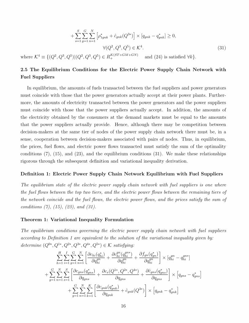
Theorem 1: Variational Inequality Formulation

The equilibrium conditions governing the electric power supply chain network with fuel suppliers

according to Definition 1 are equivalent to the solution of the variational inequality given by:

determine (Q0∗, Q1∗, Q2∗, Q3∗, Q4∗, Q5∗) ∈ K satisfying:

H∑

h=1

I∑

i=1

G∑

g=1

N∑

n=1

[∂chi(q

∗hi)

∂qgnhi

+∂cgn

hi (qgn∗hi )

∂qgnhi

+∂fgn(q∗gn)

∂qgnhi

]× [qgn

hi − qgn∗hi ]

+G∑

g=1

N∑

n=1

S∑

s=1

[∂cgns(q

∗gns)

∂qgns+

∂cs(Q1∗, Q2∗, Q4∗)

∂qgns+

∂cgns(q∗gns)

∂qgns

]×

[qgns − q∗gns

]

+G∑

g=1

N∑

n=1

K∑

k=1

[∂cgnk(q

∗gnk)

∂qgnk+ cgnk(Q

3∗)

]×

[qgnk − q∗gnk

]

16

+G∑

g=1

M∑

m=1

S∑

s=1

[∂fgm(q∗gm)

∂qgms+

∂cgms(q∗gms)

∂qgms+

∂cs(Q1∗, Q2∗, Q4∗)

∂qgms

+∂cgms(q

∗gms)

∂qgms

]×

[qgms − q∗gms

]

+G∑

g=1

M∑

m=1

K∑

k=1

[∂fgm(q∗gm)

∂qgmk+

∂cgmk(q∗gmk)

∂qgmk+ cgmk(Q

5∗)

]×

[qgmk − q∗gmk

]

+S∑

s=1

K∑

k=1

T∑

t=1

[∂cs(Q

1∗, Q2∗, Q4∗)

∂qtsk

+∂ct

sk(qt∗sk)

∂qtsk

+ ctsk(Q

2∗)

]×

[qtsk − qt∗

sk

]≥ 0,

∀(Q0, Q1, Q2, Q3, Q4, Q5) ∈ K, (32)

where

K ≡ K1 ×K2 × K3 ×K4.

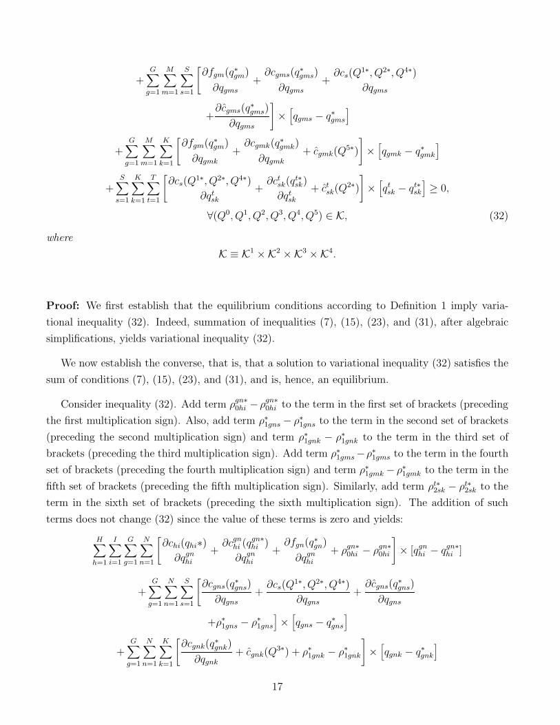
Proof: We first establish that the equilibrium conditions according to Definition 1 imply varia-

tional inequality (32). Indeed, summation of inequalities (7), (15), (23), and (31), after algebraic

simplifications, yields variational inequality (32).

We now establish the converse, that is, that a solution to variational inequality (32) satisfies the

sum of conditions (7), (15), (23), and (31), and is, hence, an equilibrium.

Consider inequality (32). Add term ρgn∗0hi −ρgn∗

0hi to the term in the first set of brackets (preceding

the first multiplication sign). Also, add term ρ∗1gns − ρ∗

1gns to the term in the second set of brackets

(preceding the second multiplication sign) and term ρ∗1gnk − ρ∗

1gnk to the term in the third set of

brackets (preceding the third multiplication sign). Add term ρ∗1gms −ρ∗

1gms to the term in the fourth

set of brackets (preceding the fourth multiplication sign) and term ρ∗1gmk − ρ∗

1gmk to the term in the

fifth set of brackets (preceding the fifth multiplication sign). Similarly, add term ρt∗2sk − ρt∗

2sk to the

term in the sixth set of brackets (preceding the sixth multiplication sign). The addition of such

terms does not change (32) since the value of these terms is zero and yields:

H∑

h=1

I∑

i=1

G∑

g=1

N∑

n=1

[∂chi(qhi∗)

∂qgnhi

+∂cgn

hi (qgn∗hi )

∂qgnhi

+∂fgn(q∗gn)

∂qgnhi

+ ρgn∗0hi − ρgn∗

0hi

]× [qgn

hi − qgn∗hi ]

+G∑

g=1

N∑

n=1

S∑

s=1

[∂cgns(q

∗gns)

∂qgns+

∂cs(Q1∗, Q2∗, Q4∗)

∂qgns+

∂cgns(q∗gns)

∂qgns

+ρ∗1gns − ρ∗

1gns

]×

[qgns − q∗gns

]

+G∑

g=1

N∑

n=1

K∑

k=1

[∂cgnk(q

∗gnk)

∂qgnk+ cgnk(Q

3∗) + ρ∗1gnk − ρ∗

1gnk

]×

[qgnk − q∗gnk

]

17

+G∑

g=1

M∑

m=1

S∑

s=1

[∂fgm(q∗gm)

∂qgms+

∂cgms(q∗gms)

∂qgms+

∂cs(Q1∗, Q2∗, Q4∗)

∂qgms+

∂cgms(q∗gms)

∂qgms

+ρ∗1gms − ρ∗

1gms

]×

[qgms − q∗gms

]

+G∑

g=1

M∑

m=1

K∑

k=1

[∂fgm(q∗gm)

∂qgmk+

∂cgmk(q∗gmk)

∂qgmk+ cgmk(Q

5∗) + ρ∗1gmk − ρ∗

1gmk

]×

[qgmk − q∗gmk

]

+S∑

s=1

K∑

k=1

T∑

t=1

[∂cs(Q

1∗, Q2∗, Q4∗)

∂qtsk

+∂ct

sk(qt∗sk)

∂qtsk

+ ctsk(Q

2∗) + ρt∗2sk − ρt∗

2sk

]×

[qtsk − qt∗

sk

]≥ 0,

∀(Q0, Q1, Q2, Q3, Q4, Q5) ∈ K, (33)

which can be rewritten as a sum of equilibrium conditions (7), (15), (23), and (31). Therefore, the

fuel and electric power flow and price pattern is an equilibrium according to Definition 1.

The variational inequality problem (32) can be rewritten in standard variational inequality form

(cf. Nagurney (1999)) as follows: determine X∗ ∈ K satisfying

〈F (X∗)T , X − X∗〉 ≥ 0, ∀X ∈ K, (34)

where X ≡ (Q0, Q1, Q2, Q3, Q4, Q5)T , and F (X) ≡ (F gnhi , Fgns, Fgnk, Fgms, Fgmk, Ftsk), with indices

h = 1, . . . , H; i = 1, . . . , I; g = 1, . . . , G; n = 1, . . . , N ; m = 1, . . . , M ; s = 1, . . . , S; t = 1, . . . , T ;

k = 1, . . . , K and the specific components of F given by the functional terms preceding the multipli-

cation signs in (32), respectively. Here 〈·, ·〉 denotes the inner product in Y -dimensional Euclidian

space where Y = HIGN + GNS + GNK + GMS + GMK + STK.

18

3. Qualitative Properties and Computational Procedure

In this Section, we provide some qualitative properties of the solution to variational inequality

(32). In particular, we derive existence and uniqueness results. We also discuss a computational

procedure.

The feasible set K (see ff. (32)) is compact since the demands for electric power are assumed

to be finite. Hence, one can derive existence of a solution X∗ to (34), respectively, (32) simply

from the assumption of continuity of the functions that enter F (X), which is the case in our

model. Following Kinderlehrer and Stampacchia (1980) (see also Nagurney (1999)), one then has

the following theorems:

Theorem 2: Existence

Assume that the feasible set K is nonempty. Then variational inequality (34) (equivalently, (32))

admits a solution.

Moreover, we also have the following:

Theorem 3: Uniqueness

Assume the conditions in Theorem 2 and that the function F (X) that enters variational inequality

(34) is strictly monotone on K, that is,

〈(F (X ′) − F (X ′′))T , X ′ − X ′′〉 > 0, ∀X ′, X ′′ ∈ K, X ′ 6= X ′′. (35)

Then the solution X∗ to variational inequality (34) is unique.

Computational Procedure

We now consider the computation of solutions to (32). The algorithm that we propose is the

Euler-type method, which is induced by the general iterative scheme of Dupuis and Nagurney (1993).

It has been applied to-date to solve a plethora of network models (see, e.g., Nagurney and Zhang

(1996), Nagurney and Dong (2002), and Nagurney et al. (2003)) and convergence results can be

found in the preceding references. In view of the compactness of the feasible set K of the variational

inequality problem (32), one may also apply the projection method (cf. Nagurney (1999) and the

references therein).

19

The Euler Method

Step 0: Initialization Set X0 ∈ K. Let T denote an iteration counter and set T = 1. Set the

sequence {aT } so that∑∞

T =1 aT = ∞, aT > 0, aT → 0, as T → ∞ (which is a requirement

for convergence).

Step 1: Computation Compute XT ∈ K by solving the variational inequality subproblem:

〈XT + aT F (XT −1) − XT −1, X − XT 〉 ≥ 0, ∀X ∈ K. (36)

Step 2: Convergence Verification If |XT − XT −1| ≤ ε, with ε > 0, a pre-specified tolerance,

then stop; otherwise, set T := T + 1, and go to Step 1.

Note that at each iteration, the Euler method resolves the variational inequality problem into

quadratic programming problems that are separable and, hence, a plethora of algorithms can be

used to solve the embedded quadratic programming problems, subject to constraints as defined by

the feasible set K. We will explore computational issues in a future paper.

4. Summary and Conclusions

In this paper we developed a new electric power supply chain network equilibrium model and

formulated it as a finite-dimensional variational inequality problem. The notable features of the

model include that it explicitly incorporates fuel suppliers, along with nonrenewable and renewable

fuels, and with the accompanying behavior of the fuel suppliers, and also allows for direct supply of

electric power to the consumers. We established qualitative properties of existence and uniqueness

of an equilibrium fuel and electric power flow pattern, under suitable assumptions. Finally, we

proposed a computational procedure which can be applied to solve the model. The generality of

the proposed electric power supply chain network modeling framework allows one to explore the

effects of changes in demand, cost structure, the addition/deletion of various decision-makers, as

well as fuels, etc. Given the importance of electric power supply chains to economic prosperity and

national security, we hope that we have made a contribution.

Acknowledgments

The authors are grateful to the Editor and to the anonymous reviewer for helpful comments and

suggestions.

The research of the second and third authors was supported, in part, by NSF Grant No. IIS

0002647. The second author also acknowledges support from the Radcliffe Institute for Advanced

20

Study at Harvard University and from the John F. Smith Memorial Fund at the Isenberg School of

Management.

References

Bazaraa, M. S., H. D. Sherali, and C. M. Shetty (1993). Nonlinear Programming: Theory and

Algorithms. John Wiley & Sons, New York.

Beckmann, M. J., C. B. McGuire, and C. B. Winsten (1956). Studies in the Economics of Trans-

portation. Yale University Press, New Haven, Connecticut.

Bertsekas, D. P. and J. N. Tsitsiklis (1997). Parallel and Distributed Computation: Numerical

Methods, second and revised edition. Athena Scientific, Belmont, Massachusetts.

BNSF Today (2006). Railroads urge FERC to examine electricity supply chain reliability. May 3.

Chao, H. P. and S. Peck (1996). A market mechanism for electric power transmission. Journal of

Regulatory Economics 10 , 25–59.

Conejo, A. J. and F. J. Prieto (2001). Mathematical programming and electricity markets. Sociedad

de Estadıstica e Investigacion Operativa TOP 9 , 1–54.

Contreras, J., M. Klusch, and J. B. Krawczyk (2004). Numerical solutions to Nash-Cournot equi-

libria in coupled constraint electricity markets. IEEE Transactions on Power Systems 19, 195-206.

Dafermos, S. and A. Nagurney (1987). Oligopolistic and competitive behavior of spatially separated

markets. Regional Science and Urban Economics 17 , 245–254.

Day, C. J., B. F. Hobbs, and J.-S. Pang (2002). Oligopolistic competition in power networks: A

conjectural supply function approach. IEEE Transactions on Power Systems 17 , 597–607.

Dupuis, P. and A. Nagurney (1993). Dynamical systems and variational inequalities. Annals of

Operations Research 44, 9–42.

Edison Electric Institute (2000). Statistical Yearbook of the Electric Utility Industry 1999. Edison

Electric Institute, Washington, DC.

Faruqui, A., H. P. Chao, V. Niemeyer, J. Platt, and K. Stahlkopf (2001). Analyzing California’s

power crisis. Energy Journal 22 , 29–52.

Gale Research Inc. (2006). Encyclopedia Of Global Industries (Online ed.). Gale Research Inc.

21

Hobbs, B. F., C. B. Metzler, and J. S. Pang (2000). Strategic gaming analysis for electric power

systems: An MPEC approach. IEEE Transactions on Power Systems 15 , 638–645.

Hogan, W. W. (1992). Contract networks for electric-power transmission. Journal of Regulatory

Economics 4 , 211–242.

Kahn, E. P. (1998). Numerical techniques for analyzing market power in electricity. The Electricity

Journal 11 , 34–43.

Kinderlehrer, D. and G. Stampacchia (1980). An Introduction to Variational Inequalities and Their

Applications. Academic Press, New York.

Manur, E. T. (2003). Vertical integration in restructured electricity markets: Measuring market

efficiency and firm conduct. University of California Energy Institute, working paper.

Matsypura, D. and A. Nagurney (2005). Dynamics of electric power supply chain networks un-

der risk and uncertainty. Isenberg School of Management, University of Massachusetts, Amherst,

Massachusetts; see: http://supernet.som.umass.edu

McGuire, B. (1997). Price driven coordination in a lossy power grid, PWP-045, California Energy

Institute, Berkeley, California.

McGuire, B. (1999). Power-grid decentralization, PWP-061, California Energy Institute, Berkeley,

California.

Nagurney, A. (1999). Network Economics: A Variational Inequality Approach, Revised Second

Edition. Kluwer Academic Publishers, Boston, Massachusetts.

Nagurney, A. (2006). Supply Chain Network Economics: Dynamics of Prices, Flows, and Profits.

Edward Elgar Publishing, Cheltenham, England.

Nagurney, A., J. Cruz, and D. Matsypura (2003). Dynamics of global supply chain supernetworks.

Mathematical and Computer Modelling 37 , 963–983.

Nagurney, A. and J. Dong (2002). Supernetworks: Decision-Making for the Information Age.

Edward Elgar Publishing, Cheltenham, England.

Nagurney, A., J. Dong, and D. Zhang (2002). A supply chain network equilibrium model. Trans-

portation Research: Part E 38 , 281-303.

Nagurney, A., Z. Liu, M.-G. Cojocaru, and P. Daniele (2006a). Dynamic electric power supply

22

chains and transportation networks: An evolutionary variational inequality formulation. To appear

in: Transportation Research: Part E ; available online through Elsevier June 5, 2006.

Nagurney, A., Z. Liu, and T. Woolley (2006b). Optimal endogenous carbon taxes for electric power

supply chains with power plants. Mathematical and Computer Modelling 44, 899–916.

Nagurney, A. and D. Matsypura (2004). A supply chain network perspective for electric power

generation, supply, transmission, and consumption. Proceedings of the International Conference on

Computing, Communications and Control Technologies, Austin, Texas, Volume VI, pp. 127–134.

Nagurney, A. and D. Matsypura (2006). A supply chain network perspective for electric power

generation, supply, transmission, and consumption. In Optimisation, Econometric and Financial

Analysis, E. J. Kontoghiorghes and C. Gatu, Editors, Springer, Heidelberg, Germany, pp. 3-27.

Nagurney, A. and D. Zhang (1996). On the stability of an adjustment process for spatial price equi-

librium modeled as a projected dynamical system. Journal of Economic Dynamics & Control 20 ,

43–62.

Nash, J. F. (1950). Equilibrium points in n-person games. Proceedings of the National Academy of

Sciences of the United States of America 36 , 48–49.

Nash, J. F. (1951). Non-cooperative games. Annals of Mathematics 54 , 286–295.

Schweppe, F. C. (1988). Spot Pricing of Electricity. Kluwer Academic Publishers, Boston, Massa-

chusetts.

Singh, H., Editor (1999). IEEE Tutorial on Game Theory Applications in Power Systems. IEEE.

The Boston Globe (2006). The lures and limits of natural gas. July 16.

US Energy Information Administration (2002). The changing structure of the electric power indus-

try 2000: An update. Technical report.

US Energy Information Administration (2005). Annual energy review 2004. Technical report

DOE/IEA-0384 (2004).

Van Welie, G. (2006). A less power hungry New England. The Boston Globe, July 26.

Wu, F., P. Varaiya, P. Spiller, and S. Oren (1996). Folk theorems on transmission access: Proofs

and counterexamples. Journal of Regulatory Economics 10 , 5–23.

Wu, K., A. Nagurney, Z. Liu, and J. Stranlund (2006). Modeling generator power plant portfolios

23

and pollution taxes in electric power supply chain networks: A transportation network equilibrium

transformation. Transportation Research D 11, 171–190.

Zaccour, G., Editor (1998). Deregulation of Electric Utilities. Kluwer Academic Publishers, Boston,

Massachusetts.

24