Modeling LED street lighting

Modeling LED street lighting

Ivan Moreno,1,* Maximino Avendaño-Alejo,2 Tonatiuh Saucedo-A,1

and Alejandra Bugarin1

1Unidad Academica de Fisica, Universidad Autónoma de Zacatecas, 98060 Zacatecas, Mexico2Universidad Nacional Autónoma de México, Centro de Ciencias Aplicadas y Desarrollo Tecnológico,

C. P. 04510, Distrito Federal, Mexico

*Corresponding author: [email protected]

Received 17 March 2014; accepted 7 May 2014;posted 2 June 2014 (Doc. ID 208353); published 3 July 2014

LED luminaires may deliver precise illumination patterns to control light pollution, comfort, visibility,and light utilization efficiency. Here, we provide simple equations to determine how the light distributesin the streets. In particular, we model the illuminance spatial distribution as a function of Cartesiancoordinates on a floor, road, or street. The equations show explicit dependence on the luminary position(pole height and arm length), luminary angle (fixture tilt), and the angular intensity profile (radiationpattern) of the LED luminary. To achieve this, we propose twomathematical representations tomodel thesophisticated intensity profiles of LED luminaries. Furthermore, wemodel the light utilization efficiency,illumination uniformity, and veiling luminance of glare due to one or several LED streetlamps. © 2014Optical Society of AmericaOCIS codes: (150.2950) Illumination; (230.3670) Light-emitting diodes; (150.2945) Illumination

design; (080.1510) Propagation methods; (120.5240) Photometry.http://dx.doi.org/10.1364/AO.53.004420

1. Introduction

The superior performance of light-emitting diode(LED) street illumination is changing the way wethink about city lighting [1]. LED luminaires for roadlighting have the potential to deliver precise beampatterns to minimize light pollution, increase com-fort and visibility, and maximize efficiency bydirecting light to the appropriate area. To date, how-ever, a photometric theory of light distribution inLED street lighting has not been reported (Fig. 1).In this paper, we provide a simplified theoreticalplatform for light management that provides guid-ance toward high-performance optical designs. Wepresent a set of simple but accurate equations forphotometric modeling.

To build the lighting model, we begin by analyzingtwo mathematical representations to model the

sophisticated angular intensity patterns of LEDluminaries. Then, we develop a simple equation ofthe illuminance spatial distribution as a functionof the Cartesian coordinates on a road surface. Itis an analytical model of the two-dimensional illumi-nance map on the street. The equation depends onkey parameters, such as lamp height (pole), tilt(luminary angle), and the angular intensity profileof the luminary (radiation pattern). Finally, to showthe potential of this theoretical framework, we modelthe illumination efficiency, illumination uniformity,and veiling luminance of glare due to one or severalLED streetlamps.

2. Modeling the Radiation Pattern

The illumination properties of LED lamps are gener-ally described by means of the radiation pattern,which is the angular intensity distribution or lumi-nous flux in a given direction [2]. It is, perhaps,the most important characteristic of a lamp to be in-cluded in its light source model. In contrast to other

1559-128X/14/204420-11$15.00/0© 2014 Optical Society of America

4420 APPLIED OPTICS / Vol. 53, No. 20 / 10 July 2014

http://dx.doi.org/10.1364/AO.53.004420

LED applications, LED street luminaries usuallyhave sophisticated radiation patterns because theyuse optical components that greatly modify the dis-tribution of the light emitted from each LED [3–7].The resulting light distribution is difficult to modelanalytically because an LED luminary is an ex-tended source. Fortunately, to model its radiationpattern, an LED luminary can be treated as a pointsource because it is located at a significant heightfrom the ground [8,9].

In street lighting, goniometric diagrams are usedto represent the radiation pattern, for a rapid inter-pretation of how light is distributed in all directions(Fig. 2). These diagrams represent a slice through

the emission field and, thus, plot the intensity as afunction of angular direction. The radiation patternmay be represented in polar [Fig. 2(a)] or Cartesian[Fig. 2(b)] diagrams. The polar curve shows how thelight is distributed in all directions, and the Carte-sian curve shows the precise shape of pattern. A sim-ple way to guess how much the luminary lightspreads in the street is through the viewing angleof luminous intensity (Fig. 2). We incorporate thisparameter, the angle of peak intensity θp (or totalview angle 2θp), in our modeling of the radiation pat-tern of LED luminaries.

In this section, we propose two mathematical rep-resentations to model the sophisticated intensityprofiles of LED luminaries. In general, the radiationpattern of LED luminaries has a “whale tail” shape,which we classify as smooth and sharp intensitycurves, which describes the intensity curve model.

A. Smooth Intensity Curves

Some LED luminaries emit light with a smooth an-gular variation, and then their radiation patternsmay be mathematically represented by adding threeGaussian functions [2]. Therefore, the intensity I�θ�[lumens/sr], defined as the luminous flux emitted perunit solid angle in a given direction θ, is

I�θ� �X3i�1

gi1 exp�−gi2�jθj − gi3�2�; (1)

where θ is the polar angle in a coordinate system cen-tered in the LED lamp. Coefficients gi1 − gi3 dependon the specific shape of the radiation pattern. Equa-tion (1) may be modeled in degrees or radians,depending on the g coefficients.

It is apparent from Eq. (1) that I�θ� is a Gaussian-weighted sum of the luminary LED optics contribu-tions over a set of emitting directions [2]. Equation (1)is widely applicable for many kinds of LED lampswithout a high degree of edge steepness at the peakangle, which is related to gi3. Figure 3(a) shows themodeled radiation pattern of a major manufacturer.It is the intensity curve of an LED street luminaryfrom CREE. The angular distribution reported bythe manufacturer is also shown for comparison.Appendix A shows the coefficients of Eq. (1) usedto plot Fig. 3(a).

B. Sharp Intensity Curves

High-performance LED luminaries emit light with acut-off angular variation in order to put light onlywhere it is necessary [3–7]. Then, such angular dis-tributions show a discontinuity in the first derivativedI∕dθ, at the peak angle θp [10]. In this case, wemathematically represent the radiation distributionby adding two Gaussian functions and a step func-tion, given by

I�θ� � UG�θ� � �1 −U�G�θp� exp�−g5�jθj − θp�2�; (2)

Fig. 1. How LED luminaries distribute light is usually answeredby Monte Carlo ray-tracing and radiosity-based software. How-ever, a mathematical model may be able to handle rapid calcula-tions and become an additional and complementary design tool.

Fig. 2. Graphic representations of the angular radiation patternof LED luminaries: (a) in polar coordinates and (b) in Cartesiancoordinates. Note that the same radiation pattern is shown insub-figures (a) and (b).

10 July 2014 / Vol. 53, No. 20 / APPLIED OPTICS 4421

where θ is the polar angle for a given direction and θpis the characteristic peak angle of sharp intensitycurves. Function G is a Gaussian, given by

G�θ� � g1 − g2 exp�−g3�jθj − g4�2�; (3)

and U function is a simple step function, defined as

U ��1 if jθj < θp0 if jθj ≥ θp

�: (4)

Coefficients g1 to g5 depend on the specific shape ofthe LED luminary emission.

We can interpret Eq. (2) as a consequence of therapid falling of lighting at the boundaries of rectan-gular illumination distributions. As an ideal opticallimit, a perfect rectangular illumination requirestotal steepness at the peak angle [10], but such inten-sity gradient is Gaussian-smoothed with real optics.

Now let us apply Eq. (2) for modeling LED lumi-naries of some major manufacturers. Figure 3(b)shows the modeled radiation pattern of the GoldenDragon with Argus lens lamp from OSRAM, wherecoefficients of Eq. (2) are g1 � 0.272, g2 � −0.749,g3 � 0.00107, g4 � 75.19, g5 � 0.017, and θp � 70°.The plot also shows the curve reported in the man-ufacturer’s datasheet, for comparison. Figure 4shows the modeled radiation pattern for a LD48luminary of BBE LEDs. Figure 4(a) shows the inten-sity curve along the horizontal plane (Y–Z plane),and Fig. 4(b) shows the modeled pattern in the ver-tical plane (X–Z plane). To render this pattern, thecoefficients of Eq. (2) are g1 � 1.515, g2 � 1.14,

g3 � 0.0003, g4 � 0, and g5 � 0.015, which are thesame for both vertical and horizontal directions(X–Z and Y–Z planes). For X–Z plane, θp � 23°and for the Y–Z plane θp � 51.5°. These coefficientvalues normalize the intensity and make Eq. (2) afunction of angle θ in degrees.

C. Three-Dimensional Radiation Patterns

Although it is unusual that manufacturers report the3D intensity curves, most of the LED luminaries aredesigned to have an asymmetric radiation pattern intwo perpendicular azimuthal directions. The radia-tion pattern usually has a large peak angle alongthe roadway (Y–Z plane), and a short peak anglethrough the cross section of the roadway (X–Z plane).This is because light distributes better on the streetarea that is usually, but not always [7], rectangular-shaped. Therefore, to fully model the radiationpattern, an appropriate angular variation in threedimensions should be introduced.

1. Smooth 3D Radiation PatternsIn the case of smooth radiation patterns, a simplemodel is

I�θ;ϕ� �X3i�1

gi1�ϕ� expf−gi2�ϕ��jθj − gi3�ϕ��2g; (5)

where θ is the polar angle and ϕ is the azimuthal an-gle in a spherical coordinate system centered in theluminary. Because Eq. (5) is intended for smooth

Fig. 3. Modeled radiation patterns of two commercial LED lumi-naries. (a) Pattern from CREE, and modeled with Eq. (1). (b)Pattern from OSRAM, and modeled with Eq. (2). Plot also showsthe curve reported in manufacturers’ datasheets, for comparison.

Fig. 4. Modeled radiation pattern of the LED streetlight of BBELEDs. Intensity curve through two perpendicular azimuthal direc-tions ismodeledwith Eq. (2). (a) Pattern along the horizontal planeand (b) is the pattern across the vertical plane. Plot also shows thecurve reported in manufacturers’ datasheets, for comparison.


radiation patterns, dependence of functions gi1–gi3on ϕ may be simply represented by a super-ellipseequation [11]:

gik�ϕ� �gxikgyik��

�gxik sin ϕ�mik � �gyik cos ϕ�mikmikp ; (6)

where k � 1, 2, 3. Coefficients mik, gxik, and gyik de-pend on the specific shape of the radiation pattern.Here, mik is an even integer, e.g., Eq. (6) becomesthe ellipse equation in polar coordinates if mik � 2(see Fig. 5). In most cases, only two or four of theseazimuthal functions are needed to render the radia-tion pattern, and the remaining values of g becomeconstant, i.e., independent of ϕ.

Equation (5) is very suitable for some LED lumi-naries because the Gaussian functions switchsmoothly from vertical to horizontal azimuthalplanes. The change between azimuthal profilesmay be simplified because several of the equationparameters may be the same in the X–Z and Y–Zazimuthal planes.

2. Sharp 3D Radiation PatternsHigh-performance LED luminaries emit light with aradiation pattern that illuminates a rectangulararea to put light only where it is necessary [3].The radiation pattern is sharp, as that representedby Eq. (2), but the peak angle θp changes with theazimuthal direction. We therefore propose the follow-ing mathematical representation for the radiationpattern:

I�θ;ϕ� � UG�θ�� 1 −U�G�θp�ϕ�� expf−g5�ϕ��jθj − θp�ϕ��2g;

(7)

where θ and ϕ are the direction angles in sphericalcoordinates. Function G�θ� is given by Eq. (3), andfunction g5 is

g5�ϕ� �gx5gy5��

�gx5 sin ϕ�2 � �gy5 cos ϕ�22p ; (8)

where gx5 and gy5 are the parameters in the X–Z andY–Z planes. The step function U is

U ��1 if jθj < θp�ϕ�0 if jθj ≥ θp�ϕ�

�; (9)

where the peak angle function θp�ϕ� determines therectangular shape of the illumination distribution.We derived a simple expression for θp�ϕ� that assuresthe rectangular shape of the illuminance pattern,given by

θp�ϕ�� arctan�

tan θpx tan θpy��tan θpx sin ϕ�m��tan θpy cos ϕ�mmp

�;

(10)

where θpx and θpy are the peak angles in the X–Z andY–Z planes, respectively, and m is an even integerthat gives the rectangular contour shape for m ≥ 4.

Let us apply Eqs. (5) and (7) for modeling theluminaire datasheets of two major manufacturers.Figure 6 shows the modeled 3D intensity plot of botha BBE and an OSRAM LED streetlight source. InFig. 6(a), the coefficients of Eq. (7) are g1 � 1.491,g2 � 1.122, g3 � 0.0003, g4 � 0, g5x � g5y � 0.015,which are the same for both the horizontal and ver-tical planes. The parameter of rectangular shape ism � 6. The parameters related to the planes X–Zand Y–Z are θpx � 23° and θpy � 51.5°. These param-eters make Eq. (7) a function of angle θ in degrees.Coefficients to model Fig. 6(b) by Eq. (5) are givenin Appendix A.

3. Modeling the Illumination Distribution on the Street

The main photometric quantity for roadway lightinganalysis and design calculations is the illuminance,which measures lumens per unit area (lm∕m2, foot-candles, or lux) of light arriving at the road surface.The light distribution on the street may be modeledas the spatial variation �x; y� of the illuminance, inwhich x and y are the spatial coordinates on the road-way [Fig. 7(a)].

Fig. 5. Azimuthal variation modeled by a super-ellipse in polar coordinates.


For simplicity, let us consider that the LED lumi-nary is, virtually always, so high that it may be con-sidered a point source, and then the illuminanceE onthe street is

E � I�θ;ϕ� cos θsr2

; (11)

where I is the luminous intensity of the lamp, r is thedistance between the lamp and an illuminated pointin �θ;ϕ� direction, and θs is the angle subtended bythe lamp and the normal of the floor at the illumi-nated point [see Fig. 7(a)].

A. Two-Dimensional Illuminance Distribution

Let us begin with a two-dimensional case, a trans-verse cross section of the street in which the lightrays all lie in the X–Z plane. In the first case, we con-sider a simple street illumination setup, with oneluminary, whose optical axis points into the floorwithout tilt, σ � 0 [see Fig. 7(b)]. In such a case,the illuminance as a function of the distance x fromthe pole base, is

E�x� � I�θ�h�x2 � h2�3∕2 ; (12)

where h is the mounting height. Function I�θ� is theangular intensity distribution of the luminary

(lumens/sr), which may be modeled by Eqs. (1) or (2).Angle θ may be simply computed by θ �arccos�h�x2 � h2�−0.5�.

If the luminary is attached to one arm to be dis-placed into the road by a distance d [Fig. 7(b)], thenthe illuminance function may be calculated just bymaking E�x − d� in Eq. (12).

In general, the 2D illuminance distribution, from aluminary inclined σ, and mounted in an arm withlength d, is

E�x� � I�θ − σ�h��x − d�2 � h2�3∕2 ; (13)

where angle θ � arcosfh��x − d�2 � h2�−0.5g. Equa-tion (13) may be useful for rapid calculations acrossthe street. Note that the origin of the coordinatesystem is located at the pole base, i.e., is at x � 0.

B. Three-Dimensional Illuminance Distribution

Let us consider the three-dimensional case, in whichthe illuminance distribution of the entire street is ob-tained. In the case where the optical axis of lamppoints into the floor (σ � 0), the illuminance in everypoint with coordinates �x; y� is

E�x; y� � I�θ;ϕ�h�x2 � y2 � h2�3∕2 ; (14)

where I�θ;ϕ� is the 3D angular intensity distributionof the luminary (lumens/sr), which can be modeled byEqs. (5) or (7). The radial angle θ may be simply

Fig. 6. Three-dimensional radiation pattern in spherical coordi-nates �θ;ϕ�, modeled with Eqs. (5) and (7). (a) shows the sharp pro-file of the BBE LED lamp, i.e., the 3D pattern of Fig. 4. Inset showsa spherical coordinate system for reference. Luminary is locatedat 0 in the z direction. (b) shows the smooth profile of an OSRAMLED lamp. The inset shows the 2D pattern in the X–Z and Y–Zplanes.

Fig. 7. Schematic for calculating illuminance on the road.(a) Schematic diagram of street for calculating the illuminanceat each point P on the road due to a street lamp with radiationpattern I�θ;ϕ�. (b) Two-dimensional scheme showing: arm lengthd, height of luminary h, and the luminary angle σ.


computed by θ � arcos�h�x2 � y2 � h2�−0.5�, and theazimuthal angle by ϕ � arc sin�y�x2 � y2�−0.5�.

If the luminary is attached to one arm or displacedd into the road and the luminary is tilted by σ, thenthe illuminance function is

E�x; y� � I�θ;ϕ�h��x − d�2 � y2 � h2�3∕2 ; (15)

where I�θ;ϕ� is again the 3D angular intensity pat-tern given by Eqs. (5) or (7). But the dependence �x; y�of direction angles changes with luminary inclina-tion σ; thus we derived an equation for θ and ϕ.The radial angle θ is

θ � arcos�h cos σ � �x − d� sin σ

��x − d�2 � y2 � h2�0.5�; (16)

and the azimuthal angle ϕ is

ϕ � arcsin�

y

f��x − d� cos σ − h sin σ�2 � y2g0.5�: (17)

Note that the origin of the coordinate system islocated at (x � 0, y � 0).

Let us apply Eq. (15) for the luminaires with theradiation pattern shown in Fig. 6. Figures 8 and 9show the modeled illuminance distribution. Figure 8shows the illuminance plot through plane X–Y by

Eq. (15) for the luminary emission of Fig. 6(a). Theillumination pattern is shown for different lamp in-clinations. The modeled illuminance at the road-way is illustrated in gray levels and in color graphs.Figure 9 shows the illuminance plot for the inten-sity pattern of Fig. 6(b). For visual display, eachsub-figure shows a gray-level picture that is thegamma correction of Eq. (15), i.e., E�x; y�0.45. Eachsub-figure is normalized to its maximum value ofilluminance.

Finally, we compare our model with the most pre-cise rival, theMonte Carlo ray tracing. Computationsare performed for a novel luminaire, recently re-ported in [3]. Figure 10 shows the comparison, where(a) and (b) are the illuminance distributions on thestreet, produced by a luminary tilted by σ � 0° and15°, respectively. The realistic calculation is per-formed with ASAP software using Monte Carlo raytracing to simulate the LED luminary with all its op-tical components (see [3]). We assess the similaritybetween the ray-trace and the model calculationby using the normalized cross correlation (NCC)[12]. As the similarity increases, the NCC rangesfrom 0% to 100%, where 100%means that the illumi-nation distributions are identical. Even though ourmodel is a point source approximation [8,9], the sim-ilarity is very high (see Fig. 10). Parameters for cal-culating the right-hand figures in (a) and (b) are:illumination area 14 m × 30 m, h � 10 m, d � 7 min (a), and d � 3.61 m in (b). Figure 10 also shows,

Fig. 8. Illuminance distribution on the street, modeled with Eq. (15) for different lamp tilts. Sub-figures (a)–(d) show light patterns fordifferent luminary inclinations: σ � 0°, 10°, 15°, and 25°, respectively. In each sub-figure, the left side shows a gray-level illuminancepicture of area 10 m× 25 m, and a color plot is shown at the right, where the area enclosed by the red dotted rectangle is10 m× 25 m. Parameters are: h � 6 m, d � 1.5 m, and intensity pattern of Fig. 6(a).


in (c), the modeled radiation pattern using Eq. (7).The coefficients required to model the radiationpattern with Eq. (7) are: g1 � 36.73, g2 � 36.25,g3 � 7.237 × 10−6, g4 � 0, and g5 � 0.027, whichare azimuthally independent, and the only coeffi-cients for the X–Z and Y–Z planes are: θpx � 26°and θpy � 44.5°. The parameter of the rectangularshape is m � 12.

Figures 8–10 illustrate the versatility of ourlight distribution model. In addition, the equationsproposed may be suitable to introduce specificationsand tolerances in d, h, σ, and I�θ;ϕ�. In addition,this model may help to select and set up LED lumi-naries in a street lighting system to meet specificperformance criteria for efficiency and lightingquality [10].

4. Modeling Performance: Efficiency, Uniformity, andGlare

Street lighting performance is mainly assessed byboth the quality and efficiency of light utilization[13–15]. It is then important to calculate theefficiency of light utilization, light pollution, theillumination uniformity, and the disability glare.Improving these lighting parameters ensures sus-tainable development, and improves the visual per-formance of drivers and pedestrians. The purpose ofthis section is to illustrate the potential of our modelto assess LED street lighting performance.

A. Efficiency of Illumination and Light Pollution

Efficiency of illumination is the percentage of lightemitted by the LED luminary that illuminates the

Fig. 9. Illuminance distribution on the street, modeled with Eq. (15). Sub-figures (a)–(d) show light distributions for tilts σ � 0°, 10°, 15°,and 25°. In each sub-figure, the left side shows a gray-level illuminance picture of area 10 × 30 m, and a color plot is shown at the right,where the red dotted area is 10 m× 30 m. Parameters are: h � 6 m, d � 1.5 m, and the intensity distribution of Fig. 6(b).

Fig. 10. Comparison of ourmodel with ray-tracing simulation. (a), (b) Illuminance distribution on the street, of a luminary tilted by 0° and15°, respectively. Ray-tracing is performed using ASAP software. The similarity between the ray-trace and the model calculation is high:NCC � 98.5% in (a) and 98.1% in (b). (c) Cross sections of radiation pattern analyzed [3], modeled using Eq. (7).


target area of the street. Since, typically, a consider-able part of light falls outside of the roadway, theillumination efficiency becomes an important factorto evaluate the energy savings and lightingperformance. Here, we consider the illumination ef-ficiency as the ratio of the luminous flux falling onthe target region of the street (Φstreet) to the totalluminous flux emitted by the luminary (Φluminary):

η � Φstreet

Φluminary�

REdARIdΩ

�RR

E�x; y�dxdyRRI�θ;ϕ� sin θdθdϕ

; (18)

where the relative illuminanceE [given by Eq. (14) orEq. (15)] is integrated over the target area A. Thearea A may be only the roadway, or slightly largerto include some light falling out of the roadway forpedestrian use. In general, however, the integratedarea A should be rectangular shaped. Due to thenature of LED sources, the intensity I is integratedover the hemisphere Ω � π steradians (0 ≤ θ ≤ π∕2,0 ≤ ϕ < 2π). Note that, because Eq. (18) is a ratio,E and I may be given in absolute or relative units.

As much as illumination efficiency increases, lightpollution decreases. Luminaries emitting much lightin unwanted directions can obscure views of thestars, waste energy, and make it harder for driversand pedestrian to see. There are three main conse-quences of light pollution [16]: sky glow, light tres-pass, and discomfort glare. Each of these effects isindependent of the other, but the overall effect canbe assessed by a light pollution ratio, which maybe calculated by:

LP � Φout-street

Φluminary� Φluminary −Φstreet

Φluminary� 1 − η: (19)

Here, Φout-street is the luminous flux falling out of thetarget region of the street. Usually, for assessinglight pollution, the target region A is a rectangularregion of finite size. Light pollution is that light fall-ing in a virtual box enclosing the target region, con-sisting of a top–down plane and four vertical planes.The lumens falling on this virtual box are consideredas pollutant lumens, contributing to sky glow be-cause this light, either directly or through reflection,reaches the sky.

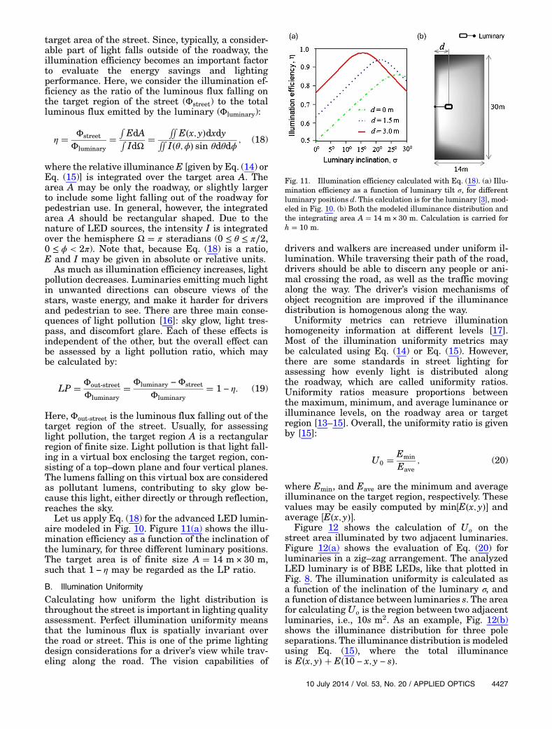
Let us apply Eq. (18) for the advanced LED lumin-aire modeled in Fig. 10. Figure 11(a) shows the illu-mination efficiency as a function of the inclination ofthe luminary, for three different luminary positions.The target area is of finite size A � 14 m × 30 m,such that 1 − η may be regarded as the LP ratio.

B. Illumination Uniformity

Calculating how uniform the light distribution isthroughout the street is important in lighting qualityassessment. Perfect illumination uniformity meansthat the luminous flux is spatially invariant overthe road or street. This is one of the prime lightingdesign considerations for a driver’s view while trav-eling along the road. The vision capabilities of

drivers and walkers are increased under uniform il-lumination. While traversing their path of the road,drivers should be able to discern any people or ani-mal crossing the road, as well as the traffic movingalong the way. The driver’s vision mechanisms ofobject recognition are improved if the illuminancedistribution is homogenous along the way.

Uniformity metrics can retrieve illuminationhomogeneity information at different levels [17].Most of the illumination uniformity metrics maybe calculated using Eq. (14) or Eq. (15). However,there are some standards in street lighting forassessing how evenly light is distributed alongthe roadway, which are called uniformity ratios.Uniformity ratios measure proportions betweenthe maximum, minimum, and average luminance orilluminance levels, on the roadway area or targetregion [13–15]. Overall, the uniformity ratio is givenby [15]:

U0 � Emin

Eave; (20)

where Emin, and Eave are the minimum and averageilluminance on the target region, respectively. Thesevalues may be easily computed by min�E�x; y�� andaverage �E�x; y��.

Figure 12 shows the calculation of Uo on thestreet area illuminated by two adjacent luminaries.Figure 12(a) shows the evaluation of Eq. (20) forluminaries in a zig–zag arrangement. The analyzedLED luminary is of BBE LEDs, like that plotted inFig. 8. The illumination uniformity is calculated asa function of the inclination of the luminary σ, anda function of distance between luminaries s. The areafor calculatingUo is the region between two adjacentluminaries, i.e., 10s m2. As an example, Fig. 12(b)shows the illuminance distribution for three poleseparations. The illuminance distribution is modeledusing Eq. (15), where the total illuminanceis E�x; y� � E�10 − x; y − s�.

Fig. 11. Illumination efficiency calculated with Eq. (18). (a) Illu-mination efficiency as a function of luminary tilt σ, for differentluminary positions d. This calculation is for the luminary [3], mod-eled in Fig. 10. (b) Both the modeled illuminance distribution andthe integrating area A � 14 m× 30 m. Calculation is carried forh � 10 m.


C. Disability Glare

The purpose of any luminary is to illuminate thestreet surface to make visible the environment. Butthe luminary light that directly hits the eye createsa glare, which is an unwanted effect in street lightingthat may cause disability and discomfort to driversand pedestrians. The loss of visual image contrast isa consequence of the veiling luminance �lm∕m2 sr�,which is due to scattering inside the eye [18].

The luminary glare may cause a feeling of discom-fort or disturbance in the visual field. The magnitudeof glare may be estimated by calculating the equiv-alent veiling luminance. There are several metricsto assess the veiling luminance [13,15,18]. In gen-eral, this luminance is directly proportional to theilluminance lighting the human eye, and inverselyproportional to the angular separation from thefield-of-view. A commonly used expression is

Lv � 10Ev

θ2v � 1.5θv; (21)

where θv is the angle (in degrees) between theluminaire and the line-of-sight of an observer [seeFig. 13(a)], which is usually regarded as parallel tothe roadway or y axis. Ev is the veiling illuminance,which is the vertical illuminance in the eye of theobserver. We may rewrite Eq. (21) as a function ofthe luminary intensity I:

Lv � 10I cos θv

r2�θ2v � 1.5θv�: (22)

Then, the veiling luminance may be written as afunction of Cartesian coordinates �x; y� for a positionon the street:

Lv�x; y� �10I�θ;ϕ�jyj�θ2v � 1.5θv�−1

��x − d�2 � y2 � �h − ho�2�3∕2: (23)

Here, I�θ;ϕ� is the 3D angular intensity distributionof the luminary, which may be modeled by Eq. (5) orEq. (7). The direction angles, θ and ϕ, are those givenby Eqs. (16) and (17). The veiling angle θv is

θv � arcos� jyj��x − d�2 � y2 � �h − ho�2�1∕2

�; (24)

where ho is the eye height above the street, which isusually taken as 1.45 m [15].

Figure 13(b) shows the calculation of veiling lumi-nance distribution at each observer position on thestreet. The observer stands at point P�x; y� on theroad, at the standard eye height above the roadho � 1.45 m. Calculated light is due to three lumi-naries in the observer’s field-of-view, i.e., Lv�x; y��Lv�x; y − 30� � Lv�x; y − 60�, where pole separationis 30 m. The calculation is carried out for h � 6 m,d � 1.5 m, σ � 15°, and the radiation pattern ofFig. 6(b). A spatial map of veiling luminance mayhelp to design LED street lighting in such a way that

Fig. 12. Calculation of the illumination uniformityUo, with lumi-naries in zig–zag configuration. (a) Illumination uniformity as afunction of both luminary tilt σ and pole distance s. (b) Illuminancedistribution for the three points marked in (a). The red-dotted rec-tangle encloses the area for the Uo calculation, as tens of m2. Themodeling is carried for h � 6 m, d � 0 m, and the intensity patternof Fig. 6(a).

Fig. 13. Veiling luminance (glare) calculation. (a) Schematic of the geometry for calculating the veiling luminance at the observer posi-tion, standing on a point P�x; y� on the road due to one luminary. (b) Veiling luminance, calculated by Eq. (23), at each observer’s position�x; y�, due to three luminaries in the field-of-view.


drivers’ and pedestrians’ vision is not impaired byglare in their field-of-view [10].

This section illustrated the potential of our modelto calculate the street lighting performance, whichmay be assessed by quality and efficiency parame-ters. Several other parameters are also importantand their calculation may be approached by themathematical model reported here. These parame-ters are well defined in standards that give the re-quirements for various classes of roads [13–15].Important examples include: the surround ratio,which indicates how drivers see vehicles, pedestriansand animals on the side of the road for safety pur-poses; and the luminance, which determines howdrivers and walkers see the light reflected by thesurface of the street [19].

5. Summary

We have derived simple equations to determine howlight is distributed in LED street lighting. First, weproposed two mathematical representations tomodel the sophisticated intensity profiles of LEDluminaries: one equation for smooth intensity pat-terns, and one for intensity profiles with sharp peaks.Secondly, we modeled the illumination of the street,i.e., we determined equations to model the illumi-nance distribution at any point on the floor, road,or street. Because the model is analytic, the equa-tions show explicit dependence on key parameterslike: the luminary height, arm length, luminary tilt,and the luminous intensity curve. Finally, we mod-eled the performance of LED luminaries. In particu-lar, we calculated four important parameters of LEDstreet lighting: light utilization efficiency, light pollu-tion, illumination uniformity, and veiling luminanceof glare. In general, the simplicity of the modelmakes it easy to understand, apply, and perhapsbe enhanced. This model is the theoretical counter-part of Monte Carlo ray tracing and radiosity calcu-lations [20], which may further improve the analysisand performance of LED street lighting systems.For example, this model may be useful to introducerandom manufacturing and installation variationsof LED luminaries to analyze and design streetlighting systems. Future work may include derivingdesign conditions so that LED street lightinginstallations minimize light pollution, increase com-fort and visibility, and maximize both illuminationuniformity and light utilization efficiency.

Appendix A: Coefficients for Modeling the RadiationPattern of LED Luminaries [Figs. 3(a) and 6(b)].

Coefficients of Eq. (1) for modeling Fig. 3(a) are:

g11 � 0.203; g12 � 0.0780; g13 � 55.99

g21 � 0.579; g22 � 0.0067; g23 � 58.06

g31 � 0.318; g32 � 0.0009; g33 � 38.17

Coefficients of Eq. (5) for modeling Fig. 6(b) are:

gx11 � 0.035; gy11 � 0.4610; g21 � 2.984;

gx31 � 43; gy31 � 61.81

gx12 � 0.035; gy12 � 0.4738;

g22 � 11.15; gx32 � 43; gy32 � 60.80

g13 � 0.1693; g23 � 38.78; g33 � 19.57

m11 � m12 � 8; m31 � m32 � 2.

Note that the set of coefficients given normalizes theintensity equation to 1 at its maximum, and makesthe equation a function of θ in degrees. To computeluminous intensity in lumens/sr, just multiplyI�θ;ϕ� by the maximum value of lm/sr or candelas.

This research was supported by CONACYT(Consejo Nacional de Ciencia y Tecnológia) grant128452.

References1. K. J. Gaston, “Sustainability: a green light for efficiency,”

Nature 497, 560–561 (2013).2. I. Moreno and C. C. Sun, “Modeling the radiation pattern of

LEDs,” Opt. Express 16, 1808–1819 (2008).3. X. H. Lee, I. Moreno, and C. C. Sun, “High-performance LED

street lighting using microlens arrays,” Opt. Express 21,10612–10621 (2013).

4. Z. Feng, Y. Luo, and Y. Han, “Design of LED freeform opticalsystem for road lighting with high luminance/illuminanceratio,” Opt. Express 18, 22020–22031 (2010).

5. H.-C. Chen, J.-Y. Lin, and H.-Y. Chiu, “Rectangular illu-mination using a secondary optics with cylindrical lensfor LED street light,” Opt. Express 21, 3201–3212(2013).

6. Y. C. Lo, K. T. Huang, X. H. Lee, and C. C. Sun, “Opticaldesign of a butterfly lens for a street light based on a dou-ble-cluster LED,” Microelectron. Reliab. 52, 889–893(2012).

7. R. Wu, K. Li, P. Liu, Z. Zheng, H. Li, and X. Liu, “Conceptualdesign of dedicated road lighting for city park and housingestate,” Appl. Opt. 52, 5272–5278 (2013).

8. X. Liu, W. Cai, X. Lei, X. Du, and W. Chen, “Far-field distancefor surface light source with different luminous area,” Appl.Opt. 52, 1629–1635 (2013).

9. I. Moreno, C.-C. Sun, and R. Ivanov, “Far-field condition forlight-emitting diode arrays,” Appl. Opt. 48, 1190–1197(2009).

10. I. Moreno, T. Saucedo-A, J. S. Pérez-Huerta, and E. de la Rosa-Miranda, “Designing LED street lighting,” Appl. Opt. (to bepublished).

11. M. Gardner, “Piet Hein’s Superellipse,” in Mathematical Car-nival: A New Round-Up of Tantalizers and Puzzles (ScientificAmerican, 1977), pp. 240–254.

12. C. C. Sun, T. X. Lee, S. H. Ma, Y. L. Lee, and S. M. Huang,“Precise optical modeling for LED lighting verified by crosscorrelation in the midfield region,” Opt. Lett. 31, 2193–2195 (2006).

13. P. Raynham, “An examination of the fundamentals of roadlighting for pedestrians and drivers,” Lighting Res. Technol.36, 307–316 (2004).

14. W. Luo, M. Puolakka, M. Viikari, S. Kufeoglu, A. Ylinen, andL. Halonen, “Lighting criteria for road lighting: a review,”Light Eng. 20, 64–74 (2012).

15. M. S. Rea, ed., “Roadway lighting,” in IESNA Lighting Hand-book: Reference and Application, 9th ed. (IESNA, 2000),Chap. 22.

16. J. A. Brons, J. D. Bullough, and M. S. Rea, “Outdoor site-lighting performance: a comprehensive and quantitativeframework for assessing light pollution,” Lighting Res. Tech-nol. 40, 201–224 (2008).


17. I. Moreno, “Illumination uniformity assessment based onhuman vision,” Opt. Lett. 35, 4030–4032 (2010).

18. J. J. Vos, “On the cause of disability glare and its dependenceon glare angle, age and ocular pigmentation,” Clin. Exp.Optom. 86, 363–370 (2003).

19. A. M. Ylinen, T. Pellinen, J. Valtonen, M. Puolakka, and L.Halonen, “Investigation of pavement light reflection charac-teristics,” Road Mater. Pavement 12, 587–614 (2011).

20. For example, ASAP (http://www.breault.com/index.php), andDIALux (www.dial.de/DIAL/en/dialux.html) software.


http://www.breault.com/index.php




www.dial.de/DIAL/en/dialux.html

Modeling LED street lighting

Documents

Transcript of Modeling LED street lighting