Modeling Heart Rate Regulation—Part I: Sit-to-stand Versus Head-up Tilt

Modeling Heart Rate Regulation—Part I: Sit-to-stand Versus Head-up Tilt

Mette S. Olufsen, April V. Alston, and Hien T. TranDepartment of Mathematics, North Carolina State University, Campus Box 8205, Raleigh, NC27695, USA e-mail: [email protected]

Johnny T. OttesenDepartment of Mathematics and Physics, Roskilde University, Roskilde, Denmark

Vera NovakDepartment of Gerontology, Beth Israel Deaconess Medical Center, Harvard Medical School,Boston, MA, USA

AbstractIn this study we describe a model predicting heart rate regulation during postural change from sittingto standing and during head-up tilt in five healthy elderly adults. The model uses blood pressure asan input to predict baroreflex firing-rate, which in turn is used to predict efferent parasympatheticand sympathetic outflows. The model also includes the combined effects of vestibular and centralcommand stimulation of muscle sympathetic nerve activity, which is increased at the onset of posturalchange. Concentrations of acetylcholine and noradrenaline, predicted as functions of sympatheticand parasympathetic outflow, are then used to estimate the heart rate response. Dynamics of the heartrate and the baroreflex firing rate are modeled using a system of coupled ordinary delay differentialequations with 17 parameters. We have derived sensitivity equations and ranked sensitivities of allparameters with respect to all state variables in our model. Using this model we show that duringhead-up tilt, the baseline firing-rate is larger than during sit-to-stand and that the combined effect ofvestibular and central command stimulation of muscle sympathetic nerve activity is less pronouncedduring head-up tilt than during sit-to-stand.

KeywordsMathematical modeling; Heart rate regulation; Sensitivity analysis

IntroductionShort-term cardiovascular regulation is often studied by imposing orthostatic stress challengessuch as head-up tilt or sit-to-stand tests. During both passive (head-up tilt) and active standing(sit-to-stand) blood is pooled in the lower extremities due to gravitational forces. As a result,venous return is reduced, which leads to a decrease in cardiac stroke volume, a decline inarterial blood pressure, and an immediate decrease of blood flow to the brain. The reductionin arterial blood pressure unloads the baroreceptors located in the carotid and aortic walls,which leads to parasympathetic withdrawal and sympathetic activation through baroreflex-mediated autonomic regulation. Parasympathetic withdrawal induces a fast (within 1–2 cardiaccycles) increase in heart rate, while sympathetic activation yields a slow (within 6–8 cardiaccycles) increase in vascular resistance, vascular tone, cardiac contractility, and a furtherincrease in heart rate (Smith and Kampine 1990; Guyton and Hall 1996). The main differencesbetween head-up tilt and sit-to-stand are: (i) Head-up tilt was carried out using a slow-tiltprocedure: it takes 5–10 s to tilt the subject from supine to standing, thus regulatory response

NIH Public AccessAuthor ManuscriptCardiovasc Eng. Author manuscript; available in PMC 2009 October 27.

Published in final edited form as:Cardiovasc Eng. 2008 June ; 8(2): 73–87. doi:10.1007/s10558-007-9050-8.

NIH

-PA Author Manuscript

NIH


NIH


is activated before the subject is fully tilted. In addition since the procedure is passive, it requireslimited muscle activity. Finally, due to the tilt-angle, gravitational forces act between the headand the torso leading to a transient decrease of intracranial pressure and increased venousdraining from cerebral circulation to the heart. Simultaneously forces act between the torsoand the lower body, leading to increased venous pooling in to the lower body. With these twomechanisms, venous return to the heart from cerebral circulation may transiently increase,while venous return from the periphery to the heart is decreased. These processes in turn affectbeat-to-beat blood pressure and baroreflex firing-rate. (ii) The sit-to-stand occurs rapidly over1–5 s and requires active muscle contraction and engagement of “central command” formovement initiation, which leads to an immediate increase in heart rate as the subject contractshis/her muscles to initiate standing (Olufsen et al. 2006). This increase in heart rate is observedbefore the initial drop in blood pressure and is possibly activated by combined effects ofvestibular and central command stimulation of muscle sympathetic nerve activity.

Previous studies have demonstrated a strong vestibular stimulation of muscle sympatheticnerve activity in response to postural change, primarily in response to headdown rotation (Ray2000;Ray and Monahan 2002;Ray and Carter 2003). However, a recent study in conscious catsshow vestibular stimulation during head-up tilt (Wilson et al. 2006), and previous work byKaufmann et al. (2002) suggests that the vestibular sympathetic reflex, originating in the otolithorgans, may be one of the earliest mechanisms to be activated to sustain blood pressure uponstanding. Studies analyzing vestibular stimulation of muscle sympathetic nerve activity usinghead-down rotation indicate that the vestibular system is activated independently of thebaroreflex response, and that the two responses may be additive (Ray 2000;Ray and Carter2003). Typically these responses have been studied by analyzing systemic measurements ofblood pressure obtained using a Finapres device positioned at the level of the heart and heartrate obtained from analysis of ECG signals (Low 1997;Robertson et al. 2005). The majorityof these experimental studies analyzed data using linear response models. For example,baroreflex sensitivity (Robbe et al. 1987;Johnson et al. 2006) has been assessed using spectraltransfer functions relating changes in systolic blood pressure to interbeat intervals. This methodis limited to analysis of relationships between two signals. Another limitation is that these dataanalysis methods lack the ability to predict how changes in neural responses interact to maintainarterial blood pressure.

In a previous study (Olufsen et al. 2006), we showed that a model for sit-to-stand clearlydistinguishes between the baroreflex and vestibular/central command stimulation, we alsoshowed significant differences between three groups of healthy young, healthy elderly andhypertensive elderly subjects. In addition, we were able to identify all 17 model-parametersusing an inverse least-squares formulation. To solve the least squares problem we used theNelder-Mead method, which is based on the simplex algorithm. However, we did not analyzethe model in further detail or compared it to the response observed during head-up tilt.Furthermore, we lacked measures indicating how good our parameter estimates were. Also,we did not investigate which parameters were sensitive and which were not. In this study wederive sensitivity equations, which enable us to better understand the importance of eachelement in the model. We also compare computations from sit-to-stand where the vestibularsystem is believed to be an important contributor to the heart rate regulation with computationsfrom head-up tilt, where the vestibular system appears to be engaged to a lesser degree. Anotherimportant issue is the methodologies for parameter estimation. The model proposed in (Olufsenet al. 2006) and studied further here has 17 parameters, and we have limited information aboutthese parameters. Therefore, in a second part of this study we will analyze a number ofoptimization techniques used to identify model parameters.

Olufsen et al.

Cardiovasc Eng. Author manuscript; available in PMC 2009 October 27.

NIH


NIH


NIH


MethodsExperimental Design

We analyzed data from five healthy elderly subjects (two woman and three men) aged 55–75years (mean 60 ± 7 years), which participated in both sit-to-stand and headup tilt protocols.The subjects had no medical history of and were not treated for any systemic diseases, theydid not take any cardiovascular active medications, had no history of head or brain injury, andhad no history of more than one episode of syncope. Each subject was instrumented with athree-lead ECG to obtain heart rate. A photoplethysmographic device on the middle finger ofthe non-dominant hand was used to obtain noninvasive beat-to-beat blood pressure (Finapresdevice, Ohmeda Monitoring Systems, Englewood, Colorado). To eliminate effects of gravity,the hand was held at the level of the right atrium and supported by a sling. All physiologicalsignals were digitized at 500 Hz using Labview NIDAQ software (National Instruments,Austin, TX) and stored for offline analysis. Times indicating the start of every cardiac cyclewere extracted from the ECGs sampled at 500 Hz and validated off line. Blood pressure datawere down-sampled to 50 Hz before being used as input to the mathematical model. Sit-to-stand protocol: After instrumentation, subjects sat in a straightbacked chair with their legselevated at 90° in front of them. After 5 min of stable recordings, the subjects were asked tostand-up. Standing was defined as the moment both feet touched the floor, recorded by a forceplatform. Head-up tilt protocol: The subjects rested in supine position on the table for 10 min.Then, the table was tilted to 70° for 10 min. All subjects provided informed consent approvedby the Institutional Review Board at Beth Israel Deaconess Medical Center, Boston, MA.

ModelingIn the analysis here we used the model put forward in (Olufsen et al. 2006). This modelpredicted heart rate using a chain of responses as illustrated in Fig. 1. Note that the model issequential, i.e., all elements are linked in a chain. This allows for simpler implementation ofthe system of delay differential equations. Input to the model is the weighted mean bloodpressure, which can be computed as

1

The parameter α is the weight. A large value of α gives rise to a small weight of the past time(short memory), while a small value of α gives a larger weight (long memory). The weightedmean pressure is a function of time, which oscillates with the same frequency as theinstantaneous pressure p, but with a smaller amplitude, see Fig. 2.

As shown in Fig. 1, the mean blood pressure is used as an input to predict baroreflex firing-rate. Similar to previous work (Ottesen 1997;Olufsen et al. 2006) firing-rate is determinedusing a nonlinear differential equations of the form

2

where ni [1/s] denotes the firing-rate with i = S, I, L accounting for short, intermediate, andlong thresholds for the different receptors, [mmHg] denotes the weighted mean bloodpressure. This equation has a total of eight parameters: ki [1/mmHg] are gain constants, M =120 [1/s] is the maximal firing-rate, N [1/s] denotes the baseline firing-rate, and τi [s] are

Olufsen et al.


NIH


NIH


NIH


characteristic times related to resetting. The baseline firing-rate N cannot exceed the maximumfiring-rate and we assume that N > M/2. To enforce these bounds we have parameterized Nusing a sigmoid function of the form

3

where η is an unknown parameter. The baroreceptor firingrate model in (2) exhibits nonlinearcharacteristics: it increases with increased carotid pressure and the response exhibits,hysteresis, threshold, and saturation. We use the term hysteresis to describe the nonlinearphenomenon between two quantities, the change in pressure and the change in firing-rate (dni/dt) described by Eq. 2. If then the two terms in the equation work in oppositedirection yielding a smaller net derivative of dni/dt. However if then the two termswork in the same direction yielding a larger net derivative of dni/dt. This dynamic responseagree with experimental studies, which suggest that a sufficiently fast decrease in pressurecauses a step change in firing-rate followed by a resetting (adaptation) phenomenon and thatthe response to a decrease in pressure is faster than the response to an increase in pressure(Poitras et al. 1966;Spickler and Kedzi 1967;Franz 1969;Srinivasen and Nudelman1972;Cecchini et al. 1982;Taher et al. 1988).

Using the baroreflex firing-rate n we predict the sympathetic and the parasympathetic outflows.The parasympathetic outflow Tpar is proportional to the firingrate whereas sympathetic outflowTsym is inversely related to the firing-rate (Danielsen and Ottensen 1997; Ottesen 1997). Thesympathetic response is delayed 6–8 cardiac cycles; furthermore, an increased parasympatheticresponse dampens the sympathetic response (Levy and Zieske 1969). Finally, we accountedfor additional activation u(t) mediated by muscle sympathetic nerves and by central command.Combining all effects discussed above gives the following models for parasympathetic andsympathetic outflows

4

Parameters in these expressions include τd [s], the delay of the sympathetic response, and β,which is the parasympathetic dampening factor. The activation function u(t) is represented bya quadratic impulse function of the form

5

This equation has three parameters, u0 the amplitude of the response, tstart, and tper the starttime and duration of the response. A detailed description of the impulse function can be foundin (Olufsen et al. 2006).

Using the sympathetic and parasympathetic outflows, nondimensionalized concentrations ofacetylcholine Cach and noradrenaline Cnor were computed from the first order equation

Olufsen et al.


NIH


NIH


NIH


6

where the parameters τnor, τach [s] denote characteristic time scales for noradrenaline andacetylcholine. It should be noted that when i = sym then j = nor and when i = par then j =ach. In this equation we have lumped the long chain of bio-chemical reactions into one firstorder reaction equation and taken the accumulated release time to be equal to the averageclearance and consumption time for the respective substances. The heart rate potential wascomputed using an integrate and fire model of the form

7

When ø = 1 the heart beats and the interbeat interval (R–R interval, see Fig. 3) is taken as thetime from ø = 0 to ø = 1. Then heart rate is found as the inverse of the interbeat interval. Theparameter H0 denotes intrinsic heart rate. Several studies have shown that intrinsic heart ratevary with age. Following ideas proposed in studies by Jose and Opthof et al. (Jose andCollison 1970; Opthof 2000) we let H0 = 1.97 − 9.50· 10−3 × age [bps]. These studies assessedintrinsic heart rate under simultaneous presence of propranolol and atropine in 432 subjectsand used linear regression to relate heart rate and age. This relation was also confirmed in anonpharmacological study in cardiac transplant recipients (Strobel et al. 1999). The remainingparameters MS and MP represent the strength of the response to changes in the concentrations.To bound heart rate within physiological values, we constrained MS and MP in the interval[0,1]. This was done by introducing the parameters ξS and ξP so that

8

In summary, the heart rate model proposed for this study can be written as a system of nonlineardelay differential equations of the form

9

In the above system of equations contains the seven state variables and θ contains the 17model-parameters to be identified. Note that the model contains one more parameter (themaximum firing-rate M = 120 [1/s]), however, in this study we do not attempt to identify M.Initial values for the state variables and model parameters were estimated from physiologicalconditions. Table 4 lists all states and parameteres.

To validate this model against data we used Kelley's implementation of the Nelder–Meadoptimization method (Kelley 1999) that minimizes the least-squared error J between computedHRc(ti) and measured HRd(ti) values of heart rate. We defined the least squares cost J by

Olufsen et al.


NIH


NIH


NIH


10

In this equation Nd denotes the number of measurements of heart rate.

Initial iterates for all parameter values were determined using results from previous work(Olufsen et al. 2006). Thus, the initial iterate for the weighting parameter was set to α = 1 [1/s], the firing-rate scaling parameters were set to kS = kL = 2, and kI = 1.5 [1/mmHg s], and thetimescales were set to τS = 1, τI = 5, and τL = 250 [s]. Initial iterates for the parasympatheticand sympathetic time scales and the sympathetic delay were given by τnor = τach = 1, τd = 7[s] and the parasympathetic damping of sympathetic outflow was set to β = 1. The initial iteratesfor the impulse function were amplitude, u0 = 1, and the duration, tper = 5 [s]. The start timeststart [s] were obtained from the experimental data. This parameter value indicates the time ofinitiation of standing and tilting, respectively.

Initial iterates for the parameters ξS and ξP used to determine MS and MP were calculated suchthat complete parasympathetic withdrawal (Cach = 0) and maximal sympathetic stimulation(Cnor = 1) resulted in maximal heart rate Hmax = 3.62 − 1.42· 10−2× age [bps], while completesympathetic inhibition (Cnor = 0) and maximal parasympathetic stimulation (Cach = 1) resultedin “minimal” heart rate Hmin = 0.75 [bps]. These considerations gave

11

It should be noted that in previous work (Olufsen et al. 2006) we did not account for the age-dependence when calculating maximal and intrinsic heart rates. The final initial iterate is forthe parameter η, which is used to estimate the baseline firing-rate N. To estimate this value,we let the potential dø/dt = Hr, where Hr is the resting heart rate found by averaging the firstfive cardiac cycles. Then we solved for N, and used (4) to determine η as

12

It should be emphasized that the considerations discussed above give rise to a set of initialiterates for the model parameters, which are within physiological range for each subject studied.To obtain individual patient specific parameter values that accurately predict dynamicsobserved for a given subject we performed non-linear optimization, identifying a set ofparameters that minimize the least squares error between the computed and measured valuesof heart rate.

Numerical ConsiderationsThe equations discussed above were solved using Matlab's built in differential equations solverode15s. This solver is designed to solve stiff-differential equations using a variable ordermultistep method based on numerical differentiation formulas (Shampine and Reichelt 1997;Shampine et al. 1999).

Olufsen et al.


NIH


NIH


NIH


The system of Eqs. 1–8 includes a delay variable (τd) used when calculating sympatheticoutflow Tsym (n(t –τd)). Thus, the differential equations cannot explicitly be solved usingode15s. Matlab does have a delay differential equations solver dde23 based on a 2–3'rd orderRunge–Kutta method. However, this method cannot handle stiff equations, thus we could notuse it for the model discussed here. Now, it is possible to avoid implementing a stiffdelaysolver, by taking advantage of the sequential structure of the model (see Fig. 1). To do so wefirst solve and store numerical values for and n and then use the stored values for both n(t)and n(t – τd) to compute parasympathetic and sympathetic outputs as described in Eqs. 4–8.Initial conditions used for this study are similar to previous work (Olufsen et al. 2006), i.e., welet ni(0) = 0, (0) = mean ( i = 1,…,5) dCi/dt = 0 which gives that

13

Finally, the initial value for the heart rate potential ø (0) = 0.

Subject specific parameter values were, as discussed earlier, obtained using Kelley'simplementation of the Nelder-Mead method (Kelley 1999). This method is one of manynonlinear optimization methods that can be used to identify model parameters. In part II of thisarticle, we have compared the Nelder-Mead method to implicit filtering and a geneticalgorithm.

Sensitivity AnalysisTo determine the sensitivity of the states with respect to each of the model parameters we usedlocal sensitivity analysis as described in (Carmichel et al. 1997; Ellwein et al. 2007). Usingthis analysis we determine how the model states (defined in Eq. 9) change with respect toeach of the parameters θ as a function of time, i.e., the goal is to calculate . Thesesensitivities can be found by solving a system of differential equations obtained by implicitlydifferentiating the state equations in (9) with respect to each of the model parameters in θ, i.e.,

14

The switch in order of differentiation is valid if all concerned derivatives are continuous(Kaplan 1991). Given that has seven elements and that θ has 17elements we get (7 × 17) differential equations (sensitivity equations), which should be besolved simultaneously with the seven differential equations in (9) that describe the dynamicsof the system. Consequently, we need to solve a total of (7 + 7 × 17 = 136) coupled differentialequations. When solving these equations, we assume that , i.e., initially (at timet = t0) we assume that the model does not depend on the parameters. The structure of thesensitivity equations is described in Appendix A.

Data to be analyzed in this study predict heart rate as a function of time, however, we do nothave an explicit differential equation predicting heart rate. Heart rate is predicted using anintegrate-and-fire model as described above. Furthermore, we do not solve the delaydifferential equations explicitly, but take advantage of the sequential structure of the model,and first solve for { , nS, nI, nL} and then use both ni (t) and ni (t – τd) to compute {Cnor,Cach, ø}. Thus we cannot use the implicit differentiation approach described above to computethe sensitivity to the time-delay τd and to the heart rate.

Olufsen et al.


NIH


NIH


NIH


One way to compute sensitivities of all parameters with respect to heart rate and of the delaytime with respect to {Cnor, Cach, ø} is to use finite differences. We do so using a central finitedifference scheme in which we calculate

15

which has error O(h2). This finite difference formula requires two function evaluations or twosolves of the state equations: for (θ − h) and for (θ + h). We use this methodology tocalculate ∂HR/∂θi, i = 1,…,17 and i = Cnor, Cach,. The main drawback of this methodis the difficulty of analyzing the accuracy of the sensitivity estimates due to the finite-precisionarithmetic on a computer. If h is too small in relation to θj we loose most of the significant

digits when calculating the difference between two almost equal numbers and

. On the other hand, if h is so large that the finite differenceapproximation of the derivative becomes inaccurate. A simple rule (Dennis and Schnable1983) for the case where can be computed accurately to machine precision is to choose h ≈(macheps)1/3, macheps denotes machine epsilon; the smallest positive number ε for, which 1+ ε >1 on the given computer. In our model, the solution to the differential equations in (9)is computed using Matlab's differential equations solver ode15s with both absolute and relativeerror tolerances set to 10−6; thus our “macheps = 10−6”. Therefore, in our calculation of thenormalized sensitivity functions using central finite difference formula we used h = 10−2 toprovide a balance between the finiteprecision arithmetic and function evaluation errors.

To rank the sensitivities of the various states and parameters we define a global time-invariantnormalized sensitivity using a weighted 2-norm of the form (Sorteleder 1998)

16

If the matrix Z = (zij) has a row whose elements are all near zero, then the corresponding statevariable is not dependent on any of the model parameters. That is, measurements of thecorresponding state variable will not contribute to more reliable estimates of the parameters.On the other hand, if the column of the matrix Z is zero, then the corresponding model parameterwill have no influence on the model responses and can therefore not be estimated.

It should be noted that the total firing-rate is given by n = nS + nI + nL + N; hence, ∂n/∂θj =∂nS/∂θj + ∂nI/∂θj + ∂nL/∂θj. Therefore, we normalize the sensitivity functions of n with respectto model parameters as (θj/n – N(∂n/∂θj). For the other sensitivity variables, we normalize themas described in Eq. 16.

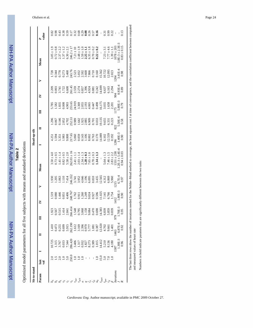
ResultsSimulations were carried out for five healthy elderly subjects undergoing two orthostatic stresstests: sit-to-stand and head-up tilt. Demographic and physiologic characteristics are shown inTable 1. Table 2 shows parameter values obtained for each of the five subjects. For eachexperiment we have included 15–25 s of baseline data followed by either active standing orpassive tilt.

Olufsen et al.


NIH


NIH


NIH


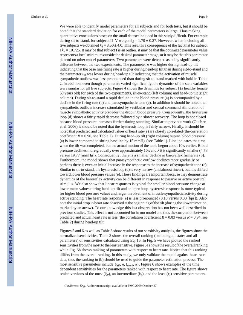
We were able to identify model parameters for all subjects and for both tests, but it should benoted that the standard deviation for each of the model parameters is large. Thus makingquantitative conclusions based on the small dataset included in this study difficult. For exampleduring sit-to-stand, for subjects II–V we got kS = 1.70 ± 0.27. However, when including allfive subjects we obtained kS = 3.50 ± 4.0. This result is a consequence of the fact that for subjectI kS = 10.725. It may be that subject I is an outlier, it may be that the optimized parameter valuerepresents a local minimum outside the desired parameter range, or it may be that this parameterdepend on other model parameters. Two parameters were detected as being significantlydifferent between the two experiments: The parameter η was higher during head-up tiltindicating that the base line firing rate is higher during head-up tilt than during sit-to-stand andthe parameter u0 was lower during head-up tilt indicating that the activation of musclesympathetic outflow was less pronounced than during sit-to-stand marked with bold in Table2. In addition, even though parameters varied significantly, the dynamics of the state variableswere similar for all five subjects. Figure 4 shows the dynamics for subject I (a healthy female60 years old) for each of the two experiments, sit-to-stand (left column) and head-up tilt (rightcolumn). During sit-to-stand a rapid decline in the blood pressure (a) is accompanied by adecline in the firing-rate (b) and parasympathetic tone (c). In addition it should be noted thatsympathetic outflow increase stimulated by vestibular and central command stimulation ofmuscle sympathetic activity precedes the drop in blood pressure. Consequently, the hysteresisloop (d) shows a fairly rapid decrease followed by a slower recovery. The loop is not closedbecause blood pressure increases further during standing. Similar to previous work (Olufsenet al. 2006) it should be noted that the hysteresis loop is fairly narrow. Finally, it should benoted that predicted and calculated values of heart rate (e) are closely correlated (the correlationcoefficient R = 0.96, see Table 2). During head-up tilt (right column) supine blood pressure(a) is lower compared to sitting baseline by 15 mmHg (see Table 1). Line indicates the timewhen the tilt was completed, but the actual motion of the table begun about 10 s earlier. Bloodpressure declines more gradually over approximately 10 s and is significantly smaller (4.78versus 19.77 [mmHg]). Consequently, there is a smaller decline in baroreflex firingrate (b).Furthermore, the model shows that parasympathetic outflow declines more gradually orperhaps there is even an initial increase in the response to the increase of sympathetic tone (c).Similar to sit-to-stand, the hysteresis loop (d) is very narrow (and almost linear), but it is shiftedtoward lower blood pressure values (e). These findings are important because they demonstratedynamics of the baroreflex activity can be different in response to passive or active posturalstimulus. We also show that linear responses is typical for smaller blood pressure change atlower mean values during head-up tilt and an open loop-hysteresis response is more typicalfor higher blood pressure values and larger involvement of muscle sympathetic activity duringactive standing. The heart rate response (e) is less pronounced (0.18 versus 0.33 [bps]). Alsonote the initial drop in heart rate observed at the beginning of the tilt (during the upward motion,marked by an arrow). To our knowledge this last observation has not been well described inprevious studies. This effect is not accounted for in our model and thus the correlation betweenpredicted and actual heart rate is less (the correlation coefficient R = 0.83 versus R = 0.94, seeTable 2) during head-up tilt.

Figures 5 and 6 as well as Table 3 show results of our sensitivity analysis, the figures show thenormalized sensitivities. Table 3 shows the overall ranking (including all states and allparameters) of sensitivities calculated using Eq. 16. In Fig. 5 we have plotted the rankedsensitivities from the most to the least sensitive. Figure 5a shows the result of the overall rankingwhile Fig. 5b shows ranking of parameters with respect to heart rate. Notice that this rankingdiffers from the overall ranking. In this study, we only validate the model against heart ratedata, thus the ranking in (b) should be used to guide the parameter estimation process. Themost sensitive parameters include {ξP, η, tstart, α}. Figure 6 shows examples of the timedependent sensitivities for the parameters ranked with respect to heart rate. The figure showsscaled versions of the most (ξP), an intermediate (kS), and the least (τI) sensitive parameters.

Olufsen et al.


NIH


NIH


NIH


Panel (a) shows time dependent sensitivities for all three parameters calculated using theoptimized parameter values and panels (b–d) show these parameters effect on heart rate. Inthese panels, the black lines are computed using the optimized parameter values and the greyline represents a 10% increase of the parameter in question. Note that a 10% change in ξP givesrise to a significant decrease in HR, while a 10% increase in kS or in has almost no effect onheart rate.

DiscussionResults show that it is possible to use our previously developed model (Olufsen et al. 2006) topredict heart rate changes during sit-to-stand and head-up tilt. The main contributions fromthis study were: (i). We were able to predict heart rate for all five subjects and dynamics of theintermediate responses looked similar for all subjects, thus we are able to (at least qualitatively)discuss impact of the model. (ii). We were able to calculate and rank sensitivities. Results ofthis ranking can be used to estimate how many parameters that can be uniquely identified. (iii).The most important observation is that different dynamics were observed between head-up tiltand sit-to-stand. During sit-to-stand heart rate increased immediately upon preparation tostanding, while during head-up tilt heart rate decreased before it started to increase. (iv). Thisstudy showed that inclusion of age dependence in initial iterates for parameters used to predictbaseline firing-rate and intrinsic heart rate gave rise to better prediction of the overall firing-rate n. Below, we will discuss advantages and limitations for each of these observations.

(i–ii): Similar to previous work, we found that our model has potential to be analyzed in moredetail, and results from this study have enabled us to identify several important features. First,we noticed that parameters varied significantly between subjects while the dynamics(illustrated in Fig. 4) follow similar trends. There are several reasons for the discrepanciesobserved in the parameter values. The parameter estimation methods are local, thus, there isno guarantee that the parameters identified represent the absolute minimal cost, and even if aminimal cost has been obtained the optimization may have identified a parameter outside thephysiological range. Second, we used the Nelder–Mead optimization method (a simplexmethod), which do not allow us to constrain parameters. Furthermore, we try to identify a largenumber (17) of parameters, which may not all be identifiable. In fact, results of our sensitivityanalysis showed that at least three parameters are unidentifiable. Finally, model parametersmay depend on each other. To understand our results better, we have analyzed severaloptimization methods. Results of this study are discussed in part II of this manuscript.

(iii): Probably the most important observation gained from this study is that while the modeldisplays excellent fits to the sit-to-stand data, four out of five subjects showed a decrease inheart rate during head-up tilt. These changes most likely reflect reductions of intracranialpressure and increases in central venous pressure in the right atrium, which, in turn, lead toincreases in cardiac output and the observed decrease in heart rate. These results may stemfrom the hydrostatic pressure changes opposed during headup tilt, which are different than theones observed during sit-to-stand. During head-up tilt, the head is slowly moved to a locationabove the heart, while during sit-to-stand no hydrostatic pressure changes are enforced betweenthe head and the heart. Notice that during standing (or during sitting) the hydrostatic pressurein the head is approximately 10 mmHg less than in the heart (Guyton and Hall 1996).

(iv): Another difference between our previous study and this study is that we adjusted intrinsicand maximum heart rates to age. These adjustments are physiological, it is well known thatadaptation to orthostatic stress, mainly parasympathetic withdrawal, declines with age. Thisrelative minor change had a fairly significant effect on the dynamics, in particular, for thedynamics of the overall firing-rate n, as well as on parasympathetic and sympathetic outflows,which are proportionally and inverse proportionally related to the firing-rate. This is a

Olufsen et al.


NIH


NIH


NIH


significant improvement over our previous study (Olufsen et al. 2006), where for most subjects,the steady-state baroreflex firing-rate was close to the maximal firing-rate.

A limitation of this study is that our model only included an empirical description of thecombined effect of vestibular and central command stimulation of muscle sympathetic nerveactivity, which may likely be activated differently during tilt than during sit-to-stand. It isinteresting though, that sympathetic activation occurs approximately at the same time in bothconditions and with a similar amplitude. One way to address this further would be to developa biophysical model for this response. Also, it should be noted that the tilt study was done onan automatic tilt-table, which uses an electrical engine to tilt the table to 70°. While thisautomated tilt-table allows for a more accurate tilt angle, it has the disadvantage that the tiltingprocess is fairly slow, it takes about 5 s to tilt the subject to upright position. This relativelyslow tilt time has an effect on the immediate drop in blood pressure, since, in particular,parasmpathetic response acts within this time-frame and thus already is activated before thesubject is fully tilted, thus preventing a more drastic blood pressure drop.

AcknowledgmentsDrs. Olufsen and Tran were supported by the National Science Foundation (OISE) #0437037. In addition Dr. Tranwas supported by a grant from the National Institue of Health (NIH) NIH/NIAID #9 RO1 AI071915-05. This workwas a response to discussion supported by the American Institute of Mathematics in Palo Alto, CA. Data collectionat the SAFE Laboratory, Beth Israel Deaconess Medical Center, Boston, MA was supported by an American DiabetesAssociation Grant to 1-06-CR-25, an NIH-NINDS 1R01-NS045745-01A21 to V. Novak, an NIH Older AmericanIndependence Center Grant 2P60 AG08812 and a General Clinical Research Center Grant MO1-RR01032. Alston,AV was partially supported by NIH-NIA (1 T32 AG023480-01) BIDMC/Harvard Translational research in AgingTraining Program traineeship.

Appendix A

Sensitivity EquationsThe model presented in (1–8) includes five state equations with a total of 17 model parameters.To derive sensitivity equations we differentiate each of the states with respect to each of theparameters, except for the delay parameter τd for which sensitivities will be computed usingcentral finite differences as described in (15). Because the system is coupled in the forwarddirection, parameter dependence carries through the model. The five state equations dependon the 17 parameters as follows:

A1

Mean PressureThe mean pressure was modeled using the differential equation in (1), which depends on oneparameter α.

Olufsen et al.


NIH


NIH


NIH


A2

Thus, only one sensitivity equation can be formed, namely

A3

Baroreflex Firing RateThe baroreflex firing rate is combined of three firing rates ni as described in Eqs. 2-3. Theseequations were given by

A4

These three differential equations depend on eight parameters α, ki, τi, η, for i = S, I, L. Thuswe get 3 × 8 = 24 sensitivity equations.

1. For the parameter α:

A5

2. For i = j, i є {S, I, L}:

A6

3. For i ≠ j, j ε {S, I, L}, y = {kj, sj}:

A7

Acetylcholine ConcentrationThe concentration of acetylcholine was modeled using a first order set-point equation asdescribed in (6).

Olufsen et al.


NIH


NIH


NIH


A8

This equation depends on nine parameters α, ki, τi, η, ηach, for i = S, I, L. Thus we formulate 1× 9 = 9 sensitivity equations. For γ = {α, ki, τi, η}, i = S, I, L the sensitivity equations have theform:

A9

The sensitivity equation for τach is given by

A10

Noradrenaline ConcentrationThe noradrenaline concentration was also modeled using the first-order set-point equationdescribed in (6). Accounting for vestibular stimulation of muscle sympathetic activation andcentral command this equation was given by

A11

In the above equation u denote an impulse function accounting for vestibular feedback. Thisfunction was given by

A12

This one differential equation has 14 parameters. Thus we get additional 14 sensitivityequations. For γ = {α, ki, τi, η}, i = S, I, L we get sensitivity equations of the form:

A13

The remaining six sensitivity equations are given by

Olufsen et al.


NIH


NIH


NIH


Heart Rate PotentialThe heart rate potential ø in (7) was modeled using the differential equation

A14

A15

This equation depends on all 17 model parameters. It should be noted that H0 is not a parameterbut is determined directly as a function of age as described above. Thus, this differentialequation gives rise to the following 17 sensitivity equations. Only the parameters ξs and ξpappear directly in the equation. Parameters γ = {α, ki, τi, η }, i ε{S, I, L} appear in both Cnorand Cach thus sensitivities with respect to these parameter have the form

A16

Cach also depend on τach, which gives rise to the sensitivity equation

A17

Furthermore, Cnor depends on parameters λ = {τnor,τd, u0, tstart, tper, β}, which gives sensitivityequations on the form

A18

Only two additional sensitivity equations needs to be derived, namely for ξs and ξp. These aregiven by

Olufsen et al.


NIH


NIH


NIH


A19

Again, it should be noted that the final sensitivities with respect to heart rate and to the delayparameter τd are computed using finite differences as described in (15).

ReferencesCarmichel G, Sandu A, et al. Sensitivity analysis for atmospheric chemistry models via automatic

differentiation. Atmos Environ 1997;31:475–89.Cecchini A, Tiplitz K, et al. Baroreceptor activity related to cell properties. Proc 35th Ann Conf Med

Biol 1982;24Danielsen M, Ottensen J. A dynamical approach to the baroreceptor regulation of the cardiovascular

system. Proc 5th Int Symp, Symbiosis 1997:25–29.Dennis, J.; Schnable, R. Numerical methods for unconstrained optimization and nonlinear equations.

Englewood Cliffs: Prentice Hall Inc; 1983.Ellwein L, Tran H, et al. Sensitivity analysis and model assessment: mathematical models for arterial

blood flow and blood pressure. J Cardiovasc Eng. (this issue). doi: 10.1007/s10558-007-9047-3Franz G. Nonlinear rate sensitivity of carotid sinus reflex as a consequence of static and dynamic

nonlinearities in baroreceptor behavior. Ann NY Acad Sci 1969;156:811–24. [PubMed: 5258020]Guyton, A.; Hall, J. Textbook of medical physiology. Philadelphia: WB Saunders; 1996.Johnson P, Shore A, et al. Baroreflex sensitivity measured by spectral and sequence analysis in

cerebrovascular disease: methodological considerations. Clin Auton Res 2006;16:270–5. [PubMed:16770526]

Jose A, Collison D. The normal range and determinants of the intrinsic heart rate in man. Cardiovasc Res1970;4:160–7. [PubMed: 4192616]

Kaplan, W. Advanced calculus. Rdwood City CA: Addison Wesley Publishing Company; 1991.Kaufmann H, Biaggioni I, et al. Vestibular control of sympathetic activity: an otolith-sympathetic reflex

in humans. Exp Brain Res 2002;143:463–9. [PubMed: 11914792]Kelley, C. Iterative methods for optimization. Philadelphia: SIAM; 1999.Levy M, Zieske H. Autonomic control of cardiac pacemaker. J Appl Physiol 1969;27:465–70. [PubMed:

5822553]Low, P. Clinical autonomic disorders: evaluation and management. Philadelphia: Lippincott Williams &

Wilkins; 1997.Olufsen M, Tran H, et al. Modeling baroreflex regulation of heart rate during orthostatic stress. Am J

Physiol 2006;291:R1355–68.Opthof T. The normal range and determinants of the intrinsic heart rate in man. Cardiovasc Res

2000;45:173–6. [PubMed: 10728332]Ottesen J. Nonlinearity of baroreceptor nerves. Surv Math Ind 1997;7:187–201.Poitras J, Pantelakis N, et al. Analysis of the blood pressure – baroreceptor nerve firing relationship. Proc

19th Ann Conf Eng Med Biol 1966:8–105.Ray C. Interaction of the vestibular system and baroreflexes on sympathetic nerve activity in humans.

Am J Physiol 2000;279:H2399–404.Ray C, Carter J. Vestibular activation of sympathetic nerve activity. Acta Physiol Scand 2003;177:313–

9. [PubMed: 12609001]Ray C, Monahan K. The vestibulosympathetic reflex in humans: neural interactions between

cardiovascular reflexes. Clin Exp Pharmacol Physiol 2002;29:98–102. [PubMed: 11906466]Robbe H, Mulder L, et al. Assessment of baroreceptor reflex sensitivity by means of spectral analysis.

Hypertension 1987;10:538–43. [PubMed: 3666866]

Olufsen et al.


NIH


NIH


NIH


Robertson, D.; Biaggioni, I., et al. Primer on the autonomic nervous system. Boston: Academic Press;2005.

Shampine L, Reichelt M. The MATLAB ODE suite. SIAM J Sci Comput 1997;18:1–22.Shampine L, Reichelt M, et al. Solving index-1 DAEs in MATLAB and Simulink. SIAM Rev

1999;41:538–52.Smith, J.; Kampine, J. Circulatory physiology, the essentials. Baltimore: Williams and Wilkins; 1990.Sorteleder, W. Parameter estimation in nonlinear dynamical systems Amsterdam. Netherlands: Stichting

Mathematisch Centrum; 1998.Spickler J, Kedzi P. Dynamic response characteristics of carotid sinus baroreceptors. Am J Physiol

1967;212(2):472–6. [PubMed: 6018034]Srinivasen R, Nudelman H. Modeling the carotid sinus baroreceptor. Biophys J 1972;12:1171–82.

[PubMed: 5056961]Strobel J, Epstein A, et al. Nonpharmacologic validation of the intrinsic heart rate in cardiac transplant

recipients. J Interv Card Electrophysiol 1999;3:15–8. [PubMed: 10354971]Taher M, Cecchini A, et al. Baroreceptors responses derived from a fundamental concept. Ann Biomed

Eng 1988;16:429–43. [PubMed: 3189973]Wilson T, Cotter L, et al. Vestibular inputs elicit patterned changes in limb blood flow in conscious cats.

J Physiol 2006;575:671–84. [PubMed: 16809368]

Olufsen et al.


NIH


NIH


NIH


Fig. 1.Model diagram. The model uses blood pressure as an input to predict baroreflex firing rate.From this we predict sympathetic and parasympathetic outflows, accounting for vestibularstimulation of muscle sympathetic and central command systems. These outflows give rise tochanges in concentrations of noradrenaline (nor) and acetylcholine (ach), which in turn givesrise to heart rate changes

Olufsen et al.


NIH


NIH


NIH


Fig. 2.Actual (black line) and mean (grey line) blood pressure [mmHg]. The actual blood pressure isobtained directly from data (down-sampled to 50 Hz). The mean blood pressure is calculatedusing (1) as an average running mean that is continuous in time

Olufsen et al.


NIH


NIH


NIH


Fig. 3.The heart rate potential ø. We use an “integrate and fire” model to predict the heart rate potentialø, when the potential reaches one it is reset to 0 and the heart rate (1/RR interval) is computedas the time elapsed since the potential was last reset to 0

Olufsen et al.


NIH


NIH


NIH


Fig. 4.Model results for a typical subject, the left column shows response to sit-to-stand while theright column shows the response to head-up tilt. The first row shows the input blood pressure(black line) and the computed average mean blood pressure (grey line). The second row showsthe baroreflex firing rate. The bottom three lines shows each of the three components (nS, nI,nL) and the top line shows the combined response n = nS + nI + nL + N including the baselineresponse N. The third row shows the parasympathetic (top line) and sympathetic (bottom line)response. The fourth row shows the mean firing rate as a function of mean blood pressure.Finally, the last row shows computed (line with triangles) and measured (black line with stars)values of heart rate as a function of time

Olufsen et al.


NIH


NIH


NIH


Fig. 5.This figure shows relative sensitivities for the parameters θi = ξP, kS, τI, where ξP is the mostsensitive parameter, kS is an intermediate sensitivity parameter, and τI is the least sensitiveparameter (see Fig. 6)

Olufsen et al.


NIH


NIH


NIH


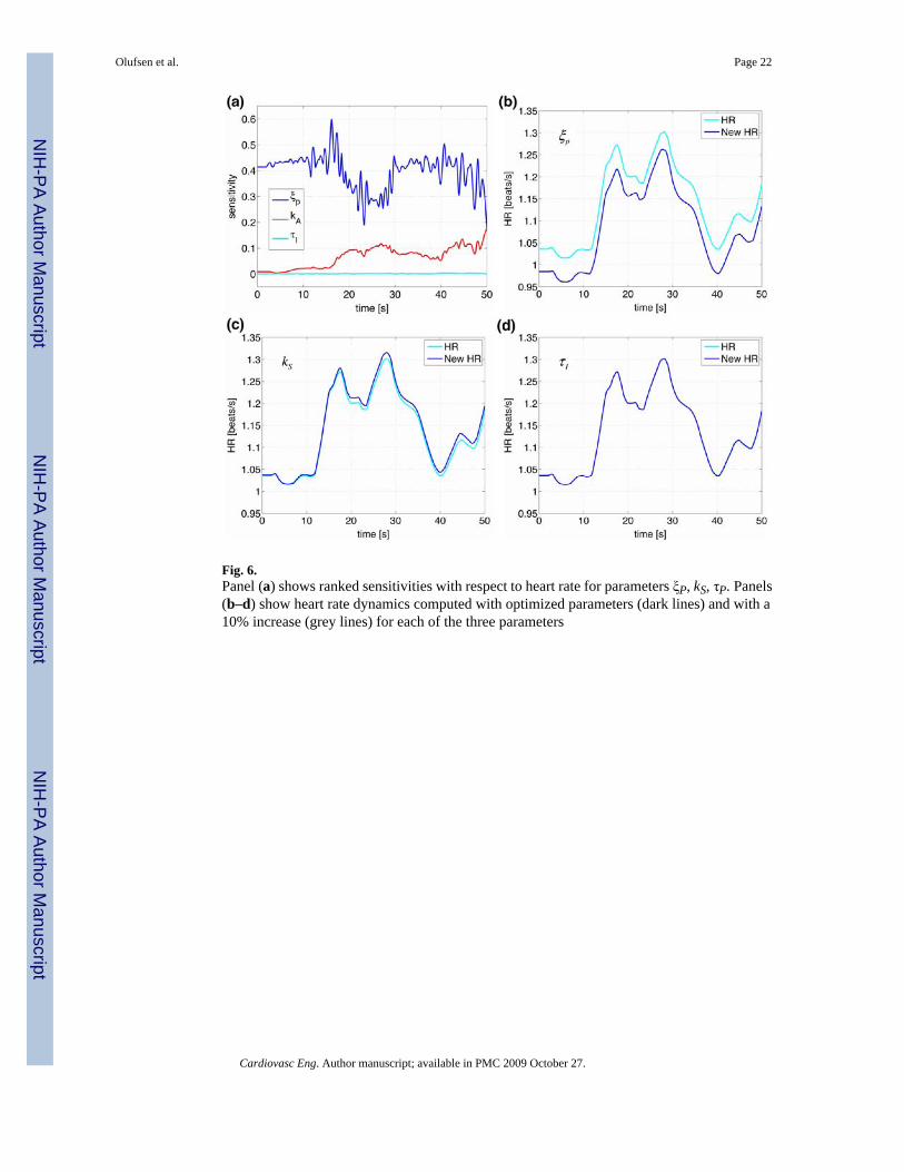
Fig. 6.Panel (a) shows ranked sensitivities with respect to heart rate for parameters ξP, kS, τP. Panels(b–d) show heart rate dynamics computed with optimized parameters (dark lines) and with a10% increase (grey lines) for each of the three parameters

Olufsen et al.


NIH


NIH


NIH


NIH


NIH


NIH


Olufsen et al. Ta

ble

1

Phys

iolo

gica

l cha

ract

eris

tics f

or th

e fiv

e su

bjec

ts

III

III

IVV

Mea

n

HR

sitti

ng1.

31 ±

0.0

30.

94 ±

0.0

41.

28 ±

0.0

31.

03 ±

0.0

61.

06 ±

0.0

31.

14 ±

0.1

6H

R su

pine

1.30

± 0

.05

0.94

± 0

.03

1.25

± 0

.08

1.00

± 0

.05

1.00

± 0

.03

1.12

± 0

.16

HR

stan

ding

1.55

± 0

.09

1.07

± 0

.04

1.49

± 0

.11

1.17

± 0

.08

1.25

± 0

.09

1.31

± 0

.22

HR

tilt

1.44

± 0

.04

0.96

± 0

.03

1.46

± 0

.06

1.07

± 0

.05

1.16

± 0

.06

1.26

± 0

.20

∆HR

sit-t

o-st

and

0.33

0.16

0.37

0.59

0.29

0.35

± 0

.16

∆HR

supi

ne-to

-tilt

0.18

0.04

0.28

0.46

0.24

0.24

± 0

.15

BP

sitti

ng89

.90

± 17

.85

98.3

0 ±

21.8

410

5.99

± 2

0.09

72.2

7 ±

19.4

091

.17

± 11

.73

92.2

4 ±

22.9

8B

P su

pine

75.2

9 ±

14.9

778

.05

± 21

.81

76.5

6 ±

19.4

179

.23

± 21

.61

79.9

4 ±

14.3

877

.53

± 18

.98

BP

stan

ding

87.2

3 ±

18.4

097

.21

± 26

.88

99.6

5 ±

25.0

274

.65

± 22

.41

90.8

8 ±

15.9

289

.92

± 23

.83

BP

tilt

74.0

0 ±

12.2

080

.08

± 19

.86

78.3

3 ±

17.1

981

.45

± 18

.27

71.3

6 ±

13.8

777

.53

± 18

.98

∆BP

sit-t

o-st

and

19.7

733

.76

43.0

120

.31

25.4

128

.45

± 9.

89∆B

P su

pine

-to-ti

lt4.

7828

.20

28.0

05.

7118

.92

17.1

2 ±

11.4

8

The

first

four

row

s giv

e m

ean

valu

es fo

r hea

rt ra

te d

ata

[bea

ts/s

] dur

ing

sitti

ng, s

upin

e, st

andi

ng, a

nd ti

lt po

sitio

ns. T

he n

ext t

wo

row

s giv

es th

e m

axim

um c

hang

e ob

serv

ed b

etw

een

base

line

(sitt

ing

or su

pine

) and

stan

ding

or t

ilt, r

espe

ctiv

ely.

The

last

six

row

s pro

vide

the

sam

e m

easu

res f

or th

e m

ean

bloo

d pr

essu

re d

ata


NIH


NIH


NIH


Olufsen et al. Ta

ble

2

Opt

imiz

ed m

odel

par

amet

ers f

or a

ll fiv

e su

bjec

ts w

ith m

eans

and

stan

dard

dev

iatio

ns

Sit-t

o-st

and

Hea

d-up

-tilt

Para

mIn

itva

lI

IIII

IIV

VM

ean

III

III

IVV

Mea

nP va

lue

k S2.

010

.725

1.41

01.

923

1.51

91.

930

3.50

± 4

.04.

251

1.29

65.

785

2.20

91.

728

3.05

± 1

.90.

82k I

1.5

1.31

50.

473

0.56

70.

080

1.20

50.

73 ±

0.5

1.59

40.

067

1.58

20.

003

0.34

40.

72 ±

0.8

0.98

k L2.

03.

767

0.25

50.

515

1.44

61.

063

1.41

± 1

.45.

351

0.14

61.

835

3.74

10.

778

2.37

± 2

.20.

43τ S

1.0

0.03

30.

699

1.41

40.

851

1.11

00.

82 ±

0.5

1.98

32.

852

0.00

81.

722

0.27

31.

37 ±

1.2

0.38

τ I5.

07.

344

5.91

52.

841

4.40

67.

414

5.58

± 2

.09.

808

4.70

24.

903

6.60

85.

468

6.30

± 2

.10.

59τ L

250.

028

6.42

026

2.19

026

6.41

424

8.76

724

6.35

226

2.03

± 1

621

7.65

252.

5325

5.65

261.

4524

3.76

246.

2 ±

170.

17τ n

or1.

03.

406

1.61

21.

548

1.76

23.

741

2.41

± 1

.15.

060

0.98

924

.919

2.55

92.

523

7.21

± 1

00.

32τ a

ch1.

01.

317

3.16

90.

795

0.91

13.

952

2.03

± 1

.40.

059

1.64

23.

369

2.27

45.

032

2.48

± 1

.90.

68α

1.0

0.93

22.

396

3.06

81.

260

4.04

62.

34 ±

1.3

0.14

31.

925

2.05

50.

857

2.59

21.

59 ±

1.0

0.29

η–

1.82

70.

970

1.15

81.

249

1.19

61.

28 ±

0.3

1.10

62.

885

2.19

31.

396

3.66

82.

25 ±

1.1

0.08

ξ s–

8.27

35.

777

9.08

49.

024

6.09

57.

65 ±

1.6

8.00

26.

909

4.06

54.

924

7.86

66.

35 ±

1.8

0.26

ξ p–

0.38

91.

081

0.47

00.

927

0.81

00.

78 ±

0.3

0.76

30.

701

0.44

70.

881

0.71

00.

70 ±

0.2

0.57

u 01.

01.

015

0.38

70.

698

0.59

63.

435

1.14

± 1

.30.

170

0.03

30.

498

0.24

20.

160

0.22

± 0

.20.

16t st

art

15.0

14.4

1212

.020

14.3

8311

.025

12.5

65–

14.0

8919

.135

16.1

7514

.699

15.5

62–

–t pe

r5.

05.

210

4.70

26.

839

7.14

14.

312

5.64

± 1

.36.

102

9.65

53.

035

6.63

710

.722

7.23

± 3

.10.

31τ d

7.0

8.13

69.

661

5.85

96.

766

6.86

97.

46 ±

1.5

12.5

596.

331

1.65

86.

163

12.0

957.

77 ±

4.6

0.99

β1.

04.

180

1.40

10.

839

1.75

45.

960

2.83

± 2

.20.

192

0.22

32.

201

2.29

42.

023

1.39

± 1

.10.

22Ite

ratio

ns15

8714

6397

914

1212

1513

31 ±

238

1286

822

1175

904

1204

1078

± 2

03–

J1.

30E-

36.

87E-

41.

70E-

31.

80E-

36.

7E-4

1.2E

-3 ±

5.4

E-4

1.40

E-3

5.50

E-4

5.80

E-3

8.93

E-4

3.41

E-4

1.8E

-3 ±

2.3

E-3

–R

0.96

0.92

0.95

0.90

0.97

0.94

± 0

.03

0.90

0.58

0.79

0.89

0.98

0.83

± 0

.15

0.13

The

last

thre

e ro

ws s

how

the

num

ber o

f ite

ratio

ns n

eede

d fo

r the

Nel

der–

Mea

d m

etho

d to

con

verg

e, th

e le

ast s

quar

es c

ost J

at t

ime

of c

onve

rgen

ce, a

nd th

e co

rrel

atio

n co

effic

ient

bet

wee

n co

mpu

ted

and

mea

sure

d va

lues

of h

eart

rate

Num

bers

in b

old

indi

cate

par

amet

s tha

t are

sign

ifica

ntly

diff

eren

t bet

wee

n th

e tw

o ta

sks


NIH


NIH


NIH


Olufsen et al.

Table 3

Maximum sensitivities for each state with respect to each parameterBold entries indicate the most sensitive state for that given parameter

p̄ nS nI nL n Cach Cnor ø HR Max

tstart 0.766 0.016 0.234 0.766kI 0.002 0.610 0.004 0.018 0.007 0.011 0.002 0.003 0.610τd 0.457 0.014 0.105 0.457ξp 0.266 0.403 0.403kL 0.037 0.042 0.386 0.312 0.128 0.187 0.043 0.098 0.386α 0.039 0.322 0.215 0.374 0.353 0.130 0.182 0.053 0.110 0.374kS 0.363 0.068 0.234 0.236 0.092 0.127 0.036 0.077 0.363tper 0.321 0.024 0.097 0.321β 0.290 0.054 0.091 0.290η 0.158 0.141 0.179 0.169 0.064 0.086 0.015 0.235 0.235u0 0.203 0.023 0.063 0.203τI 0.002 0.192 0.001 0.005 0.002 0.003 0.000 0.001 0.192τS 0.182 0.009 0.006 0.052 0.021 0.025 0.001 0.031 0.182τnor 0.099 0.003 0.030 0.099τL 0.022 0.011 0.018 0.008 0.003 0.005 0.001 0.032 0.032τach 0.028 0.001 0.012 0.028ξs 0.002 0.004 0.004


NIH


NIH


NIH


Olufsen et al.

Table 4

A list and explanation of all state variables and model parameters

States Description Parameters Description

p̄ Weighted mean pressure α Weight parameter (for mean pressure)nS Short term baroreceptor firing rate kS Gain constant for short term firing ratenI Intermediate baroreceptor firing rate kI Gain constant for intermediate firing ratenL Long term baroreceptor firing rate kL Gain constant for long term firing rateCach Acetylcholine concentration τS Time constant for short term firing rateCnor Noradrenaline concentration τI Time constant for intermediate firing rateØ Heart rate potential τL Time constant for long term firing rate

η Scaling factor for baseline firing rateβ Parasympathetic dampening factoru0 Amplitude of impulse functiontstart Start time of impulse functiontper Duration of impulse functionτd Time delay constant for sympathetic toneτnor Noradrenaline time scaleτach Acetylcholine time scaleξs Scaling factor for sympathetic responseξp Scaling factor for parasympathetic response


Modeling Heart Rate Regulation—Part I: Sit-to-stand Versus Head-up Tilt

Documents

Transcript of Modeling Heart Rate Regulation—Part I: Sit-to-stand Versus Head-up Tilt