Editorial

Mining usage scenarios in business processes: Outlier-aware discovery andrun-time prediction

Francesco Folino a, Gianluigi Greco b, Antonella Guzzo c,⁎, Luigi Pontieri a

a Institute ICAR, CNR, Via P.Bucci 41C, 87036 Rende, Italyb Dept. of Mathematics, University of Calabria, Via P.Bucci 30B, 87036 Rende, Italyc Dept. DEIS, University of Calabria, Via P.Bucci 41C, 87036 Rende, Italy

a r t i c l e i n f o a b s t r a c t

Article history:Received 11 January 2010Received in revised form 20 December 2010Accepted 5 July 2011Available online 28 July 2011

A prominent goal of process mining is to build automatically a model explaining all theepisodes recorded in the log of some transactional system. Whenever the process to be minedis complex and highly-flexible, however, equipping all the traces with just one model mightlead to mixing different usage scenarios, thereby resulting in a spaghetti-like processdescription. This is, in fact, often circumvented by preliminarily applying clustering methodson the process log in order to identify all its hidden variants. In this paper, two relevantproblems that arise in the context of applying such methods are addressed, which havereceived little attention so far: (i) making the clustering aware of outlier traces, and (ii) findingpredictive models for clustering results.The first issue impacts on the effectiveness of clustering algorithms, which can indeed be led toconfuse real process variants with exceptional behavior or malfunctions. The second issueinstead concerns the opportunity of predicting the behavioral class of future process instances,by taking advantage of context-dependent “non-structural” data (e.g., activity executors,parameter values). The paper formalizes and analyzes these two issues and illustrates variousmining algorithms to face them. All the algorithms have been implemented and integrated intoa system prototype, which has been thoroughly validated over two real-life applicationscenarios.

© 2011 Elsevier B.V. All rights reserved.

Keywords:Business processesProcess miningClusteringDecision trees

1. Introduction

In the context of enterprise automation, process mining has recently emerged as a powerful approach to support the analysisand the design of complex business processes [1]. In a typical process mining scenario, a set of traces registering the sequence oftasks performed along several enactments of a transactional system – such as a Workflow Management (WFM), an EnterpriseResource Planning (ERP), a Customer Relationship Management (CRM), a Business to Business (B2B), or a Supply ChainManagement (SCM) system – is given to hand, and the goal is to (semi-)automatically derive a model explaining all the episodesrecorded in it. Eventually, the “mined”model can be used to design a detailed process schema capable of supporting forthcomingenactments, or to shed light on its actual behavior.

Traditional process mining approaches focus on capturing the “structure” of the process by discovering models that mainlyexpress inter-task dependencies via precedence/causality links and other routing constructs specifying, for instance, theactivation/synchronization of concurrent branches, exclusive choices, and loops over all the registered traces. As an example,given the event log (over tasks a,b,…h) consisting of the traces shown on the right side of Fig. 1 along with their associated

Data & Knowledge Engineering 70 (2011) 1005–1029

⁎ Corresponding author. Tel.: +39 0984 494618; fax: +39 0984 839054.E-mail addresses: ffolino@icar.cnr.it (F. Folino), ggreco@mat.unical.it (G. Greco), guzzo@deis.unical.it (A. Guzzo), pontieri@icar.cnr.it (L. Pontieri).

0169-023X/$ – see front matter © 2011 Elsevier B.V. All rights reserved.doi:10.1016/j.datak.2011.07.002

Contents lists available at ScienceDirect

Data & Knowledge Engineering

j ourna l homepage: www.e lsev ie r.com/ locate /datak

frequency,1 a traditional process mining algorithm would derive an explicative model such as the one shown on the left, whichrepresents a simplified process schema with no routing constructs, and where precedence relationships are depicted as directedarrows between tasks.2 While this kind of approach naturally fits those cases where processes are very well-structured, it wouldhardly be effective in real-life processes that tend to be less structured and more flexible. Indeed, in such cases, equipping all thetraces with one single model would lead to mixing different usage scenarios, thereby resulting in a spaghetti-like model, which israther useless in practice.

To deal with the inherent flexibility of real-life processes, recent process mining research [2–4] has affirmed the opportunity torecognize automatically different usage scenarios by clustering the input traces based on their behavioral/structural similarity. Inparticular, great effort has been spent on defining suitable metrics for measuring the similarity between log traces, which is a pre-requisite for clustering algorithms.

However, some technical and conceptual questions involved in the problem of clustering process traces have not beeninvestigated so far, despite their relevance for practical applications. In this paper, we shall focus on two questions arising there:

(1) Outlier Detection. In the case where no exceptional circumstances occurred in the enactments, clustering approaches forprocess mining have been proven to be effective in discovering accurate sets of process models. However, logs often reflecttemporary malfunctions and anomalies in evolutions, whose understanding may help recognize critical points in theprocess potentially yielding invalid or inappropriate behavior. Indeed, if such exceptional individuals (referred to as outliersin the literature) are not properly identified, then clustering algorithms will likely mix the actual variants with specificbehaviors that do not represent any usage scenario, but which rather reflect some malfunctioning in the system.

(2) Predictive Models. A tacit assumption in the approaches to clustering log traces is that the “structure” of each trace reflectssome specific behavior of the enactment, so that each cluster can be associatedwith a scenario that is characterized by somehomogeneous features (ranging from the executors of the tasks, to the performance metrics, and to the data managed andqueried by the transactional system). If such additional non-structural information is available at run-time, a naturalquestion then comes into play about whether it can be used to predict the cluster where the current enactment will likelybelong to. In other words, one may ask for revealing the hidden associations between the cluster structure and theunderlying non-structural data. Knowing these associations, in fact, paves the way for building forecasting tools (in thespirit of [5,6]) predicting as accurately as possible the behavioral class of the current enactment.

Despite their relevance for practical applications, the problems of singling out outliers from the input traces and of findingpredictive models for clustering results have received little attentions so far. The aim of this paper is to complement currentresearch on clustering approaches for process mining applications, and to discuss techniques devoted to provide support in thesetwo contexts.

In more detail, after reviewing relevant related works in Section 2, the problem of identifying anomalous traces in the contextof process mining applications is faced in Section 3. To this end, an approach is proposed which characterizes the “normality” of agiven set of traces, by mining structural patterns frequently occurring in the log and by clustering the traces based on theircorrelations with those patterns. Outliers are eventually reckoned as those individuals that hardly belong to any of the computedclusters or that belong to clusters whose size is definitively smaller than the average cluster size. In Section 4, the problem ofidentifying the links between the various structural classes (i.e., the execution scenarios) discovered via the above clusteringalgorithm and the non-structural features of the process at hand is addressed. The goal here is to build a predictive model for thestructure of forthcoming process instances. Technically, this model is conceived as a decision tree, which is constructedwith an ad-hoc induction algorithm guaranteeing that the sooner an attribute tends to be known along the course of process enactments, the

1 E.g., the log contains 2 instances of s1.2 E.g., m must be executed after f, while it can be executed concurrently with both l and n. Notice that, in addition to precedence links between task nodes, a

number of subgraphs (labeled with p1,…,p5), are depicted over the flow graph. Roughly speaking, this is the kind of core structural patterns exploited in ourapproach to discover both clusters and outliers in the given log traces, as discussed in detail in Section 3.

s1 : (2) s9 : (1)s2 : (2) s10 : (10)s3 : (3) s11 : (8)s4 : (1) s12 : (1)s5 : (2) s13 : (1)s6 : (2) s14 : (2)s7 : (2) s15 : (1)s8 : (3) s16 : (2)

Fig. 1. A schema (left) and a log (right).

1006 F. Folino et al. / Data & Knowledge Engineering 70 (2011) 1005–1029

closer it appears to the root. Indeed, this feature is crucial to classify as soon as possible novel enactments at run-time and, hence,to use the decision tree as an actual forecasting tool. Finally, the synergical application of the two above techniques (for outlierdetection and for building a predictive model, respectively) is illustrated with a simple example in Section 5, and over several realapplication scenarios in Section 6.

2. Related work

2.1. Clustering in process mining applications

Moving from the observation that classical process mining techniques often yield inaccurate “spaghetti-like” models whenapplied to a loosely-structured process, a recent research stream has proposed the clustering of log traces as a way to separatelymodel different execution scenarios of the process itself [2–4]. In particular, in order to partition the log traces effectively, ad-hocclustering approaches accounting for the peculiar nature of log traces have been devised, which actually record the execution overthe time of possibly concurrent activities.

Most of the proposals in the literature focus on identifying an adequate similarity/dissimilarity measure for traces, in order topossibly reuse some existing distance-based clustering method [16]. For example, in [4] log traces are regarded as strings over thealphabet of task labels, and are compared via an edit distance measure quantifying their best (pairwise) mutual alignment. Inparticular, in order to go beyond a purely syntactical comparison of task labels and to make the clustering less sensitive tomismatches due to optional or parallel activities, the cost of each edit operation is chosen according to the context of the involvedactivities—where the context of a task is determined by the tri-grams (i.e., triples of consecutive activities) it appears in.

Instead of working directly on the sequential representation of log traces, some approaches [3,2] map them in a feature space,where computationally efficient vector-based algorithm, such as k-means, can be used. For instance, different kinds of features(e.g., tasks, transitions, data attributes, performances) are considered in [3] for mapping each trace into a propositionalrepresentation, named “profile”, possibly in a combined way. As specifically concerns structural aspects, two options are availablefor mapping a trace into a vector: (i) the task profile, where each task corresponds to a distinct feature and a sort of “bag-of-task”representation is obtained; and (ii) the transition profile, where the dimensions coincide with all possible pairs of consecutivetasks (i.e. a sort of bi-grams over the traces), viewed as a clue for inter-task dependencies. Looking at the usage of patterns forclustering complex objects and, in particular, sequential data (see, e.g., [17]), the latter approach may be well extended toaccommodate more powerful structural features, such as sets of activities, higher order k-grams (with kN2), and generic (non-contiguous) subsequences. In fact, a special kind of pattern, based just on non-contiguous subsequences, is used in [2] to partitionthe log iteratively via the k-means algorithm.

2.2. Outlier-detection

Outlier detection (a.k.a. anomaly detection, exception mining, deviation detection) is a major data analysis task, aimed atidentifying instances of abnormal behavior [18,25]. Depending on the availability of labeled examples for normal and/or abnormalbehavior, the outlier detection problem can be posed in three different settings: supervised, semi-supervised and unsupervised.Unsupervised approaches are the most closely related to the techniques discussed in this paper. Basically, they can be classifiedinto three categories: model-based, NN-based, and clustering-based.

The first category, which embraces early statistics approaches to outlier detection (e.g., [19]), covers those approaches wheresome given kind of parametric or non-parametric distributionmodel is built that fits the given data, and where objects that do notconform enough with the model are pointed at as outliers.

NN-based methods (where NN stands for Nearest Neighbor) base instead the detection of outliers on comparing each objectwith its neighbors, according to either plain distances measures or to density measures. As an example of the first option, in [20],an object is classified as outlier if at least a fraction p of the data instances are more distant than r from it (for some user-definedthresholds p and r). Conversely, in [21] an outlier is an object whose density is quite lower than the average density of its neighbors(i.e., data instances fallingwithin a given radius r)—where the density of an object is still computed based on its distance from its k-th nearest neighbor.

Finally, clustering-based approaches (e.g., [22–24]) assume that normal instances form large (and/or dense) clusters, whileanomalies belong either to very small clusters or to no cluster at all (or, equivalently, to singleton clusters). By the way, theadequateness of clustering algorithms for outlier detection is a somewhat controversial matter, specially as concerns algorithms,like k-means, which are rather sensitive to both noisy and anomalous instances, and which may fail to recognize adequately thereal groups of normal objects in the dataset. To overcome this limitation, certain authors developed ad-hoc extensions of classicalmethods (e.g., the outlier-adaptive strategy of [23]), instead of simply using generic clustering algorithmmore robust to noise andto outliers.

The above strategies have been extended to cope with complex data. We next only consider the cases of symbolic sequencesand of process traces, due to their stronger connection with our work. Three main families of anomaly detection techniques havebeen proposed for symbolic sequences: Kernel-Based, Window-Based, and Markovian techniques. In the first case, an appropriatesimilarity measure (e.g., edit distance, longest common subsequence) is defined over the sequences, and existing distance-oriented anomaly detection techniques (e.g., NN-based or clustering-based) are trivially reused. In Window-Based techniques(e.g., [26]), a fixed size sliding window is used to logically split each input sequence s in smaller subsequences; the anomaly of s is

1007F. Folino et al. / Data & Knowledge Engineering 70 (2011) 1005–1029

then estimated by combining per-window (frequency-based) anomaly scores. Finally, Markovian approaches train a probabilisticgenerativemodel on the given sequences, assuming that the probability of any symbol in a sequence is conditioned on the symbolspreceding it in the sequence. By estimating these per-symbol probabilities, one can compute the probability of the wholesequence, and derive an “outlierness” score for it (the lower the probability, the higher the score). Different kinds of model havebeen used in the literature to this end (e.g., k-order Markov chains [27], variable order Markov chains, usually kept as(probabilistic) suffix trees [28], and Hidden Markov Models [29]). Since all such approaches focus on the pure sequencing of tasksand assume that there exists some kind of dependence between elements appearing contiguously in a sequence, they will hardlywork effectively in a process mining setting, where the traces in input may be generated by a non purely-sequential workflowprocess, wheremultiple parallel branches can proceed concurrently. See Section 3.1 and the last section in [40] for further remarkson this subject matter.

Primarily aimed at modeling normal behavior, classical process mining approaches gave little attention to outliers and toanomalies. In fact, most of these earlier approaches simply attempt to make the discovered control-flow model robust to thepresence of noisy log records, by pruning unfrequent task dependencies, according to some user-driven threshold (see, e.g.,[1,13]). A few proposals appeared recently in the process mining community for the unsupervised detection of anomalies [30,31],which remarked the importance of the task in flexible collaboration environments, particularly vulnerable to fraudulent/undesirable behaviors. The solution proposed in [30] consists in finding an appropriate workflow model, with the help oftraditional control-flowmining techniques, and in judging a trace as anomalous if it does not conform with this model. Of course,the main limitation of this approach is that normal behavior is still modeled with the help of classical control-flow miningalgorithms, which are not robust enough to the presence of several different outliers in the training log (but, at most, to recordswith random noise). Instead, in [31] the detection of outliers in a given log L relies on comparing any candidate (i.e. unfrequent)trace twith an AND/OR graph-like modelMt, built in a dynamic way. Differently from [30], the model is induced from the subsetL− {t} (or from a random sample of it). The outlierness of t is then estimated either by verifying whether t is an instance ofMt, orby taking account for the structural changes required to make Mt represent t as well (the higher the cost, the more likely thetrace is an outlier). A major drawback of this method is however that it requires to perform workflow induction for eachcandidate trace, thereby leading to prohibitive computational costs.

2.3. Supervised classification via decision trees

Supervised classification aims at inducing a model for predicting which class (from a given set of a-priori classes) an objectbelongs to, based on other features of the object itself. This problem (a.k.a. discriminant analysis in classical statistics) has beentargeted of intensive research for decades, giving rise to a great variety of alternative approaches (see, e.g., [32,35,37]).

Decision Trees are popular logic-based formalisms for representing classification models [16,38]. A decision tree is a rooteddirected tree, where each leaf is mapped to a class, while any internal node is associated with a test (decision) splitting theinstances space based on the values of one or more attributes—in the latter case, the model is called oblique [33,34]. Any (possiblynovel) object can then be classified by following a suitable path from the root to one leaf, based on the outcome of the associatedtests.

Inducing a decision tree from a given training set is an optimization problem where the goal is usually to minimize thegeneralization error, i.e., the error committed when classifying a test set. Other options are also possible such as to minimize thenumber of nodes or the average depth of the tree. However, finding a minimal decision tree is NP-hard (in any of these variants),and as such it claims for efficient search heuristics. In practice, decision trees are built by growing them iteratively according to top-down strategies. Essentially, a top-down induction algorithm initially builds a tree consisting of just one node, which contains thewhole training set. Then, in a recursive way, a split test is chosen greedily for the current node, and applied to partition itsassociated instances. Different criteria have been proposed for guiding the splitting choice, which mainly rely on impuritymeasures (e.g., Information Gain [36], Gini index [33], and Gain Ratio [11]). The growth continues until either no more split ispossible or some specific stop condition holds. This induction scheme is adopted, for example, by the classical algorithms ID3 [12],C4.5 [11], and CART [33] (where the selection of split tests is made according to Information Gain, Gain Ratio, and Gini index,respectively).

The choice of limiting the expansion of the tree is connectedwith the risk of overfitting [33] the training set, so that themodel isunable to classify unseen records correctly. Pruning methods [33,36] are an alternative solution. The basic idea is to first allow acomplete growing of the tree; this possibly overfitted model is then trimmed by cutting portions of it that have low impact on thegeneralization error (i.e. the error made on unseen test instances). For example, an error-based pruning method is used in C4.5[11], whereas a cost-complexity mechanism is exploited by CART [33].

3. Outlier detection in process mining applications

3.1. Limitations of existing methods and overview of the approach

Outlier detection has already found important applications in bioinformatics fraud detection, and intrusion detection, just tocite a few. The basic observation underlying the various approaches is that abnormality of outliers cannot, in general, be defined in“absolute” terms, since outliers show up as individuals whose behavior or characteristics “significantly” deviate from the normal

1008 F. Folino et al. / Data & Knowledge Engineering 70 (2011) 1005–1029

one(s) that can be inferred through some statistical computation on the data to hand. When extending this line of reasoningtowards process mining applications, some novel challenges come into play:

(C1) On the one hand, looking at the statistical properties of the sequencing of the events might be misleading in some cases.Indeed, real processes usually allow for a high degree of concurrency in the execution of tasks and, hence, a lot of processtraces are likely to occur that only differ among each other in the ordering between parallel tasks. As a consequence, themere application of existing outlier detection approaches for sequential data (e.g. [27–29]) to process logsmay suffer from arather high rate of false positives, as a notable fraction of task sequences might have very low frequency in the log. Forexample, in Fig. 1, each of the sequences s1,…,s5 rarely occurs in the log, but should not be classified as anomalous, as theyare different interleaving of a single enactment, which occurs in 10 out of 43 traces. As an extreme case, consider anadditional trace tnew exhibiting the task sequence acdflegh, which conceptually corresponds to the same execution scenarioas the sequences s6,…,s9. When a Markov chain model is learned from the example log, like in [27,28], the probability scoreestimated for tnew will be very low, since no other trace in the training log features the subsequence le, and this trace will beincorrectly deemed as an outlier. Further details on this matter can be found in [40].

(C2) On the other hand, considering the compliance with an ideal (possibly concurrent) worklfow schema might lead to falsenegatives, since some trace might well be supported by a model, even though it identifies a behavior that deviates from theone observed in the majority of the traces. For example, in Fig. 1, trace s16 corresponds to cases where all the tasks but bwere executed. Even though this behavior is admitted by themodel in the same figure, it is anomalous since it only occurs in2 out of 43 traces. In addition, when such an ideal schema is not known a-priori and classical workflow discovery techniquesare used for its discovery (as proposed in [30]), the presence of several outliers in the training instances may well lead to adistorted model of normal behaviors, which will eventually produce both false negatives and false positives.

In addition, facing (C1) and (C2) above is complicated by the fact that the process model underlying a given set of traces isgenerally unknown and has to be inferred from the data. Indeed, the key question is how we can recognize the abnormality of atrace, without any a-priori knowledge about the model for the given process.

Addressing this question and subsequently (C1) and (C2) is precisely the aim of this section, where an outlier detectiontechnique tailored for process mining applications is discussed. In a nutshell, rather than extracting a model accurately describingall possible execution paths for the process (but, the anomalies as well), the idea is of capturing the “normal” behavior of theprocess by simpler (partial) models consisting of frequent structural patterns. Outliers are then identified in a two-steps approach:

• first, patterns of executions are mined which are likely to characterize the behavior of a given log; in fact, our contribution is tospecialize earlier frequent patternmining approaches to the context of process logs, by (i) defining a notion of pattern effectivelycharacterizing concurrent processes, and by (ii) presenting an algorithm for their identification;

• second, an outlier detection approach is used which is cluster-based, i.e., it computes a clustering for the logs and finds outliers asthose individuals that hardly belong to any of the computed clusters or that belong to clusters whose size is definitively smallerthan the average.

Note that a key point in the methodology concerns the kinds of patterns adopted for the clustering task. In fact, the usage ofbasic structural elements extracted from the traces (such as activities or pairs of contiguous activities like in [3], or the sequentialpatterns introduced in [2]) completely disregards the concurrent semantics of process logs—where parallel execution branchesmay be registered in an interleaved way—and risks not to recognize adequately the groups of traces corresponding to differentexecution scenarios. The above two-steps methodology, instead, reduces the risk of both false positives (traces are comparedaccording to their characterization in terms of patterns rather than in terms of tasks' sequencing) and false negatives (tracescompliant with the model might be seen as outliers, if their behavior is witnessed just in a small group of other traces)—cf. (C1)and (C2). Moreover, in order to better deal with high-dimensionality and with the uncertainty linked to both noise andparallelism, patterns are not used to map the traces into a vectorial space (as in [3,2]) where classic clustering methods can beapplied, but rather a sort of coclustering method is adopted which focuses on the association between traces and patterns.

The above techniques are illustrated in Section 3.2, while some basic algorithmic issues are discussed in the subsequentSection 3.3.

3.2. Formal framework for outlier detection

Process-aware commercial systems usually store information on process enactments by tracing the events related to theexecution of the various tasks. Abstracting from the specificity of the various systems, as commonly done in the literature, we viewa log L over a set of tasks Τ as a bag of traces over T, where each trace t in L is a sequence of the form t[1]t[2]… t[n], with t[i]∈T foreach 1≤ i≤n. Next, a log is assumed to be given and the problem of identifying anomalies in it is investigated.

3.2.1. Behavioral patterns over process logsThe first step for implementing outlier detection is to characterize the “normal” behavior emerging from a given process log. In

the literature, this is generally done by assessing the causal relationships that hold between pairs of tasks (e.g., [8]). However, thisis not sufficient to our aims, since abnormality of traces may emerge not only w.r.t. the sequencing of the tasks, but also w.r.t. other

1009F. Folino et al. / Data & Knowledge Engineering 70 (2011) 1005–1029

more complex constructs such as branching and synchronization. Hence, toward a richer view of process behavior, we next focuson the identification of those features that emerge as complex patterns of executions.

Definition 1. S-patternA structural pattern (short: S-pattern) over a given set T of tasks is a graph p= ⟨Tp,Ep⟩, with Tp={n,n1,…nk}pT such that

either:

(i) Ep={n}×({n1,…nk})—in this case, p is called a FORK-pattern—, or(ii) Ep=({n1,…nk})×{n}—in this case, p is called a JOIN-pattern.

Moreover, the size of p, denoted by size(p), is the cardinality of Ep. □Notice that, as a special case, an S-pattern with unitary size is both a FORK-pattern and a JOIN-pattern, and simply models a

causal precedence between two tasks. This is, for instance, the case of patterns p3, p4, and p6 in Fig. 1. Instead, higher-sized patternsaccount for fork and join constructs, specifying parallel execution (cf. p2) and synchronization (cf. p5), respectively, in concurrentprocesses. The crucial question is now to formalize the way in which patterns emerge for process logs.

Definition 2. Pattern supportLet t be a trace and let p= ⟨Tp,Ep⟩ be an S-pattern.We say that t complies with p, if t includes all the tasks in Tp, and the projection

of t over Tp is a topological sorting of p, i.e., there are not two positions i, j inside t such that ib j and (t[j], t[i])∈Ep. Then, the supportof p w.r.t. t is defined as:

supp p; tð Þ =min t i½ �;t j½ �ð Þ∈Ep

e− j t k½ �∉Tp j i<k<jf gj; if t complies with p

0;otherwise:

8<:

This measure is naturally extended to any trace bag L and pattern set P as follows: supp(p,L)= 1jL j × ∑t∈L supp p; tð Þ and supp

(P, t)= 1jP j × ∑p∈P supp p; tð Þ. □

In other words, a pattern p is not supported in a trace t if some relation of precedence encoded in the edges of p is violated by t.Otherwise, the support of p decreases, according to a negative exponential law, at the growing of theminimumnumber of spurioustasks (i.e., {t[k]∉Tp|ibkb j}) that occur between any pair of tasks in the endpoints of the edges in p. Essentially, the usage of anegative exponential weighting function allows for a more aggressive penalization of the support score when an increasingnumber of such spurious tasks appears in the log traces. In fact, the superiority of such a choice to other (e.g., linear) weightingschemes was confirmed by some tests on synthesized logs.

Example 1. Consider again the example in Fig. 1. It is clear that all traces corresponding to any of the sequences s10,…,s15 do notcomply with p1. For the remaining traces, the application of the support function defined above gives the following results:

supp p1; s1ð Þ = supp p1; s6ð Þ = supp p1; s7ð Þ = supp p1; s8ð Þ = supp p1; s9ð Þ = e−0 = 1supp p1; s2ð Þ = supp p1; s3ð Þ = supp p1; s4ð Þ = supp p1; s5ð Þ = e−1 = 0:368supp p1; s16ð Þ = e−2 = 0:135:

Thus, given the frequencies in Fig. 1, the support of p1 w.r.t. the whole log is 0.307. By similar calculationswe can also see that p5gets full support (i.e 1) by s1,…,s5 and a support of 0.368 by s16, for a total of 0.249 over the whole log. ⊲

While at a first sight the above notions may appear similar to classical definitions from frequent pattern mining research, somecrucial and substantial differences come instead into play. Indeed, the careful readermay have noticed that our notion of support isnot anti-monotonic regarding graph containment. This happens because adding an edge of the form (x,y) to a given pattern maywell lead to increasing its support, since one further task (either x or y) may be no longer viewed as a spurious one. Consequently,in order to find all patterns with support greater than a given threshold σ (hereinafter called σ-frequent patterns), we cannotsimply reuse classical level-wise approaches (like the popular Apriori algorithm), which efficiently prune portions of the lattice3 ofall the possible S-patterns—by exploiting the anti-monotonicity property (a.k.a. downward closure) of classical frequency-orientedsupport measures (i.e., for any frequent pattern all of its sub-pattern must be frequent as well). In addition, differently frommanypattern mining approaches, the frequency of a pattern p is not necessarily an indication of its relevance in the regard of modelingprocess behavior. Instead, the relevance of a pattern is captured in the following definition.

Definition 3. Interesting patternsLet L be a log, σ,γ be two real numbers. Given two S-patterns p and p′, we say that p′ γ-subsumes p1, denoted by p⊑γp′, if p is a

subgraph of p′ and supp(p,L)−supp(p′,L)≤γ×supp(p′,L). Moreover, an S-pattern p is (σ,γ)-maximalw.r.t. L if (a) p is σ-frequenton L and (b) there is no other S-pattern p′ s.t. size(p′)=size(p)+1, p′ is σ-frequent on L, and p⊑γp′. □

In other words, we are not interested in a frequent pattern p if it its frequency is not significantly different from that of someother pattern p′ that includes it; conversely, if p is much more frequent than p′, one can assume that the subpattern p has its own

3 A lattice is a partially ordered set of elements, whose union and intersection are the least upper bound and the greatest lower bound, respectively, for allelements.

1010 F. Folino et al. / Data & Knowledge Engineering 70 (2011) 1005–1029

value in characterizing the behavior of the process. Notice that, when testing the maximality of pattern p, this is only comparedwith patterns having just one more edge, in order to curb computational costs. However, owing to the peculiarity of the supportfunction adopted here, there might be some bigger pattern (having multiple edges more than p) that violates condition (b).Anyway, the above notion of maximality is expected to suffice to filter out a large portion of uninteresting patterns.

Example 2. Let us consider the patterns p5 and p1 in Fig. 1, σ=0.1 and γ=0.2. Then, even though p1 is contained in p5 (and bothof them are frequent), the former is still maximal as (supp(p1,L)−supp(p5,L))/supp(p5,L)=(0.307−0.249)/0.249=0.233Nγ.Therefore, this sub-pattern still encodes interesting knowledge as it captures a far more frequent way of executing the tasks m andg than the one expressed by its super-pattern p5. Conversely, no subgraph of p2 is (σ,γ)-maximal, being the support of all thesepatterns lower than that of p2. ⊲

3.2.2. Clusters-based outliersOnce that “normality” has been roughly captured by means of frequent patterns, one can look for those individuals whose

behavior deviates from the normal one. To this end, the second step of the outlier detection approach is based on a coclustering(see, e.g., [9]) method for simultaneously clustering both patterns and traces, on the basis of their mutual correlation, as it isexpressed by the measure supp. Intuitively, pattern clusters are to be associated with trace clusters, so that outliers emerge asthose individuals that are not associated with any pattern cluster or that belong to clusters whose size is definitively smaller thanthe average cluster size. Abstracting from the specificity of the mining algorithm (see Section 3.3), the output of this method isformalized below.

Definition 4. Coclusters and outliersAn α-coclustering for a log L and a set P of S-patterns is a tuple C= ⟨P,L,M⟩ where:

• P={p1,…,pk} is a set of non-empty P's subsets (named pattern clusters) s.t. ∪ j=1k pj=P;

• L={l1,…, lh} is a set of non-empty disjoint L's subsets (named trace clusters) such that ∪ i=1h li={t∈L|∃pi∈P s. t. supp(pi, t)≥α};

• M :P↦L is an bijective function that associates each pattern cluster pj to a trace cluster li and vice-versa, i.e., li=M(pj) andpj=M−1(li).

Given α,β∈ [0..1], a trace t∈L is an (α,β)-outlier w.r.t. an α-coclustering C= ⟨P,L,M⟩ if either (a) t∉∪ i=1h li, or (b) t∈ li and

j li j < β × 1jL j ∑l∈L j l j . □

Outliers have been defined above according to a number of clusters discovered for both traces and patterns based on theirmutual correlations, which represent different behavioral classes. More specifically, two different kinds of outlier emerge; indeed,condition (a) deems as outlier any trace that is not assigned to any cluster (according to the minimum support α), while condition(b) estimates as outliers all the traces falling into small clusters (smaller than a fraction β of the average clusters' size).

Example 3. Let us consider again the example log and patterns shown in Fig. 1. By evaluating the support measure in Definition 2,one may notice that the traces corresponding to s1,…,s5 highly support patterns p2, p4 and p5, while s6,s7,s8,s9 do the same withboth patterns p1 and p3. Moreover, s10 highly supports both p3 and p6, whereas s11 is strongly associated with both p4 and p6.Finally, sequence s16 is associated with all of the patterns in Fig. 1 but p4 and p6. By using some suitable coclusteringmethod on thecorrelations between these patterns and log traces, one should hence be able to identify five trace clusters: one corresponding tothe sequences s1,…,s5; one for s6,…,s9, one for s10; one further for the trace s11, and the last for s16. All the other traces would behence perceived as outliers, for they are not correlated enough with any of these frequent behavioral patterns. A special caseconcerns the last sequence s16, which will likely originate a separate cluster just consisting of the two traces that correspond to s16.Yet, this cluster reflects a somewhat rare behavioral scheme (evidenced by only 2 of 43 traces), and should not be consideredwhenmodeling the main behavioral classes of the process. This can be accomplished by setting the threshold β, controlling the minimalcluster size, in a way that this small cluster is regarded as a set of outliers (as in many clustering-based outlier detectionapproaches). ⊲

3.3. OASC: an algorithm for detecting outliers in a process log

In this section, we discuss an algorithm, named OASC, for singling out a set of outliers, based on the computation scheme andthe framework described so far.

The algorithm, shown in Fig. 2, takes in input a log L, a natural number pattSize and four real thresholdsσ,γ, α andβ. The algorithmfirst uses the functionFindPatterns to compute a set P of (σ,γ)-maximal S-patterns, while restricting the search to patternswith nomore than pattSize arcs. Then, anα-coclustering for L and P is extractedwith the function FindCoClusters (Step 2). The subsequentsteps are justmeant tobuild a setUof traces that are (α,β)-outliersw.r.t. this coclustering, bychecking the conditions inDefinition4onevery trace. Eventually, the (α,β)-outliers are returned togetherwith the set of trace clusters (fromwhich such outliers are removed).Clearly enough, the main computation efforts hinge on the functions FindPatterns and FindCoClusters, which are thusthoroughly discussed next.

1011F. Folino et al. / Data & Knowledge Engineering 70 (2011) 1005–1029

3.3.1. Function FindPatterns

The main task in the discovery of (σ,γ)-maximal S-patterns is the mining of σ-frequent S-patterns, as the former S-patternsdirectly derive from the latter ones. Unfortunately, a straightforward level-wise approach cannot be used to this end, since thesupport supp is not anti-monotonic w.r.t. pattern containment. To face this problem, FindPatterns firstly exploits a relaxednotion of support (denoted supp′) which optimistically decreases the counting of spurious tasks by a “bonus” that depends on thesize of the pattern at hand: the lower the size the higher the bonus. More precisely, within Definition 2, for each arc (t[i], t[j]) in p,we replace the term |{t[k]∉Tp|ibkb j}| with min{|{t[k]∉Tp|ibkb j}|, pattSize− size(p)}. The reason for this is that, in the best case,each of the pattSize− size(p) arcs that might be added to p, along the level-wise computation of patterns, will just fall between iand j.

Notice that function supp′ is both anti-monotonic and “safe”, in that it does not underestimate the actual support of candidatepatterns. Therefore, based on it, we have implemented a level-wise approach explained next. After building (in Step P1) the basicset L1 of frequent S-patterns with size 1 (i.e., frequent task pairs), an iterative scheme is used to compute incrementally any otherset Lk, for increasing values of the pattern size k (Steps P4–P8), until either no more patterns can be generated or k reaches theupper bound given as input. In more detail, for each kN1, we first generate the set Candk of k-sized candidate patterns, by suitablyextending the patterns in Lk−1 with the ones in L1, by means of function generateCandidates (Step P4). The set Lk is then filled onlywith the candidate patterns in Candk that really achieve an adequate support in the log (Steps P5-P6). By construction of supp′, weare then guaranteed that Lk includes (at least) all σ-frequent S-patterns with size k. Eventually, by applying Definition 3 to thepatterns in Lk−1 and Lk, we can single out all (σ,γ)-maximal S-patterns with size k-1, and add them to the set R, the ultimateoutcome of FindPatterns. In fact, in Step P7 the exact function supp is actually used for checking (σ,γ)-maximality.

3.3.2. Function FindCoClusters

The function FindCoClusters illustrates a method for coclustering a log and its associated set of S-patterns. Provided with alog L, a set P of S-patterns and a threshold α, FindCoClusters computes an α-coclustering ⟨P,L,M⟩ for L and P, where P (resp., L) isa set of pattern (resp., trace) clusters, while M is a mapping from P to L.

Fig. 2. Algorithm OASC.

1012 F. Folino et al. / Data & Knowledge Engineering 70 (2011) 1005–1029

At the start, a preliminary partition Pmcl of P is built by applying a clustering procedure to a similarity matrix S for P, where thesimilarity between two patterns pi and pj in P provides a sort of estimation for the likelihood that pi and pj occur in the same logtrace. More specifically, these similarity values are computed (Step C1) by regarding supp as a contingency table over P and L (i.e.,(p, t) measures the correlation between the pattern p and the trace t), and by filtering out low correlation values according to thethreshold α. Clearly, different classical clustering algorithms could be used to extract Pmcl out of the matrixM (Step C2). In fact, weused an enhanced implementation of theMarkov Cluster Algorithm [10], which has been proved to achieve good results on severallarge datasets and selects autonomously the number of clusters.

In the second phase (Steps C3–C13), the preliminary clustering Pmcl of the patterns is refined, and yet used as a basis forsimultaneously clustering the traces of L: new, “high order” pattern clusters are built by merging together basic pattern clusters thatrelate to the same traces.More precisely, each trace t in the log induces a pattern cluster pt, which is the union of all the (basic) clustersin Pmcl that are correlated enough to t, still based on the function supp and the thresholdα. Itmayhappen that the cluster pt is already inP, for it was induced by some other traces; in this casewe retrieve, by using themappingM, the cluster lt containing these traces (StepC7), and extend it with the insertion of t (Step C8). Otherwise, we save a new trace cluster, just consisting of t, in L, and updateM tostore the association between this new cluster and pt, which is stored as well in P as a novel pattern cluster (Step C10).

3.3.3. Complexity issuesAssume that a log of N traces over T tasks is given as input. Let Pcan be the maximum number of patterns found at any iteration

of the loop in function FindPatterns, and let Pmax be the number of patterns used for the clustering in FindCoClusters. Then,the complexity of OASC is essentially given by the expression O(N×(T+Pcan×S2)+T×Pcan+Pmax×K2), where S is the maximalsize of patterns (i.e., pattSize=S) and K is a parameter of algorithm MCL [10] (cf. Step C2)—a detailed complexity analysis isreported in [40]. Note that Pcan might in principle be exponential in T. However, in real cases where process tasks obey preciserouting rules and unfrequent patterns are pruned via the support threshold σ, the number of candidate patterns is unlikely to blowup. Moreover, notice that OASC requires a limited number of scans over the input log, and does not need to keep it into the mainmemory. Indeed, the log can just be scanned S times (Sb10 worked fine in our experiments) to find patterns of size S, plus twofurther times to build matrix M and assign the traces to clusters (Steps C4-C12). This property guarantees potential scaling overhuge datasets.

4. Discovery of context-based predictive models

After a set L* of trace clusters has been computed, the natural question comes into play about whether one can find a modelpredicting themembership into the various clusters based on the (non-structural) data available for the process instances at hand.By conceiving the predictive model as a decision tree and by regarding the clusters as different classes of traces, this problemamounts at inducing a decision tree from the given log, provided that each trace in the log has been marked with the label of thecluster it was assigned to (in the clustering phase). In particular, while inducing the decision tree, it is desirable that the decisions inthe model are primarily based on attributes that are likely to be known in the earlier steps of a process enactment, in order topossibly make prediction even on uncompleted process instances. This feature is very peculiar to process mining applications, andcalls for developing ad-hoc induction algorithms that are aware of the precedence relations over the activities (as it is inferred fromthe log). This issue, which has been not addressed in the earlier literature (see Section 2), will be faced in the rest of the section.

4.1. Formal framework for the induction of predictive models

In principle, process logs may contain a wide range of information on process executions. The notion of log traces used so far isthen extended next to represent context data associated with the execution of tasks. To this end, we assume the existence of a setof process attributes A={a1,…,an}, and we assume that each attribute is associated with one single task, referred to as task(ai) inthe following. In particular, case attributes can be associated with the starting (or final) task of the process. Moreover, for ease ofnotation, for any attribute a and its corresponding task τ (i.e., τ= task(a)), wewill sometimes refer to a as τ.a, in order to representits association with τ compactly and intuitively. Each attribute a∈A is also equipped with a domain of values, denoted by dom(a).At run-time, the enactment of the process will cause the execution of a sequence of tasks, where for each task τ being executed, theset of all its activities will be mapped to some values taken from the respective domains.

Definition 5. Data-aware logsLet T be a set of tasks and let A be a set of process attributes. A data-aware log over T and A is a tuple ⟨L,data⟩where L is a log over

T, andwhere data is a functionmapping each trace t∈L to a set of pairs data(t)={(a1,v1),…,(aq,vq)} such that vi∈dom(ai) for eachi∈ {1,…,q}, and {a1,…,aq}={a∈A|task(a)= t[j], for some task t[j]∈T}. □

Next, we assume that the set L* of trace clusters at hand has been built from a data-aware process log L. Thus, based on theknowledge of the data associated with the execution of the various traces, it is our aim to build a decision tree that can be used topredict membership into the clusters for forthcoming enactments.

Definition 6. DADT modelLet L* be a set of trace clusters (for a data-aware log) over a set T of tasks and a set A of associated attributes. Then, a data-aware

decision tree (shortly, DADT) for L* is a triple D=bH, attr,split,predN where:

1013F. Folino et al. / Data & Knowledge Engineering 70 (2011) 1005–1029

• H=(N,E)Z is a rooted tree, where N and E denote the set of nodes and the set of (parent-to-child) edges, respectively;• attr is a function mapping each non-leaf node v in N to an attribute in A;• split is a function associating each edge from v to w (where w is a child of v) with a propositional formula on attr(v);• pred:N×L*→R is a function expressing the probability of any cluster in L* conditioned on each node in N4. □

Since we are interested in predicting the happening of behavioral classes based on context data, a desirable property of a DADTconcerns its ability to take care of the task precedences holding over these classes. To formalize this concept, we need someadditional technical definitions first. We say that a trace t is active in a node v∈N of a DADT D=bH, attr,split,predN, if t satisfiesall the split tests defined in the path from the root of H to v. For a threshold σ′∈ [0..1], we say that a cluster l∈L* is σ′-active in anode v∈N if |{t∈ l|t is active in v}|/|l|Nσ′. The restriction of L* to the clusters that are σ′-active in v is denoted by L*(σ′,v).Moreover, given two tasks τ and τ′, we say that τ σ′-precedes τ′ in l, denoted by τ≺σ′

l τ′, if at least a fraction σ′ of l's traces contain τbefore τ′, and less than a fraction σ′ of l's traces contain τ after τ′.

Definition 7. DADT temporal complianceLet D=bH, attr,split,predNbe a DADT for the data-aware log L*, and let σ′ be a threshold in [0..1]. We say that D is σ′-

compliantw.r.t. L* if for each pair of nodes v and v′ of H such that v′ is an ancestor of v, it holds that on each σ′-active cluster l∈L*(σ′,v), either:

(a) task(attr(v))≺σ′l task(attr(v′)) does not hold, or

(b) there is an ancestor v″ of v′ s.t. task(attr(v″))= task(attr(v)). □

Condition (a) states that we cannot split a node v of the DADT by using an attribute of a task t, if an ancestor of v is associatedwith an attribute of a task that is usually executed after t (w.r.t. the behavioral clusters in L*(σ′,v)). This constraint is howeverrelaxed by the condition (b), which allows to reuse the attributes of a task associated with v″ in whichever node of the tree rootedin v″. These constraints guarantee that σ′-compliant DADTs are suitable models to support on-the-fly prediction.

Example 4. Two DADTmodels for the log in Fig. 1 are shown in Figs. 3 and 4, where themapping from nodes to data attributes andto predicted clusters (i.e. functions attr and pred, respectively) and the association of edges with split formulae (i.e., functionsplit) are all indicated informally via intuitive node/edge annotations. Assuming σ′=0 for simplicity, it is easy to see that themodel in Fig. 3 is σ′-compliant, whereas the other is not. This latter fact can be verified by noting that conditions (a) and (b) inDefinition 7 do not hold on the root of the tree and its left child. ⊲

4.2. LearnDADT: an algorithm for inducing a DADT model

Several decision-tree induction approaches are already available in the literature that might be used, in principle, to build acompliant DADT. However, However, by straightforwardly integrating the compliance constraint into them, one risks obtaining aDADT tree of poor accuracy. Consider, as an example, the extreme case where an attribute of the final task, say e, is chosen forperforming the first split of the training set, and consequently associated with the root of the decision tree—assuming that allprocess instances finished with task e and that a top-down, recursive, partition scheme is adopted for inducing the tree. In this

Fig. 3. A 0-compliant DADT found by algorithm LearnDADT (ω=0.35).

4 Thus, function pred can be used to predict the structural cluster associated with each node v of the tree, as the one having the maximal conditionalprobability w.r.t. v.

1014 F. Folino et al. / Data & Knowledge Engineering 70 (2011) 1005–1029

case, Definition 7 would allow further partitioning of the training set based only on attributes of e, since attributes of other tasks(which precede e in all log traces) cannot appear in any descendants of the root.

To face the problem above, we modify the greedy split-selection criterion used by classical decision-tree learning algorithms,and we introduce a bias towards attributes of tasks that were executed in earlier phases of past process enactments. This is mainlyaccomplished by considering an ad-hoc attribute-scoring function for selecting split tests, which ranks process attributes based ontheir capability to discriminate the clusters yet supporting on-the-fly prediction.

An algorithm for inducing a σ′-compliant DADT according to the above strategy is shown in Fig. 5. The algorithm starts buildinga preliminary DADT that just consists of one node (named r in the figure), gathering all log traces (the set L contains indeed thetraces of all clusters in input). Then (line 2) a decision tree is built in a top-down way, via a recursive partitioning procedure,named growDT, which will be discussed in detail later. Once such a (possibly large and overfitted) decision tree is built, a pruningprocedure (similar to the “subtree replacement”method of algorithm J48 [39]), is exploited to ensure accurate prediction even onnew process instances. The pruned DADT model is returned as the ultimate outcome of the algorithm.

4.2.1. Procedure GrowDTLet us now provide more details on the recursive procedure growDT, which encodes the core induction method for eventually

yield a DADT model. The procedure takes as input a data-aware decision tree D, the leaf node v and its associated set S of traces,

Fig. 4. A decision tree found without considering temporal aspects (i.e., ω=1).

Fig. 5. Algorithm LearnDADT.

1015F. Folino et al. / Data & Knowledge Engineering 70 (2011) 1005–1029

which are to be considered for splitting, and the original set L* of (structural) trace clusters. After checking (in Step B1) whether vcontains a significant number (according to the cardinality threshold minCard) of training instances, the procedure searches for a(locally) optimal way of partitioning these instances (Steps B3-B4). The split test for the node v is chosen greedily, by selecting theattribute that receives the highest value by a split quality metrics score. For each attribute a, this split score is computed as a linearcombination (with weight ω∈ [0..1]) of two components:

• A predictiveness measure, denoted by g(a,S) and computed through the classical Gain Ratio measure [12], mainly accounting forthe reduction of information entropy that descends from splitting S based on the values of a.

• An ad-hoc score ep that takes account for the dynamical aspects of the process, by introducing a bias towards attributes that areassociated with tasks that occur earlier in the traces corresponding to clusters correlated with v significantly.

More precisely, denoting by Lσ′ the set of L's clusters that are significantly represented in S according to minimal frequencythreshold σ′ (cf. Line B2), the latter score is computed as follows:

ep a; S; L0σ

� �=

1jS j ∑l∈L

0σ

j l j· jsucc task að Þ; lð Þ jjtasks lð Þ j

where tasks(l) stands for the set of tasks appearing in the traces of cluster l, while succ(task(a), l) is the set of tasks in task(l) thatfollow task(a) under the ordering relationship ≺σ′

l , i.e., succ(task(a), l)={t′∈ tasks(l)|t≺σ′l t′}.

We pinpoint that when making score coincides with the Gain Ratio measure (i.e., when ω=1), it may happen that the checkperformed by checkCompliance arrests the growth of the tree, without allowing the clusters in v to be separated neatly enough.It is just such an undesirable effect that we want to prevent by correcting a classical (purity-based) selection criterion through theep score.

Once a (locally) optimal attribute a* has been chosen for splitting the traces in S, the checkCompliance function is invoked toverify that the constraints in Definition 7 are satisfied (Step B5). Indeed, the application of this function to the parameters a*, D, v,and Lσ′ will return false iff (i) there is an ancestor v′ of v in D such that task(v′) precedes a* in some cluster of Cσ′ , and (ii) there isno ancestor v″ of v′ in D s.t. task(v″)=a*. Notice that such a test can be speeded up bymaintaining some compact representation ofrelevant task precedences (w.r.t. threshold σ′) for each of the behavioral clusters in the set L given as input to the algorithm. To thisaim, one could think of resorting to some kind of workflow model (possibly discovered through classical process miningtechniques, such as those presented in [1]). Since the compliance test is done only when ωb1, the behavior of algorithmLearnDADT is made to coincide with that of traditional decision tree learning algorithms in the case where ω=1.

In the case the check performed by checkCompliance is passed successfully, the current (leaf) node v is mapped to both theselected split formula π* and the associated attribute a*, by suitably updating the functions split and attr of the DADT D (line B6).The decision tree is then expanded by adding as many children of v as the groups S1…Sk of traces produced by applying thepartition formula π* to S (lines B7-B8).

Then, the procedure growDT is recursively applied to each new node vi, and its corresponding set of traces Si. Finally, theprobability of any cluster li conditioned on node v is estimated as the relative frequency of li in S (line B12).

4.2.2. Complexity issuesThe computation cost of algorithm LearnDADT is O(N×(H×F+T2)), where H is the height of the tree created by procedure

growDT, andN, T and F are the numbers of traces, tasks and attributes, respectively, in the input log—further details can be found in[40]. As in standard decision tree induction approaches (see, e.g., [39]), the tree grown is rarely complete and H≪ log(N) holds.Thus, LearnDADT often takes linear time in N. Nonetheless, in order to deal efficiently with large logs, we are investigating theusage of external-memory (possibly parallel) DT-induction approaches (see [38] for detailed references), some of which (e.g.RainForest) can naturally combine with our C4.5-like scheme.

5. Putting it all together: a toy application example

Consider the log in Fig. 6, which is a refined representation of the one in Fig. 1 where each trace is associated with non-structural data encoded as attribute-value pairs. The log concerns the processing of liability claims in an insurance company [6].The behavior of the underlying process is as follows. After registering data about the claim ( a, Register claim), either a full check (c, Check all) or a shorter one, only involving policy data ( b, Check policy only), is performed. Once the claim has been evaluated(task d, Evaluate claim), either an approval letter (task e, Send approval letter) or a rejection letter (task i, Send rejection letter) issent to the customer. In the former case, a number of tasks are performed to eventually issue a payment for the claim: f (SubmitPayment), l (Validate Payment), m (Update Reserves), n (Send Notification), g (Register Payment). Finally, the claim is archivedand closed (task h, Archive claim).

Notice that only the activities a and d have data items associated with them: the amount of money involved (Amount), thecustomer (CustomerID) and the type of policy (PolicyType) are all stored during claim registration (task a), while an annotation(Status) about claim acceptance/rejection is held after evaluating the claim ( d). In particular, Amount is a numerical attribute,while PolicyType and Status are nominals taking values from {“normal”,“premium”}, and {“approved”,“rejected”}, respectively.

1016 F. Folino et al. / Data & Knowledge Engineering 70 (2011) 1005–1029

5.1. Discovery of behavioral clusters and outliers

Let us first examine the behavior of algorithm OASC against the example log of Fig. 1, with σ=0.1, γ=0.2, α=0.4, and β=0.3.The algorithm discovers 4 different structural clusters: one with the traces t1,… t10 (corresponding to the sequences s1,…,s5 ofFig. 1), onewith the traces t11,…, t18 (corresponding to s6 and s9), onewith the traces t19,…, t28 (all corresponding to sequence s10),and one with the traces t29,…, t36 (corresponding to s11). The remaining log traces are recognized as anomalous process instances,which is in line with the observations made in Example 3 concerning desirable outcomes of such a clustering process. For instance,although s16 trivially induces a cluster with two traces, these are perceived as outliers since the cluster is too small (w.r.t. to the

Fig. 6. Example log for a claim handling process.

1017F. Folino et al. / Data & Knowledge Engineering 70 (2011) 1005–1029

average cluster size and β). Note that we have also experimented the application of other clustering approaches [4,3] to the sameexample log, taking advantage of their respective implementations provided in ProM [14]—actually, we used several clusteringprocedures (including k-means/medoid, and agglomerative clustering schemeswith different linkage options) for both [4] and [3],and several similarity/distance measures for the latter. However, in none of these trials we were able to find the same partition ofthe log as the one found by algorithm OASC (whatever was the number of clusters asked as input, the cut applied to the resultingdendrogram).

The four clusters obtained via algorithm OASC have been subsequently processed by using the HeuristicMiner plugin [13]available in the processmining framework ProM [14], in order to associate a workflowwith each of themmodeling the behavior ofthe associated traces. Fig. 7 shows the resulting workflow models,5 actually representing four major execution scenarios for theprocess itself, whichmainly differ in the kind of policy check performed— task b (Check policy only) vs. task c (Check all)— and inthe final decision on the claim— task e (Send Approval Letter) vs. task i (Send Rejection Letter). Discovering these usage scenariosimproves the precision of classical process mining approaches, by preventing the risk of having a single workflow that mixes upheterogeneous behaviors andmodels situations that do not happen in reality. This is, in fact, the case of the overall schema5 shownin Fig. 8, which was obtained by directly applying the HeuristicMiner plug-in to the whole log of Figure 6. Beside modeling someadditional spurious task links (due to the presence of outlier traces t37, …,t41), this workflow schema incorrectly allows forsimultaneously executing the tasks e (Send accept letter) and i (Send rejection letter), although they occur together only in two(anomalous) log traces. Moreover, it does not capture the fact that task n (Send Notification) never occurred in the cases where acomplete check of the claim was accomplished, by way of task c (Check all)6.

5.2. Discovery of predictive models

Let us now apply algorithm LearnDADT to the clusters found by algorithm OASC, as to find a predictive model expressing thecorrelation of these behavioral classes with non structural process attributes. To this end, we retained all data attributes butCustomerID (which is indeed useless for learning general behavior). Moreover, we fixed minCard=0 and σ′=0.05, whileconsidering two different values for ω, namely ω=0.35 and ω=1. The models returned in the two cases are sketched in Figs. 3and 4, respectively. Note thatω=1 practically corresponds to applying the classical decision-tree induction algorithm C4.5 [11]. Infact, differently from the tree that is inferred in this basic case, the topology of the model in Fig. 3 fits well the task precedencesexpressed by the schemas of Fig. 7. Incidentally, this result has been achieved without incurring any loss in the accuracy of themodel (w.r.t. the input log)—which is maximal for both trees in Figs. 3 and 4.

Note that any node of the tree in Fig. 3 is associated with a probability function relating the node itself with each cluster.Actually, beside each non-leaf node v, we only report the most probable clusters for v and the number of log traces that felt in vduring the learning process. Clearly enough, such information can be exploited to predict cluster membership for ongoing processinstances. For example, one can exploit the tree in Fig. 3 to forecast that the uncompleted trace [bRegister Claim,{(Amount,50),(PolicyType,premium)}N] will fall in Cluster 0. Conversely, the trace [bRegister Claim,{(Amount,300),(PolicyType,normal)}N,bCheck policy only,{}N] is estimated to eventually fall in either Cluster 0 or Cluster 1. In fact, in addition to its predictive capabilities, amodel like the one in Fig. 3 has an evident descriptive value, and can help to interpret the execution scenarios discovered for thegiven process in term of non-structural aspects of the process itself.

6. Experiments

The approach proposed in the paper has been implemented and integrated into a Java prototype system, which is meant tosupport the analysis of process logs represented in the MXML format used in the ProM process mining framework [14]. Inparticular, the system can be exploited to detect structurally homogeneous trace classes and anomalous traces in a given input log,as well as to discover a decision tree model for predicting class membership based on context data. This section discusses theapplication of the system on two different real-life scenarios, with the aim of providing evidence for the practical usefulness of ourproposal.

The rest of this section is organized as follows; in Section 6.1, a series of metrics enabling for a quantitative evaluation ofexperimental findings are introduced; concrete datasets used in the experimentation are illustrated in Section 6.2. Section 6.3offers a summarized view over the experiments, while further results are discussed in [40]. The capability of themethod to support“on-the-fly” prediction over uncompleted process instance is evaluated in Section 6.4, while Section 6.5 finally illustrates results ofexperimental activities meant to analyze the effectiveness of the approach in detecting a-priori known clusters and outliers, and tostudy the impact of input parameters.

6.1. Evaluation setting

In the evaluation of experimental results we focused on the (i) quality of discovered workflow models, as concernsspecifically their ability to preciselymodel the structure of process instances, by possibly capturing different execution scenarios;

5 By each workflow node the respective task ID is reported in a magnified form, for readability reasons.6 It is worth noting that these behavioral rules, effectively captured via our clustering-oriented approach, correspond to very complicated workflow patterns

(involving non-local task dependencies and hidden tasks) that are beyond the scope of most process mining approaches [13].

1018 F. Folino et al. / Data & Knowledge Engineering 70 (2011) 1005–1029

Fig.

7.Usage

scen

ariosfortheex

amplein

Section5.

1019F. Folino et al. / Data & Knowledge Engineering 70 (2011) 1005–1029

and on the (ii) quality of discovered DADT decision trees, as concerns their capability to predict the structural class of processinstances based on non-structural information, and to fit temporal aspects of the process. The metrics adopted to this end areillustrated next.

6.1.1. Quality of structural modelsThe conformance of a workflow model W w.r.t. a log L can be measured via two complementary metrics (defined in [15]),

ranging over the real interval [0..1]: the fitness (denoted by Ft), which essentially evaluates the ability ofW to parse all the tracesL, by indicating how much the events in L comply withW; and the advanced behavioral appropriateness (denoted by BA), whichestimates the level of flexibility of W (i.e., alternative/parallel behavior) used to produce L. These measures are defined for

Fig. 8. A schema mixing the various scenarios on the example in Section 5.

1020 F. Folino et al. / Data & Knowledge Engineering 70 (2011) 1005–1029

workflow schemas and do not apply directly to log clusters. Thus, each cluster identified via OASC is equipped with a workflowschema, by using the HeuristicMiner plugin [13] provided by the process mining framework ProM [14]—this choice, which isactually orthogonal to our approach, mainly descends from the fact that this plugin is robust to noise and efficient enough. Then,Ft (resp., BA) is computed by summing up the fitness (resp., advanced behavioral appropriateness) of each induced workflowschema, where the weight of each schema is the fraction of the original log traces constituting the cluster it was mined from.

6.1.2. Prediction qualityTo evaluate the precision of DADT models, we use the classical Accuracy measure expressing the percentage of correct

predictions that would bemade over all possible traces of the process (estimatedwith 10-fold cross-validation [16]). This measureis also computed on incomplete log traces, in order to assess the capability of DADT models to carry out “on-the-fly” predictions(see Section 6.4). Moreover, as a further measure, a score is introduced indicating howmuch the model complies with precedencerelationships among tasks. In order to make the evaluation independent of discoveredmodels, we only compute it against the log,by measuring, for each leaf node l and for each trace t assigned to l, how much the ordering of tasks within t agrees with thesequence of split tests that lead from the root to l. More formally:

Definition 8. DADT conformanceLet Lbea logover task set T andattribute setA, andD=bH,attr,split,predNbeaDADTmodel. For any leafνofD.H, let (i) a1ν…ak

ν

be the attributes associatedwith all non-leaf nodes n1ν…nkν in the path fromD.H's root to ν—i.e., aiν=D. attr(niν), for i=1..k—, and (ii)

path(ν)=p1ν,…,pkν be the sequence of tasks corresponding to a1ν…ak

ν—i.e., piν= task(aiν) for i=1..k. Then, the conformance of Dw.r.t. L,denoted by Conf(D,L) is defined as follows:

Conf D; Lð Þ = 1N

∑ν ∈ leaves D:Hð Þ

∑t ∈ traces νð Þ

1− mismatches t;path νð Þð ÞmaxMismatches t; path νð Þð Þ

� �

where leaves(H) and traces(ν) simply denote the leaf nodes of the tree H and the log traces assigned to its leaf node ν,respectively; mismatches(t,path(ν)) is the number of times the task precedences in t are inverted in path(ν), and maxMismatches(t,path(ν)) is the maximum number of such inversions that may occur between two sequences containing the same tasks as tand path(ν), respectively.7 Moreover, for any DADT model D= ⟨D,attr,split,p⟩, we will also denote Conf(D,L)=Conf(D.D,L).□

Essentially, this score is meant to evaluate how much a DADT model agrees with the actual ordering of tasks in the log traces,and gives a rough estimate of its ability to make accurate predictions over an ongoing process instance.

Example 5. Consider the decision trees in Figs. 3 and 4, and the example log in Fig. 6. Let ν1a and ν1b indicate the leftmost leaf in thetree of Fig. 4 and of Fig. 3, respectively. Let us also denote by t1 the first trace in the log of Fig. 6, which clearly corresponds to the tasksequence abdflenmgh. Note that t1 is assigned to ν1

a (resp., ν1b) in the tree in Fig. 3 (resp., 4), which corresponds to the task sequencepath(ν1a)=ad (resp., path(ν1b)=da). Therefore, it holds thatmismatches(t1,path(ν1

a))=1 andmismatches(t1,path(ν1b))=0. In fact,the same happens for the whole log, given that in all paths in Fig. 4 leading to leaves task d precedes task a, while this ordering isviolated in all the traces. Therefore, the overall conformance measure Conf is 0 for the tree in Fig. 4, and 1 for that in Fig. 3. ⊲

Note that the measure Conf(D,L) defined above is a pessimistic estimate for the capability of a DADT D to comply with theworkflow models that could be discovered for the log L, by using some suitable process mining technique. For instance, if d and bare parallel activities, the log L is likely to contain both some trace tdb where d precedes b and some trace tbd where conversely boccurs before d. Then, for any DADT D that uses both tasks, the Conf(D,L) will incorrectly count a mismatch on either tdb or tbd.

6.2. Datasets

Experimental activities were carried out on datasets from two different real-life application scenarios, which are describednext.

6.2.1. Data from a logistic system (logs A and B)The first application scenario concerns the operational system used in an Italian maritime container terminal. The life cycle of

any container is as follows: the container is unloaded from the ship and temporarily placed near to the dock, until it is carried tosome suitable yard slot for being stocked. Symmetrically, at boarding time, the container is first placed in a yard area close to thedock, and then loaded on the cargo. Different kinds of vehicles can be used to move a container, including, e.g., cranes, straddle-carriers (a vehicle capable of picking and carrying a container, by possibly lifting it up), and multi-trailers (a train-like vehicle thatcan transport multiple containers). Each container undergoes several logistic operations determining its displacement across the“yard”—i.e., the main area used in the harbor for storage purposes, logically partitioned into bi-dimensional slots. Slots are units ofstorage space used for containers, and are organized into disjoint sectors.

7 maxMismatches(t,path(ν))=min{|t|, |path(ν)|}×(min{|t|, |path(ν)|}−1)/2, where |t| (resp., |path(ν)|) denotes the number of distinct tasks appearing in t(resp., path(ν)).

1021F. Folino et al. / Data & Knowledge Engineering 70 (2011) 1005–1029

In our experimentation, we focused on a subset of 5389 containers, namely the ones that completed their entire life cycle in thehub along the first two months of year 2007, and which were exchanged with four given ports around the Mediterranean sea. Inorder to translate these data into a process-oriented form, we regarded the transit of any container through the hub as a singleenactment case of a (unknown) logistic process, and derived the following logs, based on two different analysis perspectives: (i)Log A (“operation-centric”), storing the sequence of logistic operations applied to the containers; and (ii) Log B (“position-centric”), registering the flow of containers across the yard. In addition, various data attributes were considered for each container,including its origin and final destination ports, its previous and next calls, diverse characteristics of the ship that unloaded it, itsphysical features (e.g., size, weight), and a series of categorical attributes concerning its contents (e.g., the presence of dangerousor perishable goods). These data were encoded as attributes of the starting task.

6.2.2. Data from a collaboration process (log CAD)The second application scenario, studied in the research project TOCAI.it,8 concerns the collaborative process performed in a

manufacturing enterprise in order to carry out the design, prototypical production, and test of new items (i.e., both final artifactsand components). In this scenario, the design of a new item is accomplished by handling one or more CAD projects through adistributed CAD platform, which allows different kinds of actors to work in a cooperative and concurrent way. The following kindsof events can be traced for each project: Creation, Construction (start of design for the item associated with the project),Modify (the project was saved and a new version of it started off), CancelModify (the last modification to the project wasundone), Prototyping (a prototype was built for an item), Test (the project was validated), TechRevision (a technicalrevision was done for an item), Share (the project was shared with other workers), Release (the project was released),PilotSeries (a pilot series was produced).

In particular, we focused on the operations performed in the first three months of year 2007, over 5794 projects. Thesehistorical data were restructured into a process log, referred to as Log CAD hereinafter, where each log trace corresponds to adistinct project, and records the sequence of CAD operations performed on the project. Each operation occurrence was alsoassociatedwith two attributes, concerning the user that performed it: the work group he/she belonged to (Group), and the role he/she was playing in the design process (Role).

6.3. Experimental results: quality of discovered models

Tables 1, 2 and 3 summarize the outcomes of a selection of experiments performed on the log data described above. Inparticular, Table 1 reports the number of clusters found by OASC, and the quality scores associated with them for the thresholdvalues σ=σ′=0.05, γ=4, α=0.4, and β=0.1. In these tests, the recognition of various kinds of outliers allowed to achievehigh quality workflow models for the behavioral clusters discovered against each dataset, as one can notice by looking inTable 2 at the outcomes of experiments carried out without the removal of outliers (i.e., we set α=β=0, while keeping fixedthe other thresholds). In particular, we did not find clusters whose size is definitively smaller than the average in Log A and LogCAD; yet, we found various outliers over these two logs, whose removal was beneficial on the quality of the resulting models.Instead, on Log B, we recognized a higher number of behavioral classes, owing to the presence of small groups of (atypical) logtraces.

Table 2 allows also for contrasting the proposed approach to two othermethods for clustering log traces, combining a k-medoidscheme with two different measures: the edit distance [4] and the Jaccard index computed over the vectorial representation oftraces proposed in [3] (precisely, a balanced combination of the “task profile” and “transition profile”). In order to apply thesemethods on each log, we used their respective implementations provided in ProM [14], and configured them to search for thesame number of clusters as those found by OASC. In all cases, algorithm HeuristicsMiner [13] was exploited for inducing theworkflow model of every cluster.

Table 3 shows instead some features of the DADTmodels obtained via LearnDADT on the clusters found by OASC. In particular,for each induced classification model, its size and accuracy are reported, as well as its conformance to the input log, measuredaccording to the Conf measure defined in Section 6.1. Different settings were considered for the application of LearnDADT, whichdiffer for the value of parameterω (while keeping fixed σ′=0.05), and for the kind of non-structural information considered: onlycase attributes (Attributes=case), only task attributes (Attributes= task), or all of them (Attribute=all). In this regard, we observe

8 TOCAI.it (Tecnologie Orientate alla Conoscenza per Aggregazioni di Imprese in Internet), research project funded by Italian Ministry of University andScientific Research.

Table 1Results of algorithm OASC.

Log Clusters Outliers Ft BA

Log A 2 53 0.8725 0.9024Log B 5 63 0.8558 0.9140Log CAD 4 50 0.6842 0.6584

1022 F. Folino et al. / Data & Knowledge Engineering 70 (2011) 1005–1029

that in the case of Log CAD, all available attributes refer to task elements, and there are no case attributes. In particular, we focus ontwo different options for setting the parameter ω:

1. ω=1, which practically makes our approach coincide with algorithm J48—indeed, in this case all precedence constraints in thestructural models are completely ignored when inducing the decision tree model—, and

2. ω=0.6, where conversely a DADT model is built by taking into account such information, based on the algorithmic schemeshown in Fig. 5. This value was pragmatically chosen based on the observation that it ensured a good compromise betweenclassification accuracy and structural conformance. However, similar results were obtained for 0.3≤ω≤0.7.

Note that results in Table 3 confirm that the proposed approach allows to achieve good effectiveness in all considered analysisscenarios, and that precision does not come with a verbose (and possibly overfitting) representation. Indeed, for all the tests, thenumber of clusters and the size of the tree are quite restrained. Moreover, by contrasting the results obtainedwithω=0.6 to thoseobtainedwithω=1,we can have a sort of comparison between the induction technique introduced of Fig. 5 and classical decision-tree induction algorithms, such as C4.5 and its variant J48 [39,11]. In this respect, we first notice that such analysis degenerates inthe case of Log A, where the non-structural information relevant to discriminating the two structural clusters is conveyed by caseattributes, with just one of task attribute (namely the distance covered in the first MOV operation) playing a marginal role. As aconsequence, even when task precedences are ignored in the induction of the classification model (ω=1), a maximalconformance value is obtained for this model. Instead, perturbing the attribute selection criterion with our heuristic based on taskprecedences produces a slight decrease in the accuracy of the model, mainly owing to the fact that additional constraints limit theselection of most predictive features. Such an effect does not arise on Log B and Log CAD, where our technique allows to improvethe conformance of the classification model. Interestingly, in these cases, the capability of the decision tree to predict the behaviorof log traces is improved when using the precedence-based heuristic in the selection of split attributes (ω=0.6). Such a beneficialeffect was completely unexpected, and seems to suggest that in some cases considering the logic of business processes canguarantee better results than inducing the classification model via the classical greedy approach, based on entropy reduction.

6.4. Experimental results: runtime-prediction power

A further kind of experiment was performed to assess the advantage of using our decision tree induction technique within an“on-the-fly” prediction setting, such as the one discussed in Section 1, where the behavioral cluster of a forthcoming processinstance should be estimated possibly before it has been completed.

In order to conduct the analysis, wemeasured the accuracy of the classificationmodel over several logs obtained from the threedatasets, by including the k-prefix of each log traces, for k ranging from 1 to the maximal trace length. For Log B and Log CAD, Fig. 9depicts the accuracy of the classification model, in correspondence of each of these log subsets (i.e., for different trace lengths).Two plots are shown for each log: one for the decision tree discovered by using the algorithm in Fig. 5 withω=0.6, and one for thedecision tree found with J48—this practically corresponds to set ω=1 in our prototype system. In all cases, classification modelsmake better predictions over longer traces, and it is encouraging to notice that our technique always guarantees more accurateresults than the classical induction method.

Table 2Comparative analysis for OASC.

Method Log A Log B Log CAD

#Cl Ft BA #Cl Ft BA #Cl Ft BA

OASC 2 0.8725 0.9024 5 0.8558 0.9140 4 0.6842 0.6584OASC—no outliers 2 0.8320 0.8821 10 0.7947 0.8247 4 0.6421 0.6341Feature-based [3] 2 0.8716 0.8842 5 0.7332 0.8121 4 0.6031 0.6341Edit-based [4] 1 0.8301 0.7631 5 0.8423 0.9076 4 0.6828 0.6307

Table 3Results of algorithm LearnDADT.

Test Clusters Data-aware classification model

Dataset Attributes ω Accuracy Tree size Conf

Log A case 1 2 96.01% 69 1.0all 1 2 98.03% 147 1.0all 0.6 2 97.49% 101 1.0

Log B case 1 5 91.64% 105 1.0all 1 5 94.98% 135 0.89all 0.6 5 95.01% 135 0.98

Log CAD task 1 4 71.62% 19 0.49task 0.6 4 72.47% 45 0.72

1023F. Folino et al. / Data & Knowledge Engineering 70 (2011) 1005–1029

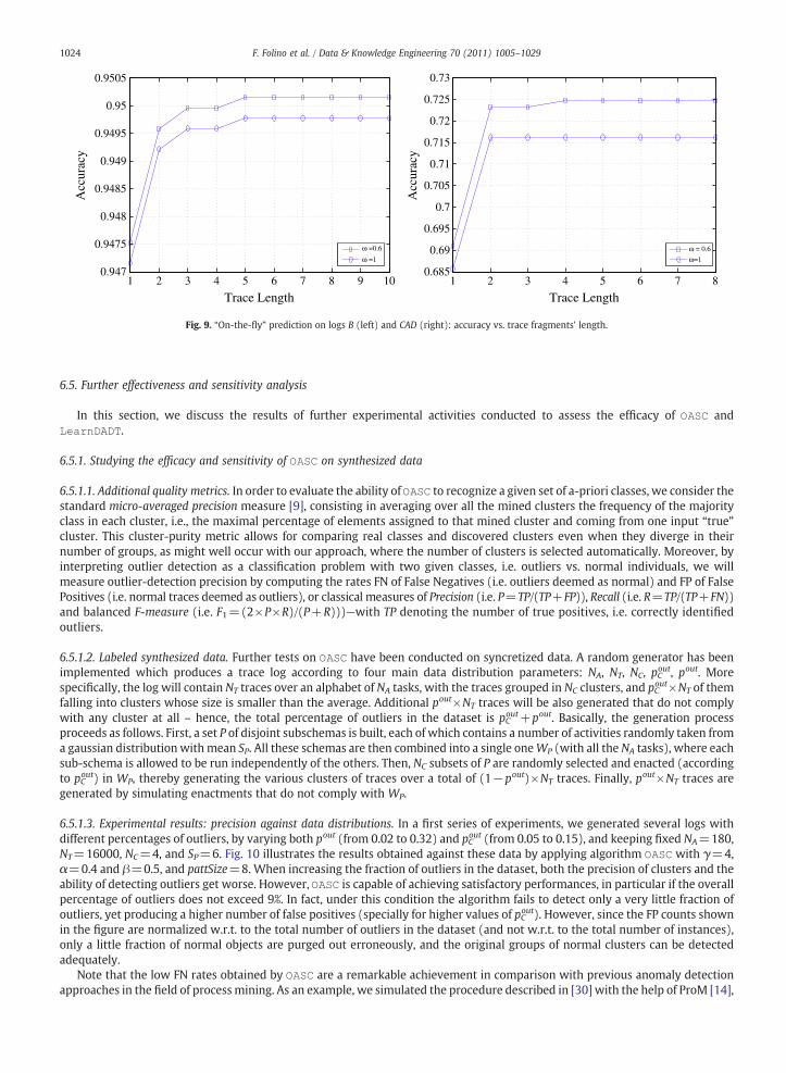
6.5. Further effectiveness and sensitivity analysis

In this section, we discuss the results of further experimental activities conducted to assess the efficacy of OASC andLearnDADT.

6.5.1. Studying the efficacy and sensitivity of OASC on synthesized data

6.5.1.1. Additional quality metrics. In order to evaluate the ability of OASC to recognize a given set of a-priori classes, we consider thestandard micro-averaged precision measure [9], consisting in averaging over all the mined clusters the frequency of the majorityclass in each cluster, i.e., the maximal percentage of elements assigned to that mined cluster and coming from one input “true”cluster. This cluster-purity metric allows for comparing real classes and discovered clusters even when they diverge in theirnumber of groups, as might well occur with our approach, where the number of clusters is selected automatically. Moreover, byinterpreting outlier detection as a classification problem with two given classes, i.e. outliers vs. normal individuals, we willmeasure outlier-detection precision by computing the rates FN of False Negatives (i.e. outliers deemed as normal) and FP of FalsePositives (i.e. normal traces deemed as outliers), or classical measures of Precision (i.e. P=TP/(TP+FP)), Recall (i.e. R=TP/(TP+FN))and balanced F-measure (i.e. F1=(2×P×R)/(P+R)))—with TP denoting the number of true positives, i.e. correctly identifiedoutliers.

6.5.1.2. Labeled synthesized data. Further tests on OASC have been conducted on syncretized data. A random generator has beenimplemented which produces a trace log according to four main data distribution parameters: NA, NT, NC, pCout, pout. Morespecifically, the log will contain NT traces over an alphabet of NA tasks, with the traces grouped in NC clusters, and pC

out×NT of themfalling into clusters whose size is smaller than the average. Additional pout×NT traces will be also generated that do not complywith any cluster at all – hence, the total percentage of outliers in the dataset is pC

out+pout. Basically, the generation processproceeds as follows. First, a set P of disjoint subschemas is built, each of which contains a number of activities randomly taken froma gaussian distribution withmean SP. All these schemas are then combined into a single oneWP (with all the NA tasks), where eachsub-schema is allowed to be run independently of the others. Then, NC subsets of P are randomly selected and enacted (accordingto pC

out) in WP, thereby generating the various clusters of traces over a total of (1−pout)×NT traces. Finally, pout×NT traces aregenerated by simulating enactments that do not comply with WP.

6.5.1.3. Experimental results: precision against data distributions. In a first series of experiments, we generated several logs withdifferent percentages of outliers, by varying both pout (from 0.02 to 0.32) and pC

out (from 0.05 to 0.15), and keeping fixed NA=180,NT=16000, NC=4, and SP=6. Fig. 10 illustrates the results obtained against these data by applying algorithm OASC with γ=4,α=0.4 and β=0.5, and pattSize=8. When increasing the fraction of outliers in the dataset, both the precision of clusters and theability of detecting outliers get worse. However, OASC is capable of achieving satisfactory performances, in particular if the overallpercentage of outliers does not exceed 9%. In fact, under this condition the algorithm fails to detect only a very little fraction ofoutliers, yet producing a higher number of false positives (specially for higher values of pCout). However, since the FP counts shownin the figure are normalized w.r.t. to the total number of outliers in the dataset (and not w.r.t. to the total number of instances),only a little fraction of normal objects are purged out erroneously, and the original groups of normal clusters can be detectedadequately.

Note that the low FN rates obtained by OASC are a remarkable achievement in comparison with previous anomaly detectionapproaches in the field of processmining. As an example, we simulated the procedure described in [30] with the help of ProM [14],

1 2 3 4 5 6 7 8 9 100.947

0.9475

0.948

0.9485

0.949

0.9495

0.95

0.9505A

ccur

acy

Acc

urac

y

ω =0.6

ω =1

1 2 3 4 5 6 7 80.685

0.69

0.695

0.7

0.705

0.71

0.715

0.72

0.725

0.73

ω = 0.6

ω=1

Trace Length Trace Length

Fig. 9. “On-the-fly” prediction on logs B (left) and CAD (right): accuracy vs. trace fragments' length.

1024 F. Folino et al. / Data & Knowledge Engineering 70 (2011) 1005–1029

by eventually extracting one single workflow model for each log, and then adopting the compliance with it as anomalousnesscriterion. The results in this case are notably worse than those in Fig. 10, since with all data distributions most of the outlier tracesare not recognized at all, thus leading to quite higher FN rates.

6.5.1.4. Experimental results: sensitivity to parameters. In a second set of experiments, we measured the sensitivity of OASC to itsinput parameters. To this end, we generated a log by setting pout=0.05 and pC

out=0.05, and the same values as above for all otherdata parameters. In the following we discuss results of experiments performed with β=0.1 and pattSize=8, by focusing on σ, γand α—which appeared to require more care in finding an appropriate setting.

Fig. 11 reports the micro-average precision scores computed for the clusterings discovered when using different values of σ, α,and γ. The first two parameters considerably impact the purity of the clusters. Probably, extreme values of σ yield too many(confusing) or too few patterns, which do not allow to separate the original classes into different clusters. Similarly, with extremevalues of α, beside having a negative effect on the quality of pattern clusters, one increases the risk of confusing normal instanceswith outliers, or viceversa. Satisfactory results are obtained with σ around 0.1 and with α between 0.25 and 0.35. Moreover, usingγ=4 seems to produce additional benefits, mainly as concerns the stability of results.

Fig. 12 sheds light on the ability to discriminate outliers from normal traces, for different configurations of the algorithm. Asexpected, recall scores tend to improve when increasing either σ or α, whereas an opposite behavior is exhibited by precisionresults. In fact, as discussed before, in both cases higher amounts of objects are likely to be assigned to no cluster (or to a small-sized outlier one). As to F-measure, a good trade-off seems to be found for α and σ near to 0.4 and to 0.1, respectively.

6.5.2. Sensitivity tests on LearnDADT

In order to better comprehend the behavior of algorithm LearnDADT, we tried it with different settings directly on the threereal datasets described in Section 6.2. Again, two different quality metrics of the DADT models were taken under consideration:

0.0025 0.005 0.01 0.02 0.04 0.08 0.16 0.320

0.1

0.2

0.3

0.4

0.5

0.6

0.7

0.8

0.9

1

σ

Mic

ro−

aver

aged

pre

cisi

on

Mic

ro−

aver

aged

pre

cisi

on

γ = 1

γ = 2

γ = 4

0.1 0.2 0.3 0.4 0.5 0.6 0.7 0.80

0.1

0.2

0.3

0.4

0.5

0.6

0.7

0.8

0.9

1

α

γ = 1

γ = 2

γ = 4

Fig. 11. Clustering accuracy vs. σ and γ (left), and vs. α and γ (right)—while fixing α=0.4 and σ=0.1, resp.

0 0.05 0.1 0.15 0.2 0.25 0.3 0.350

0.1

0.2

0.3

0.4

0.5

0.6

0.7

0.8

0.9

1M

icro

−av

erag

ed p

reci

sion

p out

C = 0.05

p out

C = 0.1

p out

C = 0.15

0 0.05 0.1 0.15 0.2 0.25 0.3 0.350

0.05

0.1

0.15

0.2

0.25

0.3

0.35

0.4

0.45

FP/F

N r

ates

pout

c = 0.05

pout

c = 0.1

pout

c = 0.15

p out

c = 0.05

pout

c = 0.1

pout

c = 0.15

FP / #outliers

FN / #outliers

poutpout

Fig. 10. Sensitivity to data distribution: clustering precision (left) and outlier detection precision (right).

1025F. Folino et al. / Data & Knowledge Engineering 70 (2011) 1005–1029

prediction accuracy—w.r.t. the clusters previously discovered by OASC (cf. Section 6)—, and conformance to task precedencescomputed through measure Conf (Section 6.1). We next focus only on the dependence of these measures on parameters ω and σ′,and consider the results of tests performed withminCard=0—actually, we noticed that this parameter (blocking the expansion ofnodes with too few instances), has little influence on the performances of themodel, and that post-pruning techniques are enoughto prevent overfitting.

The impact of ω on the metrics is illustrated in Fig. 13. As expected, in correspondence of higher values of ω we can observehigher accuracy and lower conformance, and vice-versa. This is true for all the datasets, with the exception of the first, where theconformance measure is always maximal, independently of LearnDADT parameters—maybe due to the very simple flow modelsthat characterize this case. In the other cases, it seems that a good trade-off is achieved aroundω=0.6. Lower values, indeed, causesensible accuracy loss. Fig. 14 lets us conclude that a similar effect is produced by σ′, apart from the fact that the best trade-offbetween accuracy and conformance happen for σ′∈ [0.1..0.15].

As a final remark note that further sensitivity tests were conducted on synthesized logs, with different distributions of non-structural attributes. However, since the outcomes of these tests, as far as concerns the effect of internal parameters, aresubstantially similar to those obtained on real logs, we omit their description here.

7. Discussion and conclusions

In this paper, we complemented current research on clustering approaches for process mining applications, by focusing ontwo problems that have received little attention in earlier literature: singling out outliers from input traces, and findingpredictive models for clustering results. We proposed an outlier-aware clustering method, where the similarity criterion

0.0025 0.005 0.01 0.02 0.04 0.08 0.16 0.320

0.1

0.2

0.3

0.4

0.5

0.6

0.7

0.8

0.9

1

σ

Precision

Recall

F−measure

0.1 0.2 0.3 0.4 0.5 0.6 0.7 0.80

0.1

0.2

0.3

0.4

0.5

0.6

0.7

0.8

0.9

1

α

PrecisionRecallF−measure

Fig. 12. Outlier detection accuracy vs σ, and α—while fixing α=0.4 and σ=0.1, resp., and γ=4.

0 0.2 0.4 0.6 0.8 10.4

0.5

0.6

0.7

0.8

0.9

1

ω

Acc

urac

y

Log A

Log B

Log CAD

0 0.2 0.4 0.6 0.8 10.4

0.5

0.6

0.7

0.8

0.9

1

ω

Con

f

Log A

Log B

Log CAD

Fig. 13. Sensitivity to ω (σ′=0.1): prediction accuracy (left) and conformance to task precedences (right).

1026 F. Folino et al. / Data & Knowledge Engineering 70 (2011) 1005–1029

roughly focuses on the idea of correlating the traces via a special kind of frequent (concurrency-aware) structural patterns,which are preliminary discovered as an evidence of “normal” behavior. Moreover, we discussed an algorithm for decision treelearning, which is aimed at capturing the relationships between structural execution classes (possibly found by clustering) andnon-structural process features. In order to predict as soon as possible the behavioral class of a novel enactment, the algorithmhas been devised in a way that the sooner an attribute tends to be known along the course of process enactments, the closer itappears to the root. Encouraging results on two complex real-life application scenarios confirmed the capability of theproposed approach to discover expressive and comprehensible process models, as well as to support run-time forecastingaccurately.

7.1. Comparison with related works

A first distinguishing feature of our work is its aim to induce a multi-perspective process model, capturing both typicalexecution scenarios and exceptional instances, as well as the links between these scenarios and non-structural context data.Indeed, our clustering approach is meant to identify both outliers and groups of normal instances, while previous proposalsin the field of process mining addressed just one of these kinds of tasks, possibly using the other in an instrumentalmanner. In fact, in other trace clustering approaches [2–4] no attention is given to the presence of outliers, while previousefforts for mining anomalous traces [30,31] adopt a model-based strategy, disregarding to separate multiple executionscenarios.

Technically, our approach combines the mining of advanced structural patterns with a coclustering scheme focused on theassociations between such patters and the given log traces. This makes our approach neatly different from those that simply treatthe log traces as symbolic sequences (e.g. [4]). Even though structural patterns were already used for clustering purposes inprevious works [2,3], our approach is different both for the kind of patterns adopted, and for its fuzzy notion of support (takinginto account the interleaving of parallel branches). Moreover, differently from these works, we do not use such patterns forproducing a vectorial representation of the traces, prior to the application of classic clustering methods. Rather, we look at theassociations between traces and patterns themselves in a way similar to coclustering methods [9], famous for their goodperformances against sparse high-dimensional data. In fact, in the case of a complex process with a high number of activities(and possibly of relevant structural patterns), any vector-based approach like [2,3] has a considerable risk to incur in thenotorious “curse of dimensionality” problem. These aspects also differentiate our work from other approaches to the detectionof outliers among log traces or sequences, which either disregard the presence of different behavioral clusters [30,31], or relyon proximity notions or on generative models (e.g., [27–29]) not taking care of the peculiar nature of process instances(e.g., intra-parallelism).

Finally, as to the induction of predictive models, we reused a classical top-down greedy scheme for the induction of a decisiontree, by integrating into it the constraints needed to support on-the-fly prediction. The reasons for this choice are the readability ofdiscovered models, the availability of noise-resistant and efficient induction algorithms, and the possibility to easily adapt thelearning scheme to the prediction of workflow executions' structure, by simply correcting the attribute selection criteria with theintroduction of a workflow-oriented score. Actually, our approach is independent of the particular induction algorithm andassociated purity metrics adopted in this paper (C4.5 and the Gain Ratio, respectively). In fact, our choice mainly served the goal ofdemonstrating that a pretty simple refinement of a classical induction algorithm is enough to effectively make on-the-flyprediction on the structure of a process instance.

0 0.05 0.1 0.15 0.2 0.25 0.3 0.35 0.40.4

0.5

0.6

0.7

0.8

0.9

1A

ccur

acy

Log A

Log B

Log CAD

0 0.05 0.1 0.15 0.2 0.25 0.3 0.35 0.40.4

0.5

0.6

0.7

0.8

0.9

1

σ'

Con

f

Log A

Log B

Log CAD

σ'

Fig. 14. Sensitivity to σ′ (ω=0.6): prediction accuracy (left) and conformance to task precedences (right).

1027F. Folino et al. / Data & Knowledge Engineering 70 (2011) 1005–1029

7.2. Future work

A number of challenging issues still remain open, and are left as the subject of future research work. Firstly, we are planning toenforce the practical relevance of the discovered behavioral classes by equipping our clustering approach with the capability totake into account key process performance indicators (such as task duration, task costs, and other application-dependent QoSmetrics), as well as to reuse available background knowledge on well-specified alternative usage scenarios.

Another avenue of research might be that of integrating the self-tuning techniques in [7] with our outlier detection method, asto reduce as much as possible human intervention in setting the appropriate thresholds in the mining process. More generally,based on our empirical sensitivity analysis, we notice that certain key parameters (e.g., σ, α) influence effectiveness resultsaccording to quasi-monotonic or quasi-convex curves. This behavior leaves space to the design of efficient self-tuning heuristicsfor a semi-automatic setting of the parameters.

Finally, in order to exploit fully the predictive power of discovered decision trees, it would be of interest to investigate theintegration of such models with run-time support mechanisms (involving, e.g., task scheduling and resource allocation) of somereal process management platforms.

References

[1] W.M.P. van der Aalst, B.F. van Dongen, J. Herbst, L. Maruster, G. Schimm, A.J.M.M. Weijters, Workflow mining: a survey of issues and approaches, DataKnowledge Engineering 47 (2) (2003) 237–267.

[2] G. Greco, A. Guzzo, L. Pontieri, D. Saccà, Discovering expressive process models by clustering log traces, IEEE Transactions on Knowledge and DataEngineering 18 (8) (2006) 1010–1027.

[3] M. Song, C.W. Günther, W. van der Aalst, Trace clustering in process mining, Business Process Management Workshops, 2008, pp. 109–120.[4] R.P.J.C. Bose, W.M.P. van der Aalst, Context aware trace clustering: towards improving process mining results, Proc of the SIAM International Conference on

Data Mining (SDM 2009), 2009, pp. 401–412.[5] S. Subramaniam, V. Kalogeraki, D. Gunopulos, F. Casati, M. Castellanos, U. Dayal, M. Sayal, Improving process models by discovering decision points,

Information Systems 32 (7) (2007) 1037–1055.[6] A. Rozinat, W.M.P. van der Aalst, Decision mining in ProM, Proc. of 4th Intl. Conf. on Business Process Management (BPM'06), 2006, pp. 420–425.[7] H.R.M. Nezhad, R. Saint-Paul, B. Benatallah, F. Casati, Deriving protocol models from imperfect service conversation logs, IEEE Transaction on Knowledge and

Data Engeneering 20 (12) (2008) 1683–1698.[8] L. Maruster, A.J.M.M. Weijters, W.M.P. van der Aalst, A. van den Bosch, A rule-based approach for process discovery: dealing with noise and imbalance in

process logs, Data Mining and Knowledge Discovery (1) (2006) 67–87.[9] I.S. Dhillon, S. Mallela, D.S. Modha, Information-theoretic Co-clustering, 2003, pp. 89–98.

[10] A.J. Enright, S. Van Dongen, C.A. Ouzounis, An efficient algorithm for large-scale detection of protein families, Nucleic Acids Research 30 (7) (April 2002)1575–1584.

[11] J. Quinlan, C4.5: Programs for Machine Learning, Morgan Kaufmann, 1993.[12] J.R. Quinlan, Induction of decision trees, Machine Learning 1 (1) (1986) 81–106.[13] A.J.M.M. Weijters, W.M.P. van der Aalst, Rediscovering workflow models from event-based data using little thumb, Integrated Computer-Aided Engineering

10 (2) (2003) 151–162.[14] B.F. van Dongen, A.K.A. de Medeiros, H.M.W. Verbeek, A.J.M.M. Weijters, W.M.P. van der Aalst, The ProM framework: a new era in process mining tool

support, Proc. of 26th Intl Conf on Applications and Theory of Petri Nets, 2005, pp. 444–454.[15] A. Rozinat, W.M.P. van der Aalst, Conformance checking of processes based on monitoring real behavior, Information Systems 33 (1) (2008) 64–95.[16] P.-N. Tan, M. Steinbach, V. Kumar, Introduction to Data Mining, First Edition Addison-Wesley Longman Publishing Co., Inc., 2005[17] J. Yang, W. Wang, CLUSEQ: efficient and effective sequence clustering, Proc. of 19th IEEE Int. Conf. on Data Engineering (ICDE'03), 2003, pp. 101–112.[18] V. Barnett, T. Lewis, Outliers in Statistical Data, John Wiley, 1994.[19] D. Hawkins, Identifications of Outliers, Chapman and Hall, 1980.[20] E.M. Knorr, R.T. Ng, V. Tucakov, Distance-based outliers: algorithms and applications, VLDB Journal 8 (3–4) (2000) 237–253.[21] M.M. Breunig, H.-P. Kriegel, R.T. Ng, J. Sander, LOF: identifying density-based local outliers, Proc. of 2000 ACM SIGMOD International Conference on

Management of Data (SIGMOD'00), 2000, pp. 93–104.[22] I. Gath, A. Geva, Fuzzy clustering for the estimation of the parameters of the components of mixtures of normal distribution, Pattern Recognition Letters 9

(1989) 77–86.[23] M. Jiang, S. Tseng, C. Su, Two-phase clustering process for outlier detection, Pattern Recognition Letters 22 (2001) 691–700.[24] D. Yu, G. Sheikholeslami, A. Zhang, FindOut: finding outliers in very large datasets, Knowledge and Information Systems 4 (4) (2002) 387–412.[25] V. Chandola, A. Banerjee, V. Kumar, Anomaly detection : a survey, ACM Computing Surveys 41 (3) (2009) Article 15.[26] S.A. Hofmeyr, S. Forrest, A. Somayaji, Intrusion detection using sequences of system calls, Journal of Computer Security 6 (3) (1998) 151–180.[27] C.C. Michael, A. Ghosh, Two state-based approaches to program-based anomaly detection, Proc. of 16th Annual Computer Security Applications Conference

(ACSAC'00), 2000, p. 21.[28] P. Sun, S. Chawla, B. Arunasalam, Mining for outliers in sequential databases, Proc. of 6th SIAM Int. Conf. on Data Mining, 2006, pp. 94–104.[29] C. Warrender, S. Forrest, B. Pearlmutter, Detecting intrusions using system calls: alternative data models, IEEE Symposium on Security and Privacy, 1999,

pp. 133–145.[30] F. de Lima Bezerra, J. Wainer, W.M.P. van der Aalst, Anomaly detection using process mining, Enterprise, Business-Process and Information SystemsModeling

(BPMDS'09), 2009, pp. 149–161.[31] F. de Lima Bezerra, J. Wainer, Anomaly detection algorithms in business process logs, Proc. of 10th Int. Conf. on Enterprise Information Systems (ICEIS'08),

2008, pp. 11–18.[32] T. Hastie, R. Tibshirani, J. Friedman, The Elements of Statistical Learning, Springer, 2003.[33] L. Breiman, J. Friedman, R. Olshen, C. Stone, Classification and Regression Trees, Wadsworth and Brooks, 1984.[34] D. Heath, S. Kasif, S. Salzberg, Induction of oblique decision trees, Journal of Artificial Intelligence Research 2 (2) (1993) 1–32.[35] Q.Wang, C. Suen, Large tree classifierwithheuristic searchandglobal training, IEEETransactionsonPatternAnalysis andMachine Intelligence9 (1) (1987)91–102.[36] J.R. Quinlan, Simplifying decision trees, International Journal of Man-Machine Studies 27 (3) (1987) 221–234.[37] M. Mehta, J. Rissanen, R. Agrawal, MDL-based decision tree pruning, Proc. of 1st Int. Conf. on Knowledge Discovery and Data Mining (KDD'95), 1995,

pp. 216–221.[38] L. Rokach, O.Maimon, Top-down induction of decision trees classifiers— a survey, IEEE Transactions on Systems,Man and Cybernetics 35 (4) (2005) 476–487.[39] I.H. Witten, E. Frank, Data Mining: Practical Machine Learning Tools and Techniques, 2nd Ed. Morgan Kaufmann, 2005.[40] I.H. Witten, Online Appendixavailable at, http://si.deis.unical.it/guzzo/wfmining/appendix.pdf.

1028 F. Folino et al. / Data & Knowledge Engineering 70 (2011) 1005–1029

Francesco Folino is currently researcher at the Institute of High Performance Computing and Networks (ICAR-CNR) of the NationalResearch Council of Italy. He graduated in Computer Science Engineering in 2003, and he holds a Ph.D. in Computer ScienceEngineering from the University of Calabria (Italy) in 2006. From 2003 to 2006 he was a Ph.D. student at the University of Calabria. Hisresearch interests are focused on knowledge discovery and data mining; Data Warehousing and OLAP. He is involved in severalprojects at ICAR-CNR concerning applications of data mining and knowledge discovery techniques.

Gianluigi Greco received the Laurea degree in Computer Science Engineering from the University of Calabria, Italy, in 2000. Currently,he is an Assistant Professor of computer science in the Department of Mathematics at the University of Calabria. His main researchinterests are across the areas of Databases and Artificial Intelligence and focus on database theory, knowledge representation,nonmonotonic reasoning, computational complexity, and deductive databases.

Antonella Guzzo received her Laurea degree in engineering from the University of Calabria (UNICAL) and holds a Ph.D. in SystemEngineering and Computer Science from the DEIS Department of UNICAL. Currently, she is an assistant professor in Computer Sciencein the Faculty of Engineering of UNICAL and member of the IEEE Task Force in Process Mining. Previously, she was a research fellow atthe High Performance Computing and Networks Institute (ICAR-CNR) of the National Research Council of Italy. Her research interestsinclude Process Mining, Data Mining and Knowledge Representation.

Luigi Pontieri received the Laurea Degree in Computer Engineering, in July 1996, and the Ph.D. in System Engineering and ComputerScience, in April 2001, from the University of Calabria. Currently, he is a researcher at the High Performance Computing and NetworksInstitute (ICAR-CNR) of the National Research Council of Italy, and a contract professor with the University of Calabria, Italy. Hisresearch interests mainly concern the fields of Information Integration, Data Compression, Data Mining, and Process Analysis.

1029F. Folino et al. / Data & Knowledge Engineering 70 (2011) 1005–1029