CS194/294-129 Designing, Visualizing & Understanding Deep Neural Networks SP2018

Midterm Solutions

This is a closed-book exam with 8 questions. You can use one sheet of notes. Please write all your answers in this book. There are a total of 80 points for all questions, and you have 80 minutes to complete the exam. Please budget your time accordingly. Good luck!

1. (34 points) Give short answers for each of the following questions – 2 points each a) Describe two difficulties that computer vision algorithms face in dealing with images.

i.e. two characteristics of image formation that make it difficult to recover the image content. (2 points)

There are several examples, such as: (1) they can be from various poses and perspectives, (2) they may vary in color and brightness, (3) there might be occlusion or ambiguity of objects.

b) Deep networks typically require a lot of data to train from scratch, but can be “fine tuned” for another task quickly. Explain this in terms of the features computed in the layers. (2 points)

The first training procedure can train the parameters of the network such that it works well for the task (e.g., image classification). These parameters can then be transferred to another task (e.g., image captioning) under the hypothesis that the parameters are able to process the inputs and produce lower-dimensional features which capture the essence of the data, allowing for faster fine-tuning on another task.

c) What are expected risk and empirical risk? What do machine learning algorithms minimize? (2 points)

Expected risk is the expectation, over all possible datasets, of the difference between a model’s predictions and the actual targets (where the precise meaning of “difference” is encoded via a “loss” function). Empirical risk is the difference between a model’s predictions and true targets over a fixed sample of data. Machine learning algorithms minimize empirical risk because in practice they do not have access to the expected risk, and can only approximate it with data.

d) Why isn’t L2 loss used to optimize a logistic regression model? What loss is used instead and why? (2 points)

A logistic regression model is designed for binary classification of inputs into two classes (without loss of generality, we define as 0 or 1), but an L2 loss is designed for a continuous-valued target and thus not a natural loss for the task. To optimize a logistic regression model, we use the (binary) cross-entropy loss because that will directly encourage our outputs to match either 0 or 1.

e) Newton’s second-order method converges to what kinds of points on the loss function surface? List all that apply. (2 points)

Local minima (which includes the global minima as one example) and saddle points.

f) SVMs use a hinge loss that maximizes a margin around the decision boundary. What are the benefits of a max-margin classifier such as SVM? Feel free to use a picture (2 points)

The benefit is that we can encourage the decision boundary to be such that it divides the classes in a way that maximizes the distance from the nearest points in each class to the margin. This can be useful for avoiding overfitting, as intuitively the SVMs that generalize will not have decision boundaries too close to items in the training data. [Draw diagram of SVM in the 2D case, with Xs and Os representing two classes, and the max margin such that it creates as large a gap between the X and O elements -- see lecture for examples]

g) The multi-class SVM classifier we derived in class used a margin loss. How was this margin defined? (2 points)

For each data point (x_i, y_i), it is:

f_y_i(x_i) - f_j(x_i) for all classes j =/= y

This is derived based on the original SVM loss max(0, 1 - yw^Tx) whereas now we try to maximize the margins for all other class loss, for each other class j we form a loss:

max(0, 1 - f_y_i(x_i) + f_j(x_i)) And the loss is summed/averaged during training for each data point (x_i, y_i).

This is formulated such that each f_y_i serve as a OvA classifier, and attempt to maximize the output (hence classifying x_i on the positive side of the SVM) for only the relevant class classifier y_i for each x_i. More generally the f(x) can be replaced by potentially a more complicated model like a neural network.

For a full training data, use the average of the losses of the individual terms.

h) What is the relationship between multiclass logistic regression with binary data and multiclass naïve Bayes with binary data? (2 points)

A multiclass logistic regression model can exactly learn a multiclass naive Bayes.

i) How does the effective learning rate of ADAGRAD vary with the number of steps, t ? (2 points)

The denominator contains the sum of the squares of the past gradients, and because every term is positive, the gradient will decrease proportionally to this accumulating value ≈ 1/sqrt(t).

j) The loss functions of deep networks are non-convex and there was concern in the early days of the field that gradient methods may get trapped in poor (i.e. high loss) local optima. Describe with a sketch how local optima were observed to behave on a simple model, than explain why SGD performs well in practice on such models. (2 points)

SGD can get trapped in local optima, as suggested by the following diagram where the initial point gets stuck at a local minima, because gradients vanish at

those points. (Assume that the values on the graph represent loss; higher is worse, and that the red arrow indicates the direction of the SGD update.)

In practice, SGD works well because, though neural networks have many local minima, empirically it appears that they each have similar loss values.

k) If a data block in a convolutional network has dimension , and we apply a convolutional filter to it of dimensions×W × D 200 × 200 ×128H =

, what is the dimension of the output data block? (2 points)×D ×7×128HF × W F = 7

(This depends on what assumptions we make about stride!! Since it didn’t mention padding we often assume 0. A stride of 1 is often the default, but it’s good to clarify.) With padding 0 and a stride of 1, the output will be 194 x 194 x 1. There are 194 values because a 7x7 stride, when we view strides as defined by their top left corners, they extend all the way across the 200 dimensions until hitting the 194th dimension, upon which time they can’t extend further. There are 1 depth channels as there are 1 filter of depth 128.

l) Why are convolutional layers more commonly used than fully-connected layers for image processing (2 points)

Convolutional layers are better suited for processing images because: (a) they assume that nearby pixels share similar structure, (b) the parameters for a single filter are shared across the entire input image in the sense that a single filter

“slides” across an image and produces a new output with one image channel. This allows the parameters to be invariant to the location of objects in images.

m) Dropout layers implement different forward functions at train and test time. Explain what they do. Let p be the probability that node value is retained. (2 points)

During training time, dropout will retain nodes independently with probability p (and drop with probability 1-p). The nodes that are dropped mean they multiply the input by zero. The nodes that are retained should have their inputs scaled by a factor of 1/p so that during test time, one can simply use the raw values with no adjustment (with and without dropout). Thus, during the training pass, the expected value of the output after each node will be scaled appropriately.

n) Why does prediction averaging work for most ensembles of models, but parameter

averaging only works for models which are snapshots from a single model during training? (2 points)

Prediction averaging often works because models are trained independently and then the majority vote or average of the output of the models can be more robust.

Parameter averaging rarely works when models are trained independently, because there are too many possible parameterizations of different models that can produce similar output. Using a past history of a model’s snapshots can work since the parameters will be relatively constrained in a smaller subset of the parameter space.

o) Sketch a simple recurrent network, with input x, output y, and recurrent state h. (2 points)

[See the following figure, from the Lecture 9 slides]

p) Give the update equations for a simple RNN unit in terms of x, y, and h. Assume it uses tanh non-linearity. (2 points)

[These are the update equations from the previous question.]

To generate the hidden unit at each step:

h_t = tanh(W_{hh}*h_{t-1} + W_{xh}x_t)

and to generate the y at each time step:

y_t = W_{hy}*h_t

This assumes that we generate an output at each time step (i.e., a many-to-many model with the same output size as input size, but the general idea holds for other kinds of RNNs.

q) What is the difference between the and recurrent states in an LSTM (Long c h Short-Term Memory) recurrent unit? (2 points)

On a high-level: h (hidden state) is the output at the current time step, while c is the updated cell state that keeps a memory accumulated from the previous inputs. h is a non-linear transformation dependent on c.

2. (8 points) In class, for the multivariate linear regression model we wrote the squared xy = A error loss for n data items asL

Ax ) L (A) = ∑n

i=1x A( i

T T − yiT) ( i − yi

And showed that it is minimized when:

where and MA = M yx xx−1 xM xx = ∑

n

i=1xi i

T xM yx = ∑n

i=1yi i

T

Suppose now we add an L2 regularizer term to the loss. What is the new solution for‖A‖λ 2 A? How does this regularizer make it easier to minimize the error for ill-conditioned systems?

3. (8 points) Suppose a deep network layer performs a simple bias normalization:

μ = 1N ∑

N

i=1X i

for XY i = i − μ , ,i = 1 … N

Where N is the dimension of input X and output Y. Note that the sum is taken over the coordinates of the input sample, not the elements of a minibatch as in batch normalization.

Compute the jacobian in element form, i.e.

dX i

dY j = …

Given the output jacobian vector , how quickly can you compute the input jacobian(Y )JL as a function of N?(X)JL

4. (6 points) Suppose you have a dataset with N samples. You would like to train a deep network and tune learning rate, minibatch size and regularization to give the best model.

Describe the cross-validation design you would use to tune the hyper-parameters, and produce the most accurate possible (unbiased) estimate of the model’s test loss. i.e. describe how to partition the data, and what to do with each partition.

One way is to partition the N data points into K (roughly) equal-sized folds (a common choice is K=10). Then, for a given trial, run training 10 different times, each time with a different training set and then the validation set determined by the fold index (and with the network weights randomly initialized for whatever parameters are being tuned).

Select the desired hyperparameters to tune. Generate a random hyperparameter search grid of values to get a diverse set of candidates for each hyperparameter; these values can also be generated “coarsely” by picking a wide range of possibilities (and then “fine-tuned” later). For each combination of hyperparameters, run the training for the 10 times as described earlier, and average the results on the validation set.

Choose the hyperparameter set with the best average performance on the validation set. If the best hyperparameter set occured at the “extremes” of the hyperparameter values tried (e.g., if the best learning rates are always around 0.1 but the range of values tried was around [0.0001, 1]) or if the hyperparameter values tried covered too coarsely a region, then redo the search with appropriately scaled hyperparameter regions.

This assumes we don’t have a test set, or that a test set will be provided to us later at some point.

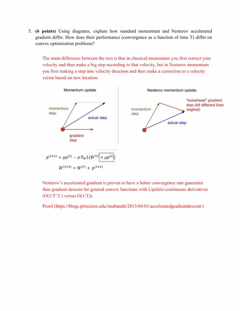
5. (6 points) Using diagrams, explain how standard momentum and Nesterov accelerated gradient differ. How does their performance (convergence as a function of time T) differ on convex optimization problems?

The main difference between the two is that in classical momentum you first correct your velocity and then make a big step according to that velocity, but in Nesterov momentum you first making a step into velocity direction and then make a correction to a velocity vector based on new location.

Nesterov’s accelerated gradient is proven to have a better convergence rate guarantee than gradient descent for general convex functions with Lipshitz-continuous derivatives (O(1/T^2 ) versus O(1/T)).

Proof (https://blogs.princeton.edu/imabandit/2013/04/01/acceleratedgradientdescent/)

6. (6 points) Compare GoogLeNet and Residual networks (ResNets). What are the main architectural features of each, and how did they lead to improvements over previous design? Use diagrams of the networks as appropriate

GoogleLeNet introduced the inception module, which passes values through four parallel convolution streams, with concatenations at the end. The 1x1 convolutions reduce the dimension of data and thus the compute bottlenecks. There is a notable improvement over prior designs in parameter efficiency; the first version has roughly 4 million parameters, compared to about 60 million for AlexNet.

ReNets introduced skip connections in the network, which introduce new connections between layers and those beyond it (not the ones directly after it), so that those values get added to other values that were passed through conventional layers. This lets values propagate forward in the network for a longer period of time before modified. In turn, gradient can propagate faster backwards since the addition gate map gradients equally through its outgoing edges, and gradients on the residual edges can “skip” other layers.

For diagrams of the networks, see Lecture 06 slides.

7. (6 points) Modify the diagram below which shows Fast R-CNN, to represent Faster R-CNN. Explain in words what changed between the models.

In words, to change the above figure to Faster R-CNN:

- Insert a “Region Proposal Network” (RPN) which will generate the proposals. (The proposals are the rectangles in the Fast R-CNN diagram which represent bounding boxes where desired objects might be located.) The RPN takes the final convolutional layer from Fast R-CNN as input, and process it to produce proposals.

- That final convolutional layer from Fast R-CNN also gets passed as input to the Region of Interest (RoI) pooling layer as usual. The main difference in Faster R-CNN is that the RoI pooling layer takes proposals from the RPN as input, instead of a non-learning algorithm such as Selective Search.

- In addition, the RPN needs its own classification and regression losses, in addition to the usual classification and regression losses for the final output layer.

8. (6 points) Briefly contrast the backward updates for a ReLU layer using (i) normal backpropagation, (ii) guided backpropagation and (iii) deconvolution

Standard Backprop: (f_current_layer(x) > 0) * Upstream Gradients

Guided Backprop: (f_current_layer(x) > 0) * (Upstream Gradients > 0) * Upstream Gradients

Deconvolution: (Upstream Gradients > 0) * Upstream Gradients

Whereas (n > 0) = 1 when it evaluates to true, else 0