Engineering Geology 179 (2014) 146–157

Contents lists available at ScienceDirect

Engineering Geology

j ourna l homepage: www.e lsev ie r .com/ locate /enggeo

Microtremor recordings in Northern Mississippi

Z. Guo, A. Aydin 1, J.S. KuszmaulDepartment of Geology and Geological Engineering, The University of Mississippi, University, MS 38677, United States

E-mail address: aaydin@olemiss.edu (A. Aydin).1 Tel.: +1 662 915 1342; fax: +1 662 915 5998.

http://dx.doi.org/10.1016/j.enggeo.2014.07.0010013-7952/© 2014 Elsevier B.V. All rights reserved.

a b s t r a c t

a r t i c l e i n f o

Article history:Received 7 August 2013Received in revised form 3 April 2014Accepted 3 July 2014Available online 15 July 2014

Keywords:MicrotremorVibration directionWind effectPredominant frequencyUnconsolidated sediment thicknessNorthern Mississippi

This paper presents the results of 305 single-point microtremor recordings, covering NorthernMississippi that issituatedwithin theUpperMississippi Embayment area. Both long- and short-term recordingswere obtained by aLE-3D/20s seismometer, over a large network of points where the unconsolidated sediment thickness (UST)varies from zero to 1400 m. Applying the Nakamura method, the recordings were processed to determine pre-dominant frequency (f0) and its relation to UST. Initial results of wind influence on the frequency spectra (partic-ularly in low frequency band, 0.05–0.2 Hz), and dominant vibration direction are also presented. It is shown thatanalysis of systematic microtremor recordings can provide a stable and reliable estimation of the predominantfrequency, from which estimates of average shear wave velocity of overall sediment profile can be derived. Pre-dominant frequency (and average shearwave velocity) is reasonably well correlatedwith UST.Wind and humanactivities are found to produce peaks over the low frequency band (b0.2 Hz) of H/V spectra. It is also establishedthat vibration direction is strongly frequency-dependent above 0.2 Hz and time-dependent below this value.

© 2014 Elsevier B.V. All rights reserved.

1. Introduction

Microtremors are uninterrupted and imperceptible ambient vibra-tions of the ground due to a multitude of natural and anthropogenicsources of disturbances, strengths of which vary in time and space.Kanai and Tanaka (1954)was thefirst to recognize thatmicrotremor re-cordings can be used to estimate the site-effect parameters. The use ofmicrotremors gained popularity after introduction of the horizontal tovertical spectral ratio (HVSR) method by Nakamura (1989). Reliabilityof theHVSRmethod in estimating the site-effect parameters is now sup-ported by two decades of countless research worldwide, especially inJapan and Europe (Bard and SESAME-Team, 2005; Nakamura, 2008).

In this study, a total of 305 single-point recordings were systemati-cally collected and analyzed using the HVSR method to determine dis-tributions of the site-effect parameters (predominant frequency f0 andamplification factor) and their relation with unconsolidated sedimentthickness (UST) across NorthernMississippi. A Lennartz LE-3D/20s seis-mometer with Eigen-frequency of 0.05 Hz and a RefTek 130-01/3 datalogger were used to capture and record the ambient noise. This seis-mometer enables stable recording of low frequency (down to 0.05 Hz)noisewhich is mainly caused by natural sources, and thus helps identifyf0 in areas with thick unconsolidated sedimentary sequence. Utilizingthis property, the low frequency band (0.05–0.2 Hz) of the recordingswas analyzed to gain insight into the time variability of noise spectra,HVSR and vibration direction, and how these variations correlate withdirection and speed of wind.

2. Study area

The study area is largely situated within theMississippi Embayment(Figure 1), northern section of which includes the NewMadrid SeismicZone (NMSZ) of moderate to heavy potential damage. The stratigraphicsequence of the area mainly consists of unconsolidated sediments withUST reaching 1400malong theMississippi River floodplainwhereas thebedrock is exposed along the eastern boundary (Table 1 and Figure 1).NMSZ is the most seismically active area in the central part of NorthAmerica (Schweig, 1996) and the earthquake potential in NMSZ ishigh (Johnston, 1985). The New Madrid earthquakes of 1811–1812, asequence of three events with moment magnitudes as large as 8.0(Johnston and Schweig, 1996), are estimated to have affected an areaof approximately 2.5 million km2 with an intensity of V or greater(Nuttli, 1974) due to strong site effects. Northern Mississippi, about160 km to the south of the estimated epicenter of these earthquakes, ex-perienced intensities ranging fromVII to IX (Stover and Coffman, 1993).

Covering that part of the Upper Mississippi Embayment (Figure 1)area to the north of the Mississippi–Tennessee state line, there are ex-cellent studies utilizing microtremors to determine f0 using the HVSRmethod and estimate shear wave velocity Vs profile by empirical rela-tions between f0, UST and Vs (Bodin and Horton, 1999; Bodin et al.,2001; Park and Hashash, 2005; Rosenblad and Goetz, 2010; Langstonand Horton, 2011). Bodin and Horton (1999) recorded microtremorsat six locations along the southern state line of Tennessee covering aUST range of 0 to 950 m. Bodin et al. (2001) correlated UST with f0 inand around Shelby County, TN where UST ranges from about 300 m to1050 m. To date, there are no similar studies to the south of the stateline, i.e. Northern Mississippi, though the area also suffered significant

Fig. 1. Geological map of the study area (MDEQ) and locations of microtremor recordingswithin the regional setting of the Upper Mississippi Embayment. Note the isopachs of unconsol-idated sediments (UST) (based on Bodin et al., 2001) and the epicenters of earthquakes in the NewMadrid Seismic Zone during 1974–2012 (from the Center for Earthquake Research andInformation at http://www.memphis.edu/ceri/seismic/catalogs/index.php).

Table 2Frequency dependent threshold values of HVSR standard deviation.Bard and SESAME-Team (2005).

Frequency range (Hz) b0.2 0.2–0.5 0.5–1.0 1.0–2.0 N2.0

147Z. Guo et al. / Engineering Geology 179 (2014) 146–157

damage during the New Madrid earthquakes of 1811–1812, and haswitnessed extensive infrastructure and population growth in the lasttwo decades. The lack of strong ground motion records in NorthernMississippi eliminates chances for independent estimates of site-effectparameters at nearby recording points.

Table 1General stratigraphic sequence of Northern Mississippi.Based on MDEQ.

Series Group Formation Description

Holocene Alluvium Loam, sand, gravel and clayLoess Grayish to yellowish-brown massive silt

Eocene Claiborne Kosciusko Irregularly bedded sand, clay and some quartziteTallahatta Predominantly sand, locally glauconitic, containing clay stone and clay lenses and abundant clay stringers

Wilcox Irregularly bedded fine to coarse sand, more or less lignitic clay, and lignitePaleocene Midway Porters Creek Dark-gray clay containing slightly glauconitic, micaceous sand lenses

Clayton Greenish-gray coarsely glauconitic sandy clay and marlThe lower part is crystalline sandy limestone and loose sand

Upper Cretaceous Selma Prairie Bluff chalk: compacted chalk, sandy chalk, and calcareous clayRipley Gray to greenish-gray glauconitic sand, clay and sandy limestone

Demopolis chalk: chalk and marly chalk containing fewer impurities than underlying and overlying formationsMooreville chalk: marly chalk and calcareous clayCoffee sand: light-gray cross-bedded to massive glauconitic sand, sandy clay and calcareous sandstoneTombigbee sand: massive fine glauconitic sand

Eutaw More or less cross-bedded and thinly laminated glauconitic sand and clayTuscaloosa Light and vari-colored irregularly bedded sand, clay and gravel

Mississippian Lime stones, chert and shale of Meramec, Osage and Kinderhook ageChattanooga shale and underlying lime stones of early Devonian age

Threshold value 3.0 2.5 2.0 1.78 1.58

× 103

×103

Frequency ofoccurrence

×103

θ

NS

EW

H

a) b)

Fig. 2. a) Polar scatter chart of vibration directions in the horizontal plane and amplitude frequency distributions of the horizontal components of vibrations. Note the amplitude frequen-cies have normal distributions centered at zero; and b) definition of the vibration direction angle θ.

148 Z. Guo et al. / Engineering Geology 179 (2014) 146–157

3. Field setup and data processing

Two types of recordings were taken (Figure 1): 1) long term re-cordings (LTRs) each lasting at least 6 h and carried out at selectedlocations with different bedrock depths, specifically exposed (AL1),

Table 3Summary of recording conditions and site effect parameters of LTR (*) and nearest STR points

Point UST(m)

Fundamentalfrequency f0

Distance tonearest LTRpoint (km)

Groundtype1

AL1* 0 NO 0 S

AL2 0 NO 7.6 NE B

AL3 0 NO 24.2 NWW B

T1* 10.2 2.018 0 C

T2* 10.2 2.466 0 C

NM 10 0.1 NO 19.5 SSE A

NM 11 9.1 1.034 3.7 N S

NM 46 26.4 0.904 6.4 S A

NM 47 10.9 2.157 11.3 S A

NM 140 0.1 7.686 55.0 NE C

NM 141 0.1 10.043 37.7 NEE C

NM 142 0.1 7.189 26.0 NE C

NM 144 0.1 NO 13.6 N GS

NM 14* 133.7 0.967 0 CT

NM 13 102.6 NR 14.1 SE A

NM 15 173.0 0.846 7.8 W S

NM 112 130.5 NR 10.2 S F

NM 113 179.3 0.846 11.3 SW C

NM 164 82.7 1.544 16.2 NE A

NM 165 100.0 0.791 7.9 E C

OC 37* 726.0 0.290 0 C

OC 38 726.0 0.290 0.4 E C

NM 34 763.8 0.271 7.1 W A

NM 93 674.2 0.310 5.1 NE A

NM 181 753.8 0.237 18.0 S C

NM 29* 1334.5 0.170 0 CT

NM 28 1267.9 NR 28.2 NNE A

NM 159 1387.6 0.159 18.7 W C

NM 160 1370.8 0.170 11.4 SW C

NM 210 1300.0 0.194 8.7 SE GS

Refer to Fig. 1 for the locations of recording points.

Abbreviations: NO — not observed; NR — not recognized.1) Ground type: C — Concrete; A — Asphalt; S — Soil; G — Gravel; CT— Ceramic Tile; F — Farm2) Exposure: A/C — Air conditioner; N — Natural wind; P — Protected by plastic box.3) Possible noise sources: F— Footsteps; RM—Runningmachines; T— Traffic;HT—Heavy traffiline; G — Grass.

shallow (T1, T2 and NM 14), moderately deep (OC 37 and OC 38) anddeep (NM 29); and 2) short term recordings (STR) each lasting15 min. The STR can be further categorized into two types in terms ofthe wind exposure of the sensor: 1) STR-I, sensor exposed to wind;and 2) STR-II, sensor protected from wind by a plastic box. Fig. 1

in Fig. 4.

Exposure2 Recordingperiod(STR in min)

Possiblenoisesources3

Winddirection

Windspeed(mph)

N 6 h

N 15 T

N 15 T

A/C 8 h F, T

A/C 8 h F, T

N 15 HT Calm Calm

N 15 LT

N 18 HT SSE 8

N 15 MT, A/C SE 8

P 15 T S 4

P 15 R, HT SSE 4

P 19 T, RM S 13

P 15 T SSE 7

A/C 11 h S Calm Calm

N 15 HT Calm Calm

N 15 G Calm Calm

N 15 Calm Calm

N 15 MT Calm Calm

P 15 LT Calm Calm

P 15 MT Calm Calm

A/C28+43+47.5

+66 hF

A/C 16 h RM

N 15 SE 4

N 15 Calm Calm

P 15 T S/SE 9

A/C 12 h S Calm Calm

N 15 MT Calm Calm

P 19 MT NW 15

P 8 NNW 16.5

P 15 R SWW 19.6

land.

c;MT—Moderate traffic; LT— Light traffic; R—River; A/C—Air conditioner unit; S— Sewer

149Z. Guo et al. / Engineering Geology 179 (2014) 146–157

illustrates the layout and types of all recording points, aswell as the USTcontours (or inversely bedrock depth contours) of the Upper Mississip-pi Embayment. The point labeled as “OC” (south central part of the sur-veyed area) is the University of Mississippi main campus where 56closely spaced (500–1000 ft apart) recordings were carried out whichare mostly STR (15–30 min long) but includes two LTRs (OC 37 andOC 38).

Microtremor recordings are time series of small amplitude groundvibrations in three orthogonal directions, aligned to Vertical (V),North–South (N–S) and East–West (E–W). In this study, long-term re-cordings were split into 15–20 min segments without overlap, compa-rable to the length of short-term (15 min) recordings. The entire dataprocessing was performed by Geopsy, a freeware software suite devel-oped for the analysis of ambient vibrations (www.geopsy.com). Thesetime series were first filtered by an anti-triggering algorithm based ona prescribed range of short- to long-term average amplitude ratios(0.2 b STA/LTA b 2.5) to avoid occasional energy bursts and determine

Fig. 3. First column of graphs depicts the HVSR curves of LTR, while the second and third columwind speed, respectively, during recording period. Each row of the graphs represents an LTR poi1, 2011); e) OC 37 (20:00Mar. 12–15:00Mar. 14, 2011); f) OC 37 (11:45 Apr. 3–12:05 Apr. 5, 20MS) (17:45 Sep. 29–09:00 Sep. 30, 2011); and i) NM 29. Note: in rows c–g, dashed lines represe9:00).

appropriate sampling intervals (data windows with quasi-stationarysignal amplitude) for the spectral analysis (www.geopsy.org). Eachsample consisted of a set of three 50 s wide data windows of simulta-neous recordings in all three directions. Fast Fourier Transformwas uti-lized to obtain the samples' amplitude–frequency spectra, which weresmoothed using a Konno–Ohmachi functionwith the bandwidth coeffi-cient set to 40. The resultant horizontal spectrum (H) for each sample

was computed from quadratic mean (H ¼ffiffiffiffiffiffiffiffiffiffiffiffiffiffiffiffiffiffiffiffiffiffiffiffiffiffiffiffiffiffiffiffiffiffiffiNS2 þ EW2

� �=2

r), which

was then used for determining HVSR of each windowwithin a frequen-cy band of 0.02–15 Hz.

The HVSR-frequency spectra for all samples of each short-term andsegmented long-term recording were plotted and geometrically aver-aged to find the representative peak frequency fp considered as f0 andthe corresponding value of HVSR was considered as the amplificationfactor. The following criteria were used to determine f0 (Bard andSESAME-Team, 2005):

ns show the paired variations of HVSR at f0 (blue lines) andmean sea level air pressure ornt: a) AL1; b) T1& T2; c) NM 14; d)OC 37 (11:00–12:00 Feb. 28; 15:00 Feb. 28–18:00Mar.11); g) OC 37 (16:15 Jan. 15–10:20 Jan. 18, 2013); h) OC 38 (Coulter Hall, Oxford Campus,nt daytime (09:00–18:00) and solid lines represent the evening tomorning hours (18:00–

Fig. 3 (continued).

150 Z. Guo et al. / Engineering Geology 179 (2014) 146–157

1) HVSR should be N2 at fp;2) In the frequency range [fp/4, 4fp], minimum value of HVSR should be

b1/2 HVSR at fp; and3) Standard deviation of HVSR at fp should be b the threshold values of

corresponding frequency rangeswithinwhich fp is located, as shownin Table 2.

3.1. Vibration directions

When the instantaneous amplitudes of the two orthogonal horizon-tal components (E–W and N–S) of ambient vibrations in the horizontalplane are plotted against each other, they form an essentially ellipticalcluster (Figure 2-a), demonstrating the stochastic nature of the

151Z. Guo et al. / Engineering Geology 179 (2014) 146–157

vibrations. As this ellipse appears to be stationary, its major axis shouldbe alignedwith steady and dominant vibration direction, which is mod-ulated and rotated by the local geological and environmental condi-tions. Resultant or dominant vibration angle can be determined bytaking the pairs of spectral amplitudes and calculating their resultantvector and the acute angle this vector makes with the east direction(Figure 2-b). This can be refined by filtering out the outliers and partic-ular frequency bands that represent known transient and intermittentsources. Note that the actual vibration directions may be aligned inthe NW–SE quadrangles, whereas this representation projects all direc-tions onto the NE–SW quadrangles (Figure 2-b).

4. Results

All spectral and HVSR curves were presented within a wide rangefrequency bandwidth (0.02–20 Hz) in order to facilitate discussion ofpossible trends at the lower end of the spectrum. It should be noted,however, that the stable response frequency of the seismometer ex-tends only down to 0.05 Hz, and hence observed trends may not be asreliable below this frequency (0.02–0.05 Hz).

4.1. Long-term recordings (LTRs)

Ambient conditions during each LTR and the site effect parameterscalculated for that LTR point were summarized in Table 3. In Fig. 3, theHVSR curves from LTR are shown in the first column. Paired variationsof HVSR at f0 and (a) mean sea level air pressure (pressure, in Hg) and(b) wind speed (mph) during the entire recording period are shown inthe second and third columns, respectively. The pressure and windspeed data were downloaded from “http://www.weatherunderground.

0

5

10

15

20

25

30

35

40

HV

SR

Frequency (Hz)

AL1AL2AL3

0

5

10

15

20

25

30

HV

SR

Freque

0

5

10

15

20

25

30

HV

SR

Frequency (Hz)

OC 37

OC 38

NM34

NM93

NM181

0

5

10

15

20

25

30

0.02 0.2 2 0.02 0.2

0.02 0.2 2 0.02 0.2

HV

SR

Freque

Fig. 4. Comparison of the HVSR curves of LTR (red lines)

com”. A summary of observations on the HSVR curves of each LTRpoint is provided below:

AL1 (Figure 3-a; Pickwood Caverns State Park, Warrior, AL)

• Continuous overnight (01:10–07:10) recording made after atornado on April 16, 2011.

• The sensor was placed on soil ground in a forest.• Instantaneous wind speed reached 17 mph at midnight.• TheHVSR curves for all 20-min segments of the recordingwereplotted in Fig. 3-a: 1) the curves have broad flat peaks over abroad frequency band of 0.35–3.0 Hz with a likely averagepeak fp at 1.03 Hz; 2) except during 3:30 am–4:30 am whenthe wind was strongest, the peaks are mostly unidentifiabledue to low (b2)HVSR; and 3) theminimumHVSR valuewithinfrequency range [fp/4: 0.25, 4fp: 4.12] is 1.21, which is N1/2HVSR at fp, i.e. fp ≠ f0 at this site.

T1& T2 (Figure 3-b; Tishomingo State Park, MS)

• Two continuous day time (08:45–17:20) recordings at thesame point in Tishomingo State Park on October 29, 2011(T1) and October 27, 2012 (T2).

• The sensorwasplaced on concrete ground inside the park gate-house.

• The HVSR curves for 20-min segments of T1 and 15-min seg-ments of T2 were plotted in Fig. 3-b with the overall average(thick solid line) and one standard deviation (thin dashedlines): 1) the curves have broadflat peaks over a broad frequen-cy band of 1.35–3.0Hzwith an average peak fp at 2.31Hz; 2) theone standard deviation range at fp is +/−0.43, which is b1.58(threshold value for N fp = 2.0); thus this peak satisfies all

ncy (Hz)

NM14NM13-30SNM15NM112-15SNM113NM164NM165

0

5

10

15

20

25

30

HV

SR

Frequency (Hz)

T1T2NM10NM11NM46-10SNM47-30SNM140NM141NM142NM144

2 0.02 0.2 2

2ncy (Hz)

NM 29

NM28

NM159

NM160

NM 210

, STR-I (blue lines) and STR-II (green lines) points.

152 Z. Guo et al. / Engineering Geology 179 (2014) 146–157

g) OC37, Apr. 3, 2011 h) OC37, Jan. 15, 2013

i) OC38 j) NM 29

0

5

10

15

20

25

04590

135180225270315360

12:5

514

:55

17:1

519

:15

21:3

523

:35

1:55

3:55

6:15

8:35

10:3

512

:55

14:5

516

:55

18:5

520

:55

22:5

50:

552:

555:

157:

159:

3511

:55

Win

d Sp

eed

(MP

H)

Win

d D

irec

tion

Time

0

5

10

15

20

25

04590

135180225270315360

16:1

519

:15

21:5

50:

553:

356:

158:

5511

:35

14:1

517

:15

19:5

522

:35

1:15

4:15

6:55

9:55

12:5

515

:55

18:5

523

:15

2:55

5:35

8:15

11:1

5

Win

d Sp

eed

(MP

H)

Win

d D

irec

tion

Time

0

5

10

15

20

25

04590

135180225270315360

17:1

517

:55

18:3

519

:15

19:5

520

:35

21:1

521

:55

22:3

523

:15

23:5

50:

351:

151:

552:

353:

153:

554:

355:

155:

556:

357:

157:

558:

35

Win

d Sp

eed

(MP

H)

Win

d D

irec

tion

Time

0

5

10

15

20

25

04590

135180225270315360

19:5

820

:28

20:5

821

:28

21:5

822

:28

22:5

823

:27

23:5

70:

270:

571:

271:

572:

272:

573:

273:

574:

274:

575:

275:

576:

276:

577:

277:

57

Win

d Sp

eed

(MP

H)

Win

d D

irec

tion

Time

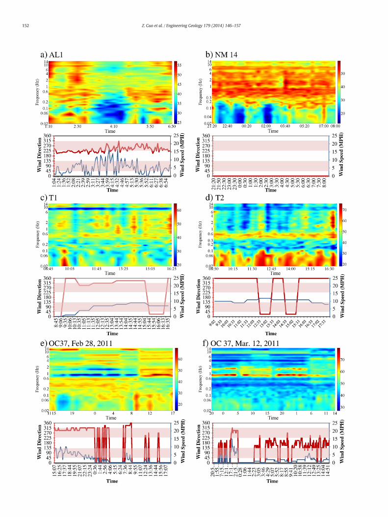
Fig. 5. Color gradientmap of the vibration angle θ of the LTR points in frequency–time space (upper), and corresponding variations inwind direction (red line) andwind speed (blue line)(lower). Note the color bar legends for the values of the vibration angle on the right-hand-side of the gradient maps. The pink shaded ranges on the wind direction axes represent ±45°from E to W direction.

153Z. Guo et al. / Engineering Geology 179 (2014) 146–157

three criteria of f0; and 3) variations of HVSR at f0 have a lowcorrelation coefficient with wind speed for both T1 and T2.

NM 14 (Figure 3-c; Corinth, MS)

• Continuous overnight (21:20–08:20) recording onMay 26–27,2012.

• The sensor was placed indoor and influenced by occasionaldoor movements and footsteps.

• The HVSR curves for 20-min segments were plotted inFig. 3-c: 1) within the frequency range of 0.02–0.2 Hz, theHVSR curves display remarkable variations with time; HVSRis significantly low during the small hours (00:00–05:00), butreaches very high levels as artificial activities in the earlymorn-ing hours intensify; 2) within the frequency range N0.5 Hz, thefirst (fp1 = f0) and second (fp2 = f1) peaks are easily identifi-able; 3) at f0, timedependency of HVSR is obviouswith a signif-icant difference between daytime and nighttime values; 4)

nighttime curves show slightly higher values in both f0 andHVSR; 5) HVSR at f1 also display time dependency but thevalue of f1 is stable; and 6)HVSR at f0 has a very low correlationwith wind speed in the recording period.

OC 37& OC 38 (Figure 3-d–h; University, MS)

• Four continuous recordings were made in the basement ofBrevard Hall (OC 37) and one recording was made in CoulterHall (OC38) both located in Oxford Campus of the Universityof Mississippi.

• The sensor was placed on concrete ground and exposed to theinfluence of A/C in the room.

• The HVSR curves were plotted in Fig. 3-d–h: 1) at nighttime,within the frequency range of 0.02–0.2 Hz, HVSR fluctuatesroughly within 1–5; during daytime, HVSR is much higher es-pecially on March 1st when the campus was busy; 2) the firstpeak (fp1 = f0) is sharp and stable with time around 0.29 Hz;

Bodin*: Bodin et al (2001): Memphis, Tennessee, U.S.A. Langston*: Langston and Horton (2011): Upper Mississippi Embayment down to Memphis City, Tennessee, U.S.A.Parolai*: Parolai et al (2002): Cologne, Germany Ibs-von Seht*: Ibs-von Seht and Wohlenberg (1999): Lower Rhine Embayment, Europe

0.1

1

10

100

0.1 1 10 100 1000

f 0 o

r f

1 (H

z)

UST (m)

f0B-1Langston*Bodin*Parolai*Ibs-von Seht*f1A-5Bodin*

a)

1

10

100

0.03

0.3

3

1000100

f 1/f

0

f 0 (

Hz)

UST (m)

A-5/A-4f1/f0

f0A-4B-4Langston*Bodin*Parolai*Ibs-von Seht*f1/f0

b)

Fig. 6. Regression models of a) UST (0–1400 m) vs. f0, and UST (100–1400 m) vs. f1, and b) UST (100–1400 m) vs. f0 and UST (100–1400 m) vs. f1/f0.

154 Z. Guo et al. / Engineering Geology 179 (2014) 146–157

3) the second peak (fp2= f1) is located at 0.79 Hz during night-time; 4) from the first two recordings, the third peak (fp3 = f2)can also be able to be identified around 1.6 Hz; and 5) correla-tions betweenHVSR at f0 and both pressure andwind speed aremedium-to-low for recordings at OC 37 and very low for thoseat OC38.

NM 29 (Figure 3-i; Clarksdale, MS)

• Continuous (20:00–08:20) indoor recording on May 27, 2012.• The HVSR curves were plotted in Fig. 3-i: 1) within 0.02–0.14 Hz range, HVSR fluctuates within 4 to 20+ during night(20:00–0:00) and early morning (05:00–08:20), but in a rela-tively low and narrow range (2–4) during the small hours(00:00–05:00); 2) during nighttime, f0 is easily identified ataround 0.170 Hz; 3) within 0.5–2 Hz range, HVSR changesslightly with time but there is no traceable separation betweendaytime and nighttime curves; 4) the likely second and thirdpeaks (fp2 = f1 and fp3 = f2) are identifiable at around0.52 Hz and 1.0 Hz respectively; 5) for f N 2 Hz, HVSR is very

Table 4Regression models of UST vs. f0 and UST vs. f1, data pairs, and model parameter values.

Source Regressionmethod

R2 SSE a

UST vs. f0A-4 (this study) R-LAR 0.991 0.162 4.789B-4 (this study) R-LAR 0.996 0.074 21.26B-1 (this study) R-BW 0.996 1.783 24.87Langston and Horton (2011) 1.04E−06Bodin et al. (2001) −3.06E−06Parolai et al. (2002) 20.466

Ibs-von Seht and Wohlenberg (1999) 26.801

UST vs. f1A-5 (this study) LAR 0.976 3.303 70.74Bodin et al. (2001)

R-LAR: Robust regression with least absolute residuals approach.R-BW: Robust regression with bisquare weights approach.

small and almost fixed in time; and 6) HVSR at f0 shows alow correlation with pressure.

4.2. Wind effect

In Fig. 3, some of the HVSR curves in the low frequency range (0.02–0.2 Hz) have much higher peaks than those considered as f0. For exam-ple, at AL1, which is an outdoor LTR point, the HVSR values in this lowfrequency range aremuch higher than in the rest of the frequency spec-trum. At other LTR points, which are all indoors, the daytime HVSRvalues in the low frequency range are generally higher than those ofthe night time values. These high peaks in the low frequency rangeare caused by the natural wind directly blowing on the sensor and byhuman activities (Bard, 1999; Mucciarelli et al., 2005; Chatelain et al.,2008). Our observations during this study supported these cause–effectrelationships as discussed below.

The graphs in Fig. 4 depict the HVSR curves of the LTR points (redlines) and those of nearby STR-I (blue lines) and STR-II (green lines)points where UST is similar. The ambient conditions of these record-ings are summarized in Table 3. For the points strongly influenced bylocal noise sources, shorter data windows than usual 50-s ones were

b c Equation UST range (m)

−0.2368 −0.7206 f0 = a (UST)b + c N100−0.6635 f0 = a (UST)b N100−0.6852 f0 = a (UST)b 0–1400−2.64E−03 0.10108 lnf0 = a (UST)2 + b (UST) + c 200–1300

7.89E−03 −0.39899 f0 = 1/[a (UST)2 + b (UST) + c] 350–1100−0.6447 f0 = a (UST)b Based on b402,

estimate N1000−0.722 f0 = a (UST)b b1219

−0.6339 −0.2796 f1 = a (UST)b + c N100f1 = 1/[a (UST)2 + b (UST) + c]

0.14

1.4

14

87.888.388.889.389.890.390.891.3

Freq

uenc

y (H

z)

Longitude (~°W)

HVSR = 5

0

500

1000

1500

UST (m)

f0 ± σ

f1

b)

a)

Fig. 7. a) UST along the profile A–A′ (Figure 1) and b) STR HVSR spectra at recording points along the profile. The solid red and blue lines indicate the values of f0 and f1respectively.

155Z. Guo et al. / Engineering Geology 179 (2014) 146–157

required to extract sufficient number of valid samples across the re-cording period. Because the HVSR values at longer periods than thelength of data window (L) (or at smaller frequencies than 1/L Hz)cannot be uniquely determined, the HVSR curves for those pointswith shorter data windows are truncated as for NM 13 below0.033 Hz (Figure 4).

Chatelain et al. (2008) pointed that the wind effect is related to theground cover type, i.e. wind modifies the HVSR when there are grassor trees around the sensor but nowind effect is evidentwhen the sensoris placed on asphalt or cement ground. In this study, however, as Fig. 4reveals, the HVSR values of STR-I within the low frequency band(0.02–0.2 Hz) are all significantly higher than those of LTR and STR-II

Fig. 8. Predominant frequency (f0) co

regardless of the ground cover type. This suggests that the effect of nat-ural wind can be largely eliminated with the protection of the sensor bya plastic box. Note, however, among the STR-II points, NM 159, NM 160and NM 210 display high HVSR values in the low frequency band, pos-sibly because of strong winds (with speeds reaching as high as15 mph) during the recordings at these points. Despite this complica-tion, f0 at these sites was more readily identifiable compared to that atNM 28, which is an STR-I point.

Bard and SESAME-Team (2005) and Angelis and Bodin (2012)pointed out that the wind can have significant influence on HVSR inthe frequency band less than 1 Hz. The results of this study (Figure 4)show that this influence is not identifiable at frequencies above 0.2 Hz.

ntours in Northern Mississippi.

0

200

400

600

800

1000

1200

0 200 400 600 800 1000 1200 1400

Vs

(m/s

)

UST or Depth (m)

Romero and Rix*Langston*Bodin*B-1

Fig. 9. Estimates of average shearwave velocity Vs as a function of UST (or depth). Note: B-1recalculatesVs fromEq. (1) using f0–USTpairs (Figure 6 and Table 4)whereas Langston* andBodin*are direct relationships of Vs vs. UST. Romero and Rix* is ameasured shear wave pro-file (Vs vs. depth) in Memphis, TN area.

156 Z. Guo et al. / Engineering Geology 179 (2014) 146–157

This observationmaybe strictly valid for the study area but it is support-ed by the vibration directions (Figure 5), as discussed in the nextsection.

5. Discussion

5.1. Vibration directions

The vibration angle θ (Figure 2) was calculated here across the fre-quency spectrum for each LTR. It was then mapped in frequency–timespace as shown in Fig. 5. The resulting color gradient maps revealtime-dependent nature of θ. In the frequency range of roughlyN0.2 Hz, θ also exhibits strong frequency-dependency. For the rangeb0.2 Hz, θ is primarily time-dependent but occasionally alsofrequency-dependent. These observations suggest that microtremorsat the low frequency range are of different origin(s). The significant cor-relation between θ of the low frequency band and the wind directionsuggests strong influence of wind even though the sensor was situatedindoor.

5.2. Correlation between UST and f0

The UST at each recording point was determined from the isopachmap of the Mississippi Embayment (Bodin et al., 2001) (Figure 1) andwas plotted against f0 observed at that location (Figure 6). The best-fitnonlinear regressions of UST vs. f0 are presented in Fig. 6 [labeled as B-1for 0 b UST (m) b1400 (Figure 6-a) and A-4 and B-4 for 100 b UST(m) b1400 (Figure 6-b)]. Fig. 6-a also presents the best-fit regressionmodels of UST and f1 data pairs (labeled as A-5 fitted for 100 b UST(m) b1400). The other lines represent regression equations derived byearlier studies. All these regression models and values of their fit-parameters are summarized in Table 4.

The regressionmodels produced in this study for both f0 and f1 havethe same general expression as the previous models and produce verysimilar trends. While at large UST values (N200 m) UST–frequencydata pairs form a narrow band, errors in predicting actual UST (due tosmoothing during preparation of the isopach map and interpolation inreading the UST at each microtremor recording point) becomes morevisible (in data scatter) as UST decreases. The scarcity of the data inthe small UST range prevents a more detailed analysis of the nature ofthe relationship between UST and frequency.

Fig. 7-a shows the variation of UST along profile A–A′ (Figure 1)whileFig. 7-b gives the smoothed HVSR spectra at each recording point alongthis profile. As UST decreases, f0 peaks gradually become flatter and di-minishes at the bedrock, and the values of f0 and f1 in general increasewhile the trend line for f0 is expected to become strongly nonlinear.

The frequency f1 may be interpreted as the first harmonics of f0 ifthe latter is taken as the fundamental frequency. The resonantfrequencies fr of a two-layer model (unconsolidated sedimentarylayer overlying bedrock) can be written as (Ibs-von Seht andWohlenberg, 1999):

f r ¼n � Vs

4 � USTð Þ n ¼ 1;3;5;… ð1Þ

where Vs is the shear wave velocity which is a function of depth.When n is 1, fr = f0, and when n is 3, fr = f1. Therefore, theoreticallyf1/f0 = 3 which is consistent with the results obtained at the major-ity of the recording points. Because f2 is unidentifiable at most STRpoints, the ratio f2/f0 was calculated only for OC 37, OC 38 and NM29 and the values are between 5.32 and 6.08 which are also closeto the theoretical value of 5.

Distribution of predominant frequency values f0 in the study areais presented by a contour map (Figure 8) based on those recordingpoints at which “reliable” identification of f0 was possible. Differentcontour intervals are used for different frequency ranges to accountfor and benefit from f0 distributions across the area. These contourlines are clearly consistent with the geological boundaries and thebasin morphology.

5.3. Average shear wave velocity and its variation with UST

According to Ibs-von Seht and Wohlenberg (1999), average shearwave velocity (Vs) of unconsolidated sediments at eachmicrotremor re-cording point can be estimated by fundamental mode of Eq. (1), forwhich n = 1 and fr = f0. These estimates of Vs were plotted againstUST values at corresponding recording points (Figure 1) as shown inFig. 9. The resulting data scatter may be interpreted as displaying twodistinct trends in UST ranges roughly below and above 500 m. Alsoshown on this figure are the trends predicted by B-1 (this study),Langston* (Langston and Horton, 2011) and Bodin* (Bodin et al.,2001) regression models (Figure 6 and Table 4). The model B-1 coin-cides very well with Bodin* in UST range 500–900 m. In addition tothese predicted trends, Fig. 9 also gives a measured Vs profile in Mem-phis, TN area by Romero and Rix (2005). The similarity of thismeasuredprofile and Vs–UST trends (especially B-1) is encouraging in terms of thevalidity of the microtremor approach and reveals that the average Vs ofthe unconsolidated sediments varies a great deal at shallow depth andreaches that of engineering bedrock (N600 m/s) around 400–500 m inNorthernMississippi. Large scatter at depths less than 200mmay be at-tributed to instability of HVSR and increased error in predicting USTfrom the contours (Figure 1). The significant scatter above 1000 mmay also be related to both the accuracy of UST contours (Figure 1)and the strong influence of local geological and environmental condi-tions on f0 in these ranges.

6. Conclusions

General conclusions that can be drawn from this study are:

1) Microtremor, as a stationary stochastic process, can provide a stableand reliable estimation of the predominant frequency.

2) Wind as a natural source and human activities can significantly in-fluence the microtremor in low frequency band (b0.2 Hz). Wind ef-fect can be significantly reduced by preventing direct exposure ofthe sensor.

3) Predominant frequency correlates well with UST.4) Average shear wave velocity and its variation as a function of UST

across a sedimentary basin can be established from systematicmicrotremor surveys.

Specific conclusions that may be valid only for the MississippiEmbayment area and in particular for Northern Mississippi are:

157Z. Guo et al. / Engineering Geology 179 (2014) 146–157

1) Highpeaks onHVSR curves in low frequency range (0.02–0.2Hz) arecaused by wind and human activities.

2) Vibration direction is strongly frequency-dependent above 0.2 Hzand time-dependent below this value.

3) The observed values of the first and second harmonics of the pre-dominant frequencies are consistent with their theoretical values.

4) Average shear wave velocity appears to vary more closely with theUST in 200–1000 m range.

References

Angelis, S.D., Bodin, P., 2012. Watching the wind: seismic data contamination at long pe-riods due to atmospheric pressure-field-induced tilting. Bull. Seismol. Soc. Am. 102,1255–1265.

Bard, P.-Y., 1999. Microtremor measurements: a tool for site effect estimation? Proc. 2ndInt. Symp. on the Effects of Surface Geology on Seismic Motion, Yokohama, Japan, pp.1251–1279.

Bard, P.-Y., SESAME-Team, 2005. Guidelines for the Implementation of the H/VSpectral Ratio Technique on Ambient Vibrations—Measurements, Processingand Interpretations. SESAME European Research Project EVG1-CT-2000-00026, D23.12.

Bodin, P., Horton, S., 1999. Broadband microtremor observation of basin resonance in theMississippi embayment, Central US. Geophys. Res. Lett. 26 (7), 903–906.

Bodin, P., Smith, K., Horton, S., et al., 2001. Microtremor observation of deep sedimentresonance in metropolitan Memphis, Tennessee. Eng. Geol. 62, 159–168.

Chatelain, J.-L., Guillier, B., Cara, F., et al., 2008. Evaluation of the influence of experimentalconditions on H/V results from ambient noise recordings. Bull. Earthquake Eng. 6,33–74.

Ibs-von Seht, M., Wohlenberg, J., 1999. Microtremor measurements used to map thick-ness of soft sediments. Bull. Seismol. Soc. Am. 89, 250–259.

Johnston, A.C., 1985. Recurrence rates and probability estimates for the NewMadrid Seis-mic Zone. J. Geophys. Res. 90, 6737–6753.

Johnston, A.C., Schweig, E.S., 1996. The enigma of the New Madrid earthquakes of1811–1812. Ann. Rev. Earth Planet. Sci. 24, 339–384.

Kanai, K., Tanaka, T., 1954. Measurement of the microtremor. Bull. Earthquake Res. Inst.32, 199–209.

Langston, C.A., Horton, S.P., 2011. 3D seismic velocity model for the unconsolidated Mis-sissippi embayment sediment from H/V ambient noise measurements. Final Techni-cal Report, USGS MEHRP award G10AP00008.

MDEQ (Mississippi Department of Environment Quality), ). Geologic maps and datafor Mississippi http://www.deq.state.ms.us/MDEQ.nsf/page/Geology_surface?OpenDocument.

Mucciarelli, M., Gallipoli, M.R., Giacomo, D.D., 2005. The influence of wind on measure-ments of seismic noise. Geophys. J. Int. 161, 303–308.

Nakamura, Y., 1989. A method for dynamic characteristics estimation of subsurface usingmicrotremor on the ground surface. QR of RTRI, 30, pp. 25–33.

Nakamura, Y., 2008. Basic structure of the H/V spectral ratio. Earthquake Disaster Sympo-sium. Society of Exploration Geophysicists, Japan (in Japanese with English abstract).

Nuttli, O.W., 1974. New Madrid earthquakes 1811–1812. Earthquake Information Bulle-tin, Vol. 6, No. 2.

Park, D., Hashash, Y.M.A., 2005. Evaluation of seismic site factors in the Mississippi Em-bayment. I. Estimation of dynamic properties. Soil Dyn. Earthq. Eng. 25, 133–144.

Parolai, S., Bormann, P., Milkereit, C., 2002. New relationships between Vs, thickness ofsediments, and resonance frequency calculated by the H/V ratio of seismic noise forthe Cologne area (Germany). Bull. Seismol. Soc. Am. 92, 2521–2527.

Romero, S.M., Rix, G.J., 2005. Ground Motion Amplification in the Upper Mississippi Em-bayment. Report No. GIT-CEE/GEO-01-1. National Science Foundation Mid AmericaCenter, Atlanta.

Rosenblad, B.L., Goetz, R., 2010. Study of the H/V spectral ratio method for determiningaverage shear wave velocities in the Mississippi embayment. Eng. Geol. 112, 13–20.

Schweig, E.S., 1996. Neotectonics of the upper Mississippi embayment. Eng. Geol. 45,185–203.

Stover, C.W., Coffman, J.L., 1993. Seismicity of the United States. USGS Professional Paper,1527 (418 pp.).