Microhabitat conditions influence mesohabitat associations and distribution of larval salamanders in...

1 23

�� ! �"#��$��%&��%��'��

��

��

1 23

Your article is protected by copyright andall rights are held exclusively by SpringerInternational Publishing Switzerland. This e-offprint is for personal use only and shall notbe self-archived in electronic repositories. Ifyou wish to self-archive your article, pleaseuse the accepted manuscript version forposting on your own website. You mayfurther deposit the accepted manuscriptversion in any repository, provided it is onlymade publicly available 12 months afterofficial publication or later and providedacknowledgement is given to the originalsource of publication and a link is insertedto the published article on Springer'swebsite. The link must be accompanied bythe following text: "The final publication isavailable at link.springer.com”.

PRIMARY RESEARCH PAPER

Microhabitat conditions influence mesohabitat associationsand distribution of larval salamanders in headwater streams

J. M. Yeiser • S. C. Richter

Received: 17 June 2014 / Revised: 26 November 2014 / Accepted: 14 January 2015! Springer International Publishing Switzerland 2015

Abstract Distribution patterns of stream biota are

the result of complex interactions between individualsand their surrounding environment. Determining the

spatial scale by which an organism is most influenced

is paramount to understanding distribution patterns.Using a multi-scale approach, we investigated factors

influencing habitat associations of larval Ambystomabarbouri (streamside salamander) and Eurycea cirri-

gera (southern two-lined salamander) in three Ken-

tucky headwater streams. We used likelihood ratioG tests to identify associations between species and

mesohabitat (i.e., runs, riffles, and pools), and we used

microhabitat variables to predict the presence andabundance of salamanders via a priori multiple

regression modeling. Ambystoma barbouri presence

and abundance were influenced by conditions atmicro-scales, which in turn dictated mesohabitat

associations. Eurycea cirrigera were also influenced

by microhabitat variables, but displayed associationsto A. barbouri presence in late spring. Associations of

larval salamanders to mesohabitat and microhabitatparameters shifted from early to late spring, likely in

response to changes in developmental stage. The

multi-scale approach of our study improved ourunderstanding of complex relationships between lar-

val salamanders and their surrounding environment in

headwaters, and underscored the importance of (1)research investigating multiple spatial and temporal

scales and (2) heterogeneous in-stream habitat to

headwater biota.

Keywords Distribution ! Headwater streams !Mesohabitat associations ! Multi-scale research !Salamanders

Introduction

The distribution of stream organisms is a result of

complex interactions among factors operating at

multiple spatial and temporal scales (Frissell et al.,1986; Vanni, 2002). Multi-scale drivers of distribution

and abundance include direct and indirect effects of

consumers (Vanni, 2002; McIntosh et al., 2004),

Handling editor: Lee B. Kats

Electronic supplementary material The online version ofthis article (doi:10.1007/s10750-015-2185-5) contains supple-mentary material, which is available to authorized users.

J. M. Yeiser ! S. C. RichterDepartment of Biological Sciences, Eastern KentuckyUniversity, Richmond, KY 40475, USA

J. M. Yeiser (&)Kentucky Department of Fish and Wildlife Resources,Research Program, Frankfort, KY 40601, USAe-mail: [email protected]

S. C. RichterDivision of Natural Areas, Eastern Kentucky University,Richmond, KY 40475, USA

123

Hydrobiologia

DOI 10.1007/s10750-015-2185-5

Author's personal copy

spatiotemporal shifts in habitat availability and suit-ability (Torgersen et al., 1999; Smith & Grossman,

2003), and interactions of abiotic and biotic factors

(Doi & Katano, 2008; McIntyre et al., 2008). Habitatwithin streams varies across spatial scales and pro-

cesses at each scale interact to influence habitat

characteristics (Frissell et al., 1986). Additionally,spatial heterogeneity shifts seasonally (Frissell et al.,

1986). Thus, multi-scale approaches should be

employed when investigating habitat associationsand distribution patterns of stream organisms (Tor-

gersen et al., 1999; Doi & Katano, 2008; Keitzer &

Goforth, 2013).In headwater streams lacking fishes, aquatic sala-

mander larvae are often the dominant vertebrate

predator (Davic & Welsh, 2004; McIntosh et al.,2004), but they also have important non-consumptive

effects (reviewed in Wells, 2007). For example,

salamanders play an important role in nutrient recy-cling in stream systems (Milanovich, 2010; Keitzer &

Goforth, 2013; Munshaw et al., 2013). Therefore,

stream salamanders are vital components of headwaterecosystems.

Distribution patterns of larval salamanders are

subject to temporal shifts as a result of complexinteractions with their environment (Smith & Gross-

man, 2003), syntopic species (Gustafson, 1994), or

combinations of both abiotic and biotic factors (Barr &Babbitt, 2002). Individual body size also influences

habitat associations (Lowe, 2005; Martin et al., 2012),

and therefore contributes to how species are distrib-uted across space and ontogeny. Thus, understanding

habitat associations of larval salamanders is important

to stream ecosystem dynamics.Our objectives were to determine the effect of

stream characteristics on the distribution of two

common salamander species in our study region,Ambystoma barbouri (streamside salamander) and

Eurycea cirrigera (southern two-lined salamander)

across meso-scales (runs, riffles, and pools) and micro-scales (within 0.25-m2 area). Larval A. barbouri have

displayed negative associations to riffle mesohabitat,likely as a passive response to high-velocity turbulent

stream flow (Petranka, 1984a; Holomuzki, 1991), and

E. cirrigera larvae are generally found in slow-movingareas (Petranka, 1998). Petranka (1984a) suggested

that because of lack of mobility, newly hatched A.

barbouri individuals were displaced from high-veloc-ity areas to low velocity, depositional habitats. Older

A. barbouri and E. cirrigera are less likely to bedisplaced downstream (Bruce, 1986; Petranka et al.,

1987). Larval A. barbouri typically do not utilize

substrate cover when fish predators are absent (Sihet al., 1992) yet larval E. cirrigera use substrate

diurnally (Petranka, 1984b). Studies on other aquatic

organisms have shown habitat variables at meso-scales to be the most important predictors of distribu-

tion (i.e., Torgerson et al., 1999; Rabeni et al., 2002;

Doi & Katano, 2008). Our study organisms aresyntopic species that utilize similar mesohabitat yet

differ in microhabitat use; therefore, we measured

abiotic factors at meso- and micro-scales that couldpotentially influence their abundance and distribution

at watershed scales. We sampled in early and late

spring, which allowed us to determine if any ontoge-netic shifts occurred in these relationships from early

to late stages of aquatic development.

Materials and methods

Study site

We studied distributions of E. cirrigera and A.barbouri in three fishless headwater streams within

the Inner Bluegrass Ecoregion of central Kentucky

(Woods et al., 2002). While some of the headwatersare exposed to residential and pastureland areas, our

study areas were surrounded by extended forest buffer

([100 m), which should be wide enough to supportthe core habitat requirements of amphibian species in

the area (Semlitsch & Bodie, 2003) and likely

remediate most negative effects of these landscapedisturbances (Naiman & Decamps, 1997). Within our

study streams, variable gradients, water velocities,

channel widths, depths, bank slopes, and substrateresult in a heterogeneous habitat that supports popu-

lations of A. barbouri (Storfer, 1999) and E. cirrigera

(Petranka, 1984b). Larval A. barbouri in centralKentucky hatch in early spring and metamorphose

after approximately 6–10 weeks (Petranka, 1984c;Petranka and Sih, 1986). Larval periods of E. cirrigera

vary regionally (Petranka, 1998), but in Kentucky

individuals metamorphose after 1–3 years of devel-opment (Barbour, 1971; Petranka, 1984b). In early

spring, newly hatched A. barbouri and older E.

cirrigera (hereafter second-year larvae) are bothpresent in our study streams. Second-year E. cirrigera

Hydrobiologia

123


larvae prey on A. barbouri as they hatch, but as A.barbouri larvae grow larger, they are no longer

suitable prey for E. cirrigera (Petranka, 1984b). In

late spring, recently hatched cohorts of E. cirrigera arepresent in the stream (hereafter first-year larvae) along

with both second-year E. cirrigera larvae and A.

barbouri that are approaching metamorphosis. Theseparate ontogenies of both species within our study

timeframe (early to late spring) allowed us to inves-

tigate differences between habitat associations of bothspecies across their aquatic life stages.

Sampling design

Within each of the study streams, we randomly selected

a 100-m reach within the longest stretch of suitablehabitat. We defined suitable habitat as areas of stream

length that had substantial forest buffer, presence of

multiple mesohabitat types, and no evidence of fishes.We sampled each 100-m reach twice in spring of 2012

(13–15 April and 18–20 May; hereafter referred to as

early spring and late spring sampling events, respec-tively). Every 3 m, we established a 1-m-wide transect

across the stream. Within each transect we arranged

three 0.25-m2 sampling plots. One plot bordered the leftshoreline, one was in the midpoint of the stream channel,

and one bordered the right shoreline. We overturned

each substrate item within the 0.25-m2 sampling plotand counted individuals, including substrate in contact

with the border of the plot. To reveal population

distributions and species coexistence within the stream,we documented the location of each observation as an x,

y coordinate along the stream channel. We measured

individuals after each capture to the nearest millimeterof total body length (TL), but we only attempted capture

when it would not displace nearby larvae. Mean lengths

were compared between mesohabitat type using one-way analysis of variance (ANOVA).

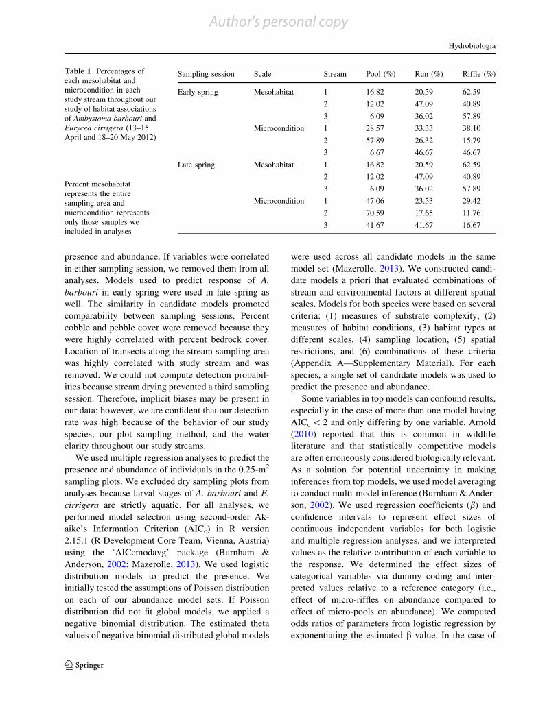
In each study stream, we mapped the 100-m reach

according to mesohabitat type—run, riffle, or pool inearly spring (Table 1). We modified the mesohabitat

definitions of Montgomery and Buffington (1997) toapply to headwaters in central Kentucky primarily

composed of bedrock, and characterizations of meso-

habitat were based on geomorphology as well ashydrology. We incorporated geomorphology in order

to strengthen the potential predictive power of our

results during non-typical weather years. Runs gener-ally had laminar flow and low gradients and were either

dominated by limestone bedrock or composed of avariety of substrate. Riffles were characterized by

relatively turbulent flow, moderate to low gradients,

and a variety of substrate that caused non-laminar flowincluding undulating bedrock or multiple vertical

incisions in bedrock. Pools had laminar flow and low

gradients but were differentiated from runs based onslower water velocity caused by an obstruction in the

stream channel or an abrupt incision in the stream bed.

We represented natural availability of mesohabitattypes by percentage of total sampling reach area, and

we used these percentages to calculate the expected

frequencies of captures within each mesohabitat type.To uncover mesohabitat associations of A. barbouri

and E. cirrigera, we compared observed frequencies of

captures within each mesohabitat type to expectedfrequencies using likelihood ratio G tests (Sokal &

Rohlf, 1995; Lowe, 2005). We calculated likelihood

ratio G values for each site from each sampling eventand graphically represented overall habitat associa-

tions by combining sites as independent replicates.

Within each sampling transect, we randomly desig-nated a 0.25-m2 sampling plot for microhabitat sam-

pling. Within each 0.25 m2 plot, we visually estimated

embeddedness as a percentage of total substrate areacovered in fine sediment, debris and vegetative cover as

the percent cover of the total surface area in the sampling

plot, and percent cover of substrate for the followingcategories: pebble (\64 mm), cobble (64–256 mm),

boulder ([256 mm with visible edges), and bedrock

([256 mm with no visible edges) (Bain, 1999). Wenoted the size class of substrate item under which an

individual was captured (or reported as exposed if under

no cover). We also characterized the microcondition(micro-pool, micro-run, or micro-riffle) within each

plot. Microcondition only refers to habitat within the

0.25-m2 sampling plot and was determined using thesame criteria used to indentify mesohabitat types. It is a

comprehensive, qualitative metric that attempts to

incorporate variables difficult to quantify in first-orderstreams (e.g., water velocity). This was a novel

measurement and it allowed us to empirically evaluatedistinct microhabitats within a dominant mesohabitat.

Statistical analyses

We used Pearson’s correlations to determine multi-collinearity among predictive variables of salamander

Hydrobiologia

123


presence and abundance. If variables were correlatedin either sampling session, we removed them from all

analyses. Models used to predict response of A.

barbouri in early spring were used in late spring aswell. The similarity in candidate models promoted

comparability between sampling sessions. Percent

cobble and pebble cover were removed because theywere highly correlated with percent bedrock cover.

Location of transects along the stream sampling area

was highly correlated with study stream and wasremoved. We could not compute detection probabil-

ities because stream drying prevented a third sampling

session. Therefore, implicit biases may be present inour data; however, we are confident that our detection

rate was high because of the behavior of our study

species, our plot sampling method, and the waterclarity throughout our study streams.

We used multiple regression analyses to predict the

presence and abundance of individuals in the 0.25-m2

sampling plots. We excluded dry sampling plots from

analyses because larval stages of A. barbouri and E.

cirrigera are strictly aquatic. For all analyses, weperformed model selection using second-order Ak-

aike’s Information Criterion (AICc) in R version

2.15.1 (R Development Core Team, Vienna, Austria)using the ‘AICcmodavg’ package (Burnham &

Anderson, 2002; Mazerolle, 2013). We used logistic

distribution models to predict the presence. Weinitially tested the assumptions of Poisson distribution

on each of our abundance model sets. If Poisson

distribution did not fit global models, we applied anegative binomial distribution. The estimated theta

values of negative binomial distributed global models

were used across all candidate models in the samemodel set (Mazerolle, 2013). We constructed candi-

date models a priori that evaluated combinations of

stream and environmental factors at different spatialscales. Models for both species were based on several

criteria: (1) measures of substrate complexity, (2)

measures of habitat conditions, (3) habitat types atdifferent scales, (4) sampling location, (5) spatial

restrictions, and (6) combinations of these criteria

(Appendix A—Supplementary Material). For eachspecies, a single set of candidate models was used to

predict the presence and abundance.

Some variables in top models can confound results,especially in the case of more than one model having

AICc \ 2 and only differing by one variable. Arnold

(2010) reported that this is common in wildlifeliterature and that statistically competitive models

are often erroneously considered biologically relevant.

As a solution for potential uncertainty in makinginferences from top models, we used model averaging

to conduct multi-model inference (Burnham & Ander-

son, 2002). We used regression coefficients (b) andconfidence intervals to represent effect sizes of

continuous independent variables for both logistic

and multiple regression analyses, and we interpretedvalues as the relative contribution of each variable to

the response. We determined the effect sizes of

categorical variables via dummy coding and inter-preted values relative to a reference category (i.e.,

effect of micro-riffles on abundance compared to

effect of micro-pools on abundance). We computedodds ratios of parameters from logistic regression by

exponentiating the estimated b value. In the case of

Table 1 Percentages ofeach mesohabitat andmicrocondition in eachstudy stream throughout ourstudy of habitat associationsof Ambystoma barbouri andEurycea cirrigera (13–15April and 18–20 May 2012)

Percent mesohabitatrepresents the entiresampling area andmicrocondition representsonly those samples weincluded in analyses

Sampling session Scale Stream Pool (%) Run (%) Riffle (%)

Early spring Mesohabitat 1 16.82 20.59 62.59

2 12.02 47.09 40.89

3 6.09 36.02 57.89

Microcondition 1 28.57 33.33 38.10

2 57.89 26.32 15.79

3 6.67 46.67 46.67

Late spring Mesohabitat 1 16.82 20.59 62.59

2 12.02 47.09 40.89

3 6.09 36.02 57.89

Microcondition 1 47.06 23.53 29.42

2 70.59 17.65 11.76

3 41.67 41.67 16.67

Hydrobiologia

123


categorical variables such as microcondition, wecompared the odds between an individual occurring

in one microhabitat type versus another. We used

confidence intervals of 85% for parameter estimates.Arnold (2010) argued that using 85% confidence

intervals when interpreting effects of AIC parameter

estimates promotes compatibility between the infor-mation-theoretic approach and statistical inference. If

85% confidence intervals included zero, we inter-

preted the variable as having no effect on the response.

Results

We observed 672 A. barbouri larvae (pools = 137,

runs = 369, riffles = 166) and 160 E. cirrigera larvae(pools = 11, runs = 75, riffles = 75) across all sites

during this study. In early spring, we observed 453 A.

barbouri (observed: pools = 120, runs = 214, andriffles = 119; expected: pools = 46, runs = 168, and

riffles = 237), with densities reaching 90 individuals/

m2 (l ± 1 SE = 8.11 ± 0.94). We captured and mea-sured 274 A. barbouri in early spring (l ± 1

SE = 18.52 ± 0.22 mm). We observed 17 second-

year E. cirrigera (observed: pools = 6, runs = 5, andriffles = 6; expected: pools = 1, runs = 5, and rif-

fles = 9) and captured and measured 12 individuals

(l ± 1 SE = 48.17 ± 1.93 mm). Due to low samplesize, interpretations of E. cirrigera results for this

sampling period were limited, but A. barbouri displayed

clumped distribution throughout each sampling reach(Fig. 1). In late spring, we observed 219 A. barbouri

(observed: pools = 17, runs = 155, and riffles = 47;

expected: pools = 25, runs = 75, and riffles = 117),110 first-year E. cirrigera (observed: pools = 5,

runs = 70, and riffles = 69; expected: pools = 16,

runs = 49, and riffles = 77), and 34 second-year E.cirrigera (observed: pools = 1, runs = 18, and

riffles = 15; expected: pools = 4, runs = 11, and

riffles = 17). Densities of A. barbouri reached 60individuals/m2 (l ± 1 SE = 3.91 ± 0.54), and density

of E. cirrigera reached 40 individuals/m2 (l =2.52 ± 0.38 SE). We captured and measured 70 A.

barbouri (l ± 1 SE = 30.34 ± 1.05 mm) and 27 E.

cirrigera (first-year larvae, n = 19, l ± 1 SE =17.33 ± 0.63 mm; second-year larvae, n = 6, l ± 1

SE = 44.67 ± 4.03 mm). Both species displayed

clumped spatial distribution and often shared the samehabitat space (Fig. 2). Mean length of A. barbouri did

not differ between mesohabitats in early or late spring(early spring ANOVA P = 0.21, late spring ANOVA

P = 0.19). Mean length of E. cirrigera did not differ in

early spring (ANOVA P = 0.86), and although lowsample size restricted statistical analysis, mean length of

first-year E. cirrigera was relatively similar between

mesohabitats in late spring (pools: l ± 1 SE =17.50 ± 2.50 mm, runs: l ± 1 SE = 18.57 ±

1.72 mm, and riffles: l ± 1 SE = 16.56 ± 0.56 mm).

Habitat associations: early spring

Ambystoma barbouri displayed positive associationsto runs and pools and a negative association to riffles

(Fig. 3a). Observed frequencies of individuals within

each mesohabitat type were not equal to expectedfrequencies based on natural availability (Site 1:

G = 9.91, df = 2, P = 0.007; Site 2: G = 135.00,

df = 2, P \ 0.0001; and Site 3: G = 73.73, df = 2,P \ 0.0001). Eurycea cirrigera were positively

associated with pools (Fig. 3b), and observed propor-

tions were different than expected at stream 2(G = 8.48, df = 2, P = 0.01).

Percent bedrock, percent boulder, and microcondi-

tion best predicted the presence of A. barbouri(Table 2). The weight of the top model was less than

0.90; therefore, we performed model averaging on top

predictive variables. An increase in 1% bedrockpredicted an individual to be approximately

1.03x more likely to be present than absent (Table 3;

Fig. 4). Bedrock cover was greatest in runs and likelyhad an influence on positive associations of individuals

to this habitat (Fig. 5). Ambystoma barbouri abundance

in early spring was best predicted by percent bedrock,percent boulder, and microcondition (Table 2). Micro-

riffles had the greatest effect on abundance, with

approximately 2.0 fewer individuals per sample pre-dicted to be present in micro-riffles compared to micro-

pools. The difference in effect of micro-runs compared

to micro-pools was not different from zero. Compared tomeso-scale riffles, both pools and runs contained fewer

micro-riffles (Fig. 6). Sampling site also contributedconsiderably to A. barbouri abundance. Sample size of

E. cirrigera precluded regression analysis.

Habitat associations: late spring

In late spring, A. barbouri displayed a strong positiveassociation with runs and a strong negative association

Hydrobiologia

123


with riffles and had no associations to pools (Fig. 3a).

Observed frequencies of individual A. barbouri withineach mesohabitat type were different than expected

frequencies (site 1: G = 33.85, df = 2, P \ 0.0001;

site 2: G = 105.42, df = 2, P \ 0.0001; and site 3:G = 11.72, df = 2, P = 0.004).

Site 1 Site 2 Site 3A. barbouri E. cirrigera A. barbouri E. cirrigera A. barbouri E. cirrigera

UpstreamPOOL RIFFLE RUN

RIFFLERUN RUN

RIFFLE RIFFLE RUN* RUNRI P

RIFFLE

RIFFLE *RIFFLE

RUN*

* * RUN

RIFFLE

*RUN RIFFLE RUN

RIFFLE

RIFFLE

RUNRIFFLE RUN

POOLRIFFLERUN

*POOL

*RUN RUN

Downstream P RI * * POOL

1 2 3 1 2 3 1 2 3 1 2 3 1 2 3 1 2 3Plot Plot Plot Plot Plot Plot

= 0= 1-3= 4-6= 7-9

* = 10+

Fig. 1 Graphical representation of distribution patterns of A.barbouri and E. cirrigera during early spring (13–15 April2012). Solid outlines represent areas of the stream that held

water. Shaded areas represent number of observations in asampling plot. Dotted lines represent boundaries betweenmesohabitat types within streams

Site 1 Site 2 Site 3A. barbouri E. cirrigera A. barbouri E. cirrigera A. barbouri E. cirrigera

UpstreamPOOL RIFFLE RUN

RIFFLERUN RUN

RIFFLE RIFFLERUNRUNRI P

RIFFLE

RIFFLERIFFLE

RUN RUN

RIFFLE

*RUN RIFFLE RUN

RIFFLE

RIFFLE

RUNRIFFLE * RUN

POOLRIFFLERUN

POOLRUN RUNDownstream P RI POOL

1 2 3 1 2 3 1 2 3 1 2 3 1 2 3 1 2 3Plot Plot Plot Plot Plot Plot

= 0= 1-3= 4-6= 7-9

* = 10+

= 0= 1-3= 4-6= 7-9

* = 10+

Fig. 2 Graphical representation of distribution patterns of A.barbouri and E. cirrigera during late spring (18–20 May 2012).Solid outlines represent areas of the stream that held water.

Shaded areas represent number of observations in a samplingplot. Dotted lines represent boundaries between mesohabitattypes within streams

Hydrobiologia

123


Multiple predictive models of A. barbouri presenceheld similar weight (Table 2). Depth had positive

effects on A. barbouri presence, with an increase in

1 cm of depth predicting an individual to be 1.5x morelikely to be present than absent (Fig. 7; Table 3). The

best model predicting abundance of A. barbouri was

depth and microcondition (Table 2). An increase inapproximately 5 cm in depth was predicted to result in

the increase in 1.0 A. barbouri individual (Table 3).

Micro-runs were predicted to contain approximately1.0 more individual than micro-pools per sample, and

micro-riffles were predicted to contain approximately

2.0 less individuals than micro-pools per sample.Depth was lowest in micro-riffles (Fig. 8), and riffle

mesohabitat contained greater number of micro-riffles

than other mesohabitats (Fig. 6).In order to compare differences in habitat associ-

ations between E. cirrigera in different stages of

aquatic development, we analyzed second- and first-year individuals separately. Low sample size pre-

cluded AICc modeling for second-year E. cirrigera.

Both second- and first-year E. cirrigera were nega-tively associated with pools and riffles and positively

associated with runs at meso-scales (Fig. 3b). There

was a difference between observed and expectedfrequencies of second- and first-year E. cirrigera at

one site (second-year, stream 1: G = 8.63, df = 2,P = 0.01; first-year, stream 1: G = 10.01, df = 2,

P = 0.007), but these differences were not as pro-nounced as in A. barbouri. The model best predicting

the presence of first-year E. cirrigera in late spring was

sampling stream; however, multiple candidate modelshad relatively substantial weights (Table 2). Only 1

first-year E. cirrigera was sampled in stream 2 and this

was likely driving model selection. First-year E.cirrigera were predicted to be approximately

4.0x more likely to be present in areas of A. barbouri

presence than in areas of A. barbouri absence, and1.24x more likely to be present with an increase in

1 cm of depth (Table 3). The model best predicting

the abundance of first-year E. cirrigera in late springwas microcondition and depth (Table 2). An increase

in 4.85 cm of depth was predicted to result in an

increase in 1.0 E. cirrigera individual (Table 3). Adecrease in 8.20% boulder cover was predicted to

result in an increase in 1.0 E. cirrigera individual.

Discussion

The multi-scale approach of our study improved our

understanding of the distribution of larval salamanders

in relatively undisturbed headwater systems. Strongmesohabitat associations dictated locations of

clumped individuals. Micro-scale environmental vari-ables differentially predicted the presence and

(a) (b)Fig. 3 Deviations ofobserved proportions ofa Ambystoma barbouri andb Eurycea cirrigera fromexpected proportions in eachmesohabitat in early (13–15April) and late spring(18–20 May), 2012. Errorbars represent 95%confidence intervals

Hydrobiologia

123


abundance of both species within mesohabitats,therefore influencing overall distribution patterns.

Micro-scale environmental variables effectively pre-

dicted distribution of A. barbouri across their ontogeny.Micro-riffles had a strong negative influence on A.

barbouri abundance in early and late stages of devel-

opment. The high frequency of micro-riffles within rifflemesohabitat likely dictated the negative association of

A. barbouri to these areas throughout their aquatic stage.

The frequency of A. barbouri observed in rifflesthroughout our study contrasted the literature, however

(Petranka, 1984a; Holomuzki, 1991). We observed 166A. barbouri in riffle mesohabitat throughout this study.

The presence of low velocity, laminar microhabitats

(i.e., micro-pools and micro-runs) within meso-scaleriffles resulted in A. barbouri inhabiting normally

unsuitable mesohabitat. Positive mesohabitat associa-

tions were also driven by a prevalence of micro-poolsand micro-runs. Our results indicate that the distribution

of micro-pools, micro-runs, and micro-riffles within

headwaters dictates A. barbouri in-stream distribution.Distributions of our study organisms were also

Table 2 Top models predicting the presence and abundance of Ambystoma barbouri and Eurycea cirrigera in early (13–15 April)and late spring (18–20 May) 2012

Species Sampling session Response Modela Kb Log-likelihood Di wi

Ambystoma barbouri Early spring Presence Bedrock ? boulder ? microcon 5 -19.16 0 0.73

Microcon 3 -23.31 3.54 0.13

Abundance Bedrock ? boulder ? microcon 6 -114.12 0 0.54

Global 14 -101.97 0.46 0.43

Late spring Presence Bedrock ? depth 3 -23.80 0 0.28

Depth 2 -25.05 0.20 0.25

Depth ? microcon 4 -22.87 0.54 0.21

Embed 2 -25.91 1.93 0.11

Bedrock ? depth ? debris ? Veg 5 -23.17 3.66 0.04

Abundance Depth ? microcon 5 -66.99 0 0.64

Microcon ? embed 5 -67.73 1.48 0.30

Eurycea cirrigera Late spring Presence Stream 3 -22.99 0 0.23

A. barbouri presence 2 -24.62 0.97 0.14

Depth 2 -24.94 1.61 0.10

Bedrock ? depth 3 -24.02 2.05 0.08

Intercept 1 -26.40 2.34 0.07

Depth ? embed 3 -24.22 2.45 0.07

Depth ? bedrock ? boulder 4 -23.38 3.19 0.05

Microcon ? A. Barbouri presence 4 -23.44 3.30 0.04

Debris ? depth 3 -24.93 3.89 0.03

Bedrock 2 -26.09 3.90 0.03

Bedrock ? boulder 3 -24.98 3.97 0.03

Abundancec Depth ? microcon 5 -28.84 0 0.53

Depth ? embed 4 -30.69 1.17 0.29

Bedrock ? boulder ? embed 5 -30.76 3.85 0.08

Cutoff for top models was Di \ 4a Microcon (microcondition: micro-run, micro-riffle, micro-pool), bedrock (%bedrock cover within 0.25-m2 plot), boulder(%boulder cover within 0.25-m2 plot), embed (% of substrate embedded within 0.25-m2 plot), debris (%debris cover within 0.25-m2

plot), veg (%vegetation cover within 0.25-m2 plot), depth (depth at midpoint of sampling plot)b Includes error term and intercept for abundance models and intercept for presence modelsc Indicates Quasi Akaike’s Information Criterion (QAICc) results

Hydrobiologia

123


Table 3 Effects of top predictive parameters (i.e., different from zero) on the presence and abundance of Ambystoma barbouri andEurycea cirrigera in early (13–15 April) and late spring (18–20 May) 2012

Species Sampling session Response Parametera b 85% CIlower

85% CIupper

Oddsratio

Ambystoma barbouri Early spring Presence Bedrock 0.029 0.010 0.047 1.029

Abundance Bedrock 0.010 0.003 0.018 –

Veg -0.019 -0.035 -0.004 –

Boulder -0.044 -0.075 -0.013 –

Debris -0.047 -0.078 -0.016 –

Stream 3 versus stream 1 1.410 0.785 2.034 –

Stream 2 versus stream 1 0.584 0.012 1.156 –

Micro-riffle versus micro-pool -1.955 -2.942 -0.968 –

Late spring Presence Depth 0.433 0.212 0.655 1.542

Embed 0.036 0.016 0.056 1.037

Abundance Depth 0.220 0.141 0.299 –

Embed 0.026 0.015 0.038 –

Micro-run versus micro-pool 0.930 0.362 1.498 –

Micro-riffle versus micro-pool -1.843 -3.572 -0.114 –

Eurycea cirrigera Late spring Presence Depth 0.194 0.037 0.352 1.214

A. barbouri presence 1.408 0.291 2.525 4.087

Stream 2 versus stream 1 -2.167 -3.821 -0.513 0.115

Abundance Depth 0.206 0.096 0.317 –

Boulder -0.122 -0.196 -0.048 –

Parameter estimates were averaged across top models if the top model wi \ 0.90. Results are presented by species, sampling session,response, and type of parameter (continuous or categorical)a Bedrock (%bedrock cover within 0.25-m2 plot), boulder (%boulder cover within 0.25-m2 plot), embed (% of substrate embeddedwithin 0.25-m2 plot), depth (depth at midpoint of sampling plot), veg (%vegetation cover within 0.25-m2 plot), debris (%debris coverwithin 0.25-m2 plot), stream (sampling stream 1, 2, or 3), microcondition (micro-pool, micro-riffle, or micro-run), mesohabitat (pool,riffle, or run)

Fig. 4 Box plot of%bedrock and Ambystomabarbouri presence (left) andadjusted variable plot of theinfluence of %bedrock onabundance compared toother predictive variables(right) in early spring(13–15 April 2012)

Hydrobiologia

123


influenced by stream depth, and this was not unexpectedbecause our study streams began to dry in late spring,

and both species are restricted to aquatic habitats during

their larval stage (Petranka, 1998).Evolutionary and life history of A. barbouri likely

contributed to their micro-scale associations in early

spring (Holomuzki, 1991; Petranka, 1998). Weobserved the majority of A. barbouri exposed in the

water column shortly after hatching (l ± 1SE = 83.2 ± 5.9%), indicating that individuals would

have little resistance to downstream displacement.

Body size–interstitial space relationships did not influ-ence A. barbouri but negative associations of first-year

E. cirrigera to large substrate reflected what is reported

in the literature and likely influenced their distribution(Gustafson, 1994; Lowe, 2005; Martin et al., 2012).

The low abundance of E. cirrigera in our streams in

early spring indicates that predation risk to A. barbouriis minimal and likely does not influence distribution of

A. barbouri (Petranka, 1984b). The presence of E.

cirrigera was influenced by the presence of A.barbouri in late spring, and the introduction of a

new cohort of E. cirrigera may have initiated inter-specific interactions between our study organisms that

influenced their distributions. Alternatively, similar

mesohabitat associations of both species could be arelic of life history requirements of all aquatic larval

salamanders. Our modeling reflects differing

Fig. 5 Distribution of%bedrock within meso-scale (left) and micro-scale(right) habitat types in earlyspring (13–15 April 2012)

Early Spring

Sam

plin

g P

lots

05

1015

2025

Pools Riffles Runs

Late Spring

Pools Riffles Runs

Micro−poolsMicro−rifflesMicro−runs

Mesohabitat

Fig. 6 Abundance ofmicro-pools, micro-riffles,and micro-runs within eachmesohabitat type in early(13–15 April) and latespring (18–20 May) 2012

Hydrobiologia

123


associations to microhabitat parameters between spe-

cies, and this suggests that mechanisms behind theirsimilar mesohabitat associations differ.

Habitat associations of our study organisms shifted

in response to ontogeny. The top predictive model ofabundance and the presence of A. barbouri in early

spring held no weight in late spring. Lack of associ-

ations to pool habitat at meso- and micro-scalessuggests that displacement from high velocity to low

velocity areas was likely not influencing habitat

associations of larval salamanders in late spring.

Active selection of areas with high densities of someprey species or differences in time to metamorphosis

between individuals in different mesohabitats could

have contributed to this shift in habitat associations ofA. barbouri (Holomuzki, 1991). Our data do not

address the mechanism behind shifts in habitat asso-

ciations, but an important implication of our findingsis the differing influence of microhabitat parameters

on a species across ontogeny.

Fig. 7 Box plot of depthand Ambystoma barbouripresence (left) and adjustedvariable plot of the influenceof depth on abundancecompared to other predictivevariables (right) in latespring (18–20 May 2012)

Fig. 8 Distribution ofdepth within meso-scale(left) and micro-scale (right)habitat types in late spring(18–20 May 2012)

Hydrobiologia

123


We attempted to acknowledge extrinsic variabilityby including stream sampling location as a blocking

factor in our predictive regression model sets. The

influence of stream location on abundance and presenceof salamanders was not unexpected, as natural vari-

ability in habitat structure both within and outside of

our stream channels was present. Strong mesohabitatassociations and associations to micro-scale conditions

indicate that our top models are effective predictors of

the presence and abundance of A. barbouri across largelandscapes. Relatively weak associations to mesohab-

itat and lack of strong abiotic predictors in top models

suggest that our models likely would not effectivelypredict E. cirrigera distribution within headwater

streams across their geographic range.

Our study demonstrated that multi-scale research isvital to understanding complex relationships between

aquatic organisms and their surrounding environment.

Our model predictions paired with observed patternsindicated habitat at micro-scales dictated mesohabitat

associations of larval salamanders, which in turn

contributed to their spatial distribution throughoutheadwaters. Our study highlights the complexity of

interactions between aquatic organisms and their

abiotic and biotic surroundings across spatial andtemporal scales, and reinforces the use of hierarchical

habitat classifications for aquatic research (Frissell

et al., 1986; Poff, 1997).

Acknowledgments This work was supported by the KentuckySociety of Natural History and Eastern Kentucky University’sDepartment of Biological Sciences and University ResearchCommittee. We thank L. Kats, L. Naselli-Flores, and ananonymous reviewer for their helpful comments andsuggestions. Our thanks go to D. Brown and A. Braccia forinput on study design, A. Phillips, S. Lundsford, and T. Morrisfor assistance in data collection, and to M. Guidugli, C. St.Andre, S. King, J. Godbold, and B. Huron, whose commentsassisted in the development and execution of this project.Research was performed under the Eastern Kentucky UniversityInstitutional Animal Care and Use Committee protocol No.04-2012.

References

Arnold, T. W., 2010. Uninformative parameters and modelselection using Akaike’s Information Criterion. Journal ofWildlife Management 74: 1175–1178.

Bain, M. B., 1999. Substrate. In Bain, M. B. & N. J. Stevenson(eds), Aquatic Habitat Assessment: Common Methods.American Fisheries Society, Bethesda, MD.

Barbour, R. W., 1971. Amphibians and Reptiles of Kentucky.University Press of Kentucky, Lexington, KY.

Barr, G. E. & K. J. Babbitt, 2002. Effects of biotic and abioticfactors on the distribution and abundance of larval two-lined salamanders (Eurycea bislineata) across spatialscales. Oecologia 133: 176–185.

Bruce, R. C., 1986. Upstream and downstream movements ofEurycea bislineata and other salamanders in a southernAppalachian stream. Herpetologica 42: 149–155.

Burnham, K. P. & D. R. Anderson, 2002. Model Selection andMultimodel Inference: A Practical Information-TheoreticApproach. Springer, New York, NY.

Davic, R. D. & H. H. Welsh Jr., 2004. On the ecological role ofsalamanders. Annual Review of Ecology, Evolution, andSystematics 35: 405–434.

Doi, H. & I. Katano, 2008. Distribution patterns of streamgrazers and relationships between grazers and periphytonat multiple spatial scales. Journal of the North AmericanBenthological Society 27: 295–303.

Frissell, C. A., W. J. Liss, C. E. Warren & M. D. Hurley, 1986. Ahierarchical framework for stream habitat classification:viewing streams in a watershed context. EnvironmentalManagement 10: 199–214.

Gustafson, M. P., 1994. Size-specific interactions among larvaeof the Plethodontid salamanders Gyrinophilus porphyriti-cus and Eurycea cirrigera. Journal of Herpetology 28:470–476.

Holomuzki, J. R., 1991. Macrohabitat effects on egg depositionand larval growth, survival, and instream dispersal inAmbystoma barbouri. Copeia 1991: 687–694.

Keitzer, S. C. & R. R. Goforth, 2013. Spatial and seasonalvariation in the ecological significance of nutrient recy-cling by larval salamanders in Appalachian headwaterstreams. Freshwater Science 32: 1136–1147.

Lowe, W. H., 2005. Factors affecting stage-specific distributionin the stream salamander Gyrinophilus porphyriticus.Herpetologica 61: 135–144.

Martin, S. D., B. A. Harris, J. R. Collums & R. M. Bonett, 2012.Life between predators and a small space: substrateselection of an interstitial space-dwelling stream sala-mander. Journal of Zoology 287: 205–214.

Mazerolle, M. J., 2013. Model selection and multimodel inferencebased on (Q)AIC(c) [available on internet at http://www.cran.r-project.org/web/packages/AICcmodavg/AICcmodavg.pdf].Accessed 25 March 2013.

McIntosh, A. R., B. L. Peckarsky & B. W. Taylor, 2004. Pred-ator-induced resource heterogeneity in a stream food web.Ecology 85: 2279–2290.

McIntyre, P. B., A. S. Flecker, M. J. Vanni, J. M. Hood, B.W. Taylor & S. A. Thomas, 2008. Fish distributions andnutrient cycling in streams: can fish create biogeochemicalhotspots? Ecology 89: 2335–2346.

Milanovich, J. R., 2010. Modeling the current and future roles ofstream salamanders in headwater streams. Unpublisheddoctoral dissertation. University of Georgia, Athens.

Montgomery, D. R. & J. M. Buffington, 1997. Channel-reachmorphology in mountain drainage basins. GeologicalSociety of America Bulletin 109: 596–611.

Munshaw, R. G., W. J. Palen, D. M. Courcelles & J. C. Finlay,2013. Predator-driven nutrient recycling in California

Hydrobiologia

123


stream ecosystems. PLoS One 8: e58542. doi:10.1371/journal.pone.0058542.

Naiman, R. J. & H. Decamps, 1997. The ecology of interfaces:riparian zones. Annual Review of Ecology and Systematics28: 621–658.

Petranka, J. W., 1984a. Incubation, larval growth, and embry-onic and larval survivorship of smallmouth salamanders(Ambystoma texanum) in streams. Copeia 1984: 862–868.

Petranka, J. W., 1984b. Ontogeny of the diet and feedingbehavior of Eurycea bislineata larvae. Journal of Herpe-tology 18: 48–55.

Petranka, J. W., 1984c. Breeding migrations, breeding season,clutch size, and oviposition of stream-breeding Ambystomatexanum. Journal of Herpetology 18: 106–112.

Petranka, J. W., 1998. Salamanders of the United States andCanada. Smithsonian Institution Press, Washington, D.C.

Petranka, J. W. & A. Sih, 1986. Environmental instability,competition, and density-dependent growth and survivor-ship of a stream-dwelling salamander. Ecology 67:729–736.

Petranka, J., A. Sih, L. B. Kats & J. R. Holomuzki, 1987. Streamdrift, size-specific predation, and the evolution of ovumsize in an amphibian. Oecologia 71: 624–630.

Poff, N. L., 1997. Landscape filters and species traits: towardsmechanistic understanding and prediction in stream ecol-ogy. Journal of the North American Benthological Society16: 391–409.

Rabeni, C. F., K. E. Doisy & D. L. Galat, 2002. Testing thebiological basis of a stream habitat classification usingbenthic invertebrates. Ecological Applications 12: 782–796.

Semlitsch, R. D. & J. R. Bodie, 2003. Biological criteria forbuffer zones around wetlands and riparian habitats for

amphibians and reptiles. Conservation Biology 17:1219–1228.

Sih, A., L. B. Kats & R. D. Moore, 1992. Effects of predatorysunfish on the density, drift, and refuge use of stream sal-amander larvae. Ecology 73: 1418–1430.

Smith, S. & G. D. Grossman, 2003. Stream microhabitat use bylarval southern two-lined salamanders (Eurycea cirrigera)in the Georgia Piedmont. Copeia 2003: 531–543.

Sokal, R. R. & F. J. Rohlf, 1995. Biometry: The Principles andPractices of Statistics in Biological Research, 3rd ed. W. H.Freeman and Company, San Francisco, CA.

Storfer, A., 1999. Gene flow and population subdivision in thestreamside salamander, Ambystoma barbouri. Copeia1999: 174–181.

Torgerson, C. E., D. M. Price, H. W. Li & B. A. McIntosh, 1999.Multiscale thermal refugia and stream habitat associationsof Chinook salmon in northeastern Oregon. EcologicalApplications 9: 301–319.

Vanni, M. J., 2002. Nutrient cycling by animals in freshwaterecosystems. Annual Review of Ecology and Systematics33: 341–370.

Wells, K. D., 2007. The Ecology and Behavior of Amphibians.University of Chicago Press, Chicago, IL.

Woods, A. J., J. M. Omernik, W. H. Martin, G. J. Pond, W.M. Andrews, S. M. Call, J. A. Comstock & D. D. Taylor,2002. Ecoregions of Kentucky (color poster with map,descriptive text, summary tables, and photographs): (mapscale 1:1,000,000). United States Geological Survey,Reston, VA.

Hydrobiologia

123


Microhabitat conditions influence mesohabitat associations and distribution of larval salamanders in...

Documents

Transcript of Microhabitat conditions influence mesohabitat associations and distribution of larval salamanders in...