METHODS OF INTEGRATION - IME-USP

METHODS OF INTEGRATION

10.1INTRODUCTION. TH E

BASIC FORMULAS

If we start with the constants and the seven familiar functions x, ex, ln x, sin x,

cos x, sin-1 x, and tan-1 x, and go on to build all possible finite combinations

of these by applying the algebraic operations and the process of forming a func-

tion of a function, then we generate the class of elementary functions. Thus,

, [ tan-1 (x2 + 35x3)In --------------= =

. ex + sin V x3 + 1 -

is an elementary function. These functions are often said to have closed form ,

because they can be written down in explicit formulas involving only a finite

number of familiar functions.

It is clear that the problem of calculating the derivative of an elementary func-

tion can always be solved by a systematic application of the rules developed in

the preceding chapters, and this derivative is always an elementary function. How-

ever, the inverse problem of integration— which in general is much more im-

portant— is very different and has no such clear-cut solution.

As we know, the problem of calculating the indefinite integral of a function

fix ),

f f(x) dx = F(x), (1)

is equivalent to finding a function F(x) such that

- £ F(x) = fix). (2)

It is true that we have succeeded in integrating a good many elementary func-

tions by inverting differentiation formulas. But this doesn’t carry us very far, be-

cause it amounts to little more than calculating the integral (1) by knowing the

answer (2) in advance.

The fact of the matter is this: There does not exist any systematic procedure

that can always be applied to any elementary function and leads step by step to

a guaranteed answer in closed form. Indeed, there may not even be an answer.

For example, the function f ix ) = e~xl looks simple enough, but its integral

| e- *2 dx (3)

334

10.1 INTRODUCTION. THE BASIC FORMULAS

cannot be calculated within the class of elementary functions. This assertion is

more than merely a report on the present inability o f mathematicians to integrate

(3); it is a statement of a deep theorem, to the effect that no elementary function

exists whose derivative is e~x2*

If all this sounds discouraging, it shouldn’t be. There is much more that can

be done in the way of integration than we have suggested so far, and it is very

important for students to acquire a certain amount of technical skill in carrying

out integrations whenever they are possible. The fact that integration must be

considered as more of an art than a systematic process really makes it more in-

teresting than differentiation. It is more like solving puzzles, because there is less

certainty and more scope for individual ingenuity. Many students find this an

agreeable change from the cut-and-dried routines that make some parts of math-

ematics rather dull.

Since integration is differentiation read backwards, our starting point must be

a short table of standard types of integrals obtained by inverting differentiation

formulas as we have done in the previous chapters. Much more extensive tables

than the one given below are available in libraries, and with the aid of these ta-

bles most of the problems in this chapter can be solved by merely looking them

up. However, students should realize that if they follow such a course they will

defeat the intended purpose of developing their own skills. For this reason we

make no use of integral tables beyond the short list of 15 formulas given below.

Instead, we urge students to concentrate their efforts on gaining a clear under-

standing of the various methods of integration and learning how to apply them.

In addition to the method of substitution, which is already familiar to us, there

are three principal methods of integration to be studied in this chapter: reduction

to trigonometric integrals, decomposition into partial fractions, and integration

by parts. These methods enable us to transform a given integral in many ways.

The object of these transformations is always to break up the given integral into

a sum of simpler parts that can be integrated at once by means of familiar for-

mulas. Students should therefore be certain that they have thoroughly memorized

all the following basic formulas. These formulas should be so well learned that

when one of them is needed it pops into the mind almost involuntarily, like the

name of a friend.

*Let there be no misunderstanding. The indefinite integral (3) does exist, because the function F(x)

defined by

2

is a perfectly respectable function with the property that

d— F(x) = e~x .dx

[See equations (12) and (13) in Section 6.7.] The difficulty is that it can be proved that there is no

way of expressing F(x) as an elementary function. Some of the facts in this interesting part of cal-

culus are described in Appendix A.9.

336 METHODS OF INTEGRATION

3

4

5

6

7

8

9

10

11

12

1 3

1 4

1 5

eu du = eu + c.

cos u du = sin u + c.

sin u du = —cos u + c.

sec2 u du = tan u + c.

csc2 u du = —cot u + c.

sec u tan u du = sec u + c.

csc u cot u du = —csc u + c.

du ■ _ 1 = c m 1 —

V a2 — u2

+ c.

du 1 _- u= — tan 1----he.

a2 + u2 a a

tan u du = —In (cos u) + c.

cot u du = ln (sin u) + c.

sec u du = ln (sec u + tan u) + c.

csc u du = —In (csc u + cot u) + c.

The last four formulas are new, and complete our list of the integrals of the six

trigonometric functions. Formulas 12 and 13 can be found by a straightforward

process:

tan, f sin u du f d(cos u) , ,

u du = ------------ = — --------------= —ln (cos u) + cJ cos u J cos u

and

f , f cos u du C d(sin u) . ,cot u du = ----:------ = — :-------- ln (sin u) + c.

J j sin u J sin u

Many people find that the easiest way to remember these two formulas is to think

of the process by which they are obtained. Formula 14 can be found by an in-

genious trick: If we multiply the integrand by 1 = (sec u + tan m)/(sec u + tan u),

then we obtain

f , f (sec u + tan u) sec u du [ (sec2 u + sec u tan u) dusec u du = ------------------------------ = -------------------------------

J J sec u + tan u J sec u + tan u

d{ sec u + tan u)

sec u + tan u= ln (sec u + tan u) + c.

A similar trick yields formula 15.

We repeat: These 15 formulas constitute the foundation on which we build

throughout this chapter, and they must be at our fingertips. Take 20 or 30 min-

utes to memorize them. And then tomorrow, when they have been partially for-

gotten, memorize them again. And so on. The effort will be well rewarded.

10.2 THE METHOD OF SUBSTITUTION 337

In the method of substitution we introduce the auxiliary variable u as a new sym-

bol for part of the integrand in the hope that its differential du will account for

some other part and thereby reduce the complete integral to an easily recogniz-

able form. Success in the use of this method depends on choosing a fruitful sub-

stitution, and this in turn depends on the ability to see at a glance that part of the

integrand is the derivative of some other part.

We give several examples to help students review the procedure and make cer-

tain that they fully understand it.

Example 1 Find fx e x'2 dx.

Solution If we put u = —x 2, then du = —2x dx, x dx = — \ du, and therefore

| xe~x~ dx = — \ J eu du = —\e u = —\e~*2 + c.

It will be noticed that we insert the constant of integration only in the last step.

Strictly speaking, this is incorrect; but we willingly commit this minor error in

order to avoid cluttering up the previous steps with repeated c ’s. We also point

out that this integral is easy to calculate even though the similar integral Je~x2 dx

is impossible. The reason for this is clearly the presence of the factor x, which

is essentially (that is, up to a constant factor) the derivative of the exponent — x 2.

Example 2 Find

r cos x dx

■* V l + sin x

Solution Here we notice that cos x dx is the differential of sin x, and also of

1 + sin x. Thus, if we put u = 1 + sin x, then du = cos x dx and

r cos x dx |r du r

V l + sin x ^ V J

= - — = 2 Vm = 2 V 1 + sin x + c.

2

Example 3 Find

f dx

x ln x

Solution The fact that dx/x is the differential of ln x suggests the substitution

u = ln x, so du - dx/x and

dx f duf -=?— = f — = ln u = ln (ln x) + c. J x ln x J u

r dx

V 9 - 4x2

Example 4 Find

10.2TH E M ETH O D OF

SUBSTITUTION


Solution Since Ax2 = (2x)2 we put u = 2x, so that du = 2dx, dx = \ du, and

f dx I f du 1 . _ i w 1 . 2x--, = -z , = z sin — = — sin 1 — + c.V9 — 4x2 V9 — u2 3 2 3

Example 5 Find

f x dx

V9 - Ax2

Solution Here the fact that the x in the numerator is essentially the derivative

of the expression 9 — Ax2 inside the radical suggests the substitution u = 9 —

Ax2. Then du — - 8x dx, and

x dx

V9 - Ax2

1 f du

8 J V ^ '

1 _8 ±

1/2 du

+ c.

In any particular integration problem the choice of the substitution is a matter

of trial and error guided by experience. If our first substitution doesn’t work, we

should feel no hesitation about discarding it and trying another. Example 5 is

similar in appearance to Example 4 and it might be thought that the same sub-

stitution will work again, but in fact— as we have seen— it requires an entirely

different substitution.

We remind students of the summary of the method of substitution given at the

end of Section 5.3. Also, we repeat the justification of the method given there

because we now wish to extend this method to cover the case of definite inte-

grals as well.

We start with a complicated integral of the form

jf\g(x)]g'(x)dx. (1)

If we put u = g(x), then du = g'(x) dx and the integral takes the new form

J f(u ) du.

If we can integrate this, so that

J f(u) du = F(u) + c, (2)

then since u = g(.x) we ought to be able to integrate (1) by writing

f f[g(x)]g'(x) dx = F[g(x)] + c. (3)

All that is needed to justify our procedure is to notice that (3) is a correct result,

because

10.2 THE METHOD OF SUBSTITUTION 339

^ [#(-*)] = = /[?(■*)]£'(■*)

by the chain rule.

The method of substitution applies to definite integrals as well as indefinite

integrals. The crucial requirement is that the limits of integration must be suit-

ably changed when the substitution is made. This can be expressed as follows:

I f[g(x)]g'(x) dx = JT f(u) du,

where c = g(a) and d = g(b). The proof uses (2) and (3) and two applications

of the Fundamental Theorem of Calculus,

AThus, once the original integral is changed into a simpler integral in the variable

u, the numerical evaluation can be carried out entirely in terms of u, provided

the limits of integration are also correctly changed.

Example 6 Compute

f sin x dx

Jo cos2 x

f f[g(x)]g'(x) dx = F[g(b)] - F[g(a)]Ja

= F(d) - F(c) = £df(u ) du.

Solution We put u = cos x, so that du = — sin x dx. Observe that u = 1 when

x = 0 and u = y when x = tt/3. By changing both the variable of integration

and the limits of integration we obtain

f- 3 sin x dx _ f

Jo cos2 x Jii/2 -du 1/2

= 2 - 1 = 1.

This technique removes the necessity of returning to the original variable in or-

der to make the final numerical evaluation.

PR O B L E M S

Find the following integrals.

1 [ V 3 — 2x dx.2 1

f ln x dx4 f

i x[l + (In x)2\ 4 J

5 sin 2x dx.‘ /

7 1 cot (3x — 1) dx.8 1

9 f xV x 2 + 1 dx. 1° /

2x dx

{Ax2 - l)2'

cos x e5 dx.

x dx

V l6 —

sin x cos x dx.

dx

x + 2'

11 J e5x dx. 12 J x cos x2 dx.

13 | csc2 (3x + 2) dx. 14 J ^

15 I

I

1 dx

17

19 If

3 V3 — 2x

sin x dx

V l — cos x

tan -1 x

+ Xdx.

x2 + 16'

16 J (xs + 1):

18 /

dx.

(2x + 1) dx

x2 + x + 2 '

sin V3c20 | dx.

V x


21

23

25

27

29

31

33

35

37

39

41

43

, ^ Compute each of the following definite integrals by making

sec 5x tan 5x dx. 22 I — ----- . a suitable substitution and changing the limits of integration.■Vln x

In x dx 24 j sin x dx " Vx2 + x + 2

f2 (2x + I) dx 2 245 — — . 46 tan2 x sec2 x dx.

h \ j i o Jo

x j cos x

w/2 cos x dxfe VhTx dx f^/3

47 ------------. 48 sec3 x tan x dx.26 I cos 3x dx. •*/

* + s'n x 49 Each of the following integrals is easy to compute for a

ex dx f dx particular value of n. Find this value and carry out the2o

iy / l — e2x ' ~ J cos 2x" integration. For example, Jx" sin x2 dx is easily com-

puted for n = 1 :

sin2 x cos x dx. 30 j tan2 jx sec2 jx dx.

ex dx f cos (ln x) dxx sin x2 dx = — j cos x2 + c.

/ + e x (a) Jx" e^ dx. (b) Jxn cos x3 dx.

sec2 x dx (c) /x" ln x (d) f x n sec2 V x dx.tan 3x dx. 34

I V l + tan~x derivation giyen in the text for formula 14 is some-what tainted by rabbit-out-of-the-hat trickery. Derive this

^x dx „ f e x dx formula in a more reasonable way by usingJ -v/C ‘

36Vx2 + 1 J V x

ex dx f sin- 1 x dxJO /

f , f du f cos M f COS M d wsec u du = ------ - ----- 5----= ------- —

J J cos u J cosz u J 1 — sinz u

to write the given integral as an integral of the form

fdu/( 1 - u2), and then use

i + ^ - ‘ j v r ^ '

(ex + 1 )6ex dx. 40 f 6x2e~x3 dx.

f _ l _ = i p _ + _L_sec2 5x dx. 42 J cot 4jc dx. 1 — u2 2 \ 1 + u 1 — u

3 2x dx 51 Give a similar derivation for formula 15.

'2 x2 - 3'csc 2x cot 2x dx. 44

i

10.3In the next two sections we discuss several methods for reducing a given inte-

gral to one involving trigonometric functions. It will therefore be useful to in-

CERTAIN crease our ability to calculate such trigonometric integrals.

TRIGONOM ETRIC ^ Power a trig°nometric function multiplied by its differential is easy to in-

INTEGRALS tegrate‘ Thus’

J sin3 x cos x dx = J sin3 x d(sin x) = } sin4 x +

and

J tan2 x sec2 x dx = J tan2 x d(tan x) = { tan3 x + c.

Other trigonometric integrals can often be reduced to problems of this type by

using appropriate trigonometric identities.

We begin by considering integrals of the form

J sinm x cos" x dx, (1)

10.3 CERTAIN TRIGONOMETRIC INTEGRALS

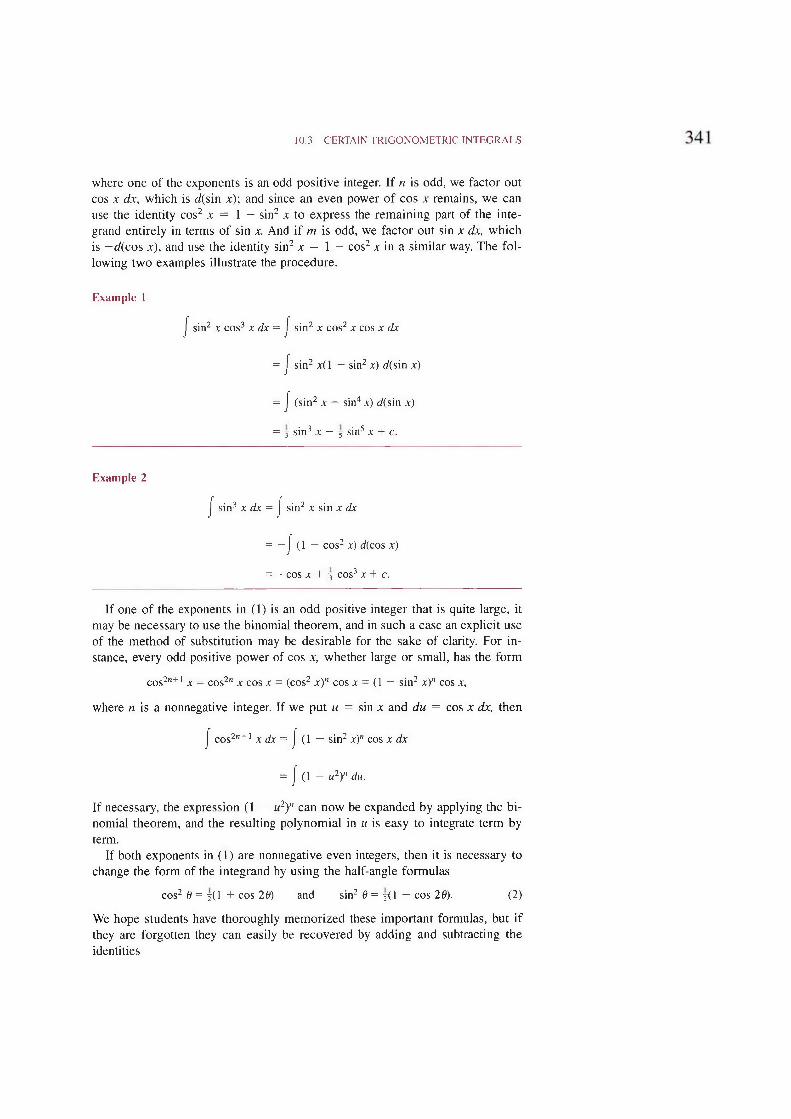
where one of the exponents is an odd positive integer. If n is odd, we factor out

cos x dx , which is d(sin jc); and since an even power of cos jc remains, we can

use the identity cos2 jc = 1 — sin2 jc to express the remaining part of the inte-

grand entirely in terms of sin x. And if m is odd, we factor out sin jc dx, which

is —d(cos jc), and use the identity sin2 jc = 1 — cos2 jc in a similar way. The fol-

lowing two examples illustrate the procedure.

Example 1

J sin2 jc cos3 x dx = J sin2 jc cos2 x cos jc dx

= J sin2 j c ( 1 — sin2 x) d(sin j c )

= J (sin2 jc — sin4 j c ) d(sin j c )

= y sin3 jc — y sin5 jc + c.

Example 2

J sin3 jc dx = J sin2 jc sin j c dx

= — J (1 — cos2 j c ) d{cos j c )

= —cos X + y COS3 X + C.

If one of the exponents in (1) is an odd positive integer that is quite large, it

may be necessary to use the binomial theorem, and in such a case an explicit use

of the method of substitution may be desirable for the sake of clarity. For in-

stance, every odd positive power of cos jc, whether large or small, has the form

cos2”+1 x = cos2” jc cos jc = (cos2 x)n cos jc = (1 — sin2 x)n cos jc,

where n is a nonnegative integer. If we put u = sin x and du = cos x dx, then

J cos2”+1 jc dx = J (1 — sin2 jc)” cos x dx

= J (1 — u2)n du.

If necessary, the expression (1 - u2)'1 can now be expanded by applying the bi-

nomial theorem, and the resulting polynomial in u is easy to integrate term by

term.

If both exponents in (1) are nonnegative even integers, then it is necessary to

change the form of the integrand by using the half-angle formulas

cos2 6 = y(l + cos 26) and sin2 6 = y(l — cos 26). (2)

We hope students have thoroughly memorized these important formulas, but if

they are forgotten they can easily be recovered by adding and subtracting the

identities


cos2 9 + sin2 0=1, cos2 9 — sin2 6 = cos 29.

The uses of (2) are shown in the following examples.

Example 3 The half-angle formula for the cosine enables us to write

J cos2 x dx = 7 J ( 1 + cos 2x) dx = j J dx + j J cos 2x dx

= 7x + j J cos 2x d(2x) = jx + j sin 2x + c.

If we wish to express this result in terms of the variable x (instead of 2x), we use

the double-angle formula sin 2x = 2 sin x cos x and write

J cos2 x dx = 7* + 7 sin x cos x + c.

Example 4 Two successive applications of the half-angle formula for the cosine

give

cos4 x = (cos2 x)2 = {(1 + cos 2x)2 = |(1 + 2 cos 2x + cos2 2x)

= {[1 + 2 cos 2x + {(I + cos 4.x)]

= | + 7 cos 2x + 7 cos 4x,

so

cos4 x dx = Ix + 1 sin 2x + w sin 4x + c.1

As these examples show, the value of the half-angle formulas (2) for this work

lies in the fact that they allow us to reduce the exponent by a factor of 7 at the

expense of multiplying the angle by 2, which is a considerable advantage pur-

chased at very low cost.

Example 5 By using both of the half-angle formulas we get

f . , , , f 1 — cos 2x 1 + cos 2x ,J sinz x cos/ x dx = J ------ --------------- —------ dx

= 4 J ( 1 — cos2 2x) dx = } J [1 —7(1 + cos 4x)] dx

= i J dx — j J cos 4x dx = — 72 sin 4x + c.

We can also find this integral by combining the results of Examples 3 and 4:

J sin2 x cos2 x dx = J (1 — cos2 x) cos2 x dx

= J cos2 x dx — J cos4 x dx

= jx + 7 sin 2x — fx — | sin 2x — sin 4x

10.3 CERTAIN TRIGONOMETRIC INTEGRALS 343

We next consider integrals of the form

J tanm x secn x dx,

where n is an even positive integer or m is an odd positive integer. Our work is

based on the fact that o?(tan jc ) = sec2 x dx and d(sec x) = sec jc tan x dx, and we

exploit the identity tan2 jc + 1 = sec2 jc . An example illustrating each case will

be enough to show the general method.

Example 6

J tan4 jc sec6 jc dx = J tan4 jc sec4 x sec2 jc dx

= J tan4 jc (tan2 jc + 1 )2 d(tan jc)

= J tan4 jc (tan4 jc + 2 tan2 jc + 1) c/(tan jc)

= J (tan8 jc + 2 tan6 jc + tan4 jc) d(tan jc)

= j- tan9 jc + j tan7 jc + j tan5 jc + c .

Example 7

| ta n 3 x s e c 5 jc dx = J ta n 2 jc s e c 4 jc s e c jc tan jc

= J ( s e c 2 jc - 1) s e c 4 jc d ( s e c jc)

= J ( s e c 6 jc - s e c 4 jc) d ( s e c jc)

= y s e c 7 jc — j s e c 5 x + c.

In essentially the same way we can handle integrals of the form

J c o tm x csc" jc dx,

where n is an even positive integer or m is an odd positive integer. O ur tools in

these cases are the formulas d (cot x ) = - c s c 2 jc d x and d (csc jc ) = —csc x cot jc •

dx , and when necessary we use the identity 1 + cot2 x = csc2 x.

Another approach to trigonom etric integrals that is sometimes useful is to ex-

press each function occurring in the integral in term s of sines and cosines alone.

Example 8 We already know from our work with derivatives that

| s e c x ta n x dx = s e c x + c.

However, this form ula can also be obtained directly, by writing

1 s in x , f s in x dxf i f 1 sin x , fsec x tan x dx = --------------- dx =

J J cos x cos x J cos x


sin x dx

If we now put u = cos jc and du = — sin x dx, then we get

sec x tan x dx

PR O B L E M S

- I

- (

c o s ^ X

—du

cos x= sec x + c.

Find each of the following integrals.

/ sin2 x dx.

/ cos6 x dx.

f sin3 x cos2 x dx.

J cos3 x dx.

9 J Vsin x cos3 x dx.

11 J sin2 3x cos2 3x dx.

fn/4

13 sec4 x dx.Jo

15 / tan5 x sec3 x dx.

17 J cot2 x dx.

19 J —J S1I

21 f ‘ 7 ; dx.J sin 2x

2 3 f sin 3 jc cot 3x dx.

2 4 Find / tan x dx (which we already know) by the method

of Example 7.

dx

sin2 Ax'1 + cos 2x

10

12

14

16

18

20

22

f sin4 x dx.

f cos2 3x dx.

/ sin2 x cos5 x dx.[tt/2

snr x cos^ x dx.Jo

J sin3 5x cos 5x dx.

f dx

J sin x cos x '

f - T - -j C O Sz X

f csc4 x dx.

f cot3 x dx.

J cot2 5 jc csc4 5x dx.

J tan2 x cos x dx.

2 5

2 6

Use the identity tan2 x = sec2 j c — 1 to find

(a) / tan2 x dx, / tan4 x dx, f tan6 x dx\

(b) J tan3 x dx, J tan5 jc dx, f tan7 jc dx.

If n is any positive integer > 2, show that

tan” x dx =tan"

1tann - 2 x dx.

2 7

2 8

2 9

3 0

This is called a reduction formula, because it reduces the

problem of integrating tan” jc to the problem of integrat-

ing tan"-2 x.

Find the volume of the solid of revolution generated

when the indicated region under each of the following

curves is revolved about the jc-axis:

(a) y = sin j c, 0 < jc < t t \

(b) y — sec jc, 0 £ Jt £ 7t/4;

(c) y = tan 2 jc, 0 < x ^ 77/ 8 ;

(d) y = cos2 j c, 7 t /2 < x < tt.

Find the length of the curve y = ln (cos jc) between

jc = 0 and jc = t t /4 .

Find f sec3 jc dx by exploiting the observation that sec3 jc

will clearly appear in the derivative of sec jc tan j c.

Find / csc3 jc dx by adapting the idea suggested for Prob-

lem 29.

10.4TRIGONOM ETRIC

SUBSTITUTIONS

An integral involving one of the radical expressions V a 2 - jc2 , V a 2 + jc2 ,

V x 2 — a2 (where a is a positive constant) can often be transformed into a fa-

miliar trigonometric integral by using a suitable trigonometric substitution or

change of variable.

There are three cases, which depend on the trigonometric identities

1 — sin2 6 = cos2 8,

1 + tan2 9 = sec2

sec2 9 — 1 = tan2

( 1)

(2)

(3)

If the given integral involves V a 2 — jc2 , then changing the variable from jc to 6

by writing

jc = a sin 6 replaces V a 2 —jc2 by a cos 9, (4)

10.4 TRIGONOMETRIC SUBSTITUTIONS 345

because a2 — x2 = a2 - a2 sin2 9 = a2( 1 — sin2 9) = a2 cos2 9. Similarly, if the

given integral involves v a 2 + jc2 , then by identity (2) we see that the substitu-

tion

x = a tan 9 replaces v a 2 + jc2 by a sec 6, (5)

because a2 + x2 = a2 + a2 tan2 9 = a2( 1 + tan2 9) = a2 sec2 9\ and if it in-

volves V j c 2 — a2, then by identity ( 3 ) the substitution

jc = a sec 6 replaces Vjc2 — a 2 by a tan 9, (6)

because j c 2 — a2 = a2 sec2 9 — a2 = a2{sec2 9 — 1) = a2 tan2 9. We illustrate

these procedures as follows.

Example 1 Find

V a2 —dx.

So lu tion This integral is of the first type, so we write

j c = a sin 9, dx = a cos 9 d9, V a 2 — j c 2 = a cos

Then

f V a 2 — j c 2

dx - I -J a

cos 9

- I 1

sin 9

— sin2 9

a cos 9 d9

d9

= a f

= a J (csc

cos2 9

sin 9d 9

sin 9

= —a ln (csc 9 + cot 9) + a cos

6 — sin 9) d 9

(7)

This completes the integration, and we now must write the answer in terms of

the original variable x. We do this quickly and easily by drawing a right triangle

(Fig. 10.1) whose sides are labeled in the simplest way that is consistent with the

equation j c = a sin 9 or sin 9 = x/a. This figure tells us at once that

CSC 9 = - , X

cot 9 =V a 2 —

andv a 2

so from (7) we have

IV a 2 —

dx = v a 2 — j c 2 — a lna + V a2 —

+ c.

Figure 10.1

Example 2 Find

r dx

V a2 + x2

Solution Here we have an integral of the second type, so we write

j c = a tan 9, dx = a sec2 9 d9, V a 2 + j c2 = a sec 9.

This yields

f - ^ = = (J \ / J I i ..2 J

a sec2 9 d9

V ^ T x 2 J a sec= J sec 9 d9

= ln (sec 9 + tan 9). (8)


Figure 10.2

The substitution equation x = a tan 6 or tan 6 = x/a is pictured in Fig. 10.2, and

from this figure we obtain

V a2 + x2 xsec 9 = ------------ and tan 9 = —.

a a

We therefore continue the calculation in (8) by writing

f dx . t V a 2 + x2 + x= ln + c'

V a 2 + x2 \ a

= ln (V a2 + x2 + *) + c.

Students will notice that since

' V a 2 + x2 + x sln = ln (V a2 + x2 + x) — ln a,

(9)

(10)

the constant - In a has been grouped together with the constant of integration c ',

and the quantity - I n a + c' is then rewritten as c. Usually we don’t bother to

make notational distinctions between one constant of integration and another, be-

cause all are completely arbitrary; but we do so here in the hope of clarifying

the transition from (9) to (10).

Example 3 Find

dx.

Solution This integral is of the third type, so we write

x = a sec 9, dx = a sec 9 tan 9 dd, Vx2 — a2 = a tan 9.

Then

} y Z E Z d x = (£J x J a

tan 6a sec 9 tan 9 d9

sec 9

= a J tan2 9 d9 = a J (sec2 9 — 1) d9

= a tan 9 — a6.

In this case our substitution equation sec 6 = x/a is portrayed in Fig. 10.3, which

tells us that

Vx:2 — a2tan 9 = and 9 = tan'

Vx2 — a2

The desired integral can therefore be written as

f V c2 — a2 a H>----- ? Vx2 — a2dx = V xz — — a tan 1---------------1- c.

There is one feature of these calculations that we have not taken into account.

In (4) we tacitly wrote

10.4 TRIGONOMETRIC SUBSTITUTIONS 347

without checking the correctness of the algebraic sign. This was careless, because

cos 9 is sometimes negative and sometimes positive. However, the variable 9,

which in this case is sin-1 x/a , is restricted to the interval — 7t/2 < 0 < 77/2, and

on this interval cos 9 is nonnegative, as we assumed. Similar comments apply to

the substitutions (5) and (6).

Example 4 As a concrete illustration of the use of these methods, we determine

the equation of the tractrix. This famous curve can be defined as follows: It is

the path of an object dragged along a horizontal plane by a string of constant

length when the other end of the string moves along a straight line in the plane.

(The word “tractrix” comes from the Latin tractere, meaning “to d rag ”)

Suppose the plane is the xy-plane and the object starts at the point (a, 0) with

the other end of the string at the origin. If this end moves up the y-axis as shown

on the left in Fig. 10.4, then the string is always tangent to the curve, and the

length of the tangent between the y-axis and the point of contact is always equal

to a. The slope of the tangent is therefore given by the formula

dy _ V a2 - x2

dx x

and by separating the variables and using the result of Example 1, we have

f V a 2 — x2 , , (a + V a2 — x2\ r-z----- ry = —J -------------dx = a ln (------------------- j — V a2 — x2 + c.

Since y = 0 when jc = a, we see that c = 0, so

(a + V a 2 - x2\ /-^----- ^y = a ln I------------------ I - V r - j r

is the equation of the tractrix, or at least of the part shown in the figure.

If the end of the string moves down the y-axis, then another part of the curve

is generated; and if these two parts are revolved about the y-axis, the resulting

“double-trumpet” surface shown on the right in Fig. 10.4 is called a pseudo-

sphere. In the branch of mathematics concerned with the geometry of curved sur-

faces, the pseudosphere is a model for Lobachevsky’s version of non-Euclidean

geometry. It is a surface of constant negative curvature, and the sum of the an-

gles of any triangle on the surface is less than 180°.

Vl — sin2 6 = cos 6

Another famous curve whose equation can be determ ined by these methods of

integration is the c a t e n a r y , which is the curve assum ed by a flexible chain or ca-

ble hanging betw een two fixed points. The details are a bit com plicated, so we

give a derivation in Appendix 1 at the end of this chapter for students who have

chosen to omit the optional Section 9.7.

The substitution procedures described in this section can be given a general

justification or p roof similar to that provided in Section 10.2. Students who are

interested in such m atters will find the details in A ppendix A. 10.

F ig u re 10.4



PROBLEMS

1

15

17

V a2 — x2

^2

dx

((a2 + x2)2'

x3 dx

dx.

V9 - x2

dx

xVa2 + x2

dx

V a ^ T x 2

Vx2 — a2dx.

x2 dx

V4 — x2'

dx

0 f

• /

10 f

x2V a 2 + x2

dx

xV a2 — x2

dx

x + j c 3 '

dx

Vx2 — a2 J x3Vx2 — a2

x3 <±C11 J V a2 + x2 dx.* 12 J —

13 J - 2 ^ - 2 . 14 /J a1 — x1 J

~T72dx. 16

2 + x2'

dx

18

(a2 — x2) 3/2

J x3V a 2 + x2 dx.

dxI (x2 - a2)3'2'

19 J x2V a 2 — x2 (ix. 2 0 | ( 1 — 4x2) 372 dx.

The following integrals would normally be found in a differ-

ent way, but this time work them out by using trigonometric

substitutions.

21

23

x dx _ f x dx

V4 - x 2 ’22

h

dx

2 + x 2‘24

(a2 — x2)312'

x dx

4 + x-.2-

25

27

J xV9 — x2 dx. 26 Jdx

v a 2

(x dx

28 / x dx

Vx2 - 4 'V 9 + X2

29 Use integration to show that the area of a circle of radius

a is7t o2.

3 0 In a circle of radius a, a chord b units from the center

cuts off a chunk of the circle called a segment. Find a

formula for the area of this segment.

31 If the circle (x — b)2 + y2 = a2 (0 < a < b) is revolved

about the y-axis, the resulting solid of revolution is called

a torus (see Problem 11 in Section 7.3). Use the shell

method to find the volume of this torus.

32 Find the length of the parabola y = x2 between x = 0

and x = 1. Hint: Use the result of Problem 29 in Section

10.3.

3 3 Find the length of the curve y = ln x between x = 1 and

x = V8.

3 4 The given region under each of the following curves is

revolved about the x-axis. Find the volume of the solid

of revolution.v-3/2

(a) y =

(b) y =

Vx 2 + 4between x = 0 and x = 4.

1

x2 + 1between x = 0 and x = 1.

(c) y = V 4 — x2 between x = 1 and x = 2.

35 The curve jx 2 + y2 = 1 is an ellipse. Sketch the graph

and show that its complete length equals the length of

one cycle of y = sin x. (This integral is a so-called

elliptic integral, and is known to be impossible to eval-

uate in terms of elementary functions. For more details

see Appendix A.9.)

*Hint: See Problem 29 in Section 10.3.

In Section 10.4 we used trigonometric substitutions to calculate integrals con-

taining V a 2 - x2, v a2 + x2, and V x 2 - a2. By the algebraic device of com-

COMPLETING THE P^ting the square, we can extend these methods to integrals involving general

SQUARE quadratic polynomials and their square roots, that is, expressions of the form

ax2 + bx + c and V o x 2 + bx + c. We remind students that the process of com-

pleting the square is based on the simple fact that

(x + A ) 2 = x2 + 2Ax + A2;

this tells us that the right side is a perfect square (the square of x + A) because

its constant term is in the square of half the coefficient of x.

10.5 COMPLETING THE SQUARE 349

Example 1 Find

f (jc + 2) dx

J V 3 + 2 x - x2

Solution Since the coefficient of the term x2 under the radical is negative, we

place the terms containing x in parentheses preceded by a minus sign, leaving

space for completing the square,

3 + 2x — x2 = 3 — ( j c 2 — 2x + ) = 4 — {x2 — 2x + 1)

= 4 — (jc - I)2 = a2 — u 2 ,

where u = jc — 1 and a = 2. Since x = u + 1, we have dx - du and x + 2 =

u + 3, and therefore

f (jc + 2) dx f (w + 3) du _f M 1

r du

’ V 3 + 2x - x2 V a 2 — w2 \ / 2 2 V aA — uz V a2 — u2

= — V a 2 — u2 + 3 sin 1 — a

= — V 3 + 2 jc — jc2 + 3 sin 1 I X ) + c.

Example 2 Find

f dx

x2 + 2x + 10

Solution We complete the square on the terms containing x, and write

JC2 + 2 jc + 10 = (j c2 + 2 jc + ) + 10 = ( jc2 + 2 jc + 1) + 9

= (jc + I ) 2 + 9 = w 2 + a 2,

where u = jc + 1 and a = 3. We now have = dx or dx = du, so

f dx

x2 + 2jc + 10

1 + 1 i ,— tan 1 —^— + c.

Example 3 Find

f jc dx

Vjc2 — 2jc + 5

Solution We write

j c 2 - 2jc + 5 = (jc2 — 2jc + ) + 5 = (jc2 — 2jc + 1 ) + 4

= (jc — I ) 2 + 4 = w2 + a 2,

where u = x — 1 and a = 2. Then x = u + 1, dx = du, and we have

f x dx f (u + 1) du f u du f du

V jc2 — 2x + 5 Vm2 + a2 V m2 + a2 V u2 + a2


The second integral here is the one considered in Example 2 in Section 10.4, so

we have

f du

Vw2 + a2= ln (m + Vw2 + a2),

and therefore

f x dxV u2 + a2 + ln (u + Vw2 + a2)

J Vjc2 - 2x + 5

= V jc2 — 2jc + 5 + ln (jc — 1 + V jc2 — 2 x + 5) + c.

Example 4 Find

f dx

J Vjc2 - 4jc - 5

Solution Here we have

jc2 — 4jc — 5 = (jc2 — 4x + ) — 5 = (x2 - 4x + 4 ) — 9

= (x - 2)2 - 9 = u2 - a2,

where u = x — 2 and a = 3. By using the result of Problem 9 in Section 10.4

(or by quickly working out the necessary formula again by putting u = a sec 9)

we complete the calculation as follows:

[ dx f du

Vx2 — 4 jc — 5 Vm2 — a2— [ — = ln (m + Vm2 — a2)

= ln (x — 2 + V x2 — 4x — 5) + c.

If an integral involves the square root of a third-, fourth-, or higher-degree

polynomial, then it can be proved that there does not exist any general method

for carrying out the integration. A few integrals of this kind are discussed in Ap-

pendix A.9.

P R O B L E M S

Calculate the following integrals.

f dx dx

V2x - x2 J V5 + 4x - x2

dx4

f dx

x2 + 4x + 5 ' i x2 - x + 1 ’

(x + 1) dx6

T (x + 3) dx

*1K<N>

V 5 + 4x - x2

x2 dx8

f (x — 1) dx

''h1

>

Vx2 + 4x + 5

» I

13

(x + 7) dx

x2 + 2x + 5'

_____dx

V x2 — 2x —

dx

V4x2 + 4x + 17-

15 (x2 — 2x — 3)3 /2 '

V x2 + 2x — 3

X + 1

dx

,o /

12 / ------------------J V5 + 3x — 2 x2

14 J + 3) ^

16 /

dx.

(x2 — 2 x + 2 )3/2'

dx

(x + 2)Vx2 + 4x + 3

10.6 THE METHOD OF PARTIAL FRACTIONS 351

We recall that a rational function is a quotient of two polynomials. By taking the

denominator of such a quotient to be 1, we see that the polynomials themselves

are included among the rational functions. As we know, the simple rational func-

tions

1 1 x 12x + 1, -3 , —, 7 , - / , and

x x

have the following integrals

+ 1 ’ x 2 + 1

x2 + x, ——, ln x, \ ln (x2 + 1), and tan'x

Our purpose in this section is to describe a systematic procedure for computing

the integral of any rational function, and we shall find that this integral can al-

ways be expressed in terms of polynomials, rational functions, logarithms, and

inverse tangents. The basic idea is to break up a given rational function into a

sum of simpler fractions (called partial fractions) which can be integrated by

methods discussed earlier.

A rational function is called proper if the degree of the numerator is less than

the degree of the denominator. Otherwise, it is said to be improper. For example,

x2 + 2

are proper, while

(x — l)(x + 2)2 and x(x2 — 9)

2x3 — 3x2 + 2x — 4and

4 - 1 x2 + 4

are improper. If we have to integrate an improper rational function, it is essen-

tial to begin by performing long division until we reach a remainder whose de-

gree is less than that of the denominator. We illustrate with the second improper

rational function just mentioned. Long division yields

2x — 3

x2 + 4|2x3 — 3x2 + 2x — 4

2x3______+ 8x

- 3x2 - 6x - 4

- 3x2 - 12

— 6x + 8

This means that the rational function in question can be written in the form

2x3 — 3x2 + 2x — 4 „ „ , -6x + 8---------- 2——--------- = 2x - 3 H-----T~n~- (1)

x2 + 4 x2 + 4

By applying this process, any improper rational function P(x)/Q(x) can be ex-

pressed as the sum of a polynomial and a proper rational function,

P(x) , . , R(x) ...— = polynomial + — , (2)

where the degree of R(x) is less than the degree of Q(x). In the particular case of

(1), this decomposition by means of long division enables us to carry out the in-

tegration quite easily, by writing

10.6THE M ETH O D OF

PARTIAL FRACTIONS


2x3 - 3x2 + 2x - 4 , „ f x dx „ f dxdx = xz — 3x

J xz + 4 ' ' ' J x2 + 4 J x2 + 4

= x2 — 3x — 3 ln (x2 + 4) + 4 tan- 1 y + c.

In the general case (2), these remarks tell us that we can restrict our attention to

proper rational functions, since the integration of polynomials is always easy.

This restriction is not only convenient, but also necessary, because it is only to

proper rational functions that the following discussions apply.

In elementary algebra we learned i’ow to combine fractions over a common

denominator. We must now learn how to reverse this process and split a given

fraction into a sum of fractions having simpler denominators. This procedure is

called decomposition into partial fractions.

Example 1 It is clear that

3 | 2 3(x + 3) + 2(x - 1) 5x + 7

x - 1 x + 3 (x — l)(x + 3) (x — l)(x + 3) '

In the reverse process we start with the right side of (3) as our given rational

function and seek constants A and B such that

5x + 7 A B------------------ = --------- 1--------- (4)(x — l)(x + 3) x - 1 x + 3

( For the sake of understanding the method, let us pretend for a moment that we

don’t know that A = 3 and B = 2 will work.) If we clear fractions in (4) by mul-

tiplying through by (x — l)(x + 3), we get

5x + 7 = A(x + 3 ) + B(x — 1) (5)

or

5x + 7 = (A + B)x + (3A - B). (6)

Since (6) is to be an identity in x, we can find A and B by equating coefficients

of like powers of x. This gives a system of two equations in the two unknowns

A and B,

A + B = 50 . „ „ whose solution is A = 3, B = 2.3A — B = 7,

There is another convenient way to find A and B, by using (5) directly. Since (5)

must hold for all x, it must hold in particular for x = 1 (which removes B) and

for x = —3 (which removes A). Briefly,

x = 1: 5 + 7 = A(1 + 3) + 0, 4A = 12, A = 3;

x = -3 : -15 + 7 = 0 + 5 ( - 3 - 1 ) , - 4 5 = - 8 , B = 2.

This method is faster than it looks, and can be carried out by inspection.

Whichever method we use to find A and B, (4) becomes

5x + 7 3 2

(x — l)(x + 3) x — 1 x + 3 ’

and this is the partial fractions decomposition of the rational function on the left.

Of course, the purpose of this decomposition is to enable us to integrate the given

function,


/ (x - 1 ) 1 /+ 3) dx = I ( t ^ i + I T ? ) *

= 3 ln (jc — 1) + 2 ln ( x + 3) + c.

The type of expansion used in (4) works in just the same way under more gen-

eral circumstances, as follows: Let P(x)/Q(x) be a proper rational function whose

denominator Q(x) is an «th-degree polynomial. If Q(x) can be factored completely

into distinct linear factors x - r\, x — r2, . . . , x — rn, then there exist n constants

A i, A 2, . . . , An such that

P(x) = A\ + A 2 + . . . + An

Q(x) x - r | x ~ r2 x - rn

The constants in the numerators can be determined by either of the methods sug-

gested in Example 1; and when this is done, the partial fractions decomposition

(7) provides an easy way to integrate the given rational function.

Example 2 Find

6 j c2 + 14 jc - 2 0 ,

------- ---- a------ dx.j c3 — Ax

Solution We factor the denominator by writing x 3 — 4x = x(x2 — 4) =

jc(jc + 2 )(jc - 2 ) . Accordingly, we have a decomposition of the form

6jc2 + 14jc - 20 6jc2 + 1 4 x - 20 A B | C

jc3 — 4jc x(x + 2)(x — 2) jc jc + 2 x — 2

for certain constants A, B, C. To find these constants we clear fractions in (8),

which yields

6 jc2 + 14 jc - 2 0 = A(x + 2 ) ( j c - 2 ) + Bx(x - 2 ) + Cx(x + 2).

By setting jc = 0, - 2 , 2 (this is the second method in Example 1), we easily see

that A = 5, B = —3, C = 4, so (8) becomes

6 j c2 + 14jc — 2 0 _ 5 3 4

j c3 — Ax x x + 2 jc — 2 ’

We therefore have

r 6x2 + 14jc — 2 0-------- ,----- --------- dx = 5 ln jc — 3 ln (x + 2 ) + 4 ln (x — 2 ) + c.

J x 3 — Ax

In theory, every polynomial <2(jc) with real coefficients can be factored com-

pletely into real linear and quadratic factors, some of which may be repeated.

In practice, this factorization is hard to carry out for polynomials of degree 3 or

more, except in special cases. Nevertheless, let us assume this has been done,

and let us see how the decomposition (7) must be altered to take account of the

most general circumstances that can arise.

*This statement is a consequence of the Fundamental Theorem of Algebra, which is discussed in Sec-

tion 14.8.


If a linear factor jc — r occurs with multiplicity m, then the corresponding term

A/(x — r) in the decomposition (7) must be replaced by a sum of the form

B'- + - ^ + - - +x — r (x — r)2 (x — r)m'

A quadratic factor jc2 + bx + c of multiplicity 1 gives rise to a single term

A j c + B

x2 + bx + c'

and if this quadratic factor occurs with multiplicity m, then it gives rise to a sum

of the form

AiX + B i A 2x + B2 + . . . , + B m

x2 + bx + c (x2 + bx + c ) 2 (jc 2 + bx + c)m ’

This is the whole story, and the theory guarantees that every proper rational func-

tion can be expanded into a sum of partial fractions in the manner described

above.*

Example 3 Find

f 2>x3 — 4 jc 2 — 3jc + 2dx.

Solution We have

3 jc3 — 4 jc2 — 3jc + 2 _ 3 jc3 - 4 jc2 — 3 jc + 2

jc2 (jc + 1 ) (jc — 1)

= A + 4 + - ^ + 0

,4 _ v2

X X 2 J C + 1 JC — 1

Clearing fractions gives the identity

3 x 3 — 4x2 — 3jc + 2 = A jc(jc + 1 )(jc - 1 ) + B(x + 1)(jc - 1 ) + Cx2(x - 1 ) + D jc 2(jc + 1 ).

Now put

jc = 0: 2 = -B , B= - 2 ;

j c = 1: - 2 = 2D, D= - 1 ;

j c = —1: - 2 = - 2 C, C = 1.

Equating coefficients of jc3 gives

3 = A + C + D, so A = 3 .

Our partial fractions decomposition is therefore

3 jc3 — 4 jc2 — 3 jc + 2 _ 3 2 + 1 1X 4 - X 2 X JC2 JC+1 JC - 1 ’

so

f 3 jc3 — 4 x 2 — 3 jc + 2 2

J --------y4 _ _y2-----^ = 3 ln jc + j + ln (jc + 1) - ln (jc - 1) + c.

‘This statement is called the Partial Fractions Theorem', it is proved in Appendix A.l 1. Students will

notice that the above description of the partial fractions decomposition assumes that the highest power

of x in Q(x) has coefficient 1; this can always be arranged by a minor algebraic adjustment.


Example 4 Find

f 2 jc 3 + x 2 + 2 x — 1dx.

Solution We have

2jc3 + x 2 + 2x — 1 2jc3 + x2 + 2x — 1

C4 - 1 (JC + 1)(JC - 1)( JC2 + 1)

jc + 1 jc — 1 jc 2 + 1

s o

2jc3 + jc2 + 2 jc — 1 = A(jc — 1)(jc2 + 1 ) + 5 ( x + 1)(jc2 + 1 ) + Cx(x2 — 1) + D(x2 — 1).

N o w p u t

JC = 1: 4 = 4 5 , 5 = 1 ;

jc = — 1: - 4 = - 4 A, A = 1;

jc = 0: — 1 = —A + B — D, D = 1.

E q u a t i n g c o e f f i c i e n t s o f jc3 g i v e s

2 = A + 5 + C, so C = 0.

O u r p a r t ia l f r a c t i o n s d e c o m p o s i t i o n i s t h e r e f o r e

2 jc 3 + jc 2 + 2 jc — 1 _ 1 1 1

jc4 - i - jc + i + jc - i + jc2 + r

s o

f + “I- — 1J ------------jc4 '— ' l------------- d x = ln (jc + 1) + ln (jc — 1) + t a n - 1 x + c.

As a final comment, we point out that all the partial fractions that can possi-

bly arise have the form

A Ax + 5 1 0 ¾n = 1, 2, 3 , . . . .

(jc - r)” (jc2 + bx + c ) " ’

Functions of the first type can be integrated by using the substitution u = x — r,

and it is clear that the results are always logarithms or rational functions. A func-

tion of the second type in which the quadratic polynomial x2 + bx + c has no

real linear factors, that is, in which the roots of x2 + bx + c = 0 are imaginary,

can be integrated by completing the square and making a suitable substitution.

When this is done, we get integrals of the form

f u du f du

J (w2 + k2)n' J (m2 + k2)n'

The first of these is \ ln (u2 + k2) if n = 1, and (u2 + A:2)1 “ ”/2(1 - n) if

n > 1. When n = 1, the second integral is calculated by the formula

f du 1 , u—5---- t t = — tan 1 —

J u2 + k2 k k


The case n > 1 can be reduced to the case n = 1 by repeated application of the

reduction formula

f du _ 1 ____ u_____ 2n — 3 f du

J (u2 + k2)n ~ 2k \n - 1) ’ (w2 + k2)n~ l 2k\n - 1 ) J (w2 + k2)n~1'

We state this complicated formula for the sole purpose of showing that the only

functions that arise from the indicated reduction procedure are rational functions

and inverse tangents. The formula itself can either be verified by differentiation

or obtained from scratch by the methods of the next section.

This discussion shows that the integral of every rational function can be ex-

pressed in terms of polynomials, rational functions, logarithms, and inverse tan-

gents. The detailed work can be very laborious, but at least the path that must be

followed is clearly visible.

P R O B L E M S

1 Express each of the following improper rational func-

tions as the sum of a polynomial and a proper rational

function, and integrate:

(a)

(d)

jc — 1 ’

jc + 3

jc + 2 ’

(b)

(e)

3jc + 2 ’

jc2 - 1

jc2 + 1 '

(c)JC2 + 1’


12x - 17

(x - l)(x - 2)

10 - 2x ,

~ ? r & r

9x2 - 24x + 6

J x3 — 5x2 + 6x

8 j ^

dx. 3

dx.

14x - 12

10

12

14

16x2 + 3x — 7

x

T

x3 + 4x

2x2 - 2x — 12

2x + 21 ,

x2 + 46x - 48

x3 + 5x2 — 24x

4x2 + llx - 117

x3 + 10x2 — 39x

dx.

dx.

dx.

6x2 — 9x + 9 . f —4x2 - 5x — 3

x3 — 3x2dx. 11

4x2 + 2x + 4dx. 13

x3 + 2x2 + x

3x2 - x + 4

c3 + 2x2 + 2x

dx.

dx.

x2 + 4dx.

15x4 + 3x2 - 4x + 5

(x - 1 )2(x2 + 1)

f x2 + 2x

16 1 ( P m ? * '

18 i ^ J x .J X — 1

dx.

17 /

- I

x + 2

x2 + 1

x + 2

dx.

dx.

f x3 - 3x2 -I- 2x - 3 20 J --------- -------------- dx.

21 I

22 f

23 [

x2 + 1

cos 8

sin2 8 + 3 sin 8 — 4

16 sec2 8

dd.

tan3 8 — 4 tan2 8

e* dx.

d8.

24J e2x _ 4 j 1 _|_ e

25 Use partial fractions to obtain the formula

dx.

h

dx 1 , a + x= "r— In

2 — x2 2a ' a — x

Also calculate this integral by trigonometric substitution,

and verify that the two answers agree.

26 Find

3 sin 8 dd f 5e' dt(a) fcos2 d — cos <»> I ?2f + el — 6

27 In Problem 14 of Section 8.5 it is stated that the differ-

ential equation

dx— = kab(A — x)(B — x), A B,

has

— X ) _ kab(A—B)t

A(B - x)

as a solution for which x = 0 when t = 0. Derive this so-

lution by using partial fractions.

28 Verify the reduction formula (9) by differentiating the

first term on the right.

29 Suppose that a given population can be divided into two

10.7 INTEGRATION BY PARTS 357

groups: those who have a certain infectious disease, and those such contacts, and (3) that the two groups mingle freely with

who do not have it but can catch it by having contact with an each other, so that the number of contacts is jointly propor-

infected person. If j c and y are the proportions of infected and tional to j c and y. If j c = j c o when t = 0, find j c as a function of

uninfected people, then j c + y = 1. Assume (1) that the dis- t, sketch the graph, and use this function to show that ulti-

ease spreads by the contacts just mentioned between sick peo- mately the disease will spread through the entire population,

pie and well people, (2) that the rate of spread dx/dt is pro- When the formula for the derivative of a product (the

portional to the number of such contacts, and (3) that the two

When the formula for the derivative of a product (the product rule) is written in

the notation of differentials, it is 10.7d(uv) = u dv + v du or u dv = d(uv) — v du, IN T E G R A T IO N

j , - • Kt ■ b y p a r t sand by integrating we obtain

J u dv = uv — J v du. (1)

This formula provides a method of finding fu dv if the second integral f v du is

easier to calculate than the first. The method is called integration by parts, and

it often works when all other methods fail.

Example 1 Find fx cos x dx.

Solution If we put

u = j c , dv = cos x dx,

then

du = dx, v = sin j c ,

and (1) gives

J x cos j c dx = j c sin x — J sin x dx.

This is good luck, because the integral on the right is easy. We therefore have

j c cos x dx = j c sin x + cos j c + c.I

It is worth noticing that in this example we could have chosen u and dv dif-

ferently. If we put

u = cos j c , dv = j c dx,

then

du = —sin x dx, v = jx2,

and (1) gives

J x cos x dx = \x 2 cos x + \ J x2 sin x dx.

This equation is true, but it is completely worthless as a means of solving our

problem, because the second integral is harder than the first. We urge students to


learn from experience, and to use trial and error as intelligently as possible in

choosing u and dv. Also, students should feel free to abandon a choice that

doesn’t seem to work, and quickly go on to another choice that offers more hope

of success.

The method of integration by parts applies particularly well to products of dif-

ferent types of functions, like x cos x in Example 1, which is a product of a poly-

nomial and a trigonometric function. In using the method, the given differential

must be thought of as a product u • dv. The part called dv must be something we

can integrate, and the part called u should usually be something that is simpli-

fied by differentiation, as in our next example.

Example 2 Find / ln jc dx.

Solution Here our only choice is

In some cases it is necessary to carry out two or more integrations by parts in

succession.

Example 3 Find f x 2ex dx.

Solution If we put

w = ln jc , dv = dx,

so

dxu = — ,

JCV = JC,

and we have

Jlnjcdjc = jc ln jc - j jc — = jc ln jc - jc + c.

dv = ex dx,

then

du = 2jc dx, v = ex,

and (1) gives

(2)

Here the second integral is easier than the first, so we are encouraged to con-

tinue in the same way. When the second integral is integrated by parts with

When this is inserted in (2), our final result is

| x2ex dx = x 2ex — 2xex + 2ex + c.

It sometimes happens that the integral we start with appears a second time dur-

ing the integration by parts, in which case it is often possible to solve for this in-

tegral by elementary algebra.

Example 4 Find f e x cos x dx.

Solution For convenience we denote this integral by J. If we put

u = ex, dv = c o s x dx,

then

du = ex dx, v = s in x,

and (1) yields

J = ex s in x — J ex s in x dx. (3)

Now we come to the interesting part of this problem. Even though the new in-

tegral is no easier than the old, it turns out to be fruitful to apply the same method

again to the new integral. Thus, we put

u = ex, dv = s in x dx,

10.7 INTEGRATION BY PARTS

so that

and obtain

du = ex dx, v = —cos x,

J ex sin x dx = —ex cos x + J ex cos x dx. (4)

The integral on the right is J again, so (4) can be written

J ex sin x dx = - e x cos x + J. (5)

In spite of appearances, we are not going in a circle, because substituting (5) in

(3) gives

J = ex sin x + ex cos x — J.

It is now easy to solve for J by writing

2 J = ex sin x + ex cos x or J = j(ex sin x + ex cos x),

and all that remains is to insert the constant of integration:

J ex cos x dx = ye*(sin x + cos x) + c.

The method of this example is often used to make an integral depend on a sim-

pler integral of the same type, and thus to obtain a convenient reduction formula,

by repeated use of which the given integral can easily be calculated.

Example 5 Find a reduction formula for = / sin” x dx.

Solution We integrate by parts with

u = sin”-1*, dv = sin x dx,

so that

du = {n — 1) sin”-2 x cos x dx, v = —cos x,

and therefore

Jn = —sin”-1 x cos x + (n — 1) J sin”-2 x cos2 x dx

= —sin”-1 x cos x + (n — 1) J sin”-2 x(l — sin2 x) dx

= —sin”-1 x cos x + (n — 1) J sin”-2 x dx — (n — 1) J sin” x dx

= —sin”-1 x cos x + (n — 1) Jn- 2 — (n — 1) Jn.

We now transpose the term involving Jn and obtain

nJn = -s in ”-1 x cos x + in - 1)/,,-2,

so that

1 ft — 1Jn = ----sin”-1 X COS X H---------- Jn-2,

n n

or equivalently,

[ sin" x dx = —- sin”-1 x cos x + —----— f sin”-2 x dx. (6)J n n J

The reduction formula (6) allows us to reduce the exponent on sin x by 2. By

repeated application of this formula we can therefore ultimately reduce Jn to J0

or J i, according as n is even or odd. But both of these are easy:

J0 = f sin0 x d x = f dx = x and 7, = f sin x dx = -cos x

For example, with n = 4 we get

J sin4 x dx = — j sin3 x cos x + f J sin2 * dx,

and with n = 2,

J sin2 x dx = — \ sin x cos jc + \ J dx

= sin x cos x + jx.

J sin4 x dx = — j sin3 x cos x + sin x cos x + l x)

= — t sin3 x cos jc — | sin x cos jc + lx + c.


Therefore,

10.7 INTEGRATION BY PARTS

The same result can be achieved by earlier techniques depending on repeated use

of the half-angle formulas, but our present methods are more efficient for large

exponents. In our next example we illustrate another way in which the reduction

formula (6) can be used.

Example 6 Calculate

[■nilsin8 x dx.

Jo

Solution For convenience we write

r tt/2

'» = 1

By formula (6) we have

sin" x dx.

/„ = — sin" 1 x cos x n

17/2 n — 1 f77-/2 . ,H----------sin" x dx,

o n Jo

so

/ - 1 IIn ~ In -2 -n

We apply this formula with n = 8, then repeat with n = 6, n = 4, n = 2:

/ - 2 / - 1 h — 2 I 2/ _ 2 1 2 1/'8 — 8-*6 8 ' 6-*4 — 8 ' 6 4 ‘ 2 8 ' 6 ' 4 2^0-

Therefore

f™'2 ■ s , 7 5 3 1 2 7 sin8 x dx = — • — • — • — dx = —

Jo 8 6 4 2 Jo 86 4 2 Jo 8 6 4 2 2 256

Remark 1 The reduction formula (6) can also be used to establish one of the

most fascinating formulas of mathematics, Wallis’s infinite product for 7t/2:

JL = 12 ~ 1 3 3 5 5 7 '

For the details of the proof, see Appendix 2 at the end of the chapter.

Remark 2 In Section 9.5 we stated Leibniz’s formula for 77-/4,

For students who are interested in little-known corners of the history of mathe-

matics, we describe in Appendix 3 at the end of the chapter how Leibniz him-

self discovered his formula by a very ingenious application of integration by parts.

At this point we have described all the standard methods of integration that the

student is expected to be acquainted with. A few additional techniques of minor

importance remain, and two of these are briefly sketched in the problems at the

end of Appendix A.9; but for most practical purposes we have reached the end

of this particular road.


PROBLEMS

Find each of the following integrals by the method of inte-

gration by parts.22

1 fx ln x dx. 2 / tan-1 x dx.

3 fx tan-1 x dx. 4 fxeax dx.

5 fe x sin x dx. 6 fe™ cos bx dx.

7 / V 1 — x2 dx. 8 f sin-1 x dx.

9 J x sin-1 x dx. 10r tt/2

x sin x dx.Jo 23

11 J x cos (3x — 2) dx. 12f tan-1 x ,J ,2 dx. 24

13 fx sec2 x dx. 14 f sin (ln x) dx.

15 f ln (a2 + x2) dx. 16 fx 2 ln (x + 1) dx.

17 18 J (ln x)2 dx. 25

19 The region under the curve y = cos x between jc = 0 and

jc = 7t/2 is revolved about the y-axis. Find the volume of

the resulting solid.

20 Find /(sin-1 jc)2 dx. Hint: Make the substitution y =

sin-1 jc.

21 If P(x) is a polynomial, show that

f P(x)ex dx = (P - P' + P” - P"' + • • -)ex.

In the next two problems, derive the given reduction formula

and apply it to the indicated special case(s).

26

cos" x d x = —- sin x cos" 1

cos7 x d x .

x dx.

cos8 x dx.

d x .

(a) /

<»> f

f 77 <CH(a) /(In j c ) " d x = x(ln x ) n — «/(ln x ) n ~

(b) /(In j c ) 5 d x .

The region under the curve y = sin x between jc = 0 and

x = t t is revolved about the y-axis. Find the volume of

the resulting solid (a) by the shell method; and (b) by the

washer method.

The curve in Problem 24 is revolved about the x-axis.

Find the area of the resulting surface of revolution.

(The volcanic ash problem) When a volcano erupts, the

cloud of ejected ash gradually settles onto the surface of

the nearby land. The depth of the deposited layer of ash

decreases with distance from the volcano. Assume that

the depth of the ash r feet from the volcano is a e ~ br feet,

where a and b are positive constants.

(a) Find the total volume of ash that falls within a dis-

tance c of the volcano. Hint: What is the element of

volume d V of ash that falls on a narrow ring of width

d r and inner radius r centered on the volcano?

(b) What is the limit of this volume a s c -» » ?

10.8A MIXED BAG.

STRATEGY FO R

DEALING W ITH

INTEGRALS O F

MISCELLANEOUS TYPES

As the student understands by now, differentiation is straightforward but inte-

gration is not. In finding the derivative of a function it is obvious which formula

must be applied. But it may not be at all obvious which method should be used

to integrate a given function.

Since the problems in each section of this chapter have focused on the meth-

ods of that section, it has usually been clear what method to use on a given in-

tegral. Generally speaking, the methods at our disposal now are direct substitu-

tion, trigonometric substitution, partial fractions, and parts. But what if an integral

is met out of context, with no obvious clue as to how to work it out? In this sec-

tion we try to suggest a strategy for this common situation.

An essential prerequisite is a knowledge of the basic integration formulas. For

the sake of emphasis, we repeat the list given in Section 10.1, together with three

additional formulas arising from our work in this chapter. As we pointed out ear-

lier, the first 15 formulas should be memorized, and we hope students will take

our advice seriously this time. It is useful to know them all, but the last three

(marked with an asterisk) need not be memorized since they are easy to derive,

as follows. Formulas 16 and 17 are immediate from the simple partial fractions

decompositions

10.8 A MIXED BAG. DEALING WITH INTEGRALS OF MISCELLANEOUS TYPES 363

and

A -

-,2 _ v2

1

(.x + a ) ( x — a )

1

( a + x ) ( a — x )

J _

2 a

J _

2 a+

1

x + a

1

a + x a — x

These decompositions can easily be understood by mentally recombining the

terms in brackets with the aid of a common denominator; we then see directly

what the constant factor outside the brackets must be. Formula 18 is almost im-

mediate from the trigonometric substitutions x = a tan 6 and jc = a sec 6, re-

spectively. In this list of formulas we use jc instead of u as the variable of inte-

gration— since the usefulness of the ^-notation is now thoroughly familiar to us

— and for the sake of simplicity we omit the constant of integration.

1

2

3

4

5

6

7

8

9

10

11

12

13

14

15

*16

*17

* 1 8

jc” d x =

rn+ 1

n + 1(tt * -1).

d x— = ln j c .

JC

e x d x = e x .

c o s x d x = s in x .

s in jc d x = —c o s x .

s e c 2 jc d x = ta n jc.

c s c 2 jc d x = — c o t jc.

s e c x tan x d x = s e c jc.

c s c jc c o t jc d x = — c s c jc.

d x . jc— , = s in 1 — .

V a ^ 7 2 a

d x 1= — ta n

- l _

a 'a + x a

ta n jc d x = —In ( c o s jc).

c o t x d x = ln ( s in jc).

s e c jc d x = ln ( s e c jc + tan jc).

c s c jc d x = — In ( c s c jc + c o t jc).

x — a 'd x 1

x 2 — a 2 2 a

d x 1

a 2 — x 2 2 a

d x— = 1

jc + a

a + x

a — x

V jc2 ± a 2

= ln (jc + V jc2 ± a 2).


These formulas constitute our arsenal of weapons for attacking integrals, and

it is up to us to decide which to use in a particular case. If we do not see what

to do immediately, the following strategy may be helpful.

STRATEGY FOR INTEGRATION

1 Simplify the integrand. The use of algebraic or trigonometric identities will

sometimes simplify the integrand and make a method of integration obvious.

For example:

J Vx(Vx + Vx) dx = J (x + x5/6) dx;

J (sin jc + cos j c ) 2 dx = J (sin2 jc + 2 sin jc c o s jc + cos2 j c ) dx

= J (1 + 2 sin jc cos j c ) dx;

f 1 - tan2 x , ( , . , , - , ,----- ~----- dx = (1 — tan- jc ) c o s z jc dx

J sec- jc J

= f 11 _ i i n M cos2 x dxj \ C O S z JC /

= J (cos2 x - sin2 x) dx = J cos 2x dx.

In the second problem, if we fail to notice that sin2 jc + cos2 jc = 1, and in-

stead integrate sin2 x and cos2 jc separately, then we can still solve the prob-

lem, but we have missed an opportunity to do things the easy way. A simi-

lar remark applies to the third problem, with its use of the double-angle

formula for the cosine.

2 Look fo r an obvious substitution. Try to find some function u = g(jc) in the

integrand whose differential du — g'(x) dx is also present, apart from a con-

stant factor. For example, in

f x dx

J

we notice that if u = 4 — x2, then du = — 2x dx and x dx = — j du. It is there-

fore much simpler to use this substitution than to use partial fractions or the

trigonometric substitution x = 2 sin 6, each of which also works but takes

longer to carry out.

3 Classify the integrand. This is the heart of the matter. If Steps 1 and 2 have

not helped, then we turn to a more careful examination of the form of the in-

tegrand /(jc).

(a) If f{x) is (or can be written as) a product of powers of sin x and cos x,

or tan x and sec x, or cot j c and csc x, then the methods of Section 10.3

can be used.*

*A special method for integrating any rational function of sin x and cos x is described in Appendix

A.9 at the end of the book. This method will not be needed for any of the review problems at the

end of this section.

10.8 A MIXED BAG. DEALING WITH INTEGRALS OF MISCELLANEOUS TYPES 365

(b) If/0 0 involves V a 2 ± j c 2 or V x 2 ± a2, or powers of these expressions,

use the trigonometric substitutions of Section 10.4.

(c) If f(x ) is a rational function, use partial fractions as explained in Sec-

tion 10.6— unless there is a better way for a particular integral.

(d) If / ( j c ) is a product of functions of different types, try integration by

parts. As we have seen in Section 10.7, this method also works for many

individual inverse functions like ln x, sin-1 x, and tan-1 x.

(e) Be observant, thoughtful, flexible and persistent— all of which are of

course easier said than done. If a method doesn’t work, be ready to try

another. Sometimes several methods work. Keep your options open and

do things the easy way— if any. And remember that doing a problem

more than one way is a good learning experience.

Our purpose in the following examples is to try to suggest possible lines of at-

tack by “thinking out loud.” We are interested mainly in brainstorming these in-

tegrals, and in most cases we will not work out all the details to the final answer.

r x 2Example 1 J —g-----— dx.

Comments Since the integrand is a rational function, partial fractions will work.

This requires factoring x6 - 1 into ( jc 3 + 1)(jc3 — 1) = ( j c + 1)(jc2 — x + 1 ) -

( j c — 1)(jc2 + j c + 1) and then finding constants A, B, C, D, E, F such that

x 2 A Bx + C D Ex + F— ------ - --------—I----~---------------1-------- -—I----~ .X 1 X + 1 JC2 — J C + 1 X — 1 JC2 + X + 1

We can do this if we must, but actually carrying out this work is not an attrac-

tive prospect.

Let us probe in a different direction. A much more promising method is to no-

tice that j c 6 is the square of j c 3 and that the numerator of the integrand is almost

the derivative of j c 3 . Accordingly, if we put u = j c 3 , then du = 3jc2 dx, x 2 dx =

y du, and the integral becomes

i r * 4 4 4 ^ - 13 J u2 — 1 6 \m + 1/ 6 \x 3 + 1 /

by formula 16.

f XExample 2 ------- 7 dx.

J 1 + JCZ

Comments The trigonometric substitution x = tan 9 will work. Partial fractions

will also work, but since the integrand is an improper rational function, we must

begin with long division. However, an easier way to accomplish the result with-

out actually carrying out the long division is simply to add and subtract 1 in the

numerator,

I l T ? * = / (^iV J ') * = /( ' ~TT?) *

= x — tan-1 x.


Example3 [ J ^ L J e 1

Comments We begin by noticing that e7* dx = ex(ex dx) = ex d(ex). This sug-

gests that we put u = ex, so that e2 dx = u du and the integral can be written

u du f w — 1 + 1 , ( ( 11 H------ du

C _udu _ f u_- 1 + 1_ ^ = f

J u — 1 J m — 1 J U — 1

= u + ln (w - 1) = e* + ln (ex — 1).

By subtracting and adding 1 here we employ a slight variation of the idea used

in Example 2.

r 4jc + 1Example 4 —-------7 dx.

J 1 + jcz

Comments The numerator is nearly (but not quite) the derivative of the de-

nominator. This suggests that we break the integrand into a sum and rearrange

the constants to achieve this desirable condition:

( 4x + 1 , f / 2x , 1 \ ,

J TT7 J (2' "m? TT j

= 2 f -2^ + f = 2 In (1 + x2) + tan"1 xJ 1 + j r J 1 + xz

( 2x + 6 ,

Example5 J ^2 -+ 7 ,+ 1 0 ^

Comments In Example 4 we arranged part of the numerator to be the deriva-

tive of the denominator. A similar purpose here suggests that we write

f 2x + 6 = f (2x + 7 ) - 1

J x2 + 7x + 10 X ~ J x 2 + 7x+ 10

C (2x + 7) dx _ f ____ dx

~ j x2 + Ix + 1 0 j X 2 + Ix + 1 0 '

The first of these integrals has been arranged to be ln (x 2 + Ix + 10), and we

can easily work out the second by factoring the denominator into (jc + 2)( jc + 5)

and using partial fractions.

Example 6 f (1*+ * )4.

Comments The trigonometric substitution j c = tan 6 will work. Partial fractions

will also work, but if we try this there will be eight unknown constants to find.

We hope for something better.

Let us try the substitution u = 1 + j c 2 . Our only reason for this is that it sim-

plifies the denominator to u4. Then du = 2x dx, and we have

10.8 A MIXED BAG. DEALING WITH INTEGRALS OF MISCELLANEOUS TYPES

f x5 dx _ f (.x2)2 (x dx) _ J_ f (u - I)2 du

J (1 + x2)4 ~ J (1 + x2)4 ~ 2 J u4

which is easy.

= j j ~--+ 1 du = j f (u 2 - 2m 3 + u 4) du,

Example 7dx

jc(ln jc)2

Comments We notice at once that the differential of ln x is dx/x. We therefore

put u = ln x, so that du = dx/x and

r dx _ r du_ ___ i_ _ l

J jcCln x)2 J u2 u ln x '

Example 8x dx

Comments This requires a so-called rationalizing substitution, that is, one that

eliminates the radical. We put u = V x + 1, so that m3 = jc + 1, 3u2 du = dx, and

x = u3 — 1. We can now write

C _ x d x _ = [■ (u > r ! )3«2du = I _

1 i / 7 T \ 1 “ 1

which is easy.

f / 1 + jc ,Example 9 J J —-------dx.

Comments The rationalizing substitution

u =

will work here, but the result is a messy rational function. A better idea is to mul-

tiply both numerator and denominator by V l + jc, which gives

[ / m ^ . r / I ± £ . ^ S ± i A = f L t J L dxH l - X J \ 1 - x v T + 7 J \/TZTZ2V l + x J V l - X 2

f x dx

V T T 2 + j V T ^ 2

f dx f X dx . , . r ----------r= , + , = sin-1 x - V \ - x2.

J \ / i J \ / i __ 2

Example 10 f —-------------dx.J 1 + cos X

Comments This time we multiply both numerator and denominator by 1 — cos jc

to obtain a somewhat different application of the idea in Example 9:


1 + cos x

1 1 — COS X

1 + COS X 1 — COS X

1 — COS X

dx =/

sirr xdx = J csc2 x dx — J

cos x dx

1 — cos X1 — cos2 X

dx

sin- x

= —cot x +

Example 11 J e^~x dx.

Comments It is natural to try the substitution u = Vjc, even though we have no

idea what is likely to happen. Then i r = x, 2u du = dx, and we have

J e ^ dx = J 2 ue“ du.

This integral is now an obvious candidate for integration by parts.

The following list of problems contains integrals of all the types we have en-

countered, arranged in random order so that students can test their diagnostic

powers.

PR O B L E M S

19

21

v T ^ 2'

sin2 x cos5 x dx.

V l + ln x

x ln x

sin V x dx.

dx.

Find the following integrals.

I , x dx

3

5

7

9

11

13

15

17

cos x tan x dx.

x sin2 x dx.

p2x

dx.1 + e

x2 dx

v t ^ t

tan-1 V x

V x

3x + 5

dx.

x — 2

V4 - x

dx.

dx.

2

4

6

8

10

12

14

16

18

20

22

x4 ln x dx.

dx

x3 + 4x

((e3 r)4 ex dx.

x3

X4 - 1

COS X

dx.

1 + sin2 x

ln x + Vx

x

ln (x + 1)

dx.

dx.

dx.X“

sin x cos (cos x) dx.

sec4 x dx.

(1 + Vx)8 dx.

dx

23 Jx5 e *3 dx.

e2-' + 5ex'

24 f(ex + I)2 dx.

25

27

29

33

35

(x + 3)2

x

dx.

x4 + 2x2 + 10

x ln xdx.

26

dx. 28

30

(x2 + 1 )(x2 + 4)

x2 dx

t —J (x -( X - I ) 3 ’

37 J tan3 x sec4 x dx. 38

39 dx.

V x - 1

x + 3dx

J x Vx + 5 dx.

x 2 V x3 — 4 dx.

sin 2x

V ^ T

31 Jx2 sin x3 dx. 32

\ xdx. 34

36

1 — x2 + V l — x2

40 f x 3e ~ 2x dx.

41 J sin2 x cos4 x dx. 42

V4 — cos'* x

Jx sec x tan x dx.

r dx

' xV2x - 16’

x3 ln x dx.

1 V ^e* - — | dx.

x dx

dx.

/(

4443 f

45 J ln (x2 + 3) dx. 46

V l - 4x2

v3

16 + x8dx.

1 + X2dx.

10.9 NUMERICAL INTEGRATION. SIMPSON'S RULE 369

49

51

53

55

57

59

61

63

65

67

69

71

73

75

77

79

81

83

85

87

47 e5x cos 3x dx.

x dx

x4 - 2x2 - 3'

x4 + 1

x5 + 5x + 3 dx

dx.

x + 7 + 5 V x + l

sin x dx

1 + 3 cos2 x ’.3

X ‘

(x+ 1)*

tan6 x dx.

dx.

dx.x2 + 5x + 6

ln V 2 x — 1 dx.

1 + xdx.

V x — 1

sin2 5x cos2 5x dx.

cot x ln (sin x) dx.

cot3 2x csc3 2x dx.

ln (2x + x2) dx.

Vx( 1 — y/x) dx.

ln (1 + x2) dx.

x tan2 x dx.

sec7 x tan x dx.

x sin-1 x dx.

v-3

-------a dx.1 + X8

sec2 x dx

Vsec2 x — 1

48x + 1

x2 - 2x + 2

50 J ex+e' dx.

52 J x sin-1 (x2) dx.

54 J

78

dx.

dr

X3 + X 2 + X +

56

58

2x + 3

x2 + 1IJ sin (ln x)

f sin x +

J sin x —

dx.

dx.

60 | .......c o s x dx.

62 f

64 J

66 f

68 /

sin x — cos x dx

V l - 4x2 '

4 dx

x2 + 4x + 20 '

dx.V l 6 - x 4

dx

x2 + 5x — 6 ’

70r dxJ s,3x _

72 f e '— '■

74 h

76 /

ex - I

dx

sin 4x'

dx

e2* - 1 „4

dx.(x5 + I)3

80 J 7". dx.

82

tan 1 2x

1 + 4x2

dx

x2 + 5x + 6 ’

1 + cos2 x84 | -------- 5— dx.

tan-1 x

cos^ x

86

88I t

dx

+ 2ex - e

89

91

93

95

119

Vx

ln x10

dx.

dx.

Vx - 2

x + 2

dx

sin2 x '

dx.

92

94

96

90

97 / V( 1 + 3x)(l — 3x) dx.

98 / sin3 x cos2 x dx.

2x + 599

101

102

103

105

107

109

x2 + 5x + 6I2x2 — 3

dx.

dx.

^ ~ d x . cos3 X

J sin x cos 2x dx.

x dx

Vx - l '/111 J in (ax + £>) dx.

113 J ex cos (ex) dx.

115 /V x ln x dx.

116 / - J sn

cos x

sin2 x — 2 sin x + 3

117 /(tan x + cot x)2 dx. 118

32x + 80f ___32

i (x -(x — l)(x + 3)2

121 J ln (1 — Vx) dx.

123 J x tan-1 (x — 1) dx.

125 I - x 2

V T ^ I 2dx.

f V x2 + 9 ,------------ dx.

I

x

dx

cos 5x’

dx.Vx + Vx + 1

dx

V9x2 + 12x - 5

100 /sin2 x cos3 x dx.

/ V l T V r T v ? dx.

f x4, , dx. 104

J x3 — 1J x sec2 x dx.

106

108

110

112

114

dx.

sin 2x cos x dx.

dx

cos4 x ,—T ,---dx.

dx

dx. 120

122

124

3x2 - 13x + 4'

/ ln (xVx) dx.

f dx

J a2 + b2x2

f x2 dx

J (x2 + 1 )3'

f _____dx_____

J 2x2 — 2x + 1‘

From the point of view of the theorist, the main value of calculus is intellectual;

it helps us comprehend the underlying connections among natural phenomena.

However, anyone who uses calculus as a practical tool in science or engineering

must occasionally face the question of how the theory can be applied to yield

useful methods for performing actual numerical calculations.

In this section we consider the problem of computing the numerical value of

a definite integral

10.9NUMERICAL

INTEGRATION.

SIM PSON’S RULE


f fix) dx (1)Ja

in decimal form to any desired degree of accuracy. In order to find the value of

(1) by using the formula

\b f{x) dx = F{b) - Fia), (2)Ja

we must be able to find an indefinite integral F(x) and we must be able to eval-

uate it at both x = a and x = b. When this is not possible, formula (2) is useless.

This approach fails even for such simple-looking integrals as

f TT /-.------ [5 e*

Vsin x dx and — dx,Jo J i x

because there are no elementary functions whose derivatives are V sin x and ex/x

(see Appendix A.9).

Our purpose here is to describe two methods of computing the numerical value

of (1) as accurately as we wish by simple procedures that can be applied re-

gardless of whether an indefinite integral can be found or not. The formulas we

develop use only simple arithmetic and the values of f ix ) at a finite number of

points in the interval [a, b]. In comparison with the use of the approximating

sums that are used in defining the integral (see Section 6.4), the formulas of this

section are more efficient in the sense that they give much better accuracy for

the same amount of computational labor.

Figure 10.5

TH E TRAPEZOIDAL RULE

Let the interval [a, b] be divided into n equal parts by points xo, x \ , . . . , xn from

xo = a to xn = b. Let yo , yi, . . . , y„ be the corresponding values of y = fix ). We

then approximate the area between y = f ix ) and the x-axis, for xk- \ < x ^ x*, by

the trapezoid whose upper edge is the segment joining the points (ty -i, y*-i)

and (xk, yk) [see Fig. 10.5]. The area of this trapezoid is clearly

7 ( ^ -1 + yk)ixk - xk- 1).

If we write

Ax = xk - xk- i =b — a

(3)

(4)

then adding the expressions (3) for k = 1 ,2 , . . . , n gives the approximation for-

mula

f fix) dx = (jyo + ^ 1 + ^ 2 + - - - + y«-i + b n ) Ax,Ja

because each of the y ’s except the first and the last occurs twice. This formula

is called the trapezoidal rule.

Example 1 Use the trapezoidal rule with n = 4 to calculate an approximate value

for the integral

f V l — x3 dx. Jo

10.9 NUMERICAL INTEGRATION. SIMPSON’S RULE

Here y = fix ) = V l — x3 and xq = 0 , xi = x2 — j , x j = f , X4 = 1. We can

compute the y ’s easily by using a calculator:

Jo = 1,

yi = i f = VO.984 = 0.992,

y2 = v? = VO.875 = 0.935,

>-3 = v l = VO.578 = 0.760,

y4 = 0.

By the trapezoidal rule, we therefore have

f V l - x 3 dx = j(0.500 + 0.992 + 0.935 + 0.760 + 0.000) = 0.797.

SIM PSO N ’S RULE*

Our second method is based on a more ingenious device than approximating each

small piece of the curve by a line segment; this time we approximate each piece

by a portion of a parabola that “fits” the curve in a manner to be described.

Again we divide the interval [a, b] into n equal parts, but now we require that

n be an even integer. Consider the first three points xo, x\, x2 and the corre-

sponding points on the curve y = f ix ) , as shown in Fig. 10.6. If these points are

not collinear, then there is a unique parabola that has vertical axis and that passes

through all three points. To see this, recall that the equation of any parabola with

vertical axis has the form y = P(x) where Pix) is a quadratic polynomial, and ob-

serve that this polynomial can always be written in the form

P(x) = a + b(x — X \ ) + c(x — x \ ) 2. (5)

We choose the constants a, b, c to make the parabola pass through the three points

under consideration, as indicated in the figure. Three conditions are necessary

for this:

xo, a + b(x0 - Xi) + c(x0 ~ xi)2 = y 0; (6)

at x = ■ xi, a = yi;

.xi, a + b (x 2 ~ * 0 + c(x2 ~ x \ )2 = y 2. (7)

Equations (6) and (7) can be solved for the constants b and c. However, it is more

convenient to use the definition (4) of Ajc and the fact that a = yi to write these

equations in the form

- b Ajc + c A jc2 = y 0 - y h

b Ajc + c A jc2 = y 2 ~ y u

from which we obtain

2c Ax2 = yo — 2yi + y2. (8)

‘Thomas Simpson (1710-1761), an English mathematics teacher whose name is wrongly attached

to the rule that bears his name, was in his earlier years a professional astrologer and confidence man

(one of his escapades forced him to flee to another town). His eventual success as a writer of ele-

mentary mathematics textbooks was greatly helped by accusations of plagiarism. This success en-

abled him to escape from poverty and leave his shady past behind him.

\\\\\

y 0

*0

Figure 10.6


We now think of the parabola (5) as a close approximation to the curve y =

f(x ) on the interval [xo, x2], and we compute this part of the integral (1) accord-

ingly,

/(x) dx = [a + b(x — xi) + c(x — xO2] dxJ x0 Jx0

ax + { b(x — xi)2 + jc(x — xO3

When this is evaluated in terms of Ax, we obtain

2a Ax + fc Ax3.

By using (8) and the fact that a = y i, we can write this in the form

2yi Ax + y(y0 - 2yi + y2) Ax = y(y0 + 4yi + y2) Ax.

The same procedure can be applied to each of the intervals [x2, x4], [x4, X6], . . . .

When the results are all added together, we get the approximation formula

f f(x) dx = }(y0 + + 2y2 + • • • + 4yn- X + yn) Ax,Ja

which is called Sim pson’s rule. We specifically point out the structure of the ex-

pression in parentheses: yo and yn occur with coefficient 1, the remaining y ’s with

even subscripts occur with coefficient 2, and the y ’s with odd subscripts occur

with coefficient 4.

Example 2 Use Simpson’s rule with n = 4 to calculate an approximate value

for the integral

r -Jo 1

dx

+ x4

This time we have y = / ( j c ) = 1/(1 + x 4 ) and jco = 0 , x\ = y, JC2 = 1, JC3 = y,

X4 = 2. A simple table helps to keep the computations in order:

y0 = l y0 = 1-000

yi = w = 0.941 4yi = 3.764

y2 = { — 0.500 2½ = 1 .000

y3 = I f = 0.165 4^3 = 0.660

y4 = t t = 0-059 y4 = 0-059

Simpson’s rule now yields

f2 dx

Jo \ + x4

sum = 6.483

s {(6.483) = 1.081.

Sometimes data is obtained from a scientific experiment with equally spaced

observations. If this data represents isolated values of a function whose analytic

expression is not known, then it may be wished to obtain an approximation to

the integral of this function over the range of observation. Simpson’s rule can be

used in such a situation.

10.9 NUMERICAL INTEGRATION. SIMPSON'S RULE 373

Example 3 If the experimental data is

X 0 0.5 1 1.5 2

y 1.0000 1.6487 2.7183 4.4817 7.3891

then

Jo ydx = ~[\ + 4(1.6487) + 2(2.7183) + 4(4.4817) + 7.3891]

= 6.3912.

As a matter of fact, y = ex was the function used to generate this table of val-

ues, so the value of the integral is — 1 — 6.3890560989 to 10 decimal places.

Any serious study of a method of approximate calculation must include a de-

tailed estimate of the magnitude of the error committed so that definite knowl-

edge is available of the level of accuracy attained. We do not pursue this matter

very far here, but merely state that the error in Simpson’s rule is known to be at

most

M(b - a)

180Ax4, (9)

where M is the maximum value of f (4\x ) on [a, b]. Derivations of this bound for

the error can be found in books on numerical analysis. The power of Ax that ap-

pears in (9) tells us that if we reduce the width Ax by a factor of 10 (using 10

times as many subintervals), then we expect the maximum error to shrink by a

factor of 104 = 10,000. If we replace Ax in (9) by (b — a)/n, the bound (9) takes

the form

M(b - a)5

180/74(10)

This formula enables us to impose a previously determined bound on the error

by specifying a suitable value for n.

Example 3 (continued) We see that the actual error in the above calculation is

about 0.0021 when n = 4. What value of n will guarantee that the error will be

at most 0.0001?

In this case, assuming f(x ) = ex really was the function underlying our data,

then /<4>(x) = ex and M = e1. By (10) we therefore have

e2 • 25

180n4= 0.0001,

so

?2 • 25

180104 or n = 10.7.

Any integer n > 11 will therefore provide this level of accuracy.

Students who own calculators and enjoy working with them should note that

the methods and problems of this section— and also of others to come, espe-


daily Section 14.5— provide plenty of raw material for these calculator enthu-

siasts.

P R O B L E M S

1 Clearly,

j 1 Vx dx = j = 0.666 . . . .

Calculate the value of this integral approximately with

n = 4 by using

(a) the trapezoidal rule (recall that \ f l = 1.414 . . . and

V3 = 1.732...);

(b) Simpson’s rule.

Since the two rules are almost equally easy to apply, and

Simpson’s rule is usually more accurate, the trapezoidal

rule is rarely used in practical computations.

Clearly,

sin x dx = 2.Jo

Calculate the value of this integral approximately by us-

ing Simpson’s rule with n = 4.

The exact value of

r v i h TJo

x dx

is not known. Find its approximate value by using Simp-

son’s rule with n = 4.

The exact value of

f5^J i x

is not known. Use Simpson’s rule when n = 4 to find its

approximate value.

The exact value of

dx

is not known, but to 10 decimal places it is 0.8820813908.

Calculate this integral approximately by using Simpson’s

rule with n = 4.

Find an approximate value for ln 2 by using the fact that

ln 22 dx

x

and applying Simpson’s rule with n = 4. (To 10 decimal

places, ln 2 = 0.6931471806.)

Use the formula

77 _ f 1

4 Jo

dx

1 + x 2

to find an approximate value for 77 by using Simp-

son’s rule with n = 4. (To 10 decimal places, 77 =

3.1415926536.)

Figure 10.7 A dogleg fairway on a golf course.

ADDITIONAL PROBLEMS FOR CHAPTER 10 375

8 In Example 3, what positive integers n will guarantee that

the error is at most 0.000001?

9 The width, in feet, at equally spaced points along the fair-

way of a hole on a golf course is given in Fig. 10.7. The

management wishes to estimate the number of square

yards of the fairway as a basis for deciding how long it

should take a groundskeeper to mow it. Use Simpson’s

rule to provide such an estimate.

10 Suppose that the three points on the curve in the deriva-

tion of Simpson’s rule are collinear. Use (8) to show that

in this case c = 0, and conclude that under this as-

sumption the curve through the points is a straight line

instead of a parabola.

11 Simpson’s rule is designed to be exactly correct if/(x)

is a quadratic polynomial. It is a remarkable fact that it

also gives an exact result for cubic polynomials. Prove

this. Hint: Notice that it suffices to establish the state-

ment for /7 = 2; then prove it in this case for the func-

tion f { x ) = x3; then extend it to any cubic polynomial.

12 Use formula (9) to prove the statement in Problem 11.

C H A PT E R 10 REVIEW : FO R M U L A S, M E T H O D S

Think through and learn the following.

1 The 15 basic formulas (write them down from memory).

2 Method of substitution.

3 Integrals of the form

J sin"' x cos” x d x , J tan"’ x sec" x d x ,

J cotm x csc” x d x .

4 The trigonometric substitutions x = a sin 9, x = a tan 9,

x = a sec 9.

5 Completing the square: (x + A)2 = x2 + 2Ax + A2.

6 Method of partial fractions.

7 Integration by parts.

8 Simpson’s rule.

A D D IT IO N A L PR O B L E M S FO R C H A P T E R 10

SECTION 10.2

Find each of the following integrals. 19 J 6 x 2 cot x3 csc x3 d x . 20

V IT T s d x . 2 [(!!” £ *J x 21 J

1

3

5

7

9

11

13

15

17

1 + xA'

x[l + (In x)2]6x d x [ e l lx d x

l + 3x2' J x2 23 f dx , . 24J (3x + 5)2

cos (1 — 5x) d x . 6 j sin x sin (cos x) d x .

sec V x tan Vx d x f *3 d x

I25 1A 26r x" ax

V x ” V 1 - x8 27 J x 2 cos (1 + x3) dx. 28

2 x dx + rI® J x2 _|_ 4 dx. 29 J x csc2 (x2 + l) dx. 30

cot 4x d x . 12 | . -. „„ f cos x d x

+ sin2 x ‘

tan 2x

sec.2 * dx 16 f inv4^5 A f tan-1 x dx| 10xV5 dx. 35 Jtan x J J I + X2

3x — 5 \ , f d x

32f dx

J sin 2x’ 31 JT

dx , . f dx ,

x(ln x)2‘ J 3 — x’ 33 / 7^ 7 . 34

36

d x . 18 [ csc2 (2 — x) d x . 37 [ —------—. 38J J 2x + 1

sec2 x d x

V 1 — tan2 x

cot t t x d x .

tan x sec4 x d x .

(ex + 2 x ) d x

ex + x2 — 2 ’

sin (2 — x) d x .

d x

V3 - 4x2 ’

d x

1 + 4x2 ’

(csc x — 1 )2 d x .

V3x — 2 d x .

(ex — e~x) d x

ex + e~x

41

42

43

45

47

49

51

53

55

57

59

61

63

65

67

69

71

73

74

75

77


sec2 (sin x) dr sec x

(csc x — cot x) csc x dx.

ex13 dr. 40 J dx

sec 2x'

dx

1 + sec2 x

(ln x)2 dx

dx

sin (ln x) dx

csc 1/x cot 1/x dx

e2x dx

ex + x

2dx

V 7 X'

dx

sin2 x

x dx

44dr

Vl - 25x2 ” J 16 + 25x2

sec x tan x dr46 J (1 + sec x)

48

50

dx.

f cos xdx

J sisin" x

6 csc2 x dr

x

sin x dr f 6 cs

1 + cos x " J 1 — 3 cot x

52 J ex cos ex dx.

54

56 J

csc2 Vx dr

V ^ '

4 dx

3 + 4x2'

58 /x dx1 + e4-*' j sin x"

x dxx3V2 + x4 dx. 60 J

(1 + ex) dx

V Y ^ x 2'

62 xex dx.

64 J x sin (1 — x2) dr.

66 J - - - - - -J V 4 - 9x2

x tan x2 dr. 68 J

dx

sec2 x dr

Vtan x

, , , . 70 \2 e 2xdx.I + xz J

xe3x'~2 dx. 72 J 3x2 sin x3 dr.

sec x (sec x + tan x) dr.

x2 dx

9 + x6

4x3 dr

1 + x4x2/3V 1 + x573 dr. 76 J

sec2 x etan ■* dx. 78 J x sec2 x2 dr.

f . . , [ (1 + cosx )d x79 (1 + cos x)4 sin x dr. 80 ---------- :------- .

J J x + sin x

[ , i , f esc2 (ln x) dx81 J cos (tan x) sec2 x dr. 82 J ----------------- .

Compute each of the following definite integrals by making

a suitable substitution and changing the limits of integration.

83 IV 2/2 2x dr84

fV ,x sin x2 dx.

Jo

85

Vl -x4

f7774 „ (^2 cos xdxcot 2x csc2 2x dr. 86 —J 77-/8 Jo 1

87 P 2xVx2 + 9 dr.Jo

+ sin2 x ’

88 rJo

3 x dxVx2 + 16

SECTION 10.3

Calculate each of the following integrals.

89 J sin2 5x dr. 90 J cos4 3x dx.

91 J cos2 7x dr. 92 J sin6 x dx.

93 J sin5 x cos2 x dr. 94 J sin5 x dr.

95 J cos3 4x dr. 96 J cos3 2x sin 2x dx.

cos3 x dr97 1 98

J t

sin5 x dx

Vcos x

99 J sin3/5 x cos x dr. 100 J sin2 x cos4 x dx.

101 f sec6 x dr. 102 f —J J cos* X

103 J tan3 x sec7 x dx. 104 J cot4 x dx.

105 [ cot5 x dr. 106 f . d* .J J sin4 3x

107 J (sec 3x + csc 3x)2 dr.

108 J ^sec x tan x

SECTION 10.4


109

111

J V 3 - x2 dr. 110 J dr2 4- v 2 \3 /2 '

Ix2 dr

113 f x3V ca2 — x2 dx.

112

114

/

(a2 + x2)

V4 - 9x2dx.

x3 dx

Va2 + x2'

ADDITIONAL PROBLEMS FOR CHAPTER 10 377

117 /119 f

121 f

115 IV a 2 + x 2

dx.

dx

x4V a2 - x2

x2 dx

(ia2 + x2)2 ’

dx

123 / 7 T 3

125 /

x2 Vx2 - 9

dx

(1 - 9x2)3/2'

dx

127 J

129 /

131 f

x V 9 + 4x2

x2 dx

(ia2 — x2)3/2'

x 2 dx

(a2 + x2)3/2'

x2 dx

Vx2 — a2

118

120

122

124

126

128

130

132

116dx

x 2V a2 — x2

dx

X 2 + X 4 '

J x3(a2 — x2)3/2 dx.

J Vx2 — 1 dx.

J x2 dx

Vo2”1- x

dx

V9 - (x - I)2

j dx

1x W a 2 + x 2

V a2 — x2dx.

xH

x 3 dxf xj d.

J (x2 — a2)2\3/2 ■

SECTION 10.5

Calculate each of the following integrals.

133 {

135 J

137 f

dx

139

141

143

144

145

147

V65 - 8x - x2

dx

5x2 + lOx + 15

_____ dx_____

V 2 + 2x - 3x2

x2 dx

V 2;

dx

3x2 — 6x + 15

dx

I(x — l)Vx2 — 2x — 3

T (2x — 5) dx

J V4x - x2 ’

| (3x + 7) dx

134

136

138

140

142

dxf ,__________J V l + 4 x - x2

f (3x — 5) dx

J x2 + 2x + 2'

j (1 — x) dx

I

V8 + 2x — x2

x dx

V x 2 - 4x + 5 '

(3x + 4) dx

V2x + x2

IV x2 + 4x + 8

(2x — 3) dx

(x2 + 2x - 3)3/2 ’

146 J V x 2 + 2x + 2 dx.

148 | Vx2 — 2x dx.

SECTION 10.6


16x + 69149

151

153

154

155

156

157

158

159

160

f 16x + 6

J x2 - x - 12

f — 8x - 16

dx.

dx.4x2 - 1

3x2 — 1 Ox — 60

x3 + x2 — 12x

8x2 + 55x — 25

150

152

3x - 56

x2 + 3x — 28

12x - 63

dx.

3xdx.

25x

dx.

dx.

-2x2 — 18x + 18 dx.

dx.

x3 — 9x

4x2 - 2x - 108

x3 + 5x2 — 36x

— 3x3 + x2 + 2x + 3

x4 + x3

9x2 - 35x + 28

dx.

f 9xL -

J x3 -xJ - 4x2 + 4x

x2 — 5x — 8

x3 + 4x2 + 8x

3x2 — 5x + 4

dx.

dx.

f 3xzJ x3 _ x2 + x - 1

dx.

SECTION 10.7

Calculate the integrals in Problems 161-176 by the method

of integration by parts.

161 | x2 tan 1 x dx.

163 J cos (ln x) dx.

165 f x3 cos x dx.

I

f V \ + x 2 '

| e " sin bx dx.

167

169

171

173

175

ln x dx

(x + l)2'

x3 dx

/x dx ~er '

J x3e~2x dx.

162

164

166

168

170

172

174

x2 cos x dx.

x sin2 x dx.

VTTx2 dx.

xex dx

(x + 1 r

x(x + 3)10 dx.

x" ln x dx (h + — 1).

x2 sin x dx.

176 | ln (x + Vx2 + a2) dx.

177 Find the area under the curve y = sin Vx from x = 0 to x = TT2.

178 Calculate the integral

identity V l + x2dx by using the


= x ( l + x ^ l )

V i + x2 V i + x2 Vi + x2

Make sure your answer agrees with the result of Prob-

lem 169.

179 Calculate the integral x 2\ fa ~ — ~x dx (a) by using the

substitution u = v a — x; (b) by parts.

180 Use integration by parts to show that

J V a 2 — x 2 dx = xV a 2 — x 2 + J

V a2 — x 2dx.

Write x 2 — — ( —x 2) — — (a2 — x 2 — a 2) in the nu-

merator of the second integral and thereby obtain the

formula

J Va2 — x2 dx = yxVa2 — x 2 + \ a 2 Jdx

Va2 — x2

= Ix V a2 —x2 + j a 2 sin 1----1- c.a

181 Use the method of Problem 180 to obtain the formula

J (a 2 — x2)n dx

J (a2 — x 2)nx(a2 — x 2)n 2 a2n

2n + 1 2n + 1dx.

*182 Use the idea of Problem 181 to obtain formula (9) in

Section 10.6,

f dx 1 x

(.a2 + x 2)n 2 a 2(n — 1) ( a 2 + x 2)n 1

2n — 3 f dxn — 3 f

(n - 1) J2a2(n — 1) J (a2 + x2)n 1'

In the next three problems, derive the given reduction formula

and apply it to the indicated special case.

f jcm+1flnx')n183 (a) xm(ln x)n dx = - ----

J m + 1

-------- f xm(lnx)”-1 dx.m + 1 J

(b) /jc5(ln x)3 dx.

184 (a) f xneax dx = — xneax — — f x n~ ]eax dx.J a a J

(b) J x3e~2x dx.

185 (a) f sec” x dx = — sec"-2 x tan xJ n — 1

+ —---- \ f sec”-2 x dx.n — 1 J

(b) / sec3 x dx (see Problem 29 in Section 10.3).

APPENDIX 1: T H E

CATENARY, OR CURVE

O F A HANGING CH AIN

As a specific example of the use of the methods of integration discussed in Section 10.4,

we solve the classical problem of determining the exact shape of the curve assumed by a

flexible chain (or cable, or rope) of uniform density which is suspended between two

points and hangs under its own weight. This curve is called a catenary, from the Latin

word for chain, catena*

Let the y-axis pass through the lowest point of the chain (Fig. 10.8), let 5 be the arc

length from this point to a variable point (x, y), and let w0 be the linear density (weight

per unit length) of the chain. We obtain the differential equation of the catenary from the

fact that the part of the chain between the lowest point and (x, y) is in static equilibrium

under the action of three forces: the tension T0 at the lowest point; the variable tension T

at (x, y), which acts in the direction of the tangent because of the flexibility of the chain;

and a downward force equal to the weight of the chain between these two points.

Equating the horizontal component of T to T0 and the vertical component of T to the

weight of the chain gives

T cos 6 = T0 and T sin 6 = woJ,

and by dividing we eliminate T and get tan 9 = wqs/T q or

dy

dx= as, where

wo

To

*The catenary problem is also solved in the optional Section 9.7 by using methods depending on hy-

perbolic functions. The solution given here does not depend on these methods and can therefore be

understood by students who have omitted that optional section.

APPENDIX I : THE CATENARY, OR CURVE OF A HANGING CHAIN 379

We next eliminate the variable s by differentiating with respect to x,

(1)

This is the differential equation of the catenary.

We now solve equation (1) by two successive integrations. This process is facilitated

by introducing the auxiliary variable p = dy/dx, so that (1) becomes

To calculate the integral on the left, we make the trigonometric substitution p = tan ¢, so

If we now place the origin of the coordinate system in Fig. 10.8 at just the right level so

that y = Ma when x = 0, then c2 = 0 and our equation takes its final form,

Equation (3) reveals the precise mathematical nature of the catenary and can be used as

the basis for further investigations of its properties.*

The problem of finding the true shape of the catenary was proposed by James Bernoulli

in 1690. Galileo had speculated long before that the curve was a parabola, but Huygens

had shown in 1646 (at the age of 17), largely by physical reasoning, that this is not cor-

rect, without, however, shedding any light on what the shape might be. Bernoulli’s chal-

lenge produced quick results, for in 1691 Leibniz, Huygens (now aged 62), and James’s

brother John all published independent solutions of the problem. John Bernoulli was ex-

*The hyperbolic cosine defined in Section 9.7 enables us to write the function (3) in the form

^ = a V T T p 2.dx

On separating variables and integrating, we get

(2)

that dp = sec2 0 d4> and V l + p2 = sec ¢). Then

= ln (sec 4> + tan ¢) = ln (V 1 + p2 + p),

so (2) becomes

ln (V 1 + p2 + p) = ax + c\.

Since p = 0 when x = 0, we see that c\ = 0, so

ln (V 1 + p2 + p) = ax.

It is easy to solve this equation for p, which yields

and by integrating we obtain

y = T ~ (e ax + e- ^ ) + c2. 2 a

y = -z- (em + e-™). (3)

y = — cosh ax.a


A P P E N D IX 2:

W ALLIS’S P R O D U C T

7 i _ 2 2 4 4 6 6

ceedingly pleased that he had been successful in solving the problem, while his brother

James, who proposed it, had failed. The taste of victory was still sweet 27 years later, as

we see from this passage in a letter John wrote in 1718:

The efforts of my brother were without success. For my part, I was more fortunate, for

I found the skill (I say it without boasting; why should I conceal the truth?) to solve it

in full.. . . It is true that it cost me study that robbed me of rest for an entire night. It

was a great achievement for those days and for the slight age and experience I then had.

The next morning, fdled with joy, I ran to my brother, who was struggling miserably

with this Gordian knot without getting anywhere, always thinking like Galileo that the

catenary was a parabola. Stop! Stop! I say to him, don’t torture yourself any more try-

ing to prove the identity of the catenary with the parabola, since it is entirely false.

However, James evened the score by proving in the same year of 1691 that of all possi-

ble shapes a chain hanging between two fixed points might have, the catenary has the

lowest center of gravity, and therefore the smallest potential energy. This was a very sig-

nificant discovery, because it was the first hint of the profound idea that in some myste-

rious way the actual configurations of nature are those that minimize potential energy.

As an application of integration by parts in Section 10.7, we obtained the following re-

duction formula:

f sin" x dx = —— sin"-1 x cos x + —---- — f sin"-2 x dx. (1)J n n J

This formula leads in an elementary but ingenious way to a very remarkable expression

for the number t t / 2 as an infinite product,

77 _ 2 2 4 4 6 6 2n 2 n

~2 ~ T Y Y 5 ~ T 7 " ' 2n - f 2n + 1 ’ “ ' ( )

This expression was discovered by the English mathematician John Wallis in 1656 and is

called Wallis’s product. Apart from its intrinsic interest, formula (2) underlies other im-

portant developments in both pure and applied mathematics, so we prove it here.

If we define /,, by

f 77-/2

/" = Jo sin" x dx,

then (1) tells us that

It is clear that

In = !L—1 In-2- (3)

r 77-/2 77 r 77/2Io = dx = — and It = sin x dx = 1.

Jo 2 Jo

We now distinguish the cases of even and odd subscripts, and use (3) to calculate I2n and

/2,7+1, as follows:

, _ 2n — 1 T _ 2n — 1 2n — 3 r Iln ~ Iln — 2 t ri TT Iln—A

2 n 2 n 2n — 2

2n — 1 2n — 3 2n — 5 1

_ ” ~ Y n 2« - 2 ' 2« — 4 " '2 0

1 3 5 2n — 1 77

2 4 6 2n 2 ’(4)

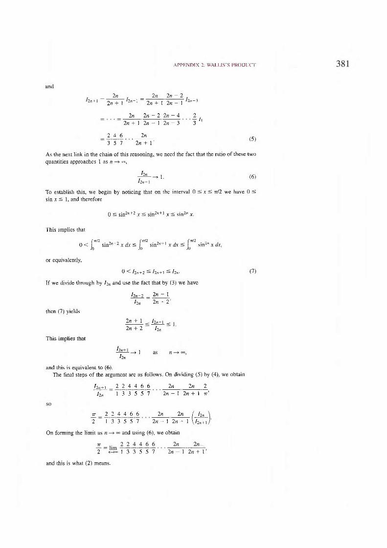
APPENDIX 2: WALLIS’S PRODUCT

and

— 2n _ 2 n 2n — 2

2”+1 ~ 2n + 1 2"“ ‘ ~~ 2n + 1 *2n - 1 2"~3

2n 2« — 2 2n — 4 2t t / 1

2n + 1 2n — 1 2n — 3 3

2 ± 6 _ _ 2rc

3 5 7 2« + 1'(5)

As the next link in the chain of this reasoning, we need the fact that the ratio of these two

quantities approaches 1 as n —» °°,

hn > 1. (6)h n +

To establish this, we begin by noticing that on the interval 0 < x < tt/2 we have 0 <

sin x ^ 1, and therefore

0 ^ sin2"+2 x < sin2"+1 x ^ sin2n x.

This implies that

fT T /2 , „ f 77/2 . , , f 77/2

0 < sin2”+2 x dx ^ sin2n 1 x dx < sin2"xdx,Jo Jo Jo

or equivalently,

0 < /2/1+2 — hn+l — hn- (7)

If we divide through by /2„ and use the fact that by (3) we have

h n + 2 _ 2 n + 1

then (7) yields

This implies that

l2n 2n + 2'

2n + 1 /2n+i

2n + 2 I2n< 1.

/2/1+- —> 1 as

h n

and this is equivalent to (6).

The final steps of the argument are as follows. On dividing (5) by (4), we obtain

I 2n+ \ 2 2 4 4 6 6 2n 2 n 2

l 2n 1 3 3 5 5 7 2n - 1 2n + 1 t t '

t t 2 2 4 4 6 6 2n 2 n ( h n

2 1 3 3 5 5 7 2 n — 1 2 « + 1 \ I 2n+ 1 /

On forming the limit as and using (6), we obtain

77 _ — — — — —

2 /!-»«> 1 3 3 5 5 7 2n - 1 2n + 1’

and this is what (2) means.


We also remark that Wallis’s product (2) is equivalent to the formula

This is easy to see if we write each number in parentheses on the left in factored form.

This gives

or

n 3 5 5 7 _ _2_

2 2 4 4 6 6 tt-’

which is clearly equivalent to (2). Formula (8) will reappear in Appendix 1 at the end of

Chapter 13 as a special case of another even more wonderful formula.*

APPENDIX 3: H O W

L E IB N IZ D IS C O V E R E D

H IS FO R M U L A

1_

5f — ? ♦ 7

The area of the quarter-circle of radius 1 shown in Fig. 10.9 is obviously 77-/4. We follow

Liebniz and calculate this area in a different way. The part that we actually calculate is

the area A of the circular segment cut off by the chord OT, because the remainder of the

quarter-circle is clearly an isosceles right triangle of area j.

We obtain the stated area A by integrating the sliverlike elements of area OPQ, where

the arc PQ is considered to be so small that it is virtually straight. We think of OPQ as a

triangle whose base is the segment PQ of length ds and whose height is the perpendicu-

lar distance OR from the vertex O to the base PQ extended. The two similar right trian-

gles in the figure tell us that

ds

dx

OS

OR— = ——- or OR ds = OS dx,

so the area dA of OPQ is

dA = \OR ds = \OS dx = \y dx,

’Wallis was Savilian Professor of Geometry at Oxford for 54 years, from 1649 until his death in 1703

at the age of 87, and played an important part in forming the climate of thought in which Newton

flourished. He introduced negative and fractional exponents as well as the now-standard symbol °°

for infinity, and was the first to treat conic sections as plane curves of the second degree. His infi-

nite product stimulated his friend Lord Brouncker ( first president of the Royal Society) to discover

the astonishing formula

* = i +77' 32

2 + -------

722 + ---------92

2 +2 + --- ,

from which the theory of continued fractions later arose. [No one knows how Brouncker made this

discovery, but a proof based on the work of Euler in the next century is given in the chapter on

Brouncker in J. L. Coolidge’s The Mathematics of Great Amateurs (Oxford University Press, 1949).]

Among the activities of Wallis’s later years was a lively quarrel with the famous philosopher Hobbes,

who was under the impression that he had succeeded in squaring the circle and published his erro-

neous proof. Wallis promptly refuted it, but Hobbes was both arrogant and too ignorant to under-

stand the refutation, and defended himself with a barrage of additional errors, as if a question about

the validity of a mathematical proof could be settled by rhetoric and invective.

APPENDIX 3: HOW LEIBNIZ DISCOVERED HIS FORMULA 383

where y denotes the length of the segment OS. The element of area dA sweeps across the

circular segment in question as x increases from 0 to 1, so

A = J d A = j l ' y d x ;

and integrating by parts in order to reverse the roles of x and y gives

. 1A = — xy 1 1 f1 j 1 1 f1 s - - xdy = - - - xdy,

o I Jo I I Jo(1)

the calculation, we observe that since

y = tan j #

the trigonometric identity

sin2 \4>

COS2 \(f)

yields

and x = 1 — cos (b = 2 sin2 1,

2 U ^tan2 2</> = sin2 \(p sec2 j<j> = sin2 {</>(1 + tan2 y<£)

x_ _ yA

2 ~ 1 + y 2'

The version of the geometric series given in formula (13) in Section 9.5 enables us to

write this as

— = y2(l - y2 + y4 - / + . . . ) = y2 _ yi + +

so (1) becomes

1 3 1 5 + 1 7 1 9 ,

1 1 1 1

2 3 5 7 9

When j is added to this to account for the area of the isosceles right triangle, and the re-

sult is equated to the known area 7t/4 of the quarter-circle, we have Leibniz’s formula

4 3 5 7

Is it any wonder that he took great pleasure and pride in this discovery for the rest of his

life?

METHODS OF INTEGRATION - IME-USP

Documents

Transcript of METHODS OF INTEGRATION - IME-USP