MPRAMunich Personal RePEc Archive

Meta-analysis of nature conservationvalues in Asia & Oceania: Dataheterogeneity and benefit transfer issues

Tuan, Tran Hu and Lindhjem, Henrik

Hue College of Economics, Hue University, 100 Phung Hung

Street, Hue City, Vietnam., Norwegian University of Life

Sciences, Econ Poyry

July 2008

Online at http://mpra.ub.uni-muenchen.de/11470/

MPRA Paper No. 11470, posted 08. November 2008 / 18:26

1

Meta-analysis of nature conservation values in Asia & Oceania:

Data heterogeneity and benefit transfer issues

Tran Huu Tuana and Henrik Lindhjembc∗

a Hue College of Economics, Hue University, 100 Phung Hung Street, Hue City, Vietnam.

b Department of Economics and Resource Management, Norwegian University of Life Sciences, P.O. Box 5003, N-1432 Ås, Norway.

c ECON Pöyry, P.O. Box 5, N-0051, Oslo, Norway.

∗ Corresponding author. E-mail: henrik.lindhjem@poyry.com.

2

Meta-analysis of nature conservation values in Asia & Oceania:

Data heterogeneity and benefit transfer issues

Abstract

We conduct a meta-analysis (MA) of around 100 studies valuing nature conservation in

Asia and Oceania. Dividing our dataset into two levels of heterogeneity in terms of

good characteristics (endangered species vs. nature conservation more generally) and

valuation methods, we show that the degree of regularity and conformity with theory

and empirical expectations is higher for the more homogenous dataset of contingent

valuation of endangered species. For example, we find that willingness to pay (WTP)

for preservation of mammals tends to be higher than other species and that WTP for

species preservation increases with income. Increasing the degree of heterogeneity in

the valuation data, however, preserves much of the regularity, and the explanatory

power of some of our models is in the range of other MA studies of goods typically

assumed to be more homogenous (such as water quality). Subjecting our best MA

models to a simple test forecasting values for out-of-sample observations, shows median

(mean) forecasting errors of 24 (46) percent for endangered species and 46 (89) percent

for nature conservation more generally, approaching levels that may be acceptable in

benefit transfer for policy use. We recommend that the most prudent MA practice is to

control for heterogeneity in regressions and sensitivity analysis, rather than to limit

datasets by non-transparent criteria to a level of heterogeneity deemed acceptable to the

individual analyst. However, the trade-off will always be present and the issue of

acceptable level of heterogeneity in MA is far from settled.

Keywords: Valuation; biodiversity; Asia; meta-analysis; meta-regression; benefit transfer. JEL Classification: Q26; Q51; Q57; H41

3

Introduction According to the Millennium Ecosystem Assessment, more than 60 per cent of the

world’s ecosystems are being degraded or used unsustainably (Millennium Ecosystem

Assessment 2005). The pressure on nature is among the highest in the many rapidly

growing economies of Asia and Oceania, home to four of the world’s 12 megadiversity

countries (Australia, China, India, Indonesia). The (neoclassical) economist’s

prescription to stemming this deteriorating trend is to value changes in the provision of

environmental goods in economic terms, and create markets or other mechanisms to

internalise their values in the billions of everyday decisions of consumers, producers

and government officials. Faced with this challenge, environmental economists have

produced an enormous amount of primary valuation research using stated and revealed

preference methods. However, paraphrasing Glass et al. (1981: p11)1, results of much of

this work “are strewn among the scree of a hundred journals and lies in the unsightly

rubble of a million dissertations.” This large body of valuation research could be much

better utilised to demonstrate to decision-makers the social return to nature

conservation, a key area where environmental economists need to do more in the future,

as pointed out by David Pearce (2005). For a range of environmental goods meta-

analysis (MA) techniques has been used to synthesize valuation research, test

hypotheses, and facilitate the transfer of existing welfare estimates to new, unstudied

policy sites (“benefit transfer” – BT) where such information can be useful, e.g. in cost-

benefit analysis (Smith and Pattanayak 2002; Navrud and Ready 2007). Responding to

Pearce’s challenge, we use MA to review and take stock of the literature to date on

1 Originally quoted in Stanley and Jarrel (2005).

4

environmental valuation of a complex and somewhat heterogeneous good – (changes in)

conservation of habitat, biodiversity and endangered species – in a specific geographical

region; Asia and Oceania. We attempt to answer the following two research questions;

(1) To what extent do welfare estimates for this complex good conform with

theoretically and empirically derived expectations regarding the good characteristics,

valuation methods, study quality, socio-economics and other variables?; (2) How

sensitive are the meta-regression results and the value forecasts for unstudied sites to;

(a) the “scope of the MA”, i.e. the level of heterogeneity of the good valued and the

valuation methods used; and (b) the choice of meta-regression models?

The first question investigates whether the welfare estimates display the degree of

validity and regularity more typically found for less complex environmental goods with

higher share of use-values, and offers a first check of the potential for using such data

for BT applications (Johnston et al. 2005; Lindhjem 2007). The second question

contributes to our understanding and refinement of MA methodology in environmental

economics, where the meta-analyst typically is left to make a number of choices,

potentially introducing various subjective biases (Hoehn 2006; Rosenberger and

Johnston 2007). An important analyst choice both for the robustness of MA models and

their suitability for use in BT applications, relates to the scope of the MA, i.e. the trade-

off between the number of observations and the acceptable level of heterogeneity in the

data, as pointed out by e.g. Engel (2002) (Question 2a above). Another, related choice is

which model to choose for BT, for example how to treat insignificant variables

(Question 2b)2. There are different practices and little is known of the empirical effects

2 An alternative approach to dealing with classical MA challenges, not pursued here, is to use Bayesian techniques

(e.g. Moeltner et al (2007) and Moeltner and Rosenberger (2008)).

5

of these choices, though Lindhjem and Navrud (2008c) have shown that the precision of

meta-analytical BT (MA-BT) depends on the model specifications, sometimes in

unexpected ways.

Previous MA studies have primarily analysed the values of more homogenous types of

environmental goods (e.g. water and air quality, recreation days) often within the same

country (Desvousges et al. 1998; Rosenberger and Loomis 2000a; Van Houtven et al.

2007), though there is a trend towards studying more complex goods in international

settings (e.g. wetlands, coral reefs, forests) (Brander et al. 2006; Brander et al. 2007;

Lindhjem 2007). Only two studies have attempted an MA for a similar good to ours;

Loomis and White (1996) (endangered species in the USA), and Jacobsen and Hanley

(2007) (relationship between income and willingness to pay (WTP) for biodiversity

worldwide). Neither of these studies focus specifically on MA methodology or

implications for BT. Compared to previous work, we add several new and interesting

dimensions; (1) To investigate the effect of the MA scope, we divide our dataset into

two levels of heterogeneity; endangered species (more similar good and methods used)

and nature conservation more generally (more heterogeneity in good and methods

used); (2) We then estimate a number of meta-regression models for these two main

datasets using different cleaning procedures investigating conformity with expectations

and the robustness of results, and finally; (3) We report the level of forecast (or transfer)

errors for unstudied sites broken down by type of models, nature conservation habitat,

geographic region and valuation method used, based on a jackknife resampling

technique introduced in MA by Brander et al (2006). Using a random effects meta-

regression model we find that welfare estimates show some degree of regularity, though

this decreases with the increased heterogeneity of the meta-data, as expected. However,

even the heterogeneous models show explanatory and predictive power at the same

6

level or better compared with other MA studies of goods assumed to be more

homogenous.

Conceptual framework and data

Conceptual framework

We start by defining “nature conservation” broadly as the protection or active

management of any natural terrestrial or aquatic ecosystem, resource or amenity, Q. The

economic value measure for an increase in the level of nature conservation (Q) is the

change in the quantity and/or quality (QUAL) of Q, or some set of services provided by

Q, and is referred to as consumers’ surplus (CS) or Willingness to pay (WTP). From the

standard indirect utility function, the bid function for a representative individual j for

this change can be given by (Bergstrom and Taylor 2006)3:

(1) )H,SUBSUB,QUALQUAL,QQ,M,P(fWTP jRj

Tj

Rj

Tj

Rj

Tjjj −−−=

Where P = a price index of market goods (assumed constant), M = (individual or

household) income (assumed constant), QT-QR and QUALT-QUALR are the changes in

quantity and quality from a reference situation (“status quo”) (R) to a target state-of-the-

world (T), SUB = substitutes for Q available to individual j, H = non-income household

or individual characteristics. Further to make (1) elastic enough for use in MA, we

assume, following Bergstrom and Taylor (2006), a “weak structural utility theoretic

approach” in which the underlying variables in the bid function are assumed to be

derivable from some unknown utility function, but that flexibility is maintained to

3 For simplicity and brevity we do not elaborate the details of how nature conservation may increase utility e.g.

related to market goods and household production, e.g. as done by Van Houtven et al. (2007) for water quality.

7

introduce explanatory variables into the WTP model, such as study design and different

valuation methods, that do not necessarily follow from (1). This is the most common

approach in MA, where the meta-analyst records estimates of mean WTP from different

studies and corresponding explanatory variables both informed by theory and empirical

expectations. In this process, the empirical specification chosen for (1) needs to trade

off the availability of variable information reported in valuation studies with the range

of potentially relevant variables that can explain variation in welfare estimates. For

example, information about substitute sites to a national park will most often not be

reported, even if important for WTP. In addition, if information is reported, for example

about the exact change in nature conservation valued, this change may not easily be

comparable across sites and studies. No MA studies are free of this problem. Some try

to map changes to a common unit of measurement in terms of hectares or to a water

quality ladder or similar, though such simplified common units may mask differences in

other dimensions of the good important to individuals (see e.g. discussion in Lindhjem

(2007)). There are no easy solutions to this problem, and in our rather general case we

interpret mean WTP from different studies as welfare estimates for a (small, though not

marginal) change in Q and/or in one or more elements in an attribute vector of QUAL

describing the quality of the nature site4. We then use dummy variables to detect

differences in WTP depending on the type of habitat or change valued. Before

discussing the empirical specification of (1), we first describe the data used for the MA.

Meta-data from nature conservation studies

4 The ecosystem services and functions and total economic value from nature and biodiversity conservation are

discussed in depth elsewhere, and for sake of brevity not elaborated in detail here (see e.g. Fromm (2000)).

8

Given this conceptual framework, we conducted a broad search for studies (published

papers, reports, book chapters etc5) internationally available in English valuing nature

conservation in the region drawn from various databases, including EVRI

(Environmental Valuation Reference Inventory), ECONLIT, ISI Web of Science,

EEPSEA’s (Environment and Economy Programme for Southeast Asia), etc6. The first

valuation studies related to nature conservation were conducted in Australia in the

1980s. In the rest of Asia, valuation started much later, but has grown in number

substantially during the 1990’s and 2000’s. Based on the literature search we compiled a

gross meta-dataset of 577 mean WTP estimates (i.e. observations) from 99 studies. A

first crude screening of the studies was conducted by excluding the ones reporting

negative mean WTP or very high or low estimates (2 standard deviations of the mean),

leaving 550 estimates from 95 studies for detailed analysis. This reduces the influence

of outlier estimates in our regression analysis. The resulting distribution of studies by

region, by type of habitat or service valued, and valuation method used are given in

Tables 1-3 below7.

Most of the studies are from Southeast Asia, East Asia or Oceania (mostly Australia),

with a smaller number of studies from South and Southwest Asia (Table 1). Australia

5 We did not include Master degree theses for practical reasons (hard to find and/or to get hold of) and because many

are written in the native language.

6 Since the Australian database ENVALUE is no longer updated, has been (partly) integrated with EVRI, and include

limited study information, our main search used the EVRI database.

7 We do not claim to have achieved to collect an exhaustive database of all studies in Asia and Oceania, but the extent

of our search makes us confident that we cover the majority of such studies. Further, it is unlikely that our search

has been biased in any way (except for the focus on studies in English), which means that our data will give a

objective picture of the valuation literature in the region. Finally, to answer our research questions, completeness

is also not strictly necessary.

9

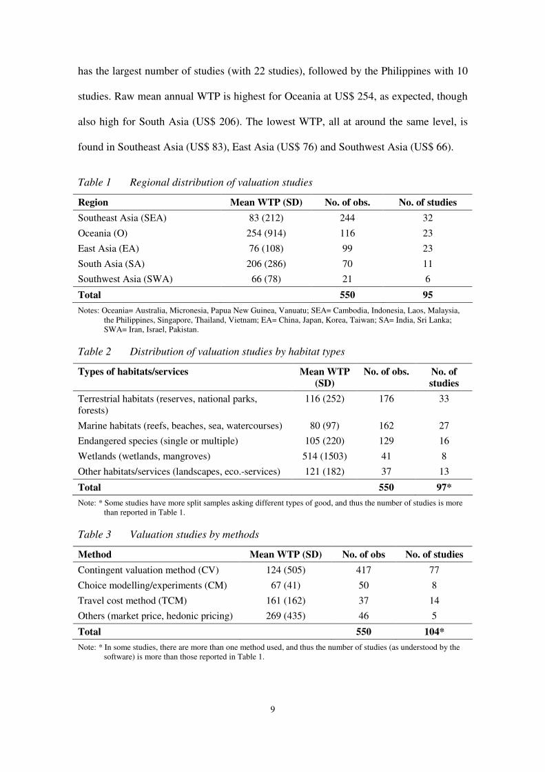
has the largest number of studies (with 22 studies), followed by the Philippines with 10

studies. Raw mean annual WTP is highest for Oceania at US$ 254, as expected, though

also high for South Asia (US$ 206). The lowest WTP, all at around the same level, is

found in Southeast Asia (US$ 83), East Asia (US$ 76) and Southwest Asia (US$ 66).

Table 1 Regional distribution of valuation studies

Region Mean WTP (SD) No. of obs. No. of studies

Southeast Asia (SEA) 83 (212) 244 32

Oceania (O) 254 (914) 116 23

East Asia (EA) 76 (108) 99 23

South Asia (SA) 206 (286) 70 11

Southwest Asia (SWA) 66 (78) 21 6

Total 550 95

Notes: Oceania= Australia, Micronesia, Papua New Guinea, Vanuatu; SEA= Cambodia, Indonesia, Laos, Malaysia, the Philippines, Singapore, Thailand, Vietnam; EA= China, Japan, Korea, Taiwan; SA= India, Sri Lanka; SWA= Iran, Israel, Pakistan.

Table 2 Distribution of valuation studies by habitat types

Types of habitats/services Mean WTP

(SD)

No. of obs. No. of

studies

Terrestrial habitats (reserves, national parks, forests)

116 (252) 176 33

Marine habitats (reefs, beaches, sea, watercourses) 80 (97) 162 27

Endangered species (single or multiple) 105 (220) 129 16

Wetlands (wetlands, mangroves) 514 (1503) 41 8

Other habitats/services (landscapes, eco.-services) 121 (182) 37 13

Total 550 97*

Note: * Some studies have more split samples asking different types of good, and thus the number of studies is more than reported in Table 1.

Table 3 Valuation studies by methods

Method Mean WTP (SD) No. of obs No. of studies

Contingent valuation method (CV) 124 (505) 417 77

Choice modelling/experiments (CM) 67 (41) 50 8

Travel cost method (TCM) 161 (162) 37 14

Others (market price, hedonic pricing) 269 (435) 46 5

Total 550 104*

Note: * In some studies, there are more than one method used, and thus the number of studies (as understood by the software) is more than those reported in Table 1.

10

The most frequently valued habitat is terrestrial habitats (including forests, nature

reserves and national parks), grouped together here for ease of exposition (Table 2).

Marine and freshwater habitats (i.e. coral reefs, beaches, sea, rivers, watercourses) for

simplicity termed “marine habitats”, follow second. Wetlands have the highest value at

US$ 514, mostly due to the market price methods often used to value such habitats (see

next paragraph). Studies that value named and endangered (often iconic or charismatic)

species or groups of species are categorised as “endangered species”. Marine habitats

provide the lowest value (US$ 80) compared to other types of habitats, while terrestrial

habitats (US$ 116), endangered species (US$ 105), and other habitats (US$ 121) have

values that are around 40-50 percent higher.

The by far most frequently used method of valuation is CV, with 77 studies, while the

TCM comes second with only 14 studies (Table 3). Some studies find that CV yields

lower WTP than TCM (e.g. Carson et al (1996)). A small number of studies (5) use

other methods, such as the hedonic pricing method or calculating the value of wetlands

and forests using the market price approach. These methods frequently calculate a

different welfare measure than CV, CM and TCM studies, and also yield twice as high

estimates as the other methods. Details of the individual studies (including reference)

are given in the Appendix.

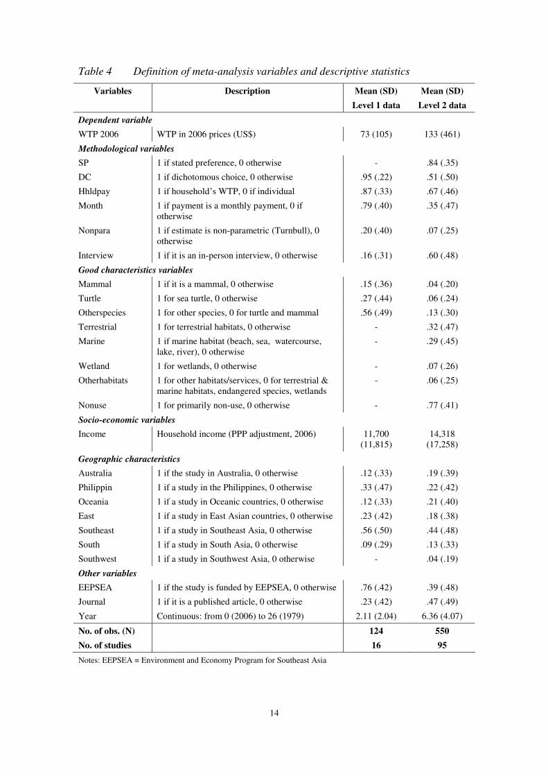
Information from the studies was then coded in a spreadsheet originally containing 30

variables, with between 1 and 36 observations drawn from each study (average 5.8).

The same study typically has several sub-samples varying the methods used, scope and

other aspects of the good being valued. The two first columns in Table 4 below give the

variable names and definitions. Since there is no standardised way of reporting welfare

estimates in the literature, a wide variety of units are typically used, e.g. WTP per

11

individual or household, per unit of area8, per visitor, for different time periods (e.g. per

month, per visit, per year, one-time amount etc.), and in different currencies and

reporting years. To deal with this, we standardized the values to a common metric, i.e.

WTP (US$ in 2006 prices) per household per year as a default, and coded WTP per

individual, WTP per month etc., using dummies. For WTP per visit from CV or TCM

studies, we calculated per visit WTP per year (if the study had information about how

many trips a person would make per year, we converted to WTP per year). Values from

different years were converted to 2006 prices using GDP deflators from the World Bank

World Development Indicators. Purchase Power Parity (PPP) corrected exchange rates

were used to correct for differences in price levels between countries, which is the

common procedure in international BT and MA (Ready and Navrud 2006). Some

theoretical models predict that WTP given per household is higher than individual WTP

(e.g. Strand 2007), though empirical evidence is mixed (Lindhjem 2007; Lindhjem and

Navrud 2008a). It can also be expected that WTP given per month multiplied by 12 to

convert to an annual amount is higher than WTP originally stated on an annual basis (a

well-known bias).

We also included other methodological variables that are often used in MA studies:

whether the study used personal interviews, if the CV method applied a dichotomous

choice (DC) WTP question format (i.e. the respondent says yes or no to a given bid,

rather than stating max WTP), and whether the CV data were analysed using non-

parametric statistical methods. DC formats are often found to give higher mean WTP (a

main reason is so-called yea-saying), while non-parametric methods typically give a

lower bound on WTP. There is no clear prior for use of interviews vs. other modes,

8 Studies that reported results with per unit of area were excluded, as there total size typically was not given.

12

though type of survey mode is known to influence results (Boyle 2003; Lindhjem and

Navrud 2008b). Further, we include a set of geographic and good characteristics

variables to control for differences in welfare estimates between types of species

(mammals, turtles) and habitat types, between regions and countries, and between

primarily non-use vs. use value. Larger and more charismatic or iconized species (for

example elephants or pandas) are likely to yield higher welfare estimates than non-

charismatic species or biodiversity/nature conservation in general (e.g. as found in

Jacobsen et al (2008)), though it is uncertain a priori if our MA will be able to detect

such a pattern across several studies. Studies that primarily estimate non-use values are

likely to give lower value estimates. There are no strong priors regarding other habitat

types or regional/country dummies, though it is expected that these dimensions may

influence WTP9. We considered including a dummy for the season of the study (e.g.

rainy-dry season) similar to Lindhjem (2007), however in most cases such information

was not reported.

The only socio-economic variable generally reported is income of the sample, which we

include in our analysis. Around 78 percent of the studies report this. For those which

don’t, we follow common practice from other MA studies to use a proxy for income

from other sources instead (we use GDP/capita for the country). It is expected that

income will positively influence WTP, an often-found result in the literature for single

studies. However, in MA studies WTP is often relatively insensitive to income levels

(see e.g. Johnston et al. 2005; Jacobsen and Hanley 2007). One reason for this is the low

variation in income levels in MA studies conducted within the same country or in

9 We also considered using population density of the country of study as a variable, for example as done by Brander

et al (2006) for wetlands. However, we think link between nature conservation and population density may be

overly speculative, and excluded this variable in our analysis.

13

Western countries with similar income levels. In our case we have a fairly large

variation in income levels, so should expect that WTP may increase with income.

Finally, we include a proxy variable for study quality; whether a study is a published or

unpublished paper (i.e. a journal article or research report/working paper). Though

published studies may be expected to apply more stringent and perhaps conservative

methods, it is not clear if this would result in lower WTP. There may also be publication

bias with unknown influence on WTP (Rosenberger and Stanley 2007). To capture

trends in WTP values over time not captured by income (or other coded variables), we

include a trend variable for the year of the study (rather than publication year). MA

studies generally find WTP to increase over time, reflecting, perhaps, both increased

nature scarcity and “greener” preferences. Since a portion of our studies is funded by

the same institution and may share similarities we have not otherwise coded, we include

a dummy (EEPSEA) to control for that. This procedure is similar to Bateman and Jones

(2003), which find indications of similarities in WTP estimates from the same authors.

14

Table 4 Definition of meta-analysis variables and descriptive statistics

Variables Description Mean (SD)

Level 1 data

Mean (SD)

Level 2 data

Dependent variable

WTP 2006 WTP in 2006 prices (US$) 73 (105) 133 (461)

Methodological variables

SP 1 if stated preference, 0 otherwise - .84 (.35)

DC 1 if dichotomous choice, 0 otherwise .95 (.22) .51 (.50)

Hhldpay 1 if household’s WTP, 0 if individual .87 (.33) .67 (.46)

Month 1 if payment is a monthly payment, 0 if otherwise

.79 (.40) .35 (.47)

Nonpara 1 if estimate is non-parametric (Turnbull), 0 otherwise

.20 (.40) .07 (.25)

Interview 1 if it is an in-person interview, 0 otherwise .16 (.31) .60 (.48)

Good characteristics variables

Mammal 1 if it is a mammal, 0 otherwise .15 (.36) .04 (.20)

Turtle 1 for sea turtle, 0 otherwise .27 (.44) .06 (.24)

Otherspecies 1 for other species, 0 for turtle and mammal .56 (.49) .13 (.30)

Terrestrial 1 for terrestrial habitats, 0 otherwise - .32 (.47)

Marine 1 if marine habitat (beach, sea, watercourse, lake, river), 0 otherwise

- .29 (.45)

Wetland 1 for wetlands, 0 otherwise - .07 (.26)

Otherhabitats 1 for other habitats/services, 0 for terrestrial & marine habitats, endangered species, wetlands

- .06 (.25)

Nonuse 1 for primarily non-use, 0 otherwise - .77 (.41)

Socio-economic variables

Income Household income (PPP adjustment, 2006) 11,700 (11,815)

14,318 (17,258)

Geographic characteristics

Australia 1 if the study in Australia, 0 otherwise .12 (.33) .19 (.39)

Philippin 1 if a study in the Philippines, 0 otherwise .33 (.47) .22 (.42)

Oceania 1 if a study in Oceanic countries, 0 otherwise .12 (.33) .21 (.40)

East 1 if a study in East Asian countries, 0 otherwise .23 (.42) .18 (.38)

Southeast 1 if a study in Southeast Asia, 0 otherwise .56 (.50) .44 (.48)

South 1 if a study in South Asia, 0 otherwise .09 (.29) .13 (.33)

Southwest 1 if a study in Southwest Asia, 0 otherwise - .04 (.19)

Other variables

EEPSEA 1 if the study is funded by EEPSEA, 0 otherwise .76 (.42) .39 (.48)

Journal 1 if it is a published article, 0 otherwise .23 (.42) .47 (.49)

Year Continuous: from 0 (2006) to 26 (1979) 2.11 (2.04) 6.36 (4.07)

No. of obs. (N) 124 550

No. of studies 16 95

Notes: EEPSEA = Environment and Economy Program for Southeast Asia

15

For our meta-regressions, we divided the dataset into two primary levels of scope,

according to level of homogeneity of the good and methods used: Level 1: Endangered

species; and Level 2: Biodiversity and nature conservation more generally. The

endangered species data include WTP estimates from 16 studies using the CV method

to value the preservation of single or multiple species. These CV studies typically ask

how much local/domestic populations are willing to pay for various conservation

programs for endangered species (e.g. WTP to conserve a viable population of sea

turtles)10. 10 of the studies are funded by EEPSEA (hence the importance of the control

variable discussed above). The species valued in these studies include sea turtles

(several countries), black-faced spoonbill (Macau), rhinos (Vietnam), eagles and whale

shark (Phillipines), and various species such as dugong dugong, elephants, rhinos,

dolphins and tigers (Thailand). In addition we found six non-EEPSEA funded studies in

the region using CV to value the preservation of the possum (a marsupial species native

to Australia) and glider (the Mahogany Glider: a type of endangered possum), giant

panda (China), and elephants (India, Sri Lanka)11. The 16 studies provide 124 estimates

that will be used in meta-regression analysis. Although the species are different, we

consider the preservation of them as a good with many similar attributes in valuation

(i.e. a larger degree of homogeneity of the good), as compared to nature and

biodiversity conservation more generally. In addition, methodological heterogeneity is

reduced since all the studies in this level use CV.

10 A small number of studies survey foreign populations, e.g. Bandara and Tisdell (2005) study OECD citizens’ WTP

for the preservation of the Giant Panda in China.

11 We found another valuation study on endangered species in Asia. Adhikari et al. (2005) use CM to investigate

rhino conservation in Nepal, but was excluded since it does not provide welfare measures.

16

The second level of the data, include the studies from Level 1 and all the rest of the

studies that value nature conservation more generally, with different types of methods

(though the majority also use CV here). This dataset includes welfare estimates for a

fairly heterogeneous good, however, not more so, it can be argued, than many other

complex environmental goods studied in MA. Further, as almost all non-textbook goods

in general (and environmental goods in particular) are heterogeneous to some degree, it

is unclear from theory where to draw the line in practice. All in all the Level 2 dataset

contains between 67 to 95 studies and 390 to 550 estimates, depending on the cleaning

procedures used in the meta-regressions (see section on results below). The details of

the Level 1 and 2 datasets are given in Tables A and B, respectively, in the appendix

(reference, country, year, species/habitat/service types, method, survey mode, payment

vehicle and format, number of values in the MA and WTP range). We will conduct

several meta-regressions models based on these two levels of our data, to investigate the

effects of heterogeneity.

Meta-regression model

We estimate meta-regression models to explain the variation in welfare estimates for

conservation of species, biodiversity and nature more generally across studies in the

literature. As most studies provide more than one WTP estimate, the data should most

prudently be treated as a panel to account for the correlation between the errors of

estimates from the same study12. Thus we used the procedure proposed by Rosenberger

and Loomis (2000b) to check for panel structures in the data. The panel structure model,

our empirical specification of equation (1) above, can be written as:

17

(2) i

n

i

ijijiij xWTP εµβα +++= ∑=1

where WTP is the i’th observation from the j’th study, α is a constant, xij is a vector of

explanatory variables (as defined in Table 4), with a panel effect µij and an error εi ~N(0,

σε2). We chose a double-log specification of (2), common in the MA literature, which

fitted our data better than linear or other specifications. A Breusch and Pagan’s

Lagrange multiplier statistic test of whether panel effects are significant was conducted.

The null hypothesis is that an equal effects model is correct ( 0 : 0ijH µ = ), and the

alternative hypothesis that a panel effects model is correct 1( : 0)ijH µ ≠ . For a model

with income as the only explanatory variable13, this test showed that a model with equal

effects ( 0 : 0ijH µ = ) was rejected, confirming the appropriateness of a panel estimation

model (χ2 = 274.90, p=0.000 with N=550 and j=95). In order to test whether a random

effects specification (which has a panel specific error component) is outperformed by a

fixed effects model (which keeps the panel specific error component constant), a

Hausman χ2 test was performed for the whole dataset. The results in Table 5 show that

the random effects model (B) cannot be rejected, and thus, it is used in the next sections

12 We also tested two other stratifications of the data: by-survey and by-author. Results show that in many model

specifications of these two stratifications equal effects (and random effects) cannot be rejected.

13 A comprehensive test would have included other explanatory variables with different model specifications, but for

sake of simplicity and brevity, we only present the model with the income variable here

18

Table 5 Test of random vs fixed effects panel structure ( N=550, j=95)

b Fixed effects model B Random effects model b-B S.E.

Income variable .0305127 -.0494427 .0799554 .2193994

p> χ2: 0.7155

We also performed the Hausman test for all the models used in this study (see next

section for results), i.e. for different subsets of the data and different explanatory

variables included, and find that a random effects model is the best estimation approach

for Level 1 and 2 of our data.

Meta-regression results and discussion

Results of four random-effects GLS regression models for the Level 1 data (species) are

reported in Table 6. Moving from Model 1 to Model 4, we include more explanatory

variables in the models. Model 1 contains methodological variables only, Model 2 adds

good characteristics, Model 3 adds country variables, and Model 4 includes socio-

economic (income) and other variables (survey year). For all models we present both a

full and reduced version, in which variables not significant at the 20 per cent level are

taken out14. This reduced form is often used in MA-BT applications (see for example

Rosenberger and Loomis 2000a, Lindhjem and Navrud (In press)), demonstrated in the

next section. Going from Model 1 to 4, the models gradually explain more of the

variation in WTP for species preservation. The methodological variables in Model 1

explain around 40 percent of the variation (R2 = 0.398), while adding characteristics of

the species explain another 14 percent of the variation (R2 = 0.536). Adding country

14 A range of models was tried using combinations of variables in Table 4. Models presented here were chosen to

avoid collinearity (excluding e.g. the EEPSEA variable), to include dummies reflecting a significant share of the

data (i.e. excluding region dummies for Level 1 data), to obtain best fit with the data and to enhance comparison

between models and between Level 1 and Level 2 data.

19

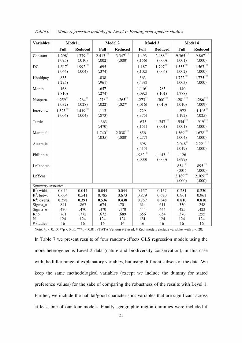
specifics and income and year in Models 3 and 4 help explain another 22-27 percentage

points of the variation. Model 4, the best fitting of the models, obtains an overall R2 of

0.81, which is very high compared to other MA studies. It is comforting for our belief in

the validity of the data and for the potential use of such value estimates for BT that

around half of the explained variation in the best model is due to non-study specific,

observable characteristics related to the good, geographical area, year of study and

income level of the population surveyed. Note that the models are directly comparable

since they all include the same observations.

Individual parameter estimates in the fully specified and best Model 4 confirm well with

expectations, where such priors exist. The DC format tends to provide higher estimates

than other formats, as expected. Monthly payment is significantly higher than other

vehicles of payment, as expected. Non-parametric estimates are significantly lower than

estimates using parametric methods, also as expected. Household payment is

significantly higher than WTP from individual payment, though theoretical and

empirical expectations here are not clear. Personal interview is not significantly

different than other survey modes in the fully specified Model 4 (but significantly

higher in the reduced model). Not controlling for good characteristics and other

variables make interviews significantly lower, in Model 1. Valuation of turtle

preservation is significantly lower than for other species (though insignificant in Model

2), while mammals are valued significantly higher15. Higher values for mammals can be

explained by their higher degree of “charisma” than for other, lower-profile species. The

result for sea turtles, on the other hand, is somewhat puzzling. Australian studies

15 We also tried other groupings or specifications of types of species, such as size, degree of ”charisma” across types

of species etc, but found that using the biological classification ”mammal” worked best in our models. Adding

dummies for each species is not feasible due to the limited number of observations for each.

20

provide higher values than studies in other countries in Model 3, but when controlling

for income level, this parameter becomes negative and significant. Studies conducted in

the Philippines are likely to give lower values (though only significant in Model 3) than

studies conducted in other countries. The income parameter, i.e. the income elasticity of

WTP in our double-log formulation, is 0.85 and highly significant. Income elasticity of

WTP in the 0-1 range is commonly found in the CV literature (e.g. Kriström and Riera

1996). In Model 4 more recent studies yield significantly higher WTP estimates,

reflecting perhaps increased scarcity or greening of preferences over time.

21

Table 6 Meta-regression models for Level I: Endangered species studies

Note: *p < 0.10, **p < 0.05, ***p < 0.01. STATA Version 9.2 used. # Red. models exclude variables with p>0.20.

In Table 7 we present results of four random-effects GLS regression models using the

more heterogeneous Level 2 data (nature and biodiversity conservation), in this case

with the fuller range of explanatory variables, but using different subsets of the data. We

keep the same methodological variables (except we include the dummy for stated

preference values) for the sake of comparing the robustness of the results with Level 1.

Further, we include the habitat/good characteristics variables that are significant across

at least one of our four models. Finally, geographic region dummies were included if

Variables Model 1 Model 2 Model 3 Model 4

Full Reduced Full Reduced Full Reduced Full Reduced

Constant 1.298* (.095)

1.779*** (.010)

2.413*** (.002)

3.347*** (.000)

1.493 (.156)

2.488*** (.000)

-9.365*** (.001)

-9.867*** (.000)

DC 1.517* (.064)

1.992*** (.004)

.695 (.374)

1.187 (.102)

1.797*** (.004)

1.555*** (.002)

1.567*** (.000)

Hholdpay .855 (.295)

.038 (.961)

.563 (.438)

1.722*** (.003)

1.775*** (.000)

Month .168 (.810)

.657 (.274)

1.116* (.092)

.785 (.101)

.140 (.788)

Nonpara. -.259** (.032)

-.264** (.028)

-.278** (.022)

-.265** (.027)

-.273** (.016)

-.300*** (.010)

-.281*** (.010)

-.286*** (.009)

Interview 1.525*** (.004)

1.419*** (.004)

.113 (.873)

.729 (.375)

-.972 (.192)

-1.105** (.025)

Turtle -.363 (.470)

-.675 (.151)

-1.347*** (.001)

-.954*** (.001)

-.919*** (.000)

Mammal 1.740** (.035)

2.038*** (.000)

.856 (.277)

1.569*** (.004)

1.678*** (.000)

Australia .698 (.415)

-2.048** (.019)

-2.221*** (.000)

Philippin. -.982*** (.000)

-1.143*** (.000)

-.126 (.699)

LnIncome .854*** (001)

.895*** (.000)

LnYear

2.189*** (.000)

2.309*** (.000)

Summary statistics: R2: within 0.044 0.044 0.044 0.044 0.157 0.157 0.231 0.230 R2: betw. 0.604 0.541 0.785 0.673 0.879 0.690 0.961 0.961 R

2: overa. 0.398 0.391 0.536 0.438 0.757 0.548 0.810 0.810

Sigma_u .841 .867 .674 .701 .614 .611 .330 .248 Sigma_e .470 .470 .470 .470 .444 .444 .425 .423 Rho .761 .772 .672 .689 .656 .654 .376 .255 N 124 124 124 124 124 124 124 124 # studies 16 16 16 16 16 16 16 16

22

significant or if data from these regions dominate our dataset. Model 1 investigates the

full dataset of 550 observations (27 obs. <0 or outside 2 std. dev. of the mean range

were screened out initially as described in a previous section). This full dataset is

contained in Table A and B in the Appendix. Model 2 excludes observations from

studies that did not report income information, a procedure sometimes used in MA. In

Model 1 GDP/capita was substituted for the missing income information. Model 3

contains the Model 2 observations, excluding values estimated using other methods than

CV, CM, and TCM (i.e. market price and hedonic pricing methods), as these methods

typically estimate conceptually different (and typically higher) welfare measures. Model

4 contains studies of endangered species only (the same observations as in Model 4

from Level 1), for sake of comparison. As for the Level 1 data we use both full and

reduced forms of the models. For the most heterogeneous version of the data in Model 1

R2 (overall) is 16 percent, which is somewhat lower but comparable to the 25-26

percent obtained in two national level MA studies of an apparently more homogenous

good; recreation activity days in the USA (see Rosenberger and Loomis (2000a) and

Shresta and Loomis (2003))16. Our R2 for the full dataset is generally higher than

Jacobsen and Hanley’s (2007) random-effects MA models of international biodiversity

studies. Excluding the studies from Model 1 for which a crude GDP/Capita measure

was substituted for missing income information, more than doubles the explained

variation (Model 2, R2 = 0.34). This is an indication that mean WTP is more sensitive to

reported sample income than GDP/capita, as expected (though Jacobsen and Hanley

(2007) somewhat surprisingly finds the opposite result).

16 Since R2 obtained from random-effects models is not directly comparable to standard R2 OLS, the comparison

should be interpreted with caution.

23

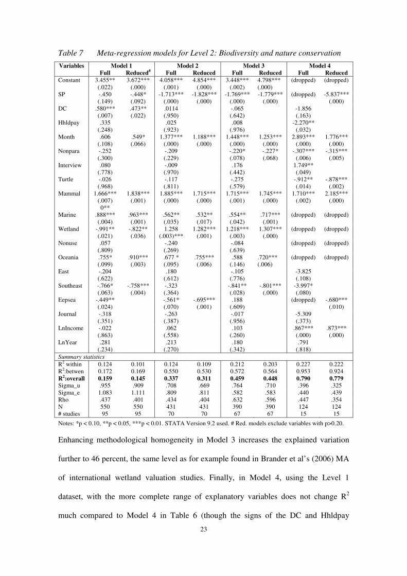
Table 7 Meta-regression models for Level 2: Biodiversity and nature conservation

Variables Model 1 Model 2 Model 3 Model 4

Full Reduced# Full Reduced Full Reduced Full Reduced

Constant 3.455** (.022)

3.672*** (.000)

4.058*** (.001)

4.854*** (.000)

3.448*** (.002)

4.798*** (.000)

(dropped) (dropped)

SP -.450 (.149)

-.448* (.092)

-1.713*** (.000)

-1.828*** (.000)

-1.769*** (.000)

-1.779*** (.000)

(dropped) -5.837*** (.000)

DC .580*** (.007)

.473** (.022)

.0114 (.950)

-.065 (.642)

-1.856 (.163)

Hhldpay .335 (.248)

.025 (.923)

.008 (.976)

-2.270** (.032)

Month .606 (.108)

.549* (.066)

1.377*** (.000)

1.188*** (.000)

1.448*** (.000)

1.253*** (.000)

2.893*** (.000)

1.776*** (.000)

Nonpara -.252 (.300)

-.209 (.229)

-.220* (.078)

-.227* (.068)

-.307*** (.006)

-.315*** (.005)

Interview .080 (.778)

-.009 (.970)

.176 (.442)

1.749** (.049)

Turtle -.026 (.968)

-.117 (.811)

-.275 (.579)

-.912** (.014)

-.878*** (.002)

Mammal 1.666*** (.007) 0**

1.838*** (.001)

1.885*** (.000)

1.715*** (.000)

1.715*** (.001)

1.745*** (.000)

1.710*** (.002)

2.185*** (.000)

Marine .888*** (.004)

.963*** (.001)

.562** (.035)

.532** (.017)

.554** (.042)

.717*** (.001)

(dropped) (dropped)

Wetland -.991** (.021)

-.822** (.036)

1.258 (.003)***

1.282*** (.001)

1.218*** (.003)

1.307*** (.000)

(dropped) (dropped)

Nonuse .057 (.809)

-.240 (.269)

-.084 (.639)

(dropped) (dropped)

Oceania .755* (.099)

.910*** (.003)

.677 * (.095)

.755*** (.006)

.588 (.146)

.720*** (.006)

(dropped) (dropped)

East -.204 (.622)

.180 (.612)

-.105 (.776)

-3.825 (.108)

Southeast -.766* (.063)

-.758*** (.004)

-.323 (.364)

-.841** (.028)

-.801*** (.000)

-3.997* (.080)

Eepsea -.449** (.024)

-.561* (.070)

-.695*** (.001)

.188 (.609)

(dropped) -.680*** (.010)

Journal -.318 (.351)

-.263 (.387)

-.017 (.956)

-5.309 (.373)

LnIncome -.022 (.863)

.062 (.558)

.103 (.260)

.867*** (.000)

.873*** (.000)

LnYear .281 (.234)

.213 (.270)

.180 (.342)

.791 (.818)

Summary statistics

R2 within 0.124 0.101 0.124 0.109 0.212 0.203 0.227 0.222 R2:betwen 0.172 0.169 0.550 0.530 0.572 0.564 0.953 0.924 R2:overall 0.159 0.145 0.337 0.311 0.459 0.448 0.790 0.779 Sigma_u .955 .909 .708 .669 .764 .710 .396 .325 Sigma_e 1.083 1.111 .809 .811 .582 .583 .440 .439 Rho .437 .401 .434 .404 .632 .596 .447 .354 N 550 550 431 431 390 390 124 124 # studies 95 95 70 70 67 67 15 15

Notes: *p < 0.10, **p < 0.05, ***p < 0.01. STATA Version 9.2 used. # Red. models exclude variables with p>0.20.

Enhancing methodological homogeneity in Model 3 increases the explained variation

further to 46 percent, the same level as for example found in Brander et al’s (2006) MA

of international wetland valuation studies. Finally, in Model 4, using the Level 1

dataset, with the more complete range of explanatory variables does not change R2

much compared to Model 4 in Table 6 (though the signs of the DC and Hhldpay

24

parameters are not preserved). Despite a higher degree of heterogeneity than for the

Level 1 dataset, the data show some degree of regularity, and many of the parameters

have the expected signs. Stated preference (SP) methods tend to give lower estimates

than revealed preference (RP) methods, as expected. It is also as expected that monthly

payments yield higher estimates than other payment vehicles and that non-parametric

estimates are lower than parametric ones, like for the Level 1 dataset. The other

methodological parameter estimates (i.e. household WTP, personal interview) are not

robust across models and there are no strong priors for their signs. The signs and

significance of the turtle and mammal parameters are preserved from the Level 1

models. Marine habitats are valued significantly higher than other habitats across

Models 1-3, while the wetland parameter is not robust. Estimates with primarily non-use

values are only lower in Models 2 and 3 (not significant). Studies conducted in Oceania

(mostly Australia) tend to yield significantly higher values (most significant in reduced

model versions), after controlling for the higher income level, which may be an

indication of “greener” preferences. Studies from Southeast Asia (significant) and East

Asia (not significant) give lower values, compared to other regions. Interestingly,

studies funded by EEPSEA give lower values than studies funded by other institutions.

Published papers seem to yield lower estimates (not significant), a possible indication of

the more conservative valuation methods and reported values in the published literature.

The income parameter is positive for studies that have reported income information

from their samples, but only significantly so in Model 4 for the endangered species data.

Year is positive but not significant in any models.

Increasing the degree of homogeneity of our data in terms of good characteristics and

methods, then, generally increases the explanatory power of the models, as expected.

For the more homogenous Level 1 data, observable characteristics of the type of

25

species, region and other variables (income, year) add significantly to the explanatory

power of the models. Even with the fairly heterogeneous Level 2 dataset, the models are

still able to explain a significant part of the variation giving some credibility to pooling

valuation estimates drawn from a varied base of studies for MA. Many of the parameter

signs (and significance) are preserved when going from Level 1 to Level 2. The

explanatory power of our Level 2 models is comparable and our Level 1 models in the

high range, compared to other MA studies in environmental economics. For example,

the R2 for our Level 2 Model 3 is only about 10-15 percentage points lower than Van

Houtven et al’s (2007) MA of water quality valuation studies in the USA. They

screened 300 publications related to water quality valuation and found only 11 studies

(96 observations) they considered “sufficiently comparable” to include in an MA. Their

protocol used for excluding studies is not very transparent. In contrast, we chose to

follow the recommendation to “err on the side of inclusion” (Stanley and Jarrel 2005:

p137) and exclude studies only by clear criteria. Given the degree of confirmed validity

of our data, the next, and directly policy relevant question, is how the MA models will

perform forecasting values for unstudied sites, i.e. used for BT. This is the question we

turn to in the next section.

A check of the transferability of nature conservation values

MA-BT involves transferring one or more estimated meta-regression equations (2) to an

unstudied policy site, and insert values from this site for the geographic, socio-

economic, good characteristics variables and relevant year, and predict or forecast

annual WTP per household. The values of methodological variables would typically be

set at some best practice level, at the average sample value or drawn from the MA

sample (Johnston et al. 2006), since there is no such information for an unstudied policy

26

site. To the extent that observable characteristics of the habitats/good valued and the

population, and not only the methodological differences between the studies, explain a

significant portion of the variation in WTP, it gives us confidence that MA-BT may be a

credible alternative to a new valuation study or other BT techniques as input for

example in cost-benefit analysis. The performance of MA-BT can only be accurately

assessed if we knew the “true value”, or an estimate of this, for a range of sites, and then

used the MA models to predict the value at those sites, and calculate so-called transfer

errors (TE)17. Lindhjem and Navrud (In press) and a few other studies referenced

therein, use different “benchmark” values from within their sample or from new studies

to “simulate” the true value to assess TE performance. We will not conduct a full such

investigation, but only carry out a first check on how our MA models forecast nature

conservation values for our two datasets. We use a jacknife data splitting technique,

introduced in BT by Loomis (1992) and used in MA e.g. by Santos (1998) and Brander

et al (2006), where we estimate n-1 separate meta-regression equations to predict (or

forecast) the value of the omitted observation in each case (i.e. “the site” we predict).

We then calculate the percentage difference between observed and predicted values, the

TE in our simple exercise, and the overall median and mean TE for all observations18.

This measure gives a first indication of how far off our MA models would be in a real

17 B

BT

WTP|WTPWTP|

TE−

= , where T = Transferred (predicted) value from study site(s), B = Estimated true

value (“benchmark”) at policy site.

18 The mean prediction error is often termed Mean Absolute Percentage Error (MAPE).

27

BT exercise. We start by reporting the results for the four models using the Level 1 and

Level 2 data (Table 8 and 9 below, respectively)19.

Table 8 Median and mean transfer error (percent) for full and reduced models

Level 1: Endangered species

Model 1 Model 2 Model 3 Model 4 Full Reduced Full Reduced Full Reduced Full Reduced Median 61 69 59 44 33 68 24 25 Mean 108 108 85 77 58 103 46 44 N 124 124 124 124 124 124 123 123

Table 9 Median and mean transfer error (percent) for full and reduced models Level

2: Biodiversity and nature conservation

Model 1 Model 2 Model 3 Model 4 Full Reduced Full Reduced Full Reduced Full Reduced Median 68 67 52 58 46 46 22 26 Mean 7344 10449 377 279 89 86 45 44 N 547 547 428 428 387 387 121 121

Introducing variables other than study-specific methodological variables in the Level 1

models, reduces median TE from 61 percent (full Model 1) to 24 percent for the best-

fitting Model 4 (Table 8). Mean TE for Model 4 is 46 percent. This is fairly low

compared to other studies performing this check, e.g. Lindhjem and Navrud (In press)

(62-266 percent), and Brander et al (2006; 2007) (74-186 percent), indicating a level of

precision that could be acceptable for policy use. Such levels would have to be

determined on a case-by-case basis, but a general level of 20-40 percent has been

suggested (Kristofersson and Navrud 2007). Precision increases with the more fully

19 To account for econometric error in transforming ln(WTP) to WTP using antilog, we add standard deviation (s2/2),

which estimate varies when the sample changes, prior to transformation of ln(WTP) (see e.g. Johnston et al.

2006). Some of the observations were dropped by STATA performing the TE estimations in Tables 8-9 as

compared to Tables 7-8..

28

specified models. There is no clear relationship between mean and median TE and the

reduced vs. full models20.

For the Level 2 data median TE is comparable to the Level 1 results across all models,

but the Level 2 data produce more high TE values (i.e. the mean is much higher than the

median) (Table 9). Reducing methodological heterogeneity for the Level 2 data from

Model 2 to 3 reduces median TE from around 52 percent to 46, while mean TE comes

down from an unacceptably high level of 279-377 percent to a more reasonable 86-89

percent. For both Level 1 and 2 models there is an inverse relationship between the level

of explained variation and TE, as expected. Hence, increasing degree of homogeneity of

the data in terms of good characteristics (biodiversity and nature conservation in general

to endangered species) increases the precision, as does the enhanced homogeneity of

valuation methods used within Level 2. However, even with a heterogeneous dataset,

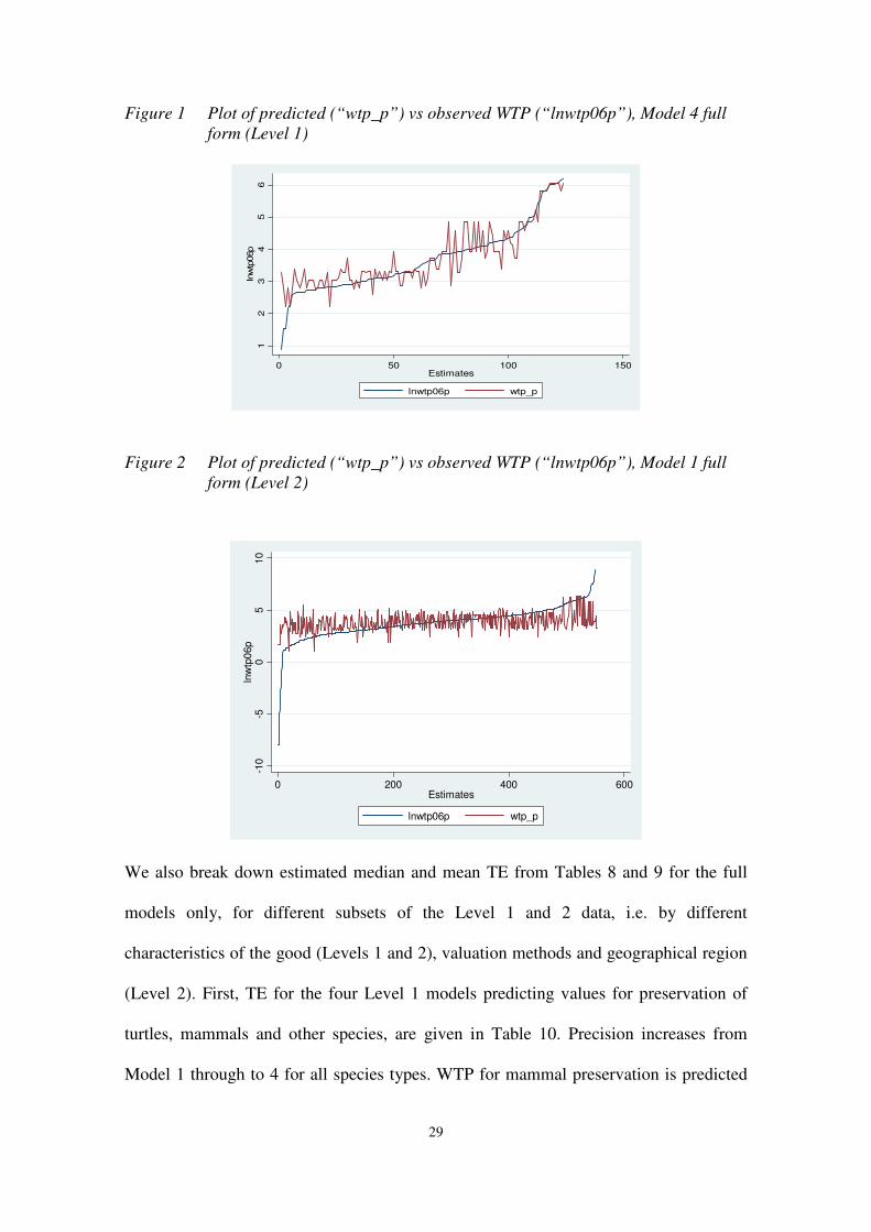
TE may approach acceptable levels for policy use. The plot of observed WTP values

(estimates sorted in ascending order, lnwtp06) vs. predicted (zig-zag line, wtp_p) for

Model 4 (Level 1 data) is illustrated in Figure 1. The forecasts follow the observed

values well except at the extremities of the data, a characteristic of forecasting models.

For comparison, Model 1 (the whole dataset, 550 observations) for Level 2 is plotted in

Figure 2. This plot shows a lower level of precision than for Level 1 in Figure 1 (though

the scale is different).

20 We also ran the same TE simulations using a rule-of-thumb of p>0.1 instead of p>0.2 for the reduced models,

detecting no clear(er) relationship with TE.

29

Figure 1 Plot of predicted (“wtp_p”) vs observed WTP (“lnwtp06p”), Model 4 full

form (Level 1)

12

34

56

lnw

tp06p

0 50 100 150Estimates

lnwtp06p wtp_p

Figure 2 Plot of predicted (“wtp_p”) vs observed WTP (“lnwtp06p”), Model 1 full

form (Level 2)

-10

-50

510

lnw

tp06p

0 200 400 600Estimates

lnwtp06p wtp_p

We also break down estimated median and mean TE from Tables 8 and 9 for the full

models only, for different subsets of the Level 1 and 2 data, i.e. by different

characteristics of the good (Levels 1 and 2), valuation methods and geographical region

(Level 2). First, TE for the four Level 1 models predicting values for preservation of

turtles, mammals and other species, are given in Table 10. Precision increases from

Model 1 through to 4 for all species types. WTP for mammal preservation is predicted

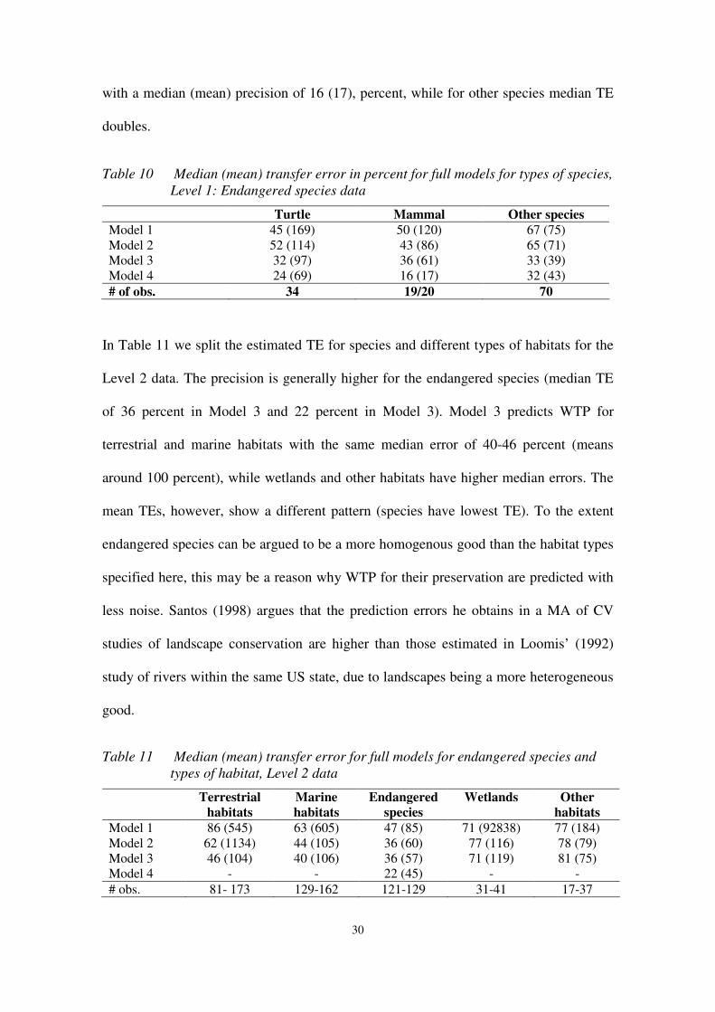
30

with a median (mean) precision of 16 (17), percent, while for other species median TE

doubles.

Table 10 Median (mean) transfer error in percent for full models for types of species,

Level 1: Endangered species data

Turtle Mammal Other species

Model 1 45 (169) 50 (120) 67 (75) Model 2 52 (114) 43 (86) 65 (71) Model 3 32 (97) 36 (61) 33 (39) Model 4 24 (69) 16 (17) 32 (43) # of obs. 34 19/20 70

In Table 11 we split the estimated TE for species and different types of habitats for the

Level 2 data. The precision is generally higher for the endangered species (median TE

of 36 percent in Model 3 and 22 percent in Model 3). Model 3 predicts WTP for

terrestrial and marine habitats with the same median error of 40-46 percent (means

around 100 percent), while wetlands and other habitats have higher median errors. The

mean TEs, however, show a different pattern (species have lowest TE). To the extent

endangered species can be argued to be a more homogenous good than the habitat types

specified here, this may be a reason why WTP for their preservation are predicted with

less noise. Santos (1998) argues that the prediction errors he obtains in a MA of CV

studies of landscape conservation are higher than those estimated in Loomis’ (1992)

study of rivers within the same US state, due to landscapes being a more heterogeneous

good.

Table 11 Median (mean) transfer error for full models for endangered species and

types of habitat, Level 2 data

Terrestrial

habitats Marine

habitats Endangered

species Wetlands Other

habitats Model 1 86 (545) 63 (605) 47 (85) 71 (92838) 77 (184) Model 2 62 (1134) 44 (105) 36 (60) 77 (116) 78 (79) Model 3 46 (104) 40 (106) 36 (57) 71 (119) 81 (75) Model 4 - - 22 (45) - - # obs. 81- 173 129-162 121-129 31-41 17-37

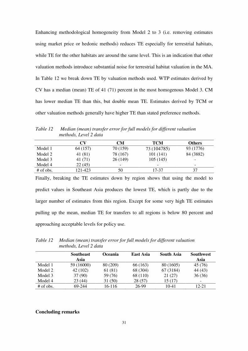
31

Enhancing methodological homogeneity from Model 2 to 3 (i.e. removing estimates

using market price or hedonic methods) reduces TE especially for terrestrial habitats,

while TE for the other habitats are around the same level. This is an indication that other

valuation methods introduce substantial noise for terrestrial habitat valuation in the MA.

In Table 12 we break down TE by valuation methods used. WTP estimates derived by

CV has a median (mean) TE of 41 (71) percent in the most homogenous Model 3. CM

has lower median TE than this, but double mean TE. Estimates derived by TCM or

other valuation methods generally have higher TE than stated preference methods.

Table 12 Median (mean) transfer error for full models for different valuation

methods, Level 2 data

CV CM TCM Others Model 1 64 (157) 70 (159) 73 (104785) 93 (1776) Model 2 41 (81) 78 (167) 101 (141) 84 (3882) Model 3 41 (71) 26 (149) 105 (145) - Model 4 22 (45) - - - # of obs. 121-423 50 17-37 37

Finally, breaking the TE estimates down by region shows that using the model to

predict values in Southeast Asia produces the lowest TE, which is partly due to the

larger number of estimates from this region. Except for some very high TE estimates

pulling up the mean, median TE for transfers to all regions is below 80 percent and

approaching acceptable levels for policy use.

Table 12 Median (mean) transfer error for full models for different valuation

methods, Level 2 data

Southeast

Asia Oceania East Asia South Asia Southwest

Asia Model 1 59 (16000) 80 (209) 66 (163) 80 (1605) 45 (76) Model 2 42 (102) 61 (81) 68 (304) 67 (3184) 44 (43) Model 3 37 (90) 59 (76) 68 (110) 21 (27) 36 (36) Model 4 23 (44) 31 (50) 28 (57) 15 (17) - # of obs. 69-244 16-116 26-99 10-41 12-21

Concluding remarks

32

Pushing the boundaries of meta-analysis (MA) in environmental economics, we have

taken stock of studies estimating willingness to pay for conservation of endangered

species, biodiversity and nature more generally in Asia and Oceania. Our literature

review shows that nature conservation is highly valued, probably more so in many cases

than the opportunity costs of increasing conservation efforts in the region, though such a

comparison is beyond the scope of our study. Dividing our dataset into two levels of

heterogeneity in terms of good characteristics and valuation methods, we show that the

degree of regularity and conformity with theory and empirical expectations as well as

the explanatory power of our MA models is higher for the more homogenous dataset of

endangered species values, as expected. In fact, though the species are different, the

values to preserve them generally follow predictable patterns. For example, we find that

mammals are generally valued higher than other species, likely due to the “charismatic”

nature of this family. Further, WTP increases significantly with income (elasticity

equals 0.85). The analysis of the endangered species data show that around half of the

variation in the best model is due to non-study specific observable characteristics of the

good and population surveyed, boding well for use of such data in benefit transfer (BT)

applications.

However, importantly, increasing the scope of the MA, i.e. gradually including more

heterogeneous observations, generally preserves much of the regularity and the

explanatory power of some of our models is in the range of other MA studies of goods

typically assumed to be more homogenous (such as national water quality, recreation

days, etc). Judging whether the relatively low variation of value estimates across types

of goods and regions can be interpreted as a sign of invalid values (WTP for example an

expression of “moral dump” or “purchase of moral satisfaction” (Kahneman and

Knetsch 1992)), or that total values may have a large share of non-use values expected

33

to stay more constant across social groups and environmental domains (e.g. as

hypothesised in Kristofersson and Navrud (2007) and Brouwer (2000)), is an unsettled

issue and beyond the scope of this study. In any case, it is generally easier to detect

sensitivity of WTP to the scope of a good within individual studies than across a range

of studies in a MA. However, even within single studies, it is hard to define and

communicate the important dimensions of scope of complex goods such as endangered

species or biodiversity to the respondent (see e.g. discussion in Carson and Hanemann

(2005: p912-914) and Lindhjem (2007), and Loomis (2006) for use of such welfare

estimates in cost-benefit analysis).

Subjecting both our dataset levels to a simple check of level of transfer error (TE), using

the MA models to predict observations one-by-one when excluded from the datasets,

show median (mean) TE of 24 (46) percent for the endangered species data and 46 (89)

percent for the more heterogeneous nature and biodiversity data. This is in the low

range compared to other MA studies. Results suggest that such levels of forecasting

errors may approach acceptable levels for policy use. However, caution should be

exercised in using values for single species for benefit transfer, as such estimates may

include values of biodiversity or habitats more generally (see e.g. Veisten et al. (2004)).

The common practice in MA to exclude a large amount of valuation studies and

estimates based on subjective, often arbitrary and not very transparent criteria of

“acceptable level of heterogeneity”, is in any case not to be recommended (Stanley and

Jarrel 2005), but our results show that the loss of explanatory and predictive power of

MA models from accepting a higher level of heterogeneity may be lower than expected.

The more prudent approach we follow is first to include all value estimates in a gross

dataset, and increase the degree of homogeneity by varying model specifications and

34

data subsets to investigate sensitivity. While it is appealing to include studies of exactly

the same good (if such a good exists outside the textbook) using the same valuation

methods, the strength of MA is that such differences to some extent can be controlled

for in a transparent way in the regression analysis. This study is, to our knowledge, one

of the first attempts to systematically investigate the issue of heterogeneity in MA for

environmental valuation. More research for other goods and geographical areas is

needed to inform the development of a more consistent and generally applicable MA

methodology, especially as MA is gradually being applied for BT to inform policy. Use

of MA in economics is growing and the aim should be to move more of the

methodological choices out of the black box.

Acknowledgements

We would like to thank Vic Adamowicz, University of Alberta, Canada for constructive

comments and Ståle Navrud, Norwegian University of Life Sciences for discussions,

comments and the idea of looking at the scope of MA. Funding from the Environment

and Economy Programme for Southeast Asia (EEPSEA) is greatly appreciated.

35

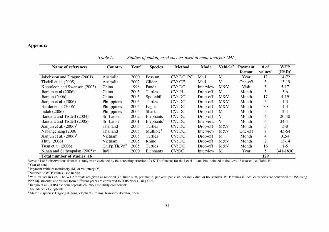
Appendix

Table A Studies of endangered species used in meta-analysis (MA)

Name of references Country Yeara Species Method Mode Vehicle

b Payment

format

# of

valuesc

WTP

(USD)d

Jakobsson and Dragun (2001) Australia 2000 Possum CV: DC, PC Mail M Year 12 14-72 Tisdell et al. (2005) Australia 2002 Glider CV: OE Mail V One-off 3 13-19 Kontoleon and Swanson (2003) China 1998 Panda CV: DC Interview M&V Visit 3 5-17 Jianjun et al.(2006)e China 2005 Turtles CV: PL Drop-off M Month 5 5-6 Jianjun (2006) China 2005 Spoonbill CV: DC Drop-off M&V Month 17 4-19 Jianjun et al. (2006)e Philippines 2005 Turtles CV: DC Drop-off M&V Month 5 1-3 Harder et al. (2006) Philippines 2005 Eagles CV: DC Drop-off M&V Month 30 1-3 Indab (2006) Philippines 2005 Shark CV: DC Drop-off M Month 5 2-4 Bandara and Tisdell (2004) Sri Lanka 2002 Elephants CV: DC Drop-off V Month 4 20-40 Bandara and Tisdell (2005) Sri Lanka 2001 Elephantsf CV: DC Interview V Month 6 34-41 Jianjun et al. (2006)e Thailand 2005 Turtles CV: DC Drop-off M&V Month 5 3-8 Nabangchang (2006) Thailand 2005 Multipleg CV: DC Interview M&V One-off 7 43-64 Jianjun et al. (2006)e Vietnam 2005 Turtles CV: DC Drop-off M Month 4 0.2-4 Thuy (2006) Vietnam 2005 Rhino CV: DC Drop-off M&V Month 2 13-14 Tuan et al. (2008) Cn,Pp,Th,Vnh 2005 Turtles CV: DC Drop-off M&V Month 16 1-5 Ninan and Sathyapalan (2005)* India 2000 Elephants CV:DC Interview M Year 5 341-1830 Total number of studies=16 129

Notes: *4 of 5 observations from this study were excluded by the screening criterion (2x STD of mean) for the Level 1 data, but included in the Level 2 dataset (see Table B) a Year of data. b Payment vehicle: mandatory (M) or voluntary (V). c Number of WTP values used in MA. d WTP values in US$. The WTP formats are given as reported (i.e. lump sum, per month, per year, per visit, per individual or household). WTP values in local currencies are converted to US$ using PPP adjustments; and values from different years are converted to 2006 prices using CPI. e Jianjun et al. (2006) has four separate country case study components. f Abundance of elephants. g Multiple species: Dugong dugong, elephants, rhinos, Irawaddy dolphin, tigers.

36

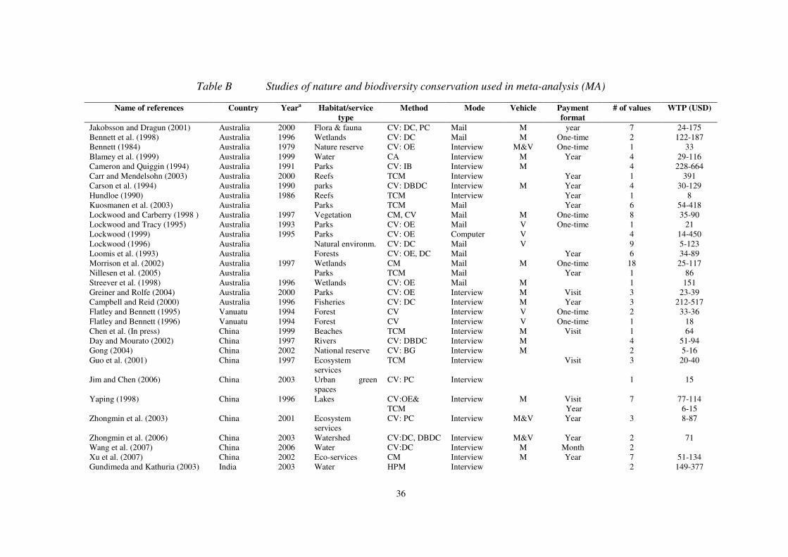
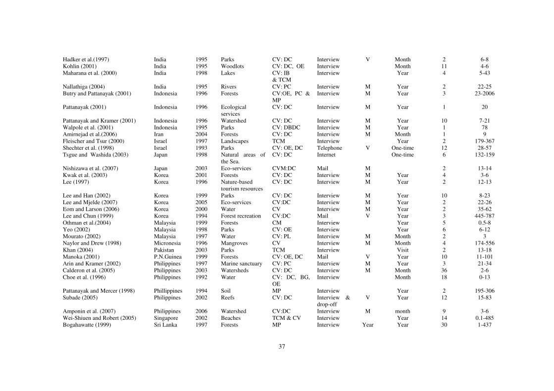
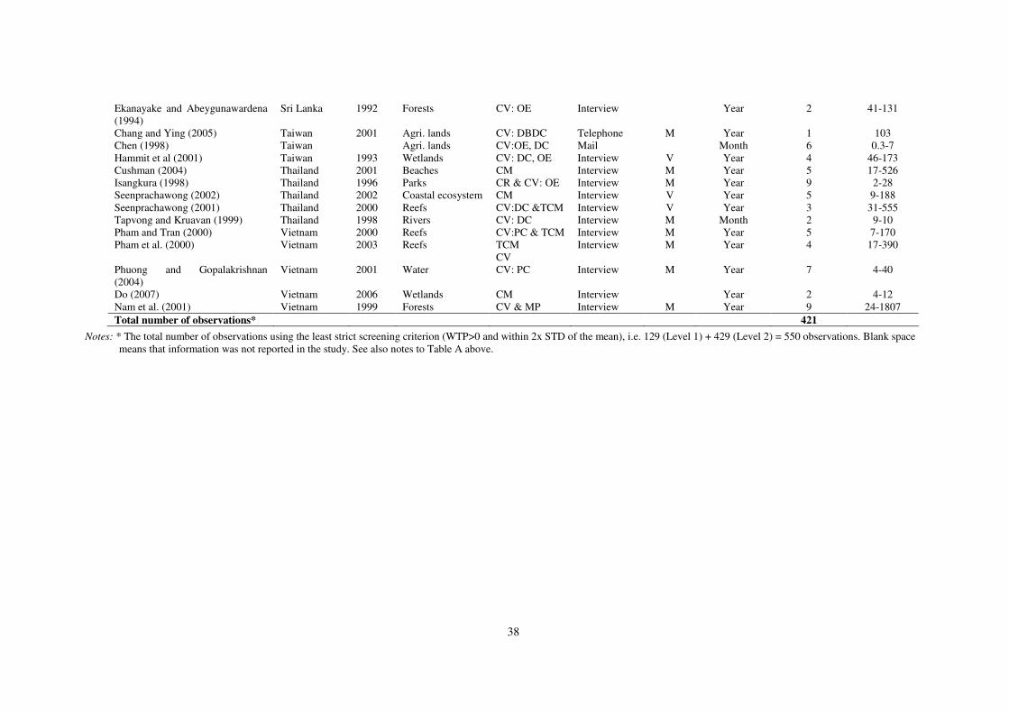
Table B Studies of nature and biodiversity conservation used in meta-analysis (MA)

Name of references Country Yeara Habitat/service

type

Method Mode Vehicle Payment

format

# of values WTP (USD)

Jakobsson and Dragun (2001) Australia 2000 Flora & fauna CV: DC, PC Mail M year 7 24-175 Bennett et al. (1998) Australia 1996 Wetlands CV: DC Mail M One-time 2 122-187 Bennett (1984) Australia 1979 Nature reserve CV: OE Interview M&V One-time 1 33 Blamey et al. (1999) Australia 1999 Water CA Interview M Year 4 29-116 Cameron and Quiggin (1994) Australia 1991 Parks CV: IB Interview M 4 228-664 Carr and Mendelsohn (2003) Australia 2000 Reefs TCM Interview Year 1 391 Carson et al. (1994) Australia 1990 parks CV: DBDC Interview M Year 4 30-129 Hundloe (1990) Australia 1986 Reefs TCM Interview Year 1 8 Kuosmanen et al. (2003) Australia Parks TCM Mail Year 6 54-418 Lockwood and Carberry (1998 ) Australia 1997 Vegetation CM, CV Mail M One-time 8 35-90 Lockwood and Tracy (1995) Australia 1993 Parks CV: OE Mail V One-time 1 21 Lockwood (1999) Australia 1995 Parks CV: OE Computer V 4 14-450 Lockwood (1996) Australia Natural environm. CV: DC Mail V 9 5-123 Loomis et al. (1993) Australia Forests CV: OE, DC Mail Year 6 34-89 Morrison et al. (2002) Australia 1997 Wetlands CM Mail M One-time 18 25-117 Nillesen et al. (2005) Australia Parks TCM Mail Year 1 86 Streever et al. (1998) Australia 1996 Wetlands CV: OE Mail M 1 151 Greiner and Rolfe (2004) Australia 2000 Parks CV: OE Interview M Visit 3 23-39 Campbell and Reid (2000) Australia 1996 Fisheries CV: DC Interview M Year 3 212-517 Flatley and Bennett (1995) Vanuatu 1994 Forest CV Interview V One-time 2 33-36 Flatley and Bennett (1996) Vanuatu 1994 Forest CV Interview V One-time 1 18 Chen et al. (In press) China 1999 Beaches TCM Interview M Visit 1 64 Day and Mourato (2002) China 1997 Rivers CV: DBDC Interview M 4 51-94 Gong (2004) China 2002 National reserve CV: BG Interview M 2 5-16 Guo et al. (2001) China 1997 Ecosystem

services TCM Interview Visit 3 20-40

Jim and Chen (2006) China 2003 Urban green spaces

CV: PC Interview 1 15

Yaping (1998) China 1996 Lakes CV:OE& TCM

Interview M Visit Year

7 77-114 6-15

Zhongmin et al. (2003) China 2001 Ecosystem services

CV: PC Interview M&V Year 3 8-87

Zhongmin et al. (2006) China 2003 Watershed CV:DC, DBDC Interview M&V Year 2 71 Wang et al. (2007) China 2006 Water CV:DC Interview M Month 2 Xu et al. (2007) China 2002 Eco-services CM Interview M Year 7 51-134 Gundimeda and Kathuria (2003) India 2003 Water HPM Interview 2 149-377

37

Hadker et al.(1997) India 1995 Parks CV: DC Interview V Month 2 6-8 Kohlin (2001) India 1995 Woodlots CV: DC, OE Interview Month 11 4-6 Maharana et al. (2000) India 1998 Lakes CV: IB

& TCM Interview Year 4 5-43

Nallathiga (2004) India 1995 Rivers CV: PC Interview M Year 2 22-25 Butry and Pattanayak (2001) Indonesia 1996 Forests CV:OE, PC &

MP Interview M Year 3 23-2006

Pattanayak (2001) Indonesia 1996 Ecological services

CV: DC Interview M Year 1 20

Pattanayak and Kramer (2001) Indonesia 1996 Watershed CV: DC Interview M Year 10 7-21 Walpole et al. (2001) Indonesia 1995 Parks CV: DBDC Interview M Year 1 78 Amirnejad et al.(2006) Iran 2004 Forests CV: DC Interview M Month 1 9 Fleischer and Tsur (2000) Israel 1997 Landscapes TCM Interview Year 2 179-367 Shechter et al. (1998) Israel 1993 Parks CV: OE, DC Telephone V One-time 12 28-57 Tsgue and Washida (2003) Japan 1998 Natural areas of

the Sea. CV: DC Internet One-time 6 132-159

Nishizawa et al. (2007) Japan 2003 Eco-services CVM:DC Mail M 2 13-14 Kwak et al. (2003) Korea 2001 Forests CV: DC Interview M Year 4 3-6 Lee (1997) Korea 1996 Nature-based

tourism resources CV: DC Interview M Year 2 12-13

Lee and Han (2002) Korea 1999 Parks CV: DC Interview M Year 10 8-23 Lee and Mjelde (2007) Korea 2005 Eco-services CV:DC Interview M Year 2 22-26 Eom and Larson (2006) Korea 2000 Water CV Interview M Year 2 35-62 Lee and Chun (1999) Korea 1994 Forest recreation CV:DC Mail V Year 3 445-787 Othman et al.(2004) Malaysia 1999 Forests CM Interview Year 5 0.5-8 Yeo (2002) Malaysia 1998 Parks CV: OE Interview Year 6 6-12 Mourato (2002) Malaysia 1997 Water CV: PL Interview M Month 2 3 Naylor and Drew (1998) Micronesia 1996 Mangroves CV Interview M Month 4 174-556 Khan (2004) Pakistan 2003 Parks TCM Interview Visit 2 13-18 Manoka (2001) P.N.Guinea 1999 Forests CV: OE, DC Mail V Year 10 11-101 Arin and Kramer (2002) Philippines 1997 Marine sanctuary CV: PC Interview M Year 3 21-34 Calderon et al. (2005) Philippines 2003 Watersheds CV: DC Interview M Month 36 2-6 Choe et al. (1996) Philippines 1992 Water CV: DC, BG,

OE Interview Month 18 0-13

Pattanayak and Mercer (1998) Phillippines 1994 Soil MP Interview Year 2 195-306 Subade (2005) Philippines 2002 Reefs CV: DC Interview &

drop-off V Year 12 15-83

Amponin et al. (2007) Philippines 2006 Watershed CV:DC Interview M month 9 3-6 Wei-Shiuen and Robert (2005) Singapore 2002 Beaches TCM & CV Interview Year 14 0.1-485 Bogahawatte (1999) Sri Lanka 1997 Forests MP Interview Year Year 30

1-437

38

Ekanayake and Abeygunawardena (1994)

Sri Lanka 1992 Forests CV: OE Interview Year 2 41-131

Chang and Ying (2005) Taiwan 2001 Agri. lands CV: DBDC Telephone M Year 1 103 Chen (1998) Taiwan Agri. lands CV:OE, DC Mail Month 6 0.3-7 Hammit et al (2001) Taiwan 1993 Wetlands CV: DC, OE Interview V Year 4 46-173 Cushman (2004) Thailand 2001 Beaches CM Interview M Year 5 17-526 Isangkura (1998) Thailand 1996 Parks CR & CV: OE Interview M Year 9 2-28 Seenprachawong (2002) Thailand 2002 Coastal ecosystem CM Interview V Year 5 9-188 Seenprachawong (2001) Thailand 2000 Reefs CV:DC &TCM Interview V Year 3 31-555 Tapvong and Kruavan (1999) Thailand 1998 Rivers CV: DC Interview M Month 2 9-10 Pham and Tran (2000) Vietnam 2000 Reefs CV:PC & TCM Interview M Year 5 7-170 Pham et al. (2000) Vietnam 2003 Reefs TCM

CV Interview M Year 4 17-390

Phuong and Gopalakrishnan (2004)

Vietnam 2001 Water CV: PC Interview M Year 7 4-40

Do (2007) Vietnam 2006 Wetlands CM Interview Year 2 4-12 Nam et al. (2001) Vietnam 1999 Forests CV & MP Interview M Year 9 24-1807 Total number of observations* 421

Notes: * The total number of observations using the least strict screening criterion (WTP>0 and within 2x STD of the mean), i.e. 129 (Level 1) + 429 (Level 2) = 550 observations. Blank space means that information was not reported in the study. See also notes to Table A above.

39

References

Adhikari, B., W. Haider, O. Gurung, M. Poudyal, B. Beardmore, D. Knowler and P.

Van Beukering (2005), 'Economic incentives and poaching of the one-horned Indian

rhinoceros in Nepal: Stakeholder Analysis', PREM Working paper.

Amirnejad, H., S. Khalilian, M. H. Assareh and M. Ahmadian (2006), 'Estimating the

existence value of north forests of Iran by using a contingent valuation method',

Ecological Economics 58(4): 665-675.

Amponin, J. A. R., M. E. C. Bennagen, S. Hess and J. D. S. d. Cruz (2007), 'Willingness

to pay for watershed protection by domestic water users in Tuguegarao City,

Philippines', PREM 07/06 Working paper.

Arin, T. and R. A. Kramer (2002), 'Divers' willingness to pay to visit marine

sanctuaries: an exploratory study', Ocean Coastal Manage. 45(2-3): 171-183.

Bandara, D. and C. Tisdell (2004), 'The net benefit of saving the Asian elephant: a

policy and contingent valuation study', Ecological Economics 48: 93- 107.

Bandara, R. and C. Tisdell (2005), 'Changing Abundance of Elephants and Willingness

to Pay for their Conservation', Journal of Environmental Management 76: 47-59.

Bateman, I. J. and A. P. Jones (2003), 'Contrasting conventional with multi-level

modeling approaches to meta-analysis: Expectation consistency in UK woodland

recreation values', Land Economics 79(2): 235-258.

40

Bennett, J., M. Morrison and R. Blamey (1998), 'Testing the validity of responses to

contingent valuation questioning', Australian Journal of Agricultural and Resource

Economics 42(2): 131-148.

Bennett, J. W. (1984), 'Using Direct Questioning to Value the Existence Benefits of

Preserved Natural Areas ', Australian Journal of Agricultural Economics 28(2/3): 136-

152.

Bergstrom, J. C. and L. O. Taylor (2006), 'Using meta-analysis for benefits transfer:

Theory and practice', Ecological Economics 60: 351-360.

Blamey, R., J. Gordon and R. Chapman (1999), 'Choice Modelling: Assessing the

Environmental Values of Water Supply Options', Australian Journal of Agricultural

and Resource Economics 43(3): 337 - 357.

Bogahawatte, C. (1999). Forestry Policy, Non-timber Forest Products and the Rural

Economy in the Wet Zone Forests in Sri Lanka. Research report, EPPSEA,

Boyle, K. J. (2003), 'Contingent valuation in practice', in P. A. Champ, K. J. Boyle and

T. C. Brown, eds, A primer on nonmarket valuation. Kluwer Academic Publishers.

Brander, L. M., R. J. G. M. Florax and J. E. Verrmaat (2006), 'The Empirics of Wetland

Valuation: A Comprehensive Summary and a Meta-Analysis of the Literature',

Environmental & Resource economics 33: 223-250.

Brander, L. M., P. van Beukering and H. Cesar (2007), 'The recreational value of coral

reefs: a meta-analysis', Ecological Economics 63(1): 209-218.

Brouwer, R. (2000), 'Environmental value transfer: state of the art and future prospects',

Ecol. Econ. 32(1): 137-152.

41

Butry, D. T. and S. K. Pattanayak (2001). Economic Impacts of Tropical Forest

Conservation: The Case of Logger Households around Ruteng Park, Environment and

Natural Resource Economics Program, Research Triangle Institute, North Carolina

Calderon, M. M., L. D. Camacho, M. G. Carandang, J. T. Dizon, L. L. Rebugio and N.

L. Tolentino (2005). A Water User Fee For Households in Metro Manila, Philippines.

EEPSEA research report, No. 2005-RR2,

Cameron, T. A. and J. Quiggin (1994), 'Estimation Using Contingent Valuation Data

From A Dichotomous Choice With Follow-Up Questionnaire', J.Environ.Econ.Manage.

27(3): 218-234.

Campbell, H. P. and C. R. M. Reid (2000), 'Consumption Externalities in a Commercial

Fishery: The Queensland Beam Trawl Fishery', Economic Record 76(232): 1-14.

Carr, L. and R. Mendelsohn (2003), 'Valuing Coral Reefs: A Travel Cost Analysis of

the Great Barrier Reef', Ambio 32(5): 353-357.

Carson, R. T., N. E. Flores, K. M. Martin and J. L. Wright (1996), 'Contingent valuation

and revealed preference methodologies: Comparing the estimates for quasi-public

goods', Land Economics 72(1): 80-99.

Carson, R. T. and M. Hanemann (2005), 'Contingent valuation', in K.-G. Mäler and J. R.

Vincent, eds, Handbook of Environmental Economics, Volume 2. Elsevier.

Carson, R. T., L. Wilks and D. Imber (1994), 'Valuing The Preservation Of Australia

Kakadu Conservation Zone', Oxf. Econ. Pap.-New Ser. 46: 727-749.

Chang, K. and Y. Ying (2005), 'External Benefits of Preserving Agricultural Land:

Taiwan's Rice Fields', The Social Science Journal 42: 285-293.

42

Chen, W., H. Hong, Y. Liu, L. Zhang, X. Hou and M. Raymond (In press), 'Recreation

Demand and Economic Value: An Application of Travel Cost Method for Xiamen

Island', China Economic Review.

Chen, Y. (1998). Biodiversity in the Framework of Ecological Economics. Ph.D.,

University of Wisconsin Milwaukee:

Choe, K. A., D. Whittington and D. T. Lauria (1996), 'The economic benefits of surface

water quality improvements in developing countries: A case study of Davao,

Philippines', Land Econ. 72(4): 519-537.

Cushman, C. (2004). External costs from increased island visitation: case study from

Southern Thailand, Department of Resource Economics, University of Massachusetts

Day, B. and S. Mourato (2002), 'Valuing River Water Quality in China ', in D. Pearce,

C. Pearce and C. Palmer, eds, Valuing the Environment in Developing Countries: Case

Studies. Edward Elgar.

Desvousges, W. H., F. R. Johnson and H. S. Banzhaf (1998), Environmental policy

analysis with limited information: Principles and applications of the transfer method.

Cheltenham, UK: Edward Elgar.

Do, N. T. (2007). Impacts of dykes on wetland values in Vietnam’s mekong river delta:

a case study in the plain of reeds. Research report submitted to EEPSEA, IDRC,

Ekanayake, E. R. M. and P. Abeygunawardena (1994), 'Valuation of Conservation

Commodity of the Sinharaja Forest: Towards Total Economic Value', Sri Lanka Journal

of Agricultural Economics 2(1): 115-129.

43

Engel, S. (2002), 'Benefit Function Transfer versus Meta-analysis as Policy-Making

Tools: A Comparison', in R. J. G. M. Florax, P. Nijkamp and K. G. Willis, eds,

Comparative environmental economic assessment. Cheltenham, U.K. and Northampton,

Mass.: Edward Elgar, pp. 133-53.

Eom, Y.-S. and D. M. Larson (2006), 'Valuing housework time from willingness to

spend time and money for environmental quality improvements', Review of the

Economics of the Household 4: 205-227.

Flatley, G. and J. Bennet (1995). International Values of Tropical Forest Conservation:

A Cross-cultural Contingent Valuation Experiment. Perth, Western Australia,

Flatley, G. W. and J. W. Bennet (1996), 'Using Contingent Valuation to Determine

Australian Tourists' Values for Forest Conservation in Vanuatu', Economic Analysis and

Policy 26(2): 111-127.

Fleischer, A. and Y. Tsur (2000), 'Measuring the recreational value of agricultural

landscape', Eur Rev Agric Econ 27(3): 385-398.

Fromm, O. (2000), 'Ecological structure and functions of biodiversity as elements of its

total economic value', Environmental and Resource Economics 16(3): 303-328.

Glass, G. V., B. McGaw and M. L. Smith (1981), Meta-analysis in Social Research.

Beverly Hills: Sage.

Gong, Y. (2004). Distribution of Benefits and Costs among Stakeholders of a Protected

Area: An Empirical Study from China. EEPSEA Research Report 3, IDRC

44

Greiner, R. and J. Rolfe (2004), 'Estimating consumer surplus and elasticity of demand

of tourist visitation to a region in North Queensland using contingent valuation',

Tourism Economics 10(3): 317-328.

Gundimeda, H. and V. Kathuria (2003), 'Estimation of Economic Value of Water

scarcity and quality in Chennai, India: The Hedonic Approach', South Asian Network of

Economic Initiatives Project.

Guo, Z., X. Xiao, Y. Gan and Y. Zheng (2001), 'Ecosystem functions, services and their

values - a case study in Xingshan County of China', Ecological Economics 38(1): 141-

154.

Hadker, N., S. Sharma, A. David and T. R. Muraleedharan (1997), 'Willingness-to-pay

for Borivli National Park: Evidence from a contingent valuation', Ecol. Econ. 21(2):

105-122.

Hammit, J. K., J.-T. Liu and J.-L. Liu (2001), 'Contingent Valuation of a Taiwanese

Wetland', Environment and Development Economics 6: 259-268.

Harder, D. S., R. Labao and F. I. Santos (2006). Saving the Philippine eagles: How

much will this cost and are Filipinos willing to pay for it? Singapore

Hoehn, J. P. (2006), 'Methods to address selection effects in the meta regression and

transfer of ecosystem values', Ecological Economics 60(2): 389-398.

Hundloe, T. (1990), 'Measuring the Value of the Great Barrier Reef', Australian Parks

and Recreation 26(3): 11-15.

Indab, A. (2006). Rationalizing WTP for whale shark conservation in Sorsogon

province. Cebu, the Philippines

45

Isangkura, A. (1998). Environmental Valuation: An Entrance Fee System for National

Parks in Thailand. Economy and Environment Program for Southeast Asia, IDRC

Jacobsen, J. B., J. H. Boiesen, B. J. Thorsen and N. Strange (2007), 'What’s in a name?

The use of quantitative measures versus ‘Iconised’ species when valuing biodiversity',

Environmental & Resource Economics 39(3): 247-263.

Jacobsen, J. B. and N. Hanley (2007). Are there income effects on global willingness to

pay for biodiversity conservation? Working Paper.

Jakobsson, K. M. and A. K. Dragun (2001), 'The Worth of a Possum: Valuing Species

with the Contingent Valuation Method', Environmental and Resource Economics 21:

287-302.

Jianjun, J. (2006). Economic valuation of the Black-faced Spoonbill conservation in

Macao. Singapore

Jianjun, J., A. Indab, O. Nabangchang, T. D. Thuy, D. Harder and R. Subade (2006).

WTP for Marine Turtle Conservation: A Cross-country Comparison in Asia

Jim, C. Y. and W. Y. Chen (2006), 'Recreation - Amenity Use and Contingent

Valuation of Urban Greenspaces in Guangzhou, China', Landscape and Urban Planning

75(1-2): 81-96.

Johnston, R. J., E. Y. Besedin, R. Iovanna, C. J. Miller, R. F. Wardwell and M. H.

Ranson (2005), 'Systematic variation in willingness to pay for aquatic resource

improvements and implications for benefit transfer: a meta-analysis', Canadian Journal

of Agricultural Economics 53(2-3): 221-248.

46

Johnston, R. J., E. Y. Besedin and M. H. Ranson (2006), 'Characterizing the effects of

valuation methodology in function-based benefits transfer', Ecological Economics

60(2): 407-419.

Kahneman, D. and J. L. Knetsch (1992), 'Valuing Public-Goods - The Purchase Of

Moral Satisfaction', Journal of Environmental Economics and Management 22(1): 57-

70.

Khan, H. (2004). Demand of eco-tourism: estimating recreational benefits from the

Margalla Hills national park in the northern Pakistan,

Kohlin, G. (2001), 'Contingent valuation in project planning and evaluation: the case of

social forestry in Orissa, India', Environment and Development Economics 6(02): 237-

258.

Kontoleon, A. and T. Swanson (2003), 'The Willingness to Pay for Property Rights for

the Giant Panda: Can a Charismatic Species Be an Instrument for Nature Conservation?'

Land Economics 79(4): 483-499.

Kristofersson, D. and S. Navrud (2007), 'Can Use and Non-Use Values be Transferred

Across Countries?' in S. Navrud and R. Ready, eds, Environmental Value Transfer:

Issues and Methods. Kluwer Academic Publishers.

Kriström, B. and P. Riera (1996), 'Is the income elasticity of environmental

improvements less than one?' Environmental and Resource Economics 7: 45-55.

Kuosmanen, T., E. Nillesen and J. Wesseler (2003). Does Ignoring Multi-Destination

Trips in the Travel Cost Method Cause a Systematic Downward Bias?

47

Kwak, S. J., S. H. Yoo and S. Y. Han (2003), 'Estimating the public's value for urban

forest in the Seoul metropolitan area of Korea: A contingent valuation study', Urban

Studies 40(11): 2207-2221.

Lee, C.-K. and S.-Y. Han (2002), 'Estimating the Use and Preservation Values of

National Parks' Tourism Resources Using a Contingent Valuation Method', Tourism

Management 23: 531-540.

Lee, C.-K. and J. W. Mjelde (2007), 'Valuation of ecotourism resources using a

contingent valuation method: The case of the Korean DMZ', Ecological Economics 63:

511-520.

Lee, C. K. (1997), 'Valuation of nature-based tourism resources using dichotomous

choice contingent valuation method', Tourism Management 18(8): 587-591.

Lee, H.-C. and H.-S. Chun (1999), 'Valuing environmental quality change on

recreational hunting in Korea: A contingent valuation analysis', Journal of

Environmental Management 57(1): 11-20.

Lindhjem, H. (2007), '20 Years of stated preference valuation of non-timber benefits

from Fennoscandian forests: A meta-analysis', Journal of Forest Economics 12(4): 251-

277.

Lindhjem H and Navrud S (2008a) Asking for Individual or Household Willingness to

Pay for Environmental Goods: Implication for aggregate welfare measures.

Forthcoming in Environmental and Resource Economics.

48

Lindhjem H and Navrud S (2008b) Internet CV surveys - a cheap, fast way to get large

samples of biased values?, Department of Economics and Resource Management,

Norwegian University of Life Sciences

Lindhjem, H. and S. Navrud (2008c), 'How Reliable are Meta-Analyses for

International Benefit Transfer?' Ecological Economics 66(2-3): 425-435.

Lockwood, M. (1996), 'Non-compensatory preference structures in non-market

valuation of natural area policy', Aust. J. Agric. Econ. 40(2): 85-101.

Lockwood, M. (1999), 'Preference structures, property rights, and paired comparisons',

Environmental and Resource Economics 13(1): 107-122.

Lockwood, M. and D. Carberry (1998 ). Stated Preference Surveys of Remnant Native

Vegetation Conservation, Johnstone Centre, Albury, NSW

Lockwood, M. and K. Tracy (1995), 'Nonmarket Economic Valuation Of An Urban

Recreation Park', Journal of Leisure Research 27(2): 155-167.

Loomis, J. (2006), 'Use of contingent values of wildlife and habitat preservation in

policy and cost-benefit analysis', in A. Alberini and J. R. Kahn, eds, Handbook on

contingent valuation. Edward Elgar.

Loomis, J., M. Lockwood and T. Delacy (1993), 'Some Empirical-Evidence On

Embedding Effects In Contingent Valuation Of Forest Protection', Journal of

Environmental Economics and Management 25(1): 45-55.

Loomis, J. B. (1992), 'The Evolution Of A More Rigorous Approach To Benefit

Transfer - Benefit Function Transfer', Water Resources Research 28(3): 701-705.

49

Loomis, J. B. and D. S. White (1996), 'Economic benefits of rare and endangered

species: Summary and meta-analysis', Ecological Economics 18(3): 197-206.

Maharana, I., S. C. Rai and E. Sharma (2000), 'Valuing ecotourism in a sacred lake of

the Sikkim Himalaya, India', Environmental Conservation 27(3): 269-277.

Manoka, B. (2001). Existence Value: A Re-appraisal and Cross-Cultural Comparison.

Economy and Environment Program for Southeast Asia (EEPSEA) Research Report

No. 2001-RR1, IDRC,

Millennium Ecosystem Assessment (2005), Synthesis Report. Washington DC: Island

Press.

Moeltner, K., K. Boyle and R. W. Paterson (2007), 'Meta-analysis and benefit transfer

for resource valuation - addressing classical challenges with Bayesian modeling',

Journal of Environmental Economics and Management 53: 250-269.

Moeltner, K. and R. Rosenberger (2008). Meta-Regression and Benefit Transfer: Data

Space, Model Space, and the Quest for ‘Optimal Scope’

Morrison, M., J. Bennett, R. Blamey and J. Louviere (2002), 'Choice modeling and tests

of benefit transfer', Am. J. Agr. Econ. 84(1): 161-170.

Mourato, S. (2002), 'Valuing Improvements to Sanitation in Malaysia', in D. Pearce, C.

Pearce and C. Palmer, eds, Valuing the Environment in Developing Countries: Case

Studies. Cheltenham: Edward Elgar, pp. 67 - 113.

Nabangchang, O. (2006). Motivations for Charitable Behavior for Protection of Wildlife

and Endangered Species of Thailand.

50

Nallathiga, R. and R. B. Paravastu (2004). Benefit Estimation of River Water Quality

Conservation Using Contingent Valuation Survey: a Case-Study in the Yamuna River

Sub-basin. Budapest, Hungary

Nam, M. V., N. T. Nhan, B. V. Trihn and P. L. Thong (2001). Forest Management

Systems in the Mekong River Delta, Vietnam. EEPSEA research report,

Navrud, S. and R. Ready, Eds. (2007), Environmental Value Transfer: Issues and

Methods, Dordrecht: Kluwer Academic Publishers.

Naylor, R. and M. Drew (1998), 'Policy Options: Valuing mangrove resources in

Kosrae, Micronesia', Environment and Development Economics 3: 471-490.

Nillesen, E., J. Wesseler and A. Cook (2005), 'Estimating the Recreation-Use Value for

Hiking in Bellenden Ker National Park, Australia', Environmental Management 36(2):

311-316.

Ninan, K. N. and J. Sathyapalan (2005), 'The economics of biodiversity conservation: a

study of a coffee growing region in the Western Ghats of India', Ecological Economics

55(1): 61-72.

Nishizawa, E., T. Kurokawa and M. Yabe (2007), 'Policies and resident’s willingness to

pay for restoring the ecosystem damaged by alien fish in Lake Biwa, Japan',

Environmental Science & Policy 9: 448-456.

Othman, J., J. Bennet and R. Blamey (2004), 'Environmental values and resource

management options: a choice modelling experience in Malaysia', Environment and

Development Economics 9: 803–824.

51

Pattanayak, S. K. (2001). How Green Are These Valleys? Combining Revealed and

Stated Preference Methods to Account for Ecosystem Costs of Deforestation,

Environment and Natural Resource Economics Program, Research Triangle Institute

Pattanayak, S. K. and R. A. Kramer (2001), 'Pricing ecological services: Willingness to

pay for draught mitigation from watershed protection in eastern Indonesia', Water

Resour. Res. 37(3): 771-778.

Pattanayak, S. K. and D. E. Mercer (1998), 'Valuing soil conservation benefits of

agroforestry: contour hedgerows in the Eastern Visayas, Philippines', Agricultural

Economics 18(1): 31-46.

Pearce, D. (2005). Economists and biodiversity conservation: What can we contribute?

Bremen

Pham, K. N. and V. H. S. Tran (2000). Recreation Value of the Coral-surrounded Hon

Mun Islands in Vietnam. Economy and Environment Program for Southeast Asia,

IDRC,

Phuong, D. M. and C. Gopalakrishnan (2004), 'Optimal Management of Water for

Sustainable Fisheries and Aquaculture ', International Journal of Water Resources

Development 20(4): 493-506.

Rosenberger, R. and R. J. Johnston (2007). Selection effects in meta-valuation function

transfers. Sønderborg, Denmark

Rosenberger, R. and J. Loomis (2000b), 'Panel stratification in meta-analysis of

economic studies: an investigation of its effects in the recreation valuation literature',

Journal of Agricultural and Applied Economics 32(1): 131-149.

52

Rosenberger, R. and T. D. Stanley (2007). Is the literature biased? Publication

selection effects in recreation valuation. Portland, Oregon

Rosenberger, R. S. and J. B. Loomis (2000a), 'Using meta-analysis for benefit transfer:

In-sample convergent validity tests of an outdoor recreation database', Water Resources

Research 36(4): 1097-1107.

Santos, J. M. L. (1998), The Economic Valuation of Landscape Change. Theory and

Policies for Land Use and Conservation. Cheltenham: Edward Elgar.

Seenprachawong, U. (2001). An Economic Analysis of Coral Reefs in the Andaman Sea

of Thailand. EEPSEA research report,

Seenprachawong, U. (2002). An Economic Valuation of Coastal Ecosystems in Phang

Nga Bay, Thailand. EEPSEA Research Report No. 2002-RR5, IDRC,

Shechter, M., B. Reiser and N. Zaitsev (1998), 'Measuring Passive Use Value: Pledges,

Donations and CV Responses in Connection with an Important Natural Resource',

Environmental and Resource Economics 12: 457-478.

Shrestha, R. K. and J. B. Loomis (2003), 'Meta-Analytic Benefit Transfer of Outdoor

Recreation Economic Values: Testing Out-of-Sample Convergent Validity',

Environmental & Resource economics 25: 79-100.

Smith, V. K. and S. K. Pattanayak (2002), 'Is Meta-Analysis a Noah’s Ark for Non-

Market Valuation?' Environmental and Resource Economics 22: 271-296.

Stanley, T. D. and S. D. Jarrel (2005), 'Meta-Regression Analysis: A Quantitative

Method of Literature Surveys', Journal of Economic Surveys 19(3): 299-308.

53

Strand, J. (2007), 'Public-good valuation and intrafamily allocation', Environmental and

Resource Economics 38(4): 527-543.

Streever, W., J. M. Callaghan-Perry, A. Searles, T. Stevens and P. Svoboda (1998),

'Public attitudes and values for wetland conservation in New South Wales, Australia',

Journal of Environmental Management 54: 1-14.

Subade, R. F. (2005). Valuing Biodiversity Conservation in a World Heritage Site:

Citizens' Non-Use Values for Tubbataha Reefs National Marine Park, Philippines

Economy an Environment Program for Southeast Asia (EEPSEA), IDRC,

Tapvong, C. and J. Kruavan (1999). Water Quality Improvements: A Contingent

Valuation Study of the Chao Phraya River. EEPSEA, IDRC,

Thuy, T. D. (2006). Willingness to Pay for Conservation of Vietnamese Rhinoceros.

Cebu, the Philippines

Tisdell, C., C. Wilson and H. S. Nantha (2005), 'Policies for Saving a Rare Australian

Glider: Economics and Ecology', Biological Conservation 123: 237-248.

Tsuge, T. and T. Washida (2003), 'Economic valuation of the Seto Inland Sea by using

an Internet CV survey', Marine Pollution Bulletin 47: 230-236.

Tuan, T. H., T. D. Thuy, J. Jianjun, A. Indab and O. Nabangchang (2008). WTP for

Marine Turtle Conservation in Four Countries: Benefit Transfer Testing.

Van Houtven, G., J. Powers and S. K. Pattanayak (2007), 'Valuing water quality

improvements using meta-analysis: Is the glass half-full or half-empty for national

policy analysis?' Resource and Energy Economics 29(3): 206-228.

54

Veisten K, Hoen H F, Navrud S and Strand J (2004) Scope insensitivity in contingent

valuation of complex environmental amenities. Journal of Environmental Management

73(4): 317-331.

Walpole, M. J., H. J. Goodwin and K. G. R. Ward (2001), 'Pricing policy for tourism in

protected areas: Lessons from Komodo National Park, Indonesia', Conserv. Biol. 15(1):

218-227.

Wang, X., J. Bennett, C. Xie, Z. Zhang and D. Liang (2007), 'Estimating non-market

environmental benefits of the Conversion of Cropland to Forest and Grassland Program:

A choice modeling approach', Ecological Economics 63(1): 114-125.

Wei-Shiuen, N. and M. Robert (2005), 'The impact of sea level rise on Singapore',

Environment and Development Economics 1002: 201-215.

Xu, Z. M., G. D. Cheng, J. Bennet, Z. Q. Zhang, A. H. Long and H. Kunio (2007),

'Choice modeling and its application to managing the Ejina Region, China', Journal of

Arid Environments 69: 331-343.

Yaping, D. (1998). The Value of Improved Water Quality for Recreation in East Lake,

Wuhan, China: Application of Contingent Valuation and Travel Cost Methods, .

Economy and Environment Program for Southeast Asia, IDRC.

Yeo, B. H. (2002), 'Valuing a Marine Park in Malaysia', in D. Pearce, C. Pearce and C.

Palmer, eds, Valuing the Environment in Developing Countries: Case Studies. Edward

Elgar.

55

Zhongmin, X., C. Guodong, Z. Zhiqiang, S. Zhiyong and J. Loomis (2003), 'Applying

Contingent Valuation in China to Measure the Total Economic Value of Restoring

Ecosystem Services in Ejina Region', Ecological Economics 44: 345-358.

Zhongmin, X., J. Loomis, Z. Zhiqiang and K. Hamamura (2006), 'Evaluating the

performance of different willingness to pay question formats for valuing environmental

restoration in rural China', Environment and Development Economics 11: 585-601.