BONN-TH-2021-08

Meromorphic modular forms and the

three-loop equal-mass banana integral

Johannes Broedel,a Claude Duhr,b Nils Matthes,c

aInstitute for Theoretical Physics, ETH Zurich, Wolfgang-Pauli-Str. 27, 8093 Zurich,

SwitzerlandbBethe Center for Theoretical Physics, Universitat Bonn, D-53115, GermanycMathematical Institute, University of Oxford, Andrew Wiles Building, Radcliffe Observa-

tory Quarter, Woodstock Road, Oxford OX2 6GG, United Kingdom

E-mail: jbroedel@ethz.ch, cduhr@uni-bonn.de,

nils.matthes@maths.ox.ac.uk

Abstract: We consider a class of differential equations for multi-loop Feynman in-

tegrals which can be solved to all orders in dimensional regularisation in terms of

iterated integrals of meromorphic modular forms. We show that the subgroup under

which the modular forms transform can naturally be identified with the monodromy

group of a certain second-order differential operator. We provide an explicit decom-

position of the spaces of modular forms into a direct sum of total derivatives and

a basis of modular forms that cannot be written as derivatives of other functions,

thereby generalising a result by one of the authors form the full modular group to ar-

bitrary finite-index subgroups of genus zero. Finally, we apply our results to the two-

and three-loop equal-mass banana integrals, and we obtain in particular for the first

time complete analytic results for the higher orders in dimensional regularisation for

the three-loop case, which involves iterated integrals of meromorphic modular forms.

Keywords: Feynman integrals, elliptic polylogarithms, modular forms.

arX

iv:2

109.

1525

1v1

[he

p-th

] 3

0 Se

p 20

21

Contents

1 Introduction 2

2 Differential equations and modular parametrisations 4

2.1 Feynman integrals and differential equations . . . . . . . . . . . . . . 4

2.2 Linear differential operators and their monodromy group . . . . . . . 6

2.3 A class of differential equations allowing for a modular parametrisation 10

3 Review of (quasi-)modular forms and their iterated integrals 14

3.1 The modular group SL2(Z) and its subgroups . . . . . . . . . . . . . 14

3.2 Modular curves . . . . . . . . . . . . . . . . . . . . . . . . . . . . . . 15

3.3 Review of (quasi-)modular forms . . . . . . . . . . . . . . . . . . . . 16

3.3.1 Meromorphic modular forms . . . . . . . . . . . . . . . . . . . 16

3.3.2 Meromorphic quasi-modular forms . . . . . . . . . . . . . . . 17

3.4 Iterated integrals of holomorphic quasi-modular forms . . . . . . . . . 18

4 Iterated integrals of meromorphic modular forms 19

4.1 A decomposition theorem for meromorphic quasi-modular forms . . . 19

4.2 Sketch of the proof for neat subgroups . . . . . . . . . . . . . . . . . 22

5 The monodromy groups of the equal-mass sunrise and banana inte-

grals 29

5.1 The sunrise family . . . . . . . . . . . . . . . . . . . . . . . . . . . . 30

5.2 The banana family . . . . . . . . . . . . . . . . . . . . . . . . . . . . 33

6 Banana integrals and iterated integrals of meromorphic modular

forms 40

6.1 The iterated integrals for the sunrise integral . . . . . . . . . . . . . . 40

6.2 The iterated integrals for the three-loop banana integral . . . . . . . 42

7 Conclusion 45

A The case of a general finite-index subgroup of genus zero 46

A.1 The case k ≤ 1 . . . . . . . . . . . . . . . . . . . . . . . . . . . . . . 47

A.2 The case k ≥ 2 . . . . . . . . . . . . . . . . . . . . . . . . . . . . . . 48

A.3 Divisors of meromorphic modular forms in negative weight . . . . . . 49

A.4 Proof of Theorem 5 . . . . . . . . . . . . . . . . . . . . . . . . . . . . 50

B The differential equations for the sunrise and banana integrals 52

B.1 The differential equations for the sunrise integrals . . . . . . . . . . . 52

B.2 The differential equations for the banana integrals . . . . . . . . . . . 52

1 Introduction

Feynman integrals are a cornerstone of perturbative computations in Quantum Field

Theory, and so it is important to have a good knowledge of the mathematics underly-

ing them, including efficient techniques for their computation and a solid understand-

ing of the space of functions needed to express them. The simplest class of functions

that arise in Feynman integral computations are multiple polylogarithms (MPLs) [1–

3] (see also refs. [4–6]). The success of MPLs in Feynman integral computations can

to a large extent be traced back to the fact that their algebraic properties are well

understood (see, e.g., ref. [7]), and there are several efficient public implementations

for their numerical evaluation [8–14]. Moreover, it is well known that Feynman inte-

grals satisfy systems of coupled first-order differential equations [15–18], and MPLs

are closely connected to the concepts of pure functions [19] and canonical differential

equations [20]. It is fair to say that, whenever one can find a system of canoni-

cal differential equations that can be solved in terms of MPLs, the problem can be

considered solved.

However, it was realised already early on that MPLs do not suffice to express

solutions to higher-loop Feynman diagrams [21–35], though no analytic results in

terms of a well-defined class of functions was available. The situation changed less

than a decade ago, when it was shown that the two-loop sunrise integral can be ex-

pressed in terms of so-called elliptic dilogarithms [36–43]. The elliptic dilogarithm is

a special case of elliptic multiple polylogarithms [44–47], which also play a prominent

role in the context of string amplitudes at one-loop, cf. e.g., refs. [48–50]. Soon after,

it was realised that in the equal-mass case the two-loop sunrise integral can also be

expressed as iterated integrals of modular forms [51, 52]. This class of functions is

also of interest in pure mathematics [53–57], and it is understood how to manipulate

and evaluate these integrals efficiently [58, 59]. More generally, it was suggested that

modularity is an important feature of Feynman integrals associated to families of

elliptic curves [60].

Despite all this progress in understanding Feynman integrals that do not eval-

uate to MPLs, there are still many questions left unanswered, and no general and

algorithmic solution to evaluate and manipulate them is known, contrary to the case

of ordinary MPLs. For example, while the importance of iterated integrals of mod-

ular forms is by now well established, the reason for why modular forms appear in

the first place, and if so of which type, is not completely settled in the literature,

and there was even an argument in the literature as to which congruence subgroup

– 2 –

to attach to the two-loop sunrise integral [51, 61]. Also the link between differen-

tial equations and the appearance of these functions is not completely satisfactory

(though there are indications that the concepts of pure functions and canonical forms

known from MPLs carry over to Feynman integrals associated to families of elliptic

curves [62–64]). Finally, and probably most importantly, holomorphic modular forms

are not sufficient to cover even the simplest cases of Feynman integrals depending on

one variable. Indeed, it is known that, while in general higher-loop analogues of the

sunrise integral – the so-called l-loop banana integrals – are associated to families of

Calabi-Yau (l− 1)-folds [65–71], the three-loop equal-mass banana integral in D = 2

dimensions can be expressed in terms of the same class of functions as the two-loop

equal-mass sunrise integral [65, 66, 72]. However, if higher terms in the ε-expansion

in dimensional regularisation are considered, new classes of iterated integrals are

required, which cannot be expressed in terms of modular forms alone.

The goal of this paper is to describe the (arguably) simplest class of differential

equations beyond MPLs for which the space of solutions can be explicitly described,

to all orders in the ε-expansion. The relevance of this class of differential equations

for Feynman integrals stems from the fact that they cover in particular the two- and

three-loop equal-mass banana integrals. Their solution space can be described in

terms of iterated integrals of meromorphic modular forms, introduced and studied by

one of us in the context of the full modular group SL2(Z) [57]. For Feynman integrals,

however, modular forms for the full modular group are insufficient. We extend the

results of ref. [57] to arbitrary finite-index subgroups of genus zero, and we provide in

particular a basis for the algebra of iterated integrals they span. Our construction also

naturally provides an identification of the type of modular forms required, namely

those associated to the monodromy group of the associated homogeneous differential

operator. This explains in particular the origin and the type of iterated integrals of

modular forms encountered in Feynman integral computations. As an application of

our formalism, we provide for the first time complete analytic for results for all master

integrals of the three-loop equal-mass banana integrals in dimensional regularisation,

including the higher orders in the ε-expansion, and we see the explicit appearance of

iterated integrals of meromorphic modular forms.

The article is organized as follows: in section 2 we review general material on

Feynman integrals and the differential equations they satisfy, and we describe the

class of differential operators that we consider. In section 3 we review modular

and quasi-modular forms. Section 4 presents the main results of this paper, and

we consider iterated integrals of meromorphic modular forms and present the main

theorems. In section 5 we calculate the monodromy groups for the equal-mass two-

and three-loop and banana integrals, while section 6 is devoted to framing the higher-

orders in ε results for the three-loop banana integrals in terms of iterated integrals

of meromorphic modular forms. We include several appendices. In appendix A

we present a rigorous mathematical proof the main theorem from section 4, and in

– 3 –

appendix B we collect formulas related to the sunrise and banana integrals

2 Differential equations and modular parametrisations

2.1 Feynman integrals and differential equations

The goal of this paper is to study a certain class of Feynman integrals and to charac-

terize the functions necessary for their evaluation. We work in dimensional regulari-

sation in d = d0−2ε dimensions, where d0 is an even integer. The Feynman integrals

to be considered depend on a single dimensionless variable x or – equivalently – two

dimensionful scales.

It is well known that using integration-by-parts identities [73, 74], all Feynman

integrals that share the same set of propagators raised to different integer powers

can be expressed as linear combinations of a small set of so-called master integrals.

Those master integrals satisfy a system of first-order linear differential equations of

the form [15–18, 20]

∂xI(x, ε) = A(x, ε)I(x, ε) +N (x, ε) , (2.1)

where I(x, ε) = (I(x, ε), ∂xI(x, ε), . . . , ∂r−1x I(x, ε))T is the vector of independent mas-

ter integrals depending on the maximal set of propagators in the family. N (x, ε) is

an inhomogeneous term stemming from integrals with fewer propagators, which we

assume to be known and expressible to all orders in the dimensional regulator ε as

a linear combination with rational functions in x as coefficients of multiple polylog-

arithms (MPLs), defined by:

G(a1, . . . , an;x) =

∫ x

0

dt

t− a1

G(a2, . . . , an; t) , (2.2)

where the ai are complex constants that are independent of x. The entries of A(x, ε)

are rational functions in x and ε. The differential equation (2.1) is equivalent to the

inhomogeneous differential equation:

L(r)x,εI(x, ε) = N(x, ε) , (2.3)

where L(r)x,ε is a differential operator of degree r whose coefficients are rational func-

tions in x and ε.

In order to solve the differential equation (2.1), we first note that it is always

possible to choose the basis of master integrals such that the matrix A(x, ε) is finite

as ε → 0 (see, e.g., refs. [75, 76]). In that case we can change the basis of master

integrals according to

I(x, ε) = Wr(x)J (x, ε) , (2.4)

– 4 –

where Wr(x) is the Wronskian matrix of the homogeneous part of eq. (2.3) at ε = 0,

L(r)x u(x) = 0 , (2.5)

where L(r)x = L(r)

x,ε=0. Let us write

L(r)x =

r∑j=0

aj(x)∂jx , (2.6)

with aj(x) being rational functions and ar(x) = 1. If we denote the solution space

of L(r)x by

Sol(L(r)x ) =

r⊕s=1

Cψs(x) , (2.7)

then the Wronskian is Wr(x) = (ψ(p−1)s (x))1≤p,s≤r, where ψ

(p)s (x) := ∂pxψs(x). The

Wronskian is in fact the matrix for a basis of maximal cuts for I(x, ε) [77–80].

After the change of variables in eq. (2.4), the differential equation for J (x, ε)

takes the form

∂xJ (x, ε) = Wr(x)−1(A(x, ε)− A(x, 0)

)Wr(x)J (x, ε) +Wr(x)−1N (x, ε)

= εA(x, ε)J (x, ε) + N (x, ε) .(2.8)

This solution to the above system can be written as a path-ordered exponential:

J (x, ε) = P exp

[ε

∫ x

x0

dx′ A(x′, ε)

]J (x0, ε) . (2.9)

The path-ordered exponential can easily be expanded into a series in ε, and the

coefficients of this expansion involve iterated integrals over one-forms multiplied by

polynomials in the entries of the Wronskian. We see that in our setting where the

ε-expansion of the differential operator L(r)x,ε and the inhomogeneity N (x, ε) involve

rational functions and MPLs only, the class of iterated integrals needed to express

J (x, ε) is determined by the solution space of L(r)x in eq. (2.7). It is an interesting

question when these iterated integrals can be expressed in terms of other classes of

special functions studied in the literature. For example, in the case where A(x, ε) is

rational in x, these iterated integrals can be evaluated in terms of MPLs. In general,

however, little is known about these iterated integrals.

The main goal of this paper is to discuss a certain class of differential equations

where the resulting iterated integrals can be completely classified and an explicit

basis can be constructed algorithmically. Before we describe this class of differential

equations, we need to review some general material on linear differential equations.

– 5 –

2.2 Linear differential operators and their monodromy group

A point x0 is called a singular point of eq. (2.5) if one of the coefficient functions

aj(x) in eq. (2.6) has a pole at x0. The point at infinity is called singular if after

a change of variables x → 1/y in eq. (2.5) the transformed equation has a pole at

y = 0 in one of the coefficient functions. Points which are not singular are called

ordinary points of the differential equation. A singular point xi is called regular, if

the coefficients ar−j have a pole of at most order j at xi. If all singular points of

eq. (2.5) are regular, the equation is called Fuchsian. In the following we only discuss

Fuchsian differential equations, and we denote the (finite) set of singular points by

Σ := {x0, . . . , xq−1} ⊂ P1C, and use the notation X := P1

C \ Σ. The differential

operators obtained from Feynman integrals are expected to be of Fuchsian type.

For every point y0 ∈ P1C of a Fuchsian differential operator, the Frobenius method

can be used to construct a series representation of r independent local solutions in

a neighbourhood of this point. The starting point is the indicial polynomial of a

point, which can be obtained as follows: The differential equation (2.5) is equivalent

to L(r)x u(x) = 0, where L(r)

x has the form

L(r)x =

r∑j=0

aj(x)θjx , θx = x∂x , (2.10)

where the aj(x) are polynomials that are assumed not to have a common zero. Note

that the singular points are precisely the zeroes of ar(x). The indicial polynomial

of L(r)x at y0 = 0 is then P0(s) =

∑rj=0 aj(0)sj. The roots si of P0(s) are called

the indicials or local exponents at 0. The indicial polynomial Py0(s) and the local

exponents at another point y0 can be obtained by changing variables to y = x − y0

(or y = 1/x if y0 = ∞). The local exponents characterise the solution space locally

close to the point y0 in the form of convergent power series. More precisely, if

y0 ∈ X = P1C \ Σ is a regular point, then Py0(s) has degree r, and so there are

precisely r local exponents s1, . . . , sr (counted with multiplicity). Correspondingly,

there are r linearly independent power series solutions φi(y0;x), i ∈ {1, ..., r}, to

eq. (2.5) of the form

φi(y0;x) =∑n≥0

ci,n(x− y0)si+n , ci,0 = 1 . (2.11)

Note that this representation holds for y0 6=∞; if y0 =∞, the expansion parameter

is 1/x.

If y0 ∈ Σ is a singular point, the degree of the indicial polynomial is less than r,

and so there are less than r local exponents (even when counted with multiplicity)

and thus less than r local solutions of the form (2.11). Without loss of generality

we assume y0 = x0 ∈ Σ. The missing solutions generically exhibit a logarithmic

behaviour as one approaches x0. In particular, in the case of a single local exponent

– 6 –

s1, there is a single power series solution, and a tower of (r−1) logarithmic solutions

(we only consider the case x0 6=∞)

φi(x0;x) = (x− x0)s1i∑

k=1

1

(k − 1)!logk−1(x− x0)σk(x0;x) , (2.12)

where the σk(x0;x) are holomorphic at x = x0. A singular point with such a hi-

erarchical logarithmic structure of solutions with s1 an integer is called a point of

maximal unipotent monodromy (MUM-point).

The power series obtained from the Frobenius method have finite radius of con-

vergence: the solutions φ(y0;x) := (φi(y0;x))1≤i≤r converge in a disc whose radius

is the distance to the nearest singular point. It is possible to analytically continue

the basis of solutions φ(y0;x) to all points in X. We can cover P1C by a finite set of

open discs Dyk centered at yk ∈ P1C such that φ(yk;x) converges inside Dyk . Since

the solutions φ(yk, x) and φ(yl, x) have to agree for each value of x in the overlapping

region Dyk ∩Dyl , one can find a matching matrix from the following equation:

φ(yk;x) =

φr(yk;x)...

φ1(yk;x)

= Ryk,ylφ(yl;x) = Ryk,yl

φr(yl;x)...

φ1(yl;x)

. (2.13)

Note that the matching matrix Ryk,yl must be constant. Practically, it can be found

by numerically evaluating each component of the above equation for several numerical

points in the overlapping region. This allows one to determine the matching matrices

at least numerically to high precision by taking enough orders in the expansion. In

some cases, one may even be able to determine its entries analytically by solving for

them in an ansatz for the matrix Ryk,yl . A precise numerical evaluation allows one

to identify corresponding analytic expressions in many situations.

The monodromy group. The Frobenius method allows one to construct a basis

of solutions locally for each point y0 ∈ P1C. The local solutions can be analytically

continued to a global basis of solutions defined for all x ∈ X. We can also take a point

x ∈ X and a closed loop γ starting and ending at x and analytically continue the

solution φ(y0;x) along γ. Clearly, if γ does not encircle any singular point, Cauchy’s

theorem implies that the value of φ(y0;x) must be the same before and after analytic

continuation. One can now ask the question how the vector of solutions φ(y0;x) is

altered if transported along the small loop γ encircling a singular point xk. Let us

denote by φ(y0;x) the value of φ(y0, x) after analytic continuation along γ. Since

φ(y0;x) must still satisfy the differential equation even after analytic continuation,

it must be expressible in the original basis φ(y0;x), and so there must be a constant

r × r matrix ρy0(γ) – called the monodromy matrix – such that

φ(y0;x) = ρy0(γ)φ(y0;x) . (2.14)

– 7 –

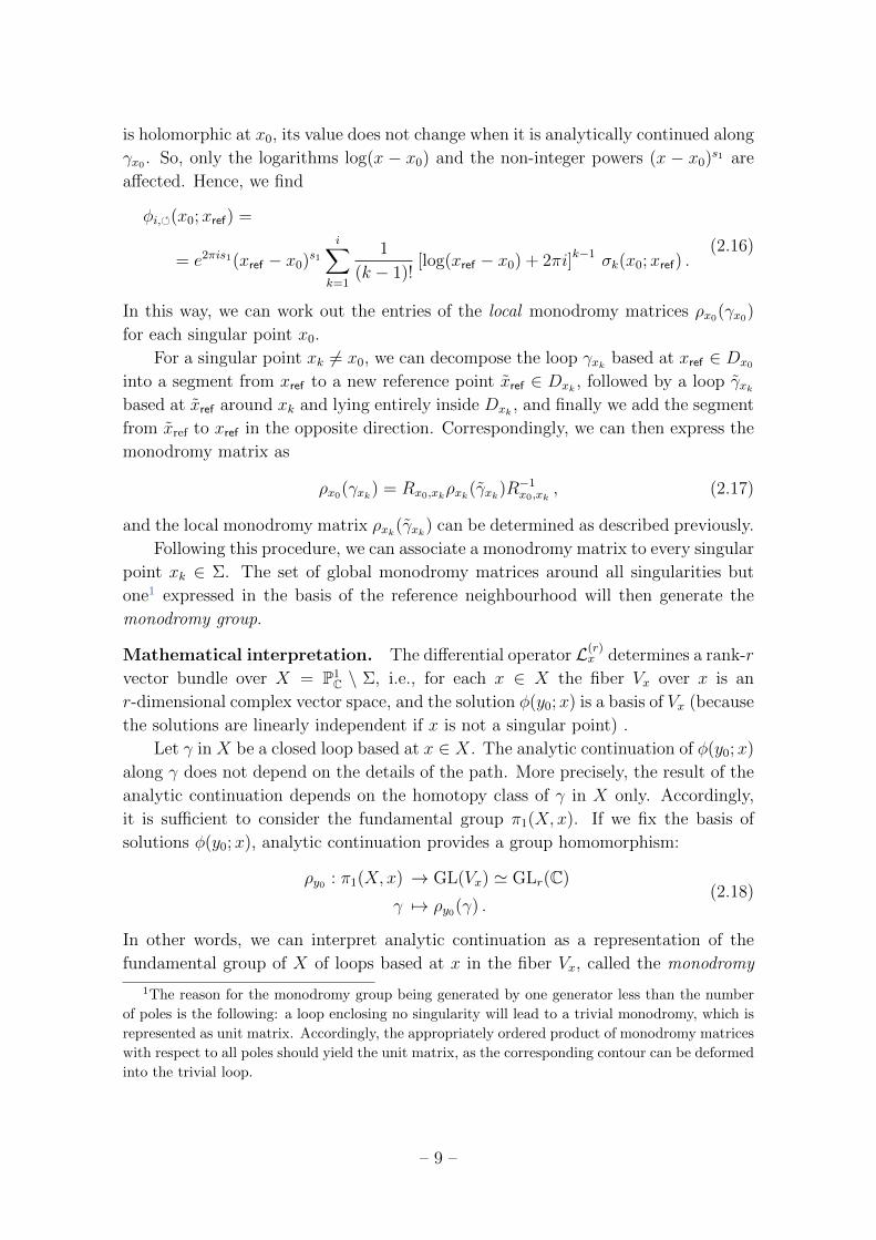
Figure 1. Paths for the analytic continuation and the calculation of the monodromies

for a differential operator with q regular singular poles, one of which at zero and one at

infinity. The (blue) reference point xref has been conveniently chosen in the (green) disc

Dx0 around x0 = 0.

The subindex on ρ denotes the local basis in which the monodromy is expressed.

Changing the local basis from y0 to y1 amounts to conjugating the monodromy

matrix by the matching matrix from eq. (2.13):

ρy0(γ) = Ry0,y1ρy1(γ)R−1y0,y1

. (2.15)

Let us now explain how we can find the monodromy matrix for a collection of

loops γxk encircling the singular points xk in the counter-clockwise direction, but

no other singular points (see figure 1). We focus for now on the singular point x0.

We can fix a reference point xref ∈ Dx0 , and we can also choose the loop γx0 to lie

entirely inside Dx0 . The effect of the analytic continuation on φ(x0;xref) is easy to

describe. Indeed, consider for example the local solution in eq. (2.12). Since σk(x0;x)

– 8 –

is holomorphic at x0, its value does not change when it is analytically continued along

γx0 . So, only the logarithms log(x − x0) and the non-integer powers (x − x0)s1 are

affected. Hence, we find

φi,(x0;xref) =

= e2πis1(xref − x0)s1i∑

k=1

1

(k − 1)![log(xref − x0) + 2πi]k−1 σk(x0;xref) .

(2.16)

In this way, we can work out the entries of the local monodromy matrices ρx0(γx0)

for each singular point x0.

For a singular point xk 6= x0, we can decompose the loop γxk based at xref ∈ Dx0

into a segment from xref to a new reference point xref ∈ Dxk , followed by a loop γxkbased at xref around xk and lying entirely inside Dxk , and finally we add the segment

from xref to xref in the opposite direction. Correspondingly, we can then express the

monodromy matrix as

ρx0(γxk) = Rx0,xkρxk(γxk)R−1x0,xk

, (2.17)

and the local monodromy matrix ρxk(γxk) can be determined as described previously.

Following this procedure, we can associate a monodromy matrix to every singular

point xk ∈ Σ. The set of global monodromy matrices around all singularities but

one1 expressed in the basis of the reference neighbourhood will then generate the

monodromy group.

Mathematical interpretation. The differential operator L(r)x determines a rank-r

vector bundle over X = P1C \ Σ, i.e., for each x ∈ X the fiber Vx over x is an

r-dimensional complex vector space, and the solution φ(y0;x) is a basis of Vx (because

the solutions are linearly independent if x is not a singular point) .

Let γ in X be a closed loop based at x ∈ X. The analytic continuation of φ(y0;x)

along γ does not depend on the details of the path. More precisely, the result of the

analytic continuation depends on the homotopy class of γ in X only. Accordingly,

it is sufficient to consider the fundamental group π1(X, x). If we fix the basis of

solutions φ(y0;x), analytic continuation provides a group homomorphism:

ρy0 : π1(X, x) → GL(Vx) ' GLr(C)

γ 7→ ρy0(γ) .(2.18)

In other words, we can interpret analytic continuation as a representation of the

fundamental group of X of loops based at x in the fiber Vx, called the monodromy

1The reason for the monodromy group being generated by one generator less than the number

of poles is the following: a loop enclosing no singularity will lead to a trivial monodromy, which is

represented as unit matrix. Accordingly, the appropriately ordered product of monodromy matrices

with respect to all poles should yield the unit matrix, as the corresponding contour can be deformed

into the trivial loop.

– 9 –

representation. The monodromy group is then the image of π1(X, x) in GLr(C)

under ρy0 . In the case of the punctured Riemann sphere X = P1C \ {x0, . . . , xq−1} the

structure of the fundamental group is easy to describe: it is the free group generated

by the loops γxk , 0 ≤ k < q − 1. Hence, we see that the monodromy group is

generated by the matrices ρy0(γxk) with 0 ≤ k < q − 1, which are precisely the

matrices we have constructed earlier in this section.

2.3 A class of differential equations allowing for a modular parametrisa-

tion

After the general review in the previous subsection, we are now going to describe the

class of differential equations we want to discuss in the remainder of this paper. Our

starting point is a differential equation of the form (2.3) satisfying the assumptions

from section 2.1, that is, to all orders in the ε-expansion L(r)x,ε and N(x, ε) only involve

rational functions and MPLs. Here, we would like to make the following additional

assumptions:

1. The operator L(r)x is the (r − 1)th symmetric power of a degree-two operator

L(2)x . That is, if the solution space of L(2)

x is

Sol(L(2)x ) = Cψ1(x)⊕ Cψ2(x) , (2.19)

then the solution space of Lx reads

Sol(L(r)x ) =

⊕a+b=r−1

Cψ1(x)aψ2(x)b . (2.20)

2. We make the following assumptions about L(2)x . First, we assume that all

singular points of L(2)x are MUM-points. We denote the holomorphic and

logarithmically-divergent solutions at x = x0 by ψ1(x) and ψ2(x) respectively.

Second, its monodromy group, which we will call Γ2 in the following, is conju-

gate to a subgroup of SL2(Z) of finite index, i.e., there exists γ ∈ SL2(C) such

that γΓ2γ−1 is a subgroup of SL2(Z) of finite index.

Note that these assumptions imply that the determinant of the Wronskian matrix,

D(x) := det(ψ1(x) ψ2(x)ψ′1(x) ψ′2(x)

), ψ′a(x) = ∂xψa(x) , (2.21)

is a rational function of x. While it may seem that these assumptions are rather re-

strictive, differential equations of this type cover several cases of interesting Feynman

integrals. For example, they cover the case of (several) Feynman integrals associated

to one-parameter families of elliptic curves (n = 2) and K3 surfaces [81] (n = 3)

where the subtopologies can be expressed in terms of MPLs without additional non-

rationalisable square roots. This includes in particular the case of the equal-mass

two- and three-loop banana integrals, which are going to be discussed explicitly in

section 6. In the remainder of this section, we present a characterisation of the space

of functions that is needed to express the result.

– 10 –

The modular parametrisation for L(2)x . Let us first discuss the structure of

the solution space Sol(L(2)x ). We assume that x0 = 0 is a MUM-point, and ψ1(x) =

φ1(0;x) is holomorphic at x = 0, while ψ2(x) = φ2(0;x) is logarithmically divergent.

We define

τ :=ψ2(x)

ψ1(x), q := e2πiτ . (2.22)

We can always choose a basis of Sol(L(2)x ) such that =τ > 0 for x ∈ X = P1

C \ Σ,

and so τ ∈ H := {τ ∈ C : =τ > 0}. We see that the change of variable from x to

q is holomorphic at x = 0. It can be inverted (at least locally, as a power series)

to express x in terms of q. This series will converge for |q| < 1, or equivalently, for

all τ ∈ H. It may, however, diverge whenever x approaches a singular point of the

differential equation.

Let us analyse how the monodromy group Γ2 acts in the variable τ . Consider

γ ∈ π1(X, x). We know that if we analytically continue ψ(x) = (ψ2(x), ψ1(x))T

along γ, then the solution changes to ψ(x) = ρ0(γ)ψ(x) = ( a bc d )ψ(x), for some

( a bc d ) ∈ Γ2 ⊆ SL2(Z). It is then easy to see that the monodromy group acts on τ via

Mobius transformations:

τ =aτ + b

cτ + d=: γ · τ . (2.23)

Clearly, x should not change under analytic continuation (because x is a rational

function, and thus free of branch cuts), and so x(τ) must be invariant under the

action of the monodromy group:

x

(aτ + b

cτ + d

)= x(τ) , for all ( a bc d ) ∈ Γ2 . (2.24)

A (meromorphic) function from H to C that satisfies eq. (2.24) is called a modular

function for Γ2. If we define h1(τ) := ψ1(x(τ)), then h1 changes under analytic

continuation according to:

h1

(aτ + b

cτ + d

)= h1(τ) = ψ1(x(τ))

= c ψ2(x(τ)) + dψ1(x(τ)) = (cτ + d)h1(τ) .

(2.25)

A holomorphic function from H∗ := H ∪ P1Q to C that satisfies eq. (2.25) is called a

modular form of weight 1 for Γ2 (see section 3.1). We see that whenever Γ2 ⊆ SL2(Z),

the differential equation L(2)x u(x) = 0 admits a modular parametrisation, by which

we mean that there is a modular function x(τ) and a modular form h1(τ) of weight

1 for Γ2 such that

Sol(L(2)x ) = h1(τ)

(C⊕ Cτ

). (2.26)

Mathematical interpretation. The solutions of L(2)x define multivalued holomor-

phic functions on X. We can ask the question: On which surface these functions

– 11 –

are single-valued holomorphic functions? This can be realised when expressing the

solutions in the new variable τ ∈ H. The monodromy group Γ2 ⊂ GL2(C) associated

to the differential operator acts on H via Mobius transformations. We can identify

the space on which ψ1(x(τ)) = h1(τ) is holomorphic and single-valued with H. Let

us mention, however, that the action of Γ2 on H factors through its projection Γ2 on

PGL2(C), where we have identified matrices that only differ by a non-zero multiplica-

tive constant. Indeed, it is easy to see that ( a bc d ) ∈ GL2(C) and λ ( a bc d ) ∈ GL2(C)

lead to the same Mobius transformation in eq. (2.23), for all λ ∈ C∗. The action on

h1(τ), however, may be sensitive to λ.

Different points τ in H correspond to the same value of x in our original space

X, and the points that are identified are precisely those related by the action of the

monodromy group Γ2. It is thus natural to consider the space YΓ2 = Γ2\H. The

function x(τ) defines a holomorphic map from H to X, and it is a bijection between

YΓ2 and X. The punctured Riemann sphere can be compactified to X ' P1C by

adding the singularities. Similarly, we can compactify YΓ2 to the space XΓ2 = Γ2\H∗,with H∗ := H ∪ P1

Q the extended upper half-plane. The pre-images of the singular

points at the orbits Γ2\P1Q are called the cusps of XΓ2 (see section 3.1).

Let us finish this interlude by mentioning that XΓ2 and YΓ2 are not manifolds,

but orbifolds. Loosely speaking, an n-dimensional manifold is a topological space

that locally ‘looks like’ Rn. Similarly, an n-dimensional orbifold locally looks like a

quotient Γ2\Rn. This has a bearing on how we choose coordinates on XΓ2 and YΓ2 .

Indeed, the chosen coordinate in a neighbourhood of τ ∈ H∗ will depend on whether

τ has a non-trivial stabilizer (Γ2)τ = {γ ∈ Γ2 : γ · τ = τ}. We will discuss this in

more detail in section 3.1.

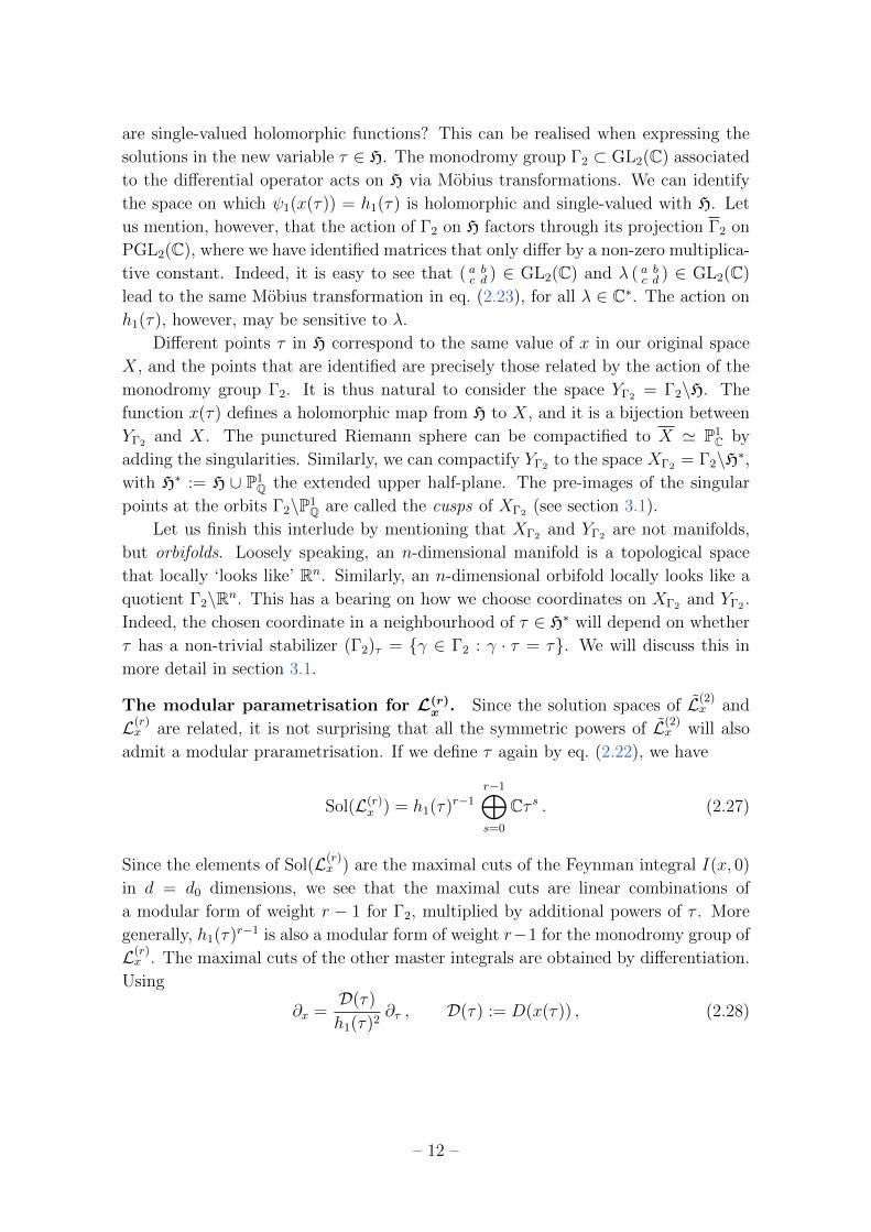
The modular parametrisation for L(r)x . Since the solution spaces of L(2)

x and

L(r)x are related, it is not surprising that all the symmetric powers of L(2)

x will also

admit a modular prarametrisation. If we define τ again by eq. (2.22), we have

Sol(L(r)x ) = h1(τ)r−1

r−1⊕s=0

Cτ s . (2.27)

Since the elements of Sol(L(r)x ) are the maximal cuts of the Feynman integral I(x, 0)

in d = d0 dimensions, we see that the maximal cuts are linear combinations of

a modular form of weight r − 1 for Γ2, multiplied by additional powers of τ . More

generally, h1(τ)r−1 is also a modular form of weight r−1 for the monodromy group of

L(r)x . The maximal cuts of the other master integrals are obtained by differentiation.

Using

∂x =D(τ)

h1(τ)2∂τ , D(τ) := D(x(τ)) , (2.28)

– 12 –

we see that the maximal cuts of the other master integrals also involve the derivatives

of h1(τ) (with respect to τ). As we will see in the next section, the latter are no

longer modular forms, but they give rise to so-called quasi-modular forms.

Let us now return to the original inhomogeneous differential equation. To solve

this equation in terms iterated integrals, we can turn it into a first-order inhomoge-

neous system for the vector I(x, ε) and proceed similar to section 2.1. The entries

of the Wronskian matrix of L(r)x can be expressed in terms of ψ1(x) and ψ2(x):

Wr(x)ij = (2.29)

=

(r − 1

i− 1

)−1 j−1∑k=0

(r − j

i− k − 1

)(j − 1

k

)ψ1(x)r−i−j+k+1 ψ2(x)j−k−1ψ′1(x)i−k−1 ψ′2(x)k ,

with determinant

detWr(x) = D(x)r(r−1)/2

r−1∏k=1

k!

kk. (2.30)

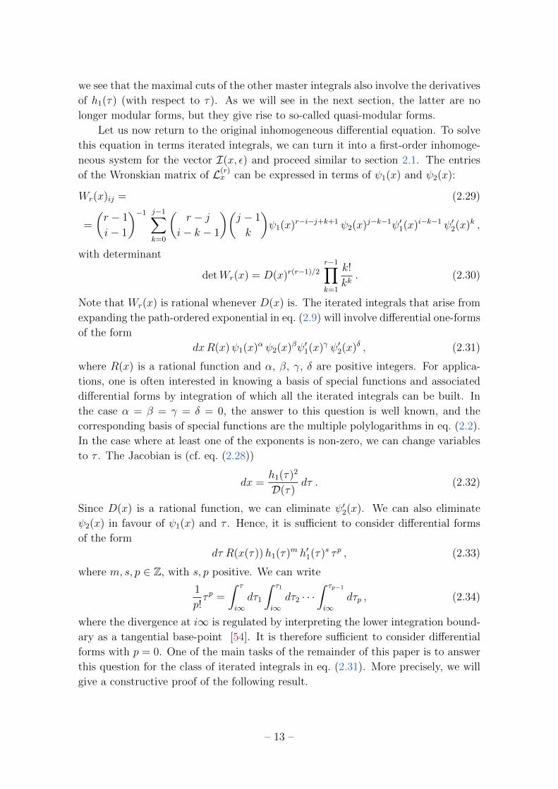
Note that Wr(x) is rational whenever D(x) is. The iterated integrals that arise from

expanding the path-ordered exponential in eq. (2.9) will involve differential one-forms

of the form

dxR(x)ψ1(x)α ψ2(x)βψ′1(x)γ ψ′2(x)δ , (2.31)

where R(x) is a rational function and α, β, γ, δ are positive integers. For applica-

tions, one is often interested in knowing a basis of special functions and associated

differential forms by integration of which all the iterated integrals can be built. In

the case α = β = γ = δ = 0, the answer to this question is well known, and the

corresponding basis of special functions are the multiple polylogarithms in eq. (2.2).

In the case where at least one of the exponents is non-zero, we can change variables

to τ . The Jacobian is (cf. eq. (2.28))

dx =h1(τ)2

D(τ)dτ . (2.32)

Since D(x) is a rational function, we can eliminate ψ′2(x). We can also eliminate

ψ2(x) in favour of ψ1(x) and τ . Hence, it is sufficient to consider differential forms

of the form

dτ R(x(τ))h1(τ)m h′1(τ)s τ p , (2.33)

where m, s, p ∈ Z, with s, p positive. We can write

1

p!τ p =

∫ τ

i∞dτ1

∫ τ1

i∞dτ2 · · ·

∫ τp−1

i∞dτp , (2.34)

where the divergence at i∞ is regulated by interpreting the lower integration bound-

ary as a tangential base-point [54]. It is therefore sufficient to consider differential

forms with p = 0. One of the main tasks of the remainder of this paper is to answer

this question for the class of iterated integrals in eq. (2.31). More precisely, we will

give a constructive proof of the following result.

– 13 –

Theorem 1. With assumptions and notations as in section 2.3, at every order in ε,

the solution of the differential equation (2.3) can be written as a C-linear combination

of iterated integrals of meromorphic modular forms for the monodromy group Γ2.

We will give a constructive proof of Theorem 1 in section 4. In addition, in

section 4 we will completely classify the relevant iterated integrals and give an explicit

basis.

3 Review of (quasi-)modular forms and their iterated inte-

grals

The previous section has shown that there are certain classes of Feynman integrals

whose differential equations admit a modular parametrisation. This is to say that

their maximal cuts in D = d0 dimensions are linear combinations of derivatives of

modular forms multiplied by powers of τ , and the higher orders in ε of the maximal

cuts and the full uncut integral can be expressed in terms of iterated integrals of

such functions. The aim of this section is to briefly review the theory of holomorphic

modular forms and their iterated integrals. In the next section we will extend this

to include iterated integrals of meromorphic modular forms.

3.1 The modular group SL2(Z) and its subgroups

We start by reviewing some general facts about (certain) subgroups of the modular

group SL2(Z). For a review, see ref. [82], and references therein. Let Γ denote

a subgroup of SL2(Z) of finite index, i.e., the quotient Γ\SL2(Z) is finite (which

means, intuitively, the we can cover SL2(Z) by a finite number of copies of Γ). In

the following we denote the index of Γ in SL2(Z) by

[SL2(Z) : Γ] = |Γ\SL2(Z)| <∞ . (3.1)

An important example of finite-index subgroups are the congruence subgroups of

level N , with N a positive integer, defined as those subgroups Γ that contain the

principal congruence subgroups Γ(N) = {( a bc d ) ∈ SL2(Z) : ( a bc d ) = ( 1 00 1 ) mod N}.

An important example of congruence subgroup are the groups

Γ1(N) := {( a bc d ) ∈ SL2(Z) : ( a bc d ) = ( 1 ∗0 1 ) mod N} . (3.2)

In the following we will keep the discussion general, and we do not restrict ourselves

to congruence subgroups, unless specified otherwise.

The modular group and its subgroups naturally act on the extended upper half-

plane H∗ = H ∪ P1Q by Mobius transformations via

γ · τ =aτ + b

cτ + d, γ = ( a bc d ) ∈ SL2(Z). (3.3)

– 14 –

Γ acts separately on H and P1Q, and decomposes P1

Q into disjoint orbits, called cusps

of Γ:2

SΓ := Γ \ P1Q . (3.4)

The number of cusps of Γ is always finite and we denote it by ε∞(Γ) := #SΓ < ∞.

The stabilizer of a cusp s ∈ P1Q is generated by an element of the form ±T h = ± ( 1 h

0 1 ),

for some integer h called the width of the cusp. In case the stabilizer of the cusp s

contains an element−T h ∈ Γs, the cusp is called irregular, otherwise it is regular. The

numbers of regular and irregular cusps are denoted by εr(Γ) and εi(Γ) respectively.

Note that for every cusp s ∈ Q there exists a γ ∈ SL2(Z) such that γ · s = i∞.

A point τ ∈ H is called an elliptic point for Γ if τ has a non trivial stabilizer

group in Γ:

Γτ := {γ ∈ Γ : γ · τ = τ} . (3.5)

One can show that Γτ is always a finite-cyclic group. If Γτ is cyclic of order n, then

τ is called an elliptic point of order n. SL2(Z) = Γ(1) has exactly two elliptic points,

i and ρ := e2πi/3 in its fundamental domain D1 ∪ D2 ∪ D3, with

D1 :={τ ∈ H : |τ | > 1 and |<τ | < 1

2

},

D2 :={τ ∈ H : |τ | ≥ 1 and <τ = −1

2

},

D3 :={τ ∈ H : |τ | = and −1

2< <τ ≥ 0

}.

(3.6)

They are of order two and three respectively,

Γi ' Z/2Z and Γρ ' Z/3Z , ρ := e2πi/3 . (3.7)

Every elliptic point is SL2(Z)-equivalent to either i or ρ := e2πi/3. The number

of elliptic points of order two or three of Γ will be denoted by ε2(Γ) and ε3(Γ).

The principal congruence subgroups Γ(N) have no elliptic points for N > 1. The

subgroups Γ1(N) have no elliptic points for N > 3, while Γ1(3) has no elliptic points

of order two and Γ1(2) has no elliptic points of order three.

3.2 Modular curves

The space of orbits XΓ := Γ\H∗ can be equipped with the structure of a compact

Riemann surface, called the modular curve for Γ. The genus of Γ is defined as the

genus of XΓ and is related to the number of cusp and elliptic points of Γ:

g = 1 + dΓ −ε2(Γ)

4− ε3(Γ)

3− ε∞(Γ)

2, (3.8)

where we introduced the shorthand dΓ := [SL2(Z):{±1}Γ]12

. In the remainder of this

paper we are only concerned with the case where Γ has genus zero. It is known that

2By abuse of language, one also often calls the elements of P1(Q) cusps.

– 15 –

Γ1(N) an Γ(N) have genus zero for N ≤ 12 and N ≤ 5 respectively. In particular,

the group Γ1(6) relevant to the equal-mass sunrise and banana graphs has genus

zero. A complete list of all genus zero subgroups can be found in refs. [83, 84].

In the following it will be important to know how we can define local coordinate

charts on the Riemann surface XΓ. We recall that XΓ is an orbifold, and the points of

XΓ are equivalence classes [τ ] = {γ · τ : γ ∈ Γ}. Let P = [τ0] ∈ XΓ. To define a local

coordinate z such that z(P ) = 0 in a neighbourhood of P , we need to distinguish

three cases:

• If τ0 is an elliptic point of order h, a local coordinate is defined by z = (τ−τ0)h.

• If τ0 is a cusp of width h, such that γ · τ0 = i∞, a local coordinate is defined

by z = e2πi(γ·τ)/h′ , with h′ = h is τ0 is a regular cusp, and h′ = 2h otherwise.

• If τ0 is neither a cusp nor an elliptic point, z = τ−τ0 is a good local coordinate.

The field of meromorphic functions of XΓ is isomorphic to the field M0(Γ) of

modular functions, i.e., meromorphic functions f : H∗ → C that satisfy

f

(aτ + b

cτ + d

)= f(τ) , ∀ ( a bc d ) ∈ Γ . (3.9)

For every meromorphic function, we denote by νP (f) ∈ Z the order of vanishing at

P , i.e., νP (f) > 0 (< 0) if f has a zero (pole) of order |νP (f)| at P . If z denotes

the local coordinate introduced above, we have f(τ) = AzνP (f) + O(zνP (f)+1), with

A 6= 0.

If XΓ has genus zero, the field of meromorphic functions on XΓ has a single

generator,M0(Γ) ' C(ξ), for some ξ ∈M0(Γ) called a Hauptmodul. Every modular

function is a rational function in the Hauptmodul ξ. If h is the width of the infinite

cusp, then we can choose the Hauptmodul to have the q-expansion [83]

ξ(τ) = q−1/h +∑n≥0

a0 qn/h , q = e2πiτ . (3.10)

In the following we always assume that such a Hauptmodul ξ has been fixed.

3.3 Review of (quasi-)modular forms

3.3.1 Meromorphic modular forms

Let k be an integer, Γ ⊆ SL2(Z). We define the action of weight k of Γ on a function

f : H∗ → C by

f [γ]k(τ) := (cτ + d)−k f(γ · τ) , γ = ( a bc d ) ∈ Γ . (3.11)

A weakly modular form of weight k for Γ is a function that is invariant under this

Γ-action,

f [γ]k(τ) = f(τ) , ∀γ ∈ Γ . (3.12)

– 16 –

A meromorphic modular form of weight k for Γ is a weakly modular form f of weight

k for Γ that is meromorphic on H and at every cusp, i.e., it admits a q-expansion of

the form

f [γ]k(τ) =∑n≥n0

an qn/h , ∀γ = ( a bc d ) ∈ SL2(Z) , (3.13)

where h is the width of the cusp ac. We denote the C-vector space of meromorphic

modular forms of weight k for Γ by Mk(Γ), and we write M(Γ) :=⊕

kMk(Γ).

In particular, M0(Γ) is the field of modular functions for Γ (see eq. (3.9)). Holo-

morphic modular forms are defined in an analogous manner. The C-vector space

of holomorphic modular forms of weight k for Γ is denoted by Mk(Γ), and we

define M(Γ) :=⊕

kMk(Γ). Note that Mk(Γ) is always finite-dimensional, and

dimCMk(Γ) = 0 for k ≤ 0. In the following we refer to holomorphic modular

forms simply as modular forms.

A (meromorphic) cusp form is a (meromorphic) modular form for which a0 = 0

for every cusp. We denote the vector space of (meromorphic) cusp forms of weight k

by Sk(Γ) (Sk(Γ)). The space of cusp forms Sk(Γ) is an ideal in Mk(Γ). The quotient

is the space of Eisenstein series Ek(Γ), and there is a direct sum decomposition

Mk(Γ) = Ek(Γ)⊕ Sk(Γ) . (3.14)

3.3.2 Meromorphic quasi-modular forms

In general, the derivative of a (meromorphic) modular form is no longer a modular

form, but we need to introduce a more general class of functions. A meromorphic

quasi-modular form of weight k and depth p for Γ is a function f : H∗ → C that is

meromorphic on H and at the cusps, and it transforms according to

f [γ]k(τ) =

p∑r=0

fr(τ)

(c

cτ + d

)r, γ = ( a bc d ) ∈ Γ , (3.15)

where the f0, . . . , fp are meromorphic functions, with fp 6= 0. Note that eq. (3.15) for

γ = id implies that f0 = f . The C-vector space of meromorphic quasi-modular forms

of weight k and depth at most p is denoted by QM≤pk (Γ). Quasi-modular forms of

depth zero are precisely the modular forms. Holomorphic quasi-modular forms are

defined in an analogous way, and the corresponding (finite-dimensional) vector space

is denoted by QM≤pk (Γ). Note that dimCQM

≤pk (Γ) = 0 for k ≤ 0 and 2p > k. We

also use the notations

QMk(Γ) :=⋃p≥0

QM≤pk (Γ) and QM(Γ) :=

⊕k

QMk(Γ) . (3.16)

The vector spaces QMk(Γ) and QM(Γ) are defined in a similar fashion.

The algebra of all (meromorphic) quasi-modular forms is closed under differenti-

ation. We use the notation δ := 12πi∂τ = q ∂q. If f is a quasi-modular form of weight

k and depth at most p, then δf has weight k + 2 and depth at most p+ 1.

– 17 –

The Eisenstein seriesG2(τ) of weight two is the prime example of a quasi-modular

form of depth 1. The Eisenstein series are defined as3

G2k(τ) =∑

(m,n)∈Z2\(0,0)

1

(mτ + n)2k. (3.17)

For k 6= 1, G2k(τ) is a modular form of weight 2k for SL2(Z). For k = 1, we have

G2[γ]2(τ) = (cτ + d)−2G2(γ · τ) = G2(τ)− 1

4πi

c

cτ + d, (3.18)

for every γ = ( a bc d ) ∈ SL2(Z). Hence G2(τ) defines a (holomorphic) quasi-modular

form of weight 2 and depth 1 for SL2(Z). In fact, one can show that every meromor-

phic quasi-modular form of depth p can be written as a polynomial of degree p in

G2(τ):

QM(Γ) =M(Γ)[G2(τ)] . (3.19)

3.4 Iterated integrals of holomorphic quasi-modular forms

The previous discussion makes it clear that the functions f(τ) := R(x(τ))h1(τ)m h′1(τ)s

in eq. (2.33) (with p = 0) are a meromorphic quasi-modular forms of weight m+ 3s

and depth at most s. Hence, we see that the iterated integrals encountered at the

end of section 2 are iterated integrals of meromorphic quasi-modular forms for the

monodromy group Γ2. In the remainder of this section we give a short review of

iterated integrals of holomorphic quasi-modular forms, following refs. [53, 54]. In the

next section we present the extension to the meromorphic case.

Let h1, . . . , hk be meromorphic quasi-modular forms for Γ ⊆ SL2(Z) We define

their iterated integral by [53, 54]

I(h1, . . . , hk; τ) :=

∫ τ

i∞dτ1 h1(τ1)

∫ τ1

i∞dτ2 h2(τ2)

∫ τ2

i∞· · ·∫ τk−1

i∞dτk hk(τk) . (3.20)

At this point we have to mention that this definition requires a regularisation of the

divergence at τ = i∞, already in the holomorphic case (at least for Eisenstein series).

For the holomorphic case we follow ref. [54], and interpret the lower integration

boundary as a tangential base point. In the meromorphic case, the regularisation

requires the use of tools from renormalisation theory, see ref. [57]. We refer to

refs. [54, 57] for a detailed discussion.

The iterated integrals in eq. (3.20) are not necessarily independent, even if the

h1, . . . , hk are linearly independent in QM(Γ). Rather, we have to identify a set

of quasi-modular forms that are linearly independent up to total derivatives, i.e.,

modulo δQM(Γ) (see also the discussion in section 4.1). Said differently, we need

3For k = 1 the series is not absolutely convergent. Here we assume the standard summation

convention for G2(τ), cf., e.g., ref. [82]

– 18 –

to would like to know which quasi-modular forms can be expressed as derivatives of

(quasi-)modular forms. This question can be answered completely in the holomorphic

case. Writing QMk(Γ) :=⋃p≥0QM

≤pk (Γ), we have the decomposition [85, 86]

QMk(Γ) =

C , k = 0 ,

M1(Γ) , k = 1 ,

M2(Γ)⊕ CG2(τ) , k = 2 ,

Mk(Γ)⊕ δQMk−2(Γ) , k > 3 .

(3.21)

Note that the sums are direct, i.e., every holomorphic quasi-modular form of weight

k > 2 can be written modulo derivatives as a holomorphic modular form, and this

decomposition is unique. The decomposition can be performed in an algorithmic way,

cf. ref. [86]. In other words, modulo derivatives, QM(Γ) is generated as a vector

space by M(Γ) and G2(τ). Consequently, in the holomorphic case it is sufficient

to consider iterated integrals of modular forms and G2(τ) [55]. The equivalent of

the decomposition in eq. (3.21) in the meromorphic case for general subgroups Γ is

currently still unknown, and results are only available for weakly holomorphic modular

forms (i.e., with poles at most at the cusps) [87] and for meromorphic quasi-modular

forms for the whole modular group, Γ = SL2(Z) [57]. One of the main results of

this paper is the generalisation of eq. (3.21) and the results of ref. [57] to arbitrary

subgroups of genus zero.

4 Iterated integrals of meromorphic modular forms

4.1 A decomposition theorem for meromorphic quasi-modular forms

In this section we state and prove the generalisation of eq. (3.21) for all genus-zero

subgroups. The special case Γ = SL2(Z) was proved by one of us in ref. [57], and

the proof presented here is a generalisation of that proof. Before we state the main

theorem in this section, we need to introduce some notation. Let R ⊂ XΓ \ SΓ be

a finite set of points which are not cusps, and let s0 ∈ SΓ be a cusp of XΓ, and

Rs0 := R∪{s0} and RS := R∪SΓ. We defineMk(Γ, Rs0) to be the sub-vector space

of Mk(Γ) consisting of all meromorphic modular forms of weight k for Γ with poles

at most at points in Rs0 .

Definition 1. Define Mk(Γ, Rs0) to be the subset of those f ∈ Mk(Γ, Rs0) which

satisfy:

1. νP (f) ≥ 1−khP

, for all P ∈ R;

2. νs(f) ≥ 0, for all s ∈ SΓ \ {s0};

3. bνs0(f)c ≥ − dimSk(Γ).

– 19 –

In the previous definition bxc is the floor function, i.e., the largest integer less or

equal than x ∈ R.

Theorem 2. Let Γ ⊆ SL2(Z) have genus zero, Rs0 as defined above. We have a

decomposition

QMk(Γ, RS) =

{δQMk−2(Γ, RS)⊕Mk(Γ, RS) , for k < 2 ,

δQMk−2(Γ, RS)⊕M2−k(Γ, RS)Gk−12 ⊕ Mk(Γ, Rs0) , for k ≥ 2 .

The proof is presented in appendix A. Theorem 2 generalises the result of ref. [57]

to arbitrary subgroups of genus zero. In section 4.2 we sketch the proof for a subset

of subgroups of genus zero, the so-called neat subgroups (see Definition 2). The

proof of section 4.2 is constructive, and allows one to perform the decomposition in

Theorem 2 explicitly for neat subgroups. We expect that this case covers most of the

applications to Feynman integrals. Before we discuss the proof for neat subgroups,

however, we review some consequences of Theorem 2.

Proof of Theorem 1. We now show that the decomposition in Theorem 2 im-

mediately leads to a proof of Theorem 1. We have already argued that the class of

differential equations considered in section 2.3 leads to iterated integrals involving the

one-forms in eq. (2.33) with p = 0, and the functions f(τ) := R(x(τ))h1(τ)m h′1(τ)s

are quasi-modular forms of weight k := 3s + m and depth at most s for the mon-

odromy group Γ2. Let f have poles at most at the cusps and at some finite set of

points R ⊂ H, i.e., f ∈ QM≤sk (Γ2, RS). Theorem 2 then implies that, for some fixed

choice of cusp s0 ∈ SΓ2 :

• If k < 2, there is h ∈Mk(Γ2, RS) and g ∈ QMk−2(Γ2, RS) such that f = h+δg.

• If k ≥ 2, there are modular forms h ∈ Mk(Γ2, Rs0), h ∈ M2−k(Γ2, RS) and a

quasi-modular form g ∈ QMk−2(Γ2, RS) such that f = h+ hGk−12 + δg.

The derivatives δg can be trivially integrated away, and we see that we only need

to consider the meromorphic modular form h or the quasi-modular form hGk−12 ,

the latter being characterised by the fact that it has the maximally allowed depth,

s = k − 1. In order to show that Theorem 1 holds, we need to show that these

quasi-modular forms with maximally allowed depth s = k − 1 do not arise from our

class of differential equations. To see this, we start from eq. (2.31) with α, β, γ, δ

positive integers, and we change variables from x to τ , and we trace the powers of

G2 that are produced along the way. The Jacobian is given in eq. (2.32). Moreover,

we use eq. (2.28) to obtain

ψ′1(x) = h′1(τ) ∂xτ = h′1(τ)D(τ)

h1(τ)2, (4.1)

– 20 –

and

ψ′2(x) =ψ2(x)ψ′1(x) +D(x)

ψ1(x)=D(τ)

h1(τ)2(τ h′1(τ) + h1(τ)) . (4.2)

Since h1 is a modular form of weight 1, h′1 is a quasi-modular form of weight 3

and depth at most 1, i.e., there are A1 ∈ M1(Γ2) and A3 ∈ M3(Γ2) such that

h′1 = A1G2 + A3. This gives:

dxψ1(x)α ψ2(x)β ψ′1(x)γ ψ′2(x)δ =

= dτ D(τ)γ+δ−2 h1(τ)2+α+β−2γ−2δ τβ (A1G2 + A3)γ

× (τ A1(τ)G2(τ) + τ A3(τ) + h1(τ))δ

= dτ D(τ)γ+δ−2 h1(τ)2+α+β−2γ−2δ τβ

×γ∑p=0

δ∑q=0

(γ

p

)(δ

q

)A1(τ)p+q G2(τ)p+q τ q A3(τ)γ−p (τ A3(τ) + h1(τ))δ−q .

(4.3)

The term with the highest power of G2 is:

dτ D(τ)γ+δ−2 h1(τ)2+α+β−2γ−2δ τβ A1(τ)γ+δ G2(τ)γ+δ τ δ . (4.4)

It has depth s = γ + δ and weight k = α + β + γ + δ + 2 = α + β + s + 2. Since α

and β are positive integers, we have k ≥ s + 2 > s + 1, and so we never reach the

maximally allowed depth s = k − 1.

To finish the proof of Theorem 1, we need to comment on the inhomogeneous

term N(x, ε) in eq. (2.3). By assumption, the ε-expansion of N(x, ε) involves at

every order only sums of rational functions of x multiplied by MPLs of the form

G(a1, . . . , an;x), with ai independent of x. It is easy to see that MPLs of this form

can always be written as iterated integrals of modular forms for Γ2, because

dx

x− ai=

h1(τ)2 dτ

D(τ) (x(τ)− x(τi)), with x(τi) = ai . (4.5)

This finishes the proof of Theorem 1.

Linear independence for iterated integrals. We have seen how Theorem 2

leads to a proof of Theorem 1, which characterises the iterated integrals that arise

as solutions to a certain class of differential equations. In applications one is usu-

ally also interested in having a minimal set of of iterated integrals, i.e., a basis of

linearly-independent iterated integrals. We now show how Theorem 2 yields the

desired linear independence result. The crucial mathematical ingredient is a linear

independence criterion for iterated integrals, which is very general and not at all

limited to meromorphic modular forms. We first describe this criterion in a special

case which, while being far from the most general possible statement, is sufficiently

general to exhibit all essential features of the general case (for details, see ref. [88]).

– 21 –

Suppose that F = {fi}i∈I is a family of meromorphic functions on the upper half-

plane, and let K be a differential subfield of the field of meromorphic functions on H,

which contains all fi. Here, ‘differential subfield’ means that K is a subfield which

is closed under differentiation of meromorphic functions. The following theorem is a

variant of a classical result due to Chen, [89, Theorem 4.2].

Theorem 3 ([88, Theorem 2.1]). The following assertions are equivalent.

(i) The family of all iterated integrals (viewed as functions of τ) of the form∫ τ

i∞dτ1 fi1(τ1)

∫ τ1

i∞dτ2 fi2(τ2) . . .

∫ τn−1

i∞dτn fin(τn) ,

for all n ≥ 0 and all fi ∈ F , is K-linearly independent.

(ii) The family F is C-linearly independent and we have

∂τ (K) ∩ SpanCF = {0} ,

where SpanCF denotes the vector space of all C-linear combinations of func-

tions in F .

Let us apply this theorem to our setting. Here K := M(Γ2, RS)(G2) is the

field of fractions of QM(Γ2, RS), i.e., the field whose elements are ratios of quasi-

modular forms, or equivalently ratios of polynomials in G2 with coefficients that are

meromorphic modular forms. K is a differential subfield, because quasi-modular

forms are closed under differentiation. Clearly, we have QM(Γ2, RS) ⊂ K. For Fwe choose

F =⋃k∈Z

Fk , (4.6)

with Fk := {f (k)1 , . . . , f

(k)pk } a C-linearly independent set of modular forms from

Mk(Γ2, RS) for k < 2 and from Mk(Γ2, Rs0) for k ≥ 2 and some fixed choice

of cusp s0 ∈ SΓ2 (see section 4.2 how to construct explicit bases for these vector

spaces). Since the sums in Theorem 2 are direct, it is easy to see that we have

∂τ (K) ∩ SpanCF = {0}, and so Theorem 3 implies that the corresponding iterated

integrals are K-linear independent.

4.2 Sketch of the proof for neat subgroups

We now return to the proof of Theorem 2 for a special class of of subgroups.

Definition 2. A subgroup Γ ⊆ SL2(Z) is called neat if( −1 0

0 −1

)/∈ Γ and Γ has no

elliptic points nor irregular cusps, ε2(Γ) = ε3(Γ) = εi(Γ) = 0.

One can show that

– 22 –

1. Γ1(N) is neat and has genus zero for N ∈ {5, . . . , 10, 12};

2. Γ(N) is neat and has genus zero for N ∈ {3, 4, 5}.

In particular, the congruence subgroup Γ1(6) relevant to the banana graph is neat

and has genus zero.

For k < 2, the proof of Theorem 2 is identical to the proof for Γ = SL2(Z)

considered in ref. [57], and we do not consider it here. In order to see that Theo-

rem 2 holds also for k ≥ 2, we first note that for every f ∈ QMk(Γ, Rs0) there are

meromorphic modular forms h1 ∈ Mk(Γ, Rs0) and h2 ∈ M2−k(Γ, Rs0) and a mero-

morphic quasi-modular form g ∈ QMk−1(Γ, Rs0) such that f = h1 + h2Gk−12 + δg.

This decomposition holds for all subgroups Γ, and does not require Γ to be neat. It

is a direct consequence of the algorithms of ref. [86]. Theorem 2 then follows from

the following claim: For every meromorphic modular form f ∈Mk(Γ, Rs0) of weight

k ≥ 2 there is h ∈ Mk(Γ, Rs0) and g ∈ QMk−2(Γ, Rs0) such that

f = h+ δg . (4.7)

In the remainder of this section we show how to construct h and g explicitly for

neat subgroups of genus zero. Before doing so, we review some mathematical tools

required to achieve this decomposition.

Bol’s identity. A complication when trying to decompose a meromorphic modular

f into an elements h ∈ Mk(Γ, Rs0) up to a total derivative is the fact that in general

derivatives of modular forms are themselves not modular, but only quasi-modular.

However, an important result due to Bol [90] states that we recover again a modular

form if we take enough derivatives. More precisely, Bol’s identity states that for

k ≥ 2 there is a linear map

δk−1 :M2−k(Γ)→ Sk(Γ) . (4.8)

In other words, if k ≥ 2 and f ∈M2−k(Γ), then in general δf will not be a modular

form, i.e., δf /∈M4−k(Γ), but the (k−1)th derivative will be a modular form of weight

k, δk−1f ∈ Mk(Γ) (and in fact, it will even be a cusp form). Note that eq. (4.8)

remains true if we replace M2−k(Γ) and Sk(Γ) by M2−k(Γ, Rs0) and Sk(Γ, Rs0) re-

spectively.

The main idea to achieve the decomposition in eq. (4.7) then goes as follows:

Assume we are given f ∈Mk(Γ, Rs0) with a pole of order m > 0 at a point P ∈ Rs0 ,

and assume the order of the pole is too high for f to lie in Mk(Γ, Rs0). We will

show how to construct g ∈ M2−k(Γ, Rs0) such that f − δk−1g has a pole of order at

most m− 1 at P . Applying this approach recursively, we obtain the decomposition

in eq. (4.7).

– 23 –

Divisors and the valence formula. From the previous discussion it becomes

clear that an important step in achieving the decomposition in eq. (4.7) is the con-

struction of g ∈ M2−k(Γ, Rs0) with prescribed poles. An important tool to un-

derstand meromorphic functions (or, more generally, meromorphic sections of line

bundles) on a Riemann surface are divisors, which we review in this section. The

material in this section is well-known in the mathematics literature, but probably

less so in the context of Feynman integrals.

A divisor on XΓ is an element in the free group Div(XΓ) generated by the

points of XΓ (divided by their order hP ), i.e., a divisor is an expression of the form

D =∑

P∈XΓ

nP

hP[P ], where the nP are integers, and only finitely many of the nP are

non zero. We can use divisors to encode the information on the zeroes and poles of

a meromorphic function or modular form. More precisely, if 0 6= f ∈Mk(Γ), we can

associate a divisor to it, defined by

(f) =∑s∈SΓ

νs(f)

hs[s] +

∑P∈XΓ\SΓ

νP (f)

#ΓP[P ] , (4.9)

where hs = 2 if s is irregular and hs = 1 otherwise, and ΓP is the projection of ΓP to

PSL2(Z) (i.e., we have identified γ ∈ SL2(Z) and −γ ∈ SL2(Z)). Note that we have

the obvious relation (fg) = (f) + (g).

To every divisorD =∑

P∈XΓ

nP

hP[P ] we can associate its degree degD =

∑p∈XΓ

np.

Since every meromorphic function on a compact Riemann surface must have the same

number of zeroes and poles (counted with multiplicity), we must have deg(f) = 0

for all f ∈ M0(Γ). For meromorphic modular forms of weight k, the degree of the

associated divisor is no longer zero, but it is given by the valence formula:

deg(f) = k dΓ . (4.10)

Modular forms for neat subgroups of genus zero. From now on we focus on

the case where Γ is neat and has genus zero. Equation (3.8) then implies

ε∞(Γ) = 2(1 + dΓ) . (4.11)

As we will now show, the spaces of meromorphic modular forms for neat subgroups

can be described very explicitly.

Lemma 1. Let Γ be a neat subgroup of genus zero. Then there exists ℵk ∈Mk(Γ)

such that ν∞(ℵk) = k dΓ and νP (ℵk) = 0 otherwise. In particular, for k > 0, ℵk is a

modular form of weight k for Γ.

Proof. If k = 0, we simply choose ℵ0 = 1, and for k < 0 we set ℵk = 1/ℵ−k. So it

– 24 –

is sufficient to discuss k > 0. Since dimCMk(Γ) 6= 0,4 it contains a meromorphic

modular form h with divisor

(h) =∑P∈XΓ

nP [P ] = kdΓ [∞] +D , (4.12)

where we used the fact that hP = 1 for neat subgroups, and we defined

D := (n∞ − kdΓ) [∞] +∑P∈XΓP 6=∞

nP [P ] . (4.13)

The valence formula implies degD = 0, and so there is a meromorphic function

f ∈M0(Γ) such that (f) = D. Since Γ has genus zero, every meromorphic function

is a rational function in the Hauptmodul ξ, and it is sufficient to pick

f :=∏P∈XΓP 6=∞

(ξ − P )nP . (4.14)

It is now easy to check that ℵk := 1fh has the desired property. The fact that ℵk is

holomorphic follows from νP (ℵk) ≥ 0 for all P ∈ XΓ.

Note that ℵk is unique, up to overall normalisation. Indeed, assume that ℵ(1)k and

ℵ(2)k both satisfy the condition, then (ℵ(1)

k /ℵ(2)k ) = (ℵ(1)

k )− (ℵ(2)k ) = 0, and so there is

α ∈ C such that ℵ(1)k = αℵ(2)

k . We assume from now on that the normalisation of ℵkis chosen such that at the infinite cusp we have the q-expansion (h is the width at

the infinite cusp):

ℵk(τ) = qkdΓ/h

[1 +

∑n≥1

an qn/h

], q = e2πiτ . (4.15)

We can use ℵk to give an explicit representation of the spaces of modular forms

of weight k in terms of rational functions,

Mk(Γ) = ℵk · C(ξ) , (4.16)

with holomorphic modular forms of weight k corresponding to polynomials of degree

at most k dΓ:

Mk(Γ) = ℵk · C[ξ]≤kdΓ, (4.17)

4This can be seen by thinking of (meromorphic) modular forms of weight k for the group Γ

as (meromorphic) sections of a certain line bundle (the k-th power of the Hodge bundle) on the

modular curve XΓ. It then follows from the Riemann–Roch formula that every line bundle on a

compact Riemann surface admits a meromorphic section. See also ref. [82], the discussion after

Theorem 3.6.1, for a detailed proof.

– 25 –

where C[X]≤m denotes the vector space of polynomials of degree at most m. We can

use this representation to write down a generating set for Mk(Γ). For p ∈ XΓ and

m ∈ Z>0, we define:

uP,m(τ) =

{(ξ(τ)− P )−m , if P 6=∞ ,

ξ(τ)m , if P =∞ ,

u∞,0(τ) = 1 .

(4.18)

It is an easy exercise (based on partial fractioning) to show that every rational

function has a unique representation as a finite linear combination of the uP,m. As a

consequence, the meromorphic modular forms Uk,P,m := ℵk uP,m are a generating set

for Mk(Γ). In particular, a basis for Mk(Γ) is {ℵk u∞,m : 0 ≤ m ≤ kdΓ}. Moreover,

we can use this generating set to write down an explicit basis for Mk(Γ, R∞) in

definition 1. For k ≥ 2, we have

Mk(Γ, R∞) := Mk(Γ) ∪ Sk(Γ) ∪ Mk(Γ, R) , (4.19)

where we defined

Mk(Γ, R) :=⊕

p∈R\{∞}1≤m≤k−1

CUk,P,m =⊕P∈R

1≤m≤k−1

Cℵk

(ξ − P )m,

Sk(Γ) :=⊕

kdΓ<m<2dΓ (k−1)

CUk,∞,m =⊕

kdΓ<m<2dΓ (k−1)

Cℵk ξm .(4.20)

Note that dimC Sk(Γ) = dimC Sk(Γ).

Sketch of the proof of Theorem 2 for neat subgroups. We now show how

we can use Bol’s identity to construct for each f = Uk,P,m a function g such that the

decomposition in eq. (4.7) holds. We will make repeated use of the following result:

Lemma 2. Let Γ be neat and have genus zero, f ∈M2−k(Γ), for k ≥ 2.

1. If P ∈ XΓ \ SΓ, then νP (δk−1f) ≥ 0 or νP (δk−1f) = 1− k + νP (f).

2. If s ∈ SΓ, then νs(δk−1f) ≥ 0 or νs(δ

k−1f) = νs(f).

Proof. It is sufficient to prove the claim for the elements of the generating set,

U2−k,P,m = ℵ2−kuP,m = ℵ−1k−2uP,m.

We need to show that if δk−1f has a pole at P , i.e., νP (δk−1f) < 0, then it

satisfies the claim of the lemma. Note that if νP (δk−1f) < 0, then also νP (f) < 0.

Let P ∈ XΓ \ SΓ. We have νP (U2−k,P,m) = −m < 0. Then, if τP is such that

t(τP ) = P , Uk,P,m admits a Laurent expansion of the form

U2−k,P,m(τ) =α

(τ − τP )m+O

(1

(τ − τP )m−1

), α ∈ C \ {0} (4.21)

– 26 –

and so

δk−1U2−k,P,m(τ) = (2πi)1−k∂k−1τ U2−k,P,m(τ)

=(m)k−2 α

(−2πi)k−1 (τ − τP )m+k−1+O

(1

(τ − τP )m+k−2

),

(4.22)

where (a)n = a(a + 1) . . . (a + n). Hence νP (δk−1U2−k,P,m) = 1 − k −m = 1 − k +

νP (U2−k,P,m).

Let s ∈ SΓ, s 6= [∞]. We have νP (U2−k,P,m) = −m < 0. If q is a local coordinate

in a neighbourhood of the cusp s, U2−k,P,m admits the Fourier expansion:

U2−k,P,m(q) =α

qm+O(q−m+1) , α ∈ C \ {0} , (4.23)

and so

δk−1U2−k,P,m(q) = (q∂q)k−1U2−k,P,m(q) =

(−1)k−1 (m)k−2 α

qm+O(q−m+1) . (4.24)

Hence, νs(δk−1U2−k,P,m) = νs(U2−k,P,m).

If s = [∞], then ν∞(U2−k,∞,m) = −m−ν∞(ℵk−2) = −m−(k−2)dΓ. By the same

argument as in the case s 6= [∞], we conclude ν∞(δk−1U2−k,P,m) = −m− (k− 2)dΓ =

ν∞(U2−k,P,m).

We are now in a position to prove the decomposition in eq. (4.7). The proof

is constructive, and allows one to recursively construct the functions h and g in

eq. (4.7). The decomposition in eq. (4.7) is equivalent to the following result:

Theorem 4. For k ≥ 2, there is a decomposition

Mk(Γ, RS) = Mk(Γ, R∞)⊕ δk−1M2−k(Γ, RS) . (4.25)

Proof. It is sufficient to consider the case #R = 1.

We first show surjectivity. For this it is sufficient to show that all those Uk,P,mnot in Mk(Γ, R∞) do not define independent classes modulo objects that lie in the

image of Bol’s identity, i.e., these classes can be expressed as linear combinations in

Mk(Γ, R∞), modulo δk−1M2−k(Γ, RS).

Let s ∈ SΓ, s 6= [∞] and m > 0. Let q be a local coordinate around s. Then

there are α1, α2 ∈ C \ {0} such that

Uk,s,m(q) =α1

qm+O(q−m+1) ,

U2−k,s,m(q) =α2

qm+O(q−m+1) .

(4.26)

Lemma 2 implies

Uk,s,m(q)− α1

α2

(−m)1−k δk−1U2−k,s,m(q) = O(q−m+1) . (4.27)

– 27 –

Applying this identity recursively, we arrive at the conclusion that

Uk,s,m = 0 mod δk−1M2−k(Γ, RS) , for all m > 0 . (4.28)

For the infinite cusp, we know from the proof of Lemma 2 that ν∞(δk−1U2−k,∞,m′) =

ν∞(U2−k,∞,m′) = −m′− (k−2)dΓ, for all m′ > 0. Hence, for all m ≥ 2dΓ(k−1) there

is m′ = m− 2dΓ(k− 1) ≥ 0, and we can pick a local coordinate q at the infinite cusp

such that there is α1, α2 6= 0 such that

Uk,∞,m(q) =α1

qm−kdΓ+O(q−m+kdΓ+1) ,

U2−k,∞,m′(q) =α2

qm′−(2−k)dΓ+O(q−m

′+(2−k)dΓ+1) =α2

qm−kdΓ+O(q−m+kdΓ+1) .

(4.29)

Lemma 2 then implies

Uk,∞,m(q)− α1

α2

(kdΓ −m)1−k δk−1U2−k,∞,m′(q) = O(q−m+kdΓ+1) . (4.30)

It follows that Uk,∞,m for m ≥ 2dΓ(k−1) does not define an independent class modulo

total derivatives.

Finally, let R = {P}, and m > k − 1. We can take m′ = m − k + 1 > 0, and

Lemma 2 implies νP (δk−1U2−k,P,m′) = 1 − k −m′ = −m. Hence, with τP such that

t(τP ) = P , there is α1, α2 6= 0 such that

Uk,P,m(τ) =α1

(τ − τP )m+O((τ − τP )−m+1) ,

δk−1U2−k,P,m(τ) =α2

(τ − τP )m′+k−1+O((τ − τP )−m

′−k+2)

=α2

(τ − τP )m+O((τ − τP )−m+1) .

(4.31)

Hence

Uk,P,m(τ)− α1

α2

δk−1U2−k,P,m(τ) = O((τ − τP )−m+1) , (4.32)

and so Uk,P,m for m > k − 1 does not define an independent class modulo total

derivatives. This finishes the proof of surjectivity.

Let us now show injectivity (for R = {P}). Consider the following general linear

combination of elements from Mk(Γ, R∞):

f :=k−1∑m=1

αm Uk,P,m +

2dΓ(k−1)−1∑n=0

βn Uk,∞,n

= ℵkk−1∑m=1

αm(ξ − P )m

+ ℵk2dΓ(k−1)−1∑

n=0

βnξn .

(4.33)

We need to show that whenever there is g ∈ M2−k(Γ, RS) such that f = δk−1g,

then necessarily αm = 0 for 1 ≤ m < k and βm = 0 for 0 ≤ n < 2dΓ(k − 1). Let

– 28 –

us start by showing that the coefficients αm must vanish. To see this, assume that

αm 6= 0 for some 1 ≤ m < k. Then f has a pole at ξ = P , i.e., 0 > νP (f) > −k.

Hence, g must also have a pole at ξ = P , i.e., νP (g) < 0. Lemma 2 then implies

νP (f) = νP (δk−1g) = 1 − k + νP (g) ≤ −k, which is a contradiction. Hence αm = 0

for all 1 ≤ m < k.

Next, let us assume that βn 6= 0 for some 2dΓk < n < 2dΓ(k − 1). Then f has

a pole at the infinite cusp, with 0 > ν∞(f) ≥ ν∞(Uk,∞,2dΓ(k−1)−1) = (2 − k)dΓ + 1.

Then g must also have a pole. The order of the pole is bounded by

ν∞(f) = ν∞(δk−1g) ≤ ν∞(δk−1U2−k,∞,0) = (2− k)dΓ < ν∞(f) , (4.34)

which is a contradiction. Hence βn = 0 for all 2dΓk < n < 2dΓ(k−1). It follows that

f must be a holomorphic modular form of weight k, but Mk(Γ)∩δk−1(M2−k(Γ)) = 0

for k ≥ 0, and therefore f = 0.

5 The monodromy groups of the equal-mass sunrise and ba-

nana integrals

In the remainder of this paper we will illustrate the abstract mathematical concepts

on two very concrete families of Feynman integrals, namely the equal-mass two-loop

sunrise and three-loop banana integrals, defined by:

Isuna1,...,a5(p2,m2; d) = (5.1)

=

∫ 2∏i=1

Dd`i(`1 · p)a4(`2 · p)a5

[`21 −m2]a1 [`2

2 −m2]a2 [(`1 − `2 − p)2 −m2]a3,

Ibana1,...,a9(p2,m2; d) = (5.2)

=

∫ 3∏i=1

Dd`i(`2

3)a5(`1 · p)a6(`2 · p)a7(`3 · p)a8(`1 · `2)a9

[`21 −m2]a1 [`2

2 −m2]a2 [(`1 − `3)2 −m2]a3 [(`2 − `3 − p)2 −m2]a4,

where ai ≥ 0 are positive integers, m2 > 0 and p2 are real. We work in dimensional

regularisation in d = 2− 2ε dimensions. The integration measure reads∫Dd` =

1

Γ(2− d

2

) ∫ dd`

iπd/2. (5.3)

We follow refs. [91, 92] for the choice of master integrals and the differential equations

(see also section 6 and appendix B).

In this section we focus on identifying the maximal cuts of these integrals as

modular forms for the congruence subgroup Γ1(6), and in the next section we see

how iterated integrals of meromorphic modular forms arise. This gives another way to

– 29 –

resolve the debate in the literature whether the two-loop sunrise integral is associated

with modular forms for Γ1(12) or Γ1(6); see, e.g., refs. [51, 61]. While the discussion

in this section focuses on these specific Feynman integrals, it is easy to transpose

the discussion to other differential operators of degree two or three. This may then

provide a roadmap to identify the modular forms obtained from maximal cuts of

one-parameter families of Feynman integrals that are not described by the same

Picard-Fuchs operators as the examples considered here.

5.1 The sunrise family

The monodromy group. The maximal cuts of the integral Isun1,1,1,0,0(p2,m2; 2) are

annihilated by the second-order differential operator [25]:

Lsunt := ∂2

t +

(1

t− 9+

1

t− 1+

1

t

)∂t +

(1

12(t− 9)+

1

4(t− 1)− 1

3t

), (5.4)

where we defined

t :=p2

m2. (5.5)

It is well-known that Lsunt is the Picard-Fuchs operator describing a family of elliptic

curves. Consequently, its solutions can be expressed in terms of elliptic integrals

of the first kind (see appendix B.1). In the following we explicitly construct the

solutions using the Frobenius method reviewed in section 2.2 in order to outline the

general strategy. While we only perform the calculations for the differential operator

Lsunt , the different steps can be applied very generally to second-order differential

operators describing one-parameter families of elliptic curves.

The coefficients in Lsunt have poles at (t0, . . . , t3) = (0, 1, 9,∞), all of which are

regular singular points. One can show that all of these points are MUM-points [70],

and close to each singular point we can choose a basis of solutions that consists of

one holomorphic and one logarithmically-divergent function. For the singular point

t0 at the origin, the Frobenius method delivers the two power series solutions whose

first terms in the expansion read:

φ2(t0; t) =4t

9+

26t2

81+

526t3

2187+

1253t4

6561+O(t5) + φ1(t0; t) log t ,

φ1(t0; t) = 1 +t

3+

5t2

27+

31t3

243+

71t4

729+O(t5) .

(5.6)

It is easy to check that these two local solution can be used to express the functions

Ψ1(t) and Ψ2(t) in eq. (B.2):

Ψ1(t) =2π√

3φ1(0; t) ,

Ψ2(t) = − i√3φ2(0; t)− 2i√

3log(3)φ1(0; t) .

(5.7)

– 30 –

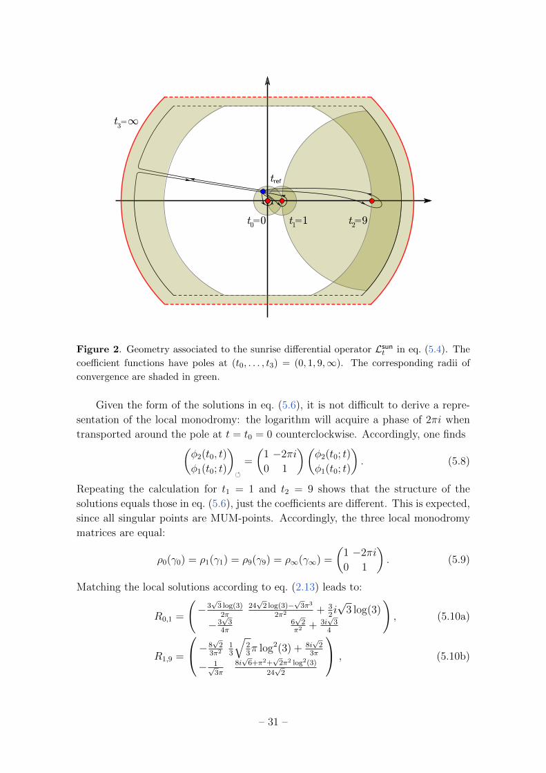
Figure 2. Geometry associated to the sunrise differential operator Lsunt in eq. (5.4). The

coefficient functions have poles at (t0, . . . , t3) = (0, 1, 9,∞). The corresponding radii of

convergence are shaded in green.

Given the form of the solutions in eq. (5.6), it is not difficult to derive a repre-

sentation of the local monodromy: the logarithm will acquire a phase of 2πi when

transported around the pole at t = t0 = 0 counterclockwise. Accordingly, one finds(φ2(t0, t)

φ1(t0; t)

)

=

(1 −2πi

0 1

)(φ2(t0; t)

φ1(t0; t)

). (5.8)

Repeating the calculation for t1 = 1 and t2 = 9 shows that the structure of the

solutions equals those in eq. (5.6), just the coefficients are different. This is expected,

since all singular points are MUM-points. Accordingly, the three local monodromy

matrices are equal:

ρ0(γ0) = ρ1(γ1) = ρ9(γ9) = ρ∞(γ∞) =

(1 −2πi

0 1

). (5.9)

Matching the local solutions according to eq. (2.13) leads to:

R0,1 =

(−3√

3 log(3)2π

24√

2 log(3)−√

3π3

2π2 + 32i√

3 log(3)

−3√

34π

6√

2π2 + 3i

√3

4

), (5.10a)

R1,9 =

−8√

23π2

13

√23π log2(3) + 8i

√2

3π

− 1√3π

8i√

6+π2+√

2π2 log2(3)

24√

2

, (5.10b)

– 31 –

R9,∞ =

(−3π2+3

√2π2 log2(3)

4√

2−4√

3π

−6√

3π

0

). (5.10c)

Using eq. (2.17) one can straightforwardly calculate the monodromy matrices in the

basis of solutions φ(0; t):

ρ0(γ0) =

(1 −2iπ

0 1

), ρ0(γ9) =

(1− 6i log(3)

π12i log2(3)

π

−3iπ

1 + 6i log(3)π

), (5.11)

ρ0(γ1) =

(7− 18i log(3)

π−4i(π−3i log(3))2

π

−9iπ

−5 + 18i log(3)π

), ρ0(γ∞) =

(7− 12i log(3)

π−6i(π−2i log(3))2

π

−6iπ

−5 + 12i log(3)π

).

This form of the monodromy matrices is not very enlightening. However, we can

choose a basis of solutions such that the entries of the monodromy matrices have in-

teger entries. Using a little algebra one can show that conjugation with the following

matrix will bring all three monodromy matrices into integral form:

a

(1 −2 log(3) + 2πi p

0 2iπ s

), p ∈ Z, s = ±1. (5.12)

While the scaling parameter a will drop out in the similarity transformation, choosing

different parameters p and s will lead to different choices of generators. Setting p = 0

and s = −1 for example leads to the following four matrices:

ρ0(γ0) =

(1 1

0 1

), ρ0(γ1) =

(1 0

−6 1

),

ρ0(γ9) =

(7 2

−18 −5

), ρ0(γ∞) =

(7 3

−12 −5

).

(5.13)

Combining the four matrices according to the succession of poles in figure 2, one

finds ρ0(γ∞)ρ0(γ9)ρ0(γ1)ρ0(γ0) = ( 1 00 1 ). Note that the change of basis in eq. (5.7)

corresponds to (a, s, p) = (−i/√

3, 1, 0). This shows that the monodromy matrices

in the basis (Ψ2(t),Ψ1(t)) have integer entries.

The matrices ρ0(γi), i ∈ {0, 1, 9}, generate the monodromy group of Lsun2 . We

can see that

ρ0(γi) =

(1 ∗0 1

)mod 6 . (5.14)

Since this relation holds for the generators, it must hold for all elements of the

monodromy group, and so we see that the monodromy group must be a subgroup of

Γ1(6) (cf. eq. (3.2)). We can show that the converse is also true. A short crosscheck

shows that the generators for Γ1(6) delivered5 by SAGE [93] indeed generate the

matrices in eq. (5.13). Checking furthermore independence of the three matrices and

noting that dim Γ1(6) = 3, the monodromy group of Lsun2 is indeed Γ1(6).

5The SAGE command to get a 2×2 matrix representation of a minimal set of generators of Γ1(6)

reads Gamma1(6).generators() and delivers ( 1 10 1 ), ( −5 1

−6 1 ) and ( 7 −312 −5 ).

– 32 –

The modular forms for the sunrise graph. Having identified the monodromy

group of the two-loop sunrise integral with the congruence subgroup Γ1(6), it follows

from the general discussion in section 2 that we expect the maximal cuts to define

modular forms of weight 1 for Γ1(6). This agrees with the findings of refs. [36, 51].

To make this explicit, we introduce a modular parametrisation and we define the

new variables τ and q by (cf. eq. (2.22)):

τ =Ψ2(t)

Ψ1(t)= log(t/9) +

4t

9+

14t2

81+O(t3) ,

q = e2πiτ =t

9+

4t2

81+O(t3) .

(5.15)

Note that we have chosen Ψ1(t) and Ψ2(t) such that =τ > 0 for t ∈ Xsun = P1C \

{0, 1, 9,∞}, and so τ ∈ H. The change of variable from t to q is holomorphic at

t = 0 and can be inverted to express t in terms of q. The result is the well-known

expression for Hauptmodul for Γ1(6) in terms of Dedekind’s eta function [36, 94]:

t(τ) = 9η(τ)4η(6τ)8

η(2τ)8η(3τ)4= 9 q +O(q2) , (5.16)

where η(τ) denotes Dedekind’s eta function:

η(τ) = eiπτ/12

∞∏n=1

(1− e2πinτ ) . (5.17)

It is easy to check (e.g., by comparing q-expansions with the basis of modular forms

given by Sage) that the function h1(τ) := Ψ1(t(τ)) defines a modular form of weight

1 for Γ1(6), as expected. In fact, it admits itself an expression in terms of Dedekind

eta functions [36, 51, 94]:

h1(τ) =2π√

3

η(2τ)6η(3τ)

η(τ)3η(6τ)2. (5.18)

Note that this is another way to see that the congruence subgroup naturally asso-

ciated to the two-loop equal-mass sunrise integrals is Γ1(6) rather than Γ1(12), in

agreement with the analysis in the literature [51, 61]. Moreover, we emphasise that

nothing in our analysis is specific to the sunrise integral, and the exact same reason-

ing can be applied to other second-order differential operators describing families of

elliptic curves, in particular those that appear in Feynman integrals computations.

5.2 The banana family

The third-order operator for the banana graph. We now repeat the com-

putations of the previous section in the case of the three-loop equal-mass banana

– 33 –

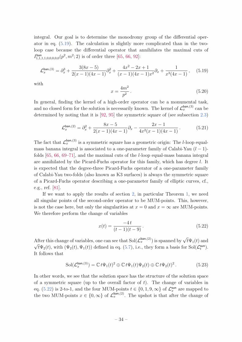
integral. Our goal is to determine the monodromy group of the differential oper-

ator in eq. (5.19). The calculation is slightly more complicated than in the two-

loop case because the differential operator that annihilates the maximal cuts of

Iban1,1,1,1,0,0,0,0,0(p2,m2; 2) is of order three [65, 66, 92]:

Lban,(3)x = ∂3

x +3(8x− 5)

2(x− 1)(4x− 1)∂2x +

4x2 − 2x+ 1

(x− 1)(4x− 1)x2∂x +

1

x3(4x− 1), (5.19)

with

x =4m2

p2. (5.20)

In general, finding the kernel of a high-order operator can be a monumental task,

and no closed form for the solution is necessarily known. The kernel of Lban,(3)x can be

determined by noting that it is [92, 95] the symmetric square of (see subsection 2.3)

Lban,(2)x = ∂2

x +8x− 5

2(x− 1)(4x− 1)∂x −

2x− 1

4x2(x− 1)(4x− 1). (5.21)

The fact that Lban,(3)x is a symmetric square has a geometric origin: The l-loop equal-

mass banana integral is associated to a one-parameter family of Calabi-Yau (l − 1)-

folds [65, 66, 69–71], and the maximal cuts of the l-loop equal-mass banana integral

are annihilated by the Picard-Fuchs operator for this family, which has degree l. It

is expected that the degree-three Picard-Fuchs operator of a one-parameter family

of Calabi-Yau two-folds (also known as K3 surfaces) is always the symmetric square

of a Picard-Fuchs operator describing a one-parameter family of elliptic curves, cf.,

e.g., ref. [81].

If we want to apply the results of section 2, in particular Theorem 1, we need

all singular points of the second-order operator to be MUM-points. This, however,

is not the case here, but only the singularities at x = 0 and x =∞ are MUM-points.

We therefore perform the change of variables

x(t) =−4 t

(t− 1)(t− 9). (5.22)

After this change of variables, one can see that Sol(Lban,(2)x ) is spanned by

√tΨ1(t) and√

tΨ2(t), with (Ψ2(t),Ψ1(t)) defined in eq. (5.7), i.e., they form a basis for Sol(Lsunt ).

It follows that

Sol(Lban,(3)x ) = C tΨ1(t)2 ⊕ C tΨ1(t)Ψ2(t)⊕ C tΨ2(t)2 . (5.23)

In other words, we see that the solution space has the structure of the solution space

of a symmetric square (up to the overall factor of t). The change of variables in

eq. (5.22) is 2-to-1, and the four MUM-points t ∈ {0, 1, 9,∞} of Lsunx are mapped to

the two MUM-points x ∈ {0,∞} of Lban,(2)x . The upshot is that after the change of

– 34 –

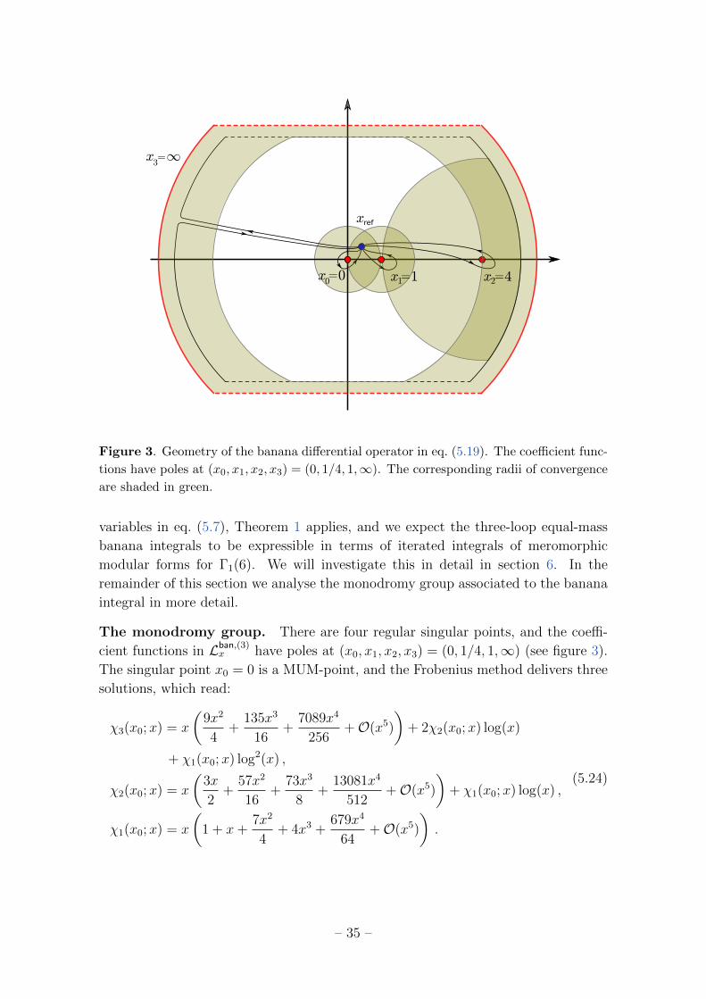
Figure 3. Geometry of the banana differential operator in eq. (5.19). The coefficient func-

tions have poles at (x0, x1, x2, x3) = (0, 1/4, 1,∞). The corresponding radii of convergence

are shaded in green.

variables in eq. (5.7), Theorem 1 applies, and we expect the three-loop equal-mass

banana integrals to be expressible in terms of iterated integrals of meromorphic

modular forms for Γ1(6). We will investigate this in detail in section 6. In the

remainder of this section we analyse the monodromy group associated to the banana

integral in more detail.

The monodromy group. There are four regular singular points, and the coeffi-

cient functions in Lban,(3)x have poles at (x0, x1, x2, x3) = (0, 1/4, 1,∞) (see figure 3).

The singular point x0 = 0 is a MUM-point, and the Frobenius method delivers three

solutions, which read:

χ3(x0;x) = x

(9x2

4+

135x3

16+

7089x4

256+O(x5)

)+ 2χ2(x0;x) log(x)

+ χ1(x0;x) log2(x) ,

χ2(x0;x) = x

(3x

2+

57x2

16+

73x3

8+

13081x4

512+O(x5)

)+ χ1(x0;x) log(x) ,

χ1(x0;x) = x

(1 + x+

7x2

4+ 4x3 +

679x4

64+O(x5)

).

(5.24)

– 35 –

This basis is related to the basis of ref. [92] (see also eq. (B.7)) via a constant rotationχ3(x0;x)

χ2(x0;x)

χ1(x0;x)

= B

I1(x)

J1(x)

H1(x)

, (5.25)

with

B =

43−8 log(2)

π+ 4i

3−1 + 4 log2(2)

π2 − 4i log(2)π

0 − 2π

2 log(2)π2 − i

π

0 0 1π2

. (5.26)

In eq. (B.7) we also show how the functions (H1(x), I1(x), J1(x)) are related to the

maximal cuts of the two-loop sunrise integral.

The hierarchy of logarithms in eq. (5.24) allows us to read off the monodromy

matrix:6

ρ0(γ0) =

1 −4iπ −4π2

0 1 −2iπ

0 0 1

. (5.27)

The structure of the local solutions around the poles at x1 = 1/4 and x2 = 1 is

different. For the singularity point x1 = 1/4, the Frobenius method delivers the

following functions:

χ3(x1;x) = 1 + 4 (x− 1/4) +64

45(x− 1/4)3 − 512

945(x− 1/4)4 +O

((x− 1/4)5) ,

χ2(x1;x) =√x− 1/4

(1 + 2 (x− 1/4)− 2 (x− 1/4)2 +

548

105(x− 1/4)3

−1306

105(x− 1/4)4 +O

((x− 1/4)5)) ,

χ1(x1;x) = (x− 1/4)

(1 +

4

3(x− 1/4)− 16

9(x− 1/4)2 +

1088

189(x− 1/4)3

−8704

567(x− 1/4)4 +O

((x− 1/4)5)) .

(5.28)

The structure of the solution space close to x2 = 1 is similar. We see that the

local exponents for x1 and x2 are 0, 1/2, 1. Hence, the singular points x1 and x2

are not MUM-points. However, the corresponding monodromy matrices can be read

off immediately also in this case: while the polynomials in χ3 and χ1 have trivial

monodromy, the square root in χ2(x1;x) acquires a minus sign when transported

6Different than for the sunrise above, this time we are not going to normalize the matrix right

away, for reasons to become clear below.

– 36 –

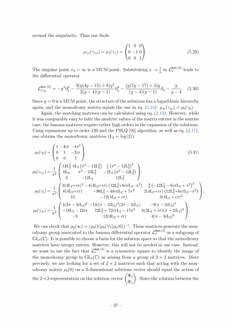
around the singularity. Thus one finds:

ρ1/4(γ1/4) = ρ1(γ1) =

1 0 0

0 −1 0

0 0 1

. (5.29)

The singular point x3 =∞ is a MUM-point. Substituting x→ 1y

in Lban,(3)x leads to

the differential operator

Lban,(3)1/y = −y3∂3

y −3(y(4y − 15) + 8)y2

2(y − 4)(y − 1)∂2y −

(y(7y − 17) + 4)y

(y − 4)(y − 1)∂y −

y

y − 4(5.30)

Since y = 0 is a MUM point, the structure of the solutions has a logarithmic hierarchy

again, and the monodromy matrix equals the one in eq. (5.24): ρ∞(γ∞) = ρ0(γ0).Again, the matching matrices can be calculated using eq. (2.13). However, while

it was comparably easy to infer the analytic values of the matrix entries in the sunrisecase, the banana matrices require rather high orders in the expansion of the solutions.Using expansions up to order 120 and the PSLQ [96] algorithm, as well as eq. (2.17),one obtains the monodromy matrices (L2 = log(2)):

ρ0(γ0) =

1 −4iπ −4π2

0 1 −2iπ

0 0 1

, (5.31)

ρ0(γ1/4) =1

π2

12L22 4L2

(π2 − 12L2

2

)13

(π2 − 12L2

2

)26L2 π2 − 24L2

2 −2L2

(π2 − 12L2

2

)3 −12L2 12L2

2

,ρ0(γ1) =

1

π2

3(4L2+iπ)2 −4(4L2+iπ)(12L2

2+6iπL2−π2)

43

(−12L2

2 − 6iπL2 + π2)2

6(4L2+iπ) −96L22 − 48iπL2 + 7π2 2(4L2+iπ)

(12L2

2+6iπL2−π2)

12 −12(4L2 + iπ) 3(4L2 + iπ)2

,ρ0(γ∞) =

1

π2

4(2π − 3iL2)2 −12i(π − 2iL2)2(2π − 3iL2) −9(π − 2iL2)4

−18L2 − 12iπ 72L22 + 72iπL2 − 17π2 6(3L2 + iπ)(π − 2iL2)2

−9 12(3L2 + iπ) 4(π − 3iL2)2

.

We can check that ρ0(∞) = (ρ0(1)ρ0(1/4)ρ0(0))−1. These matrices generate the mon-

odromy group associated to the banana differential operator Lban,(3)x as a subgroup of

GL3(C). It is possible to choose a basis for the solution space so that the monodromy

matrices have integer entries. However, this will not be needed in our case. Instead,

we want to use the fact that Lban,(3)x is a symmetric square to identify the image of

the monodromy group in GL3(C) as arising from a group of 2 × 2 matrices. More

precisely, we are looking for a set of 2 × 2 matrices such that acting with the mon-

odromy matrix ρ0(0) on a 3-dimensional solutions vector should equal the action of

the 2×2-representation on the solution vector

(Ψ2

Ψ1

). Since the relation between the

– 37 –

two- and three-dimensional solution spaces is most transparent from eq. (B.7), we

prefer to work here with the basis of the solution space of Lbanx from eq. (B.7). Due

to the change of basis we need to conjugate the monodromy matrices in eq. (5.31)

with the matrix B from eq. (5.25) resulting in

ρ0(γ0) =

1 6i −5

0 1 i

0 0 1

, ρ0(γ1/4) =

1 0 0

−2i 3 2i

4 4i −3

, (5.32)

ρ0(γ1)

−3 −10i 7

−12i 31 21i

16 40i −27

.

The comparison is made in components, here for example the equation for the third

component: B−1ρ0(0)B︸ ︷︷ ︸ρ0(γ0)

I1(x)

J1(x)

H1(x)

3

!= −1

2t(Ψ1(t)2

), (5.33)

where we use the following ansatz for the monodromy matrices:(Ψ2(t)

Ψ1(t)

)

=

(c11 c12

c21 c22

)(Ψ2(t)

Ψ1(t)

). (5.34)

Plugging in a couple of numerical values for t, which are selected such as to place

x in the corresponding region, allows to determine the values cij in the ansatz in

eq. (5.34) for each generator. Finally, one finds the following representations for the

generators of the monodromy group:

R0 := ρ2×20 (γ0) =

(1 −1

0 1

), R1/4 := ρ2×20 (γ1/4) = −i

√3

(1 2/3

−2 −1

),

R1 := ρ2×20 (γ1) = −i√

3

(1 1/3

−4 −1

).

(5.35)

These three matrices generate a subgroup Γban,(2) of GL2(C), which is closely related

to the monodromy group Γban,(3) ⊂ GL3(C) generated by the matrices ρ0(γ0), ρ0(γ1/4)

and ρ0(γ1) in eq. (5.32). More precisely, consider the map σ : GL2(C) → GL3(C)

defined by

σ ( a bc d ) =1

3

((a+c)(3a+c) 2i(6a2−9ab+8ac−6ad−6bc+2c2−3cd) −3(3a−3b+c−d)(a−b+c−d)

ic(a+c) −4ac+3ad+3bc−4c2+6cd −3i(c−d)(a−b+c−d)

−c2 −2ic(2c−3d) 3(c−d)2

).

(5.36)

One can show that σ is a group homomorphism with kernel Ker σ = Z2 such that

ρ0 = σ ◦ ρ2×20 . (5.37)

– 38 –

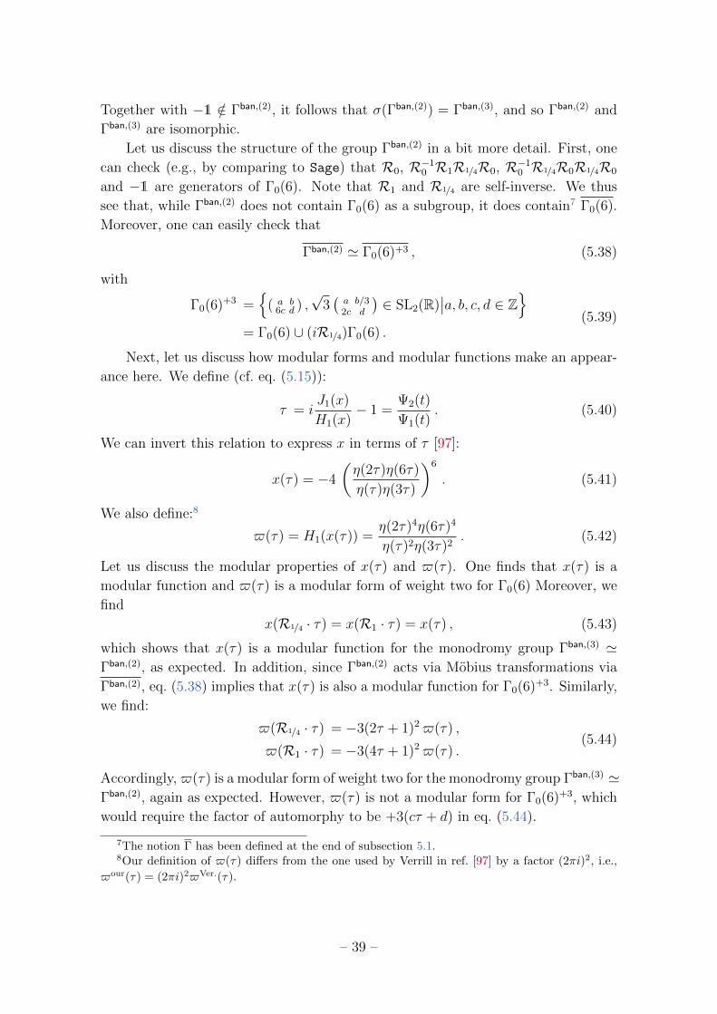
Together with −1 /∈ Γban,(2), it follows that σ(Γban,(2)) = Γban,(3), and so Γban,(2) and

Γban,(3) are isomorphic.

Let us discuss the structure of the group Γban,(2) in a bit more detail. First, one

can check (e.g., by comparing to Sage) that R0, R−10 R1R1/4R0, R−1

0 R1/4R0R1/4R0

and −1 are generators of Γ0(6). Note that R1 and R1/4 are self-inverse. We thus

see that, while Γban,(2) does not contain Γ0(6) as a subgroup, it does contain7 Γ0(6).

Moreover, one can easily check that

Γban,(2) ' Γ0(6)+3 , (5.38)

with

Γ0(6)+3 ={

( a b6c d ) ,

√3(a b/32c d

)∈ SL2(R)

∣∣a, b, c, d ∈ Z}

= Γ0(6) ∪ (iR1/4)Γ0(6) .(5.39)

Next, let us discuss how modular forms and modular functions make an appear-

ance here. We define (cf. eq. (5.15)):

τ = iJ1(x)

H1(x)− 1 =

Ψ2(t)

Ψ1(t). (5.40)

We can invert this relation to express x in terms of τ [97]:

x(τ) = −4

(η(2τ)η(6τ)

η(τ)η(3τ)

)6

. (5.41)

We also define:8

$(τ) = H1(x(τ)) =η(2τ)4η(6τ)4

η(τ)2η(3τ)2. (5.42)

Let us discuss the modular properties of x(τ) and $(τ). One finds that x(τ) is a

modular function and $(τ) is a modular form of weight two for Γ0(6) Moreover, we

find

x(R1/4 · τ) = x(R1 · τ) = x(τ) , (5.43)

which shows that x(τ) is a modular function for the monodromy group Γban,(3) 'Γban,(2), as expected. In addition, since Γban,(2) acts via Mobius transformations via

Γban,(2), eq. (5.38) implies that x(τ) is also a modular function for Γ0(6)+3. Similarly,

we find:

$(R1/4 · τ) = −3(2τ + 1)2$(τ) ,

$(R1 · τ) = −3(4τ + 1)2$(τ) .(5.44)

Accordingly, $(τ) is a modular form of weight two for the monodromy group Γban,(3) 'Γban,(2), again as expected. However, $(τ) is not a modular form for Γ0(6)+3, which

would require the factor of automorphy to be +3(cτ + d) in eq. (5.44).

7The notion Γ has been defined at the end of subsection 5.1.8Our definition of $(τ) differs from the one used by Verrill in ref. [97] by a factor (2πi)2, i.e.,

$our(τ) = (2πi)2$Ver.(τ).

– 39 –

6 Banana integrals and iterated integrals of meromorphic

modular forms

The analysis of the monodromy group of the sunrise and banana integrals implies via

Theorem 1 that both integrals can be expressed through all orders in ε in terms of

iterated integrals of meromorphic modular forms for the congruence subgroup Γ1(6),

which is a neat subgroup in the sense of Definition 2. In the remainder of this section

we make this statement concrete, and we derive a form of the differential equation

satisfied by the master integrals for the sunrise and banana families that involves the

basis of meromorphic modular forms defined in Theorem 2 only.

The strategy of section 2.1 of solving the first-order systems then implies that all

iterated integrals that appear in the solution, to all orders in the dimensional regula-

tor ε, only involves the basis of meromorphic modular forms implied by Theorem 2.

Note that once this form of the differential equation is known, it is straightforward

to solve it explicitly. In particular, the initial condition is known to all orders in ε in

terms of Γ functions for banana integrals of arbitrary loop order [71].

6.1 The iterated integrals for the sunrise integral

We start by discussing the case of the two-loop equal-mass sunrise integral. This

case is in principle well known, and we will show that we can recover the results

of ref. [63]. However, we discuss this case in some detail, as it allows us to set our

conventions and to point out differences with respect to the three-loop equal-mass

banana integral, which will be discussed in section 6.2.

There are two master integrals (S1(ε; t),S2(ε; t)) for the two-loop equal-mass

sunrise integral, which are accompanied by a tadpole integral (which is constant in

our normalisation: Isun2,2,0,0,0(p2,m2; 2− 2ε) = 1)[91]:

S1(ε; t) = −Isun1,1,1,0,0(p2,m2; 2− 2ε) ,

S2(ε; t) = −[

1

3(t2 − 6t+ 21)− 12ε(t− 1)

]Isun1,1,1,0,0(p2,m2; 2− 2ε)

− 2(t− 1)(t− 9) Isun2,1,1,0,0(p2,m2; 2− 2ε) ,

(6.1)

where the variable t is defined in eq. (5.16). Both master integrals are finite for ε = 0

and satisfy the differential equation:

∂t

(S1(ε; t)

S2(ε; t)

)=[Bsun(t)− 2εDsun(t)

](S1(ε; t)

S2(ε; t)

)+

(0

1

). (6.2)

Explicit expression for the matrices Bsun(t) and Dsun(t) are collected in appendix B.1.

In a next step, we want to introduce a modular parametrisation and apply the

results of section 4. In order to do this, the Hauptmodul needs to be normalised as

– 40 –

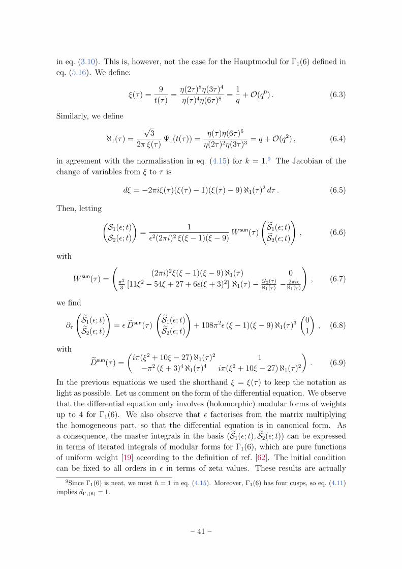
in eq. (3.10). This is, however, not the case for the Hauptmodul for Γ1(6) defined in

eq. (5.16). We define:

ξ(τ) =9

t(τ)=η(2τ)8η(3τ)4

η(τ)4η(6τ)8=

1

q+O(q0) . (6.3)

Similarly, we define

ℵ1(τ) =

√3

2π ξ(τ)Ψ1(t(τ)) =

η(τ)η(6τ)6

η(2τ)2η(3τ)3= q +O(q2) , (6.4)

in agreement with the normalisation in eq. (4.15) for k = 1.9 The Jacobian of the

change of variables from ξ to τ is

dξ = −2πiξ(τ)(ξ(τ)− 1)(ξ(τ)− 9)ℵ1(τ)2 dτ . (6.5)

Then, letting(S1(ε; t)

S2(ε; t)

)=

1

ε2(2πi)2 ξ(ξ − 1)(ξ − 9)W sun(τ)

(S1(ε; t)

S2(ε; t)

), (6.6)

with

W sun(τ) =

((2πi)2ξ(ξ − 1)(ξ − 9)ℵ1(τ) 0

π2

3[11ξ2 − 54ξ + 27 + 6ε(ξ + 3)2] ℵ1(τ)− G2(τ)

ℵ1(τ)− 2πiεℵ1(τ)

), (6.7)

we find

∂τ

(S1(ε; t)

S2(ε; t)

)= ε Dsun(τ)

(S1(ε; t)

S2(ε; t)

)+ 108π2ε (ξ − 1)(ξ − 9)ℵ1(τ)3

(0

1

), (6.8)

with

Dsun(τ) =

(iπ(ξ2 + 10ξ − 27)ℵ1(τ)2 1

−π2 (ξ + 3)4 ℵ1(τ)4 iπ(ξ2 + 10ξ − 27)ℵ1(τ)2

). (6.9)

In the previous equations we used the shorthand ξ = ξ(τ) to keep the notation as

light as possible. Let us comment on the form of the differential equation. We observe

that the differential equation only involves (holomorphic) modular forms of weights

up to 4 for Γ1(6). We also observe that ε factorises from the matrix multiplying

the homogeneous part, so that the differential equation is in canonical form. As

a consequence, the master integrals in the basis (S1(ε; t), S2(ε; t)) can be expressed

in terms of iterated integrals of modular forms for Γ1(6), which are pure functions

of uniform weight [19] according to the definition of ref. [62]. The initial condition

can be fixed to all orders in ε in terms of zeta values. These results are actually

9Since Γ1(6) is neat, we must h = 1 in eq. (4.15). Moreover, Γ1(6) has four cusps, so eq. (4.11)

implies dΓ1(6) = 1.

– 41 –

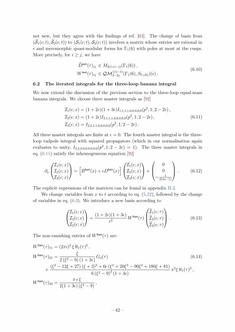
not new, but they agree with the findings of ref. [63]. The change of basis from

(S1(ε; t), S2(ε; t)) to (S1(ε; t),S2(ε; t)) involves a matrix whose entries are rational in

ε and meromorphic quasi-modular forms for Γ1(6) with poles at most at the cusps.

More precisely, for i ≥ j, we have

Dsun(τ)ij ∈M2(1+i−j)(Γ1(6)) ,

W sun(τ)ij ∈ QM≤(i−1)3−2j (Γ1(6), SΓ1(6))(ε) .

(6.10)

6.2 The iterated integrals for the three-loop banana integral

We now extend the discussion of the previous section to the three-loop equal-mass

banana integrals. We choose three master integrals as [92]

I1(ε;x) = (1 + 2ε)(1 + 3ε)I1,1,1,1,0,0,0,0,0(p2, 1; 2− 2ε) ,

I2(ε;x) = (1 + 2ε)I2,1,1,1,0,0,0,0,0(p2, 1; 2− 2ε) ,

I3(ε;x) = I2,2,1,1,0,0,0,0,0(p2, 1; 2− 2ε) .

(6.11)

All three master integrals are finite at ε = 0. The fourth master integral is the three-

loop tadpole integral with squared propagators (which in our normalisation again

evaluates to unity, I2,2,2,0,0,0,0,0,0(p2, 1; 2 − 2ε) = 1). The three master integrals in

eq. (6.11) satisfy the inhomogeneous equation [92]

∂x

I1(ε;x)

I2(ε;x)

I3(ε;x)

=[Bban(x) + εDban(x)

]I1(ε;x)

I2(ε;x)

I3(ε;x)

+

0

0

− 12(4x−1)

. (6.12)

The explicit expressions of the matrices can be found in appendix B.2.

We change variables from x to t according to eq. (5.22), followed by the change

of variables in eq. (6.3). We introduce a new basis according toI1(ε;x)

I2(ε;x)

I3(ε;x)

=(1 + 2ε)(1 + 3ε)

ε2W ban(τ)

I1(ε; τ)

I2(ε; τ)

I3(ε; τ)

. (6.13)

The non-vanishing entries of W ban(τ) are:

W ban(τ)11 = (2πi)2 ξ ℵ1(τ)2 ,

W ban(τ)21 =ξ

2 (ξ2 − 9) (1 + 3ε)G2(τ) (6.14)

+(ξ2 − 12ξ + 27) (ξ + 3)2 + 6ε (ξ4 + 20ξ3 − 90ξ2 + 180ξ + 81)

6 (ξ2 − 9)2 (1 + 3ε)π2ξ ℵ1(τ)2 ,

W ban(τ)22 =π ε ξ

2(1 + 3ε) (ξ2 − 9),

– 42 –

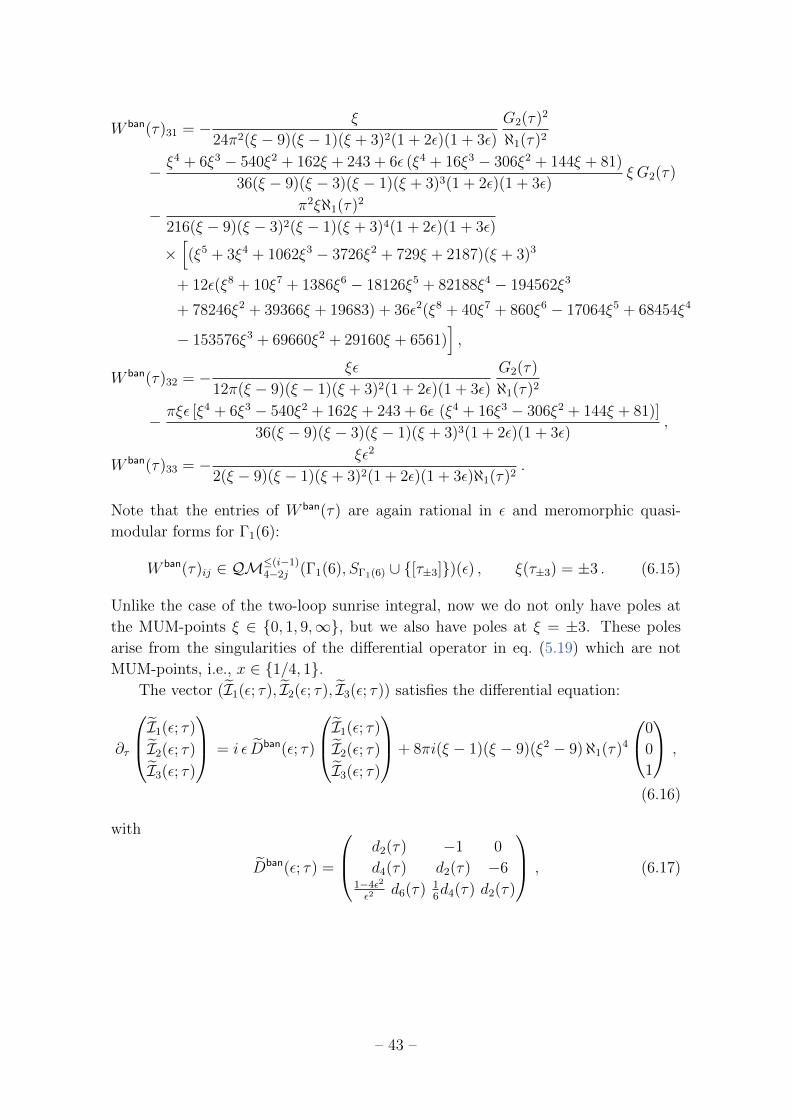
W ban(τ)31 = − ξ

24π2(ξ − 9)(ξ − 1)(ξ + 3)2(1 + 2ε)(1 + 3ε)

G2(τ)2

ℵ1(τ)2

− ξ4 + 6ξ3 − 540ξ2 + 162ξ + 243 + 6ε (ξ4 + 16ξ3 − 306ξ2 + 144ξ + 81)

36(ξ − 9)(ξ − 3)(ξ − 1)(ξ + 3)3(1 + 2ε)(1 + 3ε)ξ G2(τ)

− π2ξℵ1(τ)2

216(ξ − 9)(ξ − 3)2(ξ − 1)(ξ + 3)4(1 + 2ε)(1 + 3ε)

×[(ξ5 + 3ξ4 + 1062ξ3 − 3726ξ2 + 729ξ + 2187)(ξ + 3)3

+ 12ε(ξ8 + 10ξ7 + 1386ξ6 − 18126ξ5 + 82188ξ4 − 194562ξ3

+ 78246ξ2 + 39366ξ + 19683) + 36ε2(ξ8 + 40ξ7 + 860ξ6 − 17064ξ5 + 68454ξ4

− 153576ξ3 + 69660ξ2 + 29160ξ + 6561)],

W ban(τ)32 = − ξε

12π(ξ − 9)(ξ − 1)(ξ + 3)2(1 + 2ε)(1 + 3ε)

G2(τ)

ℵ1(τ)2

− πξε [ξ4 + 6ξ3 − 540ξ2 + 162ξ + 243 + 6ε (ξ4 + 16ξ3 − 306ξ2 + 144ξ + 81)]

36(ξ − 9)(ξ − 3)(ξ − 1)(ξ + 3)3(1 + 2ε)(1 + 3ε),

W ban(τ)33 = − ξε2

2(ξ − 9)(ξ − 1)(ξ + 3)2(1 + 2ε)(1 + 3ε)ℵ1(τ)2.

Note that the entries of W ban(τ) are again rational in ε and meromorphic quasi-

modular forms for Γ1(6):

W ban(τ)ij ∈ QM≤(i−1)4−2j (Γ1(6), SΓ1(6) ∪ {[τ±3]})(ε) , ξ(τ±3) = ±3 . (6.15)

Unlike the case of the two-loop sunrise integral, now we do not only have poles at

the MUM-points ξ ∈ {0, 1, 9,∞}, but we also have poles at ξ = ±3. These poles

arise from the singularities of the differential operator in eq. (5.19) which are not

MUM-points, i.e., x ∈ {1/4, 1}.The vector (I1(ε; τ), I2(ε; τ), I3(ε; τ)) satisfies the differential equation:

∂τ

I1(ε; τ)

I2(ε; τ)

I3(ε; τ)

= i ε Dban(ε; τ)

I1(ε; τ)

I2(ε; τ)

I3(ε; τ)

+ 8πi(ξ − 1)(ξ − 9)(ξ2 − 9)ℵ1(τ)4

0

0

1

,

(6.16)

with

Dban(ε; τ) =

d2(τ) −1 0

d4(τ) d2(τ) −61−4ε2

ε2d6(τ) 1

6d4(τ) d2(τ)

, (6.17)

– 43 –

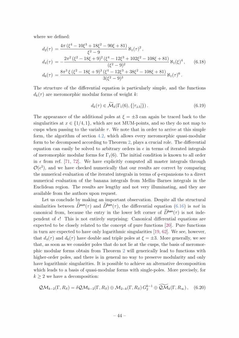
where we defined:

d2(τ) =4π (ξ4 − 10ξ3 + 18ξ2 − 90ξ + 81)

ξ2 − 9ℵ1(τ)2 ,

d4(τ) = −2π2 (ξ2 − 18ξ + 9)2 (ξ4 − 12ξ3 + 102ξ2 − 108ξ + 81)

(ξ2 − 9)2ℵ1(ξ)4 ,

d6(τ) =8π3 ξ (ξ2 − 18ξ + 9)3 (ξ4 − 12ξ3 + 38ξ2 − 108ξ + 81)

3(ξ2 − 9)3ℵ1(τ)6 .

(6.18)

The structure of the differential equation is particularly simple, and the functions

dk(τ) are meromorphic modular forms of weight k:

dk(τ) ∈ Mk(Γ1(6), {[τ±3]}) . (6.19)

The appearance of the additional poles at ξ = ±3 can again be traced back to the

singularities at x ∈ {1/4, 1}, which are not MUM-points, and so they do not map to

cusps when passing to the variable τ . We note that in order to arrive at this simple

form, the algorithm of section 4.2, which allows every meromorphic quasi-modular

form to be decomposed according to Theorem 2, plays a crucial role. The differential

equation can easily be solved to arbitrary orders in ε in terms of iterated integrals

of meromorphic modular forms for Γ1(6). The initial condition is known to all order

in ε from ref. [71, 72]. We have explicitly computed all master integrals through

O(ε2), and we have checked numerically that our results are correct by comparing

the numerical evaluation of the iterated integrals in terms of q-expansions to a direct

numerical evaluation of the banana integrals from Mellin–Barnes integrals in the

Euclidean region. The results are lengthy and not very illuminating, and they are

available from the authors upon request.

Let us conclude by making an important observation. Despite all the structural

similarities between Dsun(τ) and Dban(τ), the differential equation (6.16) is not in

canonical from, because the entry in the lower left corner of Dban(τ) is not inde-

pendent of ε! This is not entirely surprising: Canonical differential equations are

expected to be closely related to the concept of pure functions [20]. Pure functions

in turn are expected to have only logarithmic singularities [19, 62]. We see, however,

that d4(τ) and d6(τ) have double and triple poles at ξ = ±3. More generally, we see

that, as soon as we consider poles that do not lie at the cusps, the basis of meromor-

phic modular forms obtain from Theorem 2 will generically lead to functions with

higher-order poles, and there is in general no way to preserve modularity and only

have logarithmic singularities. It is possible to achieve an alternative decomposition

which leads to a basis of quasi-modular forms with single-poles. More precisely, for

k ≥ 2 we have a decomposition:

QMk−2(Γ, RS) = δQMk−2(Γ, RS)⊕M2−k(Γ, RS)Gk−12 ⊕ QMk(Γ, R∞) , (6.20)

– 44 –

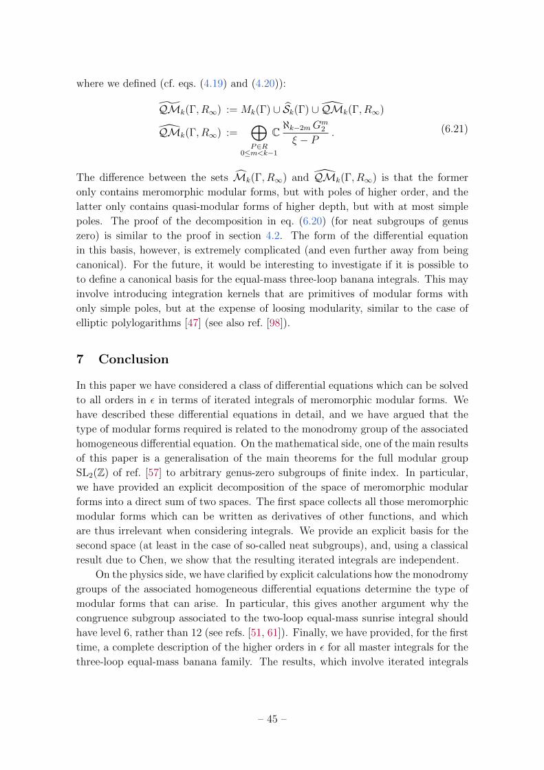
where we defined (cf. eqs. (4.19) and (4.20)):

QMk(Γ, R∞) := Mk(Γ) ∪ Sk(Γ) ∪ QMk(Γ, R∞)

QMk(Γ, R∞) :=⊕P∈R

0≤m<k−1

Cℵk−2mG

m2

ξ − P. (6.21)

The difference between the sets Mk(Γ, R∞) and QMk(Γ, R∞) is that the former

only contains meromorphic modular forms, but with poles of higher order, and the

latter only contains quasi-modular forms of higher depth, but with at most simple

poles. The proof of the decomposition in eq. (6.20) (for neat subgroups of genus

zero) is similar to the proof in section 4.2. The form of the differential equation

in this basis, however, is extremely complicated (and even further away from being

canonical). For the future, it would be interesting to investigate if it is possible to

to define a canonical basis for the equal-mass three-loop banana integrals. This may

involve introducing integration kernels that are primitives of modular forms with

only simple poles, but at the expense of loosing modularity, similar to the case of

elliptic polylogarithms [47] (see also ref. [98]).

7 Conclusion

In this paper we have considered a class of differential equations which can be solved

to all orders in ε in terms of iterated integrals of meromorphic modular forms. We

have described these differential equations in detail, and we have argued that the

type of modular forms required is related to the monodromy group of the associated

homogeneous differential equation. On the mathematical side, one of the main results

of this paper is a generalisation of the main theorems for the full modular group

SL2(Z) of ref. [57] to arbitrary genus-zero subgroups of finite index. In particular,

we have provided an explicit decomposition of the space of meromorphic modular

forms into a direct sum of two spaces. The first space collects all those meromorphic

modular forms which can be written as derivatives of other functions, and which

are thus irrelevant when considering integrals. We provide an explicit basis for the

second space (at least in the case of so-called neat subgroups), and, using a classical

result due to Chen, we show that the resulting iterated integrals are independent.

On the physics side, we have clarified by explicit calculations how the monodromy

groups of the associated homogeneous differential equations determine the type of

modular forms that can arise. In particular, this gives another argument why the

congruence subgroup associated to the two-loop equal-mass sunrise integral should

have level 6, rather than 12 (see refs. [51, 61]). Finally, we have provided, for the first

time, a complete description of the higher orders in ε for all master integrals for the

three-loop equal-mass banana family. The results, which involve iterated integrals

– 45 –

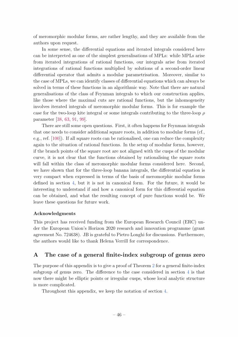
of meromorphic modular forms, are rather lengthy, and they are available from the

authors upon request.

In some sense, the differential equations and iterated integrals considered here

can be interpreted as one of the simplest generalisations of MPLs: while MPLs arise

from iterated integrations of rational functions, our integrals arise from iterated

integrations of rational functions multiplied by solutions of a second-order linear

differential operator that admits a modular parametrisation. Moreover, similar to

the case of MPLs, we can identify classes of differential equations which can always be

solved in terms of these functions in an algorithmic way. Note that there are natural

generalisations of the class of Feynman integrals to which our construction applies,

like those where the maximal cuts are rational functions, but the inhomogeneity

involves iterated integrals of meromorphic modular forms. This is for example the

case for the two-loop kite integral or some integrals contributing to the three-loop ρ

parameter [38, 63, 91, 99].

There are still some open questions. First, it often happens for Feynman integrals

that one needs to consider additional square roots, in addition to modular forms (cf.,

e.g., ref. [100]). If all square roots can be rationalised, one can reduce the complexity

again to the situation of rational functions. In the setup of modular forms, however,

if the branch points of the square root are not aligned with the cusps of the modular

curve, it is not clear that the functions obtained by rationalising the square roots

will fall within the class of meromorphic modular forms considered here. Second,

we have shown that for the three-loop banana integrals, the differential equation is

very compact when expressed in terms of the basis of meromorphic modular forms

defined in section 4, but it is not in canonical form. For the future, it would be

interesting to understand if and how a canonical form for this differential equation

can be obtained, and what the resulting concept of pure functions would be. We

leave these questions for future work.

Acknowledgments

This project has received funding from the European Research Council (ERC) un-

der the European Union’s Horizon 2020 research and innovation programme (grant

agreement No. 724638). JB is grateful to Pietro Longhi for discussions. Furthermore,

the authors would like to thank Helena Verrill for correspondence.

A The case of a general finite-index subgroup of genus zero

The purpose of this appendix is to give a proof of Theorem 2 for a general finite-index

subgroup of genus zero. The difference to the case considered in section 4 is that

now there might be elliptic points or irregular cusps, whose local analytic structure

is more complicated.

Throughout this appendix, we keep the notation of section 4.

– 46 –

A.1 The case k ≤ 1

Proposition 1. For k ≤ 1, we have

QMk(Γ, RS) = δ(QMk−2(Γ, RS))⊕Mk(Γ, RS).

In other words, the following statements are true.

(i) We have

δ(QMk−2(Γ, RS)) ∩Mk(Γ, RS) = {0},

as subspaces of QMk(Γ, RS).

(ii) We have

QMk(Γ, RS) = δ(QMk−2(Γ, RS)) +Mk(Γ, RS).

Proof. To prove (i), we need to show that, if f ∈ δ(QMk−2(Γ, RS)) ∩Mk(Γ, RS),

then f = 0. The proof is essentially the same as in ref. [57, Theorem 6.1], so we will

omit some details. Let g ∈ QMk−2(Γ, RS) be such that δ(g) = f , and denote by

g0, . . . , gp the coefficient functions of g. The coefficient functions of f are then given

by

fr = δ(gr) +k − 2− r + 1

12gr−1, 0 ≤ r ≤ p+ 1,

with the convention that g−1 = gp+1 ≡ 0. On the other hand, since f is modular, we

have fr = 0 for 1 ≤ r ≤ p + 1. In particular, for r = p + 1, we have k−2−p12

gp = 0,

hence gp = 0 (here, we use that k ≤ 1). By recursion on p, the same argument

yields that gr = 0 for all 0 ≤ r ≤ p, so that g = 0, by uniqueness of the coefficient

functions.

For the proof of (ii), we need to show that every f ∈ QMk(Γ, RS) can be

written as f = δ(g) + h, for some g ∈ QMk−2(Γ, RS) and some h ∈Mk(Γ, RS). Let

f0, . . . , fp denote the coefficient functions of f and assume without loss of generality

that fp 6= 0. We can write (cf. ref. [101, Theorem 4.1])

f =

p∑r=0

f r · Er2 ,

for uniquely determined f r ∈Mk−2r(Γ, RS), where E2 denotes the normalized, holo-

morphic Eisenstein series of weight two, and the integer p is, by definition, the depth

of f . Moreover, we have fp = fp. We now prove the desired statement by induction

on p, the case p = 0 being trivial (take g = 0 and h = f = f 0). In the general case,

a direct computation shows that the meromorphic quasi-modular form

fp · Ep2 −

12

k − p− 1δ(fp · E

p−12 )

has depth ≤ p− 1, and we conclude by the induction hypothesis.

– 47 –

A.2 The case k ≥ 2

Proposition 2. For k ≥ 2, we have

(δ(QMk−2(Γ, RS)) +Mk(Γ, RS))⊕M2−k(Γ, RS)Ek−12 = QMk(Γ, RS).

Proof. We begin by proving that

(δ(QMk−2(Γ, RS)) +Mk(Γ, RS)) ∩M2−k(Γ, RS)Ek−12 = {0}.

Let g ∈ QMk−2(Γ, RS) with coefficient functions g0, . . . , gp and assume that f +

δ(g) = h · Ek−12 , for some f ∈Mk(Γ, RS) and h ∈M2−k(Γ, RS). Then

δ(gr) +k − 2− r + 1

12gr−1 = 0, for all r ≥ k,

which shows that g necessarily has depth ≤ k − 2. Moreover, since g has weight

k − 2, one can show that δ(g) has depth ≤ k − 2. On the other hand, h · Ek−12 has

depth k− 1, unless h = 0, so that the equality f + δ(g) = h ·Ek−12 yields that h = 0.

Therefore, also g = 0, as was to be shown.

We next show that

δ(QMk−2(Γ, RS)) +Mk(Γ, RS) +M2−k(Γ, RS)Ek−12 = QMk(Γ, RS).

Let f ∈ QMk(Γ, RS) with coefficient functions f0, . . . , fp, such that fp 6= 0, and

write f =∑p

r=0 f r ·Er2 , for some f r ∈Mk−2r. As remarked above, we have fp = fp.

If p 6= 0, k − 1, then the same argument as in the proof of Proposition 1 shows that

fp · Ep2 − 12

k−p−1δ(fp · E

p−12 ) has depth ≤ p − 1. The desired statement now follows

by descending induction on r.

Proposition 3. For k ≥ 2, we have

δ(QMk−2(Γ, RS)) ∩Mk(Γ, RS) = δk−1(M2−k(Γ, RS)).

Proof. Again, the proof is essentially the same as in ref. [57, Theorem 6.1]. Let

g ∈ QMk−2(Γ, RS) be such that δ(g) = f , and denote by g0, . . . , gp the coefficient

functions of g. We may assume without loss of generality that gp 6= 0. As in the case

k < 2, we have

fr = δ(gr) +k − 2− r + 1

12gr−1, 0 ≤ r ≤ p+ 1,

and fr = 0, for 1 ≤ r ≤ p + 1. In particular, the equality fp+1 = 0 implies that

p = k − 2. Likewise, by recursion on r, the equality fr = 0 shows that δ(gr) =

−k−r−112

gr−1, for all 1 ≤ r ≤ p. The desired statement now follows from g = g0 and

gp ∈ M2−k(Γ, RS), which are both general facts about the coefficient functions of

quasi-modular forms (cf. ref. [101]).

– 48 –

In order to conclude the proof of Theorem 2 for arbitrary genus zero subgroups

in the case k ≥ 2, it now suffices to prove the following analogue of Theorem 4.

Theorem 5. There is a direct sum decomposition

Mk(Γ, RS) = δk−1(M2−k(Γ, RS))⊕ Mk(Γ, Rs0).

A.3 Divisors of meromorphic modular forms in negative weight

The key ingredient for the proof of Theorem 5 is a formula for the degree of the

divisor

bdiv fc :=∑P∈XΓ

bνP (f)c · [P ] ∈ Div(XΓ),

where 0 6= f ∈M2−k(Γ). Since the vanishing order of f at an elliptic point or irreg-

ular cusp might be half- or third-integral, the divisor bdiv fc is in general different

from div(f) =∑

P∈XΓνP (f) · (P ).

Proposition 4. We have

deg bdiv fc =

{0 k = 2

−1− dimSk(Γ) k ≥ 3.

Proof. The valence formula yields that

deg div(f) =(2− k)dΓ

12= −(2− k)−

(k

4− 1

2

)ε2 −

(k

3− 2

3

)ε3 −

(k

2− 1

)ε∞,

(A.1)

where in the second equality we have also used that XΓ has genus zero. This proves

the statement for k = 2, since in that case we necessarily have div(f) = bdiv fc. If

k ≥ 3, we first need a lemma which provides some arithmetic information about the

vanishing order of f at an elliptic point or an irregular cusp.

Lemma 3. Let k be an integer and 0 6= g ∈Mk(Γ). Then

νP (g) ≡

k4

mod Z if P is elliptic of order two,k3

mod Z if P is elliptic of order three,k2

mod Z if P is an irregular cusp.

Proof of Lemma 3. The statement is trivial for k = 0, since g is then a holomorphic

function on XΓ and therefore νP (g) ∈ Z. In general, if Γ = SL2(Z), then the desired

assertion follows immediately by comparing both sides of the valence formula (where

i and ρ denote the elliptic points defined in eq. (4.11) above)

ν[i](g) + ν[ρ](g) +∑

P∈XΓ\{[i],[ρ]}

νP (g) =k

12.

– 49 –

For general Γ, if k is even, then we can write g = g′g′′ where g′ ∈ M0(Γ) and

g′′ ∈Mk(SL2(Z)), and the desired statement follows from the above, as every elliptic

point is SL2(Z)-equivalent to either i or ρ, and every cusp is SL2(Z)-equivalent to∞.

If Γ is arbitrary and k is odd, then the existence of a non-zero meromorphic modular

form of weight k implies that −I /∈ Γ, hence that there are no elliptic points of order

two. On the other hand, if P is elliptic of order three, then νP (g) = 12νP (g2) ≡ k

3

mod Z, by what was just established in the case of even weights. This proves the

statement for elliptic points. Finally, if P is an irregular cusp of width h, then

g(τ + h) = (−1)kg(τ). On the other hand, the Fourier coefficients∑∞

m=n ameπimτ/h

of g at P satisfy am = (−1)mam, and the result follows.

We now return to the proof of Proposition 4. If k is even, then combining (A.1)

with Lemma 3 yields that

deg bdiv fc = −(2− k)−⌊k

4

⌋ε2 −

⌊k

3

⌋ε3 −

(k

2− 1

)ε∞ = −1− dimSk(Γ),

proving the desired statement in that case. If k is odd, then a similar argument

yields that

deg bdiv fc = −(2− k)−⌊k

3

⌋ε3 −

(k

2− 1

)εreg∞ −

(k

2− 1

2

)εirr∞ = −1− dimSk(Γ),

where εreg∞ (respectively, εirr

∞) denotes the number of regular (respectively, irregular)

cusps. This ends the proof of Proposition 4.

Remark 1. If Γ is an arbitrary finite-index subgroup of SL2(Z), not necessarily of

genus zero, and 0 6= f ∈M2−k(Γ), then essentially the same proof yields that

deg bdiv fc =

{0, k = 2,

g − 1− dimSk(Γ), k ≥ 3,

where g denotes the genus of XΓ. We expect that this formula is well-known to the

experts but did not find it in the literature.

A.4 Proof of Theorem 5

Theorem 5 follows by combining the assertions in the next two propositions.

Proposition 5. We have

δk−1(M2−k(Γ, RS)) ∩ Mk(Γ, Rs) = {0}.

Proof. Let f ∈ δk−1(M2−k(Γ, RS))∩Mk(Γ, Rs), so that in particular f = δk−1(g), for

some g ∈M2−k(Γ, RS). If P ∈ XΓ \SΓ were such that νP (g) < 0, then νP (f) < 1−khP

,

– 50 –

which contradicts f ∈ Mk(Γ, Rs). Therefore νP (g) ≥ 0 and a similar argument

shows that νs(g) ≥ 0, for all s ∈ SΓ \ {s0}.We now distinguish between the cases k = 2 and k ≥ 3. If k = 2, then f ∈

Mk(Γ, Rs) implies that νs0(f) ≥ 0 which in turn yields that νs0(g) ≥ 0. Therefore

the meromorphic function g has no poles on XΓ, hence must be constant, and we

conclude that f = δ(g) = 0. If k ≥ 3 and g 6= 0, then Proposition 4 now implies that

bνs0(g)c = −1− dimSk(Γ)−∑

P∈XΓ\{s0}

bνP (g)c ≤ −1− dimSk(Γ).

In particular, νs0(g) < 0, hence that νs0(f) = νs0(g) ≤ −1 − dimSk(Γ), which

contradicts f ∈ Mk(Γ, Rs). Therefore we must have g = 0, hence also f = 0, ending

the proof.

Proposition 6. We have

δk−1(M2−k(Γ, RS)) + Mk(Γ, Rs) =Mk(Γ, RS).

Proof. Let f ∈Mk(Γ, RS). If f ∈ Mk(Γ, Rs), there is nothing to prove. Otherwise,

one of the conditions (i)-(iii) in Theorem 5 must be violated. We shall prove that it

is always possible to add an element of δk−1(M2−k(Γ, RS)) to f such that the result

is contained in Mk(Γ, Rs), which clearly implies the desired result.

Assume first that there exists P ∈ XΓ\SΓ such that νP (f) < 1−khP

and choose 0 6=g ∈M2−k(Γ, RS). There exists ϕ ∈M0(Γ, RS) such that νP (ϕ) = νP (f)+ k−1

hP−νP (g)

(the right hand side is an integer by Lemma 3) and such that νQ(ϕ) > |νQ(g)|, for all

Q ∈ XΓ \ {P, s0}. Then νP (δk−1(ϕ · g)) = νP (f), hence there exists α ∈ C such that

νP (f −αδk−1(ϕ · g)) > νP (f) and νQ(f −αδk−1(ϕ · g)) ≥ νQ(f) for all Q ∈ XΓ \ {s0}.Repeating this step a finite number of times, we may thus ensure that, up to adding

an element of δk−1(M2−k(Γ, RS)), we have νP (f) ≥ 1−khP

, for all P ∈ XΓ \ SΓ. A

similar argument shows that we may also assume that νs(f) ≥ 0 for all s ∈ SΓ \{s0}.Now assume that bνs0(f)c < − dimSk(Γ) and choose 0 6= g ∈M2−k(Γ, RS). Up

to possibly multiplying g by a suitable modular function that only has a pole at s0,

we may assume that νP (g) ≥ 0, for all P ∈ XΓ \ {s0}. Moreover, by Proposition 4

and since XΓ has genus zero , there exists ϕ ∈ M0(Γ) such that νP (ϕ · g) ≥ 0, for

all P ∈ XΓ \ {s0}, and νs0(ϕ · g) = νs0(f). As before, one can now show that, up to

adding an element of δk−1(M2−k(Γ, RS)), we have bνs0(f)c ≥ − dimSk(Γ), proving

the proposition.

– 51 –

B The differential equations for the sunrise and banana in-

tegrals

B.1 The differential equations for the sunrise integrals

The matrices appearing in the differential equation in eq. (6.2) are

Bsun(t) =1

6t(t− 1)(t− 9)

3(3 + 14t− t2) −9

(t+ 3)(t3 − 15t2 + 75t+ 3) 3(3 + 14t− t2)

,

Dsun(t) =1

6t(t− 1)(t− 9)

(6(t− 1)t 0

(t+ 3)(t3 − 9t2 + 63t+ 9) 3(t− 9)(t+ 1)

).

(B.1)

A basis of maximal cuts for the two-loop equal-mass sunrise integral in d = 2

dimensions, i.e., a basis for the solution space of the differential operator in eq. (5.4)

is

Ψ1(t) =4

[(3−√t)(1 +

√t)3]1/2

K

(t14(t)t23(t)

t13(t)t24(t)

),

Ψ2(t) =4i

[(3−√t)(1 +

√t)3]1/2

K

(t12(t)t34(t)

t13(t)t24(t)

),

(B.2)

with tij(t) = ti(t)− tj(t) and

t1(t) = −4 , t2(t) = −(1 +√t)2 , t3(t) = −(1−

√t)2 , t4(t) = 0 , (B.3)

and K(λ) denotes the complete elliptic integral of the first kind:

K(λ) =

∫ 1

0

dt√t(1− t)(1− λt)

. (B.4)

B.2 The differential equations for the banana integrals

The matrices Bban(x) and Dban(x) entering the differential equation (6.12) are:

Bban(x) =

1x

4x

01

4(1−x)1x

+ 21−x

3x

+ 31−x

− 18(1−x)

+ 18(1−4x)

− 11−x + 3

2(1−4x)1x

+ 61−4x− 3

2(1−x)

, (B.5)

Dban(x) =

3x

12x

01

1−x2x

+ 61−x

6x

+ 61−x

− 12(1−x)

+ 12(1−4x)

− 31−x + 9

2(1−4x)1x

+ 121−4x− 3

1−x

. (B.6)

– 52 –

A basis of the solution space for the differential operator Lban,(3)x in eq. (5.19) can

then be chosen as (for 0 ≤ t ≤ 1)

I1(x(t)) =1

3t (Ψ1(t) + Ψ2(t)) (Ψ1(t) + 3Ψ2(t)) ,

J1(x(t)) =i

3tΨ1(t) (Ψ1(t) + Ψ2(t)) ,

H1(x(t)) = −1

3tΨ1(t)2 ,

(B.7)

where Ψ1(t) and Ψ1(t) are the maximal cuts of the sunrise integral, and x(t) is defined

in eq. (5.22).

References

[1] J. A. Lappo-Danilevsky, Theorie algorithmique des corps de Riemann, Rec. Math.

Moscou 34 (1927) 113–146.

[2] A. B. Goncharov, Multiple polylogarithms and mixed Tate motives, math/0103059.

[3] A. B. Goncharov, Multiple polylogarithms, cyclotomy and modular complexes,

Math.Res.Lett. 5 (1998) 497–516, [1105.2076].

[4] E. Remiddi and J. A. M. Vermaseren, Harmonic polylogarithms, Int. J. Mod. Phys.

A15 (2000) 725–754, [hep-ph/9905237].

[5] T. Gehrmann and E. Remiddi, Two loop master integrals for γ∗ → 3 jets: The

Planar topologies, Nucl.Phys. B601 (2001) 248–286, [hep-ph/0008287].

[6] J. Ablinger, J. Blumlein, and C. Schneider, Harmonic Sums and Polylogarithms

Generated by Cyclotomic Polynomials, J. Math. Phys. 52 (2011) 102301,

[1105.6063].

[7] C. Duhr, Mathematical aspects of scattering amplitudes, in Proceedings, Theoretical

Advanced Study Institute in Elementary Particle Physics: Journeys Through the

Precision Frontier: Amplitudes for Colliders (TASI 2014): Boulder, Colorado,

June 2-27, 2014, pp. 419–476, 2015. 1411.7538.

[8] T. Gehrmann and E. Remiddi, Numerical evaluation of harmonic polylogarithms,

Comput. Phys. Commun. 141 (2001) 296–312, [hep-ph/0107173].

[9] T. Gehrmann and E. Remiddi, Numerical evaluation of two-dimensional harmonic

polylogarithms, Comput. Phys. Commun. 144 (2002) 200–223, [hep-ph/0111255].

[10] S. Buehler and C. Duhr, CHAPLIN - Complex Harmonic Polylogarithms in

Fortran, Comput. Phys. Commun. 185 (2014) 2703–2713, [1106.5739].

[11] J. Vollinga and S. Weinzierl, Numerical evaluation of multiple polylogarithms,

Comput. Phys. Commun. 167 (2005) 177, [hep-ph/0410259].

– 53 –

[12] H. Frellesvig, D. Tommasini, and C. Wever, On the reduction of generalized

polylogarithms to Lin and Li2,2 and on the evaluation thereof, JHEP 03 (2016) 189,

[1601.02649].

[13] J. Ablinger, J. Blumlein, M. Round, and C. Schneider, Numerical Implementation

of Harmonic Polylogarithms to Weight w = 8, Comput. Phys. Commun. 240

(2019) 189–201, [1809.07084].

[14] L. Naterop, A. Signer, and Y. Ulrich, handyG —Rapid numerical evaluation of

generalised polylogarithms in Fortran, Comput. Phys. Commun. 253 (2020) 107165,

[1909.01656].

[15] A. V. Kotikov, Differential equations method: New technique for massive Feynman

diagrams calculation, Phys. Lett. B254 (1991) 158–164.

[16] A. V. Kotikov, Differential equations method: The Calculation of vertex type

Feynman diagrams, Phys. Lett. B259 (1991) 314–322.

[17] A. V. Kotikov, Differential equation method: The Calculation of N point Feynman

diagrams, Phys. Lett. B267 (1991) 123–127.

[18] T. Gehrmann and E. Remiddi, Differential equations for two loop four point

functions, Nucl.Phys. B580 (2000) 485–518, [hep-ph/9912329].

[19] N. Arkani-Hamed, J. L. Bourjaily, F. Cachazo, and J. Trnka, Local Integrals for

Planar Scattering Amplitudes, JHEP 1206 (2012) 125, [1012.6032].

[20] J. M. Henn, Multiloop integrals in dimensional regularization made simple, Phys.

Rev. Lett. 110 (2013) 251601, [1304.1806].

[21] A. Sabry, Fourth order spectral functions for the electron propagator, Nucl. Phys.

33 (1962), no. 17 401–430.

[22] D. J. Broadhurst, The Master Two Loop Diagram With Masses, Z. Phys. C47

(1990) 115–124.

[23] S. Bauberger, F. A. Berends, M. Bohm, and M. Buza, Analytical and numerical

methods for massive two loop selfenergy diagrams, Nucl. Phys. B434 (1995)

383–407, [hep-ph/9409388].

[24] S. Bauberger and M. Bohm, Simple one-dimensional integral representations for

two loop selfenergies: The Master diagram, Nucl. Phys. B445 (1995) 25–48,

[hep-ph/9501201].

[25] S. Laporta and E. Remiddi, Analytic treatment of the two loop equal mass sunrise

graph, Nucl. Phys. B704 (2005) 349–386, [hep-ph/0406160].

[26] B. A. Kniehl, A. V. Kotikov, A. Onishchenko, and O. Veretin, Two-loop sunset

diagrams with three massive lines, Nucl. Phys. B738 (2006) 306–316,

[hep-ph/0510235].

[27] U. Aglietti, R. Bonciani, L. Grassi, and E. Remiddi, The Two loop crossed ladder

– 54 –

vertex diagram with two massive exchanges, Nucl. Phys. B789 (2008) 45–83,

[0705.2616].

[28] M. Czakon and A. Mitov, Inclusive Heavy Flavor Hadroproduction in NLO QCD:

The Exact Analytic Result, Nucl. Phys. B824 (2010) 111–135, [0811.4119].

[29] F. Brown and O. Schnetz, A K3 in φ4, Duke Math. J. 161 (2012), no. 10

1817–1862, [1006.4064].

[30] S. Muller-Stach, S. Weinzierl, and R. Zayadeh, A Second-Order Differential

Equation for the Two-Loop Sunrise Graph with Arbitrary Masses,

Commun.Num.Theor.Phys. 6 (2012) 203–222, [1112.4360].

[31] S. Caron-Huot and K. J. Larsen, Uniqueness of two-loop master contours, JHEP

10 (2012) 026, [1205.0801].

[32] R. Huang and Y. Zhang, On Genera of Curves from High-loop Generalized

Unitarity Cuts, JHEP 04 (2013) 080, [1302.1023].

[33] F. Brown and O. Schnetz, Modular forms in Quantum Field Theory, Commun.

Num. Theor Phys. 07 (2013) 293–325, [1304.5342].

[34] D. Nandan, M. F. Paulos, M. Spradlin, and A. Volovich, Star Integrals,

Convolutions and Simplices, JHEP 05 (2013) 105, [1301.2500].

[35] J. Ablinger, J. Blumlein, A. De Freitas, M. van Hoeij, E. Imamoglu, C. G. Raab,

C. S. Radu, and C. Schneider, Iterated Elliptic and Hypergeometric Integrals for

Feynman Diagrams, J. Math. Phys. 59 (2018), no. 6 062305, [1706.01299].

[36] S. Bloch and P. Vanhove, The elliptic dilogarithm for the sunset graph, J. Number

Theor. 148 (2015) 328–364, [1309.5865].

[37] L. Adams, C. Bogner, and S. Weinzierl, The iterated structure of the all-order

result for the two-loop sunrise integral, J. Math. Phys. 57 (2016), no. 3 032304,

[1512.05630].

[38] L. Adams, C. Bogner, A. Schweitzer, and S. Weinzierl, The kite integral to all

orders in terms of elliptic polylogarithms, J. Math. Phys. 57 (2016), no. 12 122302,

[1607.01571].

[39] L. Adams, C. Bogner, and S. Weinzierl, The two-loop sunrise graph in two

space-time dimensions with arbitrary masses in terms of elliptic dilogarithms, J.

Math. Phys. 55 (2014), no. 10 102301, [1405.5640].

[40] L. Adams, C. Bogner, and S. Weinzierl, The two-loop sunrise graph with arbitrary

masses, J.Math.Phys. 54 (2013) 052303, [1302.7004].

[41] L. Adams, C. Bogner, and S. Weinzierl, The two-loop sunrise graph with arbitrary

masses, J. Math. Phys. 54 (2013) 052303, [1302.7004].

[42] L. Adams, C. Bogner, and S. Weinzierl, The two-loop sunrise integral around four

space-time dimensions and generalisations of the Clausen and Glaisher functions

towards the elliptic case, J. Math. Phys. 56 (2015), no. 7 072303, [1504.03255].

– 55 –

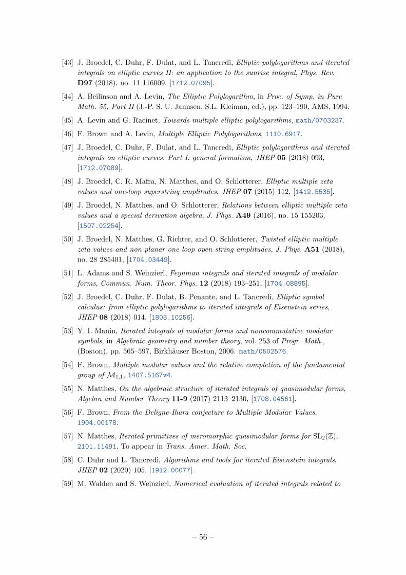
[43] J. Broedel, C. Duhr, F. Dulat, and L. Tancredi, Elliptic polylogarithms and iterated

integrals on elliptic curves II: an application to the sunrise integral, Phys. Rev.

D97 (2018), no. 11 116009, [1712.07095].

[44] A. Beilinson and A. Levin, The Elliptic Polylogarithm, in Proc. of Symp. in Pure

Math. 55, Part II (J.-P. S. U. Jannsen, S.L. Kleiman, ed.), pp. 123–190, AMS, 1994.

[45] A. Levin and G. Racinet, Towards multiple elliptic polylogarithms, math/0703237.

[46] F. Brown and A. Levin, Multiple Elliptic Polylogarithms, 1110.6917.

[47] J. Broedel, C. Duhr, F. Dulat, and L. Tancredi, Elliptic polylogarithms and iterated

integrals on elliptic curves. Part I: general formalism, JHEP 05 (2018) 093,

[1712.07089].

[48] J. Broedel, C. R. Mafra, N. Matthes, and O. Schlotterer, Elliptic multiple zeta

values and one-loop superstring amplitudes, JHEP 07 (2015) 112, [1412.5535].

[49] J. Broedel, N. Matthes, and O. Schlotterer, Relations between elliptic multiple zeta

values and a special derivation algebra, J. Phys. A49 (2016), no. 15 155203,

[1507.02254].

[50] J. Broedel, N. Matthes, G. Richter, and O. Schlotterer, Twisted elliptic multiple

zeta values and non-planar one-loop open-string amplitudes, J. Phys. A51 (2018),

no. 28 285401, [1704.03449].

[51] L. Adams and S. Weinzierl, Feynman integrals and iterated integrals of modular

forms, Commun. Num. Theor. Phys. 12 (2018) 193–251, [1704.08895].

[52] J. Broedel, C. Duhr, F. Dulat, B. Penante, and L. Tancredi, Elliptic symbol

calculus: from elliptic polylogarithms to iterated integrals of Eisenstein series,

JHEP 08 (2018) 014, [1803.10256].

[53] Y. I. Manin, Iterated integrals of modular forms and noncommutative modular

symbols, in Algebraic geometry and number theory, vol. 253 of Progr. Math.,

(Boston), pp. 565–597, Birkhauser Boston, 2006. math/0502576.

[54] F. Brown, Multiple modular values and the relative completion of the fundamental

group of M1,1, 1407.5167v4.

[55] N. Matthes, On the algebraic structure of iterated integrals of quasimodular forms,

Algebra and Number Theory 11-9 (2017) 2113–2130, [1708.04561].

[56] F. Brown, From the Deligne-Ihara conjecture to Multiple Modular Values,

1904.00178.

[57] N. Matthes, Iterated primitives of meromorphic quasimodular forms for SL2(Z),

2101.11491. To appear in Trans. Amer. Math. Soc.

[58] C. Duhr and L. Tancredi, Algorithms and tools for iterated Eisenstein integrals,

JHEP 02 (2020) 105, [1912.00077].

[59] M. Walden and S. Weinzierl, Numerical evaluation of iterated integrals related to

– 56 –

elliptic Feynman integrals, Comput. Phys. Commun. 265 (2021) 108020,

[2010.05271].

[60] S. Weinzierl, Modular transformations of elliptic Feynman integrals, Nucl. Phys. B

964 (2021) 115309, [2011.07311].

[61] H. Frellesvig, C. Vergu, M. Volk, and M. von Hippel, Cuts and Isogenies, JHEP 05

(2021) 064, [2102.02769].

[62] J. Broedel, C. Duhr, F. Dulat, B. Penante, and L. Tancredi, Elliptic Feynman

integrals and pure functions, JHEP 01 (2019) 023, [1809.10698].

[63] L. Adams and S. Weinzierl, The ε-form of the differential equations for Feynman

integrals in the elliptic case, Phys. Lett. B781 (2018) 270–278, [1802.05020].

[64] C. Bogner and F. Brown, Feynman integrals and iterated integrals on moduli spaces

of curves of genus zero, Commun. Num. Theor. Phys. 09 (2015) 189–238,

[1408.1862].

[65] S. Bloch, M. Kerr, and P. Vanhove, A Feynman integral via higher normal

functions, Compos. Math. 151 (2015) 2329–2375, [1406.2664].

[66] S. Bloch, M. Kerr, and P. Vanhove, Local mirror symmetry and the sunset

Feynman integral, Adv. Theor. Math. Phys. 21 (2016), no. 6 [1601.08181].

[67] J. L. Bourjaily, Y.-H. He, A. J. Mcleod, M. Von Hippel, and M. Wilhelm,

Traintracks through Calabi-Yau Manifolds: Scattering Amplitudes beyond Elliptic

Polylogarithms, Phys. Rev. Lett. 121 (2018), no. 7 071603, [1805.09326].

[68] J. L. Bourjaily, A. J. McLeod, M. von Hippel, and M. Wilhelm, A (Bounded)

Bestiary of Feynman Integral Calabi-Yau Geometries, Phys. Rev. Lett. 122 (2019),

no. 3 031601, [1810.07689].

[69] A. Klemm, C. Nega, and R. Safari, The l-loop Banana Amplitude from GKZ

Systems and relative Calabi-Yau Periods, JHEP 04 (2020) 088, [1912.06201].

[70] K. Bonisch, F. Fischbach, A. Klemm, C. Nega, and R. Safari, Analytic structure of

all loop banana integrals, JHEP 05 (2021) 066, [2008.10574].

[71] K. Bonisch, C. Duhr, F. Fischbach, A. Klemm, and C. Nega, Feynman Integrals in

Dimensional Regularization and Extensions of Calabi-Yau Motives, 2108.05310.

[72] J. Broedel, C. Duhr, F. Dulat, R. Marzucca, B. Penante, and L. Tancredi, An

analytic solution for the equal-mass banana graph, JHEP 09 (2019) 112,

[1907.03787].

[73] K. Chetyrkin and F. Tkachov, Integration by Parts: The Algorithm to Calculate

beta Functions in 4 Loops, Nucl.Phys. B192 (1981) 159–204.

[74] F. V. Tkachov, A Theorem on Analytical Calculability of Four Loop

Renormalization Group Functions, Phys. Lett. B100 (1981) 65–68.

[75] K. G. Chetyrkin, M. Faisst, C. Sturm, and M. Tentyukov, epsilon-finite basis of

– 57 –

master integrals for the integration-by-parts method, Nucl. Phys. B 742 (2006)

208–229, [hep-ph/0601165].

[76] R. N. Lee and A. I. Onishchenko, ε-regular basis for non-polylogarithmic multiloop

integrals and total cross section of the process e+e− → 2(QQ), JHEP 12 (2019)

084, [1909.07710].

[77] A. Primo and L. Tancredi, On the maximal cut of Feynman integrals and the

solution of their differential equations, Nucl. Phys. B916 (2017) 94–116,

[1610.08397].

[78] H. Frellesvig and C. G. Papadopoulos, Cuts of Feynman Integrals in Baikov

representation, JHEP 04 (2017) 083, [1701.07356].

[79] M. Harley, F. Moriello, and R. M. Schabinger, Baikov-Lee Representations Of Cut

Feynman Integrals, JHEP 06 (2017) 049, [1705.03478].

[80] J. Bosma, M. Sogaard, and Y. Zhang, Maximal Cuts in Arbitrary Dimension,

JHEP 08 (2017) 051, [1704.04255].

[81] C. F. Doran, Picard-Fuchs uniformization: Modularity of the mirror map and

mirror moonshine, in Proceedings of NATO-ASI and CRM Summer School on the

Arithmetic and Geometry of Algebraic Cycles, 12, 1998. math/9812162.

[82] F. Diamond, B. Sturmfels, J. Shurman, and S. S. Media, A First Course in

Modular Forms. Graduate Texts in Mathematics. Springer, 2005.

[83] Y. Yifan, Transformation formulas for generalized dedekind

eta functions, Bulletin of the London Mathematical Society 36 (2004), no. 5 671–682,

[https://londmathsoc.onlinelibrary.wiley.com/doi/pdf/10.1112/S0024609304003510].

[84] K. S. Chua, M. L. Lang, and Y. Yang, On Rademacher’s conjecture: congruence

subgroups of genus zero of the modular group, Journal of Algebra 277 (2003) 408 –

428.

[85] D. Zagier, Elliptic Modular Forms and Their Applications, in The 1-2-3 of Modular

Forms, Springer, 2008.

[86] E. Royer, Quasimodular forms: an introduction, Annales Mathematiques Blaise

Pascal 19 (2012), no. 2 297–306.

[87] P. Guerzhoy, Hecke operators for weakly holomorphic modular forms and

supersingular congruences, Proc. Amer. Math. Soc. 136 (2008), no. 9 3051–3059.

[88] M. Deneufchatel, G. H. E. Duchamp, V. H. N. Minh, and A. I. Solomon,

Independence of hyperlogarithms over function fields via algebraic combinatorics, in

Algebraic informatics, vol. 6742 of Lecture Notes in Comput. Sci., pp. 127–139.

Springer, Heidelberg, 2011.

[89] K. T. Chen, Iterated path integrals, Bull. Amer. Math. Soc. 83 (1977) 831.

[90] G. Bol, Invarianten linearer Differentialgleichungen, Abh. Math. Sem. Univ.

Hamburg 16 (1949), no. nos. 3-4 1–28.

– 58 –

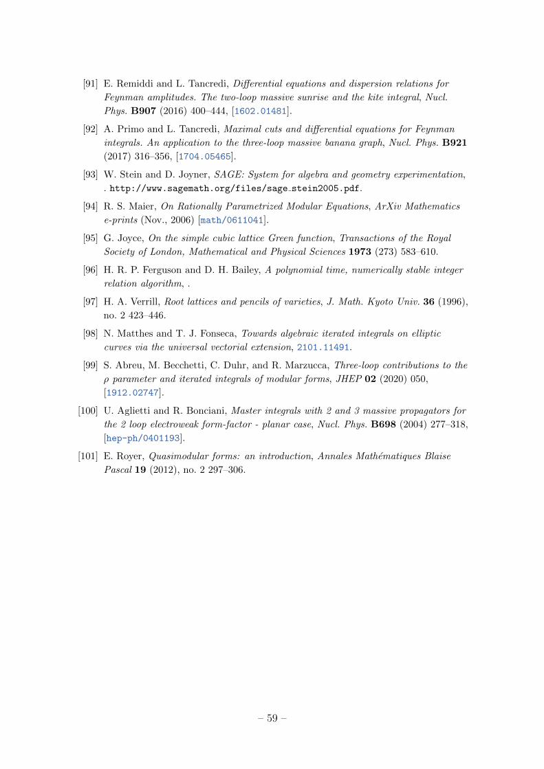
[91] E. Remiddi and L. Tancredi, Differential equations and dispersion relations for

Feynman amplitudes. The two-loop massive sunrise and the kite integral, Nucl.

Phys. B907 (2016) 400–444, [1602.01481].

[92] A. Primo and L. Tancredi, Maximal cuts and differential equations for Feynman

integrals. An application to the three-loop massive banana graph, Nucl. Phys. B921

(2017) 316–356, [1704.05465].

[93] W. Stein and D. Joyner, SAGE: System for algebra and geometry experimentation,

. http://www.sagemath.org/files/sage stein2005.pdf.

[94] R. S. Maier, On Rationally Parametrized Modular Equations, ArXiv Mathematics

e-prints (Nov., 2006) [math/0611041].

[95] G. Joyce, On the simple cubic lattice Green function, Transactions of the Royal

Society of London, Mathematical and Physical Sciences 1973 (273) 583–610.

[96] H. R. P. Ferguson and D. H. Bailey, A polynomial time, numerically stable integer

relation algorithm, .

[97] H. A. Verrill, Root lattices and pencils of varieties, J. Math. Kyoto Univ. 36 (1996),

no. 2 423–446.

[98] N. Matthes and T. J. Fonseca, Towards algebraic iterated integrals on elliptic

curves via the universal vectorial extension, 2101.11491.

[99] S. Abreu, M. Becchetti, C. Duhr, and R. Marzucca, Three-loop contributions to the

ρ parameter and iterated integrals of modular forms, JHEP 02 (2020) 050,

[1912.02747].

[100] U. Aglietti and R. Bonciani, Master integrals with 2 and 3 massive propagators for

the 2 loop electroweak form-factor - planar case, Nucl. Phys. B698 (2004) 277–318,

[hep-ph/0401193].

[101] E. Royer, Quasimodular forms: an introduction, Annales Mathematiques Blaise

Pascal 19 (2012), no. 2 297–306.

– 59 –