Mercury in the Nation's Streams—Levels, Trends, and ...

The Quality of Our Nation’s Waters

Mercury in the Nation’s Streams—Levels, Trends, and Implications

U.S. Department of the InteriorU.S. Geological Survey

Circular 1395

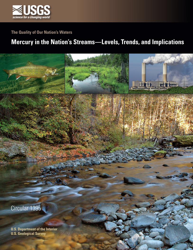
Cover: Front cover photographs, clockwise from top left: (1) Brook trout (© iStock); (2) Sixmile Brook and adjacent wetland, New York (Dennis A. Wentz); (3) Coal-burning power plant (© iStock); (4) Lookout Creek, Oregon (Dennis A. Wentz).

The Quality of Our Nation’s Waters

Mercury in the Nation’s Streams—Levels, Trends, and Implications

By Dennis A. Wentz, Mark E. Brigham, Lia C. Chasar, Michelle A. Lutz, and David P. Krabbenhoft

Circular 1395

U.S. Department of the InteriorU.S. Geological Survey

U.S. Department of the InteriorSALLY JEWELL, Secretary

U.S. Geological SurveySuzette M. Kimball, Acting Director

U.S. Geological Survey, Reston, Virginia: 2014

For more information on the USGS—the Federal source for science about the Earth, its natural and living resources, natural hazards, and the environment, visit http://www.usgs.gov or call 1–888–ASK–USGS.

For an overview of USGS information products, including maps, imagery, and publications, visit http://www.usgs.gov/pubprod

To order this and other USGS information products, visit http://store.usgs.gov

Any use of trade, product, or firm names is for descriptive purposes only and does not imply endorsement by the U.S. Government.

Although this information product, for the most part, is in the public domain, it also may contain copyrighted materials as noted in the text. Permission to reproduce copyrighted items must be secured from the copyright owner.

Suggested citation:Wentz, D.A., Brigham, M.E., Chasar, L.C., Lutz, M.A., and Krabbenhoft, D.P., 2014, Mercury in the Nation’s streams—Levels, trends, and implications: U.S. Geological Survey Circular 1395, 90 p., http://dx.doi.org/10.3133/cir1395.

Library of Congress Cataloging-in-Publication Data

Wentz, Dennis A.The quality of our nation’s waters : mercury in the nation’s streams—levels, trends, and implications / by Dennis A. Wentz, Mark E. Brigham, Lia C. Chasar, Michelle A. Lutz, and David P. Krabbenhoft.90 p. cm. — (Circular ; 1395)Includes bibliographic references and index. ISBN 978-1-4113-3786-2 (alk. paper)1. Mercury–Environmental aspects—United States. 2. Stream ecology—United States. 3. Water quality—United States. I. Wentz, Dennis A. II. Geological Survey (U.S.) III. Series: U.S. Geological Survey circular ; 1395. TD427.M4W45 2014 628.1'683–dc23

2014019008ISSN 1067-084X (print) ISSN 2330-5703 (online)

http://www.usgs.gov

http://www.usgs.gov/pubprod

http://store.usgs.gov

iii

Foreword

The United States has made major investments in assessing, managing, regulating, and conserving natural resources, such as water, minerals, soil, and timber. Sustaining the quality of the Nation’s water resources and the health of our ecosystems depends on the availability of sound water-resources data and information to develop effective, science-based policies. Effective management of water resources also brings more certainty and efficiency to important economic sectors. Taken together, these actions lead to immediate and long-term economic, social, and environmental benefits that make a difference to the lives of millions of people.

The U.S. Geological Survey (USGS) is committed to providing the Nation with reliable scientific information that helps to enhance and protect the overall quality of life and that facilitates effective management of water, biological, energy, and mineral resources (http://www.usgs.gov). Information on water resources is critical to ensuring long-term availability of water that is safe for drinking and recreation, and that is suitable for industry, irrigation, and fish and wildlife. Population growth and increasing demands for water make the availability of water, measured in terms of quantity and quality, essential to the long-term sustainability of our communities and ecosystems.

Mercury is a pervasive contaminant of streams and lakes, and has resulted in fish consumption advisories in all 50 States. The current report, “Mercury in the Nation’s Streams—Levels, Trends, and Implications,” presents a summary of results from USGS investigations conducted since the late 1990s on the sources, occurrence, trends, transport, and bioaccumulation of mercury in stream ecosystems. The report draws from studies conducted by several USGS Programs, including the National Water-Quality Assessment, Toxics Substances Hydrology, and National Research Programs. This report is one of a series of publications, The Quality of Our Nation’s Waters, which describe major findings of the USGS on water-quality issues of regional and national concern. Other reports in this series focus on the occurrence and distribution of nutrients, pesticides, and volatile organic compounds in streams and groundwater; the effects of contaminants and streamflow alteration on the condition of aquatic communities in streams; and the quality of untreated water from private domestic and public supply wells. Each report builds toward a more comprehensive understanding of the quality of regional and national water resources (http://water.usgs.gov/nawqa/nawqa_sumr.html).

The information in this series is intended primarily for those interested or involved in resource management and protection, conservation, regulation, and policymaking at regional and national levels. In addition, the information should be of interest to those at a local level who wish to know more about the general quality of streams and groundwater in areas near where they live and how that quality compares with other areas across the Nation. We hope this publication will provide you with insights and information to meet your needs, and will foster increased citizen awareness and involvement in the protection and restoration of our Nation’s waters.

William H. Werkheiser Associate Director for Water

U.S. Geological Survey

http://www.usgs.gov

http://water.usgs.gov/nawqa/nawqa_sumr.html

iv

Abbreviations, Acronyms, and Conventions Used in This Report

AMNet Atmospheric Mercury NetworkCMAQ-Hg Community Multiscale Air Quality modeling system

(mercury)Hg Chemical symbol for mercuryMDN Mercury Deposition NetworkMETAALICUS Mercury Experiment to Assess Atmospheric

Loadings in Canada and the United StatesMPCA Minnesota Pollution Control AgencyNADP National Atmospheric Deposition NetworkNCBP National Contaminant Biomonitoring Programppb Parts per billionppm Parts per millionTMDL Total Maximum Daily LoadUSEPA United States Environmental Protection AgencyUSGS United States Geological Survey

Mercury in fish muscle tissue is measured as total mercury; however, it has been shown that greater than 95 percent of such mercury is in the methylmercury form (Bloom, 1992). Thus, all fish tissue mercury discussed in this report is assumed to be methylmercury.

Mercury concentrations in fish and bird tissue are reported on a wet weight basis, unless otherwise noted. Mercury concentrations in soil and sediment are reported on a dry weight basis.

Water samples for mercury analysis were typically collected by the USGS during low streamflow, when differences between whole water (unfiltered) and dissolved (0.7-micrometer filtered) mercury concentrations are small and unimportant. We do not distinguish between these forms in this report.

The first use of each term listed in the Glossary is given in bold underline font.

v

Contents

Chapter 1. Major Findings and Implications ..............................................................................................1

Chapter 2. Why Is Mercury in Fish a Concern? ......................................................................................11

Chapter 3. How Does Mercury Cycle Through Aquatic Ecosystems? ................................................21

Chapter 4. Where Are Environmental Mercury Concentrations Highest Across the Nation? .......43

Chapter 5. How Do Environmental Mercury Levels Vary over Time? ..................................................53

References Cited .......................................................................................................................................73

Glossary.........................................................................................................................................................85

Appendix 1. Supporting Information for Selected Figures ..................................................................89

Phot

ogra

ph b

y De

nnis

A. W

entz

.

Lookout Creek, Oregon

Major Findings and Implications

Introduction

Mercury is a potent neurotoxin that accumulates in fish to levels of concern for human health and the health of fish-eating wildlife. Mercury contamination of fish is the primary reason for issuing fish consumption advisories, which exist in every State in the Nation. Much of the mercury originates from combustion of coal and can travel long distances in the atmosphere before being deposited. This can result in mercury-contaminated fish in areas with no obvious source of mercury pollution.

A posted advisory communicates the risk of eating fish that contain high concentrations of mercury. (Photograph by Dennis A. Wentz.)

Three key factors determine the level of mercury contamination in fish—the amount of inorganic mercury available to an ecosystem, the conversion of inorganic mercury to methylmercury, and the bioaccumulation of methylmercury through the food web. Inorganic mercury originates from both natural sources (such as volcanoes, geologic deposits of mercury, geothermal springs, and volatilization from the ocean) and anthropogenic sources (such as coal combustion, mining, and use of mercury in products and industrial processes; fig. 1-1). Humans have doubled the amount of inorganic mercury in the global atmosphere since pre-industrial times, with substantially greater increases occurring at locations closer to major urban areas.

Chapter 1

Major Findings and Implications 1

Chapter

1

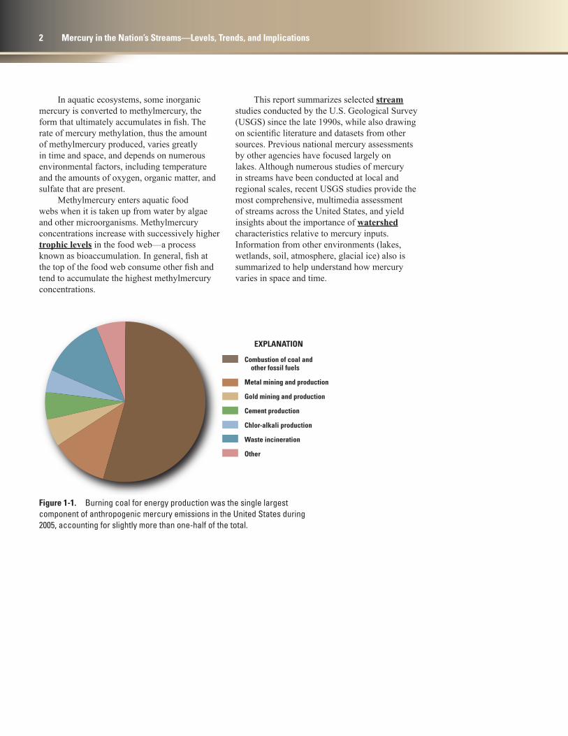
In aquatic ecosystems, some inorganic mercury is converted to methylmercury, the form that ultimately accumulates in fish. The rate of mercury methylation, thus the amount of methylmercury produced, varies greatly in time and space, and depends on numerous environmental factors, including temperature and the amounts of oxygen, organic matter, and sulfate that are present.

Methylmercury enters aquatic food webs when it is taken up from water by algae and other microorganisms. Methylmercury concentrations increase with successively higher trophic levels in the food web—a process known as bioaccumulation. In general, fish at the top of the food web consume other fish and tend to accumulate the highest methylmercury concentrations.

This report summarizes selected stream studies conducted by the U.S. Geological Survey (USGS) since the late 1990s, while also drawing on scientific literature and datasets from other sources. Previous national mercury assessments by other agencies have focused largely on lakes. Although numerous studies of mercury in streams have been conducted at local and regional scales, recent USGS studies provide the most comprehensive, multimedia assessment of streams across the United States, and yield insights about the importance of watershed characteristics relative to mercury inputs. Information from other environments (lakes, wetlands, soil, atmosphere, glacial ice) also is summarized to help understand how mercury varies in space and time.

Figure 1-1. Burning coal for energy production was the single largest component of anthropogenic mercury emissions in the United States during 2005, accounting for slightly more than one-half of the total.

2 Mercury in the Nation’s Streams—Levels, Trends, and Implications

tac11-0651_fig01-01

Combustion of coal and other fossil fuels

Metal mining and production

Gold mining and production

Cement production

Chlor-alkali production

Waste incineration

Other

EXPLANATION

Highlights of Major Findings and Implications

• Methylmercury concentrations in fish exceeded the U.S. Environmental Protection Agency criterion for the protection of human health at about one in four streams across the United States. High methylmercury concentrations in fish are the primary cause of fish consumption advisories, which exist in every State in the Nation. The predominant source of mercury in fish is deposition of atmospheric inorganic mercury produced by coal combustion. In response to the widespread contamination of fish, mercury has been effectively removed from many products and waste streams, resulting in about a 60-percent decrease in emissions in the United States since 1990. However, to reduce mercury levels in fish to fully meet human health criteria, further reductions in mercury emissions are necessary.

• Wetlands increase the amount of inorganic mercury that is converted to methylmercury, the form that accumulates to harmful levels in fish. Wetland characteristics, such as limited dissolved oxygen concentrations and abundant organic matter, provide favorable environments for microorganisms to effect the conversion of inorganic mercury to methylmercury. Thus, wetland construction or restoration (for example, to improve habitat or to filter nutrients and sediment) should balance the potential for increased methylmercury production against the anticipated ecological and water-quality benefits of the wetlands.

• In contrast to other environmental contaminants, mercury emission reduction strategies need to consider global mercury sources in addition to domestic sources. Reductions in domestic mercury emissions are likely to result in lower mercury levels in fish in the Eastern United States, where domestic emissions contribute a large portion of atmospherically deposited mercury. In contrast, emission controls will provide smaller benefits in the Western United States, where reduced domestic emissions may be offset by increased emissions from Asia. Implementation of the recently adopted U.S. Mercury and Air Toxics Standards and worldwide Minamata Convention goals should lead to reductions in both U.S. and global mercury emissions.

• Existing mercury monitoring programs focus mostly on methylmercury concentrations in fish, and lack design elements and data to link these levels to mercury sources. Most programs do not track methylmercury concentrations in fish over time in ways that support rigorous, nationally consistent trend assessments. Given the complexities of mercury emissions, transport pathways, and ecological factors that influence the extent of methylmercury contamination in fish, a multimedia monitoring approach is critical to track the effectiveness of management actions intended to reduce mercury emissions and resulting environmental mercury levels.

Chapter 1


(Photograph by Dennis A. Wentz.)

tac11-0651_fig01-02

EXPLANATION

MinedNon-mined

≤ 0.10

> 0.10 – ≤ 0.20

> 0.20 – ≤ 0.30

> 0.30

Methylmercury, game fish fillet, in parts per million

Major Findings

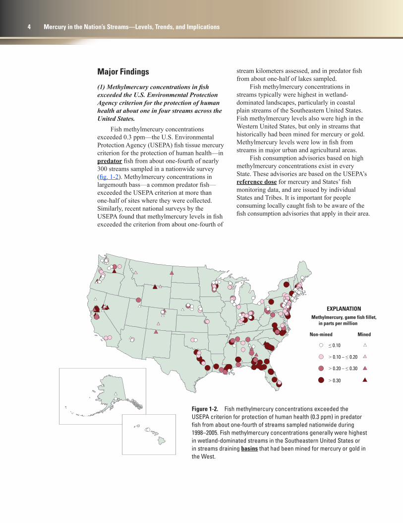
(1) Methylmercury concentrations in fish exceeded the U.S. Environmental Protection Agency criterion for the protection of human health at about one in four streams across the United States.

Fish methylmercury concentrations exceeded 0.3 ppm—the U.S. Environmental Protection Agency (USEPA) fish tissue mercury criterion for the protection of human health—in predator fish from about one-fourth of nearly 300 streams sampled in a nationwide survey (fig. 1-2). Methylmercury concentrations in largemouth bass—a common predator fish—exceeded the USEPA criterion at more than one-half of sites where they were collected. Similarly, recent national surveys by the USEPA found that methylmercury levels in fish exceeded the criterion from about one-fourth of

stream kilometers assessed, and in predator fish from about one-half of lakes sampled.

Fish methylmercury concentrations in streams typically were highest in wetland-dominated landscapes, particularly in coastal plain streams of the Southeastern United States. Fish methylmercury levels also were high in the Western United States, but only in streams that historically had been mined for mercury or gold. Methylmercury levels were low in fish from streams in major urban and agricultural areas.

Fish consumption advisories based on high methylmercury concentrations exist in every State. These advisories are based on the USEPA’s reference dose for mercury and States’ fish monitoring data, and are issued by individual States and Tribes. It is important for people consuming locally caught fish to be aware of the fish consumption advisories that apply in their area.

Figure 1-2. Fish methylmercury concentrations exceeded the USEPA criterion for protection of human health (0.3 ppm) in predator fish from about one-fourth of streams sampled nationwide during 1998–2005. Fish methylmercury concentrations generally were highest in wetland-dominated streams in the Southeastern United States or in streams draining basins that had been mined for mercury or gold in the West.


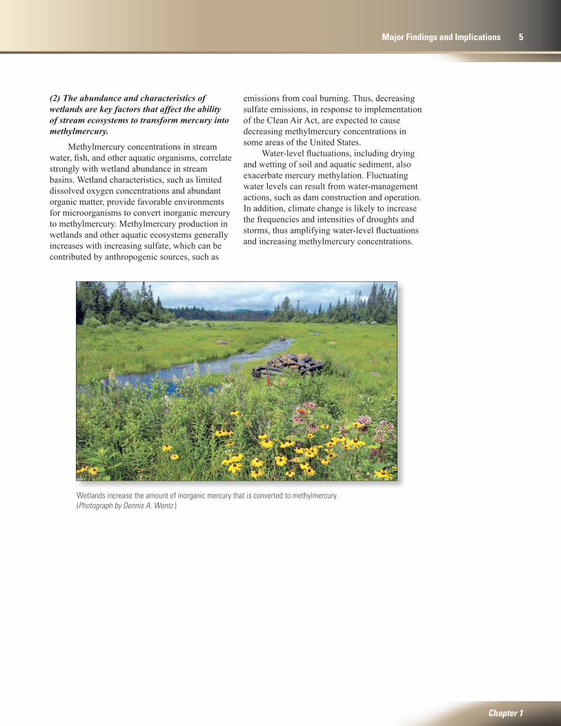
Wetlands increase the amount of inorganic mercury that is converted to methylmercury. (Photograph by Dennis A. Wentz.)

(2) The abundance and characteristics of wetlands are key factors that affect the ability of stream ecosystems to transform mercury into methylmercury.

Methylmercury concentrations in stream water, fish, and other aquatic organisms, correlate strongly with wetland abundance in stream basins. Wetland characteristics, such as limited dissolved oxygen concentrations and abundant organic matter, provide favorable environments for microorganisms to convert inorganic mercury to methylmercury. Methylmercury production in wetlands and other aquatic ecosystems generally increases with increasing sulfate, which can be contributed by anthropogenic sources, such as

emissions from coal burning. Thus, decreasing sulfate emissions, in response to implementation of the Clean Air Act, are expected to cause decreasing methylmercury concentrations in some areas of the United States.

Water-level fluctuations, including drying and wetting of soil and aquatic sediment, also exacerbate mercury methylation. Fluctuating water levels can result from water-management actions, such as dam construction and operation. In addition, climate change is likely to increase the frequencies and intensities of droughts and storms, thus amplifying water-level fluctuations and increasing methylmercury concentrations.

Chapter 1


(3) Methylmercury concentrations in fish depend more on the amount of methylmercury in an ecosystem than on the amount of inorganic mercury released to the ecosystem.

Methylmercury concentrations in fish correlate strongly with methylmercury concentrations in stream water, indicating that the amount of methylmercury available to the base of the food web is an important control on fish methylmercury concentrations. Fish near the top of a food web have higher methylmercury concentrations than fish at lower trophic levels, because with each increase in trophic level, the methylmercury in the prey organism is accumulated into the tissue of the consumer (fig. 1-3).

Across the United States, methylmercury concentrations in fish and stream water generally were highest in undeveloped areas with abundant wetlands, which provide ideal conditions for methylmercury production. In contrast, methylmercury levels in largemouth bass from urban streams were the lowest of all land uses and land covers studied (fig. 1-4). This occurred even though inorganic mercury inputs were higher in urban settings than in agricultural, undeveloped, or mixed land use/land cover settings. Methylmercury

concentrations were lower than expected in urban streams because factors conducive to methylmercury production, such as the amount of wetlands and dissolved organic carbon, also generally are low in these ecosystems. These findings contrast starkly with those for many other contaminants in rivers and streams, which tend to be high in urban and agricultural areas.

Although methylmercury concentrations in fish from some mined basins were as high as anywhere in the Nation, with values up to 50 times the USEPA criterion for the protection of human health, most fish tissue mercury levels in mined basins were no higher than in rural undeveloped basins. Some streams draining mined basins in the West have concentrations of inorganic mercury in water and sediment that are hundreds-of-thousands of times greater than streams in unmined areas. However, a relatively small portion of the inorganic mercury typically is converted to methylmercury because wetlands and dissolved organic carbon generally are low in these ecosystems. The large amounts of mercury in mined ecosystems still contaminate fish decades after mining activity has ceased and, without costly remediation, will likely continue to contaminate fish into the future.


tac11-0651_fig01-03

Biomagnification

Bioc

once

ntra

tion

Met

hylm

ercu

ry c

once

ntra

tion,

in p

arts

per

mill

ion USEPA fish tissue mercury criterion = 0.3 parts per million

Water

Algae and othermicroorganisms

Invertebrates

Toppredator fish

Forage fish

0.00000001

0.0000001

0.000001

0.00001

0.0001

0.001

0.01

0.1

1

10

Increasing trophic level

Figure 1-3. Methylmercury concentrations in aquatic organisms increase with increasing methylmercury concentrations in water and with increasing trophic level. Fish at the top of the food web tend to have the highest concentrations of methylmercury.

tac11-0651_fig01-04

0

0.5

1.0

1.5

2.0

2.5

Undeveloped Mixed Mined Agricultural Urban

Med

ian

met

hylm

ercu

ry c

once

ntra

tion

in

larg

emou

th b

ass,

in p

arts

per

mill

ion

per m

eter

Figure 1-4. Mercury concentrations in largemouth bass were lowest in streams draining urban areas.

Chapter 1


(4) Mercury concentrations in lake sediment, fish tissue, and precipitation have decreased in some areas during recent decades, coincident with legislation regulating discharges of contaminants to air and water.

Downward trends of mercury in lake sediment, fish, and precipitation coincide with implementation of the Clean Air Act (1970), the Clean Water Act (1972), and other legislation designed to limit pollutants to the environment. These measures address reductions in mercury use, controls on mercury emissions from waste incinerators, and incidental capture of mercury by controlling sulfur and particulate emissions from coal-fired power plants.

Lake Sediment.—From 1970 to 2000, downward trends of mercury in lake sediment cores, which record the history of mercury delivery to a lake, outnumbered upward trends by about a 2:1 ratio. Downward trends were most common in lakes in dense urban areas, and are consistent with controls on industrial discharges of mercury and a shift in coal combustion from residential and commercial heating to electrical power

generation. The relative lack of decreasing mercury concentrations in reference lakes (less than 1.5 percent urban land) reflects stable or increasing global atmospheric mercury sources.

Fish Tissue.—During 1969–87, downward trends in fish methylmercury concentrations were measured at 20 of 22 sites outside the Southeastern United States. The numbers of upward and downward trends were about equal in the Southeast. Decreasing concentrations occurred primarily during the 1970s, followed by relatively stable concentrations during the 1980s. The rate of decrease ranged from 3 to 12 percent annually.

Precipitation.—Total mercury concentrations in precipitation at Mercury Deposition Network sites decreased in almost one-half of 49 sites monitored during 1996–2005, but showed no discernible change at the remaining sites (fig. 1-5). Decreases were particularly evident in the Northeast and are consistent with large reductions in mercury emissions—especially from medical and municipal incinerators—during this period.

Insufficient data for trend determination

Trends in mercury concentration in precipitation

No significant trend

Significant decreasing trend

EXPLANATION

tac11-0651_fig05-08

Figure 1-5. Total mercury concentrations in precipitation decreased at about one-half of monitoring sites during 1996–2005.


This report is organized around the following questions:

• What are mercury concentrations in streams across the Nation, and where are concentrations highest? (Chapter 4)

• How do environmental mercury levels vary over time? What is the outlook for the future? (Chapter 5)

• Why is mercury in fish a concern? (Chapter 2)

• Where does mercury in aquatic ecosystems come from? How does mercury move through stream ecosystems? Why are mercury concentrations in fish high when concentrations in stream water are typically low? Why do some fish species have higher mercury concentrations than others, and what factors control mercury bioaccumulation in fish? (Chapter 3)

Chapter 1


Little Wekiva River, Florida

Phot

ogra

ph ty

Den

nis

A. W

entz

.

Phot

ogra

ph ty

Den

nis

A. W

entz

.

Why Is Mercury in Fish a Concern?

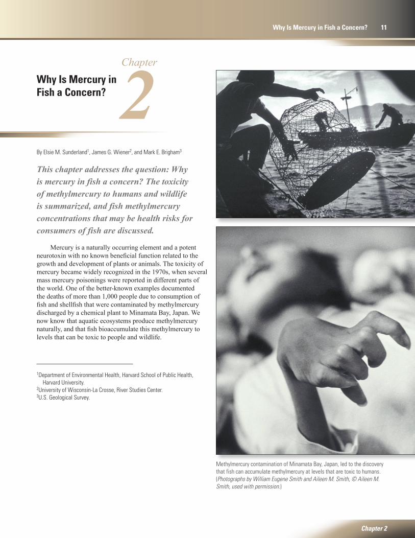
This chapter addresses the question: Why is mercury in fish a concern? The toxicity of methylmercury to humans and wildlife is summarized, and fish methylmercury concentrations that may be health risks for consumers of fish are discussed.

Mercury is a naturally occurring element and a potent neurotoxin with no known beneficial function related to the growth and development of plants or animals. The toxicity of mercury became widely recognized in the 1970s, when several mass mercury poisonings were reported in different parts of the world. One of the better-known examples documented the deaths of more than 1,000 people due to consumption of fish and shellfish that were contaminated by methylmercury discharged by a chemical plant to Minamata Bay, Japan. We now know that aquatic ecosystems produce methylmercury naturally, and that fish bioaccumulate this methylmercury to levels that can be toxic to people and wildlife.

By Elsie M. Sunderland1, James G. Wiener2, and Mark E. Brigham3

Methylmercury contamination of Minamata Bay, Japan, led to the discovery that fish can accumulate methylmercury at levels that are toxic to humans. (Photographs by William Eugene Smith and Aileen M. Smith, © Aileen M. Smith, used with permission.)

Chapter 2

Why Is Mercury in Fish a Concern? 11

Chapter

2

1Department of Environmental Health, Harvard School of Public Health, Harvard University.2University of Wisconsin-La Crosse, River Studies Center.3U.S. Geological Survey.

tac11-0651_fig02-01abc

1992 1994 1996 1998 2000 2002 2004 2006 2008 20101992 1994 1996 1998 2000 2002 2004 2006 2008 2010

A. Rivers B. Lakes

C.

02,000,000

4,000,000

6,000,000

8,000,000

10,000,000

12,000,000

14,000,000

16,000,000

18,000,000

Mercury

0

200,000

400,000

600,000

800,000

1,000,000

1,200,000

1,400,000

Mercury

All othercontaminants

All othercontaminants

Tota

l lak

e ar

ea u

nder

fish

con

sum

ptio

n ad

viso

ry, i

n ac

res

Tota

l riv

er le

ngth

und

er fi

sh c

onsu

mpt

ion

adv

isor

y, in

mile

s

Advisories for specific waterbodies

Statewide freshwater advisory

Statewide freshwater advisoryand additional advisories onspecific waterbodies

Statewide coastal advisories

Statewide advisory for lakes only

EXPLANATION

Methylmercury Toxicity is a Global Concern

Methylmercury is an organic form of mercury that readily bioaccumulates in aquatic food webs, reaching its highest concentrations in predatory fish, fish-eating wildlife, and humans that consume these animals. The toxicity of mercury has been known for centuries; however, it gained widespread attention during the early 1970s, when a number of mass poisonings occurred around the world. In one of the most highly publicized incidents, it has been reported that more than 1,000 people have died since about 1960 from eating fish and shellfish contaminated with methylmercury discharged by a chemical manufacturing company to Minamata Bay, Japan (Harada, 1995).

Certain bacteria in water bodies and wetlands can naturally convert inorganic mercury to methylmercury. Between 1962 and 1970, for example, mercury discharged from a chlor-alkali plant to the English-Wabigoon River system in Ontario, Canada, was rapidly methylated and bioaccumulated, causing extremely high concentrations of methylmercury in fish and exposing many First Nations subsistence fishers to harmful amounts of methylmercury (Rudd and others, 1983; Wheatley and Paradis, 1995). We

now understand that much lower levels of methylmercury exposure than those in Minamata Bay or the English-Wabigoon River are known to adversely affect human health, especially for children and pregnant women.

In many areas of North America, methylmercury levels in fish and in fish-eating wildlife are associated with harmful effects, such as diminished health and reproduction. These effects have been documented at tissue concentrations that are equivalent to or lower than the USEPA fish tissue mercury criterion for the protection of human health (0.3 ppm).

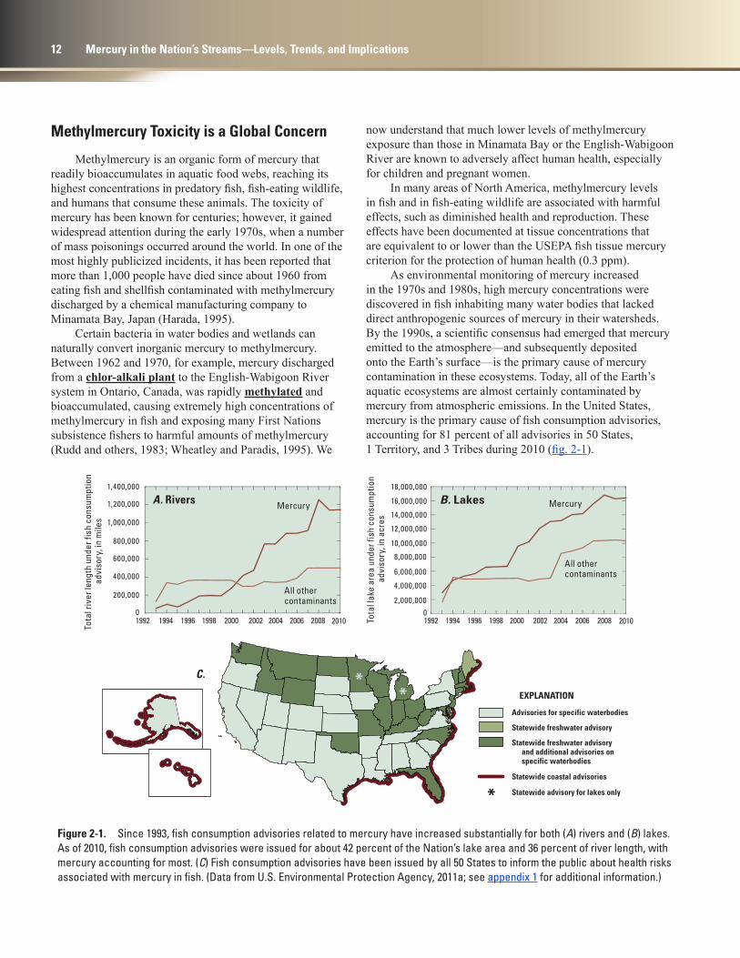
As environmental monitoring of mercury increased in the 1970s and 1980s, high mercury concentrations were discovered in fish inhabiting many water bodies that lacked direct anthropogenic sources of mercury in their watersheds. By the 1990s, a scientific consensus had emerged that mercury emitted to the atmosphere—and subsequently deposited onto the Earth’s surface—is the primary cause of mercury contamination in these ecosystems. Today, all of the Earth’s aquatic ecosystems are almost certainly contaminated by mercury from atmospheric emissions. In the United States, mercury is the primary cause of fish consumption advisories, accounting for 81 percent of all advisories in 50 States, 1 Territory, and 3 Tribes during 2010 (fig. 2-1).

Figure 2-1. Since 1993, fish consumption advisories related to mercury have increased substantially for both (A) rivers and (B) lakes. As of 2010, fish consumption advisories were issued for about 42 percent of the Nation’s lake area and 36 percent of river length, with mercury accounting for most. (C) Fish consumption advisories have been issued by all 50 States to inform the public about health risks associated with mercury in fish. (Data from U.S. Environmental Protection Agency, 2011a; see appendix 1 for additional information.)


tac11-0651_fig02-02

Atlantic Coast

(1.55 ppb)

Inland Northeast(0.77 ppb)

Great Lakes Coast(0.80 ppb)

Inland Midwest(0.63 ppb)

Inland Midwest(0.63 ppb)Inland West

(0.73 ppb)Inland West

(0.73 ppb)

Inland South(0.74 ppb)

Inland South(0.74 ppb)

Gulf Coast(0.96 ppb)

Pacific Coast

(1.18 ppb)

Blood mercury concentration, in parts per billion (ppb)

Exposure to Methylmercury is Associated with Human Health Risks

Most mercury exposure in the U.S. population is from fish consumption. Methylmercury exposure from fish consumption has been associated with various adverse effects on human health, ranging from central nervous system toxicity in adults exposed at extremely high levels to diminished cardiovascular health and endocrine disruption at lower exposure levels (Clarkson and others, 2003; Choi and Grandjean, 2008; Tan and others, 2009). Long-term reductions or impairments in brain function in children associated with methylmercury exposure have been reported in many studies around the world. The most well established effects on humans at the relatively low levels of methylmercury exposure typical of fish-consuming populations are neurological impacts on children exposed in the womb, particularly during the third trimester (Mahaffey and others, 2011). Data on children followed from before birth into childhood provide the scientific basis for the current reference dose for methylmercury used by the USEPA and established by a National Academy of Sciences panel of experts in 2000 (National Research Council, 2000). The reference dose is the level of daily intake (of a chemical) that is not associated with an appreciable increase in risk of adverse health effects during a lifetime. For methylmercury, the USEPA reference dose is equivalent to 0.1 microgram per kilogram of body weight per day. This intake rate is equivalent to approximately 5.8 micrograms of mercury per liter (ppb) in blood. Data from the National Health and Nutrition Examination Survey suggest that from 4 to 8 percent of U.S. women of childbearing age exceed the USEPA reference dose for methylmercury. This corresponds to hundreds of thousands of children born in the United States each year with blood mercury concentrations exceeding the USEPA reference dose (Mahaffey and others, 2009).

Blood mercury levels in the U.S. population vary with fish consumption patterns and, in general, are higher in coastal areas with greater fish consumption rates than in inland communities (fig. 2-2). Most seafood consumed in the United States is sold in the commercial market. Methylmercury exposure is a function of how much seafood people eat and

Figure 2-2. Average (geometric mean) blood mercury concentrations in humans are higher in coastal areas than in many inland areas, likely because fish consumption is higher in coastal areas. (Data from 2004 National Health and Nutrition Examination Survey; modified from Mahaffey and others, 2009.)

Chapter 2


tac11-0651_fig02-03ab

0 1 2 3 4

Tuna

Shrimp

Pollock

Salmon

Cod

Whiting

Flatfish

Clams

Crab

Scallops

Squid

Herring

Oysters

Sardine

Lobster

Mackerel

Halibut

Haddock

Swordfish

0 10 20 30 40

Tuna (canned, frozen, and fresh)

Swordfish

Pollock

Shrimp

Cod

Crab

Salmon (canned, frozen, and fresh)

Anchovies, herring, and shad

Orange Roughy

Halibut

Flounder, Plaice, and Sole

Haddock, hake, and monkfish

Grouper, rockfish, and sea bass

Snapper, porgy, and sheepshead

Mackerel

A. B.

Seafood consumption, in grams per day Population-wide methylmercury intake, in percent

concentrations of methylmercury in the seafood they choose. Tuna (both fresh and canned) are the largest contributor to methylmercury exposure in the United States because they are eaten in large quantities (fig. 2-3) and contain moderately high mercury concentrations (see “Balancing the Benefits and Risks of Fish Consumption,” p. 16). Species, such as pollock, are low in mercury but contribute substantially

to population-wide exposure because people consume large quantities of these fish. Freshwater environments are important sources of methylmercury exposure for some of the most highly exposed human populations, such as recreational fishers and Native Americans, that harvest large quantities of fish from local lakes and streams (Mergler and others, 2007).

Figure 2-3. Per capita seafood consumption (A) and methylmercury intake from commercial estuarine and marine fish and shellfish (B) in the United States indicate that several species with some of the highest mercury concentrations also are species that are most likely to be consumed. (Modified from Sunderland, 2007; see appendix 1 for additional information.)


High levels of exposure to inorganic mercury (primarily through inhalation of elemental mercury) also can cause negative health effects, such as kidney failure and central nervous system toxicity. However, inorganic mercury concentrations in the atmosphere are much lower than levels known to elicit such effects, even adjacent to point sources, such as coal-fired power plants. Dental amalgams contain elemental mercury and may result in low-level inorganic mercury exposures, but are not thought to be associated with substantial health risks for the general population (Clarkson and others, 2003; Bellinger and others, 2006). Unlike methylmercury, inorganic mercury consumed orally is not well absorbed by the human body and does not cross the blood-brain or placental barriers.

One of the challenges associated with understanding the impacts of methylmercury exposure on the developing brain is the co-occurrence of beneficial nutrients, such as polyunsaturated omega-3 fatty acids, with mercury in fish. Increasing dietary intake of omega-3 fatty acids during pregnancy is associated with improved childhood performance on neurocognitive tests (Choi and Grandjean, 2008; Strain and others, 2008). In

addition, a variety of studies show benefits to cardiovascular health from omega-3 fatty acid intake (Mozaffarian and Rimm, 2006). These effects make it difficult to detect the full extent of methylmercury impacts on the developing brain and cardiovascular health because the main source of dietary exposure (seafood) contains both methylmercury and omega-3 fatty acids. For example, recent studies of neurocognitive performance in children in the Seychelles, an island republic in the Indian Ocean, show significant adverse effects from methylmercury exposure are only apparent after adjusting for the positive impacts of omega-3 fatty acids (Strain and others, 2008; Lynch and others, 2011).

A variety of studies also have suggested that selenium may be helpful in mitigating the effects of mercury toxicity (Choi and Grandjean, 2008). However, there have been few studies designed to assess the role of selenium in preventing methylmercury induced developmental neurotoxicity in humans. For example, selenium did not confer protection against methylmercury associated neurocognitive deficits in Faroe Island residents (Choi and others, 2008). Environmental interactions between mercury and selenium remain an area of active research.

Chapter 2


Balancing the Benefits and Risks of Fish Consumption

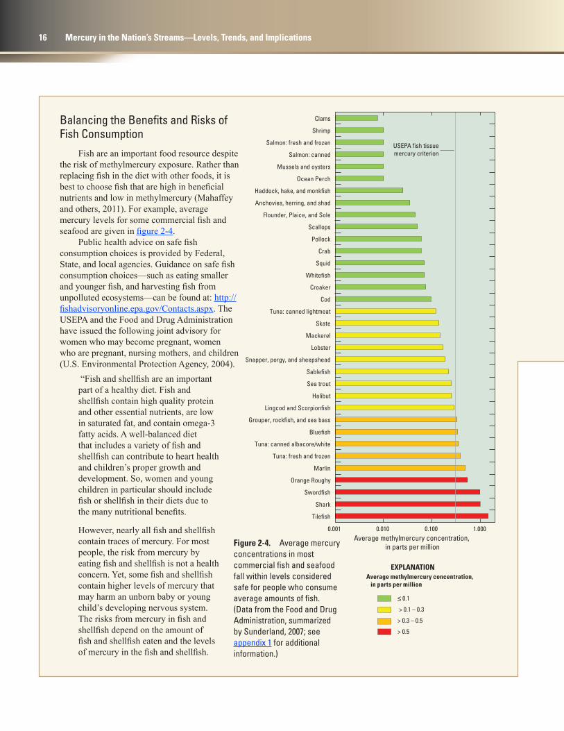
Fish are an important food resource despite the risk of methylmercury exposure. Rather than replacing fish in the diet with other foods, it is best to choose fish that are high in beneficial nutrients and low in methylmercury (Mahaffey and others, 2011). For example, average mercury levels for some commercial fish and seafood are given in figure 2-4.

Public health advice on safe fish consumption choices is provided by Federal, State, and local agencies. Guidance on safe fish consumption choices—such as eating smaller and younger fish, and harvesting fish from unpolluted ecosystems—can be found at: http://fishadvisoryonline.epa.gov/Contacts.aspx. The USEPA and the Food and Drug Administration have issued the following joint advisory for women who may become pregnant, women who are pregnant, nursing mothers, and children (U.S. Environmental Protection Agency, 2004).

“Fish and shellfish are an important part of a healthy diet. Fish and shellfish contain high quality protein and other essential nutrients, are low in saturated fat, and contain omega-3 fatty acids. A well-balanced diet that includes a variety of fish and shellfish can contribute to heart health and children’s proper growth and development. So, women and young children in particular should include fish or shellfish in their diets due to the many nutritional benefits.

However, nearly all fish and shellfish contain traces of mercury. For most people, the risk from mercury by eating fish and shellfish is not a health concern. Yet, some fish and shellfish contain higher levels of mercury that may harm an unborn baby or young child’s developing nervous system. The risks from mercury in fish and shellfish depend on the amount of fish and shellfish eaten and the levels of mercury in the fish and shellfish.

tac11-0651_fig02-04

0.001 0.010 0.100 1.000

Clams

Shrimp

Salmon: fresh and frozen USEPA fish tissuemercury criterionSalmon: canned

Mussels and oysters

Ocean Perch

Haddock, hake, and monkfish

Anchovies, herring, and shad

Flounder, Plaice, and Sole

Scallops

Pollock

Crab

Squid

Whitefish

Croaker

Cod

Tuna: canned lightmeat

Skate

Mackerel

Lobster

Snapper, porgy, and sheepshead

Sablefish

Sea trout

Halibut

Lingcod and Scorpionfish

Grouper, rockfish, and sea bass

Bluefish

Tuna: canned albacore/white

Tuna: fresh and frozen

Marlin

Orange Roughy

Swordfish

Shark

Tilefish

Average methylmercury concentration, in parts per million

≤ 0.1

> 0.1 – 0.3

> 0.3 – 0.5

> 0.5

EXPLANATIONAverage methylmercury concentration, in parts per million

Figure 2-4. Average mercury concentrations in most commercial fish and seafood fall within levels considered safe for people who consume average amounts of fish. (Data from the Food and Drug Administration, summarized by Sunderland, 2007; see appendix 1 for additional information.)


http://fishadvisoryonline.epa.gov/Contacts.aspx

http://fishadvisoryonline.epa.gov/Contacts.aspx

Therefore, the Food and Drug Administration (FDA) and the Environmental Protection Agency (EPA) are advising women who may become pregnant, pregnant women, nursing mothers, and young children to avoid some types of fish and eat fish and shellfish that are lower in mercury.

By following these three recommendations [below] for selecting and eating fish or shellfish, women and young children will receive the benefits of eating fish and shellfish and be confident that they have reduced their exposure to the harmful effects of mercury.

1. Do not eat Shark, Swordfish, King Mackerel, or Tilefish because they contain high levels of mercury.

2. Eat up to 12 ounces (2 average meals) a week of a variety of fish and shellfish that are lower in mercury.

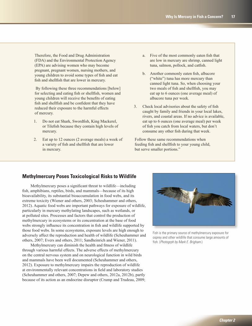
Fish is the primary source of methylmercury exposure for osprey and other wildlife that consume large amounts of fish. (Photogrph by Mark E. Brigham.)

a. Five of the most commonly eaten fish that are low in mercury are shrimp, canned light tuna, salmon, pollock, and catfish.

b. Another commonly eaten fish, albacore (“white”) tuna has more mercury than canned light tuna. So, when choosing your two meals of fish and shellfish, you may eat up to 6 ounces (one average meal) of albacore tuna per week.

3. Check local advisories about the safety of fish caught by family and friends in your local lakes, rivers, and coastal areas. If no advice is available, eat up to 6 ounces (one average meal) per week of fish you catch from local waters, but don’t consume any other fish during that week.

Follow these same recommendations when feeding fish and shellfish to your young child, but serve smaller portions.”

Methylmercury Poses Toxicological Risks to Wildlife

Methylmercury poses a significant threat to wildlife—including fish, amphibians, reptiles, birds, and mammals—because of its high bioavailability, its substantial bioaccumulation in food webs, and its extreme toxicity (Wiener and others, 2003; Scheuhammer and others, 2012). Aquatic food webs are important pathways for exposure of wildlife, particularly in mercury methylating landscapes, such as wetlands, or at polluted sites. Processes and factors that control the production of methylmercury in ecosystems or its concentration at the base of food webs strongly influence its concentration in fish and wildlife supported by those food webs. In some ecosystems, exposure levels are high enough to adversely affect the reproduction and health of wildlife (Scheuhammer and others, 2007; Evers and others, 2011; Sandheinrich and Wiener, 2011).

Methylmercury can diminish the health and fitness of wildlife through various harmful effects. The adverse effects of methylmercury on the central nervous system and on neurological function in wild birds and mammals have been well documented (Scheuhammer and others, 2012). Exposure to methylmercury impairs the reproduction of wildlife at environmentally relevant concentrations in field and laboratory studies (Scheuhammer and others, 2007; Depew and others, 2012a, 2012b), partly because of its action as an endocrine disruptor (Crump and Trudeau, 2009;

Chapter 2


Tan and others, 2009). Methylmercury also can affect the immune system, making wildlife more susceptible to disease. Moderately high exposure to methylmercury can damage cells and tissues. In freshwater fish, for example, liver tissue undergoes changes in color and biochemical properties in direct relation to methylmercury exposure (Sandheinrich and Wiener, 2011).

It is becoming increasingly evident that the scope and severity of the mercury problem for wildlife have been substantially underestimated. Recent findings show that methylmercury impairs the health and reproduction of fish and birds at much lower dietary or tissue concentrations than previously recognized (Evers and others, 2011; Sandheinrich and Wiener, 2011; Depew and others, 2012a). For example, concentrations of methylmercury in piscivorous fish from many North American fresh waters exceed estimated threshold levels (0.5 ppm in axial muscle tissue or 0.3 ppm in whole fish) that are associated with altered biochemical processes, damage to cells and tissues, and diminished reproduction (Dillon and others, 2010; Sandheinrich and Wiener, 2011). In birds, methylmercury in the diet of reproducing females is transferred to the developing egg—the most sensitive life stage (Scheuhammer and others, 2007; Heinz and others, 2009a). Reduced reproductive success has been associated with methylmercury exposure in field studies of several aquatic and marsh birds.

Criteria established to protect human health from the adverse effects of methylmercury exposure are not protective of fish-eating wildlife. The USEPA fish tissue criterion for methylmercury, established to protect the health

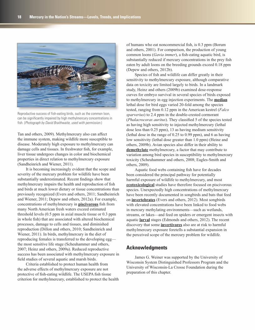
of humans who eat noncommercial fish, is 0.3 ppm (Borum and others, 2001). For comparison, the production of young common loons (Gavia immer), a fish-eating aquatic bird, is substantially reduced if mercury concentrations in the prey fish eaten by adult loons on the breeding grounds exceed 0.18 ppm (Depew and others, 2012b).

Species of fish and wildlife can differ greatly in their sensitivity to methylmercury exposure, although comparative data on toxicity are limited largely to birds. In a landmark study, Heinz and others (2009b) examined dose-response curves for embryo survival in several species of birds exposed to methylmercury in egg injection experiments. The median lethal dose for bird eggs varied 20-fold among the species tested, ranging from 0.12 ppm in the American kestrel (Falco sparverius) to 2.4 ppm in the double-crested cormorant (Phalacrocorax auritus). They classified 5 of the species tested as having high sensitivity to injected methylmercury (lethal dose less than 0.25 ppm), 13 as having medium sensitivity (lethal dose in the range of 0.25 to 0.99 ppm), and 6 as having low sensitivity (lethal dose greater than 1.0 ppm) (Heinz and others, 2009b). Avian species also differ in their ability to demethylate methylmercury, a factor that may contribute to variation among bird species in susceptibility to methylmercury toxicity (Scheuhammer and others, 2008; Eagles-Smith and others, 2009).

Aquatic food webs containing fish have for decades been considered the principal pathway for potentially harmful exposure of wildlife to methylmercury, and most ecotoxicological studies have therefore focused on piscivorous species. Unexpectedly high concentrations of methylmercury have been recently documented in songbirds and bats that feed on invertebrates (Evers and others, 2012). Most songbirds with elevated concentrations have been linked to food webs in mercury methylating environments—such as wetlands, streams, or lakes—and feed on spiders or emergent insects with aquatic larval stages (Edmonds and others, 2012). The recent discovery that some invertivores also are at risk to harmful methylmercury exposure foretells a substantial expansion in the perceived scope of the mercury problem for wildlife.

Acknowledgments

James G. Weiner was supported by the University of Wisconsin System Distinguished Professors Program and the University of Wisconsin-La Crosse Foundation during the preparation of this chapter.

Reproductive success of fish-eating birds, such as the common loon, can be significantly impaired by high methylmercury concentrations in fish. (Photograph by David Braithwaite, used with permission.)


This page left intentionally blank

Chapter 2


Fishing Brook, New York

Phot

ogra

ph b

y De

nnis

A. W

entz

.

Phot

ogra

ph b

y De

nnis

A. W

entz

.

How Does Mercury Cycle Through Aquatic Ecosystems?

This chapter addresses the questions: Where does mercury in aquatic ecosystems come from? How does mercury move through stream ecosystems? Why are mercury concentrations in fish high when concentrations in stream water are typically low? Why do some fish species have higher mercury concentrations than others, and what factors control mercury bioaccumulation in fish? Major sources of inorganic mercury to aquatic ecosystems, transformation of inorganic mercury to methylmercury, and bioaccumulation of methylmercury in aquatic food webs are discussed.

In the past, industrial wastewater discharges were important sources of inorganic and organic mercury; however, today most mercury emissions in the United States are from coal combustion. This mostly inorganic mercury is carried tens to thousands of kilometers by the atmosphere, and a portion is eventually deposited back to Earth, either in precipitation or dry deposition. Because mercury can be transported long distances, emissions from other countries are an important source of mercury deposited in the United States. In aquatic ecosystems, inorganic mercury is converted to methylmercury (an organic form) by natural bacterial processes that are particularly active in wetlands. Some methylmercury enters aquatic food webs, where it is bioaccumulated, resulting in elevated concentrations in fish and other organisms at or near the top of the food web.

Mercury from power plants and other sources enters aquatic ecosystems and is bioaccumulated through food webs. (Graphic courtesy of Washington State Department of Health.)

Chapter 3

How Does Mercury Cycle Through Aquatic Ecosystems? 21

Chapter

3

Hg2+ MeHg

Oxidation

Atmosphericdepositon

Wet Dry

Re-emission

Methylation

Cropland and other settings with erodible soils contribute sediment-bound mercury to surface waters.

Emissions from coal-fired power plants are the largest anthropogenic source of mercury to the atmosphere in the United States.

Gaseous elemental mercury in the atmosphere originates from natural and anthropogenic sources and can be transported long distances before it is deposited onto the earth’s surface.

Some gaseous elemental mercury is oxidized to reactive mercury, which is more readily deposited.

Gaseous elemental mercury, reactive gaseous mercury, and particulate mercury are mostly deposited by precipitation and by dry deposition.

Mercury deposition rates are typically greater near large urban areas than in more remote areas.

Mercury mines, gold mines, and some industries have historically contributed high concentrations of mercury to aquatic ecosystems. Some of this “legacy mercury” remains a problem today.

Natural bacteria convert reactive inorganic mercury to methylmercury—the form accumulated in fish, wildlife, and humans. Wetlands are especially important zones of mercury methylation.

Some gaseous elemental mercury emissions are deposited locally, but most are transported long distances through the atmosphere.

Most reactive gaseous and particulate forms of mercury tend to be deposited regionally.

Organic carbon from wetlands binds with mercury and facilitates its transport in natural waters.

The Mercury Cycle Describes How Mercury Moves Through the Environment

The mercury cycle (fig. 3-1) describes where mercury comes from, how it enters an aquatic ecosystem, how it is transported through the system, what processes transform it along the way, where it accumulates, and how it leaves the system. In the United States, the predominant source of mercury to most aquatic ecosystems is emission of inorganic mercury to the atmosphere from burning coal for energy production. This mercury takes one of three forms: gaseous elemental mercury, reactive gaseous mercury, or particulate mercury. The atmospheric mercury enters aquatic ecosystems through wet and dry deposition. In

Figure 3-1. The mercury cycle illustrates where mercury originates, how it enters an aquatic ecosystem, how it is transported and transformed within the ecosystem, and how it leaves the ecosystem. (Drawing © Frank Ippolito/Production Post Studios/www.ProductionPost.com.)


addition, many ecosystems in the Western United States have been contaminated by past mercury and gold mining, which can provide large sources of inorganic mercury to streams, lakes, and wetlands. Some inorganic mercury is converted to methylmercury by bacteria in organic-rich areas, such as

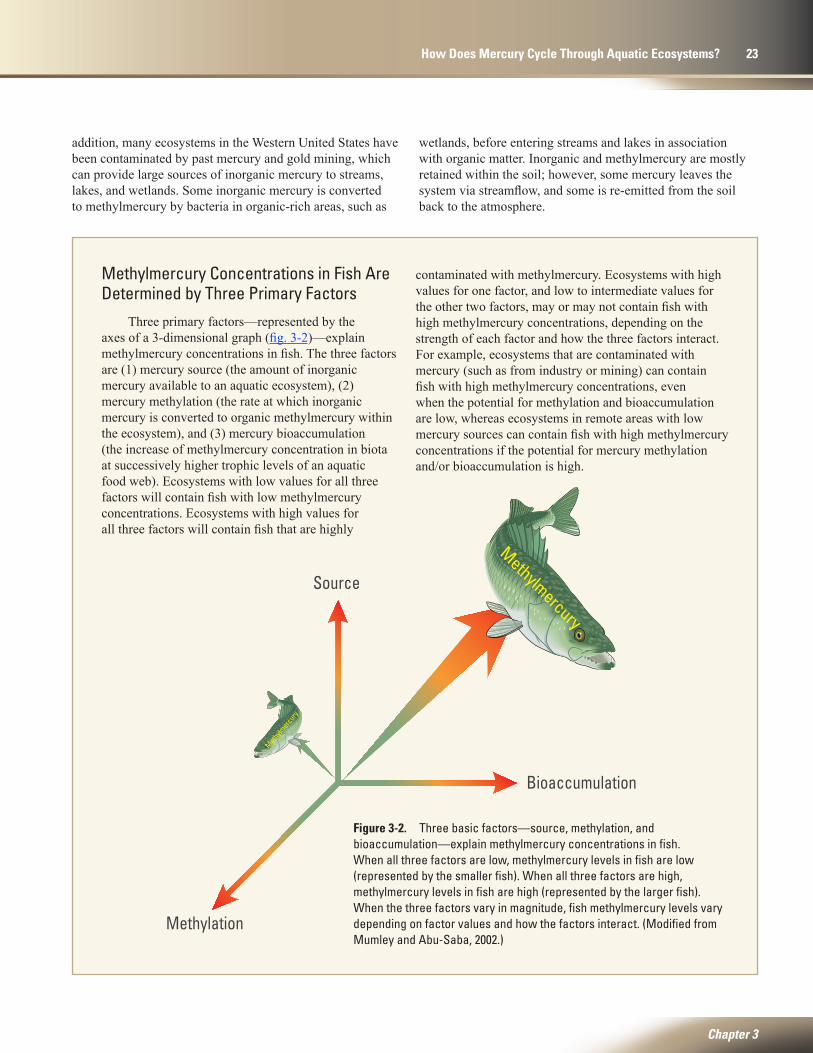
Methylmercury Concentrations in Fish Are Determined by Three Primary Factors

Three primary factors—represented by the axes of a 3-dimensional graph (fig. 3-2)—explain methylmercury concentrations in fish. The three factors are (1) mercury source (the amount of inorganic mercury available to an aquatic ecosystem), (2) mercury methylation (the rate at which inorganic mercury is converted to organic methylmercury within the ecosystem), and (3) mercury bioaccumulation (the increase of methylmercury concentration in biota at successively higher trophic levels of an aquatic food web). Ecosystems with low values for all three factors will contain fish with low methylmercury concentrations. Ecosystems with high values for all three factors will contain fish that are highly

tac11-0651_fig03-02

Source

Bioaccumulation

Methylation

Methylmercury

Meth

ylmer

cury

Figure 3-2. Three basic factors—source, methylation, and bioaccumulation—explain methylmercury concentrations in fish. When all three factors are low, methylmercury levels in fish are low (represented by the smaller fish). When all three factors are high, methylmercury levels in fish are high (represented by the larger fish). When the three factors vary in magnitude, fish methylmercury levels vary depending on factor values and how the factors interact. (Modified from Mumley and Abu-Saba, 2002.)

wetlands, before entering streams and lakes in association with organic matter. Inorganic and methylmercury are mostly retained within the soil; however, some mercury leaves the system via streamflow, and some is re-emitted from the soil back to the atmosphere.

contaminated with methylmercury. Ecosystems with high values for one factor, and low to intermediate values for the other two factors, may or may not contain fish with high methylmercury concentrations, depending on the strength of each factor and how the three factors interact. For example, ecosystems that are contaminated with mercury (such as from industry or mining) can contain fish with high methylmercury concentrations, even when the potential for methylation and bioaccumulation are low, whereas ecosystems in remote areas with low mercury sources can contain fish with high methylmercury concentrations if the potential for mercury methylation and/or bioaccumulation is high.

Chapter 3


tac11-0651_fig03-03

0

100

200

300

400

500

600

700

800

900

China India UnitedStates

Russia Indonesia SouthAfrica

Brasil Australia SouthKorea

Columbia

Mer

cury

em

issi

ons,

in m

etric

tons

Combustion of coal and other fossil fuels

Metal mining and production

Gold mining and production

Cement production

Chlor-alkali production

Waste incineration

Other

EXPLANATION

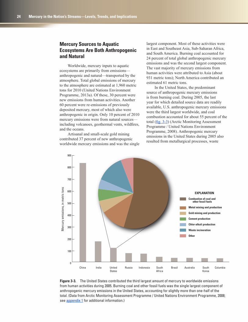
Mercury Sources to Aquatic Ecosystems Are Both Anthropogenic and Natural

Worldwide, mercury inputs to aquatic ecosystems are primarily from emissions—anthropogenic and natural—transported by the atmosphere. Total global emissions of mercury to the atmosphere are estimated at 1,960 metric tons for 2010 (United Nations Environment Programme, 2013a). Of these, 30 percent were new emissions from human activities. Another 60 percent were re-emissions of previously deposited mercury, most of which also were anthropogenic in origin. Only 10 percent of 2010 mercury emissions were from natural sources—including volcanoes, geothermal vents, wildfires, and the oceans.

Artisanal and small-scale gold mining contributed 37 percent of new anthropogenic worldwide mercury emissions and was the single

largest component. Most of these activities were in East and Southeast Asia, Sub-Saharan Africa, and South America. Burning coal accounted for 24 percent of total global anthropogenic mercury emissions and was the second largest component. The vast majority of mercury emissions from human activities were attributed to Asia (about 931 metric tons); North America contributed an estimated 61 metric tons.

In the United States, the predominant source of anthropogenic mercury emissions is from burning coal. During 2005, the last year for which detailed source data are readily available, U.S. anthropogenic mercury emissions were the third largest worldwide, and coal combustion accounted for about 55 percent of the total (fig. 3-3) (Arctic Monitoring Assessment Programme / United Nations Environment Programme, 2008). Anthropogenic mercury emissions in the United States during 2005 also resulted from metallurgical processes, waste

Figure 3-3. The United States contributed the third largest amount of mercury to worldwide emissions from human activities during 2005. Burning coal and other fossil fuels was the single largest component of anthropogenic mercury emissions in the United States, accounting for slightly more than one-half of the total. (Data from Arctic Monitoring Assessment Programme / United Nations Environment Programme, 2008; see appendix 1 for additional information.)


tac11-0651_fig03-04

Amount of total mercury emitted, in kilograms per yearType of mercury source

EXPLANATION

Coal combustion

Other fuel combustion

Incineration

Metallurgical and mining

Manufacturing and other

5 – 10

10 – 100

100 – 1,000

1,000 – 5,500

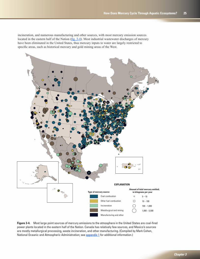
incineration, and numerous manufacturing and other sources, with most mercury emission sources located in the eastern half of the Nation (fig. 3-4). Most industrial wastewater discharges of mercury have been eliminated in the United States, thus mercury inputs to water are largely restricted to specific areas, such as historical mercury and gold mining areas of the West.

Figure 3-4. Most large point sources of mercury emissions to the atmosphere in the United States are coal-fired power plants located in the eastern half of the Nation. Canada has relatively few sources, and Mexico’s sources are mostly metallurgical processing, waste incineration, and other manufacturing. (Compiled by Mark Cohen, National Oceanic and Atmospheric Administration; see appendix 1 for additional information.)

Chapter 3


A recent global scale mercury deposition model suggests that about 70 percent of current mercury deposition to the United States is anthropogenic, of which 20 percent is from North American emissions and the remainder is from the rest of the world, including re-emission of older anthropogenic mercury that has accumulated in soil and the oceans since pre-industrial times (Selin and others, 2008). North American emissions represent a major portion of mercury deposition in the Eastern United States—up to about 60–80 percent in the industrialized Midwest—but a relatively minor portion in Western States (Seigneur and others, 2004; Selin and others, 2007).

Mercury Reaching the Nation’s Aquatic Ecosystems Is Transported Primarily by the Atmosphere

Atmospheric transport and deposition constitute the predominant pathway of anthropogenic mercury to most aquatic ecosystems in the United States, especially those in remote areas (Fitzgerald and others, 1998). Mercury is emitted either as gaseous elemental mercury, reactive (oxidized) gaseous mercury, or mercury adsorbed to solid particles and aerosols. Combustion of coal, which contains mercury as an impurity associated with pyrite (Tewalt and others, 2001), releases mercury to the atmosphere in all three forms.

Gaseous elemental mercury comprises more than 95 percent of global atmospheric mercury (Grigal, 2002) and becomes rapidly and efficiently mixed in the atmosphere. Average atmospheric transport distances for gaseous elemental mercury are tens of thousands of kilometers (Schroeder and Munthe, 1998; Lin and Pehkonen, 1999; Selin, 2009), thus giving rise to the designation of mercury as a global pollutant. Some gaseous elemental mercury is converted in the atmosphere to more reactive forms that fall out quickly and/or are absorbed by vegetation.

Less than about 5 percent of global atmospheric mercury is in the reactive form, either as reactive gaseous mercury or particulate mercury. These reactive mercury forms have transport distances of only tens to hundreds of kilometers, and they are typically deposited closer to their sources than gaseous elemental mercury (Schroeder and Munthe, 1998; Seigneur and others, 2006; Selin and others, 2007; Selin, 2009). The shorter transport distances for reactive mercury forms than for gaseous elemental mercury may lead to higher total mercury deposition rates near urban areas (where atmospheric sources are common) than in remote areas (Van Metre, 2012).

Atmospheric Mercury Deposition Rates Are Higher Near Major Urban Centers Than in Remote AreasBy Peter C. Van Metre, U.S. Geological Survey

Analyses of sediment cores collected during 1999–2009 from 12 lakes distributed across the United States indicate that atmospheric mercury deposition rates are higher near major urban centers than in remote areas (Van Metre, 2012). The lakes are 10–310 kilometers downwind from the center of the nearest large city (fig. 3-5). On average, modern (post-1990) atmospheric mercury deposition rates to lakes within 50 kilometers of urban areas were about 5 times higher than deposition rates to lakes that were farther than 150 kilometers from urban areas. In addition, the modern deposition rates were about 10 times historical background rates in lakes near urban areas, but only 3–4 times background rates for remote lakes.


tac11-0651_fig03-05

Portland

TampaOrlando

HartfordNew Haven

BostonAlbany

Montréal

Chicago

Minneapolis

Denver

Salt Lake City

Sampling site

City

EXPLANATION

tac11-0651_fig03-06

Mer

cury

dep

ositi

on ra

te, i

n m

icro

gram

spe

r squ

are

met

er p

er y

ear

Distance to major city, in kilometers

80

60

0 100 200 300

HgWET

HgTOTAL

0

20

40

100

Figure 3-5. Sediment cores, used to assess historical rates of mercury deposition, were collected from 12 lakes that are 10–310 kilometers downwind from major U.S. cities. (Modified from Van Metre, 2012.)

Figure 3-6. Post-1990 total mercury deposition rates increased rapidly as the distance to a major urban area decreased; however, increases in wet mercury deposition rates were much smaller. (Modified from Van Metre, 2012.)

Modern atmospheric mercury deposition rates measured in the lakes correlate strongly with distance from the nearest city, and to total population and estimated mercury emissions near the lake. The single strongest correlation with modern atmospheric mercury deposition rates measured in the lakes is the distance to the nearest major city (HgTOTAL; fig. 3-6), which explained 87 percent of the variation in mercury deposition rate. Modern mercury deposition rates also correlate strongly with total population within a 100-kilometer radius of each lake (72 percent of variation explained) and to emissions of reactive gaseous plus particulate mercury within about 150 kilometers of each lake (77 percent of variation explained). These results indicate that some urban mercury emissions are deposited locally, with an apparent distance of influence of the urban airshed on the order of 100 kilometers (fig. 3-6). Urban air quality might play a role in near-urban mercury deposition by altering local atmospheric mercury to reactive forms that are more likely to be deposited.

The increase in total atmospheric deposition rate of mercury measured using lake sediment cores is considerably larger than the increase in wet deposition rate (HgWET; fig. 3-6), as measured at nearby Mercury Deposition Network sites, thus suggesting that dry deposition is more important near urban areas. A number of sources and atmospheric processes in or near urban

areas might contribute to wet and dry mercury deposition, including point and diffuse sources of mercury, emissions from contaminated soil, increased concentrations of oxidants (such as ozone) in urban air, and elevated concentrations of atmospheric particulate mercury. Reactive gaseous mercury and particulate mercury can be especially high in urban areas and tend to be deposited more rapidly than gaseous elemental mercury.

Chapter 3


tac11-0651_fig03-07

Re-emissionThroughfall

Wet deposition Dry deposition

Litterfall

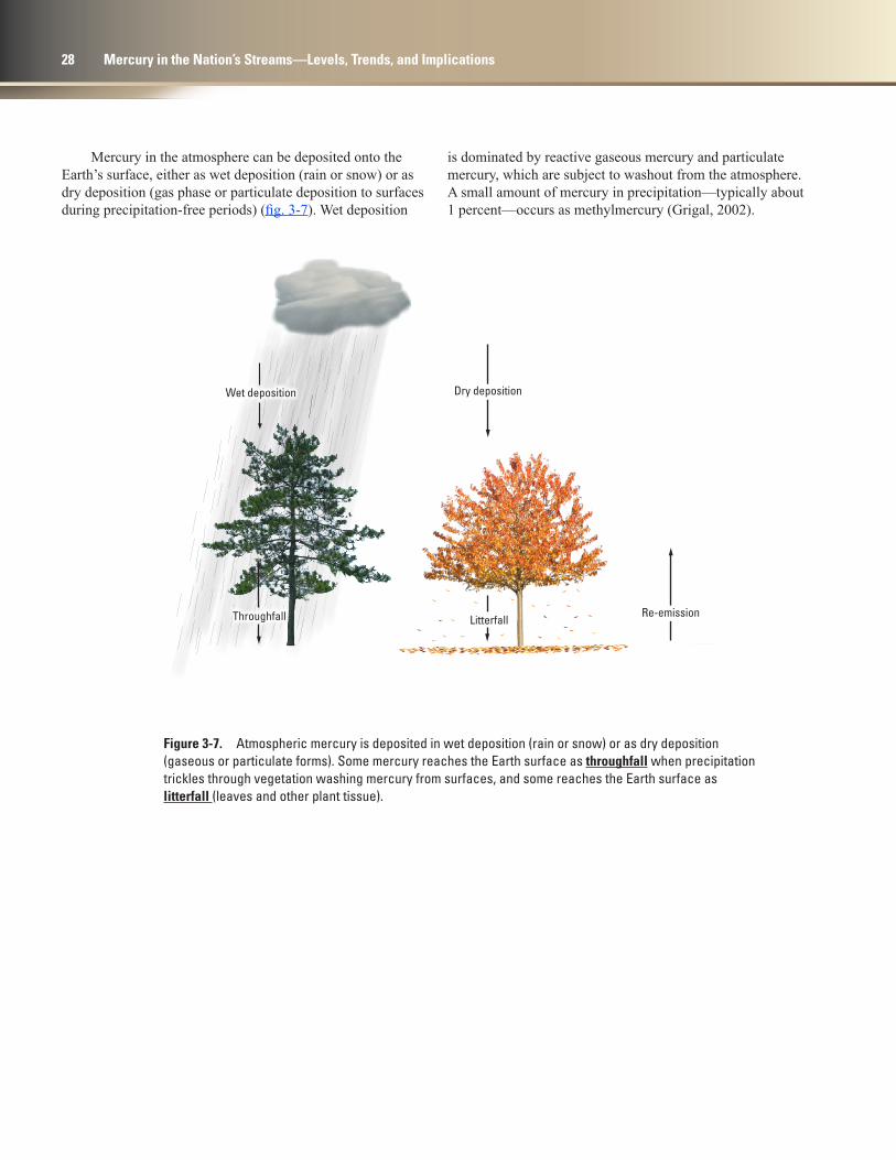
Figure 3-7. Atmospheric mercury is deposited in wet deposition (rain or snow) or as dry deposition (gaseous or particulate forms). Some mercury reaches the Earth surface as throughfall when precipitation trickles through vegetation washing mercury from surfaces, and some reaches the Earth surface as litterfall (leaves and other plant tissue).

Mercury in the atmosphere can be deposited onto the Earth’s surface, either as wet deposition (rain or snow) or as dry deposition (gas phase or particulate deposition to surfaces during precipitation-free periods) (fig. 3-7). Wet deposition

is dominated by reactive gaseous mercury and particulate mercury, which are subject to washout from the atmosphere. A small amount of mercury in precipitation—typically about 1 percent—occurs as methylmercury (Grigal, 2002).


tac11-0651_fig03-08

0 1,000 KILOMETERS200400600 800

0 200 400 600 800 1,000 MILES

0 ≥ 18

Mercury wet deposition, 2005–2011, in micrograms per square meter

EXPLANATION

tac11-0651_fig03-09

0.001

0.01

0.1

1

10

0.1 1 10 100 1,000

Orlando, Florida W

et m

ercu

ry d

epos

ition

, in

mic

rogr

ams

per s

quar

e m

eter

Precipitation, in millimeters

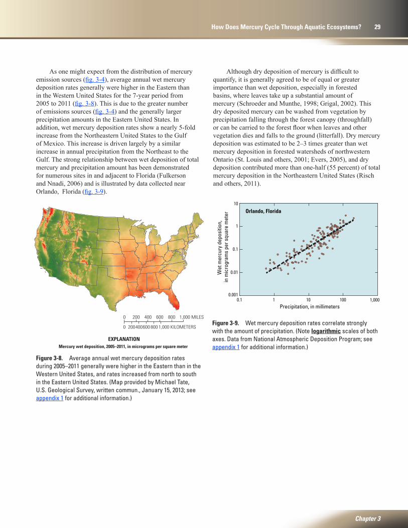
As one might expect from the distribution of mercury emission sources (fig. 3-4), average annual wet mercury deposition rates generally were higher in the Eastern than in the Western United States for the 7-year period from 2005 to 2011 (fig. 3-8). This is due to the greater number of emissions sources (fig. 3-4) and the generally larger precipitation amounts in the Eastern United States. In addition, wet mercury deposition rates show a nearly 5-fold increase from the Northeastern United States to the Gulf of Mexico. This increase is driven largely by a similar increase in annual precipitation from the Northeast to the Gulf. The strong relationship between wet deposition of total mercury and precipitation amount has been demonstrated for numerous sites in and adjacent to Florida (Fulkerson and Nnadi, 2006) and is illustrated by data collected near Orlando, Florida (fig. 3-9).

Although dry deposition of mercury is difficult to quantify, it is generally agreed to be of equal or greater importance than wet deposition, especially in forested basins, where leaves take up a substantial amount of mercury (Schroeder and Munthe, 1998; Grigal, 2002). This dry deposited mercury can be washed from vegetation by precipitation falling through the forest canopy (throughfall) or can be carried to the forest floor when leaves and other vegetation dies and falls to the ground (litterfall). Dry mercury deposition was estimated to be 2–3 times greater than wet mercury deposition in forested watersheds of northwestern Ontario (St. Louis and others, 2001; Evers, 2005), and dry deposition contributed more than one-half (55 percent) of total mercury deposition in the Northeastern United States (Risch and others, 2011).

Figure 3-8. Average annual wet mercury deposition rates during 2005–2011 generally were higher in the Eastern than in the Western United States, and rates increased from north to south in the Eastern United States. (Map provided by Michael Tate, U.S. Geological Survey, written commun., January 15, 2013; see appendix 1 for additional information.)

Figure 3-9. Wet mercury deposition rates correlate strongly with the amount of precipitation. (Note logarithmic scales of both axes. Data from National Atmospheric Deposition Program; see appendix 1 for additional information.)

Chapter 3


tac11-0651_fig03-10

Mercury Deposition Network (MDN) site

Atmospheric Mercury Network (AMNet) site

MDN and AMNet site

Sites

EXPLANATION

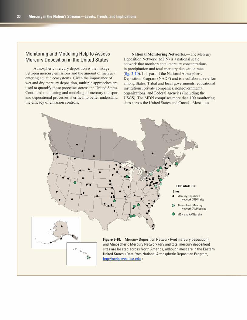
Figure 3-10. Mercury Deposition Network (wet mercury deposition) and Atmospheric Mercury Network (dry and total mercury deposition) sites are located across North America, although most are in the Eastern United States. (Data from National Atmospheric Deposition Program, http://nadp.sws.uiuc.edu.)

Monitoring and Modeling Help to Assess Mercury Deposition in the United States

Atmospheric mercury deposition is the linkage between mercury emissions and the amount of mercury entering aquatic ecosystems. Given the importance of wet and dry mercury deposition, multiple approaches are used to quantify these processes across the United States. Continued monitoring and modeling of mercury transport and depositional processes is critical to better understand the efficacy of emission controls.

National Monitoring Networks.—The Mercury Deposition Network (MDN) is a national scale network that monitors total mercury concentrations in precipitation and total mercury deposition rates (fig. 3-10). It is part of the National Atmospheric Deposition Program (NADP) and is a collaborative effort among States, Tribal and local governments, educational institutions, private companies, nongovernmental organizations, and Federal agencies (including the USGS). The MDN comprises more than 100 monitoring sites across the United States and Canada. Most sites


http://nadp.sws.uiuc.edu

(Continued on page 32)

The Mercury Deposition Network site at the H.J. Andrews Experimental Forest, Oregon, is one of more than 100 locations across the United States and Canada where precipitation has been collected for analysis of mercury. (Photograph by Dennis A. Wentz.)

The USGS mobile atmospheric mercury laboratory can be deployed across the United States to measure key forms of atmospheric mercury—information that will improve our understanding of mercury transport and deposition from different emission sources. (Photograph by Mercury Research Laboratory staff.)

are in rural areas and are somewhat removed from large mercury sources, although a few MDN sites are in or near urban areas. Standardized procedures are used at all MDN monitoring sites to measure total mercury at concentrations less than 1 part per trillion. The MDN Program produces annual maps for the contiguous United States and southern Canada showing average mercury concentrations in precipitation and average mercury wet deposition rates.

The Atmospheric Mercury Network (AMNet) was established in 2009 by the NADP to measure gaseous elemental mercury, reactive gaseous mercury, particulate mercury, and various meteorological variables needed for estimating dry mercury deposition. As of February 2013, 17 sites were included in AMNet (fig. 3-10). Most AMNet sites are co-located with existing MDN sites.

USGS Mobile Atmospheric Mercury Laboratory.—The USGS Mercury Research Laboratory in Middleton, Wisconsin, has a mobile atmospheric mercury laboratory that can be driven to various locations to collect data on mercury chemical forms in response to specific local and/or regional objectives (Kolker and others, 2007; U.S. Geological Survey, 2010). The laboratory is equipped with instrumentation that measures gaseous elemental mercury, reactive gaseous mercury, particulate mercury, wet mercury deposition, atmospheric gases (ozone, nitrogen oxides, sulfur dioxide, carbon monoxide), and a full suite of standard meteorological variables. Dry mercury deposition of reactive mercury (reactive gaseous mercury plus particulate mercury) can be calculated from the various measurements.

Data from 13 locations across the United States as of June 2012 show that atmospheric mercury concentrations near urban sites were 2–6 times those at rural and coastal sites, depending on the form of the mercury (Engle and others, 2010). These values are consistent with impacts by local and regional mercury sources at urban sites. Urban sites also received considerably greater dry deposition of reactive mercury than did rural and coastal sites.

Chapter 3


(Continued from page 31)

tac11-0651_fig03-12

0 1,000 KILOMETERS200 400 600 800

0 200 400 600 800 1,000 MILES

Mercury mineGold mine

EXPLANATION

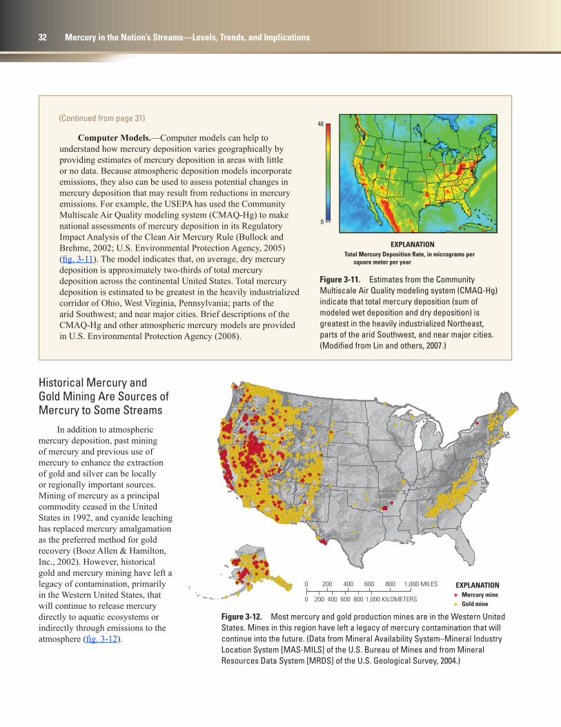
Computer Models.—Computer models can help to understand how mercury deposition varies geographically by providing estimates of mercury deposition in areas with little or no data. Because atmospheric deposition models incorporate emissions, they also can be used to assess potential changes in mercury deposition that may result from reductions in mercury emissions. For example, the USEPA has used the Community Multiscale Air Quality modeling system (CMAQ-Hg) to make national assessments of mercury deposition in its Regulatory Impact Analysis of the Clean Air Mercury Rule (Bullock and Brehme, 2002; U.S. Environmental Protection Agency, 2005) (fig. 3-11). The model indicates that, on average, dry mercury deposition is approximately two-thirds of total mercury deposition across the continental United States. Total mercury deposition is estimated to be greatest in the heavily industrialized corridor of Ohio, West Virginia, Pennsylvania; parts of the arid Southwest; and near major cities. Brief descriptions of the CMAQ-Hg and other atmospheric mercury models are provided in U.S. Environmental Protection Agency (2008).

Historical Mercury and Gold Mining Are Sources of Mercury to Some Streams

In addition to atmospheric mercury deposition, past mining of mercury and previous use of mercury to enhance the extraction of gold and silver can be locally or regionally important sources. Mining of mercury as a principal commodity ceased in the United States in 1992, and cyanide leaching has replaced mercury amalgamation as the preferred method for gold recovery (Booz Allen & Hamilton, Inc., 2002). However, historical gold and mercury mining have left a legacy of contamination, primarily in the Western United States, that will continue to release mercury directly to aquatic ecosystems or indirectly through emissions to the atmosphere (fig. 3-12).

Figure 3-11. Estimates from the Community Multiscale Air Quality modeling system (CMAQ-Hg) indicate that total mercury deposition (sum of modeled wet deposition and dry deposition) is greatest in the heavily industrialized Northeast, parts of the arid Southwest, and near major cities. (Modified from Lin and others, 2007.)

tac11-0651_fig03-11

Total Mercury Deposition Rate, in micrograms per square meter per year

48

0

EXPLANATION

Figure 3-12. Most mercury and gold production mines are in the Western United States. Mines in this region have left a legacy of mercury contamination that will continue into the future. (Data from Mineral Availability System–Mineral Industry Location System [MAS-MILS] of the U.S. Bureau of Mines and from Mineral Resources Data System [MRDS] of the U.S. Geological Survey, 2004.)


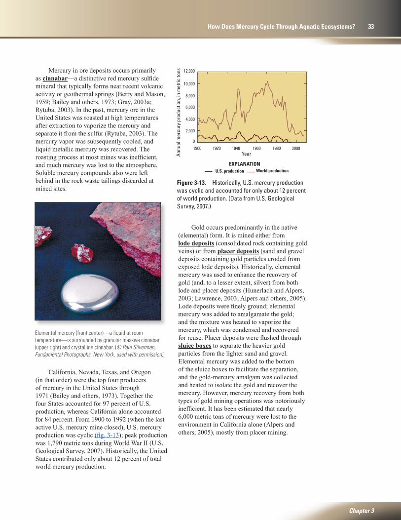
Mercury in ore deposits occurs primarily as cinnabar—a distinctive red mercury sulfide mineral that typically forms near recent volcanic activity or geothermal springs (Berry and Mason, 1959; Bailey and others, 1973; Gray, 2003a; Rytuba, 2003). In the past, mercury ore in the United States was roasted at high temperatures after extraction to vaporize the mercury and separate it from the sulfur (Rytuba, 2003). The mercury vapor was subsequently cooled, and liquid metallic mercury was recovered. The roasting process at most mines was inefficient, and much mercury was lost to the atmosphere. Soluble mercury compounds also were left behind in the rock waste tailings discarded at mined sites.

Elemental mercury (front center)—a liquid at room temperature—is surrounded by granular massive cinnabar (upper right) and crystalline cinnabar. (© Paul Silverman, Fundamental Photographs, New York, used with permission.)

Figure 3-13. Historically, U.S. mercury production was cyclic and accounted for only about 12 percent of world production. (Data from U.S. Geological Survey, 2007.)

California, Nevada, Texas, and Oregon (in that order) were the top four producers of mercury in the United States through 1971 (Bailey and others, 1973). Together the four States accounted for 97 percent of U.S. production, whereas California alone accounted for 84 percent. From 1900 to 1992 (when the last active U.S. mercury mine closed), U.S. mercury production was cyclic (fig. 3-13); peak production was 1,790 metric tons during World War II (U.S. Geological Survey, 2007). Historically, the United States contributed only about 12 percent of total world mercury production.

tac11-0651_fig03-13

0

2,000

4,000

6,000

8,000

10,000

12,000

1900 1920 1940 1960 1980 2000

Annu

al m

ercu

ry p

rodu

ctio

n, in

met

ric to

ns

Year

U.S. productionEXPLANATION

World production

Gold occurs predominantly in the native (elemental) form. It is mined either from lode deposits (consolidated rock containing gold veins) or from placer deposits (sand and gravel deposits containing gold particles eroded from exposed lode deposits). Historically, elemental mercury was used to enhance the recovery of gold (and, to a lesser extent, silver) from both lode and placer deposits (Hunerlach and Alpers, 2003; Lawrence, 2003; Alpers and others, 2005). Lode deposits were finely ground; elemental mercury was added to amalgamate the gold; and the mixture was heated to vaporize the mercury, which was condensed and recovered for reuse. Placer deposits were flushed through sluice boxes to separate the heavier gold particles from the lighter sand and gravel. Elemental mercury was added to the bottom of the sluice boxes to facilitate the separation, and the gold-mercury amalgam was collected and heated to isolate the gold and recover the mercury. However, mercury recovery from both types of gold mining operations was notoriously inefficient. It has been estimated that nearly 6,000 metric tons of mercury were lost to the environment in California alone (Alpers and others, 2005), mostly from placer mining.

Chapter 3


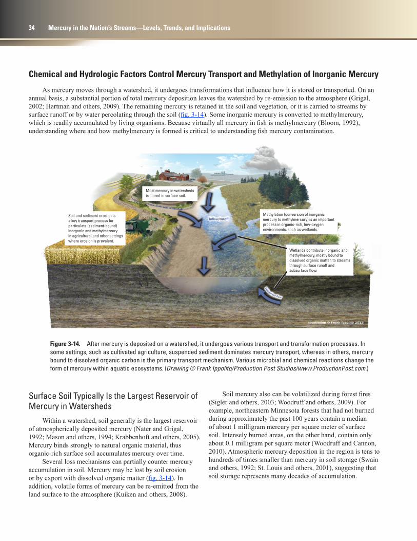
tac11-0651_fig03-14

Subsurface flow

Inflow/runoffSoil and sediment erosion is a key transport process for particulate (sediment-bound) inorganic and methylmercury in agricultural and other settings where erosion is prevalent.

Wetlands contribute inorganic and methylmercury, mostly bound to dissolved organic matter, to streams through surface runoff andsubsurface flow.

Methylation (conversion of inorganic mercury to methylmercury) is an important process in organic-rich, low-oxygen environments, such as wetlands.

Most mercury in watershedsis stored in surface soil.

Chemical and Hydrologic Factors Control Mercury Transport and Methylation of Inorganic Mercury

As mercury moves through a watershed, it undergoes transformations that influence how it is stored or transported. On an annual basis, a substantial portion of total mercury deposition leaves the watershed by re-emission to the atmosphere (Grigal, 2002; Hartman and others, 2009). The remaining mercury is retained in the soil and vegetation, or it is carried to streams by surface runoff or by water percolating through the soil (fig. 3-14). Some inorganic mercury is converted to methylmercury, which is readily accumulated by living organisms. Because virtually all mercury in fish is methylmercury (Bloom, 1992), understanding where and how methylmercury is formed is critical to understanding fish mercury contamination.

Figure 3-14. After mercury is deposited on a watershed, it undergoes various transport and transformation processes. In some settings, such as cultivated agriculture, suspended sediment dominates mercury transport, whereas in others, mercury bound to dissolved organic carbon is the primary transport mechanism. Various microbial and chemical reactions change the form of mercury within aquatic ecosystems. (Drawing © Frank Ippolito/Production Post Studios/www.ProductionPost.com.)

Surface Soil Typically Is the Largest Reservoir of Mercury in Watersheds

Within a watershed, soil generally is the largest reservoir of atmospherically deposited mercury (Nater and Grigal, 1992; Mason and others, 1994; Krabbenhoft and others, 2005). Mercury binds strongly to natural organic material, thus organic-rich surface soil accumulates mercury over time.

Several loss mechanisms can partially counter mercury accumulation in soil. Mercury may be lost by soil erosion or by export with dissolved organic matter (fig. 3-14). In addition, volatile forms of mercury can be re-emitted from the land surface to the atmosphere (Kuiken and others, 2008).

Soil mercury also can be volatilized during forest fires (Sigler and others, 2003; Woodruff and others, 2009). For example, northeastern Minnesota forests that had not burned during approximately the past 100 years contain a median of about 1 milligram mercury per square meter of surface soil. Intensely burned areas, on the other hand, contain only about 0.1 milligram per square meter (Woodruff and Cannon, 2010). Atmospheric mercury deposition in the region is tens to hundreds of times smaller than mercury in soil storage (Swain and others, 1992; St. Louis and others, 2001), suggesting that soil storage represents many decades of accumulation.


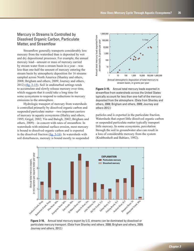
tac11-0651_fig03-15

1

10

100

1,000

10,000

100,000

1,000,000

1 10 100 1,000 10,000 100,000 1,000,000Annu

al to

tal m

ercu

ry lo

ad e

xpor

ted

from

st

ream

bas

in, i

n gr

ams

per y

ear

Annual atmospheric deposition of total mercury to stream basin, in grams per year

1:1 line

tac11-0651_fig03-16

0

1

2

3

4

5

Particulate mercuryDissolved mercury

Annu

al to

tal m

ercu

ry e

xpor

t, in

mic

rogr

ams

per s

quar

e m

eter

per

yea

r

EXPLANATION

Looko

ut Creek,

Oreg.

Beaverto

n Creek, Oreg.

Pike Rive

r, Wis.

Evergreen Rive

r, Wis.

Oak Creek,

Wis.

St Marys

River, F

la.

Santa Fe Rive

r, Fla.

Little

Wekiv

a, Fla.

McTier C

reek, S.C.

Edisto Rive

r, S.C.

Fishing Brook,

N.Y.

Hudson Rive

r, N.Y.

Sleepers Rive

r, Vt.

Allequash

Creek, W

is.

Mercury in Streams Is Controlled by Dissolved Organic Carbon, Particulate Matter, and Streamflow

Streamflow generally transports considerably less mercury from the watershed than is deposited by wet and dry depositional processes. For example, the annual mercury load—amount or mass of mercury carried by stream water from a stream basin in a year—was less than one-half the amount of mercury entering the stream basin by atmospheric deposition for 16 streams sampled across North America (Shanley and others, 2008; Brigham and others, 2009; Journey and others, 2012) (fig. 3-15). Soil in undisturbed settings tends to accumulate and slowly release mercury over time, which suggests that it could take a long time for some ecosystems to respond to reductions in mercury emissions to the atmosphere.

Hydrologic transport of mercury from watersheds is controlled primarily by dissolved organic carbon and suspended particulate matter—two important carriers of mercury in aquatic ecosystems (Hurley and others, 1995; Grigal, 2002; Yin and Balogh, 2002; Brigham and others, 2009)—in concert with rates of streamflow. In watersheds with minimal surface erosion, most mercury is bound to dissolved organic carbon and is exported in the dissolved fraction (fig. 3-16). In watersheds with soil disturbances, mercury is bound mostly to suspended

particles and is exported in the particulate fraction. Watersheds that export little dissolved organic carbon or suspended particulate matter typically transport little mercury. In some ecosystems, percolation through the soil to groundwater also can result in a loss of considerable mercury from the system (Krabbenhoft and Babiarz, 1992).

Figure 3-15. Annual total mercury loads exported in streamflow from watersheds across the United States typically account for less than one-half of the mercury deposited from the atmosphere. (Data from Shanley and others, 2008; Brigham and others, 2009; Journey and others 2012.)

Figure 3-16. Annual total mercury export by U.S. streams can be dominated by dissolved or particulate mercury transport. (Data from Shanley and others. 2008; Brigham and others, 2009; Journey and others, 2012.)

Chapter 3


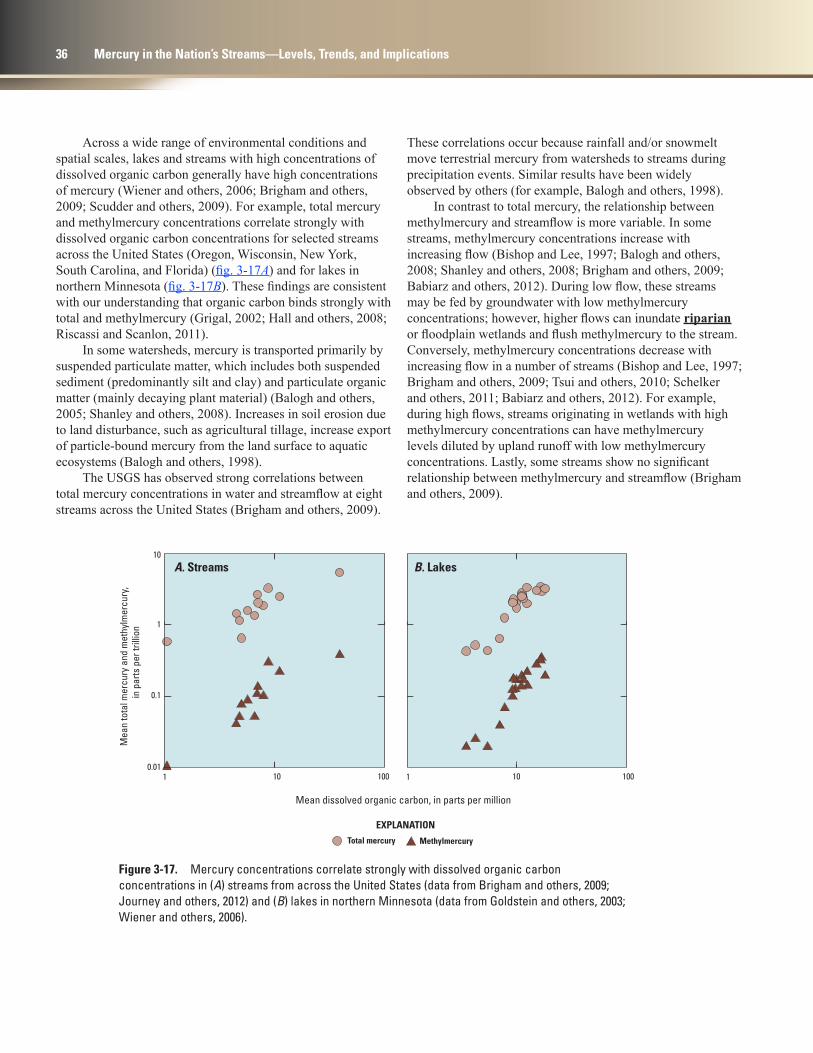
tac11-0651_fig03-17

Total mercury

EXPLANATION

Methylmercury

0.01

0.1

1

10

10 100 1 10 1001

Mean dissolved organic carbon, in parts per million

Mea

n to

tal m

ercu

ry a

nd m

ethy

lmer

cury

,

in p

arts

per

trill

ion

A. Streams B. Lakes

Across a wide range of environmental conditions and spatial scales, lakes and streams with high concentrations of dissolved organic carbon generally have high concentrations of mercury (Wiener and others, 2006; Brigham and others, 2009; Scudder and others, 2009). For example, total mercury and methylmercury concentrations correlate strongly with dissolved organic carbon concentrations for selected streams across the United States (Oregon, Wisconsin, New York, South Carolina, and Florida) (fig. 3-17A) and for lakes in northern Minnesota (fig. 3-17B). These findings are consistent with our understanding that organic carbon binds strongly with total and methylmercury (Grigal, 2002; Hall and others, 2008; Riscassi and Scanlon, 2011).

In some watersheds, mercury is transported primarily by suspended particulate matter, which includes both suspended sediment (predominantly silt and clay) and particulate organic matter (mainly decaying plant material) (Balogh and others, 2005; Shanley and others, 2008). Increases in soil erosion due to land disturbance, such as agricultural tillage, increase export of particle-bound mercury from the land surface to aquatic ecosystems (Balogh and others, 1998).

The USGS has observed strong correlations between total mercury concentrations in water and streamflow at eight streams across the United States (Brigham and others, 2009).

These correlations occur because rainfall and/or snowmelt move terrestrial mercury from watersheds to streams during precipitation events. Similar results have been widely observed by others (for example, Balogh and others, 1998).

In contrast to total mercury, the relationship between methylmercury and streamflow is more variable. In some streams, methylmercury concentrations increase with increasing flow (Bishop and Lee, 1997; Balogh and others, 2008; Shanley and others, 2008; Brigham and others, 2009; Babiarz and others, 2012). During low flow, these streams may be fed by groundwater with low methylmercury concentrations; however, higher flows can inundate riparian or floodplain wetlands and flush methylmercury to the stream. Conversely, methylmercury concentrations decrease with increasing flow in a number of streams (Bishop and Lee, 1997; Brigham and others, 2009; Tsui and others, 2010; Schelker and others, 2011; Babiarz and others, 2012). For example, during high flows, streams originating in wetlands with high methylmercury concentrations can have methylmercury levels diluted by upland runoff with low methylmercury concentrations. Lastly, some streams show no significant relationship between methylmercury and streamflow (Brigham and others, 2009).

Figure 3-17. Mercury concentrations correlate strongly with dissolved organic carbon concentrations in (A) streams from across the United States (data from Brigham and others, 2009; Journey and others, 2012) and (B) lakes in northern Minnesota (data from Goldstein and others, 2003; Wiener and others, 2006).


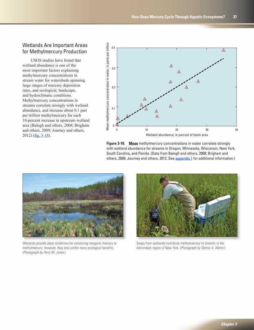
Seeps from wetlands contribute methylmercury to streams in the Adirondack region of New York. (Photograph by Dennis A. Wentz.)

tac11-0651_fig03-18

0

0.1

0.2

0.3

0.4

0 10 20 30 40 Mea

n m

ethy

lmer

cury

con

cent

ratio

n in

wat

er, i

n pa

rts p

er tr

illio

n

Wetland abundance, in percent of basin area

Wetlands Are Important Areas for Methylmercury Production

USGS studies have found that wetland abundance is one of the most important factors explaining methylmercury concentrations in stream water for watersheds spanning large ranges of mercury deposition rates, and ecological, landscape, and hydroclimatic conditions.Methylmercury concentrations in streams correlate strongly with wetland abundance, and increase about 0.1 part per trillion methylmercury for each 10-percent increase in upstream wetland area (Balogh and others, 2008; Brigham and others, 2009; Journey and others, 2012) (fig. 3-18).

Figure 3-18. Mean methylmercury concentrations in water correlate strongly with wetland abundance for streams in Oregon, Minnesota, Wisconsin, New York, South Carolina, and Florida. (Data from Balogh and others, 2008; Brigham and others, 2009; Journey and others, 2012. See appendix 1 for additional information.)

Wetlands provide ideal conditions for converting inorganic mercury to methylmercury; however, they also confer many ecological benefits. (Photograph by Perry M. Jones.)

Chapter 3


Wetlands are efficient at converting inorganic mercury deposited by the atmosphere into methylmercury because they provide favorable conditions for mercury methylation, including abundant organic matter and low dissolved oxygen levels (St. Louis and others, 1994; Grigal, 2002). Mercury methylation occurs naturally under these conditions as sulfate-reducing bacteria obtain energy by breaking down organic matter, using sulfate much like we use oxygen to respire (Compeau and Bartha, 1985; Gilmour and others, 1992; St. Louis and others, 1994). Methylmercury is formed as an incidental byproduct of this process and is transported from the wetlands bound to dissolved organic carbon. Moderate sulfate concentrations in wetlands have been shown to exacerbate methylmercury formation (see “Anticipated Future Trends and Possible Confounding Factors,” p. 65).

Wetlands also confer many ecological benefits, including habitat for plant and animal species, and trapping and retaining nutrients and sediment from runoff. More than one-half of all wetlands originally present in the contiguous 48 States have been lost largely due to drainage for agriculture, urban development, and other human uses (Dahl, 1990, 2011). In some areas, the loss has been substantially greater. California, for example, has lost more than 90 percent of its original wetlands (Dahl, 1990). Efforts to restore previously drained or degraded wetlands, or to construct new wetlands for ecological benefit, should seek to optimize these benefits while mitigating factors that promote methylmercury production.

Bioaccumulation Causes Methylmercury Concentrations in Aquatic Biota to Increase with Trophic Level

Bioaccumulation within an aquatic food web can cause methylmercury concentrations in fish to increase to levels that are potentially harmful to both people and fish-eating wildlife. Methylmercury is incorporated and bioconcentrated at the base of the food web by algae and other microorganisms attached to submerged surfaces in smaller streams or by algae and other microorganisms suspended in the water of larger rivers or lakes. Higher in the food web, the accumulation of methylmercury from one trophic level to the next (biomagnification) occurs almost exclusively through dietary consumption. Thus, algae are eaten by aquatic invertebrates; invertebrates are eaten by small fish; small fish are eaten by larger fish; and larger fish are eaten by wildlife, such as wading birds and mammals, or by humans. At each step, the methylmercury in the prey organism is accumulated in the tissue of the consumer. Methylmercury in fish occurs predominantly in muscle tissue in association with sulfur (Kuwabara and others, 2007), and because methylmercury in this form is eliminated slowly, it biomagnifies, or increases in concentration as it moves up the food web.

Bioaccumulation caused methylmercury concentrations to increase by nearly 1 million times from water to top predator fish in USGS studies conducted nationwide during 2002–2009 (fig. 3-19). Most of the increase (10,000 times) occurred during bioconcentration (from water to algae), whereas the increase due to biomagnification (from invertebrates to top predator fish) was only about 100 times. These results are typical of other freshwater food webs (Bodaly and others, 1997; Cleckner and others, 1998; Wiener and others, 2003; Kuwabara and others, 2005).

Sediment from a rice field in the Yolo Bypass Wildlife Area, California, is analyzed to determine how much methylmercury is produced in this type of agricultural setting. (Photograph by Mark Marvin-DiPasquale.)


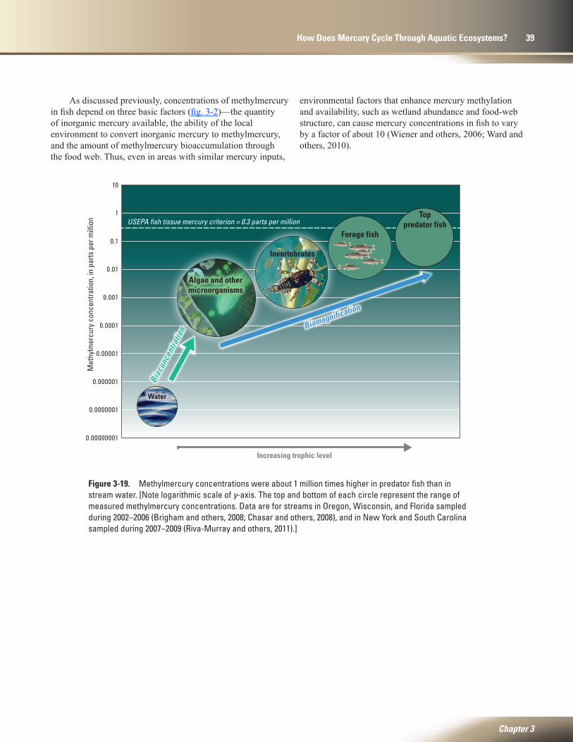
tac11-0651_fig01-03

Biomagnification

Bioc

once

ntra

tion

Met

hylm

ercu

ry c

once

ntra

tion,

in p

arts

per

mill

ion USEPA fish tissue mercury criterion = 0.3 parts per million

Water

Algae and othermicroorganisms

Invertebrates

Toppredator fish

Forage fish

0.00000001

0.0000001

0.000001

0.00001

0.0001

0.001

0.01

0.1

1

10

Increasing trophic level

Figure 3-19. Methylmercury concentrations were about 1 million times higher in predator fish than in stream water. [Note logarithmic scale of y-axis. The top and bottom of each circle represent the range of measured methylmercury concentrations. Data are for streams in Oregon, Wisconsin, and Florida sampled during 2002–2006 (Brigham and others, 2008; Chasar and others, 2008), and in New York and South Carolina sampled during 2007–2009 (Riva-Murray and others, 2011).]

As discussed previously, concentrations of methylmercury in fish depend on three basic factors (fig. 3-2)—the quantity of inorganic mercury available, the ability of the local environment to convert inorganic mercury to methylmercury, and the amount of methylmercury bioaccumulation through the food web. Thus, even in areas with similar mercury inputs,

environmental factors that enhance mercury methylation and availability, such as wetland abundance and food-web structure, can cause mercury concentrations in fish to vary by a factor of about 10 (Wiener and others, 2006; Ward and others, 2010).

Chapter 3


Figure 3-21. Mean methylmercury concentrations in (A) invertebrates, (B) forage fish, and (C) predator fish from streams in Oregon, Wisconsin, and Florida correlate strongly with percentages of wetland in the upstream basins. (Modified from Chasar and others, 2009. Because methylmercury concentrations for invertebrates are typically reported on a dry weight basis, methylmercury concentrations for forage and predator fish also are shown on a dry weight basis in this figure for ease of comparison among the graphs.)

tac11-0651_fig03-20

0.1

1

10

0.01 0.1 1 10

Methylmercury concentration in water, in parts per trillion

Met

hylm

ercu

ry c

once

ntra

tion

in la

rgem

outh

bas

sin

par

ts p

er m

illio

n pe

r met

er

tac11-0651_fig03-21

0

0

50

100

150

200

200

400

600

800

0

2,000

4,000

6,000

0 10 20 30 40 Percent wetland

Mea

n m

ethy

lmer

cury

con

cent

ratio

n, in

par

ts p

er b

illio

n dr

y w

eigh

t

A. Invertebrates

B. Forage fish

C. Predator fish

Methylmercury Levels in Stream Biota Are Determined by the Supply of Methylmercury to the Base of the Food Web

A nationwide study during 1998 demonstrated that methylmercury concentrations in fish correlate strongly with methylmercury concentrations in stream water (Brumbaugh and others, 2001). Methylmercury in water accounted for 51 percent of the variation of mercury levels in largemouth bass (fig. 3-20), and about 39 percent of the variation for all fish species combined. Other variables, such as dissolved organic carbon concentration, sulfate concentration, pH, wetland percentage in the basin, and methylmercury concentration of bed sediment, showed significant, though weaker, correlations with fish methylmercury levels. Methylmercury concentrations in invertebrates, forage fish, and top predator fish also correlate strongly with methylmercury concentrations in water from streams in Oregon, Wisconsin, and Florida (Chasar and others, 2009). The strong correlations of methylmercury concentrations in fish and aquatic invertebrates with methylmercury concentrations in stream water suggest that the supply of methylmercury to the base of the food web is the most important factor influencing methylmercury levels in biota across these diverse ecosystems.

Methylmercury concentrations in invertebrates, forage fish, and predator fish collected from streams in Oregon, Wisconsin, and Florida correlate strongly with the percentage of wetland in the upstream basin (fig. 3-21) (Chasar and others, 2009). This is expected, given (1) that methylmercury supply to the base of the food web is an important control on mercury bioaccumulation in these streams, and (2) there

is a strong positive relationship between methylmercury concentration in water and wetland percentage for these streams (fig. 3-18). The relationships in figure 3-21 may provide useful and simple methods for estimating the potential for mercury contamination in streams with similar environmental characteristics to the streams studied.

Figure 3-20. Methylmercury concentrations in water correlate strongly with methylmercury concentrations in largemouth bass collected across the United States during 1998. (Modified from Brumbaugh and others, 2001; see appendix 1 for additional information.)


Methylmercury Levels in Stream Biota also Are Determined by Trophic Position within the Food Web

Across the large ranges of environmental conditions encompassed by streams in Oregon, Wisconsin, and Florida, the increases of mercury through food webs were similar to those for previously studied lakes and other aquatic ecosystems (Wiener and others, 2003; Chasar and others, 2009). Methylmercury concentrations in attached algae and other microorganisms were 2,900–1,700,000 times the methylmercury concentrations in water (Bell and Scudder, 2007) (fig. 3-19) and compare well to previously published values of 10,000–1,000,000 (Ward and others, 2010). In addition, methylmercury concentrations increased by 2.1–8.6 times from invertebrates to forage fish, and by 1.2–8.2 times from forage fish to predator fish (Chasar and others, 2009)—values that are close to the increases of 2–5 times previously reported (Ward and others, 2010).

Food webs for urban streams in Oregon, Wisconsin, and Florida were simpler (top predator fish generally were smaller and/or less piscivorous) than those for nonurban streams, and average trophic positions for top predator fish from urban streams were considerably lower than for nonurban streams (Chasar and others, 2009). Consequently, the methylmercury biomagnification potential for urban streams was considerably lower than for nonurban streams, and urban streams tended to have lower methylmercury concentrations in fish at the top of the food web.

Trophic position also can be an important control on mercury levels in biota when streams with similar environmental conditions are compared. For example, median trophic positions for forage and predator fish were higher for streams in South Carolina than in New York, and these differences apparently were sufficient to account for higher measured fish methylmercury levels for streams in South Carolina (Riva-Murray and others, 2011). This was true despite methylmercury concentrations (potentially available to the base of the food webs) for streams in South Carolina that were, on average, only about one-half those for streams in New York.

Chapter 3


Evergreen River, Wisconsin Phot

ogra

ph b

y De

nnis

A. W

entz

.

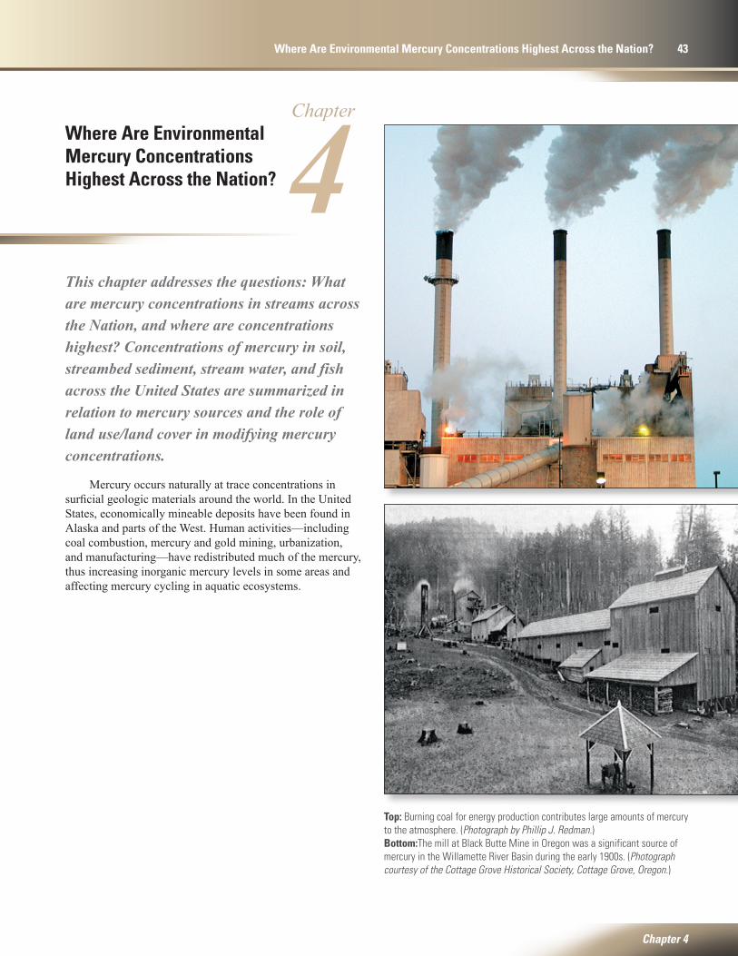
Phot

ogra

ph b

y De

nnis

A. W

entz

.

This chapter addresses the questions: What are mercury concentrations in streams across the Nation, and where are concentrations highest? Concentrations of mercury in soil, streambed sediment, stream water, and fish across the United States are summarized in relation to mercury sources and the role of land use/land cover in modifying mercury concentrations.

Mercury occurs naturally at trace concentrations in surficial geologic materials around the world. In the United States, economically mineable deposits have been found in Alaska and parts of the West. Human activities—including coal combustion, mercury and gold mining, urbanization, and manufacturing—have redistributed much of the mercury, thus increasing inorganic mercury levels in some areas and affecting mercury cycling in aquatic ecosystems.

Top: Burning coal for energy production contributes large amounts of mercury to the atmosphere. (Photograph by Phillip J. Redman.) Bottom:The mill at Black Butte Mine in Oregon was a significant source of mercury in the Willamette River Basin during the early 1900s. (Photograph courtesy of the Cottage Grove Historical Society, Cottage Grove, Oregon.)

Where Are Environmental Mercury Concentrations Highest Across the Nation?

Chapter 4

Where Are Environmental Mercury Concentrations Highest Across the Nation? 43

Chapter

4

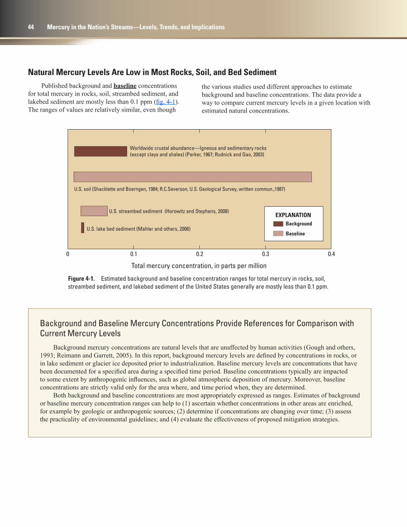
Natural Mercury Levels Are Low in Most Rocks, Soil, and Bed Sediment

Figure 4-1. Estimated background and baseline concentration ranges for total mercury in rocks, soil, streambed sediment, and lakebed sediment of the United States generally are mostly less than 0.1 ppm.

Background and Baseline Mercury Concentrations Provide References for Comparison with Current Mercury Levels

Background mercury concentrations are natural levels that are unaffected by human activities (Gough and others, 1993; Reimann and Garrett, 2005). In this report, background mercury levels are defined by concentrations in rocks, or in lake sediment or glacier ice deposited prior to industrialization. Baseline mercury levels are concentrations that have been documented for a specified area during a specified time period. Baseline concentrations typically are impacted to some extent by anthropogenic influences, such as global atmospheric deposition of mercury. Moreover, baseline concentrations are strictly valid only for the area where, and time period when, they are determined.

Both background and baseline concentrations are most appropriately expressed as ranges. Estimates of background or baseline mercury concentration ranges can help to (1) ascertain whether concentrations in other areas are enriched, for example by geologic or anthropogenic sources; (2) determine if concentrations are changing over time; (3) assess the practicality of environmental guidelines; and (4) evaluate the effectiveness of proposed mitigation strategies.

Published background and baseline concentrations for total mercury in rocks, soil, streambed sediment, and lakebed sediment are mostly less than 0.1 ppm (fig. 4-1). The ranges of values are relatively similar, even though

the various studies used different approaches to estimate background and baseline concentrations. The data provide a way to compare current mercury levels in a given location with estimated natural concentrations.

tac11-0651_fig04-01

0 0.1 0.2 0.3 0.4

Total mercury concentration, in parts per million

Worldwide crustal abundance—Igneous and sedimentary rocks (except clays and shales) (Parker, 1967; Rudnick and Gao, 2003)

U.S. soil (Shacklette and Boerngen, 1984; R.C.Severson, U.S. Geological Survey, written commun.,1987)

U.S. streambed sediment (Horowitz and Stephens, 2008)

U.S. lake bed sediment (Mahler and others, 2006)

EXPLANATIONBackground

Baseline


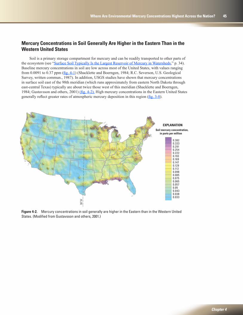
tac11-0651_fig04-02

0.3820.3330.2910.2540.2220.1930.1690.1470.1290.1120.0980.0850.0750.0650.0570.050.0430.0380.033

Soil mercury concentration, in parts per million

EXPLANATION

98˚W

Mercury Concentrations in Soil Generally Are Higher in the Eastern Than in the Western United States

Soil is a primary storage compartment for mercury and can be readily transported to other parts of the ecosystem (see “Surface Soil Typically Is the Largest Reservoir of Mercury in Watersheds,” p. 34). Baseline mercury concentrations in soil are low across most of the United States, with values ranging from 0.0091 to 0.37 ppm (fig. 4-1) (Shacklette and Boerngen, 1984; R.C. Severson, U.S. Geological Survey, written commun., 1987). In addition, USGS studies have shown that mercury concentrations in surface soil east of the 98th meridian (which runs approximately from eastern North Dakota through east-central Texas) typically are about twice those west of this meridian (Shacklette and Boerngen, 1984; Gustavsson and others, 2001) (fig. 4-2). High mercury concentrations in the Eastern United States generally reflect greater rates of atmospheric mercury deposition in this region (fig. 3-8).

Figure 4-2. Mercury concentrations in soil generally are higher in the Eastern than in the Western United States. (Modified from Gustavsson and others, 2001.)

Chapter 4


tac11-0651_fig04-03

0.00 0.02 0.04 0.06 0.08 0.10 0.12 0.14

Populationdensity≥ 50th

percentile

Urban land

Rangeland

Forest

Pasture

Cropland

Total mercury concentration, in parts per million

Baselineconcentration

range

Land

use

/land

cov

er

Mercury Concentrations in Streambed Sediment Are Higher in Urbanized Areas Than in Areas Affected by Other Land Uses or Land Covers

USGS studies have shown that baseline total mercury concentrations in streambed sediment have a range of about 0.02–0.06 ppm (fig. 4-1; calculated from data in Horowitz and Stephens, 2008). Except for areas contaminated by mercury and gold mining, the largest enrichments of mercury in bed sediment are in urbanized areas—those basins with more than 25 percent urban land or with population densities greater than the 50th percentile (fig. 4-3) (Horowitz and Stephens, 2008; Scudder and others, 2009). In these areas, anthropogenic sources of mercury are numerous, and can include wastewater- treatment plants, waste incinerators, crematoriums, steel mills, cement kilns, and disposal sites for batteries, thermometers, fluorescent bulbs, and a variety of other mercury-containing wastes. Basins with more than 50 percent forested land showed a slight enrichment of mercury greater than baseline values (fig. 4-3), an effect attributed primarily to dry deposition on leaf surfaces, and possibly to elevated organic matter in these systems (Horowitz and Stephens, 2008).

Figure 4-3. Total mercury concentrations in streambed sediment are somewhat enhanced in streams draining forested land; however, urbanized areas, with their many anthropogenic mercury sources, exhibit concentrations that are about two to three times baseline levels and are higher than for any other land use/land cover. (Data from Horowitz and Stephens, 2008; see appendix 1 for additional information.)


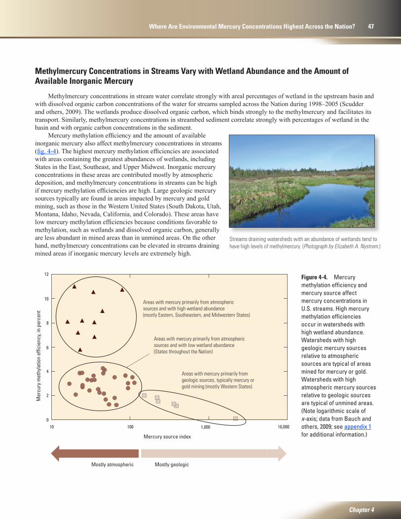
tac11-0651_fig04-04

0

2

4

6

8

10

12

1,000 10,000

Mer

cury

met

hyla

tion

effic

ienc

y, in

per

cent

Mercury source index

Areas with mercury primarily from geologic sources, typically mercury or gold mining (mostly Western States)

Areas with mercury primarily from atmospheric sources and with high wetland abundance (mostly Eastern, Southeastern, and Midwestern States)

Areas with mercury primarily from atmospheric sources and with low wetland abundance (States throughout the Nation)

Mostly atmospheric Mostly geologic

10 100

Streams draining watersheds with an abundance of wetlands tend to have high levels of methylmercury. (Photograph by Elizabeth A. Nystrom.)

Methylmercury Concentrations in Streams Vary with Wetland Abundance and the Amount of Available Inorganic Mercury

Methylmercury concentrations in stream water correlate strongly with areal percentages of wetland in the upstream basin and with dissolved organic carbon concentrations of the water for streams sampled across the Nation during 1998–2005 (Scudder and others, 2009). The wetlands produce dissolved organic carbon, which binds strongly to the methylmercury and facilitates its transport. Similarly, methylmercury concentrations in streambed sediment correlate strongly with percentages of wetland in the basin and with organic carbon concentrations in the sediment.

Mercury methylation efficiency and the amount of available inorganic mercury also affect methylmercury concentrations in streams (fig. 4-4). The highest mercury methylation efficiencies are associated with areas containing the greatest abundances of wetlands, including States in the East, Southeast, and Upper Midwest. Inorganic mercury concentrations in these areas are contributed mostly by atmospheric deposition, and methylmercury concentrations in streams can be high if mercury methylation efficiencies are high. Large geologic mercury sources typically are found in areas impacted by mercury and gold mining, such as those in the Western United States (South Dakota, Utah, Montana, Idaho, Nevada, California, and Colorado). These areas have low mercury methylation efficiencies because conditions favorable to methylation, such as wetlands and dissolved organic carbon, generally are less abundant in mined areas than in unmined areas. On the other hand, methylmercury concentrations can be elevated in streams draining mined areas if inorganic mercury levels are extremely high.

Chapter 4


Figure 4-4. Mercury methylation efficiency and mercury source affect mercury concentrations in U.S. streams. High mercury methylation efficiencies occur in watersheds with high wetland abundance. Watersheds with high geologic mercury sources relative to atmospheric sources are typical of areas mined for mercury or gold. Watersheds with high atmospheric mercury sources relative to geologic sources are typical of unmined areas. (Note logarithmic scale of x-axis; data from Bauch and others, 2009; see appendix 1 for additional information.)

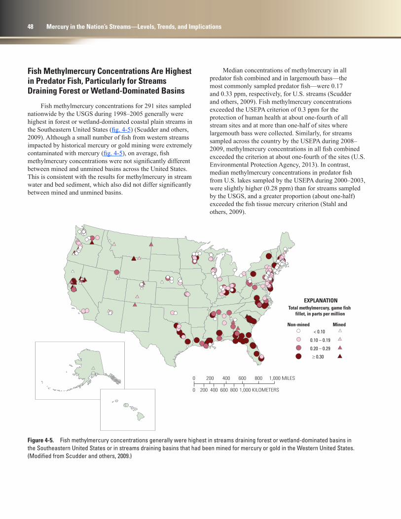
tac11-0651_fig04-05

0 1,000 KILOMETERS200 400 600 800

0 200 400 600 800 1,000 MILES

EXPLANATION

MinedNon-mined< 0.10

0.10 – 0.19

0.20 – 0.29

≥ 0.30

Total methylmercury, game fish fillet, in parts per million

Fish Methylmercury Concentrations Are Highest in Predator Fish, Particularly for Streams Draining Forest or Wetland-Dominated Basins

Fish methylmercury concentrations for 291 sites sampled nationwide by the USGS during 1998–2005 generally were highest in forest or wetland-dominated coastal plain streams in the Southeastern United States (fig. 4-5) (Scudder and others, 2009). Although a small number of fish from western streams impacted by historical mercury or gold mining were extremely contaminated with mercury (fig. 4-5), on average, fish methylmercury concentrations were not significantly different between mined and unmined basins across the United States. This is consistent with the results for methylmercury in stream water and bed sediment, which also did not differ significantly between mined and unmined basins.

Median concentrations of methylmercury in all predator fish combined and in largemouth bass—the most commonly sampled predator fish—were 0.17 and 0.33 ppm, respectively, for U.S. streams (Scudder and others, 2009). Fish methylmercury concentrations exceeded the USEPA criterion of 0.3 ppm for the protection of human health at about one-fourth of all stream sites and at more than one-half of sites where largemouth bass were collected. Similarly, for streams sampled across the country by the USEPA during 2008–2009, methylmercury concentrations in all fish combined exceeded the criterion at about one-fourth of the sites (U.S. Environmental Protection Agency, 2013). In contrast, median methylmercury concentrations in predator fish from U.S. lakes sampled by the USEPA during 2000–2003, were slightly higher (0.28 ppm) than for streams sampled by the USGS, and a greater proportion (about one-half) exceeded the fish tissue mercury criterion (Stahl and others, 2009).

Figure 4-5. Fish methylmercury concentrations generally were highest in streams draining forest or wetland-dominated basins in the Southeastern United States or in streams draining basins that had been mined for mercury or gold in the Western United States. (Modified from Scudder and others, 2009.)


tac11-0651_fig04-06

0

0.5

1.0

1.5

2.0

2.5

Undeveloped Mixed Mined Agricultural Urban

Med

ian

met

hylm

ercu

ry c

once

ntra

tion

in la

rgem

outh

bas

s, in

par

ts p

er m

illio

n pe

r met

er

The highest median fish methylmercury concentration for streams was 0.42 ppm for spotted bass, a mostly piscivorous fish (Scudder and others, 2009). The median methylmercury concentration for smallmouth bass—a somewhat more omnivorous species than spotted or largemouth bass—was 0.20 ppm. Conversely, the lowest median fish methylmercury concentration was 0.07 ppm for rainbow and cutthroat trout. Low mercury concentrations in trout probably occur because their diets include significant portions of insects and other invertebrates, which occupy lower food-web trophic positions (thus, are lower in mercury), than do the diets of most predator fish, which feed at higher trophic levels (Scott and Crossman, 1973).

Methylmercury concentrations in largemouth bass during 1998–2005 typically were highest for streams draining undeveloped basins and basins with mixed land use/land cover (fig. 4-6) (Scudder and others, 2009). These areas contain high percentages of forest and wetland,

and high concentrations of methylmercury, all of which are strong predictors of mercury concentrations in fish (Krabbenhoft and others, 1999; Brumbaugh and others, 2001; Scudder and others, 2009). In fact, methylmercury levels in largemouth bass correlated most strongly with percentages of the upstream basin in evergreen forest and woody wetland.

Methylmercury concentrations in largemouth bass were lowest in urban streams (fig. 4-6) (Scudder and others, 2009), even though these streams had the highest total mercury concentrations in streambed sediment. The low mercury levels in fish from urban streams are attributed to a relative absence of factors conducive to methylmercury production (such as wetlands) compared to forested, undeveloped basins, and to the generally simpler food webs in urban streams, whereby top predator fish are smaller and less piscivorous than in nonurban streams. Methylmercury concentrations in largemouth bass from mined and agricultural areas were intermediate between those from undeveloped/mixed areas and urban areas.

Mining of Mercury and Gold Can Cause High Mercury Concentrations in Stream Water, Streambed Sediment, and Fish

Mercury concentrations in stream water, streambed sediment, and fish from selected mercury mining areas of Alaska and California and gold mining areas of California and Nevada have been summarized by Gray (2003b, table 3). Maximum mercury concentrations downstream of these mining areas can be extremely high and can have adverse effects on aquatic ecosystems.

Figure 4-6. Length-normalized methylmercury concentrations in largemouth bass were highest in streams draining undeveloped basins and basins with mixed land use/land cover. (Data from Bauch and others, 2009; see appendix 1 for additional information.)

Chapter 4


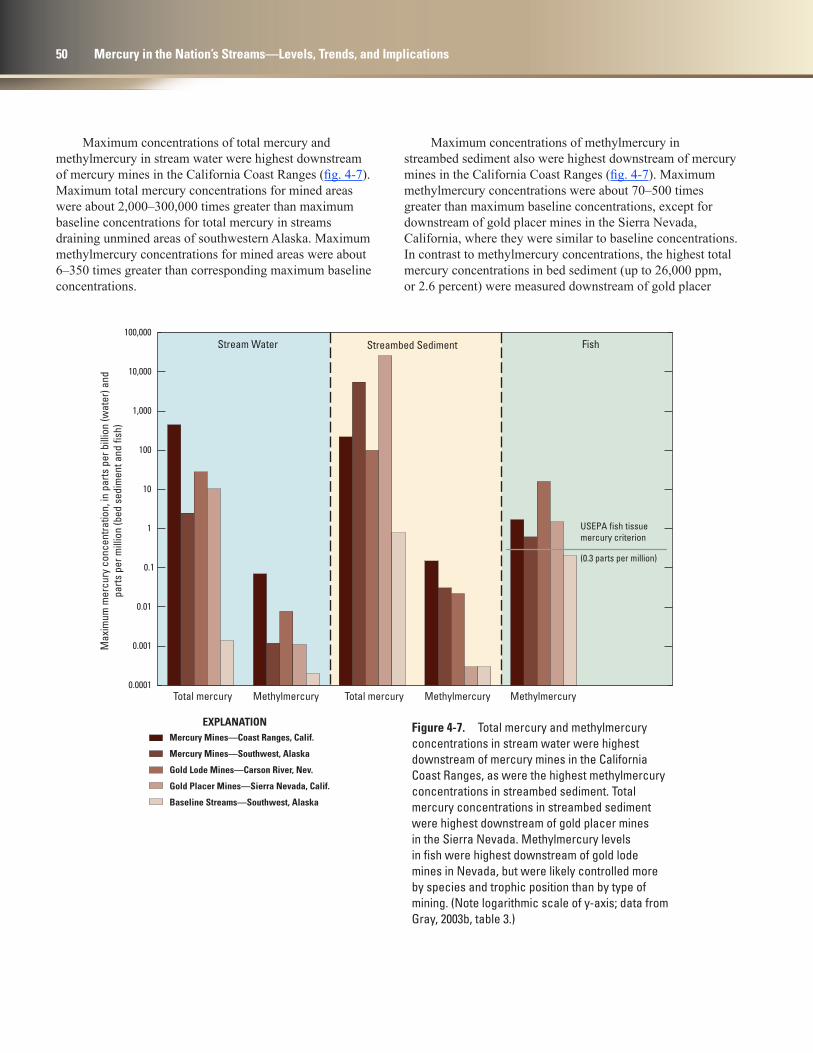
tac11-0651_fig04-07

0.0001

0.001

0.01

0.1

1

10

100

1,000

10,000

100,000

Total mercury Methylmercury Total mercury Methylmercury Methylmercury

Max

imum

mer

cury

con

cent

ratio

n, in

par

ts p

er b

illio

n (w

ater

) and

pa

rts p

er m

illio

n (b

ed s

edim

ent a

nd fi

sh)

Stream Water Streambed Sediment Fish

Mercury Mines—Coast Ranges, Calif.

Mercury Mines—Southwest, Alaska

Gold Lode Mines—Carson River, Nev.

Gold Placer Mines—Sierra Nevada, Calif.

Baseline Streams—Southwest, Alaska

EXPLANATION

USEPA fish tissuemercury criterion

(0.3 parts per million)

Maximum concentrations of total mercury and methylmercury in stream water were highest downstream of mercury mines in the California Coast Ranges (fig. 4-7). Maximum total mercury concentrations for mined areas were about 2,000–300,000 times greater than maximum baseline concentrations for total mercury in streams draining unmined areas of southwestern Alaska. Maximum methylmercury concentrations for mined areas were about 6–350 times greater than corresponding maximum baseline concentrations.

Figure 4-7. Total mercury and methylmercury concentrations in stream water were highest downstream of mercury mines in the California Coast Ranges, as were the highest methylmercury concentrations in streambed sediment. Total mercury concentrations in streambed sediment were highest downstream of gold placer mines in the Sierra Nevada. Methylmercury levels in fish were highest downstream of gold lode mines in Nevada, but were likely controlled more by species and trophic position than by type of mining. (Note logarithmic scale of y-axis; data from Gray, 2003b, table 3.)

Maximum concentrations of methylmercury in streambed sediment also were highest downstream of mercury mines in the California Coast Ranges (fig. 4-7). Maximum methylmercury concentrations were about 70–500 times greater than maximum baseline concentrations, except for downstream of gold placer mines in the Sierra Nevada, California, where they were similar to baseline concentrations. In contrast to methylmercury concentrations, the highest total mercury concentrations in bed sediment (up to 26,000 ppm, or 2.6 percent) were measured downstream of gold placer


operations in the Sierra Nevada, California, and are consistent with the large losses of mercury attributed to these placer operations. Maximum total mercury concentrations in bed sediment were 100–30,000 times greater than maximum baseline concentrations.

The maximum methylmercury concentration in bed sediment downstream of gold placer mines in the Sierra Nevada was similar to the maximum baseline methylmercury concentration, despite having total mercury concentrations that were more than 30,000 times greater than baseline concentrations (fig. 4-7). This observation indicates that basins mined for placer gold in the Sierra Nevada may have environmental characteristics that are less conducive to mercury methylation than baseline areas and is consistent with the degraded nature of stream channels that have undergone significant placer mining in this area (Alpers and others, 2005).

Maximum methylmercury concentrations in fish collected downstream of mined areas in Alaska, California, and Nevada were about 4–200 times greater than in fish from baseline streams (fig. 4-7); however, results from the different areas can not be directly compared because the fish were from varying, and sometimes unspecified, species. Maximum fish methylmercury levels were about 2–50 times greater than the USEPA criterion of 0.3 ppm for the protection of human health.

The highest reported fish methylmercury concentration (16 ppm) was in a walleye (a piscivorous fish) captured in Lahontan Reservoir, which is downstream of the Comstock Lode in Nevada and part of the Carson River Mercury Superfund site (Lawrence, 2003) (fig. 4-7). Fish methylmercury levels in largemouth, smallmouth, and spotted bass from five California reservoirs affected by historical hydraulic gold mining were as high as 1.5 ppm (May and others, 2000). The maximum fish methylmercury concentration in streams from southwestern Alaska (0.62 ppm) was in a Dolly Varden—an omnivorous resident salmonid (Gray and others, 2000). The maximum measured fish methylmercury levels are consistent with trophic positions typically occupied by the fish.

Chapter 4


Phot

ogra

ph b

y De

nnis

A. W

entz

.

Healing Springs, South Carolina

Phot

ogra

ph b

y De

nnis

A. W

entz

.

ChapterHow Do Environmental Mercury Levels Vary Over Time?

This chapter addresses the questions: How do environmental mercury levels vary over time? What is the outlook for the future? Historical and recent U.S. trends of atmospheric mercury deposition and mercury concentrations in fish are presented, and expectations for the future are discussed.

Important questions currently facing natural resource managers, and environmental scientists in general, include: “How much of the mercury falling on our land and water from atmospheric deposition is derived from human activities?,” “Are mercury concentrations in aquatic ecosystems and fish increasing or decreasing over time?,” “How are mercury concentrations likely to change in the future?.” The answers to these questions have important implications regarding the effectiveness of regulations designed to control emissions of mercury to air and discharges of mercury to water.

(Photograph by Mark E. Brigham.)

Chapter 5

How Do Environmental Mercury Levels Vary Over Time? 53

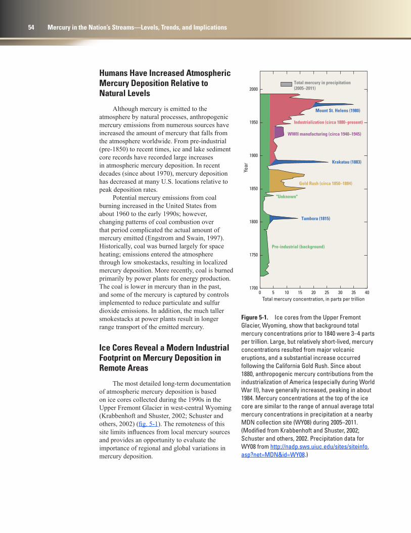
tac11-0651_fig05-01

Pre-industrial (background)

"Unknown"

Gold Rush (circa 1850–1884)

Krakatau (1883)

WWII manufacturing (circa 1940–1945)

Industrialization (circa 1880–present)

Mount St. Helens (1980)

2000

1950

1900

1850

1800

1750

17000 5 10 15 20 25 30 35 40

Total mercury concentration, in parts per trillion

Year

Tambora (1815)

Total mercury in precipitation (2005–2011)

Humans Have Increased Atmospheric Mercury Deposition Relative to Natural Levels

Although mercury is emitted to the atmosphere by natural processes, anthropogenic mercury emissions from numerous sources have increased the amount of mercury that falls from the atmosphere worldwide. From pre-industrial (pre-1850) to recent times, ice and lake sediment core records have recorded large increases in atmospheric mercury deposition. In recent decades (since about 1970), mercury deposition has decreased at many U.S. locations relative to peak deposition rates.

Potential mercury emissions from coal burning increased in the United States from about 1960 to the early 1990s; however, changing patterns of coal combustion over that period complicated the actual amount of mercury emitted (Engstrom and Swain, 1997). Historically, coal was burned largely for space heating; emissions entered the atmosphere through low smokestacks, resulting in localized mercury deposition. More recently, coal is burned primarily by power plants for energy production. The coal is lower in mercury than in the past, and some of the mercury is captured by controls implemented to reduce particulate and sulfur dioxide emissions. In addition, the much taller smokestacks at power plants result in longer range transport of the emitted mercury.

Ice Cores Reveal a Modern Industrial Footprint on Mercury Deposition in Remote Areas

The most detailed long-term documentation of atmospheric mercury deposition is based on ice cores collected during the 1990s in the Upper Fremont Glacier in west-central Wyoming (Krabbenhoft and Shuster, 2002; Schuster and others, 2002) (fig. 5-1). The remoteness of this site limits influences from local mercury sources and provides an opportunity to evaluate the importance of regional and global variations in mercury deposition.

Figure 5-1. Ice cores from the Upper Fremont Glacier, Wyoming, show that background total mercury concentrations prior to 1840 were 3–4 parts per trillion. Large, but relatively short-lived, mercury concentrations resulted from major volcanic eruptions, and a substantial increase occurred following the California Gold Rush. Since about 1880, anthropogenic mercury contributions from the industrialization of America (especially during World War II), have generally increased, peaking in about 1984. Mercury concentrations at the top of the ice core are similar to the range of annual average total mercury concentrations in precipitation at a nearby MDN collection site (WY08) during 2005–2011. (Modified from Krabbenhoft and Shuster, 2002; Schuster and others, 2002. Precipitation data for WY08 from http://nadp.sws.uiuc.edu/sites/siteinfo.asp?net=MDN&id=WY08.)


http://nadp.sws.uiuc.edu/sites/siteinfo.asp?net=MDN&id=WY08

http://nadp.sws.uiuc.edu/sites/siteinfo.asp?net=MDN&id=WY08

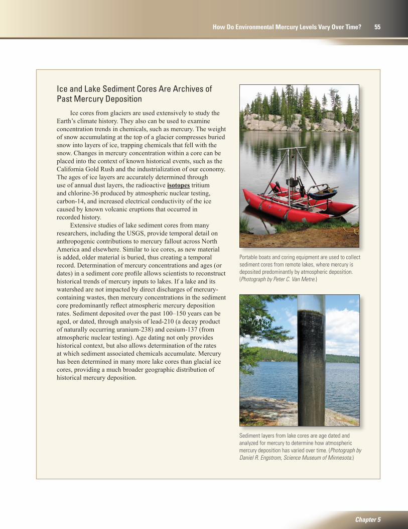
Portable boats and coring equipment are used to collect sediment cores from remote lakes, where mercury is deposited predominantly by atmospheric deposition. (Photograph by Peter C. Van Metre.)

Sediment layers from lake cores are age dated and analyzed for mercury to determine how atmospheric mercury deposition has varied over time. (Photograph by Daniel R. Engstrom, Science Museum of Minnesota.)

Ice and Lake Sediment Cores Are Archives of Past Mercury Deposition

Ice cores from glaciers are used extensively to study the Earth’s climate history. They also can be used to examine concentration trends in chemicals, such as mercury. The weight of snow accumulating at the top of a glacier compresses buried snow into layers of ice, trapping chemicals that fell with the snow. Changes in mercury concentration within a core can be placed into the context of known historical events, such as the California Gold Rush and the industrialization of our economy. The ages of ice layers are accurately determined through use of annual dust layers, the radioactive isotopes tritium and chlorine-36 produced by atmospheric nuclear testing, carbon-14, and increased electrical conductivity of the ice caused by known volcanic eruptions that occurred in recorded history.

Extensive studies of lake sediment cores from many researchers, including the USGS, provide temporal detail on anthropogenic contributions to mercury fallout across North America and elsewhere. Similar to ice cores, as new material is added, older material is buried, thus creating a temporal record. Determination of mercury concentrations and ages (or dates) in a sediment core profile allows scientists to reconstruct historical trends of mercury inputs to lakes. If a lake and its watershed are not impacted by direct discharges of mercury-containing wastes, then mercury concentrations in the sediment core predominantly reflect atmospheric mercury deposition rates. Sediment deposited over the past 100–150 years can be aged, or dated, through analysis of lead-210 (a decay product of naturally occurring uranium-238) and cesium-137 (from atmospheric nuclear testing). Age dating not only provides historical context, but also allows determination of the rates at which sediment associated chemicals accumulate. Mercury has been determined in many more lake cores than glacial ice cores, providing a much broader geographic distribution of historical mercury deposition.

Chapter 5


Three distinct volcanic events were recorded by the Upper Fremont Glacier ice-core profile. The eruptions of Mount Tambora and Mount Krakatau—the two largest in recorded history—are easily distinguished despite their location in equatorial Indonesia. The eruption of Mount St. Helens, although orders of magnitude smaller than those of the two Indonesian volcanoes, also is easily seen because of its relative closeness (about 600 kilometers) to the Upper Fremont Glacier. These three events together contributed 6 percent of the total mercury in the ice core.

Two mercury peaks are consistent with the timing of the California Gold Rush, during which mercury was used as an amalgamating agent to enhance the recovery of gold (see “Historical Mercury and Gold Mining Are Sources of Mercury to Some Streams,” p. 32). The high volatility of mercury, along with its high loss rate during gold mining, are expected to cause contamination considerable distances from mined areas. The first Gold Rush peak in the ice core approximates the period from the discovery of gold in 1848 until its peak production in 1852 (Hill, 1926). The second (later) Gold Rush peak coincides approximately with a large increase in mercury production that may have been fueled by the widespread use of hydraulic mining (Hill, 1926; Alpers and Hunerlach, 2000). The Sawyer Decision (issued in 1884) considerably limited this form of mining (Alpers and Hunerlach, 2000), and subsequent mercury peaks from mining were not seen in the ice core. The two peaks that correlate with gold mining activities in California account for 13 percent of the total mercury in the ice core.

Beginning about 1880, total mercury concentrations in the Upper Fremont Glacier ice core were slightly greater than background concentrations until the period encompassed by World War II, then gradually increased to 20–25 parts per trillion until about 1984. These elevated concentrations coincide with the industrialization of the United States and are likely due to emissions from coal-fired power plants, waste incinerators, chlor-alkali plants, and other industries. Decreasing mercury concentrations in the ice core since 1984 correspond with declines in U.S. and world mercury production (fig. 3-13), and with implementation of U.S. legislation designed to control industrial mercury emissions

(see “Nationwide Trends of Mercury in Fish Generally Were Downward during the 1970s and 1980s,” p. 60). Mercury concentrations at the top of the ice core are similar to annual average total mercury concentrations measured in precipitation at the nearest MDN collection site (WY08) during 2005–2011 (fig. 5-1). Anthropogenic mercury sources throughout the post-1900 period of industrialization have contributed most of mercury deposited during that time.

Natural mercury contributions (background and volcanic eruptions) and anthropogenic contributions (Gold Rush, World War II, and industrialization) to the Upper Fremont Glacier ice core account for 48 and 52 percent, respectively, of total mercury in the core. It is important to realize, however, that all anthropogenic mercury contributions have occurred since about 1840 and make up a much larger percentage of the total contributions since that time.

Historical Rates of Mercury Deposition Reflected by Lake Sediment Cores Have Increased Since Pre-Industrial Times, and the Increases Are Greatest in Major Urban Areas

Sediment cores from lakes in extremely remote regions, unaffected by regional anthropogenic emissions, typically show that mercury inputs during recent years are about double input rates in pre-industrial times (before about 1850). Cores from lakes in the remote Canadian Arctic, for example, show an approximate doubling of mercury accumulation rate relative to pre-industrial times (fig. 5-2). Similar findings for other remote areas, including northern Canada (Lockhart and others, 1995), southeastern Alaska (Engstrom and Swain, 1997), northern Alaska (Fitzgerald and others, 2005), and northern Scandinavia (Johansson, 1985; Verta and others, 1989; Bindler and others, 2001) typically show about a 1.5- to 3-fold increase in mercury concentration and accumulation rate, with a central value close to a 2-fold increase (Verta and others, 1989; Fitzgerald and others, 1998).


tac11-0651_fig05-02

1800

1850

1900

1950

2000

2050

0 10 20 30 40 50 60 70 80 90

Year

Mercury accumulation rate, in micrograms per square meter per year

Remote Canadian Arctic Rural Continental United States

Major U.S. Urban Area

Sediment cores collected from undisturbed, rural lakes across the continental United States typically show about a 3- to 5-fold increase in mercury accumulation rate relative to pre-industrial times (fig. 5-2; Swain and others, 1992; Engstrom and Swain, 1997; Lorey and Driscoll, 1999; Van Metre and Fuller, 2009; Drevnick and others, 2012; Van Metre, 2012). These are greater increases than for remote locations in Alaska and Canada, as discussed above. Similarly large increases in mercury concentrations and accumulation rates have been observed in southern Scandinavia—close to continental Europe (Johansson, 1985; Bindler and others, 2001). The greater mercury deposition rates, relative to remote regions, reflect the many sources of mercury emissions within the continental United States (see “Mercury Sources to Aquatic Ecosystems Are Both Anthropogenic and Natural,” p. 24) and within continental Europe.

Undisturbed lakes within or near major urban areas receive much greater mercury deposition than more rural lakes, and therefore show much larger increases relative to pre-industrial times (fig. 5-2). A USGS study of lakes across the United States, in settings ranging from rural to urban, found that recent mercury accumulation rates in near-urban lakes averaged about 10 times the accumulation rates in pre-industrial times, although this factor varied considerably among locations (Van Metre, 2012). Other studies have similarly found larger modern mercury accumulation rates in urban lakes compared to undisturbed rural settings (Engstrom and others, 2007).

Figure 5-2. Mercury accumulation rates in lake sediment cores reflect historical increases in anthropogenic mercury emissions. Typical sediment core profiles are shown for three general settings: a remote area (Little Coal Lake, Yukon Territories in the Canadian Arctic); rural United States (Hobbs Lake, Wyoming); and a major urban area (Carlton Lake, Florida). The core profiles reveal increases of approximately 2, 4.5, and 10 times, respectively, compared to background concentrations measured at the bottoms of the remote and rural cores. (Modified from Van Metre and Wilson, 2003; Van Metre. 2012.)

Chapter 5


tac11-0651_fig05-03

Alaska Rural continentalUnited States

Near major U.S. urban areas

Total annual mercury deposition, in micrograms per square meter

Deposition sourceEXPLANATION

Natural (background)

Global

Regional

Urban

7.4 19 78

The spatial and temporal information derived through analysis of lake cores in remote areas of Alaska, rural continental United States, and near major U.S. urban areas, can be used to apportion mercury sources into four generalized types (fig. 5-3). Three scales of anthropogenic mercury are important: global—mercury emissions that are dispersed widely in the atmosphere; regional—mercury that falls out at a regional to national scale; and local—mercury that falls out within tens of kilometers of major urban areas. In addition, natural (or background) mercury is deposited from the atmosphere. Background mercury levels can be determined from deeper sediment-core layers that reflect mercury deposition before industrialization, and therefore lack significant anthropogenic mercury. Lakes in or near urban areas receive mercury from all four of these general source types and typically have the highest mercury inputs. Knowledge of general source types helps State and Federal environmental regulatory agencies set realistic goals with respect to fish mercury levels and desired reductions in mercury emissions.

Lake Sediment Cores Show Decreasing Mercury Deposition in Recent Decades, Particularly in Urban Areas

Trends in mercury concentrations were determined for sediment cores collected from 31 lakes and reservoirs nationwide (fig. 5-4) (Mahler and others, 2006). The trends were evaluated for the period after 1970 (generally 25–30 years), which corresponds to the period following enactment of the National Environmental Policy Act and the Clean Air Act (1969 and 1970, respectively)—legislation that affected emissions of mercury and other trace elements to the atmosphere (see “Nationwide Trends of Mercury in Fish Generally Were Downward during the 1970s and 1980s,” p. 60).

Figure 5-3. Atmospheric mercury source types include anthropogenic (global, regional, and urban) and natural (background). Remote regions, such as Alaska, receive roughly equal portions of background and global anthropogenic mercury. Rural regions within the continental United States receive additional mercury from regional to national emission sources. Large U.S. urban areas receive a still greater mercury load. (See appendix 1 for additional information.)


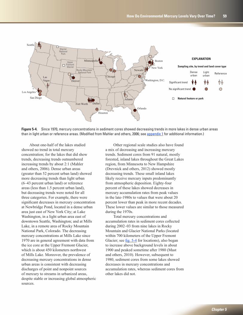
tac11-0651_fig05-04

Atlanta

Denver

Rocky Mountain National Park

GlacierNational

Park

Upper Fremont Glacier

San Diego

Los Angeles

Las Vegas

Seattle

Houston

Fort Worth Dallas

Minneapolis

Chicago

Orlando

Boston

New YorkNewark

Washington, D.C.

Sampling site, by trend and land cover type

Natural feature or park

Lighturban

Denseurban

Reference

Significant trend


EXPLANATION

About one-half of the lakes studied showed no trend in total mercury concentration; for the lakes that did show trends, decreasing trends outnumbered increasing trends by about 2:1 (Mahler and others, 2006). Dense urban areas (greater than 52 percent urban land) showed more decreasing trends than light urban (6–43 percent urban land) or reference areas (less than 1.5 percent urban land), but decreasing trends were noted for all three categories. For example, there were significant decreases in mercury concentration at Newbridge Pond, located in a dense urban area just east of New York City; at Lake Washington, in a light urban area east of downtown Seattle, Washington; and at Mills Lake, in a remote area of Rocky Mountain National Park, Colorado. The decreasing mercury concentrations at Mills Lake since 1970 are in general agreement with data from the ice core at the Upper Fremont Glacier, which is about 450 kilometers northwest of Mills Lake. Moreover, the prevalence of decreasing mercury concentrations in dense urban areas is consistent with decreasing discharges of point and nonpoint sources of mercury to streams in urbanized areas, despite stable or increasing global atmospheric sources.

Other regional scale studies also have found a mix of decreasing and increasing mercury trends. Sediment cores from 91 natural, mostly forested, inland lakes throughout the Great Lakes region, from Minnesota to New Hampshire (Drevnick and others, 2012) showed mostly decreasing trends. These small inland lakes likely receive mercury inputs predominantly from atmospheric deposition. Eighty-four percent of these lakes showed decreases in mercury accumulation rates from peak values in the late-1980s to values that were about 20 percent lower than peak in more recent decades. These lower values are similar to those measured during the 1970s.

Total mercury concentrations and accumulation rates in sediment cores collected during 2002–03 from nine lakes in Rocky Mountain and Glacier National Parks (located within 700 kilometers of the Upper Fremont Glacier; see fig. 5-4 for locations), also began to increase above background levels in about 1900 and peaked sometime after 1980 (Mast and others, 2010). However, subsequent to 1980, sediment cores from some lakes showed decreases in mercury concentrations and accumulation rates, whereas sediment cores from other lakes did not.

Figure 5-4. Since 1970, mercury concentrations in sediment cores showed decreasing trends in more lakes in dense urban areas than in light urban or reference areas. (Modified from Mahler and others, 2006; see appendix 1 for additional information.)

Chapter 5


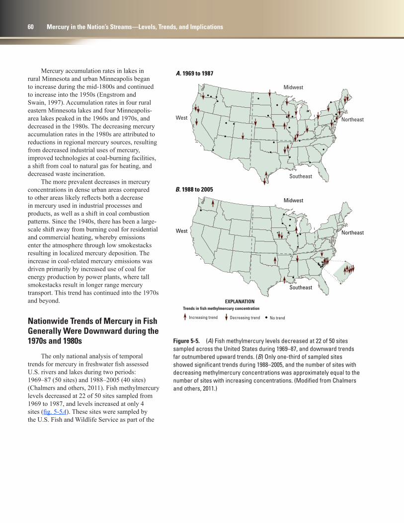
tac11-0651_fig05-05

West

Southeast

Midwest

Northeast

West

Southeast

Midwest

Northeast

Trends in fish methylmercury concentration

Increasing trend Decreasing trend No trend

A. 1969 to 1987

B. 1988 to 2005

EXPLANATION

Mercury accumulation rates in lakes in rural Minnesota and urban Minneapolis began to increase during the mid-1800s and continued to increase into the 1950s (Engstrom and Swain, 1997). Accumulation rates in four rural eastern Minnesota lakes and four Minneapolis-area lakes peaked in the 1960s and 1970s, and decreased in the 1980s. The decreasing mercury accumulation rates in the 1980s are attributed to reductions in regional mercury sources, resulting from decreased industrial uses of mercury, improved technologies at coal-burning facilities, a shift from coal to natural gas for heating, and decreased waste incineration.

The more prevalent decreases in mercury concentrations in dense urban areas compared to other areas likely reflects both a decrease in mercury used in industrial processes and products, as well as a shift in coal combustion patterns. Since the 1940s, there has been a large-scale shift away from burning coal for residential and commercial heating, whereby emissions enter the atmosphere through low smokestacks resulting in localized mercury deposition. The increase in coal-related mercury emissions was driven primarily by increased use of coal for energy production by power plants, where tall smokestacks result in longer range mercury transport. This trend has continued into the 1970s and beyond.

Nationwide Trends of Mercury in Fish Generally Were Downward during the 1970s and 1980s

The only national analysis of temporal trends for mercury in freshwater fish assessed U.S. rivers and lakes during two periods: 1969–87 (50 sites) and 1988–2005 (40 sites) (Chalmers and others, 2011). Fish methylmercury levels decreased at 22 of 50 sites sampled from 1969 to 1987, and levels increased at only 4 sites (fig. 5-5A). These sites were sampled by the U.S. Fish and Wildlife Service as part of the

Figure 5-5. (A) Fish methylmercury levels decreased at 22 of 50 sites sampled across the United States during 1969–87, and downward trends far outnumbered upward trends. (B) Only one-third of sampled sites showed significant trends during 1988–2005, and the number of sites with decreasing methylmercury concentrations was approximately equal to the number of sites with increasing concentrations. (Modified from Chalmers and others, 2011.)


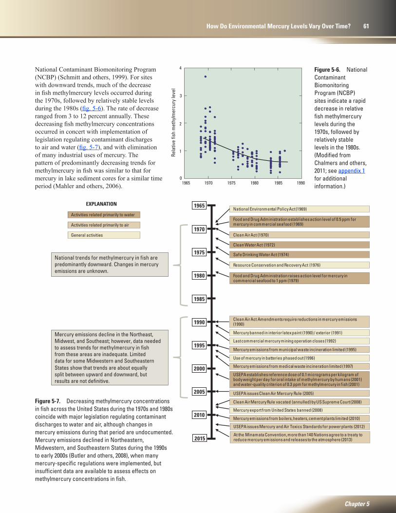
tac11-0651_fig05-07

National trends for methylmercury in fish are predominantly downward. Changes in mercuryemissions are unknown.

Mercury emissions decline in the Northeast, Midwest, and Southeast; however, data needed to assess trends for methylmercury in fish from these areas are inadequate. Limited data for some Midwestern and Southeastern States show that trends are about equally split between upward and downward, but results are not definitive.

1970

1975

1980

1985

1990

1995

2000

2005

2010

1965

Use of mercury in batteries phased out (1996)

Clean Air Act (1970)

Clean Water Act (1972)

Mercury emissions from medical waste incineration limited (1997)

Resource Conservation and Recovery Act (1976)

Safe Drinking Water Act (1974)

Clean Air Mercury Rule vacated (annulled) by US Supreme Court (2008)

Mercury emissions from boilers, heaters, cement plants limited (2010)

USEPA issues Clean Air Mercury Rule (2005)

Last commercial mercury mining operation closes (1992)

Clean Air Act Amendments require reductions in mercury emissions (1990)

USEPA establishes reference dose of 0.1 micrograms per kilogram of body weight per day for oral intake of methylmercury by humans (2001) and water- quality criterion of 0.3 ppm for methylmercury in fish (2001)

Mercury banned in interior latex paint (1990) / exterior (1991)

Food and Drug Administration establishes action level of 0.5 ppm for mercury in commercial seafood (1969)

Food and Drug Administration raises action level for mercury in commercial seafood to 1 ppm (1979)

Mercury emissions from municipal waste incineration limited (1995)

Mercury export from United States banned (2008)

USEPA issues Mercury and Air Toxics Standards for power plants (2012)

National Environmental Policy Act (1969)

2015At the Minamata Convention, more than 140 Nations agree to a treaty to reduce mercury emissions and releases to the atmosphere (2013)

EXPLANATION

Activities related primarily to water

Activities related primarily to air

General activities

tac11-0651_fig05-06

Rela

tive

fish

met

hylm

ercu

ry le

vel

1965 1970 1975 1980 1985 19900

2

1

3

4National Contaminant Biomonitoring Program (NCBP) (Schmitt and others, 1999). For sites with downward trends, much of the decrease in fish methylmercury levels occurred during the 1970s, followed by relatively stable levels during the 1980s (fig. 5-6). The rate of decrease ranged from 3 to 12 percent annually. These decreasing fish methylmercury concentrations occurred in concert with implementation of legislation regulating contaminant discharges to air and water (fig. 5-7), and with elimination of many industrial uses of mercury. The pattern of predominantly decreasing trends for methylmercury in fish was similar to that for mercury in lake sediment cores for a similar time period (Mahler and others, 2006).

Figure 5-6. National Contaminant Biomonitoring Program (NCBP) sites indicate a rapid decrease in relative fish methylmercury levels during the 1970s, followed by relatively stable levels in the 1980s. (Modified from Chalmers and others, 2011; see appendix 1 for additional information.)

Figure 5-7. Decreasing methylmercury concentrations in fish across the United States during the 1970s and 1980s coincide with major legislation regulating contaminant discharges to water and air, although changes in mercury emissions during that period are undocumented. Mercury emissions declined in Northeastern, Midwestern, and Southeastern States during the 1990s to early 2000s (Butler and others, 2008), when many mercury-specific regulations were implemented, but insufficient data are available to assess effects on methylmercury concentrations in fish.

Chapter 5


For 1988–2005, consistent records for methylmercury in fish tissue were available for only 40 sites in Southeastern and Midwestern States; these sites were primarily sampled by various State resource agencies (Chalmers and others, 2011). Only 13 of 40 sites showed trends, and these were about equally split between downward (7) and upward (6) trends (fig. 5-5B). Elimination of nationally coordinated fish contaminant monitoring after 1987 has resulted in insufficient data to analyze national trends since that time. The higher ratio of upward to downward trends for methylmercury in fish in the Southeast may be partly due to the greater importance of global mercury sources in the Southeast compared to the Northeast and Midwest (Seigneur and others, 2004; Chalmers and others, 2011).

Changes in methylmercury concentrations in fish over the decadal time scales of the above studies may have affected human exposure through fish consumption in some areas. Of the 39 sites with detectable trends of methylmercury concentrations in fish (fig. 5-5A and 5-5B), 6 sites had concentrations that started above the USEPA criterion of 0.3 ppm for the protection of human health, but ended below the criterion; all were in the Northeast, Midwest, or West and were sampled during 1969–87 (Chalmers and others, 2011). In the Southeast, on the other hand, three sites—all sampled in the 1988–2005 period—had upward trends that started below the USEPA criterion but ended above the criterion.

(Photograph by Mark E. Brigham.)

In contrast to the approximately equal numbers of upward and downward trends for other parts of the Southeast reported by Chalmers and others (2011), trends for mercury in largemouth bass for more than 60 sites in the Florida Everglades were almost exclusively downward during approximately the same period (Atkeson and others, 2005; Axelrad and others, 2011). Moreover, a recent analysis of fish monitoring data from the Great Lakes region of the United States and Canada found that mercury concentrations in largemouth bass generally decreased during 1970–2009; however, walleye mercury concentrations decreased early in that period, then leveled off or began to increase during the 1990s (Monson and others, 2011). An explanation for this apparent inconsistency was not given, but it was noted that decreasing fish mercury levels would be expected given recent reductions in mercury emissions in North America and Europe.


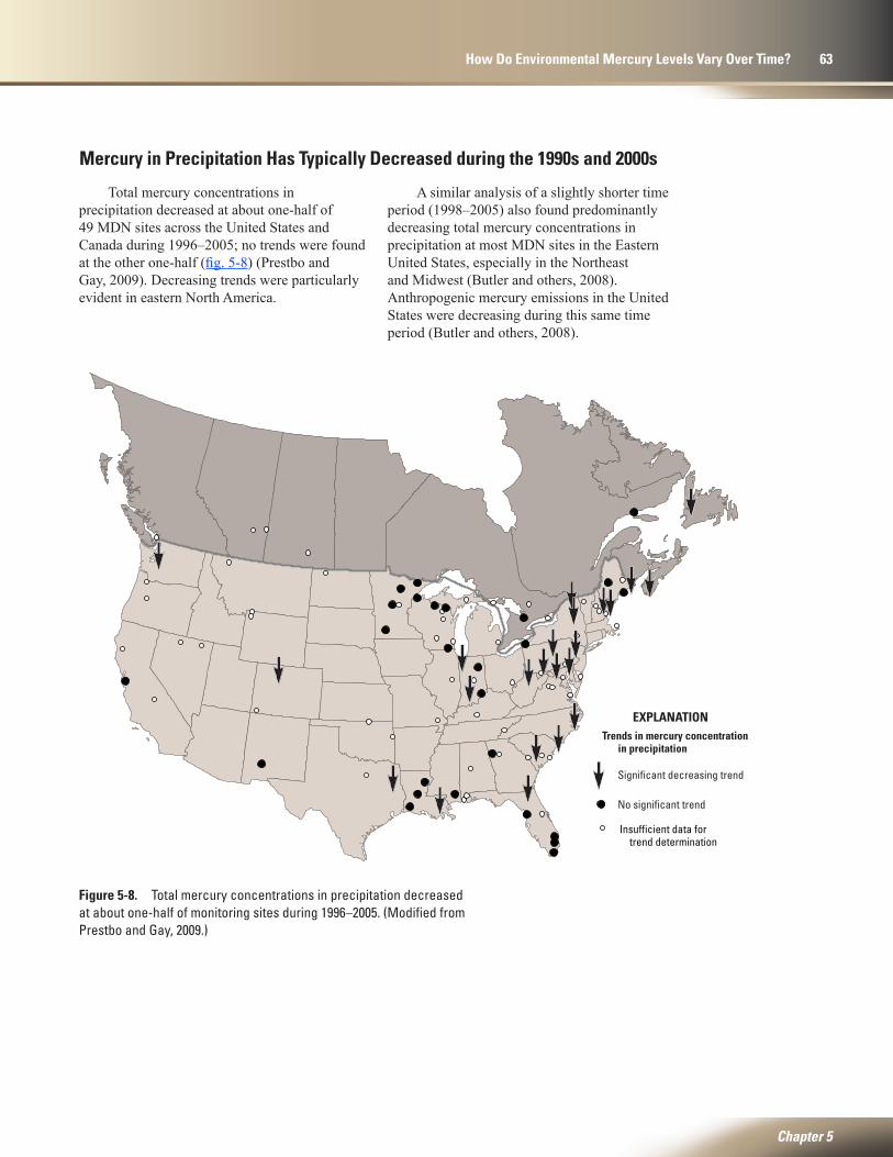
Insufficient data for trend determination

Trends in mercury concentration in precipitation


Significant decreasing trend

EXPLANATION

tac11-0651_fig05-08

Total mercury concentrations in precipitation decreased at about one-half of 49 MDN sites across the United States and Canada during 1996–2005; no trends were found at the other one-half (fig. 5-8) (Prestbo and Gay, 2009). Decreasing trends were particularly evident in eastern North America.

Figure 5-8. Total mercury concentrations in precipitation decreased at about one-half of monitoring sites during 1996–2005. (Modified from Prestbo and Gay, 2009.)

A similar analysis of a slightly shorter time period (1998–2005) also found predominantly decreasing total mercury concentrations in precipitation at most MDN sites in the Eastern United States, especially in the Northeast and Midwest (Butler and others, 2008). Anthropogenic mercury emissions in the United States were decreasing during this same time period (Butler and others, 2008).

Mercury in Precipitation Has Typically Decreased during the 1990s and 2000s

Chapter 5


Recent Trends in Environmental Mercury Concentrations Are Consistent with Legislation Designed to Limit Mercury Discharges

Table 5-1 summarizes how environmental mercury concentrations in the United States have changed over time based on the information presented in this chapter. Ice cores and lake sediment cores provide considerable evidence that environmental mercury levels began to rise above background levels during the mid- to late-1800s in concert with the industrialization of the Nation (fig. 5-1). Concentrations continued to increase until the 1970s or 1980s, when world

Table 5-1. Trends in U.S. environmental mercury levels are consistent with trends in atmospheric source levels and with legislation designed to limit mercury discharged to air and water.

Preindustrial (pre-1850s)

Industrial (1850s–1970s)

Recent (post-1970s)

Envi

ronm

enta

l Dri

vers

Natural background mercury concentrations resulted primarily from volcanic and geothermal emissions, and rock weathering.

Mercury concentrations increased due to increasing world production and to increasing anthropogenic emissions, including burning of coal for heat and electricity, waste incineration, and industrial uses.

U.S. and worldwide mercury production declined. U.S. and worldwide emissions of mercury to the atmosphere decreased. The United States implemented legislation to regulate discharges of mercury and other contaminants to air and water.

Envi

ronm

enta

l Mer

cury

Res

pons

es

Ice Core Background concentrations averaged 3–4 parts per trillion.

Concentrations continued to rise above background levels.

Concentrations peaked at 20–25 parts per trillion in the mid-1980s, then decreased to about 10–15 parts per trillion during the late 1980s and early 1990s.

Lake Sediment Cores Background concentrations were low and stable.

Concentrations doubled in globally remote areas, increased by 3–5 times in U.S. rural areas, and exhibited greater increases in large U.S. metropolitan areas.

Concentrations generally leveled off or decreased.

Fish No data No data Concentrations decreased during the 1970s–80s, but showed no widespread trends during the 1990s–2000s.

Precipitation No data No data Concentrations in the Eastern United States ranged from about 5 to 13 parts per trillion and generally decreased during the 1990s–2000s.

production of mercury began to decrease, and when U.S. consumption and emissions of mercury began to decline in response to legislation intended to reduce uses of mercury and its discharge to air and water. Since then, the preponderance of monitoring data indicates that U.S. environmental mercury levels have generally been stable or decreasing. Based on the above associations of environmental mercury concentrations with mercury use and consumption statistics, it is likely that further reductions in mercury use would result in subsequent decreases in environmental mercury levels.


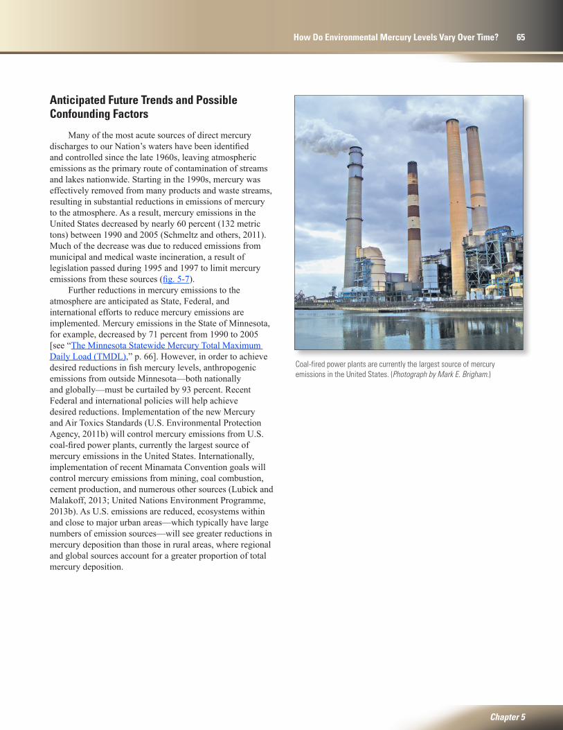
Coal-fired power plants are currently the largest source of mercury emissions in the United States. (Photograph by Mark E. Brigham.)

Anticipated Future Trends and Possible Confounding Factors

Many of the most acute sources of direct mercury discharges to our Nation’s waters have been identified and controlled since the late 1960s, leaving atmospheric emissions as the primary route of contamination of streams and lakes nationwide. Starting in the 1990s, mercury was effectively removed from many products and waste streams, resulting in substantial reductions in emissions of mercury to the atmosphere. As a result, mercury emissions in the United States decreased by nearly 60 percent (132 metric tons) between 1990 and 2005 (Schmeltz and others, 2011). Much of the decrease was due to reduced emissions from municipal and medical waste incineration, a result of legislation passed during 1995 and 1997 to limit mercury emissions from these sources (fig. 5-7).

Further reductions in mercury emissions to the atmosphere are anticipated as State, Federal, and international efforts to reduce mercury emissions are implemented. Mercury emissions in the State of Minnesota, for example, decreased by 71 percent from 1990 to 2005 [see “The Minnesota Statewide Mercury Total Maximum Daily Load (TMDL),” p. 66]. However, in order to achieve desired reductions in fish mercury levels, anthropogenic emissions from outside Minnesota—both nationally and globally—must be curtailed by 93 percent. Recent Federal and international policies will help achieve desired reductions. Implementation of the new Mercury and Air Toxics Standards (U.S. Environmental Protection Agency, 2011b) will control mercury emissions from U.S. coal-fired power plants, currently the largest source of mercury emissions in the United States. Internationally, implementation of recent Minamata Convention goals will control mercury emissions from mining, coal combustion, cement production, and numerous other sources (Lubick and Malakoff, 2013; United Nations Environment Programme, 2013b). As U.S. emissions are reduced, ecosystems within and close to major urban areas—which typically have large numbers of emission sources—will see greater reductions in mercury deposition than those in rural areas, where regional and global sources account for a greater proportion of total mercury deposition.

Chapter 5


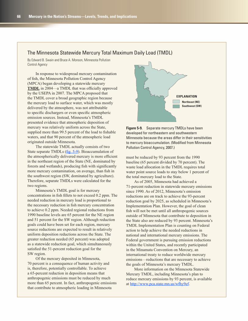
EXPLANATION

Northeast (NE)Southwest (SW)

tac11-0651_fig05-09

By Edward B. Swain and Bruce A. Monson, Minnesota Pollution Control Agency

In response to widespread mercury contamination of fish, the Minnesota Pollution Control Agency (MPCA) began developing a statewide mercury TMDL in 2004—a TMDL that was officially approved by the USEPA in 2007. The MPCA proposed that the TMDL cover a broad geographic region because the mercury load to surface water, which was mostly delivered by the atmosphere, was not attributable to specific dischargers or even specific atmospheric emission sources. Instead, Minnesota’s TMDL presented evidence that atmospheric deposition of mercury was relatively uniform across the State, supplied more than 99.5 percent of the load to fishable waters, and that 90 percent of the atmospheric load originated outside Minnesota.

The statewide TMDL actually consists of two State separate TMDLs (fig. 5-9). Bioaccumulation of the atmospherically delivered mercury is more efficient in the northeast region of the State (NE, dominated by forests and wetlands), producing fish with significantly more mercury contamination, on average, than fish in the southwest region (SW, dominated by agriculture). Therefore, separate TMDLs were calculated for the two regions.

Minnesota’s TMDL goal is for mercury concentrations in fish fillets to not exceed 0.2 ppm. The needed reduction in mercury load is proportional to the necessary reduction in fish mercury concentration to achieve 0.2 ppm. Needed regional reductions from 1990 baseline levels are 65 percent for the NE region and 51 percent for the SW region. Although reduction goals could have been set for each region, mercury source reductions are expected to result in relatively uniform deposition reductions across the State. The greater reduction needed (65 percent) was adopted as a statewide reduction goal, which simultaneously satisfied the 51-percent reduction goal for the SW region.

Of the mercury deposited in Minnesota, 70 percent is a consequence of human activity and is, therefore, potentially controllable. To achieve a 65-percent reduction in deposition means that anthropogenic emissions must be reduced by much more than 65 percent. In fact, anthropogenic emissions that contribute to atmospheric loading in Minnesota

must be reduced by 93 percent from the 1990 baseline (65 percent divided by 70 percent). The waste load allocation in the TMDL requires total water point source loads to stay below 1 percent of the total mercury load to the State.

As of 2005, Minnesota had achieved a 71-percent reduction in statewide mercury emissions since 1990. As of 2012, Minnesota’s emission reductions are on track to achieve the 93-percent reduction goal by 2025, as scheduled in Minnesota’s Implementation Plan. However, the goal of clean fish will not be met until all anthropogenic sources outside of Minnesota that contribute to deposition in the State also are reduced by 93 percent. Minnesota’s TMDL Implementation Plan is counting on Federal action to help achieve the needed reductions in national and international mercury emissions. The Federal government is pursuing emission reductions within the United States, and recently participated in the Minamata Convention on Mercury, an international treaty to reduce worldwide mercury emissions—reductions that are necessary to achieve the goals of Minnesota’s mercury TMDL.

More information on the Minnesota Statewide Mercury TMDL, including Minnesota’s plan to reduce mercury emissions by 93 percent, is available at http://www.pca.state.mn.us/wfhy9ef.

Figure 5-9. Separate mercury TMDLs have been developed for northeastern and southwestern Minnesota because the areas differ in their sensitivities to mercury bioaccumulation. (Modified from Minnesota Pollution Control Agency, 2007.)

The Minnesota Statewide Mercury Total Maximum Daily Load (TMDL)


http://www.pca.state.mn.us/wfhy9ef

Reductions in mercury emissions should result in decreased mercury levels in aquatic ecosystems, including fish. As described previously, concentrations of mercury in fish in streams generally have been declining in recent decades as a result of reductions in both mercury emissions to the atmosphere and direct discharge from industrial sources (Chalmers and others, 2011). In addition, controlled experiments have shown a direct relationship between the amount of added inorganic mercury and the resulting methylmercury concentrations in lake water and aquatic biota (Orihel and others, 2006, 2007).

A study in the Experimental Lakes Area of Canada—the Mercury Experiment to Assess Atmospheric Loadings in Canada and the United States (METAALICUS)—examined the fate of mercury added to the lake surface, an adjacent wetland, and the upland forested catchment. Traceable mercury, in the form of specific, stable (nonradioactive) isotopes was added each year from 2001 to 2007 by aerial application (Harris and others, 2007b; U.S. Geological Survey, 2013a). Most of the mercury that was deposited onto the upland catchment accumulated in the plants and soil. Although runoff contained a substantial amount of mercury that had been deposited to the land surface prior to the study, less than 1 percent of the new mercury was

transported to the lake in runoff (Harris and others, 2007b). This finding showed that in upland, terrestrial environments, it takes longer than a decade for newly fallen mercury to be transported in runoff. In contrast, methylmercury levels in lake water and biota responded rapidly to mercury added directly to the lake surface during the first 3 years of study (Harris and others, 2007b).

The METAALICUS study has yielded several important lessons (Harris and others, 2007b). Water bodies that receive most mercury inputs by direct deposition onto the water surface, such as lakes with relatively small watersheds, should respond within a few years to mercury emission reductions. In contrast, water bodies that receive most mercury inputs through runoff from the terrestrial environment, including streams and lakes with large watersheds relative to the lake surface area, could take as long as centuries to reach a new, lower mercury level in response to mercury emission reductions, due to the slow release of mercury from soil. Many lakes receive a mix of direct mercury deposition to the lake surface and mercury in runoff from the watershed. Fish methylmercury levels in these lakes should exhibit both a rapid decrease as a result of decreased deposition to the lake surface, and a slower response driven by slow equilibration of newly deposited mercury with mercury in runoff.

The United States Agrees to a Global Treaty to Reduce Mercury in the Environment

In January 2013, more than 140 United Nations member states, including the United States, agreed to a global, legally binding treaty to prevent emissions and releases of mercury to the atmosphere (Lubick and Malakoff, 2013; United Nations Environment Programme, 2013b). Known as the Minamata Convention on Mercury, the agreement provides controls and reductions across a wide range of products, processes, and industries where mercury is used, released, or emitted.

The treaty will require actions to reduce mercury emissions to the air from power plants and other sources (industrial boilers, smelters, waste incinerators, and cement plants), reduce the use of mercury in a variety of industrial processes and products (batteries, switches, relays, fluorescent lamps, soaps, cosmetics, thermometers, and blood pressure devices), and address mercury supply and trade. The treaty also will require the development of strategies to reduce the amount of mercury used by artisanal and small-scale miners and to increase public awareness of the dangers inherent in this process.

Chapter 5


The Mercury Experiment to Assess Atmospheric Loadings in Canada and the United States (METAALICUS)

To directly test the response of fish mercury concentrations to changes in mercury deposition rate, an international team of scientists conducted a whole ecosystem experiment—known as METAALICUS—at a remote lake in Canada starting in 1999 (Harris and others, 2007b). Different stable (nonradioactive) mercury isotopes were aerially applied to the lake surface, an adjacent wetland, and to the upland watershed. Isotopes allowed researchers to distinguish between experimentally applied mercury and mercury already present in the ecosystem. The METAALICUS study demonstrated several key findings that advanced our understanding of mercury cycling within watersheds.

Fish methylmercury concentrations increased rapidly with increases in mercury deposition onto the lake surface over the first 3 years of study. In contrast, less than 1 percent of the mercury isotope deposited to the upland watershed was exported to the lake. Mercury entering the lake in runoff from the uplands was mostly “older” mercury—that is, mercury that had been deposited prior to the beginning of the experiment, aged in the upland ecosystem, and exported along with dissolved organic matter.

The importance of mercury deposited to wetlands was strongly dependent on their hydrologic connectivity. In the METAALICUS study, the wetland surface was hydrologically

disconnected from anoxic zones within the wetland. Thus, methylmercury formation and delivery to the lake from the wetland was minimal (Harris and others, 2007b). Conversely, in wetlands with greater hydrologic connectivity, newly deposited mercury is more readily converted to methylmercury and more readily transported to adjacent lakes (Branfireun and others, 2005).

METAALICUS findings indicate that reductions in mercury emissions will yield rapid (on the order of years) reductions in fish methylmercury concentrations—particularly in lakes that receive a significant portion of their mercury by deposition onto the lake surface (Harris and others, 2007b). However, a full response will be delayed by the gradual export of mercury stored in associated watersheds. In lakes with larger watershed areas relative to lake areas, responses may take longer.

Traceable mercury isotopes were applied to the METAALICUS experimental watershed in Canada to distinguish added mercury from previously existing mercury. (Photograph by Vincent L. St. Louis, University of Alberta.)

Variability in ecosystem responses is expected, due to the numerous environmental and ecological factors that relate to mercury cycling and bioaccumulation; these factors vary both temporally and spatially. In addition to mercury inputs, disturbances, such as sulfate inputs, wetland restoration and water management, and climate change can have marked effects on methylmercury production within aquatic ecosystems.

Sulfate Inputs.—Sulfate stimulates microbial methylmercury formation in low-sulfur environments, thus decreasing sulfate concentrations should result in lower fish methylmercury levels in many of the Nation’s waters. In the Florida Everglades, the USGS showed that agricultural drainage containing elevated sulfate—primarily

from agricultural use—in combination with high regional atmospheric mercury deposition resulted in elevated methylmercury levels (Orem and others, 2011). Sulfur is widely used in agriculture, both as sulfate, and as elemental sulfur, which oxidizes to sulfate (Hagstrom, 1986). However, outside the Everglades, the role of agricultural sulfate in the mercury cycle has largely not been studied.

Atmospheric deposition also is an important source of sulfate—particularly for ecosystems that lack agricultural and other sources. In north-central Minnesota, sulfate deposition to a natural wetland was artificially increased for 4 years. The added sulfate markedly increased both methylmercury concentrations within the wetland and the export of methylmercury from the wetland to downstream waters (Jeremiason and others, 2006).


2011). High methylmercury levels are produced by sulfate-reducing bacteria, as flooded organic matter decays and sulfate is converted to sulfide. The sulfide can be re-oxidized to sulfate when the sediment dries, thus providing a renewed source of sulfate to fuel additional mercury methylation. Water management and hydrologic cycles associated with agricultural wetlands also have the potential to exacerbate mercury methylation (see “Wetland Restoration and Mercury in the San Francisco Bay and California’s Central Valley,” p. 71).

In the years following the experiment, after sulfate additions had ceased, methylmercury levels decreased (Coleman Wasik and others, 2012).

Increased atmospheric sulfate deposition since pre-industrial times likely has increased methylmercury concentrations in many locations more than would be expected based solely on anthropogenic mercury emissions. More recently, atmospheric sulfate deposition has been decreasing—by about 57 percent nationally between 1985 and 2009—due to controls mandated as part of the Clean Air Act Amendment (Burns and others, 2011; Lehmann and Gay, 2011). Continued decreases in sulfate emissions and sulfate deposition are projected in coming decades, as further controls are implemented (Burns and others, 2011). These controls on sulfate should confer a benefit in the form of lower methylmercury production (Coleman Wasik and others, 2012) and, therefore, lower methylmercury levels in fish. For example, in a study of lakes within Isle Royale National Park, decreases in fish methylmercury levels were attributed to reductions in sulfate deposition in the absence of any decrease in mercury deposition (Drevnick and others, 2007).

Due to the complex interactions of mercury, sulfur, and natural organic matter, the side benefit of decreased sulfate-driven methylmercury formation may not be realized in all locations. Dissolved organic matter concentrations have been increasing in many acid-sensitive aquatic ecosystems, partly as a response to decreased sulfate deposition (Clark and others, 2010). In some locations, the increased mobilization of dissolved organic matter has concomitantly increased mercury concentrations in runoff (Hongve and others, 2012). However, other locations where dissolved organic matter has increased have not had increases in mercury in runoff (Eklöf and others, 2012).

Wetland Restoration and Water Management.—The potential for mercury methylation should be considered among the many ecological and water-quality characteristics that may be altered by wetland restoration and water-management activities. Restoration of wetlands is a major thrust in many parts of the Nation due to the loss of about 53 percent of the original wetlands in the lower 48 States (Dahl, 1990).

Changes in water management, such as areal extent and frequency of inundation, also can exacerbate methylmercury formation. Recently flooded terrestrial soil (in newly constructed reservoirs and wetlands) and repeated cycles of wetting and drying of sediment (in reservoirs managed for flood control) are known to exacerbate mercury methylation (Bodaly and others, 1997, 2007; Snodgrass and others, 2000; Brigham and others, 2002; Hall and others, 2004, 2005; St. Louis and others, 2004; Orem and others,

Elevated methylmercury levels are commonly associated with newly constructed impoundments and with large water-level fluctuations in impoundments. (Photograph by Mark E. Brigham.)

Salt evaporation ponds (top) in South San Francisco Bay, California, are being restored to functional wetlands (bottom). (Photographs by Mark Marvin-DiPasquale.)

Chapter 5


Climate Change.—Changes in hydrology due to climate change have the potential to change methylmercury production in aquatic ecosystems. For example, precipitation patterns in many regions are predicted to shift to a regime of greater extremes in response to climate change (Intergovernmental Panel on Climate Change, 2007). Increased precipitation intensity and frequency of storm events are likely to lead to increased mercury inputs to aquatic systems (Krabbenhoft and Sunderland, 2013). Also, extreme dry periods punctuated by large rainfall events will likely increase methylmercury production in many settings (Monson, 2009; Orem and others, 2011).

Are Current Monitoring and Assessment Programs Sufficient to Evaluate Future Mercury Trends?

As the amount and global distribution of mercury emissions to the atmosphere change, effective monitoring of mercury emissions, deposition, and environmental levels is needed to understand how aquatic ecosystems respond to the changes. Global emissions of mercury to the atmosphere seem to have peaked in the 1970s, and worldwide anthropogenic mercury emissions have been relatively stable since at least 1990 (United Nations Environment Programme, 2013a). Although emissions in Asia rose steadily from 1990 to 2005 due to increased coal burning, these increases were offset by decreases in North America and Europe. However, recent evidence suggests that mercury emissions from industrial sectors (coal combustion, and production of cement, pig iron and steel, and nonferrous metals) may be increasing.

Estimates of mercury emissions have improved over time, but some sources still remain poorly characterized. This results in considerable uncertainty in estimates of total anthropogenic mercury emissions to the atmosphere. For example, the 2010 estimate for worldwide anthropogenic mercury emissions is 1,960 metric tons, but the estimated range for this estimate is quite large (1,010–4,070 metric tons) (United Nations Environment Programme, 2013a).

The Mercury Deposition Network (MDN) provides a useful framework for monitoring mercury in precipitation across the Nation. This program provides standardized equipment and procedures to participating agencies, based on a specific agency’s needs and available funding. However, because participation in the MDN is voluntary, some parts of the country are under-represented.

Furthermore, the collaborator funding model used by the MDN has resulted in some long-term sites being discontinued in response to changing priorities or budget shortfalls. As sites are discontinued, the ability to assess spatial or temporal trends in mercury deposition is compromised.

Dry deposition of mercury accounts for a large portion of total atmospheric mercury deposition, yet our understanding of geographic and time trends for this component is hampered by a lack of standardized methods and limited data. In 2009, the MDN established the Atmospheric Mercury Network (AMNet) to help fill this data need (see “Monitoring and Modeling Help to Assess Mercury Deposition in the United States,” p. 30); however, this relatively new network is small with substantial gaps in geographic coverage.

Data suitable for assessing long-term trends in fish mercury concentrations have not been collected across the United States since the mid-1980s, when the NCBP was discontinued. The USEPA currently analyzes mercury in fish tissue and bed sediment on a 5-year cycle as part of their National Aquatic Resource Surveys for lakes, streams, coastal waters, and wetlands. In addition, State agencies monitor fish mercury levels, mostly in support of fish consumption advisories. However, none of these efforts is both (1) national in scope and (2) comprised of consistently and routinely sampled locations—two characteristics essential for adequately determining long-term trends.

Continued monitoring and assessment are important to determine how changing mercury emissions to the atmosphere ultimately impact mercury levels in aquatic ecosystems. Currently, there are no nationally consistent, continuing programs to assess mercury concentrations in U.S. aquatic ecosystems over time. A national monitoring and research plan to assess ecosystem responses to mercury emission reductions has been proposed (Mason and others, 2005; Harris and others, 2007a; Negra and Lambert, 2009; Schmeltz and others, 2011), but has not been implemented. A consistent, stable, mercury monitoring program would provide important information on the efficacy of reductions in mercury emissions, whereas the lack of such a program makes addressing key policy questions at the national level difficult.


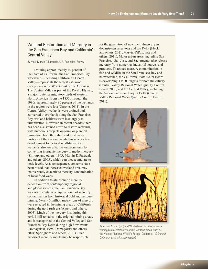
American Avocet (top) and White-faced Ibis (bottom) are wading birds commonly found in wetland areas, such as the Merced National Wildlife Refuge, California. (© Donald Quintana, used with permission.)

Wetland Restoration and Mercury in the San Francisco Bay and California’s Central ValleyBy Mark Marvin-DiPasquale, U.S. Geological Survey

Draining approximately 40 percent of the State of California, the San Francisco Bay watershed—including California’s Central Valley—represents the largest estuarine ecosystem on the West Coast of the Americas. The Central Valley is part of the Pacific Flyway, a major route for migratory birds of western North America. From the 1850s through the 1980s, approximately 90 percent of the wetlands in the region were lost (Garone, 2011). In the Central Valley, wetlands were drained and converted to cropland; along the San Francisco Bay, wetland habitats were lost largely to urbanization. However, in recent decades there has been a sustained effort to restore wetlands, with numerous projects ongoing or planned throughout both the saline and freshwater portions of the system. While this is a positive development for critical wildlife habitat, wetlands also are effective environments for converting inorganic mercury to methylmercury (Zillioux and others, 1993; Marvin-DiPasquale and others, 2003), which can bioaccumulate to toxic levels. As a consequence, concerns have been raised that increased wetland area may inadvertently exacerbate mercury contamination of local food webs.

In addition to atmospheric mercury deposition from contemporary regional and global sources, the San Francisco Bay watershed contains a large amount of mercury contamination from historical gold and mercury mining. Nearly 6 million metric tons of mercury were released in the mining areas of California during the gold rush era (Alpers and others, 2005). Much of the mercury lost during this period still remains in the original mining areas, and is transported to the Central Valley and San Francisco Bay Delta during high flow events (Domagalski, 1998; Domagalski and others, 2004; Springborn and others, 2011). Such historical mercury inputs may be responsible

for the generation of new methylmercury in downstream reservoirs and the Delta (Fleck and others, 2011; Marvin-DiPasquale and others, 2011). Major urban areas, including San Francisco, San Jose, and Sacramento, also release mercury from numerous industrial sources and products. To reduce mercury contamination in fish and wildlife in the San Francisco Bay and its watershed, the California State Water Board is developing TMDL targets for both the estuary (Central Valley Regional Water Quality Control Board, 2006) and the Central Valley, including the Sacramento-San Joaquin Delta (Central Valley Regional Water Quality Control Board, 2011).

Chapter 5


Rice fields in the Yolo Bypass Wildlife Area, California, are flooded each fall, and this may increase production of methylmercury. (Top photograph by Mark Marvin-DiPasquale; bottom photograph by © Michael Layefsky, used with permission)

The South Bay Salt Pond Restoration Project, one of the largest in the Nation, is converting more than 65 square kilometers of former salt production ponds to either managed ponds or tidal wetlands (South Bay Salt Pond Restoration Project, 2013). Because runoff from the largest historical mercury mining area in North America (New Almaden) drains right through the restoration area, mercury monitoring and research are a primary component of the restoration project (Ackerman and others, 2013). Results from these studies indicate that fish-eating bird species are at particular risk from mercury contamination in this region of the Bay (Ackerman and others, 2010), and that across the greater South San Francisco Bay there is a correlation between the percentage of total mercury as methylmercury in wetland sediment and the amount of mercury in the blood of marsh song sparrows (Grenier and others, 2010).

The salt pond restoration efforts also are changing the hydrology of one of the largest and most mercury contaminated slough channels in South San Francisco Bay. Of an estimated 1,650 kilograms of mercury currently buried in the top 2 meters of slough sediment, about 125 kilograms of mercury are expected to be mobilized by changes in hydrology associated with the restoration (Marvin-DiPasquale and Cox, 2007). Although, it is currently unclear exactly where this sediment associated mercury will be deposited, one recent study concluded that the degree of methylmercury production should actually decrease in the most contaminated salt pond once it is returned to full tidal flushing (Grenier and others, 2010), a transition currently scheduled for 2015.

Another wetland environment that has received increased attention with respect to mercury cycling and bioaccumulation are agricultural wetlands—specifically rice growing areas of the Central Valley. A recent research effort in this environmental setting has resulted in a re-evaluation of the importance of these managed wetland areas with respect to methylmercury production, bioaccumulation, and export in the context of the San Francisco Bay Delta mercury TMDL process. One important finding from this work is that resident biota within these agricultural wetlands can readily bioaccumulate mercury, and that most of the export of methylmercury from these areas to the larger Delta region takes place during the high precipitation events that occur in winter. The extent of methylmercury production also appears to be linked to how rice straw

is managed during the post-harvest period. For example, flooding the rice field (post-harvest) for the purpose of rotting the rice straw during the fall/winter period may increase methylmercury production (Marvin-DiPasquale and others, 2013; Windham-Myers and others, 2013). A project description and list of publications is provided in U.S. Geological Survey (2013b).


References Cited

Ackerman, J.T., Eagles-Smith, C.A., Herzog, M.P., Herring, G., Strong, C., and Mruz, E., 2010, Response of waterbird breeding effort, nest success, and mercury concentrations in eggs and fish to altered salt pond water management—Data summary: U.S. Geological Survey, Western Ecological Research Center, Davis, Calif., 28 p.

Ackerman, J.T., Marvin-DiPasquale, Mark, Slotton, Darrell, Eagles-Smith, C.A., Herzog, M.P., Hartman, C.A., Agee, J.L., and Ayers, Shaun, 2013, The South Bay Mercury Project—Using biosentinels to monitor effects of wetland restoration for the South Bay Salt Pond Restoration Project: U.S. Geological Survey, Report prepared for the South Bay Salt Pond Restoration Project and Resources Legacy Fund, 227 p., accessed September 18, 2013, at http://www.southbayrestoration.org/documents/technical.

Acosta-Ruiz, Gildardo, and Powers, Bill, 2001, Preliminary atmospheric emissions inventory of mercury in Mexico: Sonora, Mexico, Acosta and Associates, Prepared for Commission for Environmental Cooperation, 14 p., accessed September 18, 2013, at http://www.epa.gov/ttnchie1/conference/ei12/mexico/acosta-ruiz.pdf.

Alpers, C.N., and Hunerlach, M.P., 2000, Mercury contamination from historic gold mining in California: U.S. Geological Survey Fact Sheet FS-061-00, 6 p., http://pubs.er.usgs.gov/publication/fs06100.

Alpers, C.N., Hunerlach, M.P., May, J.T., and Hothem, R.L., 2005, Mercury contamination from historical gold mining in California: U.S. Geological Survey Fact Sheet 2005-3014, Version 1.1, 6 p., http://pubs.usgs.gov/fs/2005/3014.

Arctic Monitoring Assessment Programme/United Nations Environment Programme, 2008, Technical background report to the global atmospheric mercury assessment: Geneva, Switzerland, Arctic Monitoring and Assessment Programme, United Nations Environment Programme Chemicals Branch, 159 p.

Atkeson, T.D., Pollman, C.D., and Axelrad, D.M., 2005, Recent trends in mercury emissions, deposition, and biota in the Florida Everglades—A monitoring and modeling analysis, in Pirrone, N., and Mahaffey, K.R., eds., Dynamics of mercury pollution on regional and global scales—Atmospheric processes and human exposures around the world: New York, Springer, p. 637–655.

Axelrad, D.M., Lange, T., Gabriel, M.C., Aiken, G.R., Brandon, A., Cunningham, M.W., DeBusk, T., Dierberg, F., Donner, B.A., Frederick, P., Gilmour, C., Harris, R., Jansen, D., Krabbenhoft, D.P., McCray, J.M., Orem, W.H., Oronato, D.P., Pollman, C.D., Rumbold, D.G., White, G., Wright, A.L., and Ye, R., 2011, Mercury and sulfur monitoring, research and environmental assessment in South Florida, 2011 South Florida environmental report: West Palm Beach, Florida, South Florida Water Management District and Florida Department of Environmental Protection, p. 53.

Babiarz, C., Hoffmann, S., Wieben, A., Hurley, J., Andren, A., Shafer, M., and Armstrong, D., 2012, Watershed and discharge influences on the phase distribution and tributary loading of total mercury and methylmercury into Lake Superior: Environmental Pollution, v. 161, p. 299–310.

Bailey, E.H., Clark, A.L., and Smith, R.M., 1973, Mercury: U.S. Geological Survey Professional Paper 820, p. 401–414, http://pubs.er.usgs.gov/publication/pp820.

Balogh, S.J., Meyer, M.L., and Johnson, D.K., 1998, Transport of mercury in three contrasting river basins: Environmental Science and Technology, v. 32, no. 4, p. 456–462.

Balogh, S.J., Nollet, Y.H., and Offerman, H.J., 2005, A comparison of total mercury and methylmercury export from various Minnesota watersheds: Science of the Total Environment, v. 340, p. 261–270.

Balogh, S.J., Swain, E.B., and Nollet, Y.H., 2008, Characteristics of mercury speciation in Minnesota rivers and streams: Environmental Pollution, v. 154, no. 1, p. 3–11.

Bauch, N.J., Chasar, L.C., Scudder, B.C., Moran, P.W., Hitt, K.J., Brigham, M.E., Lutz, M.A., and Wentz, D.A., 2009, Data on mercury in water, streambed sediment, and fish from selected streams across the United States, 1998–2005: U.S. Geological Survey Data Series 307, 32 p., http://pubs.usgs.gov/ds/307.

Bell, A.H., and Scudder, B.C., 2007, Mercury accumulation in periphyton of eight river ecosystems: Journal of the American Water Resources Association, v. 43, no. 4, p. 1–12.

Bellinger, D.C., Trachtenberg, F., Barregard, L., Tavares, M., Cernichiari, E., Daniel, D., and McKinlay, S., 2006, Neuropsychological and renal effects of dental amalgam in children—A randomized clinical trial: The Journal of the American Medical Association, v. 295, no. 15, p. 1,775–1,783.

References Cited 73

http://www.southbayrestoration.org/documents/technical

http://www.southbayrestoration.org/documents/technical

http://www.epa.gov/ttnchie1/conference/ei12/mexico/acosta-ruiz.pdf

http://www.epa.gov/ttnchie1/conference/ei12/mexico/acosta-ruiz.pdf

http://pubs.er.usgs.gov/publication/fs06100

http://pubs.er.usgs.gov/publication/fs06100

http://pubs.usgs.gov/fs/2005/3014

http://pubs.er.usgs.gov/publication/pp820

http://pubs.usgs.gov/ds/307


Berry, L.G., and Mason, B.H., 1959, Mineralogy—Concepts, descriptions, determinations: San Francisco, Calif., W.H. Freeman and Company, A Series of books in geology, 630 p.

Bindler, R., Olofsson, C., Renberg, I., and Frech, W., 2001, Temporal trends in mercury accumulation in lake sediments in Sweden: Water Air and Soil Pollution Focus, p. 343–355.

Bishop, K.H., and Lee, Y.-H., 1997, Catchments as a source of mercury/methylmercury in boreal surface waters, in Sigel, A., and Sigel, H., eds., Metal ions in biological systems: New York, Marcel Dekker, p. 113–130.

Bloom, N.S., 1992, On the chemical form of mercury in edible fish and marine invertebrate tissue: Canadian Journal of Fisheries and Aquatic Sciences, v. 49, no. 5, p. 1,010–1,017.

Bodaly, R.A., Jansen, W.A., Majewski, A.R., Fudge, R.J., Strange, N.E., Derksen, A.J., and Green, D.J., 2007, Postimpoundment time course of increased mercury concentrations in fish in hydroelectric reservoirs of northern Manitoba, Canada: Archives of Environmental Contamination and Toxicology, v. 53, no. 3, p. 379–389.

Bodaly, R.A., St. Louis, V.L., Paterson, M.J., Fudge, R.J.P., Hall, B.D., Rosenberg, D.M., and Rudd, J.W.M., 1997, Bioaccumulation of mercury in the aquatic food chain in newly flooded areas, in Sigel, A., and Sigel, H., eds., Metal ions in biological systems: New York, Marcel Decker, Inc., p. 259–287.

Booz Allen & Hamilton, Inc., 2002, Multi-state inventory of gold ore processing facilities: Tysons Corner, Va., Booz Allen & Hamilton, Inc., Document Control No. REPA2-09920-004.

Borum, D., Manibusan, M.K., Schoeny, R., and Winchester, E.L., 2001, Water quality criterion for the protection of human health—Methylmercury: U.S. Environmental Protection Agency, EPA-823-R-01-001, 306 p.

Branfireun, B.A., Krabbenhoft, D.P., Hintelmann, H., Hunt, R.J., Hurley, J.P., and Rudd, J.W.M., 2005, Speciation and transport of newly deposited mercury in a boreal forest wetland—A stable mercury isotope approach: Water Resources Research, v. 41, no. W06016, p. 1–11.

Brigham, M.E., Duris, J.W., Wentz, D.A., Button, D.T., and Chasar, L.C., 2008, Total mercury, methylmercury, and ancillary water-quality and streamflow data for selected streams in Oregon, Wisconsin, and Florida, 2002–06: U.S. Geological Survey Data Series 341, 11 p., http://pubs.usgs.gov/ds/341.

Brigham, M.E., Krabbenhoft, D.P., Olson, M.L., and DeWild, J.F., 2002, Methylmercury in flood-control impoundments and natural waters of Northwestern Minnesota, 1997–99: Water, Air, and Soil Pollution, v. 138, no. 1/4, p. 61–78.

Brigham, M.E., Wentz, D.A., Aiken, G.R., and Krabbenhoft, D.P., 2009, Mercury cycling in stream ecosystems. 1. Water column chemistry and transport: Environmental Science and Technology, v. 43, no. 8, p. 2,720–2,725.

Brumbaugh, W.G., Krabbenhoft, D.P., Helsel, D.R., Wiener, J.G., and Echols, K.R., 2001, A national pilot study of mercury contamination of aquatic ecosystems along multiple gradients—Bioaccumulation in fish: U.S. Geological Survey, Biological Resources Division, Biological Science Report USGS/BRD/BSR—2001-0009, 25 p., http://pubs.er.usgs.gov/publication/bsr20010009.

Bullock, O.R., and Brehme, K.A., 2002, Atmospheric mercury simulation using the CMAQ model—Formulation description and analysis of wet deposition results: Atmospheric Environment, v. 36, no. 13, p. 2,135–2,146.

Burns, D.A., Lynch, J.A., Cosby, B.J., Fenn, M.E., Baron, J.S., and U.S. Environmental Protection Agency Clean Air Markets Division, 2011, National Acid Precipitation Assessment Program report to Congress 2011—An Integrated Assessment: National Science and Technology Council, 114 p.

Butler, T.J., Cohen, M.D., Vermeylen, F.M., Likens, G.E., Schmeltz, D., and Artz, R.S., 2008, Regional precipitation mercury trends in the eastern USA, 1998–2005—Declines in the Northeast and Midwest, no trend in the Southeast: Atmospheric Environment, v. 42, no. 7, p. 1,582–1,592.

Central Valley Regional Water Quality Control Board, 2006, Mercury in San Francisco Bay, Proposed basin plan amendment and staff report for revised total maximum daily load (TMDL) and proposed mercury water quality objectives: California Regional Water Quality Control Board, San Francisco Bay Region, 116 p., accessed September 18, 2013, at http://www.waterboards.ca.gov/rwqcb2/water_issues/programs/TMDLs/sfbaymercurytmdl.shtml.

Central Valley Regional Water Quality Control Board, 2011, The Water Quality Control Plan (Basin Plan) for the California Regional Water Quality Control Board, Central Valley Region, The Sacramento River Basin and the San Joaquin River Basin, fourth edition, revised October 2011: Central Valley Regional Water Quality Control Board, 148 p., accessed September 18, 2013, at http://www.waterboards.ca.gov/rwqcb5/water_issues/basin_plans/sacsjr.pdf.




http://pubs.er.usgs.gov/publication/bsr20010009

http://www.waterboards.ca.gov/rwqcb2/water_issues/programs/TMDLs/sfbaymercurytmdl.shtml



http://www.waterboards.ca.gov/rwqcb5/water_issues/basin_plans/sacsjr.pdf



Chalmers, A.T., Argue, D.M., Gay, D.A., Brigham, M.E., Schmitt, C.J., and Lorenz, D.L., 2011, Mercury trends in fish from rivers and lakes in the United States, 1969–2005: Environmental Monitoring and Assessment, v. 175, no. 1, p. 175–191.

Chasar, L.C., Scudder, B.C., Bell, A.H., Wentz, D.A., and Brigham, M.E., 2008, Total mercury, methylmercury, and carbon and nitrogen stable isotope data for biota from selected streams in Oregon, Wisconsin, and Florida, 2002–04: U.S. Geological Survey Data Series 349, 10 p., http://pubs.usgs.gov/ds/349.

Chasar, L.C., Scudder, B.C., Stewart, A.R., Bell, A.H., and Aiken, G.R., 2009, Mercury cycling in stream ecosystems. 3. Trophic dynamics and methylmercury bioaccumulation: Environmental Science and Technology, v. 43, no. 8, p. 2,733–2,739.

Choi, A.L., Budtz-Jorgensen, E., Jorgensen, P.J., Steuerwald, U., Debes, F., Weihe, P., and Grandjean, P., 2008, Selenium as a potential protective factor against mercury developmental neurotoxicity: Environmental Research, v. 107, p. 45–52.

Choi, A.L., and Grandjean, P., 2008, Methylmercury exposure and health effects in humans: Environmental Chemistry, v. 5, no. 2, p. 112–120.

Clark, J.M., Bottrell, S.H., Evans, C.D., Monteith, D.T., Bartlett, R., Rose, R., Newton, R.J., and Chapman, P.J., 2010, The importance of the relationship between scale and process in understanding long-term DOC dynamics: Science of the Total Environment, v. 408, no. 13, p. 2,768–2,775.

Clarkson, T.W., Magos, L., and Myers, G.J., 2003, Human exposure to mercury–The three modern dilemmas: Journal of Trace Elements in Experimental Medicine, v. 16, no. 4, p. 321–344.

Cleckner, L.B., Garrison, P.J., Hurley, J.P., Olson, M.L., and Krabbenhoft, D.P., 1998, Trophic transfer of methyl mercury in the northern Florida Everglades: Biogeochemistry, v. 40, no. 2/3, p. 347–361.

Coleman Wasik, J.K., Mitchell, C.P.J., Engstrom, D.R., Swain, E.B., Monson, B.A., Balogh, S.J., Jeremiason, J.D., Branfireun, B.A., Eggert, S.L., Kolka, R.K., and Almendinger, J.E., 2012, Methylmercury declines in a boreal peatland when experimental sulfate deposition decreases: Environmental Science and Technology, v. 46, no. 12, p. 6,663–6,671.

Compeau, G.C., and Bartha, R., 1985, Sulfate-reducing bacteria—Principal methylators of mercury in anoxic estuarine sediment: Applied and Environmental Microbiology, v. 50, no. 2, p. 498–502.

Crump, K.L., and Trudeau, V.L., 2009, Mercury-induced reproductive impairment in fish: Environmental Toxicology and Chemistry, v. 28, no. 5, p. 895–907.

Dahl, T.E, 1990, Wetlands losses in the United States, 1780’s to 1980’s: Washington, D.C., U.S. Department of the Interior, Fish and Wildlife Service, 13 p.

Dahl, T.E., 2011, Status and trends of wetlands in the conterminous United States, 2004 to 2009: U.S. Fish and Wildlife Service Report to Congress, 107 p., accessed September 18, 2013, at http://www.fws.gov/wetlands/Status-And-Trends-2009/.

Daly, C., Halbleib, M., Smith, J.I., Gibson, W.P., Doggett, M.K., Taylor, G.H., Curtis, J., and Pasteris, P.P., 2008, Physiographically sensitive mapping of climatological temperature and precipitation across the conterminous United States: International Journal of Climatology, v. 28, no. 15, p. 2,031–2,064.

Depew, D.C., Basu, N., Burgess, N.M., Campbell, L.M., Devlin, E.W., Drevnick, P.E., Hammerschmidt, C.R., Murphy, C.A., Sandheinrich, M.B., and Wiener, J.G., 2012a, Toxicity of dietary methylmercury to fish—Derivation of ecologically meaningful threshold concentrations: Environmental Toxicology and Chemistry, v. 31, no. 7, p. 1,536–1,547.

Depew, D.C., Basu, N., Burgess, N.M., Campbell, L.M., Evers, D.C., Grasman, K.A., and Scheuhammer, A.M., 2012b, Derivation of screening benchmarks for dietary methylmercury exposure for the common loon (Gavia immer)—Rationale for use in ecological risk assessment: Environmental Toxicology and Chemistry, v. 31, no. 10, p. 2,399–2,407.

Dillon, T., Beckvar, N., and Kern, J., 2010, Residue-based mercury dose-response in fish—An analysis using lethality-equivalent test endpoints: Environmental Toxicology and Chemistry, v. 29, no. 11, p. 2,559–2,565.

Domagalski, J., 1998, Occurrence and transport of total mercury and methyl mercury in the Sacramento River Basin, California: Journal of Geochemical Exploration, v. 64, p. 277–291.

References Cited 75


http://www.fws.gov/wetlands/Status-And-Trends-2009/

http://www.fws.gov/wetlands/Status-And-Trends-2009/

Domagalski, J.L., Alpers, C.N., Slotton, D.G., Suchanek, T.H., and Ayers, S.M., 2004, Mercury and methylmercury concentrations and loads in the Cache Creek watershed, California: Science of the Total Environment, v. 327, no. 1–3, p. 215–237.

Drevnick, P.E., Canfield, D.E., Gorski, P.R., Shinneman, A.L.C., Engstrom, D.E., Muir, D.C.G., Smith, G.R., Garrison, P.J., Cleckner, L.B., Hurley, J.P., Noble, R.B., Otter, R.R., and Oris, J.T., 2007, Deposition and cycling of sulfur controls mercury accumulation in Isle Royale fish: Environmental Science and Technology, v. 41, p. 7,266–7,272.

Drevnick, P.E., Engstrom, D.R., Driscoll, C.T., Swain, E.B., Balogh, S.J., Kamman, N.C., Long, D.T., Muir, D.G.C., Parsons, M.J., Rolfhus, K.R., and Rossmann, R., 2012, Spatial and temporal patterns of mercury accumulation in lacustrine sediments across the Laurentian Great Lakes region: Environmental Pollution, v. 161, p. 252–260.

Duffus, J.H., Nordberg, Monica, and Templeton, D. M., 2007, IUPAC glossary of terms used in toxicology (2nd ed.): Pure and Applied Chemistry, v. 79, no. 7, p. 1,153–1,344.

Dunne, Thomas, and Leopold, L.B., 1978, Water in environmental planning: San Francisco, W.H. Freeman and Company, 818 p.

Eagles-Smith, C.A., Ackerman, J.T., Yee, J., and Adelsbach, T.L., 2009, Mercury demethylation in waterbird livers—Dose-response thresholds and differences among species: Environmental Toxicology and Chemistry, v. 28, p. 568–577.

Edmonds, S.T., O’Driscoll, N.J., Hillier, N.K., Atwood, J.L., and Evers, D.C., 2012, Factors regulating the bioavailability of methylmercury to breeding rusty blackbirds in northeastern wetlands: Environmental Pollution, v. 171, p. 148–154.

Eklöf, K., Fölster, J., Sonesten, L., and Bishop, K., 2012, Spatial and temporal variation of THg concentrations in run-off water from 19 boreal catchments, 2000–2010: Environmental Pollution, v. 164, p. 102–109.

Engle, M.A., Tate, M.T., Krabbenhoft, D.P., Schauer, J.J., Kolker, A., Shanley, J.B., and Bothner, M.H., 2010, Comparison of atmospheric mercury speciation and deposition at nine sites across central and eastern North America: Journal of Geophysical Research—Atmospheres, v. 115, no. D18, p. D18306.

Engstrom, D.R., Balogh, S.J., and Swain, E.B., 2007, History of mercury inputs to Minnesota lakes—Influences of watershed disturbance and localized atmospheric deposition: Limnology and Oceanography, v. 52, p. 2,467–2,483.

Engstrom, D.R., and Swain, E.B., 1997, Recent declines in atmospheric mercury deposition in the Upper Midwest: Environmental Science and Technology, v. 31, no. 4, p. 960–967.

Environment Canada, 2005, National pollutant release inventory, 2005 data: Government of Canada, accessed June 21, 2013, at http://www.ec.gc.ca/inrp-npri.

Evers, D.C., 2005, Mercury connections—The extent and effects of mercury pollution in northeastern North America: Ecotoxicology, v. 14, variously paged.

Evers, D.C., Jackson, A.K., Tear, T.H., and Osborne, C.E., 2012, Hidden risk—Mercury in terrestrial ecosystems of the Northeast: Gorham, Maine, Biodiversity Research Institute, 33 p.

Evers, D.C., Wiener, J.G., Driscoll, C.T., Gay, D.A., Basu, N., Monson, B.A., Lambert, K.F., Morrison, H.A., Morgan, J.T., Williams, K.A., and Soehl, A.G., 2011, Great Lakes mercury connections—The extent and effects of mercury pollution in the Great Lakes region: Biodiversity Research Institute BRI 2011-18, 44 p.

Fitzgerald, W.F., Engstrom, D.R., Lamborg, C.H., Tseng, C.-M., Balcom, P.H., and Hammerschmidt, C.R., 2005, Modern and historic atmospheric mercury fluxes in northern Alaska—Global sources and Arctic depletion: Environmental Science and Technology, v. 39, p. 557–568.

Fitzgerald, W.F., Engstrom, D.R., Mason, R.P., and Nater, E.A., 1998, The case for atmospheric mercury contamination in remote areas: Environmental Science and Technology, v. 32, no. 1, p. 1–7.

Fleck, J.A., Alpers, C.N., Marvin-DiPasquale, M., Hothem, R.L., Wright, S.A., Ellett, K., Beaulieu, E., Agee, J.L., Kakouros, E., Kieu, L.H., Eberl, D.D., Blum, A.E., and May, J.T., 2011, The effects of sediment and mercury mobilization in the South Yuba River and Humbug Creek Confluence Area, Nevada County, California—Concentrations, speciation, and environmental fate, Part 1—Field characterization: U.S. Geological Survey Open-File Report 2010-1325A, 104 p., http://pubs.usgs.gov/of/2010/1325A.


http://www.ec.gc.ca/inrp-npri

http://pubs.usgs.gov/of/2010/1325A

http://pubs.usgs.gov/of/2010/1325A

Fulkerson, M., and Nnadi, F.N., 2006, Predicting mercury wet deposition in Florida—A simple approach: Atmospheric Environment, v. 40, p. 3,962–3,968.

Garone, P., 2011, The fall and rise of wetlands of California’s Great Central Valley: Berkeley, University of California Press, Stephen Bechtel Fund Book on Ecology and the Environment, 448 p.

Gary, Margaret, McAfee, Robert, Jr., and Wolf, C.L., eds., 1972, Glossary of geology: Washington, D.C., American Geological Institute, 805 p.

Gilmour, C.C., Henry, E.A., and Mitchell, R., 1992, Sulfate stimulation of mercury methylation in freshwater sediments: Environmental Science and Technology, v. 26, no. 11, p. 2,281–2,287.

Goldstein, R.M., Brigham, M.E., Stuewe, L., and Menheer, M.A., 2003, Mercury data from small lakes in Voyageurs National Park, northern Minnesota, 2000–02: U.S. Geological Survey Open-File Report 03-480, 18 p., http://pubs.er.usgs.gov/publication/ofr2003480.

Gough, L.P., Asher-Bolinder, S., Bales, C.A., Runberg, S.K., and Wells, R.K., 1993, Understanding our fragile environment: U.S. Geological Survey Circular 1105, 34 p., http://pubs.er.usgs.gov/publication/cir1105.

Gray, J.E., 2003a, Introduction, in Gray, J.E., ed., Geologic studies of mercury by the U.S. Geological Survey: U.S. Geological Survey Circular 1248, p. 1–7, http://pubs.usgs.gov/circ/2003/c1248.

Gray, J.E., 2003b, Summary, in Gray, J.E., ed., Geologic studies of mercury by the U.S. Geological Survey: U.S. Geological Survey Circular 1248, p. 39–40, http://pubs.usgs.gov/circ/2003/c1248.

Gray, J.E., Theodorakos, P.M., Bailey, E.A., and Turner, R.R., 2000, Distribution, speciation, and transport of mercury in stream-sediment, stream-water, and fish collected near abandoned mercury mines in southwestern Alaska, USA: Science of the Total Environment, v. 260, nos. 1–3, p. 21–33.

Grenier, L., Marvin-DiPasquale, M., Drury, D., Hunt, J., Robinson, A., Bezalel, S., Melwani, A., Agee, J., Kakouros, E., Kieu, L., Windham-Myers, L., and Collins, J., 2010, South Baylands Mercury Project: San Francisco Estuary Institute, U.S. Geological Survey, and Santa Clara Valley Water District, 97 p.

Grigal, D.F., 2002, Inputs and outputs of mercury from terrestrial watersheds—A review: Environmental Reviews, v. 10, no. 1, p. 1–39.

Gustavsson, N., Bølviken, B., Smith, D.B., and Severson, R.C., 2001, Geochemical landscapes of the conterminous United States—New map presentations for 22 elements: U.S. Geological Survey Professional Paper 1648, 38 p., http://pubs.er.usgs.gov/publication/pp1648.

Hagstrom, G.R., 1986, Fertilizer sources of sulfur and their use, in Tabatabai, M.A., ed., Sulfur in Agriculture: Madison, Wis., American Society of Agronomy, Inc., Crop Science Society of America, Inc., and Soil Science Society of America, Inc., chap. 20, p. 567–581.

Hall, B.D., Aiken, G.R., Krabbenhoft, D.P., Marvin-DiPasquale, M., and Swarzenski, C.M., 2008, Wetlands as principal zones of methylmercury production in southern Louisiana and the Gulf of Mexico region: Environmental Pollution, v. 154, no. 1, p. 124–134.

Hall, B.D., St. Louis, V.L., Rolfhus, K.R., Bodaly, R.A., Beaty, K.G., Paterson, M.J., and Cherewyk, K.A., 2005, Impacts of reservoir creation on the biogeochemical cycling of methyl mercury and total mercury in boreal upland forests: Ecosystems, v. 8, p. 248–266.

Hall, B.D., St. Louis, V.L., and Bodaly, R.A., 2004, The stimulation of methylmercury production by decomposition of flooded birch leaves and jack pine needles: Biogeochemistry, v. 68, no. 1, p. 107–129.

Harada, Masazumi, 1995, Minamata disease: Methylmercury poisoning in Japan caused by environmental pollution: Critical Reviews in Toxicology, v. 25, no. 1, p. 1-24.

Harris, R., Krabbenhoft, D.P., Mason, R., Murray, M.W., Reash, R., and Saltman, T., 2007a, Ecosystem responses to mercury contamination–Indicators of change: Boca Raton, Florida, CRC Press, 216 p.

Harris, R.C., Rudd, J.W.M., Amyot, M., Babiarz, C.L., Beaty, K.G., Blanchfield, P.J., Bodaly, R.A., Branfireun, B.A., Gilmour, C.C., Graydon, J.A., Heyes, A., Hintelmann, H., Hurley, J.P., Kelly, C.A., Krabbenhoft, D.P., Lindberg, S.E., Mason, R.P., Paterson, M.J., Podemski, C.L., Robinson, A., Sandilands, K.A., Southworth, G.R., St. Louis, V.L., and Tate, M.T., 2007b, Whole-ecosystem study shows rapid fish-mercury response to changes in mercury deposition: Proceedings of the National Academy of Sciences, v. 104, no. 42, p. 16,586–16,591.

Hartman, J.S., Weisberg, P.J., Pillai, R., Ericksen, J.A., Kuiken, T., Lindberg, S.E., Zhang, H., Rytuba, J.J., and Gustin, M.S., 2009, Application of a rule-based model to estimate mercury exchange for three background biomes in the continental United States: Environmental Science and Technology, v. 43, no. 13, p. 4,989–4,994.

References Cited 77

http://pubs.er.usgs.gov/publication/ofr2003480

http://pubs.er.usgs.gov/publication/ofr2003480

http://pubs.er.usgs.gov/publication/cir1105

http://pubs.usgs.gov/circ/2003/c1248




http://pubs.er.usgs.gov/publication/pp1648

Heinz, G.H., Hoffman, D.J., Klimstra, J.D., and Stebbins, K.R., 2009a, Rapid increases in mercury concentrations in the eggs of mallards fed methylmercury: Environmental Toxicology and Chemistry, v. 28, no. 9, p. 1,979–1,981.

Heinz, G.H., Hoffman, D.J., Klimstra, J.D., Stebbins, K.R., Kondrad, S.L., and Erwin, C.A., 2009b, Species differences in the sensitivity of avian embryos to methylmercury: Archives of Environmental Contamination and Toxicology, v. 56, no. 1, p. 129–138.

Hill, J.M., 1926, California gold production, 1849–1923: Society of Economic Geologists, Inc., v. 21, p. 172–179.

Hongve, D., Haaland, S., Riise, G., Blakar, I., and Norton, S., 2012, Decline of acid rain enhances mercury concentrations in fish: Environmental Science and Technology, v. 46, no. 5, p. 2,490–2,491.

Horowitz, A.J., and Stephens, V.C., 2008, The effects of land use on fluvial sediment chemistry for the conterminous U.S.—Results from the first cycle of the NAWQA Program—Trace and major elements, phosphorus, carbon, and sulfur: Science of the Total Environment, v. 400, nos. 1–3, p. 290–314.

Hunerlach, M.P., and Alpers, C.N., 2003, Studies of mercury contamination from gold mining–Mercury contamination from hydraulic gold mining in the Sierra Nevada, California, in Gray, J.E., ed., Geologic studies of mercury by the U.S. Geological Survey: U.S. Geological Survey Circular 1248, p. 23–27, http://pubs.usgs.gov/circ/2003/c1248.

Hurley, J.P., Benoit, J.M., Shafer, M.M., Andren, A.W., Sullivan, J.R., Hammond, R., and Webb, D.A., 1995, Influences of watershed characteristics on mercury levels in Wisconsin rivers: Environmental Science and Technology, v. 29, no. 7, p. 1,867–1,875.

Intergovernmental Panel on Climate Change, 2007, Section 10.3.6.1—Precipitation Extremes, in Contribution of Working Group I to the Fourth Assessment Report of the Intergovernmental Panel on Climate Change—The Physical Science Basis: Intergovernmental Panel on Climate Change, accessed September 18, 2013, at http://www.ipcc.ch/publications_and_data/ar4/wg1/en/ch10s10-3-6-1.html.

Jeremiason, J.D., Engstrom, D.R., Swain, E.B., Nater, E.A., Johnson, B.M., Almendinger, J.E., Monson, B.A., and Kolka, R.K., 2006, Sulfate addition increases methylmercury production in an experimental wetland: Environmental Science and Technology, v. 40, p. 3,800–3,806.

Johansson, K., 1985, Mercury in sediment in Swedish forest lakes: Verhandlungen Internationale Vereinigung fur Theoretische und Angewandte Limnologie, v. 22, p. 2,359–2,363.

Journey, C.A., Burns, D.A., Riva-Murray, K., Brigham, M.E., Button, D.T., Feaster, T.D., Petkewich, M.D., and Bradley, P.M., 2012, Fluvial transport of mercury, organic carbon, suspended sediment, and selected major ions in contrasting stream basins in South Carolina and New York, October 2004–September 2009: U.S. Geological Survey Scientific Investigations Report 2012-5173, 125 p., http://pubs.er.usgs.gov/publication/sir20125173.

Kolker, A., Engle, M.A., Krabbenhoft, D.P., and Olson, M.L., 2007, Investigating atmospheric mercury with the U.S. Geological Survey mobile mercury laboratory: U.S. Geological Survey Fact Sheet 2007-3071, http://pubs.usgs.gov/fs/2007/3071.

Krabbenhoft, D., and Shuster, P., 2002, Glacial ice cores reveal a record of natural and anthropogenic atmospheric mercury deposition for the last 270 years: U.S. Geological Survey FS-051-02, 2 p., http://toxics.usgs.gov/pubs/FS-051-02.

Krabbenhoft, D.P., and Babiarz, C.L., 1992, The role of groundwater transport in aquatic mercury cycling: Water Resources Research, v. 28, no. 12, p. 3,119–3,128.

Krabbenhoft, D.P., Branfireun, B.A., and Heyes, A., 2005, Biogeochemical cycles affecting the speciation, fate, and transport of mercury in the environment, in Parsons, M.B., and Percival, J.B., eds., Mercury—Sources, Measurements, Cycles, and Effects: Quebec, Mineralogical Society of Canada, p. 297.

Krabbenhoft, D.P., and Sunderland, E.M., 2013, Global change and mercury: Science, v. 341, p. 1,457–1,458.

Krabbenhoft, D.P., Wiener, J.G., Brumbaugh, W.G., Olson, M.L., DeWild, J.F., and Sabin, T.J., 1999, A National pilot study of mercury contamination of aquatic ecosystems along multiple gradients, in Morganwalp, D.W., and Buxton, H.T., eds., U.S. Geological Survey Toxic Substances Hydrology Program—Proceedings of the Technical Meeting, Charleston, South Carolina, March 8-12, 1999—Volume 2 of 3—Contamination of Hydrologic Systems and Related Ecosystems: U.S. Geological Survey Water-Resources Investigations Report 99-4018-B, p. 147–160, http://toxics.usgs.gov/pubs/wri99-4018/Volume2/sectionB/2301_Krabbenhoft/index.html.




http://www.ipcc.ch/publications_and_data/ar4/wg1/en/ch10s10-3-6-1.html

http://www.ipcc.ch/publications_and_data/ar4/wg1/en/ch10s10-3-6-1.html

http://pubs.er.usgs.gov/publication/sir20125173

http://pubs.er.usgs.gov/publication/sir20125173



http://toxics.usgs.gov/pubs/FS-051-02

http://toxics.usgs.gov/pubs/wri99-4018/Volume2/sectionB/2301_Krabbenhoft/index.html

http://toxics.usgs.gov/pubs/wri99-4018/Volume2/sectionB/2301_Krabbenhoft/index.html

Kuiken, T., Gustin, M., Zhang, H., Lindberg, S., and Sedinger, B., 2008, Mercury emission from terrestrial background surfaces in the eastern USA, II—Air/surface exchange of mercury within forests from South Carolina to New England: Applied Geochemistry, v. 23, no. 3, p. 356–368.

Kuwabara, J.S., Arai, Yuji, Topping, B.R., Pickering, I.J., and George, G.N., 2007, Mercury speciation in piscivorous fish from mining-impacted reservoirs: Environmental Science and Technology, v. 41, no. 8, p. 2,745–2,749.

Kuwabara, J.S., Topping, B.R., Moon, G.E., Husby, Peter, Lincoff, Andrew, Carter, J.L., and Croteau, M-N., 2005, Mercury accumulation by lower trophic-level organisms in lentic systems within the Guadalupe River watershed, California: U.S. Geological Survey Scientific Investigations Report 2005-5037, 52 p., http://pubs.usgs.gov/sir/2005/5037.

Langbein, W.B., and Iseri, K.T., 1960, Manual of hydrology, Part I, General surface-water techniques—General introduction and hydrologic definitions: U.S. Geological Survey Water-Supply Paper 1541–A, 29 p., http://pubs.er.usgs.gov/publication/wsp1541A.

Latysh, N.E., and Wetherbee, G.A., 2012, Improved mapping of National Atmospheric Deposition Program wet-deposition in complex terrain using PRISM-gridded data sets: Environmental Monitoring and Assessment, v. 184, p. 913–928.

Lawrence, S.J., 2003, Mercury in the Carson River Basin, Nevada, in Gray, J.E., ed., Geologic studies of mercury by the U.S. Geological Survey: U.S. Geological Survey Circular 1248, p. 29–33, http://pubs.usgs.gov/circ/2003/c1248.

Lehmann, C.M.B., and Gay, D.A., 2011, Monitoring long-term trends of acidic wet deposition in US precipitation—Results from the National Atmospheric Deposition Program: Power Plant Chemistry, v. 13, no. 7, p. 378–385.

Lewis, M.E., and Brigham, M.E., 2004, Low-level mercury: U.S. Geological Survey Techniques of Water-Resource Investigation, book 9, chap. A5, section 5.6.4.B, 26 p., http://water.usgs.gov/owq/FieldManual/index.html.

Lin, C.-J., and Pehkonen, S.O., 1999, The chemistry of atmospheric mercury—A review: Atmospheric Environment, v. 33, no. 13, p. 2,067–2,079.

Lin, C.-J., Pongprueksa, P., Bullock, O.R., Jr., Lindberg, S.E., Pehkonen, S.O., Jang, C., Braverman, T., and Ho, T.C., 2007, Scientific uncertainties in atmospheric mercury models II—Sensitivity analysis in the CONUS domain: Atmospheric Environment, v. 41, no. 31, p. 6,544–6,560.

Lockhart, W.L., Wilkinson, P., Billeck, B.N., Hunt, R.V., Wagemann, R., and Brunskill, G.J., 1995, Current and historical inputs of mercury to high-latitude lakes in Canada and to Hudson Bay: Water, Air, and Soil Pollution, v. 80, nos. 1–4, p. 603–610.

Lorey, P., and Driscoll, C.T., 1999, Historical trends of mercury deposition in Adirondack lakes: Environmental Science and Technology, v. 33, no. 5, p. 718–722.

Lubick, Naomi, and Malakoff, David, 2013, With pact’s completion, the real work begins: Science, v. 341, p. 1,443–1,445.

Lynch, M.L., Huang, L.-S., Cox, C., Strain, J.J., Myers, G.J., Bonham, M.P., Shamlaye, C.F., Stokes-Riner, A., Wallace, J.M.W., Duffy, E.M., Clarkson, T.W., and Davidson, P.W., 2011, Varying coefficient function models to explore interactions between maternal nutritional status and prenatal methylmercury toxicity in the Seychelles Child Development Nutrition Study: Environmental Research, v. 111, no. 1, p. 75–80.

Mahaffey, K.R., Clickner, R.P., and Jeffries, R.A., 2009, Adult women’s blood mercury concentrations vary regionally in the Unites States: association with patterns of fish consumption (NHANES 1999-2004): Environmental Health Perspectives, v. 117, no. 1, p. 47–53.

Mahaffey, K.R., Sunderland, E.M., Chan, H.M., Choi, A.L., Grandjean, P., Mariën, K., Oken, E., Sakamoto, M., Schoeny, R., Weihe, P., Yan, C.-H., and Yasutake, A., 2011, Balancing the benefits of n-3 polyunsaturated fatty acids and the risks of methylmercury exposure from fish consumption: Nutrition Reviews, v. 69, no. 9, p. 493–508.

Mahler, B.J., Van Metre, P.C., and Callender, E., 2006, Trends in metals in urban and reference lake sediments across the United States, 1970 to 2001: Environmental Toxicology and Chemistry, v. 25, no. 7, p. 1,698–1,709.

Marvin-DiPasquale, M., Agee, J.L., Kakouros, E., Kieu, L.H., Fleck, J.A., and Alpers, C.N., 2011, The effects of sediment and mercury mobilization in the South Yuba River and Humbug Creek confluence area, Nevada County, California—Concentrations, speciation and environmental fate—Part 2— Laboratory Experiments: U.S. Geological Survey Open-File Report 2010−1325B, 53 p., http://pubs.usgs.gov/of/2010/1325B.

Marvin-DiPasquale, M., and Cox, M.H., 2007, Legacy mercury in Alviso Slough, South San Francisco Bay, California—Concentration, speciation and mobility: U.S. Geological Survey Open-File Report 2007-1240, 99 p., http://pubs.usgs.gov/of/2007/1240/.

References Cited 79

http://pubs.usgs.gov/sir/2005/5037


http://pubs.er.usgs.gov/publication/wsp1541A

http://pubs.er.usgs.gov/publication/wsp1541A



http://water.usgs.gov/owq/FieldManual/index.html

http://pubs.usgs.gov/of/2010/1325B

http://pubs.usgs.gov/of/2010/1325B

http://pubs.usgs.gov/of/2007/1240/

Marvin-DiPasquale, M., Windham-Myers, L., Agee, J.L., Kakouros, E., Kieu, L.H., Fleck, J., Alpers, C.N., and Stricker, C., 2013, Methylmercury production in sediment from agricultural and non-agricultural wetlands in the Yolo Bypass, California: Science of the Total Environment, accessed November 1, 2013, at http://www.sciencedirect.com/science/article/pii/S0048969713011364.

Marvin-DiPasquale, M., Agee, J.L., Bouse, R.M., and Jaffe, B.E., 2003, Microbial cycling of mercury in contaminated pelagic and wetland sediments of San Pablo Bay, California: Environmental Geology, v. 43, no. 3, p. 260–267.

Mason, R.P., Abbott, M.L., Bodaly, R.A., Bullock, O.R., Jr., Driscoll, C.T., Evers, D., E., L.S., Murray, M., and Swain, E.B., 2005, Monitoring the response to changing mercury deposition: Environmental Science and Technology, v. 39, no. 1, p. 14A-22A.

Mason, R.P., Fitzgerald, W.F., and Morel, F.M.M., 1994, The biogeochemical cycling of elemental mercury—Anthropogenic influences: Geochimica et Cosmochimica Acta, v. 58, no. 15, p. 3,191–3,198.

Mast, M.A., Manthorne, D.J., and Roth, D.A., 2010, Historical deposition of mercury and selected trace elements to high-elevation National Parks in the Western U.S. inferred from lake-sediment cores: Atmospheric Environment, v. 44, nos. 21–22, p. 2,577–2,586.

May, J.T., Hothem, R.L., Alpers, C.N., and Law, M.A., 2000, Mercury bioaccumulation in fish in a region affected by historic gold mining—The South Yuba River, Deer Creek, and Bear River watersheds, California, 1999: U.S. Geological Survey Open-File Report 00-367, 30 p., accessed September 20, 2013, at http://ca.water.usgs.gov/archive/reports/ofr00367/.

Mergler, D., Anderson, H.A., Chan, L.H.M., Mahaffey, K.R., Murray, M., Sakamoto, M., and Stern, A.H., 2007, Methylmercury exposure and health effects in humans—A worldwide concern: Ambio, v. 36, no. 1, p. 3–11.

Minnesota Pollution Control Agency, 2007, Minnesota statewide mercury total maximum daily load: Minnesota Pollution Control Agency, March 2007, 56 p., accessed September 19, 2013, at http://www.pca.state.mn.us/index.php/view-document.html?gid=8507.

Monson, B., Staples, D., Bhavsar, S., Holsen, T., Schrank, C., Moses, S., McGoldrick, D., Backus, S., and Williams, K., 2011, Spatiotemporal trends of mercury in walleye and largemouth bass from the Laurentian Great Lakes Region: Ecotoxicology, v. 20, no. 7, p. 1,555–1,567.

Monson, B.A., 2009, Trend reversal of mercury concentrations in piscivorous fish from Minnesota lakes—1982–2006: Environmental Science and Technology, v. 43, no. 6, p. 1,750–1,755.

Mozaffarian, D., and Rimm, E.B., 2006, Fish intake, contaminants, and human health—Evaluating the risks and the benefits: The Journal of the American Medical Association, v. 296, no. 15, p. 1,885–1,899.

Mumley, T.E., and Abu-Saba, K.E., 2002, The view from downstream—A TMDL strategy to attain water quality standards for mercury in San Francisco Bay: Proceedings of the Water Environment Federation, National TMDL Science and Policy 2002 Specialty Conference, p. 533–555.

Nater, E.A., and Grigal, D.F., 1992, Regional trends in mercury distribution across the Great Lakes States, north central USA: Nature, v. 358, p. 139–141.

National Research Council, 2000, Toxicological effects of methylmercury: Washington, D.C., National Academy Press, 344 p.

Negra, C., and Lambert, K.F., 2009, MercNet—Establishing a comprehensive national mercury monitoring network: U.S. Environmental Protection Agency, EPA 430-K-09-001, 35 p.

Orem, W., Gilmour, C., Axelrad, D., Krabbenhoft, D., Scheidt, D., Kalla, P., McCormick, P., Gabriel, M., and Aiken, G., 2011, Sulfur in the south Florida ecosystem—Distribution, sources, biogeochemistry, impacts, and management for restoration: Critical Reviews in Environmental Science and Technology, v. 41, no. 6, supp. 1, p. 249–288.

Orihel, D.M., Paterson, M.J., Blanchfield, P.J., Bodaly, R.A., and Hintelmann, H., 2007, Experimental evidence of a linear relationship between inorganic mercury loading and methylmercury accumulation by aquatic biota: Environmental Science and Technology, v. 41, no. 14, p. 4,952–4,958.

Orihel, D.M., Paterson, M.J., Gilmour, C.C., Bodaly, R.A., Blanchfield, P.J., Hintelmann, H., Harris, R.C., and Rudd, J.W.M., 2006, Effect of loading rate on the fate of mercury in littoral mesocosms: Environmental Science and Technology, v. 40, p. 5,992–6,000.

Parker, R.L., 1967, Composition of the Earth’s crust: U.S. Geological Survey Geological Survey Professional Paper 440-D, 19 p., http://pubs.er.usgs.gov/publication/pp440D.

Prestbo, E.M., and Gay, D.A., 2009, Wet deposition of mercury in the U.S. and Canada, 1996–2005—Results and analysis of the NADP mercury deposition network (MDN): Atmospheric Environment, v. 43, no. 27, p. 4,223–4,233.


http://www.sciencedirect.com/science/article/pii/S0048969713011364


http://ca.water.usgs.gov/archive/reports/ofr00367/

http://ca.water.usgs.gov/archive/reports/ofr00367/

http://www.pca.state.mn.us/index.php/view-document.html?gid=8507

http://www.pca.state.mn.us/index.php/view-document.html?gid=8507

http://pubs.er.usgs.gov/publication/pp440D

Reid, G.K., and Wood, R.D., 1976, Ecology of inland waters and estuaries (2nd ed.): New York, D. Van Nostrand Company, 485 p.

Reimann, C., and Garrett, R.G., 2005, Geochemical background—Concept and reality: Science of the Total Environment, v. 350, nos. 1–3, p. 12–27.

Riscassi, A.L., and Scanlon, T.M., 2011, Controls on stream water dissolved mercury in three mid-Appalachian forested headwater catchments: Water Resources Research, v. 47, no. 12, p. W12512.

Risch, M.R., DeWild, J.F., Krabbenhoft, D.P., Kolka, R.K., and Zhang, L., 2011, Litterfall mercury dry deposition in the eastern USA: Environmental Pollution, v. 161, p. 284–290.

Riva-Murray, K., Chasar, L.C., Bradley, P.M., Burns, D.A., Brigham, M.E., Smith, M.J., and Abrahamsen, T.A., 2011, Spatial patterns of mercury in macroinvertebrates and fishes from streams of two contrasting forested landscapes in the eastern United States: Ecotoxicology, v. 20, p. 1,530–1,542.

Rudd, J.W.M., Turner, M.A., Furutani, I., Swick, A.L., and Townsend, B.E., 1983, The English-Wabigoon River system—I. A synthesis of recent research with a view towards mercury amelioration: Canadian Journal of Fisheries and Aquatic Sciences, v. 40, no. 12, p. 2,206–2,217.

Rudnick, R.L., and Gao, S., 2003, Composition of the continental crust, in Heinrich, D.H., and Karl, K.T., eds., Treatise on geochemistry: Oxford, Pergamon, p. 1–64.

Rytuba, J.J., 2003, Mercury mine studies—Environmental impact of mercury mines in the Coast Ranges, California, in Gray, J.E., ed., Geologic studies of mercury by the U.S. Geological Survey: U.S. Geological Survey Circular 1248, p. 13–17, http://pubs.usgs.gov/circ/2003/c1248.

Sandheinrich, M.B., and Wiener, J.G., 2011, Methylmercury in freshwater fish—Recent advances in assessing toxicity of environmentally relevant exposures, in Beyer, W.N., and Meador, J.P., eds., Environmental contaminants in biota—Interpreting tissue concentrations (2nd ed.): Boca Raton, Florida, Taylor and Francis, p. 169–190.

Schelker, J., Burns, D.A., Weiler, M., and Laudon, H., 2011, Hydrological mobilization of mercury and dissolved organic carbon in a snow-dominated, forested watershed—Conceptualization and modeling: Journal of Geophysical Research—Biogeosciences, v. 116, no. G1, p. G01002.

Scheuhammer, A.M., Basu, N., Burgess, N.M., Elliott, J.E., Campbell, G.D., Wayland, M., Champoux, L., and Rodrigue, J., 2008, Relationships among mercury, selenium, and neurochemical parameters in common loons (Gavia immer) and bald eagles (Haliaeetus leucocephalus): Ecotoxicology, v. 17, p. 93–101.

Scheuhammer, A.M., Basu, N., Evers, D.C., Heinz, G.H., Sandheinrich, M.B., and Bank, M.S., 2012, Ecotoxicology of mercury in fish and wildlife—Recent advances, in Bank, M.S., ed., Mercury in the environment—Pattern and process: Berkeley, California, University of California Press, chap. 11, p. 223–238.

Scheuhammer, A.M., Meyer, M.W., Sandheinrich, M.B., and Murray, M.W., 2007, Effects of environmental methylmercury on the health of wild birds, mammals, and fish: Ambio, v. 36, no. 1, p. 12–18.

Schmeltz, D., Evers, D., Driscoll, C., Artz, R., Cohen, M., Gay, D., Haeuber, R., Krabbenhoft, D., Mason, R., Morris, K., and Wiener, J., 2011, MercNet—A national monitoring network to assess responses to changing mercury emissions in the United States: Ecotoxicology, v. 20, no. 7, p. 1,713–1,725.

Schmitt, C.J., Zajicek, J.L., May, T.W., and Cowman, D.F., 1999, Organochlorine residues and elemental contaminants in U.S. freshwater fish, 1976–1986—National Contaminant Biomonitoring Program, in Ware, G.W., Nigg, H.N., and Doerge, D.R., eds., Reviews of environmental contamination and toxicology: New York, Springer-Verlag, p. 43–104.

Schroeder, W.H., and Munthe, J., 1998, Atmospheric mercury—An overview: Atmospheric Environment, v. 32, no. 5, p. 809–822.

Schuster, P.F., Krabbenhoft, D.P., Naftz, D.L., Cecil, L.D., Olson, M.L., DeWild, J.F., Susong, D.D., Green, J.R., and Abbott, M.L., 2002, Atmospheric mercury deposition during the last 270 years—A glacial ice core record of natural and anthropogenic sources: Environmental Science and Technology, v. 36, no. 11, p. 2,303–2,310.

Scott, W.B., and Crossman, E.J., 1973, Freshwater fishes of Canada—Bulletin 184: Ottawa, Fisheries Research Board of Canada Bulletin, v. 184, 966 p.

Scudder, B.C., Chasar, L.C., Wentz, D.A., Bauch, N.J., Brigham, M.E., Moran, P.W., and Krabbenhoft, D.P., 2009, Mercury in fish, bed sediment, and water from streams across the United States, 1998–2005: U.S. Geological Survey Scientific Investigations Report 2009-5109, 74 p., http://pubs.usgs.gov/sir/2009/5109.

References Cited 81



Seigneur, C., Lohman, K., Vijayaraghavan, K., Jansen, J., and Levin, L., 2006, Modeling atmospheric mercury deposition in the vicinity of power plants: Journal of the Air and Waste Management Association, v. 56, no. 6, p. 743–751.

Seigneur, C., Vijayaraghavan, K., Lohman, K., Karamchandani, P., and Scott, C., 2004, Global source attribution for mercury deposition in the United States: Environmental Science and Technology, v. 38, p. 555–569.

Selin, N.E., 2009, Global biogeochemical cycling of mercury—A review: Annual Review of Environment and Resources, v. 34, no. 1, p. 43–63.

Selin, N.E., Jacob, D.J., Park, R.J., Yantosca, R.M., Strode, S., Jaeglé, L., and Jaffe, D., 2007, Chemical cycling and deposition of atmospheric mercury—Global constraints from observations: Journal of Geophysical Research, v. 112, no. D2, p. D02308.

Selin, N.E., Jacob, D.J., Yantosca, R.M., Strode, S., Jaeglé, L., and Sunderland, E.M., 2008, Global 3-D land-ocean-atmosphere model for mercury—Present-day versus preindustrial cycles and anthropogenic enrichment factors for deposition: Global Biogeochemical Cycles, v. 22, no. 2, p. GB2011.

Shacklette, H.T., and Boerngen, J.G., 1984, Element concentrations in soils and other surficial materials of the conterminous United States: U.S. Geological Survey Survey Professional Paper 1270, 63 p., http://pubs.usgs.gov/pp/1270.

Shanley, J.B., Mast, M.A., Campbell, D.H., Aiken, G.R., Krabbenhoft, D.P., Hunt, R.J., Walker, J.F., Schuster, P.F., Chalmers, A., Aulenbach, B.T., Peters, N.E., Marvin-DiPasquale, M., Clow, D.W., and Shafer, M.M., 2008, Comparison of total mercury and methylmercury cycling at five sites using the small watershed approach: Environmental Pollution, v. 154, p. 143–154.

Sigler, J.M., Lee, X., and Munger, W., 2003, Emission and long-range transport of gaseous mercury from a large-scale Canadian boreal forest fire: Environmental Science and Technology, v. 37, no. 19, p. 4,343–4,347.

Snodgrass, J.W., Jagoe, C.H., Bryan, A.L., Jr., Brant, H.A., and Burger, J., 2000, Effects of trophic status and wetland morphology, hydroperiod, and water chemistry on mercury concentrations in fish: Canadian Journal of Fisheries and Aquatic Sciences, v. 57, no. 1, p. 171–180.

South Bay Salt Pond Restoration Project, 2013, The largest tidal wetland restoration project on the West Coast: Website, accessed November 30, 2013, at http://www.southbayrestoration.org/.

Springborn, M., Singer, M.B., and Dunne, T., 2011, Sediment-adsorbed total mercury flux through Yolo Bypass, the primary floodway and wetland in the Sacramento Valley, California: Science of the Total Environment, v. 412–413, p. 203–213.

St. Louis, V.L., Rudd, J.W.M., Kelly, C.A., Beaty, K.G., Bloom, N.S., and Flett, R.J., 1994, Importance of wetlands as sources of methyl mercury to boreal forest ecosystems: Canadian Journal of Fisheries and Aquatic Sciences, v. 51, p. 1,065–1,076.

St. Louis, V.L., Rudd, J.W.M., Kelly, C.A., Bodaly, R.A., Paterson, M.J., Beaty, K.G., Hesslein, R.H., Heyes, A., and Majewski, A.R., 2004, The rise and fall of mercury methylation in an experimental reservoir: Environmental Science and Technology, v. 38, p. 1,348–1,358.

St. Louis, V.L., Rudd, J.W.M., Kelly, C.A., Hall, B.D., Rolfhus, K.R., Scott, K.J., Lindberg, S.E., and Dong, W., 2001, Importance of the forest canopy to fluxes of methyl mercury and total mercury to boreal ecosystems: Environmental Science and Technology, v. 35, no. 15, p. 3,089–3,098.

Stahl, L.L., Snyder, B.D., Olsen, A.R., and Pitt, J.L., 2009, Contaminants in fish tissue from US lakes and reservoirs—A national probabilistic study: Environmental Monitoring and Assessment, v. 150, p. 3–19.

Strain, J.J., Davidson, P.W., Bonham, M.P., Duffy, E.M., Stokes-Riner, A., Thurston, S.W., Wallace, J.M.W., Robson, P.J., Shamlaye, C.F., Georger, L.A., Sloane-Reeves, J., Cernichiari, E., Canfield, R.L., Cox, C., Huang, L.S., Janciuras, J., Myers, G.J., and Clarkson, T.W., 2008, Associations of maternal long-chain polyunsaturated fatty acids, methyl mercury, and infant development in the Seychelles Child Development Nutrition Study: Neurotoxicology, v. 29, no. 5, p. 776–782.

Sunderland, E.M., 2007, Mercury exposure from domestic and imported estuarine and marine fish in the U.S. seafood market: Environmental Health Perspectives, v. 115, no. 2, p. 235–242.

Swain, E.B., Engstrom, D.R., Brigham, M.E., Henning, T.A., and Brezonik, P.L., 1992, Increasing rates of atmospheric mercury deposition in midcontinental North America: Science, v. 257, p. 784–787.

Tan, S.W., Meiller, J.C., and Mahaffey, K.R., 2009, The endocrine effects of mercury in humans and wildlife: Critical Reviews in Toxicology, v. 39, no. 3, p. 228–269.


http://pubs.usgs.gov/pp/1270

http://pubs.usgs.gov/pp/1270

http://www.southbayrestoration.org/

http://www.southbayrestoration.org/

Tewalt, S.J., Bragg, L.J., and Finkelman, R.B., 2001, Mercury in U.S. coal—Abundance, distribution, and modes of occurrence: U.S. Geological Survey Fact Sheet 095-01, 4 p., http://pubs.usgs.gov/fs/fs095-01.

Tsui, M.T.K., Finlay, J.C., Balogh, S.J., and Nollet, Y.H., 2010, In situ production of methylmercury within a stream channel in northern California: Environmental Science and Technology, v. 44, no. 18, p. 6,998–7,004.

U.S. Environmental Protection Agency, 2003, Methodology for deriving ambient water quality criteria for the protection of human health (2000)—Technical support document, Volume 2, Development of national bioaccumulation factors: U.S. Environmental Protection Agency, EPA–822–R–03–030, variously paged.

U.S. Environmental Protection Agency, 2004, What you need to know about mercury in fish and shellfish: U.S. Environmental Protection Agency, 2 p., accessed September 19, 2013, at http://water.epa.gov/scitech/swguidance/fishshellfish/outreach/advice_index.cfm.

U.S. Environmental Protection Agency, 2005, Regulatory impact analysis of the final Clean Air Mercury Rule: U.S. Environmental Protection Agency, EPA-452/R-05-003, 570 p.

U.S. Environmental Protection Agency, 2008, Model-based analysis and tracking of airborne mercury emissions to assist in watershed planning: U.S. Environmental Protection Agency’s Office of Wetlands, Oceans, and Watersheds under EPA Contracts EP-W-08-018 and 68-W-03-028, accessed November 23, 2013, at http://water.epa.gov/lawsregs/lawsguidance/cwa/tmdl/mercury/upload/2008_10_28_tmdl_pdf_final300report_10072008.pdf.

U.S. Environmental Protection Agency, 2011a, 2010 Biennial National Listing of Fish Advisories: U.S. Environmental Protection Agency, EPA-820-F-11-014, 7 p.

U.S. Environmental Protection Agency, 2011b, Mercury and air toxics standards for power plants: U.S. Environmental Protection Agency, 6 p., accessed September 19, 2013, at http://www.epa.gov/mats/pdfs/20111221MATSsummaryfs.pdf.

U.S. Environmental Protection Agency, 2013, National rivers and streams assessment 2008–2009—A collaborative survey (draft): U.S. Environmental Protection Agency, EPA 841-D-13-001, 110 p.

U.S. Geological Survey, 2004 Mineral Resources Data System (MRDS) [digital data]: U.S. Geological Survey, accessed September 19, 2013, at http://tin.er.usgs.gov/mrds.

U.S. Geological Survey, 2007, Mercury statistics, in Kelly, T.D., and Matos, G.R., comps. Historical statistics for mineral and material commodities in the United States: U.S. Geological Survey Data Series 140, 5 p. accessed September 20,2013, at http://pubs.usgs.gov/ds/2005/140/.

U.S. Geological Survey, 2010, USGS mobile atmospheric mercury lab: U.S. Geological Survey, accessed September 19, 2013, at http://wi.water.usgs.gov/mercury-lab/mobile-atmospheric-mercury-lab.html.

U.S. Geological Survey, 2013a, The METAALICUS project: Website, accessed November 30, 2013, at http://wi.water.usgs.gov/mercury/metaalicus-project.html.

U.S. Geological Survey, 2013b, Mercury studies in the Yolo Bypass, California: Website, accessed November 30, 2013, at http://ca.water.usgs.gov/mercury/riceFields.html.

United Nations Environment Programme, 2013a, Global mercury assessment 2013—Sources, emissions, releases and environmental transport: Geneva, Switzerland, United Nations Environment Programme Chemicals Branch, 32 p.

United Nations Environment Programme, 2013b, Minamata convention agreed by nations: United Nations Environment Programme, accessed September 20, 2013, at http://www.unep.org/newscentre/default.aspx?DocumentID=2702&ArticleID=9373.

Van Metre, P.C., 2012, Increased atmospheric deposition of mercury in reference lakes near major urban areas: Environmental Pollution, v. 162, p. 209–215.

Van Metre, P.C., and Fuller, C.C., 2009, Dual-core mass-balance approach for evaluating mercury and 210Pb atmospheric fallout and focusing to lakes: Environmental Science and Technology, v. 43, no. 1, p. 26–32.

Van Metre, P.C., and Wilson, J.T., 2003, Sediment-core samples, in Schuster, P.F., Water and sediment quality in the Yukon River basin, Alaska, during Water Year 2001: U.S. Geological Survey Open-File Report 03-427, chap. 15, p. 67–114, http://pubs.usgs.gov/of/2003/ofr03427/.

Verta, M., Tolonen, K., and Simola, H., 1989, History of heavy metal pollution in Finland as recorded by lake sediments: Science of the Total Environment, v. 87/88, p. 1–18.

Ward, D.M., Nislow, K.H., and Folt, C.L., 2010, Bioaccumulation syndrome—Identifying factors that make some stream food webs prone to elevated mercury bioaccumulation: Annals of the New York Academy of Sciences, v. 1195, p. 62–83.

Wetzel, R.G., 2001, Limnology (3rd ed.): San Diego, California, Academic Press, 1,006 p.

References Cited 83

http://pubs.usgs.gov/fs/fs095-01

http://water.epa.gov/scitech/swguidance/fishshellfish/outreach/advice_index.cfm

http://water.epa.gov/scitech/swguidance/fishshellfish/outreach/advice_index.cfm

http://water.epa.gov/lawsregs/lawsguidance/cwa/tmdl/mercury/upload/2008_10_28_tmdl_pdf_final300report_10072008.pdf




http://www.epa.gov/mats/pdfs/20111221MATSsummaryfs.pdf

http://www.epa.gov/mats/pdfs/20111221MATSsummaryfs.pdf

http://tin.er.usgs.gov/mrds

http://pubs.usgs.gov/ds/2005/140/

http://wi.water.usgs.gov/mercury-lab/mobile-atmospheric-mercury-lab.html

http://wi.water.usgs.gov/mercury-lab/mobile-atmospheric-mercury-lab.html

http://wi.water.usgs.gov/mercury/metaalicus-project.html

http://wi.water.usgs.gov/mercury/metaalicus-project.html

http://ca.water.usgs.gov/mercury/riceFields.html

http://www.unep.org/newscentre/default.aspx?DocumentID=2702&ArticleID=9373



http://pubs.usgs.gov/of/2003/ofr03427/

Wheatley, B., and Paradis, S., 1995, Exposure of Canadian aboriginal peoples to methylmercury: Water, Air, and Soil Pollution, v. 80, nos. 1–4, p. 3–11.

Wiener, J.G., Knights, B.C., Sandheinrich, M.B., Jeremiason, J.D., Brigham, M.E., Engstrom, D.R., Woodruff, L.G., Cannon, W.F., and Balogh, S.J., 2006, Mercury in soils, lakes, and fish in Voyageurs National Park (Minnesota)—Importance of atmospheric deposition and ecosystem factors: Environmental Science and Technology, v. 40, p. 6,261–6,268.

Wiener, J.G., Krabbenhoft, D.P., Heinz, G.H., and Scheuhammer, A.M., 2003, Ecotoxicology of mercury, in Hoffman, D.J., B.A. Rattner, G.A. Burton, Jr., and J. Cairns, Jr., eds., Handbook of Ecotoxicology (2nd ed.): Boca Raton, Florida, CRC Press, chap. 16, p. 409–463.

Windham-Myers, L., Marvin-DiPasquale, M., Stricker, C., Agee, J.L., Kieu, L.H., and Kakouros, E., 2013, Mercury cycling in agricultural and managed wetlands of California, USA—Experimental evidence of vegetation-driven changes in sediment biogeochemistry and methylmercury production: Science of The Total Environment, accessed July 1, 2013, at http://www.sciencedirect.com/science/article/pii/S0048969713005718.

Woodruff, L.G., and Cannon, W.F., 2010, Immediate and long-term fire effects on total mercury in forests soils of northeastern Minnesota: Environmental Science and Technology, v. 44, no. 14, p. 5,371–5,376.

Woodruff, L.G., Sandheinrich, M., Brigham, M.E., and Cannon, W.F., 2009, Impact of wildfire on levels of mercury in forested watershed systems–Voyageurs National Park, Minnesota: U.S. Geological Survey Scientific Investigations Report 2009-5151, 19 p., http://pubs.usgs.gov/sir/2009/5151.

Yin, X., and Balogh, S.J., 2002, Mercury concentrations in stream and river water—An analytical framework applied to Minnesota and Wisconsin (USA): Water, Air, and Soil Pollution, v. 138, p. 79–100.

Zillioux, E.J., Porcella, D.B., and Benoit, J.M., 1993, Mercury cycling and effects in freshwater wetland ecosystems: Environmental Toxicology and Chemistry, v. 12, no. 12, p. 2,245–2,264.






GlossaryAerosol Microscopic particles in the atmosphere.Amalgam An alloy of mercury with another metal, often gold or silver.Average A general term used to describe the central tendency of a group of observations.Background Natural levels of an environmental chemical that are unaffected by human activities (Gough and others, 1993; Reimann and Garrett, 2005). Baseline Levels of an environmental chemical that are documented for a specified area during a specified time period; they are typically impacted to some extent by anthropogenic influences (Gough and others, 1993; Reimann and Garrett, 2005).Basin (or Drainage Basin) See watershed.Bioaccumulation An increase in the concentration of a chemical in the tissue of an organism that occurs when the rate of intake through ingestion, respiration, and other mechanisms from all environmental sources exceeds the rate of removal. Both bioconcentration and biomagnification are forms of bioaccumulation (U.S. Environmental Protection Agency, 2003; Duffus and others, 2007; Chasar and others, 2008).Bioconcentration An increase in the concentration of a chemical in the tissue of an organism relative to the environmental medium to which it is exposed; it occurs through direct (non-dietary) uptake from the medium (U.S. Environmental Protection Agency, 2003; Duffus and others, 2007).Biomagnification An increase in the concentration of a chemical in the tissue of an organism that is associated with increasing trophic level of the organism in a food web, primarily through the mechanism of dietary accumulation. At its simplest, an increase in the concentration of a chemical in an organism relative to its food (U.S. Environmental Protection Agency, 2003; Duffus and others,2007).

Chlor-alkali plant An industrial facility that produces chlorine and sodium hydroxide by electrolysis of sodium chloride solutions. Older chlor-alkali plants used mercury cathodes, and losses of mercury often contaminated local water resources.Cinnabar A red mercuric sulfide (HgS) that forms at relatively low temperatures and at shallow depths, typically near recent volcanic activity or geothermal springs. The most common mercury mineral (Bailey and others, 1973; Rytuba, 2003).Consumer An animal that eats plants or other animals.Demethylate (demethylation) The process by which organic methylmercury is converted to inorganic reactive mercury. Dissolved Used to describe chemicals that pass through a filter of known pore size and that are analytically determined by a defined procedure.Dry deposition Accumulation of particles and gases by impact on environmental surfaces during periods of no precipitation.Ecosystem The aggregation of the biological community, the physical environment, and the interactions between them in a given area. Ecotoxicological Pertaining to the study of the nature, effects, and interactions of substances that are harmful to the environment.Elemental mercury The basic chemical form of mercury; it cannot be chemically broken down into simpler substances. Mercury is the only metal that is a liquid at room temperature.Endocrine disruption The process whereby a chemical interferes with the normal functioning of hormones in animals. Endocrine disruptors are known to affect brain function and sexual development, and to cause various cancers.

Glossary 85

Fish consumption advisory A recommendation to limit or avoid consumption of certain species of locally caught fish to help protect human health. Advisories may be directed toward the general public (including recreational and subsistence fishers) or sensitive populations (such as women of childbearing age, nursing mothers, and children). Federal, state and local governments issue fish consumption advisories.Food web Feeding relationships among the various species of organisms in a natural community. A diagram of these relationships typically resembles a spider’s web (Reid and Wood, 1976).Forage fish Smaller fish that are primary consumers (herbivores) and/or secondary consumers (omnivores or carnivores), and that serve as prey for larger predator fish. Game fish A fish caught by anglers for sport. They are often large predator fish at or near the top of the food web.Gaseous elemental mercury Elemental mercury in the gaseous phase in the atmosphere.Geometric mean The mean of the logarithms of a group of observations transformed back to the original measurement units of the data. The numeric value of the geometric mean is similar to the median.Inorganic mercury Used to describe elemental mercury and/or reactive mercury not associated with carbon atoms. Invertebrate Aquatic invertebrates include organisms, such as insect larvae, snails, and crayfish. Invertebrates eat other small animals, plant material, or particulate organic matter, and comprise the lower levels of aquatic food webs. Invertebrates are eaten primarily by forage fish, which, in turn, are eaten by predator fish.Invertivore An animal that feeds primarily on invertebrates.

Isotopes Atoms of the same element that contain the same number of protons but different numbers of neutrons. Stable isotopes, which can be used to trace the movement of certain chemicals through the environment, are not radioactive.Land use/land cover Land use describes how people use the land for particular purposes. Land cover describes the vegetation and human construction, such as roads and buildings that cover the earth’s surface. Larva (larval) The immature form of an aquatic insect, such as a mayfly, that does not change greatly in appearance as it grows. Aquatic insect larvae often comprise much of the invertebrate population of a stream. Litterfall Freshly fallen leaves, twigs, and other plant tissues. Litterfall is an important mechanism for cycling nutrients and other constituents, including mercury, in forested ecosystems.Lode deposit A mineral deposit consisting of veins in consolidated rock. Logarithm (logarithmic) The base 10 logarithm (Y) of a number (X) is determined as Y=log10 (X); it is the power to which the base (10) must be raised to obtain the original number (10Y=X). For example, log10 (1,000,000) = 6, because 106 = 1,000,000. Base 10 (or common) logarithms are used in this report when a variable spans an extremely large range.Mean The sum of all observations divided by the number of observations. A measure of central tendency.Median The central value of a group of observations when the data are ranked in order by magnitude. The 50th percentile. A measure of central tendency.


Median absolute deviation (MAD) For a series of observations, the absolute values of the differences (deviations) between each observation and the median of the observations are determined. The median of these deviations is the MAD. Mercury A chemical element designated by the symbol Hg; it has an atomic number of 80. In this report, the term mercury also is used to describe the sum of all mercury forms (inorganic mercury plus methylmercury) in a given medium.Methylate (methylation) The bacterial conversion of inorganic reactive mercury to organic methylmercury.Methylmercury Used to describe the organic form of mercury with one methyl group attached to a mercury atom (monomethylmercury). Although dimethylmercury exists in the natural environment, the preponderance of environmental methylmercury is monomethylmercury, and the term methylmercury has become synonymous with that form.Neurocognitive Of or related to the process of acquiring knowledge and understanding through thought, experience, and the senses.Omega-3 fatty acid Polyunsaturated fatty acids that are essential for human growth and nutrition. Salmon and other fatty fish are important sources of omega-3 fatty acids.Omnivore (omnivorous) An animal that consumes food from more than one trophic level. For example, crayfish eat both animals and plants. Order of magnitude Typically, 10 times greater or lesser than another value.Particulate In air, used to describe chemicals attached to particles and aerosols. For mercury, this is typically reactive mercury. In water, used to describe chemicals attached to particles that are retained on a filter. For mercury, the filter pore size used in USGS studies has typically been 0.7 micrometers.

Piscivore (piscivorous) An animal that feeds almost exclusively on fish.Placer deposit A surficial mineral deposit formed when a heavy mineral or element, such as gold, is concentrated from weathered debris by the action of moving water, such as a stream.Predator An animal that eats other animals, including fish and invertebrates.Prey An animal that is pursued and eaten for food.Reactive gaseous mercury Reactive inorganic mercury in the gaseous phase in the atmosphere. Reactive mercury Used to describe nonelemental forms of mercury that can chemically combine with other elements or molecules. Reactive mercury also is known as oxidized mercury.Reference dose The level of daily intake (of a chemical) that is not associated with an appreciable increase in risk of adverse health effects during a lifetime.Riparian Of or related to the narrow corridor of land adjacent to both sides of a stream, where terrestrial and aquatic ecosystems interact.River Sometimes used to refer to large streams.Salmonid Any fish species of the family Salmonidae, including salmon, trout, char, grayling, and whitefish.Sluice box Long, narrow, wooden boxes used to separate fine placer gold particles from stream water and sediment by amalgamation.Stream A natural, well-defined channel with flowing water on the earth’s surface, regardless of size (Langbein and Iseri, 1960; Gary and others, 1972).

Glossary 87

Sulfate-reducing bacteria Bacteria that live in low-oxygen conditions and use sulfate (instead of oxygen) to break down organic matter and obtain energy. Some sulfate-reducing bacteria can methylate mercury.Throughfall Water from precipitation that reaches the ground by falling unimpeded through plants or that drips onto the ground from branches and leaves. Top predator fish The species of fish occupying the highest trophic level in a food web. Top predator fish may be piscivorous, but are often opportunistic, feeding on any prey item that is readily available.TMDL (Total Maximum Daily Load) A calculation of the maximum amount of a pollutant that a water body can receive and still safely meet established water-quality standards (http://water.epa.gov/lawsregs/lawsguidance/cwa/tmdl/index.cfm; accessed February 22, 2013).Total mercury Used to describe the sum of inorganic mercury plus methylmercury in a given medium.Trophic level A given level of a food web. A trophic level consists of multiple, functionally equivalent species of organisms that compete with each other for available resources, particularly food. (Wetzel, 2001)Trophic position Similar to trophic level, except that trophic position is a quantifiable number. Trophic position typically is calculated as the difference in the abundance of nitrogen-15 (a stable isotope of nitrogen) in organisms at a given trophic level and those at the base of the food web (Chasar and others, 2009).Watershed Used to describe the entire surface of the earth that is defined by a drainage divide and that drains water falling as precipitation to a common outlet on a stream channel. The term is synonymous with drainage basin (Gary and others, 1972; Dunne and Leopold, 1978).Wet deposition Rain, snow, or fog that deposits particles or dissolved chemicals onto environmental surfaces.


http://water.epa.gov/lawsregs/lawsguidance/cwa/tmdl/index.cfm

http://water.epa.gov/lawsregs/lawsguidance/cwa/tmdl/index.cfm

Appendix 1 89

Chapter 1.

No supporting information.

Chapter 2.

Figure 2-1. Data are from U.S. Environmental Protection Agency (2011a) (http://water.epa.gov/scitech/swguidance/fishshellfish/fishadvisories/upload/technical_factsheet_2010.pdf). The figures were simplified relative to their original form. The data for figure 2-1A are from figure 4 in the USEPA document, and the data for figure 2-1B are from figure 3 in the USEPA document. The category “all other contaminants” combines PCBs (polychlorinated biphenyls), chlordane, dioxins, DDT, and other contaminants in the original USEPA document. Figure 2-1C is a map of advisories as of 2010 and is from figure 2 in the original USEPA document.

Figure 2-3. The graph is modified from Sunderland (2007). Data were supplied by Elsie Sunderland (Harvard University, written commun., June 26, 2012).

Figure 2-4. Data are from the Food and Drug Administration; compiled by Elsie Sunderland (Harvard University, written commun., November 29, 2012).

Chapter 3.

Figure 3-3. Data are from Arctic Monitoring Assessment Programme / United Nations Environment Programme (2008; Table AppA.6, p. 132). The category “Metal Mining and Production” includes nonferrous metals plus pig iron and crude steel; the category “Chlor-alkali Production” is equivalent to caustic soda production.

Figure 3-4. U.S. data are from U.S. Environmental Protection Agency (2008); Canadian data are from Environment Canada (2005); Mexican data are from Acosta-Ruiz and Powers (2001). Sources smaller than 5 kilograms per year are not shown. Data were compiled by Mark Cohen (National Oceanic and Atmospheric Administration, written commun., January 16, 2013).

Figure 3-8. The map was produced by Michael Tate (U.S. Geological Survey, written commun., January 15, 2013), using methods of Latysh and Wetherbee (2012). Annual mean precipitation-weighted total mercury concentrations were obtained from the Mercury Deposition Network (http://nadp.sws.uiuc.edu/mdn). Concentration data for individual sites were spatially interpolated using inverse distance weighting. Interpolated concentrations were then multiplied by average annual modeled precipitation from the Parameter-elevation Regressions on Independent Slopes Model (PRISM) model (Daly and others, 2008), resulting in a map showing continuous mean wet deposition of total mercury for the continental United States.

Figure 3-9. Weekly total mercury deposition and precipitation volume for September 2003–September 2007 at Orlando, Florida (site FL32), were downloaded from National Atmospheric Deposition Program at http://nadp.sws.uiuc.edu/sites/siteinfo.asp?net=MDN&id=FL32.

Figure 3-18. Each dot represents the mean filtered (dissolved) methylmercury concentration from 20 to 59 samples collected at each stream over several years, encompassing a range of seasons and streamflow conditions. Data from Balogh and others (2008) were provided by Steven Balogh (Metropolitan Council Environmental Services, written commun., February 7, 2006).

Figure 3-20. Mercury concentrations, expressed on a wet weight basis, were divided by the length of fish (mean length was used for composite samples). This removes the effect of fish length on mercury concentration, so sites with a range of fish lengths can be compared. Note that these length-normalized units cannot be compared to the USEPA fish tissue mercury criterion for the protection of human health.

Chapter 4.

Figure 4-3. Data are from Horowitz and Stephens (2008; table 3, p. 300). The baseline concentration range for mercury in streambed sediment was calculated as the median baseline mercury concentration plus or minus the median absolute deviation (MAD) for mercury (Horowitz and Stephens, 2008; table 2, p. 294). The calculated range is 0.04 ± 0.02, or 0.02–0.06 ppm. This is the range presented in figure 4-1.

Appendix 1. Supporting Information for Selected Figures

http://water.epa.gov/scitech/swguidance/fishshellfish/fishadvisories/upload/technical_factsheet_2010.pdf



http://nadp.sws.uiuc.edu/sites/siteinfo.asp?net=MDN&id=FL32

http://nadp.sws.uiuc.edu/sites/siteinfo.asp?net=MDN&id=FL32


Figure 4-4. Data are from Bauch and others (2009). Mercury methylation efficiency was calculated as the average ratio of methylmercury to total mercury concentration for water and bed sediment, and has been used as an indicator of an ecosystem’s propensity to methylate mercury (Krabbenhoft and others, 1999). Mercury source index was calculated as total mercury concentration in streambed sediment divided by organic content of the sediment and by local wet plus dry deposition rate. Wet mercury deposition rate was the average for 2000–2003, as measured by the Mercury Deposition Network. Dry deposition rate was modeled by Seigneur and others (2004); gridded data were supplied by the authors (Krish Vijayaraghavan, Atmospheric & Environmental Research, Inc., written commun., February 3, 2004). Wet and dry deposition rates for each stream location are reported in Bauch and others (2009; appendix 5). The units of the mercury source index are complex and are not included on the figure; however, the units are consistent and allow a comparison of the sites on a relative basis. The mercury source index is based on the AHA (Atmospheric Hg Accumulation) index in Krabbenhoft and others (1999). Both methylation efficiency and mercury source index are median values by study area.

Figure 4-6. Land use/land cover categories are described in Scudder and others (2009; p. 3, p. 6). For a description of the y-axis label units, see supporting information for Figure 3-20 (above).

Chapter 5.

Figure 5-3. Background and global anthropogenic mercury deposition were determined from lake sediment cores in southeast Alaska and rural Midwestern United States (data from Engstrom and Swain, 1997). Regional anthropogenic mercury deposition was determined by subtracting background plus global anthropogenic mercury deposition from total mercury deposition recorded in sediment cores from six rural lakes in the continental United States (data from Van Metre, 2012). Urban mercury deposition was determined by subtracting background plus global anthropogenic plus regional anthropogenic mercury deposition from total mercury deposition recorded in sediment cores from six urban lakes across the continental United States (data from Van Metre, 2012).

Figure 5-4. This map displays trend results from Mahler and others (2006); data for individual sites were supplied by Barbara Mahler (U.S. Geological Survey, written commun., August 18, 2013).

Figure 5-6. Relative fish methylmercury levels were obtained by dividing the mercury concentration of each fish by the mean concentration for a given fish species and site (Chalmers and others, 2011).

For more information concerning the research in this report, contact: Chief, National Water-Quality Assessment Program U.S. Geological Survey 413 National Center 12201 Sunrise Valley Drive Reston, Virginia 20192or visit our Web site at:http://water.usgs.gov/nawqa/mercury/

Back cover photographs show locations and sampling activities associated with mercury research discussed in this report.

AcknowledgmentsSpecial thanks to the following individuals and organizations for their contributions:USGS personnel in study areas across the Nation for their contributions of data and research results.

USGS’s many partners in the governmental and non-governmental sectors who have helped guide scientific efforts and ensure that USGS information meets the needs of local, State, Tribal, regional, and national stakeholders.

Technical peer reviewers:• James Kuwabara, U.S. Geological Survey• Edward Swain, Minnesota Pollution Control Agency

Other reviewers:• Jeff Bigler, U.S. Environmental Protection Agency• Judy Campbell Bird, U.S. Geological Survey contractor• Doug Burns, U.S. Geological Survey• Ruth Chemerys, U.S. Environmental Protection Agency• Mark Cohen, National Oceanic and Atmospheric Administration• Ken Davis, U.S. Environmental Protection Agency• Neil Dubrovsky, U.S. Geological Survey• Stan Durkee, U.S. Environmental Protection Agency• Barbara Eikenberry, U.S. Geological Survey• Colleen Flannagan and Kristi Morris, National Park Service• David Gay, National Atmospheric Deposition Program• Ellen Kurlansky, U.S. Environmental Protection Agency• Leonard Levin, Electric Power Research Institute• Greg Masson, U.S. Fish and Wildlife Service• David Schmeltz, U.S. Environmental Protection Agency• Pete Van Metre, U.S. Geological Survey • John Wathen, U.S. Environmental Protection Agency

Technical editor:• Linda Rogers, U.S. Geological Survey

Layout Production:• Sharon Wahlstrom, U.S. Geological Survey

Graphic Design:• Bill Gibbs, U.S. Geological Survey

Publishing support provided by the U.S. Geological SurveyPublishing Network, Tacoma Publishing Service Center

Wentz and others—

Mercury in the N

ation’s Streams—

Levels, Trends, and Implications—

Circular 1395

ISSN 1067-084X (print) ISSN 2330-5703 (online)http://dx.doi.org/10.3133/cir13954

Mercury in the Nation's Streams—Levels, Trends, and ...

Documents

Transcript of Mercury in the Nation's Streams—Levels, Trends, and ...