memory replay with data compression for continual learning

Published as a conference paper at ICLR 2022

MEMORY REPLAY WITH DATA COMPRESSION FORCONTINUAL LEARNING

Liyuan Wang1,2,3∗ Xingxing Zhang1∗ Kuo Yang6 Longhui Yu6 Chongxuan Li4,5†

Lanqing Hong6 Shifeng Zhang6 Zhenguo Li6 Yi Zhong2,3† Jun Zhu1†

1Dept. of Comp. Sci. & Tech., Institute for AI, BNRist Center, THBI Lab, Tsinghua University2School of Life Sciences, IDG/McGovern Institute for Brain Research, Tsinghua University3Tsinghua-Peking Center for Life Sciences 4Gaoling School of AI, Renmin University of China5Beijing Key Laboratory of Big Data Management and Analysis Methods 6Huawei Noah’s Ark Lab{wly19,xxzhang2020}@mails.tsinghua.edu.cn,[email protected],{yang.kuo,honglanqing,zhangshifeng4,li.zhenguo}@huawei.com,[email protected],{zhongyithu, dcszj}@tsinghua.edu.cn

ABSTRACT

Continual learning needs to overcome catastrophic forgetting of the past. Memoryreplay of representative old training samples has been shown as an effective solution,and achieves the state-of-the-art (SOTA) performance. However, existing work ismainly built on a small memory buffer containing a few original data, which cannotfully characterize the old data distribution. In this work, we propose memory replaywith data compression (MRDC) to reduce the storage cost of old training samplesand thus increase their amount that can be stored in the memory buffer. Observingthat the trade-off between the quality and quantity of compressed data is highlynontrivial for the efficacy of memory replay, we propose a novel method basedon determinantal point processes (DPPs) to efficiently determine an appropriatecompression quality for currently-arrived training samples. In this way, usinga naive data compression algorithm with a properly selected quality can largelyboost recent strong baselines by saving more compressed data in a limited storagespace. We extensively validate this across several benchmarks of class-incrementallearning and in a realistic scenario of object detection for autonomous driving.

1 INTRODUCTION

The ability to continually learn numerous tasks and infer them together is critical for deep neuralnetworks (DNNs), which needs to mitigate catastrophic forgetting (McCloskey & Cohen, 1989) ofthe past. Memory replay of representative old training samples (referred to as memory replay) hasbeen shown as an effective solution, and achieves the state-of-the-art (SOTA) performance (Hou et al.,2019). Existing memory replay approaches are mainly built on a small memory buffer containinga few original data, and try to construct and exploit it more effectively. However, due to the lowstorage efficiency of saving original data, this strategy of building memory buffer will lose a lotof information about the old data distribution. On the other hand, this usually requires huge extracomputation to further mitigate catastrophic forgetting, such as by learning additional parameters(Liu et al., 2021a) or distilling old features (Hu et al., 2021).

Different from “artificial” memory replay in DNNs, a significant feature of biological memory is toencode the old experiences in a highly compressed form and replay them to overcome catastrophicforgetting (McClelland, 2013; Davidson et al., 2009; Carr et al., 2011). Thus the learned informationcan be maintained in a small storage space as comprehensively as possible, and flexibly retrieved.Inspired by the compression feature of biological memory replay, we propose memory replay with∗Equal Contribution†Corresponding Authors

1

arX

iv:2

202.

0659

2v2

[cs

.LG

] 9

Mar

202

2


Figure 1: Averaged incremental accuracy and training time on ImageNet-sub. Using JPEG for datacompression can achieve comparable or better performance than recent strong approaches with lessextra computation (purple arrow), and can further improve their performance (gray arrow).

data compression (MRDC), which can largely increase the amount of old training samples that canbe stored in the memory buffer by reducing their storage cost in a computationally efficient way.

Given a limited storage space, data compression introduces an additional degree of freedom toexplicitly balance the quality and quantity for memory replay. With a properly selected quality, usinga naive JPEG compression algorithm (Wallace, 1992) can achieve comparable or better performancethan recent strong approaches with less extra computation (Fig. 1, purple arrow), and can furtherimprove their performance (Fig. 1, gray arrow). However, to empirically determine the compressionquality is usually inefficient and impractical, since it requires learning a task sequence or sub-sequencerepeatedly1. We propose a novel method based on determinantal point processes (DPPs) to efficientlydetermine it without repetitive training. Further, we demonstrate the advantages of our proposal inrealistic applications such as continual learning of object detection for autonomous driving, wherethe incremental data are extremely large-scale.

Our contributions include: (1) We propose memory replay with data compression, which is both animportant baseline and a promising direction for continual learning; (2) We empirically validate thatthe trade-off between quality and quantity of compressed data is highly nontrivial for memory replay,and provide a novel method to efficiently determine it without repetitive training; (3) Extensiveexperiments show that using a naive data compression algorithm with a properly selected quality canlargely improve memory replay by saving more compressed data in a limited storage space.

2 RELATED WORK

Continual learning needs to overcome catastrophic forgetting of the past when learning a newtask. Regularization-based methods (Kirkpatrick et al., 2017; Wang et al., 2021b) approximated theimportance of each parameter to the old tasks and selectively penalized its changes. Architecture-based methods (Rusu et al., 2016) allocated a dedicated parameter subspace for each task to preventmutual interference. Replay-based methods (Rebuffi et al., 2017; Shin et al., 2017) approximated andrecovered the old data distribution. In particular, memory replay of representative old training samples(referred to as memory replay) can generally achieve the best performance in class-incrementallearning (Liu et al., 2021a; Hu et al., 2021) and in numerous other continual learning scenarios, suchas audio tasks (Ehret et al., 2020), few-shot (Tao et al., 2020b), semi-supervised (Wang et al., 2021a),and unsupervised continual learning (Khare et al., 2021).

Most of the work in memory replay attempted to more effectively construct and exploit a smallmemory buffer containing a few original data. As the pioneer work, iCaRL (Rebuffi et al., 2017)proposed a general protocol of memory replay for continual learning. To better construct the memorybuffer, Mnemonics (Liu et al., 2020b) parameterized the original data and made them optimizable,while TPCIL (Tao et al., 2020a) constructed an elastic Hebbian graph by competitive Hebbianlearning. On the other hand, BiC (Wu et al., 2019), LUCIR (Hou et al., 2019), PODNet (Douillardet al., 2020), DDE (Hu et al., 2021) and AANets (Liu et al., 2021a) attempted to better exploit thememory buffer, such as by mitigating the data imbalance between old and new classes (Hou et al.,2019; Wu et al., 2019; Hu et al., 2021).

1A naive grid search approach is to train continual learning processes with different qualities and choose thebest one, resulting in huge computational cost. Also, this strategy will be less applicable if the old data cannot berevisited, or the future data cannot be accessed immediately.

2


In contrast to saving original data, several work attempted to improve the efficiency of rememberingthe old data distribution. One solution is to continually learn a generative model to replay generateddata (Shin et al., 2017; Wu et al., 2018) or compress old training data (Caccia et al., 2020). However,continual learning of such a generative model is extremely challenging, which limits its applicationsto relatively simple domains, and usually requires a lot of extra computation. Another solutionis feature replay: GFR (Liu et al., 2020a) learned a feature generator from a feature extractor toreplay generated features, but the feature extractor suffered from catastrophic forgetting since it wasincrementally updated. REMIND (Hayes et al., 2020) saved the old features and reconstructed thesynthesized features for replay, but it froze the majority of feature extractor after learning the initialphase, limiting the learning of representations for incremental tasks.

Data compression aims to improve the storage efficiency of a file, including lossless compressionand lossy compression. Lossless compression needs to perfectly reconstruct the original data from thecompressed data, which limits its compression rate (Shannon, 1948). In contrast, lossy compressioncan achieve a much higher compression rate by degrading the original data, so it has been broadly usedin realistic applications. Representative hand-crafted approaches include JPEG (or JPG) (Wallace,1992), which is the most commonly-used algorithm of lossy compression (Mentzer et al., 2020),WebP (Lian & Shilei, 2012) and JPEG2000 (Rabbani, 2002). On the other hand, neural compressionapproaches generally rely on optimizing Shannon’s rate-distortion trade-off, through RNNs (Todericiet al., 2015; 2017), auto-encoders (Agustsson et al., 2017) and GANs (Mentzer et al., 2020).

3 CONTINUAL LEARNING PRELIMINARIES

We consider a general setting of continual learning that a deep neural network (DNN) incrementallylearns numerous tasks from their task-specific training dataset Dt = {(xt,i, yt,i)}Nt

i=1, where Dt isonly available when learning task t, (xt,i, yt,i) is a data-label pair and Nt is the number of suchtraining samples. For classification tasks, the training samples of each task might be from one orseveral new classes. All the classes ever seen are evaluated at test time, and the classes from differenttasks need to be distinguished. This setting is also called class-incremental learning (van de Ven &Tolias, 2019). Suppose such a DNN with parameter θ has learned T tasks and attempts to learn anew task. Since the old training datasets

⋃Tt=1Dt are unavailable, the DNN will adapt the learned

parameters to fit DT+1, and tend to catastrophically forget the old tasks McClelland et al. (1995).

An effective solution of overcoming catastrophic forgetting is to select and store representative old

training samples Dmbt = {(xt,i, yt,i)}

Nmbt

i=1 in a small memory buffer (mb), and replay them whenlearning the new task. For classification tasks, mean-of-feature is a widely-used strategy to selectDmbt (Rebuffi et al., 2017; Hou et al., 2019). After learning each task, features of the training data

can be obtained by the learned embedding function F eθ (·). In each class, several data points nearestto the mean-of-feature are selected into the memory buffer. Then, the training dataset of task T + 1becomes D′T+1 = DT+1

⋃Dmb

1:T , including both new training samples DT+1 and some old trainingsamples Dmb

1:T =⋃Tt=1D

mbt , so as to prevent forgetting of the old tasks.

However, due to the limited storage space, only a few original data can be saved in the memory buffer,namely, Nmb

t � Nt. Although numerous efforts in memory replay attempted to more effectivelyexploit the memory buffer, such as by alleviating the data imbalance between the old and new classes,this strategy of building memory buffer is less effective for remembering the old data distribution.

4 METHOD

In this section, we first present memory replay with data compression for continual learning. Then,we empirically validate that there is a trade-off between the quality and quantity of compressed data,which is highly nontrivial for memory replay, and propose a novel method to determine it efficiently.

4.1 MEMORY REPLAY WITH DATA COMPRESSION

Inspired by the biological memory replay that is in a highly compressed form (Carr et al., 2011), wepropose an important baseline for memory replay, that is, using data compression to increase theamount of old training samples that can be stored in the memory buffer, so as to more effectively

3


Figure 2: Memory replay with data compression on ImageNet-sub. We make a grid search of the JPEGquality in {10, 25, 50, 75, 90}. The quality of 100 refers to the original data without compression.

recover the old data distribution. Data compression can be generally defined as a function F cq (·) ofcompressing the original data xt,i to xq,t,i = F cq (xt,i) with a controllable quality q. Due to the smallerstorage cost of each xq,t,i than xt,i, the memory buffer can maintain more old training samples for

replay, namely, Nmbq,t > Nmb

t for Dmbq,t = {(xq,t,i, yt,i)}

Nmbq,t

i=1 in Dmbq,1:T =

⋃Tt=1D

mbq,t . For notation

clarity, we will use Dmbq to denote Dmb

q,t without explicitly writing out its task label t, likewise for xi,yi, Nmb

q , Nmb and D. The compression rate can be defined as rq = Nmbq /Nmb ∝ Nmb

q .

In analogy to the learning theory for supervised learning, we argue that continual learning will alsobenefit from replaying more compressed data, assuming that they approximately follow the originaldata distribution. However, the assumption is likely to be violated if the compression rate is toohigh. Intuitively, this leads to a trade-off between quality and quantity: if the storage space is limited,reducing the quality q of data compression will increase the quantity Nmb

q of compressed data thatcan be stored in the memory buffer, and vice versa.

Here we evaluate the proposed idea by compressing images with JPEG (Wallace, 1992), a naive butcommonly-used lossy compression algorithm. JPEG can save images with a quality in the range of[1, 100], where reducing the quality results in a smaller file size. Using a memory buffer equivalentto 20 original images per class (Hou et al., 2019), we make a grid search of the JPEG quality withrepresentative memory replay approaches, such as LUCIR (Hou et al., 2019) and PODNet (Douillardet al., 2020). As shown in Fig. 2, memory replay of compressed data with an appropriate quality cansubstantially outperform that of original data. However, whether the quality is too large or too small,it will affect the performance. In particular, the quality that achieves the best performance varies withthe memory replay approaches, but is consistent for different numbers of splits of incremental phases.

4.2 QUALITY-QUANTITY TRADE-OFF

Since the trade-off between quality q and quantityNmbq is highly nontrivial for memory replay, it needs

to be carefully determined. Formally, after learning each task from its training datasetD, let’s consider

several compressed subsets Dmbq = {(xq,i, yi)}

Nmbq

i=1 , where q is from a set of finite candidates

Q = {q1, q2, q3, ...}. Each Dmbq is constructed by selecting a subset Dmb∗

q = {(xi, yi)}Nmb

q

i=1 of Nmbq

original training samples from D (following mean-of-feature or other principles). The size Nmbq is

determined as the maximum number such that the compressed version of Dmb∗q to a quality q can

be stored in the memory buffer (see details in Appendix A). Thereby, a smaller q enables to save alarger Nmb

q , and vice versa. The objective is to select a compressed subset that can best represent D,namely, to determine an appropriate q for memory replay.

To understand the effects of data compression, which depends on the compression function F cq (·) andthe continually-learned embedding function F eθ (·), we focus on analyzing the features of compresseddata fq,i = F eθ (F cq (xi)). We first calculate the feature matrix M c

q = [fq,1, fq,2, ..., fq,Nmbq

] of eachcompressed subset Dmb

q , where each column vector fq,i is obtained by normalizing fq,i under L2-norm to keep ||fq,i||2 = 1. Similarly, we obtain the feature matrix M∗q = [f1, f2, ..., fNmb

q] of each

original subset Dmb∗q . Then, we can analyze the quality-quantity trade-off from two aspects:

On the empirical side, in Fig. 3 we use t-SNE (Van der Maaten & Hinton, 2008) to visualize featuresof the original subset (light dot), which includes different amounts of original data, and its compressedsubset (dark dot), which is obtained by compressing the original subset to just fit in the memory

4


Figure 3: t-SNE visualization of features of the original subset (light dots) and its compressed subset(dark dots) after learning 5-phase ImageNet-sub with LUCIR. From left to right, the quantity isincreased from 37, 85 to 200, while the JPEG quality is reduced from 90, 50 to 10. We plot fiveclasses out of the latest task and label them in different colors. The crossed area is out-of-distribution.

buffer. With the increase of quantity and the decrease of quality, the area of compressed subset isinitially similar to that of original subset and expands synchronously. However, as a large number oflow-quality compressed data occur out-of-distribution, the area of compressed subset becomes muchlarger than that of its original subset, where the performance also severely declines (see Fig. 2, 3).

On the theoretical side, given a training dataset D, we aim to find the compressed subset Dmbq that

can best represent D by choosing an appropriate compression quality q from its range. To achievethis goal, we introduce Pq(Dmb

q |D) to characterize the conditional likelihood of selecting Dmbq given

input D under parameter q. The goal of learning is to choose appropriate q based on the training tasksfor making accurate predictions on unseen inputs. While there are a variety of objective functions forlearning, here we focus on the widely-used maximum likelihood estimation (MLE), where the goal isto choose q to maximize the conditional likelihood of the observed data:

maxqPq(Dmb

q |D). (1)

The construction of Dmbq can be essentially viewed as a sampling problem with the cardinality

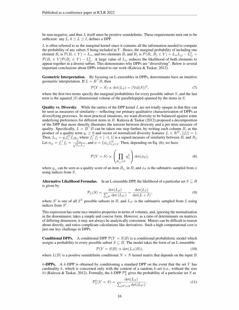
Nmbq . Here, we apply Determinantal Point Processes (DPPs) to formulate the conditional likelihoodPq(Dmb

q |D), since DPPs are not only elegant probabilistic sampling models (Kulesza & Taskar,2012), which can characterize the probabilities for every possible subset by determinants, but alsoprovide a geometric interpretation of the probability by the volume spanned by all elements in thesubset (detailed in Appendix C.2). In particular, a conditional DPP is a conditional probabilistic modelwhich assigns a probability Pq(Dmb

q |D) to each possible subset Dmbq . Since the network parameter

θ is fixed during compression, and the feature matrix M cq = F eθ (Dmb

q ), we rewrite Pq(Dmbq |D) as

Pq(M cq |D) equivalently. Formally, such a DPP formulates the probability Pq(Dmb

q |D) as

Pq(M cq |D) =

det(LMcq(D; q, θ))∑

|M |=Nmbq

det(LM (D; q, θ)), (2)

where |M cq | = Nmb

q and L(D; q, θ) is a conditional DPP |D| × |D| kernel matrix that depends onthe input D, the parameters θ and q. LM (D; q, θ) (resp., LMc

q(D; q, θ)) is the submatrix sampled

from L(D; q, θ) using indices from M (resp., M cq ). The numerator defines the marginal probability

of inclusion for the subset M cq , and the denominator serves as a normalizer to enforce the sum

of Pq(M cq |D) for every possible M c

q to 1. Generally, there are many ways to obtain a positivesemi-definite kernel L. In this work, we employ the most widely-used dot product kernel function,where LMc

q= M c>

q M cq and LM = M>M .

However, due to the extremely high complexity of calculating the denominator in Eq. (2) (analyzedin Appendix C.1), it is difficult to optimize Pq(M c

q |D). Alternatively, by introducing Pq(M∗q |D)to characterize the conditional likelihood of selecting M∗q given input D under parameter q, wepropose a relaxed optimization program of Eq. (1), in which we (1) maximize Pq(M∗q |D) sincePq(M c

q |D) ≤ Pq(M∗q |D) is always satisfied under lossy compression; and meanwhile, (2) constrainthat Pq(M c

q |D) is consistent with Pq(M∗q |D). The relaxed program is solved as follows.

First, by formulating Pq(M∗q |D) similarly as Pq(M cq |D) in Eq. (2) (detailed in Appendix C.2), we

need to maximize

L1(q) = Pq(M∗q |D) =det(LM∗q (D; θ))∑

|M∗|=Nmbq

det(LM∗(D; θ)), (3)

5


where the conditional DPP kernel matrix L(D; θ) only depends on D and θ. For our task, Pq(M∗q |D)

monotonically increases with Nmbq . Thus, optimizing L1 is converted into maxq N

mbq equivalently,

with significantly reduced complexity (detailed in Proposition 1 of Appendix C.3).

Second, to constrain that Pq(M cq |D) is consistent with Pq(M∗q |D), we propose to minimize

L2(q) =

∣∣∣∣Pq(M cq |D)

Pq(M∗q |D)− 1

∣∣∣∣ =

∣∣∣∣∣ det(M c>q M c

q )

det(M∗>q M∗q )Zq − 1

∣∣∣∣∣ =

∣∣∣∣∣(

VolcqVol∗q

)2

Zq − 1

∣∣∣∣∣ =∣∣R2

qZq − 1∣∣ , (4)

where Zq =

∑|M∗|=Nmb

qdet(LM∗ (D;θ))∑

|M|=Nmbq

det(LM (D;q,θ)) . In particular, det(M∗>q M∗q ) has a geometric interpretation

that it is equal to the squared volume spanned by M∗q (Kulesza & Taskar, 2012), denoted as Vol∗q,

likewise for det(M c>q M c

q ) with respect to Volcq. Then we define Rq =VolcqVol∗q

as the ratio of the twofeature volumes. To avoid computing Zq, we can convert optimizing L2 into minimizing |Rq − 1|equivalently, since both of them mean maximizing q (detailed in Proposition 2 of Appendix C.4).

Putting L1 and L2 together, our method is finally reformulated asmaxq

g(q)

s.t., q ∈ Q, |Rq − 1| < ε,(5)

where ε is a small positive number to serve as the threshold of Rq. g(·) : R → N represents thefunction that outputs the maximum number (i.e., Nmb

q ) such that the compressed version of Dmb∗q

to a quality q can be stored in the memory buffer. Note that we relax the original restriction ofminimizing |Rq − 1| by enforcing |Rq − 1| < ε, since maximizing Nmb

q for L1 and maximizingq for L2 cannot be achieved simultaneously. Of note, Rq is calculated by normalizing the featurevolume Volcq with Vol∗q, both of which depend on q (i.e., Nmb

q ). Therefore, ε can largely mitigate thesensitivity of q to various domains and can be empirically set as a constant value (see Sec. 4.3).

Since the function g(·) in Eq. (5) is highly non-smooth, gradient-based methods are not applicable.Indeed, we solve it by selecting the best candidate in a finite-size set Q. Generally, the candidatevalues in Q can be equidistantly selected from the range of q, such as [1, 100] for JPEG. Morecandidate values can determine a proper q more accurately, but the complexity will grow linearly. Wefound that selecting 5 candidate values is a good choice in our experiments. Once we solve Eq. (5), agood trade-off is achieved by reducing q as much as possible to obtain a larger Nmb

q , while keepingthe feature volume Volcq similar to Vol∗q. This is consistent with our empirical analysis in Fig. 3.

4.3 VALIDATE OUR METHOD WITH GRID SEARCH RESULTS

Figure 4: Properly select a quality without repetitive training.

In essence, the grid search describedin Sec. 4.1 can be seen as a naive ap-proach to determine the compressionquality, which is similar to selectingother hyperparameters for continuallearning (Fig. 4, a). This strategy is tolearn a task sequence or sub-sequenceusing different qualities and choosethe best one (Fig. 4, b), which leadsto huge extra computation and will beless applicable if the old data cannotbe revisited, or the future data cannotbe accessed immediately. In contrast,our method described in Sec. 4.2 onlyneeds to calculate the feature volumesof each compressed subset Dmb

q andoriginal subset Dmb∗

q (Fig. 4, c), with-out repetitive training.

Now we validate the quality determined by our method with the grid search results, where LUCIR andPODNet achieve the best performance at the JPEG quality of 50 and 75 on ImageNet-sub, respectively

6


Figure 5: For 5-phase ImageNet-sub, we present Rq in each incremental phase with various compres-sion qualities q, and the averaged Rq of all incremental phases.

(see Fig. 2). We present Rq in each incremental phase and the averaged Rq of all incremental phasesfor 5-phase split in Fig. 5 and for 10- and 25-phase splits in Appendix Fig.13. Based on the principlein Eq. (5) with ε = 0.5, it can be clearly seen that 50 and 75 are the qualities chosen for LUCIR andPODNet, respectively, since they are the smallest qualities that satisfy |Rq − 1| < ε. Therefore, thequality determined by our method is consistent with the grid search results, but the computationalcost is saved by more than 100 times. Interestingly, for each quality q, whether |Rq − 1| < ε isgenerally consistent in each incremental phase and the average of all incremental phases. We furtherexplore the scenarios where Rq might be more dynamic in Appendix D.4.

5 EXPERIMENT

In this section, we first evaluate memory replay with data compression (MRDC) in class-incrementallearning of large-scale images. Then, we demonstrate the advantages of our proposal in realisticsemi-supervised continual learning of large-scale object detection for autonomous driving.2

5.1 CLASS-INCREMENTAL LEARNING

Benchmark: We consider three benchmark datasets of large-scale images for continual learning.CUB-200-2011 (Wah et al., 2011) is a large-scale dataset including 200-class 11,788 colored imagesof birds with default format of JPG, split as 30 images per class for training while the rest for testing.ImageNet-full (Russakovsky et al., 2015) includes 1000-class large-scale natural images with defaultformat of JPEG. ImageNet-sub (Hou et al., 2019) is a subset derived from ImageNet-full, consistingof randomly selected 100 classes of images. Following Hou et al. (2019), we randomly resize, cropand normalize the images to the size of 224×224, and randomly split a half of the classes as the initialphase while split the rest into 5, 10 and 25 incremental phases. We report the averaged incrementalaccuracy with single-head evaluation (Chaudhry et al., 2018) in the main text, and further present theaveraged forgetting in Appendix E.3.

Implementation: We follow the implementation of representative memory replay approaches (Houet al., 2019; Douillard et al., 2020) (detailed in Appendix B.1), where we focus on constraining acertain storage space of the memory buffer rather than a certain number of images. The storagespace is limited to the equivalent of 20 original images per class, if not specified. We further discussthe effects of different storage space in Fig. 7, a fixed memory budget in Appendix E.4 and lesscompressed samples in Appendix E.5. For data compression, we apply a naive but commonly-usedJPEG (Wallace, 1992) algorithm to compress images to a controllable quality in the range of [1, 100].

Baseline: We evaluate representative memory replay approaches such as LwF (Li & Hoiem, 2017),iCaRL (Rebuffi et al., 2017), BiC (Wu et al., 2019), LUCIR (Hou et al., 2019), Mnemonics (Liuet al., 2020b), TPCIL (Tao et al., 2020a), PODNet (Douillard et al., 2020), DDE (Hu et al., 2021)and AANets (Liu et al., 2021a). In particular, AANets and DDE are the recent strong approachesimplemented on the backbones of LUCIR and PODNet, so we also implement ours on the twobackbones. Since both AANets and DDE only release their official implementation on LUCIR, wefurther reproduce LUCIR w/ AANets and LUCIR w/ DDE for fair comparison.

Accuracy: We summarize the performance of the above baselines and memory replay with datacompression (MRDC, ours) in Table 1. Using the same extra storage space, ours achieves comparableor better performance than AANets and DDE on the same backbone approaches, and can furtherboost their performance by a large margin. The improvement from ours is due to mitigating the

2All experiments are averaged by more than three runs with different random seeds.

7


Table 1: Averaged incremental accuracy (%) of classification tasks. The reproduced results arepresented with ± standard deviation, while others are reported results. The reproduced results mightslightly vary from the reported results due to different random seeds. 1With class-balance finetuning.2PODNet reproduced by Hu et al. (2021) underperforms that in Douillard et al. (2020).

CUB-200-2011 ImageNet-sub ImageNet-full

Method 5-phase 10-phase 25-phase 5-phase 10-phase 25-phase 5-phase 10-phase

LwF (Li & Hoiem, 2017) 39.42 ±0.48 38.53 ±0.96 36.33 ±0.74 53.62 47.64 44.32 44.35 38.90

iCaRL (Rebuffi et al., 2017) 39.49 ±0.58 39.31 ±0.66 38.77 ±0.73 65.44 59.88 52.97 51.50 46.89

BiC (Wu et al., 2019) 45.29 ±0.88 45.25 ±0.70 45.17 ±0.27 70.07 64.96 57.73 62.65 58.72

Mnemonics (Liu et al., 2020b) – – – 72.58 71.37 69.74 64.54 63.01

TPCIL (Tao et al., 2020a) – – – 76.27 74.81 – 64.89 62.88

LUCIR (Hou et al., 2019) 44.63 ±0.32 45.58 ±0.28 45.48 ±0.66 70.84 68.32 61.44 64.45 61.57

w/ AANets (Liu et al., 2021a) – – – 72.55 69.22 67.60 64.94 62.39

w/ DDE (Hu et al., 2021) – – – 72.34 70.20 – 67.511 65.771

w/ MRDC (Ours) 46.68 ±0.60 47.28 ±0.51 48.01 ±0.72 73.56 ±0.27 72.70 ±0.47 70.53 ±0.57 67.53 ±0.081 65.29 ±0.10

1

w/ AANets (Reproduced) 46.87 ±0.66 47.34 ± 0.77 47.35 ±0.95 72.91 ±0.45 71.93 ±0.52 70.70 ±0.46 63.37 ±0.26 62.46 ±0.14

w/ AANets + MRDC (Ours) 49.02 ±1.07 49.84 ±0.87 51.33 ±1.42 73.79 ±0.42 73.73 ±0.37 73.47 ±0.35 64.99 ±0.13 63.04 ±0.11

w/ DDE (Reproduced) 45.86 ±0.65 46.48 ±0.69 46.46 ±0.33 73.04 ±0.36 70.84 ±0.59 66.61 ±0.68 66.95 ±0.091 65.21 ±0.05

1

w/ DDE + MRDC (Ours) 47.16 ±0.60 48.33 ±0.48 48.37 ±0.34 75.12 ±0.17 73.39 ±0.29 70.83 ±0.34 67.90 ±0.051 66.67 ±0.23

1

PODNet (Douillard et al., 2020) 44.92 ±0.31 44.49 ±0.65 43.79 ±0.44 75.54 74.33 68.31 66.95 64.13

w/ AANets (Liu et al., 2021a) – – – 76.96 75.58 71.78 67.73 64.85

w/ DDE (Hu et al., 2021) – – – 76.71 75.41 – 66.422 64.71

w/ MRDC (Ours) 46.00 ±0.28 46.09 ±0.37 45.84 ±0.43 78.08 ±0.66 76.02 ±0.54 72.72 ±0.74 68.91 ±0.16 66.31 ±0.26

averaged forgetting, detailed in Appendix E.3. For CUB-200-2011 with only a few training samples,all old data can be saved in the memory buffer with a high JPEG quality of 94. In contrast, forImageNet-sub/-full, only a part of old training samples can be selected, compressed and saved in thememory buffer, where our method can efficiently determine the compression quality for LUCIR andPODNet (see Sec. 4.3 and Appendix D.2), and for AANets and DDE (see Appendix D.3).

Figure 6: Averaged incremental accuracy (the column, leftY-axis) and computational cost (the triangle, right Y-axis) onImageNet-sub. We run each baseline with one Tesla V100.

Computational Cost: Limiting thesize of memory buffer is not onlyto save its storage, but also to savethe extra computation of learning allold training samples again. Here weevaluate the computational cost ofAANets, DDE and memory replaywith data compression (MRDC, ours)on LUCIR (see Fig. 6 for ImageNet-sub and Appendix Table 3 for CUB-200-2011). Both AANets and DDErequire a huge amount of extra com-putation to improve the performanceof continual learning, which is gener-ally several times that of the backbone approach. In contrast, ours achieves competing or moreperformance improvement but only slightly increases the computational cost.

Figure 7: The effects of different storage space (equal to 10, 20, 40 and 80 original images per class)on ImageNet-sub. LUCIR (a) and PODNet (b) are reproduced from their officially-released codes.

8


Storage Space: The impact of storage space is evaluated in Fig. 7. Limiting the storage space toequivalent of 10, 20, 40 and 80 original images per class, ours can improve the performance ofLUCIR and PODNet by a similar margin, where the improvement is generally more significant formore splits of incremental phases. Further, ours can achieve consistent performance improvementwhen using a fixed memory budget (detailed in Appendix E.4), and can largely save the storage costwithout performance decrease when storing less compressed samples (detailed in Appendix E.5).

5.2 LARGE-SCALE OBJECT DETECTION

Figure 8: We present the grid search results (left), Rq in eachincremental phase (middle), and the averaged Rq of all incre-mental phases (right) for SSCL on SODA10M. The qualitydetermined by our method is 50, which indeed achieves thebest performance in the grid search.

The advantages of memory replaywith data compression are more sig-nificant in realistic scenarios such asautonomous driving, where the incre-mental data are extremely large-scalewith huge storage cost. Here we eval-uate continual learning on SODA10M(Han et al., 2021), a large-scale objectdetection benchmark for autonomousdriving. SODA10M contains 10M un-labeled images and 20K labeled im-ages of size 1920× 1080 with defaultformat of JPEG, which is much largerthan the scale of ImageNet. The la-beled images are split into 5K, 5K and10K for training, validation and testing, respectively, annotating 6 classes of road objects for detection.

Table 2: Detection results with ± standard deviation (%)of semi-supervised continual learning on SODA10M. FT:finetuning. MR: memory replay.

Method AP AP50 AP75

Pseudo

Labeling

FT 40.36 ±0.34 63.83 ±0.35 43.82 ±0.34

MR 40.75 ±0.30 / +0.39 65.11 ±0.64 / +1.28 43.53 ±0.20 / -0.29

Ours 41.50 ±0.06 / +1.14 65.36 ±0.47 / +1.53 44.95 ±0.22 / +1.13

Unbiased

Teacher

FT 42.88 ±0.32 66.70 ±0.59 45.99 ±0.32

MR 43.10 ±0.06 / +0.22 66.88 ±0.51 / +0.18 46.62 ±0.02 / +0.63

Ours 43.72 ±0.25 / +0.84 67.80 ±0.46 / +1.10 47.36 ±0.23 / +1.37

Since the autonomous driving data aretypically partially-labeled, we followthe semi-supervised continual learn-ing (SSCL) proposed by Wang et al.(2021a) for object detection. Specifi-cally, we randomly split 5 incremen-tal phases containing 1K labeled dataand 20K unlabeled data per phase, anduse a memory buffer to replay labeleddata. The storage space is limitedto the equivalent of 100 original im-ages per phase. Following Han et al.(2021), we consider Pseudo Labelingand Unbiased Teacher (Liu et al., 2021b) for semi-supervised object detection (the implementationis detailed in Appendix B.2). Using the method described in Sec. 4.2 with the same threshold (i.e.,ε = 0.5), we can efficiently determine the compression quality for SSCL of object detection, andvalidate that the determined quality indeed achieves the best performance in grid search (see Fig. 8).Then, compared with memory replay of original data, our proposal can generally achieve severaltimes of the performance improvement on finetuning, as shown in Table 2.

6 CONCLUSION

In this work, we propose that using data compression with a properly selected compression qualitycan largely improve the efficacy of memory replay by saving more compressed data in a limitedstorage space. To efficiently determine the compression quality, we provide a novel method based ondeterminantal point processes (DPPs) to avoid repetitive training, and validate our method in bothclass-incremental learning and semi-supervised continual learning of object detection. Our work notonly provides an important yet under-explored baseline, but also opens up a promising new avenue forcontinual learning. Further work could develop adaptive compression algorithms for incremental datato improve the compression rate, or propose new regularization methods to constrain the distributionchanges caused by data compression. Meanwhile, the theoretical analysis based on DPPs can be usedas a general framework to integrate optimizable variables in memory replay, such as the strategy of

9


selecting prototypes. In addition, our work suggests how to save a batch of training data in a limitedstorage space to best describe its distribution, which will motivate broader applications in the fieldsof data compression and data selection.

ACKNOWLEDGEMENTS

This work was supported by NSF of China Projects (Nos. 62061136001, 61620106010, 62076145,U19B2034, U181146), Beijing NSF Project (No. JQ19016), Beijing Outstanding Young ScientistProgram NO. BJJWZYJH012019100020098, Tsinghua-Peking Center for Life Sciences, BeijingAcademy of Artificial Intelligence (BAAI), Tsinghua-Huawei Joint Research Program, a grant fromTsinghua Institute for Guo Qiang, and the NVIDIA NVAIL Program with GPU/DGX Acceleration,Major Innovation & Planning Interdisciplinary Platform for the “Double-First Class” Initiative,Renmin University of China.

ETHIC STATEMENT

This work presents memory replay with data compression for continual learning. It can be used toreduce the storage requirement in memory replay and thus may facilitate large-scale applicationsof such methods to real-world problems (e.g., autonomous driving). As a fundamental research inmachine learning, the negative consequences in the current stage are not obvious.

REPRODUCIBILITY STATEMENT

We ensure the reproducibility of our paper from three aspects. (1) Experiment: The implementationof our experiment described in Sec. 4.1, Sec. 4.3 and Sec. 5 is further detailed in Appendix B. (2)Code: Our code is included in supplementary materials. (3) Theory and Method: A complete proofof the theoretical results described in Sec. 4.2 is included in Appendix C.

10


REFERENCES

Eirikur Agustsson, Fabian Mentzer, Michael Tschannen, Lukas Cavigelli, Radu Timofte, LucaBenini, and Luc Van Gool. Soft-to-hard vector quantization for end-to-end learning compressiblerepresentations. arXiv preprint arXiv:1704.00648, 2017.

Lucas Caccia, Eugene Belilovsky, Massimo Caccia, and Joelle Pineau. Online learned continual com-pression with adaptive quantization modules. In International Conference on Machine Learning,pp. 1240–1250. PMLR, 2020.

Margaret F Carr, Shantanu P Jadhav, and Loren M Frank. Hippocampal replay in the awake state: apotential substrate for memory consolidation and retrieval. Nature Neuroscience, 14(2):147–153,2011.

Arslan Chaudhry, Puneet K Dokania, Thalaiyasingam Ajanthan, and Philip HS Torr. Riemannianwalk for incremental learning: Understanding forgetting and intransigence. In Proceedings of theEuropean Conference on Computer Vision (ECCV), pp. 532–547, 2018.

Thomas J Davidson, Fabian Kloosterman, and Matthew A Wilson. Hippocampal replay of extendedexperience. Neuron, 63(4):497–507, 2009.

Amit Deshpande and Luis Rademacher. Efficient volume sampling for row/column subset selection.In 2010 IEEE 51st Annual Symposium on Foundations of Computer Science, pp. 329–338. IEEE,2010.

Arthur Douillard, Matthieu Cord, Charles Ollion, Thomas Robert, and Eduardo Valle. Podnet:Pooled outputs distillation for small-tasks incremental learning. In Proceedings of the EuropeanConference on Computer Vision (ECCV), volume 12365, pp. 86–102, 2020.

Benjamin Ehret, Christian Henning, Maria R Cervera, Alexander Meulemans, Johannes Von Os-wald, and Benjamin F Grewe. Continual learning in recurrent neural networks. arXiv preprintarXiv:2006.12109, 2020.

Jianhua Han, Xiwen Liang, Hang Xu, Kai Chen, Lanqing Hong, Chaoqiang Ye, Wei Zhang, ZhenguoLi, Chunjing Xu, and Xiaodan Liang. Soda10m: Towards large-scale object detection benchmarkfor autonomous driving. arXiv preprint arXiv:2106.11118, 2021.

Tyler L Hayes, Kushal Kafle, Robik Shrestha, Manoj Acharya, and Christopher Kanan. Remind yourneural network to prevent catastrophic forgetting. In European Conference on Computer Vision,pp. 466–483. Springer, 2020.

Saihui Hou, Xinyu Pan, Chen Change Loy, Zilei Wang, and Dahua Lin. Learning a unified classifierincrementally via rebalancing. In Proceedings of the IEEE Conference on Computer Vision andPattern Recognition, pp. 831–839, 2019.

Xinting Hu, Kaihua Tang, Chunyan Miao, Xian-Sheng Hua, and Hanwang Zhang. Distilling causaleffect of data in class-incremental learning. arXiv preprint arXiv:2103.01737, 2021.

Shivam Khare, Kun Cao, and James Rehg. Unsupervised class-incremental learning through confu-sion. arXiv preprint arXiv:2104.04450, 2021.

James Kirkpatrick, Razvan Pascanu, Neil Rabinowitz, Joel Veness, Guillaume Desjardins, Andrei ARusu, Kieran Milan, John Quan, Tiago Ramalho, Agnieszka Grabska-Barwinska, et al. Overcomingcatastrophic forgetting in neural networks. Proceedings of the National Academy of Sciences, 114(13):3521–3526, 2017.

Alex Kulesza and Ben Taskar. Determinantal point processes for machine learning. arXiv preprintarXiv:1207.6083, 2012.

Zhizhong Li and Derek Hoiem. Learning without forgetting. IEEE Transactions on Pattern Analysisand Machine Intelligence, 40(12):2935–2947, 2017.

Li Lian and Wei Shilei. Webp: A new image compression format based on vp8 encoding. Microcon-trollers & Embedded Systems, 3, 2012.

11


Tsung-Yi Lin, Piotr Dollar, Ross Girshick, Kaiming He, Bharath Hariharan, and Serge Belongie.Feature pyramid networks for object detection. In Proceedings of the IEEE Conference onComputer Vision and Pattern Recognition, pp. 2117–2125, 2017.

Xialei Liu, Chenshen Wu, Mikel Menta, Luis Herranz, Bogdan Raducanu, Andrew D Bagdanov,Shangling Jui, and Joost van de Weijer. Generative feature replay for class-incremental learning. InProceedings of the IEEE/CVF Conference on Computer Vision and Pattern Recognition Workshops,pp. 226–227, 2020a.

Yaoyao Liu, Yuting Su, An-An Liu, Bernt Schiele, and Qianru Sun. Mnemonics training: Multi-classincremental learning without forgetting. In Proceedings of the IEEE Conference on ComputerVision and Pattern Recognition, pp. 12245–12254, 2020b.

Yaoyao Liu, Bernt Schiele, and Qianru Sun. Adaptive aggregation networks for class-incrementallearning. In Proceedings of the IEEE/CVF Conference on Computer Vision and Pattern Recognition,pp. 2544–2553, 2021a.

Yen-Cheng Liu, Chih-Yao Ma, Zijian He, Chia-Wen Kuo, Kan Chen, Peizhao Zhang, Bichen Wu,Zsolt Kira, and Peter Vajda. Unbiased teacher for semi-supervised object detection. arXiv preprintarXiv:2102.09480, 2021b.

James L McClelland. Incorporating rapid neocortical learning of new schema-consistent informationinto complementary learning systems theory. Journal of Experimental Psychology: General, 142(4):1190, 2013.

James L McClelland, Bruce L McNaughton, and Randall C O’Reilly. Why there are complementarylearning systems in the hippocampus and neocortex: insights from the successes and failures ofconnectionist models of learning and memory. Psychological review, 102(3):419, 1995.

Michael McCloskey and Neal J Cohen. Catastrophic interference in connectionist networks: Thesequential learning problem. In Psychology of Learning and Motivation, volume 24, pp. 109–165.Elsevier, 1989.

Fabian Mentzer, George Toderici, Michael Tschannen, and Eirikur Agustsson. High-fidelity genera-tive image compression. arXiv preprint arXiv:2006.09965, 2020.

Majid Rabbani. Jpeg2000: Image compression fundamentals, standards and practice. Journal ofElectronic Imaging, 11(2):286, 2002.

Sylvestre-Alvise Rebuffi, Alexander Kolesnikov, Georg Sperl, and Christoph H Lampert. icarl:Incremental classifier and representation learning. In Proceedings of the IEEE Conference onComputer Vision and Pattern Recognition, pp. 2001–2010, 2017.

Shaoqing Ren, Kaiming He, Ross Girshick, and Jian Sun. Faster r-cnn: Towards real-time objectdetection with region proposal networks. In Advances in Neural Information Processing Systems,volume 28, pp. 91–99, 2015.

Olga Russakovsky, Jia Deng, Hao Su, Jonathan Krause, Sanjeev Satheesh, Sean Ma, Zhiheng Huang,Andrej Karpathy, Aditya Khosla, Michael Bernstein, et al. Imagenet large scale visual recognitionchallenge. International journal of computer vision, 115(3):211–252, 2015.

Andrei A Rusu, Neil C Rabinowitz, Guillaume Desjardins, Hubert Soyer, James Kirkpatrick, KorayKavukcuoglu, Razvan Pascanu, and Raia Hadsell. Progressive neural networks. arXiv preprintarXiv:1606.04671, 2016.

Claude Elwood Shannon. A mathematical theory of communication. The Bell System TechnicalJournal, 27(3):379–423, 1948.

Hanul Shin, Jung Kwon Lee, Jaehong Kim, and Jiwon Kim. Continual learning with deep generativereplay. In Advances in Neural Information Processing Systems, pp. 2990–2999, 2017.

Xiaoyu Tao, Xinyuan Chang, Xiaopeng Hong, Xing Wei, and Yihong Gong. Topology-preservingclass-incremental learning. In European Conference on Computer Vision, pp. 254–270. Springer,2020a.

12


Xiaoyu Tao, Xiaopeng Hong, Xinyuan Chang, Songlin Dong, Xing Wei, and Yihong Gong. Few-shotclass-incremental learning. In Proceedings of the IEEE/CVF Conference on Computer Vision andPattern Recognition, pp. 12183–12192, 2020b.

George Toderici, Sean M O’Malley, Sung Jin Hwang, Damien Vincent, David Minnen, ShumeetBaluja, Michele Covell, and Rahul Sukthankar. Variable rate image compression with recurrentneural networks. arXiv preprint arXiv:1511.06085, 2015.

George Toderici, Damien Vincent, Nick Johnston, Sung Jin Hwang, David Minnen, Joel Shor, andMichele Covell. Full resolution image compression with recurrent neural networks. In Proceedingsof the IEEE Conference on Computer Vision and Pattern Recognition, pp. 5306–5314, 2017.

Gido M van de Ven and Andreas S Tolias. Three scenarios for continual learning. arXiv preprintarXiv:1904.07734, 2019.

Laurens Van der Maaten and Geoffrey Hinton. Visualizing data using t-sne. Journal of MachineLearning Research, 9(11), 2008.

Catherine Wah, Steve Branson, Peter Welinder, Pietro Perona, and Serge Belongie. The caltech-ucsdbirds-200-2011 dataset. 2011.

Gregory K Wallace. The jpeg still picture compression standard. IEEE Transactions on ConsumerElectronics, 38(1):xviii–xxxiv, 1992.

Liyuan Wang, Kuo Yang, Chongxuan Li, Lanqing Hong, Zhenguo Li, and Jun Zhu. Ordisco:Effective and efficient usage of incremental unlabeled data for semi-supervised continual learning.In Proceedings of the IEEE/CVF Conference on Computer Vision and Pattern Recognition, pp.5383–5392, 2021a.

Liyuan Wang, Mingtian Zhang, Zhongfan Jia, Qian Li, Chenglong Bao, Kaisheng Ma, Jun Zhu, andYi Zhong. Afec: Active forgetting of negative transfer in continual learning. In Advances in NeuralInformation Processing Systems, volume 34, 2021b.

Chenshen Wu, Luis Herranz, Xialei Liu, Joost van de Weijer, Bogdan Raducanu, et al. Memory replaygans: Learning to generate new categories without forgetting. In Advances In Neural InformationProcessing Systems, pp. 5962–5972, 2018.

Yue Wu, Yinpeng Chen, Lijuan Wang, Yuancheng Ye, Zicheng Liu, Yandong Guo, and Yun Fu. Largescale incremental learning. In Proceedings of the IEEE/CVF Conference on Computer Vision andPattern Recognition, pp. 374–382, 2019.

13


A TRADE-OFF BETWEEN QUALITY AND QUANTITY

Figure 9: Limiting the storage space to the equivalent of(a) 20 original images per class for ImageNet and (b) 50original images per phase for SODA10M, we plot the relationbetween the quality and quantity of compressed data. Thequality of 100 refers to the original data without compression.

Given a limited storage space, thereis an intuitive trade-off between thequality q and quantity Nmb

q of com-pressed data. Here we plot the re-lation of q and Nmb

q for ImageNetand SODA10M used in our paper. Asshown in Fig. 9, reducing the qualityenables to save more compressed datain the memory buffer, and vice versa.Then, we present compressed imageswith various qualities in Fig. 10. Al-though reducing the quality tends todistort the compressed data and thushurts the performance of continuallearning, it can be clearly seen thatthe semantic information of such com-pressed data is hardly affected. There-fore, a potential follow-up work is to regularize the differences between compressed data and originaldata, so as to further improve the performance of memory replay.

Figure 10: Compressed images of ImageNet. (a) Each column contains compressed images of aspecific JPEG quality. (b) Two exemplar images with different qualities.

14


B IMPLEMENTATION DETAIL

B.1 CLASS-INCREMENTAL LEARNING

Following the implementation of Hou et al. (2019); Douillard et al. (2020); Tao et al. (2020a); Liuet al. (2021a); Hu et al. (2021), we train a ResNet-18 architecture for 90 epochs, with minibatchsize of 128 and weight decay of 1× 10−4. We use a SGD optimizer with initial learning rate of 0.1,momentum of 0.9 and cosine annealing scheduling. We run each baseline with one Tesla V100, andmeasure the computational cost. We evaluate the performance of class-incremental learning with theaveraged incremental accuracy (AIC) (Hou et al., 2019). After learning each phase, we can calculatethe test accuracy on all classes learned so far in the previous t phases as At. Then we can calculateAICt = 1

t

∑ti=1 Ai.

To evaluate the effects of class similarity on the determined quality of data compression, we selectsimilar or dissimilar superclasses from ImageNet, which includes 1000 classes ranked by theirsemantic similarity. Specifically, we select 10 adjacent classes as a superclass, and construct 10adjacent (similar) or remote (dissimilar) superclasses. The index of classes selected in 10 similarsuperclasses is [1, 2, 3, ..., 100], while in 10 dissimilar superclasses is [1, 2, ..., 10, 101, 102, ..., 110,..., 910].

B.2 LARGE-SCALE OBJECT DETECTION

For memory replay, we follow Wang et al. (2021a) to randomly select the old labeled data andsave them in the memory buffer, which indeed achieves competitive performance as analyzed byChaudhry et al. (2018). We follow the implementation of Han et al. (2021) for semi-supervisedobject detection. Specifically, we use Faster-RCNN (Ren et al., 2015) with FPN (Lin et al., 2017)and ResNet-50 backbone as the object detection network for Pseudo Labeling (Han et al., 2021) andUnbiased Teacher (Liu et al., 2021b). For each incremental phase, we train the network for 10Kiterations using the SGD optimizer with initial learning rate of 0.01, momentum of 0.9, and constantlearning rate scheduler. The batch size of supervised and unsupervised data are both 16 images.For Pseudo Labeling, we first train a supervised model on the labeled set in the first 2K iterations.Then we evaluate the supervised model on the unlabeled set. A bounding box with a predicted scorelarger than 0.7 in the evaluation results is selected as a pseudo label, which would be used to trainthe supervised model in the later 8K iterations in each phase. For Unbiased Teacher, we follow thedefault setting and change the input size to comply with SODA10M. We run each baseline with 8Tesla V100. The performance is evaluated by the metrics (AP, AP50, AP75) used in the prior works(Liu et al., 2021b; Han et al., 2021).

C THEORETICAL ANALYSIS

C.1 DETERMINANTAL POINT PROCESSES (DPPS) PRELIMINARIES

Arising in quantum physics and random matrix theory, determinantal point processes (DPPs) areelegant probabilistic models of global, negative correlations, and offer efficient algorithms forsampling, marginalization, conditioning, and other inference tasks.

A point process P on a ground set V is a probability measure on the power set 2N , where N = |V|is the size of the ground set. Let B be a D ×N matrix with D ≥ N . In practice, the columns ofB are vectors representing items in the set V . Denote the columns of B by Bi for i = 1, 2, · · · , N .A sample from P might be the empty set, the entirety of B, or anything in between. P is calleda determinantal point process if, given a random subset Y drawn according to P (2N possibleinstantiations for Y ), we have for every S ⊆ B,

P(Y = S) ∝ det(LS), (6)

where S = {Bi1 , Bi2 , · · · , Bi|S|}, P(Y = S) characterizes the likelihood of selecting the subsetS from B. For some symmetric similarity kernel L ∈ RN×N (e.g., L = BTB), where LS isthe similarity kernel of subset S (e.g., L = STS). That is, LS is the submatrix sampled from Lusing indices from S. Since P is a probability measure, all principal minors det(LS) of L must

15


be non-negative, and thus L itself must be positive semidefinite. These requirements turn out to besufficient: any L, 0 � L � I , defines a DPP.

L is often referred to as the marginal kernel since it contains all the information needed to computethe probability of any subset S being included in Y . Hence, the marginal probability of including oneelement Bi is P(Bi ∈ Y ) = Lii, and two elements Bi and Bj is P(Bi, Bj ∈ Y ) = LiiLjj −L2

ij =

P(Bi ∈ Y )P(Bj ∈ Y ) − L2ij . A large value of Lij reduces the likelihood of both elements to

appear together in a diverse subset. This demonstrates why DPPs are “diversifying”. Below is severalimportant conclusions about DPPs related to our work (Kulesza & Taskar, 2012).

Geometric Interpretation. By focusing on L-ensembles in DPPs, determinants have an intuitivegeometric interpretation. If L = B>B, then

P(Y = S) ∝ det(LS) = (Vol(S))2, (7)

where the first two terms specify the marginal probabilities for every possible subset S, and the lastterm is the squared |S|-dimensional volume of the parallelepiped spanned by the items in S.

Quality vs. Diversity. While the entries of the DPP kernel L are not totally opaque in that they canbe seen as measures of similarity— reflecting our primary qualitative characterization of DPPs asdiversifying processes. In most practical situations, we want diversity to be balanced against someunderlying preferences for different items in B. Kulesza & Taskar (2012) proposed a decompositionof the DPP that more directly illustrates the tension between diversity and a per-item measure ofquality. Specifically, L = B>B can be taken one step further, by writing each column Bi as theproduct of a quality term qi ≥ 0 and vector of normalized diversity features fi ∈ RD, ‖fi‖ = 1.Then, Lij = qif

Ti fjqj , where f>i fj ∈ [−1, 1] is a signed measure of similarity between Bi and Bj .

Let φij = f>i fj =Lij√LiiLjj

, and φ = {φij}Ni,j=1. Then, depending on Eq. (6), we have

P(Y = S) ∝

∏Bij∈Sq2ij

det(φS), (8)

where qij can be seen as a quality score of an item Bij in B, and φS is the submatrix sampled from φusing indices from S.

Alternative Likelihood Formulas. In an L-ensemble DPP, the likelihood of a particular set S ⊆ Bis given by

PL(S) =det(LS)∑S′ det (LS′)

=det(LS)

det(L+ I), (9)

where S′ is one of all 2N possible subsets in B, and LS′ is the submatrix sampled from L usingindices from S′.

This expression has some nice intuitive properties in terms of volumes, and, ignoring the normalizationin the denominator, takes a simple and concise form. However, as a ratio of determinants on matricesof differing dimension, it may not always be analytically convenient. Minors can be difficult to reasonabout directly, and ratios complicate calculations like derivatives. Such a high computational cost isjust one key challenge in DPPs.

Conditional DPPs. A conditional DPP P(Y = S|B) is a conditional probabilistic model whichassigns a probability to every possible subset S ⊆ B. The model takes the form of an L-ensemble:

P(Y = S|B) ∝ det(LS(B)), (10)

where L(B) is a positive semidefinite conditional N ×N kernel matrix that depends on the input B.

k-DPPs. A k-DPP is obtained by conditioning a standard DPP on the event that the set Y hascardinality k, which is concerned only with the content of a random k-set (i.e., without the sizek) (Kulesza & Taskar, 2012). Formally, the k-DPP PkL gives the probability of a particular set S as

PkL(Y = S) =det(LS)∑

|S′|=k det(LS′), (11)

16


where |S| = k and L is a positive semidefinite kernel. Although numerous optimization algorithmshave been proposed to solve DPPs problems, the high computational complexity about denominatorcannot be avoided generally. On the one hand, computing denominator is a sum over

(Nk

)terms. On

the other hand, computing the determinant of each term through matrix decomposition is with O(k3)time. Just as Kulesza & Taskar (2012) claimed, sparse storage of larger matrices is possible for DPPs,but computing determinants remains prohibitively expensive unless the level of sparsity is extreme.

If the dot product kernel function is adopted to compute the kernel L in Eq. (11), similar to GeometricInterpretation of standard DPPs above, the probability PkL(Y = S) is further defined with volumesampling (Deshpande & Rademacher, 2010), i.e.,

PkL(Y = S) =det(LS)∑

|S′|=k det(LS′)∝ det(LS) = (k! · (Vol(Conv(0 ∪ S)))2), (12)

where L = B>B, Conv(·) denotes the convex hull, and Vol(·) is the k-dimensional volume of such aconvex hull.

C.2 MODELING OUR CASE AS A CONDITIONAL Nmbq -DPP

Figure 11: Construction of Dmb∗q , Dmb

q ,M∗q and M c

q . θ is fixed in this stage.

In this work, we aim to find the compressed subset Dmbq

that can best represent the training dataset D by choos-ing an appropriate compression quality q from its range.To achieve this goal, we introduce Pq(Dmb

q |D) to charac-terize the conditional likelihood of selecting Dmb

q giveninput D under parameter q. Since the network parame-ter θ is fixed during compression, and the feature matrixM cq = F eθ (Dmb

q ), we rewrite Pq(Dmbq |D) as Pq(M c

q |D)equivalently (see Fig. 11 for the details of constructingDmbq and M c

q ). Depending on the nice properties of DPPsin Sec. C.1, we formulate our goal as a conditional DPP,where D is the associated ground set, and M c

q is a desiredsubset in feature space. Then Pq(M c

q |D) is a distributionover all subsets of D with cardinality Nmb

q , which is for-mally called a conditional Nmb

q -DPP, since |M cq | = Nmb

qfor any possible subset. Thus, such a DPP formulates theconditional probability Pq(M c

q |D) as

Pq(M cq |D) =

det(LMcq(D; q, θ))∑

|M |=Nmbq

det(LM (D; q, θ)), (13)

where L(D; q, θ) is a conditional DPP |D| × |D| kernel matrix that depends on the input D parame-terized in terms of parameters θ and q. LM (D; q, θ) (resp., LMc

q(D; q, θ))) is the submatrix sampled

from L(D; q, θ) using indices from M (resp., M cq ).

Similarly, Pq(M∗q |D) can be formulated by a conditional Nmbq -DPP as

Pq(M∗q |D) =det(LM∗q (D; θ))∑

|M∗|=Nmbq

det(LM∗(D; θ)), (14)

where |M∗q | = Nmbq . Unlike L(D; q, θ) above, the conditional DPP kernel matrix L(D; θ) only

depends on D and θ without q, since q is fixed at its maximum, i.e., without compression. LM∗(D; θ)(resp., LM∗q (D; θ)) is the submatrix sampled from L(D; θ) using indices from M∗ (resp., M∗q ).

Differences: Of note, two important differences between standard k-DPPs and our Nmbq -DPP lie in

the optimization variable and objective. For this work, we need to find an optimal set cardinality (i.e.,Nmbq ), while it is fixed for standard k-DPPs. Although both of them can finally determine a desired

subset with the maximum volume, our Nmbq -DPP can uniquely determine it by Nmb

q , while standardk-DPPs obtain it by maximizing Eq. (11).

17


C.3 THE FIRST GOAL

First, we need to maximize

L1(q) = Pq(M∗q |D) =det(LM∗q (D; θ))∑

|M∗|=Nmbq

det(LM∗(D; θ))

∝ det(M∗>q M∗q ) = (Vol∗q)2

= (Nmbq ! · (Vol(Conv(0 ∪M∗q)))2),

(15)

where |M∗q | = Nmbq . L(D; θ) is a conditional DPP |D| × |D| kernel matrix that depends on the

input D parameterized in terms of θ. LM∗(D; θ) (resp., LM∗q (D; θ)) is the submatrix sampled fromL(D; θ) using indices from M∗ (resp., M∗q ). The numerator defines the marginal probability ofinclusion for the subset M∗q , and the denominator serves as a normalizer to enforce the sum ofPq(M∗q |D) for every possible M∗q to 1. Here we employ the commonly-used dot product kernelfunction, where LM∗q = M∗>q M∗q and LM∗ = M∗>M∗. Conv(·) denotes the convex hull, and Vol(·)is the Nmb

q -dimensional volume of such a convex hull.

Eq. (15) provides a geometric interpretation that the conditional probabilityPq(M∗q |D) is proportionalto the squared volume of M∗q with respect to Nmb

q , denoted as Vol∗q. For our task, Pq(M∗q |D)

monotonically increases with Nmbq . Thus, optimizing L1 is converted into maxq N

mbq equivalently

(detailed in Proposition 1 as below).

Proposition 1 For any matrix X = (x1,x2, · · · ,xn), where xi ∈ Rd is the i-th column of X ,d > n and X>X 6= I , defineM = {i1, i2, · · · , im} as a subset of [n] containing m elements, andXM as the submatrix sampled from X using indices fromM. Then for

P (M) :=det(X>MXM

)∑|M′|=m det

(X>M′XM′

) ,we can ensure that the following two optimization programs

maxm

P (M)

and

maxm|M|

are equivalent.

Below is one critical lemma for the proof of Proposition 1.

Lemma 1 For any matrix X = (x1,x2, · · · ,xn), where xi ∈ Rd is the i-th column of X andd > n, define M = {i1, i2, · · · , im} as a subset of [n] containing m elements, and XM as thesubmatrix sampled from X using indices fromM. Then for

P (M) :=det(X>MXM

)∑|M′|=m det

(X>M′XM′

) ,we can ensure that

[n] = argmaxMP (M).

This means when |M| = n, the probability P (M) takes the maximum value.

Proof. From the definition, we have

0 ≤ P (M) =det(X>MXM

)∑|M′|=m det

(X>M′XM′

)=

det(X>MXM

)det(X>MXM

)+∑{|M′|=m}∩{M′ 6=M} det

(X>M′XM′

) ≤ 1.

18


If |M′| = m < n, we have(nm

)> 1 possible options for subset XM′ , where det

(X>M′XM′

)≥ 0.

Only if |M| = n, then(nm

)= 1 and the probability P (M) will definitely take the maximum value,

i.e. P (M) = 1. In addition, X>X has full rank due to d > n, and then det(X>X) > 0 alwaysholds. That is, P (M) = 1 can be guaranteed only when selecting all n items together. This means[n] = argmaxMP (M). It completes the proof.

Proof of Proposition 1 From the definition in Deshpande & Rademacher (2010), we have

P (M) =det(X>MXM

)∑|M′|=m det

(X>M′XM′

)∝ det

(X>MXM

)= (m! · (Vol(Conv(0 ∪XM)))2),

(16)

where Conv(·) denotes the convex hull, and Vol(·) is the m-dimensional volume of such a convexhull. Here, from the monotonicity side, it can be easily verified that for XM ∪ xim+1

, wherexim+1 ∈ {XXM, we have

(m! · (Vol(Conv(0 ∪XM∗)))2) < ((m + 1)! · (Vol(Conv(0 ∪XM ∪ xim+1

)))2),

which means P (M) is monotonically increasing with the increase of |M|.From the extremum side, by using Lemma 1, we can ensure that the following two optimizationprograms

maxm

P (M)

and

maxm|M|

have the same optimal value. Thus, maximizing P (M) with respect to |M| can be converted intomaxm |M| equivalently.

C.4 THE SECOND GOAL

Second, we need to minimize

L2(q) =

∣∣∣∣Pq(M cq |D)

Pq(M∗q |D)− 1

∣∣∣∣ =

∣∣∣∣∣det(LMcq(D; q, θ))

det(LM∗q (D; θ))Zq − 1

∣∣∣∣∣=

∣∣∣∣∣ det(M c>q M c

q )

det(M∗>q M∗q )Zq − 1

∣∣∣∣∣ =

∣∣∣∣∣(

VolcqVol∗q

)2

Zq − 1

∣∣∣∣∣ =∣∣R2

qZq − 1∣∣ , (17)

where Zq =

∑|M∗|=Nmb

qdet(LM∗ (D;θ))∑

|M|=Nmbq

det(LM (D;q,θ)) . In particular, det(M∗>q M∗q ) has a geometric interpretation

that it is equal to the squared volume spanned by M∗q (Kulesza & Taskar, 2012), denoted as Vol∗q,

likewise for det(M c>q M c

q ) with respect to Volcq. Then we define Rq =VolcqVol∗q

as the ratio of the twofeature volumes. To avoid computing Zq, we can convert optimizing L2 into minimizing |Rq − 1|equivalently, since both of them mean maximizing q (detailed in Proposition 2 as below).

Below we are going to introduce Proposition 2. We first introduce some necessary assumptions, thenwe present the theoretical guarantee of Proposition 2.

Assumption 1 We make the following assumptions:

1. Image dataset: For any image dataset D = (x1, x2, · · · , xn), where xi is the i-th imagein D, define Dq = (x1, x2, · · · , xn) as a compressed image dataset with the compressionquality q for D. The compression quality is bounded as q ∈ Q (Q can be a finite/infiniteset), in which the higher of q, the better of image quality.

19


2. Feature matrix: Denote X = (f1,f2, · · · ,fn) ∈ Rd×n and Xq = (f q1 ,fq2 , · · · ,f qn) ∈

Rd×n as the feature matrices ofD andDq with the same fixed feature extractor, respectively.Here, d > n, X>X 6= I and X>q Xq 6= I .

3. Selection principle: DefineM = {i1, i2, · · · , im} as a subset of [n] containingm elements,and XM as the submatrix sampled from X using indices fromM. Likewise, defineMq ={j1, j2, · · · , jm} as a subset of [n] containing m elements, and XMq as the submatrixsampled from Xq using indices fromMq . Both of them use the same selection principle.

4. Buffer storage space: g(·) : R → N represents the function that outputs the maximumnumber (i.e. m ) such that the compressed version of Dq to a quality q can be stored in thememory buffer. That is, m is uniquely determined by q.

Proposition 2 Under Assumption 1, for two probabilities

P (M) :=det(X>MXM

)∑|M′|=m det

(X>M′XM′

)and

P (Mq) :=det(X>Mq

XMq

)∑|M|=m det

(X>MXM

) ,we can ensure that the following two optimization programs

minq

∣∣∣∣∣∣det(X>Mq

XMq

)det(X>MXM

) − 1

∣∣∣∣∣∣and

minq

∣∣∣∣P (Mq)

P (M)− 1

∣∣∣∣are equivalent.

Below are two critical lemmas for the proof of Proposition 2.

Lemma 2 Under Assumption 1, for a ratio

Rq :=det(X>Mq

XMq

)det(X>MXM

) ,

we can ensure that

supQ = argminq |Rq − 1|.

This means when q = supQ (i.e, without image compression), |Rq − 1| takes the minimum value.

Proof. From the definition, we know |Rq − 1| ≥ 0. To minimize |Rq − 1|, we need the ratio Rq = 1,i.e.,

det(X>Mq

XMq

)= det

(X>MXM

). (18)

Of note, both XMq and XM are selected from the source dataset D with the same feature extractor,selection principle and set cardinality (i.e., m). That is, the only difference between them is imagecompression with respect to q.

By recurring to the Geometric Interpretation in k-DPPs (i.e., Eq. (12)), we have

det(X>Mq

XMq

)= (m! · (Vol(Conv(0 ∪XMq

)))2)

20


and

det(X>MXM

)= (m! · (Vol(Conv(0 ∪XM)))2).

Then, Eq. (18) holds only when XMqand XM have the same convex hull. Due to great difficulty

of analytically defining compression function, the two convex hull cannot be mathematically given.However, by conducting extensive experiments on this task (as shown in Fig. 3, Fig. 5, Fig. 8, Fig. 13and Fig. 14), we find that the volume of XMq is larger than that of XM for a specific m (i.e., q).Additionally, with q decreasing (i.e., m increasing), the volume of XMq

is increasing more quickly.Thus, we have an empirical conclusion that the two volumes are the same only when q = supQ(without image compression). It is reasonable since without image compression, the two selectionproblems about XMq

and XM are identical. This means when q = supQ, |Rq − 1| takes theminimum value, which completes the proof.

Lemma 3 Under Assumption 1, for

P (M) :=det(X>MXM

)∑|M′|=m det

(X>M′XM′

)and

P (Mq) :=det(X>Mq

XMq

)∑|M|=m det

(X>MXM

) ,we can ensure that

supQ = argminq

∣∣∣∣P (Mq)

P (M)− 1

∣∣∣∣ .This means when q = supQ (i.e, without image compression),

∣∣∣P (Mq)P (M) − 1

∣∣∣ takes the minimumvalue.

Proof. From the definition, we know∣∣∣P (Mq)P (M) − 1

∣∣∣ ≥ 0. To minimize∣∣∣P (Mq)P (M) − 1

∣∣∣, we need the ratioP (Mq)P (M) = 1. In fact,

P (Mq)

P (M)=

det(X>Mq

XMq

)det(X>MXM

) · ∑|M′|=m det(X>M′XM′

)∑|M|=m det

(X>MXM

) = Rq · Zq, (19)

where Rq =det(X>Mq

XMq

)det(X>MXM)

and Zq =∑|M′|=m det(X>M′XM′)∑|M|=m

det(X>MXM

) .

By using Lemma 2, we know that when q = supQ, Rq = 1 always holds. More importantly,Zq = 1 also holds if q = supQ, since the numerator and denominator in Zq will be equal without

compression. That is, when q = supQ, the ratio P (Mq)P (M) = 1 and

∣∣∣P (Mq)P (M) − 1

∣∣∣ takes the minimumvalue. This completes the proof.

Proof of Proposition 2 From Lemma 2 and Lemma 3, we can ensure that under Assumption 1, thefollowing two optimization programs

minq

∣∣∣∣∣∣det(X>Mq

XMq

)det(X>MXM

) − 1

∣∣∣∣∣∣and

minq

∣∣∣∣P (Mq)

P (M)− 1

∣∣∣∣have the same optimal value. Thus, maximizing

∣∣∣P (Mq)P (M) − 1

∣∣∣ with respect to q can be converted into

minq |Rq − 1| equivalently, where Rq =det(X>Mq

XMq

)det(X>MXM)

.

21


D EMPIRICAL ANALYSIS

D.1 T-SNE VISUALIZATION OF NORMALIZED FEATURES

Figure 12: t-SNE visualization of features of original subsets (dark dots) and all training data (lightdots) for 5-phase ImageNet-sub with LUCIR. We randomly select five classes out of the latest taskand label them in different colors.

To provide an empirical analysis of the quality-quantity trade-off and validate the theoretical inter-pretation, we use t-SNE (Van der Maaten & Hinton, 2008) to visualize features of all training data,the compressed subset Mq, and the original subset M∗q . First, with the increase of quantity Nmb

q ,the area of original subset is expanded and can better cover the training data distribution, as shownin Fig. 12. This result is consistent with maximizing Nmb

q for L1. Second, with the decrease ofquality q and increase of quantity Nmb

q , the compressed data tend to be distorted and thus becomeout-of-distribution, which has been discussed in the main text Fig. 3. This result is consistent withenforcing |Rq − 1| < ε for L2.

D.2 Rq FOR 5-, 10- AND 25-PHASE IMAGENET-SUB

Figure 13: We present Rq in each incremental phase with various compression qualities (left), andthe averaged Rq of all incremental phases (right). From top to bottom are 5-, 10- and 25-phaseImageNet-Sub, respectively.

22


We presentRq in each incremental phase and the averagedRq of all incremental phases for 5-, 10- and25-phase ImageNet-sub in Fig.13. Based on the principle in Eq. (5) (we set ε = 0.5 as the thresholdof Rq), it can be clearly seen that 50 and 75 is a good quality for LUCIR and PODNet, respectively.Also, the determined quality is the same for different numbers of splits, which is consistent with theresults of grid search in Fig. 2.

D.3 AANETS AND DDE

Figure 14: Determine the compression quality for AANets and DDE. We present Rq in eachincremental phase (left), and the averaged Rq of all incremental phases (right) for 5-phase ImageNet-sub. The quality of 100 refers to the original data without compression.

Similar to LUCIR and PODNet, we apply the method described in Sec. 4.2 to determine the com-pression quality for AANets and DDE. Since both AANets and DDE only release their officialimplementation on LUCIR, here we focus on LUCIR w/ AANets and LUCIR w/ DDE. We presentRq in each incremental phase and the averaged Rq of all incremental phases for 5-phase ImageNet-sub in Fig. 14. The determined qualities for both LUCIR w/ AANets and LUCIR w/ DDE areconsistent in different incremental phases, and are the same as that of LUCIR.

D.4 STATIC VS DYNAMIC QUALITY

For ImageNet-sub with randomly-split classes, whether |Rq − 1| < ε of each quality q is consistentamong incremental phases and their average (see Fig. 13 and Fig. 14). Thus, the determined quality byour method usually serves as a static hyperparameter in continual learning, which has been validatedby the results of gird search (see Fig. 2). Now, we wonder in which case the determined qualityis dynamic, and whether using a dynamic quality is better than using a static one. Intuitively, thedetermined quality might be affected by the similarity of incremental classes, because the modellearned to predict similar classes might be more sensitive to the image distortion caused by datacompression.

Figure 15: Continual learning of ten similar or dissimilarsuperclasses with LUCIR.

Since the ImageNet classes are rankedby their semantic similarity, we select10 adjacent classes as a superclass,and construct 10 adjacent (similar)or remote (dissimilar) superclasses(detailed in Appendix B.1). Simi-lar to the 5-phase ImageNet-sub, wefirst learn 5 superlcasses as the initialphase, and then incrementally learnone superclass per phase with LUCIR.The results are presented in Fig. 15.For dissimilar superclasses, whether|Rq − 1| < ε is consistent in each in-cremental phase and their average, sothe determined quality is stable at 50,validated by the results of grid search.For similar superclasses, the qualitydetermined by the averaged Rq is 75,where using a stable quality of 75 in-

23


deed achieves the best performance in grid search. On the other hand, it can be clearly seen that|R75 − 1| > ε before phase 3 while |R75 − 1| < ε after it. Then we use the dynamically-determinedquantity and quantity for each incremental phase. However, the dynamic quality and quantity resultin severe data imbalance, so the performance is far lower than using a static quality of either 50,75 or 90. A promising further work is to alleviate the data imbalance for the scenarios where thedetermined quality is highly dynamic.

E ADDITIONAL RESULTS

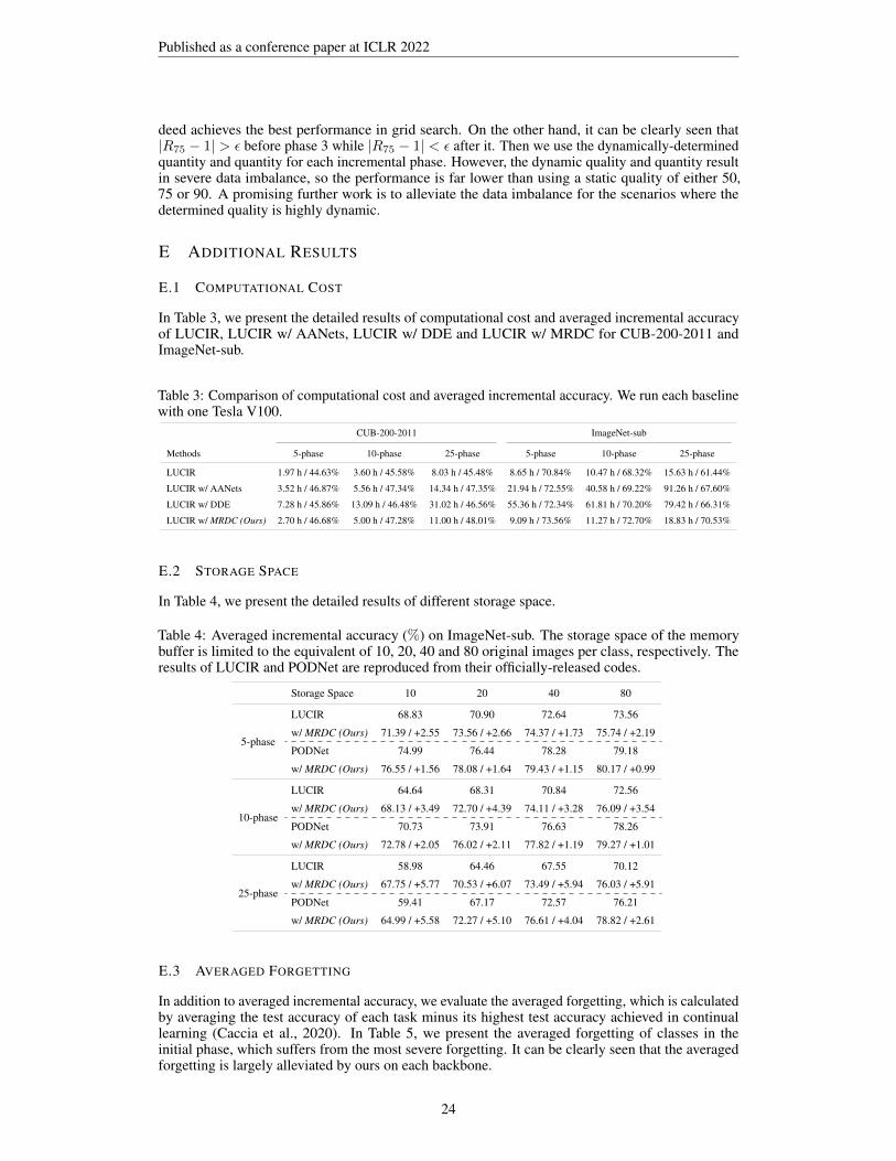
E.1 COMPUTATIONAL COST

In Table 3, we present the detailed results of computational cost and averaged incremental accuracyof LUCIR, LUCIR w/ AANets, LUCIR w/ DDE and LUCIR w/ MRDC for CUB-200-2011 andImageNet-sub.

Table 3: Comparison of computational cost and averaged incremental accuracy. We run each baselinewith one Tesla V100.

CUB-200-2011 ImageNet-sub

Methods 5-phase 10-phase 25-phase 5-phase 10-phase 25-phase

LUCIR 1.97 h / 44.63% 3.60 h / 45.58% 8.03 h / 45.48% 8.65 h / 70.84% 10.47 h / 68.32% 15.63 h / 61.44%

LUCIR w/ AANets 3.52 h / 46.87% 5.56 h / 47.34% 14.34 h / 47.35% 21.94 h / 72.55% 40.58 h / 69.22% 91.26 h / 67.60%

LUCIR w/ DDE 7.28 h / 45.86% 13.09 h / 46.48% 31.02 h / 46.56% 55.36 h / 72.34% 61.81 h / 70.20% 79.42 h / 66.31%

LUCIR w/ MRDC (Ours) 2.70 h / 46.68% 5.00 h / 47.28% 11.00 h / 48.01% 9.09 h / 73.56% 11.27 h / 72.70% 18.83 h / 70.53%

E.2 STORAGE SPACE

In Table 4, we present the detailed results of different storage space.

Table 4: Averaged incremental accuracy (%) on ImageNet-sub. The storage space of the memorybuffer is limited to the equivalent of 10, 20, 40 and 80 original images per class, respectively. Theresults of LUCIR and PODNet are reproduced from their officially-released codes.

Storage Space 10 20 40 80

5-phase

LUCIR 68.83 70.90 72.64 73.56

w/ MRDC (Ours) 71.39 / +2.55 73.56 / +2.66 74.37 / +1.73 75.74 / +2.19

PODNet 74.99 76.44 78.28 79.18

w/ MRDC (Ours) 76.55 / +1.56 78.08 / +1.64 79.43 / +1.15 80.17 / +0.99

10-phase

LUCIR 64.64 68.31 70.84 72.56

w/ MRDC (Ours) 68.13 / +3.49 72.70 / +4.39 74.11 / +3.28 76.09 / +3.54

PODNet 70.73 73.91 76.63 78.26

w/ MRDC (Ours) 72.78 / +2.05 76.02 / +2.11 77.82 / +1.19 79.27 / +1.01

25-phase

LUCIR 58.98 64.46 67.55 70.12

w/ MRDC (Ours) 67.75 / +5.77 70.53 / +6.07 73.49 / +5.94 76.03 / +5.91

PODNet 59.41 67.17 72.57 76.21

w/ MRDC (Ours) 64.99 / +5.58 72.27 / +5.10 76.61 / +4.04 78.82 / +2.61

E.3 AVERAGED FORGETTING

In addition to averaged incremental accuracy, we evaluate the averaged forgetting, which is calculatedby averaging the test accuracy of each task minus its highest test accuracy achieved in continuallearning (Caccia et al., 2020). In Table 5, we present the averaged forgetting of classes in theinitial phase, which suffers from the most severe forgetting. It can be clearly seen that the averagedforgetting is largely alleviated by ours on each backbone.

24


Table 5: Averaged forgetting (%) of classes in the initial phase. The storage space is limited to theequivalent of 20 original images per class. DDE (Hu et al., 2021) and AANets (Liu et al., 2021a) arereproduced from their officially-released code.

CUB-200-2011 ImageNet-sub

Method 5-phase 10-phase 25-phase 5-phase 10-phase 25-phase

LUCIR (Hou et al., 2019) -2.86 -4.56 -4.72 -15.08 -17.32 -22.40

w/ MRDC (Ours) -0.84 -1.08 -0.75 -14.11 -14.64 -17.96

w/ AANets (Reproduced) -4.03 -6.58 -10.37 -11.78 -9.54 -12.86

w/ AANets + MRDC (Ours) -1.40 -3.77 -6.82 -7.46 -8.13 -12.32

w/ DDE (Reproduced) -1.41 -5.24 -3.91 -14.02 -17.68 -23.73

w/ DDE + MRDC (Ours) -0.22 -0.97 -0.71 -11.24 -12.36 -17.80

E.4 FIXED MEMORY BUDGET

Here we evaluate memory replay with data compression (MRDC, ours) under a fixed memory budget(i.e., storage space) on ImageNet-sub. Following a widely-used setting (Rebuffi et al., 2017; Wu et al.,2019), the memory budget (i.e., storage space) is limited to equivalent of 2000 original images (20original images per class × a total of 100 classes in ImageNet-sub). We further evaluate a muchsmaller memory budget, fixed to 1000 original images. Under such a fixed memory budget, ourssubstantially boosts the performance of each backbone approach as shown in Table 6.

Table 6: Averaged incremental accuracy (%) on ImageNet-sub, under a fixed memory budget of 1000or 2000 original images.

1000 Original Images 2000 Original Images

Method 5-phase 10-phase 25-phase 5-phase 10-phase 25-phase

LUCIR (Hou et al., 2019) 70.16 66.32 62.07 71.87 69.37 65.72

w/ MRDC (Ours) 72.37 69.63 68.16 73.73 73.07 72.02

w/ DDE (Reproduced) 72.61 70.82 65.58 73.47 71.92 66.70

w/ DDE + MRDC (Ours) 74.40 72.62 69.03 75.35 73.93 71.17

E.5 LESS COMPRESSED SAMPLES

In Table 7, we present the results of LUCIR with different numbers of compressed samples onImageNet-sub. Similar to the main text, we select the JPEG quality of 50 for LUCIR, where thestorage space of 20 original images can save 85 such compressed images. Memory replay of 85compressed images of quality 50 achieves a much better performance than that of 20 original images.When reducing the quantity from 85 to 70, 55 and 40, the accuracy will also decline. However,memory replay of 40 compressed images of quality 50 still outperforms that of 20 original images,where the average memory can be saved by 52.94%.

Table 7: Averaged incremental accuracy (%) of LUCIR on ImageNet-sub with different numbers ofcompressed data. “5-phase”, “10-phase” and “25-phase” refer to the accuracy of 5-, 10- and 25-phaseImageNet-sub, respectively.

Quality 50 50 50 50 Original

Quantity 85 70 55 40 20

Total Storage 100% 82.35% 64.71% 47.06% 100%

5-phase 73.63 73.22 72.79 72.29 72.06

10-phase 72.65 72.01 71.35 70.16 68.59

25-phase 70.38 68.37 66.90 65.33 63.27

25

memory replay with data compression for continual learning

Documents

Transcript of memory replay with data compression for continual learning