Attorney Grievance Commission v. John T. Riely Misc. Docket ...
Upload
khangminh22Category
view
0download
0
MIDWEST RESIDENTIAL MARKET ASSESSMENT AND DSM POTENTIAL STUDY
Commissioned by:
Midwest Energy Efficiency Alliance 645 North Michigan Ave, Suite 990
Chicago, IL 60611
Sponsored by:
March 2006
Midwest Energy Efficiency Alliance i www.mwalliance.org
TABLE OF CONTENTS 1. Executive Summary.................................................................................................................. 1
1.1 Project Goals.................................................................................................................... 1
1.2 Methodology..................................................................................................................... 1
1.3 Findings and Conclusions................................................................................................ 2
1.3.1 Conclusions Regarding Midwest DSM Programs and Residential Energy Use. 2
1.3.2 Conclusions Regarding DSM Measure Saturations............................................ 3
1.3.3 Conclusions Regarding Natural Gas DSM Potentials ......................................... 4
1.3.4 Conclusions Regarding Electric DSM Potentials ................................................ 5
1.4 Natural Gas Recommendations ...................................................................................... 5
1.5 Electric Recommendations .............................................................................................. 6
2. Introduction ............................................................................................................................... 8
2.1 Background...................................................................................................................... 8
2.2 Project Goals and Methods ............................................................................................. 8
2.3 Organization of Report..................................................................................................... 9
3. Methodology............................................................................................................................ 10
3.1 Characterize the Midwest residential housing markets for states that have already conducted market assessments.................................................................................... 10
3.1.1 MEEA Illinois Residential Market Analysis ........................................................ 10
3.1.2 Xcel Energy Residential DSM Market Assessment Report .............................. 12
3.1.3 Energy Center of Wisconsin’s Energy and Housing in Wisconsin.................... 13
3.1.4 State of Iowa DSM Potential Studies ................................................................ 14
3.2 Characterize the five Midwest states for which residential market assessments have not yet been completed. ................................................................................................ 15
3.2.1 Design and Conduct of the RASS ..................................................................... 15
3.2.2 Trade Ally Surveys ............................................................................................. 17
3.2.3 Issues Related to Developing Population and Sample ..................................... 19
Midwest Energy Efficiency Alliance ii www.mwalliance.org
3.3 Characterize DSM Measures......................................................................................... 20
3.3.1 Climate-Independent End-Uses ........................................................................ 20
3.3.2 Climate-Dependent End-Uses........................................................................... 20
3.3.3 Climate-Independent Measures ........................................................................ 21
3.3.4 Climate-Dependent Measures........................................................................... 21
3.3.5 Measure Costs and Lifetimes ............................................................................ 21
3.4 Estimate technical, economic, and market DSM potential............................................ 22
3.4.1 Technical energy efficiency potential ................................................................ 22
3.4.2 Measure Stacking and Interaction Effects......................................................... 23
3.4.3 Economic Energy Efficiency Potential ............................................................... 23
3.4.4 Achievable Potential .......................................................................................... 25
4. Market Research Results ....................................................................................................... 27
4.1 Results from Interviews with Midwest Energy Organizations ....................................... 27
4.1.1 Introduction ........................................................................................................ 27
4.1.2 Current Residential Energy Efficiency Programs.............................................. 28
4.1.3 Previous Residential Market Assessment Research........................................ 29
4.1.4 Interest in Study ................................................................................................. 29
4.2 Data Sources ................................................................................................................. 30
4.3 Comparative Customer Demographic and Energy Use Statistics................................ 31
4.3.1 Electricity and Natural Gas Use......................................................................... 31
4.3.2 Customer Income............................................................................................... 32
4.4 Housing Characteristics................................................................................................. 33
4.4.1 Housing Unit Types and Sizes .......................................................................... 33
4.4.2 Insulation Levels ................................................................................................ 35
4.4.3 Windows............................................................................................................. 36
4.5 Lighting, HVAC, and Appliance DSM Measure Saturations ......................................... 37
Midwest Energy Efficiency Alliance iii www.mwalliance.org
4.5.1 Lighting............................................................................................................... 37
4.5.2 HVAC ................................................................................................................. 38
4.5.3 Water Heating .................................................................................................... 42
4.5.4 Appliances.......................................................................................................... 44
4.6 Customer Awareness of Energy Efficiency................................................................... 49
5. DSM Potential Results ............................................................................................................ 50
5.1 Natural Gas Potentials ................................................................................................... 50
5.2 Electric Potentials .......................................................................................................... 60
6. Conclusions and Recommendations ...................................................................................... 71
6.1 Housing Characteristics and Energy Use...................................................................... 71
6.2 DSM Program Activity and Measure Saturations .......................................................... 71
6.3 Natural Gas DSM Potentials .......................................................................................... 72
6.4 Electric DSM Potentials ................................................................................................. 73
6.5 Recommendations ......................................................................................................... 74
6.5.1 Key Natural Gas Measures................................................................................ 74
6.5.2 Electric DSM Measures ..................................................................................... 77
6.5.3 Residential Program Recommendations........................................................... 79
Midwest Energy Efficiency Alliance 1 www.mwalliance.org
1. EXECUTIVE SUMMARY This section provides a brief summary of the project goals and methods, findings and conclusions, and recommendations.
1.1 Project Goals
The Midwest Energy Efficiency Alliance’s (MEEA) project goals as specified in the original project RFP are to:
• Characterize the Midwest residential market, including estimating saturation rates for existing energy efficiency technologies, products, practices, and behavior.
• Evaluate efficiency opportunitie s in this market sector.
• Estimate a baseline to assess future residential demand side management (DSM) programs.
• Benchmark other Midwest states to Xcel Energy’s Minnesota service area.
1.2 Methodology
In September 2004, MEEA selected Summit Blue Consulting to conduct a regional residential market assessment via a competitive request for proposal process. Summit Blue had partnered with Quantec LLC and Skumatz Economic Research Associates and the team was awarded to contract due to their extensive experience in conducting market potential studies both within the Midwest and nationally. The first major project task was to review and compile information from already completed residential market assessments for Xcel Energy’s Minnesota area1, MEEA’s Illinois study2, as well as similar studies conducted for Iowa3, and Wisconsin 4. Project team members had either conducted these studies, or knew of them before the start of this project. The project team did not collect additional primary data for these four states that had already conducted market assessments, but rather used the existing data from these previous studies to characterize these states. The project team used this approach to conserve project resources and to focus the data collection efforts on the five Midwest states for which statistically representative data was not publicly available.
The second major project task was to conduct a thorough search for additional similar studies that had been conducted throughout the Midwest. The project team conducted telephone interviews with 40 Midwest investor-owned utilities, larger municipal utilities and coops, as well as all state energy agencies, and larger city energy agencies. The intent of these interviews was both to get a better understanding of the residential markets in the Midwest, and to identify any organizations that might be interested in teaming with MEEA to conduct additional data collection specific to the organizations’ service area.
1 Itron, “Xcel Energy Residential DSM Market Assessment Report”, (Itron, Vancouver, WA, July 26, 2003). 2 Midwest Energy Efficiency Alliance, “Illinois Residential Market Analysis”, (Midwest Energy Efficiency Alliance, Chicago, IL, May 12, 2003). 3 Global Energy Partners and Quantec, “Assessment of Energy and Capacity Savings Potential in Iowa, Volume1: Assessment of Energy Efficiency Measures” and Volume III, Technical Potential Estimates (2002). 4 Energy Center of Wis consin, “Energy and Housing in Wisconsin”, (Energy Center of Wisconsin, Madison, WI, November 2000).
Midwest Energy Efficiency Alliance 2 www.mwalliance.org
The third major project task was to collect primary data to characterize the five Midwest states (Indiana, Kentucky, Michigan, Missouri, and Ohio) for which publicly accessible in-depth market assessments have not yet been conducted. The general data collection approach was:
• Complete about 480 phone-based residential appliance saturation surveys (RASS) across the sample (96 per state) to obtain dwelling, appliance, fuel, DSM measure, demographic, attitudinal, awareness, and other information.
• Survey 5-10 HVAC equipment distributors and/or residential energy auditors per state. These surveys were done to estimate the saturations of insulation and energy-efficient equipment in the residences in each state.
The fourth major project task was to characterize the DSM measures to be analyzed for this study. Characterization of DSM measures requires: 1) determining the list of DSM measures to evaluate: 2) estimating the baseline energy consumption for each end-use (heating, cooling, cooking, hot water, etc.) or unit energy consumption (UEC); and 3) estimating the incremental savings from each measure - improving from the baseline to the new technology. In addition, the baselines must consider that different classes of homes have different penetrations of technologies, such as existing homes compared to new construction.
The fifth major project task was to estimate the technical and achievable DSM potential for the measures specified in task four. The general approach for derivation of energy efficiency resource potentials consisted of three sequential steps: 1) estimate technical energy efficiency potential; 2) subdivide the technical energy efficiency potential estimates into discrete “bundles” based on cost category, which allows the economic potential to move with the underlying volatility in fuel prices; and 3) estimate market penetration and the resulting achievable potential as a subset of each bundle. All of these estimates were derived using Quantec’s Energy ForecastPro model, an end-use forecasting and energy efficiency potentials assessment tool. The conceptual underpinnings and analytic procedures of this model are based on standard practices in the utility industry, and are consistent with the methods used in the Xcel Energy and Iowa studies mentioned above.
The last major project task was conducting an integrated analysis of all the project results. From this assessment of the project findings, the project team developed conclusions and recommendations, which are presented in the next two sections.
1.3 Findings and Conclusions
1.3.1 Conclusions Regarding Midwest DSM Programs and Residential Energy Use
Conclusion #1: The most frequently offered types of DSM programs by the sponsor organizations surveyed in the Midwest are rebate programs, energy audit programs, and other types of energy information programs.
Rebate programs frequently covered multiple technologies, such as efficient heating and cooling equipment, water heaters, lighting, appliances, and new construction measures. Direct load control programs and low income programs are also relatively common in the Midwest. Less common are financing programs and multi-family focused programs.
Conclusion #2: Residential electricity and natural gas use per customer varies over 50% from the lowest use states to the highest use states in the Midwest.

Midwest Energy Efficiency Alliance 3 www.mwalliance.org
The saturations of electric space heating and water heating have the largest influence on electricity use in the region. Variations in natural gas use are similarly influenced by saturations of natural gas space heating and water heating, as well as climate and average gas space heating efficienc ies. Average electric use per customer is lowest in Michigan, Minnesota, Illinois, and Wisconsin, while average natural gas use per customer is lowest in Missouri, Iowa, Wisconsin, and Indiana.
1.3.2 Conclusions Regarding DSM Measure Saturations
Conclusion #3: Generally 5%-15% of customers have either uninsulated ceilings or walls in their homes.
The percentage of customers with uninsulated attics varies from 3% to 11% from state to state, while the percentage of homes with uninsulated walls varies from 5% to 27%. However, more than half of these percentages were self-reported by customers through a telephone survey. Such self-reported responses often over-estimate the actual amount of insulation present in homes.
Conclusion #4: Generally 20%-36% of homes have mostly single-paned windows.
The lowest percentages of single -paned windows are found in Minnesota (20%) and Ohio (22%), while the highest percentages are found in Illinois (36%) and Wisconsin (35%).
Conclusion #5: Less than half of the homes in any Midwest state have one or more compact fluorescent lamps (CFLs).
The percentage of homes with one or more CFLs varies from 13% in Wisconsin to 43% in Kentucky. (However, Wisconsin’s data is the oldest of the states analyzed, so the saturation of CFLs there is like ly higher currently.) The median percentage of homes with one or more CFLs is 33%.
Conclusion #6: The market shares of efficient gas space heating systems are estimated to be the highest in Iowa, Minnesota, and Wisconsin at 74%, 67%, and 50% respectively.
For Indiana, Kentucky, Michigan, Missouri, and Ohio, energy auditors estimate the shares of more efficient gas furnaces at 23% on average, but slightly higher in Missouri. The higher saturations of efficient gas furnaces in Iowa, Minnesota, and Wisconsin is presumably due to the impact of long standing DSM programs promoting this DSM measure in those states.
Conclusion #7: The highest percentages of more efficient central air conditioners are found in Iowa (74% total) and Minnesota (48% total).
These percentages are much higher than the 24% market share estimated by energy auditors for efficient air conditioners in Indiana, Kentucky, Michigan, Missouri, and Ohio, or the 6% market share found from the on-site audits in Wisconsin. (However, the Wisconsin data is the oldest of that included in this report, so the efficient units’ market shares may have increased there since 1999.) The Iowa utilities and Xcel Energy in Minnesota have been promoting energy efficient central air conditioners for a long time, which is presumably mostly responsible for the higher saturations of efficient air conditioners in those states.
Conclusion #8: Midwest electric and gas water heaters are mainly minimum efficiency units.
Midwest electric water heaters are mainly minimum efficiency units, with low efficiency units’ market shares ranging from 66% to 87% from state to state. As with electric water heaters, Midwest natural gas
Midwest Energy Efficiency Alliance 4 www.mwalliance.org
water heaters are mainly minimum efficiency models, which have market shares of 63%-83% from state to state.
Conclusion #9: The saturations of ENERGY STAR ® appliances in the Midwest are likely rather low, in the range of 3%-6% depending on the appliance.
The most accurate estimates of ENERGY STAR® appliance saturations should be those provided by the energy auditors in Illinois and Minnesota, who conducted on-site inspections of appliances to determine whether they met ENERGY STAR® standards or not. Customers estimate that far higher percentages of their appliances are ENERGY STAR® units, usually ranging from 16% to 49%, depending upon the appliances and the state of residence. However, most residential customers likely do not know enough about ENERGY STAR® standards to accurately estimate whether their appliances meet these standards or not.
Conclusion #10: The saturations of programmable thermostats vary widely from state to state in the Midwest.
The saturations range from lows of 17% and 19% in Indiana and Kentucky respectively to a high of 47% in Illinois. The mean statewide saturation in the states analyzed is 29%.
1.3.3 Conclusions Regarding Natural Gas DSM Potentials
Conclusion #11: The total DSM potentials for natural gas DSM measures are remarkably consistent from state to state in the Midwest.
The total 20-year technical potential for gas DSM varies only from 44% to 48% of base case consumption between states. The total achievable potential for gas DSM varies between states from about 23% to 27% of base case consumption. In total, the gas technical DSM potential is estimated to be 9.2 billion therms for all nine Midwestern states analyzed, and the maximum achievable gas potential is estimated to be 5.0 billion therms across the Midwest, or about 54% of the gas technical potential.
Conclusion #12: In total, about 43% of the total achievable potential is available from DSM measures whose cost of conserved energy is $1 per therm or less.
About 12% of the total achievable potential is available from measures whose cost of conserved energy is $0.30 per therm or less. On the other hand, about 33% of the total achievable potential is from measures whose costs of conserved energy are more than $1.50 per therm, at or above the currently high commodity cost for natural gas.
Conclusion #13: The most cost-effective natural gas DSM measures are insulating uninsulated attics, ENERGY STAR® programmable thermostats, low flow showerheads, hot water pipe insulation, and faucet aerators.
These measures have costs of conserved energy of $0.30 per therm or less in existing single -family homes. High efficiency furnaces, comprehensive air sealing/infiltration reductions, water heater thermostat setbacks, and multi-family wall insulation are in the second tier of cost-effectiveness, with costs of conserved energy of $0.60 per them or less.
Conclusion #14: Not surprisingly, space heating natural gas DSM measures account for over 80% of total achievable gas DSM potential.
Midwest Energy Efficiency Alliance 5 www.mwalliance.org
Water heating gas DSM measures account for almost all of the remaining achievable gas DSM potential. Also not surprisingly, single -family homes account for over 80% of total achievable residential gas DSM potential.
1.3.4 Conclusions Regarding Electric DSM Potentials
Conclusion #15: Electric DSM potentials are much smaller shares of base case consumption than gas DSM potentials.
Total electric DSM technical potential equals about 24% of base case consumption which translates to almost 84 billion kWh in savings, compared to about 47% for gas technical potential, which translates to 9.2 billion therms saved. Total electric achievable potential accounts for about 10% of base case consumption, compared to about 25% for gas achievable potential. The differences between the results for the two energy types is due to two primary factors: first, the electric base case consumption estimates include electricity savings from the significant forthcoming federal efficiency standards for central air conditioners and heat pumps that will take effect in 2006. Second, electric space heating, water heating, and lighting account for less than half of total base case electric consumption, but almost all of natural gas base case consumption. The DSM potentials for other electric loads such as appliances are considerably smaller percentages of base case consumption than the DSM potentials for space heating, water heating, and lighting DSM measures.
Conclusion #16: Electric DSM potentials vary much more from state to state than gas DSM potentials.
Electric technical DSM potential varies from about 20% to 30% of base case consumption between states, while electric achievable DSM potential varies from about 8% to 14% between states. Minnesota and Wisconsin have the lowest relative amounts of DSM potential, while Kentucky and Missouri have the largest relative amounts of DSM potential. The amounts of electric DSM potential are proportionate to the saturations of electric space heating and water heating equipment in a state, and inversely proportionate to the magnitudes of historical DSM activity.
Conclusion #17: In total, about 39% of the total electric achievable potential is available from DSM measures whose cost of conserved energy is 6 cents/kWh or less.
On the other hand, 51% of total electric potential comes from DSM measures whose costs of conserved energy are 10 cents/kWh or more, at or above most current Midwest electric rates.
Conclusion #18: The most cost-effective and largest impact electric DSM measures are insulating uninsulated attics, installing ENERGY STAR ® heat pumps, installing CFLs, removing or replacing secondary or inefficient refrigerators or freezers, and low flow showerheads.
In total, these measures comprise over 75% of the achievable DSM potential for measures with costs of conserved energy of 6 cents/kWh or less. In fact, most of these measures have costs of conserved energy of 3 cents/kWh or less.
1.4 Natural Gas Recommendations
Four residential natural gas measures account for about 83% of the DSM potential with a cost of conserved energy of $1 per therm or less. The remaining DSM potential at this cost of conserved energy
Midwest Energy Efficiency Alliance 6 www.mwalliance.org
is accounted for by a variety of measures, each with relatively small impacts. Each of the four major measures are briefly discussed below.
Insulating Un-insulated Attics
The total achievable potential for this measure over the 20 year forecast period is approximately 390 million therms. This represents about two percent of total residential base case natural gas consumption over this period. The total cost of conserved energy for this measure in most Midwest single -family homes is about $0.25 per therm. This cost is based on the total installed cost for the insulation.
ENERGY STAR® Programmable Thermostats
The total achievable potential for this measure over the 20 year forecast period is approximately 210 million therms. This represents about one percent of total residential base case natural gas consumption. The total cost of conserved energy for this measure in most Midwest single -family homes is about $0.17 per therm. This cost is based on the total installed cost for the thermostat. Since the current saturations for programmable thermostats are less than 50% in all Midwest states studied, and vary by over a factor of two from state to state in the Midwest, considerable market potential exists for this measure.
High Efficiency Gas Furnaces
The total achievable potential for this measure over the 20 year forecast period with a cost of conserved energy of $1 per therm or less is approximately 930 million therms. This represents about five percent of total residential base case natural gas consumption. The cost of conserved energy for this measure varies between housing types, and whether a 92% or 96% efficient furnace is analyzed. The 96% efficient furnaces were found to have a lower total cost of conserved energy than the 92% efficient furnaces.
Efficient furnaces have a cost of conserved energy between $1.10 per therm and $1.20 per therm in the more southern states of the Midwest where the annual savings are lower. The total DSM potential from efficient furnaces in those states is about 600 million therms, or about three percent of total residential base case consumption. Whether this conservation is considered cost-effective or not depends on projections for the price of natural gas.
Conduct Comprehensive Shell Air Sealing and Infiltration Reduction
The total achievable potential for this measure over the 20 year forecast period is approximately 280 million therms, or about 1.4% of base case natural gas consumption over this period. This measure is most applicable and cost-effective in existing single family homes. The cost of conserved energy for this measure in most of the Midwest states analyzed is about $0.85 per therm, but in some of the northern states where the annual savings are larger than average, the cost of conserved energy is about $0.57 per therm.
1.5 Electric Recommendations
Six residential electric measures account for about 78% of the DSM potential with a cost of conserved energy of 10¢/kWh or less. The remaining DSM potential at this cost of conserved energy is accounted for by a variety of measures, each with relatively small impacts. Each of the six major measures are briefly discussed below.
Midwest Energy Efficiency Alliance 7 www.mwalliance.org
Compact Fluorescent Lamps (CFLs)
The total achievable potential for this measure over the 20 year forecast period is approximately 5,800 GWh, or about 1.6% of total residential base case electric consumption over this period. The total cost of conserved energy for this measure varies with how many hours per day the lamps are used. For lamps that are used six hours per day, the cost of conserved energy is about 1.2¢/kWh, while for CFLs that are used 2.5 or 0.5 hours per day, the cost of conserved energy is 2.3¢/kWh or 11¢/kWh, respectively
ENERGY STAR® Heat Pumps
ENERGY STAR® heat pumps have minimum cooling efficiencies of 14 SEER and minimum heating system performance factors of 8.5 starting in 2006. The total achievable potential for this measure over the 20 year forecast period is approximately 3,400 GWh, or about 1.0% of total residential base case electric consumption over this period. The total cost of conserved energy for this measure varies considerably with climate, and ranges from about 1.4¢/kWh to 9.4¢/kWh, and even higher. Almost all of the DSM potential for this measure is in single -family homes.
Insulating Un-insulated Attics
This measure is also a large electric savings measure, primarily in states with significant electric space heating saturations. The total achievable potential for this measure over the 20 year forecast period is approximately 1,800 GWh, or about 0.5% of total residential base case electric consumption over this period. The total cost of conserved energy for this measure in most Midwest single -family homes is about 1.8¢/kWh.
Removing Secondary Refrigerators
The total achievable potential for this measure over the 20 year forecast period is approximately 1,500 GWh, or about 0.4% of total residential base case electric consumption over this period. The total cost of conserved energy for this measure is about 6.1¢/kWh.
ENERGY STAR® Refrigerators
The total achievable potential for this measure over the 20 year forecast period is approximately 930 GWh, or about 0.3% of total residential base case electric consumption over this period. The total cost of conserved energy for this measure is about 9.3¢/kWh. All the DSM potential for this measure that costs 10¢/kWh or less is from single-family homes.
Efficient Water Heaters
The total achievable potential for high efficiency and heat pump water heaters over the 20 year forecast period is approximately 770 GWh, or about 0.2% of total residential base case electric consumption over this period. The total cost of conserved energy for high efficiency water heaters is about 6.9¢/kWh, while the cost of conserved energy for heat pump water heaters is about 9.9¢/kWh.

Midwest Energy Efficiency Alliance 8 www.mwalliance.org
2. INTRODUCTION This section provides the background and context in which this study was conducted, summarizes the project goals and methods, and provides an outline of the entire project report.
2.1 Background
Market assessment studies and DSM potential studies can be valuable sources of information for planning energy efficiency programs. There has been a resurgence of interest in these types of studies in the past five years. A recent ACEEE paper summarized the results of eleven DSM potential studies that have been conducted across the country over this period5. Interestingly, however, this ACEEE paper did not cover any such studies from the Midwest, although several studies of this type have been conducted in the Midwest in recent years.
As will be discussed in more detail in the Methodology section, large-scale market assessments or DSM potential studies covering at least residential customers have been conducted in Illinois, Iowa, Minnesota, and Wisconsin in the past five years. These studies were done for somewhat different purposes, including DSM program planning, baseline market characterizations , and utility integrated resource planning (IRPs). Most of these studies included in-depth assessments of DSM potential for those states or utility service areas, and included telephone or on-site surveys of varying degrees of comprehensiveness to provide the input data for their market characterizations and DSM potential estimates.
2.2 Project Goals and Methods
MEEA’s project goals as specified in the original project RFP are to:
• Characterize the Midwest residential market, including estimating saturation rates for existing energy efficiency technologies, products, practices, and behavior.
• Evaluate efficiency opportunities in this market sector.
• Estimate a baseline to assess future residential DSM programs.
• Benchmark other Midwest states to Xcel Energy’s Minnesota service area.
The approach used for this project was to use data and results from the four recent Midwest residential market assessments to characterize those four states, and provide the input data for conducting DSM potential estimates for those states. In addition, the project team conducted new telephone residential appliance saturation surveys and telephone surveys of energy auditors for the other five Midwest states covered by this study: Indiana, Kentucky, Michigan, Missouri, and Ohio. This data was used to characterize those five states and compare them to the four states where previous studies had been conducted, and to provide the input data for DSM potential estimates for those states.
The project team used Quantec’s Energy Forecast Pro model to develop the electric and natural gas DSM potential estimates. Quantec used a previous version of this model for the Iowa DSM potential estimates,
5 S. Nadel, A. Shipley, and R.N. Elliott, “The Technical, Economic and Achievable Potential for Energy Efficiency in the U.S.—A Meta-Analysis of Recent Studies”, Proceedings of the 2004 ACEEE Summer Study on Energy Efficiency in Buildings.

Midwest Energy Efficiency Alliance 9 www.mwalliance.org
and it uses a somewhat similar approach to the model used in Minnesota for the DSM potential estimates for that state.
2.3 Organization of Report
This report is divided into the following major sections:
1. Executive Summary
2. Introduction
3. Methodology
4. Market Research Results
5. DSM Potential Results
6. Conclusions and Recommendations
Appendix A: DSM Potential Results by State
Appendix B: DSM Measure Information
Appendix C: Residential Appliance Saturation Survey Instrument and Results

Midwest Energy Efficiency Alliance 10 www.mwalliance.org
3. METHODOLOGY This section describes the approach used for this project.
3.1 Characterize the Midwest residential housing markets for states that have already conducted market assessments.
The first major project task was to review and compile information from the already completed residential market assessments for Xcel Energy’s Minnesota area6, MEEA’s Illinois study7, as well as similar studies conducted for Iowa8, and Wisconsin 9. Project team members had either conducted these studies, or knew of them before the start of this project. The project team did not collect additional primary data for these four states where recent market assessments were conducted, but rather used the existing data from these previous studies to characterize these states. The project team used this approach to conserve project resources and to focus the data collection efforts on the five Midwest states for which statistically representative data were not publicly available.
The project team also conducted a thorough search for additional, similar studies that had been conducted throughout the Midwest, and collected additional data from the organizations interviewed to support several of the ultimate project recommendations requested by MEEA. This was accomplished by conducting telephone interviews with 40 Midwest investor-owned utilities, larger municipal utilities and coops, as well as all state energy agencies and larger city energy agencies. The intent of these interviews was both to get a better understanding of the residential markets in the Midwest, and to identify any organizations that might be interested in teaming with MEEA to conduct additional data collection specific to the organizations’ service area.
The four previously conducted studies had somewhat different objectives, and often used somewhat different approaches to accomplish their objectives. The objectives and methodology for each of the four studies is summarized briefly below.
3.1.1 MEEA Illinois Residential Market Analysis
This study was published in May 2003, and the primary data collection was conducted in June through October of 2002. The study had four primary objectives:
1. Evaluate opportunities for efficiency in the residential sector of Illinois.
2. Determine saturation rates of existing technologies, products, and practices/behavior in Illinois.
3. Understand consumer energy decision-making and consumer energy usage.
6 Itron: 2003, op.cit. 7 Midwest Energy Efficiency Alliance (MEEA): 2003, op.cit. 8 Global Energy Partners and Quantec: 2002, op.cit. We also relied on information relating to economic and achievable potential estimates contained in the individual Iowa utility Energy Efficiency Plans filed in 2002-03 by Alliant Energy, Aquila Networks, Atmos Energy, and MidAmerican Energy. 9 Energy Center of Wisconsin: 2000, op.cit.

Midwest Energy Efficiency Alliance 11 www.mwalliance.org
4. Provide a baseline to help determine future programs that will most effectively impact consumers in Illinois 10.
The data collection approach included:
• Initial telephone interviews to gather basic household information.
• On-site surveys to record appliances, household envelope features, and heating/cooling equipment. These 309 surveys were conducted in Cook County (including Chicago), the collar counties surrounding Chicago, northwest Illinois, central Illinois, and southern Illinois. Only single -family homes were surveyed, and the sample was not designed to gather representative information on newly constructed homes separately from older homes. Four to six homes per day were surveyed by each auditor.
• Completion of a survey by the homeowner. The survey covered the residents’ awareness and understanding of the ENERGY STAR® label, and general energy issues11.
Engineering estimates or DOE-2 analysis were used to estimate energy impacts for each DSM measure evaluated. One prototype home was developed using the survey results, and energy impacts were calculated separately for northern Illinois using Chicago weather data, and for southern Illinois using St. Louis weather data12.
Annual savings estimates were calculated for 34 DSM measures. These measures included HVAC system renovation or replacement measures, adding various types of insulation, replacing appliances with ENERGY STAR® models, and water heating efficiency measures such as adding low flow showerheads. Of these 34 measures, 19 were selected as priority measures for which DSM potential estimates were developed13.
Technical DSM potential was estimated by multiplying the number of homes in Illinois times the percentages of homes for which a given measure is applicable times the average impacts per DSM measure. The technical potential estimates just considered the then-current population of single family homes in Illinois. Population growth was not factored into the estimates. Technical potential was expressed in the report as a percentage of all homes for which a measure is applicable 14.
“Raw economic potential” applied an “economic feasibility percentage” to technical potential to estimate the percentage of technical conservation potential that is cost-effective. Economically feasible meant that “the homeowner has some reason (such as age or condition) to consider the idea of purchasing or replacing a technically potential measure, without regard for first cost or existing market barriers”15.
Market potential was calculated based on DSM measures’ installed cost, payback to the customer, and a “market barrier factor”. The key factor used to estimate market potential was an “annual market capture percent”, which represents the probability that a DSM measure will be adopted based on it’s installed
10 MEEA: 2003, op cit., p. 9. 11 MEEA: 2003, op cit., p. 9-12. 12 MEEA: 2003, op cit., p. 13. 13 MEEA: 2003, op cit., p. 27. 14 MEEA: 2003, op cit., p. 45-46. 15 Personal communication with Glenn Haynes, RLW Analytics, 8-15-05.

Midwest Energy Efficiency Alliance 12 www.mwalliance.org
cost, payback, and the market barrier factor. First cost was assigned an importance equal to three times the payback period. The market barrier factor captures the effects of known non-economic barriers by using a discreet value of 1-3, where one indicates no known barriers exist, two indicates average barriers, and three indicates formidable barriers. The final market potential estimates, the “yearly realizable potential” are the product of the raw economic potential and the annual market capture percent. No formal forecasting models were used to estimate market potentials.
3.1.2 Xcel Energy Residential DSM Market Assessment Report
This project was part of the third phase of a three phase project to update the Company’s DSM potential estimates for its Minnesota service area. The project report summarizing the study was published in July 2003, and the primary data was collected from November 2002 through April 2003. The primary objective of the overall project was to support developing the DSM part of the Company’s integrated resource plans. This was the third large-scale assessment of DSM potential in its Minnesota territory that the Company has conducted in the past 15 years.
Key data collection elements of this study included:
• Conducting 400 on-site surveys for a representative sample of the Company’s residential customers. Customer building types covered included single -family dwellings, apartments, and mobile homes. Separate sub-samples for newly constructed buildings were developed for each type of residential housing. The data collected included complete energy equipment inventories and building envelope specifications, as well as a substantial customer energy conservation attitude and awareness survey.
• Updating DSM measure costs and lifetime estimates based on recent Company information and other secondary sources such as the California Energy Commission’s Database of Energy Efficiency Resources.
DSM potential estimates were developed using Itron’s Assessment of Energy Technologies (ASSET) model, and covered the period 2003-2017. Xcel Energy had used this ASSET model for its last major DSM potential study in the mid-1990s, and in subsequent updates since that time16. The ASSET modeling for the residential sector focused on the Company’s two main electric energy conservation program areas: a rebate program for efficient central and room air conditioners, and residential lighting conservation programs17. Detailed processing of the on-site survey results was only conducted to the extent needed to develop DSM potential estimates for air conditioners and lighting in order to minimize project costs.
Technical potential estimates were made assuming that the most efficient equipment option, thermal shell configuration, or control device is selected at each decision point. For retrofit actions, only changes that are technically feasib le without major structural changes are included, while for new construction, a broader set of actions is considered. All measures are assumed to be installed regardless of measure cost or acceptability to the customer18.
Economic potential estimates were based on implementing all technically feasible measures that meet a stated economic criterion. The economic criterion used for this study is a modified total resource cost test
16 Itron: 2003, op cit., p. 1-1. 17 Itron: 2003, op cit., p. 2-4. 18 Itron: 2003, op cit., p 1-2

Midwest Energy Efficiency Alliance 13 www.mwalliance.org
that does not include program administrative costs. The intent of the economic screening is just to compare DSM measure costs to DSM measure benefits19.
Market or achievable potential is the most difficult to estimate of the three types of DSM potential. Achievable potential estimates incorporate the following factors:
• Customers’ awareness and attitudes towards DSM measures.
• Market barriers such as information costs.
• Decision models that are based on customer decision-making processes rather than on simpler cost-effectiveness calculations.
• Calibration factors based on previous customer actions relating to DSM program participation20.
For this study three estimates of market potential were reported: first, DSM potential based on Xcel Energy’s current customer rebates. Second, DSM potential based on setting rebates equal to zero, and third, DSM potential based on doubling the amount of the Company’s current rebates. In all cases market potential estimates are estimated relative to the minimum efficiency technology that is legally available 21.
3.1.3 Energy Center of Wisconsin’s Energy and Housing in Wisconsin
This study was published in November 2000, and the primary data collection was conducted in 1999. This study only covered single family, owner occupied housing. The primary objectives of the study were:
1. Characterize key residential housing and household behavioral factors in Wisconsin:
a. Housing structural, mechanical system, and major appliance characteristics.
b. People’s use of mechanical systems and appliances.
c. People’s knowledge and attitudes about energy efficiency, conservation, and energy costs.
2. Combine people’s attitudes towards energy efficiency with data on where opportunities exist in order to develop more realistic estimates of market potential for structural improvements or social marketing campaigns to change behavior 22.
Although the second project objective mentions market potential, traditional DSM potential estimates that show the total potential energy savings for the state for a number of DSM measures were not developed as part of the study. The study does present average annual dollar savings per customer for each measure, and the total annual dollar savings from all the measures evaluated23. However, the DSM potential for the
19 Itron: 2003, op cit., p 1-2. 20 Itron: 2003, op cit, p 1-3. 21 Itron: 2003, op cit., p 1-3-1-4. 22 ECW: 2000, op cit., p. 1. 23 ECW: 2000, op cit., p. 16-18.

Midwest Energy Efficiency Alliance 14 www.mwalliance.org
measures are not presented in energy terms, nor are traditional technical, economic, and market potential estimates presented.
A sample of 299 Wisconsin homeowners was the source of data for this study. Low-income households and newly constructed homes were over-sampled to ensure that representative data was collected for those two market segments. For each participating household, three types of data were collected:
1. Trained home energy raters conducted an on-site audit to collect data on the structure and appliances. These audits were designed to collect sufficient information to complete a HERS rating, and typically lasted two to three hours. The auditors also collected data beyond that needed to complete a HERS rating, such as a lighting inventory and measuring showerhead flow rates.
2. Homeowners completed a 32 page survey on their energy practices, energy attitudes, and demographics.
3. Natural gas and electric monthly billing histories were collected from almost all the participants’ utilities.
The HERS rating software provided an energy rating for each home on a 1-100 scale, and also estimated the annual energy use for heating, air conditioning, and water heating24.
3.1.4 State of Iowa DSM Potential Studies
State of Iowa DSM potential estimates were conducted in a series of studies between 2001 and 2003. The initial phase was a joint research effort sponsored by the Iowa Utility Association (IUA), whose members included Alliant Energy, Aquila Networks, Atmos Energy, and MidAmerican Energy. The study addressed electric and gas savings across the residential, commercial, industrial, and agricultural sectors. Three research activities were conducted:
1. Data collection.
2. Development of a base case forecast consistent with each utility’s long-run customer and sales forecasts.
3. Estimates of energy and capacity technical potential estimates for each utility using Quantec’s Quant.sim end-use forecasting and DSM potential model.25
The data collection effort assimilated data from a variety of sources including: historical and forecasted loads and customer data from the utilities; customer counts and sales by sector and market segment from the utilities’ customer information systems; historical DSM impacts reported to the Iowa Utilities Board (IUB); the Energy Information Administration’s 1997 Residential Energy Consumption Survey (RECS), and 1999 Commercial Building Energy Consumption Survey (CBECS); a survey of equipment distributors serving Iowa; and DSM measure data from dozens of vendors and industry reports.
The residential sector base case began with initial estimates of energy consumption by end-use and dwelling type using an engineering thermal load model known as BEST. Typical building parameters
24 ECW: 2000, op cit., p. 1-3. 25 Energy ForecastPro, the tool used in this study for MEEA, is the successor tool to Quant.sim.

Midwest Energy Efficiency Alliance 15 www.mwalliance.org
(such as square footage, base equipment types and efficiencies, and shell levels) were specified, providing initial estimates of base case energy usage by fuel and end-use. The values from BEST were then input into Quant.sim, along with other data such as customer counts, fuel shares, and efficiency shares, and adjusted as necessary to calibrate total energy sales to each utility’s econometric forecasts.
The assessment of potential began with a thorough assessment of DSM measures commercially available and applicable to the state of Iowa. Several hundred measures were analyzed, including nearly 100 in the residential sector alone. The analytics provided the information necessary to conduct the potential assessment: energy savings, costs, lifetime, and other key measure characteristics. All HVAC measure savings estimates were derived in subsequent runs with BEST. Overall technical potential estimates—relative to each utility’s load forecast—were then derived in Quant.sim, providing distinct estimates by dwelling type, end-use, and vintage (existing, new construction).
Following the completion of the Phase I technical potential estimates, each utility completed economic and achievable potential estimates as part of the development of the Energy Efficiency Plans required by the IUB. The basic methodology for developing these estimates was very similar to the Xcel Energy study approach:
• Each measure was first screened for economic viability using the total resource cost test. Passing measures were then considered in Quant.sim, resulting in a second set of estimates reflecting the economic potential.
• Market barriers, awareness, acceptance and other factors affecting customer choice were considered through a review of the penetration rates associated with other programs in the United States. The penetration rates associated with best program practices were deemed “achievable”, and applied to the economic potential estimates.
3.2 Characterize the five Midwest states for which residential market assessments have not yet been completed.
The focus for primary data collection for this project is the five Midwest states (Indiana, Kentucky, Michigan, Missouri, and Ohio) for which publicly accessible in-depth market assessments have not yet been conducted. The general data collection approach was:
• For the base case approach, complete about 480 phone-based residential appliance saturation surveys (RASS) across the sample (96 per state) to obtain dwelling, appliance, fuel, DSM measure, demographic, attitudinal, awareness, and other information.
• Survey 5-10 HVAC equipment distributors and/or residential energy auditors per state. These surveys were done to estimate the saturations of insulation and energy-efficient equipment in the residences in each state.
3.2.1 Design and Conduct of the RASS
The RASS survey instrument used for this project is presented in Appendix C. The survey instrument was designed to collect information such as household characteristics; energy payments; familiarity with conservation activities; conservation measures already in practice; a resident’s heating/cooling system usage; a resident’s water heating system usage; and type of fuel or energy source used for major appliances or household equipment. The information was needed to identify the saturations of existing
Midwest Energy Efficiency Alliance 16 www.mwalliance.org
equipment and fuel uses in the Midwest energy market to support estimation of the technical, economic, and market demand side management potential.
The survey was administered by telephone to residents of Indiana, Kentucky, Michigan, Missouri, and Ohio. Responses were obtained from 96 households per state, with a total of 480 respondents across the five state region.26 The study was designed to achieve the following accuracy levels for a question with a proportional response of 50%:
• For each state: +/- 10% at 95% confidence.
• Overall accuracy: +/-5% at 95% confidence.
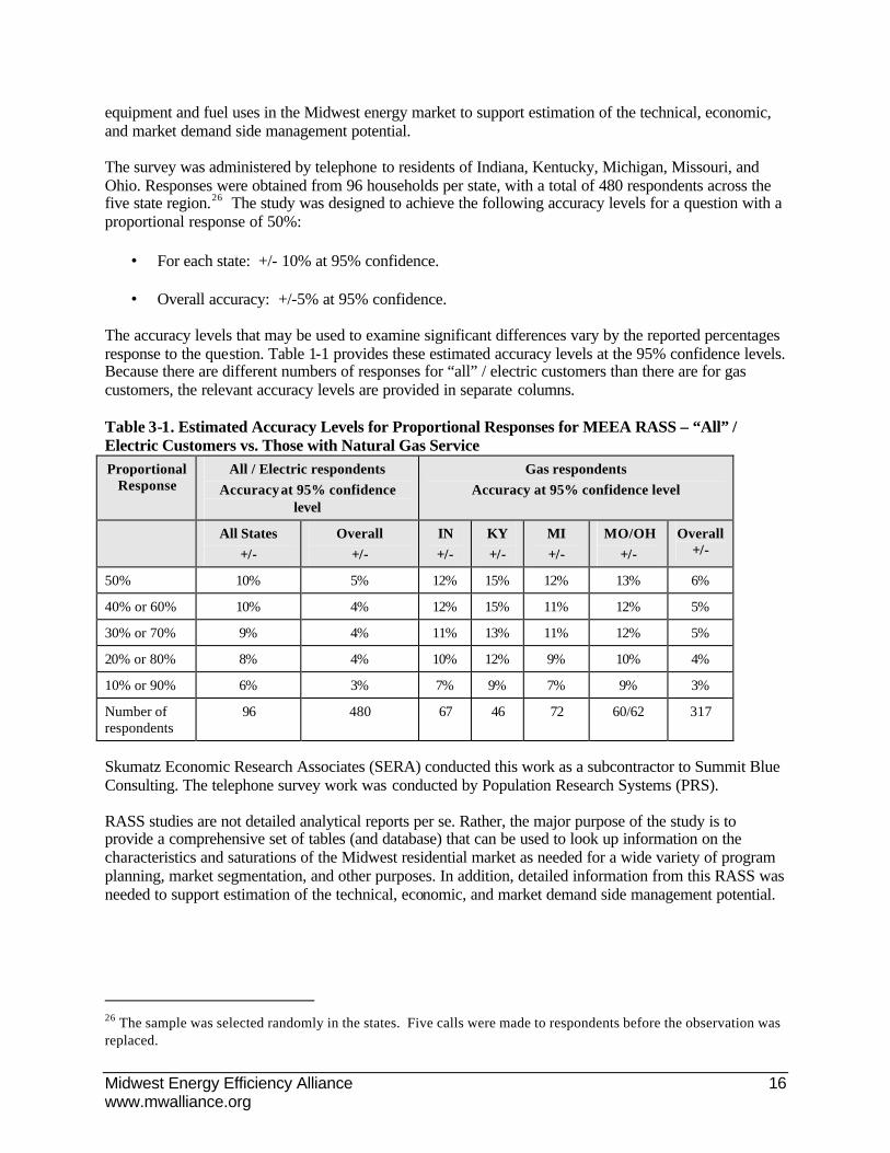
The accuracy levels that may be used to examine significant differences vary by the reported percentages response to the question. Table 1-1 provides these estimated accuracy levels at the 95% confidence levels. Because there are different numbers of responses for “all” / electric customers than there are for gas customers, the relevant accuracy levels are provided in separate columns.
Table 3-1. Estimated Accuracy Levels for Proportional Responses for MEEA RASS – “All” / Electric Customers vs. Those with Natural Gas Service Proportional
Response All / Electric respondents
Accuracy at 95% confidence level
Gas respondents Accuracy at 95% confidence level
All States +/-
Overall +/-
IN +/-
KY +/-
MI +/-
MO/OH +/-
Overall +/-
50% 10% 5% 12% 15% 12% 13% 6%
40% or 60% 10% 4% 12% 15% 11% 12% 5%
30% or 70% 9% 4% 11% 13% 11% 12% 5%
20% or 80% 8% 4% 10% 12% 9% 10% 4%
10% or 90% 6% 3% 7% 9% 7% 9% 3%
Number of respondents
96 480 67 46 72 60/62 317
Skumatz Economic Research Associates (SERA) conducted this work as a subcontractor to Summit Blue Consulting. The telephone survey work was conducted by Population Research Systems (PRS).
RASS studies are not detailed analytical reports per se. Rather, the major purpose of the study is to provide a comprehensive set of tables (and database) that can be used to look up information on the characteristics and saturations of the Midwest residential market as needed for a wide variety of program planning, market segmentation, and other purposes. In addition, detailed information from this RASS was needed to support estimation of the technical, economic, and market demand side management potential.
26 The sample was selected randomly in the states. Five calls were made to respondents before the observation was replaced.

Midwest Energy Efficiency Alliance 17 www.mwalliance.org
3.2.2 Trade Ally Surveys
The 2005 MEEA trade ally interviews were conducted to provide data to augment the information collected in the 2004 MEEA Residential Appliance Saturation Survey (RASS). The trade ally interviews were designed to provide feedback on analytical factors that residents would generally not know: stock and trends in equipment as well as measure efficiencies for HVAC equipment, water heaters, appliances, and insulation.
To gather this information, SERA conducted a phone survey of home builders and energy auditors for MEEA. The survey asked detailed questions about the saturation rates of a variety of efficiency levels for appliances and energy saving measures present in single and multifamily homes in Indiana, Kentucky, Michigan, Missouri, and Ohio.
The full data collection instrument, which is quite detailed and demanding for respondents, is provided in Appendix C. In summary, the measures and appliances and efficiency levels27 addressed in the interview included:
HVAC: For each type, respondents were asked for information separately regarding single vs. multifamily and for new vs. existing homes
• Electric heat pump: SEER28 10; SEER 12 & SEER 13; SEER 14; and SEER 15+
• Electric central AC: SEER 10; SEER 12 & SEER 13; SEER 14; and SEER 15+
• Electric room AC: EER29 9.3; EER 9.7; ENERGY STAR® or EER 10.7 and above
• Gas space heat: Base furnace 80 AFUE30; condensing furnace 92 AFUE; and condensing furnace 96 AFUE
Water Heating: For each type, respondents were asked for information separately regarding single vs. multifamily and for new vs. existing homes.
• Electric water heat: EF31 0.88; EF 0.917; and EF 0.95.
• Gas water heat: Base 40 gal EF 0.59; EF 0.63; and EF 0.70.
27 Respondents were asked about the specific technical efficiency levels (e.g. SEER 10). For purposes of the potential modeling work, these efficiency levels were then labeled, in order, “Minimum efficiency level”, “High efficiency”, and “Higher efficiency”. For several measures, an additional level was asked about, and it was labeled “Premium efficiency.” 28 Seasonal Energy Efficiency Rating (SEER). a measure of central air conditioning systems. The higher the rating, the higher the efficiency of the model. 29 Energy Efficiency Rating (EER), a measure of efficiency of room air conditioning systems. The higher the rating, the greater the efficiency of the model. 30 Annual Fuel Utilization Efficiency rating (AFUE) measures the seasonal or annual efficiency. The higher the rating, the greater the efficiency. 31 Energy Factor (EF) rates the overall efficiency of a heater. The higher the rating, the greater the efficiency.

Midwest Energy Efficiency Alliance 18 www.mwalliance.org
Appliances: For each type, respondents were asked for information separately regarding single vs. multifamily and for new vs. existing homes.
• Refrigerators: Base vs. ENERGY STAR®
• Freezers: Base vs. ENERGY STAR®
• Electric cooking oven: conventional vs. convection
• Gas cooking oven: conventional vs. convection
• Electric clothes dryer: base dryer vs. high efficiency with moisture sensor
• Gas clothes dryer: base dryer vs. high efficiency with moisture sensor
Insulation: For each type, respondents were asked for information separately regarding new vs. existing construction, as well as information on the percent that could be “feasibly upgraded.”32
• Ceiling insulation: none; medium to R-19; optimal from R-19 to R-38
• Floor insulation: none; medium to R-11; optimal R-11 to R-19.
• Wall insulation: none; medium to R-13 blow in; optimal R-13 to R-19 batt.
• Duct insulation: none; medium from R-3 to R-8; optimal above R-8.
Windows: For each type, respondents were asked for information separately regarding new vs. existing homes, as well as information on the percent that could be “feasibly upgraded.”
• Windows: low efficiency means NOT low-E33 and less efficient than U=0.3534; medium efficiency requires either not low-E or U less efficient than 0.35; optimal efficiency defined as low-E and U=0.35 or better.
Respondents were asked for percentages or ranges where possible, as well as for qualitative data and feedback on trends and factors affecting the results. The small sample size, and the difficulty of answering these technical questions about efficiency saturations led to an emphasis on qualitative and quasi-quantitative results. However, this level of detail was sufficient to allow Quantec to adjust the default data in its ForecastPro model to represent the MEEA states – the purpose of the data collection work.
The data collection work was conducted in April through June 2005. SERA staff encountered several problems throughout the process of constructing sample population lists and conducting the survey itself.
32 R-values signify the measure of resistance to heat flow. The higher the R-value, the better the insulation. 33 The term “Low-E” refe rs to coatings placed on glass that reflect specific wavelengths of energy. Low-E glass reflects heat energy while admitting visible light, keeping heat out. In winter, however, the low-angle visible light passes into the house and is absorbed by the interior. 34 The U-factor (U) reflects the numerical value of heat transfer. It combines the four ways in which glass transfers heat (conduction, convection, radiation, and air leakage). Since it is the inverse of R-values, the lower the U-value, the greater the insulation.

Midwest Energy Efficiency Alliance 19 www.mwalliance.org
Specifically, there were difficulties constructing a viable population list of equipment “specifiers” and homebuilders as well as finding qualified and knowledgeable energy professionals willing to participate in the survey. Despite these complications, enough data were obtained to draw useful and reasonably reliable conclusions about the state of heating, ventilation and air conditioning (HVAC) equipment as well as household appliances in homes in the Midwest.
3.2.3 Issues Related to Developing Population and Sample
The first step in conducting the survey involved obtaining a sample of potential respondents. Our initial approach was to try to contact distributors and other professionals that work in either household appliances or HVAC specification. SERA staff used an online index (yp.yahoo.com) to construct a population list. For the major cities in each state, SERA recorded contacts from the following categories and made calls.
SERA made over 60 calls, but could not find anyone willing to participate, and attribute the 100% non-participation rate to two main factors. First, contact names were not available for this sample, and many may have thought we were telemarketers and terminated the interview. Second, SERA mostly contacted retailers busy with customers, so they neither had the time nor desire to participate.
After the unsuccessful round of initial calls, the team considered other approaches. Summit Blue staff investigated other sample sources, and located two additional sources. The first was a list of Missouri energy auditors, provided by Ameren, and the second was a website for Energy-efficient Homes Midwest (eehmidwest.org), which provided a directory of auditors in the other states. Although the initial target audience was a broad survey of energy professionals in the Midwest, including auditors, SERA found that only calls to auditors were productive in yielding completed surveys—subsequently, all responses obtained are from energy raters or auditors. This selection may have introduced some bias into these results – although the auditors with whom we spoke worked in a wide variety of single family and multifamily homes, both new and old, there is the potential that the specific areas in which energy auditors are likely to be knowledgeable differs systematically from those of other energy professionals. As such, results from this survey should be regarded as primarily energy auditor perspectives on energy conservation potential. 35
After making several calls to the auditors on the lists provided by Summit Blue, SERA searched the web for additional lists of energy auditors in Kentucky, Ohio, Missouri, Michigan and Indiana, and found several additional sources, including:
• The Energy and Environmental Ratings Alliance (ratingsalliance.org) • The National Energy Raters Association (energyraters.org) • The Indoor Environmental Standards Organization (iestandards.org) • The National Conservation Guild (www.nationalguild.com/Contacts/inaud.html)
These new contact sources were not as productive as those previously provided by Summit Blue. They contained many wrong or outdated phone numbers as well as contacts that were not knowledgeable about household energy efficiency. One particular problem with sources from these lists was that a given contact’s primary profession was not always conducive to producing accurate estimates of what percentage of homes have equipment at specific efficiency levels. For example, one contact remodeled houses for a living and, as a result, had little experience with direct observation of heating equipment and
35 In practice, this bias is not unique to our adapted sampling strategy. The initial sample plan was simply to contact energy professionals to avert the costs associated with a detailed household survey.

Midwest Energy Efficiency Alliance 20 www.mwalliance.org
appliances. In discussions with interviewees, it became apparent that energy auditing was not a primary profession for many certified energy auditors but an ancillary qualification.
In summary, the first group of 60 provided no responses. A total of 150 sample points were then gathered from the follow-up approaches, and 28 surveys were completed, or a 19% response rate The survey team made at least 5 calls to each sample point.
3.3 Characterize DSM Measures
Characterization of DSM measures requires 1) determining the list of DSM measures to evaluate, 2) estimating the baseline energy consumption for each end-use (heating, cooling, cooking, hot water, etc.) or unit energy consumption (UEC) and 3) estimating the incremental savings from each measure - improving from the baseline to the new technology(ies). In addition, the baselines must consider that different classes of homes have different penetrations of technologies, such as existing homes compared to new construction.
The project team first drew up a list of prospective measures from past experience and added to and subtracted from that list as necessary for the project. Additions included new technologies or improvements to existing technologies, subtractions included measures that were made obsolete by shifting baselines. The goal was a comprehensive list of DSM measures applied in different segments of the residential market: new versus existing construction and single -family versus multi-family housing.
Once identified, the project team determined which measures would have a significant climate-dependent savings component. Those measures that were determined to be climate-independent (lighting, appliances, and domestic hot water) were characterized using engineering calculations and assumptions for energy savings. Climate-dependent measures (HVAC equipment, insulation, air-sealing etc) were simulated with a computer model to determine savings.
3.3.1 Climate-Independent End-Uses
Climate-independent end-uses are described in many resources, including: the US Department of Energy, EnergyStar Program36, the California Database of Energy-efficient Resources37, various utility on-line audit services and manufacturer data. These resources were particularly useful for appliances. Other end-uses were analyzed using engineering principles such as steady-state heat loss, rated power and hours of operation.
A combination of resources was used to produce consensus unit energy consumption (UECs) for the end-uses for both 1) the stock equipment, e.g. that equipment currently employed in the housing stock and 2) the standard equipment, e.g. that equipment that is the current off-the-shelf replacement. Existing homes are more likely to have stock equipment and new homes would use standard equipment.
3.3.2 Climate-Dependent End-Uses
Climate-dependent DSM end-uses were modeled using Energy-10 software, an hourly simulation tool designed specifically for small commercial and residential structures. The project team made 18 baseline models reflecting typical constructions of three building types: new single -family homes, existing single family homes, and multi-family construction; three climate zones: temperate (Louisville, KY), cold
36 http://www.energystar.gov/ 37 http://www.energy.ca.gov/deer/

Midwest Energy Efficiency Alliance 21 www.mwalliance.org
(Chicago, IL) and very cold (Minneapolis, MN), as well as two heating sources: natural gas heat and electric heat.
Model input parameters, such as building size, installed equipment type and age and insulation levels, were based on survey results and building code (new construction) information. The models were then calibrated to produce energy consumption that corresponded to published consumption for the respective states and/or climate zones.
The results of the baseline simulations were used to populate unit energy consumption (UEC) for source of heat (electric furnace, heat pump, electric room heat and gas heat) and air-conditioning (central or room). The UECs described both the stock consumption, e.g. the consumption of the average installed end-use, and the standard consumption of the same end-use if it were installed today, e.g. reflecting current efficiency standards.
3.3.3 Climate-Independent Measures
Using the same techniques and sources as for the climate-independent end-uses, the project team estimated savings for the list of conservation measures (generated in step 1). The absolute savings (kWh, Therms) were transformed to a percentage of the total UEC for the affected end-use.
For climate-independent measures, multiple measures were often ascribed to each end-use, e.g. low-flow showerheads, faucet aerators, and new water heaters could be applied to the domestic hot water end-use. Uniform savings estimates were used across all climate zones though they might vary according to construction type, e.g., single - family versus multi-family or new homes versus existing construction.
3.3.4 Climate-Dependent Measures
Similarly, the project team estimated the savings from climate-dependent measures using the same calibrated simulation models used to estimate the UECs for climate-dependent end-uses. Savings for climate dependent measures were estimated for each of the three climate zones considered. Again, absolute savings for each measure was transformed to a percentage of the total end-use UEC.
For climate-dependent measures, multiple measures were often ascribed to each end-use, e.g. furnaces of varying efficiency or type could be applied to the heating end-use. Some measures could impact multiple end-uses, such as high-efficiency windows affect heating and cooling end-uses. Separate savings estimates were simulated for each of the three climate zones and each construction type.
3.3.5 Measure Costs and Lifetimes
The project team has determined that there is general uniformity of measure cost and lifetimes across the geography considered in this study. Variations in costs exist for certain higher cost measures such as HVAC equipment and insulation where labor costs factor in more heavily. Measure cost estimates for these measures were weighted by factors contained in industry sources such as the RS Means Mechanical Cost Data. The project team estimated measure lifetimes from a combination of resources including: manufacturer data, typical economic depreciation assumptions, the California DEER database, various studies reviewed for this report and survey responses from residential customers interviewed for this assessment.

Midwest Energy Efficiency Alliance 22 www.mwalliance.org
3.4 Estimate technical, economic, and market DSM potential.
The general approach for derivation of energy efficiency resource potentials consisted of three sequential steps: (1) estimate technical energy efficiency potential, (2) subdivide the technical energy efficiency potential estimates into discrete “bundles” based on cost category, which allows the economic potential to move with the underlying volatility in fuel prices, and (3) estimate market penetration and the resulting achievable potential as a subset of each bundle.
All of these estimates were derived using Quantec’s Energy ForecastPro model, an end-use forecasting and energy efficiency potentials assessment tool. The conceptual underpinnings and analytic procedures of this model are based on standard practices in the utility industry, and are consistent with the methods used in the Xcel energy and Iowa studies referenced above.
Each set of potential estimates (technical, economic, and achievable) is derived as follows:
1. Produce base case end use energy forecasts of loads over a 20-year planning horizon for each state building type and vintage, calibrating total residential electric and gas usage by climate zone to actual residential energy sales as estimated by the Energy Information Administration.38
2. Develop a second forecast incorporating the current saturations, DSM measures’ applicability and expected penetration, and energy saving impacts of all commercially available energy efficiency measures, and
3. Determine the potential estimates by subtracting the second forecast from the base case forecast.
3.4.1 Technical energy efficiency potential
The technical potential scenario assumes 100% market penetration of energy efficiency measures over the forecast horizon. For each end-use, such as air conditioners, heat pumps, and furnaces, the technical potential scenario modifies the base case efficiency shares by assigning a 100% market share to the most efficient equipment level.
Energy ForecastPro then modifies equipment energy usage given the upgrade in the efficiency of the end-use equipment. Classic examples of this are insulation, windows, duct sealing, showerheads, and lighting retrofits. The accurate assessment of retrofit savings also requires the characterization of physical applicability factors, and the percentage of applicable shares where the measure has yet to be installed. The basic retrofit equation is
ijcfmijcfmijcfmijcfijcfm INCFACTORAPPFACTORPCTSAVEUISAVE ×××= ,
where
38 The base case provides an estimate of future energy consumption in the absence of new energy efficiency programs. It establishes a benchmark against which the impacts of technical and achievable energy efficiency potentials can be assessed. The effects of equipment standards and naturally occurring efficiency improvements, which emanate from the reduction of usage as low-efficiency equipment is retired, are also taken into account in the base case forecast.
Midwest Energy Efficiency Alliance 23 www.mwalliance.org
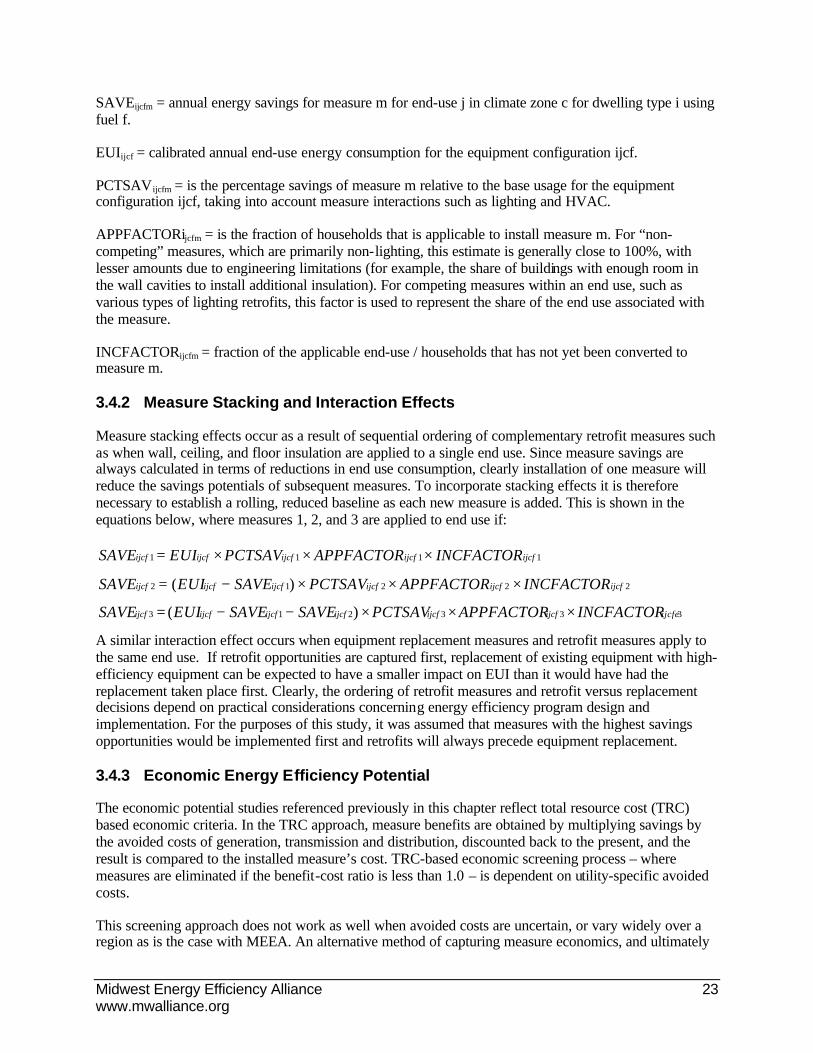
SAVEijcfm = annual energy savings for measure m for end-use j in climate zone c for dwelling type i using fuel f.
EUIijcf = calibrated annual end-use energy consumption for the equipment configuration ijcf.
PCTSAVijcfm = is the percentage savings of measure m relative to the base usage for the equipment configuration ijcf, taking into account measure interactions such as lighting and HVAC.
APPFACTORijcfm = is the fraction of households that is applicable to install measure m. For “non-competing” measures, which are primarily non-lighting, this estimate is generally close to 100%, with lesser amounts due to engineering limitations (for example, the share of buildings with enough room in the wall cavities to install additional insulation). For competing measures within an end use, such as various types of lighting retrofits, this factor is used to represent the share of the end use associated with the measure.
INCFACTORijcfm = fraction of the applicable end-use / households that has not yet been converted to measure m.
3.4.2 Measure Stacking and Interaction Effects
Measure stacking effects occur as a result of sequential ordering of complementary retrofit measures such as when wall, ceiling, and floor insulation are applied to a single end use. Since measure savings are always calculated in terms of reductions in end use consumption, clearly installation of one measure will reduce the savings potentials of subsequent measures. To incorporate stacking effects it is therefore necessary to establish a rolling, reduced baseline as each new measure is added. This is shown in the equations below, where measures 1, 2, and 3 are applied to end use if:
1111 ijcfijcfijcfijcfijcf INCFACTORAPPFACTORPCTSAVEUISAVE ×××=
22212 )( ijcfijcfijcfijcfijcfijcf INCFACTORAPPFACTORPCTSAVSAVEEUISAVE ×××−=
333213 )( ijcfeijcfijcfijcfijcfijcfijcf INCFACTORAPPFACTORPCTSAVSAVESAVEEUISAVE ×××−−=
A similar interaction effect occurs when equipment replacement measures and retrofit measures apply to the same end use. If retrofit opportunities are captured first, replacement of existing equipment with high-efficiency equipment can be expected to have a smaller impact on EUI than it would have had the replacement taken place first. Clearly, the ordering of retrofit measures and retrofit versus replacement decisions depend on practical considerations concerning energy efficiency program design and implementation. For the purposes of this study, it was assumed that measures with the highest savings opportunities would be implemented first and retrofits will always precede equipment replacement.
3.4.3 Economic Energy Efficiency Potential
The economic potential studies referenced previously in this chapter reflect total resource cost (TRC) based economic criteria. In the TRC approach, measure benefits are obtained by multiplying savings by the avoided costs of generation, transmission and distribution, discounted back to the present, and the result is compared to the installed measure’s cost. TRC-based economic screening process – where measures are eliminated if the benefit-cost ratio is less than 1.0 – is dependent on utility-specific avoided costs.
This screening approach does not work as well when avoided costs are uncertain, or vary widely over a region as is the case with MEEA. An alternative method of capturing measure economics, and ultimately

Midwest Energy Efficiency Alliance 24 www.mwalliance.org
economic potential, is to use the levelized cost of each measure. Levelized costs are traditionally used by regionally planning organizations to provide a broad comparison of energy efficiency resources to supply resources.39 It is important to recognize that levelized costs themselves do not represent cost-effectiveness criteria, and are not the same as total resource costs. They represent the cost of energy efficiency in terms of a level payment, similar to a mortgage payment. They do not include generation, transmission or distribution costs, or quantifiable non-energy benefits such as operation and maintenance savings attributable to energy efficiency measures. When combined with the size of the resource (kWh or therms saved), the levelized costs effectively represented the “supply curve” of energy efficiency resources. 40
The first step in this process is to calculate each measure’s levelized cost, which reflects the cost per kWh saved over its lifetime, subject to a discount rate (usually a utility’s cost of capital). The formula is as follows:
∑=
+=L
l
lteDiscountRaSAVEostInstalledCCostLevelized1
**)1/(/
where the denominator is the total savings of the measure over its lifetime (l), discounted back to the present. Suppose for example, a measure costs $50, and will save 100 kWh per year over a 10 year life. If the discount rate is 7.5%, the net present amount of the lifetime savings is 686 kWh. We then divide the installed cost of $50 by 686 to yield the levelized cost of $0.073. Each kWh saved over the lifetime of the measure costs 7.3 cents.
The next step is to aggregate measure savings potential into logical groups or bundles, and associated cost points. This grouping exercise is important in fully integrated resource planning because individual measure savings are generally not large enough to weigh against supply-side alternatives. The idea is to give the measures enough critical mass so that they can be selected by the resource planning model. 41
For MEEA, the categories (bundles) in the table below are illustrative of the types of thresholds that can be employed using levelized costs. As one move up the ladder from cost group A to E, it is less likely that the measures contained therein would be cost-effective in a utility resource plan.
39 See, for example, The Fifth Northwest Electric Power and Conservation Plan, Northwest Power and Conservation Council (NWPCC), May 2005, http://www.nwcouncil.org/energy/powerplan/default.htm. 40 Some utilities are also using the supply curve (cost category) approach in integrated resource planning. In this approach, the economic potential is a subset of the achievable potential, with the economically viable amount of DSM resources s elected as part of the integrated planning process. Put differently, the avoided costs are an output rather than input in the process. This approach also follows utility industry risk management approaches, allowing multi-attribute selection criteria to be employed. A resource with less cost volatility may be selected over a more cost volatile resource even when their expected costs are identical. For an example of the use of this fully integrated demand and supply-side resource selection approach, see Puget Sound Energy’s 2005 Least Cost Plan, http://www.pse.com/about/supply/LCP/20050503. 41 For example, in the previously referenced Puget Sound Energy plan, the DSM measures were grouped by sector, building type, end-use, and vintage – across retrofit and replacement categories – to give the planning model a sense of possible DSM program activity should the resource block be selected.

Midwest Energy Efficiency Alliance 25 www.mwalliance.org
Table 3-2. Electric and Gas Measure Categories and Levelized Cost Thresholds
Category or Bundle
Electric Measure Levelized
Cost Thresholds
Gas Measure Levelized Cost Thresholds
Cost Level A ≤ $0.03/kWh ≤ $0.30/Therm Cost Level B $0.03 to $0.06/kWh $0.30 to $0.60/Therm Cost Level C $0.06 to $0.10/kWh $0.60 to $1.00/Therm Cost Level D $0.10 to $0.15/kWh $1.00 to $1.50/Therm Cost Level E > $0.15/kWh > $1.50/Therm
In this breakout, measures in category A are cost-effective with any fuel price forecast, even one with natural gas prices returning to $3/MMbtu. Conversely, measures in Categories D and E are unlikely to be cost-effective, unless the recent energy industry price shocks continue unabated and natural gas rises to$20/MMbtu or more. The great uncertainty, therefore, is associated with categories B and C.42
3.4.4 Achievable Potential
The next step is to apply market penetration rates to the technical potential estimates within each cost category to obtain to obtain achievable potential. A variety of factors affect market penetration of energy efficiency measures, including inherent market barriers resulting from customers’ tendency to avoid administrative and financial burdens, program marketing strategies, and delivery mechanisms. This is why some energy efficiency programs, even with full incremental cost incentives, can have a wide range of penetration rates, seldom achieving full market saturation. The available information suggests that, although incentive levels do play a significant role in determining program success, other, non-financial factors may play an equal, if not more important, role.
In estimating market potential, we apply what some industry analysts call the “experiential approach”, where the maximum achievable penetration rate is based on the penetration rates achieved from similar utility energy efficiency programs.43 The following penetration rates were applied to the technical potential estimates in each state to obtain maximum achievable potential:44
• Gas new construction: 50%
42 The key to developing categories in an actual resource planning application is to discern categories that would also always be selected, such as A, and categories that would never be selected, such as E, and then iteratively focus on the middle categories within the resource planning model to discern the appropriate assessment threshold(s). 43 There was a great deal of research conducted on DSM market penetration rates in the mid-1990s. Interestingly, with the new era of post-2000 utility programs, there has yet to be a comprehensive assessment of market penetration rates that looks beyond simple payback relationships. That is, we are not aware of any recent studies that look at all program design elements, including incentives. Most of the maximum achievable penetration rates applied here are derived from a 1995 mu lti-client study conducted by Barakat and Chamberlin, Inc., Market Penetration of DSM Programs: The Effects of Price and Nonprice Program Features. We note that the incentives in the “best” programs (in terms of market penetration) approached 100% of incre mental measure cost, a level that is far higher than has historically been applied in Iowa, Minnesota, and most other mid-western states. 44 For comparison purposes, see Chapter 3 of The Fifth Northwest Electric Power and Conservation Plan. The NWPPC has always assumed that 85% of the cost-effective conservation potential can be accomplished over the course of 20 years, where the cost-effective threshold is variable and follows the levelized cost approach described above.

Midwest Energy Efficiency Alliance 26 www.mwalliance.org
• Electric new construction: 50% except for lighting measures, which are set equal to 25%
• Gas and electric equipment replacement, existing construction: 60%
• Existing construction retrofit: 50%, except lighting, which is set equal to 30%
Midwest Energy Efficiency Alliance 27 www.mwalliance.org
4. MARKET RESEARCH RESULTS This chapter discusses the results of the market research that was conducted for this project, as well as the results of previous market assessments or DSM potential studies from four Midwestern states. Three original market research studies were conducted for this project:
1. Surveys of 40 utilities, state and municipal energy offices across all nine Midwestern states.
2. Residential appliance saturation surveys with 480 residential customers in the five Midwestern States that had not previously conducted market assessments or DSM potential studies that are publicly available.
3. Surveys of energy auditors in the same five Midwestern states.
4.1 Results from Interviews with Midwest Energy Organizations
4.1.1 Introduction
The project team surveyed forty Midwest energy organizations by telephone regarding their residential EE programs and any previous residential market assessments studies they might have conducted. The organizations interviewed included representatives from electric and gas investor-owned utilities, larger municipal and cooperative utilities, cooperative and municipal utility associations, and state or municipal energy and regulatory agencies.
The purpose of these interviews was to determine:
• The existence of already completed residential market assessment studies, or primary data on residential customers that they have collected that they would be willing to share for this study, such as utility residential appliance saturation surveys (RASS) or billing data for customers who are part of the primary data collection effort.
• Their willingness to fund either primary on-site data collection or RASS research for samples of about 100 to 300 of their customers.
• Their current DSM programs and details on such, especially ENERGY STAR® programs.
The respondent distribution by state is shown in Figure 4-1.

Midwest Energy Efficiency Alliance 28 www.mwalliance.org
Figure 4-1. Survey Respondents
0
1
2
3
4
5
6
7
8
IA IL IN KY MI MN MO OH PA WI
# of
Par
ticip
ants
4.1.2 Current Residential Energy Efficiency Programs
Twenty-seven of the 40 organizations are currently conducting residential EE programs in the Midwest and half of respondents have more than one type of program currently in place. Table 4-1 documents the number of energy organizations with common program types.
Table 4-1. Residential Program Offerings
Residential EE Program Type Number of
Organizations with Programs
Rebate programs 13
RCS style energy audits 11
Direct load control 9
Other information programs 7
Web-based energy audits 7
Low-income 8
Financing programs 4
Other 3
Additional Load Management 0
Multi-family 2
Rebate programs were the most common type of residential energy efficiency program, with most of the programs covering multiple technologies including:
• Space heating equipment – furnaces and heat pumps (including geothermal systems) • Cooling equipment • Water heating equipment • Lighting – both bulbs and fixtures

Midwest Energy Efficiency Alliance 29 www.mwalliance.org
• Appliances (e.g., ENERGY STAR® clothes washers) • Comprehensive new construction
4.1.3 Previous Residential Market Assessment Research
Nineteen of the organizations surveyed have previously conducted market assessment research on residential customers of various types. Table 4-2 lists the types of research reported and the number of organizations that have conducted them. Four of the 15 organizations surveyed have conducted multiple types of research projects.
Table 4-2. Market Research Efforts
Research Type Number of
Organizations Conducting Research
Broad Based Market Assessment 1
DSM Potential Studies 6
Appliance Saturation Survey 9
Other Market Assessment Research 3
Although many market studies have been completed, only seven of the 19 organizations that responded thought their study results were publicly available. All others were unsure (4) or knew the reports were confidential (8). The status of information availability is listed in Table 4-3.
Table 4-3. Information Availability
Research Availability Number of Utilities
Responding
Publicly Available 7
Unsure 4
Not Publicly Available 5
Confidential 3
Total 19
The only four studies that were comprehensive enough and allowed sufficient analysis of the underlying data for the purposes of this study were those discussed in the Methodology section. These studies covered Illinois, Iowa, Minnesota and Wisconsin.
4.1.4 Interest in Study
All the energy organizations were either unsure or knew that their company would not be willing to release a representative sample of 100-200 residential customer billing histories for this project, as shown in Table 4-4. Significant follow-up with the initially unsure organizations did not locate any willing to release such data for this project, so that aspect of the project plan could not be implemented.
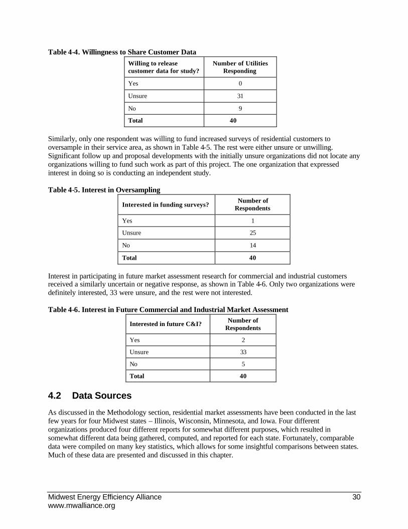
Midwest Energy Efficiency Alliance 30 www.mwalliance.org
Table 4-4. Willingness to Share Customer Data Willing to release customer data for study?
Number of Utilities Responding
Yes 0
Unsure 31
No 9
Total 40
Similarly, only one respondent was willing to fund increased surveys of residential customers to oversample in their service area, as shown in Table 4-5. The rest were either unsure or unwilling. Significant follow up and proposal developments with the initially unsure organizations did not locate any organizations willing to fund such work as part of this project. The one organization that expressed interest in doing so is conducting an independent study.
Table 4-5. Interest in Oversampling
Interested in funding surveys? Number of
Respondents
Yes 1
Unsure 25
No 14
Total 40
Interest in participating in future market assessment research for commercial and industrial customers received a similarly uncertain or negative response, as shown in Table 4-6. Only two organizations were definitely interested, 33 were unsure, and the rest were not interested.
Table 4-6. Interest in Future Commercial and Industrial Market Assessment
Interested in future C&I? Number of Respondents
Yes 2
Unsure 33
No 5
Total 40
4.2 Data Sources
As discussed in the Methodology section, residential market assessments have been conducted in the last few years for four Midwest states – Illinois, Wisconsin, Minnesota, and Iowa. Four different organizations produced four different reports for somewhat different purposes, which resulted in somewhat different data being gathered, computed, and reported for each state. Fortunately, comparable data were compiled on many key statistics, which allows for some insightful comparisons between states. Much of these data are presented and discussed in this chapter.

Midwest Energy Efficiency Alliance 31 www.mwalliance.org
Also, as discussed in the Methodology section, the project team conducted primary research on residential customers in five additional Midwest states – Indiana, Kentucky, Michigan, Missouri, and Ohio – where previous publicly available broad based market assessments had not recently been conducted. The project team conducted detailed telephone residential appliance saturation surveys (RASS), and separate telephone surveys of energy auditors familiar with residential construction and equipment use. While these surveys collected similar but somewhat different data than the four residential market assessments mentioned above, their results allow for comparisons of certain key efficiency indicators across the entire nine-state region.
The type(s) of residential customers surveyed or audited, and the basis for the study’s market assessments are summarized here for each state:
• Illinois – on-site surveys conducted for single -family homes, detached only.
• Wisconsin – on-site surveys of owner-occupied single-family homes, attached and detached.
• Minnesota – on-site surveys of single -family homes, individual apartment units, and mobile homes.
• Iowa – distributor surveys of equipment efficiencies. The entire residential segment was assessed.
• Indiana, Kentucky, Michigan, Missouri, and Ohio – the two surveys characterized a cross-section of the entire residential market, including new and existing homes, single -family and multi-family dwellings, and both all-electric and natural gas customers.
4.3 Comparative Customer Demographic and Energy Use Statistics
In this and the next three sections, we present data compiled from the four residential market assessment studies, and the surveys covering the five additional states, as introduced above. The accompanying tables organize data for comparisons between states. For many of the statistics discussed below, there is some variability between what each study reports. Also there are several statistics that lack data entirely in one or more studies. As a result, meaningful comparisons are difficult to draw for some statistics.
4.3.1 Electricity and Natural Gas Use
The market assessment studies for Illinois and Wisconsin (broken down by home type) contained data on residential customer energy use from the on-site audits, and similar data were available from a supplementary database for Minnesota. No energy consumption data were included as part of the Iowa study, however, nor as part of the surveys of Indiana, Kentucky, Michigan, Missouri, and Ohio. Hence, only EIA data45 are presented in Table 4-7, showing a simple average of residential electricity and natural gas consumption for customers in each state. The electric data in Table 4-7 was calculated, from utility-by-utility EIA data, from the largest utilitie s in each state, while the gas data was calculated from state-by-state production and consumption data.
45 Energy Information Administration, Electric Sales and Revenue 2003 Spreadsheets,
www.eia.doe.gov/cneaf/electricity/esr/esr_tabs.html; and Energy Information Administration, Summary Statistics for (individual state), www.eia.doe.gov/oil_gas/natural_gas/data_publications/natural_gas_annual/nga.html .

Midwest Energy Efficiency Alliance 32 www.mwalliance.org
Overall average annual electrical use appears to correlate most strongly with electric space heating and water heating saturations, as will be shown later in this chapter. The four states with the lowest overall annual electric use, Michigan, Minnesota, Illinois, and Wisconsin, also have the lowest electric space heating saturations, as well as the lowest electric water heating saturations. Conversely, the three states with the highest average annual electrical use, Missouri, Indiana, and Kentucky, have the highest penetrations of electric space heating and water heating systems. Since space heating and water heating systems are usually the largest energy using systems in residences, these results are not surprising.
Overall average annual natural gas use appears to be a bit more complicated to explain, varying with the saturations of gas space heating and water heating systems, as well as climate and gas space heating efficiencies. Illinois residents use the most natural gas of any state in the region, and the saturations of gas space heating and water heating systems in Illinois are also the highest in the region. Missouri residents use the least amount of natural gas of any state in the region, which appears to be a function of its second lowest saturations of gas space heating and water heating systems, as well as having the most southern climate in the region.
Table 4-7. Average Annual Residential Energy Use
Electricity
(kWh) Natural Gas
(therms)
Michigan 7,907 1,266
Minnesota 8,169 1,087
Illinois 8,336 1,318
Wisconsin 8,593 950
Iowa 9,243 917
Ohio 11,112 1,096
Missouri 11,930 879
Indiana 12,120 986
Kentucky 12,893 1,124
4.3.2 Customer Income
The Illinois and Minnesota studies report stratified customer income information, and similar information was as part of the RASS surveys of customers in Indiana, Kentucky, Michigan, Missouri, and Ohio. The customer income data is presented in Table 4-8. In general, the household incomes in the five states surveyed by telephone were significantly lower than in Illinois and Minnesota. Half or more of the customers surveyed in Indiana, Kentucky, Michigan, Missouri, and Ohio reported incomes less than $40,000, while only about one-third of the customers audited in Illinois and Minnesota did so. This discrepancy could simply be due to sampling differences between customers who agreed to be audited in Illinois and Minnesota compared to the simpler telephone interviews in the other five states.

Midwest Energy Efficiency Alliance 33 www.mwalliance.org
Table 4-8. Total Household Income
Illinois Minnesota Indiana Kentucky Michigan Missouri Ohio
Under $20,000 6% 13% 22% 22% 24% 10% 22%
$20,000 - $40,000 22% 23% 29% 34% 26% 40% 32%
$40,000 - $60,000 24% 21% 22% 13% 24% 20% 25%
$60,000 - $80,000 17% 18% 9% 9% 9% 17% 11%
$80,000 - $120,000 22% 16% 15% 18% 10% 8% 8%
Over $120,000 9% 9% 3% 4% 7% 5% 2%
4.4 Housing Characteristics
4.4.1 Housing Unit Types and Sizes
Almost all of the studies report information on housing type and size. These data are presented in Tables 4-9 and 4-10. As seen in Table 4-9, all of the samples consisted predominantly of one- and two-story single-family detached homes. Some states’ data includes a sizeable proportion of multi-family and/or mobile homes, as well – most notably Minnesota, Michigan, Ohio, and Kentucky.
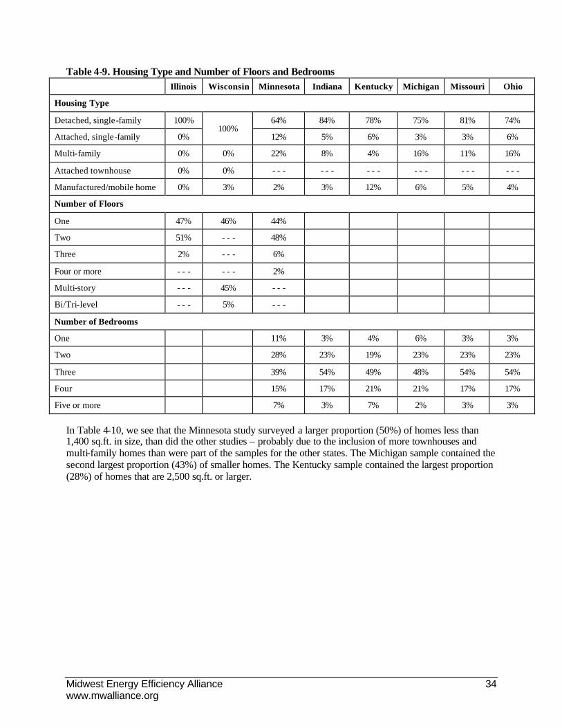
Midwest Energy Efficiency Alliance 34 www.mwalliance.org
Table 4-9. Housing Type and Number of Floors and Bedrooms Illinois Wisconsin Minnesota Indiana Kentucky Michigan Missouri Ohio
Housing Type
Detached, single-family 100% 64% 84% 78% 75% 81% 74%
Attached, single-family 0% 100%
12% 5% 6% 3% 3% 6%
Multi-family 0% 0% 22% 8% 4% 16% 11% 16%
Attached townhouse 0% 0% - - - - - - - - - - - - - - - - - -
Manufactured/mobile home 0% 3% 2% 3% 12% 6% 5% 4%
Number of Floors
One 47% 46% 44%
Two 51% - - - 48%
Three 2% - - - 6%
Four or more - - - - - - 2%
Multi-story - - - 45% - - -
Bi/Tri-level - - - 5% - - -
Number of Bedrooms
One 11% 3% 4% 6% 3% 3%
Two 28% 23% 19% 23% 23% 23%
Three 39% 54% 49% 48% 54% 54%
Four 15% 17% 21% 21% 17% 17%
Five or more 7% 3% 7% 2% 3% 3%
In Table 4-10, we see that the Minnesota study surveyed a larger proportion (50%) of homes less than 1,400 sq.ft. in size, than did the other studies – probably due to the inclusion of more townhouses and multi-family homes than were part of the samples for the other states. The Michigan sample contained the second largest proportion (43%) of smaller homes. The Kentucky sample contained the largest proportion (28%) of homes that are 2,500 sq.ft. or larger.

Midwest Energy Efficiency Alliance 35 www.mwalliance.org
Table 4-10. Housing Size (Total Conditioned Square Footage)
Illinois Wisconsin Minnesota Indiana Kentucky Michigan Missouri Ohio
less than 1,400 35% 39% 50% 18% 23% 43% 21% 28%
1,400 to 2,499 48% 51% 36% 61% 49% 49% 56% 53%
2,500 to 3,499 12% 8% 11% 15% 21% 5% 15% 14%
more than 3,500 5% 2% 3% 6% 7% 3% 8% 5%
Mean (ft^2) 1,800 1,632 1,605 2,047 2,094 1,674 2,065 1,935
Median (ft^2) 1,660 1,502 1,392
4.4.2 Insulation Levels
The Illinois, Wisconsin, and Minnesota studies report information on the insulation found in the homes audited for these studies. Data on the percentage of homes found with insulation in their walls and roof are presented in Table 4-11, along with similar data collected in the telephone surveys of customers in Indiana, Kentucky, Michigan, Missouri, and Ohio.
It should be understood that the data presented in Table 4-11 for Indiana, Kentucky, Michigan, Missouri, and Ohio, is based on homeowners’ responses to telephone questions. In each of the five states, at least 85-90% of these homeowners believe that their homes have insulation in the walls and roof. However, when experienced residential energy auditors were interviewed in each state, they estimated a significantly higher percentage of uninsulated walls and roofs – approximately 30% for the five-state region. It is likely that the auditors are more correct, since their opinions are based on many on-site observations of residential insulation in their areas. Homeowners are sometimes unaware that their walls or roofs are uninsulated. Therefore the data for Indiana, Kentucky, Michigan, Missouri, and Ohio in Table 4-11 are maybe overestimated.
From Table 4-11, it appears that Indiana, Ohio, and especially Illinois, have higher percentages of homes without wall insulation than the other Midwest states. All nine states are remarkably comparable regarding roof insulation however, with approximately 90 to 95 percent of homes having at least some roof insulation.
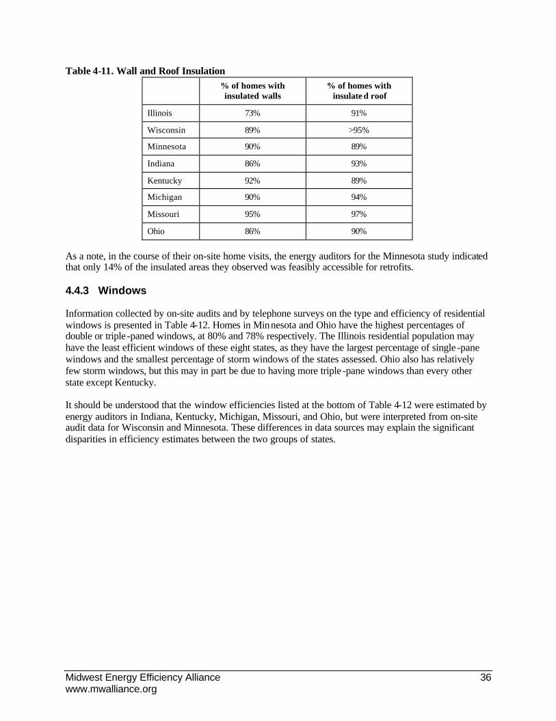
Midwest Energy Efficiency Alliance 36 www.mwalliance.org
Table 4-11. Wall and Roof Insulation
% of homes with insulated walls
% of homes with insulate d roof
Illinois 73% 91%
Wisconsin 89% >95%
Minnesota 90% 89%
Indiana 86% 93%
Kentucky 92% 89%
Michigan 90% 94%
Missouri 95% 97%
Ohio 86% 90%
As a note, in the course of their on-site home visits, the energy auditors for the Minnesota study indicated that only 14% of the insulated areas they observed was feasibly accessible for retrofits.
4.4.3 Windows
Information collected by on-site audits and by telephone surveys on the type and efficiency of residential windows is presented in Table 4-12. Homes in Minnesota and Ohio have the highest percentages of double or triple -paned windows, at 80% and 78% respectively. The Illinois residential population may have the least efficient windows of these eight states, as they have the largest percentage of single -pane windows and the smallest percentage of storm windows of the states assessed. Ohio also has relatively few storm windows, but this may in part be due to having more triple -pane windows than every other state except Kentucky.
It should be understood that the window efficiencies listed at the bottom of Table 4-12 were estimated by energy auditors in Indiana, Kentucky, Michigan, Missouri, and Ohio, but were interpreted from on-site audit data for Wisconsin and Minnesota. These differences in data sources may explain the significant disparities in efficiency estimates between the two groups of states.

Midwest Energy Efficiency Alliance 37 www.mwalliance.org
Table 4-12. Type and Efficiency of Windows
Illinois Wisconsin Minnesota Indiana Kentucky Michigan Missouri Ohio
Homes with DSM measures
% of windows with storm windows
36% 54% 48% 42% 43% 54% 38%
Window Glass (% of windows)
Single Pane 36% 35% 20% 26% 25% 24% 26% 22%
Double Pane 63% 64% 78% 66% 60% 68% 63% 63%
Triple Pane 1% 1% 2% 8% 15% 8% 12% 15%
Window Efficiency
Low 85% 97% 39% 39% 39% 39% 39%
Medium 39% 39% 39% 39% 39%
Optimal 15% 3% 22% 22% 22% 22% 22%
Qualitative Assessment of Relative Efficiency Average
Higher than
Average Average
Lower than
Average Average
4.5 Lighting, HVAC, and Appliance DSM Measure Saturations
All of the studies reported information on the penetration of energy-efficient appliances, compact fluorescent lamps, and other DSM measures. As with other statistics, there is variability in the exact data that was reported. The Illinois, Wisconsin, and Minnesota information was gathered during their on-site audits, while the information from Iowa came from their survey of equipment distributors, and the Indiana, Kentucky, Michigan, Missouri, and Ohio information was either self-reported by residential customers, or estimated by local energy auditors, in telephone surveys.
4.5.1 Lighting
As seen in Table 4-13, compact fluorescent lamps are still somewhat uncommon in residential light fixtures. Only in Kentucky and Missouri are CFL’s found in more than one-third of homes. Illinois and Wisconsin appear to have the lowest percentage of homes with compact fluorescents. For Wisconsin, this is likely due to the older vintage of that study, for which the on-site data was collected in 1999.
Tubular fluorescent lamps are quite common in residences in the Midwest, however, with 42% to 78% of homes having at least one such fixture. The saturations of tubular fluorescent lamps is highest in Illinois and Minnesota, with 78% and 60% of homes respectively having at least one tubular fluorescent fixture.

Midwest Energy Efficiency Alliance 38 www.mwalliance.org
Table 4-13. Penetration of Energy-Efficient Lighting
Illinois Wisconsin Minnesota Indiana Kentucky Michigan Missouri Ohio
Homes with at least one CFL 23% 13% 33% 33% 43% 32% 39% 34%
Homes with fluorescent tubes 78% 60% 50% 53% 42% 43% 50%
No. CFLs in household (if any)
1 – 2 98% 54% 30% 32% 42% 18% 27%
3 – 6 2% 24% 39% 41% 36% 36% 36%
More than six 0% 22% 31% 27% 22% 46% 37%
4.5.2 HVAC
Data from all four previously conducted studies and the five-state RASS surveys on HVAC equipment are presented in Tables 4-14 and 4-15. The saturations of different types of HVAC equipment vary considerably by state, and some of this variation is explained by the varying compositions of customer types surveyed or audited in each state.
As shown in Table 4-14, the saturations of natural gas space heating systems vary considerably across the Midwest, from a low of 46% in Kentucky to 92% and 97% in Wisconsin and Illinois respectively. In Kentucky, only 48% of the customers surveyed report that they have natural gas service to their homes, compared to an average of 66% of customers across the five states covered by the RASS surveys.
The market shares of efficient gas space heating systems are the highest in Iowa, Minnesota and Wisconsin at 74%, 67% and 50% respectively. The high percentages of efficient furnaces in these states is presumably due to the effects of long-standing DSM programs promoting this technology in these states. For Indiana, Kentucky, Michigan, Missouri, and Ohio, energy auditors estimate the shares of more efficient gas furnaces at 23% on average, but slightly higher in Missouri.
The saturations of heat pumps throughout the Midwest are quite low, ranging from 1% in Illinois, Michigan and Wisconsin up to a high of 8% in Kentucky. The saturations of efficient heat pumps is estimated to be the highest in Iowa at 74%, compared to an average of 25% for the five state group of Indiana, Kentucky, Michigan, Missouri and Ohio, but slightly higher in Missouri.
The saturations of regular electric space heating systems vary considerably across the Midwest, from lows of 2% in Illinois, 4% in Minnesota, 5% in Wisconsin, and 7% in Michigan to highs of 20% to 22% in Kentucky and Missouri.
The highest saturations for central air conditioners are shown to be in Illinois (90%), Missouri (85%), and Kentucky (76%). Missouri and Kentucky are the most southern states included in this study, so one would expect their air conditioning saturations to be among the highest of the states studied. The high saturation for Illinois is partly explained by the fact that only single -family homes were studied in that state, and such homes usually have higher central air conditioning saturations than apartments do. For example, in Minnesota the saturation of central air conditioners in single family homes is 65%, compared to 18% in multi-family dwellings.

Midwest Energy Efficiency Alliance 39 www.mwalliance.org
The highest percentages of more efficient central air conditioners are found in Iowa (74% total) and Minnesota (48% total). The high penetrations of efficient central air conditioners in these areas are presumably due to the effects of Iowa and Minnesota utilities promotion of this measure through their DSM programs. Xcel Energy in Minnesota has covered efficient central air conditioners in their DSM programs for 25 years.
These percentages are much higher than the 24% market share estimated by energy auditors for efficient air conditioners in Indiana, Kentucky, Michigan, Missouri, and Ohio, or the 6% market share found from the on-site audits in Wisconsin. However, the Wisconsin data is the oldest of that included in this report, so the efficient units’ market shares may have increased there since 1999. The RASS survey results shown for the five state region (Indiana through Ohio) at the top of Table 4-15 show that residential customers estimate the percentages of their central air conditioners that are ENERGY STAR® units as far higher than the corresponding efficient units’ market shares estimated by the energy auditors. The energy auditors’ estimates are likely more accurate, as they have more knowledge about central air conditioners efficiency than most residential customers do.
The highest saturation of room air conditioners is found in Minnesota at 28% for all residential customers, considerably higher than the next highest saturations found in Wisconsin at 20% saturation, and Indiana at 19% saturation. Minnesota’s relatively high saturation is likely due to the large share of multi-family homes in its customer sample. The penetration of efficient room air conditioners is estimated to be relatively low across the Midwest at 16%-25% market shares.

Midwest Energy Efficiency Alliance 40 www.mwalliance.org
Table 4-14. Space Heating Efficiency Illinois Wisconsin Minnesota Iowa Indiana Kentucky Michigan Missouri Ohio
Homes with DSM measures
Programmable Thermostat 47% 35% 27% 17% 19% 29% 31% 26%
Heating Duct Insulation 4% 8% 63% 72% 54% 70% 63%
Gas-Fired Space Heat Efficiency
Overall Saturation 97% 92% 83% 65% 46% 73% 62% 64%
Minimum 50% 33% 27% 77% 77% 77% 77% 77%
High 47% 27% 64% 21% 21% 21% 21% 21%
Higher 3% 40% 10% 2% 2% 2% 2% 2%
Qual. Assessment of Relative Eff.
Average Average Average Higher than Average
Average
Heat Pumps Efficiency
Overall Saturation 1% 1% 3% 5% 8% 1% 4% 2%
Minimum 27% 74% 74% 74% 74% 74%
High 64% 23% 23% 23% 23% 23%
Higher 2% 2% 2% 2% 2%
Premium 10% <1% <1% <1% <1% <1%
Qual. Assessment of Relative Eff.
Average Average Average Higher than Average
Average
Other Electric Heating
Central Systems Saturation 2% 1% 1% 5% 18% 4% 19% 7%
Other Primary Heating Systems Saturation 0% 2% 3% 11% 2% 3% 3% 6%
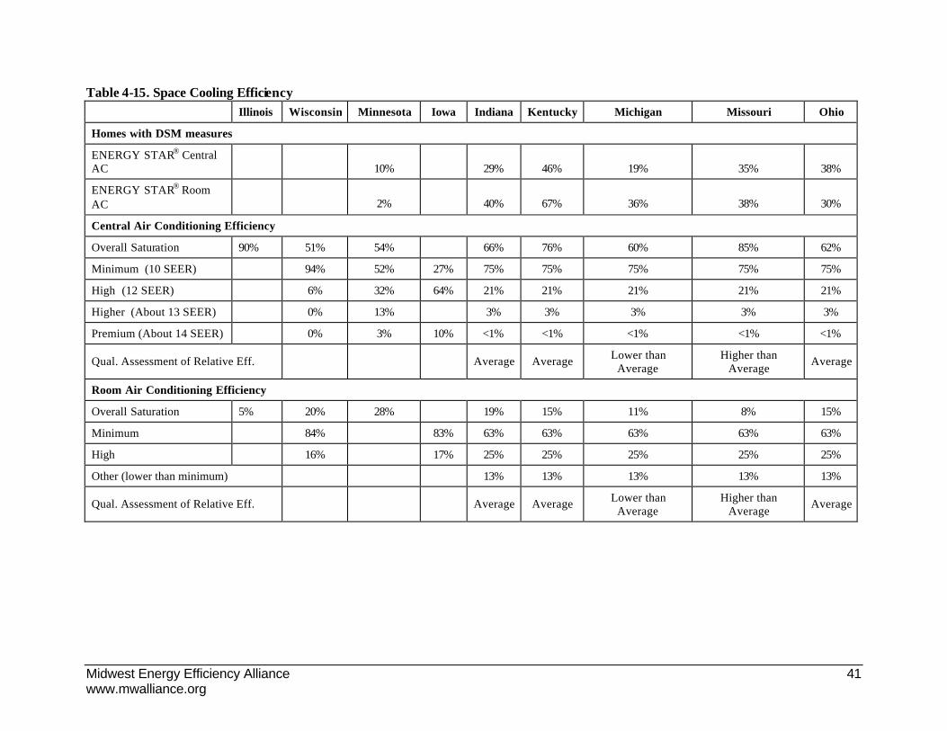
Midwest Energy Efficiency Alliance 41 www.mwalliance.org
Table 4-15. Space Cooling Efficiency Illinois Wisconsin Minnesota Iowa Indiana Kentucky Michigan Missouri Ohio
Homes with DSM measures
ENERGY STAR® Central AC 10% 29% 46% 19% 35% 38%
ENERGY STAR® Room AC 2% 40% 67% 36% 38% 30%
Central Air Conditioning Efficiency
Overall Saturation 90% 51% 54% 66% 76% 60% 85% 62%
Minimum (10 SEER) 94% 52% 27% 75% 75% 75% 75% 75%
High (12 SEER) 6% 32% 64% 21% 21% 21% 21% 21%
Higher (About 13 SEER) 0% 13% 3% 3% 3% 3% 3%
Premium (About 14 SEER) 0% 3% 10% <1% <1% <1% <1% <1%
Qual. Assessment of Relative Eff.
Average Average Lower than Average
Higher than Average
Average
Room Air Conditioning Efficiency
Overall Saturation 5% 20% 28% 19% 15% 11% 8% 15%
Minimum 84% 83% 63% 63% 63% 63% 63%
High 16% 17% 25% 25% 25% 25% 25%
Other (lower than minimum) 13% 13% 13% 13% 13%
Qual. Assessment of Relative Eff.
Average Average Lower than Average
Higher than Average
Average

Midwest Energy Efficiency Alliance 42 www.mwalliance.org
4.5.3 Water Heating
As seen in Table 4-16, Kentucky is the only Midwestern state with a majority of electric water heaters, as 61% of its units are heated with electricity. This is likely due to the 48% availability of natural gas service in Kentucky, as discussed in the previous section. Illinois and Minnesota have the lowest saturations of electric water heaters in the Midwest, at 4% and 13% respectively.
Midwest electric water heaters are mainly minimum efficiency units, with low efficiency units’ market shares ranging from 66% to 87%. The percentage of more efficient electric units is estimated to be highest in the five states of Indiana, Kentucky, Michigan, Missouri, and Ohio, at an average of 30%, and slightly higher than the 30% average in Indiana and Kentucky.
Illinois and Minnesota have the largest market shares of natural gas water heaters at 96% and 83% saturations respectively. Kentucky and Missouri have the smallest market shares of gas water heaters at 36% and 52% respectively.
As with electric water heaters, Midwestern natural gas water heaters are mainly minimum efficiency models, which have market shares of 63%-83%. The percentage of more efficient gas units is estimated to be highest in the five state Indiana to Ohio region at an average of 38%, and slightly higher than 38% in Kentucky.
As with air conditioning equipment, residents of the five states of Indiana, Kentucky, Michigan, Missouri, and Ohio estimate the percentages of their water heaters that are ENERGY STAR® units as higher than similar estimates by energy auditors in those states. In contrast, though efficiency estimates were not made for Minnesota, only 1% of the water heaters were found to be ENERGY STAR® during the onsite audits conducted by trained energy auditors. Given the source for this estimate, it is likely the most accurate of these estimates for the penetration of efficient water heaters throughout the Midwest, and the other estimates for the penetrations for efficient water heaters are likely overstated.
Michigan and Indiana residents report having installed the most low-cost water heater efficiency measures – pipe insulation, tanks wraps, low-flow showerheads, and faucet aerators – while Illinois and Minnesota residents appear to have installed the fewest of these types of DSM measures.

Midwest Energy Efficiency Alliance 43 www.mwalliance.org
Table 4-16. Water Heating Efficiency
Illinois Wisconsin Minnesota Iowa Indiana Kentucky Michigan Missouri Ohio
Electric Water Heaters
Overall Saturation 4% 28% 13% 39% 61% 27% 41% 28%
Minimum Efficiency Units 87% 83% 66% 66% 66% 66% 66%
High Efficiency Units 7% 13% 26% 26% 26% 26% 26%
Highest Efficiency Units 6% 5% 4% 4% 4% 4% 4%
Other (lower than minimum) 5% 5% 5% 5% 5%
Qual. Assessment of Relative Eff.
Higher than Average
Higher than Average
Lower than Average
Lower than Average Average
Natural Gas Water Heat
Overall Saturation 96% 62% 83% 55% 36% 68% 52% 64%
Minimum Efficiency Units 82% 83% 63% 63% 63% 63% 63%
High Efficiency Units 15% 13% 28% 28% 28% 28% 28%
Highest Efficiency Units 3% 5% 10% 10% 10% 10% 10%
Qual. Assessment of Relative Eff.
Lower than
Average Higher than
Average Average Average Average
Homes with DSM measures
Pipe Insulation 10% 12% 19% 15% 31% 19% 12%
Hot Water Tank Wrap 7% 11% 6% 26% 15% 17% 10% 12%
Water Heater Timer 3% 6% 6% 7% 5%
Low Flow Showerhead 29% 51% 66% 60% 68% 61% 60%
ENERGY STAR® Water Heater 1% 44% 57% 40% 50% 40%

Midwest Energy Efficiency Alliance 44 www.mwalliance.org
4.5.4 Appliances
Refrigerator and freezer data are presented in Table 4-17. Residents of Indiana, Michigan and Ohio have the highest percentages of just one refrigerator in their homes at 82%-85% of all homes surveyed respectively. Kentucky and Missouri have the highest percentages of homes with two or three refrigerators, at 34% and 27% respectively. The saturations of stand alone freezers vary from 40%-43% in Ohio and Minnesota respectively to 60% in Wisconsin.
The energy auditors surveyed in Indiana, Kentucky, Michigan, Missouri, and Ohio report saturations of efficient refrigerators in the region at 31% and efficient freezers at 18%. These estimates are quite close to the percentages of these appliances that residents of these states report as being ENERGY STAR® units: they report that 26% of their refrigerators are ENERGY STAR® units, and 18% of their freezers are ENERGY STAR® units. However, these estimates may all be too high, as the energy auditors that conducted the on-site surveys in Illinois and Minnesota found only 5% and 3% ENERGY STAR® refrigerators, respectively.
Data on kitchen stoves, ovens, dishwashers, and microwave ovens is presented in Table 4-18. The majority of Midwestern stoves use electricity as the heating fuel. Electric stoves have market shares ranging from a low of 48% in Michigan to 83% in Kentucky. Natural gas stoves have market shares ranging from a low of 15% in Kentucky to 44% in Michigan. Midwestern ovens have similar market shares to those of stoves. Electric ovens have market shares ranging from a low of 49% in Michigan to 85% in Kentucky. Natural gas ovens have market shares ranging from a low of 11% in Kentucky to a high of 40% in Michigan.
The energy auditors surveyed in Indiana, Kentucky, Michigan, Missouri, and Ohio report average saturations of efficient electric ovens in the region at 19% and efficient gas ovens at 22%. These estimates are quite similar to these states’ residents estimates that 25% of their ovens are ENERGY STAR® units.
The saturations of dishwashers throughout the Midwest varies from lows of 54%-57% in Ohio and Kentucky respectively to highs of 71%-77% in Missouri, Minnesota, and Illinois. Estimates of the percentages of ENERGY STAR® dishwashers made by residents vary from lows of 31% in Indiana and Ohio to highs of 46%-47% in Missouri and Kentucky respectively. However, these estimates may be considerably overstated, as the energy auditors who conducted the Illinois and Minnesota on-site surveys estimated that only 4% of dishwashers in those states were ENERGY STAR® units. Since no known Midwest organizations are conducting DSM programs promoting ENERGY STAR® dishwashers, it is unlikely that the market shares of ENERGY STAR® units could vary by a factor of ten from state to state in the Midwest.
The saturations of microwave ovens are quite high for the five state region from Indiana to Ohio, varying only from a low of 92% in Ohio to 100% in Indiana. Residents of those states estimated the saturations of ENERGY STAR® units as varying from lows of 16% to 18% in Michigan and Ohio to a high of 30% in Kentucky.
Data on clothes washers and dryers are presented in Table 4-19. The saturations of clothes washers where such data was collected varies from 80% in Minnesota to 98% in Illinois and Wisconsin. The saturation of ENERGY STAR® clothes washers as estimated by the energy auditors during the on-site surveys in Illinois and Minnesota was 5%-6% respectively.
Most Midwestern clothes dryers use electricity as the heating fuel, except in Minnesota and Michigan. The market share of electric clothes dryers varies from lows of 34%-43 in those two states respectively to

Midwest Energy Efficiency Alliance 45 www.mwalliance.org
highs of 79%-89% in Indiana and Kentucky respectively. The market shares of natural gas fired clothes dryers varies from lows of 6% in Kentucky to highs of 43%-44% in Minnesota and Michigan respectively.
Energy auditors estimate that the average share of efficient electric clothes dryers is 8% in Indiana, Kentucky, Michigan, Missouri, and Ohio, while their estimate of the share of efficient natural gas clothes dryers is considerably larger at 26%. Residents estimate that the percentage of dryers that are ENERGY STAR® units in these states is considerably larger than the auditors, varying from 32% in Ohio to 49% in Missouri.
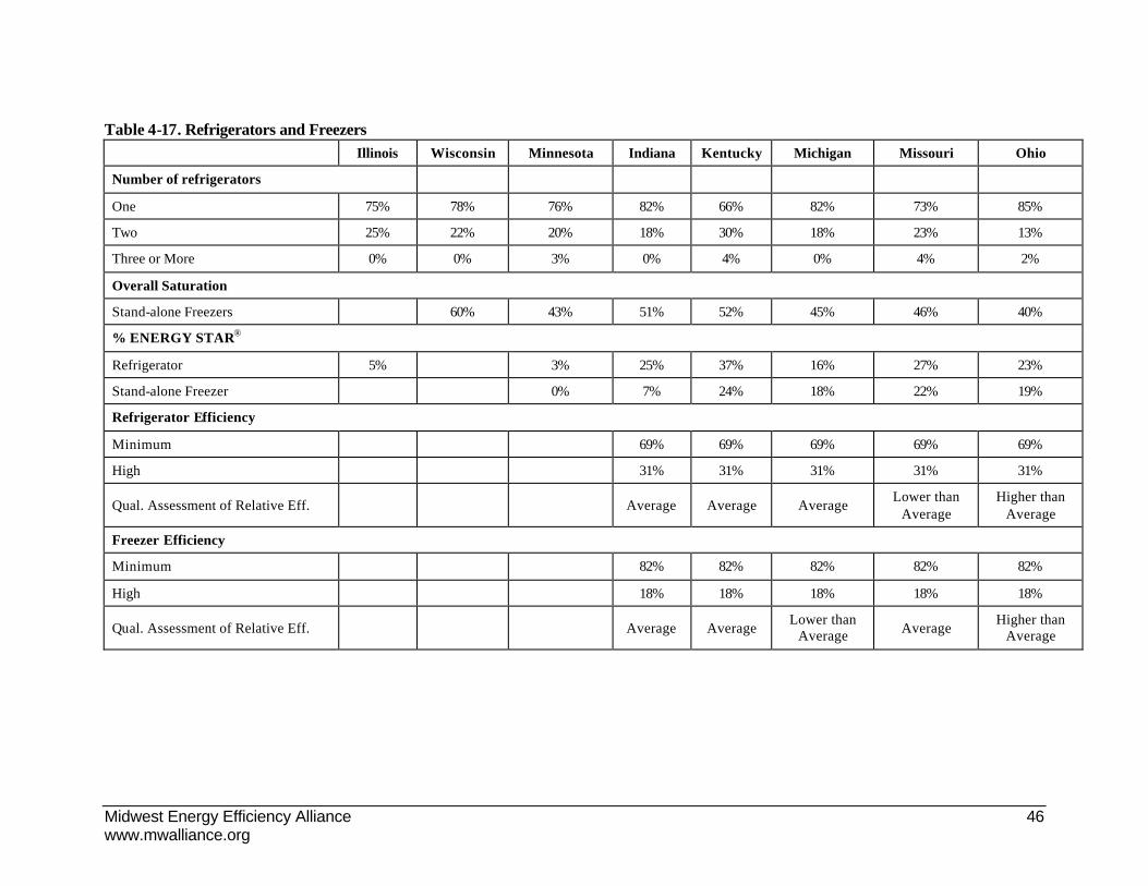
Midwest Energy Efficiency Alliance 46 www.mwalliance.org
Table 4-17. Refrigerators and Freezers Illinois Wisconsin Minnesota Indiana Kentucky Michigan Missouri Ohio
Number of refrigerators
One 75% 78% 76% 82% 66% 82% 73% 85%
Two 25% 22% 20% 18% 30% 18% 23% 13%
Three or More 0% 0% 3% 0% 4% 0% 4% 2%
Overall Saturation
Stand-alone Freezers 60% 43% 51% 52% 45% 46% 40%
% ENERGY STAR®
Refrigerator 5% 3% 25% 37% 16% 27% 23%
Stand-alone Freezer 0% 7% 24% 18% 22% 19%
Refrigerator Efficiency
Minimum 69% 69% 69% 69% 69%
High 31% 31% 31% 31% 31%
Qual. Assessment of Relative Eff. Average Average Average Lower than
Average Higher than
Average
Freezer Efficiency
Minimum 82% 82% 82% 82% 82%
High 18% 18% 18% 18% 18%
Qual. Assessment of Relative Eff. Average Average Lower than
Average Average Higher than
Average

Midwest Energy Efficiency Alliance 47 www.mwalliance.org
Table 4-18. Kitchen Appliances Illinois Wisconsin Minnesota Indiana Kentucky Michigan Missouri Ohio
Overall Saturation
Electric Stove 61% 61% 63% 83% 48% 62% 66%
Natural Gas Stove 27% 37% 35% 15% 44% 32% 31%
Electric Oven 67% 66% 66% 85% 49% 72% 67%
Natural Gas Oven 27% 35% 32% 11% 40% 24% 27%
Dishwasher 77% 64% 72% 60% 57% 62% 71% 54%
Microwave Oven 100% 96% 98% 96% 92%
% ENERGY STAR®
Stove 33% 33% 23% 34% 31%
Oven 26% 24% 22% 27% 26%
Dishwasher 4% 4% 31% 47% 37% 46% 31%
Microwave Oven 22% 30% 16% 22% 18%
Electric Oven Efficiency
Minimum 81% 81% 81% 81% 81%
High 19% 19% 19% 19% 19%
Qual. Assessment of Relative Eff. Lower than
Average Average Average Average
Higher than Average
Natural Gas Oven Efficiency
Minimum 78% 78% 78% 78% 78%
High 22% 22% 22% 22% 22%
Qual. Assessment of Relative Eff. Lower than
Average Average Higher than
Average Lower than
Average Average

Midwest Energy Efficiency Alliance 48 www.mwalliance.org
Table 4-19. Clothes Washers & Dryers
Illinois Wisconsin Minnesota Indiana Kentucky Michigan Missouri Ohio
Overall Saturation
Clothes Washer 98% 98% 80%
Electric Clothes Dryer 73% 34% 79% 89% 43% 73% 68%
Natural Gas Clothes Dryer 98%
23% 43% 13% 6% 44% 16% 21%
% ENERGY STAR®
Clothes Washer 5% 6%
Clothes Dryer 0% 3% 38% 36% 39% 49% 32%
Electric Dryer Efficiency
Minimum 94% 94% 94% 94% 94%
High 8% 8% 8% 8% 8%
Qual. Assessment of Relative Eff.
Average Average Average Average Average
Gas-Fired Dryer Efficiency
Minimum 74% 74% 74% 74% 74%
High 26% 26% 26% 26% 26%
Qual. Assessment of Relative Eff.
Lower than Average
Average Average Average Average

Midwest Energy Efficiency Alliance 49 www.mwalliance.org
4.6 Customer Awareness of Energy Efficiency
The RASS survey of residential homeowners in Indiana, Kentucky, Michigan, Missouri, and Ohio assessed customer awareness of the ENERGY STAR® label. Similarly, homeowners receiving the energy audits in Illinois and Minnesota were asked a few questions about the ENERGY STAR® label, as well. All of this data is presented in Table 4-20. Only the Minnesota study gathered any data on familiarity (including current usage) with efficient equipment in general, however.
Over half of the residential customers, in every state surveyed, reported being entirely unfamiliar with the ENERGY STAR® label. The percentages of customers who are somewhat or very familiar with the ENERGY STAR® label vary from lows of 31%-37% in Minnesota and Illinois to a high of 47%-48% of customers in Kentucky and Indiana.
Table 4-20. Customer Awareness of Energy Efficiency Measures Awareness of ENERGY STAR® label Illinois Minnesota Indiana Kentucky Michigan Missouri Ohio
Very Familiar 6% 19% 16% 20% 12% 13% 18%
Somewhat Familiar 31% 12% 32% 27% 28% 29% 23%
Not at all Familiar 63% 69% 52% 53% 60% 58% 59%

Midwest Energy Efficiency Alliance 50 www.mwalliance.org
5. DSM POTENTIAL RESULTS This section contains the results of the technical, economic, and achievable residential energy efficiency potentials in the nine-state area addressed by MEEA in this study.
As noted in the Methodology section, it is important to recognize that the estimates of achievable potential represent an upper limit or maximum as to what the programs could achieve if there were no restrictions on the incentive budgets up to full incremental cost rebates. However, most energy efficiency programs pay less than full incremental cost rebates to mitigate rate impacts of programs, and to ensure that the customer contribution is a fair one.
The results below provide both total and state specific results. Results are presented first for natural gas, followed by electric savings. The results are first summarized by cost category for both technical and achievable potential for the region in terms of aggregate savings in year twenty after 20 years of resource acquisition (participation).
Individual measure savings are then reported in aggregate by building type (single - and mult i-family) and vintage (existing and new construction) for the nine-state region based on the tables in Appendix A, which detail measures ordered by the magnitude of savings within a cost category.46 Note that some measures in the tables have savings that vary by climate zone / state, which means the regional total tables may contain a measure multiple times. Finally, a series of pie charts describe the aggregate breakouts by end-use, state, market, and dwelling type. The formula used to calculate levelized cost is as follows:
∑=
+=L
l
lteDiscountRaSAVEostInstalledCCostLevelized1
**)1/(/
where the denominator is the total savings of the measure over its lifetime (l), discounted back to the present. Suppose for example, a measure costs $50, and will save 100 kWh per year over a 10 year life. If the discount rate is 7.5%, the net present amount of the lifetime savings is 686 kWh. We then divide the installed cost of $50 by 686 to yield the levelized cost of $0.073. Each kWh saved over the lifetime of the measure costs 7.3 cents. 5.1 Natural Gas Potentials
Natural gas energy-efficiency technical potential in the residential sector is estimated at 9.2 billion therms across all states in the 20th year of a planning horizon (Table 5.1). This represents nearly 47% savings relative to the base case. Maximum achievable potential is estimated at approximately 5.0 billion therms, or approximately 54% of the technical potential. Approximately 12% (595 million therms) of the achievable potential can be achieved at an average cost of 30 cents per therm or less.
Maximum technical and achievable gas energy-efficiency potential in the 20th year of the planning horizon, broken out by cost category for the individual states can be found in Tables 5.2 – 5.10. The maximum achievable potential in the 20th year ranged from a minimum of 172 million therms in Kentucky to a maximum of 1.2 billion therms in Illinois. Not surprisingly, larger states like Illinois, Michigan and Ohio tend to have higher energy-efficiency potentials than smaller states like Kentucky and Missouri.
46 Measure tables are contained in Appendix A.
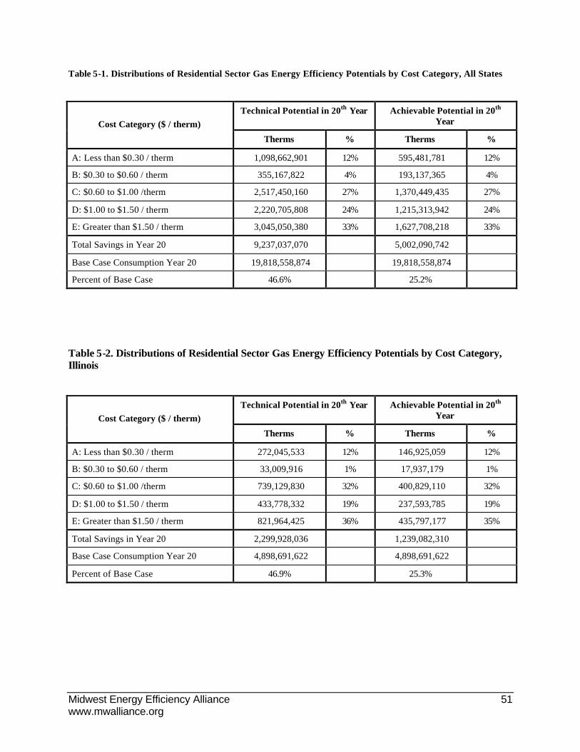
Midwest Energy Efficiency Alliance 51 www.mwalliance.org
Table 5-1. Distributions of Residential Sector Gas Energy Efficiency Potentials by Cost Category, All States
Technical Potential in 20th Year Achievable Potential in 20th Year
Cost Category ($ / therm)
Therms % Therms %
A: Less than $0.30 / therm 1,098,662,901 12% 595,481,781 12%
B: $0.30 to $0.60 / therm 355,167,822 4% 193,137,365 4%
C: $0.60 to $1.00 /therm 2,517,450,160 27% 1,370,449,435 27%
D: $1.00 to $1.50 / therm 2,220,705,808 24% 1,215,313,942 24%
E: Greater than $1.50 / therm 3,045,050,380 33% 1,627,708,218 33%
Total Savings in Year 20 9,237,037,070 5,002,090,742
Base Case Consumption Year 20 19,818,558,874 19,818,558,874
Percent of Base Case 46.6% 25.2%
Table 5-2. Distributions of Residential Sector Gas Energy Efficiency Potentials by Cost Category, Illinois
Technical Potential in 20th Year Achievable Potential in 20th Year
Cost Category ($ / therm)
Therms % Therms %
A: Less than $0.30 / therm 272,045,533 12% 146,925,059 12%
B: $0.30 to $0.60 / therm 33,009,916 1% 17,937,179 1%
C: $0.60 to $1.00 /therm 739,129,830 32% 400,829,110 32%
D: $1.00 to $1.50 / therm 433,778,332 19% 237,593,785 19%
E: Greater than $1.50 / therm 821,964,425 36% 435,797,177 35%
Total Savings in Year 20 2,299,928,036 1,239,082,310
Base Case Consumption Year 20 4,898,691,622 4,898,691,622
Percent of Base Case 46.9% 25.3%

Midwest Energy Efficiency Alliance 52 www.mwalliance.org
Table 5-3. Distributions of Residential Sector Gas Energy Efficiency Potentials by Cost Category, Indiana
Technical Potential in 20th Year Achievable Potential in 20th Year
Cost Category ($ / therm)
Therms % Therms %
A: Less than $0.30 / therm 98,937,042 12% 53,827,967 12%
B: $0.30 to $0.60 / therm 75,469,319 9% 41,112,951 9%
C: $0.60 to $1.00 /therm 304,982,158 37% 167,195,691 38%
D: $1.00 to $1.50 / therm 159,130,439 20% 88,071,510 20%
E: Greater than $1.50 / therm 176,102,154 22% 93,781,670 21%
Total Savings in Year 20 814,621,113 443,989,790
Base Case Consumption Year 20 1,696,998,544 1,696,998,544
Percent of Base Case 48.0% 26.2%
Table 5-4. Distributions of Residential Sector Gas Energy Efficiency Potentials by Cost Category, Iowa
Technical Potential in 20th Year Achievable Potential in 20th Year
Cost Category ($ / therm)
Therms % Therms %
A: Less than $0.30 / therm 46,549,681 12% 25,252,356 12%
B: $0.30 to $0.60 / therm 30,052,745 8% 16,251,015 8%
C: $0.60 to $1.00 /therm 143,529,328 38% 78,622,346 38%
D: $1.00 to $1.50 / therm 72,520,029 19% 40,024,585 19%
E: Greater than $1.50 / therm 89,453,943 23% 47,369,021 23%
Total Savings in Year 20 382,105,726 207,519,324
Base Case Consumption Year 20 801,829,001 801,829,001
Percent of Base Case 47.7% 25.9%
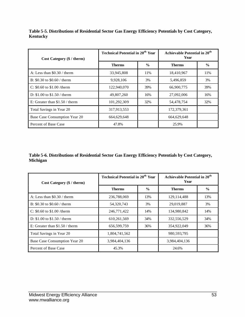
Midwest Energy Efficiency Alliance 53 www.mwalliance.org
Table 5-5. Distributions of Residential Sector Gas Energy Efficiency Potentials by Cost Category, Kentucky
Technical Potential in 20th Year Achievable Potential in 20th Year
Cost Category ($ / therm)
Therms % Therms %
A: Less than $0.30 / therm 33,945,808 11% 18,410,967 11%
B: $0.30 to $0.60 / therm 9,928,106 3% 5,496,859 3%
C: $0.60 to $1.00 /therm 122,940,070 39% 66,900,775 39%
D: $1.00 to $1.50 / therm 49,807,260 16% 27,092,006 16%
E: Greater than $1.50 / therm 101,292,309 32% 54,478,754 32%
Total Savings in Year 20 317,913,553 172,379,361
Base Case Consumption Year 20 664,629,648 664,629,648
Percent of Base Case 47.8% 25.9%
Table 5-6. Distributions of Residential Sector Gas Energy Efficiency Potentials by Cost Category, Michigan
Technical Potential in 20th Year Achievable Potential in 20th Year
Cost Category ($ / therm)
Therms % Therms %
A: Less than $0.30 / therm 236,788,069 13% 129,114,488 13%
B: $0.30 to $0.60 / therm 54,320,743 3% 29,019,887 3%
C: $0.60 to $1.00 /therm 246,771,422 14% 134,980,842 14%
D: $1.00 to $1.50 / therm 610,261,569 34% 332,556,529 34%
E: Greater than $1.50 / therm 656,599,759 36% 354,922,049 36%
Total Savings in Year 20 1,804,741,562 980,593,795
Base Case Consumption Year 20 3,984,404,136 3,984,404,136
Percent of Base Case 45.3% 24.6%

Midwest Energy Efficiency Alliance 54 www.mwalliance.org
Table 5-7. Distributions of Residential Sector Gas Energy Efficiency Potentials by Cost Category, Minnesota
Technical Potential in 20th Year Achievable Potential in 20th Year
Cost Category ($ / therm)
Therms % Therms %
A: Less than $0.30 / therm 87,038,050 14% 46,807,982 14%
B: $0.30 to $0.60 / therm 19,782,826 3% 10,524,011 3%
C: $0.60 to $1.00 /therm 79,452,697 13% 42,919,653 13%
D: $1.00 to $1.50 / therm 187,009,799 30% 100,240,954 30%
E: Greater than $1.50 / therm 251,150,474 40% 133,100,741 40%
Total Savings in Year 20 624,433,846 333,593,341
Base Case Consumption Year 20 1,420,350,670 1,420,350,670
Percent of Base Case 44.0% 23.5%
Table 5-8. Distributions of Residential Sector Gas Energy Efficiency Potentials by Cost Category, Missouri
Technical Potential in 20th Year Achievable Potential in 20th Year
Cost Category ($ / therm)
Therms % Therms %
A: Less than $0.30 / therm 30,490,536 5% 16,609,660 5%
B: $0.30 to $0.60 / therm 55,364,983 9% 30,339,312 9%
C: $0.60 to $1.00 /therm 63,719,462 10% 34,571,062 10%
D: $1.00 to $1.50 / therm 242,544,040 38% 133,063,463 39%
E: Greater than $1.50 / therm 240,652,083 38% 130,299,571 38%
Total Savings in Year 20 632,771,103 344,883,068
Base Case Consumption Year 20 1,314,639,694 1,314,639,694
Percent of Base Case 48.1% 26.2%

Midwest Energy Efficiency Alliance 55 www.mwalliance.org
Table 5-9. Distributions of Residential Sector Gas Energy Efficiency Potentials by Cost Category, Ohio
Technical Potential in 20th Year Achievable Potential in 20th Year
Cost Category ($ / therm)
Therms % Therms %
A: Less than $0.30 / therm 212,058,885 12% 114,564,251 12%
B: $0.30 to $0.60 / therm 38,412,539 2% 21,355,201 2%
C: $0.60 to $1.00 /therm 730,266,919 42% 397,275,419 43%
D: $1.00 to $1.50 / therm 275,076,283 16% 152,959,890 16%
E: Greater than $1.50 / therm 468,230,122 27% 248,588,743 27%
Total Savings in Year 20 1,724,044,747 934,743,504
Base Case Consumption Year 20 3,616,664,889 3,616,664,889
Percent of Base Case 47.7% 25.8%
Table 5-10. Distributions of Residential Sector Gas Energy Efficiency Potentials by Cost Category, Wisconsin
Technical Potential in 20th Year Achievable Potential in 20th Year
Cost Category ($ / therm)
Therms % Therms %
A: Less than $0.30 / therm 80,809,296 13% 43,969,049 13%
B: $0.30 to $0.60 / therm 38,826,644 6% 21,100,950 6%
C: $0.60 to $1.00 /therm 86,658,275 14% 47,154,538 14%
D: $1.00 to $1.50 / therm 190,578,057 30% 103,711,220 30%
E: Greater than $1.50 / therm 239,605,111 38% 129,370,492 37%
Total Savings in Year 20 636,477,383 345,306,250
Base Case Consumption Year 20 1,420,350,670 1,420,350,670
Percent of Base Case 44.8% 24.3%

Midwest Energy Efficiency Alliance 56 www.mwalliance.org
Tables A-1 through A-5, in Appendix A, show the gas achievable potential breakouts and levelized costs by cost category and measure for single family existing construction, single family new construction, multifamily existing construction, and multifamily new construction across the 9-state region. Notice that the totals across these tables necessarily sum to the achievable potential column in Table 5-1.
As expected, retrofit space and water heating measures are dominant in natural gas cost categories A and B. For example, if a home has no attic insulation or poor thermostat control, it is not surprising that these measures provide the greatest savings within category A. Similarly, tried and true measures like low-flow showerheads, aerators, and pipe insulation – the heart of water heater retrofit programs nationwide – are in category A.
Interestingly, condensing furnaces with an efficiency factor (EF) of 96% or greater are incrementally more cost-effective than their 92% counterparts. This is due to the relatively low incremental cost per EF of furnaces between 92% and 96% (less than $150) vs. the incremental cost between 80% and 92% (approximately $1,100). A similar effect holds for high-efficiency water heaters, and suggests that programs with bonus or tiered incentives for higher efficiency levels make sense given the current incremental cost structure. All cooking and drying measures fall into cost categories D and E. Again, note that some measures in the tables appear more than once due to differences in levelized cost categorization across climate zones or states.
It is also important to recognize that the value of other resource savings – such as electricity (cooling) savings for building envelope measures, and electric dryer and water savings for clothes washers – are not considered in the levelized cost calculations for natural gas DSM measures. If a utility applies a TRC test that must consider benefits over all fuels (water), then a more comprehensive analysis is required.

Midwest Energy Efficiency Alliance 57 www.mwalliance.org
As shown in Figure 5.1, expected savings in space heating is the largest component of the achievable gas energy efficiency potential in the residential sector, and accounts for 82% of the gas achievable potential. Retrofit measures to existing construction accounts for the largest share (48%) of achievable gas energy-efficiency potentials in the residential sector, with the installation of replacement measures in existing construction accounting for 24% of the potential. New construction accounts for the remaining 28% (Figure 5.2).
State-specific breakouts of achievable potential follow population patterns, with Illinois, Ohio, and Michigan constituting approximately 63% of the estimated savings, approximately consistent with those states’ shares of the total Midwest population (Figure 5.3). Within all of the states, the achievable potential gas savings represent approximately 25% of the baseline usage, with little fluctuation from state to state (Figure 5.5).
Single-family dwellings account for the largest share (83%) of achievable gas energy-efficiency potentials in the residential sector. Multi-family dwellings account for 17% of the gas energy-efficiency potential in the residential sector (Figure 5.4).
Figure 5-1. Distribution of Residential Sector Achievable Gas Energy Efficiency Potential by End-Use
Space_Heat82%
Water_Heat18%
Cooking0%
Dryer0%
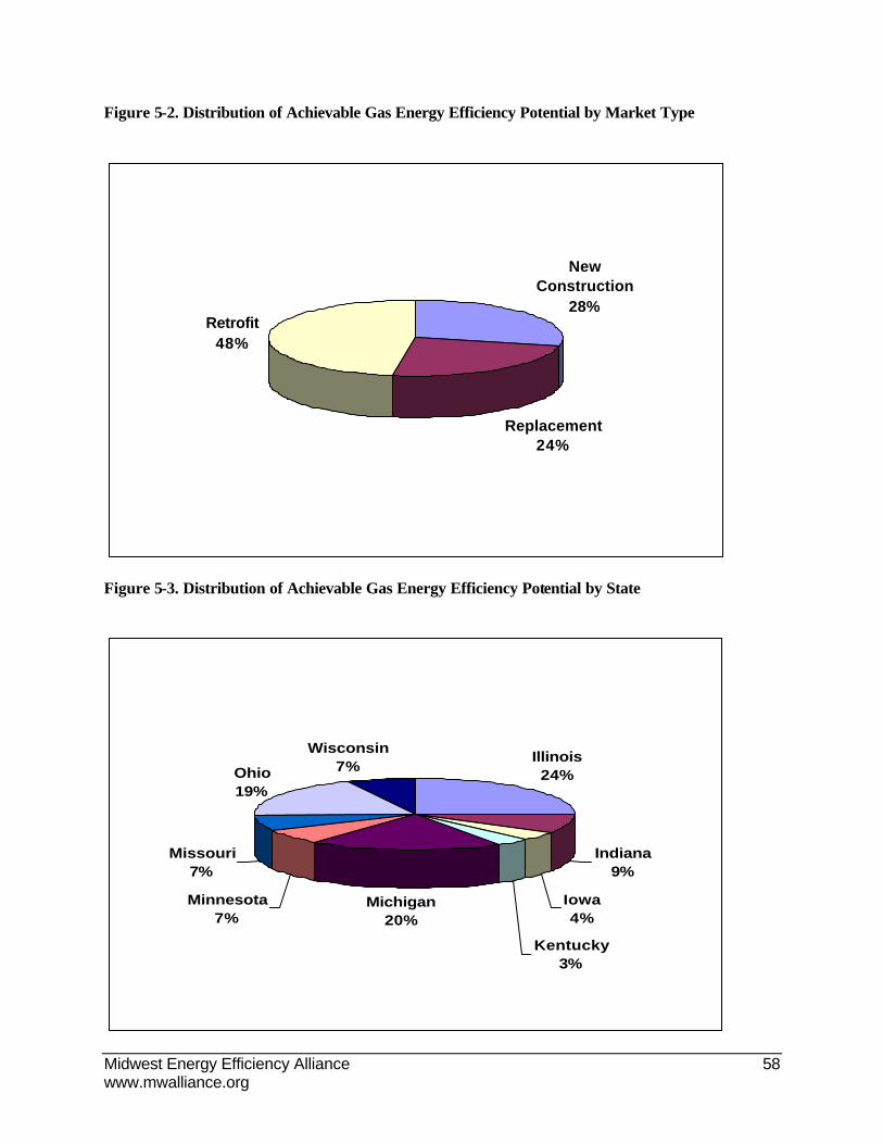
Midwest Energy Efficiency Alliance 58 www.mwalliance.org
Figure 5-2. Distribution of Achievable Gas Energy Efficiency Potential by Market Type
New Construction
28%
Replacement24%
Retrofit48%
Figure 5-3. Distribution of Achievable Gas Energy Efficiency Potential by State
Illinois24%
Indiana9%
Iowa4%
Kentucky3%
Michigan20%
Minnesota7%
Missouri7%
Ohio19%
Wisconsin7%
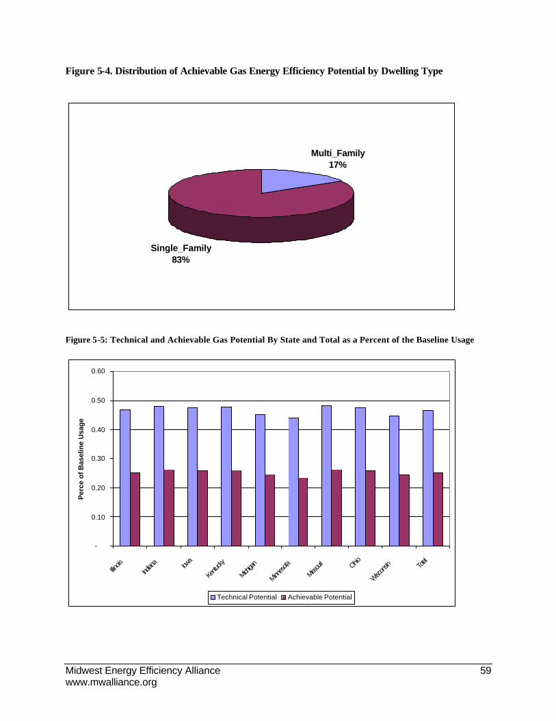
Midwest Energy Efficiency Alliance 59 www.mwalliance.org
Figure 5-4. Distribution of Achievable Gas Energy Efficiency Potential by Dwelling Type
Multi_Family17%
Single_Family83%
Figure 5-5: Technical and Achievable Gas Potential By State and Total as a Percent of the Baseline Usage
-
0.10
0.20
0.30
0.40
0.50
0.60
Illinois
Indian
a Iowa
Kentu
cky
Michiga
n
Minneso
ta
Missouri Ohio
Wiscon
sin Total
Per
ce o
f B
asel
ine
Usa
ge
Technical Potential Achievable Potential
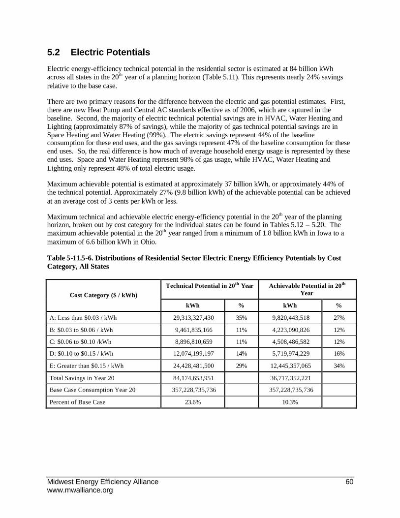
Midwest Energy Efficiency Alliance 60 www.mwalliance.org
5.2 Electric Potentials
Electric energy-efficiency technical potential in the residential sector is estimated at 84 billion kWh across all states in the 20th year of a planning horizon (Table 5.11). This represents nearly 24% savings relative to the base case.
There are two primary reasons for the difference between the electric and gas potential estimates. First, there are new Heat Pump and Central AC standards effective as of 2006, which are captured in the baseline. Second, the majority of electric technical potential savings are in HVAC, Water Heating and Lighting (approximately 87% of savings), while the majority of gas technical potential savings are in Space Heating and Water Heating (99%). The electric savings represent 44% of the baseline consumption for these end uses, and the gas savings represent 47% of the baseline consumption for these end uses. So, the real difference is how much of average household energy usage is represented by these end uses. Space and Water Heating represent 98% of gas usage, while HVAC, Water Heating and Lighting only represent 48% of total electric usage.
Maximum achievable potential is estimated at approximately 37 billion kWh, or approximately 44% of the technical potential. Approximately 27% (9.8 billion kWh) of the achievable potential can be achieved at an average cost of 3 cents per kWh or less.
Maximum technical and achievable electric energy-efficiency potential in the 20th year of the planning horizon, broken out by cost category for the individual states can be found in Tables 5.12 – 5.20. The maximum achievable potential in the 20th year ranged from a minimum of 1.8 billion kWh in Iowa to a maximum of 6.6 billion kWh in Ohio.
Table 5-11.5-6. Distributions of Residential Sector Electric Energy Efficiency Potentials by Cost Category, All States
Technical Potential in 20th Year Achievable Potential in 20th Year
Cost Category ($ / kWh)
kWh % kWh %
A: Less than $0.03 / kWh 29,313,327,430 35% 9,820,443,518 27%
B: $0.03 to $0.06 / kWh 9,461,835,166 11% 4,223,090,826 12%
C: $0.06 to $0.10 /kWh 8,896,810,659 11% 4,508,486,582 12%
D: $0.10 to $0.15 / kWh 12,074,199,197 14% 5,719,974,229 16%
E: Greater than $0.15 / kWh 24,428,481,500 29% 12,445,357,065 34%
Total Savings in Year 20 84,174,653,951 36,717,352,221
Base Case Consumption Year 20 357,228,735,736 357,228,735,736
Percent of Base Case 23.6% 10.3%

Midwest Energy Efficiency Alliance 61 www.mwalliance.org
Table 5-12. Distributions of Residential Sector Electric Energy Efficiency Potentials by Cost Category, Illinois
Technical Potential in 20th Year Achievable Potential in 20th Year
Cost Category ($ / kWh)
kWh % kWh %
A: Less than $0.03 / kWh 5,139,493,249 41% 1,653,410,182 32%
B: $0.03 to $0.06 / kWh 1,181,046,524 10% 491,091,350 10%
C: $0.06 to $0.10 /kWh 789,152,082 6% 391,264,325 8%
D: $0.10 to $0.15 / kWh 1,335,075,056 11% 596,826,345 12%
E: Greater than $0.15 / kWh 3,985,783,621 32% 2,013,765,823 39%
Total Savings in Year 20 12,430,550,533 5,146,358,025
Base Case Consumption Year 20 58,131,856,214 58,131,856,214
Percent of Base Case 21.4% 8.9%
Table 5-13. Distributions of Residential Sector Electric Energy Efficiency Potentials by Cost Category, Indiana
Technical Potential in 20th Year Achievable Potential in 20th Year
Cost Category ($ / kWh)
kWh % kWh %
A: Less than $0.03 / kWh 3,349,254,462 33% 1,144,342,637 26%
B: $0.03 to $0.06 / kWh 972,281,553 10% 429,385,094 10%
C: $0.06 to $0.10 /kWh 855,537,302 8% 437,564,369 10%
D: $0.10 to $0.15 / kWh 2,113,122,727 21% 1,024,035,531 23%
E: Greater than $0.15 / kWh 2,874,270,539 28% 1,431,319,457 32%
Total Savings in Year 20 10,164,466,583 4,466,647,087
Base Case Consumption Year 20 40,895,246,529 40,895,246,529
Percent of Base Case 24.9% 10.9%

Midwest Energy Efficiency Alliance 62 www.mwalliance.org
Table 5-14. Distributions of Residential Sector Electric Energy Efficiency Potentials by Cost Category, Iowa
Technical Potential in 20th Year Achievable Potential in 20th Year
Cost Category ($ / kWh)
kWh % kWh %
A: Less than $0.03 / kWh 1,547,167,966 37% 523,981,269 30%
B: $0.03 to $0.06 / kWh 402,432,826 10% 175,292,089 10%
C: $0.06 to $0.10 /kWh 385,247,500 9% 182,154,870 10%
D: $0.10 to $0.15 / kWh 704,086,274 17% 332,239,727 19%
E: Greater than $0.15 / kWh 1,125,151,973 27% 560,567,139 32%
Total Savings in Year 20 4,164,086,538 1,774,235,094
Base Case Consumption Year 20 17,278,311,161 17,278,311,161
Percent of Base Case 24.1% 10.3%
Table 5-15. Distributions of Residential Sector Electric Energy Efficiency Potentials by Cost Category, Kentucky
Technical Potential in 20th Year Achievable Potential in 20th Year
Cost Category ($ / kWh)
kWh % kWh %
A: Less than $0.03 / kWh 2,397,270,570 24% 880,278,862 19%
B: $0.03 to $0.06 / kWh 1,224,533,284 12% 587,423,666 13%
C: $0.06 to $0.10 /kWh 2,321,333,291 23% 1,172,543,622 25%
D: $0.10 to $0.15 / kWh 1,079,011,574 11% 518,991,025 11%
E: Greater than $0.15 / kWh 2,947,374,864 30% 1,502,781,453 32%
Total Savings in Year 20 9,969,523,582 4,662,018,628
Base Case Consumption Year 20 32,941,385,188 32,941,385,188
Percent of Base Case 30.3% 14.2%
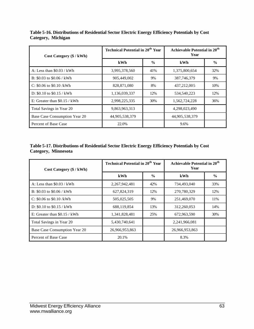
Midwest Energy Efficiency Alliance 63 www.mwalliance.org
Table 5-16. Distributions of Residential Sector Electric Energy Efficiency Potentials by Cost Category, Michigan
Technical Potential in 20th Year Achievable Potential in 20th Year
Cost Category ($ / kWh)
kWh % kWh %
A: Less than $0.03 / kWh 3,995,378,560 41% 1,375,800,654 32%
B: $0.03 to $0.06 / kWh 905,449,002 9% 387,746,379 9%
C: $0.06 to $0.10 /kWh 828,871,080 8% 437,212,005 10%
D: $0.10 to $0.15 / kWh 1,136,039,337 12% 534,540,223 12%
E: Greater than $0.15 / kWh 2,998,225,335 30% 1,562,724,228 36%
Total Savings in Year 20 9,863,963,313 4,298,023,490
Base Case Consumption Year 20 44,905,538,379 44,905,538,379
Percent of Base Case 22.0% 9.6%
Table 5-17. Distributions of Residential Sector Electric Energy Efficiency Potentials by Cost Category, Minnesota
Technical Potential in 20th Year Achievable Potential in 20th Year
Cost Category ($ / kWh)
kWh % kWh %
A: Less than $0.03 / kWh 2,267,942,481 42% 734,493,040 33%
B: $0.03 to $0.06 / kWh 627,824,319 12% 270,780,329 12%
C: $0.06 to $0.10 /kWh 505,025,505 9% 251,469,070 11%
D: $0.10 to $0.15 / kWh 688,119,854 13% 312,260,053 14%
E: Greater than $0.15 / kWh 1,341,828,481 25% 672,963,590 30%
Total Savings in Year 20 5,430,740,641 2,241,966,081
Base Case Consumption Year 20 26,966,953,863 26,966,953,863
Percent of Base Case 20.1% 8.3%
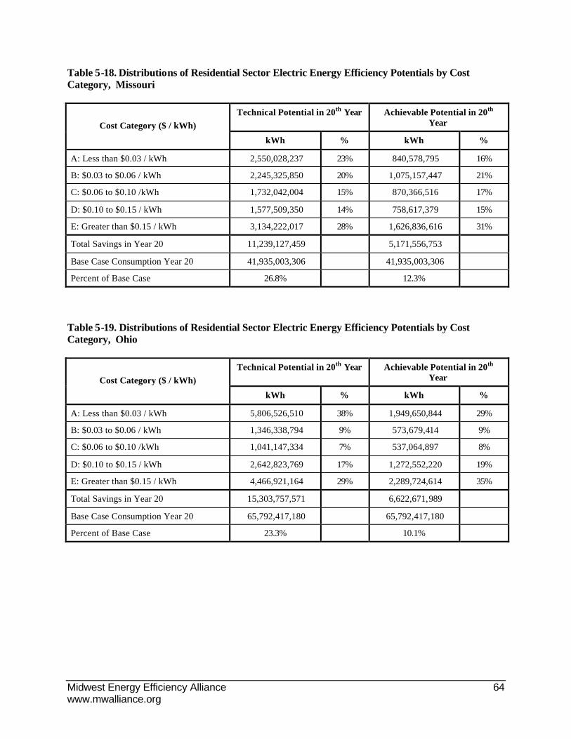
Midwest Energy Efficiency Alliance 64 www.mwalliance.org
Table 5-18. Distributions of Residential Sector Electric Energy Efficiency Potentials by Cost Category, Missouri
Technical Potential in 20th Year Achievable Potential in 20th Year
Cost Category ($ / kWh)
kWh % kWh %
A: Less than $0.03 / kWh 2,550,028,237 23% 840,578,795 16%
B: $0.03 to $0.06 / kWh 2,245,325,850 20% 1,075,157,447 21%
C: $0.06 to $0.10 /kWh 1,732,042,004 15% 870,366,516 17%
D: $0.10 to $0.15 / kWh 1,577,509,350 14% 758,617,379 15%
E: Greater than $0.15 / kWh 3,134,222,017 28% 1,626,836,616 31%
Total Savings in Year 20 11,239,127,459 5,171,556,753
Base Case Consumption Year 20 41,935,003,306 41,935,003,306
Percent of Base Case 26.8% 12.3%
Table 5-19. Distributions of Residential Sector Electric Energy Efficiency Potentials by Cost Category, Ohio
Technical Potential in 20th Year Achievable Potential in 20th Year
Cost Category ($ / kWh)
kWh % kWh %
A: Less than $0.03 / kWh 5,806,526,510 38% 1,949,650,844 29%
B: $0.03 to $0.06 / kWh 1,346,338,794 9% 573,679,414 9%
C: $0.06 to $0.10 /kWh 1,041,147,334 7% 537,064,897 8%
D: $0.10 to $0.15 / kWh 2,642,823,769 17% 1,272,552,220 19%
E: Greater than $0.15 / kWh 4,466,921,164 29% 2,289,724,614 35%
Total Savings in Year 20 15,303,757,571 6,622,671,989
Base Case Consumption Year 20 65,792,417,180 65,792,417,180
Percent of Base Case 23.3% 10.1%
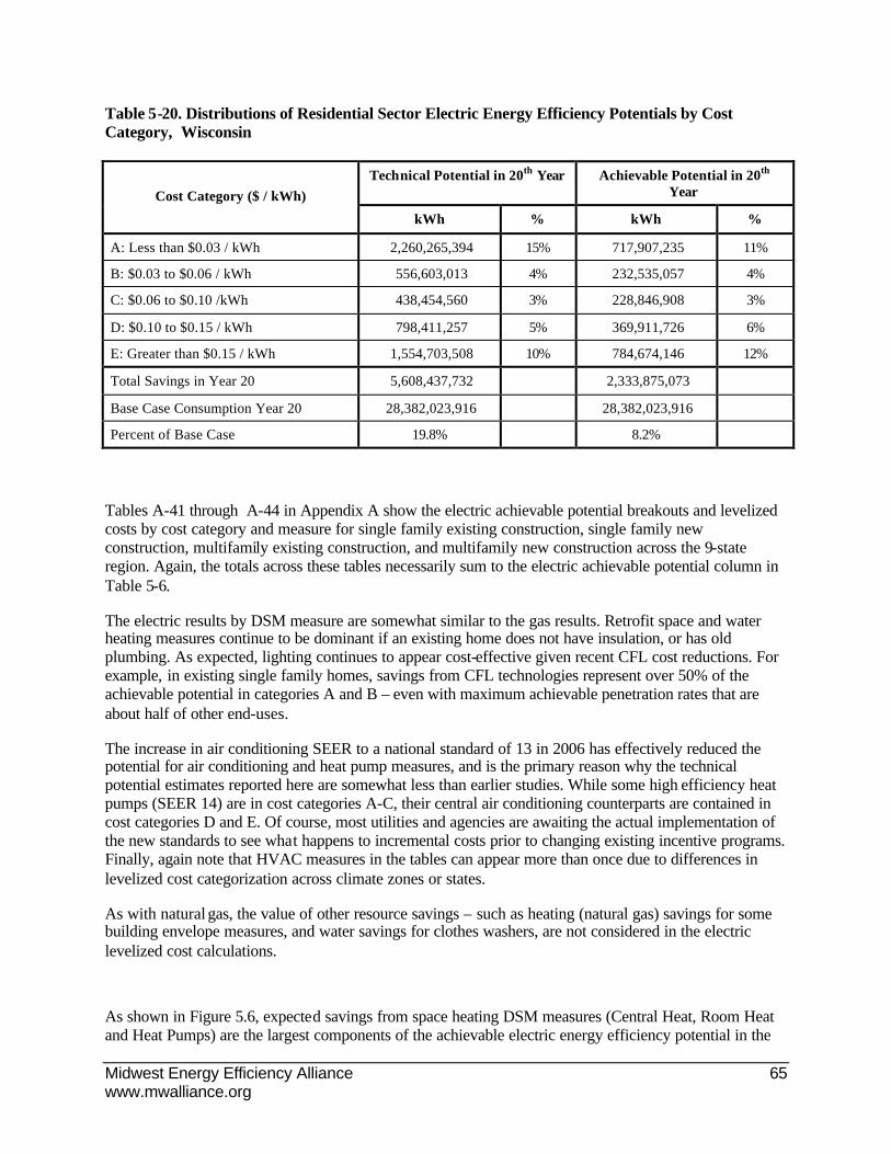
Midwest Energy Efficiency Alliance 65 www.mwalliance.org
Table 5-20. Distributions of Residential Sector Electric Energy Efficiency Potentials by Cost Category, Wisconsin
Technical Potential in 20th Year Achievable Potential in 20th Year
Cost Category ($ / kWh)
kWh % kWh %
A: Less than $0.03 / kWh 2,260,265,394 15% 717,907,235 11%
B: $0.03 to $0.06 / kWh 556,603,013 4% 232,535,057 4%
C: $0.06 to $0.10 /kWh 438,454,560 3% 228,846,908 3%
D: $0.10 to $0.15 / kWh 798,411,257 5% 369,911,726 6%
E: Greater than $0.15 / kWh 1,554,703,508 10% 784,674,146 12%
Total Savings in Year 20 5,608,437,732 2,333,875,073
Base Case Consumption Year 20 28,382,023,916 28,382,023,916
Percent of Base Case 19.8% 8.2%
Tables A-41 through A-44 in Appendix A show the electric achievable potential breakouts and levelized costs by cost category and measure for single family existing construction, single family new construction, multifamily existing construction, and multifamily new construction across the 9-state region. Again, the totals across these tables necessarily sum to the electric achievable potential column in Table 5-6.
The electric results by DSM measure are somewhat similar to the gas results. Retrofit space and water heating measures continue to be dominant if an existing home does not have insulation, or has old plumbing. As expected, lighting continues to appear cost-effective given recent CFL cost reductions. For example, in existing single family homes, savings from CFL technologies represent over 50% of the achievable potential in categories A and B – even with maximum achievable penetration rates that are about half of other end-uses.
The increase in air conditioning SEER to a national standard of 13 in 2006 has effectively reduced the potential for air conditioning and heat pump measures, and is the primary reason why the technical potential estimates reported here are somewhat less than earlier studies. While some high efficiency heat pumps (SEER 14) are in cost categories A-C, their central air conditioning counterparts are contained in cost categories D and E. Of course, most utilities and agencies are awaiting the actual implementation of the new standards to see what happens to incremental costs prior to changing existing incentive programs. Finally, again note that HVAC measures in the tables can appear more than once due to differences in levelized cost categorization across climate zones or states.
As with natural gas, the value of other resource savings – such as heating (natural gas) savings for some building envelope measures, and water savings for clothes washers, are not considered in the electric levelized cost calculations.
As shown in Figure 5.6, expected savings from space heating DSM measures (Central Heat, Room Heat and Heat Pumps) are the largest components of the achievable electric energy efficiency potential in the

Midwest Energy Efficiency Alliance 66 www.mwalliance.org
residential sector across all cost categories, and account for 30% of the electric achievable potential. Expected savings in lighting (20%), water heating (20%), and central air conditioning (15%) provide a majority of the remaining savings. Retrofit measures to existing construction accounts for the largest share (62%) of achievable electric energy-efficiency potentials in the residential sector, with the installation of replacement measures in existing construction accounting for 13% of the potential. New construction accounts for the remaining 25% (Figure 5.7).
State-specific breakouts of achievable potential again approximately follow population patterns, with Illinois, Ohio, and Michigan constituting approximately 44% of the estimated savings (Figure 5.8). Additionally, those states further south (Missouri and Kentucky) constitute approximately 27% of the estimated savings due to higher saturations of electric HVAC and Water Heating equipment, and a lower incidence of DSM intervention programs The achievable potential electric savings, as a percent of the baseline usage, averages approximately 10% across states but there is more variation between states than was seen in the gas model. (Figure 5.10).
Single-family dwellings account for the largest share (80%) of achievable electric energy-efficiency potentials in the residential sector. Multi-family dwellings account for 20% of the electric energy-efficiency potential in the residential sector (Figure 5.9).
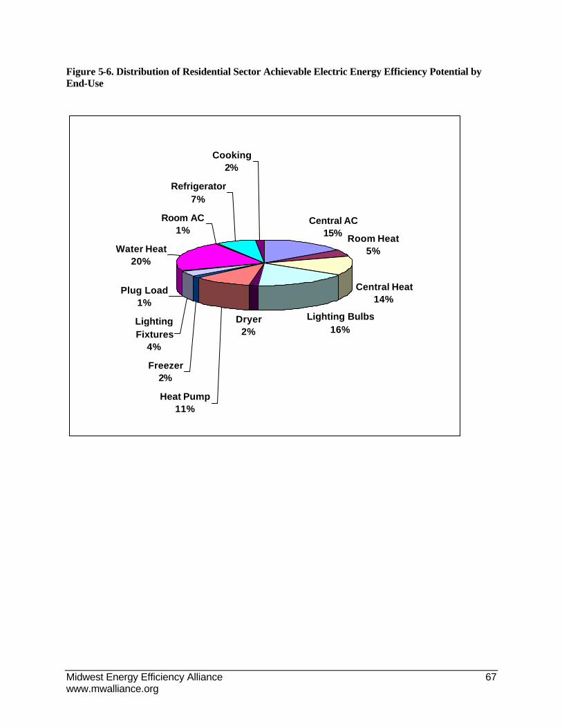
Midwest Energy Efficiency Alliance 67 www.mwalliance.org
Figure 5-6. Distribution of Residential Sector Achievable Electric Energy Efficiency Potential by End-Use
Central AC15% Room Heat
5%
Central Heat14%
Lighting Bulbs16%
Dryer2%
Heat Pump11%
Freezer2%
Lighting Fixtures
4%
Plug Load1%
Water Heat20%
Room AC1%
Refrigerator7%
Cooking2%
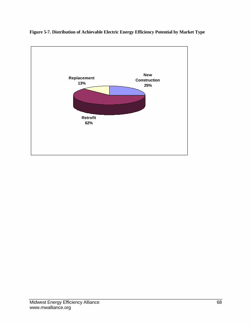
Midwest Energy Efficiency Alliance 68 www.mwalliance.org
Figure 5-7. Distribution of Achievable Electric Energy Efficiency Potential by Market Type
New Construction
25%
Retrofit62%
Replacement13%
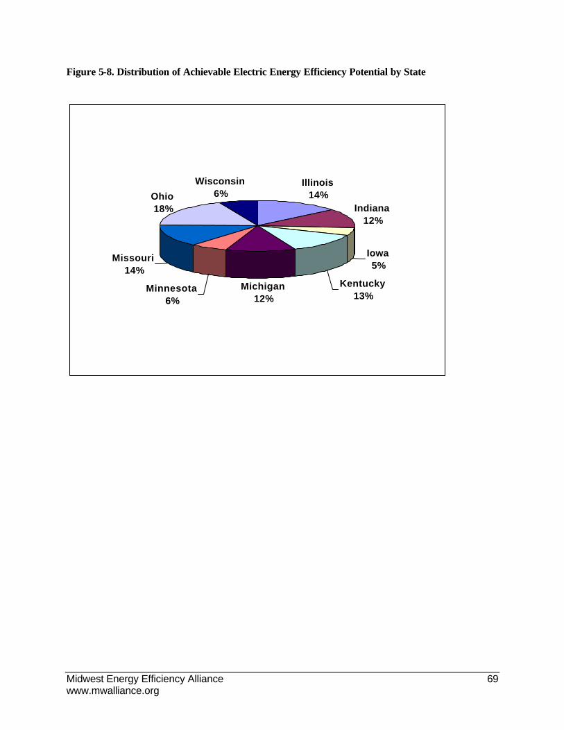
Midwest Energy Efficiency Alliance 69 www.mwalliance.org
Figure 5-8. Distribution of Achievable Electric Energy Efficiency Potential by State
Illinois14%
Indiana12%
Iowa5%
Kentucky13%
Michigan12%
Minnesota6%
Missouri14%
Ohio18%
Wisconsin6%
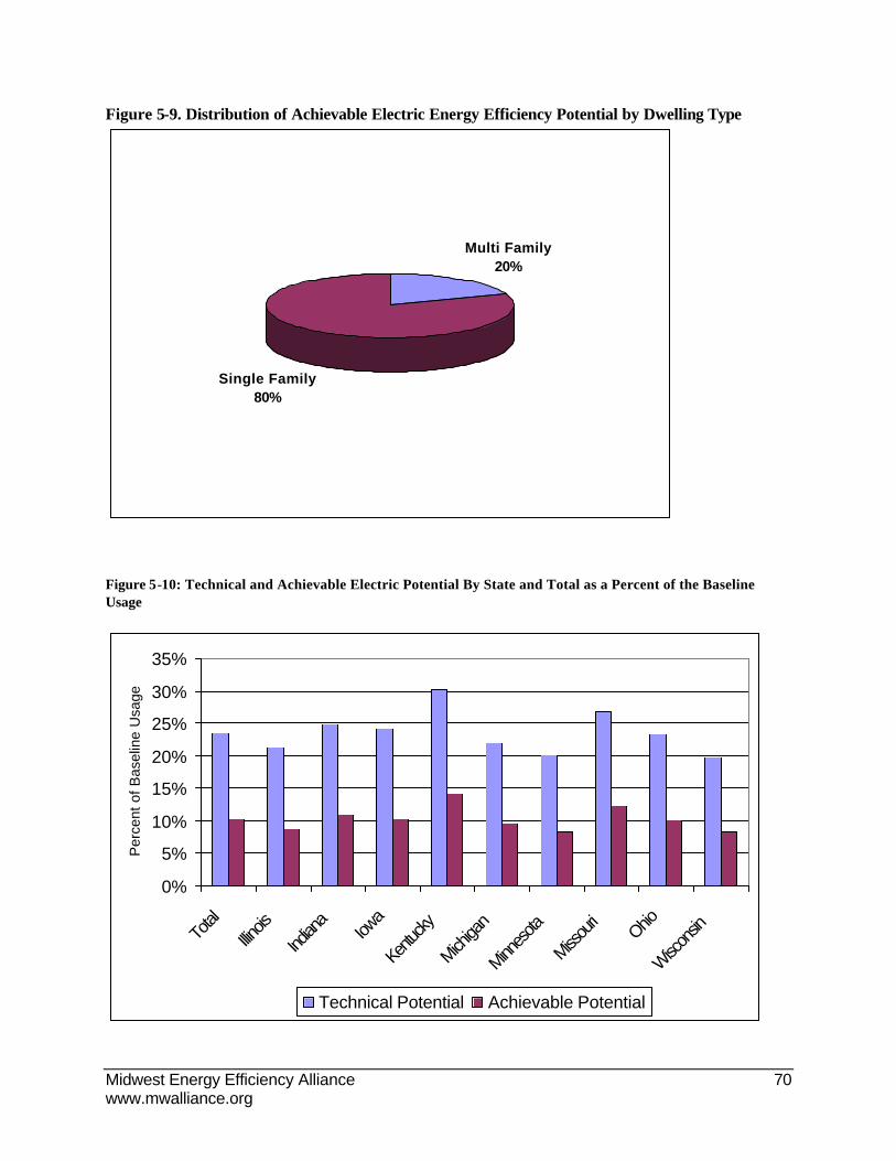
Midwest Energy Efficiency Alliance 70 www.mwalliance.org
Figure 5-9. Distribution of Achievable Electric Energy Efficiency Potential by Dwelling Type
Multi Family20%
Single Family80%
Figure 5-10: Technical and Achievable Electric Potential By State and Total as a Percent of the Baseline Usage
0%
5%
10%
15%
20%
25%
30%
35%
Total
Illinois
Indian
aIow
a
Kentu
cky
Michiga
n
Minnes
ota
Missou
riOhio
Wiscon
sin
Per
cent
of B
asel
ine
Usa
ge
Technical Potential Achievable Potential

Midwest Energy Efficiency Alliance 71 www.mwalliance.org
6. CONCLUSIONS AND RECOMMENDATIONS The results of this study demonstrate that while there are differences across Midwest states in terms of residential customer characteristics, energy use, and historical DSM program activity and related measure saturations, significant electric and natural gas DSM opportunities remain.
6.1 Housing Characteristics and Energy Use
The residential customer surveys revealed significant differences in housing size and heating equipment system characteristics across the Midwest. Customers in half of the states analyzed report mean house sizes of 1,600 to 1,800 square feet, while customers in the other half of the states report mean house sizes of 1,900 to 2,100 square feet. Illinois, Wisconsin, Minnesota, and Michigan are the states with the smaller house sizes, while Indiana, Kentucky, Missouri, and Ohio report larger house sizes.
More importantly, the relative fuel shares of electric and gas space heating and water heating also vary across the states. For example, electric space heating shares exceed 25% in Kentucky and Missouri, while in the northern states of Minnesota, Wisconsin, and Michigan the electric space heating share is less than 10%. This is the primary reason behind the fact that residential electricity use is 50% higher in the southern Midwest region. Similarly, variations in natural gas use are influenced by saturations of natural gas space heating and water heating, as well as climate, dwelling envelope characteristics, and average gas space heating efficiencies.
6.2 DSM Program Activity and Measure Saturations
The most prevalent residential Midwestern DSM programs are rebates, energy audits, and other types of energy information programs. Direct load control programs and low-income programs are also relatively common in the Midwest.
Despite the successes of many of these programs, most dwellings can benefit from one or more energy efficiency measures:
• Insulation. Approximately 5 – 15% of customers have either uninsulated ceilings or walls in their homes. The percentage of customers with uninsulated attics varies from 3% to 11% from state to state, while the percentage of homes with uninsulated walls varies from 5% to 27%. However, more than half of these percentages were self-reported by customers through a telephone survey. Such self-reported responses sometimes over-estimate the actual amount of insulation present in homes.
• Windows. Generally 20%-36% of homes have single-paned windows. The lowest percentages of single-paned windows are found in Minnesota (20%) and Ohio (22%), while the highest percentages are found in Illinois (36%) and Wisconsin (35%).
• Compact Fluorescent Lamps. Less than half of the homes in any Midwest state have one or more compact fluorescent lamps (CFLs). The percentage of homes with one or more CFLs varies from 13% in Wisconsin to 43% in Kentucky. (However, Wisconsin’s data is the oldest of the states analyzed, so the saturation of CFLs there is likely higher currently.) The median percentage of homes with one or more CFLs is 33%.
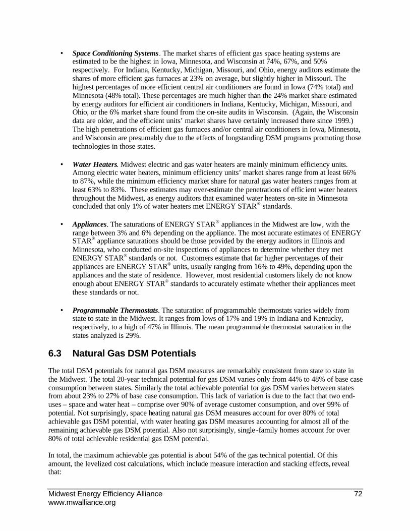
Midwest Energy Efficiency Alliance 72 www.mwalliance.org
• Space Conditioning Systems. The market shares of efficient gas space heating systems are estimated to be the highest in Iowa, Minnesota, and Wisconsin at 74%, 67%, and 50% respectively. For Indiana, Kentucky, Michigan, Missouri, and Ohio, energy auditors estimate the shares of more efficient gas furnaces at 23% on average, but slightly higher in Missouri. The highest percentages of more efficient central air conditioners are found in Iowa (74% total) and Minnesota (48% total). These percentages are much higher than the 24% market share estimated by energy auditors for efficient air conditioners in Indiana, Kentucky, Michigan, Missouri, and Ohio, or the 6% market share found from the on-site audits in Wisconsin. (Again, the Wisconsin data are older, and the efficient units’ market shares have certainly increased there since 1999.) The high penetrations of efficient gas furnaces and/or central air conditioners in Iowa, Minnesota, and Wisconsin are presumably due to the effects of longstanding DSM programs promoting those technologies in those states.
• Water Heaters. Midwest electric and gas water heaters are mainly minimum efficiency units. Among electric water heaters, minimum efficiency units’ market shares range from at least 66% to 87%, while the minimum efficiency market share for natural gas water heaters ranges from at least 63% to 83%. These estimates may over-estimate the penetrations of effic ient water heaters throughout the Midwest, as energy auditors that examined water heaters on-site in Minnesota concluded that only 1% of water heaters met ENERGY STAR® standards.
• Appliances. The saturations of ENERGY STAR® appliances in the Midwest are low, with the range between 3% and 6% depending on the appliance. The most accurate estimates of ENERGY STAR® appliance saturations should be those provided by the energy auditors in Illinois and Minnesota, who conducted on-site inspections of appliances to determine whether they met ENERGY STAR® standards or not. Customers estimate that far higher percentages of their appliances are ENERGY STAR® units, usually ranging from 16% to 49%, depending upon the appliances and the state of residence. However, most residential customers likely do not know enough about ENERGY STAR® standards to accurately estimate whether their appliances meet these standards or not.
• Programmable Thermostats. The saturation of programmable thermostats varies widely from state to state in the Midwest. It ranges from lows of 17% and 19% in Indiana and Kentucky, respectively, to a high of 47% in Illinois. The mean programmable thermostat saturation in the states analyzed is 29%.
6.3 Natural Gas DSM Potentials
The total DSM potentials for natural gas DSM measures are remarkably consistent from state to state in the Midwest. The total 20-year technical potential for gas DSM varies only from 44% to 48% of base case consumption between states. Similarly the total achievable potential for gas DSM varies between states from about 23% to 27% of base case consumption. This lack of variation is due to the fact that two end-uses – space and water heat – comprise over 90% of average customer consumption, and over 99% of potential. Not surprisingly, space heating natural gas DSM measures account for over 80% of total achievable gas DSM potential, with water heating gas DSM measures accounting for almost all of the remaining achievable gas DSM potential. Also not surprisingly, single -family homes account for over 80% of total achievable residential gas DSM potential.
In total, the maximum achievable gas potential is about 54% of the gas technical potential. Of this amount, the levelized cost calculations, which include measure interaction and stacking effects, reveal that:
Midwest Energy Efficiency Alliance 73 www.mwalliance.org
• About 12% of the total achievable potential is available from measures whose cost of conserved energy is $0.30 per therm or less.
• Approximately 31% of the total achievable potential is available from DSM measures whose cost of conserved energy is between $0.30 and $1.00 per therm.
• About 57% of the total achievable potential is from measures whose costs of conserved energy are more than $1.00 per therm, at or above the currently high commodity cost for natural gas.
The most cost-effective natural gas DSM measures are insulating uninsulated attics, ENERGY STAR® programmable thermostats, low flow showerheads, hot water pipe insulation, and faucet aerators. These measures have costs of conserved energy of $0.30 per therm or less in existing single -family homes. High efficiency furnaces, comprehensive air sealing/infiltration reductions, water heater thermostat setbacks, and multi-family wall insulation are in the second tier of cost-effectiveness, with costs of conserved energy of $0.60 per them or less.
6.4 Electric DSM Potentials
Electric DSM potentials are much smaller shares of base case consumption than gas DSM potentials. Total electric DSM technical potential equals about 24% of base case consumption, compared to about 47% for gas technical potential. Total electric achievable potential accounts for about 10% of base case consumption, compared to about 25% for gas achievable potential. These differences are due to two primary factors: first, the electric base case consumption estimates include electricity savings from the significant forthcoming federal efficiency standards for central air conditioners and heat pumps that will take effect in 2006. Second, electric space heating, water heating, and lighting account for less than half of total base case electric consumption, but almost all of natural gas base case consumption. The DSM potentials for other electric loads such as appliances are considerably smaller percentages of base case consumption than the DSM potentials for space heating, water heating, and lighting DSM measures.
Electric DSM potentials vary much more from state to state than gas DSM potentials. Electric technical DSM potential varies from about 20% to 30% of base case consumption between states, while electric achievable DSM potential varies from about 8% to 14% between states. Minnesota and Wisconsin have the lowest relative amounts of DSM potential, while Kentucky and Missouri have the largest relative amounts of DSM potential. The amounts of electric DSM potential are proportionate to the saturations of electric space heating and water heating equipment in a state, and inversely proportionate to the magnitudes of historical DSM activity.
In total, about 39% of the total electric achievable potential is available from DSM measures whose cost of conserved energy is 6¢/kWh or less. On the other hand, 51% of total electric potential comes from DSM measures whose costs of conserved energy are 10¢/kWh or more, at or above most current Midwest electric rates.
The most cost-effective and largest impact electric DSM measures are insulating uninsulated attics, installing ENERGY STAR® heat pumps, installing CFLs, removing or replacing secondary or inefficient refrigerators or freezers, and low flow showerheads.
In total, these measures comprise over 75% of the achievable DSM potential for measures with costs of conserved energy of 6¢/kWh or less. In fact, most of these measures have costs of conserved energy of 3¢/kWh or less.
Midwest Energy Efficiency Alliance 74 www.mwalliance.org
6.5 Recommendations
This section focuses on the DSM measures that have the largest DSM potentials and are the most cost-effective based on the simplified cost of conserved energy calculations done for this project. The study authors do not intend to imply that other DSM measures beyond those discussed in this section are without merit or inappropriate for Midwest DSM programs. We conclude with how the residential natural gas and electric achievable potentials may influence program offerings in the region.
6.5.1 Key Natural Gas Measures
Natural gas DSM measures in total show greater DSM potential as a percentage of baseline consumption than is the case for electric DSM measures. Natural gas DSM potentials are also more consistent percentages of baseline natural gas forecast consumption between Midwest states. Natural gas prices are currently quite high in the Midwest, and MEEA’s Midwest Natural Gas Initiative has a main goal of reducing long-term natural gas prices through energy conservation efforts.
Four residential natural gas measures account for about 83% of the DSM potential with a cost of conserved energy of $1 per therm or less. The remaining DSM potential at this cost of conserved energy is accounted for by a variety of measures, each with relatively small impacts. Each of the four major measures is discussed below.
Insulating Uninsulated Attics
The total achievable potential for this measure over the 20 year forecast period is approximately 390 million therms. This represents about two percent of total residential base case natural gas consumption over this period. The total cost of conserved energy for this measure in most Midwest single -family homes is about $0.25 per therm. This cost is based on the total installed cost for the insulation.
Residential attic insulation measures are usually covered by large-scale utility or agency DSM portfolios. For example, Xcel Energy, the main sponsor of this study, in December 2005 proposed a revised incentive for attic insulation, a rebate of $300, for its Minnesota residential customers that is currently under regulatory review. As a second example, MidAmerican Energy offers its Iowa residential customers rebates for 70% of the cost of attic insulation, up to a maximum of $600.
MEEA requested a discussion of the economics and cost-effectiveness of sample gas and electric DSM programs. As the gas example, we will discuss the economics of Xcel Energy’s recently proposed attic insulation program. 47 This information is contained in a public document, and contains updated assumptions about natural gas prices.
This program is cost-effective from all four perspectives considered for natural gas programs in Minnesota:
• The program has a benefit-cost ratio to program participants of 5.10, meaning that the energy savings to program participants have a net present value (NPV) of slightly more than five times the net (after rebate) cost of the insulation.
47 Xcel Energy, “Accelerated Gas CIP Proposal for 2006, Docket No. E,G002/CIP-04-820”, (Xcel Energy, Minneapolis, MN, December 21, 2005).

Midwest Energy Efficiency Alliance 75 www.mwalliance.org
• The societal benefit-cost ratio is 3.22, meaning that the NPV of the conserved gas is slightly more than three times the sum of the installed cost of the attic insulation and program administrative costs.
• The revenue requirements test has a benefit-cost ratio of 4.44. This test is similar to the utility test used for electric program benefit-cost analysis in Minnesota, and compares the NPV of the conserved energy to the total program costs.
• The cost comparison test has a benefit-cost ratio of 3.58. This test is similar to but different from the rate impact test used in electric DSM benefit-cost analysis. This test compares the NPV of the conserved energy to the NPV sum of the program costs and the lost margins that the utility experiences from not selling the gas conserved by the program.
Attic insulation is often not covered by smaller scale DSM portfolios. Sponsors of smaller scale DSM program portfolios may be most interested in a MEEA program promoting attic insulation, but no market research was conducted to specifically assess this matter.
Enrolling customers with uninsulated attics in a DSM program covering attic insulation is likely to be somewhat challenging, for two reasons. First, the survey results indicate that generally only 5%-10% of homes in any state have no attic insulation. Secondly, many customers having inadequate insulation are not aware of that fact. As part of ECW’s Energy and Housing Study in Wisconsin study, it was found that only 27% of homeowners that had inadequate insulation were aware of that situation. 48 However, energy audits conducted by qualified energy auditors are ideal methods for identifying such customers. Many utilities and agencies offer such energy audits to their customers at a reduced cost through their DSM programs.
ENERGY STAR® Programmable Thermostats
The total achievable potential for this measure over the 20 year forecast period is approximately 210 million therms. This represents about one percent of total residential base case natural gas consumption. The total cost of conserved energy for this measure in most Midwest single -family homes is about $0.17 per therm. This cost is based on the total installed cost for the thermostat. Since the current saturations for programmable thermostats are less than 50% in all Midwest states studied, and vary by over a factor of two from state to state in the Midwest, considerable market potential exists for this measure.
However, concerns exist about the actual in-the-field energy savings impacts from programmable thermostats. For example, ECW’s Energy and Housing Study in Wisconsin found that although homeowners with programmable thermostats had a 2.5% lower energy intensity than homes with manual thermostats, the statistical uncertainty associated with such savings was +/- 7%, or several times larger than the savings estimate. Furthermore, few homeowners with manual thermostats that participated in detailed interviews that were done as part of that project were interested in installing programmable thermostats. 49
Nevertheless, utilities and agencies sponsoring large-scale DSM portfolios often include programmable thermostats as a measure covered by their DSM programs. For example, MidAmerican Energy offers its residential customers in Iowa a programmable thermostat as part of its HomeCheck™ energy audit
48 ECW: 2000, op.cit., p. 21. 49 Ibid, p. 32-33.

Midwest Energy Efficiency Alliance 76 www.mwalliance.org
program. The energy auditor will install a unit for an additional $30 charge. 50 Xcel Energy includes programmable thermostats as part of its Home Energy residential new construction program, but not as part of its DSM programs for customers in existing homes, due to concerns about the energy savings impacts of the measure in that application.
High Efficiency Gas Furnaces
The total achievable potential for this measure over the 20 year forecast period with a cost of conserved energy of $1 per therm or less is approximately 930 million therms. This represents about five percent of total residential base case natural gas consumption. The cost of conserved energy for this measure varies between housing types, and whether a 92% or 96% efficient furnace is analyzed. Interestingly, the 96% efficient furnaces were found to have a lower total cost of conserved energy than the 92% efficient furnaces.
Efficient furnaces have a cost of conserved energy between $1.10 per therm and $1.20 per therm in the more southern states of the Midwest where the annual savings are lower. The total DSM potential from efficient furnaces in those states is about 600 million therms, or about three percent of total residential base case consumption. Whether this conservation is considered cost-effective or not depends on projections for the price of natural gas.
Efficient natural gas furnaces are often covered by larger-scale utility or agency DSM programs. For example, Alliant Energy offers its residential customers in Iowa rebates for efficient furnaces that range from $200 for a 90% efficient furnace to $350 for a 96% efficient furnace.51 As a second example, the Wisconsin Focus on Energy offers Wisconsin residents a rebate of $150 for a gas furnace with at least a 90% efficiency rating and two stages of firing. 52
The current penetrations for efficient gas furnaces vary widely in the Midwest, from highs of 50% to 74% in Iowa, Minnesota, and Wisconsin to about 23% in the rest of the region. The DSM potential for efficient gas furnaces will be highest in the states where the current penetrations are the lowest. Again, utilities or agencies in these states may be the most interested in a MEEA program promoting efficient gas furnaces, but no market research was conducted to specifically assess this matter. Another option that can be considered to increase the installation of efficient gas furnaces is issuing statewide minimum efficiency standards for these products. The U.S. DOE has been conducting a rulemaking on a national gas furnace efficiency standard since 1997, but has not yet issued a proposed standard. States would have to apply to DOE for a waiver to issue a state energy efficiency standard for this product.
Conduct Comprehensive Shell Air Sealing and Infiltration Reduction
Comprehensive air sealing includes sealing all visible cracks and penetrations, plus using enhanced leak detection techniques such as a blower door test and/or thermal imaging if outdoor conditions merit. In general, we assumed a 50% reduction in infiltration heating and cooling loads in existing construction and a much smaller reduction to a minimum one-third air changes per hour in new construction. Tighter air sealing can raise indoor air quality issues without added ventilation.
The total achievable potential for this measure over the 20 year forecast period is approximately 280 million therms, or about 1.4% of base case natural gas consumption over this period. This measure is
50 See MidAmerican’s Energy’s web site: midamericanenergy.com/html/energy3g.asp 51 See Alliant Energy’s web site: alliantenergy.com. 52 See the Focus on Energy web site: focusonenergy.com.
Midwest Energy Efficiency Alliance 77 www.mwalliance.org
most applicable and cost-effective in existing single -family homes. The cost of conserved energy for this measure in most of the Midwest states analyzed is about $0.85 per therm, but in some of the northern states where the annual savings are larger than average, the cost of conserved energy is about $0.57 per therm.
Utilities and energy agencies most commonly promote these types of DSM measures through energy audit programs. Energy auditors will estimate how much energy installing these measures will save, often using a blower door test to estimate infiltration levels in homes. Energy auditing programs are very common elements of DSM program portfolios in the Midwest, but programs specifically focused on promoting comprehensive shell air sealing are not common. These measures are part of the Home Performance with ENERGY STAR® program that the Wisconsin Focus on Energy is conducting. 53
6.5.2 Electric DSM Measures
While electric residential DSM potential is not as high in percentage terms as natural gas DSM potential, there are many electric measures that are or may be cost-effective. The six measures discussed below account for 78% of the DSM potential for measures with costs of conserved energy of 10¢/kWh or less. As discussed previously, the costs of conserved energy are calculated based on the total installed costs of the DSM measures.
Compact Fluorescent Lamps (CFLs)
The total achievable potential for this measure over the 20 year forecast period is approximately 5,800 GWh, or about 1.6% of total residential base case electric consumption over this period. The total cost of conserved energy for this measure varies with how many hours per day the lamps are used. For lamps that are used six hours per day, the cost of conserved energy is about 1.2¢/kWh, while for CFLs that are used 2.5 or 0.5 hours per day, the cost of conserved energy is 2.3¢/kWh or 11¢/kWh, respectively.
DSM programs promoting CFLs to residential customers are widespread in the Midwest. The Change-A-Light, Change-The-World program is MEEA’s most popular program in the Midwest, with over a dozen sponsors, and many utilities and agencies in the Midwest also operate their own residential lighting DSM programs that are focused on promoting CFLs. The CFL potential estimates demonstrate that despite the success of these efforts, lighting potential remains very high in the Midwest.
MEEA requested a discussion of the economics and cost-effectiveness of sample gas and electric DSM programs. As the electric example, we will discuss the economics of Xcel Energy’s Residential Lighting Programs. 54 This information is contained in a public document, and the project team is very familiar with the analysis done for this regulatory filing.
This program is cost-effective from four of the five perspectives considered for electric DSM programs in Minnesota:
53 Ibid. 54 Xcel Energy, “2005/2006 Biennial Plan, Minnesota Natural Gas and Electric Conservation Improvement Program”, (Xcel Energy, Minneapolis, MN, June 1, 2004), p. 220. This analysis covers both Xcel Energy’s Home Lighting Direct Purchase program, and its sponsorship of the Change-A-Light, Change-the-World program in its service area.

Midwest Energy Efficiency Alliance 78 www.mwalliance.org
• The program has a benefit-cost ratio to program participants of 18.81. This means that the energy savings to program participants have a net present value (NPV) of almost 19 times the net cost of CFLs to program participants.
• The societal benefit-cost ratio is 1.43, meaning that the NPV of the avoided electric costs is 43% more than the sum of the CFL’s costs and program administrative costs.
• The total resource cost (TRC) test benefit-cost ratio is 1.26. The TRC test is very similar to the societal test, but does not include the benefits of reduced pollution costs from the conserved energy.
• The utility cost test has a benefit-cost ratio of 1.47. This test compares the NPV of the avoided electric costs from the conserved energy from the CFLs to the program costs.
• The rate impact test has a benefit-cost ratio of 0.36. This test compares the NPV of the avoided electric costs from the conserved energy from the CFLs to the sum of the program costs and the lost revenues that the utility experiences from not selling the electricity conserved by the CFLs. The benefit-cost ratio of less than one indicates that this program will tend to cause long-term electric rates to be somewhat higher than they would be if the utility were not operating this program, if all other factors were equal. This benefit-cost ratio for this program is lower than for many electric conservation programs. This is due to the fact that the probability that residential indoor lights will be operating dur ing the utility’s summer peak (afternoon) times (the “coincidence factor”) is rather low, about 3% in this case.
ENERGY STAR® Heat Pumps
ENERGY STAR® heat pumps have minimum cooling efficiencies of 14 SEER and minimum heating system performance factors of 8.5 starting in 2006. The total achievable potential for this measure over the 20 year forecast period is approximately 3,400 GWh, or about 1.0% of total residential base case electric consumption over this period. The total cost of conserved energy for this measure varies considerably with climate, and ranges from about 1.4¢/kWh to 9.4¢/kWh, and even higher. Almost all of the DSM potential for this measure is in single -family homes.
Most of the DSM potential for this measure comes from replacing less effic ient electric heating systems with heat pumps. The saturations for heat pumps in the Midwest are quite low, five percent or less in every state analyzed except Kentucky, where the saturation is 8%.
Air source heat pumps are often covered in utility DSM programs. For example, Xcel Energy offers its Minnesota customers a $150 rebate for purchasing these units, while Alliant Energy offers its Iowa customers a $100 rebate for purchasing these units.
Insulating Uninsulated Attics
This measure is also a large electric savings measure, primarily in states with significant electric space heating saturations. The total achievable potential for this measure over the 20 year forecast period is approximately 1,800 GWh, or about 0.5% of total residential base case electric consumption over this period. The total cost of conserved energy for this measure in most Midwest single -family homes is about 1.8¢/kWh. This measure was discussed at some length in the previous section.

Midwest Energy Efficiency Alliance 79 www.mwalliance.org
Removing Secondary Refrigerators
The total achievable potential for this measure over the 20 year forecast period is approximately 1,500 GWh, or about 0.3% of total residential base case electric consumption over this period. The total cost of conserved energy for this measure is about 6.1¢/kWh.
The saturations of secondary refrigerators vary considerably throughout the Midwest, from a low of 13% in Ohio to a high of 30% in Kentucky. The median saturation of secondary refrigerators is about 20%, so considerable technical potential exists for these programs.
Ameren has contracted with MEEA to run a DSM program promoting this practice for the past several years in their Missouri service area. The 2005 version of this program offered customers a $50 rebate for recycling a working refrigerator while buying an ENERGY STAR® unit, and an additional $50 rebate was offered to customers for recycling a second refrigerator at the same time. Alliant Energy also offers its Iowa customers a $35 rebate for turning in a working secondary refrigerator.
ENERGY STAR® Refrigerators
The total achievable potential for this measure over the 20 year forecast period is approximately 900 GWh, or about 0.3% of total residential base case electric consumption over this period. The total cost of conserved energy for this measure is about 9.3¢/kWh. All the DSM potential for this measure that costs 10¢/kWh or less is from single-family homes.
Efficient Water Heaters
The total achievable potential for high efficiency and heat pump water heaters over the 20 year forecast period is approximately 770 GWh, or about 0.2% of total residential base case electric consumption over this period. The total cost of conserved energy for high efficiency water heaters is about 6.9¢/kWh, while the cost of conserved energy for heat pump water heaters is about 9.9¢/kWh.
6.5.3 Residential Program Recommendations
This DSM potential study provides a wealth of information that can be readily used as a starting point for residential DSM program planning in the Midwest. However, the scope of work for this study did not include DSM program design or detailed DSM benefit-cost analysis. MEEA, utilities, and energy agencies in the Midwest must factor in other considerations and conduct program development and benefit-cost analyses before turning the DSM potential estimates in this report into concrete program designs and goals. Such other considerations could include historical experiences with certain types of DSM measures and programs, utility or state-specific benefit-cost analysis assumptions, and the specific circumstances or needs of a utility or state.
Still, the potential analysis yields several important insights relating to program development:
• Midwest Natural Gas Initiative. There is certainly enough cost-effective DSM potential to achieve the residential sector share of the 1% per year reduction for five years goal set by the sponsors of this initiative. This study suggests that high efficiency furnace replacements and building envelope retrofit programs (insulation, comprehensive air sealing, and programmable thermostats) will form the cornerstone of these efforts.
• Electric HVAC Programs. Despite the changes in central air conditioning and heat pump standards, efficient heat pumps (SEER 14+) are likely to continue to be cost-effective. This holds

Midwest Energy Efficiency Alliance 80 www.mwalliance.org
for both the replacement of central electric furnaces and in the normal replacement of existing heat pumps. Additionally, since attic insulation and possibly other envelope measures are likely to be cost-effective, there are opportunities to jointly deliver natural gas and electric building envelope measures.
• Change-A-Light, Change-The-World . While MEEA’s flagship program has had a very successful five-year run, much work remains to be done in residential lighting. There is more than enough savings potential to continue this program for several years.
• Electric Appliances. Appliance recycling, particularly older refrigerators and freezers, continue to offer high, and likely cost-effective, savings potential. High efficiency water heaters and refrigerators also offer potential savings in replacement markets.
MICHIGAN’S
21ST CENTURY ELECTRIC ENERGY PLAN
SUBMITTED TO
HONORABLE JENNIFER M. GRANHOLM GOVERNOR OF MICHIGAN
BY
J. PETER LARK CHAIRMAN, MICHIGAN PUBLIC SERVICE COMMISSION
JANUARY 2007

STATE OF MICHIGAN
Jennifer M. Granholm GOVERNOR
PUBLIC SERVICE COMMISSION DEPARTMENT OF LABOR & ECONOMIC GROWTH
ROBERT W. SWANSON DIRECTOR
J. Peter Lark CHAIRMAN
Laura Chappelle COMMISSIONER
Monica Martinez COMMISSIONER
6545 MERCANTILE WAY • P.O. BOX 30221 • LANSING, MICHIGAN 48909 www.michigan.gov • (517) 241-6180
January 31, 2007
The Honorable Jennifer M. Granholm Governor of Michigan P.O. Box 30013 Lansing, MI 48909 Dear Governor Granholm: Attached please find Michigan’s 21st Century Electric Energy Plan. I hereby submit the plan to you pursuant to Executive Directive No. 2006-02.
Very truly yours, J. Peter Lark, Chairman Michigan Public Service Commission

Acknowledgements Electricity provided the power by which Henry Ford and other manufacturing pioneers transitioned Michigan’s 19th Century agricultural economy into a 20th Century industrial leader. In the 21st Century it will continue to play a vital role in the transition of Michigan’s economy into the digital age. Regulators and energy providers must ensure that the electric supply necessary to power Michigan through the next two decades is readily available, providing safe, reliable, affordable, and efficient power. To meet that goal, on April 6, 2006 Governor Jennifer M. Granholm signed Executive Directive No. 2006-02, directing the Chairman of the Michigan Public Service Commission to prepare a 21st Century Electric Energy Plan – a comprehensive energy plan to address the short and long term electric needs of the citizens of Michigan. As Executive Directive No. 2006-02 states, a reliable, safe, clean, and affordable supply of energy is critical to the public good. It was important that construction of the Plan be a transparent and all-inclusive process. I actively sought input and welcomed participation from all individuals and organizations interested in Michigan’s electric industry and energy future. Representatives from customer groups, business groups, jurisdictional1 and non-jurisdictional utilities, independent transmission companies, environmental groups, energy efficiency advocates, independent power developers, and alternative and renewable energy providers were active in the planning stages. The timeline for producing the Plan has been aggressive, and I am indebted to the Commission Staff for its thorough and rapid work. The first planning meeting was convened on April 24, 2006 and attended by over 160 industry stakeholders. Nearly 200 additional participants were added over the course of the following six-month planning process, ultimately representing over 150 organizations. Interested persons from this group were divided into four Workgroups – the Capacity Need Forum Update Workgroup (chaired by Paul Proudfoot, Manager of the Commission’s Safety and Reliability Section), the Energy Efficiency Workgroup (chaired by Robert Ozar, Commission Engineer in the Regulated Energy Division), the Renewable Energy Workgroup (chaired by Tom Stanton, Coordinator of the Commission’s Renewable Energy Program), and the Alternative Technologies Workgroup (chaired by Steve Kulesia, representing the Department of Environmental Quality) – which were further subdivided into Teams. Workgroups and Teams began meeting in earnest in early May and continued throughout the summer. In all, over 35 Workgroup/Team meetings and five large group meetings were held, and approximately 4,000 pages of documents were filed with, or prepared by, the Commission Staff.2
1 The Commission’s jurisdiction extends to investor owned electric utilities and cooperatively owned electric distribution companies in Michigan. The Commission’s jurisdiction does not extend to municipal utilities. 2 The website at < http://www.dleg.state.mi.us/mpsc/electric/capacity/energyplan/index.htm> was used to post relevant information. Workgroup reports, membership lists, presentation handouts, participants’ comments, and other draft documents, can be found on the website. The final Workgroup reports can also be found in Appendix Volume II. A complete list of participants can be found in Appendix Volume I, Section 6.

During June and July, strawman proposals for building new traditional and renewable generation, and for undertaking energy efficiency programming, were submitted by participants and several opportunities for comment were provided. The Staff also issued invitations to all participants for one-on-one colloquies to discuss policy issues. Over 35 individuals accepted and met with the Staff during September, October and November. The Workgroup Chairs drafted the final Workgroup reports, which were then submitted to me. These appear in the Appendices. Despite the exceedingly short timeframe, the Plan is comprehensive in its scope and inclusive in its development. I would like to thank the following individuals for their highly instructive presentations: Vinson Hellwig, Michigan Department of Environmental Quality; Aldo Colandrea, DTE Energy; Lincoln Warriner, Consumers Energy; Dale Heydlauff, American Electric Power; Jacob Williams, Peabody Coal; Jeff Anthony, We Energies; Gale Horst, Whirlpool Corp.; Janet Brandt, Wisconsin Energy Conservation Corporation; and John Sarver, State Energy Office. I would like to extend my special thanks to George Stojic, and to Pat Poli, Paul Proudfoot, Tom Stanton, Rob Ozar, Steve Kulesia, Steve Paytash, Lisa Babcock, Julie Baldwin, Brian Mills, Jack Mason, Cathy Cole, Stacy Stiffler, Sheila Aleshire, Lisa Gold, and last, but certainly not least, Lois Gruesbeck, for their indispensable assistance in preparing the Plan. J. Peter Lark, Chairman Michigan Public Service Commission January 31, 2007 Lansing, Michigan
Table of Contents
Executive Summary ................................................................................................................... 1 I. Michigan’s Electric Supply Needs Through 2025......................................................... 7 A. The Forecasting Process .................................................................................... 7 B. Forecasted Demand............................................................................................ 9 C. Forecasted Reliability ........................................................................................ 9 II. Recommendations for Meeting Michigan’s Electric Needs .......................................... 13 A. Integrated Resource Planning ............................................................................ 13 B. Cost Based Rates and Return to Service............................................................ 21 C. Reliability Improvements .................................................................................. 23 III. Renewable Resources and Alternative Technologies For Michigan ............................. 25 A. Renewable Resource Forecasting ...................................................................... 25 B. Renewable Portfolio Standard ......................................................................... 27 C. Alternative Technologies and Distribution Reliability ...................................... 29 IV. Energy Efficiency for Michigan .................................................................................... 32 A. Forecasted Energy Savings ................................................................................ 32 B. Statewide Energy Efficiency Program............................................................... 34 C. Load Management and Demand Response Programs ....................................... 38 D. Appliance Efficiency Standards......................................................................... 39 E. Building Code Update........................................................................................ 40 V. Conclusion ..................................................................................................................... 40 Outline of Recommendations .................................................................................................... 42 List of Acronyms/Terms ............................................................................................................ 46
Copies of the 21st Century Electric Energy Plan, and Appendices I and II are available on the Michigan Public Service Commission’s website at: http://www.dleg.state.mi.us/mpsc/electric/capacity/energyplan/index.htm.

EXECUTIVE SUMMARY
This Plan provides the backbone for a growing 21st century Michigan economy by
enhancing the state’s ability to power itself through the use of renewable resources, energy
efficiency measures, and the cleanest available utility-built generation. This is Michigan’s first
electric energy plan in 20 years, and it is sorely needed. During those 20 years the production
and delivery of electric power was transformed by the introduction of regional wholesale
markets and competition. Without a comprehensive electric supply plan, Michigan is left to the
vagaries of the Midwest Independent Transmission System Operator (MISO)3 energy market.
Current trends with respect to wholesale market prices and transmission congestion suggest that
future electric energy in the markets operated by MISO will be costly and volatile.4
The Plan looks at Michigan’s electric needs for the next two to 20 years. Extensive
modeling was done to enhance our understanding of Michigan’s energy needs and to verify
policy initiatives. As the Governor aptly stated, energy is critical to the public good, and
enhancement of the public good is the underlying principle of the Plan. The Plan advances the
goals of supporting economic development, improving environmental quality and promoting
resource diversity, while ensuring reliable electric power.
This Plan will grow Michigan’s 21st century economy by making investment in baseload
generation possible, by fostering investment in energy efficiency programming and renewable
energy, and by adopting procedures to enable the use of emerging technologies. Each of these
areas will see job growth in the areas of design, construction, operation and maintenance, as the
fundamentals of the Plan are put into place. The Plan strengthens the state’s economy by
3 MISO is the independent transmission organization serving Michigan. MISO operates the transmission systems of member companies in 15 states and the province of Manitoba, consisting of 100,000 miles of high voltage transmission lines. MISO is also responsible for coordination of electric reliability in this area, and for managing the Midwest’s wholesale markets. 4 For example, on August 3, 2006, wholesale market prices in Michigan increased from $33 per megawatt-hour (MWh) in the early morning to $475 per MWh in the evening. For the entire month of August, prices were above $100 per MWh for 20 percent of the on-peak hours, much higher than the average price for which our in-state utilities can deliver power to their customers.
1

enabling the growth and use of in-state generated resources, unleashing the entrepreneurial talent
of developers of renewable and distributed resources and efficiency-related products, and by
allowing the state to avoid undue reliance on energy produced by other states.
This Plan will protect customers by allowing utilities to meet their obligation to serve
through utility-built generation that remains subject to the protections offered by state
regulation - protections that require prudent and reasonable management of energy assets and
concern for the consumer. By ensuring that utilities can meet their obligation to serve, and
putting in place renewable energy and energy efficiency programs, Michigan can be certain of
stable rates for all customers over the long term.
This Plan will protect our environment by requiring that all utilities, cooperatives, and
alternative electric suppliers begin to grow their renewable energy portfolios and make efficiency
a priority. Michigan currently generates about 105 million mega-watt hours (MWh) of electric
power annually. Every MWh that is generated by a renewable resource or that is avoided
through use of efficiency measures displaces a MWh of fossil-fuel-fired generation and its
associated emissions. While protecting our health, these measures also make economic sense by
making Michigan’s electric capacity more reliable and affordable.
Michigan’s peak electric demand is forecast to grow at approximately 1.2 percent per
year over the next 20 years. At this rate, and given the long lead-time necessary for major plant
additions, additional baseload generation5 is projected to be necessary as soon as practicable but
no later than 2015. No new baseload units have been built or even started in recent years,6 due,
at least in part, to the structure of Michigan’s hybrid market that makes reasonable financing
terms difficult, if not impossible, to obtain.
5 Baseload refers to plants that are intended to run constantly at near-capacity levels. Such plants are highly capital intensive to build, but have low operating costs. 6 The last new baseload plant began commercial operation 18 years ago.
2

Moreover, reliance on only traditional, central station generating units7 that typically
burn coal or natural gas, exposes Michigan’s ratepayers to higher costs arising from fuel price
volatility and future air emissions regulations. If new baseload generation is to be built, it must
be within the context of a larger state policy that requires the use of renewable resources and
energy efficiency measures first. These measures will promote job growth and the stability of
Michigan’s economy, protect the health of our citizens, and, if fully carried out, save money for
Michiganians. Adoption of the Plan’s recommendations is projected to lower Michigan’s total
electric generating costs over the next 20 years by $4 billion. Failure to adopt the Plan’s
recommendations will force Michigan to rely on natural gas fueled combustion turbines and
volatile wholesale electric markets that modeling shows will cost significantly more than a
portfolio that includes energy efficiency, renewable energy and traditional baseload generation.
Two billion dollars of the cost savings is projected to arise from use of new baseload generation;
and $2 billion of the cost savings is projected to arise from employment of energy efficiency and
renewable energy programs.
The Plan proposes three major policy initiatives that will require a combination of
regulatory action, executive or administrative proposals, and statutory changes to provide the
state with access to an expanded portfolio of electric resources.
(1) Building New Generation Plant
The Plan provides the opportunity for utility-built generation, within the context of a
comprehensive electric resource portfolio that includes renewable resource and energy efficiency
measures. A utility that will need additional power supplies can choose to build new generation
under one of two regulatory frameworks, the traditional regulatory approach or a new option
recommended under the Plan. Under the traditional “used and useful” option, the utility could
7 Most electricity in the U.S., including Michigan, is produced by large, centralized power plants fueled by fossil fuels (coal, natural gas, oil) or uranium. Central station plants produce many megawatts of power and usually serve thousands of customers.
3

follow existing procedures and request recovery of its costs in rates after the plant is built.
Alternatively, a utility will be able to file an integrated resource plan that evaluates the ability of
renewable resources, energy efficiency measures, external markets, and existing traditional
generation to meet forecasted demand. This filing initiates a contested case proceeding allowing
public input in the planning process. If the utility demonstrates a need for new baseload
generation, the Commission may approve the decision to build the plant by issuing a Certificate
of Need.
Once the Certificate of Need is granted, the utility would be required to competitively bid
the engineering, procurement, and construction aspects of the project. The Commission, at its
discretion, could extend its current policy of allowing recovery of financing costs during
construction for pollution control investments to part, or all, of the financing costs of the
proposed plant. The plant would not receive rate base treatment until it began commercial
operation and the Commission determined its cost to be prudent. The Certificate of Need,
however, precludes any later challenge to the usefulness of the plant. Creating the Certificate of
Need option will enhance utilities’ ability to obtain financing for such a project by reducing the
risk that future revenues will not be available to cover the reasonable project costs.
To further enable utilities to construct new generation to meet expected needs, the Plan
recommends additional regulatory measures to make it easier for utilities to predict customer
demand and revenues available to cover reasonable power costs while maintaining Michigan’s
hybrid market. The Plan recommends that the Commission move toward rates based on the
actual cost of serving customers, requires customers who cause a plant to be constructed to
contribute to the plant’s cost recovery, and imposes new time limits on customers who have left
regulated service and wish to return.
4

(2) Renewable and Alternative Energy
The Plan recommends a statutorily required renewable energy portfolio standard
implemented by the Commission with the flexibility to deal with changing circumstances, and
cost implementation. The standard will apply to all load serving utilities in Michigan. The
portfolio standard requires load serving entities to reach 10 percent of their energy sales from
renewable energy options by the end of 2015. Entities could meet the standard by building and
owning renewable generators, by contracting with in-state renewable generators, by buying
qualifying renewable energy credits, or by making an alternate compliance payment. The
Commission would be empowered to defer the standards if the cost was unexpectedly high,
insufficient renewable power was available, or it posed a hardship on a utility’s customers. The
Commission would also be required to determine, contingent upon a review of the performance
of the program prior to 2015, whether to extend the goal to 20 percent of energy sales from
renewable energy options by the end of 2025.
A required RPS is a win-win proposition. It will encourage the creation of in-state jobs,
reduce pollution and dependence on fossil fuels, diversify Michigan’s fuel mix, and provide a
measure of protection from potential expensive emissions regulations.
The Commission’s rules, regulations and tariffs should be reviewed to assure that they do
not obstruct development and adoption of distributed generation8 and alternative energy
technologies. The Plan recommends property tax relief be made available to homeowners who
install solar, wind, fuel cell, or other small renewable generation resources. The Plan also
recommends that the Commission be authorized to conduct a pilot program on solar applications,
to establish distribution system use tariffs that allow distributed generators to use a utility’s
8 Distributed generation refers to small scale, non-utility generation that provides power at a site closer to the customer.
5

distribution system to move power to customers, and to increase the maximum participant size of
its net metering program.
In addition to obtaining the benefits of portfolio diversity, greater protection of the
distribution system is warranted. To harden the state’s infrastructure, reduce distribution
vulnerability, and enhance the beauty of Michigan, the Plan recommends that the Commission
undertake an investigation of the cost of extending the requirement to bury power lines to poorly
performing circuits, all secondary distribution line extensions (and primary lines on the same
poles), and all primary and secondary lines along road rights-of-way that are undergoing
reconstruction. If the cost is deemed reasonable, the Plan further recommends that the
Commission undertake rulemaking to require this extension.
(3) Energy Efficiency
The Plan recommends creation of the Michigan Energy Efficiency Program, a
comprehensive, statewide energy efficiency program. To assure performance and public
accountability, a third party will administer the program under the supervision of the
Commission. The program’s initial funding level will be $68 million annually, and will be
adjusted for the subsequent two years at the conclusion of a contested case (with a budget goal of
$110 million by the third year of operation). The program will be funded by a non-bypassable
surcharge.9 The program administrator will receive performance-based incentive payments for
achieving specific energy savings goals. The Commission will conduct a public proceeding
every three years for all retail electric distribution utilities, to adjust the scope and goals of the
program.
Resource modeling indicates that even a conservative energy efficiency program could,
after 10 years, reduce Michigan electric peak demand by 660 MW resulting in long term cost
9 An energy efficiency program with a budget of $110 million would require a non-bypassable charge of approximately one mill per kilowatt-hour (kWh) (a mill is one-tenth of one cent). For a customer taking 500 kWh of service per month, this would translate to a cost of about 50¢ per month.
6

savings to customers. Moreover, use of energy efficiency reduces use of fossil fuels and their
attendant emissions, and can reduce exposure to unpredictable fuel prices and potential future air
emissions restrictions.
The Plan also recommends that the Commission be authorized to require the use of active
load management measures by utilities immediately. Active load management measures are
estimated to reduce demand by 570 MW in 10 years. Pilot programs, designed to assist
customers in managing their electric load and reducing their costs, are also recommended. These
pilot programs will employ advanced metering infrastructure to provide real time price
information to customers.
The Plan further recommends that the Governor direct the Department of Labor &
Economic Growth (DLEG) to conduct a collaborative process to improve the energy efficiency
of new construction in Michigan, and analysis and development of state appliance efficiency
standards by the State Energy Office.
I. MICHIGAN’S ELECTRIC SUPPLY NEEDS THROUGH 2025
A. The Forecasting Process
Michigan relies on coal and nuclear fueled baseload generation units for about 83 percent
of its annual electricity production, natural gas for about 13 percent of its annual production, and
hydro-power and other sources for about 4 percent of its generation. Michigan’s electric
transmission network is integrated with a very large and complex electrical system comprising
North America’s Eastern Interconnection. The Eastern Interconnection stretches from Manitoba
to the Florida Keys and from Canada’s Atlantic Provinces to New Mexico, and consists of over
half a million megawatts (MW) of interconnected generation capacity with large and diverse
load centers.
7
The projected annual energy requirements and peak demands used in the modeling for
the Plan are a compilation of forecasts prepared by each Michigan utility. These were compiled
and aggregated into the three geographic areas used both in the Capacity Need Forum Report
(CNF) and in the Plan analyses: Southeast Michigan, the balance of the Lower Peninsula, and
the Upper Peninsula. The forecasts provided demand and energy projections for use in modeling
the state’s electric generation and transmission resource needs for the next two decades, and for
use in assessing electric reliability. The reliability assessment was completed by MISO.
These three geographic regions within Michigan correspond to electric transmission
operating areas. Southeast Michigan comprises the area served by the International
Transmission Company (ITC). The balance of the Lower Peninsula is primarily served by the
Michigan Joint Zone, including the Michigan Electric Transmission Company (METC),
Wolverine Power Supply Cooperative, Inc., and certain municipal entities in the Michigan Public
Power Agency and the Michigan South Central Power Agency.10 The Upper Peninsula is served
by the American Transmission Company (ATC).
The forecasted electric energy requirements and peak demands include all retail energy
sales requirements for each of the three regions. This includes regulated investor owned utilities,
regulated electric cooperatives, municipal utilities, and alternative electric suppliers. In other
words, the forecast covers energy requirements for all customers.
10 Although ITC and METC have recently merged, continued use of the three regions is helpful for modeling purposes.
8
B. Forecasted Demand11
Michigan’s total electric generation requirements are expected to grow at an annual
average rate of 1.3 percent from 2006 to 2025 – from 112,183 gigawatt hours (GWh) to 143,094
GWh. Southeast Michigan’s generation requirements are expected to grow 1.2 percent annually,
and growth for the balance of the Lower Peninsula is expected to average 1.4 percent. The
Upper Peninsula’s annual average growth rate is 0.9 percent for this period. Summer peak
electricity demand is likewise expected to grow from 23,756 MW in 2006 to 29,856 MW in
2025, an annual average rate of growth of 1.2 percent. The expected peak load growth for
Southeast Michigan and the balance of the Lower Peninsula is 1.2 percent per year, and for the
Upper Peninsula it is 0.9 percent. These numbers represent a decrease by almost half from the
forecasted demand in the CNF Report, due to lower forecasted sales growth. This change in the
projected growth rate caused the Staff to undertake renewed reliability and expansion modeling
efforts.
C. Forecasted Reliability
Electric energy is of little use to Michigan’s economy if it is not reliable. Power outages
lead to severe economic disruption. For example, it is estimated that the economic cost of the
widespread August 2003 blackout on Michigan was close to $1 billion; and a single automotive
plant can lose approximately half a million dollars within the first 5-10 minutes of a power
interruption.
Although the combined METC and ITC regions satisfy general reliability standards for
2009, reliability modeling shows that the ITC region, analyzed separately, does not meet these
11 Forecasting is based on normal weather patterns, but actual weather can and will vary significantly from the assumed normal. Additionally, forecasts cannot flawlessly capture business cycle impacts, trends in economic conditions, or market penetration of new products and services. As an example, The Detroit Edison Company’s (Detroit Edison) forecasted peak for 2006 was 12,577 MW, but the actual summer peak was 12,778 MW or 13,091 MW if load interruptions had not been in effect – a difference of 4.1 percent; and Consumers Energy Company’s (Consumers Energy) forecasted peak for 2006 was 8,710 MW, as compared to its actual peak of 8,994 MW – a difference of 3.3 percent. Despite these known weaknesses, forecasting remains the best way to begin to assess future needs.
9

standards beginning in 2009.12 These results occur under a normal growth scenario. Though
forecasting can never achieve perfection and the projected violation is small, this result indicates
that additional generating resources will be required in the near term, and, as annual load growth
of 1.2 percent continues, in the long term as well. If higher growth or transmission limitations
should materialize, this will give rise to a more serious need in the Lower Peninsula.
Reliability in the Upper Peninsula is highly dependent on the timely completion of
ATC’s Northern Umbrella Project. This project will increase electric transmission into the UP to
approximately 500 MW, or nearly half the UP's peak load, when completed. Failure to complete
the project on schedule, however, would jeopardize electric reliability and could cause electricity
prices to increase significantly in the Upper Peninsula.
We now have the benefit of nearly two years of developing and assessing scenarios and
sensitivities involving a broad set of resource options. The sensitivities and scenarios used in the
modeling allowed for analysis of: (1) the effects of broad changes to the demand and energy
forecasts; (2) the impact of high fuel costs on resource selection; (3) the potential impact of
greenhouse gas controls; and (4) resource combinations that can help manage future risk.
To meet near term potential reliability needs, the modeling selected natural gas fueled
combustion turbine units to be added to the state’s generating portfolio until a baseload
generation plant, or its equivalent, could be constructed. The model selected combustion turbine
units because of their short construction schedule of one to two years. These units are chosen
because the model attempts to preserve reliability until it has time to add a baseload unit.
Modeling, however, has shown that many of the combustion turbines can be eliminated or
deferred through use of energy efficiency and renewable resource measures. Even with energy
12When assessing the reliability of the electric grid, the target reliability level widely used by regulators and utilities is 0.1 day in 1 year loss of load probability (LOLP), or 2 hours and 40 minutes per year. LOLP is the proportion of expected number of hours per year for which available generating capacity and transmission is projected to be insufficient to serve the daily peak demand. It does not correspond to an actual predicted outage, but is used to determine whether the risk of an outage is sufficiently low, given that that risk can never be zero. Reliability modeling for the Plan shows a violation of this general reliability standard for the ITC region by 2009, when it is forecast to experience approximately 0.3 days LOLP.
10

efficiency and renewable energy, however, the modeling demonstrates that new baseload
generation should be brought online no later than 2015.
The modeling effort assessed a wide range of potential baseload unit technologies. Due
to its price volatility, natural gas was not selected as a long term energy production fuel.13
Nuclear power was also eliminated from consideration as a long term energy source during the
first half of the planning period, due to the extremely long lead-time (assumed to be 12 years)
required to bring a nuclear plant on-line. No new nuclear plants have been started in almost
three decades, and issues regarding the permanent disposal of spent nuclear fuel remain
unresolved. Failure of the Yucca Mountain repository to open in 1998 (as originally scheduled),
and the lack of any present plan for acceptance of spent nuclear fuel at that site or any other, are
significant deterrents. Nationally, there is renewed interest in nuclear power due to concerns
about global warming and fuel costs, along with the incentives offered in the Energy Policy Act
of 2005. Nuclear plants have no significant air emissions (including greenhouse gases), and new
designs for nuclear plants are currently being evaluated. While nuclear power may be
appropriate for consideration now, it will clearly not be available until the second half of our
planning period, after 2015.
This leaves Michigan reliant on coal. Coal-fired generation is a major source of air
pollutants, including mercury, nitrogen oxides and sulfur dioxide.14 Perhaps more significantly,
coal-fired plants are the major stationary source of carbon dioxide – the primary component of
13 Price volatility results from many factors. Natural gas prices are highly vulnerable to extreme weather conditions (such as hurricanes or colder-than-normal winters), and are often linked to crude oil prices that are themselves changeable. Major crude oil producing nations include Iraq, Iran, Nigeria, and Venezuela. 14 Michigan utilities have installed pollution control devices that have resulted in improvement in air quality. While Michigan still has 25 counties that are designated by the U.S. Environmental Protection Agency (EPA) as non-attainment for ozone, air quality monitoring shows that 24 of those counties are now in attainment of the ozone standard, and the Michigan Department of Environmental Quality (DEQ) has requested redesignation of those counties. The only remaining county, Allegan County, experiences ozone violations as a result of transport from the Chicago area. Coal plants do, however, contribute to violation of the PM2.5 (particulate matter of 2.5 micrometers or less) standard in Wayne County.
11

greenhouse gas. Michigan’s coal fired generating units emit approximately 70 million tons of
carbon dioxide emissions annually, or an estimated 40% of the state’s total emissions. The
urgent problem of global climate change is expected to be addressed at the federal level within
the next five years. While there are no known state proposals to tax carbon dioxide, discussion
at the federal level is heating up, and it would be imprudent not to consider that such a tax, or
other greenhouse gas controls, could emerge in the near future. Hence, the emissions modeling
scenario tested Michigan’s potential financial exposure to a federal tax on carbon dioxide that
begins with $10 per ton in 2010 and increases to $30 per ton in 2018. This causes generation
costs to rise substantially. Carbon dioxide emissions regulation could raise the cost of electricity
produced by conventional coal units by 1.5 to 2.0 cents per kilowatt-hour (kWh).
Utilities around the country are looking at integrated gasification combined cycle
(IGCC)15 technology, because of its potential for capture of carbon dioxide emissions. It is also
possible that conventional plants can be retrofitted to achieve carbon capture. If IGCC16 proves
to be superior to other coal-based technologies, then air permitting agencies, including the DEQ
and the EPA, as well as the Commission, may eventually require consideration of IGCC as an
alternative to conventional coal-fired power plants before issuing any new permit or authority.
In the meantime, the best protection against the risks associated with new coal-based generation
is greater reliance on energy efficiency and renewable resource measures.
In sum, reliability modeling indicates that additional resources (from renewables, energy
efficiency programming, or short-term generation options) will be needed to meet Michigan’s
15 IGCC is a power plant technology using synthetic gas (syngas) as a source of clean fuel. Syngas is produced in a gasification unit built for combined cycle purposes that gasifies coal. High sulfur coal, heavy petroleum residues, and even biomass are possible feed materials for the gasification process. IGCC offers higher thermal efficiency than conventional coal-fired technology, and currently appears to offer the lowest cost long term option for capture and storage of carbon dioxide emissions. 16 In 2006, 4,000 MW of IGCC capacity is in the planning stage in the U.S., but only a handful of small demonstration projects/plants are currently operating in the U.S. Fitch Ratings, “Wholesale Power Market Update,” October 25, 2006, p. 8.
12
electric needs by 2009, and additional baseload generation will be needed as soon as practicable
but no later than 2015. The best way to obtain these additional resources is discussed in the
sections below.
II. RECOMMENDATIONS FOR MEETING MICHIGAN’S ELECTRIC NEEDS
A. Integrated Resource Planning
It is important to remember that Michigan’s baseload generating units are now an average
of 48 years old. Modeling for the Plan assumed that older, less efficient units, totaling
approximately 3,500 MW of capacity, will be retired by 2025.17 Most of these retirements are
baseload units for which there are no known plans for replacement.
In recent years, new electric generation in Michigan has been confined to natural gas
fueled facilities. Natural gas fueled units represented about 10 percent of the state’s generating
capacity in 1992, but now represent about 29 percent of that generating capacity. These units
were built by independent power producers. Many IPPs have recently gone through bankruptcy
as natural gas prices over the past several years made even the most efficient of these units
uneconomic to run for more than a few hours each year. Market prices driven by natural gas
costs expose Michigan to volatile electricity prices.
Due to lower forecasted sales, the updated demand forecast shows a smaller increase than
was predicted by the CNF Report. However, extensive modeling of Michigan’s electric utility
industry still demonstrates the need for additional electric generating resources in order to
preserve electric reliability and provide affordable energy over the next 20 years. This modeling
outcome is confirmed even in the presence of increased use of energy efficiency and renewable
resources. It is also confirmed in the presence of expanded transmission and access to external
17 Michigan’s generating capacity, statewide, is presently approximately 27,000 MW. Each MW of capacity from a baseload coal plant is projected to cost approximately $1.6 million (excluding financing costs). A MW of capacity will serve about 500 residential customers.
13
markets, and reflects the diminishing availability of the MISO region’s baseload generation
capacity. Reserve margins in the region are expected to decline steadily over the next 10 years,
and supply is likely to tighten. Recent estimates show that the cost of natural gas (or equivalent
fuel) is often setting the wholesale on-peak prices within the MISO region. If regulated baseload
capacity is not increased in the near future, natural gas prices will drive up wholesale costs and
market prices for an increasing number of hours each year.18
The passage of 2000 PA 141 represented a major policy shift in the regulated electric
utility industry. PA 141 encouraged the vertically integrated utilities to join independent
regional transmission organizations such as MISO, or to divest their transmission operations.
Michigan’s investor owned utilities chose to divest their transmission assets. This state is now
unique in that it is served primarily by independent, or stand-alone, transmission companies.
This allows alternative electric suppliers (AES) access to wholesale power markets so that they
can compete with incumbent, regulated electric utilities. By encouraging the development of
independent third party transmission and retail choice of generation suppliers, the state has
attempted to foster a competitive electric market.
In Michigan’s restructured market, utilities have retained their generating assets. This
has kept Michigan prices affordable compared to states that have required generation to be spun-
off and prices to be fully deregulated.19 This price advantage exists because the Commission
uses the average, historical cost of building and maintaining generation plant to set rates. The
Michigan ratemaking method for recovering the cost of building baseload generation (which is
18 Midwest wholesale electricity market prices, also known as locational marginal prices, are set hourly by the highest priced generator selected by MISO to supply electricity and bring generation supply and demand into balance. All generators supplying power in that hour receive the same price based on the highest cost generator used in the hour, regardless of their actual costs. These prices are passed on to Michigan customers through the power supply cost recovery charges provided for in 1982 PA 304. 19 See, e.g., Rose, Kenneth, and Karl Meeusen, “2006 Performance Review of Electric Power Markets,” August 27, 2006, p. 3, available at <http://www.ipu.msu.edu/programs/annual/pdfs/Annual06-Rose-reading.pdf> (visited on November 28, 2006); The New York Times, “Competitive Era Fails to Shrink Electric Bills,” October 15, 2006, available at <http://www.nytimes.com> (visited on October 15, 2006).
14

the same method used in all states that have not deregulated generation) begins with the
historical cost of a plant and reduces it for accumulated depreciation. Market pricing, on the
other hand, tends to be based upon the current replacement cost of a plant. Since generating
plant costs have typically been rising, unregulated prices have experienced an upward drift over
the past several years. Market prices have also risen because most new generating units
constructed over the past decade have been natural gas fueled, and natural gas prices have
recently experienced record highs.
Michigan’s current market structure is a two-part hybrid; it consists of a regulated utility
sector and a competitive (customer choice) sector. Incumbent utilities still own and operate
generating plants and sell power at regulated rates. At the same time, AESs market and sell to
Michigan commercial and industrial customers at unregulated, market prices (AESs have chosen
not to market to residential customers). Customers are permitted easy passage between these
sectors. The ability of customers to move between the regulated and competitive markets creates
permanent uncertainty about the size of the customer base for both utilities and AESs. This
uncertainty makes planning and financing of expensive, long-lived baseload generating units
very difficult. Because of their obligation to serve all potential customers in their territory, the
utilities bear the responsibility to plan (and construct) for this load, despite the fact that
customers may migrate at any time from the utilities’ regulated rates to the competitive sector’s
market rates.
Protection against volatile market prices can be provided by a clean baseload generating
plant. In Michigan’s current hybrid market, however, it is not clear whether investor owned
utilities (IOU) or independent power producers (IPP) would build this type of plant. Michigan’s
regulated utilities indicate that without increased revenue certainty, financing such a plant on
15

favorable terms is unlikely.20 The same conclusion was reached by the Staff in the CNF Report.
It is also clear that an IPP is unlikely to build a baseload plant21 without a long term power
purchase agreement (PPA) with a regulated utility. Major utilities, however, are unwilling to
sign a long term PPA with an IPP. Customer migration is always possible, and this could lead to
a utility and its shrinking customer base being saddled with rising fixed costs from the PPA.
Given this conundrum, the Commission Staff identified three possible approaches to
addressing Michigan’s electric capacity needs. First, PA 141 could be repealed and the market
re-regulated. Second, the market could be fully deregulated, requiring utilities to sell off their
generation resources. Third, new legislation could reduce the risks associated with building new
generation, and promote sustainability of Michigan’s hybrid market.
Michigan’s electric restructuring represented a major policy initiative made by then
Governor John Engler and the Legislature. Reversing the restructuring required by PA 141 is an
option available to Governor Granholm and the Legislature. It would remedy the inability to site
and build new baseload plant in Michigan. The drawback is that it forecloses an option for
customers who find it desirable or economic to take service from a competitive supplier. The
preservation of an option that prohibits Michigan from securing a sound electric future, however,
may be unwise.
Deregulation, on the other hand, could lead to an unprecedented transfer of real economic
wealth from ratepayers to the owners of the deregulated generation assets. Under this option,
generating plant that is currently priced at its actual, depreciated historical value would be
allowed to price at market rates. This would serve to significantly raise rates on all customers
and further undermine Michigan’s economy, while providing no additional certainty that new
generation plant would be built. Moreover, wild volatility in electric markets would have a 20 Wolverine Power Cooperative, Inc. (Wolverine) has recently begun to develop a new baseload power plant in Rogers City. Wolverine's member cooperatives, however, have non-bypassable charges on their distribution tariffs to fund the plant's development. 21 In fact, since enactment of PA 141, no IPP has built a baseload power plant in Michigan.
16
severe negative effect on the state’s economic security. Due to the turmoil created by fully
deregulated markets (rates have risen in Maryland by 35-72 percent, in Illinois by 24-55 percent,
and in Delaware by 59 percent), the Plan does not recommend this option.
To make Michigan’s current electric market sustainable, and balance the interests of
Michigan’s various ratepayers, this Plan proposes legislative change to enable construction of
new generation by authorizing the Commission to grant a Certificate of Need for utility
construction of new baseload generation.22 The legislation would require utilities that wish to
seek a Certificate of Need to file an integrated resource plan (IRP) with the Commission. The
IRP will detail how the utility plans to use energy efficiency, renewable energy, transmission,23
existing regional resources, and new generation to meet its customers’ needs. When a new
generating unit is proposed in an IRP, the utility would request a Certificate of Need for the
plant. The Commission would have 270 days to issue or deny a certificate. The Certificate of
Need satisfies the traditional “usefulness” standard, and will remove the barrier to new
generation development that is presented by having to prove a need for the plant after it is built,
even where forecasted demand has changed in the meantime, or customers have migrated to
AESs. The utility would still need to demonstrate that the plant’s cost was prudent prior to being
allowed cost recovery.
22 The Commission’s current rate treatment for new generation plant will also remain available. 23 Recently, ITC and American Electric Power (AEP) signed a memorandum of understanding to study an extension of AEP's 765 kilovolt transmission system through Michigan. The current proposal is for an alternating current (AC) line. This proposal must be studied carefully, as new rights-of-way needed to build a major AC line can make construction expensive and delay the completion schedule. In addition, the nation's falling generation reserve margins, even with expanded transmission (but without significant new generation from other states), may mean that reliance by Michigan on external markets will not provide power at reasonable rates. However, the transmission expansion option should continue to be studied as a long term project that may, in the future, help integrate the Midwest energy markets.
17

The IRP will begin with a long term forecast of full service24 demand and energy
requirements, and will explain how the utility’s plan fits into the state’s overall electric capacity
needs. The utility would be required to incorporate energy efficiency investment and renewable
energy capacity (as outlined in this Plan) into its IRP. It would also be required to assess the
availability and cost of external market power and transmission options that could help satisfy its
capacity needs. Incorporating all these resources, the utility would need to demonstrate that a
central station generating plant was required for meeting future demand. The IRP proceeding
would be conducted as a contested case, with participation from interested parties.
If a Certificate of Need is granted, reasonableness and prudence of the decision to build
the plant is not subject to later challenge. The Certificate of Need will allow the utilities to move
forward with new generation to meet Michigan’s growing demand.25 If the utility receives a
Certificate of Need from the Commission, then the utility must competitively bid the
engineering, procurement, and construction (EPC) aspects of the project. The EPC contracts
represent approximately 85 percent of a new plant’s cost. Once it has competitively bid its EPC
contract, the utility will supplement its IRP by filing a financing plan. After reviewing the
financial plan, and if the Commission finds the utility’s request to be reasonable, the
Commission could, at its discretion, allow the utility to recover financing costs associated with
the new plant construction, in the same way the Commission currently allows utilities to recover
certain environmentally-related construction financing costs.26
24 The phrase “full service” refers to customers who take both generation and distribution services from the utility. It is also sometimes referred to as bundled service, meaning that the customer takes the complete package (bundle) of services from the utility. Customers whose generation is supplied by an AES are not full service customers, because they take only distribution service from the utility. 25 Thus, the Plan recommends that Michigan join the other 35 states that currently require regulated utilities (and, in some cases, IPPs) to obtain approval from a siting board or a certificate of need from a regulatory commission prior to construction of a new power plant. 26 See, March 14, 1980 order in Case No. U-5281, p. 76. Financing costs related to investment in pollution control equipment are treated as construction work in progress without an allowance for funds used during construction offset. This means that these financing costs may receive rate recovery treatment during construction of the plant.
18
State laws and policies governing rate recovery for new generating plants vary
considerably, from traditional, after-the-fact prudence reviews in rate cases (20 states, including
Michigan) to rate base treatment of construction costs prior to use of the plant (13 states). The
latter treatment amounts to pre-approval of the entire cost of building the plant, including
financing costs. The Plan proposes a middle course, authorizing a finding of need and potential
approval of some or all of the financing costs alone, but not the actual construction costs until the
plant becomes operational. Of course, no costs associated with construction of the plant will be
approved absent a public hearing and finding by the Commission that the plant’s costs are
reasonable and prudent.
The Plan does not recommend mandatory competitive bidding for long term electric
generation capacity secured through a PPA with an IPP. Competitive bidding for long term
generation is currently required in only 13 states, and continues to be an option available to
Michigan utilities as part of their strategy for meeting future capacity needs. While competitive
bidding a PPA has some important advantages, it also exposes ratepayers to additional risks and
costs.
For example, IPPs make use of highly leveraged construction financing that can lower
their construction costs by making extensive use of debt. However, according to a presentation
made by the Electric Power Supply Association (EPSA), an independent power producers’
advocacy group, to last year’s CNF, PPAs may be viewed as utility debt and may contribute to
lower utility ratings by rating agencies. This would cause the required rate of return on all of a
utility’s investments to increase. State commissions have recognized this tendency of PPAs to
be treated as the debt of a utility and have adjusted the bids of IPPs or addressed the issue in cost
of capital proceedings to account for this treatment. PPAs entered into by Michigan utilities are
likely to be viewed as debt because of the ability of the utilities’ customers to leave utility
service at any time. The cost advantage of an IPP’s highly leveraged construction secured by a
19

PPA can only be accomplished by transferring the risk and resulting financial burden and costs
onto the utility and its customers.
Moreover, IPP-built generation plant is, for ratemaking purposes, never paid off. Under
regulatory practices in Michigan and throughout the country, utility owned power plants must be
used to supply power to customers at the actual cost of the plant. Once a utility’s generation
plant cost has been fully recovered in rates, ratepayers will continue to receive power from the
paid-off plant, potentially for a very long time, because the useful life of the plant exceeds its
depreciated life. By contrast, when an IPP builds a plant, the generation is owned by a company
that is not under the jurisdiction of the Commission. After the PPA has expired, the private
owner can continue to sell the power into the wholesale markets indefinitely, even if the
ratepayers of the utility purchasing power under that PPA have paid the full cost of the plant. In
order for ratepayers to continue receiving power after the expiration of the PPA, they must
purchase the power at existing market prices that are likely to be significantly higher than the
actual cost of the fully depreciated plant.
Protection from construction cost overruns is frequently cited as one reason to make
competitive bidding mandatory. This protection is already afforded by Michigan’s hybrid
market. Competitive markets work by allowing customers to take service from the low cost
provider. If a utility invests too much money, or fails to complete a project within schedule, it
risks losing customers to competitive suppliers. Michigan’s hybrid market should serve as a
check on excessive costs when a Michigan utility builds a baseload generating plant for its
customers. Customers not happy with the rate impact of the utility construction are free to
exercise their choice to leave the utility’s generation service. Since the new plant’s cost will be
subject to a competitive bid process and customers will have the option to leave the utility for a
choice supplier, there seems to be little to gain from requiring a competitive PPA solicitation.
20
IPPs – in Michigan or out-of-state – remain free to build generation and a customer base
in any way they see fit. If they provide attractive rates, customers will migrate to them. Utilities
may make use of PPAs, but for the reasons articulated above the Plan does not mandate that
utilities competitively bid PPAs.
B. Cost Based Rates and Return to Service
The Plan recommends that the Commission move toward rates based on the actual cost of
serving customers, and adopt a two-year return-to-service term.
As currently structured, regulated utilities have an obligation to serve all customers at
regulated rates.27 This includes large and small customers, customers with good load shapes and
difficult load shapes, and customers who elect to take service from AESs. Michigan’s
experience has shown that the opportunity to leave and return to regulated rates can cause both
an erosion of revenues for the utilities when customers leave for lower market prices, and sudden
cost increases when rising market prices cause the same customers to return to utility service,
requiring the purchase of additional high cost power on short notice.
This problem is exacerbated by a rate structure that is not based on the true
cost-of-service.28 Residential service is heavily subsidized by commercial customers, and may
be subsidized by industrial customers. In order to subsidize residential service, regulated utilities
must maintain non-competitive rates for commercial, and, to a lesser extent, industrial customers.
The subsidy artificially inflates commercial and industrial customers’ rates, giving those
customers an incentive to leave the regulated market for the competitive market. Thus,
customers are denied an accurate cost comparison, and the utilities may be denied their most
valuable customers for reasons not based on cost.
27 See, June 3, 2004 order in Case No. U-14109, pp. 3-8. 28 The Commission has recognized the necessity of moving to cost based rates and has begun this process in recent orders. See, December 22, 2005 orders in Case Nos. U-14399, U-14347; August 31, 2006 order in Case No. U-14838. Distribution rates for commercial and industrial choice customers are now based on the cost of providing the service.
21

If utility generation rates are not based on cost, migration of high margin customers
occurs for reasons having nothing to do with the parties’ competitive advantages in providing
service. The Commission is then faced with a continuing need to consider raising rates for
customers who remain with the incumbent utility due to diminished revenues caused by
departing customers.29 This policy hits the residential customer class particularly hard, since
AESs select only customers that are profitable to serve, and so do not market to residential
customers. Sending proper price signals based on the real cost of serving customers is an
important step in assuring that migration decisions are made on a rational economic basis. Cost
based rates will provide for a more stable customer choice program, since accurate price signals
will govern the decision to move away from the utility to an AES, and vice versa.
In Michigan’s unique hybrid market, all parties must assume a measure of risk if new
baseload generation is to be built, including migrating customers. Currently, migrating
customers avoid the full cost of maintaining the regulated system, but still benefit from that
system. Whenever new baseload is added to the regulated system it serves to lower market
prices and improve reliability for everyone, including those customers that are not paying any of
the cost of building the new generation. Therefore, the Plan recommends that all customers who
contribute to the need for the new plant must participate in paying for new baseload generation.
The Commission has 270 days to issue the Certificate of Need, and during that time the utility
must provide notice to its customers of the pendency of its request. The Plan recommends that
the Commission initially fix the customer market to be served by any new baseload generation as
of the date that the Certificate of Need is granted. On that date, customers will fall into three
categories: (1) customers taking regulated service on that date, and customers who return to
29 For example, in its November 23, 2004 order in Case No. U-13808, rates were increased for Detroit Edison by approximately $300 million to account for about 9,200 GWh of electric sales losses associated with the migration of commercial and industrial customers to AESs. When market prices began a sustained increase in 2004-2006, many of these customers returned to regulated service, forcing the utility to purchase more expensive power in the volatile wholesale market. Again, the increased cost of this power was passed on to all regulated customers, including the residential customers.
22
regulated service after that date, will see traditional rate base treatment of the cost of the new
generation; (2) customers leaving regulated service after that date will carry a non-bypassable
surcharge with them that reflects the customer’s share of the cost of the new generating unit; and
(3) customers off regulated service as of that date, and who never return to service, will pay
nothing toward the cost of the new generation, despite receiving the indirect benefits just
mentioned from the availability of regulated utility service and the new generation.
The Plan also recommends that the Commission fix the lead-time necessary to bring a
returning full service customer back to regulated rates to two years from the date that the
customer notifies the utility that it wishes to return. Customers may return to the utility’s
generation service 60 days after notification on a market-based tariff, and will remain on the
market tariff for two years. This will give the utility a reasonable opportunity to arrange the
necessary power supply for returning customers without causing undue rate increases on existing
customers. Lengthening this lead-time will bring about greater certainty of customer base for
both utilities and AESs, and make long term power planning more efficient.
C. Reliability Improvements
Electric reliability depends upon maintenance of operating reserves and planning
reserves. Operating reserves are usually small and can cover immediate contingencies like a
surge in load or a load-generation imbalance. Planning reserves are large, and are critical for
addressing major unit or transmission line outages, unexpected weather, or unanticipated
economic growth.30 The utilities are expected to maintain planning reserves to assure electric
reliability. Planning reserves are crucial at times like this past summer, when actual electric
30 Operating reserve is the generating capability above firm daily system demand needed to cover potential shortages caused by daily load forecasting errors, scheduled and unplanned equipment outages, and local area protection. Operating reserves are provided by quick-start gas or oil fueled units that can be brought on-line within 10 minutes or less. The operating reserve is a subset of the planning reserve. Planning reserve is the difference between a utility’s electric generating capacity (usually expressed in MW) and its anticipated annual peak load. The planning reserve assures that sufficient generation will be available over a longer period of time to meet load growth and unanticipated surges in demand caused by unusually hot or cold weather, and covers major, longer-term contingencies like the loss of a major generating unit or transmission line.
23

demand growth substantially outpaced the forecasted growth. Major unit outages occurred
during this summer’s heat wave without service disruption, largely due to the maintenance of
planning reserves by regulated utilities. Planning and operating reserves are crucial for
preventing the severe economic disruption that takes place when a blackout occurs.
Although AESs are required by MISO to maintain operating reserves, they are not
required to carry planning reserves. Thus, currently, AESs are not required to satisfy generally
accepted reliability standards. The obligation to maintain planning reserves may cause
incumbent utilities to incur higher fixed costs than their AES competitors.
The Plan recommends that the Commission be authorized to require planning reserves for
all jurisdictional utilities, electric cooperatives, and AESs in the state.31 AESs should, however,
be allowed to demonstrate that the electricity they purchase is already backed by adequate
planning reserves. The legislation should permit the Commission to penalize a load serving
entity that does not meet the reliability standards.
31 The Plan does not recommend planning reserves be required of municipal utilities; that responsibility is inherent in city government.
24

III. RENEWABLE RESOURCES AND ALTERNATIVE TECHNOLOGIES FOR MICHIGAN
A. Renewable Resource Forecasting
“Renewable energy” means energy generated by solar, wind, geothermal, biomass
(including waste-to-energy and landfill gas) or hydroelectric sources.32 While there is wide
variation among the utilities, approximately 3 percent of the total electricity currently sold to
Michigan utility customers is generated by renewable energy sources. Twenty-four states
currently have a renewable portfolio standard (RPS) program in place, with targets between
1.1 percent and 30 percent, and target years ranging from 2009 to 2022. Ten-thousand MW of
new renewable generation was announced in the first eight months of 2006.33 It is time for
Michigan to join these states, to encourage development of wind turbines and biodigesters in
Michigan in the near term, and solar and fuel cell applications in the longer term. A required
RPS is a win-win proposition. It will encourage the creation of in-state jobs, reduce pollution
and dependence on fossil fuels, and provide a measure of protection from potential expensive
future emissions regulations.
The more renewable resources are present to improve fuel diversity, the less the price of
electricity will increase in response to increased coal and natural gas costs. Fuel diversity and
the use of indigenous resources – especially those not subject to price volatility and shortages –
represent valuable safeguards to utility ratepayers. Renewable and alternative energy
technologies also produce less air pollution and greenhouse gases than the existing fleet of
32 MCL 460.10g(1)(f). Michigan does not have access to geothermal sources of power. Hydro-power was not modeled for the Plan because the small scale of such projects does not, at present, justify the expense associated with permitting. Likewise, solar power was not modeled. The comparatively high capital costs and low capacity factor make it difficult to forecast solar energy market potential in Michigan at this time. However, it is noteworthy that United Solar Ovonic LLC and Hemlock Semiconductor Corporation, two manufacturers of solar-related products, have recently expanded production capability in Michigan, and the market across the country is growing. As the scale of operations and technology continue to improve, the cost and performance of solar applications will likely lead to their growth in Michigan. 33 Fitch Ratings, “Wholesale Power Market Update,” October 25, 2006, p. 9.
25

central station power plants. For example, wind and solar energy produce zero emissions during
normal operations.
Modeling indicates a potential for at least 1,100 MW, and up to 2,700 MW, of new
electric power capacity development in Michigan from renewable resources with another
180 MW available from combined heat and power, or CHP.34 Forecasting in this area is
particularly problematic, in light of the rapid pace of technological advancements and policy
changes that will affect renewables. It is thus important to revisit renewable resource modeling
on a regular basis, and to expand the renewable portfolio when appropriate.
For purposes of the Plan, modeling was performed for biomass and wind resources.
Electricity can be produced from three major sources of biomass: (1) combustion of
cellulose-containing biomass such as wood and cornstalks; (2) anaerobic digestion of wastewater
treatment plant waste, and cattle, swine and poultry waste; and (3) combustion of landfill gas.
Wind energy production from utility-scale wind generators was also modeled.
Uncertainties about markets, interconnection and production costs, and renewable energy policy
have currently slowed new wind development in Michigan, but this area shows great potential.
Estimates for Michigan’s wind energy resources were based on data that generally depict wind
regimes in the state, but should be supplemented by local wind studies. Based on units in the
MISO queue and discussions with wind energy participants in Michigan, a minimum of 525 MW
of wind resources should be available in Michigan over the next few years. A more robust
estimate based on policy changes contemplated in this Plan could yield 2,400 MW of wind
capacity.
Renewable resource assessment modeling for the Plan shows that Michigan’s electric
supply portfolio can achieve 7-10 percent renewable energy by the end of 2015. Based on the
34 CHP is useful when there is need for both electricity and process steam at a location. CHP facilities use fuel to make steam to turn an electric generator, and then use the leftover steam in the factory’s processes.
26

energy forecast, this amounts to approximately 5,200 to 9,200 GWh of additional renewable
energy by December 31, 2015. The resource assessment conducted for the Plan demonstrates
that Michigan has ample resources available to meet this level of renewable energy for electricity
production.
B. Renewable Portfolio Standard
The Plan proposes an RPS that requires all load serving entities35 (LSEs) in Michigan to
gradually increase the percentage of renewable energy in their electric generation resource
portfolios, until a minimum of 10 percent of total electricity generation requirement is met from
qualifying renewable resources by the end of 2015.36 This proposal calls for passage of enabling
legislation in 2007, and would require all LSEs to obtain 3 percent of their generation
requirements from qualifying renewable resources by the end of 2009. From that time forward,
each LSE would be expected to increase the percentage of new37 renewable resources utilized to
meet their generation needs, until the 10 percent level is reached by the end of 2015.38 If an LSE
is already above the three percent level, then it must obtain the next 7 percent from new sources
by the end of 2015. Prior to 2015, the Commission will review the performance and impact of
the RPS, and contingent upon the results of this review, the Plan recommends that the
Commission be authorized to require a further goal of a 20 percent RPS to be met by 2025.
35 The term Load Serving Entity (LSE) encompasses all entities providing electric retail sales service to Michigan customers. This includes investor owned utilities, cooperatively owned utilities, municipal utilities, and alternative electric suppliers with retail sales. The Commission does not have regulatory authority over municipal utilities, or utilities engaged only in wholesale sales. While the Plan recommends a renewable portfolio standard for municipal utilities, the Plan does not contemplate that the Commission would enforce such a standard. 36 The quantity of renewable energy needed to achieve renewable portfolio targets will be based on each LSE’s annual retail sales, measured in MWh. 37 Pre-existing in-state renewable resources can be used until the utility meets the initial 3 percent target. The remaining seven percent must be obtained from new renewable sources. 38 The proposed RPS would not require specific proportions of different renewable resource types, nor would it establish special treatment for any types. Instead, it would simply require LSEs to meet an overall percentage of qualifying renewable resources in their supply mix, and then let the LSEs achieve that goal by any means they find effective.
27

Under this RPS proposal, the risk of cost increases is reduced by allowing for: (1) rate
impact limits, established by customer class; (2) one-year deferrals for LSEs that can
demonstrate hardship in meeting the RPS target; and (3) reasonable alternate compliance
payments (ACP) for LSEs with fewer than 100,000 customers, and for LSEs with more than
100,000 customers until the end of 2012. The ACP is a payment made to the energy efficiency
fund (discussed in the following section) in lieu of meeting the RPS, and will make compliance
easier for the smaller utilities.39 For ease of administration, ACPs will be held in the energy
efficiency fund, but will be used only for renewables projects.
The RPS will be met through the use of in-state renewable power. The Commission will
develop rules allowing generators to initially self-certify their eligibility as renewable resources.
LSEs would be authorized to meet their RPS obligations by building and owning renewable
generation, by contracting with in-state renewable generators, or by buying qualifying renewable
energy credits (REC) or ACPs. All reasonable compliance costs will be approved for cost
recovery.
Most states with RPSs have incorporated REC trading. The Plan recommends that REC
trading be approved for the Michigan RPS program. A REC is a unique, independently certified
and verifiable record of the production of one megawatt hour of renewable energy. When
employed in an RPS program, one REC is retired to represent each MWh of qualifying
renewable energy sales to the LSE’s customers. Renewable resources serve to improve
Michigan’s economy, help manage fuel costs, and reduce air emissions. To the degree that
out-of-state RECs provide the same benefits, they should be recognized for use in Michigan.
Thus, RECs may be purchased from out-of-state resources as long as the REC produced an air
quality or economic benefit to Michigan. The Plan recommends that the Commission be charged
with the task of finalizing details of the REC program.
39 Twelve other states are experiencing success with ACPs.
28
ACP receipts, if any, will go into the energy efficiency fund and will thereafter be
primarily dedicated to providing financial incentives for renewable energy systems in
community-based renewables programs that will serve customers of the LSEs that are paying the
ACP. In this way, ACP receipts will work to support the addition of in-state renewable resources
and will leverage additional investment.
The Commission should be authorized to defer annual RPS targets for one year at a time
if the LSE demonstrates hardship in meeting the target, or if it can be shown that the cumulative
rate impact of meeting the RPS target exceeds an amount deemed reasonable by the
Commission. The Commission should further be authorized to require remedies, issue and
enforce penalties, or revoke licenses in response to LSEs that are found to be in violation of their
RPS obligation. Prior to 2015, the Commission will conduct a study to determine the cost and
performance impacts of the RPS, along with the availability and cost of renewable resources, and
will consider adjustment of the RPS and associated deadlines. Contingent upon the results of
this review, the Plan recommends that the Commission be authorized to require a further goal of
a 20 percent RPS to be met by 2025.
C. Alternative Technologies and Distribution Reliability
The Alternative Technologies Workgroup concluded that although some alternative
generation technologies are already in use, many other alternative technologies will play an
important role in the future.40 Nevertheless, from a regulatory standpoint, it is important that
steps are taken now to make it easier to implement promising alternative technologies when they
do become available. Thus, the Plan recommends that the Commission review tariff terms, and
conditions of service, to identify and remove unnecessary barriers to renewable, alternative, and
distributed energy applications.
40 Alternative technologies include fuel cells, solar photovoltaic resources, and smart grid technologies.
29
The Plan proposes that net metering tariffs be made available for all qualifying renewable
and CHP facilities less than 150 kW in size.41 This size corresponds to a grade school or middle
school. The Plan further recommends that the Commission be authorized to establish tariffs for
the use of a utility’s distribution system in order to transmit electricity to wholesale market nodes
or customers. A fixed monthly service charge could be applied to ensure that net metering
customers would continue to pay their fair share of distribution system and utility administrative
expenses.
As the scale of solar photovoltaic (PV) production increases and performance continues
to improve, solar based applications are likely to grow in Michigan. These applications have a
number of benefits including protection from fuel cost increases and harmful air emissions, as
well as job creation within Michigan. To encourage adoption of this technology the Plan calls
for residential property tax relief for homeowners who add solar PV, wind, fuel cell, or other
renewable energy installations to their homes. Because of solar energy’s long term potential to
meet on-peak energy needs, the Plan further recommends that the Legislature authorize the
Commission to conduct a pilot program involving one or more utilities to investigate the impact
of solar-generated electricity on distribution reliability and on managing summer power costs in
Michigan.
Finally, on the issue of distribution reliability, an ongoing concern is the quality of power
delivered to the end user. Distribution lines are particularly vulnerable to disruptions caused by
weather or growing trees. Sometimes problems confined to specific circuits or local distribution
areas are due to recurring faults on existing lines. At other times they may be due to failure of
the circuit to handle growing loads. Customers indicate that distribution failures cost them
thousands of dollars of lost product. When major storms occur, distribution outages can be
widespread and service restoration may take several days.
41 Net metering is currently available only to installations less than 30 kW in size.
30
The transformation of Michigan’s economy from traditional manufacturing to
computer-assisted, high precision, flexible manufacturing processes, along with the growing role
of sophisticated communications, requires better distribution reliability. In the near term,
underground placement of distribution lines will harden our infrastructure and reduce
distribution vulnerability, as well as enhance the beauty of the state.
Underground wires do a better job of keeping electricity flowing to homes, businesses,
and neighborhoods. Currently, underground distribution facilities are required for new
residential subdivisions and commercial developments. When roads are dug up for pipeline
installation or widening, opportunities are being missed to bury lines at a reduced price. The
Plan proposes that the Commission undertake an investigation of the cost of extending the
requirement of underground placement to: (1) poorly performing existing circuits, (2) all
secondary distribution line extensions and primary lines on the same poles, and (3) all primary
and secondary distribution lines that are subject to roadway reconstruction work.42 If the cost is
deemed reasonable, the Plan further recommends that the Commission undertake rulemaking to
mandate this extension of the burial requirement. Transmission and sub-transmission lines will
not be affected by this effort.
42 A primary electrical distribution system delivers electricity from a substation to neighborhoods and back yards. It is operated at a voltage level that is too high for most customers to use. This higher voltage is used for efficiency in delivering electricity over long distances. A primary system, depending on the utility and the circuit, is usually operated at 4,800 volts to 14,400 volts. A secondary electric system is that part of a utility’s system that actually connects to customers. Separating a primary system and a secondary system is a transformer that is used to bring the primary voltage down to levels that customers can use. The particular voltage depends on the customer’s needs, and could include 480, 277, 240, 208 or 120 volts for a commercial or small industrial customer. Most, if not all, residences are served with a secondary voltage of 120 and 240 volts. Thus, the new standard would cover all residential neighborhoods, and many commercial and small industrial facilities.
31
IV. ENERGY EFFICIENCY FOR MICHIGAN
A. Forecasted Energy Savings
Energy efficiency means using less energy to provide the same level of service to the
consumer.43 Energy efficiency is a proactive and technology-driven process that yields long
term benefits to energy consumers. It replaces costly new generation resources with end-use
technology improvements. For example, modeling for the Plan showed that, in the absence of
any energy efficiency programming, Michigan would need no fewer than four new 500 MW
baseload units by 2015 to meet forecasted demand. With energy efficiency programming, the
model decreased the forecasted need to two new baseload units on a staggered basis; and with
the addition of the RPS, this projection has been decreased further to one new unit by 2015.
Energy efficiency makes strong business sense irrespective of economic conditions.
Utility-administered energy efficiency programming efforts that began in the mid-1980s came to
a halt by the mid-1990s, with the advent of utility restructuring initiatives and the resulting
assumption that low-cost energy from competitive markets would render efficiency programs
uneconomic. These assumptions have not proved true.
Michigan is in need of a comprehensive energy efficiency program. The Plan proposes a
program that will be funded through a direct uniform charge on customers’ bills, and
administered by an independent third party working under a performance-based contract, to
ensure that real energy savings goals are realized. Resource modeling indicates that even a
conservative energy efficiency program could,44 after 10 years, reduce Michigan electric peak
demand by 660 MW and annual energy use by 4,952 GWh, resulting in long term cost savings to
43 U.S. Department of Energy and U.S. Environmental Protection Agency, “National Action Plan for Energy Efficiency” (NAPEE), July 2006, p. 12. This important report can be viewed online at <http://www.epa.gov/cleanrgy/pdf/ActionPlanReport_PrePublication_073106.pdf>. The goal of the NAPEE is to create a sustainable, aggressive national commitment to energy efficiency. 44 Because utility energy efficiency programming in Michigan ceased more than 10 years ago, Michigan has more potential savings available from the use of energy efficiency measures than many other states.
32

customers. By displacing traditional fossil fuel energy, the energy efficiency program alone
could save Michigan $3 billion in electricity costs over the next 20 years. These results compare
favorably to other statewide energy efficiency programs.45
In addition to savings from the third-party-administered energy efficiency program,
Michigan utilities can also expand their ability to actively manage peak demand and encourage
customers to do so, thereby shaving an additional 570 MW from peak demand. These measures
will reduce the number of combustion turbines necessary in the short run to maintain electric
reliability within Michigan. Under the Plan, utilities will also undertake pilot programs to gauge
the ability of “real-time” electricity pricing to reduce energy consumption during high demand
periods, making use of advanced metering and communications technologies.46
Advanced metering technologies involve using digital, two-way communication between
meters and the utility, allowing many points on the grid to be monitored from a central location.
These technologies will make it possible for utilities to reduce the loss of electricity from the
lines, and will greatly increase their ability to instantly detect and correct faults on the system.
Advanced metering will also allow for greater use of remote control of large appliances like air
conditioners and water heaters, leading to reduced peak load.
Modeling also indicates that there is a significant energy savings potential from updating
the Michigan commercial building code. For example, updating Michigan’s commercial
building code from the current 1999 ASHRAE Standard to ASHRAE Standard 90.1-2004 (2004)
45 Fifteen states have enacted statewide energy efficiency programs. The proposal contained herein draws heavily from the highly-praised Vermont program. 46 The cost of providing electric energy fluctuates over the course of the day and throughout the year. For example, the cost of providing electricity is normally highest during the afternoon and early evening in the summer, and lowest during the evening in the fall or spring. Rates charged to customers for electric service, however, are calculated on the average cost of providing service over a year and do not vary from month to month. Time-of-use rates are designed to more closely match the actual price of electricity with the rates that are charged to customers. Time-of-use rate methods result in higher rates for electricity during peak summer periods, and lower rates for the off-peak periods. Real time rates are a form of time-of-use rates that match customer rates directly to electricity prices incurred at the moment when the electricity is used.
33
is estimated to result in an annual electric energy savings of 477 GWh over a 10-year period.
Additionally, peak demand could be reduced by 99 MW.
Finally, though most major appliances are covered by federal appliance efficiency
standards, these standards are not all inclusive.47 At least 10 electric products not covered by
federal standards may be appropriate for state regulation, and could result in significant electric
energy and demand savings.
The Plan makes five recommendations: (1) the Legislature should create the authorities
and structures necessary for a comprehensive, statewide, third-party-administered energy
efficiency program, and authorize the Commission to implement the program; (2) the
Commission should be authorized to require implementation of utility programs for managing
load; (3) the Commission should initiate pilot programs for investigating new ways customers
can shave peak demand using advanced metering technologies; (4) the State Energy Office
should undertake an investigation of the costs and benefits of mandating state appliance
efficiency standards; and (5) DLEG should convene a collaborative process to improve the
energy efficiency of new construction in Michigan. The first three recommended actions alone
are forecasted to reduce peak demand over the next 10 years by 1,330 MW.
B. Statewide Energy Efficiency Program
The Plan recommends that the Commission be authorized to create the Michigan Energy
Efficiency Program (MEEP) within the Michigan Public Service Commission. The statewide
energy efficiency program would be administered by a third-party administrator (Program
Administrator). The Program Administrator would operate in an independent capacity, and not
as an officer, employee, or agent of the Commission or the state of Michigan, but under the
guidance, budget determinations, and oversight of the Commission.
47 See, The American Council for an Energy-Efficient Economy (ACEEE), and Appliance Standards Awareness Project (ASAP), “Leading the Way: Continued Opportunities for New State Appliance and Equipment Efficiency Standards,” March 2006, available online at http://www.aceee.org/pubs/a062.htm.
34

Program expenses would be paid out of a new statewide public benefits fund, the
Michigan Energy Efficiency Fund (MEEF). The MEEF would be created within the Department
of Treasury and administered by the Commission. The MEEF would be funded through uniform
electric utility surcharges, set by the Commission. The program’s initial funding level will be
$68 million annually, adjusted for the subsequent two years at the conclusion of a contested case
(with a budget goal of $110 million by the third year of operation). All regulated investor owned
utilities, retail electric cooperatives, municipal utilities, and AESs should be required to
participate in the statewide MEEP.
There is an inherent conflict of interest between the utilities’ dependence on sales for
revenues and the need for aggressive promotion of energy efficiency programming. The
incentive to increase sales is embedded in the utility, and has posed a significant hurdle in past
efforts under utility administered energy efficiency programs. Use of a third-party administrator
to manage a statewide energy efficiency program addresses this problem by taking
administration of the program out of the hands of the utilities. A third-party administrator allows
utilities to focus on their core business of generating, acquiring, and distributing electric energy.
Moreover, the creation of the MEEP allows for a true statewide program scope, resulting
in several significant benefits. A statewide program will more effectively bring about change in
the culture of energy use in the state. A statewide program also has particular benefits for small
utilities, cooperatives and municipal utilities that may not have the sales base to support diverse
energy efficiency programs. In addition, retail appliance vendors, businesses engaged in the
provision of energy efficiency services, and their customers will benefit from consistent and
comprehensive statewide programming. Finally, the economies of scale associated with a single
35

statewide program administrator will allow the spread of program administrative costs over a
large customer base reducing the absolute level of required funding.48
Public input would be incorporated by way of the creation of a MEEP Advisory
Committee. The MEEP Advisory Committee would be an independent body, appointed by the
Chairman of the Commission. The committee would consist of Staff from the Commission,
representatives of the regulated utilities, electric cooperatives, municipal utilities, AESs,
customer groups, and consumer advocates. While the MEEP Advisory Committee would
provide advice, it would have no authority over the Program Administrator. Nevertheless, the
MEEP Advisory Committee is viewed as an essential link between stakeholders and the Program
Administrator.
The Commission would initiate a competitive Request-for-Proposal (RFP) process to
select the program administrator. The criteria for selection would be established in a contested
case that will allow for public input. The Program Administrator will have no affiliation with
retail electric providers. The Commission will select the Program Administrator, with advice
from a five-member Screening Committee, chaired by the Chairman of the Commission, that
would include the Director of the Department of Management and Budget, the Director of the
Department of Treasury, as well as two outside experts in energy efficiency and programming
appointed by the Chairman. The Program Administrator would be governed by the enabling
legislation and Commission rules and orders, and would operate under a direct contract with the
Commission. The Program Administrator would draw a base salary, but would also qualify for
incentive payments for reaching concrete energy savings targets. The contract would be for a
period of at least three years, with the possibility of renewal. The contract will define the scope
of the services sought and the savings targets. 48 State government is already carrying out a statewide program pursuant to Governor Granholm’s Executive Directive No. 2005-4, Energy Efficiency in State Facilities and Operations, which requires reduced energy use in state buildings, and use of energy efficiency measures in state purchasing. In addition, all state capital outlay projects over $1 million must be designed and constructed in accordance with the Leadership in Energy and Environmental Design Green Building Rating System.
36

The Program Administrator will be compensated from the MEEF, and reimbursed from
the MEEF for the actual costs incurred in promoting energy efficiency. The Program
Administrator will be allowed to deliver energy efficiency programs either directly or through
sub-contractors. The program structure would be reviewed every three years in subsequent
proceedings. The Commission would, in the required triennial contested case proceeding,
review and evaluate the MEEP, review and adjust the surcharge, develop and improve
reconciliation and audit procedures, authorize the development of energy efficiency potential
studies, verify savings claims, and review cost/benefit analyses. A summary of findings will be
conveyed to the Legislature and Governor every three years, with the first due six months after
the end of the initial three-year implementation period.
Money disbursed from the MEEF would be used for expenses related to program
administration, education, marketing, research and development grants, evaluation studies and
other oversight expenses as determined by the Commission and defined by the contract. In order
to minimize adverse ratepayer impact, the MEEF should be permitted to obtain financing from
non-utility capital sources such as private foundations, personal or corporate donations, and state
or federal funding opportunities. The Program Administrator should be charged with the goal of
facilitating the development of independent energy efficiency funding sources.49
Program spending in each utility’s service territory would, as much as practicable, be
proportional to the amount of funding provided by each utility. The Commission would be
required to ensure that each utility recovers from its ratepayers and forwards to the MEEF the
amounts that the Commission has adopted for the three-year period. Reconciliation of utility
payments into the MEEF with amounts collected from customers via the MEEF charge should be
done annually, with over or under recoveries carried forward into the next year.
49 To the extent possible, related energy efficiency programs (such as Pay-As-You-Save™ (PAYS®)) should be administered under the umbrella of the MEEP program.
37

Michigan has a high level of commercial and industrial electric sales. Large electric
users have proficient energy managers who can identify and undertake energy efficiency
investments. Therefore, the Plan recommends a large industrial customer opt-out option. Large
electric users designated as “manufacturers” with above 1 MW of load will be able to opt out of
the statewide program after demonstrating that they have undertaken energy efficiency projects
in their own facilities.
C. Load Management and Demand Response Programs
Active load management and passive demand response programs50 are designed to
decrease utility power supply costs by reducing utility peak loads. Load management refers to
action taken by the utility to instantly decrease demand. An example of a program using active
load management is Detroit Edison’s air conditioning cycling program.51 In this program, once
a customer enrolls in the program and the required equipment is installed, the utility can send a
signal that interrupts the customer’s air conditioner or hot water heater during peak demand
times. The customer takes no action (other than signing-up), but reaps the benefit of a reduced
rate by allowing for the automatic reduction of demand. These programs have been shown to be
very cost effective. Therefore, legislation should authorize the Commission to require utilities to
engage in active load management programs.
Passive demand response programs rely on prices to incent consumer behavior. For
example, the utility could provide customers with information regarding rates for various times-
of-day, and allow the customer to make the decision to selectively limit use at expensive times.
Effective use of passive price controls requires information. In the Midwest electricity
markets, wholesale prices are market-driven and can vary significantly from hour-to-hour, day-
50 The terms active and passive correspond, in this context, to the utility’s point of view. Active load management occurs when the utility takes instant action to cut load. Passive demand response occurs when load is reduced through a customer’s instantaneous choice, without utility involvement. 51 Detroit Edison’s AC cycling program has approximately 250,000 participants. However, all other energy efficiency programs in Michigan have very low participation rates.
38

to-day, or season-to-season. There is currently no connection between the movement of
wholesale prices and Michigan retail electric rates, because retail rates are generally set on an
annual weighted-average cost basis. While these rates produce price stability at the retail level
by smoothing out the dynamic movements in utility power costs at the wholesale level, they
effectively break the connection between retail demand for electricity and wholesale prices.
Thus, retail rates currently mask the impact of a customer’s electricity-usage decisions on system
costs.
Utilities have significant experience with load management measures, but not with
demand response. The Plan recommends that pilot programs investigate passive demand
response measures utilizing advanced metering. These pilot programs will assess quantitative
impacts, technical feasibility, and operational aspects of these programs, providing both data and
practical experience. Both retail customers of the regulated utilities and retail customers of
AESs should be able to participate in demand response programs that allow the customer to rely
on time-of-day pricing information to cut their demand at expensive times.
Legislation should authorize the Commission to require implementation of demand
response programs if the pilot programs demonstrate they are cost effective and in the public
interest.
D. Appliance Efficiency Standards
Based on the analysis developed by the ACEEE/ASAP,52 the Plan proposes consideration
of state specific appliance standards for appliance categories not subject to federal regulation,
including DVD players and recorders, compact audio products, and walk-in freezers. The Plan
proposes that the State Energy Office be directed by the Governor to provide further analysis and
recommendations for the development of Michigan-specific appliance efficiency standards.
52 See, supra, note 47.
39

Upon completion of its review, the State Energy Office should file with the Legislature a report
and recommendations pertaining to appropriate legislation.
E. Building Code Update
Lighting is a major source of electricity consumption, and improvements in lighting
efficiency typically show the largest savings impact of any efficiency program. Updating
construction standards can result in highly cost-effective reductions in lighting related energy
use. For example, updating the current Michigan Commercial Building Code to
ASHRAE 90.1-2004 would provide electricity savings for new commercial construction of about
6 percent of total building electricity use and 25 percent of lighting demand. The incremental
construction cost of achieving these savings is actually negative, with construction cost savings
averaging 63 cents per square foot for commercial buildings. The Staff found that this is less
than what developers are currently spending to comply with the outdated standards.
The Plan proposes that the Governor direct DLEG to conduct a broad based collaborative
process, including participants from throughout the energy and construction industries, to
improve energy efficiency of new residential and commercial construction. The process would
result in recommendations to incorporate energy improvements in new construction, improve the
cost-benefit analysis undertaken to evaluate new standards, and develop procedures to facilitate
adoption of the latest codes and standards.
V. CONCLUSION
Michigan must have an energy plan that supports and underpins its 21st century
economy. This Plan will grow Michigan’s economy by making investment in baseload
generation possible, and by fostering investment in energy efficiency programming and
renewable energy. This Plan enhances the state’s use of environmentally sensitive energy
resources that will support economic growth and attract new investment, while protecting the
40

long term reliability and affordability of Michigan electricity. These initiatives will send a signal
to the market that Michigan is a good place to do business, and a healthy place to live.
The Plan demonstrates that Michigan can diversify its energy resources by accessing a
broad set of assets including renewables and the energy that is available through the use of
efficiency measures. This resource diversification will lower the present value cost of powering
Michigan’s future by up to $4 billion over the next 20 years and lead to reduced dependence on
fossil-fueled power plants, while enhancing our electric energy reliability. Without these
actions, our state is left simply to buy energy from the wholesale market and hope for the best
when it comes to availability and future prices. The Plan will prevent this from happening, and
this is no small achievement. While implementation of the Plan will be challenging, it is the
most important step the state can take to ensure safe, clean, reliable and affordable electric power
for Michigan.
41
OUTLINE OF RECOMMENDATIONS I. New Power Plant Construction Financing Program
A. Legislative Recommendations
1. This Plan recommends new legislation that allows a utility to file an integrated resource plan (IRP) seeking a Certificate of Need for construction of a new power plant.
a. The IRP will include an assessment of alternative means to
meet future demand for electricity, the cost of each option, the utility’s plans to manage future fuel, environmental, and other risks, and a financial plan for constructing the plant. The IRP must also incorporate energy efficiency and renewable energy targets.
b. Within 270 days of filing the IRP, the Commission may
grant or deny a Certificate of Need. If granted, the need for the plant cannot be challenged in a future proceeding. Once the Certificate of Need is issued, the utility must competitively bid the engineering, procurement, and construction (EPC) costs of the new plant.
c. Customers returning to full service will receive regulated
rates two years from the date of notification that they wish to return. The utility will use its best efforts to provide electric service at market rates during that two-year time period. Customers leaving full service after a Certificate of Need has been granted will carry a surcharge with them for the new plant.
2. All load serving entities will be required to maintain planning reserves;
and the Commission will be authorized to penalize entities that do not meet the reserve requirement.
B. Regulatory Recommendations
1. The Commission may, at its discretion, extend its present policy of
allowing recovery of financing costs on investments in pollution control equipment to part, or all, new plant financing costs during construction. The new plant would receive rate base treatment only after it began to be used.
2. The Commission should move rates toward each customer class’s cost of
service.
42

II. Renewable Energy Program
A. Legislative Recommendations
1. This Plan recommends new legislation that establishes a renewable portfolio standard (RPS) for all load serving entities (LSE) in Michigan of 10 percent of load by the end of 2015. LSEs would have until the end of 2009 to reach the statewide average of 3 percent, and could rely on pre-existing sources. The remaining 7 percent must be new renewable resources, regardless of what percentage of renewables the LSE is currently using. The mix and type of renewable resources is at the discretion of the LSE. The Commission would be empowered to extend the RPS to 20 percent by 2025, after review prior to 2015.
a. Alternate compliance payments (ACP) can be made to the Commission for deposit in the energy efficiency fund by LSEs with fewer than 100,000 customers who cannot meet the RPS, and by LSEs with more than 100,000 customers through 2012. ACP receipts will go into the Michigan Energy Efficiency Fund for use on renewables projects.
b. A utility may seek a waiver from the RPS for one year
based on hardship, or if compliance causes rates to rise above an amount deemed reasonable by the Commission.
c. Adoption of a renewable energy credit (REC) program, for
use in complying with the RPS. Out-of-state RECs may be used if they produced an air quality or economic benefit to Michigan.
d. The Commission may impose penalties for non-compliance
with the RPS. e. Compliance may be met through any combination of
construction or purchase of renewable generation, purchase of RECs, or ACP payments. All reasonable and prudent compliance costs will be approved for cost recovery.
f. The Commission should review the performance and goals
of the RPS program prior to 2015, with the goal, if feasible, of extending the RPS to 20 percent by the end of 2025.
2. The Commission should be authorized to adopt distribution system use
tariffs for transmitting customer-generated power over a utility’s distribution system.
3. Legislation is recommended that will grant residential property owners relief from property tax for solar photovoltaic, wind, fuel cell, or other renewable resource installations.
43
4. Legislation is recommended that will authorize the Commission to conduct a pilot program to investigate expanded use of solar-generated electricity in Michigan, involving one or more utilities.
5. Legislation is recommended to authorize the Commission to review net
metering tariffs available to renewable facilities up to 150 kW in size.
B. Regulatory Recommendations
1. The Commission should undertake an investigation of the cost, and, if deemed feasible, a rulemaking effort to require underground placement of poorly performing existing circuits, all secondary line extensions (and primary lines on the same poles), and primary and secondary lines undergoing reconstruction on rights-of-way.
III. Energy Efficiency Program
A. Legislative Recommendations
1. This Plan recommends new legislation that creates the Michigan Energy Efficiency Program (MEEP), a statewide energy efficiency program under the authority, oversight, and guidance of the Commission, applicable to all load serving entities; and the Michigan Energy Efficiency Fund (MEEF), a statewide public benefits fund created within the Department of Treasury and administered by the Commission. The MEEP will have an initial funding level of $68 million, with a budget goal of $110 million in the third year.
a. An independent Program Administrator will be selected
after initiation of a contested case for determining selection criteria, and a competitive RFP process. Final selection will be made by the Commission with advice from a five-member Screening Committee, chaired by the Chairman of the Commission, and including the Directors of the DMB and the Department of Treasury, and two outside experts in energy efficiency appointed by the Chairman. The Program Administrator will operate under a three-year contract, with potential for renewal. The Program Administrator will receive incentive payments for achieving specific energy savings goals.
b. The Program Administrator may conduct energy efficiency
programs or subcontract program components. c. The MEEF will be funded through a nonbypassable
surcharge set by the Commission. The selected amount will be collected from all retail ratepayers in Michigan. The MEEF will be used to pay the Program Administrator’s salary, costs and incentives (if goals are met). Program spending in each utility’s service territory would, as much as
44

practicable, be proportional to the amount of funding provided by each utility. The Commission will ensure recovery of the required amounts from ratepayers.
d. Every three years, the Commission should conduct a public
hearing to review the program and the surcharge, and establish budgets and surcharges for the next three years. A summary of findings will be conveyed to the Legislature and Governor every three years.
e. Large manufacturing customers with billing demands of
1 MW or more of load may opt out of the program on a showing that they have undertaken a self-directed program.
f. The MEEP Advisory Committee would be an independent
body, appointed by the Chairman of the Commission. The committee would consist of Staff from the Commission, representatives of the regulated utilities, electric cooperatives, municipal utilities, customer groups, and consumer advocates. The MEEP Advisory Committee would provide advice, but would have no authority over the Program Administrator.
2. The Commission should be provided with authority to require active load
management programming immediately, and passive demand response programming by regulated utilities at the conclusion of pilot programs, if they are determined to be in the public interest.
B. Regulatory Recommendations
1. An Executive Directive should be issued to commence a collaborative
process to assure that energy efficiency improvements will be incorporated into new Michigan residential and commercial construction. Upon completion of the collaborative process, the Department of Labor & Economic Growth should file a report with recommendations to the Legislature.
2. The State Energy Office should analyze and develop state appliance
efficiency standards and file a report with the Legislature.
3. The Commission should commence a “Notice of Inquiry Into Demand Response Programs” to initiate a statewide collaborative process culminating in pilot demand response programs incorporating advanced metering technologies.
45

LIST OF ACRONYMS/TERMS
Acronym/Term n
rent
E ient Economy
g entities in lieu of meeting the RPS.
Power
upplier
P ss Project
E ioning Engineers, Inc.
ompany
d
ower
orum
on mmission
ergy mpany
ental Quality
on mpany
ation closer to the customers.
G ic Growth
Definitio AC Alternating cur
ACEE American Council for an Energy-Effic
ACP Alternate compliance payment – payments made to the Commission by load servin
AEP American Electric
AES Alternative electric s
ASA Appliance Standards Awarene
ASHRA American Society of Heating, Refrigerating and Air-Condit
ATC American Transmission C
Baseloa Plants that are intended to run constantly near capacity levels. Such plants are highly capital intensive to build, but have low operating costs.
CHP Combined heat and p
CNF Capacity Need F
Commissi Michigan Public Service Co
Consumers En Consumer Energy Co
DEQ Michigan Department of Environm
Detroit Edis The Detroit Edison Co
Distributed gener Small scale, non-utility generation that provides power at a site
DLE Department of Labor & Econom
46
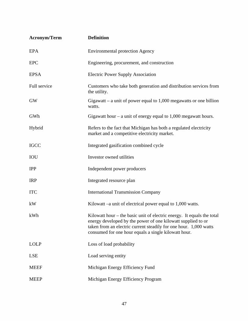
Acronym/Term n
Agency
nstruction
sociation
ce ces from the utility.
one billion watts.
egawatt hours.
d market and a competitive electricity market.
ilities
ducers
plan
ompany
o 1,000 watts.
l d to or
taken from an electric current steadily for one hour. 1,000 watts consumed for one hour equals a single kilowatt hour.
P bility
ntity
F ncy Fund
P y Program
Definitio EPA Environmental protection
EPC Engineering, procurement, and co
EPSA Electric Power Supply As
Full servi Customers who take both generation and distribution servi
GW Gigawatt – a unit of power equal to 1,000 megawatts or
GWh Gigawatt hour – a unit of energy equal to 1,000 m
Hybri Refers to the fact that Michigan has both a regulated electricity
IGCC Integrated gasification combined cycle
IOU Investor owned ut
IPP Independent power pro
IRP Integrated resource
ITC International Transmission C
kW Kilowatt –a unit of electrical power equal t
kWh Kilowatt hour – the basic unit of electric energy. It equals the totaenergy developed by the power of one kilowatt supplie
LOL Loss of load proba
LSE Load serving e
MEE Michigan Energy Efficie
MEE Michigan Energy Efficienc
47

Acronym/Term Definition
C n Company
independent transmission organization serving Michigan.
or one million watts.
kilowatt hours.
E y Efficiency
rve
t
provided by quick-start gas or oil fueled units that can be brought on-line within 10 minutes or less. The operating reserve is a subset of the planning reserve.
® veTM
ic
rves
load growth and unanticipated surges in demand caused by unusually hot or cold weather; and covers major, longer-term contingencies like the loss of a major generating unit or transmission line.
5 ers or less
ement
osal
andard
credit
ne tive, Inc.
MET Michigan Electric Transmissio
MISO Midwest Independent Transmission System Operator, Inc. – the
MW Megawatt – a unit of electric power equal to 1,000 kilowatts
MWh Megawatt hour – a unit of energy equal to 1,000
NAPE National Action Plan for Energ
Operating Rese Operating reserve is the generating capability above firm daily system demand needed to cover potential shortages caused by daily load forecasting errors, scheduled and unplanned equipmenoutages, and local area protection. Operating reserves are
PAYS Pay-As-You-Sa
PV Photovolta
Plan 21st Century Electric Energy Plan
Planning Rese Planning reserve is the difference between a utility’s electric generating capacity (usually expressed in MW) and its anticipated annual peak load. The planning reserve assures that sufficient generation will be available over a longer period of time to meet
PM2. Particulate matter of 2.5 micromet
PPA Power purchase agre
RFP Request for prop
RPS Renewable portfolio st
REC Renewable energy
Wolveri Wolverine Power Coopera
48
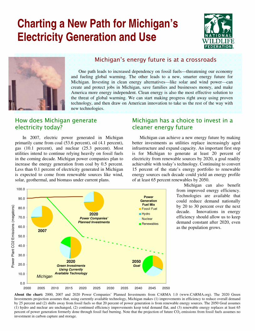
For more information, visit www.nwf.org/globalwarming.
Michigan’s energy future is at a crossroads
One path leads to increased dependency on fossil fuels—threatening our economy
and fueling global warming. The other leads to a new, smarter energy future for Michigan. Investing in clean energy alternatives—like solar and wind power—can create and protect jobs in Michigan, save families and businesses money, and make America more energy independent. Clean energy is also the most effective solution to the threat of global warming. We can start making progress right away using proven technology, and then draw on American innovation to take us the rest of the way with new technologies.
How does Michigan generate electricity today?
In 2007, electric power generated in Michigan primarily came from coal (53.6 percent), oil (4.1 percent), gas (10.1 percent), and nuclear (25.3 percent). Most utilities intend to continue relying heavily on fossil fuels in the coming decade. Michigan power companies plan to increase the energy generation from coal by 0.5 percent. Less than 0.1 percent of electricity generated in Michigan is expected to come from renewable sources like wind, solar, geothermal, and biomass under current plans.
Michigan has a choice to invest in a cleaner energy future
Michigan can achieve a new energy future by making better investments as utilities replace increasingly aged infrastructure and expand capacity. An important first step is for Michigan to generate at least 20 percent of electricity from renewable sources by 2020, a goal readily achievable with today’s technology. Continuing to convert 15 percent of the state’s energy portfolio to renewable energy sources each decade could yield an energy profile of at least 65 percent renewables by 2050.
Michigan can also benefit from improved energy efficiency. Technologies are available that could reduce demand nationally by 20 to 30 percent over the next decade. Innovations in energy efficiency should allow us to keep demand constant after 2020, even as the population grows.
0.0
10.0
20.0
30.0
40.0
50.0
60.0
70.0
80.0
90.0
100.0
2000 2005 2010 2015 2020 2025 2030 2035 2040 2045 2050
Pow
er
Pla
nt C
O2 E
mis
sio
ns (
megato
ns)
Michigan
2007
2020 Green Investments
Using Currently
Available Technology
2020 Power Companies’
Planned Investments
2050 Goal
Power
Generation
Fuel Mix
Fossil Fuel
Hydro
Nuclear
Renewables
Charting a New Path for Michigan’s Electricity Generation and Use
About the chart: 2000, 2007 and 2020 Power Companies’ Planned Investments from CARMA 1.0 (www.CARMA.org). The 2020 Green Investments projection assumes that, using currently available technology, Michigan makes (1) improvements in efficiency to reduce overall demand by 25 percent and (2) shifts away from fossil fuels so that 20 percent of power generation is from renewable energy sources. The 2050 Goal assumes (1) hydro and nuclear are unchanged, (2) continued efficiency improvements keep total demand flat, and (3) renewable energy replaces at least 65 percent of power generation formerly done through fossil fuel burning. Note that the projection of future CO2 emissions from fossil fuels assumes no investment in carbon capture and storage.

For more information, visit www.nwf.org/globalwarming.
Making a Difference in Michigan
Mayor Virg Bernero of Lansing has emerged as green leader in the state. Bernero has set goals for Lansing to produce 10 percent of its energy through renewable sources by 2010, 15 percent by 2015, and 20 percent by 2020. The Greater Lansing Go Green! Initiative is working to make city facilities more energy efficient and help local communities, business and schools go green. Lansing’s Urban Option non-profit also helps individuals reduce their energy needs by providing information and education, installing and repairing renewable energy systems, and installing energy saving devices in homes. Urban Option has been around for 30 years and reaches about 60,000 people a year.
Large companies throughout the state are aggressively cutting energy consumption. In Detroit, the GM headquarters performed an energy overhaul by installing energy efficient heating and cooling, lighting, and windows. The center now saves about $500,000 a year on energy costs.
Sources:
http://www.urbanoptions.org/about_us.php http://www.lansingmi.gov/get_city.jsp http://www.urbanoptions.org/RenewableEnergy/EnergyEfficiencySuccessStories.htm
Making a dent in global warming pollution
Simply by shifting to renewable energy sources and improving energy efficiency over the next decade or so, Michigan can reduce its future carbon dioxide (CO2) emissions from electricity generation by 46 percent compared to the business-as-usual path that utilities are following now.
Given that 39 percent of Michigan’s CO2 emissions come from electricity generation, diversifying and updating our power sources is critical for cutting the state’s total global warming pollution.
Increasing Michigan’s energy and economic security
Investing in renewable energy sources will reduce Michigan’s dependence on fossil fuels and at the same time create new green collar jobs. A new energy future in Michigan could include:
Expanded solar power. Michigan has enough solar resources to produce 4,000 to 4,500 Whr per square meter using photovoltaic systems and 3,000 to 3,500 Whr per square meter using concentrating solar power systems.
This means that devoting just 1 square mile in Michigan to solar power can provide enough electricity for about 0,900 households each year.
Expanded wind power. Michigan is currently ranked 25th for wind power, with 0,055 MW of existing electricity generation capacity and 60 MW under construction. The American Wind Energy Association ranks Michigan 14th in terms of its future wind potential, with 7,460 MW of potential capacity.
Biomass power. Michigan has 12.2 million dry tons of biomass available each year that could be used to generate about 2,400 MW of electricity.
New jobs. Committing to a 30 percent growth in solar energy use in the United States will bring 613 jobs and $498 million investment to Michigan.
A stronger economy. Michigan could realize as many as 8,549 jobs manufacturing wind turbines and $2.85 billion investment in the wind industry alone if 50,000 MW of new wind energy is created on a national level.
Consumer savings. Reducing electricity demand in Michigan by 15 percent below what is projected for 2023 could result in 3,888 jobs and a cumulative net savings of $693 billion.
References and Additional Reading: American Council for an Energy-Efficiency Economy,
www.aceee.org. American Wind Energy Association, www.awea.org. Bioenergy Feedstock Information Network. bioenergy.ornl.gov CARMA (Carbon Monitoring for Action), www.CARMA.org. Database of State Incentives for Renewables and Efficiency,
www.dsireusa.org. Department of Energy, Energy Efficiency and Renewable Energy.
apps1.eere.energy.gov/states/alternatives/electricity.cfm.
Energy Information Administration, State Energy Data System, www.eia.doe.gov/emeu/states/_seds_updates.html.
Environmental Protection Agency, Energy CO2 emissions by state, www.epa.gov/climatechange/emissions/state_energyco2inv.html.
Geothermal Energy Association, www.geo-energy.org. McKinsey Global Institute, 2007: Wasted Energy: How the U.S. Can
Reach its Energy Productivity Potential. Political Economy Research Institute, www.peri.umass.edu. Renewable Energy Policy Project, www.repp.org.

E N E R G Y S E C U R I T Y A N D
C L I M AT E S T EWA R D S H I P
P L A T F O R MF O R T H E M I D W E S T
2 0 0 7

2
PREAMBLERising energy prices, increasing dependence on imported energy, growth in domestic and global
demand for energy, and mounting concern over how to address climate change while sustaining
and enhancing economic growth and job creation pose serious challenges to the Midwest’s
energy future. As Midwestern leaders, we recognize our region’s obligation to provide
leadership on these challenges, and the clear benefits of cooperating regionally to meet them.
To satisfy the energy needs of a rapidly growing world population, while significantly
reducing carbon dioxide (CO2) and other greenhouse gas (GHG) emissions, we must by
mid-century produce twice as much low-carbon energy globally as all energy consumed in the
world today. It will also require dramatic efficiency improvements in buildings,
transportation, and technology and new production from every renewable and lower-carbon
fossil energy resource and technology we can muster.
Midwestern states and our Canadian provincial partners can lead this global transition and
prosper economically by manufacturing and exporting next-generation energy technologies and
supplying lower-carbon energy. The U.S. Midwest depends heavily on electricity generated by
traditional coal-fired plants and on largely imported petroleum to fuel our agricultural,
transportation and industrial sectors, all of which presently represent major sources of
GHG emissions. However, because of our vast base of energy resources, ingenuity and
manufacturing prowess, the Midwest has the greatest potential of any region in North
America to transform our present energy vulnerabilities into advantages. Through policy
approaches adapted to the different needs of our individual jurisdictions, we will use these
advantages to meet our region’s energy security and climate stewardship challenges.
ENERGY SECURITY & CLIMATE STEWARDSHIPPLATFORM FOR THE MIDWESTERN REGIONOF THE UNITED STATES AND CANADA

3
We have only begun to tap the world-class biomass, wind and other renewable energy potential that
the farm belt and Great Lakes regions have to provide North America with home-grown energy.
Our region’s large and secure reserves of coal lie in close proximity to geologic reservoirs for
permanent storage of CO2, including partially depleted oil fields suitable for enhanced oil and gas
recovery. Midwestern states are national leaders in energy efficiency, which is a critical component
in reducing energy demand and keeping electricity costs affordable. Midwestern state universities
are already national and world leaders in research exploring energy frontiers and in developing
solutions for our energy future. Hundreds of Midwestern inventors and entrepreneurs, designers,
architects, engineers and builders are hard at work designing and bringing to market a broad range
of technologies needed to propel the transition to the world’s low-carbon energy future. Lastly, we
can build on strong relations with interested Canadian provinces to further develop transmission
and clean renewable energy sources.
It takes a long time to influence the overall direction of the energy system. Power plants,
biorefineries, wind farms and other energy production facilities and infrastructure will require
major investments that will last 25 to 50 years and more. We need policies and programs in place
now to encourage innovation and reinvention when energy infrastructure is replaced, upgraded or
expanded in the future. We will aid in the transition through market-based deployment of new
technologies and programs, thoughtful, far-sighted policy design and the prudent dedication of
public resources and incentives. Through this transition, in addition to reducing GHG emissions
our states will spur investment, create new jobs, and protect customers by stabilizing energy prices.
We have gathered at this Energy Summit to demonstrate our commitment to this long-term
transition to a lower-carbon energy economy. Through the Midwestern Governors Association
(MGA), we have brought together leaders from industry, agriculture, nongovernmental
organizations, and the public sector to gather their ideas and collective wisdom in crafting goals,
policy recommendations and practical cooperative initiatives to be undertaken jointly by our states.
The Energy Security and Climate Stewardship Platform we announce today draws on that input
and outlines a strategic blueprint and action plan to guide future development of the Midwest’s
energy economy.
Following this summit, our respective
states and interested Canadian
provinces will continue to work
through MGA to support
implementation of the platform and
help ensure economic prosperity, energy
security and a healthy environment in
the Midwest for decades to come.
4
GOALAs part of our Energy Security and Climate Stewardship Platform, we
commit to the following goal for the region:
�� Maximize the energy resources and economic advantages and
opportunities of Midwestern states while reducing emissions of
atmospheric CO2 and other greenhouse gases.
OBJECT IVESReaching this goal will require meeting the following objectives over
time:
1. Achieve continuous improvement in levels of cost-effective energy
efficiency across the economy;
2. Deploy lower-carbon renewable and fossil fuels and technologies
comprehensively;
3. Implement geologic CO2 storage, terrestrial carbon sequestration
and other technological utilization of CO2 on a large scale; and
4. Add economic value and high-paying jobs to the Midwest’s energy,
agriculture, manufacturing and technology sectors through the
development and deployment of lower-carbon energy production
and technologies.
TRANSITIONING TO A LOWER CARBON ENERGY ECONOMY

5
KEY STRATEG IESIn order to achieve these objectives, we endorse and commit our respective states to
implementation of a comprehensive, multi-pronged approach that includes the
following integrated strategies:
1. Maximize economy-wide investment in energy efficiency initiatives that are
less expensive than other energy options;
2. Accelerate the commercialization of advanced coal and natural gas
technologies and infrastructure for the capture and geologic storage of CO2emissions, including for enhanced oil and gas recovery;
3. Maximize the economic and reliable integration of wind energy, both into
the electrical grid and as a resource for energy applications that do not require the
bulk transmission of electricity;
4. Expand on existing biofuels production through the development of a bio-
refinery industry that minimizes GHG emissions and produces liquid fuels,
biogas, electricity, heat and bio-products from cellulosic biomass;
5. Establish a secure, domestic transportation fuel supply and infrastructure
that relies on the region’s sustainable production of electricity, biofuels, hydrogen
and other low- and zero-carbon fuels;
6. Develop regional electric transmission and energy delivery capacity sufficient
to accommodate the substantial increases needed in low- and zero-carbon energy
production; and
7. Support the regional development and manufacturing of highly efficient and
lower-carbon technologies in vehicles and equipment, renewable and fossil
energy production, consumer appliances and products, and other key energy
sectors, both for use in the North American market and for global export.
6
To implement the Energy Security and Climate Stewardship Platform, the governors and
premier of Illinois, Indiana, Iowa, Kansas, Manitoba, Michigan, Minnesota, Ohio,
South Dakota and Wiscconsin endorse the following specific objectives and goals by which
to measure progress, and offer a menu of policy options to reach our common goals. We
recognize that the geographic, economic and resource diversity of the Midwest calls for
flexibility in the implementation of regional goals and objectives. Some jurisdictions may
contribute more or less than others to the implementation of a given regional objective or
goals, due to their particular resource advantages. Also, each jurisdiction will work to
achieve these shared regional objectives and goals by implementing a mix of options from
the policy menu that is best tailored to fit its needs.
Energy EfficiencyMEASURABLE GOAL �� Meet at least 2 percent of regional annual retail sales of natural gas and
electricity through energy efficiency improvements by 2015, and continue
to achieve an additional 2 percent in efficiency improvements every year
thereafter.
OBJECT IVES• Identify the technical and economically achievable energy efficiency
potential for each MGA state and for the region as a whole.
• Establish a policy and regulatory environment that enables and encourages
implementation of cost-effective energy efficiency investments and
practices.
• Accelerate adoption of economically achievable energy efficiency measures by
building greater awareness and facilitating financing and delivery.
AGREEMENTS BY PLATFORM THEME: GOALS, OBJECTIVES AND POLICY OPTIONS
1

7
• Measure and report, on a state-by-state and regional basis, annual progress on
reaching these energy efficiency targets.
POL ICY OPT IONS1. Establish quantifiable goals for energy efficiency. Policy-makers need to
determine what level of efficiency improvement is economically achievable for
their jurisdiction to meet the regional goal. If each state identified targets for
megawatt-hours and therms saved, it would be possible to determine what role
each jurisdiction can play in achieving the region’s overall 2 percent energy
efficiency objective. Progress should be continually measured and evaluated, and
adjustments should be made as necessary.
2. Undertake state assessments that quantify the amount of energy efficiency
that would cost less on a unit cost basis than new generation. This analysis
should include a cost-benefit analysis of pursuing this amount of efficiency.
3. Require retail energy providers to make energy efficiency a priority. Resource
plans should begin with all cost-effective energy efficiency goals, targets and
strategies before reliance upon any additional supply.
4. Remove financial disincentives and enable investment recovery for energy
efficiency program costs. Regulatory practices and rate designs sometimes result
in barriers to efficiency investments because efficiency reduces potential energy
sales. Changes should be implemented to remove financial disincentives and
provide appropriate incentives for prudent expenditures on energy efficiency.
5. Strengthen building codes and appliance standards and requisite training,
quality assurance and enforcement. The experience of other countries and
regions in developing progressive codes and standards should be a model for this
region. For example, leading states have updated state building codes to keep up
with technological advances in energy efficiency.

8
Other options for improving energy efficiency in buildings and
appliances include:
a. Adapt effective, market-based certification programs to buildings and
appliances not now covered, so that energy efficiency becomes a visible
selling point for a wider array of products.
b. Automatically update building codes to reflect the latest in proven
conservation and building technology.
c. Automatically upgrade home and commercial building energy performance at
the point of sale, while implementing financing mechanisms to aid in such
upgrades, so that buildings will reflect the latest in proven, cost-effective
techniques and practices for conservation and energy efficiency.
d. Invest in training of architects, builders and local code officials in how to
effectively and efficiently comply with new building energy codes in order to
reap the full benefits of the codes.
e. Establish incentives to exceed building codes. For example, if developers
build an “Energy Star structure,” they might qualify for preferential and/or
lower-interest financing.
f. Encourage development of zero-energy building design and construction.

Energy Efficiency
9
6. Have the public sector lead by example. The federal government and several
states have taken the lead in establishing challenging energy-use reduction goals for
state and federal buildings. These programs provide leadership and set an example
for the private sector. Public initiatives also represent opportunities for testing
more-effective energy management programs, shared savings contracts and other
technical and programmatic plans that can help show the private sector how these
programs can work and reduce per capita energy use. Recommissioning existing
commercial properties is a good example of how the public sector can initiate these
programs on public buildings and monitor results to show the payback for the
private sector.
7. Accelerate adoption of energy efficiency technologies and best practices by
commercial and residential customers. This could start with using the “bully
pulpit” by developing an education campaign (e.g., public service announcements),
but could also entail changing local government aid to reward communities with
specific energy efficiency goals. A great deal of progress could be made by
building capacity to conduct more residential, commercial and industrial
energy efficiency assessments and providing carefully targeted incentives for
consumers to act on the recommendations. Whatever combination of
“carrots and sticks” that policy-makers use to encourage greater efficiency,
low-income customers will need programs to assist them with the front-end
costs of efficiency improvements.

10
MEASURABLE GOALS�� By 2012 : Advanced cellulosic and other low-carbon transportation fuels
should be commercially produced in the region.
�� By 2015: E85 will be offered at 15 percent of retail filling stations, or around4,400 stations, approximately a five-fold increase. Currently, E85 is available at 3
percent of filling stations regionally.
�� By 2020: E85 will be offered at 20 percent of retail filling stations, or around5,900 stations, approximately a six-fold increase.
�� BY 2025 : E85 will be offered at 33 percent of retail filling stations, or around9,700 stations, approximately a 10-fold increase.
�� By 2025 : Average fossil fuel inputs in the production of conventional biofuelsin the region will be reduced by at least 50 percent.
�� BY 2025 : At least 50 percent of all transportation energy consumed in theregion will be supplied by regionally produced biofuels and other low-carbon
advanced transportation fuels, with the expectation that a significant and additional
portion of the region’s biofuel production will help the U.S. meet a national
25 x' 25 goal.
OBJECT IVES • Develop the Midwest’s capacity for production of biofuels and other low-carbon
advanced transportation fuels to advance national energy independence, add value
for consumers, revitalize rural economies and the region’s manufacturing base, and
decrease greenhouse gas emissions.
• Accelerate strategies for improving the efficiency of biofuels production and use,
reduce fossil fuel inputs, minimize GHG emissions, decrease water use and
strengthen the existing biofuels industry.
• Develop, demonstrate and commercialize a variety of biomass-utilizing
technologies and other low-carbon advanced fuels covering a portfolio of energy
products and biobased products.
Biobased Products and Transportation 2

11
• Pursue innovative opportunities to increase the biofuels supply while improving
water quality, soil quality and wildlife habitat.
• Build the infrastructure to allow the bioeconomy to expand.
POL ICY OPT IONS1. Provide market pull and the distribution infrastructure for biofuels and
advanced transportation fuels by:
• Promoting broad renewable fuels standards that include specific carve-outs
for lower-carbon advanced biofuels;
• Creating incentives for increased public demand for fuel-efficient, lower-
carbon vehicles;
• Expanding state government’s use of biofuels and advanced transportation
fuels;
• Developing regional quality standards for biodiesel and other fuels; and
• Adopting retail tax incentives encouraging retailers to sell biofuels, advanced
transportation fuels and biobased products.
2. Advance conversion technology commercialization. While the current ethanol
and biodiesel industry continues to grow, , it is crucial that action be taken to
mitigate risk in developing next-generation technologies in order to speed the
transition of new technologies to commercialization.
3. Broaden existing bioenergy incentives and create new incentives that
promote many uses of biomass, including not only a range of different liquid
fuels, but also natural gas, heat and electricity.
4. Develop next-generation regulation. New technologies can deliver
environmental benefits, but often do not fit neatly into existing regulatory schemes.
This can create challenges for regulatory agencies and industry. Collaboration is
needed to develop permitting rules for advanced technologies, share information
about the environmental impact of various advanced technologies, provide

12
regulatory exemptions for novel demonstrations to allow experimentation, and
promote innovative regulatory strategies that seek to reward projects with good
overall environmental characteristics.
5. Provide technical assistance to advanced technology projects. By funding
front-end engineering and design studies and other feasibility studies, providing
business planning and mentoring, and expanding technical capabilities, states can
help develop advanced technology projects.
6. Increase regional research collaboration. Coordinate state and private research
to develop an information clearinghouse on advanced bioenergy research and
demonstration projects in the region; identify crucial research needs; organize and
launch regional research and other initiatives addressing key challenges to
development of the bioeconomy; and promote regional commercial-scale
demonstrations of various biomass feedstocks.
7. Develop the Midwestern infrastructure for the manufacture of biobased
products. A key to the advanced bioenergy complex will be the profitability of
the manufacturing of biobased materials that are co-products of biobased fuels.
This materials industry is in its infancy. Support research determining how the
biomaterials supply chain can mature in conjunction with the biofuels sector and
how new products can achieve economic viability.
8. Develop Midwestern biobased products. Adopt biobased product procurement
rules at the state level, participate in a regional biobased product procurement
program with a common list of products, and consider expanding the program
further by creating a regional certification program and promoting it through
education and incentives for business participation as a means to foster biobased
product development.
9. Overcome the difficulty of biomass feedstock logistics. Employ technical
assistance and incentives to projects that are seeking to develop a supply of
cellulosic biomass for bioenergy projects.

13
10. Create a uniform, regional low-carbon fuels policy – implemented at the
state level as a standard, objective or incentive – and report annually on
progress. Convene affected stakeholders to develop the common policy, including
reporting mechanisms and other details.
11. Develop incentives for increasing vehicle fuel efficiency and reducing
greenhouse gas emissions.
12. Create local wealth. Recognizing that a diversity of financing models will be
necessary to develop a new generation of advanced technologies, ensure that the
benefits of biofuels, advanced transportation fuels and biobased product
developments accrue to public and private entities in the communities where they
are produced. Assure that cooperatives, municipal authorities, other local and
community-owned entities, and small investors are not excluded from government
incentive programs. Give bonding authority or access to bonding funds to co-ops,
municipal utilities, and other local and community-owned entities to fund biomass
projects. Wherever possible, make the opportunity available for local ownership in
projects receiving public investments.
13. Promote a perennial biomass supply. Because of the synergies between farm
economics, biofuel production and environmental objectives, support the
development of a perennial biomass supply. Develop and expand programs and
incentives that encourage landowners to grow perennial crops and supply products
to a bioenergy plant in a way that targets improvements in soil/water quality,
wildlife habitat, soil erosion and carbon sequestration.
14. Create collaborative workforce development programs between industry,
state governments and educational institutions. Curriculum should be
developed at all levels of the educational system on biofuels, advanced
transportation fuels and biobased products.
14
MEASURABLE GOALS 1
�� BY 2015 : 10 percent of electricity consumed in the region (equivalent to 103million MWh of retail sales) will be from renewable resources.
�� BY 2020 : 20 percent of electricity consumed in the region (equivalent to 219million MWh of retail sales) will be from renewable resources.
�� BY 2025 : 25 percent of electricity consumed in the region (equivalent to 293million MWh of retail sales) will be from renewable resources.
�� BY 2030: 30 percent of electricity consumed in the region (equivalent to 376million MWh of retail sales) will be from renewable resources.
OBJECT IVES• Maximize cost-effective renewable electricity production in the region and its
integration on the grid.
• Make most efficient use of the existing transmission infrastructure and develop
new infrastructure, as necessary, to accommodate the region’s economical
renewable electricity.
• Ensure retention of local economic benefits from wind and other renewable power
development.
• Expand the region’s domestic production of wind turbines, towers and blades, solar
technologies, and other renewable energy technologies to provide high-paying
manufacturing and operational support jobs.
• Create a stable regulatory environment for renewable energy development.
Renewable Electricity
1 For the purposes of these measurable goals, renewable electricity includes electric power generated from wind, biomass, solar and geothermal energysources, from new hydroelectric facilities and new hydroelectric capacity obtained through re-powering of existing facilities, and from hydrogen producedfrom the preceding renewable energy sources.
3

15
POL ICY OPT IONS1. Implement appropriate policies for development of renewable electricity
generation. Enact, where appropriate, or enhance existing state renewable energy
standards or objectives in the region to stimulate the development of new
renewable electricity generation.
• Promote a multi-year extension of the federal production tax credit (PTC) for
renewable energy for up to eight years, effective once the current two-year
extension expires on December 31, 2008. A longer extension will bring
needed industry stability and help achieve more development than would
otherwise be possible with repeated short-term extensions.
• Promote expansion of federal Clean Renewable Energy Bonds to increase
incentives available for development of renewable energy projects by entities
that cannot utilize the PTC effectively, such as tax-exempt electric
cooperatives, municipal utilities, and local and tribal governments.
2. Expand collaborative regional transmission planning and siting to enable
future development of renewable electricity generation. Inter-jurisdictional
transmission planning and siting involving state regulators, utilities, regional
transmission organizations, project developers, advocates, and others must be
strengthened to optimize future transmission investments and ensure that the
region’s grid infrastructure enables robust development of renewable electricity
generation and ensures broader system adequacy. In addition, state regulatory
commissions need to be empowered to define the “public interest” more broadly
to include regional benefits.
3. Incorporate transmission development requirements into existing state
renewable energy objectives and standards. Given the potential mismatch in
timing between rapid wind farm development and the much longer time required
to study, approve and construct electric transmission lines, adequate transmission
needs to be coordinated with state renewable energy standards and objectives.

States should engage interested parties in integrated resource planning, including the
identification of additional transmission resources needed to meet state renewable
energy obligations. Approval for transmission improvements should be sought
through the appropriate utility regulatory process, and construction should
commence, to enable timely development of renewable generation facilities.
4. Pursue a multi-state transmission initiative to facilitate construction and
delivery to market of a large amount of new renewable electricity generation,
together with power from other lower-carbon generation facilities. Utility
transmission planners have long identified bottlenecks in the transmission system that
must be addressed in order to deliver to market large quantities of new wind energy as
well as other renewable and low carbon electricity. Policy-makers and other
stakeholders need to engage in regional integrated resource planning efforts to
identify multi-state transmission and generation initiatives. In conjunction with this
effort, a cost-benefit analysis and cost allocation issues must be addressed.
5. Develop and implement comprehensive siting principles and policies for wind
farms to encourage orderly development of the resource. Achieving wind energy
generation on a large scale will require sustained public acceptance of the siting and
construction of wind farms. Wind energy must be deployed with a clear awareness of
the need for appropriate siting that takes into account ecological, scenic, cultural and
other concerns. In some parts of the Midwest, local opposition to wind farm
construction already presents a barrier to development of the resource. Crafting
adequate and consistent state siting policies and procedures should be done
cooperatively and inter-jurisdictionally to ensure that wind development proceeds in
ways that foster long-term public support for the industry and that avoid pitting states
against one another or impeding a regional approach to wind development.
6. Encourage a diversity of approaches to renewable electricity development,
including projects that have significant components of local ownership. Policy-
makers should evaluate the experience with local ownership incentives in Minnesota,
Iowa and elsewhere and consider further measures to foster local equity participation
in wind and other renewable energy projects to enhance local economic returns.
However, policy-makers should continue to support a diversity of ownership
structures in the marketplace and avoid creating barriers to achieving significant levels
of renewable electricity development and associated transmission expansion.16
Renewable Electricity1
7. Demonstrate technology, engineering and operating strategies for
maximizing the total electricity generation from the region’s wind resources.
Policy-makers should support the development and deployment of strategies and
technologies to maximize wind energy’s contribution to the region’s electric power
generation. Such efforts should focus on:
• Applying the findings of wind integration studies, such as the 2006 Minnesota
Wind Integration Study. (These studies show that higher percentages of wind
power can be incorporated reliably into the electric power system given the
Midwest’s tremendous wind resource.)
• Making better use of existing transmission infrastructure and capacity
through next generation grid management;
• Commercializing all practical and economical energy storage options, such as
advanced batteries and compressed air storage.
• Developing new uses of wind energy such as wind electrolysis to produce
hydrogen or wind-to-ammonia for fertilizer production that do not require
bulk transmission and readily substitute for existing GHG-emitting fossil
energy sources.
8. Develop economic incentives and workforce development policies to attract
renewable energy component manufacturers and service providers to the
region. Take steps to integrate state economic development and workforce
development programs and incentives into renewable energy development policies
and strategies with the goal of attracting manufacturers and service providers,
both for regional economic benefit and to stem the rising capital and labor costs
associated with all energy projects. The Midwest already benefits, for example,
from the presence of major wind turbine blade and tower manufacturers, turbine
assembly operations, engineering and wind farm construction firms, and
operations and maintenance providers whose commercial success extends
well beyond the region.
17

MEASURABLE GOALS�� BY 2010 : A regional regulatory framework for carbon capture and storage
(CCS) will have been implemented that enables permanent geologic storage of
CO2, provides regulators and industry clear direction with regards to CO2 capture,
injection, monitoring, verification and compliance, and addresses ultimate liability
for stored CO2.
�� BY 2012 : A multi-jurisdiction pipeline will have been sited and permitted totransport CO2 captured from one or more new advanced coal plants and
potentially biofuels plants to an appropriate reservoir for use in enhanced oil and
gas recovery (EOR).
�� BY 2012 : The region will have operating at least one commercial-scaleintegrated gasification-combined cycle (IGCC) power plant with CCS that uses
bituminous coal.
�� BY 2015 : The region will have:
• Three or more commercial-scale IGCC plants with CCS operating with
bituminous coals;
• Operating at commercial scale at least two IGCC plants with CCS that use
sub-bituminous and lignite coals, respectively;
• Commercial scale post-combustion capture of CO2 emissions at one or more
pulverized coal plants; and
�� BY 2020: All new coal gasification and coal combustion plants will capture andstore CO2 emissions.
�� BY 2050: The region’s fleet of coal plants will have transitioned to CCS.
18
Advanced Coal and Carbon Capture and Storage 4
OBJECT IVES• Support development of a CO2 management infrastructure and demonstration and
commercialization of large-scale geologic carbon storage projects that take
advantage of our region’s EOR potential.
• Support research, development, demonstration and deployment of carbon capture
technologies at existing plants and re-powering of existing facilities, where
appropriate, and at biorefineries to increase efficiency and reduce CO2 emissions.
• Create a policy and regulatory environment that advances new coal plants with CCS.
• Develop the commercial manufacturing, technical and operational expertise in
our region to operate and export these technologies globally.
• Support the development and eventual deployment of technologies that
enable effective commercial utilization of captured CO2 as a feedstock for
energy and for the manufacture of advanced materials and other useful
products.
POL ICY OPT IONSCommercializing advanced coal-based generation technologies and CCS presents a
classic chicken-and-egg challenge. Without a pipeline infrastructure and appropriate
policy and regulatory framework in place, it is very difficult to justify the extra capital
and operating expense of building a power plant capable of CCS. It is similarly difficult
to contemplate financing a CO2 pipeline without guaranteed availability of captured
CO2 and of commercial EOR opportunities to market that CO2. Therefore, building
capture-ready power plants and CO2 pipelines and the development of commercial
EOR opportunities must be pursued simultaneously.
MGA states should consider implementing the following menu of policy options so
that integrated power generation and CCS operations can be deployed early in the next
decade.
1. Establish a regional CCS infrastructure for management of captured CO2through EOR and deep saline aquifer storage. Safe, reliable and permanent
injection of CO2 into oil and gas formations for EOR is a fully commercial
practice in the United States today. DOE estimates of CO2 storage capacity in oil
and gas formations suggest the ability to store at least two decades worth of U.S.
stationary source emissions, while extending oil production from depleted domestic
oil reserves. Storage over a much longer time scale will require demonstration of
the cost-effectiveness and reliability of CO2 storage in deep saline aquifer
formations, which has yet to be accomplished at commercial scale.
19

20
a. Develop a legal and regulatory framework for geologic storage of CO2.
In order to set the stage for geologic storage projects to move forward in a
five to 10-year timeframe, states must establish the necessary legal and
regulatory framework in partnership with the federal government. State
agencies should begin to develop the necessary permitting processes for
geologic storage, including guidance on pipelines, drilling, storage,
measurement, monitoring, verification and long-term liability.
b. Provide state-based incentives for CCS, including projects that use
captured CO2 for EOR. A number of states have made such credits
available, and others should consider offering similar incentives.
c. Provide EOR project development assistance. The Midwest has a mature
oil and gas industry with many small oil and gas producers that have not
traditionally used EOR, in part because they are not large enough to develop
projects. The public sector, companies and trade associations can play a
useful role in helping to identify the specific mechanisms by which producers
can band together to leverage cost-effective projects.
d. Support comprehensive assessments of geologic reservoirs at the state
and federal levels to determine the CO2 storage potential and
feasibility. Governments should build on work of the U.S. DOE-funded
regional sequestration partnerships to complete comprehensive, basin-level
geologic assessments of storage potential and CO2 injection rates. Regions
with a history of oil and gas exploration tend to have better data available on
geologic formations, making such assessments easier and less expensive.
Detailed, accurate mapping of lesser known potential reservoirs for CCS will
require continued federal and state investment.
e. Fund sufficient large-scale geologic storage tests to prepare for future
storage on a widespread commercial basis. Congress and the president
should support sufficient federal funding for the U.S. DOE to ensure a robust
program of large-scale tests to demonstrate to the private sector,
policymakers and the public the viability, efficacy and safety of widespread
commercial geologic storage of CO2. These tests should focus on a variety
of geologic formation types, including reservoirs other than oil and gas
bearing formations, and produce guidelines for appropriate measuring,
monitoring and verification.
Advanced Coal and Carbon Capture and Storage

21

22
f. Evaluate the feasibility of CO2 transport and “advanced
sequestration” options for jurisdictions without documented
geologic storage potential, such as Minnesota and Wisconsin.
This includes evaluating the cost and feasibility of CO2 pipelines
to geologically appropriate areas in neighboring states, CO2 storage
in nontraditional geologic formations and advanced sequestration
options, such as mineralization, the use of carbon nano-fibers or
algae.
2. Provide financial and regulatory incentives to build advanced coal
generation projects with CCS, using bituminous, sub-bituminous
and lignite coals.
Advanced Coal and Carbon Capture and Storage
23
a. Provide state support for front-end engineering and design (FEED).
FEED studies provide the cost estimates needed to secure private investment
in power plant projects. State tax credits or grants can help offset FEED
study costs and allow utilities and developers to recoup those initial
engineering costs that are most difficult to finance. This approach has been
effective in Illinois, North Dakota and Wyoming in spurring project
development, and is under consideration in other parts of the Midwest.
b. Provide direct state financial incentives (grants, tax credits, loan
guarantees and performance wrap engineering/procurement/
construction or EPC coverage). States should establish the same or
complementary incentives to those in the federal Energy Policy Act of 2005
to help reduce the financial cost of the overall project once engineering and
cost studies are completed.
c. Allow regulated utilities cost recovery for appropriate commercial
projects. Utilities committed to developing advanced technology coal plants
with CCS should be ensured cost recovery, as long as they meet a state
commission’s standards for proper spending decisions. States should also
consider a comparable process for merchant and independent power
producers involved in request for proposal bidding processes.
d. Enhance integrated resource planning (IRP) policies, where
applicable, by using them to encourage low-CO2 coal technologies.
Regional leaders should adopt well-designed IRP rules to weigh the full costs,
benefits and risk characteristics of various resource options. Doing so would
improve the accuracy of “least cost” planning for generation options, which
currently penalizes advanced coal and CCS proposals because it does not fully
address future regulatory and environmental costs. Future risks to be
factored in should include fuel price fluctuation, carbon constraints, emission
limits of criteria pollutants and mercury, and technology uncertainty.

Advanced Coal and Carbon Capture and Storagee. Modify state policies and regulatory programs to favor advanced CO2-
limiting generation technologies with CCS over conventional pulverized
coal units. These policies could include:
1) A low-carbon electricity portfolio standard or objective that combines
fossil electricity generation resources (such as IGCC with CCS) with
traditional renewable resources;
2) A CCS portfolio standard for electricity providers;
3) A CO2 performance standard for all new electric power plants;
4) Innovative, long-term power purchase agreements to provide developers
with higher rates of return and reduced risk in exchange for price stability
that benefits ratepayers (allowing regulators to qualify more stable prices as a
benefit);
5) Specific incentives and financing assistance to replace or re-power existing
coal plants in favor of advanced generation technologies with CCS;
6) Market-based environmental regulatory programs to provide incentives to
invest in low CO2 emission technologies with flexibility and certainty for
achieving reductions; and
7) Three-party covenants in which the federal government provides credit,
the state regulatory commission provides an assured revenue stream from the
syngas to protect the federal credit, and a project developer provides equity
and initiative to build the project.
f. Increase federal funding of incentives to accelerate deployment of
advanced coal technologies with CCS at commercial scale. Current
federal funding is completely inadequate given the scale of the task and
urgency of commercializing advanced coal technologies with CCS.
Midwestern governors call on the region’s congressional delegation to expand
significantly the federal commitment of resources in this area.
24

g. Provide incentives for deployment of innovative coal gasification
technologies, including co-gasification of biomass and underground
coal gasification, and the utilization of captured CO2. Co-gasification
of biomass feed stocks with coal has been commercially demonstrated in
Europe and, when combined with CCS, could provide CO2-neutral or even
CO2-negative energy production. Underground coal gasification has entered
commercial operation overseas and has the potential to bring the capital costs
of CCS with coal to at or below that of conventional pulverized coal
generation. Finally, research is underway to convert captured CO2 into useful
and advanced materials and other products.
h. Update workforce training, with a focus on the gasification and carbon
storage industries. A major barrier to development of IGCC technologies
is the lack of trained personnel in the power industry familiar with the design,
construction and operation of gasifiers and associated systems, which are
operationally more closely associated with petroleum refining than traditional
power generation. Similarly, the development of EOR operations is
constrained by a lack of commercial experience in much of the oil and gas
industry, especially among the smaller-scale companies that dominate
production in the Midwest. The utility and oil and gas industries will need
expanded workforce training in order to adopt IGCC and CCS on the scale
required.
3. Develop incentives targeted at biorefineries that appropriately parallel those
targeted at power plants.
25

Establishing a Carbon Management Infrastructure Partnership
26
WHEREAS, the development and deployment of systems for capturing carbon dioxide (CO2) emissions from power
plants and other industrial facilities represents one critical component in a menu of options for reducing
CO2 emissions; and
WHEREAS, the effectiveness of such systems depends on the development of an infrastructure supporting the
transportation and permanent geologic storage of the captured CO2; and
WHEREAS, there are extensive coal reserves and a number of advanced coal plants with CO2 capture already have
been proposed to date in the Midwest; and
WHEREAS, large-scale ethanol plants also produce a pure stream of CO2 suitable for capture and storage in the
Midwest; and
WHEREAS, the Midwest contains many deep saline aquifers that are likely to provide extensive capacity for long-
term CO2 storage; and
WHEREAS, using the captured CO2 to inject and pressurize aging oil and gas fields, a process known as enhanced
oil and gas recovery (EOR), has become a fully mainstream commercial practice for extending oil
production, involving the permanent geologic storage of tens of millions of tons of CO2 annually in
Texas, the Northern Plains states, Michigan, the North Sea and Algeria; and
WHEREAS, the market for CO2 for use in EOR is currently robust because of high oil prices; and
WHEREAS, in our region, experience to date with CO2 EOR projects operated in North Dakota and Michigan
provides a high degree of confidence in the technical viability and safety of systems that capture,
compress, and transport CO2 for EOR purposes; and
WHEREAS, future CO2 management on such a scale will require a major and coordinated investment in a
supporting infrastructure specific to CO2 capture, transportation, underground injection, and storage or
sequestration, an infrastructure not unlike the current systems relied on for the collection, distribution
and storage of natural gas and liquid fuels; and
WHEREAS, regional cooperation to develop such infrastructure for CO2 capture, transportation, underground
injection and storage will accelerate the implementation of CO2 management; and
WHEREAS, regional cooperation on planning early CO2 pipeline infrastructure will allow for a rational, cost-
effective build-out of that infrastructure over time; and

27
WHEREAS, regional cooperation on the development of a regulatory framework for the siting, operation and
monitoring of CO2 capture, transportation, underground injection and storage facilities will facilitate
the near-term coordinated development of such systems;
NOW THEREFORE BE IT:
RESOLVED, that the states of Illinois, Iowa, Michigan, Minnesota, Ohio and Wisconsin and province of Manitoba
agree to establish a Carbon Management Infrastructure Partnership (hereafter Partnership) to promote
the rational near-term development of a regional CO2 transportation and storage infrastructure; and be it
RESOLVED, that the Partnership pledges to work in a cooperative and coordinated fashion that maximizes each
member’s particular strengths and assets; and be it
RESOLVED, that the Partnership agrees that specific deliverable products will result from its efforts, including, but
not limited to:
1. a report that quantifies the potential costs and benefits of EOR; and
2. an expanded assessment of geologic reservoirs for CO2 storage in Partnership states that lack oil and
gas bearing formations known to be suitable for CO2 injection and storage, notably Minnesota and
Wisconsin; and
3. a state-by-state inventory of Partnership member’s regulations governing or potentially relating to
CO2 capture, compression, pipeline transportation, and underground injection; and
4. a uniform regional model state regulatory framework specific to CO2 capture, compression,
pipelines, and underground injection and storage, informed by emerging federal approaches and the
draft Interstate Oil and Gas Commission regulations due out in 2007; and
5. a study and proposed siting of a regional pipeline system serving more than one Partnership member
(and possibly connecting Partnership members with other regions) that links one or more sources of
captured CO2 with appropriate geologic reservoirs (e.g. Illinois Basin and Michigan, Ohio and Northern
Plains EOR formations) and injection and storage facility for EOR and deep saline aquifer storage; and
6. Partnership-wide commercial plan for CO2 management that incorporates the above elements and
emphasizes EOR as important steps toward deep saline aquifer CO2 storage; and
7. coordinated Partnership FY 2009 request for federal investment in CO2 capture and storage
infrastructure build-out in the MGA region; and be it
RESOLVED, that the governors and premier, through the MGA, will establish a working group that shall develop and
recommend to the governors and premier no later than February 15, 2008, a proposed structure,
participation and process for the Partnership, as well as a work plan for achieving the deliverables set
forth herein.
DONE, this 15th day of November, 2007, in Milwaukee, Wisconsin.

Establishing a Midwestern BioproductProcurement Program
WHEREAS, biobased products are an important aspect of the profitability of biorefineries, create new domestic
demand for agricultural commodities, expand the industrial base through value-added agricultural
processing and manufacturing, and enhance the nation’s energy security by substituting domestically-
produced biobased products for those made from fossil energy inputs; and
WHEREAS, the U.S. departments of Agriculture and Energy, following authorization in the 2002 Farm Security and
Rural Investment Act, have created a system called the FB4P program under which federal agencies
must purchase designated biobased products that are available and cost-competitive with fossil-based
equivalents; and
WHEREAS, the U.S. departments of Agriculture and Energy have already contracted with Iowa State University to
conduct life cycle testing on a list of products and has conducted a series of rule-makings to designate
products “biobased”; and
WHEREAS, at least two Midwestern states, Illinois and North Dakota, have adopted biobased product procurement laws;
NOW, THEREFORE, BE IT:
RESOLVED, that the states of Illinois, Indiana, Iowa, Kansas, Michigan, Minnesota, Missouri, Nebraska, North
Dakota, Ohio, South Dakota and Wisconsin and province of Manitoba jointly establish a Midwestern
Biobased Product Procurement System (hereafter System) to support growth of the region’s
bioeconomy; and be it
RESOLVED, that the System should create a common approach to listing biobased products consistent with the federal
program, with System members adopting products based on their own procurement rules; and be it
RESOLVED, that System members agree to seek authorizing legislation, where necessary, to enable participation in the
System; and be it
RESOLVED, that System members agree to form a regional task force of state procurement officials and others to
design the rules of a regional biobased product system and make other recommendations as necessary to
establish the System; and be it
RESOLVED, that the governors and premier, through the MGA, will appoint a regional task force of state
procurement officials that shall work with the public and private sectors to oversee and implement the
System and to develop and recommend to the governors and premier, no later than June 1, 2008, model
rules for the System.
DONE, this 15th day of November, 2007, in Milwaukee, Wisconsin.
28

Establishing a Regional Electricity TransmissionAdequacy Initiative
WHEREAS, the expansion of regional electricity transmission capacity and improvement of system reliability has
been and continues to represent major infrastructure priorities for the Midwest; and
WHEREAS, six of the top 10 wind resource states in the nation are members of of the MGA; and
WHEREAS, many Midwestern governments have already passed standards, objectives, or goals and directives
regarding renewable electricity, and wind power currently serves as the primary type of generation being
developed to meet such obligations; and
WHEREAS, through 2025, thousands of new megawatts of wind power will be developed in Midwestern states,
requiring additional transmission infrastructure to deliver that wind-generated energy to load; and
WHEREAS, system-wide challenges of an aging and outmoded transmission infrastructure, combined with growing
demands on that infrastructure, call for focused and sustained attention to ensuring broader system
reliability and adequacy over the long-term; and
WHEREAS, successful transmission adequacy efforts must carefully consider a comprehensive cost-benefit analysis,
appropriate cost allocation methodologies, feasible transmission build-out alternatives, and the impact
of increased transmission capacity and cost to the full range of Midwestern stakeholders impacted by
regional transmission, including utilities, power marketers, suppliers, purchasers, and customers;
NOW, THEREFORE, BE IT:
RESOLVED, that the governors and premier of the states of Illinois, Iowa, Kansas, Michigan, Minnesota, Missouri,
North Dakota, Ohio, South Dakota and Wisconsin and province of Manitoba agree to direct their staffs
and designees through the MGA to develop and recommend to governors and premier specific
strategies and steps to be taken for ensuring regional transmission adequacy; and be it
RESOLVED, that the scope of work for the working group shall include, but not be limited to, recommendations
regarding the following deliverables:
1. identified partners, methodology and timeline for conducting a state-by-state evaluation of expected
new megawatts of wind power development through 2020, including interim megawatt targets, the need
for that growth to meet state/provincial, Midwestern, and national RPS goals, and corresponding
needed transmission infrastructure; and
2. proposed recommendations for how to resolve short-term RTO interconnection and queue
congestion that results in long lead times for interconnects into the grid; and
29

30
3. a proposed mechanism for dialogue and planning among utilities, transmission companies, state
utility regulatory commissions, state electric transmission authorities, regional transmission organizations
(RTOs) and nongovernmental stakeholders to:
• facilitate construction of transmission needed for wind power (modeled after CAPEX 2020
transmission initiative in Minnesota); and
• create a regional transmission plan for wind power development that identifies what transmission
needs to be built where; and
• ensure broader system reliability over time; and
4. key elements and next steps for developing a transmission cost share and cost recovery mechanism
for the build-out of resource transmission. (These efforts should take a fresh look at cost-sharing
methodologies, identifying beneficiaries in a broad sense – sellers/developers, buyers/loads as well as
jobs and tax beneficiaries and the burdens borne by different states, in order to develop an equitable
cost allocation mechanism. In addition, these efforts should ensure any major expansion plan permits
equitable participating in the ownership of improvements by each state’s utilities/transmission
companies, so that the load serving needs of each state are properly accounted for.)
RESOLVED, that the governors’ and premier’s staff and designees shall report back to governors and premier with
recommendations no later than June 1, 2008.
DONE, this 15th day of November, 2007, in Milwaukee, Wisconsin.

31
Establishing Renewable Fuels Corridors andCoordinated Signage Across the Midwest
WHEREAS, the Midwest is the “biobelt,” the source of a majority of the nation’s production of conventional
biofuels feed stocks and biofuels, and the region with the greatest potential to produce advanced fuels
from cellulosic biomass; and
WHEREAS, despite rapid growth on the production side, there is a need to better connect consumers with
regionally-produced biofuels; and
WHEREAS, adopting a regional “brand” and coordinated signage for biofuels and advanced transportation fuels will
help consumers traveling around the Midwest and facilitate growth in biofuels usage and sales; and
WHEREAS, efforts are already underway in several Midwestern states to establish E85 corridors;
NOW, THEREFORE, BE IT:
RESOLVED, the governors and premiers of the states of Illinois, Indiana, Iowa, Kansas, Michigan, Minnesota,
Missouri, Nebraska, North Dakota, Ohio, South Dakota and Wisconsin and the province of Manitoba
direct state transportation, agriculture and regulatory officials to develop a system of coordinated
signage across the region for biofuels and advanced transportation fuels and to collaborate to create
regional E85 corridors; and be it
RESOLVED that, in addition to coordinated signage, this initiative should work with the private sector to ensure:
1. standardized product coding at the station level for fleet reporting purposes; and
2. increased education for retailers about converting pumps to E85, highlighting the regional economic
and social advantages of E85; and
3. uniform “frequently asked questions” information material on E85 and biodiesel for the region’s
retailers; and be it
RESOLVED, that state transportation, agriculture and regulatory officials shall report back to governors and premier
with a report on implementation no later than April 1, 2008.
DONE, this 15th day of November, 2007 in Milwaukee, Wisconsin.

Advancing a Bioenergy Permitting Collaborative
WHEREAS, advanced bioenergy projects around the region present challenges to both project developers and
regulators; and
WHEREAS, in many cases, these new technologies offer environmental improvements by increasing the use of
biomass in the energy system, but they also have uncertain emissions, water use, and other
environmental characteristics; and
WHEREAS, a major challenge for state regulatory agencies is not having adequate data on
emissions and other characteristics of new technologies; and
WHEREAS, regulators do not have adequate information about projects under development in other states that
could save them time in learning about and reviewing projects in their own states;
NOW, THEREFORE, BE IT:
RESOLVED, the governors and premier of the states of Illinois, Iowa, Kansas, Michigan, Minnesota, Missouri,
Nebraska, North Dakota, Ohio, South Dakota and Wisconsin and the province of Manitoba direct state
regulatory agencies to collaborate regionally and share information about advanced bioenergy
technologies in order to avoid unnecessary duplication of effort in each state and province; and be it
RESOLVED, that the governors and premier, through the MGA, will create a work group that will work to establish
the following items:
1. development of siting and permitting guidance for advanced bioenergy technology plants; and
2. creation of a regional database of relevant information about advanced bioenergy technologies
that may include manufacturers testing data on individual units, plant-wide test reports and
emissions data; and be it
RESOLVED, that the governors and premier, through the MGA, will establish a working group to develop and
recommend to the governors and premier, no later February 15, 2008, a work plan for achieving the
deliverables set forth herein.
DONE, this 15th day of November, 2007, in Milwaukee, Wisconsin.
32

Developing Regional Low-Carbon EnergyTransmission Infrastructure Initiative
WHEREAS, the Midwest has potential advantages for the development of particular low-carbon renewable and fossil
energy resources; and
WHEREAS, regional leaders in the Midwest have a shared interest in the joint development of transmission capacity
that enables robust development of all the Midwest’s economical low-carbon energy options; and
WHEREAS, the practical demonstration of how the Midwest can regionally share in economic and other benefits
from improvements to an inter-jurisdictional transmission corridor or corridors is necessary to build
public and political support for needed transmission policies and investments over time; and
WHEREAS, joint development of a regional low-carbon energy infrastructure would provide a cost-effective way to
supply the Midwest with sustainable and environmentally responsible energy;
NOW, THEREFORE, BE IT:
RESOLVED, that the governors and premier of the states of Illinois, Iowa, Kansas, Michigan, Minnesota, Missouri,
North Dakota, Ohio, South Dakota and Wisconsin and the province of Manitoba, through the MGA,
will appoint a working group consisting of state and provincial regulators, utilities, regional transmission
organizations, project developers and advocates to pursue a collaborative, multi-jurisdictional
transmission initiative that demonstrates how various economical low-carbon energy resources and
generation technologies can be deployed synergistically and for broad regional benefit; and be it
RESOLVED, that elements of such a project or projects should include, but not be limited to:
1. common transmission initiatives serving multiple jurisdictions; and
2. multiple wind farms in participating jurisdictions, including some projects with local ownership
components; and
3. wind-hydro, wind-biomass, wind-compressed air and biomass power demonstrations with the
potential to qualify for capacity payments under FERC tariffs for renewable generators that establish a
threshold of 65 percent firm capacity; and
4. base load IGCC coal plant with carbon capture and storage; and
5. hydrogen and fertilizer production using wind, coal with carbon capture and storage, and possibly
biomass or biofuels as energy sources; and be it
RESOLVED, that the working group, through the MGA, shall report back to governors and premier with
recommendations of specific project opportunities and proposed next steps no later than June 1, 2008.
DONE, this 15th day of November, 2007, in Milwaukee, Wisconsin.33

34
MGA Energy SummitPPoowweerr SSeecc ttoorr WWoorrkkiinngg GGrr oouupp
Gary ConnettDirector of Environmental StewardshipGreat River Energy
Mike EgglSenior Vice President of External Affairs and CommunicationsBasin Electric Power Cooperative
John GossExecutive DirectorIndiana State Wildlife Federation
David HadleyVice President of State Regulatory RelationsMidwest Independent System Operator
Gary HansonCommissionerSouth Dakota Utilities Commission
Carl HolmesKansas State Representative District 125
Rob KelterDirector of Environmental Programs and Sr. Legal CounselIllinois Citizens Utility Board
Zoe LipmanManager of Midwest Global Warming ProgramNational Wildlife FederationGreat Lakes Field Office
Paul LoeffelmanDirector of Environmental Public PolicyAmerican Electric Power, Inc.
Robert MannesPresidentCore Energy, LLC
Karl-Heinz MertensDirector, Technologies & Operations - Wind Energy John Deere Credit
Mark MeyerCommissionerPublic Service Commission of Wisconsin
Darlene RadcliffeDirector of Environmental Policy & Fuel TechnologyDuke Energy
Keith ReopelleClean Wisconsin
Tom ScharffDirector of Power & EnergyStora Enso North America
Beth SoholtDirectorWind on the Wires
John ThompsonDirector of Coal Transition ProjectClean Air Task Force
Alicia WardExecutive DirectorMidwest Energy Efficiency Alliance
Cathy WoollumsMidAmerican Energy Holdings Company
MGA Energy Summit CCaarrbboonn MMaarrkkeettss WWoorrkkiinngg GGrr oouupp
Derik BroekhoffSenior Associate World Resources Institute
Terry CullumDirector, Corporate Responsibility and Environment and EnergyGM Public Policy Center
Betsy EngelkingManager, Resource Planning and BiddingXcel Energy
Cynthia FaurConfidential Senior Policy AdvisorU.S. Environmental Protection AgencyGreat Lakes National Program Office
Bill GerwingDirector of Western Hemisphere,Health, Safety, Security & EnvironmentGroup BP America Inc.
Bill GrantMidwest DirectorIzaak Walton League of America
Dale EnersonDirectorNorth Dakota Farmers Union Carbon Credit Program
Mike KoerberExecutive DirectorLake Michigan Air Directors Consortium
ACKNOWLEDGEMENTS

35
Dave Miller Commodity Services DirectorIowa Farm Bureau
Tia Nelson Executive SecretaryWI Board of Commissioners of Public Lands
Chela O’ConnorExecutive Assistant to Commissioner MeyerPublic Service Commission of Wisconsin
Marisa MartinAttorney at LawBaker & McKenzie LLP
Doug ScottDirectorIllinois Environmental Protection Agency
Roy ThillyPresident and CEOWisconsin Public Power Inc.
Michael Walsh, Ph.D.Senior Vice PresidentChicago Climate Exchange
Patrick Zimmerman, Ph.D.Director of Institute of Atmospheric SciencesSouth Dakota School of Mines and Technology
MGA Energy SummitAAddvvaanncceedd TTrraannssppoorr ttaatt iioonn FFuuee llss,, aannddBBiioobbaasseedd PPrr oodduuccttss WWoorrkkiinngg GGrroouupp
Mike DohertySenior Economist and Policy AnalystIllinois Farm Bureau
Jack HugginsUpper Mississippi River Alternative Ag CoordinatorThe Nature Conservancy
Kellie WalshExecutive DirectorCentral Indiana Clean Cities Alliance Inc.
Chris StandleeExecutive Vice President and General CounselAbengoa Bioenergy
Greg KrissekGovernmental Affairs DirectorICM
Mary Culler North Central Regional Government Affairs Manager FordMotor Company
Brian Hazen Manager Advanced Technologies and Alternative FuelsGeneral Motors
David NomsenVice President of Government AffairsPheasants Forever
Peter SullivanGreen Product ManagerGE Fleet Services
Dale LudwigExecutive Director and CEO Missouri Soybean Association
Dan Cassidy Chief Administrative OfficerMissouri Farm Bureau
Jocie IszlerDirectorMidwest Ag Energy Network
Harlan FuglestenCommunity & Government Relations Director/LegalCounselNorth Dakota Association of Rural Electric Cooperatives
Paul SymensRetired State Senator, South Dakota
Francis VogelExecutive DirectorWisconsin Clean Cities
Mary BlanchardDirector of MarketingVirent Energy Systems Inc.
Doug BervenDirector of Corporate AffairsPoet Energy
ACKNOWLEDGEMENTS

Midwestern Governors AssociationHall of States
444 N. Capitol Street, NW - Suite 401Washington, D.C. 20001
P: 202.624.5460 F: 202.624.5452
The Energy Security and Climate Stewardship Summit
was organized by the Midwestern Governors Association
and funded by The Joyce Foundation.
Working groups of public and private-sector
stakeholders, staffed by the Great Plains Institute,
developed the agreements for the Summit.
170C Market Place Boulevard • Knoxville, TN 37922 • Tel: 865-691-5540 • Fax: 865-691-5046 www.enernex.com
Final Report - 2006 Minnesota Wind Integration Study
Volume I
Prepared for:
The Minnesota Public Utilities Commission
c/o Mr. Ken Wolf Reliability Administrator
121 7th Place E. Suite 350
Saint Paul, MN 55101-2147
Prepared by:
EnerNex Corporation 170C Market Place Boulevard
Knoxville, Tennessee 37922 Tel: (865) 691-5540
FAX: (865) 691-5046 www.enernex.com
In Collaboration with:
The Midwest Independent System Operator
November 30, 2006

Page i
PROJECT TEAM
EnerNex Corporation
Robert Zavadil – Project Manager
Jack King
Nader Samaan
Jeff Lamoree
WindLogics
Mark Ahlstrom
Dr. Bruce Lee
Dr. Dennis Moon
Dr. Cathy Finley
Dave Savage
Ryan Koehnen
Patrick Heinis
Midwest Independent System Operator
Dale Osborn
Chuck Tyson
Zheng Zhou
Minnesota Public Utilities Commission
Ken Wolf – Reliability Administrator
Matt Schuerger – Technical Advisor
Page ii
Technical Review Committee
Steve Beuning, Xcel Energy
Ed DeMeo, Utility Wind Integration Group
John Dunlop, American Wind Energy Association
Dave Geschwind, Southern Minnesota Municipal Power Agency
Brian Glover, Mid-Continent Area Power Pool/ Midwest Reliability Organization
Jeff Haase, MN Department of Commerce
Daryl Hanson, Otter Tail Power
Mike Jacobs, American Wind Energy Association
Paul Johnson, Minnesota Power
Brendan Kirby, Oak Ridge National Laboratory
Andrew Lucero, Minnesota Power
David Lemmons, Xcel Energy
Michael McMullen, Xcel Energy
Mike Michaud, Community-Based Energy Development
Michael Milligan, National Renewable Energy Laboratory
Dale Osborn, Midwest Independent System Operator
Brian Parsons, National Renewable Energy Laboratory
Rick Peterson, Xcel Energy
Dean Schiro, Xcel Energy
Matt Schuerger (TRC Chair), Technical Advisor to the MN PUC
John Seidel, Mid-Continent Area Power Pool / Midwest Reliability Organization
Stan Selander, Great River Energy
Charlie Smith, Utility Wind Integration Group
JoAnn Thompson, Otter Tail Power
Jerry Tielke, Missouri River Energy Services
Lise Trudeau, Minnesota Department of Commerce
Chuck Tyson, Midwest Independent System Operator
Ray Wahle, Missouri River Energy Services
Ken Wolf, Minnesota Public Utilities Commission
Zheng Zhou, Midwest Independent System Operator
Page iii
Contents – Volume I
Project Team i Preface x Executive Summary xiii Approach xiv Models and Assumptions xvi Reliability Impacts xvii Operating Impacts xviii Study Conclusions xxi Project and Report Overview xxii Section 1 Introduction 1 Characteristics of Wind Generation 1 Overview of Utility System Operations 2
Short-Term Planning and Real-Time Operation 2 Wind Generation and Long-Term Power System Reliability 4 Influence of the MISO Market on Minnesota Utility Company Operations 5
Project Organization 5 Report Overview 6 Section 2 Characterizing the Minnesota Wind Resource 7 Synthesis of Wind Speed Data for the MN Wind Generation Scenarios 7 Wind Generation Forecasts 13 Spatial and Geographic Diversity 13 Section 3 Models and Assumptions 16 MISO Market Structure 16 Analytical Approach 18
Reliability Analysis 18 Operating Impacts 21
Study Data and Assumptions 23 Modeling Minnesota Electric Load in 2020 25 Developing Wind Generation Data 27
Estimating Reserve and Other Operational Requirements 32 Regulating Reserves 33 Contingency Reserves 35 Load Following 36 Operating Reserve “Margin" 38
Page iv
Discussion 40 Modeling Time-Varying Reserve Requirements in PROMOD 41 Section 4 Reliability Impacts 46 GE-MARS Analysis 48
Results 48 Discussion 51
Results from Marelli 53 Discussion 57 Summary 60 Section 5 Operating Impacts 61 Overview 61 “Base” Cases 61 Reserve Costs 66 Market Impacts 68 The Cost of Integrating Wind Generation 71
Background 71 Results of PROMOD Cases 72
Impacts of Wind Generation on Unit Utilization and Transactions 72 Effect of Wind Generation Forecasting 73 Section 6 Conclusions 76 Section 7 References 78 Appendix A – West RSG Study Assumptions 80 Introduction 80 Fuel Forecast 80 Load Forecast 81 Generating Units and parameters 81
Existing Units 81 New units for West RSG study 81
Transmission Upgrades 82 Appendix B - West RSG Study New Generating Units 84 Appendix C – Method for Converting Wind Speed Data to Wind Generation 86
Page v
Figures
Figure 1: Location of “proxy towers” (model data extraction points) on inner grid. xv Figure 2: Unit commitment costs for three penetration levels and pattern years. Cost of
incremental operating reserves is embedded. xx Figure 3: Inner and outer nested grids used in MM5 meteorological simulation model. 9 Figure 4: Location of “proxy towers” (model data extraction points) on inner grid (yellow are
existing / contracted). 10 Figure 5: Location of “proxy towers” in MM5 nested grid model. Legend: - Red: Existing wind
generation; Green: Additional sites for 15% scenario; Yellow: Additional sites for 20% scenario; Blue: Additional sites for 25% scenario 11
Figure 6: Mean annual wind speed at 80 m AGL (r) and net annual capacity factor (l). 12 Figure 7: Mean annual wind speed at 80 m AGL (r) and net annual capacity factor assuming
14% losses from gross and Vestas V82 1.65 MW MkII power curve, (left) by county.12 Figure 8: Correlation of wind generation power changes to distance between plants/turbines.
From NREL/CP-500-26722, July, 1999 14 Figure 9: Reduction in hourly variability (change) of wind generation as wind generation over
the region is aggregated. 14 Figure 10: Annual histogram of occurrence percentage of hourly capacity factor for four levels of
geographic dispersion. Data is based on hourly performance for the Vestas V82 1.65 MW turbine and reflects gross capacity factors. See legend for specific geographic dispersion scenario. Note: MN_SW = Minnesota Southwest, MN_SE = Minnesota Southeast, MN_NE = Minnesota Northeast, and ND_C = North Dakota Central. 15
Figure 11: Structure of MISO market and reliability footprints. (from MISO Business Practices Manual) Note: Southern Minnesota Municipal Power Agency is now a MISO market participant; LGE is leaving MISO). 18
Figure 12: MISO structure for generation dispatch and control. 19 Figure 13: Determining wind generation capacity value by LOLP analysis. 21 Figure 14: Flowchart for Technical Analysis 23 Figure 15: Overview of West RSG study PROMOD model, used as the basis for this study.
Companies shown in red are represented in detail. 24 Figure 16: Single turbine versus “plant” power curves, from empirical data for 30 MW plant 28 Figure 17: Wind generation regions and network injection buses 29 Figure 18: Installed wind generation capacity by region and scenario 31 Figure 19: Wind energy production by region and scenario. 31
Page vi
Figure 20: Approximate regulating requirements for a Balancing Authority as a function of peak demand. 33
Figure 21: Variation of the standard deviation of the regulation characteristic for each of nine sample days by number of turbines comprising measurement group. 34
Figure 22: Five-minute variability – 15% wind generation 37 Figure 23: Five-minute variability – 20% wind generation 37 Figure 24: Five-minute variability – 25% wind generation 38 Figure 25: Next-hour deviation from persistence forecast – 15% wind generation 39 Figure 26: Next-hour deviation from persistence forecast – 20% wind generation 39 Figure 27: Next-hour deviation from persistence forecast – 25% wind generation 40 Figure 28: Hourly wind generation changes as functions of production level. 15% (left);
20% (middle); 25% (right) 42 Figure 29: Empirical next-hour wind variability curves (top) and quadratic approximation (middle)
and equations (bottom). Vertical axis quantity on charts is standard deviation. 43 Figure 30: Illustration of time varying “operating reserve margin” developed from statistical
analysis of hourly wind generation variations. 44 Figure 31: New conventional generation in West RSG expansion plan 47 Figure 32: Wind generation capacity factor for varying number of highest load hours. (2003,
2004, and 2005 wind and load patterns) 49 Figure 33: LOLE for Minnesota Area based on 2003 load and wind patterns 50 Figure 34: LOLE for Minnesota Area based on 2004 load and wind patterns 50 Figure 35: LOLE for Minnesota Area based on 2005 load and wind patterns 50 Figure 36: Hourly wind production for highest 100 load hours of year (20% scenario) 52 Figure 37: LOLH (Loss of Load Hours) from Marelli analysis for 2003 wind and load patterns 53 Figure 38: LOLH (Loss of Load Hours) from Marelli analysis for 2004 wind and load patterns 54 Figure 39: LOLH (Loss of Load Hours) from Marelli analysis for 2005 wind and load patterns 54 Figure 40: GE-MARS results for isolated MN system; 2003 wind and load patterns 55 Figure 41 GE-MARS results for isolated MN system; 2004 wind and load patterns 55 Figure 42: GE-MARS results for isolated MN system; 2005 wind and load patterns 55 Figure 43: Weekly LOLP results for 2003 for GE-MARS and Marelli 57 Figure 44: Weekly LOLP results for 2004 for GE-MARS and Marelli 58 Figure 45: Weekly LOLP results for 2005 for GE-MARS and Marelli 59 Figure 46: Production cost for Minnesota companies as a function of wind penetration and
operating reserve level. 63 Figure 47: Load payments for Minnesota companies as a function of wind penetration and
operating reserve level. 64 Figure 48: Gas unit capacity factor as functions of wind generation and operating reserve level 65

Page vii
Figure 49: Coal unit capacity factor as functions of wind generation and operating reserve level66 Figure 50: Production cost as a function of wind penetration and operating reserve level. 67 Figure 51: Wind generation impact on relative locational marginal price – Great River Energy and
Minnkota hubs 69 Figure 52: Wind generation impact on relative locational marginal price – Minnesota Power and
Xcel Energy hubs 70 Figure 53: Wind generation impact on relative locational marginal price – Ottertail Power and
Southern Minnesota Municipal Power Agency hubs 70 Figure 54: Unit commitment costs for three penetration levels and pattern years. Cost of
incremental operating reserves is embedded. 72 Figure 55: Effect of wind generation forecast on Minnesota company production and load costs74 Figure 56: Turbine power curve used for calculating generation data from wind speed
measurements. 86 Figure 57: Empirical “Power Curve” for wind plant from measured values. 87 Figure 58: Wind plant “power curve” calculated from 10-minute wind speed values. 87 Figure 59: Calculated vs. Measured wind generation. 88 Figure 60: Measured and calculated plant power curves. 89 Figure 61: Exponential modification of measured wind speed. 89 Figure 62: Measured and modified calculated plant power curves. 90 Figure 63: Comparison of measured wind generation to that calculated with wind speed
modification. 91

Page viii
Tables
Table 1: Estimated Operating Reserve Requirement for MN Balancing Authority – 2020 Load xvii Table 2: Capacity Value of Wind Generation for 2003 Load and Wind Patterns xviii Table 3: Capacity Value of Wind Generation for 2004 Load and Wind Patterns xviii Table 4: Capacity Value of Wind Generation for 2005 Load and Wind Patterns xviii Table 5: Incremental Reserve Cost for 20% Wind Case, 2004 Patterns xx Table 6: 2020 Projections of Minnesota electric retail sales and wind generation at assumed
annual capacity factors. 8 Table 7: Control Areas within MISO’s Reliability Authority Footprint 20 Table 8: Minnesota retail sales by company for CY2004 and Total Retail Sales assumptions for
study 25 Table 9: Loads by Company from PROMOD West RSG case for 2020. 26 Table 10: Meteorological Tower Assignments by Region and Scenario 30 Table 11: Installed Capacity by Region and Penetration Scenario 31 Table 12: Adjustment of Wind Generation Model to Achieve Study Target Penetrations 32 Table 13: Characteristics of Wind Generation Model – Capacity Factor by Season & Region 32 Table 14: Estimated Regulating Requirements for Individual MN Balancing Authorities and
Aggregate 34 Table 15: Estimated Regulation Requirement for MN Balancing Authority in 2020 35 Table 16: Summary of Five-minute Variability 36 Table 17: Next-hour Deviation from Persistence Forecast by Wind Generation Scenario 38 Table 18: Estimated Operating Reserve Requirement for MN Balancing Authority – 2020 Load 41 Table 19: Standard Deviation of One-Hour Production Changes by Generation Level 42 Table 20: Characteristics of Additional Variable Reserve 45 Table 21: ELCC Results for 2003 Wind and Load Patterns 51 Table 22: ELCC Results for 2004 Wind and Load Patterns 51 Table 23: ELCC Results for 2005 Wind and Load Patterns 51 Table 24: Comparison of ELCC Results from GE-MARS and Marelli LOLP Analysis 56 Table 25: Capacity Accreditation of Wind Generation for Study per MAPP RSG Methodology 60 Table 26: Incremental Reserve Cost for 20% Wind Case, 2004 Patterns 68 Table 27: Wind Generation Impacts on Energy Market Metrics – 2004 Wind and Load Patterns 69
Page ix
Table 28: MN Company Emissions for ”No Wind” case and offsets for wind generation levels 70 Table 29: Load and Production for 20% Case, 2004 Patterns 73 Table 30: Summary of Case Results for various treatment of wind in unit commitment (2004
wind and load patterns) 74 Table 31: Summary of Unit Commitment Cases: Variable Reserve, Load and Wind Forecast
Error in Unit Commitment 75 Table 32 81 Table 33: New Transmission Lines in West RSG Study 83
Page x
PREFACE
In May of 2005 the Minnesota Legislature adopted a requirement for a Wind Integration Study of the impacts on reliability and costs associated with increasing wind capacity to 20% of Minnesota retail electric energy sales by the year 2020, and to identify and develop options for utilities to use to manage the intermittent nature of wind resources1. The law authorizes and directs the Reliability Administrator to manage the study. In July of 2005 the Minnesota Public Utilities Commission ordered2: 1) All Minnesota electric utilities to participate in the study; 2) The Minnesota electric utilities to contract jointly with an independent firm to conduct the study and to cooperate with completion of the study; and 3) The Minnesota electric utilities to use the study results to estimate impacts on their electric rates of increasing wind capacity to 20 percent and incorporate the study’s findings in resource plans and renewable energy objectives reports.
In the summer of 2005, a thorough and complete review of the current status and understanding of integrating wind power into electric power systems was completed. In September 2005, a broad stakeholder group was convened to develop the detailed study scope. This group included representatives of the Minnesota electric utilities, renewable energy advocates, community-based energy development, the Minnesota legislature, the Minnesota Department of Commerce, MISO, MAPP, and national technical experts. The resulting study scope focused on characterization of the Minnesota wind resource and quantifying reliability and operating impacts resulting from significant increases in wind generation.
The objectives of the study are to:
1. Evaluate the impacts on reliability and costs associated with increasing wind capacity to 15%, 20%, and 25% of Minnesota retail electric energy sales by 2020;
2. Identify and develop options to manage the impacts of the wind resources; 3. Build upon prior wind integration studies and related technical work; 4. Coordinate with recent and current regional power system study work; 5. Produce meaningful, broadly supported results through a technically rigorous,
inclusive study process.
The study was competitively bid. The Reliability Administrator selected a study team led by EnerNex Corporation, an electric power engineering and consulting firm. WindLogics was responsible for characterization of the wind resource and the detailed wind plant output modeling. The Midwest Independent System Operator (MISO) has been a key study participant supplying power system data and models, contributing technical expertise, and, in collaboration with the study contractor, has run much of the power system modeling.
1 Minnesota Laws 2005, Chapter 97, Article 2, Section 6. 2 Order Directing Participation in and Implementation of a Wind Integration Study, July 22, 2005, Docket No. E-
999/CI-05-973

Page xi
The study began in December 2005 and was completed in November 2006. Both the challenging study scope and the aggressive schedule have been very significant challenges.
The study has benefited from extensive expert guidance and review by a Technical Review Committee (TRC). Four TRC meetings, each a full day, and numerous conference calls were held throughout the course of the study to review and discuss the study methods and assumptions, wind scenarios, model development, results, and conclusions. With excellent input from the utilities, MISO, wind interests, and national experts, we have reached consensus on overall study methods and assumptions, on the wind scenarios to be studied, on the modeling approach, and on the key results and conclusions. Participants in the TRC included:
Steve Beuning, Xcel Energy
Ed DeMeo, Utility Wind Integration Group
John Dunlop, American Wind Energy Association
Dave Geschwind, Southern Minnesota Municipal Power Agency
Brian Glover, Mid-Continent Area Power Pool/ Midwest Reliability Organization
Jeff Haase, MN Department of Commerce
Daryl Hanson, Otter Tail Power
Mike Jacobs, American Wind Energy Association
Paul Johnson, Minnesota Power
Brendan Kirby, Oak Ridge National Laboratory
Andrew Lucero, Minnesota Power
David Lemmons, Xcel Energy
Michael McMullen, Xcel Energy
Mike Michaud, Community-Based Energy Development
Michael Milligan, National Renewable Energy Laboratory
Dale Osborn, Midwest Independent System Operator
Brian Parsons, National Renewable Energy Laboratory
Rick Peterson, Xcel Energy
Dean Schiro, Xcel Energy
Matt Schuerger (TRC Chair), Technical Advisor to the MN PUC
John Seidel, Mid-Continent Area Power Pool / Midwest Reliability Organization
Stan Selander, Great River Energy
Charlie Smith, Utility Wind Integration Group
JoAnn Thompson, Otter Tail Power
Jerry Tielke, Missouri River Energy Services
Lise Trudeau, Minnesota Department of Commerce
Chuck Tyson, Midwest Independent System Operator

Page xii
Ray Wahle, Missouri River Energy Services
Ken Wolf, Minnesota Public Utilities Commission
Zheng Zhou, Midwest Independent System Operator
Thank you to all of the study participants for an extraordinary effort and a ground breaking study.
Ken Wolf
Reliability Administrator
Minnesota Public Utilities Commission
Page xiii
EXECUTIVE SUMMARY
Wind generation cannot be controlled or precisely predicted. While these attributes are not unique to wind generation, variability of the fuel supply and its associated uncertainty over short time frames are more pronounced than with conventional generation technologies. Energy from wind generating facilities must be taken “as delivered”, which necessitates the use of other controllable resources to keep the demand and supply of electric energy in balance.
Integrating wind energy involves the use of supply side resources to serve load not served by wind generation and to maintain the security of the bulk power supply system. Conventional resources must then be used to follow the net of wind energy delivery and electric demand and to provide essential services such as regulation and contingency reserves that ensure power system reliability. To the extent that wind generation increases the required quantity of these generating services, additional costs are incurred.
The high reliability of the electric power system is premised on having adequate supply resources to meet demand at any moment. In longer term planning, system reliability is often gauged in terms of the probability that the planned generation capacity will be sufficient to meet the projected system demand. It is recognized that conventional electric generating plants and units are not completely reliable – there is some probability that in a given future hour capacity from the unit would be unavailable or limited in capability due to a forced outage – i.e. mechanical failure. Even if the installed capacity in the control area exceeds the peak projected load, there is some non-zero probability that the available capacity might be insufficient to meet load in a given hour
The capacity value of wind plants for long term planning analyses is currently a topic of significant discussion in the wind and electric power industries. Characterizing the wind generation to appropriately reflect the historical statistical nature of the plant output on hourly, daily, and seasonal bases is one of the major challenges. Several techniques that capture this variability in a format appropriate for formal reliability modeling have been proposed and tested. The lack of adequate historical data for the wind plants under consideration is an obstacle for these methods.
By any of these methods, it can be shown that wind generation does make a calculable contribution to system reliability in spite of the fact that it cannot be directly dispatched like most conventional generating resources. The magnitude of that contribution and the appropriate method for its determination are the important questions.
The work reported here addresses two major questions:
1. To what extent would wind generation contribute to the electric supply capacity needs for Minnesota electric utility companies?
2. What are the costs associated with scheduling and operating conventional generating resources to accommodate the variability and uncertainty of wind generation?
Page xiv
APPROACH The critical first step in answering either of these overarching questions is to determine what the wind generation would “look like” to the operators of the power system. This step is surprisingly difficult. The aggregate production from individual wind turbines spread out over thousands of square miles depends on the meteorology over the entire region as well as the influences of terrain and ground cover in the vicinity of a single turbine.
In addition, the meteorological patterns that dictate wind energy production also have an influence on electric demand. Periods of extended heat or cold significantly influence electric demand, and the meteorological patterns responsible for these conditions also effect the energy production from wind generation facilities.
The correlation between electric demand and wind generation has a significant effect on the costs associated with integrating wind energy. If the daily pattern of wind generation matched the daily load cycles, wind generation would likely have no integration cost. As previous studies and assessments have shown, however, this is not the case in most parts of the United States.
Consequently, the wind generation model used for this study is critically important. Because of this sensitivity, and the large geographic expanse in the 20% wind scenario, the latest technology for characterizing wind generation was employed in this study.
The technique used in this study to create the wind generation characteristics and profiles for analysis is based on re-simulating the weather over the Upper Great Plains for historical years. The simulation model is adapted from the atmospheric models used by the National Weather Service and other agencies for generating short-term forecasts. The advantage of considering historical years for this study lies in the fact that observations of actual conditions both inside and outside the area of interest were made and archived. In addition, we also know the patterns of electric demand.
The initial portions of this project were focused on characterizing the wind resource in Minnesota and developing chronological wind speed and wind generation forecast data for use in later analytical tasks.
Minnesota wind development scenarios were constructed to support the development of the wind generation model for the analytical tasks. The target wind penetration level is based on 15%, 20%, and 25% of projected retail electricity sales in the study year 2020.
Data at 152 grid points (proxy towers or wind plants, nominally 40 MW each) were calculated every 5 min as the simulation progressed through historical years 2003, 2004, and 2005. This process ensured that the character and variability of the wind resource over several time scales across geographically dispersed locations is captured.
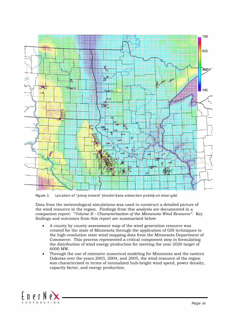
Page xv
Figure 1: Location of “proxy towers” (model data extraction points) on inner grid.
Data from the meteorological simulations was used to construct a detailed picture of the wind resource in the region. Findings from this analysis are documented in a companion report: “Volume II – Characterization of the Minnesota Wind Resource”. Key findings and outcomes from this report are summarized below:
• A county by county assessment map of the wind generation resource was created for the state of Minnesota through the application of GIS techniques to the high-resolution state wind mapping data from the Minnesota Department of Commerce. This process represented a critical component step in formulating the distribution of wind energy production for meeting the year 2020 target of 6000 MW.
• Through the use of extensive numerical modeling for Minnesota and the eastern Dakotas over the years 2003, 2004, and 2005, the wind resource of the region was characterized in terms of normalized hub-height wind speed, power density, capacity factor, and energy production.
Page xvi
• Meteorological time series were generated at 152 locations within the modeling domain for the three years. The time series data were extracted at 5-min intervals while the numerical simulations were proceeding. Each model extraction location represents a 4-km x 4-km region where wind energy generation already exists, is proposed for development, or has development or strategic potential.
• The spatial and temporal variability of the wind resource for Minnesota and the eastern Dakotas was presented along with a description of the meteorology of the Upper Midwest that controls this variability.
• Idealized wind energy geographic dispersion analysis revealed that a progressive increase in the distribution of wind production, utilizing four widely spaced generation areas, substantially reduces the hourly frequency when little or no power was being produced, and increases the hourly frequency of production in the general capacity factor range of 20 to 80% for the ensemble of wind plants. Further, a progressive increase in the distribution of wind production had a dramatic effect on reducing the frequency of very large hourly ramp rates for the ensemble production to values near zero for greatest degrees of geographic dispersion.
• Wind energy forecasting experiments that utilized a computational learning system (CLS) with two forecast models from the National Centers for Environmental Prediction showed considerable skill in both short-term (several hours ahead) and day-ahead (up to 48 hours ahead) time frames. In general, the CLS starts outperforming persistence by one hour into the forecast and shows considerable benefit over persistence by the 3-hour point. In the day-ahead time frame, the CLS forecast yields energy production errors (as a percent of actual energy produced) in the low to mid 20% range.
• An investigation of geographically dispersed wind production forecasts revealed that forecasts for the ensemble of sites were substantially more accurate than for a single site. Forecast errors for power and energy production were reduced by 43% and 30%, respectively, when comparing forecasts from a single site to a forecast for four sites. Similarly large short-term forecast error improvements were also realized as the forecast geographic dispersion increased.
MODELS AND ASSUMPTIONS The analytical methodology used for this study is based on chronological simulations of generation unit commitment and dispatch over an extended data record. The “rules” for conducting these simulations must reflect the business rules and operating realities of the system or systems being modeled. Defining these rules and other assumptions so that they can modeled and appropriately factored into the analytical methodology is a critical part of the study process. Scenarios that are substantially out into the future can be especially challenging.
A significant amount of effort was placed into defining the assumptions for the 2020 study scenario through a collaborative process involving the study sponsors and Technical Review Committee (TRC).
The Midwest Independent System Operator (MISO) market and reliability footprints are comprised of thousands of individual generating units, many tens of thousands of megawatts of load, and many thousands of miles of transmission lines. Given the influence of the MISO energy market on the daily operations of the Minnesota companies, along with the geographical expanse of the wind generation to be
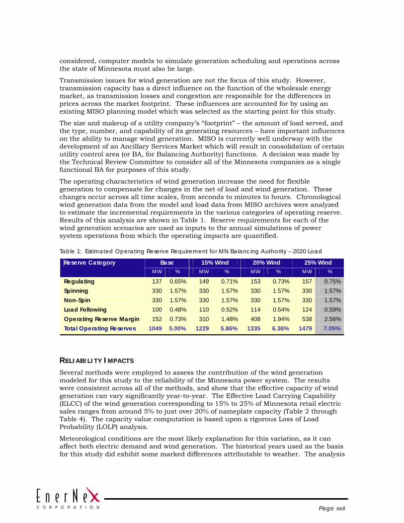
Page xvii
considered, computer models to simulate generation scheduling and operations across the state of Minnesota must also be large.
Transmission issues for wind generation are not the focus of this study. However, transmission capacity has a direct influence on the function of the wholesale energy market, as transmission losses and congestion are responsible for the differences in prices across the market footprint. These influences are accounted for by using an existing MISO planning model which was selected as the starting point for this study.
The size and makeup of a utility company’s “footprint” – the amount of load served, and the type, number, and capability of its generating resources – have important influences on the ability to manage wind generation. MISO is currently well underway with the development of an Ancillary Services Market which will result in consolidation of certain utility control area (or BA, for Balancing Authority) functions. A decision was made by the Technical Review Committee to consider all of the Minnesota companies as a single functional BA for purposes of this study.
The operating characteristics of wind generation increase the need for flexible generation to compensate for changes in the net of load and wind generation. These changes occur across all time scales, from seconds to minutes to hours. Chronological wind generation data from the model and load data from MISO archives were analyzed to estimate the incremental requirements in the various categories of operating reserve. Results of this analysis are shown in Table 1. Reserve requirements for each of the wind generation scenarios are used as inputs to the annual simulations of power system operations from which the operating impacts are quantified.
Table 1: Estimated Operating Reserve Requirement for MN Balancing Authority – 2020 Load
Base 15% Wind 20% Wind 25% Wind Reserve Category MW % MW % MW % MW %
Regulating 137 0.65% 149 0.71% 153 0.73% 157 0.75% Spinning 330 1.57% 330 1.57% 330 1.57% 330 1.57% Non-Spin 330 1.57% 330 1.57% 330 1.57% 330 1.57% Load Following 100 0.48% 110 0.52% 114 0.54% 124 0.59% Operating Reserve Margin 152 0.73% 310 1.48% 408 1.94% 538 2.56% Total Operating Reserves 1049 5.00% 1229 5.86% 1335 6.36% 1479 7.05%
RELIABILITY IMPACTS Several methods were employed to assess the contribution of the wind generation modeled for this study to the reliability of the Minnesota power system. The results were consistent across all of the methods, and show that the effective capacity of wind generation can vary significantly year-to-year. The Effective Load Carrying Capability (ELCC) of the wind generation corresponding to 15% to 25% of Minnesota retail electric sales ranges from around 5% to just over 20% of nameplate capacity (Table 2 through Table 4). The capacity value computation is based upon a rigorous Loss of Load Probability (LOLP) analysis.
Meteorological conditions are the most likely explanation for this variation, as it can affect both electric demand and wind generation. The historical years used as the basis for this study did exhibit some marked differences attributable to weather. The analysis
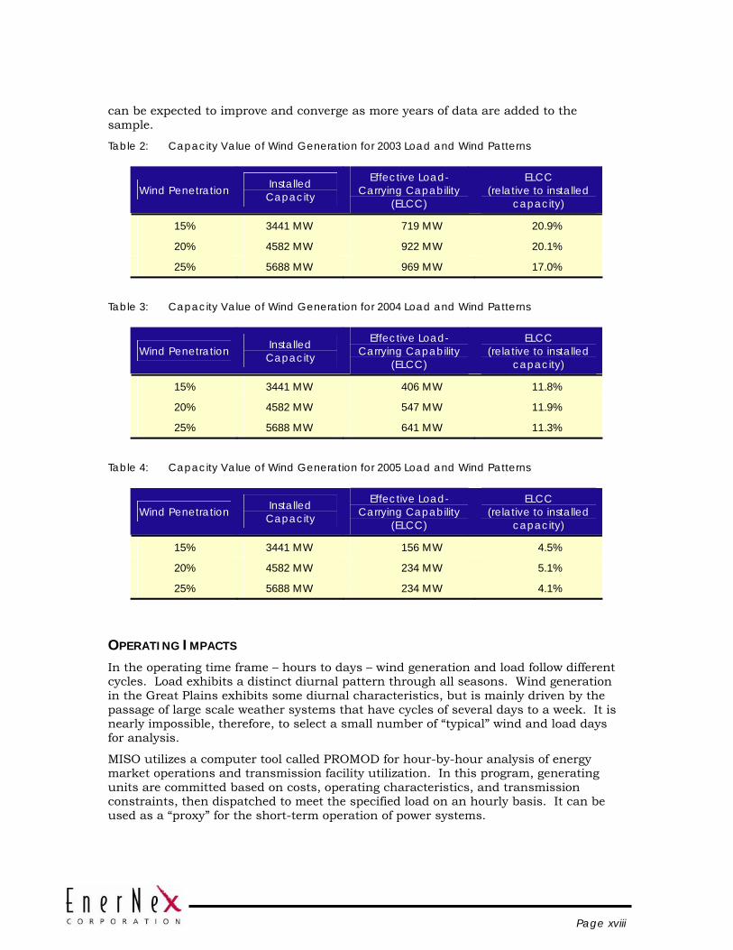
Page xviii
can be expected to improve and converge as more years of data are added to the sample.
Table 2: Capacity Value of Wind Generation for 2003 Load and Wind Patterns
Wind Penetration Installed Capacity
Effective Load-Carrying Capability
(ELCC)
ELCC (relative to installed
capacity)
15% 3441 MW 719 MW 20.9%
20% 4582 MW 922 MW 20.1%
25% 5688 MW 969 MW 17.0%
Table 3: Capacity Value of Wind Generation for 2004 Load and Wind Patterns
Wind Penetration Installed Capacity
Effective Load-Carrying Capability
(ELCC)
ELCC (relative to installed
capacity)
15% 3441 MW 406 MW 11.8%
20% 4582 MW 547 MW 11.9%
25% 5688 MW 641 MW 11.3%
Table 4: Capacity Value of Wind Generation for 2005 Load and Wind Patterns
Wind Penetration Installed Capacity
Effective Load-Carrying Capability
(ELCC)
ELCC (relative to installed
capacity)
15% 3441 MW 156 MW 4.5%
20% 4582 MW 234 MW 5.1%
25% 5688 MW 234 MW 4.1%
OPERATING IMPACTS In the operating time frame – hours to days – wind generation and load follow different cycles. Load exhibits a distinct diurnal pattern through all seasons. Wind generation in the Great Plains exhibits some diurnal characteristics, but is mainly driven by the passage of large scale weather systems that have cycles of several days to a week. It is nearly impossible, therefore, to select a small number of “typical” wind and load days for analysis.
MISO utilizes a computer tool called PROMOD for hour-by-hour analysis of energy market operations and transmission facility utilization. In this program, generating units are committed based on costs, operating characteristics, and transmission constraints, then dispatched to meet the specified load on an hourly basis. It can be used as a “proxy” for the short-term operation of power systems.
Page xix
Commitment of generating resources when the load is known perfectly results in an optimized solution. These optimized hourly cases show the following impacts of wind generation:
• As more wind energy is added, the production cost and load payments decline. This is due to the displacement of conventional generation and the resulting reduction in variable (fuel) costs.
• Generation from both coal and gas units is displaced.
• Production costs rise with the level of required operating reserves. This is intuitive, since more generation must be available or online.
• Production costs rise slowly from the baseline assumption of 5% total operating reserves to about 7%.
• As the operating reserve requirement is increased, coal units are further displaced in favor of more flexible gas units.
Production costs rise as total operating reserves are increased, which is the expected result. It is recognized, however, that a higher reserve requirement for all hours of the annual simulation is overly conservative, since there are many hours where wind generation is very low, and changes up or down would be of little note to operators. Further, an incremental operating reserve pegged to hourly changes in wind generation would not need to be comprised of spinning generation only – changes in the later part of the hour could be covered by quick-start units, if available. The significance here is that no costs accrue with this type of reserve unless it is used.
A case was run for the 2004 load patterns at 20% wind generation with operating reserves for wind generation modeled less conservatively:
• The additional operating reserve for wind generation is a variable hourly profile based on the previous hourly average value.
• The incremental reserves for wind generation were further required only to be non-spinning.
As expected, these assumptions resulted in a decreased production costs over the fixed additional reserves case.
The cost of the additional reserves required to manage the system with wind generation can be estimated from cases where only the operating reserve requirement is varied. Table 5 documents the production cost results from four cases with differing operating reserve assumptions. It shows that for the treatment of reserves deemed to be the most appropriate, the addition cost is $0.11 per MWH of wind generation delivered to the system.
Page xx
Table 5: Incremental Reserve Cost for 20% Wind Case, 2004 Patterns
Case Production CostFull Reserves Case $1,928 M20% Variable Reserve Margin Case $1,923 MOperating Reserve Margin as non-spin $1,921 MBase Case - 5% Operating Reserve Assumption $1,919 M
Wind Production - 20%/2004 Cases 16,895,658 MWH
Inremental Cost - "Full" Reserves $9,368,744Cost per MWH Wind $0.55
Incremental Cost - "Variable" Reserves $3,955,303Cost per MWH Wind $0.23
Incremental Cost - Variable Reserves, non-spin $1,898,352Cost per MWH Wind $0.11
The operating cost results show that, relative to the same amount of energy stripped of variability and uncertainty of the wind generation, there is a cost paid by the load that ranges from a low $2.11 (for 15% wind generation, based on year 2003) to a high of $4.41 (for 25% wind generation, based on year 2005) per MWH of wind energy delivered to the Minnesota companies. This is a total cost and includes the cost of the additional reserves (per the assumptions) These results are shown graphically in Figure 2.
Unit Commitment Costs
$-
$1.00
$2.00
$3.00
$4.00
$5.00
15% Wind 20% Wind 25% Wind
Penetration Level
Inte
grat
ion
Cos
t ($
/MW
H W
ind
Ener
gy)
2003
2004
2005
Figure 2: Unit commitment costs for three penetration levels and pattern years. Cost of
incremental operating reserves is embedded.
Page xxi
STUDY CONCLUSIONS The analytical results from this study show that the addition of wind generation to supply 20% of Minnesota retail electric energy sales can be reliably accommodated by the electric power system if sufficient transmission investments are made to support it.
The degree of the operational impacts was somewhat less than expected by those who have participated in integration studies over the past several years for utilities around the country. The technical and economic impacts calculated are in the range of those derived from other analyses for smaller penetrations of wind generation.
Discussion of the analytical results with the Technical Review Committee and the Minnesota utility company representatives has established the following as the key findings and the principal reasons that wind generation impacts were not larger:
1. These results show that, relative to the same amount of energy stripped of variability and uncertainty of the wind generation, there is a cost paid by the load that ranges from a low of $2.11 (for 15% wind generation, based on year 2003) to a high of $4.41 (for 25% wind generation, based on year 2005) per MWH of wind energy delivered to the Minnesota companies. This is a total cost and includes the cost of the additional reserves (per the assumptions) and costs related to the variability and day-ahead forecast error for wind generation.
2. The cost of additional reserves above the assumed levels attributable to wind generation is included in the total integration cost. Special hourly cases were run to isolate this cost, and found it to be about $0.11/MWH of wind energy at 20% penetration by energy.
3. The TRC decision to combine the Minnesota balancing authorities into a single functional balancing authority had a significant impact on results. Sharing balancing authority functions substantially reduces requirements for certain ancillary services such as regulation and load following (with or without wind generation). The required amount of regulation capacity is reduced by almost 50%. Additional benefits are found with other services such as load following. In addition, there are a larger number of discrete units available to provide these services.
4. The expanse of the wind generation scenario, covering Minnesota and the eastern parts of North and South Dakota, provides for substantial “smoothing” of wind generation variations. This smoothing is especially evident at time scales within the hour, where the impacts on regulation and load following were almost negligible. Smoothing also occurs over multiple hour time frames, which reduces the burden on unit commitment and dispatch, assuming that transmission issues do not intervene to affect operations. Finally, the number of hours at either very high or very low production are reduced, allowing the aggregate wind generation to behave as a more stable supply of electric energy
5. The transmission expansion as described in the assumptions and detailed in Appendix A combined with the decision to inject wind generation at high voltage buses was adequate for transportation of wind energy in all of the scenarios. Under these assumptions, there were no significant congestion issues attributable to wind generation and no periods of negative Locational Marginal Price (LMP) observed in the hourly simulations.
6. The MISO energy market also played a large role in reducing wind generation integration costs. Since all generating resources over the market footprint are

Page xxii
committed and dispatched in an optimal fashion, the size of the effective system into which the wind generation for the study is integrated grows to almost 1200 individual generating units. The aggregate flexibility of the units on line during any hour is adequate for compensating most of the changes in wind generation.
The magnitude of this impact can be gauged by comparing results from recent integration studies for smaller systems. In the 2004 study for Xcel Energy, for example, integration costs were determined to be no higher than $4.60/MWH for a wind generation penetration by capacity of 15%, which would be closer to 10% penetration on an energy basis.
7. The contribution of wind generation to power system reliability is subject to substantial inter-annual variability. Annual Effective Load Carrying Capability (ELCC) values for the three wind generation scenarios from rigorous Loss of Load Probability (LOLP) analysis ranged from a low of 5% of installed capacity to over 20%. These results were consistent with those derived through approximate methods.
PROJECT AND REPORT OVERVIEW EnerNex Corporation, of Knoxville, Tennessee was selected to be the prime contractor for the study. WindLogics, of St. Paul, Minnesota was subcontracted by EnerNex to perform the wind resource characterization and develop the long-term chronological wind speed data sets upon which the analyses of the Minnesota power system were based.
The study was conducted through an open and transparent process that involved the Commission, technical representatives from the Minnesota utility companies, the Midwest Independent System Operator, and stakeholder groups, along with technical experts in wind generation from across the country. The approach, data, assumptions, and analytical methodology were reviewed and extensively discussed at review meetings over the course of the project. Interim results were presented and evaluated, with recommendations from this Technical Review Committee (TRC) guiding subsequent analyses.
The technical scope for the project was based on the original Request-for-Proposal from the Minnesota Public Utilities Commission. As the project progressed, some revisions to this original scope were necessary as a result of assumptions and decisions made in conjunction with the TRC. This report documents the project as conducted.
The contribution of the Midwest Independent System Operator to this effort was very significant. Analysis of an electric power system of the geographic extent and operation complexity considered in this study would have been extremely difficult if not impossible without the support and collaboration of the MISO engineering staff. The project team thanks MISO staff for their efforts and significant contribution.
This report is comprised of four main sections. In Section 2, the approach used to develop the chronological wind generation data so critical to the analytical methodology is described. Characterizations of the wind resource in the state of Minnesota are also presented, and are documented in detail in the companion volume to this report.
Section 3 details the assumptions made in conjunction with the project Technical Review Committee to govern the analysis. Data comprising the models of the electric power system in Minnesota to be used in the analysis are also described. Analysis and

Page xxiii
assumptions regarding the impact of wind generation on system reserve requirements is presented.
In Section 4 the analytical approach to determining the contribution of the wind generation model to system reliability is documented, along with results of the analytical procedures and conclusions.
Finally, Section 5 details how wind generation affects the operation of the Minnesota power system, as determined from annual hour-by-hour simulations of generation unit commitment and dispatch.
Page 1
Section 1 INTRODUCTION
In 2005 the Minnesota Legislature adopted a requirement for a study “of the impacts on reliability and costs associated with increasing wind capacity to 20% of Minnesota retail electric energy sales by the year 2020, and to identify and develop options for utilities to use to manage the intermittent nature of wind resources.” The office of the Reliability Administrator of the Minnesota Public Utilities Commission was assigned responsibility for management of the study.
All utilities with Minnesota retail electric sales participated in this study (totaling approximately 62,000 GWH in 2004). Eight Balancing Authorities are represented with over 85% of the retail sales in the four largest Balancing Authorities: Xcel (NSP), Great River Energy, Minnesota Power, and Otter Tail Power. Projected to 2020, 20% of retail sales will require approximately 5,000 MW of total wind generation. The study area is within the Midwest Reliability Organization (MRO) NERC reliability region and the Mid-Continent Area Power Pool (MAPP) Generation Reserve Sharing Pool. Nearly 95% of the retail sales are within the Midwest Independent System Operator (MISO). Prior wind integration studies of relevance include the 2004 Xcel Energy / MN DOC study and the 2005 NYSERDA / NYISO study. Recent and current regional power studies of relevance include the 2006 MISO Transmission Expansion Plan, the 2003 MAPP Reserve Capacity Obligation Review, and CapX 2020 transmission planning.
CHARACTERISTICS OF WIND GENERATION The nature of its “fuel” supply distinguishes wind generation from more traditional means for producing electric energy. The electric power output of a wind turbine depends on the speed of the wind passing over its blades. The effective speed (since the wind speed across the swept area of the wind turbine rotor is not necessarily uniform) of this moving air stream exhibits variability on a wide range of time scales – from seconds to hours, days, and seasons. Terrain, topography, other nearby turbines, local and regional weather patterns, and seasonal and annual climate variations are just a few of the factors that can influence the electrical output variability of a wind turbine generator.
It should be noted that variability in output is not confined only to wind generation. Hydro plants, for example, depend on water storage that can vary from year to year or even seasonally. Generators that utilize natural gas as a fuel can be subject to supply disruptions or storage limitations. Cogeneration plants may vary their electric power production in response to demands for steam rather than the wishes of the power system operators. That said, the effects of the variable fuel supply are likely more significant for wind generation, if only because the experience with these plants accumulated thus far is so limited.
An individual turbine is negligibly small with respect to the load and other supply resources in a control area, so the aggregate performance of a large number of turbines
Page 2
is what is of primary interest with respect to impacts on the transmission grid and system operations. Large wind generation facilities that connect directly to the transmission grid employ large numbers of individual wind turbine generators, with the total nameplate generation on par with other more conventional plants. Individual wind turbine generators that comprise a wind plant are usually spread out over a significant geographical area. This has the effect of exposing each turbine to a slightly different fuel supply. This spatial diversity has the beneficial effect of “smoothing out” some of the variations in electrical output. The effects of physical separation are also apparent on larger geographical scales, as the combined output of multiple wind plants will be less variable (as a percentage of total output) than for each plant individually.
Another aspect of wind generation, which applies to conventional generation but to a much smaller degree, is the ability to predict with reasonable confidence what the output level will be at some time in the future. Conventional plants, for example, cannot be counted on with 100% confidence to produce their rated output at some coming hour since mechanical failures or other circumstances may limit their output to a lower level or even result in the plant being taken out of service. The probability that this will occur, however, is low enough that such an occurrence is often discounted or completely ignored by power system operators in short-term planning activities.
Because wind generation is driven by the same physical phenomena that control the weather, the uncertainty associated with a prediction of generation level at some future hour, even maybe the next hour, is significant. In addition, the expected accuracy of any prediction will degrade as the time horizon is extended, such that a prediction for the next hour will almost always be more accurate than a prediction for the same hour tomorrow.
The combination of production variability and relatively high uncertainty of prediction makes it difficult, at present, to “fit” wind generation into established practices and methodologies for power system operations and short-term planning and scheduling. These practices, and even emerging concepts such as hour and day-ahead competitive markets, have a necessary bias toward “capacity” - because of system security and reliability concerns so fundamental to power system operation - with energy a secondary consideration.
OVERVIEW OF UTILITY SYSTEM OPERATIONS
Short-Term Planning and Real-Time Operation Interconnected power systems are large and extremely complex machines, consisting of tens of thousands of individual elements. The mechanisms responsible for their control must continually adjust the supply of electric energy to meet the combined and ever-changing electric demand of the system’s users. There are a host of constraints and objectives that govern how this is done. For example, the system must operate with very high reliability and provide electric energy at the lowest possible cost. Limitations of individual network elements – generators, transmission lines, substations – must be honored at all times. The capabilities of each of these elements must be utilized in a fashion to provide the required high levels of performance and reliability at the lowest overall cost.
Operating the power system, then, involves much more than adjusting the combined output of the supply resources to meet the load. Maintaining reliability and acceptable performance, for example, require that operators:

Page 3
• Keep the voltage at each node (a point where two or more system elements – lines, transformers, loads, generators, etc. – connect) of the system within prescribed limits;
• Regulate the system frequency (the steady electrical speed at which all generators in the system are rotating) of the system to keep all generating units in synchronism;
• Maintain the system in a state where it is able to withstand and recover from unplanned failures or losses of major elements.
The activities and functions necessary for maintaining system performance and reliability and minimizing costs are generally classified as “ancillary services.” While there is no universal agreement on the number or specific definition of these services, the following items adequately encompass the range of technical aspects that must be considered for reliable operation of the system:
• Voltage regulation and reactive power dispatch – deploying of devices capable of generating reactive power to manage voltages at all points in the network;
• Regulation – the process of maintaining system frequency by adjusting certain generating units in response to fast fluctuations in the total system load;
• Load following – moving generation up (in the morning) or down (late in the day) in response to the daily load patterns;
• Frequency-responding spinning reserve – maintaining an adequate supply of generating capacity (usually on-line, synchronized to the grid) that is able to quickly respond to the loss of a major transmission network element or another generating unit;
• Supplemental Reserve – managing an additional back-up supply of generating capacity that can be brought on line relatively quickly to serve load in case of the unplanned loss of significant operating generation or a major transmission element.
The frequency of the system and the voltages at each node are the fundamental performance indices for the system. High interconnected power system reliability is a consequence of maintaining the system in a secure state – a state where the loss of any element will not lead to cascading outages of other equipment - at all times.
The electric power system in the United States (contiguous 48 states) is comprised of three interconnected networks: the Eastern Interconnection (most of the states East of the Rocky Mountains), the Western Interconnection (Rocky Mountain States west to the Pacific Ocean), and ERCOT (most of Texas). Within the Eastern and Western interconnections, dozens of individual “control” areas coordinate their activities to maintain reliability and conduct transactions of electric energy with each other. A number of these individual control areas are members of Regional Reliability Organizations (RROs), which oversee and coordinate activities across a number of control areas for the purposes of maintaining the security of the interconnected power systems.
A control area consists of generators, loads, and defined and monitored transmission ties to neighboring areas. Each control area must assist the larger interconnection with maintaining frequency at 60 Hz, and balance load, generation, out-of-area purchases and sales on a continuous basis. In addition, a prescribed amount of backup or reserve capacity (generation that is unused but available within a certain amount of time) must

Page 4
be maintained at all times as protection against unplanned failure or outage of equipment.
To accomplish the objectives of minimizing costs and ensuring system performance and reliability over the short term (hours to weeks), the activities that go on in each control area consist of:
• Developing plans and schedules for meeting the forecast load over the coming days, weeks, and possibly months, considering all technical constraints, contractual obligations, and financial objectives;
• Monitoring the operation of the control area in real time and making adjustments when the actual conditions - load levels, status of generating units, etc. - deviate from those that were forecast.
A number of tools and systems are employed to assist in these activities. Developing plans and schedules involves evaluating a very large number of possibilities for the deployment of the available generating resources. A major objective here is to utilize the supply resources so that all obligations are met and the total cost to serve the projected load is minimized. With a large number of individual generating units with many different operational characteristics and constraints, fuel types, efficiencies, and other supply options such as energy purchases from other control areas, software tools must be employed to develop optimal plans and schedules. These tools assist operators in making decisions to “commit” generating units for operation, since many units cannot realistically be stopped or started at will. They are also used to develop schedules for the next day or days that will result in minimum costs if adhered to and if the load forecasts are accurate.
The Energy Management System (EMS) is the technical core of modern control areas. It consists of hardware, software, communications, and telemetry to monitor the real-time performance of the control area and make adjustments to generating unit and other network components to achieve operating performance objectives. A number of these adjustments happen very quickly without the intervention of human operators. Others, however, are made in response to decisions by individuals charged with monitoring the performance of the system.
The nature of control area operations in real-time or in planning for the hours and days ahead is such that increased knowledge of what will happen correlates strongly to better strategies for managing the system. Much of this process is already based on predictions of uncertain quantities. Hour-by-hour forecasts of load for the next day or several days, for example, are critical inputs to the process of deploying electric generating units and scheduling their operation. While it is recognized that load forecasts for future periods can never be 100% accurate, they nonetheless are the foundation for all of the procedures and process for operating the power system. Increasingly sophisticated load forecasting techniques and decades of experience in applying this information have done much to lessen the effects of the inherent uncertainty
Wind Generation and Long-Term Power System Reliability In longer term planning of electric power systems, overall reliability is often gauged in terms of the probability that the planned generation capacity will be insufficient to meet the projected system demand. This question is important from the planning perspective because it is recognized that even conventional electric generating plants and units are not completely reliable – there is some probability that in a given future hour capacity from the unit would be unavailable or limited in capability due to a forced outage – i.e.
Page 5
mechanical failure. This probability of not being able to meet the load demand exists even if the installed capacity in the control area exceeds the peak projected load.
In this sense, conventional generating units are similar to wind plants. For conventional units, the probability that the rated output would not be available is rather low, while for wind plants the probability could be quite high. Nevertheless, a rigorous statistical computation of system reliability would reveal that the probability of not being able to meet peak load is lower with a wind plant on the system than without it.
The capacity value of wind plants for long term planning analyses is currently a topic of significant discussion in the wind and electric power industries. Characterizing the wind generation to appropriately reflect the historical statistical nature of the plant output on hourly, daily, and seasonal bases is one of the major challenges. Several techniques that capture this variability in a format appropriate for formal reliability modeling have been proposed and tested. The lack of adequate historical data for the wind plants under consideration is an obstacle for these methods.
The capacity value issue also arises in other, slightly different contexts. In the Mid-Continent Area Power Pool (MAPP), the emergence of large wind generation facilities over the past decade led to the adaptation of a procedure use for accrediting capacity of hydroelectric facilities for application to wind facilities. Capacity accreditation is a critical aspect of power pool reserve sharing agreements. The procedure uses historical performance data to identify the energy delivered by these facilities during defined peak periods important for system reliability. A similar retrospective method was used in California for computing the capacity payments to third-party generators under their Standard Offer 4 contract terms.
By any of these methods, it can be shown that wind generation does make a calculable contribution to system reliability in spite of the fact that it cannot be directly dispatched like most conventional generating resources. The magnitude of that contribution and the appropriate method for its determination are important questions.
Influence of the MISO Market on Minnesota Utility Company Operations Electric power industry developments over the past two decades have brought a new framework for system planning and operations. Traditional utility company functions such as the commitment and scheduling of generation have been supplanted by new mechanisms that seek to optimize operation of the electric supply and transportation system over a footprint much larger than a single utility company service territory.
MISO wholesale energy markets have changed the process by which Minnesota utility companies commit and schedule generation and buy and sell energy to meet their load obligations. It has been found in previous wind generation integration studies that modeling the “business environment” in the analytical methodology can have a significant effect on the results. As such, the operation of the MISO markets is a major consideration in the analytical methodology assembled for this study.
PROJECT ORGANIZATION EnerNex Corporation, of Knoxville, Tennessee was selected to be the prime contractor for the study. WindLogics, of St. Paul, Minnesota was subcontracted by EnerNex to perform the wind resource characterization and develop the long-term chronological wind speed data sets upon which the analyses of the Minnesota power system were based.

Page 6
The study was conducted through an open and transparent process that involved the Commission, technical representatives from the Minnesota utility companies, the Midwest Independent System Operator, and stakeholder groups, along with technical experts in wind generation from across the country. The approach, data, assumptions, and analytical methodology were reviewed and extensively discussed at review meetings over the course of the project. Interim results were presented and evaluated, with recommendations from this Technical Review Committee (TRC) guiding subsequent analyses.
The technical scope for the project was based on the original Request-for-Proposal from the Minnesota Public Utilities Commission. As the project progressed, some revisions to this original scope were necessary as a result of assumptions and decisions made in conjunction with the TRC. This report documents the project as conducted.
The contribution of the Midwest Independent System Operator to this effort was very significant. Analysis of an electric power system of the geographic extent and operation complexity considered in this study would have been extremely difficult if not impossible without the support and collaboration of the MISO engineering staff. The project team thanks MISO staff for their efforts and significant contribution.
REPORT OVERVIEW This report is comprised of four main sections followed by conclusions. In Section 2 “Characterizing the Minnesota Wind Resource”, the approach used to develop the chronological wind generation data so critical to the analytical methodology is described. Characterizations of the wind resource in the state of Minnesota are also presented, and are documented in detail in the companion volume to this report.
Section 3 “Models and Assumptions” details the assumptions made in conjunction with the project Technical Review Committee to govern the analysis. Data comprising the models of the electric power system in Minnesota to be used in the analysis are also described. Analysis and assumptions regarding the impact of wind generation on system reserve requirements is presented.
In Section 4 “Reliability Impacts”, the analytical approach to determining the contribution of the wind generation model to system reliability is documented, along with results of the analytical procedures and conclusions.
Finally, Section 5 “Operating Impacts” details how wind generation affects the operation of the Minnesota power system, as determined from annual hour-by-hour simulations of generation unit commitment and dispatch.
Page 7
Section 2 CHARACTERIZING THE MINNESOTA WIND RESOURCE
Variability and uncertainty are the two attributes of wind generation that underlie most of the concerns related to power system operations and reliability. In day-ahead planning, whether it be for conventional unit commitment or offering generation into an energy market, forecasts of the demand for the next day will drive the process. In real-time operations, generating resource must be maneuvered to match the ever-changing demand pattern. To the extent that wind generation adds to this variability and uncertainty, the challenge for meeting demand at the lowest cost while maintaining system security is increased.
Recent studies have shown that a high-fidelity, long-term, chronological representation of wind generation is perhaps the most critical element of this type of study. For large wind generation development scenarios, it is very important that the effects of spatial and geographic diversity be neither under- or over-estimated. The approach for this task has been used by EnerNex and WindLogics in at least six wind integration studies, including the Minnesota study of the Xcel system completed in 2004 for the Minnesota Department of Commerce.
The initial task of this project was focused on characterizing the wind resource in Minnesota and developing chronological wind speed and wind generation forecast data for use in later analytical tasks. The procedure and results of this effort are documented in detail in a companion report (Volume II).
SYNTHESIS OF WIND SPEED DATA FOR THE MN WIND GENERATION SCENARIOS The base data for both the wind resource characterization and the production of wind speed and power time series were generated from the MM5 mesoscale model (Grell et al. 1995). This prognostic regional atmospheric model is capable of resolving mesoscale meteorological features that are not well represented in coarser-grid simulations from the standard weather prediction models run by the National Centers for Environmental Prediction (NCEP). The MM5 was run in a configuration utilizing two grids as shown in Fig. 1. This “telescoping” two-way nested grid configuration allowed for the greatest resolution in the area of interest with coarser grid spacing employed where the resolution of small mesoscale meteorological phenomena were not as important. This methodology was computationally efficient while still providing the necessary resolution for accurate representation of the meteorological scales of interest within the inner grid.
More specifically, the 4 km innermost grid spacing was deemed necessary to capture topographic influences on boundary layer flow and resolve mesoscale meteorological phenomena such as thunderstorm outflows. The 12 and 4 km grid spacing utilized in grids 1 and 2, respectively, yield the physical grid sizes of 2400 x 2400 km for grid 1, and 760 x 760 km for grid 2.
To provide an accurate assessment of the character and variability of the wind resource for Minnesota and the eastern Dakotas, three full years of MM5 simulations were completed. To initialize the model, the WindLogics archive of NCEP Rapid Update Cycle (RUC) model analysis data was utilized. The years selected for simulation were 2003, 2004 and 2005. The RUC
Page 8
analysis data were used both for model initialization and for updating the model boundary conditions every 3 hours. This RUC data had a horizontal grid spacing of 20 km for all three years.
A Minnesota wind development scenario was constructed to support the development of the wind generation model for the analytical tasks. The target penetration level is based on a fraction of projected retail electricity sales in the 2020 study year, which from Table 6 is estimated to be 20% of 85,093 GWH. The next step in defining the scenario is to determine the actual installed wind generation capacity, which requires an estimate of the aggregate annual capacity factor. From this, the number of extraction points in the meteorological simulation model to reasonably represent the total installed capacity can be determined.
Table 6: 2020 Projections of Minnesota electric retail sales and wind generation at assumed annual capacity factors.
RetailSales Wind Wind
Annual Percent AnnualGrowth Retail CapacityRate Sales Factor 2004 2011 20201.0% MN Retail Sales (GWh) 61,986 66,457 72,683
15% 40% Nameplate wind (MW) 2,653 2,845 3,11120% 35% 4,043 4,335 4,74120% 40% 3,538 3,793 4,14925% 40% 4,422 4,741 5,186
2.0% MN Retail Sales (GWh) 61,986 71,202 85,09315% 40% Nameplate wind (MW) 2,653 3,048 3,64320% 35% 4,043 4,645 5,55120% 40% 3,538 4,064 4,85725% 40% 4,422 5,080 6,071
Data at 152 grid points (proxy towers) in the inner model nest were extracted every 5 min as the simulation progressed through historical years 2003, 2004, and 2005. This process ensured that the character and variability of the wind resource over several time scales across geographically dispersed locations is captured. Figure 3 depicts the MM5 innermost grid with selected locations for high time-resolution data extraction shown in Figure 3 and Figure 4. The sites were selected in coordination with the utility and government stakeholders represented on the Technical Review Committee to correspond to 1) existing wind plant locations such as those along the Buffalo Ridge and other regions of southern Minnesota, 2) proposed locations for near-future wind plant development or 3) favorable locations for future wind production with emphasis given to a distribution of wind energy plants that would provide beneficial geographic dispersion. The 2005 Minnesota Department of Commerce high resolution state wind map was used, in part, for guidance in assessing favorable development areas. Overall, 152 sites were located in 62 counties in the three state domain at locations within the county with an expected favorable wind resource. Consideration was also given to the existence of nearby transmission and substations. Model data extracted at each site included wind direction and speed, temperature and pressure at 80 and 100 m hub heights.
Each data extraction point was assigned to one or more of the wind generation scenarios to be considered in the study. The TRC was consulted to help define the makeup of each scenario. The result of these discussions is shown in Figure 5. The 15% scenario includes all of the existing wind generation, which is mostly on the
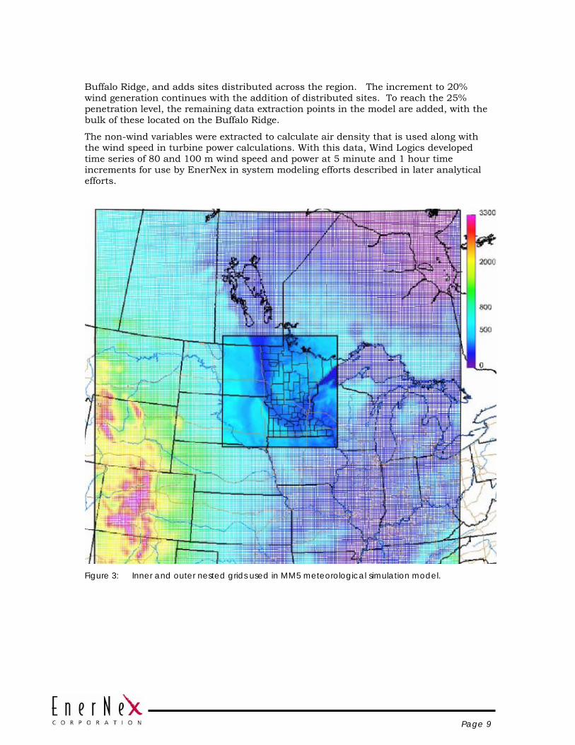
Page 9
Buffalo Ridge, and adds sites distributed across the region. The increment to 20% wind generation continues with the addition of distributed sites. To reach the 25% penetration level, the remaining data extraction points in the model are added, with the bulk of these located on the Buffalo Ridge.
The non-wind variables were extracted to calculate air density that is used along with the wind speed in turbine power calculations. With this data, Wind Logics developed time series of 80 and 100 m wind speed and power at 5 minute and 1 hour time increments for use by EnerNex in system modeling efforts described in later analytical efforts.
Figure 3: Inner and outer nested grids used in MM5 meteorological simulation model.
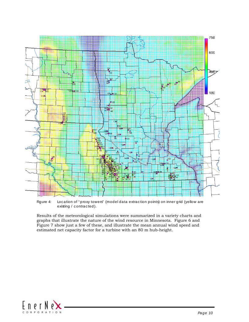
Page 10
Figure 4: Location of “proxy towers” (model data extraction points) on inner grid (yellow are
existing / contracted).
Results of the meteorological simulations were summarized in a variety charts and graphs that illustrate the nature of the wind resource in Minnesota. Figure 6 and Figure 7 show just a few of these, and illustrate the mean annual wind speed and estimated net capacity factor for a turbine with an 80 m hub-height.
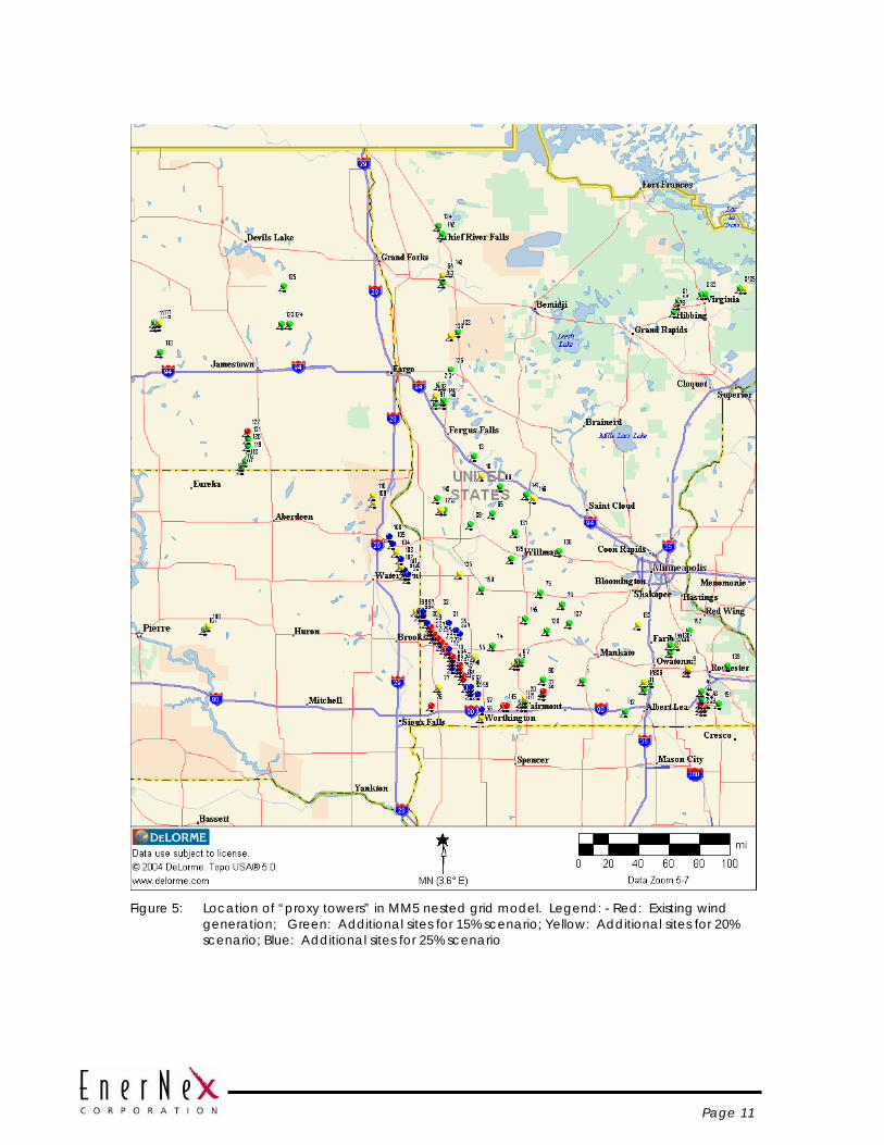
Page 11
Figure 5: Location of “proxy towers” in MM5 nested grid model. Legend: - Red: Existing wind
generation; Green: Additional sites for 15% scenario; Yellow: Additional sites for 20% scenario; Blue: Additional sites for 25% scenario
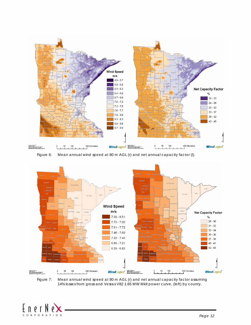
Page 12
Figure 6: Mean annual wind speed at 80 m AGL (r) and net annual capacity factor (l).
Figure 7: Mean annual wind speed at 80 m AGL (r) and net annual capacity factor assuming
14% losses from gross and Vestas V82 1.65 MW MkII power curve, (left) by county.
Page 13
WIND GENERATION FORECASTS The uncertainty attribute of wind generation stems from the errors in forecasts of wind generation over forward periods. Because this attribute is to be explicitly represented in the later analytical tasks, a companion time series of wind generation forecasts for a time period 18 to 42 hours in the future was developed. This corresponds to the forecast that would be used for generation unit commitment in general, or participation in day-ahead market in the case of MISO. Information on short-term forecasting (one to a few hours ahead) was utilized in the assessment of wind generation impacts on real-time operation of the power system.
The day-ahead 24-hour forecast time series used for the hourly analysis described later in the report has a mean absolute error of around 20% of rated capacity.
Further information on the development and assessment of wind generation forecasting can be found in the Volume II report.
SPATIAL AND GEOGRAPHIC DIVERSITY When wind generation is an appreciable fraction of the supply picture, variations in production over time drive the need for maneuverable generation to compensate. The nature of the wind generation changes over various operational time scales from minutes to multiple hours is a critical consideration in assessing wind integration costs. The variation of the aggregate wind generation resource is very much affected by the location of the wind turbines and wind plants with respect to each other, as illustrated in Figure 8. As the distance between individual wind turbines, then individual wind plant on a larger scale grows, production variation exhibit less correlation (a correlation coefficient of 1.0 means that the changes happen at the same time; a coefficient of 0.0 means that the changes are not related). The consequence for system operations is that spatially and geographically dispersed wind generation will be less variable in the aggregate than the same amount of wind generation concentrated at a single site or within a single region.
The effects of spatial and geographic diversity were quantified for this study through analysis of the wind generation data developed from meteorological simulations. Figure 9 shows the hourly changes in wind generation for a single location along with combinations of regionally-dispersed locations. Reduction in the hourly variability due to the aggregation of individual wind generation sources over the region is very evident from the plot.
Figure 10 illustrates another significant effect of geographic diversity. The distribution of hour production over an annual period is shown for scenarios of increasing geographic diversity. As wind generation from an increasing number of geographically separated locations in the region is aggregated, the number of very high and very low production hours drops substantially. Hours at production levels between the extremes is increased. This influence has important implications for power system operations, as will be seen later.

Page 14
Figure 8: Correlation of wind generation power changes to distance between plants/turbines.
From NREL/CP-500-26722, July, 1999
Figure 9: Reduction in hourly variability (change) of wind generation as wind generation over
the region is aggregated.
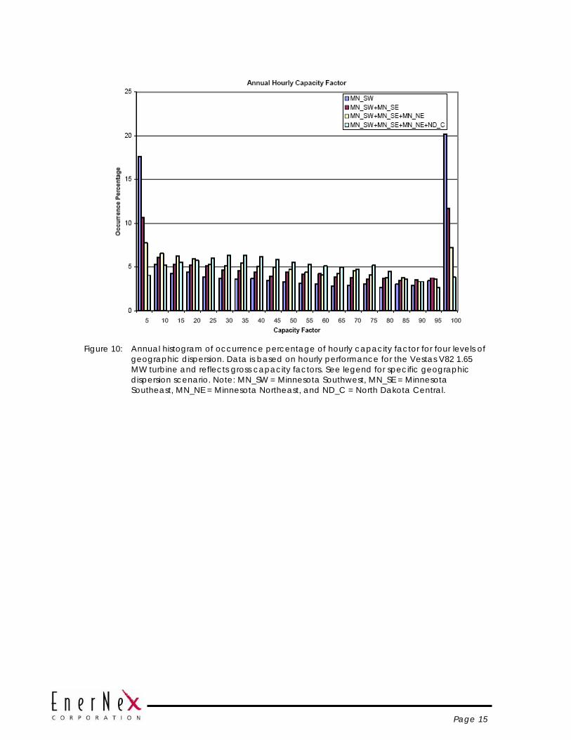
Page 15
Figure 10: Annual histogram of occurrence percentage of hourly capacity factor for four levels of
geographic dispersion. Data is based on hourly performance for the Vestas V82 1.65 MW turbine and reflects gross capacity factors. See legend for specific geographic dispersion scenario. Note: MN_SW = Minnesota Southwest, MN_SE = Minnesota Southeast, MN_NE = Minnesota Northeast, and ND_C = North Dakota Central.

Page 16
Section 3 MODELS AND ASSUMPTIONS
The analytical methodology used for this study is based on chronological simulations of generation unit commitment and dispatch over an extended data record. The “rules” for conducting these simulations must reflect the business rules and operating realities of the system or systems being modeled. Defining these rules and other assumptions so that they can be modeled and appropriately factored into the analytical methodology is a critical part of the study process. Scenarios that are substantially out into the future can be especially challenging since many of the rules and regulations that govern current-day power system operations may no longer be relevant to the time of interest.
A significant amount of effort was placed into defining the assumptions for the 2020 study scenario through a collaborative process involving the study sponsors and Technical Review Committee. The purpose of this section is to describe and document those assumptions.
MISO MARKET STRUCTURE Power system operation is governed by both technical and economic considerations. On the technical side, system security must be maintained at all times, and the dispatching of generation to meet obligations (primarily serving load plus delivering on promises to buy or sell energy) must be performed in a manner which constitutes acceptable control performance. The economic objective is to meet these obligations in the most favorable financial sense, based on minimizing variable operating costs within the market.
Startup of MISO energy market operations has brought some significant changes to the way that Minnesota utilities manage their generating resources. In essence, under MISO market operations, the Minnesota utility companies pool their resources and obligations with other MISO market participants. The market then determines what resources are used to meet load in the most economic manner while respecting all constraints on individual units, the needs of the system as a whole, transmission facilities, and considerations for secure operation.
The arrangement of the MISO market and reliability authority footprint is shown in Figure 11. MISO operates a daily Day-Ahead Energy Market that closes at 11:00 am the day prior to the operating day, and a Real-Time energy market that closes 30 minutes prior to the Operating Hour. Energy cost in the day-ahead and real-time market is based on the highest priced energy that is offered into the market and is required to meet load, or “cleared”. All generators are paid the clearing price for that period and all loads pay the clearing price for that time period. The net of payments results in simply a net cost of fuel for energy supplied to a utility’s loads from its owned portfolio of resources. The portion of utility load supplied from the market resources pays a net delivered purchased power price. Because transmission congestion and losses may prevent a generator in one physical part of the market from serving load in

Page 17
another part, the clearing price will vary by location. Another term for this geographically-varying price is locational marginal price, or “LMP”.
At present, the MISO market structure accepts output from wind generation resources “as delivered”, recognizing its fundamental inability to follow dispatch instructions. The financial supply cost optimization that occurs in the market automatically ramps down energy supply from the least efficient dispatchable generators in response to increases in wind generation that occur as a trend over many minutes. Conversely, the market will increase supply from the next most efficient available units in response to reductions in wind generation output that occur over many minutes.
The effect of the MISO market overlay extends beyond the day-ahead energy time frame. To facilitate the real-time market which is cleared at five minute intervals, it is necessary for MISO to have influence on the real-time dispatch of generation within each control area in the footprint. Figure 12 illustrates this structure. It should be noted that this represents a more sophisticated grid control and dispatch than traditional control area or control center operations. The net effect is that the real-time operation of all control areas within the market footprint is coordinated via this hierarchical structure. In more conventional operations, each control area is on its own with respect to balancing supply and demand and honoring scheduled transactions with neighbors.
There are currently 37 individual control areas within the MISO reliability footprint (Table 7). Not all of these control areas participate in the energy markets, but nonetheless are impacted by MISO dispatch and generation control structure. Development of MISO’s Ancillary Services Market (ASM) is well underway and will result in consolidation of certain balancing authority (control area) functions. The effect of such functional consolidation, as will be discussed later, will be to reduce the quantity of services required to maintain system security and control performance across the footprint. The ASM will transfer the source of short-interval responses to changes in wind output from today’s default of the individual utility control areas to the least-cost supply option available from the broader market footprint.

Page 18
Figure 11: Structure of MISO market and reliability footprints. (from MISO Business Practices
Manual) Note: Southern Minnesota Municipal Power Agency is now a MISO market participant; LGE is leaving MISO).
ANALYTICAL APPROACH The technical analysis falls into two general categories – Reliability and Operating Impacts. The data and tools to be used to assess the impacts of the defined wind generation are described below.
Reliability Analysis The objective here is to determine to what extent wind generation would reduce the need for additional conventional capacity. This analysis involves assessing the probability of not being able to meet load in any given hour over a period due to outage of generating units. “LOLP” stands for “loss of load probability” and is the metric which defines the reliability of a system. A LOLP of one day in ten years, or 2.4 hours per year, a common target reliability level, is used in this analysis.
The reliability analysis is performed with two different tools. The first is GE-MARS (Multi-Area Reliability Simulation) from GE Energy which has been used by the MAPP Generation Reserve Sharing Pool in recent years to analyze the Reserve Capacity Obligation. The database compiled for the 2003 study conducted by GE for MAPP was obtained. The database was updated to reflect the generation expansion for the 2020 study year, and Minnesota load was increased as described in later sections of this document.

Page 19
Wind generation was represented as a load modifier, meaning that the hourly demand in the Minnesota “area” in the MARS input data is the net of load and wind for each hour of the year. The analysis was conducted for three different “versions” of 2020, where the hourly wind and load patterns are based on the historical years 2003, 2004, and 2005. Using three years rather than a single year provides a relatively better characterization of the wind production during periods of high demand or risk to the system than would be obtained with just a single year.
Figure 12: MISO structure for generation dispatch and control.
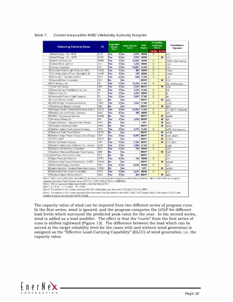
Page 20
Table 7: Control Areas within MISO’s Reliability Authority Footprint
The capacity value of wind can be imputed from two different series of program runs. In the first series, wind is ignored, and the program computes the LOLP for different load levels which surround the predicted peak value for the year. In the second series, wind is added as a load modifier. The effect is that the “curve” from the first series of runs is shifted rightward (Figure 13). The difference between the load which can be served at the target reliability level for the cases with and without wind generation is assigned as the “Effective Load-Carrying Capability” (ELCC) of wind generation, i.e. the capacity value.
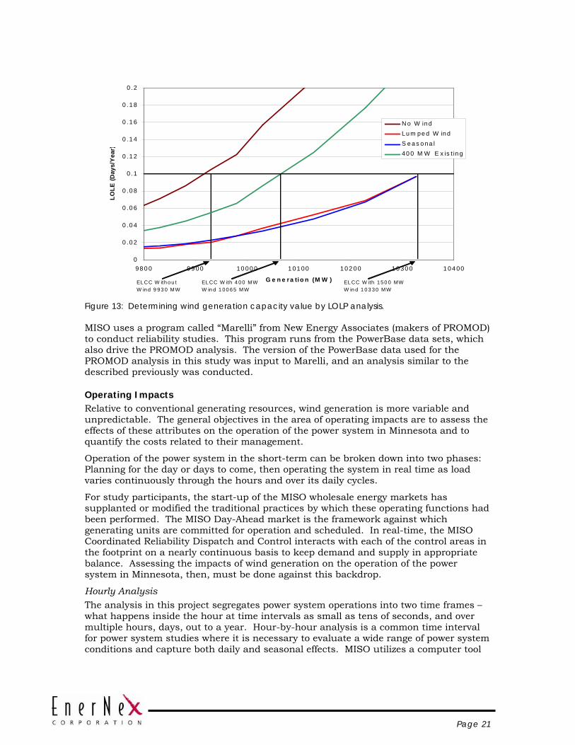
Page 21
0
0 .0 2
0 .0 4
0 .0 6
0 .0 8
0 . 1
0 .1 2
0 .1 4
0 .1 6
0 .1 8
0 . 2
9 8 0 0 9 9 0 0 10 0 0 0 1 0 1 0 0 1 0 2 0 0 1 0 3 0 0 1 0 4 00
G e n e ra tio n (M W )
LOLE
(Day
s/Y
ear)
N o W in dLu m pe d W in dS e a s o na l40 0 M W E x is t in g
EL CC W ith o u t W in d 9 9 3 0 MW
ELCC W ith 4 0 0 MW W in d 1 0 0 6 5 MW
EL CC W ith 1 5 0 0 MW W in d 1 0 3 3 0 MW
Figure 13: Determining wind generation capacity value by LOLP analysis.
MISO uses a program called “Marelli” from New Energy Associates (makers of PROMOD) to conduct reliability studies. This program runs from the PowerBase data sets, which also drive the PROMOD analysis. The version of the PowerBase data used for the PROMOD analysis in this study was input to Marelli, and an analysis similar to the described previously was conducted.
Operating Impacts Relative to conventional generating resources, wind generation is more variable and unpredictable. The general objectives in the area of operating impacts are to assess the effects of these attributes on the operation of the power system in Minnesota and to quantify the costs related to their management.
Operation of the power system in the short-term can be broken down into two phases: Planning for the day or days to come, then operating the system in real time as load varies continuously through the hours and over its daily cycles.
For study participants, the start-up of the MISO wholesale energy markets has supplanted or modified the traditional practices by which these operating functions had been performed. The MISO Day-Ahead market is the framework against which generating units are committed for operation and scheduled. In real-time, the MISO Coordinated Reliability Dispatch and Control interacts with each of the control areas in the footprint on a nearly continuous basis to keep demand and supply in appropriate balance. Assessing the impacts of wind generation on the operation of the power system in Minnesota, then, must be done against this backdrop.
Hourly Analysis The analysis in this project segregates power system operations into two time frames – what happens inside the hour at time intervals as small as tens of seconds, and over multiple hours, days, out to a year. Hour-by-hour analysis is a common time interval for power system studies where it is necessary to evaluate a wide range of power system conditions and capture both daily and seasonal effects. MISO utilizes a computer tool

Page 22
called PROMOD for this type of analysis. PROMOD contains representation of loads, transmission lines, and generating units. For the hourly load data provided as input, PROMOD determines the optimum plan for meeting the load while honoring constraints for the system (e.g. reserves, emissions, etc.) individual generating units, and the transmission network.
PROMOD can also be used to estimate locational marginal prices (LMP), since the cost functions and loading level of each generator in the optimized solution are known.
Intra-Hourly Analysis The hour-by-hour simulation in PROMOD assumes that load, wind, and generation are “flat” for each hour. In reality, load (and wind) is continuously varying, and provisions must be made by system operators for adjustments so that demand and supply are closely matched at all times.
An approach that has been used in previous studies for estimating the impact of wind generation on requirements for regulation, load following, and other reserve impacts is based on analysis of high resolution chronological wind and load data sets. Various statistical metrics that quantify variability are first computed for the load data alone. Wind data is then combined with load data, and new metrics are calculated. The changes in these quantities are directly attributable to wind generation.
Assessing the costs of these inside-the hour impacts has been done in a variety of ways. Direct costs, for example, can be computed for incremental regulation capacity if there is a regulation market or capacity cost that can be identified. However, if the incremental requirements for the various operating reserves are brought into the hourly analysis, much of the cost impact, especially those that are associated with opportunity cost, are accrued. A good example would be where regulation and load following is performed with relatively inexpensive units. The capacity that must be held back to provide ancillary services cannot be used to serve load and generate revenue. There is, therefore, an “opportunity” cost that comes with providing ancillary services from these units. The hourly modeling will accrue these costs since other resources must be used to meet the load.
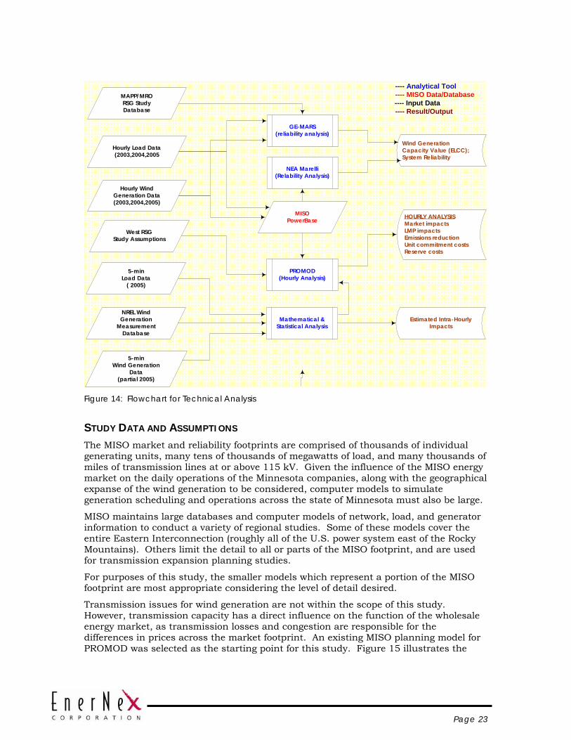
Page 23
PROMOD(Hourly Analysis)
Mathematical &Statistical Analysis
GE-MARS(reliability analysis)
Hourly Load Data(2003,2004,2005
Hourly WindGeneration Data(2003,2004,2005)
NREL WindGeneration
MeasurementDatabase
5-minWind Generation
Data(partial 2005)
5-minLoad Data
( 2005)
NEA Marelli(Relability Analysis)
MISOPowerBase
MAPP/MRORSG StudyDatabase
Wind GenerationCapacity Value (ELCC);System Reliability
HOURLY ANALYSISMarket impactsLMP impactsEmissions reductionUnit commitment costsReserve costs
---- Analytical Tool---- MISO Data/Database---- Input Data---- Result/Output
Estimated Intra-HourlyImpacts
West RSGStudy Assumptions
Figure 14: Flowchart for Technical Analysis
STUDY DATA AND ASSUMPTIONS The MISO market and reliability footprints are comprised of thousands of individual generating units, many tens of thousands of megawatts of load, and many thousands of miles of transmission lines at or above 115 kV. Given the influence of the MISO energy market on the daily operations of the Minnesota companies, along with the geographical expanse of the wind generation to be considered, computer models to simulate generation scheduling and operations across the state of Minnesota must also be large.
MISO maintains large databases and computer models of network, load, and generator information to conduct a variety of regional studies. Some of these models cover the entire Eastern Interconnection (roughly all of the U.S. power system east of the Rocky Mountains). Others limit the detail to all or parts of the MISO footprint, and are used for transmission expansion planning studies.
For purposes of this study, the smaller models which represent a portion of the MISO footprint are most appropriate considering the level of detail desired.
Transmission issues for wind generation are not within the scope of this study. However, transmission capacity has a direct influence on the function of the wholesale energy market, as transmission losses and congestion are responsible for the differences in prices across the market footprint. An existing MISO planning model for PROMOD was selected as the starting point for this study. Figure 15 illustrates the

Page 24
scope of this West Regional Study Group (RSG) model created to encompass a number of separate transmission planning efforts so that they could be studied simultaneously.
WPL
ASEC
BREC, EKPC, TVA
IMO
KCPL
MIDAM
MIPU
MPC, NWPS, WAPA
STHRN
SWPA
ALWST
AUEP, CIPS, CIL
CGE, PSI
EEI
FE
GRE HUC
HEC
ILPC
IP&L
LG&E
MDU
MGE
CONS, DETED, LBWL, WPSC
MP
NIPS
NSP
OTP
SIGE
WEP
WPPI
WPS
SIPC, SPRIL
DPC
SMMPA
PJM, COED, AEP, DPL
MISO Market
LES, NPPD, OPPD
MPW
MHSP SASK
Figure 15: Overview of West RSG study PROMOD model, used as the basis for this study.
Companies shown in red are represented in detail.
The transmission and non-wind generation expansion assumptions in the MISO West RSG model were used because this study is focused on the reliability and operating impacts of wind generation and is not intended to be a transmission plan or an integrated resource plan. The wind generation in the RSG model was removed and replaced with the wind scenarios developed for this study. The makeup of the West RSG PROMOD model and assumptions underlying it are detailed in Appendix A
The size and makeup of an individual control area has a significant influence on its ability to manage wind generation. Currently there are several major control areas, or Balancing Authorities (BAs), in the state of Minnesota. MISO is currently well underway with the development of an Ancillary Services Market which will result consolidation of certain BA functions. This consolidation will decrease the aggregate amount of certain ancillary services.
Most of the transmission expansion in the model adapted for this study consists of additions to the existing EHV (extra high voltage, 345 kV or higher) network. The wind generation developed for the study is “injected” at EHV buses. This assumption is used by MISO in other studies where focus is on the larger picture, and bolstering of lower voltage transmission infrastructure is not part of the study scope. The underlying local and regional transmission infrastructure was not analyzed in this study

Page 25
Because the study year is more than a decade into the future, and the move toward functional consolidation of Balancing Authorities is already underway, the Minnesota companies will be considered as a single BA for the study. This could actually be a conservative assumption if after consolidation of BA’s in the MISO footprint the resulting regional BA is larger than Minnesota.
The PROMOD West RSG model, with the wind generation scenarios developed for this study, is used to represent the MISO energy market operations. It is assumed that this cost-based approach will adequately reflect the function of the day-ahead and real-time markets.
Modeling Minnesota Electric Load in 2020 Table 8 documents the retail sales statistics upon which the Minnesota study is premised. The total retail sales for 2004 were 61,965 GWH. Assuming a 2.0% annual growth rate, retail sales in 2020 are projected to be 85,093 GWH.
Table 8: Minnesota retail sales by company for CY2004 and Total Retail Sales assumptions for study
RetailSales Wind Wind
Annual Percent AnnualGrowth Retail CapacityRate Sales Factor 2004 2011 20201.0% MN Retail Sales (GWh) 61,986 66,457 72,683
15% 40% Nameplate wind (MW) 2,653 2,845 3,11120% 35% 4,043 4,335 4,74120% 40% 3,538 3,793 4,14925% 40% 4,422 4,741 5,186
2.0% MN Retail Sales (GWh) 61,986 71,202 85,09315% 40% Nameplate wind (MW) 2,653 3,048 3,64320% 35% 4,043 4,645 5,55120% 40% 3,538 4,064 4,85725% 40% 4,422 5,080 6,071
Table 9 shows the loads from the West RSG PROMOD case for 2020. The highlighted (in yellow) companies are those having significant Minnesota load. The aggregated load, however, for these companies is 142,177 GWH, well in excess of the study projections for 2020.
` 2004 MN RetailSales in kWh1
Investor-Owned UtilitiesXcel 30,559,280,490 49.3%MP 8,580,900,000 13.8%OTP 1,957,456,566 3.2%IPL 841,511,856 1.4%NWEC 524,992 0.0%
TOTAL IOU 41,939,673,904 67.7%
Cooperative UtilitesGRE 10,408,968,000 16.8%Minnkota 1,808,326,904 2.9%Dairyland 737,462,789 1.2%Basin 751,736,085 1.2%
TOTAL COOP 13,706,493,778 22.1%
Municipal UtilitiesSMMPA 2,714,070,325 4.4%MRES 805,570,000 1.3%MMPA 2,302,721,000 3.7%CMMPA 516,974,120 0.8%TOTAL MUNI 6,339,335,445 10.2%
TOTAL ALL 61,985,503,127 100.0%1 July 1, 2003 to June 30, 2004 (MN DOC 1/15/05)
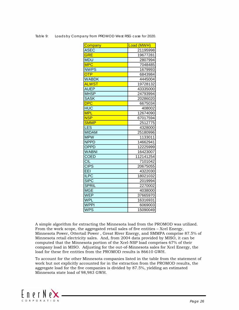
Page 26
Table 9: Loads by Company from PROMOD West RSG case for 2020.
Company Load (MWH)ASEC 21195998GRE 19677281MDU 2807994MPC 7048485NWPS 1679993OTP 6843984WABDK 4445004ALWST 19728132AUEP 43335000MHSP 24793994SASK 20286020DPC 6675034HUC 408002MPL 12674090NSP 67017594SMMP 2512775LES 4328000MIDAM 25180996MPW 1133011NPPD 14662941OPPD 12225999WABNI 16423007COED 112141254CIL 7101042CIPS 20675055EEI 4322030ILPC 18021032SIPC 2019994SPRIL 2270002MGE 4038000WEP 37665970WPL 16316931WPPI 6069003WPS 15090049
A simple algorithm for extracting the Minnesota load from the PROMOD was utilized. From the work scope, the aggregated retail sales of five entities – Xcel Energy, Minnesota Power, Ottertail Power , Great River Energy, and SMMPA comprise 87.5% of Minnesota retail electricity sales. And, from 2004 data provided by MISO, it can be computed that the Minnesota portion of the Xcel-NSP load comprises 67% of their company load in MISO. Adjusting for the out-of-Minnesota sales for Xcel Energy, the load for these five entities from the PROMOD results is 86610 GWH.
To account for the other Minnesota companies listed in the table from the statement of work but not explicitly accounted for in the extraction from the PROMOD results, the aggregate load for the five companies is divided by 87.5%, yielding an estimated Minnesota state load of 98,983 GWH.
Page 27
The PROMOD load is not “retail sales” as it is comprised of the energy transported to high voltage delivery points (substations). Losses in the distribution system are estimated to be about 7%. Applying this factor to the PROMOD load to estimate “retail sales” at customer metering points yields estimated Minnesota retail sales of 92,054 GWH.
From information exchanged with MISO, it was confirmed that an average growth rate of 2.5% was assumed for scaling loads for the 2020 West RSG PROMOD case. The number above is almost identical to the 2004 Minnesota retail sales escalated at 2.5% annual growth to 2020. It appears, therefore, that the simple algorithm proposed does a good job in estimating Minnesota retail sales from the PROMOD data.
A consequence of the PROMOD loads in the 2020 West RSG case is that the wind generation data provided earlier amounts to slightly less than the target energy penetration levels due to slightly increased retail sales. After discussions, it was decided that the most straightforward way to compensate would be to increase the wind generation slightly. This was accomplished by increasing the installed capacity numbers by a factor equal to 92,054/86,610, or 1.063.
Correlated hourly wind generation and load data is a foundation for the hourly analysis in this study. Because wind generation and electric demand are both affected by the regional meteorology, it is important to preserve the correlations that might exist between these data sets. As previously described, chronological wind speed and generation data profiles were developed at five minute intervals for the historical years 2003, 2004, and 2005. To create the load data corresponding to these years, hourly load data from these years for the Minnesota companies was retrieved from archives and scaled per the discussion above to create load data for the study. CY2004 was selected as the “base” year in that it was modified to achieve the target annual retail electric sales. The ratio between the new peak hourly load for the 2020 data and the peak load for the historical 2004 load data was then applied to load data from 2003 and 2005.
Developing Wind Generation Data The basic approach for developing wind generation profiles is to apply a “power curve” from a commercial wind turbine to the wind speed values at each five-minute interval. With 152 observation points in the MM5 model and up to 6000 MW of wind generation potentially required in the model, each wind speed observation must represent more than a single turbine.
Appendix C describes the approach used for this study, which approximates spatial diversity, terrain, and turbine shadowing effects by adjusting raw wind speed values at high resolution before calculating power (Figure 16). Wind speed data at five-minute intervals over three consecutive calendar years across 152 separate locations across Minnesota and the eastern half of the Dakotas was processed to yield five-minute and hourly wind generation data for each of the scenarios.
In an earlier section and in the companion report, it was noted that net capacity factors were calculated by assuming a constant loss factor of 14%. The wind generation data calculated from the method described in the appendix makes no such assumption, as the effective plant power curve takes those factors which contribute to the losses into account.
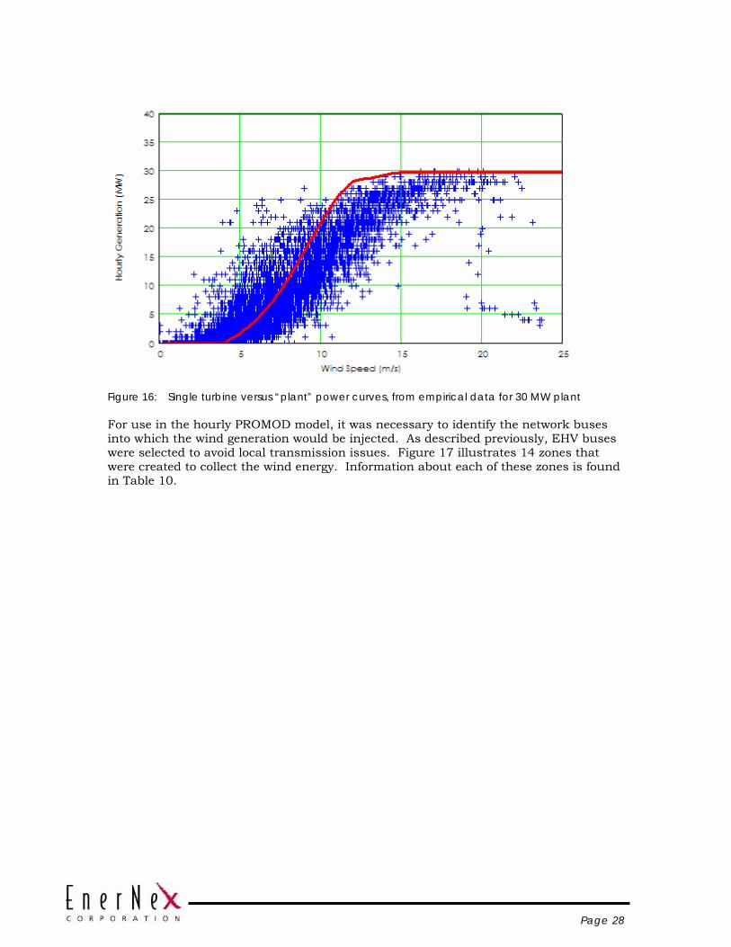
Page 28
Figure 16: Single turbine versus “plant” power curves, from empirical data for 30 MW plant
For use in the hourly PROMOD model, it was necessary to identify the network buses into which the wind generation would be injected. As described previously, EHV buses were selected to avoid local transmission issues. Figure 17 illustrates 14 zones that were created to collect the wind energy. Information about each of these zones is found in Table 10.

Page 29
Figure 17: Wind generation regions and network injection buses
Inje
ctio
n st
atio
ns
Tow
ers
to s
tatio
n
12
3
4
56
7
8
9
1011
1213
14
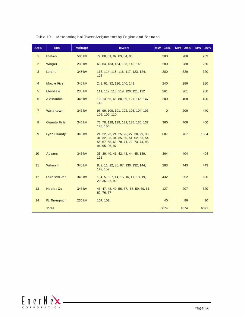
Page 30
Table 10: Meteorological Tower Assignments by Region and Scenario
Area Bus Voltage Towers MW – 15% MW – 20% MW – 25%
1 Forbes 500 kV 79, 80, 81, 82, 83, 84, 85 200 280 289
2 Winger 230 kV 63, 64, 133, 134, 138, 142, 143 200 280 280
3 Leland 345 kV 113, 114, 115, 116, 117, 123, 124, 125
280 320 320
4 Maple River 345 kV 2, 3, 91, 92, 126, 140, 141 240 280 280
5 Ellendale 230 kV 111, 112, 118, 119, 120, 121, 122 261 261 280
6 Alexandria 345 kV 10, 13, 65, 68, 88, 89, 127, 146, 147, 148
280 400 400
7 Watertown 345 kV 98, 99, 100, 101, 102, 103, 104, 105, 106, 109, 110
0 200 440
8 Granite Falls 345 kV 75, 78, 128, 129, 131, 135, 136, 137, 145, 150
360 400 400
9 Lyon County 345 kV 21, 22, 23, 24, 25, 26, 27, 28, 29, 30, 31, 32, 33, 34, 35, 50, 51, 52, 53, 54, 55, 67, 68, 69, 70, 71, 72, 73, 74, 93, 94, 95, 96, 97
607 767 1364
10 Adams 345 kV 38, 39, 40, 41, 42, 43, 44, 45, 139, 151
364 404 404
11 Willmarth 345 kV 8, 9, 11, 12, 86, 87, 130, 132, 144, 149, 152
283 443 443
12 Lakefield Jct. 345 kV 1, 4, 5, 6, 7, 14, 15, 16, 17, 18, 19, 20, 36, 37, 90
432 552 600
13 Nobles Co. 345 kV 46, 47, 48, 49, 56, 57, 58, 59, 60, 61, 62, 76, 77
127 207 520
14 Ft. Thompson 230 kV 107, 108 40 80 80
Total 3674 4874 6091
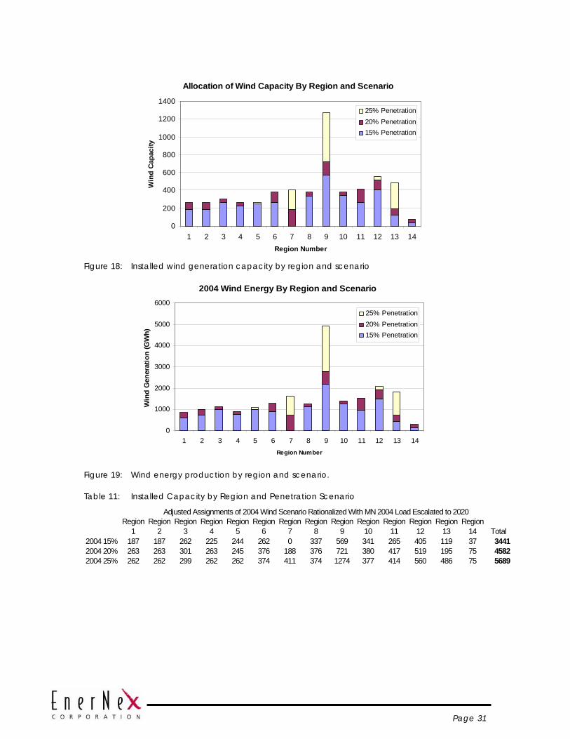
Page 31
Figure 18: Installed wind generation capacity by region and scenario
Figure 19: Wind energy production by region and scenario.
Table 11: Installed Capacity by Region and Penetration Scenario
Region 1
Region 2
Region 3
Region 4
Region 5
Region 6
Region 7
Region 8
Region 9
Region 10
Region 11
Region 12
Region 13
Region 14 Total
2004 15% 187 187 262 225 244 262 0 337 569 341 265 405 119 37 34412004 20% 263 263 301 263 245 376 188 376 721 380 417 519 195 75 45822004 25% 262 262 299 262 262 374 411 374 1274 377 414 560 486 75 5689
Adjusted Assignments of 2004 Wind Scenario Rationalized With MN 2004 Load Escalated to 2020
2004 Wind Energy By Region and Scenario
0
1000
2000
3000
4000
5000
6000
1 2 3 4 5 6 7 8 9 10 11 12 13 14Region Number
Win
d G
ener
atio
n (G
Wh)
25% Penetration20% Penetration15% Penetration
Allocation of Wind Capacity By Region and Scenario
0
200
400
600
800
1000
1200
1400
1 2 3 4 5 6 7 8 9 10 11 12 13 14Region Number
Win
d Ca
paci
ty
25% Penetration20% Penetration15% Penetration
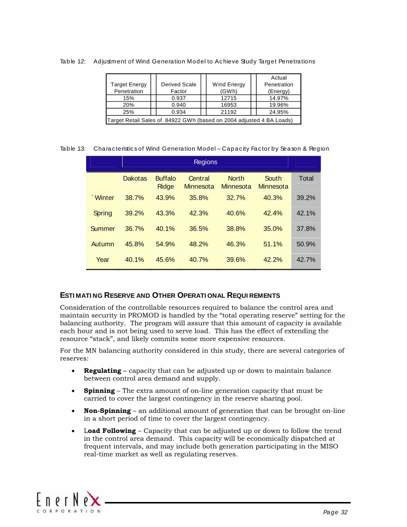
Page 32
Table 12: Adjustment of Wind Generation Model to Achieve Study Target Penetrations
Target Energy Penetration
Derived Scale Factor
Wind Energy (GWh)
Actual Penetration
(Energy)15% 0.937 12715 14.97%20% 0.940 16953 19.96%25% 0.934 21192 24.95%
Target Retail Sales of 84922 GWh (based on 2004 adjusted 4 BA Loads)
Table 13: Characteristics of Wind Generation Model – Capacity Factor by Season & Region
Regions
Dakotas Buffalo Ridge
Central Minnesota
North Minnesota
South Minnesota
Total
`Winter 38.7% 43.9% 35.8% 32.7% 40.3% 39.2%
Spring 39.2% 43.3% 42.3% 40.6% 42.4% 42.1%
Summer 36.7% 40.1% 36.5% 38.8% 35.0% 37.8%
Autumn 45.8% 54.9% 48.2% 46.3% 51.1% 50.9%
Year 40.1% 45.6% 40.7% 39.6% 42.2% 42.7%
ESTIMATING RESERVE AND OTHER OPERATIONAL REQUIREMENTS Consideration of the controllable resources required to balance the control area and maintain security in PROMOD is handled by the “total operating reserve” setting for the balancing authority. The program will assure that this amount of capacity is available each hour and is not being used to serve load. This has the effect of extending the resource “stack”, and likely commits some more expensive resources.
For the MN balancing authority considered in this study, there are several categories of reserves:
• Regulating – capacity that can be adjusted up or down to maintain balance between control area demand and supply.
• Spinning – The extra amount of on-line generation capacity that must be carried to cover the largest contingency in the reserve sharing pool.
• Non-Spinning – an additional amount of generation that can be brought on-line in a short period of time to cover the largest contingency.
• Load Following – Capacity that can be adjusted up or down to follow the trend in the control area demand. This capacity will be economically dispatched at frequent intervals, and may include both generation participating in the MISO real-time market as well as regulating reserves.
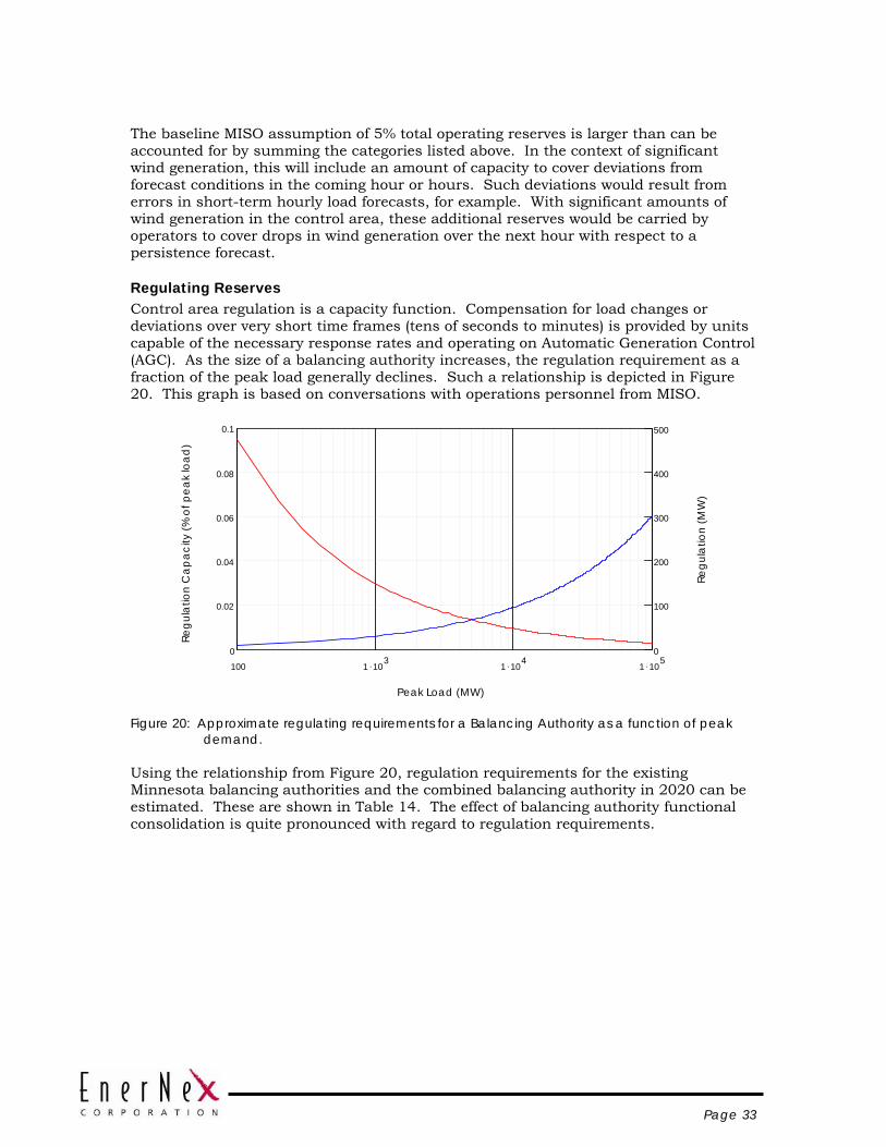
Page 33
The baseline MISO assumption of 5% total operating reserves is larger than can be accounted for by summing the categories listed above. In the context of significant wind generation, this will include an amount of capacity to cover deviations from forecast conditions in the coming hour or hours. Such deviations would result from errors in short-term hourly load forecasts, for example. With significant amounts of wind generation in the control area, these additional reserves would be carried by operators to cover drops in wind generation over the next hour with respect to a persistence forecast.
Regulating Reserves Control area regulation is a capacity function. Compensation for load changes or deviations over very short time frames (tens of seconds to minutes) is provided by units capable of the necessary response rates and operating on Automatic Generation Control (AGC). As the size of a balancing authority increases, the regulation requirement as a fraction of the peak load generally declines. Such a relationship is depicted in Figure 20. This graph is based on conversations with operations personnel from MISO.
100 1 .103
1 .104
1 .105
0
0.02
0.04
0.06
0.08
0.1
0
100
200
300
400
500
Peak Load (MW)
Regu
latio
n C
apa
city
(% o
f pea
k lo
ad)
Regu
latio
n (M
W)
Figure 20: Approximate regulating requirements for a Balancing Authority as a function of peak
demand.
Using the relationship from Figure 20, regulation requirements for the existing Minnesota balancing authorities and the combined balancing authority in 2020 can be estimated. These are shown in Table 14. The effect of balancing authority functional consolidation is quite pronounced with regard to regulation requirements.
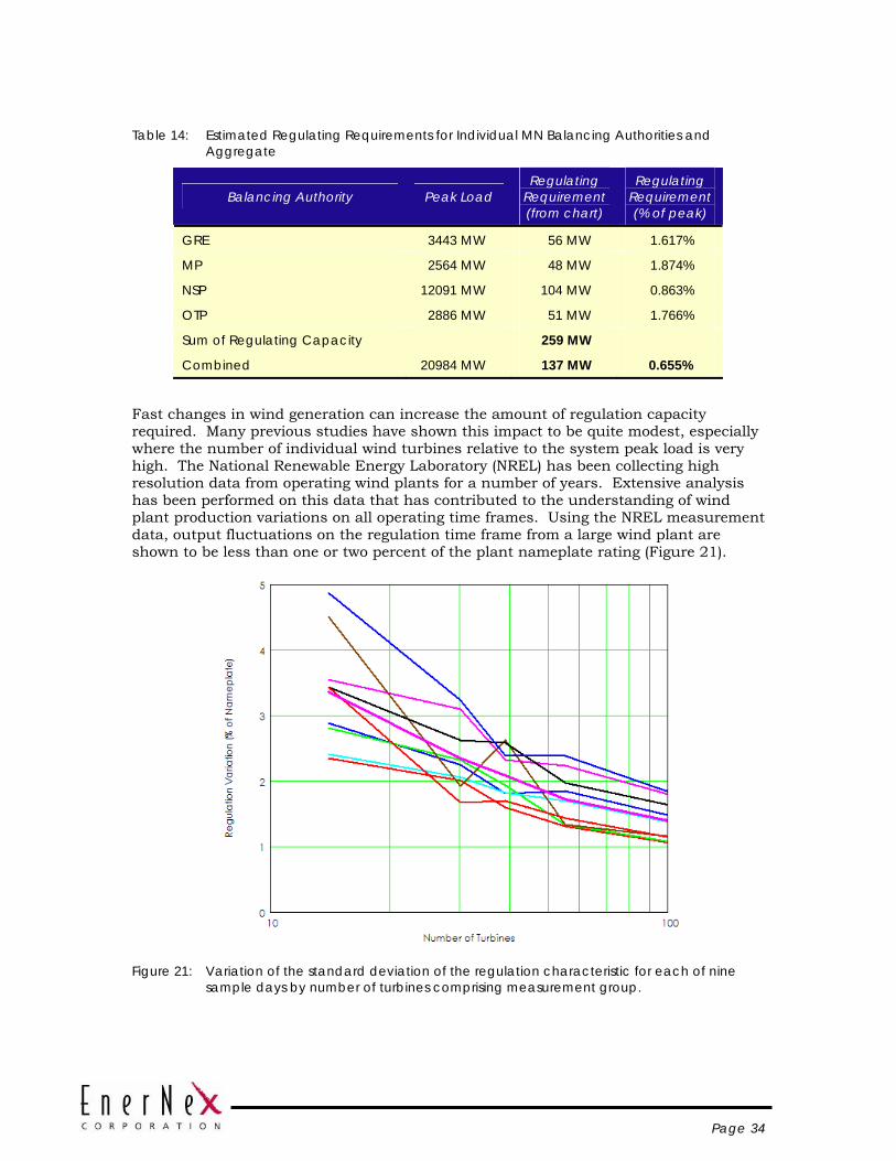
Page 34
Table 14: Estimated Regulating Requirements for Individual MN Balancing Authorities and Aggregate
Balancing Authority Peak Load Regulating
Requirement (from chart)
Regulating Requirement (% of peak)
GRE 3443 MW 56 MW 1.617%
MP 2564 MW 48 MW 1.874%
NSP 12091 MW 104 MW 0.863%
OTP 2886 MW 51 MW 1.766%
Sum of Regulating Capacity 259 MW
Combined 20984 MW 137 MW 0.655%
Fast changes in wind generation can increase the amount of regulation capacity required. Many previous studies have shown this impact to be quite modest, especially where the number of individual wind turbines relative to the system peak load is very high. The National Renewable Energy Laboratory (NREL) has been collecting high resolution data from operating wind plants for a number of years. Extensive analysis has been performed on this data that has contributed to the understanding of wind plant production variations on all operating time frames. Using the NREL measurement data, output fluctuations on the regulation time frame from a large wind plant are shown to be less than one or two percent of the plant nameplate rating (Figure 21).
Figure 21: Variation of the standard deviation of the regulation characteristic for each of nine
sample days by number of turbines comprising measurement group.

Page 35
Using a conservative estimate of 2 MW for each 100 MW of wind generation in the scenarios for this study, the regulation requirement for the combined MN balancing authority with the prescribed amounts of wind generation can be computed. By assuming that the regulation variations between each wind plant and the load are uncorrelated, the regulation requirement for the load and wind combination is computed with the following formula:
New_Regulating_Requirement k σLoad2 N σw100
2⎛⎝
⎞⎠⋅+:=
Where
k = a factor relating regulation capacity requirement to the standard deviation of the regulation variations; assumed to be 5
σLoad = standard deviation of regulation variations from the load
σw100 = standard deviation of the regulation variations from a 100 MW wind plant
N = wind generation capacity in the scenario divided by 100
Results of this computation for the three wind generation scenarios are shown in Table 15.
Table 15: Estimated Regulation Requirement for MN Balancing Authority in 2020
Scenario Regulation Capacity Requirement
Base 137 MW
15% Wind Generation 149 MW
20% Wind Generation 153 MW
25% Wind Generation 157 MW
Contingency Reserves The present reserve obligation for the Minnesota balancing authorities and companies is defined by the rules of the MAPP Generation Reserve Sharing Pool. The largest contingency which defines the pool’s reserve requirement is the loss of 1500 MW important from Manitoba on a 500 kV transmission line.
In the scenario defined for the study, the reserve obligation of the Minnesota utilities is projected to remain unchanged because:
• Loss of the Manitoba import is still assumed to be the largest single contingency
• The share of load in the reserve sharing pool, and the end-use load obligation (EULO) ratio of the Minnesota utilities to the larger pool is also assumed to remain the same.
Consequently, the Minnesota balancing authority would be required to carry 660 MW of reserve, of which 330 MW is spinning and 330 MW is quick-start.

Page 36
Note: After this study was well underway, the consolidation of the MAPP Generation Reserve Sharing Pool into a new, larger entity that largely encompasses the MISO Reliability Footprint was announced. The Midwest Contingency Reserve Sharing Group filed its participation agreement with the Federal Energy Regulatory commission in the fall of 2006. Beginning January 1, 2007, the Midwest contingency Reserve Sharing Group is scheduled to commence operations and is anticipated to reduce the contingency reserve obligation of the Minnesota utilities.
Load Following Within the hour, enough generation must be available to compensate for the underlying trends in the load beyond the fast regulation time frame. In MISO, load trends are accommodated by a combination of the real-time market and regulation capability. Either response cannot be directly considered in the PROMOD hourly analysis. Therefore, no distinction will be made, and the effects of wind generation will be gauged from analysis of load and wind time series data alone.
Figure 22 through Figure 24 depict the distributions of absolute changes over a five-minute interval for load and load net wind generation. The effect of wind generation on these changes is relatively modest, owing to the significant geographic diversity present in the wind scenarios.
Additional amounts of generic reserve can be estimated as some multiple of the standard deviations. As shown in Table 16, two standard deviations, which would encompass over 95% of all variations in the sample, was assumed. This assumption is consistent with operational practice for power systems. The metric by which control over periods of ten minutes is judged, CPS2 (Control Performance Standard 2) requires that the difference between load and generation over a ten-minute period must be smaller than a specified limit for 90% or more of the ten-minute intervals over the month. Consequently, not all deviations in the control area demand are fully compensated, as CPS2 scores for existing control areas vary across the range from 90 to 100%.
Table 16: Summary of Five-minute Variability
Scenario Standard Deviation of 5-minute changes
Base 50 MW
15% Wind Generation 55 MW
20% Wind Generation 57 MW
25% Wind Generation 62 MW
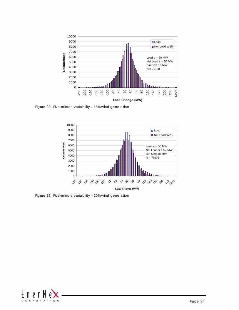
Page 37
0100020003000400050006000700080009000
10000
-250
-220
-190
-160
-130
-100 -7
0
-40
-10 20 50 80 110
140
170
200
230
Mor
e
Load Change (MW)
Occ
urre
nces
LoadNet Load W15
Load s = 50 MWNet Load s = 55 MW Bin Size 10 MWN = 79138
Figure 22: Five-minute variability – 15% wind generation
0
1000
2000
3000
4000
5000
6000
7000
8000
9000
10000
-250 -220 -190 -160 -130 -100 -70 -40 -10 20 50 80 110
140
170
200
230
More
Load Change (MW)
Occ
urre
nces
LoadNet Load W20
Load s = 50 MWNet Load s = 57 MW Bin Size 10 MWN = 79138
Figure 23: Five-minute variability – 20% wind generation
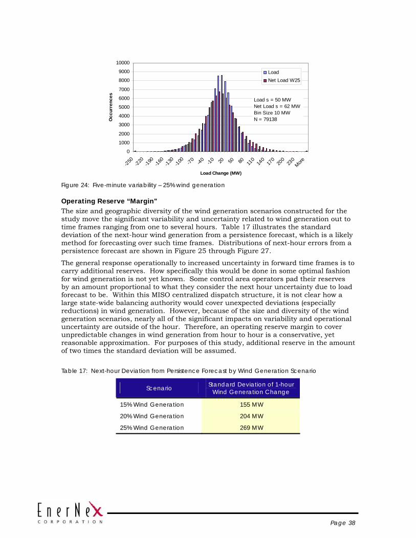
Page 38
0
1000
2000
3000
4000
5000
6000
7000
8000
9000
10000
-250 -220 -190 -160 -130 -100 -70 -40 -10 20 50 80 110
140
170
200
230
More
Load Change (MW)
Occ
urre
nces
LoadNet Load W25
Load s = 50 MWNet Load s = 62 MW Bin Size 10 MWN = 79138
Figure 24: Five-minute variability – 25% wind generation
Operating Reserve “Margin" The size and geographic diversity of the wind generation scenarios constructed for the study move the significant variability and uncertainty related to wind generation out to time frames ranging from one to several hours. Table 17 illustrates the standard deviation of the next-hour wind generation from a persistence forecast, which is a likely method for forecasting over such time frames. Distributions of next-hour errors from a persistence forecast are shown in Figure 25 through Figure 27.
The general response operationally to increased uncertainty in forward time frames is to carry additional reserves. How specifically this would be done in some optimal fashion for wind generation is not yet known. Some control area operators pad their reserves by an amount proportional to what they consider the next hour uncertainty due to load forecast to be. Within this MISO centralized dispatch structure, it is not clear how a large state-wide balancing authority would cover unexpected deviations (especially reductions) in wind generation. However, because of the size and diversity of the wind generation scenarios, nearly all of the significant impacts on variability and operational uncertainty are outside of the hour. Therefore, an operating reserve margin to cover unpredictable changes in wind generation from hour to hour is a conservative, yet reasonable approximation. For purposes of this study, additional reserve in the amount of two times the standard deviation will be assumed.
Table 17: Next-hour Deviation from Persistence Forecast by Wind Generation Scenario
Scenario Standard Deviation of 1-hour Wind Generation Change
15% Wind Generation 155 MW
20% Wind Generation 204 MW
25% Wind Generation 269 MW
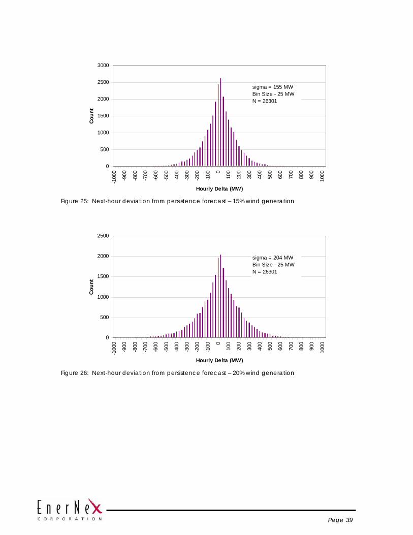
Page 39
0
500
1000
1500
2000
2500
3000
-100
0
-900
-800
-700
-600
-500
-400
-300
-200
-100 0
100
200
300
400
500
600
700
800
900
1000
Hourly Delta (MW)
Cou
ntsigma = 155 MWBin Size - 25 MWN = 26301
Figure 25: Next-hour deviation from persistence forecast – 15% wind generation
0
500
1000
1500
2000
2500
-100
0
-900
-800
-700
-600
-500
-400
-300
-200
-100 0
100
200
300
400
500
600
700
800
900
1000
Hourly Delta (MW)
Cou
nt
sigma = 204 MWBin Size - 25 MWN = 26301
Figure 26: Next-hour deviation from persistence forecast – 20% wind generation
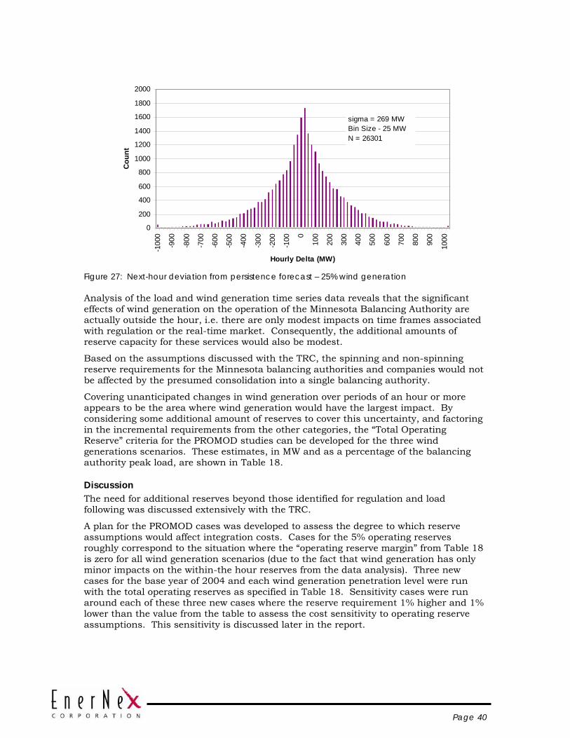
Page 40
0
200
400
600
800
1000
1200
1400
1600
1800
2000
-100
0
-900
-800
-700
-600
-500
-400
-300
-200
-100 0
100
200
300
400
500
600
700
800
900
1000
Hourly Delta (MW)
Cou
ntsigma = 269 MWBin Size - 25 MWN = 26301
Figure 27: Next-hour deviation from persistence forecast – 25% wind generation
Analysis of the load and wind generation time series data reveals that the significant effects of wind generation on the operation of the Minnesota Balancing Authority are actually outside the hour, i.e. there are only modest impacts on time frames associated with regulation or the real-time market. Consequently, the additional amounts of reserve capacity for these services would also be modest.
Based on the assumptions discussed with the TRC, the spinning and non-spinning reserve requirements for the Minnesota balancing authorities and companies would not be affected by the presumed consolidation into a single balancing authority.
Covering unanticipated changes in wind generation over periods of an hour or more appears to be the area where wind generation would have the largest impact. By considering some additional amount of reserves to cover this uncertainty, and factoring in the incremental requirements from the other categories, the “Total Operating Reserve” criteria for the PROMOD studies can be developed for the three wind generations scenarios. These estimates, in MW and as a percentage of the balancing authority peak load, are shown in Table 18.
Discussion The need for additional reserves beyond those identified for regulation and load following was discussed extensively with the TRC.
A plan for the PROMOD cases was developed to assess the degree to which reserve assumptions would affect integration costs. Cases for the 5% operating reserves roughly correspond to the situation where the “operating reserve margin” from Table 18 is zero for all wind generation scenarios (due to the fact that wind generation has only minor impacts on the within-the hour reserves from the data analysis). Three new cases for the base year of 2004 and each wind generation penetration level were run with the total operating reserves as specified in Table 18. Sensitivity cases were run around each of these three new cases where the reserve requirement 1% higher and 1% lower than the value from the table to assess the cost sensitivity to operating reserve assumptions. This sensitivity is discussed later in the report.
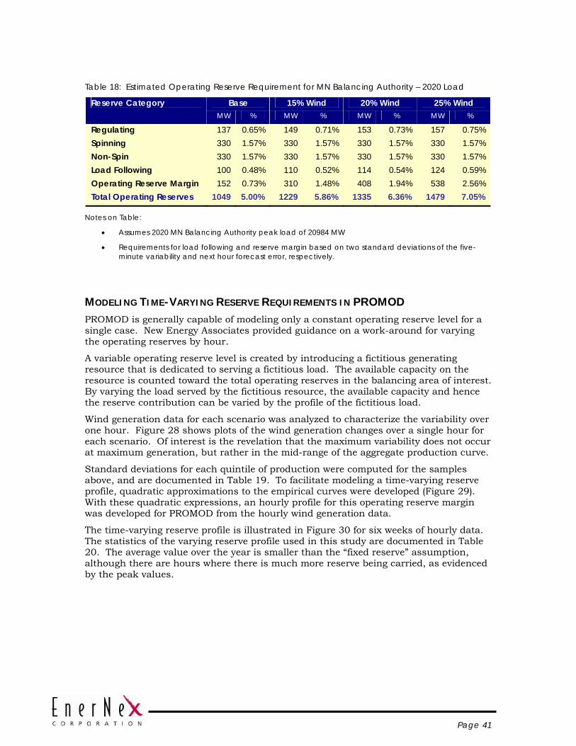
Page 41
Table 18: Estimated Operating Reserve Requirement for MN Balancing Authority – 2020 Load
Base 15% Wind 20% Wind 25% Wind Reserve Category MW % MW % MW % MW %
Regulating 137 0.65% 149 0.71% 153 0.73% 157 0.75% Spinning 330 1.57% 330 1.57% 330 1.57% 330 1.57% Non-Spin 330 1.57% 330 1.57% 330 1.57% 330 1.57% Load Following 100 0.48% 110 0.52% 114 0.54% 124 0.59% Operating Reserve Margin 152 0.73% 310 1.48% 408 1.94% 538 2.56% Total Operating Reserves 1049 5.00% 1229 5.86% 1335 6.36% 1479 7.05%
Notes on Table:
• Assumes 2020 MN Balancing Authority peak load of 20984 MW
• Requirements for load following and reserve margin based on two standard deviations of the five-minute variability and next hour forecast error, respectively.
MODELING TIME-VARYING RESERVE REQUIREMENTS IN PROMOD PROMOD is generally capable of modeling only a constant operating reserve level for a single case. New Energy Associates provided guidance on a work-around for varying the operating reserves by hour.
A variable operating reserve level is created by introducing a fictitious generating resource that is dedicated to serving a fictitious load. The available capacity on the resource is counted toward the total operating reserves in the balancing area of interest. By varying the load served by the fictitious resource, the available capacity and hence the reserve contribution can be varied by the profile of the fictitious load.
Wind generation data for each scenario was analyzed to characterize the variability over one hour. Figure 28 shows plots of the wind generation changes over a single hour for each scenario. Of interest is the revelation that the maximum variability does not occur at maximum generation, but rather in the mid-range of the aggregate production curve.
Standard deviations for each quintile of production were computed for the samples above, and are documented in Table 19. To facilitate modeling a time-varying reserve profile, quadratic approximations to the empirical curves were developed (Figure 29). With these quadratic expressions, an hourly profile for this operating reserve margin was developed for PROMOD from the hourly wind generation data.
The time-varying reserve profile is illustrated in Figure 30 for six weeks of hourly data. The statistics of the varying reserve profile used in this study are documented in Table 20. The average value over the year is smaller than the “fixed reserve” assumption, although there are hours where there is much more reserve being carried, as evidenced by the peak values.
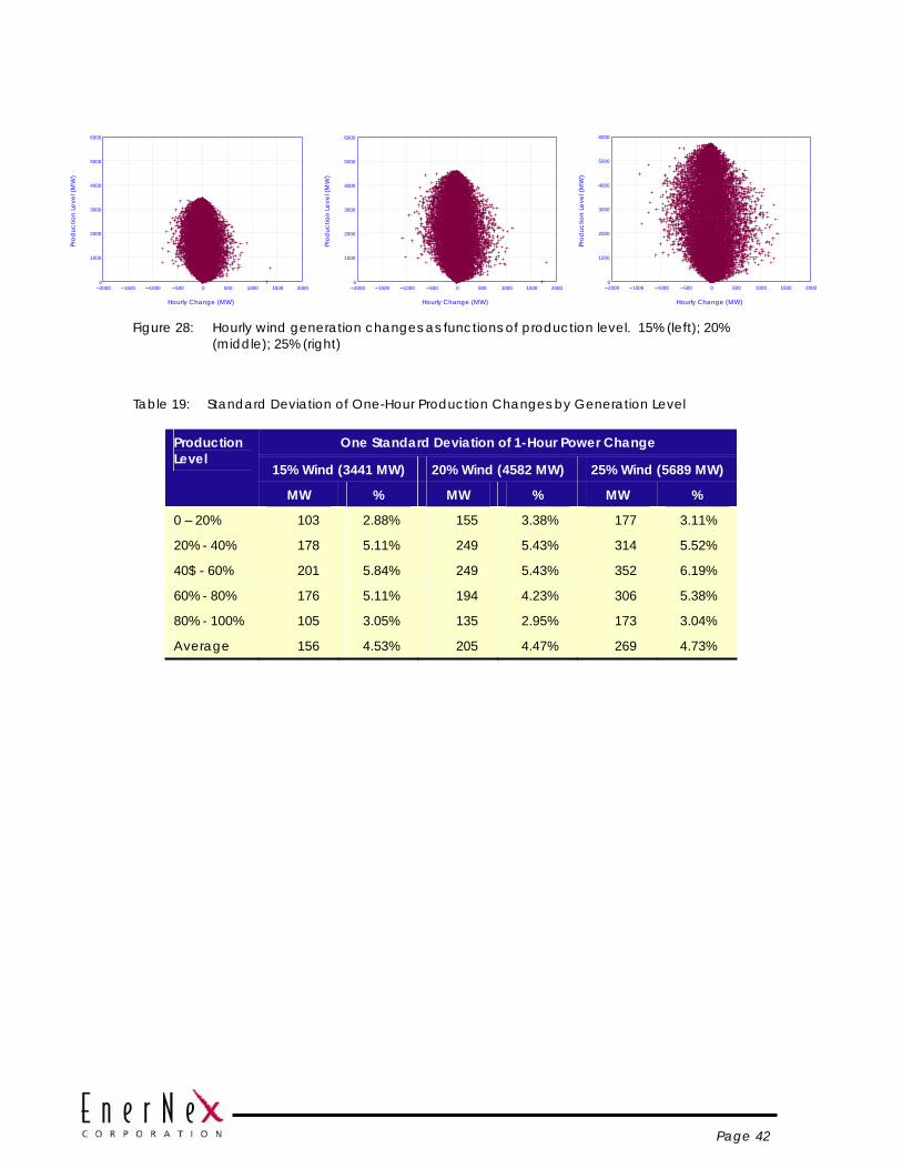
Page 42
2000 1500 1000 500 0 500 1000 1500 20000
1000
2000
3000
4000
5000
6000
Hourly Change (MW)
Prod
uctio
n Le
vel (
MW
)
2000 1500 1000 500 0 500 1000 1500 20000
1000
2000
3000
4000
5000
6000
Hourly Change (MW)
Prod
uctio
n Le
vel (
MW
)
2000 1500 1000 500 0 500 1000 1500 20000
1000
2000
3000
4000
5000
6000
Hourly Change (MW)
Prod
uctio
n Le
vel (
MW
)
Figure 28: Hourly wind generation changes as functions of production level. 15% (left); 20%
(middle); 25% (right)
Table 19: Standard Deviation of One-Hour Production Changes by Generation Level
One Standard Deviation of 1-Hour Power Change
15% Wind (3441 MW) 20% Wind (4582 MW) 25% Wind (5689 MW)
Production Level
MW % MW % MW %
0 – 20% 103 2.88% 155 3.38% 177 3.11%
20% - 40% 178 5.11% 249 5.43% 314 5.52%
40$ - 60% 201 5.84% 249 5.43% 352 6.19%
60% - 80% 176 5.11% 194 4.23% 306 5.38%
80% - 100% 105 3.05% 135 2.95% 173 3.04%
Average 156 4.53% 205 4.47% 269 4.73%
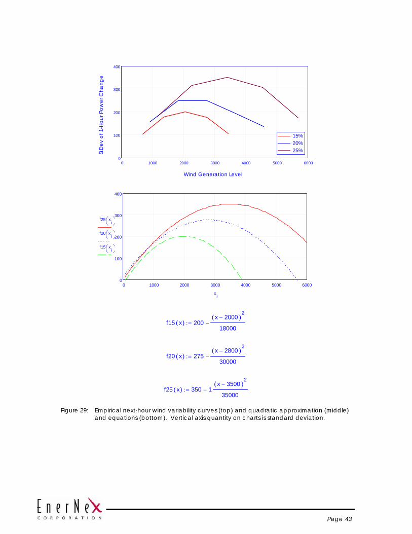
Page 43
0 1000 2000 3000 4000 5000 60000
100
200
300
400
15%20%25%
15%20%25%
Wind Generation Level
StD
ev o
f 1-H
our P
ower
Cha
nge
0 1000 2000 3000 4000 5000 60000
100
200
300
400
f25 xi⎛
⎝⎞⎠
f20 xi⎛
⎝⎞⎠
f15 xi⎛
⎝⎞⎠
xi
f15 x( ) 200x 2000−( )
2
18000−:=
f20 x( ) 275x 2800−( )
2
30000−:=
f25 x( ) 350 1x 3500−( )
2
35000−:=
Figure 29: Empirical next-hour wind variability curves (top) and quadratic approximation (middle)
and equations (bottom). Vertical axis quantity on charts is standard deviation.
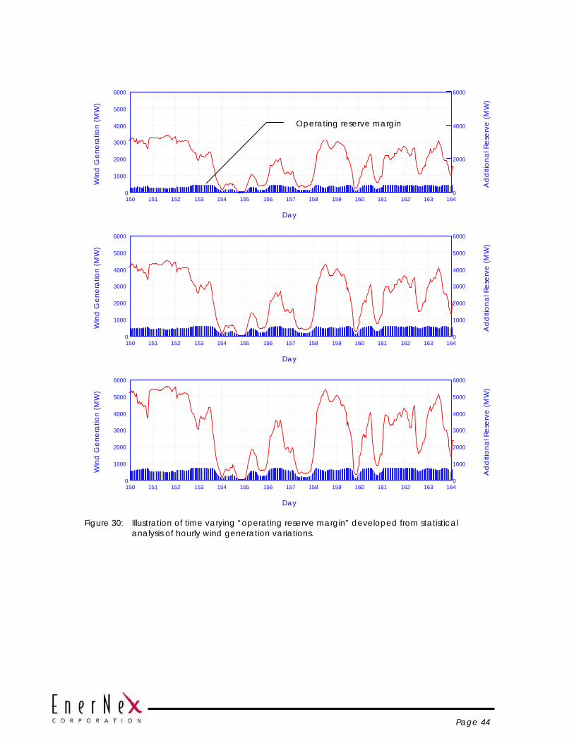
Page 44
150 151 152 153 154 155 156 157 158 159 160 161 162 163 1640
1000
2000
3000
4000
5000
6000
0
2000
4000
6000
Day
Win
d G
ener
atio
n (M
W)
Ad
diti
onal
Res
erve
(MW
)
150 151 152 153 154 155 156 157 158 159 160 161 162 163 1640
1000
2000
3000
4000
5000
6000
0
1000
2000
3000
4000
5000
6000
Day
Win
d G
ener
atio
n (M
W)
Ad
diti
onal
Res
erve
(MW
)150 151 152 153 154 155 156 157 158 159 160 161 162 163 1640
1000
2000
3000
4000
5000
6000
0
1000
2000
3000
4000
5000
6000
Day
Win
d G
ener
atio
n (M
W)
Ad
diti
onal
Res
erve
(MW
)
Figure 30: Illustration of time varying “operating reserve margin” developed from statistical
analysis of hourly wind generation variations.
Operating reserve margin
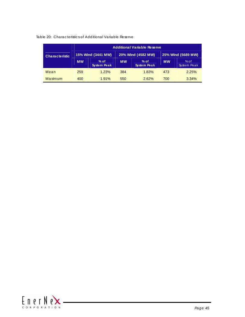
Page 45
Table 20: Characteristics of Additional Variable Reserve
Additional Variable Reserve
15% Wind (3441 MW) 20% Wind (4582 MW) 25% Wind (5689 MW) Characteristic MW % of
System Peak MW % of
System Peak MW % of
System Peak
Mean 259 1.23% 384 1.83% 473 2.25%
Maximum 400 1.91% 550 2.62% 700 3.34%
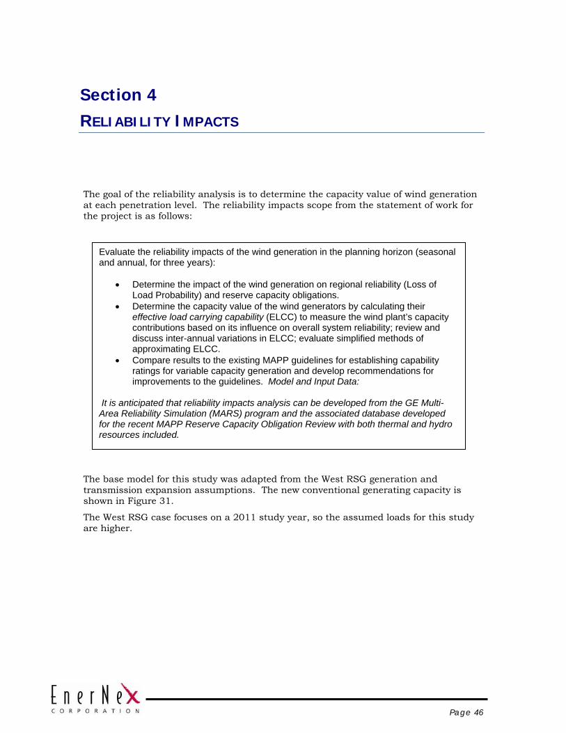
Page 46
Section 4 RELIABILITY IMPACTS
The goal of the reliability analysis is to determine the capacity value of wind generation at each penetration level. The reliability impacts scope from the statement of work for the project is as follows:
The base model for this study was adapted from the West RSG generation and transmission expansion assumptions. The new conventional generating capacity is shown in Figure 31.
The West RSG case focuses on a 2011 study year, so the assumed loads for this study are higher.
Evaluate the reliability impacts of the wind generation in the planning horizon (seasonal and annual, for three years):
• Determine the impact of the wind generation on regional reliability (Loss of Load Probability) and reserve capacity obligations.
• Determine the capacity value of the wind generators by calculating their effective load carrying capability (ELCC) to measure the wind plant’s capacity contributions based on its influence on overall system reliability; review and discuss inter-annual variations in ELCC; evaluate simplified methods of approximating ELCC.
• Compare results to the existing MAPP guidelines for establishing capability ratings for variable capacity generation and develop recommendations for improvements to the guidelines. Model and Input Data:
It is anticipated that reliability impacts analysis can be developed from the GE Multi-Area Reliability Simulation (MARS) program and the associated database developed for the recent MAPP Reserve Capacity Obligation Review with both thermal and hydro resources included.

Page 47
biomass, 15 MW
Wind, 2933 MW
Natural Gas, 300 MW
Coal, 2861 MW
Coal and/or a blend of Petroleum coke and
coal, 580 MW
Figure 31: New conventional generation in West RSG expansion plan
An initial assessment of wind energy production during the highest system load hours is presented in Figure 32. Three years of wind and load data (2003, 2004, and 2005) are sorted in descending order by load. Wind generation for the highest load hours is then summed, and the capacity factor for that number of hours is computed as an estimate of the contribution to system reliability.
An initial assessment of the capacity value of wind generation can be made with chronological wind and load data only. High load hours generally represent times when the system could be at risk of not having sufficient generation to meet demand. While these peak load hours may not represent the only times when the system is “at risk”, they are the major considerations for capacity planning studies.
Focusing only on the peak hours ignores the characteristics of the conventional generation portfolio, and assumes that load level is the only indicator of system reliability risk. It is, however, much less intensive in terms of data and computing time, and has been shown to provide an indication of the relative capacity contribution of wind generation in a particular system context.
The mathematical procedure is straightforward:
1. Construct a 2 x 8760 matrix, where the first column is hourly load and the second is hourly wind generation.
2. Sort the matrix of hourly load and wind generation pairs by the hourly load value, in descending order.
3. Calculate the wind energy delivery for the x highest load hours
4. Divide the wind energy delivered over those hours by the maximum that could have been delivered (installed capacity times number of hours)
5. Plot the results for various values of x.
Results of this procedure for each wind generation and load pattern year are shown in Figure 32.

Page 48
GE-MARS ANALYSIS The data set developed for the most recent MAPP Reserve Capacity Obligation (RCO) review was updated to reflect the assumptions for this study. The new generation capacity per Figure 31 was added, using forced outage data from similar units already in the data set. Hourly loads in the Minnesota area were replaced by those developed for this study. Loads in other areas were scaled by the same factor used to develop the 2020 loads for Minnesota.
Wind is treated as a load modifier. This involves running two separate cases – one with load alone (no wind), and the other with the hourly loads net of wind generation. All three sets of wind and load patterns corresponding to calendar years 2003, 2004, and 2005 were used.
A significant amount of new capacity in the Minnesota area was required to bring the reliability level to the target 1 day in 10 years for the no wind case. This shows that the baseline generation expansion assumptions for the study would not provide adequate reliability for projected 2020 loads.
Results Results of the GE-MARS simulations are presented in Figure 33 through Figure 35 and Table 21 through Table 23.

Page 49
1 10 100 1 .1030.2
0.36
0.52
0.68
0.84
1
15%20%25%
15%20%25%
2003 Wind and Load Patterns
# of Hours (1-year period)
Cap
acity
Fac
tor (
pu)
1 10 100 1 .1030
0.2
0.4
0.6
0.8
1
15%20%25%
15%20%25%
2004 Wind and Load Patterns
# of Hours (1-year period)
Ca
paci
ty F
act
or (p
u)
1 10 100 1 .1030
0.2
0.4
0.6
0.8
1
15%20%25%
15%20%25%
2005 Wind and Load Patterns
# of Hours (1-year period)
Ca
paci
ty F
act
or (p
u)
Figure 32: Wind generation capacity factor for varying number of highest load hours. (2003, 2004,
and 2005 wind and load patterns)

Page 50
0
0.1
0.2
0.3
0.4
0.5
0.97 0.98 0.99 1 1.01 1.02 1.03 1.04 1.05 1.06 1.07 1.08
Load (pu)
LOLE
2003 Base2003 15%2003 20%2003 25%
Figure 33: LOLE for Minnesota Area based on 2003 load and wind patterns
0
0.1
0.2
0.3
0.4
0.5
0.97 0.98 0.99 1 1.01 1.02 1.03 1.04 1.05 1.06
Load (pu)
LOLE
2004 Base2004 15%2004 20%2004 25%
Figure 34: LOLE for Minnesota Area based on 2004 load and wind patterns
0
0.1
0.2
0.3
0.4
0.5
0.97 0.98 0.99 1 1.01 1.02 1.03 1.04 1.05 1.06
Load (pu)
LOLE
2005 Base2005 15%2005 20%2005 25%
Figure 35: LOLE for Minnesota Area based on 2005 load and wind patterns
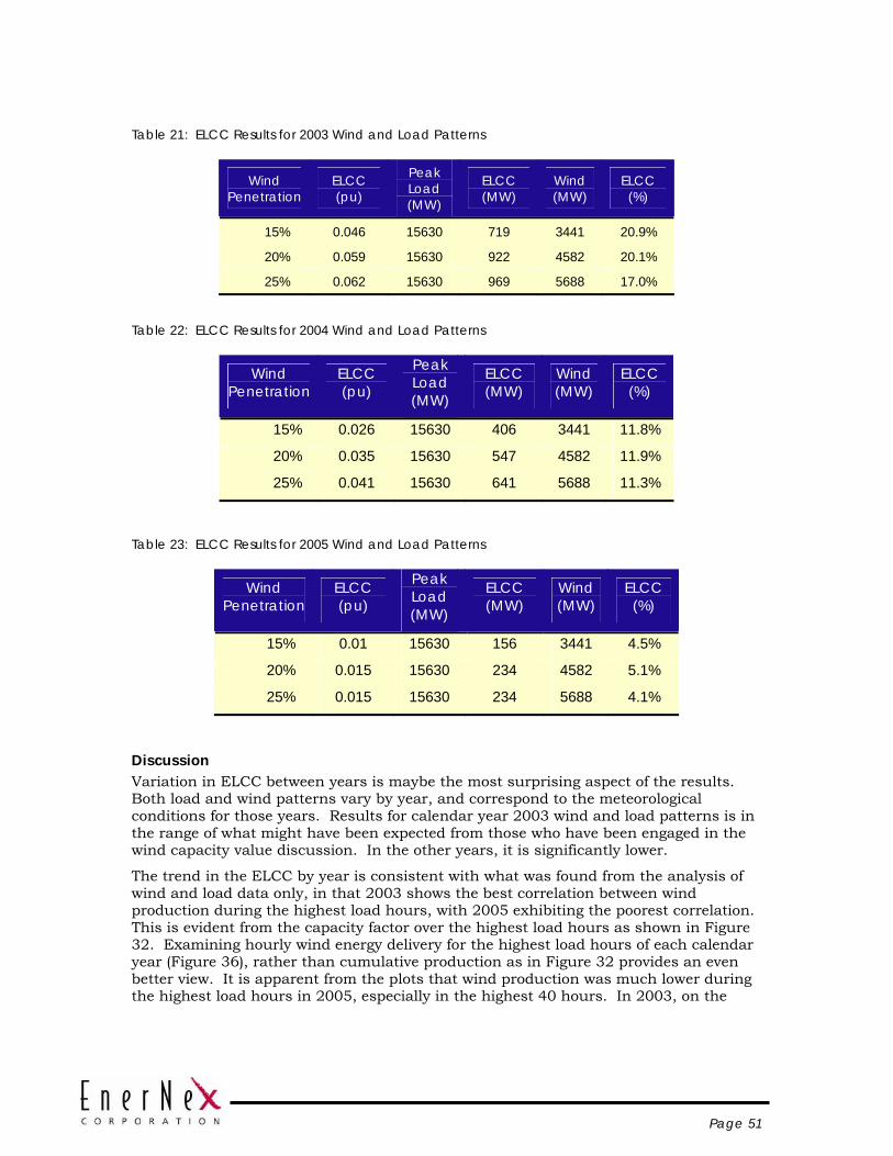
Page 51
Table 21: ELCC Results for 2003 Wind and Load Patterns
Wind Penetration
ELCC (pu)
Peak Load (MW)
ELCC (MW)
Wind (MW)
ELCC (%)
15% 0.046 15630 719 3441 20.9%
20% 0.059 15630 922 4582 20.1%
25% 0.062 15630 969 5688 17.0%
Table 22: ELCC Results for 2004 Wind and Load Patterns
Wind Penetration
ELCC (pu)
Peak Load (MW)
ELCC (MW)
Wind (MW)
ELCC (%)
15% 0.026 15630 406 3441 11.8%
20% 0.035 15630 547 4582 11.9%
25% 0.041 15630 641 5688 11.3%
Table 23: ELCC Results for 2005 Wind and Load Patterns
Wind Penetration
ELCC (pu)
Peak Load (MW)
ELCC (MW)
Wind (MW)
ELCC (%)
15% 0.01 15630 156 3441 4.5%
20% 0.015 15630 234 4582 5.1%
25% 0.015 15630 234 5688 4.1%
Discussion Variation in ELCC between years is maybe the most surprising aspect of the results. Both load and wind patterns vary by year, and correspond to the meteorological conditions for those years. Results for calendar year 2003 wind and load patterns is in the range of what might have been expected from those who have been engaged in the wind capacity value discussion. In the other years, it is significantly lower.
The trend in the ELCC by year is consistent with what was found from the analysis of wind and load data only, in that 2003 shows the best correlation between wind production during the highest load hours, with 2005 exhibiting the poorest correlation. This is evident from the capacity factor over the highest load hours as shown in Figure 32. Examining hourly wind energy delivery for the highest load hours of each calendar year (Figure 36), rather than cumulative production as in Figure 32 provides an even better view. It is apparent from the plots that wind production was much lower during the highest load hours in 2005, especially in the highest 40 hours. In 2003, on the
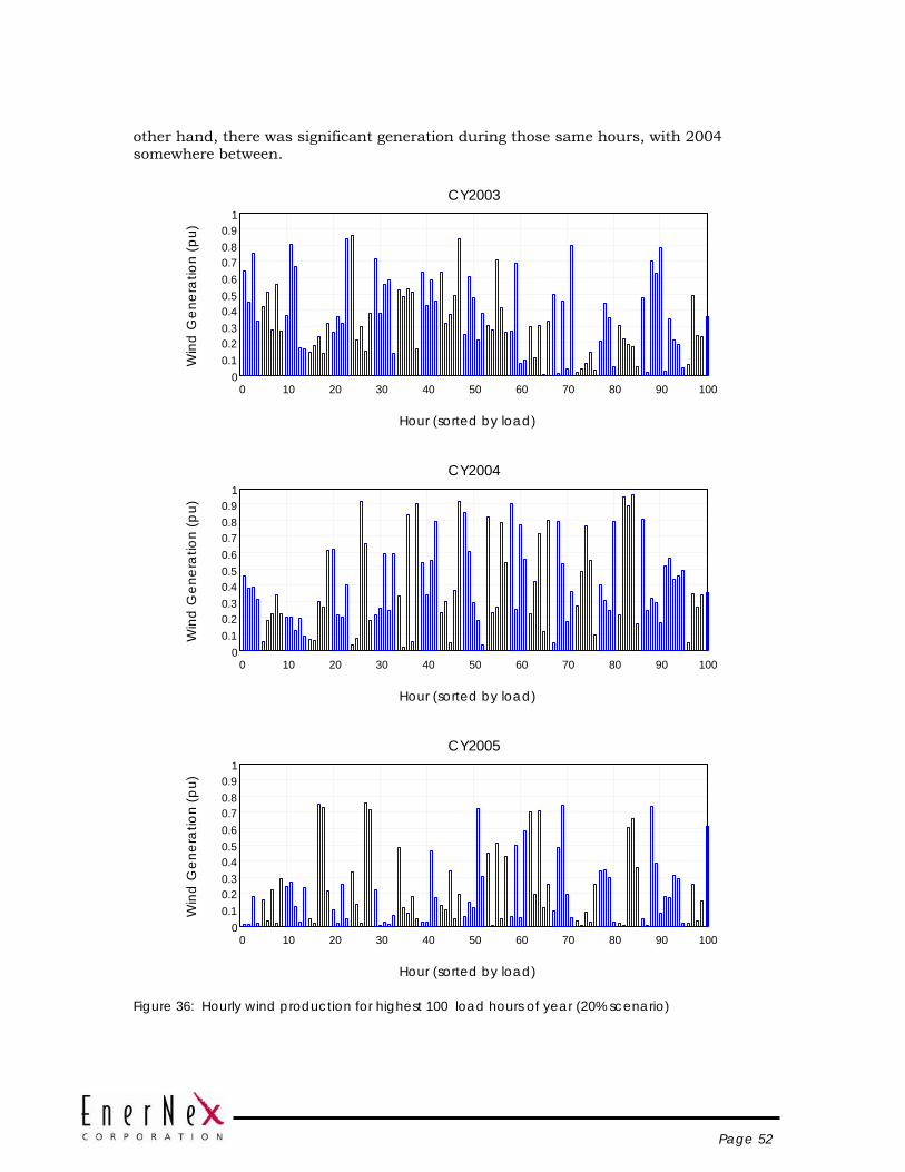
Page 52
other hand, there was significant generation during those same hours, with 2004 somewhere between.
0 10 20 30 40 50 60 70 80 90 1000
0.10.20.30.40.50.60.70.80.9
1CY2003
Hour (sorted by load)
Win
d G
ener
atio
n (p
u)
0 10 20 30 40 50 60 70 80 90 1000
0.10.20.30.40.50.60.70.80.9
1CY2004
Hour (sorted by load)
Win
d G
ener
atio
n (p
u)
0 10 20 30 40 50 60 70 80 90 1000
0.10.20.30.40.50.60.70.80.9
1CY2005
Hour (sorted by load)
Win
d G
ener
atio
n (p
u)
Figure 36: Hourly wind production for highest 100 load hours of year (20% scenario)
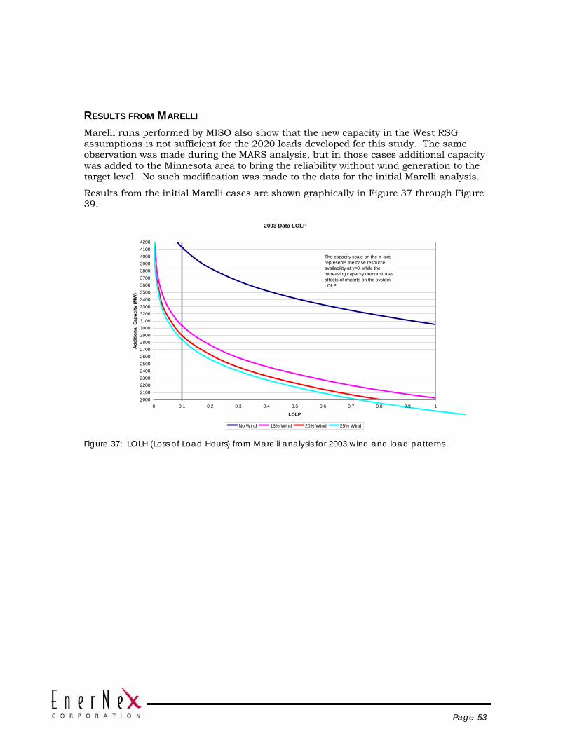
Page 53
RESULTS FROM MARELLI Marelli runs performed by MISO also show that the new capacity in the West RSG assumptions is not sufficient for the 2020 loads developed for this study. The same observation was made during the MARS analysis, but in those cases additional capacity was added to the Minnesota area to bring the reliability without wind generation to the target level. No such modification was made to the data for the initial Marelli analysis.
Results from the initial Marelli cases are shown graphically in Figure 37 through Figure 39.
2003 Data LOLP
20002100220023002400250026002700280029003000310032003300340035003600370038003900400041004200
0 0.1 0.2 0.3 0.4 0.5 0.6 0.7 0.8 0.9 1
LOLP
Add
ition
al C
apac
ity (M
W)
No Wind 15% Wind 20% Wind 25% Wind
The capacity scale on the Y-axis represents the base resource availability at y=0, while the increasing capacity demonstrates affects of imports on the system LOLP.
Figure 37: LOLH (Loss of Load Hours) from Marelli analysis for 2003 wind and load patterns
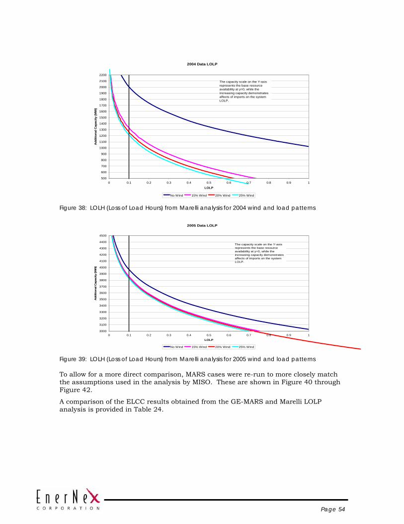
Page 54
2004 Data LOLP
500
600
700
800
900
1000
1100
1200
1300
1400
1500
1600
1700
1800
1900
2000
2100
2200
0 0.1 0.2 0.3 0.4 0.5 0.6 0.7 0.8 0.9 1
LOLP
Add
ition
al C
apac
ity (M
W)
No Wind 15% Wind 20% Wind 25% Wind
The capacity scale on the Y-axis represents the base resource availability at y=0, while the increasing capacity demonstrates affects of imports on the system LOLP.
Figure 38: LOLH (Loss of Load Hours) from Marelli analysis for 2004 wind and load patterns
2005 Data LOLP
3000
3100
3200
3300
3400
3500
3600
3700
3800
3900
4000
4100
4200
4300
4400
4500
0 0.1 0.2 0.3 0.4 0.5 0.6 0.7 0.8 0.9 1
LOLP
Add
ition
al C
apac
ity (M
W)
No Wind 15% Wind 20% Wind 25% Wind
The capacity scale on the Y-axis represents the base resource availability at y=0, while the increasing capacity demonstrates affects of imports on the system LOLP.
Figure 39: LOLH (Loss of Load Hours) from Marelli analysis for 2005 wind and load patterns
To allow for a more direct comparison, MARS cases were re-run to more closely match the assumptions used in the analysis by MISO. These are shown in Figure 40 through Figure 42.
A comparison of the ELCC results obtained from the GE-MARS and Marelli LOLP analysis is provided in Table 24.
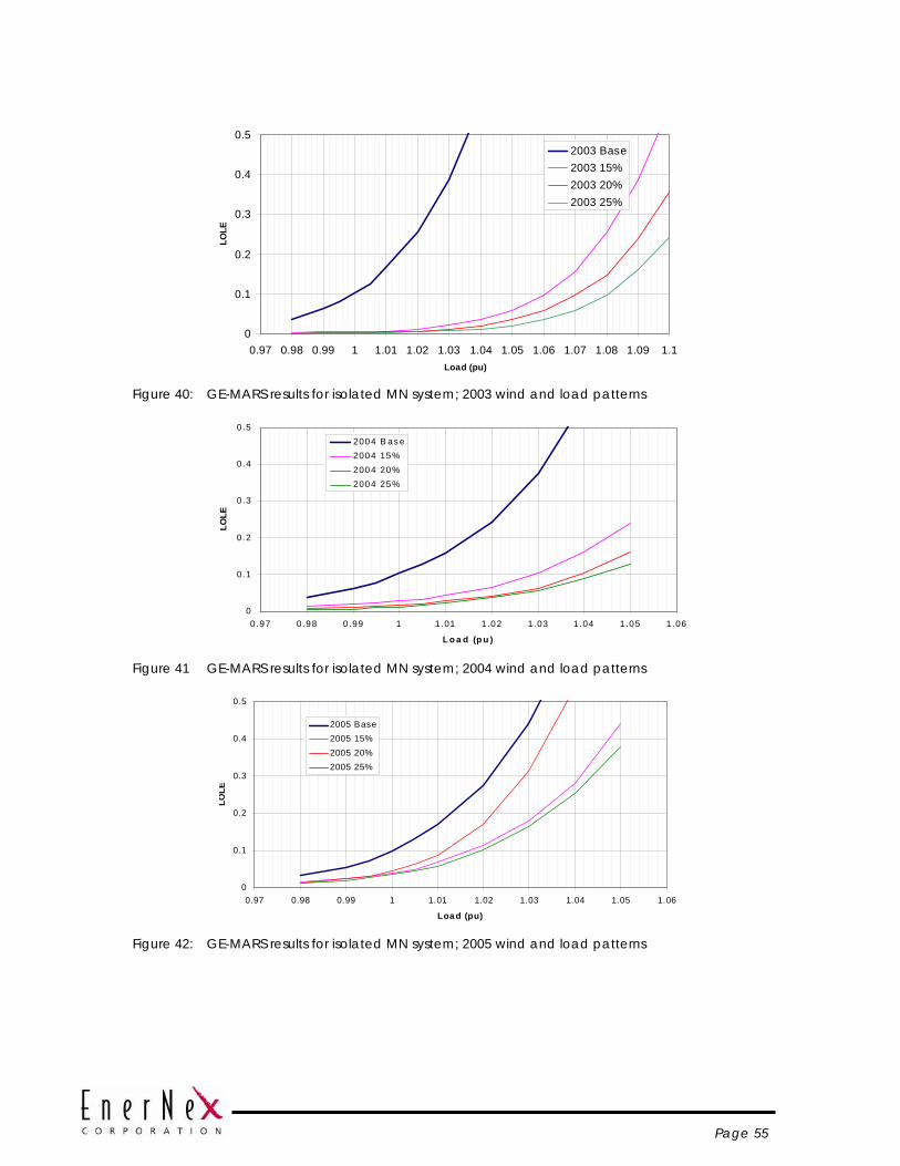
Page 55
0
0.1
0.2
0.3
0.4
0.5
0.97 0.98 0.99 1 1.01 1.02 1.03 1.04 1.05 1.06 1.07 1.08 1.09 1.1Load (pu)
LOLE
2003 Base2003 15%2003 20%2003 25%
Figure 40: GE-MARS results for isolated MN system; 2003 wind and load patterns
0
0.1
0.2
0.3
0.4
0.5
0 .97 0.98 0.99 1 1.01 1 .02 1.03 1.04 1 .05 1.06
L o a d (p u )
LOLE
2004 B as e2004 15%2004 20%2004 25%
Figure 41 GE-MARS results for isolated MN system; 2004 wind and load patterns
0
0.1
0.2
0.3
0.4
0.5
0.97 0.98 0.99 1 1.01 1.02 1.03 1.04 1.05 1.06
Loa d (pu)
LOLE
2005 Base2005 15%2005 20%2005 25%
Figure 42: GE-MARS results for isolated MN system; 2005 wind and load patterns
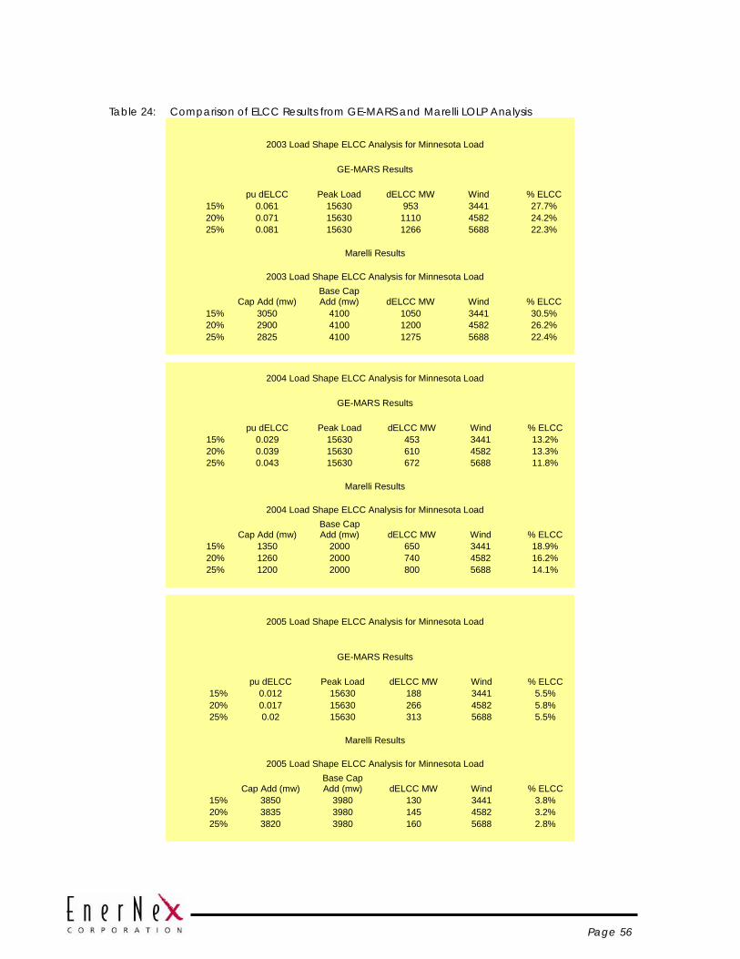
Page 56
Table 24: Comparison of ELCC Results from GE-MARS and Marelli LOLP Analysis
2003 Load Shape ELCC Analysis for Minnesota Load
GE-MARS Results
pu dELCC Peak Load dELCC MW Wind % ELCC 15% 0.061 15630 953 3441 27.7% 20% 0.071 15630 1110 4582 24.2% 25% 0.081 15630 1266 5688 22.3%
Marelli Results
2003 Load Shape ELCC Analysis for Minnesota Load
Cap Add (mw) Base Cap Add (mw) dELCC MW Wind % ELCC
15% 3050 4100 1050 3441 30.5% 20% 2900 4100 1200 4582 26.2% 25% 2825 4100 1275 5688 22.4%
2004 Load Shape ELCC Analysis for Minnesota Load
GE-MARS Results
pu dELCC Peak Load dELCC MW Wind % ELCC 15% 0.029 15630 453 3441 13.2% 20% 0.039 15630 610 4582 13.3% 25% 0.043 15630 672 5688 11.8%
Marelli Results
2004 Load Shape ELCC Analysis for Minnesota Load
Cap Add (mw) Base Cap Add (mw) dELCC MW Wind % ELCC
15% 1350 2000 650 3441 18.9% 20% 1260 2000 740 4582 16.2% 25% 1200 2000 800 5688 14.1%
2005 Load Shape ELCC Analysis for Minnesota Load
GE-MARS Results
pu dELCC Peak Load dELCC MW Wind % ELCC 15% 0.012 15630 188 3441 5.5% 20% 0.017 15630 266 4582 5.8% 25% 0.02 15630 313 5688 5.5%
Marelli Results
2005 Load Shape ELCC Analysis for Minnesota Load
Cap Add (mw) Base Cap Add (mw) dELCC MW Wind % ELCC
15% 3850 3980 130 3441 3.8% 20% 3835 3980 145 4582 3.2% 25% 3820 3980 160 5688 2.8%
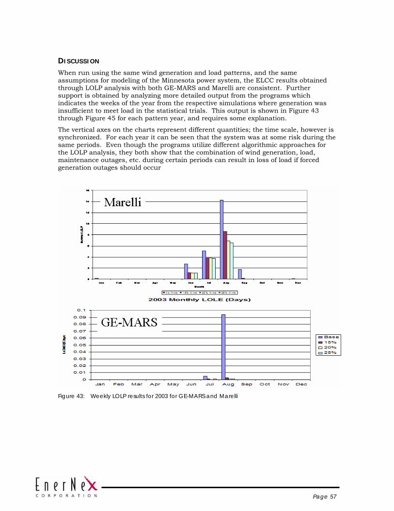
Page 57
DISCUSSION When run using the same wind generation and load patterns, and the same assumptions for modeling of the Minnesota power system, the ELCC results obtained through LOLP analysis with both GE-MARS and Marelli are consistent. Further support is obtained by analyzing more detailed output from the programs which indicates the weeks of the year from the respective simulations where generation was insufficient to meet load in the statistical trials. This output is shown in Figure 43 through Figure 45 for each pattern year, and requires some explanation.
The vertical axes on the charts represent different quantities; the time scale, however is synchronized. For each year it can be seen that the system was at some risk during the same periods. Even though the programs utilize different algorithmic approaches for the LOLP analysis, they both show that the combination of wind generation, load, maintenance outages, etc. during certain periods can result in loss of load if forced generation outages should occur
Figure 43: Weekly LOLP results for 2003 for GE-MARS and Marelli
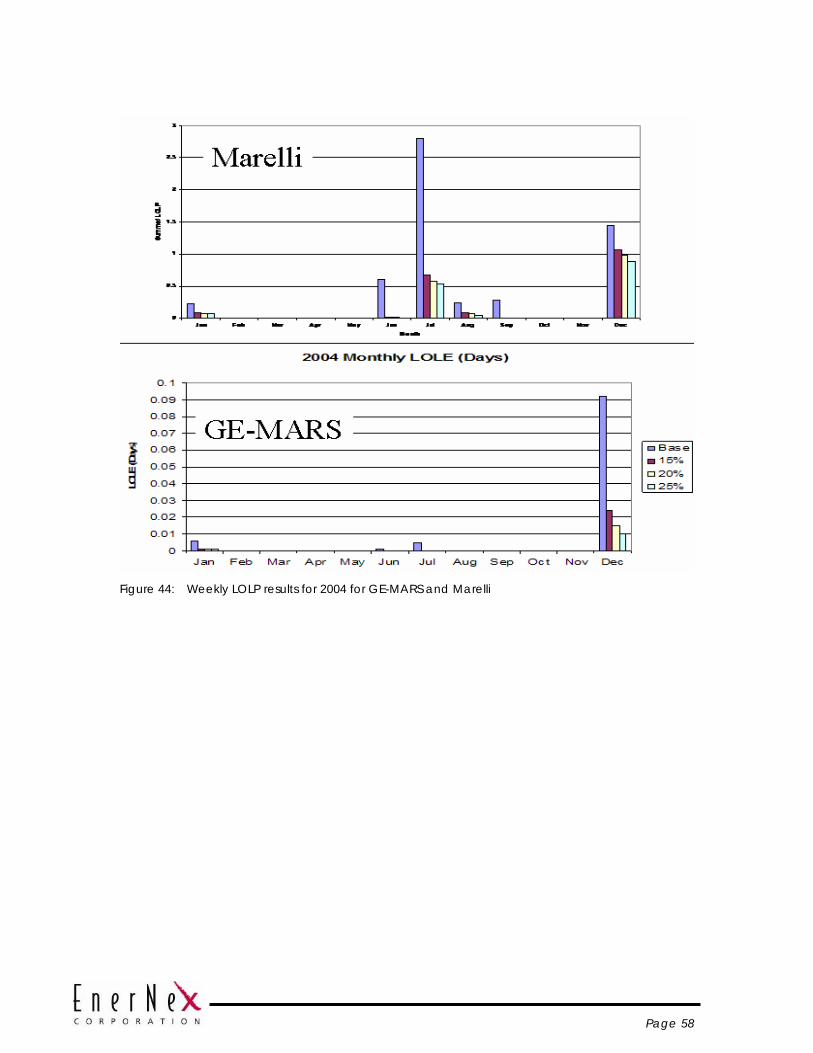
Page 58
Figure 44: Weekly LOLP results for 2004 for GE-MARS and Marelli
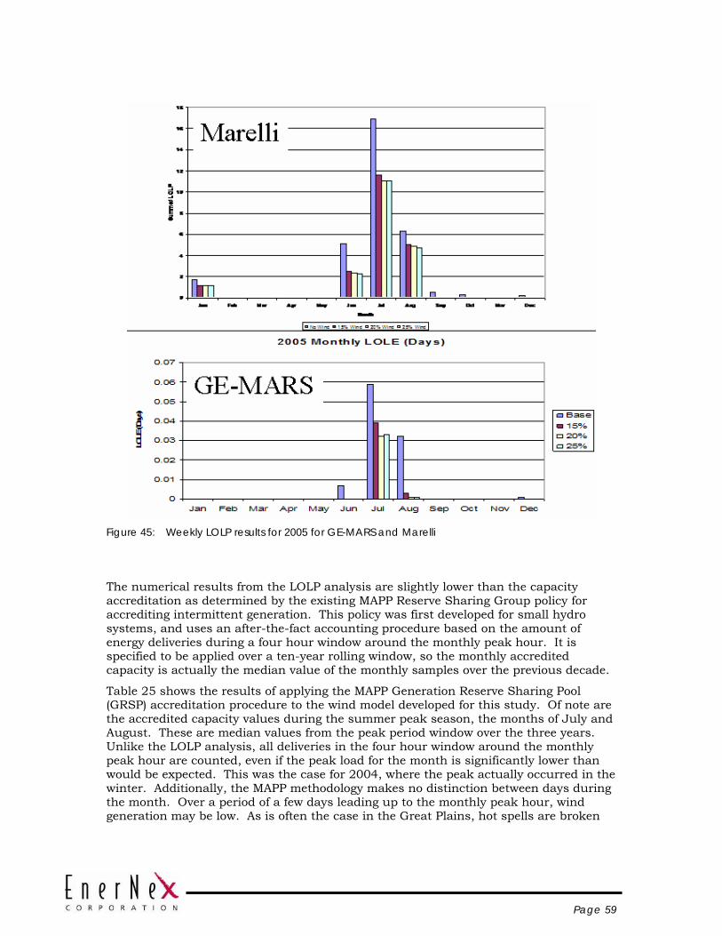
Page 59
Figure 45: Weekly LOLP results for 2005 for GE-MARS and Marelli
The numerical results from the LOLP analysis are slightly lower than the capacity accreditation as determined by the existing MAPP Reserve Sharing Group policy for accrediting intermittent generation. This policy was first developed for small hydro systems, and uses an after-the-fact accounting procedure based on the amount of energy deliveries during a four hour window around the monthly peak hour. It is specified to be applied over a ten-year rolling window, so the monthly accredited capacity is actually the median value of the monthly samples over the previous decade.
Table 25 shows the results of applying the MAPP Generation Reserve Sharing Pool (GRSP) accreditation procedure to the wind model developed for this study. Of note are the accredited capacity values during the summer peak season, the months of July and August. These are median values from the peak period window over the three years. Unlike the LOLP analysis, all deliveries in the four hour window around the monthly peak hour are counted, even if the peak load for the month is significantly lower than would be expected. This was the case for 2004, where the peak actually occurred in the winter. Additionally, the MAPP methodology makes no distinction between days during the month. Over a period of a few days leading up to the monthly peak hour, wind generation may be low. As is often the case in the Great Plains, hot spells are broken
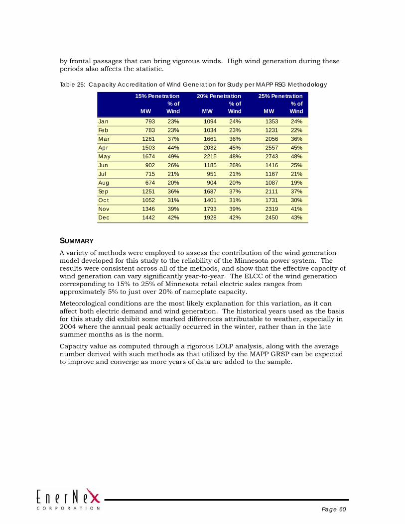
Page 60
by frontal passages that can bring vigorous winds. High wind generation during these periods also affects the statistic.
Table 25: Capacity Accreditation of Wind Generation for Study per MAPP RSG Methodology
MW% of Wind MW
% of Wind MW
% of Wind
Jan 793 23% 1094 24% 1353 24%Feb 783 23% 1034 23% 1231 22%Mar 1261 37% 1661 36% 2056 36%Apr 1503 44% 2032 45% 2557 45%May 1674 49% 2215 48% 2743 48%Jun 902 26% 1185 26% 1416 25%Jul 715 21% 951 21% 1167 21%Aug 674 20% 904 20% 1087 19%Sep 1251 36% 1687 37% 2111 37%Oct 1052 31% 1401 31% 1731 30%Nov 1346 39% 1793 39% 2319 41%Dec 1442 42% 1928 42% 2450 43%
15% Penetration 20% Penetration 25% Penetration
SUMMARY A variety of methods were employed to assess the contribution of the wind generation model developed for this study to the reliability of the Minnesota power system. The results were consistent across all of the methods, and show that the effective capacity of wind generation can vary significantly year-to-year. The ELCC of the wind generation corresponding to 15% to 25% of Minnesota retail electric sales ranges from approximately 5% to just over 20% of nameplate capacity.
Meteorological conditions are the most likely explanation for this variation, as it can affect both electric demand and wind generation. The historical years used as the basis for this study did exhibit some marked differences attributable to weather, especially in 2004 where the annual peak actually occurred in the winter, rather than in the late summer months as is the norm.
Capacity value as computed through a rigorous LOLP analysis, along with the average number derived with such methods as that utilized by the MAPP GRSP can be expected to improve and converge as more years of data are added to the sample.
Page 61
Section 5 OPERATING IMPACTS
OVERVIEW In the operating time frame – hours to days – wind generation and load follow different cycles. Load exhibits a distinct diurnal pattern through all seasons. Wind generation in the Great Plains exhibits some diurnal characteristics, but is mainly driven by the passage of large scale weather systems that have cycles of several days to a week. It is nearly impossible, therefore, to select a small number of “typical” wind and load days for analysis.
The approach first used in the study for Xcel Energy in 2004 overcomes this difficulty by utilizing synchronized historical load and wind generation data sets extending over several years. Correlations due to the common meteorology are automatically embedded in these records, and a much wider range of combinations of wind generation and load behavior are represented. With multiple annual data sets, inter-annual variations in the meteorology can be captured.
With these data sets as the starting point, assessment of wind integration issues can be accomplished through a “simulation” of operational activities. For most utilities, this involves a forward-looking process where resources are committed for operation based on forecasts of load and wind. The selected resources are then dispatched against the “actual” load and wind generation to simulate real-time operations. Using planning tools that operate on time steps of one hour, an entire annual set of wind and load data can be processed.
MISO utilizes PROMOD for hour-by-hour analysis of energy market operations and transmission facility utilization. In this program, generating units are committed based on costs, operating characteristics, and transmission constraints, then dispatched to meet the specified load on an hourly basis. Like other hourly production costing programs, it can be used as a “proxy” for the short-term operation of power systems.
In this study, PROMOD is utilized to simulate the operation of the MISO energy markets. Annual data sets of wind generation and load developed from synthesized and historical data for calendar years 2003, 2004, and 2005 are the primary inputs to the program. System characteristics, such as transmission network data and generating unit costs and capabilities, are drawn from the database that MISO utilizes for transmission planning studies.
“BASE” CASES The initial PROMOD cases utilized the Minnesota load patterns from 2004 scaled to 2020 levels, and wind generation from the same year. Wind generation was injected at 14 buses in Minnesota and the Dakotas, and treated as a “firm” transaction. PROMOD uses firm transactions in the unit commitment step of the simulation, so the results represent an optimized commitment and dispatch for the entire year.
Page 62
Output from the PROMOD analysis can include the hourly profile of load at any bus, flows in any line, or output from any generator. The results presented here and throughout this section are based on summary information, and consist of the following quantities:
• Load – The annual energy consumed by end-users in the Minnesota company footprints in the PROMOD case. The target Minnesota retail electric energy sales are based on load patterns from 2004. Units are terawatt-hours (TWH), which is 1 million MWH.
• Wind Generation – Annual energy delivered by the wind generation in the scenarios constructed for this study. The amount varies by year, with target fraction of retail electric energy sales for wind based on meteorology from the year 2004. Units are terawatt-hours (TWH), which is 1 million MWH.
• Generation (non-wind) – Annual electric energy production from conventional generating resources. Units are terawatt-hours (TWH), which is 1 million MWH.
• Load Cost – The annual amount paid by the loads for the electric energy consumed. This quantity is equal to the summation over all hours of the year and all utilization buses in the Minnesota companies’ PROMOD footprints of the hourly amount at each utilization bus times the hourly locational marginal price at that utilization bus. Units are in millions of dollars.
• Production Cost – Variable costs associated with electric energy production. Includes fuel, startup and shutdown, and O&M costs. This amount does not include any consideration for capital recovery. Units are in millions of dollars.
• Generator Revenue – The annual amount paid to the generators. This quantity is equal to the summation over all hours of the year and all delivery buses in the Minnesota companies’ PROMOD footprints of the hourly amount at each delivery bus times the hourly locational marginal price at that delivery bus. Units are in millions of dollars.
• Imports – The amount of energy utilized by loads in the Minnesota companies’ PROMOD footprint but produced outside of that footprint. Units are terawatt-hours (TWH), which is 1 million MWH.
The case was run multiple times for different operating reserve assumptions to generate a curve for each wind generation level. Production costs and load payments are shown in Figure 46 and Figure 47. The effect on the utilization of conventional generation is shown in Figure 48 and Figure 49.
These optimized hourly cases show the following impacts of wind generation:
• As more wind energy is added, the production cost and load payments decline. This is due to the displacement of conventional generation and the resulting reduction in variable (fuel) costs.
• Generation from both coal and gas units is displaced.
• Production costs rise with the level of required operating reserves. This is intuitive, since more generation must be available or online.
• Production costs rise slowly from the baseline assumption of 5% total operating reserves out to about 7%. From there, costs rise more quickly.
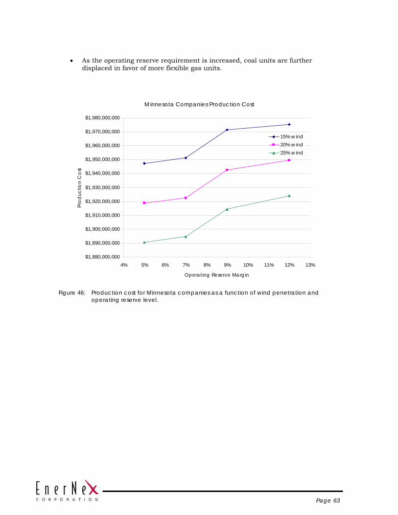
Page 63
• As the operating reserve requirement is increased, coal units are further displaced in favor of more flexible gas units.
Minnesota Companies Production Cost
$1,880,000,000
$1,890,000,000
$1,900,000,000
$1,910,000,000
$1,920,000,000
$1,930,000,000
$1,940,000,000
$1,950,000,000
$1,960,000,000
$1,970,000,000
$1,980,000,000
4% 5% 6% 7% 8% 9% 10% 11% 12% 13%
Operating Reserve Margin
Pro
duc
tion
Co
st
15% wind20% wind25% wind
Figure 46: Production cost for Minnesota companies as a function of wind penetration and
operating reserve level.

Page 64
Minnesota Companies Load Cost
$3,650,000,000
$3,700,000,000
$3,750,000,000
$3,800,000,000
$3,850,000,000
$3,900,000,000
4% 5% 6% 7% 8% 9% 10% 11% 12% 13%
Operating Reserve Margin
Loa
d P
aym
ents
15% wind20% wind25% wind
Figure 47: Load payments for Minnesota companies as a function of wind penetration and
operating reserve level.
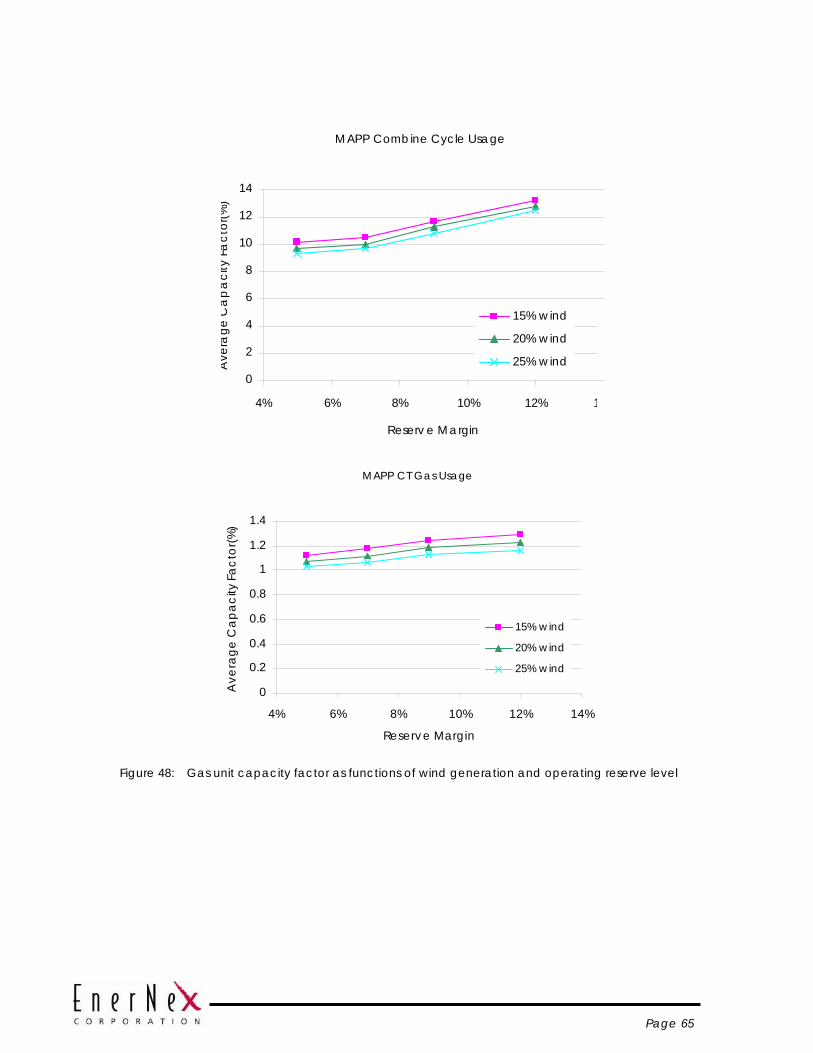
Page 65
MAPP Combine Cycle Usage
0
2
4
6
8
10
12
14
4% 6% 8% 10% 12% 1
Reserv e Margin
Ave
rage
Ca
pa
city
Fa
ctor
(%)
15% wind
20% wind
25% wind
MAPP CT Gas Usage
0
0.2
0.4
0.6
0.8
1
1.2
1.4
4% 6% 8% 10% 12% 14%
Reserve Margin
Ave
rage
Cap
acity
Fac
tor(%
)
15% wind
20% wind
25% wind
Figure 48: Gas unit capacity factor as functions of wind generation and operating reserve level
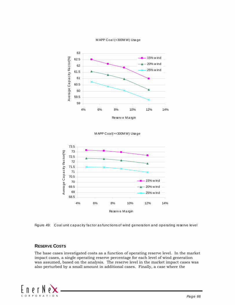
Page 66
MAPP Coal (<300MW) Usage
59
59.5
60
60.5
61
61.5
62
62.5
63
4% 6% 8% 10% 12% 14%
Reserv e Margin
Ave
rage
Ca
pa
city
Fa
ctor
(%) 15% wind
20% wind
25% wind
MAPP Coal(>=300MW) Usage
68.569
69.570
70.571
71.572
72.573
73.5
4% 6% 8% 10% 12% 14%
Reserv e Margin
Ave
rage
Ca
pa
city
Fa
ctor
(%)
15% wind
20% wind
25% wind
Figure 49: Coal unit capacity factor as functions of wind generation and operating reserve level
RESERVE COSTS The base cases investigated costs as a function of operating reserve level. In the market impact cases, a single operating reserve percentage for each level of wind generation was assumed, based on the analysis. The reserve level in the market impact cases was also perturbed by a small amount in additional cases. Finally, a case where the

Page 67
operating reserve level was varied according to the amount of wind generation actually being delivered each hour was run.
2004 load and wind generation patterns were used in this analysis.
Figure 50 summarizes all reserve cases run, showing production cost as a function of operating reserve level. A trend line based on an exponential fit has been added to each wind penetration level.
$1,880 M
$1,900 M
$1,920 M
$1,940 M
$1,960 M
$1,980 M
4.00% 6.00% 8.00% 10.00% 12.00% 14.00%
Total Operating Reserve
Prod
uctio
n C
ost 15% wind
20% wind
25% wind
Expon. (15% wind)
Expon. (20% wind)
Expon. (25% wind)
Figure 50: Production cost as a function of wind penetration and operating reserve level.
Production costs rise as total operating reserves are increased, which is the expected result. It is recognized, however, that a higher reserve requirement for all hours of the annual simulation is overly conservative, since there are many hours where wind generation is very low, and changes up or down would be of little note to operators. Further, an incremental operating reserve pegged to hourly changes in wind generation would not need to be comprised of spinning generation only – changes in the later part of the hour could be covered by quick-start units, if available. The significance here is that no costs accrue with this type of reserve unless it is used.
A case was run for the 2004 load patterns at 20% wind generation with operating reserves for wind generation modeled less conservatively:
• The additional operating reserve for wind generation is a variable hourly profile based on the previous hourly average value
• The incremental reserves for wind generation were further required only to be non-spinning.
As expected, these assumptions resulted in a decreased production costs over the fixed additional reserves case.
The cost associated with increased operating reserve can be placed in context by assigning it as an “integration cost” for wind generation and amortizing it over the wind energy delivered. Table 26 documents this calculation, and shows that for 20% wind generation, the fixed additional reserve options leads to a increased cost of $0.55 per
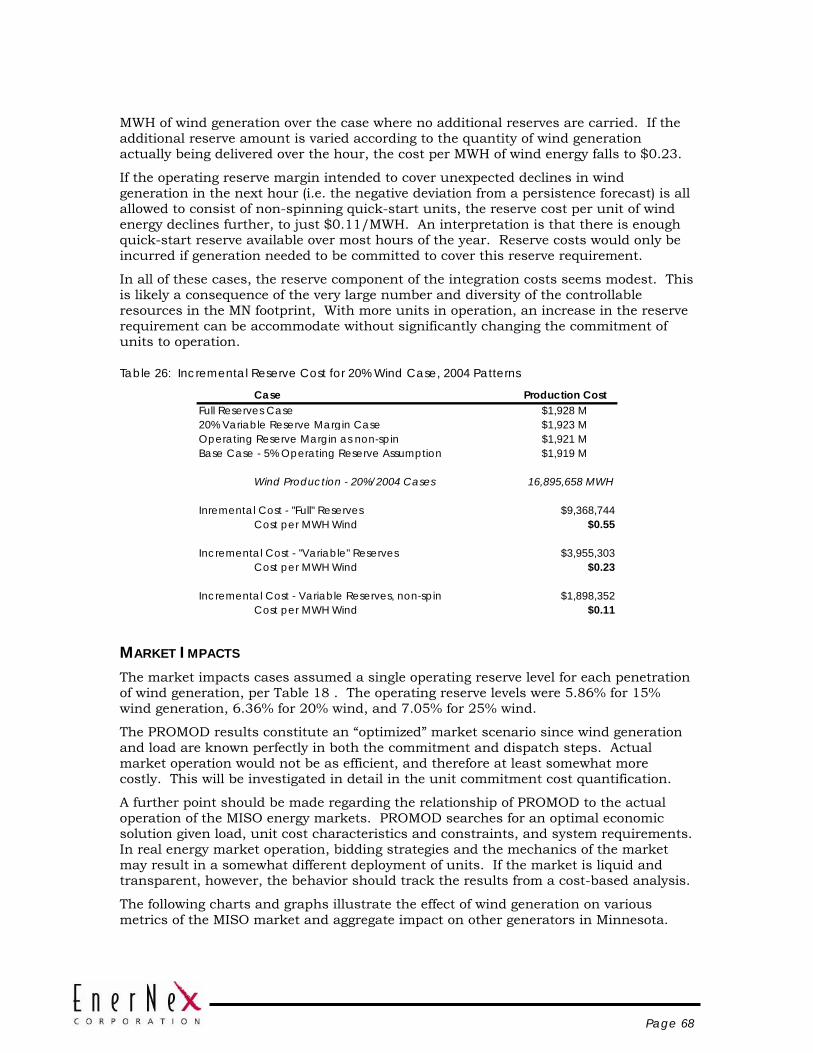
Page 68
MWH of wind generation over the case where no additional reserves are carried. If the additional reserve amount is varied according to the quantity of wind generation actually being delivered over the hour, the cost per MWH of wind energy falls to $0.23.
If the operating reserve margin intended to cover unexpected declines in wind generation in the next hour (i.e. the negative deviation from a persistence forecast) is all allowed to consist of non-spinning quick-start units, the reserve cost per unit of wind energy declines further, to just $0.11/MWH. An interpretation is that there is enough quick-start reserve available over most hours of the year. Reserve costs would only be incurred if generation needed to be committed to cover this reserve requirement.
In all of these cases, the reserve component of the integration costs seems modest. This is likely a consequence of the very large number and diversity of the controllable resources in the MN footprint, With more units in operation, an increase in the reserve requirement can be accommodate without significantly changing the commitment of units to operation.
Table 26: Incremental Reserve Cost for 20% Wind Case, 2004 Patterns
Case Production CostFull Reserves Case $1,928 M20% Variable Reserve Margin Case $1,923 MOperating Reserve Margin as non-spin $1,921 MBase Case - 5% Operating Reserve Assumption $1,919 M
Wind Production - 20%/2004 Cases 16,895,658 MWH
Inremental Cost - "Full" Reserves $9,368,744Cost per MWH Wind $0.55
Incremental Cost - "Variable" Reserves $3,955,303Cost per MWH Wind $0.23
Incremental Cost - Variable Reserves, non-spin $1,898,352Cost per MWH Wind $0.11
MARKET IMPACTS The market impacts cases assumed a single operating reserve level for each penetration of wind generation, per Table 18 . The operating reserve levels were 5.86% for 15% wind generation, 6.36% for 20% wind, and 7.05% for 25% wind.
The PROMOD results constitute an “optimized” market scenario since wind generation and load are known perfectly in both the commitment and dispatch steps. Actual market operation would not be as efficient, and therefore at least somewhat more costly. This will be investigated in detail in the unit commitment cost quantification.
A further point should be made regarding the relationship of PROMOD to the actual operation of the MISO energy markets. PROMOD searches for an optimal economic solution given load, unit cost characteristics and constraints, and system requirements. In real energy market operation, bidding strategies and the mechanics of the market may result in a somewhat different deployment of units. If the market is liquid and transparent, however, the behavior should track the results from a cost-based analysis.
The following charts and graphs illustrate the effect of wind generation on various metrics of the MISO market and aggregate impact on other generators in Minnesota.

Page 69
Table 27 shows how increasing wind generation displaces conventional generation in Minnesota, and the corresponding impacts on load payments and production cost.
The effect of wind generation on the locational margin price relative to a case with no wind generation at the Minnesota company trading hubs is shown in Figure 51 through Figure 53.
Finally, reductions in emissions relative to a case with no wind generation are provided in Table 28. In analyzing these emission reductions, it is important to remember that wind generation displaces both fossil generation and imports. In fact, for these cases, about two-thirds of the wind energy displaces imports from outside of the Minnesota company footprints. The emission reductions shown are for only those units within this footprint, so they do not reflect offsets from fossil units outside of Minnesota.
Table 27: Wind Generation Impacts on Energy Market Metrics – 2004 Wind and Load Patterns
LMP - GRE Hub
0
0.2
0.4
0.6
0.8
1
1.2
1 1001 2001 3001 4001 5001 6001 7001 8001
Hours
LMP
- Nor
mal
ized
to N
o W
ind No Wind
15% Wind
20% Wind
25% Wind
LMP - MPC Hub
0
0.2
0.4
0.6
0.8
1
1.2
1 1001 2001 3001 4001 5001 6001 7001 8001
Hours
LMP
- Nor
mal
ized
to N
o W
ind No Wind
15% Wind
20% Wind
25% Wind
Figure 51: Wind generation impact on relative locational marginal price – Great River Energy and
Minnkota hubs
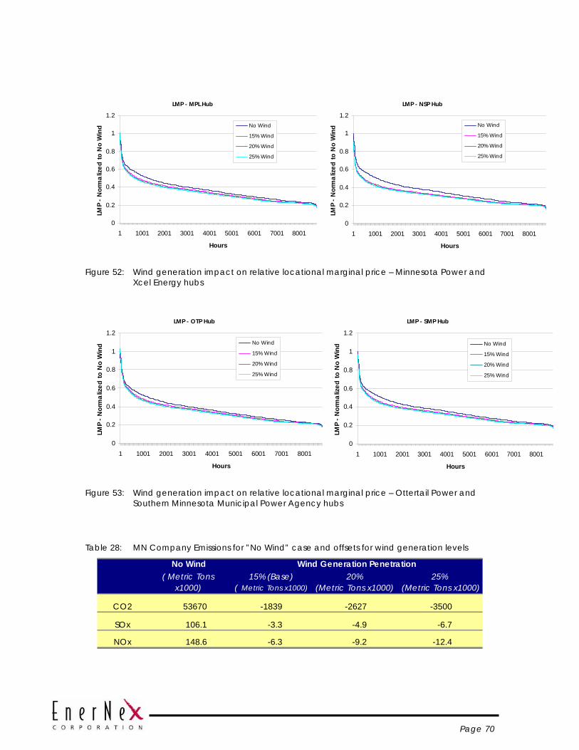
Page 70
LMP - MPL Hub
0
0.2
0.4
0.6
0.8
1
1.2
1 1001 2001 3001 4001 5001 6001 7001 8001
Hours
LMP
- Nor
mal
ized
to N
o W
ind No Wind
15% Wind
20% Wind
25% Wind
LMP - NSP Hub
0
0.2
0.4
0.6
0.8
1
1.2
1 1001 2001 3001 4001 5001 6001 7001 8001
Hours
LMP
- Nor
mal
ized
to N
o W
ind No Wind
15% Wind
20% Wind
25% Wind
Figure 52: Wind generation impact on relative locational marginal price – Minnesota Power and
Xcel Energy hubs
LMP - OTP Hub
0
0.2
0.4
0.6
0.8
1
1.2
1 1001 2001 3001 4001 5001 6001 7001 8001
Hours
LMP
- Nor
mal
ized
to N
o W
ind No Wind
15% Wind
20% Wind
25% Wind
LMP - SMP Hub
0
0.2
0.4
0.6
0.8
1
1.2
1 1001 2001 3001 4001 5001 6001 7001 8001
Hours
LMP
- Nor
mal
ized
to N
o W
ind No Wind
15% Wind
20% Wind
25% Wind
Figure 53: Wind generation impact on relative locational marginal price – Ottertail Power and
Southern Minnesota Municipal Power Agency hubs
Table 28: MN Company Emissions for ”No Wind” case and offsets for wind generation levels
No Wind( Metric Tons
x1000)15% (Base)
( Metric Tons x1000)20%
(Metric Tons x1000)25%
(Metric Tons x1000)
CO2 53670 -1839 -2627 -3500
SOx 106.1 -3.3 -4.9 -6.7
NOx 148.6 -6.3 -9.2 -12.4
Wind Generation Penetration

Page 71
THE COST OF INTEGRATING WIND GENERATION
Background The purpose of these hourly cases is to determine how the major characteristics of wind generation – variability and uncertainty – affect the commitment and dispatch of conventional generators.
The object of the analysis is to quantify the cost differential to serve the load not served by wind generation due to these characteristics. Using PROMOD and the data assembled for this study, this cost differential is determined through the following process:
1. Run PROMOD to simulate the MISO day-ahead market clearing and RAC (reliability assessment and commitment) process. In this step, the actual wind generation and load for the next day are not known perfectly. For wind generation, the day-ahead forecast developed in the resource characterization task is used. The load is more problematic. In the market clearing, demand bids, rather than actual forecasts, are used to clear the day-ahead offers. Later in the day, MISO performs a reliability assessment using security-constrained unit commitment, assesses this result versus the cleared offers. If the offers are short of what is determined necessary for reliability, more generation is committed. This process utilizes an actual forecast of load.
If load is assumed to be known perfectly, all uncertainty costs will be attributed to wind generation, which is not the case in reality. PROMOD performs the unit commitment part of the simulation using only “firm” demand and transactions. From this commitment, an economic dispatch is performed against both firm and non-firm load and transactions. So to represent the actual wind generation in this sub-step, a second wind energy transaction was created. This non-firm transaction consists of the difference between forecast and actual wind generation.
Load forecasts must also be handled through firm and non-firm transactions. In the commitment phase, firm transactions that represent the difference between actual and forecast loads are included. A non-firm transaction in the economic dispatch step is used to negate the firm transaction. What remains for dispatch, then, is the actual load.
2. A second reference case is analyzed with PROMOD where wind generation has no uncertainty or variability on a daily basis. The energy delivered over the course of each day, however, is identical to that in Step 1. Further, because of the attributes of this proxy energy resource, there are no additional reserves required to cover within the hour variability or short-term uncertainty.
3. The results of the unit commitment/economic dispatch simulation from the two cases are then compared. The differences in the load cost are assigned to the variability and uncertainty of wind generation.
The unit commitment component of the integration cost measures how the variability and uncertainty of wind generation decreases the efficiency of the market. The uncertainty impact shows up in the day-ahead market clearing, as significant wind generation forecast errors cause the market to respond to incorrect information. Over- and under-commitment of conventional generation will increase costs. The variability cost results from conventional units being dispatched “around” wind energy delivery. Increased costs result from less efficient operation of conventional units.
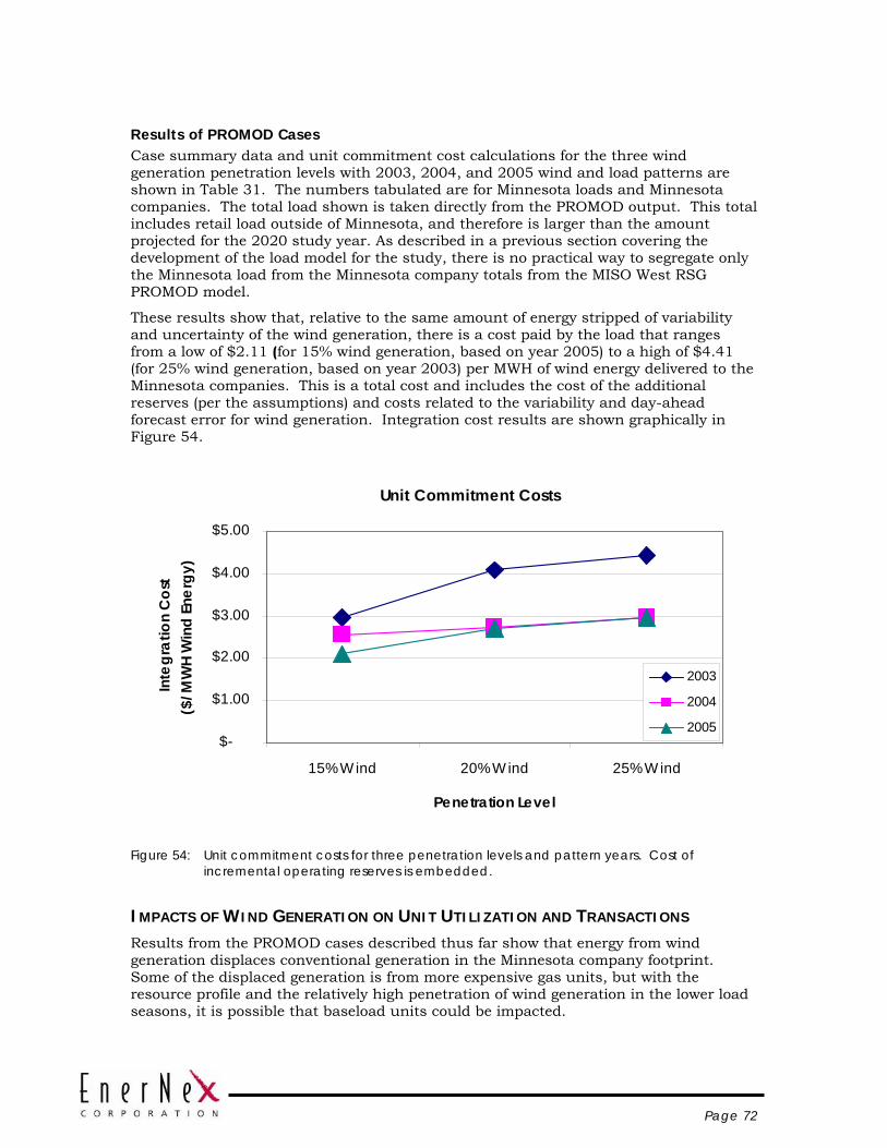
Page 72
Results of PROMOD Cases Case summary data and unit commitment cost calculations for the three wind generation penetration levels with 2003, 2004, and 2005 wind and load patterns are shown in Table 31. The numbers tabulated are for Minnesota loads and Minnesota companies. The total load shown is taken directly from the PROMOD output. This total includes retail load outside of Minnesota, and therefore is larger than the amount projected for the 2020 study year. As described in a previous section covering the development of the load model for the study, there is no practical way to segregate only the Minnesota load from the Minnesota company totals from the MISO West RSG PROMOD model.
These results show that, relative to the same amount of energy stripped of variability and uncertainty of the wind generation, there is a cost paid by the load that ranges from a low of $2.11 (for 15% wind generation, based on year 2005) to a high of $4.41 (for 25% wind generation, based on year 2003) per MWH of wind energy delivered to the Minnesota companies. This is a total cost and includes the cost of the additional reserves (per the assumptions) and costs related to the variability and day-ahead forecast error for wind generation. Integration cost results are shown graphically in Figure 54.
Unit Commitment Costs
$-
$1.00
$2.00
$3.00
$4.00
$5.00
15% Wind 20% Wind 25% Wind
Penetration Level
Inte
grat
ion
Cos
t ($
/MW
H W
ind
Ener
gy)
2003
2004
2005
Figure 54: Unit commitment costs for three penetration levels and pattern years. Cost of
incremental operating reserves is embedded.
IMPACTS OF WIND GENERATION ON UNIT UTILIZATION AND TRANSACTIONS Results from the PROMOD cases described thus far show that energy from wind generation displaces conventional generation in the Minnesota company footprint. Some of the displaced generation is from more expensive gas units, but with the resource profile and the relatively high penetration of wind generation in the lower load seasons, it is possible that baseload units could be impacted.
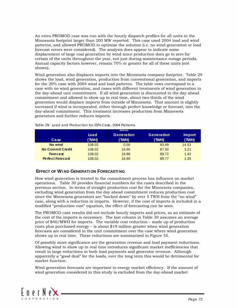
Page 73
An extra PROMOD case was run with the hourly dispatch profiles for all units in the Minnesota footprint larger than 200 MW reported. This case used 2004 load and wind patterns, and allowed PROMOD to optimize the solution (i.e. no wind generation or load forecast errors were considered). The analysis does appear to indicate some displacement of large coal generation by wind since production does go to zero for certain of the units throughout the year, not just during maintenance outage periods. Annual capacity factors however, remain 70% or greater for all of these units (not shown).
Wind generation also displaces imports into the Minnesota company footprint. Table 29 shows the load, wind generation, production from conventional generation, and imports for the 20% case with 2004 wind and load patterns. The table rows correspond to a case with no wind generation, and cases with different treatments of wind generation in the day-ahead unit commitment. If all wind generation is discounted in the day ahead commitment and allowed to show up in real time, about two-thirds of the wind generation would displace imports from outside of Minnesota. That amount is slightly increased if wind is incorporated, either through perfect knowledge or forecast, into the day-ahead commitment. This treatment increases production from Minnesota generators and further reduces imports.
Table 29: Load and Production for 20% Case, 2004 Patterns
CaseLoad (TWH)
Wind Generation
(TWH)Generation
(TWH)Import (TWH)
No wind 108.02 0.00 93.49 14.53 No Commit Credit 108.02 16.90 87.92 3.21
Forecast 108.02 16.88 89.72 1.42Perfect Forecast 108.02 16.90 89.77 1.35
EFFECT OF WIND GENERATION FORECASTING How wind generation is treated in the commitment process has influence on market operations. Table 30 provides financial numbers for the cases described in the previous section. In terms of straight production cost for the Minnesota companies, excluding wind generation from the day ahead commitment reduces production cost since the Minnesota generators are “backed down” by over 5 TWH from the “no wind” case, along with a reduction in imports. However, if the cost of imports is included in a modified “production cost” equation, the effect of forecasting can be seen.
The PROMOD case results did not include hourly imports and prices, so an estimate of the cost of the imports is necessary. The last column in Table 30 assumes an average price of $40/MWH for imports. The variable cost reduction – made up of production costs plus purchased energy – is about $19 million greater when wind generation forecasts are considered in the unit commitment over the case where wind generation shows up in real time. These reductions are summarized in Figure 55.
Of possibly more significance are the generation revenue and load payment reductions. Allowing wind to show up in real time introduces significant market inefficiencies that result in large reductions in both load payments and generator revenue. Although apparently a “good deal” for the loads, over the long term this would be detrimental for market function.
Wind generation forecasts are important to energy market efficiency. If the amount of wind generation considered in this study is excluded from the day-ahead market
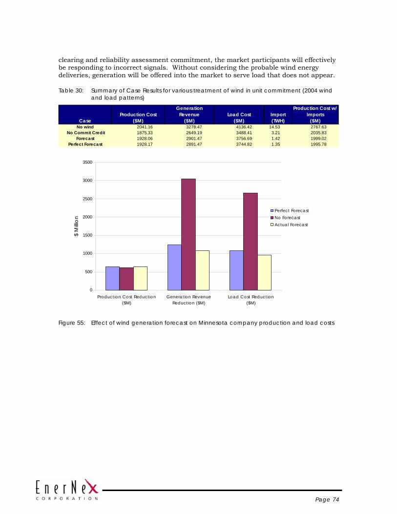
Page 74
clearing and reliability assessment commitment, the market participants will effectively be responding to incorrect signals. Without considering the probable wind energy deliveries, generation will be offered into the market to serve load that does not appear.
Table 30: Summary of Case Results for various treatment of wind in unit commitment (2004 wind and load patterns)
CaseProduction Cost
($M)
Generation Revenue
($M)Load Cost
($M)Import (TWH)
Production Cost w/ Imports
($M)No wind 2041.16 3278.47 4136.42 14.53 2767.63
No Commit Credit 1875.33 2649.19 3488.41 3.21 2035.83Forecast 1928.06 2901.47 3756.69 1.42 1999.02
Perfect Forecast 1928.17 2891.47 3744.82 1.35 1995.78
0
500
1000
1500
2000
2500
3000
3500
Production Cost Reduction($M)
Generation RevenueReduction ($M)
Load Cost Reduction($M)
$ M
illion
Perfect ForecastNo Forecast Actual Forecast
Figure 55: Effect of wind generation forecast on Minnesota company production and load costs
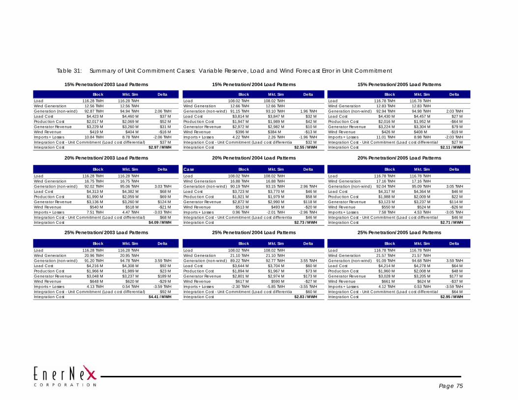
Page 75
Table 31: Summary of Unit Commitment Cases: Variable Reserve, Load and Wind Forecast Error in Unit Commitment
15% Penetration/2003 Load Patterns 15% Penetration/2004 Load Patterns 15% Penetration/2005 Load Patterns
Block Mkt. Sim Delta Block Mkt. Sim Delta Block Mkt. Sim DeltaLoad 116.28 TWH 116.28 TWH Load 108.02 TWH 108.02 TWH Load 116.78 TWH 116.78 TWHWind Generation 12.56 TWH 12.56 TWH Wind Generation 12.66 TWH 12.66 TWH Wind Generation 12.83 TWH 12.83 TWHGeneration (non-wind) 92.87 TWH 94.94 TWH 2.06 TWH Generation (non-wind) 91.15 TWH 93.10 TWH 1.96 TWH Generation (non-wind) 92.94 TWH 94.98 TWH 2.03 TWHLoad Cost $4,423 M $4,460 M $37 M Load Cost $3,814 M $3,847 M $32 M Load Cost $4,430 M $4,457 M $27 MProduction Cost $2,017 M $2,069 M $52 M Production Cost $1,947 M $1,989 M $42 M Production Cost $2,016 M $1,952 M -$64 MGenerator Revenue $3,229 M $3,260 M $31 M Generator Revenue $2,972 M $2,982 M $10 M Generator Revenue $3,224 M $3,304 M $79 MWind Revenue $419 M $404 M -$16 M Wind Revenue $396 M $384 M -$13 M Wind Revenue $426 M $408 M -$19 MImports + Losses 10.84 TWH 8.78 TWH -2.06 TWH Imports + Losses 4.22 TWH 2.26 TWH -1.96 TWH Imports + Losses 11.01 TWH 8.98 TWH -2.03 TWHIntegration Cost - Unit Commitment (Load cost differential) $37 M Integration Cost - Unit Commitment (Load cost differentia $32 M Integration Cost - Unit Commitment (Load cost differential $27 MIntegration Cost $2.97 /MWH Integration Cost $2.55 /MWH Integration Cost $2.11 /MWH
20% Penetration/2003 Load Patterns 20% Penetration/2004 Load Patterns 20% Penetration/2005 Load Patterns
Block Mkt. Sim Delta Case Block Mkt. Sim Delta Block Mkt. Sim DeltaLoad 116.28 TWH 116.28 TWH Load 108.02 TWH 108.02 TWH Load 116.78 TWH 116.78 TWHWind Generation 16.75 TWH 16.75 TWH Wind Generation 16.88 TWH 16.88 TWH Wind Generation 17.16 TWH 17.16 TWHGeneration (non-wind) 92.02 TWH 95.06 TWH 3.03 TWH Generation (non-wind) 90.19 TWH 93.15 TWH 2.96 TWH Generation (non-wind) 92.04 TWH 95.09 TWH 3.05 TWHLoad Cost $4,313 M $4,382 M $68 M Load Cost $3,723 M $3,770 M $46 M Load Cost $4,317 M $4,364 M $46 MProduction Cost $1,990 M $2,059 M $69 M Production Cost $1,921 M $1,979 M $58 M Production Cost $1,988 M $2,009 M $22 MGenerator Revenue $3,136 M $3,260 M $124 M Generator Revenue $2,872 M $2,990 M $118 M Generator Revenue $3,123 M $3,237 M $114 MWind Revenue $540 M $518 M -$21 M Wind Revenue $513 M $493 M -$20 M Wind Revenue $550 M $524 M -$26 MImports + Losses 7.51 TWH 4.47 TWH -3.03 TWH Imports + Losses 0.96 TWH -2.01 TWH -2.96 TWH Imports + Losses 7.58 TWH 4.53 TWH -3.05 TWHIntegration Cost - Unit Commitment (Load cost differential) $68 M Integration Cost - Unit Commitment (Load cost differentia $46 M Integration Cost - Unit Commitment (Load cost differential $46 MIntegration Cost $4.09 /MWH Integration Cost $2.73 /MWH Integration Cost $2.71 /MWH
25% Penetration/2003 Load Patterns 25% Penetration/2004 Load Patterns 25% Penetration/2005 Load Patterns
Block Mkt. Sim Delta Block Mkt. Sim Delta Block Mkt. Sim DeltaLoad 116.28 TWH 116.28 TWH Load 108.02 TWH 108.02 TWH Load 116.78 TWH 116.78 TWHWind Generation 20.96 TWH 20.95 TWH Wind Generation 21.10 TWH 21.10 TWH Wind Generation 21.57 TWH 21.57 TWHGeneration (non-wind) 91.20 TWH 94.78 TWH 3.59 TWH Generation (non-wind) 89.22 TWH 92.77 TWH 3.55 TWH Generation (non-wind) 91.09 TWH 94.68 TWH 3.59 TWHLoad Cost $4,216 M $4,308 M $92 M Load Cost $3,644 M $3,704 M $60 M Load Cost $4,214 M $4,278 M $64 MProduction Cost $1,966 M $1,989 M $23 M Production Cost $1,894 M $1,967 M $73 M Production Cost $1,960 M $2,008 M $48 MGenerator Revenue $3,048 M $3,237 M $189 M Generator Revenue $2,801 M $2,974 M $173 M Generator Revenue $3,028 M $3,205 M $177 MWind Revenue $648 M $620 M -$29 M Wind Revenue $617 M $590 M -$27 M Wind Revenue $661 M $624 M -$37 MImports + Losses 4.13 TWH 0.54 TWH -3.59 TWH Imports + Losses -2.30 TWH -5.85 TWH -3.55 TWH Imports + Losses 4.12 TWH 0.53 TWH -3.59 TWHIntegration Cost - Unit Commitment (Load cost differential) $92 M Integration Cost - Unit Commitment (Load cost differentia $60 M Integration Cost - Unit Commitment (Load cost differential $64 MIntegration Cost $4.41 /MWH Integration Cost $2.83 /MWH Integration Cost $2.95 /MWH
Page 76
Section 6 CONCLUSIONS
The analytical results from this study show that the addition of wind generation to supply 20% of Minnesota retail electric energy sales can be reliably accommodated by the electric power system if sufficient transmission investments are made to support it.
The degree of the operational impacts was somewhat less than expected by those who have participated in integration studies over the past several years for utilities around the country. The technical and economic impacts calculated are in the range of those derived from other analyses for smaller penetrations of wind generation.
Discussion of the analytical results with the Technical Review Committee (TRC) and the Minnesota utility company representatives has established the following as the key findings and the principal reasons that wind generation impacts were not larger:
1. These results show that, relative to the same amount of energy stripped of variability and uncertainty of the wind generation, there is a cost paid by the load that ranges from a low of $2.11 (for 15% wind generation, based on year 2003) to a high of $4.41 (for 25% wind generation, based on year 2005) per MWH of wind energy delivered to the Minnesota companies. This is a total cost and includes the cost of the additional reserves (per the assumptions) and costs related to the variability and day-ahead forecast error for wind generation.
2. The cost of additional reserves above the assumed levels attributable to wind generation is included in the total integration cost. Special hourly cases were run to isolate this cost, and found it to be about $0.11/MWH of wind energy at 20% penetration by energy.
3. The TRC decision to combine the Minnesota balancing authorities into a single functional balancing authority had a significant impact on results. Sharing balancing authority functions substantially reduces requirements for certain ancillary services such as regulation and load following (with or without wind generation). The required amount of regulation capacity is reduced by almost 50%. Additional benefits are found with other services such as load following. In addition, there are a larger number of discrete units available to provide these services.
4. The expanse of the wind generation scenario, covering Minnesota and the eastern parts of North and South Dakota, provides for substantial “smoothing” of wind generation variations. This smoothing is especially evident at time scales within the hour, where the impacts on regulation and load following were almost negligible. Smoothing also occurs over multiple hour time frames, which reduces the burden on unit commitment and dispatch, assuming that transmission issues do not intervene to affect operations. Finally, the number of hours at either very

Page 77
high or very low production are reduced, allowing the aggregate wind generation to behave as a more stable supply of electric energy
5. The transmission expansion as described in the assumptions and detailed in Appendix A combined with the decision to inject wind generation at high voltage buses was adequate for transportation of wind energy in all of the scenarios. Under these assumptions, there were no significant congestion issues attributable to wind generation and no periods of negative Locational Marginal Price (LMP) observed in the hourly simulations.
6. The MISO energy market also played a large role in reducing wind generation integration costs. Since all generating resources over the market footprint are committed and dispatched in an optimal fashion, the size of the effective system into which the wind generation for the study is integrated grows to almost 1200 individual generating units. The aggregate flexibility of the units on line during any hour is adequate for compensating most of the changes in wind generation.
The magnitude of this impact can be gauged by comparing results from recent integration studies for smaller systems. In the 2004 study for Xcel Energy, for example, integration costs were determined to be no higher than $4.60/MWH for a wind generation penetration by capacity of 15%, which would be closer to 10% penetration on an energy basis.
7. The contribution of wind generation to power system reliability is subject to substantial inter-annual variability. Annual Effective Load Carrying Capability (ELCC) values for the three wind generation scenarios from rigorous Loss of Load Probability (LOLP) analysis ranged from a low of 5% of installed capacity to just over 20%. These results were consistent with those derived through approximate methods.
Page 78
Section 7 REFERENCES
[1] Xcel Energy and the Minnesota Department of Commerce: “Wind Integration Study – Final Report”, September, 2004; available at http://www.uwig.org/opimpactsdocs.html
[2] The New York State Energy Research and Development Authority (NYSERDA): “The Effects of Integrating Wind Power on Transmission System Planning, Reliability, and Operations”, March, 2005; available at http://www.uwig.org/opimpactsdocs.html
[3] Utility Wind Interest Group (UWIG): “Characterizing the Impacts of Significant Wind Generation Facilities on Bulk Power System Operations Planning” May, 2003 www.uwig.org
[4] Hirst, E. and Kirby, B. “Separating and Measuring the Regulation and Load Following Ancillary Services” November, 1998 (available at www.EHirst.com)
[5] Hirst, E. and Kirby, B. “What is the Correct Time-Averaging Period for the Regulation Ancillary Service?” April, 2000 (available at www.EHirst.com)
[6] Piwko, R., et.al. “The Effects of Integrating Wind Power on Transmission System Planning, Reliability, and Operations - Report on Phase 1: Preliminary Overall Reliability Assessment” for the New York State Energy Research and Development Authority (NYSERDA), published February, 2004 (available at www.nyserda.org/energyresources/wind.html)
[7] NREL/CP-500-26722: “Short-term Power fluctuation of Wind Turbines: Analyzing data from the German 250 MW Measurement Program from the Ancillary Services Viewpoint”
[8] Parsons, B.P, et. al. “Grid Impacts of Wind Power; A Summary of Recent Studies in the United States” presented at the 2003 European Wind Energy Conference, Madrid, Spain, June 2003.
[9] Milligan, M.R. “A Sliding Window Technique for Calculating System LOLP Contributions of Wind Power Plants” presented at the 2001 AWEA Windpower Conference, Washington, DC, June 4-7, 2001. NREL/CP-500-30363
[10] Milligan, M.R., et. al. “An Enumerative Technique for Modeling Wind Power Variations in Production Costing” presented at the International Conference on Probabilistic Methods Applied to Power Systems, Vancouver, BC, Canada, September 21-25, 1997. NREL/CP-440-22868
[11] Milligan, M.R., et. al. “An Enumerated Probabilistic Simulation Technique and Case Study: Integrating Wind Power into Utility Production Cost Models” presented at the IEEE Power Engineering Society Summer Meeting, Denver, CO, July 29 – August 1, 1996. NREL/TP-440-21530
Page 79
[12] Milligan, M.R., “Measuring Wind Plant Capacity Value” NREL White Paper
[13] Milligan, M. “Windpower and System Operation in the Hourly Time Domain” presented at the 2003 AWEA Windpower Conference, May 18-21, 2003, Austin, TX. NREL/CP-500-33955
[14] Hirst, Eric, “Interaction of Wind Farms with Bulk Power Operations and Markets” prepared for the Project for Sustainable FERC Energy Policy, September 2001
[15] Milligan, M.R. “A Chronological Reliability Model to Assess Operating Reserve Allocation to Wind Power Plants” presented at the 2001 European Wind Energy Conference, July 2-6, 2001, Copenhagen, Denmark. NREL/CP-500-30490
[16] Milligan, M.R. “A Chronological Reliability Model Incorporating Wind Forecasts to Assess Wind Plant Reserve Allocation” presented at 2002 AWEA Windpower Conference, June 3-5, 2002, Portland, OR. NREL/CP-500-32210
[17] Karady, George G., et. al., “Economic Impact Analysis of Load Forecasting”, IEEE Transactions on Power Systems, Volume 12, No. 3, August, 1997. pp. 1388 – 1392.
[18] L.L. Garver, Effective Load Carrying Capability of Generating Units IEEE Transactions on Power Apparatus and Systems VOL PAS-85, No 8, pp 910-919 August, 1966
Page 80
APPENDIX A – WEST RSG STUDY ASSUMPTIONS
Note: The following is a reproduction of the assumptions document for the West Regional Studies Group (RSG) dated May, 2006. The base model for the West RSG is the starting point for the Minnesota PUC wind integration study.
INTRODUCTION There are several exploratory studies performed in West Region. These studies are: CapX 2020, Buffalo Ridge Incremental Generation Outlet (BRIGO) study, Southwest Minnesota to Twin Cities EHV Development study, Southeastern Minnesota – Southwestern Wisconsin Reliability Enhancement Study, American Transmission Company (ATC) Access Project study, NW Exploratory study, Iowa-Southern Minnesota exploratory study. The transmission upgrades proposed in these studies are corresponding to their generation scenario assumptions.
The West RSG is a collaborative effort of MISO staff, the MISO Transmission Owners, stakeholders, regulatory staff and a voluntary participation of SEAMS transmission owners to direct the studies for the MISO Transmission Expansion Plan. Midwest ISO is trying to roll the results of all the above exploratory studies into one study – West RSG Exploratory Study. This collaborative study will be included in MTEP for information purpose. The Goal of this collaborative study is to determine if transmission needs to be built for energy delivery, REO or economics. It can also determine multi-use requirements that may not be supportable by a single entity.
The West RSG study is based on the MAPPMAIN reduced footprint, the topology is shown in the above figure, a total of 34 companies are included in the MAPPMAIN reduced footprint.
FUEL FORECAST3 The source for the fuel forecasts in the Powerbase database is the Platt’s database, Henry hub forecasts and EIA forecasts. New Energy Associates (NEA) contracts with Platt’s for various fuel forecasts. NEA starts with Platt’s forecasts for natural gas and then uses the basis differential inherent in Platt’s forecast for Natural Gas combined with NYMEX Henry Hub futures prices for the first 18 months of the forecast. For the forecast beyond 18 months, the Energy Information Administration (EIA) natural gas forecast for the Henry Hub serves as the base index. The basis differential to each area are then applied against the EIA forecast of the Henry Hub prices.
West RSG study will be a multi-year study. The base case is set at year 2020. Starting from the 2011 fuel forecast in the Powerbase, we scaled the gas price within MAPPMAIN footprint to $9.00/mmBtu. As we added new coal plants into the CAPX study the coal price used is $1.77/mmBtu. All the new coal plants should run at a 60% and above
3 Platts Fuel Forecasting methodology, found on NEA PowerBase support web site
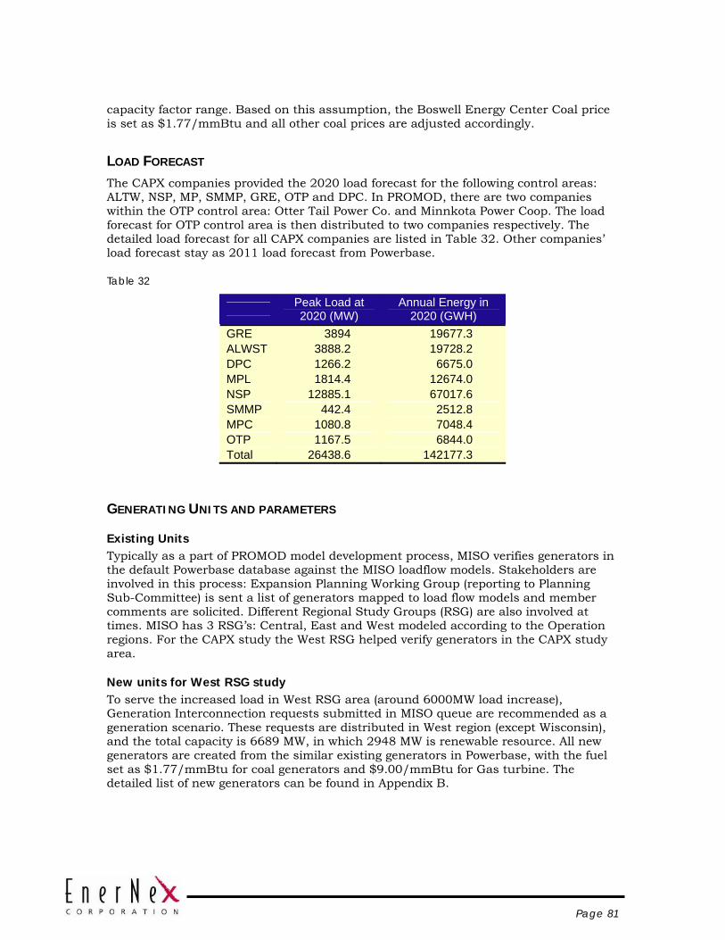
Page 81
capacity factor range. Based on this assumption, the Boswell Energy Center Coal price is set as $1.77/mmBtu and all other coal prices are adjusted accordingly.
LOAD FORECAST The CAPX companies provided the 2020 load forecast for the following control areas: ALTW, NSP, MP, SMMP, GRE, OTP and DPC. In PROMOD, there are two companies within the OTP control area: Otter Tail Power Co. and Minnkota Power Coop. The load forecast for OTP control area is then distributed to two companies respectively. The detailed load forecast for all CAPX companies are listed in Table 32. Other companies’ load forecast stay as 2011 load forecast from Powerbase.
Table 32
Peak Load at 2020 (MW)
Annual Energy in 2020 (GWH)
GRE 3894 19677.3 ALWST 3888.2 19728.2 DPC 1266.2 6675.0 MPL 1814.4 12674.0 NSP 12885.1 67017.6 SMMP 442.4 2512.8 MPC 1080.8 7048.4 OTP 1167.5 6844.0 Total 26438.6 142177.3
GENERATING UNITS AND PARAMETERS
Existing Units Typically as a part of PROMOD model development process, MISO verifies generators in the default Powerbase database against the MISO loadflow models. Stakeholders are involved in this process: Expansion Planning Working Group (reporting to Planning Sub-Committee) is sent a list of generators mapped to load flow models and member comments are solicited. Different Regional Study Groups (RSG) are also involved at times. MISO has 3 RSG’s: Central, East and West modeled according to the Operation regions. For the CAPX study the West RSG helped verify generators in the CAPX study area.
New units for West RSG study To serve the increased load in West RSG area (around 6000MW load increase), Generation Interconnection requests submitted in MISO queue are recommended as a generation scenario. These requests are distributed in West region (except Wisconsin), and the total capacity is 6689 MW, in which 2948 MW is renewable resource. All new generators are created from the similar existing generators in Powerbase, with the fuel set as $1.77/mmBtu for coal generators and $9.00/mmBtu for Gas turbine. The detailed list of new generators can be found in Appendix B.
Page 82
TRANSMISSION UPGRADES West RSG study is based on MTEP06 Phase 2 power flow model. In corresponding to the new generation/load increase, the following transmission upgrades are added, which are based on the recommended facilities from several studies in West region.
o Big Stone II interconnection/delivery upgrades (Alternative 1)
o Common facility upgrades recommended both in Minnesota and North/West bias scenarios in CapX 2020, Boswell-Wilton 230kV line is also included;
o Facility upgrades recommended in Buffalo Ridge Incremental Generation Outlet (BRIGO) study;
o Facility upgrades recommended in Southwest Minnesota to Twin Cities EHV Development study;
o Facility upgrades recommended in Southeastern Minnesota – Southwestern Wisconsin Reliability Enhancement Study;
o Some facility upgrades recommended in ATC Access project study, including Paddock-Rockdale project (P-R), LaCrosse-Columbia project (portion of Prairie Island-Columbia), and Salem-North Madison (S-NM) project.
o Some facility upgrades recommended in Iowa-Southern Minnesota exploratory study, including Hazelton-Salem, Salem-Nelson Dewey-Spring Green 345 kV lines.
The line list for these projects can be found in Table 33.
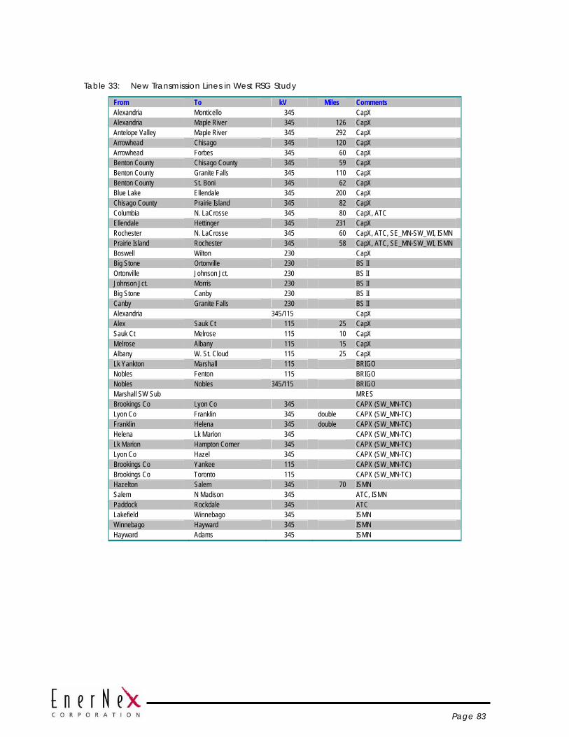
Page 83
Table 33: New Transmission Lines in West RSG Study
From To kV Miles Comments Alexandria Monticello 345 CapX Alexandria Maple River 345 126 CapX Antelope Valley Maple River 345 292 CapX Arrowhead Chisago 345 120 CapX Arrowhead Forbes 345 60 CapX Benton County Chisago County 345 59 CapX Benton County Granite Falls 345 110 CapX Benton County St. Boni 345 62 CapX Blue Lake Ellendale 345 200 CapX Chisago County Prairie Island 345 82 CapX Columbia N. LaCrosse 345 80 CapX, ATC Ellendale Hettinger 345 231 CapX Rochester N. LaCrosse 345 60 CapX, ATC, SE_MN-SW_WI, ISMN Prairie Island Rochester 345 58 CapX, ATC, SE_MN-SW_WI, ISMN Boswell Wilton 230 CapX Big Stone Ortonville 230 BS II Ortonville Johnson Jct. 230 BS II Johnson Jct. Morris 230 BS II Big Stone Canby 230 BS II Canby Granite Falls 230 BS II Alexandria 345/115 CapX Alex Sauk Ct 115 25 CapX Sauk Ct Melrose 115 10 CapX Melrose Albany 115 15 CapX Albany W. St. Cloud 115 25 CapX Lk Yankton Marshall 115 BRIGO Nobles Fenton 115 BRIGO Nobles Nobles 345/115 BRIGO Marshall SW Sub MRES Brookings Co Lyon Co 345 CAPX (SW_MN-TC) Lyon Co Franklin 345 double CAPX (SW_MN-TC) Franklin Helena 345 double CAPX (SW_MN-TC) Helena Lk Marion 345 CAPX (SW_MN-TC) Lk Marion Hampton Corner 345 CAPX (SW_MN-TC) Lyon Co Hazel 345 CAPX (SW_MN-TC) Brookings Co Yankee 115 CAPX (SW_MN-TC) Brookings Co Toronto 115 CAPX (SW_MN-TC) Hazelton Salem 345 70 ISMN Salem N Madison 345 ATC, ISMN Paddock Rockdale 345 ATC Lakefield Winnebago 345 ISMN Winnebago Hayward 345 ISMN Hayward Adams 345 ISMN

Page 84
APPENDIX B - WEST RSG STUDY NEW GENERATING UNITS
MISO Project Num
Bus numb Bus name Pmax Pmin Qmax Qmin
MISO Queue Date
Control Area County State
In Service Date Study Status
IA Status Project manager
Interconnection Service Type Fuel Type
NE group
G424 61710 MINNTAC7 100 0 0.00 0.00 19-Apr-04 MN St. Louis MN 01-Dec-06 FEC SIC FE Diwakar Tewari ER Wind
G509 61705 BABBITT7 75 0 0.00 0.00 18-Mar-05 MP St. Louis MN 01-Aug-06 FEC SIE Diwakar Tewari NR Wind
G519 61625 BLCKBRY4 580 0 190.64 -190.64 19-May-05 MP Itasca MN 01-Apr-09 SIE Diwakar Tewari NR
Coal and/or a blend of Petroleum coke and coal
G591_592 60101 FORBES 2 800 0 262.95 -262.95 25-Jan-06 MP St. Louis MN 01-Mar-13 FEP Raja Srivastava NR Coal
G597 61625 BLCKBRY4 606 0 199.18 -199.18 14-Feb-06 MP Itasca MN 01-Jan-13 FEP Ron Arness NR Coal
G600 63254 VIKING 7 110 0 0.00 0.00 16-Feb-06 OTP Marshall MN 31-Dec-08 FEP Ron Arness ER Wind
ND group
G380 63279 RUGBOTP7 150 0 0.00 0.00 21-Nov-03 OTP Pierce ND 01-Dec-05 IC/FC IAF Kun Zhu ER Wind
G531 63049 STANTON4 80 0 26.29 -26.29 01-Jul-05 GRE Mercer ND 01-Apr-09 SIE Raja Srivastava NR Coal
G581 66791 CENTER 3 600 0 197.21 -197.21 27-Dec-05 MP Oliver ND 01-Jan-15 FEP Raja Srivastava NR Coal
G607 67316 COYOTE 3 25 0 8.22 -8.22 01-Mar-06 OTP Mercer ND 25-Oct-08 FEP Ron Arness NR Coal
Group 4
G389 63043 ELK RIV4 200 0 65.74 -65.74 03-Nov-03 GRE Sherburne MN 01-Jan-07 IP Raja Srivastava NR Natural Gas
G390 63043 ELK RIV4 100 0 32.87 -32.87 03-Nov-03 GRE Sherburne MN 01-Jan-09 IP Raja Srivastava NR Natural Gas
G417 60896 SHAKOPE8 15 0 4.93 -4.93 22-Mar-04 NSP Scott MN 31-Dec-05 IP Raja Srivastava NR biomass
G474 63220 ELBOWLK7 20 0 0.00 0.00 01-Oct-04 OTP Grant MN 01-Nov-05 IP Raja Srivastava NR Wind
G489 60119 LKYNKTN7 20 0 0.00 0.00 19-Jan-05 NSP Lyon MN 01-Oct-06 IP Raja Srivastava NR Wind
G491 60715 CHANRMB9 150 0 0.00 0.00 29-Dec-04 NSP Pipestone MN 01-May-07 FEP Raja Srivastava NR Wind
G502 66752 DRAYTON4 50 0 0.00 0.00 14-Mar-05 MP Oliver ND 01-Nov-05 SIC FE Raja Srivastava NR Wind
G514 60331 LKFLDXL3 200 0 0.00 0.00 20-Apr-05 NSP Jackson MN 01-Oct-06 FEE Raja Srivastava NR Wind
G517 34226 STORDEN8 150 0 0.00 0.00 02-May-05 ALTW Cottonwood MN 01-Oct-06 SIE Raja Srivastava NR Wind
G518 62371 WLKFLTP 8 0 0.00 0.00 02-May-05 GRE Jackson MN 01-Nov-06 FE Raja Srivastava NR Wind

Page 85
MISO Project Num
Bus numb Bus name Pmax Pmin Qmax Qmin
MISO Queue Date
Control Area County State
In Service Date Study Status
IA Status Project manager
Interconnection Service Type Fuel Type
G520 60119 LKYNKTN7 150 0 0.00 0.00 20-May-05 NSP Lyon MN 31-Dec-06 SIE Raja Srivastava NR Wind
G530 34164 GR JCT 9 14 0 0.00 0.00 15-Jun-05 ALTW Greene IA 01-Sep-06 IP Raja Srivastava NR Wind
G532 62792 ODIN 19.95 0 0.00 0.00 06-Jul-05 ALTW Cottonwood/Watonwan MN 01-Sep-06 IP Raja Srivastava NR Wind
G536 62371 WLKFLTP 20 0 0.00 0.00 20-Jul-05 ALTW Jackson MN 01-Oct-06 SIE Raja Srivastava NR Wind
G538 34137 TRIBOJI5 150 0 0.00 0.00 08-Aug-05 ALTW Dickinson IA 01-Oct-06 FEP Raja Srivastava NR Wind
Group 5
G540 34015 LIME CK5 80 0 0.00 0.00 01-Sep-05 ALTW Worth IA 31-Dec-07 NR Wind
G548 34015 LIME CK6 80 0 0.00 0.00 17-Sep-05 ALTW Worth IA 31-Dec-06 NR Wind
G551 34371 RICE 8 100 0 0.00 0.00 27-Sep-05 ALTW Howard IA 01-Sep-07 NR Wind
G552 62053 MAPLE H8 50.4 0 0.00 0.00 28-Sep-05 ALTW Emmet IA 01-Aug-06 NR Wind
G555 66555 MORRIS 7 100 0 0.00 0.00 24-Oct-05 OTP Stevens MN 01-Nov-07 NR Wind
G573 64239 FRANKLN5 80 0 0.00 0.00 09-Dec-05 ALTW Franklin IA 01-Oct-06 NR Wind
G574 64239 FRANKLN6 80 0 0.00 0.00 09-Dec-05 ALTW Franklin IA 30-Sep-07 NR Wind
G575 64239 FRANKLN7 40 0 0.00 0.00 09-Dec-05 ALTW Franklin IA 01-Oct-06 NR Wind
G576 60128 SPLT RK5 40 0 0.00 0.00 12-Dec-05 GRE Rock MN 01-Sep-07 ER Wind
G586 60050 YANKEE 1 30 0 0.00 0.00 30-Dec-05 NSP Lincoln MN 01-Jun-07 NR Wind
G587 60728 FRANKLN8 20 0 0.00 0.00 30-Dec-05 NSP Sibley MN 01-Jun-07 NR Wind
G589 34018 HAZLTON3 750 0 246.51 -246.51 12-Jan-06 ALTW Black Hawk IA 01-Dec-09 NR Coal
G593 34007 LAKEFLD5 100 0 0.00 0.00 07-Feb-06 ALTW Jackson MN 01-Oct-07 NR Wind
G594 62369 ROUND LK 50 0 0.00 0.00 07-Feb-06 GRE Jackson MN 01-Oct-07 NR Wind
G595 34139 HANCOCK5 210 0 0.00 0.00 13-Feb-06 ALTW Hancock IA 30-Jul-07 ER Wind
G602 60369 FENTON 31.5 0 0.00 0.00 23-Feb-06 NSP Nobles MN 01-Nov-07 NR Wind
G604 62886 OWATONNA 47.5 0 0.00 0.00 27-Feb-06 Steele MN 01-Nov-06 ER Wind
G608 60760 PAYNES8 6.3 0 0.00 0.00 02-Mar-06 Pope MN 01-Oct-06 ER Wind
G612 34071 FERNALD7 150 0 0.00 0.00 20-Mar-06 ALTW Story IA 31-Aug-07 ER Wind
G614 34008 FOX LK5 250 0 0.00 0.00 24-Mar-06 NSP Emmet/Dickinson IA 01-Jul-07 NR Wind
Exira #3 67469 EXIRA 3G 40 0 MRES 1-Jun-07 Gas
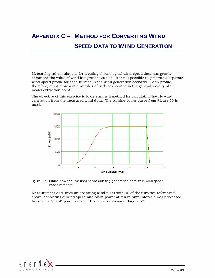
Page 86
APPENDIX C – METHOD FOR CONVERTING WIND
SPEED DATA TO WIND GENERATION
Meteorological simulations for creating chronological wind speed data has greatly enhanced the value of wind integration studies. It is not possible to generate a separate wind speed profile for each turbine in the wind generation scenario. Each profile, therefore, must represent a number of turbines located in the general vicinity of the model extraction point.
The objective of this exercise is to determine a method for calculating hourly wind generation from the measured wind data. The turbine power curve from Figure 56 is used.
Figure 56: Turbine power curve used for calculating generation data from wind speed
measurements.
Measurement data from an operating wind plant with 30 of the turbines referenced above, consisting of wind speed and plant power at ten minute intervals was processed to create a “plant” power curve. This curve is shown in Figure 57.
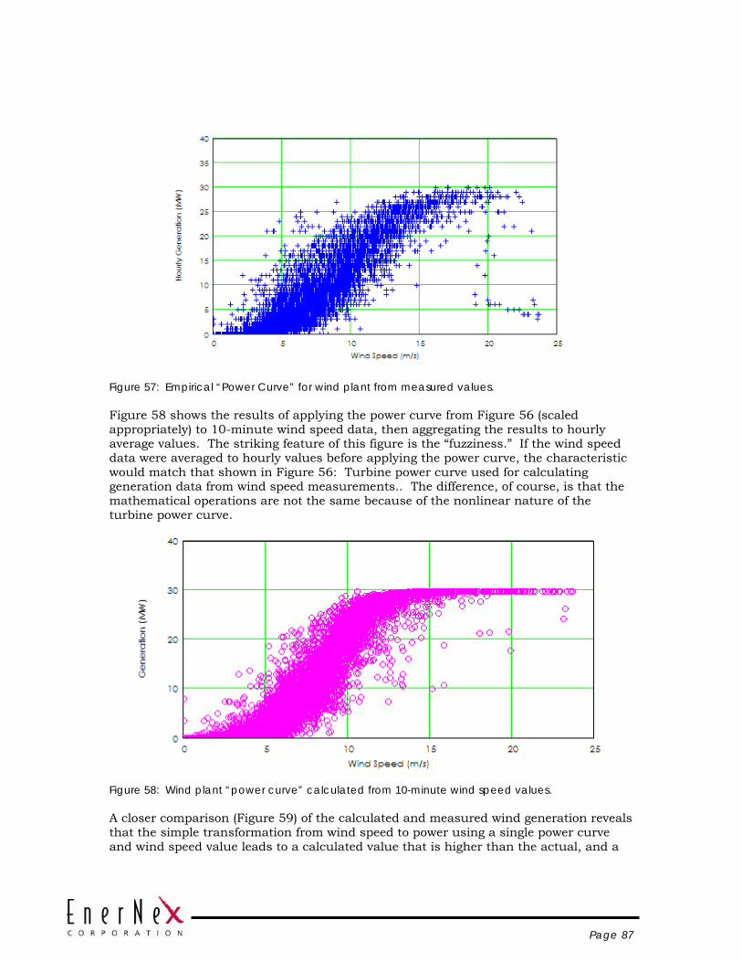
Page 87
Figure 57: Empirical “Power Curve” for wind plant from measured values.
Figure 58 shows the results of applying the power curve from Figure 56 (scaled appropriately) to 10-minute wind speed data, then aggregating the results to hourly average values. The striking feature of this figure is the “fuzziness.” If the wind speed data were averaged to hourly values before applying the power curve, the characteristic would match that shown in Figure 56: Turbine power curve used for calculating generation data from wind speed measurements.. The difference, of course, is that the mathematical operations are not the same because of the nonlinear nature of the turbine power curve.
Figure 58: Wind plant “power curve” calculated from 10-minute wind speed values.
A closer comparison (Figure 59) of the calculated and measured wind generation reveals that the simple transformation from wind speed to power using a single power curve and wind speed value leads to a calculated value that is higher than the actual, and a

Page 88
tendency to “saturate” during periods of high wind, sometimes unlike the measured data. A computation of the energy delivered shows that the calculated value is about 25% higher than what was actually metered.
Figure 60 illustrates this qualitatively. The “knee” of the calculated plant power curve is much more pronounced, although the “fit” is reasonable at lower power levels. Therefore, shifting the plant power curve to the right to approximately account for the diversity of wind speeds over the plant area would degrade the fit at lower wind speed levels.
Figure 59: Calculated vs. Measured wind generation.
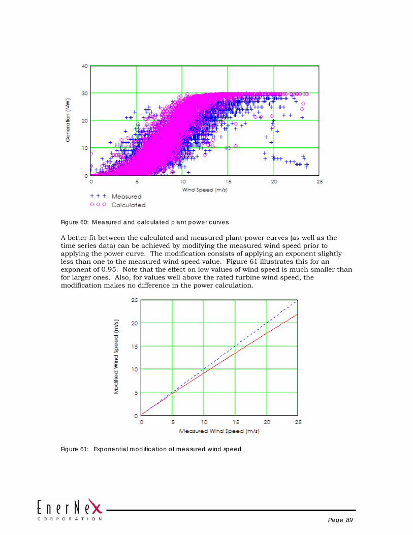
Page 89
Figure 60: Measured and calculated plant power curves.
A better fit between the calculated and measured plant power curves (as well as the time series data) can be achieved by modifying the measured wind speed prior to applying the power curve. The modification consists of applying an exponent slightly less than one to the measured wind speed value. Figure 61 illustrates this for an exponent of 0.95. Note that the effect on low values of wind speed is much smaller than for larger ones. Also, for values well above the rated turbine wind speed, the modification makes no difference in the power calculation.
Figure 61: Exponential modification of measured wind speed.
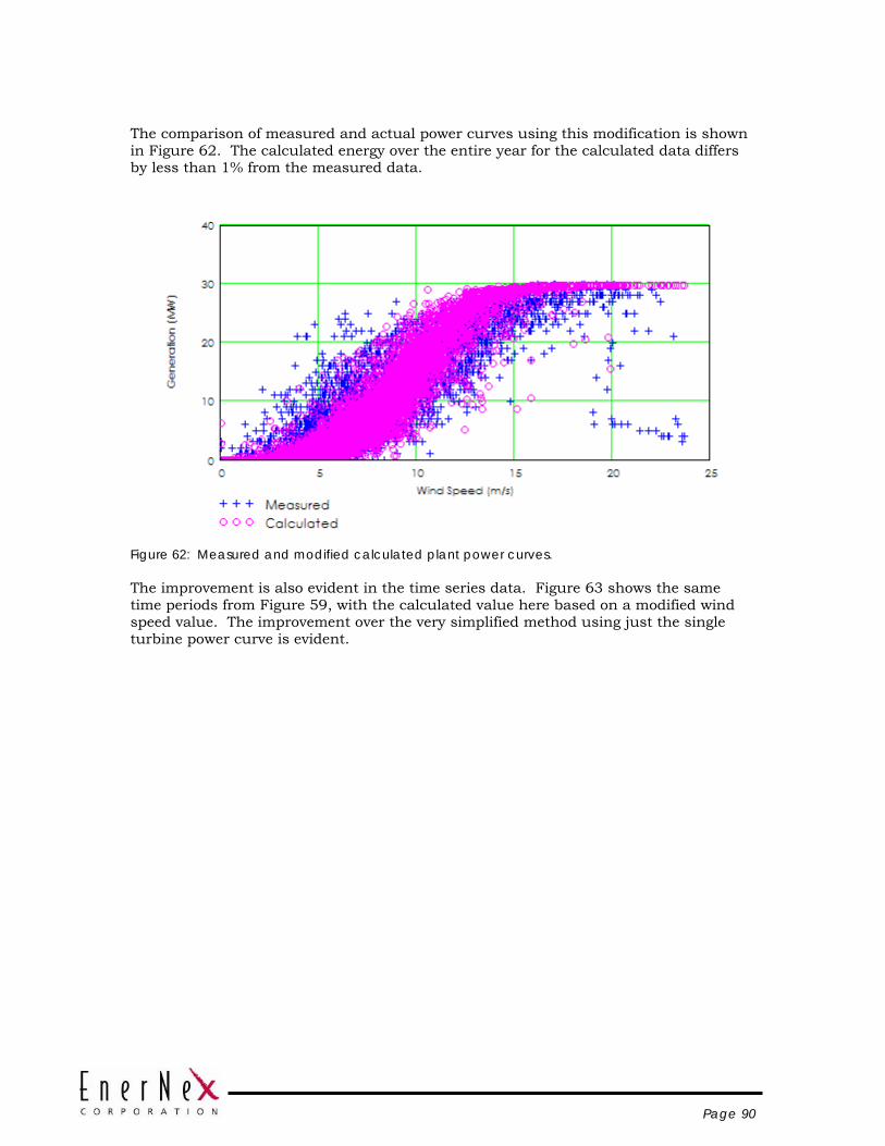
Page 90
The comparison of measured and actual power curves using this modification is shown in Figure 62. The calculated energy over the entire year for the calculated data differs by less than 1% from the measured data.
Figure 62: Measured and modified calculated plant power curves.
The improvement is also evident in the time series data. Figure 63 shows the same time periods from Figure 59, with the calculated value here based on a modified wind speed value. The improvement over the very simplified method using just the single turbine power curve is evident.

Page 91
Figure 63: Comparison of measured wind generation to that calculated with wind speed
modification.
=
Joint Intervenors
Exhibit 1
BEFORE THE SOUTH DAKOTA PUBLIC UTILITIES COMMISSION
In the Matter of the Application by Otter Tail Power
Company on behalf of the Big Stone II Co-owners for
an Energy Conversion Facility Siting Permit for the
Construction of the Big Stone II Project
)
)
)
)
Case No EL05-022
Direct Testimony of
David A. Schlissel and Anna Sommer
Synapse Energy Economics, Inc.
On Behalf of
Minnesotans for an Energy-Efficient Economy
Izaak Walton League of America – Midwest Office
Union of Concerned Scientists
Minnesota Center for Environmental Advocacy
May 19, 2006

Joint Intervenors
Exhibit 1
List of Joint Intervenors Exhibits
JI-1-A Resume of David Schlissel
JI-1-B Resume of Anna Sommer
JI-1-C EIA Natural Gas Price Forecasts 1990-2006
JI-1-D Interrogatory 18 of Joint Intervenors’ First Set and First Amended Set of Interrogatories
JI-1-E Descriptive Slide Submitted to Commission by Co-owners on 10.5.2005
JI-1-F Climate Change and Power: Carbon Dioxide Emissions Costs and Electricity Resource Planning
JI-1-G Minnesota PUC Order Establishing Environmental Cost Values
JI-1-H Joint Intervenors’ First Set of Requests for Admission

Direct Testimony of David A. Schlissel and Anna Sommer Joint Intervenors South Dakota Public Utilities Commission Case No. EL05-022 Exhibit 1
Page 1
Q. Mr. Schlissel, please state your name, position and business address. 1
A. My name is David A. Schlissel. I am a Senior Consultant at Synapse Energy 2
Economics, Inc, 22 Pearl Street, Cambridge, MA 02139. 3
Q. Ms. Sommer, please state your name position and business address. 4
A. My name is Anna Sommer. I am a Research Associate at Synapse Energy 5
Economics, Inc., 22 Pearl Street, Cambridge, MA 02139. 6
Q. On whose behalf are you testifying in this case? 7
A. We are testifying on behalf of Minnesotans for an Energy-Efficient Economy, 8
Izaak Walton League of America – Midwest Office, Union of Concerned 9
Scientists, and Minnesota Center for Environmental Advocacy (“Joint 10
Intervenors”). 11
Q. Please describe Synapse Energy Economics. 12
A. Synapse Energy Economics ("Synapse") is a research and consulting firm 13
specializing in energy and environmental issues, including electric generation, 14
transmission and distribution system reliability, market power, electricity market 15
prices, stranded costs, efficiency, renewable energy, environmental quality, and 16
nuclear power. 17
Synapse’s clients include state consumer advocates, public utilities commission 18
staff (and have included the Staff of the South Dakota Public Utilities 19
Commission), attorneys general, environmental organizations, federal government 20
and utilities. 21
Q. Mr. Schlissel, please summarize your educational background and recent 22
work experience. 23
A. I graduated from the Massachusetts Institute of Technology in 1968 with a 24
Bachelor of Science Degree in Engineering. In 1969, I received a Master of 25
Science Degree in Engineering from Stanford University. In 1973, I received a 26
Law Degree from Stanford University. In addition, I studied nuclear engineering 27
at the Massachusetts Institute of Technology during the years 1983-1986. 28

Direct Testimony of David A. Schlissel and Anna Sommer Joint Intervenors South Dakota Public Utilities Commission Case No. EL05-022 Exhibit 1
Page 2
Since 1983 I have been retained by governmental bodies, publicly-owned utilities, 1
and private organizations in 28 states to prepare expert testimony and analyses on 2
engineering and economic issues related to electric utilities. My clients have 3
included the Staff of the Arizona Corporation Commission, the General Staff of 4
the Arkansas Public Service Commission, the Staff of the Kansas State 5
Corporation Commission, municipal utility systems in Massachusetts, New York, 6
Texas, and North Carolina, and the Attorney General of the Commonwealth of 7
Massachusetts. 8
I have testified before state regulatory commissions in Arizona, New Jersey, 9
Connecticut, Kansas, Texas, New Mexico, New York, Vermont, North Carolina, 10
South Carolina, Maine, Illinois, Indiana, Ohio, Massachusetts, Missouri, and 11
Wisconsin and before an Atomic Safety & Licensing Board of the U.S. Nuclear 12
Regulatory Commission. 13
A copy of my current resume is attached as Exhibit JI-1-A. 14
Q. Have you previously submitted testimony before this Commission? 15
A. No. 16
Q. Ms. Sommer, please summarize your educational background and work 17
experience. 18
A. I am a Research Associate with Synapse Energy Economics. I provide research 19
and assist in writing testimony and reports on a wide range of issues from 20
renewable energy policy to integrated resource planning. My recent work includes 21
aiding a Florida utility in its integrated resource planning, evaluating the 22
feasibility of carbon sequestration and reviewing the analyses of the air emissions 23
compliance plans of two Indiana utilities and one Nova Scotia utility. 24
I also have participated in studies of proposed renewable portfolio standards in the 25
United States and Canada. In addition, I have evaluated the equity of utility 26
renewable energy solicitations in Nova Scotia and the feasibility and prudence of 27
the sale and purchase of existing gas and nuclear capacity in Arkansas and Iowa. 28

Direct Testimony of David A. Schlissel and Anna Sommer Joint Intervenors South Dakota Public Utilities Commission Case No. EL05-022 Exhibit 1
Page 3
Prior to joining Synapse, I worked at EFI and XENERGY (now KEMA 1
Consulting) and Zilkha Renewable Energy (now Horizon Wind Energy). At 2
XENERGY and Zilkha I focused on policy and economic aspects of renewable 3
energy. While at Zilkha, I authored a strategy and information plan for the 4
development of wind farms in the western United States. 5
I hold a BS in Economics and Environmental Studies from Tufts University. A 6
copy of my current resume is attached as Exhibit JI-1-B. 7
Q. Ms. Sommer, have you previously submitted testimony before this 8
Commission? 9
A. No. 10
Q. What is the purpose of your testimony? 11
A. Synapse was asked by Joint Intervenors to investigate the following four issues 12
regarding the proposed Big Stone II coal-fired generating facility: 13
A. The need and timing for new supply options in the utilities’ service 14 territories. 15
B. Whether there are alternatives to the proposed facility that are technically 16 feasible and economically cost-effective. 17
C. Whether the applicants have included appropriate emissions control 18 technologies in the design of the proposed facility. 19
D. Whether the applicants have appropriately reflected the potential for the 20 regulation of greenhouse gases in the design of the proposed facility and in 21 their analyses of the alternatives. 22
This testimony and the testimony of our colleague Dr. Ezra Hausman presents the 23
results of our investigations of Issue D. Our testimony regarding Issues A, B and 24
C will be submitted on May 26, 2006. 25
Q. Please summarize your conclusions on the issue of whether the Big Stone II 26
Co-owners have appropriately reflected the potential for the regulation of 27
greenhouse gases in the design of the proposed facility and in their analyses 28
of the alternatives. 29
A. Our conclusions on this issue are as follows: 30
Direct Testimony of David A. Schlissel and Anna Sommer Joint Intervenors South Dakota Public Utilities Commission Case No. EL05-022 Exhibit 1
Page 4
1. Climate change is causing and can be expected in the future to cause 1
“significant” environmental harm, as explained in detail in the Testimony 2
of Dr. Ezra Hausman. 3
2. There is scientific consensus that emissions of carbon dioxide cause 4
climate change. 5
3. Big Stone Unit II would emit significant amounts of additional carbon 6
dioxide. 7
4. As a result, the Big Stone Unit II will pose a serious threat to the 8
environment. 9
5. The potential for the regulation of carbon dioxide must be considered as 10
part of any prudent cost estimates of Big Stone Unit II and alternatives. 11
6. However, the Big Stone II Co-owners have not adequately analyzed the 12
potential for future carbon regulation. 13
7. The externality values for carbon dioxide established by the Minnesota 14
Public Utilities Commission and used in resource planning by some of the 15
Co-owners are meant to recognize “external” costs, or, in other words, 16
costs that are not directly paid by utilities or their customers. The 17
Minnesota Commission’s externality values are not reflective of any 18
concerns about the real costs of complying with future carbon dioxide 19
regulation. 20
8. Synapse Energy Economics has developed a greenhouse gas allowance 21
price forecast that reflects a range of prices that could reasonably be 22
expected through 2030. 23
9. Adopting Synapse’s range of prices would increase Big Stone Unit II’s 24
annual projected costs by $35,152,128 to $137,463,322 on a levelized 25
basis. 26

Direct Testimony of David A. Schlissel and Anna Sommer Joint Intervenors South Dakota Public Utilities Commission Case No. EL05-022 Exhibit 1
Page 5
Q. In the process of your investigation did you keep in mind the interests of the 1
Big Stone Co-owners’ customers? 2
A. Absolutely. Synapse regularly works for consumer advocates and has worked for 3
over half of the members of the National Association of State Utility Consumer 4
Advocates. Fundamentally, we believe that greenhouse gas regulation not only is 5
an environmental issue. It also is a consumer issue in that it will have direct and 6
tangible impacts on future rates. 7
Q. You have mentioned the terms “carbon dioxide regulation” and “greenhouse 8
gas regulation.” What is the difference between these two? 9
A. As we use these terms throughout our testimony, there is no difference. While we 10
believe that the future regulation we discuss here will govern emissions of all 11
types of greenhouse gases, not just carbon dioxide (“CO2”), for the purposes of 12
our discussion we are chiefly concerned with emissions of carbon dioxide. 13
Therefore, we use the terms “carbon dioxide regulation” and “greenhouse gas 14
regulation” interchangeably. Similarly, the terms “carbon dioxide price,” 15
“greenhouse gas price” and “carbon price” are interchangeable. 16
Q. Is it prudent to expect that a policy to address climate change will be 17
implemented in the U.S. in a way that should be of concern to coal-dependent 18
utilities in the Midwest? 19
A. Yes. The prospect of global warming and the resultant widespread climate 20
changes has spurred international efforts to work towards a sustainable level of 21
greenhouse gas emissions. These international efforts are embodied in the United 22
Nations Framework Convention on Climate Change (“UNFCCC”), a treaty that 23
the U.S. ratified in 1992, along with almost every other country in the world. The 24
Kyoto Protocol, a supplement to the UNFCCC, establishes legally binding limits 25
on the greenhouse gas emissions of industrialized nations and economies in 26
transition. 27
Despite being the single largest contributor to global emissions of greenhouse 28
gases, the United States remains one of a very few industrialized nations that have 29

Direct Testimony of David A. Schlissel and Anna Sommer Joint Intervenors South Dakota Public Utilities Commission Case No. EL05-022 Exhibit 1
Page 6
not signed the Kyoto Protocol. Nevertheless, individual states, regional groups of 1
states, shareholders and corporations are making serious efforts and taking 2
significant steps towards reducing greenhouse gas emissions in the United States. 3
Efforts to pass federal legislation addressing carbon, though not yet successful, 4
have gained ground in recent years. These developments, combined with the 5
growing scientific understanding of, and evidence of, climate change as outlined 6
in Dr. Hausman’s testimony, mean that establishing federal policy requiring 7
greenhouse gas emission reductions is just a matter of time. The question is not 8
whether the United States will develop a national policy addressing climate 9
change, but when and how. The electric sector will be a key component of any 10
regulatory or legislative approach to reducing greenhouse gas emissions both 11
because of this sector’s contribution to national emissions and the comparative 12
ease of regulating large point sources. 13
There are, of course, important uncertainties with regard to the timing, the 14
emission limits, and many other details of what a carbon policy in the United 15
States will look like. 16
Q. If there are uncertainties with regard to such important details as timing, 17
emission limits and other details, why should a utility engage in the exercise 18
of forecasting greenhouse gas prices? 19
A. First of all, utilities are implicitly assuming a value for carbon allowance prices 20
whether they go to the effort of collecting all the relevant information and create a 21
price forecast or whether they simply ignore future carbon regulation. In other 22
words, a utility that ignores future carbon regulations is implicitly assuming that 23
the allowance value will be zero. The question is whether it’s appropriate to 24
assume zero or some other number. There is uncertainty in any type of utility 25
forecasting and to write off the need to forecast carbon allowance prices because 26
of the uncertainties is not prudent. 27
For example, there are myriad uncertainties that utility planners have learned to 28
address in planning. These include randomly occurring generating unit outages, 29
load forecast error and demand fluctuations, and fuel price volatility and 30

Direct Testimony of David A. Schlissel and Anna Sommer Joint Intervenors South Dakota Public Utilities Commission Case No. EL05-022 Exhibit 1
Page 7
uncertainty. These various uncertainties can be addressed through techniques 1
such as sensitivity and scenario analyses. 2
To illustrate that there is significant uncertainty in other types of forecasts, we 3
think it is informative to examine historical gas price forecasts by the Energy 4
Information Administration (EIA). Exhibit JI-1-C compares EIA forecasts from 5
the period 1990 - 2006 with actual price data through 2005. The data, over more 6
than a decade, shows considerable volatility, even on an annual time scale.1 But 7
the truly striking thing that jumps out of the figure is how wrong the forecasts 8
have sometimes been. For example, the 1996 forecast predicted gas prices would 9
start at $2.61/MMBtu and remain under $3/MMBTU through 2010, but by the 10
year 2000 actual prices had already jumped to $4.82/MMBTu and by 2005 they 11
were up to $8.09/MMBtu. 12
In view of the forecasting track record for gas prices one might be tempted to give 13
up, and either throw darts or abandon planning altogether. But thankfully 14
modelers, forecasters, and planners have taken on the challenge – and have 15
improved the models over time, thereby producing more reliable (although still 16
quite uncertain) price forecasts, and system planners have refined and applied 17
techniques for addressing fuel price uncertainty in a rational and proactive way. 18
It is, therefore, troubling and wrong to claim that forecasting carbon allowance 19
prices should not be undertaken as a part of utility resource decision-making 20
because it is “speculative.” 21
Q. Do the Co-owners have any opinions or thoughts as to when carbon 22
regulation will happen? 23
A. No. Interrogatory 18 of Joint Intervenors’ First Set and First Amended Set of 24
Interrogatories2 asked each of the Co-owners to state whether it: 25
1 Gas prices also show terrific volatility on shorter time scales (e.g., monthly or weekly prices).
2 The Co-owners’ response to Interrogatory 18 is attached as Exhibit JI-1-D.

Direct Testimony of David A. Schlissel and Anna Sommer Joint Intervenors South Dakota Public Utilities Commission Case No. EL05-022 Exhibit 1
Page 8
believes it is likely that greenhouse gas regulation (ghg) will be 1 implemented in the U.S. (a) in the next five years, (b) in the next ten 2 years, and (c) in the next twenty years. 3
None of the co-owners had any thoughts as to when or even if greenhouse gas 4
regulation would occur. Two of the Co-owners (GRE and HCPD) claim to 5
closely follow discussion of GHG regulation at the federal and State levels, but 6
apparently had no opinions about what might result from such discussions. 7
Q. If the siting permit for Big Stone Unit II were to be approved and the unit 8
were built, is carbon regulation an issue that could be reasonably dealt with 9
in the future, once the timing and stringency of the regulation is known? 10
A. Unfortunately, no. Unlike for other power plant air emissions like sulfur dioxide 11
and oxides of nitrogen, there currently is no commercial or economical method 12
for post-combustion removal of carbon dioxide from supercritical pulverized coal 13
plants. The Big Stone II Co-owners agree on that point. During the public hearing 14
in Milbank held on September 13, 20005, the Co-owners presented several slides 15
on the expected combined emissions from Big Stone Units I & II. The descriptive 16
slide for the CO2 emissions chart submitted to the South Dakota PUC states there 17
is “no commercially available capture and sequestration technology.” This slide 18
is attached as Exhibit JI-1-E. Regardless of the uncertainty, this is an issue that 19
needs to be dealt with before new resource decisions are made. 20
Q. Do other utilities have opinions about whether and when greenhouse gas 21
regulation will come? 22
A. Yes. For example, James Rogers, CEO of Duke Energy, has publicly said “[I]n 23
private, 80-85% of my peers think carbon regulation is coming within ten years, 24
but most sure don’t want it now.”3 Not wanting carbon regulation from a utility 25
perspective is understandable because carbon price forecasting is not simple and 26
easy, it makes resource planning more difficult and is likely to change “business 27
3 “The Greening of General Electric: A Lean, Clean Electric Machine,” The Economist, December 10, 2005, at page 79.
Direct Testimony of David A. Schlissel and Anna Sommer Joint Intervenors South Dakota Public Utilities Commission Case No. EL05-022 Exhibit 1
Page 9
as usual.” For many utilities, including the Big Stone II Co-owners, that means 1
that it is much more difficult to justify building a pulverized coal plant. 2
Regardless, it is imprudent to ignore the risk. 3
Duke is not alone in believing that carbon regulation is inevitable and, indeed, 4
some utilities are advocating for mandatory greenhouse gas reductions. In a May 5
6, 2005, statement to the Climate Leaders Partners (a voluntary EPA-industry 6
partnership), John Rowe, Chair and CEO of Exelon stated, “At Exelon, we accept 7
that the science of global warming is overwhelming. We accept that limitations 8
on greenhouse gases emissions [sic] will prove necessary. Until those limitations 9
are adopted, we believe that business should take voluntary action to begin the 10
transition to a lower carbon future.” 11
In fact, several electric utilities and electric generation companies have 12
incorporated assumptions about carbon regulation and costs into their long term 13
planning, and have set specific agendas to mitigate shareholder risks associated 14
with future U.S. carbon regulation policy. These utilities cite a variety of reasons 15
for incorporating risk of future carbon regulation as a risk factor in their resource 16
planning and evaluation, including scientific evidence of human-induced climate 17
change, the U.S. electric sector’s contribution to emissions, and the magnitude of 18
the financial risk of future greenhouse gas regulation. 19
Some of the companies believe that there is a high likelihood of federal regulation 20
of greenhouse gas emissions within their planning period. For example, 21
Pacificorp states a 50% probability of a CO2 limit starting in 2010 and a 75% 22
probability starting in 2011. The Northwest Power and Conservation Council 23
models a 67% probability of federal regulation in the twenty-year planning period 24
ending 2025 in its resource plan. Northwest Energy states that CO2 taxes “are no 25
longer a remote possibility.”4 26
4 Northwest Energy 2005 Electric Default Supply Resource Procurement Plan, December 20, 2005; Volume 1, p. 4.

Direct Testimony of David A. Schlissel and Anna Sommer Joint Intervenors South Dakota Public Utilities Commission Case No. EL05-022 Exhibit 1
Page 10
Even those in the electric industry who oppose mandatory limits on greenhouse 1
gas regulation believe that regulation is inevitable. David Ratcliffe, CEO of 2
Southern Company, a predominantly coal-fired utility that opposes mandatory 3
limits, said at a March 29, 2006, press briefing that “There certainly is enough 4
public pressure and enough Congressional discussion that it is likely we will see 5
some form of regulation, some sort of legislation around carbon.”5 6
Q. Do companies outside of electric utilities support greenhouse gas regulation? 7
Support for the passage of greenhouse gas regulation has been expressed by 8
senior executives in companies such as Wal-Mart, General Electric, BP, Shell, 9
and Goldman Sachs. For example, on April 4, 2006, during a Senate hearing on 10
the design of a CO2 cap-and-trade system, a representative of GE Energy said the 11
following: 12
“GE supports development of market-based programs to slow, eventually stop, 13
and ultimately reverse the growth of greenhouse gases (GHG).” 14
--David Slump, GE Energy, General Manager, Global Marketing, executive 15
summary of comments to Senate Energy and Natural Resources Committee 16
Q. Why would so many electric utilities, in particular, be concerned about 17
future carbon regulation? 18
A. Electricity generation is very carbon-intensive. Electric utilities are likely to be 19
one of the first, if not the first, industries subject to carbon regulation because of 20
the relative ease in regulating stationary sources as opposed to mobile sources 21
(automobiles) and because electricity generation represents a significant portion 22
of total U.S. greenhouse gas emissions. A new generating facility may have a 23
book life of twenty to forty years, but in practice, the utility may expect that that 24
asset will have an operating life of 50 years or more. By adding new plants, 25
especially new coal plants, a utility is essentially locking-in a large quantity of 26
5 Quoted in “U.S. Utilities Urge Congress to Establish CO2 Limits,” Bloomberg.com, http://www.bloomberg.com/apps/news?pid=10000103&sid=a75A1ADJv8cs&refer=us

Direct Testimony of David A. Schlissel and Anna Sommer Joint Intervenors South Dakota Public Utilities Commission Case No. EL05-022 Exhibit 1
Page 11
carbon dioxide emissions for decades to come. In general, electric utilities are 1
increasingly aware that the fact that we do not currently have federal greenhouse 2
gas regulation is irrelevant to the issue of whether we will in the future, and that 3
new plant investment decisions are extremely sensitive to the expected cost of 4
greenhouse gas regulation throughout the life of the facility. 5
Q. Have mandatory greenhouse gas emissions reductions programs begun to be 6
examined and debated in the U.S. federal government? 7
A. To date, the U.S. government has not required greenhouse gas emission 8
reductions. However, legislative initiatives for a mandatory market-based 9
greenhouse gas cap and trade program are under consideration.6 10
Several mandatory emissions reduction proposals have been introduced in 11
Congress. These proposals establish carbon dioxide emission trajectories below 12
the projected business-as-usual emission trajectories, and they generally rely on 13
market-based mechanisms (such as cap and trade programs) for achieving the 14
targets. The proposals also include various provisions to spur technology 15
innovation, as well as details pertaining to offsets, allowance allocation, 16
restrictions on allowance prices and other issues. Through their consideration of 17
these proposals, legislators are increasingly educated on the complex details of 18
different policy approaches, and they are laying the groundwork for a national 19
mandatory program. Federal proposals that would require greenhouse gas 20
emission reductions are summarized in Table 5.1 in Exhibit JI-1-F. 21
It is significant that the U.S. Congress is examining and debating these emissions 22
reduction proposals. However, as shown in Figure 5.2 in Exhibit JI-1-F, the 23
emissions trajectories contained in the proposed federal legislation are in fact 24
quite modest compared with the emissions reductions that are anticipated to be 25
necessary to achieve stabilization of atmospheric concentrations of greenhouse 26
gases. Figure 5.2 in Exhibit JI-1-F compares various emission reduction 27
trajectories and goals in relation to a 1990 baseline. U.S. federal proposals, and 28
6 Exhibit JI-1-F, at pages 11- 16.
Direct Testimony of David A. Schlissel and Anna Sommer Joint Intervenors South Dakota Public Utilities Commission Case No. EL05-022 Exhibit 1
Page 12
even Kyoto Protocol reduction targets, are small compared with the current E.U. 1
emissions reduction target for 2020, and the emissions reductions that most 2
scientists claim will ultimately be necessary to avoid the most dangerous impacts 3
of global warming. 4
Q. Are any states developing and implementing climate change policies that will 5
have a bearing on resource choices in the electric sector? 6
A. Yes. A growing number of states are developing and implementing the following 7
types of policies that will affect greenhouse gas emissions in the electric sector: 8
(1) direct policies that require specific emissions reductions from electric 9
generation sources; (2) indirect policies that affect electric sector resource mix 10
such as through promoting low-emission electric sources; (3) legal proceedings; 11
or (4) voluntary programs including educational efforts and energy planning.7 12
Direct policies include the New Hampshire and Massachusetts laws imposing 13
caps on carbon dioxide emissions from power plants in those states. 14
Indirect policies include the requirements by various states to either consider 15
future carbon dioxide regulation or use specific “adders” for carbon dioxide in 16
resource planning. It also includes policies and incentives to increase energy 17
efficiency and renewable energy use, such as renewable portfolio standards. 18
Some of these requirements are at the direction of state public utilities 19
commissions, others are statutory requirements. 20
Lawsuits make up the majority of the third category. For example, several states 21
are suing the U.S. Environmental Protection Agency (EPA) to have carbon 22
dioxide regulated as a pollutant under the Clean Air Act. 23
Among the voluntary programs undertaken at the state level are the climate 24
change action plans developed by 28 states. 25
7 Exhibit JL-1-F, at pages 16 through 20.
Direct Testimony of David A. Schlissel and Anna Sommer Joint Intervenors South Dakota Public Utilities Commission Case No. EL05-022 Exhibit 1
Page 13
But states are not just acting individually; there are a number of examples of 1
innovative regional policy initiatives that range from agreeing to coordinate 2
information (e.g., Southwest governors and Midwestern legislators) to 3
development of a regional cap and trade program through the Regional 4
Greenhouse Gas Initiative in the Northeast (“RGGI”). The objective of the RGGI 5
is the stabilization of CO2 emissions from power plants at current levels for the 6
period 2009-2015, followed by a 10 percent reduction below current levels by 7
2019. These regional activities are summarized in Table 5.5 in Exhibit JI-1-F. 8
Q. Have any states adopted direct policies that require specific emissions 9
reductions from electric sources? 10
A. Yes. The states of Massachusetts, New Hampshire, Oregon and California have 11
adopted policies requiring greenhouse gas emission reductions from power 12
plants.8 13
Q. Do any states require that utilities or default service suppliers evaluate costs 14
or risks associated with greenhouse gas emissions in long-range planning or 15
resource procurement? 16
A. Yes. As shown in Table 1 below, several states require companies under their 17
jurisdiction to account for the emission of greenhouse gases in resource planning. 18
8 Exhibit JI-1-F, Table 5.3 on page 18.
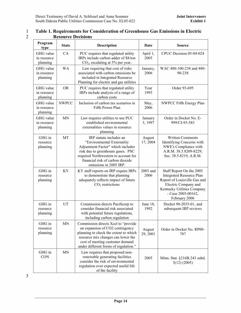
Direct Testimony of David A. Schlissel and Anna Sommer Joint Intervenors South Dakota Public Utilities Commission Case No. EL05-022 Exhibit 1
Page 14
Table 1. Requirements for Consideration of Greenhouse Gas Emissions in Electric 1 Resource Decisions 2
Program
type State Description Date Source
GHG value in resource planning
CA PUC requires that regulated utility IRPs include carbon adder of $8/ton CO2, escalating at 5% per year.
April 1, 2005
CPUC Decision 05-04-024
GHG value in resource planning
WA Law requiring that cost of risks associated with carbon emissions be included in Integrated Resource
Planning for electric and gas utilities
January, 2006
WAC 480-100-238 and 480-90-238
GHG value in resource planning
OR PUC requires that regulated utility IRPs include analysis of a range of
carbon costs
Year 1993
Order 93-695
GHG value in resource planning
NWPCC Inclusion of carbon tax scenarios in Fifth Power Plan
May, 2006
NWPCC Fifth Energy Plan
GHG value in resource planning
MN Law requires utilities to use PUC established environmental
externalities values in resource planning
January 3, 1997
Order in Docket No. E-999/CI-93-583
GHG in resource planning
MT IRP statute includes an "Environmental Externality
Adjustment Factor" which includes risk due to greenhouse gases. PSC required Northwestern to account for financial risk of carbon dioxide
emissions in 2005 IRP.
August 17, 2004
Written Comments Identifying Concerns with NWE's Compliance with A.R.M. 38.5.8209-8229; Sec. 38.5.8219, A.R.M.
GHG in resource planning
KY KY staff reports on IRP require IRPs to demonstrate that planning
adequately reflects impact of future CO2 restrictions
2003 and 2006
Staff Report On the 2005 Integrated Resource Plan
Report of Louisville Gas and Electric Company and
Kentucky Utilities Company - Case 2005-00162, February 2006
GHG in resource planning
UT Commission directs Pacificorp to consider financial risk associated with potential future regulations, including carbon regulation
June 18, 1992
Docket 90-2035-01, and subsequent IRP reviews
GHG in resource planning
MN Commission directs Xcel to “provide an expansion of CO2 contingency planning to check the extent to which resource mix changes can lower the cost of meeting customer demand under different forms of regulation.”
August 29, 2001
Order in Docket No. RP00-787
GHG in CON
MN Law requires that proposed non-renewable generating facilities
consider the risk of environmental regulation over expected useful life
of the facility
2005
Minn. Stat. §216B.243 subd. 3(12) (2005)
3

Direct Testimony of David A. Schlissel and Anna Sommer Joint Intervenors South Dakota Public Utilities Commission Case No. EL05-022 Exhibit 1
Page 15
Q. What carbon dioxide values are being used by utilities in electric resource 1
planning? 2
A. Table 2 below presents the carbon dioxide costs, in $/ton CO2, that are presently 3
being used in the industry for both resource planning and modeling of carbon 4
regulation policies. 5
Table 2. Carbon Dioxide Costs Used by Utilities 6
Company CO2 emissions trading assumptions for various years
($2005)
PG&E* $0-9/ton (start year 2006)
Avista 2003* $3/ton (start year 2004)
Avista 2005 $7 and $25/ton (2010) $15 and $62/ton (2026 and 2023)
Portland General Electric*
$0-55/ton (start year 2003)
Xcel-PSCCo $9/ton (start year 2010) escalating at 2.5%/year
Idaho Power* $0-61/ton (start year 2008)
Pacificorp 2004 $0-55/ton
Northwest Energy 2005
$15 and $41/ton
Northwest Power and Conservation Council
$0-15/ton between 2008 and 2016
$0-31/ton after 2016
*Values for these utilities from Wiser, Ryan, and Bolinger, Mark. “Balancing Cost and Risk: The 7 Treatment of Renewable Energy in Western Utility Resource Plans.” Lawrence Berkeley National 8 Laboratories. August 2005. LBNL-58450. Table 7. 9 Other values: PacifiCorp, Integrated Resource Plan 2003, pages 45-46; and Idaho Power 10 Company, 2004 Integrated Resource Plan Draft, July 2004, page 59; Avista Integrated Resource 11 Plan 2005, Section 6.3; Northwestern Energy Integrated Resource Plan 2005, Volume 1 p. 62; 12 Northwest Power and Conservation Council, Fifth Power Plan pp. 6-7. Xcel-PSCCo, 13 Comprehensive Settlement submitted to the CO PUC in dockets 04A-214E, 215E and 216E, 14 December 3, 2004. Converted to $2005 using GDP implicit price deflator. 15
Q. How should utilities plan for and mitigate the risk of greenhouse gas 16
regulation? 17
A. The key part of that question is “plan for the risk of greenhouse gas regulation.” 18
Mitigating risk begins with the resource planning process and the decision as to 19
the demand-side and supply-side options that should be pursued. A utility that 20
chooses to go forward with a new, carbon intensive energy resource without 21
proper consideration of carbon regulation is imprudent. To give an analogy it 22
would be like choosing to build a gas-fired power plant without consideration of 23

Direct Testimony of David A. Schlissel and Anna Sommer Joint Intervenors South Dakota Public Utilities Commission Case No. EL05-022 Exhibit 1
Page 16
the cost of gas because one believes that building the plant is “worth it” regardless 1
of what gas might cost. 2
A utility that desires to be prudent about the risk of carbon regulation would, at a 3
minimum, consider carbon regulation by developing an expected carbon price 4
forecast as well as reasonable sensitivities around that case. 5
Q. Please explain how Synapse developed its carbon price forecast. 6
A. Our forecast is described in more detail in Exhibit JI-1-F starting on page 39. 7
During the decade from 2010 to 2020, we anticipate that a reasonable range of 8
carbon emissions prices will reflect the effects of increasing public concern over 9
climate change (this public concern is likely to support increasingly stringent 10
emission reduction requirements) and the reluctance of policymakers to take steps 11
that would increase the cost of compliance (this reluctance could lead to increased 12
emphasis on energy efficiency, modest emission reduction targets, or increased 13
use of offsets). We expect that the widest uncertainty in our forecasts will begin at 14
the end of this decade, that is, from $10 to $40 per ton of CO2 in 2020, depending 15
on the relative strength of these factors. 16
After 2020, we expect the price of carbon emissions allowances to trend upward 17
toward a marginal mitigation cost. This number will depend on currently 18
uncertain factors such as technological innovation and the stringency of carbon 19
caps, but it is likely that, by this time, the least expensive mitigation options (such 20
as simple energy efficiency and fuel switching) will have been exhausted. Our 21
projection for greenhouse gas emissions costs at the end of this decade ranges 22
from $20 to $50 per ton of CO2 emissions. 23
We currently believe that the most likely scenario is that as policymakers commit 24
to taking serious action to reduce carbon emissions, they will choose to enact both 25
cap and trade regimes and a range of complementary energy policies that lead to 26
lower cost scenarios, and that technology innovation will reduce the price of low-27
carbon technologies, making the most likely scenario closer to (though not equal 28
to) low case scenarios than the high case scenario. We expect that the probability 29

Direct Testimony of David A. Schlissel and Anna Sommer Joint Intervenors South Dakota Public Utilities Commission Case No. EL05-022 Exhibit 1
Page 17
of taking this path will increase over time, as society learns more about optimal 1
carbon reduction policies. 2
After 2030, and possibly even earlier, the uncertainty surrounding a forecast of 3
carbon emission prices will increase due to the interplay of factors such as the 4
level of carbon constraints required and technological innovation. As discussed in 5
Exhibit JI-1-F, scientists anticipate that very significant emission reductions will 6
be necessary, in the range of 80 percent below 1990 emission levels, to achieve 7
stabilization targets that will keep global temperature increases to a somewhat 8
manageable level. As such, we believe there is a substantial likelihood that 9
response to climate change impacts will require much more aggressive emission 10
reductions than those contained in U.S. policy proposals, and in the Kyoto 11
Protocol, to date. If the severity and certainty of climate change are such that 12
emissions levels 70-80% below current rates are mandated, this could result in 13
very high marginal emissions reduction costs, though we have not quantified the 14
cost of such deeper cuts on a per ton basis. 15
Q. What is Synapse’s forecast of carbon dioxide emissions prices? 16
A. Synapse’s forecast of future carbon dioxide emissions prices are presented in 17
Figure 1 below. This figure superimposes Synapse’s forecast on the results of 18
other cost analyses of proposed federal policies: 19
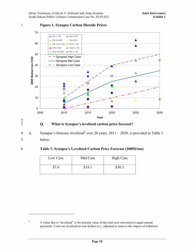
Direct Testimony of David A. Schlissel and Anna Sommer Joint Intervenors South Dakota Public Utilities Commission Case No. EL05-022 Exhibit 1
Page 18
Figure 1. Synapse Carbon Dioxide Prices 1
0
10
20
30
40
50
60
70
2005 2010 2015 2020 2025 2030
Year
2005 $/short ton CO2 Synapse High Case
Synapse Mid Case
Synapse Low Case
2 Q. What is Synapse’s levelized carbon price forecast? 3
A. Synapse’s forecast, levelized9 over 20 years, 2011 – 2030, is provided in Table 3 4
below. 5
Table 3. Synapse’s Levelized Carbon Price Forecast (2005$/ton) 6
Low Case Mid Case High Case
$7.8 $19.1 $30.5
9 A value that is “levelized” is the present value of the total cost converted to equal annual payments. Costs are levelized in real dollars (i.e., adjusted to remove the impact of inflation).

Direct Testimony of David A. Schlissel and Anna Sommer Joint Intervenors South Dakota Public Utilities Commission Case No. EL05-022 Exhibit 1
Page 19
Q. The Minnesota Public Utilities Commission has established environmental 1
externality values for a number of pollutants including CO2. Wouldn’t it be 2
sufficient and more efficient to simply use the CO2 externality values? The 3
effect is the same, to bias resource selection towards non-CO2 emitting 4
resources. 5
A. That would appear to be an easy solution, but the MN PUC values are meant to 6
reflect external costs arising from damage to the environment caused by climate 7
change (as a percentage of GDP). The Commission’s order of January 3, 1997 8
explained: 10 9
The environmental values for CO2 quantified in this Order follow 10 MPCA witness Ciborowski’s general methodology. First, Ciborowski 11 estimated long-term global costs based on the existing economic 12 literature and discounted them to current values. Then, he divided 13 that amount by the amount of long-term CO2 emissions to arrive at an 14 average cost per ton. Ciborowski essentially converted published 15 damage estimates made by economists from percentages of gross 16 domestic product (GDP) into costs per ton of CO2.
17
The full order is attached as Exhibit JI-1-G. Clearly this order shows that the 18
Minnesota environmental externality values contain no consideration of future 19
carbon regulation and the actual costs that regulation would impose on utilities. 20
Indeed, the range of CO2 values adopted by the Minnesota PUC is much smaller 21
than the range of Synapse’s price forecasts, $0.35 – 3.64 per ton of CO2 (2004$). 22
Q. Have the Big Stone II co-owners adequately considered the risk of 23
greenhouse gas regulation? 24
A. No. The Co-owners’ approach is what might be called keeping their heads in the 25
sand and hoping that the problem of global warming goes away. For example, the 26
Co-owners could not answer basic questions about the United Nations Framework 27
Convention on Climate Change. Request for Admission No. 22 in the Joint 28
Intervenors’ First Set of Requests for Admission asked the Co-owners to: 29
10 Page 27 of the Order Establishing Environmental Cost Values in Docket No. E-99/CI-93-583 issued January 3, 1997.
Direct Testimony of David A. Schlissel and Anna Sommer Joint Intervenors South Dakota Public Utilities Commission Case No. EL05-022 Exhibit 1
Page 20
Admit that in 1992 the United Nations Framework Convention on 1 Climate Change was adopted [IPCC 2005, p 5]. 2
The Co-owners responded by saying that: 3
Applicant has made reasonable inquiry and the information known to 4 it is insufficient to enable Applicant to admit or deny this statement. 5
Similarly, Request for Admission No. 25 asked the Co-owners to: 6
Admit that the most recent Assessment Report released by the IPCC is 7 the Third Assessment Report (TAR), released in 2001, and that part of 8 the TAR is the report of the Working Group I of the IPCC, entitled 9 “Climate Change 2001: The Scientific Basis.” 10
Again, the Co-owners responded, in part: 11
Applicant has made reasonable inquiry and the information known to 12 it is insufficient to enable Applicant to admit or deny this statement. 13
In twenty separate instances, the Co-owners could not answer requests for 14
admission requiring them to do nothing more than admit facts that could easily be 15
verified by an internet search (starting with the internet addresses that Joint 16
Intervenors in many cases provided in the questions) or by referring to the 17
document(s) attached to the request. Attached as Exhibit JI-1-H, is the Joint 18
Intervenors’ First Set of Requests for Admission with these twenty responses 19
highlighted. 20
Q. How are such responses relevant to the issue of considering carbon 21
regulation in resource planning? 22
A. If a utility does not rely upon outside expertise to, at a basic level, advise the 23
utility on future carbon regulation and second to forecast carbon allowance prices, 24
it must rely upon its own knowledge and information gathering to do so. A major 25
step in that process is to understand the various parties involved and what their 26
recommendations mean to policymakers. Organizations such as the 27
Intergovernmental Panel on Climate Change are well recognized and regarded 28
and their thoughts on topics such as climate change do not go by the wayside. 29
The inability to answer these basic questions, let alone put in the small effort that 30

Direct Testimony of David A. Schlissel and Anna Sommer Joint Intervenors South Dakota Public Utilities Commission Case No. EL05-022 Exhibit 1
Page 21
would be necessary to answer such questions, bodes poorly for the Co-owners’ 1
decision-making. 2
Q. Did the Co-owners reflect any potential greenhouse gas regulations in their 3
resource planning for Big Stone II? 4
A. No. In certain instances they used the Minnesota PUC environmental externality 5
value for carbon dioxide, which as we discussed above is not adequate 6
consideration of regulatory risk and uncertainty. 7
Q. Are the Big Stone II Co-owners already heavily dependent upon coal-fired 8
generation? 9
A. Yes. The testimony in this proceeding reveals that each of the Co-owners already 10
is heavily dependent upon coal-fired generation. Although some Co-owners are 11
making some efforts to add wind, participation in Big Stone II will further 12
increase the Co-owners’ dependence upon coal-fired generation and, 13
consequently, their exposure to future greenhouse gas regulations. 14
For example, Otter Tail Power’s testimony in this proceeding reveals that as of 15
2004, 60.3 percent (winter) to 65.3 percent (summer) of the Company’s 16
generating capacity was coal-fired.11 When oil and natural gas fired capacity is 17
included, more than 75 percent of Otter Tail’s current generating capacity is 18
fossil-fired. 19
GRE’s 2006 generation mix is 76 percent from coal, not including additional 20
coal-fired generation that might be the sources for the other purchased power 21
listed in the Company’s testimony.12 22
CMMPA’s listing of its existing and planned capacity resources includes 43 MW 23
of coal-fired capacity (75 percent of the total) and 13.5 MW of wind.13 24
11 Applicants’ Exhibits 10-D and 10-E.
12 Applicants’ Exhibit 2, page 14, lines 19-23.
13 Applicants’ Exhibit 6, page 10, lines 1-2.

Direct Testimony of David A. Schlissel and Anna Sommer Joint Intervenors South Dakota Public Utilities Commission Case No. EL05-022 Exhibit 1
Page 22
Seventy-six percent of Montana-Dakota Utilities existing owned-generation is 1
coal-fired.14 However, despite this reliance on coal, Montana-Dakota Utilities 2
2005 Integrated Resource Plan reveals that, other than possible purchases from 3
other utilities or the energy market, the only new baseload options that the 4
company was considering were coal-fired units.15 5
Approximately 50 percent of MRES’ existing capacity, and all of its baseload 6
capacity, is coal-fired.16 7
Approximately 59 percent of SMMPA’s existing generating capacity is coal-8
fired.17 9
Finally, Heartland’s existing resources appear to be a mix of coal-fired generation 10
and purchased power contracts.18 Heartland has indicated that from 2013 to 2020, 11
i.e., after the end of its purchased power agreement with Nebraska Public Power 12
District, it plans to have the following resources available for its customers: 13
Laramie River Station (50 MW); Customer-owned peaking generation (24 MW); 14
Big Stone Unit II (25 MW); and Whelan Energy Center Unit 2 (80 MW).19 This 15
means that all of the resources that Heartland plans to have available for its 16
customers during these years will be fossil-fired, and approximately 86 percent 17
will be coal-fired. 18
Q. How much additional CO2 will Big Stone II emit into the atmosphere? 19
A. At its projected 88 percent capacity factor (i.e., 4625 GWH), Big Stone II will 20
emit approximately 4,506,000 tons of CO2 annually. 21
14 Applicants’ Exhibit 11, page 8, lines 9-17.
15 Montana-Dakota Utilities Co. 2005 Integrated Resource Plan submitted to the Montana Public
Service Commission, dated September 15, 2005, at pages (iii) and (iv).
16 Applicants’ Exhibit 14, at page 9, line 6, to page 10, line 3.
17 Applicants’ Exhibit 13, page 4, line 14, to page 5, line 8.
18 Applicants’ Exhibit 15, page 16, lines 16-23.
19 Co-owners’ Response to Interrogatory 62 of the Intervenors’ Sixth Set of Interrogatories in this Docket.
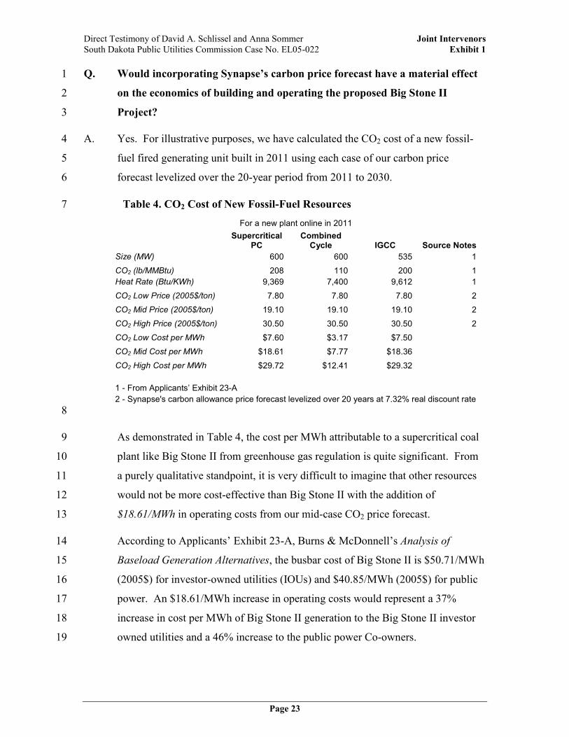
Direct Testimony of David A. Schlissel and Anna Sommer Joint Intervenors South Dakota Public Utilities Commission Case No. EL05-022 Exhibit 1
Page 23
Q. Would incorporating Synapse’s carbon price forecast have a material effect 1
on the economics of building and operating the proposed Big Stone II 2
Project? 3
A. Yes. For illustrative purposes, we have calculated the CO2 cost of a new fossil-4
fuel fired generating unit built in 2011 using each case of our carbon price 5
forecast levelized over the 20-year period from 2011 to 2030. 6
Table 4. CO2 Cost of New Fossil-Fuel Resources 7
For a new plant online in 2011
Supercritical
PC Combined Cycle IGCC Source Notes
Size (MW) 600 600 535 1
CO2 (lb/MMBtu) 208 110 200 1
Heat Rate (Btu/KWh) 9,369 7,400 9,612 1
CO2 Low Price (2005$/ton) 7.80 7.80 7.80 2
CO2 Mid Price (2005$/ton) 19.10 19.10 19.10 2
CO2 High Price (2005$/ton) 30.50 30.50 30.50 2
CO2 Low Cost per MWh $7.60 $3.17 $7.50
CO2 Mid Cost per MWh $18.61 $7.77 $18.36
CO2 High Cost per MWh $29.72 $12.41 $29.32
1 - From Applicants’ Exhibit 23-A
2 - Synapse's carbon allowance price forecast levelized over 20 years at 7.32% real discount rate
8
As demonstrated in Table 4, the cost per MWh attributable to a supercritical coal 9
plant like Big Stone II from greenhouse gas regulation is quite significant. From 10
a purely qualitative standpoint, it is very difficult to imagine that other resources 11
would not be more cost-effective than Big Stone II with the addition of 12
$18.61/MWh in operating costs from our mid-case CO2 price forecast. 13
According to Applicants’ Exhibit 23-A, Burns & McDonnell’s Analysis of 14
Baseload Generation Alternatives, the busbar cost of Big Stone II is $50.71/MWh 15
(2005$) for investor-owned utilities (IOUs) and $40.85/MWh (2005$) for public 16
power. An $18.61/MWh increase in operating costs would represent a 37% 17
increase in cost per MWh of Big Stone II generation to the Big Stone II investor 18
owned utilities and a 46% increase to the public power Co-owners. 19

Direct Testimony of David A. Schlissel and Anna Sommer Joint Intervenors South Dakota Public Utilities Commission Case No. EL05-022 Exhibit 1
Page 24
Q. What would be the annual CO2 cost to the Big Stone II Co-owners? 1
A. Assuming the Analysis of Baseload Generation Alternatives will accurately 2
reflect the operating parameters of Big Stone Unit II including an 88% capacity 3
factor, the range of annual, levelized cost to the Big Stone II Co-owners of CO2 4
regulation would be: 5
Low Case - 4,625,280 MWh · $7.74/MWh = $35,152,128 6
Mid Case - 4,625,280 MWh · $19.60/MWh = $86,076,461 7
High Case - 4,625,280 MWh · $30.39/MWh = $137,463,322 8
Q. Does this conclude your testimony? 9
A. No. The remainder of our testimony will be filed on May 26, 2006. 10
11
12
13
14
15
16
17
18
19
20
21
22
%, PUBLIC VERSION
STATE OF IOWA FILED WITH BEFORE THE IOWA UTILITIES BOARD Executive Secretary
2 2 20071 1
IN RE: ) IOWA UTILITIES BOARD
) APPLICATION OF INTERSTATE POWER ) DOCKET NO. GCU-07-01 AND LIGHT COMPANY FOR A 1 GENERATING FACILITY SITING ) CERTIFICATE )
)
DIRECT TESTIMONY OF DAVID A. SCHLISSEL ON BEHALF OF
THE OFFICE OF CONSUMER ADVOCATE
PUBLIC VERSION
OCTOBER 22,2007

PUBLIC VERSION
Table of Contents Introduction .............................................................................................................. 1
IPL Has Not Adequately Considered The Risks Associated With Building A .......................................................................... New Coal-Fired Generating Unit 5
IPL Has Not Adequately Considered The Risks Associated With Future Federally Mandated Greenhouse Gas Reductions ..................................... 14
IPL Has Not Adequately Considered The Risk Of Further Increases In The Estimated Cost Of The SGS Unit 4 Project ...................................................... 55
Adding SGS Unit 4 Would Not Increase the Diversity in IPL's Generation Supply ..................................................................................................................... 64
IPL's Modeling Analyses Do Not Show that SGS Unit 4 Would Be the Lowest Cost and the Lowest Risk Option for the Company's Ratepayers.. 67
Appendix A:
Schedule A:
Schedule B:
Schedule C:
Schedule D:
Schedule E:
Schedule F:
Schedule G:
List of Exhibits Resume of David Schlissel
IPL Responses to OCA Data Requests cited in Exhibit-DAS-1
Summary of Senate Greenhouse Gas Cap-and-Trade Proposals in Current U.S. 1 loth Congress
Climate Change and Power: Carbon Dioxide Emissions Costs and Electricity Resource Planning
New Mexico Public Regulation Commission June 2007 Order Adopting Standardized Carbon Emissions Cost for Integrated Resource Plans
Scenarios and Carbon Dioxide Emissions Costs from the Assessment of US. Cap-and-Tvade Proposals recently issued by the MIT Joint Program on the Science and Policy of Global Change
Increasing Construction Costs Could Hamper U.S. Utilities' Plans to Build New Power Generation, Standard & Poor's Rating Services, June 2007.
Rising Utility Construction Costs: Sources and Impacts, the Brattle Group, September 2007.
Interstate Power and Light Docket No. GCU-07-01
1 1. Introduction
2 Q. What is your name, position and business address?
3 A. My name is David A. Schlissel. I am a Senior Consultant at Synapse Energy
4 Economics, Inc, 22 Pearl Street, Cambridge, MA 02139.
5 Q. Please describe Synapse Energy Economics.
6 A. Synapse Energy Economics ("Synapse") is a research and consulting firm
7 specializing in energy and environmental issues, including electric generation,
8 transmission and distribution system reliability, market power, electricity market
9 prices, stranded costs, efficiency, renewable energy, environmental quality, and
10 nuclear power.
11 Synapse's clients include state consumer advocates, public utilities commission
12 staff, attorneys general, environmental organizations, federal government and
13 utilities. A complete description of Synapse is available at our website,
14 www.synapse-energy.com.
15 Q. Please summarize your educational background and recent work experience.
16 A. I graduated from the Massachusetts Institute of Technology in 1968 with a
17 Bachelor of Science Degree in Engineering. In 1969, I received a Master of
18 Science Degree in Engineering from Stanford University. In 1973, I received a
19 Law Degree from Stanford University. In addition, I studied nuclear engineering
20 at the Massachusetts Institute of Technology during the years 1983-1986.
2 1 Since 1983 I have been retained by governmental bodies, publicly-owned utilities,
22 and private organizations in 28 states to prepare expert testimony and analyses on
23 engineering and economic issues related to electric utilities. My recent clients
24 have included the New Mexico Public Regulation Commission, the General Staff
25 of the Arkansas Public Service Commission, the Staff of the Arizona Corporation
26 Commission, the U.S. Department of Justice, the Commonwealth of
27 Massachusetts, the Attorneys General of the States of Massachusetts, Michigan,
Page 1
Interstate Power and Light Docket No. GCU-07-01 Direct Testimony of David A. Schlissel - - --.-:,. %z,z.=.F.z
:.'.:..:;..."::";;.z:.= ./'."-';".- .,.,.... .; .'. . p ~ B & $ C = ~ E - ~ ~ ~ Q N ii::l-.-i.. . . ... ... .,. .,.*,..,.... , ..,
New York, and Rhode Island, the General Electric Company, cities and towns in
Connecticut, New York and Virginia, state consumer advocates, and national and
local environmental organizations.
I have testified before state regulatory commissions in Arizona, New Jersey,
Connecticut, Kansas, Texas, New Mexico, New York, Vermont, North Carolina,
South Carolina, Maine, Illinois, Indiana, Ohio, Massachusetts, Missouri, Rhode
Island, Wisconsin, Iowa, South Dakota, Georgia, Minnesota, Michigan, Florida
and North Dakota and before an Atomic Safety & Licensing Board of the U.S.
Nuclear Regulatory Commission.
A copy of my current resume is attached as Appendix A.
On whose behalf are you testifying in this case?
I am testifying on behalf of the Office of Consumer Advocate. ("OCA")
Have you testified previously before this Commission?
Yes. I testified in Docket No. SPU-05-15.
What is the purpose of your testimony?
Synapse was retained by the OCA to assist in its evaluation of the Application of
Interstate Power and Light Company's ("IPL" or "the Company") for authority to
construct, maintain and operate Sutherland Generating Station Unit 4, a new
baseload coal-fired generation plant. ("SGS Unit 4")
This testimony presents the results of our analyses.
Please identify the other Synapse witnesses who are presenting expert
testimony in this proceeding on behalf of the OCA.
In addition to myself, the following witnesses also are presenting expert testimony
in this Docket on behalf of OCA.
Dr. Ezra Hausman is explaining the scientific understanding and risks of global
climate change.
Page 2

Interstate Power and Light Docket No. GCU-07-01
2 territory and the Company's use of an unreasonably high and unsupported 18
3 percent reserve margin in its 2007 Resource Plan modeling.
4 Michael Drunsic is addressing a significant limitation that biases the Company's
5 EGEAS modeling in favor of adding SGS Unit 4, a new coal-fired power plant, in
6 2013.
7 Bill Powers from Powers Engineering is presenting a critique of Black &
8 Veatch's assessments of IGCC technology and the suitability of employing air
9 cooling at the SGS Unit 4 site.
10 Scudder Parker from Scudder Parker Consulting Services is evaluating the
11 feasibility of deferring or avoiding the construction of SGS Unit 4 through
12 increased investment in energy efficiency resources.
13 Larry Shi from the OCA staff is presenting the computer output from the OCA's
14 EGEAS model runs.
15 Q. Were there other members of the Synapse staff who also assisted in the
16 analyses undertaken by Synapse as part of its evaluation of IPL's proposed
17 Sutherland Generating Station Unit 4?
18 A. Yes. Dr. David White, Bruce Biewald, Ben Warfield and Lucy Johnston from
19 Synapse also were members of our project team. Copies of their resumes are
20 available at www.synapse-energv.com.
21 Q. Please summarize your conclusions.
22 A. My conclusions are as follows:
23 1. IPL has not adequately considered the risks associated with building a new
24 coal-fired power plant in its modeling analyses.
25 2. The most significant uncertainties and risks associated with the proposed
26 Sutherland Generating Station Unit 4 project are the potential for future
Page 3
Interstate Power and Light Docket No. GCU-07-01 Direct Testimony of David A. ..... Schlissel .. -. ..................
:.:i_ .................. .,..: ...:.. ~ u B I ; I ~ $ R - ~ ~ N .. , .. ............... <: ......:=2.s....L........ . .:.. ........ 8. .
federal restrictions on COz emissions and further increases in the project's
capital cost.
In particular, it is important for IPL to justify its participation in the SGS
Unit 4 project in light of coming federal regulation of greenhouse gas
emissions. It would be imprudent for the Company to continue its
participation in the Project by merely considering a narrow range of COz
prices in its modeling analyses. Instead, to reflect the uncertainties and
risks, IPL should use a wider range of possible C02 prices such as the
forecasts presented by Synapse in this Docket.
Contrary to IPL's claim, it has not shown that adding SGS Unit 4 is the
lowest risk option for its ratepayers.
The EGEAS analyses prepared by IPL in its 2007 Resource Plan modeling
are flawed and unreasonably limited. These flaws and limitations bias the
results of the modeling analyses in favor of adding a new coal-fired power
plant in 2013.
With our assistance, the OCA staff has rerun the EGEAS model to reflect
more reasonable assumptions concerning wind availability, DSM
availability, power plant construction costs and reduced reserve margins.
When IPL's higher COz price forecast was used the EGEAS model did not
select a coal plant as part of a lowest cost plan in any of the scenarios
more reasonable input assumptions for wind availability, DSM
availability, and power plant conslmction costs. The model only selected
a new coal plant in one scenario in which natural gas prices were
increased by ten percent and, in that scenario, the coal plant was not added
until 2019, six years later than IPL proposes to install SGS Unit 4.
When Synapse's high COz price forecast was used, the EGEAS model
also did not select a coal plant as part of a lowest cost plan in any
scenarios.
Page 4
Interstate Power and Light Docket No. GCU-07-01 Direct Testimony of David A. Schlissel
zE,:T.;t.3: '~.2~.e,~>:,:...*.-.,,.>.,,,~ ..,.3... -.- --..::- .-..== ,, ,. ,.,.%.,.,.>. .. *- p ; ~~~J . ;Q-p~~r~J .o :~ ,. , I..; ,,_, ;:..,;;;::,.:...: .. .. .. ..,= :." ".. .,
9. Even when IPL's low C02 price forecast was used, 2016 was the earliest
year in which the EGEAS added a new coal-fired power plant as part of a
lowest cost plan in any of the scenarios. In some scenarios a new coal
plant was not added until 2019. In two scenarios involved increased wind
and DSM availability, no new coal plant was added as part of a lowest
cost plan even with IPL's unreasonably low C02 price forecast.
10. For these reasons, the Board should reject IPL's application for a
generating facility siting certificate.
Please explain how you conducted your investigations in this proceeding.
We have reviewed the application, testimony and exhibits filed by IPL in this
proceeding. In addition, we have participated in discovery. As part of that work,
we have reviewed the information and documents provided by IPL in response to
data requests submitted by the OCA. We also have reviewed public information
related to the issues addressed in IPL's application, testimony and exhibits and in
our testimony and exhibits.
We also have worked with Larry Shi from the OCA staff in rerunning the EGEAS
model.
IPL Has Not Adequately Considered The Risks Associated With Building A New Coal-Fired Generating Unit
Why is it important that IPL consider risk when evaluating the economics of
building SGS Unit 4?
Risk and uncertainty are inherent in all enterprises. But the risks associated with
any options or plans need to be balanced against the expected benefits from each
such option or plan.
In particular, parties seeking to build new generating facilities and the associated
transmission face of a host of major uncertainties, including, for example, the
expected cost of the facility, future restrictions on emissions of carbon dioxide,
and future fuel prices. The risks and uncertainties associated with each of these
Page 5

Interstate Power and Light Docket No. GCU-07-01
Direct Testimony of David AtSchlissel ,,,.,.!.2..G-q!,,cv,. ..,,.," :-.~. =...=...-. . . ~ : , .(ii:ii. .( , _ . ,:.., . . , ,.,. mE$,C;.WERf$JOfcJ , ..-.. ...., ~ . . . . ... . . . . . .
1 factors needs to be considered as partof the econ&ic evaluation of whether to
2 pursue the proposed facility or other alternatives.
3 Q. Has IPL identified any risks associated with its proposed SGS Unit 4?
4 A. Yes. IPL has identified a number of risks associated with its proposed generation
5 resource plan. For example, the following risks were identified at the June 24 and
6 25,2007 Strategic Planning Conference of Alliant Energy's Board of Directors:
15 A March 2007 presentation for Alliant Energy's senior management as part of the
16 Company's Strategic Planning Process 2008 summarized the risks and
17 considerations related to the goal of building - 23 The same presentation also discussed the changing landscape for building new
24 generation in more detail:
1 IPL Confidential Response to OCA DR. No. 19, Attachment B, pages 10 and 11 of 15 2 IPL's Confidential Response to OCA DR. No. 60, Attachment A, page 3 of 24.
Page 6
Interstate Power and Light Docket No. GCU-07-01 Direct Testimony of David A. Sehlissel
This same presentation also noted the following:
Have you seen any evidence that IPL has adequately considered these risks
and uncertainties in its evaluations of the proposed SGS Unit 4?
No. The Company has claimed that SGS Unit 4 provides lower risk to IPL and its
ratepayers than other options:
It is IPL's opinion that constructing SGS Unit 4 provides lower risk to IPL and its ratepayers than other options. The term "risk" includes both economic and environmental factors. IPL believes that construction of SGS Unit 4 will, among other things, provide the least possible environmental impact with a significant cost to
3 Id, at page 4 of 24. 4 Id, at page 5 of 24. - 5 Id, at page 15 of 24. -
Page 7
Interstate Power and Light Docket NO. GCU-07-01
2 with the greatesi reliability, and will benefit the economy of the 3 Marshalltown area as well as the state of ~ o w a . ~
4 However, we have not found any evidence in the Company's Application or
5 supporting testimony and exhibits to support this claim that building SGS Unit 4
6 represents a lower risk to IPL and its ratepayers than other options.
In fact, we have found that IPL has not adequately considered in its economic
analyses the risks associated with building a new baseload coal-fired generating
unit. For example, although the Company did prepare two COz price sensitivity
modeling runs, its base IRP plan, that includes SGS Unit 4, was developed
through modeling that assumed no greenhouse gas regulation costs. As I will
discuss below, this is an extremely unrealistic and imprudent assumption.
Moreover, the two C02 price forecasts used in IPL's sensitivity analyses were
based on old information and reflect an unreasonably low range of possible future
C02 emissions allowances prices.
16 In addition, the IPL modeling analyses that we have examined do not include any
17 assessment of the uncertainty or risks associated with higher capital costs.
18 Q. Is it reasonable to expect that IPL could reflect uncertainty and risk in its
19 economic analyses of whether to pursue SGS Unit 4 or alternatives?
20 A. Yes. There are a number of ways that IPL could have considered uncertainty and
2 1 risk. The most simple way would have been to perform sensitivity analyses
22 reflecting engineering type bounding in which the key variables would be
23 expected to vary by X% above or below their projected values. In my experience,
24 utilities regularly consider risk in this way.
6 IPL Response to OCA DR. No. 90.B.
Page 8
Interstate Power and Light Docket No. GCU-07-01
of resource plans?
A. Yes. IPL's modeling for its 2005 Resource Plan presented expansion plans and
costs for 18 scenarios:
Reference Case (Proposed Plan)
All Purchased Power
Higher Coal Capital Cost
Nigh Reliability
Some Retirements
Higher Natural Gas Prices
Lower Natural Gas Prices
Higher Coal Fuel Prices
Higher Wind Prices
Lower Load Forecast
Higher Load Forecast
50% of New Resources are DSM and Renewables
75% of New Resources are DSM and Renewables
Minnesota DSM - base
Minnesota DSM - high
Minnesota DSM- medium
Minnesota DSM - low
Each of these scenarios was evaluated in developing the 2005 Resource Plan at
zero externalities, at minimum externalities and at maximum externalities.
Unfortunately, the Company's 2007 Resource Plan that now forms the basis for
the SGS Unit 4 project consists of only one base case and two C02 price
sensitivities. IPL apparently has not completed any other modeling runs.
Page 9

Interstate Power and Light Docket No. GCU-07-01
2 considering whether to approve the proposed SGS Unit 4 Project?
No. As I will discus in detail later in this testimony, there are a number of
significant flaws and out-of-date assumptions in IPL's 2005 Resource Plan
modeling that render the results of that modeling unreasonable and unrealistic
given current circumstances. In particular, the Company's projected coal plant
capital costs are much higher than the figures that were used in the 2005 Resource
Plan modeling and that modeling did not reflect any federal regulation of
greenhouse gas emissions - in other words, it assumed no COz emissions
allowance prices.
11 Q. What are the most significant fossil plant-specific uncertainties and risks
12 associated with building new coal-fired generating plants like SGS Unit 4?
13 A. The most significant uncertainties and risks associated with new coal-fired
14 generating plants like the proposed SGS Unit 4 are the potential for future
15 restrictions on COz emissions and the potential for hrther increases in the
16 project's capital cost. Other potential uncertainties and risks for new coal plants
17 include the potential for fuel supply disruptions that could affect plant operating
18 performance and fuel prices and the potential for increasing stringency of
19 regulations of current criteria pollutants.
20 Q. Have any proposed coal-fired generating projects been cancelled as a result
2 1 of concern over increasing construction costs or the potential for federal
22 regulation of greenhouse gas emissions?
23 A. Yes. A number of coal-fired power plant projects have been cancelled within the
24 past year, in part, because of concern over rising construction costs and climate
25 change. For example:
26 . Tenaska Energy cancelled plans to build a coal-fired power plant in 27 Nebraska because of rising steel and construction prices. According to the 28 company's general manager of business development:
Page 10
Interstate Power and Light Docket No. GCU-07-01 Direct Testimony of David A. .. Schlissel , .i_i-_i-
..iiiiv.l....7..-?i ../in. ... ................... l,l!cr,... i,ii: .,... $ ? ~ ~ ~ ~ ~ 2 V & R ; $ $ ~ N .............. .. <, .... ~ . , b : . A 8. ......... 8, ....... -s; ...........
.. coal prices have gone up "dramatically" since Tenaska started - planning the project more than a year ago.
And coal plants are largely built with steel, so there's the cost of the unit that we would build has gone up a lot.. . At one point in our development, we had some of the steel and equipment at some very attractive prices and that equipment all of a sudden was not available.
We went immediately trying to buy additional equipment and the pricing was so high, we looked at the price of the power that would be produced because of those higher prices and equipment and it just wouldn't be a prudent business decision to build it.7
. TXU cancelled 8 of 11 proposed coal-fired power plants, in large part because of concern over global warming and the potential for federal legislation restricting greenhouse gas emission^.^ . Westar Energy announced in December 2006 that it was deferring site selection for a new 600 MW coal-fired power plant due to significant increases in the facility's estimated capital cost. . Tampa Electric just cancelled a proposed integrated gasification combined cycle plant ("IGCC") due to uncertainty related to C02 regulations, particularly capture and sequestration issues, and the potential for related project cost increases. According to a press release, "Because of the economic risk of these factors to customers and investors, the company believes it should not proceed with an IGCC project at this time," although it remains steadfast in its support of IGCC as a critical component of future fuel diversity in Florida and the nation. . Four public power agencies suspended permitting activities for the coal- fired Taylor Energy Center because of growing concerns about greenhouse gas emissions?
Q. Have you seen any instance where a participant in a jointly-owned coal-fired
power plant project has withdrawn because of concern over increasing
construction costs or potential COz emissions costs?
A. Yes. Great River Energy ("GRE) just withdrew from the proposed Big Stone I1
coal-fired power plant project in South Dakota. According to GRE, four factors
7 Available at www.swtimes.comlartic1es/2007/07/09/news/news02.prt. 8 See www.marketwatch.comlnews/story/txu-reversal-coal-plmt-emissions 9 See www.taylorenergycenter.org/s_l6asp?n=40.
Page 1 1
Interstate Power and Light Docket No. GCU-07-01 Direct Testimony of David A. -F2..,.ys.-ry Schlissel :,; ::;rq3,e ,. ,.,.,,. , ,,",=.,b.-p.,,., .,,. ,.. ,,, , .. .: .: ,..,. :.,- ..,.A: ...... 2,:;. ~ p ~ ; ~ ~ ~ ~ ~ q q + ~ g g - ~ : ~ ;
',,.,., ,., "_ . ."..;l.5.ict>.~.=;; r-..:ir
contributed most prominently to the decision to withdraw, including uncertainty
about changes in environmental requirements and new technology and that fact
that "The cost of Big Stone I1 has increased due to inflation and project delays."'0
Have any proposed coal-fired generating projects been rejected by state
regulatory commissions due to concerns over increasing construction costs or
the potential for federal regulation of greenhouse gas emissions?
Yes. Just since last December, proposed coal-fired power plant projects have
been rejected by the Oregon Public Utility Commission, , the Florida Public
Service Commission, and the Oklahoma Corporation Commission. The North
Carolina Utilities Commission rejected one of the two coal-fired plants proposed
by Duke Energy Carolinas for is Cliffside Project.
The decision of the Florida Public Service Commission in denying approval for
the 1,960 MW Glades Power Project was based on concern over the uncertainties
over plant costs, coal and natural gas prices, and future environmental costs,
including carbon allowance costs." In addition, the Oklahoma Corporation
Commission has just voted to reject Public Service Company of Oklahoma's
application to build a new coal-fired power plant although the Commission has
not yet issued a written order.
On October 18,2007, the Kansas Department of Health and Environment rejected
an application to build two 700 MW coal-fired units at an existing power plant
site. In a prepared statement explaining the basis for this decision, Rod Bremby,
Kansas's secretary of health and environment noted that "I believe it would be
irresponsible to ignore emerging information about the contribution of carbon
dioxide and other greenhouse gases to climate change and the potential harm to
our environment and health if we do nothing.""
10 See ww.greatriverenergy.com/press/newslO91707~big~stone~ii.htm1. 11 Order No. PSC-07-0557-FOF-EI, Docket No. 070098-EI, July 2,2007. I Z See www.kansascity.com/IO5isto1y/323833.html.
Page 12
Interstate Power and Light Docket No. GCU-07-01
2 regulatory commissions?
3 A. Yes. A March 2007 presentation for Alliant Energy's senior management
4 reported that:
13 IPL's Confidential Response to OCA DR. No. 60, Attachment A, at page 4 of 24. 14 Id, at page 15 of 24. -
Page 13

Interstate Power and Light Docket No. GCU-07-01
alternatives to the SGS Unit 4 Project as well?
A. Yes. The risks associated with building natural gas-fired alternatives include
potential COz emissions costs, possible capital cost escalation and fuel price
uncertainty and volatility.
Renewable alternatives and DSM also have some uncertainties and risks. These
include potential capital cost escalation, contract uncertainty and customer
participation uncertainty.
9 3. IPL Has Not Adequately Considered The Risks Associated With 10 Future Federally Mandated Greenhouse Gas Reductions
Is it prudent to expect that a policy to address climate change will be
implemented in the U.S. in a way that should be of concern to coal-dependent
utilities in the Midwest?
Yes. The prospect of global warming and the resultant widespread climate
changes has spurred international efforts to work towards a sustainable level of
greenhouse gas emissions. These international efforts are embodied in the United
Nations Framework Convention on Climate Change ("UNFCCC"), a treaty that
the US. ratified in 1992, along with almost every other country in the world. The
Kyoto Protocol, a supplement to the UNFCCC, establishes legally binding limits
on the greenhouse gas emissions of industrialized nations and economies in
transition.
Despite being the single largest contributor to global emissions of greenhouse
gases, the United States remains one of a very few industrialized nations that have
not signed the Kyoto ~rotocol . '~ Nevertheless, individual states, regional groups
Is As I use the terms "carbon dioxide regulation" and "greenhouse gas regulation" throughout our testimony, there is no difference. While I believe that the future regulation we discuss here will govern emissions of all types of greenhouse gases, not just carbon dioxide ("COP), for the purposes of our discussion we are chiefly concerned with emissions of carbon dioxide. Therefore, we use the terms "carbon dioxide regulation" and "greenhouse gas regulation" interchangeably.
Page 14

Interstate Power and Light Docket No. GCU-07-01 Direct Testimony of David A. --.-...-...-...TTz Schlissel ..====. . :.-" ..-.....,, . - . 2.. ..... ..% ,.=. . . . . ,:,- .......... ..., "m .; ......,.... .. p~.B&~'JC-~jR::S$;~N
.a>.; .................... s .......... 8 ..,,* ............. of states, shareholders and corporations are making serious efforts and taking
significant steps towards reducing greenhouse gas emissions in the United States.
Efforts to pass federal legislation addressing carbon, though not yet successful,
have gained ground in recent years. These developments, combined with the
growing scientific understanding of, and evidence of, climate change as outlined
in Dr. Hausman's testimony, mean that establishing federal policy requiring
greenhouse gas emission reductions is just a matter of time. The question is not
whether the United States will develop a national policy addressing climate
change, but when and how. The electric sector will be a key component of any
regulatory or legislative approach to reducing greenhouse gas emissions both
because of this sector's contribution to national emissions and the comparative
ease of regulating large point sources.
There are, of course, important uncertainties with regard to the timing, the
emission limits, and many other details of what a carbon policy in the United
States will look like.
Q. If there are uncertainties with regard to such important details as timing,
emission limits and other details, why should a utility engage in the exercise
of forecasting greenhouse gas prices?
A. First of all, utilities are implicitly assuming a value for carbon allowance prices
whether they go to the effort of collecting all the relevant information and create a
price forecast, or whether they simply ignore future carbon regulation. In other
words, a utility that ignores future carbon regulations is implicitly assuming that
the allowance value will be zero. The question is whether it's appropriate to
assume zero or some other number. There is uncertainty in any type of utility
forecasting and to write off the need to forecast carbon allowance prices because
of the uncertainties is not prudent.
Similarly, the terms "carbon dioxide price," "greenhouse gas price" and "carbon price" are interchangeable.
Page 15
Interstate Power and Light Docket No. GCU-07-01 Direct Testimony of David A. Schlissel nii>;..~:~:-~(Tii:~:!~r: -r.m,F,:y-= =..> ~J~:B.C:#@~J+R.$~$JN:
.. . .,,~. .:.. . . ... , ..,..,., :" !'. .,C,,,,V,",, d,.", . For example, there are myriad uncertainties that utility planners have learned to
address in planning. These include randomly occurring generating unit outages,
load forecast error and demand fluctuations, and fuel price volatility and
uncertainty. These various uncertainties can be addressed through techniques
such as sensitivity and scenario analyses.
If SGS Unit 4 were to be built, is carbon regulation an issue that could be
definitely could be addressed in the future, and at a reasanable cost, once the
timing and stringency of the regulation is known?
No. Unlike for other power plant air emissions like sulfur dioxide and oxides of
nitrogen, there currently is no commercial or economical method for post-
combustion removal of carbon dioxide from supercritical pulverized coal plants.
IPL agrees on this point, noting that "Unlike with other criteria air emissions,
commercially-available back-end C02 emissions control technologies do not
currently exist."I6 This conclusion is consistent with that of other coal utilities
and with the general view in the electric industry.
Even if such technology were available, retrofitting an existing coal plant with the
technology for carbon capture and sequestration is expected to be very expensive,
increasing the cost of generating power at the plant by perhaps as much as 68
percent to 80 percent, or higher.
Do other utilities have opinions about whether and when greenhouse gas
regulation will come?
Yes. A number of utility executives have argued that mandatory federal
regulation of the emissions of greenhouse gases is inevitable.
For example, in April 2006, the Chairman of Duke Energy, Paul Anderson, stated:
From a business perspective, the need for mandatory federal policy in the United States to manage greenhouse gases is both urgent and
-
Page 16
Response to OCA DRNo. 19, Attachment A, page 46 of 55.
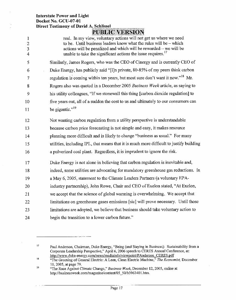
Interstate Power and Light Docket No. GCU-07-01
real. In my view, voluntary actions will not get us where we need to be. Until business leaders know what the rules will be - which actions will be penalized and which will be rewarded - we will be unable to take the significant actions the issue requires.17
Similarly, James Rogers, who was the CEO of Cinergy and is currently CEO of
Duke Energy, has publicly said "[Iln private, 80-85% of my peers think carbon
regulation is coming within ten years, but most sure don't want it now."18 Mr.
Rogers also was quoted in a December 2005 Business Week article, as saying to
his utility colleagues, "If we stonewall this thing [carbon dioxide regulation] to
five years out, all of a sudden the cost to us and ultimately to our consumers can
be gigantic."19
Not wanting carbon regulation from a utility perspective is understandable
because carbon price forecasting is not simple and easy, it makes resource
planning more difficult and is likely to change "business as usual." For many
utilities, including IPL, that means that it is much more difficult to justify building
a pulverized coal plant. Regardless, it is imprudent to ignore the risk.
Duke Energy is not alone in believing that carbon regulation is inevitable and,
indeed, some utilities are advocating for mandatoly greenhouse gas reductions. In
a May 6,2005, statement to the Climate Leaders Partners (a voluntary EPA-
industry partnership), John Rowe, Chair and CEO of Exelon stated, "At Exelon,
we accept that the science of global warming is overwhelming. We accept that
limitations on greenhouse gases emissions [sic] will prove necessary. Until those
limitations are adopted, we believe that business should take voluntary action to
begin the transition to a lower carbon future."
I7 Paul Anderson, Chairman, Duke Energy, "Being (and Staying in Business): Sustainability %om a Corporate Leadership Perspective," April 6,2006 speech to CERES Annual Conference, at: hnw: M M \?_d_uke-enel~. cQrn n w s ~neJiailiio t impoinr I'.!lncl<r~pn CERTS.l>df
IS 'The (ire:ning oiGeneral Electric: A Lean, Clcan Elecrric Machine," The F,.o~?onii\r. Decenibr.r 10,2005, at page 79.
19 "The Race Against Climate Change," Business Week, December 12,2005, online at http:libusinessweek.comimagazine/content/3963401 .htm.
Page 17

Interstate Power and Light Docket No. GCU-07-01 Direct Testimony of David A. Schlissel -..__-",,gpI*,,
:.\::.'r(i.-;li;,?+?f<: ,-: ; +.--....., n",':: . .. . . .... !RUiB.SE(iT-i?J7E.RSg0.N: ..,;:..*. --.:-- .- " ',,?;,,,",. r%-,~,~i~...:~:.~
1 In fact, several electric utilities and electric generation companies have
2 incorporated assumptions about carbon regulation and costs into their long term
3 planning, and have set specific agendas to mitigate shareholder risks associated
4 with future U.S. carbon regulation policy. These utilities cite a variety of reasons
5 for incorporating risk of future carbon regulation as a risk factor in their resource
6 planning and evaluation, including scientific evidence of human-induced climate
7 change, the U.S. electric sector's contribution to emissions, and the magnitude of
8 the financial risk of future greenhouse gas regulation.
9 Duke Energy and FPL Group are participating in the high profile U.S. Climate
10 Action Partnership ("USCAP") which advocates for federal, mandatory
11 legislation of greenhouse gases. The six principles of this group are:
12 Account for the global dimensions of climate change;
13 Create incentives for technology innovation;
14 Be environmentally effective;
15 Create economic opportunity and advantage;
16 Be fair to sectors disproportionately impacted; and
17 Reward early action.20
18 Most significantly, USCAP has argued that C02 emissions should be reduced by
19 60% to 80% by 2050. As I will discuss later, this is relatively the same goal as
20 many of the climate change bills that have been introduced in the current U.S.
2 1
22 Some of the companies believe that there is a high likelihood of federal regulation
23 of greenhouse gas emissions within their planning period. For example,
24 Pacificorp states a 50% probability of a C02 limit starting in 2010 and a 75%
20 www.us-cap.org. 21 A Call for Action, at page 7, available at www.us-cap.org.
Page 18

Interstate Power and Light Docket No. GCU-07-01 Direct Testimony of David A. Sch@~! ............ - .... --; ...... -...wzr-;.eL.:.-2::y... ........
~ ; ~ B I , I C ... VJERSPO~ ..:..-...!.+A" ...............: L..!Li;=:.== r= ...... &..2
probability starting in 201 1. The Northwest Power and Conservation Council
models a 67% probability of federal regulation in the twenty-year planning period
ending 2025 in its resource plan. Northwest Energy states that C02 taxes "are no
longer a remote possibility."22
Even those in the electric industry who oppose mandatory limits on greenhouse
gas regulation believe that regulation is inevitable. David Ratcliffe, CEO of
Southern Company, a predominantly coal-fired utility that opposes mandatory
limits, said at a March 29,2006, press briefing that "There certainly is enough
public pressure and enough Congressional discussion that it is likely we will see
some form of regulation, some sort of legislation around carbon."23
Q. Why would electric utilities, in particular, be concerned about future carbon
regulation?
A. Electricity generation is very carbon-intensive. Electric utilities are likely to be
one of the first, if not the first, industries subject to carbon regulation because of
the relative ease in regulating stationary sources as opposed to mobile sources
(automobiles) and because electricity generation represents a significant portion
of total US. greenhouse gas emissions. A new generating facility may have a
book life of twenty to forty years, but in practice, the utility may expect that that
asset will have an operating life of 50 years or more. By adding new plants,
especially new coal plants, a utility is essentially locking-in a large quantity of
carbon dioxide emissions for decades to come. In general, electric utilities are
increasingly aware that the fact that we do not currently have federal greenhouse
gas regulation is irrelevant to the issue of whether we will in the future, and that
new plant investment decisions are extremely sensitive to the expected cost of
greenhouse gas regulation throughout the life of the facility.
22 Northwest Energy 2005 Electric Default Supply Resource Procurement Plan, December 20,2005; Volume 1, p. 4.
23 Quoted in "U.S. Utilities Urge Congress to Establish C02 Limits," Bloomberg.com, h~:l/www.bloombere.coin/au~~lnews?uid=I 0000103&sid=a75AIADJvScs&refer=us
Page 19
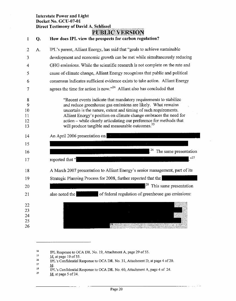
Interstate Power and Light Docket No. GCU-07-01
Q. How does IPL view the prospects for carbon regulation?
A. IPL's parent, Alliant Energy, has said that "goals to achieve sustainable
development and economic growth can be met while simultaneously reducing
GHG emissions. While the scientific research is not complete on the rate and
cause of climate change, Alliant Energy recognizes that public and political
consensus indicates sufficient evidence exists to take action. Alliant Energy
agrees the time for action is now."24 Alliant also has concluded that
"Recent events indicate that mandatory requirements to stabilize and reduce greenhouse gas emissions are likely. What remains uncertain is the nature, extent and timing of such requirements. Alliant Energy's position on climate change embraces the need for action - while clearly articulating our preference for methods that will produce tangible and measurable outcomes.25
." The same presentation
A March 2007 presentation to Alliant Energy's senior management, part of its
Strategic Planning Process for 2008, further reported that the
also noted the of federal regulation of greenhouse gas emissions:
24 IPL Response to OCA DR. No. 19, Attachment A, page 29 of 55. 25 Id, at page 19 of 55. - 26 IPL's Confidential Response to OCA DR. No. 3 1, Attachment D, at page 4 of 20. 27 7 ~1
10. - 28 IPL's Confidential Response to OCA DR. No. 60, Attachment A, page 4 of 24. 29 Id, at page 5 of 24. -
Page 20
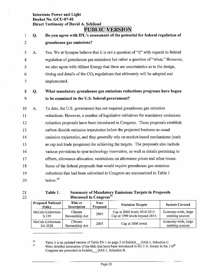
Interstate Power and Light Docket No. GCU-07-01
greenhouse gas emissions?
Yes. We at Synapse believe that it is not a question of "if' with regards to federal
regulation of greenhouse gas emissions but rather a question of "when." However,
we also agree with Alliant Energy that there are uncertainties as to the design,
timing and details of the COZ regulations that ultimately will be adopted and
implemented.
What mandatory greenhouse gas emissions reductions programs have begun
to be examined in the U.S. federal government?
To date, the U.S. government has not required greenhouse gas emission
reductions. However, a number of legislative initiatives for mandatory emissions
reduction proposals have been introduced in Congress. These proposals establish
carbon dioxide emission trajectories below the projected business-as-usual
emission trajectories, and they generally rely on market-based mechanisms (such
as cap and trade programs) for achieving the targets. The proposals also include
various provisions to spur technology innovation, as well as details pertaining to
offsets, allowance allocation, restrictions on allowance prices and other issues.
Some of the federal proposals that would require greenhouse gas emission
reductions that had been submitted in Congress are summarized in Table 1
below.30
Table 1. Summary of Mandatory Emissions Targets in Proposals Discussed in congress3' -
30 Table 1 is an updated version of Table ES-1 on page 5 of Exhibit-DAS-1, Schedule C. 31 More detailed summaries of the bills that have been introduced in the US. Senate in the 110'
Congress are presented in Exhibit-DAS-1, Schedule B.
McCain Liebeman S.139
McCain Lieberman SA 2028
Page 2 1
Sectors Covered Proposed National Policy
Climate Stewardship Act
Climate Stewardship Act
Title or Description
2003
2003
Year Proposed Emission Targets
Cap at 2000 levels 2010-2015. Cap at 1990 levels beyond 2015.
Cap at 2000 levels
Economy-wide, large emitting sources
Economy-wide, large emitting sources
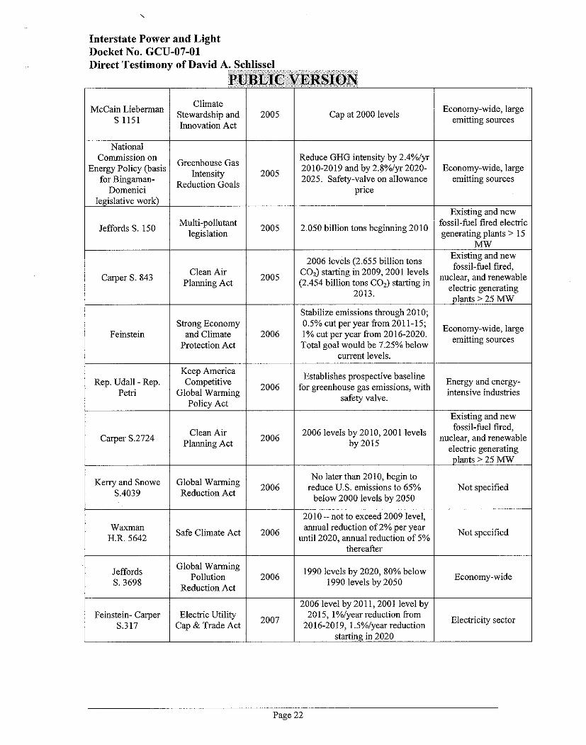
Interstate Power and Light Docket No. GCU-07-01 Direct Testimony of David A. .... SI .
jpl ....
WcCain Lieberman S 1151
National Commission on
hergy Policy (basis for Bingaman-
Domenici legislative work)
Jeffords S. 150
Carper S. 843
Feinstein
Rep. Udall -Rep. Petri
Carper S.2724
Keny and Snowe S.4039
Waxman H.R. 5642
Jeffords S. 3698
Feinstein- Carper S.317
Climate Stewardship and Innovation Act
Greenhouse Gas Intensity
Reduction Goals
Multi-pollutant legislation
Clean Air Planning Act
Strong Economy and Climate
Protection Act
Keep America Competitive
Global Warming Policy Act
Clean Air Planning Act
Global Warming Reduction Act
Safe Climate Act
Global Warming Pollution
Reduction Act
Electric Utility Cap & Trade Act
lissel t:;qr7;J!::??:> &kT:c:; . , . . . . ..
2005
2005
2005
2005
2006
2006
2006
2006
2006
2006
2007
Cap at 2000 levels Economy-wide, large emitting sources
I Existing and new
Reduce GHG intensity by 2.4%/yr 2010-2019 and by 2.8%/yr 2020- 2025. Safety-valve on allowance
price
2.050 billion tons beginning 2010 fossil-fuel fired electric generating plants > 15
Economy-wide, large emitting sources
2006 levels (2.655 billion tons
Stabilize emissions through 2010; 1 0.5%cut peryearfromf611-15; Economy-wide, large 1% cut per year from 2016-2020. emitting sources
Total goal would be 7.25% below - current levels. I
I Existine and new
Establishes prospective baseline for greenhouse gas emissions, with
safety valve.
fossil-&el fired, 2006 levels by 2010,2001 levels nuclear, and renewable by 2015 electric generating
Energy and energy- intensive industries
plants ; 25 MW-
1990 levels by 2020,80% below 1990 levels by 2050 Economy-wide
No later than 2010, begin to reduce US. emissions to 65%
below 2000 levels by 2050
2010 -not to exceed 2009 level, annual reduction of 2% per year
until 2020, annual reduction of 5%
I
2006 level bv 201 1.2001 level bv I
Not specified
Not specified
2015, l%/year reduction from Electricity sector 20 16-20 19. 1.5%/vear reduction
Page 22
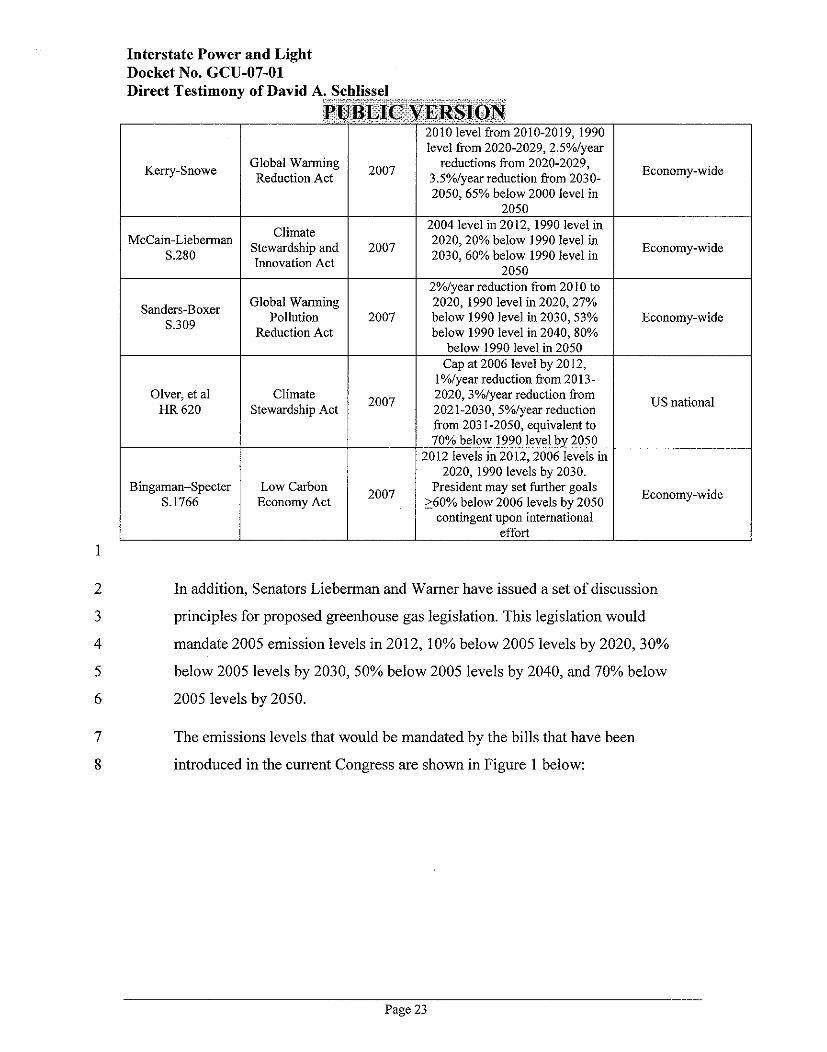
Interstate Power and Light Docket No. GCU-07-01 Direct Testimony of David A. S'
Keny-Snowe
Sanders-Boxer S.309
Olver, et a1 HR 620
Bingaman-Specter S.1766
Global Wanning Reduction Act
Climate Stewardship and Innovation Act
Global Warming Pollution
Reduction Act
Climate Stewardship Act
Low Carbon Economy Act
level from 2020-2029,2.5%/year reductions from 2020-2029,
3.5%/year reduction from 2030- 2050, 65% below 2000 level in
2050 2004 level in 2012, 1990 level in 2020,20% below 1990 level in 2030,60% below 1990 level in
2050 2%/year reduction from 2010 to 2020, 1990 level in 2020,27% below 1990 level in 2030,53% below 1990 level in 2040, 80%
below 1990 level in 2050 Cap at 2006 level by 2012,
l%/year reduction from 2013- 2020,3%/year reduction from 2021-2030,5%/year reduction from 2031-2050, equivalent to 70% below 1990 level by 2050
LO12 levels in 2012,2006 levels in 2020, 1990 levels by 2030.
President may set further goals >60% below 2006 levels by 2050
contingent upon international effort
US national
In addition, Senators Liebeman and Warner have issued a set of discussion
principles for proposed greenhouse gas legislation. This legislation would
mandate 2005 emission levels in 2012, 10% below 2005 levels by 2020, 30%
below 2005 levels by 2030,50% below 2005 levels by 2040, and 70% below
2005 levels by 2050.
The emissions levels that would be mandated by the bills that have been
introduced in the current Congress are shown in Figure 1 below:
Page 23
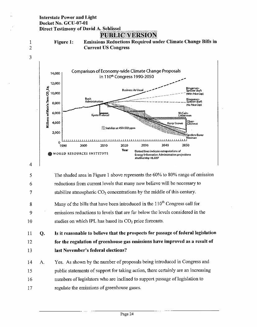
Interstate Power and Light Docket No. GCU-07-01
Current US Congress
14,000 Comparison of Economy-wide Climate Change Proposals in 1 lorh Congress 1990-2050
12,000 ri
8 10.000 m c
f - 8,000 L 0
5 6,M)O 0 '+ r 2 4,000 % ?3 Stabilireat450-550 PW
2.000 Waxman
n 1 1 1 1 1 1 1 1 1 1 1 1 1 1 1 1 1 1 1 I I I I I I I I 1 1 1 I I I I I I I I l l l l l i l i l l l l l l l l l 1 1 1 1 " 1990 2WO 2010 2020 2030 2040 2050
Domd l iner indicateema~daa'~~~ of @ W O R L D RESOURCES INSTITUTE Enersylnfonaa'en Admintrtration projjectionr
Madfled:Mw l0,2W7
The shaded area in Figure 1 above represents the 60% to 80% range of emission
reductions from current levels that many now believe will be necessary to
stabilize atmospheric COz concentrations by the middle of this century.
Many of the bills that have been introduced in the 1 loth Congress call for
emissions reductions to levels that are far below the levels considered in the
studies on which IPL has based its COz price forecasts.
Is it reasonable to believe that the prospects for passage of federal legislation
for the regulation of greenhouse gas emissions have improved as a result of
last November's federal elections?
Yes. As shown by the number of proposals being introduced in Congress and
public statements of support for taking action, there certainly are an increasing
numbers of legislators who are inclined to support passage of legislation to
regulate the emissions of greenhouse gases.
Page 24
Interstate Power and Light Docket No. GCU-07-01 Direct Testimony of David A. 8~,~..J~3..a.x Schlissel .es-,,,.. ... , .,.,,.,..,.,., ,.-.,. ..... , r.:.. - :.=,:,=.:. .,.:a.,, :.,. A:..,,,,,:,. p;vBIj:I;@ #EJ&@OR
,.ia.iliii.____ %%,_." ........ ,.,.:.>. A..~.+
Nevertheless, my conclusion that significant greenhouse gas regulation in the U S .
is inevitable is not based on the results of any single election or on the fate of any
single bill introduced in Congress.
Q. Are individual states also taking actions to reduce greenhouse gas emissions?
A. Yes. A number of states are taking significant actions to reduce greenhouse gas
emissions. In fact, as Alliant Energy has note4
For example, Table 2 below lists the emission reduction goals that have been
adopted by states in the U.S. Regional action also has been taken in the Northeast
and Western regions of the nation.
32 IPL's Confidential Response to OCA DR. No. 60, Attachment A, page 6 of 24.
Page 25
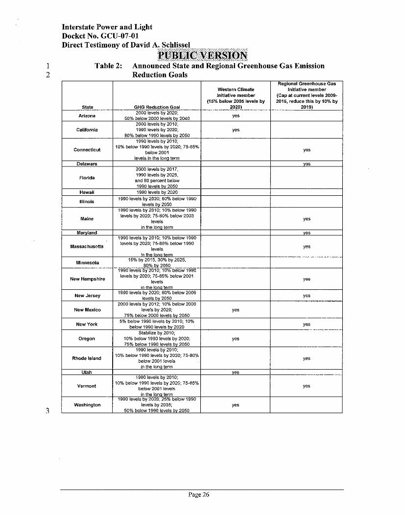
Interstate Power and Light Docket No. GCU-07-01 Direct Testimony of David A. .... --.- Schlissel .-.T-r..= :*.>" ... .,.... .% -. ,,: .... . .. .., .-,,:. . .. ip~;Qpy~g@~o~
~.."T .-.. d , , , " , S ...., ",.a
Table 2: Announced State and Regional Greenhouse Gas Emission
. . (15% below 2005 levels by 2015, reduce this by 10% by
State GHG Reduction Goal 2020) 2019)
Arizona 50% t
- Reduction Goals
California 80% t
10% below Connecticut
Western Climate initiative member
Regional Greenhouse Gas initiative member
ICao at current levels 2009-
Minnesota
New Hampshire
New Jersey
New Mexico
in the lona t e n 15% by 2015. 30% by 2025,
80% by 2050 1990 levels by 2010; 10% below 1990 levels by 2020: 75.85% below 2001
levels
New York
yes
in the lona term 1990 levels by 2020; 80% below 2006
levels by 2050 2000 levels by 2012; 10% below 2000
levels by 2020: 75% below 2000 levels by 2050
Oregon
Rhode Island
Page 26
I Stablllze by 2010, I I
5% below 1990 levels by 2010, 10% below 1990 levels by 2020
Utah
Vermont
Washington
yes
yes
10% below 1990 levels by 2020. 75% below 1990 levels by 2050
1990 levels by 2010, 10% below 1990 levels by 2020, 75.00%
below 2001 levels
yes
in the Ions term
1990 levels by 2010; 10% beiow 1990 levels by 2020; 75.85%
below 2001 levels in the lona term
1990 levels by 2020; 25% below 1990 levels by 2035;
50% below 1990 levels by 2050
yes
yes
yes
yes
yes
Interstate Power and Light Docket No. GCU-07-01
2 favor of government action to address global warming concerns?
3 A. Yes. A summer 2006 poll by Zogby International showed that an overwhelming
4 majority of Americans are more convinced that global warming is happening than
5 they were even two years ago. In addition, Americans also are connecting intense
6 weather events like Hurricane Katrina and heat waves to global warming.33
7 Indeed, the poll found that 74% of all respondents, including 87% of Democrats,
8 56% of Republicans and 82% of Independents, believe that we are experiencing
9 the effects of global warming.
10 The poll also indicated that there is strong support for measures to require major
11 industries to reduce their greenhouse gas emissions to improve the environment
12 without harming the economy - 72% of likely voters agreed such measures
13 should be taken.34
14 Other recent polls reported similar results. For example, a recent Stanford
15 University/Associated Press poll found that 84 percent of Americans believe that
16 global warming is occurring, with 52 percent expecting the world's natural
17 environment to be in worse shape in ten years than it is now.35 Eighty-four
18 percent of Americans want a great deal or a lot to be done to help the environment
19 during the next year by President Bush, the Congress, American businesses and/or
20 the American public. This represents ninety-two percent of Democrats and
2 1 seventy-seven percent of Republicans.
22 At the same time, according to a recent public opinion survey for the
23 Massachusetts Institute of Technology, Americans now rank climate change as
24 the country's most pressing environmental problem-a dramatic shift from three
33 "Americans Link Hurricane Katrina and Heat Wave to Global Warming," Zogby International, August 21, 2006, available at www.zogby.com/news.
34 r > 1". -
35 The SecondAnnual "America's Report Card on the Environment" Survey by the Woods Institute for the Environment at Stanford ~ i i v e r s i t ~ in collaboration with The Associated Press, September 25, 2007. http:/lwoods.stanford.edu~docslsurveys/2006~ClimatePoll.pdf.
Page 27
Interstate Power and Light Docket No. GCU-07-01 Direct Testimony of David A. :.-:, Sehlissel...._........_.. .-:.=?-.- ...........
...r":-("::". i,.i::, ........... ~.u~J;@%~E;Rs_T~gJ~ ........ "..i .............. " :.:1.;.;:; .......
years ago, when they ranked climate change sixth out of 10 environmental
concerns.36 Almost three-quarters of the respondents felt the government should
do more to deal with global warming, and individuals were willing to spend their
own money to help.
Q. What CO2 prices has IPL used in its modeling of the proposed SGS Unit 4
Project?
A. IPL did not assume any annual carbon or C02 emissions cost for the base case of
its 2007 Electric Resource Plan although it did prepare two sensitivity analyses
assuming what it calls low CO2 and high CO2 emissions allowance prices.37
Q. Is it prudent and reasonable to assume no CO2 emissions allowance prices in
the Reference Case Analysis?
A. No. It is not prudent to project that there will be no regulation of greenhouse gas
emissions at any point over the next thirty or more years. As I have discussed
above and Alliant Energy has acknowledged, federal regulation of greenhouse gas
emissions is highly likely in the near future. States also have started to take
actions to reduce greenhouse gas emissions both on their own and as part of
regional initiatives. Given all of its public statements and - about the l i k e l i h o o d , , of mandating requirements for
reducing greenhouse gas emissions and that the time for action is now, I find it
very hard to accept that IPL believes that this is a reasonable scenario on which to
base decisions about future generation alternatives.
36 MIT Carbon Sequestration Initiative, 2006 Survey, h t t p : l l s e q u e s t r a t i o o . m i t . e d u / r e s e a r c ~ l
37 IPL Response to OCA DR No. 16, IPL Response to OCA DR. No. 15 and IPL Response to OCA DR. No. 19, Attachment A, page 47 of 55.
Page 28

Interstate Power and Light Docket No. GCU-07-01 Direct Testimony of David A. m Schlissel -r...<y-l-..l- ",- ..:-- _ _ .._?,,. .....I. .r,..,r;-. .... .-.:r!'z .:,. ;:-.- ... :-.-:... . ,. :@U:B:LIC$cVE;Rt$IQ:H
,r,zi.;;,,<.;;~.'; .iliL:'~., ir.;Lr.:.x
Does IPL discuss in its Application what its total greenhouse gas emissions
will be if its adds SGS Unit 4 to its generation mix, as it proposes?
Not really. All that IPL does is to compare the projected C02, methane and
Nitrous Oxide emissions from the proposed supercritical SGS Unit 4 against a
hypothetical comparable sub critical unit.38 However, this comparison does
reveal that SGS Unit 4 would emit 5.935 million tons of COz into the atmosphere
each year.
Have you seen any projections of what IPL's future total annual COz
emissions would be under the Company's base case IRP which is based on
the assumption that there will be no regulation of greenhouse gas emissions?
Yes. As shown in Figures 2 and 3 below, IPL's annual COz emissions would
percent 2008 and 2020 if the Company's completes
it Resource Plan that includes the addition of SGS Unit 4 in 2013. Total Alliant
Energy C02 emissions would - percent during the
same period.
38 Table 1.6.6-1, at page 37 of IPL's Application for A Generating Facility Siting Certificate.
Page 29

Interstate Power and Light Docket No. GCU-07-01 Direct Testimony of David A. Schlissel
1 Fimre 2: Future IPL C 0 2 Emissions Under Current IW including SGS - 2 Unit 439 [CONFIDENTIAL]
RLED WITH Executive Secretav
IOWA UTILITIES BOARD
39 Source: IPL's Confidential Response to OCA DR. No. 76, Attachment A.
Page 30
Interstate Power and Light Docket No. GCU-07-01 Direct Testimony of David A. Schlissel
8>.*. .~~~~~-:~;- ;<: :2r~;~-~,%-;~~.~,~! .~! ; : . ; >E$p,:z - p ~ ~ g & g - @ y ~ $ @ ~ ~ ~ . ,: ..~.,...,., ..., "..,:s3:iL2-~%->c ..... 8iiiiiii
1 Figure 3: Future Alliant Energy COz missions Under Current IRP 2 including SGS Unit 440 3 [CONFIDENTIAL]
How do these future IPL and Alliant emissions levels compare to the
emissions target levels in the bills that have been introduced in the current
U.S. Congress?
Alliant Energy has compared its projected C02 emissions with the emissions
levels that would be mandated by six of the current bills in Congress. As shown
in Figure 4 below, Alliant's C02 emissions under its preferred Resource Plan that
includes SGS Unit 4 would be
40 Source: IPL's Confidential Response to OCA DR. No. 76, Attachment A
Page 3 1
Interstate Power and Light Docket No. GCU-07-01
4 Q. Is IPL aware that carbon costs are becoming a more significant factor in
5 resource planning?
6 A. Yes. A March 2007 presentation for Alliant Energy's senior management as part
7 of the Company's Strategic Planning Process 2008 summarized the risks and
8 considerations related to the goal of building iY-
9 This presentation contained the following observations:
41 Source: Climate Change Strategy, presentation at Alliant Energy's Strategic Planning Committee Meeting, May 3 1,2007. Provided in IPL's Confidential Response to OCA DR. No. 21, Attachment A, at page 157 of 212.
Page 32
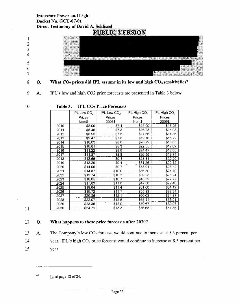
Interstate Power and Light Docket No. GCU-07-01
Q. What COz prices did IPL assume in its low and high COz sensitivities?
A. IPL's low and high C02 price forecasts are presented in Table 3 below:
Table 3: IPL COz Price Forecasts
12 Q. What happens to these price forecasts after 2030?
13 A. The Company's low C02 forecast would continue to increase at 5.3 percent per
14 year. IPL's high COz price forecast would continue to increase at 8.5 percent per
15 year.
42 Id, at page 12 of 24. -
Page 33
Interstate Power and Light Docket No. GCU-07-01
Q. How did IPL develop its low and high COZ price forecasts?
A. IPL has said that its low C02 price forecast is based on a 2003 MIT analysis of
Senate Bill 139, the original McCain-Lieberman climate change legislation.43
The Company also has said that its high CO2 price forecast is similarly based on a
2003 analysis of the same legislation by the Energy Information Administration
of the US. Department of
Q. Is it reasonable and prudent to base current C 0 2 price forecasts on just these
two analyses of a single piece of proposed legislation that was introduced in
Congress back in 2003?
A. No. As I will discuss below, we looked at the results of these same two analyses
when we developed our Synapse C02 price forecasts in the spring of 2006.
However, we also considered the results of another eight analyses of both the
2003 McCain-Lieberman bill and of other proposed climate change legislation
that had been introduced in Congress between 2003 and 2006.~' Thus, we
examined a much wider range of inputs when we developed our COz price
forecasts. We believe that it is necessary to do so because of the uncertainties
associated with the design, timing and implementation of federal greenhouse gas
regulations. IPL, in contrast, has based its projected C02 prices on optimistic
scenarios involving a single bill.
As I also will discuss in detail below, we also have continued to re-evaluate the
reasonableness of our C02 price forecasts in light of the proposed climate change
legislation that is being considered in the current Congress.
43 IPL Response to OCA DR. No. 19, Attachment A, at page 47 of 55. 44 Id. - 45 See the discussion in E x h i h i t D A S - I , Schedule C, beginning at page 41 of 63
Page 34
Interstate Power and Light Docket No. GCU-07-01
compare to the emissions target levels in the bills that have been introduced
in the current U.S. Congress?
A. The emissions levels considered in the 2003 McCain-Lieberman legislation
(Senate Bill S. 139), on which IPL bases it COz price forecasts, are significantly
less stringent (that is, higher) than would be required under the great majority of
the bills currently under consideration in Congress.
Table 4: Targets in Current National Climate [CONFIDENTIAL]
46 Source: IPL's Confidential Response to OCA DR. No. 21, Attachment A. page 116 of 212.
Page 35
Interstate Power and Light Docket No. GCU-07-01
emissions reductions that Congress is currently considering.
Q. By how much would IPL and Alliant Energy have to reduce their COz
emissions to reach 1990 levels by 2020?
A. Alliant has estimated that IPL would have to reduce its projected base case C02
emissions .47 Alliant
Energy would have to
Q. Is IPL's "high" COz price a reasonable high end of a range of COz price
forecasts?
A. No. Although the forecast is far more reasonable than the Company's low CO;?
price forecast, it still is too low to be considered the high end of a reasonable
range of possible future CO;? emissions allowance prices. In particular, IPL's high
COz price forecast does not reflect the emissions allowance prices that could
result from a number of the bills that have been introduced in Congress which
propose very significant emissions reductions.
Q. Has Synapse developed a carbon price forecast that would assist the Board in
evaluating the proposed SGS Unit 4?
A. Yes. Synapse's forecast of future carbon dioxide emissions prices are presented in
Figure 5 below.
47 IPL Confidential Response to OCA DR. No. 21, Attachment A, at pages 58 and 65 of 212. 48 IPL Confidential Response to OCA DR. No. 21, Attachment A, at page 56 of 212.
Page 36
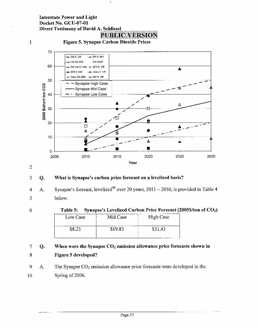
Interstate Power and Light Docket No. GCU-07-01
Figure 5. Synapse Carbon Dioxide Prices
- -Synapse High Case Synapse Mid Case
- - ,Synapse Low Case
2005 2010 2015 2020 2025 2030
Year
What is Synapse's carbon price forecast on a levelized basis?
Synapse's forecast, ~eve l ized~~ over 20 years, 201 1 - 2030; is provided in Table 4
below.
Table 5: Synapse's Levelized Carbon Price Forecast (2005$/ton of COz)
When were the Synapse COz emission allowance price forecasts shown in
Figure 5 developed?
The Synapse C02 emission allowance price forecasts were developed in the
Spring of 2006.
Page 37

For the purposes of the OCA's EGEAS modeling in this case, we have
conservatively assumed that C02 prices will increase at only the overall rate of
inflation after 2030, that is, they will not increase in constant 2005 dollars.
How were these COz price forecasts developed?
The basis for the Synapse CO2 price forecasts is described in detail in
Exhib i tDAS-1 , Schedule C, starting on page 41 of 63.
In general, the price forecasts were based, in part, on the results of economic
analyses of individual bills that had been submitted in the 108'~ and 109'
Congresses. We also considered the likely impacts of state, regional and
international actions, the potential for offsets and credits, and the likely future
trajectories of both emissions constraints and technological programs.
Are the Synapse COz price forecasts shown in Figure 5 based on any
independent modeling?
Yes. Although Synapse did not perform any new modeling to develop our CO2
price forecasts, our C02 price forecasts were based on the results of independent
modeling prepared at the Massachusetts Institute of Technology ("MIT"), the
Energy Information Administration of the Department of Energy ("EIA"), Tellus,
and the U.S. Environmental Protection Agency ("EPA").~'
In fact, two of the studies on which we relied when we developed the Synapse
C02 price forecasts are the same MIT and EPA assessments of the 2003 McCain
Liebeman bill which IPL has taken its low and high COz prices.
49 A value that is "levelized" is the present value of the total cost converted to equal annual payments. Costs are levelized in real dollars (i.e., adjusted to remove the impact of inflation).
50 See Table 6.2 on page 42 of 63 of Exhib i tDAS-1 , Schedule C.
Page 38
Interstate Power and Light Docket No. GCU-07-01 Direct Testimony of David A. ., ,.,. Schlissel ,7.m=...,....: -m2.r..x-ze -Ly-,.-- ..+.: i;,..'. .- ---- .- .. . . L. .. . . -.... C'L?'. "". .::*;:F.. . ~QBL~;E$;~ERs~~JN:
G.:!&.;., . :.r. . . ...,,............... n"i;r:-:i..,;:L
Q. Do the triangles, squares, circles and diamond shapes in Figure 5 above
reflect the results of all of the scenarios examined in the MIT, EIA, EPA and
Tellus analyses upon which Synapse relied?
A. As a general rule, Synapse focused our attention either on the modeler's primary
scenario or on the presented high and low scenarios to bracket the range of
results.
For example, the blue triangles in Figure 5 represent the results from EIA's
modeling of the 2003 McCain Lieberman bill, S.139. Synapse used the results
from EIA's primary case which reflected the bill's provisions that allowed: (a)
allowance banking; (b) use of up to 15 percent offsets in Phase 1 (2010-2015) and
up to 10 percent offsets in Phase I1 (2016 and later years). The S.139 case also
assumed commercial availability of advanced nuclear plants and of geological
carbon sequestration technologies in the electric power industry.
Similarly, the blue diamonds in Figure 5 represent the results from MIT's
modeling of the same 2003 McCain Lieberman bill, S.139. MIT examined 14
scenarios which considered the impact of factors such as the tightening of the cap
in Phase 11, allowance banking, availability of outside credits, and assumptions
about GDP and emissions growth. Synapse included the results from Scenario 7
which included allowance banking and zero-cost credits, which effectively
relaxed the cap by 15% and 10% in Phase I and Phase 11, respectively. Synapse
selected this scenario as the closest to the S.139 legislative proposal since it
assumed that the cap was tightened in a second phase, as in Senate Bill 139.
At the same time, some of the studies only included a single scenario representing
the specific features of the legislative proposal being analyzed. For example, SA
2028, the Amended McCain Lieberman bill set the emissions cap at constant 2000
levels and allowed for 15 percent of the carbon emission reductions to be met
through offsets from non-covered sectors, carbon sequestration and qualified
international sources. EIA presented one scenario in its table for this policy. The
results from this scenario are presented in the green triangles in Figure 5.
Page 39

Interstate Power and Light Docket No. GCU-07-01
reduce the cost of COz emissions?
A. Yes. Exhib i tDAS-1 , Schedule C identifies a number of factors that will
affect projected allowance prices. These factors include: the base case emissions
forecast; whether there are complimentary policies such as aggressive investments
in energy efficiency and renewable energy independent of the emissions
allowance market; the policy implementation timeline; the reduction targets in a
proposal; program flexibility involving the inclusion of offsets @erhaps
international) and allowance banking; technological progress; and emissions co-
benefik5' In particular, Synapse anticipates that technological innovation will
temper allowance prices in the out years of our forecast.
Q. Could carbon capture and sequestration be a technological innovation that
might temper or even put a ceiling on COz emissions allowance prices?
A. Yes.
Q. Does IPL see carbon capture technology as a currently commercially viable
way to mitigate COz emissions from pulverized coal plants like SGS Unit 4?
A. No. As I noted earlier, IPL has concluded that "commercially-available back-end
C02 emissions control technologies do not currently exist."52
Q. Do you agree with this assessment?
A. Yes. I agree with this view of the current status of carbon capture and
sequestration technology although I would note that there is some experience with
the piping of C02 gas for enhanced oil recovery and industrial use in certain
geographical areas.
5 1 E x h i b i t D A S - 1 , Schedule C, at pages 46 to 49 of 63. 52 IPL Response to OCA DR. No. 44.
Page 40
Interstate Power and Light Docket No. GCU-07-01
2 will become commercially viable for plants like SGS Unit 4?
3 A. No. I have seen estimates that carbon capture and sequestration technology may
4 be proven and commercially viable from as early as 2015 to 2030 or later. For
5 example, the February 2007 Future of Coal study from the Massachusetts
6 Institute of Technology:
7 Many years of development and demonstration will be required to 8 prepare for its successful, large scale adoption in the U.S. and 9 elsewhere. A rushed attempt at CCS [carbon capture and
10 sequestration] implementation in the face of urgent climate 11 concerns could lead to excess cost and heightened local 12 environmental concerns, potentially lead to long delays in 13 implementation of this important option.53
14 Q. What are the currently estimated costs for carbon capture and sequestration
15 at pulverized coal facilities?
16 A. Hope has been expressed concerning potential technological improvements and
17 learning curve effects that might reduce the estimated cost of carbon capture and
18 sequestration. However, I have seen recent studies by objective sources that
19 estimate that the cost of carbon capture and sequestration could increase the cost
20 of producing electricity at coal-fired power plants by 60-80 percent, on a $IMWh
2 1 basis. For example, a very recent study by the National Energy Technology
22 Laboratory ("NETL") projects that the cost of carbon capture and sequestration
23 would be $68/ton of C02 avoided, in 2007 dollars, for pulverized coal plants.54
24 This translates in to $65/ton of COZ avoided, in 2005 dollars.
25 The March 2007 "Future of Coal Study" from the Massachusetts Institute of
26 Technology estimated that the cost of carbon capture and sequestration would be
53 The Future of Coal, Options for a Carbon-Constrained World, an Interdisciplinary MIT Study, February 2007, at page 15. Available at http://web.mit.edu/coal/.
54 Cost and Performance Baseline for Fossil Energy Plants, National Energy Technology Laboratory, Revised August 2007, at page 27. Available at http:/lwww.netl.doe.govlenergy- analyseslpubs/Bituminous%20BaselineeFinal%2OReport.pdf
Page 41
Interstate Power and Light Docket No. GCU-07-01
figure.55 The tables in that study also indicated significantly higher costs for
carbon capture for pulverized coal facilities, in the range of about $40/ton and
higher.56
However, even when the technology for CO* capture matures, there will always
be significant regional variations in the cost of storage due to the proximity and
quality of storage sites.
Q. Have you seen any Company estimates of what it would cost to add carbon
capture and sequestration technologies to the proposed SGS Unit 4?
A. No. IPL has only provided some generic estimates of the cost of employing
carbon capture and sequestration technologies to coal plants. For example, the
Company has cited
. 5 7 Using data from the February 2007 MIT Future of
Coal Study, the Company has estimated that - 55 The Future of Coal, Options for a Carbon-Constrained World, Massachusetts Institute of
Technology, March 2007, at page xi. Available at http:l/web.mit.edulcoall. 56 Id, at page 19. - 57 IPL Response to OCA DR No. 97, Attachment A, at page 10. 58 IPL Response to OCA DR No. 97, Attachment B, at page 1. 59 IPL Response to OCA DR No. 97, Attachment C, at page 1.
Page 42

Interstate Power and Light Docket No. GCU-07-01
Q. Does IPL reflect any costs associated with employing carbon capture and
sequestration technologies in any of its economic analyses of SGS Unit 4?
A. No.
Q. Has IPL included any carbon capture and sequestration equipment or
features in the current design or cost estimate for SGS Unit 4?
A. No. The Company has said that at this time no specific equipment has been
included in the design of SGS Unit 4 exclusively for the purpose of carbon
capture and sequestration.60 However, some design features have been made for
other reasons that IPL contends will make carbon capture less expensive.6'
According to the Company, other design features may also be feasible. IPL has
committed to developing a white paper to study this issue in more depth and to
evaluate the options that are a ~ a i l a b l e . ~ ~
Q. Has IPL reflected in its economic analyses any of the performance penalties
that can be expected to be experienced as a result of the addition and use of
carbon capture and sequestration technologies at SGS Unit 4?
A. No. Recent studies, such as the 2007 study by the National Energy Technology
Laboratory, project that the output of a coal plant could be reduced by between 10
percent and 29 percent as a result of the addition of carbon capture and
sequestration technologies. However, IPL has not included any such performance
penalties in any of the economic analyses we have reviewed. In fact, IPL has not
made any specific assessments of the performance penalties associated with the
addition of carbon capture and sequestration equipment to the proposed unit.63
All that IPL could do is to refer to a generic, and confidential, EPRI study of
"Updated Cost and Performance Estimates for Clean Coal Technologies including
C02 Capture - 2006." However, the Company has not used in its analyses any of
60 IPL Response to OCA DR. No. 180. 61 IPL Responses to OCA DR. No. 180 and OCA DR. No. 181 62 IPL Response to OCA DR. No. 181.
Page 43

Interstate Power and Light Docket No. GCU-07-01 Direct Testimony of David A. Schlissel
T-;:i-~?'S~-.:~~~~'~IL$!-.:<~iii;~~.,Y~ii~p.% g;UBEEC-VER.fjIQPJ ..* ...,.,.. G" - ..., % ,.,... " li=-.,~;r;;~; t
the available information from that study, or from any of the public studies that
have been released in recent years on the costs and performance penalties
associated with the addition of carbon capture and sequestration technologies.
Q. Do the Synapse COz price forecasts reflect the potential for the inclusion of
domestic offsets and, perhaps, international offsets in U.S. carbon regulation
policy?
A. Yes. Even the Synapse high COz price forecast is consistent with, and in some
cases lower than, the results of studies that assume the use of some levels of
offsets to meet mandated emission limits. For example, as shown in Figure 6 the
highest price scenarios in the years 2015,2020 and 2025 were taken from the EIA
and MIT modeling of the original and the amended McCain-Lieberman proposals.
Each of the prices for these scenarios shown in Figure 5 reflects the allowed use
of offsets.
Q. How do the Synapse CO2 price forecasts compare to the C02 prices used by
IPL in its recent analyses of the proposed SGS Unit 4?
A. The Synapse and IPL COz price forecasts are shown in Figure 6 below. As this
Figure demonstrates, IPL's high C02 price forecast is similar to our mid-forecast.
63 IPL Response to OCA DR. No. 35
Page 44
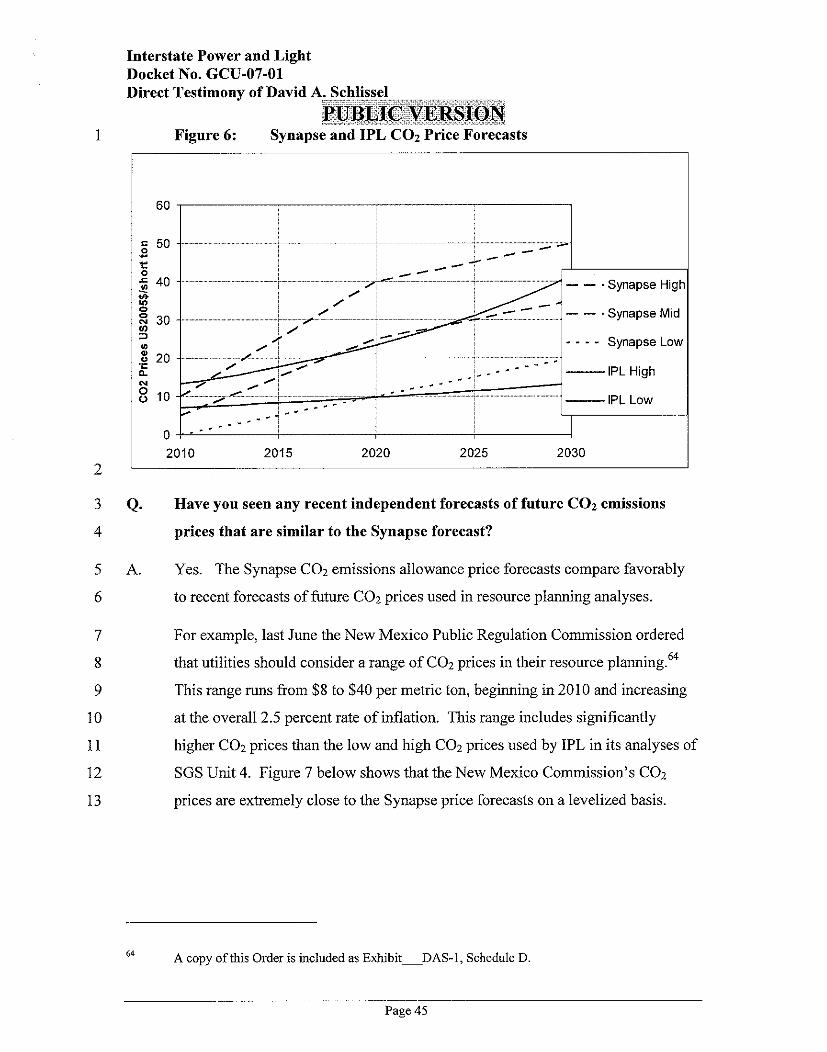
Interstate Power and Light Docket No. GCU-07-01
Figure 6: Synapse and IPL C02 Price Forecasts
Q. Have you seen any recent independent forecasts of future COz emissions
prices that are similar to the Synapse forecast?
A. Yes. The Synapse CO2 emissions allowance price forecasts compare favorably
to recent forecasts of future COz prices used in resource planning analyses.
For example, last June the New Mexico Public Regulation Commission ordered
that utilities should consider a range of C02 prices in their resource planning.64
This range runs from $8 to $40 per metric ton, beginning in 201 0 and increasing
at the overall 2.5 percent rate of inflation. This range includes significantly
higher C02 prices than the low and high CO2 prices used by IPL in its analyses of
SGS Unit 4. Figure 7 below shows that the New Mexico Commission's CO2
prices are extremely close to the Synapse price forecasts on a levelized basis.
64 A copy of this Order is included as Exhib i tDAS-1 , Schedule D
Page 45
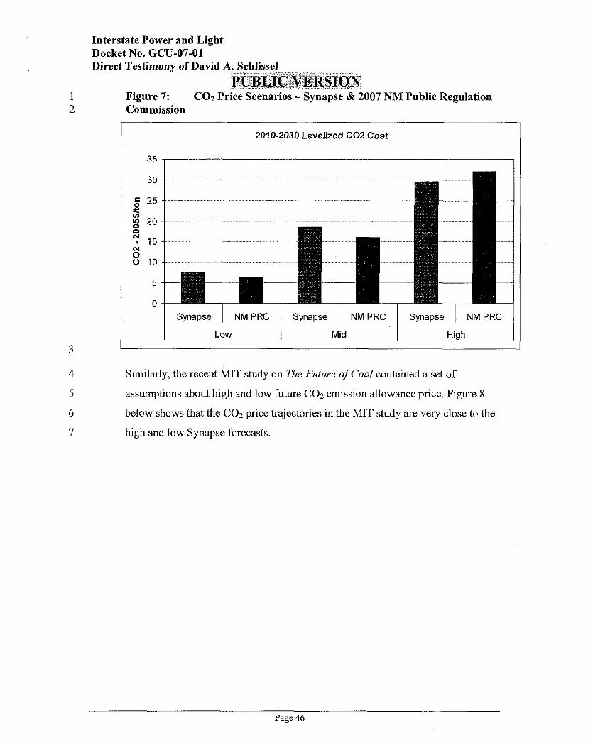
Interstate Power and Light Docket No. GCU-07-01 Direct Testimony of David A. F..7.~,=~...~e Schlissel .%>.).T,ep :.: -:,,.,. *, . _. ,.,... . .. ..,,.,.,,.: .-.$ .,,. .,, . . ... . . , . , ~ J ~ J B . ~ ~ ; ~ ~ ~ T E R ~ $ Q . N
.., , _*" A=<.-;'.r.; ..a ,,,. ",,"!:.;.-. Figure 7: CO2 Price Scenarios - Synapse & 2007 NM Public Regulation Commission
2070-2030 Levelized C02 Cost
Synapse I NM PRC Synapse I NM PRC Synapse 1 NM PRC
Low Mid High
Similarly, the recent MIT study on The Future of Coal contained a set of
assumptions about high and low future COl emission allowance price. Figure 8
below shows that the COz price trajectories in the MIT study are very close to the
high and low Synapse forecasts.
Page 46
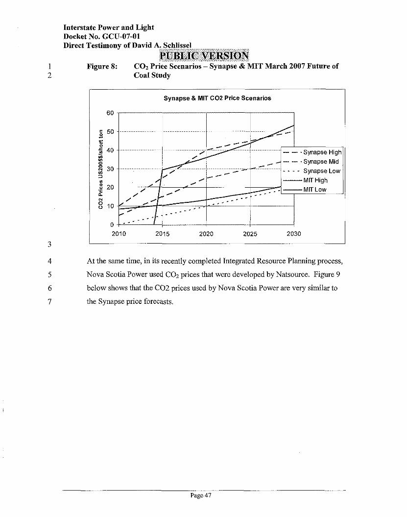
Interstate Power and Light Docket No. GCU-07-01
Coal Study
Synapse & MIT C02 Price Scenarios I
4 At the same time, in its recently completed Integrated Resource Planning process,
5 Nova Scotia Power used COz prices that were developed by Natsource. Figure 9
6 below shows that the C 0 2 prices used by Nova Scotia Power are very similar to
7 the Synapse price forecasts.
Page 47
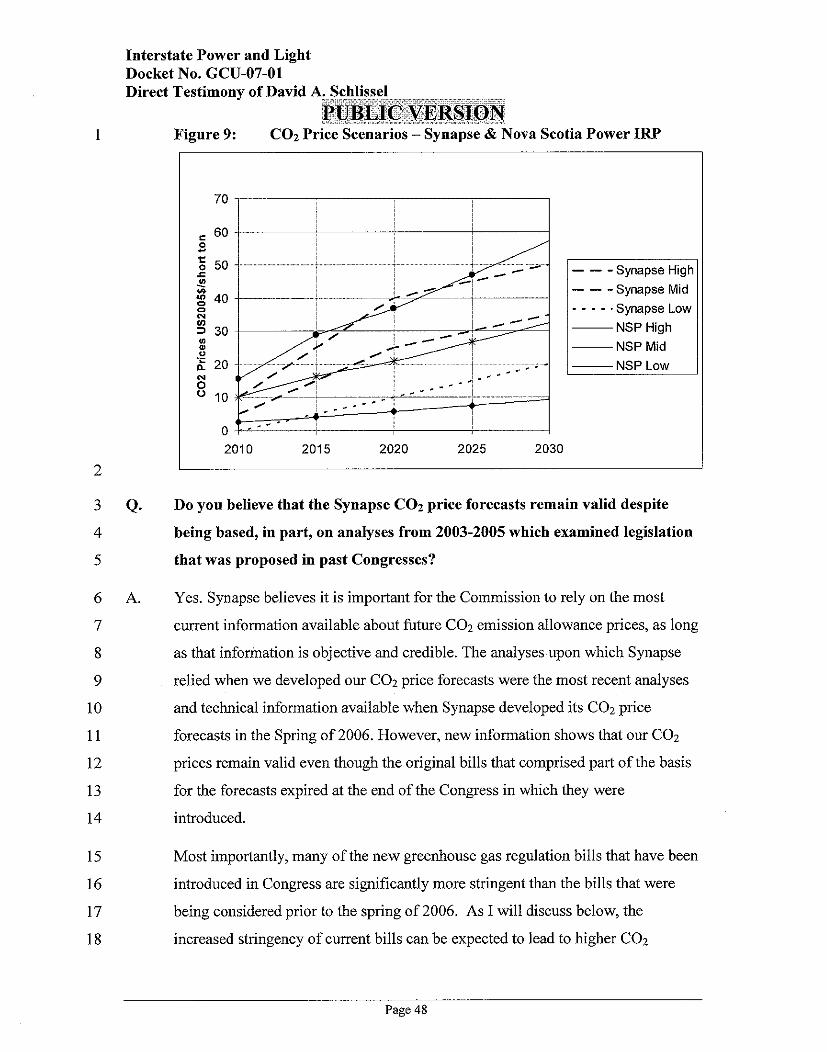
Interstate Power and Light Docket No. GCU-07-01
-Synapse Mid . Synapse Low NSP High NSP Mid NSP Low
Do you believe that the Synapse COz price forecasts remain valid despite
being based, in part, on analyses from 2003-2005 which examined legislation
that was proposed in past Congresses?
Yes. Synapse believes it is important for the Commission to rely on the most
current information available about hture C02 emission allowance prices, as long
as that information is objective and credible. The analyses upon which Synapse
relied when we developed our C02 price forecasts were the most recent analyses
and technical information available when Synapse developed its CO2 price
forecasts in the Spring of 2006. However, new information shows that our C02
prices remain valid even though the original bills that comprised part of the basis
for the forecasts expired at the end of the Congress in which they were
introduced.
Most importantly, many of the new greenhouse gas regulation bills that have been
introduced in Congress are significantly more stringent than the bills that were
being considered prior to the spring of 2006. As I will discuss below, the
increased stringency of current bills can be expected to lead to higher C02
Page 48
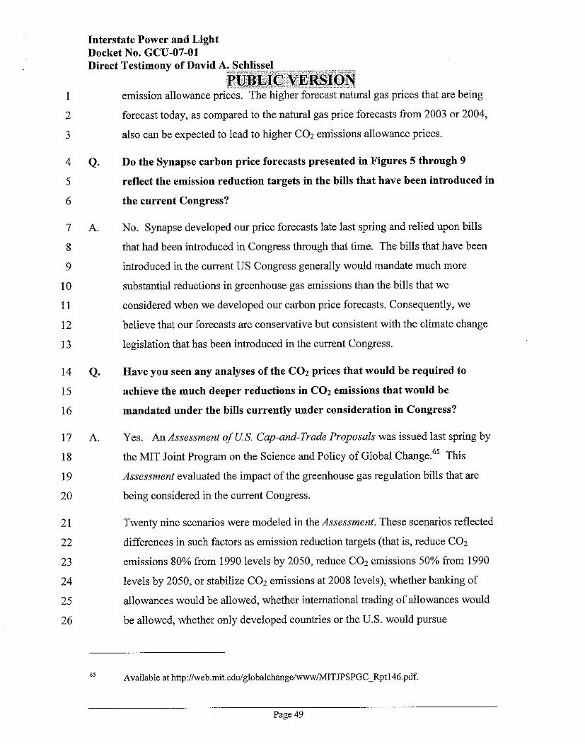
Interstate Power and Light Docket No. GCU-07-01
forecast today, as compared to the natural gas price forecasts from 2003 or 2004,
also can be expected to lead to higher COz emissions allowance prices.
Do the Synapse carbon price forecasts presented in Figures 5 through 9
reflect the emission reduction targets in the bills that have been introduced in
the current Congress?
No. Synapse developed our price forecasts late last spring and relied upon bills
that had been introduced in Congress through that time. The bills that have been
introduced in the current US Congress generally would mandate much more
substantial reductions in greenhouse gas emissions than the bills that we
considered when we developed our carbon price forecasts. Consequently, we
believe that our forecasts are conservative but consistent with the climate change
legislation that has been introduced in the current Congress.
Have you seen any analyses of the COz prices that would be required to
achieve the much deeper reductions in C02 emissions that would be
mandated under the bills currently under consideration in Congress?
Yes. An Assessment of US. Cap-and-Trade Proposals was issued last spring by
the MIT Joint Program on the Science and Policy of Global This
Assessment evaluated the impact of the greenhouse gas regulation bills that are
being considered in the current Congress.
Twenty nine scenarios were modeled in the Assessment. These scenarios reflected
differences in such factors as emission reduction targets (that is, reduce COz
emissions 80% from 1990 levels by 2050, reduce COl emissions 50% from 1990
levels by 2050, or stabilize COz emissions at 2008 levels), whether banking of
allowances would be allowed, whether international trading of allowances would
be allowed, whether only developed countries or the U.S. would pursue
65 Available at http:llweb.mit.edulglobalchange/\~\~~lMITJPSPGC~Rptl46.pdf.
Page 49
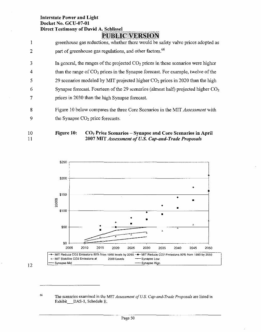
Interstate Power and Light Docket No. GCU-07-01
2 part of greenhouse gas regulations, and other factors.66
3 In general, the ranges of the projected C02 prices in these scenarios were higher
4 than the range of CO2 prices in the Synapse forecast. For example, twelve of the
5 29 scenarios modeled by MIT projected higher C02 prices in 2020 than the high
6 Synapse forecast. Fourteen of the 29 scenarios (almost half) projected higher CO2
7 prices in 2030 than the high Synapse forecast.
8 Figure 10 below compares the three Core Scenarios in the MIT Assessment with
9 the Synapse CO2 price forecasts.
10 Figure 10: COz Price Scenarios - Synapse and Core Scenarios in April 11 2007 MIT Assessment of U.S. Cap-and-Trade Proposals
2005 2010 2015 2020 2025 2030 2035 2040 2045 2050
1990 levels by 2050 -t MIT Reduce C02 Em~ss~ons 50% from 1990 by 2050
a MIT Stablllze C02 Em~ssms at 2008 Levels -Synapse Low
12 -Synapse Hlgh
66 The scenarios examined in the MIT Assessment of US. Cap-and-Trade Proposals are listed in Exh ib i tDAS-1 , Schedule E.
Page 50
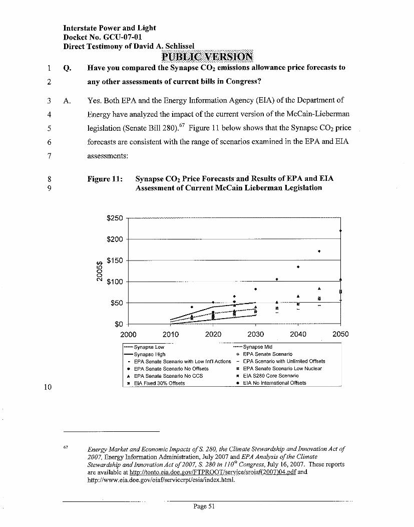
Interstate Power and Light Docket No. GCU-07-01
any other assessments of current bills in Congress?
A. Yes. Both EPA and the Energy Information Agency (EIA) of the Department of
Energy have analyzed the impact of the current version of the McCain-Lieberman
legislation (Senate Bill 2 8 0 ) . ~ ~ Figure 11 below shows that the Synapse COz price
forecasts are consistent with the range of scenarios examined in the EPA and EIA
assessments:
Figure 11: Synapse COz Price Forecasts and Results of EPA and EIA Assessment of Current McCain Lieberman Legislation
-Synapse High a EPA Senate Scenario - EPA Senate Scenario with Low int'l Actions - EPA Scenario with Unlimited Offsets
EPA Senate Scenario No Offsets E EPA Senate Scenario Low Nuclear A EPA Senate Scenario No CCS EIA 5280 Core Scenario
EIA Fixed 30% Offsets EIA No International Offsets
67 Energy Market andEconomic Impacts of S. 280, the Climate Stewardship andlnnovation Act of 2007, Energy Information Administration, July 2007 and EPA Analysis of the Climate Stewardship andlnnovation Act of 2007, S. 280 in 110'~ Congress, July 16,2007. These reports are available at h~://tonto.eia.doe.~oviFTPR00T/se~ice/soiaf200704.dfand http://www.eia.doe.gov/oiaWservice1pt/csia/index.htm1.
Page 5 1
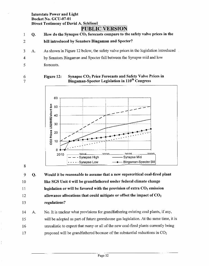
Interstate Power and Light Docket No. GCU-07-01 Direct Testimony of David A. Schlissel :. :i"i.;:-.:?:i7.3ii:g::'r--- --:-.i.-:.:,l,qn;z-
,pG;B2D$.C;i!ViERSFQN ; ..-., ;.. : ...,.. *" ",r.~L:...d.,.-; - i-. ,..- ".., --
Q. How do the Synapse COz forecasts compare to the safety valve prices in the
bill introduced by Senators Bingaman and Specter?
A. As shown in Figure 12 below, the safety valve prices in the legislation introduced
by Senators Bingaman and Specter fall between the Synapse mid and low
forecasts.
Figure 12: Synapse COz Price Forecasts and Safety Valve Prices in Bingaman-Specter Legislation in 110'~ Congress
2010 qn?n 9 m = qnm
- - -Synapse High -Synapse Mid
d Bingaman-Specter Bill
Q. Would it be reasonable to assume that a new supercritical coal-fired plant
like SGS Unit 4 will be grandfathered under federal climate change
legislation or will be favored with the provision of extra COZ emission
allowance allocations that could mitigate or offset the impact of COz
regulations?
A. No. It is unclear what provisions for grandfathering existing coal plants, if any,
will be adopted as part of future greenhouse gas legislation. At the same time, it is
unrealistic to expect that many or all of the new coal-fired plants currently being
proposed will be grandfathered because of the substantial reductions in C02
Page 52
Interstate Power and Light Docket NO. GCU-07-01
atmospheric concentrations of COz at 450 ppm to 550 ppm.
Meeting these goals will require either a reduction in dependence on coal for
electricity generation or a very large investment in conversion of the current coal
generating fleet in the US. The only realistic way either of these is going to
happen is with a large marginal cost on greenhouse gas emissions such as a C02
tax or higher emissions allowance prices. It is not reasonable to expect that a new
supercritical coal plant, like SGS Unit 4, which will substantially increase the
emissions of CO2 into the atmosphere, will receive significant emission
allowances under any U.S. carbon regulation plan.
For example, the National Commission on Energy Policy has recently
recommended that "new coal plants built without [carbon capture and
sequestration] not be "grandfathered" (i.e., awarded free allowances) in any future
regulatory program to limit greenhouse gas emission^."^^ A report of an
interdisciplinary study at the Massachusetts Institute of Technology on The
Future of Coal similarly noted that:
There is the possibility of a perverse incentive for increased early investment in coal-fired power plants without capture, whether SCPC or IGCC, in the expectation that the emissions from these plants would potentially be "grandfathered" by the grant of free C02 allowances as part of future carbon emissions regulations and that (in unregulated markets) they would also benefit from the increase in electricity prices that will accompany a carbon control regime. Congress should act to close this "grandfathering" loophole before it becomes a problem.69
68 Energy Policy Recommendations to the President and the 110'~ Congress, National Commission on Energy Policy, April 2007, at page 21. Available at http:l/energycommission.org/files/contentFiles~CEP~Recommendations~April~2OO7~46S6~759 c345.pdf.
69 The Future of Coal, Options for a Carbon-Constrained World, an Interdisciplinary MIT Study, March 2007, at page (xiv). Available at http:llweb.mit.edulcoal/.
Page 53

Interstate Power and Light Docket No. GCU-07-01
be required to actually have carbon capture and sequestration technology. For
example, a bill by Massachusetts Senator Kerry's bill limit C02 emissions from
new coal-fired facilities to 285 lbs/MWh. New coal-fired facilities would be
defined as those that begin construction on or after April 26,2007 and would
certainly include the proposed Hempstead Project.
What are you recommendations concerning the C 0 2 prices that the
Commission should use in evaluating IPL's proposed SGS Unit 4?
Given the uncertainty associated with the legislation that eventually will be
passed by Congress, we believe that the Commission should use the wide range of
forecasts of C02 prices shown in Figure 4 above to evaluate the relative
economics of the proposed Repowering Project.
How much additional COz would SGS Unit 4 emit into the atmosphere?
SGS Unit 4 can be expected to emit approximately five million tons of C02
annually.70
What would he the annual costs of greenhouse gas regulations to IPL and its
ratepayers under the Synapse C o t price forecasts if the Company proceeds
with its proposed SGS Unit 4?
The range of the incremental annual, levelized cost to the Company and its
ratepayers from greenhouse gas regulations would be:
Synapse Low C02 Case: 2.75 million tons of C 0 2 . $8.23/ton = $23 million
Synapse Mid CO2 Case: 2.75 million tons of CO2 . $19.83/ton = $55 million
Synapse High CO2 Case: 2.75 million tons of C02 . $3 1.43lton = $86 million
70 This reflects an 90 percent average annual capacity factor and projected CO, emissions of 1991 1bsIMWh.
Page 54
Interstate Power and Light Docket No. GCU-07-01
emissions could have on its customers electric rates?
An April 2007 presentation to the Company's senior management on New
Generation Support Strategy Update did look at the impact that $15 and $29/ton
COz taxes would have on customers. This analysis
IPL Has Not Adequately Considered The Risk Of Further Increases In The Estimated Cost Of The SGS Unit 4 Project
What is the currently estimated cost for SGS Unit 4?
The currently estimated cost of SGS Unit 4, without AFUCD or any other
financing costs, is m.72 Is it reasonable to expect that the actual cost of the project will be higher
than IPL now estimates?
Yes. The costs of building power plants have soared in recent years as a result of
the worldwide demand for power plant design and construction resources and
commodities. There is no reason to expect that plant costs will not continue to
rise during the years when the detailed engineering, procurement and construction
of SGS Unit 4 will be underway. This is especially true given the very early stage
of the engineering and procurement for the project.
For example, Duke Energy Carolinas' originally estimated cost for the two unit
coal-fired Cliffside Project was approximately $2 billion. In the fall of 2006,
Duke announced that the cost of the project had increased by approximately 47
percent ($1 billion). After the project had been downsized because the North
-
Page 55
IPL's Confidential Response to OCA DR. No. 21, Attachment A, at page 69 of 212. IPL Confidential Response to OCA DR. No. 183, Attachment A, page 1 of 1.
Interstate Power and Light Docket No. GCU-07-01
announced that the cost of that single unit would be about $1.53 billion, not
including financing costs. In late May 2007, Duke announced that the cost of
building that single unit had increased by about another 20 percent. As a result,
the estimated cost of the one unit that Duke is building at Cliffside is now $1.8
billion exclusive of financing costs. Thus, the single Cliffside unit is now
expected to cost almost as much as Duke originally estimated for a two unit plant.
Q. Did Duke explain to the North Carolina Utilities Commission the reasons for
the skyrocketing cost of the Cliffside Project?
A. Yes. In testimony filed at the North Carolina Utilities Commission on November
29,2006, Duke Energy Carolinas emphasized that the competition for resources
had had a significant impact on the costs of building new power plants. This
testimony was presented to explain the approximate 47 percent ($1 billion)
increase in the estimated cost of Duke Energy Carolinas' proposed coal-fired
Cliffside Project that the Company announced in October 2006.
For example, Duke Energy Carolinas explained that:
The costs of new power plants have escalated very rapidly. This effect appears to be broad based affecting many types of power plants to some degree. One key steel price index has doubled over the last twelve months alone. This reflects global trends as steel is traded internationally and there is international competition among power plant suppliers. Higher steel and other input prices broadly affects power plant capital costs. A key driving force is a very large boom in U.S. demand for coal power plants which in turn has resulted from unexpectedly strong U.S. electricity demand growth and high natural gas prices. Most integrated US. utilities have decided to pursue coal power plants as a key component of their capacity expansion plan. In addition, many foreign companies are also expected to add large amounts of new coal power plant capacity. This global boom is straining supply. Since coal power plant equipment suppliers and bidders also supply other types of
Page 56
Interstate Power and Light Docket No. GCU-07-01 Direct Testimony of David A. Schlissel ...A..2 . ..... "~ ...... .............-.. ....... -.=. :~.-. ...... . _: . . ' ........ . : . . . . . :pu~cg:f?;~y~;~$g(jN
s,.a:,:,=z .... .z.....m ..%.. " .=,.. ...- .. '.* :. > ............ '; ....... plants, there is a spill over effect to other types of electric generating plants such as combined cycle plants.73
Duke further noted that the actual coal power plant capital costs as reported by
plants already under construction exceed government estimates of capital costs by
"a wide margin (i.e., 35 to 40 percent). Additionally, current announced power
plants appear to face another increase in costs (i.e., approximately 40 percent
addition."74 Thus, according to Duke, new coal-fired power plant capital costs had
increased approximately 90 to 100 percent since 2002.
Q. Have other coal-fired plant projects experienced similar cost increases?
A. Yes. A large number of projects have announced significant construction cost
increases over the past few years. For example, the cost of Westar's proposed
coal-fired plant in Kansas, originally estimated at $1 billion, increased by 20
percent to 40 percent, over just 18 months. This prompted Westar's Chief
Executive to warn: "When equipment and construction cost estimates grow by
$200 million to $400 million in 18 months, it's necessary to proceed with
caution."75 As a result, the company has suspended site selection for the coal-
plant and is considering other options, including building a natural gas plant, to
meet growing electricity demand.
The estimated cost of the now-cancelled Taylor Energy Center in Florida
increased by 25 percent, $400 million, in just 17 months between November 2005
and March 2007. The estimated cost of the Big Stone I1 coal-fired power plant
project in South Dakota has increased by about 60 percent since the project was
73 Direct Testimony of Judah Rose for Duke Energy Carolinas, North Carolina Utilities Commission Docket No. E-7, SUB 790, at page 4, lines 2-14. Mr. Rose's testimony is available on the North Carolina Utilities Commission website. Available at http://ncuc.commerce.state.nc.uslcgi- ~ ~ ~ / ~ ~ ~ ~ ~ ~ ~ ~ . ~ ~ ~ / I N P U T ? ~ ~ ~ ~ ~ ~ ~ ~ = D U K E ~ ~ O E N E R G Y % ~ O C A R O L I N A S % ~ C % ~ O L L C & ~ O C ketdesc=&comptype=E&docknumb=7&Search=Search&suffix1=&subnumb=790&suffix2=&par ml=000123542&pann2=01/09/2007&parm3=WBAAAAAA9007OB.
74 Ibid, at page 6, lines 5-9, and page 12, lines 11-16. 75 Available at
http://www.westarenergy.com/corp_com/co~6BE1277A768F0E486257269005558 1C /$file/122806%20coal~2OpIant%2Ofmal2.pdf
Page 57

Interstate Power and Light Docket No. GCU-07-01 Direct Testimony of David A. Schlissel . , ,,,... iii;i -..? i--=. -l.l,. . . . . , . . . .. ... . .. .. . . .- . , ..,. . . .. .... . .- .. . %... :>. : ~ : ~ : B & I ; c . ~ ~ E J R . $ ~ ~ : N
:;.,.;-;i.,;.~-.. - , , - ..,. #;.,;i i'.:.
first announced. Finally, the estimated cost of the Little Gypsy Repowering
Project (gas to coal) increased by 55 percent between announcement of the project
in April 2007 and the filing of a request for a license to build in July 2007.
What are the sources of the worldwide competition for power plant design
and construction resources, commodities and equipment?
The worldwide competition is driven mainly by huge demands for power plants in
China and India and by a rapidly increasing demand for power plants and power
plant pollution control modifications in the United States required to meet SO2
and NO, emissions standards. The demand for labor and resource to rebuild the
Gulf Coast area after Hurricanes Katrina and Rita hit in 2005 also has contributed
to rising costs for construction labor and materials.
Is it commonly accepted that domestic United States and worldwide
competition for power plant design and construction resources, commodities
and manufacturing have led to these significant increases in power plant
construction costs in recent years?
Yes. A wide range of energy, construction and financial industry studies have
identified the worldwide competition for power plant resources as the driving
force for the skyrocketing construction costs.
For example, a June 2007 report by Standard & Poor's, Increasing Construction
Costs Could Hamper US. Utilities' Plan to Build New Power Generation, has
noted that:
As a result of declining reserve margins in some US. regions . . . brought about by a sustained growth of the economy, the domestic power industry is in the midst of an expansion. Standing in the way are capital costs of new generation that have risen substantially over the past three years. Cost pressures have been caused by demands of global infrastructure expansion. In the domestic power industry, cost pressures have arisen from higher demand for pollution control equipment, expansion of the transmission grid, and new generation. While the industry has experienced buildout cycles in the past, what makes the current environment different is
Page 58

Interstate Power and Light Docket No. GCU-07-01 Direct Testimony of David A. ..,,&.,",A,., Schlissel ,,. ,:8,,,: SF ---- ...,.. .,,.> :. ,:L.:<>..,... ,:.,,.= . 2-:.:.."~,.:~~:-..-.r.- :,:<,.,, p@~~~G:rn i$ j$ ,o~ Us =.>= &,,‘&L- . .
~ :>, &L%,:.,A; .=s.= %sa,:<.-..:,..
the supply-side resource challenges faced by the construction industry. A confluence of resource limitations have contributed, which Standard & Poors' Rating Services broadly classifies under the following categories
. Global demand for commodities
. Material and equipment supply
. Relative inexperience of new labor force, and . Contractor availability
The power industry has seen capital costs for new generation climb by more than 50% in the past three years, with more than 70% of this increase resulting from engineering, procurement and construction (EPC) costs. Continuing demand, both domestic and international, for EPC services will likely keep costs at elevated levels. As a result, it is possible that with declining reserve margins, utilities could end up building generation at a time when labor and materials shortages cause capital costs to rise, well north of $2,500 per kW for supercritical coal plants and approaching $1,000 per kW for combined-cycle gas turbines (CCGT). In a separate yet key point, as capital costs rise, energy efficiency and demand side management already important from a climate change perspective, become even more crucial as any reduction in demand will mean lower requirements for new capacity.76
More recently, the president of the Siemens Power Generation Group told the
New York Times that "There's real sticker shock out there."77 He also estimated
that in the last 18 months, the price of a coal-fired power plant has risen 25 to 30
percent.
A September 2007 report on Rising Utility Construction Costs prepared by the
Brattle Group for the EDISON Foundation similarly concluded that:
Construction costs for electric utility investments have risen sharply over the past several years, due to factors beyond the industry's control. Increased prices for material and manufactured components, rising wages, and a tighter market for construction
Increasing Construction Costs Could Hamper US. Utilities' Plans to Build New Power Generation, Standard & Poor's Rating Services, June 12,2007, at page 1. A copy of this report is included in Exhibit-DAS-I, Schedule F. "Costs Surge for Building Power Plants, New York Times, July 10,2007.
Page 59
Interstate Power and Light Docket No. GCU-07-01
project management services have contributed to an across-the- board increase in the costs of investing in utility infrastructure. These higher costs show no immediate signs of abating.78
The report further found that:
. Dramatically increased raw materials prices (e.g., steel, cement) have increased construction cost directly and indirectly through the higher cost of manufactured components common in utility infrastructure projects. These cost increases have primarily been due to high global demand for commodities and manufactured goods, higher production and transportation costs (in part owing to high fuel prices), and a weakening U.S. dollar. . Increased labor costs are a smaller contributor to increased utility construction costs, although that contribution may rise in the future as large construction projects across the country raise the demand for specialized and skilled labor over current or project supply. There also is a growing backlog of project contracts at large engineering, procurement and construction (EPC) firms, and construction management bids have begun to rise as a result. Although it is not possible to quantify the impact on future project bids by EPC, it is reasonable to assume that bids will become less cost-competitive as new construction projects are added to the queue. . The price increases experienced over the past several years have affected all electric sector investment costs. In the generation sector, all technologies have experienced substantial cost increases in the past three years, from coal plants to windpower projects.. . . As a result of these cost increases, the levelized capital cost component of baseload coal and nuclear plants has risen by $20/MWh or more - substantially narrowing coal's overall cost advantages over natural gas-fired combined-cycle plants - and thus limiting some of the cost-reduction benefits expected from expanding the solid-fuel fleet. . The rapid increases experienced in utility construction costs have raised the price of recently completed infrastructure projects, but the impact has been mitigated somewhat to the extent that construction or materials acquisition preceded the most recent price increases. The impact of rising costs has a more dramatic impact on the estimated cost of proposed utility infrastructure projects, which fully incorporates recent price trends. This has raised significant concerns that the next wave of utility investments
78 Rising Utility Construction Costs: Sources and Impacts, prepared by The Brattle Group for the EDISON Foundation, September 2007, at page 3 1. A copy of this report is attached as Exh ib i tDAS-1 , Schedule G.
Page 60
Interstate Power and Light Docket No. GCU-07-01 Direct Testimony of David A. Schlissel
p: >:.-.*...,< :.:.rc<3:>r-.:>.:7;:B+? ...>, ~ ~ e * , - , : . : ~ > F 7 ~ " T ~ 2 :RJJB&!&;C$mjRSgoN ===,! .=...,. . . ~ , ~ ,',... 2 ;..LC.=..>. .~ ..,,.,,....,., A
may be imperiled by the high cost environment. These rising construction costs have also motivated utilities and regulators to more actively pursue energy efficiency and demand response initiatives to reduce the future rate impacts on consumers.79
Is it reasonable to expect that these same factors will lead to construction
delays as well as rising costs?
Yes.
Does the current SGS Unit 4 cost estimate include a contingency to reflect
possible future cost increases?
Yes. It appears that the current SGS Unit 4 construction cost estimate includes a - contingency which would be about I percent of the estimate, far
below the double digit annual escalation experienced by other coal-fired power
plant construction projects in recent years.
What is the current status of contracting and procurement for SGS Unit 4?
Basically, it appears that none of the major contracts for SGS Unit 4 have been
finalized. IPL has indicated that it does not expect to give even a limited notice to
proceed to its Engineering, Procurement and Construction ("EPC") contractor
until December 2007, with a full notice to proceed not expected until July 2008.
Similarly, the full notices to proceed with procurement of the steam turbine
generator, steam generator and air quality control system are not expected to be
issued until July 2008. The current estimated start for construction is October
2 0 0 8 . ~ ~
The extremely early status of contracting and procurement render the project very
susceptible to cost increases and construction delays.
79 Id, at pages 1-3. - 80 IPL Response t o OCA DR No. 24.
Page 6 1
Interstate Power and Light Docket No. GCU-07-01 Direct Testimony of David A. .- Schlissel , .,.,,,. ,,.....m*.,7..x .s.-: ..,..,..,. . . . . , . ,,, _.jr ~ 2 ~ ~ ~ ~ J , $ C <V'J$$@XQN
L;/ .;.-.... ;..:. - ,.,. ;r ......... %..r.:: ,..A
Q. Has the Company recognized the risks associated with rising power plant
construction costs?
A. Yes. Internal Alliant Energy presentations reflect the risks associated with
building new power plants in the current environment. For example, a February
2,2007 presentation to Alliant Energy's Board of Directors concerning the
proposed Nelson Dewey #3 coal plant noted that the U.S. Department of Energy
current forecasts the "largest coal generation capacity installation in 40 years."81
The same presentation also listed the risks associated with pursuing that project:
Q. Did IPL reflect the potential for higher capital costs in its recent 2007
Resource Plan modeling for SGS Unit 4?
A. No. The Company used the same plant capital cost in its base case modeling and
the two COz price sensitivity scenarios.
Q. Did IPL reflect the potential for a schedule delay as a result of the increased
competition for power plant design and construction resources, commodities
and manufacturing capacity?
A. No.
81 IPL's Confidential Response to OCA DR. No. 60, Attachment B, at page 6 of 12. 82 Id, at page 8 of 12. -
Page 62
Interstate Power and Light Docket No. GCU-07-01 Direct Testimony of David A. Schlissel ,.. . ,, ',.. ..--= % =... >,.,,,r>., .... .,.,. . ., ". :- .rm7F: ,-... ~ %-: sz.,.,...p,. .. . i@~:l&~~~.~ VE;RrfJE=N
r .... i ;- -... l...h:.i: +... F . ; . ~ L L : : ~ ~ ~ ~ ~ ~ ~ ~ ~ ~ .:-.. . 1 Q. Is it your testimony that IPL should change its current cost estimate for SGS
2 Unit 4?
Not necessarily. However, in order to evaluate the risks of continuing with the
proposed project, IPL should have prepared sensitivity studies that examined the
relative economics of SGS Unit 4 against alternatives assuming that the capital
cost of the project is substantially higher than the Company now estimates. For
example, IPL should have prepared sensitivity analyses that reflected capital costs
20 percent and 40 percent higher than its current estimated cost for SGS Unit 4. It
is not unreasonable to expect such additional cost increases at SGS Unit 4 in light
of the industry-wide experience and the expectation that worldwide demand will
continue to be a driving force for rising prices.
12 Q. Have you seen any such capital cost sensitivity analyses that have been
13 prepared by IPL?
14 A. Not in this proceeding. However, IPL did prepare a higher capital cost sensitivity
15 analysis as part of its 2005 Resource Plan modeling. In that sensitivity, IPL
16 assumed a capital cost for a coal-fired power plant that was approximately 32
17 percent higher than the base case capital cost.
18 Q. Is it reasonable to expect that these same current market conditions also will
19 lead to increases in the estimated costs of other supply-side alternatives such
20 as natural gas-fired or wind facilities?
21 A. Yes.
22 Q. What impact would higher coal-plant capital costs have on the relative
23 economics of energy efficiency as compared to SGS Unit 4?
24 A. I have seen no evidence that the same worldwide demand for power plant
25 resources has led to significant increase in the costs of energy efficiency
26 measures. Therefore, it is reasonable to expect that higher coal-plant capital costs
27 increase the relative economics and attractiveness of energy efficiency.
Page 63
Interstate Power and Light Docket No. GCU-07-01 Direct Testimony of David A. Schlissel ,,;:>.: .: ..,.>.*.: ,!.=, :: .:.>, -?:.:..:: z:y.v" ..:x*:. ,:. ..:.-.: ..2,; -.<
I ) ~ B L ~ ~ ~ : ~ ] C R ~ ~ ~ ~ ~ .z:....:;;;- . -.-.-.. -.,-. ._r ;:.. ;: ;.r .... ".',....
1 Q. Have you seen any evidence that potential participants in SGS Unit 4 are
2 very concerned about the potential for increasing plant construction costs?
9 Q. What was IPL's response to this demand?
Have you seen any subsequent correspondence between IPL and CIPCO or
Corn Belt, or any other potential co-owners of SGS Unit 4, that addresses
this issue?
No. IPL has said that there is no additional correspondence that is related to this
provision.
Adding SGS Unit 4 Would Reduce, Not Increase, the Diversity in IPL's Generation Supply
Is supply diversity an issue that the Commission should consider as it
evaluates IPL's proposed SGS Unit 4?
Yes. I think supply diversity is a very important consideration. Reducing the
Company's current heavy dependence on fossil-fired generation, especially coal-
fired power, and moving towards greater use of renewable resources and energy
efficiency, should be a major goal given the threat posed by global climate change
83 IPL Confidential Response to OCA DR. No. 7, Attachment A, page 128 of 579. 84 IPL Confidential Response to OCA DR. No. 51A.
Page 64
Interstate Power and Light Docket No. GCU-07-01
future. Building SGS Unit 4 would be a major step in the wrong direction.
Q. What would be the Company's energy supply mix under its proposed
Resource Plan that includes SGS Unit 4?
A. As shown in Figures 13 and 14 below, IPL's generation supply which is already
very heavily dependent on coal and other COz emitting fossil fuels
with the Company's base
resource plan that includes SGS Unit 4. In fact, of the energy supplied
by IPL in the year 2022 would be generated at coal-fired facilities. The data for
this figure were taken from IPL's base case EGEAS model for the year 2022.
Page 65
Interstate Power and Light Docket No. GCU-07-01
2
3 Figure 14: IPL Energy Supply Mix in 2022 [CONFIDENTIAL]
Page 66
Interstate Power and Light Docket No. GCU-07-01 Direct Testimony of David A. Schlissel --." ,..,,,.v
. ...,. .. .. .,. ....., ;,r,s:.r-,:.; :L ... 1.:: S..., i:.-.~,:~i.Y=:-E-T.?-i p u ~ ~ x c v B ~ - g l ; ~ ; ~ L.!: ',%? 3,.::..* ......:., ,-.~ . . ..,. .,.,,, ,,,,, 2,. ,,,A
Thus, under its base case 2007 Resource Plan, IPL's dependence on coal-fired
generation would l p r c e n t in 2007 percent in
2022.
Why is considering a company's generation mix the appropriate way to
evaluate its fuel diversity?
Because the issue of he1 diversity is a matter of the amount of each type of fuel
that the company bums, and the cost consequences of burning that fuel. Simply
looking at its capacity mix does not offer any information about the utilization of
that capacity.
Is fuel diversity a broader issue than merely deciding whether to build a eoal-
or gas-fired generating unit?
Yes, it should be. Implementing demand side management and energy efficiency
programs and building or buying power from non- or low-carbon emitting
renewable resource facilities also would increase a company's supply diversity.
Investments in demand side management and renewable resources would provide
real benefits in terms of supply diversity by reducing IPL's dependency on coal,
oil and gas.
IPL's Modeling Analyses Do Not Show that SGS Unit 4 Would Be the Lowest Cost and the Lowest Risk Option for the Company's Ratepayers
Is it IPL's position that the construction of SGS Unit 4 will provide greater
economic benefits than any other options available to the Company?
No. The Company has said that the language of Code Section 476.53 does not
require that a utility choose the option that provides the "greatest economic
benefits."85 The Company goes on to state that "An option that provides the
"greatest economic benefits" would not necessarily also adequately balance
IPL Response to OCA DR. No. 90.a.
Page 67

Interstate Power and Light Docket No. GCU-07-01
option that will balance economic with environmental benefits, as supported by its
~ ~ ~ l i c a t i o n . " ~ ~
Does the Company provide any evidence of a balancing the economic and
environmental benefits of available options that shows that SGS Unit 4 is a
prudent option?
No. The Company's Application and supporting testimony and exhibits do not
provide any comparative balancing of the environmental and economic benefits
and costs of SGS Unit 4 and other available options. Instead, IPL merely makes a
number of claims about the environmental benefits of the SGS Unit 4 project,
while completely ignoring the plain fact that the plant, if built, will be emitting
approximately 5 million tons of additional C02 into the atmosphere each year for
a 40 to 60 year operating life. The Company does not compare the relative
environmental benefits of building SGS Unit 4 as a supercritical coal-fired power
plant to the benefits of undertaking non-carbon emitting options such as energy
efficiency and wind resources, in conjunction with the addition of some new gas
capacity, if needed.
What evidence does IPL provide to show the relative economic benefits of
SGS Unit 4 as compared to other available options?
The only evidence that IPL provides in its Application and supporting testimony
and exhibits in support of the economic benefits of SGS Unit 4 is to say that the
EGEAS model picked the plant in the Company's most recent 2007 resource
planning analyses.87 It does not show the amount by which the cost of the
resource plan with SGS Unit 4 is lower than the costs of other reasonable resource
plans without the plant. Indeed, IPL witness Kitchen does not even state that SGS
Unit 4 is the most economic option for meeting IPL's capacity and energy needs.
86 Id. - 87 See the Direct Testimony of Brent R. Kitchen
Page 68
Interstate Power and Light Docket No. GCU-07-01 Direct Testimony of David A. Schlissel
,; ,r.. ;?x.:v.:,:::ry%, z .*..,. :.:.-r,--.>,).F..,,,L ,, . ,=:.-:. . . . ~~B:~~:~-;~$R~@IQ~~ :,..7. .~.. ,,,. "..:L,..::.z.=.=L=r. .,. . ;.>.-.L-,2
Instead, his testimony is limited to saying that "In its evaluation, IPL concluded a
coal-fired generating unit met the overall economic flexibility to meet IPL's
demand and energy requirements in the 2013 timeframe."
Q. Mr. Kitchen testifies that IPL considers a wide of future resource
alternatives in its resource planning using the EGEAS model:
IPL evaluates its customers' capacity and energy needs using the Electric Generation Expansion Analysis System (EGEAS). By using EGEAS, all combinations of existing resources and future resource alternatives are considered when determining the most reasonable expansion plan. IPL evaluates many different resource alternative, both traditional and nontraditional, including purchased power agreements (market, short- and long-term), simple cycle gas turbines, combined cycle gas turbines, coal technologies, renewable resources (wind, biomass, biogas and ethanol-fueled generation) and demand-side management (load management and conservation) resources.88
Have you seen any evidence that IPL considered such a wide range of
alternatives in the 2007 Resource Plan modeling that it cites in support of
SGS Unit 4?
A. No. The Company only prepared three EGEAS scenarios in its 2007 Resource
Plan modeling. These were a base case scenario in which IPL determined that
SGS Unit 4 was the preferred generation resource to add in 2013 and the two C02
price sensitivities. In all three of these scenarios, the Company only allowed the
model to select from a limited range of possible alternatives:
. No load management
programs or energy efficiency investments were made available to the model.
Nor do we see where the model had the option of selecting biomass or ethanol-
fueled generation. Thus, there was no way that the EGEAS model could select
Page 69
Interstate Power and Light Docket No. GCU-07-01 Direct Testimony of David A. . Schlissel-,,,,",,,,,,,,. - ..., .. .--
.,., ..,,. i2T-i:"v.. .. :: ....., ., . .p:Q~jg&%gggg~,ojy . : : . : , : . : : . , : . - ,, :.,3,-
these alternatives even if they were, in fact, lower cost options. In addition, as Mr.
Drunsic and Mr. Fagan explain, IPL limited the amount of wind generation that
the model could select, even if adding more wind beyond that needed to meet its
reserve margin requirement would provide an economic advantage.
Q. Are there any other flaws or limitations in the 2007 Resource Plan modeling
that the Company uses to justify the selection of SGS Unit 4?
Yes. There are a number of flaws that bias the analysis in favor of the coal-fired
SGS Unit 4 project:
. As OCA witness Parker explains, IPL failed to allow the model to select any additional energy efficiency to meet its projected capacity and energy needs. . As I explain in Section 4 above, IPL did not use a reasonable range of COz emissions allowance prices in its 2007 Resource Plan modeling. . As OCA witness Drunsic explains, IPL set the maximum number of so- called "superfluous units" that the model could select at two (that is, the model was set at SU=2). This unreasonably limited the amount of wind capacity that the model could add in early years beyond that needed to meet the chosen system reserve margin, even if adding more wind resources would result in lower cost plans. . As OCA witness Fagan explains, IPL assumed an unnecessarily high, and unsupported, 18 percent reserve margin. . As OCA witness Fagan explains, IPL unreasonably limited the total amount of new wind that IPL can add through the year 2022.
As I explain in Section 5 above, IPL failed to reflect the very real risk that power plant capital costs could increase significantly above the figures assunled in its 2007 EGEAS modeling. . IPL assumed that its new coal unit could operate at an extremely high capacity for all of the years of the study period.
88 Id, at page 3, line 21, to page 4, line 6. -
Page 70
Interstate Power and Light Docket No. GCU-07-01
Plan modeling?
A. The coal-fired power plant added in 2013 in IPL's base case, that is, SGS Unit 4,
operates at a percent average annual capacity factor.
Q. Is it reasonable to expect that SGS Unit 4 will be able to operate at this
average annual capacity factor over a projected 40 to 60 year sewice life?
A. No. It is very optimistic to assume that a plant that has not yet started commercial
operations or, indeed, is not even under construction, will achieve such a high
capacity factor in every year of an expected 40 to 60 year service life, especially
during the plant's early immature "breaking-in" years of operation.
Q. What has been the recent operating performance of supercritical coal-fired
power plants of the same size as SGS Unit 4?
A. According to data provided by IPL, coal-fired power plants sized between 600-
799 MW, achieved an average 75.75 percent net capacity factor during the years
2001-2005.'~ These same units achieved an 87 percent availability factor and an
84.44 percent equivalent availability factor (which reflects deratings) during the
same five year period.
Q. Isn't it reasonable to expect that a new supercritical unit like SGS Unit 4 will
be able to perform better than the older units operating today?
A. Yes. It is reasonable to expect some improvement in performance from a new
power plant after it completes an initial breaking-in period. However, expecting
SGS Unit 4 to operate at an average annual percent capacity factor for its
entire 40 to 60 year service life still is not reasonable.
89 IPL Response to OCA DR. No. 114, Attachment A.
Page 71

Interstate Power and Light Docket No. GCU-07-01
2 supercritical coal-fired power plants in its 2007 Power Station
3 Characterization Study for Alliant Energy?
4 A. Black & Veatch assumes that the average net generation of a 600 MW
5 supercritical coal-fired unit would be 4,470,000 M W ~ . ~ ' This translates into an
6 85 percent average annual capacity factor. This is slightly lower than the average
7 87.8 percent annual capacity factors that Black & Veatch projects for 500 MW
8 and 750 MW coal-fired supercritical power plants in the 2003 and 2005 Power
9 Station Characterization Studies it prepared for Alliant Energy."
10 Black & Veatch also assumes an percent average annual capacity factor for a
11 600 MW supercritical coal-fired power plant in its March 2007 Site Evaluation
12 Study - Coal Technology, prepared for Alliant Energy?'
13 Q. What capacity factors do other companies assume for their proposed coal-
14 fired power plants?
15 A. Much of the projected operating performance information we have seen for other
16 coal-fired power plants is confidential. However, the owners of the proposed Big
17 Stone I1 coal-fired power plant in South Dakota have publicly assumed an 88
18 percent average annual capacity factor for that unit. Entergy Louisiana has
19 publicly assumed an 85 percent capacity in its reference case analyses for its
20 proposed repowering of its natural-gas fired Little Gypsy Unit 3 as a coal-fired
2 1 power plant.
90 IPL's Response to OCA DR. No. 12, Attachment C, at page 97 of 212. 91 IPL's Response to OCA DR. No. 12, Attachment A, at page 71 of 117, and Attachment B, at page
75 of 157. 92 IPL's Confidential Response to OCA DR. No. I , Attachment A, page 48 of 56.
Page 72
Interstate Power and Light Docket No. GCU-07-01
maintenance, that could result in the plant's failing to achieve an assumed
percent capacity factor?
A. Yes. The primary source of fuel for SGS Unit 4 is planned to be Wyoming's
Power River Basin. ("PRB") New coal-fired facilities, like SGS Unit 4, may be
subject to some of the same production and coal-deliverability problems that
occurred in 2005 and 2006 and that plagued existing coal-fired units throughout
the Midwest that depend on coal supplies from the Powder River Basin. Such
problems could adversely affect the reliability of SGS Unit 4 and its ability to
operate at a consistently high average annual capacity factor.
Q. Could such production and deliverability problems also affect the prices of
the coal that would be burned at SGS Unit 4?
A. Yes.
Q. Hasn't IPL effectively mitigated the risks associated with supply disruptions
by requiring that the plant be designed to burn a range of fuel supplies?
A. IPL has mitigated the risk in part, but not fully. There still is a risk of being
primarily dependent upon PRB coal because of the rising demand for PRB low
sulfur sub-bituminous coal, the substantial investments that will be required to
increase the amount of coal that can be transported from the PRB to power plants
in the Midwest, and the market power that can be exercised by the small number
of railroads that control the rail lines out of the PRB. In addition, there is a risk
that the alternative fuel supplies that SGS Unit 4 would bum in place of PRB
would, themselves, be unavailable when required or would be more expensive.
Page 73

Interstate Power and Light Docket No. GCU-07-01
Has IPL prepared any sensitivity analyses as part of their recent modeling to
determine whether higher than expected coal prices and/or less than optimal
plant performance due to coal deliverability problems would affect the
overall economics of SGS Unit 4?
No. IPL has not prepared any such sensitivity analyses as part of its 2007
Resource Plan modeling that we have seen.
Is it prudent to not even consider the potential for coal supply disruptions or
price increases as a risk associated with developing SGS Unit 4?
No. Given the serious deliverability problems that have been experienced with
coal from the Powder River Basin in 2005 and 2006 and the disputes that have
arisen between coal shippers, utilities and the railroads that deliver coal from the
Powder River Basin, it is not prudent to ignore this risk when evaluating the
economics of proposed coal-fired facilities like SGS Unit 4. Due to disruptions in
supplies from the Power River Basin, some utilities were forced to import coal
from Columbia in South America or as far away as Indonesia.
Did you undertake any modeling to correct for the flaws and limitations in
IPL's 2007 Resource Planning modeling?
Yes. With our input, and that of OCA witness Parker, OCA staff has rerun the
Company EGEAS modeling to reflect more reasonable assumptions.
What scenarios has the OCA run to examine whether the lowest cost
expansion plans selected by the EGEAS model include the proposed SGS
Unit 4?
The scenarios that OCA witness Shi ran with our inputs are presented in Table 6
below:
Page 74
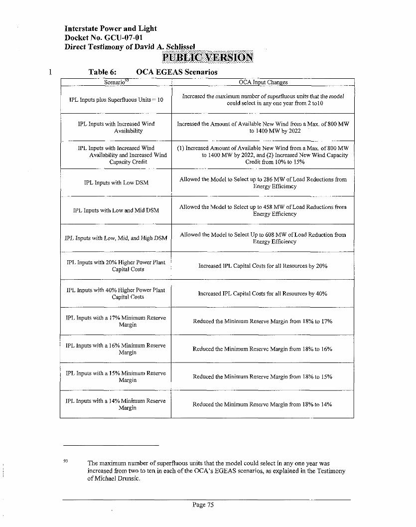
Interstate Power and Light Docket No. GCU-07-01
Table 6: OCA EGEAS Scenarios ~cenario"
IPL Inputs plus Superfluous Units = 10
IPL Inputs with lncreased Wind Availability
IPL Inputs with Increased Wind Availability and Increased Wind
Capacity Credit
IPL Inputs with Low DSM
IPL Inputs with Low and Mid DSM
IPL Inputs with Low, Mid, and High DSM
IPL Inputs with 20% Higher Power Plant Capital Costs
IPL Inputs with 40% Higher Power Plant Capital Costs
IPL Inputs with a 17% Minimum Reserve Margin
IPL Inputs with a 16% Minimum Reserve Margin
IPL Inputs with a 15% Minimum Reserve Margin
IPL Inputs with a 14% Minimum Reserve Margin
OCA Input Changes
Increased the maximum number of superfluous units that the model could select in any one year from 2 to10
lncreased the Amount of Available New Wind from a Max. of 800 MW to 1400 MW by 2022
(1) Increased Amount of Available New Wind from a Max. of 800 MW to 1400 MW by 2022, and (2) Increased New Wind Capacity
Credit from 10% to 15%
Allowed the Model to Select up to 286 MW of Load Reductions from Energy Efficiency
Allowed the Model to Select up to 458 MW of Load Reductions from Energy Efficiency
Allowed the Model to Select Up to 608 MW of Load Reduction from Energy Efficiency
Increased IPL Capital Costs for all Resources by 20%
Increased IPL Capital Costs for all Resources by 40%
Reduced the Minimum Reserve Margin from 18% to 17%
Reduced the Minimum Reserve Margin from 18% to 16%
Reduced the Minimum Reserve Margin from 18% to 15%
Reduced the Minimum Reservc Margin from 18% to 14%
93 The maximum number o f superflnous units that the model could select in any one year was increased fiom two to ten in each o f t h e OCA's EGEAS scenarios, a s explained in the Testimony of Michael Drunsic.
Page 75

Interstate Power and Light Docket No. GCU-07-01 Direct Testimony of David A. F ~ ~ . . ~ ~ ~ ~ ~ , 3 ~ ~ ~ = . ~ ~ . ~ ~ . ~ ~ : T , . , I ~ ~ - . ~ ~ - . . ~ ~ ~ . ~ . . ~ ~ : ~ ~ ~ ~ ~ ~ Schlissel ,.,, ., , , ,. . . . . . .. : I : '
p ~ ~ ' [ c ; ~ v ; ~ ~ ~ ~ ~ @ j q ..., <,. ,. .. ., .. ,. . . , ..... . I I I
IPL Inputs but with Natural Gas piices Increased by 10% Increased IPL's Natural Gas Prices by 10% starting in 2010 I
IPL Inputs with Increased Wind and Low, Mid and High DSM
2 Q. What were the results of the OCA's modeling?
(I) Increased Amt. of Available New Wind from a Maw. of 800 MW to 1400 MW by 2022, and (2) Allowed Up to 608 MW of Load
Reduction from Energy Efficiency
IPL Inputs with (1) Increased Wind, (2) Low, Mid and High DSM, (2) 20% Higher Capital Costs %,
and (4) 88% New Coal Capacity Factor
3 A. The results of our EGEAS modeling, in terms of when a new coal plant is
(I) Increased Amt. of Available New Wind from a Maw. of800 MW to 1400 MW by 2022; (2) Allowed Up to 608 MW of Load
Reduction from Energy Efficiency; (3) Increased Capital Costs for all Resources by 20%; and (4) Increased the Forced Outage
Rate for New Coal from 4% to 8.5%
4 selected, are presented in Table 7 below.
1
Page 76
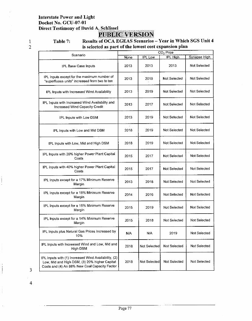
Scenario
IPL Base Case lnputs
IPL lnputs except for the maximum number of "superfluous units" increased from two to ten
is selected as part of the lowest cost expansion plan 1 C02 Price
IPL lnputs with lncreased Wind Availability
IPL lnputs with lncreased Wind Availability and lncreased Wind Capacity Credit
IPL lnputs with Low DSM
IPL lnputs with Low and Mid DSM
IPL lnputs with Low, Mid and High DSM
IPL lnputs with 20% higher Power Plant Capital costs
IPL lnputs with 40% higher Power Plant Capital costs
IPL lnputs except for a 17% Minimum Reserve Margin
IPL lnputs except for a 16% Minimum Reserve Margin
IPL lnputs except for a 15% Minimum Reserve Margin
IPL lnputs except for a 14% Minimum Reserve Margin
IPL lnputs plus Natural Gas Prices lncreased by 10%
PL lnputs with lncreased Wind and Low. Mid and High DSM
PL lnputs with (1) lncreased Wind Availability, (2: Low. Mid and High DSM. (3) 20% higher Capital Costs and (4) An 88% New Coal Capacity Factor
None
2013
2013
2013
2013
2013
2018
2018
2015
2015
2013
2013 1 2013 I Not Selected
2019 Not Selected Not Selected
2019 Not Selected Not Selected
2017 Not Selected Not Selected
2019 Not Selected Not Selected
2019 Not Selected Not Selected
2019 Not Selected Not Selected
2017 Not Selected Not Selected
2017 Not Selected Not Selected
2018 Not Selected Not Selected
2016 Not Selected Not Selected
2019 Not Selected Not Selected
2018 Not Selected Not Selected
N/A 2019 Not Selected
Jot Selected Not Selected Not Selected
Jot Selected Not Selected Not Selected
Page 77

Interstate Power and Light Docket No. GCU-07-01
coal plant only as part of the lowest cost plan in one of the scenarios, other than in
the Company's flawed base case model run. Even in that case, which assumed ten
percent higher natural gas prices, the new coal plant still was not added until
2019, or six years later than IPL proposes to add SGS Unit 4.
As shown in Table 7, when IPL's low C02 prices were used, the installation date
for the new coal plant in the lowest cost plan was delayed a minimum of between
three and six years (that is, 2016 to 2019). These delays occurred in the scenarios
which included increased wind availability or increased DSM availability or
higher capital costs or the target reserve margins were reduced from 18 percent.
When combined sensitivities reflecting increased wind and increased DSM were
run, the new coal plant was not selected as part of the lowest cost plan even with
the Company's low COz prices.
A new coal plant was not selected in any of the lowest cost plans with the
Synapse high C02 prices.
Is it possible that natural gas demand could be higher due to COz emission
regulations and, as a result, natural gas prices can be expected to be higher
than otherwise would be the case?
Yes. However, the effect is very complicated and will depend on a number of
factors such as how much new natural gas capacity is built as a result of the
higher coal-plant operating costs due to the COZ emission allowance prices, how
much additional DSM and renewable alternatives become economic and are
added to the U.S. system, the levels and prices of any incremental natural gas
imports, and changes in the dispatching of the electric system. Thus, it is very
difficult to determine, at this time, the degree to which natural gas prices might be
affected due to C02 emission regulations.
Page 78
Interstate Power and Light Docket No. GCU-07-01 Direct Testimony of David A. Schlissel
' ".:'.":$<i:;x'l'" .:-.ii'i;i- ?... '-'----.- .....,., ,. %,,-:'., .2.2:.,..,.- ,~u:~Jt't'~~;V;~:@~@~ .. , . ... . .. ,:x. .: '. ,,..,~.':~A~Z:.L~-..:. = '.~. .,....,,,.,."
1 Q. Did you ask the OCA to rerun the EGEAS model to reflect some increases in
2 natural gas prices as a result of federal regulation of greenhouse gas
3 emissions?
4 A. Yes. To illustrate the possible impact of higher natural gas prices as a result of
5 federal regulation of greenhouse gas emissions, the OCA reran the EGEAS model
6 to reflect a ten percent increase in natural gas prices in scenarios with the IPL
7 high COz and the Synapse high C02 price forecasts. As shown in Table 7 above,
8 the model still did not add SGS Unit 4 in 2013 even with the increased natural gas
9 prices. In the scenario with IPL's high COz prices, the model added a 350 MW
10 coal unit in 2019. No coal plant was selected in the scenario with Synapse's high
11 C02 price forecast and the 10 percent higher natural gas prices.
12 Q. Did IPL explore whether the need for SGS Unit 4 could be eliminated or
13 deferred if it engaged in joint and integrated planning with WPL?
14 A. No. Alliant Energy IPL has not conducted joint and integrated planning for both
15 IPL and WPL. Each of Alliant Energy's wholly owned utility subsidiaries
16 conducts integrated planning on an individual utility basis.94 Therefore, IPL is
17 unable to say that botk companies would need to build their proposed coal-fired
18 power plants in Wisconsin and lows?'
19 Q. Has Alliant Energy conducted any analysis to determine if significant
20 efficiencies are achievable through joint and integrated electric resource
2 1 planning between its wholly owned utility subsidiaries?
94 IPL Response to OCA DR. No. 173. 95 IPL Confidential Response to OCA DR. No. 174. 96 IPL Response to OCA DR. No. 175.
Page 79

Interstate Power and Light Docket No. GCU-07-01
between Alliant Energy's wholly owned utility subsidiaries would produce
significant efficiencies and benefits for Iowa ratepayers?
A. Yes. The Company made those claims in Board Docket No. 96-6?7
Q. IPL has claimed that its 2003 and 2005 Electric Resource Plans also
supported the need for a coal-fired resource in the same timeframe as the
proposed Sutherland Generating Unit 4. Should the Board rely on the
results of these Electric Resource Plans when considering whether to approve
the Company's request for permission to build SGS Unit 4?
A. No. Circumstances have changed significantly since the Company prepared its
2003 and 2005 Electric Resource Plans. In particular, IPL's 2005 IRP modeling
did not reflect any C02 prices and much lower capital costs for the generating
alternatives it considered. For example, the coal plant and wind facility capital
costs that IPL has used in its
these reasons, the results of the 2005 are obsolete and should not be relied upon
Q. Does this conclude your testimony?
A. Yes.
97 For example, see the Direct Testimony of Glen E. Jablonka in Iowa Utilities Board Docket No. SPU-96-6, at pages 16-22. See also, IES Industries Inc, Interstate Power Co., and WPL Holdings, Inc, Docket No. SPU-96-6, IUB Order, dated September 16, 1997, at pages 4 and 8.
Page 80
Copyright © 2022 FDOKUMEN