© GWS mbH 2011

gws Discussion Paper 2011/3 ISSN 1867-7290

Medium Term Economic Effects

of Peak Oil Today

Ulrike Lehr

Christian Lutz

Kirsten Wiebe

Gesellschaft für Wirtschaftliche Strukturforschung mbH

Heinrichstr. 30

D - 49080 Osnabrück

Email: wiebe @ gws-os.com

Phone: +49 541 40933-230

Fax: +49 541 40933-110

Internet: www.gws-os.com

gws Discussion Paper 2011/3

© GWS mbH 2011 II

Osnabrück, May 2011

gws Discussion Paper 2011/3

© GWS mbH 2011 III

CONTENT

CONTENT ............................................................................................................................................... III

1 INTRODUCTION .............................................................................................................................1

2 MACROECONOMIC OIL PRICE EFFECTS...............................................................................1

2.1 QUANTITATIVE EFFECTS OF OIL PRODUCTION DECREASES OR PRICE INCREASES .........................2

2.2 TRANSMISSION CHANNELS ..........................................................................................................4

2.3 OIL PRICE FORMATION ................................................................................................................5

3 MODEL AND SCENARIO SETUP.................................................................................................6

3.1 GLOBAL INTERINDUSTRY FORECASTING SYSTEM .....................................................................6

3.2 SCENARIOS .................................................................................................................................7

4 RESULTS ...........................................................................................................................................7

4.1 OIL PRICE ....................................................................................................................................9

4.2 ENERGY SUPPLY AND DEMAND .................................................................................................10

4.3 MACROECONOMIC EFFECTS ......................................................................................................11

4.3.1 International comparison ....................................................................................................11

4.3.2 Detailed results for Germany ..............................................................................................12

4.3.3 Assessment of results ...........................................................................................................14

5 CONCLUSIONS ..............................................................................................................................15

ACKNOWLEDGEMENTS .....................................................................................................................16

REFERENCES .........................................................................................................................................17

gws Discussion Paper 2011/3

© GWS mbH 2011 1

1 INTRODUCTION

The recent crisis in Libya and the imminent oil supply shortage as well as high energy price fluctuations in the past years elucidate that energy security is becoming just as important as efficiency and sustainability of energy production. This was already stressed in a study by the Bundeswehr Transformation Centre of the German Federal Ministry of Defence (ZTB, 2010), which recognized that fossil fuels, especially oil, are not only necessary for a functioning of the global economy, but also for strategic issues. While the World Energy Outlook (IEA, 2010) as well as many others expect world oil production paths that are able to meet world oil demand in the coming decade, the discussion about peak oil today shows that these projections might be too optimistic. When comparing projections of world-wide oil supply of LBST (2010), which assumes that oil production has recently peaked, to projections of oil demand from e.g. the reference scenario of the WEO (IEA, 2009), it becomes obvious that it might well be possible that oil supply shortages arise and grow over the next decade. This would mean, given the IEA oil prices, oil supply will not match oil demand.

Given that this is the case, the paper at hand presents results of a model-based scenario analysis on the economic implications in the next decade of an oil peak today and significantly decreasing oil production in the coming years. For that the extraction paths of oil and other fossil fuels given in LBST (2010) are implemented in the global macroeconomic model GINFORS. Additionally, the scenarios incorporate different technological potentials for energy efficiency and renewable energy, which cannot be forecast using econometric methods. GINFORS then endogenously determines world-wide energy demand and energy prices. In modelling terms this means that the oil price is increased until global oil demand equals global oil supply. The resulting oil price is by no means to be understood as the most likely oil price development. This exercise should rather be understood as an if-then-analysis in a research area that still needs extensive explorations. Given the assumption of a fixed medium term oil supply, the effects described in the following might be too strong.

The next section reviews the literature on economic effects of oil price changes. The GINFORS model, the implementation of the fossil fuel production paths in the model and the scenarios are described in section 3. Section 4 describes the macroeconomic effects on a country level and sectoral effects for selected countries. Section 5 gives some conclusions of the discussion..

2 MACROECONOMIC OIL PRICE EFFECTS

Modelling the macroeconomic effects of decreasing oil supply in GINFORS is done via matching global oil demand to global supply by adjusting the oil price. As there exists very little literature on direct macroeconomic effects of oil shortages and the oil shortage is modelled via increasing oil prices, the effects we will see in this exercise correspond to macroeconomic oil price effects. For an extensive literature review the interested reader is referred to Hamilton (2005) and Kilian (2007).

gws Discussion Paper 2011/3

© GWS mbH 2011 2

2.1 QUANTITATIVE EFFECTS OF OIL PRODUCTION DECREASES OR PRICE INCREASES

According to Jones et al. (2004) the effects of oil price shocks are difficult to model at the aggregated macroeconomic level, i.e. GDP. Most suitable are sectorally disaggregated econometric models, as for example vector-autoregressive (VAR) or vector-error-correction (VEC) models, or models such as the MULTIMOD model of the IMF or the INTERLINK model of the OECD. They give a short overview of these types of models and shortly summarize the findings about the oil price shock effect on the American economy. The different studies show a rather minor short run economic impact of oil price shocks. The literature on quantitative oil price effects can be roughly divided into two strands: one uses some form of theoretical or applied economic or econometric model to estimate the absolute effects on production and consumption. The other also makes use of models, but rather than reporting absolute effects they estimate short and long run oil price elasticities.

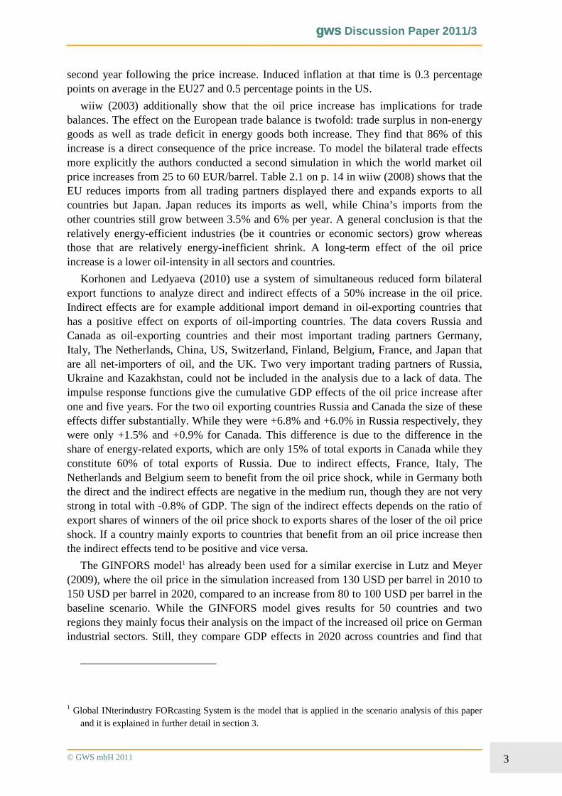
Jiménez-Rodríguez (2008) belongs to the first strand of literature and analyzes the effect of an increasing oil price on different sectors in six OECD countries (France, Germany, Italy, Spain, US and UK) using a VAR model. The model is based on monthly data of eight industrial sectors and the total industry sector. He comes to the result that the negative shocks of a unit price increase of oil are higher in the US and UK compared with the other countries. The sectoral effects depend on the corresponding oil intensity. The average effects for the total industry sector in the different countries are displayed in row 3 of table 1.

Table 1: Macroeconomic oil price effects in the literature

Source Oil price increase Economic effect

DE NL FR IT UK USA JP CN RU OPEC CA

1 Korhnoen & Ledyaeva (2010)

50% GDP: 1 yearGDP: 5 years

0.5% -0.8%

0.8%0.45%

1.0% 3.0%

0.5% 0.3%

-0.5% -0.6%

-1.5% -2.0%

-3.3% -3.1%

-2.0% -1.2%

6.0% 6.8%

-- 2.1% 3.2%

2 Lutz & Meyer (2009)

Baseline 2010: 80$ 2020: 100$Scenario 2010: 130$ 2020: 150$

GDP in 2020 in relation to baseline

-0,20% -- -- -- -0,70% -1,60% -3,80% -2,60% 10,40% 17.1% --

3 Jiménez-Rodríguez (2008)

Unit shock 40 monthIndustry sector

-0,05 -- -0,06 -0,07 -0,13 -0,15 -- -- -- -- --

4 OECD (2004)

Increase from 32 USD to 47 USD

GDP: 1 yearGDP: 2 years

-- -0.45% -0.55%

-0.6% -0.6%

-- -- -- --

5 wiiw (2008) Increase by 10 USD nach 2 Jahren -- -0,50% -- -- -- -- --

6 Gupta (2008)

Oil-vulnarability index 0,44 0,55 0,45 0,55 -- 0,37 0,51 0,66 -- -- --

Euro-Raum: -0.5% -0.35%

EU 27: -0.4%

The Vienna Institute for International Economic Studies (wiiw, 2008) analyzes the effects on the European and American economies of a one time increase of the oil price of 10 USD/barrel. In this simulation, the highest negative economic effects occur within the first two years after the price increase. The cumulative GDP loss in the US is 0.5% and in the EU27 0.4% of GDP after the second year, though the differences within the EU are quite large as a result of large differences in the energy intensity of production. The New Member States (NMS) are therefore more strongly affected than the Northern and WesternEuropean countries. The effect on the price level can be altered by adapting appropriate monetary policy measures. Still the simulation runs show that the effect is strongest in the

gws Discussion Paper 2011/3

© GWS mbH 2011 3

second year following the price increase. Induced inflation at that time is 0.3 percentage points on average in the EU27 and 0.5 percentage points in the US.

wiiw (2003) additionally show that the oil price increase has implications for trade balances. The effect on the European trade balance is twofold: trade surplus in non-energy goods as well as trade deficit in energy goods both increase. They find that 86% of this increase is a direct consequence of the price increase. To model the bilateral trade effects more explicitly the authors conducted a second simulation in which the world market oil price increases from 25 to 60 EUR/barrel. Table 2.1 on p. 14 in wiiw (2008) shows that theEU reduces imports from all trading partners displayed there and expands exports to all countries but Japan. Japan reduces its imports as well, while China’s imports from the other countries still grow between 3.5% and 6% per year. A general conclusion is that the relatively energy-efficient industries (be it countries or economic sectors) grow whereas those that are relatively energy-inefficient shrink. A long-term effect of the oil price increase is a lower oil-intensity in all sectors and countries.

Korhonen and Ledyaeva (2010) use a system of simultaneous reduced form bilateral export functions to analyze direct and indirect effects of a 50% increase in the oil price. Indirect effects are for example additional import demand in oil-exporting countries that has a positive effect on exports of oil-importing countries. The data covers Russia and Canada as oil-exporting countries and their most important trading partners Germany, Italy, The Netherlands, China, US, Switzerland, Finland, Belgium, France, and Japan thatare all net-importers of oil, and the UK. Two very important trading partners of Russia, Ukraine and Kazakhstan, could not be included in the analysis due to a lack of data. The impulse response functions give the cumulative GDP effects of the oil price increase after one and five years. For the two oil exporting countries Russia and Canada the size of these effects differ substantially. While they were +6.8% and +6.0% in Russia respectively, they were only +1.5% and +0.9% for Canada. This difference is due to the difference in the share of energy-related exports, which are only 15% of total exports in Canada while they constitute 60% of total exports of Russia. Due to indirect effects, France, Italy, The Netherlands and Belgium seem to benefit from the oil price shock, while in Germany both the direct and the indirect effects are negative in the medium run, though they are not very strong in total with -0.8% of GDP. The sign of the indirect effects depends on the ratio of export shares of winners of the oil price shock to exports shares of the loser of the oil price shock. If a country mainly exports to countries that benefit from an oil price increase then the indirect effects tend to be positive and vice versa.

The GINFORS model1 has already been used for a similar exercise in Lutz and Meyer (2009), where the oil price in the simulation increased from 130 USD per barrel in 2010 to 150 USD per barrel in 2020, compared to an increase from 80 to 100 USD per barrel in the baseline scenario. While the GINFORS model gives results for 50 countries and two regions they mainly focus their analysis on the impact of the increased oil price on German industrial sectors. Still, they compare GDP effects in 2020 across countries and find that

1 Global INterindustry FORcasting System is the model that is applied in the scenario analysis of this paper and it is explained in further detail in section 3.

gws Discussion Paper 2011/3

© GWS mbH 2011 4

the effect on German GDP (-0.2%) is by far the smallest among the oil importing countries. The effects on GDP of the US, China and Japan in the high energy price scenario are significantly higher with -1.6%, -2.6% and -3.8%, respectively. Even in the UK, which is still a net oil exporter, the negative impact on the country’s GDP (-0.7%) is stronger than in Germany in this simulation. The relatively modest effect on the German economy is explained by positive indirect effects as the shares of the oil exporting countries in German exports are rather high. For the two biggest oil exporters OPEC and Russia GDP increases by 17.1% and 10.4% compared to the baseline scenario.

OECD (2004) not only analyzes the economic effects of an oil price increase but also factors that influence the oil price and possible policy measures after an oil price increase.Given a business-as-usual energy consumption, it is expected that in 2030 fossil fuels will still be 90% of total primary energy consumption, with the transport sector requiring the highest share. Using the global Interlink model to describe the effects of a permanent increase in the oil price from 32 to 47 USD per barrel in 2004. OECD (2004) find that there are only minor macroeconomic effects in the short run. GDP losses in the OECD countries amount to 0.45% in the two following years (US: -0.45% and -0.5%; Japan: -0.6% in both years; EURO-region: 0.5% and -0.35%), inflation increases by 0.6% and 0.25% assuming constant real interest rates. When assuming constant nominal interest rates, the GDP effects are even smaller.

In addition to their own analysis, OECD (2004) reviews studies that estimated price and income elasticities of oil demand. Price elasticities are between -0.1 and -0.64, which confirms the findings below. Elasticities are generally lower in emerging economies than in OECD countries. Kilian (2007) for example estimates price elasticities of US consumption and investment to be about -0.15 to -0.16, respectively. Price elasticities for energy demand are significantly higher: for heating oil and coal they are -1.47, for gasoline -0.48 and for natural gas -0.33. Electricity demand though has an oil price elasticity of only -0.15.

Fattouh (2007) also reviews literature on price and income elasticities of oil demand and comes to similar conclusions as Kilian and the OECD. The short run elasticities are between -0.03 and -0.09 and the long run elasticities somewhat larger between -0.03 and -0.64, depending on time frame and region. He also confirms the finding that price elasticities in industrialized countries are higher than in emerging economies while the opposite is true for income elasticities. Hamilton (2008) confirms these findings with own calculations and a literature review. One of his main conclusions is that in general long run elasticities are about three times the short run elasticities.

Gupta (2008) uses a very different approach to possible oil price effects: he constructs an oil vulnerability index which is a combination of market risk and supply risk indicators. He finds that from the 26 emerging and industrialised countries that he analyses the Philippines, Korea and India are the most vulnerable and Austria, France, Germany, the US, Sweden and Australia are the least vulnerable countries.

2.2 TRANSMISSION CHANNELS

Kilian (2007) not only calculates oil price elasticities, but also analyzes possible transmission channels distinguishing between supply-side and demand-side. The main

gws Discussion Paper 2011/3

© GWS mbH 2011 5

supply-side channel is higher input costs, be it due to cost increases in production factors, e.g. oil itself in the chemical industry, higher energy costs for the remaining industries or simply higher transportation costs. Higher production costs can only be partly passed on to consumers so that industry profits are lowered.

There are five different demand-side channels. First, there is the discretionary income effect, i.e. higher energy costs lower a households’ disposable income after having paid for energy. The “precautionary savings” channel has the same effect as higher savings. It goeshand in hand with lower disposable income and hence lower consumption. The third channel “uncertainty effect” also results in lower consumption as fluctuating/increasing energy prices may lead people to “postpone irreversible purchases of consumer durables”(Kilian, 2007, p. 10). The fourth effect is the “operating cost effect” which describes the decrease in purchases of energy intensive durable goods such as cars. The last channel Kilian (2007) describes deals with the indirect effects through changing consumption and investment patterns. These imply not only redistribution within but also between sectors. GINFORS is able to reproduce the supply side channel of higher input and transportation costs, the income effects, indirect effects and substitution effects.

Substitution effects relate to a possible replacement of oil by other energy carriers. The literature mainly deals with fossil fuel substitution neglecting the possibility to substitute renewable energies for oil. Stern (2009) examines the substitution effects between oil, gas, coal and electricity in a meta-analysis based on 46 studies published between 1979 and 2009. He finds that the substitution effects between oil and gas are less than one, between coal and gas larger than one and the remaining about one. The substitution effects seem to be higher the more observations there are, the higher the sectoral aggregation and the higher the countries’ GPD is. Söderholm (1999) additionally stresses the importance of distinguishing between short run and long run effects, as modification of a given power plant fleet is not easily possible in the short run. He also suggests that short run substitutions are mainly cost induced whereas the long run energy mix is strongly influenced by policy makers.

2.3 OIL PRICE FORMATION

Until now, only the effects of changing oil prices on the economy and how they are transmitted through the economy have been described. The oil price itself though is not exogenously given to the world but develops over time depending on different demand and supply side factors as explained below. There exist different approaches to modelling the oil price. Fattouh (2007) distinguishes between “economics of scarce resources”, supply-and-demand systems and what he calls the “informal approach”. Hamilton (2008) also considers supply-and-demand systems, but then further suggests a model of dynamic interactions between storage, futures and scarcity rent and statistical analysis. GINFORS includes equations that can be used to determine the equilibrium between oil supply, oil demand and their determinants such as economic growth, oil price, and oil reserves.

On the demand side, price and income elasticities are most important for the formation of the oil price. In GINFORS, sectoral oil demand is econometrically estimated depending on sectoral production and absolute and relative oil prices. When interpreting the elasticities we have to keep in mind that the share of the oil price in the price of petroleum products varies across countries depending on taxes and subsidies. While taxes on gasoline

gws Discussion Paper 2011/3

© GWS mbH 2011 6

are high in most industrialised countries, the petroleum products in oil producing countries are often heavily subsidized and therefore distort market effects. IEA estimates world wide subsidies on oil to amount to 312 billion USD in 2009 and 558 billion USD in 2008. These considerations show that oil consumers in different countries are differently exposed to changes in the price of crude oil.

Price elasticities are not only important on the demand side, but also on the supply side. However, short run elasticities are generally very small depending on production capacity utilization as building new production capacities is time and capital intensive. In addition, production costs tend to increase more than proportionally with the increasing exploitation of oil fields. Hamilton (2008) discovers in a statistical analysis that there exist no reliable macroeconomic indicators for oil price predictions. He concludes that the oil price is a random walk with drift, i.e. that it is the best predictor for itself. According to his analysis, given an oil price of 115 USD per barrel today the oil price in four years will be somewhere between 34 USD and 391 USD per barrel, which is quite a large bandwidth.

Due to the cartel-like nature of oil production, OPEC, which owns about three quarters of global (conventional) oil reserves and controls 40% of global oil production (Gupta, 2008), has a major influence on the oil market and can more or less determine total oil production quantities and price. According to neo-classical assumption the marginal price should equal marginal costs for cartels. Additionally, the Hotelling rule for scarce resources could also apply to oil. But, according to Hamilton (2008), there is no historical evidence that either of these economic theories holds for the oil market. Though, it is still true that OPEC has a significant influence on the oil market and hence also on the oil price.

3 MODEL AND SCENARIO SETUP

Assuming that oil production just peaked, i.e. in 2010, we calculate two scenarios that can be compared to the baseline scenario in which we assume the oil production path given in the IEA WEO 2009. According to this scenario in IEA (2009) world oil supply will exceed world oil demand, so that there will not be an oil shortage until at least 2030. The two scenarios “Peak Oil” and “Peak Oil Eff/RE” assume that oil production has peaked and declines over the next decade. “Peak Oil Eff/RE” additionally assumes massive energy efficiency improvements and increased use of renewable resources on a global level.

3.1 GLOBAL INTERINDUSTRY FORECASTING SYSTEM

To model the macroeconomic effects of this oil shortage we use the sectorally disaggregated global energy-environment-economy model GINFORS. It combines econometric-statistical analysis with input-output analysis embedded in a complete macroeconomic framework ensuring the accounting identities of the system of national accounts. GINFORS has recently been applied to various economic questions, ranging from an European environmental tax reform (Lutz and Meyer 2010, Ekins and Speck 2011) and environmental and economic effects of Post-Kyoto regimes (Lutz and Meyer 2009b) to the impact of higher energy prices through international trade (Lutz and Meyer 2009a). A detailed description of GINFORS can be found in Lutz et al. (2010) or Lutz and Meyer (2009a/b, 2010).

gws Discussion Paper 2011/3

© GWS mbH 2011 7

3.2 SCENARIOS

The scenarios differ according to world oil supply and demand. The baseline scenario is based on the reference scenario of the IEA WEO 2009. World energy demand is steadily increasing, mainly due to increasing demand in the emerging economies. There are no supply shortages until 2030. The price for crude oil increases to 100 USD2009 in 2020 and 115 USD2009 in 2030. The baseline scenario in the most recent WEO (IEA, 2010) more or less complies with this one, but puts slightly more emphasis on a possible influence of global climate change action on global energy demand and hence on energy prices.

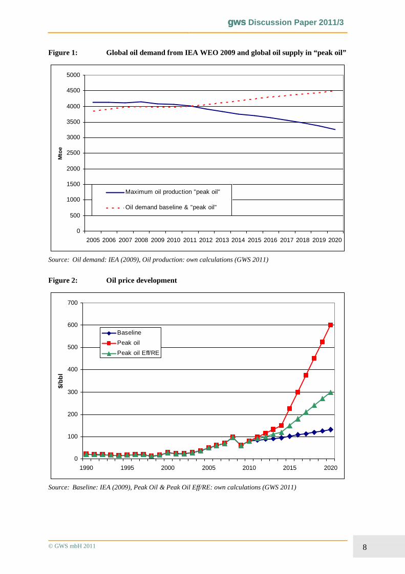
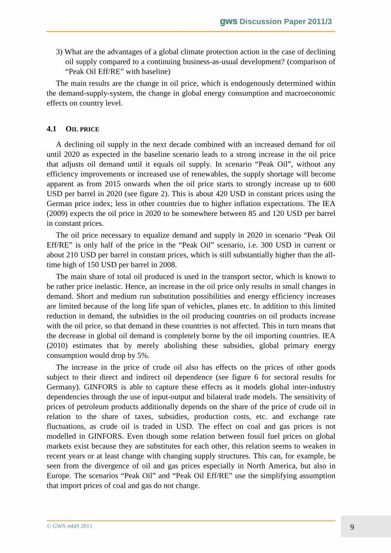
Energy demand in scenario “Peak Oil” is equivalent to energy demand in the baseline. For the supply side though it is assumed that world oil production has peaked and will significantly decline over the next decade until 2020, so that global oil supply does no longer match global oil demand as shown in figure 1. This shortage can not only occur due to shrinking oil production but also due to political disruptions or military disputes as started in early 2011 in the MENA (Middle-East North-African) countries.

For the model we assume that world oil production is price independent in the medium term and decreasing after 2010. The assumption of a fixed oil supply in the short to medium term is feasible because of limited production expansion possibilities due to necessary time and capital consuming investments. In the long run oil production is less price inelastic, which should then be considered. Price elasticities of oil demand are estimated in the model. Using these results, it is possible to increase the oil price until global oil demand has dropped so that it equals global oil supply. The implication of the price-inelastic demand is a strong increase of the price for crude oil after 2015.

The third scenario “Peak Oil Eff/RE” also assumes peak oil, but uses the 450 ppm-scenario of the IEA WEO (2009) as a guideline for demand side development. The assumptions are increased energy efficiency and extended use of renewables.

4 RESULTS

The results for the three scenarios have all been calculated using the same model. The differences between the scenario specifications have been explained above. The remaining assumptions are the same in all three scenarios so that the differences in the results must be due to the different assumptions concerning oil supply and demand. The development as projected in this analysis should be interpreted using if-then-statements and should be seen relative to each other and not in absolute terms. The three central questions that can be answered with this analysis are

1) What are the effects of an oil supply shortage when demand is developing as in thebusiness-as-usual case? (Comparison of “Peak Oil” scenario with baseline)

2) What are the effects of a shrinking global oil production with a contemporaneous global climate protection action, i.e. improved energy efficiency and expansion of renewable energy? (Comparison of scenarios “Peak Oil Eff/RE” and “Peak Oil”)

gws Discussion Paper 2011/3

© GWS mbH 2011 8

Figure 1: Global oil demand from IEA WEO 2009 and global oil supply in “peak oil”

0

500

1000

1500

2000

2500

3000

3500

4000

4500

5000

2005 2006 2007 2008 2009 2010 2011 2012 2013 2014 2015 2016 2017 2018 2019 2020

Mto

e

Maximum oil production "peak oil"

Oil demand baseline & "peak oil"

Source: Oil demand: IEA (2009), Oil production: own calculations (GWS 2011)

Figure 2: Oil price development

0

100

200

300

400

500

600

700

1990 1995 2000 2005 2010 2015 2020

$/b

bl

Baseline

Peak oil

Peak oil Eff/RE

Source: Baseline: IEA (2009), Peak Oil & Peak Oil Eff/RE: own calculations (GWS 2011)

gws Discussion Paper 2011/3

© GWS mbH 2011 9

3) What are the advantages of a global climate protection action in the case of declining oil supply compared to a continuing business-as-usual development? (comparison of “Peak Oil Eff/RE” with baseline)

The main results are the change in oil price, which is endogenously determined within the demand-supply-system, the change in global energy consumption and macroeconomic effects on country level.

4.1 OIL PRICE

A declining oil supply in the next decade combined with an increased demand for oiluntil 2020 as expected in the baseline scenario leads to a strong increase in the oil price that adjusts oil demand until it equals oil supply. In scenario “Peak Oil”, without any efficiency improvements or increased use of renewables, the supply shortage will become apparent as from 2015 onwards when the oil price starts to strongly increase up to 600 USD per barrel in 2020 (see figure 2). This is about 420 USD in constant prices using the German price index; less in other countries due to higher inflation expectations. The IEA (2009) expects the oil price in 2020 to be somewhere between 85 and 120 USD per barrel in constant prices.

The oil price necessary to equalize demand and supply in 2020 in scenario “Peak Oil Eff/RE” is only half of the price in the “Peak Oil” scenario, i.e. 300 USD in current or about 210 USD per barrel in constant prices, which is still substantially higher than the all-time high of 150 USD per barrel in 2008.

The main share of total oil produced is used in the transport sector, which is known to be rather price inelastic. Hence, an increase in the oil price only results in small changes in demand. Short and medium run substitution possibilities and energy efficiency increases are limited because of the long life span of vehicles, planes etc. In addition to this limited reduction in demand, the subsidies in the oil producing countries on oil products increase with the oil price, so that demand in these countries is not affected. This in turn means that the decrease in global oil demand is completely borne by the oil importing countries. IEA (2010) estimates that by merely abolishing these subsidies, global primary energy consumption would drop by 5%.

The increase in the price of crude oil also has effects on the prices of other goods subject to their direct and indirect oil dependence (see figure 6 for sectoral results for Germany). GINFORS is able to capture these effects as it models global inter-industry dependencies through the use of input-output and bilateral trade models. The sensitivity of prices of petroleum products additionally depends on the share of the price of crude oil in relation to the share of taxes, subsidies, production costs, etc. and exchange rate fluctuations, as crude oil is traded in USD. The effect on coal and gas prices is not modelled in GINFORS. Even though some relation between fossil fuel prices on global markets exist because they are substitutes for each other, this relation seems to weaken in recent years or at least change with changing supply structures. This can, for example, be seen from the divergence of oil and gas prices especially in North America, but also in Europe. The scenarios “Peak Oil” and “Peak Oil Eff/RE” use the simplifying assumption that import prices of coal and gas do not change.

gws Discussion Paper 2011/3

© GWS mbH 2011 10

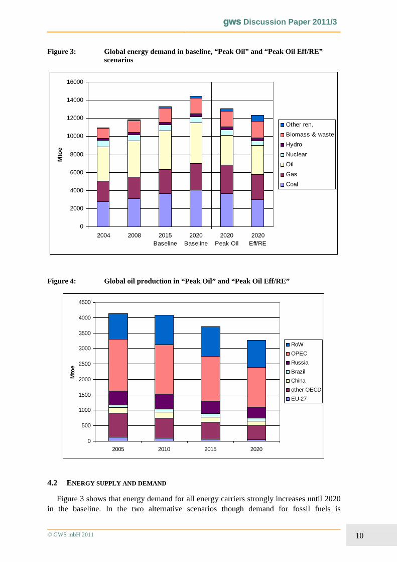
Figure 3: Global energy demand in baseline, “Peak Oil” and “Peak Oil Eff/RE” scenarios

0

2000

4000

6000

8000

10000

12000

14000

16000

2004 2008 2015Baseline

2020Baseline

2020Peak Oil

2020Eff/RE

Mto

e

Other ren.

Biomass & waste

Hydro

Nuclear

Oil

Gas

Coal

Figure 4: Global oil production in “Peak Oil” and “Peak Oil Eff/RE”

0

500

1000

1500

2000

2500

3000

3500

4000

4500

2005 2010 2015 2020

Mto

e

RoW

OPEC

Russia

Brazil

China

other OECD

EU-27

4.2 ENERGY SUPPLY AND DEMAND

Figure 3 shows that energy demand for all energy carriers strongly increases until 2020 in the baseline. In the two alternative scenarios though demand for fossil fuels is

gws Discussion Paper 2011/3

© GWS mbH 2011 11

significantly lower in 2020 as can be seen from the two bars on the right in figure 3. The increase in the demand for gas in “Peak Oil” partly absorbs the decrease in oil demand. The lower use of coal though is due to lower global economic activity, especially in China. Biomass, other renewables as well as nuclear energy only play a minor role in the “Peak Oil” scenario until 2020. The efficiency effect and the expansion in the use of renewables are clearly visible in the energy mix in “Peak Oil Eff/RE” in 2020. Global demand for fossil fuels is significantly lower than in the other two scenarios.

Global oil production for scenarios “Peak Oil” and “Peak Oil Eff/RE” is displayed in figure 4. Production declines in all regions, while relative production shares hardly change.

4.3 MACROECONOMIC EFFECTS

For the OECD countries GINFORS models production, prices and employment for 41 economic sectors. Macroeconomic aggregates such as GDP, private and government consumption, investments, imports, exports, total employment, price index or hourly wages are available for all countries and regions.

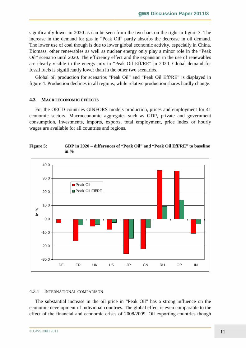
Figure 5: GDP in 2020 – differences of “Peak Oil” and “Peak Oil Eff/RE” to baseline in %

-30,0

-20,0

-10,0

0,0

10,0

20,0

30,0

40,0

DE FR UK US JP CN RU OP IN

in %

Peak Oil

Peak Oil Eff/RE

4.3.1 INTERNATIONAL COMPARISON

The substantial increase in the oil price in “Peak Oil” has a strong influence on the economic development of individual countries. The global effect is even comparable to the effect of the financial and economic crises of 2008/2009. Oil exporting countries though

gws Discussion Paper 2011/3

© GWS mbH 2011 12

strongly benefit from the increased oil price: the GDP of both Russia and the OPEC is by about 35% higher in “Peak Oil” than in the baseline (see figure 5) even though physical oil exports shrink. This decrease though is more than levelled by the price increase. Even though the UK and the US will be net importers of oil in 2020, due to their domestic oil production their GDP loss in “Peak Oil” compared to the baseline is substantially lower than the GDP loss in countries such as France, Japan or India that, if at all, have only little domestic oil production. China however, which is ranked among the top 15 countries according to proven oil reserves (IEA, 2010), is also highly negatively affected. This is due to the strong increase in energy demand, which exceeds by far possible domestic production increases. Still, GDP growth rates remain positive in all countries but Japan. Efficiency measures and increased use of renewables as modelled in “Peak Oil Eff/RE” could significantly lower the oil price increase and hence also the negative economic impacts. Overall, the economic influence of the oil exporting countries grows in both scenarios (Peak Oil and Peak Oil Eff/RE) whereas the other countries’ influence on the world market shrinks.

4.3.2 DETAILED RESULTS FOR GERMANY

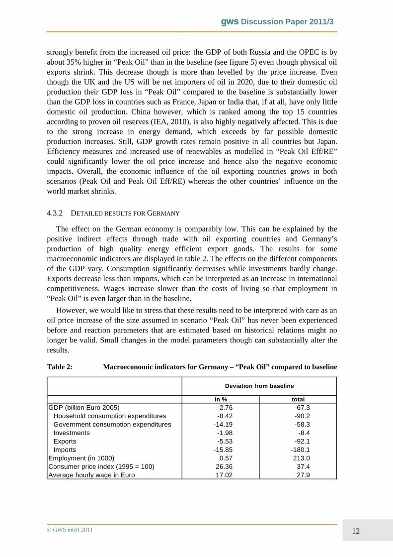
The effect on the German economy is comparably low. This can be explained by the positive indirect effects through trade with oil exporting countries and Germany’sproduction of high quality energy efficient export goods. The results for some macroeconomic indicators are displayed in table 2. The effects on the different components of the GDP vary. Consumption significantly decreases while investments hardly change. Exports decrease less than imports, which can be interpreted as an increase in international competitiveness. Wages increase slower than the costs of living so that employment in “Peak Oil” is even larger than in the baseline.

However, we would like to stress that these results need to be interpreted with care as an oil price increase of the size assumed in scenario “Peak Oil” has never been experienced before and reaction parameters that are estimated based on historical relations might no longer be valid. Small changes in the model parameters though can substantially alter the results.

Table 2: Macroeconomic indicators for Germany – “Peak Oil” compared to baseline

in % total

GDP (billion Euro 2005) -2.76 -67.3Household consumption expenditures -8.42 -90.2Government consumption expenditures -14.19 -58.3Investments -1.98 -8.4Exports -5.53 -92.1Imports -15.85 -180.1

Employment (in 1000) 0.57 213.0Consumer price index (1995 = 100) 26.36 37.4Average hourly wage in Euro 17.02 27.9

Deviation from baseline

gws Discussion Paper 2011/3

© GWS mbH 2011 13

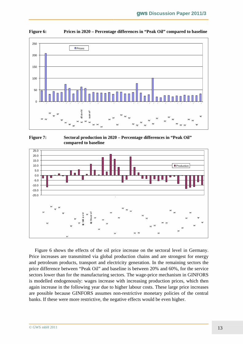
Figure 6: Prices in 2020 – Percentage differences in “Peak Oil” compared to baseline

0

50

100

150

200

250(1) A

griculture

(2) Min

ing and

…

(3) Fo

od

(4) Textiles

(5) Wo

od

(6) Pulp

, Pap

er

(7) Co

ke, Refin

ed …

(8) Ch

emicals excl.

…

(9) Ph

armaceuticals

(10) Rubber an

d

…

(11) No

n-Metallic

…

(12) Iron

& S

teel

(13) No

n-Ferrous

…

(14) Metal P

rod

ucts

(15) Mach

inery and

…

(16) Office M

achinery

(18) Rad

io, T

V

(19) Med

ical, …

(20) Mo

tor V

ehicles

(21) Sh

ips

(22) Aircraft

(23) Railro

ad

(24) Man

ufacturing …

(25) Electricity, G

as, …

(26) Co

nstruction

(27) Trad

e; Rep

airs

(28) Ho

tels and

…

(29) Tran

sport and …

(30) Po

st and

…

(32) Real E

state …

(33) Ren

ting

(34) Co

mp

uter

(35) Research

and …

(36) Oth

er Business

…

(37) Public S

ervices

(38) Ed

ucation

(39) Health

and

…

(40) Oth

er Services

(41) Private

…

Prices

Figure 7: Sectoral production in 2020 – Percentage differences in “Peak Oil” compared to baseline

-20.0

-15.0

-10.0

-5.0

0.0

5.0

10.0

15.0

20.0

25.0

(1) A

gric

ultu

re

(2) M

inin

g a

nd

Qu

arry

ing

(3) F

oo

d

(4) T

ex

tiles

(5) W

oo

d

(6) P

ulp

, Pa

pe

r

(7) C

ok

e, R

efin

ed

Pe

trole

um

Pro

du

cts

(8) C

he

mic

als

ex

cl. Ph

arm

a

(9) P

ha

rma

ce

utica

ls

(10

) Ru

bb

er a

nd

Pla

stics

(11

) No

n-Me

tallic M

ine

rals

(12

) Iron

& S

tee

l

(13

) No

n-Fe

rrous

Me

tals

(14

) Me

tal P

rod

uc

ts

(15

) Ma

ch

ine

ry an

d E

qu

ipm

en

t

(16

) Offic

e M

ac

hin

ery

(17

) Ele

ctric

al M

ac

hin

ery

(18

) Ra

dio

, TV

(19

) Me

dic

al, P

rec

ision a

nd

Op

tical

…

(20

) Mo

tor V

eh

icles

(21

) Sh

ips

(22

) Airc

raft

(23

) Ra

ilroa

d

(24

) Ma

nu

fac

turin

g N

ec; R

ec

yclin

g

(25

) Ele

ctric

ity, G

as, W

ate

r Su

pp

ly

(26

) Co

ns

truc

tion

(27

) Tra

de

; Re

pa

irs

(28

) Ho

tels

an

d R

es

tau

ran

ts

(29

) Tra

ns

po

rt an

d S

tora

ge

(30

) Po

st a

nd

Te

leco

mm

un

icatio

ns

(31

) Fin

an

ce, In

suran

ce

(32

) Re

al E

sta

te A

tivitie

s

(33

) Re

ntin

g

(34

) Co

mp

ute

r

(35

) Re

se

arc

h a

nd

De

ve

lopm

en

t

(36

) Oth

er B

us

ine

ss A

ctivitie

s

(37

) Pu

blic

Se

rvic

es

(38

) Ed

uc

atio

n (39

) He

alth

an

d s

ocia

l wo

rk

(40

) Oth

er S

erv

ices

(41

) Priv

ate

Ho

us

eh

old

s

Production

Figure 6 shows the effects of the oil price increase on the sectoral level in Germany.Price increases are transmitted via global production chains and are strongest for energy and petroleum products, transport and electricity generation. In the remaining sectors the price difference between “Peak Oil” and baseline is between 20% and 60%, for the service sectors lower than for the manufacturing sectors. The wage-price mechanism in GINFORS is modelled endogenously: wages increase with increasing production prices, which then again increase in the following year due to higher labour costs. These large price increases are possible because GINFORS assumes non-restrictive monetary policies of the central banks. If these were more restrictive, the negative effects would be even higher.

gws Discussion Paper 2011/3

© GWS mbH 2011 14

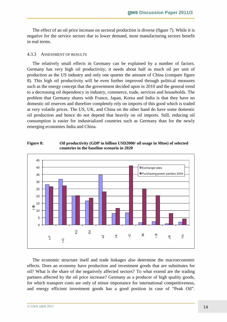
The effect of an oil price increase on sectoral production is diverse (figure 7). While it is negative for the service sectors due to lower demand, most manufacturing sectors benefit in real terms.

4.3.3 ASSESSMENT OF RESULTS

The relatively small effects in Germany can be explained by a number of factors.Germany has very high oil productivity; it needs about half as much oil per unit of production as the US industry and only one quarter the amount of China (compare figure 8). This high oil productivity will be even further improved through political measures such as the energy concept that the government decided upon in 2010 and the general trend to a decreasing oil dependency in industry, commerce, trade, services and households. The problem that Germany shares with France, Japan, Korea and India is that they have no domestic oil reserves and therefore completely rely on imports of this good which is traded at very volatile prices. The US, UK, and China on the other hand do have some domestic oil production and hence do not depend that heavily on oil imports. Still, reducing oil consumption is easier for industrialized countries such as Germany than for the newly emerging economies India and China.

Figure 8: Oil productivity (GDP in billion USD2000/ oil usage in Mtoe) of selected countries in the baseline scenario in 2020

0

5

10

15

20

25

30

35

40

45

France

Germ

any

UK

US

Japan

Ko

rea

China

India

Brazil

Russia

OP

EC

Billio

n U

SD

/Mto

e

Exchange rates

Purchasing power parities 2004

The economic structure itself and trade linkages also determine the macroeconomic effects. Does an economy have production and investment goods that are substitutes for oil? What is the share of the negatively affected sectors? To what extend are the trading partners affected by the oil price increase? Germany as a producer of high quality goods, for which transport costs are only of minor importance for international competitiveness, and energy efficient investment goods has a good position in case of “Peak Oil”.

gws Discussion Paper 2011/3

© GWS mbH 2011 15

Moreover, the oil producing countries have a high share in German exports so that the indirect effects for Germany are positive.

Not only economic factors have an influence on the magnitude of the effects of the oil price increase, but also geographic factors. Generally, countries that are densely populated, have a high domestic demand and are in close proximity to export markets are better protected against a strong increase in the oil price than other countries. This explains why the negative effects on Japan are higher in comparison to the European countries despite its rather high oil productivity.

Important factors that are not modelled in GINFORS are possible alternative transportation means, e.g. powerful electricity-based train networks, or a switch from petroleum-based cars to biofuel, electricity or LPG driven cars.

5 CONCLUSIONS

This analysis shows possible economic effects of a significant drop in world oil production over the next decade. Assuming that global demand for oil and petroleum products remains increasing, the oil price will increase sharply due to the price inelastic nature of the oil market in the short to medium run. Large fluctuations in the oil price occur for only small changes in supply and demand. This is also supported by findings in the literature and shows that the strong price fluctuations as experienced in the past years are quite possible. The oil shortage firstly and strongly affects the transport sector but then has indirect effects on all other sectors through global supply chains. The medium termreactions to the oil shortage and corresponding substantial increase in the oil price of the global energy system and the individual sectors are energy saving and substitution, lowering global energy demand. The global macroeconomic effects of an increase of the oil price as high as modelled here are comparable to the effects of the financial and economic crises of 2008/2009. Country-specific effects are very different as the oil exporting countries gain importance in the global economy while the influence of the strong oil-importing economies of today decreases.

Comparing scenarios “Peak Oil” and “Peak Oil Eff/RE” shows that global climate protection actions may very well reduce the negative economic impacts of oil supply shortages and associated strong increases in the oil price.

Note that GINFORS is only able to display effects in monetary terms and that the results depend on a variety of model assumptions. Actual real world outcomes also depend on a number of other – not easily modellable – factors, such as the price dependence of oil supply over time, especially with regard to unconventional oil fields, obstacles such as financing gaps or interests of national oil producers (as also noted by IEA, 2010, p. 125), long run oil substitution possibilities and their cost development next to efficiency improvements, increased use of renewables, and potentials in the transport sector (biofuels, electricity, LPG, coal-to-liquids). The model only captures part of the oil price effects as described in the literature. When interpreting the results one should also consider that there are high uncertainties with regard to the future behaviour of economic agents, not only on the oil market, so that one possible extension of the research at hand will be a variety of sensitivity analyses.

gws Discussion Paper 2011/3

© GWS mbH 2011 16

The reasons for the oil shortage, which in this paper is assumed to be peak oil, could as well be political disruptions, military conflicts or terror attacks in the oil producing countries. For the analysis of the macroeconomic effects though the actual source of the oil shortage and corresponding oil price increase does not matter. This analysis shows that not only the reduction in emissions but also fossil fuel shortage, especially oil shortage, and energy security are good reasons for global climate action programmes regarding increases in energy efficiency and further development of renewable energy sources.

ACKNOWLEDGEMENTS

This paper is based on research supported by the German Federal Ministry for the Environment, Nature Conservation and Nuclear Safety (BMU). The research was conducted in cooperation with Ludwig-Bölkow-Systemtechnik GmbH.

gws Discussion Paper 2011/3

© GWS mbH 2011 17

REFERENCES

Ekins, P. and Speck, S. (2011) Environmental Tax Reform (ETR): Resolving the conflict between Economic Growth and the Environment. Oxford University Press.

Fattouh, B. (2007) The Drivers of Oil Prices: The Usefulness and Limitations of Non-Structural model, the Demand-Supply Framework and Informal Approaches. Working Paper 32. Oxford Institute of Energy Studies, March 2007.

Gupta, E. (2008) Oil vulnerability index of oil-importing countries. Energy Policy 36, 1195-1211.

Hamilton, J.D. (2005) Oil and the macroeconomy. In S. Durlauf and L.Blume (eds), The New Palgrave Dictionary of Economics, 2nd ed., Palgrave MacMillan Ltd.

Hamilton, J.D. (2008) Understanding crude oil prices. Department of Economics, UC San Diego, December 2008.

IEA (2009) World Energy Outlook (2009), International Energy Agency, Paris.

IEA (2010) World Energy Outlook (2010) International Energy Agency, Paris.

IMF (2009) International Financial Statistics Yearbook, Washington, D.C.

Jiménez-Rodríguez, R. (2008) The impact of oil price shocks: Evidence from the industries of six OECD countries. Energy Economics 30, 3095-3108.

Jones, D.W., P.N. Leiby, and I.K. Paik (2004): Oil Price Shocks and the Macroeconomy: What Has Been Learned Since 1996, Energy Journal 25(2), 1-33.

Kilian, L. (2007) The Economic Effects of Energy Price Shocks. (published 2008 in Journal of Economic Literature 46 (4), 871-909.)

Korhonen, I. & Ledyaeva, S. (2010) Trade linkages and the macroeconomic effect of the price of oil. Energy Economics, 32 (4), 848-856.

LBST (2010): Reserven und Fördermöglichkeiten von Erdöl bis 2050, Fourth interim report of the project “Erneuerbare Energien und Energieeffizienz als zentraler Baustein zur europäischen Energiesicherheit” on behalf of the German Federal Ministry for the Environment, Nature Conservation and Nuclear Safety. W. Zittel & W. Weindorf, Ludwig-Bölkow-Systemtechnik GmbH, Ottobrun, September 2010. Unpublished.

Lutz, C., Meyer, B., und Wolter, M. I. (2010) The Global Multisector/Multicountry 3-E Model GINFORS. A Description of the Model and a Baseline Forecast for Global Energy Demand and CO2 Emissions. International Journal of Global Environmental Issues 10(1-2), pp. 25-45.

Lutz, C. and Meyer, B. (2009a) Economic impacts of higher oil and gas prices. The role of international trade for Germany. Energy Economics, 31, pp. 882-887.

Lutz, C. and Meyer, B. (2009b) Environmental and Economic Effects of Post-Kyoto Carbon Regimes. Results of Simulations with the Global Model GINFORS. Energy Policy, 37, pp. 1758-1766.

Lutz, C. und Meyer, B. (2010) Environmental Tax Reform in the European Union: Impact on CO2 Emissions and the Economy. Zeitschrift für Energiewirtschaft, 34, pp. 1-10

gws Discussion Paper 2011/3

© GWS mbH 2011 18

Stern, D.I. (2009) Interfuel substitution: A meta analysis. Australian National University Environmental Economics Research Hub Research Reports No. 33, Canberra, June 2009.

wiiw (2008) Economic and trade policy impacts of sustained high oil prices. wiiw Research Report 346, Vienna, April 2008.

ZTB (2010) Teilstudie 1: Peak Oil – Sicherheitspolitische Implikationen knapper Ressourcen. Zentrum für Transformation der Bundeswehr, Dezernat Zukunftsanalyse, Strausberg, Juli 2010.