D C ig S t, F

ED 023 290 24 EF 002 4%

By -Kiesling, Herbert J.High School Size and Cost Factors Final Report.Indiana Univ., Bloomington.Spons Agency -Office of Education (DHEW), Washington, DC. Bureau of Research.

Bureau No -BR -6 -1590Pub Date Mar 68Contract -OEC -3 -7 -061590 -0372Note -153p.EDRS Price MF -$0.75 hC -$7.75Descriptors -*Cost Effectiveness, Enrollment Influences, lExpenditure Per Student, *Facility Guidelines, Facility

Improvement, *School Size, *Secondary Schools,Socioeconomic Influences, Standards, Student Needs

Identifiers -Project TalentThe relationship of public high school performance to expenditure per pupil and

high school size was examined. Data from 775 public high schools in ihe continentalUnited States generated by the American institute for Re;:earch (Profect Talent) wasused to evaluate twelve potential measures of high school performance. Nine of thesemeasures were either achievement tests or factor scores based on all tests. Whatwere fudged to be the most important of these output measures were then related tohigh school expenditure and size in a simple model of the educational process in which

perfc)rmance of pupils from similar socio-economic backgrounds was explained by ageneral intelligence factor score, school expenditure, school size, and an index of pupilsocio-economic background. (RLP)

\

FINAL REPORTProject No. 64590,2-1

Contract No. OEC-3-7-061590-0372

HIGH SCHOOL SIZE AND COST FACTORS

March, 1968

U.S. DEPARTMENT OFHEALTH, EDUCATION, AND WELFARE

Office of EducationBureau of Research

Final Report

Project No. 6-1590

Contract No. OEC-3-7-061590-0372

HIGH SCHOOL SIZE AND COST FACTORS

Herbert J. Kiesling

Indiana University

Bloomington, Indiana

March, 1968

The research reported herein was performed pursuant to a contract

with the Office of Education, U.S. Department of Health, Education,

and Welfare. Contractors undertaking such projects under Government

sponsorship are encouraged to express freely eheir professional

judgment in the conduct of the project. Points of view or opinions

stated do not, therefore, necessarily represent official Office of

Education position or policy.

U.S. DEPARTMENT OFHEALTH, EDUCATION, AND WELFARE

Office of EducationBureau of Research

TABLE OF CONTENTS

Page

Table of Contents ii

List of Tables iv

List of Charts viii

Preface and Acknowledgments xv

SUMMARY 1

I. INTRODUCTION 2

The Project Talent Data 3

The Plan of This Study Related to Prior Work 5

II. CONSTRUCTING A QUALITY MEASURE FOR EDUCATION 8

Individual Tests Associated with Each Factor 10

The Verbal Knowledges Factor 11

English Factor 11

Mathematics Factor 12

Visual Reasoning Factor Score 12

Perceptual Speed and Accuracy and Memory Factor

Scores 12

Summary: Factor Scores 13

'Empirical Exploration Concerning the Measures of

School Quality 13

Pupil Intelligence and.Quality 13

Pupil Socio-Economic Index and Quality 18

A Digression:. Some Implications of the Socio-

Economic Findings 21

Empirical Eviddnce Relating Selected QualityMeasure to Starting Salary of Male Teachers

and Class Size in Science and Non-Science Courses 24

Summary: Implications for the Quality Measures of

Che Empirical Relationships 25

III. EXPENDITURE AND SIZE RELATIONSHIPS 26

General Summary: Expenditure 26

General Summary: Size 30

The Model in More Detail: The Effect of the Intel-

ligence and Socio-Economic Variables Upon the

Findings 33

The Analytical Model: Theoretical Discussion 33

School Performance and Pupil Ability 34

School Performance and School Environment 34

Empirical Findings Concerning the Effect of the

Intelligence and Socio-Economic Variables 36

ii

Page

The Expenditure-Performance Relationship in MoreDetail: Individual Pupils Used as Observations 43

General Summary: Expenditure Dummy Variables,All Pupils 63

Results When Pupils Are Stratified According toFather's Education 64

The Dummy Variable Findings Continued: High SchoolSize Related to High School Performance 76

IV. tHE EXPENDITURE AND SIZE RELATIONSHIPS CONTINUED:REGIONAL AND URBANNESS EFFECTS 95

Regional Differences: Individual Pupils asObservations 98

Urbanness Characteristics: Individual Pupils asObservations 105

Summary: Regional and Urbanness Findings Using. Individual Pupils as Observations 105Regional and Urban Classifications Cross-Classified:

High Schools Used as Observations 112Cross-Classification Findings: Size 129General Summary: Findings When the High Schools

are Cross-ClaSsified According to'Urbanness andRegion 130

V. SUMMARY AND CONCLUSIONS 132

Table

No.

1

2

3

LIST OF TABLES

RELATIONSHIP OF PUPIL INTELLIGENCE AS MEASURED.BY THEVERBAL KNOWLEDGES FACTOR SCORE TO 12 POSSIBLE MEASURESOF SCHOOL QUALITY, FOUR SOCIO-ECONOMIC QUARTILES ANDALL PUPILS TOGETHER, GRADES 9 AND 12

page

15

RELATIONSHIP OF THE PUPIL SOCIO-ECONOMIC INDEX TO 12POSSIBLE MEASURES OF SCHOOL QUALITY, FOUR SOCIO-ECONOMIC QUARTILES AND ALL PUPILS TOGETHER, GRADES 9AND 12 19

THREE IMPORTANT SCHOOL VARIABLES RELATED TO NINGSCHOOL QUALITY MEASURES, GRADES'9 AND 12 22

4 RELATIONSHIP OF HIGH SCHOOL EXPENDITURE PER PUPIL.TOSEVEN MEASURES OF SCHOOL QUALITY, FOUR SOCIO-ECONOMICQUARTILES AND ALL PUPILS TOGETHER, GRADES 9 AND 12 . . . 27

5

6

7

RELATIONSHIP OF HIGH SCHOOL SIZE AS MEASURED BY PUPILSIN AVERAGE DAILY ATTENDANCE TO SEVEN MEASURES OFSCHOOL QUALITY, FOUR SOCIO-ECONOMIC QUARTILES AND ALLPUPILS TOGETHER, GRADES 9 AND 12 31

VALUE OF THE t4TATISTIC FOR COEFFICIENTS OF NETREGRESSION FOR VARIABLES IN THE SCHOOL EXPENDITUREMODEL ENTERED IN VARIOUS COMBINATIONS WITH APPLICABLECOEFFICIENTS OF MULTIPLE DETERMINATIONS, ALL PUPILS,GRADE 9 37

VALUE OF THE t-STATISTICREGRESSION FOR VARIABLESMODEL ENTERED IN VARIOUS

COEFFICIENTS OF MULTIPLEGRADE 12

FOR COEFFICIENTS OF NETIN THE SCHOOL EXPENDITURECOMBINATIONS WITH APPLICABLEDETERMINATIONS, ALL PUPILS,

39

8 PERCENTAGE INCREASE IN THE MAGNITUDE AND STATISTICALSIGNIFICANCE OF THE EXPENDITURE RELATIONSHIP TOGENERAL SCHOOL APTITUDE AND GENERAL TECHNICAL APTITUDEWHICH RESULTS WHEN THE INTELLIGENCE VARIABLE ISOMMITTED FROM THE MULTIPLE REGRESSION EQUATION FOR POP-ULATIONS IN WHICH THE RELATIONSHIP IS STATISTICALLYSIGNIFICANT, GRADES 9 AND 12 41

11/

TableNo. Eagp_

9 COMPARATIVE BETA COEFFICIENTS OF NET REGRESSION ANDVALUES OF THE t-STATISTIC WHEN THE UNITS OF OBSERVATIONARE SCHOOLS AND INDIVIDUAL PUPILS, EXPENDITURE PERPUPIL AND SCHOOL SIZE RELATIVE TO GENERAL SCHOOL APTI-TUDE SCORE, FOUR SOCIO-ECONOMIC QUARTILES, GRADE 12 . . 45

10 SUMMARY OF DUMMY VAPTABLE FINDINGS, EXPENDITURE, HIGH,MEDIUM, LOW FATHER i UCATION, GRADES 9 AND 12 (English). 69

11 SUMMARY OF DUMMY VARIABLE FINDINGS, EXPENDITURE, HIGH,MEDIUM, LOW FATHER EDUCATION, GRADES 9 AND 12,(Mathematics) 70

12 SUMMARY OF DUMMY VARIABLE FINDINGS, EXPENDITURE, HIGH,MEDIUM, LOW FATHER EDUCATION, GRADES 9 AND 12,(General School Aptitude) 71

13 SUMMARY OF DUMMY VARIABLE FINDINGS, EXPENDITURE, HIGH,MEDIUM, LOW FATHER EDUCATION, GRADES 9 AND 12,(General Technical Aptitude) 72

14 SUMMARY OF DUMMY VARIABLE FINDINGS, EXPENDITURE, HIGH,MEDIUM, LOW 'FATHER EDUCATION, GRADE& 9 AND 12,(English Factor) 73

15 SUMMARY OF DUMMY VARIABLE FINDINGS, EXPENDITURE, HIGH,MEDIUM, LOW FATHER EDUCATION, GRADES 9 AND 12,(Mathematics Factor) 74

16 SUMMARY OF DUMMY VARIABIE FINDINGS COMPARED TO COMPUTEDSLOPE COEFFICIENTS, SIZE-PERFORMANCE RELATIONSHIP, SIXQUALITY MEASURES, GRADE 9 91

17 SUMMARY OF DUMMY VARIABLE FINDINGS COMPARED TO COMPUTEDSLOPE COEFFICIENTS, SIZE-PERFORMANCE RELATIONSHIP, SIXQUALITY MEASURES, GRADE 12 92

18 CHARACTERISTICS OF THE PROJECT TALENT HIGH SCHOOLS WHENCONSIDERED ACCORDING TO REGION

19 CHARACTERISTICS OF THE PROJECT TALENT HIGH SCHOOLS WHENCONSIDERED ACCORDING TO URBAN TYPE 97

20 PERFORMANCE IN PROJECT TALENT HIGH SCHOOLS RELATIVE TOEXPENDITURE PER PUPIL BY REGION, GREAT LAKES, PLAINS,SOUTHEAST,. FOUR SOCIO-ECONOMIC QUARTILES, GRADE 12,MATHEMATICS AND GENERAL SCHOOL APTITUDE 99

Table,

No. page.

21 PERFORMANCE IN PROJECT TALENT HIGH SCHOOLS RELATIVE TOEXPENDITURE PER PUPIL BY REGION, GREAT LAKES, PLAINS,SOUTHEAST, FOUR SOCIO-ECONOMIC QUARTILES, GRADE 12,GENERAL TECHNICAL APTITUDE AND MATHEMATICS FACTOR . . . 101

22 PERFORMANCE IN PROJECT TALENT HIGH SCHOOLS RELATIVE TOSIZE IN AVERAGE DAILY ATTENbANCE BY REGION, GREAT LAKES,PLAINS, AND SOUTHEAST. FOUR SOCIO-ECONOMIC QUARTILES,GRADE 12, MATHEMATICS AND GENERAL SCHOOL APTITUDE . . . 103

23 INDIVIDUAL PUPIL PERFORMANCE RELATIVE TO EXPENDITURE PERPUPIL IN PROJECT TALENT HIGH SCHOOLS BY URBAN CLASSIFI-CATION, FOUR SOCIO-ECONOMIC QUARTILES, GRADE 12, MATHE-MATICS AND GENERAL SCHOOL APTITUDE

24 INDIVIDUAL PUPIL PERFORMANCE RELATIVE TO EXPENDITURE PERPUPIL IN PROJECT TALENT HIGH SCHOOLS BY URBAN CLASSIFI-

CATION, FOUR SOCIO-ECONOMIC QUARTILES, GRADE 12, GENERALTECHNICAL APTITUDE AND MATHEMATICS FACTOR

106

108

25 INDIVIDUAL PUPIL PERFORMANCE RELATIVE TO SIZE IN AVERAGEDAILY ATTENDANCE IN PROJECT TALENT HIGH SCHOOLS BY URBANCLASSIFICATION, FOUR SOCIO-ECONOMIC QUARTILES, GRADE 12,MATHEMATICS AND GENERAL SCHOOL APTITUDE 110

26 CROSS-CLASSIFICATION BY REGION AND URBAN CHARACTERISTICS,BETA COEFFICIENTS, ENGLISH, GRADE 9, ALL PUPILS . . . . 113

27 CROSS-CLASSIFICATION BY REGION AND URBAN CHARACTERISTICS,

BETA COEFFICIENTS, MATHEMATICS, GRADE 9, ALL PUPILS 114

28 CROSS-CLASSIFICATION BY RtGION AND URBAN CHARACTERISTICS,BETA COEFFICIENTS, GENERAL SCHOOL APTITUDE, GRKDE 9, ALLPUPILS 115

29 CROSS-CLASSIFICATION BY REGION AND URBAN CHARACTERISTICS,BETA COEFFICIENTS, GENERAL TECHNICAL APTITUDE,. GRADE 9,ALL PUPILS 116

30 CROSS-CLASSIFICATION BY REGION AND URBAN CHARACTERISTICS,BETA COEFFICIENTS, ENGLISH FACTOR, GRADE 9, ALL PUPILS 117

31 CROSS-CLASSIFICATION BY REGION AND URBAN CHARACTERISTICS,BETA COEFFICIENTS, MATHEMATICS FACTOR, GRADE 9, ALLPUPILS 118

vi

Table

No.2-4-at

3k CROSS-CLASSIFICATION BY REGION AND URBAN CHARACTERISTICS,BETA COEFFICIENTS, CURRICULUM MEASURE, GRADE 9, ALLPUPILS 119

33 CROSS-CLASSIFICATION BY REGION AND URBAN CHARACTERISTICS,BETA COEFFICIENTS, ENGLISH, GRADE 12, ALL PUPILS . . . 120

34 .CROSS-CLASSIFICATION BY REGION AND URBAN CHARACTERISTICS,BETA COEFFICIENTS, MATHEMATICS, GRADE 12, ALL PUPILS . . 121

35 CROSS-CLASSIFICATION BY REGION AND URBAN CHARACTERISTICS,BETA COEFFICIENTS, GENERAL SCHOOL APTITUDE, GRADE 12,ALL PUPILS 122

36 CROSS-CLASSIFICATION BY REGION AND URBAN CHARACTERISTICS,BETA' COEFFICIENTS, GENERAL TECHNICAL APTITUDE, GRADE*12,ALL PUPILS 121

37 CROSS-CLASSIFICATION BY REGION AND URBAN CH/RACTERISTICS,BETA COEFFICIENTS, ENGLISH FACTOR, GRADE 12, ALL PUPILS. 124

38 CROSS-CLASSIFICATION BY REGION AND URBAN CHARACTERISTICS,BETA COEFFICIENTS, MATHEMATICS FACTOR, GRADE 12, ALLPUPILS 125

39 CROSS-CLASSIFICATION BY REGION AND URBAN CHARACTERISTICS,BETA COEFFICIENTS, CURRICULUM ,MEASURE, GRADE 12, ALLPUPILS 126

vii

Chart

No.

1

LIST OF CHARTS

Page

EXPENDITURE DUMMY VARIABLES RELATED TO PUPIL PERFORM-ANCE, ENGLISH SCORE, NO ALLOWANCE MADE FOR THE EFFECTSOF PUPIL INTELLIGENCE, HIGH SCHOOL SIZE, AND PUPILSOCIO-ECONOMIC BACKGROUND, GRADE 9 48

2 EXPENDITURE DUMMY VARIABLES RELATED TO PUPIL PERFORM-ANCE, ENGLISH SCORE, ALLOWANCE MADE FOR THE EFFECTS OFPUPIL INTELLIGENCE, HIGH SCHOOL SIZE, AND PUPIL SOCIO-ECONOMIC BACKGRO9ND, GRADE 9

3

48

EXPENDITURE DUMMY VARIABLES RELATED TO PUPIL PERFORM-ANCE, MATHEMATICS SCORE, NO ALLOWANCE MADE FOR THEEFFECTS OF PUPIL INTELLIGENCE, HIGH SCHOOL SIZE, ANDPUPIL SOCIO-ECONOMIC BACKGROUND, GRADE 9 . . . . . . 49

4 EXPENDITURE DUMMY VARIABLES RELATED TO PUPIL PERFORMANCE, MATHEMATICS SCORE, ALLOWANCE MADE FOR THE EFFECTSJJF PUPIL INTELLIGENCE, HIGH SCHOOL SIZE, AND PUPILSOCIO-ECONOMIC BACKGROUND, GRADE 9 . . . ....... 49

5 EXPENDITURE DUMMY VARIABLES RELATED TO PUPIL PERFORM-ANCE, GENERAL SCHOOL APTITUDE 'SCORE, NO ALLOWANCE MADEFOR THE EFFECTS OF PUPIL INTELLIGENCE, HIGH. SCHOOL SIZE,AND PUPIL SOCIO-ECONOMIC BACKGROUND, GRADE 9 50

6 EXPENDITURE DUMMY VARIABLES RELATED TO PUPIL PERFORM-ANCE, GENERAL SCHOOL APTITUDE SCORE, ALLOWANCE MADE FORTHE EFFECTS OF PUPIL INTELLIGENCE, HIGH SCHOOL SIZE,AND PUPIL SOCIO-ECONOMIC BACKGROUND, GRADE 9 50

7 EXPENDITURE DUMMY VARIABLES RELATED TO PUPIL PEANCE, GENERAL TECHNICAL APTITUDE, NO ALLOWANCETHE EFFECTS OF PUPIL INTELLIGENCE, HIGH SCHOOLAND PUPIL SOCIO-ECONOMIC BACKGROUND, GRADE 9 .

RF6RM-MALE VOASIZE:

8 EXPENDITURE DUMMY VARIABLES RELATED TO PUPIL PERFORM-ANCE, GENERAL TECHNICAL APTITUDE, ALLOWANCE MADY.FOR THEEFFECTS OF PUPIL INTELLIGENCE, HIGH SCHOOL SIZE, ANDPUPIL SOCIO-ECONOMIC BACKGROUND, GRADE 9

51

51

ChartNo. Laze

9 EXPENDITURE DUMMY VARIABLES RELATED TO PUPIL PERFORM-ANCE, ENGLISH FACTOR SCORE, NO ALLOWANCE MADE FOR THEEFFECTS OF PUPIL INTELLIGENCE, HIGH SCHOOL SIZE, ANDPUPIL SOCIO-ECONOMIC BACKGROUND, GRADE 9 52

10 EXPENDITURE DUMMY VARIABLES RELATED TO PUPIL PERFORM-ANCE, ENGLISH FACTOR SCORE, ALLOWANCE MADE FOR THEEFFECTS OF PUPIL INTELLIGENCE, HIGH SCHOOL SIZE, ANDPUPIL SOCIO-ECONOMIC BACKGROUND, GRADE 9 52

11 EXPENDITURE DUMMY VARIABLES RELATED TO PUPIL PERFORM-ANCE, MATHEMATICS FACTOR SCORE, NO ALLOWANCE MADE FORTHE EFFECTS OF PUPIL INTELLIGENCE, HIGH SCHOOL SIZE,AND PUPIL SOCIO-ECONOMIC BACKGROUND, GRADE 9 53

12 EXPENDITURE DUMMY VARIABLES RELATED TO PUPIL PERFORM-ANCE, MATHEMATICS FACTOR SCORE, ALLOWANCE MADE FOR THEEFFECTS OF PUPIL INTELLIGENCE, HIGH SCHOOL SIZE, ANDPUPIL SOCIO-ECONOMIC BACKGROUND, GRADE 9 53

13 EXPENDITURE DUMMY VARIABLES RELATED TO PUPIL PERFORM-ANCE, ENGLISH SCORE, NO ALLOWANCE MADE FOR THE EFFECTSOF PUPIL INTELLIGENCE, HIGH SCHOOL SIZE, AND PUPILSOCIO-ECONOMIC BACKGROUND, GRADE 12

14 EXPENDITURE DUMMY VARIABLES RELATED TO PUPIL PERFORM-ANCE, ENGLISH SCORE, ALLOWANCE MADE FOR THE EFFECTS OFPUPIL INTELLIGENCE, HIGH SCHOOL SIZE, AND PUPIL SOCIO-

ECONOMIC BACKGROUND, GRADE 12

54

54

15 EXPENDITURE DUMMY VARIABLES RELATED TO PUPIL PERFORM-ANCE, MATHEMATICS SCORE, NO ALLOWANCE MADE FOR THEEFFECTS OF PUPIL INTELLIGENCE, HIGH SCHOOL SIZE, ANDPUPIL SOCIO-ECONOMIC BACKGROUND, GRADE 12 55

16 EXPENDITURE DUMMY VARIABLES RELATED TO PUPIL PERFORM-ANCE, MATHEMATICS SCORE, ALLOWANCE MADE FOR THE EFFECTSOF PUPIL INTELLIGENCE, HIGH SCHOOL SIZE, AND PUPILSOCIO-ECONOMIC BACKGROUND, GRADE 12

17 EXPENDITURE DUMMY VARIABLES RELATED TO PUPIL PERFORM-ANCE, GENERAL SCHOOL APTITUDE SCORE, NO ALLOWANCE MADEFOR THE EFFECTS OF PUPIL INTELLIGENCE, HIGH SCHOOL SIZE,AND PUPIL SOCIO-ECONOMIC BACKGROUND, GRADE 12

ix

55

56

ChartNo.

18 EXPENDITURE DUMMY VARIABLES RELATED TO PUPIL PERFORM-ANCE, GENERAL SCHOOL APTITUDE SCORE, ALLOWANCE MADE FORTHE EFFECTS OF PUPIL INTELLIGENCE, HIGH SCHOOL SIZE,AND PUPIL SOCIO-ECONOMIC BACKGROUND, GRADE 12

19 EXPENDITURE DUMMY VARIABLES RELATED TO PUPIL PERFORM-ANCE, GENERAL TECHNICAL APTITUDE, NO ALLOWANCE MADE FORTHE EFFECTS OF PUPIL INTELLIGENCE, HIGH SCHOOL SIZE,AND PUPIL SOCIO-ECONOMIC BACKGROUND, GRADE 12

20 EXPENDITURE DUMMY VARIABLES RELATED TO PUPIL PERFORM-ANCE, GENERAL TECHNICAL APTITUDE, ALLOWANCE MADE FOR THEEFFECTS OF PUPIL INTELLIGENCE, HIGH SCHOOL SIZE, ANDPUPIL SOCIO-ECONOMIC BACKGROUND, GRADE 12

Page

56

57

57

21 EXPENDITURE DUMMY VARIABLES RELATED TO PUPIL PERFORM-ANCE, ENGLISH FACTOR SCORE, NO ALLOWANCE MADE FOR THEEFFECTS OF PUPIL INTELLIGENCE, HIGH SCHOOL SIZE, ANDPUPIL SOCIO-ECONOMIC BACKGROUND, GRADE 12 . . . . . 58

22 EXPENDITURE DUMMY VARIABLES RELATED TO PUPIL PERFORM-ANCE, ENGLISH FACTOR SCORE, ALLOWANCE MADE FOR THEEFFECTS OF PUPIL INTELLIGENCE, HIGH SCHOOL SIZE, ANDPUPIL SOCIO-ECONOMIC BACKGROUND, GRADE 12 . . . 58

23 EXPENDITURE DUMMY VARIABLES RELATED TO PUPIL PERFORM-ANCE, MATHEMATICS FACTOR SCORE, NO ALLOWANCE MADE FORTHE EFFECTS OF PUPIL INTELLIGENCE, HIGH SCHOOL SIZE,AND YUPIL SOCIO-ECONOMIC BACKGROUND, GRADE 12 . . . 59

24 EXPENDITURE DUMMY VARIABLES RELATED TO PUPIL PERFORM-ANCE, MATHEMATICS FACTOR SCORE, ALLOWANCE MADE FOR THEEFFECTS OF PUPIL INTELLIGENCE, HIGH SCHOOL SIZE, ANDPUPIL SOCIO-ECONOMIC BACKGROUND, GRADE 12 59

25 EXPENDITURE DUMMY VARIABLES RELATED TO THE PERFORM-ANCE OF PUPILS FROM HIGH EDUCATION HOMES, NO ALLOWANCEMADE FOR THE EFFECTS OF PUPIL INTELLIGENCE, HIGH SCHOOLSIZE, AND PUPIL SOCIO-ECONOMIC BACKGROUND, GRADE 9 . . . 65

26 EXPENDITURE DUMMY VARIABLES RELATED TO THE PERFORM-ANCE OF PUPILS FROM HIGH EDUCATION HOMES, NO ALLOWANCEMADE FOR THE EFFECTS OF PUPIL INTELLIGENCE, HIGH SCHOOLSIZE, AND PUPIL SOCIO-ECONOMIC BACKGROUND, GRADE 12 . . 65

ChartNo.

27 EXPENDITURE DUMMY VARIABLES RELATED TO THE PERFORM-ANCE OF PUPILS FROM INTERMEDIATE LEVEL EDUCATION HOMES,NO ALLOWANCE MADE FOR THE EFFECTS OF PUPIL INTELLIGENCE,HIGH SCHOOL SIZE, AND PUPIL SOCIO-ECONOMIC BACKGROUND,GRADE 9

zaat

66

28 EXPENDITURE DUMMY VARIABLES RELATED TO THE PERFORM-ANCE OF PUPILS FROM INTERMEDIATE LEVEL EDUCATION HOMES,NO ALLOWANCE MADE FOR THE EFFECTS OF PUPIL INTELLIGENCE,HIGH SCHOOL SIZE, AND PUPIL SOCIO-ECONOMIC BACKGROUND,GRADE 12 66

29 EXPENDITURE DUMMY VARIABLES RELATED TO THE PERFORM-ANCE OF PUPILS FROM LOW EDUCATION HOMES, NO ALLOWANCEMADE FOR THE EFFECTS OF PUPIL INTELLIGENCE, HIGH SCHOOLSIZE, AND PUPIL SOCIO-ECONOMIC BACKGROUND, GRADE 9 . . . 67

30 EXPENDITURE DUMMY VARIABLES RELATED TO THE PERFORM-ANCE OF PUPILS FROM LOW EDUCATION HOMES, NO ALLOWANCEMADE FOR THE EFFECTS OF PUPIL INTELLIGENCE, HIGH SCHOOLSIZE, AND PUPIL SOCIO-ECONOMIC BACKGROUND, GRADE 12 . . 67

31 SIZE DUMMY VARIABLES RELATED TO PUPIL PERFORMANCE,ENGLISH SCORE, NO ALLOWANCE MADE FOR THE EFFECTS OFPUPIL INTELLIGENCE, HIGH SCHOOL SIZE, AND PUPIL SOCIO-ECONOMIC BACKGROUND, GRADE 9 78

32 SIZE DUMMY VARIABLES RELATED TO PUPILENGLISH SCORE, ALLOWANCE MADE FOR THEPUPIL INTELLIGENCE, HIGH SCHOOL SIZE,ECONOMIC BACKGROUND, GRADE 9

PERFORMANCE,EFFECTS OFAND PUPIL SOCIO-

78

33 SIZE DUMMY VARIABLES RELATED TO PUPIL PERFORMANCE,MATHEMATICS SCORE, NO ALLOWANCE MADE FOR THE EFFECTS OFPUPIL INTELLIGENCE, HIGH SCHOOL SIZE, AND PUPIL SOCIO-ECONOMIC BACKGROUND, GRADE 9 79

34 SIZE DUMMY VARIABLES RELATED TO PUPIL PERFORMANCE,MATHEMATICS SCORE, ALLOWANCE MADE FOR THE EFFECTS OFPUPIL INTELLIGENCE, HIGH SCHOOL SIZE, AND PUPIL SOCIO-ECONOMIC BACKGROUND, GRADE 9 79

35 SIZE DUMMY VARIABLES RELATED TO PUPIL PERFORMANCE,GENERAL SCHOOL APTITUDE SCORE, NO ALLOWANCE MADE FORTHE EFFECTS OF PUPIL INTELLIGENCE, HIGH SCHOOL SIZE,AND PUPIL SOCIO-ECONOMIC BACKGROUND, GRADE 9 80

xi.

ChartNo. Page

36 SIZE DUMMY VARIABLES RELATED TO PUPIL PERFORMANCE,GENERAL SCHOOL APTITUDE SCORE, ALLOWANCE MADE FOR THEEFFECTS OF PUPIL INTELLIGENCE, HIGH SCHOOL SIZE, ANDPUPIL SOCIO-ECONOMIC BACKGROUND, GRADE 9 80

37 SIZE DUMMY VARIABLES RELATED TO PUPIL PERFORMANCE,GENERAL TECHNICAL APTITUDE, NO ALLOWANCE MADE FOR THEEFFECTS OF PUPIL INTELLIGENCE, HIGH SCHOOL SIZE, ANDPUPIL SOCIO-ECONOMIC BACKGROUND, GRADE 9 81

38 SIZE DUMMY VARIABLES RELATED TO PUPIL PERFORMANCE,GENERAL TECHNICAL APTITUDE, ALLOWANCE MADE FOR THEEFFECTS OF PUPIL INTELLIGENCE, HIGH SCHOOL SIZE, ANDPUPIL SOCIO-ECONOMIC BACKGROUND, GRADE 9 81

39 SIZE DUMMY VARIABLES RELATED TO PUPIL PERFORMANCE,ENGLISH FACTOR SCORE, NO ALLOWANCE MADE FOR THE EFFECTSOF PUPIL INTELLIGENCE, HIGH SCHOOL SIZE, AND PUPILSOCIO-ECONOMIC BACKGROUND, GRADE 9 82

40 SIZE DUMMY VARIABLES RELATED TOENGLISH FACTOR SCORE, ALLOWANCEPUPIL INTELLIGENCE, HIGH SCHOOLECONOMIC BACKGROUND, GRADE 9

41

PUPIL PERFORMANCE,MADE FOR THE EFFECTS OFSIZE, AND PUPIL SOCIO-

82

SIZE DUMMY VARIABLES RELATED TO PUPIL PERFORMANCE,MATHEMATICS FACTOR SCORE, NO ALLOWANCE MADE FOR THEEFFECTS OF PUPIL INTELLIGENCE, HIGH SCHOOL SIZE, ANDPUPIL SOCIO-ECONOMIC BACKGROUND, GRADE 9 83

42 SIZE DUMMY VARIABLES RELATED TO PUPIL PERFORMANCE,MAISEMATICS FACTOR SCORE, ALLOWANCE MADE FOR THE EFFECTSOF PUPIL INTELLIGENCE, HIGH SCHOOL SIZE, AND PUPIL SOCIO-ECONOMIC BACKGROUND, GRADE 9

43 SIZE DUMMY VARIABLES RELATED TO PUPIL PERFORMANCE, ENG-LISH SCORE, NO ALLOWANCE MADE FOR THE EFFECTS OF PUPILINTELLIGENCE, HIGH SCHOOL SIZE, AND PUPIL SOCIO-ECONOMIC BACKGROUND, GRADE 12

44 SIZE DUMMY VARIABLES RELATED TO PUPIL PERFORMANCE,ENGLISH SCORE, ALLOWANCE MADE FOR THE EFFECTS OF PUPILINTELLIGENCE, HIGH SCHOOL SIZE, AND PUPIL SOCIO-ECONOMICBACKGROUND, GRADE 12

xii

83

84

84

ChartNo.

45 SIZE DUMMY VARIABLES RELATED TO PUPIL PERFORMANCE,MATHEMATICS SCORE, NO ALLOWANCE MADE FOR THE EFFECTSOF PUPIL INTELLIGENCE, HIGH SCHOOL SIZE, AND PUPILSOCIO-ECONOMIC BACKGROUND, GRADE 12

46 SIZE DUMMY VARIABLES RELATED TO PUPILMATHEMATICS SCORE, ALLOWANCE MADE FORPUPIL INTELLIGENCE, HIGH SCHOOL SIZE,ECONOMIC BACKGROUND, GRADE 12

PERFORMANCE,THE EFFECTS OFAND PUPIL SOCIO-

47 SIZE DUMMY VARIABLES RELATED TO PUPIL PERFORMANCE,GENERAL SCHOOL APTITUDE SCORE, NO ALLOWANCE MADE FORTHE EFFECTS OF PUPIL INTELLIGENCE, HIGH SCHOOL SIZE, ANDPUPIL SOCIO-ECONOMIC BACKGROUND, GRADE 12

48 SIZE DUMMY VARIABLES RELATED TO PUPILSCHOOL APTITUDE SCORE, ALLOWANCE MADEPUPIL INTELLIGENCE, HIGH SCHOOL SIZE,ECONOMIC BACKGROUNM, GRADE 12

PERFORMANCE, GENERALFOR THE EFFECTS OFAND PUPIL SOCIO-

49 SIZE DUMMY VARIABLES RELATED TO PUPIL PERFORMANCE,GENERAL TECHNICAL APTITUDE, NO ALLOWANCE MADE FOR THEEFFECTS OF PUPIL INTELLIGENCE, HIGH SCHOOL SIZE, ANDPUPIL SOCIO-ECONOMIC BACKGROUND, GRADE 12

50 SIZE DUMMY VARIABLES RELATED TO PUPIL PERFORMANCE,GENERAL TECHNICAL APTITUDE, ALLOWANCE MADE FOR THEEFFECTS OF PUPIL INTELLIGENCE, HIGH SCHOOL SIZE, ANDPUPIL'SOCIO-ECONOMIC BACKGROUND, GRADE 12

51 SIZE DUMMY VARIABLES RELATED TO PUPIL PERFORMANCE,ENGLISH FACTOR SCORE, NO ALLOWANCE MADE FOR THE EFFECTSOF PUPIL INTELLIGENCE, HIGH SCHOOL SIZE, AND PUPILSOCIO-ECONOMIC BACKGROUND, GRADE 12

52 SIZE DUMMY VARIABLES RELATED TO PUPIL PERFORMANCE,ENGLISH FACTOR SCORE, ALLOWANCE MADE FOR THE EFFECTSOF PUPIL INTELLIGENCE, HIGH SCHOOL SIZE, AND PUPIL

SOCIO-ECONOMIC BACKGROUND, GRADE 12

53 SIZE DUMMY VARIABLES RELATED TO PUPIL PERFORMANCE,MATHEMATICS FACTOR SCORE, NO ALLOWANCE MADE FOR THEEFFECTS OF PUPIL INTELLIGENCE, HIGH SCHOOL SIZE, ANDPUPIL SOCIO-ECONOMIC BACKGROUND, GRADE 12

Page

85

85

86

86

87

87

88

88

89

ChartNo.

54 SIZE DUMMY VARIABLES RELATED TO PUPIL PERFORMANCE,MATHEMATICS FACTOR SCORE, ALLOWANCE MADE FOR THE EFFECTSOF PUPIL INTELLIGENCE, HIGH SCHOOL SIZE, AND PUPILSOCIO-ECONOMIC BACKGROUND, GRADE 12

x iv

Page

89

PREFACE AND ACKNOWLEDGMENTS

In the early 1950's James Flanigan and others at the University

of Pittsburgh conceived the idea of making a nation-wide survey of

high school students, their schools, and their social backgrounds.

With financing from the U. S. Office of Education, this idea

culminated in the well-known Project Talent study of high school

pupils and performance.

Flanigan was not an economist and the Project Talent data were

not particularly collected from a point of view of economists, a

fact which, in the opinion of the present author, is unfortunate.

Even so, however, there was a great deal of information assembled

in the Talent study which could be useful to economic analysis.

The possibilities for the present study were perceived by the

author in 1963 and 1964 when he performed a similar exercise with

a sample of New York school districts as part of the requirements

for his doctorate in economics at Harvard. The project has been

financed by the U. S. Office of Education and was conducted over

a 16-month period beginning in September, 1966.

Perhaps the author's greatest debt of gratitude is to the

U. S. Office of Education for financing the project in the first

place. In addition, three Project Talent people were extremely

helpful. Dr. Lyle Schoenfeldt and Mrs. Mary Kay Garee were most

helpful in doing the work involved in getting the rather consider-

able volume of data from Project Talent data tapes to the author's

data tapes. Dr. William Cooley, the Project Director at Che time

these data were being obtained, gave friendly support and counsel.

Greatest thanks must go to Professor Richard L. Rimer, an educa-

tional psychologist in the Indiana University School of Education,

without whose help the manuscript as it now stands would not have

beer possible. Even so, the author found himself dangerously out-

side his own area of competence on some of the pages that follow

and therefore reserves (and deserves) responsibility for any errors

of interpretation that the more competent reader may find there.

Thanks also go to the assistants who. worked on the project.

These include Ronald Bond, Linda Bohren, H. James Brown, and

Theodosius Roussos. Some mention should also be made of the

full support and cooperation of the Research Computing Center

Pt Indiana University. In designing the project, the author

asked for funds to pay for (what he thought was) the large total

of eight hours of computer time. The project used in excess of

one hundred hours on one of the fastest machines now commercially

available. Much of the remaining time was generously contributed

by the I. U. Research Computing Center in what is tantamount to a

large element of profit sharing which did not show up in the contract.

XV

Finally, investigators who use Project Talent material are asked

to include the following statement.

This investigation utilized the Project TALENT Data Bank,

a cooperative effort of the U.S. Office of Education, the

University of Pittsburgh, and the American Institutes for

Research. The design and interpretation of the research re-

ported herein, however,are solely the responsibility of the

author..

Bloomington, IndianaFebruary, 1968

xvi

Herbert J. Kiesling

SUMMARY

This is a study of the relationship of public high school per-

formance to expenditure per pupil and high school size. The data used

were generated by the American Institute for Research (Projecc

Talent) for 775 puric high schools in the continental United States.

An attempt was made to evaluate 12 potential measures of high school

performance. Nine of these were either achievement tests or factor

scores based on all tests. The remaining three were constructed

to measure the breadth of curriculum and facilities. What were

judged to be the most important of these output measures were

than related to high school expenditure and size in a simple model

of the educational process in which performance of pupils from

similar socio-economic backgrounds is explained by a general intel-

ligence factor score, school expenditure, school size, and an index

of pupil socio-economic background.

When all the public high schools were considered together, it

was found that expenditure was significantly related to performance

with $100 of expenditure typically being associated with between

one and two tenths of a Eitandard deviation of the output variable.

Also for all high schools, it was found that increased size was

negatively related to most measures of performance. With respect

to pupils from different home environments, it was found that school

expenditure is related more consistently to the performance of

children from better socio-economic environments.

The study also analyzes in great detail the differences in

the performance of the variables in the model relative to regional

and urbanness differences. The results for within groups of high

schools cross-classified by both region and urbanness was that

there seemed to be little relationship of expenditure and size to

performance. At a slightly higher level of aggregation, however,

relationships similar to those for all schools taken together were

often found for all northern and western high schools and for high

schools in the urban, small town, and rural urbanness categories.

Further work is necessary with this sample in the area of re-

lating individual school characteristics to the measures of per-

formance.

1

INTRODUCTION

Two things critically curtail the ability of economists to pro-vide insight into the efficiency of government operations. First,

there are no profits to serve as guideposts, and secondly, the productitself is poorly defined. While the first of these facts makes itextremely important that economic analysis of government operationsbe undertaken, the second makes such analysis highly impractical.

In the education sector, the project definition difficulty isbasically the inability to isolate differences in educational quality.Thus, the quantity of children educated is easily learned, but thequality of the individual educations received, other things equal, isextremely difficult to determine. To conduct economic analysis of apublic sector such as education, therefore, a measure of output, whichmeans a measure of output quality, is required. In the past severalyears, ecOnamists have come to believe Chat the achievement testscore in basic subjects, while not perfect, might be such a measure.1This study is within that tradition.

Assuming that scores on objective tests are viable measures ofschool quality, and also that good objective test data are available,what kind of analysis would then be possible? While the possibilitiesfor useful research would undoubtedly be many, there are three generaltypes of problem which would be of central interest, at least toeconomists. First, what can be discovered concerning the effect uponschool efficiency of increases in school size? Secondly, how muchapparent return is there in terms of educational quality from theexpenditure of additional dollars per pupil and how does this differfor children from different kinds of socio-economic backgrounds?

Thirdly, what combinations of school inputs produce the most efficientoutcomes? The last of these questions has been the subject of con-siderable attention on the part of economists in the past few years.Attempts to construct school "production functions"2 have not metwith unqualified success, to say the least, and it is probably fairto say that the problem is not capable of meaningful solution at thepresent state of the arts. Since this is true, the present studywill deal almost exclusively in attempting to provide answers to ehe

111 despite qualifications, we take the position thatachievement in basic subjects is the mo3t widely accepted and the mostimportant dimension of educational output. Learning in these subjectsis a necessary part of the foundatioA for accomplishing the thingsthat most people, individually or al nations, seem to want. We think,

therefore, that scholastic performance is an appropriate measure ofoutput to use in comparing educational policy." Joseph A. Kershawand Roland N. McKean, Systems Analisis and Education (Santa Monica,California: RAND Corporation, R1.12473-FF, 1959), 9.

2"Production Function" can be defined as the set of causal rela-tionships between output of a process and various possible combinations

2

first two problems posed above with respect to the public high schoolsin the Project Talent Sample.3

The analytical scheme upon which most of the findings in thisstudy are based is similar to that used by the author in an earlierstudy of school districts in New York State.4 It is based upon thehypothesis that a person's education is dependent upon his native

ability and home background (through which comes most of his educa-tional motivation), besides his formal education. The analyticalscheme is discussed in much more detail below.

After a brief description of the Project Talent data and someother studies, the remaining parts of thiS report will deal with thecharacteristics of alternative measures of performance and the analyt-ical scheme in more detail (Part II), and detailed presentation of find-ings concerning the relationships of expenditure and size to perform-ance (Parts III & IV). Finally, in Part V the findings from the studyare related to Chose of other studies and some conclusi.ons are given.

The Proiect Talent Data

There is much published material concerning the Project Talentsample of high schools and there is little reason Cherefore to des-cribe it in great detail here.5 The original Talent sample was

of inputs. Possible inputs into school production functions wouldinclude the quantity and quality of teachers, physical plant, train-ing aids, etc.

. 3This does not mean Chat much cannot be learned from an investi-gation into the apparent relationships which exist between school"inputs" and school quality, and the author intends to further pursuethis issue with the 2roject Talent High Schools. An adequate attemptto delve into these relationships would have been too expensive andtime consuming to come within the present study,however, especiallysince Che data are such that supplemental data collection would haveto be undertaken. Relationships between three important schoolcharacteristics and pupil performance on nine different measures aregiven in Table 3 below.

4See, Herbert J. Kiesling, "Measuring a Local Government Service:A Study of School Districts in New York State," Review of Economicsand Statistics, August, 1967, pp. 356-367.

5The quickest way for Che reader to gain a full appreciation ofthe Project talent Study would be to obtain a specimen set of theProject Talent testing materials and a description of the data foundin "The Project Talent Data Bank," (Project Talent, University ofPittsburgh, 1965). The latter publication includes a listing of themajor publications of Project Talent on the inside front cover. Amajor publication not mentioned there, however, is the discussion of

comprised of 1353 high schools of all types, or about 5 percent of allthe secondary schools in the United States,picked on a stratified

random basis. Of the high schools in the Project Talent Sample, only

the public general comprehensive and/or college preparatory high schools,

of which there are 775, are used in the present study. Characteristics

upon which the Project Talent Sample was stratified included geograph-ical area, size of senior class, school category, and retention ratio

(holding power). The stratification by geographical area was doneaccording to 56 strata, including the five largest cities plus theDistrict of Columbia along with the 50 states. Weights were assigned

such that larger schools would be represented somewhat mo-e frequentlY

than smaller schools.6 No effort has been made: to correct for these

sampling ratio differences. Since the purpose of this study isanalytical in nature instead of descriptive, such a procedure wouldhave been most expensive and time consuming considering the benefits

received. Differences in sampling ratio are not great for rhe schoOlswhich are of greatest interest to this study, high schoots with 25 or

more seniors. Nor has there been a correction made for differencesin weighting according to region for the same reasons. The within-

region analysis given below should make such correction unnecessary in

any case.

The Project Talent data were collected in the spring of the 1959-1960 school year, when pupils in the four high school grades were givensixty different tests in a two-day period. Long questionnaires were

filled out by the principal, chief guidance counselor,-and each indi-

vidual pupil. The questionnaires were, from the point of view ofeconomists, somewhat deficient, which is unfortunate since it wouldhave taken little additional effort to improve some of the items of

economic data a great dea1.7

the Talent factor score findings in Paul R. Lohnes, Measuring AdolescentPersonality, (Project Talent, University of Pittsburgh) 1966).

6The sampling ratios used were:

Schools with fewer than 25 seniors 1:50

Schools with 25 to 399 senior: 1:20

Schools with 400 or more seniors 1:13

7The main criticism to be made is that the questionnaire wasdesigned to provide intervals when many of fhe variables could have

been made continuous just as easily. For example, one crucial item

for economists has to do with teaCher salary. The question for male

teachers'starting salary was:"What is the annual starting salary in your school for male

secondary teachers with a bachdlors degree and no experience?"

( ) 1. Less than $1000 ( ) 6, $3000-$3499

( ) 2. $1000-$1499 ( ) 7. $3500-$3999

( ) 3. $1500-$1999 ( ) 8. $4000-$4499

( ) 4. $2000-$2499 ( ) 9. $4500-$5000

( ) 5. $2500-$2999 ( ) 10. $5000 or more

Footnote continued on next page.

There were originally approximately 100,000 individual pupil

observations in each grade. Of these, Project Talent picked a

random 10 percent sample of pupils in grades 9 and 12 and performed

a complete factor analysis of their scores. Since these factor

scores were important to the present study, the two 10 percent

samples which include factor scores for grades 9 and 12 are those

forming the basis for the analysis herein. For the 775 public

comprehensive and college preparatory high schools there were about

10,700 useful observations, of which 5,000 were in grade 9 and

5,700 were in grade 12. These observations were summarized into

averages according to grade, high school, and socio-economic back-

ground, and these summary statistics are the school observations for

the study. As the reader will see below, the individual pupil records

are also used extensively in the analysis.

The Plan of This Study Related to Prior Work

The working hypothesis being used in this study is that specific

control must be exercised to account for differences both of pupil

intelligence and socio-economic background before problems of tha

relationship of school variables to school quality can be investigated.

The procedure used for accounting for socio-economic background dif-

ferences has been to stratify pupils into (hopefully) homogeneous

groupings, i.e., to fit the basic regression model to the performance

of pupils from similar socio-economic backgrounds. The intelligence

effect is accounted for, on the other hand, by introducing the intel-

ligence variable as one of the variables in the multiple regression

explanatory equation. There are ng other studies, with the exception

of one earlier work by the authol.,° which accounts for the important

socio-economic variable with a stratification scheme. There are

three studies, however, which attempt to control for intelligential

and socio-economic differences before expining the formal school

process. These are studies by Burkhead,' Coleman,10 and Katzman. 11

It would have been just as easy and much more exact for the

principal to have filled in the exact figure. The question still

would not have been bad if it had not been for the open end at the top.

8Kiesling, op. cit. Also see Herbert J. Kiesling, "Measuring a

Local Government Service: A Study of the Efficiency of School

Districts in New York State," Unpublished Ph.D. Dissertation, Harvard

University Library, 1965.

9 Jesse Burkhead, with Thomas G. Fox and John W. Holland, Input

and Output in Large-City High Schools, Syracuse, N.Y., Syracuse

University Press, 1967.

10James S. Coleman et al., Equality of Educational Opportunity,

Washington, D.C., U. S. Government Printing Office, 1966.

11Martin T. Katzman, Distribution and Production in a Big City

The Burkhead work is a study of high schools in Chicago,Atlanta, and in the Project Talent Small Community Sample, whichcontains some high schbols also included in this study. Quality

measures used include post-high-school education, number of drop-outs,and reading scores for grade 11. Burkhead introduces both intelli-

gence and a good socio-economic variable (median family income) as

explanatory variables along with various school inputs. His use ofthe intelligence variable leaves something to be desired, however.12

The study by Coleman and associates introduces eight variablesto explain pupil performance, although it would appear that none ofthese variables is pupil intelligence as such. The eight variablesinclude three to represent student backgrounds and attitudes; twoto represent school factors; two to represent teacher factors; andone to.represent student body qualities.

Elementary School System, Unpublished Ph.D. Dissertation, YaleUniversity Library, 1967.

Two other studies, while not attempting specifically to controlfor socio-economic and intelligential differences before examiningschool quality, are nevertheless relevant to the work in this study.These are studies by Benson and James et al. (Senate of the Stateof California, Committee on Revenue and Taxation, State and LocalFiscal Relations in Public Education in California, March, 1965,Chapter 4, "A.Study of Pupil Achievement." H. Thomas James,J. Alan Thomas, and H. J. Dyck, Wealth, Exenditures and DecisionMaking for Education, Office of Education, Cooperative ResearchProject No. 1241, 1963.) Both studies are content to examine thegross relationship of various school and community variables topupil performance. Professor Benson has a variable for pupilintelligence, however, but feels that the high correlation betweenthe intelligence and achievement variables (which he argues is dueto overlaPping of the variables) precludes the effective use of theintelligence variable.

120f the two models used, one does not use the intelligencevariable at all while the other uses it incorrectly. Thus, in what

Burkhead claims to be a "value added approach to high-school educa-tion" (page 53), the llth grade test scores are predicted on thebasis of 9th grade I.Q. scores and then Che residuals are used asthe explained variable for the explanatory model. This is an incor-

rect procedure which leads to biased estimators for the other explan-atory variables in the model and undoubtedly greatly overstates theeffect of the I.Q. variable. The basic problem involved is Chat theprocedure does not properly allow Cor interaction effects. The cor-rect procedure would have been to make I.Q. one of the explanatoryvariables along with the others. For a proof of this, see Arthur S.Goldberger, Econometric Theory., New York, John Wiley and Sons, 1964,

pp. 194-195.

6

Finally, Martin Katzman has studied 56 school "districts" inBoston in an attempt to explain school quality as measured by six

variables. The quality variables used in!lude attendance rate,membership rate, gains in reading score between grades 2 and 6, thepercentage of children applying to Boston Latin School, the percen-tap of children being admitted to Boston Latin School, and continua-

tion rate. These measures of performance are related to variousschool characteristics net of the effect of an aggregate socio-

economic background variable. Katzman does not account for differ-

ences in pupil intelligence. The explanatory variables in Katzman's

model include, besides the socio-economic background variable, thepercentage of students in crowded classrooms, pupil staff ratio, per-cent teachers with permanent status, percent of permanent teacherswith Masters Degrees or better, percent teachers with one to tenyears' experience, percent annual teacher turnover, and percent ofstudent members in the district. One problem with the Katzman

study is that the independent observations might not be trulyindependent.13

Some of the findings from the study just mentioned plus those

mentioned in Footnote 11 will be discussed in the final section ofthis paper after the findings from the present study have been dis-

cussed. Before the findings can be given, however, it will benecessary to discuss the quality measures being used in somedetail (Part III).

13Katzman's "school district" is not the school districtusing the accepted meaning of the term which is an independentpolicy-making, often highly autonomous, educational entity. The

56 school "districts" in the city of Boston have little or noindependent policy-making discretion, do not decide teacher salarylevels, do not in the main decide other expenditure questions.These questions are all settled centrally by the Boston SchoolCommittee. There is some question, therefore, whether Katzmanhas 56 observations in the accepted sense oC degrees of freedomfor econometric analysis. The fact that Katzman gets unbelievablyhigh coefficients of corrected multiple determination in many ofhis multiple regressions is probably in part due to this lack ofindependence.

This criticism is also applicable to the Burkhead study ofhigh schools in Chicago and Atlanta.

7

II

CONSTRUCTING A QUALITY MEASURE FOR EDUCATION

It is probably true that objective comparison of relatively large

numbers of schools or school districts will require results of objec-

tive tests. But what kind of tests, concerned with what kind of sub-

ject matter, might be best as a measure of school quality? Also, and

just as important, is it possible to construct a good measure of pupil

native ability? It is to these questions that Part II is devoted.

A total of 12 different measures were considered for use as qual-

ity measures for this study. These measures belong to three distinct

sets or types, according to the methodology of their construction.

The first set, comprising four tests, are "traditional" types of tests,

where pupils are asked to answer multiple choice questions constructed

along various subject lines. The four tests used have for their sub-

ject matter English, Mathematics, General School (academic subject)

Aptitude, and General Technical Aptitude. The Technical Aptitude test

covers such things as the knowledge of engines, electricity, physical

laws, etc. The teaching of such skills conceivably is an importantfacet of school quality which is not captured in the more academic

measures.

The second type of measure used, consisting of three tests, is

based.upon the presumption that one important aspect of school quality

has to do with the number of facilities offered by the school to its

pupils.14 Three such measures were constructed by the author to be

made up of various combinations of answers on the General School

Questionnaire. They are based upon the special facilities availele,

and total number of courses available in the school curriculum.

14Two political scientists, Henry J. Schmandt and G. Ross Stevens,

have argued that a good indication of the quality of public service

outputs is obtained by counting the number of services offered.

("Measuring Municipal Output," National Tax Journal, December 1960,

pp. 369-375.) There are serious drawbacks to such a procedure and yet

the basic idea might in certain instances be useful. The basic draw-

back to the approach is that the relative importance and quality of

the different services is ignored.

15The three measures were constructed as follows:

Special Facilities Measure. The special facilities measure was

meant to capture the facilities available for educating better-than-

average pupils. The measure contains 22 items: number of tracks (4),

number of separate classes available (such as classes for the mentally

retarded, non-English speaking, rapid learners, etc.) (12), and number

of types of accelerated curriculum available (6).

Total Facilities. Principals were asked to check the number of

facilities provided from a list on the back of the school questionnaire.

There were 37 items on the list and three more provided rather often by

the principals, for a total of 40. The first 10 items on the list are:

The third set of potential measures of output consists of fivefactor scores, which along with the sixth factor score for pupil in-telligence, must be discussed in somewhat more detail. While not asstraight forward to interpret, the pattern of underlying trait rela-tionships for these factors seems to be accepted fairly widely byeducational psychologists. If this is true, it would be of great im-portance, since the chances are that similar normalized factor scoresmight be drawn from dissimilar starting batteries of tests.

To understand the factors themselves, it is necessary to be awareof the general theoretical construct on which they are based, and,although this is outside the author's professional competence2 a briefattempt to give the rudiments of the construct is given here.16 Thediscussion is based upon the Project Talent description of the factorswritten by Paul R. Lohnes.17 According to Lohnes, human abilities arearranged into a hierarchy of traits, with general intelligence servingas the basic foundation stone. Lohnes attributes this approach toRobert Gagne, although a similar theory was also enunciated in Vernon.18

"Gagn holds that individual differences in rate of achieve-ment are related to differences in amount and kinds of avail-able relevant knowledge. These knowledges are organized in ahierarch of learning sets, in which subordinate sets mediatetransfer to higher level sets. Incidently, he hypothesizeslower-level learning sets that are quite similar in nature towhat we will define as aptitudes. He makes acquisition of

health examination, school library, health clinic, social worker orvisiting teacher, teacher of the "home bound," free lunches, schooldoctor, school dentist, recreation worker, and school psychologist.

Curriculum Measure. The principals were also asked to checkwhich courses were available at their high schools on a long list ofpotential courses provided in the questionnaire. The total number ofitems possible in this measure is 308. The following are the typesof courses included in the measure along with the number of possibleofferings for each provided for in the questionnaire: English (28),Social Studies (29), Science (42), Mathematics (15), Foreign Languages(49), Industrial Arts non-vocational (34), Business Education (32),Home Economics (22), Religious (7), Agriculture (15), Music (14),Art (13), Other Instruction (8).

16The author is deeply indebted to Professor Richard L. Turner,an educational psychologist in the Indiana University School ofEducation, for helpful insights into dhe general meaning of the theo-retical issues underlying the discussion to follow. It must be mostemphatically stated, however, that Professor Turner should not be heldresponsible for any errors of interpretation that exist.

1722. cit.

18Philip E. Vernon, The Structure of Human Abilities, New York,John Wiley and Sons, 1950. Also see Anne Anastasi, IndividualDifferences, New York, John Wiley and Sons, 1965.

required specific knowledges dependent upon the mediation ofappropriate aptitudes, in part, and in turn, higher levelachievements (what we would call higher mental processes)depend primarily on transfer from immediately subordinatespecific knowledges. Gagne's paradigm is essentially this:

COMPLEX ABILITIES

BASAL KNOWLEDGES

DIFFERENTIAL APTITUDES

Gagne's theory suggests that there is a particular bundle ofspecial knowledges that must be assembled td permit mastery ofa particular complex ability. Our footnote to this is that apervasive source trait of general intelligence collaborateswith a special set of lower-level aptitudes in facilitatingthe acquisition of any special set of basal knowledges." (Page

1-32)

Standing on the foundation of intelligence, there are two other sourcetraits upon which, together with intelligence, all other abilities arebased, i.e., all ability traits are constructed from differing combina-tions from these three "building blocks." There are two "basal knowledges,"having to do with language and mathematics skills.

"A knowledge is a performance trait that enables the sub-ject to reproduce associations or to complete Gestalts from abroad class of cognitive holdings. A knowledge trait is anability to generate and apply information in a subject-matterarea. Knowledges may depend more on specific learning oppor-tunities and less on inate characteristics of the central nervousafferent and efferent systems than do aptitudes. . . . Two

important knowledge factors, uncorrelated with Verbal Knowledgesand uncorrelated with each other, appear in our theory: EnglishLanguage and Mathematics." (Page 1-33)

Finally, there are the specialized abilities.

"An aptitude is a performance trait that facilitates speedand precision of response to items from a specific, unique classof relatively simple tasks. Our theory locates three such classesof tasks in the TALENT abilities test, and defines as a set ofthree differential aptitude factors Visual Reasoning, PerceptualSpeed and Accuracy, and Memory, each of which has ample,precedentin the literature." (Page 1-33)

Individual Tests Associated with Each Factor

Additional insight can be obtained from :an examination of the natureof the individual Project Talent tests which make up, or "load highlyupon," each factor score. This is done in this section for the sixscores beginning wi h the one for pupil intelligence.

10

The Verbal Knowledges Factor

The Verbal Knowledges Factor is meaningfully associated positivelywith 37 of the 60 Project Talent tests and the factor itself accountsfor 18.7 percent of the total variance generated by the 60 tests.According to Lohnes the Verbal Knowledges Factor is:

I Iour closest approximation to General Intelligence

or I.Q. Technically, (Verbal Knowledges) is a a factor, sinceevery single one of the 60 ability tests has a positive non-zerocorrelation with this factor. Spearman insisted on theIII

purely formal character" of Bo saying: 'It consists.in justthat constituent--whatever it may be--which is common to allthe abilities ' He defined & not by what it is, but by whereit can be found. The only requirement is that a must 'enterinto all abilities whatsoever.' (The Verbal Knowledges FactorScore) satisfied this requirement." (Page 3-20)

It is not possible to list all 25 of the tests which loaded stronglyand consistently with the Verbal Knowledges Factor. The reader is referredto the Lohnes' discussion for more detail. The ten tests which were mostcorrelated with the factor, in order of importance, are: Art, SocialStudies, Literature, Foreign Travel, Vocabulary, Music, Theatre and Ballet,Reading Comprehension, Bible, and Miscellaneous Information.

It is important to notice that the title "Verbal Knowledges" isprobably sOmewhat artificial since it is used merely as a name lesssusceptible of misunderstanding than the term "intelligence."19 It istrue, also, that the factor is made up more of language traits than, say,mathematics traits. Many educational psychologists seem to feel.thatgeneral intellectual ability is highly associated with language skills.

20

English Factor

The tests which are highly correlated with the English Factor in-clude Disguised Words, Spelling, Capitalization, Punctuation, EnglishUsage, Effective Expression, Word Functions and Sentences, Reading Com-prehension, Arithmetic Reasoning, and Arithmetic Computation. Of thesethe disguised words and reading comprehension tests were more highlyassociated with the Verbal Knowledges Factor than the English Factor.It might be hypothesized perhaps that the tests which are listed, withthe exception of the reading comprehension and arithmetic tests, seem tobe English skills of a more mechanical or secretarial variety. If so,it could be that such skills would not be more prevalent at high schoolswhich are better academic institutions. Also, pupils who are moreinterested in such skills might be found in low (but not the lowest)socio-economic strata.

19See Lohnes, 92. cit., page 3-20.

20Lohnes, ibid.

11

Mathematics Factor

It is possible that the Project Talent Mathematics Factor istheoretically a good measure of school quality, since mathematicalability is probably a more school-related trait than language ability.Verbal ability can easily be learned in highly literate homes; somesuch knowledge is transmitted regardless of how good or how bad theformal education process might be. Mathematical skills are, on theother hand, gained at home much less often. Even when the parentsare adept at mathematics, such as would be true with engineers forexample, there must still be a conscious effort made on the part ofthe parent to teach the skill (helping with homework). It is problem-atical that such an effort is often made to teach the child conceptswhen they are not being covered at the same time in school.

A second, somewhat more tenuous, reason why the Mathematics Factormight be a good school quality measure is that the Verbal KnowledgcsFactor, while removing some academic language skills from the EnglishFactor, does not do the same with academic mathematics skills withrespect to the Mathematics Factor.21 Individual tests which arehighly correlated with the Mathematics Factor include Mathematics (atest also used as an output measure in this s.tudy), Physical Sciences,Introductory Mathematics, and Advanced Mathematics.

Visual Reasoning Factor Score

Tests which are associated with the Visual Reasoning Factor areCreativity, Mechanical Reasoning, Visualization in Two Dimensions,Visualization in Three Dimensions, and Abstract Reasoning. From thenames of ehese tests, it seems likely that ehe Visual Reasoning Factormeasures a kind of intelligence trait. Evidence presented below seemsto indicate that it is an ability learned by pupils who are pursuingstudies which are vocational in nature.

Perceptual Speed and Accuracy and Memory Factor Scores

The final two factors seem to represent skills that are unrelatedto academic excellence and also, perhaps, to general intelligence.The first of these, Perceptual Speed and Accuracy, is a clerical check-ing factor which includes loadings on the following tests: ArithmeticComputations, Table Reading, Clerical Checking, Object Inspection, andPreferences. The Memory Factor has to do with the ability to do rotememorization. Two tests load on it, Memory for Sentences, and Memoryfor Wordc;." It might be hypothesized that institutions which stressclerical and rote memory skills do so at the expense of academicexcellence.

21my thanks go to Professor Richard Turner for suggesting thispoint.

12

Summary: Factor Scores

To summarize what has been said thus far with respect to Che ProjectTalent factor scores, mathematics would seem to be on a priori grounds

the best measure. The English Factor appears to include only Chemechanical side of English skills, although perhaps it is importantfor Chis facet of formal education to be carefully examined also. It

is reasonable to accept the general intelligence factor (VerbalKnowledges) as a good I.Q. measure. The Visual Reasoning Factor couldmeasure a type of intelligence Chat goes with vocational education.The Perceptual Speed and Accuracy and Memory factors are probably un-related to sChool academic excellence, and it may also be possible tosay the same Ching, to some extent at least, about the English Factor.

Empirical Exploration Concerning the Measures of School Quality

It might be possible to learn something more about these 12 poten-tial measures of school quality by examining their reIationShips toother variables about which we can reasonably expect to have some

a priori notions. Five such variables are related to Che qualitymeasures: one to represent pupil intelligence, one for pupil socio-economic background, and three for school quality.

Such a procedure includes an element of non-rigorous reasoning.To illustrate this, suppose it is assumed, perhaps on'the basis ofpast empirical investigation, that average class size is highly re-lated negatively to school excellence. Having made this assumption,class size is related to (regressed upon) a potential quality measure.Suppose further Chat Chis yields a finding of "no relationship" betweenthe two variables. In this situation there is reason to suspect thatthe quality measure is a poor one. But Che measure may in fact be a

good one; the problem is that the hypothesized relationship betweenaverage class size and quality is false. Formally, there are two

unknowns but only one equation. Or, more correctly, the second equa-tion is somewhat intuitive in nature, since no one can be absolutelycertain Chat Che variables measure Che qualities attributed to them.Despite this lack of complete rigor, there is evidence which can becited in support of the hypothesized relationships for five variablesand the value of this procedure should not be underestimated.22 Thehypothetical and empirical relationships of these five variables tothe output measures will be discussed in turn, beginning with theintelligence variable.

Pupil Intelligence and Quality

Two possibilities exist with respect to the relationship of pupilintelligence to school quality. The first, which is Che relationship

22See Herbert J. Kiesling, "Empirical Evidence Concerning theRelative Educational Performance of Children from Disadvantaged

13

that will be assumed here, is that good schools make material avail-

able such that more intellipnt pupils learn relatively more than they

would in inferior schools.2J A second, less plausible, relationshipmight be that more intelligent pupils are bright enough to learn well

even in poor schools.24

The 12 potential measures of quality are related to general pupil

intelligence (the Verbal Knowledges Factor score) in Table 1. The

relationships there are given in the form of beta weights with the

applicable values of the t-statistic given under each.25 The beta

weights in Table I represent the intelligence-performance relationships

net of the effects of school expenditure, school size, and average

pupil socio-economic index. The reader is advised that for purposes

of this discussion the term "intelligence" is meant to mean the Project

Talent Verbal Knowledges Factor score, and not some more generalized

or popular interpretation of the term.

On the basis of the assumption made above, it would appear from

Table 1 that the traditional achievement measures (English, Mathematics,

General School Aptitude, and General Technical Aptitude) are good ones

and the Facilities and Curriculum Measures are poor ones. The Verbal

Knowledges Factor is strongly and significantly related to all four

of the traditional measures while its relationship to the facilities

and curriculum measure is practically nonexistent. The relationship

Backgrounds," Federal Programs of the Development of Human Resources:A Compendium of papers Providing an Economic Analysis, Joint EconomicCommittee, U.S. Congress, forthcoming.

23The word relatively is important to the argument here. Thus,

better schools would be expected to give better educations to all pupils,

whether of high or low intelligence. But the very concept of intelli-

gence would give support to the argument that better schools importrelatively more, i.e., greater absolute amounts of, learning to the

more intelligent pupils. If this is true, the result Chat pupil

intelligence and a good school quality measure should be highlycorrelated follows.

24Certainly all of the evidence from the author's own empiricalresearch would seem to substantiate the former claim. Thus, more in-

telligent pupils do in fact perform better in "beLter" schools, althoughthe relationship is often not strong enough to allow total confidence

on the point.Some insight can also be gained here about the identification

problem between the intelligence test and achievement tests which will

be discussed more thoroughly below (pages 36 ). Thus, when the school

is of high quality, the index of brightness itself is higher. For

purposes of this particular section, however, that relationship is

not detrimental, since it leads to the hypothesized close relationshipbetween the intelligence score and school excellence.

25A more complete discussion of the meaning of the figures in

the tables are given in the notes to each table.

14

Ln

TABLE 1

RELATIONSHIP OF PUPIL INTELLIGENCE ASMEASURED BY THE VERBAL KNOWLEDGES FACTOR

SCORE TO 12 POSSIBLE

MEASURES OF SCHOOL QUALITY, POUR

SOCIO-ECONOMIC QUARTILES AND ALL PUPILS TOGETHER,

GRADES 9 AND 12.

TESTS

GRADE 9

GRADE 12

S-E 1

S-E 2

S-E 3

S-E 4

All Pupils

S-E 1

S-E 2

S-E 3

S-E 4

All Pupils

English

0,,476

0.319

0.303

0.233

0.345

0.370

0.404

0.382

0.352

0.375

(8.06)*

(6.19)1

(6.56)

(5.20):

(7.70)4

(6.65)4

(8.65)1

(8.56)4

(8.19)4

(11.23)4

Mathematics

0.586

0.359

0.385

0.314

0.439

0.366

0.419

0.431

0.385

0.508

(10.95)*

(7.14)

(8.82)1

(7.36):

(8.48)4

(6.7

6)34

.(8.94)1

(9.97)4

(8.99)4

(11.14)4

General School Aptitude

0.664

0.500

0.485

0.438

0.536

0.531

0.568

0.584

0.555

0.596

(13.28)*

(10.61)*

(11.84)4

(11.054

(12.36)1

(10.63)4

(13.58)4

(15.

14)4

4(3.4.77):

(17.41):

General Technical

0.674

0.625

0.492

0.573

0.700

0.541

0.539

0.541

0.553.

0.641

Aptitud.

(13.83)*

(14.77)4

(12.08):

(16.14)1

(15.36):

(10.71):

(12.31):

(13.40)1

(14.03)31.

(14.84)4

Visual Reasoning Factor

0.155

0.190

0.056

0.129

0.235

-0.013

0.022

0.064

0.121

0.049

(2.41)*

(3.55)*

(1.12)

(2.85)*

(4.51)*

(0.22)

(0.42)

(1.33)

(2,56)*

(0.99)

Perceptual Speed and

-0.207

-0.058

0.010

-0.073

-0.017

-0.108

-0.009

-0.083

-0.017

-0.132

Accuracy Factor

(3.24)*

(1.06)

(0.20)

(1.57)

(0.28)

(1.80)

(0.17)

(1.74)*

(0.34)

(2.46)*

Memory Factor

-3.169

-0.125

-0.078

0.019

-0.081

-0.190

-0.057

.0.169

-0.016

-0.091

(2.58)*

(2.30)*

(1.56)

(0.39)

(1.37)

(3.22)4

(1.09)

(3.51)4

(0.33)

(1.76)

English Factor

-0.042

-0.170

-0.049

-0.161

-0.066

-0.210

-0.178

0.131

-0.128

-0.080

(0.63)

(3.15)#

(0.97)

(3.39)1

(1.10)

(3.56)1

(3.49)4

(2.69)

(2.72)4

(1.59)

Mathematics Factor

0.122

0.019

-0.057

-0.042

0.048

0.196

0.205,

0.138

-0.009

0.040

(1.86)

(0.34)

(1.12)

(0.87)

(0.86)

(3.41)

(4.00)

(2.84)1

(0.19)

(0.77)

Special Facilities

0.017

0.007

0.039

0.064

0.072

0.065

-0.005

0.044

-0.065

0.014

Measure

(0.31)

(0.18)

(1.02)

(1.80)

(1.46)

(1.41)

(0. 13)

(1.23)

(1.86)*

(0.30)

Total Facilities

-0.006

0.088

0.021

0.022

0.080

0.065

0.065

0.073

0.042

0.129

Measure

(0.10)

(1.75)

(0.45)

(0.51)

(1.27)

(1.41)

(1.34)

(1.62)

(0.97)

(2.26)*

Curriculum Measure

0.058

0.035

-0.002.

-0.005

-0.002

0.073

0.058

0.057

0.011

0.090

(1.14)

(0.85)

(0.06)

(0.15)

(0.03)

(0.85)

(1.43)

(1.53)

(0.32)

(1.94)*

Number of Schools

233

348

428

49].

589

301

396

464

516

636

NOTES:

See next page.

Notes, Table I

Beta Coefficient

A beta coefficient is defined as the relative number of standarddeviations of the dependent variable associated with a change of onestandard deviation of the independent variable.

§tatistical Significance

The statistical significance for these tables is shown by thevalues of the t-statistic which is always shown in parenthesis underthe beta coefficients. The level of statistical significance is de-noted by the asterisks nekt to the value of t. Thus, one asteriskmeans that the probability is only 5 out of 100 that the beta coeffi-cient associated with.that value of t could have been generated com-pletely by chance. The presence of two asterisks next to the valueof t means that the chances are only 1 in 100 of this being true.Statisticians often describe these two situations as being "significantat the 95 percent level" and "significant at the 99 percent level,"respectively.

A convenient rule of thumb for statistical significance is thatif the t-value is in excess of 1.6 the relationships is, except whenthere are only a very few observations, significant at 90 percent;that when the t-value is in excess of 2.0 the relationship is signifi-cant at 9.5jiercent; and when the value of t is in excess of 2.6 the.relationship is significant at the 99 percent level. Finally, avalue for the t-statistic in excess of 2.7 normally indicates, forthe number of observations in this study, a level of significance of99.9 perdent.

Other Variables in the Multiple Regression Equation

The beta coefficients given are net of the effects of pupilsocio-economic background, high'school expenditure per pupil andhigh school size. .See also the detailed discussion of the modelon pages 33-43.

of the intelligence factor to the other five factor scores is moreambiguous, however. Findings for each factor score are discussedin turn.

1. English. The relationship between intelligence and the EnglishFactor is generally negative, with the relationship being stronger ingrade 12 than in grade 9. This relationship is somewhat surprising,even dispite the fact that the English Factor was represented above as

being more related to English skills of a mechanical nature than toacademic language ability. The evidence here would seem to suggestthat such mechanical English skills are taught at the expense ofoverall academic quality, and that Chis relationship becomes morepronounced as pupils move through the formal education process.

2. Mathematics Factor. As discussed above, the Mathematics Factoris probably a much more legitimate academic factor than the EnglishFactor. The findings in Table 1 tend to support such a contention.Thus, the general intelligence factor and the mathematics factors aremore positively and highly correlated for pupils from the high socio-economic backgrounds as opposed to lower, and also for pupils ingrade 12 as opposed to grade 9. The high socio-economic class findingshows the effect of the better motivation of such children, while thedifference in grade can be explained by the fact that mathematics isindeed a subject that is taught in the four high school grades. Asthe grade level becomes higher the content of mathematics coursesbecomes more closely related to the formal education process.

3. Visual Reasoning Factor. Intelligence :1- related to theVisual Reasoning Factor strongly in the 9th graae with one exception,but is unrelated, again with one exception (the lowest socio-economicquartile) in grade 12. A plausible explanation for this finding,perhaps, is Chat Visual Reasoning is a skill which is acquired inrelatively greater amounts by pupils who study vocational as opposedto academic courses of stuly. The significant relationship for pupilsin the lowest socio-econcJiic backgrounds would also support thisfinding, since it is such pupils who more often pursue studies invocational training. An alternative explanation for the finding whichcannot be ruled out is that, although such skills are necessary andimportant, American high schools are merely failing to impart thistype of skill to their students.26

26These remarks can be related to findings cited by Professor Vernon(22e cit., pages 73-74), in which the relationship of technical-vocational skills to mechanical-spacial-mathematical skills changesfrom lower to higher grades. In the lower grades the two trait pattarnsare unrelated while in the higher grades they seem to link-up with themechanical-spacial-mathematical trait pattern becoming disassociatedfrom general academic traits where it is at the lower grade levels.Vernon explains this as "probably due to the influence of sciencetraining both on mechanical-spacial and mathematical abilities." (page

73). If this is true, it is still difficult to explain why the ProjectTalent Visual Reasoning Factor, which represents special abilities, be-comes less related to the intelligence factor in the higher grades.

17

4. Perceptual Speed and Accuracy and Memory Factor Scores.These two factors are similar and can therefore be discussed together.The findings tend to confirm the hypothetical speculations given

above: Both are unrelated or negatively related to intelligence at

both grade levels. It would appear that clerical and rote-learningskills are not related to academic excellence in any positive way.

Pupil Socio-Economic Index and Quality

What can be hypothesized about the relationship of the socio-economic

index and school quality? Ideally, perhaps, it would be desirable tohave schools that teach the same.amount of material to children regard-

less of their socio-economic background. But the real world is not

ideal, and parents in higher socio-economic situations succeed inmotivating their offspring into having a greater relative demand for

education. The hypothesized relationship therefore is positive and

significant, but not as strong as the positive relationship for

intelligence.

The Project Talent socio-economic index is composed of eight sub-indexes which are weighted equally. These include: value of,home,

family income, number of books in the home, number of Appliances in dhehome, number of high cost appliances in the home, amount of study spaceenjoyed by the pupil, father's occupation,'father's education, andmother's education. The findings for the relationship of the socio-economic index to the 12 output measures, which is net of the effectsof pupil intelligence, school size, and school expenditure, are given

in Table 2.

The relationship of the socio-economic variable to the four "tra-ditional" quality measures is not unlike that for the intelligencevariable except for the lack of relationship, further discussed below,between performance and socio-economic index in the top two quartiles.Also the relationship is much greater for all pupils taken togetherthan for pupils when broken into quartiles, a finding which is onlyto be expected since the quartile breakdown is itself based upon the

socio-economic index. In vie!' of the general strength of the socio-

economic index when all pupils are taken together, the insignificantrelationship for all pupils for the technical aptitude score is in-

teresting. The non-importance of the relationship in the top.twoquartiles (including a negative relationship in the second quartile)evidently swamps the significant relationships for children in the

lower socio-economic categories. That a non-academic subject such

as Technical Aptitude is relatively more important for pupils in the

lower socio-economic strata is itself quite reasonable.

With respect to the five factor scores, the results for the fourquartiles are quite similar to the results for the intelligence factordiscussed above, perhaps for the same reasons. However,when all pupils

are considered together, all five of these traits are characteristics

which increase with better socio-economic background. The difference

in the results for all pupils for the socio-economic variable as

18

TABLE 2

RELATIONSHIP OF THE PUPIL

SOCIO-ECONOMIC INDEX TO 12 POSSIBLEMEASURES OF

SCHOOL QUALITY, FOUR

SOCIO-ECONOMIC QUARTILES AND ALL

PUPILS TOGETHER, GRADES 9 AND

12

TESTS

GRADE 9

GRADE 12

S-E 1

S-E 2

S-E 3

S-E 4

All Pupils

S-E 1

S-E 2

S-E 3

S-E 4

All Pupils

English

0.0076

0.047

0.174

0.131

0. 4 39

0.069

0.155

0.130

0.267

0.563

(0.13)

(0.86)

(3.70)*

(2.95)*

(9

.9 3 )*

(1.18)

(3.27)*

(2.80):

(6.04)U

(17.59):

Mathematics

0.002

0.021

0.137

0.166

0.178

0.082

0.100,

0.137

0.200

0.220

(0.00)

(0.39)

(3.08)*

(3.90)4

(3.48)r_

(1.43)

(2.11)

(3.05)4

(4.54)4

(5.04)4

General School Aptitude

0.013

0.030

0.160

0.150

0.233

0.051

0.134

1.131

0.230

0.311

(0.25)

(0.61)

(3.84)*

(3.81):

(5.45):

(0.97)

(3.16)4

(3.26)4

(5.96)4

(9.49)*

General Technical Aptitude

0.041

-0.044

0.112

0.119

-0.007

0.048

0.026

0.079

0.082

0.126

(0.81)

(0.97)

(2.70)*

(3.37)*

(0.15)

(0.90)

(0.59)

(1.88)*

(2.01)*

(3.04)1

Visual Reasoning Factor

0.117

-0.036

0.108

0.154

0.438

0.049

0.046

0.009

0.113

0.609

(1.74)*

(0.63)

(2.12)*

(3.41)4

(8.55):

(0.77)

(0.87)

(0.18)

(2.33)*

(13.03)I

1-t

v)

Perceptual Speed and

-0.055

0.031

-0.047

0.026

0.517

0.034

-0.092

-0.158

-0.078

0.607

Accuracy Factor

(0.84)

(0.53)

(0.91)

(0.56)

(8.91):

(0.54)

(1.72)*

(3.16):

(1.56)

(11.79)4

Memory Factor

0.034

-0.017

-0.042

0.012

0.575

-0.079

-0.067

-0.034

0.018

0.639

(0.50)

(0.29)

(0.82)

(0.24)

(9.86)*

(1.28)

(1.27)

(0.68)

(0.36)

(12.85)*

English Factor

-0.098

0.053

0.107

0.057

0.537

0.006

0.149

0.118

0.227

0.677

(1.42)

(0.92)

(2.08)*

(1.22)

(9.07)4

(0.10)

(2.87)

it(2.33)*

(4.69)4

(14.00):

Mathematics Factor

0.026

-0.075

-0.048

-0.568

0.553

0.067

0.001

0.040

-0.059

0.545

(0.38)

(1.31)

(0.94)

(0.57)

(10.05):

(1.12)

(0.02)

(0.70)

(1.19)

(10.99)*

Special Facilities

-0.013

0.050

0.054

0.049

0.002

0.020

-0.005

0.058

0.101

0.023

Measure

(0.24)

(1.11)

(1.39)

(1.39)

(0.03)

(0.41)

(0.11)

(1.55)

(2.82):

(0.53)

Total Facilities Measure

-0.120

0.101

0.110

0.199

0.051

-0.015

0.001

0.071

0.167

0.058

(1.84)*

(1.90)*

(2.30)*

(4.54):

(0.82)

(0.26)

(0.02)

(1.53)

(3.75):

(1.07)

Curriculum Measure

-0.020

0.093

0.161

0.224

0.134

-0.042

0.053

0.122

0.202,

0.062

(0.37)

(2.13)*

(4.11)4

(6.17)4

(2.68*

(0.85)

(1.28)

(3.15):

(5.56)U

(1.39)

Number of Schools

233

348

428

491

589

301

396

464

516

636

NOTES:

See next page

Notes, Table 2

Beta Coefficient

A beta coefficient is defined as the relative number of standard

deviations of the dependent variable associated with a change of one

standard deviation of the independent variable.

Statistical Significance

* = Significant at 95%

Significant at 99%

See also the notes to Table 1, page 16.

ther Variables in the Multiple Regression Equation

The beta coefficients are net of the effects of pupil intelli-

gence, high school expenditure per pupil, and high school size. See

also the detailed discussion of the model on pages 33-43.

20

opposed to those for the intelligence variable might be attributableto the difference between the effects of increased motivation on theone hand as opposed to increased intelligence on the other.

Of the three facilities measures, finally, only those foi totalfacilities and curriculumare related to the socio-economic index.This result is curious because the special facilities measure is basedprimarily upon the facilities available for better-than-average pupils.The Curriculum Measure is most consistently related to the socio-economic nature of the community. This positive relationship, plusthat for expenditure (See below), suggests that the curriculum measure(also, to a lesser extent, the total facilities measure.) is a viablequality measure when the effect of size is properly taken into account.As will be seen below, the relationship of these measures to size isalmost overwhelming.

A Digression: Some Implications of the Socio-Economic Findings,

Since the relationship of the performance of these high schoolpupils to the socio-economic backgrounds of their classmates will notbe discussed elsewhere in this report, it will be worthwhile, due tothe importance of Che subject, to make a brief comment here.27

Perhaps the most important finding in Table 2, especially inlight of the similar results shown ir the Equal Opportunities Study,

28

is that the socio-economic variable is much more highly correlatedwith the performance of pupils in the lower two socio-economic quar-tiles. .The social background of classmates seems much more importantto pupils whose background are relatively disadvantaged. The perform-ance of children in the top socio-economic quartile, on"the other hand,is completely unrelated to the socio-economic backgrounds of their peers.

Secondly, it is interesting that the socio-economic relationshipsare remarkably stable between the 9th and 12th grade levels. Thissuggests perhaps that"the changes noted between the grades for theschool variables are in fact attributable to the schools and not toenvironmental changes.

A third interesting result for the socio-economic variable is theincreased importance it assumes in the regreSsions which include allpupils over those which include pupils belonging to a single socio-economic quartile. This is especially true for the factor scores. Animportant implication of this difference in relationship is that thestratification scheme probably does not do a bad job of holding socio-economic background differences constant despite the fact that theintervals used (quartiles) could be a great deal narrower.

27This subject is disclused also and in more detail in Kiesling,Joint Economic Committee, 22. cit.

28Coleman et al, 22.. cit.

21.

TABLE 3

THREE IMPORTANT SCHOOL VARIABLES RELATED TO NINE SCHOOL QUALITY MEASURES,

GRADES 9 AND 12

Variable

Quality

Measure

GRADE 9

GRADE 12

Starting Salary

Male Teachers

Class Size,

Class Size,

Science and

Non-Science and

Mathematics Courses Mathematics Courses

Class Size,

Class Size,

Starting Salary

Science and

Non-Science and

Male Teachers

Mathematics Courses Mathematics Courses

English

0.086

-0.043

-0.097

-0.028

-0.0012

-0.0009

(2.90)*

(1.62)*

(3.20

(1.18)*

(0.06)

(0.04)

[6.35]it

[1.12]

[3.50]

[5.33]*

[0.40]

[0.23]

Mathematics

0.232

-0.023

-0.196*

0.154*

-0.046

-0.080

(6.71)1

(0.70)

(5.51)

(4.82)*

(1.59)

(2.44)*

[7.69]*

[1.10]

[6.120

[8.90]t

[0.36]

[0.76]

General School

0.192

-0.045

-0.164*

0.082*

-0.038

-0.059

Aptitude

(6.72):

(1.69)*

(5.58)*

(3.43)*

(1.80)*

(2.44)*

[8.27]*

[1.45]

[5.25]t

[8.42]:

[0.12]

[0.40]

General Technical

0.184

-0.056

-0.159

0.164

-0.068

-0.152

Aptitude

(6.04)4

(2.01)*

(5.11)1

(5.42):

(2.47)*

(4.94)

[6.14] *

[2.43]*

[6.72]*

[8.04]:

[1.36]

[3.70

r.) "

English Language

0.029

-0.022

-0.056

-0.112*

0.013

0.051

Factcr

(0.73)

(0.60)

(1.38)

(3.14)*

(0.40)

(1.41)

[3.39]:

[0.39]

[1.97]*

[0.53]

[0.09]

[0.51]

Mathematics

-0.133

0.019

0.022

0.039

0.0029

-0.010

Factor

(3.67):

(0.57)

(0.59)

(1.08)

(0.09)

(0.27)

[0.29]

[0.22]

[1.67]*

[4.81]

[0.40]

[0.571

Special Facilities

0.143

-0.011

0.023

0.141

-0.0091

-0.024

Measure

(4.29):

(0.35)

(0.67)

(4.39);

(0.31)

(0.74)*

[11.35]:

[2.93]

[7.85]:

[11.84)*

[3.231*

[9.02] *

Total Facilities

0.126

0.005

-0.016

0.108

0.0046

0.015

Measure

(2.96)

(0.13)

(0.37)

(2.68)11

(0.13)

(0.36)

[7.29)4

[1.811*

[3.754

[8.02A

[2.15]*

[5.271:

Curriculum Measure

0.150

0.052

0.022

0.132

0.048

0.026

(4.48 44

)4

(1.71)*

(0.63)

(4.07)t

(1.66)*

(0.78)

[11.87]*

[4.480

[8.49]1

[12.08]:

[4.5611

[9.54] :

Number of Schools

607

608

607

659

655

656

NOTES:

See next page.

Notes, Table 3

Beta Coefficient

A beta coefficient is defined as the relative number of standard

deviations of the dependent variable associated with a change of one

standard deviation of the independent variable.

Statistical Significance

* = Significant at 95%

= Significant at 99%

See also the notes to Table 1, page 16.

Other Variables in the Multi le Re ression E uation

The beta coefficients are net of the effects of pupil intelli-

gence and pupil socio-economic background. The values of the t-

statistic in the parentheses under the beta coefficients are applic-able to the computed beta coefficients which are given. The values

of dhe t-statistics which are given in the brackets, however, areapplicable to the beta coefficients of net regression which obtainwhen the explanatory variable (the variable named at the top of the

column) is the only explanatory variable in the multiple regression

equation. See also the detailed discussion of the model on

pages 33-43.

23

Empirical Evidence Relating Selected Quality Measures to StartingSalary of Male Teachers and Class Size in Science and Non-ScienceCourses

There is of course no problem in postulating the expected rela-tionship of school quality to variables representing class size andteacher salary. The author's own past work seems to strongly suggestthat such variables are more conSistently related to school qualitythan any other.29

Table 3 gives the relationships of the three variables--net ofthe effect of school size, pupil intelligence, and pupil socio-economicbackground--to nine of the quality measures for all pupils." The

three "Pbilities" factor scores--shown above to be unsuitable measuresfor school quality--are not included. The reader is reminded that thecorrect sign for the bdo class-size variables is negative.

In general the relationships shown in Table 3 are similar to thosefor intelligence and socio-economic background, demonstrating againthat all of these variables work in the same direction.31 Teachersalary is strongly related to all the "traditional"32 and facilitiesmeasures in grade 9 and to all of these except for the English scorein grade 12. Again the hypothesis that English is a relatively non-school related skill and thus an inferior measure of school qualityseems to be supported.

The class-size variables are with one exception quite similar tothose for teacher salary for the four traditional measures. The

exception is that class size in science and mathematics coursc is

related only to the General Technical Aptitude score. That the sizeof science and mathematics classes would be most related to technicalskills is of course quite plausible.

The class-size variables are not very highly related to the facili-ties measures.

The relationships shown for the English and Mathematics Factorscores, finally, are consistent with the roles for these measureswhich are hypothesized above, except that a more significant rela-tionship between the Mathematics Factor score and starting salary in

29Kiesling, Joint Economic Committee, 22 cit.

"Unfortunately, it was not possible to perform the computationsfor the individual socio-economic background (by quartile) at the timeof writing. The findings for all pupils taken together should be in-structive enough for our purposes,however.

31This does not necessarily mean that the variables represent thesame things.

32The term "traditional" is used here and below to mean achievementtype objective tests and the quotations will not be used further.

24

grade 12 would be indicated if the supposition that the Mathematics

Factor score is a good quality measure is true.

Summary: Implications for the Quality Measures of the Empirical

Relationships

To summarize Che empirical findings for the quality measures, it

would appear that the four traditional measures are good quality

measures in general, although this is less certain perhilps for English

and Technical Aptitude. The three "abilities" factor scores do not

seem useful for our purposes and will not be used further in the study.

The facilities measures seem to be moderately good measures of school

quality, with the curriculum measures being the most consistent. Of

the facilities measures, only that for curriculum is used below. Tt

would seem that the English Language Factor is not a good measure of

school quality while Chat the Mathematics probably is, although this

is less than certaifi.

Finally, it is to be reiterated once more that no claim is being

made that these assertions have been "established" in any rigorous

sense but only that they are suggested by the hypothetical and

empirical discussions above.

25

III

EXPENDITURE AND SIZE RELATIONSHIPS

The remainder of the study will d1 with various aspects of the

expenditure-performance and the size-performance relationships, as well

as some discussion of the model. This section includes the generalfindings for expenditure and size for seven performance variables whilethe next section will deal with the effect of having the intelligenceand socio-economic variables in the multiple regression equation. Sub-

sequent sections will then deal with various aspects of the size and

expenditure influences in more detail.

General Summary: Expenditure

Table 4 contains the expenditure findings for grades 9 and 12,

respectively. Before the information in that table is summarized, aword is necessary concerning the construction of the expenditure figure

itself. The Project Talent Questionnaire asked.school principals tosupply two figures, the expenditure-per-pupil figure for their schooldistrict and the same figure for their own high school. Whilq the

latter figure would be the better of the two for this study,'" it is

the former that is being used, for two reasons: First, only three-

quarters of the principals who supplied the district figure also

supplied the school figure. Second, of those that supplied both

figures, a great majority listed the same figure in both'places.34

Both these facts confirm to the author what he has also learned in

earlier work: An accurate figure for per-pupil expenditure for indi-

vidual school plants is extremely difficult to obtain. Thus, since the

value of information to be gained by using the school figure was doubt-

ful and the loss of information quite large, it was decided to use the

district figure, which is used in all the findings that follow.

Turning now to Table 4, the information there can perhaps be

summarized into the following general conclusions concerning theexpenditure-performance relationships in the Project Talent High

Schools:

1. The relationship of high school expenditt:re to pupil perr

formance and curriculum is in most instances disappointingly weak.If expenditure-per-pupil can be taken as a rough indicator of the

n goodness" of high schools, then it would seem that high school

"goodness" does not affect pupil performance nearly as much as we

would perhaps prefer to see. This finding will be qualified some-

what below, however, in the discussion of the role of the intelli-

gence variable in the educational model being used.

33In some large school districts the expenditure-per-pupil'figure undoubtedly varies from high school to high school.

34The coefficient af correlation between the two for thepublic schools was in excess of .95.

26

TABLE 4

RELATIONSHIP OF HIGH SCHOOL EXPENDITURE PER PUPIL TO SEVENMASURES OF

SCHOOL QUALITY, FOUR SOCIO-ECONOMIC QUARTILES AND ALL

PUPILS TOGETHER, GRADES 9 AND 12.

TESTS

GRADE 9

GRADE 12

S-E 1

S-E 2

S-E 3

S-E 4

All Pupils

S-E 1

S-E 2

S-E 3

S-E 4

All Pupils

English

0.013

0.065

0.090

0.177

0.098

-0.010

0.040

-0.017

-0.079

-0.049

(0.22)

(1.18)

(1.94)

(3.97)

(3.47)

(0.17)

(0.82)

(0.38)

(1.87)

(2.19)

Mathematics

0.050

0.110

0.175

0.182

0.128

0.129

0.051

0.030

0.028

0.100

(0.91)

(2.06)

(3.99)

(4.27)

(6.64)

(2.27)

(1.05)

(0.68)

(0.67)

(3.31)

General School Aptitude

0.047

0.075

0.138

0.195

0.175

0.103

0.065

0.026

-0.009

0.050

(0.91)

(1.51)

(3.36)

(4.94)

(6.38)

(1.98)

(1.50)

(0.67)

(0.25)

(2.21)

General Technical

0.003

0.093

0.138

0.150

0.178

0.073

0.029

0.082

0.066

0.112

Aptitude

(0.06)

(2.07)

(3.37)

(4.24)

(6.15)

(1.38)

(0.64)

(1.98)

(1.72)

(3.91)

English Factor

0.040

0.002

0.068

0.136

0.034

-0.036

0.043

-0.050

-0.089

-0.099

(0.58)

(0.03)

(1.33)

(2.87)

(0.90)

(0.58)

(0.80)

(1.01)

(1.92)

(2.96)

Mathematics Factor

0.018

0.092

0.062

-0.014

-0.043

0.173

0.050

0.045

0.039

0.034

(0.37)

(1.62)

(1.23)

(0.30)

(1.23)

(2.89)

(0.93)

(0.91)

(0.82)

(0.99)

Curriculum Measure

0.134

0.107

0.091

0.083

0.074

0.132

0.098

0.084

0.062

0.07.

(2.56)

(2.44)

(2.35)

(2.28)

(2.31)

(2.72)

(2.30)

(2.22)

(1.79)

(2.55)

Number of Schools

233

348

428

491

589

301

396

464

516

636

NOTES:

See next page.

Notes, Table 4

Beta Coefficients

A beta coefficient is defined as the relative number of standarddeviations of the dependent variable associated with a change of oneitandard deviation of the independent variable.

Statistical Significance

* = Significant at 95i

4i = Significant at 99%

See also the notes to Table 1, page 16.

Other Variables in the Multiple Regression Equation

The beta coefficients are net of the effects of pupil intelligence,pupil socio-economic background, and high school size. See also thedetailed discussion of the model on pages 33-43.

2. High-school expenditure seems to be much less related to pupilperformance in the 12th grade than in the 9th grade, a result which isdifficult to explain. Again, this finding will be qualified below inthe discussion of the effect of the intelligence variable because co-varying for intelligence reduces the apparent importance of expendituremuch more in grade 12 than in grade 9.-"

3. The relationohip of the expenditure variable for the averagescores of all pupils taken together is consistently stronger than thatfor the individual socio-economic quartiles. This would indicate per-haps that what seems to be the influence of expenditure for all pupilstaken together is in fact explained to some extent by socio-economicdifferences.

4. The traditional tests are more related to expenditure thanthe factor scores.

5. The curridulum measure is consistently and significantlyrelated to expenditure per punil, although the effect is not nearlyas large as that for size (see below).

6. An interesting difference exists in the relationship of ex-penditure to the performance of pupils from varying socio-economicbackgrounds between grades 9 and 12. In grade 9 the relationshipbecomes stronger as the socio-economic background goes lower, while ingrade 12 the relationship is strongest for pupils in the top quartile.This situation could be the result of drop-outs.36

7. The difference pointed out in (6) is even more Striking withthe English scores, which are both Licreasingly significant positivelyas socio-economic level becomes lower in grade 9 and increasinglysignificant negatively as socio-economic level decreases in grade 12.

C. In light of the observation made above that the MathematicsFactor score might be a relatively good measure of school quality, thepoor relationship between expenditure and the Mathematics Factor scoreis disappointing.

350ne big difference between grades 9 and 12 is of course drop-outs. But it seems logical that there would be relatively few drop-outs in the top two socio-economic quartiles and it is precisely herethat the differences in expenditure-performance relationship betweenthe rwo grades is greatest.

36Thus, if there were a great many poorly performing pupils in low-expenditure schools, this would help to make the expenditure-performancerelationship seem strong. But by the time of grade 12, many of thesepoorly performing pupils have dropped out which raises the average scoredisproportionately more for the lower spending schools. One way toallow for this is to use the performance of individual pupils and toco-vary for the individual socio-economic backgrounds of each. Thisis done below.

9. It would be helpful to discuss in somewhat more detail therelative magnitudes of the effects shown in Table 4. Except for thecurriculum measure, the magnitudes are much greater in the 9th grade.One standard deviation of the expenditure-per-pupil variable for thehigh schools represented in Table 4 is in the neighborhood of $90.00.(This varies, of course, with the individual regression, since eachpopulation used had differing numbers of missing observations,) Forconvenience, we can use the slightly conservative figure of $100.00for the standard deviation.37 The beta weights given represent thenumber of standard deviations of the dependent variable which areassociated with one standard deviation of the independent variable.Thus, for example, the effect of $100.00 additional expenditure perpupil in pupil performance on the Mathematics score, grade 9, is (withthe exception of the top S-E quartile) between 0.1 and 0.2 standarddeviations, or in this instance about one additional question correcton a test where average correct answers number about 20. Alternatively,since one standard deviation (if wL are speaking of schools not ex-tremely far from the mean) is associated with advancing about 34percent in the ranks of all scho)ls, then the additional $100.00 perpupil is associated with additional performance equal to increasingschool rank between 3 and 6 percent.

General Summary: Size

The size variable used is number of pupils ii average dailyattendance (ADA). While there is a slight problem connected with theuse of ADA because of differences in absentee rates, it is nonetheless-quite adequate for our purpose here, which is merely to have a reason-ably accurate measure of overall school size.

Size findings for the seven key output measures are given in Table 5in format identical to that in Table 4. The following points summarizethe size findings.

1. In general the relationship of high school size to high schoolperformance, net of the effects of pupil intelligence, pupil socio-economic background, and high school expenditure-per-pupil, is negativeat meaningful levels of statistical significance. This is not true forthe curric.nlum measure,however.

2. The relationship of size to breadth of high school curriculum(and also number of special and total facilities, not shown) is highlypositive at extremely high levels of significance. It would appearthat size of institution accounts for a great majority, but not all, ofadditional facility and course offerings. Since.increase in size isotherwise associated in general with decrease in performance, the in-vestigator must be extremely wary in using curriculum and facilities as

37The range of observations was from about $50.00 to about $1100.00per pupil. The mean expenditure for the public schools (with somemissing observations), grade 9, was $507.75.

5

RELATIONSHIP OF HIGH SCHOOL SIZE AS MEASURED BY PUPILS IN

AVERAGE DAILY ATTENDANCE

TO SEVEN MEASURES OF SCHOOL QUALITY, FOUR SOCIO-ECONOMIC

QUARTILES AND UL PUPILS TOGETHER, GRADES 9 AND 12.

TESTS

GRADE 9

GRADE 12

S-E

S-E 2

S-E 3

S-E 4

All Pupils

S-E 1

S-E 2

S-E 3

S-E 4

English

-0.079

-0.083

-0.019

-0.082

-0.094.,

-0.008

-0.072

-0.083

-0.216

(1.33)

(1.58)

(2.41)*

(1.87)*

(3.35)N

(0.13)

(1.48)

(1.82)*

(5.08)g

Mathematics

-0.218

-0.172

-0.174

-0.154

-0.196

0.027

-0.087

-0.097

-0.152

(4.06)g

(3.37)2

(4.05)g

(3.70)1t

(6.07)n

(0.48)

(1.79)*

(2.19)*

(3.58)4

General School Aptitude

-0.155

-0.127

-0.162,

-0.135

-0.148

0.006

-0.098

-0.106

-0.213

(3.08)g

(2.67)a

(4.02)3i.

(4.94)4

(4.94)1

(0.11)

(2.26)*

(2.68):4

(5.73)1

General Technical

Aptitude

-0.201

(4.11)g

-0.175

(4.07)a

-0.260

(6.49)g

-0.278

(8.03)g

-0.276

(9.68)g

-0.108

(2.09) *

-0.246.,

(5.40);

-0.236.,

(5.70;1

-0.229.,

(5.85)-4

English Factor

-0.031

0.019

-0.043

0.0007

-0.048

-0.015

0.028

-0.020

-0.150

(0.46)

(0.34)

(0.87)

(3.02)

(1.28)

(0.25)

(0.53)

(0.39)

(3.22) a

Mathematics Factor

-0.182

-0.175

-0.053

-0.079

-0.116

0.031

-0.095

-0.016

0.113

(2.76)g

(3.21)g

(1.06)

(1.68)*

(0.86)

(0.53)

(1.79)*

(0.33)

(2.36)*

Curriculum Measure

0.621

0.599

0.580

0.553

0.629

0.584

0.562

0.562

0.566

(12.23)*

(14.37)t

(15.32)1t

(15.58)g

(19.93)a.

(12.84)g

(13.33)g

(14.76) it.

(16.20) g

Number of Schools

233

348

428

491

589

301

396

464

516

NOTES:

See next page

All Pupils

(4.08) 41

-0.088

(2.85)#

-0.103

(4.43):

-0.227

(7.74)

4

-0.085

(2.48)31

-0.026

(0.73)

0.599

(19.06) I.

636

Notes, Table 5

Beta Coefficient

A beta coefficient is defined as the relative number of standard

deviations of the dependent variable associated with a change of one

standard deviation of the independent variabla.

Statistical Si nificance

* = Significant at 957

** = Significant at 99%

See also the notes to Table 1, page 16.

Other Variables in the Multi le Re ression E uation

The beta coefficients are net of the effects of pupil

intelligence, pupil socio-economic background, and high school

expenditure per pupil in average daily attendance. See also the

detailed discussion of the model on pages 33-43,

32

tr

a qua)sity measure unless he has gone to great pains to account forsize."

3. The negative size-to-performance relationship seems somewhatmore pronounced for children in the lower two socio-economic quartilesand in the 9th grade as opposed to the 12th.

The Model in More Detail: The Effect of the Intelli/ence and Socio-Economic Variables Upon the Findings

Having given this general introduction of the size and expenditurefindings of the study (the reader is reminded that more detailed dis-cussion below may alter the thrust of some of the above), it isnecessary, before pursuing the expenditure and size findings in moredetail, to pause momentarily for some further discussion of the model.

The Analytical Model: Theoretical Discussion

The model which was used In the discussion above was of the form

Yi = a + 1)1)4 + b2X2 + b3X3 + b4X4 + e

where

Yi is the measure of quality, and

Xi = Verbal Knowledges Factor score (intelligence)

X2 = expenditure-per-pupil in ADA

X3 = high school size in ADA

X4 = average value of the socio-economic index for pupils in thepopulation for which Y is applicable.

e = an error term.

For all but the curriculum and facilities measures, this modelwas fitted to pupils from similar socio-economic backgrounds.

The basic reasoning standing behind this simple model was alreadydiscussed to some extent above. The effect of school resources uponeducational quality can only be examined after pupil ability and schoolenvironmental differenceP are accounted for. One "environmental"characteristic, in the sense that it is not within the control of theschool administrators, is school size.

38Some investigators (e.g., Schmandt and Stevens) have basedarguments for economies of scale on results such as those in (2), aconclusion that is shown to be obviously untenable by the findings in (1).

33

There does not exist enough space in this study to critically dis-cuss this model in as much detail as the subject warrants. However, it

will be instructive to discuss the problems involved in accounting fordifferences in pupil ability and in school "environment."

School Performance and Pup_il Ability

The criticism to which the model is most vulnerable is that (heuse of a variable to control for pupil intelligence in fact removes someof the variance for which the school itself is responsible. Or to put

it differently, the formal education process is itself responsible forsome of the performance of pupils on I.Q. tests. Two points are per-tinent to this criticism. First, as everyone knows, there is no measurethat shows native ability exactly. All intelligence tests includeachievement at least to some extent, and one educational psychologist,Cronbach,39cites two studies where the overlap between intelligence andachievement is 59 percent and 71 percent,respectively, although he goeson to say that this is higher than the correlation found between themost commenly used test (the Stanford-Binet) and achievement. Insofar

as such overlapping exists the criticism stated above is correct andthz model understates the relationship of expenditure to performance.

The second point is that there is such a thing as innate learningability along with a long tradition concerning its measurement. Any

model which did not make the attempt--imperfect though it may be--toallow for this would be most naive. Indeed, this tradition is so widelyaccepted that educational psychologists would not consider the findingsfor any study which failed to control for intelligence as meaningful.Finally, it should be added that the Project Talent measure of intelli-gence is a relatively good one. It is improbable that the overlapbetween the Verbal Knowledges Factor score and the performance measuresis anything like the magnitudes in the two studies mentioned by Cronbach.

To summarize the discussion with respect to the place of a nativeability variable in the model, then, the presence of the Verbal KnowledgesFactor score in the regression equation undoubtedly biases the effect offormal schooling downward (potentially how much downward will be ex-amined in a moment), although omitting the variable would probablyintroduce an opposite error of even greater magnitude. Omitting andincluding the intelligence variable undoubtedly provides the extremevalue6 between which the true value is to be found.

School Performance and School Environment

An even more intractable problem attends any attempt to hold schoolenvironmental factors constant. In searching for a variable to representpupil native ability, there is at least no doubt concerning the thing

39Lee J. Cronbach, Essentials of Psychological Testing, 2nd edition,New York, Harper and Brothers, 1960, page 224.

34

sought, while meaningful factors influencing school environment may run

into the hundreds. How snould one even begin to hold environmental

differences constant?

Obviously, any complete accounting for environmental differences

is impossible. On the other hand, it is true that the important en-

vironmental differences which should be held constant are all highly

related to the socio-economic status of the people who live in the par-

ticular school district. There is a great wealth of evidence to show

the close relptionship to pupil performance of such variables as income,

educational level of parents, wealth, and occupation of parents. Indeed,

all of these variables are highly related to pupil performance and to

each other,° and it is this fact, in the author's opinion, which makes

the isolation of environmental differences feasible. If it is possible

merely to construct.a good measure of the socio-economic status of each

pupil's family, the environment problem is to an important extent, solved.

Fortunately,Project Talent has an excellent socio-economic (S-E) measure

for each pupil, consisting of the sum of eight characteristics, each

weighted equally. These are: value of home, family income, number of

books in the home, number of appliances in the home, number of high-cost

appliances in the home, amount of study space enjoyed by the pupil,

father's occupation, father's education, and mother's education. Use

of this index should give an excellent although not perfect accounting

of environmental differences and thereface it has been made a part of

dhe basic model.

But there is more to be said concerning the socio-economic influence.

The reader will have noticed by now that S-E is in fact accounted for

twice, once by using the S-E index as one of the continuous variables

in the multiple-regression equation and secondly by stratifying the

pupils into quartiles according to the same socio-economic index.

Doesn't this procedure over-compensate for differences in socio-

economic environment?

The justification for using the socio-economic variable in this

way involves the fact that there are two separate effects (both working

primarily on motivation) of socio-economic differences--an individual

effect and an aggregate effect. The individual effect involves the

pupil's relationship with his own family, e.g., highly educated parents

create pressures upon their children in many subtle ways with the end

result that the pupil is highly motivated to learn. The aggregate

effect involves what motivation is obtained by the pupil from his class-

mates. If a pupil's classmates are highly motivated toward learning,

a certain amount of this will be translated to the pupil. In the

present analytical scheme the introduction of the continuous variable

is meant to capture the aggregate, or "classmates," effect, while

stratification is meant to capture the individual, or "parents," effect.

°Almost all the literature given reference to above points this

out. See especially the studies by Burkhead, Coleman, and the Joint

Economic Committee paper by the author.

35

Finally, a word should be mentioned concerning the role of school

size in all this. Size is a kind of "environmental" variable which isof particular interest to economists who, as indicated in the intro-duction above, are interested in seeing if anything can be learned

concerning the important issue of optimum school size. The size vari-

able is properly considered as one of the unknowns in the model,therefore, although its inclusion may possibly capture environmentaleffects which should be captured, even though investigators find them-selves at a loss to understand their exact causes.

Empirical Findings Concerning the Effect of the Intelligence and Socio-

Econamic Variables

To provide further explication of the role of the intelligence andsocio-economic variables in the model, in Tables 6 and 7 the intelligenceand socio-economic variables are "stepped-in" the multiple regressionmodel for seven quality measures (all pupils) to demonstrate their effects

upon expenditure and size. Further findings concerning the impact ofintelligence and S-E are given below in the discussion of dummy variables.

Taking the effect of the two variables upon expenditure first,three general conclusions are possible. First, the expenditure-performance relationship is affected much less by intelligence and S-Efor the traditional scores than for the factor scores. The only

exception to this is the English score in grade 12. Secondly, theimpact of intelligence and S-E is greater in the 12th grade than in the

9'th. Finally, the relationship of expenditure to school curriculum,size being held constant, is not affected much by the MO variables..

The result concerning traditional versus factor scores is somewhatcurious in light of the hypothesis presented above that traditionalscores overlap with intelligence to greater degree Chan do factor scores.

On the other hand, it should be recalled Chat the English and MathematicsFactor scores are constructed from residual variant left in the data

after the Verbal Knowledges Factor has been removed. This being true

a good case can probably be made for not including the Verbal Knowledg6s

Factor score in the explanatory equations for the factor scores. Doing

Chis does not change the significance of the expenditure variable verymuch, however, since the Verbal Knowledges Factor score is highlycolinear with the socio-economic index.

Because of Che hypothesized overlapping between the traditionalscores and intelligence, it would be instructive to consider the rami-

fications of including the intelligence variable in the regressionequation for these measures a little more carefully. In Table 8 are

presented some figures showing the relative size of the beta weightsand t-values with intelligence in and out of the equation for two of

the traditional measures. Notice that the introduction of the intelli-

gence variable has much more impact upon the expenditure relationshipsfor all pupils taken together than when they are broken into quartiles

by socio-economic background. Average figures for percentage changes

36

TABLE 6

VALUE OF THE t-STATISTIC FOR COEFFICIENTS OF NET REGRESSION FOR VARIABLES

IN THE SCHOOL EXPENDITURE MODEL ENTERED IN VARIOUS COMBINATIONS

WITH APPLICABLE COEFFICIENTS OF MULTIPLE DETERMINATIONS, ALL PUPILS, GRADE 9

Explanatory Variables

Test

English

S-E R2

5.76 -0.72 .050

3.29 -3.42 23.12 .503

4.18 -2.53 24.56 .531

3.47 -3.35 7.70 9.93 .574

Mathematics 8.29 -3.44 .103

6.61 -6.13 17.91 .420

7.24 -5.01 15.43 .361

6.64 -6.07 8.48 3.48 .430

General School Aptitude 7.89 1.88 .091

6.27 -5.51 26.22 5.82

6.99 -3.86 21.78 .497

6.38 -5.45 12.38 5.45 .601

General Technical Aptitude 7.84 -5.02 .104

6.15 -9.69 24.59 .559

6.73 -7.01 16.20 .381

6.15 -9.68 15.36 -0.15 .558

English Factor 2.57 -0.51 .006

0.91 -1.49 9.09 .128

0.78 -1.39 13.24 .234

0.90 -1.28 -1.10 9.07 .234

Mathematics Factor 1.34 -1.80 .002

-1.06 -3.39 13.02 .225

-1.14 -3.26 17.30 .338

-1.23 -3.32 0.86 10.05 .338

Curriculum Measure 3.00 20.04 .443

2.32 19.75 3.33 .452

2.32 20.03 4.29 .459

2.31 19.93 0.03 2.68 .458

NOTES: See next page.37

Notes, Table 6

Table Format

In this table the beta coefficients of net regression are notincluded but their applicable values of the t-statistic are. Thesign given for the t-statistic is the correct sign for the applicA-b 1 e beta coefficient of net regression.

Number of Observations

The number of high schools for which the data in Table 6 areapplicable is 589.

Statistical Significance

Value of t Significance Level1.96 95%2.59 99%

R2

The coefficient of multiple determination is corrected for degreesof freedom lost.

38

TABLE 7

VALUE OF THE t-STATISTIC FOR COEFFICIENTS OF NET REGRESSION FOR VARIABLES

IN THE SCHOOL EXPENDITURE MODEL ENTERED IN VARIOUS COMBINATIONS

WITH APPLICABLE COEFFICIENTS OF MULTIPLE DETERMINATIONS, ALL PUPILS, GRADE 12

Explanatory Variables

Test

English

Expenditure Size I. Q. S-E R2

1.98 2.43 .016

- 2.54 -4.37 29.39 .584

- 0.32 -2.34 35.01 .665

- 2.19 -4.80 11.23 17.59 .720

Mathematics 5.46 2.29 .062

3.00 -2.95 21.59 .459

4.77 -0.53 17.96 .378

3.31 -2.85 11.14 5.04 .479

General School Aptitude 4.85 2.95 .059

1.62 -4.42 33.84 .665

4.32 -0.73 27.20 .566

2.21 -4.43 17.41 9.49 .706

General Technical Aptitude

English Factor

6.09 -0.72 .052

3.73 -7.78 25.13 .525

5.54 -4.14 17.85 .369

3.91 -7.74 14.84 3.04 .531

- 1.01 0.50 .000

- 3.22 -2.53 11.31 .165

-3.26 -2.86 18.97 .360

- 2.96 -2.48 -1.59 14.00 .362

Mathematics Factor 2.44 2.15 .018

0.39 -0.97 12.05 .200

1.13 -0.59 17.12 .328

0.99 -0.73 0.76 10.99 .327

Curriculum Measure 3.32 20.69 .445

2.48 19.02 4.39 .461

2.90 19.84 4.17 .459

2.55 19.06 1.94 1.39 .462

NOTES: See next page.

39

1

Notes, Table 7

Table Format

See notes for Table 6, page 38.

Number of Observations

The number of high schools for which the dala in Table 7 are

applicable is 636.

Statistical Significance

Value of t Significance Level

1.96 95%

2.59 99%

The coefficient of multiple determination is correctec for degrees

of freedom lost.

TABLE 8

RCENTAGE INCREASE IN THE MAGNITUDE AND "TATISTICAL SIGNIFICANCE OF THE EXPENDITURE

LATIONSHIP TO GENERAL SCHOOL APTITUDE AND GENERAL TECHNICAL APTITUDE WHICH RESULTS

EN THE INTELLIGENCE VARIABLE IS OMMITTED FROM THE MULTIPLE REGRESSION EQUATION 7OR

PULATIONS IN WHICH THE RELATIONSHIP IS STATISTICALLY SIGNIFICANT, GRADES 9 AND 12.

Grade 9

Grade 12

General School Aptitude General Technical Aptitude

Magnitude Significance Magnitude Signi;lcance

All pupile 82 26 79 28

S-E 1 NS NS NS M

S-E 2

s-e iS-E 4

All pupils

S-E 1

S-E 2

S-E 3

S-E 4

Notes: See next page.

47 28 61 .28

49 30 52 32

43 33 82 47

400 200 128 64

19 5 5 -11

43 100 NS

113 69 54. 30

NS NS 178 138

41

Notes, Table 8

ns The computed coefficients of net regression for this

population were not statistically significant enough to

be meaningful.

42

have been computed for the significant expenditure-performance relation-

ships for the quartiles and are given in the table. The impact of the

intelligence variable is much more erratic in the 12th grade, and in

three of the five popUlations the effect is quite large.

The figures in Table 8 should allow some conclusions concerning the

expenditure-performance relationship for these two tests. Thus, we

might say that the relationships 'shown above in Table 4 are minimumvalues and that, if the I.Lypothesis concerning the overlap of 'intelligence

performance test scores is correct, the true relationship might be asmuch stronger as the percentages given ih Table 8. For example, in

Table 4 the beta value for the General School Aptitude test for pupilsin the second quartile in grade 9 is 0.075 and its t-value 1.51. This

can be interpreted as a minimum value for the relationship with the

maximum value being 47 percent greater for the beta coefficient (0.110)

.and 28 percent for the value of the t-statistic (1.92). Thus, if the

model is at all correct, the true value for the relationship falls

somewhere between these two.

Turning to the size relationship, the effect of the intelligenceand socio-economic variables is to make it more negative and more sig-

nificant. In point of fact, many of the negative size findings in thestudy depend upon the presence of the intelligence.variable in the model

as the reader can see in Tables 6 and 7. This seems to be more often

true for the grade 12 populatians than the grad: 9 ones. As a rule of

thumb with respect to the measures of performance used in Tables 6 and 7,

the deletion of intelligence from the regression equation would lowerboth the strength and statistical significance of the negative effect

to about one-half. However, for several of the measures, especiallyin grade 9, dhe Introduction of either intelligence or S-E changes the

relationship from one that is significantly positive to one that is

significantly negative. The fact that either environmental factor will

cause this result makes the negative relationship much more believable,

at least to the author.

The Expenditure-Performance Relationship in More Detail: Individual

Pupils Used as Observations

Having completed the discussion of the model itself, we are finally

in a position to analyze the expenditure-performance and siLe-performance

relationships much more carefully. In this section will be presented

findings obtained when using individual pupil performance as dhe unitof observation and breaking the size and expenditure variables into

categories to be represented as dummy variables.

The use of dummy variables involves a simple technique in which

one variable is introduced to measure the presence or absense of a

particular quality. If the quality in question is present, this isdenoted simply by listing the value of the variable as 1.0. If it does

not have that quality, the value of the variable is zero. When a dummy

variable is entered as a variable in a multiple regression equation,the value of the computed b-weight will indicate the amount of the

43

dependent variable that is associated with the one particular qualitybeing represented by the dummy variable. For example, if the dependentvariable were rainfall, the dummy variable might be "summer" and tnevalue of rainfall beyond some average figure for a certain region in

the summer ia +18.0 inches, etc.

In the present study, dummy variables have been used extensivelyto represent intervals in the expenditure and size functions, the pur-pose being to find the exact functional relationships that exist in thedata between these two variables and the various measures of performance.The expenditure range was broken into 20 discrete intervals and a dummyvariable made of each interval; the corresponding number of intervalsfor the size relationship is 45. The values of these intervals willbecome clear to the reader as he examines the individual charts whichcontain the dummy variable findings.

The procedure of using the individual pupil as the unit of obser-vation has one key advantage and (at least potentially) one key dis-advantage. The advantage is of course that the approach yields a great

deal more information. In the Project Talent 10 percent sample of pupilsin grades 9 and 12, which is what was utilized here, there are betweenfive and six thousand pupils which are useful observations after thedeletion of missing observations. The benefit of having all this infor-mation, especially from the standpoint of using dummy variables, isobvious.

The potential drawback has to do with bias introduced because thenumber of observations (pupils) for each school is not equal. This is

acceptable so long as the model itself is not misspecified with respectto school attributes (as opposed to pupil attributes). Thus, if theunit of observation were individual schools in such a situation, itmight be that the misspecification is absorbed in random fashion in the

error term. But when the change is made to individual pupils as ob-servations, the misspecification can no longer result in random errorssince the error terms of the larger schools assume relatively greateiimportance. This problem could be enhanced if the misspecificationwere related to school size in the first place, although this moresystematic bias should be removed from the regression equation bythe introduction of the size variable.

It would appear that this potential bias is not important,

however. Table 9 contains comparative data for the General SchoolAptitude score using both approaches and there seems to be little

systematic difference between the Beta coefficients of net regres-sion and the computed t-statistics whether the computation is madefor schools or pupils with the unimportant exception that thevalues of t are somewhat greater for the latter. Findings obtained

using both approaches would seem to be directly comparable.

44

TABLE 9

COMPARATIVE BETA COEFFICIENTS OF NET REGRESSION AND VALUES OF THEt-STATISTIC WHEN THE UNITS OF OBSERVATION ARE SCHOOLS AND

INDIVIDUAL PUPILS, EXPENDITURE PER PUPIL AND SCHOOL SIZE RELATIVE

TO GENERAL SCHOOL APTITUDE SCORE, FOUR SOCIO-ECONOMIC QUARTILES,GRADE 12

Hi h Schools Pupils

Expenditure

Beta t N Beta t

S-E 1 .118 2.38 301 .110 4.28 1085

S-E 2 .094 2.17 396 .072 3.20 1426

S-.E 3 .052 1.35 464 .013 0.72 2350

S-E 4 .022 0.56 516 .019 0.63 834

Size

S-E 1 .012 0.23 301 -.003 0.11 1085

S-E 2 -.082 .,..87 396 -.045 2.01 1426

S-E 3 -.083 2.11 464 -.039 2.23 2350

S-E 4 -.155 4.18 516 -.115 3.84 834

Notes: See next page.

45

Notes, Table 9

Variables in the Multiple Regression Equation

The multiple regression equation from which these estimates

were taken for both schools and pupils has achievement performance

dependent upon high school expenditure per pupil, high school sizein average daily attendance, and average pupil intelligence (Verbal

Knowledges Factor) score.

46

The central purpose for examining the relationships with dummy

variables has been to test for linearity. If the relationships are

not linear, this procedure constitutes a powerful device for giving

us proper insight into what the correct relationship is. Since this

is true, and assuming the relationships are found to be reasonably

linear, the actual statistical significance of the individual variables

is less important to us than the descriptive information contained in

each chart. That is to.say, the statistical significance of the size

and expenditure variables as they are related linearly to performance

is already known from findings presented elsewhere. The dummy variable

analysis is meant to show whether these estimates are reliable by

testing the degree to which the assumption of linearity is correct.

With apologies to the reader for this long introduction, we may

now begin to examine the results which obtain when the continuous

variable for high school expenditure-per-pupil is broken into 20

segments which become 20 dummy variables. The values of each indi-

vidual dummy variable can be read directly froM the charts. A

suggested way to interpret the lines entered for each.dummy variable

interval would be as follows: To obtain the predicted value of ehe

performance of the pupils whose schools have expenditure-per-pupil

levels falling within the interval, take the beginning value (the value

of the computed intercept, shown by the base line in the charts) and

algebraically add the value shown. Taking all the values together

graphically gives a detailed picture of the functional relationship

over ehe range of the explanatory variable. The lines for each interval

must be taken as descriptively accurate even though not significant

statistically. Statistical significance means in effect that the dis-

persion.around the mean value for the interval (which represented by

ehe line itself) is relatively small. It is to be noted that not all

dummy variables are represented on a given chart; this represents.the

decision to delete findings for dummy variables representing fewer than

20 pupils as being undependable.41 The statistical significance of each

individual variable is shown on each chart as explained in the notes.

The first.24 charts give the expenditure-performance relationships

for the six most important measures (as determined above) in. grades 9

and 12. Each inding is given first when the expenditure variable is

alone in the regression equation and then when the continuous variables

for pupil intelligence, school size, and pupil socio-economic index.are

also in the equation. These two situations will be referred to below

as "gross" and net",respectively. The inclusion of both relationships

will give ehe reader an idea of the limiting values of these important

41This cutoff point was chosen rather arbitrarily. It represents

.a comproraise from the traditional figure of 20 for a "large sample."

Due to the potential capriciousness of individual pupil performance on

achievement tests, it is highly desirable to have the law of large

numbers working at least to this extent.

47

Cha

rt 1

MIM

I GR

AD

E

EN

GLI

SH

(No

allo

wan

ce m

ode

for

the

effe

cts

of in

telli

genc

e,

soci

o-ec

onom

ic b

ackg

roun

d,

and

high

sch

ool s

ize)

Cha

rt 2

IMIT

H G

RA

DE

EN

GLI

SH

(Net

of t

he e

ffect

s of

inte

llige

nce,

soci

o-ec

onom

ic b

ackg

roun

d,

and

high

sch

ool s

ize)

Not

es to

Cha

rts

1-24

app

ear

an p

oge

60

12-

10+ 8- 6 4 -

2 - -

-417

,111

-

.-41

1-0-

111-

..41-

111.

416-

ass

111

10

$100

$200

$100

$200

$300 $3

00

$400

$500

Leve

l of e

xpen

ditu

re p

er p

upil

(eac

h in

terv

al r

epre

sent

s a

rang

e of

$50

.00)

$400

$600

$700

$800

MO

OLe

vel o

f exp

endi

ture

per

pup

il

(eac

h in

terv

al r

epre

sent

s a

rang

e of

$50

.00

$600

$700

$800

$900

$100

0

$900

$100

0

NU

M G

RA

DE

MA

TH

EM

AT

ICS

(No

ollo

wan

ce m

ade

for

the

effe

cts

of in

telli

genc

e,

soci

o-ec

onom

ic b

ackg

roun

d,

ond

high

sch

ool s

ize)

Cha

rt 4

NM

SP

AD

E

MA

TH

EM

AT

ICS

(Net

of t

he e

ffect

s of

inte

llige

nce,

soci

o-ec

onom

k bo

ckgr

ound

,

ond

high

sch

ool s

ize)

Not

es to

Cho

rts

1-24

app

ear

on p

age

60

5 4 3

w. 2 _

I

- _ ...

S10

0S

200

S30

0$4

00

6 - 5 -

4

w. - -

I

-

5500

S60

057

0058

0059

0051

000

Leve

l of e

xpen

ditu

re p

er p

upil

(eac

h in

terv

al r

epre

sent

s o

rong

e of

550

.00)

411m

4Z-

-

SIO

0S

200

5300

5400

5500

5600

5700

WO

$900

5100

0

Leve

l of e

xper

ditu

re p

er p

upil

(eoc

h in

terv

ol r

epre

sent

s o

rong

e of

S50

10)

Cha

rt 5

NM

I WA

DE

GE

NE

RA

L S

CH

OO

L A

PT

ITU

DE

(No

ollo

won

ce m

ade

for

the

effe

cts

of in

telli

genc

e,

soci

o-ym

norn

ic b

ackg

roun

d,

and

high

sch

ool s

ize)

tn 0

NIN

TH

6H

AD

E

GE

NE

RA

L S

CH

OO

L A

PT

ITU

DE

120

-.-

100.

.. -,r

80

...

60

..,

40 -

..

20 o

-20

.-

120

100

80;

60

(Net

of t

he e

ffect

s of

inte

llige

nce,

40

soci

o-ec

orm

mic

bac

kgro

und,

and

high

sch

ool s

ize)

20

o

- 20

- 40

Not

es m

Cha

rts

1-24

app

ear

on p

oge

60

ii

$100

$200

$300

$400

ti

$500

5600

4100

$800

Leve

l of e

xpen

ditu

re p

er p

upil

(eac

h in

terv

al r

epre

sent

s a

rang

e of

$50

.00)

S90

051

000

5100

S20

0S

300

S40

0$5

00Le

vel o

f exp

endi

ture

per

pup

a

(eac

h in

ren.

ol r

epre

sent

s a

rang

e of

S50

.00)

$600

S70

1"$8

00S

900

5100

0

Cha

rt 7

6RA

DE

GE

NE

RA

L T

EC

HN

ICA

L A

PT

ITU

DE

(No

allo

wan

ce m

ade

for

the

effe

cts

of in

telli

genc

s-,

soci

o-ec

onom

ic b

ackg

roun

d,

and

high

sch

ool s

ize)

U.

Cho

rt 8

MIM

I 6R

AD

E

GE

NE

RA

L T

EC

HN

ICA

L A

PT

ITU

DE

(Net

of t

he e

ffect

s of

inte

llige

nce,

solil

-eco

nom

ic b

ackg

roun

d,

ana

high

sch

ool s

ize)

Not

es io

Cha

rts

1-24

app

ear

on p

age

60

12--

10-

8- 6- -r

2 --

411-

411-

410

-4 -

12-

10-

84'

6- 4-

illia

liiiil

ligai

.111

4444

1.10

1144

0611

4420

44O

aere

lAk*

dalk

a

$100

$200

$300

$400

$100

$200

$300

S.

411-

1F.

$500

$600

$700

$800

$900

$100

0

Leve

l of e

xpen

ditu

re p

er p

upil

(eac

h in

terv

ol r

epre

sent

s o

rong

e of

$50

.00)

$400

$500

$600

Leve

l of e

xpen

ditu

re p

er p

upil

(eoc

h in

terv

ol r

epre

sent

s o

rang

e of

$55

0.00

)af

t.r.A

.Am

Mt.

AA

AA

,A,A

rA,

$700

.As

$900

$100

0

Cha

rt 9

NM

I U

M

EN

GLI

SH

FA

CT

OR

SC

OR

E

(No

allo

wan

ce m

ode

for

the

effe

cts

of in

telli

genc

e,

soci

o-ec

onom

ic b

ackg

roun

d,

and

high

sch

ool s

ize)

Cha

rt 1

0 MIM

I W

AD

E

EN

GLI

SH

FA

CT

OR

SC

OR

E

-2

6. 5 4 3

(Net

of t

he e

ffect

s of

inte

llige

nce,

2

soci

o-ec

onom

ic b

ackg

roun

d,

and

high

sch

ool s

ize)

0

Not

es to

Cha

rts

1-24

app

ear

on p

oge

60

$100

$200

$300

$400

Mom

.

$100

.4ea

kt,

$200

$500

Leve

l of e

xpen

ditu

re p

er p

upil

(eac

h in

terv

al r

epre

sent

s a

rang

e of

$50

.00)

$600

$700

$800

$900

$100

0

$300

$400

$500

$600

$700

$800

Leve

l of e

xpen

ditu

re p

er p

upil

(eac

h in

terv

al r

epre

sent

s a

rang

e of

$50

.00)

$900

$100

0

illon

ownw

rieno

nnpm

r....

.C

hart

11

NO

M G

RA

DE

(No

allo

wan

ce m

ode

for

the

effe

cts

of in

telli

genc

e,

soci

o-ec

onom

ic b

ackg

roun

d,

and

high

sch

ool s

ize)

Cha

rt 1

2

NIN

TH

6R

AD

E

MA

TH

EM

AT

ICS

FA

CT

OR

SC

OR

E

4- 3 2 -

-2- 6- s- 4 3--

(Net

of t

he e

ffect

s of

inte

llige

nce,

2-

soci

o-ec

onor

nic

back

grou

nd,

and

high

sch

ool s

ize)

1-

Not

es to

Cha

rts

1-24

app

ear

on p

oge

60

$100

$200

$300

$400

$500

$600

$7t,.

:$8

00$9

00

Leve

l of e

xpen

ditu

re p

er p

upH

(eac

h in

terv

al r

epre

sent

s a

rong

e of

$50

.00)

$100

0

-1-

-2 -

$100

$200

$300

5400

$500

$600

$700

$800

$900

$100

0

Leve

l of e

xpen

ditu

re p

er p

upa

(eac

h in

terv

al r

epre

sent

s a

rang

e of

$50

.00)

Cha

rt 1

3 ME

M G

RA

DE

'E

NG

LIS

H

(No

allo

wan

ce m

ade

for

the

effe

cts

of in

telli

genc

e,

soci

o-ec

onom

ic b

ackg

roun

d,

ond

high

sch

ool s

ize)

Cha

rt 1

4 1WE

LIM

GR

AD

E

EN

GLI

SH

(Net

of t

he e

ffect

s of

inte

llige

nce,

soci

o-ec

onom

k ba

ckgr

ound

,

and

high

sch

ool s

ize)

Not

es to

Cha

rts

1-24

app

ear

on p

age

60

4 -

2

-0-1

1111

1.-1

-111

-0-.

-2 -

-4 - 12

-

10-

s- 6- 4-

$100

$200

$300

$400

$500

$600

$700

$800

Leve

l of e

xpen

ditu

re p

er p

upil

(eac

h in

terv

al r

epre

sent

s o

rang

e of

$50

.00)

$900

$100

0

-2-

-4-

$100

$200

$300

$400

$500

Leve

l of e

xpen

ditu

re p

er p

upil

(eac

h in

terv

al r

epre

sent

s

rang

e of

$50

.00)

$600

$700

$800

$900

S10

00

Cha

rt 1

5 TW

ELF

TH

GR

AD

E

MA

T H

EM

A T

ICS

10- -

6

(No

allo

wan

ce m

ode

for

4 -.

-

the

effe

cts

of in

telli

genc

e,

soci

o-ec

onom

ic b

ackg

roun

d,

and

high

sch

ool s

ize)

-2-

0 -2- -

-4

Cho

rt 1

6

TW

ELF

TH

MA

DE

MA

TH

EM

AT

ICS

(Net

of t

he e

ffect

s of

inte

llige

nce,

soci

o-ec

onom

ic b

ackg

roun

d,

and

high

sch

ool s

ize)

Not

es to

Cha

rts

1-24

app

eur

on p

age

60

8- 6- 2- 0-4

4111

1141

1^4

1=11

1141

1

$IC

°$2

00$3

00$4

00

.d§.

1111

1.11I

lwew

ew-

$SC

°$6

00

Leve

l of e

xpen

ditu

re p

er p

upil

(eac

h in

terv

al r

epre

sent

s o

rang

e of

$50

.00)

$700

$800

$900

$100

0

-2-

$1C

0$2

00$3

00$4

00$S

CO

Leve

l of e

xpen

ditu

re p

er p

upil

(eoc

h in

terv

al r

epre

sent

s a

!ono

! of $

50.0

0)

$600

$700

$800

$00

$100

0

Cho

rt 1

7 1WE

LFIN

GR

AD

E

GE

NE

RA

L S

CH

OO

L A

PT

ITU

DE

(No

ollo

wan

ce m

ade

for

the

effe

cts

of in

telli

genc

e,

soci

o-ec

onom

ic b

ackg

roun

d,

ond

high

sch

ool s

ize)

Cho

rt 1

8 IIVE

LIT

H G

RA

DE

1201

100-

80-

60-

40-

20*

-40-

120- -

100-

GE

NE

RA

L S

CH

OO

L A

PT

ITU

DE

80- -4-

60-

(Net

of t

he e

ffect

s of

inte

llige

nce,

40-

soci

o-ec

onom

ic b

ackg

roun

d,

ond

high

sch

ool s

ize)

20-

Not

es to

Cha

rts

1-24

opp

eor

on p

oge

60

4-

,4-4

1541

11.

5200

$300

$400

$500

Leve

l of e

xpen

ditu

re p

er p

upil

(eoc

h in

terv

ol r

epre

sent

s o

rong

e of

$50

.00)

$600

1114

1111

11

$700

$800

5900

$100

0

-20- -

-40-

$100

$200

$300

$400

$500

Leve

l of e

xpen

ditu

re p

er p

upil

(eoc

h in

terv

ol r

epre

sent

s o

rong

e of

$50

.00)

4."

S60

0$7

00$8

0050

00$1

000

Cho

rt 1

9 TW

ELF

TH

GR

AD

E10

-

11-1

11-1

11-

1..4

6411

11G

EN

ER

AL

TE

CH

NIC

AL

AP

TIT

UD

E8- 6

-

(No

ollo

wan

ce m

ade

for

the

effe

cts

of in

telli

genc

e,

soci

o-ec

onom

ic b

ackg

roun

d,

and

high

sch

ool s

ize)

4 2

- -

-2-

-4-

$100

-4.8

Cho

rt 2

0

TW

ELF

TH

GR

AD

E

12-

10-

GE

NE

RA

L T

EC

HN

ICA

L A

PT

ITU

DE

(Net

of t

he e

ffect

s of

inte

llige

nce,

4...-

soci

o-ec

onom

ic b

ackg

roun

d,-

and

high

sch

ool s

ize)

$200

$300

$400

S50

0

Leve

l of e

xpen

ditu

re p

er p

upil

(eoc

h in

terv

ol r

epre

sent

s o

rong

e of

$50

.00)

$600

-2-

-4-

$100

$200

$300

S40

0S

500

Leve

l of e

xpen

ditu

re p

er p

upa

(eoc

h in

terv

ol r

epre

sent

s o

Not

es to

Cha

rts

1-24

app

ear

on p

age

60ro

nge

of $

5.50

.00)

6151

4411

6611

1060

3046

44sw

iress

eset

wie

ssee

ver.

,.-4.

0e...

..ies

e.,-

SO T

$600

Cha

rt 2

1

IWE

LFIN

&R

AD

E

EN

GLI

SH

FA

CT

OR

SC

OR

E4 3

(No

ollo

wan

ce m

ade

for

the

effe

cts

of in

telli

genc

e,

soci

o-ec

onom

ic b

ackg

roun

d,

and

high

sch

ool s

ize)

2 1--

-I-

co

Cha

rt 2

2

--2

1WE

LFM

6R

AD

E

EN

GLI

SH

FA

CT

OR

SC

OR

E

(Net

of t

he e

ffect

s of

inte

llige

nce,

soci

o-ec

onom

ic b

ackg

roun

d,

and

high

sch

ool s

ize)

$100

$200

$300

$400

SIQ

O$2

00

Not

es to

Cha

rts

1-24

app

ear

on p

age

60

$500

Leve

l of e

xpen

ditu

re p

er p

upil

(eoc

h in

terv

al r

epre

sent

s o

rang

e of

$50

. 00)

S30

0$4

00

$600

$500

Leve

l of e

xpen

ditu

re p

er p

upil

(eoc

h in

terv

al r

epre

<en

ts o

rong

e of

$50

.00)

$700

$800

$900

$100

0

$600

$700

5800

$900

$100

0

Cho

rt 2

3

1WE

LfT

li W

AD

E

MA

TH

EM

AT

ICS

FA

CT

OR

SC

OR

E

(No

allo

wan

ce m

ode

for

the

effe

cts

of in

telli

genc

e,

soci

o-ec

onom

ic b

ackg

roun

d,

and

high

sch

ool s

ize)

ch .0

Cha

rt 2

4

1V11

1FM

6R

AD

E

12 10 84,

6 -1

. ...

4 ...

2 -b

. -..

0. -2

12...

10...

MA

TH

EM

AT

ICS

FA

CT

OR

SC

OR

E8- 1- 6

(Net

of t

he e

r.,-

ur

inte

llige

nce,

A...

soci

o-ec

onom

ic b

ackg

roun

d,

and

high

sch

ool s

ize)

2 -

1-i

I1

i1

1100

1200

1300

$400

$500

$600

1700

$800

Leve

l of e

xpen

ditu

re p

e, p

upil

(eoc

h in

terv

ol r

epre

sent

s o

rong

e of

$50

.00)

1i

1900

1100

0

-24

- 1

Not

es to

Cha

rts

1-24

app

ear

on p

age

60

1100

1200

1300

$400

1500

1600

Leve

l of e

xpen

ditu

re p

er p

upil

(eoc

h in

terv

ol r

epre

sent

s a

$700

--

1800

WO

O11

000

Notes, Charts 1-24

Description: Dummy Variables

The details of the construction of the dummy variables are given

in the text, page 44. In general, the value of the line drawn inthe chart for each dummy variable interval is the predicted value,vis-a-vis some startinr point, of the performance of pupils whose highschools fall in the ,,rticul.ar expenditure interval represented by the

dummy variable. The starting point in these charts is the value ofthe base line which can also be taken as the value of the first dummy

variable.

Statistical Significance

Asterisks have been added to the lines for each dummy variable

value to denote statistical significance. The presence of one tothree asterisks denotes significance at the 90 percent, 95 percent,

and 99 percents levels, respectively. However; the reader is advised

that the overall expenditure-performance relationship can be signifi-

cant even if the individual dummy variable values comprising it are

not. As explained in the, text, the primary purpose of using dummy

variables is to trace the shape of the functional relationships.

Beta Coefficients

The values given in the charts are b-weights and not beta coef-

ficients. To give the reader an idea of the relative magnitude ofthe effects, the following standard deviations are provided:,

Grade 9 Grade 12

English 13.5 12.0

Mathematics 6.5 8.2

General School Aptitude 111.4 117.9

General Technical Aptitude 15.4 18.5

English Factor Score 10.3 9.8

Mathematics Factor Score 9,5 10.4

Number of Observations

The number of pupils in Grade 9 was 5,122 and in Grade 12,

5,692. Dummy variables for which there were fewer than 20 pupils'

have been omitted from the charts.

60

functions, since it is probably true, as discussed above, that the twosituations bracket the true value. The "gross" and "net" relationshipsfor each measure are superimposed on the same page for convenience inreading and interpretation.

The findings for grade 9 are presented in Charts 1-12. Ihey canbe summarized into the f011owing points.

1. With the exception of the Mathematics Factor score, the expen-diture performance relationship, whether gross or net of the intelligence,size, and'socio-economic variables, seems fairly linear. The Mathe-matics Factor score relationship is curiously U-shaped, however.

2. When the four non-factor measures are considered (English,Mathematics, TeChnical Aptitude, and.School Aptitude), it is curiousthat one category of expenditure, that for the range from $750. to $799per pupil, stands out as producing much better performance than any ofthe rest. This is more curious because this relationship disappearswhen the intelligence, size, and socio-economic variables are enteredinto the regression equation. If it were not for the $750 to $799category, it would be easy to conclude for the four scores that perform-ance of pupils in high schools is fairly constant between the $350 and$1000 levels of expenditure, i.e., that pupil performance at the $400level is almost as good as pupil performance at the $900 level. As itis, it is difficult to decide what the shape of the relationship forehese four scores should be, especially if we consider the low perform-ance'of pupils in the $950 to $999 category. Possibly the best com-promise would be a straight line.

3. When the intelligence, size, and socio-economic variables areentered into the regression equation for the four non-factor scores,the importance of additional expenditure appears to be much less.However, the net expenditure-performance.relationship, unlike thecorresponding gross relationships, could easily be unambiguously linear.A possible interpretation for the shape of the relationship for theSchool Aptitude and English scores might be one which increases loga-rithmically, with performance increasing relatively less as expenditureincreases beyond the $400-per-pupil level.

4. The English Language Factor score seems related, both gross andnet, to expenditure in linear fashion, although the relationship is notas well defined for the English Factor score as it is for the non-factorscore. The introduction of the intelligence, size, and socio-economicvariables does not appear to affect the English Language Factor scorerelationship to expenditure very much.

5. A most curious-9th grade result is the apparent U-shapedrelationship between expenditure and the Mathematics Factor score.The relationship is not overly well defined, however, as can be seenby the lack of significance of most of the individual dummy variables.Why it would be that.schools which spend as little as $100 per pupil

would have pupils which score high on the Mathematics Factor score is

something of a mystery to the author. The result could be a statis-

tical quirk, especially since none of the indivi.dual dununy variables

is significant at 10 percent level. Even so, the relationship is

interesting and must be taken to be descriptively correct despite the

lack of statistical significance. It would appear that the functional

relationship for the exi.enditure-performance relationship for ehe

Mathematics Factor score in the 9th grade should have been quadratic.

6. Turning to the magnitude of the relationships, the lines as

drawn in Charts 1-12 would suggest that the expenditure of an additional

$100 per pupil is associated with the increased performance of about

one tenth of a standard deviation of the dependent variable. If the

relationship is taken net of the intelligence, size, and socio-economic

variables, then the relationship would appear to .be about one third

this great.

7. The relationships shown in Charts 1-12 confirm the findings

shown above for grade 9 (see page 36) that the introduction of the

intelligence, size, and socio-economic variables does not lessen the

significance of the expenditure-performance relationship to a great

extent, although it does reduce its magnitude.

The findings which correspond to those just presented for grade 9

are presented'in Charts 13-24 for grade 12. There are some interestiag

differences between the 9th grade and 12th grade relationships. The

following points briefly summarize the information shown in Charts 13-

24.

1. As in the 9th grade, the four non-factor score relationships

gross of the intelligence, size, and socio-economic variables, are

highly related to expenditure and well defined..

2. With dhe possible exception of the English score the relation-

ships are also quite linear. The English relationship could be loga-

rithmic with performance increasing at a decreasing rate beyond the $300

to $400 level Of expenditure.

3. An important difference for the four traditional scores between

9th grade and 12th grade is that at the 12th grade.level the intrd-

duction of intelligence, size, and socio-economic background reduces

ehe importance of the expenditure variable a good deal more dhan it

does in the 9th grade. This is especially true for English and

Technical Aptitude.

4. The factor score results are topsy-turvy from what was found

to be true in dhe 9th grade. That is to say, the relationship of

expenditure to the Mathematics Factor score is well defined while that

for the English Factor score is poorly defined, or perhaps better ex-

pressed, non-existent.

5. The relationship of expenditure ta both factor scores'at the

12th grade level seems to be reduced to meaninglessness by the intro-

duction of ehe intelligence, size, and socio-economic variables. Judging

62

from the discussion on pages 36 and 43 above, the effect Of theintelligence variable is probably overstated, however. This is

especially true with the factor scores which are eonstructed fromresidual variation left after extraction of the Verbal KnowledgesFactor,

GeneralmSumLELL_Ilcoenditure Dummy...Variables,'All Pupils

To summarize the general relationships for grades 9 and 12 then,it would appear that the following are true with respect to the dummy

variable findings.

1. The relationships seem fairly.linear.

2. The appa:cent relationship between the four non-factor scoreaand expenditure is quite strong when the intelligence, size, and socio-economic Variables are not entered into the equation. They are still

fairly strong and well defined in the 9th grade even with the intro-duction of these variables but much less so at the 12th grade level.

3. The behavior of the factor scores is curious with a well-

defined relationship for Mathematics (gross) in.the 12th grade and forEnglish in the 9th grade. The reason that the Mathematics score misfit

be more 'mportant in the 12th grade and English score more importantin the 9th grade has been discussed above. Briefly, Mathematics is a

subject which is more asiociated with what is taught in the high achool.Tha English Factor used is one in which the atademic aspects may havebeen more or less eliminated by the Verbal Knowledges Factor score,leaving a residual of more mechanical English skills. Stith skills are

taught in grade levels immediately prior to the 9th grade such that

they would be strong at that grade level, but theyare not taught asmuch in high school where the emphasis is more upon literature. .

4. Finally, the relationship of expenditure to performance, netof the three other variables in the model, is quite weak. This.is

especially true in grade 12. One explanation for this phenomenon, at

least in part, would involve the effects of high school drop outs.Thus, at the 9th grade level there are more poorly performing studentspercentage-wise in the low spending, low socio-economic schools and solow performance is hitched to low expenditure. By the time the pupils

have reached the 12th grade level, however, the poorer students in thelow socio-economic high schools have dropped out and such high schoolsappear therefore to perform better than they actually do. This hypothesis

will be checked in part in the next section when we will'examine'pupilpopulc.Llons which are stratified according to father's education. A.good :Irgument against the hypothesis is the fact that the effect of suchsocio-economic differences between grades 9 and 12 should be captured

through the use of the socio-economic variable itself.

63

Results When Pupils are Stratified According to Father's Education

It is important to inquire into what can be learned with the use

of dummy variables concerning functional relationshiPs for pupils from

more homogeneous socio-economic backgrounds. In this section findings

are given for pupils stratified according to three levels of father's

education.42 Because of limitations of space, results are given for

only the Mathematics score in chart form (Charts 25-30). In addition,

the findings for all six of the scores are summarized verbally in some

detail in Tables 10-15. In those tables are given the authors best

estimate of how well defined the relationships are, their statistical

significance, a graphic representation of the function, a rough esti-

mate of the normalized slope coefficients assuming a linear relation-

ship, and finally, the actual computed beta coefficients along with the

applicable values of the t-.statistic.

Perhaps the most important finding in Tables 10-15 is that dhere

is little noticeable difference in the relationships of expenditure.to

pupil performance according to differences in educational backgrounds.

In particular, many of the relationships for pupils from the lowest

educational backgrounds are as strong or stronger than for the two

higher groups. This is an important finding in light of some of the

author's past work and constitutes one badly needed vote for the propo-

sition that American schools are not doing a particularly terrible job

with pupils from the lowest socio-economic backgrounds. The only

exception to this generalization, and it would be an important one,

might be with respect to performance on the Mathematics Factor score

in.grade 12. This is not conclusive,however, since the values of the

t-statistic for the coefficients of net regression computed for the

continuous variable are themselves fairly high.

The relationships traced by the dummy variables would seem to

suggest either simple linearity or else linearity in logarithms."

There is only one notable aberration from this, and that is the

expenditure relationship for pupils from low education homes in grade

9 for the Mathematics Factor score which is curiously U-shaped. The

majority of the expenditure performance relationships are positive

and most ul= the positive relationships hold up even after pupil

intelligence, pupil socio-economic background, and school size, have

been entered into the regression equation. Most of the computed

t-statistics are quite significant statistically and it is interesting

to notice that even when the individual dummy variables are not sta-

tistically significant, the computed relationship for the continuous

variable often is. This observation is relevant to the observation

WENN*

42The three levels are: gradu.ition from grade school or less;

some high school or graduation from high school; and some college or

more.

43That is to say, the function is well described by an' equation

of the.formY = a +'b (logarithm of expenditure)

64

WV

.

MN

GR

AD

E..

MA

TH

EM

AT

ICS

HIG

H F

AT

HE

R E

DU

CA

TIO

N8- _

6 4

1(N

o al

low

ance

mad

e fo

r

the

effe

cts

of in

telli

genc

e,

soci

o-ec

onom

ic b

ackg

rocn

d,

and

high

sch

ool s

ize)

a

Chc

rt 2

6

1WE

LFT

H S

PAD

E

MA

TH

EM

AT

ICS

HIG

H F

AT

HE

R E

DU

CA

TIO

N

2

_ _

-2

...

-4 121

10 8 6-.- ...

(No

ollo

wan

ce m

ode

for

4-..

the

effe

cts

of in

teH

igen

ce,

soci

o-ec

onom

ic b

ackg

roun

d,2

ond

high

sch

ool s

ize)

0 -2 -41-

Not

es to

Cha

rts

25-3

0 ap

peor

on

page

68

I

1100

1200

1300

$400

$100

1200

1300

1500

Leve

l of e

xpen

ditu

re p

er p

upil

(eac

h in

terv

al r

epre

sent

s o

rang

e of

150

.00)

$600

1700

5800

1900

1100

0

I$4

00M

OO

Leve

l of e

xpen

ditu

re p

er p

upil

(eac

h in

terv

al r

epre

sent

s o

rang

e of

150

.00)

$600

1700

$800

1900

1100

0

100A

MP

IP=

P91

011e

ntel

eene

risee

eee.

Cha

rt 2

7 NM

I MN

.4t tO-

MA

TH

EM

AT

ICS

8 -

ME

DIU

M F

AT

HE

R E

DU

CA

TIO

N

(No

allo

wan

ce m

ode

for

the

effe

cts

of in

telli

genc

e,

sock

-eco

nom

ic b

ackg

roun

d,

and

high

sch

ool s

ize)

Cha

rt 2

8

TW

ELF

TH

GR

AD

E

2 -

- 2

-

- 4

-

127

10-

MA

TH

EM

AT

ICS

8..

ME

DIU

M F

AT

HE

R E

DU

CA

TIO

N

(No

ollo

wan

ce m

ode

for

the

effe

cts

of in

telli

genc

e,

soci

o-ec

onom

ic b

ackg

roun

d,

and

high

sch

ool s

ize)

Not

es to

Cha

rts

25-3

0 ap

pear

on

page

68

6 -

/Mr

0. - 2- -4-

$100

$100

$200

$300

$400

$200

$300

$500

Leve

l of e

xpen

ditu

re p

er p

upil

(eac

h in

terv

al r

epre

sent

s a

rang

e of

$50

.00)

$400

$600

$500

Leve

l of e

xpen

ditu

re p

er p

upil

(eac

h in

terv

al r

epre

sent

s

rang

e of

$55

0.00

)

$600

$700

$800

$700

$800

$900

$100

0

0

PO

O

"No.

.

$100

0

NM

I GR

AD

E.0

..

MA

TH

EM

AT

ICS

8LO

W F

AT

HE

R E

DU

CA

TIO

N

6

(No

allo

wan

ce m

ade

for

the

effe

cts

of in

telli

genc

e,

soci

o-ec

onom

icba

ckgr

ound

,

anti

high

sch

ool s

ize)

4 2 0

Cha

rt 3

0

WIE

WIN

GR

AD

E

MA

TH

EM

AT

ICS

LOW

FA

TH

ER

ED

UC

AT

ION

(No

allo

wan

ce m

ode

for

the

effe

cts

of in

telli

genc

e,

soci

a-ec

anor

nic

back

grou

nd,

and

high

sch

ool s

ize)

Not

es to

Cha

rts

25-3

0 ap

pear

on

poge

68-2 -4

121

10 8

T

$200

$300

$400

$500

Leve

l of e

xpen

ditu

re p

er p

upil

(eac

h in

terv

al r

epre

sent

s a

rang

e of

$50

.00)

$600

$701

Sa0

0$9

00$1

000

$100

$200

$300

$400

$500

Leve

l of e

xpen

ditu

re p

er p

upil

(eac

h in

terv

al r

epre

sent

s a

rang

e of

$50

.00)

$600

$700

S800 -.

...A

ZM

ag."

0170

.0~

1Offe

$900

$100

0

Notes, Charts 25-30

Description: Dummy Variables

See notes to Charts 1-24,, page 60.

Statistical Significance.

-44- = Significant at 907

Significant at 95%AAA = Significant at 99%

See also notes to charts 1-24 page 60.

Beta Coefficients

The values given in the charts are b-weights and mit beta coef-

ficients. To give the reader an idea of the relative magnitudes Of

the effetts, the following standard deviations are provided:

Mathematics Score Grade 9 Grade 12

High Father Education 7.4 8.4

Intermediate Father Education 6.4 8.3

Low Father Education 5,7 7.7

Number of Observations

The number of pupils to which the pupil performance in each

chart was fitted were as follows:

Grade 9 Grade 12

High Education 821 1041

Intermediate Education 1309 1515.

Low Education 1867 2462

Dummy variables for which there are fewer than 10 pupils were

omitted from the charts.

68

TABLE 10

SUMMARY OF DUMMY VARIABLE FINDINGS,

EXPENDITURE,

HIGH, MEDIUM, LOW FATHER EDUCATION,

GRADES 9 AND 12

English

Relationship

How Well

Defined

Statistical

Significance

Function

Shape

Estimated

Beta

Coefficient

Computed

Beta

Coefficient

t-value of

Computed Beta

Coefficient

GRADE

9

High Education, Gross

Undefined

Poor

Mo.

.138

3.97

High Education, Net

Undefined

Poor

.060

1.92

Medium Education, Gross

Good

Good

.125

.097

3.52

Medium Education, Net

Excellent

Excellent

.134

.066

2.57

Low Education, Gross

Fair

Fair

.062

.079

3.41

Low Education, Net

Undefined

Poor

.031

1.34

GRADE

12

High Education, Gross

Good

Poor

.067

.045

1.45

High Education, Net

Undefined

Poor

.013

0.45

Medium Education, Gross

Undefined

Poor

MID

*ea

.004

0.16

Medium Education, Net

Undefined

Poor

-.007

0.31

Low Education, Gross

Poor

Fair

.090

.053

2.60

Low Education, Net

Undefined

Poor

-.023

1.20

NOTES:

Notes to Tables 10-15 appear on page 75.

TABLE 33.

SUMMARY OF DUMMY VARIABLE FINDINGS, EXPENDITURE,

HIGH, MEDIUM, LOW FATHER EDUCATION, GRADES 9 AND 12

Mathematics

How Well

Defined

IStatistical

ignificance

Relationship

Function

Shape

GRADE,

9

High Education, Gross

Good

Poor

High Education, Net

Good

Poor

Medium Education, Gross

Good

Poor

Medium Education, Net

Fair

Poor

Low Education, Gross

Low Education, Net

Fair

Fair

Good

Fair

GRADE

12

High Education, Gross

High Education, Net

Medium ;'ducation, Gross

Medium Education, Net

Good

Fair

Poor

Fair

Good

Fair

Poor

Fair

Low Education, Gross

Good

Good

Low Education, Net

Undefined

Poor

Estimated

Beta

Coefficient

Computed

Beta

Coefficient

t-value of

Computed Beta

Coefficient

.146

.179

5.19

.108

.091

3.09

.159

.100

3.62

.122.

.063

2.59

.090

.122

5.31

.098

.067

3.04

.150

.121

3.93

.125

.088

3.19

.148

.066

2.55

.105

.058

2.49

.100

.124

6.16

.037

1.96

NOTES:

Notes to Tables 10-15 appear on page 75.

TABLE 12

SUMMARY OF DUMMY VARIABLE FINDINGS, EXPENDITURE,

HIGH, MEDIUM, LOW FATHER EDUCATION, GRADES 9 AND 12

General School Aptitude

Relationship

How Well

Defined

Statistical

Significance

Function

Shape

Estimated

Beta

Coefficient

Computed

Beta

Coefficient

t-value of

Computed Beta

Coefficient

,

GRADE

9

High Education, Gross

,

Good

Poor

I/"..

.188

.127

5.44

High Education, Net

Poor

Poor

../".°....

.032

.084

3.10

Medium Education, Gross

Good

Poor

./...

.160

.110

4.01

Medium Education, Net

Fair-Good

Poor

.075

.066

2.92

Low Education, Gross

Good

Fair

.'''w'..."

.122

.140

,

6.11

Low Education, Net

Poor

Poor

...."'."4

.050

.068

3.30

GRATIN'

12

High Education, Gross

Good-Excellent

Good

.115

.108

3.51

High Education, Net

Good

Poor

.064

.068

2.74

Medium Education, Gross

Poor

Poor

.075

.058

2.23

Medium Education, Net

Fair

Poor

.064

.047

2.24

Low Education, Gross

Fair

Good

.076

.130

6.50

Low Education, Net

I

Undefined

Poor

--

.023

1.37

NOTES:

Notes to Tables 10-15 appear on page 75.

TABLE 13

SUMMARY OF DUMMY VARIABLE FINDINGS, EXPENDITURE,

HIGH, MEDIUM, LOW FATHER EDUCATION, GRADES 9 AND 12

General Technical Aptitude

Relationship

How Well

Defined

Statistical

Significance

Function

Shape

Estimated

Beta

Coefficient

Computed

Beta

Coefficient

t-value of

Computed Beta

Coefficient

GRAJE

9

High Education, Gross

Good

Poor

.161

.158

4.58

High Education, Net

Fair

Poor

.n35

.060

2.23

Medium Education, Gross

Poor

Poor

.096

.097

3.52

Medium Education, Net

Good

Poor

./"..°*"."'

.071

.061

2.80

Low Education, Gross

Good

Excellent

.099

.121

5.28

Low Education, Net

Good

Good

....0.01"...61.1...

.052

.059

3.08

GRADE

12

High Education, Gross

Poor

Fair

.....0'''.

.080

.025

0.81

High Education, Net

Undefined

Poor

--

.005

0.19

Medium Education, Gross

Undefined

Poor

--

.024

0.94

Medium Education, Net

Undefined

Poor

--

.027

1.27

Low Education, Gross

Poor

Poor

.090

.147

7.07

Low Education, Net

Undefined

Poor

--

.065

3.89

NOTES:

Votes to Tables 10-15 appear on page 75.

TABLE lit-

SUMMARY OF DUMMY VARIABLE FINDINGS,

EXPENDITURE,

HIGH, MEDIUM, LOW FATHER EDUCATION,

GRADES 9 AND 12

English Factor

Relationship

How Well

Defined

Statistical

Significance

Function

Shape

Estimated

Beta

Coefficient

Computed

Beta

Coefficient

t-value of

Computed Beta

Coefficient

GRADE

9

High Education, Gross

Undefined

Poor

--

.024

0.69

High Education, Net

Undefined

Poor

--

.021

0.59

Medium Education, Gross

Good

Poor

.089

.033

1.21

Medium Education, Net

Good

Poor

doe........

.069

.035

1.26

Low Education, Gross

Undefined

Poor

--

.018

0.77

Low Education, Net

Poor

Poor

,

.022

.029

1.22

GRADE

12

High Education, Gross

Undefined

Poor

--

.017

0.54

High Education, Net

Undefined

Poor

--

.014

0.46

Medium Education, Gross

Undefined

Door

--

-.013

0.51

Medium Education, Net

Undefined

Poor

--

-.019

0.76

Low Education, Gross

Undefined

Poor

--

-.056

2.77

Low Education, Net

Undefined

Poor

--

-.036

1.75

NOTES:

Notes to Tables 10-15 appear onpage 75.

P'

TABLE 15

SUMMARY OF DUMMY VARIABLE FINDINGS, EXPENDITURE,

HIGH, MEDIUM, LOW FATHER EDUCATION, GRADES 9 AND 12

Mathematics Factor

IRelationship

How Well

Defined

Statistical

Significance

Function

Shape

Estimated

Beta

Coefficient

Computed

Beta

Coefficient

t-value of

Computed Beta

Coefficient

GRADE

9

High Education, Gross

Fair

Poor

.066

.054

1.55

High Education, Net

Undefined

Poor

--

.039

1.12

Medium Education, Gross

Undefined

'

Poor

--

.010

0.36

Medium Education, Net

Fair

Poor

.016

.014

0.50

Low Education, Gross

Poor

P^or

--

I

-.024

1.14

Low Education, Net

Fair

Poor

--

-.004

0.18

GRADE

12

High Education, Gross

Good

Fa4,--nood

.159

.114

3.68

High Education, Net

Poor

Poor

.100

.094

3.15

Medium Education, Gross

Fair

Poor

.038

.051

1.97

Medium Education, Net

Fair

Poor

.235

.051

1.99

Low Education, Gross

Undefined

Poor

--

.073

3.66

Low Education, Net

Undefined

Poor

--

.038

1.85

NOTES:

Notes to Tables 10-15 appear on page 75.

4.1

Notes, Tables 10-15

Meaning_of Gross and Net

"Gross" means that the dependent variable is explained by

expenditure dummy variables without allowance being made for the

effects of school size, pupil intelligence (Verbal Knowledges

Factor Score), and pupil socio-economic index. "Net" means that

such allowance has been made.

Definition of Function

This is a subjective estimate by the author of how sharply the

function represented under "Function Shape" is traced by the succes-

sive values for the dummy variable expenditure.interva1s. Thus, if

a function is discernible but the plotted dummy variables often de-

viate from the function, it might be described as being "poor", etc.

Statisticql_sioifiainse

This is an estimate of the overall statistical significance of

the function made from the number of individual dummy variables which

were statistically significant.

Estimated and Com uted Beta Coefficients

The estimated beta coefficient is that for i hand-fitted line

to the function on the assumption that the function is linear. The

computed beta coefficient is that computed for the expenditure-

performance relationship when the continuous expenditure variable

is used.

Number of Observations

The number of pupils in each of the three education level cate-

gories are as follows.

Grade 9 Grade 12

High 821 1037

Intermediate 1309 1504

Low 1867 2445

75

made above that the true contribution of the dummy variable approachis to show the shapes of the relationships and not their statisticalsignificance, which is better computed with continuous variables oncethe probable shapes of the relationships are known.

The results showh in Tables 10-15 for the two factor scores aresimilar to what has been seen in Part II. Both are insignificant ingrade 9 while only the Mathematics Factor score is significant ingrade 12 and then only for pupils from dhe highest socio-economicbackground. All this is perhaps consistent with the hypothesis .thatmathematics is a more school-related skill and also that the EnglishFactor score is itself a poor measure of quality. If the MathematicsFactor score is in fact a good measure of quality, as hypothesizedabove, then the findings for grade 12 are somewhat disturbing, sincethe relationships for pupils from the two lowest educational groupingsdemonstrate Mathematics Factor performance which is poorly related toschool expenditure.

The highly significant value for the continuous relationship forthe Technical Aptitude score in grade 12 for pupils from the lowesteducational background is consistent with the supposition made abovedhat high schools may substitute a technical education for an academicone for such pupils. If this is true, it suggests that merely toMeasure pupil performance on academic subject matter is not enough.Another hypothesis which was enunciated above with respect to pupilsfrom disadvantaged backgrounds is that they are relatively more de-pendent upon their schools to give them language training. Accordingto.these findings this does not appear to be happening,however, as

the English score for such pupils is poorly related to high schoolexpenditure at both grade levels.

By comparing the estimated slopes as well as the computed slopecoefficients before ahd after the introduction of the pupil intelli-gence, socio-economic, and school size variables, the reader can com-pare again the apparent affect of the presence of those variables inthe multiple regression equation, this time for the situation wherepupils are used as observations. The net expenditure relationshipsseem to hold up fairly well both with the dummy variable approach andcontinuous variable approach, although it is interesting that theslopes of the hand-fitted lines are much more overstated relative totheir mathematically computed counterparts for the net relationshipsthan or the gross relationships.

The Dummy Variable Findings Continued: High School Size Related toHigh School Performance

The dummy variable technique is also an excellent one with whichto explore the relationship of high school size to high school per-formance. The procedure for constructing dummy variables for sizewas identical to that for expenditure, except that there are 45

beginning size intervals instead of 20. 44 As with expenditure, the ,

central purpose of performing a dummy variable analysis for high schoolsize is that it is a useful device for explaining the shape of thefunctional relationship. The introduction of the three control vari-ables into the multiple-regression equation changes the size findingappreciably, and therefore charts are included for both the net andgross relationships for the six most important measures for grades 9and 12 (Charts 31-54). The information in dhe charts is summarizedin a form the reader may find convenient in Tables 16 and 17.

The findings for high school size demonstrate a much more consis-tent pattern than those for expenditure. In general the size-performancerelationship before the introduction of the three control variabLes isnot very well defined. The functional relationship would appear eitherto be positive or the shape of a parabola of the general type definedby the quadratic a + bx - cx2, (i.e., the shape of an inverted shallow.bowl.) With the introduction of intelligence, socio-economic index,and high school expenditure into the multiple regression equation,however, the sie-performance relationship becomes consistently nega-tive with a functional shape that is almost always demonstrably linear.

A plausible explanation for the overall negative size finding isthat it is due to differences in urban characteristics. In Part IVbelow there is evidence to show that the size-performance relationshipwithin each of ehe four urbanness classifications is rarely signifi-cantly negative. If, on the other hand, it is possible to argue thatthese urbanness differences are themselves not important, ehen thetentative conclusion would have to be that, other things equal, increasedschool, size is somehow detrimental to better school performance.45

Ihe other interesting finding with respect to size is the differ-ence in the relationship before and after the introduction of the threecontrol variables. Thus many of the gross relationships, especially ingrade 12, seem to attain a maximum at some size level in the neighbor-hood of 1200 to 1600 pupils in ADA and then to decline, while after the

44There are also some other differences in'detail. Thus thereare two changes in interval width along the size axis. The first 20intervals each represent a width of 50 pupils in ADA up to the sizeof 1000. The next ten intervals are in widths of 100 pupils in ADAwhile the laSt 15 have widths of 200. In the analysis it was foundthat there were very few pupils in high schools which had more than4000 pupils in ADA and therefore the size axis on the charts ends atthat figure.

45The size findings in this study are very similar to findingsobtained in an earlier study by the author of 97 school districts inNew York State.(Kiesling, Review of Economics and Statistics, op. cit.)In that study there was an overall negative relationship that could(but just barely) be explained away by differences in urban character-istics.

77

Cha

rt 3

1

NIN

E W

AD

E

EN

GLI

SH

6 5 4 3

(No

allo

wan

ce m

ode

for

the

effe

cts

of in

telli

genc

e,

soci

o-ec

onom

ic b

ackg

roun

d,

and

high

sch

ool s

ize)

a

Cha

rt 3

2

NIN

TH

GR

AD

E

AN

IMM

- 5

- 7

6 5- 3-

EN

GLI

SH

2: 1."

(Net

of t

he e

ffect

s of

inte

llige

nce,

soci

o-ec

onom

ic b

ackg

roun

d,

and

high

sch

ool s

ize)

Not

es to

Cha

rts

31-5

4 ap

pear

on

poge

90

-2-

-3-

-4 - 5

- 6 -7--

-9

WII

WPw 20

040

060

080

010

0012

0014

00

Siz

e in

ave

roge

dai

ly a

ttend

ance

moo

2000

220

0 24

00 2

600

2800

300

0 32

00 3

400

3600

380

0 40

0042

00

-.1-

.w11

1

1111

11-

200

400

600

800

1000

1200

Siz

e in

ave

rage

dai

ly a

ttend

ance

1400

1600

1800

2000

220

0 24

00 2

6002

800

3000

320

0 34

00 3

600

3800

4000

420

0

Cha

rt 3

3

MT

h W

AD

E

MA

TH

EM

AT

ICS

(No

allo

wan

ce m

ode

for

the

effe

cts

of in

telli

genc

e,

soci

o-ec

onom

ic b

ackg

roun

d,

and

high

sch

ool s

ize)

Cha

rt 3

4

NM

SP

AD

E ,

MA

TH

EM

AT

ICS

3.0

2.5

2.0 1.5

1.0

4I41

1110

1.

II

II

II

11

ir

-

-1.0

---

1-

-1.5 -

-2.0

-.--

-2.5 ...

.

-3.0 -

-3.5

-4.0 -

-4.5

---

200

400

600

(Net

of t

he e

ffect

s of

inte

llige

nce,

soci

o-ec

onom

ic'b

ackg

roun

d,

and

high

sch

ool s

ize)

3.- 0-

-.5

-1.0

- 1.

5

-2.0

- 2.

5

- 3.

0

-oft-

II

I1

1811

t1

1411

w41

.

1IP

.4-0

.

800

1000

1200

1400

1600

1800

2000

220

0 24

00 2

600

2800

300

0 32

00 3

400

3600

380

0 40

0042

00

Siz

e in

ave

rage

dai

ly a

ttend

ance

.. - '- - - -

--Il

lo-

..411

-.

.1-

--

.411

-0..

-,-

- l.

41*

.41F

41.

Lb

,- .. .. .-41

0.40

4

- 3.

5.-

- 4.

0

- 4.

5

Not

es to

Cha

rts

31-5

4 ap

pear

on

poge

90

200

400

600

800

1000

1200

Siz

e in

ave

roge

dai

ly a

ttend

ance

1400

1600

1800

2000

220

0 24

00 2

6002

800

3000

320

0 34

00 3

600

3800

4

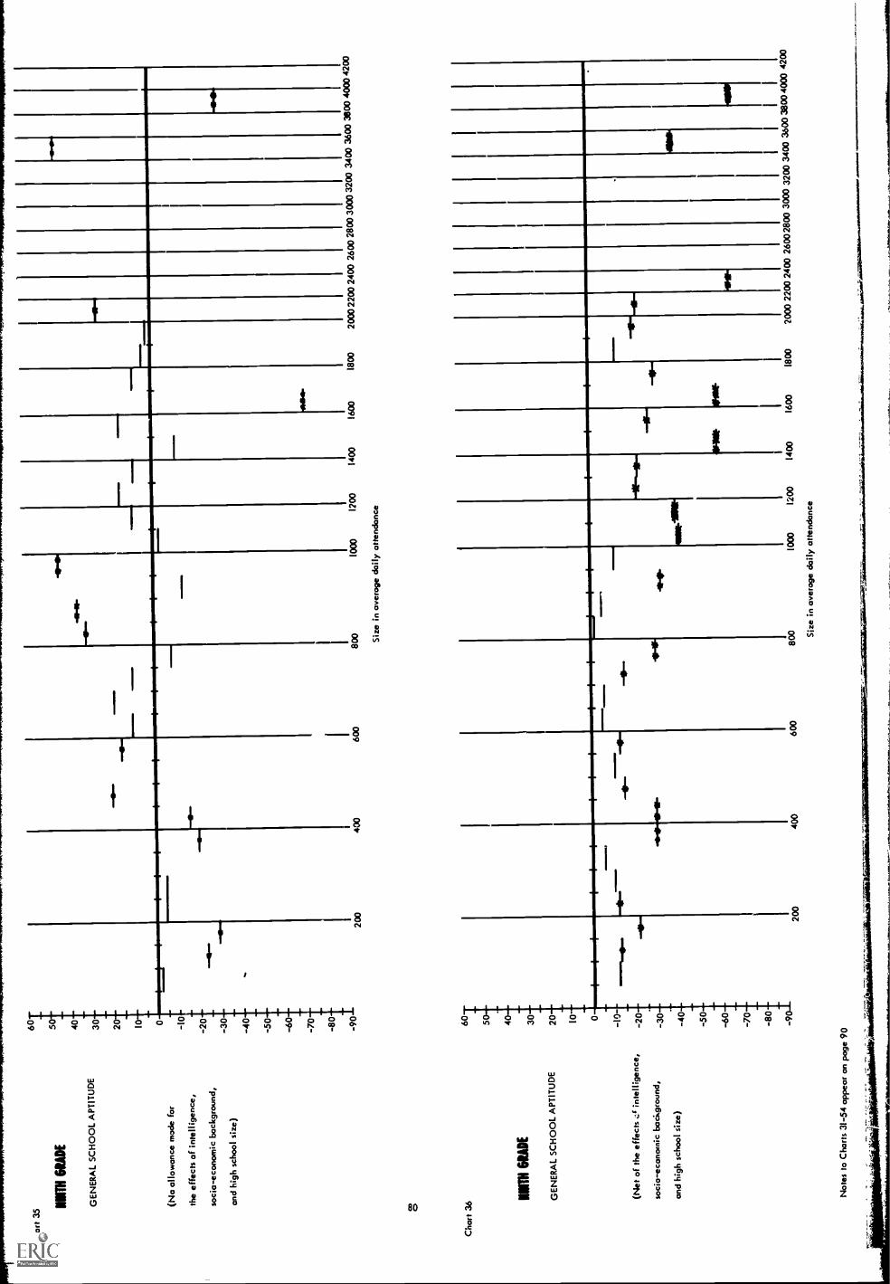
Cha

rt 3

5

MIM

I GR

AD

E

GE

NE

RA

L S

CH

OO

L A

PT

ITU

DE

(No

allo

wan

ce m

ode

for

the

effe

cts

of in

telli

genc

e,

soci

o-ec

onom

ic b

ackg

roun

d,

and

high

sch

ool s

ize)

Cha

rt 3

6

MIM

I GR

AD

E

GE

NE

RA

L S

CH

OO

L A

PT

ITU

DE

(Net

of t

he e

ffect

sin

telli

genc

e,

soci

o-ec

onom

ic b

ackg

roun

d,

and

high

sch

ool s

ize)

Not

es to

Cha

rts

31-5

4 ap

pear

on

page

9060 40 30 20 -1

0

- 20 - 30

- 40

- 50 -70

-so

-90 60 30 20 10

-

- 10

-

- 20

- 30 - 40

-50

-60

- 70 -80

- 9

Lj 4

fis

II

200

400

11..

=41

110

41

ItI

1

1111

11.

..-t1

P

IrI

aNI1

6

4111

1141

600

800

1000

1200

1400

1600

1800

2000

220

0 24

00 2

600

2800

300

0 32

00 3

400

3600

3800

400

0 42

00

Siz

e in

ove

rage

dai

ly a

ttend

ance

- - - - - - . .--

.-- - . - - _ - . - - _ _ _

-is-

--is

io

-i-e

--o-

--o

r-

4411

1114

-so-

figg

e-*O

P

.

re 1

-is-

---

41-

-vp-

o-

-e-

200

400

600

800

1000

1200

Siz

e in

ove

roge

dai

ly a

ttend

ance

1400

1600

1800

2000

220

0 24

00 2

6002

800

3000

320

0 34

00 3

600

3800

400

0 4

00

Cho

rt 3

7 RIM

GR

AD

E

GE

NE

RA

L T

EC

HN

ICA

L A

PT

ITU

DE

(No

allo

wan

ce m

ode

for

the

effe

cts

of in

telli

genc

e,

soci

o-ec

onom

ic b

ackg

roun

d,

ond

high

sch

ool s

ize)

3.0

2.5-

2.0-

1.5:

I. 0- .5-

IP... - - -

iI

II

II

II

II

II

II

II

II

tl'

- - - - - _ _ - - _ - - i.. - - --*

11

-

0-1

-.51

-1.0

- 1.

5

- 2.

0

-2.5

- 3.

0

- 3.

5

- 4.

0

-4.5

200

400

600

800

1000

1200

1400

1600

1800

2000

220

0 24

00 2

600

2800

300

0

Siz

e in

ove

roge

dai

ly o

ttend

ance

CO

-10.

5111

-111

1

Cha

rt 3

86 5- 4-

NIN

TH

GR

AD

E3-

GE

NE

RA

L T

EC

HN

ICA

L A

PT

ITU

DE

2- 0 -1-

(Net

of t

he e

ffect

s of

inte

llige

nce,

-2

soci

o-ec

onom

ic b

ackg

roun

d,-3

and

Mgh

sch

ool s

ize)

-4 -5:

-6 -7-

41i1

W

-8 -920

040

060

08

2000

2200

240

026

0028

0030

0032

00 3

400

3600

380

0400

0 42

00

Not

es to

Cho

rts

31-5

4 ap

peor

on

poge

90

_ _ _ - --I

v--

'..4e

lf4I

-1-

41-

-IN

--4

1-. - - _

,-rie

--0

-0-

-44

014

4041

1..

-It-

- .*e

lf*n

u -SW

1- .11

8111

,-

-AN

N- -

illA

rff-

-IW

O-

.--

' '--

---

ww

,..w

siw

wm

wse

4s.s

eirs

siim

esas

ide

-10.

2 11

1111

11.-

Siz

e in

ave

rage

dai

ly a

ttend

ance

,-al

titas

ielle

WU

ro's

edos

siss

.ss.

u.or

.ft

-10.

75-A

IM-

-16.

3414

81E

Cha

rt 3

9 NM

I GR

AD

E

EN

GLI

SH

FA

CT

OR

SC

OR

E

(No

allo

wan

ce m

ode

for

the

effe

cts

of in

telli

genc

e,

sock

-eco

nom

ic b

ackg

roun

d,

and

high

sch

ool s

ize)

CO

2.5

2.0

1.5

- I.

0

-1.5

- 2.

0

- 2.

5

- 3.

0

4.0t

-4.5

Cha

rt 4

0 NIN

TH

GR

AD

E

2.5-

2.0

EN

GLI

SH

FA

CT

OR

SC

OR

E1.

0

-

(Net

of t

he e

ffect

s of

inte

llige

nce,

soci

o-ec

onom

ic b

ackg

roun

d,

ond

high

sch

ool s

ize)

-1.

-1. 5

-2.

Not

es to

Cho

rts

31-5

4 op

peor

on

poge

90

-2.5

-

- 3.

5-

- 4.

0-

-

-.-1

0-

-4.5

-

200

400

600

800

1000

1200

Siz

e in

ove

roge

dai

ly a

ttend

ance

14 -

4 7

1800

2000

220

0 24

00 2

600

2800

300

0-4

.8-0

"-

-6.5

AM

P*

II,

II

II

II

I -I

II

II

II

II

I

-*a-

--N

I--

--0-

200

400

600

800

1000

1200

Siz

e in

ave

rage

dai

ly a

ttend

ance

1400

1600

1800

2000

220

0 24

00 2

6002

00

3000

320

0

O 1

0411

1.

Cha

rt 4

1

6RA

DE

6 5 4

MA

TH

EM

AT

ICS

FA

CT

OR

SC

OR

E3 2

(No

ollo

won

ce m

ode

for

the

effe

cts

of in

telli

genc

e,-2

soci

o-ec

onom

ic b

ackg

roun

d,

and

high

sch

ool s

ize)

-8-

co

Cha

rt 4

23.

02.

52.

0N

INT

H 6

RA

DE

1.5

MA

TH

EM

AT

ICS

FA

CT

OR

SC

OR

E1.

0 .5

(Net

of t

he e

ffect

s of

inte

llige

nce,

- 1.

0so

cio-

econ

omic

back

grou

nd,

- 1.

5an

d M

gh s

choo

l siz

e)20

-

-3.0

--

- 3.

5

- 4.

5

Not

es to

Cha

rts

31-5

4 ap

pear

on

poge

90

11.

I

200

400

I

--1

-411

.4(-

0

600

800

1000

1200

1400

1600

1800

2000

220

0 24

00 2

600

2800

300

0 32

00 3

400

3600

380

0 40

0042

00

Siz

e in

ove

rage

dai

ly a

ttend

ance

II

I4

1010

.

,11=

1.

200

400

600

800

1000

1200

1400

1600

Siz

e in

ove

rage

dai

ly a

ttend

ance

11t

lbs7

.!*7

1416

00 2

200

2400

260

0280

0 30

00 3

200

3400

360

0 38

00 4

000

4200

Alli

taki

lli;A

r411

1.01

1114

6111

1iiif

ak;0

111K

.061

.,'t-

^A

t -1.

1..e

...0*

101:

44,0

1WA

NO

ND

Cha

rt 4

3 11tIR

1Th

GR

AD

E

EN

GLI

SH

(No

allo

wan

ce m

ode

for

the

effe

cts

of in

telli

genc

e,

scci

o-ec

cnor

nic

back

grou

nd,

ond

high

sch

ool s

ize)

Cha

rt 4

4

TW

ELF

TH

6R

AD

E

EN

GLI

SH

(Net

of t

he e

ffect

s of

inte

llige

nce,

soci

o-ec

onom

ic b

ackg

roun

d,

ond

high

sch

ool s

ize)

Not

es to

Cha

rts

31-5

4 ap

pear

on

page

90

6 5- 4- 3- 2- 1 0 -I -2 -3

_ - _ . - _ _ - _

.

-4,-

-

4-*

1

-II-

- _ - --1

,---

or-

--O

Wili

tIP.

--O

OP

-.

4111

01-.

~"W

O- - - - - -

411.

1P.

b

- 4-

- 5 - 6

- 7 - 8

- 9 0

_

- I-

-8-

- 9

200

400

600

800

1000

1200

Siz

e in

ave

rage

dai

ly a

ttend

ance

1400

1600

1800

2000

220

0 24

00 2

6W 2

800

3000

320

0 34

00 3

600

- _ " - _

-_

--1

11

II

Ir-

II

111-

111-

1. .

-le-

-40-

-.

-IP

-4-

7_4

- .-.

IF-

.4.-

.0 1

ill-lh

. .44

.44

.ill

iti*M

b- - - _ - - -

200

400

600

800

1000

1200

Siz

e in

ave

roge

dai

ly a

ttend

ancd

1400

1600

1800

2000

220

0 24

00 2

6002

800

3000

320

0 34

00

Cha

rt' 4

5 MU

M G

RA

DE

MA

TH

EM

AT

ICS

(No

allo

wan

ce m

ode

for

the

effe

cts

of in

telli

genc

e,

soci

o-ec

onom

ic b

ackg

roun

d,

ond

high

sch

ool s

ize)

CO U.

Cha

rt 4

66

ME

M G

RA

DE

3 4

II

41W

4-4"

-044

*tw

o

200

400

=1

444

I4

-..=

1011

m=

^-41

8-.m

,11.

11

600

800

1000

1200

Siz

e :n

ove

roge

doi

ly a

ttend

ance

.n4

4.44

0

1400

1600

1800

2000

220

0 24

00 2

600

2800

300

0 32

00 3

400

3600

3800

400

0 42

00

- - - _ - - - - - - - -I

II

Ir-

r-4

- ..7"

-1I

1 -

II

4I

1I -4

1-

4114

4

I -4,-

.

4101

11.

,

-10-

.114

181

--4.

-- - H H - - ,.

-411

---o

- HIP

4

3-

MA

TH

EM

AT

ICS

2

(Net

of t

he e

ffect

s of

inte

llige

nce,

sbci

o-ec

onom

ic b

ackg

roun

d,

ond

high

sch

ool s

ize)

Not

es to

Cho

rts

31-5

4 op

peor

on

page

90

Eiro

ttiftw

oisa

titra

iiim

erow

e:::

e- -2 -3 -5 -6 -7 -8 -912

00

Siz

e in

ove

roge

doi

ly a

ttend

ance

1400

1600

1800

2000

220

0 24

00 2

600

2800

300

0 32

00 3

400

3600

3800

4000

420

0

Cha

rt 4

7 IWE

LFIN

MO

E

GE

NE

RA

L S

CH

OO

L A

PT

ITU

DE

(No

allo

wan

ce m

ode

for

the

effe

cts

of in

telli

genc

e,

soci

o-ec

onom

ic b

ocic

grou

nd,

ond

high

sch

ool s

ize)

Cho

rt 4

8

WIE

UT

II S

PA

DE

GE

NE

RA

L S

CH

OO

L A

PT

ITU

DE

(Net

of t

hef

fect

s of

ir.tt

!!;ge

nce,

soci

o-ec

onom

ic b

ockg

roun

d,

and

high

sch

ool s

ize)

Not

es to

Cho

rts

31-5

4 ap

pear

on

poge

90

50 40 30 20 10

4I

4

-10

- 20

- 30 -40

- 50 -60

- 70 - 80

- 90 60

T

50 30 2-t

-I

-1 - 20 - 30

- 40 -50

-60

- 70 -80

-90

t o

.004

11.

II

I

-IN

**

200

400

1111

....

......

m.

INm

lI

4141

114-

200

400

-

Ii

I

1111

.

4410

4110

iI

iI

600

800

1000

1200

1,I

II

IIII- 41

1-11

1-

Siz

e in

ave

rage

dai

ly a

ttend

once

II

I1

11

.41.

. .411

14w

.

I

111,

#110

111.

0-4

1400

1600

1800

2000

220

0 24

00 2

600

2800

300

0 32

00 3

400

3600

380

0 40

0042

00

40,

..119

.0.

--lb

,

1

. 1

Al.

.411

1111

.

1

.111

-111

-

4410

.

4141

1PIP

4111

4/*

Lim

*

600

800

1000

1200

1400

1600

1800

2000

220

0 24

00 2

6002

800

3000

320

0 34

00 3

600

3800

4000

420

0

Siz

e in

ave

roge

doi

ly a

ttend

once

hort

49

TW

ELF

TH

GR

AD

E

GE

NE

RA

L T

EC

HN

ICA

L A

PT

ITU

DE

(rgo

ollo

t:onc

e m

ode

for

the

effe

cts

of in

telli

genc

e,

soci

o-ec

onom

ic b

ockg

roun

d,

ond

high

sch

ool s

ize)

CO

Cho

rt 5

0

TW

ELF

TH

GR

AD

E

6 5- 4- 3- 2 1 0 -2 - 3 -4 -5 - 6 - 7 - 8 6

.. - .. , ...

..

..

. 1.11

1141

11.. r ...

. '- ... ....

..-el

lr

--11

11-.

.

..- .- ..-41

1111

.0p.

... ..- ... ..- ..--

. _...

.... .

......

..,

5- 4- 3-

GE

NE

RA

L T

EC

HN

ICA

L A

PT

ITU

DE

2 1

(Net

of t

he e

ffect

s of

inte

Hig

ence

,

soci

o-ec

onom

ic b

ackg

roun

d,

ond

high

sch

ool s

ize)

Not

es to

Cho

rts

31-5

4 op

peor

on

page

90

200

400

600

800

1000

1200

1400

1600

1600

2000

220

0 24

00 2

600

2 00

3

Siz

e in

ove

roge

doi

ly o

ttend

once

rr1

1141

,--.

.--.

7 .- ' 4- 0- - r r - _ _

o- -920

040

060

980

010

0012

00

Siz

e in

ove

roge

dai

ly o

ttend

once

400

10.1

441m

Mae

.rirK

CA

Rar

..ia.

r...r

..*.

Cha

rt 5

1

1WE

LFT

H 6

RA

DE

EN

GLI

SH

FA

CT

OR

SC

OR

E

(No

allo

wan

ce m

ade

for

the

effe

cts

of in

telli

genc

e,

soci

o-ec

onom

k ba

ckgr

ound

,

and

high

sch

ool s

ize)

3.0

2.5

2.0

1.5

1.0 .5 0

- 1.

0-- -

-2.0

-2.5

-3.0

- 3.

5

- 4.

0

Cha

rt 5

23-

0T

2.5

2.0

1WE

LFR

I 6R

AD

E

EN

GLI

SH

FA

CT

OR

SC

OR

E

(Net

of t

he e

ffect

s of

inte

llige

nce,

soci

o-ec

onom

ic b

ackg

roun

d,

and

high

sch

ool s

ize)

1.5

411-

41D

-

200

400

600

800

1000

1200

1400

1600

-1.0

-1.5

- 2.

0

- 2.

5

- 3.

0

- 3.

5

- 4.

0

-4.5

Not

es to

Cha

rts

31-5

4 ap

pear

on

page

90

200

400

II.

Siz

e in

ave

rage

dai

ly a

ttend

ance

1800

2000

220

0 24

00 2

600

2800

300

0 32

00 3

400

3600

380

040

00 4

200

-6.1

-46

-4-

600

800

1000

1200

Siz

e in

ave

rage

dai

ly a

.tend

ance

1400

1600

1800

2000

220

0 24

00 2

6002

800

3000

320

0 34

00 3

600

3800

4000

4200

Cha

rt 5

3

NE

M 6

RA

DE

Cha

rt 5

4MA

TH

EM

AT

ICS

FA

CT

OR

SC

OR

E

(No

allo

wan

ce m

ode

far

6 5 4 3 2 1

the

effe

ch o

f int

ellig

ence

,-2

soci

o-ec

onom

ic b

ockg

roun

d,-3

and

high

sch

ool s

ize)

- 5-

4-

- 6

- 7

- 8-

4-

- 9

1WE

LFT

H G

RA

DE

MA

TH

EM

AT

ICS

FA

CT

OR

SC

OR

E

(Net

of t

he e

ffect

s of

inte

llige

nce,

soci

o-ec

onom

ic b

ackg

roun

d,

and

high

sch

ool s

izz;

Not

es to

Cho

rts

31-5

4 ap

pear

on

page

90

5 4

1

200

400

600

1111

1110

I.1

11.

800

1000

1200

1400

1600

1800

2000

220

0 24

00 2

600

2800

300

0 32

00 3

400

3600

380

040

00 4

200

Siz

e in

ove

rage

doi

ly a

ttend

ance

1111

111.

..

- 9

4.41

200

400

600

800

1000

tOiA

CC

OM

iiiiit

iwoA

lt

.411

1.41

1.

1200

1400

1600

1800

2000

220

0 24

00 2

6002

800

3000

320

0 34

00 3

600

3800

4000

4200

Siz

e in

ove

rage

dai

ly a

ttend

ance

rtiC

etl:

OV

.111

AV

V.

Notes, Charts 31-54

Description:_ Dummy Variables

See notes to Charts 1-24, page 60.

Statistical Significance

= Significant at 90%** = Significant at 95%

Significant at 99%

See also notes to Charts 1-24, page 60.

Beta Coefficients

The values given in the charts are b-weights and not beta coef-ficients. To give the reader an idea of the relative magnitude ofthe effects,' the following standard deviations are provided:

Grade 9 Grade 12

English 13.5 12.0Mathematics 6.5 . 8;2General SchoOl Aptitude 111.4 117.9General r,chnical Aptitude 15.4 18.5English Factor Score 10.3 9.8Mathematics Factor Score 9.5 10.4

Number of Observations

The number of pupils in Grade 9 was 5;122 and in Grade 12,5,692. Dummy variables for which .there were fewer than 20 pupilshave been omitted from the charts.

Size of Intervals

It was cohvenient to group the high schools into size intervalswhich were not of equal width. Therefore the number of pupils includedin each dummy variable range changes twice over the size range on thecharts. Interval size below 1000 pupils in average daily attendanceis 50 pupils. Between lop() and 2000 pupils in ADA the interval is100 pupils, while the interval is 200 for sizes above 2000. The readershould make a mental recalculation in reading the charts, therefore,imagining the distances from 0 to 1000 pupils and from 2000 to 4000pupils as half as large and twice as large, respectively.

There were very few pupils in high schools larger than 4200 inADA and therefore sizes above that level were omitted from the charts.

90

TABLE 16

SUMMARY OF DUMMY VARIABLE FINDINGS

COMPARED TO COMPUTED SLOPE COEFFICIENTS,

SIZE-PERFORMANCE RELATIONSHIP, SIX QUALITY MEASURES, GRADE 9

Quality Measure

Relationship

How Well

Defined

Statistical

Significance

Estimated

Beta

Coefficient

Computed

Beta

Coefficient

t-value of

Computed Beta

Coefficient

English, Gross

Undefined

Fair

--

nc

nc

English, Net

Fair-Good

Good

-.145

-.059

4.51

Mathematics, Gross

Fair

Fair

Non-linear

nc

nc

Mathematics, Net

Fair-Good

Fair

-.145

-.082

6.63

School Aptitude, Gross

Poor

Poor

Non-linear

nc

nc

School Aptitude, Net

Fair

Fair

-.129

-.077

6.75

Technical Aptitude, Gross

Undefined

Fair

--

nc

nc

Technical Aptitude, Net

Good

Good

-.197

-.141

12.96

English Factor, Gross

Undefined

Poor

--

nc

nc

English Factor, Net

Poor

Fair

-.071

-.013

0.91

Mathematics Factor, Gross

Undefined

Poor

--

nc

nc

Mathematics Factor, Net

Fair

Fair

-.159

-.070

4.83

NOTES:

Notes to Tables 16 and 17 appear on page 93.

TABLE 17

SUMMARY OF DUMMY VARIABLE FINDINGS

COMPARED TO COMPUTED SLOPE COEFFICIENTS,

SIZE-PERFORMANCE RELATIONSHIP, SIX QUALITY MEASURES, GRADE

12

Quality Measure

Relationship

How Well

Defined

Statistical

Significance

Estimated

Beta

Coefficient

Computed

Beta

Coefficient

t-value of

Computed Beta

Coefficient

English, Gross

Good

Good

.087

nc

nc

English, Net

Fair

Good

-.052

-.030

2.47

Mathematics, Gross

Poor

Fair

.104

nc

nc

Mathematics, Net

Fair-Good

Good

-.079

-.036

2.96

School Aptitude, Gross

Good

Good

.120

nc

nc

School Aptitude, Net

Good

Good

-.107

-.046

4.34

Technical Aptitude, Gross

Poor

Poor

.065

nc

nc

Technical Aptitude, Net

Good

Good

-.183

-.120

10.72

English Factor, Gross

Undefined

Poor

--

nc

nc

English Factor, Net

Undefined

Poor

--

nc

nc

Mathematics Factor, Gross

Poor

Fair

.065

nc

nc

Mathematics Factor, Net

Poor

Poor

.000

-.003

0.25

NOTES:

Notes to Tables 16 and 17 appear en page 93.

Notes, Tables 16 and 17

Meaning of Gross and Net

"Gross" means that the dependent variable is explained by thesize dummy variables without allowance being made for the effects ofschool: expenditure per pupil, pupil intelligence (Verbal KnowledgesFactor Score), and pupil socio-economic index. "Net" means thatsuch allowance has been made.

Definition of Function

This is a subjective estimate by the author of how sharply thefunction represented under "Function Shape" is traced by the succes-sive values for the dummy variable expenditure intervals. Thus, ifa function is discernible but the plotted dummy ariables often de-viate from the function, it might be described as being "poor", etc.

Statistical Significance

This is an estimate of th t? overall statistical significance ofthe function made from the number of individual dummy variables whichwere statistically significant.

Estimated and Computed Beta Coefficients

The estimated beta coefficient is that for a hand-fitted lineto the function on the assumption that the function is linear. Thecomputed beta coefficient is that computed for the expenditure-performance relationship when the continuous expenditure variableis used.

nc = not computed.

three control variables are introduced, the entire relationship becomesnegative and linear. A possible explanation for this is that medium-sized schools exhibit better performance because they have pupils whoare either more intelligent or come from better socio-economic back-grounds, or both. If this were true, the introduction of the intelli-gence and socio-economic variables would have the effect of producingthe observed phenomenon.

..

94

IV

THE EXPENDITURE AND SIZE RELATIONSHIPS

CONTINUED: REGIONAL AND URBANNESS EFFECTS

Thus far the findings in this report have been given with respect

to all of the public general comprehensive and college preparatory

high schools in the Project Talent Sample. The task of Part IV will

be to examine whether any of these findings could be due to differences

in the regional and urban settings in which the high schools are found.

Project Talent divided their sample into six regions and four

classifications according to urbanness. Some key characteristics of

the six regions are included in Table 18. From a careful perusal of

the information in that table, it would appear that there is little

difference between the regions except for the 12 Southeastern states

where average expenditure, intelligence, and performance levelq are

much lower.46 The only regional difference with respect to size which

seems noteworthy is that high schools in the Atlantic states were a

great deal larger than in other regions.

The four urbanness categories used by Project Talent are Large

City, Urban, Rural, and Small Town. Characteristics for these four

categories are summarized in Table 19. It is interesting that the

urban districts appear to be getting the most in return for their money.

as they have the highest average figures for performance and the lowest

figure for average expenditure per pupil. This is at least in part due

to socio-economic differences as the reader can see by examining the

average figures for _he socio-economic index included in the table.

The value for urban districts is much higher in the 9th grade, which

is probably the important grade for such a calculation since drop-outs

have not yet occurred.47 Other differences between the four urban

categories are not as pronounced although therural high schools per-

form on the average somewhat more poorly and the large cities spend

approximately $100 per pupil more than the other three categories.There are great size differences, of course, which are only to be

expected from the nature of the breakdown.

In the remainder of Part IV regional and urban differences are

analyzed in two ways. First, individual pupils will be used as

"The high schools.in the Rocky Mountain states also had much

lower scores for intelligence and achievement performahce, although,

with only 13 observations, this cannot be assigned much importance.

47With respect to drop-outs it is interesting that the average

value of the socio-economic index increases a great deal more from

grade 9 to grade 12 in the large cities than in Che other three

categories. This probably means that Chere are a great many more

drop-outs in the large city high schools. In any event, unless great

pains were taken to strictly account for differences in drop-out rates,

95

TABLE 18

CHARACTERISTICS OF"THE PROJECT TALENT HIGH SCHOOLS

WHEN CONSIDERED ACCORDING TO REGION

Region

Characteristic

Number

of

Schools

Mean Size

(ADA)

Standard

Deviation:

Mean Size

Standard

Mean

Deviation:

Expenditure

Mean

(0

Expenditure

.($)

.

Mean School

"Aptitude

Score,

Grade 9

Stand

Deviat

Scho

Aptit

Scor

Northeast

26

635

520

$415

$104

576

49

Atlantic

108

1690

1590

$511

$139

536

72

Great Lakes

111

583

740

$383

$114

530

63

Plains

81

302

363

.

$455

$158

.

529

74

Southeast

147

368

382

$217

$176

457

113

Southwest

40

491

638

$357

$154

506

110

Mountain

13

414

575

$338

.$ 61

461

209

Far West

26

713

660

$525

$120

516

117

TABLE 19

CHARACTERISTICS OF THE PROJECT TALENT HIGH

SCHOOLS WHEN CONSIDERED ACCORDING TO URBAN

TYPE

Characteristic

Urban Type

Large Cities

Urban

Rural

Small Town

Total Number

94

181

164

196

Mean Size in ADA

2482

686

191

245

Standard Deviation of Mean Size

1316

468

168

146

Mean Expenditure per Pupil

$495

$340

$352

$391

Standard Deviation of Mean Expenditure

$93

$133

$183

$162

Mean Score, General School Aptitude, Grade 9

416

441

411

438

Standard Deviation, General School Aptitude

84

68

97

79

Mean Value, Project Talent, Socio-Economic

95.0

97.2

90.2

93.6

Index, Grade 9

Mean Value, Project Talent, Socio-Economic

99.4

98.0

91.2

94.5

Index, Grade 12

Standard Deviation, Socic-Economic

13.0

6.3

14.9

9.5

Index, Grade 9

observations and attention given to the differences in relationshipswhich obtain because of differences in pupil socio-economic background.After this has been done, the high school will be used as the unit ofobservation and a detailed analysis will be performed complete withcross-classifications for seven quality measures for all pupils taken

together.

Regional Differences: Individual Pupils as Observations

Tables 20 and 21 give findings F.or expenditure-performance rela-tionships for four quality measures, Mathematics, General SchoolAptitude, General Technical Aptitude, and Che Mathematics Factor score.

Since the discussion in this section includes the socio-economic break-down, it was considered appropriate to include the Technical Aptitudemeasure because it is possible that schools give some pupils, esPeciallythose from lower socio-economic backgrounds, good training in technicalsubjects even if not doing so in academic subjects. As the reader willrecall, this was found Co be true .for 12th grade children in the lowestfather education category in the dummy variable analysis above.48

The regional breakdowns given in Tables 20 and 21 use three re-

gions: Northeast (New England and Atlantic states), Southeast, and

the Rest of the Country. These are the Chree breakdowns most oftenused by Project Talent and it is employed here, although the authorfeels, as previously discussed, that a two-fold breakdown--Southeastand Rest of the Country--is adequate. Such a two-region breakciu,11 is

used in the cross-classification analysis presented below.

As the reader can readily tell from an examination of Tables 20and 21, making the regional breakdown has a large effect upon the com-puted significance of the expenditure-performance relationships, asalmost all of the relationships shown are quite weak. The only consis-

tent exception to this is the performance for pupils in the top twosocio-economic quartiles in Che Northeast. There are no relationships

which are positive and statistically significant.in the rest of the

country. Nor is it true that "better" schools are teaching pupils inthe bottom two quartiles more skills in technical subjects.

Size findings for the three regions are given for two of themeasures in Table 22. In light.of the overall negative relationshipsshown above, it is interesting that most of the significant or near-significant relationships in Table 22 are positive. Otherwise there

is little that can be said about within-region size variations. One

interesting point is that pupils in socio-economic quartile 3 seem toperform relatively better in larget high schools, especially in the

Southeast.

the 9th grade is much superior to the 12th for the calculation ofsocio-economic avefages.

48The possibility that education in technical skills might be animportant facet of education which is sometimes neglected was discussedin Part II.

98

TABU! 20

PERFORMANCE IN PROJECT TALENT HIGH SCHOOLS

RELATIVE TO EXPENDITURE PER PUPIL BY REGION, GREAT LAKES, PLAINS,

SOUTHEAST,

FOUR SOCIO-ECONOMW QUARTILES,

GRADE 12, MATHEMATICS AND GENERAL SCHOOLAPTITUDE

Pupil Population

by Socio-Economic

InOlx

Mathemati,:s Score

No.rtheast

Mie-aost and West

Southeast

Beta

tN

Beta

tN

Beta

tN

Top Quartile

0.171

2.724

230

0.055

1.18

402

0.100

1.15

165

Second Quartile

0.121

2.22*

304

0.001

0.04

589

-0.019

0.28

195

Third Quartile

0.005

0.11

435

-0.009

0.31

982

0.009

0.22

459

Lowest Quartile

-0.094

0.88

90

-0.008

0.15

306

-0.011

0.21

303

General School Aptitude

Northeast

Midwest and West

Southeast

Beta

tN

Beta

tN

Beta

tN

Top Quartile

0.131

2.23*

230

0.021

0.49

402

0.086

1.10

165

Second Quartile

0.129

2.574

304

0.026

0.76

589

0.007

0.11

195

Third Quartile

-0.015

0.36

435

-0.009

0.36

982

-0.007

0.19

459

Lowest Quartile

-0.023

0.25

90

-0.066

1.35

306

0.004

0.08

303

NOTES:

See next page.

Notes, Table 20

Beta Coefficient

beta coefficient is defined as the relative number of standard

deviations of the dependent variable associated with a change of one

standard deviation of the independent variable.

Statistical Si nificance.

* = Significant at 95%

4ce = Significant at 997

See also the notes to Table 1, page 16.

N in this table refers to the number of individual pupils in

the applicable categories; the individual unit of observations is

the individual pupil and not the high school.

Other Variables in dhe Multiple Regression Equation

The beta coefficients are net of the effects of pupil intel-

ligence, high school expenditure per pupil, and high school size.

See also the detailed discussion of the model on pages 33-43.

1 00

TABLE 21

PERFORMANCE IN PROJECT TALENT HIGH SCHOOLS RELATIVE TO EXPENDITURE PER PUPIL BY REGION, GREAT LAKES, PLAINS, SOUTHEAST,

FOUR SOCIO-ECONOMIC QUARTILES, GRADE 12, GENERAL TECHNICAL APTITUDE AND MATHEMATICS FACTOR

Pupil Population

by Socio-Economid

Index

General Technical Aptitude

Northeast

Midwest and West

Southeast

Beta

tN

Beta

tN

Beta

tN

Top Quartile

0.104

1.83*

230

0.076

1.83*

402

-0.009

0.11

165

Second Quartile

0.013

0.2"

304

0.013

0.35

589

0.024

0.38

195

Third Quartile

0.047

1.12

435

0.023

0.86

982

-0.052

1.46

459

Lowest Quartile

-0.166

2.181

90

0.050

1.06

306

-0.042

0.85

303

Mathematics Factor

Northeast

Midwest and West

Southeast

Beta

tN

Beta

tN

Beta

tN

Top Quartile

0.215

3.351

230

0.114

2.36fc

402

0.059

0.65

165

Second Quartile

0.056

0.98

304

-0.029

0.65

589

-0.045

0.59

195

Third Quartile

0.035

0.73

435

-0.013

0.42

982

-0.011

0.23

459

Lowest Quartile

-0.120

1.08

90

0.064

1.12

306

-0.015

0.26

303

NOTES:

See next page

Notes, Table 21

Beta Coefficient

A beta coefficient is defined as the relative number of standard

deviations of the dependent variable associated with a change of one

standard deviation of the independent variable.

Statistical Significance

* = Significant at 95%

** = Significant at 99%

See also the notes to Table 1, page 16.

N

N in this table refers to the number of individual pupils in

the applicable categories, the individual unit of observations is

the individual pupil and not the high school.

Other Variables in the Multi le Re ression E uation

The beta coefficients are net of the effects of pupil intel-

ligence, high school expenditure per pupil, and high school size.

See also the detailed discussion of the model on pages 33-43.

102

TABLE 22

PERFORMANCE IN PROJECT TALENT HIGH SCHOOLS RELATIVE TO

SIZE IN AVERAGE DAILY ATTENDANCE BY REGION, GREAT LAKES, PLAINS,

AND SOUTIEAST, FOUR SOCIO-ECONOMIC QUARTILES, GRADE 12, MATHEMATICS AND GENERALSCHOOL APTITUDE

Pupil Population

by Socio-Economic

Index

Mathematics

Northeast

Midwest and West

Southeast

Beta

tN

Beta

tN

Beta

tN

Top Quartile

0.025

0.39

230

0.093

2.01*

402

-0.029

0.33

165

Second Quartile

-0.018

0.33

304

-0.014

0.38

589

0.072

1.04

195

Third Quartile

-0.023

0.50

435

-0.033

1.11

982

0.156

3.54

459

Lowest Quartile

0.074

0.71

90

-0.065

1.21

306

0.003

0.05

303

General School Aptitude

Northeast

Midwest and West

Southeast

Beta

tN

Beta

tN

Beta

tN

Top Quartile

0.030

0.51

230

0.088

2.04

402

0.011

0.14

165

Second Quartile

0.008

0.16

304

-0.021

0.60

589

0.089

1.40

195

Third Quartile

0.025

0.62

435

-0.018

0.66

982

0.019

4.74

459

Lowest Quartile

-0.032

0.34

90

-0.080

1.65*

306

0.017

0.34

303

NOTES:

See next page.

Notes, Table 22

Beta Coefficient

A beta coefficient is defined as the relative number of standard

deviations of the dependent variable associated with a change of one

standard deviation of the independent variable.

Statistical Si nificance

* = Significant at 95%

* = Significant at 99%

See also the notes to Table 1, page 16.

N in this table.refers to the number of individual pupils in

the applicable categories; the individual unit of observations is

the individual pupil and not the high school.

Other Variables in the Multiple Regression Equation

The beta coefficients are net of the effects of pupil intel-

ligence, high school expenditure per pupil, and high school size.

See also the detailed discussion of the model on pages 33-43.

104

Urbanness Characteristics: Individual Pupils as Observations

Tables 23 and 24 contain normalized coefficients of partial re-

gression for expenditure-perfGrmance relationships for the four urban-

ness classifications. Expenditure is positively and significantly

related to performance in very few of the populations. The most fre-

quent exceptions to this occur in the urban high schools where the

relationship is significant in the top two quartiles for Mathematics,

Quartile 3 for General Technical Aptitude, and the top quartile for

the Mathematics Factor score. In light of our earlier reasoning that

Mathematics scores are good quality measures, it is interesting that

the urban high schools do seem to be doing a good job with mathematics

for the top two socio-economic quartiles.

The only significantly positive relationship for the Large Cities

is in socio-economic group 2 for the Mathematics Factor score. Other-

wise, expenditure in the large city high schools seems to have little

positive relationship to pupil performance. Indeed, most of the rela-

tionships for the bottom two socio-economic quartiles are negative and

three of these are statistically significant.

There are too few observations for both the rural and small town

high schools to make for meaningful analysis. Especially is this true

with the rural districts, although it is interesting that the relation-

ship between General Technical Aptitude and rural expenditure is highly

significant in the lowest quartile. It could be that rural schools

pay more attention to this type of thing but there are far too few

observations here to establish such a conclusion. The village schools

seem to do relatively well with their lower socio-economic background

pupils, especially with mathematics and technical subjects.

There is no meaningful relationship between size and performance

within the urban classifications. The figures in Table 25 could easily

have been generated completely by chance.

Summary: Regional and Urbanness Findings Using Individual Pupils as

Observations

The information for urban and regional breakdowns given in Tables

20-25 can be summarized into the following points:

1. ;he relationship between both high school expenditure and size

to pupil performance is in general strikingly weak.

2. Pupil performance is more closely related to school expendi-

ture in the urbanness categories than in regions.

3. The almost total lack of relationship between score andexpenditure in the regional breakdowns can perhaps be explained by the

existence of different combinations of districts in each region accord-ing to urbanness characteristics. If the urbanness classifications aremeaningful, and if there are different combinations of high schools

105

TABLE 23

INDIVIDUAL PUPIL PERFORMANCE RELATIVE TO EXPENDITURE PER PUPIL IN PROJECT TALENT HIGH SCHOOLS BY URBAN CLASSIFICATION, FOUR

SOCIO-ECONOMIC QUARTILES, GRADE 12, MATHEMATICS AND GENERAL SCHOOL APTITUDE

Pupil Population by

Socio-Economic Index

Mathematics Score

Urban

Large Cities

Rural

Small Towns

NBeta

tN

Beta

tN

Beta

tN

Beta

t

Top Quartile

0.170

4.52:

620

0.044

0.83

291

N/A

0.163

1.65*

107

Second Quartile

0.072

2.16:

778

0.082

1.53

341

0.035

0.40

124

0.084

1.27

186

Third Quartile

0.008

0.30

1128

-0.052

1.19

477

N/A

0.106

2.15:

365

Lowest Quartile

0.039

0.70

318

-0.182

2.34

138

0.109

1.62*

199

0.041

0.57

182

General School Aptitude

Urban

Large Cities

Rural

Small Towns

Beta

tN

Beta

tN

Beta

tN

Beta

tN

Top Quartile

0.129

3.71:

620

0.039

0.77

291

N/A

0.102

1.13

107

Second Quartile

0.066

2.15:

778

0.080

1.61*

341

0.034

0.44

124

0.128

2.21*

186

Third Quartile

0.005

0.18

1128

-0.07

1.71*

477

N/A

----

0.061

1.38

365

Lowest Quartile

0.083

1.66*

318

-0.074

1.06

138

0.047

0.76

199

-0.051

0.78

182

NOTES:

See next page.

Notes, Table 23

Beta Coefficient

A beta coefficient is defined as the relative number of standard

deviations of the dependent variable associated with a change of one

standard deviation of the independent variable.

Statistical Significance

* = Significant at 95%

** = Significant at 99%

See also the notes to Table 1, page 16.

N

N in this table refers to the number of individual pupils in

the applicable categories; the individual unit of observations is

the individual pupil *and not the high school.

Other Variables in the Multiple Regression Equation

The beta coefficients are net of the effects of pupil intel-

ligence, high school expenditure per pupil, and high school size.

See also the detailed discussion of the model on pages 33-43.

107

-

TABLE 24

INDIVIDUAL PUPIL PERFORMANCE RELATIVE TO EKPENDITURE

PER PUPIL IN PROJECT TALENT HIGH SCHOOLS BY URBAN CLASSIFICATION,

FOUR

SOCIO-ECONOMIC QUARTILES, GRADE 12, GENERALTECHNICAL APTITUDE AND MATHEMATICS FACTOR

Pupil Population by

Socio-Economic Index

General Technical Aptitude

Urban

Large Cities

Rural

Small Towns

NBeta

tN

Beta

tN

Beta

tN

Beta

t

Top Quartile

0.049

1.43

620

0.029

0.54

291

N/A

0.101

1.21

107

Second Quartile

0.039

1.28

778

0.022

0.44

341

0.094

1.15

124

0.001

0.02

186

Third Quartile

0.060

2.41*

1128

-0.044

1.13

477

N/A

0.084

1.93*

365

Lowest Quartile

0.007

0.14

318

-0.148

2.06:

138

0.164

2.701

199

0.107

1.79*

182

Mathematics Factor

Urban

Large Cities

Rural

Small Towns

Beta

tN

Beta

tN

Beta

tN

Beta

tN

Top Quartile

0.167

4.341

620

0.084

1.47

291

N/A

----

---

0.168

1.67*

107

Second Quartile

0.037

1.05

778

0.108

1.92*

341

0.067

0.72

124

-0.001

0.C1

186

Third Quartile

0.012

0.41

112?

0.073

1.54

477

N/A

---

0.061

1.13

365

Lowest Quartile

0.076

1.20

318

-0.088

1.00

138

0.106

1.47

199

0.146

1.91*

182

NOTES:

See next page.

Notes, Table 24

Beta Coefficient

A beta coefficient is defined as the relative number of standard

deviations of the dependent variable associated with a change of one

standard deviation of the independent variable.

Statistical Significance

* = Significant at 95%

** = Significant at 99%

See also the notes to Table 1, page 16.

N in this table refers to the number of individual pupils in

the applicable categories; the individual unit of observations is

the individual pupil and not the high school.

Other Variables in the Multiple Regression Equation

The beta coefficients are net of the effects of pupil intel-

ligence, high school expenditure per pupil, and high school size.

See also the detailed discussion of the model on pages 33-43.

109

TABLE 25

INDIVIDUAL PUPIL PERFORMANCERELATIVE TO SIZE IN AVERAGEDAILY DAILY ATTENDANCE IN

PROJECT TALENT HIGH SCHOOLS

BY URBAN

CLASSIFICATION, FOUR

SOCIO-ECONOMIC QUARTILES, GRADE 12,

MATHEMATICS AND GENERAL SCHOOLAPTITUDE

Pupil Population by

Socio-Economic Index

Mathematics

Urban

Large Cities

Rural

Small Towns

Beta

tBeta

Beta

tN

Beta

Top Quartile

0.034

0.91

620

-0.031

0.59

291

N/A

0.023

0.41

107

Second Quartile

-0.050

1.51

778

-0.022

0.41

341

-0.106

1.23

124

-0.077

1.16

186

Third Quartile

0.054

1.87*

1128

0.056

1.27

477

N/A

__-_

-0.059

1.19

365

Lowest Quartile

0.002

0.05

318

0.045

0.57

138

0.124

1.83*

199

-0.045

0.63

182

General School Aptitude

Urban

Large Cities

Rural

Small Towns

Beta

tBeta

Beta

Beta

Top Quartile

0.039

1.12

620

-0.046

0.92

291

NJA

0.027

0.29

107

Second Quartile

-0.040

1.33

778

-0.051

1.03

341

-0.114

1.48

124

-0.032

0.56

186

Third Quartile

0.041

1.59

1128

-0.0006

0.02

477

N/A

----

-0.072

1.62*

365

Lowest Quartile

-0.007

0.14

318

0.031

0.44

138

0.074

1.20

199

-0.092

1.43

182

NOTES:

See next page.

Notes, Table 25

Beta Coefficient

A beta coefficient is (1.17ined as the relative number of standard

deviations of the dependent variable associated with a change of one

standard deviation of the independent variable.

Statistical Significance

* = Significant at 95%

* = Significant at 990/a

See also the notes to Table 1, page 16.

N in this table refers to the number of individual pupils in

the appliqable categories; the individual unit of observations is

the individual pupil and not the high school.

Other Variables in the Multiple Regression Equation

The beta coefficients are net of the effects of pupil intel-

ligence, high school expenditure per pupil, and high school size.

See also the detailed discussion of the model on pages 33-43.

111

according to such classifications in each region, then conclusionsconcerning region are not possible. It will be possible to exploreChis point further in the next section.

4. Generally, pupil performance in the lowest quartiles is lessrelated to school expenditure than in the top quartiles.

5. Pupils in the lowest quartile do not appear to perform betteron the Technical Aptitude test in higher spending schools.

Regional and Urban Classifications Cross-Classified: High Schools Usedas Observations

Because of limitations of time and cost, the breakdowns just dis-cussed did not include cross-classifications by urbanness and regionalcategories taken together. This will be undertaken for all pupils inthis section. As discussed above, it was decided to collapse the sixregions into two regions, Southeast and Northern/Western (for con-veniences the latter region will often be referred to below as "North.")This was made feasible because of the relatively heavy representationin Che Project Talent sample of the high schools in the Southeast.There are, therefore, represented in Tables 26-39 cross-classificationsbetween two regions and four urbanness characteristics along with allof Che applicable marginal totals. These are given for the seven out-put measures which would have been considered as the most importantthroughout the study. Tables 26-39 contain a great deal of informationand, in fact, can be thought of as summarizing the overall empiricalfindings for the Project Talent high schools. Because of the problemof the overlapping of Che intelligence and achievement performancevariables, equations are given in the tables with the Verbal KnowledgesFactor score both in and out of the multiple regression equation. Asdiscussed above, the correct expenditure-performance relationships arethought to be somewhere between these two situations. As the readercan see, when expenditure is omitted Che computed values for the betacoefficients and values of the t-statistic are greater for theexpenditure-performance relationships, although the magnitude of thedifference is not large. In discussing Che findings in Tables 26-39,it would perhaps be best to discuss each of the seven output measuresin turn.

1. English Score

In gener.H, Che relationship of high school expenditure to Englishperformance is more positive in grade 9 than in grade 12. In bothgrades therejs very little relationship between expenditure andEnglish score in the eight cross-classification cells when all fourvariables are entered into the model. In Che 9th grade the only signi-ficant relationships are found when all districts are taken togetherand in all Northern districts, the latter being weak. The net rela-tionships in grade 12 are either completely insignificant or signifi-cantly negative. Possible reasons for this change from positive to

112

'LZI aud g6E aIquy aaajuauaddu 6E-9z saIquy aol saqom

:sa4014

ELS

OW

L8g = M

V'TI = s

(L8'6)

(1L'L)

(CCE)

LEV*0

9VCO

£60'0-

(LV'VZ)

(Wz)

SOL*0

VLO*0-

irEL = x

(WC) (WL)

6600

1V*9

(8I') (IS'L)

VZI*0

LS'S

g09'

9gg'

Z9I = M

I'VI = E

689 = x

(WV)

(Vg'47)

(99'0)

(£6'0) (Z8'8)

ZOV*0

EZV*0

g£0'0-

LVO*0

£6'1-

(V6'£I)

(WO)

(Z8'0) (g£'6)

EgL*0

g00'0-

VVO*0

6£'0-

86V.

Vgli'

SZV = M

9'6 = E

(gE*8)

(0I'9)

(9£'£)

I£V*0

8Z£'0

9ZI*0-

(g47.8I)

(96.Z)

g99'

8010-

L 5 L = x

(68'1) (08'9)

L900

9Z.7I

(ZV'Z) (60.0

8800

69.S1

nuaoy

119'

6LS'

TOZ = M

O'VT = 5

(£47'9)

(VI'V)

(Ig'0)

9847'0

9I£'0

£Z0'0-

(6L*S1)

(947'0)

8EL*0

IZO*0-

O'ZL . x

(98'1) (89'8)

g80.0

0'47

(VrZ) (£0'6)

011*0

IT'L

V69'

Z99'

LL = M

L'91 = 9

L'99 = *

(9V'£)

(ZCZ)

(£9'0)

(901) (61'6)

LLV*0

0047'0

OVO*0-

L900

CUT-

(OV'ZI)

(89'0)

(VO'I) (g9'6)

££8'0

9V0'0-

6900

£10

g8£'

SW

VZI = M

801

(£9.47)

(£9'Z)

(£Z*0)

g£V*0

OgZ*0

9100-

(8Zi8)

(81.0)

8650

ETWO-

(g0-1) (047'8)

gLO*0

Ig'VT

(8V'1) (09'8)

L01*0

8L'8I

-maul!

LVS'

0647'

6g1 = M

8'6 = s

(96.47)

(£5'47)

(SV'T)

66£0

69£.0

8L0'0-

(LS'IT)

(Vg'I)

L990

8800-

I'SL = *

(VL'I) (66'9)

L600

VV.8

(LUZ) (66'9)

8E1*0

606

V9Z.

VVZ'

ZE = M

O'II = E

8'0L = x

(LZ*Z)

(CUT)

(WO)

(Z£'0) (VZ.6)

0VV.0

LVZ*0

6L00

000- Lira-

(V9'£)

(gL'O)

(8Z'O) (L£'6)

LWO

8110

V70*0-

V8'LI-

g09'

8Vg'

LZI = M

Z*6 = U

(g8'V)

(WV)

(V6'I)

Z£V*0

L8£'0

01I.0-

(16.II)

(LZ.Z)

8ZL*0

LE1*0-

Z*9L = *

(90-0 (6L'g)

1900

WZI

(ZV'T) (61'9)

L800

TV'ET

umoy uuws

L6£'

LLZ'

6VI = M

V*8

= s

(L9'I)

(LV'S)

(L9'0)

OgI*0

£647'0

g6V*0

(8V'S)

(9V'1)

LEV*0

gOI*0

Z'SL = x

(69'0) (947'9)

0g0'0

8CL

(£9'.1) (800

8ZI*0

£g*VI

ZLV'

SZE'

6V = M

T'II = s

L'OL = x

(gg'I)

(V9'£)

(TZ'O)

(19.I) (Z0'8)

ZZZ*0

gIg'0

VZO*0

gLI*0

£0'LZ-

(9Z.V)

(ZL'O)

(86'0) (V0'6)

giig'0

V600

611'0

9Z.SZ-

SVI'

ISO'

00I = M

V'S

= E

(WO)

(OV'£)

(L0'0)

09000

IZV*0

LOWO

(gO'Z)

(99'0)

TVZ*0

V900

va, = x_

(CI*0) (VCV)

9100

90'£V

(IZ'T) (OZ'S)

9ZI*0

Vg'cg

urgan

9E9'

119'

8L = M

L'IT = S

(900

(LV'Z)

(£.1'0)

ELS*0

8LZ*0

6000

(ZZ'IT)

(WO)

96L'O

IZO*0

Th-ro-'77r

Z'EL = *

(ZVI) (TO'L)

8600

980-

(LZ'T) (SZ'L)

8600

gV'T-

V = M

V'S

= E

L'69 = lc

(alndwoo ol epussod loll)

£V9'

OZ9'

VL = M

6'11 = E

(80.0

(VVZ)

(£i'0)

9850

0LZ*0

6000

(Ertl)

(9Z'O)

1080

0ZO*0

Z'EL . x

(99'1) (VO'L)

ZZI*0

ZL'E-

(Zg'I) (9Z'L)

TWO

EVE-

saT1-10 a8aui

z11

H-S

sa

uz u

H-S

TUTY-

sa

uz u

H-S

---76-q

sa

uiomps toTH

alp Jo Suillas

IuopiduaSoa9

Tuloy

lsuamlnos

qsam puu IllacN

UOT

OU

sITTna 77V ges HOPAID gliSTIONH

'slmaIoIaaaoo was 'sousIuslovuvmo mvsun amv moioau

As mouvoIaIssvao-ssouo

9Z TICIVI

'al oftd '6C otqua, aoqgu aueddu 6C-9Z solquI aog soqom

:seqoisl

I9E

L85 = N

(WC)

(05'8)

5LI*0

Ii7'7.0

(5E'5I)

9150

= 2

(50'9)

9610-

(000

TWO-

L'5I = x

(L9'9)

(5C'E)

61Z.0

605-

('7Z.L)

(55.0

05Z*0

T5"7-

59i7'

Z17E'

Z9I = N

(OU'O)

(ZI.9)

(WO)

IZ0*0

C990

9E0'0

(89'8)

(ZVI)

IL5'0

Z800

Z'ET =

(08'0

(Eo'c)

Li70'0

Z5'E-

('790)

(9C'E)

Zi70'0

08*Z-

0i7E.

LLV

5Zi7 = N

(7Z.E)

(W9)

ZWO

C8C*0

(ZV.II)

CLi7'0

= 2

(OZ.9)

05Z*0-

(6C.5)

9ZZ'0-

991 = 3.5

(58*Z)

(8C'E)

5110

8Z*E-

(5C'E)

(WC)

Ii7r0

C5'Z-

06E'

I9E'

TOZ = N

078.0

(ZrE)

69Z*0

8000

(76'8)

5T50

6"7 = s

(9C.0)

0Z0*0-

(CE.0)

6100-

0'5I

(WC)

OZZ*0

(ZZ"7)

i7i7Z*0

=(8L'E)

OZ"E-

(L8'E)

8517'

ZZE'

LL=M

CV = 2

(09'0)

(8E) (WO)

60.10-

0080

910'0-

(5C.9)

(8Z '0)

C09.0

LZ0*0-

= x

(0) (CCE)

0i700

16'0

(0) (C5'E)

5'1700

91'0-

16I'

Z8I'

I7ZIM

(80.0

ZECO

(WO

=

(75'i)

8910

'7"7 = 2

(CVO)

6100-

(WO)

LI0.0-

L'9I =

(06'0)

(56.0

i7L0'0

5L'I-

(LI'T)

(L6.0

9600

WO-

i7Z5'

65I = N

(Z8-1)

(660

05.1'0

0050

(CE.8)

5'17 = 2

(95-1)

9800-

(Z9-1)

6600-

5'9T

(05"7)

95Z*0

(Z0'5)

ITC%)

=(90"E)

C6'8-

(6C'E)

C5'8-

6CE'

09Z.

ZC = N

6c= s

(LO'Z)

(60.Z)

(WO)

'BC()

59C*0

8Z0'0-

(SVC)

(WO)

665'0

0E00

9.ci = x

(Z1'0)

(ZI.E)

LI0*0-

i717'8T-

(50'0)

(0C'E)

8000-

Zi781-

005'

08E'

LZI = N(T5'5)

Z550

(05'L)

LC5'0

OZ..°

LLO*0-

(C9'T)

5II*0-

Z'LT = x

(97'E)

(CO'C)

i7OZ*0

50'L-

(8C'E)

(LC'E)

Zi7Z.0

L17.9-

607I = N

C'9I = U

= N

6.0 = s

cif( = x

00I = N

O'C =

E'LI =

(C8.0

(LI'5)

(WO)

(7I.Z)

(T9'Z)

(7I.C)

(7Z97)

(WO)

(Ce'T)

(CVO

(00-0

(L8'Z)

(L8'0)

(09.1)

(99.Z)

6EZ*0

8Ci7'0

0E0'0-

9i7r0

8191-

5E9'

i7LE*0

66070

910'0-

59I*0

89'LZ-

ZIZ

ZIT*0

Zi7C0

0800-

651'0

9Z*5-

(99'9)

(cc.0)

(96.Z)

('78.Z)

(VZ

*9)(W

O(90.1)

(i7L'Z)

078'Z)

(9C.0)

(ES'Z)

(5L'Z)

9LE'

EWO

EZ0'0

giro

i7ET-

L6i7'

L890

T500

M*0

80LZ-

Z5T'

08Z'O

817r0

Z5'0-

8L = N

'7"7.1= U

17 =6'ET =

5"7I = x

(WO)

(SVC)

(C0.0)

(OL'O)

(WE)

(WO)

(05.0

('70.0)

(Z8.0)

(WC)

6CE'

51700

CL5'0

CO0'0

IL0*0-

L9'0

EEC'

Z900

Z55.0

Zi700"0-

C80.0-

Z5'T

(owidmoo oq oicassod qoti)

(66"7)

(5Z.0)

(99'0)

(7L'E)

(88"7)

(WO)

(68'0)

(WC)

ZZZ'

TWO

LZ0*0

ZL0*0-

CVO

TWO

910.0

960'0-

Z5'T

H-S

SZ

H-S

SH-S

b1

Sa

TE

30j,gsuotIgnos

quell puu qqaom

uoTW

ouSlIana TN '6 HaVED 'SOILVICHIVN

SINHIOIAIHOO V1HU 'SOILSIUMOVIIVHO Mrallfl MTV MOIDHU AU mommaissvao-ssom

Tuana

UM

OI IT

EM

S

uuqa.n.

sopT3 oael

Toogos qWTH

otp go 2u-pqe5

Tuopldua2o90

LzI a2rd 46E aplry aeljr araddr 6E-9z sappy .10; SOWN :SOWN

109

9647'

LEK = N

9'978 = E

(9E'5)

(Z47'ZI) (WS)

6ZZ'0

6E50

LI7I*0-

(L9'1Z)

078.0

94790

9110-

9.9Z7 = x

(W9) (WES)

9LI*0

I6'475-

(000

(0009)

SIZ*0

IS'I47-

L09'

EL47'

Z9I = N

(6I'I)

OII*0

(55.II)

0890

I'476 = E

(WO (tI.0)

889'0

8000

(I6'0)

5500

I'6LE = 3.5

(I6'0)

(I8'85)

94700

E47.19-

(89'0)

(6089)

0470'0

479'4747-

ICS'

OW

5Z47 = N

E'EL = 2

(ZO*5)

(66'6)

(86'5)

05Z.0

E050

Coro-

(69'91)

(WO

0Z9'0

ZLI'0-

9'474747 = 3.5

(56*Z)

(8I'05)

IOI*0

ZE'8-

(WO (8L'55)

5EI*0

006

steloy

IOZ = N

696 = s

O'II47 = 3.5

LL = N

610I = s

L'09E =

WI = N

Z'6L = s

Z*Z4747 = x

(479.0

(EV9)

(9L'O)

(56'E)

(9019)

(WO)

(5Z.5)

(L9'0)

(ZL'O)

(EE'65)

(WE)

(E6'E)

(WO)

(475-I)

(6609)

109'

6LZ*0

47L47*0

47E00-

Z8I*0

81'8E-

959'

47L00

E9L*0

54700-

84700

80'61-

E047'

WC()

89E*0

IE0'0-

6010

8Z*L-

Irani;

(5Z*EI)

(99'0)

(Z47"7)

(84799)

(E5'6)

(OL'O)

(89'0)

(Or 69)

(99.0

(9C0)

(ZI.Z)

(95479)

LZ5'

L590

ZE0*0-

0ZZ*0

E6'0I-

ICS'

475L'O

5500-

E500

9,' Z-

TEE'

47950

9Z0'0-

95I*0

0I'6E

651 = N

6'8L = E

8*LE47 =

ZE = N

47'58 = s

8'68C . x

LZT = N

9'ZL = 2

66477 = x

(58.Z)

0790

(5Z.I)

(SVC)

(68.L47)

(5E.Z)

(ZrZ) (WO)

(ZE*0)

(0I.Z9)

(5E.Z)

(LE'L)

(80.I)

(I8*Z)

(8E'ZI7)

6Z9*

L0Z*0

E950

1900-

8810

59'478-

47547'

Z6E*0

47E470

ZZO*0

E4700-

Z5'51E-

L59'

561'0

1190

L50'0-

051'0

06'LE-

umoy IIBmS

(IL'OI)

(ZVI)

(EE"7)

(9090

(6Z.47)

(09'0)

(IZ'O)

(Z8'89)

(Z47.0I)

(WI)

(IO'E)

(EL'05)

Z647*

LI9'0

5L0'0-

ISZ*0

0L'9L-

OEE'

I59.0

0600

IE0'0-

EO'SLE.

805'

47990

00I'0-

1610

50'LZ-

6'7I = N

47'89(= 2

47'1'7'7 = x

6'7 = N

0'478 = s_

066E = lc

00I = N

47'L47 = s

I'Z947 = x_

(9Z'Z)

(WL)

(I0'0)

(WI)

(56547)

(05-Z)

(WS)

(E0.0)

(6I'Z)

(917'847)

(EI'0)

(68'47)

(08'0)

(WO)

(L9'6E)

5475'

9LI*0

IL5'0

I00'0-

6800

LZ*50Z-

099'

L8Z*0

6L5"0

E000

1610

Z9.0L"7-

Z6Z'

'1E0'0

ZS.:*0

6900-

L470.0

1019

urcian

(16'9)

(470.I)

(WZ) (WES)

(9L*5)

(OL'O)

(6I'I)

(9'7'09)

(98"Z)

(50'0)

(I6'I)

(5I'4747)

Z8E'

6050

0L0*0

La%)

647LE1-

IL'7'

0590

180'0

8ZI*0

895547-

EZI'

L8Z*0

5000

1610

08181

8L = N

8E8 = E

95147 = X

47 = N

S'6L = s

L5047 = 3S

47L = N

5'478 = E

I'9I47 =

(OCZ)

(89"7)

(WO)

(5.5-0)

(I8'Z5)

(LCZ)

(547'47)

(WO)

(Z9.0)

(9I'ES)

865'

47LZ*0

L550

47ZO*0-

E4700

991'47E-

665'

68Z.0

474750

0E0.0-

64700

478L'9E-

(alndwoo ol apussod qoN)

saT4T0 agari

(8L'8)

(I0'0)

(WO) (0860

(89'8)

(WO)

(WO) (9860

17847'

LW()

I000

I4700

I9*Z47-

I647'

EZCO

6000-

5E00

88'9E-

e l

H-S 7.5-1-- SS

aE

zli

H-S

75"-i

Sa

ETOOROS IVITH

alp ;01:0 2uTales

IropidraitoaD

-ploy

gsratianos

3sam pur tilioN

TIMM TINT '6 HaVUO 'aanivav 100HOS 11013N39

6sImaioidaaoo wag (SOTISTUHIONAWHO !man ow rumall xa mouvoiansTio-ssoup

n' 31HV

Ioto

*LZI agud 46E op:my aolgs

isadds 6c-9z sappy iox solo's"

:solo's'

SgS

18E'

LSS = N

S'OI = 2

(i1.0)

(ECM (L9.6)

9000- 0000

9LZ*0-

(6191)

(ZO*L)

9ES*0

9EZ*0-

E*6E = x

(E1.9)

(VT.L)

LL1'0

SE'ZI-

(69.9)

(58)

LZZ'O

EI*OI-

1LS*

-TIE'

Z91 = N

9*OI = E

(607.n

(78.6)

(WO)

OVZ*0-

SS6*0

Z00*0-

(OZ*8)

(E6'0)

ZSS*0

1790'0

ErEE = x

(L8.0)

(06.9)

91700

98*L-

(LS*0)

(SL'S)

8E0'0

VZ*S-

ITS'

SCE'

SZV = N

ITT = F

(Oro)

(zzen) (TWOT)

I170*0

8Z9*0

LvE*0-

(L9*ZI)

(L9.0

EOS*0

80C*0-

VIi7 = X-

(LCZ)

(EO*L)

Z800

LE*6-

(TVE)

(81'8)

SZI*0

OV*9-

sTuqoy

L9S'

VSE'

10Z = N

E'II = s

(9E*1)

(16'6)

(SE*0)

6010-

L6L*0

9100-

(01'6)

(EZ*0)

LZS*0

EI0*0-

wsE = x

(11'E)

(IV*L)

671'0

18.1-

(99*E)

(SO*6)

E1Z*0

9V*Z-

E6S*

917E'

LL = N

6*OI = 2

(SO*Z)

(VL*9)

(LS*0)

SZE*0-

9901

ZV0*0-

(89'9)

(09.0)

VZ9*0

9600-

9*ZE = lc

(SS*0)

(E6.9)

Z90'0

89*Z-

(SL'O)

(6L*8)

6900

ZI*0-

SSV*

UT'

VZI = N

Z'OI = E

(LZ*0)

(LrL)

(V0*0)

17ZO*0-

E0L*0

Z00*0-

(VC'S)

(80'0)

SEV*0

L00*0

ETi7 = x

(EV*0) (WO

6Z0*0

1717*0I-

(9V*I)

(IZ*6)

671'0

L6'0

Tr1m'

SLS*

86E'

6S1 = N

Z*11 = s-

(51'0)

(81'8)

(01'Z)

110.0-

E179*0

6010-

(6Z*L)

(E0*Z)

LS7*0

9Z1*0-

-17'IV = 1;

(SZ'S)

(9Z*L)

Z8Z*0

OZ*LI-

(Z9'S)

(L9'8)

17SE*0

I6*SI-

Z6S*

LSI'

ZE = N

V"II = E

(ZE*0)

(SS'S)

(98'0)

9700

L9L*0

ZOI*0-

(96*Z)

(II*0)

17OS*0

8I0*0

1EE = x-

(19*0) (WO

OLO*0-

6L'EV-

(0E*0)

(SZ'OI)

OSO*0-

L9*E17-

LZS*

9LE'

LZI = N

Z*01 = E

(gZ*3)

(EE.9)

(SL'I)

VZ0*0

LI9*0

60I*0-

(E6.9)

(VI*Z)

86170

ZSI*0-

9.E.,7 = x

(98*E)

(86'9)

E17Z.0

9601-

(96*E)

(IO*8)

V8Z*0

VV*6-

umoy rums

ti7S'

6EV*

6VI = N

Z*8 = 2

(ES)

(LS'S)

(LL'I)

ESC*0

19170

C01'0-

(98.8)

(VCO)

1Z9*0

L170*0-

E*117 = li

(8L*0)

(ZS'S)

OSO*0

Z17*917-

(LL-E)

(1.9)

ZZ1*0

L8'6E-

EEL*

SZS*

607 = N

S*6 = s

(90'E)

(Z0.9)

(WO)

Z1E*0

1709.0

17IO*0-

(SV*9)

(Z9'0)

0690

8900

6*SE = x

(VS*Z)

(98197)

961'0

1089-

(SZ*I)

(817'9)

0E10

SZ*99-

L9Z*

OZZ*

001 = N

O*9 = s

(06*Z)

(L9*Z)

(EL*Z)

VICO

90E*0

017Z*0-

(I6*V)

(EZ*Z)

S9V*0

6610-

6*E17 = 3..

(VZ*0)

(60*S)

EZO*0-

SZ*SI-

(09.0)

(SZ'S)

LSO*0

E8*9-

ascii('

SSS'

69E'

8L = N

601 = 2

(15'0)

(99*S)

(WI)

V9C-0

L0L*0

VZI*0-

(E6.9)

(96.0)

9Z90

V60*0-

--77-rf-

Erin = x

(EO*0)

(SZ*L)

E00*0-

OEL*I1-

(SO*0)

(E9.8)

SOO*0-

WEI-

V = M

L'S = E

0*SE =

(alndwoo ol aTqTssod lois')

ZSS*

ELZ'

VL = N

I'I1 = 2

(ES*0)

(IV'S)

(WI)

8900

MVO IWO-

(WS)

(EE*0)

LVS*0

VE0*0

S'VE = lc

(VO*0)

(SE*L)

E00*0

SWII-

(WO)

(SI'S)

I80*0-

EWEI

sar4TD oaxel

11

Z2-S

Sa

uuZ

2-S

75-41--

sa

uu

Z2-S

-75-71-

Sa

uTomps 'PITH

alp go Su-plas

ToopiduiSoao

-ploy

4su9glno5

_-

Isom pus 'Pao's"

SelIalla 77V '6 HQVED 42anumav 7VDINHDHI IVUNHO

'sxmaImaaaop waif 'sonsIumovuvuo mvaun arm moIpau xa moImvpIassm-ssoup

6Z 37SY1

'LZI ard 46c 9Iva, aaajr

araddu 6C-9Z saIgra, aol seam :saaoti

ZCZ'

ZCZ'

L85 = R

16 = s

(668)

(LO'I)

(LZ'T)

VC5'0

V90'0-

8V0'0-

(VI'CI)

(LE'I)

V8V'0

1500-

005 = x

(C6'0)

(V6*L)

9E00

ZI'51

(Z8.0)

(V6*L)

IC0*0

56'VI

OVV

.CVV'

Z9I : Isl

6'6 = s

(8Z*9)

(LO*0)

(Z9'0)

1690

8000-

6E0'0-

(ZC*II)

(V9'0)

5890

OVO*0-

.

I'8V = U

(WO) (WO

I10"0

505

(WO)

(9C'L)

1100

CO'g

CZI'

ZZI*

5ZV = R

L*8 = s

(OZ*9)

(ZC*I)

(6I*I)

CZV*0 1600- 5500-

(8L*L)

(ZC*I)

95C*0

1900-

L'05 = x

(9L*0)

(01'8)

5E0'0

I9*ZZ

(C9.0)

(II'S)

6ZO*0

VZ*ZZ

sIr3oI

SVC'

ISE'

TOZ = N

C*II = s

(C6'5)

(WO)

(CVO)

1850

110'0

6100-

(91'01)

(CVO)

0650

6100-

9'6V = x

(IO'I)

(60'6)

6500

9Z*8

(CO*1)

(LO*6)

0900

CC'S

995'

1LS'

LL = N

I'ZI = s

(6Z*V)

(05'0)

(55'0)

VOL'O

1800

ZVO*0-

(9Z'OI)

(L5'0)

LW()

CVO*0-

6'9V = lc

(8Z*0) (WO

IZ0*0

5I*C

(8Z*0)

(98.0

IZ0*0

9C*C

OZI*

9ZI*

VZI = N

5'0I =

(69*C)

(C5*0)

(ZI*0)

gIV'0

0900- 6000-

(9V*V)

(CVO)

9LC*0

II0*0-

(6I'I)

C0I*0

(ZI*I)

5600

_

(8L*6)

LO*LI

(5L'6)

9091

Iranu

C61'

L61'

651 = N

9'L = E

(VL*V)

(CV'0)

(L0'0)

8050

LVO*0-

5000-

(95'9)

(50'0)

VLV*0

VOO*0-

805 = 1;

(61-0

(V8*9)

8800-

Ira

(8Z'I)

(Z8*9)

C60.0-

50*LI

VVI'

901'

Ze = N

6*L = s

(98.Z)

(05*I)

(9C*I)

8650

IOC*0-

CCZ*0

(6C*Z)

(60*I)

6IV*0

981'0

V05 = x

(C8*0)

(ZZ*L)

6CI*0-

50.9

(98.0)

(8C*L)

LVI*0-

ZO*9

VOZ'

IIZ*

LZI = N

9'L = s

(V8*C)

(ZI*0)

(85'0)

58V*0

5100

9VO*0-

(5I*9)

(65.0)

L6V*0

LVO'0-

0*I5 = lc

(6C*I)

(VL*9)

CII'0-

1061

(6C*I)

(IL*9)

ZII*0-

170'6I

umca urwS

900'

000'

6VI = N

Z'9 = s

(90'1)

(Vg'I)

(00'I)

ZZI'0-

8L1*0

9800

(61'0)

(LZ*I)

8100-

801'0

8'6V = 5S

(6L'O)

(LI'9)

VLO*0

669V

(On')

(OZ*9)

101'0

I6'8V

060'

860'

6V = N

O'L = 2

(VO'I)

(8L*0)

(CC*0)

561'0

5VI*0

1500

(V6'I)

(LV*0)

98Z*0

IL0*0

c'sv . x

(65*I)

(V9*9)

9ZZ*0

OL*II

(05*I)

(Z9*9)

IIZ*0

IO*ZI

5C0*

9C0*

00I = R

(C8*3)

(Z6'0)

(OV'0)

I5C*0-

IZI*0

OVO*0

(9L'Z)

(L5'0)

I6Z*0-

9500

(6C*0)

CVO*0

(ZL*0)

5L0*0

(L5'5)

ZI*9L

(95.5)

IC*6L

urgan

90Z'

8L1'

8L = N

001 = s

(1C'V)

(16'1)

(90'0)

TZL'O

OZC*0-

LOWO

(C5*V)

.(90'0)

LWO

4100-0-

=b'1--

L'6V = x

(V6'0)

(V8*8)

C01*0

VV9*6

(C6.0)

(00.6)

VGT*0

U.'0I

V = N

L'V = s_

gig = x

(a3ndwo3 cn alcussod 3oN)

VIZ'

c8I*

i7L . M

Z'OI = s

(VZ*V)

(88*T)

(60'0)

9ZL*0

CZC*0- 96000

(5V*V)

(CO*0)

69V*0

C00.0-

9'6V = x

(VZ*I)

(66'8)

9E1'0

V8Z*9

(6Z*I)

(0'6)

VVI*0

6Z*9

saTaTD aitara

z'II

'a-S

sa

rel

H-S

M'f-

sa

rZli

a-S

'5-9 ,s

ar

Tomps IVITH

alp jo 2uT33as

iropidraitoa9

Iraca

3samganos

3sam pur claim

suana IVY '6 HaV119 'uomova HSII9N3

'sImaimaaaop vIza 4spimsmaImilivap 'man arm NOIDHU AEI riumvpIaIssvap-ssow

Geographical

Setting of the

High School

Large Cities

TABLE

CROSS-CLASSIFICATION BY REGION AND URBAN CHARACTERISTICS, BETA COEFFICIENTS,

MATHEMATICS FACTOR, GRADE 9, ALL PUPILS

North and West

Re

ion

Southwest

Total

aS

I. Q.

S-E

18.80

-0.128

0.122

2

0.583

.339

(6.56)

(1.28)

(1.23)

(6.14)

18.802

-0.129

0.124

-0.053

0.626

.330

(6.60)

(1.28)

(1.24)

(0.34)

(3.96)

R = 48.0

N = 74

aI. Q.

S-E

R2

(Not possible to compute)

x = 48.8

N = 4

aS

I. Q.

S-E

R2

17.83

-0.123

0.119

0.580

.333

(6.43)

(1.22)

(1.19)

(6.25)

17.745

-0.123

0.122

-0.058

0.627

.325

(6.46)

(1.22)

(1.20)

(0.38)

(4.06)

x = 48.0

N = 78

Urban

32.58

0.092

-0.163

0.259

.068

(3.47)

(0.89)

(1.67)

(2.50)

32.99

0.098

-0.159

-0.024

0.271

.058

(3.49)

(0.90)

(1.60)

(0.19)

(2.22)

X = 51.0

N = 127

55.82

-0.239

-0.212

-0.032

.060

(2.91)

(1.67)

(1.38)

(0.21)

55.91

-0.250

-0.199

-0.098

0.029

.044

(2.93)

(1.71)

(1.26)

(0.51)

(0.15)

R = 50.4

N = 32

43.51

0.020

-0.214

0.142

.025

(3.37)

(0.22)

(2.55)

(1.54)

43.90

0.030

-0.206

-0.065

0.180

.021

(3.38)

(0.33)

(2.41)

(0.57)

(1.57)

x = 50.9

N = 159

Small Town

11.89

0.179

-0.194

0.592

.423

(5.19)

(2.59)

(2.84)

(8.58)

11.78

0.174

-0.189

0.063

0.544

.420

(5.20)

(2.51)

(2.75)

(0.59)

(5.04)

X = 49.9

N = 124

87.04

-0.064

-0.256

0.477

.119

(4.74)

(0.37)

(1.50)

(2.74)

87.03

-0.069

-0.286

0.194

-0.592

.116

(4.74)

(0.40)

(1.64)

(0.95)

(2.79)

X = 48.0

- s = 10.5

N = 77

19.73

0.152

-0.150

0.474

.278

(5.54)

(2.21)

(2.21)

(6.91)

19.62

0.142

-0.148

0.094

0.406

.276

(5.54)

(2.03)

(2.17)

(0.91)

(4.00)

X = 50.9

N = 159

Rural

22.98

-0.153

0.061

0.475

.224

(6.55)

(1.92)

(0.77)

(6.00)

22.58

-0.157

0.060

0.034

0.453

.218

(6.58)

(1.94)

(0.76)

(0.32)

(4.28)

x = 499

N = 124

6.97

-0.020

-0.038

0.859

.719

(5.54)

(0.33)

(0.63)

(.4.04)

6.66

-0.021

-0.036

0.137

0.738

.720

(5.54)

(0.35)

(0.60)

(1.04)

(5.59)

R = 48.0

g = 10.5

N = 77

13.24

-0.148

0.024

0.719

.490

(6.26)

(2.86)

(0.48)

(13.96)

12.67

-0.157

0.024

0.108

0.632

.491

(6.26)

(3.01)

(0.47)

(1.24)

(7.31)

X = 49.2

N = 201

Totals

18.51

0.012

-0.119

0.515

.268

(5.77)

(0.29)

(2.82)

(12.35)

18.43

0.010

-0.121

0.026

0.500

.266

(5.78)

(0.24)

(2.85)

(0.40)

(7.96)

X = 49.9

N = 425

13.48

-0.032

-0.152

(5.39)

(0.58)

(2.67)

0.753

.527

17.50

-0.047

-0.116

0.600

.349

(13.50)

(5.70)

(1.34)

(3.38)

(17.71)

13.28

-0.031

-0.159

0.099

0.670

.526

17.41

-0.050

-0.119

0.040

0.569

.349

(5.39)

(0.56)

(2.77)

(U.98)

(6.62)

(5.70)

(1.41)

(3.43)

(0.73) (10.41)

R = 49.2

N = 162

R = 49.8

g = 7.1

N = 587

Notes:

Notes for Tables 26-39 appear after Table 39, page 127.

Geographical

Setting of the

High School

Large Cities

TABLE 32

CROSS-CLASSIFICATION BY REGION AND URBAN CHARACTERISTICS, BETA COEFFICIENTS,

URRICULUM MEASURE, GRADE 9, ALL PUPILS

Region

North and West

Southeast

Total

aS

I. Q.

S-E

R2

27.64

0.029

0.615

0.195

.395

(17.51)

(0.30)

(6.45)

(2.15)

27.643

0.029

0.614

0.020

0.179

.386

(17.63)

(0.30)

(6.38)

(0.13)

(1.19)

R = 90.7

g = 22.7

N = 74

aE

SI.Q.

S-E

R2

(Not possible to compute)

R = 88.8

g = 21.0

N = 4

aS

I. Q.

S-E

R2

39.79

-0.028

0.589

0.178

.334

(18.22)

(0.28

(5.86)

(1.91)

39.79

-0.028

0.589

0.002

0.177

.325

(18.34)

(0.27)

(5.81)

(0.01)

(1.14)

R = 90.6

g = 22.5

N = 78

Urban

68.67

0.149

0.473

-0.052

.218

(18.75)

(1.57)

(5.30)

(0.55)

50.08

0.099

0.448

0.189

-0.145

.231

(18.59)

(1.01)

(4.98)

(1.61)

(1.31)

R = 73.6

g = 21.3

N = 100

2.96

0.208

0.204

(16.41)

(1.47)

(1.34)

0.132

.078

(0.89)

4.48

0.177

0.244

-0.286

0.312

.107

(16.16)

(1.26)

(1.60)

(1.56)

(1.67)

I = 56.4

g = 17.3

N = 49

30.05

0.270

0.397

0.031

.263

(18.48)

(3.43)

(5.44)

(0.39)

29.31

0.267

0.395

0.020

0.020

.258

(18.54)

(3.31)

(5.31)

(0.20)

(0.20)

= 68.0

; = 21.6

N = 149

Small Town

27.38

0.054

0.578

0.056

.321

(13.36)

(0.72)

(7.82)

(0.75)

27.89

0.063

0.569

-0.128

0.154

.322

(13.35)

(0.84)

(7.66)

(1.10)

(1.32)

= 54.4

g = 16.3

N = 127

21.65

0.200

0.171

(15.19)

(1.07)

(0.91)

0.067

.000

(0.35)

21.62

0.196

0.150

0.128

-0.010

.000

(15.38)

(1.04)

(0.78)

(0.57)

(0.04)

49.2

g = 14.9

N = 32

23.28

0.136

0.482

0.074

.228

(14.10)

(1.91)

(6.87)

(1.0s)

23.55

0.146

0.480

-0.093

0.142

.227

(14.11)

(2.02)

(6.82)

(0.88)

(1.35)

= 53.3

g = 16.1

N = 159

Rural

22.47

0.069

0.494

0.114

.233

(14.64)

(0.87)

(6.24)

(1.45)

25.73

0.085

0.500

-0.122

0.194

.235

(14.62)

(1.05)

(6.27)

(1.15)

(1.85)

= 49.9

g = 16.8

N = 124

39.62

-0.076

0.481

(11.85)

(0.74)

(4.65)

-0.01:6

.195

(0.44)

39.92

-0.075

0.480

-0.102

0.045

.186

(11.92)

(0.73)

(4.61)

(0.56)

(0.20)

R = 43.5

5 = 13.3

N = 77

26.58

0.163

0.479

0.076

.239

(13.76)

(2.58)

(7.72)

(1.21)

28.02

0.175

0.479

-0.154

0.199

.243

(13.72)

(2.76)

(7.75)

(1.44)

(1.88)

47.4

g = 15.8

N = 201

Totals

22.57

-0.013

0.677

0.138

.477

(17.59)

(0.36) (18.94)

(3.90)

22.27

-0.015

0.675

0.027

0.118

.476

(17.61)

(0.41) (18.80)

(0.50)

(2.24)

R = 63.9

g = 24.4

N = 425

30.84

0.095

0.391

(15.52)

(1.31)

(5.20)

0.067

.174

(0.91)

31.42

0.094

0.400

-0.130

0.175

.174

(15.53)

(1.29)

(5.27)

(0.97)

(1.:)1)

49.6

; = 17.1

N = 162

21.48

0.074

0.629

0.131

.459

(17.21)

(2.34) (20.03)

(4.24)

21.49

0.074

0.629

-0.001

0.132

.458

(17.22)

(2.33) (19.93)

(0.01)

(2.64)

R = 59.9

; = 23.4

N = 587

Notes:

Notes for Tables 26-39 appear after Table 39, page 127.

Geographical

Setting of the

High School

Large Cities

TABLE 33

CROSS-CLASSIFICATION BY REGION AND URBAN CHARACTERISTICS, BETA COEFFICIENTS,

ENGLISH, GRADE 12, ALL PUPILS

Region

North and West

Southeast

Total

aS

I. Q.

S-E

R2

10.69

0.042

-0.042

0.581

.294

(6.14)

(0.44)

(0.44)

(6.34)

14.84

0.009

-0.095

0.367

0.402

.387

(5.72)

(0.10)

(1.04)

(3.76)

(4.12)

= 84.1

N = 90

aI. Q.

S-E

R2

(Note possible to compute)

= 84.4

N = 4

aS

I. Q.

S-E

R2

10.40

0.024

-0.041

0.597

.318

(6.03)

(0.25)

(0.43)

(6.78)

14.54

-0.002

-0.091

0.367

0.413

.409

(5.61)

(0.02)

(1.01)

(3.86)

(4.35)

= 84.1

N = 94

Urban

33.46

0.029

0.002

0.426

.164

(5.09)

(0.33)

(0.02)

(4.79)

33.19

-0.004

0.012

0.231

0.312

.196

(4.99)

(0.05)

(0.14)

(2.41)

(3.14)

= 87.4

N = 125

- 9.41

0.042

0.064

0.911

.860

(5.46)

(0.81)

(1.17)

(17.14)

- 8.53

0.058

0.007

0.279

0.688

.876

(5.14)

(1.18)

(0.12)

(2.78)

(7.28)

= 80.2

; = 14.7

N = 56

-1.96

0.026

0.019

(5.39)

(0.60)

(0.45)

0.830

.704

(19.18)

o.59

-0.009

0.007

0.267

0.631

.728

(5.17)

(0.23)

(0.17)

(4.07)

(9.85)

= 85.2

N = 181

Small Town

5.14

0.007

-0.020

0.874

.755

(7.12)

(0.15)

(0.45)

(20.05)

5.14

-0.034

-0.014

0.428

0.540

.824

(6.03)

(0.91)

(0.38)

(7.11)

(9.04)

= 82.9

g = 14.4

N = 131

37.09

-0.232

-0.031

0.326

.032

(9.09)

(1.35)

(0.18)

(1.88)

27.06

-0.267

-0.076

0.417

0.247

.189

(8.31)

(1.69)

(0.48)

(2.57)

(1.52)

= 81.5

N = 33

7.19

-0.025

-0.024

(7.52)

(0.55)

(0.56)

0.839

.690

(19.09)

7.78

-0.088

-0.025

0.420

0.536

.766

(6.53)

(2.24)

(0.64)

(7.29)

(9.48)

= 82.6

g = 13.6

N = 164

Rural

4.95

-0.021

-0.032

0.829

.672

(7.68)

(0.40)

(0.61)

(15.80)

5.63

-0.039

-0.048

0.288

0.629

.713

(7.18)

(0.79)

(0.96)

(4.20)

(9.21)

= 81.9

g = 13.5

N = 121

7.72

-0.044

0.035

0.765

.580

(10.84)

(0.59)

(0.46)

(10.02)

11.64

-0.095

-0.042

0.616

0.274

.704

(9.11)

(1.50)

(0.65)

(5.52)

(2.50)

= 76.8

g = 16.9

N = 75

5.22

-0.015

-0.008

(8,94)

(0.35)

(0.18)

0.810

.644

(18.71)

6.71

-0.054

-0.037

0.390

0.523

.707

(8.11)

(1.36)

(0.94)

(6.48)

(8.83)

= 79.9

- s = 15.0

N = 196

Totals

6.44

-0.015

-0.077

0.825

.660

(6.61)

(0.53)

(2.74)

(29.98)

7.22

-0.036

-0.128

0.335

0.596

.712

(6.C9)

(1.42)

(4.84)

(9.08) (16.64)

= 84.1

; = 11.4

N = 467

5.82

-0.057

0.028

0.796

.641

(8.85)

(1.20)

(0.56)

(16.51)

8.20

-0.076

-0.047

0.464

0.449

.715

(7.89)

(1.80)

(1.02)

(6.60)

(6.61)

= 79.0

; = 14.8

N = 168

4.73

-0.008

-0.057

(7.25)

(0.33)

(2.33)

0.828

.665

34.99

6.60

-0.049

-0.109

0.376

0.573

.720

(6.62)

(2.19)

(4.81) (11.22) (17.55)

= 82.7

= 12.5

N = 635

Notes:

Notes for Tables 26-39 appear after Table 39, page 127.

Geographical

Setting of dhe

High School

Large Cities

TABLE 34

CROSS-CLASSIFICATION BY REGION AND URBAN CHARACTERISTICS, BETA COEFFICIENTS,

MATHEMATICS, GRADE 12, ALL PUPILS

Region

North and West

Southeast

Total

aS

I. Q.

S-E

R2

- 39.48

0.097

0.070

0.650

.419

(3.83)

(1.12)

(0.80)

(7.83)

- 36.62

0.064

0.017

0.369

e.472

.515

(3.50)

(0.80)

(0.21)

(4.24)

(5.43)

= 19.7

N = 90

aE

SI. Q.

S-E

R

(Not pogsj_ble to compute)

ii = 19.7

§ = 5.4

N = 4

2a

4-38.13

0.064

(3.78)

(0.74)

- 35.25

0.038

(3.45)

(0.48)

ic = 19.7

I. Q.

_S-E

2

0.068

0.658

.430

(0.78)

(8.18)

0.017

0.372

0.471

.526

(0.22)

(4.38)

(5.54)

N = 94

Urban

- 16.39

0.094

-0.090

0.487

.239

(2.99)

(1.13)

(1.12)

(5.73)

- 16.69

0.034

-0.072

0.421

0.279

.361

(2.74)

(0.44)

(0.97)

(4.92)

(3.15)

= 21.8

N = 125

-9.80

0.099

0.223

(4.03)

(1.00)

(2.15)

0.616

.493

(6.10)

- 8 86

0.143

0.066

0.763

0.004

.625

(3.47)

(1.67)

(0.69)

(4.40)

(0.02)

= 16.9

N = 56

- 11.72

0.236

0.047

(3.52)

(4.13)

(0.82)

0.570

.466

(9.82)

- 8.98

0.158

0.019

0.591

0.130

.589

(3.09)

(3.09)

(2.38)

(7.34)

(1.65)

= 20.3

N = 181

Small Town

- 1.11

0.119

-0.052

0.592

.353

(4.27)

(1.69)

(0.74)

(8.36)

- 1.11

0.073

-0.046

0.487

0.212

.440

(3.98)

(1.09)

(0.70)

(4.54)

(1.99)

= 19.8

N = 131

.415.70

-0.062

-0.048

(3.82)

(3.38)

(0.29)

0.473

.112

(2.84)

-19.19

-0.090

-0.083

0.330

0.410

.201

(3.63)

(0.58)

(0.52)

(2.05)

(2.55)

= 16.3

N = 33

- 2.99

0.201

-0.057

(4.22)

(3.17)

(0.91)

0.559

.362

(8.86)

- 2.74

0.134

-0.058

0.442

0.239

.444

(3.94)

(2.22)

(0.98)

(4.98)

(2.75)

= 19.1

N = 164

Rural

- 4.14

0.029

0.062

0.557

.299

(4.82)

(0.38)

(0.80)

(7.25)

-3.74

0.004

0.041

0.390

0.286

.373

(4.56)

(0.06)

(0.56)

(3.85)

(2.83)

x = 19.2

N = 121

- 2.46

0.021

-0.018

(5.08)

(0.21)

(0.18)

0.550

.259

(5.43)

- 0.78

-0.041

-0.112

0.749

-0.046

.439

(4.42)

(0.47)

(1.25)

(4.89)

(0.31)

= 15.5

N = 75

- 5.22

0.138

0.038

(4.95)

(2.35)

(0.64)

0.560

.340

(9.50)

- 4.47

0.090

0.001

0.482

0.205

.435

(4.57)

(1.64)

(0.02)

(5.78)

(2.49)

= 17.8

N = 196

Totals

- 4.84

0.051

-0.043

0.570

.316

(4.19)

(1.31)

(1.09)

(14.60)

- 4.36

0.021

-0.113

0.461

0.255

.413

(3.88)

(0.59)

(3.01)

(8.76)

(4.99)

= 20.2

N = 467

- 4.75

0.020

0.124

(4.45)

(0.31)

(1.87)

0.561

.355

(8.6C)

- 3.60

-0.005

0.028

0.602

0.111

.479

(4.00)

(0.08)

(0.45)

(6.33)

(1.21)

R = 16.2

s = 5.6

N = 168

- 6.88

0.155

-0.017

(4.31)

(4.75)

(0.52)

0.579

.378

(17.95)

-/7

"...100

-0.088

0.507

0.220

.479

0.:11)

(2.84) (11.11)

(5.03)

Notes:

Notes for Tables 26-39 appear after Table 39, page 127.

Wag

aNW

ON

/WW

Ww

giw

atA

wow

,im-n

ow,

= 5.5

N = 635

Geographical

Setting of the

High School

Large Cities

TABLE 35

CROSS-CLASSIFICATION BY REGION AND URBAN CHARACTERISTICS, BETA COEFFICIENTS,

GENERAL SCHOOL APTITUDE, GRADE 12, ALL PUPILS

Region

North and West

Southeast

Total

aS

I. Q.

S-E

R2

- 370.80

.092

.024

(59.84)

(1.04)

(0.26)

.649

.397

(7.67)

- 313.03

0.048

-0.046

0.485

0.414

.568

(50.68)

(0.64)

(0.60)

(5.91)

(5.04)

= 525.5

g = 77.5

N = 90

aS

I. Q.

S-E

(Not possible to compute)

R = 519.1

g = 93.0

N = 4

aS

I. Q.

S-E

R2

- 368.46

.071

.020

.663

.418

(58.92)

(0.81)

(0.23)

(8.15)

- 310.58

0.037

-0.046

0.485

0.419

.585

(49.78)

(0.50)

(0.60)

(6.09)

(5.27)

R = 525.2

- s = 77.7

N = 94

Urban

- 99.40

0.099

-0.054

(41.90)

(1.27)

(0.71)

0.559

.327

(7.01)

- 104.48

0.031

-0.033

0.479

0.323

.488

(36.53)

(0.45)

(0.50)

(6.26)

(4.07)

x = 556.0

g = 51.3

N = 125

- 148.92

0.066

0.188

(57.95)

(0.91)

(2.47)

0.784

.728

(10.61)

- 134.38

0.101

0.064

0.606

0.301

.811

(48.28)

(1.65)

(0.94)

(4.89)

(2.58)

X = 473.9

g = 112.1

N = 56

- 154.67

0.171

(49.70)

(3.69)

- 110.37

0.099

(41.49)

(2.50)

X = 530.6

0.054

.0.729

.650

(1.16)

(15.50)

0.028

0.548

0.321

.756

(0.73)

(8.83)

(5.29)

g = 84.2

N = 181

Small Town

1.42

0.086

-0.038

(65.47)

(1.55)

(0.68)

0.774

.600

(13.90)

1.39

0.028

-0.030

0.607

0.300

.740

(52.83)

(0.62)

(0.67)

(8.31)

(4.13)

= 518.0

g = 104.0

N = 131

- 57.40

-0.13S

-0.022

(69.46)

(0.81)

(0.13)

0.444

.097

(2.65)

- 167.44

-0.184

-0.084

0.578

0.334

.433

(55.02)

(1.40)

(0.63)

(4.27)

(2.46)

R = 466.9

g = 74.2

N = 33

- 16.20

0.133

0.042

(66.23)

(2.53)

(0.80)

0.734

.564

(14.08)

-9.93

0.043

-0.042

0.594

0.304

.718

(53.27)

(0.99)

(0.99)

(9.40)

(4.91)

= 507.7

g = 100.6

N = 164

Rural

- 31.83

0.017

0.019

(68.55)

(0.28)

(0.30)

0.744

.541

(11.98)

- 22.91

-0.014

-0.008

0.499

0.397

.669

(58.26)

(0.27)

(0.16)

(6.78)

(5.41)

X = 503.5

g = 101.7

N = 121

- 21.22

0.029

0.034

(90.22)

(0.33)

(0.39)

0.678

.437

-49.16

0.100

0.025

0.716

.533

(7.67)

(77.45)

(2.03)

(0.51)

18.32

-0.044

-0.075

0.865

-0.011

.683

(67.66)

(0.66)

(1.10)

(7.50)

(0.09)

= 439.2

S = 121.0

N = 75

(14.44)

- 31.83

0.041

-0.020

0.597

0.276

.682

(63.92)

(1.00)

(0.49)

(9.54)

(4.48)

= 478.9

s = 113.6

N = 196

Totals

- 36.13

0.039

-0.045

(60.81)

(1.20)

(1.37)

0.739

.535

(22.91)

- 25.97

0.003

-0.129

0.553

0.359

.675

(50.80)

(0.12)

(4.61) (14.14)

(9.46)

= 525.9

g = 89.2

N = 467

-50.16

0.006

0.106

(75.16)

(0.11)

(1.88)

0.701

.534

(12.76)

- 23.62

-0.023

-0.005

0.695

0.181

.702

(60.12)

(0.52)

(0.11)

(9.66)

(2.61)

= 458.1

s = 110.4

N = 168

- 71.04

0.115

(65.55)

(4.20)

- 47.45

0.050

(53.95)

(2.21)

R = 507.9

- 0.019

0.732

.566

(0.71)

(27.20)

- 0.103

0.595

0.311

.706

(4.42) (17.36)

(9.48)

g = 99.6

N = 635

Notes:

Notes for Tables 26-39 appear after Table 39, page 127.

Geographical

TABLE 36

CROSS-CLASSIFICATION BY REGION AND URBAN CHARACTERISTICS, BETA COEFFICIENTS,

GENERAL TECHNICAL APTITUDE, GRADE 12, ALL PUPILS

North and West

Re

ion

Southeast

Total

Setting of the

High School

aE

Large Cities

SI. Q.

S-E

R2

- 50.01

-0.001

0.007

0.530

.246

(9.24)

(0.01)

(0.07)

(5.60)

-40.84

-0.050

-0.087

0.558

0.260

.472

(7.73)

(3.60)

(1.03)

(6.15)

(2.86)

R = 45.9

= 10.7

N = 90

aS

I. Q.

S-E

R2

(Not possitle to compute)

- x = 43.9

g = 12.8

N = 4

aS

I.Q.

S-E

R2

- 52.91

0.007

-0.016

0.550

.267

(9.13)

(0.07)

(0.16)

(6.02)

-43.78

-0.031

-0.091

0.554

0.271

.485

(7.66)

(0.38)

(1.08)

(6.24)

(3.05)

= 45.9

g = 10.7

N = 94

Urban

- 20.54

0.106

-0.168

(6.11)

(1.26)

(2.06)

0.458

.218

(5.33)

21.31

0.029

-0.144

0.541

0.191

.423

(5.24)

(0.40)

(2.07)

(6.66)

(2.23)

X = 51.3

N = 125

- 20.29

0.123

0.123

(10.24)

(1.15)

(1.09)

0.610

.407

(5.59)

- 18.69

0.155

0.008

0.560

0.164

.471

(9.67)

(1.52)

(0.07)

(2.70)

(0.84)

R = 41.6

= 13.4

N = 56

- 19.96

0.221

-0.020

(7.115)

(3.74)

(0.34)

0.575

.430

(9.58)

- 14.14

0.144

-0.047

0.582

0.142

.548

(6.99)

(2.68)

(0.89)

(6.89)

(1.72)

R = 48.3

g = 10.4

N = 181

- 2.07

0.099

-0.084

(9.95)

(1.43)

(1.23)

Small Town

0.627

.391

-39.23

-0.028

-0.077

(9.12)

(10.25)

(0.17)

(0.45)

0.444

.080

(2.62)

-7.43

0.193

-0.089

(10.12)

(3.12)

(1.43)

0.580

.386

(9.38)

- 2.07

0.042

-0.077

0.585

0.170

.518

-56.00

-0.079

-0.141

0.599

0.329

.443

(8.85)

(0.69)

(1.25)

(5.88)

(1.72)

(7.97)

(0.60)

(1.06)

(4.46)

(2.45)

= 49.4

= 12.8

N = 131

x = 40.1

3 = 10.9

N = 33

- 6.63

0.105

-0.089

0.588

0.155

.536

(8.80)

(1.89)

(1.65)

(7.25)

(1.94)

R = 47.5

g = 13.0

N = 164

Rural

-4.17

0.051

0.045

0.572

.313

(10.45)

(0.66)

(0.58)

(7.53)

- 2.91

0.015

0.014

0.567

0.179

.477

(9.12)

(0.22)

(0.21)

(6.12)

(1.94)

X = 48.7

g = 12.7

N = 121

-1.36

0.086

-0.071

(10.90)

(0.87)

(0.70)

0.561

.266

(5.56)

3.47

0.003

-0.196

0.998

-0.234

.595

(8.10)

(0.04)

(2.56)

(7.65)

(1.82)

R = 39.1

g = 12.8

N = 75

- 7.13

0.190

0.012

0.563

.363

(10.77)

(3.30)

(0.21)

(9.73)

- 4.84

0.125

-0.038

0.662

0.075

.546

(9.09)

(2.53)

(0.77)

(8.85)

(1.02)

= 45.0

g = 13.5

N = 196

Totals

- 5.87

0.059

-0.183

0.577

.325

-7.53

0.065

0.025

(9.21)

(1.52)

(4.64)

(14.87)

(10.46)

(0.99)

(0.36)

0.558

.308

-11.00

0.181

-0.136

0.581

.370

(8.33)

(9.69)

(5.49)

(4.10)

-4.51

0.021

-0.273

0.591

0.172

.485

-4.22

0.034

-0.096

0.759

-0.010

.507

(8.04)

(0.62)

(7.75) (11.99)

(3,60)

(8.82)

(0.61)

(1.61)

(8.21)

(0.12)

= 49.1

g = 11.2

N = 467

x = 40.2

= 12.6

N = 168

(17.88)

- 7.89

0.111

-0.226

0.639

0.128

.531

(8.36)

(3.87)

(7.69) (14.76)

(3.09)

= 46.7

= 12.2

N = 635

Notes:

Notes for Tables 26-39 appear after Table 39, page 127.

vorm

iori

aiiii

ism

idin

i:Lia

mt;m

b4.:1

4.1

-

Geographical

Setting of ehe

High School

Large Cities

TABLE 37

CROSS-CLASSIFICATION BY REGION AND URBAN CHARACTERISTICS, BETA COEFFICIENTS,

ENGLISH FACTOR, GRADE 12, ALL PUPILS

North

andWest

Re

ion

Southeast

Total

aS

I. Q.

S-E

31.28

-0.010

-0.109

(6.51)

(0.09)

(0.94)

0.168

.000

(1.53)

27.71

0.022

-0.058

-0.357

0.341

.074

(6.23)

(0.20)

(0.52)

(2.97)

(2.84)

x = 47.9

N = 90

aI. Q.

S-E

R2

(Not possible to compute)

ic = 49.6

N = 4

aI. Q.

S-E

R2

30.56

-0.029

-0.105

0.183

.000

(6.39)

(0.25)

(0.91)

(1.72)

27.08

-0.005

-0.057

-0.353

0.361

.080

(6.13)

(0.04)

(0.51)

(2.98)

(3.05)

48.0

s = 6.4

N = 94

Urban

40.79

-0.052

0.059

(5.31)

(0.54)

(0.64)

0.083

.000

(0.84)

41.08

-0.014

0.048

-0.270

0.216

.024

(5.20)

(0.14)

(0.52)

(2.55)

(1.97)

= 50.2

= 5.3

N = 125

- 0.40

-0.021

0.010

(6.39)

(0.24)

(0.10)

0.775

.578

(8.42)

- 0.97

-0.037

0.064

-0.269

0.990

.587

(6,32)

(0.41)

(0.64)

(1.47)

(5.75)

= 48.0

N = 56

6.04

-0.109

0.015

(5.76)

(1.72)

(0.24)

0.611

.338

(9.45)

4.29

-0.076

0.027

-0.256

0.802

.358

(5.67)

(1.18)

(0.43)

(2.54)

(8.15)

= 49.6

N = 181

Small Town

5.93

-0.049

0.005

(7.01)

(0.78)

(0.09)

0.714

.493

52.41

-0.308

-0.075

(11.39)

5.93

-0.064

0.007

0.155

0.593

.498

(6.97)

(1.01)

(0.12)

(1.53)

(5.88)

= 48.2

N = 131

(7.54

(1.75)

(0.42)

-0.056

.000

(0.31)

53.96

-0.301

-0.067

-0.080

0.071

.000

(7.65)

(1.68)

(0.37)

(0.43)

(0.38)

rc = 51.1

N = 33

10.34

-0.154

-0.010

(7.24)

(2.54)

(0.17)

0.656

.418

(10.90)

10.42

-0.167

-0.010

0.087

0.593

.417

(7.24)

(2.69)

(0.17)

(0.96)

(6.66)

= 48.8

s = 9.5

N = 164

Rural

4.84

-0.018

-0.062

(8.74)

(0.24)

(0.82)

0,594

.325

6.21

-0.051

-0.008

(7.88)

4.66

-0.012

-0.057

-0.097

0.661

.324

(8.75)

(0.16)

(0.74)

(0.93)

(6.30)

= 48.0

g = 10.7

N = 121

(8.67)

(0.59)

(0.09)

0.681

.441

(7.73)

7.42

-0.074

-0.043

0.275

0.462

.458

(3.53)

(0.86)

(0.48)

(1.82)

(3.12)

ic = 47.8

g = 11.7

N = 75

7.16

-0.096

-0.046

(8.67)

(1.68)

(0.80)

0.634

.380

(11.09)

7.20

-0.097

-0.047

0.012

0.625

.377

(8.70)

(1.67)

(0.81)

(0.14)

(7.24)

= 47.9

; = 11.0

N = 196

Totals

8.45

-0.044

-0.108

(7.04)

(1.14)

(2.73)

0.583

.324

7.84

-0.097

-0.046

(15.01)

8.25

-0.037

-0.091

-0.109

0.658

.328

(7.02)

(0.96)

(2.26)

(1.94) (12.04)

x = 48.6

N = 467

(7.69)

(1.64)

(0.75)

0.674

.437

(11.16)

8.03

-0.099

-0.055

0.056

0.632

.435

(7.71)

(1.67)

(0.86)

(0.56)

(6.61)

= 48.6

s = 10.3

N = 168

8.98

-0.107

-0.097

(7.22)

(3.22)

(2.89)

0.621

.360

(18.98)

8.70

-0.098

-0.086

-0.077

0.675

.362

(7.21)

(2.93)

(2.52)

(1.53) (13.94)

ic = 48.6

g = 9.03

N = 635

Notes:

Notes for Tables 26-39 appear after Table 39, page 127.

Aui

rlili

ro0m

13,,,

....

.04

),..k

ooas

okw

,-0

TABLE 38

CROSS-CLASSIFICATION BY REGION AND URBAN CHARACTERISTICS,

BETA COEFFICIENTS,

MATHEMATICS FACTOR, GRADE 12, AIL PUPILS

Geographical

North and West

Setting of ehe

High School

aE

SI. Q.

S-E

R2

Large Cities

Region

Southeast

- 8.40

0.130

0.081

0.358

.120

(7.86)

(1.21)

(0.75)

(3.50)

- 5.93

0.113

0.054

0.191

0.266

.138

(7.78)

(1.06)

(0.49)

(1.65)

(2.29)

= 50.4

N = 90

aS

I. Q.

S-E

(not possible to compute)

= 49.1

N = 4

Total

aE

I. Q.

S-E

R2

- 3.74

0.110

0.086

0.346

.114

(7.73)

(1.07)

(0.78)

(3.44)

- 1.33

0.103

0.060

0.190

0.250

.130

(7.66)

(0.96)

(0.55)

(1.65)

(2.17)

R = 50.3

g = 8.3

N = 94

Urban

0.45

0.117

-0.066

(6.09)

(1.31)

(0.76)

0.330

.113

(3.60)

0,03

0.072

-0.052

0.317

0.173

.179

(5.86)

(0.82)

(0.63)

(3.27)

(1.73)

= 50.3

g = 6.5

N = 125

13.06

-0.056

-0.103

(6.69)

(0.52)

(0.90)

0.677

.392

(6.12)

12.94

-0.060

-0.089

-0.068

0.731

.381

(6.75)

(0.55)

(0.72)

(0.30)

(3.47)

R = 47.3

N = 56

8.34

0.093

-0.078

(6.24)

(1.39)

(1.18)

0.522

.273

(7.70)

9.82

0.065

-0.088

0.210

0.366

.285

(6.19)

(0.96)

(1.33)

(1.98)

(3.52)

R = 49.3

g = 7.3

N = 181

Small Town

- 0.10

0.064

-0.022

0.632

.388

(9.19)

(0.92)

(0.32)

(9.17)

-0.10

0.058

-0.021

0.057

0.587

.385

(9.22)

(0.83)

(0.31)

(0.51)

(5.26)

R = 47.7

; = 11.8

N = 131

5.56

0.064

-0.133

0.362

.021

(6.44)

(0.37)

(0.76)

(2.07)

9.38

0.033

-0.109

-0.225

0.405

.042

(6.38)

(0.48)

(0.63)

(1.20

(2.30)

R = 46.2

g = 6.6

N = 33

1.02

0.053

-0.035

0.617

.373

(8.65)

(0.85)

(0.56)

(9.87)

1.01

0.054

-0.035

-0.005

0.620

.369

(8.67)

(0.84)

(0.56)

(0.06)

(6.69)

ic = 47.4

g = 11.0

N = 164

Rural

2.48

0.013

0.039

0.585

.327

(9.22)

(0.17)

(0.52)

(7.78)

2.53

0.011

0.038

0.024

0.568

.322

(9.26)

(0.15)

(0.50)

(0.23)

(5.41)

= 49.5

g = 11.3

N = 121

11.52

-0.076

-0.100

0.643

.380

(8.64)

(0.84)

(1.09)

(6.93)

11.19

-0.070

-0.091

-0.078

0.705

.373

(8.69)

(0.75)

(0.95)

(0.48)

(4.42)

ic = 46.4

g = 11.1

N = 75

5.54

-0.001

0.005

0.614

.363

(8.97)

(0.01)

(0.09)

(10.61)

5.50

0.001

-0.004

-0.014

0.624

.360

(8.99)

(0.02)

(0.07)

(0.15)

(7.13)

= 48.3

g = 11.3

N = 196

Totals

0.95

0.066

-0.015

0.558

.310

(8.22)

(1.69)

(0.37)

(14.21)

1.15

0.060

-0.030

0.099

0.490

313

(8.20)

(1.52)

(0.73)

(1.74)

(8.86)

= 49.3

N = 467

11.40

-0.054

-0.089

0.630

.364

(7.45)

(0.85)

(1.34)

(9.81)

10.97

-0.049

-0.068

-0.131

0.728

.366

(7.43)

(0.77)

(0.99)

(1.25)

(7.19)

ic = 46.7

N = 168

5.22

0.037

-0.019

0.574

.328

(8.03)

(1.09)

(0.57)

(17.13)

5.36

0.033

-0.025

0.037

0.548

.328

(8.04)

(0.96)

(0.70)

(0.72) (11.02)

= 48.7

g = 9.8

N = 635

Notes:

Notes for Tables 26-39 appear

after Table 39, page 127.

Geographical

TABLE 39

CROSS-CLASSIFICATION BY REGION AND URBAN

CHARACTERISTICS, BETA COEFFICIENTS,

CURRICULUM MEASURE, GRADE 12, ALL PUPILS

Region

North and West

Setting of the

High School

a

Large Cities

S-E

R2

75.58

-0.110

0.591

0.004

.286

(19.74)

(1.14)

(6.06)

(0.04)

80.31

-0.122

0.571

0.131

-0.060

.291

(19.68)

(1.26)

(5.82)

(1.25)

(0.57)

X = 90.9

= 23.5

N = 90

Southeast

a

Total

I. O.

S-E

R2

a

(Not possible to compute.)

= 88.8

3 = 21.0

N = 4

SI. O.

S-E

R2

90.39

-0.143

0.580

(20.02)

(1.45)

(5.79)

-0.024

.253

(0.26)

95.31

-0.153

.0.561

0.137

-0.093

.259

(19.95)

(1.54)

(5.57)

(1.29)

(0.88)

= 90.8

= 23.3

N = 94

Urban

11.99

0.116

0.475

(19.27)

(1.42)

(5.99)

0.080

.255

(0.95)

11.37

0.097

0.481

0.135

0.014

.262

(19.18)

(1.18)

(6.09)

(1.46)

(0.14)

X = 76.4

5 = 22.4

N = 125

10.32

0.232

0.189

(16.39)

(1.77)

(1.38)

0.220

.117

(1.65)

9.52

0.219

0.233

-0.212

0.389

.111

(16.45)

(1.66)

(1.57)

(0.79)

(1.54)

= 57.5

5 = 17.6

N = 56

15.89

0.248

0.418

(18.75)

(3.84)

(6.49)

0.113

.318

(1.71)

17.31

0.239

0.415

0.065

0.064

.315

(18.78)

(3.62)

(6.42)

(0.63)

(0.63)

R = 70.5

= 22.8

N = 181

Small Town

28.33

0.080

0.582

(13.27)

(1.11)

(8.07)

0.056

.329

(0.78)

28.33

0.104

0.579

-0.248

0.249

.347

(13.09)

(1.47)

(8.14)

(2.14)

(2.17)

- 45.62

0.174

0.061

(14.13)

(1.02)

(0.35)

0.340

.049

(1.98)

- 49.02

0.167

0.051

0.090

0.323

.024

(14.32)

(0.96)

(0.29)

(0.51)

(1.82)

25.58

0.160

0.451

(14.22)

(2.27)

(6.42)

0.087

.209

(1.24)

25.29

0.185

0.451

-0.169

0.209

.217

(14.15)

(2.58)

(6.45)

(1.61)

(2.02)

X = 53.9

g = 16.3

N = 131

= 49.1

= 14.7

N = 33

= 52.9

5 = 16.0

N = 164

Rural

34.13

0.077

0.504

(14.98)

(0.96)

(6.22)

0.040

.231

(0.50)

34.73

0.064

0.493

0.199

-0.098

.245

(14.84)

(0.80)

(6.12)

(1.79)

(0.88)

x = 51.4

g = 17.2

N = 121

31.77

-0.064

0.464

0.062

.192

(12.10)

(0.61)

(4.40)

(0.59)

30.98

-0.051

0.484

-0.154

0.185

.188

(12.12)

(0.48)

(4.47)

(0.84)

(1.02)

= 43.5

g = 13.5

N = 75

25.67

0.191

0.480

(14.06)

(3.05)

(7.65)

0.077

.251

(1.22)

26.16

0.179

0.471

0.117

-0.010

.253

(14.04)

(2.83)

(7.46)

(1.22)

(0.10)

X = 48.4

g = 16.3

N = 196

Totals

32.80

-0.003

0.656

(18.55)

(0.08) (18.57)

0.099

.458

19.50

0.122

0.356

(2.85)

(15.61)

(1.72)

(4.83)

0.162

.200

22.87

0.088

0.611

(2.24)

(17.96)

(2.89) (19.82)

33.32

-0.009

0.640

0.100

0.031

.462

19.24

0.124

0.363

-0.042

0.193

.196

23.74

(18.49)

(0.27) (17.78)

(1.98)

(0.63)

(15.65)

(1.74)

(4.75)

(0.36)

(1.69)

(17.92)

X66.5

g = 25.2

N = 467

= 50.3

= 17.5

N = 168

0.125

.459

(4.17)

0.079

0.599

0.090

0.062

.462

(2.55) (19.04)

(1.93)

(1.39)

= 62.2

3 = 24.4

N = 635

Notes:

Notes for Tables 26-39 appear after

Table 39, page 127.

iiiO

440.

014.

1161

1021

71.4

1.11

8*.Y

.144

.1a"

..X-4

44.1

7:11

,4,1

*VA

AV

oekt

,_

-

Notes Tables 26-39

Table Format

For dhe fifteen combinations of high schools denoted by the rowand column headings, two complete multiple regression equations aregiven, one including and one excluding the pupil intelligence variable.

The value under the columns headed by an "a" is the intercept and thevalue in parentheses under the intercept is the standard error of the

estimate. The other column headings are to be interpreted as follows:

E = Expenditure per pupil in average daily attendanceS = Size of high school in average daily attendance

I. Q. = Average pupil score on the Verbal Knowledge Factor ScoreS-§ = Average value of the Project Talent pupil socio-economic index.RL = Coefficient of multiple determination, corrected for degrees

of freedom lost.

The values in these columns not enclosed in parentheses are the beta

coefficients of net regression. The values enclosed in parentheses underthe beta coefficients are values of the computed t-statistic.

Other information is given in each category as.follows:

= Mean value of the dependent variable (e.g., English Score

in Table 26).g = Standard deviation of the dependant variable.N = Total number'of high schools

Statistical Significance

Because these tables are quite complicated already, asterisks for thepurpose of denoting statistical significance have been omitted

The following information is included so the reader can evaluate statis-

tical significance. To arrive at a figure for degrees of freedom, subtractthe number of variables (including the intercept) in the multiple regressionequation from the number of high schools, N. The t- value is statistically

significant if greater than the following listed 'Nialues.

Number of degreesof freedom

Value of t forsignificance at

Value of t forsignificance at

95% 99%

27 2.05 2.77

100 1.98 2.63

500 1.96 2.59

negativeS as the pupils move through the grades have been discussed in

detail above and is consistent with hypotheses advanced in Part 11

concerning the English score.

When intelligence is omitted from the ultiple regression equation,

the relationships usually become a great deal more positive, especially

in Northern school populations. The relationship in all the South-

eastern classifications remains meaningless, however. The lack of a

significant expenditure-performance relationship in the 12 Southern

states is a finding that is repeated consistently in the findings for

all seven of these quality measures.

Mathematics Score

The relationship of the Mathematics score to high school expendi-

ture is much more positive in general Chan is the English score, again .

a possible ramification of the fact that the Mathematics score is a

better quality measure than is the English score as has been suggested

repeatedly above. The positive relationship is more significant at the

9th grade level than in grade 12, however, a finding which is contrary

to an hypothesis made above. Again the omission of the intelligence

variable from the multiple regression equation serves to make the re-

lationships larger and more significant. There is some hint of a

meaningful expenditure performance relationship in Che high schools in

the ulhan Southeast, but no other Southeastern high schools display any

relationship between expenditure and performance. This is also true

with the high schools that are found in rural settings,and in large

cities, and, in grade 12, in the Northern, urban, and small town high

schools. Thus, the only cross-classified.populations in which expen-

diture is meaningfully related to Mathematics achievement is the

Northern, urban, and small town high schools in grade 9. This lack of

relationship within the eight cross-classification cells is generally

true for Che other Performance measures as well. The relationships for

all urban, small town, and rural high schools,respectivelyore on the

other hand quite strong.

3. and 4. General School Aptitude Score and General Technical Aptitude

Score

The findings for Chese two scores are very similar and therefore

it is convenient to discuss Chem together. Both scores are related

positively to school expenditure for aggregated urbanness classifica-

tions and for all pupils taken together. The deletion of the intelli-

gence variable from the regression equation tends to make the relation-

ships in the Northern populations much more significant and positive

at both grade levels (except in the large city schools). It is

interesting that for both variables in grade 9 the expenditure perform-

ance relationship becomes less pronounced with Che deletion of the

intelligence variable in Che urban South, which is the only Southern

population of high schools which had otherwise had a meaningful rela-

tionship. For both output measures the relationship of expenditure to

128

performance in all high schools classified according to urbannessand in all the high schools in the sample is quite strong.

EnRlish Factor Score

The findings for the English Factor score are again consistentwith the hypothesis developed above that the English Factor is a

poor measure of school quality. In the 9th grade the relationships

are positive but not statistically significant. In grade 12 the

relationships are even less positive air' in grade 9 with a nUmberof negative relationships that are stat stically significant.

The Mathematics Factor Score

The findings for the expenditure relationship to the Mathematics,Factor score are quite disappointing. This is especially true whenthe complete model is used when there are no significant relation-ships in grade 12 and a general negative relationship in grade 9.The findings when the intelligence Variable is not included in theequations are more positive although still not very strong. .Inthe 9th grade significant relationships obtain.in the Northernsmall towns and in all small towns. In the 12th grade there are nopopulations where expenditure is significantly.and positively re-

lated .to the Mathematics Factor.

The Curriculum Measure

In most populations of high schools the breadth of schoolcurriculum is positively related to expenditure but little more.The relationships are not strong except for in all schools takentogether and for all urban, small town, and rural high .schools

respectively...

Cross-Classification Findin s: Size

The overall size finding contained in Tables 29 through 42,'with the exception of those for the curriculum measure, display

two overall characteristics. First, the relationship of size toperformance becomes more negative as the high school populationinvolved becomes more aggregated, and secondly, the size-performance relationships become more negative when the conty.R1variables are entered into the multiple regression equation.'

49 That this is true for the introduction of the intelligencevariable the reader can see by examining the table. A very'similar

result obtains also when the socio-economic index variable is en-

tered intO the equation.

129

Both of these tendencies have already been discussed above, theformer in the'tection just preceding this one, and the latter inthe dummy variable section with respect to size. In the latter

section, reasons were given as to why the negative size findingswhich obtain when the two control variables are entered into theregression equation might be more believable than th more posi-tive findings whe- :hose two variables are omitted. Also above

(Pagen) were g fen aome reasons why the urbannegi categoriesmight be truly mote homogeneous than the regions. If this is

true, we should pay particular attention to the size relationshipswithin, each of the urbanness categories because, if a consistentnegative relationship were found within categories which werethought to be in other respects similar, such might constituteimportant evidence for diseconomies of scale. Such a consistentnegative relationship does not seem to be present, however, withthe exception of the relationship of size to the Technical Apti-tude and Mathematics Factor scores in the urban and small town

districts. Since, as was discussed above, these two scores areimportant measures of school performance,.these two exceptionsshould perhaps be assigned some importance. Nevertheless, there

is no consistent overall negative relationship within these cate-

gories. The only consistent negative relationships seem to obtainfor a11 Northern high schools and for all high schools taken to-

gethei.

General Summary: Findings When the High Schools are Cross-Classified According to Urbanness and Region

In summary, then, when the high schools are cross-c.lassifiedboth according to urbanness and region, the expenditure-performanceand size-performance relationships are both quite weak. When moreaggregated groupings of high schools are considered, the relation-ships seem better defined and this is more lrue in the non-

. Southeastern and non-large-city high schools. Deletion of the

"The complete model may be more accurate with respect tothe size variable than the school expenditure variable becausethere is less reason to believe that the intelligence variableoverlaps with the' size variable to the extent that it does with

the expenditure variable.

51These reasons were given when there were three regions in

the analysis instead of two, however. The division between theSoutheastern region and the rest of the country is probably moremeaningful than the three-region breakdown used in the preceding

section.

130

intelligence variable (and also the socio-economic variable, notshown) from the multiple regression equation makes most of theexpenditure-performance relationships more significantly positiveand most of the size relationships more positive. Of the South-eastern categories, the urban high schools seem to have perform-ance which is more highly related to higher spending schools thanany of the others. The differences in the relative expenditure-performance relationships between the seven quality measureswere found to be about the same as they were above, although theexpenditure relationships to the Mathematics Factor score wasperhaps somewhat weaker. In general, the model explains thetraditional achievement measures better.than the factor measures.Finally, with respect to the relationship to performance of schoolsize, it might be possible to reason that the overall negativerelationships which have been demonstrated to exist throughoutthe study for all high schools are due to geographical differencesaccording to urbanness, at least if such differences are themselvessignificant. This same argument does not of course work in similarfashion for explaining insignificant expenditure-performance rela-tionships in the cross-classified populations since expenditure ishighly associated with perforMance in dhree of the four totalurbanness categories.

131

PART V

SUMMARY AND CONCLUSIONS

There have been three basic objectives to this study. The first,which provided Che subject matter of Part II, was to see if somethingcould not be learned within the professional competence of the authorabout the efficacy of various quality measures of school performance.From Chat analysii some tentative conclusions were reached concerningwhich of a number of quality measures were most usefill.

The second purpose of the study was to explore carefully the rela-tionship of expenditure levels to school quality as measured by pupilperformance. This procedure makes the implicit assumption that "bettet"schools are those which, other thingz equal, average more expenditureper pupil. Part of the purpose of examining the expenditure relation-ship, alo, waS,to examine how educational returns vary with differencesin the socio-economic background of Che individual pupils.

Most of the studies of school performance which were 'discussed inPart I found that dhe formal education process has little influenceupon educatiOnal quality after accounting for pupil intelligential andenvironmental differences, even though Che apparent relationship,before accounting for Chese important things, is very large. Thefindings for expenditure in Part III do not warrant a similar conclu-sion for Che Project Talent high schools, at least when all of them areconsidered together. Considerable variat,ion in performance was ex-plained by expenditure per pupil at advanced levels of statisticalsignificance even after carefully accounting for intelligence once andsocio-economic background Mee. After allowing for these controlvariables, it was often found for the better measures of quality Chatan additional $100 of expenditure per pupil was associated with between.1 and .2 of a standard deviation in the dependent variable. This isno small effect.

It was also found (Table 3) that three of the most importantschool characteristics are quite highly related to expenditure perpupil, even after allowing for intelligence and socio-economic back-ground. The relationship was especially large for starting salary ofmale teachers and class sire in non-science and mathematiCs courseSwhere the amount of pupil performance associated with one standarddeviation of these variables was often close to .2 of a standard devi-ation of the dependent variable at highly meaningful levels of statis-tical significance. Thus it would appear that the present study hasbeen unique in showing considerable relationship between these variablesand school quality after carefully accounting for intelligential andsocio-economic differences.52

52Another study which was .in part also successful in doingthis was the large school districts in the author's prior study ofschool districts in New York State. (See Kiesling, Review of Economicsand Statistics, 92. cit.)

132

Part III also contains a detailed discussion of the theoretical

considerations which went into the construction of the analytical model.

Since there is good reason to suspect Chat an explanatory variable for

intelligence often overlaps with the measures of performance, a section

was devoted to an empirical investigation meant to show what the maximum

effect of such overlap might be.

There were also interesting findings in Part III concerning the

effects of school and socio-economic variables upon pupils from

different home environments. Thus, the background of clasamates seems

to be more important to the progress of children from low sdcio-econamic

backgrounds and school expenditure more important to children from

good.home environments.

A major task of the study has been to explore in great detail the

shape or the functional form of the relationships between expenditure

and school quality with the use, of dummy variables. That is to say,

the purpose was to explore whether there are any ranges of expenditure

per pupil which seem to be associated with grzater returns than other

ranges. These detailed relationships are contained in Charts 1-30,

where it appears that expenditure-performance relationships are liner

to a surprisingly consistent degree. When the relationships are not

linear, it appears as if expenditure levels beyond $400-$500 of expen-

diture per pupil seem to yield less return per dollar than lower levels.

Many of such relaticnships would be accurately represented by a loga-

rithmic function in which the expenditure performance relationship

increases more quickly at first and then more slowly thereafter.

A final major objective of the study was to inquire into the rela-

tionship betWeen performance and school size. This question was

analyzed both with the use of a continuous size variable and with dummy

variables for size intervals in the same fashion as was done for the

expenditure-performance relationship. The' overall size performance

relationship found in the data, especially when allowance was made for

the effects of pupil intelligence and socio-econoMic background, was

negative with surprising consistency. This finding is modified,con-

siderably when the high schools are divided into groupings according

to region and urbanness characteristics, however. None the less,

there is little evidence in the study that larger high schools are

more efficient high schools, while ehere is considerable, evidence that

larger high schools are less efficient. In an age of school consoli-

dation, this should serve as at least a word of caution.

When the Project Talent high schools were considered in regional

an(;.or urbanness categories, however, the picture with respect to

school influence ui)on pupil performance becomes more clouded. Within

the populations which were cross-classified both by region and by

urbanness, expenditure was rarely related to anything, although some

fairly strong relationships remained when the separations were made

according to urbanness (with the exception of the large city category).

The concluding note of the study is, therefore, left upon the question,

of how important are the regional amd urbanness categories shown in

the eight cross-classification cells in Tables 26-39. If they are

meaningful in themselves, then the findings demonstrated in Parts II

and III are modified considerably. It is obvious Chat further inquiryis needed in this matter. It could be that many of the individualcross-classification cells in Tables 26-39 have high school populationswhich are too small for meaningful analysis.

It is important that this study be viewed only as an importan'tfirst step towards a complete analysis of the Project Talent highschools. A model was built, performance measures were examined, andthe relationship of some of those measures to expenditure and size hasbeen examined. In the next step, individual characteristics of thehigh schools should be examined in more detail. Unfortunately, thiswill probably require a great deal of expense, although there is adoctoral dissertation completed at the University of Pittsburgh (which.the author has not seen at the time of writing) yhich extends theanalysis somewhat farther in this direction.5i It is almost certain,

however, Chat more intensive analysis of these high schools cannot beundertaken by an economist, or ami other researcher or group of .

researchers in a single discipline, working alone. Such work will ofnecessity require interdisciplinary team efforts by members of educa-tional research institutes, by that name or some other, if the researchis to be conducted in the depth And degree of sophistication that thesubject deserves.

53Bernard H. Booms, "Empirical Estimates of Secondary EducationProduction Functions," Unpublished Doctoral Dissertation, University'of Pittsburgh, 1968.

134

00

01

02

03

04

05

06

00

01

02

0304

05

80607

08

09

810

811

812

813

814815

816147818819

820

821

822

OE 6000 (REv. 9-66)DEPARTMEN OF HEAL TH. EDUCATION. AND WELFARE

ERIC ACCESSION NO.wrri

ERIC

L4.f %dr

REPORT RESUME

IS DOCUMENT COPYRIGHTED? YES

ERIC REPRODUCTION RELEASE' YES

0 No giCLEARINGHOUSE

ACCESSION NUMBER RESUME DATE03-15 68

P A. T.A.Ea Fir.) 0

-.....

TITLE

HIGH SCHOOL COST FACTORS, FINAL REPORT

PERSONAL AU rHontsrHerbert J. Kiesling

_INsriTu [ION SOU R C r I

. Indiana University.

'tio I M C I,

___

REPORT/SERI,ES NO.OTHER SOURCE

SOURCE COM:

OTHER REPORT NO. .

OTHER SOURCE

SOURCT COM

OTHER REPORT NO.TcoN1RAC1:PUWL.DATE 04 O. 68 GRANT NUMBER OEC-3-7-061590-0372

PAGINATION.ETC

RETRIEVAL TERMSS

.

Economies of Secondary Schools

Efficiency of Secondary Schools

Objective Measures of Public School PerforMance

Relative Educational SuCcess of Secondary Schools, Pupils Irom

Varying Socio-Ecommic Background

IDENTIFIERS .

Project Talent High Schools

ABSTRACTThis is a study of the relationship of public high school performance to

expenditure per pupil and high school size. The data used were generated by

the American Inaticate for Research (Project Talent) fot 775 public high schools

in the continental United States. An attempt was made to evaluate 12 potential

measures of high school performance. What were.judged to be the most important

of the output measures were related to high school expenditure and size in a

simple model of the educational process in which performance of pupils from

similar socio-economic backgrounds is explained by a general intelligence

factor score, school expenditure, school size, and an index of pupil socio-

economic background.nen all the public high schools were considered together, it was

found Chat expenditure was significantly related to performance with*$100 of

expenditure typically being associated with between one and two-tenths of a

.standard deviation of the output variable. Also for all high schools, it was .

found that increased size was negatively related to most measures of performance.

With respect to pupils from different home environments, it was found that

school expenditure is related more consistently to the performance of children

from better socio-economic environments.

The study also analyzes in great detail the differences in the

performance of the variables in the model relative to regional and urbannesa

characteristics. The results for within groups of high schools cross-classified

by both region and urbanness was that there seemed to be little relationship of

ex.enditure and size to .erformance. At a sli:htl hi:her level of a: re:ation

however, relationships similar to those for all schools taken together were found.

E 6000 (Rev, 9-66)

INSTRUCTIONS FOR COMPLETING ERIC REPORT RESUME

The resume is used to identify summary data and information about each document acquired, processed,

and stored within the ERIC system. In addition to serving as a permanent record of the document in the col-

lection, the resume is also a means of dissemination. All fields of the form must be completed in the allotted

spaces, but inapplicable fields should be left blank. The following instructions are keyed to the line numbers

appearing in the left margin of the form:

'TOP LINE. ERIC Accession No, Leave blank. A permanent El)nu mbcr will be assigned to each resume and its correspondingdocument as they are processed into the ERIC system.

-LINE 001 . Clearinghouse Accession No. For use only by ERIC

Clearinghouses. Enter the alpha code and 6-digit document

, number.Resume Date. In numeric form, enter month, day, and year

that resume is compkted. ( Example: 07 14 66)

P.A. Leave blank.T.A. Leave blank.Coyyright. Check appropriate block to denote presence of'

copyrighted material within the document.ERIC Reproduction Release. Cheek appropriate block to indi-

cate that ERIC has permission to reproduce the document and

its resume form.

LINES 100-103. Title, Enter the complete document title, in-cluding subtitles if they add significant information. Where

applicable, also enter volume number or part number, and thc

type of document ( Final Relxut, Interim Report, Thesit, etc.).

LI NE 200. Personal Author(s). Enter personal author(s), last

name first. ( Example: Doe, .7ohn .7.) If two authors arc given,

enter both. ( Example: Doe, john Smith, 'I ed). If there are

three or more authors, list only one followed by "and others."

LINE 300. Institution (Sourcil Enter the name of the organiza-

tion which originated the report. Include the achlress (city and

State) and the subordinate unit of the organization. ( Example:

Harvard (mnw., Cambridge, A4ass., School of Education.)

Source. Code. Leave blank.

LINE 310. Report/Scrim No. Enter any unique number assigned

to the document by the institutional source. ( SC-1234)

LI NE 320. Other Source. Use only when a second source is

associated with the document. Follow instructions fbr Line 3(X)

above.Source thdr. Leave blank.

LINE 330. Other R./Tort No. Enter document 'timber assigned

by the second source.

LI NE 340. Other.Source. Use only when a third source is asso-____.elated with the chwument. Follow instructions Ibr Line 300 above

Source Code. Leave blank.

LINE 350. Other Report No. Enter document number assigned

by the third source.

LINE 400. Publication Date. Enter the day. month, and year of'

the document. ( Example: 12 jun 66)Contract/Grant Number. Applicable only for documents gen-

erated from research sponsored by the U.S. Office or Education.Enter appropriate contract or grant number and its prefix.

( Example: OEC-1 -6-061234-0033)

LINES 500-501. Pagination, etc. Enter the total number ofpages of the document, 117iTari-ig illustrations and appendixes.

( Example.. 115p. ) USE TIIIS SPACE FOR ADDITIONAL IN-FORMATION PERTINENT TO '11 IE DOCUMENT, such aspublisher, journal citation, and other contract numbers

LI NES 600-606. Retrieval Terms. Enter the important subject

terms ( descriptors) which, taken as a group, adequately describe

the contents of the document.

LI NE 607. Identifiers. Enter any additional important terms,more specific than descriptors, such as trade names, equipmentmodel names and numbers, organization and project names,

discussed in the. document.

LINES 800-822. Abstract. Enter an infbrmative abstract of the

document. Its style and content must be suitable fbr public

announeement awl dissemination.

GoVIIINPRINT PRINTING MICR ; 1144 0-231-$31