MCMC Inference for a Model with Sampling Bias: An

Illustration using SAGE data.

February 17, 2013

Russell Zaretzki

Department of Statistics, Operations, and Management Science

The University of Tennessee

331 Stokely Management Center, Knoxville, TN, 37996

email: rzaretzk@utk.edu

and

Michael A. Gilchrist

Department of Ecology and Evolutionary Biology,

The University of Tennessee

569 Dabney Hall, Knoxville, TN, 37996

email: mikeg@utk.edu

and

William M. Briggs

Dept. of Mathematics

1

arX

iv:0

711.

3765

v1 [

stat

.AP]

23

Nov

200

7

Central Michigan University

email: mattstat@gmail.com

and

Artin Armagan

Department of Statistics, Operations, and Management Science

The University of Tennessee

405B Aconda Court, Knoxville, TN, 37996

email: aarmagan@utk.edu

Abstract

This paper explores Bayesian inference for a biased sampling model in situations

where the population of interest cannot be sampled directly, but rather through an in-

direct and inherently biased method. Observations are viewed as being the result of a

multinomial sampling process from a tagged population which is, in turn, a biased sam-

ple from the original population of interest. This paper presents several Gibbs Sampling

techniques to estimate the joint posterior distribution of the original population based

on the observed counts of the tagged population. These algorithms efficiently sam-

ple from the joint posterior distribution of a very large multinomial parameter vector.

Samples from this method can be used to generate both joint and marginal posterior

inferences. We also present an iterative optimization procedure based upon the con-

ditional distributions of the Gibbs Sampler which directly computes the mode of the

posterior distribution. To illustrate our approach, we apply it to a tagged population

of messanger RNAs (mRNA) generated using a common high-throughput technique,

Serial Analysis of Gene Expression (SAGE). Inferences for the mRNA expression levels

in the yeast Saccharomyces cerevisiae are reported.

KEYWORDS: Statistical Analysis of Gene Expression(SAGE), Gibbs Sampling, Biased

Sampling.

2

1 Introduction

This paper develops methods for making Bayesian inferences about the composition of a

population whose members have different probabilities of being observed. Our approach

applies to situations where the categorical composition of a population is of interest and

where some members of the population may be more easily observed than others. The

sampling process can be viewed as a multinomial process where the probability of a sample

being chosen will differ for each category in a known way. An example: survey samples

of males and female birds that differ greatly in their coloration, markings, and degree of

vocalization. Alternatively, sampling rates may be differentiated by age classes or species

that differ in their activity level or size. Similar problems exist in studies of molecular

biology where observations are generally indirect and the ability to observe a molecule varies

by type. Specific examples include proteins that differ in their hydrophobicity or size. We

will illustrate our ideas, by considering a data set generated using Serial Analysis of Gene

Expression (SAGE), a bioinformatic technique used to measure mRNA expression levels.

SAGE is a high-throughput method for inferring mRNA expression levels from an ex-

perimentally generated set of sequence tags. A SAGE dataset consists of a list of counts

for the number of tags that can be unambiguously attributed to the mRNA of a specific

gene. These observed tag counts can be thought of as a sample from a much larger pool

of mRNA tags. The tag counts are then used to make inferences about the proportion of

mRNA from each gene within the mRNA population from a group of cells. The standard

approach for interpreting SAGE data is through the use of a multinomial sampling model

(Velculescu et al., 1995, 1997). Morris et al. (2003) directly applied a Bayesian multinomial-

Dirichlet model to the observed vector of tag counts. This approach improves upon most

earlier work by considering simultaneous inference on all proportions. They provide a simple

computationally tractable approach and consider the result of the statistical shrinkage effect

3

which offers improved estimates for proportions with low tag counts while underestimating

the expression proportions for tags with large counts. This leads them to propose a mixture

Dirichlet prior in order to mitigate the propensity to underestimate highly expressed genes.

An alternative analysis, which was not based on a multinomial model directly, was de-

veloped by Thygesen & Zwinderman (2006), who modeled the marginal distribution of the

counts across tag types as though they were independent observations from a Poisson dis-

tribution. They applied a hierarchical zero-truncated Poisson model with mean parameter

which followed either a gamma or log-normal distribution. A non-parametric adjustment

factor was required in order to correctly capture the overabundance of larger counts. Similar

analysis (Kuznetsov et al., 2002; Kuznetsov, 2006) modeled SAGE counts using a discrete

Pareto-like distribution. These studies found that this model effectively predicted counts

greater than zero. One drawback is that the variance of expression cannot be explicitly

separated from sample variance. However, in the context of differential expression, Baggerly

et al. (2003) suggests that treating genes individually offers less power than a model, such

as the multinomial, which incorporates all tags simultaneously.

One common thread is the explicit assumption that an mRNA’s frequency in the sampled

tag pool is equivalent to its frequency in the mRNA population from which the tag pool

was derived. However, because the ability to form tags from an mRNA transcript varies

from gene to gene, the tag pool that is sampled is actually a biased sample of the mRNA

population (Gilchrist et al., 2007). Gilchrist et al. (2007) illustrated how the tag formation

bias could be estimated and incorporated through the calculation of a gene specific tag

formation probability. The complicating factor is that the sampling bias of one gene is not

only a function of its own tag formation probability, but is also inversely proportional to a

mean tag formation probability where the contribution of each gene to this mean is weighted

by its frequency in the mRNA population, i.e. the very parameters we wish to estimate.

As a result of the sampling bias, the probability of observing an individual gene depends

4

on both its tag formation probability and the distribution of these probabilities across all

other genes weighted by their mRNA frequency. Gilchrist et al. (2007) derive an implicit

solution for the maximum likelihood and joint posterior mode estimators of the composition

of the mRNA population. However, there are a number of numerical stability issues that

severely limit the range of prior parameters that can be used, i.e. those priors with appre-

ciable weight relative to the observed sample sizes. There is also the restrictive assumption

that the contribution of an individual gene to the weighted average is small in order to derive

approximations for the marginal credible sets for a given gene. We introduce several new

hierarchical models for the posterior distribution of the mRNA proportions given the bias in

the observed data. These methods are more robust, flexible, and require fewer assumptions

than the analytic approach outlined in Gilchrist et al. (2007).

In addition to the bias introduced through the tag formation process itself, other steps in

the experimental process can introduce errors which will affect the ability to interpret SAGE

data. These include sampling error, sequencing error, non-uniqueness and non-randomness of

tag sequences (Stollberg et al., 2000). For example, the use of PCR to amplify mRNA samples

can introduce copying errors into tag sequences. Tags are identified via DNA sequencing,

which is an imperfect processes and errors occur on a per nucleotide basis. As a result

the error rate depends on the length of the tag’s generated. A number of sophisticated

techniques have been developed to correct for such errors (Colinge & Feger, 2001; Akmaev &

Wang, 2004; Beissbarth et al., 2004). In this study we ignore such complications but believe

that it is also possible to address these sources of error by incorporating them into a more

complicated model of the experimental process.

Because we are using SAGE data as an illustration, Section 2 describes the experimental

process used to generate a SAGE data set as well as the sources of biases that can result and

additional sources of errors. Section 3 discusses the basic sampling and inference. Section

3.1 introduces a model for tag formation, and discusses the variation in tag formation. It

5

also introduces a posterior distribution which explicitly considers bias in tag formation and

its consequences on inferences for expression rates. Section 4 introduces several approaches

to simulate and estimate the posterior distribution. These include both MCMC based sam-

pling methods as well as direct optimization of the posterior. Finally, Section 5 discusses

implications of this method for analysis of SAGE and compares this methodology to that

discussed by Morris et al. (2003). Further applications of this methodology to SAGE along

with more general applications of the models are also discussed.

2 The SAGE Methodology

The goal of a SAGE experiment is to sample the mRNA population within a group of

cells and was developed by Velculescu et al. (1995). Broadly speaking, the SAGE method

generates a set of short sequence-based cDNA tags from the mRNA population of a group

of cells. Initially, a pool of mRNA is extracted from a group of cells. The unstable single

stranded mRNA is reverse transcribed into a double stranded DNA copy (cDNA) using a

modified primer that allows the cDNA to be bound to a streptavidin bead. The cDNA is

cut into small ‘tags’, using restriction enzymes, whihc are concatenated together into longer

cDNA molecules referred to as concatemers. These concatemers are then amplified and

sequenced. A cleavage motif of the anchoring enzyme allows the start and stop points of

tags to be identified in the sequence data. Each time a tag from a specific gene is observed

in the sequence data, it contributes a count to the dataset. The data is then summarized by

the number of tag counts for each individual gene within a genome, whihc are then used to

make inferences about the mRNA population within a group of cells.

The restriction enzymes used to create the tags only cut at very specific sites within the

cDNA. For example, the restriction enzyme used by Velculescu et al. (1995) could only cleave

the cDNA at the four nucleotide motif CATG. Thus, tags can only be created at specific

6

points within a gene. Because the site where the cDNA is cut serves as an ‘anchor’ between

tags, the restriction enzyme used is often referred to as the anchoring enzyme (AE). We also

refer to the specific points in the cDNA cleaved by the anchoring enzyme as AE sites.

While some genes will have no AE sites, many genes will have multiple sites at which

the AE could cleave the cDNA. Given that the AE is expected to act in a site-independent

manner, a single cDNA molecule can be cut by the AE in multiple places. However, because

only the fragment of cDNA that is attached to a streptavidin bead is retained during the

experimental process, the site closest to the bead (i.e. the 3’ most site) that is actually

cleaved is the only site that can lead to an observable tag (see Figure 1). If the AE worked

with 100% efficiency, then each mRNA could only lead to one observable tag. However, the

cutting efficacy of the AE is always less than 100% and as a result multiple tags may be

generated due to the multiple copies of a gene’s mRNA in the mRNA population of interest.

We discuss the overall probability that a gene’s mRNA transcript can be tagged as well as

the expected distribution of the tags it can form in Section 3.1. The critical point is that

differences in the number of AE sites between genes result in different probabilities that their

mRNA will form a tag. Genes whose mRNA transcript lacks any AE site represent a most

extreme example of this bias since such genes have have zero probability of forming a tag.

Such genes are impossible to observe using the SAGE methodology. A further complication

is a lack of independence between the mRNA sequences of different genes. This is mainly due

to the fact that most genes are the result of gene duplication events. While most genes do

contain an AE site, many of these sites lead to non-unique or ‘ambiguous’ tags which cannot

be readily assigned to a particular gene. Ambiguous tags are ‘uninformative’ using current

technologies; tag-to-gene mapping is discussed at length in Vencio & Brentani (2006).

Experimentalists have attempted to deal with the problem of ambiguous tags by increas-

ing the size of the tag and, thus, decreasing the probability a tag can be attributed to more

than one gene. The actual tag length depends on the specific tagging enzyme used (which is

7

another type of restriction enzyme), but is invariant within an experiment. Initially SAGE

tags were 14 bp long. However, four of these bp reflect the cutting motif of the AE and, as

a result, were shared by all tags. Experimental advances have been able to extend the tag

length to over 20 bp. For example, ‘SuperSAGE’ techniques can lead to tags up to 26 bp

long (Matsumura et al., 2003, 2006). Unfortunately, extending the length of a tag comes at

a cost (Stollberg et al., 2000). This is because neither the reverse transcription, the PCR

amplification, or sequencing process is error free. For example, Velculescu et al. (1997) esti-

mate that the sequencing error rate of a tag is 0.007/bp, thus the probability of obtaining

an error free tag decreases geometrically with sequence length, ranging from approximately

10% to 15% in 14 and 22 bp tags, respectively. Transcription errors, either by the cell or

during the conversion to cDNA or amplification by the experimentalist, can create either

novel ‘orphan’ tags which cannot be mapped to a particular gene or misleading tags which

are attributed to the wrong gene.

3 Basic Statistical Inference

Before the SAGE tag counts are considered, we assume that the data is processed to retain

only informative tags, i.e. all ambiguous or orphan tags are removed, as is standard practice.

The result can be viewed as a vector of observed tag counts for individual genes, i.e. T =

(t1, . . . tk) where k is the number of genes that contain at least one unambiguous AE site

and ti is the sum of all counts which can be uniquely attributed to gene i. It is natural here

to view this vector as a sample from a multinomial distribution with k categories. Thus

T ∼ Multi (Ttot,θ) where θi represents the frequency of gene i tags in the tag pool and Ttot

represents the total number of informative tags sequenced, i.e. Ttot =∑

j tj. Until recently,

inferences about a gene’s frequency in the mRNA population, the population of interest, were

assumed to be equivalent to any inferences made about its tag frequency, i.e. the tag pool

8

was viewed as an unbiased sample of the mRNA population. As pointed out by Gilchrist et

al. (2007), this equivalence only holds when all genes have the same tag formation probability.

Given the variation between genes, this condition will never be met. Consequently, genes

with greater than average tag formation probabilities will be over-represented in the tag

pool. Conversely, tags with a lower than average tag formation probability will be under-

represented. This sampling bias in the formation of the tag pool, however, can be estimated

and used to correct the inferences made from the SAGE data. The first step in adjusting for

this bias is the calculation of the tag formation probabilities for every gene in the genome.

3.1 Biased Sampling and Tag Formation Probabilities

As pointed out in Section 2, only cDNA that is attached to a streptavidin bead is retained

during the experimental process. As a result, tags are created from the 3’ most AE site that

is actually cleaved (Figure 1). Let ki be the number of restriction enzyme sites which may

be cleaved by the AE on mRNA generated from gene i, let p be the probability the AE will

cleave a site, and assume that cleavage probability is independent between sites and does not

vary between genes. If we label sites 1 through ki starting at the 3’ most site (i.e. the site

closest to the bead; see Figure 1). It follows that the probability of generating a tag through

AE cleavage at site j ∈ {1, . . . , ki} is (1− pi)j−1pi. This corresponds to the probability of no

cleaving in sites 1 to j−1, and a cleaving at site j. Note that this probability is independent

of what happens at the AE sites 5’ from the jth site. Thus, the probability of creating a

tag at site j on an mRNA generated from gene i follows a geometric distribution. The fact

that the expected distribution of tags varies with AE cleavage probability p can be used to

estimate p from the set of intra-genic tag distributions (Gilchrist et al., 2007).

If the set of tags which can be created from the AE sites within a gene’s mRNA trascript

are all informative (i.e. can be uniquely assigned to a single gene), the probability of gener-

9

ating any of the possible tags from the ith category of mRNA is

φi =

ki∑j=1

(1− p)j−1p = 1− (1− p)ki . (1)

When ambiguous tagging sites occur within a gene’s mRNA transcript, say sites l and m,

these sites are simply excluded from the summation over j in eq. (1). The reduction in φi

due to tag ambiguity is greatest when an ambiguous tag is formed at the 3’ most AE site

(site 1 in Figure 1) and is least when such a tag occurs in the 5’ most AE site (site ki). But

note that it is possible for transcripts to have multiple ambiguous AE tag formation sites.

For purposes of our analysis, we will assume that the value of φi has been estimated for

all genes and treat these as known constants (see Gilchrist et al. (2007) for a more details

on these calculations). The variation in the tag formation probability between genes stems

from the two basic facts. First, genes vary in the number of AE sites they contain. Second,

genes also vary in the number and location of AE sites which are ambiguous. As a result

the tag pool represents a biased sample of the mRNA population of interest. The degree of

bias exhibited is a function of both the distribution of tag formation probabilities across the

genome, and the distribution of these genes within the mRNA population itself, as we will

now demonstrate.

3.2 Maximum Likelihood and the Joint Posterior Distribution

As discussed earlier, an obvious model for the observed tag data is the multinomial distri-

bution. Let Ttot =∑k

i=1 ti be the total count of all observed tags. Then

P (T |θ) =

(Ttot

t1, t2, . . . , tk

)∏i

θtii

10

where θi are the frequencies of tags in the tag pool. Section 3.1 indicates that frequency of

SAGE tags generated from gene i is,

θi =miφi∑jmjφj

(2)

where, we remind the reader, that φi is known and represents the probability that a mRNA

strand from gene i in the group of cells will be converted into a tag and where mi, the

quantity of interest, is the relative proportion of mRNA from gene i in those cells. Hence,

the bias corrected likelihood model is,

P (T |m) =

(Ttot

t1, t2, . . . , tk

)∏i

(miφi∑jmjφj

)tj

(3)

Because the vector m = {m1,m2, . . .mk} is a vector representing relative proportions, or

equivalently the probability that an individual mRNA strand represents gene i, the compo-

nents of m must satisfy the conditions: mi ≥ 0 and∑k

i=1mi = 1.

Direct maximization of the likelihood with respect to the parametersmi is straightforward

via the invariance property of the MLE. Consider the observed sample proportion θ̂i = ti/Ttot.

Given constraints on the possible values of mi and equation (2), the MLE estimates of

m̂ = {m̂1, m̂2, . . . , m̂k} must satisfy the following equality,

k∑i

θ̂iφi

=1∑k

i m̂iφi. (4)

While estimation of the MLE is relatively straightforward, estimating confidence intervals

for m is difficult. The existence of the normalization term∑

jmjφj in the denominator of

the l.h.s. of eq. (4) makes computation of the information matrix taxing, particularly for

the large dimensional vectors encountered when working with SAGE data (i.e. k is of the

order 103 to 104). In addition, because the number of categories is generally within an order

11

of magnitude of, or possibly even greater than, the number of tags sampled, most categories

have either zero or only a few observations. These relatively small cell counts make any

inferences based on asymptotic approximations questionable.

As an alternative, we consider a Bayesian approach to the problem. The constraints lead

naturally to the assumption of a Dirichlet prior on m,

m ∼ Dk(α1, . . . , αk) =Γ(∑αi)∏k

i=1 Γ(αi)

k∏i=1

mαi−1i .

Combining this prior distribution with the likelihood function Equation 3 leads to a posterior

distribution proportional to the product

[m|T] ∝ (k∑i=1

miφi)Tt

k∏i=1

(miφi)αi+ti−1 (5)

Gilchrist et al. (2007) discuss methods for the direct maximization of this quantity and

also discuss the choice of a prior and its consequences on the marginal inferences of mi

for particular values of i. A main inferential difficulty is the existence of the normalizing

term∑k

i=1miφi which is required to force the values θi to sum to one. Because the form of

the posterior is not standard, this leads to difficulties when trying to numerically estimate

the normalizing constant. Therefore, we adopt a Monte-Carlo approach to inference on the

posterior distribution.

4 Gibbs Sampling Strategies for Posterior Analysis

We explicitly consider three strategies to simulate from the posterior distribution given by

eq. (5). The first strategy is presented in Subsection 4.1. This approach extends the

Binomial - Poisson hierarchical model of Cassella and George given in Arnold (1993). Given

a random count Ti, this model proposes a binomial distribution Ti ∼ Binomial(gi, φi). gi,

12

the number of trials, is assumed to be Poisson distributed and represents the total number

of mRNA’s of a given type in the cells. Here, we extend the model to take into account

the multinomial nature of the original mRNA population. The second strategy is presented

in Subsection 4.2. This approach proposes that a count Ti ∼ Binomial(gi, p) and that the

vector g ∼ Multinomial(N,m). We believe this strategy represents the data generating

process of SAGE slightly more realistically than the first strategy. Finally, in Subsection

4.3 we consider a missing data strategy. This approach applies a modified version of the

conjugate Dirichlet-Multinomial model and is more computationally expedient than the first

two strategies. Overall, each of the three strategies offers its own unique strengths and

weaknesses, which we discuss below.

The algorithms discussed were all applied to a published SAGE data set which analyzed

the yeast Saccharomyces cerevisiae (Velculescu et al., 1997). In particular, data collected

from the log-phase were analyzed. There were 6096 genes included in the data. The maxi-

mum tag count was 392 and the minimum was zero. 3560 of the genes included had observed

counts of 0. Gene dependent sampling probabilities ranges from ≈ .003 to 1. Tag assign-

ments to unique genes and assignment of non-unique tags for this analysis were described

in Gilchrist et al. (2007). All simulations described below were computed using R (Version

2.3.1) on dual core Intel desktop computer running Linux Fedora 5.

In what follows, the symbol T will represent the vector of observed tag counts, φ the

known vector of gene dependent sampling probabilities, g a latent vector representing the

actual number of mRNA’s from each gene, m the vector of mRNA proportions and N

the total mRNA copy number in the cell. Throughout this analysis, we assume that gene

dependent tag formation probabilities φi are known constants.

13

4.1 Gibbs Sampling based on a Dirichlet-Poisson-Binomial Model.

Mechanically, the SAGE technique proceeds as discussed in Section 2 where the pool of

mRNA from the cells are first converted to cDNA, tagged and then amplified. In the model

discussed below, inspired by Cassella and George, we assume that a fixed population of

mRNA’s exists of size N which we will suppose is random within the cells. The total size

N is determined by a gamma distribution which is rounded off to the nearest integer. The

choice of gamma here is convenient due to its role as a conjugate prior. Given the population

of size N , the relative proportions mi of different categories of mRNA are unknown and may

be modeled as a Dirichlet distribution with prior α = (α1, . . . , αk) where the αi will often be

chosen to be identical, i.e. αi = c ∀i and some constant c.

Because cells contain mRNA transcripts from thousands of different genes, the probability

of seeing any particular gene is low. It is therefore logical to assume, given N and mi, that

the actual number of mRNA’s of a certain type gi, i = 1, . . . k, extracted from the group

of cells, satisfies a Poisson law with mean µ = N · mi. Finally, the restriction enzyme

process generates a tag count ti for a particular complimentary DNA strand in a binomial

fashion based upon the tag formation probability φi. Hence, the hierarchical data generating

mechanism follows, Ti ∼ Binomial(gi, φi), gi ∼ Poisson(N∗mi), m ∼ Dirichlet(α1, . . . , αk),

N ∼ ceiling(Gamma(γ1, γ2)). We refer to this model as the Dirichlet-Poisson-Binomial

(DPB) model. A first weakness of this model is that the sum of all counts∑gi may not

add up to the total counts N . However, this approach allows us to infer the total population

size N . In constructing this hierarchical model, we have essentially provided a multivariate

extension of the model investigated in Thygesen & Zwinderman (2006) while integrating the

14

sampling bias. Together, the elements described above give a joint posterior distribution,

[m,g, N |T,α, γ1, γ2] ∝k∏i=1

(giti

)φtii (1− φi)gi−ti e

−Nmi(Nmi)gi

gi!

×miαi−1e−γ2NNγ1−1

From this expression, we can deduce the set of full conditional distributions (Ghosh et al.,

2006),

[mi|ti, gi, N,α, γ1, γ2] ∼ Γ(gi + αi, N)

[gi|T,m, N,α, γ1, γ2] ∼ ti + Poisson(Nmi(1− φi))

[N |T,g,m,α, γ1, γ2] ∼ Γ(k∑i=1

gi + γ1, 1 + γ2)

A Gibbs sampler can be implemented based on this full set of conditionals; however,

a second weakness of this approach is the need to update each value of mi independently.

Because the vector m is typically on the order of thousands or tens of thousands, this is a

costly computation.

In order to minimize autocorrelation between samples, our experiments stored only the

last of every hundred samples for analysis. Inference for means was based upon the final 1000

of these stored samples drawn after an extensive burn in period of 400,000 simulations. The

two prior parameter vectors tested were α = 1 and αi = 1/k ∀i. k = 6096 is the number of

genes in the sample. The distribution of population size, N , used a shape parameter γ1 = 100

and prior scale 1/γ2 = 200. The mean of a gamma with these parameters is 20000 which

is somewhat larger than a natural estimate of the population size,∑

i(ti/φi) = 16438.81.

This was chosen intentionally to determine if the posterior would converge to a reasonable

estimate of N. Experimentalists assume that there are ∼ 15, 000 mRNA in a cell which also

15

justifies this assumption.

As mentioned above, in addition to lags of 100 between samples, a very large burn-in

period was used in the analyses of Sections 4.1 − 4.3. In order to ensure that autocorrelation

did not adversely effect parameter estimates, some basic convergence analysis was performed.

Convergence was evaluated on 2 sampled quantities, the total mRNA population size N and

the gene at the third locus in the data set: YAL003W. Both quantities have direct inferential

value and autocorrelation could adversely affect estimates. YAL003W was selected randomly

among the set of genes with medium to large tag counts. Out of the 12799 tags observed, 32

could be attributed to gene YAL003W. Direct autocorrelations of both sequences were tested

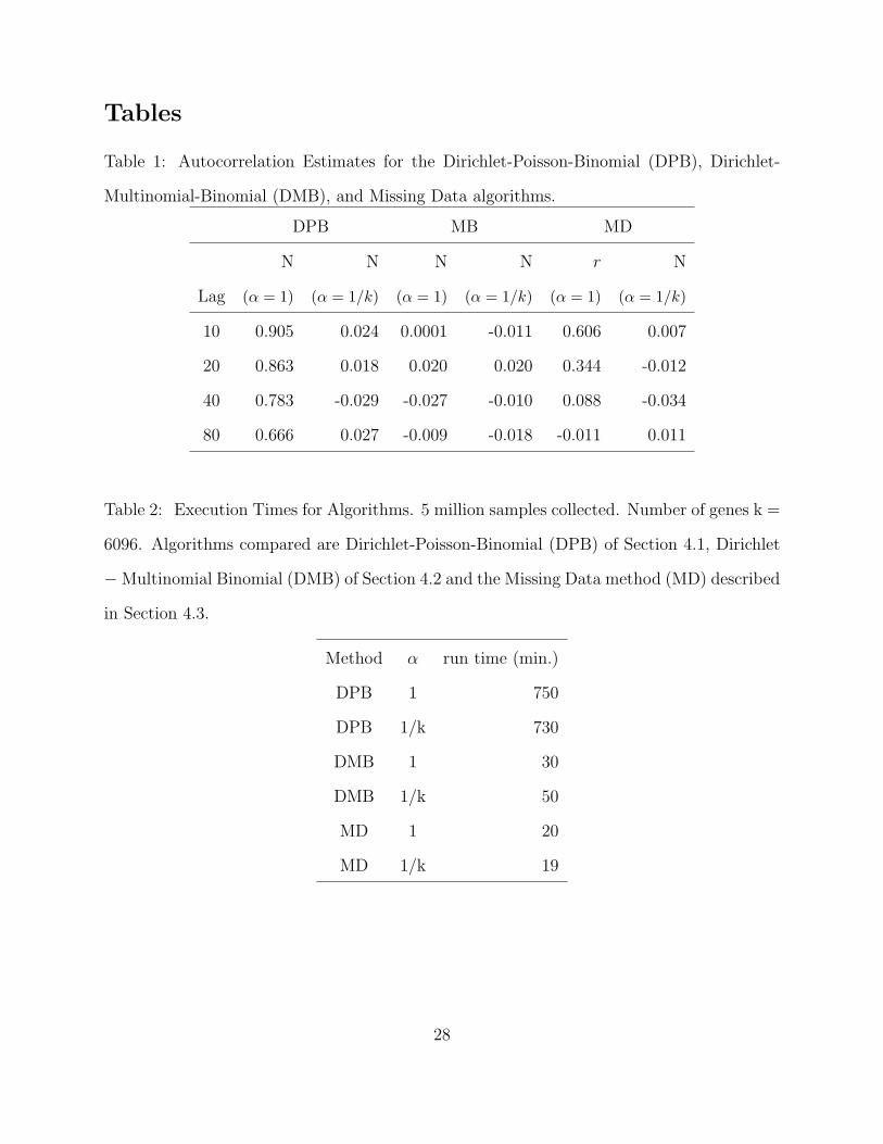
at various lags. Table 1 examines correlations among samples for different lags and suggests

that for inference on proportions mi, autocorrelations are very low between samples with

lags as small as 10. Conversely, correlations, for sample size N are extremely high leading

to much less reliable inference.

In practice, if only the vector m is of interest, far fewer samples are needed which would

significantly speed up the algorithm. Physical timings for runs of these and other algorithms

are given in Table 2. These show that as executed, this algorithm required about 11-12 hours

to run. If only every 10th sample were collected, 50,000 total samples, the algorithm would

have required approximately 1 hour.

In order to understand the behavior of the proportions, we compared various estimates of

the mi. These include posterior means from the Gibbs sampler, standard MLE’s, corrected

MLE’s based on Formula 4, and analytically derived posterior modes from Gilchrist et al.

(2007). In addition, 95% posterior credible regions are also computed. Figure 2 plots the

above quantities versus rank for the 20 genes with largest tag counts. Rank 1 corresponds

to the most frequent gene and the prior used is α = 1 . As one would expect, the corrected

MLE and the posterior mode coincide perfectly in this case. Both posterior means and

posterior modes based on the biased sampling correction deviate strongly from the standard

16

MLE for many of the most frequently tagged genes. Posterior modes and means follow

nearly identical trends with the modal estimates being uniformly larger. As one can see,

modal estimates typically lie slightly above the 97.5th percentile of the simulated posterior

distribution in this case.

Figure 3 summarizes results when each αi = 1/k. This parametrization corresponds to

a U-shaped prior distribution. Here one can see the ith corrected MLE and posterior mean

now coincide almost perfectly while the posterior mode lies at or above the 97.5th percentile

of posterior samples. Again, all estimators deviate significantly from the unadjusted MLE’s.

Due to the similarity of the corrected MLE and posterior mean, it is tempting to interpret

the posterior intervals as frequentist confidence intervals. To date, no work has been done

to verify the frequentist coverage properties of these intervals.

For inferential purposes, the posterior mean vector and both joint and marginal intervals

can be derived from the Monte Carlo samples. However, as discussed below in Section 5, it

may be useful to compute the joint posterior mode for use as an estimator. For example,

the posterior mode reduces to the MLE when the parameter αi = 1 for all i. A second

advantage of this model is that the joint mean can be computed through the Lindley-Smith

maximization method (Lindley, D. V. & Smith, A. F. M., 1972; Chen et al., 2000).

Lindley and Smith proved that an algorithm that iteratively maximized each of the full

conditional distributions will eventually converge to the global maximum of the posterior.

Because each of the conditionals in this model has a closed form expression for its maximum,

this optimization approach is both simple and extremely fast. Similar to Gibbs sampling,

this procedure starts from an arbitrary point. Maximization proceeds by iterating across the

full set of conditional distributions, maximizing each and substituting the maximum into

the next conditional. The hierarchical model considered here is not identical to eq. (3), but

depends upon hyperparameters (γ1, γ2) which effect the mode of the posterior distribution.

One possibility for choosing these hyper-parameters is to pick them to minimize the distance

17

between analytical mode and iteratively computed mode.

Algorithm 1: Dirichlet-Poisson-Binomial posterior mode estimation via the Lindley-Smith algorithm

//InitializationSet the initial values γ1, γ2,N,m0,g.//Main loop

while∑|mnew

i −mi| > 10−5 domnewi = max[π(mi|ti, gi, N,φ,α, γ1, γ2] = (gi + α)/(N)

gnewi = max[π(gi|T,m, N,φ,α, γ1, γ2] = ti + floor(Nmi(1− φi))Nnew = max[π(N |T,g,m,φ,α, γ1, γ2] = (

∑gi + γ1)/(1 + γ2)

end

4.2 A Dirichlet-Multinomial-Binomial Approach.

A second approach is both more computationally efficient and arguably more directly compa-

rable to the sampling mechanism inherent in SAGE. For convenience, we begin by assuming

that the total number of mRNA in the sample is N ∼ Pois(λ). Given this mRNA popula-

tion size, the vector g of counts of each category of mRNA prior to tag formation follows a

multinomial distribution,

[g|α] ∼(

N

g1, g2, . . . , gk

)mg1

1 mg22 , . . . ,m

gk

k

whose probabilities are the mi and are assumed to follow a Dirichlet distribution with pa-

rameter vector α.

The joint posterior distribution can now be written as,

[m,g, N |T,α, γ1, γ2] ∝k∏i=1

(giti

)φtii (1− φi)gi−ti e

−λλN

N !

×(

N

g1, g2, . . . , gk

)mg1+α1−1

1 mg2+α2−12 , . . . ,mgk+αk−1

k .

18

Reminding readers that φ = (φ1, φ2, . . . , φk) be the vector of known gene dependent

tagging probabilities, the full conditional distributions here are,

[T|ti, gi, N, γ1, γ2] ∼ Dirichlet(α +G)

[g|T,m, N,α, γ1, γ2] ∼ ti +Multinom(N − Tt,m ∗ (1− φ))

[N |T,g,m,α, γ1, γ2] ∼ Γ(Ttot + γ2, 1 + γ1)

where m ∗ (1 − φ) is an element wise product with 1 representing a vector of identical

dimension to m. Hence, the ith element of the vector is given by mi(1− φi).

We refer to this hierarchical model as the Dirichlet-Multinomial-Binomial (DMB) model.

Inference in this case is much faster because the entire m vector can be updated at once

instead of requiring separate updates for each gene level i. This formulation is also more

natural in the sense that it restricts the pre-tagging counts to sum to the population total

N . One drawback is that the observed data provides no information for posterior inference

about the population size N . A minor drawback of this approach is that it is more difficult

to perform a Lindley - Smith maximization to derive the mode. Maximizing the conditional

distribution of g, the vector of mRNA counts, would require maximizing a multinomial

distribution over the discrete counts.

Experimental testing of this algorithm provided results similar to the first procedure.

Five-million variates were drawn with every hundredth stored. The DMB algorithm was

dramatically faster than the DPB approach finishing simulation in just over 30 minutes.

Table 1 shows little if any correlation at any lag. For sample size N , this is to be expected

since the conditional distributions depend only on the data and hyperparameters which are

fixed. We conclude that the algorithm could be accelerated without loss of accuracy by

reducing the number of simulations. Inference was based on the final 1000 stored samples.

Figure 4 below displays inferential results from this model for the 20 most frequently tagged

19

genes ranked from largest to smallest. Behavior and trends are almost identical to the DPB

model. For the case where all αi = 1, the posterior mean was systematically smaller than

the posterior-mode/MLE for cases with large tag counts. The posterior-mode was distinctly

different than the unadjusted tag proportions and both sets were above the upper credible

bounds for the posterior mean. In the case where all αi = 1/k, the posterior-mean again

matches the corrected MLE almost exactly. The posterior mode tracks the mean closely but

is always larger and the unadjusted proportions are usually outside the credible region.

4.3 A Missing Data Approach.

Instead of renormalizing the probabilities θi = (miφi)/(∑miφi) and doing inference based

on the posterior of eq. (5), a second more straightforward approach uses missing data.

Considering again a data generation process as described in section 3.2, we augment

the observed data vector T with an extra category which represents any cDNA that is not

converted to a SAGE tag. This count is not observed, but if a distribution such as a Poisson

is proposed, we may consider a Bayesian approach. The resulting posterior distribution for

the data is,

[m|T,α] ∝ (1−k∑i=1

miφi)r

k∏i=1

(miφi)ti+αi−1

where we have assumed a Dirichlet prior on the unknown initial proportions m ∼ Dk(α1, . . . , αk)

. The resulting posterior distribution is a Dirichlet distribution with k + 1 categories, com-

pared with the k categories in the initial distribution m. In particular the distribution is a

Dk+1(t1 + α1, . . . , tk + αk, r + 1).

By integrating over the missing data term or otherwise eliminating it, it is possible to

sample from the joint distribution whose success probability is miφi. According to the

marginalization property of the Dirichlet (Bilodeau & Brenner, 1999) the distribution of any

subset of variables (θi1 , θi2 , . . . , θij ) from a Dk(α1, α2, . . . , αk) with∑αi = p is distributed

20

Dj+1(αi1 , αi2 , . . . , αij , q). Here q = p −∑j

i=1 αij corresponds to the total of the variables

being marginalized over. In words, by considering only a subset of j categories we observe a

Dirichlet distribution on j+1 categories with∑

i αi = p remaining the same. In our case, the

value of r will be a component of the parameter q. Several modes of inference are available

based on this missing data approach. Suppose first that we are particularly interested in

the posterior means of the mi parameters. An exact calculation is possible based upon the

marginalization properties of the Dirichlet (Bilodeau & Brenner, 1999, Corollary 3.4).

Theorem 4.1 Let θ = (θ1, . . . , θp, θp+1) ∼ Dirichlet(α1, . . . , αp, αp+1). Let α0 =∑p+1

i=1 αi.

Suppose that S =∑p

i=1 θi, and for j < p, let θ1 = (θi1, . . . , θij) be any subset of components

of θ. It follows that δ1 = θ1/S ∼ Dirichlet(αi1, . . . , αij, δ) with α0 − αp+1 = δ +∑j

d=1 αid

This result demonstrates that, ignoring the missing categories, the distribution of the

(m1φ1, . . . ,mk−1φk−1,mkφk)∑k1 miφi

∼ Dirichlet(α1 + t1, . . . , αk−1 + tk−1, δ),

with δ = tk + αk. Let wi = (αi + ti)/∑

(αi + ti). Then by reweighting, we can compute,

E(mi) =1

φi∑

iwi

αi + ti∑(αi + ti)

.

More generally, Gibbs sampling is also available for this problem and extends inference

to Bayesian interval estimates. Again observing the posterior distribution,

[m, r|T, µ] ∝ (1−k∑i=1

miφi)r

k∏i=1

(miφi)ti+αi−1 e

−µµr

r!(6)

21

The full conditional distributions are derived to be,

[r|T,m,α,µ] = Poisson((1−∑

miφi)µ)

[mφ|T, r,φ,α,µ] = D(r, α1 + t1, . . . , αk + tk)

In order to apply Gibbs Sampler a value for the hyperparameter µ must be selected. In the

case where all αi = 1, a logical mean for the Poisson is Ttot∑

imi(1 − φi)/∑

imiφi since∑mi(1 − φi) = 1 −

∑miφi is the probability that an mRNA is not converted into a tag.

Equation 4 provides a useful estimate of∑miφi.

Like the DPB algorithm above, the missing data algorithm also admits a simple Lindley-

Smith optimization procedure in order to compute the posterior mode. If the prior mean of

r, µ = 10, 100 then the posterior mode of the missing data model is nearly identical to the

exact analytical mode. The mode of the Dirichlet conditional is

m̂iφi =ti + αi − 1∑

i(αi + ti) + r − k, (7)

see Gelman et al. (2005). The mode for the Poisson is the mean rounded down to the nearest

smaller integer (Wikipedia, 2007). Results for this case are very similar to the previous

two. This algorithm is clearly the fastest, completing 5 million samples in 20 minutes.

Autocorrelation in the untagged population size r decreases to 0 after 50 simulations but

proportions mi seem uncorrelated at all lags. Conclusions for Figures 6 and 7 are largely

identical to the above. In fact, as implemented quantitative differences do exist between the

methods in the case where all αi = 1 with this method providing the smallest or most heavily

shrunk estimates of genes with large counts and the DPB method giving the largest estimates.

Because probabilities must sum to one, the opposite effect should exist for categories with

22

small counts although the mass will be spread over thousands of categories leading to very

minute differences.

5 Conclusions

Sampling bias is a ubiquitous problem in studying biological problems. This work focuses

on a general biasing mechanism of which data generation from in SAGE is a protype. We

present three hierarchical models which provide posterior inference for the biased sampling

model given in eq. (3). This work compliments earlier work by Gilchrist et al. (2007) in

two notable ways. First, it provides a flexible and efficient methodology which extends the

range of the prior distributions that are available. It is important to point out the effect

of the typical flat prior α = 1 on inference: analogously to the binomial case (Christensen,

1997), this prior assumes that each category was seen once in previous experiments, a very

strong assumption due to the small size of the tag sample compared to the number of

categories. The result is that the prior overwhelms the data for many of the categories. In

the context of SAGE, it may be more appealing to the scientist to choose a weaker prior such

as α = 1/k, which, as we’ve seen, gives the actual data more voice. Because the analytical

approximations of Gilchrist et al. (2007) do not extend easily to this regime of priors, the

simulation based results presented here are increasingly valuable. Second, the more robust

methodology presented here provides a foundation for extending the analysis to include

more realistic models of the tag formation process (such as the inclusion of transcription or

sequencing errors) or more complex priors.

Our approach may be contrasted with Morris et al. (2003), who investigated joint estima-

tors of the relative proportions of different mRNA transcripts in SAGE experiments based on

posterior inference from a conjugate Dirichlet-Multinomial model. They note that while the

shrinkage properties of the posterior mean provide improved average inference with respect

23

to squared error loss across all categories, they tend to shrink categories where large counts

are observed excessively in order to boost the estimated probabilities of cells with few or no

counts. Due to the massive number of categories and the extreme imbalance in observed

frequencies (e.g. more than half of the categories have zero counts in our data), the estimates

for frequently observed genes tend to be fairly poor. This observation highlights the main

weakness of shrinkage estimators, while they perform better on average across categories,

they may perform poorly on particular categories which may be of primary interest. Morris

et al. (2003) resolve the problem by introducing a hierarchical Dirichlet-Multinomial model

which clusters genes into two categories, high and low frequency, partitioning the overall

mass in order to mitigate the shrinkage in the high frequency categories.

Our contribution is clearly distinct from that of Morris et al. (2003) since it focuses on

a discrepancy in the sampling model. Nevertheless, it should be possible to extend our

methods to allow for the mixture priors used by Morris et al. (2003). Even without such

an extension, our results offer alternative methods and important insights into shrinkage

in models with large or massive numbers of categories. For example, we’ve shown that by

using the prior α = 1/k, the posterior mean is equal to the corrected MLE. The additional

advantage of a sampling model is that it generates marginal posterior credible sets for the

proportion mi. If inference focuses only on genes with large expression levels, we gain one of

the main advantages of Monte Carlo sampling without the concern of excessive shrinkage.

If one is only interested in point estimates, and excessive shrinkage is a concern, it may also

be appropriate to use the analytical mode as an estimator. For example, the posterior mode

for model 5 is identical to the MLE for model 3 when α = 1 , while the posterior mean

becomes equivalent when α = 1/k. Given the stated hyper-parameters, posterior means are

shrunk for more frequently observed categories and increased for rarely observed categories.

The models provide different levels of shrinkage, with the Dirichlet-Poisson-Binomial (DPB)

model providing the least, and the missing data model providing the most shrinkage. In

24

terms of computation time, the DPB method is much less efficient and arguably offers no

advantage over the other methods for SAGE. However, in other applications the DPB model

may be closer to the model of interest.

A number of important statistical questions remain to be answered. Besides the sampling

errors dealt with here, there are other sources of errors inherent in SAGE’s tag formation and

sampling processes (Stollberg et al., 2000), which future work could address. This analysis

also presumed that the category dependent sampling probabilities were fixed when in fact

they were estimated from the data. A model that views φ as a random quantity would also

represent an improvement. Finally, a major emphasis of SAGE analysis regards evaluation

of differential expression levels (Baggerly et al., 2003, 2004) between related cell samples.

Because the AE cutting probability p is experiment dependent (Gilchrist et al., 2007), it is

important that the biasing mechanism be taken into account when evaluating differential

expression across experiments. Indeed, this should lead to increased power and accuracy in

such studies.

References

Akmaev, V. R., & Wang, C. J.(2004). Correction of sequence-based artifacts in serial analysis

of gene expression. Bioinformatics, 20, 1254-1263.

Arnold, S. F.(1993). Handbook of statistics. In C. Rao (Ed.), (Vol. 9, p. 599-625). Elsevier

Science.

Baggerly, K. A., Deng, L., Morris, J. S., & Aldaz, C.(2004). Overdispersed logistic regression

for SAGE: Modelling multiple groups and covariates. BMC Bioinformatics, 5, 144.

Baggerly, K. A., Deng, L., Morris, J. S., & Aldaz, C. M. (2003). Differential expression in

SAGE: accounting for normal between-library variation. Bioinformatics, 19, 1477-1483.

25

Beissbarth, T., Hyde, L., Smyth, G. K., Job, C., Boon, W.-M., Tan, S.-S., et al. (2004).

Statistical modeling of sequencing errors in SAGE libraries. Bioinformatics, 20 Suppl

1 (NIL), I31-I39.

Bilodeau, M., & Brenner, D.(1999). Theory of multivariate statistics. New York: Springer.

Chen, M.-H., Shao, Q.-M., & Ibrahim, J. G. (2000). Monte carlo methods in bayesian

computation.

Christensen, R. (1997). Log-linear models and logistic regression (2 ed.). New York, USA:

Springer Verlag.

Colinge, J., & Feger, G. (2001). Detecting the impact of sequencing errors on SAGE data.

Bioinformatics, 17, 840-842.

Gelman, A., Carlin, B., Stern, H., & Rubin, D. (2005). Bayesian data analysis (2 ed.).

Chapman and Hall.

Ghosh, J. K., Delampady, M., & Samanta, T. (2006). An introduction to bayesian analysis.

New York: Springer.

Gilchrist, M., Qin, H., & Zaretzki, R. (2007, In Press). Modeling SAGE tag formation and

its effects on data interpretation within a Bayesian framework. (In Press)

Kuznetsov, V. A.(2006). Statistical methods in serial analysis of gene expression(SAGE). In

W. Zhang & I. Shmulevich (Eds.), Computational and statistical approaches to genomics

(p. 163-2008). New York: Springer Verlag. (2nd Edition)

Kuznetsov, V. A., Knott, G. D., & Bonner, R. F. (2002). General Statistics of Stochastic

Process of Gene Expression in Eukaryotic Cells. Genetics, 161 (3), 1321-1332.

26

Lindley, D. V., & Smith, A. F. M. (1972). Bayes estimates for the linear model. Journal of

the Royal Statistical Society. Series B (Methodological), 34.

Matsumura, H., Bin Nasir, K. H., Yoshida, K., Ito, A., Kahl, G., Kruger, D. H., et al.(2006).

SuperSAGE array: the direct use of 26-base-pair transcript tags in oligonucleotide arrays.

Nature Methods, 3, 469-474.

Matsumura, H., Reich, S., Ito, A., Saitoh, H., Kamoun, S., Winter, P., et al. (2003). Gene

expression analysis of plant host-pathogen interactions by SuperSAGE. Proceedings of the

National Academy of Sciences, 100 (26), 15718-15723.

Morris, J. S., Baggerly, K. A., & Coombes, K. R. (2003). Bayesian shrinkage estimation of

the relative abundance of mRNA transcripts using SAGE. Biometrics, 59, 476-486.

Stollberg, J., Urschitz, J., Urban, Z., & Boyd, C. D. (2000). A quantitative evaluation of

SAGE. Genome Research, 10, 1241-1248.

Thygesen, H. H., & Zwinderman, A. H.(2006). Modeling Sage data with a truncated gamma-

Poisson model. BMC Bioinformatics, 7, 157.

Velculescu, V. E., Zhang, L., Vogelstein, B., & Kinzler, K. W. (1995). Serial Analysis of

Gene Expression. Science, 270 (5235), 484-487.

Velculescu, V. E., Zhang, L., Zhou, W., Vogelstein, J., Basrai, M. A., Bassett, J., D E, et

al. (1997). Characterization of the yeast transcriptome. Cell, 88, 243-251.

Vencio, R. Z. N., & Brentani, H. (2006). Statistical methods in serial analysis of gene

expression(sage). In W. Zhang & I. Shmulevich (Eds.), Computational and statistical

approaches to genomics (p. 209-233). New York: Springer Verlag. (2nd Edition)

Wikipedia.(2007). Poisson distribution. ([Online; accessed 25-Oct 2007])

27

Tables

Table 1: Autocorrelation Estimates for the Dirichlet-Poisson-Binomial (DPB), Dirichlet-

Multinomial-Binomial (DMB), and Missing Data algorithms.

DPB MB MD

N N N N r N

Lag (α = 1) (α = 1/k) (α = 1) (α = 1/k) (α = 1) (α = 1/k)

10 0.905 0.024 0.0001 -0.011 0.606 0.007

20 0.863 0.018 0.020 0.020 0.344 -0.012

40 0.783 -0.029 -0.027 -0.010 0.088 -0.034

80 0.666 0.027 -0.009 -0.018 -0.011 0.011

Table 2: Execution Times for Algorithms. 5 million samples collected. Number of genes k =

6096. Algorithms compared are Dirichlet-Poisson-Binomial (DPB) of Section 4.1, Dirichlet

−Multinomial Binomial (DMB) of Section 4.2 and the Missing Data method (MD) described

in Section 4.3.

Method α run time (min.)

DPB 1 750

DPB 1/k 730

DMB 1 30

DMB 1/k 50

MD 1 20

MD 1/k 19

28

Figure Captions

Figure 1. Plot showing cDNA cleavage sites for SAGE with associated probabilities of tag

formation.

Figure 2. Probability estimates and inferences for the Dirichlet -Poisson -Binomial with

each αi = 1. The 20 genes with the largest tag counts are arranged in decreasing rank order

along the X-axis. The observed tag proportions are marked in dark circles, the standard

MLE in dark triangles. The analytically computed posterior mode αi = 1 coincides exactly

with the MLE. Also included are the estimated posterior mean and upper and lower 95%

Bayesian Credible bounds based on MCMC sampling.

Figure 3. Probability estimates and inferences for the Dirichlet -Poisson -Binomial with each

αi = 1/k. The 20 genes with the largest tag counts are arranged in decreasing rank order

along the X-axis. The observed tag proportions are marked in dark circles, the standard MLE

in dark triangles. In this case analytically derived posterior modes deviate substantially from

MLE. However, estimated posterior mean is identical to MLE in this case. Upper and lower

95% Bayesian Credible bounds are also given.

Figure 4. Probability estimates for the Dirichlet -Multinomial -Binomial where all αi = 1.

The 20 genes with the largest tag counts are arranged in decreasing rank order along the

X-axis. The observed tag proportions are marked in dark circles, the standard MLE in dark

triangles. The analytically computed posterior mode αi = 1 coincides exactly with the MLE.

Also included are the estimated posterior mean and upper and lower 95% Bayesian Credible

bounds based on MCMC sampling.

29

Figure 5. Probability estimates for the Dirichlet -Multinomial -Binomial model with all

αi = 1/k. The 20 genes with the largest tag counts are arranged in decreasing rank order

along the X-axis. The observed tag proportions are marked in dark circles, the standard MLE

in dark triangles. In this case analytically derived posterior modes deviate substantially from

MLE. However, estimated posterior mean is identical to MLE in this case. Upper and lower

95% Bayesian Credible bounds are also given.

Figure 6. Probability estimates for the Missing Data Algorithm where all αi = 1. The

20 genes with the largest tag counts are arranged in decreasing rank order along the X-

axis. The observed tag proportions are marked in dark circles, the standard MLE in dark

triangles. The analytically computed posterior mode αi = 1 coincides exactly with the MLE.

Also included are the estimated posterior mean and upper and lower 95% Bayesian Credible

bounds based on MCMC sampling.

Figure 7. Probability estimates for the Missing Data Algorithm where αi = 1/k. The 20

genes with the largest tag counts are arranged in decreasing rank order along the X-axis. The

observed tag proportions are marked in dark circles, the standard MLE in dark triangles.

In this case analytically derived posterior modes deviate substantially from MLE. However,

estimated posterior mean is identical to MLE in this case. Upper and lower 95% Bayesian

Credible bounds are also given.

30

Figures

Figure 1: Plot showing cDNA cleavage sites for SAGE with associated probabilities of tag

formation.

31

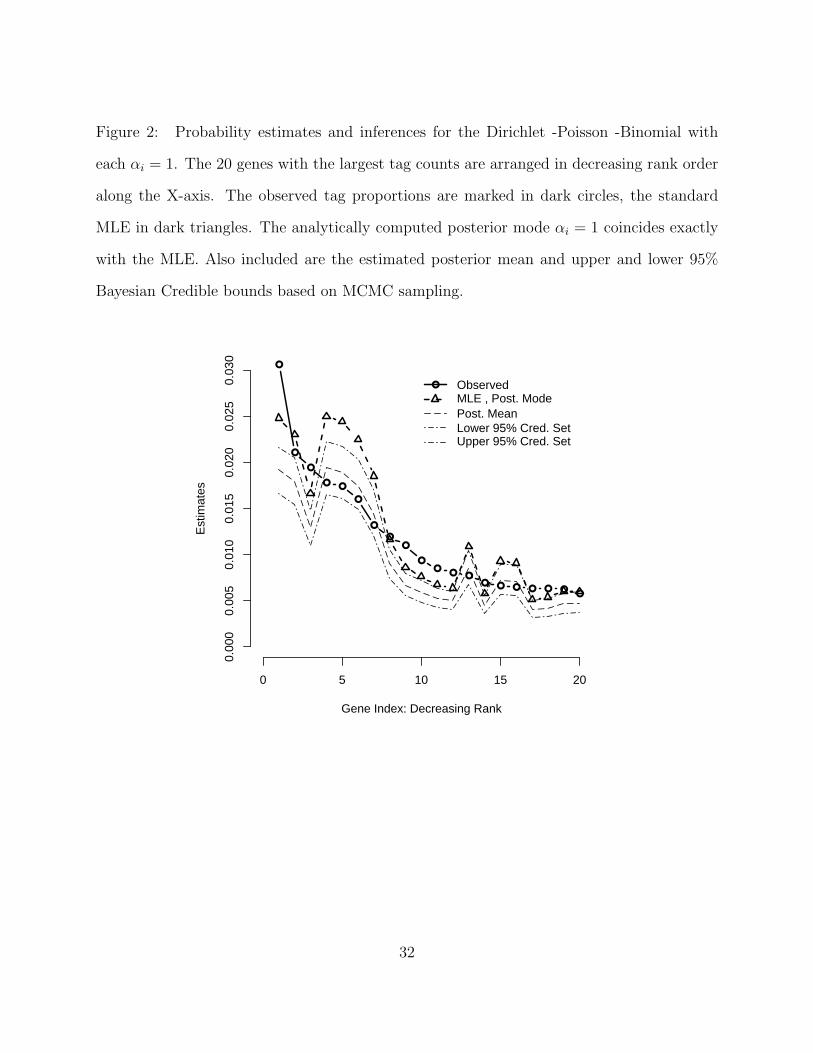
Figure 2: Probability estimates and inferences for the Dirichlet -Poisson -Binomial with

each αi = 1. The 20 genes with the largest tag counts are arranged in decreasing rank order

along the X-axis. The observed tag proportions are marked in dark circles, the standard

MLE in dark triangles. The analytically computed posterior mode αi = 1 coincides exactly

with the MLE. Also included are the estimated posterior mean and upper and lower 95%

Bayesian Credible bounds based on MCMC sampling.

●

●

●

●●

●

●

●●

●●

● ●● ● ● ● ● ●

●

Gene Index: Decreasing Rank

Est

imat

es

0 5 10 15 20

0.00

00.

005

0.01

00.

015

0.02

00.

025

0.03

0

● ObservedMLE , Post. ModePost. MeanLower 95% Cred. SetUpper 95% Cred. Set

32

Figure 3: Probability estimates and inferences for the Dirichlet -Poisson -Binomial with each

αi = 1/k. The 20 genes with the largest tag counts are arranged in decreasing rank order

along the X-axis. The observed tag proportions are marked in dark circles, the standard MLE

in dark triangles. In this case analytically derived posterior modes deviate substantially from

MLE. However, estimated posterior mean is identical to MLE in this case. Upper and lower

95% Bayesian Credible bounds are also given.

●

●

●

● ●

●

●●

●

●● ● ●

● ● ● ● ● ● ●

Gene Index: Decreasing Rank

Est

imat

es

0 5 10 15 20

0.00

0.01

0.02

0.03

0.04

● ObservedMLE, Post.MeanPost. ModeLower 95% Cred. SetUpper 95% Cred. Set

33

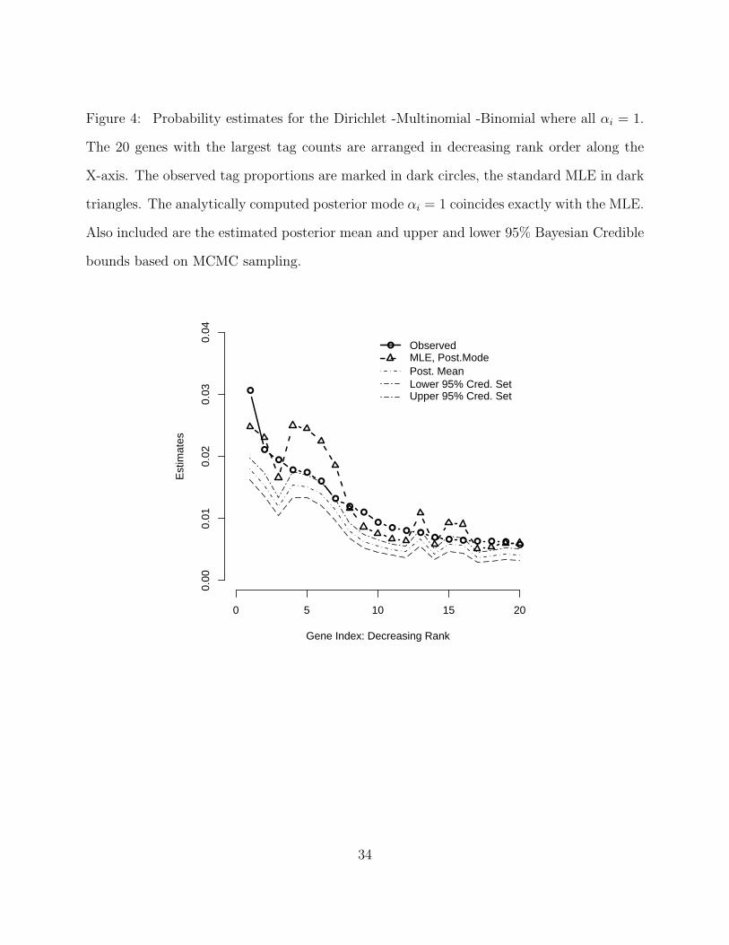
Figure 4: Probability estimates for the Dirichlet -Multinomial -Binomial where all αi = 1.

The 20 genes with the largest tag counts are arranged in decreasing rank order along the

X-axis. The observed tag proportions are marked in dark circles, the standard MLE in dark

triangles. The analytically computed posterior mode αi = 1 coincides exactly with the MLE.

Also included are the estimated posterior mean and upper and lower 95% Bayesian Credible

bounds based on MCMC sampling.

●

●

●

● ●

●

●●

●

●● ● ●

● ● ● ● ● ● ●

Gene Index: Decreasing Rank

Est

imat

es

0 5 10 15 20

0.00

0.01

0.02

0.03

0.04

● ObservedMLE, Post.ModePost. MeanLower 95% Cred. SetUpper 95% Cred. Set

34

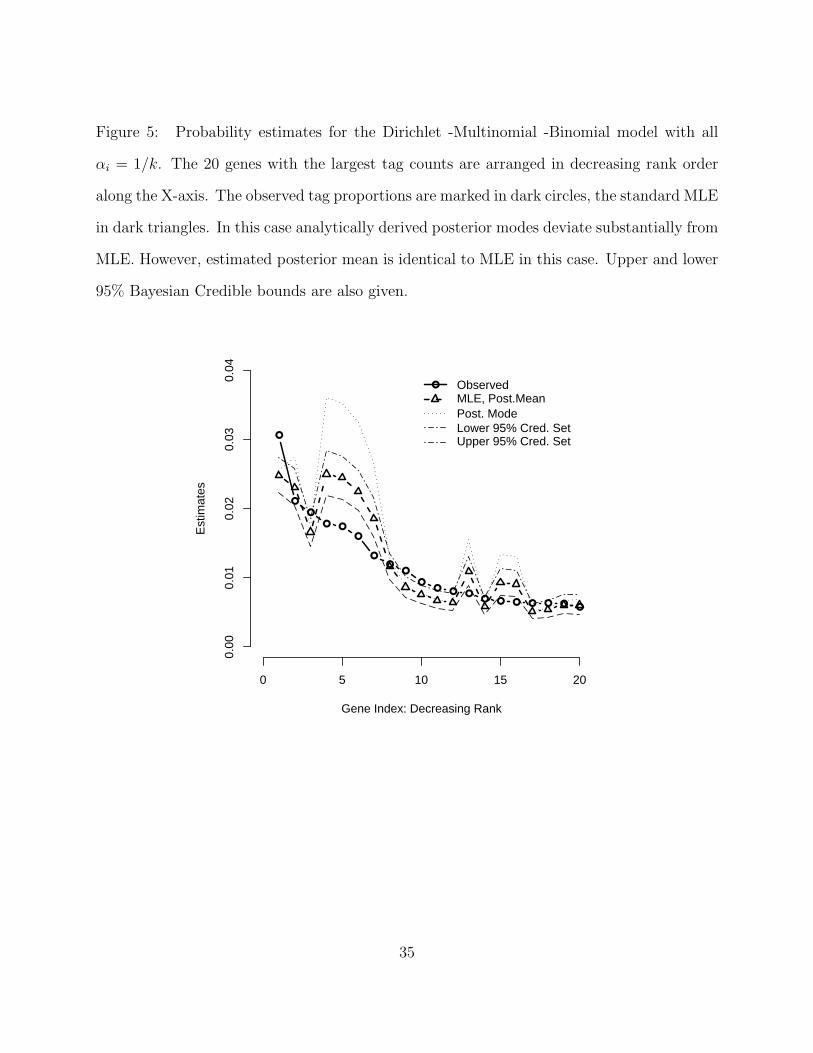
Figure 5: Probability estimates for the Dirichlet -Multinomial -Binomial model with all

αi = 1/k. The 20 genes with the largest tag counts are arranged in decreasing rank order

along the X-axis. The observed tag proportions are marked in dark circles, the standard MLE

in dark triangles. In this case analytically derived posterior modes deviate substantially from

MLE. However, estimated posterior mean is identical to MLE in this case. Upper and lower

95% Bayesian Credible bounds are also given.

●

●

●

● ●

●

●●

●

●● ● ●

● ● ● ● ● ● ●

Gene Index: Decreasing Rank

Est

imat

es

0 5 10 15 20

0.00

0.01

0.02

0.03

0.04

● ObservedMLE, Post.MeanPost. ModeLower 95% Cred. SetUpper 95% Cred. Set

35

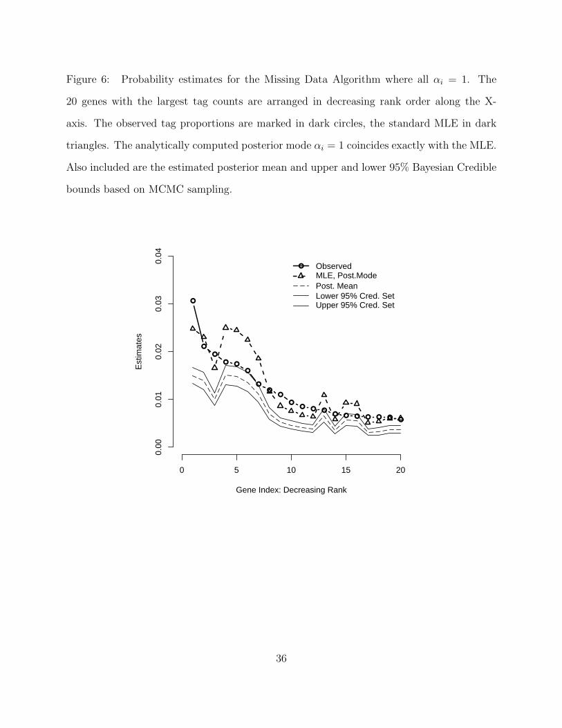
Figure 6: Probability estimates for the Missing Data Algorithm where all αi = 1. The

20 genes with the largest tag counts are arranged in decreasing rank order along the X-

axis. The observed tag proportions are marked in dark circles, the standard MLE in dark

triangles. The analytically computed posterior mode αi = 1 coincides exactly with the MLE.

Also included are the estimated posterior mean and upper and lower 95% Bayesian Credible

bounds based on MCMC sampling.

●

●

●

● ●

●

●●

●

●● ● ●

● ● ● ● ● ● ●

Gene Index: Decreasing Rank

Est

imat

es

0 5 10 15 20

0.00

0.01

0.02

0.03

0.04

● ObservedMLE, Post.ModePost. MeanLower 95% Cred. SetUpper 95% Cred. Set

36

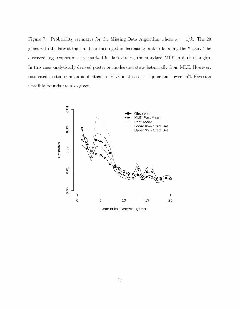
Figure 7: Probability estimates for the Missing Data Algorithm where αi = 1/k. The 20

genes with the largest tag counts are arranged in decreasing rank order along the X-axis. The

observed tag proportions are marked in dark circles, the standard MLE in dark triangles.

In this case analytically derived posterior modes deviate substantially from MLE. However,

estimated posterior mean is identical to MLE in this case. Upper and lower 95% Bayesian

Credible bounds are also given.

●

●

●

● ●

●

●●

●

●● ● ●

● ● ● ● ● ● ●

Gene Index: Decreasing Rank

Est

imat

es

0 5 10 15 20

0.00

0.01

0.02

0.03

0.04

● ObservedMLE, Post.MeanPost. ModeLower 95% Cred. SetUpper 95% Cred. Set

37