Mathematical Modelling of a Small Biomass Gasifier for ...
191
Northumbria Research Link Citation: Mbikan, Atainu (2019) Mathematical modelling of a small biomass gasifier for synthesis gas production. Doctoral thesis, Northumbria University. This version was downloaded from Northumbria Research Link: http://nrl.northumbria.ac.uk/id/eprint/42812/ Northumbria University has developed Northumbria Research Link (NRL) to enable users to access the University’s research output. Copyright © and moral rights for items on NRL are retained by the individual author(s) and/or other copyright owners. Single copies of full items can be reproduced, displayed or performed, and given to third parties in any format or medium for personal research or study, educational, or not-for-profit purposes without prior permission or charge, provided the authors, title and full bibliographic details are given, as well as a hyperlink and/or URL to the original metadata page. The content must not be changed in any way. Full items must not be sold commercially in any format or medium without formal permission of the copyright holder. The full policy is available online: http://nrl.northumbria.ac.uk/policies.html
-
Upload
khangminh22 -
Category
Documents
-
view
1 -
download
0
Transcript of Mathematical Modelling of a Small Biomass Gasifier for ...
Northumbria Research Link
Citation: Mbikan, Atainu (2019) Mathematical modelling of a small biomass gasifier forsynthesis gas production. Doctoral thesis, Northumbria University.
This version was downloaded from Northumbria Research Link:http://nrl.northumbria.ac.uk/id/eprint/42812/
Northumbria University has developed Northumbria Research Link (NRL) to enable usersto access the University’s research output. Copyright © and moral rights for items onNRL are retained by the individual author(s) and/or other copyright owners. Single copiesof full items can be reproduced, displayed or performed, and given to third parties in anyformat or medium for personal research or study, educational, or not-for-profit purposeswithout prior permission or charge, provided the authors, title and full bibliographicdetails are given, as well as a hyperlink and/or URL to the original metadata page. Thecontent must not be changed in any way. Full items must not be sold commercially in anyformat or medium without formal permission of the copyright holder. The full policy isavailable online: http://nrl.northumbria.ac.uk/policies.html
Mathematical Modelling of a Small
Biomass Gasifier for Synthesis Gas
Production
Atainu Ernest Mbikan
A thesis submitted in partial fulfilment of the
requirements of the University of Northumbria at
Newcastle for the award of Doctor of Philosophy
Research undertaken in the Mechanical and
Construction Engineering Department of the
Faculty of Engineering and Environment
March 2019
i
Abstract
The depletion of fossil fuels coupled with the growing demands of the world energy
has ignited the interest for renewable energies including biomass for energy
production. A reliable affordable and clean energy supply is of major importance to
the environment and economy of the society. In this context, modern use of biomass
is considered a promising clean energy alternative for the reduction of greenhouse gas
emissions and energy dependency. The use of biomass as a renewable energy source
for industrial application has increased over the last decade and is now considered as
one of the most promising renewable sources. The direct combustion of biomass in
small scales often results in incomplete and inconsistent burning process which could
produce carbon monoxide, particulates and other pollutants. Therefore, biomass is
required to be transformed into more easily handled fuel such as gases, liquids and
charcoal using technologies such as pyrolysis, gasification, fermentation, digestion etc.
Biomass gasification upon which this thesis focuses is one of the promising routes
amongst the renewable energy options for future deployment. Gasification is a process
of conversion of solid biomass into combustible gas, known as producer gas by partial
oxidation.
This research work is carried out to investigate various methods employed for
modelling biomass gasifiers, it also studies the chemistry of gasification and reviews
various gasification models. In this work, a mathematical model is developed to
simulate the behaviour of downdraft gasifiers operating under steady state and
determine the synthesis gas composition. The model distinctly analyses the processes
in each of the three zones of the gasifier; pyrolysis, oxidation and reduction zones. Air
is used as the gasifying agent and is introduced into the pyrolysis and oxidation zones
of the gasifier for both single and double air operations. These zones have been
modelled based on thermodynamic equilibrium and kinetic modelling; the model
equations are solved in MATLAB. Given the biomass properties, consumption, air
input, moisture content and gasifier specifications, the MATLAB model is able to
accurately predict the temperature and distribution of the molar concentrations of the
synthesis gas constituents. The downdraft gasifier is also represented in Aspen HYSYS
based on the same models to study the effect of both single and double air gasification
operation. For known biomass properties, consumption, air input, moisture content and
ii
gasifier operating conditions, the Aspen HYSYS model can accurately predict the
distributions of the molar concentrations of the syngas constituents (CO, CO2, H2, CH4,
and N2). The models were validated by comparing obtained theoretical results with
experimental data published in the open literature. Parametric studies were carried out
to study the effects of equivalence ratio, moisture content, temperature on the gas
compositions and its energy content. The proposed equilibrium model displayed a
variable ability for the prediction of various product yields with this being a function
of the feedstock studied. It also demonstrated the ability to predict product gases from
various biomasses using both single and double stage air input. In the case of
gasification with double air stage supply, higher amounts of methane are obtained with
specific tendencies of the gases reaching a peak at certain conditions. The kinetic model
was partially successful in predicting results and comparable with experimentally
published results for a range of conditions. There were discrepancies particularly with
CH4 formation and the operating temperatures predictions which were usually
consistently lower than those actually measured experimentally. The use of the PFR,
however, did show a greater potential for the use in further modelling.
iii
Declaration
I declare that the work contained in this thesis has not been submitted for any other
award and it is all my own work. I also confirm that this work fully acknowledges the
ideas, opinions and contributions from the work of others.
Word count of main body of Thesis:
Name: Atainu Ernest Mbikan
Signature:
Date: March 2019

iv
Acknowledgement
I wish to express my sincere appreciation and gratitude to my supervisor Prof. Khamid
Mahkamov whose support and guidance have been immensely invaluable all through
this study.
I will also like to thank Dr Dave Pritchard for his assistance. My thanks also go to my
friends; Joshua Benamaisia, Ayodeji Sowale and others for all their various support.
Finally, I will like to give special thanks to my parents Chief Ernest Duke and Mrs
Mabel Mbikan and to all my siblings Mr Eneile Mbikan, Engr.Cliff-Njah, Mrs
Amanowaji Uloyok, Mr Munyeowaji Mbikan, Mr Mowon Mbikan, Mr Ufikairo
Dickson, Mrs Owajima Atteng and Mrs Helen Edward for their constant care, prayers,
financial and moral support throughout my study.
v
Table of Contents
Chapter 1 Introduction............................................................................................................ 1
1.1 The Energy situation of the world .................................................................................... 1
1.2 Biomass as a source of clean and renewable energy ........................................................ 2
1.3 Biomass Conversion Technology ..................................................................................... 4
1.3.1 Biochemical processes ............................................................................................... 5
1.3.2 Physical/chemical processes ...................................................................................... 7
1.3.3 Thermochemical gasification process ....................................................................... 9
1.4 Application of Biomass Gasification ............................................................................. 17
1.4.1 Thermal application ................................................................................................. 17
1.4.2 Power generation ............................................................................................... 19
1.4.3 Combined heat and power (CHP) ...................................................................... 19
1.5 Aim and objectives of this research ............................................................................... 23
1.6 Methodology of research ................................................................................................ 23
1.7 Original Contribution to Knowledge .............................................................................. 24
1.8 Thesis Structure .............................................................................................................. 26
Chapter 2 Literature Review ................................................................................................ 27
2.1 Characteristics of Gasifier fuels ................................................................................ 27
2.1.1 Energy Content ........................................................................................................ 27
2.1.2 Moisture Content ..................................................................................................... 29
2.1.3 Dust content ............................................................................................................. 32
2.1.4 Tar content ............................................................................................................... 32
2.2.1 Equivalence Ratio .................................................................................................... 33
2.2.2 Superficial Velocity ................................................................................................. 35
2.3 Gasifier Types ................................................................................................................ 35
2.3.1 Classification of biomass gasifiers .......................................................................... 37
2.4 Biomass gasification models .......................................................................................... 44
vi
2.4.1 Aspen Plus/HYSYS Models .................................................................................... 45
2.4.2 Kinetic Rate Models ................................................................................................ 49
2.4.3 Thermodynamic Equilibrium Models ..................................................................... 53
2.4.4 Computational Fluid Dynamics (CFD) Models ...................................................... 58
2.4.5 Artificial Neural Networks Model (ANNs) ............................................................. 60
Chapter 3 Modelling and Simulation of Biomass ............................................................... 63
3.1 Thermodynamic Equilibrium Models ............................................................................ 64
3.1.1 Stoichiometric Equilibrium Models ........................................................................ 65
3.1.2 The Model development and assumptions ......................................................... 70
3.2 Kinetic model ................................................................................................................. 74
3.3 Non-Stoichiometric equilibrium model: the thermodynamic basis for the Gibbs reactor
in HYSYS ............................................................................................................................. 78
Chapter 4 Implementation of the developed mathematical ............................................... 81
4.1 Biomass gasification in a downdraft gasifier using HYSIS simulator and MATLAB
solver 81
4.2 HYSYS ........................................................................................................................... 81
4.3 Physical property method ............................................................................................... 83
4.3.1 The Peng-Robinson Stryjek-Vera Equation ............................................................ 84
4.3.2 Process description .................................................................................................. 86
4.4 The Kinetic Reactor in HYSYS using Plug flow reactor PFR ....................................... 89
4.5 Double air stream model ................................................................................................ 95
4.6 Numerical simulation of a biomass gasifier using codes in MATLAB ......................... 97
4.6.1 Procedure for numerical simulation ........................................................................ 98
Chapter 5 Modelling Approach and Data Used in Numerical Simulations on Properties
of Various Biomass Feedstock ............................................................................................ 100
5.1 Introduction .................................................................................................................. 100
5.2 Interactive components in HYSYS modelling ............................................................. 101
5.2.1 Process flow diagrams ........................................................................................... 102
5.3 Principles of the gasifier operations for modelling in MATLAB ................................ 104
5.4 Biomass feedstock modelled ........................................................................................ 105
vii
5.4.1 Wood chips ............................................................................................................ 105
5.4.2 Wood Pellets .......................................................................................................... 106
5.4.3 Eucalyptus Wood ................................................................................................... 108
5.4.4 Rubber wood.......................................................................................................... 109
5.4.5 Palm oil Fronds ...................................................................................................... 109
Chapter 6 Description of Obtained Numerical Results and Their Discussion ............... 112
6.1 Introduction .................................................................................................................. 112
6.2 Modelling and simulation results of biomass using MATLAB ................................... 112
6.3 Comparison and validation of results with thermodynamic equilibrium modelling
(Aspen HYSYS) ................................................................................................................. 116
6.4 Biomass equilibrium and kinetic modelling ................................................................. 122
6.5 Parametric studies ........................................................................................................ 127
6.5.1 Influence of moisture content ................................................................................ 127
6.5.2 Effect of equivalence ratio ..................................................................................... 130
6.5.3 Influence of temperature ........................................................................................ 133
6.6 Summary ...................................................................................................................... 136
Chapter 7 Conclusions and Recommendations ................................................................. 138
7.1 Conclusions .................................................................................................................. 138
7.2 Recommendations ........................................................................................................ 140
REFERENCES ..................................................................................................................... 142
Appendix – MATLAB code for modelling a gasification reactor.................................... 150
viii
List of Figures
Figure 1.1 Bus with an on-board gasifier during the Second World War][6] ........................... 2
Figure 1.2 Main Parts of biomass transformation [9] ................................................................ 3
Figure 1.3 Biochemical conversion process [17] ....................................................................... 7
Figure 1.4 Reactions taking place in fast pyrolysis [33] ......................................................... 13
Figure 1.5 Modified Broido-Shafizadeh model of cellulose [6] .............................................. 13
Figure 1.6 Thermochemical conversion process [17] .............................................................. 17
Figure 1.7 Biomass Gasifier Technology for food processing [33] ......................................... 18
Figure 1.8 Process flow sheet of the Gussing Plant [38] ......................................................... 20
Figure 1.9 Flow diagram of an IGCC plant [34] .................................................................... 22
Figure 2.1 Classification of gasifier [36] ................................................................................. 37
Figure 2.2 Updraft Gasifier [61] .............................................................................................. 38
Figure 2.3 Schematic diagram of downdraft gasifier [66] ....................................................... 39
Figure 2.4 Imbert Gasifier [56] ................................................................................................ 41
Figure 2.5 Basic systems for gas/solid fluidised-bed reactors [68] ......................................... 42
Figure 2.6 Circulating Fluidised-Bed [41] ............................................................................... 42
Figure 2.7 Schematic diagram of entrained flow gasifier [71] ................................................ 44
Figure 3.1 Sub-models for conversion of biomass to producer gases ..................................... 68
Figure 3.2 Three zone equilibrium and Kinetic model of downdraft gasifier [44] .................. 69
Figure 4.1 Flow sheet of biomass gasification process in a downdraft gasifier ...................... 82
Figure 5.1 Process flow diagram with conversion and Gibbs reactors and Mixer ................ 102
Figure 5.2 Process flow diagram with Gibbs reactors and mixer .......................................... 103
Figure 5.3 Process flow diagram with Gibbs reactors and mixer and Plug flow reactors ..... 103
Figure 5.4 Chipped woody biomass in the form of pieces with a defined particle size
produced by mechanical treatment with sharp tools such as knives ...................................... 106
Figure 5.5 Light and dark wood pellet ................................................................................... 106
Figure 5.6 Wood pellets with particles .................................................................................. 107
Figure 5.7 Densified biofuel made from pulverised woody biomass with or without additives
................................................................................................................................................ 107
Figure 5.8 Eucalyptus wood chips [135] ............................................................................... 108
Figure 5.9 Oil Palm Tree [139] .............................................................................................. 110
Figure 5.10 Oil palm fronds [139] ........................................................................................ 111
ix
Figure 6.1 Comparison of producer gas composition predicted by the developed model
against experimental data ....................................................................................................... 113
Figure 6.2 Comparison of producer gas composition predicted by model against the
experimental results of Barrio et al. with wood pellets: the calculated equivalent ratio is 0.265
................................................................................................................................................ 114
Figure 6.3 Comparison of producer gas composition predicted by model against the
experimental results of Barrio et al. with wood pellets as fuel: the calculated equivalent ratio
is 0.26 ..................................................................................................................................... 114
Figure 6.4 Comparison of producer gas composition predicted by model against the
experimental results of Barrio et al. with wood pellets as fuel: the calculated equivalent ratio
is 0.272 ................................................................................................................................... 115
Figure 6.5 Comparison of producer gas composition predicted by model against the
experimental results of Barrio et al. with wood pellets: the calculated equivalent ratio is 0.269
................................................................................................................................................ 115
Figure 6.6 Product composition comparisons with experimental data of Matthew et al. [140]
................................................................................................................................................ 116
Figure 6.7 Dry gas composition comparisons of present model with experimental data ...... 117
Figure 6.8 Comparison of dry gas composition by the model against experimental data ..... 118
Figure 6.9 Comparison of the predicted synthesis gas composition of oil palm fronds with
experimental data by Samson et al. [41] at ER of 0.41.......................................................... 119
Figure 6.10 Comparison of predicted synthesis gas composition of oil palm fronds with
experimental data by Samson et al. [41] at ER of 0.51.......................................................... 119
Figure 6.11 Comparison of predicted H2 gas composition of Eucalyptus wood with
experimental data of Martinez et al [60] (single stage air supply) ........................................ 120
Figure 6.12 Comparison of predicted CO gas composition of Eucalyptus wood with
experimental data of Martinez et al [60] (single stage air supply) ........................................ 121
Figure 6.13 Comparison of predicted CH4 gas of Eucalyptus wood with experimental data of
Martinez et al [60] (single stage air supply) .......................................................................... 122
Figure 6.14 Comparison of Rubber Wood gas composition by model against the experimental
results (Equilibrium and Kinetic Modelling) ......................................................................... 123
Figure 6.15 Comparison of Wood Chips gas composition by model against experimental data
(Equilibrium and Kinetic) ...................................................................................................... 123
Figure 6.16 Comparison of gas composition by model against the experimental results (C1)
................................................................................................................................................ 125
x
Figure 6.17 Comparison of gas composition by model against the experimental results (C2)
................................................................................................................................................ 125
Figure 6.18 Comparison of gas composition by model against the experimental results (C3)
................................................................................................................................................ 125
Figure 6.19 Comparison of gas composition by model against the experimental results (C4)
................................................................................................................................................ 126
Figure 6.20 Comparison of gas composition by model against the experimental results (C5)
................................................................................................................................................ 126
Figure 6.21 Effect of moisture content on Wood Pellet gas composition ............................. 128
Figure 6.22 Effect of moisture content on Wood Chips gas composition ............................. 128
Figure 6.23 Effect of moisture content on Rubber Wood gas composition ........................... 128
Figure 6.24 Effect of moisture content on Rubber Wood gas composition and LHV........... 129
Figure 6.25 Effect of ER on wood pellet synthesis gas composition .................................... 130
Figure 6.26 Effect of ER on wood chip synthesis gas composition ...................................... 131
Figure 6.27 Effect of ER on rubber wood synthesis gas composition ................................... 131
Figure 6.28 Effect of A/F ration on palm oil frond gas composition .................................... 132
Figure 6.29 Effect of A/R on LHV and Eucalyptus wood gas composition.......................... 133
Figure 6.30 Wood chips gas compositions versus temperature ............................................. 134
Figure 6.31 Wood pellets gas compositions versus temperature ........................................... 134
Figure 6.32 Rubber wood gas compositions versus temperature .......................................... 134
Figure 6.33 Palm frond gas compositions versus temperature .............................................. 135
Figure 6.34 Effect of gasification temperature on LHV (A/F =1) ......................................... 136
xi
List of Tables
Table 2.1 Correlation for estimation of HHV .......................................................................... 29
Table 2.2 Comparison of predicted result of Jarungthammachote and Dutta with the
experimental data from Jayah et al . ........................................................................................ 55
Table 2.3 Comparison between experiment al and model compositions for the producer gas of
rubber wood with 14.7% moisture content. ............................................................................. 57
Table 3.1 Rates of four reactions in the reduction zone are evaluated using Arrhenius type
kinetic rate equations ............................................................................................................... 76
Table 3.2 Rate of formation of species per unit volume in terms of the rates of reaction ....... 77
Table 4.1 Components identification, name and type .............................................................. 83
Table 4.2 Block specification .................................................................................................. 86
Table 4.3 Values of equilibrium constant obtained at different temperatures ......................... 92
Table 4.4 Collision factor and Activation energies for the Reactions 1-4 ............................... 93
Table 4.5 Calculated values for K1 and K2 at different temperatures ...................................... 94
Table 4.6 Activation energies for the reactions 1- 4 ................................................................ 94
Table 4.7 Products from Pyrolysis and Combustion reactors at AR = 50% ............................ 96
Table 4.8 Products from Pyrolysis and combustion reactor when air ratio is changed to 85%
.................................................................................................................................................. 97
Table 5.1 Characterisation of wood chips.............................................................................. 105
Table 5.2 Characterization of wood Pellets ........................................................................... 107
Table 5.3 Characterization of Eucalyptus wood [135] .......................................................... 108
Table 5.4 Characterization of rubber wood [136] .................................................................. 109
Table 5.5 Characteristics of oil palm fronds [139] ................................................................ 111
Table 6.1 Experimental planning of gasification test ............................................................ 124
xii
Nomenclature
Symbols
Ai Frequency factor of reaction i, s-1
Cp Heat capacity J kg-1 K-1
Dp Average particle diameter in the bed, m
Ei Activation energy of reaction i, J
Frg gasification relative fuel/air ratio
G Gibbs function of formation, J mol-1
K Equilibrium constant
M Biomass moisture %
Rx Rate of formation of species x by chemical reactions in mol.m-3. s-1
T Temperature, K
V Superficial gas velocity, m. s-1 or volume, m3
a Molar flow rate of oxygen from the air, mol s-1
bvC Molar flow rate of carbon from biomass, mol s-1
bvH Molar flow rate of hydrogen from biomass, mol s-1
bnvC Molar flow rate of non-volatile specie mol s-1
bvO Molar flow rate of oxygen from biomass, mol s-1
cx Molar heat capacity of the gas J.K-1.mol-1
hf Enthalpy of formation, J mol-1
nx Molar density of species x in mol.m-3
mb Amount of oxygen per kmol of feedstock
xiii
ri Rate of reaction i, mol.m-3. s-1
w Molar flow rate of biomass moisture, mol s-1
W Mass of moisture kg
y Mole fraction
z Depth, m
Greek symbols
ε Void fraction
μ Fluid viscosity, kg m-1 s-1
ρ Mass density, kg m-3
φ Equivalence ratio
ωi Acentric factor
Subscripts
bnvC Molar flow rate of non-volatile species in biomass, mol s-1
e Electric
i Reaction m Mole fraction of hydrogen in biomass
n Mole fraction of oxygen in biomass
p In the pyrolysis zone
o In the oxidation zone
th Thermal
x Chemical species
Supercripts
0 Ambient
xiv
a Air
Abbreviations
CRF Char reactivity factor
HHV Higher heating value
LHV Lower heating value
PFR Plug flow reactor
1
Chapter 1 Introduction
1.1 The Energy situation of the world
The demand for sources of energy to satisfy human energy consumption is on the
sharp increase [1]. A considerable part of population in the world is still not serviced
with energy at the minimum level even in this 21st century. This is true with
developing countries like Pakistan, India, Bangladesh, Brazil, Chile, Costa Rica etc.
This is also including countries in Africa like Zimbabwe, Zambia, Uganda etc. which
have a large part of their population living in remote locations which makes it
uneconomical to extend the centralised grid. Also, their economic structure is not
sufficiently strong towards importing oil for generating power [2]. Furthermore, as
concerns over the problems of global warming and climate change have increased,
renewable energy is of growing importance in fulfilling the energy demands over the
usage of fossil fuel. In contrast to the conventional sources of energy, which is more
in limited number of countries, renewable energy resources exist over the wide
geographical area. Deployment of renewable energy technologies can contribute
significantly to energy independence of the region including both economic and
environmental benefits [3]. Biomass is considered as the renewable energy source
with the most potential to contribute to the energy needs for both the developed and
developing societies [4].
Biomass gasification is a very mature technology, its discovery and development
dates back to the 18th century. In 1789, a French engineer, Philippe Le Bon, studied
the distilling of wood to produce gas. In 1785, another French author, Jean Pierre
Minckelen reported using the first gas lights: these gases were produced from wood
and coal. There was a renewed interest in wood gas by the 1900s, this time as a
transport fuel. In 1901, a British inventor Thomas Hugh Parker built the first car to
run on wood gas and during the 1920s, George Imbert developed the first wood
gasifier suitable for a vehicle and from then the development of commercial wood
vehicles began to increase especially in France [5]. A number of cars and trucks in
Europe operated on coal or biomass gasified in on-board gasifiers. Within this
period, many small gasifiers were developed mainly for transportation (see Figure 1).
2
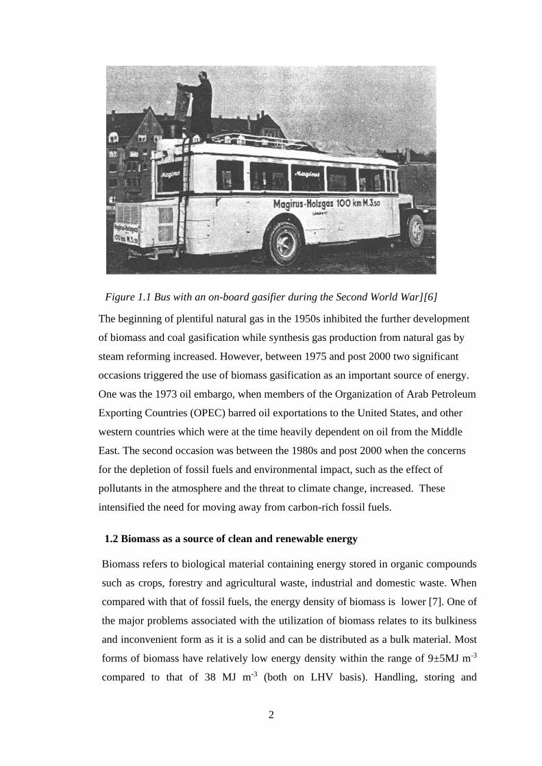
Figure 1.1 Bus with an on-board gasifier during the Second World War][6]
The beginning of plentiful natural gas in the 1950s inhibited the further development
of biomass and coal gasification while synthesis gas production from natural gas by
steam reforming increased. However, between 1975 and post 2000 two significant
occasions triggered the use of biomass gasification as an important source of energy.
One was the 1973 oil embargo, when members of the Organization of Arab Petroleum
Exporting Countries (OPEC) barred oil exportations to the United States, and other
western countries which were at the time heavily dependent on oil from the Middle
East. The second occasion was between the 1980s and post 2000 when the concerns
for the depletion of fossil fuels and environmental impact, such as the effect of
pollutants in the atmosphere and the threat to climate change, increased. These
intensified the need for moving away from carbon-rich fossil fuels.
1.2 Biomass as a source of clean and renewable energy
Biomass refers to biological material containing energy stored in organic compounds
such as crops, forestry and agricultural waste, industrial and domestic waste. When
compared with that of fossil fuels, the energy density of biomass is lower [7]. One of
the major problems associated with the utilization of biomass relates to its bulkiness
and inconvenient form as it is a solid and can be distributed as a bulk material. Most
forms of biomass have relatively low energy density within the range of 9±5MJ m-3
compared to that of 38 MJ m-3 (both on LHV basis). Handling, storing and
3
transportation of biomass in its raw form becomes more expensive in contrast to fossil
fuels. Thus, to productively utilize biomass, it is necessary to improve its properties
which enhances its handling, storing and transportation. Also similar kinds of biomass
can have very different composition and appearance thus making it difficult to assure
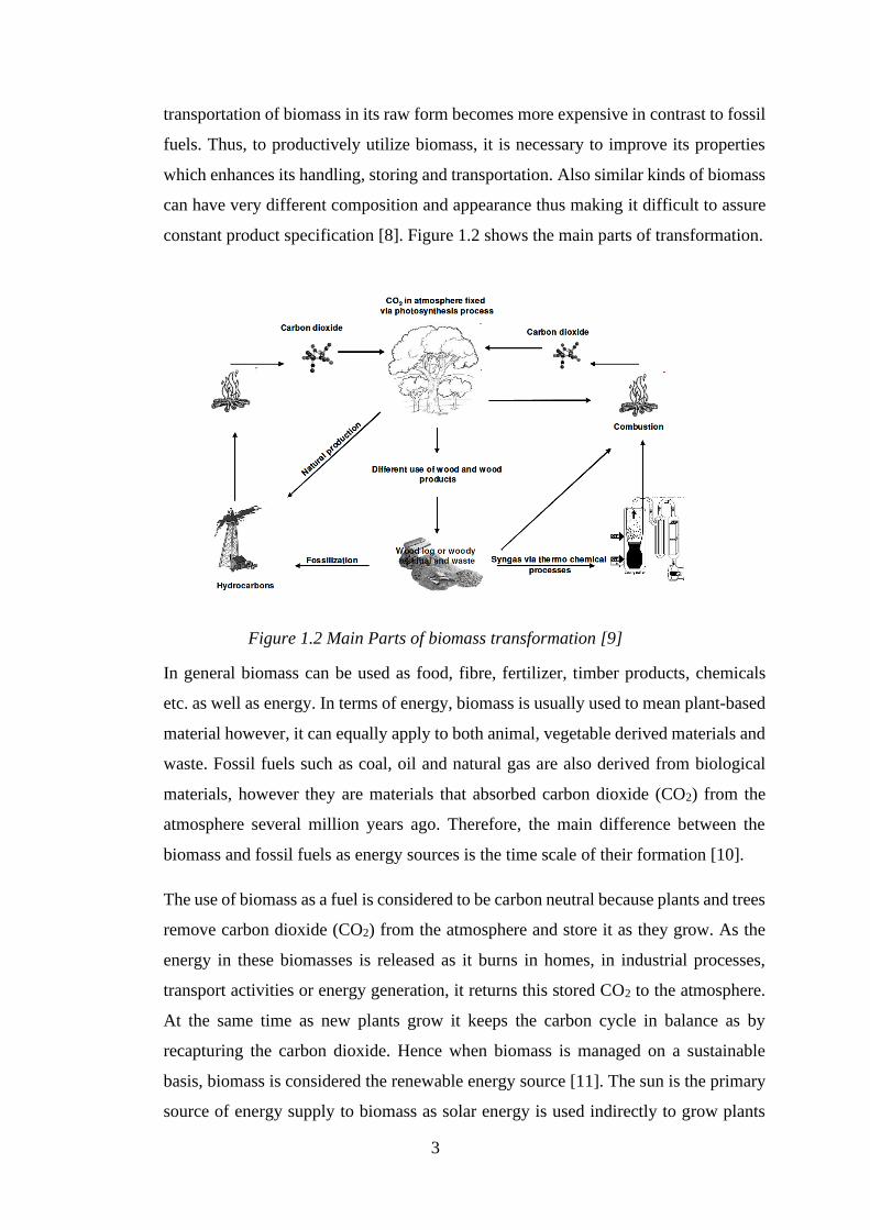
constant product specification [8]. Figure 1.2 shows the main parts of transformation.
Figure 1.2 Main Parts of biomass transformation [9]
In general biomass can be used as food, fibre, fertilizer, timber products, chemicals
etc. as well as energy. In terms of energy, biomass is usually used to mean plant-based
material however, it can equally apply to both animal, vegetable derived materials and
waste. Fossil fuels such as coal, oil and natural gas are also derived from biological
materials, however they are materials that absorbed carbon dioxide (CO2) from the
atmosphere several million years ago. Therefore, the main difference between the
biomass and fossil fuels as energy sources is the time scale of their formation [10].
The use of biomass as a fuel is considered to be carbon neutral because plants and trees
remove carbon dioxide (CO2) from the atmosphere and store it as they grow. As the
energy in these biomasses is released as it burns in homes, in industrial processes,
transport activities or energy generation, it returns this stored CO2 to the atmosphere.
At the same time as new plants grow it keeps the carbon cycle in balance as by
recapturing the carbon dioxide. Hence when biomass is managed on a sustainable
basis, biomass is considered the renewable energy source [11]. The sun is the primary
source of energy supply to biomass as solar energy is used indirectly to grow plants
4
via photosynthesis. The photosynthesis captures 3000 EJ from the solar energy of
about 3,850,000 EJ per year and produces more than 100 billion tons of dry biomass
[12].
Solar Energy Photosynthesis Biomass (complex Polymers)
The energy of the sun is absorbed by the green pigment chlorophyll in the plant leaves
and is stored within the plant in the form of chemical bond energy. Less than five
percent of solar energy incident on a leaf is absorbed while the rest is reflected and
transmitted. In the process, water and CO2 molecules are broken down and a
carbohydrate is formed with the release of pure oxygen. A simple chemical equation
for photosynthesis can be written as follows:
Carbon dioxide + water + Energy → carbohydrate + Oxygen (1.1)
6𝐶𝑂2 + 6𝐻2𝑂 + 𝐿𝑖𝑔ℎ𝑡 → 𝐶6𝐻12𝑂6 + 6𝑂2 (1.2)
The stored energy is recycled through a series of chemical and physical conversions
processes in the plant, soil, surrounding atmosphere and living matter. Thus when
biomass is burnt, this reaction is reversed and energy is released [13]. Biomass energy
is derived from the plant sources such as natural forests, industrial human or animal
wastes, they can also be sourced from agricultural and forestry processes. The energy
stored in the plants and animals and in the waste they produce is referred to as
bioenergy. Biomass decomposes via natural process to its molecules with the release
of heat. The combustion of biomass imitates the natural process [14]. Biomass is
known to be the major source of energy for mankind. In 2010, biomass accounted for
about 12.2% of global energy consumption, which makes up 73.1% of the world’s
renewable [15] and is the fourth source of energy following oil, coal and natural gas.
In most developing countries, biomass plays a significant role in the energy sector,
especially as the main source of energy for cooking in the domestic sector and thermal
energy for many small and medium industries and commercial establishments.
1.3 Biomass Conversion Technology
To gain from the chemical energy contained in the biomass, this energy has to be
transformed into more convenient energy forms like heat or electricity. Some
processes involve an intermediate transformation from the solid fuel into another
5
energy carrier such as gas or liquid fuel [8] . There are in principle, mainly three types
of conversion processes namely:
• Biochemical via microbial action
• Physical/chemical processing
• Thermochemical via heat treatment
1.3.1 Biochemical processes
With biochemical conversion, biomass molecules are broken down into smaller
molecules by bacteria and enzymes [6]. This process is a lot slower than
thermochemical conversion but does not require external energy. The three principal
routes for biochemical conversion are
• Digestion (anaerobic and aerobic)
• Fermentation
• Enzymatic or acid hydrolysis [6]
Anaerobic digestion is the use of microorganisms in oxygen- free environments to
break down organic material. Anaerobic digestion is widely used for the production of
methane and carbon-rich biogas from crop residues, food scraps and manure (human
and animal). It is also used in treatment of waste water and to reduce emissions from
landfills. Anaerobic digestion process has several stages. Firstly, bacteria are used in
hydrolysis to break down carbohydrates into forms digestible by other bacteria. The
next set of bacteria converts the resulting sugars and amino acids into carbon dioxide,
hydrogen, ammonia and organic acids. Finally, these products are acted upon by other
bacteria and converted into methane and carbon dioxide. Optimal temperature ranges
from 0 to 60 degrees C are used to characterise mixed bacterial cultures. At optimal
functions, the bacteria could convert 90% of the biomass feedstock into biogas which
contains up to 55% of methane and is a readily usable energy source. The by-products
in form of solid remnants from the original biomass, which are leftovers, have potential
uses such as fertilizers, animal bedding and low-grade building products like fibre
board. The advantage of anaerobic digestion is that it naturally occurs to organic
material and releases methane, a potent greenhouse gas, into the atmosphere.
Capturing and combusting the methane makes use of the energy inherent in the gas
and produces carbon dioxide which is a less potent greenhouse gas. The disadvantages
6
of anaerobic digestion are that the required microbes pose a health risk to people and
animals. Also, the microbes are sensitive to changes in the feedstock such as anti-
microbial compounds and changes in reactor conditions; they require constant
circulation of the reactor fluid and a constant operating temperatures and pH [16].
Aerobic digestion or composting, on the other hand, is also a biochemical process
except that it takes place in the presence of oxygen. It uses different types of
microorganisms that access oxygen from the air producing carbon dioxide, heat and
solid digestate.
In fermentation, part of the biomass is converted into sugar using acid or enzymes. The
sugar is then converted in ethanol or other chemicals with the help of yeasts. The lignin
is not converted and is left either for combustion or thermochemical conversion into
chemicals. Unlike anaerobic digestion, the by-product of fermentation is liquid [6].
The overall process involves various stages. In the first stage, the crop material is
crushed and mixed with water to form slurry. Heat and enzymes are then applied to
break down the crushed material into a finer slurry. Other enzymes are added to
convert starches into glucose sugar. The sugary slurry is then pumped into a
fermentation chamber to which yeasts are added. After about two days the fermented
liquid is distilled to separate the alcohol from the solid left-over materials.
Lignocellulose which is the structural material of plant must first be broken down into
sugars before being fermented into alcohol (ethanol). Molecules of cellulose,
hemicellulose and lignin; the components of lignocellulose have strong chemical
bonds and are difficult to separate. Mechanical pre-treatment and zymotics are
essential to break down lignocellulose. Consequently, at present, conversion of
lignocellulosic materials into ethanol is less cost effective than conversion of starch
and sugar crops into ethanol. Improving the efficiency and reducing the cost of
separating and converting cellulosic materials into fermentable sugars is one of the
characteristics of a viable industry. Research and development efforts are focusing on
the development of cost-effective biochemical hydrolysis and pre-treatment process to
overcome this barrier. Hydrolysis is a chemical process in which molecules are split
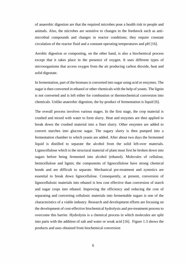
into parts with the addition of salt and water or weak acid [16]. Figure 1.3 shows the
products and uses obtained from biochemical conversion
7
Figure 1.3 Biochemical conversion process [17]
1.3.2 Physical/chemical processes
This is mainly related to wood densification and drying. Wood densification is a
process of using wood by-products such as sawdust, residues, slabs, chips and
processing them into uniform sized particle so they can be compressed into a fuel
product [18] The physio-chemical technology involves various processes to improve
physical and chemical properties of solid waste. The part of the waste that is
combustible is converted into high energy fuel pellets which could be used for steam
generation. Firstly, the waste is dried in other to lower the moisture levels then the
incombustible matter is separated mechanically before the waste is converted. The
mostly used methods of densification based on shapes and sizes are logs, pellets and
briquettes. Fuel pellets have several unique advantages over coal and wood as it is
cleaner, free from incombustibles, uniform in size, cost effective, eco-friendly and
contains lower ash and moisture contents [19]. Pellets are used more in commercial
applications for industrial boilers where ease of handling and burning characteristics
offer a competitive alternative. The main advantage of pellets is the higher energy
density which significantly brings down the cost of transportation, storage and
handling costs per energy unit. However, the drawback of pellet is about the global
energy efficiency drop and the rise in cost resulting from investment and operation.
The energy cost of producing pellets may rise by 30% as compared to wood chip as
drying is a requirement.
8
Torrefaction
Torrefaction is a thermal pre-treatment step of biomass in an inert atmosphere and in
a relatively low temperature range of about 200-3000C for the purpose of producing a
fuel with increased energy density [20]. Nitrogen is the mostly used carrier gas to
provide a non- oxidizing environment for most laboratory tests. Torrefaction is
sometimes described as mild pyrolysis since it is conducted at conditions similar to
those of pyrolysis which takes place between 350 -6500C. Torrefaction not only
removes moisture and reduces organic volatile components in the biomass but also
induces chemical reactions of the polymers found in the plant cell wall such as
cellulose (a polymer glucosan), hemicellulose (also known as polyose) and lignin (a
complex phenolic polymer) including organic extractives and inorganic extracts (ash).
Thus, it affects the mechanical strength of the material and as a result, torrefied
biomass has higher calorific value and carbon content in comparison to its parent
biomass [21]. Biomass is characterized by its high moisture content, low calorific value
with a tendency to absorb moisture. Other characteristics include its large volume or
low bulk density which results in in low conversion efficiency including difficulties
associated with its collection, grinding, storage and transportation. The evidences from
research suggests that the properties of biomass improve to a good extent after
undergoing torrefaction, the benefits include higher heating value, improved
grindability and reactivity, hydrophobicity and more uniform properties of biomass.
When biomass is torrefied, the pre-treatment can further be classified into light, mild
and severe torrefaction processes corresponding to temperatures approximated to 200-
235, 235-275 and 275-3000C respectively [22]. When biomass undergoes light
torrefaction, the moisture and low molecular weight volatiles within the biomass is
released and hemicellulose which is the more active constituent in the biomass is
degraded to an extent, however, the cellulose and lignin constituents are slightly or
hardly affected. With mild torrefaction, hemicellulose decomposition and the
liberation of volatiles are intensified while cellulose is consumed to an extent. With
respect to severe torrefaction, hemicellulose is almost completely depleted while
cellulose is oxidised to an extent. Lignin is the most difficult constituent to be
thermally degraded [23].
9
1.3.3 Thermochemical gasification process
Gasification is a process of energy production via thermochemical route [24]. It is a
partial thermal oxidation resulting in a high proportion of gaseous products (carbon
dioxide, water, carbon monoxide, hydrogen and gaseous hydrocarbons), small quantity
of char ( solid products), ash and condensable compounds [tars and oils) [25]. The
chemical energy contained in the solid fuel is converted into both chemical and thermal
energy of the gas [26]. Gasification has been given a great deal of attention in the past
few decades as a result of increasing demand for clean gaseous fuels as well as
chemical feedstock. The mechanism of gasification has been studied comprehensively.
Recent modelling efforts include the application of equilibrium model to predict the
performance of commercial gasifiers (which are reactors in which gasification of solid
fuel takes place giving out synthesis or producer gas) and several kinetic models for
particular reactor types [27]. In the downdraft gasifier which is the reactor we are
considering in this work; the carbonaceous material undergoes several processes. The
reason for developing a downdraft gasifier is its specific advantages. The most
important is its capability to produce low tar containing producer gas for engine
applications. The principle stages of gasification process are drying, pyrolysis,
oxidation and gasification.
Drying
The main purpose of the drying zone is the drying of the biomass (solid fuel). In this
stage, considering the downdraft gasifier, the feed goes down the downdraft gasifier
as a result of consumption of the feed in the reaction zone. Drying of the biomass takes
place due to the heat transfer from the hotter zones beneath the drying [28] hence the
moisture content of the biomass reduces. The physical moisture present in the wood
evaporates and the rate at which it gives up moisture depends on the prevailing
temperature in this zone. Typically, the moisture content of biomass is within the range
of 5% to 35% and drying occurs at temperatures between 100 and 200oC [25]. The
water vapour descends and adds to the water vapour formed in the oxidation zone as
represented Part of the water vapour reduced to hydrogen while the rest ends up as
moisture in the gas [29].
10
Pyrolysis
Pyrolysis is the application of heat to raw materials in the absence of air. This is
basically, the thermal decomposition of the biomass, in this process the volatile matter
in the biomass is reduced as the large molecules such as cellulose, hemi-cellulose and
lignin are broken down into carbon (char), various gases and liquids [29]. During
pyrolysis the volatile matter in the biomass corresponds to the pyrolysis yield while
the carbon and ash content estimates the char yield. The hydrocarbon gases can
condense at a low temperature to generate liquid tars [25]. It is the starting step in the
combustion and gasification processes where it is preceded by total or partial
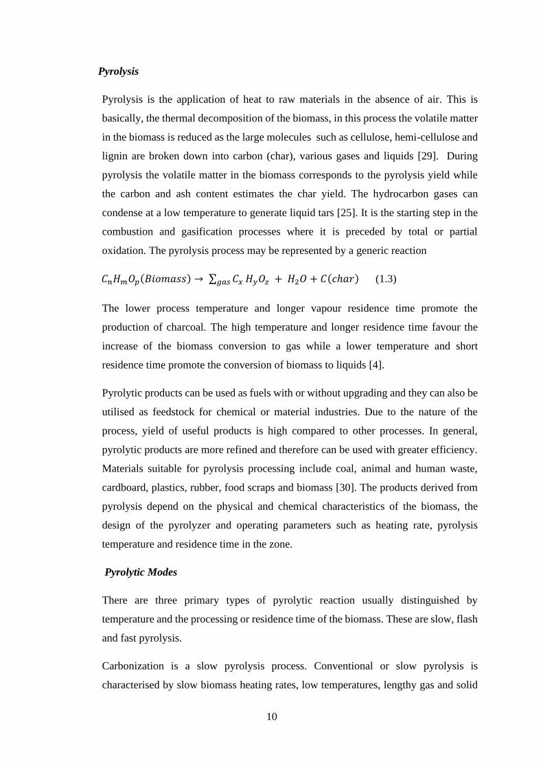
oxidation. The pyrolysis process may be represented by a generic reaction
𝐶𝑛𝐻𝑚𝑂𝑝(𝐵𝑖𝑜𝑚𝑎𝑠𝑠) → ∑ 𝐶𝑥𝑔𝑎𝑠 𝐻𝑦𝑂𝑧 + 𝐻2𝑂 + 𝐶(𝑐ℎ𝑎𝑟) (1.3)
The lower process temperature and longer vapour residence time promote the
production of charcoal. The high temperature and longer residence time favour the
increase of the biomass conversion to gas while a lower temperature and short
residence time promote the conversion of biomass to liquids [4].
Pyrolytic products can be used as fuels with or without upgrading and they can also be
utilised as feedstock for chemical or material industries. Due to the nature of the
process, yield of useful products is high compared to other processes. In general,
pyrolytic products are more refined and therefore can be used with greater efficiency.
Materials suitable for pyrolysis processing include coal, animal and human waste,
cardboard, plastics, rubber, food scraps and biomass [30]. The products derived from
pyrolysis depend on the physical and chemical characteristics of the biomass, the
design of the pyrolyzer and operating parameters such as heating rate, pyrolysis
temperature and residence time in the zone.
Pyrolytic Modes
There are three primary types of pyrolytic reaction usually distinguished by
temperature and the processing or residence time of the biomass. These are slow, flash
and fast pyrolysis.
Carbonization is a slow pyrolysis process. Conventional or slow pyrolysis is
characterised by slow biomass heating rates, low temperatures, lengthy gas and solid
11
residence times. Depending on the system, heating rates are about 0.1 to 2°C per
second and the temperatures are usually around 500°C. The vapour (gas-phase)
products have ample opportunity to react with other products to form char. During the
conventional pyrolysis the biomass is slowly devolatilised hence tar and char are the
main products. Flash pyrolysis is characterised by moderate temperature around (400
to 600°C) and rapid heating rates (>2°C/s). Vapour residence times are usually less
than two seconds, when compared to slow pyrolysis, considerably low tar is produced
however, the oil and tar products are maximised. Entrained flow or fluidised bed
reactors are considered the best reactors for Flash pyrolysis. Due to the rapid heating
rates and short reaction time, this process requires smaller particle size for better yields
compared to the other processes. Fast pyrolysis is a process in which very high heat
flux are exerted to biomass particles leading to very high heating rates in the absence
of oxygen [31]. Fast pyrolysis is a process in which organic materials are rapidly
heated to 450 – 600°C in the absence of air. Under these conditions, organic vapours,
pyrolysis gases and charcoal are produced. The vapours are condensed to bio-oil. The
main difference between flash and fast pyrolysis (more accurately defined as
thermolysis) is the heating rates and hence the residence times and products derived.
Heating rates are between 105 – 200°C per second and the prevailing temperatures are
usually higher than 550°C. As a result of the short residence time, products are high
quality, ethylene- rich gases that could subsequently be used for the production of
alcohols or gasoline. Notably, the production of char and tar is considerably less during
this process [26].
Physical process of pyrolysis
The basic phenomena that takes place during pyrolysis are heat transfer from a heat
source leading to an increase in temperature inside the fuel. Sequel to this, initiation of
pyrolysis reactions occurs as a result of increased temperature. This leads to the release
of volatiles and the formation of char. The released volatiles flow towards the ambient
temperature resulting in heat transfer between the hot volatiles and cooler un-pyrolysed
fuel. Some of the volatiles condense in the cooler parts of the fuel, as result, tars are
formed. Due to these interactions, auto catalytic secondary pyrolysis reactions occur
[32]. From a thermal viewpoint, the pyrolysis process can be divided into four stages
and distinguished by their temperature, however, the boundaries between them are not
sharp so there is always some overlap. At the initial stage with temperatures within
12
100-300°C, exothermic dehydration of biomass takes place releasing water along with
low molecular weight gases such as CO and CO2. The intermediate stage also known
as the primary pyrolysis stage takes place within the range of 200 -600°C. Most of the
vapour or precursor to bio-oil is produced at this stage. Large molecules of biomass
particles decompose into char (primary char), condensable gases (vapours and
precursors of the liquid yield) and non-condensable gases. In the final stage where
temperatures are within 300-900oC, secondary pyrolysis takes place given rise to
secondary cracking of volatiles into char and condensable gases. If the condensable
gases are quickly removed from the reaction site, condenses as tar or bio-oil in the
downstream reactor [6].
Chemical process of pyrolysis
The chemical composition of the fuel strongly influences the chemistry of pyrolysis.
The elemental composition of the fuel may be obtained from ultimate analysis. Also,
a reasonable idea of the percentage of the major products of pyrolysis (char and
volatiles) is obtained from the proximate analysis. The biomass wood or material is
directly affected as the pyrolysis process begins. These effects include the colour,
weight, size, flexibility, strength, flexibility and mechanical strength. Size and weight
are reduced while flexibility and mechanical strength are lost. Around the temperatures
of 350 °C, weight loss reaches about 80% and the remaining biomass is converted to
char. Extended heating, to about 600oC reduces char fraction to about 9% of the
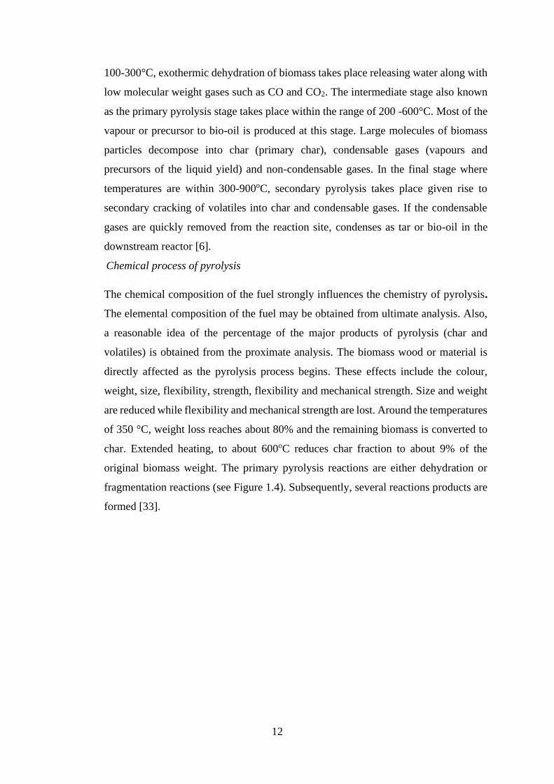
original biomass weight. The primary pyrolysis reactions are either dehydration or
fragmentation reactions (see Figure 1.4). Subsequently, several reactions products are
formed [33].
13
Figure 1.4 Reactions taking place in fast pyrolysis [33]
Biomass has three main components which are cellulose, hemicellulose and lignin.
These constituents have different rates of degradation and preferred temperature
ranges of decomposition. The decomposition of cellulose involves various complex
multiple stages. The Broido-Shafizadeh model [4] has been proposed to explain it
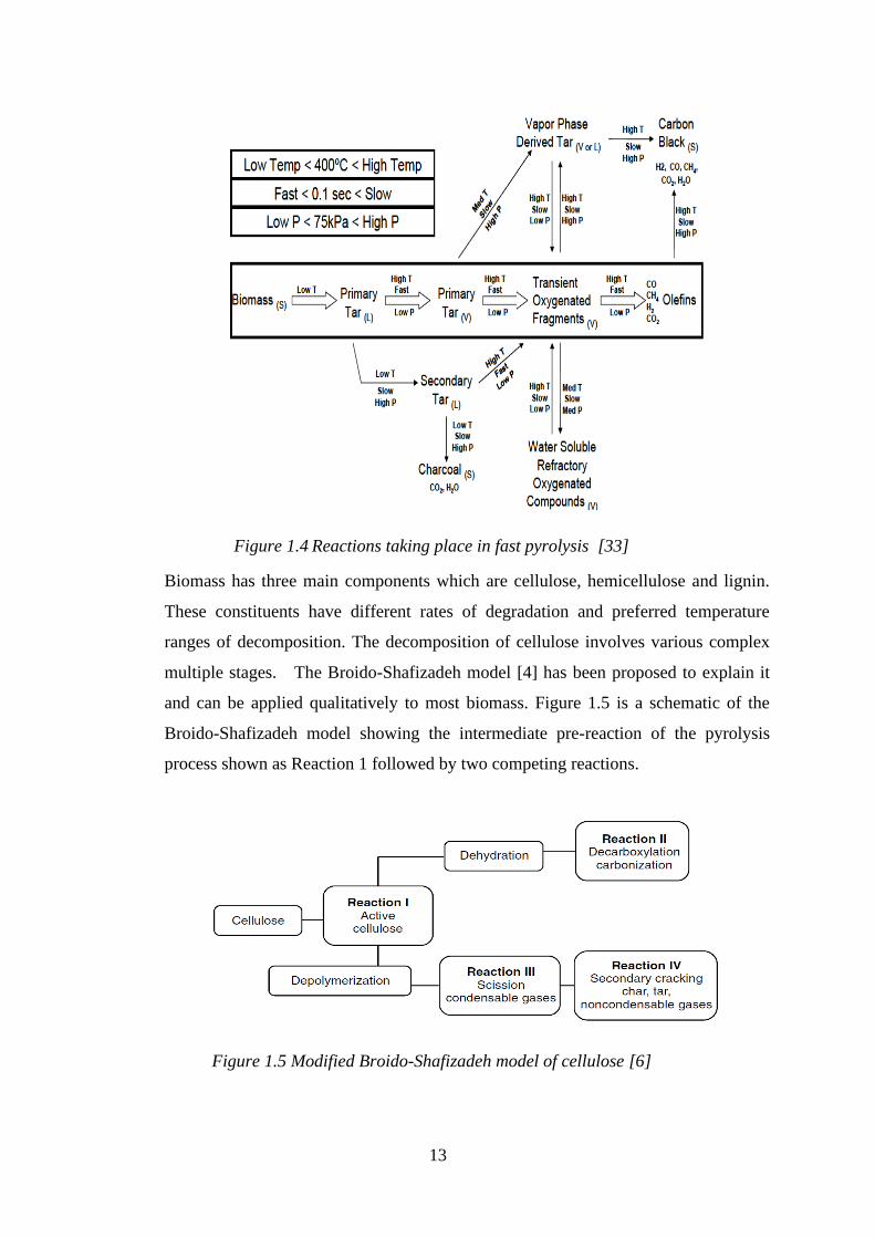
and can be applied qualitatively to most biomass. Figure 1.5 is a schematic of the
Broido-Shafizadeh model showing the intermediate pre-reaction of the pyrolysis
process shown as Reaction 1 followed by two competing reactions.
Figure 1.5 Modified Broido-Shafizadeh model of cellulose [6]
14
Reaction II involves the dehydration, decarboxylation and carbonization through an
order of steps to produce char and non-condensable gases like water vapour, carbon
monoxide and carbon dioxide. It is favoured at low temperatures of less than 300 °C.
In reaction III, depolymerisation and scission takes place producing condensable gases
and tar. It is favoured with faster heating rates and higher temperatures of over 300 °C,
the condensable vapour can condense to form bio-oil or tar if left to escape the reactor
quickly. If, however, it is held within the reactor in contact with the biomass it can
undergo secondary reactions (reaction IV) cracking the vapour into secondary char, tar
and gases. Cellulose is a polymer consisting of linear chains of B (1, 4) d-glucopyanose
units with an average molecular weight of 100,000. Cellulose components normally
constitutes about 45-50% of the dry wood. The study carried out by Shafizadeh on the
pyrolysis of cellulose with respect to temperature shows that at temperatures less than
300 °C, a reduction in the degree of polymerization takes dominates, above this
temperature, there is formation of char, gaseous products and tar which mainly
comprises of laevoglucosan that vaporises and decomposes with increased
temperature.
Hemicellulose is a mixture of polysaccharides mainly composed of glucose, mannose,
galactose and galacturonic acid residues. Hemicellulose produces more gas and less
tar and char compared to cellulose it constitutes about 20-40% of the dry wood.
However, it produces equal amounts of aqueous products of pyroligneous acid.
According to Soltes and Elder [34], Hemicellulose is thermally most sensitive and
decomposes within the temperature range of 200 °C – 260 °C. This decomposition
may occur in two steps; the decomposition of the polymer into soluble fragments
and/or the subsequent conversion into monomer units that further decompose into
volatile products.
Lignin is a random polymer of substituted phenyl propane units that can be converted
to aromatics. Lignin is amorphous in nature and is considered the binder for
agglomeration of fibrous components. Lignin constitutes between 17-30% of the
biomass component and decomposes when subjected to temperatures around 280 oC -
500 oC. Char yield is more in the products of lignin pyrolysis as it constitutes about
55%, pyroligneous acid consists of 20% and tar residue is about 15%.
15
Oxidation or Combustion
The oxidation zone lies in the section where air/oxygen is supplied. This is a reaction
between the volatile products of pyrolysis and oxygen in the air. The oxidation part of
the biomass is necessary to obtain thermal energy required for the endothermic
processes to maintain the operative temperature at the required level [35]. The
oxidation is carried out in stoichiometric amount of oxygen in order to oxidize part of
the fuel. It results in a rapid rise in temperature up to 1100 °C and 1500 °C; the
reactions are as shown below:
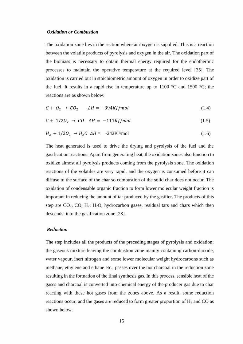
𝐶 + 𝑂2 → 𝐶𝑂2 𝛥𝐻 = −394𝐾𝐽/𝑚𝑜𝑙 (1.4)
𝐶 + 1/2𝑂2 → 𝐶𝑂 𝛥𝐻 = −111𝐾𝐽/𝑚𝑜𝑙 (1.5)
𝐻2 + 1/2𝑂2 → 𝐻2𝑂 𝛥𝐻 = -242KJ/mol (1.6)
The heat generated is used to drive the drying and pyrolysis of the fuel and the
gasification reactions. Apart from generating heat, the oxidation zones also function to
oxidize almost all pyrolysis products coming from the pyrolysis zone. The oxidation
reactions of the volatiles are very rapid, and the oxygen is consumed before it can
diffuse to the surface of the char so combustion of the solid char does not occur. The
oxidation of condensable organic fraction to form lower molecular weight fraction is
important in reducing the amount of tar produced by the gasifier. The products of this
step are CO2, CO, H2, H2O, hydrocarbon gases, residual tars and chars which then
descends into the gasification zone [28].
Reduction
The step includes all the products of the preceding stages of pyrolysis and oxidation;
the gaseous mixture leaving the combustion zone mainly containing carbon-dioxide,
water vapour, inert nitrogen and some lower molecular weight hydrocarbons such as
methane, ethylene and ethane etc., passes over the hot charcoal in the reduction zone
resulting in the formation of the final synthesis gas. In this process, sensible heat of the
gases and charcoal is converted into chemical energy of the producer gas due to char
reacting with these hot gases from the zones above. As a result, some reduction
reactions occur, and the gases are reduced to form greater proportion of H2 and CO as
shown below.
16
Boudouard Reaction
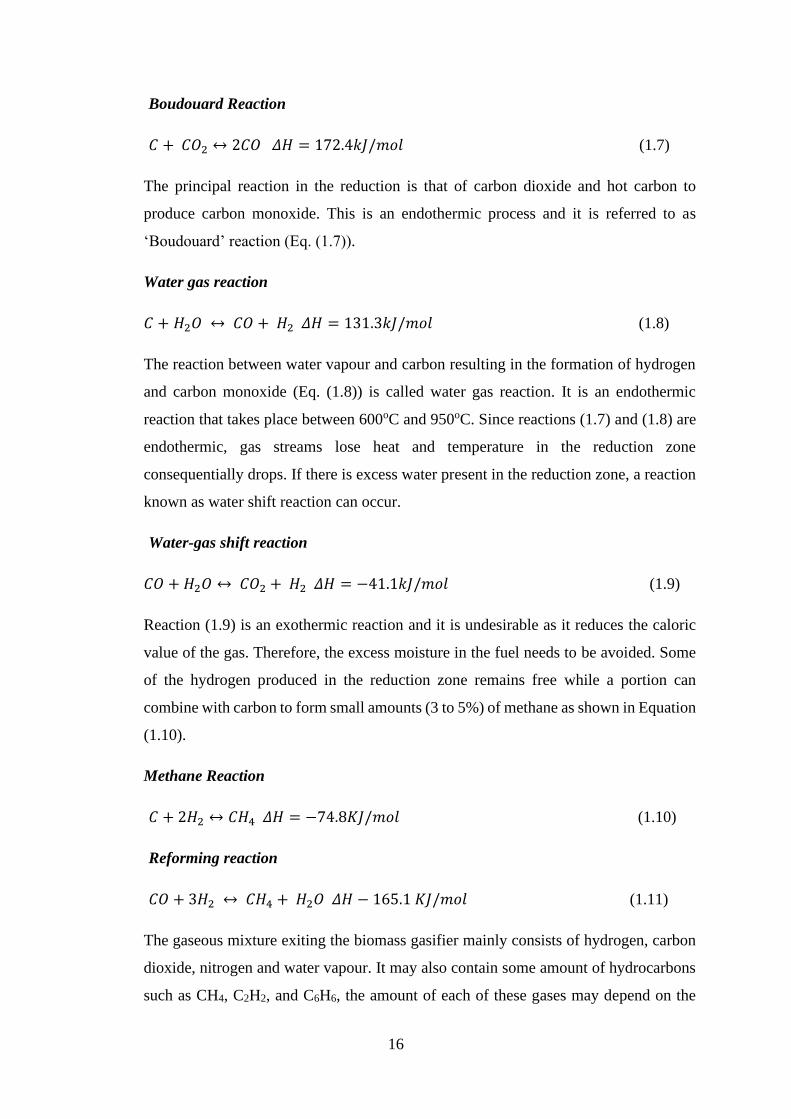
𝐶 + 𝐶𝑂2 ↔ 2𝐶𝑂 𝛥𝐻 = 172.4𝑘𝐽/𝑚𝑜𝑙 (1.7)
The principal reaction in the reduction is that of carbon dioxide and hot carbon to
produce carbon monoxide. This is an endothermic process and it is referred to as
‘Boudouard’ reaction (Eq. (1.7)).
Water gas reaction
𝐶 + 𝐻2𝑂 ↔ 𝐶𝑂 + 𝐻2 𝛥𝐻 = 131.3𝑘𝐽/𝑚𝑜𝑙 (1.8)
The reaction between water vapour and carbon resulting in the formation of hydrogen
and carbon monoxide (Eq. (1.8)) is called water gas reaction. It is an endothermic
reaction that takes place between 600oC and 950oC. Since reactions (1.7) and (1.8) are
endothermic, gas streams lose heat and temperature in the reduction zone
consequentially drops. If there is excess water present in the reduction zone, a reaction
known as water shift reaction can occur.
Water-gas shift reaction
𝐶𝑂 + 𝐻2𝑂 ↔ 𝐶𝑂2 + 𝐻2 𝛥𝐻 = −41.1𝑘𝐽/𝑚𝑜𝑙 (1.9)
Reaction (1.9) is an exothermic reaction and it is undesirable as it reduces the caloric
value of the gas. Therefore, the excess moisture in the fuel needs to be avoided. Some
of the hydrogen produced in the reduction zone remains free while a portion can
combine with carbon to form small amounts (3 to 5%) of methane as shown in Equation
(1.10).
Methane Reaction
𝐶 + 2𝐻2 ↔ 𝐶𝐻4 𝛥𝐻 = −74.8𝐾𝐽/𝑚𝑜𝑙 (1.10)
Reforming reaction
𝐶𝑂 + 3𝐻2 ↔ 𝐶𝐻4 + 𝐻2𝑂 𝛥𝐻 − 165.1 𝐾𝐽/𝑚𝑜𝑙 (1.11)
The gaseous mixture exiting the biomass gasifier mainly consists of hydrogen, carbon
dioxide, nitrogen and water vapour. It may also contain some amount of hydrocarbons
such as CH4, C2H2, and C6H6, the amount of each of these gases may depend on the
17
configuration of the gasifier. Producer gas is also loaded with dust, tar and water
vapour.
The main reactions indicate that heat is required during the reduction process. Hence,
the temperature of the gas goes down during this stage. If gasification goes to
completion, all the carbon is burned or reduced to carbon monoxide and some other
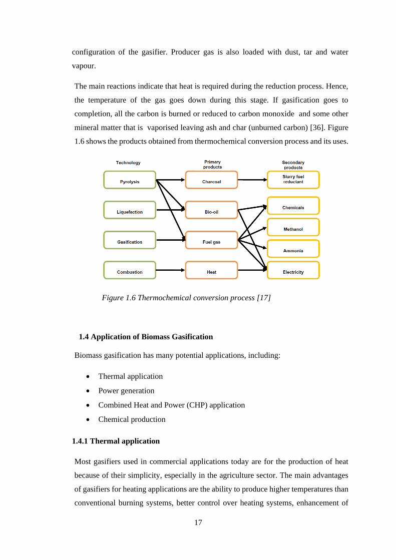
mineral matter that is vaporised leaving ash and char (unburned carbon) [36]. Figure
1.6 shows the products obtained from thermochemical conversion process and its uses.
Figure 1.6 Thermochemical conversion process [17]
1.4 Application of Biomass Gasification
Biomass gasification has many potential applications, including:
• Thermal application
• Power generation
• Combined Heat and Power (CHP) application
• Chemical production
1.4.1 Thermal application
Most gasifiers used in commercial applications today are for the production of heat
because of their simplicity, especially in the agriculture sector. The main advantages
of gasifiers for heating applications are the ability to produce higher temperatures than
conventional burning systems, better control over heating systems, enhancement of
18
boiler and total efficiency, lower emissions etc. Most conventional oil-fired thermal
installation can be run by producer gas.
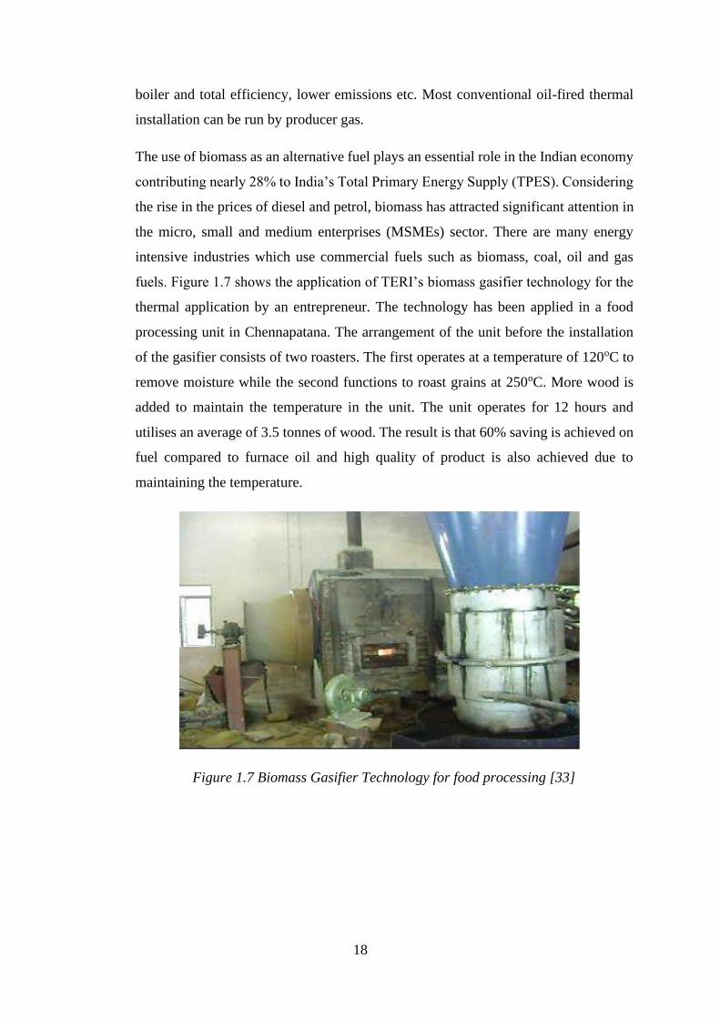
The use of biomass as an alternative fuel plays an essential role in the Indian economy
contributing nearly 28% to India’s Total Primary Energy Supply (TPES). Considering
the rise in the prices of diesel and petrol, biomass has attracted significant attention in
the micro, small and medium enterprises (MSMEs) sector. There are many energy
intensive industries which use commercial fuels such as biomass, coal, oil and gas
fuels. Figure 1.7 shows the application of TERI’s biomass gasifier technology for the
thermal application by an entrepreneur. The technology has been applied in a food
processing unit in Chennapatana. The arrangement of the unit before the installation
of the gasifier consists of two roasters. The first operates at a temperature of 120oC to
remove moisture while the second functions to roast grains at 250oC. More wood is
added to maintain the temperature in the unit. The unit operates for 12 hours and
utilises an average of 3.5 tonnes of wood. The result is that 60% saving is achieved on
fuel compared to furnace oil and high quality of product is also achieved due to
maintaining the temperature.
Figure 1.7 Biomass Gasifier Technology for food processing [33]
19
1.4.2 Power generation
The producer gases from the gasification of biomass can be used to generate heat and
electricity and can possibly be used for the synthesis of liquid fuels, chemicals or H2.
The main technologies that employ the use producer gases to generate power include
co-firing; steam turbines; gas turbines; Stirling engines; internal combustion engines;
combined cycle systems. Co-firing and combined cycle system and the integrated
gasification combined cycle (IGCC) system which uses steam turbine for power
generation are explained in the sections below.
Co-firing
In co-firing, the producer gases from biomass gasification are burned together with coal
to avoid ash mixing, this is done by the direct application of the product gas in a coal
power plant. Co-firing has the advantage of allowing the use of coal ash as a
construction material, the costs are low and this application has an existing market. The
issue with co-firing is the impact of biomass ash on quality of the boiler, fly and bottom
ash. The technical risk is minimal as the gas is utilised hot which removes the tar
products. Fuel gas produced by biomass gasification like coal can be co-fired with
natural gas either directly in turbines, duct burners or as re-burning fuel.
1.4.3 Combined heat and power (CHP)
In combined heat and power (CHP) plants, the products gas is fired on gas engine. The
producer gas even from air blown gasifier can be used after cleaning the system to
power stationary engines such as diesel engines on dual fuel mode or sterling engines.
For engine applications, the producer gas should have a heating value of approximately
5 -6MJ/m3 [37]. Typically, the energy output is one third electricity and two thirds heat.
The main challenge in the implementation of integrated biomass gasification CHP
plants is the removal of tar from the product gas. There are a few technological
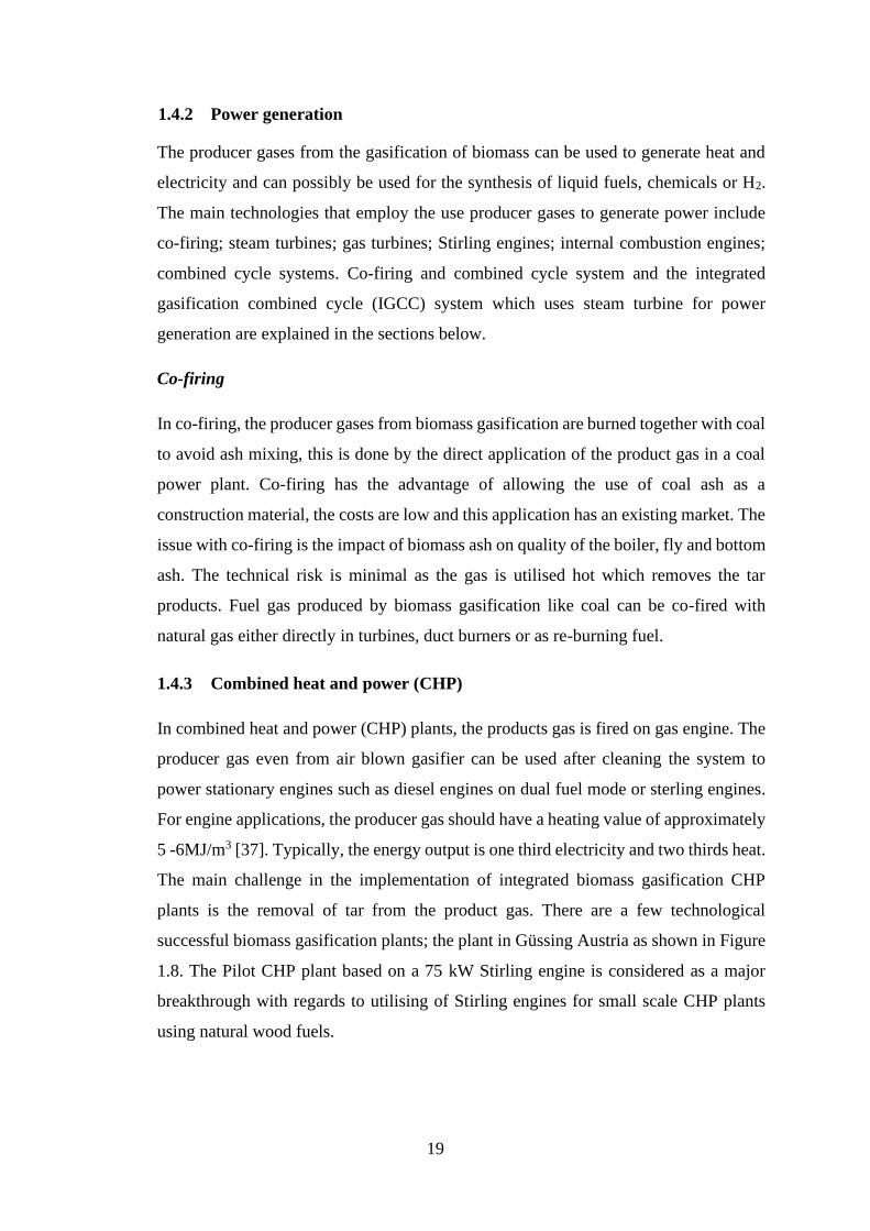
successful biomass gasification plants; the plant in Güssing Austria as shown in Figure
1.8. The Pilot CHP plant based on a 75 kW Stirling engine is considered as a major
breakthrough with regards to utilising of Stirling engines for small scale CHP plants
using natural wood fuels.
20
Figure 1.8 Process flow sheet of the Gussing Plant [38]
The combined heat and power plant has a fuel capacity of 8 MW, an electrical output
of about 2 MWe and heat output of 4.5 MWth with an electrical efficiency of about
25%. Wood chip with content of about 20-30% of water content is used as fuel. The
plant consists of a gas engine with an electrical generator, a fast circulating fluidised
bed (FICFB) steam gasifiers and a heat utilising system. The calorific value of the
producer gas is between 12-14 MJ/Nm3 with compositions; H2 35-45%, CO 20-30%,
N2 3-5%, CH4 8-12%, CO2 15-25% and tar content after the cleaning of the gas of <
20 mg/Nm3 [38]. However, some of the problems that need addressing regarding
further development and optimisation of the technology are those concerning the
overall electric efficiency i.e. reduction in heat losses and reduction in ash deposition
on the Stirling engine heater by an efficient automatic cleaning system.
Internal combustion engines
The internal combustion engine has had a colossal technological impact on the world
over the last century. The main purpose of ICE is to convert chemical fuel energy into
mechanical or useable shaft power. These engines are usually reciprocating piston
engines with various processes occurring inside the cylinders according to the
movement of the piston. The mode of conversion is carried out using either
compression ignition (CI) engines or spark ignition (SI). In SI engines, the fuel is
injected in the air flow during the intake stage, the mixture is almost adiabatically
compressed and subsequently ignited by a spark produced by a plug, and it then expands
producing useful work. This process is depicted as in the four-stroke configuration
engine: intake, compression, combustion and power stroke, and exhaust. The name

21
stems from the fact that the whole work is realised by means of four strokes each
corresponding to a thermodynamic process. With the similar configuration of CI
engines, the processes also include intake, compression, combustion/expansion and
discharge. With this operating concept, only air is compressed, the fuel is injected at
high temperature into the cylinder and the air-fuel mixture selfignites due to the high
temperature. In ICEs, the use of alternative gaseous fuels is one of the effective ways
of reducing engine emissions because it produces little or no oxides of sulphur (SOX)
and relatively small amounts of (NOX) during the combustion, which is the main
constituent of acid rain, and significantly less CO2 [39]. Whether spark or compression
ignited, synthesis gas could serve to power large stationary engines such as those
presently operated using natural gas. The main advantage achieved from the use of
synthesis gas over the use of conventional liquid, petroleum-based fuels is the reduction
of environmental impact. [40]. Usually, Diesel engines are converted the SI mode to
operate on gaseous fuels since methane (CH4) and carbon monoxide (CO) are known
for their high anti-knock properties and will not selfignite at the end of the compression
stroke.
Integrated gasification combined cycle (IGCC)
The integrated gasification combined cycle (IGCC) system is a power generation
technology that allows the use of solid and liquid fuels in a power plant that has the
environmental benefits as natural gas fuelled plant and the thermal performance of a
combined cycle. The solid or liquid fuel is gasified with air or oxygen and the resulting
gas which is syngas is cooled and clean off of its particulate matter and any sulphur
species then subsequently fired in a gas turbine. As the emission-forming constituents
is removed by pressure from the gas, IGCC plants have the potential to meet stringent
air emission standards. Also, the hot exhaust gas emitting from the gas turbine is sent
through to a heat recovery steam generator (HRSG) where it produces steam that drives
a steam turbine. Therefore, energy in form of power is produced from both steam and
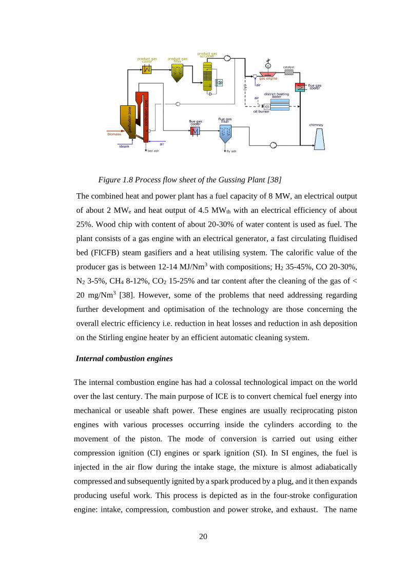
gas turbines. Figure 1.9 shows a block diagram of an IGCC plant.
22
Figure 1.9 Flow diagram of an IGCC plant [34]
An effective and practicable option of biomass utilization for the production of energy
is gasification integrated with a combined cycle. Biomass gasification integrated with
gas turbine based combined cycle (BIGCC) is an efficient biomass energy conversion
technology. BIGCC can also be applied to organic residue from all sources. This
technology has the potential of reaching high efficiencies based on clean and renewable
fuels. The plant uses low grade fuels but with reasonable efficiencies based on heating
values. BIGCC systems are based on an advanced technology; it is a gasifier used in
place of the traditional combustor that has both gasifier and gas turbine. The gas and
steam turbines operate together as a combined cycle. BIGCC systems are very clean
and more efficient than traditional fuel fired systems. In these systems, biomass is
converted into gaseous fuel which when cleaned is comparable to natural gas. The hot
gas is further cleaned with the use of an advanced cleaning process before it is burned
in the gas turbine to generate electricity [41].
Stirling engines
Stirling engine processes heat into mechanical energy without explosive combustion
process. The heat is supplied to the working medium via the heating of the external wall
of the heater and therefore it is possible to power the engines practically from any
source. Thus, the external heat could come from sources such as coal, wood, biomass
or derivatives of oil. Stirling engines are usually made up of two cold and warm pistons
23
as well as a regenerative heat exchange and heat exchangers between the working
medium and external heat sources [42]. A biomass-fired Stirling plant is an installation
which converts biomass in solid, liquid or gaseous form into carbon neutral power and
heat. In general, Stirling engines have reasonable efficiencies but at a very high cost
and these engines have a fuel-flexibility as well as better control or emissions.
1.5 Aim and objectives of this research
The aim of the study is to develop an accurate mathematical modelling method of
operation of a biomass gasifier for synthesis gas production. The downdraft gasifier is
chosen for this study due to its easy fabrication and operation and also due to low tar
content in the producer gas. They are also very suitable for small-scale applications. To
achieve this, this work is split to achieve more specific objectives:
• Investigate and review various methods employed for modelling a biomass
gasifier;
• Study the chemistry of gasification (thermodynamics and kinetics of the
gasification reactions);
• Investigate and define process parameters as it affects the performance and
operation of the downdraft gasifier;
• Modelling of the gasification process in downdraft gasifier in order to provide
information on how process variables affect gasification to allow prediction of
optimum performance.
1.6 Methodology of research
Biomass gasification as a thermochemical conversion of solid biomass to gaseous fuel
have been carried out by various researchers since the Second World War II. Various
reactor configuration has been developed in producing gases with low tar content. The
process parameters and the operating conditions that determine the performance of the
gasification include physical properties of the fuel sample such as the density, size and
shape, the design of reactor, temperature, equivalence ratio, type of oxidant, moisture
content, etc. It is important to understand how these operating conditions and
parameters affect the maximising the conversion of energy from the solid fuel to the
gaseous fuel. Important to note also, that the problem of tar in the exit gas can be
24
reduced if the pyrolysis products are exposed to elevated temperatures and longer
residence times for cracking. Downdraft gasifier which is a common type of gasifier is
chosen for this study as it is a solution to the problem of tar in the exit gas. The main
advantage of using downdraft gasifier is the possibility of producing low tar output gas
suitable for IC engine applications. Biomass feed stocks were chosen based on the
availability of experimental data and these feed stocks include woodchip, rubber wood,
wood pellets, eucalyptus wood and palm oil fronds. Gasification offers a way to convert
various low-value lignocellulosic biomass to syngas for combined heat and power
generation, production of H2 and synthesis of liquid fuels. Co-firing of syngas in
existing pulverised coal and natural gas combustors have been successfully
commercialised. However, there is need for more research to improve syngas quality
for commercial uses in a high energy efficient heat and power generator such as gas
turbines and production of liquid fuels.
With the above background, a literature survey is carried out to investigate various
methods employed for modelling a biomass gasifier, several types of gasifiers and
reviews on gasification models. A mathematical model based on equilibrium and
kinetic modelling is developed to simulate the behaviour of a downdraft gasifier divided
into three zones. The simulation tools used are MATLAB and Aspen HYSYS due to
their efficiency in modelling engineering systems. Based on the same models, the
downdraft gasifier is represented in Aspen HYSYS for both single and double air
stream operations for the production of synthesis gases. The predicted results from the
model are compared with the published experimental data. A parametric study is then
carried out to study the effect of varying the operating conditions on the predicted
synthesis gas composition and its energy content.
1.7 Original Contribution to Knowledge
Accurate mathematical models are essential for process optimization purposes in
finding optimal design parameters and operating conditions which can lead to better
process performance. The fixed bed downdraft biomass gasifier has been chosen for
this study as it has the advantage of producing low tar.
Original contribution to knowledge consists in the development of the method of
numerical simulation of a downdraft gasifier operation, which is based on

25
thermodynamic and kinetic models applied to a downdraft fixed bed. The model
presented in this work is made up from three constituent sub-models which attempt to
simulate each of the zones namely pyrolysis, oxidation and reduction zones. These are
then combined to form a complete model using both single and double air feed to the
gasifier.
Initially for the single air operation, a mathematical model was developed from the
generic biomass gasification equations and mass and energy balances applied across
the zones. The resulting modelling equations were solved using codes written in
MATLAB. The processes were subsequently simulated using Aspen HYSYS
employing Gibbs and Plug Flow Tubular Reactors (PFR) arranged in the flow sheet to
represent pyrolysis, oxidation and reduction zones of the gasifier. In one approach to
simulation the three zones were all assumed to reach thermodynamic equilibrium and
each zone was simulated using a Gibbs Reactor. In another approach an assumption
was made that the third zone, the Reduction Zone, could be simulated using a chemical
rate approach. This required chemical equations to be presented that could theoretically
represent the formation and disappearance of species in the Reduction Zone. In
HYSYS this zone was represented by a PFR. Whilst this operation requires the
presentation of chemical kinetic data it also integrates over a stated tubular reactor to
produce a unique solution according to the conditions calculated by the previous zone,
the oxidation zone represented by a Gibbs Reactor. Using such an approach for this
type of problem; simulation of a biomass gasifier is unique. This approach also gives
the possibility of dynamic modelling of the operation as allowed in HYSYS and this
could be a possibility in future work particularly in relation to the prediction of
methane formation and disappearance in the biomass gasifier.
Use of the Gibs Reactors and the PFR allows the variation of moisture levels in the
system and the flowsheet set up in HYSYS allows the creation of a double air stream
using an appropriate mixer operation where the second air stream can be introduced
prior to the oxidation stage. The use of the PFR is obviously limited by the quality of
the kinetic data available and the reactions used to represent the reduction operation
but the use of the PFR widens the flexibility of the simulation in representing this third
stage. The overall simulation of the stream, exiting the reduction section, for both
single and double air operation produces results close to the experimental ones.
26
1.8 Thesis Structure
This thesis is divided into 7 chapters. The first chapter reviews the biomass general
characteristics, actual use and potential of biomass resources. Different biomass
conversion processes are explained with the focus on biomass gasification process.
With regard to biomass gasification, different steps and reactions are described.
Finally, this chapter presents the justification for the work, aim and objectives of the
thesis together with the original contributions made.
Chapter 2 reviews different types of gasifiers and approaches to model biomass
gasification process: thermodynamic equilibrium models, kinetic models and ANN
models and Aspen Plus models.
Chapter 3 describes the process of biomass gasification assuming pyrolysis, oxidation
and reduction zones as presented in HYSYS and solved in MATLAB, the assumptions
and model developments were presented here.
Chapter 4 describes the theory behind the simulation of biomass gasification in a
downdraft gasifier using Aspen HYSYS and MATLAB in detail. Process description,
components, physical properties and block specification are described in this chapter
Chapter 5 describes the simulations carried out for validating the models developed in
this study for the various feeds utilized. Wood chips, wood pellets, rubber wood, palm
oil fronds and eucalyptus woods have been used as biomass in a downdraft gasifier.
Chapter 6 presents the results obtained for the gasification of various biomass
feedstock such as wood chips, wood pellets, rubber wood, Eucalyptus wood and oil
palm fronds. These model results were compared with experimental data from
literature.
Chapter 7 is the conclusions and recommendations section. It summarises all that have
done in this work and goals achieved. It also proposes some recommendations for
future research.
27
Chapter 2 Literature Review
2.1 Characteristics of Gasifier fuels
Since biomass fuels differ in their physical, chemical and morphological properties,
different gasification technologies, methods and gasifiers are required. Thus a fuel can
be characterised using several parameters [43]. Each type of gasifier will operate
satisfactorily with respect to stability, gas quality, efficiency and pressure losses within
certain ranges of characterised fuel properties such as;
• Energy Content
• Moisture content
• Volatile matter
• Dust content
• Tar content
• Ash and slagging features
2.1.1 Energy Content
The most important characteristics for any biomass to be considered as an energy
source depend on the actual amount of energy that can be derived from its
transformation and use. In order to calculate this, one needs to understand and
appreciate the three distinct measures of the energy content of a fuel.
• Primary energy content – This represents the total energy of the resource in its
untransformed state.
• Delivery energy- This characterises the amount of energy reaching the consumer.
In the case of wood fuel used as firewood for instance, the delivered energy is the
same as the primary energy. However, if the wood fuel is used as charcoal then the
delivery energy in the charcoal is a fraction of the primary energy.
• Useful energy- This is the actual energy used by the end user after losses due to
conversion inefficiencies have been accounted for.
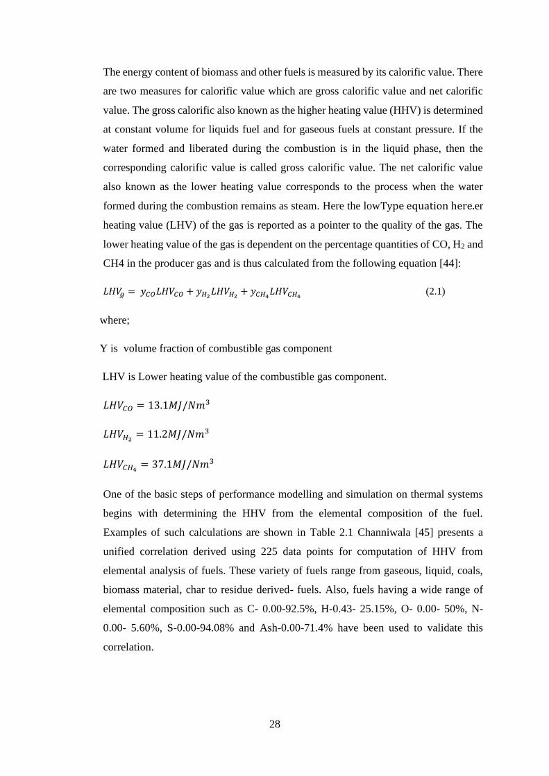
28
The energy content of biomass and other fuels is measured by its calorific value. There
are two measures for calorific value which are gross calorific value and net calorific
value. The gross calorific also known as the higher heating value (HHV) is determined
at constant volume for liquids fuel and for gaseous fuels at constant pressure. If the
water formed and liberated during the combustion is in the liquid phase, then the
corresponding calorific value is called gross calorific value. The net calorific value
also known as the lower heating value corresponds to the process when the water
formed during the combustion remains as steam. Here the lowType equation here.er
heating value (LHV) of the gas is reported as a pointer to the quality of the gas. The
lower heating value of the gas is dependent on the percentage quantities of CO, H2 and
CH4 in the producer gas and is thus calculated from the following equation [44]:
𝐿𝐻𝑉𝑔 = 𝑦𝐶𝑂𝐿𝐻𝑉𝐶𝑂 + 𝑦𝐻2𝐿𝐻𝑉𝐻2
+ 𝑦𝐶𝐻4𝐿𝐻𝑉𝐶𝐻4
(2.1)
where;
Y is volume fraction of combustible gas component
LHV is Lower heating value of the combustible gas component.
𝐿𝐻𝑉𝐶𝑂 = 13.1𝑀𝐽/𝑁𝑚3
𝐿𝐻𝑉𝐻2= 11.2𝑀𝐽/𝑁𝑚3
𝐿𝐻𝑉𝐶𝐻4= 37.1𝑀𝐽/𝑁𝑚3
One of the basic steps of performance modelling and simulation on thermal systems
begins with determining the HHV from the elemental composition of the fuel.
Examples of such calculations are shown in Table 2.1 Channiwala [45] presents a
unified correlation derived using 225 data points for computation of HHV from
elemental analysis of fuels. These variety of fuels range from gaseous, liquid, coals,
biomass material, char to residue derived- fuels. Also, fuels having a wide range of
elemental composition such as C- 0.00-92.5%, H-0.43- 25.15%, O- 0.00- 50%, N-
0.00- 5.60%, S-0.00-94.08% and Ash-0.00-71.4% have been used to validate this
correlation.
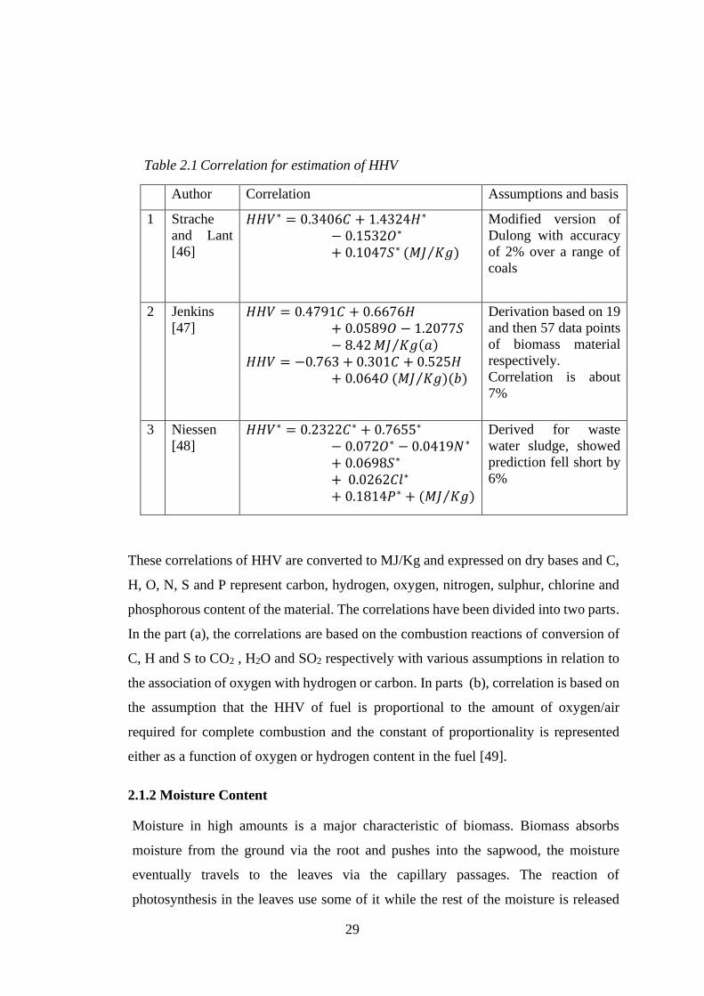
29
Table 2.1 Correlation for estimation of HHV
Author Correlation Assumptions and basis
1 Strache
and Lant
[46]
𝐻𝐻𝑉∗ = 0.3406𝐶 + 1.4324𝐻∗
− 0.1532𝑂∗
+ 0.1047𝑆∗ (𝑀𝐽 𝐾𝑔⁄ )
Modified version of
Dulong with accuracy
of 2% over a range of
coals
2 Jenkins
[47] 𝐻𝐻𝑉 = 0.4791𝐶 + 0.6676𝐻
+ 0.0589𝑂 − 1.2077𝑆− 8.42 𝑀𝐽 𝐾𝑔(𝑎)⁄
𝐻𝐻𝑉 = −0.763 + 0.301𝐶 + 0.525𝐻+ 0.064𝑂 (𝑀𝐽 𝐾𝑔⁄ )(𝑏)
Derivation based on 19
and then 57 data points
of biomass material
respectively.
Correlation is about
7%
3 Niessen
[48] 𝐻𝐻𝑉∗ = 0.2322𝐶∗ + 0.7655∗
− 0.072𝑂∗ − 0.0419𝑁∗
+ 0.0698𝑆∗
+ 0.0262𝐶𝑙∗
+ 0.1814𝑃∗ + (𝑀𝐽 𝐾𝑔)⁄
Derived for waste
water sludge, showed
prediction fell short by
6%
These correlations of HHV are converted to MJ/Kg and expressed on dry bases and C,
H, O, N, S and P represent carbon, hydrogen, oxygen, nitrogen, sulphur, chlorine and
phosphorous content of the material. The correlations have been divided into two parts.
In the part (a), the correlations are based on the combustion reactions of conversion of
C, H and S to CO2 , H2O and SO2 respectively with various assumptions in relation to
the association of oxygen with hydrogen or carbon. In parts (b), correlation is based on
the assumption that the HHV of fuel is proportional to the amount of oxygen/air
required for complete combustion and the constant of proportionality is represented
either as a function of oxygen or hydrogen content in the fuel [49].
2.1.2 Moisture Content
Moisture in high amounts is a major characteristic of biomass. Biomass absorbs
moisture from the ground via the root and pushes into the sapwood, the moisture
eventually travels to the leaves via the capillary passages. The reaction of
photosynthesis in the leaves use some of it while the rest of the moisture is released
30
into the atmosphere. For this reason, the leaves contain more moisture than the plant
trunk. The amount of moisture content of some biomass can be as high as 90% ,
however, high amounts of moisture in the biomass are not desirable as the moisture
drains much of the deliverable energy from the gasification plant. This is because the
energy used in evaporation is not recovered. The moisture in the biomass can exist in
either free or external and inherent or equilibrium form. Free moisture resides outside
the cell walls and it is above the equilibrium moisture content. Inherent moisture is
absorbed within the cell walls, when the cell walls are completely saturated, the
biomass is said to have reached its saturation point or equilibrium moisture. Moisture
content can be determined by the test protocol given in ASTM standards D-871-82 for
wood.
Moisture Basis
Biomass moisture is often expressed on dry basis. If wet biomass becomes dry after
drying then, its dry basis is expressed as
𝑀𝑑𝑟𝑦 =𝑊𝑤𝑒𝑡−𝑊𝑑𝑟𝑦
𝑊𝑑𝑟𝑦 (2.2)
For wet biomass, this can give a percentage higher than 100%, therefore it is important
to specify the basis of the moisture.
The wet basis of moisture is expressed as
𝑀𝑤𝑒𝑡 =𝑊𝑤𝑒𝑡−𝑊𝑑𝑟𝑦
𝑊𝑤𝑒𝑡 (2.3)
The relationship between the wet (𝑊𝑤𝑒𝑡 ) and dry (𝑊𝑑𝑟𝑦) basis can be expressed as
𝑀𝑑𝑟𝑦 =𝑊𝑤𝑒𝑡
1−𝑊𝑤𝑒𝑡 (2.4)
In the work carried out by Atnaw et al [50], they studied the variation of oxidation zone
temperature with time from start of batch operation for gasification of fuel with
moisture content at 22% and 29%. The results showed that the oxidation temperature
in the case of the higher moisture content was consistently low during the entire process
duration, with roughly half the average value recorded for lower moisture content. In
the both cases, the oxidation temperature showed a sharp rise during the first 10 minutes
of start-up. The oxidation temperature steadily increased with operation time for the
31
case of lower moisture content fuel, while it remained relatively stable at an average of
600 oC for that of higher moisture content fuel. They also investigated the influence of
moisture content on the composition of syngas throughout the gasification period. The
results show the variation of CO content from the start of the gasification operation of
oil palm frond (OPF) for 22% and 29% moisture content. With the 22% moisture
content of fuel, CO content increases during the initial phase of the gasification but
decreases at about the 75th minute of operation, while the CO content of the OPF with
29% moisture content of fuel was consistently lower than that of the lower moisture
content. During the 75th minutes an average of 25% CO content was obtained with
moisture content of 22% and 11.4% CO was obtained with 29% moisture content of
fuel. They also varied the calorific value of syngas with operation time for gasification
of OPF with moisture contents 22 and 29%. The results show a consistent low calorific
value concentration of CO obtained for the gasification of fuel with higher moisture
content. This is due to the lower concentration of CO obtained from the experimental
run using high moisture content of OPF.
In the study of the effects of different parameters on performance and emission of fired
stoves carried out by Bhattacharya[51], they investigated the effect of moisture content
in fuel on stove performance. Wood pellets with moisture contents of 5.9%, 9.4%,
18.2% and 22.1% were used for the test. The results show that the burning rate, cooking
power and emission factors all decreased with the increase of MC.
Ratnadhariya et al [52] presents the influence of moisture content on the gas
composition, temperature level and gasifier performance parameters at each zone with
constant equivalence ratio of 0.3. In the pyrolysis zone, the gas composition as a
function of moisture content shows that all concentrations except H2O decreased with
increasing moisture content. In the oxidation zone, all concentrations are decreasing
with increasing moisture content with an exception to H2O. Also, the influence of
moisture content on the final gas composition reveals that concentrations such as H2,
CO and CH4 are decreasing with increasing moisture. The reason is due to much
availability of moles of moisture in the system. The influence of moisture on the
temperature in each zone reveals that there is a decreasing trend. This is because higher
moisture content consumes more amount of heat as a latent and sensible heat [52].
32
For some fuels, there is little choice in the moisture content as this is determined by
the type of fuel, its origin and treatment. It is appropriate to use fuel with low moisture
content because a considerable amount of heat is used for the evaporation before the
gasification. For example, for fuel at 250 oC and raw gas temperature from the gasifier
at 3000 oC, 2875 KJ/Kg heat must be supplied to heat and evaporate the moisture [53].
Besides limiting the gasifier heat budget, high moisture content also exerts load on
cooling and filtering equipment raising the pressure drop across these units due to
condensing liquids. Thus, in other to reduce the moisture content, some pre-treatment
of the fuel is required. Normally, moisture content should be less than 20%.
2.1.3 Dust content
All gasifier fuels produce a certain amount of dust. If the dust drives with the producer
gas and used in IC engines, the dust can clog the internal combustion engine and hence
has to be removed. The gasifier design should be such that it should not produce more
than 2-6 g/m3 of dust.
2.1.4 Tar content
Tar is an unconverted volatile matter and constitutes one of the most unpleasant
components of the contents of the producer gas. It tends to condense and deposits on
various engine passages causing sticking and operational problems. The process that
results in tar formation takes place in the pyrolysis zone.
The physical properties of tar are affected by temperature of the hot zone, heating rate
and other materials in the fuel. There are about 200 chemical constituents that have
been identified in tar. Not great deal of research work has been carried out on burning
of tar inside the gasifier to produce a tar free gas. However, efforts are geared towards
removing tar from the gas stream using suitable cleaning systems. Generally, a
properly designed gasifier should have tar content less than 1 g/m3.
2.2 Gasification process parameters that affect the quality of the producer gas
The characteristics of reactor design and the pattern of flow has a strong influence on
the quality of syngas fuel generated in the gasification process. The major variable
parameters used for to maintain an acceptable quality of gas are equivalence ratio and
the superficial velocity.
33
2.2.1 Equivalence Ratio
ER is a measure of the amount of external oxygen (or air) supplied to the gasifier. ER
is obtained by dividing the actual oxygen (or air) to biomass molar ratio [54]. A good
number of researchers have addressed various gasification schemes. Zainal et al [55]
defines equivalence ratio to incorporate the effect of rate of air flow, wood supply and
duration of run in a bid to lower the number of parameters on which the biomass
gasifier depends. In their work, the equivalence ratio for each run is calculated as
Equivalence ratio Ø = (𝐹𝑙𝑜𝑤 𝑟𝑎𝑡𝑒 𝑜𝑓 𝑎𝑖𝑟 𝑠𝑢𝑝𝑝𝑙𝑦)∗(𝐷𝑢𝑟𝑎𝑡𝑖𝑜𝑛 𝑜𝑓 𝑡ℎ𝑒 𝑟𝑢𝑛)
(𝑀𝑎𝑠𝑠 𝑖𝑛𝑝𝑢𝑡 𝑜𝑓 𝑤𝑜𝑜𝑑)∗(𝐴𝐹⁄ 𝑓𝑜𝑟 Ø=1)
(2.5)
(𝐴 𝐹⁄ ) for Ø =1 is 5.22 m3 of air /kg of wood. The equivalence ratio for their gasifier is
found to be within the range of 0.268-0.43.
In order to investigate the influence of ER in a downdraft gasifier, Zainal et al, carried
out an experiment using furniture wood and wood chips under various operating
conditions. He observes that there is an increasing and then decreasing trend with CO
and CH4. The variation of the calorific value with equivalence ratio showed a peak
value indicating there is an optimum equivalence ratio, the best performance of the
downdraft gasifier yields a peak at an ER value of 0.38.
In the study of operating and performance gasification process parameters carried out
by Sharkofow [56], ER represents the ratio between the amount of air/oxygen in the
oxidant or gasification agent and the theoretical amount of air/oxygen required for
complete combustion of the biomass feedstock according to the stoichiometry. They
found that with higher ER, more CO2 can be produced while the amount of CO in the
synthesis gas is reduced. Reduction in the amount of carbon monoxide associated with
ER is attributed to the fact that with a higher ER value more oxygen is introduced and
more CO is converted to CO2. With a lower ER value, less H2 and CH4 are produced.
Low ER values approaching zero are usually encountered in the pyrolysis step whereas
higher ER values approaching or greater than 1 are encountered in the combustion
stage. A pyrolysis is carried out in the absence of oxygen, its ER is zero. In combustion,
values of ER approach or exceed 1, this is in an effort to provide sufficient air/oxygen
by which complete oxidation can take place. For partial oxidation reactions, i.e.
gasification reactions, ER is usually between 0.25 and 0.5.

34
In the three zone equilibrium and kinetic free modelling of biomass gasifier study
carried out by Ratnadhariya et al. [52]. They investigated the influence of ER on gas
compositions in the pyrolysis, oxidation and reduction zones. In the pyrolysis zone, no
effect of ER was observed as the model did not consider reaction rates and equilibrium
in this zone instead the products in this zone are obtained through mass and energy
balances including assumptions. In the oxidation zone, N2 increases with increasing
ER which is understandable while CH4, C2H2, and H2O are decreasing due to the fact
that generations of these compositions depend on the elemental content of the biomass
which is constant for a given biomass material therefore the relative compositions will
decrease with increasing air intake and consequently ER. CO and CO2 are seen to be
increasing with increase of ER due to more oxidation of char. It is noticed that the rate
of increase in CO is more than that of CO2, this is attributed to the fact that the partial
oxidation of char dominates in an oxygen deficient environment and reactive char. In
the reduction zone, CO increases while CO2 decreases with increasing ER, which is as
result of more CO being oxidized at a higher ER [52].
Prokrash et al [57] in their work on modelling of a downdraft gasifier with finite rate
kinetics in the reduction zone investigated the effect of ER on the composition of gases.
In their work, equivalence ratio is defined as the ratio of stoichiometric to air-fuel
ratios; in the gasifier, sub-stoichiometric air is supplied, and the equivalence ratio is
above unity. The range of equivalence ratio over which a gasifier may operate is
limited by the quality of the producer gases generated and the stable operation of it.
The result of varying the ER on the composition and heating value of gases shows that
increasing the equivalence ratio (that is decrease in the actual supply of air) increases
the H2 and CH4 content in the producer gas. However, the CO fraction in the gas
decreases and CO2 increases [57] their observation contradicts the apparent fact that
operating the gasifier in a richer atmosphere should produce more CO and less CO2.
Melgar et al [58] investigated the influence of varying ER on the gas compositions and
reports similar findings to the present case, they attributed the results to the fact that
equilibrium of water shift reaction in the model inclines to the production of CO2 and
H2 when the fuel contains high moisture.
Narvaez [59] observed an increase in gas yield with an increase in ER from 0.20 to
0.45 and a decrease in the lower heating value (LHV) of the gas with decreasing
fractions of H2, CO, CH4 including C2H2 and tar [59]. The increase in gas yield with
35
increase in ER infers that an increased air flow increases the rate of conversion. Some
of the contradictions on the effects of ER on the contents of H2, CO and CH4 percent
is rational because the percentage compositions of individual gases depend on both the
overall gas yield and the individual gas yield. When the increase in the overall gas
yield is more pronounced than the increase in the individual gas yield, then the
percentage composition of individual gas decreases even if the individual gas yield
may have increased. In the study of thermochemical biomass gasification performed
on a bench-scale fluidised bed gasified with steam and air as fluidising and oxidizing
agents, Kumar observed increases in gas yields, carbon conversion and energy
efficiencies with increase in ER from 0.07 to 0.25 [60]. While some authors observed
increases in gas yields with increase in equivalence ratio, some other authors observed
a decrease in H2 and CO yields with increase in ER.
2.2.2 Superficial Velocity
A superficial velocity, SV is defined as the ratio of the syngas production rate at normal
conditions and the narrowest cross-sectional area of the gasifier. The SV of a gasifier
is the most vital measure of the behaviour of the gasifier and controls most of the
aspects of its operation such as gas production rate, char production, fuel consumption
rate, gas energy content and tar production. It is not dependent on gasifier size and so
permits comparison of gasifiers of very different dimensions. It affects the heat transfer
around each particle during flaming pyrolysis of the volatiles and on combustion of
the tars as well as the degree of gasification of the charcoal. This is because it controls
the rate at which air and then gas passes through the gasifier [61]. Variations in the
amount and composition of tar/gas with SV ranging from 0.3 to 0.7 m/s have been
investigated in a downdraft biomass gasifier with air as the oxidant. Yamazaki et al
experimental investigation shows that the lowest tar yields was achieved at SV around
0.4 m/s and the highest at 0.7 m/s. High tar yields at high SV are due to short residence
time and channelling. Also, the result showed a noticeable change in the composition
of gas with SV ranging from 0.3 to 0.4 m/s. In the range of 0.4 to 0.6 m/s gas
composition is suitable for IC engines [62].
2.3 Gasifier Types
Various types of gasifiers have been developed and these gasifiers have different
hydrodynamics particularly in terms of how the solid fuel and the gasification agent
36
such as air, oxygen and or steam are contacted and operating conditions such as
temperature and pressure; authors [63]. [7, 64] agree that even though there has been
a long experience of biomass gasification, reliable and large scale operations continue
to be suffering from several problems. Those issues depending on the type of gasifier
are according to [63] related to
➢ Scale of operations and availability of biomass
➢ Size distribution of raw biomass
➢ Operability of the gasifier with fuels containing large amounts of ash especially if
the fraction of alkali, chlorine and sulphur is high
➢ Formation of condensable high hydrocarbons
➢ cleaning and upgrading of the gas for dedicated down-stream application
There are various types of gasification technology developed for converting biomass
feed stocks. Most of these have been developed and commercialised for the production
of heat and power from syngas rather than liquid fuel production. The main types are
described in the Figure 2.1 below with the main differences being:
• The manner in which the biomass is fed into the gasifier and how it moves around
within the gasifier;
• The kind of oxidant used- air dilutes the syngas due to the presence of nitrogen
which subsequently increases the cost of the downstream processing. Oxygen
however avoids but is very expensive to use;
• The temperature ranges at which the gasifier is operated;
• The method in which the heat for the gasifier is provided – whether the heat is
provided by partially combusting some of the biomass in the gasifier or from an
external source such as circulation of an inert material or steam;
• The level of pressure, the gasifier operates upon- pressurised gasification provides
higher throughputs with larger maximum capacities which promotes hydrogen
production and subsequently leads to cheaper downstream clean-up equipment.
Moreover, since no additional compression is required, the temperature of the
syngas can be kept high for downstream operations and liquid fuel catalysis.
However, at pressures between 25-30 bar, cost quickly increase since gasifiers
require more robust engineering and the needed feeding mechanisms involve
complex pressurising steps [65];
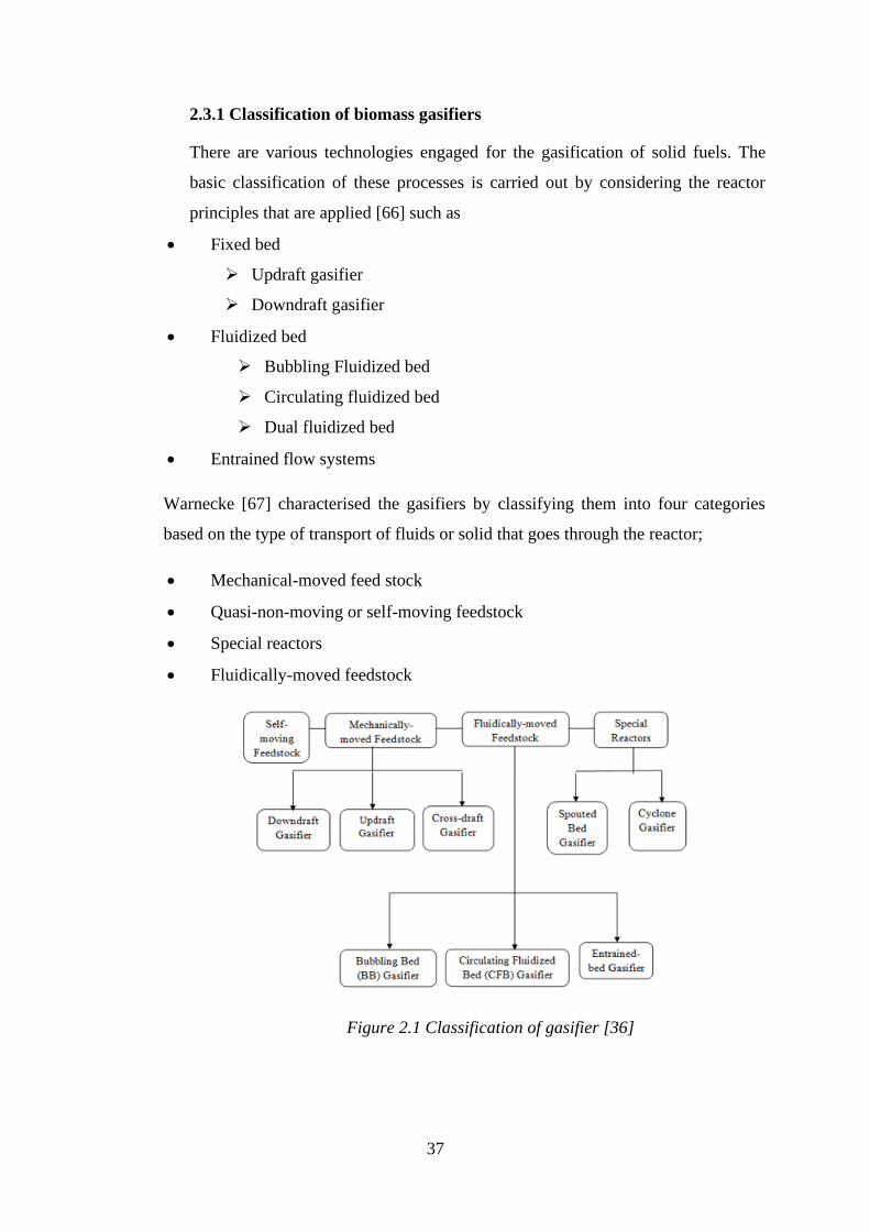
37
2.3.1 Classification of biomass gasifiers
There are various technologies engaged for the gasification of solid fuels. The
basic classification of these processes is carried out by considering the reactor
principles that are applied [66] such as
• Fixed bed
➢ Updraft gasifier
➢ Downdraft gasifier
• Fluidized bed
➢ Bubbling Fluidized bed
➢ Circulating fluidized bed
➢ Dual fluidized bed
• Entrained flow systems
Warnecke [67] characterised the gasifiers by classifying them into four categories
based on the type of transport of fluids or solid that goes through the reactor;
• Mechanical-moved feed stock
• Quasi-non-moving or self-moving feedstock
• Special reactors
• Fluidically-moved feedstock
Figure 2.1 Classification of gasifier [36]
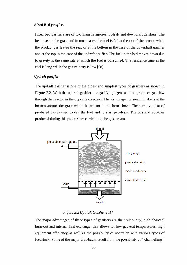
38
Fixed Bed gasifiers
Fixed bed gasifiers are of two main categories; updraft and downdraft gasifiers. The
bed rests on the grate and in most cases, the fuel is fed at the top of the reactor while
the product gas leaves the reactor at the bottom in the case of the downdraft gasifier
and at the top in the case of the updraft gasifier. The fuel in the bed moves down due
to gravity at the same rate at which the fuel is consumed. The residence time in the
fuel is long while the gas velocity is low [68].
Updraft gasifier
The updraft gasifier is one of the oldest and simplest types of gasifiers as shown in
Figure 2.2. With the updraft gasifier, the gasifying agent and the producer gas flow
through the reactor in the opposite direction. The air, oxygen or steam intake is at the
bottom around the grate while the reactor is fed from above. The sensitive heat of
produced gas is used to dry the fuel and to start pyrolysis. The tars and volatiles
produced during this process are carried into the gas stream.
Figure 2.2 Updraft Gasifier [61]
The major advantages of these types of gasifiers are their simplicity, high charcoal
burn-out and internal heat exchange; this allows for low gas exit temperatures, high
equipment efficiency as well as the possibility of operation with various types of
feedstock. Some of the major drawbacks result from the possibility of ‘’channelling’’
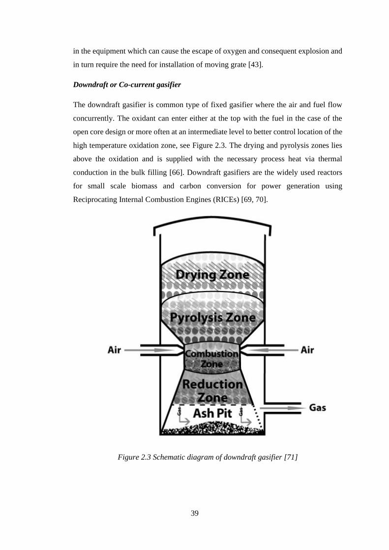
39
in the equipment which can cause the escape of oxygen and consequent explosion and
in turn require the need for installation of moving grate [43].
Downdraft or Co-current gasifier
The downdraft gasifier is common type of fixed gasifier where the air and fuel flow
concurrently. The oxidant can enter either at the top with the fuel in the case of the
open core design or more often at an intermediate level to better control location of the
high temperature oxidation zone, see Figure 2.3. The drying and pyrolysis zones lies
above the oxidation and is supplied with the necessary process heat via thermal
conduction in the bulk filling [66]. Downdraft gasifiers are the widely used reactors
for small scale biomass and carbon conversion for power generation using
Reciprocating Internal Combustion Engines (RICEs) [69, 70].
Figure 2.3 Schematic diagram of downdraft gasifier [71]
40
The product gases usually exit near the bottom of the reactor near the ash grate; this
results in products originating from the pyrolysis zone to have to pass through the
oxidation zone which is normally depicted as a treatment zone for tarry compounds.
The construction and principle of the downdraft gasifiers makes them sensitive to the
quality of fuel used; particular attention must be paid to the water content of the fuel.
The steam given off in the drying zone must be removed through bulk filling; the vapour
must be heated up in the temperatures in the oxidation zone. Some of the advantages
are higher conversion efficiencies with low tar and particulate content in producer gas.
The concentration of tar and particulates is considerably lower as compared with other
reactors due to gas passing through a high temperature in the combustion zone causing
the cracking of the tar formed during the gasification process. According to
Bhattacharya [72] high char conversion and the lower ash carry over as gas passes
through the charcoal bed allowing its filtration, catalysis and quick response to load
changing. The drawbacks are that difficult to obtain a homogenous distribution of air
in the reactors with large diameters; as the diameter of the reactor increases, so is the
likelihood for increase in low temperature zones this is why the scale up capability in
downdraft gasifiers is limited. Its inability to operate on a number of unprocessed fuels
particularly fluffy and low density materials give rise to flow problems and excessive
pressure drop. Moreover, solid fuels must be palletized, briquetted before use and face
problems with high ash content fuels (slagging). Not suitable for small particle size of
fuels [73].
The Imbert downdraft gasifiers are suitable for handling biomass fuel of uniform sizes
and shapes as they flow through the constriction heart and also with ash and moisture
content less than 5% and 20% respectively. Gases and solids flow through a
descending packed bed supported across a throat. In throated gasifiers, gasification
occurs over four zones namely pyrolysis, drying, oxidation and reduction zones. The
biomass fuels enter through the hopper flows down and get dried and pyrolysed before
being partially combusted by the gasifying media entering at the nozzles. The throat
aids cracking as it allows for maximum mixing of gases in the temperature region
which aids tar cracking. Underneath the throat the combustion gases and tar pass
through the hot char and are reduced to CO and H2 [74]. The gasifier has lower overall
efficiency since a high amount of heat content is carried over by the hot gas. The
biomass particle size limits the capacity of the Imbert downdraft gasifiers to 500KW
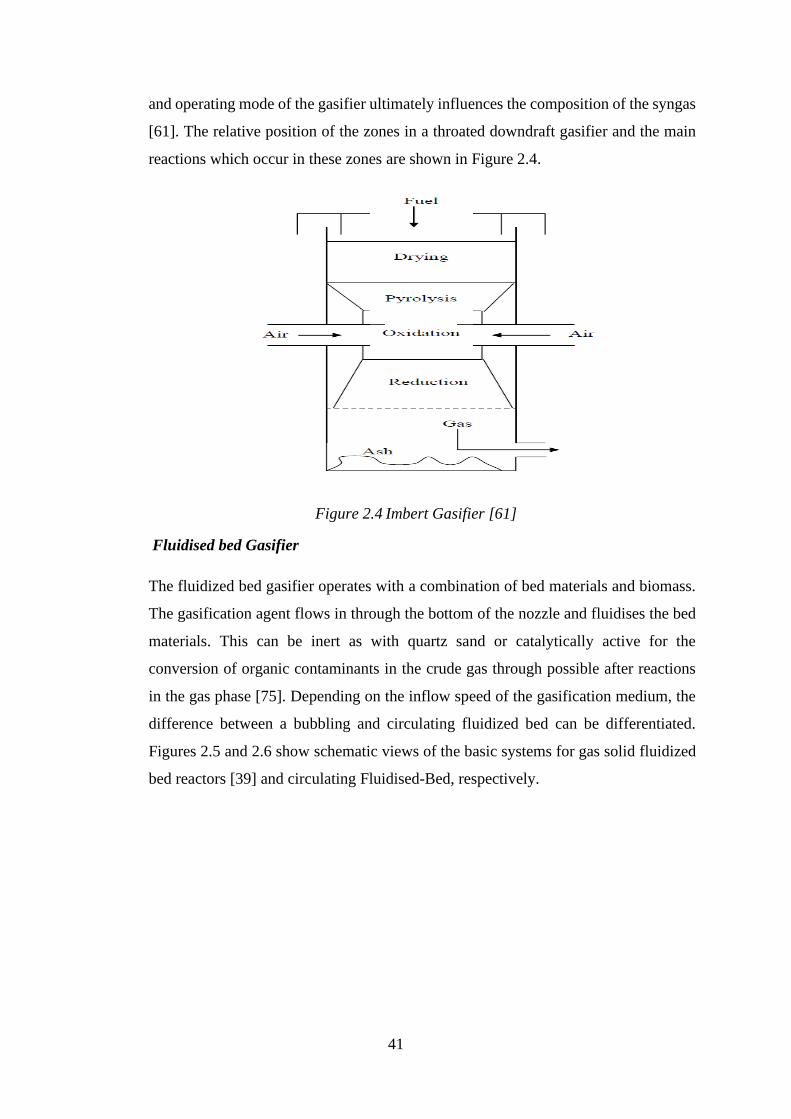
41
and operating mode of the gasifier ultimately influences the composition of the syngas
[61]. The relative position of the zones in a throated downdraft gasifier and the main
reactions which occur in these zones are shown in Figure 2.4.
Figure 2.4 Imbert Gasifier [61]
Fluidised bed Gasifier
The fluidized bed gasifier operates with a combination of bed materials and biomass.
The gasification agent flows in through the bottom of the nozzle and fluidises the bed
materials. This can be inert as with quartz sand or catalytically active for the
conversion of organic contaminants in the crude gas through possible after reactions
in the gas phase [75]. Depending on the inflow speed of the gasification medium, the
difference between a bubbling and circulating fluidized bed can be differentiated.
Figures 2.5 and 2.6 show schematic views of the basic systems for gas solid fluidized
bed reactors [39] and circulating Fluidised-Bed, respectively.
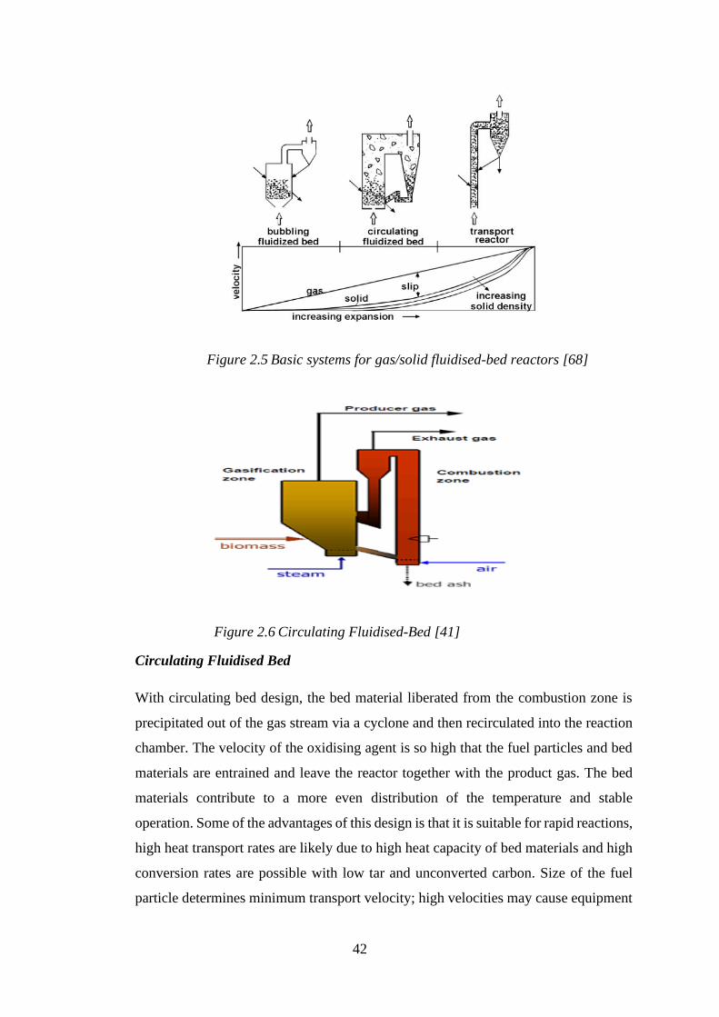
42
Figure 2.5 Basic systems for gas/solid fluidised-bed reactors [68]
Figure 2.6 Circulating Fluidised-Bed [41]
Circulating Fluidised Bed
With circulating bed design, the bed material liberated from the combustion zone is
precipitated out of the gas stream via a cyclone and then recirculated into the reaction
chamber. The velocity of the oxidising agent is so high that the fuel particles and bed
materials are entrained and leave the reactor together with the product gas. The bed
materials contribute to a more even distribution of the temperature and stable
operation. Some of the advantages of this design is that it is suitable for rapid reactions,
high heat transport rates are likely due to high heat capacity of bed materials and high
conversion rates are possible with low tar and unconverted carbon. Size of the fuel
particle determines minimum transport velocity; high velocities may cause equipment
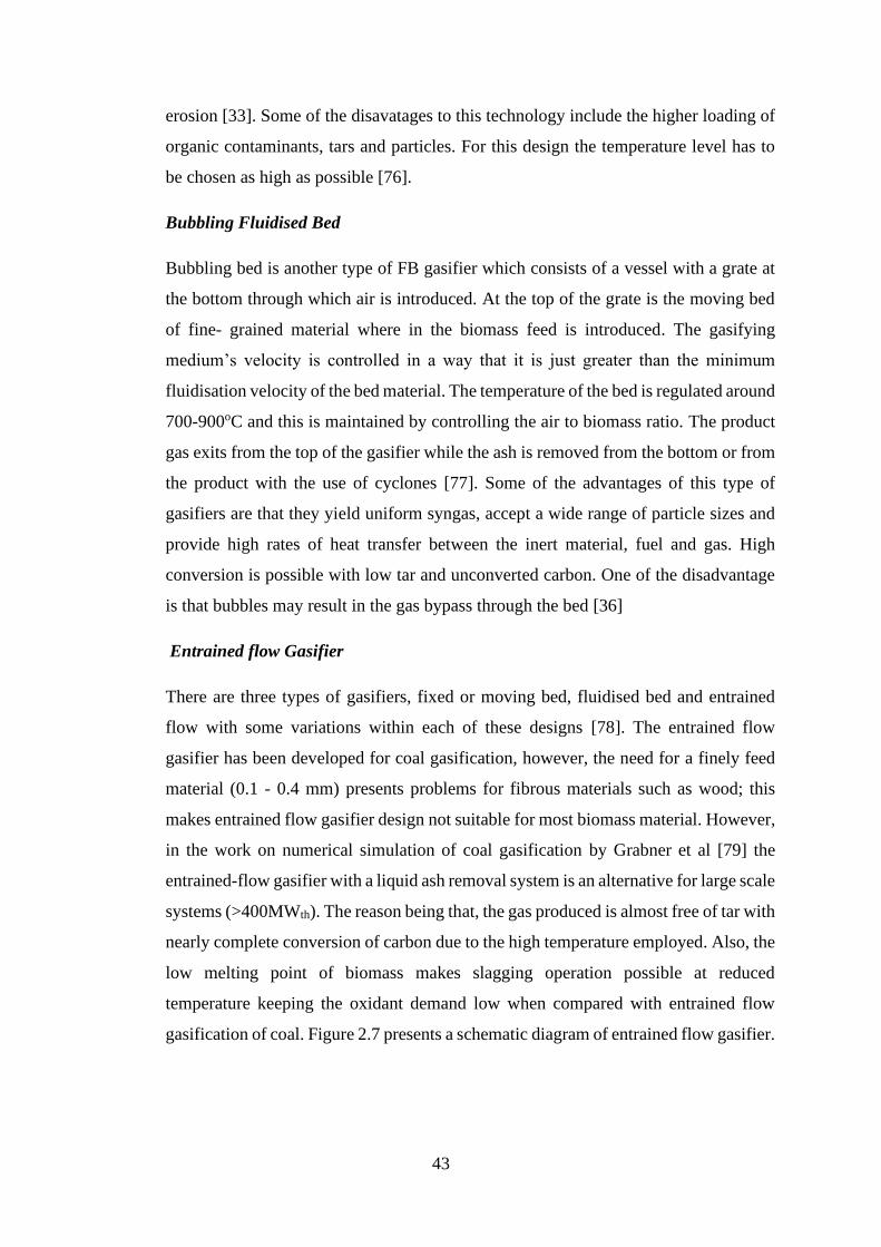
43
erosion [33]. Some of the disavatages to this technology include the higher loading of
organic contaminants, tars and particles. For this design the temperature level has to
be chosen as high as possible [76].
Bubbling Fluidised Bed
Bubbling bed is another type of FB gasifier which consists of a vessel with a grate at
the bottom through which air is introduced. At the top of the grate is the moving bed
of fine- grained material where in the biomass feed is introduced. The gasifying
medium’s velocity is controlled in a way that it is just greater than the minimum
fluidisation velocity of the bed material. The temperature of the bed is regulated around
700-900oC and this is maintained by controlling the air to biomass ratio. The product
gas exits from the top of the gasifier while the ash is removed from the bottom or from
the product with the use of cyclones [77]. Some of the advantages of this type of
gasifiers are that they yield uniform syngas, accept a wide range of particle sizes and
provide high rates of heat transfer between the inert material, fuel and gas. High
conversion is possible with low tar and unconverted carbon. One of the disadvantage
is that bubbles may result in the gas bypass through the bed [36]
Entrained flow Gasifier
There are three types of gasifiers, fixed or moving bed, fluidised bed and entrained
flow with some variations within each of these designs [78]. The entrained flow
gasifier has been developed for coal gasification, however, the need for a finely feed
material (0.1 - 0.4 mm) presents problems for fibrous materials such as wood; this
makes entrained flow gasifier design not suitable for most biomass material. However,
in the work on numerical simulation of coal gasification by Grabner et al [79] the
entrained-flow gasifier with a liquid ash removal system is an alternative for large scale
systems (>400MWth). The reason being that, the gas produced is almost free of tar with
nearly complete conversion of carbon due to the high temperature employed. Also, the
low melting point of biomass makes slagging operation possible at reduced
temperature keeping the oxidant demand low when compared with entrained flow
gasification of coal. Figure 2.7 presents a schematic diagram of entrained flow gasifier.
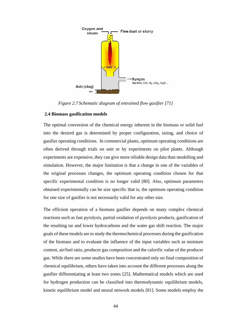
44
Figure 2.7 Schematic diagram of entrained flow gasifier [71]
2.4 Biomass gasification models
The optimal conversion of the chemical energy inherent in the biomass or solid fuel
into the desired gas is determined by proper configuration, sizing, and choice of
gasifier operating conditions. In commercial plants, optimum operating conditions are
often derived through trials on unit or by experiments on pilot plants. Although
experiments are expensive, they can give more reliable design data than modelling and
simulation. However, the major limitation is that a change in one of the variables of
the original processes changes, the optimum operating condition chosen for that
specific experimental condition is no longer valid [80]. Also, optimum parameters
obtained experimentally can be size specific that is, the optimum operating condition
for one size of gasifier is not necessarily valid for any other size.
The efficient operation of a biomass gasifier depends on many complex chemical
reactions such as fast pyrolysis, partial oxidation of pyrolysis products, gasification of
the resulting tar and lower hydrocarbons and the water gas shift reaction. The major
goals of these models are to study the thermochemical processes during the gasification
of the biomass and to evaluate the influence of the input variables such as moisture
content, air/fuel ratio, producer gas composition and the calorific value of the producer
gas. While there are some studies have been concentrated only on final composition of
chemical equilibrium, others have taken into account the different processes along the
gasifier differentiating at least two zones [25]. Mathematical models which are used
for hydrogen production can be classified into thermodynamic equilibrium models,
kinetic equilibrium model and neural network models [81]. Some models employ the
45
use of process simulator Aspen plus [25] combining thermodynamic and kinetic rate
models.
2.4.1 Aspen Plus/HYSYS Models
In trying to avoid complex processes, some authors have proposed simple models such
as Aspen Plus simulator that integrates the principal gasification reactions and physical
characteristics of the reactors. Aspen plus is a chemical process optimization software
developed at Massachusetts Institute of Technology [82]. It is a problem-oriented input
program which employs the use of unit operations, blocks such as pumps, reactors etc.
The process simulation calculator uses in-built physical property data bank. The
program solves the process scheme sequentially by calculating the outlet stream
properties using the inlet stream properties for each block. This package has been used
to model coal and biomass power generation systems.
To model a gasifier, using Aspen Plus, the total process must be broken down into
many sub-processes; a model may include several zones such as drying, pyrolysis,
oxidation and gasification zones. Each zone can be represented by separators or
reactors. The mass and energy transfer across these zones can be incorporated in such
a way that all unit operations combination represent the entire biomass gasifier [83].
Many authors have developed gasification models using Aspen Plus for coal and
biomass. Ramzan et al [84] proposed a steady state model for hybrid biomass gasifier
employing the use of Aspen plus in the comparative performance analysis of food
waste, municipal solid waste and poultry waste. The gasification process has been
modelled in three stages. In the first stage, moisture content of the solid fuel is reduced
before feeding to the reactor. In the second stage, biomass is decomposed into volatile
components and char. The yield distribution for this stage has been specified using
FORTRAN statement in calculator block. Partial oxidation and gasification reactions
has been modelled in the third stage by minimising Gibbs free energy.
Mitt et al. [85] proposed an equilibrium gasification model of a fluidised bed tyre
gasification plant with air and steam using Aspen Plus. The authors validated their
results with the gasification pilot plant at Technical University of Catalonia (UPC).
The model was divided into three stages; drying, devolatization-pyrolysis and
gasification-combustion. The first step of the modelling processing is heating and
46
drying of the particles. To model the drying stage, a ’’RSTOIC’’ module was used to
model this instantaneous drying. Because of high content of the volatiles in the tyre,
the authors considered the devolatization step of its conversion. The ’’RYIELD’’ block
is used to model the pyrolysis/devolatization section of the model. The devolatization
process produces volatiles, gases, tars and char. It was assumed that the total yield of
volatiles equals the volatile content of the parent fuel which is determined by the
ultimate analysis. The combustion and gasification have been modelled by the
’’RGIBBS’’ reactor. Stream from the ’’RYIELD’’ block and the preheated oxygen and
steam were directed into ’’RGIBBS’’ module which can predict the equilibrium
composition of the producer gas from the ’’RYIELD’’ at a specified temperature and
pressure. The hydrodynamics of the gasifier was not considered; an overall equilibrium
method was employed. The tars, oils and higher hydrocarbons were considered non-
equilibrium products to reduce the difficulty of the model. Thus, CH4 was the only
hydrocarbon considered in the calculation, while other results were normalised make
them free from tars while the sulphur was assumed to be converted to H2S. The model
could predict the flow rate, composition and temperature of the feed material and
composition of the producer gas under varied conditions.
Kong et al. [86] proposed a three-stage equilibrium model for coal gasification in the
Texaco type coal gasifiers using Aspen Plus model to calculate the carbon conversion,
and gasification temperature and composition of product gas. Pyrolysis and
combustion, char gas reaction stage and gas phase reaction stage forms the Aspen Plus
model. Some of the water produced in the pyrolysis and combustion stage is assumed
to be carried into second stage and reacts with the unburned carbon. Carbon conversion
is then estimated in the second stage by steam participation ratio expressed as a
function of temperature. The producer gas compositions were calculated from gas
phase reactions in the third stage. They concluded that by separating the gasification
process into three stages: pyrolysis and combustion, solid-gas reactions, gas phase’s
reactions, the proposed model gives the carbon conversion, product gas compositions
and gasification temperature. The model can predict the carbon conversions by
employing conventional equilibrium model with Aspen Plus simulator.
Barrio et al [87] proposed a model based on reaction kinetics and reactor
hydrodynamics for biomass gasification in an atmospheric fluidized bed gasifier using
Aspen Plus simulator. They used four Aspen Plus reactor models and external
47
FORTRAN subroutines for the hydrodynamics and kinetics nested to simulate the
gasification process. The decomposition of the feed was modelled using the Aspen
Plus yield reactor’’RYIELD’’. The step proceeded by converting biomass into its
constituent components; carbon, hydrogen, oxygen, nitrogen, sulphur and ash by
specifying the yield distribution from the biomass ultimate analysis. The separating
column is used to separate the volatiles from the solid to perform the volatiles reaction.
The’’RGIBBS’’ was used to model the combustion section while the ’’RCSTR’’
performed char gasification using reaction kinetics. Upon validation of the model with
experiment values, the effect of reactor temperature, steam to biomass ratio,
equivalence ratio and biomass particle size were investigated. The gasification process
improved with higher temperature; it increased the carbon conversion efficiency and
hydrogen. With increasing temperature, carbon monoxide and methane showed
decreasing trends. Increasing the steam-to-biomass ratio increases hydrogen and
carbon monoxide production and decreases CO2 and carbon efficiency. The
composition of the producer gas is not affected by the average particle size ranging
from 0.25-0.75 mm.
Mansaray et al [88] developed two thermodynamic models to simulate a dual-
distributor-type fluidized bed rice husk gasifier; a one compartmental model in which
the hydrodynamic difficulty of the of the fluidized bed was neglected and an overall
equilibrium applied, the two -compartmental model where the hydrodynamic
conditions were considered. The model can predict the higher heating value, reaction
temperature, gas composition, carbon conversion under varied conditions. The
reactions considered in the development of this models are pyrolysis, partial oxidation
and gasification. Predictions of the core exit temperature and annulus as well as the
mole fractions of the combustible gas components, producer gas high heating value
showed reasonable agreement with the experimental data.
Mathieu et al [89] developed a thermodynamic model of wood gasification in a
fluidized bed using Aspen Plus. The model was based on minimization of the Gibbs
free energy and the process was uncoupled in pyrolysis, combustion, Buourdard
reaction and gasification. The authors carried out a sensitivity analysis and concluded
that there is a critical air temperature above which preheating is no longer efficient role
under a certain value; the operating pressure has only a slight positive effect on process
efficiency.
48
Kuo et al [90] proposed an Aspen plus model to evaluate the gasification potentials of
raw bamboo, torrefied bamboo at 250 oC and 300 oC in a downdraft fixed bed gasifier
using thermodynamic analysis. Biomass and ash properties are not available in the
standard Aspen Plus database thus, the stream referred to as MCINCPSD class was
used. The Peng-Robinson equation of state employed to evaluate the physical
properties. The enthalpies of non-conventional components of ash and biomass have
been calculated by the stream referred to as HCOALGEN model which includes some
empirical relationships for heat of formation, heat capacity and heat of combustion.
The stream called DCOALIGT was used to model the density of the biomass. The
authors used the Gibbs energy minimization method in the RGIBBS gasification
reactor to predict the equilibrium composition of the producer gas. The simulation
results of the output compositions from the water-gas shift reactions at various
operating conditions like reaction temperatures and steam/CO ratios were compared
with the experimental data in literature.
Paviet et al [91] developed a thermochemical equilibrium model using ASPEN Plus
for downdraft and staged gasifiers. The author suggested the proposed model is easy
to develop; and predicted with accuracy the composition of the flaming pyrolysis gas
and the producer gas. The reaction temperature is the parameter that controls the whole
gasification process and influences directly the final producer gas. The models
developed in this work can be used as input parameters in the design of a gasifier. Gas
concentrations given by the flaming pyrolysis model can be used as input parameters
to the char gasification model. Concentrations given by the producer gas model used
as input data to the combustion model of a SI engine to design and predict the overall
performance of a gasification zone.
Ratnaip et al [92] carried out a simulation studies on biomass gasification reactor for
fuel in gas turbine systems. The study was carried out to arrive at the power output
under limiting conditions as well as perform changes in the fuel gas system for the
augmentation. The study was carried out on the simulation software Aspen HYSYS
and the findings show that, the available fuel gas obtained from the biomass can be
optimally used for the power generation in the gas turbine. The simulation study shows
that maximum possible power is generated with 55630 Nm3/hr of fuel gas flow
49
bypassing the heater skid which saves energy on heating the gas which saves 900 kWh
electric power.
2.4.2 Kinetic Rate Models
Thermochemical equilibrium does not occur in reality in gasification process and can
only be approximated in the high temperature zones of the downdraft gasifier.
Researchers have delved into this area of study to try and overcome the limitations of
equilibrium model [93]. Kinetic models accounts for the kinetic reactions and the
mechanics among the phases in the biomass gasifier [25, 94]. These kinds of models
can be used for estimating the composition of producer gas with varying operating
conditions which is in turn essential for evaluating, designing and improving gasifiers
[95]. In order to evaluate the transfer of fluids to and from the reaction sites, the
hydrodynamics of the gasifier is often incorporated into the kinetics modelling.
Wang and Kinoshita [96] developed a kinetic model for biomass gasification based on
the mechanism of surface reactions. The rate constants are determined from
minimising the differences between experimental and theoretical results assuming
various residence times and temperatures. When the kinetic model was validated by
comparing experimental data with the theoretical results for different equivalent ratios,
the simulations agree well with the experimental data.
Giltrap et al [26] developed a steady state kinetic model for predicting the product gas
composition and the temperature in the downdraft biomass gasifier using the values of
kinetic rate expressions proposed by Wang and Kinoshita. The model was developed
for the reduction zone of the downdraft gasifier. It assumes that all oxygen in the air is
combusted to CO2 and pyrolysis products are completely cracked. Solid carbon (char)
is considered to be present in the reduction zone. The reaction rates are considered
Arrhenius-type temperature dependence. The values for the activation energies in the
rate equation were adopted from the work of Wang and Kinoshita. It is assumed that
the (CRF) i.e. char reactivity factor which represents the reactivity of the char is
incorporated in the model. A set of seven ordinary differential equations obtained by
applying mass and energy balance including two more empirical equations for pressure
drop and velocity variation. These equations were solved by using the ODE function
in MATLAB. The model prediction of the gas composition reasonably agreed with the
experimental data sources of Chee [97] and Senelwa [98] except that CH4
50
concentration in the producer gas was over- predicted, this was as a result of the
assumption that CH4 produced by pyrolysis is rapidly combusted with the oxygen at
the air inlets and this reduced the amount of CH4 predicted but the prediction is still
higher than the concentrations found experimentally.
The model developed by Giltrap was modified by Babu et al [99]. In this model, char
reactivity factor, (CRF) along the reduction zone of the biomass gasifier was
incorporated. The CRF value was increased both linearly and exponentially along the
length of the reduction bed in the model. The model was implemented using the finite
difference method in order to predict the temperature and composition profiles in the
reduction zone of the gasifier varying CRF ranging from 1 – 10,000, both linearly and
exponentially. The different values of CRF (1, 10, 100, and 1000) were used which
were kept constant throughout the reduction zone. Based on the results, the authors of
the model concluded that the value of the CRF which constitutes the reactivity of the
char must be varied along the reduction zone of the downdraft biomass gasifier. When
the simulated results were compared with the experimental data of Jayah et al, they
were in good agreement and even better with the mathematical model of Jayah et al
when the exponentially varying CRF was considered [25, 99].
Tinaut et al [55] developed a one-dimensional stationary steady state model of biomass
gasification. The model was developed by incorporating mass and energy conservation
equations along the bed and includes heat transfer via radiation from the solid particles.
The model considers the processes taking place in the gasification reaction such as
biomass devolatization moisture evaporation; heterogeneous and homogeneous
reactions. The homogenous reactions are those such as water gas shift reaction and
reforming reactions of methane and the heterogeneous reactions are such as char with
hydrogen, water vapor carbon dioxide and oxygen. The equations developed by Di
Blasi [100] were used to calculate the terms in the conservation equation such as
convection between solid and gaseous phases and between each of the phases and the
wall. The equations proposed by Ergun are used to account for the pressure losses.
These model equations are solved iteratively considering the temperature as the
variable. The model is used as a tool to study the influence of process parameters such
as air flow velocity, biomass particle mean diameter, composition and temperature of
the gasifying agent. The model was validated with biomasses of various sizes.
51
In the study by Di Blasi [101] a mathematical model for gasification of wood pellet in
an open core downdraft gasifier with double air inlet was developed. The processes
modeled include finite rate wood kinetics of pyrolysis, primary tar cracking,
gasification of steam, gasification of stem, carbon dioxide and hydrogen, solid and gas-
phase heat transfer with the reactor walls etc. The fractions of gas, primary tar and char
produced are included in the general one step global reaction considered for wood
devolatization. The solution of the model equations was divided into three sections;
the first step is the chemical reaction processes, followed by the heat exchange between
the walls of the reactor and the phases and the transport phenomena. First order implicit
Euler method was employed to solve the ordinary differentia equations for each step
in the first two stages while transport equations were solved in the third stage using a
semi-implicit procedure. Parametric studies were carried out on the influences and
position of the secondary air the temperatures profile and conversion of tar and char
for a pilot scale reactor developed by Barrio and colleagues. Apart from the slightly
higher prediction of methane, the composition of the producer gas shows a good
agreement with the experimental data.
Scotts et al [102] developed a molecular level kinetic model for biomass gasification.
The model development proceeded in two groups; the composition of the feedstock
and the construction of the reaction network. The composition model was further
divided into three sub models for cellulose, hemicellulose and lignin and the Flory-
Stockmayer statistics to represent the distribution of the size of the polymer. The model
was formulated using ultimate analysis from literature for fractions of lignin, cellulose
and hemicellulose; the reaction network for the model comprises of pyrolysis and
gasification in which the monomers derived from cellulose and hemicellulose in other
to reduce the molecular size. The performance of the kinetic model was validated with
experimental data of six different biomasses which showed reasonable agreement.
Saravankumar et al [103] developed a computational model to evaluate the
performance characteristics of an updraft fixed bed gasifier using long stick wood as
the fuel using long stick as the fuel source. This model showed that the incoming air
was consumed in the charcoal combustion region and maintaining a specific air /fuel
ratio could lead to a poor degree of the gasifier performance. Higher combustion
temperature was found to aid gasification time but could waste energy via the exhaust
gases carried out. The authors observed that air to fuel ratio could be a more suitable
52
measure when moisture was present in the lower portion of the bed regulate the
formation of gasification products.
Gordillio et al [104] proposed a numerical model of solar downdraft gasifier using high
carbon content feedstock; biomass char with steam based on systems kinetics with char
reactivity factor (CRF) varying exponentially. The model aims to calculate the
dynamic and steady state profiles as well as predicting the concentration and
temperature profiles of the gas and solid phase based on mass and heat balances. The
study proposes the downdraft set up could be a solution to improve the performance
of the packed bed and the fluidized bed gasifiers with concentrated solar radiation in
the upper part of the reactor. The gas produced was found to be high quality syngas
the hydrogen and carbon monoxide as the main components; the concentrations of CO2
was low since there was no combustion carried out. The system efficiency was found
to be about 55% for small steam velocities. With increasing steam velocity, the energy
conversion efficiency showed a decreasing trend. The model showed a good agreement
with the experimental data.
Inyat et al [105] report the result of a parametric study performed using steam
gasification process modelling for hydrogen enriched gas production. The model
incorporates the reaction kinetics calculation of the steam gasification with in-situ CO2
capture as well as mass and energy balances. Parametric studies based on temperatures
and steam/biomass ratio have been used to analyse the hydrogen concentration in the
product gas. Hydrogen efficiency to decrease with increasing steam/biomass ratio as
more energy was required for additional steam usage. It was observed that the
temperature had a more profound effect on hydrogen yield as compared to steam to
biomass ratio.
Accurately predicting the syngas and tar compositions poses a challenge. Smith et al
[106] proposed a chemical reaction kinetics model based on comprehensive
gasification kinetics to simulate downdraft biomass gasification. The kinetic model is
validated by direct comparison to experimental results of two downdraft gasifiers
available in the literature and is found to be more accurate than the widely used Gibbs
energy-minimizing model. The kinetic model is then applied to investigate the effects
of equivalence ratio (ER), gasification temperature, bio-mass moisture content, and
biomass composition on syngas and tar production. Accurate water-gas shift and CO
shift reaction kinetics are found critical to achieve good agreement with experimental
53
results. In the kinetic model, a series of chemical reactions with kinetics were
employed to calculate the syngas compositions. To model the downdraft gasifier
using Aspen Plus, the process is modelled in three steps including RSTOIC model
which was used to simulate the drying process and controlled by a FORTRAN block.
The second stage used the RYIELD block to simulate the biomass decomposition into
its elements (C, H, O, S, and N) by specifying the yield distribution. In the third stage,
air was injected considering the gasifier as a tubular reactor.
2.4.3 Thermodynamic Equilibrium Models
The idea of chemical equilibrium is based on the second law of thermodynamics
applied to reacting systems [54]. At the chemical equilibrium, the species of a reacting
system are at a stable composition as the system does not experience a net change in
concentration over time [94]. Equilibrium models are suitable simulation tools for
processes whose duration are in most cases quite long with regard to the reaction
timescale [81]. The thermodynamic equilibrium calculations are suitable for studying
the influence of fuel and process parameters. By employing the governing equations
describing the behaviour of such state, one can formulate an equilibrium model.
Equilibrium models can be created using two general approaches, stoichiometric and
non-stoichiometric. Stoichiometric models are based on the equilibrium constants
where specific chemical reactions used in the calculation are defined; it follows that
appropriate chemical reactions are selected and information regarding the equilibrium
constants are required [107]. The disadvantage of this method lies in the fact that a set
of non- linear algebraic equations are solved for the mole numbers of each specie and
this mostly difficult if the system is large [108]. Generally, the non- stoichiometric
model can be applied for simulating various gasifier configurations as they are not
dependent on the gasifier design and not limited to a specified range of operating
conditions [95]. This modelling approach, usually referred as Gibbs free energy
minimization approach, is based on the Gibbs free energy of reaction species. To
minimise the Gibbs free energy, constrained optimization methods are generally used
and this requires complex mathematical theories.
Altafini et al [109], chemical equilibrium via minimising the Gibbs free energy is used
to model coal gasification. The authors investigated the influence of the ultimate

54
analysis, the gasifying agents and fuel ratio on the equilibrium temperature to find the
producer gas composition plus the overall and conversion efficiency.
The thermodynamic equilibrium model is a tool used to calculate the maximum yield
which can be reached for a desired product in a reacting system. Practically, it is not
possible to achieve chemical or thermodynamic equilibrium within the gasifier.
However, the model offers the designer with a sensible prediction of the maximum
feasible yield of the products desired [110]. In the study carried out by Chern et al,
they developed an equilibrium to evaluate the degree of approximation in predicting
the performance of a downdraft gasifier with air as the gasifying agent and wood as
the fuel with varying operating parameters such as exit temperature, gas composition
and char yield. The experimental results were validated with experimental data. The
gasification process was represented by a stoichiometric reaction and using the both
elemental and energy balance equations solved simultaneously in relation to the mole
fractions. The model predicts the temperature of char yield and gas compositions at
the exit of gasifier. The trends predicted were in agreement with experimental data
[111].
In order to predict the gasification process in a downdraft gasifier, Zainal et al [55]
used stoichiometric equilibrium method to model the gasification process in a
downdraft gasifier different biomass materials [112]. The model assumes that all
reactions are in thermodynamic equilibrium and that all the pyrolysis product burn
completely in the in the reduction zone of the gasifier. The chemical formula of the
wood does not contain sulphur and nitrogen and the global gasification reaction does
not yield any solid carbon. The model uses two equilibrium constant relationships,
three elemental balances (C, H and O) including mass and energy balance to solve six
unknown molar fractions (H2, CO, H2O, CH4 and CO2). However, the amount of
oxygen in that model was eliminated by defining it in terms of components in the
producer gas but was not shown when they compared their model with their
experimental data, this is what makes this model different. These sets of equations
were combined into a set of three equations involving one linear and two nonlinear
equations and solved using the Newton Raphson method. The equilibrium model
predicts the calorific value and composition of the producer gases of paddy husk, paper
and municipal waste in a downdraft waste gasifier. The predicted value compares well
the experimental values available in the literature for wood.
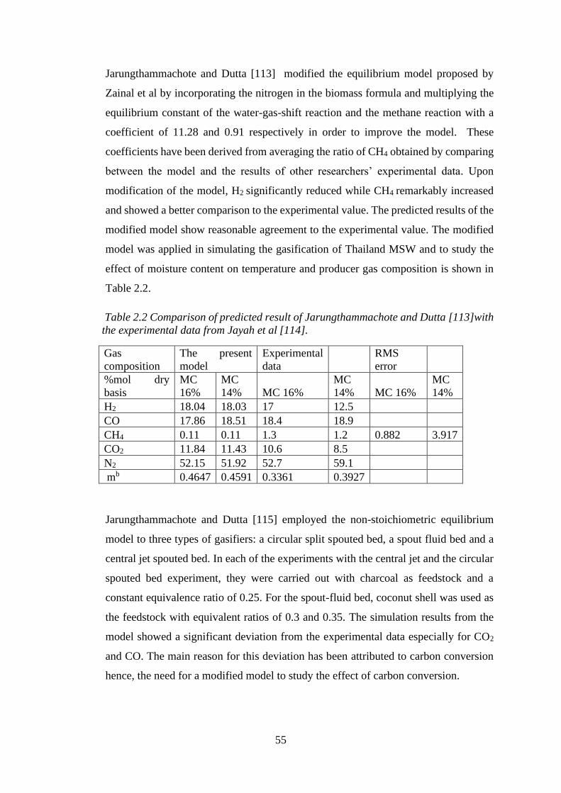
55
Jarungthammachote and Dutta [113] modified the equilibrium model proposed by
Zainal et al by incorporating the nitrogen in the biomass formula and multiplying the
equilibrium constant of the water-gas-shift reaction and the methane reaction with a
coefficient of 11.28 and 0.91 respectively in order to improve the model. These
coefficients have been derived from averaging the ratio of CH4 obtained by comparing
between the model and the results of other researchers’ experimental data. Upon
modification of the model, H2 significantly reduced while CH4 remarkably increased
and showed a better comparison to the experimental value. The predicted results of the
modified model show reasonable agreement to the experimental value. The modified
model was applied in simulating the gasification of Thailand MSW and to study the
effect of moisture content on temperature and producer gas composition is shown in
Table 2.2.
Table 2.2 Comparison of predicted result of Jarungthammachote and Dutta [113]with
the experimental data from Jayah et al [114].
Gas
composition
The present
model
Experimental
data
RMS
error %mol dry
basis
MC
16%
MC
14% MC 16%
MC
14% MC 16%
MC
14%
H2 18.04 18.03 17 12.5 CO 17.86 18.51 18.4 18.9 CH4 0.11 0.11 1.3 1.2 0.882 3.917
CO2 11.84 11.43 10.6 8.5 N2 52.15 51.92 52.7 59.1 mb 0.4647 0.4591 0.3361 0.3927
Jarungthammachote and Dutta [115] employed the non-stoichiometric equilibrium
model to three types of gasifiers: a circular split spouted bed, a spout fluid bed and a
central jet spouted bed. In each of the experiments with the central jet and the circular
spouted bed experiment, they were carried out with charcoal as feedstock and a
constant equivalence ratio of 0.25. For the spout-fluid bed, coconut shell was used as
the feedstock with equivalent ratios of 0.3 and 0.35. The simulation results from the
model showed a significant deviation from the experimental data especially for CO2
and CO. The main reason for this deviation has been attributed to carbon conversion
hence, the need for a modified model to study the effect of carbon conversion.
56
The data from the experiments showed that carbon conversion percentage for the
central jet spouted bed was in the range 55.5-65.1% and for the circular split spouted
bed, it is in the range 56.8-65.3%. For the spouted fluid bed, a value of 60% was
assumed. The simulation results from the modified model improved and were closer
to the experimental data confirming the carbon conversion as one of the important
factors for developing an equilibrium model. The heating value is another important
parameter as it is used to estimate the energy that could be derived from using the
producer gas. However, the modified model predicted heating values that were
generally higher than those from the experimental due to over predicted CO in the
producer gas especially for the central jet spouted bed gasification process.
Vaezi et al [116] developed an equilibrium model to predict the performance of a
biomass gasifier. The model seeks to find how of a particular biomass can be suited
for certain applications. The study incorporated 55 various biomass materials
published for which a wide range oxygen content and the C/H ratio was used. They
have employed a generalised format to plot the results which can allow the possibility
of selecting biomass material based on the desired conditions. These conditions
include the calorific value, volume of the syngas obtained, maximum efficiency,
temperature etc. Upon investigating the influence of varying C/H ratio together with
O2, the results show that increasing C/H ratio increases the heating value (HHV) of the
producer synthesis gas. It also reveals that the there is much higher influence of C/H
ratio on HHV than that of O2. The model slightly under predicts the experiments. This
is attributed to the characteristic of equilibrium models because the equilibrium
constant of hydrogasification reaction tends to zero at higher temperatures prevailing
in the reduction zone. As a result, the predicted CH4 amount in the final gas is small.
However, in a real gasifier, the devolatization of fuel gives high amounts of CH4 and
higher hydrocarbons which do not react completely to equilibrium. The developed
model agrees with those of the experiment.
Ratnadhariya and Channiwala [117] developed a three zone equilibrium and kinetic
free model of biomass gasifier. Drying and pyrolysis zones combine to form the first
zone while the second and third zones are oxidation and reduction respectively. The
model constitutes reaction stoichiometry, mass and energy balances including some
empirical relationships for each zone. In the drying and pyrolysis zone, species such
as CO, CO2, C, CH4, C2H2, H2 and H2O. Also, several assumptions were made based
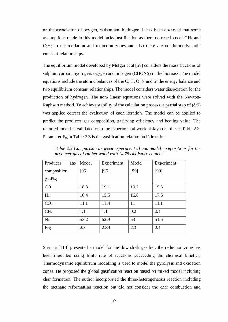
57
on the association of oxygen, carbon and hydrogen. It has been observed that some
assumptions made in this model lacks justification as there no reactions of CH4 and
C2H2 in the oxidation and reduction zones and also there are no thermodynamic
constant relationships.
The equilibrium model developed by Melgar et al [58] considers the mass fractions of
sulphur, carbon, hydrogen, oxygen and nitrogen (CHONS) in the biomass. The model
equations include the atomic balances of the C, H, O, N and S, the energy balance and
two equilibrium constant relationships. The model considers water dissociation for the
production of hydrogen. The non- linear equations were solved with the Newton-
Raphson method. To achieve stability of the calculation process, a partial step of (δ/5)
was applied correct the evaluation of each iteration. The model can be applied to
predict the producer gas composition, gasifying efficiency and heating value. The
reported model is validated with the experimental work of Jayah et al, see Table 2.3.
Parameter Frg in Table 2.3 is the gasification relative fuel/air ratio.
Table 2.3 Comparison between experiment al and model compositions for the
producer gas of rubber wood with 14.7% moisture content.
Producer gas
composition
(vol%)
Model
[95]
Experiment
[95]
Model
[99]
Experiment
[99]
CO 18.3 19.1 19.2 19.3
H2 16.4 15.5 16.6 17.6
CO2 11.1 11.4 11 11.1
CH4 1.1 1.1 0.2 0.4
N2 53.2 52.9 53 51.6
Frg 2.3 2.39 2.3 2.4
Sharma [118] presented a model for the downdraft gasifier, the reduction zone has
been modelled using finite rate of reactions succeeding the chemical kinetics.
Thermodynamic equilibrium modelling is used to model the pyrolysis and oxidation
zones. He proposed the global gasification reaction based on mixed model including
char formation. The author incorporated the three-heterogeneous reaction including
the methane reformatting reaction but did not consider the char combustion and
58
methane formation in the pyrolysis and oxidation zone. Four atomic balances (C, H, O
and N) energy balance equations including four equilibrium constants constitutes the
model. The model predicts the unreacted char at various thermodynamic condition.
The presented model has been validated with experimental data available in literature.
Antolini et al [119] developed an in-house thermodynamic equilibrium model to
predict the gas composition and char output from gasification of pelletized biomass
using air and CO2. The study was aimed at investigating the effect of CO2 feed in
biomass gasification as a viable way to directly exploit exhaust gas from the engine of
combined heat and power systems to convert CO2 to CO through Boudouard reaction,
and in doing so increase the carbon conversion and reduce char yield. The reactor is a
reverse downdraft gasifier mounted on a digital weighing balance. This approach is
based on the enthalpy of the reactants. The model results showed a good agreement
with the experimental results, especially in terms of predicted char yield.
2.4.4 Computational Fluid Dynamics (CFD) Models
Computational fluid dynamics plays an important role in the modelling of fixed bed
downdraft and fluidised bed gasifiers. CFD models numerically solve the mass,
momentum of species, hydro-dynamics, and energy flow and turbulence equations
over a distinct region. CFD models are found to be highly accurate in predicting gas
yield, temperature and the reactor if the reactor hydrodynamics is known. CFD
modelling of biomass gasification involves the combining of dense particulates flow
and specific chemistry [120]. The two aspects are very challenging in CFD; for
instance, the composition of biomass can pose some complexity due to its dependence
on geographical location, feedstock and age period of the year. These models have
been used to study characteristics of diverse types of biomass gasifiers.
Janajreh et al [121] studied the conversion of efficiency in a small scale, air blown
downdraft gasification system operated with wood as the fuel. CFD was used to model
the Lagrangian particle couple evolution after investigating the temperature field
inside the gasifier. The numerical simulation was conducted on a high-resolution mesh
accounting for the solid and gaseous phases using the k-epsilon turbulence and reacting
flow CFD model. The downdraft gasifier was modelled using the finite volume code
coupled with a conjugate heat transfer with the bulk metal separators and the insulators.
59
The results of the temperature distribution and the evolvement of the species were
validated by comparing with the experimental data of the ideal equilibrium and zero-
dimensional case. The result of CFD computed cold gas efficiency (CGE) was found
to be under predicted by 19 points less than that calculated for the ideal case. The
authors observed that equilibrium modelling could not capture the physio-chemical
processes inside the downdraft gasifier due to the complexity of the flow in the
downdraft gasifier. On the other hand, the discrete phase method (DPM) in ANSYS
was employed to model the devolatization effect of 0.1 mm particle diameter to
account for the particle size of the wood. The corresponding CFD and experimental
temperature profiles showed that the assumptions made were realistic.
Rogel et al [122] proposed a ’’1-D +2-D’’numerical model to simulate the gasification
of pure pine wood pellets in a stratified downdraft gasifier. The model considers
reactions for drying, primary pyrolysis of biomass, secondary tar cracking,
combustion, gasification and particle shrinkage. The particle model is based on
intraparticle mass and energy balances and is written in spherical coordinates for one
dimensional unsteady system. However, the gas phase model includes mass, energy
and momentum balances for two-dimensional unsteady system in cylindrical polar
coordinates. A commercially available CFD code PHOENICS was used to solve the
model numerically. The pressure drop inside the reactor is assumed constant and its
model is based on modified Ergun equation. Fine rate equations were used for all the
reactions and the transport equations were solved numerically. The model predictions
were shown to be in reasonable agreement with the experimental data with respect to
the gas temperature profiles, biomass temperature profile and biomass particle
shrinkage and syngas composition.
Jakobs et al. [41] proposed a CFD model of a high pressure entrained flow gasifier.
Finite volume solver was used to solve mass, momentum and energy balance equations
and considering several species. The atomization quality of twin fluid nozzles with
respect to gas velocity and reactor pressure was analysed. The proposed and
characterized atomizers were used in the atmospheric entrained flow gasifier, to detect
the influence of spray quality on gasification process. Sauter Mean Diameter (SMD)
of the produced spray was found to have a profoundly affected by the gas velocity and
reactor pressure. With an increase in the reactor pressure, the drop diameter was found
to increase while increasing gas velocity decreased the SMD. The impact of the SMD
60
on gasification process was observed from organic carbon and methane concentration
measurements as well as from the radial temperature profiles at various positions along
the reactor centreline. The CFD model of high pressure entrained flow gasification of
biomass based slurries showed a very significant influence of the drop size distribution
on gasification quality.
Gao et al [123] proposed a CFD model of a cyclone gasifier based on the use of CFD
package FLUENT. The model incorporates pyrolysis of sawdust, combustion of
volatiles and char. The model can predict the outlet gas composition and the
temperature in the gasifier. The influence of equivalence ratio was studied and validated
with experimental data. The carbon conversion for the cyclone gasifier was found to be
77 and 94.2% and the cold gas efficiency varied between 53.6 and 63% when the
equivalence ratio was varied from 0.23 to 0.35. The maximum lower heating value
(LHV) of 5.7 MJ/Nm3 was achieved when the equivalence ratio (λ) was between 0.23-
0.26. The predicted gas temperature and producer gas compositions were observed to
follow the same trend as the experimental data, however, the CO and CO2
concentrations were under predicted.
2.4.5 Artificial Neural Networks Model (ANNs)
Artificial Neural networks is a type of computational model in which a dense
distribution of simple processing element is supplied to give a presentation of complex
process which includes non- linear and discrete systems. The model consists of
interconnected groups of artificial neurons and then processes the information via
computation (Babu et al. 2009). ANN is a standard modelling tool which consists of
multiple layers of perception paradigm (MLP) [124]). These layers consists of an input
layer, a hidden layer and an output layer of neurons. The hidden and output layer
neurons process their inputs by multiplying each input by a corresponding weight,
summing the product, and then processing the sum using a nonlinear transfer function
to produce a result [125]. The neurons in the input layer conveys the signals to the
hidden and output layers. ANN is usually employed in signal processing, function
approximation, simulation and for identifying patterns.
Brown et al [126] proposed an equilibrium model for the design of biomass gasifiers.
From the ultimate analysis properties, fuels and chars were defined while tar was
defined as a subset of known molecular species and their distribution was determined
61
by equilibrium calculations. The reaction temperature difference for a complete set of
stoichiometric equations was used to explain the non-equilibrium behaviour of the tar
and char formation. A non-linear regression including an artificial neural network
evaluated the relationship between the changes in temperature and fuel consumption
and operational variables. This approach applied with a fluidise bed reactor data, seems
to improve the accuracy of the equilibrium calculations and reduces the number of
required data by stopping the Neural Network from identifying atomic and heat
balances. Sreejith et al. [44] proposed a feed-forward artificial neural network (ANN)
model for the predicting the gasification temperature and product gas composition.
They proposed a Redlich–Kwong real gas equilibrium correction model including tar
and unconverted char to predict the product gas composition, heating value and
thermodynamic efficiencies. A reasonable accuracy of ANN prediction with
experimental results was reported based on the computed statistical parameters of
comparison such as coefficient of correlation, root mean square error (RMSE), average
percentage error and covariance. The equilibrium model corrected was developed by
introducing correction factors for real gas equilibrium constants and these showed
satisfactory agreement with the experimental values. Maximum concentration of
hydrogen achieved experimentally was 29.1% at the equivalence ratio of 0.277 and
steam to biomass ratio (SBR) of 2.53. The corresponding predicted values were 28.2%
for ANN model and 31.6% for corrected equilibrium model. The equilibrium model
corrected for wood sawdust was validated with air–steam gasification experimental
results of other biomass materials and was found to be 95.1% accurate on average. It
was revealed from the study that the ANN model (RMSE is 2.64) was a better predictor
for the product gas composition than the corrected real gas equilibrium model (RMSE
is 5.96).
Puig-Arnavat [25] developed two ANN models; one for circulating fluidized bed
gasifiers (CFB) and the other for bubbling fluidized bed gasifiers (BFB). Both models
were used to determine the producer gas composition (CO, CO2, H2 and CH4) and gas
yield. The effect of ash, moisture, carbon, oxygen and hydrogen content of dry
biomass, equivalence ratio and gasification temperature were studied for CFB and BFB
whereas the effect of steam to dry biomass ratio (kg/kg) was studied for BFB only.
The two ANN models developed for CFB and BFB gasifiers showed the possibility
that ANN may offer some contribution to research in the area of biomass gasification
62
modelling. The results obtained by the two ANN’s showed high agreement with
published experimental data used: very good correlations in almost all cases and small
RMSE.
Considering engineering design and process optimization of biomass gasifier for the
production of synthesis gas, an extensive investigation of the plant behaviour depending
on various operating parameters is required. Whilst performing experiments on large
scales may pose problems due to associated safety risks and high costs, developing a
mathematical model can also give a good representation of the complex chemical and
physical phenomena taking place in the gasifier as this allows fewer and better
experiments to be performed with minimal costs. Also, a simulation model allows
prediction of the progress of these complex occurrences as it is needed for optimizing
the gasifier design and its operating conditions. In view of this, this work consists in
the development of the method of numerical simulation of a downdraft gasifier
operation, which is based on thermodynamic and kinetic models applied to a downdraft
fixed bed. The model presented in this work is made up from three constituent sub-
models which attempt to simulate each of the zones namely pyrolysis, oxidation and
reduction zones. These are then combined to form a complete model using both single
and double air feed to the gasifier. Whilst there are many studies in literature on biomass
gasification based on equilibrium and kinetic models, this technology is still not very
commercially viable due to the challenges related to the gasification of biomass to
produce clean gas for internal combustion engines and gas turbines as well as severe
constraints in terms of gas quality and lack of flexibility in the type of biomass. It is in
this context that this work has relevance in attempting to explore various approaches
for modeling and simulation. In one approach to simulation the three zones were all
assumed to reach thermodynamic equilibrium and each zone was simulated using a
Gibbs Reactor. In another approach an assumption was made that the third zone, the
Reduction Zone, could be simulated using a chemical rate approach. This required
chemical equations to be presented that could theoretically represent the formation and
disappearance of species in the Reduction Zone. In HYSYS this zone was represented
by a PFR. Whilst this operation requires the presentation of chemical kinetic data it also
integrates over a stated tubular reactor to produce a unique solution according to the
conditions calculated by the previous zone, the oxidation zone represented by a Gibbs
Reactor. Using such an approach for this type of problem; simulation of a biomass
gasifier is unique.
63
Chapter 3 Modelling and Simulation of Biomass
Gasification Process
Operating a biomass gasifier efficiently depends on a number of complex chemical
reactions such as fast pyrolysis, partial oxidation of the pyrolysis products, gasification
of the resulting char, conversion of tar and lower hydrocarbons, water-gas reaction and
methane formation etc. Development of mathematical models are required due to the
complexity of the reaction processes, sensitivity of the product distribution, rate of
heating and residence time in the reactor in other effectively design and operate a
particular gasifier[25].
Mathematical simulation is a very important aspect of research and development of
the Gasification technology. Simulation may not provide a very accurate prediction of
system performance however, it may provide guidance on the effect of design,
operating conditions and input variables. Also, modelling may provide a less expensive
means of evaluating the benefits and the accompanying risks in the real time situation
[80]. Understanding of chemical and physical mechanisms of biomass gasification
processes is essential to optimize the gasifier designing and operating biomass
gasification systems[127].
The importance of mathematical simulations can be summarized as follows [80]
o Allows optimizing the operation or design of the plant using available experimental
data from a plant or large-scale plant.
o Provide information on extreme operating conditions where experiments and
measurements are difficult to perform.
o Identify operating limits and related risks.
o Aid in scale-up of the gasifier from one successfully operating size to another and from
one feedstock to another.
o Assist in interpretation of experimental results and analyse anomalous behaviour of
the gasifier.
64
Gasification simulations models may be classified into thermodynamic equilibrium
model, kinetic model, computational Fluid dynamics (CFD) model and artificial neural
work. These models are based on different methods to assess and predict gas fractions
and the effects of operating conditions of a particular design including the utility and
limitations. Modelling of the gasification process using a particular approach may
consider the following reaction which are the basic gasification reactions [128]:
Bouordard reaction (R1) 𝐶 + 𝐶𝑂2 → 2𝐶𝑂 (3.1)
Water- gas reaction (R2) 𝐶 + 𝐻2𝑂 → 𝐻2 + 𝐶𝑂 (3.2)
Methane Formation (R3) 𝐶 + 2𝐻2 → 𝐶𝐻4 (3.3)
Steam reforming reaction (R4) 𝐶𝐻4 + 2𝐻2𝑂 → 4𝐻2 + 𝐶𝑂2 (3.4)
3.1 Thermodynamic Equilibrium Models
Thermodynamic equilibrium models are based on the chemical and thermodynamic
equilibrium which are determined by implication of equilibrium constants and
minimization of Gibbs free energy. The idea of chemical equilibrium is based on the
second law of thermodynamics when applied to reacting systems [54]. At chemical
equilibrium, the species of a reacting system is at a stable composition as it does not
experience a net change in concentration over time [94]. Equilibrium models are
suitable simulation tools for processes whose duration are in most cases quite long
with regard to the reaction timescale [81]. The thermodynamic equilibrium
calculations are suitable for studying the influence of fuel and process parameters such
as temperature [58].
Some major assumptions of thermodynamic equilibrium models can be presented as
follows:
o The reactor is considered as zero dimensional.
o There is perfect mixing of materials and uniform temperature in the gasifier even
though different hydrodynamics are observed in practice.
o The rates of reactions are fast enough and residence time is long enough to attain
equilibrium.
65
By employing the governing equations describing the behaviour of such state, one can
formulate an equilibrium model. These fundamental equations stated in Tigabwa et al
[94] are following equations.
Overall mass balance:
𝐹𝑖𝑛 ∑ 𝑖𝑛 𝑛𝐾,𝑖 𝑋𝑖 = 𝐹𝑜𝑢𝑡 ∑ 𝑜𝑢𝑡 𝑛𝐾,𝑖𝑋𝑖 (3.5)
Where 𝑛𝑘,𝑖 is the number of atoms k of a molecule i, and 𝑥𝑖 is the molar fraction of a
component i.
Overall energy balance:
𝐹𝑖𝑛 ∑ 𝑖𝑛 𝑋𝑖𝐻𝑖(𝑇𝑖𝑛, 𝑃) = 𝐹𝑜𝑢𝑡 ∑ 𝑜𝑢𝑡 𝑋𝑖𝐻𝑖(𝑇𝑜𝑢𝑡, 𝑃) (3.6)
3.1.1 Stoichiometric Equilibrium Models
Stoichiometric models are based on the use of equilibrium constants where specific
chemical reactions used in the calculations are defined; it follows that appropriate
chemical reactions are selected and information regarding the equilibrium constants
are required [107]. The equilibrium constant of a reaction j is
𝐾𝑗 = ∏ (𝑃𝑖
𝑃0𝑖 ) 𝑣𝑖, 𝑗 (3.7)
These sets of selected chemical reactions can be associated with the Gibbs free energy
change related to temperature:
-RTln𝐾𝑗 = ∆𝐺0𝑗 (3.8)
The disadvantage of this method lies in the fact that a set of non- linear algebraic
equations are solved for the mole numbers of each specie and this mostly difficult if
the system is large [108]. In order to predict the gasification process in a downdraft
gasifier, Zainal et al used stoichiometric equilibrium method to model the gasification
process in a downdraft gasifier different biomass materials [112]. The equilibrium
model predicts the calorific value of the gasifier reasonably well and compares well
the experimental values available in the literature for wood. However, the amount of
oxygen in that model was eliminated by defining it in terms of components in the
producer gas but was not shown when they compared their model with their
experimental data, this is what makes this model different. The thermodynamic
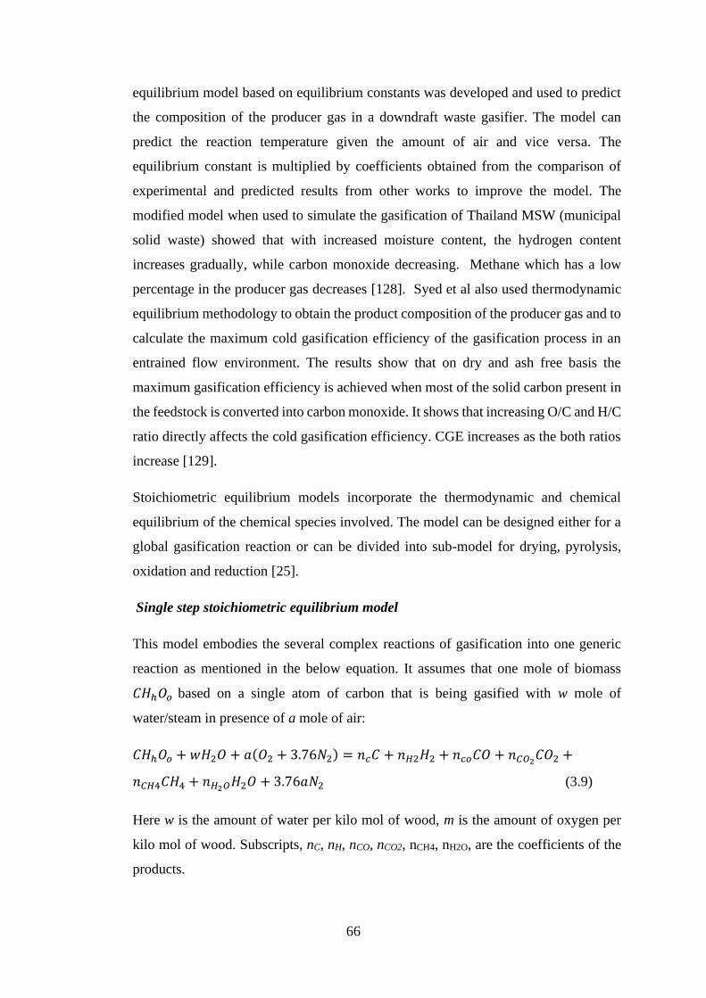
66
equilibrium model based on equilibrium constants was developed and used to predict
the composition of the producer gas in a downdraft waste gasifier. The model can
predict the reaction temperature given the amount of air and vice versa. The
equilibrium constant is multiplied by coefficients obtained from the comparison of
experimental and predicted results from other works to improve the model. The
modified model when used to simulate the gasification of Thailand MSW (municipal
solid waste) showed that with increased moisture content, the hydrogen content
increases gradually, while carbon monoxide decreasing. Methane which has a low
percentage in the producer gas decreases [128]. Syed et al also used thermodynamic
equilibrium methodology to obtain the product composition of the producer gas and to
calculate the maximum cold gasification efficiency of the gasification process in an
entrained flow environment. The results show that on dry and ash free basis the
maximum gasification efficiency is achieved when most of the solid carbon present in
the feedstock is converted into carbon monoxide. It shows that increasing O/C and H/C
ratio directly affects the cold gasification efficiency. CGE increases as the both ratios
increase [129].
Stoichiometric equilibrium models incorporate the thermodynamic and chemical
equilibrium of the chemical species involved. The model can be designed either for a
global gasification reaction or can be divided into sub-model for drying, pyrolysis,
oxidation and reduction [25].
Single step stoichiometric equilibrium model
This model embodies the several complex reactions of gasification into one generic
reaction as mentioned in the below equation. It assumes that one mole of biomass
𝐶𝐻ℎ𝑂𝑜 based on a single atom of carbon that is being gasified with w mole of
water/steam in presence of a mole of air:
𝐶𝐻ℎ𝑂𝑜 + 𝑤𝐻2𝑂 + 𝑎(𝑂2 + 3.76𝑁2) = 𝑛𝑐𝐶 + 𝑛𝐻2𝐻2 + 𝑛𝑐𝑜𝐶𝑂 + 𝑛𝐶𝑂2𝐶𝑂2 +
𝑛𝐶𝐻4𝐶𝐻4 + 𝑛𝐻2𝑂𝐻2𝑂 + 3.76𝑎𝑁2 (3.9)
Here w is the amount of water per kilo mol of wood, m is the amount of oxygen per
kilo mol of wood. Subscripts, nC, nH, nCO, nCO2, nCH4, nH2O, are the coefficients of the
products.
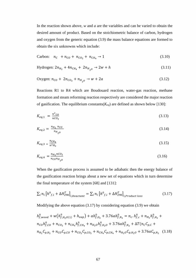
67
In the reaction shown above, w and a are the variables and can be varied to obtain the
desired amount of product. Based on the stoichiometric balance of carbon, hydrogen
and oxygen from the generic equation (3.9) the mass balance equations are formed to
obtain the six unknowns which include:
Carbon: 𝑛𝐶 + 𝑛𝐶𝑂 + 𝑛𝐶𝑂2+ 𝑛𝐶𝐻4
→ 1 (3.10)
Hydrogen: 2𝑛𝐻2+ 4𝑛𝐶𝐻4
+ 2𝑛𝐻2𝑂
→ 2𝑤 + ℎ (3.11)
Oxygen: 𝑛𝐶𝑂 + 2𝑛𝐶𝑂2+ 𝑛𝐻
2𝑂→ 𝑤 + 2𝑎 (3.12)
Reactions R1 to R4 which are Boudouard reaction, water-gas reaction, methane
formation and steam reforming reaction respectively are considered the major reaction
of gasification. The equilibrium constants(Keq) are defined as shown below [130]:
𝐾𝑒𝑞,1 = 𝑛2
𝐶𝑂
𝑛𝐶𝑂2 (3.13)
𝐾𝑒𝑞,2 = 𝑛𝐻2 𝑛𝐶𝑂
𝑛𝐻2𝑂
(3.14)
𝐾𝑒𝑞,3 = 𝑛𝐶𝐻4
𝑛2𝐻2 (3.15)
𝐾𝑒𝑞,4 =𝑛𝐻2𝑛𝐶𝑂2
𝑛𝐶𝑂𝑛𝐻2𝑂
(3.16)
When the gasification process is assumed to be adiabatic then the energy balance of
the gasification reaction brings about a new set of equations which in turn determine
the final temperature of the system [68] and [131]:
∑ 𝑛𝑖𝑖 [ℎ0𝑓,𝑖 + ∆𝐻298
𝑇 ]𝑖,𝑅𝑒𝑎𝑐𝑡𝑎𝑛𝑡
= ∑ 𝑛𝑖𝑖 [ℎ0𝑓,𝑖 + ∆𝐻298
𝑇 ]𝑖,𝑃𝑟𝑜𝑑𝑢𝑐𝑡 𝑙𝑜𝑠𝑠
(3.17)
Modifying the above equation (3.17) by considering equation (3.9) we obtain
ℎ𝑓,𝑤𝑜𝑜𝑑0 + 𝑤(ℎ𝑓,𝐻2𝑂(1)
0 + ℎ𝑣𝑎𝑝) + 𝑎ℎ𝑓,𝑂2
0 + 3.76𝑎ℎ𝑓,𝑁2
0 = 𝑛𝑐 . ℎ𝑓,𝑐0 + 𝑛𝐻2
ℎ𝑓,𝐻2
0 +
𝑛𝐶𝑂ℎ𝑓,𝐶𝑂0 + 𝑛𝐶𝑂2
+ 𝑛𝐶𝐻4ℎ𝑓,𝐶𝐻4
0 + 𝑛𝐻2𝑂ℎ𝑓,𝐻2𝑂0 + 3.76𝑎ℎ𝑓,𝑁2
0 + ∆𝑇(𝑛𝐶𝐶𝑝,𝐶 +
𝑛𝐻2𝐶𝑝,𝐻2
+ 𝑛𝐶𝑂𝐶𝑝,𝐶𝑂 + 𝑛𝐶𝑂2𝐶𝑝,𝐶𝑂2
+ 𝑛𝐶𝐻4𝐶𝑝,𝐶𝐻4
+ 𝑛𝐻2𝑂𝐶𝑝,𝐻2𝑂 + 3.76𝑎𝐶𝑝,𝑁2 (3.18)
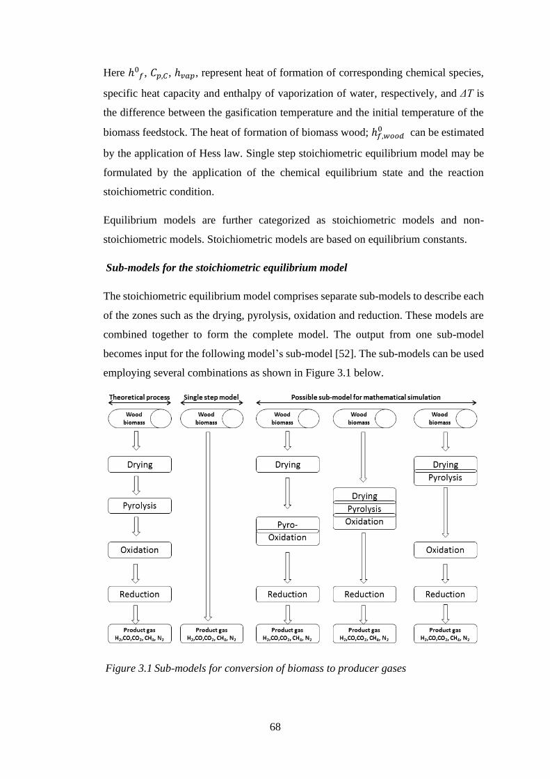
68
Here ℎ0𝑓, 𝐶𝑝,𝐶, ℎ𝑣𝑎𝑝, represent heat of formation of corresponding chemical species,
specific heat capacity and enthalpy of vaporization of water, respectively, and ΔT is
the difference between the gasification temperature and the initial temperature of the
biomass feedstock. The heat of formation of biomass wood; ℎ𝑓,𝑤𝑜𝑜𝑑0 can be estimated
by the application of Hess law. Single step stoichiometric equilibrium model may be
formulated by the application of the chemical equilibrium state and the reaction
stoichiometric condition.
Equilibrium models are further categorized as stoichiometric models and non-
stoichiometric models. Stoichiometric models are based on equilibrium constants.
Sub-models for the stoichiometric equilibrium model
The stoichiometric equilibrium model comprises separate sub-models to describe each
of the zones such as the drying, pyrolysis, oxidation and reduction. These models are
combined together to form the complete model. The output from one sub-model
becomes input for the following model’s sub-model [52]. The sub-models can be used
employing several combinations as shown in Figure 3.1 below.
Figure 3.1 Sub-models for conversion of biomass to producer gases
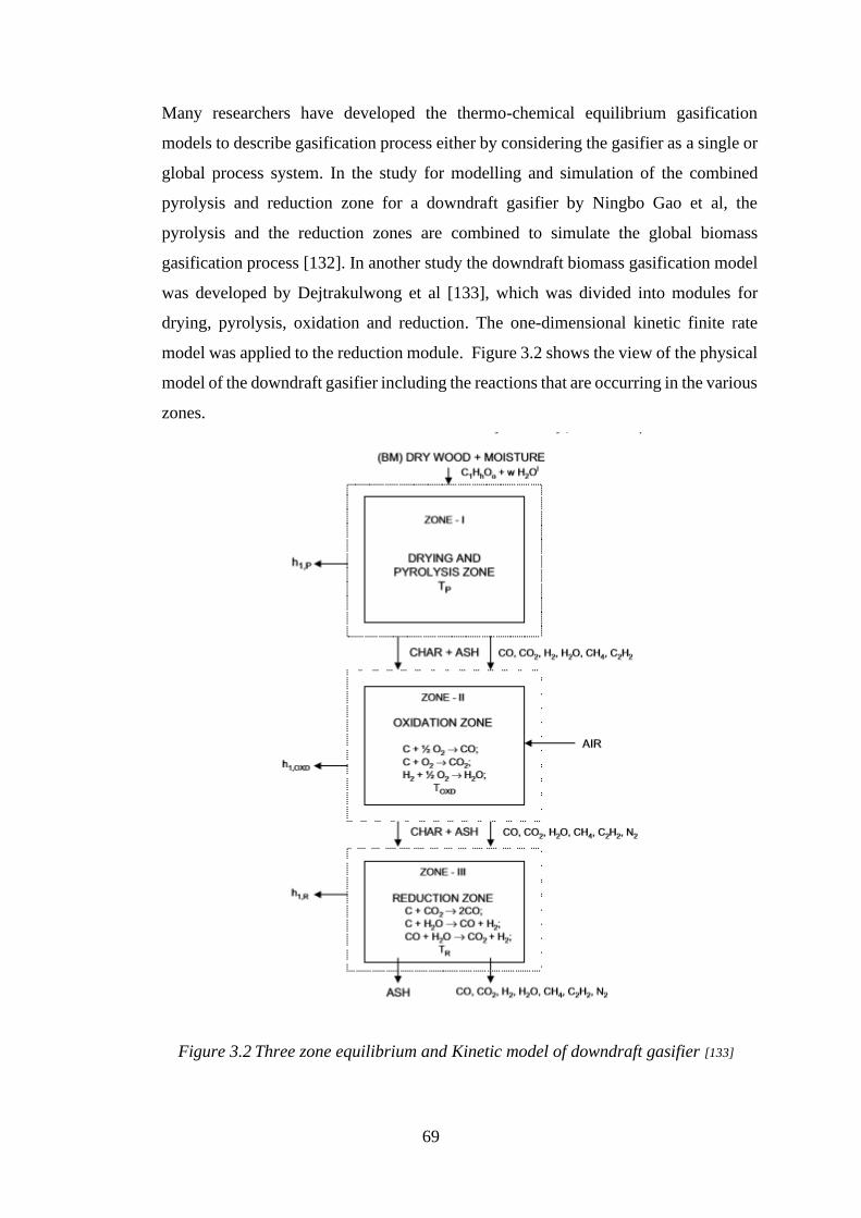
69
Many researchers have developed the thermo-chemical equilibrium gasification
models to describe gasification process either by considering the gasifier as a single or
global process system. In the study for modelling and simulation of the combined
pyrolysis and reduction zone for a downdraft gasifier by Ningbo Gao et al, the
pyrolysis and the reduction zones are combined to simulate the global biomass
gasification process [132]. In another study the downdraft biomass gasification model
was developed by Dejtrakulwong et al [133], which was divided into modules for
drying, pyrolysis, oxidation and reduction. The one-dimensional kinetic finite rate
model was applied to the reduction module. Figure 3.2 shows the view of the physical
model of the downdraft gasifier including the reactions that are occurring in the various
zones.
Figure 3.2 Three zone equilibrium and Kinetic model of downdraft gasifier [133]
70
Here drying and pyrolysis zones are combined together. The products of this zone are
assumed to be char, CO, CO2, H2, H2O, C2H2 and CH4. The drying and pyrolysis zone
is where the moisture in the biomass is released as steam and where the ligno -
cellulosic material is thermally decomposed. The decomposition of this ligno-
cellulosic material is transformed into gaseous volatile species mainly composed of
CO2, H2, CH4, C2H2, CO as well as char. These substances then move to the oxidation
zone where it contacts with air and partial combustion of the volatile species takes
place. The pyrolysis products are then transformed into the oxidation products which
consist of CO, CO2, CH4, H2, N2, steam tar and char. The heat generated from the
oxidation zone is used to drive the reactions in both drying and reductions zones. In
the reduction zone, oxidation products react to form CO, CO2, H2, CH4, N2 and water
vapour.
3.1.2 The Model development and assumptions
The model formulated in this work consists of three constituent sub-models to describe
each of the zones i.e. pyrolysis, oxidation and reduction zone. These are then combined
together to form a complete model. The sub-models are taken from Centeno et al [134]
and Roy et al [57]. The pyrolysis and oxidation zones are modelled using the chemical
equilibrium. Mass balance equations are used to calculate the amounts of pyrolysis
products. These are solved using assumptions from Centeno. The single energy
balance equation is from Roy et al and is applied across both zones to calculate the
reaction temperature at the entry into the reduction zone.
Assumptions
• The gasifier operates under atmospheric temperature.
• All gaseous species are treated as ideal gases.
• The char is modelled as carbon graphite (non-volatile carbon).
• Only the volatile part of the biomass undergoes the pyrolysis process. The non-
volatile carbon and biomass moisture proceed to the oxidation zone.
• Since the affinity between hydrogen and oxygen is higher than that of oxygen and
carbon, it is assumed that 80% of fuel oxygen i.e. 4/5 of the supplied oxygen is
associated with fuel hydrogen in the form of water while the remaining 20% i.e.
1/5 of oxygen is associated with carbon in the biomass and releases as CO and
CO2.
71
• The ratio of moles of CO and CO2 formed is inversely equated to their molecular
masses i.e. CO/CO2 =44/28.
• Fifty percent of the hydrogen in the fuel is given off as H2 upon decomposition and
the remaining fifty percent is given off in the form of CH4 and C2H2.
• The ratio of moles of CH4 and C2H2 is inversely related with their molecular masses
i.e. CH4/C2H2 = 26/16.
Formulation of the model
From the ultimate analysis data, moist biomass can be presnted as sum of volatiles,
non-volatile and components of water plus some amount of incombustible materials
such as ash:
Biomass = 𝐶𝑏𝐶𝐻𝑏𝐻𝑂𝑏𝑂 + w𝐻2𝑂 + 𝑎𝑠ℎ→ 𝐶𝑏𝑣𝐶𝐻𝑏𝑣𝐻𝑂𝑏𝑣𝑂 + 𝐶𝑏𝑛𝑣𝑐 + 𝑤𝐻2𝑂 + 𝑎𝑠ℎ
(3.19)
Here, w𝐻2𝑂 is moles of water in the feedstock moisture; 𝑏𝑣𝐶 is volatile moles of
Carbon; 𝑏𝑣𝐻 is volatile moles of Hydrogen; 𝑏𝑣𝑂 is volatile moles of Oxygen; 𝑏𝑣𝑛𝐶
is non-volatile moles of Carbon
Pyrolysis Zone
The process taking place in the pyrolysis zone can be represented symbolically as
Biomass + heat → volatile components + water vapour + char + ash (3.20)
The above chemical reaction is written as
𝐶𝑏𝑣𝐶𝐻𝑏𝑣𝐻𝑂𝑏𝑣𝑂 → 𝑋𝑝𝐶𝐶 + 𝑋𝑝𝐶𝑂2𝐶𝑂2+ 𝑋𝑝𝐶𝑂𝐶𝑂 + 𝑋𝑝𝐶𝐻4
𝐶𝐻4 + 𝑋𝑝𝐶2𝐻2𝐶2𝐻2 +
𝑋𝑝𝐻2𝐻2 + 2𝑋𝑝𝐻
2𝑂𝐻2𝑂 (3.21)
Pyrolysis zone mass balance equations are:
Carbon: 𝑏𝑣𝐶 = 𝑋𝑝𝑐 + 𝑋𝑝𝐶𝑂2+ 𝑋𝑃𝐶𝑂 + 𝑋𝑝𝐶𝐻4
+ 2𝑋𝑝𝐶2𝐻2 (3.22)
Hydrogen: 𝑏𝑣𝐻 = 4𝑋𝑝𝐶𝐻4+ 2𝑋𝑝𝐶2𝐻2
+ 2𝑋𝑝𝐻2+ 2𝑋𝑝𝐻
2𝑂 (3.23)
Oxygen: 𝑏𝑣𝑂 = 2𝑋𝑝𝐶𝑂2+ 𝑋𝑝𝐻
2𝑂+ 𝑋𝑃𝐶𝑂 (3.24)
72
Parameter 𝑋𝑝 in above equations represent amounts of products from pyrolysis zone
Oxidation zone
The oxidation zone reaction can be represented symbolically by
𝑉𝑜𝑙𝑎𝑡𝑖𝑙𝑒𝑠 + 𝑐ℎ𝑎𝑟 + 𝑎𝑖𝑟 → 𝐻2𝑂 + 𝐶𝑂 + 𝐻2 + 𝐶𝑂2 + 𝐶𝐻4 + 𝑁2 + 𝑐ℎ𝑎𝑟 + 𝑡𝑎𝑟
(3.25)
Assumptions
• Acetylene formed during the pyrolysis process is fully oxidized.
• If oxygen is supplied in sufficient amount, the hydrogen formed in the pyrolysis
zone is fully oxidized and converted to water because of its high burning rate.
• If any oxidation remains after oxidation of hydrogen and acetylene, methane
formed during this process is converted to water and carbon dioxide depending on
the availability of oxygen
• Any remaining oxygen is consumed in oxidation of char.
• Concentrations of CO and CO2 are assumed to be inversely proportional to the ratio
of exothermicity of the corresponding reactions i.e. the less the exothermic
reaction, the more the product formation.
• It is assumed that CO2, CO and H2O produced during oxidation are added to the
products from the pyrolysis zone.
• N2 form entering the oxidation zone is inert.
Products calculated from the pyrolysis zone 𝑋𝑝 react with air in the oxidation zone
and products from the oxidation zone 𝑋𝑜 are calculated as:
𝑋𝑝𝐶𝐶 + 𝑋𝑝𝐶𝑂2𝐶𝑂2 + 𝑋𝑝𝐶𝑂𝐶𝑂 + 𝑋𝑝𝐶𝐻4
𝐶𝐻4 + 𝑋𝑝𝐻2𝐻2 + 𝑋𝑝𝐶2𝐻2
𝐶2𝐻2 +
2𝑋𝑝𝐻2𝑂𝐻2𝑂 + 𝑎(𝑂2 + 3.76𝑁2)→ 𝑋𝑜𝐶𝐶 + 𝑋𝑜𝐶𝑂2𝐶𝑂2 + 𝑋𝑜𝐶𝑂𝐶𝑂 + 𝑋𝑜𝐶𝐻4
𝐶𝐻4 +
𝑋𝑜𝐻2𝐻2 + 𝑋𝑜𝐶2𝐻2
+ 𝑋𝑜𝐻2𝑂𝐻2𝑂 + 3.76𝑎𝑁2 + 𝑏𝑛𝑣𝐶 (3.26)
Mass balance equations can be written as follows.
Carbon:
𝑏𝑛𝑣𝐶 + 𝑋𝑝𝐶 + 𝑋𝑝𝐶𝐻4+ 𝑋𝑝𝐶𝑂 + 𝑋𝑝𝐶𝑂2
+ 2𝑋𝑝𝐶2𝐻2= 𝑋𝑜𝐶𝑂2
+ 𝑋𝑜𝐶𝑂 + 𝑋𝑜𝐶𝐻4+
𝑋𝑜𝐶 (3.27)
73
Hydrogen:
2𝑋𝑝𝐶2𝐻2+ 4𝑋𝑝𝐶𝐻4
+ 2𝑋𝑝𝐻2+ 2𝑋𝑝𝐻
2𝑂= 4𝑋𝑜𝐶𝐻4
+ 2𝑋𝑜𝐻2+ 2𝑋𝑜𝐻
2𝑂 (3.28)
Oxygen:
𝑋𝑝𝐶𝑂 + 𝑋𝑝𝐶𝑂2+ 𝑋𝑝𝐻
2𝑂+ 2𝑎 = 𝑋𝑜𝐶𝑂 + 2𝑋𝑜𝐶𝑂2
+ 𝑋𝑜𝐻2𝑂
(3.29)
Products amounts are calculated from the mass balance and using the following
assumption: 4/5 of the supplied oxygen is associated with fuel hydrogen in the form of
water while the remaining 20% i.e. 1/5 Oxygen is associated with carbon in the
biomass and releases as CO and CO2.
To perform calculations in MATLAB, these expressions are written thus considering
the assumptions;
𝑥𝑝𝐻2𝑂 = 0.8 ∗ 𝑏𝑣𝑂 + 𝑤𝐻2𝑂 (3.30)
𝑥𝑝𝐶𝑂 = 0.2 ∗ 𝑏𝑣𝑂 ∗ 44/(44 + 28) (3.31)
𝑥𝑝𝐶𝑂2 = 0.2 ∗ 𝑏𝑣𝑂 ∗ 28/(44 + 28) (3.32)
Fifty percent of the hydrogen in the fuel is given off as H2 upon decomposition and the
remaining fifty percent is given off in the form of CH4 and C2H2
𝑥𝑝𝐻2 = 0.5 ∗ (𝑏𝑣𝐻 − 2 ∗ 0.8 ∗ 𝑏𝑣𝑂) ∗ 0.5 (3.33)
𝑥𝑝𝐶𝐻4 = 0.5 ∗ (𝑏𝑣𝐻 − 2 ∗ 0.8 ∗ 𝑏𝑣𝑂) ∗ 26/(26 + 16) (3.34)
𝑥𝑝𝐶2𝐻2 = 0.5(𝑏𝑣𝐻 − 2 ∗ 0.8 ∗ 𝑏𝑣𝑂) ∗ 16/(26 + 16) (3.35)
Energy balance
Both exothermic and endothermic reactions occur in the gasifier. Examples of such
reactions are partial oxidation and Boudouard reactions, respectively. Some of the
heat generated from the exothermic reaction is used by the endothermic reaction and
the rest is converted to sensible heat, affecting the temperature. The reaction
temperature is an important parameter that influences the both chemical reactions and
thermodynamic calculations. It is therefore necessary to know the reaction
74
temperature. In order to obtain this value, the first law of thermodynamics or energy
balance is applied for the description of gasification process [107].
Once the composition of the pyrolysis products has been obtained from solving the
mass balance, they can be used to solve the energy balance across the pyro- oxidation
zone for the reactor temperature at entry to the reaction zone:
𝑥𝑏𝑖𝑜𝑚𝑎𝑠𝑠 ℎ𝑓𝑜 + 𝑎 ∫ 𝑐�̅�,𝑂2
𝑇𝑎
𝑇𝑜𝑑𝑇 + 3.76𝑎 ∫ 𝑐�̅�,𝑁2
𝑇𝑎
𝑇𝑜𝑑𝑇 + 𝑤ℎ𝑓,𝐻2𝑂
𝑜 + �̇�𝑙𝑜𝑠𝑠 =
∑ 𝑥𝑜𝑥6𝑥=1 [ℎ𝑓,𝑥
𝑜 + ∫ 𝑐�̅�,𝑥𝑇
𝑇𝑜𝑑𝑇] + 𝑥𝑜𝐶𝑐�̅�,𝑐(𝑇 − 𝑇𝑜) + �̇�𝑎𝑠ℎ𝑐�̅�,𝑎𝑠ℎ(𝑇 − 𝑇𝑜) (3.36)
Reduction zone
The kinetic model predicts the gas yield and product composition that a gasifier
achieves after a finite time or in a finite volume in the case of a flowing medium [6].
The model is able to predict the temperature profiles and gas composition inside the
gasifier, taking into account the gasifier operating conditions and the gasifier
configuration. It also considers both the kinetics of gasification reactions and the
hydrodynamics of the gasifier. The reaction kinetics requires reaction rates, knowledge
of bed hydrodynamics, mass and energy balance to obtain gas yields, tar and char at a
given operating condition while the reactor hydrodynamics involves the knowledge of
the physical mixing process [77].
3.2 Kinetic model
The reduction of the chemical species from the oxidation zone takes place in the
gasifier’s reduction zone. The products from oxidation zone are taken as initial input
for the first compartment of reduction zone. The reactions of the reduction zone are
slow, reversible and endothermic so they cannot be assumed to have reached
equilibrium. For this reason, a finite rate kinetic model originally presented by Giltrap
et al is employed which considers the following reactions taking place.
Bourdouard reaction:
𝐶 + 𝐶𝑂2 ⟷ 2𝐶𝑂 ΔH =172kJ/kmol (endothermic) (3.37)
Water gas reaction:
𝐶 + 𝐻2𝑂 ⟷ 𝐶𝑂 + 𝐻2 ΔH =131.4kJ/kmol (endothermic) (3.38)
75
Methanation reaction:
𝐶 + 2𝐻2 ⟷ 𝐶𝐻4 ΔH =-74.9kJ/kmol (exothermic) (3.39)
Steam Reforming:
𝐶𝐻4 + 𝐻2𝑂 ⟷ 𝐶𝑂 + 3𝐻2 ΔH = 206.4kJ/kmol (endothermic) (3.40)
The values of the equilibrium constants for the four above reactions are calculated from
Gibbs free energy
𝐾𝑝 = exp (−Δ𝐺𝑇
𝑅𝑇) (3.41)
The expressions for the equilibrium constants for the four reactions are given by
𝐾1 = 𝑒𝑥𝑝 (−2𝑔𝐶𝑂
𝑅𝑇+
𝑔𝐶𝑂2
𝑅𝑇) (3.42)
𝐾2 = 𝑒𝑥𝑝 (−𝑔𝐶𝑂
𝑅𝑇−
𝑔𝐻2
𝑅𝑇+
𝑔𝐻2𝑂
𝑅𝑇) (3.43)
𝐾3 = 𝑒𝑥𝑝 (−𝑔𝐶𝐻4
𝑅𝑇+ 2
𝑔𝐻2
𝑅𝑇) (3.44)
𝐾4 = 𝑒𝑥𝑝 (−𝑔𝐶𝑂
𝑅𝑇− 3
𝑔𝐻2
𝑅𝑇+
𝑔𝐶𝐻4
𝑅𝑇+
𝑔𝐻2𝑂
𝑅𝑇) (3.45)
Rates of four reactions in the reduction zone are evaluated using Arrhenius type kinetic
rate equations, see Table 3.1
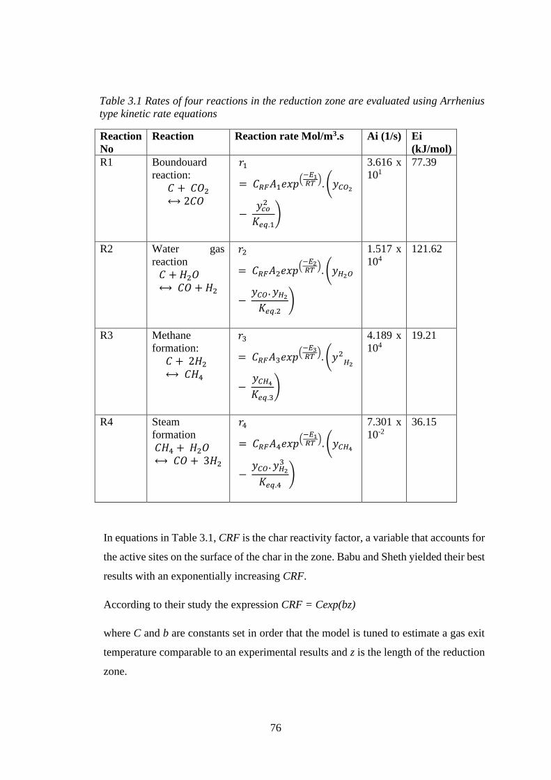
76
Table 3.1 Rates of four reactions in the reduction zone are evaluated using Arrhenius
type kinetic rate equations
Reaction
No
Reaction Reaction rate Mol/m3.s Ai (1/s) Ei
(kJ/mol)
R1 Boundouard
reaction:
𝐶 + 𝐶𝑂2
⟷ 2𝐶𝑂
𝑟1
= 𝐶𝑅𝐹𝐴1𝑒𝑥𝑝(−𝐸1𝑅𝑇
). (𝑦𝐶𝑂2
− 𝑦𝑐𝑜
2
𝐾𝑒𝑞.1)
3.616 x
101
77.39
R2 Water gas
reaction
𝐶 + 𝐻2𝑂⟷ 𝐶𝑂 + 𝐻2
𝑟2
= 𝐶𝑅𝐹𝐴2𝑒𝑥𝑝(−𝐸2𝑅𝑇
). (𝑦𝐻2𝑂
− 𝑦𝐶𝑂 . 𝑦𝐻2
𝐾𝑒𝑞.2)
1.517 x
104
121.62
R3 Methane
formation:
𝐶 + 2𝐻2 ⟷ 𝐶𝐻4
𝑟3
= 𝐶𝑅𝐹𝐴3𝑒𝑥𝑝(−𝐸3𝑅𝑇
). (𝑦2𝐻2
− 𝑦𝐶𝐻4
𝐾𝑒𝑞.3)
4.189 x
104
19.21
R4 Steam
formation
𝐶𝐻4 + 𝐻2𝑂 ⟷ 𝐶𝑂 + 3𝐻2
𝑟4
= 𝐶𝑅𝐹𝐴4𝑒𝑥𝑝(−𝐸1𝑅𝑇
). (𝑦𝐶𝐻4
− 𝑦𝐶𝑂 . 𝑦𝐻2
3
𝐾𝑒𝑞.4)
7.301 x
10-2
36.15
In equations in Table 3.1, CRF is the char reactivity factor, a variable that accounts for
the active sites on the surface of the char in the zone. Babu and Sheth yielded their best
results with an exponentially increasing CRF.
According to their study the expression CRF = Cexp(bz)
where C and b are constants set in order that the model is tuned to estimate a gas exit
temperature comparable to an experimental results and z is the length of the reduction
zone.
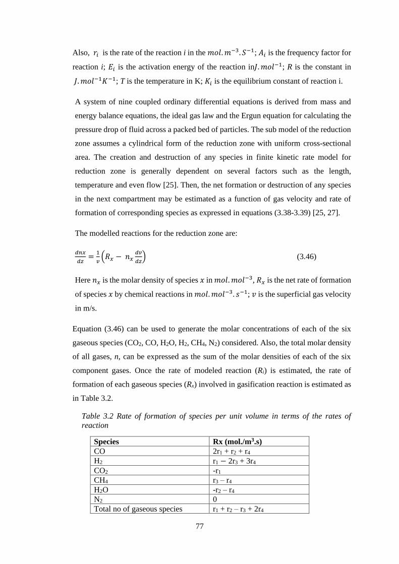
77
Also, 𝑟𝑖 is the rate of the reaction i in the 𝑚𝑜𝑙. 𝑚−3. 𝑆−1; 𝐴𝑖 is the frequency factor for
reaction i; 𝐸𝑖 is the activation energy of the reaction in𝐽. 𝑚𝑜𝑙−1; R is the constant in
𝐽. 𝑚𝑜𝑙−1𝐾−1; T is the temperature in K; 𝐾𝑖 is the equilibrium constant of reaction i.
A system of nine coupled ordinary differential equations is derived from mass and
energy balance equations, the ideal gas law and the Ergun equation for calculating the
pressure drop of fluid across a packed bed of particles. The sub model of the reduction
zone assumes a cylindrical form of the reduction zone with uniform cross-sectional
area. The creation and destruction of any species in finite kinetic rate model for
reduction zone is generally dependent on several factors such as the length,
temperature and even flow [25]. Then, the net formation or destruction of any species
in the next compartment may be estimated as a function of gas velocity and rate of
formation of corresponding species as expressed in equations (3.38-3.39) [25, 27].
The modelled reactions for the reduction zone are:
𝑑𝑛𝑥
𝑑𝑧=
1
𝑣(𝑅𝑥 − 𝑛𝑥
𝑑𝑣
𝑑𝑧) (3.46)
Here 𝑛𝑥 is the molar density of species 𝑥 in 𝑚𝑜𝑙. 𝑚𝑜𝑙−3, 𝑅𝑥 is the net rate of formation
of species 𝑥 by chemical reactions in 𝑚𝑜𝑙. 𝑚𝑜𝑙−3. 𝑠−1; 𝑣 is the superficial gas velocity
in m/s.
Equation (3.46) can be used to generate the molar concentrations of each of the six
gaseous species (CO2, CO, H2O, H2, CH4, N2) considered. Also, the total molar density
of all gases, n, can be expressed as the sum of the molar densities of each of the six
component gases. Once the rate of modeled reaction (Ri) is estimated, the rate of
formation of each gaseous species (Rx) involved in gasification reaction is estimated as
in Table 3.2.
Table 3.2 Rate of formation of species per unit volume in terms of the rates of
reaction
Species Rx (mol./m3.s)
CO 2r1 + r2 + r4
H2 r1 − 2r3 + 3r4
CO2 -r1
CH4 r3 – r4
H2O -r2 – r4
N2 0
Total no of gaseous species r1 + r2 – r3 + 2r4
78
The species created or used up are then estimated as a function of the gas velocity (V)
and the rate of rate of formation (Rx).
The overall rate of gasification reaction is also dependent on the gasifier temperature
at z-nth section and chemical equilibrium constants of individual gasification reactions
𝑑𝑇
𝑑𝑧=
1
𝑣 ∑ 𝑛𝑥𝑐𝑝𝑥
(− ∑ 𝑟𝑖𝛥𝐻𝑖𝑖 − 𝑣𝑑𝑃
𝑑𝑍− 𝑃
𝑑𝑣
𝑑𝑧− ∑ 𝑅𝑥 𝑐𝑝𝑥
𝑇) (3.47)
The first two equations (3.46 ) and (3.47) give a total of seven differential equations
when all six gaseous species are considered. Equation 3.46 was used to generate six
expressions for the molar concentrations of each of the six species considered in
MATLAB code. However, the state of the gasifier is also described by the
concentration of the gas species, the temperature and the superficial gas velocity so to
complete the system of differential equations we still expressions for the pressure
gradient and the gas velocity which are shown below
𝑑𝑣
𝑑𝑧=
1
∑ 𝑛𝑥 𝑐𝑝𝑥+𝑛𝑅𝑥
(∑ 𝑛𝑥 𝑐𝑝𝑥
∑ 𝑅𝑥𝑥𝑥
𝑛−
∑ 𝑟𝑖 𝛥𝐻𝑖𝑖
𝑇−
𝑑𝑃
𝑑𝑧(
𝑣
𝑇+
𝑣 ∑ 𝑛𝑥𝑐𝑝𝑥𝑥
𝑃) − ∑ 𝑅𝑥𝑐𝑝𝑥𝑥 )
(3.48)
𝑑𝑃
𝑑𝑧= 1183 (𝜌
𝑔𝑎𝑠𝑉2
𝜌𝑎𝑖𝑟
) + 388.19𝑣 − 79.896 (3.49)
These derivatives were solved using the ODE45 function in MATLAB which employs
the Runge-Kutta scheme to evaluate the effect of several variables such as temperature
and the final composition of the gas, pressure etc.
3.3 Non-Stoichiometric equilibrium model: the thermodynamic basis for the
Gibbs reactor in HYSYS
The non – stoichiometric equilibrium model is solely based on minimizing Gibbs free
energy of the system. Generally, the non- stoichiometric model can be applied for
simulating various gasifier configurations as they are not dependent on the gasifier
design and not limited to a specified range of operating conditions [95]. However,
moisture content and elemental composition of the feed is required and can be obtained
from the ultimate analysis data of the feed. This method is therefore well suited for
solid fuels like biomass whose exact chemical formula is not definitely known [25].
79
The Gibbs Reactor in the HYSYS simulation package is employed when it is thought
that multi-reactions are going to equilibrium at a fixed temperature and pressure or it
is required to know the maximum possible conversion for multi-reactions at a given
temperature and pressure. In the treatment presented here it is assumed that the
reactions proceed in the Gaseous Phase. The treatment given below presents the
necessary thermodynamic equations and also outlines the standard mathematical
approach for the solution of the multi equations generated.
If multi- reactions are involved, in theory, it is possible to adopt the equilibrium
constant based approach. However, such an approach requires the calculation of
individual equilibrium constants and a mathematical method for solving equations
based on equilibrium constants. The use of equilibrium constants also obviously
assumes knowledge of the chemical reactions occurring in the simulated system. This
knowledge is often not to hand and hence the approach outlined below is the only
realistic approach that can be adopted.
The approach requires a knowledge of Gibbs Energies and an ability to calculate
Chemical potentials. Some of the required data are held in a simulation package
database and some of the quantities are calculated using the Property Package specified
when the calculations are to be carried out. The multi-reaction Gibbs Reactor is based
on the fact that, at equilibrium, the Total Gibbs Energy of the system is a MINIMUM
The Gibbs free energy, Gtotal for the gasification product which consists of N species
where (i=1…. N) is represented as in the equation below:
𝐺𝑡𝑜𝑡𝑎𝑙 = ∑ 𝑛𝑖∆𝐺𝑓,𝑖0𝑁
𝑖=1 + ∑ 𝑛𝑖𝑁𝑖=1 𝑅𝑇𝑙𝑛 (
𝑛𝑖
∑ 𝑛𝑖) (3.50)
Here, 𝑛𝑖∆𝐺𝑓,𝑖0 is the standard Gibbs energy of i species, R is gas constant. The solution
of Eq. (3.50) for unknown values of 𝑛𝑖 is approached to minimize 𝐺𝑡𝑜𝑡𝑎𝑙 of the overall
reaction considering the overall mass balance, though, non-stoichiometric equilibrium
model does not specify the reaction path, type or chemical formula of the fuel, the
amount of total carbon obtained from the ultimate analysis must be equal to sum of
total of all carbon distributed among the gas mixtures and unburnt char [135]:
∑ 𝑎𝑖,𝑗𝑛𝑖𝑁𝑖=1 = A (3.51)
80
Here 𝑎𝑖,𝑗 is the number of atoms of the j element and 𝐴𝑗 is the total number of atoms
of jth element in reaction mixture. The objective of this approach is to find the values
of 𝑛𝑖 such that the Gtotal will be minimum [136]. Thus, the Lagrange function (L) can
be defined as
𝐿 = 𝐺𝑡𝑜𝑡𝑎𝑙 − ∑ 𝜆𝑗𝐾𝑗=1 (∑ 𝑎𝑖,𝑗𝑛𝑖 − 𝐴𝑖
𝑁𝑖=1 ) (3.52)
where λ is Lagrangian multipliers. The equilibrium is achieved when the partial
derivatives of Lagrange function are zero. i.e.
(𝜕𝐿
𝜕𝑛𝑖) = 0 (3.53)
(𝜕𝐿
𝜕𝑛𝑖) =
∆𝐺𝑓,𝑖0
𝑅𝑇+ ∑ 𝑙𝑛 (
𝑛𝑖
𝑛𝑡𝑜𝑡𝑎𝑙)𝑁
𝑖=1 +1
𝑅𝑇∑ 𝜆𝑗𝐾
𝑗=1 (∑ 𝑎𝑖,𝑗𝑛𝑖𝑁𝑖=1 ) = 0 (3.54)
The standard Gibbs free energy of each chemical species can be obtained by
subtracting the standard enthalpy form the standard entropy multiplied by a specific
temperature of the system [6]:
∆�̅�𝑗,𝑖0 = ∆�̅�𝑓,𝑖
0 − 𝑇∆𝑆�̅�,𝑖0 (3.56)
Here ∆𝑆�̅�,𝑖0 is the standard entropy of 𝑖 species. According to first law of
thermodynamics, the energy balance of the non- stoichiometric equilibrium model is
[137].
∑ 𝑛𝑟�̅�𝑟0(𝑇𝑟) + 𝑄𝑙𝑜𝑠𝑠𝑟=𝑟𝑒𝑎𝑐𝑡𝑎𝑛𝑡 = ∑ 𝑛𝑝𝑝𝑡=𝑝𝑟𝑜𝑑𝑢𝑐𝑡 �̅�𝑝𝑡
0 (𝑇𝑝𝑡) + ∆𝐻 (3.57)
81
Chapter 4 Implementation of the developed mathematical
Models for simulation of a biomass gasifier
4.1 Biomass gasification in a downdraft gasifier using HYSIS simulator and
MATLAB solver
This Chapter describes the simulation of biomass gasification in a downdraft gasifier
using Aspen HYSYS and MATLAB in detail. Process description, components,
physical properties and block specifications are provided below.
4.2 HYSYS
HYSYS is a powerful engineering simulation tool created with respect to program
architecture, interface design, engineering capabilities and interactive operation. The
integrated steady state and dynamic capabilities, where the same model can be
evaluated from either perspective with full sharing of process information represent a
significant advancement in the engineering software industry. The software seeks to
give appropriate mathematical models of a range of operations used in the process
industries. These operations can be mathematically modelled in isolation or can
originally or subsequently be combined to give a Process Flow Diagram (PFD). The
algorithms used to carry out the mathematical modelling are not made available as part
of the modelling although the methods used are often. Since there is no specific gasifier
model ready for use in Aspen HYSYS there is the need to separate the entire process
into different blocks that can be simulated with the existing models provided by Aspen
HYSYS.
According to the features of Aspen HYSYS and the thermodynamic equilibrium model
used for this simulation, the following assumptions were made in the current
simulation of the biomass gasification process:
• Steady state operation
• Zero-dimensional
• Particle size is not considered
• Uniform temperature distribution for the biomass particle
• Pressure drops are neglected
• All elements that compose the biomass yield into C, H, O and N
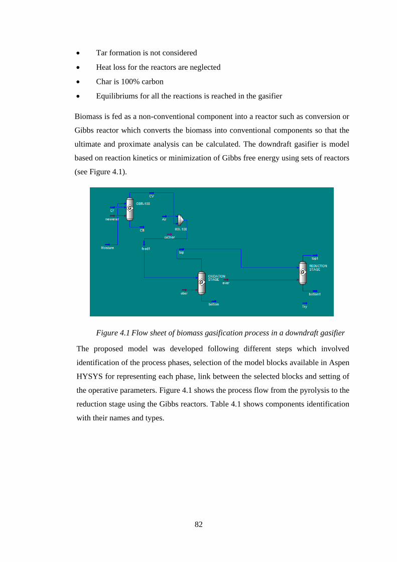
82
• Tar formation is not considered
• Heat loss for the reactors are neglected
• Char is 100% carbon
• Equilibriums for all the reactions is reached in the gasifier
Biomass is fed as a non-conventional component into a reactor such as conversion or
Gibbs reactor which converts the biomass into conventional components so that the
ultimate and proximate analysis can be calculated. The downdraft gasifier is model
based on reaction kinetics or minimization of Gibbs free energy using sets of reactors
(see Figure 4.1).
Figure 4.1 Flow sheet of biomass gasification process in a downdraft gasifier
The proposed model was developed following different steps which involved
identification of the process phases, selection of the model blocks available in Aspen
HYSYS for representing each phase, link between the selected blocks and setting of
the operative parameters. Figure 4.1 shows the process flow from the pyrolysis to the
reduction stage using the Gibbs reactors. Table 4.1 shows components identification
with their names and types.
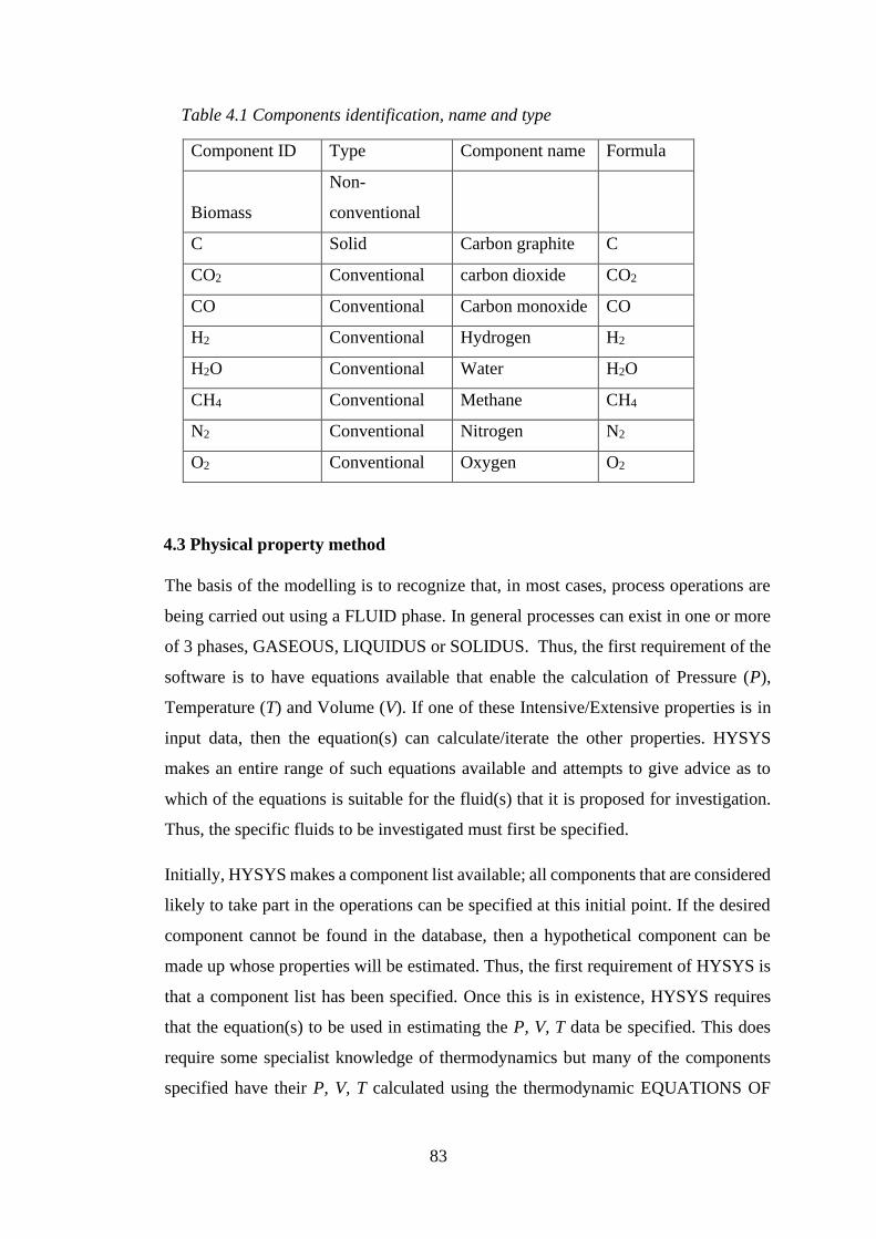
83
Table 4.1 Components identification, name and type
Component ID Type Component name Formula
Biomass
Non-
conventional
C Solid Carbon graphite C
CO2 Conventional carbon dioxide CO2
CO Conventional Carbon monoxide CO
H2 Conventional Hydrogen H2
H2O Conventional Water H2O
CH4 Conventional Methane CH4
N2 Conventional Nitrogen N2
O2 Conventional Oxygen O2
4.3 Physical property method
The basis of the modelling is to recognize that, in most cases, process operations are
being carried out using a FLUID phase. In general processes can exist in one or more
of 3 phases, GASEOUS, LIQUIDUS or SOLIDUS. Thus, the first requirement of the
software is to have equations available that enable the calculation of Pressure (P),
Temperature (T) and Volume (V). If one of these Intensive/Extensive properties is in
input data, then the equation(s) can calculate/iterate the other properties. HYSYS
makes an entire range of such equations available and attempts to give advice as to
which of the equations is suitable for the fluid(s) that it is proposed for investigation.
Thus, the specific fluids to be investigated must first be specified.
Initially, HYSYS makes a component list available; all components that are considered
likely to take part in the operations can be specified at this initial point. If the desired
component cannot be found in the database, then a hypothetical component can be
made up whose properties will be estimated. Thus, the first requirement of HYSYS is
that a component list has been specified. Once this is in existence, HYSYS requires
that the equation(s) to be used in estimating the P, V, T data be specified. This does
require some specialist knowledge of thermodynamics but many of the components
specified have their P, V, T calculated using the thermodynamic EQUATIONS OF

84
STATE (EoS). This is an area of study that occupies many textbooks but one of the
favoured equations is that due to PENG-ROBINSON (named after the originators).
This equation was made more ‘accurate’ in representing polar gases and liquids by
incorporating the proposed changes due to Styrek and Vera. The final equation is
referred (unsurprisingly) to as PRSV. This equation was used in this work because the
presence of solid carbon was only acknowledged in one of the Unit operations
(Pyrolysis) and its presence could be counted in the overall mass balance.
4.3.1 The Peng-Robinson Stryjek-Vera Equation
The Peng-Robinson Stryjek-Vera (PRSV) equation of state is a two-fold modification
of the PR equation of state that extends the application of the original PR method for
moderately non-ideal systems. It has been shown to match vapour pressures curves of
pure components and mixtures more accurately than the PR method, especially at low
vapour pressures. It has been successfully extended to handle non-ideal systems giving
results as good as those obtained using excess Gibbs energy functions like the Wilson,
NRTL or UNIQUAC equations. One of the proposed modifications to the PR equation
of state by Stryek and Vera was an expanded alpha, "α", term that became a function
of acentricity and an empirical parameter, κi, used for fitting pure component vapour
pressures [138].
The PRSV equation of state which is formally similar to the cubic equation state
proposed by Peng Robinson [139] and is represented as;
𝑃 =𝑅𝑇
𝑣−𝑏−
𝑎
𝑣2+2𝑏𝑣−𝑏2 (4.1)
where
𝑎 = (0.457235 𝑅2𝑇2
𝑃𝑐⁄ )𝛼𝑖 (4.2)
𝛼𝑖 = [1 + 𝑘(1 − 𝑇𝑟0.5)]2 (4.3)
and
𝑏 = 0.07776𝑅𝑇𝑐
𝑃𝑐⁄ (4.4)
𝑘𝑖 = 𝐾𝑂𝑖 + 𝑘( 1 + 𝑇𝑟𝑖0.5)(0.7 − 𝑇𝑟𝑖
0.5) (4.5)
85
𝑘𝑂𝑖 = 0.378893 + 1.4897153ω𝑖 − 0.17131848ω𝑖2 + 0.0196554ω𝑖
3 (4.6)
ωi = acentric factor (4.7)
Here ki is characteristic pure component adjustable parameter, k is a function of
acentric factor and reduced temperature, 𝐾𝑂𝑖 is a function of acentric factor, 𝛼𝑖 is a
function of temperature and acentric factor, 𝑃𝑐 and 𝑇𝑐 are critical pressures and
temperature respectfully.
Once the component list and Property Package have been specified (see Table 4.2),
HYSYS allows access to either modelling of a single operation, multiple operations in
isolation from each other or combine operations into a Process Flow Diagram (PFD).
HYSYS makes the Unit Operations that can be mathematically modelled available in
an Operations Palette. This is a symbolic display of the various operations. Each
identified symbol can then be loaded into the PFD as required. Operations can be
combined by making their Inputs/Outputs common to each required operation. Each
operation can have the operating conditions, stream flows and compositions input as
appropriate. If any stream flows or conditions require iteration, then HYSYS will
perform the operation to the accuracy specified by the user.
HYSYS will not make recommendations as to what changes should be made to
conditions/flows. It will issue warnings about flow imbalances for both mass and
energy. Through colour coded bars it will warn about what stage of the modelling is
the progress. Red indicates most vital parameters, which have not been specified.
Yellow indicates that some vital parameters have not been specified with indication of
these parameters. The green colour indicates a successful simulation using the
operations specified. Overall HYSYS is a powerful mathematical modelling tool that
can be used to simulate whole processes. This makes it extremely popular in carrying
out some Process Design. It is accepted that HYSYS carries out simulation through
mathematical modelling and does not represent the use of actual physical modelling of
the unit operations available.

86
Table 4.2 Block specification
HYSYS
reactor
family
Scheme Reactor use Description
Gibbs
Pyrolysis
oxidation/gasification
This reactor
models the char
gasification
processes
Conversion
Pyrolysis Models the
decomposition of
biomass which is
a hypothetical
component into a
conventional
constituent
component.
Mixer
Inlet to the oxidation Models the
mixing of
different streams
inlet into a block
PFTR
Reduction
4.3.2 Process description
Biomass is a non-conventional component which is converted into conventional
components by calculating its ultimate and proximate analysis. It was assumed that
there are 3 important stages in the process that can be modelled. After biomass drying
there is a pyrolysis stage where the Carbon, Hydrogen, Oxygen bearing volatiles can
be taken into the vapour phase with an energy input. The products from the Pyrolysis
stage can then be considered to enter an oxidation stage where the products from the
Pyrolysis stage are mixed with oxygen-bearing air and oxidation takes place at elevated
temperatures. Subsequently the products from this stage are considered to enter a
87
reduction stage where the proportions of Carbon monoxide, Carbon dioxide and
Hydrogen are altered - particularly the amount of Carbon monoxide being reduced.
This is usually then considered to be a useable Syngas.
In terms of appropriate Unit Operations available to mathematically model these
Stages, the oxidation and reduction stages are considered to be dependent on reactions
that go to chemical equilibrium although the reactions that can occur are not
necessarily well defined. This is a classic thermodynamic problem where a Gibbs Free
Energy Minimisation technique can be employed. In simple terms, this technique uses
the composition, pressure and temperature of the stream entering a specified reactor
system. The temperature and pressure of the exit product stream are also specified. The
technique calculates the total Gibbs energy of the entering stream at the specified
conditions and composition using a database of Formation Gibbs energies. The
component Formation Gibbs energies are also available for the exit stream because the
temperature and pressure of this stream are specified. To satisfy the thermodynamic
requirement that the total input and output Gibbs energies are equal the technique has
minimisation functions available e.g. Lagrange Multipliers.
Ultimately the Gibbs energies are equalised by finding the appropriate output
component compositions that meet the requirement of equal input and output total
Gibbs energies. Such a reactor is classically known as the Gibbs Reactor and such an
operation is available in HYSYS. The oxidation and reduction stages were specified
as GIBBS reactors and loaded into the HYSYS PFD. The pyrolysis section is more
equivocal for modelling in the version of HYSYS used (Version 6). Basically, a
mathematical statement of the amount of C, H and O forced into the vapour phase by
application of energy is required. If this was to be modelled the biomass available from
the drying process would need to be presented to the unit operation chosen and a phase
change introduced into the model. The version of HYSYS used has no directly
applicable model for this situation. The Pyrolysis was eventually presented using a
conversion reactor. This is a reactor model that basically asks for a reaction; reaction
stoichiometry and expected reaction conversion. This did not appear particularly
promising in modelling the pyrolysis. The Biomass was fed to the reactor as 𝐶𝑥𝐻𝑦𝑂𝑧
where x, y and z were calculated from the ultimate analysis of the specific biomass
(wood chips, wood pellets and rubber wood). A reaction was required rather than a
88
simple phase change, so it was assumed that water, H2O, was formed in the reactor.
However, the reactor conversion was specified as a small amount (usually <0.5%).
This had the effect of making the bulk of the unconverted C, H and O appear in the
output streams together with a small amount of water. These output streams could then
be fed forward to the Gibbs Reactor simulating the oxidation stage. To make it easier
to adjust the air flow into the oxidation stage; a HYSYS mixer was used to receive the
outputs from the Conversion Reactor together with a specified air Input stream,
HYSYS mass balances these streams and outputs them as a single stream which is
taken as the input stream to the oxidation stage. By the nature of the reactor and the
assumptions made about its operation it was not possible to add a moisture stream and
expect realistic outputs.
Conversion reactor
It has been demonstrated that a basic model of a Gasifier based on a simple 3 zone
model of the gasifier can be put together using Aspen HYSYS software. In one
approach, the model takes 2 basic operations available in HYSYS, the Gibbs Reactor
and the Conversion Reactor, and makes assumptions about the thermodynamic
conditions in the 3 zones. The Conversion Reactor simply requires the statement of a
reaction (or reactions) occurring in a reaction together with the expected conversion.
This reactor in HYSYS was used which was developed by M. Bassyouni et al [140]
in a paper where they tried to simulate the gasification of date palm waste.
Based on the reaction conditions set and the expected conversion, the HYSYS
operation gives an expected output. To use this operation a simple reaction of hydrogen
with water with an extremely low conversion was set. The operating pressure and
temperatures were set at values normally encountered in this stage of the operation.
The effect of this operation was to, in effect, produce a pyrolysed stream for
components in the vapour phase. A number of calculations were carried out with this
reactor in place. As calculations proceeded, it became necessary for the moisture
content of the input stream to be varied.
Gibbs reactor
In previous attempts at modelling and simulating the pyrolysis stage it has been
assumed that the stage can go to thermodynamic equilibrium and the outputs calculated
on this basis. In HYSYS there are 2 possibilities available for handling this situation,
89
an Equilibrium Reactor and a Gibbs Reactor. The Equilibrium Reactor requires the
expected reactions within the reactor to be supplied. The Gibbs Reactor does not
require this; it simply need the details of the input stream and the conditions of the
stream. Based on Gibbs free energy calculations, the output stream compositions and
conditions can be calculated. This approach has the advantage that no reactions
occurring in the reactor have to be explicitly stated. When a moisture stream was
added, this type of reactor was used to simulate the Pyrolysis stage. In various
approaches to modelling the 2nd and 3rd zones, the Combustion (Oxidation) and
Reduction zones have been modelled assuming thermodynamic equilibrium with, in
some cases, various chemical reactions occurring, explicitly assumed. An approach
has been adopted where both these zones have been assumed to approach
thermodynamic equilibrium and have been simulated using Gibbs reactors where no
explicit statement of the reactions occurring is required. The use of the 3 Gibbs
Reactors allow Input and Output streams to be incorporated. For the first Gibbs Reactor
(the Pyrolysis Stage) the addition of an extra Input Stream to the reactor allows to set
amount of moisture to be added to the system as water and this can also be varied to
allow greater or lesser moisture contents.
4.4 The Kinetic Reactor in HYSYS using Plug flow reactor PFR
Design equations exist (and can be derived) for a PFR (Plug Flow Reactor). The
important design equations are:
𝑉
𝐹𝐴= ∫
𝑑𝑧𝐴
−𝑟𝐴
𝑧𝐴
0 (4.8)
and
𝜏 = 𝐶𝐴0 ∫𝑑𝑧𝐴
−𝑟𝐴
𝑧𝐴
0 (4.9)
Here V is a reactor volume, FA is a reactant flow rate, zA is a reactant conversion, -rA
is a reaction rate, 𝜏 is a space time and CA0 is an initial reactant concentration.
Conversion within the reactor depends on the relative rates of the reactions taking
place. Reaction rate constants and a stoichiometric equation have to be supplied for
each reaction. It is assumed the reacting stream passes through the reactor in Plug flow
i.e. the stream passes through without mass or energy gradients and there is no radial
90
mixing. The conversion achieved by the reactor is computed by integrating the relevant
differential equations and energy equations over the length of the reactor. Constant gas
density for the reactants is not assumed and the density is rigorously corrected as the
reactions proceed.
In the computation, it is necessary to supply the composition and flow rate of the inlet
stream and the pressure and temperature of this stream. The reactor can be operated
isothermally, adiabatically or the outlet temperature can be specified.
Integration in the reactor is carried out numerically, both the equations listed above
can be solved for multiple reactions. The numerical integration requires difference
equations to be solved within a series of calculation ‘strips’. The larger the number of
strips the nearer the differential equation solution is to the requirement of an infinitely
small strip. HYSYS allows the number of strips to be specified up to a maximum of
10000. In the PFR used in the kinetic model the number of strips was usually set at
1000. No significant differences were observed when the longer calculations were
carried out for 10000 strips. In HYSYS it is also necessary to specify a reactor length
and reactor diameter, in the kinetic model these parameters were varied.
For a chemical reaction to be represented in HYSYS it normally requires the equation
to be represented as a reversible reaction. Typically, the reaction would be:
𝑎𝐴 + 𝑏𝐵 = 𝑐𝐶 + 𝑑𝐷 (4.10)
where A, B are reactants and C, D are products. The terms a, b and c, d are the
appropriate stoichiometric coefficients for the reaction. In HYSYS the reversible
reaction would be represented as:
𝑟1 = 𝑘1𝐶𝐴𝑎 𝐶𝐵
𝑏 … − 𝑘2𝐶𝐶𝑐 𝐶𝐷
𝑑 (4.10a)
Here k1 and k2 are the Rate Constants for the forward and reverse reactions. These can
be calculated using the ARRHENIUS EQUATION which takes the form:
𝑘 = 𝐴𝑒−𝐸
𝑅𝑇 (4.11)
where A is Collision Frequency Factor and E is the Activation Energy.
91
In HYSYS the rate constants are not normally specified directly. The required data are
the Collision Frequency Factors, A, for the forward and reverse reactions and the
Activation Energies E for the forward and reverse reactions. In terms of the data
available, the form of the equation input required by HYSYS was not immediately
available in the form required. The data available were for an equation of the form:
𝑟 = 𝑘1 (𝐶𝐴𝑎𝐶𝐵
𝑏 −𝐶𝐶
𝑐𝐶𝐷𝑑
𝐾) (4.12)
The parameters are the same as previously defined: k is an equation Equilibrium
Constant. The equilibrium constant can be written in an appropriate form:
𝐾 =𝑘1
𝑘2 (4.13)
The data available did not give values of K as a function of temperature and it was
necessary to generate these data. This would require the generation of K values as a
function of temperature for 4 reactions. No tables of K values vs Temperature were
available for the 4 reactions. The first approach to obtaining the necessary values was
to find values of ∆𝐺𝑓𝜃, the Standard Gibbs Free Energy of Formation, for all the species
in the 4 reactions. These values were available at various temperatures from JANAF
tables. Once these values were available, the following equation could be used:
∆𝐺𝑇𝜃 = ∑(∆𝐺𝑓
𝜃)𝑃𝑟𝑜𝑑𝑢𝑐𝑡𝑠
− ∑(∆𝐺𝑓𝜃)
𝑅𝑒𝑎𝑐𝑡𝑎𝑛𝑡𝑠 (4.14)
Where ∆𝐺𝑇𝜃 is the Standard Gibbs Free Energy Change for the reaction at a given
temperature. Using these values for the given reaction we can use the Equilibrium
Reaction Isotherm to find values of the Equilibrium Constant𝐾𝑎:
∆𝐺𝑇𝜃 = −𝑅𝑇𝑙𝑛𝐾𝑎 (4.15)
The amount of data garnering required here was considerable. An alternative approach
in generating values of the equilibrium constant was to use the Integrated Gibbs-
Helmholtz Equation. The form used assumed that the Standard Enthalpy Change for a
given reaction was independent of temperature. If this assumption is made, then the
Gibbs-Helmholtz can be written as:
∆𝐺𝑇2𝜃
𝑇2−
∆𝐺𝑇1 𝜃
𝑇1=∆𝐻𝜃 (
1
𝑇2−
1
𝑇1) (4.16)
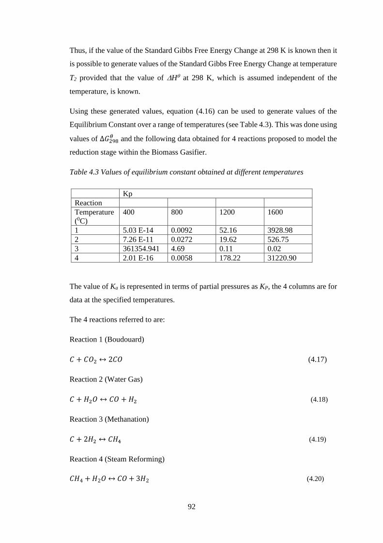
92
Thus, if the value of the Standard Gibbs Free Energy Change at 298 K is known then it
is possible to generate values of the Standard Gibbs Free Energy Change at temperature
T2 provided that the value of H at 298 K, which is assumed independent of the
temperature, is known.
Using these generated values, equation (4.16) can be used to generate values of the
Equilibrium Constant over a range of temperatures (see Table 4.3). This was done using
values of ∆𝐺298𝜃 and the following data obtained for 4 reactions proposed to model the
reduction stage within the Biomass Gasifier.
Table 4.3 Values of equilibrium constant obtained at different temperatures
The value of Ka is represented in terms of partial pressures as KP, the 4 columns are for
data at the specified temperatures.
The 4 reactions referred to are:
Reaction 1 (Boudouard)
𝐶 + 𝐶𝑂2 ↔ 2𝐶𝑂 (4.17)
Reaction 2 (Water Gas)
𝐶 + 𝐻2𝑂 ↔ 𝐶𝑂 + 𝐻2 (4.18)
Reaction 3 (Methanation)
𝐶 + 2𝐻2 ↔ 𝐶𝐻4 (4.19)
Reaction 4 (Steam Reforming)
𝐶𝐻4 + 𝐻2𝑂 ↔ 𝐶𝑂 + 3𝐻2 (4.20)
Kp
Reaction
Temperature
(0C)
400 800 1200 1600
1 5.03 E-14 0.0092 52.16 3928.98
2 7.26 E-11 0.0272 19.62 526.75
3 361354.941 4.69 0.11 0.02
4 2.01 E-16 0.0058 178.22 31220.90
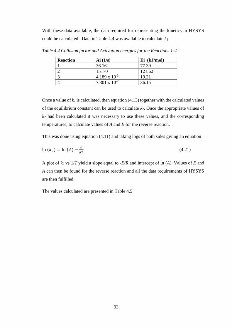
93
With these data available, the data required for representing the kinetics in HYSYS
could be calculated. Data in Table 4.4 was available to calculate k1.
Table 4.4 Collision factor and Activation energies for the Reactions 1-4
Reaction Ai (1/s) Ei (kJ/mol)
1 36.16 77.39
2 15170 121.62
3 4.189 x 10⁻³ 19.21
4 7.301 x 10⁻² 36.15
Once a value of k1 is calculated, then equation (4.13) together with the calculated values
of the equilibrium constant can be used to calculate k2. Once the appropriate values of
k2 had been calculated it was necessary to use these values, and the corresponding
temperatures, to calculate values of A and E for the reverse reaction.
This was done using equation (4.11) and taking logs of both sides giving an equation
ln (𝑘2) = ln (𝐴) −𝐸
𝑅𝑇 (4.21)
A plot of k2 vs 1/T yield a slope equal to -E/R and intercept of ln (A). Values of E and
A can then be found for the reverse reaction and all the data requirements of HYSYS
are then fulfilled.
The values calculated are presented in Table 4.5
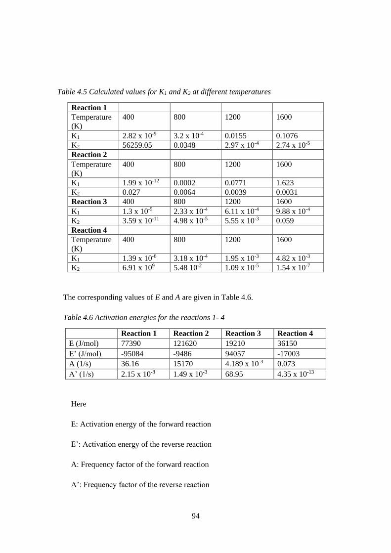
94
Table 4.5 Calculated values for K1 and K2 at different temperatures
Reaction 1
Temperature
(K)
400 800 1200 1600
K1 2.82 x 10⁻⁹ 3.2 x 10⁻⁴ 0.0155 0.1076
K2 56259.05 0.0348 2.97 x 10⁻⁴ 2.74 x 10⁻⁵
Reaction 2
Temperature
(K)
400 800 1200 1600
K1 1.99 x 10⁻¹² 0.0002 0.0771 1.623
K2 0.027 0.0064 0.0039 0.0031
Reaction 3 400 800 1200 1600
K1 1.3 x 10⁻⁵ 2.33 x 10⁻⁴ 6.11 x 10⁻⁴ 9.88 x 10⁻⁴
K2 3.59 x 10⁻¹¹ 4.98 x 10⁻⁵ 5.55 x 10⁻³ 0.059
Reaction 4
Temperature
(K)
400 800 1200 1600
K1 1.39 x 10⁻⁶ 3.18 x 10⁻⁴ 1.95 x 10⁻³ 4.82 x 10⁻³
K2 6.91 x 10⁹ 5.48 10-2 1.09 x 10⁻⁵ 1.54 x 10⁻⁷
The corresponding values of E and A are given in Table 4.6.
Table 4.6 Activation energies for the reactions 1- 4
Reaction 1 Reaction 2 Reaction 3 Reaction 4
E (J/mol) 77390 121620 19210 36150
E’ (J/mol) -95084 -9486 94057 -17003
A (1/s) 36.16 15170 4.189 x 10⁻³ 0.073
A’ (1/s) 2.15 x 10⁻⁸ 1.49 x 10⁻³ 68.95 4.35 x 10⁻¹³
Here
E: Activation energy of the forward reaction
E’: Activation energy of the reverse reaction
A: Frequency factor of the forward reaction
A’: Frequency factor of the reverse reaction

95
These values were used during modelling in HYSYS software.
It is worth noting that for Reactions 1, 2 and 4 the activation energies for the reverse
reactions are negative i.e. the rate constants for the reverse reactions decrease with
temperature. One of the problems related to HYSYS when using the kinetics to simulate
the reduction stage is that little or no methane gas is formed. If data is examined, it can
be seen that Reaction 3 is an equation representing methane formation. The rate
constants for the forward reaction (methane formation) are very low over the
temperature range considered. The rate constants for the reverse reaction are greater
than for the forward one at higher temperatures, this mirrors the conditions encountered
in the gasifier. These results are consistent with the values of the equilibrium constant.
The other reaction where methane is involved is Reaction 4. At higher temperatures,
the forward rate constant is higher than the reverse one. This would indicate that any
methane would be favoured to disappear at higher temperatures. HYSYS indicates that
this is so. The simulation of the reduction stage cannot be carried out in HYSYS simply
through kinetics and mass balancing. Simulation is carried out using the simulation of
an actual operation, thus, a Plug Flow Tubular Reactor was used in calculations.
4.5 Double air stream model
Previously for single stream operation the approach adopted had assumption that the
system could be considered in 3 sections; a pyrolysis section, a combustion section and
a reduction section. The pyrolysis section was simulated using a conversion reactor
where the components were vaporised prior to entry into the combustion section. The
combustion and reduction sections were simulated using Gibbs reactors i.e. it was
assumed that both these sections reached thermodynamic equilibrium. In this case, air
stream was directly input to the Combustion Section.
For using HYSYS to simulate the air entering as a double stream, the simulation of the
Pyrolysis section had to be changed. Of the reactors available, HYSYS require the
reactions occurring to be specified. The Gibbs Reactor balances the input and output
Gibbs Energies without requiring the designation of specific reactions, this means that
the output streams are considered to be at equilibrium. The original Conversion
Reactor was replaced by another Gibbs Reactor and the air stream was split. One part
of the stream was input to the Gibbs Reactor that was designated as the first (Pyrolysis)
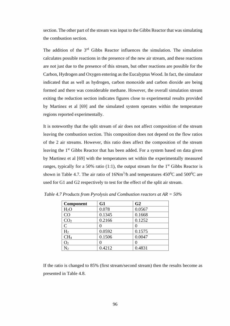
96
section. The other part of the stream was input to the Gibbs Reactor that was simulating
the combustion section.
The addition of the 3rd Gibbs Reactor influences the simulation. The simulation
calculates possible reactions in the presence of the new air stream, and these reactions
are not just due to the presence of this stream, but other reactions are possible for the
Carbon, Hydrogen and Oxygen entering as the Eucalyptus Wood. In fact, the simulator
indicated that as well as hydrogen, carbon monoxide and carbon dioxide are being
formed and there was considerable methane. However, the overall simulation stream
exiting the reduction section indicates figures close to experimental results provided
by Martinez et al [69] and the simulated system operates within the temperature
regions reported experimentally.
It is noteworthy that the split stream of air does not affect composition of the stream
leaving the combustion section. This composition does not depend on the flow ratios
of the 2 air streams. However, this ratio does affect the composition of the stream
leaving the 1st Gibbs Reactor that has been added. For a system based on data given
by Martinez et al [69] with the temperatures set within the experimentally measured
ranges, typically for a 50% ratio (1:1), the output stream for the 1st Gibbs Reactor is
shown in Table 4.7. The air ratio of 16Nm3/h and temperatures 4500C and 5000C are
used for G1 and G2 respectively to test for the effect of the split air stream.
Table 4.7 Products from Pyrolysis and Combustion reactors at AR = 50%
Component G1 G2
H2O 0.078 0.0567
CO 0.1345 0.1668
CO2 0.2166 0.1252
C 0 0
H2 0.0592 0.1575
CH4 0.1506 0.0047
O2 0 0
N2 0.4212 0.4831
If the ratio is changed to 85% (first stream/second stream) then the results become as
presented in Table 4.8.
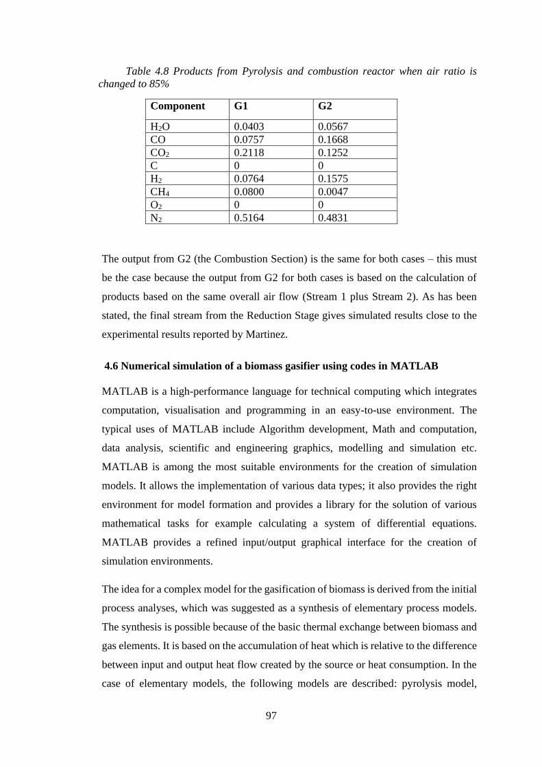
97
Table 4.8 Products from Pyrolysis and combustion reactor when air ratio is
changed to 85%
Component G1 G2
H2O 0.0403 0.0567
CO 0.0757 0.1668
CO2 0.2118 0.1252
C 0 0
H2 0.0764 0.1575
CH4 0.0800 0.0047
O2 0 0
N2 0.5164 0.4831
The output from G2 (the Combustion Section) is the same for both cases – this must
be the case because the output from G2 for both cases is based on the calculation of
products based on the same overall air flow (Stream 1 plus Stream 2). As has been
stated, the final stream from the Reduction Stage gives simulated results close to the
experimental results reported by Martinez.
4.6 Numerical simulation of a biomass gasifier using codes in MATLAB
MATLAB is a high-performance language for technical computing which integrates
computation, visualisation and programming in an easy-to-use environment. The
typical uses of MATLAB include Algorithm development, Math and computation,
data analysis, scientific and engineering graphics, modelling and simulation etc.
MATLAB is among the most suitable environments for the creation of simulation
models. It allows the implementation of various data types; it also provides the right
environment for model formation and provides a library for the solution of various
mathematical tasks for example calculating a system of differential equations.
MATLAB provides a refined input/output graphical interface for the creation of
simulation environments.
The idea for a complex model for the gasification of biomass is derived from the initial
process analyses, which was suggested as a synthesis of elementary process models.
The synthesis is possible because of the basic thermal exchange between biomass and
gas elements. It is based on the accumulation of heat which is relative to the difference
between input and output heat flow created by the source or heat consumption. In the
case of elementary models, the following models are described: pyrolysis model,
98
oxidation model and reduction model. The three models include thermal breakdown
of biomass, release of gasses and the burning of the solid by product [141].
4.6.1 Procedure for numerical simulation
The biomass gasifier is divided into four stages. Five files was created in MATBLAB
for the Input data, Pyrolysis zone, Oxidation zone, Energy balance and Reduction zone
(see codes in the Appendix section). First, the initial input values for both the constant
and variable parameters for the feedstock to be used were determined, initial
temperatures in all cells were set. The molar fraction of the hydrogen, carbon and
oxygen were determined and process models were independently implemented with
codes in a MATLAB environment as individual m-functions.
Input file
Here, a function is declared that accepts all the input data. This file describes input
data for all sections of the gasifier such as feed stock, pyrolysis, oxidation and
reduction zones. Within the feed stock section, the type of wood and the outside
temperature is specified. In the pyrolysis and oxidation sections of input file, the
conductivity of the walls, measurements of the zones are specified. The reduction zone
of this section specifies the diameter of the chamber and the temperature.
Pyrolysis zone file
The input function for this file is called the pyro. It contains the molar masses of the
carbon, hydrogen and oxygen, mass flow rates of ash, moisture and fixed carbon in
the feed stock. The equation derrived asnd based on the assumptions made and mass
balance equations are specified here. The input data from the imput file is specified in
this pyrolysis file. With data from the input file, assumptions and mass balances, the
product amounts of CO, CO2, H2, H2O, CH4 and C2H2 and char are calculated.
Oxidation zone file
The input function for this file is the ‘oxi’ wih the moles of oxygen and nitrogen
entering the zone, masses of products from the pyrolysis zone. The input function of
the pyrolysis file ‘pyro’ is also specified here. The overall composition and
temperature in this zone is obtained through mass and energy balance; the energy
balance is a function of the initial temperatures, dimensions of oxidation zone,
99
conductivity of the walls of the oxidation zone, product amounts from pyrolysis zone
etc. This gives the temperature leaving the oxidation zone and entering the reduction
zone including products from the oxidation zone which are CO, CO2, H2, H2O, CH4
and C2H2 and char.
Reduction zone file
The Reduction zone is the final stage of the biomass gasifier where the pressure,
temperature, velocity and molar concentrations of the gas constituents from the
pyrolysis zone and oxidation zone were processed and ODE 45, which is a code in
MATLAB to solve differential equations, was used to integrate their respective
functions. Then the gas compositions, pressure and temperature in the oxidation zone
were detemined along the depth of the oxidation chamber and the final wet and dry gas
compostions were produced. The algorithm was written and modified accordingly in
MATLAB in order to generate required outputs.
Energy balance calaculation file
The energy balance evaluates the temperature at the exit of the oxidation zone and
entry to the reduction zone from the energy balance equation across the pyrolysis and
oxidation zones. The temperature is then solved by Newton-Raphson Method code,
which is for solving non linear equations for number of variables.
100
Chapter 5 Modelling Approach and Data Used in Numerical
Simulations on Properties of Various Biomass Feedstock
5.1 Introduction
This Chapter describes the simulations carried out for validating the models developed
in this study for various biomass feedstock utilized. Mathematical modelling of
gasification is a very complex. As described above MATLAB and ASPEN HYSYS
software were deployed to obtain numerical results. Kinetic and equilibrium models
have been programmed in HYSYS and MATLAB to describe operation of the
downdraft gasifier.
Five feeds, namely wood chips, wood pellets, rubber wood, palm oil fronds and
eucalyptus woods were used as biomass in the downdraft gasifier. These woody
biomass feeds were chosen as they have been investigated by other researchers and
experimental and theoretical results exists for comparison. For each of these feeds, the
effects of a number of parameters are investigated theoretically and each of the output
results is compared with the theoretical and/or experimental results published by other
authors. Biomass feedstock is characterised in order to evaluate their suitability for
thermochemical conversion process operations. The analysis and methods required to
find the characteristics of the feedstock are ultimate, lignocellulosic, proximate, caloric
value, pH and thermogravimetric. Proximate analysis is carried out to identify the
moisture content, volatile matter, fixed carbon content of the feedstock and ash
content. Ultimate analysis is normally carried to determine the elemental composition
of carbon, hydrogen, nitrogen, sulphur and oxygen. The feedstocks with low sulphur
and nitrogen content produces low non- environmental gases during the
thermochemical conversion process [142]). Carbon, hydrogen and oxygen are the main
constituents of the carbohydrate chains in an organic structure and their percentages
affect the calorific value of the feedstock. The heating value of a biomass fuel may be
reported on either the higher heating value (HHV) or lower heating value (LHV)
property. The higher heating value indicates the heat release upon combustion of fuel
with the original and generated water in the condensate state while the lower heating
value is based on gaseous water as the product [143].
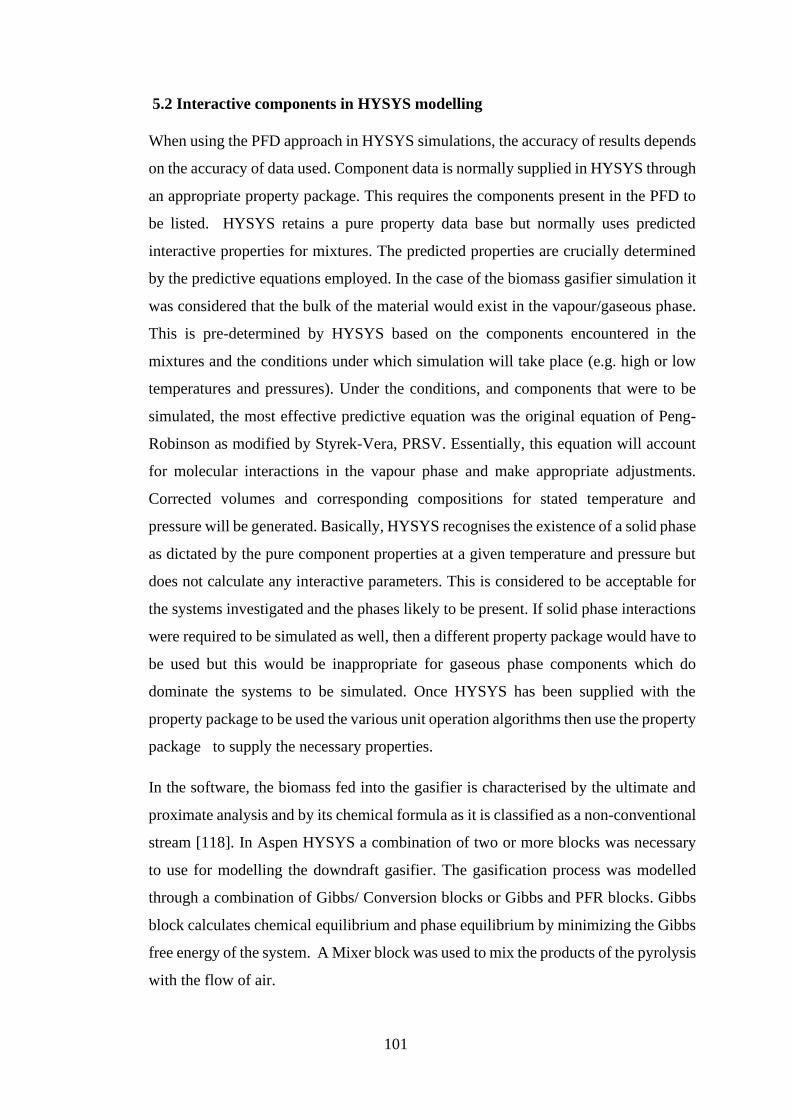
101
5.2 Interactive components in HYSYS modelling
When using the PFD approach in HYSYS simulations, the accuracy of results depends
on the accuracy of data used. Component data is normally supplied in HYSYS through
an appropriate property package. This requires the components present in the PFD to
be listed. HYSYS retains a pure property data base but normally uses predicted
interactive properties for mixtures. The predicted properties are crucially determined
by the predictive equations employed. In the case of the biomass gasifier simulation it
was considered that the bulk of the material would exist in the vapour/gaseous phase.
This is pre-determined by HYSYS based on the components encountered in the
mixtures and the conditions under which simulation will take place (e.g. high or low
temperatures and pressures). Under the conditions, and components that were to be
simulated, the most effective predictive equation was the original equation of Peng-
Robinson as modified by Styrek-Vera, PRSV. Essentially, this equation will account
for molecular interactions in the vapour phase and make appropriate adjustments.
Corrected volumes and corresponding compositions for stated temperature and
pressure will be generated. Basically, HYSYS recognises the existence of a solid phase
as dictated by the pure component properties at a given temperature and pressure but
does not calculate any interactive parameters. This is considered to be acceptable for
the systems investigated and the phases likely to be present. If solid phase interactions
were required to be simulated as well, then a different property package would have to
be used but this would be inappropriate for gaseous phase components which do
dominate the systems to be simulated. Once HYSYS has been supplied with the
property package to be used the various unit operation algorithms then use the property
package to supply the necessary properties.
In the software, the biomass fed into the gasifier is characterised by the ultimate and
proximate analysis and by its chemical formula as it is classified as a non-conventional
stream [118]. In Aspen HYSYS a combination of two or more blocks was necessary
to use for modelling the downdraft gasifier. The gasification process was modelled
through a combination of Gibbs/ Conversion blocks or Gibbs and PFR blocks. Gibbs
block calculates chemical equilibrium and phase equilibrium by minimizing the Gibbs
free energy of the system. A Mixer block was used to mix the products of the pyrolysis
with the flow of air.
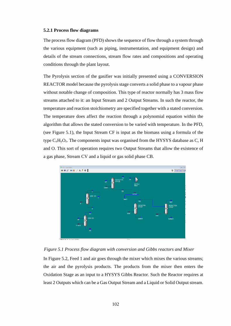
102
5.2.1 Process flow diagrams
The process flow diagram (PFD) shows the sequence of flow through a system through
the various equipment (such as piping, instrumentation, and equipment design) and
details of the stream connections, stream flow rates and compositions and operating
conditions through the plant layout.
The Pyrolysis section of the gasifier was initially presented using a CONVERSION
REACTOR model because the pyrolysis stage converts a solid phase to a vapour phase
without notable change of composition. This type of reactor normally has 3 mass flow
streams attached to it: an Input Stream and 2 Output Streams. In such the reactor, the
temperature and reaction stoichiometry are specified together with a stated conversion.
The temperature does affect the reaction through a polynomial equation within the
algorithm that allows the stated conversion to be varied with temperature. In the PFD,
(see Figure 5.1), the Input Stream CF is input as the biomass using a formula of the
type CxHyOz. The components input was organised from the HYSYS database as C, H
and O. This sort of operation requires two Output Streams that allow the existence of
a gas phase, Stream CV and a liquid or gas solid phase CB.
Figure 5.1 Process flow diagram with conversion and Gibbs reactors and Mixer
In Figure 5.2, Feed 1 and air goes through the mixer which mixes the various streams;
the air and the pyrolysis products. The products from the mixer then enters the
Oxidation Stage as an input to a HYSYS Gibbs Reactor. Such the Reactor requires at
least 2 Outputs which can be a Gas Output Stream and a Liquid or Solid Output stream.
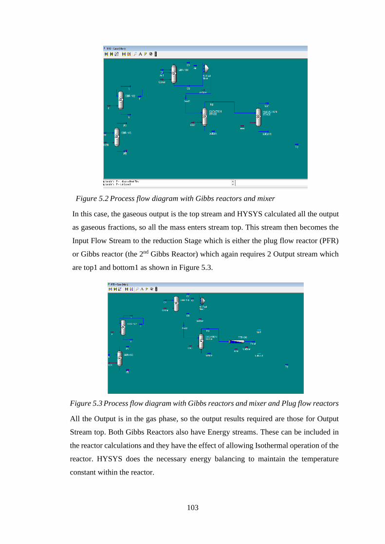
103
Figure 5.2 Process flow diagram with Gibbs reactors and mixer
In this case, the gaseous output is the top stream and HYSYS calculated all the output
as gaseous fractions, so all the mass enters stream top. This stream then becomes the
Input Flow Stream to the reduction Stage which is either the plug flow reactor (PFR)
or Gibbs reactor (the 2nd Gibbs Reactor) which again requires 2 Output stream which
are top1 and bottom1 as shown in Figure 5.3.
Figure 5.3 Process flow diagram with Gibbs reactors and mixer and Plug flow reactors
All the Output is in the gas phase, so the output results required are those for Output
Stream top. Both Gibbs Reactors also have Energy streams. These can be included in
the reactor calculations and they have the effect of allowing Isothermal operation of the
reactor. HYSYS does the necessary energy balancing to maintain the temperature
constant within the reactor.
104
5.3 Principles of the gasifier operations for modelling in MATLAB
The downdraft gasifier was presented as three distinct reaction zones: (1) drying and
pyrolysis, (2) oxidation and (3) reduction. The drying and pyrolysis zone is where the
moisture in the biomass is released as steam, and where the ligno-cellulosic material
that is the biomass thermally decomposes. It is during this decomposition phase that
the lingo-cellulosic material is transformed into gaseous volatile species, mainly
comprised of CO, CO2, H2, CH4, C2H2, as well as char (carbonised biomass) and more
steam. These substances then move to the oxidation zone where air is introduced, and
partial combustion of the volatile species and char takes place. The pyrolysis products
are now transformed into the oxidation products, which mostly consist of CO, CO2,
H2, CH4, N2, steam, char and tar. The heat generated by the combustion reactions in
the oxidation zone is used to drive the reactions in the pyrolysis zone and the reduction
zone.
In Matlab code modelling the following stages can be distinguished:
✓ Gasifier was divided into 3 zones; pyrolysis, oxidation and reduction zones.
✓ From ultimate chemical analysis data, moist biomass can be represented as a sum
of the volatile, non-volatile and water components.
✓ Mass balance equations are used to calculate the amounts of pyrolysis and
oxidation products.
✓ A single energy balance equation is then applied across both zones (as a single
pyro-oxidation zone) to calculate the reactor temperature at entry into the reduction
zone.
✓ Once the molar flow rates have been obtained from solving the mass balances, they
are used to solve the energy balance across the combined pyro-oxidation zone for
the core reactor temperature (T) at entry to the reduction zone.
✓ A finite-rate kinetic model is employed, which considers the four main reactions
taking place in the reduction zone.
✓ A system of ordinary differential equations is made up by the mass and energy
balance equations, the ideal gas law and the Ergun equation
✓ The system of derivatives was solved using the ODE45 function in MATLAB

105
The MATLAB model results were tested against the published experimental results
using the corresponding biomass properties, gasifier specifications and operating
conditions
5.4 Biomass feedstock modelled
Various types of biomass used in this study and their characteristics are discussed in
this section.
5.4.1 Wood chips
The quality of wood chips is determined by water content, tree species, the quality of
wood itself, particle size, the amount of dirt such as stones, soil, plastics etc. (see Table
5.1 and Fig. 5.4). These parameters have an important influence on bulk density,
caloric value, and share of ash. For production of wood chips, only low quality and
small diameter round wood, forest residues and wood wastes are used. Typical areas
of application for wood chip plants are agricultural and wood processing companies,
commercial companies, apartment buildings and public buildings as well as micro and
local heating systems. The biggest disadvantage of wood chips is their lower energy
density, which is caused by the lower bulk density of this type of fuel. All of this will
influence the size of storage needed. Wood chips have a sub-rectangular shape with a
length of between 5 and 50 mm and a low thickness compared to other dimensions.
Table 5.1 Characterisation of wood chips
Biomass: Wood chips
Proximate analysis % wet basis
Moisture content 7.36
Volatile matter 75.00
Fixed carbon 17.30
Ash 0.34
Ultimate analysis (% dry basis by mass)
Carbon 48.00
Hydrogen 6.00
Oxygen 46.00
Consumption 3.1 kg/h
Equivalence ratio 3.00
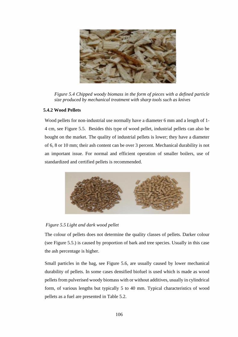
106
Figure 5.4 Chipped woody biomass in the form of pieces with a defined particle
size produced by mechanical treatment with sharp tools such as knives
5.4.2 Wood Pellets
Wood pellets for non-industrial use normally have a diameter 6 mm and a length of 1-
4 cm, see Figure 5.5. Besides this type of wood pellet, industrial pellets can also be
bought on the market. The quality of industrial pellets is lower; they have a diameter
of 6, 8 or 10 mm; their ash content can be over 3 percent. Mechanical durability is not
an important issue. For normal and efficient operation of smaller boilers, use of
standardized and certified pellets is recommended.
Figure 5.5 Light and dark wood pellet
The colour of pellets does not determine the quality classes of pellets. Darker colour
(see Figure 5.5.) is caused by proportion of bark and tree species. Usually in this case
the ash percentage is higher.
Small particles in the bag, see Figure 5.6, are usually caused by lower mechanical
durability of pellets. In some cases densified biofuel is used which is made as wood
pellets from pulverised woody biomass with or without additives, usually in cylindrical
form, of various lengths but typically 5 to 40 mm. Typical characteristics of wood
pellets as a fuel are presented in Table 5.2.
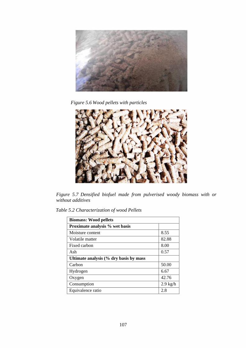
107
Figure 5.6 Wood pellets with particles
Figure 5.7 Densified biofuel made from pulverised woody biomass with or
without additives
Table 5.2 Characterization of wood Pellets
Biomass: Wood pellets
Proximate analysis % wet basis
Moisture content 8.55
Volatile matter 82.88
Fixed carbon 8.00
Ash 0.57
Ultimate analysis (% dry basis by mass
Carbon 50.00
Hydrogen 6.67
Oxygen 42.76
Consumption 2.9 kg/h
Equivalence ratio 2.8
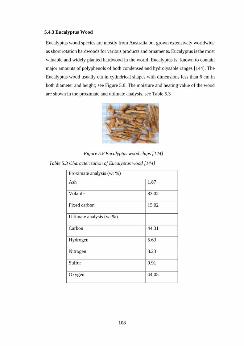
108
5.4.3 Eucalyptus Wood
Eucalyptus wood species are mostly from Australia but grown extensively worldwide
as short rotation hardwoods for various products and ornaments. Eucalyptus is the most
valuable and widely planted hardwood in the world. Eucalyptus is known to contain
major amounts of polyphenols of both condensed and hydrolysable ranges [144]. The
Eucalyptus wood usually cut in cylindrical shapes with dimensions less than 6 cm in
both diameter and height; see Figure 5.8. The moisture and heating value of the wood
are shown in the proximate and ultimate analysis, see Table 5.3
Figure 5.8 Eucalyptus wood chips [144]
Table 5.3 Characterization of Eucalyptus wood [144]
Proximate analysis (wt %)
Ash 1.87
Volatile 83.02
Fixed carbon 15.02
Ultimate analysis (wt %)
Carbon 44.31
Hydrogen 5.63
Nitrogen 3.23
Sulfur 0.91
Oxygen 44.05
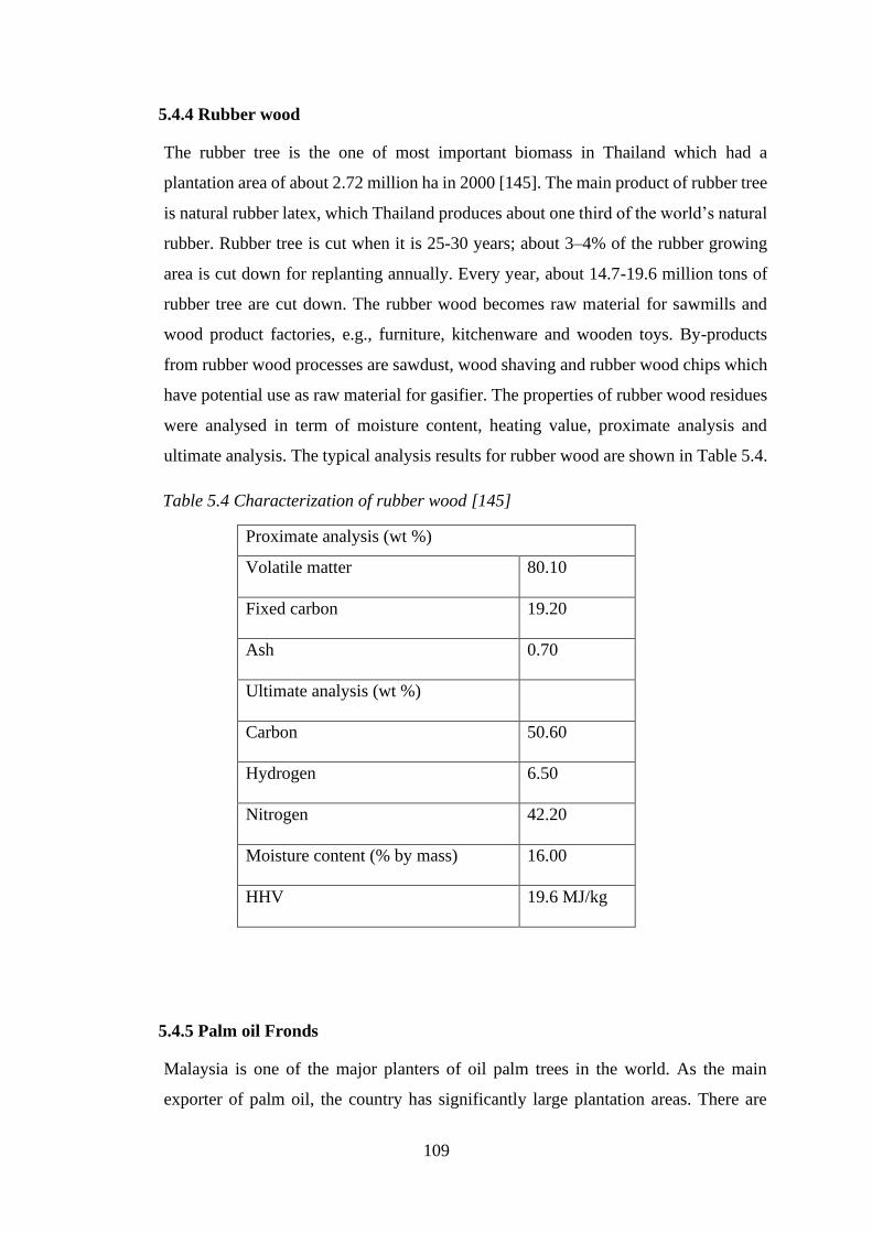
109
5.4.4 Rubber wood
The rubber tree is the one of most important biomass in Thailand which had a
plantation area of about 2.72 million ha in 2000 [145]. The main product of rubber tree
is natural rubber latex, which Thailand produces about one third of the world’s natural
rubber. Rubber tree is cut when it is 25-30 years; about 3–4% of the rubber growing
area is cut down for replanting annually. Every year, about 14.7-19.6 million tons of
rubber tree are cut down. The rubber wood becomes raw material for sawmills and
wood product factories, e.g., furniture, kitchenware and wooden toys. By-products
from rubber wood processes are sawdust, wood shaving and rubber wood chips which
have potential use as raw material for gasifier. The properties of rubber wood residues
were analysed in term of moisture content, heating value, proximate analysis and
ultimate analysis. The typical analysis results for rubber wood are shown in Table 5.4.
Table 5.4 Characterization of rubber wood [145]
Proximate analysis (wt %)
Volatile matter 80.10
Fixed carbon 19.20
Ash 0.70
Ultimate analysis (wt %)
Carbon 50.60
Hydrogen 6.50
Nitrogen 42.20
Moisture content (% by mass) 16.00
HHV 19.6 MJ/kg
5.4.5 Palm oil Fronds
Malaysia is one of the major planters of oil palm trees in the world. As the main
exporter of palm oil, the country has significantly large plantation areas. There are
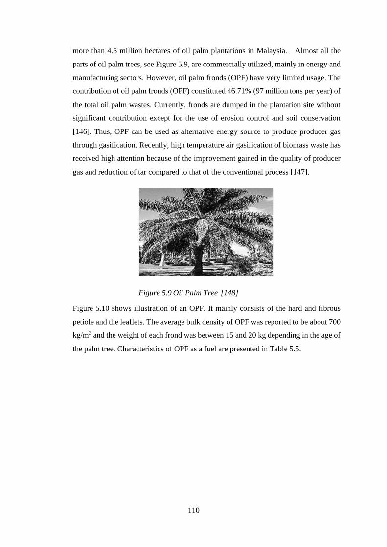
110
more than 4.5 million hectares of oil palm plantations in Malaysia. Almost all the
parts of oil palm trees, see Figure 5.9, are commercially utilized, mainly in energy and
manufacturing sectors. However, oil palm fronds (OPF) have very limited usage. The
contribution of oil palm fronds (OPF) constituted 46.71% (97 million tons per year) of
the total oil palm wastes. Currently, fronds are dumped in the plantation site without
significant contribution except for the use of erosion control and soil conservation
[146]. Thus, OPF can be used as alternative energy source to produce producer gas
through gasification. Recently, high temperature air gasification of biomass waste has
received high attention because of the improvement gained in the quality of producer
gas and reduction of tar compared to that of the conventional process [147].
Figure 5.9 Oil Palm Tree [148]
Figure 5.10 shows illustration of an OPF. It mainly consists of the hard and fibrous
petiole and the leaflets. The average bulk density of OPF was reported to be about 700
kg/m3 and the weight of each frond was between 15 and 20 kg depending in the age of
the palm tree. Characteristics of OPF as a fuel are presented in Table 5.5.
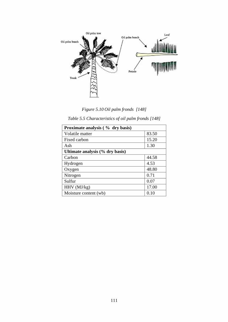
111
Figure 5.10 Oil palm fronds [148]
Table 5.5 Characteristics of oil palm fronds [148]
Proximate analysis ( % dry basis)
Volatile matter 83.50
Fixed carbon 15.20
Ash 1.30
Ultimate analysis (% dry basis)
Carbon 44.58
Hydrogen 4.53
Oxygen 48.80
Nitrogen 0.71
Sulfur 0.07
HHV (MJ/kg) 17.00
Moisture content (wb) 0.10
112
Chapter 6 Description of Obtained Numerical Results and
Their Discussion
6.1 Introduction
This chapter presents the results obtained from modelling the gasification of various
biomass feedstock such as wood chips, wood pellets, rubber wood and Eucalyptus
wood and oil palm fronds.
The robustness, performance and utility of mathematical models can be estimated by
comparing the numerical results with experimental data obtained under similar process
parameters. In the present models, the governing process parameters are moisture
content and air to fuel ratio or equivalence ratio and temperature of the reaction zone.
The composition of the product gas is mainly determined by the chemical composition
of the biomass, moisture content and the operating conditions. Therefore, based on
similar process parameters and similar biomass chemical composition, robust
mathematical models should yield amounts of products identical to that in
experimental data. The composition of the product gas mainly consists of methane,
hydrogen, carbon dioxide, and water. These final producer gas compositions are
mainly expressed on dry basis that is, without the water content.
Theoretical results obtained in this Chapter are compered to experimental data
published by various authors.
6.2 Modelling and simulation results of biomass using MATLAB
Mathematical model is developed to simulate the behaviour of a downdraft gasifier
operating in the steady state. To validate this model, predicted results from this model
is tested against published experimental data. The model is developed to describe
processes in each of the three reaction zones of the reactor, which are pyrolysis,
oxidation and reduction zones. The analysis in the pyrolysis and the oxidation zones is
based on the chemical equilibrium whilst the reduction zone processes are considered
based on finite rate chemical kinetics. The model is tested against published
experimental results from literature, namely by Chawdhury et al. [29] obtained from
the design and testing of a small downdraft gasifier JRB-1 at Durham University, UK.
The design of the JRB-1 gasifier was based on the Fluidyne gasifier. It slightly
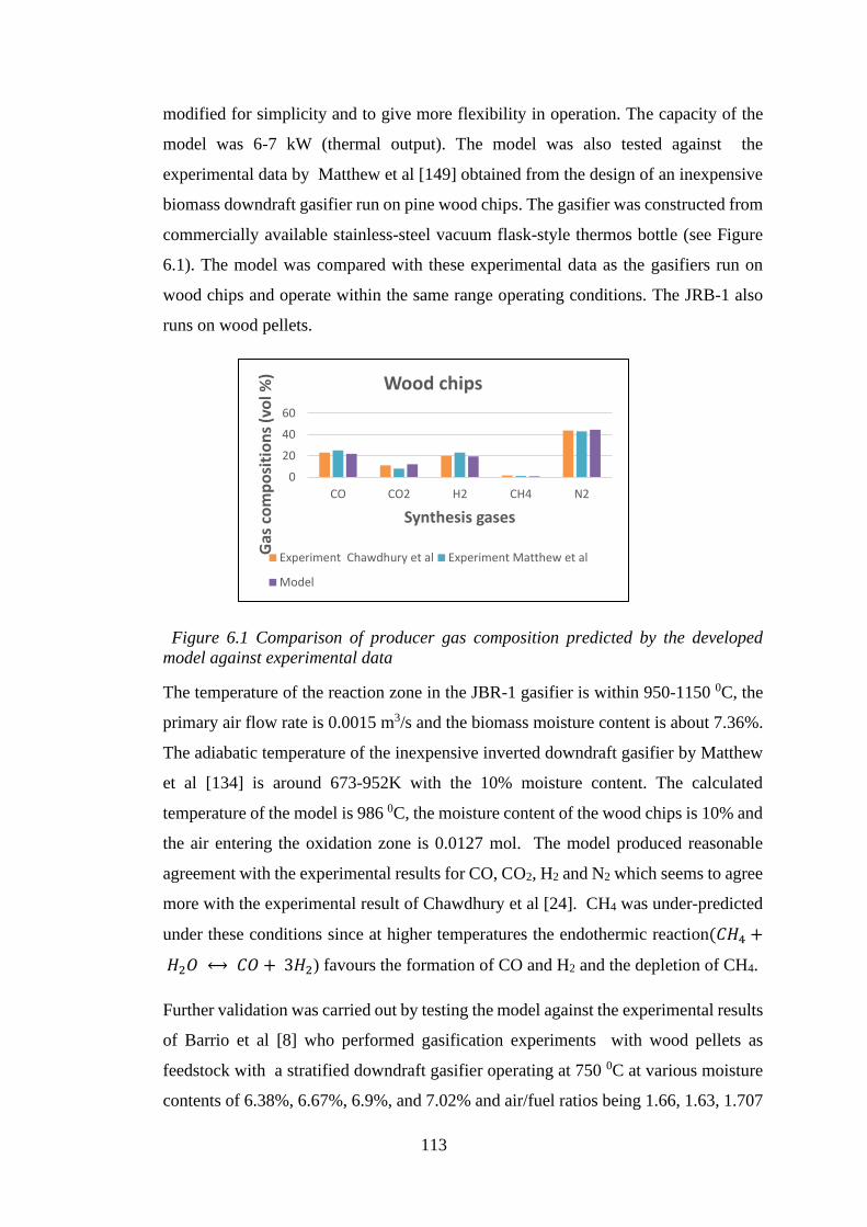
113
modified for simplicity and to give more flexibility in operation. The capacity of the
model was 6-7 kW (thermal output). The model was also tested against the
experimental data by Matthew et al [149] obtained from the design of an inexpensive
biomass downdraft gasifier run on pine wood chips. The gasifier was constructed from
commercially available stainless-steel vacuum flask-style thermos bottle (see Figure
6.1). The model was compared with these experimental data as the gasifiers run on
wood chips and operate within the same range operating conditions. The JRB-1 also
runs on wood pellets.
Figure 6.1 Comparison of producer gas composition predicted by the developed
model against experimental data
The temperature of the reaction zone in the JBR-1 gasifier is within 950-1150 0C, the
primary air flow rate is 0.0015 m3/s and the biomass moisture content is about 7.36%.
The adiabatic temperature of the inexpensive inverted downdraft gasifier by Matthew
et al [134] is around 673-952K with the 10% moisture content. The calculated
temperature of the model is 986 0C, the moisture content of the wood chips is 10% and
the air entering the oxidation zone is 0.0127 mol. The model produced reasonable
agreement with the experimental results for CO, CO2, H2 and N2 which seems to agree
more with the experimental result of Chawdhury et al [24]. CH4 was under-predicted
under these conditions since at higher temperatures the endothermic reaction(𝐶𝐻4 +
𝐻2𝑂 ⟷ 𝐶𝑂 + 3𝐻2) favours the formation of CO and H2 and the depletion of CH4.
Further validation was carried out by testing the model against the experimental results
of Barrio et al [8] who performed gasification experiments with wood pellets as
feedstock with a stratified downdraft gasifier operating at 750 0C at various moisture
contents of 6.38%, 6.67%, 6.9%, and 7.02% and air/fuel ratios being 1.66, 1.63, 1.707
0
20
40
60
CO CO2 H2 CH4 N2
Gas
co
mp
osi
tio
ns
(vo
l %)
Synthesis gases
Wood chips
Experiment Chawdhury et al Experiment Matthew et al
Model
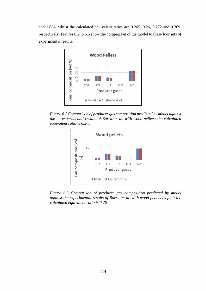
114
and 1.684, whilst the calculated equivalent ratios are 0.265, 0.26, 0.272 and 0.269,
respectively. Figures 6.2 to 6.5 show the comparison of the model to these four sets of
experimental results.
Figure 6.2 Comparison of producer gas composition predicted by model against
the experimental results of Barrio et al. with wood pellets: the calculated
equivalent ratio is 0.265
Figure 6.3 Comparison of producer gas composition predicted by model
against the experimental results of Barrio et al. with wood pellets as fuel: the
calculated equivalent ratio is 0.26
0
20
40
60
CO2 CO H2 CH4 N2
Gas
co
mp
osi
tio
n (
vol %
)
Producer gases
Wood Pellets
Model Exp(Barrio et al)
0
50
CO2 CO H2 CH4 N2
Gas
co
mp
osi
tio
ns
(vo
l %
)
Producer gases
Wood pellets
Model Exp(Barrio et al)
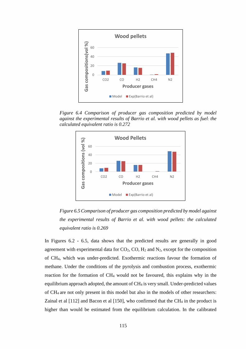
115
Figure 6.4 Comparison of producer gas composition predicted by model
against the experimental results of Barrio et al. with wood pellets as fuel: the
calculated equivalent ratio is 0.272
Figure 6.5 Comparison of producer gas composition predicted by model against
the experimental results of Barrio et al. with wood pellets: the calculated
equivalent ratio is 0.269
In Figures 6.2 - 6.5, data shows that the predicted results are generally in good
agreement with experimental data for CO2, CO, H2 and N2, except for the composition
of CH4, which was under-predicted. Exothermic reactions favour the formation of
methane. Under the conditions of the pyrolysis and combustion process, exothermic
reaction for the formation of CH4 would not be favoured, this explains why in the
equilibrium approach adopted, the amount of CH4 is very small. Under-predicted values
of CH4 are not only present in this model but also in the models of other researchers:
Zainal et al [112] and Bacon et al [150], who confirmed that the CH4 in the product is
higher than would be estimated from the equilibrium calculation. In the calibrated
0
20
40
60
CO2 CO H2 CH4 N2
Gas
co
mp
osi
tio
ns(
vol %
)Producer gases
Wood pellets
Model Exp(Barrio et al)
0
20
40
60
CO2 CO H2 CH4 N2
Gas
co
mp
osi
tio
ns
(vo
l %)
Producer gases
Wood Pellets
Model Exp(Barrio et al)
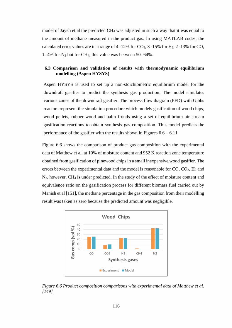
116
model of Jayeh et al the predicted CH4 was adjusted in such a way that it was equal to
the amount of methane measured in the product gas. In using MATLAB codes, the
calculated error values are in a range of 4 -12% for CO2, 3 -15% for H2, 2 -13% for CO,
1- 4% for N2 but for CH4, this value was between 50- 64%.
6.3 Comparison and validation of results with thermodynamic equilibrium
modelling (Aspen HYSYS)
Aspen HYSYS is used to set up a non-stoichiometric equilibrium model for the
downdraft gasifier to predict the synthesis gas production. The model simulates
various zones of the downdraft gasifier. The process flow diagram (PFD) with Gibbs
reactors represent the simulation procedure which models gasification of wood chips,
wood pellets, rubber wood and palm fronds using a set of equilibrium air stream
gasification reactions to obtain synthesis gas composition. This model predicts the
performance of the gasifier with the results shown in Figures 6.6 – 6.11.
Figure 6.6 shows the comparison of product gas composition with the experimental
data of Matthew et al. at 10% of moisture content and 952 K reaction zone temperature
obtained from gasification of pinewood chips in a small inexpensive wood gasifier. The
errors between the experimental data and the model is reasonable for CO, CO2, H2 and
N2, however, CH4 is under predicted. In the study of the effect of moisture content and
equivalence ratio on the gasification process for different biomass fuel carried out by
Manish et al [151], the methane percentage in the gas composition from their modelling
result was taken as zero because the predicted amount was negligible.
Figure 6.6 Product composition comparisons with experimental data of Matthew et al.
[149]
0
10
20
30
40
50
CO CO2 H2 CH4 N2
Gas
co
mp
(vo
l %)
Synthesis gases
Wood Chips
Experiment Model
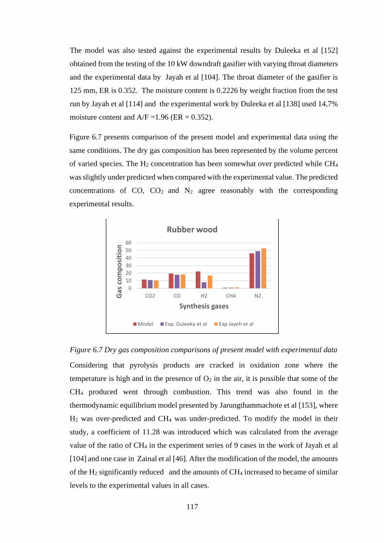
117
The model was also tested against the experimental results by Duleeka et al [152]
obtained from the testing of the 10 kW downdraft gasifier with varying throat diameters
and the experimental data by Jayah et al [104]. The throat diameter of the gasifier is
125 mm, ER is 0.352. The moisture content is 0.2226 by weight fraction from the test
run by Jayah et al [114] and the experimental work by Duleeka et al [138] used 14,7%
moisture content and A/F =1.96 (ER = 0.352).
Figure 6.7 presents comparison of the present model and experimental data using the
same conditions. The dry gas composition has been represented by the volume percent
of varied species. The H2 concentration has been somewhat over predicted while CH4
was slightly under predicted when compared with the experimental value. The predicted
concentrations of CO, CO2 and N2 agree reasonably with the corresponding
experimental results.
Figure 6.7 Dry gas composition comparisons of present model with experimental data
Considering that pyrolysis products are cracked in oxidation zone where the
temperature is high and in the presence of O2 in the air, it is possible that some of the
CH4 produced went through combustion. This trend was also found in the
thermodynamic equilibrium model presented by Jarungthammachote et al [153], where
H2 was over-predicted and CH4 was under-predicted. To modify the model in their
study, a coefficient of 11.28 was introduced which was calculated from the average
value of the ratio of CH4 in the experiment series of 9 cases in the work of Jayah et al
[104] and one case in Zainal et al [46]. After the modification of the model, the amounts
of the H2 significantly reduced and the amounts of CH4 increased to became of similar
levels to the experimental values in all cases.
0
10
20
30
40
50
60
CO2 CO H2 CH4 N2Gas
co
mp
osi
tio
n
Synthesis gases
Rubber wood
Model Exp. Duleeka et al Exp Jayeh et al
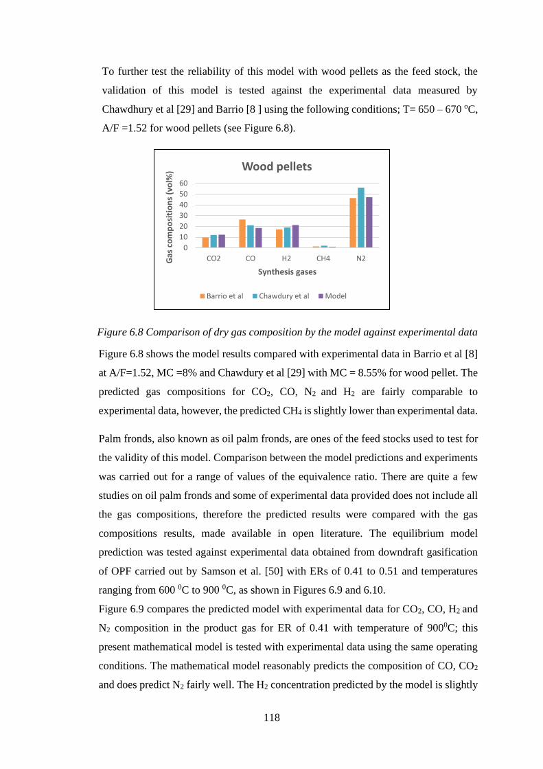
118
To further test the reliability of this model with wood pellets as the feed stock, the
validation of this model is tested against the experimental data measured by
Chawdhury et al [29] and Barrio [8 ] using the following conditions; T= 650 – 670 oC,
A/F =1.52 for wood pellets (see Figure 6.8).
Figure 6.8 Comparison of dry gas composition by the model against experimental data
Figure 6.8 shows the model results compared with experimental data in Barrio et al [8]
at A/F=1.52, MC =8% and Chawdury et al [29] with MC = 8.55% for wood pellet. The
predicted gas compositions for CO2, CO, N2 and H2 are fairly comparable to
experimental data, however, the predicted CH4 is slightly lower than experimental data.
Palm fronds, also known as oil palm fronds, are ones of the feed stocks used to test for
the validity of this model. Comparison between the model predictions and experiments
was carried out for a range of values of the equivalence ratio. There are quite a few
studies on oil palm fronds and some of experimental data provided does not include all
the gas compositions, therefore the predicted results were compared with the gas
compositions results, made available in open literature. The equilibrium model
prediction was tested against experimental data obtained from downdraft gasification
of OPF carried out by Samson et al. [50] with ERs of 0.41 to 0.51 and temperatures
ranging from 600 0C to 900 0C, as shown in Figures 6.9 and 6.10.
Figure 6.9 compares the predicted model with experimental data for CO2, CO, H2 and
N2 composition in the product gas for ER of 0.41 with temperature of 9000C; this
present mathematical model is tested with experimental data using the same operating
conditions. The mathematical model reasonably predicts the composition of CO, CO2
and does predict N2 fairly well. The H2 concentration predicted by the model is slightly
0
10
20
30
40
50
60
CO2 CO H2 CH4 N2Gas
co
mp
osi
tio
ns
(vo
l%)
Synthesis gases
Wood pellets
Barrio et al Chawdury et al Model
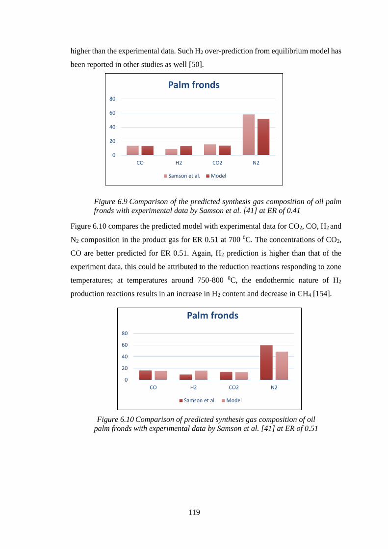
119
higher than the experimental data. Such H2 over-prediction from equilibrium model has
been reported in other studies as well [50].
Figure 6.9 Comparison of the predicted synthesis gas composition of oil palm
fronds with experimental data by Samson et al. [41] at ER of 0.41
Figure 6.10 compares the predicted model with experimental data for CO2, CO, H2 and
N2 composition in the product gas for ER 0.51 at 700 0C. The concentrations of CO2,
CO are better predicted for ER 0.51. Again, H2 prediction is higher than that of the
experiment data, this could be attributed to the reduction reactions responding to zone
temperatures; at temperatures around 750-800 0C, the endothermic nature of H2
production reactions results in an increase in H2 content and decrease in CH4 [154].
0
20
40
60
80
CO H2 CO2 N2
Palm fronds
Samson et al. Model
Figure 6.10 Comparison of predicted synthesis gas composition of oil
palm fronds with experimental data by Samson et al. [41] at ER of 0.51
0
20
40
60
80
CO H2 CO2 N2
Palm fronds
Samson et al. Model
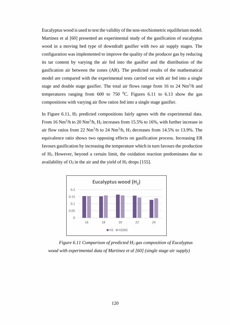
120
Eucalyptus wood is used to test the validity of the non-stochiometric equilibrium model.
Martinez et al [60] presented an experimental study of the gasification of eucalyptus
wood in a moving bed type of downdraft gasifier with two air supply stages. The
configuration was implemented to improve the quality of the producer gas by reducing
its tar content by varying the air fed into the gasifier and the distribution of the
gasification air between the zones (AR). The predicted results of the mathematical
model are compared with the experimental tests carried out with air fed into a single
stage and double stage gasifier. The total air flows range from 16 to 24 Nm3/h and
temperatures ranging from 600 to 750 0C. Figures 6.11 to 6.13 show the gas
compositions with varying air flow ratios fed into a single stage gasifier.
In Figure 6.11, H2 predicted compositions fairly agrees with the experimental data.
From 16 Nm3/h to 20 Nm3/h, H2 increases from 15.5% to 16%, with further increase in
air flow ratios from 22 Nm3/h to 24 Nm3/h, H2 decreases from 14.5% to 13.9%. The
equivalence ratio shows two opposing effects on gasification process. Increasing ER
favours gasification by increasing the temperature which in turn favours the production
of H2. However, beyond a certain limit, the oxidation reaction predominates due to
availability of O2 in the air and the yield of H2 drops [155].
Figure 6.11 Comparison of predicted H2 gas composition of Eucalyptus
wood with experimental data of Martinez et al [60] (single stage air supply)
0
0.05
0.1
0.15
0.2
16 18 20 22 24
Eucalyptus wood (H2)
H2 H2(M)

121
In Figure 6.12, the predicted CO compositions produced compares reasonably well with
the experimental data. It is observed that with an increase in the air flow ratio from 16
Nm3/h to 18 Nm3/h CO increases from 16.2% to 17.1%. It is also observed that with
further increase from 20 Nm3/h to 24 Nm3/h, CO gradually decreases from 17% to
16.9% and then to 15%. This indicates that, initially, CO increases due to increase in
the conversion of fuel but after attaining the optimum value its production begins to
decrease.
Figure 6.12 Comparison of predicted CO gas composition of Eucalyptus wood
with experimental data of Martinez et al [60] (single stage air supply)
In Figure 6.13, the predicted CH4 is seen to be consistently higher than the values of
the experimental data however, it follows a reasonable pattern; decreasing as the air
ratio increases. Using the model, the higher concentrations of the CH4 are formed in the
pyrolysis zone, as it goes into the oxidation zone. However, as it leaves the oxidation it
is reduced, this shows the effect of the temperature on the formation of methane.
0
0.05
0.1
0.15
0.2
0.25
16 18 20 22 24
Eucalyptus wood (CO)
CO CO(M)
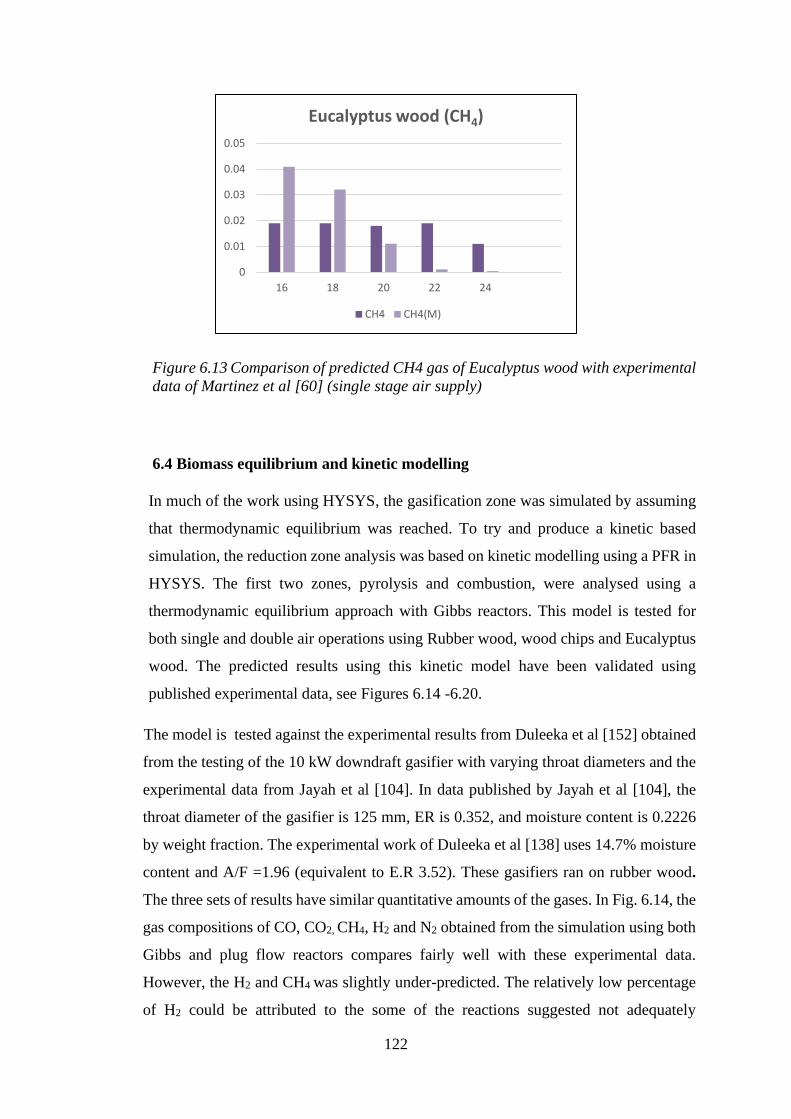
122
Figure 6.13 Comparison of predicted CH4 gas of Eucalyptus wood with experimental
data of Martinez et al [60] (single stage air supply)
6.4 Biomass equilibrium and kinetic modelling
In much of the work using HYSYS, the gasification zone was simulated by assuming
that thermodynamic equilibrium was reached. To try and produce a kinetic based
simulation, the reduction zone analysis was based on kinetic modelling using a PFR in
HYSYS. The first two zones, pyrolysis and combustion, were analysed using a
thermodynamic equilibrium approach with Gibbs reactors. This model is tested for
both single and double air operations using Rubber wood, wood chips and Eucalyptus
wood. The predicted results using this kinetic model have been validated using
published experimental data, see Figures 6.14 -6.20.
The model is tested against the experimental results from Duleeka et al [152] obtained
from the testing of the 10 kW downdraft gasifier with varying throat diameters and the
experimental data from Jayah et al [104]. In data published by Jayah et al [104], the
throat diameter of the gasifier is 125 mm, ER is 0.352, and moisture content is 0.2226
by weight fraction. The experimental work of Duleeka et al [138] uses 14.7% moisture
content and A/F =1.96 (equivalent to E.R 3.52). These gasifiers ran on rubber wood.
The three sets of results have similar quantitative amounts of the gases. In Fig. 6.14, the
gas compositions of CO, CO2, CH4, H2 and N2 obtained from the simulation using both
Gibbs and plug flow reactors compares fairly well with these experimental data.
However, the H2 and CH4 was slightly under-predicted. The relatively low percentage
of H2 could be attributed to the some of the reactions suggested not adequately
0
0.01
0.02
0.03
0.04
0.05
16 18 20 22 24
Eucalyptus wood (CH4)
CH4 CH4(M)
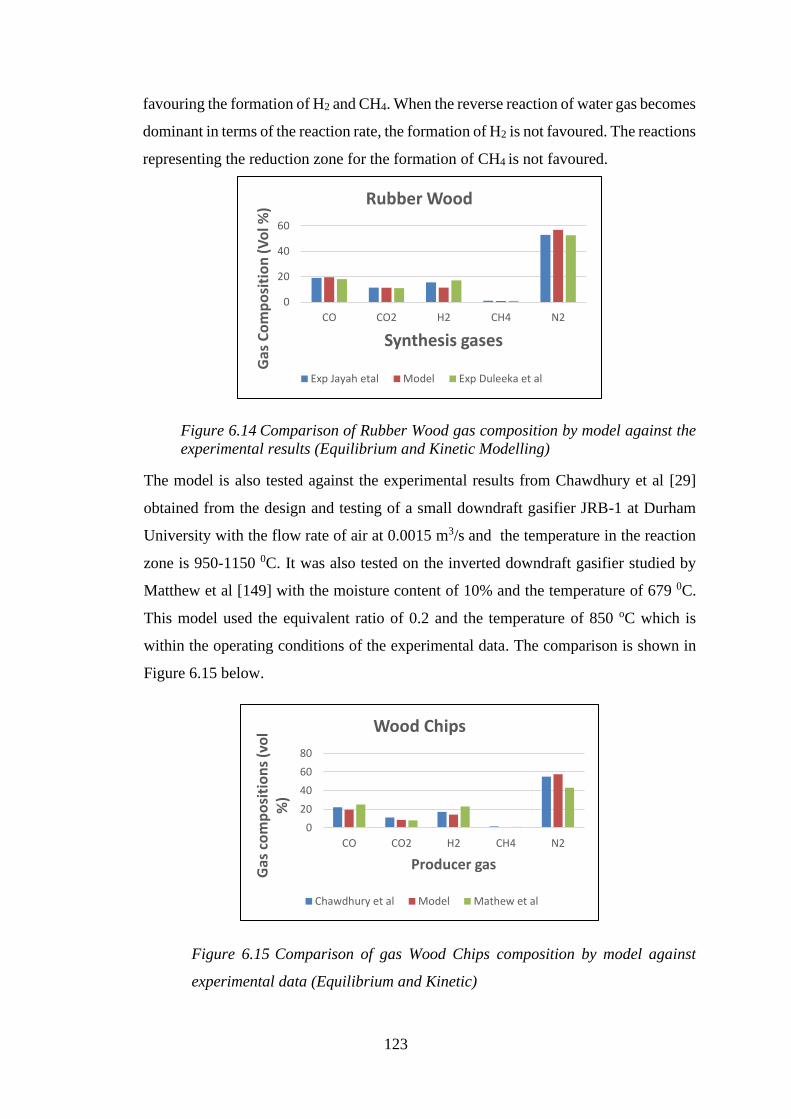
123
favouring the formation of H2 and CH4. When the reverse reaction of water gas becomes
dominant in terms of the reaction rate, the formation of H2 is not favoured. The reactions
representing the reduction zone for the formation of CH4 is not favoured.
Figure 6.14 Comparison of Rubber Wood gas composition by model against the
experimental results (Equilibrium and Kinetic Modelling)
The model is also tested against the experimental results from Chawdhury et al [29]
obtained from the design and testing of a small downdraft gasifier JRB-1 at Durham
University with the flow rate of air at 0.0015 m3/s and the temperature in the reaction
zone is 950-1150 0C. It was also tested on the inverted downdraft gasifier studied by
Matthew et al [149] with the moisture content of 10% and the temperature of 679 0C.
This model used the equivalent ratio of 0.2 and the temperature of 850 oC which is
within the operating conditions of the experimental data. The comparison is shown in
Figure 6.15 below.
Figure 6.15 Comparison of gas Wood Chips composition by model against
experimental data (Equilibrium and Kinetic)
0
20
40
60
CO CO2 H2 CH4 N2
Gas
Co
mp
osi
tio
n (
Vo
l %)
Synthesis gases
Rubber Wood
Exp Jayah etal Model Exp Duleeka et al
0
20
40
60
80
CO CO2 H2 CH4 N2
Gas
co
mp
osi
tio
ns
(vo
l %
)
Producer gas
Wood Chips
Chawdhury et al Model Mathew et al
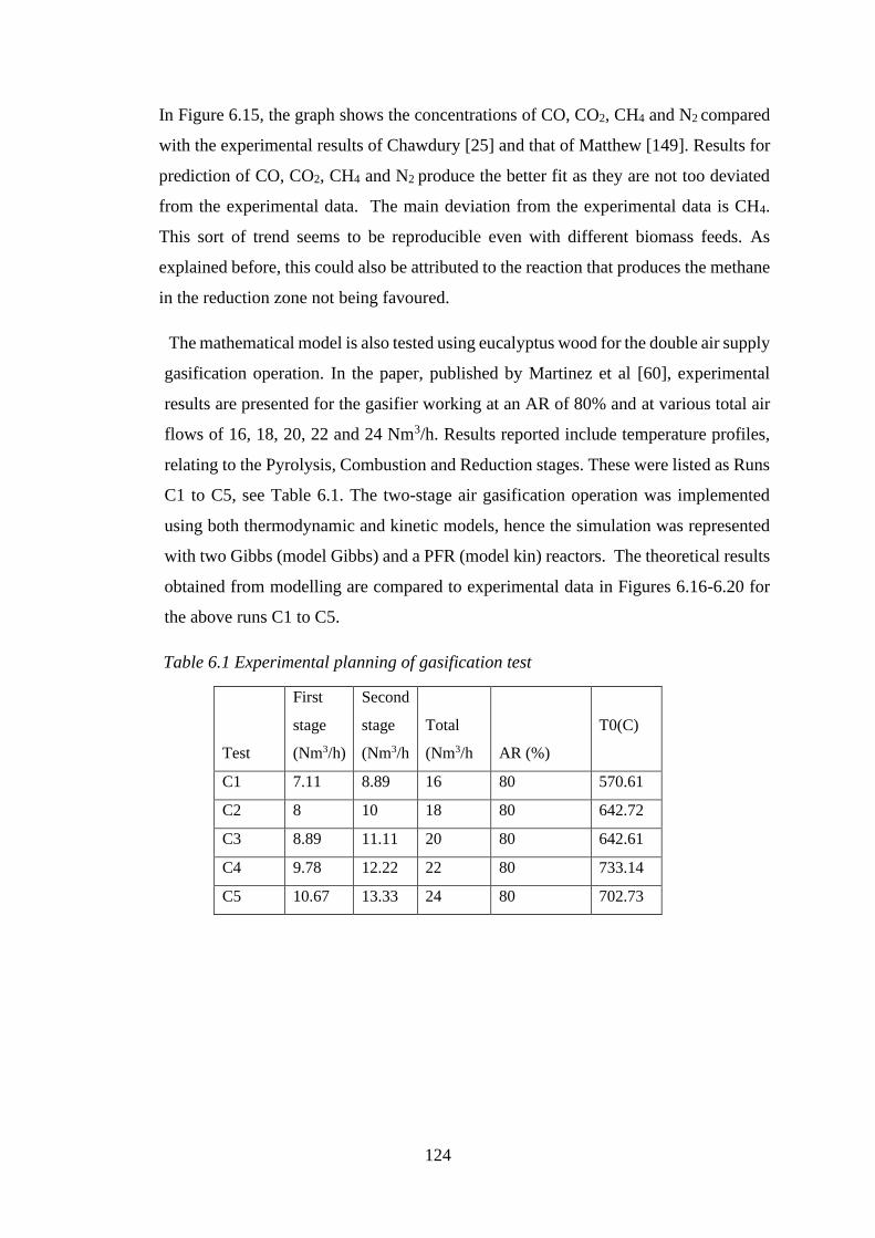
124
In Figure 6.15, the graph shows the concentrations of CO, CO2, CH4 and N2 compared
with the experimental results of Chawdury [25] and that of Matthew [149]. Results for
prediction of CO, CO2, CH4 and N2 produce the better fit as they are not too deviated
from the experimental data. The main deviation from the experimental data is CH4.
This sort of trend seems to be reproducible even with different biomass feeds. As
explained before, this could also be attributed to the reaction that produces the methane
in the reduction zone not being favoured.
The mathematical model is also tested using eucalyptus wood for the double air supply
gasification operation. In the paper, published by Martinez et al [60], experimental
results are presented for the gasifier working at an AR of 80% and at various total air
flows of 16, 18, 20, 22 and 24 Nm3/h. Results reported include temperature profiles,
relating to the Pyrolysis, Combustion and Reduction stages. These were listed as Runs
C1 to C5, see Table 6.1. The two-stage air gasification operation was implemented
using both thermodynamic and kinetic models, hence the simulation was represented
with two Gibbs (model Gibbs) and a PFR (model kin) reactors. The theoretical results
obtained from modelling are compared to experimental data in Figures 6.16-6.20 for
the above runs C1 to C5.
Table 6.1 Experimental planning of gasification test
Test
First
stage
(Nm3/h)
Second
stage
(Nm3/h
Total
(Nm3/h AR (%)
T0(C)
C1 7.11 8.89 16 80 570.61
C2 8 10 18 80 642.72
C3 8.89 11.11 20 80 642.61
C4 9.78 12.22 22 80 733.14
C5 10.67 13.33 24 80 702.73

125
Figure 6.16 Comparison of gas composition by model against the experimental
results (C1)
Figure 6.17 Comparison of gas composition by model against the experimental
results (C2)
Figure 6.18 Comparison of gas composition by model against the experimental
results (C3)
0
5
10
15
20
CO H2 CH4
Gas
co
mp
osi
tio
ns
(vo
l %)
Synthesis gases
C1
Model(Kin) Model (Gibbs) Exp Martinez
0
10
20
30
CO H2 CH4
Gas
co
mp
osi
tio
ns
(vo
l %
)
Synthesis gases
C2
Model(Kin) Model (Gibbs) Exp Martinez
0
10
20
30
CO H2 CH4
Gas
co
mp
osi
tio
ns
(vo
l %)
Synthesis gases
C3
Model(Kin) Model (Gibbs) Exp Martinez
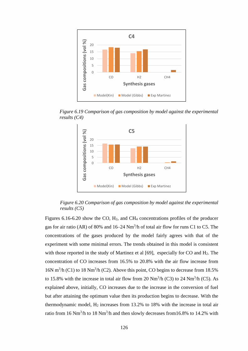
126
Figure 6.19 Comparison of gas composition by model against the experimental
results (C4)
Figure 6.20 Comparison of gas composition by model against the experimental
results (C5)
Figures 6.16-6.20 show the CO, H2, and CH4 concentrations profiles of the producer
gas for air ratio (AR) of 80% and 16–24 Nm3/h of total air flow for runs C1 to C5. The
concentrations of the gases produced by the model fairly agrees with that of the
experiment with some minimal errors. The trends obtained in this model is consistent
with those reported in the study of Martinez et al [69], especially for CO and H2. The
concentration of CO increases from 16.5% to 20.8% with the air flow increase from
16N m3/h (C1) to 18 Nm3/h (C2). Above this point, CO begins to decrease from 18.5%
to 15.8% with the increase in total air flow from 20 Nm3/h (C3) to 24 Nm3/h (C5). As
explained above, initially, CO increases due to the increase in the conversion of fuel
but after attaining the optimum value then its production begins to decrease. With the
thermodynamic model, H2 increases from 13.2% to 18% with the increase in total air
ratio from 16 Nm3/h to 18 Nm3/h and then slowly decreases from16.8% to 14.2% with
0
5
10
15
20
CO H2 CH4
Gas
co
mp
osi
tio
ns
(vo
l %)
Synthesis gases
C4
Model(Kin) Model (Gibbs) Exp Martinez
0
5
10
15
20
CO H2 CH4
Gas
co
mp
osi
tio
ns
(vo
l %)
Synthesis gases
C5
Model(Kin) Model (Gibbs) Exp Martinez
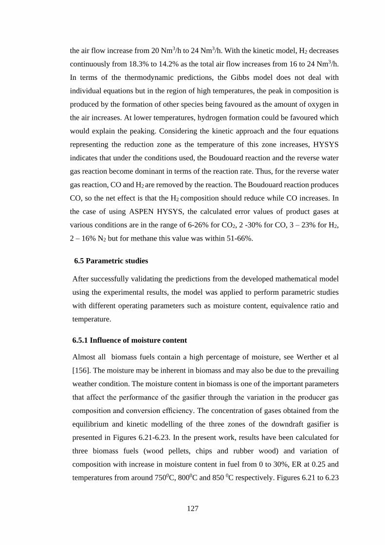
127
the air flow increase from 20 Nm3/h to 24 Nm3/h. With the kinetic model, H2 decreases
continuously from 18.3% to 14.2% as the total air flow increases from 16 to 24 Nm3/h.
In terms of the thermodynamic predictions, the Gibbs model does not deal with
individual equations but in the region of high temperatures, the peak in composition is
produced by the formation of other species being favoured as the amount of oxygen in
the air increases. At lower temperatures, hydrogen formation could be favoured which
would explain the peaking. Considering the kinetic approach and the four equations
representing the reduction zone as the temperature of this zone increases, HYSYS
indicates that under the conditions used, the Boudouard reaction and the reverse water
gas reaction become dominant in terms of the reaction rate. Thus, for the reverse water
gas reaction, CO and H2 are removed by the reaction. The Boudouard reaction produces
CO, so the net effect is that the H2 composition should reduce while CO increases. In
the case of using ASPEN HYSYS, the calculated error values of product gases at
various conditions are in the range of 6-26% for CO2, 2 -30% for CO, 3 – 23% for H2,
2 – 16% N2 but for methane this value was within 51-66%.
6.5 Parametric studies
After successfully validating the predictions from the developed mathematical model
using the experimental results, the model was applied to perform parametric studies
with different operating parameters such as moisture content, equivalence ratio and
temperature.
6.5.1 Influence of moisture content
Almost all biomass fuels contain a high percentage of moisture, see Werther et al
[156]. The moisture may be inherent in biomass and may also be due to the prevailing
weather condition. The moisture content in biomass is one of the important parameters
that affect the performance of the gasifier through the variation in the producer gas
composition and conversion efficiency. The concentration of gases obtained from the
equilibrium and kinetic modelling of the three zones of the downdraft gasifier is
presented in Figures 6.21-6.23. In the present work, results have been calculated for
three biomass fuels (wood pellets, chips and rubber wood) and variation of
composition with increase in moisture content in fuel from 0 to 30%, ER at 0.25 and
temperatures from around 7500C, 8000C and 850 0C respectively. Figures 6.21 to 6.23
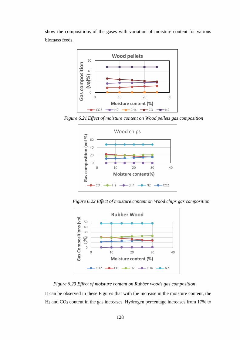
128
show the compositions of the gases with variation of moisture content for various
biomass feeds.
Figure 6.21 Effect of moisture content on Wood pellets gas composition
Figure 6.22 Effect of moisture content on Wood chips gas composition
Figure 6.23 Effect of moisture content on Rubber woods gas composition
It can be observed in these Figures that with the increase in the moisture content, the
H2 and CO2 content in the gas increases. Hydrogen percentage increases from 17% to
0
20
40
60
0 10 20 30Gas
co
mp
osi
tio
n
(vo
l%)
Moisture content (%)
Wood pellets
CO2 H2 CH4 CO N2
0
20
40
60
0 10 20 30 40
Gas
co
mp
osi
tio
n (
vol %
)
Moisture content(%)
Wood chips
CO H2 CH4 N2 CO2
0
10
20
30
40
50
0 10 20 30 40
Gas
Co
mp
osi
tio
ns
(vo
l %
)
Moisture content (%)
Rubber Wood
CO2 CO H2 CH4 N2
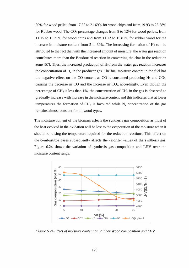
129
20% for wood pellet, from 17.82 to 21.69% for wood chips and from 19.93 to 25.58%
for Rubber wood. The CO2 percentage changes from 9 to 12% for wood pellets, from
11.15 to 15.31% for wood chips and from 11.12 to 15.81% for rubber wood for the
increase in moisture content from 5 to 30%. The increasing formation of H2 can be
attributed to the fact that with the increased amount of moisture, the water gas reaction
contributes more than the Boudouard reaction in converting the char in the reduction
zone [57]. Thus, the increased production of H2 from the water gas reaction increases
the concentration of H2 in the producer gas. The fuel moisture content in the fuel has
the negative effect on the CO content as CO is consumed producing H2 and CO2,
causing the decrease in CO and the increase in CO2, accordingly. Even though the
percentage of CH4 is less than 1%, the concentration of CH4 in the gas is observed to
gradually increase with increase in the moisture content and this indicates that at lower
temperatures the formation of CH4 is favoured while N2 concentration of the gas
remains almost constant for all wood types.
The moisture content of the biomass affects the synthesis gas composition as most of
the heat evolved in the oxidation will be lost to the evaporation of the moisture when it
should be raising the temperature required for the reduction reactions. This effect on
the combustible gases subsequently affects the calorific values of the synthesis gas.
Figure 6.24 shows the variation of synthesis gas composition and LHV over the
moisture content range.
Figure 6.24 Effect of moisture content on Rubber Wood composition and LHV
4900
4950
5000
5050
5100
5150
5200
5250
0
10
20
30
40
50
60
5 10 15 20 25
LHV
(KJ/
Nm
3)
Gas
co
mp
osi
tio
n (
vol %
)
MC(%)CO CO2 H2 CH4 N2 LHV(KJ/Nm3
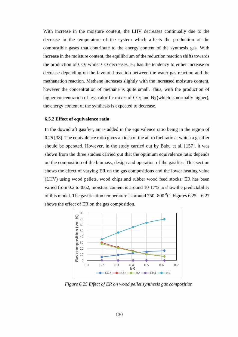
130
With increase in the moisture content, the LHV decreases continually due to the
decrease in the temperature of the system which affects the production of the
combustible gases that contribute to the energy content of the synthesis gas. With
increase in the moisture content, the equilibrium of the reduction reaction shifts towards
the production of CO2 whilst CO decreases. H2 has the tendency to either increase or
decrease depending on the favoured reaction between the water gas reaction and the
methanation reaction. Methane increases slightly with the increased moisture content,
however the concentration of methane is quite small. Thus, with the production of
higher concentration of less calorific mixes of CO2 and N2 (which is normally higher),
the energy content of the synthesis is expected to decrease.
6.5.2 Effect of equivalence ratio
In the downdraft gasifier, air is added in the equivalence ratio being in the region of
0.25 [38]. The equivalence ratio gives an idea of the air to fuel ratio at which a gasifier
should be operated. However, in the study carried out by Babu et al. [157], it was
shown from the three studies carried out that the optimum equivalence ratio depends
on the composition of the biomass, design and operation of the gasifier. This section
shows the effect of varying ER on the gas compositions and the lower heating value
(LHV) using wood pellets, wood chips and rubber wood feed stocks. ER has been
varied from 0.2 to 0.62, moisture content is around 10-17% to show the predictability
of this model. The gasification temperature is around 750- 800 0C. Figures 6.25 – 6.27
shows the effect of ER on the gas composition.
Figure 6.25 Effect of ER on wood pellet synthesis gas composition
0
10
20
30
40
50
60
70
80
0.1 0.2 0.3 0.4 0.5 0.6 0.7
Gas
co
mp
osi
tio
n (
vol %
)
ERCO2 CO H2 CH4 N2
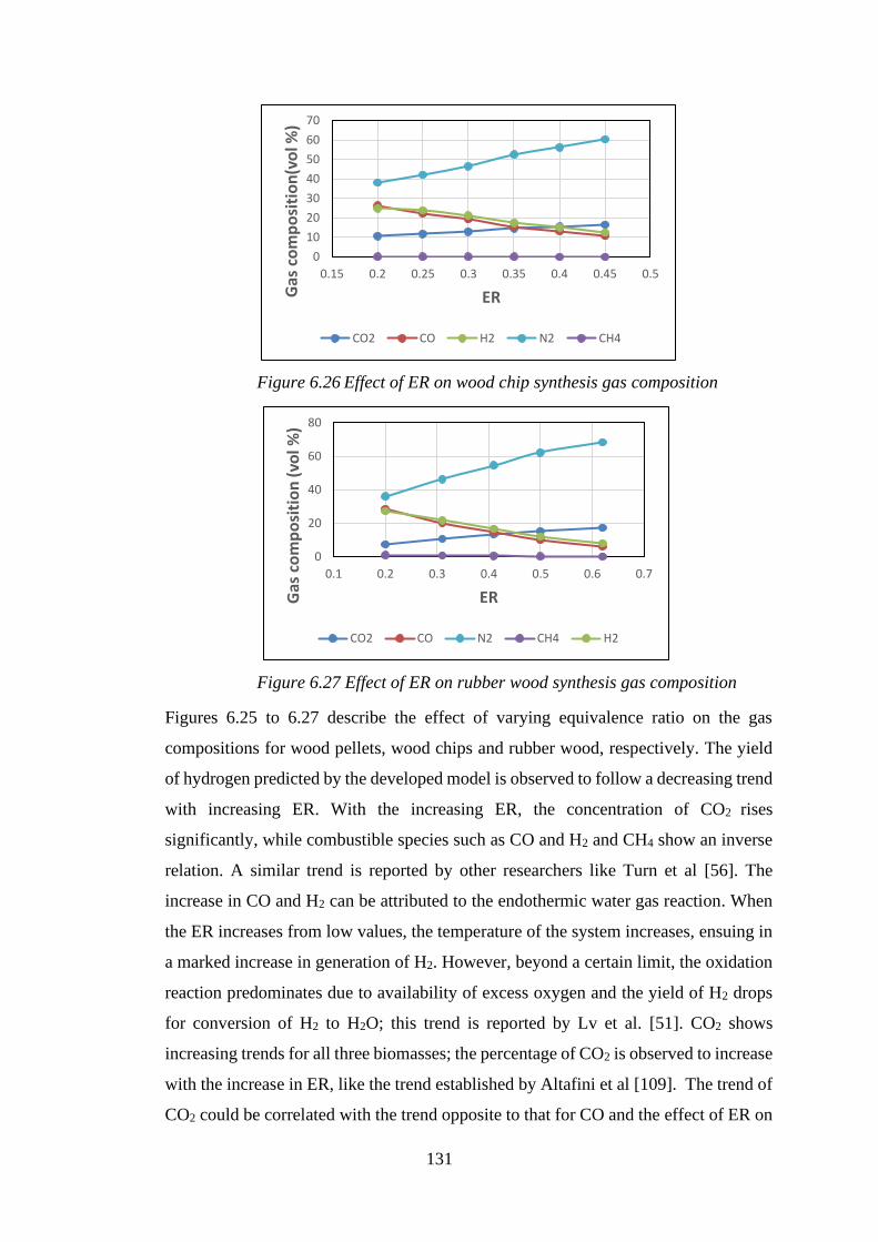
131
Figure 6.26 Effect of ER on wood chip synthesis gas composition
Figure 6.27 Effect of ER on rubber wood synthesis gas composition
Figures 6.25 to 6.27 describe the effect of varying equivalence ratio on the gas
compositions for wood pellets, wood chips and rubber wood, respectively. The yield
of hydrogen predicted by the developed model is observed to follow a decreasing trend
with increasing ER. With the increasing ER, the concentration of CO2 rises
significantly, while combustible species such as CO and H2 and CH4 show an inverse
relation. A similar trend is reported by other researchers like Turn et al [56]. The
increase in CO and H2 can be attributed to the endothermic water gas reaction. When
the ER increases from low values, the temperature of the system increases, ensuing in
a marked increase in generation of H2. However, beyond a certain limit, the oxidation
reaction predominates due to availability of excess oxygen and the yield of H2 drops
for conversion of H2 to H2O; this trend is reported by Lv et al. [51]. CO2 shows
increasing trends for all three biomasses; the percentage of CO2 is observed to increase
with the increase in ER, like the trend established by Altafini et al [109]. The trend of
CO2 could be correlated with the trend opposite to that for CO and the effect of ER on
0
10
20
30
40
50
60
70
0.15 0.2 0.25 0.3 0.35 0.4 0.45 0.5
Gas
co
mp
osi
tio
n(v
ol %
)ER
CO2 CO H2 N2 CH4
0
20
40
60
80
0.1 0.2 0.3 0.4 0.5 0.6 0.7
Gas
co
mp
osi
tio
n (
vol %
)
ER
CO2 CO N2 CH4 H2
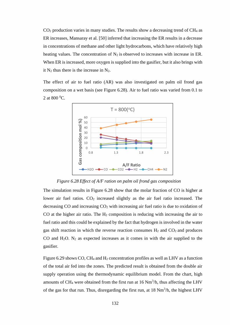
132
CO2 production varies in many studies. The results show a decreasing trend of CH4 as
ER increases, Mansaray et al. [50] inferred that increasing the ER results in a decrease
in concentrations of methane and other light hydrocarbons, which have relatively high
heating values. The concentration of N2 is observed to increases with increase in ER.
When ER is increased, more oxygen is supplied into the gasifier, but it also brings with
it N2 thus there is the increase in N2.
The effect of air to fuel ratio (AR) was also investigated on palm oil frond gas
composition on a wet basis (see Figure 6.28). Air to fuel ratio was varied from 0.1 to
2 at 800 0C.
Figure 6.28 Effect of A/F ration on palm oil frond gas composition
The simulation results in Figure 6.28 show that the molar fraction of CO is higher at
lower air fuel ratios. CO2 increased slightly as the air fuel ratio increased. The
decreasing CO and increasing CO2 with increasing air fuel ratio is due to oxidation of
CO at the higher air ratio. The H2 composition is reducing with increasing the air to
fuel ratio and this could be explained by the fact that hydrogen is involved in the water
gas shift reaction in which the reverse reaction consumes H2 and CO2 and produces
CO and H2O. N2 as expected increases as it comes in with the air supplied to the
gasifier.
Figure 6.29 shows CO, CH4 and H2 concentration profiles as well as LHV as a function
of the total air fed into the zones. The predicted result is obtained from the double air
supply operation using the thermodynamic equilibrium model. From the chart, high
amounts of CH4 were obtained from the first run at 16 Nm3/h, thus affecting the LHV
of the gas for that run. Thus, disregarding the first run, at 18 Nm3/h, the highest LHV
0
10
20
30
40
50
60
0.8 1.3 1.8 2.3
Gas
co
mp
osi
tio
n m
ol %
)
A/F Ratio
T = 800(oC)
H2O CO CO2 H2 CH4 N2
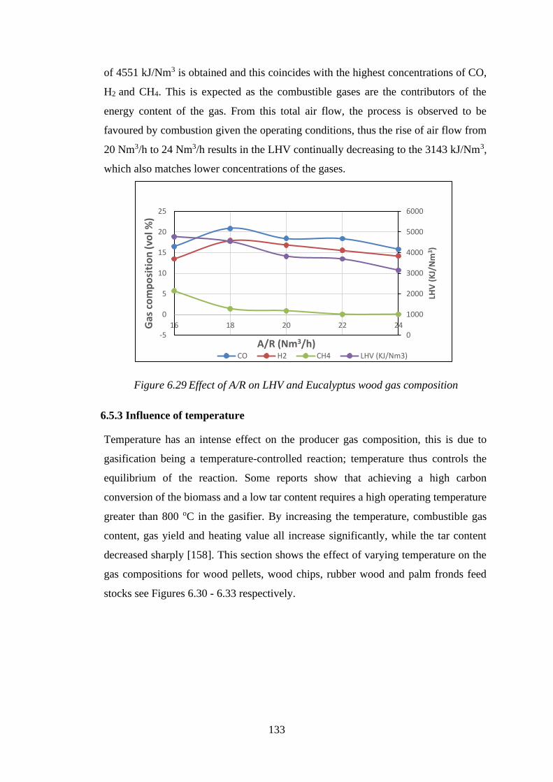
133
of 4551 kJ/Nm3 is obtained and this coincides with the highest concentrations of CO,
H2 and CH4. This is expected as the combustible gases are the contributors of the
energy content of the gas. From this total air flow, the process is observed to be
favoured by combustion given the operating conditions, thus the rise of air flow from
20 Nm3/h to 24 Nm3/h results in the LHV continually decreasing to the 3143 kJ/Nm3,
which also matches lower concentrations of the gases.
Figure 6.29 Effect of A/R on LHV and Eucalyptus wood gas composition
6.5.3 Influence of temperature
Temperature has an intense effect on the producer gas composition, this is due to
gasification being a temperature-controlled reaction; temperature thus controls the
equilibrium of the reaction. Some reports show that achieving a high carbon
conversion of the biomass and a low tar content requires a high operating temperature
greater than 800 oC in the gasifier. By increasing the temperature, combustible gas
content, gas yield and heating value all increase significantly, while the tar content
decreased sharply [158]. This section shows the effect of varying temperature on the
gas compositions for wood pellets, wood chips, rubber wood and palm fronds feed
stocks see Figures 6.30 - 6.33 respectively.
0
1000
2000
3000
4000
5000
6000
-5
0
5
10
15
20
25
16 18 20 22 24
LHV
(K
J/N
m3)
Gas
co
mp
osi
tio
n (
vol %
)
A/R (Nm3/h)CO H2 CH4 LHV (KJ/Nm3)
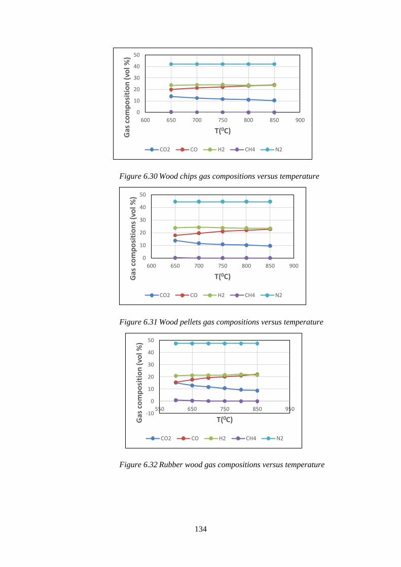
134
Figure 6.30 Wood chips gas compositions versus temperature
Figure 6.31 Wood pellets gas compositions versus temperature
Figure 6.32 Rubber wood gas compositions versus temperature
0
10
20
30
40
50
600 650 700 750 800 850 900G
as c
om
po
siti
on
(vo
l %)
T(0C)
CO2 CO H2 CH4 N2
0
10
20
30
40
50
600 650 700 750 800 850 900
Gas
co
mp
osi
tio
ns
(vo
l %)
T(0C)
CO2 CO H2 CH4 N2
-10
0
10
20
30
40
50
550 650 750 850 950
Gas
co
mp
osi
tio
n (
vol %
)
T(0C)
CO2 CO H2 CH4 N2
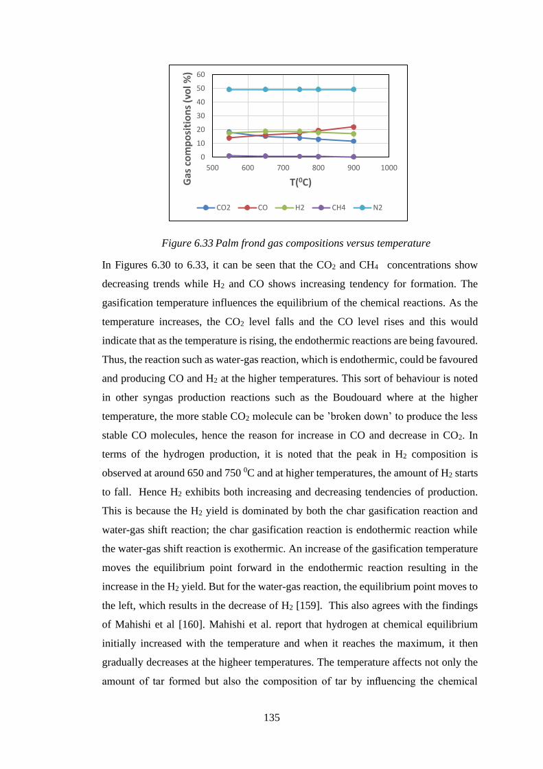
135
Figure 6.33 Palm frond gas compositions versus temperature
In Figures 6.30 to 6.33, it can be seen that the CO2 and CH4 concentrations show
decreasing trends while H2 and CO shows increasing tendency for formation. The
gasification temperature influences the equilibrium of the chemical reactions. As the
temperature increases, the CO2 level falls and the CO level rises and this would
indicate that as the temperature is rising, the endothermic reactions are being favoured.
Thus, the reaction such as water-gas reaction, which is endothermic, could be favoured
and producing CO and H2 at the higher temperatures. This sort of behaviour is noted
in other syngas production reactions such as the Boudouard where at the higher
temperature, the more stable CO2 molecule can be ’broken down’ to produce the less
stable CO molecules, hence the reason for increase in CO and decrease in CO2. In
terms of the hydrogen production, it is noted that the peak in H2 composition is
observed at around 650 and 750 0C and at higher temperatures, the amount of H2 starts
to fall. Hence H2 exhibits both increasing and decreasing tendencies of production.
This is because the H2 yield is dominated by both the char gasification reaction and
water-gas shift reaction; the char gasification reaction is endothermic reaction while
the water-gas shift reaction is exothermic. An increase of the gasification temperature
moves the equilibrium point forward in the endothermic reaction resulting in the
increase in the H2 yield. But for the water-gas reaction, the equilibrium point moves to
the left, which results in the decrease of H2 [159]. This also agrees with the findings
of Mahishi et al [160]. Mahishi et al. report that hydrogen at chemical equilibrium
initially increased with the temperature and when it reaches the maximum, it then
gradually decreases at the higheer temperatures. The temperature affects not only the
amount of tar formed but also the composition of tar by influencing the chemical
0
10
20
30
40
50
60
500 600 700 800 900 1000
Gas
co
mp
osi
tio
ns
(vo
l %)
T(0C)
CO2 CO H2 CH4 N2
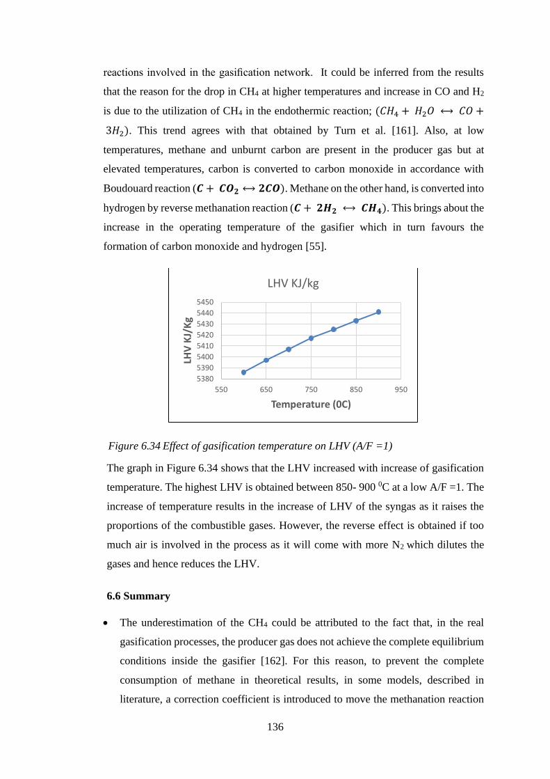
136
reactions involved in the gasification network. It could be inferred from the results
that the reason for the drop in CH4 at higher temperatures and increase in CO and H2
is due to the utilization of CH4 in the endothermic reaction; (𝐶𝐻4 + 𝐻2𝑂 ⟷ 𝐶𝑂 +
3𝐻2). This trend agrees with that obtained by Turn et al. [161]. Also, at low
temperatures, methane and unburnt carbon are present in the producer gas but at
elevated temperatures, carbon is converted to carbon monoxide in accordance with
Boudouard reaction (𝑪 + 𝑪𝑶𝟐 ⟷ 𝟐𝑪𝑶). Methane on the other hand, is converted into
hydrogen by reverse methanation reaction (𝑪 + 𝟐𝑯𝟐 ⟷ 𝑪𝑯𝟒). This brings about the
increase in the operating temperature of the gasifier which in turn favours the
formation of carbon monoxide and hydrogen [55].
Figure 6.34 Effect of gasification temperature on LHV (A/F =1)
The graph in Figure 6.34 shows that the LHV increased with increase of gasification
temperature. The highest LHV is obtained between 850- 900 0C at a low A/F =1. The
increase of temperature results in the increase of LHV of the syngas as it raises the
proportions of the combustible gases. However, the reverse effect is obtained if too
much air is involved in the process as it will come with more N2 which dilutes the
gases and hence reduces the LHV.
6.6 Summary
• The underestimation of the CH4 could be attributed to the fact that, in the real
gasification processes, the producer gas does not achieve the complete equilibrium
conditions inside the gasifier [162]. For this reason, to prevent the complete
consumption of methane in theoretical results, in some models, described in
literature, a correction coefficient is introduced to move the methanation reaction
5380
5390
5400
5410
5420
5430
5440
5450
550 650 750 850 950
LHV
KJ/
Kg
Temperature (0C)
LHV KJ/kg
137
to the CH4 production (avoiding its consumption). Other studies do not include a
fraction of CH4, formed during the pyrolysis process, in the combustion-
gasification stage bypassing it to the gasifier outlet [163].
• The reaction (C + 2H2 → CH4) is exothermic, which means that the temperature
increase results in the production of CH4 being decreased, leaving more H2 in the
gas.
• The reaction (CO2 + C → 2CO) is endothermic; therefore, the temperature
increases the amount of CO2 reacted with char to produce more CO.
• The reaction (C + H2O → H2 + CO) is endothermic, which means for increasing
temperature CO and H2 production are also increased and more char and H2O are
consumed.
• For the different biomass feeds considered the temperature at which the various
sections operate can be seen to have an effect. That said, the H2 and CH4 levels do
not vary significantly; as expected the main variation is in the CO2 and CO levels,
the latter tending to increase with temperature and the former decreasing. In a
model that is using an equilibrium approach for reactions it is inevitable that
endothermic reactions will be favoured as the temperature increases. This is
consistent with the observations made above.
• The variation of LHV is best summarised by reference to Figure 6.34 where it has
been observed that the LHV increase with temperature. This is consistent with the
observations made on the CO formation with increasing temperature but the
situation is obviously complicated by the impossibility of methane formation at the
higher temperatures but the general trend of LHV with temperature is consistent
with the observation made in the sense that overall, the quantity of combustible gas
has been increased.
138
Chapter 7 Conclusions and Recommendations
7.1 Conclusions
• The two types of the mathematical model for simulation of a biomass downdraft
gasifier and its operation was considered using different configurations, biomass
feedstock and operational conditions.
• The gasification of wood chips, wood pellets, rubber wood, Eucalyptus and oil
palm fronds were investigated. The gasification of these solid fuels was simulated
in a downdraft gasifier with pyrolysis, oxidation and reduction zones.
• Kinetic and thermodynamic equilibrium models (based on both stoichiometric and
non-stoichiometric methods) were implemented in order to predict various biomass
gasification product gases using air as the oxidizing agent in a downdraft gasifier.
These were implemented in MATLAB and ASPEN HYSYS. ASPEN HYSYS was
used since it was possible to consider biomass gasifier with two stages of air supply
(separately to pyrolysis and oxidation zones). MATLAB model in addition to
composition of product, predicts the temperature in the reduction zone, whilst this
temperature is an input in ASPEN HYSYS. Due to assumptions made, MATLAB
code provides more accurate predictions in performance of the gasifier. The
percentage error values calculated from the use of MATLAB codes are in a range
of 4 -12% for CO2, 3 -15% for H2, 2 -13% for CO, 1- 4% and 50- 64% CH4, while
the predictions from ASPEN HYSYS gives error values in the range of 6-26% for
CO2, 2 -30% for CO, 3 – 23% for H2, 2 – 16% N2 and 51-66% for methane.
• The thermodynamic equilibrium model was deployed using an Aspen HYSYS
software in which stoichiometry is not considered and various required specie’s
enthalpies and Gibbs Free Energies of formation are calculated automatically by
Aspen HYSYS.
• The kinetic model was deployed with Aspen HYSYS plug flow tubular reactor
(PFTR) model, the equilibrium constants and considering the dimensions of the
reactor.
• In MATLAB, this was implemented by solving differential equations of mass and
energy balances in gasifier zones, using some empirical assumptions and
equilibrium constants to obtain the PVT of the system and gas compositions.
139
• In the models presented in this work, operating conditions such as temperature,
equivalence ratio, moisture content and LHV were studied. The analysis show that
higher temperatures favoured the formation of CO and H2, while CH4 and CO2
reduce depending on the reaction that prevails.
• Moisture content in the biomass also affects the composition of the gases and the
energy content. Increasing MC reduces the temperature of the system and the
LHV, also the composition of H2 and CO2 increases, CH4 increases to a certain
extent while CO decreases.
• The proposed equilibrium model displayed a variable ability for the prediction of
various product yields with this being a function of the feedstock studied. It also
demonstrated the ability to predict product gases from various biomasses using
both single and double stage air input. In the case of gasification with double air
stage supply, higher amounts of methane are obtained with specific tendencies of
the gases reaching a peak at certain conditions.
• The total air quantity fed to the pyrolysis and combustion zones ranges from 16 –
22 Nm3/h at 80% of AR (runs C1-C5). The composition of gas components in the
exit, predicted by the developed model, is comparable to the experimental data
published by various authors. The simulations indicate that for each of the above
runs, there are certain conditions at which there is a peak achieved in formation of
each of the combustible gases.
• In the single stage air supply gasification, feed stocks such as rubber wood, wood
chips, wood pellets and palm fronds were used. Both thermodynamic and kinetic
models of gasification have been deployed as written codes in MATLAB and
simulations in Aspen HYSYS. The numerical results have been validated and they
reasonably compare with the published experimental data
• The double stage air supply gasification model seemed to produce more CH4. The
kinetic model can only produce CH4 at very low temperatures. In the equilibrium
model, lesser amounts of CH4 were obtained but at higher temperatures than the
kinetic model.
• There were two vital components of the kinetic modelling of biomass reactors in
this work. To incorporate the kinetics into the HYSYS simulation it was necessary
to introduce a unit operation that incorporated reaction kinetics. This work used a
Plug Flow Reactor (PFR). This required some investigation into the length of such
140
a reactor and necessary adjustment to fit in with the results obtained. Secondly, a
presentation of the modelling chemical equations was required that could
realistically represent all the known products. Four equations were used, and it was
necessary to have Rate Constants and Arrhenius equations for each reaction and to
transform these data into a form useable by HYSYS. Once this was achieved the
Reduction Section of the Gasifier could be represented by a PFR.
• The kinetic model achieved some success in that it did predict results comparable
with experimentally published results for a range of conditions. There were
discrepancies particularly with CH4 formation and the operating temperatures
required to produce results comparable with experimental values were usually
consistently lower than those actually used experimentally. The use of the PFR,
however, did show promise for the use in further modelling.
• The weakness of the kinetic approach is its need for reliable kinetic data. Unlike
thermodynamics kinetic data have to be measured and there is a shortage of reliable
measured data for relevant reactions that could be used to simulate/model
gasification reactions.
7.2 Recommendations
• Further experimental work needs to be carried out for both single and double stage
air supply gasification using various biomass feedstock as this provides extended
opportunities for detailed testing and validation of the developed mathematical
models of the biomass gasifiers.
• Accurate measurements of the chemical composition of the producer gas,
generated by the biomass gasifier, using modern technological facilities and of
other operating parameters, such as temperatures, velocities and pressures, inside
the gasifier are necessary for improvement of the developed mathematical models
of biomass gasifiers.
• Computational Fluid Dynamics methods could be further applied for modelling of
operation of biomass gasifiers to obtain additional information on flow and heat
transfer inside the biomass gasifiers.
• Further detailed kinetic data is required for the kinetic model that incorporates
PFR.
141
• Dynamic neural network-based model for gasification is a type of dynamic
modelling that can help curb the issues related to gasification process efficiency
that partly prevents biomass gasification technology to become more economically
viable. The deployment of Neural network model has the potential to predict
process parameters during plant operation with variable operating conditions. • The “superficial vel ocity” ( hearth load) of a gasi fier is the m ost important measure of its
• performance, contr olling gas pr oducti on rate, gas energy content, fuel consum pti on rate,
• pow er output, and char and tar pr oduc tion rate
• Effect of flow conditions such as SV should also be considered to measure the
performance controlling the gas production rate and the rate at which air as well as
gas passes through the gasifier. This will consequently exercise a primary effect of
heat transfer around each particle during flaming pyrolysis of the volatiles,
combustion of the of the tars and gasification of the charcoal.
142
REFERENCES
1. Kumar, A., D.D. Jones, and M.A. Hanna, Thermochemical Biomass Gasification: A Review of the Current Status of the Technology. Energies, 2009. 2(3): p. 556-581.
2. Malik, A. and S.K. Mohapatra, Biomass-based gasifiers for internal combustion (IC) engines-A review. Sadhana-Academy Proceedings in Engineering Sciences, 2013. 38(3): p. 461-476.
3. Baruah, D. and D. Baruah, Modeling of biomass gasification: a review. Renewable and Sustainable Energy Reviews, 2014. 39: p. 806-815.
4. Bridgwater, A.V., Renewable fuels and chemicals by thermal processing of biomass. Chemical Engineering Journal, 2003. 91(2-3): p. 87-102.
5. Felipe Centeno, K.M., Electo E. Silva Lora, Rubenildo V. Andrade, Theroretical and experimental investigations of a downdraft biomass gasiifer -spark ignition engine power system. 2012.
6. Basu, P., Biomass Gasification and Pyrolysis Practical design and Theory. 2010, Elsevier Inc.: 30 Corporate Drive, Suite 400 Burlington, MA 01803, USA.
7. Young-Il Son, S.J.Y., Yong Ku Kim, Jae-Goo Lee, , Gasification and power generation characteristics of woody biomass utilizing a downdraft gasifier, Biomass and Bioenergy. 2011. 35(10, ): p. 4215-4220.
8. Barrio, M., Experimental investigation of small-scale gasification of woody biomass. PhD thesis , Faculty of Engineering Science and Technology, Department of Thermal Energy and Hydro Power, The Norwegian University of Science and Technology 2002: p. 204-232.
9. Pieratti, E., Biomass gasification in small scale plants: experimental and modelling analysis. 2011, University of Trento.
10. Programme, U.N.E., Technologies for converting waste Agricultural Biomass to Energy. 2013, International Environment Technology Centre: Osaka Japan.
11. Arvind, K.A., Biomass as Fuel in Small Boilers. 2009, Asian Productivity Organisation: Tokyo, Japan. p. 4-52.
12. Mohammad, M.N.B., P., Photosynthesis: How and Why? Advances in Photosynthesis- Fundamental Aspects, ed. M.N.B. Mohammad, P. Vol. 9. 2012, China: Intech. 598.
13. Agbontalor, E.A., Overview of various biomass Energy Conversion routes. American -Eurasian Journal, 2007. 6(2): p. 662-671.
14. Twidell, J., Biomass energy. Renewable Energy World, 1998. 1(3): p. 38-39. 15. Report, G.S., Renewables 2016 Global Status Report. 2016. p. 272. 16. Hull, S., Wisconsin sustainable planting and harvest guidelines for nonforest biomass. 2011:
Wisconsin Department of Agriculture, Trade, and Consumer Protection. 17. Comission, E.-E. Biomass Green Energy for Europe. 2005. 18. (PI), J.S.T., Biomass Engineering: Size reduction, drying and densification. Bioenergy
Technologies Office, 2015.
19. Zafar, S., Waste to Energy Conversion Routes. Bioenergy Consult, 2016. 20. Tran, K.-Q., et al., Stump torrefaction for bioenergy application. Applied energy, 2013. 112: p.
539-546. 21. Van Essendelft, D., X. Zhou, and B.-J. Kang, Grindability determination of torrefied biomass
materials using the Hybrid Work Index. Fuel, 2013. 105: p. 103-111. 22. Chen, W.-H., J. Peng, and X.T. Bi, A state-of-the-art review of biomass torrefaction,
densification and applications. Renewable and Sustainable Energy Reviews, 2015. 44: p. 847-866.
23. Rousset, P., et al., Enhancing the combustible properties of bamboo by torrefaction. Bioresource Technology, 2011. 102(17): p. 8225-8231.
143
24. Antonopoulos, I.S., et al., Modelling of a downdraft gasifier fed by agricultural residues. Waste Management, 2012. 32(4): p. 710-718.
25. Puig-Arnavat, M., J.C. Bruno, and A. Coronas, Review and analysis of biomass gasification models. Renewable & Sustainable Energy Reviews, 2010. 14(9): p. 2841-2851.
26. Giltrap, D.L., R. McKibbin, and G.R.G. Barnes, A steady state model of gas-char reactions in a downdraft biomass gasifier. Solar Energy, 2003. 74(1): p. 85-91.
27. X. Li, J.R.G., A.P. Watkinson, C.J. Lim, A. ErguÈdenler, Equilibrium modelling of gasification: a free energy minimizaion approach and its application to a circulating fluidized bed coal gasifier. 2000: p. 197 -207.
28. Baxter, M.J., Downdraft gasification of biomass. PhD thesis , Birmingham, UK: Aston University, 1994.
29. M. A. Chawdhurya, K.M., Development of a Small Downdraft Biomass Gasifier for Developing Countries. 2011. 3(1): p. 51-64.
30. Samy, S., P. E Pyrolysis. 25. 31. K., Y.C.M., Thermal Conversion of Biomass, Pyrolysis and Gasification: A Review. The
International Journal of Engineering And Science (IJES), 2013. 2(3): p. 11. 32. Sinha, S., et al., Modelling of pyrolysis in wood: a review. SESI Journal, 2000. 10(1): p. 41-62. 33. Lysenko, S., S. Sadaka, and R.C. Brown, Comparison of the cost of hydrogen from air‐blown
and thermally ballasted gasifiers. Biofuels, Bioproducts and Biorefining, 2012. 6(6): p. 673-685.
34. Soltes, E.J., T. Elder, and I. Goldstein, Organic Chemicals from Biomass. 1981, CRC Press, Pyrolysis.
35. Molino, A., S. Chianese, and D. Musmarra, Biomass gasification technology: The state of the art overview. Journal of Energy Chemistry, 2016. 25(1): p. 10-25.
36. Nuno Coutoa, A.R., Valter Silvaa, Eliseu Monteiro*b, Khalid Bouziane, Influence of the biomass gasification processes on the final. elsevier, 2013(36 ): p. 596 – 606.
37. Rauch, H.B.R., Review of applications of gases from biomass gasification, in Syngas production and utilisation” in the Handbook Biomass Gasification. 2006: The Netherlands JUNE.
38. Knoef, H. and J. Ahrenfeldt, Handbook biomass gasification. 2005: BTG biomass technology group The Netherlands.
39. Henham, A. and M. Makkar, Combustion of simulated biogas in a dual-fuel diesel engine. Energy Conversion and Management, 1998. 39(16-18): p. 2001-2009.
40. Monteiro, E., et al., Syngas application to spark ignition engine working simulations by use of rapid compression machine. Internal Combustion Engines, 2012: p. 51-74.
41. Krigmont, H.V., Integrated biomass gasification combined cycle (IBGCC) power generation concept: The gateway to a clearer future. A White Paper, Allied Environmental Technologies, 1999.
42. Szewczyk, M. and T. Trzepieciński, Application of biomass-powered Stirling engines in cogenerative systems. ECONTECHMOD: An International Quarterly Journal on Economics of Technology and Modelling Processes, 2012. 1: p. 53-56.
43. Paper, F.F., Wood gas as fuel engine. 1986, FAO Forestry Department Rome Italy. p. 139. 44. Hagen, C.Y.W.B.E.B., Biomass Conversion and Technology. Vol. m 1996, Baffins Lane,
Chichester West Sussex PO 19 UD, England: John Wiley and Sons 203.
45. S.A Channiwala, P.P.P., A unified correlation for estmating HHV of solid, liquid and gaseous fuels. elsevier, 2001. 81: p. 1051-1063.
46. Selvig, W.A., Gibson, F. H., Calorific of coal, in Chemistry of coal utilization. J. Wiley and Sons: New York.
47. Jenkins, B. and J. Ebeling, Correlation of physical and chemical properties of terrestrial biomass with conversion. 1985.
144
48. Niessen, W.R., Combustion and incineration processes: applications in environmental engineering. 2010: CRC Press.
49. Graboski, M. and R. Bain, Properties of biomass relevant to gasification [Fuel gas production]. Biomass gasification; Principles and technology (USA), 1981.
50. Atnaw, S.M., S.A. Sulaiman, and S. Yusup, Influence of fuel moisture content and reactor temperature on the calorific value of syngas resulted from gasification of oil palm fronds. The Scientific World Journal, 2014. 2014.
51. Bhattacharya, S., D. Albina, and A.M. Khaing, Effects of selected parameters on performance and emission of biomass-fired cookstoves. Biomass and Bioenergy, 2002. 23(5): p. 387-395.
52. J.K Ratnadhariya, S.A.C., Three zone equillibrium and kinetic free modelling of biomass gasifier- a novel approach. Renewable & Sustainable Energy Reviews, 2009: p. 1050-1058.
53. Kaupp, A., and Goss, J. R.,, State of the Art for small Scale (to 50 kW) Gas Producer-Engine Systems,, in First International Producer Gas Conference. March 1981, , U.S.D.A., Forest Service: Colombo, Sri Lanka, .
54. Madhukar R. Mahishi, D.Y.G., Thermodynamic optimization of biomass gasifier for hydrogen production. International Journal of Hydrogen Energy, 2007. 32(16): p. 3831–3840.
55. Zainal, Z.A., et al., Experimental investigation of a downdraft biomass gasifier. Biomass & Bioenergy, 2002. 23(4): p. 283-289.
56. A.M, S., Operating and Performance Gasfication Process Parameters International Journal of Science and Research(IJSR), 2013: p. 1-8.
57. Roy, P.C., A. Datta, and N. Chakraborty, Modelling of a downdraft biomass gasifier with finite rate kinetics in the reduction zone. International Journal of Energy Research, 2009. 33(9): p. 833-851.
58. Melgar, A., Perez, J. F., Laget, H., Horillo, A., Thermodynamic equilibrium modelling of a gasifying process. energy Conversion and Management, 2007. 1(48): p. 59-67.
59. Ian Narva´ ez, A.O.o., † Maria P. Aznar,‡ and Jose´ Corella, Biomass Gasification with Air in an Atmospheric Bubbling. 1996. 35: p. 2110-2120.
60. Ajay Kumara, b., Kent Eskridgec, David D. Jonesb, Milford A. Hanna, Steam–air fluidized bed gasification of distillers grains: Effects of steam to biomass ratio, equivalence ratio and gasification temperatureFluidized Bed. Effect of Six Operational Variables on the Quality of. elsevier, 2009. 100(6): p. 2062-2068.
61. T. B. Reed., R.W., S. Ellis, A. Das, and S. Deutche,, Superficial velocity - the key to downdraft gasification, in 4th Biomass conference of the Americas, Oakland. 1999: Oakland, California, USA,.
62. Takashi Yamazaki, † Hirokazu Kozu,† Sadamu Yamagata,† Naoto Murao,† and S.S. Sachio Ohta, ‡ and Tatsuo Ohba‡, Effect of Superficial Velocity on Tar from Downdraft Gasification of Biomass. Energy and Fuel, 2005. 19: p. 1186-1191.
63. M. Siedlecki, W.d.J., Biomass gasification as the first hot step in clean syngas production process – gas quality optimization and primary tar reduction measures in a 100 kW thermal input steam–oxygen blown CFB gasifier. Biomass and Bioenergy, 2011. 35(supplement 1): p. 540 -562.
64. Meng, X.M., et al., Biomass gasification in a 100 kWth steam-oxygen blown circulating fluidized bed gasifier: Effects of operational conditions on product gas distribution and tar formation. Biomass & Bioenergy, 2011. 35(7): p. 2910-2924.
65. Fabry, F., et al., Waste gasification by thermal plasma: a review. Waste and Biomass Valorization, 2013. 4(3): p. 421-439.
66. Lettner, F., H. Timmerer, and P. Haselbacher, Biomass gasification–State of the art description. Intelligent Energy Europe, Austria, 2007.
67. Warnecke, R., Gasification of biomass: comparison of fixed bed and fluidized bed gasifier. Biomass and Bioenergy, 2000. 18(6): p. 489-497.
145
68. Held, J., Gasification–Status and technology. Swedish Gas Centre, 2012. 69. Juan Daniel Martínez, E.E.S.L., Rubenildo Viera Andrade, René Lesme Jaén, Experimental
study on biomass gasification in a double air stage downdraft reactor. Biomass and Bioenergy, 2011. 35(8): p. 3465-3480.
70. Juan Daniel Martinez, K.M., Rubenildo V. Andrade, Electo E. Silva Lora, Syngas production in downdraft biomass gasifiers and its application using internal combustion engines. Renewable Energy, 2012. 38(1): p. 1-9.
71. Abedin, M.R. and H.S. Das, Electricity from rice husk: a potential way to electrify rural Bangladesh. International Journal of Renewable Energy Research (IJRER), 2014. 4(3): p. 604-609.
72. Bhattacharya, S.C., S.S. Hla, and H.L. Pham, A study on a multi-stage hybrid gasifier-engine system. Biomass & Bioenergy, 2001. 21(6): p. 445-460.
73. Das, T.B.R.a.A., Handbook of Biomass Downdraft Gasifier Engine Systems. 1998. 74. Sastry, A.B.a.R.C., Biomass Gasification Processes in Downdraft Fixed Bed. International
Journal of Chemical Engineering and Applications, 2011. 2. 75. Hofbauer, H., et al., Biomass CHP Plant Güssing; Vortrag Pyrolysis and Gasification Expert
Meeting, Strassburg, France; 31.10. 2002. Proceedings of Pyrolysis and Gasification ExpertMeeting, 2002.
76. Bühler, R. and P. Hasler, Stand und Entwicklung der Vergasungstechnik. VDI BERICHTE, 1997. 1319: p. 81-108.
77. Sikarwar, V.S., et al., An overview of advances in biomass gasification. Energy & Environmental Science, 2016. 9(10): p. 2939-2977.
78. Gomez-Barea, A. and B. Leckner, Modeling of biomass gasification in fluidized bed. Progress in Energy and Combustion Science, 2010. 36(4): p. 444-509.
79. Gräbner, M., S. Ogriseck, and B. Meyer, Numerical simulation of coal gasification at circulating fluidised bed conditions. Fuel Processing Technology, 2007. 88(10): p. 948-958.
80. Basu, P., Biomass gasification and pyrolysis: practical design and theory. 2010: Academic press.
81. M. Baratieri P. Baggio, L.F., M. Grigiante, Biomass as an energy source: Thermodynamic constraints on the performance of the conversion process. 2008. 99(15): p. 3831–3840.
82. Plus, A., Aspen Technology Inc. Cambridge, MA, USA, 2006. 83. Patra, T.K. and P.N. Sheth, Biomass gasification models for downdraft gasifier: A state-of-
the-art review. Renewable and Sustainable Energy Reviews, 2015. 50: p. 583-593. 84. Ramzan, N., et al., Simulation of hybrid biomass gasification using Aspen plus: A comparative
performance analysis for food, municipal solid and poultry waste. Biomass and Bioenergy, 2011. 35(9): p. 3962-3969.
85. Phillips, J.N., Study of the off-design performance of integrated coal gasification combined-cycle power plants. 1986, Stanford Univ., CA (USA).
86. Xiangdong, K., et al., Three stage equilibrium model for coal gasification in entrained flow gasifiers based on aspen plus. Chinese Journal of Chemical Engineering, 2013. 21(1): p. 79-84.
87. Baggio, P., et al., Experimental and modeling analysis of a batch gasification/pyrolysis reactor. Energy Conversion and Management, 2009. 50(6): p. 1426-1435.
88. Mansaray, K., et al., Mathematical modeling of a fluidized bed rice husk gasifier: Part I-Model development. Energy sources, 2000. 22(1): p. 83-98.
89. Mathieu, P. and R. Dubuisson, Performance analysis of a biomass gasifier. Energy conversion and management, 2002. 43(9): p. 1291-1299.
90. Kuo, P.-C., W. Wu, and W.-H. Chen, Gasification performances of raw and torrefied biomass in a downdraft fixed bed gasifier using thermodynamic analysis. Fuel, 2014. 117: p. 1231-1241.
146
91. Paviet, F., F. Chazarenc, and M. Tazerout, Thermo chemical equilibrium modelling of a biomass gasifying process using ASPEN PLUS. International Journal of chemical reactor engineering, 2009. 7(1).
92. Joshi, R.R. and B. Kulkarni, Simulation of biomass gasification reactor for fuel in gas turbine. International Journal of Chemical Sciences and Applications, 2012. 3(1): p. 232-240.
93. Chowdhury, R., P. Bhattacharya, and M. Chakravarty, Modelling and simulation of a downdraft rice husk gasifier. International Journal of Energy Research, 1994. 18(6): p. 581-594.
94. Tigabwa Y. Ahmed, M.M.A., Suzana Yusup, Abrar Inayat, Zakir Khan, Mathematematical and computational approaches for design of biomass gasification for hydrogen production: A Review. Renewable & Sustainable Energy Reviews, 2012. 16
95. E, S., Catalytic steam gasification of biomass surrogates: a thermodynamic and kinetic
approach. Chem Biochem Eng. London, Ontario, Canada: university of Western Ontario, 2010: p. 266.
96. wang, Y.K.C.M., Kinetic model of biomass gasification. Solar Energy, 1993. 51(1): p. 19-25. 97. Chee, C.S., The air gasification of wood chips in a downdraft gasifier. 1987. 98. Senelwa, K.A., Air gasification of woody biomass from short rotation forests: opportunities
for small scale biomass-electricity systems: a thesis submitted in partial fulfilment of the requirements for the degree of Doctor of Philosophy in Agricultural Engineering at Massey University, New Zealand. 1997, Massey University.
99. Babu, B.V. and P.N. Sheth, Modeling and simulation of reduction zone of downdraft biomass gasifier: Effect of char reactivity factor. Energy Conversion and Management, 2006. 47(15-16): p. 2602-2611.
100. Di Blasi, C., Modeling wood gasification in a countercurrent fixed‐bed reactor. AIChE Journal, 2004. 50(9): p. 2306-2319.
101. Di Blasi, C. and C. Branca, Modeling a stratified downdraft wood gasifier with primary and secondary air entry. Fuel, 2013. 104: p. 847-860.
102. Horton, S.R., et al., Molecular-level kinetic modeling of biomass gasification. Energy & Fuels, 2015. 30(3): p. 1647-1661.
103. Saravanakumar, A., et al., Numerical modelling of a fixed bed updraft long stick wood gasifier. biomass and bioenergy, 2011. 35(10): p. 4248-4260.
104. Gordillo, E. and A. Belghit, A downdraft high temperature steam-only solar gasifier of biomass char: a modelling study. Biomass and bioenergy, 2011. 35(5): p. 2034-2043.
105. Inayat, A., et al., Process modeling for parametric study on oil palm empty fruit bunch steam gasification for hydrogen production. Fuel processing technology, 2012. 93(1): p. 26-34.
106. Smith, J.D., et al., Validation and Application of a Kinetic Model for Downdraft Biomass Gasification Simulation. Chemical Engineering & Technology, 2019. 42(12): p. 2505-2519.
107. S. jarungthammachote, A.D., Equilibrium modeling of gasification : Gibbs free enegy minimization approach and its application to stouted bed and spout-fluid bed gasifiers. 2008. 49: p. 1345 -1356.
108. WC, R., The element potentials method for chemical equilibrium analysis : implementation in the interactive programme STANJAN, in Department of mechanical Engineering, Stanford University. 1986.
109. Altafini, C.R., Mirandola A.A, Equilbrium model of coal gasification process based on minimization of Gibbs free energy. 1997: In: Flowers 97, Floreence, Italy.
110. Tapas, k.P., Patrik, N. S., Biomass gasification models for downdraft gasifier: A- state- of- the- art review. Renewable and Sustainable Energy Reviews, 2015. 50: p. 583-593.
111. Chern, S.-M.W., Walawender, WP., Fan, LT., Equilibrium modelling of a downdraft gasifier i- overall gasifier . Chemical Engineering Community, 1991. 108: p. 243-265.
147
112. Zainal, Z.A., et al., Prediction of performance of a downdraft gasifier using equilibrium modeling for different biomass materials. Energy Conversion and Management, 2001. 42(12): p. 1499-1515.
113. S. Jarunthammachote, A.D., Thermodynamic equilibrium model and second law analysis of a downdraft waste gasifier. science direct, 2007. 32: p. 1660-1669.
114. Jayah, T.H., Aye, L., Fuller, R. J., Stewart, D. F, Computer simulation of a downdarft gasifier for tea drying International technology centre, 2003. 3: p. 11.
115. Jarunthammachote, S., Dutta, A., Equilibrium modeling of gasification : Gibbs free energy minimisation approach and its application to spouted bed and spout-fluid bed gasifiers. Energy conversion and management, 2008. 49: p. 1345-1356.
116. Vaezi, M., M. Passandideh Fard, and M. Moghiman. Modeling Biomass Gasification: A New Approach to UtilizeRenewable Sources of Energy. in The 2008 ASME International Mechanical Engineering Congress and Exposition. 2008.
117. Ratnadhariya, J.K. and S.A. Channiwala, Three zone equilibrium and kinetic free modeling of biomass gasifier – a novel approach. Renewable Energy, 2009. 34(4): p. 1050-1058.
118. Sharma, A.K., Equilibrium and kinetic modeling of char reduction reactions in a downdraft biomass gasifier: A comparison. Solar Energy, 2008. 82(10): p. 918-928.
119. Antolini, D., et al., Experimental and modeling analysis of Air and CO2 biomass gasification in a reverse lab scale downdraft gasifier. Energy Procedia, 2019. 158: p. 1182-1187.
120. Pepiot, P., C. Dibble, and T. Foust, Computational fluid dynamics modeling of biomass gasification and pyrolysis. Computational modeling in lignocellulosic biofuel production, 2010: p. 273-298.
121. Janajreh, I. and M. Al Shrah, Numerical and experimental investigation of downdraft gasification of wood chips. Energy Conversion and Management, 2013. 65: p. 783-792.
122. Rogel, A. and J. Aguillon, The 2D Eulerian approach of entrained flow and temperature in a biomass stratified downdraft gasifier. American Journal of Applied Sciences, 2006. 3(10): p. 2068-2075.
123. Gao, J., et al., Experiments and numerical simulation of sawdust gasification in an air cyclone gasifier. Chemical engineering journal, 2012. 213: p. 97-103.
124. Dogru, M., et al., Gasification of hazelnut shells in a downdraft gasifier. Energy, 2002. 27(5): p. 415-427.
125. Pacelli, V. and M. Azzollini, An artificial neural network approach for credit risk management. Journal of Intelligent Learning Systems and Applications, 2011. 3(02): p. 103.
126. Brown, D., T. Fuchino, and F. Maréchal, Solid fuel decomposition modelling for the design of biomass gasification systems. Computer Aided Chemical Engineering, 2006. 21: p. 1661-1666.
127. Gu, J., et al., Differences in gasification behaviors and related properties between entrained gasifier fly ash and coal char. Energy & Fuels, 2008. 22(6): p. 4029-4033.
128. S. jarungthammachote, A.D., Thermodynamic equilibrium and second law analysis of a downdraft waste gasifier. Science Direct, 2007. 32: p. 1660 - 1669.
129. Shabbar Syed, I.J., Chauki Ghenai, Thermodynmics Equillibrium Analysis within the Entrained Flow Gasifier Enviroment. 2012. 4(1): p. 47-54.
130. Perry, R.H., D. Green, and J. Maloney, Chemical Engineers Handbook. 6th. 1997, New York: McGraw-Hill.
131. Koroneos, C. and S. Lykidou, Equilibrium modeling for a dwndraft biomass gasifier for cotton stalks biomass in comparison with experimental data. Journal of Chemical Engineering and Materials Science, 2011. 2(4): p. 61-68.
132. Gao, N., et al., Hydrogen-rich gas production from biomass steam gasification in an updraft fixed-bed gasifier combined with a porous ceramic reformer. International Journal of Hydrogen Energy, 2008. 33(20): p. 5430-5438.
148
133. Dejtrakulwong, C. and S. Patumsawad, Four zones modeling of the downdraft biomass gasification process: effects of moisture content and air to fuel ratio. Energy Procedia, 2014. 52: p. 142-149.
134. Centeno, F., et al., Theoretical and experimental investigations of a downdraft biomass gasifier-spark ignition engine power system. Renewable Energy, 2012. 37(1): p. 97-108.
135. Li, X., et al., Equilibrium modeling of gasification: a free energy minimization approach and its application to a circulating fluidized bed coal gasifier. Fuel, 2001. 80(2): p. 195-207.
136. Koukkari, P. and R. Pajarre, Calculation of constrained equilibria by Gibbs energy minimization. Calphad, 2006. 30(1): p. 18-26.
137. Jarungthammachote, S. and A. Dutta, Equilibrium modeling of gasification: Gibbs free energy minimization approach and its application to spouted bed and spout-fluid bed gasifiers. Energy Conversion and Management, 2008. 49(6): p. 1345-1356.
138. people.clarkson.edu/~wwilcox/Design/HYSYSpropSelect.pdf. A property methods and calculation.
139. Proust, P. and J. Vera, PRSV: The stryjek‐vera modification of the peng‐robinson equation of state. Parameters for other pure compounds of industrial interest. The Canadian Journal of Chemical Engineering, 1989. 67(1): p. 170-173.
140. Bassyouni, M., et al., Date palm waste gasification in downdraft gasifier and simulation using ASPEN HYSYS. Energy conversión and management, 2014. 88: p. 693-699.
141. Žecová, M. and J. Terpák, Mathematical Modeling of Gasification and Combustion of Biomass in Matlab. 2010.
142. Nikoo, M.B. and N. Mahinpey, Simulation of biomass gasification in fluidized bed reactor using ASPEN PLUS. Biomass and Bioenergy, 2008. 32(12): p. 1245-1254.
143. Telmo, C. and J. Lousada, Heating values of wood pellets from different species. Biomass and bioenergy, 2011. 35(7): p. 2634-2639.
144. Rockwood, D.L., et al., Energy product options for Eucalyptus species grown as short rotation woody crops. International journal of molecular sciences, 2008. 9(8): p. 1361-1378.
145. Krukanont, P. and S. Prasertsan, Geographical distribution of biomass and potential sites of rubber wood fired power plants in Southern Thailand. Biomass and bioenergy, 2004. 26(1): p. 47-59.
146. Shuit, S.H., et al., Oil palm biomass as a sustainable energy source: A Malaysian case study. Energy, 2009. 34(9): p. 1225-1235.
147. Doherty, W., A. Reynolds, and D. Kennedy, The effect of air preheating in a biomass CFB gasifier using ASPEN Plus simulation. Biomass and bioenergy, 2009. 33(9): p. 1158-1167.
148. Sulaiman, S., et al., Feasibility study of gasification of oil palm fronds SA Sulaiman1, S. Balamohan2, MNZ Moni1, SM Atnaw3 and AO Mohamed4.
149. Dr. Matthew J. Traum, M.S.o.E., An Inexpensive Inverted Downdraft Biomass Gasifier for Experimental Energy-
Thermal-Fluids Demonstrations, in ASEE Annual Conference & Expositition. 2013, American Society for Engineering Education: Atlanta. p. 16.
150. Bacon, D., et al., Modelling of fluidized bed wood gasifiers, in Fundamentals of thermochemical biomass conversion. 1985, Springer. p. 717-732.
151. K. Manish., P.B., Y, Singh, Effect of Moisture Content and Equivalence Ratio on the Gasification Process for Different Biomass Fuel. International Journal of mechanical Engineering and Technology(IJMET), 2016. 7(6): p. 209-220.
152. Gunarathne, D., et al., The Effect of Throat Diameter on the Performance a Downdraft Biomass Gasifier. International Journal of Energy Engineering, 2013. 3(3): p. 171-175.
153. Jarungthammachote, S. and A. Dutta, Thermodynamic equilibrium model and second law analysis of a downdraft waste gasifier. Energy, 2007. 32(9): p. 1660-1669.
154. Kumar, A., D. Jones, and M. Hanna, Thermochemical biomass gasification: a review of the current status of the technology. Energies, 2009. 2(3): p. 556-581.
149
155. Lv, P., et al., An experimental study on biomass air–steam gasification in a fluidized bed. Bioresource technology, 2004. 95(1): p. 95-101.
156. Werther, J., et al., Combustion of agricultural residues. Progress in energy and combustion science, 2000. 26(1): p. 1-27.
157. Sheth, P.N. and B. Babu, Experimental studies on producer gas generation from wood waste in a downdraft biomass gasifier. Bioresource Technology, 2009. 100(12): p. 3127-3133.
158. Hanping, C., et al., Experimental investigation of biomass gasification in a fluidized bed reactor. Energy & Fuels, 2008. 22(5): p. 3493-3498.
159. Sun, K., Optimization of biomass gasification reactor using Aspen Plus. 2015, Høgskolen i Telemark.
160. Mahishi, M.R. and D. Goswami, Thermodynamic optimization of biomass gasifier for hydrogen production. International Journal of Hydrogen Energy, 2007. 32(16): p. 3831-3840.
161. Turn, S., et al., An experimental investigation of hydrogen production from biomass gasification. International journal of hydrogen energy, 1998. 23(8): p. 641-648.
162. Institute, E.a.R., Application of Biomass gasifier technology for thermal application in food processing unit in India. 2010, GNESD Energy Access Knowledge Base: India.
163. Shafizadeh, F., Introduction to pyrolysis of biomass. Journal of Analytical and Applied Pyrolysis, 1982. 3(4): p. 283-305.
164. P.M. Lv, Z.H.X., J. Chang, C.Z. Wu, Y. Chen, J.X. Zhu, An experimental study on biomass air–steam gasification. elsevier, 2004. 95: p. 95-101.
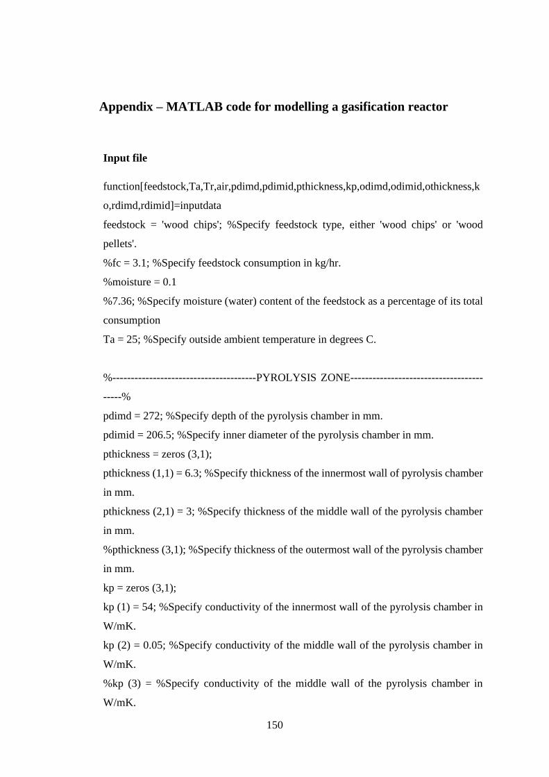
150
Appendix – MATLAB code for modelling a gasification reactor
Input file
function[feedstock,Ta,Tr,air,pdimd,pdimid,pthickness,kp,odimd,odimid,othickness,k
o,rdimd,rdimid]=inputdata
feedstock = 'wood chips'; %Specify feedstock type, either 'wood chips' or 'wood
pellets'.
%fc = 3.1; %Specify feedstock consumption in kg/hr.
%moisture = 0.1
%7.36; %Specify moisture (water) content of the feedstock as a percentage of its total
consumption
Ta = 25; %Specify outside ambient temperature in degrees C.
%---------------------------------------PYROLYSIS ZONE------------------------------------
-----%
pdimd = 272; %Specify depth of the pyrolysis chamber in mm.
pdimid = 206.5; %Specify inner diameter of the pyrolysis chamber in mm.
pthickness = zeros (3,1);
pthickness (1,1) = 6.3; %Specify thickness of the innermost wall of pyrolysis chamber
in mm.
pthickness (2,1) = 3; %Specify thickness of the middle wall of the pyrolysis chamber
in mm.
%pthickness (3,1); %Specify thickness of the outermost wall of the pyrolysis chamber
in mm.
kp = zeros (3,1);
kp (1) = 54; %Specify conductivity of the innermost wall of the pyrolysis chamber in
W/mK.
kp (2) = 0.05; %Specify conductivity of the middle wall of the pyrolysis chamber in
W/mK.
%kp (3) = %Specify conductivity of the middle wall of the pyrolysis chamber in
W/mK.
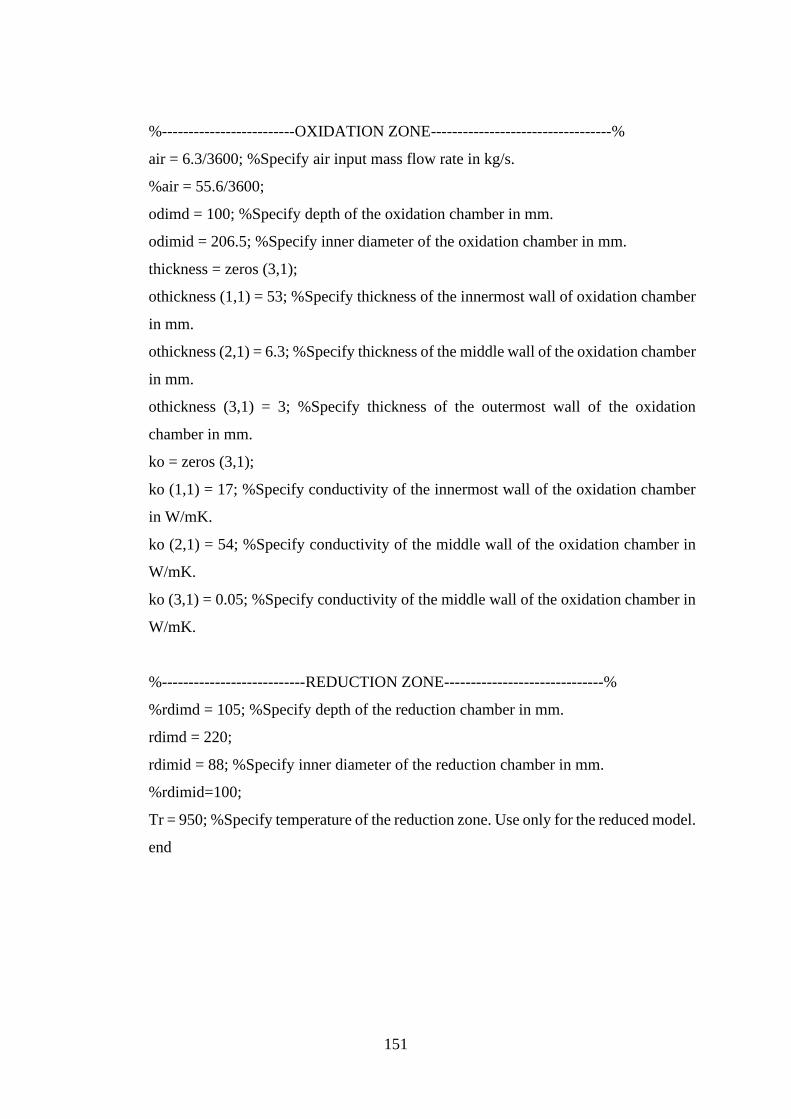
151
%-------------------------OXIDATION ZONE----------------------------------%
air = 6.3/3600; %Specify air input mass flow rate in kg/s.
%air = 55.6/3600;
odimd = 100; %Specify depth of the oxidation chamber in mm.
odimid = 206.5; %Specify inner diameter of the oxidation chamber in mm.
thickness = zeros (3,1);
othickness (1,1) = 53; %Specify thickness of the innermost wall of oxidation chamber
in mm.
othickness (2,1) = 6.3; %Specify thickness of the middle wall of the oxidation chamber
in mm.
othickness (3,1) = 3; %Specify thickness of the outermost wall of the oxidation
chamber in mm.
ko = zeros (3,1);
ko (1,1) = 17; %Specify conductivity of the innermost wall of the oxidation chamber
in W/mK.
ko (2,1) = 54; %Specify conductivity of the middle wall of the oxidation chamber in
W/mK.
ko (3,1) = 0.05; %Specify conductivity of the middle wall of the oxidation chamber in
W/mK.
%---------------------------REDUCTION ZONE------------------------------%
%rdimd = 105; %Specify depth of the reduction chamber in mm.
rdimd = 220;
rdimid = 88; %Specify inner diameter of the reduction chamber in mm.
%rdimid=100;
Tr = 950; %Specify temperature of the reduction zone. Use only for the reduced model.
end
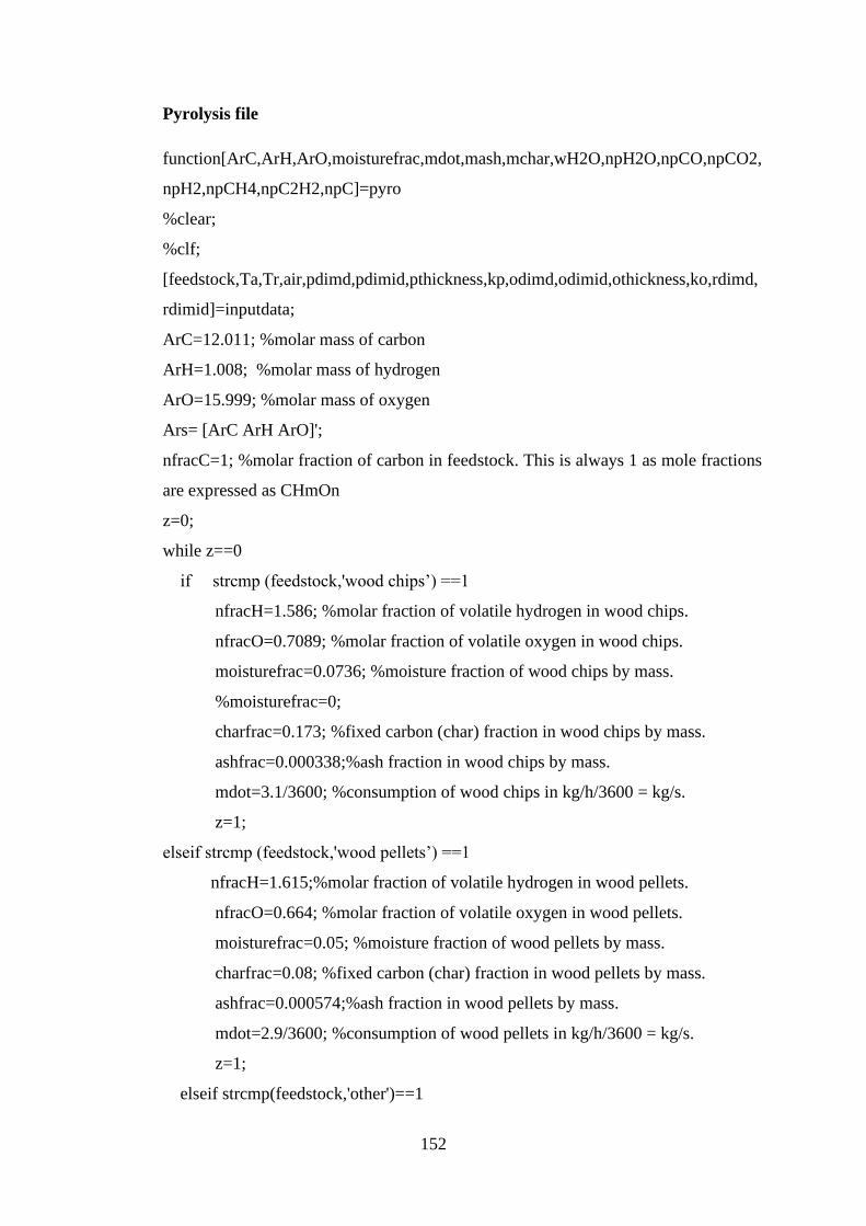
152
Pyrolysis file
function[ArC,ArH,ArO,moisturefrac,mdot,mash,mchar,wH2O,npH2O,npCO,npCO2,
npH2,npCH4,npC2H2,npC]=pyro
%clear;
%clf;
[feedstock,Ta,Tr,air,pdimd,pdimid,pthickness,kp,odimd,odimid,othickness,ko,rdimd,
rdimid]=inputdata;
ArC=12.011; %molar mass of carbon
ArH=1.008; %molar mass of hydrogen
ArO=15.999; %molar mass of oxygen
Ars= [ArC ArH ArO]';
nfracC=1; %molar fraction of carbon in feedstock. This is always 1 as mole fractions
are expressed as CHmOn
z=0;
while z==0
if strcmp (feedstock,'wood chips’) ==1
nfracH=1.586; %molar fraction of volatile hydrogen in wood chips.
nfracO=0.7089; %molar fraction of volatile oxygen in wood chips.
moisturefrac=0.0736; %moisture fraction of wood chips by mass.
%moisturefrac=0;
charfrac=0.173; %fixed carbon (char) fraction in wood chips by mass.
ashfrac=0.000338;%ash fraction in wood chips by mass.
mdot=3.1/3600; %consumption of wood chips in kg/h/3600 = kg/s.
z=1;
elseif strcmp (feedstock,'wood pellets’) ==1
nfracH=1.615;%molar fraction of volatile hydrogen in wood pellets.
nfracO=0.664; %molar fraction of volatile oxygen in wood pellets.
moisturefrac=0.05; %moisture fraction of wood pellets by mass.
charfrac=0.08; %fixed carbon (char) fraction in wood pellets by mass.
ashfrac=0.000574;%ash fraction in wood pellets by mass.
mdot=2.9/3600; %consumption of wood pellets in kg/h/3600 = kg/s.
z=1;
elseif strcmp(feedstock,'other')==1
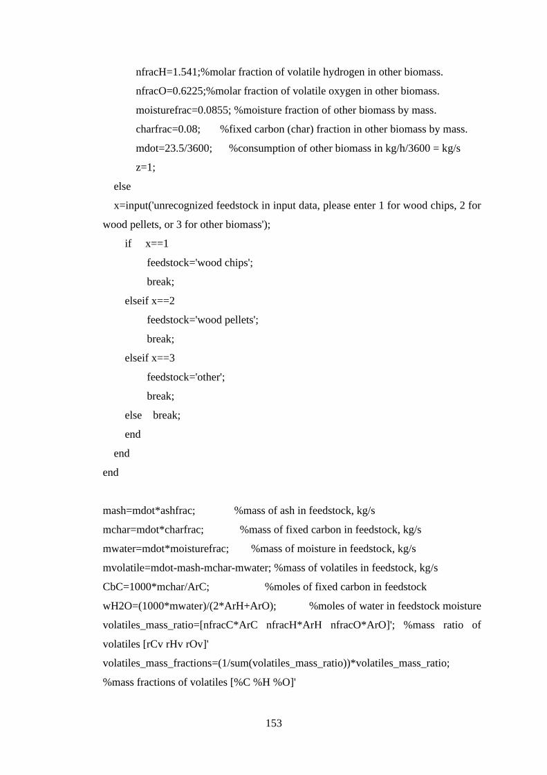
153
nfracH=1.541;%molar fraction of volatile hydrogen in other biomass.
nfracO=0.6225;%molar fraction of volatile oxygen in other biomass.
moisturefrac=0.0855; %moisture fraction of other biomass by mass.
charfrac=0.08; %fixed carbon (char) fraction in other biomass by mass.
mdot=23.5/3600; %consumption of other biomass in kg/h/3600 = kg/s
z=1;
else
x=input('unrecognized feedstock in input data, please enter 1 for wood chips, 2 for
wood pellets, or 3 for other biomass');
if x==1
feedstock='wood chips';
break;
elseif x==2
feedstock='wood pellets';
break;
elseif x==3
feedstock='other';
break;
else break;
end
end
end
mash=mdot*ashfrac; %mass of ash in feedstock, kg/s
mchar=mdot*charfrac; %mass of fixed carbon in feedstock, kg/s
mwater=mdot*moisturefrac; %mass of moisture in feedstock, kg/s
mvolatile=mdot-mash-mchar-mwater; %mass of volatiles in feedstock, kg/s
CbC=1000*mchar/ArC; %moles of fixed carbon in feedstock
wH2O=(1000*mwater)/(2*ArH+ArO); %moles of water in feedstock moisture
volatiles_mass_ratio=[nfracC*ArC nfracH*ArH nfracO*ArO]'; %mass ratio of
volatiles [rCv rHv rOv]'
volatiles_mass_fractions=(1/sum(volatiles_mass_ratio))*volatiles_mass_ratio;
%mass fractions of volatiles [%C %H %O]'
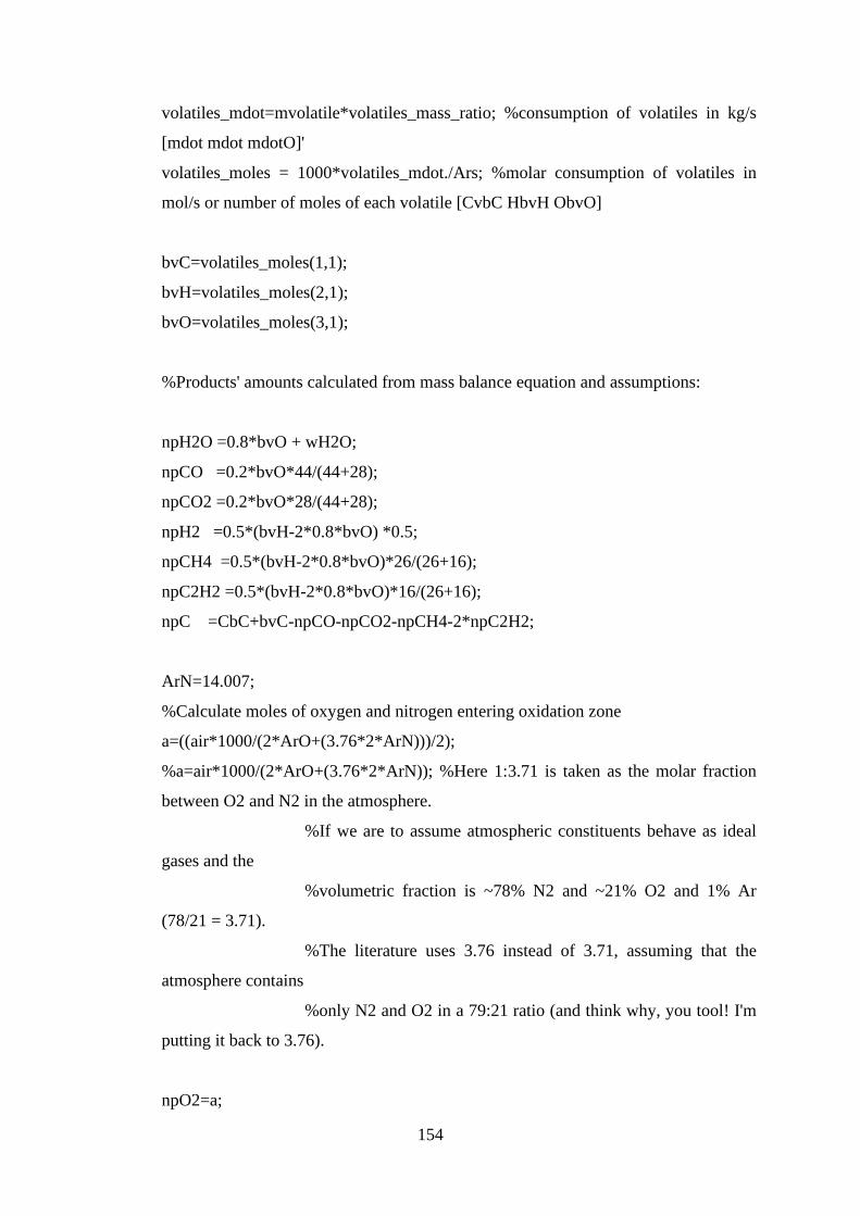
154
volatiles_mdot=mvolatile*volatiles_mass_ratio; %consumption of volatiles in kg/s
[mdot mdot mdotO]'
volatiles_moles = 1000*volatiles_mdot./Ars; %molar consumption of volatiles in
mol/s or number of moles of each volatile [CvbC HbvH ObvO]
bvC=volatiles_moles(1,1);
bvH=volatiles_moles(2,1);
bvO=volatiles_moles(3,1);
%Products' amounts calculated from mass balance equation and assumptions:
npH2O =0.8*bvO + wH2O;
npCO =0.2*bvO*44/(44+28);
npCO2 =0.2*bvO*28/(44+28);
npH2 =0.5*(bvH-2*0.8*bvO) *0.5;
npCH4 =0.5*(bvH-2*0.8*bvO)*26/(26+16);
npC2H2 =0.5*(bvH-2*0.8*bvO)*16/(26+16);
npC =CbC+bvC-npCO-npCO2-npCH4-2*npC2H2;
ArN=14.007;
%Calculate moles of oxygen and nitrogen entering oxidation zone
a=((air*1000/(2*ArO+(3.76*2*ArN)))/2);
%a=air*1000/(2*ArO+(3.76*2*ArN)); %Here 1:3.71 is taken as the molar fraction
between O2 and N2 in the atmosphere.
%If we are to assume atmospheric constituents behave as ideal
gases and the
%volumetric fraction is ~78% N2 and ~21% O2 and 1% Ar
(78/21 = 3.71).
%The literature uses 3.76 instead of 3.71, assuming that the
atmosphere contains
%only N2 and O2 in a 79:21 ratio (and think why, you tool! I'm
putting it back to 3.76).
npO2=a;
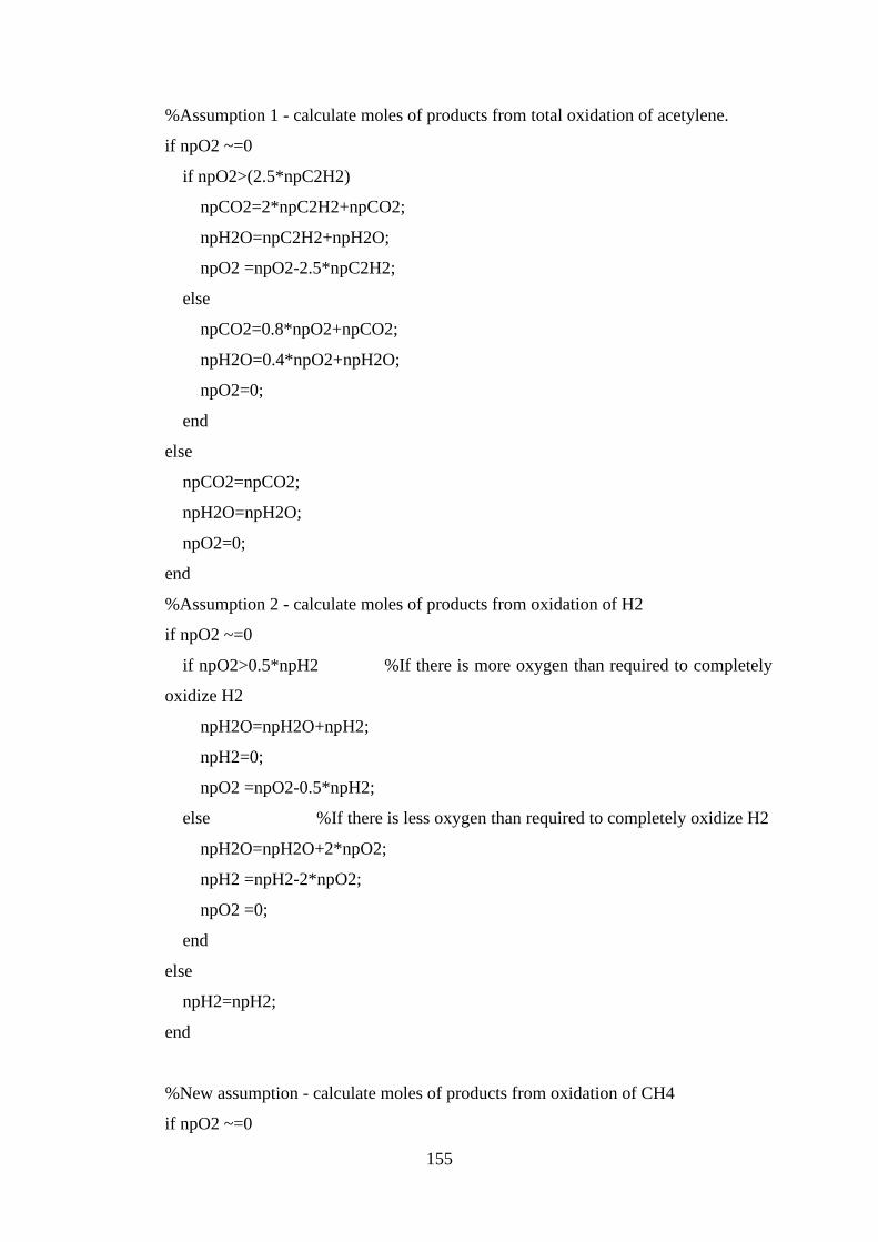
155
%Assumption 1 - calculate moles of products from total oxidation of acetylene.
if npO2 ~=0
if npO2>(2.5*npC2H2)
npCO2=2*npC2H2+npCO2;
npH2O=npC2H2+npH2O;
npO2 =npO2-2.5*npC2H2;
else
npCO2=0.8*npO2+npCO2;
npH2O=0.4*npO2+npH2O;
npO2=0;
end
else
npCO2=npCO2;
npH2O=npH2O;
npO2=0;
end
%Assumption 2 - calculate moles of products from oxidation of H2
if npO2 ~=0
if npO2>0.5*npH2 %If there is more oxygen than required to completely
oxidize H2
npH2O=npH2O+npH2;
npH2=0;
npO2 =npO2-0.5*npH2;
else %If there is less oxygen than required to completely oxidize H2
npH2O=npH2O+2*npO2;
npH2 =npH2-2*npO2;
npO2 =0;
end
else
npH2=npH2;
end
%New assumption - calculate moles of products from oxidation of CH4
if npO2 ~=0
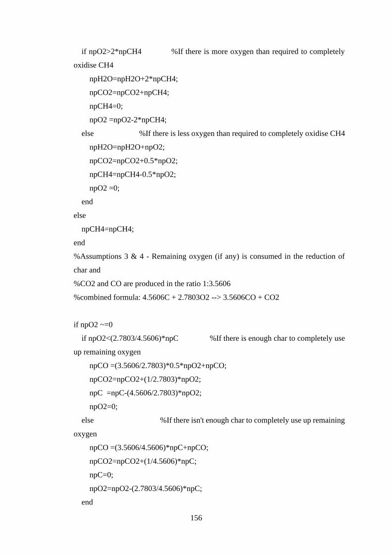
156
if npO2>2*npCH4 %If there is more oxygen than required to completely
oxidise CH4
npH2O=npH2O+2*npCH4;
npCO2=npCO2+npCH4;
npCH4=0;
npO2 =npO2-2*npCH4;
else %If there is less oxygen than required to completely oxidise CH4
npH2O=npH2O+npO2;
npCO2=npCO2+0.5*npO2;
npCH4=npCH4-0.5*npO2;
npO2 =0;
end
else
npCH4=npCH4;
end
%Assumptions 3 & 4 - Remaining oxygen (if any) is consumed in the reduction of
char and
%CO2 and CO are produced in the ratio 1:3.5606
%combined formula: 4.5606C + 2.7803O2 --> 3.5606CO + CO2
if npO2 ~=0
if npO2<(2.7803/4.5606)*npC %If there is enough char to completely use
up remaining oxygen
npCO =(3.5606/2.7803)*0.5*npO2+npCO;
npCO2=npCO2+(1/2.7803)*npO2;
npC =npC-(4.5606/2.7803)*npO2;
npO2=0;
else %If there isn't enough char to completely use up remaining
oxygen
npCO =(3.5606/4.5606)*npC+npCO;
npCO2=npCO2+(1/4.5606)*npC;
npC=0;
npO2=npO2-(2.7803/4.5606)*npC;
end
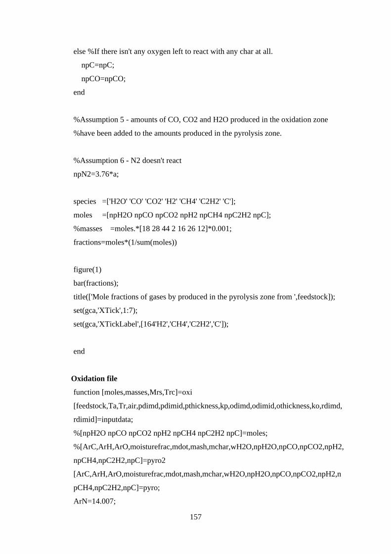
157
else %If there isn't any oxygen left to react with any char at all.
npC=npC;
npCO=npCO;
end
%Assumption 5 - amounts of CO, CO2 and H2O produced in the oxidation zone
%have been added to the amounts produced in the pyrolysis zone.
%Assumption 6 - N2 doesn't react
npN2=3.76*a;
species =['H2O' 'CO' 'CO2' 'H2' 'CH4' 'C2H2' 'C'];
moles =[npH2O npCO npCO2 npH2 npCH4 npC2H2 npC];
%masses =moles.*[18 28 44 2 16 26 12]*0.001;
fractions=moles*(1/sum(moles))
figure(1)
bar(fractions);
title(['Mole fractions of gases by produced in the pyrolysis zone from ',feedstock]);
set(gca,'XTick',1:7);
set(gca,'XTickLabel',[164'H2','CH4','C2H2','C']);
end
Oxidation file
function [moles,masses,Mrs,Trc]=oxi
[feedstock,Ta,Tr,air,pdimd,pdimid,pthickness,kp,odimd,odimid,othickness,ko,rdimd,
rdimid]=inputdata;
%[npH2O npCO npCO2 npH2 npCH4 npC2H2 npC]=moles;
%[ArC,ArH,ArO,moisturefrac,mdot,mash,mchar,wH2O,npH2O,npCO,npCO2,npH2,
npCH4,npC2H2,npC]=pyro2
[ArC,ArH,ArO,moisturefrac,mdot,mash,mchar,wH2O,npH2O,npCO,npCO2,npH2,n
pCH4,npC2H2,npC]=pyro;
ArN=14.007;
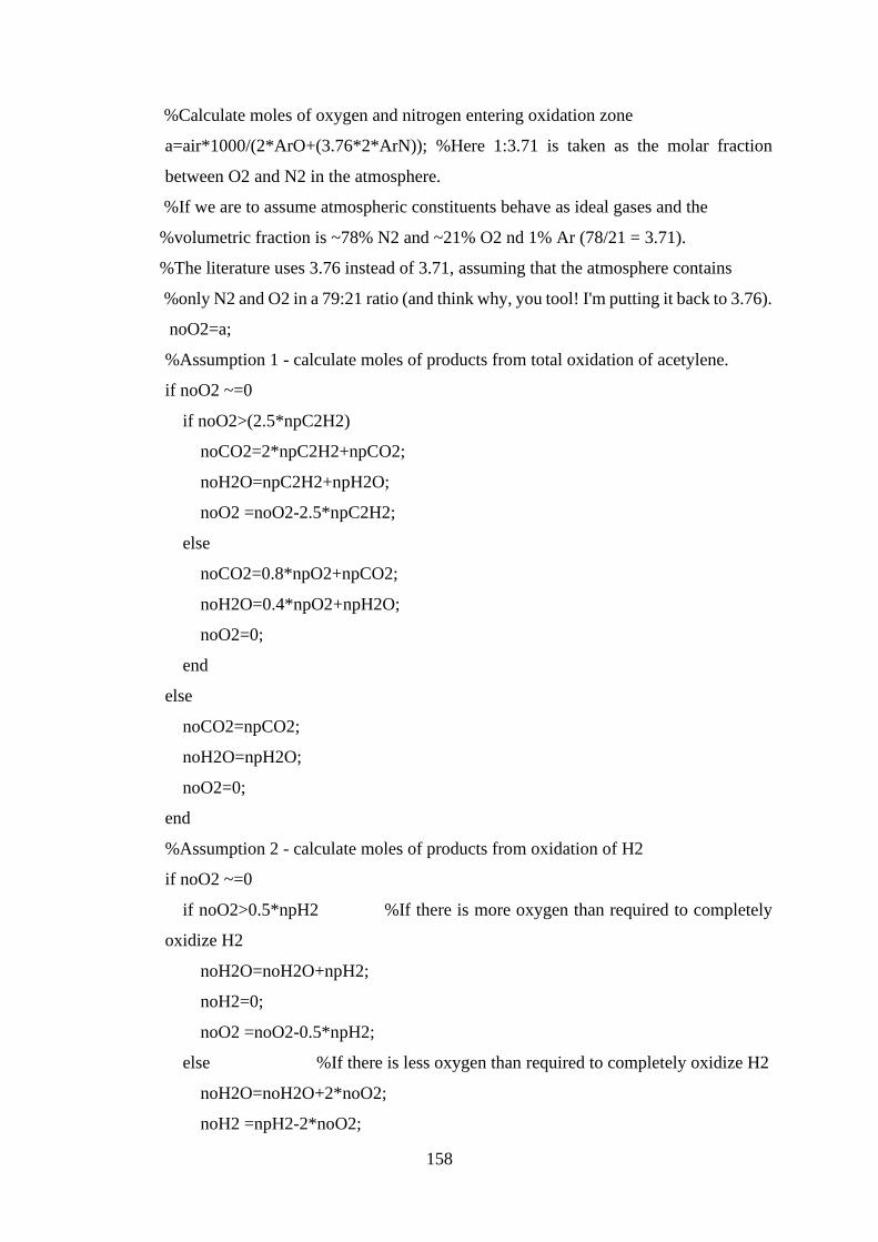
158
%Calculate moles of oxygen and nitrogen entering oxidation zone
a=air*1000/(2*ArO+(3.76*2*ArN)); %Here 1:3.71 is taken as the molar fraction
between O2 and N2 in the atmosphere.
%If we are to assume atmospheric constituents behave as ideal gases and the
%volumetric fraction is ~78% N2 and ~21% O2 nd 1% Ar (78/21 = 3.71).
%The literature uses 3.76 instead of 3.71, assuming that the atmosphere contains
%only N2 and O2 in a 79:21 ratio (and think why, you tool! I'm putting it back to 3.76).
noO2=a;
%Assumption 1 - calculate moles of products from total oxidation of acetylene.
if noO2 ~=0
if noO2>(2.5*npC2H2)
noCO2=2*npC2H2+npCO2;
noH2O=npC2H2+npH2O;
noO2 =noO2-2.5*npC2H2;
else
noCO2=0.8*npO2+npCO2;
noH2O=0.4*npO2+npH2O;
noO2=0;
end
else
noCO2=npCO2;
noH2O=npH2O;
noO2=0;
end
%Assumption 2 - calculate moles of products from oxidation of H2
if noO2 ~=0
if noO2>0.5*npH2 %If there is more oxygen than required to completely
oxidize H2
noH2O=noH2O+npH2;
noH2=0;
noO2 =noO2-0.5*npH2;
else %If there is less oxygen than required to completely oxidize H2
noH2O=noH2O+2*noO2;
noH2 =npH2-2*noO2;
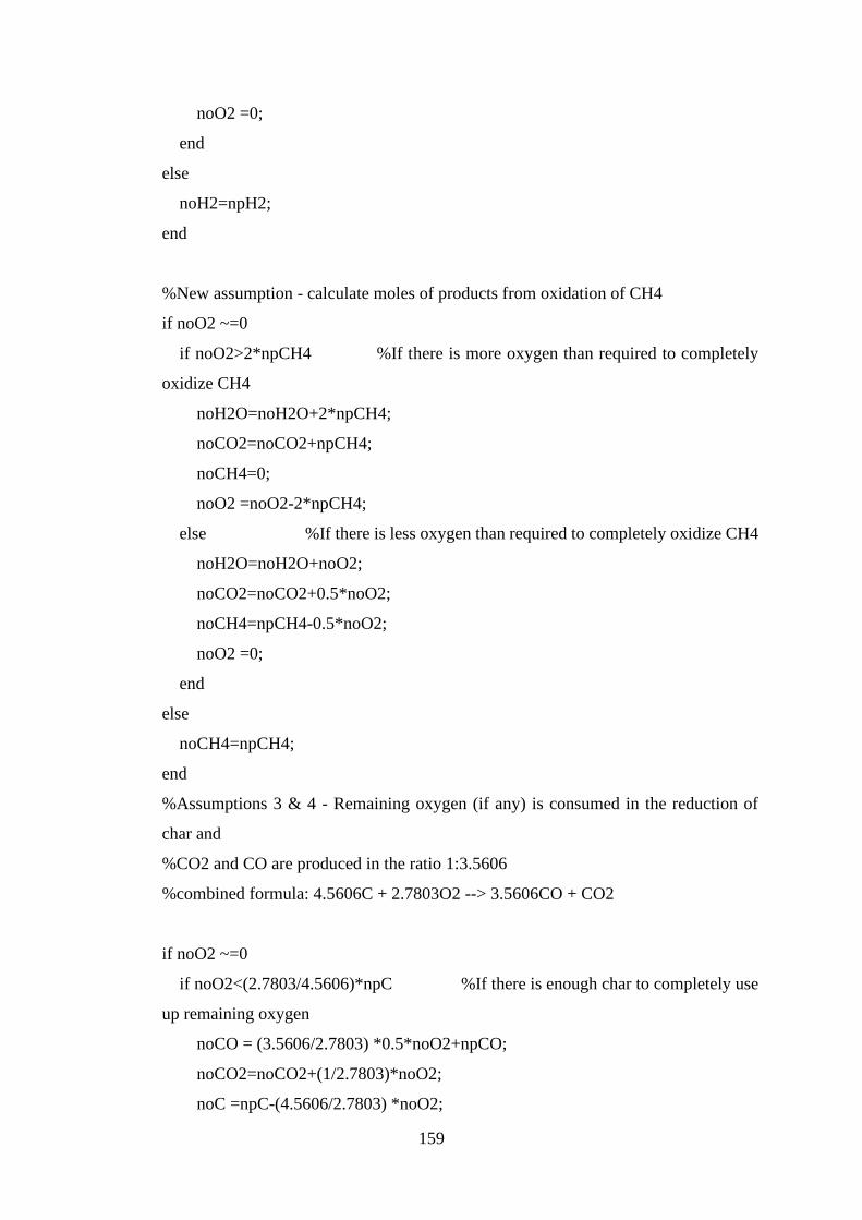
159
noO2 =0;
end
else
noH2=npH2;
end
%New assumption - calculate moles of products from oxidation of CH4
if noO2 ~=0
if noO2>2*npCH4 %If there is more oxygen than required to completely
oxidize CH4
noH2O=noH2O+2*npCH4;
noCO2=noCO2+npCH4;
noCH4=0;
noO2 =noO2-2*npCH4;
else %If there is less oxygen than required to completely oxidize CH4
noH2O=noH2O+noO2;
noCO2=noCO2+0.5*noO2;
noCH4=npCH4-0.5*noO2;
noO2 =0;
end
else
noCH4=npCH4;
end
%Assumptions 3 & 4 - Remaining oxygen (if any) is consumed in the reduction of
char and
%CO2 and CO are produced in the ratio 1:3.5606
%combined formula: 4.5606C + 2.7803O2 --> 3.5606CO + CO2
if noO2 ~=0
if noO2<(2.7803/4.5606)*npC %If there is enough char to completely use
up remaining oxygen
noCO = (3.5606/2.7803) *0.5*noO2+npCO;
noCO2=noCO2+(1/2.7803)*noO2;
noC =npC-(4.5606/2.7803) *noO2;
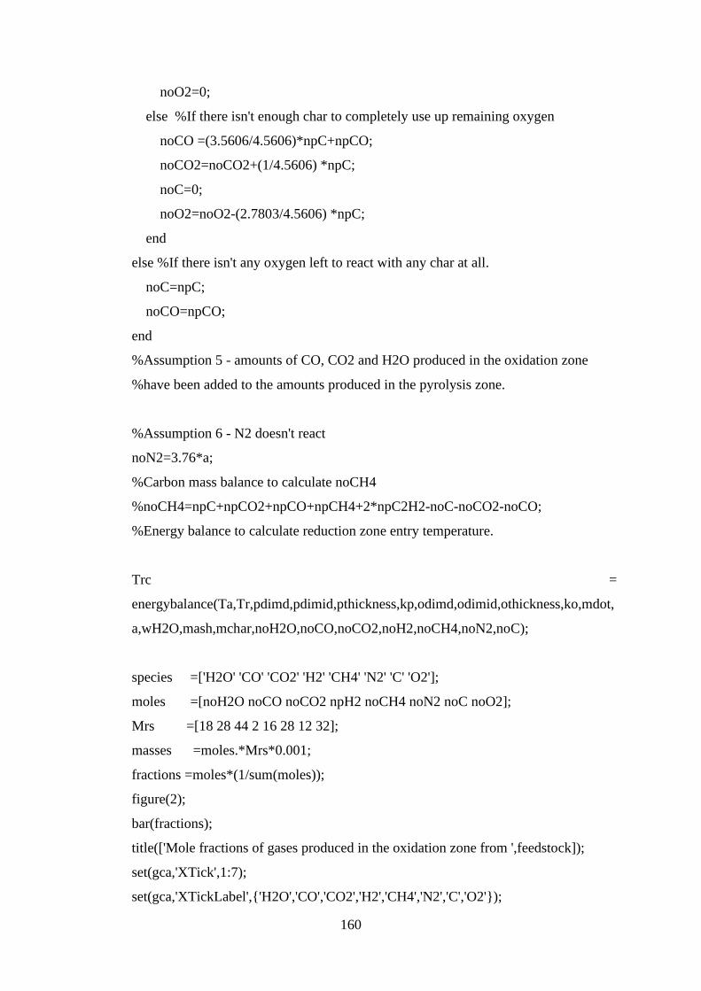
160
noO2=0;
else %If there isn't enough char to completely use up remaining oxygen
noCO =(3.5606/4.5606)*npC+npCO;
noCO2=noCO2+(1/4.5606) *npC;
noC=0;
noO2=noO2-(2.7803/4.5606) *npC;
end
else %If there isn't any oxygen left to react with any char at all.
noC=npC;
noCO=npCO;
end
%Assumption 5 - amounts of CO, CO2 and H2O produced in the oxidation zone
%have been added to the amounts produced in the pyrolysis zone.
%Assumption 6 - N2 doesn't react
noN2=3.76*a;
%Carbon mass balance to calculate noCH4
%noCH4=npC+npCO2+npCO+npCH4+2*npC2H2-noC-noCO2-noCO;
%Energy balance to calculate reduction zone entry temperature.
Trc =
energybalance(Ta,Tr,pdimd,pdimid,pthickness,kp,odimd,odimid,othickness,ko,mdot,
a,wH2O,mash,mchar,noH2O,noCO,noCO2,noH2,noCH4,noN2,noC);
species =['H2O' 'CO' 'CO2' 'H2' 'CH4' 'N2' 'C' 'O2'];
moles =[noH2O noCO noCO2 npH2 noCH4 noN2 noC noO2];
Mrs =[18 28 44 2 16 28 12 32];
masses =moles.*Mrs*0.001;
fractions =moles*(1/sum(moles));
figure(2);
bar(fractions);
title(['Mole fractions of gases produced in the oxidation zone from ',feedstock]);
set(gca,'XTick',1:7);
set(gca,'XTickLabel',{'H2O','CO','CO2','H2','CH4','N2','C','O2'});
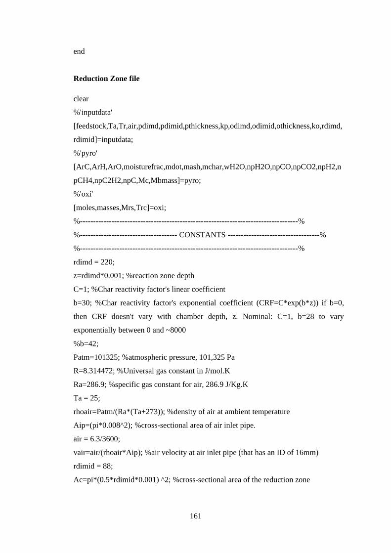
161
end
Reduction Zone file
clear
%'inputdata'
[feedstock,Ta,Tr,air,pdimd,pdimid,pthickness,kp,odimd,odimid,othickness,ko,rdimd,
rdimid]=inputdata;
%'pyro'
[ArC,ArH,ArO,moisturefrac,mdot,mash,mchar,wH2O,npH2O,npCO,npCO2,npH2,n
pCH4,npC2H2,npC,Mc,Mbmass]=pyro;
%'oxi'
[moles,masses,Mrs,Trc]=oxi;
%-----------------------------------------------------------------------------------%
%------------------------------------- CONSTANTS -----------------------------------%
%-----------------------------------------------------------------------------------%
rdimd = 220;
z=rdimd*0.001; %reaction zone depth
C=1; %Char reactivity factor's linear coefficient
b=30; %Char reactivity factor's exponential coefficient (CRF=C*exp(b*z)) if b=0,
then CRF doesn't vary with chamber depth, z. Nominal: C=1, b=28 to vary
exponentially between 0 and ~8000
%b=42;
Patm=101325; %atmospheric pressure, 101,325 Pa
R=8.314472; %Universal gas constant in J/mol.K
Ra=286.9; %specific gas constant for air, 286.9 J/Kg.K
Ta = 25;
rhoair=Patm/(Ra*(Ta+273)); %density of air at ambient temperature
Aip=(pi*0.008^2); %cross-sectional area of air inlet pipe.
air = 6.3/3600;
vair=air/(rhoair*Aip); %air velocity at air inlet pipe (that has an ID of 16mm)
rdimid = 88;
Ac=pi*(0.5*rdimid*0.001) ^2; %cross-sectional area of the reduction zone
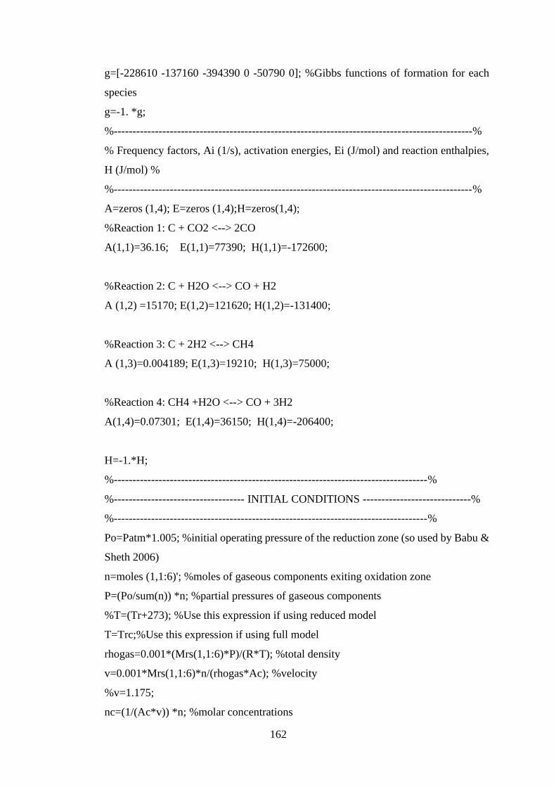
162
g=[-228610 -137160 -394390 0 -50790 0]; %Gibbs functions of formation for each
species
g=-1. *g;
%------------------------------------------------------------------------------------------------%
% Frequency factors, Ai (1/s), activation energies, Ei (J/mol) and reaction enthalpies,
H (J/mol) %
%------------------------------------------------------------------------------------------------%
A=zeros (1,4); E=zeros (1,4);H=zeros(1,4);
%Reaction 1: C + CO2 <--> 2CO
A(1,1)=36.16; E(1,1)=77390; H(1,1)=-172600;
%Reaction 2: C + H2O <--> CO + H2
A (1,2) =15170; E(1,2)=121620; H(1,2)=-131400;
%Reaction 3: C + 2H2 <--> CH4
A (1,3)=0.004189; E(1,3)=19210; H(1,3)=75000;
%Reaction 4: CH4 +H2O <--> CO + 3H2
A(1,4)=0.07301; E(1,4)=36150; H(1,4)=-206400;
H=-1.*H;
%------------------------------------------------------------------------------------%
%----------------------------------- INITIAL CONDITIONS -----------------------------%
%------------------------------------------------------------------------------------%
Po=Patm*1.005; %initial operating pressure of the reduction zone (so used by Babu &
Sheth 2006)
n=moles (1,1:6)'; %moles of gaseous components exiting oxidation zone
P=(Po/sum(n)) *n; %partial pressures of gaseous components
%T=(Tr+273); %Use this expression if using reduced model
T=Trc;%Use this expression if using full model
rhogas=0.001*(Mrs(1,1:6)*P)/(R*T); %total density
v=0.001*Mrs(1,1:6)*n/(rhogas*Ac); %velocity
%v=1.175;
nc=(1/(Ac*v)) *n; %molar concentrations
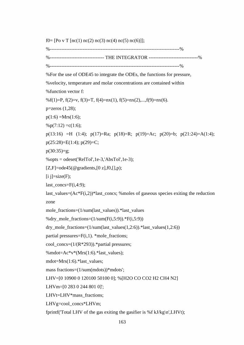
163
f0= [Po v T [nc(1) nc(2) nc(3) nc(4) nc(5) nc(6)]];
%-------------------------------------------------------------------------------%
%--------------------------------- THE INTEGRATOR ------------------------------%
%-------------------------------------------------------------------------------%
%For the use of ODE45 to integrate the ODEs, the functions for pressure,
%velocity, temperature and molar concentrations are contained within
%function vector f:
%f(1)=P, f(2)=v, f(3)=T, f(4)=nx(1), f(5)=nx(2),...,f(9)=nx(6).
p=zeros (1,28);
p(1:6) =Mrs(1:6);
%p(7:12) =c(1:6);
p(13:16) =H (1:4); p(17)=Ra; p(18)=R; p(19)=Ac; p(20)=b; p(21:24)=A(1:4);
p(25:28)=E(1:4); p(29)=C;
p(30:35)=g;
%opts = odeset('RelTol',1e-3,'AbsTol',1e-3);
[Z,F]=ode45(@gradients,[0 z],f0,[],p);
[i j]=size(F);
last_concs=F(i,4:9);
last_values=(Ac*F(i,2))*last_concs; %moles of gaseous species exiting the reduction
zone
mole_fractions=(1/sum(last_values)).*last_values
%dry_mole_fractions=(1/sum(F(i,5:9)).*F(i,5:9))
dry_mole_fractions=(1/sum(last_values(1,2:6)).*last_values(1,2:6))
partial pressures=F(i,1). *mole_fractions;
cool_concs=(1/(R*293)).*partial pressures;
%mdot=Ac*v*(Mrs(1:6).*last_values);
mdot=Mrs(1:6).*last_values;
mass fractions=(1/sum(mdots))*mdots';
LHV=[0 10900 0 120100 50100 0]; %[H2O CO CO2 H2 CH4 N2]
LHVm=[0 283 0 244 801 0]';
LHVt=LHV*mass_fractions;
LHVg=cool_concs*LHVm;
fprintf('Total LHV of the gas exiting the gasifier is %f kJ/kg\n',LHVt);
164
fprintf('Total LHV of the gas exiting the gasifier is %f kJ/m^3\n',LHVg);
figure(3)
plot(Z,F(:,1),'.')
figure(4)
plot(Z,F(:,2),'.')
figure(5)
plot(Z,F(:,3),'.')
figure(6)
plot(Z,F(:,4),'-',Z,F(:,5),'-',Z,F(:,6),'-',Z,F(:,7),'-',Z,F(:,8),'-',Z,F(:,9),'-')
xlabel('Depth of reduction zone (m)');
ylabel('Molar concentration (mol/m3)');
title('Gas species concentration profile');
hleg1=legend('H2O','CO','CO2','H2','CH4','N2');
%figure(7)
%bar(F(i,4:9));
%title(['Molar concentrations of gases leaving the reduction zone from ',feedstock]);
%set(gca,'XTick',1:7);
%set(gca,'XTickLabel',{'H_2O','CO','CO_2','H_2','CH_4','N_2'});
%figure(8)
%bar(mass_fractions);
%title(['Final gas composition, by mass, for ',feedstock]);
%set(gca,'XTick',1:7);
%
%set(gca,'XTickLabel',{'H_2O','CO','CO_2','H_2','CH_4','N_2'});
figure(7)
bar(mole_fractions);
title(['Final wet gas composition, mole fractions, for ',feedstock]);
set(gca,'XTick',1:6);
set(gca,'XTickLabel',{'H2O','CO','CO2','H2','CH4','N2'});
figure(8)
bar(dry_mole_fractions);
title(['Final dry gas composition, mole fractions, for ',feedstock]);
set(gca,'XTick',1:5);
set(gca,'XTickLabel',{'CO','CO2','H2','CH4','N2'});
165
Energy balance file
function Trc =
energybalance(Ta,Tr,pdimd,pdimid,pthickness,kp,odimd,odimid,othickness,ko,mdot,
a,wH2O,mash,mchar,noH2O,noCO,noCO2,noH2,noCH4,noN2,noC)
%This function evaluates the temperature at exit of the oxidation zone
%and entry to the reduction zone from the energy balance equation across
%the pyrolysis and oxidation zones. It is solved by the Newton-Raphson
%method.
%The energy balance equation "energy of reactants = energy of products"
%is rearranged to take the form
%"Final temperature dependent terms - independent terms = 0"
%To satisfy the f(T)=0 condition for Newton-Rhapson iteration.
%Ambient temperature
T0=Ta+273;
%Enthalpies of formation
hfbm = -616.6*1000; %J/kg enthalpy of formation for typical wood biomass
hflH2O = -285.83*1000; %J/mol liquid water
hfgH2O = -241.83*1000; %J/mol steam
hfCO = -110.53*1000; %J/mol carbon monoxide
hfCO2 = -393.52*1000; %J/mol carbon dioxide
hfH2 = 0; %J/mol hydrogen
hfCH4 = -74.87*1000;%J/mol methane
hfN2 = 0;%J/mol nitrogen
hfC = 0;%J/mol solid carbon
hfO2 = 0;%J/mol oxygen
hfx=zeros(6,1);
hfx(1,1)=hfgH2O;
hfx(2,1)=hfCO;
hfx(3,1)=hfCO2;
hfx(4,1)=hfH2;
hfx(5,1)=hfCH4;
166
hfx(6,1)=hfN2;
%Heat capacities for solid species (constants)
Cpwood = 2.3*1000; %J/kg/K
Cpash = 0.84*1000; %J/kg/K
Cpchar = 23.4; %J/mol/K
%Specific enthalpies at room temperature (298K) from Haywood 1990 (steam
%tables)
hsO2 = 8.66*1000; %J/mol oxygen
hsN2 = 8.67*1000; %J/mol nitrogen
hsH2O = 1.886*1000; %J/mol liquid water
%Shomate equation coefficients for gaseous species, Cp = A + BT + CT^2 + DT^3 +
E/T^2 J/mol/K
A=zeros(6,1); B=zeros(6,1); C=zeros(6,1); D=zeros(6,1); E=zeros(6,1);
A(1,1)=30.092; B(1,1)=6.832514; C(1,1)=6.793435; D(1,1)=-2.53448;
E(1,1)=0.082139; %H2O
A(2,1)=25.56759; B(2,1)=6.09613; C(2,1)=4.054656; D(2,1)=-2.671301;
E(2,1)=0.131021; %CO
A(3,1)=24.99735; B(3,1)=55.18696; C(3,1)=-33.69137; D(3,1)=7.948387; E(3,1)=-
0.136638; %CO2
A(4,1)=33.066178; B(4,1)=-11.363417; C(4,1)=11.432816; D(4,1)=-2.772874;
E(4,1)=-0.158558; %H2
A(5,1)=-0.703029; B(5,1)=108.4773; C(5,1)=-42.52157; D(5,1)=5.862788;
E(5,1)=0.678565; %CH4
A(6,1)=26.092; B(6,1)=8.218801; C(6,1)=-1.976141; D(6,1)=0.159274;
E(6,1)=0.044434; %N2
%molar values of species at exit from oxidation zone
nx=zeros(1,7);
nx(1,1)=noH2O;
nx(1,2)=noCO;
nx(1,3)=noCO2;
167
nx(1,4)=noH2;
nx(1,5)=noCH4;
nx(1,6)=noN2;
nx(1,7)=noC;
%heat loss expressions
h= 25; %Surface heat transfer coefficients in W/m^2K
%n=size(kp,1)+1;
%pr=zeros(n,1); %
%pr(1,1)=(pdimid/2)*0.001; %
%for m=2:n %array of rp (cylinder radii in pyrolysis zone) values
% pr(m,1) = pr(m-1,1) + pthickness(m-1,1)*0.001; %
%end %
%par1=pr(1:n-1,1); %array of rn values
%par2=pr(2:n,1); %array pf rn+1 values
%pak =kp(:,1); %array of k values
%pnzak=pak(pak~=0); %k value array trimmed of 0 elements (to prevent division by
0)
%plr=log(par2./par1);%array of ln(rn+1/rn) values.
%pnzlr=plr(plr~=0); %ln array trimmed of 0 elements (to prevent division by 0)
%Qp = (pdimd*0.001*2*pi)/(sum(pnzlr./pnzak)+1/(pr(n,1)*h)); %Heat transfer
temperature gradient multiplier for the pyrolysis zone
n=size(ko,1)+1;
or=zeros(n,1); %
or(1,1)=(odimid/2)*0.001; %
for m=2:n %array of rp (cylinder radii in oxidation zone) values
or(m,1) = or(m-1,1) + othickness(m-1,1)*0.001; %
end %
oar1=or(1:n-1,1); %array of rn values
oar2=or(2:n,1); %array pf rn+1 values
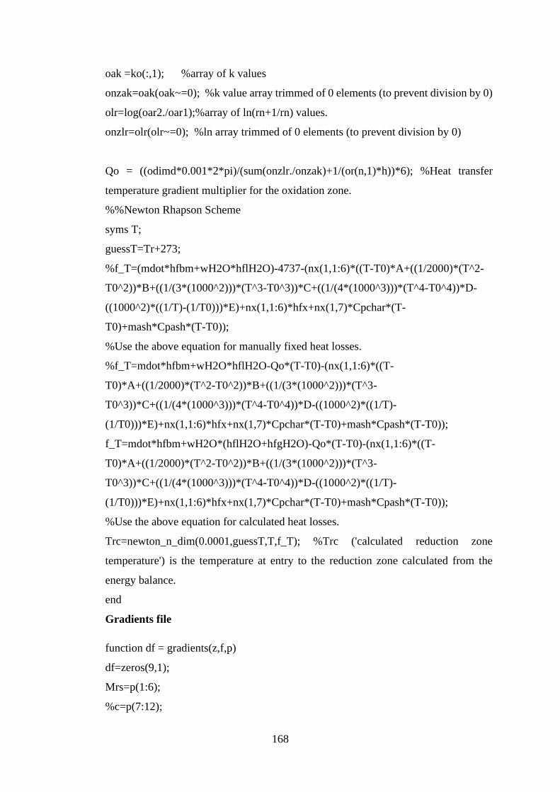
168
oak =ko(:,1); %array of k values
onzak=oak(oak~=0); %k value array trimmed of 0 elements (to prevent division by 0)
olr=log(oar2./oar1);%array of ln(rn+1/rn) values.
onzlr=olr(olr~=0); %ln array trimmed of 0 elements (to prevent division by 0)
Qo = ((odimd*0.001*2*pi)/(sum(onzlr./onzak)+1/(or(n,1)*h))*6); %Heat transfer
temperature gradient multiplier for the oxidation zone.
%%Newton Rhapson Scheme
syms T;
guessT=Tr+273;
%f_T=(mdot*hfbm+wH2O*hflH2O)-4737-(nx(1,1:6)*((T-T0)*A+((1/2000)*(T^2-
T0^2))*B+((1/(3*(1000^2)))*(T^3-T0^3))*C+((1/(4*(1000^3)))*(T^4-T0^4))*D-
((1000^2)*((1/T)-(1/T0)))*E)+nx(1,1:6)*hfx+nx(1,7)*Cpchar*(T-
T0)+mash*Cpash*(T-T0));
%Use the above equation for manually fixed heat losses.
%f_T=mdot*hfbm+wH2O*hflH2O-Qo*(T-T0)-(nx(1,1:6)*((T-
T0)*A+((1/2000)*(T^2-T0^2))*B+((1/(3*(1000^2)))*(T^3-
T0^3))*C+((1/(4*(1000^3)))*(T^4-T0^4))*D-((1000^2)*((1/T)-
(1/T0)))*E)+nx(1,1:6)*hfx+nx(1,7)*Cpchar*(T-T0)+mash*Cpash*(T-T0));
f_T=mdot*hfbm+wH2O*(hflH2O+hfgH2O)-Qo*(T-T0)-(nx(1,1:6)*((T-
T0)*A+((1/2000)*(T^2-T0^2))*B+((1/(3*(1000^2)))*(T^3-
T0^3))*C+((1/(4*(1000^3)))*(T^4-T0^4))*D-((1000^2)*((1/T)-
(1/T0)))*E)+nx(1,1:6)*hfx+nx(1,7)*Cpchar*(T-T0)+mash*Cpash*(T-T0));
%Use the above equation for calculated heat losses.
Trc=newton_n_dim(0.0001,guessT,T,f_T); %Trc ('calculated reduction zone
temperature') is the temperature at entry to the reduction zone calculated from the
energy balance.
end
Gradients file
function df = gradients(z,f,p)
df=zeros(9,1);
Mrs=p(1:6);
%c=p(7:12);

169
H=p(13:16); Ra=p(17); R=p(18); Ac=p(19); b=p(20); A=p(21:24); E=p(25:28);
C=p(29); g=p(30:35);
%%%EVERY VARIABLE IS A ROW VECTOR, APART FROM f(1:9) AND df(1:9)
WHICH ARE
%%%COLUMNS; IF IT'S TRANSPOSED IT'S BECOME A COLUMN VECTOR.
df(1)=1183*(rhogas(Ac,Mrs,R,f(1),f(2),f(3),f(4:9))*(f(2)^2)/rhoair(Ra,f(1),f(3)))+38
8.19*f(2)-79.896; %dP/dz
df(2)=(1/(c(f(3))*f(4:9)+sum(f(4:9))*R))*(((c(f(3))*f(4:9))*sum(srates(Ac,R,b,A,E,f
(1),f(2),f(3),f(4:9),C,z,g))/sum(f(4:9)))-
((rspeeds(Ac,R,b,A,E,f(1),f(2),f(3),f(4:9),C,z,g)*H')/f(3))-
df(1)*(f(2)/f(3)+(f(2)*(c(f(3))*f(4:9))/f(1)))-
(srates(Ac,R,b,A,E,f(1),f(2),f(3),f(4:9),C,z,g)*(c(f(3)))')); %dv/dz
df(3)=(1/(f(2)*c(f(3))*f(4:9)))*(-
1*rspeeds(Ac,R,b,A,E,f(1),f(2),f(3),f(4:9),C,z,g)*H'-f(2)*df(1)-f(1)*df(2)-
(srates(Ac,R,b,A,E,f(1),f(2),f(3),f(4:9),C,z,g)*(c(f(3)))')*f(3)); %dT/dz
df(4:9)=(1/f(2))*((srates(Ac,R,b,A,E,f(1),f(2),f(3),f(4:9),C,z,g))'-(df(2)*f(4:9))); %
dnx/dz
end
%Density and velocity of gas in zone
function gas_density = rhogas(Ac,Mrs,R,P,v,T,nx)
n=Ac*v*nx; %moles of gaseous components exiting the last control volume
Pp=(P/sum(n))*n; %partial pressures of gaseous components
gas_density=0.001*(Mrs*Pp)/(R*T); %total density
end
function air_density = rhoair (Ra, P,T)
air_density=P/(Ra*T);
end
function heat_capacities =c(T) %Species heat capacities in the form Cp = A + Bt +
Ct^2 + Dt^3 + E/t^2
t=T/1000;
Cp (1,1) = 30.092 + 6.832514*t + 6.793435*(t^2) - 2.53448*(t^3) + 0.082139/(t^2);
%Cp H2O
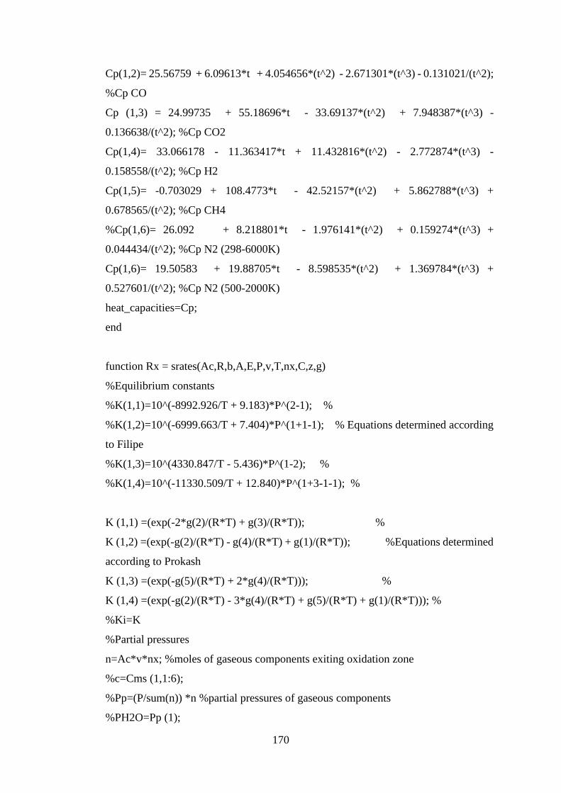
170
Cp(1,2)= 25.56759 + 6.09613*t + 4.054656*(t^2) - 2.671301*(t^3) - 0.131021/(t^2);
%Cp CO
Cp (1,3) = 24.99735 + 55.18696*t - 33.69137*(t^2) + 7.948387*(t^3) -
0.136638/(t^2); %Cp CO2
Cp(1,4)= 33.066178 - 11.363417*t + 11.432816*(t^2) - 2.772874*(t^3) -
0.158558/(t^2); %Cp H2
Cp(1,5)= -0.703029 + 108.4773*t - 42.52157*(t^2) + 5.862788*(t^3) +
0.678565/(t^2); %Cp CH4
%Cp(1,6)= 26.092 + 8.218801*t - 1.976141*(t^2) + 0.159274*(t^3) +
0.044434/(t^2); %Cp N2 (298-6000K)
Cp(1,6)= 19.50583 + 19.88705*t - 8.598535*(t^2) + 1.369784*(t^3) +
0.527601/(t^2); %Cp N2 (500-2000K)
heat_capacities=Cp;
end
function Rx = srates(Ac,R,b,A,E,P,v,T,nx,C,z,g)
%Equilibrium constants
%K(1,1)=10^(-8992.926/T + 9.183)*P^(2-1); %
%K(1,2)=10^(-6999.663/T + 7.404)*P^(1+1-1); % Equations determined according
to Filipe
%K(1,3)=10^(4330.847/T - 5.436)*P^(1-2); %
%K(1,4)=10^(-11330.509/T + 12.840)*P^(1+3-1-1); %
K (1,1) =(exp(-2*g(2)/(R*T) + g(3)/(R*T)); %
K (1,2) =(exp(-g(2)/(R*T) - g(4)/(R*T) + g(1)/(R*T)); %Equations determined
according to Prokash
K (1,3) =(exp(-g(5)/(R*T) + 2*g(4)/(R*T))); %
K (1,4) =(exp(-g(2)/(R*T) - 3*g(4)/(R*T) + g(5)/(R*T) + g(1)/(R*T))); %
%Ki=K
%Partial pressures
n=Ac*v*nx; %moles of gaseous components exiting oxidation zone
%c=Cms (1,1:6);
%Pp=(P/sum(n)) *n %partial pressures of gaseous components
%PH2O=Pp (1);
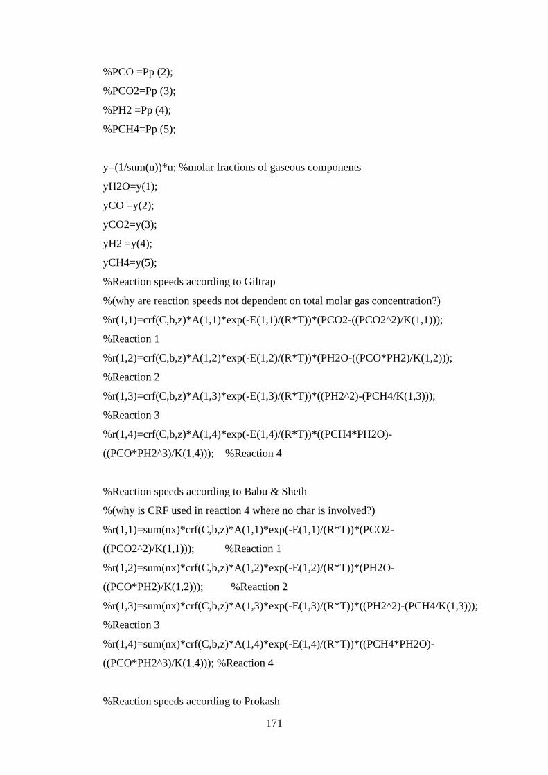
171
%PCO =Pp (2);
%PCO2=Pp (3);
%PH2 =Pp (4);
%PCH4=Pp (5);
y=(1/sum(n))*n; %molar fractions of gaseous components
yH2O=y(1);
yCO =y(2);
yCO2=y(3);
yH2 =y(4);
yCH4=y(5);
%Reaction speeds according to Giltrap
%(why are reaction speeds not dependent on total molar gas concentration?)
%r(1,1)=crf(C,b,z)*A(1,1)*exp(-E(1,1)/(R*T))*(PCO2-((PCO2^2)/K(1,1)));
%Reaction 1
%r(1,2)=crf(C,b,z)*A(1,2)*exp(-E(1,2)/(R*T))*(PH2O-((PCO*PH2)/K(1,2)));
%Reaction 2
%r(1,3)=crf(C,b,z)*A(1,3)*exp(-E(1,3)/(R*T))*((PH2^2)-(PCH4/K(1,3)));
%Reaction 3
%r(1,4)=crf(C,b,z)*A(1,4)*exp(-E(1,4)/(R*T))*((PCH4*PH2O)-
((PCO*PH2^3)/K(1,4))); %Reaction 4
%Reaction speeds according to Babu & Sheth
%(why is CRF used in reaction 4 where no char is involved?)
%r(1,1)=sum(nx)*crf(C,b,z)*A(1,1)*exp(-E(1,1)/(R*T))*(PCO2-
((PCO2^2)/K(1,1))); %Reaction 1
%r(1,2)=sum(nx)*crf(C,b,z)*A(1,2)*exp(-E(1,2)/(R*T))*(PH2O-
((PCO*PH2)/K(1,2))); %Reaction 2
%r(1,3)=sum(nx)*crf(C,b,z)*A(1,3)*exp(-E(1,3)/(R*T))*((PH2^2)-(PCH4/K(1,3)));
%Reaction 3
%r(1,4)=sum(nx)*crf(C,b,z)*A(1,4)*exp(-E(1,4)/(R*T))*((PCH4*PH2O)-
((PCO*PH2^3)/K(1,4))); %Reaction 4
%Reaction speeds according to Prokash
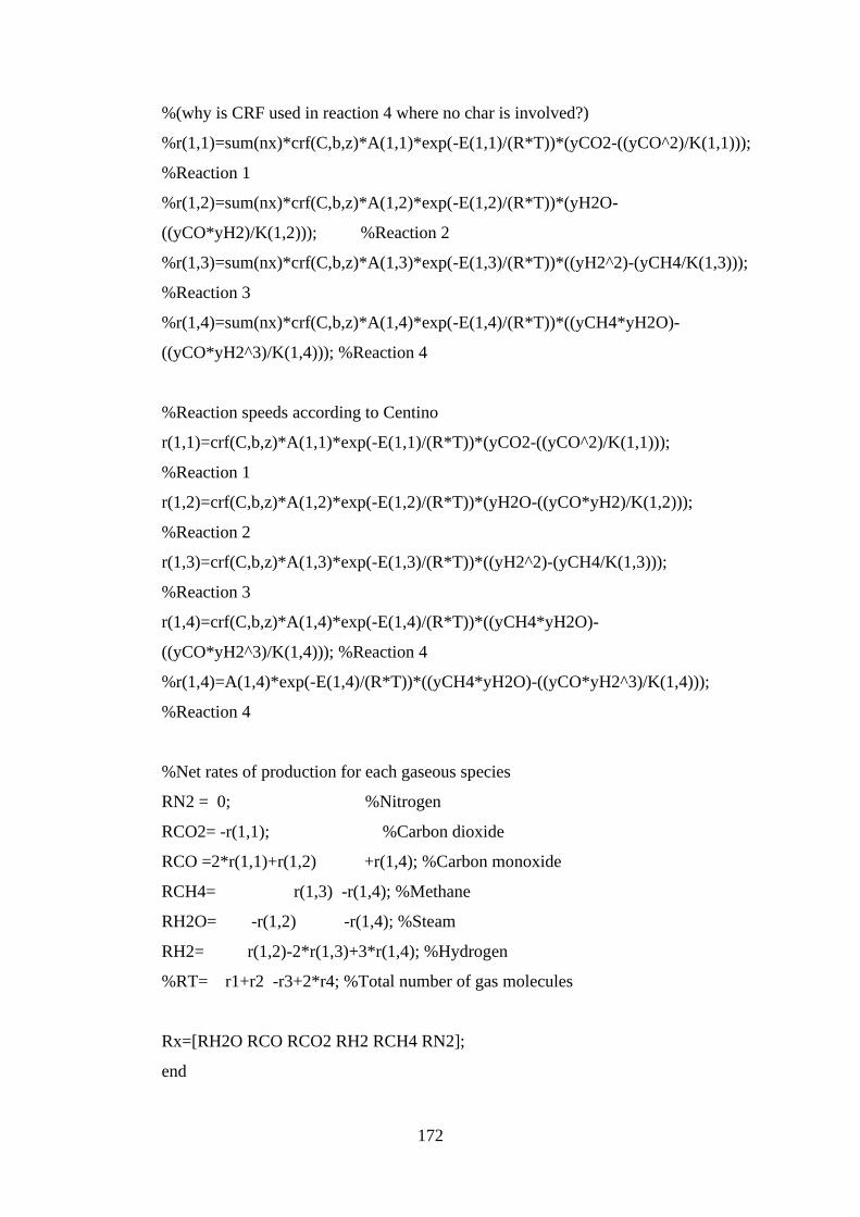
172
%(why is CRF used in reaction 4 where no char is involved?)
%r(1,1)=sum(nx)*crf(C,b,z)*A(1,1)*exp(-E(1,1)/(R*T))*(yCO2-((yCO^2)/K(1,1)));
%Reaction 1
%r(1,2)=sum(nx)*crf(C,b,z)*A(1,2)*exp(-E(1,2)/(R*T))*(yH2O-
((yCO*yH2)/K(1,2))); %Reaction 2
%r(1,3)=sum(nx)*crf(C,b,z)*A(1,3)*exp(-E(1,3)/(R*T))*((yH2^2)-(yCH4/K(1,3)));
%Reaction 3
%r(1,4)=sum(nx)*crf(C,b,z)*A(1,4)*exp(-E(1,4)/(R*T))*((yCH4*yH2O)-
((yCO*yH2^3)/K(1,4))); %Reaction 4
%Reaction speeds according to Centino
r(1,1)=crf(C,b,z)*A(1,1)*exp(-E(1,1)/(R*T))*(yCO2-((yCO^2)/K(1,1)));
%Reaction 1
r(1,2)=crf(C,b,z)*A(1,2)*exp(-E(1,2)/(R*T))*(yH2O-((yCO*yH2)/K(1,2)));
%Reaction 2
r(1,3)=crf(C,b,z)*A(1,3)*exp(-E(1,3)/(R*T))*((yH2^2)-(yCH4/K(1,3)));
%Reaction 3
r(1,4)=crf(C,b,z)*A(1,4)*exp(-E(1,4)/(R*T))*((yCH4*yH2O)-
((yCO*yH2^3)/K(1,4))); %Reaction 4
%r(1,4)=A(1,4)*exp(-E(1,4)/(R*T))*((yCH4*yH2O)-((yCO*yH2^3)/K(1,4)));
%Reaction 4
%Net rates of production for each gaseous species
RN2 = 0; %Nitrogen
RCO2= -r(1,1); %Carbon dioxide
RCO =2*r(1,1)+r(1,2) +r(1,4); %Carbon monoxide
RCH4= r(1,3) -r(1,4); %Methane
RH2O= -r(1,2) -r(1,4); %Steam
RH2= r(1,2)-2*r(1,3)+3*r(1,4); %Hydrogen
%RT= r1+r2 -r3+2*r4; %Total number of gas molecules
Rx=[RH2O RCO RCO2 RH2 RCH4 RN2];
end
173
function r = rspeeds(Ac,R,b,A,E,P,v,T,nx,C,z,g)
%Equilibrium constants
%K(1,1)=10^(-8992.926/T + 9.183)*P^(2-1); %
%K(1,2)=10^(-6999.663/T + 7.404)*P^(1+1-1); % Equations determined according
to Filipe
%K(1,3)=10^(4330.847/T - 5.436)*P^(1-2); %
%K(1,4)=10^(-11330.509/T + 12.840)*P^(1+3-1-1); %
K(1,1)=(exp(-2*g(2)/(R*T) + g(3)/(R*T))); %
K(1,2)=(exp(-g(2)/(R*T) - g(4)/(R*T) + g(1)/(R*T)) %Equations determined
according to Prokash
K(1,3)=(exp(-g(5)/(R*T) + 2*g(4)/(R*T))); %
K(1,4)=(exp(-g(2)/(R*T) - 3*g(4)/(R*T) + g(5)/(R*T) + g(1)/(R*T))); %
%Partial pressures
n=Ac*v*nx; %moles of gaseous components exiting oxidation zone
%c=Cms(1,1:6);
%Pp=(P/sum(n))*n %partial pressures of gaseous components
%PH2O=Pp(1);
%PCO =Pp(2);
%PCO2=Pp(3);
%PH2 =Pp(4);
%PCH4=Pp(5);
y=(1/sum(n))*n; %molar fractions of gaseous components
yH2O=y(1);
yCO =y(2);
yCO2=y(3);
yH2 =y(4);
yCH4=y(5);
%Reaction speeds according to Giltrap
%(why are reaction speeds not dependent on total molar gas concentration?)
%r(1,1)=crf(C,b,z)*A(1,1)*exp(-E(1,1)/(R*T))*(PCO2-((PCO^2)/K(1,1)));
%Reaction 1
174
%r(1,2)=crf(C,b,z)*A(1,2)*exp(-E(1,2)/(R*T))*(PH2O-((PCO*PH2)/K(1,2)));
%Reaction 2
%r(1,3)=crf(C,b,z)*A(1,3)*exp(-E(1,3)/(R*T))*((PH2^2)-(PCH4/K(1,3)));
%Reaction 3
%r(1,4)=crf(C,b,z)*A(1,4)*exp(-E(1,4)/(R*T))*((PCH4*PH2O)-
((PCO*PH2^3)/K(1,4))); %Reaction 4
%Reaction speeds according to Babu & Sheth
%(why is CRF used in reaction 4 where no char is involved?)
%r(1,1)=sum(nx)*crf(C,b,z)*A(1,1)*exp(-E(1,1)/(R*T))*(PCO2-((PCO^2)/K(1,1)));
%Reaction 1
%r(1,2)=sum(nx)*crf(C,b,z)*A(1,2)*exp(-E(1,2)/(R*T))*(PH2O-
((PCO*PH2)/K(1,2))); %Reaction 2
%r(1,3)=sum(nx)*crf(C,b,z)*A(1,3)*exp(-E(1,3)/(R*T))*((PH2^2)-(PCH4/K(1,3)));
%Reaction 3
%r(1,4)=sum(nx)*crf(C,b,z)*A(1,4)*exp(-E(1,4)/(R*T))*((PCH4*PH2O)-
((PCO*PH2^3)/K(1,4))); %Reaction 4
%Reaction speeds according to Prokash
%(why is CRF used in reaction 4 where no char is involved?)
%r(1,1)=sum(nx)*crf(C,b,z)*A(1,1)*exp(-E(1,1)/(R*T))*(yCO2-((yCO^2)/K(1,1)));
%Reaction 1
%r(1,2)=sum(nx)*crf(C,b,z)*A(1,2)*exp(-E(1,2)/(R*T))*(yH2O-
((yCO*yH2)/K(1,2))); %Reaction 2
%r(1,3)=sum(nx)*crf(C,b,z)*A(1,3)*exp(-E(1,3)/(R*T))*((yH2^2)-(yCH4/K(1,3)));
%Reaction 3
%r(1,4)=sum(nx)*crf(C,b,z)*A(1,4)*exp(-E(1,4)/(R*T))*((yCH4*yH2O)-
((yCO*yH2^3)/K(1,4))); %Reaction 4
%Reaction speeds according to Centino
r(1,1)=crf(C,b,z)*A(1,1)*exp(-E(1,1)/(R*T))*(yCO2-((yCO^2)/K(1,1)));
%Reaction 1
r(1,2)=crf(C,b,z)*A(1,2)*exp(-E(1,2)/(R*T))*(yH2O-((yCO*yH2)/K(1,2)));
%Reaction 2
175
r(1,3)=crf(C,b,z)*A(1,3)*exp(-E(1,3)/(R*T))*((yH2^2)-(yCH4/K(1,3)));
%Reaction 3
r(1,4)=crf(C,b,z)*A(1,4)*exp(-E(1,4)/(R*T))*((yCH4*yH2O)-
((yCO*yH2^3)/K(1,4))); %Reaction 4
%r(1,4)=A(1,4)*exp(-E(1,4)/(R*T))*((yCH4*yH2O)-((yCO*yH2^3)/K(1,4)));
%Reaction 4
%ri=r
%ri=r
end
function CRF =crf(C,b,z) %Exponential CRF function
%Char reactivity factor
CRF=C*exp(b*z);
end
%function CRF =crf(C,b,z) %Linear CRF function
%Char reactivity factor
%CRF=C*b*z;
%end