Mathematical practices and mathematical modes of enquiry: same or different?

MATHEMATICAL COMBINATORICS
(INTERNATIONAL BOOK SERIES)
Edited By Linfan MAO
THE MADIS OF CHINESE ACADEMY OF SCIENCES AND
BEIJING UNIVERSITY OF CIVIL ENGINEERING AND ARCHITECTURE
September, 2012

Vol.3, 2012 ISBN 978-1-59973-199-5
Mathematical Combinatorics
(International Book Series)
Edited By Linfan MAO
The Madis of Chinese Academy of Sciences and
Beijing University of Civil Engineering and Architecture
September, 2012

Aims and Scope: The Mathematical Combinatorics (International Book Series)
(ISBN 978-1-59973-199-5) is a fully refereed international book series, published in USA quar-
terly comprising 100-150 pages approx. per volume, which publishes original research papers
and survey articles in all aspects of Smarandache multi-spaces, Smarandache geometries, math-
ematical combinatorics, non-euclidean geometry and topology and their applications to other
sciences. Topics in detail to be covered are:
Smarandache multi-spaces with applications to other sciences, such as those of algebraic
multi-systems, multi-metric spaces,· · · , etc.. Smarandache geometries;
Differential Geometry; Geometry on manifolds;
Topological graphs; Algebraic graphs; Random graphs; Combinatorial maps; Graph and
map enumeration; Combinatorial designs; Combinatorial enumeration;
Low Dimensional Topology; Differential Topology; Topology of Manifolds;
Geometrical aspects of Mathematical Physics and Relations with Manifold Topology;
Applications of Smarandache multi-spaces to theoretical physics; Applications of Combi-
natorics to mathematics and theoretical physics;
Mathematical theory on gravitational fields; Mathematical theory on parallel universes;
Other applications of Smarandache multi-space and combinatorics.
Generally, papers on mathematics with its applications not including in above topics are
also welcome.
It is also available from the below international databases:
Serials Group/Editorial Department of EBSCO Publishing
10 Estes St. Ipswich, MA 01938-2106, USA
Tel.: (978) 356-6500, Ext. 2262 Fax: (978) 356-9371
http://www.ebsco.com/home/printsubs/priceproj.asp
and
Gale Directory of Publications and Broadcast Media, Gale, a part of Cengage Learning
27500 Drake Rd. Farmington Hills, MI 48331-3535, USA
Tel.: (248) 699-4253, ext. 1326; 1-800-347-GALE Fax: (248) 699-8075
http://www.gale.com
Indexing and Reviews: Mathematical Reviews(USA), Zentralblatt fur Mathematik(Germany),
Referativnyi Zhurnal (Russia), Mathematika (Russia), Computing Review (USA), Institute for
Scientific Information (PA, USA), Library of Congress Subject Headings (USA).
Subscription A subscription can be ordered by an email to [email protected]
or directly to
Linfan Mao
The Editor-in-Chief of International Journal of Mathematical Combinatorics
Chinese Academy of Mathematics and System Science
Beijing, 100190, P.R.China
Email: [email protected]
Price: US$48.00

Editorial Board (2nd)
Editor-in-Chief
Linfan MAO
Chinese Academy of Mathematics and System
Science, P.R.China
and
Beijing University of Civil Engineering and
Architecture, P.R.China
Email: [email protected]
Deputy Editor-in-Chief
Guohua Song
Beijing University of Civil Engineering and
Architecture, P.R.China
Email: [email protected]
Editors
S.Bhattacharya
Deakin University
Geelong Campus at Waurn Ponds
Australia
Email: [email protected]
Dinu Bratosin
Institute of Solid Mechanics of Romanian Ac-
ademy, Bucharest, Romania
Junliang Cai
Beijing Normal University, P.R.China
Email: [email protected]
Yanxun Chang
Beijing Jiaotong University, P.R.China
Email: [email protected]
Jingan Cui
Beijing University of Civil Engineering and
Architecture, P.R.China
Email: [email protected]
Shaofei Du
Capital Normal University, P.R.China
Email: [email protected]
Baizhou He
Beijing University of Civil Engineering and
Architecture, P.R.China
Email: [email protected]
Xiaodong Hu
Chinese Academy of Mathematics and System
Science, P.R.China
Email: [email protected]
Yuanqiu Huang
Hunan Normal University, P.R.China
Email: [email protected]
H.Iseri
Mansfield University, USA
Email: [email protected]
Xueliang Li
Nankai University, P.R.China
Email: [email protected]
Guodong Liu
Huizhou University
Email: [email protected]
Ion Patrascu
Fratii Buzesti National College
Craiova Romania
Han Ren
East China Normal University, P.R.China
Email: [email protected]
Ovidiu-Ilie Sandru
Politechnica University of Bucharest
Romania.
Tudor Sireteanu
Institute of Solid Mechanics of Romanian Ac-
ademy, Bucharest, Romania.
W.B.Vasantha Kandasamy
Indian Institute of Technology, India
Email: [email protected]

ii International Journal of Mathematical Combinatorics
Luige Vladareanu
Institute of Solid Mechanics of Romanian Ac-
ademy, Bucharest, Romania
Mingyao Xu
Peking University, P.R.China
Email: [email protected]
Guiying Yan
Chinese Academy of Mathematics and System
Science, P.R.China
Email: [email protected]
Y. Zhang
Department of Computer Science
Georgia State University, Atlanta, USA
Famous Words:
The world can be changed by man’s endeavor, and that this endeavor can lead
to something new and better. No man can sever the bonds that unite him to his
society simply by averting his eyes. He must ever be receptive and sensitive to
the new; and have sufficient courage and skill to face novel facts and to deal with
them.
Franklin Roosevelt, an American president.

Math.Combin.Book Ser. Vol.3(2012), 1-9
Neutrosophic Groups and Subgroups
Agboola A.A.A.†, Akwu A.D.† and Oyebo Y.T.‡
†. Department of Mathematics, University of Agriculture, Abeokuta, Nigeria
‡. Department of Mathematics, Lagos State University, Ojoo, Lagos, Nigeria
E-mail: [email protected], [email protected], [email protected]
Abstract: This paper is devoted to the study of neutrosophic groups and neutrosophic
subgroups. Some properties of neutrosophic groups and neutrosophic subgroups are pre-
sented. It is shown that the product of a neutrosophic subgroup and a pseudo neutrosophic
subgroup of a commutative neutrosophic group is a neutrosophic subgroup and their union
is also a neutrosophic subgroup even if neither is contained in the other. It is also shown that
all neutrosophic groups generated by the neutrosophic element I and any group isomorphic
to Klein 4-group are Lagrange neutrosophic groups. The partitioning of neutrosophic groups
is also presented.
Key Words: Neutrosophy, neutrosophic, neutrosophic logic, fuzzy logic, neutrosophic
group, neutrosophic subgroup, pseudo neutrosophic subgroup, Lagrange neutrosophic group,
Lagrange neutrosophic subgroup, pseudo Lagrange neutrosophic subgroup, weak Lagrange
neutrosophic group, free Lagrange neutrosophic group, weak pseudo Lagrange neutro-
sophic group, free pseudo Lagrange neutrosophic group, smooth left coset, rough left coset,
smooth index.
AMS(2010): 03B60, 20A05, 97H40
§1. Introduction
In 1980, Florentin Smarandache introduced the notion of neutrosophy as a new branch of
philosophy. Neutrosophy is the base of neutrosophic logic which is an extension of the fuzzy logic
in which indeterminancy is included. In the neutrosophic logic, each proposition is estimated
to have the percentage of truth in a subset T, the percentage of indeterminancy in a subset I,
and the percentage of falsity in a subset F. Since the world is full of indeterminancy, several
real world problems involving indeterminancy arising from law, medicine, sociology, psychology,
politics, engineering, industry, economics, management and decision making, finance, stocks and
share, meteorology, artificial intelligence, IT, communication etc can be solved by neutrosophic
logic.
Using Neutrosophic theory, Vasantha Kandasamy and Florentin Smarandache introduced
the concept of neutrosophic algebraic structures in [1,2]. Some of the neutrosophic algebraic
1Received May 14, 2012. Accepted August 18, 2012.

2 Agboola A.A.A., Akwu A.D. and Oyebo Y.T.
structures introduced and studied include neutrosophic fields, neutrosophic vector spaces, neu-
trosophic groups, neutrosophic bigroups, neutrosophic N-groups, neutrosophic semigroups, neu-
trosophic bisemigroups, neutrosophic N-semigroup, neutrosophic loops, neutrosophic biloops,
neutrosophic N-loop, neutrosophic groupoids, neutrosophic bigroupoids and so on. In [5], Ag-
boola et al studied the structure of neutrosophic polynomial. It was shown that Division
Algorithm is generally not true for neutrosophic polynomial rings and it was also shown that a
neutrosophic polynomial ring 〈R ∪ I〉 [x] cannot be an Integral Domain even if R is an Integral
Domain. Also in [5], it was shown that 〈R ∪ I〉 [x] cannot be a Unique Factorization Domain
even if R is a unique factorization domain and it was also shown that every non-zero neutro-
sophic principal ideal in a neutrosophic polynomial ring is not a neutrosophic prime ideal. In
[6], Agboola et al studied ideals of neutrosophic rings. Neutrosophic quotient rings were also
studied. In the present paper, we study neutrosophic group and neutrosophic subgroup. It
is shown that the product of a neutrosophic subgroup and a pseudo neutrosophic subgroup
of a commutative neutrosophic group is a neutrosophic subgroup and their union is also a
neutrosophic subgroup even if neither is contained in the other. It is also shown that all neutro-
sophic groups generated by I and any group isomorphic to Klein 4-group are Lagrange neutro-
sophic groups. The partitioning of neutrosophic groups is also studied. It is shown that the set
of distinct smooth left cosets of a Lagrange neutrosophic subgroup (resp. pseudo Lagrange neu-
trosophic subgroup) of a finite neutrosophic group (resp. finite Lagrange neutrosophic group)
is a partition of the neutrosophic group (resp. Lagrange neutrosophic group).
§2. Main Results
Definition 2.1 Let (G, ∗) be any group and let 〈G ∪ I〉 = a + bI : a, b ∈ G. N(G) =
(〈G ∪ I〉 , ∗) is called a neutrosophic group generated by G and I under the binary operation ∗.I is called the neutrosophic element with the property I2 = I. For an integer n, n+I, and nI
are neutrosophic elements and 0.I = 0. I−1, the inverse of I is not defined and hence does not
exist.
N(G) is said to be commutative if ab = ba for all a, b ∈ N(G).
Theorem 2.2 Let N(G) be a neutrosophic group.
(i) N(G) in general is not a group;
(ii) N(G) always contain a group.
Proof (i) Suppose that N(G) is in general a group. Let x ∈ N(G) be arbitrary. If x is a
neutrosophic element then x−1 6∈ N(G) and consequently N(G) is not a group, a contradiction.
(ii) Since a group G and an indeterminate I generate N(G), it follows that G ⊂ N(G) and
N(G) always contain a group.
Definition 2.3 Let N(G) be a neutrosophic group.
(i) A proper subset N(H) of N(G) is said to be a neutrosophic subgroup of N(G) if N(H)
is a neutrosophic group such that is N(H) contains a proper subset which is a group;

Neutrosophic Groups and Subgroups 3
(ii) N(H) is said to be a pseudo neutrosophic subgroup if it does not contain a proper
subset which is a group.
Example 2.4 (i) (N (Z) , +), (N (Q) , +) (N (R) , +) and (N (C) , +) are neutrosophic groups
of integer, rational, real and complex numbers respectively.
(ii) (〈Q − 0 ∪ I〉 , .), (〈R − 0 ∪ I〉 , .) and (〈C − 0 ∪ I〉 , .) are neutrosophic groups
of rational, real and complex numbers respectively.
Example 2.5 Let N(G) = e, a, b, c, I, aI, bI, cI be a set where a2 = b2 = c2 = e, bc =
cb = a, ac = ca = b, ab = ba = c, then N(G) is a commutative neutrosophic group under
multiplication since e, a, b, c is a Klein 4-group. N(H) = e, a, I, aI, N(K) = e, b, I, bIand N(P ) = e, c, I, cI are neutrosophic subgroups of N(G).
Theorem 2.6 Let N(H)be a nonempty proper subset of a neutrosophic group (N(G), ⋆). N(H)is
a neutrosophic subgroup of N(G) if and only if the following conditions hold:
(i) a, b ∈ N(H) implies that a ⋆ b ∈ N(H) ∀ a, b ∈ N(H);
(ii) there exists a proper subset A of N(H) such that (A, ⋆) is a group.
Proof Suppose that N(H) is a neutrosophic subgroup of ((N(G), ⋆). Then (N(G), ⋆) is a
neutrosophic group and consequently, conditions (i) and (ii) hold.
Conversely, suppose that conditions (i) and (ii) hold. Then N(H) = 〈A ∪ I〉 is a neutro-
sophic group under ⋆. The required result follows.
Theorem 2.7 Let N(H) be a nonempty proper subset of a neutrosophic group (N(G),*). N(H) is
a pseudo neutrosophic subgroup of N(G) if and only if the following conditions hold:
(i) a, b ∈ N(H) implies that a ∗ b ∈ N(H) ∀ a, b ∈ N(H);
(ii) N(H) does not contain a proper subset A such that (A,*) is a group.
Definition 2.8 Let N(H) and N(K) be any two neutrosophic subgroups (resp. pseudo neu-
trosophic subgroups) of a neutrosophic group N(G). The product of N(H) and N(K) denoted by
N(H).N(K) is the set N(H).N(K) = hk : h ∈ N(H), k ∈ N(K).
Theorem 2.9 Let N(H) and N(K) be any two neutrosophic subgroups of a commutative
neutrosophic group N(G). Then:
(i) N(H) ∩ N(K) is a neutrosophic subgroup of N(G);
(ii) N(H).N(K) is a neutrosophic subgroup of N(G);
(iii) N(H) ∪ N(K) is a neutrosophic subgroup of N(G) if and only if N(H) ⊂ N(K) or
N(K) ⊂ N(H).
Proof The proof is the same as the classical case.
Theorem 2.10 Let N(H) be a neutrosophic subgroup and let N(K) be a pseudo neutro-
sophic subgroup of a commutative neutrosophic group N(G). Then:
4 Agboola A.A.A., Akwu A.D. and Oyebo Y.T.
(i) N(H).N(K) is a neutrosophic subgroup of N(G);
(ii) N(H) ∩ N(K) is a pseudo neutrosophic subgroup of N(G);
(iii) N(H)∪N(K) is a neutrosophic subgroup of N(G) even if N(H) 6⊆ N(K) or N(K) 6⊆N(H).
Proof (i) Suppose that N(H) and N(K) are neutrosophic subgroup and pseudo neutro-
sophic subgroup of N(G) respectively. Let x, y ∈ N(H).N(K). Then xy ∈ N(H).N(K). Since
N(H) ⊂ N(H).N(K) and N(K) ⊂ N(H).N(K), it follows that N(H).N(K) contains a proper
subset which is a group. Hence N(H).N(K) is a neutrosophic of N(G).
(ii) Let x, y ∈ N(H) ∩ N(K). Since N(H) and N(K) are neutrosophic subgroup and
pseudo neutrosophic of N(G) respectively, it follows that xy ∈ N(H) ∩ N(K) and also since
N(H)∩N(K) ⊂ N(H) and N(H)∩N(K) ⊂ N(K), it follows that N(H)∩N(K) cannot contain
a proper subset which is a group. Therefore, N(H)∩N(K) is a pseudo neutrosophic subgroup
of N(G).
(iii) Suppose that N(H) and N(K) are neutrosophic subgroup and pseudo neutrosophic sub-
group of N(G) respectively such that N(H) 6⊆ N(K) or N(K) 6⊆ N(H). Let x, y ∈ N(H) ∪N(K). Then xy ∈ N(H)∪N(K). But then N(H) ⊂ N(H)∪N(K) and N(K) ⊂ N(H)∪N(K)
so that N(H) ∪ N(K) contains a proper subset which is a group. Thus N(H) ∪ N(K) is a
neutrosophic subgroup of N(G). This is different from what is obtainable in classical group
theory.
Example 2.11 N(G) = 〈Z10 ∪ I〉 = 0, 1, 2, 3, 4, 5, 6, 7, 8, 9, I, 2I, 3I, 4I, 5I, 6I, 7I, 8I, 9I, 1 +
I, 2 + I, 3 + I, 4 + I, 5 + I, 6 + I, 7 + I, 8 + I, 9 + I, · · · , 9 + 9I is a neutrosophic group under
multiplication modulo 10. N(H) = 1, 3, 7, 9, I, 3I, 7I, 9I and N(K) = 1, 9, I, 9I are neu-
trosophic subgroups of N(G) and N(P ) = 1, I, 3I, 7I, 9I is a pseudo neutrosophic subgroup
of N(G). It is easy to see that N(H) ∩ N(K), N(H) ∪ N(K), N(H).N(K), N(P ) ∪ N(H),
N(P ) ∪ N(K), N(P ).N(H) and N(P ).N(K) are neutrosophic subgroups of N(G) while
N(P ) ∩ N(H) and N(P ) ∪ N(K) are pseudo neutrosophic subgroups of N(G).
Definition 2.12 Let N(G) be a neutrosophic group. The center of N(G) denoted by Z(N(G))
is the set Z(N(G)) = g ∈ N(G) : gx = xg ∀ x ∈ N(G).
Definition 2.13 Let g be a fixed element of a neutrosophic group N(G). The normalizer of g
in N(G) denoted by N(g) is the set N(g) = x ∈ N(G) : gx = xg.
Theorem 2.14 Let N(G) be a neutrosophic group. Then
(i) Z(N(G)) is a neutrosophic subgroup of N(G);
(ii) N(g) is a neutrosophic subgroup of N(G);
Proof (i) Suppose that Z(N(G)) is the neutrosophic center of N(G). If x, y ∈ Z(N(G)),
then xy ∈ Z(N(G)). Since Z(G), the center of the group G is a proper subset of Z(N(G)),
it follows that Z(N(G)) contains a proper subset which is a group. Hence Z(N(G)) is a
neutrosophic subgroup of N(G).
(ii) The proof is the same as (i).

Neutrosophic Groups and Subgroups 5
Theorem 2.15 Let N(G) be a neutrosophic group and let Z(N(G)) be the center of N(G) and
N(x) the normalizer of x in N(G). Then
(i) N(G) is commutative if and only if Z(N(G)) = N(G);
(ii) x ∈ Z(N(G)) if and only if N(x) = N(G).
Definition 2.16 Let N(G) be a neutrosophic group. Its order denoted by o(N(G)) or | N(G) |is the number of distinct elements in N(G). N(G) is called a finite neutrosophic group if
o(N(G)) is finite and infinite neutrosophic group if otherwise.
Theorem 2.17 Let N(H)and N(K)be two neutrosophic subgroups (resp. pseudo neutrosophic
subgroups) of a finite neutrosophic group N(G). Then o(N(H).N(K)) = o(N(H)).o(N(K))o(N(H)∩N(K)) .
Definition 2.18 Let N(G)and N(H)be any two neutrosophic groups. The direct product of
N(G) and N(H) denoted by N(G)×N(H) is defined by N(G)×N(H) = (g, h) : g ∈ N(G), h ∈N(H).
Theorem 2.19 If (N(G), ∗1) and (N(H), ∗2) are neutrosophic groups, then (N(G) × N(H), ∗)is a neutrosophic group if (g1, h1) ∗ (g2, h2) = (g1 ∗1 g2, h1 ∗2 h2) ∀ (g1, h1) , (g2, h2) ∈ N(G) ×N(H).
Theorem 2.20 Let N(G)be a neutrosophic group and let H be a classical group. Then N(G)×H
is a neutrosophic group.
Definition 2.21 Let N(G) be a finite neutrosophic group and let N(H) be a neutrosophic sub-
group of N(G).
(i) N(H) is called a Lagrange neutrosophic subgroup of N(G) if o(N(H)) | o(N(G));
(ii) N(G) is called a Lagrange neutrosophic group if all neutrosophic subgroups of N(G)
are Lagrange neutrosophic subgroups;
(iii) N(G) is called a weak Lagrange neutrosophic group if N(G) has at least one Lagrange
neutrosophic subgroup;
(iv) N(G) is called a free Lagrange neutrosophic group if it has no Lagrange neutrosophic
subgroup.
Definition 2.22 Let N(G) be a finite neutrosophic group and let N(H) be a pseudo neutrosophic
subgroup of N(G).
(i) N(H) is called a pseudo Lagrange neutrosophic subgroup of N(G) if o(N(H)) | o(N(G));
(ii) N(G) is called a pseudo Lagrange neutrosophic group if all pseudo neutrosophic sub-
groups of N(G) are pseudo Lagrange neutrosophic subgroups;
(iii) N(G) is called a weak pseudo Lagrange neutrosophic group if N(G) has at least one
pseudo Lagrange neutrosophic subgroup;
(iv) N(G) is called a free pseudo Lagrange neutrosophic group if it has no pseudo Lagrange
neutrosophic subgroup.
Example 2.23 (i) Let N(G) be the neutrosophic group of Example 2.5. The only neutrosophic
6 Agboola A.A.A., Akwu A.D. and Oyebo Y.T.
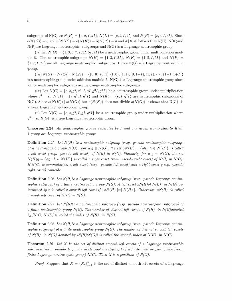
subgroups of N(G)are N(H) = e, a, I, aI, N(K) = e, b, I, bI and N(P ) = e, c, I, cI. Since
o(N(G)) = 8 and o(N(H)) = o(N(K)) = o(N(P )) = 4 and 4 | 8, it follows that N(H), N(K)and
N(P)are Lagrange neutrosophic subgroups and N(G) is a Lagrange neutrosophic group.
(ii) Let N(G) = 1, 3, 5, 7, I, 3I, 5I, 7I be a neutrosophic group under multiplication mod-
ulo 8. The neutrosophic subgroups N(H) = 1, 3, I, 3I, N(K) = 1, 5, I, 5I and N(P ) =
1, 7, I, 7I are all Lagrange neutrosophic subgroups. Hence N(G) is a Lagrange neutrosophic
group.
(iii) N(G) = N (Z2)×N (Z2) = (0, 0), (0, 1), (1, 0), (1, 1), (0, 1+I), (1, I), · · · , (1+I, 1+I)is a neutrosophic group under addition modulo 2. N(G) is a Lagrange neutrosophic group since
all its neutrosophic subgroups are Lagrange neutrosophic subgroups.
(iv) Let N(G) = e, g, g2, g3, I, gI, g2I, g3I be a neutrosophic group under multiplication
where g4 = e. N(H) = e, g2, I, g2I and N(K) = e, I, g2I are neutrosophic subgroups of
N(G). Since o(N(H)) | o(N(G)) but o(N(K)) does not divide o(N(G)) it shows that N(G) is
a weak Lagrange neutrosophic group.
(v) Let N(G) = e, g, g2, I, gI, g2I be a neutrosophic group under multiplication where
g3 = e. N(G) is a free Lagrange neutrosophic group.
Theorem 2.24 All neutrosophic groups generated by I and any group isomorphic to Klein
4-group are Lagrange neutrosophic groups.
Definition 2.25 Let N(H) be a neutrosophic subgroup (resp. pseudo neutrosophic subgroup)
of a neutrosophic group N(G). For a g ∈ N(G), the set gN(H) = gh : h ∈ N(H) is called
a left coset (resp. pseudo left coset) of N(H) in N(G). Similarly, for a g ∈ N(G), the set
N(H)g = hg : h ∈ N(H) is called a right coset (resp. pseudo right coset) of N(H) in N(G).
If N(G) is commutative, a left coset (resp. pseudo left coset) and a right coset (resp. pseudo
right coset) coincide.
Definition 2.26 Let N(H)be a Lagrange neutrosophic subgroup (resp. pseudo Lagrange neutro-
sophic subgroup) of a finite neutrosophic group N(G). A left coset xN(H)of N(H) in N(G) de-
termined by x is called a smooth left coset if | xN(H) |=| N(H) |. Otherwise, xN(H) is called
a rough left coset of N(H) in N(G).
Definition 2.27 Let N(H)be a neutrosophic subgroup (resp. pseudo neutrosophic subgroup) of
a finite neutrosophic group N(G). The number of distinct left cosets of N(H) in N(G)denoted
by [N(G):N(H)] is called the index of N(H) in N(G).
Definition 2.28 Let N(H)be a Lagrange neutrosophic subgroup (resp. pseudo Lagrange neutro-
sophic subgroup) of a finite neutrosophic group N(G). The number of distinct smooth left cosets
of N(H) in N(G) denoted by [N(H):N(G)] is called the smooth index of N(H) in N(G).
Theorem 2.29 Let X be the set of distinct smooth left cosets of a Lagrange neutrosophic
subgroup (resp. pseudo Lagrange neutrosophic subgroup) of a finite neutrosophic group (resp.
finite Lagrange neutrosophic group) N(G). Then X is a partition of N(G).
Proof Suppose that X = Xini=1 is the set of distinct smooth left cosets of a Lagrange

Neutrosophic Groups and Subgroups 7
neutrosophic subgroup (resp. pseudo Lagrange neutrosophic subgroup) of a finite neutro-
sophic group (resp. finite Lagrange neutrosophic group) N(G). Since o(N(H)) | o(N(G)) and
| xN(H) |=| N(H) | ∀ x ∈ N(G), it follows that X is not empty and every member of N(G) be-
longs to one and only one member of X. Hence ∩ni=1Xi = ∅ and ∪n
i=1Xi = N(G). Consequently,
X is a partition of N(G).
Corollary 2.30 Let [N(H) : N(G)] be the smooth index of a Lagrange neutrosophic subgroup in
a finite neutrosophic group (resp. finite Lagrange neutrosophic group) N(G). Then | N(G) |=|N(H) | [N(H) : N(G)].
Proof The proof follows directly from Theorem 2.29.
Theorem 2.31 Let X be the set of distinct left cosets of a neutrosophic subgroup (resp. pseudo
neutrosophic subgroup) of a finite neutrosophic group N(G). Then X is not a partition of N(G).
Proof Suppose that X = Xini=1 is the set of distinct left cosets of a neutrosophic subgroup
(resp. pseudo neutrosophic subgroup) of a finite neutrosophic group N(G). Since N(H) is a non-
Lagrange pseudo neutrosophic subgroup, it follows that o(N(H)) is not a divisor of o(N(G))
and | xN(H) |6=| N(H) | ∀ x ∈ N(G). Clearly, X is not empty and every member of N(G) can
not belongs to one and only one member of X. Consequently, ∩ni=1Xi 6= ∅ and ∪n
i=1Xi 6= N(G)
and thus X is not a partition of N(G).
Corollary 2.32 Let [N(G) : N(H)] be the index of a neutrosophic subgroup (resp. pseudo
neutrosophic subgroup) in a finite neutrosophic group N(G). Then | N(G) |6=| N(H) | [N(G) :
N(H)].
Proof The proof follows directly from Theorem 2.31.
Example 2.33 Let N(G)be a neutrosophic group of Example 2.23(iv).
(a) Distinct left cosets of the Lagrange neutrosophic subgroup N(H) = e, g2, I, g2I are:
X1 = e, g2, I, g2I, X2 = g, g3, gI, g3I, X3 = I, g2I, X4 = gI, g3I. X1, X2 are smooth
cosets while X3, X4 are rough cosets and therefore [N(G) : N(H)] = 4, [N(H) : N(G)] = 2.
| N(H) | [N(G) : N(H)] = 4 × 4 6=| N(G) | and | N(H) | [N(H) : N(G)] = 4 × 2 =| N(G) |.X1 ∩ X2 = ∅ and X1 ∪ X2 = N(G) and hence the set X = X1, X2 is a partition of N(G).
(b) Distinct left cosets of the pseudo non-Lagrange neutrosophic subgroup N(H) = e, I, g2Iare: X1 = e, I, g2I, X2 = g, gI, g3I, X3 = g2, I, g2I, X4 = g3, gI, g3I, X5 = I, g2I,X6 = gI, g3I. X1, X2, X3, X4 are smooth cosets while X5, X6 are rough cosets. [N(G) :
N(H)] = 6, [N(H) : N(G)] = 4, | N(H) | [N(G) : N(H)] = 3 × 6 6=| N(G) | and
| N(H) | [N(H) : N(G)] = 3 × 4 6=| N(G) |. Members of the set X = X1, X2, X3, X4are not mutually disjoint and hence do not form a partition of N(G).
Example 2.34 Let N(G) = 1, 2, 3, 4, I, 2I, 3I, 4I be a neutrosophic group under multipli-
cation modulo 5. Distinct left cosets of the non-Lagrange neutrosophic subgroup N(H) =
1, 4, I, 2I, 3I, 4I are X1 = 1, 4, I, 2I, 3I, 4I, X2 = 2, 3, I, 2I, 3I, 4I, X3 = I, 2I, 3I, 4I.X1, X2 are smooth cosets while X3 is a rough coset and therefore [N(G) : N(H)] = 3,

8 Agboola A.A.A., Akwu A.D. and Oyebo Y.T.
[N(H) : N(G)] = 2, | N(H) | [N(G) : N(H)] = 6 × 3 6=| N(G) | and | N(H) | [N(H) :
N(G)] = 6 × 2 6=| N(G) |. Members of the set X = X1, X2 are not mutually disjoint and
hence do not form a partition of N(G).
Example 2.35 Let N(G)be the Lagrange neutrosophic group of Example 2.5. Distinct left
cosets of the Lagrange neutrosophic subgroup N(H) = e, a, I, aI are: X1 = e, a, I, aI,X2 = b, c, bI, cI, X3 = I, aI, X4 = bI, cI. X1, X2 are smooth cosets while X3, X4 are
rough cosets and thus [N(G) : N(H)] = 4, [N(H) : N(G)] = 2, | N(H) | [N(G) : N(H)] =
4 × 4 = 16 6=| N(G) | and | N(H) | [N(H) : N(G)] = 4 × 2 = 8 =| N(G) |. Members of the set
X = X1, X2 are mutually disjoint and N(G) = X1 ∪ X2. Hence X is a partition of N(G).
Example 2.36 Let N(G)be the Lagrange neutrosophic group of Example 2.23(iii).
(a) Distinct left cosets of the Lagrange neutrosophic subgroup N(H) = (0, 0), (0, 1), (0, I),
(0, 1+I) are respectively X1 = (0, 0), (0, 1), (0, I), (0, 1+I), X2 = (1, 0), (1, 1), (1, I), (1, 1+
I), X3 = (I, 0), (I, 1), (I, I), (I, 1 + I), X4 = (I + I, 0), (1 + I, 1), (1 + I, I), (1 + I, 1 + I),X5 = (1+ I, 0), (1+ I, 1), (1+ I, 1+ I). X1, X2, X3, X4 are smooth cosets while X5 is a rough
coset. Thus, [N(G) : N(H)] = 5, [N(H) : N(G)] = 4, | N(H) | [N(G) : N(H)] = 4 × 5 =
20 6=| N(G) |= 16 and | N(H) | [N(H) : N(G)] = 4 × 4 = 16 =| N(G) |. Members of the set
X = X1, X2, X3, X4 are mutually disjoint and N(G) = X1 ∪ X2 ∪ X3 ∪ X4 so that X is a
partition of N(G).
(b) Distinct left cosets of the pseudo Lagrange neutrosophic subgroup N(H) = (0, 0), (0, I),
(I, 0), (I, I) are respectively X1 = (0, 0), (0, I), (I, 0), (I, 1), X2 = (0, 1), (0, 1 + I), (I, 1),
(I, 1+I), X3 = (1, 0), (1, I), (1+I, 0), (1+I, I), X4 = (1, 1), (1, 1+I), (1+I, 1), (1+I, 1+I).X1, X2, X3, X4 are smooth cosets and [N(G) : N(H)] = [N(H) : N(G)] = 4. Consequently,
| N(H) | [N(G) : N(H)] =| N(H) | [N(H) : N(G)] = 4 × 4 = 16 =| N(G) |. Members of the
set X = X1, X2, X3, X4 are mutually disjoint, N(G) = X1 ∪ X2 ∪ X3 ∪ X4 and hence X is a
partition of N(G).
References
[1] Vasantha Kandasamy W.B. and Florentin Smarandache, Some Neutrosophic Algebraic
Structures and Neutrosophic N-Algebraic Structures, Hexis, Phoenix, Arizona, 2006.
[2] Vasantha Kandasamy W.B. and Florentin Smarandache, Basic Neutrosophic Algebraic
Structures and Their Applications to Fuzzy and Neutrosophic Models, Hexis, Church Rock,
2004.
[3] Florentin Smarandache, A Unifying Field in Logics: Neutrosophic Logic, Neutrosophy,
Neutrosophic Set, Neutrosophic Probability, (3rd edition), American Research Press, Re-
hoboth, 2003.
[4] Agboola A.A.A. and Akinola L.S., On the bicoset of a bivector space, International J.
Math. Combin. Vol.4, 1-8, 2009.
[5] Agboola A.A.A., Akinola A.D. and Oyebola O.Y., Neutrosophic rings I, International J.
Math. Combin. Vol.4, 1-14, 2011.
[6] Agboola A.A.A., Adeleke E.O. and Akinleye S.A., Neutrosophic rings II, International J.

Neutrosophic Groups and Subgroups 9
Math. Combin., Vol.2, 1-8, 2012.
[7] Herstein I.N., Topics in Algebra, Wiley Eastern Limited, 1975.
[8] Fraleigh J.B., A First Course in Abstract Algebra (5th edition), Addison-Wesley Publishing
Company, 1994.
[9] Marshall H., Theory of Groups, The Macmillan Company, New York, 1994.
[10] Lang S., Algebra, Addison Wesley, 1984.

Math.Combin.Book Ser. Vol.3(2012), 10-19
On Bitopological Supra B-Open Sets
M.Lellis Thivagar
(Department of Mathematics, Madurai Kamaraj University, Madurai-625 021, Tamil Nadu, India)
B.Meera Devi
(Department of Mathematics,Sri.S.R.N.M College, Sattur-626203, Tamil Nadu, India)
E-mail: [email protected], [email protected]
Abstract: In this paper, we introduce and investigate a new class of sets and maps be-
tween bitopological spaces called supra(1,2) b-open, and supra (1,2) b-continuous maps,
respectively. Furthermore, we introduce the concepts of supra(1,2) locally-closed, supra(1,2)
locally b-closed sets. We also introduce supra(1,2) extremely disconnected. Finally, addi-
tional properties of these sets are investigated.
Key Words: Supra(1,2) b-open set, supra(1,2) locally closed, supra(1,2) b-closed,
supra(1,2) extremely disconnected.
AMS(2010): 54C55
§1. Introduction
In 1983 A.S.Mashhour et al [5] introduced supra topological spaces and studied s-continuous
maps and s∗-continuous maps. Andrijevic [1] introduced a class of generalized open sets in a
topological space,the called b-open sets in 1996. In 1963, J.C.Kelly [3] introduced the concept
of bitopological spaces. The purpose of this present paper is to define some properties by
using supra(1,,2) b-open sets, supra(1,2) locally-closed, supra(1,2) locally b-closed in supra
bitopological spaces and investigate the relationship between them.
§2. Preliminaries
Throughout this paper by (X, τ1, τ2), (Y, σ1, σ2) and (Z, η1, η2). (or simply X, Y and Z) rep-
resent bitopological spaces on which no separation axioms are assumed unless otherwise men-
tioned. For a subset A of X , Ac denote the complement of A. A subcollection µ is called a supra
topology [5] on X if X ∈ µ, where µ is closed under arbitrary union. (X, µ) is called a supra
topological space. The elements of µ are said to be supra open in (X, µ) and the complement of
a supra open set is called a supra closed set. The supra topology µ is associated with the topol-
1Received July 13, 2012. Accepted August 20, 2012.

On Bitopological Supra B-Open Sets 11
ogy τ if τ ⊂ µ. A subset A of X is τ1τ2-open [4] if A∈ τ1 ∪ τ2 and τ1τ2-closed if its complement
is τ1τ2-open in X . The τ1τ2-closure of A is denoted by τ1τ2cl(A) and τ1τ2cl(A) = ∩ F : A ⊂ F
and F c is τ1τ2-open. Let (X,µ1, µ2) be a supra bitopological space. A set A is µ1µ2-open if
A ∈ µ1 ∪ µ2 and µ1µ2-closed if its complement is µ1µ2-open in (X, µ1, µ2). The µ1µ2-closure
of A is denoted by µ1µ2cl(A) and µ1µ2cl(A) = ∩ F : A ⊂ F and F c is µ1µ2 − open.
Definition 2.1 Let (X, µ) be a supra topological space. A set A is called
(1) supra α-open set [2] if A ⊆ intµ(clµ(intµ(A)));
(2) supra semi-open set [2] if A ⊆ clµ(intµ(A));
(3) supra b-open set [6] if A ⊆ clµ(intµ(A)) ∪ intµ(clµ(A)).
Definition 2.2([4]) Let (X, τ1, τ2) be a bitopological space. A subset A of (X, τ1, τ2) is called
(1) (1,2)semi-open set if A ⊆ τ1τ2cl(τ1int(A));
(2) (1,2)pre-open set if A ⊆ τ1int(τ1τ2cl(A));
(3) (1,2)α-open-set if A ⊆ τ1int(τ1τ2cl(τ1int(A)));
(4) (1,2)b-open-set A ⊆ τ1τ2cl(τ1int(A)) ∪ τ1int(τ1τ2cl(A)).
§3. Comparison
In this section we introduce a new class of generalized open sets called supra(1,2) b-open sets
and investigate the relationship between some other sets.
Definition 3.1 Let (X, τ1, τ2) be a supra bitopological space. A set A is called a supra(1,2)
b-open set if A ⊆ µ1µ2cl(µ1int(A)) ∪ µ1int(µ1µ2cl(A)).The compliment of a supra(1,2) b-open
is called a supra(1,2) b-closed set.
Definition 3.2 Let X be a supra bitopological space. A set A is called
(1) supra (1,2) semi-open set if A ⊆ µ1µ2cl(µ1int(A));
(2) supra (1,2) pre-open set if A ⊆ µ1int(µ1µ2cl(A));
(3) supra (1,2) α-open-set if A ⊆ µ1int(µ1µ2cl(µ1int(A))).
Theorem 3.3 In a supra bitopological space (X, µ1, µ2), any supra open set in (X, µ1) is
supra(1,2) b-open set and any supra open set in (X, µ2) is supra (2,1) b-open set.
Proof Let A be any supra open in (X, µ1). Then A = µ1int(A). Now A ⊆ µ1µ2cl(A) =
µ1µ2cl(µ1int(A)) ⊆ µ1µ2cl(µ1int(A) ∪ µ1int(µ1µ2cl(A)). Hence A is supra(1,2) b-open set.
Similarly, any supra open in (X, µ2) is supra(2,1) b-open set.
Remark 3.4 The converse of the above theorem need not be true as shown by the following
example.
Example 3.5 Let X = a, b, c, d, µ1 = φ, X, a, b, a, c, d, µ2 = φ, a, a, b, b, c, d, X;µ1µ2-open = φ, a, a, b, a, c, d, b, c, d, X, µ1µ2-closed = φ, a, b, c, d, b, c, d, X,

12 M.Lellis Thivagar and B.Meera Devi
supra(1,2) bO(X) = φ, a, b, a, c, a, d, a, b, c, a, b, d, a, c, d,X. It is obvious that
a,d∈ supra(1,2) b-open but a, d /∈ µ1-open. Also, supra(2,1) bO(X) = (φ, a, a, b,a, c, a, d, b, c, b, d, a, b, c, a, c, d, a, b, d, b, c, d,X. Here a, c ∈ supra(2,1) b-
open set but a, c /∈ µ2-open.
Theorem 3.6 In a supra bitopological space (X, µ1, µ2), any supra open set in (X, µ1) is
supra(1,2) α-open set and any supra open set in (X, µ2) is supra (2,1) α-open set.
Proof Let A be any supra open in (X, µ1). Then A = µ1int(A). Now A ⊆ µ1µ2cl(A).
Then µ1int(A) ⊆ µ1int(µ1µ2cl(A)). Since A = µ1int(A), A ⊆ µ1int(µ1µ2cl(µ1int(A))). Hence
A is supra(1,2) α-open set. Similarly, any supra open in (X, µ2) is supra(2,1) α-open set.
Remark 3.7 The converse of the above theorem need not be true as shown in the following
example.
Example 3.8 Let X = a, b, c, d, µ1 = φ, a, c, a, b, c, a, b, d, X, µ2 = φ, c, d, a, b, d,b, c, d, X, µ1µ2-open = φ, a, c, c, d, a, b, c, a, b, d, b, c, d, X, µ1µ2-closed = φ, a,c, d, a, b, b, d, X. supra(1,2) αO(X) = φ, a, c, a, b, c, a, c, d, a, b, d,X. Here
a, c, d ∈ supra(1, 2) α-open but a, c, d /∈ µ1-open. Also, supra(2,1) αO(X) = (φ, c, d,a, c, d, a, b, d, b, c, d, X. Here a, c, d ∈ supra(2, 1)α-open but a, c, d /∈ µ2-open.
Theorem 3.9 Every supra(1,2) α-open is supra(1,2) semi-open.
Proof Let A be a supra (1,2) α-open set in X . Then A ⊆ µ1int(µ1µ2cl(µ1int(A))) ⊆µ1µ2cl(µ1int(A)). Therefore, A ⊆ µ1µ2cl(µ1int(A)). Hence A is supra(1,2) semi-open set.
Remark 3.10 The converse of the above theorem need not be true as shown below.
Example 3.11 Let X = a, b, c, d, µ1 = φ, b, a, d, a, b, c, X, µ2 = φ, b, c, a, b, d, X,µ1µ2-open =φ, b, a, d, b, c, a, b, c, a, b, d, X, µ1µ2-closed = φ, c, d, a, d, b, c,a, c, d, X. supra(1,2) αO(X) = φ, b, a, d, a, b, c, a, b, d, X, supra(1,2) SO(X) =
φ, b, a, d, b, c, a, b, c, a, b, d, X. Here b, c is a supra(1,2) α-open but not supra(1,2)
semi-open.
Theorem 3.12 Every supra(1,2) semi-open set is supra(1,2) b-open.
Proof Let A be a supra(1,2) semi-open set X . Then A ⊆ µ1µ2cl(µ1int(A)). Hence
A ⊆ µ1µ2cl(µ1int(A)) ∪ µ1int(µ1µ2cl(A)). Thus A is supra(1,2) b-open set.
Remark 3.13 The converse of the above theorem need not be true as shown in the following
example.
Example 3.14 Let X = a, b, c, d, µ1 = φ, a, a, b, b, c, d, X, µ2 = φ, b, a, d, a, b, d,b, c, d, X, µ1µ2-open = φ, a, b, a, b, a, d, a, b, d, b, c, d, X, µ1µ2-closed = φ, a,c, b, c, c, d, a, c, d, b, c, d,X, supra(1,2) bO(X) = φ, a, a, b, b, d, a, b, c, a, b, d,b, c, d, X, supra(1,2) SO(X) = φ, a, a, b, a, b, c, a, b, d, b, c, d, X. Here b, d ∈supra(1, 2)b-open set but b, d /∈ supra(1,2) semi-open.

On Bitopological Supra B-Open Sets 13
Theorem 3.15 Every supra(1,2) α-open is supra(1,2) b-open.
Proof Let A be an supra(1,2) α-open in X . Then A ⊆ µ1int(µ1µ2cl(µ1int(A))). It is obvi-
ous that µ1int(µ1µ2cl(µ1int(A))) ⊆ µ1µ2cl(µ1int(A)) ⊆ µ1µ2cl(µ1int(A)) ∪ µ1int(µ1µ2cl(A)).
Hence A ⊆ µ1µ2cl(µ1int(A)) ∪ µ1int(µ1µ2cl(A)). Thus A is supra(1,2) b-open set.
Remark 3.16 The reverse claim in Theorem 3.15 is not usually true.
Example 3.17 Let X = a, b, c, d,µ1 = φ, a, c, a, b, c, a, b, d, X,µ2 = φ, c, d, b, c, d,a, b, dX,µ1µ2-open= φ, a, c, c, d, a, b, c, a, b, db, c, d, Xµ1µ2-closed = φ, a, c,d, a, b, b, d, X, supra(1,2) αO(X) = φ, a, c, a, b, c, a, c, d, a, b, d,X, supra(1,2)
bO(X) = φ, a, c, a, d, b, c, c, da, b, c, a, c, d, a, b, d, b, c, d, X. Here a, d ∈supra(1,2) b-open but a, d /∈ supra(1,2) α-open.
Theorem 3.18 In a supra bitopological space (X, µ1, µ2), any supra open set in (X, µ1) is
supra(1,2) semi-open set and any supra open set in (X, µ2) is supra (2,1) semi-open set.
Proof This follows immediately from Theorems 3.6 and 3.9.
Remark 3.19 The converse of the above theorem need not be true as shown in the Example
3.8, a, c, d is both supra(1,2) semi-open and supra(2,1) semi-open but it is not supra µ1-open
and also is not µ2-open.
Remark 3.20 From the above discussions we have the following diagram. A →B represents A
implies B, A 9 B represents A does not implies B.
2
3
1
4
¸
Fig. 1 1=supra (1,2) b-open, 2=µ1-open,¸
3=supra (1,2) α-open, 4=supra (1,2) semi-open
§4. Properties of Supra(1,2) b-Open Sets
Theorem 4.1 A finite union of supra(1,2) b-open sets is always supra(1,2) b-open.
Proof Let A and B be two supra(1,2) b-open sets. Then A ⊆ µ1µ2cl(µ1int(A)) ∪

14 M.Lellis Thivagar and B.Meera Devi
µ1int(µ1µ2cl(A)) and B ⊆ µ1µ2cl(µ1int(B))∪µ1int(µ1µ2cl(B)). Now, A∪B ⊆ µ1µ2cl(µ1int(A∪B)) ∪ µ1int(µ1µ2cl(A ∪ B)). Hence A ∪ B is supra(1,2) b-open set.
Remark 4.2 Finite intersection of supra(1,2) b-open sets may fail to be supra(1,2) b-open
since, in Example 3.14, both a, b and b, d are supra(1,2) b-open sets, but their intersection
c is not supra(1,2) b-open.
Definition 4.3 The supra(1,2) b-closure of a set A is denoted by supra(1, 2)bcl(A) and defined
as supra(1, 2)bcl(A) = ∩B : B is a supra(1,2) b-closed set and A ⊂ B. The supra(1,2)
interior of a set A is denoted by supra(1,2)bint(A), and defined as supra(1,2)b int(A)= ∪B : B
is a supra(1,2) b-open set and A ⊇ B.
Remark 4.4 It is clear that supra(1, 2)bint(A) is a supra(1,2) b-open and supra(1, 2)bcl(A) is
supra(1,2) b-closed set.
Definition 4.5 A subset A of supra bitopological space X is called
(1) supra(1,2)locally-closed if A = U∩V, where U ∈ µ1 and V is supraµ1µ2 closed;
(2) supra(1,2) locally b-closed if A = U ∩ V , where U ∈ µ1 and V is supra(1,2) b-closed;
(3) supra (1,2)D(c,b) set if µ1int(A) = supra(1, 2)bint(A).
Theorem 4.6 The intersection of a supra open in (X, µ1) and a supra(1,2) b-open set is a
supra(1,2) b-open set.
Proof Let A be supra open in (X, µ1). Then A is supra(1,2) b-open and A = µ1int(A) ⊆supra(1, 2)bint(A). Let B be supra(1,2) b-open then B = supra(1, 2)bint(B). Now A ∩ B ⊆supra(1, 2)bint(A) ∩ supra(1, 2)bint(B) = supra(1, 2)bint(A ∩ B). Hence the intersection of
supra open set in (X, µ1) and a supra(1,2) b-open set is a supra(1,2) b-open set.
Theorem 4.7 For a subset A of X, the following are equivalent:
(1) A is supra-open in (X, µ1);
(2) A is supra (1,2) b-open and supra(1,2) D(c,b)-set.
Proof (1)⇒(2) If A is supra-open in (X, µ1), then A is supra (1,2) b-open and A =
µ1int(A), A = supra(1, 2)bint(A). Hence µ1int(A) = supra(1, 2)bint(A). Therefore, A is
supra(1, 2)D(c, b)-set.
(2)⇒(1) Let A be supra (1,2) b-open and supra (1, 2)D(c, b)-set. Then A = supra(1, 2)bint(A)
and µ1int(A) = supra(1, 2)bint(A). Hence A = µ1int(A). This implies that A is supra-open in
(X, µ1).
Definition 4.8 A space X is called an supra(1,2) extremely disconnected space (briefly supra(1,2)
E.D) if supraµ1µ2 closure of each supra-open in (X, µ1) is supra open set in (X, µ1). Similarly
supraµ1µ2 closure of each supra-open in (X, µ2) is supra open set in (X, µ2).
Example 4.9 Let X = a, b, c, µ1 = φ, b, a, b, a, c, X, µ2 = φ, a, b, c, a, c,µ1µ2open = φ, a, b, a, b, a, c, b, c, X, µ1µ2 closed = φ, a, b, c, a, cb, c, X.

On Bitopological Supra B-Open Sets 15
Hence every µ1µ2 closure of supra-open is (X, µ1) and also every supraµ1µ2 closure of supra-
open in (X, µ2).
Theorem 4.10 Let A be a subset of supra bitopological space (X, µ1, µ2) if A is supra(1,2)
locally b-closed, then
(1) supra(1, 2)bcl(A) − A is supra(1,2) b-closed set:
(2) [A ∪ (X − supra(1, 2)bcl(A))] is supra(1,2) b-open;
(3) A ⊆ supra(1, 2)bint(A ∪ (X − supra(1, 2)bcl(A)).
Proof (1) If A is an supra(1,2) locally b-closed, there exist an U is supra-open in (X, µ1)
such that A = U ∩ supra(1, 2)bcl(A). Now, supra(1, 2)bcl(A) − A = supra(1, 2)bcl(A) − [U ∩supra(1, 2)bcl(A)] = supra(1, 2)bcl(A) ∩ [X − (U ∩ supra(1, 2)bcl(A))] = supra(1, 2)bcl(A) ∩[(X −U)∪ (X − supra(1, 2)bcl(A))] = supra(1, 2)bcl(A)∩ (X −U), which is supra(1,2) b-closed
by Theorem 4.5.
(2) Since supra(1, 2)bcl(A)− A is supra(1,2) b closed, then [X − (supra(1, 2)bcl(A)− A)]
is supra(1,2) b-open and [X − (supra(1, 2)bcl(A)− A)] = (X − supra(1, 2)bcl(A)) ∪ (X ∩ A) =
A ∪ [X − supra(1, 2)bcl(A)]. Hence [A ∪ (X − supra(1, 2)bcl(A))] is supra(1,2) b-open.
(3) It is clear that
A ⊆ [A ∪ (X − supra(1, 2)bcl(A)] = supra(1, 2)bint[A ∪ (X − supra(1, 2)bcl(A))].
§5. Supra (1,2) b-Continuous Functions
In this section, We introduce a new class of continuous maps called a supra (1,2) b-continuous
maps and obtain some of their properties.
Definition 5.1 Let (X, τ1, τ2) and (Y, σ1, σ2) be two bitopological spaces and µ1, µ2 be an
associated supra bitopology with τ1, τ2. A map f : (X, τ1, τ2) → (Y, σ1, σ2) is called a supra
(1,2) b-continuous map [resp. supra (1,2) α-continuous, supra (1,2) semi-continuous] if the
inverse image of each σ1σ2-open set in Y is supra (1,2) b-open set [resp. supra (1,2 ) α-open,
supra (1,2) semi-open] in X.
Definition 5.2 Let (X, τ1, τ2) and (Y, σ1, σ2) be two bitopological spaces and µ1, µ2 be an
associated supra bitopology with τ1, τ2. A function f : (X, τ1, τ2) → (Y, σ1, σ2) is called supra
(1,2) continuous if f−1(V ) is µ1-open in X for each σ1σ2-open set V of Y .
Theorem 5.3 Every (1,2) continuous is supra (1,2) b-continuous.
Proof Let f : (X, τ1, τ2) → (Y, σ1, σ2) be an (1,2)-continuous map and let A be an σ1σ2-
open set in (Y, σ1, σ2). Then f−1(A) is an τ1-open set in (X, τ1, τ2). Since µ1 and µ2 are
associated with τ1 and τ2, then τ1 ⊆ µ1. This implies that f−1(A) is µ1-open in X and it is
supra (1,2) b-open in X . Hence f is supra (1,2)b-continuous.
Theorem 5.4 Every supra (1,2)-continuous is supra (1,2) b-continuous function.
16 M.Lellis Thivagar and B.Meera Devi
Proof Let f : (X, τ1, τ2) → (Y, σ1, σ2) be an supra (1,2)-continuous and let A be an σ1σ2
open set in Y . Since f is supra (1,2)-continuous and µ1, µ2 associated with τ1, τ2, f−1(A) is
µ1-open in X and it is supra (1,2) b-open in X. Hence f is supra (1,2) b-continuous.
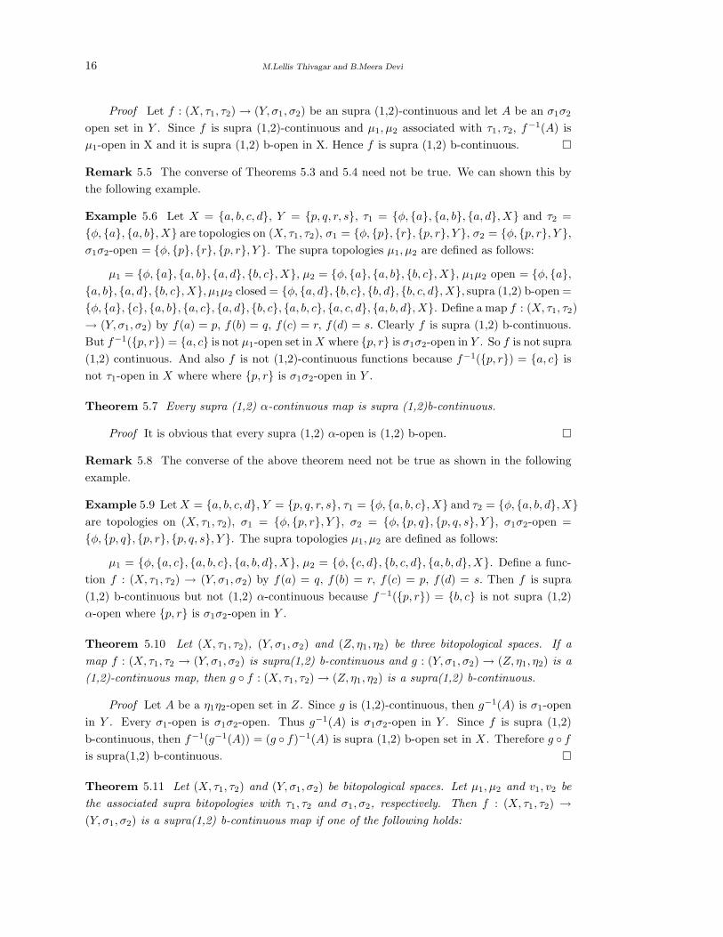
Remark 5.5 The converse of Theorems 5.3 and 5.4 need not be true. We can shown this by
the following example.
Example 5.6 Let X = a, b, c, d, Y = p, q, r, s, τ1 = φ, a, a, b, a, d, X and τ2 =
φ, a, a, b, X are topologies on (X, τ1, τ2), σ1 = φ, p, r, p, r, Y , σ2 = φ, p, r, Y ,σ1σ2-open = φ, p, r, p, r, Y . The supra topologies µ1, µ2 are defined as follows:
µ1 = φ, a, a, b, a, d, b, c, X, µ2 = φ, a, a, b, b, c, X, µ1µ2 open = φ, a,a, b, a, d, b, c, X, µ1µ2 closed = φ, a, d, b, c, b, d, b, c, d, X, supra (1,2) b-open =
φ, a, c, a, b, a, c, a, d, b, c, a, b, c, a, c, d, a, b, d, X. Define a map f : (X, τ1, τ2)
→ (Y, σ1, σ2) by f(a) = p, f(b) = q, f(c) = r, f(d) = s. Clearly f is supra (1,2) b-continuous.
But f−1(p, r) = a, c is not µ1-open set in X where p, r is σ1σ2-open in Y . So f is not supra
(1,2) continuous. And also f is not (1,2)-continuous functions because f−1(p, r) = a, c is
not τ1-open in X where where p, r is σ1σ2-open in Y .
Theorem 5.7 Every supra (1,2) α-continuous map is supra (1,2)b-continuous.
Proof It is obvious that every supra (1,2) α-open is (1,2) b-open.
Remark 5.8 The converse of the above theorem need not be true as shown in the following
example.
Example 5.9 Let X = a, b, c, d, Y = p, q, r, s, τ1 = φ, a, b, c, X and τ2 = φ, a, b, d, Xare topologies on (X, τ1, τ2), σ1 = φ, p, r, Y , σ2 = φ, p, q, p, q, s, Y , σ1σ2-open =
φ, p, q, p, r, p, q, s, Y . The supra topologies µ1, µ2 are defined as follows:
µ1 = φ, a, c, a, b, c, a, b, d, X, µ2 = φ, c, d, b, c, d, a, b, d, X. Define a func-
tion f : (X, τ1, τ2) → (Y, σ1, σ2) by f(a) = q, f(b) = r, f(c) = p, f(d) = s. Then f is supra
(1,2) b-continuous but not (1,2) α-continuous because f−1(p, r) = b, c is not supra (1,2)
α-open where p, r is σ1σ2-open in Y .
Theorem 5.10 Let (X, τ1, τ2), (Y, σ1, σ2) and (Z, η1, η2) be three bitopological spaces. If a
map f : (X, τ1, τ2 → (Y, σ1, σ2) is supra(1,2) b-continuous and g : (Y, σ1, σ2) → (Z, η1, η2) is a
(1,2)-continuous map, then g f : (X, τ1, τ2) → (Z, η1, η2) is a supra(1,2) b-continuous.
Proof Let A be a η1η2-open set in Z. Since g is (1,2)-continuous, then g−1(A) is σ1-open
in Y . Every σ1-open is σ1σ2-open. Thus g−1(A) is σ1σ2-open in Y . Since f is supra (1,2)
b-continuous, then f−1(g−1(A)) = (g f)−1(A) is supra (1,2) b-open set in X . Therefore g f
is supra(1,2) b-continuous.
Theorem 5.11 Let (X, τ1, τ2) and (Y, σ1, σ2) be bitopological spaces. Let µ1, µ2 and v1, v2 be
the associated supra bitopologies with τ1, τ2 and σ1, σ2, respectively. Then f : (X, τ1, τ2) →(Y, σ1, σ2) is a supra(1,2) b-continuous map if one of the following holds:

On Bitopological Supra B-Open Sets 17
(1) f−1(supra(1, 2)bint(A)) ⊆ τ1int(f−1(A)) for every set A in Y ;
(2) τ1τ2cl(f−1(A)) ⊆ f−1(supra(1, 2)bcl(A)) for every set A in Y ;
(3) f(τ1τ2cl(B)) ⊆ supra(1, 2)bcl(f(B)) for every set B in X.
Proof Let A be any σ1σ2-open set of Y . If condition (1) is satisfied, then
f−1(supra(1, 2)bint(A)) ⊆ τ1int(f−1(A)).
We get, f−1(A) ⊆ τ1int(f−1(A)). Therefore f−1(A) is supra open set in (X, µ1). Every supra
open set in (X, µ1) is supra(1,2) b-open set. Hence f is supra (1,2) b-continuous function.
If condition (2) is satisfied, then we can easily prove that f is supra(1,2) b-continuous
function.
Now if the condition (3) is satisfied and A be any σ1σ2-open set of Y . Then f−1(A) is a set
in X and f(τ1τ2cl(f−1(A))) ⊆ supra(1, 2)bcl(f(f−1(A))). This implies f(τ1τ2cl(f
−1(A))) ⊆supra(1, 2)bcl(A). It is nothing but just the condition (2). Hence f is a supra(1,2) b-continuous
map.
§6. Applications
Now we introduce a new class of space called a supra(1,2)-extremely disconnected space.
Definition 6.1 A space X is called an supra(1,2)-extremely disconnected space (briefly supra
(1,2)-E.D) if µ1µ2 closure of each supra-open in (X, µ1) is supra-open set in (X, µ1). Similarly
µ1µ2-closure of each supra-open in (X, µ2) is supra-open set in (X, µ2).
Theorem 6.2 For a subset A of a supra(1,2) extremely disconnected space X, the following
are equivalent:
(1) A is supra-open in (X, µ1);
(2) A is supra(1,2) b-open and supra(1,2) locally closed.
Proof (1)⇒(2) It is obvious.
(2)⇒(1) Let A be supra(1,2) b-open and supra(1,2) locally closed. Then
A ⊆ µ1µ2cl(µ1int(A)) ∪ µ1int(µ1µ2cl(A)) and A = U ∩ µ1µ2cl(A),
where U is supra-open in (X, µ1). So A ⊆ U ∩ (µ1int(µ1µ2cl(A)) ∪ µ1µ2cl(µ1int(A)) ⊆[µ1int(U∩µ1µ2cl(A))]∪[U∩µ1µ2cl(µ1int(A))] ⊆ [µ1int(U∩µ1µ2cl(A))]∪[U∩µ1int(µ1µ2cl(A))]
(since X is supra(1,2) E.D)⊆ [µ1int(U ∩ µ1µ2cl(A))] ∪ [µ1int(U ∩ µ1µ2cl(A))] = µ1int(A) ∪µ1int(A) = µ1int(A). Hence A ⊆ µ1int(A). Therefore A is supra-open in (X, µ1).
Theorem 6.3 Let (X, τ1, τ2) and (Y, σ1, σ2) be two bitopological spaces and µ1, µ2 be associated
supra topologies with τ1, τ2. Let f : X → Y be a map. Then the following are equivalent.
(1) f is supra (1,2) b-continuous map;
(2) The inverse image of a σ1σ2-closed set in Y is a supra (1,2) b-closed set in X;

18 M.Lellis Thivagar and B.Meera Devi
(3) Supra (1, 2)bcl(f−1(A) ⊆ f−1(σ1σ2cl(A)) for every set A in Y ;
(4) f(supra(1, 2)bcl(A)) ⊆ σ1σ2cl(f(A)) for every set A ∈ X;
(5) f−1(σ1(B)) ⊆ supra(1, 2)int(f−1(B)) for every B in Y .
Proof (1)⇒(2) Let A be a σ1σ2 closed set in Y , then Y −A is σ1σ2 open set in Y . Since
f is supra (1,2) b-continuous, f−1(Y −A) = X − f−1(A) is a supra (1,2) b-open set in X . This
implies that f−1(A) is a supra (1,2) b-closed subset of X .
(2)⇒(3) Let A be any subset of Y . Since σ1σ2cl(A) is σ1σ2 closed in Y , then f−1(σ1σ2cl(A))
is supra (1,2) b-closed in X . Hence supra (1, 2)bcl(f−1(A) ⊆ supra(1, 2)bcl(f−1(σ1σ2cl(A))) =
f−1(σ1σ2cl(A)).
(3)⇒(4) Let A be any subset of X . By (3), we obtain
f−1(σ1σ2cl(f(A))) ⊇ supra(1, 2)bclf−1(f(A)) ⊇ supra(1, 2)bcl(A).
Hence f(supra(1, 2)cl(A)) ⊆ σ1σ2cl(f(A)).
(4)⇒(5) Let B be any subset of Y . By (5), f(supra(1, 2)bcl(X−f−1(B))) ⊂ σ1σ2cl(f(X−f−1(B))) and f(X − supra(1, 2)bint(f−1(B))) ⊆ σ1σ2cl(Y −B) = Y −σ1int(B). Therefore we
have
X − supra(1, 2)bint(f−1(B)) ⊂ f−1(Y − σ1int(B))
and
f−1(σ1int(B)) ⊂ supra(1, 2)bint(f−1(B)).
(5)⇒(1) Let B be a σ1-open set in Y . Then by (4), f−1(σ1int(B)) ⊆ supra(1, 2)int(f−1(B)).
Therefore f−1(B) ⊆ supra(1, 2)int(f−1(B)). But supra(1, 2)bint(f−1(B)) ⊆ f−1(B). Hence
f−1(B) = supra(1, 2)bint(f−1(B)). Therefore f−1(B) is supra (1,2) b-open in X . Thus f is
supra (1,2) b-continuous map.
We introduce the following definition.
Definition 6.4 Let (X, τ1, τ2) and (Y, σ1, σ2) be two bitopological spaces and µ1, µ2 be associated
supra bitopologies with τ1, τ2. A map f : (X, τ1, τ2) → (Y, σ1, σ2) is called a supra (1,2) locally
closed continuous [resp. supra (1,2) D(c,b) continuous, supra (1,2) locally b-closed continuous]
if f−1(B) is supra (1,2) locally closed [resp. supra (1,2) D(c,b) set, supra (1,2) locally b-closed]
in X for each σ1σ2 open set V of Y .
Theorem 6.5 Let X be supra (1,2) extremely disconnected space, the function f : (X, τ1, τ2) →(Y, σ1, σ2) is supra (1,2)-continuous iff f is supra (1,2) b-continuous and supra (1,2) locally
closed continuous.
Proof Let V be a σ1σ2-open set in Y . Since f is supra (1,2)-continuous, f−1(V ) is µ1-open
in X . Then by Theorem 3.3, f−1(V ) is supra (1,2) b-open and supra (1,2) locally closed in
X . Hence f is supra (1,2) b-continuous and supra (1,2) locally closed continuous. Conversely,
let U be a σ1σ2-open set in Y . Since f is supra (1,2) b-continuous and supra (1,2) locally
closed continuous, f−1(U) is supra (1,2) b-open and supra (1,2) locally-closed in X . Since X is
supra (1,2) extremely disconnected, by Theorem 6.1, f−1(U) is µ1-open in X. Hence f is supra
(1,2)-continuous.

On Bitopological Supra B-Open Sets 19
Theorem 6.6 The function f : (X, τ1, τ2) → (Y, σ1, σ2) is supra (1,2) continuous iff f is supra
(1,2) b-continuous and supra (1,2) D(c,b)-continuous.
Proof Let V be a σ1σ2 open set in Y . Since f is supra (1,2) continuous, f−1(V ) is µ1-open
in X. By Theorem 4.7, f−1(V ) is supra (1,2) b-open and supra (1,2) D(c,b)set. Then f is supra
(1,2) b-continuous and supra (1,2) D(c,b)continuous. Conversely, let U be a σ1σ2 open in Y .
Since f is supra (1,2) b-continuous and supra (1,2) D(c,b)-continuous, f−1(U) is supra (1,2)
b-open and supra (1,2) D(c,b)set. By Theorem 4.7, f−1(U) is supra open in (X,µ1). Hence f
is supra (1,2) continuous.
References
[1] Andrijevic D., On b-open sets, Mat. Vesnik, 48(1996), 59-64.
[2] Devi R, Sampathkumar S. and Caldas M., On supra α-open sets and sα-continuous maps,
Genaral Mathematics, 16 (2)(2008), 77-84.
[3] Kelly J. C., Bitopological spaces, Proc. London Math. Soc., 13 (1963), No.3, 71-89.
[4] Lellis Thivagar M. and Ravi O., on strong forms of (1,2) quotient mappings, Int. J. of
Mathematics, Game theory and Algebra, Vol.14, 6(2004), 481-492.
[5] Mashhour A.S., Allam A.A., Mahmoud F.S., Khedr F.H., On supra topological spaces,
Indian J. Pure and Appl. Math., 14(4) (1983), 502-510.
[6] Sayed O.R. and Takashi Noiri, On supra b-open sets and supra b-continuity on topological
spaces, European J. Pure and Appl. Math., Vol.3, No.2 (2010), 295-302.

Math.Combin.Book Ser. Vol.3(2012), 20-29
On Finsler Space with Randers Conformal Change
— Main Scalar, Geodesic and Scalar Curvature
H.S.Shukla and Arunima Mishra
(Department of Mathematics and Statistics, D.D.U. Gorakhpur University, Gorakhpur (U.P.)-273009, India)
E-mail: [email protected], [email protected]
Abstract: Let Mn be an n-dimensional differentiable manifold and F n be a Finsler space
equipped with a fundamental function L(x, y), (yi = xi) of Mn. In the present paper we
define Randers conformal change as
L(x, y) → L∗(x, y) = eσ(x)L(x, y) + β(x, y)
where σ(x) is a function of x and β(x, y) = bi(x)yi is a 1- form on Mn.
This transformation is more general as it includes conformal, Randers and homothetic trans-
formation as particular cases. In the present paper we have found out the expressions for
scalar curvature and main scalar of two-dimensional Finsler space obtained by Randers con-
formal change of F n. We have also obtained equation of geodesic for this transformed space.
Key Words: two-dimensional Finsler space, β-change, homothetic change, conformal
change, one form metric, main scalar, scalar curvature, geodesic.
AMS(2010): 53B40, 53C60
§1. Introduction
Let Mn be an n-dimensional differentiable manifold and Fn be a Finsler space equipped with a
fundamental function L(x, y), (yi = xi) of Mn. If a differential 1-form β(x, y) = bi(x)yi is given
on Mn, then M. Matsumoto [1] introduced another Finsler space whose fundamental function
is given by
L(x, y) = L(x, y) + β(x, y)
This change of Finsler metric has been called β-change [2,3].
The conformal theory of Finsler spaces has been initiated by M.S. Knebelman [4] in 1929
and has been investigated in detail by many authors [5-8] etc. The conformal change is defined
as
L(x, y) → eσ(x)L(x, y),
where σ(x) is a function of position only and known as conformal factor.
1Received July 15, 2012. Accepted August 24, 2012.

On Finsler Space with Randers Conformal Change — Main Scalar, Geodesic and Scalar Curvature 21
In the present paper, we construct a theory which generalizes all the above mentioned changes.
In fact, we consider a change of the form
L(x, y) → L∗(x, y) = eσ(x)L(x, y) + β(x, y), (1)
where σ(x) is a function of x and β(x, y) = bi(x)yi is a 1- form on Mn, which we call a Randers
conformal change. This change generalizes various types of changes. When β = 0, it reduces
to a conformal change. When σ = 0, it reduces to a Randers change. When β = 0 and σ is a
non-zero constant then it reduces to homothetic change.
In the present paper we have obtained the relations between
(1) the main scalars of F 2 and F ∗2;
(2) the scalar curvatures of F 2 and F ∗2.
Further, we have derived the equation of geodesic for F ∗n.
§2. Randers Conformal Change
Definition 2.1 Let (Mn, L) be a Finsler space Fn, where Mn is an n-dimensional differentiable
manifold equipped with a fundamental function L. A change in fundamental metric L, defined by
equation (1), is called Randers conformal change, where σ(x) is conformal factor and function
of position only and β(x, y) = bi(x)yi is a 1- form on Mn. A space equipped with fundamental
metric L∗(x, y) is called Randers conformally changed space F ∗n.
This change generalizes various changes studied by Randers [11], Matsumuto [12], Shibata
[13], Pandey [10] etc. Differentiating equation (1) with respect to yi, the normalized supporting
element l∗i = ∂iL∗ is given by
l∗i (x, y) = eσ(x)li(x, y) + bi(x), (2)
where li = ∂iL is the normalized supporting element in the Finsler space Fn. Differentiating
(2) with respect to yj, the angular metric tensor h∗ij = L∗∂i∂jL
∗ is given by
h∗ij = eσ(x) L
∗
Lhij (3)
where hij = L∂i∂jL is the angular metric tensor in the Finsler space Fn .
Again the fundamental tensor g∗ij = ∂i∂jL∗2
2 = h∗ij + l∗i l∗j is given by
g∗ij = τgij + bibj + eσ(x)L−1(biyj + bjyi) − βeσ(x)L−3yiyj (4)
where we put yi = gij(x, y)yj , τ = eσ(x) L∗
Land gij is the fundamental tensor of the Finsler
space Fn. It is easy to see that the det(g∗ij) does not vanish, and the reciprocal tensor with
components g∗ij is given by
g∗ij = τ−1gij + φyiyj − L−1τ−2(yibj + yjbi) (5)

22 H.S.Shukla and Arunima Mishra
where φ = e−2σ(x)(Leσ(x)b2 + β)L∗−3, b2 = bibi, bi = gijbj and gij is the reciprocal tensor of
gij . Here it will be more convenient to use the tensors
hij = gij − L−2yiyj, ai = βL−2yi − bi (6)
both of which have the following interesting property:
hijyj = 0, aiy
i = 0 (7)
Now differentiating equation (4) with respect to yk and using relation (6), the Cartan covariant
tensor C∗ with the components C∗ijk = ∂k(
g∗ij
2 ) is given as:
C∗ijk = τ [Cijk − 1
2L∗(hijak + hjkai + hkiaj)] (8)
where Cijk is (h)hv-torsion tensor of Cartan’s connection CΓ of Finsler space Fn.
In order to obtain the tensor with the components C∗ijk , paying attention to (7), we obtain
from (5) and (8),
C∗jik = Cj
ik − 1
2L∗(hj
iak + hjkai + hikaj) (9)
−(τL)−1Cikryjbr − τ−1
2LL∗(2aiaj + a2hij)y
j
where aiai = a2.
Proposition 2.1 Let F ∗n = (Mn, L∗) be an n-dimensional Finsler space obtained from the
Randers conformal change of the Finsler space Fn = (Mn, L), then the normalized supporting
element l∗i , angular metric tensor h∗ij, fundamental metric tensor g∗ij and (h)hv-torsion tensor
C∗ijk of F ∗n are given by (2), (3), (4) and (8) respectively.
§3. Main Scalar of Randers Conformally Changed Two-Dimensional Finsler Space
The (h)hv-torsion tensor for a two-dimensional Finsler space F 2 is given by [9]:
Cijk = Imimjmk (10)
where I = C222 is the main scalar of F 2.
Similarly, the (h)hv-torsion tensor for a two-dimensional Finsler space F ∗2 is given by
C∗ijk = I∗m∗
i m∗jm
∗k (11)
where I∗ is the main scalar of F ∗2, and m∗i is unit vector orthogonal to l∗i in two-dimensional
Finsler space.
Putting j = k in equation (9), we get
C∗i = Ci −
(n + 1)
2L∗ai (12)

On Finsler Space with Randers Conformal Change — Main Scalar, Geodesic and Scalar Curvature 23
The normalized torsion vectors are mi = Ci
Cin F 2 and m∗i = C∗i
C∗ in F ∗2, where C and C∗ are
the lengths of Ci and C∗i in F 2 and F ∗2 respectively. The equation (12) can also be written as
m∗i = λmi + µai (13)
where λ = CC∗ and µ = − (n+1)
2C∗ L∗−1.
Now
C∗2 = g∗ijC∗i C∗
j = τ−1[C2 +(n + 1)
L∗Aγ ], (14)
where Aγ = Cγ + (n+1)4L∗ a2 and Cγ = Cib
i are scalars.
The contravariant components of l∗i and m∗i are given below:
l∗i = g∗ij l∗j = Ali + Bbi (15)
where A = eσ(x)τ−1 − τ−2βeσ(x) + βφL − b2τ−2 + eσ(x)L2 and B = (−eσ(x)τ−2 − τ−1 −βL−1τ−2) are scalars, lil
i = 1 and bili = bili = Lβ. Also
m∗i = Dmi + Eli + Fai (16)
where D = τ−1λ, E = (−τ−2λH − τ−2µ(β2L−1 − b2)), F = µτ−1 and H = mibi are scalars.
Hence, we have
Proposition 3.1 Let F ∗n = (Mn, L∗) be an n-dimensional Finsler space obtained from the
Randers conformal change of the Finsler space Fn = (Mn, L), then contravariant components of
the Berwald frame (l, m) in two-dimensional Finsler space are given by (15) and (16), whereas
covariant components are given by (2) and (13) respectively.
Proposition 3.2 Let F ∗n = (Mn, L∗) be an n-dimensional Finsler space obtained from the
Randers conformal change of the Finsler space Fn = (Mn, L), then the relationship between
the lengths of the components Ci and C∗i is given by (14).
Since the (h)hv-torsion tensor given by (8) can be rewritten in two-dimensional form as
follows:
I∗m∗i m
∗jm
∗k = τ [Imimjmk − 3
2L∗a2mimjmk] (17)
where hij = mimj and ai = a1li + a2mi, then aiyi = 0 =⇒ a1 = 0. So, ai = a2mi, a1 and a2
are certain scalars.
From equations (13) and (17), we have
I∗(λ + µa2)3mimjmk = τ [Imimjmk − 3
2L∗a2mimjmk] (18)
Contracting (18) by mimjmk, we have
I∗ =τ
(λ + µa2)3[I − 3
2L∗a2] (19)

24 H.S.Shukla and Arunima Mishra
Theorem 3.1 Let F ∗n = (Mn, L∗) be an n-dimensional Finsler space obtained from the Ran-
ders conformal change of the Finsler space Fn = (Mn, L), then the relationship between the
Main scalars I∗ and I of the Finsler space F ∗2 and F 2 is given by (19).
Corollary 3.1 For σ(x) = 0, i.e. for Randers change, the relationship between the Main
scalars I∗ and I of the Finsler space F ∗2 and F 2 is given by [10]:
I∗ =(L + β)L−1
(λ + µa2)3I − 3L−1
2(λ + µa2)3a2.
Corollary 3.2 For β = 0, i.e. for conformal change, the relationship between the Main scalars
I∗ and I of the Finsler space F ∗2 and F 2 is given by
I∗ =eσ(x)
λ3I.
Corollary 3.3 For β = 0 and σ = a non-zero constant i.e. for homothetic change, the
relationship between the Main scalars I∗ and I of the Finsler space F ∗2 and F 2 is given by
I∗ =eσ
λ3I.
§4. Geodesic of Randers Conformally Changed Space
Let s be the arc-length, then the equation of a geodesic [14] of Fn = (Mn, L) is written in the
well-known form:d2xi
ds2+ 2Gi(x,
dx
ds) = 0, (20)
where functions Gi(x, y) are given by
2Gi = gir(yj ∂r∂jF − ∂rF ), F =L2
2.
Now suppose s∗ is the arc-length in the Finsler space F ∗n = (Mn, L∗), then the equation
of geodesic in F ∗n can be written as
d2xi
ds∗2+ 2G∗i(x,
dx
ds∗) = 0, (21)
where functions G∗i(x, y) are given by
2G∗i = g∗ir(yj ∂r∂jF∗ − ∂rF
∗), F ∗ =L∗2
2.
Since ds∗ = L∗(x, dx), this is also written as
ds∗ = eσ(x)L(x, dx) + bi(x)dxi = eσ(x)ds + bi(x)dxi
Since ds = L(x, dx), we havedxi
ds=
dxi
ds∗[eσ(x) + bi
dxi
ds] (22)

On Finsler Space with Randers Conformal Change — Main Scalar, Geodesic and Scalar Curvature 25
Differentiating (22) with respect to s, we have
d2xi
ds2=
d2xi
ds∗2[eσ(x) + bi
dxi
ds]2 +
dxi
ds∗(deσ(x)
ds+
dbi
ds
dxi
ds+ bi
d2xi
ds2).
Substituting the value ofdxi
ds∗from (22), the above equation becomes
d2xi
ds2=
d2xi
ds∗2[eσ(x) + bi
dxi
ds]2 (23)
+dxi
ds
[eσ(x) + bidxi
ds](deσ(x)
ds+
dbi
ds
dxi
ds+ bi
d2xi
ds2)
Since 2G∗i = g∗ir(yj ∂r∂jL∗2
2 − ∂rL∗2
2 ), we have
2G∗i = e2σ(x)Gi + yj[eσ(x)L∂i(∂je
σ(x))L + eσ(x)L∂i∂jβ + (24)
β∂i(∂jeσ(x))L + βeσ(x)∂i∂jL + β∂i∂jβ + (eσ(x)li + bi)((∂je
σ(x))L
+∂jβ) + eσ(x)br∂jL] − [eσ(x)L(∂ieσ(x))L + eσ(x)L∂iβ + β∂i(e
σ(x))L
+βeσ(x)∂iL + β∂iβ]
Now we have
2G∗i = g∗irG∗r = JGi + M i (25)
where J = e2σ(x)τ−1 and
M i = e2σ(x)Gr[φyiyr − L−1τ−2(yibr + yrbi)] + [τ−1gir + φyiyr (26)
−L−1τ−2(yibr + yrbi)][yj [eσ(x)L∂r(∂jeσ(x))L + eσ(x)L∂r∂jβ
+β∂r(∂jeσ(x))L + βeσ(x)∂r∂jL + β∂r∂jβ + (eσ(x)lr + br)((∂je
σ(x))L
+∂jβ) + eσ(x)br∂jL] − [eσ(x)L(∂reσ(x))L + eσ(x)L∂rβ + β∂r(e
σ(x))L
+βeσ(x)∂rL + β∂rβ]
Proposition 4.1 Let F ∗n = (Mn, L∗) be an n-dimensional Finsler space obtained from the
Randers conformal change of the Finsler space Fn = (Mn, L), then the relationship between
the Berwald connection function G∗i and Gi is given by (25).
Theorem 4.1 Let F ∗n = (Mn, L∗) be an n-dimensional Finsler space obtained from the Ran-
ders conformal change of the Finsler space Fn = (Mn, L), then the equation of geodesic of F ∗n
is given by (21), whered2xi
ds∗2and G∗i are given by (23) and (25) respectively.
Corollary 4.1 For σ(x) = 0, i.e. for Randers change, the equation of geodesic of F ∗n is given
by (21), whered2xi
ds∗2and G∗i are given below [10]:
d2xi
ds2=
d2xi
ds∗2[1 + bi
dxi
ds]2 +
dxi
ds∗(dbi
ds
dxi
ds+ bi
d2xi
ds2)

26 H.S.Shukla and Arunima Mishra
and
2G∗i = L(L + β)−1Gi + Gr[−L(L + β)−2((yibr + yrbi) + (Lb2 + β)(L + β)−3yiyr]
+[L(L + β)−1gir − L(L + β)−2((yibr + yrbi) + (Lb2 + β)(L + β)−3yiyr][yj(2L∂jbr
+β∂j∂rL + 2β∂jbr + br∂jL+) − (βlr + (L + β)∂jbryj)].
Corollary 4.2 For β = 0, i.e. for conformal change, the equation of geodesic of F ∗n is given
by (21), where d2xi
ds∗2 and G∗i are given below:
d2xi
ds2=
d2xi
ds∗2e2σ(x) +
dxi
ds∗deσ(x)
ds
and
2G∗i = Gi + e−2σ(x)gir[yj[eσ(x)L∂r(∂jeσ(x))L + eσ(x)lr(∂je
σ(x))L] − eσ(x)L(∂reσ(x))L].
Corollary 4.3 For β = 0 and σ = a non-zero constant i.e. for homothetic change, the equation
of geodesic of F ∗n is given by (21), whered2xi
ds∗2and G∗i are given below
d2xi
ds2=
d2xi
ds∗2e2σ
and 2G∗i = Gi.
§5. Scalar Curvature of Randers Conformally Changed Two-Dimensional
Finsler Space
The (v)h-torsion tensor Rijk in two-dimensional Finsler space may be written as [9]
Rijk = LRmi(ljmk − lkmj), (27)
where R is the h-scalar curvature in F 2.
Similarly the (v)h-torsion tensor R∗ijk in Finsler space F ∗2 is given by
R∗ijk = L∗R∗m∗i(l∗j m∗
k − l∗km∗j ), (28)
where R∗ is the h-scalar curvature in F ∗2. If we are concerned with Berwald connection BΓ,
the non-vanishing (v)h-torsion tensor Rijk [9] is given as
Rijk = δkGi
j − δjGik = ∂kGi
j − ∂jGik + Gr
jGirk − Gr
kGirj , (29)
where δi = ∂i − Gri ∂r, Gi
j = ∂jGi and Gi
jk = ∂kGij .
Similarly the (v)h-torsion tensor R∗ijk for Berwald connection BΓ in F ∗n is
R∗ijk = δkG∗i
j − δjG∗ik = ∂kG∗i
j − ∂jG∗ik + G∗r
j G∗irk − G∗r
k G∗irj , (30)
On Finsler Space with Randers Conformal Change — Main Scalar, Geodesic and Scalar Curvature 27
where δi = ∂i − G∗ri ∂r, G∗i
j = ∂jG∗i and G∗i
k = ∂kG∗ij .
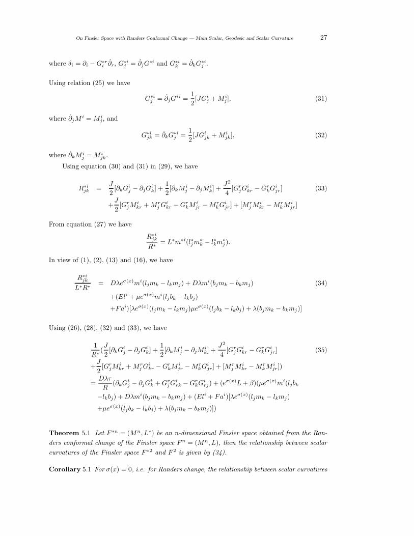
Using relation (25) we have
G∗ij = ∂jG
∗i =1
2[JGi
j + M ij ], (31)
where ∂jMi = M i
j , and
G∗ijk = ∂kG∗i
j =1
2[JGi
jk + M ijk], (32)
where ∂kM ij = M i
jk.
Using equation (30) and (31) in (29), we have
R∗ijk =
J
2[∂kGi
j − ∂jGik] +
1
2[∂kM i
j − ∂jMik] +
J2
4[Gr
jGikr − Gr
kGijr] (33)
+J
2[Gr
jMikr + M r
j Gikr − Gr
kM ijr − M r
kGijr ] + [M r
j M ikr − M r
kM ijr]
From equation (27) we have
R∗ijk
R∗= L∗m∗i(l∗j m∗
k − l∗km∗j ).
In view of (1), (2), (13) and (16), we have
R∗ijk
L∗R∗= Dλeσ(x)mi(ljmk − lkmj) + Dλmi(bjmk − bkmj) (34)
+(Eli + µeσ(x)mi(ljbk − lkbj)
+Fai)[λeσ(x)(ljmk − lkmj)µeσ(x)(ljbk − lkbj) + λ(bjmk − bkmj)]
Using (26), (28), (32) and (33), we have
1
R∗(J
2[∂kGi
j − ∂jGik] +
1
2[∂kM i
j − ∂jMik] +
J2
4[Gr
jGikr − Gr
kGijr] (35)
+J
2[Gr
jMikr + M r
j Gikr − Gr
kM ijr − M r
kGijr ] + [M r
j M ikr − M r
kM ijr])
=Dλτ
R(∂kGi
j − ∂jGik + Gr
jGirk − Gr
kGirj) + (eσ(x)L + β)(µeσ(x)mi(ljbk
−lkbj) + Dλmi(bjmk − bkmj) + (Eli + Fai)[λeσ(x)(ljmk − lkmj)
+µeσ(x)(ljbk − lkbj) + λ(bjmk − bkmj)])
Theorem 5.1 Let F ∗n = (Mn, L∗) be an n-dimensional Finsler space obtained from the Ran-
ders conformal change of the Finsler space Fn = (Mn, L), then the relationship between scalar
curvatures of the Finsler space F ∗2 and F 2 is given by (34).
Corollary 5.1 For σ(x) = 0, i.e. for Randers change, the relationship between scalar curvatures

28 H.S.Shukla and Arunima Mishra
of the Finsler space F ∗2 and F 2 is given as [10]:
1
R∗(J1
2[∂kGi
j − ∂jGik] +
1
2[∂kM i
1j − ∂jMi1k] +
J21
4[Gr
jGikr − Gr
kGijr ]
+J1
2[Gr
jMi1kr + M r
1jGikr − Gr
kM i1jr − M r
1kGijr ] + [M r
1jMi1kr − M r
1kM i1jr])
=D1λτ1
R(∂kGi
j − ∂jGik + Gr
jGirk − Gr
kGirj) + (L + β)(µ1m
i(ljbk − lkbj)
+D1λmi(bjmk − bkmj) + (E1li + F1a
i)[λ(ljmk − lkmj) + µ1(ljbk − lkbj)
+λ(bjmk − bkmj)]),
where
J1 =L(L + β)−1
2, τ1 =
L + β
L, µ1 = − (n + 1)
2C∗(L + β)−1,
D1 =L
L + β
C
C∗, E1 = −(
L + β
L)−2(λH + µ1(β
2L−1 − b2)), F1 = µ1L
L + β
and
M i1 =
1
2[Gr[−L(L + β)−2((yibr + yrbi) + (Lb2 + β)(L + β)−3yiyr]
+[L(L + β)−1gir − L(L + β)−2((yibr + yrbi) + (Lb2 + β)(L + β)−3yiyr]
×[yj(2L∂jbr + β∂j∂rL + 2β∂jbr + br∂jL) − (βlr + (L + β)∂jbryj)]],
M i1j = ∂jM
i1, M i
1jk = ∂kM i1j .
Corollary 5.2 For β = 0, i.e. for conformal change, the relationship between scalar curvatures
of the Finsler space F ∗2 and F 2 is given as:
1
R∗(1
2[∂kGi
j − ∂jGik] +
1
2[∂kM i
2j − ∂jMi2k] +
1
4[Gr
jGikr − Gr
kGijr ]
+1
2[Gr
jMi2kr + M r
2jGikr − Gr
kM i2jr − M r
2kGijr ] + [M r
2jMi2kr − M r
2kM i2jr ])
=D2λτ2
R(∂kGi
j − ∂jGik + Gr
jGirk − Gr
kGirj),
where
τ2 = eσ(x), D2 = e−σ(x) C
C∗
and
M i2 = e−2σ(x)gir[yj [eσ(x)L∂r(∂je
σ(x))L + eσ(x)lr(∂jeσ(x))L] − eσ(x)L(∂re
σ(x))L],
M i2j = ∂jM
i2, M i
2jk = ∂kM i2j.
Corollary 5.3 For β = 0 and σ = a non-zero constant i.e. for homothetic change, the
relationship between scalar curvatures of the Finsler space F ∗2 and F 2 is given as:
1
R∗(1
2[∂kGi
j − ∂jGik] +
1
4[Gr
jGikr − Gr
kGijr ]) =
D3λτ3
R(∂kGi
j − ∂jGik + Gr
jGirk − Gr
kGirj),
where
τ3 = eσ, D3 = e−σ C
C∗.

On Finsler Space with Randers Conformal Change — Main Scalar, Geodesic and Scalar Curvature 29
References
[1] M.Matsumoto, On some transformation of locally Minkowskian space, Tensor, N. S.,
22(1971), 103-111.
[2] Prasad B. N. and Singh J. N., Cubic transformation of Finsler spaces and n-fundamental
forms of their hypersurfaces, Indian J.Pure Appl. Math., 20 (3) (1989), 242-249.
[3] Shibata C., On invariant tensors of β-changes of Finsler spaces, J. Math. Kyato Univ., 24
(1984), 163-188.
[4] M.S.Knebelman, Conformal geometry of generalized metric spaces, Proc.Nat.Acad. Sci.USA.,
15(1929) pp.33-41 and 376-379.
[5] M.Hashiguchi, On conformal transformation of Finsler metric, J. Math. Kyoto Univ.,
16(1976) pp. 25-50.
[6] H.Izumi, Conformal transformations of Finsler spaces I, Tensor, N.S., 31 (1977) pp. 33-41.
[7] H.Izumi, Conformal transformations of Finsler spaces II, Tensor, N.S.,33 (1980) pp. 337-
359.
[8] M.Kitayama, Geometry of transformations of Finsler metrics, Hokkaido University of Ed-
ucation, Kushiro Compus.. Japan(2000).
[9] M.Matsumoto, Foundations of Finsler Geometry and Special Finsler Spaces, Kaiseisha
Press, Saikawa, Otsu, Japan, 1986.
[10] T.N.Pandey, V. K.Chauney and D.D.Tripathi, Randers change of two-dimensional Finsler
space, Journal of Investigations in Mathematical Sciences(IIMS), Vol. 1, (2011), pp, 61-70.
[11] G.Randers, On the asymmetrical metric in the four-space of general relativity, Phys. Rev.,
2(1941)59, pp, 195-199.
[12] M.Matsumoto, On Finsler spaces with Randers metric and special forms of important
tensors, J. Math. Kyoto Univ., 14(1974), pp. 477-498.
[13] C.Shibata, On invariant tensors of β - change of Finsler metrics, J. Math. Kyoto Univ.,
24(1984), pp. 163-188.
[14] M.Kitayama, M.Azuma and M.Matsumoto, On Finsler spaces with (α, β)-metric, regular-
ity, gerodesics and main scalars, J. Hokkaido Univ., Edu., Vol. 46(1), (1995), 1-10.

Math.Combin.Book Ser. Vol.3(2012), 30-39
On the Forcing Hull and Forcing Monophonic Hull
Numbers of Graphs
J.John
(Department of Mathematics , Government College of Engineering, Tirunelveli - 627 007, India)
V.Mary Gleeta
(Department of Mathematics ,Cape Institute of Technology, Levengipuram- 627114, India)
E-mail: [email protected], [email protected]
Abstract: For a connected graph G = (V, E), let a set M be a minimum monophonic hull
set of G. A subset T ⊆ M is called a forcing subset for M if M is the unique minimum
monophonic hull set containing T . A forcing subset for M of minimum cardinality is a
minimum forcing subset of M . The forcing monophonic hull number of M , denoted by
fmh(M), is the cardinality of a minimum forcing subset of M . The forcing monophonic
hull number of G, denoted by fmh(G), is fmh(G) = min fmh(M), where the minimum is
taken over all minimum monophonic hull sets in G. Some general properties satisfied by this
concept are studied. Every monophonic set of G is also a monophonic hull set of G and so
mh(G) ≤ h(G), where h(G) and mh(G) are hull number and monophonic hull number of
a connected graph G. However, there is no relationship between fh(G) and fmh(G), where
fh(G) is the forcing hull number of a connected graph G. We give a series of realization
results for various possibilities of these four parameters.
Key Words: hull number, monophonic hull number, forcing hull number, forcing mono-
phonic hull number, Smarandachely geodetic k-set, Smarandachely hull k-set.
AMS(2010): 05C12, 05C05
§1. Introduction
By a graph G = (V, E), we mean a finite undirected connected graph without loops or multiple
edges. The order and size of G are denoted by p and q respectively. For basic graph theoretic
terminology, we refer to Harary [1,9]. A convexity on a finite set V is a family C of subsets of
V , convex sets which is closed under intersection and which contains both V and the empty set.
The pair(V, E) is called a convexity space. A finite graph convexity space is a pair (V, E), formed
by a finite connected graph G = (V, E) and a convexity C on V such that (V, E) is a convexity
space satisfying that every member of C induces a connected subgraph of G. Thus, classical
convexity can be extended to graphs in a natural way. We know that a set X of Rn is convex if
1Received March 14, 2012. Accepted August 26, 2012.

On the Forcing Hull and Forcing Monophonic Hull Numbers of Graphs 31
every segment joining two points of X is entirely contained in it. Similarly a vertex set W of a
finite connected graph is said to be convex set of G if it contains all the vertices lying in a certain
kind of path connecting vertices of W [2,8]. The distance d(u, v) between two vertices u and v in
a connected graph G is the length of a shortest u− v path in G. An u− v path of length d(u, v)
is called an u − v geodesic. A vertex x is said to lie on a u − v geodesic P if x is a vertex of P
including the vertices u and v. For two vertices u and v, let I[u, v] denotes the set of all vertices
which lie on u−v geodesic. For a set S of vertices, let I[S] =⋃
(u,v)∈S I[u, v]. The set S is convex
if I[S] = S. Clearly if S = vor S = V , then S is convex. The convexity number, denoted
by C(G), is the cardinality of a maximum proper convex subset of V . The smallest convex set
containing S is denoted by Ih(S) and called the convex hull of S. Since the intersection of two
convex sets is convex, the convex hull is well defined. Note that S ⊆ I[S] ⊆ Ih[S] ⊆ V . For an
integer k ≥ 0, a subset S ⊆ V is called a Smarandachely geodetic k-set if I[S⋃
S+] = V and a
Smarandachely hull k-set if Ih(S⋃
S+) = V for a subset S+ ⊂ V with |S+| ≤ k. Particularly, if
k = 0, such Smarandachely geodetic 0-set and Smarandachely hull 0-set are called the geodetic
set and hull set, respectively. The geodetic number g(G) of G is the minimum order of its
geodetic sets and any geodetic set of order g(G) is a minimum geodetic set or simply a g- set
of G. Similarly, the hull number h(G) of G is the minimum order of its hull sets and any hull
set of order h(G) is a minimum hull set or simply a h- set of G. The geodetic number of a
graph is studied in [1,4,10] and the hull number of a graph is studied in [1,6].A subset T ⊆ S is
called a forcing subset for S if S is the unique minimum hull set containing T . A forcing subset
for S of minimum cardinality is a minimum forcing subset of M . The forcing hull number of
S, denoted by fh(S), is the cardinality of a minimum forcing subset of S. The forcing hull
number of G, denoted by fh(G),is fh(G) = min fh(S), where the minimum is taken over all
minimum hull sets S in G. The forcing hull number of a graph is studied in[3,14]. A chord of
a path uo, u1, u2, ..., un is an edge uiuj with j ≥ i + 2(0 ≤ i, j ≤ n). A u − v path P is called
a monophonic path if it is a chordless path. A vertex x is said to lie on a u − v monophonic
path P if x is a vertex of P including the vertices u and v. For two vertices u and v, let J [u, v]
denotes the set of all vertices which lie on u − v monophonic path. For a set M of vertices, let
J [M ] = ∪u,v∈MJ [u, v]. The set M is monophonic convex or m-convex if J [M ] = M . Clearly if
M = v or M = V , then M is m-convex. The m-convexity number, denoted by Cm(G), is the
cardinality of a maximum proper m-convex subset of V . The smallest m-convex set containing
M is denoted by Jh(M) and called the monophonic convex hull or m-convex hull of M . Since
the intersection of two m-convex set is m-convex, the m-convex hull is well defined. Note that
M ⊆ J [M ] ⊆ Jh(M) ⊆ V . A subset M ⊆ V is called a monophonic set if J [M ] = V and
a m-hull set if Jh(M) = V . The monophonic number m(G) of G is the minimum order of
its monophonic sets and any monophonic set of order m(G) is a minimum monophonic set or
simply a m- set of G. Similarly, the monophonic hull number mh(G) of G is the minimum
order of its m-hull sets and any m-hull set of order mh(G) is a minimum monophonic set or
simply a mh- set of G. The monophonic number of a graph is studied in [5,7,11,15] and the
monophonic hull number of a graph is studied in [12]. A vertex v is an extreme vertex of a
graph G if the subgraph induced by its neighbors is complete.Let G be a connected graph and
M a minimum monophonic hull set of G. A subset T ⊆ M is called a forcing subset for M

32 J.John and V.Mary Gleeta
if M is the unique minimum monophonic hull set containing T . A forcing subset for M of
minimum cardinality is a minimum forcing subset of M . The forcing monophonic hull number
of M , denoted by fmh(M), is the cardinality of a minimum forcing subset of M . The forcing
monophonic hull number of G, denoted by fmh(G), is fmh(G) = min fmh(M), where the
minimum is taken over all minimum monophonic hull sets M in G.For the graph G given in
Figure 1.1, M = v1, v8 is the unique minimum monophonic hull set of G so that mh(G) = 2
and fmh(G) = 0. Also S1 = v1, v5, v8 and S2 = v1, v6, v8 are the only two h-sets of G
such that fh(S1) = 1, fh(S2) = 1 so that fh(G) = 1 . For the graph G given in Figure 1.2,
M1 = v1, v4 , M2 = v1, v6 , M3 = v1, v7 and M4 = v1, v8 are the only four mh-sets of
G such that fmh(M1) = 1, fmh(M2) = 1, fmh(M3) = 1 and fmh(M4) = 1 so that fmh(G) = 1.
Also, S = v1, v7 is the unique minimum hull set of G so that h(G) = 2 and fh(G) = 0.
Throughout the following G denotes a connected graph with at least two vertices.
v1 v2
v3
v8
v9
v7
v4v5 v6
G
Figure 1.1
v1 v2
v3
v7v4
v5
v6
G
Figure 1.2
v8
The following theorems are used in the sequel
Theorem 1.1 ([6]) Let G be a connected graph. Then
a) Each extreme vertex of G belongs to every hull set of G;

On the Forcing Hull and Forcing Monophonic Hull Numbers of Graphs 33
(b) h(G) = p if and only if G = Kp.
Theorem 1.2 ([3]) Let G be a connected graph. Then
(a) fh(G) = 0 if and only if G has a unique minimum hull set;
(b) fh(G) ≤ h(G) − |W |, where W is the set of all hull vertices of G.
Theorem 1.3 ([13]) Let G be a connected graph. Then
(a) Each extreme vertex of G belongs to every monophonic hull set of G;
(b) mh(G) = p if and only if G = Kp.
Theorem 1.4 ([12]) Let G be a connected graph. Then
(a) fmh(G) = 0 if and only if G has a unique mh-set;
(b) fmh(G) ≤ mh(G) − |S|, where S is the set of all monophonic hull vertices of G.
Theorem 1.5 ([12]) For any complete Graph G = Kp(p ≥ 2), fmh(G) = 0.
§2. Special Graphs
In this section, we present some graphs from which various graphs arising in theorem are
generated using identification.
Let Ui : αi, βi, γi, δi, αi(1 ≤ i ≤ a) be a copy of cycle C4. Let Vi be the graph obtained from
Ui by adding three new vertices ηi, fi, gi and the edges βiηi, ηifi, figi, giδi, ηiγi, fiγi, giγi(1 ≤i ≤ a). The graph Ta given in Figure 2.1 is obtained from Vi’s by identifying γi−1 of Vi−1 and
αi of Vi(2 ≤ i ≤ a).
f1
g1
f2
g2
fa
ga
Ta
Figure 2.1
α1
β1 β2 βa
η2
γa
ηa
δ2δ1 δa
γ1γ2 αa
η1
Let Pi : ki, li, mi, ni, ki(1 ≤ i ≤ b) be a copy of cycle C4. Let Qi be the graph obtained from
Pi by adding three new vertices hi, pi and qi and the edges lihi, hipi, piqi, and qimi(1 ≤ i ≤ b).
The graph Wb given in Figure 2.2 is obtained from Qi’s by identifying mi−1 of Qi−1 and ki of
Qi(2 ≤ i ≤ b).

34 J.John and V.Mary Gleeta
k1
l1
h1
n1
p1 q1
m1
l2
n2
h2
p2 q2
m2 kb
lb
nb
mbhb
pb qb
Wb
Figure 2.2
The graph Zb given in Figure 2.3 is obtained from Wb by joining the edge lini(1 ≤ i ≤ b).
k1
l1
h1
n1
p1 q1
m1
l2
n2
h2
p2 q2
m2 kb
lb
nb
mbhb
pb qb
Za
Figure 2.3
Let Fi : si, ti, xi, wi, si(1 ≤ i ≤ c) be a copy of cycle C4. Let Ri be the graph obtained from
Fi by adding two new vertices ui, vi and joining the edges tiui, uiwi, tiwi, uivi and vixi(1 ≤ i ≤c). The graph Hc given in Figure 2.4 is obtained from Ri’s by identifying the vertices xi−1 of
Ri−1 and si of Ri(1 ≤ i ≤ c).
s1
t1
u1v1
w1
x1
t2
u2
v2
w2
x2 sc
tc
uc
vc
wc
xc
Hc
Figure 2.4
Every monophonic set of G is also a monophonic hull set of G and so mh(G) ≤ h(G),
where h(G) and mh(G) are hull number and monophonic hull number of a connected graph G.
However, there is no relationship between fh(G) and fmh(G), where fh(G) is the forcing hull
number of a connected graph G. We give a series of realization results for various possibilities
of these four parameters.

On the Forcing Hull and Forcing Monophonic Hull Numbers of Graphs 35
§3. Some Realization Results
Theorem 3.1 For every pair a, b of integers with 2 ≤ a ≤ b, there exists a connected graph G
such that fmh(G) = fh(G) = 0, mh(G) = a and h(G) = b.
Proof If a = b, let G = Ka. Then by Theorems1.3(b) and 1.1(b), mh(G) = h(G) = a and
by Theorems 1.5 and 1.2(a), fmh(G) = fh(G) = 0. For a < b, let G be the graph obtained from
Tb−a by adding new vertices x, z1, z2, · · · , za−1 and joining the edges xα1, γb−az1, γb−az2, · · · ,
γb−aza−1. Let Z = x, z1, z2, · · · , za−1 be the set of end-vertices of G. Then it is clear that Z
is a monophonic hull set of G and so by Theorem 1.3(a), Z is the unique mh-set of G so that
mh(G) = a and hence by Theorem 1.4(a), fmh(G) = 0. Since Ih(Z) 6= V, Z is not a hull set of
G. Now it is easily seen that W = Z ∪ f1, f2, · · · , fb−a is the unique h-set of G and hence by
Theorem 1.1(a) and Theorem 1.2(a), h(G) = b and fh(G) = 0.
Theorem 3.2 For every integers a, b and c with 0 ≤ a < b < c and c > a + b, there exists a
connected graph G such that fmh(G) = 0, fh(G) = a, mh(G) = b and h(G) = c.
Proof We consider two cases.
Case 1. a = 0. Then the graph Tb constructed in Theorem 3.1 satisfies the requirements of
the theorem.
Case 2. a ≥ 1. Let G be the graph obtained from Wa and Tc−(a+b) by identifying the vertex
ma of Wa and α1 of Tc−(a+b) and then adding new vertices x, z1, z2, · · · , zb−1 and joining the
edges xk1, γc−b−az1, γc−b−az2, · · · , γc−b−azb−1. Let Z = x, z1, z2, · · · , zb−1. Since Jh(Z) = V ,
Z is a monophonic hull set G and so by Theorem 1.3(a), Z is the unique mh- set of G so that
mh(G) = b and hence by Theorem 1.4(a), fmh(G) = 0. Next we show that h(G) = c. Let S be
any hull set of G. Then by Theorem 1.1(a), Z ⊆ S. It is clear that Z is not a hull set of G. For
1 ≤ i ≤ a, let Hi = pi, qi. We observe that every h-set of G must contain at least one vertex
from each Hi(1 ≤ i ≤ a) and each fi(1 ≤ i ≤ c−b−a) so that h(G) ≥ b+a+c−a−b = c. Now,
M = Z∪q1, q2, · · · , qa∪f1, f2, · · · , fc−b−a is a hull set of G so that h(G) ≤ b+a+c−b−a = c.
Thus h(G) = c. Since every h-set contains S1 = Z ∪ f1, f2, · · · , fc−b−a, it follows from
Theorem 1.2(b) that fh(G) = h(G) − |S1| = c− (c− a) = a. Now, since h(G) = c and every h-
set of G contains S1, it is easily seen that every h-set S is of the form S1∪d1, d2, · · · , da,where
di ∈ Hi(1 ≤ i ≤ a). Let T be any proper subset of S with |T | < a. Then it is clear that there
exists some j such that T ∩ Hj = φ, which shows that fh(G) = a.
Theorem 3.3 For every integers a, b and c with 0 ≤ a < b ≤ c and b > a + 1, there exists a
connected graph G such that fh(G) = 0, fmh(G) = a, mh(G) = b and h(G) = c.
Proof We consider two cases.
Case 1. a = 0. Then the graph G constructed in Theorem 3.1 satisfies the requirements of
the theorem.
Case 2. a ≥ 1.

36 J.John and V.Mary Gleeta
Subcase 2a. b = c. Let G be the graph obtained from Za by adding new vertices x, z1, z2, · · · ,
zb−a−1 and joining the edges xk1, maz1, maz2, · · · , mazb−a−1. Let Z = x, z1, z2, · · · , zb−a−1be the set of end-vertices of G. Let S be any hull set of G. Then by Theorem 1.1(a), Z ⊆ S.
It is clear that Z is not a hull set of G. For 1 ≤ i ≤ a, let Hi = hi, pi, qi. We observe that
every h-set of G must contain only the vertex pi from each Hi so that h(G) ≤ b − a + a = b.
Now S = Z ∪ p1, p2, p3, · · · , pa is a hull set of G so that h(G) ≥ b − a + a = b. Thus
h(G) = b. Also it is easily seen that S is the unique h-set of G and so by Theorem 1.2(a),
fh(G) = 0.Next we show that mh(G) = b. Since Jh(Z) 6= V, Z is not a monophonic hull set of
G. We observe that every mh-set of G must contain at least one vertex from each Hi so that
mh(G) ≥ b−a+a = b. Now M1 = Z ∪q1, q2, q3, · · · , qa is a monophonic hull set of G so that
mh(G) ≤ b− a + a = b. Thus mh(G) = b. Next we show that fmh(G) = a. Since every mh-set
contains Z, it follows from Theorem 1.4(b) that fmh(G) ≤ mh(G)−|Z| = b− (b−a) = a. Now,
since mh(G) = b and every mh-set of G contains Z, it is easily seen that every mh-set M is of
the form Z ∪ d1, d2, d3, · · · , da, where di ∈ Hi(1 ≤ i ≤ a). Let T be any proper subset of M
with |T | < a. Then it is clear that there exists some j such that T ∩Hj = φ, which shows that
fmh(G) = a.
Subcase 2b. b < c. Let G be the graph obtained from Za and Tc−b by identifying the
vertex ma of Za and α1 of Tc−b and then adding the new vertices x, z1, z2, · · · , zb−a−1 and
joining the edges xα1, γc−bz1, γc−bz2, · · · , γc−bzb−a−1. Let Z = x, z1, z2, · · · , zb−a−1 be the
set of end vertices of G. Let S be any hull set of G. Then by Theorem 1.1(a), Z ⊆ S. Since
Ih(Z) 6= V, Z is not a hull set of G. For 1 ≤ i ≤ a, let Hi = hi, pi, qi. We observe that every
h-set of G must contain only the vertex pi from each Hi and each fi(1 ≤ i ≤ c − b) so that
h(G) ≥ b − a + a + c − b = c. Now S = Z ∪ p1, p2, p3, · · · , pa ∪ f1, f2, f3, · · · , fc−bis a hull
set of G so that h(G) ≤ b − a + a + c − b = c. Thus h(G) = c. Also it is easily seen that S
is the unique h-set of G and so by Theorem 1.2(a), fh(G) = 0. Since Jh(Z) 6= V , Z is not a
monophonic hull set of G. We observe that every mh-set of G must contain at least one vertex
from each Hi(1 ≤ i ≤ a) so that mh(G) ≥ b − a + a = b. Now, M1 = Z ∪ h1, h2, h3, · · · , hais a monophonic hull set of G so that mh(G) ≤ b − a + a = b. Thus mh(G) = b. Next we
show that fmh(G) = a. Since every mh-set contains Z, it follows from Theorem 1.4(b) that
fmh(G) ≤ mh(G) − |Z| = b − (b − a) = a. Now, since mh(G) = b and every mh-set of G
contains Z, it is easily seen that every mh-set S is of the form Z ∪ d1, d2, d3, · · · , da, where
di ∈ Hi(1 ≤ i ≤ a). Let T be any proper subset of S with |T | < a. Then it is clear that there
exists some j such that T ∩ Hj = φ, which shows that fmh(G) = a.
Theorem 3.4 For every integers a, b and c with 0 ≤ a < b ≤ c and b > a + 1 , there exists a
connected graph G such that fmh(G) = fh(G) = a, mh(G) = b and h(G) = c.
Proof We consider two cases.
Case 1. a = 0, then the graph G constructed in Theorem 3.1 satisfies the requirements of the
theorem.
Case 2. a ≥ 1.

On the Forcing Hull and Forcing Monophonic Hull Numbers of Graphs 37
Subcase 2a. b = c. Let G be the graph obtained from Ha by adding new vertices x, z1, z2, · · · ,
zb−a−1 and joining the edges xs1, xaz1, xaz2, · · · , xazb−a−1. Let Z = x, z1, z2, · · · , zb−a−1 be
the set of end-vertices of G. Let M be any monophonic hull set of G. Then by Theorem 1.3(a),
Z ⊆ M . First we show that mh(G) = b. Since Jh(Z) 6= V, Z is not a monophonic hull set of
G. Let Fi = ui, vi (1 ≤ i ≤ a). We observe that every mh-set of G must contain at least one
vertex from each Fi(1 ≤ i ≤ a). Thus mh(G) ≥ b − a + a = b. On the other hand since the set
M = Z ∪ v1, v2, v3, · · · , va is a monophonic hull set of G, it follows that mh(G) ≤ |M | = b.
Hence mh(G) = b. Next we show that fmh(G) = a. By Theorem 1.3(a), every monophonic hull
set of G contains Z and so it follows from Theorem 1.4(b) that fmh(G) ≤ mh(G) − |Z| = a.
Now, since mh(G) = b and every mh-set of G contains Z, it is easily seen that every mh-set
M is of the form Z ∪ c1, c2, c3, · · · , ca, where ci ∈ Fi(1 ≤ i ≤ a). Let T be any proper subset
of S with |T | < a. Then it is clear that there exists some j such that T ∩ Fj = φ, which shows
that fmh(G) = a. By similar way we can prove h(G) = b and fh(G) = a.
Subcase 2b. b < c. Let G be the graph obtained from Ha and Tc−b by identifying the vertex
xa of Ha and the vertex α1 of Tc−b and then adding the new vertices x, z1, z2, · · · , zb−a−1 and
joining the edges xs1, γc−bz1, γc−bz2, · · · , γc−bzb−a−1. First we show that mh(G) = b. Since
Jh(Z) 6= V, Z is not a monophonic hull set of G. Let Fi = ui, vi (1 ≤ i ≤ a) .We observe that
every mh-set of G must contain at least one vertex from each Fi(1 ≤ i ≤ a). Thus mh(G) ≥b−a+a = b. On the other hand since the set M = Z∪v1, v2, v3, · · · , va is a monophonic hull
set of G, it follows that mh(G) ≥ |M | = b. Hence mh(G) = b. Next, we show that fmh(G) = a.
By Theorem 1.3(a), every monophonic hull set of G contains Z and so it follows from Theorem
1.4(b) that fmh(G) ≤ mh(G) − |Z| = a. Now, since mh(G) = b and every mh-set of G
contains Z, it is easily seen that every mh-set is of the form M = Z ∪c1, c2, c3, · · · , ca, where
ci ∈ Fi(1 ≤ i ≤ a). Let T be any proper subset of M with |T | < a. Then it is clear that there
exists some j such that T ∪Fj = φ, which shows that fmh(G) = a. Next we show that h(G) = c.
Since Ih(Z) 6= V, Z is not a hull set of G. We observe that every h-set of G must contain at least
one vertex from each Fi(1 ≤ i ≤ a) and each fi(1 ≤ i ≤ c−b) so that h(G) ≥ b−a+a+c−b = c.
On the other hand, since the set S1 = Z ∪ u1, u2, u3, · · · , ua ∪ f1, f2, f3, · · · , fc−b is a hull
set of G, so that h(G) ≤ |S1| = c. Hence h(G) = c. Next we show that fh(G) = a. By
Theorem 1.1(a), every hull set of G contains S2 = Z ∪ f1, f2, f3, · · · , fc−b and so it follows
from Theorem 1.2(b) that fh(G) ≤ h(G) − |S2| = a. Now, since h(G) = c and every h-set of
G contains S2, it is easily seen that every h-set S is of the form S = S2 ∪ c1, c2, c3, · · · , ca,where ci ∈ Fi(1 ≤ i ≤ a). Let T be any proper subset of S with |T | < a. Then it is clear that
there exists some j such that T ∩ Fj = φ, which shows that fh(G) = a.
Theorem 3.5 For every integers a, b, c and d with 0 ≤ a ≤ b < c < d, c > a + 1, d > c− a + b,
there exists a connected graph G such that fmh(G) = a, fh(G) = b, mh(G) = c and h(G) = d.
Proof We consider four cases.
Case 1. a = b = 0. Then the graph G constructed in Theorem 3.1 satisfies the requirements
of this theorem.
Case 2. a = 0, b ≥ 1. Then the graph G constructed in Theorem 3.2 satisfies the requirements

38 J.John and V.Mary Gleeta
of this theorem.
Case 3. 1 ≤ a = b. Then the graph G constructed in Theorem 3.4 satisfies the requirements
of this theorem.
Case 4. 1 ≤ a < b. Let G1 be the graph obtained from Ha and Wb−a by identifying the vertex
xa of Ha and the vertex k1 of Wb−a. Now let G be the graph obtained from G1 and Td−(c−a+b)
by identifying the vertex mb−a of G1 and the vertex α1 of Td−(c−a+b) and adding new vertices
x, z1, z2, · · · , zc−a−1 and joining the edges xs1, γd−(c−a+b)z1, γd−(c−a+b)z2, · · · , γd−(c−a+b)zc−a−1.
Let Z = x, z1, z2, · · · , zc−a−1 be the set of end vertices of G. Let Fi = ui, vi (1 ≤ i ≤ a).
It is clear that any mh-set S is of the form S = Z ∪ c1, c2, c3, · · · , ca, where ci ∈ Fi(1 ≤i ≤ a). Then as in earlier theorems it can be seen that fmh(G) = a and mh(G) = c. Let
Qi = pi, qi. It is clear that any h-set W is of the form W = Z ∪
f1, f2, f3, · · · , fd−(c−a+b)
∪c1, c2, c3, · · · , ca∪d1, d2, d3, · · · , db−a, where ci ∈ Fi(1 ≤ i ≤ a) and dj ∈ Qj(1 ≤ j ≤ b−a).
Then as in earlier theorems it can be seen that fh(G) = b and h(G) = d.
Theorem 3.6 For every integers a, b, c and d with a ≤ b < c ≤ d and c > b + 1 there exists a
connected graph G such that fh(G) = a, fmh(G) = b, mh(G) = c and h(G) = d.
Proof We consider four cases.
Case 1. a = b = 0. Then the graph G constructed in Theorem 3.1 satisfies the requirements
of this theorem.
Case 2. a = 0, b ≥ 1. Then the graph G constructed in Theorem 3.2 satisfies the requirements
of this theorem.
Case 3. 1 ≤ a = b. Then the graph G constructed in Theorem 3.4 satisfies the requirements
of this theorem.
Case 4. 1 ≤ a < b.
Subcase 4a. c = d. Let G be the graph obtained from Ha and Zb−a by identifying the
vertex xa of Ha and the vertex k1 of Zb−a and then adding the new vertices x, z1, z2, ..., zc−b−1
and joining the edges xs1, mb−az1, mb−az2, ..., mb−azc−b−1. First we show that mh(G) = c.
Let Z = x, z1, z2, ..., zc−b−1 be the set of end vertices of G. Let Fi = ui, vi (1 ≤ i ≤ a)
and Hi = hi, pi, qi (1 ≤ i ≤ b − a). It is clear that any mh-set of G is of the form S =
Z∪c1, c2, c3, ..., ca∪d1, d2, d3, ..., db−a, where ci ∈ Fi(1 ≤ i ≤ a) and dj ∈ Hj(1 ≤ j ≤ b−a).
Then as in earlier theorems it can be seen that fmh(G) = b and mh(G) = c. It is clear that any
h-set W is of the form W = Z∪p1, p2, p3, ..., pb−a∪c1, c2, c3, ..., ca, where ci ∈ Fi(1 ≤ i ≤ a).
Then as in earlier theorems it can be seen that fh(G) = a and h(G) = c.
Subcase 4b. c < d. Let G1 be the graph obtained from Ha and Zb−a by identifying
the vertex xa of Ha and the vertex k1 of Zb−a. Now let G be the graph obtained from G1
and Td−c by identifying the vertex mb−a of G1 and the vertex α1 of Td−c and then adding
new vertices x, z1, z2, · · · , zc−b−1 and joining the edges xs1, γd−cz1, γd−cz2, · · · , γd−czc−b−1. Let
Z = x, z1, z2, · · · , zc−b−1 be the set of end vertices of G. Let Fi = ui, vi (1 ≤ i ≤ a) and
Hi = hi, pi, qi (1 ≤ i ≤ b − a). It is clear that any mh-set of G is of the form S = Z ∪

On the Forcing Hull and Forcing Monophonic Hull Numbers of Graphs 39
c1, c2, c3, · · · , ca∪d1, d2, d3, · · · , db−a, where ci ∈ Fi(1 ≤ i ≤ a) and dj ∈ Hj(1 ≤ j ≤ b−a).
Then as in earlier theorems it can be seen that fmh(G) = b and mh(G) = c. It is clear that any h-
set W is of the form W = Z ∪p1, p2, p3, · · · , pb−a∪f1, f2, f3, · · · , fd−c∪c1, c2, c3, · · · , ca,where ci ∈ Fi(1 ≤ i ≤ a). Then as in earlier theorems it can be seen that fh(G) = a and
h(G) = d.
References
[1] F.Buckley and F.Harary, Distance in Graphs, Addition- Wesley, Redwood City, CA, 1990.
[2] G.Chartrand and P.Zhang, The forcing geodetic number of a graph, Discuss. Math. Graph
Theory, 19 (1999), 45-58.
[3] G.Chartrand and P.Zhang, The forcing hull number of a graph, J. Combin Math. Comput.,
36(2001), 81-94.
[4] G.Chartrand, F.Harary and P.Zhang, On the geodetic number of a graph, Networks,39(2002)
1-6.
[5] Carmen Hernando, Tao Jiang, Merce Mora, Ignacio. M. Pelayo and Carlos Seara, On the
Steiner, geodetic and hull number of graphs, Discrete Mathematics, 293 (2005) 139 - 154.
[6] M. G. Evertt, S. B. Seidman, The hull number of a graph , Discrete Mathematics, 57 (1985)
217-223.
[7] Esamel M. Paluga, Sergio R. Canoy Jr, Monophonic numbers of the join and Composition
of connected graphs, Discrete Mathematics 307(2007) 1146 - 1154.
[8] M.Faber, R.E. Jamison, Convexity in graphs and hypergraphs, SIAM Journal Algebraic
Discrete Methods, 7(1986) 433-444.
[9] F.Harary, Graph Theory, Addison-Wesley, 1969.
[10] F.Harary, E.Loukakis and C.Tsouros, The geodetic number of a graph, Math.Comput Mod-
eling 17(11)(1993) 89-95.
[11] J.John and S.Panchali, The upper monophonic number of a graph, International J.Math.
Combin, 4(2010),46-52.
[12] J.John and V.Mary Gleeta, The Forcing Monophonic Hull Number of a Graph, Interna-
tional Journal of Mathematics Trends and Technology, 3(2012),43-46.
[13] J.John and V.Mary Gleeta, Monophonic hull sets in graphs, submitted.
[14] Li-Da Tong, The forcing hull and forcing geodetic numbers of graphs, Discrete Applied
Math., 157(2009), 1159-1163.
[15] Mitre C.Dourado, Fabio protti and Jayme L.Szwarcfiter, Algorithmic Aspects of Mono-
phonic Convexity, Electronic Notes in Discrete Mathematics 30(2008) 177-182.
Math.Combin.Book Ser. Vol.3(2012), 40-45
Simplicial Branched Coverings of the 3-Sphere
Keerti Vardhan Madahar
(Department of Mathematics (DES), Panjab University Chandigarh, 160014, India)
E-mail: [email protected]
Abstract: In this article we give, for each d > 1, a simplicial branched covering map
λd : S33(d+1) → S3
6 of degree d. And by using the simplicial map λ2 we demonstrate a well
known topological fact that the space obtained by identifying diagonally opposite points of
the 3-sphere is homeomorphic to the 3-sphere.
Key Words: Branched Covering, simplicial map, triangulation of map.
AMS(2010): 57M12, 57N12, 55M25, 57M20
§1. Introduction
In articles [5] and [6] we have given simplicial branched coverings of the Real Projective Plane
and the 2-Sphere respectively. The present article is in continuation of these articles. Here we
give, for each d > 1, a simplicial branched covering map, λd : S33(d+1) → S3
6 , from a 3(d+1)
vertex triangulation of the 3-sphere onto a 6 vertex triangulation of the 3-sphere. For d = 2, we
show that the simplicial branched covering map λ2 : S39 → S3
6 is a minimal triangulation of the
well known two fold branched covering map S3 → S3/(x, y) ∼ (y, x). Moreover the simplicial
map λ2 verifies a familiar topological fact that after identifying diagonally symmetric points
of the 3-sphere we get a homeomorphic copy of the 3-sphere. Branched coverings of the low
dimensional manifolds have been discussed extensively (e.g. see [1], [3] and [4]) but the explicit
constructions, which we are giving here are missing. The purpose here is to give some concrete
examples, which are not at all trivial but explain some important topological facts.
§2. Preliminary Notes
Definition 2.1 An abstract simplicial complex K on a finite set V is a collection of subsets
of V , which is closed under inclusion i.e. if s ∈ K and s′ ⊂ s then s′ ∈ K. The elements of
K are called simplices and in particular a set γ ∈ K of cardinality n+1 is called an n-simplex;
0-simplices are called vertices, 1-simplices are called edges and so on.
A geometric n-simplex is the convex hull of n + 1 affinely independent points of RN (see
[2]). A geometric simplicial complex is a collection of geometric simplices such that all faces of
1Received February 27, 2012. Accepted August 28, 2012.

Simplicial Branched Coverings of the 3-Sphere 41
these simplices are also in the collection and intersection of any two of these simplices is either
empty or a common face of both of these simplices. It is easy to see that corresponding to each
geometric simplicial complex there is an abstract simplicial complex. Converse is also true i.
e. corresponding to any abstract simplicial complex K there is a topological space |K| ⊂ RN ,
made up of geometric simplices, called its geometric realization (see [2], [7], [8]). If K is an
abstract simplicial complex and M is a subspace of RN such that there is a homeomorphism
h : |K| → M then we say (|K|, h) is a triangulation of M or K triangulates the topological
space M .
Definition 2.2 A map f : K → L, between two abstract simplicial complexes K and L, is called
a simplicial map if image, f(σ) = f(v0), f(v1), ..., f(vk), of any simplex σ = v0, v1, ..., vk of
K is a simplex of L. Further if |K| and |L| are geometric realizations of K and L respectively then
there is a piecewise-linear continuous map |f | : |K| → |L| defined as follows. As each point x of
|K| is an interior point of exactly one simplex (say σ = v0, .., vk) of |K|, so for each x ∈ σ we
have x =∑k
i=1 λivi where λi ≥ 0,∑
λi = 1. Therefore we may define |f |(x) =∑k
i=1 λif(vi).
Definition 2.3 A simplicial branched covering map between two triangulated n-manifolds K
and L is defined by a dimension preserving piecewise linear map p : |K| → |L|, which is an
ordinary covering over the complement of some specific co-dimension 2 sub-complex L′ of L
(for more detailed definition see [1], [3], [4], [5]). The sub-complex L′ is called branch set of
the branched covering map and a point x ∈ p−1(L′) is called a singular point if p fails to be a
local homeomorphism at x.
§3. Main Results
3.1 Simplicial branched covering map λd : S33(d+1) → S3
6
We first define a simplicial branched covering map λ2 : S39 → S3
6 of degree 2 and then show that
the same method gives, for each d > 2, a simplicial branched covering map λd : S33(d+1) → S3
6
of degree d.
Since the join of two 1-spheres is a 3-sphere, so in order to get the desired 9 vertex 3-
sphere S39 , we take join of a three vertex 1-sphere S1
3 = A0, E0, F0, A0E0, E0F0, F0A0 with
the six vertex 1-sphere S16 = B0, C0, D0, B1, C1, D1, C0B0, B0D0, D0C1, C1B1, B1D1, D1C0.
The 3-sipmlices of S39 = S1
3 ∗ S16 are shown in Figure 1.
We define a map on the vertex set of S39 , as A0 → A, E0 → E, F0 → F, Xi → X for
each X ∈ B, C, D, i ∈ 0, 1 and extend it linearly on the 3-simplices of S39 . The image of
this map is a simplicial complex whose 3-simplices are ABCE, ACDE, ABDE, EDBF, EBCF,
EDCF, CDAF, DBAF and CBAF. This simplicial complex triangulates the 3-sphere because
its geometric realization is homeomorphic to the 3-sphere as it is a disjoint union of two 3-
balls having a common boundary S2 (see figure 2 below). We denote this simplicial complex
by S36 and the map just defined is the simplicial map λ2 : S3
9 → S36 . Notice that the map
λ2 : S39 → S3
6 is a 2-fold simplicial branched covering map because pre-image of each 3-simplex
of S36 consists of exactly two 3-simplices of S3
9 ; each is being mapped, under the map λ2, with

42 Keerti Vardhan Madahar
the same orientation. Branching set and the singular set of the map are AE + EF + FA and
A0E0 + E0F0 + F0A0 respectively.
Figure 1
In order to get a simplicial branched covering map, λd : S33(d+1) → S3
6 , of degree d (for
each d > 2) we consider the join of a 3 vertex 1-sphere with the 3d vertex 1-sphere. i.e.
S33(d+1) = S1
3 ∗S13d = A0, E0, F0, A0E0, E0F0, F0A0∗Bi, Ci, Di, CiBi, BiDi, DiCi+1 : i ∈ Zd.
Figure 2
The 3-simplices of S33(d+1) are A0E0CiBi, A0E0BiDi, A0E0DiCi+1, E0F0CiBi, E0F0BiDi,
E0F0DiCi+1, F0A0CiBi, F0A0BiDi, F0A0DiCi+1 : i ∈ Zd, addition in the subscripts is mod d.Notice that a map, defined on the vertices of the simplicial complex S3
3(d+1), as A0 → A, E0 →

Simplicial Branched Coverings of the 3-Sphere 43
E, F0 → F, Xi → X for each X ∈ B, C, D and for i ∈ 0, 1, , d − 1 is a simplicial branched
covering map λd : S33(d+1) → S3
6 of degree d.
Remark 3.1.1 We shall now show that the simplicial map λ2 : S39 → S3
6 triangulates the
2-fold branched covering map S3 → S3/(x, y) ∼ (y, x) but before that we prove the following
theorem.
Theorem 3.1.1 The simplicial map λ2 : S39 → S3
6 is a minimal triangulation of the 2-fold
branched covering map q: S3 → S3/(x, y) ∼ (y, x).
Proof Notice that branching of the map q occurs along the diagonal circle of the quotient
space and pre-image of the branching circle is the diagonal circle of the domain of the map q.
Let λ2 : S3α0
→ S3β0
be a minimal triangulation of the map q, so the branching circle and the
singular circle are at least triangles. Since the polygonal link of any singular 1-simplex of S3α0
,
is to be mapped with degree 2 by the map λ2 so the link will have at least 6-vertices. The
image of this link will be a circle with at least 3 vertices, which are different from the vertices
of the branching circle. This implies that the domain 3-sphere of the map λ2 will have at least
9 vertices and its image will have at least 6 vertices i.e. α0 ≥ 9 and β0 ≥ 6.
Note 3.1.1 Following description of the simplicial complex S39 enables us to show that the
simplicial map λ2 : S39 → S3
6 triangulates the 2-fold branched covering map q: S3 → S3/(x, y) ∼(y, x). It also leads to a combinatorial proof of the fact that after identification of diagonally
symmetric points of the 3-sphere we get the 3-sphere again.
3.2 Diagonally Symmetric Triangulation of the 3-Sphere
The diagonal of the standard 3-sphere S3 = (z1, z2) ∈ C2 : |z1|2 + |z2|2 = 1 is the subspace
∆ = (z1, z2) ∈ S3 : z1 = z2. A triangulation of S3 will be called diagonally symmetric
if whenever there is a vertex at a point (z1, z2) there is a vertex at the point (z2, z1) and
whenever there is a 3-simplex on the vertices (zi1 , zi2), (zi3 , zi4), (zi5 , zi6), (zi7 , zi8), there is a
3-simplex on the vertices (zi2 , zi1), (zi4 , zi3), zi6 , zi5), (zi8 , zi7). We show that the simplicial
complex S39 obtained above is a diagonally symmetric triangulation of the 3-sphere and the
simplicial branched covering map λ2 : S39 → S3
6 is equivalent to the map q: S3 → S3/(x, y) ∼(y, x). In order to show this we consider the following description of the 3-sphere:
S3 = T1
⋃
T2,
where T1 = (z1, z2) ∈ S3 : |z1| ≤ |z2|, T2 = (z1, z2) ∈ S3 : |z1| ≥ |z2| and
T = T1
⋂
T2 = (z1, z2) ∈ S3 : |z1| = |z2| = 1/√
2 ∼= S1 × S1.
A map θ : S3 → S3 defined as (z1, z2) → (z2, z1) swaps the interiors of the solid tori T1
and T2 homeomorphically. We triangulate T1 and T2 in such a way that the homeomorphism θ
induces a simplicial isomorphism between the triangulations of T1 and T2. The triangulations
of T, T1 and T2 are described as follows.

44 Keerti Vardhan Madahar
In Figure 3 below we give a triangulated 2-torus T, which is the common boundary of both
of the solid tori T1 and T2. The vertices X0, X1 for each X ∈ B, C, D are symmetric about
the diagonal ∆ and the vertices A0, E0, F0 triangulate the diagonal.
Since there are precisely two ways to fold a square to get a torus, viz (i) first identify vertical
boundaries and then identify horizontal boundaries of the square (ii) first identify horizontal
boundaries and then vertical boundaries of the square, so we use this fact to obtain the solid
tori T1 and T2.
Figure 3
The solid torus T1 has been obtained by first identifying the vertical edges, of the square of
Figure 3, and then top and bottom edges (see Figure 4 below). Its three, of the total nine,
3-simplices are A0B0C0E0, A0C0E0D1 and A0D1E0B1 and remaining six 3-simplices can be
obtained from an automorphism defined by A0 → E0 → F0 → A0, B0 → D1 → C1 → B0 and
C0 → B1 → D0 → C0.
The solid torus T2 has been obtained by first identifying the horizontal edges, of the square
of Figure 3, and then the other two sides as shown in Figure 4. The nine 3-simplices of T2 are
A0D0E0B0, E0A0C1D0, A0B1C1E0, E0C0F0D1, F0E0B0C0, E0D0B0F0, F0B1A0C1, A0F0D1B1,
F0C0D1A0. These simplices can also be obtained from the 3-simplices of T1 by using the per-
mutation ρ = (B0B1)(C0C1)(D0D1), which is equivalent to the Z2-action defined by the map
θ : (x, y) → (y, x) on S3.
The nine 3-simplices of T1 together with the nine 3-simplices of T2 constitute a diagonally
symmetric triangulation of the 3-sphere with 9 vertices. And since the list of 3-simplices of
S13 ∗ S1
6 is same as that of the 3-simplices of the simplicial complex obtained now, so the two
simplicial complexes are isomorphic.
Notice that the identification of diagonally symmetric vertices / simplices of the 3-sphere
(obtained now) is equivalent to the identifications provided by the simplicial map λ2. This
equivalence implies that the identification of diagonally symmetric points of the 3-sphere gives

Simplicial Branched Coverings of the 3-Sphere 45
a 3-sphere.
Remark 3.2.1 In Figure 3 (triangulation of T) if we replace the edges A0D0 and A0D1 by
the edges B0C1 and B1C0 respectively then we get another triangulation of T , which is also
symmetric about the diagonal. But this triangulation under the diagonal action does not give
a simplicial branched covering map.
Figure 4
References
[1] I.Berstein and A. L. Edmond, On construction of branched coverings of low dimensional
manifolds, Trans. Amer. Math. Soc., 247(1979) 87-124.
[2] B.Datta, Minimal triangulations of manifolds, Journal of Indian Institute of Science,
87(2007), 429 - 449.
[3] B.A.Dubrovin, A.T.Fomenko and S.P.Novikov, Modern Geometry - Methods and Applica-
tions, Springer-Verlag, 1985.
[4] R. C.Gunning, Lectures on Riemann Surfaces, Princeton University Press, 1966.
[5] K.V.Madahar, On branched coverings, International Journal of Applied Mathematics and
Statistics, 15 (D09)(2009), 37-46
[6] K.V.Madahar and K.S.Sarkaria, Minimal simplicial self maps of the 2-sphere, Geometriae
Dedicata , 84 (2001) 25-33.
[7] J.R.Munkres, Elements of Algebraic Topology, Addison - Wesley, 1984.
[8] E. H.Spanier, Algebraic Topology, McGraw-Hill, 1981.

Math.Combin.Book Ser. Vol.3(2012), 46-53
On the Osculating Spheres of a Real Quaternionic Curve
In the Euclidean Space E4
Derya Saglam
Derya Saglam Afyonkarahisar Kocatepe University
Faculty of Art and Sciences, Department of Mathematics, Afyonkarahisar, Turkey
E-mail: [email protected]
Abstract: In the Euclidean space E4, there is a unique quaternionic sphere for a real
quaternionic curve α : I ⊂ R → QH such that it touches α at the fourth order at α(0). In
this paper, we studied some characterizations of the osculating sphere of the real quaternionic
curves in the four dimensional Euclidean space.
Key Words: Euclidean space, quaternion algebra, osculating spheres.
AMS(2010): 14Q05, 53A17, 53C50
§1. Introduction
The quaternions introduced by Hamilton in 1843 are the number system in four dimensional
vector space and an extension of the complex number. There are different types of quaternions,
namely: real, complex dual quaternions. A real quaternion is defined as q = q0 + q1e1 + q2e2 +
q3e3 is composed of four units 1, e1, e2, e3 where e1, e2, e3 are orthogonal unit spatial vectors,
qi (i = 0, 1, 2, 3) are real numbers and this quaternion can be written as a linear combination
of a real part (scalar) and vectorial part (a spatial vector) [1,5,8].
The space of quaternions Q are isomorphic to E4, four dimensional vector space over the
real numbers. Then, Clifford generalized the quaternions to bi-quaternions in 1873 [11]. Hence
they play an important role in the representation of physical quantities up to four dimensional
space. Also they are used in both theoretical and applied mathematics. They are important
number systems which use in Newtonian mechanics, quantum physics, robot kinematics, orbital
mechanics and three dimensional rotations such as in the three dimensional computer graphics
and vision. Real quaternions provide us with a simple and elegant representation for describing
finite rotation in space. On the other hand, dual quaternions offer us a better way to express
both rotational and translational transformations in a robot kinematic [5].
In 1985, the Serret-Frenet formulas for a quaternionic curve in Euclidean spaces E3 and E4
are given by Bharathi and Nagaraj [9]. By using of these formulas Karadag and Sivridag gave
some characterizations for quaternionic inclined curves in the terms of the harmonic curvatures
in Euclidean spaces E3 and E4 [10]. Gok et al. defined the real spatial quaternionic b-slant
1Received June 30, 2012. Accepted September 4, 2012.

On the Osculating Spheres of a Real Quaternionic Curve in the Euclidean Space E4 47
helix and the quaternionic B2-slant helix in Euclidean spaces E3 and E4 respectively and they
gave new characterization for them in the terms of the harmonic curvatures [7].
In the Euclidean space E3, there is a unique sphere for a curve α : I ⊂ R → E3 such
that the sphere contacts α at the third order at α(0). The intersection of the sphere with
the osculating plane is a circle which contacts α at the second order at α(0) [2,3,6]. In [4],
the osculating sphere and the osculating circle of the curve are studied for each of timelike,
spacelike and null curves in semi- Euclidean spaces; E31 , E4
1 and E42 .
In this paper, we define osculating sphere for a real quaternionic curve α : I ⊂ R → E4
such that it contacts α at the fourth order at α(0). Also some characterizations of the osculating
sphere are given in Euclidean space E4.
§2. Preliminaries
We give basic concepts about the real quaternions. Let QH denote a four dimensional vector
space over a field H whose characteristic grater than 2. Let ei (1 ≤ i ≤ 4) denote a basis for the
vector space. Let the rule of multiplication on QH be defined on ei (1 ≤ i ≤ 4) and extended
to the whole of the vector space by distributivity as follows:
A real quaternion is defined by q = a−→e1 + b−→e2 + c−→e3 + de4 where a, b, c, d are ordinary
numbers such that−→e1 ×−→e2 = −→e3 = −−→e2 ×−→e1 ,
−→e2 ×−→e3 = −→e1 = −−→e3 ×−→e2 ,
−→e3 ×−→e1 = −→e2 = −−→e1 ×−→e3 ,
−→e12 = −→e2
2 = −→e32 = −1, e2
4 = 1.
We can write a real quaternion as a linear combination of scalar part Sq = d and vectorial
part Vq = a−→e1 + b−→e2 + c−→e3 . Using these basic products we can now expand the product of two
quaternions as
p × q = SpSq −⟨−→Vp,
−→Vq
⟩
+ Sp
−→Vq + Sq
−→Vp +
−→Vp ∧ −→
Vq for every p, q ∈ QH ,
where 〈, 〉 and ∧ are inner product and cross product on E3, respectively. There is a unique
involutory antiautomorphism of the quaternion algebra, denoted by the symbol γ and defined
as follows:
γq = −a−→e1 − b−→e2 − c−→e3 + d
for every q = a−→e1 + b−→e2 + c−→e3 + de4 ∈ QH which is called the Hamiltonian conjugation. This
defines the symmetric, real valued, non-degenerate, bilinear form h as follows:
h(p, q) =1
2(p × γq + q × γp) for every p, q ∈ QH .
Now we can give the definition of the norm for every quaternion. the norm of any q real
quaternion is denoted by
‖q‖2= h(q, q) = q × γq = a2 + b2 + c2 + d2

48 Derya Saglam
in [5,8].
The four-dimensional Euclidean space E4 is identified with the space of unit quaternions.
A real quaternionic sphere with origin m and radius R > 0 in E4 is
S3(m, R) = p ∈ QH : h(p − m, p − m) = R2.
The Serret-Frenet formulas for real quaternionic curves in E4 are as follows:
Theorem 2.1([10]) The four-dimensional Euclidean space E4 is identified with the space of
unit quaternions. Let I = [0, 1] denotes the unit interval in the real line R and −→e4 = 1. Let
α : I ⊂ R → QH
s → α(s) =4∑
i=1
αi(s)−→ei ,
be a smooth curve in E4 with nonzero curvatures K, k, r − K and the Frenet frame of the
curve α is T, N, B1, B2. Then Frenet formulas are given by
T ′
N ′
B′1
B′2
=
0 K 0 0
−K 0 k 0
0 −k 0 (r − K)
0 0 −(r − K) 0
T
N
B1
B2
(2.1)
where K is the principal curvature, k is torsion and (r − K) is bitorsion of α.
§3. Osculating Sphere of a Real Quaternionic Curve in E4
We assume that the real quaternionic curve α : I ⊂ R → QH is arc-length parametrized,
i.e, ‖α′(s)‖ = 1. Then the tangent vector T (s) = α′(s) =4∑
i=1
α′i(s)
−→ei has unit length. Let
(y1, y2, y3, y4) be a rectangular coordinate system of R4. We take a real quaternionic sphere
h(y − d, y − d) = R2 with origin d and radius R, where y = (y1, y2, y3, y4). Let f(s) = h(α(s)−d, α(s) − d) − R2. If we have the following equations
f(0) = 0, f ′(0) = 0, f ′′(0) = 0, f ′′′(0) = 0, f (4)(0) = 0
then we say that the sphere contacts at fourth order to the curve α at α(0). The sphere is called
osculating sphere.
Theorem 3.1 Let α : I ⊂ R → QH be a real quaternionic curve with nonzero curvatures
K(0), k(0) and (r − K)(0) at α(0). Then there exists a sphere which contacts at the fourth
order to the curve α at α(0) and the equation of the osculating sphere according to the Frenet
frame T0, N0, B10, B20
is
x21+(x2−ρ0)
2+(x3−ρ′0σ0)2+(x4−ω0((ρ
′0σ0)
′+ρ0
σ0))2 = ρ2
0+(ρ′0σ0)2+ω2
0((ρ′0σ0)
′+ρ0
σ0)2, (3.1)

On the Osculating Spheres of a Real Quaternionic Curve in the Euclidean Space E4 49
where
ρ0 =1
K(0), σ0 =
1
k(0), ω0 =
1
r(0) − K(0).
Proof If f(0) = 0 then h(α(0) − d, α(0) − d) = R2. Since we have
f ′ = 2h(α′, α − d) and f ′(0) = 0
then
h(T0, α(0) − d) = 0. (3.2)
Similarly we have
f ′′ = 2[h(α′′, α − d) + h(α′, α′)] and f ′′(0) = 0
implies h(K(0)N0, α(0) − d) + h(T0, T0) = 0. Since h(T0, T0) = 1, then
h(N0, α(0) − d) = − 1
K(0)= −ρ0. (3.3)
Considering
f ′′′ = 2[h(α′′′, α − d) + 3h(α′′, α′)] and f ′′′(0) = 0
we get
h(−K2(0)T0 + K ′(0)N0 + K(0)k(0)B10, α(0) − d) = 0.
From the equations (3.2) and (3.3) we obtain
h(B10, α(0) − d) =
K ′(0)
K2(0)k(0)= −ρ′0σ0. (3.4)
Since
f (4) = 2[h(α(4), α − d) + 4h(α′′′, α′) + 3h(α′′, α′′)] and f (4)(0) = 0,
from the equations (2.1), (3.1)-(3.4), we obtain
h(B20, α(0) − d) = − 1
r(0) − K(0)
[
(ρ′0σ0)′ +
ρ0
σ0)
]
= −ω0
[
(ρ′0σ0)′ +
ρ0
σ0)
]
. (3.5)
Now we investigate the numbers u1, u2 , u3 and u4 such that
α(0) − d = u1T0 + u2N0 + u3B10+ u4B20
.
From h(T0, α(0) − d) = u1 and the equation (3.2), then we find u1 = 0. From h(N0, α(0) −d) = u2 and the equation (3.3), then we find u2 = −ρ0. From h(B10
, α(0) − d) = u3 and
the equation (3.4), then we obtain u3 = −ρ′0σ0. From the equation (3.5), we obtain u4 =
−ω0
[
(ρ′0σ0)′ +
ρ0
σ0)
]
. Also the origin of the sphere that contacts at the fourth order to the
curve at the point α(0) is
d = α(0) − u1T0 − u2N0 − u3B10− u4B20
(3.6)
Given a real quaternionic variable P on the osculating sphere, suppose
P = α(0) + x1T0 + x2N0 + x3B10+ x4B20

50 Derya Saglam
and from the equation (3.6)
P − d = x1T0 + (x2 − ρ0)N0 + (x3 − ρ′0σ0)B10+ (x4 − ω0
[
(ρ′0σ0)′ +
ρ0
σ0)
]
)B20.
Also
h(P − d, P − d) = x21 + (x2 − ρ0)
2 + (x3 − ρ′0σ0)2 + (x4 − ω0((ρ
′0σ0)
′ +ρ0
σ0))2
and using (3.6), we obtain
R2 = h(α(0) − d, α(0) − d) = ρ20 + (ρ′0σ0)
2 + ω20((ρ
′0σ0)
′ +ρ0
σ0)2.
Definition 3.2 Let α : I ⊂ R → QH be a real quaternionic curve with nonzero curvatures K,
k and r − K. The functions mi : I → R, 1 ≤ i ≤ 4 such that
m1 = 0,
m2 =1
K,
m3 =m′
2
k,
m4 =m′
3 + km2
r − K
(3.7)
is called mi curvature function.
Corollary 3.3 Let α : I ⊂ R → QH be a real quaternionic curve with nonzero curvatures K,
k, r − K and the Frenet frame T, N, B1, B2. If d(s) is the center of the osculating sphere at
α(s), then
d = α(s) + m2(s)N(s) + m3(s)B1(s) + m4(s)B2(s). (3.8)
Moreover the radius of the osculating sphere at α(s) is
R =√
m22(s) + m2
3(s) + m24(s). (3.9)
Let α : I ⊂ R → QH be a real quaternionic curve. If α(I) ⊂ S3(m, R), then α is called
spherical curve. We obtain new characterization for spherical curve α.
Theorem 3.4 Let α : I ⊂ R → QH be a real quaternionic curve and α(I) ⊂ S3(0, R). Then
h(α(s), Vj(s)) = −mj(s), 1 ≤ j ≤ 4,
where V1 = T, V2 = N, V3 = B1 and V4 = B2.
Proof Since α(s) ∈ S3(0, R) for all s ∈ I, then h(α(s), α(s)) = R2. Derivating of this
equation with respect to s four times and from the equation (3.7), we get
h(V1(s), α(s)) = h(T (s), α(s)) = 0,
h(V2(s), α(s)) = h(N(s), α(s)) = − 1
K(s)= −m2(s),

On the Osculating Spheres of a Real Quaternionic Curve in the Euclidean Space E4 51
h(V3(s), α(s)) = h(B1(s), α(s)) = −(
1
K(s)
)′1
k(s)= −m′
2(s)
k(s)= −m3(s)
and
h(V4(s), α(s)) = h(B2(s), α(s))
= −[(
(
1
K(s)
)′1
k(s)
)′
+k(s)
K(s)
]
1
r(s) − K(s)
= −m′3(s) + k(s)m2(s)
r(s) − K(s)
= −m4(s).
Theorem 3.5 Let α : I ⊂ R → QH be a real quaternionic curve. If α(I) ⊂ S3(0, R), then the
osculating sphere at α(s) for each s ∈ I is S3(0, R).
Proof We assume α(I) ⊂ S3(0, R). From the equation (3.8), the center of the osculating
sphere at α(s) is
d = α(s) + m2(s)N(s) + m3(s)B1(s) + m4(s)B2(s)
= α(s) + m2(s)V2(s) + m3(s)V3(s) + m4(s)V4(s).
According to Theorem 3.4
d = α(s) −4∑
j=2
h(α(s), Vj(s))Vj(s). (3.10)
On the other hand
α(s) =
4∑
j=1
h(α(s), Vj(s))Vj(s)
and since h(α(s), V1(s)) = 0, we have
α(s) =
4∑
j=2
h(α(s), Vj(s))Vj(s). (3.11)
From the equations (3.10) and (3.11), we get d = 0. In addition we have
h(α(s), d) = R.
In general, above theorem is valid for the sphere S3(b, R) with the center b. As well as
S3(0, R) isometric to S3(b, R), the truth can be avowable. Now, we give relationship between
center and radius of the osculating sphere following.
Theorem 3.6 Let α : I ⊂ R → QH be a real quaternionic curve with nonzero curvatures K,
k, r − K and m4. The radii of the osculating spheres at α(s) for all s ∈ I is constant iff the
centers of the osculating spheres at α(s) are fixed.

52 Derya Saglam
Proof We assume that the radius of the osculating sphere at α(s) for all s ∈ I is constant.
From the equation (3.9)
R(s)2 = m22(s) + m2
3(s) + m24(s).
Derivating of the equation with respect to s, we obtain
m2(s)m′2(s) + m3(s)m
′3(s) + m4(s)m
′4(s) = 0.
Since m3(s) =m′
2(s)
k(s)and m4(s) =
m′3(s) + k(s)m2(s)
r(s) − K(s), then
(r(s) − K(s))m3(s) + m′4(s) = 0. (3.12)
On the other hand derivating of the equation (3.8) with respect to s and from the equations
(3.7), (3.12), we get
d′(s) = 0.
Thus the center d(s) of the osculating sphere at α(s) is fixed.
Conversely, let the center d(s) of the osculating sphere at α(s) for all s ∈ I be fixed. Since
h(d(s) − α(s), d(s) − α(s)) = R2(s),
derivating of the equation with respect to s, we obtain
h(T (s), α(s) − d(s)) = R′(s)R(s).
Left hand side this equation is zero. Hence R′(s) = 0 and than the radius of the osculating
sphere at α(s) for all s ∈ I is constant.
Theorem 3.7 Let α : I ⊂ R → QH be a real quaternionic curve. The curve is spherical iff the
centers of the osculating spheres at α(s) are fixed.
Proof We assume α(I) ⊂ S3(b, R). According to Theorem 3.6 the proof is clearly. Con-
versely, according to Theorem 3.5 if the centers d(s) of the osculating spheres at α(s) for all s ∈ I
are fixed point b, then the radii of the osculating spheres is constant R. Thus h(α(s), b) = R
and than α is spherical.
Now we give a characterization for spherical curve α in terms of its curvatures K, k and
r − K in following theorem.
Theorem 3.8 Let α : I ⊂ R → QH be a real quaternionic curve with nonzero curvatures K,
k, r − K and m4. The curve α is spherical iff
r − K
k
(
1
K
)′
+
[(
(
1
K
)′1
k
)′
+k
K
]
1
r − K
′
= 0. (3.13)
Proof Let the curve α be spherical. According to Theorem 3.7 the centers d(s) of the
osculating spheres at α(s) for all s ∈ I are fixed. From the equations (3.7) and (3.12) we obtain
(3.13).

On the Osculating Spheres of a Real Quaternionic Curve in the Euclidean Space E4 53
Conversely we assume
r − K
k
(
1
K
)′
+
[(
(
1
K
)′1
k
)′
+k
K
]
1
r − K
′
= 0
From the equation (3.7), we get
(r − K)m3 + m′4 = 0.
Derivating equation (3.8) with respect to s and from the last equation and (3.7), we obtain
d′(s) = 0. Hence d(s) is fixed point. According to Theorem 3.7 the curve α is spherical.
References
[1] A.C.Coken A. Tuna, On the quaternionic inclined curves in the semi-Euclidean space E42 ,
Applied Mathematics and Computation, 155 (2004), 373-389.
[2] A.Sabuncuoglu, Diferensiyel Geometri, Nobel Press, 2010.
[3] D.J.Struik, Lectures on Classical Differential geometry, New-York, 1951.
[4] E.Soyturk, K.Ilarslan, D.Saglam, Osculating spheres and osculating circles of a curve in
semi-Riemannian space, Commun. Fac. Sci. Univ. Ank. Series, A1, 54 (2)(2005), 39-48.
[5] F.Kahraman, I. Gok, H. H. Hacısalihoglu, On the quaternionic B2 slant helices in the
semi-Euclidean space E42 . Applied Mathematics and Computation, 218(2012), 6391-6400.
[6] H.H.Hacısalihoglu, Diferensiyel Geometri, Faculty of Sciences, University of Ankara Press,
1993.
[7] I. Gok, O. Z. Okuyucu, F. Kahraman, H. H. Hacısalihoglu, On the quaternionic B2 slant
helices in the Euclidean space E4, Adv Appl. Clifford Algebras, 21(2011), 707-719.
[8] J.P.Ward, Quaternions and Cayley Numbers, Kluwer Academic Publishers, Boston-London,
1997.
[9] K.Bharathi, M.Nagaraj, Quaternion valued function of a real variable Serret-Frenet for-
mulae, Indian J. Pure Appl. Math., 16(1985), 741-756.
[10] M. Karadag, A. I. Sivridag, Characterisations for the quaternionic inclined curves, Erc.
Univ. Fen Bil. Derg., 13, 1-2(1997), 37-53.
[11] W.K.Clifford, Preliminary sketch of biquaternions, Proc. London Math. Soc., 4(1873),
361-395.

Math.Combin.Book Ser. Vol.3(2012), 54-57
Cover Pebbling Number for Square of a Path
A.Lourdusamy and T.Mathivanan
(Department of Mathematics, St.Xavier’s College (Autonomous), Palayamkottai, India)
E-mail: [email protected], tahit van [email protected]
Abstract: Given a graph G and a configuration C of pebbles on the vertices of G, a pebbling
step (move) removes two pebbles from one vertex and places one pebble on an adjacent
vertex. The cover pebbling number γ(G) is the minimum number so that every configuration
of γ(G) pebbles has the property that after some sequence of pebbling steps(moves), every
vertex has a pebble on it. In this paper we determine the cover pebbling number for square
of a path.
Key Words: Cover pebbling, square of a path, Smarandachely cover H-pebbling.
AMS(2010): 05C78
§1. Introduction
The game of pebbling was first suggested by Lagarias and Saks as a tool for solving a number-
theoretical conjecture of Erdos. Chung successfully used this tool to prove the conjecture and
established other results concerning pebbling numbers. In doing so she introduced pebbling to
the literature [1].
Begin with a graph G and a certain number of pebbles placed on its vertices. A pebbling
step consists of removing two pebbles from one vertex and placing one on an adjacent vertex.
In pebbling, the target is selected, and the goal is to move a pebble to the target vertex. The
minimum number of pebbles such that regardless of their initial placement and regardless of
the target vertex, we can pebble that target is called the pebbling number of G. In cover
pebbling, the goal is to cover all the vertices with pebbles, that is, to move a pebble to every
vertex simultaneously. Generally, for a connected subgraph H < G, a Smarandachely cover
H-pebbling is to move a pebble to every vertex in H but not in G \ H simultaneously. The
minimum number of pebbles required such that, regardless of their initial placement on G, there
is a sequence of pebbling steps at the end of which every vertex has at least one pebble on it, is
called the cover pebbling number of G. In [2], Crull et al. determine the cover pebbling number
of several families of graphs, including trees and complete graphs. Hulbert and Munyan [4]
have also announced a proof for the cover pebbling of the n-dimensional cube. In [5], Maggy
Tomova and Cindy Wyles determine the cover pebbling number for cycles and certain graph
products. In the next section, we determine the cover pebbling number for square of a path.
1Received November 7, 2011. Accepted September 6, 2012.
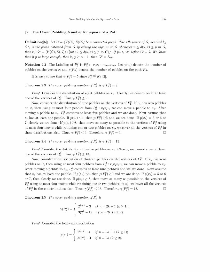
Cover Pebbling Number for Square of a Path 55
§2. The Cover Pebbling Number for square of a Path
Definition([6]) Let G = (V(G), E(G)) be a connected graph. The nth power of G, denoted by
Gp, is the graph obtained from G by adding the edge uv to G whenever 2 ≤ d(u, v) ≤ p in G,
that is, Gp = (V (G), E(G) ∪ uv : 2 ≤ d(u, v) ≤ p in G). If p=1, we define G1=G. We know
that if p is large enough, that is, p ≥ n − 1, then Gp = Kn.
Notation 2.2 The Labeling of P 2n is P 2
n : v1v2 · · · vn−1vn. Let p(vi) denote the number of
pebbles on the vertex vi and p(PA) denote the number of pebbles on the path PA.
It is easy to see that γ(P 23 ) = 5 since P 2
3∼= K3 [2].
Theorem 2.3 The cover pebbling number of P 24 is γ(P 2
4 ) = 9.
Proof Consider the distribution of eight pebbles on v1. Clearly, we cannot cover at least
one of the vertices of P 24 . Thus,γ(P 2
4 ) ≥ 9.
Now, consider the distribution of nine pebbles on the vertices of P 24 . If v4 has zero pebbles
on it, then using at most four pebbles from P 23 : v1v2v3 we can move a pebble to v4. After
moving a pebble to v4, P 23 contains at least five pebbles and we are done. Next assume that
v4 has at least one pebble. If p(v4) ≤4, then p(P 23 ) ≥5 and we are done. If p(v4) = 5 or 6 or
7, clearly we are done. If p(v4) ≥8, then move as many as possible to the vertices of P 23 using
at most four moves while retaining one or two pebbles on v4, we cover all the vertices of P 24 in
these distributions also. Thus, γ(P 24 ) ≤ 9. Therefore, γ(P 2
4 ) = 9.
Theorem 2.4 The cover pebbling number of P 25 is γ(P 2
5 ) = 13.
Proof Consider the distribution of twelve pebbles on v1. Clearly, we cannot cover at least
one of the vertices of P 25 . Thus,γ(P 2
5 ) ≥ 13.
Now, consider the distribution of thirteen pebbles on the vertices of P 25 . If v5 has zero
pebbles on it, then using at most four pebbles from P 24 : v1v2v3v4 we can move a pebble to v5.
After moving a pebble to v5, P 24 contains at least nine pebbles and we are done. Next assume
that v5 has at least one pebble. If p(v5) ≤4, then p(P 24 ) ≥9 and we are done. If p(v5) = 5 or 6
or 7, then clearly we are done. If p(v5) ≥ 8, then move as many as possible to the vertices of
P 24 using at most four moves while retaining one or two pebbles on v5, we cover all the vertices
of P 25 in these distributions also. Thus, γ(P 2
5 ) ≤ 13. Therefore, γ(P 25 ) = 13.
Theorem 2.5 The cover pebbling number of P 2n is
γ(P 2n) =
2k+2 − 3 if n = 2k + 1 (k ≥ 1);
3(2k − 1) if n = 2k (k ≥ 2).
Proof Consider the following distribution
p(v1) =
2k+2 − 4 if n = 2k + 1 (k ≥ 1);
3(2k) − 4 if n = 2k (k ≥ 2).

56 A.Lourdusamy and T.Mathivanan
and p(vi) = 0, i 6= 1. Notice that we cannot cover at least one of the vertices of P 2n . Thus,
γ(P 2n) ≥
2k+2 − 3 if n = 2k + 1 (k ≥ 1);
3(2k − 1) if n = 2k (k ≥ 2).
. Next, we are going to prove the upper bound by induction on n. Obviously, the result is
true for n = 4 and 5, by Theorem 2.3 and Theorem 2.4. So, assume the result is true for
m ≤ n-1. If vn has zero pebbles on it, then using at most 2k pebbles from the vertices of
P 2n−1 : v1v2 · · · vn−2vn−1 we can cover the vertex vn. Then P 2
n−1contains at least
3(2k − 1), where k =n − 1
2;
2k+1 − 3, where k =n
2
pebbles and we are done by induction. Next, assume that vn has a pebble on it. If p(vn) ≤2(2k − 1), then
p(P 2n−1) ≥
2k+1 − 3 if n is odd;
2k − 1 if n is even.
In these both cases, either P 2n−1 has enough pebbles or we can make it by retaining one or
two pebbles on vn and moving as many pebbles as possible from vn to vn−1 or vn−2. So, we
are done easily if p(vn) ≤ 2(2k − 1). Suppose p(vn) ≥ 2(2k − 1) + 1, then by moving as many
pebbles as possible to the vertices of P 2n−1, using at most
2k+1 − 2 if n is odd;
3(2k−1) − 2 if n is even
pebbling steps while retaining one or two pebbles on vn, and hence we are done. Thus,
γ(P 2n) ≤
2k+2 − 3 if n = 2k + 1 (k ≥ 1);
3(2k − 1) if n = 2k (k ≥ 2).
Therefore,
γ(P 2n) =
2k+2 − 3 if n = 2k + 1 (k ≥ 1);
3(2k − 1) if n = 2k (k ≥ 2).
References
[1] Chung, Pebbling in hypercubes, SIAM J. Discrete Math. 2 (1989), no.4, 467-472.
[2] Crull, Cundiff, Feltman, Hulbert, Pudwell, Szaniszlo, Tuza, The cover pebbling number of
graphs, Discrete Math., 296 (2005), 15-23.
[3] Hulbert, A survey of graph pebbling, Congressus Numerantium, 139 (1999), 41-64.
[4] Hulbert and Munyan, The cover pebbling number of hypercubes, Bull. Inst.Combin.Appl.,
47(2006),71-76.

Cover Pebbling Number for Square of a Path 57
[5] Maggy Tomova and Cindy Wyles, Cover pebbling cycles and certain graph products,
preprint.
[6] L.Pachter, H. S. Snevily and B. Voxman, On pebbling graphs, Congr. Numer., 107(1995),
65-80.
[7] Watson and Yerger, Cover pebbling numbers and bounds for certain families of graphs,
Bull. Inst. Combin. Appl., 48(2006), 53-62.

Math.Combin.Book Ser. Vol.3(2012), 58-63
Switching Equivalence in Symmetric n-Sigraphs-V
P.Siva Kota Reddy, M.C.Geetha and K.R.Rajanna
(Department of Mathematics, Acharya Institute of Technology, Soldevanahalli, Bangalore-560 090, India)
E-mail: [email protected]
Abstract: An n-tuple (a1, a2, ..., an) is symmetric, if ak = an−k+1, 1 ≤ k ≤ n. Let
Hn = (a1, a2, · · · , an) : ak ∈ +,−, ak = an−k+1, 1 ≤ k ≤ n be the set of all symmetric
n-tuples. A symmetric n-sigraph (symmetric n-marked graph) is an ordered pair Sn = (G, σ)
(Sn = (G, µ)), where G = (V, E) is a graph called the underlying graph of Sn and σ : E → Hn
(µ : V → Hn) is a function. In this paper, we introduced a new notion S-antipodal symmetric
n-sigraph of a symmetric n-sigraph and its properties are obtained. Also we give the relation
between antipodal symmetric n-sigraphs and S-antipodal symmetric n-sigraphs. Further, we
discuss structural characterization of S-antipodal symmetric n-sigraphs.
Key Words: Symmetric n-sigraphs, Smarandachely symmetric n-marked graph, sym-
metric n-marked graphs, balance, switching, antipodal symmetric n-sigraphs, S-antipodal
symmetric n-sigraphs, complementation.
AMS(2010): 05C22
§1. Introduction
Unless mentioned or defined otherwise, for all terminology and notion in graph theory the
reader is refer to [1]. We consider only finite, simple graphs free from self-loops.
Let n ≥ 1 be an integer. An n-tuple (a1, a2, · · · , an) is symmetric, if ak = an−k+1, 1 ≤k ≤ n. Let Hn = (a1, a2, · · · , an) : ak ∈ +,−, ak = an−k+1, 1 ≤ k ≤ n be the set of all
symmetric n-tuples. Note that Hn is a group under coordinate wise multiplication, and the
order of Hn is 2m, where m = ⌈n
2⌉.
A Smarandachely k-marked graph (Smarandachely k-signed graph) is an ordered pair
S = (G, µ) (S = (G, σ)) where G = (V, E) is a graph called underlying graph of S and
µ : V → e1, e2, ..., ek (σ : E → e1, e2, ..., ek) is a function, where ei ∈ +,−. An n-
tuple (a1, a2, ..., an) is symmetric, if ak = an−k+1, 1 ≤ k ≤ n. Let Hn = (a1, a2, ..., an) :
ak ∈ +,−, ak = an−k+1, 1 ≤ k ≤ n be the set of all symmetric n-tuples. A Smaran-
dachely symmetric n-marked graph (Smarandachely symmetric n-signed graph) is an ordered
pair Sn = (G, µ) (Sn = (G, σ)) where G = (V, E) is a graph called the underlying graph of Sn
and µ : V → Hn (σ : E → Hn) is a function. Particularly, a Smarandachely 1-marked graph
(Smarandachely 1-signed graph) is called a marked graph (signed graph).
1Received February 25, 2012. Accepted September 9, 2012.

Switching Equivalence in Symmetric n-Sigraphs-V 59
In this paper by an n-tuple/n-sigraph/n-marked graph we always mean a symmetric n-
tuple/symmetric n-sigraph/symmetric n-marked graph.
An n-tuple (a1, a2, · · · , an) is the identity n-tuple, if ak = +, for 1 ≤ k ≤ n, otherwise
it is a non-identity n-tuple. In an n-sigraph Sn = (G, σ) an edge labelled with the identity
n-tuple is called an identity edge, otherwise it is a non-identity edge. Further, in an n-sigraph
Sn = (G, σ), for any A ⊆ E(G) the n-tuple σ(A) is the product of the n-tuples on the edges of
A.
In [7], the authors defined two notions of balance in n-sigraph Sn = (G, σ) as follows (See
also R. Rangarajan and P.S.K.Reddy [4]):
Definition 1.1 Let Sn = (G, σ) be an n-sigraph. Then,
(i) Sn is identity balanced (or i-balanced), if product of n-tuples on each cycle of Sn is
the identity n-tuple, and
(ii) Sn is balanced, if every cycle in Sn contains an even number of non-identity edges.
Note 1.1 An i-balanced n-sigraph need not be balanced and conversely.
The following characterization of i-balanced n-sigraphs is obtained in [7].
Proposition 1.1 (E. Sampathkumar et al. [7]) An n-sigraph Sn = (G, σ) is i-balanced if, and
only if, it is possible to assign n-tuples to its vertices such that the n-tuple of each edge uv is
equal to the product of the n-tuples of u and v.
Let Sn = (G, σ) be an n-sigraph. Consider the n-marking µ on vertices of Sn defined as
follows: each vertex v ∈ V , µ(v) is the n-tuple which is the product of the n-tuples on the
edges incident with v. Complement of Sn is an n-sigraph Sn = (G, σc), where for any edge
e = uv ∈ G, σc(uv) = µ(u)µ(v). Clearly, Sn as defined here is an i-balanced n-sigraph due to
Proposition 1.1 ([10]).
In [7], the authors also have defined switching and cycle isomorphism of an n-sigraph
Sn = (G, σ) as follows (See also [2,5,6,10]):
Let Sn = (G, σ) and S′n = (G′, σ′), be two n-sigraphs. Then Sn and S′
n are said to be
isomorphic, if there exists an isomorphism φ : G → G′ such that if uv is an edge in Sn with
label (a1, a2, · · · , an) then φ(u)φ(v) is an edge in S′n with label (a1, a2, · · · , an).
Given an n-marking µ of an n-sigraph Sn = (G, σ), switching Sn with respect to µ is
the operation of changing the n-tuple of every edge uv of Sn by µ(u)σ(uv)µ(v). The n-sigraph
obtained in this way is denoted by Sµ(Sn) and is called the µ-switched n-sigraph or just switched
n-sigraph. Further, an n-sigraph Sn switches to n-sigraph S′n (or that they are switching
equivalent to each other), written as Sn ∼ S′n, whenever there exists an n-marking of Sn such
that Sµ(Sn) ∼= S′n.
Two n-sigraphs Sn = (G, σ) and S′n = (G′, σ′) are said to be cycle isomorphic, if there
exists an isomorphism φ : G → G′ such that the n-tuple σ(C) of every cycle C in Sn equals to
the n-tuple σ(φ(C)) in S′n. We make use of the following known result (see [7]).
Proposition 1.2 (E. Sampathkumar et al. [7]) Given a graph G, any two n-sigraphs with G

60 P.Siva Kota Reddy, M.C.Geetha and K.R.Rajanna
as underlying graph are switching equivalent if, and only if, they are cycle isomorphic.
Let Sn = (G, σ) be an n-sigraph. Consider the n-marking µ on vertices of S defined
as follows: each vertex v ∈ V , µ(v) is the product of the n-tuples on the edges incident
at v. Complement of S is an n-sigraph Sn = (G, σ′), where for any edge e = uv ∈ G,
σ′(uv) = µ(u)µ(v). Clearly, Sn as defined here is an i-balanced n-sigraph due to Proposition
1.1.
§2. S-Antipodal n-Sigraphs
Radhakrishnan Nair and Vijayakumar [3] has introduced the concept of S-antipodal graph of a
graph G as the graph A∗(G) has the vertices in G with maximum eccentricity and two vertices
of A∗(G) are adjacent if they are at a distance of diam(G) in G.
Motivated by the existing definition of complement of an n-sigraph, we extend the notion
of S-antipodal graphs to n-sigraphs as follows:
The S-antipodal n-sigraph A∗(Sn) of an n-sigraph Sn = (G, σ) is an n-sigraph whose
underlying graph is A∗(G) and the n-tuple of any edge uv is A∗(Sn) is µ(u)µ(v), where µ is the
canonical n-marking of Sn. Further, an n-sigraph Sn = (G, σ) is called S-antipodal n-sigraph, if
Sn∼= A∗(S′
n) for some n-sigraph S′n. The following result indicates the limitations of the notion
A∗(Sn) as introduced above, since the entire class of i-unbalanced n-sigraphs is forbidden to be
S-antipodal n-sigraphs.
Proposition 2.1 For any n-sigraph Sn = (G, σ), its S-antipodal n-sigraph A∗(Sn) is i-balanced.
Proof Since the n-tuple of any edge uv in A∗(Sn) is µ(u)µ(v), where µ is the canonical
n-marking of Sn, by Proposition 1.1, A∗(Sn) is i-balanced.
For any positive integer k, the kth iterated S-antipodal n-sigraph A∗(Sn) of Sn is defined
as follows:
(A∗)0(Sn) = Sn, (A∗)k(Sn) = A∗((A∗)k−1(Sn))
Corollary 2.2 For any n-sigraph Sn = (G, σ) and any positive integer k, (A∗)k(Sn) is i-
balanced.
In [3], the authors characterized those graphs that are isomorphic to their S-antipodal
graphs.
Proposition 2.3(Radhakrishnan Nair and Vijayakumar [3]) For a graph G = (V, E), G ∼=A∗(G) if, and only if, G is a regular self-complementary graph.
We now characterize the n-sigraphs that are switching equivalent to their S-antipodal
n-sigraphs.
Proposition 2.4 For any n-sigraph Sn = (G, σ), Sn ∼ A∗(Sn) if, and only if, G is regular
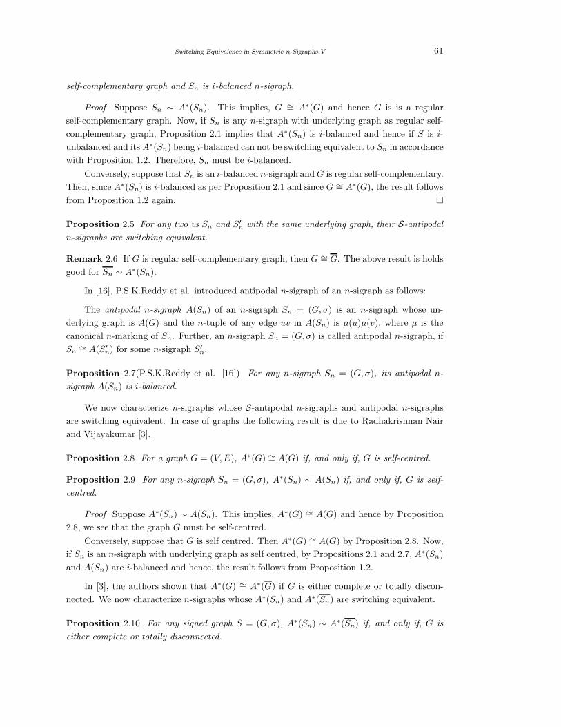
Switching Equivalence in Symmetric n-Sigraphs-V 61
self-complementary graph and Sn is i-balanced n-sigraph.
Proof Suppose Sn ∼ A∗(Sn). This implies, G ∼= A∗(G) and hence G is is a regular
self-complementary graph. Now, if Sn is any n-sigraph with underlying graph as regular self-
complementary graph, Proposition 2.1 implies that A∗(Sn) is i-balanced and hence if S is i-
unbalanced and its A∗(Sn) being i-balanced can not be switching equivalent to Sn in accordance
with Proposition 1.2. Therefore, Sn must be i-balanced.
Conversely, suppose that Sn is an i-balanced n-sigraph and G is regular self-complementary.
Then, since A∗(Sn) is i-balanced as per Proposition 2.1 and since G ∼= A∗(G), the result follows
from Proposition 1.2 again.
Proposition 2.5 For any two vs Sn and S′n with the same underlying graph, their S-antipodal
n-sigraphs are switching equivalent.
Remark 2.6 If G is regular self-complementary graph, then G ∼= G. The above result is holds
good for Sn ∼ A∗(Sn).
In [16], P.S.K.Reddy et al. introduced antipodal n-sigraph of an n-sigraph as follows:
The antipodal n-sigraph A(Sn) of an n-sigraph Sn = (G, σ) is an n-sigraph whose un-
derlying graph is A(G) and the n-tuple of any edge uv in A(Sn) is µ(u)µ(v), where µ is the
canonical n-marking of Sn. Further, an n-sigraph Sn = (G, σ) is called antipodal n-sigraph, if
Sn∼= A(S′
n) for some n-sigraph S′n.
Proposition 2.7(P.S.K.Reddy et al. [16]) For any n-sigraph Sn = (G, σ), its antipodal n-
sigraph A(Sn) is i-balanced.
We now characterize n-sigraphs whose S-antipodal n-sigraphs and antipodal n-sigraphs
are switching equivalent. In case of graphs the following result is due to Radhakrishnan Nair
and Vijayakumar [3].
Proposition 2.8 For a graph G = (V, E), A∗(G) ∼= A(G) if, and only if, G is self-centred.
Proposition 2.9 For any n-sigraph Sn = (G, σ), A∗(Sn) ∼ A(Sn) if, and only if, G is self-
centred.
Proof Suppose A∗(Sn) ∼ A(Sn). This implies, A∗(G) ∼= A(G) and hence by Proposition
2.8, we see that the graph G must be self-centred.
Conversely, suppose that G is self centred. Then A∗(G) ∼= A(G) by Proposition 2.8. Now,
if Sn is an n-sigraph with underlying graph as self centred, by Propositions 2.1 and 2.7, A∗(Sn)
and A(Sn) are i-balanced and hence, the result follows from Proposition 1.2.
In [3], the authors shown that A∗(G) ∼= A∗(G) if G is either complete or totally discon-
nected. We now characterize n-sigraphs whose A∗(Sn) and A∗(Sn) are switching equivalent.
Proposition 2.10 For any signed graph S = (G, σ), A∗(Sn) ∼ A∗(Sn) if, and only if, G is
either complete or totally disconnected.

62 P.Siva Kota Reddy, M.C.Geetha and K.R.Rajanna
The following result characterize n-sigraphs which are S-antipodal n-sigraphs.
Proposition 2.11 An n-sigraph Sn = (G, σ) is a S-antipodal n-sigraph if, and only if, Sn is
i-balanced n-sigraph and its underlying graph G is a S-antipodal graph.
Proof Suppose that Sn is i-balanced and G is a A(G). Then there exists a graph H
such that A∗(H) ∼= G. Since Sn is i-balanced, by Proposition 1.1, there exists an n-marking
µ of G such that each edge uv in Sn satisfies σ(uv) = µ(u)µ(v). Now consider the n-sigraph
S′n = (H, σ′), where for any edge e in H , σ′(e) is the n-marking of the corresponding vertex in
G. Then clearly, A∗(S′n) ∼= Sn. Hence Sn is a S-antipodal n-sigraph.
Conversely, suppose that Sn = (G, σ) is a S-antipodal n-sigraph. Then there exists an
n-sigraph S′n = (H, σ′) such that A∗(S′
n) ∼= Sn. Hence G is the A∗(G) of H and by Proposition
2.1, Sn is i-balanced.
§3. Complementation
In this section, we investigate the notion of complementation of a graph whose edges have signs
(a sigraph) in the more general context of graphs with multiple signs on their edges. We look
at two kinds of complementation: complementing some or all of the signs, and reversing the
order of the signs on each edge.
For any m ∈ Hn, the m-complement of a = (a1, a2, · · · ., an) is: am = am. For any
M ⊆ Hn, and m ∈ Hn, the m-complement of M is Mm = am : a ∈ M. For any m ∈ Hn,
the m-complement of an n-sigraph Sn = (G, σ), written (Smn ), is the same graph but with each
edge label a = (a1, a2, ..., an) replaced by am. For an n-sigraph Sn = (G, σ), the A∗(Sn) is
i-balanced (Proposition 2.1). We now examine, the condition under which m-complement of
A(Sn) is i-balanced, where for any m ∈ Hn.
Proposition 3.1 Let Sn = (G, σ) be an n-sigraph. Then, for any m ∈ Hn, if A∗(G) is
bipartite then (A∗(Sn))m is i-balanced.
Proof Since, by Proposition 2.1, A∗(Sn) is i-balanced, for each k, 1 ≤ k ≤ n, the number
of n-tuples on any cycle C in A∗(Sn) whose kth co-ordinate are − is even. Also, since A∗(G)
is bipartite, all cycles have even length; thus, for each k, 1 ≤ k ≤ n, the number of n-tuples on
any cycle C in A∗(Sn) whose kth co-ordinate are + is also even. This implies that the same
thing is true in any m-complement, where for any m,∈ Hn. Hence (A∗(Sn))t is i-balanced.
Problem 3.2 Characterize these n-sigraphs for which
(1) (Sn)m ∼ A∗(Sn);
(2) (Sn)m ∼ A(Sn);
(3) (A∗(Sn))m ∼ A(Sn);
(4) A∗(Sn) ∼ (A(Sn))m;
(5) (A∗(S))m ∼ A∗(Sn);
(6) A∗(Sn) ∼ (A∗(Sn))m.

Switching Equivalence in Symmetric n-Sigraphs-V 63
References
[1] F. Harary, Graph Theory, Addison-Wesley Publishing Co., 1969.
[2] V.Lokesha, P.S.K.Reddy and S. Vijay, The triangular line n-sigraph of a symmetric n-
sigraph, Advn. Stud. Contemp. Math., 19(1) (2009), 123-129.
[3] R.Radhakrishnan Nair and A.Vijaykumar, S-Antipodal graphs, Indian J. Pure Appl. Math.,
28(5) (1997), 641-645.
[4] R.Rangarajan and P.S.K.Reddy, Notions of balance in symmetric n-sigraphs, Proceedings
of the Jangjeon Math. Soc., 11(2) (2008), 145-151.
[5] R.Rangarajan, P.S.K.Reddy and M.S.Subramanya, Switching Equivalence in Symmetric
n-Sigraphs, Adv. Stud. Comtemp. Math., 18(1) (2009), 79-85. R.
[6] R.Rangarajan, P.S.K.Reddy and N.D.Soner, Switching equivalence in symmetric n-sigraphs-
II, J. Orissa Math. Sco., 28 (1 & 2) (2009), 1-12.
[7] E.Sampathkumar, P.S.K.Reddy, and M.S.Subramanya, Jump symmetric n-sigraph, Pro-
ceedings of the Jangjeon Math. Soc., 11(1) (2008), 89-95.
[8] E.Sampathkumar, P.S.K.Reddy, and M.S.Subramanya, The Line n-sigraph of a symmetric
n-sigraph, Southeast Asian Bull. Math., 34(5) (2010), 953-958.
[9] R. Singleton, There is no irregular moore graph, Amer. Math. Monthly, 75(1968), 42-43.
[10] P.S.K.Reddy and B.Prashanth, Switching equivalence in symmetric n-sigraphs-I, Advances
and Applications in Discrete Mathematics, 4(1) (2009), 25-32.
[11] P.S.K.Reddy, S.Vijay and B.Prashanth, The edge C4 n-sigraph of a symmetric n-sigraph,
Int. Journal of Math. Sci. & Engg. Appls., 3(2) (2009), 21-27.
[12] P.S.K.Reddy, V.Lokesha and Gurunath Rao Vaidya, The Line n-sigraph of a symmetric
n-sigraph-II, Proceedings of the Jangjeon Math. Soc., 13(3) (2010), 305-312.
[13] P.S.K.Reddy, V.Lokesha and Gurunath Rao Vaidya, The Line n-sigraph of a symmetric
n-sigraph-III, Int. J. Open Problems in Computer Science and Mathematics, 3(5) (2010),
172-178.
[14] P.S.K.Reddy, V.Lokesha and Gurunath Rao Vaidya, Switching equivalence in symmetric
n-sigraphs-III, Int. Journal of Math. Sci. & Engg. Appls., 5(1) (2011), 95-101.
[15] P.S.K.Reddy, B. Prashanth and Kavita. S. Permi, A Note on Switching in Symmetric
n-Sigraphs, Notes on Number Theory and Discrete Mathematics, 17(3) (2011), 22-25.
[16] P.S.K.Reddy, M. C. Geetha and K. R. Rajanna, Switching Equivalence in Symmetric n-
Sigraphs-IV, Scientia Magna, 7(3) (2011), 34-38.
Math.Combin.Book Ser. Vol.3(2012), 64-71
Further Results on Product Cordial Labeling
S.K.Vaidya
(Saurashtra University, Rajkot - 360005, Gujarat, India)
C.M.Barasara
(Atmiya Institute of Technology and Science, Rajkot - 360005, Gujarat, India)
E-mail: [email protected], [email protected]
Abstract: We prove that closed helm CHn, web graph Wbn, flower graph F ln, double
triangular snake DTn and gear graph Gn admit product cordial labeling.
Key Words: Graph labeling, cordial labeling, Smarandachely p-product cordial labeling,
product cordial labeling.
AMS(2010): 05C78
§1. Introduction
We begin with finite, connected and undirected graph G = (V (G), E(G)) without loops and
multiple edges. For any undefined notations and terminology we rely upon Clark and Holton
[3]. In order to maintain compactness we provide a brief summery of definitions and existing
results.
Definition 1.1 A graph labeling is an assignment of integers to the vertices or edges or both
subject to certain condition(s). If the domain of the mapping is the set of vertices (or edges)
then the labeling is called a vertex labeling (or an edge labeling).
According to Beineke and Hegde [1] labeling of discrete structure serves as a frontier
between graph theory and theory of numbers. A dynamic survey of graph labeling is carried
out and frequently updated by Gallian [4].
Definition 1.2 A mapping f : V (G) → 0, 1 is called binary vertex labeling of G and f(v) is
called the label of the vertex v of G under f .
The induced edge labeling f∗ : E(G) → 0, 1 is given by f∗(e = uv) = |f(u) − f(v)|. Let
us denote vf (0), vf (1) be the number of vertices of G having labels 0 and 1 respectively under
f and let ef(0), ef (1) be the number of edges of G having labels 0 and 1 respectively under f∗.
1Received March 26, 2012. Accepted September 12, 2012.

Further Results on Product Cordial Labeling 65
Definition 1.3 A binary vertex labeling of a graph G is called a cordial labeling if |vf (0) −vf (1)| ≤ 1 and |ef(0) − ef (1)| ≤ 1. A graph G is called cordial if it admits cordial labeling.
The concept of cordial labeling was introduced by Cahit [2] in which he investigated several
results on this newly defined concept. After this some labelings like prime cordial labeling, A -
cordial labeling, H-cordial labeling and product cordial labeling are also introduced as variants
of cordial labeling.
This paper is aimed to report some new families of product cordial graphs.
Definition 1.4 For an integer p > 1. A mapping f : V (G) → 0, 1, 2, · · · , p is called a
Smarandachely p-product cordial labeling if |vf (i) − vf (j)| ≤ 1 and |ef (i) − ef (j)| ≤ 1 for
any i, j ∈ 0, 1, 2, · · · , p − 1, where vf (i) denotes the number of vertices labeled with i, ef (i)
denotes the number of edges xy with f(x)f(y) ≡ i(mod p). Particularly, if p = 2, i.e., a
binary vertex labeling of graph G with an induced edge labeling f∗ : E(G) → 0, 1 defined
by f∗(e = uv) = f(u)f(v), such a Smarandachely 2-product cordial labeling is called product
cordial labeling. A graph with product cordial labeling is called a product cordial graph.
The product cordial labeling was introduced by Sundaram et al. [5] and they investigated
several results on this newly defined concept. They have established a necessary condition
showing that a graph with p vertices and q edges with p ≥ 4 is product cordial then q <
(p2 − 1)/4 + 1.
The graphs obtained by joining apex vertices of k copies of stars, shells and wheels to a new
vertex are proved to be product cordial by Vaidya and Dani [6] while some results on product
cordial labeling for cycle related graphs are reported in Vaidya and Kanani [7].
Vaidya and Barasara [8] have proved that the cycle with one chord, the cycle with twin
chords, the friendship graph and the middle graph of path admit product cordial labeling. The
same authors in [9] have proved that the graphs obtained by duplication of one edge, mutual
vertex duplication and mutual edge duplication in cycle are product cordial graphs. Vaidya and
Vyas [10] have discussed product cordial labeling in the context of tensor product of some graphs
while Vaidya and Barasara [11] have investigated some results on product cordial labeling in
the context of some graph operations.
Definition 1.5 The wheel graph Wn is defined to be the join K1+Cn. The vertex corresponding
to K1 is known as apex vertex and vertices corresponding to cycle are known as rim vertices
while the edges corresponding to cycle are known as rim edges. We continue to recognize apex
of respective graphs obtained from wheel in Definitions 1.6 to 1.9.
Definition 1.6 The helm Hn is the graph obtained from a wheel Wn by attaching a pendant
edge to each rim vertex.
Definition 1.7 The closed helm CHn is the graph obtained from a helm Hn by joining each
pendant vertex to form a cycle.
Definition 1.8 The web graph Wbn is the graph obtained by joining the pendant vertices of a
helm Hn to form a cycle and then adding a pendant edge to each vertex of outer cycle.

66 S.K.Vaidya and C.M.Barasara
Definition 1.9 The flower Fln is the graph obtained from a helm Hn by joining each pendant
vertex to the apex of the helm.
Definition 1.10 The double triangular snake DTn is obtained from a path Pn with vertices
v1, v2, · · · , vn by joining vi and vi+1 to a new vertex wi for i = 1, 2, · · · , n − 1 and to a new
vertex ui for i = 1, 2, · · · , n − 1.
Definition 1.11 Let e = uv be an edge of graph G and w is not a vertex of G. The edge e is
subdivided when it is replaced by edges e′ = uw and e′′ = wv.
Definition 1.12 The gear graph Gn is obtained from the wheel by subdividing each of its rim
edge.
§2. Main Results
Theorem 2.1 Closed helm CHn is a product cordial graph.
Proof Let v be the apex vertex, v1, v2, . . . , vn be the vertices of inner cycle and u1, u2, . . . , un
be the vertices of outer cycle of CHn. Then |V (CHn)| = 2n + 1 and |E(CHn)| = 4n.
We define f : V (CHn) → 0, 1 to be f(v) = 1, f(vi) = 1 and f(ui) = 0 for all i. In view
of the above labeling patten we have vf (0) = vf (1)− 1 = n, ef(0) = ef (1) = 2n. Thus we have
|vf (0) − vf (1)| ≤ 1 and |ef(0) − ef (1)| ≤ 1. Hence CHn is a product cordial graph.
Illustration 2.2 The Fig.1 shows the closed helm CH5 and its product cordial labeling.
Fig.1
Theorem 2.3 Web graph Wbn admits product cordial labeling.
Proof Let v be the apex vertex, v1, v2, · · · , vn be the vertices of inner cycle, vn+1, vn+2, · · · , v2n
be the vertices of outer cycle and v2n+1, v2n+2, · · · , v3n be the pendant vertices in Wbn. Then
|V (Wbn)| = 3n + 1 and |E(Wbn)| = 5n.
To define f : V (Wbn) → 0, 1 we consider following two cases.
Case 1. n is odd
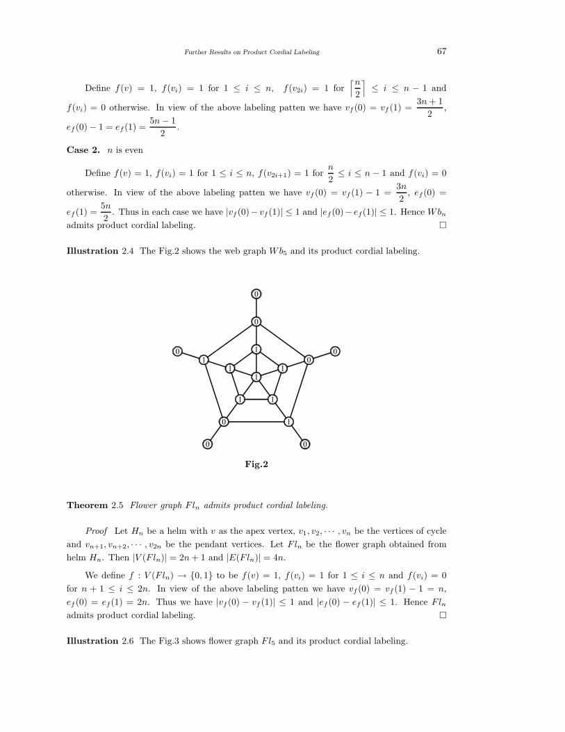
Further Results on Product Cordial Labeling 67
Define f(v) = 1, f(vi) = 1 for 1 ≤ i ≤ n, f(v2i) = 1 for⌈n
2
⌉
≤ i ≤ n − 1 and
f(vi) = 0 otherwise. In view of the above labeling patten we have vf (0) = vf (1) =3n + 1
2,
ef (0) − 1 = ef (1) =5n − 1
2.
Case 2. n is even
Define f(v) = 1, f(vi) = 1 for 1 ≤ i ≤ n, f(v2i+1) = 1 forn
2≤ i ≤ n − 1 and f(vi) = 0
otherwise. In view of the above labeling patten we have vf (0) = vf (1) − 1 =3n
2, ef (0) =
ef (1) =5n
2. Thus in each case we have |vf (0)− vf (1)| ≤ 1 and |ef (0)− ef(1)| ≤ 1. Hence Wbn
admits product cordial labeling.
Illustration 2.4 The Fig.2 shows the web graph Wb5 and its product cordial labeling.
Fig.2
Theorem 2.5 Flower graph Fln admits product cordial labeling.
Proof Let Hn be a helm with v as the apex vertex, v1, v2, · · · , vn be the vertices of cycle
and vn+1, vn+2, · · · , v2n be the pendant vertices. Let Fln be the flower graph obtained from
helm Hn. Then |V (Fln)| = 2n + 1 and |E(Fln)| = 4n.
We define f : V (Fln) → 0, 1 to be f(v) = 1, f(vi) = 1 for 1 ≤ i ≤ n and f(vi) = 0
for n + 1 ≤ i ≤ 2n. In view of the above labeling patten we have vf (0) = vf (1) − 1 = n,
ef (0) = ef(1) = 2n. Thus we have |vf (0) − vf (1)| ≤ 1 and |ef (0) − ef (1)| ≤ 1. Hence Fln
admits product cordial labeling.
Illustration 2.6 The Fig.3 shows flower graph Fl5 and its product cordial labeling.

68 S.K.Vaidya and C.M.Barasara
Fig.3
Theorem 2.7 Double triangular snake DTn is a product cordial graph for odd n and not a
product cordial graph for even n.
Proof Let v1, v2, · · · , vn be the vertices of path Pn and vn+1, vn+2, · · · , v3n−2 be the newly
added vertices in order to obtain DTn. Then |V (DTn)| = 3n − 2 and |E(DTn)| = 5n − 5.
To define f : V (DTn) → 0, 1 we consider following two cases.
Case 1. n is odd
f(vi) = 0 for 1 ≤ i ≤⌊n
2
⌋
, f(vi) = 0 for n + 1 ≤ i ≤ n +⌊n
2
⌋
and f(vi) = 1 otherwise. In
view of the above labeling patten we have vf (0) + 1 = vf (1) =
⌈
3n − 2
2
⌉
, ef (0) − 1 = ef (1) =
5n − 5
2. Thus we have |vf (0) − vf (1)| ≤ 1 and |ef (0) − ef (1)| ≤ 1.
Case 2. n is even
Subcase 1. n = 2.
The graph DT2 has p = 4 vertices and q = 5 edges since
p2 − 1
4+ 1 =
19
4< q.
Thus the necessary condition for product cordial graph is violated. Hence DT2 is not a product
cordial graph.
Subcase 2. n 6= 2
In order to satisfy the vertex condition for product cordial graph it is essential to assign
label 0 to3n − 2
2vertices out of 3n− 2 vertices. The vertices with label 0 will give rise at least
5n
2− 1 edges with label 0 and at most
5n
2− 4 edge with label 1 out of total 5n − 5 edges.
Therefore |ef (0) − ef (1)| = 3. Thus the edge condition for product cordial graph is violated.
Therefore DTn is not a product cordial graph for even n.
Hence Double triangular snake DTn is a product cordial graph for odd n and not a product
cordial graph for even n.

Further Results on Product Cordial Labeling 69
Illustration 2.8 The Fig.4 shows the double triangular snake DT7 and its product cordial
labeling.
Fig.4
Theorem 2.9 Gear graph Gn is a product cordial graph for odd n and not product cordial graph
for even n.
Proof Let Wn be the wheel with apex vertex v and rim vertices v1, v2, · · · , vn. To obtain
the gear graph Gn subdivide each rim edge of wheel by the vertices u1, u2, · · · , un. Where each
ui subdivides the edge vivi+1 for i = 1, 2, · · · , n − 1 and un subdivides the edge v1vn. Then
|V (Gn)| = 2n + 1 and |E(Gn)| = 3n.
To define f : V (Gn) → 0, 1 we consider following two cases.
Case 1. n is odd
f(v) = 1; f(vi) = 1 for 1 ≤ i ≤⌈n
2
⌉
; f(vi) = 0, otherwise;
f(ui) = 1 for 1 ≤ i ≤ n +⌊n
2
⌋
; f(ui) = 0, otherwise.
In view of the above labeling patten we have vf (0) = vf (1) − 1 = n, ef (0) = ef(1) + 1 =3n + 1
2. Thus we have |vf (0) − vf (1)| ≤ 1 and |ef (0) − ef (1)| ≤ 1.
Case 2. n is even
In order to satisfy the vertex condition for product cordial graph it is essential to assign
label 0 to n vertices out of 2n + 1 vertices. The vertices with label 0 will give rise at least3n
2+1 edges with label 0 and at most
3n
2−1 edge with label 1 out of total 3n edges. Therefore
|ef (0) − ef (1)| = 2. Thus the edge condition for product cordial graph is violated. So Gn is
not a product cordial graph for even n.
Hence gear graph is a product cordial graph for odd n and not product cordial graph for
even n.
Illustration 2.10 The Fig.5 shows the gear graph G7 and its product cordial labeling.

70 S.K.Vaidya and C.M.Barasara
Fig.5
§3. Concluding Remarks
Some new families of product cordial graphs are investigated. To investigate some charac-
terization(s) or sufficient condition(s) for the graph to be product cordial is an open area of
research.
Acknowledgement
The authors are deeply indebted to the referee for critical comments and suggestions.
References
[1] L.W.Beineke and S.M.Hegde, Strongly Multiplicative graphs, Discuss. Math. Graph The-
ory, 21(2001), 63-75.
[2] I.Cahit, Cordial Graphs: A weaker version of graceful and harmonious Graphs, Ars Com-
binatoria, 23(1987), 201-207.
[3] J.Clark and D.Holton, A First Look at Graph Theory, Allied Publishers, New Delhi, 1995.
[4] J.A.Gallian, A dynamic survey of graph labeling, The Electronic Journal of Combinatorics,
18(2011), #DS6. Available also online: http://www.combinatorics.org/Surveys/ds6.pdf.
[5] M.Sundaram, R.Ponraj and S.Somasundaram, Product cordial labeling of graphs, Bull.
Pure and Applied Science (Mathematics and Statistics), 23E(2004), 155-163.
[6] S.K.Vaidya and N.A.Dani, Some new product cordial graphs, Journal of App. Comp. Sci.
Math., 8(4)(2010), 62-65. Available also online: http://jacs.usv.ro/getpdf.php?paperid=
811.
[7] S.K.Vaidya and K.K.Kanani, Some cycle related product cordial graphs, Int. J. of Algo-
rithms, Comp. and Math., 3(1)(2010), 109-116. Available also online: http://eashwarpubli
cations.com/doc/corrected14.pdf.
Further Results on Product Cordial Labeling 71
[8] S.K.Vaidya and C.M.Barasara, Product cordial labeling for some new graphs, Journal of
Mathematics Research, 3(2)(2011), 206-211. (doi: 10.5539/jmr.v3n2p206)
[9] S.K.Vaidya and C.M.Barasara, Some product cordial graphs, Elixir Discrete Mathematics,
41(2011), 5948-5952. Available also online: http://www.elixirjournal.org.
[10] S.K.Vaidya and N.B.Vyas, Product cordial labeling in the context of tensor product of
graphs, Journal of Mathematics Research, 3(3)(2011), 83-88. (doi: 10.5539/jmr.v3n3p83)
[11] S.K.Vaidya and C.M.Barasara, Product cordial graphs in the context of some graph op-
erations, International Journal of Mathematics and Scientific Computing, 1(2)(2011), 1-6.
Available also online: http://www.vel-tech.org/ijmsc/index.html.

Math.Combin.Book Ser. Vol.3(2012), 72-82
Around The Berge Problem And Hadwiger Conjecture
Ikorong Anouk Gilbert Nemron
Centre De Calcul; D’Enseignement Et De Recherche
Universite’ De Paris VI ( Pierre et Marie Curie ), France
E-mail: [email protected]
Abstract: We say that a graph B is berge, if every graph B′ ∈ B, B does not contain an
induced cycle of odd length ≥ 5 [B is the complementary graph of B]. A graph G is perfect if
every induced subgraph G′ of G satisfies χ(G′) = ω(G′), where χ(G′) is the chromatic number
of G′ and ω(G′) is the clique number of G′. The Berge conjecture states that a graph H is
perfect if and only if H is berge. Indeed, the difficult part of the Berge conjecture consists to
show that χ(B) = ω(B) for every berge graph B. The Hadwiger conjecture states that every
graph G satisfies χ(G) ≤ η(G) [ where η(G) is the hadwiger number of G (i.e., the maximum
of p such that G is contractible to the complete graph Kp)]. The Berge conjecture (see [1]
or [2] or [3] or [5] or [6] or [7] or [9] or [10] or [11] ) was proved by Chudnovsky, Robertson,
Seymour and Thomas in a paper of at least 140 pages (see [1]), and an elementary proof of
the Berge conjecture was given by Ikorong Nemron in a detailled paper of 37 pages long (see
[9]). The Hadwiger conjecture (see [4] or [5] or [7] or [8] or [10] or [11] or [12] or [13] or [15]
or [16]) was proved by Ikorong Nemron in a detailled paper of 28 pages long (see [13]), by
using arithmetic calculus, arithmetic congruences, elementary complex analysis, induction
and reasoning by reduction to absurd. That being so, in this paper, via two simple Theorems,
we rigorously show that the difficult part of the Berge conjecture (solved) and the Hadwiger
conjecture (also solved), are exactly the same conjecture. The previous immediately implies
that, the Hadwiger conjecture is only a non obvious special case of the Berge conjecture.
Key Words: True pal, parent, berge, the berge problem, the berge index, representative,
the hadwiger index, son.
AMS(2010): 05CXX
§0. Preliminary and Some Denotations
We recall that in a graph G = [V (G), E(G), χ(G), ω(G), G], V (G) is the set of vertices, E(G)
is the set of edges, χ(G) is the chromatic number, ω(G) is the clique number and G is the
complementary graph of G. We say that a graph B is berge if every B′ ∈ B, B does not
contain an induced cycle of odd length ≥ 5. A graph G is perfect if every induced subgraph
G′ of G satisfies χ(G′) = ω(G′). The Berge conjecture states that a graph H is perfect if
1Received January 15, 2012. Accepted September 14, 2012.

Around The Berge Problem And Hadwiger Conjecture 73
and only if H is berge. Indeed the difficult part of the Berge conjecture consists to show that
χ(B) = ω(B) for every berge graph B. Briefly, the difficult part of the Berge conjecture will
be called the Berge problem. In this topic, we rigorously show that the Berge problem and the
Hadwiger conjecture are exactly the same problem [the Hadwiger conjecture states that every
graph G is η(G) colorable (i.e. we can color all vertices of G with η(G) colors such that two
adjacent vertices do not receive the same color). η(G) is the hadwiger number of G and is the
maximum of p such that G is contractible to the complete graph Kp]. That being so, this paper
is divided into six simple Sections. In Section 1, we present briefly some standard definitions
known in Graph Theory. In Section 2 , we introduce definitions that are not standard, and
some elementary properties. In Section 3 we define a graph parameter denoted by β (β is
called the berge index ) and we give some obvious properties of this parameter. In Section 4
we introduce another graph parameter denoted by τ (τ is called the hadwiger index) and we
present elementary properties of this parameter. In Section 5 , using the couple (β, τ), we show
two simple Theorems which are equivalent to the Hadwiger conjecture and the Berge problem.
In Section 6, using the two simple Theorems stated and proved in Section 5, we immediately
deduce that the Berge problem and the Hadwiger conjecture are exactly the same problem, and
therefore, the Hadwiger conjecture is only a non obvious special case of the Berge conjecture.
In this paper, all results are simple, and every graph is finite, is simple and is undirected. We
start.
§1. Standard Definitions Known in Graph Theory
Recall (see [2] or [14]) that in a graph G = [V (G), E(G)], V (G) is the set of vertices and E(G)
is the set of edges. G is the complementary graph of G (recall G is the complementary graph
of G, if V (G) = V (G) and two vertices are adjacent in G if and only if they are not adjacent
in G). A graph F is a subgraph of G, if V (F ) ⊆ V (G) and E(F ) ⊆ E(G). We say that a graph
F is an induced subgraph of G by Z, if F is a subgraph of G such that V (F ) = Z, Z ⊆ V (G),
and two vertices of F are adjacent in F , if and only if they are adjacent in G. For X ⊆ V (G),
G \ X denotes the subgraph of G induced by V (G) \ X . A clique of G is a subgraph of G that
is complete; such a subgraph is necessarily an induced subgraph (recall that a graph K is
complete if every pair of vertices of K is an edge of K); ω(G) is the size of a largest clique of
G, and ω(G) is called the clique number of G. A stable set of a graph G is a set of vertices of
G that induces a subgraph with no edges; α(G) is the size of a largest stable set, and α(G) is
called the stability number of G. The chromatic number of G (denoted by χ(G)) is the smallest
number of colors needed to color all vertices of G such that two adjacent vertices do not receive
the same color. It is easy to see:
Assertion 1.0 Let G be a graph. Then ω(G) ≤ χ(G)
The hadwiger number of a graph G (denoted by η(G)), is the maximum of p such that G
is contractible to the complete graph Kp. Recall that, if e is an edge of G incident to x and y,
we can obtain a new graph from G by removing the edge e and identifying x and y so that the
resulting vertex is incident to all those edges (other than e) originally incident to x or to y. This

74 Ikorong Anouk Gilbert Nemron
is called contracting the edge e. If a graph F can be obtained from G by a succession of such
edge-contractions, then, G is contractible to F . The maximum of p such that G is contractible
to the complete graph Kp is the hadwiger number of G, and is denoted by η(G). The Hadwiger
conjecture states that χ(G) ≤ η(G) for every graph G. Clearly we have:
Assertion 1.1 Let G be a graph, and let F be a subgraph of G. Then η(F ) ≤ η(G).
§2. Non-Standard Definitions and Some Elementary Properties
In this section, we introduce definitions that are not standard. These definitions are crucial
for the two theorems which we will use in Section 6 to show that the Berge problem and the
Hadwiger conjecture are exactly the same problem. We say that a graph B is berge, if every
B′ ∈ B, B does not contain an induced cycle of odd length ≥ 5. A graph G is perfect, if
every induced subgraph G′ of G is ω(G′)-colorable. The Berge conjecture states that a graph
G is perfect if and only if G is berge. Indeed, the Berge problem (i.e. the difficult part of the
Berge conjecture, see Preliminary of this paper) consists to show that χ(B) = ω(B), for every
berge graph B. We will see in Section6 that the Berge problem and the Hadwiger conjecture
are exactly the same problem.
We say that a graph G is a true pal of a graph F , if F is a subgraph of G and χ(F ) = χ(G);
trpl(F ) denotes the set of all true pals of F (so, G ∈ trpl(F ) means G is a true pal of F ).
Recall that a set X is a stable subset of a graph G, if X ⊆ V (G) and if the subgraph of
G induced by X has no edges. A graph G is a complete ω(G)-partite graph (or a complete
multipartite graph), if there exists a partition Ξ(G) = Y1, · · · , Yω(G) of V (G) into ω(G) stable
sets such that x ∈ Yj ∈ Ξ(G), y ∈ Yk ∈ Ξ(G) and j 6= k, ⇒ x and y are adjacent in G. It
is immediate that χ(G) = ω(G), for every complete ω(G)-partite graph. Ω denotes the set of
graphs G which are complete ω(G)-partite. So, G ∈ Ω means G is a complete ω(G)-partite
graph. Using the definition of Ω, then the following Assertion becomes immediate.
Assertion 2.0 Let H ∈ Ω and let F be a graph. Then we have the following two properties.
(2.0.0) χ(H) = ω(H);
(2.0.1) There exists a graph P ∈ Ω such that P is a true pal of F .
Proof Property (2.0.0) is immediate (use definition of Ω and note H ∈ Ω). Property (2.0.1)
is also immediate. Indeed, let F be graph and let Ξ(F ) = Y1, · · · , Yχ(F ) be a partition of
V (F ) into χ(F ) stable sets (it is immediate that such a partition Ξ(F ) exists). Now let Q
be a graph defined as follows: (i) V (Q) = V (F ); (ii) Ξ(Q) = Y1, ..., Yχ(F ) is a partition of
V (Q) into χ(F ) stable sets such that x ∈ Yj ∈ Ξ(Q), y ∈ Yk ∈ Ξ(Q) and j 6= k, ⇒ x and
y are adjacent in Q. Clearly Q ∈ Ω, χ(Q) = ω(Q) = χ(F ), and F is visibly a subgraph of
Q; in particular Q is a true pal of F such that Q ∈ Ω (because F is a subgraph of Q and
χ(Q) = χ(F ) and Q ∈ Ω). Now putting Q = P , the property (2.0.1) follows.
So, we say that a graph P is a parent of a graph F , if P ∈ Ω⋂
trpl(F ). In other words, P
is a parent of F , if P is a complete ω(P )-partite graph and P is also a true pal of F ( observe

Around The Berge Problem And Hadwiger Conjecture 75
that such a P exists, via property (2.0.1) of Assertion 2.0). parent(F ) denotes the set of all
parents of a graph F ( so, P ∈ parent(F ) means P is a parent of F ). Using the definition of a
parent, then the following Assertion is immediate.
Assertion 2.1 Let F be a graph and let P ∈ parent(F ). We have the folowing two properties.
(2.1.0) Suppose that F ∈ Ω. Then χ(F ) = ω(F ) = ω(P ) = χ(P );
(2.1.1) Suppose that F 6∈ Ω. Then χ(F ) = ω(P ) = χ(P ).
§3. The Berge Index of a Graph
In this section, we define a graph parameter called the berge index and we define a representative
of a graph; we also give some elementary properties concerning the berge index. We recall that
a graph B is berge, if every B′ ∈ B, B does not contain an induced cycle of odd length ≥ 5. A
graph G is perfect, if every induced subgraph G′ of G is ω(G′)-colorable. The Berge conjecture
states that a graph G is perfect if and only if G is berge. Indeed the Berge problem, consists
to show that χ(B) = ω(B) for every berge graph B. Using the definition of a berge graph and
the definition of Ω the following assertion becomes immediate.
Assertion 3.0 Let G ∈ Ω. Then, G is berge.
Assertion 3.0 says that the set Ω is an obvious example of berge graphs. Now, we define
the berge index of a graph G. Let G be a graph. Then the berge index of G (denoted by β(G) )
is defined in the following two cases (namely case where G ∈ Ω and case where G 6∈ Ω).
First, we define the berge index of G in the case where G ∈ Ω.
Case i Suppose that G ∈ Ω, and put B(G) = F ; G ∈ parent(F ) and F is berge; clearly B(G)
is the set of graphs F such that G is a parent of F and F is berge. Then, β(G) = minF∈B(G)
ω(F ).
In other words, β(G) = ω(F ′′), where F ′′ ∈ B(G), and ω(F ′′) is minimum for this property.
We prove that such a β clearly exists via the following remark.
Remark i Suppose that G ∈ Ω. Then, the berge index β(G) exists. Indeed put B(G) =
F ; G ∈ parent(F ) and F is berge. Recall G ∈ Ω, so G is berge (use Assertion 3.0); clearly
G ∈ B(G), so minF∈B(G)
ω(F ) exists, and the previous clearly says that β(G) exists.
Now, we define the berge index of G, in the case where G 6∈ Ω.
Case ii Suppose that G 6∈ Ω and let parent(G) be the set of all parents of G. Then,
β(G) = minP∈parent(G)
β(P ). In other words, β(G) = β(P ′′), where P ′′ ∈ parent(G), and β(P ′′) is
minimum for this property.
We prove that such a β clearly exists, via the following remark.
Remark ii Suppose that G 6∈ Ω. Then, the berge index β(G) exists. Indeed, let P ∈ Ω
such that P is a true pal of G [such a P exists (use property (2.0.1) of Assertion 2.0)], clearly
P ∈ parent(G); note P ∈ Ω, and Remark.(i) implies that β(P ) exists. So minP∈parent(G)
β(P )
exists, and clearly β(G) also exists.
76 Ikorong Anouk Gilbert Nemron
Remark iii Let G be a graph. Then the berge index β(G) exists. In fact, applying Remark i
if G ∈ Ω, and Remark ii if G 6∈ Ω, we get the conclusion.
To conclude, note that the berge index of a graph G is β(G), where β(G) is defined as
follows.
β(G) = minF∈B(G)
ω(F ) if G ∈ Ω; and β(G) = minP∈parent(G)
β(P ) if G 6∈ Ω. Recall B(G) =
F ; G ∈ parent(F ) and F is berge, and parent(G) is the set of all parents of G.
We recall (see Section 1) that η(G) is the hadwiger number of G, and we clearly have.
Proposition 3.1 Let K be a complete graph and let G ∈ Ω. Then, we have the following three
properties.
(3.1.0) If ω(G) ≤ 1, then β(G) = ω(G) = χ(G) = η(G);
(3.1.1) β(K) = ω(K) = χ(K) = η(K);
(3.1.2) ω(G) ≥ β(G).
Proof Property (3.1.0) is immediate. We prove property (3.1.1). Indeed let B(K) =
F ; K ∈ parent(F ) and F is berge, recall K is complete, and clearly B(K) = K; observe
K ∈ Ω, so β(K) = minF∈B(K)
ω(F ) (use definition of parameter β and note K ∈ Ω), and we easily
deduce that β(K) = ω(K) = χ(K). Note η(K) = χ(K) (since K is complete), and using the
previous, we clearly have β(K) = ω(K) = χ(K) = η(K). Property (3.1.1) follows.
Now we prove property (3.1.2). Indeed, let B(G) = F ; G ∈ parent(F ) and F is berge,recall G ∈ Ω, and so β(G) = min
F∈B(G)ω(F ) (use definition of parameter β and note G ∈ Ω);
observe G is berge (use Assertion 3.0), so G ∈ B(G), and the previous equality implies that
ω(G) ≥ β(G).
Using the definition of the berge index, then we clearly have:
Proposition 3.2 Let B be berge, and let P ∈ parent(B) . Then, β(P ) ≤ ω(B).
Proof Let B(P ) = F ; P ∈ parent(F ) and F is berge, clearly B ∈ B(P ); observe P ∈ Ω,
so β(P ) = minF∈B(P )
ω(F ), and we immediately deduce that β(P ) ≤ ω(B).
Now, we define a representative of a graph. Let G be a graph and let β(G) be the berge
index of G [observe β(G) exists, by using Remark iii]; we say that a graph S is a representative
of G if S is defined in the following two cases (namely case where G ∈ Ω and case where G 6∈ Ω.
First, we define a representative of G in the case where G ∈ Ω.
Case i′ Suppose that G ∈ Ω. Put B(G) = F ; G ∈ parent(F ) and F is berge. Then S is a
representative of G, if S ∈ B(G) and ω(S) = β(G). In other words, S is a representative of G,
if S is berge and G ∈ parent(S ) and ω(S) = β(G). In other terms again, S is a representative
of G if S is berge, G ∈ parent(S ), and ω(S) is minimum for this property. Via Remarks i′ and
i′.0, we prove that such a S exists, and we have χ(S) = χ(G) = ω(G).
Remark i′ Suppose that G ∈ Ω. Then, there exists a graph S such that S is a representative of
Around The Berge Problem And Hadwiger Conjecture 77
G. Indeed, let β(G) be the berge index of G, recalling that G ∈ Ω, clearly β(G) = minF∈B(G)
ω(F ),
where B(G) = F ; G ∈ parent(F ) and F is berge (use definition of parameter β and note
G ∈ Ω) ; now let B ∈ B(G) such that ω(B) = β(G) (such a B exists, since β(G) exists (use
Remark iii), clearly B is a representative of G. Now put B = S; then Remark i′ clearly follows.
Remark i′.0 Suppose that G ∈ Ω. Now let S be a representative of G (such a S exists, by
using Remark i′). Then, χ(S) = χ(G) = ω(G). Indeed, let B(G) = F ; G ∈ parent(F ) and
F is berge, and let S be a representative of G. Recall G ∈ Ω, and clearly S ∈ B(G) (use
definition of a representative and note G ∈ Ω) ; so G ∈ parent(S ), and clearly χ(S) = χ(G).
Note χ(G) = ω(G) (since G ∈ Ω), and the last two equalities immediately imply that χ(S) =
χ(G) = ω(G). Remark i′.0 follows.
Now, we define a representative of G, in the case where G 6∈ Ω.
Case ii′ Suppose that G 6∈ Ω. Now let parent(G) be the set of all parents of G, and let
P ′ ∈ parent(G) such that β(P ′) = β(G) (observe that such a P ′ exists, since G 6∈ Ω, and
by using the definition of β(G)); put B(P ′) = F ′; P ′ ∈ parent(F ′) and F ′ is berge. Then
S is a representative of G if S ∈ B(P ′) and ω(S) = β(P ′) = β(G). In other words, S is a
representative of G (recall G 6∈ Ω), if S is berge and P ′ ∈ parent(S ) and ω(S) = β(P ′) = β(G)
[where P ′ ∈ parent(G) and β(P ′) = β(G)]. Via Remarks ii′ and Remark ii′.0, we prove that
such a S exists, and we have χ(S) = χ(G).
Remark ii′ Suppose that G 6∈ Ω. Then, there exists a graph S such that S is a repre-
sentative of G. Indeed, let β(G) be the berge index of G, recalling that G 6∈ Ω, clearly
β(G) = minP∈parent(G)
β(P ). Now, let P ′ ∈ parent(G) such that β(P ′) = β(G) [observe that
such a P ′ exists, since G 6∈ Ω, and by using the definition of β(G)]; note P ′ ∈ Ω, and clearly
β(P ′) = minF ′∈B(P ′)
ω(F ′) ( note B(P ′) = F ′; P ′ ∈ parent(F ′) and F ′ is berge). Now, let
B′ ∈ B(P ′) such that ω(B′) = β(P ′). Clearly B′ is berge and ω(B′) = β(P ′) = β(G). It is easy
to see that B′ is a representative of G. Now put S = B′, then Remark ii′ follows.
Remark ii′.0 Suppose that G 6∈ Ω. Now let S be a representative of G (such a S exists by
using Remark ii′). Then χ(S) = χ(G). Indeed, let S be a representative of G, and consider
P ′ ∈ parent(G) such that P ′ is a parent of S and β(P ′) = β(G) (such a P ′ clearly exists, by
observing that S be a representative of G, G 6∈ Ω and by using the definition of a representative
of G), clearly χ(S) = ω(P ′) = χ(P ′) = χ(G) (since P ′ is a parent of G and S). So χ(S) = χ(G),
and Remark.(ii’.0) follows.
Remark iii′ Let G be a graph. Then, there exists a graph S such that S is a representative
of G. Applying Remark i′ if G ∈ Ω and applying Remark ii′ if G 6∈ Ω, we get the conclusion.
Remark iv Let G be a graph and let S be a representative of G (such a S exists, by using
Remark iii′). Then, χ(G) = χ(S). Applying Remark i′.0 if G ∈ Ω, and Remark ii′.0 if G 6∈ Ω,
the conclusion follows.
It is clear that a representative of a graph G is not necessarily unique, and in all the cases,
we have χ(G) = χ(S) for every representative S of G [use Remark iv].
78 Ikorong Anouk Gilbert Nemron
To conclude, note that a graph S is a representative of a graph G if S is defined in the
following two cases.
Case 1. Suppose that G ∈ Ω. Then S is a representative of G, if and only if S is berge and
G ∈ parent(S ) and ω(S) = β(G).
Case 2. Suppose that G 6∈ Ω. Now let P ∈ parent(G) such that β(P ) = β(G). Then S is
a representative of G if and only if S is berge and P ∈ parent(S ) and ω(S) = β(P ) = β(G);
in other words, S is a representative of G if and only if S is a representative of P , where
P ∈ parent(G) and β(P ) = β(G).
We will see in Section 5 that the berge index and a representative help to obtain an original
reformulation of the Berge problem, and this original reformulation of the Berge problem is
crucial for the result of Section 6 which clearly implies that the Hadwiger conjecture is only a
non obvious special case of the Berge conjecture.
§4. The Hadwiger Index of a Graph
Here, we define the hadwiger index of a graph and a son of a graph, and we also give some
elementary properties related to the hadwiger index. Using the definition of a true pal, the
following assertion is immediate.
Assertion 4.0 Let G be a graph. Then, there exists a graph S such that G is a true pal of S
and η(S) is minimum for this property.
Now we define the hadwiger index and a son. Let G be a graph and put A(G) = H ; G ∈trpl(H ); clearly A(G) is the set of all graphs H , such that G is a true pal of H . The hadwiger
index of G is denoted by τ(G), where τ(G) = minF∈A(G)
η(F ). In other words, τ(G) = η(F ′′),
where F ′′ ∈ A(G), and η(F ′′) is minimum for this property . We say that a graph S is a son
of G if G ∈ trpl(S ) and η(S) = τ(G). In other words, a graph S is a son of G, if S ∈ A(G) and
η(S) = τ(G). In other terms again, a graph S is a son of G, if G is a true pal of S and η(S) is
minimum for this property. Observe that such a son exists, via Assertion 4.0. It is immediate
that, if S is a son of a graph G, then χ(S) = χ(G) and η(S) ≤ η(G).
We recall that β(G) is the berge index of G, and we clearly have.
Proposition 4.1 Let K be a complete graph and let G ∈ Ω. We have the following three
properties.
(4.1.0) If ω(G) ≤ 1, then β(G) = ω(G) = χ(G) = η(G) = τ(G);
(4.1.1) β(K) = ω(K) = χ(K) = η(K) = τ(K);
(4.1.2) ω(G) ≥ τ(G).
Proof Properties (4.1.0) and (4.1.1) are immediate. Now we show property (4.1.2). Indeed,
recall G ∈ Ω, and clearly χ(G) = ω(G). Now, put A(G) = H ; G ∈ trpl(H ) and let K ′ be a
complete graph such that ω(K ′) = ω(G) and V (K ′) ⊆ V (G); clearly K ′ is a subgraph of G and
χ(G) = ω(G) = χ(K ′) = ω(K ′) = η(K ′) = τ(K ′) (4 .1 .2 .0 ).

Around The Berge Problem And Hadwiger Conjecture 79
In particular K ′ is a subgraph of G with χ(G) = χ(K ′), and therefore, G is a true pal of
K ′. So K ′ ∈ A(G) and clearly
τ(G) ≤ η(K ′) (4 .1 .2 .1 ).
Note ω(G) = η(K ′) (use (4.1.2.0)), and inequality (4.1.2.1) immediately becomes τ(G) ≤ω(G).
Observe Proposition 4.1 resembles to Proposition 3.1. Using the definition of τ , the fol-
lowing proposition becomes immediate.
Proposition 4.2 Let F be a graph and let G ∈ trpl(F ). Then τ(G) ≤ τ(F ).
Proof Put A(G) = H ; G ∈ trpl(H ), and let S be a son of F , recalling that G ∈ trpl(F ),
clearly G ∈ trpl(S ); so S ∈ A(G) and clearly τ(G) ≤ η(S). Now, observe η(S) = τ(F ) (because
S is a son of F ), and the previous inequality immediately becomes τ(G) ≤ τ(F ).
Corollary 4.3 Let F be a graph and let P ∈ parent(F ). Then τ(P ) ≤ τ(F ).
Proof Observe that P ∈ trpl(F ) and apply Proposition 4.2.
We will see in Section 5 that the hadwiger index and a son help to obtain an original
reformulation of the Hadwiger conjecture, and this original reformulation of the Hadwiger
conjecture is also crucial for the result of Section 6 which clearly implies that the Hadwiger
conjecture is only a non obvious special case of the Berge conjecture.
§5. An Original Reformulation of the Berge Problem and the Hadwiger Conjecture
In this section, we prove two simple Theorems which are equivalent to the Berge problem and
the Hadwiger conjecture. These original reformulations will help in Section 6 to show that the
Berge problem and the Hadwiger conjecture are exactly the same problem. That being so,
using the berge index β, then the following first simple Theorem is an original reformulation of
the Berge problem.
Theorem 5.1 The following are equivalent.
(1) The Berge problem is true (i.e. χ(B) = ω(B) for every berge graph B).
(2) χ(F ) = β(F ), for every graph F .
(3) ω(G) = β(G), for every G ∈ Ω.
Proof (2) ⇒ (3) Let G ∈ Ω, in particular G is a graph, and so χ(G) = β(G); observe
χ(G) = ω(G) (since G ∈ Ω), and the last two equalities imply that ω(G) = β(G). So (2) ⇒ (3)].
(3) ⇒ (1) Let B be berge and let P ∈ parent(B); Proposition 3.2 implies that β(P ) ≤ω(B). Note β(P ) = ω(P ) (because P ∈ Ω), and the previous inequality becomes ω(P ) ≤ ω(B).
It is immediate that χ(B) = χ(P ) = ω(P ) [since P ∈ parent(B)], and the last inequality
becomes χ(B) ≤ ω(B); observe χ(B) ≥ ω(B), and the previous two inequalities imply that

80 Ikorong Anouk Gilbert Nemron
χ(B) = ω(B). So (3) ⇒ (1)].
(1) ⇒ (2) Let F be a graph and let S be a representative of F , in particular S is berge
(because S is a representative of F ) and clearly χ(S) = ω(S), now, observing that ω(S) = β(F )
(because S is a representative of F ), then the previous two equalities imply that χ(S) = β(F );
note χ(S) = χ(F ) (by observing that S is a representative of F and by using Remark iv of
Section 3), and the last two equalities immediately become χ(F ) = β(F ). So (1) ⇒ (2)], and
Theorem 5.1 follows.
We recall that the Hadwiger conjecture states that χ(G) ≤ η(G) for every graph G. Us-
ing the hadwiger index τ , then the following is a corresponding original reformulation of the
Hadwiger conjecture.
Theorem 5.2 The following are equivalent.
(1) The Hadwiger conjecture is true, i.e., χ(H) ≤ η(H) for every graph H;
(2) χ(F ) ≤ τ(F ), for every graph F ;
(3) ω(G) = τ(G), for every G ∈ Ω.
Proof (2) ⇒ (3) Let G ∈ Ω, clearly G is a graph and so χ(G) ≤ τ(G). Note χ(G) = ω(G)
(since G ∈ Ω), and the previous inequality becomes ω(G) ≤ τ(G); now, using property (4.1.2)
of Proposition 4.1, we have ω(G) ≥ τ(G), and the last two inequalities imply that ω(G) = τ(G).
(3) ⇒ (1) Let H be a graph and let P ∈ parent(H ), then τ(P ) ≤ τ(H) (use Corollary
4.3); observe P ∈ Ω (since P ∈ parent(H )), clearly ω(P ) = τ(P ) (since P ∈ Ω ), and χ(H) =
χ(P ) = ω(P ) (since P ∈ parent(H )). Clearly τ(P ) = χ(H) and the previous inequality becomes
χ(H) ≤ τ(H). Recall τ(H) ≤ η(H), and the last two inequalities become χ(H) ≤ τ(H) ≤ η(H).
So χ(H) ≤ η(H), and clearly (3) ⇒ (1).
(1) ⇒ (2) Indeed, let F be a graph and let S be a son of F , clearly χ(S) ≤ η(S); now
observing that χ(S) = χ(F ) ( since F ∈ trpl(S )) and η(S) = τ(F ) (because S is a son of F ),
then the previous inequality immediately becomes χ(F ) ≤ τ(F ). So (1) ⇒ (2)] and Theorem
5.2 follows.
Theorems 5.1 and 5.2 immediately imply that the Berge problem and the Hadwiger con-
jecture are exactly the same problem, and therefore, the Hadwiger conjecture is only a special
non-obvious case of the Berge conjecture.
§6. Conclusion
Indeed, the following two theorems follow immediately from Theorems 5.1 and 5.2.
Theorem 6.1 The following are equivalent.
(i) The Berge problem is true;
(ii) ω(G) = β(G), for every G ∈ Ω.
Proof Indeed, it is an immediate consequence of Theorem 5.1.

Around The Berge Problem And Hadwiger Conjecture 81
Theorem 6.2 The following are equivalent.
(i) The Hadwiger conjecture is true;
(ii) ω(G) = τ(G) for every G ∈ Ω.
Proof Indeed, it is an immediate consequence of Theorem 5.2.
Using Theorems 6.1 and 6.2, the following Theorem becomes immediate.
Theorem 6.3 The Berge problem and the Hadwiger conjecture are exactly the same problem.
Proof Indeed observing that the Berge conjecture is true (see [1] or see [9]), then in
particular the Berge problem is true.Now using Theorem 6.1 and the previous, then it becomes
immediate to deduce that
ω(G) = β(G), for every G ∈ Ω (6 .3 .1 ).
That being so, noticing that the Hadwiger conjecture is true (see [13]) and using Theorem 6.2,
then it becomes immediate to deduce that
ω(G) = τ(G), for every G ∈ Ω (6 .3 .2 ).
(6.3.1) and (6.3.2) clearly say that the Berge problem and the Hadwiger conjecture are exactly
the same problem.
From Theorem 6.3, then it comes:
Theorem 6.4(Tribute to Claude Berge) The Hadwiger conjecture is a special case of the Berge
conjecture.
Proof It is immediate to see that
the Berge conjecture implies the Berge problem (6 .4 .1 ).
Now by Theorem 6.3
the Berge problem and the Hadwiger conjecture are exactly the same problem (6 .4 .2 ).
That being so, using (6.4.1) and (6.4.2) , then it becomes immediate to deduce that the
Hadwiger conjecture is a special case of the Berge conjecture.
References
[1] Chudnovsky, Robertson, Seymour and Thomas, The strong perfect graph theorem, Annals
of Mathematics, 2004.
[2] C.Berge, Graphs(Third Revised Edition), North Holland Mathematical Library 1991.
[3] C.Berge, Graphs(Chap. 16, Third Revised Edition), North Holland Mathematical Library
1991.
[4] Hadwiger H. Uber Eine Klassifikation Der Streckenkomplexe, Vierteljschr, Naturforsch.
Ges., Zurich, Vol.88(1943), 133-142.

82 Ikorong Anouk Gilbert Nemron
[5] Gilbert Anouk Nemron Ikorong, A curious resemblance between the difficult part of the
Berge conjecture and the Hadwiger conjecture, International Journal Of Mathematics And
Computer Sciences, Vol.1, 2006. No.3, 289-295.
[6] Gilbert Anouk Nemron Ikorong, A simplication of the difficult part of the Berge conjecture,
Journal of Discrete Mathematical Sciences And Cryptography-307, Vol.12, (2009), 561-569.
[7] Gilbert Anouk Nemron Ikorong, A simple dissertation around the difficult part of the Berge
conjecture and the Hadwiger conjecture, Journal of Discrete Mathematical Sciences And
Cryptography-308, Vol.12(2009), 571-593.
[8] Gilbert Anouk Nemron Ikorong, On Hadwiger’s conjecture, Communication in Mathemat-
ics and Application, Vol.1, No.1, 2010, 53-58.
[9] Gilbert Anouk Nemron Ikorong, An elementary proof of the Berge conjecture, International
Journal Of Applied Mathematics and Statistics, Vol.20, No.M11(2011), 102-138.
[10] Gilbert Anouk Nemron Ikorong, An original speech around the difficult part of the Berge
conjecture [Solved By Chudnovsky, Robertson, Seymour and Thomas], Communication in
Mathematics and Application, Vol.3(2010), 195-206.
[11] Gilbert Anouk Nemron Ikorong, With concern the difficult part of the general Berge last
theorem and the Hadwiger conjecture, International Mathematical Forum, Vol.6(2011),
No.9, 423-430.
[12] Gilbert Anouk Nemron Ikorong, An analytic reformulation of the Hadwiger conjecture,
Communication in Mathematics and Application, 2011, 39-51.
[13] Gilbert Anouk Nemron Ikorong, An original proof of the Hadwiger conjecture, Interna-
tional Journal Of Applied Mathematics And Statistics, Vol.25, No.M11(2012), 98-126.
[14] Michael Molloy, Bruce Reed, 23 Algorithms and Combinatorics, Graph Colouring and the
Probabilistic Method, Springer, 1998.
[15] J.Mayer, Case 6 of Hadwiger’s conjecture III — The problem of the 7 vertices, Discrete
Maths., 111(1993), 381-387.
[16] Thomas.L.Saaty and Paul C.Kainen. The Four-Color Problem — Assaults and Conquest,
Dover Publcation, Inc., New York, 1986.

Math.Combin.Book Ser. Vol.3(2012), 83-92
Graphs and Cellular Foldings of 2-Manifolds
E.M.El-Kholy
(Department of Mathematics, Faculty of Science, Tanta University, Tanta, Egypt)
S.N.Daoud
(Department of Mathematics, Faculty of Science, El-Minufiya University, Shebeen El-Kom, Egypt)
E-mail: salama [email protected]
Abstract: In this paper we considered the set of regular CW-complexes or simply com-
plexes. We obtained the necessary and sufficient condition for the composition of cellular
maps to be a cellular folding. Also the necessary and sufficient condition for the composition
of a cellular folding with a cellular map to be a cellular folding is declared. Then we proved
that the Cartesian product of two cellular maps is a cellular folding iff each map is a cellular
folding. By using these results we proved some other results. Once again we generalized the
first three results and in each case we obtained the folding graph of the new map in terms
of the original ones.
Key Words: Graph, cellular folding, 2-manifold, Cartesian product.
AMS(2010): 57M10, 57M20
§1. Introduction
A cellular folding is a folding defined on regular CW-complexes first defined by E. El-Kholy
and H. Al-Khursani [1], and various properties of this type of folding are also studied by them.
By a cellular folding of regular CW-complexes, it is meant a cellular map f : K → L which
maps i-cells of K to i- cells of L and such that f |ei for each i-cells e is a homeomorphism onto
its image.
The set of regular CW-complexes together with cellular foldings form a category denoted
by C(K, L). If f ∈ C(K, L), then x ∈ K is said to be a singularity of f iff f is not a local
homeomorphism at x. The set of all singularities of f is denoted by∑
f . This set corresponds
to the folds of map. It is noticed that for a cellular f , the set∑
f of singularities of f is a proper
subset of the union of cells of dimension≤ n − 1. Thus, when we consider any f ∈ C(K, L),
where K and L are connected regular CW-complexes of dimension 2, the set∑
f will consists
of 0- cells, 1-cells, and each 0-cell (vertex) has an even valency [2]. Of course,∑
f need not be
connected. Thus in this case∑
f has the structure of a locally finite graph Γf embedded in K,
for which every vertex has an even valency. Note that if K is compact, then Γf is finite, also any
1Received June 21, 2012. Accepted September 16, 2012.

84 E.M.El-Kholy and S.N.Daoud
compact connected 2-manifold without boundary (surface) K with a finite cell decomposition
is a regular CW-complex, then the 0-and 1-cells of the decomposition K from a finite graph Γf
without loops and f folds K along the edges or 1-cells of Γf . Let K and L be complexes of the
same dimension n. A neat cellular folding f : K → L is a cellular folding such that Ln − Ln−1
consists of a single n-cell, IntL that is f satisfies the following:
(i) f maps i-cells to i-cells;
(ii) for each e which contains n vertices, f(e) is mapped on the single n- cell, IntL, [3].
The set of regular CW-complexes together with neat cellular foldings form a category which
is denoted by NC(K, L). This category is a subcategory of cellular foldings C(K, L). From
now we mean by a complex a regular CW-complex in this paper.
§2. Main Results
Theorem 2.1 Let M, N and L be complexes of the same dimension 2 such that L ⊂ N ⊂ M .
Let f : M → N , g : N → L be cellular maps such that f(M) = N , g(N) = L. Then g f is a
cellular folding iff f and g are cellular foldings. In this case, Γgf = Γf
⋃
f−1(Γg).
Proof Let M, N and L be complexes of the same dimension 2, let f : M → N be a cellular
folding such that∑
f 6= ∅, i.e., f(M) = N 6= M . Then∑
f form a graph Γf embedded in M .
Let g : N → N be a cellular folding such that g(N) = L 6= N ,∑
g = Γg is embedded in N .
Now, let σ ∈ M (i), i = 0, 1, 2 be an arbitrary i-cell in M such that σ has S distinct vertices
then (g f)(σ) = g(f(σ)) = g(σ′), where σ′ ∈ N (i) such that σ has S distinct vertices since f is
a cellular folding. Also g(σ′) ∈ L(i) such that g(σ′) has S distinct vertices since g is a cellular
folding. Thus g f is a cellular folding. In this case∑
g f is∑
f⋃
f−1(∑
g). In other words,
Γfg = Γf
⋃
f−1(Γg).
Conversely, suppose f : M → N and g : N → L are cellular maps such that g f : M → L
is a cellular folding. Now, let σ ∈ M (i) be an i-cell in M . Suppose f(σ) = σ′ is a j-cell in
N , such that j 6= i. Then since f is a cellular map, then j ≤ i. But j 6= i, thus j < i. Since
f(σ) = σ′, then (g f)(σ) = g(f(σ)) = g(σ′). But g f is a cellular folding, thus (g f)(σ) is
an i- cell in L and so is g(σ′). Since σ′ is a j- cell in N and g is a cellular map, then i must
be less than j and this contradicts the assumption that j < i. Hence the only possibly is that
i = j. Note that the above theorem is true if we consider f and g are neat cellular foldings
instead of cellular folding.
Example 2.2 Consider a complex on M = S2 with cellular subdivision consists of six-vertices,
twelve 1-cells and eight 2-cells. Let f : M → N be a cellular folding given by:
f(e01, e
02, e
03, e
04, e
05, e
06) = (e0
1, e02, e
03, e
04, e
05, e
01),
f(e11, e
12, e
13, e
14, e
15, e
16, e
17, e
18, e
19, e
110, e
111, e
112) = (e1
1, e12, e
13, e
14, e
15, e
16, e
17, e
18, e
13, e
14, e
11, e
12),
f(e21, e
22, e
23, e
24, e
25, e
26, e
27, e
28) = (e2
1, e22, e
23, e
24, e
21, e
22).
In this case f(M) = N is a complex with five vertices, eight 1-cells and four 2-cells, see Fig.1(a).
The folding graph Γf is shown Fig.1(b).

Graphs and Cellular Incidence Matrices 85
e01
e02
e06
e04 e0
3
e05
e11 e1
2 e13
e14
e15 e1
6
e17
e18
e19 e1
10e111
e112
...........
e21
e22
e23
e24
e25
e26 e2
7
e28
........
....... .......
-f
e01
e02
e03
e04
e05
e11 e1
2
e13
e14
e15
e16
e17 e1
8
............ e22
e21e2
3
e24
M f(M) = N
(a)
e05
e04
e03
e02
e15 e1
6
e17 e1
8
(b)
Fig.1
Now, let g : N → N be given by : g(e01, e
02, e
03, e
04, e
05) = (e0
1, e02, e
03, e
04, e
05), g(e1
1, e12, e
13, e
14, e
15,
e16, e
17, e
18) = (e1
4, e12, e
13, e
14, e
16, e
16, e
18, e
18), g(e2
1, e22, e
23, e
24) = (e2
1, e22, e
21, e
22). See Fig.2(a). Again g
is a cellular folding and the folding graphs Γg and f−1(Γg) are shown in Fig.2(b).
e01
e02
e03
e04
e05
e11 e1
2 -e13
e14
e15
e16
e17
e18
............
e21e2
3
e22 fe2
4
e01
e02
e03
e05
e12
e13
e14
e16
e18
N f(N)
(a)
e03
e05
e01
e12
e13
e01
e05
e03
e06
e112 e1
9
Γf f−1(Γg)
(b)
.......
e21
e22
Fig.2
Then g f : M → L is a cellular folding with folding graph Γgf shown in Fig.3.

86 E.M.El-Kholy and S.N.Daoud
e01
e02
e03
e04
e05
e06
e12 e1
3
e15 e1
6
e17 e1
8
e19e1
12
Γgf = Γf
⋃
f−1(Γg)
Fig.3
Theorem 2.1 can be generalized for a series of cellular foldings as follows:
Theorem 2.3 Let M, M1, M2, · · · , Mn be complexes of the same dimension 2 such that Mn ⊂Mn−1 ⊂ M1 ⊂ M , and consider the cellular maps M
f1→ M1f2→ M2 · · · fn→ Mn. Then the
composition of these cellular maps φ :: M → Mn is a cellular folding iff each fr, r = 1, 2, · · · , n
is a cellular folding. In this case the folding graphs satisfy the condition
Γφ = Γf1
⋃
f−11 (Γf2
)⋃
(f1 f1)−1(Γf3
⋃
(f3 f2 f1)−1(Γf4
))⋃
· · ·⋃
(fn−1 fn−2 · · · f1)−1(Γfn
).
Theorem 2.4 Let M, N and L be complexes of the same dimension 2 such that L ⊂ N ⊂ M .
Let f : M → N be a cellular folding such that f(M) = N . Then a cellular map g : N → L is a
cellular folding iff g f : M → L is a cellular folding. In this case Γg = f [(Γgf \E(Γf ))\V ],where E(Γf ) is the set of edges of Γf and V is the set of the isolated vertices remains in
Γgf .
Proof Suppose g f is a cellular folding, f ∈ C(M, N),∑
f 6= ∅. Let σ ∈ M (i), i = 0, 1, 2
be an arbitrary i-cell in M such that σ has S vertices. Since g f is a cellular folding, then
g f(σ) = σ′ is an i-cell in L such that σ′ has S distinct vertices. But g f(σ) = g(f(σ)) and
f(σ) is an i-cell in N such that f(σ) has S distinct vertices, then g maps i-cells to i-cells and
satisfies the second condition of cellular folding, consequently, g is a cellular folding. In this
case, Γg = f [(Γgf \ E(Γf )) \ V ],where E(Γf ) is the set of edges of Γf and V is the set of
the isolated vertices remains in Γgf .
Conversely, suppose g : N → L is a cellular folding. Since f : M → N is a cellular folding,
by Theorem 2.1, g f is a cellular folding. Notice that this conclusion is also true if we consider
g and g f neat cellular foldings instead of cellular foldings.
Example 2.5 Consider a complex on |M | = S2 with cellular subdivision consisting of six

Graphs and Cellular Incidence Matrices 87
vertices, twelve 1-cells and eight 2-cells. Let f : M → M, f(M) = N be a cellular folding given
as shown in Fig.1(a) with folding graph Γf shown in Fig.1(b).
Now, let L be a 2-cell with boundary consists of three 0-cells and three 1-cells , see Fig.4(a)
and let h : M → L be a cellular folding defined by:
h(e01, e
02, e
03, e
04, e
05, e
06) = (e0
1, e02, e
03, e
02, e
03, e
01),
h(e11, e
12, e
13, e
14, e
15, e
16, e
17, e
18, e
19, e
110, e
111, e
112) = (e1
4, e14, e
13, e
14, e
18, e
18, e
18, e
18, e
13, e
14, e
14, e
14),
h(e21, e
22, e
23, e
24, e
25, e
26, e
27, e
28) = (e2
1).
The folding graph Γh is shown in Fig.4(b).
e01
e02
e06
e04 e0
3
e05
e11 e1
2 e13
e14
e15 e1
6
e17
e18
e19 e1
10e111
e112
...........
e21
e22
e23
e24
e25
e26 e2
7
e28
........
....... .......
-h e21
e01
e02
e03
e13
e14
e18
L
e01
e02
e03
e05
e06
e04
e11 e1
2e15e17
e111
e112
e13
e14
M
e16e18
e19 e1
10
Γh
(a) (b)
Fig.4
The cellular folding h is the composition of f with a cellular folding g : N → L which folds N
onto L. The graph Γg is given is given in Fig.5.
e01
e02e0
4 e03e0
5
e11 e1
2e13 e1
4
Γg = f [(Γgf \ E(Γf )) \ V ]Fig.5
where E(Γf ) is the edges of Γf and V is the set of the isolated vertices remains in Γgf = Γh.
Theorem 2.4 can be generalized for a finite series of cellular foldings as follows:
Theorem 2.6 Let M, M1, M2, · · · , Mn be complexes of the same dimension 2 such that Mn ⊂Mn−1 ⊂ · · · ⊂ M1 ⊂ M , and consider the cellular maps M
f1→ M1f2→ M2 · · ·
fn−1→ Mn−1. Then
a cellular map fn : Mn−1 → Mn is a cellular folding iff the composition fn fn−1 · · · f1 :

88 E.M.El-Kholy and S.N.Daoud
M → Mn is a cellular folding. In this case the folding graph of fn is given by:
Γfn= (fn−1 · · · f1)[(Γfn−1···f1
\ E(Γfn−1···f1) \ V ],
where E(Γfn−1···f1) is the set of edges of Γfn−1···f1
and V is the set of the isolated vertices
remains in Γfnfn−1···f1.
Theorem 2.7 Suppose K, L, X and Y are complexes of the same dimension 2. Let f : K → X
and g : L → Y be cellular maps. Then f × g : K × L → X × Y is a cellular folding iff f and g
are cellular foldings. In this case, Γf×g = (Γf × L)⋃
(Γg × K).
Proof Suppose f and g are cellular foldings. We claim that f × g is a cellular folding. Let
ei be an arbitrary i-cell in K, e′j be an arbitrary j-cell in L. Then (ei, e′j) is an (i + j)-cell in
K × L. Since (f × g)[(ei, e′j)] = (f(ei), g(e′j)), thus (f × g)(ei, e
′j) is an (i + j)-cell in X × Y
(since f(ei) is an i-cell in X , g(e′j) is a j - cell in Y , f and g are cellular foldings). Then f × g
sends cells to cells of the same dimension. Also, if σ = (ei, e′j), σ and (f × g)(σ) contains the
same number of vertices because each of f and g is a cellular folding.
Suppose now f × g is a cellular folding, then f × g maps p-cells to p-cells, i.e., if (e, e′) is a
p-cell in K × L, then (f × g)(e, e′) = (f(e), g(e′)) is a p-cell in X × Y . Let e be an i-cell in K
and e′ be a (p − i)-cell in L. The all cellular maps must map i-cells to j-cells such that j ≤ i.
If i = j, there are nothing needed to prove. So let i > j. In this case g will map (p− i)-cells to
(p − j)-cells and hence it is not a cellular map. This is a contradiction and hence i = j is the
only possibility. The second condition of cellular folding certainly satisfied in this case.
It should be noted that this conclusion is also true for neat cellular foldings, but it is not
true for simplecial complexes since the product of two positive-dimensional simplexes is not a
simplex any more.
Example 2.8 Let K be complex such that |K| = S1 with four vertices and four 1-cells, and let
f : K → K be a cellular folding defined by f(v1, v2, v3, v4) = (v1, v2, v1, v4) and L a complex
such that |L| = I with three vertices and two 1-cells and let g : L → L be a neat cellular folding
g(u1, u2, u3) = (u1, u62, u1), see Fig.6.
v1
v2
v3
v4
K
v1
v2
v4
-f
f(K)
v1
v4
Γf
u1
u2
u3
u1
u2
u2-gL g(L) Γg
Fig.6
Then the folding graphs Γf × L and Γg × K have the form shown in Fig.7.

Graphs and Cellular Incidence Matrices 89
Γf × L Γg × K
Fig.7
Now f × g : K ×L → K ×L is a cellular folding but not neat. The cell decomposition of K ×L
and (f × g)(K × L) are shown in Fig.8(a). In this case, Γf×g has the form shown in Fig.8(b).
.............................................
.......................................
-f × g
K × L (f × g)(K × L) Γf×g = (Γf × L)⋃
(Γg × K)
Fig.8
Theorem 2.7 can be generalized for the product of finite numbers of complexes as follows:
Theorem 2.9 Suppose K1, K2, · · · , Kn and X1, X2, · · · , Xn are complexes of the same di-
mension 2 and fi : Ki → Xi for i = 1, 2, · · · , n are cellular maps. Then the product map
f1 × f2 × · · · fn : K1 × K2 × · · · × Kn → X1 × X2 × · · · × Xn is a cellular folding iff each of fi
is a cellular folding for i = 1, 2, · · · , n. In this case,
Γf1×f2×···×fn= Γf1
× (K2 × K3 × · · · × Kn)⋃
Γf2× (K1 × K3 × · · · × Kn)
⋃
· · ·⋃
Γfn× (K1 × K2 × · · · × Kn−1).
Theorem 2.10 Let A, B, A1, A2, B1, B2 be complexes and let f : A → A1, g : B → B1,
h : A1 → A2, k : B1 → B2 be cellular foldings. Then (h × k) (f × g) = (h f) × (k g) is a
cellular folding with folding graph
Γ(h×k)(f×g) = Γf×g
⋃
(f × g)−1(Γh×k) = Γ(hf)×(kg) = (Γhf × B)⋃
(Γkg × A).
Proof Since h : A1 → A2, k : B1 → B2 are cellular foldings, then h×k : A1×B1 → A2×B2
is a cellular folding. Also, since f : A → A1, g : B → B1 are cellular foldings, then so is

90 E.M.El-Kholy and S.N.Daoud
f × g : A × B → A1 × B1. Thus (h × k) (f × g) : A × B → A2 × B2 is a cellular folding with
folding graph Γ(h×k)(f×g) = Γf×g
⋃
(f × g)−1(Γh×k).
On the other hand, because both of (hf) and (kg) are cellular foldings, then (hf)×(kg)
is a cellular folding with folding graph
Γ(hf)×(kg) = (Γhf × B)⋃
(Γkg × A).
The above theorem can be generalized for a finite number of cellular foldings.
Example 2.11 Suppose A, B, A1, A2, B1, B2 are complexes such that A = S1, B = |A1| =
|A2| = |B1| = |B2| = I with cell decompositions shown in Fig.9.-f -h
A f(A) = A1 Γf A1 h(A1) = A2 Γh-g -k
B g(B) = B1 Γg B1 g(B1) = B2 Γk = ∅
Fig.9
Suppose f : A → A1, g : B → B1, h : A1 → A2 and k : B1 → B2 are cellular foldings. The
cellular foldings f × g, h × k and the folding graphs Γf×g, Γh×k, Γ(h×k)(f×g) are shown in
Fig.10.
.............................................
.......................................
-f × g
A × B(f × g)(A × B) = A1 × B1Γf×g
...................................
-h × k
A1 × B1(h × k)(A1 × B1) = A2 × B2
Γh×k
Γ(h×k)(f×g) = Γf×g
⋃
(f × g)−1(Γh×k)
Fig.10

Graphs and Cellular Incidence Matrices 91
Also the cellular folding h f , k g and the folding graphs Γhf , Γkg, Γ(hf)×(kg) are
shown in Fig.11. - -A
k f
(h f)(A) = A2 Γhf B
k × g
(k g)(B) = B2
Γkg
Γ(hf)×(kg) = (Γhf × B)⋃
(Γkg × A)
Fig.11
Proposition 2.11 Let X be a complex and f : X → X any neat cellular folding. Then f
restricted to any subcomplex A of X is again a neat cellular folding over the image f(X) = Y .
This is due to the fact that fei with ei an i-cell of X , is a homeomorphism onto its image
and in the case of neat cellular folding of surfaces the image, Y must has only one 2-cell, IntY ,
and thus the restriction of f to any subcomplex of X will maps each 2-cells of A onto the 2-cell
of Y and it does so for the 0 and 1-cells of A since f in fact is cellular. Consequently f |A is a
neat cellular folding of A to Y .
Example 2.12 Consider a complex X such that |X | is a torus with a cellular subdivision
shown in Fig.12 and let f : X → X be given by
f(e01, e
02, e
03, e
04) = (e0
1, e02, e
01, e
01),
f(e11, e
12, e
13, e
14, e
15, e
16, e
17, e
18) = (e1
1, e11, e
11, e
11, e
15, e
18, e
15, e
18),
f(e2n) = e2
1 for n = 1, 2, 3, 4.
-e01
e02
e03
e04
e11
e12e1
3
e14
e15
e16
e17
e18 e2
1e22
e23
e24
X
f
e01
e02
e11
e21
e15
e18
f(X) = Y
Fig.12

92 E.M.El-Kholy and S.N.Daoud
The map f is a neat cellular folding with image f(X) = Y which is a subcomplex of X consists of
two 0-cells, three 1-cells and a single 2-cell. Now let A ⊂ X shown in Fig.13. Then f |A : A → Y
given by
f |A(e01, e
02, e
03) = (e0
1, e02, e
01),
f |A(e11, e
14, e
15, e
17, e
18) = (e1
1, e11, e
15, e
11, e
18),
f |A(e2n) = e2
1 forn = 1, 2, 3, 4
is a neat cellular folding.
-e01e0
3
e02
e11e1
4
e15
e18
e17
e21e2
2
A Y
f |A
e01
e02
e11
e21
e15
e18
Fig.13
References
[1] El-Kholy E. M. and Al-Khursani H. A., Folding of CW-complexes, J. Inst. Math. & Comp.
Sci. (Math. Ser.), Vol. 4, No.1(1991), pp. 41-48.
[2] El-Kholy E. M. and Robertson S. A., Topological foldings, Comm. Fac. Sci. Univ. Ank.,
Ser.A1, Vol.35(1986), pp. 101-107.
[3] El-Kholy E. M. and Shahin R. M., Cellular folding, J. Inst. Math. & Comp. Sci.(Math.
Ser.), Vol.11, No. 3(1998), pp. 177-181.

Math.Combin.Book Ser. Vol.3(2012), 93-104
Triple Connected Domination Number of a Graph
G.Mahadevan∗, Selvam Avadayappan†, J.Paulraj Joseph‡ and T.Subramanian∗
∗Department of Mathematics Anna University: Tirunelveli Region, India
†Department of Mathematics, VHNSN College, Virudhunagar, India
‡Department of Mathematics Manonmaniam Sundaranar University, Tirunelveli, India
E-mail: selvam [email protected],jpaulraj [email protected]
Abstract: The concept of triple connected graphs with real life application was introduced
in [7] by considering the existence of a path containing any three vertices of a graph G. In this
paper, we introduce a new domination parameter, called Smarandachely triple connected
domination number of a graph. A subset S of V of a nontrivial graph G is said to be
Smarandachely triple connected dominating set, if S is a dominating set and the induced
sub graph 〈S〉 is triple connected. The minimum cardinality taken over all Smarandachely
triple connected dominating sets is called the Smarandachely triple connected domination
number and is denoted by γtc. We determine this number for some standard graphs and
obtain bounds for general graphs. Its relationship with other graph theoretical parameters
are also investigated.
Key Words: Domination number, triple connected graph, Smarandachely triple connected
domination number.
AMS(2010): 05C69
§1. Introduction
By a graph we mean a finite, simple, connected and undirected graph G(V, E), where V denotes
its vertex set and E its edge set. Unless otherwise stated, the graph G has p vertices and q
edges. Degree of a vertex v is denoted by d(v), the maximum degree of a graph G is denoted
by ∆(G). We denote a cycle on p vertices by Cp, a path on p vertices by Pp, and a complete
graph on p vertices by Kp. A graph G is connected if any two vertices of G are connected by a
path. A maximal connected subgraph of a graph G is called a component of G. The number of
components of G is denoted by ω(G). The complement G of G is the graph with vertex set V in
which two vertices are adjacent if and only if they are not adjacent in G. A tree is a connected
acyclic graph. A bipartite graph (or bigraph) is a graph whose vertex set can be divided into
two disjoint sets V1 and V2 such that every edge has one end in V1 and another end in V2.
A complete bipartite graph is a bipartite graph where every vertex of V1 is adjacent to every
1Received May 31, 2012. Accepted September 18, 2012.

94 G.Mahadevan, Selvam Avadayappan, J.Paulraj Joseph and T.Subramanian
vertex in V2. The complete bipartite graph with partitions of order |V1| = m and |V2| = n, is
denoted by Km,n. A star, denoted by K1,p−1 is a tree with one root vertex and p − 1 pendant
vertices. A bistar, denoted by B(m, n) is the graph obtained by joining the root vertices of
the stars K1,m and K1,n. A wheel graph, denoted by Wp is a graph with p vertices, formed by
joining a single vertex to all vertices of Cp−1. A helm graph, denoted by Hn is a graph obtained
from the wheel Wn by attaching a pendant vertex to each vertex in the outer cycle of Wn.
Corona of two graphs G1 and G2, denoted by G1 G2 is the graph obtained by taking one copy
of G1 and |V (G1)| copies of G2 in which ith vertex of G1 is joined to every vertex in the ith
copy of G2. If S is a subset of V, then 〈S〉 denotes the vertex induced subgraph of G induced
by S. The open neighbourhood of a set S of vertices of a graph G, denoted by N(S) is the set
of all vertices adjacent to some vertex in S and N(S) ∪ S is called the closed neighbourhood
of S, denoted by N [S]. The diameter of a connected graph is the maximum distance between
two vertices in G and is denoted by diam(G). A cut-vertex (cut edge) of a graph G is a vertex
(edge) whose removal increases the number of components. A vertex cut, or separating set of
a connected graph G is a set of vertices whose removal results in a disconnected graph. The
connectivity or vertex connectivity of a graph G, denoted by κ(G) (where G is not complete)
is the size of a smallest vertex cut. A connected subgraph H of a connected graph G is called a
H-cut if ω(G − H) ≥ 2. The chromatic number of a graph G, denoted by χ(G) is the smallest
number of colors needed to colour all the vertices of a graph G in which adjacent vertices receive
different colours. For any real number x, ⌊x⌋ denotes the largest integer less than or equal to x.
A Nordhaus-Gaddum-type result is a (tight) lower or upper bound on the sum or product of a
parameter of a graph and its complement. Terms not defined here are used in the sense of [2].
A subset S of V is called a dominating set of G if every vertex in V − S is adjacent to at
least one vertex in S. The domination number γ(G) of G is the minimum cardinality taken over
all dominating sets in G. A dominating set S of a connected graph G is said to be a connected
dominating set of G if the induced sub graph 〈S〉 is connected. The minimum cardinality taken
over all connected dominating sets is the connected domination number and is denoted by γc.
Many authors have introduced different types of domination parameters by imposing con-
ditions on the dominating set [11-12]. Recently, the concept of triple connected graphs has been
introduced by Paulraj Joseph et. al. [7] by considering the existence of a path containing any
three vertices of G. They have studied the properties of triple connected graphs and established
many results on them. A graph G is said to be triple connected if any three vertices lie on a
path in G. All paths, cycles, complete graphs and wheels are some standard examples of triple
connected graphs. In this paper, we use this idea to develop the concept of Smarandachely
triple connected dominating set and Smarandachely triple connected domination number of a
graph.
Theorem 1.1([7]) A tree T is triple connected if and only if T ∼= Pp; p ≥ 3.
Theorem 1.2([7]) A connected graph G is not triple connected if and only if there exists a
H-cut with ω(G − H) ≥ 3 such that |V (H) ∩ N(Ci)| = 1 for at least three components C1, C2
and C3 of G − H.

Triple Connected Domination Number of a Graph 95
Notation 1.3 Let G be a connected graph with m vertices v1, v2, . . . , vm. The graph obtained
from G by attaching n1 times a pendant vertex of Pl1 on the vertex v1, n2 times a pendant
vertex of Pl2 on the vertex v2 and so on, is denoted by G(n1Pl1 , n2Pl2 , n3Pl3 , . . . , nmPlm) where
ni, li ≥ 0 and 1 ≤ i ≤ m.
Example 1.4 Let v1, v2, v3, v4, be the vertices of K4. The graph K4(2P2, P3, P4, P3) is obtained
from K4 by attaching 2 times a pendant vertex of P2 on v1, 1 time a pendant vertex of P3 on
v2, 1 time a pendant vertex of P4 on v3 and 1 time a pendant vertex of P3 on v4 and is shown
in Figure 1.1.
Figure 1.1 K4(2P2, P3, P4, P3)
§2. Triple Connected Domination Number
Definition 2.1 A subset S of V of a nontrivial connected graph G is said to be a Smarandachely
triple connected dominating set, if S is a dominating set and the induced subgraph 〈S〉 is triple
connected. The minimum cardinality taken over all Smarandachely triple connected dominating
sets is called the Smarandachely triple connected domination number of G and is denoted by
γtc(G). Any Smarandachely triple connected dominating set with γtc vertices is called a γtc-set
of G.
Example 2.2 For the graph G1 in Figure 2.1, S = v1, v2, v5 forms a γtc-set of G1. Hence
γtc(G1) = 3.
Figure 2.1 Graph with γtc = 3
Observation 2.3 Triple connected dominating set (tcd-set) does not exist for all graphs and
if exists, then γtc(G) ≥ 3.
Example 2.4 For the graph G2 in Figure 2.2, any minimum dominating set must contain all
the supports and any connected subgraph containing these supports is not triple connected and
hence γtc does not exist.

96 G.Mahadevan, Selvam Avadayappan, J.Paulraj Joseph and T.Subramanian
Figure 2.2 Graph with no tcd-set
Throughout this paper we consider only connected graphs for which triple connected dom-
inating set exists.
Observation 2.5 The complement of the triple connected dominating set need not be a triple
connected dominating set.
Example 2.6 For the graph G3 in Figure 2.3, S = v1, v2, v3 forms a triple connected
dominating set of G3. But the complement V −S = v4, v5, v6, v7, v8, v9 is not a triple connected
dominating set.
Figure 2.3 Graph in which V − S is not a tcd-set
Observation 2.7 Every triple connected dominating set is a dominating set but not conversely.
Observation 2.8 For any connected graph G, γ(G) ≤ γc(G) ≤ γtc(G) and the bounds are
sharp.
Example 2.9 For the graph G4 in Figure 2.4, γ(G4) = 4, γc(G4) = 6 and γtc(G4) = 8. For the
graph G5 in Figure 2.4, γ(G5) = γc(G5) = γtc(G5) = 3.
Figure 2.4

Triple Connected Domination Number of a Graph 97
Theorem 2.10 If the induced subgraph of each connected dominating set of G has more than
two pendant vertices, then G does not contain a triple connected dominating set.
Proof The proof follows from Theorem 1.2.
Some exact value for some standard graphs are listed in the following:
1. Let P be the petersen graph. Then γtc(P ) = 5.
2. For any triple connected graph G with p vertices, γtc(G K1) = p.
3. For any path of order p ≥ 3, γtc(Pp) =
3 if p < 5
p − 2 if p ≥ 5.
4. For any cycle of order p ≥ 3, γtc(Cp) =
3 if p < 5
p − 2 if p ≥ 5.
5. For any complete bipartite graph of order p ≥ 4, γtc(Km,n) = 3. (where m, n ≥ 2 and
m + n = p ).
6. For any star of order p ≥ 3, γtc(K1,p−1) = 3.
7. For any complete graph of order p ≥ 3, γtc(Kp) = 3.
8. For any wheel of order p ≥ 4, γtc(Wp) = 3.
9. For any helm graph of order p ≥ 7, γtc(Hn) = p−12 (where 2n − 1 = p).
10. For any bistar of order p ≥ 4, γtc(B(m, n)) = 3 (where m, n ≥ 1 and m + n + 2 = p).
Example 2.11 For the graph G6 in Figure 2.5, S = v6, v2, v3, v4 is a unique minimum
connected dominating set so that γc(G6) = 4. Here we notice that the induced subgraph of S
has three pendant vertices and hence G does not contain a triple connected dominating set.
Figure 2.5 Graph having cd set and not having tcd-set
Observation 2.12 If a spanning sub graph H of a graph G has a triple connected dominating
set, then G also has a triple connected dominating set.
Observation 2.13 Let G be a connected graph and H be a spanning sub graph of G. If H
has a triple connected dominating set, then γtc(G) ≤ γtc(H) and the bound is sharp.
Example 2.14 Consider the graph G7 and its spanning subgraphs G8 and G9 shown in Figure
2.6.

98 G.Mahadevan, Selvam Avadayappan, J.Paulraj Joseph and T.Subramanian
Figure 2.6
For the graph G7, S = u2, u4, u7 is a minimum triple connected dominating set and so
γtc(G7) = 3. For the spanning subgraph G8 of G7, S = u1, u3, u4, u5 is a minimum triple
connected dominating set so that γtc(G8) = 4. Hence γtc(G7) < γtc(G8). For the spanning
subgraph G9 of G7, S = u2, u4, u7 is a minimum triple connected dominating set so that
γtc(G9) = 3. Hence γtc(G7) = γtc(G9).
Observation 2.15 For any connected graph G with p vertices, γtc(G) = p if and only if G ∼= P3
or C3.
Theorem 2.16 For any connected graph G with p vertices, γtc(G) = p − 1 if and only if
G ∼= P4, C4, K4, K1,3, K4 − e, C3(P2).
Proof Suppose G ∼= P4, C4, K4−e, K4, K1,3, C3(P2), then γtc(G) = 3 = p−1. Conversely,
let G be a connected graph with p vertices such that γtc(G) = p−1. Let S = u1, u2, . . . , up−1be a γtc-set of G. Let x be in V − S. Since S is a dominating set, there exists a vertex vi in
S such that vi is adjacent to x. If p ≥ 5, by taking the vertex vi, we can construct a triple
connected dominating set S with fewer elements than p − 1, which is a contradiction. Hence
p ≤ 4. Since γtc(G) = p − 1, by Observation 2.5, we have p = 4. Let S = v1, v2, v3 and
V − S = v4. Since S is a γtc-set of G, 〈S〉 = P3 or C3.
Case i 〈S〉 = P3 = v1v2v3
Since G is connected, v4 is adjacent to v1 (or v3) or v4 is adjacent to v2. Hence G ∼= P4 or
K1,3.
Case ii 〈S〉 = C3 = v1v2v3v1
Since G is connected, v4 is adjacent to v1 (or v2 or v3). Hence G ∼= C3(P2). Now by adding
edges to P4, K1,3 or C3(P2) without affecting γtc, we have G ∼= C4, K4 − e, K4.
Theorem 2.17 For any connected graph G with p ≥ 5, we have 3 ≤ γtc(G) ≤ p − 2 and the
bounds are sharp.
Proof The lower bound follows from Definition 2.1 and the upper bound follows from
Observation 2.15 and Theorem 2.16. Consider the dodecahedron graph G10 in Figure 2.7, the
path P5 and the cycle C9.

Triple Connected Domination Number of a Graph 99
Figure 2.7
One can easily check that S = u6, u7, u8, u9, u10, u11, u12, u13, u14, u15 is a minimum triple
connected dominating set of G10 and γtc(G10) = 10 > 3. In addition, γtc(G10) = 10 < p − 2.
For P5, the lower bound is attained and for C9 the upper bound is attained.
Theorem 2.18 For a connected graph G with 5 vertices, γtc(G) = p− 2 if and only if G is iso-
morphic to P5, C5, W5, K5, K1,4, K2,3, K12K2, K5−e, K4(P2), C4(P2), C3(P3), C3(2P2), C3(P2,
P2, 0), P4(0, P2, 0, 0) or any one of the graphs shown in Figure 2.8.
Figure 2.8 Graphs with γtc = p − 2
Proof Suppose G is isomorphic to P5, C5, W5, K5, K1,4, K2,3, K1 2K2, K5 − e,K4(P2), C4(P2), C3(P3), C3(2P2), C3(P2, P2, 0), P4(0, P2, 0, 0) or any one of the graphs H1 to
H7 given in Figure 2.8., then clearly γtc(G) = p − 2. Conversely, let G be a connected graph
with 5 vertices and γtc(G) = 3. Let S = x, y, z be a γtc-set. Then clearly 〈S〉 = P3 or C3. Let
V − S = V (G) − V (S) = u, v. Then 〈V − S〉 = K2 or K2.
Case i 〈S〉 = P3 = xyz

100 G.Mahadevan, Selvam Avadayappan, J.Paulraj Joseph and T.Subramanian
Subcase i 〈V − S〉 = K2 = uv
Since G is connected, there exists a vertex say x (or z) in P3 which is adjacent to u (or
v) in K2. Then S = x, y, u is a minimum triple connected dominating set of G so that
γtc(G) = p − 2. If d(x) = d(y) = 2, d(z) = 1, then G ≃ P5. Since G is connected, there exists
a vertex say y in P3 is adjacent to u (or v) in K2. Then S = y, u, v is a minimum triple
connected dominating set of G so that γtc(G) = p − 2. If d(x) = d(z) = 1, d(y) = 3, then
G ∼= P4(0, P2, 0, 0). Now by increasing the degrees of the vertices, by the above arguments, we
have G ∼= C5, W5, K5, K2,3, K5 − e, K4(P2), C4(P2), C3(P3), C3(2P2), C3(P2, P2, 0) and H1 to
H7 in Figure 2.8. In all the other cases, no new graph exists.
Subcase ii 〈V − S〉 = 2
Since G is connected, there exists a vertex say x (or z) in P3 is adjacent to u and v in K2.
Then S = x, y, z is a minimum triple connected dominating set of G so that γtc(G) = p − 2.
If d(x) = 3, d(y) = 2, d(z) = 1, then G ∼= P4(0, P2, 0, 0). In all the other cases, no new graph
exists. Since G is connected, there exists a vertex say y in P3 which is adjacent to u and v in K2.
Then S = x, y, z is a minimum triple connected dominating set of G so that γtc(G) = p − 2.
If d(x) = d(z) = 1, d(y) = 4, then G ∼= K1,4. In all the other cases, no new graph exists. Since
G is connected, there exists a vertex say x in P3 which is adjacent to u in K2 and y in P3 is
adjacent to v in K2. Then S = x, y, z is a minimum triple connected dominating set of G so
that γtc(G) = p − 2. If d(x) = 2, d(y) = 3, d(z) = 1, then G ∼= P4(0, P2, 0, 0). In all the other
cases, no new graph exists. Since G is connected, there exists a vertex say x in P3 which is
adjacent to u in K2 and z in P3 which is adjacent to v in K2. Then S = x, y, z is a minimum
triple connected dominating set of G so that γtc(G) = p − 2. If d(x) = d(y) = d(z) = 2, then
G ∼= P5. In all the other cases, no new graph exists.
Case ii 〈S〉 = C3 = xyzx
Subcase i 〈V − S〉 = K2 = uv
Since G is connected, there exists a vertex say x (or y, z) in C3 is adjacent to u (or v) in K2.
Then S = x, y, u is a minimum triple connected dominating set of G so that γtc(G) = p − 2.
If d(x) = 3, d(y) = d(z) = 2, then G ∼= C3(P3). If d(x) = 4, d(y) = d(z) = 2, then G ∼= K1 2K2.
In all the other cases, no new graph exists.
Subcase ii 〈V − S〉 = K2
Since G is connected, there exists a vertex say x (or y, z) in C3 is adjacent to u and v in K2.
Then S = x, y, z is a minimum triple connected dominating set of G so that γtc(G) = p − 2.
If d(x) = 4, d(y) = d(z) = 2, then G ∼= C3(2P2). In all the other cases, no new graph exists.
Since G is connected, there exists a vertex say x(or y, z) in C3 is adjacent to u in K2 and y (or
z) in C3 is adjacent to v in K2. Then S = x, y, z is a minimum triple connected dominating
set of G so that γtc(G) = p − 2. If d(x) = d(y) = 3, d(z) = 2, then G ∼= C3(P2, P2, 0). In all
other cases, no new graph exists.
Theorem 2.19 For a connected graph G with p > 5 vertices, γtc(G) = p − 2 if and only if G

Triple Connected Domination Number of a Graph 101
is isomorphic to Pp or Cp.
Proof Suppose G is isomorphic to Pp or Cp, then clearly γtc(G) = p− 2. Conversely, let G
be a connected graph with p > 5 vertices and γtc(G) = p − 2. Let S = v1, v2, . . . , vp−2 be a
γtc-set and let V − S = V (G) − V (S) = vp−1, vp. Then 〈V − S〉 = K2, K2.
Claim. 〈S〉 is a tree.
Suppose 〈S〉 is not a tree. Then 〈S〉 contains a cycle. Without loss of generality, let
C = v1v2 · · · vqv1, q ≤ p−2 be a cycle of shortest length in 〈S〉. Now let 〈V −S〉 = K2 = vp−1vp.
Since G is connected and S is a γtc-set of G, vp−1(or vp) is adjacent to a vertex vk in 〈S〉. If
vk is in C, then S = vp−1, vi, vi+1, . . . , vi−3 ∪ x ∈ V (G) : x /∈ C forms a γtc-set of G so
that γtc(G) < p − 2, which is a contradiction. Suppose vp−1 (or vp) is adjacent to a vertex vi
in 〈S〉 − C, then we can construct a γtc-set which contains vp−1, vi with fewer elements than
p − 2, which is a contradiction. Similarly if 〈V − S〉 = K2, we can prove that no graph exists.
Hence 〈S〉 is a tree. But S is a triple connected dominating set. Therefore by Theorem 1.1, we
have 〈S〉 ∼= Pp−2.
Case i 〈V − S〉 = K2 = vp−1vp
Since G is connected and S is a γtc-set of G, there exists a vertex, say, vi in Pp−2 which
is adjacent to a vertex, say, vp−1 in K2. If vi = v1 (or) vp−2, then G ∼= Pp. If vi = v1 is
adjacent to vp+1 and vp−2 is adjacent to vp, then G ∼= Cp. If vi = vj for j = 2, 3, . . . , p − 3,
then S1 = S −v1, vp−2 ∪ vp−1 is a triple connected dominating set of cardinality p− 3 and
hence γtc ≤ p − 3, which is a contradiction.
Case ii 〈V − S〉 = K2
Since G is connected and S is a γtc-set of G, there exists a vertex say vi in Pp−2 which is
adjacent to both the vertices vp−1 and vp in K2. If vi = v1 (or vp−2), then by taking the vertex
v1 (or vp−2), we can construct a triple connected dominating set which contains fewer elements
than p − 2, which is a contradiction. Hence no graph exists. If vi = vj for j = 2, 3, . . . , n − 3,
then by taking the vertex vj , we can construct a triple connected dominating set which contains
fewer elements than p−2, which is a contradiction. Hence no graph exists. Suppose there exists
a vertex say vi in Pp−2 which is adjacent to vp−1 in K2 and a vertex vj(i 6= j) in Pp−2 which is
adjacent to vp in K2. If vi = v1 and vj = vp−2, then S = v1, v2, . . . , vp−2 is a γtc-set of G and
hence G ∼= Pp. If vi = v1 and vj = vk for k = 2, 3, . . . , n−3, then by taking the vertex v1 and vk,
we can construct a triple connected dominating set which contains fewer elements than p − 2,
which is a contradiction. Hence no graph exists. If vi = vk and vj = vl for k, l = 2, 3, . . . , n− 3,
then by taking the vertex vk and vl, we can construct a triple connected dominating set which
contains fewer elements than p − 2, which is a contradiction.
Corollary 2.20 Let G be a connected graph with p > 5 vertices. If γtc(G) = p − 2, then
κ(G) = 1 or 2, ∆(G) = 2, χ(G) = 2 or 3, and diam(G) = p − 1 or ⌊p2⌋.
Proof Let G be a connected graph with p > 5 vertices and γtc(G) = p− 2. Since γtc(G) =
p − 2, by Theorem 2.19, G is isomorphic to Pp or Cp. We know that for Pp, κ(G) = 1, ∆(G) =

102 G.Mahadevan, Selvam Avadayappan, J.Paulraj Joseph and T.Subramanian
2, χ(G) = 2 and diam(G) = p − 1. For Cp, κ(G) = 2, ∆(G) = 2, diam(G) = ⌊p2⌋ and
χ(G) =
2 if p is even,
3 if p is odd.
Observation 2.21 Let G be a connected graph with p ≥ 3 vertices and ∆(G) = p − 1. Then
γtc(G) = 3.
For, let v be a full vertex in G. Then S = v, vi, vj is a minimum triple connected
dominating set of G, where vi and vj are in N(v). Hence γtc(G) = 3.
Theorem 2.22 For any connected graph G with p ≥ 3 vertices and ∆(G) = p − 2, γtc(G) = 3.
Proof Let G be a connected graph with p ≥ 3 vertices and ∆(G) = p−2. Let v be a vertex
of maximum degree ∆(G) = p−2. Let v1, v2, . . . and vp−2 be the vertices which are adjacent to
v, and let vp−1 be the vertex which is not adjacent to v. Since G is connected, vp−1 is adjacent
to a vertex vi for some i. Then S = v, vi, vj |i 6= j is a minimum triple connected dominating
set of G. Hence γtc(G) = 3.
Theorem 2.23 For any connected graph G with p ≥ 3 vertices and ∆(G) = p − 3, γtc(G) = 3.
Proof Let G be a connected graph with p ≥ 3 vertices and ∆(G) = p− 3 and let v be the
vertex of G with degree p−3. Suppose N(v) = v1, v2, . . . , vp−3 and V −N(v) = vp−2, vp−1.If vp−1 and vp−2 are not adjacent in G, then since G is connected, there are vertices vi and vj
for some i, j, 1 ≤ i, j ≤ p− 3, which are adjacent to vp−2 and vp−1 respectively. Here note that
i can be equal to j. If i = j, then v, vi, vp−1 is a required triple connected dominating set of
G. If i 6= j, then vi, v, vj is a required triple connected dominating set of G. If vp−2 and vp−1
are adjacent in G, then there is a vertex vj , for some j, 1 ≤ j ≤ p− 3, which is adjacent to vp−1
or to vp−1 or to both. In this case, v, vi, vp−1 or v, vi, vp−2 is a triple connected dominating
set of G. Hence in all the cases, γtc(G) = 3.
The Nordhaus - Gaddum type result is given below:
Theorem 2.24 Let G be a graph such that G and G are connected graphs of order p ≥ 5. Then
γtc(G) + γtc(G) ≤ 2(p − 2) and the bound is sharp.
Proof The bound directly follows from Theorem 2.17. For the cycle C5, γtc(G) + γtc(G) =
2(p − 2).
§3. Relation with Other Graph Parameters
Theorem 3.1 For any connected graph G with p ≥ 5 vertices, γtc(G) + κ(G) ≤ 2p− 3 and the
bound is sharp if and only if G ∼= K5.
Proof Let G be a connected graph with p ≥ 5 vertices. We know that κ(G) ≤ p − 1 and
by Theorem 2.17, γtc(G) ≤ p − 2. Hence γtc(G) + κ(G) ≤ 2p − 3. Suppose G is isomorphic

Triple Connected Domination Number of a Graph 103
to K5. Then clearly γtc(G) + κ(G) = 2p − 3. Conversely, let γtc(G) + κ(G) = 2p − 3. This is
possible only if γtc(G) = p − 2 and κ(G) = p − 1. But κ(G) = p − 1, and so G ∼= Kp for which
γtc(G) = 3 = p − 2 so that p = 5. Hence G ∼= K5.
Theorem 3.2 For any connected graph G with p ≥ 5 vertices, γtc(G) + χ(G) ≤ 2p− 2 and the
bound is sharp if and only if G ∼= K5.
Proof Let G be a connected graph with p ≥ 5 vertices. We know that χ(G) ≤ p and
by Theorem 2.17, γtc(G) ≤ p − 2. Hence γtc(G) + χ(G) ≤ 2p − 2. Suppose G is isomorphic
to K5. Then clearly γtc(G) + χ(G) = 2p − 2. Conversely, let γtc(G) + χ(G) = 2p − 2. This is
possible only if γtc(G) = p− 2 and χ(G) = p. Since χ(G) = p, G is isomorphic to Kp for which
γtc(G) = 3 = p − 2 so that p = 5. Hence G ∼= K5.
Theorem 3.3 For any connected graph G with p ≥ 5 vertices, γtc(G) + ∆(G) ≤ 2p −3 and the bound is sharp if and only if G is isomorphic to W5, K5, K1,4, K1 2K2, K5 −e, K4(P2), C3(2P2) or any one of the graphs shown in Figure 3.1.
Figure 3.1 Graphs with γtc + ∆ = 2p − 3
Proof Let G be a connected graph with p ≥ 5 vertices. We know that ∆(G) ≤ p − 1
and by Theorem 2.17, γtc(G) ≤ p − 2. Hence γtc(G) + ∆(G) ≤ 2p − 3. Let G be isomorphic to
W5, K5, K1,4, K1 2K2, K5 − e, K4(P2), C3(2P2) or any one of the graphs G1 to G4 given in
Figure 3.1. Then clearly γtc(G)+∆(G) = 2p−3. Conversely, let γtc(G)+∆(G) = 2p−3. This is
possible only if γtc(G) = p− 2 and ∆(G) = p− 1. Since ∆(G) = p− 1, by Observation 2.21, we
have γtc(G) = 3 so that p = 5. Let v be the vertex having a maximum degree and let v1, v2, v3, v4
be the vertices which are adjacent to the vertex v. If d(v) = 4, d(v1) = d(v2) = d(v3) = d(v4) = 1,
then G ∼= K1,4. Now by adding edges to K1,4 without affecting the value of γtc, we have
G ∼= W5, K5, K1 2K2, K5 −e, K4(P2), C3(2P2) and the graphs G1 to G4 given in Figure 3.1.
References
[1] Cokayne E. J. and Hedetniemi S. T., Total domination in graphs, Networks, Vol.10 (1980),
211-219.
[2] John Adrian Bondy, Murty U.S.R., Graph Theory, Springer, 2008.
[3] Nordhaus E. A. and Gaddum J. W. (1956), On complementary graphs, Amer. Math.Monthly,
63: 175-177.

104 G.Mahadevan, Selvam Avadayappan, J.Paulraj Joseph and T.Subramanian
[4] Paulraj Joseph J. and Arumugam. S., Domination and connectivity in graphs, Interna-
tional Journal of Management Systems, 8 (3)(1992), 233-236.
[5] Paulraj Joseph J. and Arumugam.S., Domination in graphs, International Journal of Man-
agement Systems, 11 (1995): 177-182.
[6] Paulraj Joseph J. and Arumugam.S., Domination and coloring in graphs, International
Journal of Management Systems, 8 (1)(1997), 37-44.
[7] Paulraj Joseph J., Angel Jebitha M.K., Chithra Devi P. and Sudhana G., Triple connected
graphs, Indian Journal of Mathematics and Mathematical Sciences, Vol. 8, No. 1 (2012),
61-75.
[8] Paulraj Joseph J. and Mahadevan G., On complementary perfect domination number of a
graph, Acta Ciencia Indica, Vol. XXXI M, No. 2(2006),847-853.
[9] Sampathkumar, E., Walikar, H.B, The connected domination number of a graph, J. Math.
Phys. Sci, 13 (6)(1979), 607-613.
[10] Teresa W. Haynes, Stephen T. Hedetniemi and Peter J. Slater, Domination in graphs—
Advanced Topics, Marcel Dekker, New York, 1998.
[11] Teresa W. Haynes, Stephen T. Hedetniemi and Peter J. Slater, Fundamentals of domination
in graphs, Marcel Dekker, New York, 1998.

Math.Combin.Book Ser. Vol.3(2012), 105-112
Odd Harmonious Labeling of Some Graphs
S.K.Vaidya
(Saurashtra University, Rajkot - 360005, Gujarat, India)
N.H.Shah
(Government Polytechnic, Rajkot - 360003, Gujarat, India)
E-mail: [email protected], [email protected]
Abstract: The labeling of discrete structures is a potential area of research due to its
wide range of applications. The present work is focused on one such labeling called odd
harmonious labeling. A graph G is said to be odd harmonious if there exist an injection f :
V (G) → 0, 1, 2, . . . , 2q − 1 such that the induced function f∗ : E(G) → 1, 3, . . . , 2q − 1
defined by f∗(uv) = f(u)+ f(v) is a bijection. Here we investigate odd harmonious labeling
of some graphs. We prove that the shadow graph and the splitting graph of bistar Bn,n are
odd harmonious graphs. Moreover we show that the arbitrary supersubdivision of path Pn
admits odd harmonious labeling. We also prove that the joint sum of two copies of cycle Cn
for n ≡ 0(mod 4) and the graph Hn,n are odd harmonious graphs.
Key Words: Harmonious labeling, Smarandachely p-harmonious labeling, odd harmonious
labeling, shadow graph, splitting graph, arbitrary supersubdivision.
AMS(2010): 05C78
§1. Introduction
We begin with simple, finite, connected and undirected graph G = (V (G), E(G)) with |V (G)| =
p and |E(G)| = q. For standard terminology and notation we follow Gross and Yellen [5]. We
will provide brief summary of definitions and other information which are necessary and useful
for the present investigations.
Definition 1.1 If the vertices are assigned values subject to certain condition(s) then it is
known as graph labeling.
Any graph labeling will have the following three common characteristics:
(1) a set of numbers from which the vertex labels are chosen;
(2) a rule that assigns a value to each edge;
(3) a condition that these values must satisfy.
1Received April 5, 2012. Accepted September 18, 2012.

106 S.K.Vaidya and N.H.Shah
Graph labelings is an active area of research in graph theory which is mainly evolved
through its rigorous applications in coding theory, communication networks, optimal circuits
layouts and graph decomposition problems. According to Beineke and Hegde [1] graph labeling
serves as a frontier between number theory and structure of graphs. For a dynamic survey of
various graph labeling problems along with an extensive bibliography we refer to Gallian [2].
Definition 1.2 A function f is called graceful labeling of a graph G if f : V (G) → 0, 1, 2, . . . , qis injective and the induced function f∗ : E(G) → 1, 2, . . . , q defined as f∗(e = uv) =
|f(u) − f(v)| is bijective.
A graph which admits graceful labeling is called a graceful graph. Rosa [8] called such
a labeling a β − valuation and Golomb [3] subsequently called it graceful labeling. Several
infinite families of graceful as well as non-graceful graphs have been reported. The famous
Ringel-Kotzig tree conjecture [7] and many illustrious works on graceful graphs brought a tide
of different ways of labeling the elements of graph such as odd graceful labeling, harmonious
labeling etc. Graham and Sloane [4] introduced harmonious labeling during their study of
modular versions of additive bases problems stemming from error correcting codes.
Definition 1.3 A graph G is said to be harmonious if there exist an injection f : V (G) → Zq
such that the induced function f∗ : E(G) → Zq defined by f∗(uv) = (f(u) + f(v)) (mod q) is a
bijection and f is said to be harmonious labelling of G.
If G is a tree or it has a component that is a tree, then exactly one label may be used
on two vertices and the labeling function is not an injection. After this many researchers have
studied harmonious labeling. A labeling is also introduced with minor variation in harmonious
theme, which is defined as follows.
Definition 1.4 Let k, p be integers with p ≥ 1 and k ≤ p. A graph G is said to be Smarandachely
p-harmonious labeling if there exist an injection f : V (G) → 0, 1, 2, . . . , kq − 1 such that the
induced function f∗ : E(G) → 1, p + 1, . . . , pq − 1 defined by f∗(uv) = f(u) + f(v) is a
bijection. Particularly, if p = k = 2, such a Smarandachely 2-harmonious labeling is called an
odd harmonious labeling of G, f and f∗ are called vertex function and edge function respectively.
Liang and Bai [6] have obtained a necessary conditions for the existence of odd harmonious
labelling of graph. It has been also shown that many graphs admit odd harmonious labeling
and odd harmoniousness of graph is useful for the solution of undetermined equations. In the
same paper many ways to construct an odd harmonious graph were reported. Vaidya and Shah
[9] have also proved that the shadow and the splitting graphs of path Pn and star K1,n are odd
harmonious graphs.
Generally there are three types of problems that can be considered in this area.
(1) How odd harmonious labeling is affected under various graph operations;
(2) To construct new families of odd harmonious graph by investigating suitable function
which generates labeling;
(3) Given a graph theoretic property P, characterize the class/classes of graphs with prop-
Odd Harmonious Labeling of Some Graphs 107
erty P that are odd harmonious.
The problems of second type are largely discussed while the problems of first and third
types are not so often but they are of great importance. The present work is aimed to discuss
the problems of first kind.
Definition 1.5 The shadow graph D2(G) of a connected graph G is constructed by taking two
copies of G say G′ and G′′. Join each vertex u′ in G′ to the neighbours of the corresponding
vertex v′ in G′′.
Definition 1.6 For a graph G the splitting graph S′(G) of a graph G is obtained by adding a
new vertex v′ corresponding to each vertex v of G such that N(v) = N(v′).
Definition 1.7 The arbitrary supersubdivision of a graph G produces a new graph by replacing
each edge of G by complete bipartite graph K2,mi(where mi is any positive integer) in such
a way that the ends of each ei are merged with two vertices of 2-vertices part of K2,miafter
removing the edge ei from the graph G.
Definition 1.8 Consider two copies of a graph G and define a new graph known as joint sum
is the graph obtained by connecting a vertex of first copy with a vertex of second copy.
Definition 1.9 Hn,n is the graph with vertex set V (Hn,n) = v1, v2, · · · , vn, u1, u2, · · · , unand the edge set E(Hn,n) = viuj : 1 6 i 6 n, n − i + 1 6 j 6 n.
§2. Main Results
Theorem 2.1 D2(Bn,n) is an odd harmonious graph.
Proof Consider two copies of Bn,n. Let u, v, ui, vi, 1 ≤ i ≤ n and u′, v′, u′i, v′i, 1 ≤
i ≤ n be the corresponding vertex sets of each copy of Bn,n. Denote D2(Bn,n) as G. Then
|V (G)| = 4(n + 1) and |E(G)| = 4(2n + 1). To define f : V (G) → 0, 1, 2, 3, . . . , 16n + 7, we
consider following two cases.
Case 1. n is even
f(u) = 2, f(v) = 1, f(u′) = 0, f(v′) = 5,
f(ui) = 9 + 4(i − 1), 1 6 i 6 n, f(u′i) = f(un) + 4i, 1 6 i 6 n,
f(v1) = f(u′n) + 3, f(v2i+1) = f(v1) + 8i, 1 6 i 6 n
2 − 1,
f(v2) = f(u′n) + 5, f(v2i) = f(v2) + 8(i − 1), 2 6 i 6 n
2 ,
f(v′1) = f(vn) + 6, f(v′2i+1) = f(v′1) + 8i, 1 6 i 6 n2 − 1,
f(v′2) = f(vn) + 8, f(v′2i) = f(v′2) + 8(i − 1), 2 6 i 6 n2
Case 2: n is odd

108 S.K.Vaidya and N.H.Shah
f(u) = 2, f(v) = 1, f(u′) = 0, f(v′) = 5,
f(ui) = 9 + 4(i − 1), 1 6 i 6 n, f(u′i) = f(un) + 4i, 1 6 i 6 n,
f(v1) = f(u′n) + 3, f(v2i+1) = f(v1) + 8i, 1 6 i 6 n−1
2 ,
f(v2) = f(u′n) + 5, f(v2i) = f(v2) + 8(i − 1), 2 6 i 6 n−1
2 ,
f(v′1) = f(vn) + 2, f(v′2i+1) = f(v′1) + 8i, 1 6 i 6 n−12 ,
f(v′2) = f(vn) + 8, f(v′2i) = f(v′2) + 8(i − 1), 2 6 i 6 n−12
The vertex function f defined above induces a bijective edge function f∗ : E(G) →1, 3, . . . , 16n + 7. Thus f is an odd harmonious labeling for G = D2(Bn,n). Hence G is
an odd harmonious graph.
Illustration 2.2 Odd harmonious labeling of the graph D2(B5,5) is shown in Fig. 1.
u1
u2
3u
4
u5
u1'
u2'
u3'
u4'
u5'
v1
v2
3v
4
v5
v1'
v2' v
4'
v5'
u
u'
v
v '
2
9
1317
21
25 48
5658
64
82
8074
72
66
5
1
0
29
3337
41
45
50
v3'
Fig. 1
Theorem 2.3 S′(Bn,n) is an odd harmonious graph.
Proof Consider Bn,n with vertex set u, v, ui, vi, 1 ≤ i ≤ n, where ui, vi are pendant
vertices. In order to obtain S′(Bn,n), add u′, v′, u′i, v
′i vertices corresponding to u, v, ui, vi where,
1 ≤ i ≤ n. If G = S′(Bn,n) then |V (G)| = 4(n + 1) and |E(G)| = 6n + 3. We define vertex
labeling f : V (G) → 0, 1, 2, 3, . . . , 12n + 5 as follows.
f(u) = 0, f(v) = 3, f(u′) = 2, f(v′) = 1,
f(ui) = 7 + 4(i − 1), 1 6 i 6 n, f(v1) = f(un) + 3,
f(vi+1) = f(v1) + 4i, 1 6 i 6 n − 1,
f(u′1) = f(vn) + 5, f(u′
i+1) = f(u′1) + 2i, 1 6 i 6 n − 1,
f(v′1) = f(u′n) − 1, f(v′i+1) = f(v′1) + 2i, 1 6 i 6 n − 1.

Odd Harmonious Labeling of Some Graphs 109
The vertex function f defined above induces a bijective edge function f∗ : E(G) → 1, 3, · · · ,
12n + 5. Thus f is an odd harmonious labeling of G = S′(Bn,n) and G is an odd harmonious
graph.
Illustration 2.4 Odd harmonious labeling of the graph S′(B5,5) is shown in Fig. 2.
u
u1
u2
u3
u4
u5
47
4951
53
55
237
1115
19v
1
v2
v3
v4
v5
54
5658
60
62
4226
3034
38
v
v1'
v2' v
3'
v4'
v5'u
1'
u2' u
3'
u4'
u5'
u' v '
12
0 3
Fig. 2
Theorem 2.5 Arbitrary supersubdivision of path Pn is an odd harmonious graph.
Proof Let Pn be the path with n vertices and vi (1 6 i 6 n) be the vertices of Pn.
Arbitrary supersubdivision of Pn is obtained by replacing every edge ei of Pn with K2,mi
and we denote this graph by G. Let uij be the vertices of mi-vertices part of K2,miwhere
1 6 i 6 n − 1 and 1 6 j 6 maxmi. Let α =
n−1∑
i=1
mi and q = 2α. We define vertex labeling
f : V (G) → 0, 1, 2, 3, · · · , 2q − 1 as follows.
f(vi+1) = 2i, 0 6 i 6 n − 1,
f(u1j) = 1 + 4(j − 1), 1 6 j 6 m1,
f(uij) = f(u(i−1)n) + 2 + 4(j − 1), 1 6 j 6 mi, 2 6 i 6 n.
The vertex function f defined above induces a bijective edge function f∗ : E(G) → 1, 3, · · · ,
2q − 1. Thus f is an odd harmonious labeling of G. Hence arbitrary supersubdivision of path
Pn is an odd harmonious graph.
Illustration 2.6 Odd harmonious labeling of arbitrary supersubdivision of path P5 is shown
in Fig. 3.

110 S.K.Vaidya and N.H.Shah
v1
v2
v3 v
4 v5
u11
u12
u13
u14
u21
u22
u31
u32
u33
u34
u35
u41
u42
u43
21
25
43
39
8
47
6294
15
2
5
1
0
9
13
19
37
33
Fig. 3
Theorem 2.7 Joint sum of two copies of Cn admits an odd harmonious labeling for n ≡ 0(mod
4).
Proof We denote the vertices of first copy of Cn by v1, v2, . . . , vn and vertices of second
copy by vn+1, vn+2, . . . , v2n. Join the two copies of Cn with a new edge and denote the resultant
graph by G then |V (G)| = 2n and |E(G)| = 2n + 1. Without loss of generality we assume that
the new edge by vnvn+1 and v1, v2, · · · , vn,vn+1, vn+2, . . . , v2n will form a spanning path in G.
Define f : V (G) → 0, 1, 2, 3, · · · , 4n + 1 as follows.
f(v2i+1) = 2i, 0 6 i 6 3n4 − 1,
f(
v 3n2
+2i−1
)
= 3n2 + 2i, 1 6 i 6 n
4 ,
f(v2i) = 2i − 1, 1 6 i 6 n4 ,
f(
vn2+2i+2
)
= n2 + 3 + 2i, 0 6 i 6 3n
4 − 1.
The vertex function f defined above induces a bijective edge function f∗ : E(G) → 1, 3, . . . ,
4n + 1. Thus f is an odd harmonious labeling of G. Hence joint sum of two copies of Cn
admits odd harmonious labeling for n ≡ 0(mod 4).
Illustration 2.8 Odd harmonious labeling of the joint sum of two copies of C12 is shown in
Fig. 4.
1
12
15
14
17
16
19
20
21
22
23
24
250
13
10
11
8
9
6
5
4
3
2
v12 v
1
v2
v3
v4
v21
v22
v23
v24
v13
v14v
11
v10
v9
v8
v7
v6
v5
v15
v16
v17
v19
v18
v20
Fig. 4
Theorem 2.9 The graph Hn,n is on odd harmonious graph.

Odd Harmonious Labeling of Some Graphs 111
Proof Let V = v1, v2, · · · , vn, U = u1, u2, · · · , un be the partition of V (Hn,n). Let
G = Hn,n then |V (G)| = 2n and |E(G)| =n(n + 1)
2. We define odd harmonious labeling
f : V (G) → 0, 1, 2, 3, · · · , (n2 + n − 1) as follows.
f(vi) = i(i − 1), 1 6 i 6 n,
f(ui) = (2n + 1) − 2i, 1 6 i 6 n.
The vertex function f defined above induces a bijective edge function f∗ : E(G) → 1, 3, · · · ,
n2 + n − 1
. Thus f is an odd harmonious labeling of G. Hence the graph Hn,n is on odd
harmonious graph.
Illustration 2.10 Odd harmonious labeling of the graph H5,5 is shown in Fig. 5.
v1
v2
v3 v
4v
5
0
u5
u4
u3 u
2u
1
2 6 12 20
3 5 7 91
Fig. 5.
§3. Concluding Remarks
Liang and Bai have proved that Pn, Bn,n are odd harmonious graphs for all n and Cn is odd
harmonious graph for n ≡ 0(mod 4) while we proved that the shadow and the splitting graphs
of Bn,n admit odd harmonious labeling. Thus odd harmoniousness remains invariant for the
shadow graph and splitting graph of Bn,n. It is also invariant under arbitrary supersubdivision
of Pn. To investigate similar results for other graph families and in the context of various graph
labeling problems is a potential area of research.
Acknowledgement
The authors are thankful to the anonymous referee for valuable comments and kind suggestions.
References
[1] L.W.Beineke and S.M.Hegde, Strongly multiplicative graphs, Discuss. Math. Graph The-
ory , 21(2001), 63-75.
[2] J.A.Gallian, A dynamic survey of graph labeling, The Electronic Journal of Combinatorics,
18(2011) #DS6, Available also online: http://www.combinatorics.org/Surveys/ds6.pdf.
[3] S.W.Golomb, How to number a graph, in Graph Theory and Computing R C Read, ed.,
Academic Press, New York (1972), 23-37.

112 S.K.Vaidya and N.H.Shah
[4] R.L.Graham and N.J. A.Sloane, On additive bases and harmonious graphs, SIAM J. Al-
gebr. Disc. Meth., 1(4)(1980), 382-404.
[5] J.Gross and J.Yellen, Graph Theory and Its Applications, CRC Press, 1999.
[6] Z.Liang and Z.Bai, On the odd harmonious graphs with applications, J. Appl. Math.
Comput. 29(2009), 105-116.
[7] G.Ringel, Problem 25, Theory of graphs and its applications, Proc. of Symposium Smolenice
1963, Prague, (1964), 162.
[8] A.Rosa, On certain valuations of the vertices of a graph, Theory of graphs, International
Symposium, Rome, July (1966), Gordon and Breach, New York and Dunod Paris(1967),
349-355.
[9] S.K.Vaidya and N.H.Shah, Some new odd harmonious graphs, International Journal of
Mathematics and Soft Computing, 1(2011), 9-16, Available also online: http://www.ijmsc.
com/index.php/ijmsc.

Math.Combin.Book Ser. Vol.3(2012), 113-117
A Note on 1-Edge Balance Index Set
Chandrashekar Adiga, Shrikanth A. S., Shivakumar Swamy C.S.
(Department of Studies in Mathematics, University of Mysore, Manasagangothri, Mysore-570006, India)
E-mail: c [email protected], [email protected], [email protected]
Abstract: Let G be a graph with vertex set V and edge set E, and Z2 = 0, 1. Let f be
a labeling from E to Z2, so that the labels of the edges are 0 or 1. The edges labelled 1 are
called 1-edges and edges labelled 0 are called 0-edges. The edge labeling f induces a vertex
labeling f∗ : V −→ Z2 defined by
f∗(v) =
1 if the number of 1-edges incident on v is odd,
0 if the number of 1-edges incident on v is even.
For i ∈ Z2 let ef (i) = e(i) = |e ∈ E : f(e) = i| and vf (i) = v(i) = |v ∈ V : f∗(v) = i|.
A labeling f is said to be edge-friendly if | e(0) − e(1) |≤ 1. The 1- edge balance index set
(OEBI) of a graph G is defined by | vf (0)− vf (1) | : the edge labeling f is edge-friendly.
The main purpose of this paper is to completely determine the 1-edge balance index set of
wheel and Mycielskian graph of a path.
Key Words: Mycielskian graph, edge labeling, edge-friendly, 1-edge balance index set,
Smarandachely induced vertex labeling, Smarandachely edge-friendly graph.
AMS(2010): 05C78
§1. Introduction
A graph labeling is an assignment of integers to the vertices or edges or both, subject to certain
conditions. Varieties of graph labeling have been investigated by many authors [2], [3] [5] and
they serve as useful models for broad range of applications.
Let G be a graph with vertex set V (G) and edge set E(G) and Z2 = 0, 1. Let f be a
labeling from E(G) to Z2, so that the labels of the edges are 0 or 1. The edges labelled 1 are
called 1-edges and edges labelled 0 are called 0-edges. The edge labeling f induces a vertex
labeling f∗ : V (G) −→ Z2, defined by
f∗(v) =
1 if the number of 1-edges incident on v is odd,
0 if the number of 1-edges incident on v is even.
For i ∈ Z2, let ef (i) = e(i) = |e ∈ E(G) : f(e) = i| and vf (i) = v(i) = |v ∈ V (G) :
f∗(v) = i|. Generally, let f : E(G) → Zp be a labeling from E(G) to Zp for an integer
1Received June 28, 2011. Accepted September 20, 2012.

114 Chandrashekar Adiga, Shrikanth A. S., Shivakumar Swamy C.S.
p ≥ 2. A Smarandachely induced vertex labeling on G is defined by fv = (l1, l2, · · · , lp) with
nk(v) ≡ lk(modp), where nk(v) is the number of k-edges, i.e., edges labeled with an integer k
incident on v. Let
ek(G) =1
2
∑
e∈E(G)
nk(v)
for an integer 1 ≤ k ≤ p. Then a Smarandachely edge-friendly graph is defined as follows.
Definition 1.1 A graph G is said to be Smarandachely edge-friendly if | ek(G)− ek+1(G) |≤ 1
for integers 1 ≤ k ≤ p. Particularly, if p = 2, such a Smarandachely edge-friendly graph is
abbreviated to an edge-friendly graph.
Definition 1.2 The 1-edge balance index set of a graph G, denoted by OEBI(G), is defined
as | vf (1) − vf (0) |: f is edge-friendly.
For convenience, a vertex is called 0-vertex if its induced vertex label is 0 and 1-vertex, if
its induced vertex label is 1.
In the mid 20th century there was a question regarding the construction of triangle-free
k-chromatic graphs, where k ≤ 3. In this search Mycielski [4] developed an interesting graph
transformation known as the Mycielskian which is defined as follows:
Definition 1.3 For a graph G = (V, E), the Mycielskian of G is the graph µ(G) with vertex
set consisting of the disjoint union V ∪ V′ ∪ v0, where V
′
= x′
: x ∈ V and edge set
E ∪ x′
y : xy ∈ E ∪ x′
v0 : x′ ∈ V
′.u1
u2
u3
u4
un−2
un−1
un
v1
v2
v3
v4
vn−2
vn−1
vn
v0
Figure 1 Mycielskian graph of the path Pn
Recently Chandrashekar Adiga et al. [1] have introduced and studied the 1-edge bal-
ance index set of several classes of graphs. In Section 2, we completely determine the 1-
edge balance index set of the Mycielskian graph of path Pn. In Section 3, we establish that
OEBI(Wn) = 0, 4, 8 . . . , n if n ≡ 0(mod 4), OEBI(Wn) = 2, 6, 10 . . . , n if n ≡ 2(mod 4)
and OEBI(Wn) = 1, 2, 5 . . . , n if n is odd.

A Note on 1-Edge Balance Index Set 115
§2. The 1-Edge Balance Index Set of µ(Pn)
In this section we consider the Mycielskian graph of the path Pn (n ≥ 2), which consists of
2n+1 vertices and 4n−3 edges. To determine the OEBI(µ(Pn)) we need the following theorem,
whose proof is similar to the proof of the Theorem 1 in [6].
Theorem 2.1 If the number of vertices in a graph G is even(odd) then the 1-edge balance index
set contains only even(odd)numbers.
Now we divide the problem of finding OEBI(µ(Pn)) into two cases, viz,
n ≡ 0(mod 2) and n ≡ 1(mod 2),
Denoted by maxOEBI(µ(Pn)) the largest number in the 1-edge balance index set of
µ(Pn). Then we get the follpowing result.
Theorem 2.2 If n ≡ 0(mod 2) i.e, n = 2k(k ∈ N), then OEBI(µ(Pn)) = 1, 3, 5, . . . , 2n+1.
Proof Let f be an edge-friendly labeling on µ(Pn). Since the graph contains 2n+1 = 4k+1
vertices, 4n − 3 = 8k − 3 edges, we have two possibilities: i) e(0) = 4k − 1, e(1) = 4k − 2
ii) e(0) = 4k − 2, e(1) = 4k − 1. Now we consider the first case namely e(0) = 4k − 1 and
e(1) = 4k−2. Denote the vertices of µ(Pn) as in the Figure 1. Now we label the edges u2q−1v2q,
u2q+1v2q for 1 ≤ q ≤ k − 1, uquq+1 for 1 ≤ q ≤ 2k − 3, u2k−2v2k−1, u2kv2k−1 and u2k−1u2k by
1 and label the remaining edges by 0. Then it is easy to observe that v(0) = 4k + 1 and there
is no 1-vertex in the graph. Thus | v(1) − v(0) |= 4k + 1 = 2n + 1 = maxOEBI(µ(Pn)).Now we interchange the labels of the edges to get the remaining 1-edge balance index
numbers. By interchanging the labels of edges u2qu2q+1 and u2qv2q+1 for 1 ≤ q ≤ k − 2,
we get, | v(0) − v(1) |= 4k + 1 − 4q. Further interchanging u2k−1u2k and u2k−1v2k, we get
| v(0) − v(1) |= 5.
In the next four steps we interchange two pairs of edges as follows to see that 1, 3, 7, 11 ∈OEBI(µ(Pn))
u1v2 and v1v0, u2v3 and v2v0.
u3v2 and v3v0, u3v4 and v4v0.
u4v5 and v5v0, u5v4 and v6v0.
u5v6 and v7v0, u6v7 and v8v0.
Now we interchange u2⌊ q−1
2⌋+7 v2⌈ q−1
2⌉+6 and v2q+7 v0, u2q+6 v2q+7 and v2q+8 v0 for 1 ≤ q ≤
k − 5 to obtain | v(0) − v(1) |= 4q + 11. Finally by interchanging the labels of the edges
u2⌊ k−5
2⌋+7 v2⌈ k−5
2⌉+6 and u2k−2 u2k−1 we get | v(0) − v(1) |= 4k − 5 and u2⌊ k−4
2⌋+7 v2⌈ k−4
2⌉+6
and u2k−1 v0 we get | v(0) − v(1) |= 4k − 1.
Proof of the second case follows similarly. Thus
OEBI(µ(Pn)) = 1, 3, 5, · · · , 2n + 1.
Theorem 2.3 If n ≡ 1(mod 2) i.e, n = 2k + 1(k ∈ N), then OEBI(µ(Pn)) = 1, 3, 5, . . . ,
2n + 1.

116 Chandrashekar Adiga, Shrikanth A. S., Shivakumar Swamy C.S.
Proof Let f be an edge-friendly labeling on µ(Pn). Since the graph contains 2n+1 = 4k+3
vertices, 4n − 3 = 8k + 1 edges, we have two possibilities: i) e(0) = 4k + 1, e(1) = 4k
ii) e(0) = 4k, e(1) = 4k + 1. Now we consider the first case namely e(0) = 4k + 1 and
e(1) = 4k. Denote the vertices of µ(Pn) as in the Figure 1. Now we label the edges u2q−1v2q,
u2q+1v2q for 1 ≤ q ≤ k and uquq+1 for 1 ≤ q ≤ 2k by 1 and label the remaining edges by
0. Then it is easy to observe that v(0) = 4k + 3 and there is no 1-vertex in the graph. Thus
| v(1) − v(0) |= 4k + 3 = 2n + 1 = maxOEBI(µ(Pn)).Now we interchange the labels of the edges to get the remaining 1-edge balance index
numbers. By interchanging the labels of edges u2qu2q+1 and u2qv2q+1 for 1 ≤ q ≤ k we get
| v(0)−v(1) |= 4k+3−4q. Further interchanging u2kv2k+1 and v2k+1v0 we get | v(0)−v(1) |= 1.
In the next four steps we interchange two pairs of edges as follows to see that 5, 9, 13.17 ∈OEBI(µ(Pn))
u1v2 and v1v0, u2v3 and v2v0.
u3v2 and v3v0, u3v4 and v4v0.
u4v5 and v5v0, u5v4 and v6v0.
u5v6 and v7v0, u6v7 and v8v0.
And finally by interchanging the labels of edges u2⌊ q−1
2⌋+7 v2⌈ q−1
2⌉+6 and v2q+7 v0, u2q+6 v2q+7
and v2q+8 v0 for 1 ≤ q ≤ k − 4, we Obtain | v(0) − v(1) |= 4q + 17.
Proof of the second case follows similarly. Thus
OEBI(µ(Pn)) = 1, 3, 5, . . . , 2n + 1.
§3. The 1-Edge Balance Index Set of Wheel
In this section we consider the wheel, denoted by Wn which consists of n vertices and 2n − 2
edges. To determine the OEBI(Wn) we consider four cases, namely,
n ≡ 0(mod 4), n ≡ 1(mod 4),
n ≡ 2(mod 4), n ≡ 3(mod 4).
Theorem 3.1 If n ≡ 0(mod 4) i.e, n = 4k(k ∈ N), then OEBI(Wn) = 0, 4, 8, . . . , n.
Proof Let f be an edge-friendly labeling on Wn. Since the graph contains n = 4k vertices,
2n − 2 = 8k − 2 edges, we must have e(0) = e(1) = 4k − 1. Denote the vertices on the rim of
the wheel by v0, v1, v2, · · · , v4k−1 and denote the center by v0. Now we label the edges vqvq+1
for 1 ≤ q ≤ 4k − 2 and v4k−1v1 by 1 and label the remaining edges by 0. Then it is easy to
observe that v(0) = 4k and there is no 1-vertex in the graph. Thus | v(1) − v(0) |= 4k = n =
maxOEBI(Wn).Now we interchange the labels of the edges to get the remaining 1-edge balance index
numbers. By interchanging the labels of edges v2q−1v2q and v2q−1v0, v2qv2q+1 and v2qv0 for
1 ≤ q ≤ k we get | v(0) − v(1) |= 4k − 4q. Thus 0, 4, 8, · · · , n are elements of OEBI(Wn).

A Note on 1-Edge Balance Index Set 117
Let ai = cardv ∈ V | number of 1-edges incident on v is equal to i , i = 1, 2, 3, . . . , 4k−1.
Then we have4k−1∑
i=1
iai = a1 + 2a2 + 3a3+, . . . , +(4k − 1)a4k−1 = 8k − 2
implies that a1 + 3a3 + 5a5+, . . . , +(4k − 1)a4k−1 is even, which is possible if and only if,
a1 + a3 + a5+, . . . , +a4k−1 is even, that is, the number of 1-vertices is even and hence the
number of 0-vertices is also even. Therefore, the numbers 2, 6, 10, . . . , n− 2 are not elements of
OEBI(Wn).
Theorem 3.2 If n ≡ 1(mod 4) i.e, n = 4k + 1(k ∈ N), then OEBI(Wn) = 1, 3, 5, . . . , n.
Proof Let f be an edge-friendly labeling on Wn. Since the graph contains n = 4k + 1
vertices, 2n − 2 = 8k edges, we must have e(0) = e(1) = 4k. Denote the vertices on the rim of
the wheel by v0, v1, v2, · · · , v4k and denote the center by v0. Now we label the edges vqvq+1 for
1 ≤ q ≤ 4k − 1 and v4kv1 by 1 and label the remaining edges by 0. Then it is easy to observe
that v(0) = 4k + 1 and there is no 1-vertex in the graph. Thus | v(1) − v(0) |= 4k + 1 = n =
maxOEBI(Wn).Now we interchange the labels of the edges to get the remaining 1-edge balance index
numbers. By interchanging the labels of edges v2q−1v2q and v2q−1v0, v2qv2q+1 and v2qv0 for
1 ≤ q ≤ 2k − 1, we get | v(0) − v(1) |=| 4k + 1 − 4q | and by interchanging the labels of edges
v4k−1v4k and v4k−1v0, v4kv1 and v4kv0, we get | v(0) − v(1) |= 4k − 1. Thus
OEBI(Wn) = 1, 3, 5, . . . , n.
Similarly one can prove the following results.
Theorem 3.3 If n ≡ 2(mod 4) i.e, n = 4k + 2(k ∈ N), then OEBI(Wn) = 2, 6, 10, . . . , n.
Theorem 3.4 If n ≡ 3(mod 4) i.e, n = 4k + 3(k ∈ N), then OEBI(Wn) = 1, 3, 5, . . . , n.
References
[1] Chandrashekar Adiga, C.K.Subbaraya, Shrikanth A. S., Sriraj M. A., On 1-edge balance
index set of some graphs, Proc. Jang. Math. Soc., 14(2011), 319-331.
[2] L.W.Beineke and S.M.Hegde, Strongly multiplicative graphs, Discuss. Math. Graph The-
ory, 21(2001), 63-76.
[3] I.Cahit, Cordial graphs: A weaker version of graceful and harmonious graphs, Ars Com-
bin., 23(1987), 201-207.
[4] J.Mycielski, Sur le coloriage des graphs, Colloq. Math,, 3(1955), 161-162.
[5] A.Rosa, On certain valuations of vertices of a graph, Internat. symposium, Rome, July
1976, Gordon, New York,Breach and Dunod, Paris 1967.
[6] Yuge Zheng and Ying Wang, On the Edge-balance Index sets of Cn×P2, 2010 International
Conference on Networking and Digital Society, 2(2010)360-363.

Math.Combin.Book Ser. Vol.3(2012), 118-123
A New Proof of Menelaus’s Theorem of Hyperbolic Quadrilaterals
in the Poincare Model of Hyperbolic Geometry
Catalin Barbu1 and Florentin Smarandache2
1. Vasile Alecsandri National College - Bacau, str. Vasile Alecsandri, Nr.37, Cod 600011, Romania
2. Department of Mathematics, University of New Mexico, Gallup, NM 87301, USA
E-mail: kafka [email protected], [email protected]
Abstract: In this study, we present a proof of the Menelaus theorem for quadrilaterals in
hyperbolic geometry, and a proof for the transversal theorem for triangles.
Key Words: Hyperbolic geometry, hyperbolic quadrilateral, Menelaus theorem, the
transversal theorem, gyrovector.
AMS(2010): 51K05, 51M10
§1. Introduction
Hyperbolic geometry appeared in the first half of the 19th century as an attempt to understand
Euclid’s axiomatic basis of geometry. It is also known as a type of non-euclidean geometry,
being in many respects similar to euclidean geometry. Hyperbolic geometry includes similar
concepts as distance and angle. Both these geometries have many results in common but
many are different. Several useful models of hyperbolic geometry are studied in the literature
as, for instance, the Poincare disc and ball models, the Poincare half-plane model, and the
Beltrami-Klein disc and ball models [3] etc. Following [6] and [7] and earlier discoveries, the
Beltrami-Klein model is also known as the Einstein relativistic velocity model. Menelaus of
Alexandria was a Greek mathematician and astronomer, the first to recognize geodesics on a
curved surface as natural analogs of straight lines. The well-known Menelaus theorem states
that if l is a line not through any vertex of a triangle ABC such that l meets BC in D, CA in
E, and AB in F , then DBDC
· ECEA
· FAFB
= 1 [2]. Here, in this study, we give hyperbolic version of
Menelaus theorem for quadrilaterals in the Poincare disc model. Also, we will give a reciprocal
hyperbolic version of this theorem. In [1] has been given proof of this theorem, but to use
Klein’s model of hyperbolic geometry.
We begin with the recall of some basic geometric notions and properties in the Poincare
disc. Let D denote the unit disc in the complex z - plane, i.e.
D = z ∈ C : |z| < 1.
1Received July 28, 2012. Accepted September 22, 2012.
A New Proof of Menelaus’s Theorem 119
The most general Mobius transformation of D is
z → eiθ z0 + z
1 + z0z= eiθ(z0 ⊕ z),
which induces the Mobius addition ⊕ in D, allowing the Mobius transformation of the disc to
be viewed as a Mobius left gyro-translation
z → z0 ⊕ z =z0 + z
1 + z0z
followed by a rotation. Here θ ∈ R is a real number, z, z0 ∈ D, and z0 is the complex conjugate
of z0. Let Aut(D,⊕) be the automorphism group of the grupoid (D,⊕). If we define
gyr : D × D → Aut(D,⊕), gyr[a, b] =a ⊕ b
b ⊕ a=
1 + ab
1 + ab,
then is true gyro-commutative law
a ⊕ b = gyr[a, b](b ⊕ a).
A gyro-vector space (G,⊕,⊗) is a gyro-commutative gyro-group (G,⊕) that obeys the
following axioms:
(1) gyr[u,v]a· gyr[u,v]b = a · b for all points a,b,u,v ∈G.
(2) G admits a scalar multiplication, ⊗, possessing the following properties. For all real
numbers r, r1, r2 ∈ R and all points a ∈G:
(G1) 1 ⊗ a = a;
(G2) (r1 + r2) ⊗ a = r1 ⊗ a ⊕ r2 ⊗ a;
(G3) (r1r2) ⊗ a = r1 ⊗ (r2 ⊗ a);
(G4) |r|⊗a
‖r⊗a‖ = a
‖a‖ ;
(G5) gyr[u,v](r ⊗ a) = r ⊗ gyr[u,v]a;
(G6) gyr[r1 ⊗ v, r1 ⊗ v] =1 ;
(3) Real vector space structure (‖G‖ ,⊕,⊗) for the set ‖G‖ of one-dimensional ”vectors”
‖G‖ = ± ‖a‖ : a ∈ G ⊂ R
with vector addition ⊕ and scalar multiplication ⊗, such that for all r ∈ R and a,b ∈ G,
(G7) ‖r ⊗ a‖ = |r| ⊗ ‖a‖;(G8) ‖a ⊕ b‖ ≤ ‖a‖ ⊕ ‖b‖.
Definition 1. The hyperbolic distance function in D is defined by the equation
d(a, b) = |a ⊖ b| =
∣
∣
∣
∣
a − b
1 − ab
∣
∣
∣
∣
.
Here, a ⊖ b = a ⊕ (−b), for a, b ∈ D.
For further details we refer to the recent book of A.Ungar [7].

120 Catalin Barbu and Florentin Smarandache
Theorem 2(The Menelaus’s Theorem for Hyperbolic Gyrotriangle) Let ABC be a gyrotriangle
in a Mobius gyrovector space (Vs,⊕,⊗) with vertices A, B, C ∈ Vs, sides a,b, c ∈ Vs, and side
gyrolengths a, b, c ∈ (−s, s), a = ⊖B⊕C, b = ⊖C⊕A, c = ⊖A⊕B, a = ‖a‖ , b = ‖b‖ , c = ‖c‖ ,
and with gyroangles α, β, and γ at the vertices A, B, and C. If l is a gyroline not through any
vertex of an gyrotriangle ABC such that l meets BC in D, CA in E, and AB in F, then
(AF )γ
(BF )γ
· (BD)γ
(CD)γ
· (CE)γ
(AE)γ
= 1.
where vγ = v
1− v2
s2
[6].
§2. Main Results
In this section, we prove Menelaus’s theorem for hyperbolic quadrilateral.
Theorem 3(The Menelaus’s Theorem for Gyroquadrilateral) If l is a gyroline not through any
vertex of a gyroquadrilateral ABCD such that l meets AB in X, BC in Y , CD in Z, and DA
in W , then
(AX)γ
(BX)γ
· (BY )γ
(CY )γ
· (CZ)γ
(DZ)γ
· (DW )γ
(AW )γ
= 1. (1)
Proof Let T be the intersection point of the gyroline DB and the gyroline XY Z (See

A New Proof of Menelaus’s Theorem 121
Figure 1). If we use Theorem 2 in the gyrotriangles ABD and BCD respectively, then
(AX)γ
(BX)γ
· (BT )γ
(DT )γ
· (DW )γ
(AW )γ
= 1 (2)
and(DT )γ
(BT )γ
· (CZ)γ
(DZ)γ
· (BY )γ
(CY )γ
= 1. (3)
Multiplying relations (2) and (3) member with member, we obtain
(AX)γ
(BX)γ
· (BY )γ
(CY )γ
· (CZ)γ
(DZ)γ
· (DW )γ
(AW )γ
= 1.
Naturally, one may wonder whether the converse of Menelaus theorem for hyperbolic
quadrilateral exists. Indeed, a partially converse theorem does exist as we show in the fol-
lowing theorem.
Theorem 4(Converse of Menelaus’s Theorem for Gyroquadrilateral) Let ABCD be a gyro-
quadrilateral. Let the points X, Y, Z, and W be located on the gyrolines AB, BC, CD, and DA
respectively. If three of four gyropoints X, Y, Z, W are collinear and
(AX)γ
(BX)γ
· (BY )γ
(CY )γ
· (CZ)γ
(DZ)γ
· (DW )γ
(AW )γ
= 1,
then all four gyropoints are collinear.
Proof Let the points W, X, Z are collinear, and gyroline WXZ cuts gyroline BC, at Y ′
say. Using the already proven equality (1), we obtain
(AX)γ
(BX)γ
· (BY ′)γ
(CY ′)γ
· (CZ)γ
(DZ)γ
· (DW )γ
(AW )γ
= 1,
then we get(BY )γ
(CY )γ
=(BY ′)γ
(CY ′)γ
. (4)
This equation holds for Y = Y ′. Indeed, if we take x := |⊖B ⊕ Y ′| and b := |⊖B ⊕ C| , then
we get b ⊖ x = |⊖Y ′ ⊕ C| . For x ∈ (−1, 1) define
f(x) =x
1 − x2:
b ⊖ x
1 − (b ⊖ x)2. (5)
Because b ⊖ x =b − x
1 − bx, then f(x) =
x(1 − b2)
(b − x)(1 − bx). Since the following equality holds
f(x) − f(y) =b(1 − b2)(1 − xy)
(b − x)(1 − bx)(b − y)(1 − by)(x − y), (6)
we get f(x) is an injective function. This implies Y = Y ′, so W, X, Z, and Y are collinear.
We have thus obtained in (1) the following.

122 Catalin Barbu and Florentin Smarandache
Theorem 5(Transversal theorem for gyrotriangles) Let D be on gyroside BC, and l is a
gyroline not through any vertex of a gyrotriangle ABC such that l meets AB in M, AC in N ,
and AD in P , then(BD)γ
(CD)γ
· (CA)γ
(NA)γ
· (NP )γ
(MP )γ
· (MA)γ
(BA)γ
= 1. (7)
Proof If we use a theorem 2 for gyroquadrilateral BCNM and collinear gyropoints D, A, P ,
and A (See Figure 2), we obtain the conclusion.
The Einstein relativistic velocity model is another model of hyperbolic geometry. Many
of the theorems of Euclidean geometry are relatively similar form in the Poincare model,
Menelaus’s theorem for hyperbolic gyroquadrilateral and the transversal theorem for gyro-
triangle are an examples in this respect. In the Euclidean limit of large s, s → ∞, gamma
factor vγ reduces to v, so that the gyroinequalities (1) and (7) reduces to the
AX
BX· BY
CY· CZ
DZ· DW
AW= 1
andBD
CD· CA
NA· NP
MP· MA
BA= 1,
in Euclidean geometry. We observe that the previous equalities are identical with the equalities
of theorems of euclidian geometry.
References
[1] Barbu C., Menelaus’s theorem for quadrilaterals in the Einstein relativistic velocity model
of hyperbolic geometry, Scientia Magna, Vol.6(2010), No.1, 19-24.

A New Proof of Menelaus’s Theorem 123
[2] Honsberger R., Episodes in Nineteenth and Twentieth Century Euclidean Geometry, Wash-
ington, DC: Math. Assoc. Amer., pp. 147-154, 1995.
[3] McCleary J., Geometry from a differentiable viewpoint, Cambridge University Press, Cam-
bridge, 1994.
[4] Smarandache F. and Barbu C., The Hyperbolic Menelaus Theorem in The Poincare Disc
Model of Hyperbolic Geometry, Italian Journal of Pure and Applied Mathematics, (to
appear).
[5] Stahl S., The Poincare half plane a gateway to modern geometry, Jones and Barlett Pub-
lishers, Boston, 1993.
[6] Ungar A., Analytic hyperbolic geometry and Albert Einstein’s special theory of relativity,
World Scientific Publishing Co. Pte. Ltd., Hackensack, NJ, 2008.
[7] Ungar A., Hyperbolic triangle centers: The special relativistic approach, Springer-Verlag,
New York, 2010.

You can pay attention to the fact, in which case you will probably become a
mathematician, or you can ignore it, in which case you will probably become a
physicist.
By Len Evans, an mathematician of the United States.

Author Information
Submission: Papers only in electronic form are considered for possible publication. Papers
prepared in formats, viz., .tex, .dvi, .pdf, or.ps may be submitted electronically to one member
of the Editorial Board for consideration in Mathematical Combinatorics (International
Book Series (ISBN 978-1-59973-199-5). An effort is made to publish a paper duly recom-
mended by a referee within a period of 3 months. Articles received are immediately put the
referees/members of the Editorial Board for their opinion who generally pass on the same in
six week’s time or less. In case of clear recommendation for publication, the paper is accom-
modated in an issue to appear next. Each submitted paper is not returned, hence we advise
the authors to keep a copy of their submitted papers for further processing.
Abstract: Authors are requested to provide an abstract of not more than 250 words, lat-
est Mathematics Subject Classification of the American Mathematical Society, Keywords and
phrases. Statements of Lemmas, Propositions and Theorems should be set in italics and ref-
erences should be arranged in alphabetical order by the surname of the first author in the
following style:
Books
[4]Linfan Mao, Combinatorial Geometry with Applications to Field Theory, InfoQuest Press,
2009.
[12]W.S.Massey, Algebraic topology: an introduction, Springer-Verlag, New York 1977.
Research papers
[6]Linfan Mao, Combinatorial speculation and combinatorial conjecture for mathematics, In-
ternational J.Math. Combin., Vol.1, 1-19(2007).
[9]Kavita Srivastava, On singular H-closed extensions, Proc. Amer. Math. Soc. (to appear).
Figures: Figures should be drawn by TEXCAD in text directly, or as EPS file. In addition,
all figures and tables should be numbered and the appropriate space reserved in the text, with
the insertion point clearly indicated.
Copyright: It is assumed that the submitted manuscript has not been published and will not
be simultaneously submitted or published elsewhere. By submitting a manuscript, the authors
agree that the copyright for their articles is transferred to the publisher, if and when, the
paper is accepted for publication. The publisher cannot take the responsibility of any loss of
manuscript. Therefore, authors are requested to maintain a copy at their end.
Proofs: One set of galley proofs of a paper will be sent to the author submitting the paper,
unless requested otherwise, without the original manuscript, for corrections after the paper is
accepted for publication on the basis of the recommendation of referees. Corrections should be
restricted to typesetting errors. Authors are advised to check their proofs very carefully before
return.

September 2012
Contents
Neutrosophic Groups and Subgroups
BY AGBOOLA A.A.A., AKWU A.O., OYEBO Y.T. . . . . . . . . . . . . . . . . . . . . . . . . . . . . . . . . . . . . . . 01
On Bitopological Supra B-Open Sets BY M.LELLIS THIVAGAR, B.MEERA DEVI 10
On Finsler Space with Randers Conformal Change –Main Scalar, Geodesic
and Scalar Curvature BY H.S.SHUKLA, ARUNIMA MISHRA . . . . . . . . . . . . . . . . . . . . . . . 20
On the Forcing Hull and Forcing Monophonic Hull Numbers of Graphs
BY J.JOHN, V.MARY GLEETA . . . . . . . . . . . . . . . . . . . . . . . . . . . . . . . . . . . . . . . . . . . . . . . . . . . . . . . . . . 30
Simplicial Branched Coverings of the 3-Sphere
BY KEERTI VARDHAN MADAHAR . . . . . . . . . . . . . . . . . . . . . . . . . . . . . . . . . . . . . . . . . . . . . . . . . . . . . 40
On the Osculating Spheres of a Real Quaternionic Curve in the Euclidean
Space E4 BY DERYA SAGLAM . . . . . . . . . . . . . . . . . . . . . . . . . . . . . . . . . . . . . . . . . . . . . . . . . . . . . . . . 46
Cover Pebbling Number for Square of a Path
BY A.LOURDUSAMY, T.MATHIVANAN . . . . . . . . . . . . . . . . . . . . . . . . . . . . . . . . . . . . . . . . . . . . . . . . 54
Switching Equivalence in Symmetric n-Sigraphs-V
BY P.SIVA KOTA REDDY, M.C.GEETHA, K.R.RAJANNA. . . . . . . . . . . . . . . . . . . . . . . . . . . . . . 58
Further Results on Product Cordial Labeling
BY S.K.VAIDYA, C.M.BARASARA . . . . . . . . . . . . . . . . . . . . . . . . . . . . . . . . . . . . . . . . . . . . . . . . . . . . . 64
Around The Berge Problem And Hadwiger Conjecture
BY IKORONG ANOUK GILBERT NEMRON . . . . . . . . . . . . . . . . . . . . . . . . . . . . . . . . . . . . . . . . . . . . 72
Graphs and Cellular Foldings of 2-Manifolds
BY E.M.EL-KHOLY, S.N.DAOUD . . . . . . . . . . . . . . . . . . . . . . . . . . . . . . . . . . . . . . . . . . . . . . . . . . . . . . . . 83
Triple Connected Domination Number of a Graph
BY G.MAHADEVAN, SELVAM AVADAYAPPAN, J.PAULRAJ JOSEPH ET AL . . . . . . . . . 93
Odd Harmonious Labeling of Some Graphs BY S.K.VAIDYA, N.H.SHAH. . . . . . . . . 105
A Note on 1-Edge Balance Index Set
BY CHANDRASHEKAR ADIGA, SHRIKANTH A. S., SHIVAKUMAR SWAMY C.S. . .113
A New Proof of Menelauss Theorem BY C.BARBU, F.SMARANDACHE . . . . . . . . . 118
7319957815999
ISBN 9781599731995
90000 >
Copyright © 2022 FDOKUMEN