Martian Caves as Special Region Candidates - DiVA portal

Martian Caves as Special Region CandidatesA simulation in ANSYS Fluent on how caves on Mars are, and what their

conditions would be for being considered as special regions.

Patrik Olsson

Space Engineering, master's level

2018

Luleå University of Technology

Department of Computer Science, Electrical and Space Engineering

Martian Caves as Special Region Candidates

P7008R, Thesis, Space Engineering, specialisation Spacecraftand instrumentation, Master of Science

A simulation in ANSYS Fluent on how caves on Mars are, and whattheir conditions would be for being considered as special regions.

Author:Patrik Olsson

Supervisor:Javier Martın-Torres

September 23, 2018

This page is intentionally left blank.

Abstract

One of the most interesting questions about Mars is if life ever existed on it. One of the main requirementsfor life to exist as we know it is the presence of liquid water. It has been suggested by Martın-Torres et al.(2015a) that a daily-transient liquid water cycle takes place on the surface of Mars through deliquescenceand efflorescence (binding and releasing of water vapour) of perchloratic salts in the Martian soil. Giventhe right conditions regarding water activity and temperature, certain planetary areas have been definedas Special Regions where there is a chance of life-form reproduction to occur (Kminek et al. 2017). Sub-surface cavities and caves are defined as such and are still a relatively unexplored and not yet studiedfeature of the Martian surface.

This report is an assessment of the environmental conditions in Martian subsurface cavities such ascaves and how it can be considered as a Special Region. Based on observations of lava tubes made byCushing and Titus (2010) with atmospheric and thermal data from REMS on board the Curiosity rover byMartın-Torres et al. (2015b), simulation models were set up in ANSYS Fluent to examine the behaviourof the temperature and relative humidity within these caves. Different properties of the studied modelsincluded size, shape, inclination, materials of the ground composition and airflow behaviour. The resultsshowed that a cave roof with a thickness greater than 1-2 m prevents the ground temperature variationduring the day to have any considerable impact on the air temperature in the cave which implies thatthe thermal waves are the main driving factor of the thermal environment in larger models. The averagetemperature and relative humidities throughout the entire models resulted in unfavourable conditions(relative humidity under 20% RH) to allow for any perchloratic salts to hydrate or form brines. The mostinteresting results were found in smaller models where different phenomena with higher relative humiditynear the floor and in corners occurred for several hours during the same day. This happened at certaintimes during the day (LMST 7 and 17) when the inlet temperature surpassed the average temperature inthe cave and resulted in relative humidities of up to 90% RH which potentially could allow perchloraticsalts to stay in brine form, or at least in a hydrated state throughout the day.

While the low temperatures in today’s Martian caves may be too harsh for life forms to exist, a previouswarmer climate might have allowed for extremophiles to thrive in highly saline solutions. This could bean implication that Martian caves should be defined as Special Regions and that further studies shouldbe done on the subject.

i

Preface

Acknowledgements

I would like to thank my supervisor and examiner Javier Martın-Torres, chaired professor, in the Groupof Atmospheric Science at Lulea University of Technology for providing me with the subject of my masterthesis and guidance along the way. I would also like to thank Jonny Johansson in SRT at Lulea Universityof Technology for providing me with a computer to run my simulations on.

ii

CONTENTS

Contents

Abstract i

Preface ii

List of Figures v

List of Tables viii

Acronyms ix

1 Introduction 11.1 Scientific Background . . . . . . . . . . . . . . . . . . . . . . . . . . . . . . . . . . . . . . 1

1.1.1 Martian Environment . . . . . . . . . . . . . . . . . . . . . . . . . . . . . . . . . . 21.1.2 Volcanic Activity . . . . . . . . . . . . . . . . . . . . . . . . . . . . . . . . . . . . . 41.1.3 Thermal Properties of Basaltic Rock . . . . . . . . . . . . . . . . . . . . . . . . . . 61.1.4 Lava Tubes and Caves . . . . . . . . . . . . . . . . . . . . . . . . . . . . . . . . . . 71.1.5 Perchloratic Salts and Brines . . . . . . . . . . . . . . . . . . . . . . . . . . . . . . 121.1.6 Martian Caves and Lava Tubes as Special Regions . . . . . . . . . . . . . . . . . . 141.1.7 REMS . . . . . . . . . . . . . . . . . . . . . . . . . . . . . . . . . . . . . . . . . . . 15

2 CFD Theory and Algorithms 162.1 Computional Fluid Dynamics . . . . . . . . . . . . . . . . . . . . . . . . . . . . . . . . . . 16

2.1.1 General Theory . . . . . . . . . . . . . . . . . . . . . . . . . . . . . . . . . . . . . . 162.1.2 Pre-Processing . . . . . . . . . . . . . . . . . . . . . . . . . . . . . . . . . . . . . . 162.1.3 Solver . . . . . . . . . . . . . . . . . . . . . . . . . . . . . . . . . . . . . . . . . . . 16

2.2 Conservation Laws and Model Equations . . . . . . . . . . . . . . . . . . . . . . . . . . . . 172.2.1 Conservation Laws . . . . . . . . . . . . . . . . . . . . . . . . . . . . . . . . . . . . 172.2.2 The Navier-Stokes and Euler equations . . . . . . . . . . . . . . . . . . . . . . . . 172.2.3 The Linear Convection Equation . . . . . . . . . . . . . . . . . . . . . . . . . . . . 182.2.4 The Diffusion Equation . . . . . . . . . . . . . . . . . . . . . . . . . . . . . . . . . 182.2.5 Basic Concepts of the Finite Volume Method . . . . . . . . . . . . . . . . . . . . . 18

2.3 Model Equations in Integral Form . . . . . . . . . . . . . . . . . . . . . . . . . . . . . . . 192.3.1 The Linear Convection Equation . . . . . . . . . . . . . . . . . . . . . . . . . . . . 192.3.2 The Diffusion Equation . . . . . . . . . . . . . . . . . . . . . . . . . . . . . . . . . 20

2.4 Heat Transfer Theory and the Energy Equation . . . . . . . . . . . . . . . . . . . . . . . . 202.4.1 The Energy Equation . . . . . . . . . . . . . . . . . . . . . . . . . . . . . . . . . . 202.4.2 Volume of Fluid Model theory and the Volume Fraction Equation . . . . . . . . . 21

2.5 Volume Mixing Ratio and Relative Humidity . . . . . . . . . . . . . . . . . . . . . . . . . 23

3 Method 243.1 Modelling Process in ANSYS Fluent . . . . . . . . . . . . . . . . . . . . . . . . . . . . . . 24

3.1.1 Geometry definition . . . . . . . . . . . . . . . . . . . . . . . . . . . . . . . . . . . 243.1.2 Mesh generation . . . . . . . . . . . . . . . . . . . . . . . . . . . . . . . . . . . . . 253.1.3 General Models in Fluent . . . . . . . . . . . . . . . . . . . . . . . . . . . . . . . . 273.1.4 Material assignment . . . . . . . . . . . . . . . . . . . . . . . . . . . . . . . . . . . 283.1.5 Interface mapping . . . . . . . . . . . . . . . . . . . . . . . . . . . . . . . . . . . . 303.1.6 Boundary conditions . . . . . . . . . . . . . . . . . . . . . . . . . . . . . . . . . . . 303.1.7 Solver parameters . . . . . . . . . . . . . . . . . . . . . . . . . . . . . . . . . . . . 303.1.8 Post-Processing . . . . . . . . . . . . . . . . . . . . . . . . . . . . . . . . . . . . . . 30

3.2 Geometry models . . . . . . . . . . . . . . . . . . . . . . . . . . . . . . . . . . . . . . . . . 313.2.1 Thermal Analysis of Different Ground Compositions . . . . . . . . . . . . . . . . . 313.2.2 Different Thermal Properties of Basaltic rock . . . . . . . . . . . . . . . . . . . . . 313.2.3 Varying Diameter and Length of Models with a Skylight Entrance in the Centre . 323.2.4 Model with a Varying Skylight Entrance Diameter . . . . . . . . . . . . . . . . . . 323.2.5 Different Shape of the Model with the Entrance at the End of the Cylinder . . . . 323.2.6 2D Models and Angled Lava Tubes . . . . . . . . . . . . . . . . . . . . . . . . . . . 33

iii

CONTENTS

4 Results and Analysis 344.1 Ground Model Thermal Analysis . . . . . . . . . . . . . . . . . . . . . . . . . . . . . . . . 34

4.1.1 Different Thermal Properties of Basaltic Rock applied in a Simulation Model . . . 374.2 Thermal Waves and Airflow Behaviour in Lava Tubes . . . . . . . . . . . . . . . . . . . . 38

4.2.1 Hot and Cold Waves . . . . . . . . . . . . . . . . . . . . . . . . . . . . . . . . . . . 384.2.2 Angled Lava Tubes . . . . . . . . . . . . . . . . . . . . . . . . . . . . . . . . . . . . 404.2.3 Comparison of Angled Lava Tubes . . . . . . . . . . . . . . . . . . . . . . . . . . . 424.2.4 Small Caves . . . . . . . . . . . . . . . . . . . . . . . . . . . . . . . . . . . . . . . . 43

4.3 Average Relative Humidity and Temperature in Larger Lava Tubes . . . . . . . . . . . . . 504.3.1 Varying Length of Models with a Skylight Entrance in the Centre . . . . . . . . . 504.3.2 Varying Diameter of Models with a Skylight Entrance in the Centre . . . . . . . . 524.3.3 Comparison of the Average Temperature and Relative Humidity for the different

models . . . . . . . . . . . . . . . . . . . . . . . . . . . . . . . . . . . . . . . . . . . 53

5 Discussion 545.1 Conclusion . . . . . . . . . . . . . . . . . . . . . . . . . . . . . . . . . . . . . . . . . . . . 545.2 Limitations . . . . . . . . . . . . . . . . . . . . . . . . . . . . . . . . . . . . . . . . . . . . 55

Appendices 58Appendix A Fluent Transient Profile . . . . . . . . . . . . . . . . . . . . . . . . . . . . . . . . . 58Appendix B MATLAB Code . . . . . . . . . . . . . . . . . . . . . . . . . . . . . . . . . . . . . 59Appendix C More Angled Lava Tubes . . . . . . . . . . . . . . . . . . . . . . . . . . . . . . . . 60Appendix D More Variations of Different Parameters in Larger Lava Tubes . . . . . . . . . . . 63

iv

LIST OF FIGURES

List of Figures

1 Triple point diagram for water. Source: Wikimedia commons . . . . . . . . . . . . . . . . 22 Idealized cross-section of the Martian crust. Source: (Barlow 2008) . . . . . . . . . . . . . 33 Water equivalent hydrogen content. Source: (Catling 2014) . . . . . . . . . . . . . . . . . 34 Elevation map of Mars. Source: (Catling 2014) . . . . . . . . . . . . . . . . . . . . . . . . 55 Lava tube cross sections: a) view along the lava tube, b) view from the side. Source:

Wikimedia Commons . . . . . . . . . . . . . . . . . . . . . . . . . . . . . . . . . . . . . . . 76 THEMIS observations of skylight caves around Arsia Mons, (a) Dena, (b) Chloe, (c)

Wendy, (d) Annie, (e) Abby (1) and Nikki (2), and (f) Jeanne. Source: (Cushing, Ti-tus, Wynne, et al. 2007) . . . . . . . . . . . . . . . . . . . . . . . . . . . . . . . . . . . . . 8

7 a) Observation of a potential lava tube skylight entrance (HiRISE ESP 014380 1775)source:(Cushing and Titus 2010), b) A method for characterising the skylight entrancedimensions. Source: (Cushing 2012) . . . . . . . . . . . . . . . . . . . . . . . . . . . . . . 9

8 a) HiRISE ESP 016767 1785, Collapsed lava tube covered by wind blown dust. Source:(Cushing 2012), b) Four different APCs with different diameters and topographical fea-tures. Source: (Cushing, Titus, and Okubo 2015). . . . . . . . . . . . . . . . . . . . . . . 10

9 Formation mechanisms for APC morphologies: (A and B) collapsed surface overhang onsolidified magma in a lava tube; (C and D) collapsed surface overhang in active magmathat is transported away in the lava tube. Source: (Cushing, Titus, and Okubo 2015) . . 11

10 a) Cave air temperature over one Martian day, b) vortex airflow behaviour within the cave.Source: (Williams et al. 2010) . . . . . . . . . . . . . . . . . . . . . . . . . . . . . . . . . . 11

11 Cl and H2O concentration in the mid and low latitudes of Mars. Source: (Boynton et al.2007) . . . . . . . . . . . . . . . . . . . . . . . . . . . . . . . . . . . . . . . . . . . . . . . . 12

12 a) Phase diagram for magnesium perchlorate. Source: (Gough, Chevrier, and Tolbert2016), b) Phase diagram for calcium perchlorate. source: (Nuding et al. 2014). . . . . . . 13

13 Phase diagram for magnesium perchlorate with experimental values in the metastableregions. Source: (Primm et al. 2017) . . . . . . . . . . . . . . . . . . . . . . . . . . . . . . 13

14 REMS model. Source: NASA, JPL . . . . . . . . . . . . . . . . . . . . . . . . . . . . . . . 1515 REMS data of a typical Martian day. Source: (Martın-Torres et al. 2015b) . . . . . . . . 1516 Exploded view of a geometry model with a skylight entrance in the centre. . . . . . . . . 2417 a) View of mesh from above, b) View of the mesh of the fluid domain seen from the side. 2518 Contact match between the fluid and the solid domain . . . . . . . . . . . . . . . . . . . . 2519 a) Mesh cross section (XY.plane), b) Mesh cross section close up (XY-plane), c) Mesh

cross section close up (YZ-plane). . . . . . . . . . . . . . . . . . . . . . . . . . . . . . . . . 2620 a) Named selections list, b) Named selections geometries. . . . . . . . . . . . . . . . . . . 2621 a) Variation of thermal conductivity with temperature for volcanic rocks. Source: (Ahrens,

Clauser, and Huenges 1995) , b) Thermal conductivity of volcanic rocks subdivided ac-cording to porosity. Source: (Ahrens, Clauser, and Huenges 1995) . . . . . . . . . . . . . 28

22 Thermal conductivity for a sub-critical CO2-rich mixture. Source: (Harvey et al. 2014) . . 2923 Ground analysis geometry model. . . . . . . . . . . . . . . . . . . . . . . . . . . . . . . . . 3124 L1000D150: Model with a length of 1000 m and a diameter of 150 m with different diam-

eters of the skylight entrance(red = 100 m, yellow = 50 m). . . . . . . . . . . . . . . . . . 3225 L1000D150 side: Model with a length of 1000m, a diameter of 150m, and the entrance at

the end. . . . . . . . . . . . . . . . . . . . . . . . . . . . . . . . . . . . . . . . . . . . . . . 3226 2D model with a 0°inclination. . . . . . . . . . . . . . . . . . . . . . . . . . . . . . . . . . 3327 Ground thermal wave penetration depth cross section. . . . . . . . . . . . . . . . . . . . . 3428 Ground thermal wave propagation temperature with respect to time for: a) regolith, b)

basalt, c) ice. . . . . . . . . . . . . . . . . . . . . . . . . . . . . . . . . . . . . . . . . . . . 3529 a) Ground thermal wave peak temperature with respect to depth, b) Exponentially fitted

curves of the ground thermal wave peak temperature with respect to depth. . . . . . . . . 3630 Exponentially fitted functions to the thermal wave peak temperature for regolith, basalt

and ice. . . . . . . . . . . . . . . . . . . . . . . . . . . . . . . . . . . . . . . . . . . . . . . 3631 a) Temperature and relative humidity behaviour of the model L1000D150 with different

thermal properties during Sol 3, b) Temperature and relative humidity behaviour (scaled)of the model L1000D150 with different thermal properties during Sol 3. . . . . . . . . . . 37

32 Difference of the temperature and relative humidity between model L1000D150 and themodels with different thermal properties: Basalt 1, Basalt 2, and Basalt 3 during Sol 3. . 37

v

LIST OF FIGURES

33 Thermal hot wave propagation . . . . . . . . . . . . . . . . . . . . . . . . . . . . . . . . . 3834 Thermal cold wave propagation. . . . . . . . . . . . . . . . . . . . . . . . . . . . . . . . . 3835 Water vapour behaviour around airflow streamlines. . . . . . . . . . . . . . . . . . . . . . 3936 Thermal waves in a 0°lava tube. . . . . . . . . . . . . . . . . . . . . . . . . . . . . . . . . . 4037 a) Relative humidity , b) Temperature . . . . . . . . . . . . . . . . . . . . . . . . . . . . . 4038 Thermal waves in a 15°lava tube. . . . . . . . . . . . . . . . . . . . . . . . . . . . . . . . . 4139 a) Relative humidity , b) Temperature . . . . . . . . . . . . . . . . . . . . . . . . . . . . . 4140 Floor phenomenon. . . . . . . . . . . . . . . . . . . . . . . . . . . . . . . . . . . . . . . . . 4341 a) Temperature and relative humidity at LMST 3 , b) Temperature and relative humidity

at LMST 7 . . . . . . . . . . . . . . . . . . . . . . . . . . . . . . . . . . . . . . . . . . . . . 4342 a) Relative humidity at the floor phenomenon with an initial temperature of 225 K , b)

Relative humidity at the floor phenomenon with an initial temperature of 230K. . . . . . 4443 Phase diagram of magnesium perchlorate with applied values from floor phenomenon. . . 4544 Phase diagram of calcium perchlorate with applied values from floor phenomenon. . . . . 4545 Stability diagram of magnesium- and calcium-perchlorate with values from the floor phe-

nomenon. . . . . . . . . . . . . . . . . . . . . . . . . . . . . . . . . . . . . . . . . . . . . . 4646 Corner/wall phenomenon. . . . . . . . . . . . . . . . . . . . . . . . . . . . . . . . . . . . . 4647 a) Relative humidity at the corner phenomenon at the wall , b) Relative humidity at the

corner phenomenon on the ground. . . . . . . . . . . . . . . . . . . . . . . . . . . . . . . . 4748 Phase diagram of magnesium perchlorate with applied values from corner/wall phenomenon. 4749 Phase diagram of calcium perchlorate with applied values from corner/wall phenomenon. 4850 Stability diagram of magnesium- and calcium perchlorate with values from the corner/wall

phenomenon. . . . . . . . . . . . . . . . . . . . . . . . . . . . . . . . . . . . . . . . . . . . 4851 a) Possible fitted curve at the floor phenomenon, b) Possible fitted curve at the corner

phenomenon. . . . . . . . . . . . . . . . . . . . . . . . . . . . . . . . . . . . . . . . . . . . 4952 Stability diagram of magnesium- and calcium-perchlorate with the fitted curve from the

floor phenomenon. . . . . . . . . . . . . . . . . . . . . . . . . . . . . . . . . . . . . . . . . 4953 Temperature and relative humidity behaviour of the models with a constant diameter of

150m: L500D150 and L1000D150 during: a) 3 Sols, b) Sol 3, c) over 5 hours during Sol 3. 5054 Difference of the temperature and relative humidity measured by REMS and that of the

models with a constant diameter of 150m: L500D150 and L1000D150 during: a) Sol 3, b)Sol 3 over 10 hours. . . . . . . . . . . . . . . . . . . . . . . . . . . . . . . . . . . . . . . . 51

55 Difference of the temperature and relative humidity of model L500150 and model L1000150during Sol 3. . . . . . . . . . . . . . . . . . . . . . . . . . . . . . . . . . . . . . . . . . . . 51

56 Temperature and relative humidity behaviour of the models with a constant length of 500m:L500D100 and L500D150 during: a) Sol 2, b) Sol 2 over 5 hours during the temperaturepeak mid-day. . . . . . . . . . . . . . . . . . . . . . . . . . . . . . . . . . . . . . . . . . . . 52

57 Difference of the temperature and relative humidity measured by REMS and that of themodels with a constant length of 500m: L500D100 and L500D150 during: a) Sol 2, b)during Sol 2 over 5 hours. . . . . . . . . . . . . . . . . . . . . . . . . . . . . . . . . . . . . 52

58 Phase diagram with the averaged values(magenta) of relative humidity and temperaturein larger lava tubes for: a) magnesium perchlorate, b) calcium perchlorate. . . . . . . . . . 53

59 Thermal waves in a 30°lava tube. . . . . . . . . . . . . . . . . . . . . . . . . . . . . . . . . 6060 a) Relative humidity , b) Temperature . . . . . . . . . . . . . . . . . . . . . . . . . . . . . 6061 Thermal waves in a 45°lava tube. . . . . . . . . . . . . . . . . . . . . . . . . . . . . . . . . 6162 a) Relative humidity , b) Temperature . . . . . . . . . . . . . . . . . . . . . . . . . . . . . 6163 Thermal waves in a 90°lava tube. . . . . . . . . . . . . . . . . . . . . . . . . . . . . . . . . 6264 a) Relative humidity , b) Temperature . . . . . . . . . . . . . . . . . . . . . . . . . . . . . 6265 Temperature and relative humidity behaviour for models with a constant length of 1000m, a

constant diameter of 150m, and varied skylight entrance diameter(L1000D150, L1000D150S100,and L1000D150S50) during: a) Sol 3, b) Sol 3 with scaled values. . . . . . . . . . . . . . . 63

66 a) Difference of the temperature and relative humidity measured by REMS and that of themodels: L1000D150, L1000D150S100, and L1000D150S50 during: a) Sol 3, b) Sol 3 over4 hours. . . . . . . . . . . . . . . . . . . . . . . . . . . . . . . . . . . . . . . . . . . . . . . 64

67 Temperature and relative humidity behaviour of the models with a constant diameter of150m: L500D150 side, L1000D150 side, and L2000D150 side during: a) Sol 2, b) Sol 2over 6 hours during the temperature peak mid-day, c) Sol 3 over 6 hours during the earlytemperature drop. . . . . . . . . . . . . . . . . . . . . . . . . . . . . . . . . . . . . . . . . 65

vi

LIST OF FIGURES

68 Difference of the temperature and relative humidity measured by REMS and that ofthe models with a constant diameter of 150m: L500D150 side, L1000D150 side, andL2000D150 side during: a) Sol 2, b) Sol 2 over 6 hours during the temperature peakmid-day, c) Sol 2 over 6 hours during the early temperature drop. . . . . . . . . . . . . . . 66

69 Temperature and relative humidity behaviour of the models with a constant length of1000m: L1000D150 side and L1000D50 side during: a) Sol 3, b) Sol 3 with scaled values. 67

70 Difference of the temperature and relative humidity measured by REMS and that of themodels with a constant length of 1000m: L1000D150 side and L1000D50 side during: a)Sol 3, b) Sol 3 over 6 hours during the temperature peak mid-day. . . . . . . . . . . . . . 67

vii

LIST OF TABLES

List of Tables

1 Basic Properties of the Present Martian Atmosphere. Source: (Catling 2014) . . . . . . . 22 Volatile reservoirs. Source: (Catling 2014) . . . . . . . . . . . . . . . . . . . . . . . . . . . 33 Basaltic rock and bulk chemical makeup of Mars composition. Source: (Taylor 2013) . . . 64 Diameter, incidence angle, and minimum depth. Source: (Cushing, Titus, Wynne, et al.

2007) . . . . . . . . . . . . . . . . . . . . . . . . . . . . . . . . . . . . . . . . . . . . . . . . 85 HiRISE ESP 014380 1775 skylight entrance dimensions. Source: (Cushing 2012) . . . . . 96 List of all the model names with parameters and descriptions. . . . . . . . . . . . . . . . . 337 Thermal wave propagation depth in lava tubes with different inclinations. . . . . . . . . . 428 Temperature and relative humidity at different depths in caves with different inclinations. 429 Average temperature and relative humidity for the 3D models of interest. . . . . . . . . . 53

viii

LIST OF TABLES

Acronyms

APC - Atypical Pit CraterATS - Air Temperature SensorCAD - Computer-Aided DesignCFD - Computational Fluid DynamicsCOSPAR - Committee on Space ResearchGTS - Ground Temperature SensorHiRISE - High Resolution Imaging Science ExperimentHRIC - High Resolution Interface CapturingHS - Humidity SensorLMST Local Mean Solar TimeMRO - Mars Reconnaissance OrbiterMSL - Mars Science LaboratoryPDE - Partial Differential EquationPS - Pressure SensorQUICK - Quadratic Upstream Interpolation for Convective KinematicsREMS - Rover Environmental Monitoring StationRH - Relative HumidityRMS - Remote Sensing MastSIMPLE - Semi-Implicit Method for Pressure-Linked EquationsTDMA - Tri-Diagonal Matrix AlgorithmTHEMIS - Thermal Emission Imaging SystemVMR - Volume Mixing RatioVOF - Volume Of Fluid

ix

INTRODUCTION

1 Introduction

1.1 Scientific Background

Could there have been life on Mars? This is a long standing question of humankind, and has been ofgreat interest in the recent years with an increasing amount of missions and planned missions to Mars.An interesting subject is to understand how the martian atmosphere has evolved over time and whetherthe past climate could have allowed for widespread liquid water to exist for longer periods of time andhence been hospitable to lifeforms on the surface. According to geochemical data and models, most of theoriginal martian atmosphere was lost to space prior to 3.7 billions years ago (Catling 2014). The erosionof valley networks around this time is thought to have been the result of flowing water which implies awarmer climate in the past.

The present day atmospheric conditions on the martian surface makes it impossible for liquid water toexist for extended periods of time. There is an abundance of geological features such as valley networksystems and degraded impact craters that suggest that great amounts of liquid water was present at onepoint in time. The existence of phyllosilicates also suggest that the Noachian period (3.7 - 4.1 billionyears ago) was much wetter than ever since.

The fivefold enhancement of deuterium to hydrogen in the martian atmosphere compared to Earth sug-gest that the martian atmosphere used to be thicker in the past. Volcanism during the Noachian period,the formation of the highland Paterae and Tharsis was likely the source of the abundance of CO2 in themartian atmosphere. Volcanoes also release great quantities of water vapour, which along with the CO2

would produce a thick early atmosphere (Barlow 2008).

1

INTRODUCTION

1.1.1 Martian Environment

One of the most interesting subjects regarding the martian environment revolve around the presence ofliquid water, and because of the low surface air temperature and pressure the current atmosphere onlycontains trace amounts of water as vapour or ice clouds. The surface temperature ranges from 140 to 310K over the different seasons of the Martian year and water is often present as ice and hydrated mineralsnear the surface in large quantities. Temperatures that favour liquid water rarely exist in the atmosphere,but sometimes it can be present in a thin interface layer near the surface (Catling 2014). The surfaceair pressure is often below the triple point of water at 611 Pa (see Figure 1) which further limits theoccurrence of liquid water since the phase shift goes straight from ice to water vapour at temperaturesabove freezing. If there is liquid water near the martian surface it is most probably found in absorbedlayers of soil particles or in highly saline solutions.

Figure 1: Triple point diagram for water. Source: Wikimediacommons

The main constituent of the martian atmosphere is CO2 at 95% and the water vapour content is variableand can be up to 0.1%. Other gases that are present in minor amounts include N2, CO, O2, H2O2,O3, and trace amounts of noble gases such as Ne, Ar, Kr and Xe (Catling 2014). The composition,temperature and pressure range of the Martian atmosphere can be seen in Table 1.

Surface pressure Average: 610 Pa, varying seasonally by ∼ 30%Surface temperature Average: 215 - 218 K, range: 140 - 310 KMajor gases Mars Science Lab: CO2 96%, 14N2 1.9%, 40Ar 1.9%Significant atmosphericisotopic ratios relative tothe terrestrial values

D/H in water ≈ 5

Table 1: Basic Properties of the Present Martian Atmosphere. Source: (Catling 2014)

The upper layer of the martian crust known as the regolith can contain volatiles that play an importantrole in defining the climate. It is composed of fragments produced by weathering processes and thefragment/clast size is expected to increase with depth as can be seen in Figure 2. The regolith presumablycontains a mixture of soil and ice, particularly at higher latitudes (Barlow 2008).

2

INTRODUCTION

Figure 2: Idealized cross-section of the Martian crust. Source:(Barlow 2008)

Great amounts of H2O is permanently stored in a 5 km thick north polar ice cap that consists of 95% H2Oand 5% fine soil or dust, and this along with the south polar ice cap of similar size, and the surroundinglayered terrain, is equivalent to a global ocean depth of 20 m. The neutron spectrometer aboard NASA’sMars Odyssey orbiter has provided evidence of abundant water ice, and/or hydrated minerals in the upper1-2 m layer of the regolith at high altitudes and in some low-latitude regions (see Figure 3). However,the total water inventory is seemingly dominated by hydrated minerals rather than ice and has a depthof 200-1000 m of equivalent global ocean (Catling 2014). Approximated estimates of the water contentand location is given in Table 2 .

Figure 3: Water equivalent hydrogen content. Source: (Catling2014)

Water (H2O) Reservoir Equivalent Global Ocean Depth:Atmosphere 10−5 mPolar caps and layered terrains 20 mIce, absorbed water, and/orhydrated salts storedin the regolith

< 100 m

Alteration minerals in 10-kmcrust assuming 1-3 wt%hydration

150 - 900 m

Table 2: Volatile reservoirs. Source: (Catling 2014)

The CO2 rich, but thin atmosphere on Mars contributes to a small greenhouse effect raising the averagesurface temperature by 5-8 K above the 210 K that would occur without an atmosphere. With the coldertemperatures during the winter season, CO2 condenses out in the polar caps and the surface pressure

3

INTRODUCTION

varies seasonally by 30% as a result. The water vapour content varies both daily and seasonally and iscontrolled by the saturation and condensation, and it also sublimates from the polar ice cap northernspring to early summer and moves southward, but the majority is precipitated or absorbed at the surfacebefore reaching southern high latitudes (Catling 2014).

The seasonal variations on mars is due to its orbital parameters: the tilt of Mars axis 25.2° is relativelysimilar to that of Earths at 23.5°, a martian year is 687 earth days long, the eccentricity is a bit higherthan earth (0.09 compared to 0.015) and as a result, the asymmetry of the northern and southern seasonsare much more pronounced on Mars than on Earth. Mars rotation around its own axis is similar to thatof the earth making a Sol (Martian day) 24 hours and 37 minutes. Because of the dry, thin atmosphereand lack of an ozone layer on Mars, very low wavelengths (190-300 nm) of ultraviolet radiation is allowedto penetrate the atmosphere and reach the surface. This results in dissociation of water vapour near thesurface, and along with the lack of liquid water these conditions most likely preclude life at the surfaceof Mars today (Catling 2014).

1.1.2 Volcanic Activity

A total inventory in the order of 1017 kg SO3 has been found in visible deposits on Mars, and even withthe smaller surface area of Mars taken into consideration, its sulphur inventory is smaller than that ofthe Earth which presumably is because of less extensive volcanic out-gassing (Catling 2014).

Martian meteorites also bring evidence of volatile abundance, and these are known to be from Marsbecause of their composition, unique oxygen ratios, spread of ages, their gaseous inclusions which closelymatch the composition of the present martian atmosphere. The age of the basaltic rock found in thesemeteorites range from 4.4 to 0.15 billion years which implies a volcanic activity during this entire period(Catling 2014).

Volcanism can create a wide variety of topographical features such as flat lava plains or different types ofvolcanoes, and the produced feature depends on the eruption rate and on the viscosity of the lava/magma.The viscosity is dependent on temperature, composition, amount of solid material in the melt, and theamount of dissolved gas in the magma. The most influencing factor of the viscosity and the stickiness ofthe magma is the amount of SiO2 (a higher SiO2 results in a stickier magma). Magma with a higherviscosity can hold more gas, and hence results in a more explosive magma (Barlow 2008).

Flat lava plains are produced as a result of a low viscosity magma with a high eruption rate and arecomposed of basaltic rock which usually consists of the minerals plagiosclase, pyroxene, and olivine, andare called flood basalts (Barlow 2008).

Low viscosity magma with low eruption rates form shield volcanoes which have a slope of around < 5degrees and are usually composed of basalts even though higher amounts of silicon can be present due todifferentiation in the volcanoes magma chamber at the late stages of the eruption. Shield volcanoes canbe massive, an example is the Olympus Mons which is about 3 · 106 km3 or about the same as the entireHawaiian Emperor Seamount chain (Barlow 2008).

The fluid lava which produce flood basalts or shield volcanoes usually move from one location to anotherthrough lava channels on the surface, or through lava tubes underground (Barlow 2008).

The Tharsis region has the largest amount of topographical structures on Mars, with 12 large volcanoesand many other features, see Figure 4 around latitude 0° and longitude -100 ° (Barlow 2008).

4

INTRODUCTION

Figure 4: Elevation map of Mars. Source: (Catling 2014)

5

INTRODUCTION

1.1.3 Thermal Properties of Basaltic Rock

The thermal conductivity k of a material is the capacity the material has to conduct or transmit heat.Fouriers law of heat conduction was formulated in 1822 by Fourier (1878) and states that the heat fluxresulting from thermal conduction is proportional to the magnitude of the temperature gradient andopposite to it in sign:

q = −k · ∇T (1)

where

q = heat flux [W/m2]

k = thermal conductivity [W/mK]

∇T = temperature gradient [K/m].

According to Somerton (1992) the thermal conductivity behaviour within crystalline rocks decreaseswith an increased temperature. Rocks consisting of amorphous or poorly crystallised structures generallyhave a low thermal conductivity and might on the contrary to crystalline rocks have an increased thermalconductivity with an increased temperature. Thermal conductivity is also to some degree dependenton the stress a rock is subjected to. Increasing the stress on a poorly consolidated rock will generallyincrease the thermal conductivity while a well consolidated rock subjected to the same stress will barelyhave a change in thermal conductivity. In highly porous rocks the amount of liquid enclosed in the poreshas a large impact on the thermal conductivity. The same principle applies to unsolidated sand andas a result dry sand can be 3 times less thermally conductive than fully saturated sand. To sum it upthe thermal conductivity of dry rocks have been said to mainly be dependent on density, porosity, grainsize and shape, cementation degree and mineral composition (Somerton 1992). As previously mentioned,the thermal conductivity of volcanic rock is highly controlled by the porosity and Ahrens, Clauser, andHuenges (1995) states that the porosity range can vary between 0-1 and make the thermal conductivitydiffer by a factor of up to 2. The ambient air temperature can also play a role in thermal expansion ofvolcanic rocks which may result in thermal cracking depending on the minerals involved which decreasesthe thermal conductivity in the rock.

The heat capacity, often referred to as the specific heat capacity of a material is defined as the capacitythe material has to store heat and the SI unit used is [J/kgK]. Specific heat is defined as the amount ofheat required to raise the temperature of a unit mass of pure water one degree at standard atmosphericconditions, and for water, the specific heat capacity is around four times that of dry rock. The specificheat capacity is temperature dependent, but only to an extent since the change is only about 30% over awide temperature range (Somerton 1992). Specific heat capacity opposed to thermal conductivity is notstress dependent since it is dependent on mass and not a length dimension.

The primary minerals comprising the kind of basaltic composition to be expected in a martian lavatubeis plagioclase feldspar > pyroxene ∼ olivine >>> magnetite > ilmenite and the chemical compositioncan be seen in Table 3 below.

IUPACnomenclature

Chemicalformula

Weight %

Silicon dioxide SiO2 45-55Aluminium oxide Al2O3 15Calcium oxide CaO 9Magnesium oxide MgO 5-10Iron (II) oxide FeO 5-14Sodium oxide Na2O 2-6Potassium oxide K2O 2-6Titanium dioxide TiO2 0.5-2

Table 3: Basaltic rock and bulk chemical makeup of Marscomposition. Source: (Taylor 2013)

6

INTRODUCTION

1.1.4 Lava Tubes and Caves

A lava tube is usually formed as a result of a high viscosity magma that is drained from a lava channelbefore it solidifies. Martian lava tubes are as of today unexplored locations on Mars that have onlybeen studied by orbital imagery and even so, with very limited resolution and incidence angle to get anyhorizontal information about the structure.

The Martian surface is a really harsh environment with several hazards such as solar and space radiation,micrometeorite bombardment, dust storms and extreme temperature variations. If microbial life everexisted on Mars, the likelihood of it migrating into lava tubes for long-term protection from these hazardsis large. The lava tubes are therefore among the only accessible locations where microbial life could haveexisted and where there might be preserved evidence of it (Cushing and Titus 2010). The structure of atypical lava tube can be seen in Figure 5, and they can be bigger than on earth mainly due to the gravitydifference.

(a) (b)

Figure 5: Lava tube cross sections: a) view along the lava tube, b) view from the side. Source:Wikimedia Commons

7

INTRODUCTION

A study has been made by Cushing, Titus, Wynne, et al. (2007) of potential lava tube candidates aroundthe flanks of Arsia Mons with the Thermal Emission Imaging System (THEMIS). A comparison of thediameter and the depth of 7 different lava tube skylight entrances referred to as: Dena, Chloe, Wendy,Annie, Abby, Nikki, and Jeanne was made.

Figure 6: THEMIS observations of skylight caves around ArsiaMons, (a) Dena, (b) Chloe, (c) Wendy, (d) Annie, (e) Abby (1)and Nikki (2), and (f) Jeanne. Source: (Cushing, Titus, Wynne,

et al. 2007)

The minimum depth of the lava tubes were calculated by using the observed diameters and respectivesolar incidence angles and were not calculated for very high incidence solar angles (>80°). The results ofthe study can be seen in Table 4.

Name DiameterIncidenceAngle

Minimum depth

Annie 225 m 65.9° 101 mDena 162 m 63.6° 80Jeanne 165 m 65.7° 75Wendy 125 m 61.5° 68Chloe 252 m 83.1° N/AAbby 100 m 84.4° N/ANikki 180 m 84.4° N/A

Table 4: Diameter, incidence angle, and minimum depth.Source: (Cushing, Titus, Wynne, et al. 2007)

8

INTRODUCTION

More potential lava tube candidates have been studied by Cushing and Titus (2010), where the skylightopening of lava tube was captured by the Mars Reconnaissance Orbiters (MRO) High Resolution ImagingScience Experiment (HiRISE) with a resolution of 0.25m/pixel and can be seen in Figure 7. The entranceis approximately 50-100 m in diameter with an overhanging edge and what appears to be finely grainedbreakdown debris below. An example of the method used for characterising the different dimension ofthe skylight entrance in Figure 7a) can be seen in Figure 7b).

(a) (b)

Figure 7: a) Observation of a potential lava tube skylight entrance (HiRISE ESP 014380 1775)source:(Cushing and Titus 2010), b) A method for characterising the skylight entrance dimensions.

Source: (Cushing 2012)

The resulting dimensions of the method used in Figure 7b) can be seen in Table 5.

Solar incidence angle 35°Viewing angle 6.8°Diameter 68mDepth: A-B 4mDepth: B-C 3mDepth: A-D 22mDepth: A-E 37m

Table 5: HiRISE ESP 014380 1775 skylight entrance dimensions.Source: (Cushing 2012)

9

INTRODUCTION

Later on a more thorough study was made by Cushing (2012) about the characteristics of different typesof martian sub-surface caves. Some of the lava tube entrances included in the study did not have anytopographical rise near the entrance, but instead went down into the ground. These lava tubes mightsuggest that the channels initially began as channelised flows that crusted over time to form empty sub-surface cave channels. Since they have no visible topographical surface rise the only way to identify themis by locating the skylight entrances. In Figure 8a) a skylight entrance with this feature can be seen thatis collapsed and is almost fully covered by dust with an opening at the top left side in such a way that itcould potentially be accessible by a vehicle (Cushing 2012). There are several types of entrances to sub-surface cavities and a different type of entrance is called Atypical Pit Crater (APC) which is also discussedby Cushing, Titus, Wynne, et al. (2007) where they are characterised as almost always circular featureswith no association to surface grooves and they typically have diameters of 80-300 m. HiRISE imagingshows that the APCs tend to be of cylindrical shape, sheer-walled and deep, some without apparentsubsurface extent, and others with overhanging rims with unknown lateral extension (Cushing, Titus,Jaeger, et al. 2008). A comparison of four APCs with different diameters and topographical features canbe seen in Figure 8b). In 2017 a mapping of 1029 known cave entrances such as lava tube skylights,APCs and some additional cave entrance types was done over the Tharsis region (Cushing 2017). Outof all these, 134 are categorised as APCs and 349 are potential lava tube skylights from 27 different lavatubes with a combined length of over 1250 km.

(a) (b)

Figure 8: a) HiRISE ESP 016767 1785, Collapsed lava tube covered by wind blown dust. Source:(Cushing 2012), b) Four different APCs with different diameters and topographical features. Source:

(Cushing, Titus, and Okubo 2015).

10

INTRODUCTION

Possible formation mechanism of these different types of APCs are discussed by Cushing, Titus, andOkubo (2015) and can be seen in Figure 9.

Figure 9: Formation mechanisms for APC morphologies: (A andB) collapsed surface overhang on solidified magma in a lavatube; (C and D) collapsed surface overhang in active magmathat is transported away in the lava tube. Source: (Cushing,

Titus, and Okubo 2015)

A numerical model was developed by Williams et al. (2010) where a small Martian cave was modelled toassess the stability and lifetime of an ice patch in the cave. It was shown that the cave air temperatureremained at relatively stable level below the outside air temperature, as can be seen in Figure 10a).Another interesting result was the general cave airflow pattern (see Figure 10b)) that formed within thecave, which will be further studied in this thesis to assess what effect it has on the relative humidity andtemperature gradients.

(a) (b)

Figure 10: a) Cave air temperature over one Martian day, b) vortex airflow behaviour within the cave.Source: (Williams et al. 2010)

11

INTRODUCTION

1.1.5 Perchloratic Salts and Brines

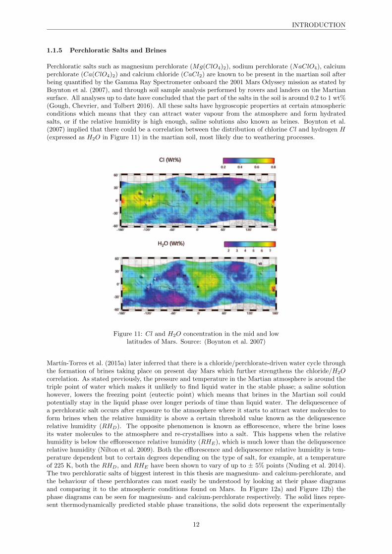
Perchloratic salts such as magnesium perchlorate (Mg(ClO4)2), sodium perchlorate (NaClO4), calciumperchlorate (Ca(ClO4)2) and calcium chloride (CaCl2) are known to be present in the martian soil afterbeing quantified by the Gamma Ray Spectrometer onboard the 2001 Mars Odyssey mission as stated byBoynton et al. (2007), and through soil sample analysis performed by rovers and landers on the Martiansurface. All analyses up to date have concluded that the part of the salts in the soil is around 0.2 to 1 wt%(Gough, Chevrier, and Tolbert 2016). All these salts have hygroscopic properties at certain atmosphericconditions which means that they can attract water vapour from the atmosphere and form hydratedsalts, or if the relative humidity is high enough, saline solutions also known as brines. Boynton et al.(2007) implied that there could be a correlation between the distribution of chlorine Cl and hydrogen H(expressed as H2O in Figure 11) in the martian soil, most likely due to weathering processes.

Figure 11: Cl and H2O concentration in the mid and lowlatitudes of Mars. Source: (Boynton et al. 2007)

Martın-Torres et al. (2015a) later inferred that there is a chloride/perchlorate-driven water cycle throughthe formation of brines taking place on present day Mars which further strengthens the chloride/H2Ocorrelation. As stated previously, the pressure and temperature in the Martian atmosphere is around thetriple point of water which makes it unlikely to find liquid water in the stable phase; a saline solutionhowever, lowers the freezing point (eutectic point) which means that brines in the Martian soil couldpotentially stay in the liquid phase over longer periods of time than liquid water. The deliquescence ofa perchloratic salt occurs after exposure to the atmosphere where it starts to attract water molecules toform brines when the relative humidity is above a certain threshold value known as the deliquescencerelative humidity (RHD). The opposite phenomenon is known as efflorescence, where the brine losesits water molecules to the atmosphere and re-crystallises into a salt. This happens when the relativehumidity is below the efflorescence relative humidity (RHE), which is much lower than the deliquescencerelative humidity (Nilton et al. 2009). Both the efflorescence and deliquescence relative humidity is tem-perature dependent but to certain degrees depending on the type of salt, for example, at a temperatureof 225 K, both the RHD, and RHE have been shown to vary of up to ± 5% points (Nuding et al. 2014).The two perchloratic salts of biggest interest in this thesis are magnesium- and calcium-perchlorate, andthe behaviour of these perchlorates can most easily be understood by looking at their phase diagramsand comparing it to the atmospheric conditions found on Mars. In Figure 12a) and Figure 12b) thephase diagrams can be seen for magnesium- and calcium-perchlorate respectively. The solid lines repre-sent thermodynamically predicted stable phase transitions, the solid dots represent the experimentally

12

INTRODUCTION

determined RHD, and the open symbols (Figure 12a): dots, Figure 12b): triangles) represent the RHE .The boundaries between different hydration states are depicted by the grey line (Figure 12a)) and thedashed lines (Figure 12b)).

(a) (b)

Figure 12: a) Phase diagram for magnesium perchlorate. Source: (Gough, Chevrier, and Tolbert 2016),b) Phase diagram for calcium perchlorate. source: (Nuding et al. 2014).

A study was made by Primm et al. (2017) where the metastable regions at low temperature, and highrelative humidity of magnesium perchlorate was examined (see Figure 13). It concluded that using onlyequilibrium thermodynamics to predict the stability of the aqueous phases results in an underestimation.It also showed that the metastability region is not restricted to salt supersaturation at low relativehumidity, but includes supercooling (supersaturation with respect to ice) at high relative humidity. Ascan be seen in the figure, the freezing of the liquid phase occurred at a relative humidity higher than 80%RH for all temperatures.

Figure 13: Phase diagram for magnesium perchlorate withexperimental values in the metastable regions. Source: (Primm

et al. 2017)

13

INTRODUCTION

1.1.6 Martian Caves and Lava Tubes as Special Regions

The definition of a special region established by COSPAR is:“A Special Region is defined as a region within which terrestrial organisms are likely to replicate. Anyregion which is interpreted to have a high potential for the existence of extant martian life forms is alsodefined as a Special Region.” - (Kminek et al. 2017)

Special regions are areas on planets that are more likely to be able to harbour lifeforms based on theknowledge we have of terrestrial life. This includes a high enough water activity and temperature whichmay result in replication of terrestrial lifeforms.

As of now the defined limits for these physical parameters are:

• Water activity: lower limit of 0.5, upper limit of 1.0

• Temperature: lower limit of -25 °C, upper limit not defined

• Timescale within which limits can be identified: 500 years

There are some observed features that are considered to have a significant probability to have liquid waterwhich should be treated as Special Regions according to Kminek et al. (2017) until proven otherwise andthese are:

• Methane sources

• Recurring slope lineae (RSL)

• Gullies

• Pasted-on terrains

• Caves, subsurface cavities below 5 meters

• Others, TBD, including dark slope streaks, possible geothermal sites, fresh craters with hydrothermal activity, modern outflow channels, or sites of recent seismic activity

When defining special regions, other features should be taken into consideration such as places with ahigh salinity which would require lifeforms to have a high halo-tolerance (organism adaption to highsalinity conditions). With the study of extremophiles on earth by Rothschild and Mancinelli (2001) andthe occurrence of daily-transient liquid water on Mars by Martın-Torres et al. (2015a) it is not impossibleto say that life could have existed in secluded places such as in caves where perchloratic salts possiblycould exist as brines, but the most limiting factor for life to exist on present day Mars is the the extremelylow temperatures.

14

INTRODUCTION

1.1.7 REMS

The Rover Environmental Monitoring Station (REMS) is an instrument on-board the Mars ScienceLaboratory (MSL) and is a contribution of Spain that is currently operating on the martian surface onthe Curiosity rover. The scientific objectives of the instrument is defined as follows: ”REMS scientificobjectives are to characterise the Martian climate and to study Mars habitability” - (Gomez-Elvira etal. 2011). The instrument is mounted on the rover Remote Sensing Mast (RMS) and contains a set ofsensors to measure pressure (PS), humidity (HS), air temperature (ATS), ground temperature (GTS),UV radiation, wind speed and direction (see Figure 14).

Figure 14: REMS model. Source: NASA, JPL

REMS records atmospheric data at∼1.7 m above the ground at different locations during the MSL missionand will help in understanding some key aspects of the Martian global water cycle. The atmosphericconditions recorded by REMS during a typical martian day can be seen in Figure 15 where Ta is the airtemperature, Tg is the ground temperature, P is the atmospheric pressure, RHa is the relative humiditymeasured in the air at the instrument, RHg is the relative humidity in the interface layer close to theground, and UV ABC is the UV radiation.

Figure 15: REMS data of a typical Martian day. Source:(Martın-Torres et al. 2015b)

In order to fully characterise and understand the habitability conditions at a location, it is importantto analyse several factors and put them together, and these are temperature, water conditions, mineralsand morphology, radiation levels and type of microorganisms. REMS records relevant data for this andhence plays an important role in the characterisation of the habitability on Mars (Gomez-Elvira et al.2011).

15

CFD THEORY AND ALGORITHMS

2 CFD Theory and Algorithms

2.1 Computional Fluid Dynamics

2.1.1 General Theory

Computional Fluid Dynamics (CFD) is computer-based simulations to predict and analyse fluid flow,heat transfer, mass flow, chemical reactions and related phenomenons. All CFD software can generallybe sub-divided into 3 stages, pre-processing, solver and post-processing.

2.1.2 Pre-Processing

• Geometry definition

• Mesh generation

• Selection of chemical and physical phenomenas to be modelled

• Material assignment

• Interface mapping between geometric domains

• Setting boundary conditions (inlet, outlet, heat source, etc.)

The solution accuracy of a fluid flow model is dependent on the number of cells in the mesh, the morecells, the longer the simulation takes to run. The aim should therefore be to find a balance betweenmaximising the number of cells in the mesh and making sure that the simulation does not take too longto solve (Versteeg and Malalasekera 2007).

2.1.3 Solver

The numerical solution technique used in most well established CFD codes is the finite volume method,which is a special formulation of the finite difference method (Versteeg and Malalasekera 2007).

The finite volume method has two main advantages over other CFD solution techniques with the first onebeing a conservative discretisation, i.e. velocities, mass, and energy are conserved. The second advantageis to not need to perform a coordinate transformation on irregular meshes which results in an increasedflexibility to generate grids around arbitrary geometry in three dimensions (Lomax, Pulliam, and Zingg1999).

According to Versteeg and Malalasekera (2007) the algorithm of the finite volume method can be roughlyoutlined as follows.

1. Integration of the fluid flow equations over all the control volumes of the domain

2. Discretisation - converting the result of the integral equations to a system of algebraic equations

3. Iterative solution of the algebraic equations

The integration of the control volume is what distinguishes the finite volume method from other CFDsolution methods. As a result each finite size cell gets an accurate conservation of relevant properties.The clear relationship between the conservation of the physical properties and the numerical algorithmis what makes the finite volume method easier to understand than other methods. Within each finitecontrol volume there are a number of general flow variables, one for example is the velocity component,another is the enthalpy etc. The conservation of this variable φ can be expressed as the balance betweendifferent processes trying to decrease or increase it and in words we can express it as:

Rate of changeof φ in the

control volumewith respect to

time

=

Net rate ofincrease ofφ due to

convection intothe control

volume

+

Net rate ofincrease ofφ due to

diffusion intothe control

volume

+

Net rate ofcreation ofφ inside the

controlvolume

(2)

16


The discretisation used in CFD is suitable for the main transport phenomena such as convection anddiffusion, as well as the creation or destruction of φ often due to source terms and the rate of change withrespect to time. An iterative solution technique is required since the involved physical phenomena arecomplex and non-linear. The TDMA (tridiagonal matrix algorithm) solver is the most commonly usedsolution technique of the algebraic equations and the SIMPLE algorithm for a correct linkage betweenpressure and velocity (Versteeg and Malalasekera 2007).

2.2 Conservation Laws and Model Equations

2.2.1 Conservation Laws

A conservation law states that a property in an isolated system does not change over time. The Eulerand Navier-Stokes equation can be written in the integral form that follows:∫

V (t2)

QdV −∫V (t1)

QdV +

∫ t2

t1

∮S(t)

n · FdSdt =

∫ t2

t1

∫V (t)

PdV dt (3)

where the vector Q consists of a set of conserved variables (mass, momentum, and energy per unitvolume). Eq. 3 states that Q will be conserved in a finite volume V (t) with surface area S(t) over a finitetime interval t2-t1. The vector n is the normal unit vector to the surface S(t) pointing outward, F is aset of vectors of the flux of Q per unit area per unit time, and P is the rate production of Q per unitvolume per unit time. Assuming that all variable in Q are continuous in time Eq. 3 can be rewritten as:

d

dt

∫V (t)

QdV +

∮S(t)

n · FdS =

∫V (t)

PdV (4)

Finding numerical approximations of Eq. 3 and Eq. 4 and solving for Q is the basis of the finite volumemethod. Gauss theorem can be applied to the flux integral in Eq. 4 to get the divergence form of theequation which yields:

∂Q

∂t+∇·F = P (5)

where ∇ is the divergence operator, in cartesian coordinates:

∇. ≡(

i∂

∂x+ j

∂

∂y+ k

∂

∂z

). (6)

and i, j, and k are unit vectors in the x, y, and z coordinate directions. By making numerical approxima-tions of the derivatives in Eq. 5 and solving for Q one uses the finite difference method (Lomax, Pulliam,and Zingg 1999).

2.2.2 The Navier-Stokes and Euler equations

A coupled system of non-linear PDE’s is formed by the Navier-Stokes equations which describes theconservation of mass, momentum and energy (Lomax, Pulliam, and Zingg 1999). For one dimension, ina Newtonian fluid the equations can be written as:

∂Q

∂t+∂E

∂x= 0 (7)

with

Q =

ρ

ρu

e

, E =

ρu

ρu2 + p

u(e+ p)

−

0

43µ

∂u∂x

43µu

∂u∂x + k ∂T∂x

(8)

where

17


ρ = density of the fluid

u = velocity

e = total energy per unit volume

p = pressure

µ = temperature

k = thermal conductivity

T = temperature

2.2.3 The Linear Convection Equation

The linear model for wave propagation can most easily be expressed by the linear convection equationwhich is given by:

∂u

∂t+ a

∂u

∂x= 0 (9)

In Eq. 9, u(x, t) is a scalar quantity moving with a real speed constant a which may be positive ornegative. Depending on how the boundary conditions are defined the equation can be used to model thefollowing two phenomena (Lomax, Pulliam, and Zingg 1999).

1. In the first, u is defined on one boundary, which means that a wave is entering the domain throughthis defined inlet boundary. No boundary condition is defined for the outlet boundary side ofthe domain. This means that the wave leaves the domain through the outlet boundary withoutdistortion. This phenomenon is known as the convection problem, and represents most convectionproblems that usually occur.

2. In the second, the simulated flow is periodic, and everything that enter the domain through theinlet must be the same as what leaves through the outlet.

2.2.4 The Diffusion Equation

Molecular motion in a fluid is associated with diffusive fluxes and a good model for describing diffusionin one dimension is:

∂u

∂t= ν

∂2u

∂x2(10)

where ν is a positive real constant (Lomax, Pulliam, and Zingg 1999).

2.2.5 Basic Concepts of the Finite Volume Method

As stated before the basic idea of the finite volume method is to make numerical approximations of Eq.3 and solve for Q. By inspecting the equation closer it can be seen that an approximation for eachterm needs to be made. First the flux must be found on the control volume boundary, which is a closedsurface in three dimensions and a closed contour in two dimensions. Then in order to acquire the netflux through the boundary this flux must be integrated. The source term must also be integrated overthe same control volume and then a time-marching method is applied to find the value of∫

V

QdV (11)

at the following time step.

The average value of Q in a cell with volume V is

18


Q ≡ 1

V

∫V

QdV (12)

and Eq. 3 can then be rewritten as

Vd

dtQ+

∮S

n · FdS =

∫V

PdV (13)

as long as the control volume is time-invariant. The averaged values of Q have been updated throughthe time-marching method for the cell. To evaluate the fluxes, Q can be represented inside a cell by apiecewise approximation that results in the correct value of Q, but every cell will have a different value.These values are then used to calculate F (Q) which usually results in different approximations of theflux at the boundary between two control volumes. A non-dissipative scheme is therefore used to find anaverage value of the flux between the two control volumes.

The finite volume method can after knowing all this be described step by step as:

1. Knowing the value of Q , make an approximation of Q(x, y, z) for each control volume. Find Qat the control volume boundary and evaluate F (Q) there. The boundary flux between two controlvolumes will be different.

2. Apply some method to find the average value of the flux between the two control volumes andproduce a single value of F (Q) at every point of the boundary.

3. Integrate the flux to find the net flux through the control volume boundary.

4. Advance the solution in time to obtain new values of Q

Sometimes the following relation between ∇Q and Q is used to include diffusive fluxes∫V

∇QdV =

∮S

nQdS (14)

(Lomax, Pulliam, and Zingg 1999)

2.3 Model Equations in Integral Form

2.3.1 The Linear Convection Equation

The convection equation, Eq. 9 can be rewritten in two dimensions as

∂u

∂t+ a cos θ

∂u

∂x+ a sin θ

∂u

∂y= 0 (15)

Eq. 15 describes a plane wave convecting the scalar quantity u(x, y, t) with speed a along a straight linemaking an angle θ with respect to the x-axis. Setting θ = 0 yields the one dimensional form of Eq. 9 again.

The two-dimensional linear convection equation is obtained from the divergence form in Eq. 5 with

Q = u (16)

F = iu cos θ + ju sin θ (17)

P = 0 (18)

Q is a scalar which makes F just a vector. Substituting Eq. 16 - Eq. 18 into the two-dimensional formof Eq. 4 yields the integral form

d

dt

∫A

udA+

∮C

n · (iu cos θ + ju sin θ)dl = 0 (19)

where A is the bounded area of the cell by the closed contour C (Lomax, Pulliam, and Zingg 1999).

19


2.3.2 The Diffusion Equation

The two-dimensional diffusion equation can be stated without a source term in the integral form wherethe diffusion coefficient ν is obtained by using the general divergence form (Eq. 5) with:

Q = u (20)

F = −∇u (21)

= −(

i∂u

∂x+ j

∂u

∂y

)(22)

P = 0 (23)

By using these three equations we find that:

d

dt

∫A

udA =

∮C

n ·(

i∂u

∂x+ j

∂u

∂y

)dl (24)

(Lomax, Pulliam, and Zingg 1999)

2.4 Heat Transfer Theory and the Energy Equation

2.4.1 The Energy Equation

The energy equation for fluids in ANSYS Fluent is solved in the following form:

∂

∂t(ρE) +∇ · (~v(ρE + p)) = ∇ ·

keff∇T −∑j

hj ~Jj + (¯τ · ~v)

+ Sh (25)

where keff = k + kt, and kt is the turbulent thermal conductivity which is 0 in this case since there isno turbulence involved. The vector ~Jj is the diffusion flux of species j. On the right hand side of theequation from the left we have energy transfer due to conduction, diffusion, viscous dissipation and ifdefined, chemical reactions or other volumetric heat sources. In Eq. 25 E is defined as

E = h− p

ρ+v2

2(26)

and for ideal gases h is sensible enthalpy which is defined as

h =∑j

Yjhj (27)

where Yj is the mass fraction of species j, and for an incompressible flow this becomes

h =∑j

Yjhj +p

ρ(28)

with hj as

hj =

∫ T

Tref

cp,jdT (29)

where Tref is 298.15 K.

The energy equation ANSYS Fluent uses for solid regions is

∂

∂t(ρh) +∇ · (~vρh) = ∇ · (k∇T ) + Sh (30)

20


where

ρ = density

h = sensible enthalpy,∫ TTref

cpdT

k = thermal conductivity

T = temperature

Sh = volumetric heat source

The terms in Eq. 30 on the right hand side is represented by the heat flux due to conduction and thevolumetric heat source if one exists. The second term on the left hand side is the convective energytransfer due to rotational or translational motion (ANSYS.Inc. 2009).

2.4.2 Volume of Fluid Model theory and the Volume Fraction Equation

The Volume of Fluid (VOF) model is a surface modelling technique used for tracking the fluid-fluidinterface between q phases and by solving the continuity equation of the volume fraction of at least oneof the phases (FLUENT.Inc. 2006a). For q number of phases the volume fraction equation becomes

1

ρq

[∂

∂t(αqρq) +∇ · (αqρq ~vq) = Sαq

+

n∑p=1

(mpq − mqp)

](31)

where

mqp = mass transfer from phase q to p

mpq = mass transfer from phase p to q

and normally the source term on the right hand side Sαq, is zero unless a constant mass source is

specified for each phase. The volume fraction equation is not solved for the primary phase, but for therest of the phases and is based on the assumption that:

n∑q=1

αq = 1 (32)

The Implicit Scheme

The implicit scheme is a time discretisation method used in ANSYS Fluent and when this method isused, ANSYS Fluent’s standard finite difference interpolation schemes, QUICK, Second Order Upwindand First Order Upwind, and the Modified HRIC schemes, are used to obtain the face fluxes for all cells,including those near the interface (FLUENT.Inc. 2006a).

αn+1q ρn+1

q − αnq ρnq∆t

V +∑f

(ρn+1q Un+1

f αn+1q,f ) =

[Sαq

+

n∑p=1

(mpq − mqp)

]V (33)

Energy Equation

The energy equation from Eq. 25 is shared for the multiple phases and becomes

∂

∂t(ρE) +∇ · (~v(ρE + p)) = ∇ · (keff∇T ) + Sh (34)

21


where ρ and keff are shared among the phases. Both the energy E and the temperature T is treated asmass averaged variables in the VOF model:

E =

n∑q=1

αqρqEq

n∑q=1

αqρq

(35)

where Eq for each phase is dependent on the shared temperature of the phases and the defined specificheat for each phase (FLUENT.Inc. 2006b).

22


2.5 Volume Mixing Ratio and Relative Humidity

RHg and H2O VMR formulation

The water mass mixing ratio (W) and water volume mixing ratio (VMR) are calculated from

W =MW

MD× RH

100× ew(T )(

P − RH100 × ew(T )

)× 1000

(36)

with

VMR =MD

MW ×W × 1000(37)

where MW is the molecular weight of water MW=18.0160, MD the molecular weight of dry air on Mars:MD=43.3400, ew(T) is the saturation water vapour pressure at a given measured temperature T whichis calculated from

ew(T ) = 6.11× e22.5×(1−TKT ) (38)

withTK = 273.14159K (39)

The REMS measured pressure P , RHa and Ta at 1.6 m are used to calculate W and then knowing theground surface temperature Tg, the surface relative humidity RHg is obtained through the water massmixing ratio W and ew(Tg) (Martın-Torres et al. 2015b).

By combining and rearranging Eq. 36 and Eq. 37 the relative humidity RH can be written as:

RH =100000×MD × P ×W

1000× ew(T )×MD ×W + ew(T )×MW(40)

23

METHOD

3 Method

3.1 Modelling Process in ANSYS Fluent

The general process of the modelling and workflow in ANSYS was

1. Geometry definition

2. Mesh generation

3. Material assignment

4. Interface mapping

5. Boundary conditions

6. Solver parameters

7. Post-processing

where each of the steps will be explained in detail in the following sections.

3.1.1 Geometry definition

Both 2D and 3D geometries were modelled in the ANSYS built in CAD-modeller SpaceClaim for easyaccess to make adjustments and for its user-friendly interface.

The modelled geometries were divided into two or more domains, the solid domains (regolith, basalticrock, ice), and the fluid domain (air inside the lava tube). For the 3D models the solid domains weremodelled as rectangles/slabs and the fluid domain was made as an extruded (subtracted) cylinder throughthe centre of the slab along the x-axis. The skylight entrance was then in a similar way extruded fromthe +y surface of the slab up until the cylinder and can be seen in Figure 16a) as the most orangesurface. The edges of the cylinder were then blended into half circular geometries to avoid problematicmeshing elements that have a tendency to appear in sharp geometries. The 2D-models were modelled ina similar fashion and had the features of the cross section of the 3D-models. The model in Figure 16 willbe mentioned as the ”main model” throughout the report with a length of 1000 m and a diameter of 150m and was used as a reference for comparison.

Figure 16: Exploded view of a geometry model with a skylightentrance in the centre.

24

METHOD

3.1.2 Mesh generation

After a geometry was created, the ANSYS meshing tool was used to generate decent meshes for thedifferent domains, two examples of the mesh can be seen in Figure 17.

(a) (b)

Figure 17: a) View of mesh from above, b) View of the mesh of the fluid domain seen from the side.

Then a contact match was made between the solid and the fluid domain to make the nodes match andhence ensure good simulation results in the transition region between the two domains.

Figure 18: Contact match between the fluid and the solid domain

The mesh was then generated with a curvature sizing function with maximum face and tetrahedron sizeranging from 3 to 10 m depending on the size of the model. A visual inspection was done of the meshquality, especially in the vicinity of the domain transitions to ensure good results. More examples of theresulting mesh can be seen in Figure 19.

25

METHOD

(a) (b)

(c)

Figure 19: a) Mesh cross section (XY.plane), b) Mesh cross section close up (XY-plane), c) Mesh crosssection close up (YZ-plane).

Thereafter named selections were created for different parts of the geometry as a preparation for settingthe boundary conditions and interface mapping in Fluent. The different named selections can be seen inFigure 20 with their corresponding geometries.

(a) (b)

Figure 20: a) Named selections list, b) Named selections geometries.

26

METHOD

3.1.3 General Models in Fluent

This section contains a brief description of each of the different models (not to be confused with geometrymodels) that were used to characterise the physical properties in the simulation models.

All simulations were set to run as transient simulations over one or more Martian Sols which is 24 hoursand 37 minutes. The data that was recorded by REMS (Figure 15) was used as input values in all simu-lations and was taken from Sol 53(Ls 180) of the MSL mission which was during the autumnal equinoxin the northern hemisphere. Most of the simulations were set to run for 3 Sols to get a somewhat diurnalbehaviour without taking unnecessarily long time.

Laminar FlowFor fluid flow in a cylinder of diameter D, it has been shown that a laminar flow occurs when the Reynoldsnumber, Re is smaller than 2300.

The Reynolds number is defined by:

Re =ρuL

µ(41)

where

ρ = density

u = velocity

L = characteristic linear dimension

µ = dynamic viscosity

which was the reason why the flow in the simulation model was set to be laminar, due to the lowvelocity (only through diffusion), multiplied by the low density, which dominates the numerator of theReynolds number equation as can be seen in Eq. 41 and makes it small (Nakayama and Boucher 1999).

Energy equationThe energy equation model was enabled in all simulations to allow for heat flow through conduction inthe solid domain and through convection in the fluid domain.

Multiphase - Modelling Relative Humidity in ANSYS FluentSince there was no built-in direct option to model relative humidity in ANSYS Fluent a different approachwas taken. This was done by enabling the multiphase model and using the Volume of Fluid (VOF) modelin Fluent. The volume fraction between the two different phases (martian air and water vapour) wasset as a boundary condition at the inlet. The relationship between the volume fraction and the relativehumidity in Eq. 36 - Eq. 40 was used to convert between the two variables. ANSYS Fluent solved forthe volume fraction, temperature and pressure in the model and the result was then converted back torelative humidity for use in the post-processing.

27

METHOD

3.1.4 Material assignment

Martian GroundAn assumption was made based on results in the following chapter that the basaltic rock and the regolithlayer on Mars could be modelled as one solid domain to simplify the simulation model. Some variationswere therefore studied regarding the thermal properties of the Martian ground where a somewhat averagedvalue of the basaltic rock and regolith was used.

The regolith density on Mars is expected to be around 1000-1500 kg/m3 and the density of the basalticrock around 2600-2800 kg/m3 depending on what volcanic rock it consists of, and since the basaltic rockis the main constituent of the Martian ground, the density was set to 2700 kg/m3 (Bell 2008).

The thermal conductivity has a lot of controlling factors, such as temperature, stress, porosity, watersaturation, cracking etc. Previous research made on thermal conductivity at sub-zero temperatures indifferent types of rocks is scarce but according to Robertson (1988) a thermal conductivity of 1 W/mKseemed reasonable for the solid domains in all models. The temperature and porosity behaviour of thethermal conductivity for volcanic rocks according to Ahrens, Clauser, and Huenges (1995) can be seen inFigure 21. The possible range of the thermal conductivity was assumed to be around 1-3.5 W/mK, sodifferent thermal properties were tested in the simulation model.

The specific heat is also temperature dependant and was very hard to find for sub-zero temperaturesof basaltic rock, but according to Robertson (1988) the values of the specific heat was in the range of600-800 J/kgK so the value for all simulation models was set to 700 J/kgK.

(a) (b)

Figure 21: a) Variation of thermal conductivity with temperature for volcanic rocks. Source: (Ahrens,Clauser, and Huenges 1995) , b) Thermal conductivity of volcanic rocks subdivided according to

porosity. Source: (Ahrens, Clauser, and Huenges 1995)

28

METHOD

Martian AirAccording to Catling and Kasting (2017) the density of the Martian atmosphere is around 0.015 kg/m3

and the specific heat is 750 J/kgK at a constant pressure, these values were used in all simulation models.

Since the Martian atmosphere is mainly dominated by CO2, an assumption was made to base the valueof the thermal conductivity on that of CO2. According to measurements taken by Harvey et al. (2014)on sub-critical vapour of CO2 rich mixtures the thermal conductivity of the Martian air was set to 0.01W/mK. As can be seen in Figure 22 the thermal conductivity for a low density CO2-rich mixture at theMartian temperature range of around 210 - 270 K used in the simulations was 0.01 - 0.015 W/mK. Itis hard to say how the thermal conductivity in the plot behaves at a density of 0.015 kg/m3 but to beon the safe side an assumption was made that it would decrease slightly and it was set to 0.01 W/mKin the simulation models (Harvey et al. 2014). The material properties for water vapour was importedfrom the ANSYS Fluent material database.

Figure 22: Thermal conductivity for a sub-critical CO2-richmixture. Source: (Harvey et al. 2014)

29

METHOD

3.1.5 Interface mapping

A coupled wall interface mapping was done between the fluid interface and solid interface created in themeshing module with the named selections to allow for heat transfer between the Martian ground andMartian air inside the model.

3.1.6 Boundary conditions

The previously defined named selections were set as boundary conditions with input and output param-eters for the main sources that were:

1. Heat source wall: The input region for the Martian ground temperature.

2. Pressure inlet: The input region for the Martian air temperature, pressure, and the volume fractionof water vapour.

3. Simulation boundary wall: A heat dissipation region to prevent the model from heating up.

The data that was recorded by REMS for the Martian air/ground temperature as well as the pressure andrelative humidity (converted to volume fraction) was used as input values for the boundary conditions.This was done through ANSYS Fluent transient profiling with the tabulated values (see ”Appendix AFluent Transient Profile”) from the REMS data to set it up as an input in the simulations (FLUENT.Inc.2006c).

The operating conditions for the simulations were set to:

• Gravity: 3.711 m/s2

• Operating pressure: 778 Pa

• Operating density: 0.015 kg/m3

Two different initial temperatures (225 K and 230 K) were used in the simulations to see the differencein the results, and both were taken around the average temperature of the surface air.

3.1.7 Solver parameters

The main parameters to be decided was the timestep size and the number of iterations for each timestep.This was decided through testing where these parameters were varied to make the simulation stable withdecent results and also taking into account that they were not chosen too small and big so the simulationwould not take too long. For all 3D models the minimum timestep size that resulted in a stable simulationwith decent results was 50 s and the minimum number of iterations for each timestep was 15. For the2D simulations the timestep size was decreased to 10 s and the number of iterations for each timestepwas increased to 30.

3.1.8 Post-Processing

For the 3D models the ANSYS CFD Post-processing module was used to analyse the simulation resultswith the function calculator to determine the temperature and water vapour volume fraction at everytimestep as a volume average over the fluid domain. These values were then exported to a MATLAB forfurther post processing (for MATLAB-script see ”Appendix B MATLAB Code”). Most of the relevantpost-processing was done on the 2D models where the nature of the airflow behaviour (thermal waves,water vapour) was studied, both visually and by calculating the temperature and water vapour volumefraction at different locations of interest.

30

METHOD

3.2 Geometry models

3.2.1 Thermal Analysis of Different Ground Compositions

In order to verify the importance of the martian ground composition, a standalone ground model was setup to analyse the extent of the thermal wave propagation from the surface layer down towards the cave.Three solid materials which are likely to be found in the top layer of the martian ground were chosen tobe studied in this analysis and these included:

• Regolith: ρ = 1300 kg/m3, cp = 700 J/kgK, k = 0.1 W/mK

• Basalt: ρ =2700 kg/m3, cp = 700 J/kgK, k = 1 W/mK

• Ice: ρ = 920 kg/m3, cp =1800 J/kgK, k = 2.6 W/mK

The materials were put side-by-side in five columns with the first three being composed of regolith, basalt,and ice; and the last two being composed of regolith and basalt in the 1 m top layer, with ice underneathsee Figure 23. By testing this before applying it to the full simulation model some simplifications couldbe made.

Figure 23: Ground analysis geometry model.

3.2.2 Different Thermal Properties of Basaltic rock

Three different thermal property sets regarding specific heat and thermal conductivity were tested on themain model to study what effect this would have on the interior air environment in the model. Thesethree sets were taken from the analysis made by Ahrens, Clauser, and Huenges (1995) and were:

1. Basalt 1: cp = 600 J/kgK, k = 1 W/mK

2. Basalt 2: cp = 700 J/kgK, k = 2 W/mK

3. Basalt 3: cp = 800 J/kgK, k = 3.5 W/mK

31

METHOD

3.2.3 Varying Diameter and Length of Models with a Skylight Entrance in the Centre

Three models with two different diameters and two different lengths were modelled. The followingdimensions were used in the models

1. Length = 500m, Diameter = 100m



3.2.4 Model with a Varying Skylight Entrance Diameter

The main model was used as a reference model with a length of 1000 m and a diameter of 150 m butthe skylight entrance diameter was varied. The two different models were designed to have a skylightentrances with diameters of 100 m and 50 m as can be seen in Figure 24.

Figure 24: L1000D150: Model with a length of 1000 m and adiameter of 150 m with different diameters of the skylight

entrance(red = 100 m, yellow = 50 m).

3.2.5 Different Shape of the Model with the Entrance at the End of the Cylinder

The model L1000D150 was used as a reference model and the entrance was put at the side of the modelinstead of at the centre as can be seen in Figure 25. The model was then compared to the modelsL1000D150 and L500D150.

Figure 25: L1000D150 side: Model with a length of 1000m, adiameter of 150m, and the entrance at the end.

Three more models with different dimensions and with the entrance at the side were made and comparedto each other.

32

METHOD

A complete list of all 3D models with names as referred by, parameters and a description can be seen inTable 6.

Name Length Diameter DescriptionL1000D150(main model) 1000 m 150m Entrance at the centre of the cylinderL500D150 500 m 150 m Entrance at the centre of the cylinderL500D100 500 m 100 m Entrance at the centre of the cylinderL1000D150S50 1000 m 150 m Entrance diameter = 50 mL1000D150S100 1000 m 150 m Entrance diameter = 100 mL1000D150 side 1000 m 150 m Entrance at one side of the cylinderL1000D50 side 1000 m 50 m Entrance at one side of the cylinderL2000D150 side 2000 m 150 m Entrance at one side of the cylinderL500D150 side 500 m 150 m Entrance at one side of the cylinderL1000D100 side 1000 m 100 m Entrance at one side of the cylinder

Basalt 1 1000 m 150 mcp = 600 J/kgKk = 1 W/mK

Basalt 2 1000 m 150 mcp = 700 J/kgKk = 2 W/mK

Basalt 3 1000 m 150 mcp = 800 J/kgKk = 3.5 W/mK

Table 6: List of all the model names with parameters and descriptions.

3.2.6 2D Models and Angled Lava Tubes

Five 2D models similar to the 3D model in Figure 25 were made with lengths of 500 m and a diameterof 50 m with different inclinations (0°, 15°, 30°, 45°, 90°) to study what impact this would have onthe results mainly regarding thermal wave propagation distance, but also the behaviour of the relativehumidity. Figure 26 shows an example of a 2D model with an inclination of 0°.

Figure 26: 2D model with a 0°inclination.

33

RESULTS AND ANALYSIS

4 Results and Analysis

The analysis of the simulation results are mainly focused on the behaviour of the relative humidity andthe temperature in the models. The pressure equalisation between the fluid domain and the inlet isalmost instantaneous and the minuscule difference between the input values and simulated values doesnot have an impact on the results. The simulations were run for 3 Sols and most of the results were takenfrom Sol 3, with some from Sol 2 due to better quality.

4.1 Ground Model Thermal Analysis

The ground model was analysed in two steps, first by a visual inspection of the thermal wave penetrationthrough the different materials and notice at what depth they fade away, and secondly, by looking at thetemperature gradient by measuring the temperature at different depths in the model.

The first way provides little to no information besides an easy visual understanding of the size andpropagation of the thermal waves as can be seen in Figure 27. The temperature range in the figure is setto 1 K above the average ground temperature so that the contours of the thermal wave can be seen moreclearly at an increasing depth where the temperature gradient is smaller. The simulation timestep thatcan be seen in the model is at LMST 20 where the maximum relevant penetration depths for regolith,basalt, and ice were 0.5 m, 1.1 m, and 1.9 m respectively. As can be seen in column four and five thethermal inertia of the regolith is not high enough to allow for the thermal wave to propagate to the secondregion (1 m depth) of the model. The thermal waves that can be seen are constituted of both a wavefrom the current and previous Sol, and this can be seen by recognising the slightly more light green areamost visible in the third column at a depth of about 1.1 m.

Figure 27: Ground thermal wave penetration depth cross section.

34


The second way of analysing the results however shows the temperature at different depths with incre-ments of 10 cm and the wave propagation speed, where the 0 cm depth corresponds to the surface groundtemperature from the REMS data in Figure 15. Regolith is the material most likely to be found as thetop layer of the martian ground and it has the lowest thermal inertia of the three making it the mostresilient to temperature changes and heat conduction. As can be seen in Figure 28a) the propagationspeed per 10 cm was 6-7 hours and a temperature drop of about 40 K occurred at a depth of 10 cm fromthe ground peak temperature. As for the basaltic rock, as can be seen in Figure 28b), with a higherthermal inertia the propagation speed was increased to 3-4 hours per 10 cm with a temperature drop of30 K at a depth of 10 cm and by another 10 K at a depth of 20 cm. As can be seen in Figure 28c) ice isthe material with highest thermal inertia that was used and the results shows a propagation speed of 1-2hours per 10 cm and a temperature decreasing with about 20, 12, 7 and 4 K at corresponding depths of10, 20, 30 and 40 cm.

(a) (b)

(c)

Figure 28: Ground thermal wave propagation temperature with respect to time for: a) regolith, b)basalt, c) ice.

35


Every peak temperature was taken for all depths down to 90 cm for all three materials to evaluateand compare them to each other by plotting them in MATLAB. A two term exponential curve fit wasperformed and the result can be seen in Figure 29 along with the original values of the thermal wavepeak temperatures. The fitting function parameters can be seen in Figure 30 for each material.

(a) (b)

Figure 29: a) Ground thermal wave peak temperature with respect to depth, b) Exponentially fittedcurves of the ground thermal wave peak temperature with respect to depth.

Figure 30: Exponentially fitted functions to the thermal wavepeak temperature for regolith, basalt and ice.

36


4.1.1 Different Thermal Properties of Basaltic Rock applied in a Simulation Model

The plots in Figure 31 show the results when varying the thermal properties of the basaltic rock used inthe model L1000D150. The first plot, Figure 31a), shows the results during Sol 3, and the second plot,Figure 31b), shows the scaled results during Sol 3.

(a) (b)

Figure 31: a) Temperature and relative humidity behaviour of the model L1000D150 with differentthermal properties during Sol 3, b) Temperature and relative humidity behaviour (scaled) of the model

L1000D150 with different thermal properties during Sol 3.

A comparison of the results when changing the thermal properties of the basaltic rock can be seen inFigure 32 where the difference between the basaltic rock used in model L1000D150 and the models withthree different thermal properties (Basalt 1, Basalt 2, Basalt 3) is shown. As can be seen there is anegligible temperature difference of up to 0.05 K and a relative humidity difference of up to 0.04% RH.

Figure 32: Difference of the temperature and relative humiditybetween model L1000D150 and the models with different thermal

properties: Basalt 1, Basalt 2, and Basalt 3 during Sol 3.

37


4.2 Thermal Waves and Airflow Behaviour in Lava Tubes

4.2.1 Hot and Cold Waves

All simulation models include hot and cold waves propagating to different extents in the cave and whenlooking at the these, the most interesting property to study is the propagation distance, i.e. how far inthe cave the thermal waves reach while maintaining a certain temperature difference compared to theaverage cave temperature. As for a simple 500 m long lava tube model with the entrance as a 50 m indiameter skylight at the right side, see Figure 33, it can be seen that the hot wave propagates to around250 m at its peak and a little further than 350 m at the very edge where the temperature gradient is verysmall.

Figure 33: Thermal hot wave propagation

The cold wave can be seen in Figure 34 even though its harder to distinguish, it has its peak at slightlyless than 250 m and the very edge at a little bit over 250 m which is slightly shorter than for the hotwave. This could possibly be explained by the behaviour of the air surface temperature during the dayhours (LMST 8 - 17), where there are lots of peaks (see Figure 15) which could result in a more chaoticbehaviour of the air around the entrance causing the hot wave to propagate further. Another more likelycause for this could be a result of how the geometry makes the cold wave push the hot wave further intothe cave than the other way around due to the nature of the cold wave ”falling” down the entrance.

Figure 34: Thermal cold wave propagation.

In most of the models, vortex formations were a common sight, and identified as a result of thermal wavepropagation. The size and velocity magnitude of these vortexes varied depending on cave size, a smaller

38


cave most often resulted in a vortex with the same diameter as the cave with average wind speeds of 0.1m/s, sometimes reaching as high as 0.2 m/s near the cave entrance. As can be seen in Figure 35 thesevortexes tend to play an important roll in the movement of water vapour in the air. On the left handside in red, a high volume fraction of water vapour is trapped in the centre of the vortex and this seemsto happen only for very brief periods of time. On the right hand side in yellow, water vapour can clearlybe seen following the velocity streamlines of the vortex and regions with higher volume fraction than thesurrounding air forms as a result. The corresponding relative humidities to the vortex phenomena in thefigure is 12% RH in the centre and 5% RH at the streamlines, and this was taken from a cave with anaverage temperature of 225 K at LMST 23.

Figure 35: Water vapour behaviour around airflow streamlines.

39


4.2.2 Angled Lava Tubes

For all angled lava tubes the main result that was analysed was the behaviour of the thermal waves, i.e.how far and how they propagated. The maximum thermal cold wave penetration depth for most modelshappened around LMST 18 (an exception was the 0 °inclination cave which had this happen at LMST15), these timesteps were used for the analysis based on the fact that the cold waves are the most drivingfactor of the airflow in the -Y direction (down in the figures). The analysis was done both visually andnumerically by inspecting and analysing the temperature and relative humidity at different depths usingthe entrance as a reference. In the visual representations in Figure 36 the left hand side shows the volumefraction of the water vapour, the top right shows the thermal cold wave and the bottom right shows thethermal hot wave. As can be seen the cold wave propagates to around 220 m and the hot wave to 350 m.In Figure 37 the relative humidity and temperature can be seen at different points in a horizontal lavatube model, where the depth 0 m is at the entrance. It can be seen that relevant changes take place upuntil depths of around 100 m and then it falls closer to the average values. The relative humidity in thecave remains rather low due to the weakness in the thermal cold wave.

Figure 36: Thermal waves in a 0°lava tube.

(a) (b)

Figure 37: a) Relative humidity , b) Temperature .

40


Figure 38 shows a lava tube with an inclination of 15 degrees from the horizontal plane. The cold wavepropagation distance is 330 m at the furthest point and the hot wave propagation distance is around 90m. Figure 39 shows the relative humidity and temperature with respect to time and as can be seen inthe diagrams the depth at which the impact on the results starts to decrease occurs at around 100 m. Inmost of the models this seemed to be a common trend, mainly because it is the interface region betweenthe cold and hot wave which tends to have more and smaller airflow vortexes around it.


(a) (b)


More results for angled lava tubes can be found in ”Appendix C More Angled Lava Tubes”, with 30°,45°and 95°inclinations.

41


4.2.3 Comparison of Angled Lava Tubes

Regarding all models with different inclinations it can be concluded that they share a similar behaviournear the entrance up until at around 25 m. When the inclination and depth is increased, the impacton the velocity streamlines caused by the thermal heat wave decreases, and the cold wave becomes themain driving factor of both the temperature and water vapour distribution. A comparison of the thermalwave propagation depths can be seen in Table 7 where there seems to be a correlation between the 15,30 and 45 degree models with some deviations in the 0 and 90 degree models, and in the 15, 30 and 45degree models both the cold and hot waves seem to propagate to similar depths, with an exception forthe hot wave in the 45 degree model. In Figure 61 (Appendix C) a more vortex like air movement can beseen forcing the hot wave about 50% further than the other models and for the 90 degree model the hotthermal wave shows a similar behaviour as for the 15 and 30 degree models without vortex formation.The thermal cold wave in the 90 degree model only propagates to about 50% of the distance of the othermodels at this timestep and as can be seen in Figure 64b) (Appendix C) the thermal wave propagationspeed and magnitude during the temperature drop is decreased leading to an offset in the thermal coldwaves at depths of 25 m, 50 m and 75 m.

Inclination (°) Hot wave propagation depth (m) Cold wave propagation depth (m)0 350 22015 90 33030 100 39045 140 37090 100 170

Table 7: Thermal wave propagation depth in lava tubes with different inclinations.

In Table 8, a comparison of the temperature and relative humidity of the different models at differentdepths near the entrance can be seen. The relative humidity seems to drop faster in the models with higherinclination (45 and 90 degree) due to the fact that the water vapour distribution is more concentratedaround the streamlines compared to that in the 0, 15, and 30 degree models where the distribution ismore even. A similar fast drop of the relative humidity at 50 m can be seen in the 15 degree model butthis is more likely due to the high temperature that occurs close to the entrance compared to the othermodels as can be seen in Figure 39.

Inclination (°) 0 m 25 m 50 m 75 m 100 m0 206/14.7 217/4.2 222/4.0 226/2.3 227/3.115 204/16.2 212/6.2 222/1.5 223/1.5 224/1.530 205/15.3 210/7.7 216/3.2 221/1.6 223/2.145 206/13.0 210/8.3 221/2.1 226/1.1 227/0.990 205/17.2 217/3.1 218/1.5 225/1.5 230/0.9

Table 8: Temperature and relative humidity at different depths in caves with different inclinations.

42


4.2.4 Small Caves

The most interesting results were found in smaller cave models where the length dimensions of the cavesmatched a certain number of vortex diameters which made it so that the vortex could remain relativelystill in the centre and not propagate further into the cave. A cave model with a length of 8 m and aheight of 4.5 m can be seen in Figure 40 where two vortexes forms around LMST 17. At the middlepart of the lower picture a phenomenon where the water vapour gets trapped between the streamlines ofthe two vortexes at the bottom can be seen. In a visual inspection it is seen to linger there for up to 3hours with a clearly higher volume fraction than the surrounding air. The temperature distribution inthe cave is relatively even at this timestep with a slightly lower temperature along the floor and at thewalls allowing for a lower relative humidity.

Figure 40: Floor phenomenon.

Another interesting result was observed at LMST 7 where an even higher concentration of water vapourgathered on the cave floor as can be seen in Figure 41. A comparison between the water vapour at LMST3 and at LMST 7 shows that the water vapour moves from being evenly distributed in the cave to beinglocated on the floor.

(a) (b)

Figure 41: a) Temperature and relative humidity at LMST 3 , b) Temperature and relative humidity atLMST 7 .

A more numerical analysis was made for this area where the results can be seen in Figure 42a) and Figure42b) where the caves have initial average temperatures of 225 K and 230 K respectively. The blue linescorrespond to the area at the bottom of the cave that can be seen as green in Figure 40 and the redlines correspond to the entire bottom area in the cave. As can be seen, the centre patch stands out inmagnitude and this behaviour clearly repeats two times a day at LMST 7 and LMST 17 and possibly a

43


third time at LMST 22. The relative humidity is very temperature sensitive hence making the cave witha lower initial average temperature have a higher relative humidity in Figure 42a).

(a) (b)

Figure 42: a) Relative humidity at the floor phenomenon with an initial temperature of 225 K , b)Relative humidity at the floor phenomenon with an initial temperature of 230K.

The results from Figure 42 were applied to the phase diagram for Magnesium- and Calcium-perchloratein order to analyse in what state it would be possible to come upon these in a cave. The temperaturerange from which the results were taken spans 225 ± 1 K at most which is shown as the horizontal darkline in Figure 43 and Figure 44 on which all the coloured dots are placed. The black arrows representthe values changing over time on that same line, starting at the green dot. Both these perchlorates havesimilar phase diagrams at this particular temperature range and this method makes it possible to get anoverview of in what state the perchlorates exists at different times of the day. The green dot is aroundthe efflorescence point at 20% RH for both perchlorates making it hard to say if they are found in thebrine or salt state in the beginning of the day. Between the green and magenta point there is a 6 hourtime interval but only about 1 hour where the conditions are above the deliquescence point and belowthe freezing point. Between the magenta and red point 1 more hour remains before the freezing pointand then it takes another hour to drop way below the efflorescence point and it remains there for about 8hours during midday. From the red point until the blue point there is 3 hour with an increase in relativehumidity peaking at around 50% RH which is below the deliquescence point for Magnesium-perchloratebut above the deliquescence point for Calcium-perchlorate. Between the blue dot and the yellow dot,the relative humidity decreases to way below the efflorescence point and then returns to the efflorescencepoint after about 4 hours. There is an uncertainty of the values used in diagram since they were takenand measured at a visually arbitrary location in the cave, meaning that this may not be the most accurateresults.

44


Figure 43: Phase diagram of magnesium perchlorate withapplied values from floor phenomenon.

Figure 44: Phase diagram of calcium perchlorate with appliedvalues from floor phenomenon.

In the diagram in Figure 45 a representation of the perchlorate states can be seen. As for both Magnesium-perchlorate and Calcium-perchlorate at 225 K the deliquescence relative humidity, RHD, efflorescencerelative humidity, RHE , and the ice formation relative humidity, RHI are basically the same with RHD ≈55%, RHE ≈ 20%, and RHI ≈ 65% but as mentioned previously studies have shown that these values,especially the RHD and RHE can vary and even be as low as ±5% RH in some cases at this temperature.The red region is where RH < RHE and the perchlorates will lose water to the surrounding air. The greenregion is a metastable region where RHD > RH > RHE , meaning that brines and hydrated perchlorateswill remain hydrated but dry perchlorates wont bind any water vapour from the surrounding air. Thedark blue region is where RHI > RH > RHD and perchlorates will hydrate enough to form brines. Thebright blue region is where RH > RHI and the brines will most likely freeze, this value can also behigher as has been previously mentioned. The most interesting results were observed at LMST 7 wherethe relative humidity transitions through all of the state regions with brine formation for a total of about1 hour. The following red region for about 8 hours likely result in some dehydration of the brines andtwo metastable regions occurs again at LMST 17 and LMST 22.

45


Figure 45: Stability diagram of magnesium- andcalcium-perchlorate with values from the floor phenomenon.

In a cave of about half the size of the previous one with a length of 5 m and a height of 4.5 m a similarphenomena is seen, but at a different location. The purpose of this cave that can be seen in Figure 46was to try and model it at a size so that there would be only one main vortex. Instead of water vapourgathering on the middle of the cave floor as in Figure 40, it gathered in the corner of the cave. Thetimestep in Figure 46 is LMST 18 and on the left hand side, the remnants of a previous vortex can beseen with much lower velocity and a very irregular shape.

Figure 46: Corner/wall phenomenon.

In Figure 47a) the relative humidity can be seen for the right side wall (along the y-direction), bothaveraged over the length of the entire wall and averaged over the bottom 1 m of the wall where the higherrelative humidity occurs and in the same way for Figure 47b) but at the ground (along the x-direction).The irregular behaviour of the peaks and troughs (LMST 15 and 18 the left figure, LMST 15 in theright figure) is due to a less laminar airflow causing an instability in the corner region which the highrelative humidity concentration at the wall move away from for some time but return the next hour. Anassumption was made in the analysis of the results to both account for and neglect these troughs to seewhat difference it would make for the results.

46


(a) (b)

Figure 47: a) Relative humidity at the corner phenomenon at the wall , b) Relative humidity at thecorner phenomenon on the ground.

In Figure 48 and Figure 49 the results from Figure 47 were applied to the phase diagrams for magnesium-and calcium-perchlorate. The behaviour of these results shows a similarity to the results of the previouscave in the manner of a relative humidity peak at LMST 17 due to a vortex formation, although it is muchbigger than the previous one. During the first 10 hours of the day the relative humidity stays under theefflorescence point of the perchlorates, but from the first green dot (bottom in the right hand side figure)at LMST 14 until the magenta dot, the relative humidity rises fast during a 2 hour interval to about90% RH which is way above the freezing point. The relative humidity then drops to about 50% RH in a3-4 hour time interval between the magenta and red dot, allowing for the perchlorates to become moredeliquescent. In the next hour the relative humidity drops to about the efflorescence relative humidityat 20% RH again.

Figure 48: Phase diagram of magnesium perchlorate withapplied values from corner/wall phenomenon.

47


Figure 49: Phase diagram of calcium perchlorate with appliedvalues from corner/wall phenomenon.

In Figure 50 a perchlorate state diagram can be seen for the smaller cave with relative humidity at thecorner using the raw values from the simulation. In this diagram the relative humidity in the early partof the day from LMST 1-13 is located in the red region where the perchlorates remain dehydrated. AtLMST 14 the relative humidity starts to rise and at LMST 16-18 possible brine formation and freezingtake place. During the remainder of the day, the perchlorates are in the metastable region.

Figure 50: Stability diagram of magnesium- and calciumperchlorate with values from the corner/wall phenomenon.

These smaller caves both have in common that the high velocity vortexes take place at around LMST 15-18 which is at the point when the surface air temperature drops below the average cave air temperaturemeaning that the thermal cold wave from the surface starts to move down the cave entrance henceresulting in these high relative humidity phenomena. It is hard to say exactly how these phenomenabehaves in reality, it might be the same oscillating behaviour of the peaks or it might be some fittedfunction averaging the peaks and troughs of in the graphs. Figure 51 shows what could be two possiblefitted functions that better represent the behaviour of the relative humidity at these phenomena.

48


(a) (b)

Figure 51: a) Possible fitted curve at the floor phenomenon, b) Possible fitted curve at the cornerphenomenon.

By using the fitted curve from Figure 51b) a possible state diagram of the perchlorates could looksomething like in Figure 52. In this diagram the relative humidity does not reach the RHI and therecould be a possible brine formation for up to 3 hours during the relative humidity peak. Since the brinesremain in a hydrated state during the metastable green region this fitted relative humidity curve couldpotentially allow for the brines to not completely dry out during the day in the red region.

Figure 52: Stability diagram of magnesium- andcalcium-perchlorate with the fitted curve from the floor

phenomenon.

49


4.3 Average Relative Humidity and Temperature in Larger Lava Tubes

This section shows the results and comparison of the average relative humidity and temperature in large3D models mainly to get a general overview of in what state it would be likely to find the perchloraticsalts as will be discussed in the end of the section.

4.3.1 Varying Length of Models with a Skylight Entrance in the Centre

A plot of the temperature and relative humidity behaviour of the models with a constant diameter of150m, L500D150 and L1000D150 can be seen below in Figure 53. The first plot, Figure 53a), shows thediurnal behaviour of the models during the 3 Sols. The second plot, Figure 53b) shows the result ofthe temperature and relative humidity behaviour during Sol 3. The third plot, Figure 53c), shows thebehaviour over 5 hours during the temperature peak mid-day.

(a) (b)

(c)

Figure 53: Temperature and relative humidity behaviour of the models with a constant diameter of150m: L500D150 and L1000D150 during: a) 3 Sols, b) Sol 3, c) over 5 hours during Sol 3.

50


In Figure 54b) during the mid-day temperature peak the temperature compared to the measured valuesby REMS can be seen to vary up to 35 K for model L1000D150 while model L500D150 varies with atemperature of up to 20 K. The relative humidity varies of up to 2% RH for model L1000D150 and withup to 1% RH for model L500D150. As can be seen the deviations from the REMS values were larger formodel L1000D150. This was expected since L500D150 had a smaller volume and therefore more easilyadapted to the REMS values.

(a) (b)

Figure 54: Difference of the temperature and relative humidity measured by REMS and that of themodels with a constant diameter of 150m: L500D150 and L1000D150 during: a) Sol 3, b) Sol 3 over 10

hours.

The analysis of the results were mainly focused on comparing the results of the simulations to themeasured values by REMS to get a relationship between the temperature and the relative humidity.Figure 55 shows the results of a comparison of the temperature and the relative humidity between modelL500D150 and L1000D150. As can be seen the values vary in such a way that one is higher during the dayand the other one is higher during the night. During the night the relative humidity in model L500D150is up to 8% RH higher than in model L1000D150.

Figure 55: Difference of the temperature and relative humidityof model L500150 and model L1000150 during Sol 3.

51


4.3.2 Varying Diameter of Models with a Skylight Entrance in the Centre

In Figure 56, the result can be seen for when the length was held constant at 500m and the diameter ofthe model was varied for the models L500D100 and L500D150. The first plot, Figure 56a), shows theresult during Sol 2. The second plot, Figure 56b), shows the result during 5 hours during the temperaturepeak mid-day.

(a) (b)

Figure 56: Temperature and relative humidity behaviour of the models with a constant length of 500m:L500D100 and L500D150 during: a) Sol 2, b) Sol 2 over 5 hours during the temperature peak mid-day.

Figure 57 shows the comparison of the difference of the models with a constant length of 500 m: L500D100and L500D150 to the REMS values of the temperature and the relative humidity. As can be seen in Figure57a), during the night, the relative humidity deviates of up to 5% RH from the values measured by REMSat the surface. As can be seen in Figure 57b), during the day there is an apparent temperature deviationof up to 20 K from that of the REMS measurements but the relative humidity is almost identical andonly deviates with up to 0.4% RH.

(a) (b)

Figure 57: Difference of the temperature and relative humidity measured by REMS and that of themodels with a constant length of 500m: L500D100 and L500D150 during: a) Sol 2, b) during Sol 2 over

5 hours.

The results for three more variations of parameters in larger lava tubes can be seen in ”Appendix D MoreVariations of Different Parameters in Larger Lava Tubes”.

52


4.3.3 Comparison of the Average Temperature and Relative Humidity for the differentmodels

In Table 9 below a comparison of the average temperature and relative humidity for most of the modelscan be seen. The models with a lower temperature has a higher relative humidity as the relation betweenthe temperature and relative humidity is inversely proportional. There is a clear relation between theentrance diameter and length (or volume) of the model, with a small D/L-ratio the temperature tendsto be lower and the relative humidity higher as a result. With a larger D/L-ratio the temperature ishigher and the relative humidity is lower. As can be seen for the models with the entrance at the sidecompared to their corresponding models with an entrance at the centre, the side entrance tend to havea slightly higher average temperature due to the thermal convection only propagating in one directionwhich results in a lower relative humidity.

Model T (average) RH% (average)REMS(surface) 227.000 3.995L1000D150 220.751 3.321L500D150 223.913 3.904L500D100 222.873 4.875L2000D50 212.306 7.237L1000D150S100 218.207 3.980L1000D150S50 212.804 6.329L1000D150 side 221.653 2.981L1000D50 side 212.794 7.834L2000D150 side 213.743 6.010L500D150 side 225.254 2.823

Table 9: Average temperature and relative humidity for the 3D models of interest.

When looking at the general behaviour in larger lava tubes and caves, the results show no areas wherebrines, or the deliquescence of perchlorates could take place for longer periods of time. As can be seen inFigure 58a) and Figure 58b) the magenta area is where the results are from the simulations of the abovemodels.

(a) (b)

Figure 58: Phase diagram with the averaged values(magenta) of relative humidity and temperature inlarger lava tubes for: a) magnesium perchlorate, b) calcium perchlorate.

53

DISCUSSION

5 Discussion

5.1 Conclusion

Although this study yielded some interesting results, it is hard to validate or compare these results toactual data or previous studies since it is a relatively unexplored area. Further studies are thereforenecessary.

The standalone ground model analysis that was performed showed that the composition and variationof the the thermal properties of the different materials used, had little to no effect on the thermalenvironment in the caves if the thickness of the cave roof was more than 1-2 m. This means thatthe driving factors in determining the thermal environment in the cave are the entrance properties(temperature, pressure, relative humidity, geometry), and the geometry of the cave itself (size, features).The different applied thermal properties of basaltic rock on the simulation model also showed that thesurface ground temperature effect on the temperature of the air inside the cave was minuscule. This mayalthough play a more important role in enclosed sub surface cavities with no entrance and this should beconsidered for study in future work.

Regarding all lava tubes with different inclinations it can be concluded that they share a similar behaviournear the entrance up until at around 25 m. When the inclination and depth is increased, the impacton the air movement induced by the thermal heat wave decreases, and the cold wave becomes the maindriving factor for both the temperature and relative humidity distribution. All angled lava tubes weremodelled with horizontal inlets which resulted in different sizes of the entrances which might have hadsome effects on the results close to the inlet but the depths at which the measurements were taken wereplaced in similar ways.

The most interesting results in this study were found in smaller caves at the phenomena where watervapour gathered and lingered for several hours on the cave floor and in the corner/wall. This firstphenomenon on the floor of the cave occurred two times (LMST 7 and LMST 17) during the day whichwas at the same hours as the surface temperature would pass the average cave temperature. At the firstpass (LMST 7), the temperature went from below to above the average temperature which means that itwent from a cold wave to a hot wave driven environment. This also means that the airflow velocity in thecave decreased since the cold wave naturally falls down the inlet and creates a more chaotic environment,while the hot wave moves against gravity, mainly through diffusion. The higher relative humidity fromthe early hours combined with a more stationary environment at the pass may be a possible explanationto why the phenomenon occurred at this hour, as the water vapour was allowed to fall to the floor. Atthe second pass (LMST 17), the temperature went from above to below the average temperature whichmeans that it went from a hot wave to a cold wave driven environment. The airflow velocity in the cavehence increased which led to the formation of two vortexes forming side by side. In between these, at thefloor, the higher relative humidity most likely formed as a result of it being trapped by the two vortexes.The second phenomenon occurred at the corner/wall for several hours at LMST 17 and was most likelyformed in a similar manner as the first phenomena at LMST 17. The higher relative humidity that wasobserved seemed to be trapped in the corner by a single vortex, and was fluctuating back and forth fromthe wall. The relative humidity and temperature at these phenomena hold great potential for perchloraticsalts to exist in a hydrated state or as brines.

A more advanced model should be setup in the future to verify the nature of these phenomena withgreater precision with different input data sets. Ultimately it should be measured in situ, either throughrover exploration when technology allows or by human researcher when they set foot on Mars. It mighteven be possible to build/dig these small caves by hand and take measurements to avoid contaminationof naturally formed caves.

As has been shown in previous studies by Martın-Torres et al. (2015a) the ground relative humidity typi-cally stays higher than the air relative humidity at the surface which implies that this should also be thecase for the results in this study. This means that the intervals at which deliquescence, efflorescence, andfreezing takes place will shifted and prolonged which further strengthens the probability for perchloraticsalts to be found in the hydrated state or as brines. This should also be modelled in future studies ina more extensive model with advanced ground modelling, suggestively including the perchlorates as amaterial embedded in the floor/wall of the cave.

54

DISCUSSION

As studied by Primm et al. (2017), experimental values of the metastable regions at which perchloratesfreeze show that the freezing conditions at high relative humidity and low temperature allows for brinesto exist in a supercooled state instead of freezing at the values at thermodynamic equilibrium. For theresult in this study it would imply that the perchlorates would stay in the brine form for longer intervalswithout freezing.

Regarding the results found when studying the average behaviour of relative humidity and temperaturein larger lava tubes, the expected results were observed. The conclusion that can be made from this isthat the longer the lava tube the less affected it is by the surface relative humidity and temperature. Thesame holds for lava tubes with smaller entrances, so in general if the entrance diameter is small comparedto the size of the cave the conditions deep in the cave are very stationary.

The relative humidity was shown to be very temperature sensitive at low temperatures and this resultedin considerable differences of the results when using different initial values of the cave air/wall tempera-tures. The average cave temperature used in the simulations was assumed to be a bit under the averagetemperature of the input value data set of the surface air temperature, but as these values can changefrom day to day more input values should be tested in future studies.

Finally, as the general temperature and relative humidity in these caves are very low it is very unlikelyto find liquid water in a stable state, however it is very likely to find perchloratic salts in brine form forlonger periods of time in these phenomena discussed. As could be seen in Figure 52 a fitted curve ofthe raw values yielded by the simulation greatly changes the conclusions about the state in which theperchloratic salts exist. Even though the conditions today in the caves may be too harsh for life forms toexist, a previous warmer climate might have allowed for extremophiles to exist in highly saline solutionsand this should be taken into account for the definition of sub surface caves as Special Regions.

5.2 Limitations

Simulation capacityWith large simulation models comes a requirement for heavy processing power, such as clusters, to avoidridiculously long simulation times but a single i5 processor was used in this work for running the simu-lations which limited the resolution of the models.

Defined variable assumptionsSome material variables such as user defined specific heat, thermal conductivity, density etc. were as-sumed to be temperature independent in the simulations due to the difficulty of finding these data atMars-like conditions.

Unstable simulationsAs a result of the limited simulation capacity some of the larger models had some instabilities which werehard to identify and made some results hard to interpret.

Condensation/freezing/sublimation of water vapour near the triple pointAs mentioned earlier these general models were not included in the simulations due to the difficulty ofimplementing all these models with each other in Fluent. First of all, some already unstable models wouldhave been even harder to stabilise and secondly a dynamic mesh would have been required to simulateice melting, but this should be considered for future work.

55

REFERENCES

References

Ahrens, T.J., C. Clauser, and E. Huenges (1995). Thermal Conductivity of Rocks and Minerals in ’RockPhysics and Phase Relations: A Handbook of Physical Constants’. American Geophysical Union.

ANSYS.Inc. (2009). ANSYS FLUENT 12.0 Theory Guide - 5.2.1 Heat Transfer Theory. url: http:/ / www . afs . enea . it / project / neptunius / docs / fluent / html / th / node107 . htm (visited on01/24/2018).

Barlow, N.G (2008). Mars: An Introduction to its Interior, Surface and Atmosphere. Cambridge Univer-sity Press.

Bell, J. (2008). The Martian Surface, Composition, Mineralogy, and Physical Properties. The EdinburghBuilding, Cambridge CB2 8RU, UK: Cambridge University Press.

Boynton, W.V. et al. (2007). “Concentration of H, Si, Cl, K, Fe, and Th in the low- and mid-latituderegions of Mars”. In: Journal of Geophysical Research 112. doi: 10.1029/2007JE002887.

Catling, D.C. (2014). Mars Atmosphere: History and Surface Interactions in ’Encyclopedia of the SolarSystem, Third Edition’. Elsevier.

Catling, D.C. and J.F. Kasting (2017). Atmospheric Evolution on Inhabited and Lifeless Worlds. Univer-sity Printing House, Cambridge CB 8BS, United Kingdom: Cambridge University Press.

Cushing, G.E. (2012). “Candidate cave entrances on Mars”. In: Journal of Cave and Karst Studies 74.1,pp. 33–47. doi: 10.4311/2010EX0167R.

– (2017). “Mars Global Cave Candidate Catalog (MGC3)”. In: Astrobiology Science Conference (LPIContrib. No. 1965).

Cushing, G.E. and T.N. Titus (2010). “Caves on Mars: Candidate Sites for Astrobiological Exploration”.In: Astrobiology Science Conference 2010.

Cushing, G.E., T.N. Titus, W.L. Jaeger, et al. (2008). “Continuing Study of Anomalous Pit Craters inthe Tharisis Region of Mars: New Observations From HiRISE and THEMIS”. In: Lunar and PlanetaryScience XXXIX.

Cushing, G.E., T.N. Titus, and C.H. Okubo (2015). “Atypical pit craters on Mars: New insights fromTHEMIS, CTX, and HiRISE observations”. In: Journal of Geophysical Research 120.6, pp. 1023–1043.doi: 10.1002/2014JE004735.

Cushing, G.E., T.N. Titus, J.J. Wynne, et al. (2007). “THEMIS observes possible cave skylights onMars”. In: Geophysical Research Letters 34.17. doi: 10.1029/2007GL030709.

FLUENT.Inc. (2006a). FLUENT 6.3 User’s Guide - 23.3.2 Volume Fraction Equation. url: https:

//www.sharcnet.ca/Software/Fluent6/html/ug/node882.htm (visited on 01/24/2018).– (2006b). FLUENT 6.3 User’s Guide - 23.3.5 Energy Equation. url: https://www.sharcnet.ca/Software/Fluent6/html/ug/node882.htm (visited on 01/24/2018).

– (2006c). FLUENT 6.3 User’s Guide - 7.1.9 Defining Transient Boundary Conditions. url: https://www.sharcnet.ca/Software/Fluent6/html/ug/node213.htm (visited on 01/24/2018).

Fourier, J. (1878). The Analytical Theory of Heat. London, Cambridge Warehouse, 17, Paternoster Row,England: Cambridge University Press.

Gomez-Elvira, J. et al. (2011). “Rover Environmental Monitoring Station for MSL Mission”. In:Gough, R.V., V.F. Chevrier, and M.A. Tolbert (2016). “Formation of liquid water at low temperatures

via the deliquescence of calcium chloride: Implications for Antarctica and Mars”. In: Planetary andSpace Science 131, pp. 79–87. doi: 10.1016/j.pss.2016.07.006.

Harvey, A.H. et al. (2014). “Thermophysical Properties of Carbon Dioxide and CO2-Rich Mixtures”. In:DOE UTSR Workshop.

Kminek, G. et al. (2017). “COSPAR’s Planetary Protection Policy”. In: Space Research Today 200.Astrobiology Science Conference 2010, pp. 12–25. doi: 10.1016/j.srt.2017.11.010.

Lomax, H., T.H Pulliam, and D.W Zingg (1999). Fundamentals of Computational Fluid Dynamics. Hei-delberg ,Berlin, Germany: Springer-Verlag.

Martın-Torres, F.J. et al. (2015a). “Transient liquid water and water activity at Gale crater on Mars”.In: Nature Geoscience. doi: 10.1038/NGEO2412.

– (2015b). “Transient liquid water and water activity at Gale crater on Mars, Supplementary Informa-tion”. In: Nature Geoscience. doi: 10.1038/NGEO2412.

Nakayama, Y. and R.F. Boucher (1999). Introduction to Fluid Mechanics. Linacre House, Jordan Hill,Oxford OX2 8DP, UK: Arnold 1999, Reprinted with revisions by Butterworth-Heinemann 2000.

56

http://www.afs.enea.it/project/neptunius/docs/fluent/html/th/node107.htm

http://www.afs.enea.it/project/neptunius/docs/fluent/html/th/node107.htm

https://doi.org/10.1029/2007JE002887

https://doi.org/10.4311/2010EX0167R

https://doi.org/10.1002/2014JE004735

https://doi.org/10.1029/2007GL030709

https://www.sharcnet.ca/Software/Fluent6/html/ug/node882.htm






https://doi.org/10.1016/j.pss.2016.07.006

https://doi.org/10.1016/j.srt.2017.11.010

https://doi.org/10.1038/NGEO2412

https://doi.org/10.1038/NGEO2412

APPENDIX

Nilton, O.R. et al. (2009). “Possible physical and thermodynamical evidence for liquid water at thePhoenix landing site”. In: Journal of Geophysical Research 114. doi: 10.1029/2009JE003362.

Nuding, D.L. et al. (2014). “Deliquescence and efflorescence of calcium perchlorate: An investigation ofstable aqueous solutions relevant to Mars”. In: Icarus 243, pp. 420–428. doi: 10.1016/j.icarus.2014.08.036.

Primm, K.M. et al. (2017). “Freezing of perchlorate and chloride brines under Mars-relevant conditions”.In: Geochemica et Cosmochimica Acta 212, pp. 221–220. doi: 10.1016/j.gca.2017.06.012.

Robertson, E.C. (1988). Thermal Properties of Rocks. United States Department of the Interior GeologicalSurvey. Reston, Virginia, US.

Rothschild, L.J. and R.L. Mancinelli (2001). “Life in extreme environments”. In: Nature 409, pp. 1092–1101. doi: 10.1038/35059215.

Somerton, W.H. (1992). Thermal Properties and Temperature-Related Behavior of Rock/Fluid Systems.Elsevier.

Taylor, G.J. (2013). “The bulk composition of Mars”. In: Chemie der Erde 73, pp. 401–420. doi: 10.1016/j.chemer.2013.09.006.

Versteeg, H.K. and W. Malalasekera (2007). An Introduction to Computational Fluid Dynamics, SecondEdition. Edinburgh Gate, Harlow, Essex, CM20 2JE, England: Pearson.

Williams, K.E. et al. (2010). “Do ice caves exist on Mars?” In: icarus 209, pp. 358–368. doi: 10.1016/j.icarus.2010.03.039.

57

https://doi.org/10.1029/2009JE003362

https://doi.org/10.1016/j.icarus.2014.08.036


https://doi.org/10.1016/j.gca.2017.06.012

https://doi.org/10.1038/35059215

https://doi.org/10.1016/j.chemer.2013.09.006

https://doi.org/10.1016/j.chemer.2013.09.006



APPENDIX

Appendix

Appendix A Fluent Transient Profile

((marsparameters transient 24 1) (time 0 3600 7200 10800 14400 18000 21600 25200 28800 32400 3600039600 43200 46800 50400 54000 57600 61200 64800 68400 72000 75600 79200 82800 )

(tempair 215 207 205 206 204 204 206 219 226 231 237 247 250 262 257 256 251 238 228 227 220 220 218214 )

(tempground 206 201 198 196 194 193 198 215 237 253 267 275 279 281 276 269 258 243 233 226 218 214211 208 )

(pressure 778 783 786 785 784 786 796 809 793 777 766 756 745 736 726 720 716 721 736 759 760 763 775777 )

(VMR 123.64e-009 50.876e-009 83.461e-009 105.44e-009 111.64e-009 117.91e-009 34.663e-009 100.21e-009 121.91e-009 112.07e-009 111.47e-009 322.70e-009 441.41e-009 551.02e-009 353.92e-009 325.01e-009202.62e-009 132.06e-009 333.47e-009 287.12e-009 121.18e-009 241.41e-009 183.94e-009 162.48e-009 ) )

58

APPENDIX

Appendix B MATLAB Code

1 % Defined cons tant s2 MD=43.3400;3 MW=18.0160;4 TK=273.14159;5

6 % Accuired array o f va lue s from ANSYS Fluent s imu la t i on7 T=T simulat ion ;8 VMR=1/VMR simulation ;9 P=P simulat ion ;

10

11 % Function f o r conver t ing va lue s from VMR to RH12 ew=6.11∗ exp (22.5∗(1−TK/T) ) ;13 W=MD/(MW∗VMR∗1000) ;14 RH=(100000∗MD∗P∗W/(1000∗ew∗MD∗W+ew∗MW) ) ;

59

APPENDIX

Appendix C More Angled Lava Tubes

A lava tube with an inclination of 30 degrees shows similar results, the cold wave propagates to 390 mand the hot wave propagates to 100 m which is further than for the previous model and this is expectedsince the extension of the cave is larger in the horizontal direction. The numerical analysis as can be seenin Figure 60 shows a small difference in the temperature peak and drop at depths closer to the entrancei.e. 25 m, 50 m, 75 m where the values are closer to the ones at the entrance. For instance, at the lowtemperature at LMST 3 in Figure 60b) the temperature is 5-10 K lower than in the previous model. Asimilar result occurs at LMST 12 at the temperature peak, where the temperature is 5-10 K higher andas a result this has an impact on the relative humidity at LMST 3 for the 25 m and 50 m peak with anincrease in relative humidity from 6 to 9% RH, and 3 to 7% RH respectively.


(a) (b)


60

APPENDIX

For a lava tube with an inclination of 45 degrees a change is seen in the behaviour of the water vapour(see left hand side in Figure 61) with a less even distribution and more water vapour forming around thestreamlines of the thermal waves. The thermal cold wave propagation distance seems to be similar as inprevious models at around 370 m and the thermal hot wave at 140 m which is a bit further than previousmodels. In Figure 62 the numerical results shows a decrease further than 25 m from the entrance withsmaller temperature gradients. The relative humidity at LMST 3 at 25 m depth is similar to that in theprevious models.


(a) (b)


61

APPENDIX

A lava tube with an inclination of 90 degrees (vertical shaft) where the driving factor of the thermalwaves is almost the thermal cold wave alone, shows an even more steady movement of the water vapourat depths near the entrance. The thermal cold wave only penetrates to about a depth of 170 m and thethermal hot wave to 100 m. As can be seen in Figure 64a) the relative humidity peak at a depth of 25 moccurs an hour later than in previous models and the same hold for the temperature drop in Figure 64b)which implies that the thermal cold wave propagation speed is decreased. The relative humidity near theentrance at a depth of 25 m is still around 8% RH at LMST 4.


(a) (b)


62

APPENDIX

Appendix D More Variations of Different Parameters in Larger Lava Tubes

Varying Skylight Entrance Diameter

The results from the comparison between the models with the same length and diameter but a differentlysized skylight entrance can be seen below in Figure 65. The first plot, Figure 65a), shows the resultsduring Sol 3. The second plot, Figure 65b), shows a scaled plot to more clearly see the difference betweenthe three models.

(a) (b)

Figure 65: Temperature and relative humidity behaviour for models with a constant length of 1000m, aconstant diameter of 150m, and varied skylight entrance diameter(L1000D150, L1000D150S100, and

L1000D150S50) during: a) Sol 3, b) Sol 3 with scaled values.

Figure 66 shows the comparison of the difference from the models with a varying skylight entrancediameter of 150m(L1000D150), 100m(L1000D150S100), and 50m(L1000D150S50) can be seen in Figure66. The first plot, Figure 66a) shows the difference compared to the measured values by REMS. Duringthe night the temperature difference is relatively small but the relative humidity difference is up to 12%RH. As can be seen in the second plot, Figure 66b), during the temperature peak mid-day for four hours,the temperature difference ranges from around 25-35 K for L1000D150, 30-40 K for L1000D150S100,and 35-50 K for L1000D150S50. The smaller diameter of the entrance allows for less surface air topass through, hence the temperature equalisation is slower and the difference is larger. For the relativehumidity the difference is approximately 1.5% RH for L1000D150, 2% RH for L1000D150S100, and 5.5%RH for L1000D150S50.

63

APPENDIX

(a) (b)

Figure 66: a) Difference of the temperature and relative humidity measured by REMS and that of themodels: L1000D150, L1000D150S100, and L1000D150S50 during: a) Sol 3, b) Sol 3 over 4 hours.

64

APPENDIX

Varying Length of the Models with the Entrance at the End of the Cylinder

In Figure 67 the results can be seen for the models with a constant diameter of 150m, a varying lengthand the entrance at the side: L500D150 side, L1000D150 side and L2000D150 side. In the first plot,Figure 67a), the results can be seen during Sol 2. In the second plot, Figure 67b), the result can be seenover 6 hours during the temperature peak mid-day. In the third plot, Figure 67c), the result can be seenover 6 hours during the early temperature drop.

(a) (b)

(c)

Figure 67: Temperature and relative humidity behaviour of the models with a constant diameter of150m: L500D150 side, L1000D150 side, and L2000D150 side during: a) Sol 2, b) Sol 2 over 6 hours

during the temperature peak mid-day, c) Sol 3 over 6 hours during the early temperature drop.

65

APPENDIX

Figure 68 shows the comparison of the difference between the values measured by REMS and that of themodels: L500D150 side, L1000D150 side and L2000D150 side can be seen in Figure 68. In Figure 68b)over 6 hours during the mid-day temperature peak it can be seen that the temperature difference is upto 50 K for L2000D150 side, up to 35 K for L1000D150 side, and up to 20 K for L500D150 side. Therelative humidity difference in the same plot is down to -4.5% RH for L2000D150 side, down to -1.5%RH for L1000D150 side and down to 0.5% RH for L500D150 side. In Figure 68c) over 6 hours duringthe temperature drop it can be seen that the temperature difference is down to -5 K for L2000D150 side,down to -15 K for L1000D150 side, and down to -8 K for L500D150 side. The relative humidity differencein the same plot is up to 8% RH for L2000D150 side, up to 14% RH for L1000D150 side and up to 10%RH for L500D150 side. This result is deviating from the expected result that should be in the size orderof L2000D150 side − > L1000D150 side − > L500D150 side and some similar behaviour has been noticedfor other models with shorter length where the simulation does not stabilise in the same way as for longermodels. From this result it was assumed that the L500D150 side model in this simulation should in facthave a lower temperature difference and higher relative humidity difference, which might have been thecase if the simulation would have been allowed to run for more Sols.

(a) (b)

(c)

Figure 68: Difference of the temperature and relative humidity measured by REMS and that of themodels with a constant diameter of 150m: L500D150 side, L1000D150 side, and L2000D150 side

during: a) Sol 2, b) Sol 2 over 6 hours during the temperature peak mid-day, c) Sol 2 over 6 hoursduring the early temperature drop.

66

APPENDIX

Varying Diameter of the Models with the Entrance at the End of the Cylinder

In Figure 69 below the results for the models with a constant length of 1000 m and a varying diameterwith the entrance at the side: L1000D150 side and L1000D50 side can be seen. In the first plot, Figure69a), the result can be seen during Sol 3. In the second plot, Figure 69b), the scaled results can be seen.

(a) (b)

Figure 69: Temperature and relative humidity behaviour of the models with a constant length of1000m: L1000D150 side and L1000D50 side during: a) Sol 3, b) Sol 3 with scaled values.

Figure 70 shows the comparison of the difference between the values measured by REMS and that ofthe models: L1000D50 side and L1000D150 side can be seen in Figure 70. As can be seen in Figure70a) the temperature difference is always higher and the relative humidity difference is always lower forthe L1000D50 model meaning that the temperature is higher and the relative humidity is lower in theL1000D150 model. In Figure 70b) it can be seen that the temperature difference varies up to 50 K forL1000D50 side and up to 30 K during the temperature peak mid-day. It can also be seen that the relativehumidity difference varies down to -7% RH for L1000D50 side and down to -1% RH for L1000D150 sidemeaning that the relative humidity is higher for both models than at the surface during the day.

(a) (b)

Figure 70: Difference of the temperature and relative humidity measured by REMS and that of themodels with a constant length of 1000m: L1000D150 side and L1000D50 side during: a) Sol 3, b) Sol 3

over 6 hours during the temperature peak mid-day.

67

Martian Caves as Special Region Candidates - DiVA portal

Documents

Transcript of Martian Caves as Special Region Candidates - DiVA portal