Food Marketing Policy Center

Market Power and Price Competition in U.S. Brewing

by Christian Rojas

Food Marketing Policy Center Research Report No. 90

November 2005

Research Report Series http://www.fmpc.uconn.edu

University of Connecticut Department of Agricultural and Resource Economics

Market Power and Price Competition in U.S.Brewing

Christian Rojas�

November, 2005

Abstract

This paper analyzes the degree of market power in the U.S. brewing indus-try as measured by the closeness between the observed pricing behavior of �rmsand the equilibrium prices predicted by various pricing models: Bertrand-Nash,leadership, and collusion. Price leadership focuses on the largest U.S. beer pro-ducer Anheuser-Busch and its heavily marketed brand Budweiser whereas collu-sion focuses on the three largest brewers. Results indicate that Bertrand-Nashpredicts the pricing behavior of �rms more closely than other models. Concernsabout non-competitive pricing of the forms studied here should hence be low inthis industry. Despite its closeness to the observed pricing behavior, Bertrand-Nash under-predicts prices of more price-elastic brands and over-predicts pricesof less price-elastic brands.

�School of Social Sciences, University of Texas at Dallas. Contact: crojas@utdallas.edu. I thankEverett Peterson for his collaboration in related work and for helpful comments. I thank CatherineEckel for her helpful comments, encouragement and support. I also thank Ronald Cotterill, Directorof the Food Marketing Policy Research Center at the University of Connecticut for making IRI andLNA data available. Research and travel grants from the Department of Economics at Virginia Techare greatfully acknowledged.

1

�With so few mass producers, there is continued concern about coop-erative behavior among the leading brewers. Further research is needed tomonitor the degree of market power in the industry�

-Victor and Carol Tremblay in The U.S. Brewing Industry: Data andEconomic Analysis, MIT Press (2005: 283).

�A price increase is needed, but it will take Anheuser-Busch to do it�

-Robert Uihlein, Chairman of the Schlitz Brewery, Fortune (November,1975: 92).

1 Introduction

A distinctive feature of U.S. brewing has been its dramatic change from a fragmentedindustry to a highly concentrated oligopoly. The number of mass-producing brewershas declined from 350 in 1950 to 24 in 2000 with a corresponding increase in theHer�ndahl-Hirschman index from 204 to 3612 (Tremblay and Tremblay, 2005: 187),making this industry one of the most concentrated in the U.S.1

This rising concentration has often raised concerns about deviations from com-petitive pricing. The concern for increased market power and cooperative behavioramong the few large producers is noted in the statement by Tremblay and Tremblay atthe beginning of this paper. In addition, another deviation from competitive pricinghas been noted in this market. Greer (1998) and Tremblay and Tremblay (2005, andreferences therein) identify Anheuser-Busch as a price leader especially through itsheavily marketed brand Budweiser.2 For example, in 1954, after a cost increase dueto a new union wage agreement, Anheuser-Busch raised the price of Budweiser. Someregional brewers in St. Louis did not follow suit. After this, Anheuser-Busch decidedto aggressively reduce Budweiser�s price in St. Louis, which elevated its market sharein the region from 12.5% to 39.3%. A few months later, Anheuser-Busch increased theprice of Budweiser and this time the regional brewers learned their costly lesson andfollowed. Evidence supports the fact that by the 1990�s Anheuser-Busch, assisted bythis punishing strategy, had become the clear price leader (Tremblay and Tremblay,2005: 171; Greer: 49-51).

1For comparison with other highly concentrated industries, the HHI�s for cigarettes, breakfast ce-reals and automobiles are 3100, 2446 and 2506, respectively. The average index for all manufacturingindustries is 91 (U.S. Census Bureau, 1997 concentration ratios).

2Price leadership has also been noted elsewhere: the cigarette industry in the 1920�s and 1930�s,the U.S. automobile industry in the 1950�s and the breakfast cereals industry between the 1960�sand 1970�s. See Scherer and Ross (1990).

2

Earlier studies (Tremblay and Tremblay; 1995 and 2005) have found that thedegree of market power in U.S. brewing is low; however, their analysis is limited to�rm-level data. This limitation is particularly relevant in the U.S. brewing marketwhere product di¤erentiation is important and can give rise to prices above marginalcosts even under healthy competition.The sources of market power in di¤erentiated products are usually attributed

to either unilateral e¤ects (i.e. a �rm�s ability to raise price above marginal costthrough product di¤erentiation) or coordinated e¤ects (i.e. collusion). In this paper,the analysis of market power focuses in a broader de�nition of the latter source inwhich collusion and several price leadership models pricing are considered possiblesources of market power (we call these �non-unilateral�e¤ects). Therefore, a numberof pricing models that range from Bertrand-Nash competition (the benchmark) tocollusion are analyzed.The brand level data and econometric approach used in this paper allow to model

the U.S. brewing market from a di¤erentiated products perspective. Also, the meth-ods employed allow for the identi�cation of the two sources of market power pre-viously described. Focus is then placed on the non-unilateral source. The generalstrategy is to compare the observed pricing behavior of �rms with the equilibriumprices predicted by various models of competition and then choose the best �t.While brand-level studies in other industries (e.g. Nevo, 2001; Slade 2004) have

considered Bertrand-Nash and collusion as the alternative modes of competition, thispaper entertains two types of leadership models in addition to Bertrand-Nash andcollusion.3 Both leadership models are intended to re�ect and formally test the formsof leadership noted earlier in the introduction. The �rst model is called �collusiveprice leadership� in which followers match Budweiser�s price changes. The secondmodel is Stackelberg with two variants. In one variant, Budweiser acts as the priceleader while in the other variant Anheuser-Busch leads other brands with its entireproduct line.The data set is comprised of brand-level prices and quantities collected by scan-

ning devices in 58 major metropolitan areas of the United States over a period of 20quarters (1988-1992). The general strategy consists of two stages. First, a structuraldemand system for 64 brands of beer is estimated. Unlike most previous work ondemand for di¤erentiated products, the demand model is based on the neoclassical�representative consumer� approach rather than on a �discrete choice� approach.While the discrete choice assumption seems appropriate for products like automo-biles, it appears less natural for beer. The major challenge of estimating numeroussubstitution coe¢ cients is dealt with the Distance Metric (DM) method devised byPinkse, Slade and Brett (2002). This paper extends previous applications of the DMmethod (Pinkse and Slade, 2004; Slade) by employing a more �exible demand system

3Two exceptions are Kadiyali, Vilcassim and Chintagunta, and Gasmi, La¤ont and Vuong whoconsider price leadership as an alternative mode of competition. These applications are limited tothe Stackelberg model and a small number of products (4 and 2, respectively).

3

and also by estimating advertising substitution patterns.Incorporating advertising into the demand system helps improve the validity of

the price instruments. Following the previous work of Hausman, Leonard and Zona(1994), this paper employs the assumption that demand shocks are independent acrossregions so that prices in other regions can be used as price instruments. Unlike previ-ous applications that employ this assumption, controlling for advertising reduces thelikelihood of common demand shocks across regions thereby making our instrumentsmore apt to be uncorrelated with the error term.Model assessment makes use of a unique natural experiment in the data: the 1991

100% increase of the federal excise tax on beer.4 In a second stage, the estimateddemand parameters are used to compute the implied marginal costs for the di¤erentmodels during the pre-tax-increase period. Then, the increase in the federal excise taxis combined with the estimated pre-tax-increase marginal costs to compute equilib-rium prices that would have prevailed under each model during the post-tax-increaseperiod. Model comparisons are based on metrics that quantify the closeness of eachmodel�s equilibrium prices to the �observed�prices in the post-increase period.Results indicate that Bertrand-Nash predicts the pricing behavior of �rms more

closely than other models, although Stackelberg leadership does not predict pricesthat are substantially di¤erent from Bertrand-Nash. Concerns about deviations fromcompetitive pricing of the forms studied in this paper should hence be low in thisindustry. Despite its closeness to the observed pricing behavior, Bertrand-Nash under-predicts prices of more price-elastic brands and over-predicts prices of less price-elasticbrands. A discussion of the implications of this �nding and its relation to previouswork is presented in the conclusion.

2 The Industry and the Tax Increase

Commercial brewing began during the colonial period. By 1810 there were 132 brew-eries producing 185,000 barrels of mainly English-type (ale, porter and stout) maltbeverages. Lager beer was introduced in the mid nineteenth century and today itaccounts for over 90 percent of the U.S. brewing industry�s output.5 Overall, totaldemand for beer in the U.S. has been constantly increasing since the mid-twentiethcentury. While strong consumption growth patterns were registered between 1960 and1980, for the last three decades total demand for beer has remained rather steady(between 180 and 210 million barrels per year). On a per capita basis, consumptionhas �uctuated but has stabilized at approximately 22 gallons.

4Hausman and Leonard (2002) use a similar strategy to evaluate di¤erent models of competition.The variation in their data is given by the introduction of a new brand.

5A commonly used classi�cation for beers sorts them into lagers and ales. Lagers are brewed withyeasts that ferment at the bottom of the fermenting tank. Ales are brewed with yeasts fermentingat high temperatures and at the top of the fermenting tank. Porter and stout are darker and sweeterthan ale, with minimal market share in the United States today.

4

Advertising has also played a central role in this industry. Currently, the advertising-to-sales ratio for beer is 8.7 percent compared to 2.9 percent for cigarettes, and 7.1percent for other beverages (Advertising Age, 2000; cited in Tremblay and Tremblay,2005.) National brewers have taken advantage of the more cost-e¤ective marketingchannel: national TV. Larger national producers have driven many regional produc-ers out of business partly because of this marketing disadvantage but also because oftechnological changes that required larger plants to achieve a minimum e¢ cient scale(MES).In 2003, nearly 80% of beer sales in the U.S. was concentrated among three �rms:

Anheuser-Busch (49.8%), SABMiller (17.8%) (formerly Miller and owned by PhilipMorris) and Coors (10.7%). Anheuser-Busch has been the largest beer producer after1960, with an ever increasing market share (Figure 1). Budweiser and Bud Light,Anheuser-Busch�s two leading brands, currently capture approximately one third ofbeer sales nationwide.<Figure 1 about here>The industry is characterized by numerous product introductions and, conse-

quently, a large number of brands. An interesting fact about brand di¤erentiation isthe increasing popularity of light beer. Since the successful introduction of Miller Litein the 1970�s, light beers have become the most popular beer type and now accountfor almost half the sales of beer in the U.S.While imports and specialty beers have increased their combined market share

from less than 1% in the 1970�s to approximately 12% and 3%, respectively, theirimpact in the industry as a whole remains limited. The reason is that imports andspecialty beers tend to compete less directly with traditional mass-producers sincethey target di¤erent types of consumers.U.S. brewing remains as one of the most interesting industries because of its rami-

�cations to other important issues such as health, taxation and regulation. Tremblayand Tremblay (2005) present the most comprehensive economic analysis of this in-dustry to date.

The Federal Excise Tax IncreaseIn 1990, U.S. Congress approved an increase in the federal excise tax on beer

from $9 to $18 per barrel. All brewers and importers were required to pay this taxon all produced units as of January of 1991. This increase, which was equivalent toan additional 64 cents in federal taxes per 288 ounces (a 24-pack), represented thelargest federal tax hike for beer in U.S. history.<Figure 2 about here>Figure 2 shows mean quarterly prices (over all cities) for three beer segments using

the data set available for this paper. There is a clear shift in the mean price of allthree categories in the �rst quarter of 1991. All mean increases are higher than theactual tax hike of 64 cents per 288 ounces: $2.2 for imports, $1.4 for super-premiumbeers and $1.2 for budget beers. These mean increases were 237%, 114%, and 84%,

5

respectively, larger than the tax increase of 64 cents per case. This is consistent withthe theoretical �ndings of Anderson, de Palma and Kreider (2001) who show that inoligopolies with di¤erentiated products an excise tax can be passed on to consumersby more than 100%.

3 The Empirical Model

In this paper, comparison of di¤erent pricing models is carried out by exploitingthe exogenous variation of an increase in the federal excise tax. Since all modelsdepend on demand parameters, the �rst step is to estimate brand-level demand.With these estimates, the implied marginal costs of all brands are computed for eachof the models. This computation is carried out in each quarter that preceded thetax increase. After combining each brand�s median marginal cost (over the pre-tax-increase period) with the demand estimates and the pre-tax-increase values of theremaining variables, a search is conducted for the equilibrium prices that would haveprevailed under each model in the post-tax-increase period. Price increases resultingfrom this exercise are then compared to the actual price increases. This sectionprovides details on demand, supply and the computation of marginal costs. Sections5.2 and 5.3 present details on the computation of equilibrium prices and actual pricesincreases.

3.1 Demand

Let = f1; :::; Jg be the product set, t = f1; :::; Tg the set of markets (in this studya market is de�ned as a city-quarter pair), qt = (q1t; :::; qJt) the vector of quanti-ties demanded, pt = (p1t; :::; pJt) the corresponding price vector and xt =

Pj pjtqjt

total expenditures. The linear approximation to the Almost Ideal Demand System(LALIDS) of Deaton and Muellbauer is used due its desirable theoretical properties:

wjt = a�jt +

Pk bjk log pkt + dj log(xt=Pt) (1)

where wjt =pjtqjtxt

is brand j�s sales share and logPt is a price index approximatedthe loglinear analogue of the Laspeyeres index:6

logPt �P

j woj log(pjt) (2)

where woj is brand j�s �base�share, de�ned as woj � T�1

Ptwjt.

7

Traditional advertising (e.g. television, radio and press) is considered the keyadvertising variable because of its crucial role in the development of the industry.

6Moschini explains how this price index can have superior approximating properties than theStone price index of Deaton and Muellbauer.

7The ��xed�base woj moderates the problem of having an additional endogenous variable on theright hand side of (1).

6

Traditional advertising is assumed to be persuasive rather than informative sincemass media beer advertising seldom informs consumers about price. Further, onlythe �ow e¤ects of advertising are considered with all lagged own- and cross-advertisingterms being omitted for the demand equation.8

Advertising for brand k (Ak) is incorporated into equation (1) by de�ning theintercept term as a�jt = ajt +

Pk cjkA

kt. The parameter is included to account

for decreasing returns to advertising. Following Gasmi, La¤ont and Voung, is setequal to 0.5. Substituting the rede�ned intercept into equation (1) and including aneconometric error term gives:

wjt = ajt +P

k cjkA kt +

Pk bjk log pkt + dj log(xt=Pt) + ejt (3)

Equation (3) is as a �rst-order approximation in prices and advertising to a de-mand function that allows unrestricted price and advertising parameters. The Dis-tance Metric (DM) method of Pinkse, Slade and Brett is employed in the estimationby specifying each cross-coe¢ cient (bjk and cjk) as a function of the distance betweenbrands j and k in product space.Distance measures may be either continuous or discrete. For example, alcohol

content can be used to construct a continuous distance measure. Dichotomous vari-ables that group brands in segments are used to construct discrete distance measures.Continuous distance measures use an inverse measure of distance (closeness) betweenbrands.9 Discrete distance measures take the value of 1 if j and k belong to the samegrouping and zero otherwise.The terms bjk and cjk are speci�ed as a linear combination of distance measures:

bjk =RPr=1

�r�rjk (4)

cjk =SPs=1

� s�sjk (5)

where �jk = f�1jk; :::; �Rjkg is the set of distance measures for cross-prices and �jk =f�1jk; :::; �Sjkg the set of measures for cross-advertising; � and � are the coe¢ cients tobe estimated.10 After replacing (4) and (5) into (3) and regrouping terms gives theempirical demand equation:

8The existence of possible stock e¤ects was investigated but the estimated coe¢ cients on laggedadvertising expenditures were found not to be statistically di¤erent than zero.

9The distance measure is an inverse expression of the distance between brands j and k: 1=[1 +2� (Euclidean distance between j and k)]10Various speci�cations of the semi-parametric estimator proposed by Pinkse, Slade and Brett

were implemented to check that the parametric speci�cation of h and g in (4) and (5) is not arestrictive functional form. These results are available upon request.

7

wjt = ajt + bjj log pjt + cjjA jt +

RPr=1

��rP

k �rjk log pkt

�+

+SPs=1

�� sP

k �sjkA

k

�+ dj log(x

�t=Pt) + ejt (6)

Cross-terms (bjk and cjk) and cross-elasticities are computed using the estimatedcoe¢ cients �l and �m and the distance measures between brands (�jk and �jk). Thedistance measures are symmetric by de�nition. Thus, symmetry (i.e. bjk = bkj andcjk = ckj) may be imposed by setting � and � to be equal across equations. Inprinciple, (J � 1) seemingly unrelated equations can be estimated. However, since Jis very large it becomes impractical to estimate such a large system. Alternatively, itis assumed that the own-price and own-advertising coe¢ cients (bjj and cjj), and theprice index coe¢ cient (dj), are equal across equations thereby reducing estimationto one equation. Since this is too strong of an assumption, and following Pinkse andSlade, the coe¢ cients bjj, cjj, and dj are speci�ed as linear functions of brand j�scharacteristics.In the analysis that follows, each cross-price and cross-advertising distance mea-

sure in a given market is depicted as a (J � J) �weighing�matrix with element (j; k)equal to the distance between brands j and k when j 6= k, and zero otherwise. Thus,when the (J � J) weighing matrix is multiplied by the (J � 1) vector of prices oradvertising, the appropriate sum over k in the share equation is obtained.

Continuous Distance MeasuresThe characteristics utilized are alcohol content (ALC), product coverage (COV ),

and container size (SIZE). Product coverage measures the fraction of the city that iscovered by a brand and is de�ned as the all commodity value (ACV) of stores carryingthe product divided by the ACV of all stores in that city. Beers with low coveragemay be interpreted as specialty brands that are targeted to a particular segment ofthe population. Beer is sold in a variety of sizes (e.g., six and twelve packs), andthe variable SIZE measures the average package �size�of a brand. Higher volumebrands (e.g., typical sales of twelve packs and cases) may compete less strongly withbrands that are sold in smaller packages (e.g., six packs).The distance measures are computed in one-and two-dimensional Euclidean space

and stored in �weighing�matrices,W , where the j; k entry in each matrix correspondsto the distance measure between brands j and k. The one-dimensional matricesare denoted WALC, WCOV , and WSIZE and the two-dimensional matrices aredenoted WAC, WAS, and WCS, where A, C, and S stand for alcohol content,product coverage and container size, respectively.

Discrete Distance MeasuresThree di¤erent types of discrete distance measures are utilized. The �rst type

focuses on various product groupings including product segment, brewer identity,

8

and national brand identity. With no clear consensus on product segment classi-�cations, �ve di¤erent classi�cations are considered: (1) budget, light, premium,super-premium, and imports, (2) light and regular, (3) budget, light, and premium,(4) domestic and import, and (5) budget, premium, super-premium, and imports.The weighing matrices for the product segment classi�cations, denoted WPROD1throughWPROD5, are constructed such that element (j; k) is equal to one if brandsj and k belong to the same product segment and zero otherwise. The weighting ma-trixWBREW has element (j; k) is equal to one if brands j and k are produced by thesame brewer and zero otherwise. The weighting matrix WREG takes a value of oneif brands j and k are either both regional or both national, and zero otherwise. Thismeasure is used to test whether brands that are national (regional) compete morestrongly with each other. These discrete measures are normalized so that weightedprices and advertising expenditures of rival brands that are in the same grouping areequal to their average.Following PSB, two other types of discrete measures are constructed based on

the nearest neighbor concept and if products share a common boundary in productspace. Brands j and k share a common boundary if there is a set of consumers thatwould be indi¤erent between both brands and prefer these two brands over any otherbrand in product space. The nearest neighbor (NN) and common boundary (CB)measures are computed for all pairs brands based on their location in alcohol contentand coverage space (weighing matrices WNNAC and WCBAC) and coverage andcontainer size space (weighing matrices WNNCS and WCBCS). A j; k entry of acommon boundary matrix is equal to one if brands j and k share a common boundaryand zero otherwise, while a j; k entry of a nearest neighbor matrix is equal to one ifbrands j and k are nearest neighbors (mutual or not) and zero otherwise.11

A second set of nearest neighbor and common boundary measures are computedusing product characteristics and price thereby allowing consumers�brand choices tobe in�uenced not only by distance in characteristics space but also by price. Forthis case nearest neighbors and common boundaries are de�ned based on the squareof the Euclidean distance between brands plus a price di¤erential between brands.The square of the Euclidean distance is employed because a common boundary isde�ned by a non-linear equation when price is added to Euclidean distance, increasingcomputational time and complexity.

Own-Price and Own-Advertising InteractionsTwo product characteristics are interacted with own-price and own-advertising in

11Because the continuous product characteristics alcohol content (ALC), product coverage(COV ), and container size (SIZE) have di¤erent units of measurement, their values are rescaledbefore computing the weighing matrices. To restrict the product space for each of these character-istics to values between 0 and 1, each continuous product characteristic is divided by its maximumvalue. Restricting the product space in this manner eases the calculation of common boundaries.Without this restriction, common boundaries of brands located on the periphery of the productspace are di¢ cult to de�ne.

9

the model: the inverse of product coverage (1=COV ) and the number of commonboundary neighbors (NCB). The number of common boundary neighbors is a mea-sure of local competition that determines the number of competitors that are closelylocated to a brand in product space. NCB is computed in product coverage-containersize space and alcohol content-coverage space.

3.2 Supply

Let Fn be the set of brands produced by �rm n. Assuming constant marginal costsand linear additivity of advertising, the pro�t of �rm n in a given market is expressedas:

�n =Pj2Fn

(pj � cj)qj(p;A)�Pj2Fn

Aj; (7)

where cj is brand j�s marginal cost, pj is its price and Aj is �rm n�s advertisingexpenditures on brand j. Firm n�s �rst order conditions can be expressed as:

qj(p;A) +Pk2Fn

(pk � ck)@qk@pj

= 0; with respect to pj (8)

Pk2Fn

(pk � ck)@qk@Aj

� 1 = 0, with respect to Aj (9)

where, @qk@pj= @qk

@pj+Pm=2Fn

@qk@pm

dpmdpj. Partial derivatives in (8) and (9) can be obtained

from demand estimates for equation 6. The term dpmdpj

in @qk@pj, however, takes di¤erent

values depending on the model of interest; this term is the �conjecture� of �rm nabout how the price of product m will react to a change in the price of product j.In principle, several games in advertising can also be considered. However, sim-

ulations of collusion, Bertrand-Nash and Stackelberg games in advertising producedequilibrium conditions that were essentially indistinguishable from each other; thereason is the small magnitude of advertising coe¢ cients obtained from demand esti-mation. Consequently, price is treated as the main strategic variable of interest andit is assumed that �rms compete in a Bertrand-Nash fashion in advertising.

Bertrand-Nash and CollusionFor Bertrand-Nash competition in prices, the conjecture takes a value of zero.

The conjecture is also zero in the case of collusion but the ownership sets (Fn) of thecolluding �rms are modi�ed to re�ect the joint pro�t-maximizing �rst order condi-tions.

Stackelberg LeadershipTwo cases are considered, one in which Budweiser leads brands produced by �rms

other than Anheuser-Busch and the other in which Anheuser-Busch leads with its

10

entire product line. For this game, the conjecture term�dpmdpj

�takes a value of zero

if j is a follower brand. If j is a leading brand, the conjecture term is computedfrom the �rst order conditions of followers by applying the implicit function theorem.Appendix A contains details of this procedure.

Collusive Price LeadershipIn this case followers exactly match Budweiser�s price changes. In this �collusive

price leadership� scenario only the �rst order conditions of the �rm producing theleading brand (i.e. Anheuser-Busch) are relevant, since followers do not price viapro�t-maximization but by imitating the leader. The term dpm

dplin (8) is set to 1

in Budweiser�s �rst order condition and to zero in Anheuser-Busch�s remaining �rstorder conditions.12

3.3 Marginal Costs

In each market, there are two equations for each unknown marginal costs (ck). Afteradding up (8) and (9) for each brand j; a solution for ck is obtained in this newsystem.13 The system in vector notation is:

Qo ��(p� c) = 0; (10)

Qo and (p � c) are J � 1 vectors with elements (qj(p;A) � 1) and (pj � cj),respectively; � is a J � J matrix with typical element �jk = ���

jk

�@qk@pj+ @qk

@Aj

�,

where ��jk takes a value of 1 if brands j and k are produced by same �rm and zero

otherwise. Applying simple inversion to � in (10) gives the implied marginal costs:

c = p���1Qo (11)

Marginal costs in each market are computed using the demand estimates andthe appropriate values of the conjectures

�dpmdpj

�for each of the models. Collusive

possibilities (e.g. between speci�c products or �rms) are investigated by modifyingthe elements��

jk (which determine the ownership sets Fn). For example, full collusion,or joint pro�t maximization, is equivalent to setting all ��

jk elements to equal one.Appendix A provides details on the computation of marginal costs for the leadershipmodels.12Appendix A contains details of computational problems (and the solutions adopted) that arise

in both types of leaderhsip models (Stackelberg and Collusive).13Since this is a linear problem, the solution is unique. Moreover, if ck is the same in both (8) and

(9) (which it is by assumption) the solution will solve (8) and (9) individually. If, on the other hand,two di¤erent ck�s solve (8) and (9), the solution of the added system will be a linear combination ofthe two ck�s.

11

4 Data

Table (1) provides a description and summary statistics of the variable used. Themain source is the Information Resources Inc. (IRI) Infoscan Database. The IRIdata includes prices and total sales for several hundred brands for up to 58 citiesover 20 quarters (1988-1992).14 Volume sales (Quantity) in each city are reportedas the number of 288-ounce units sold each quarter by all supermarkets in that cityand price is an average price for a volume of 288 oz. for each brand. To maintainfocus on brands with signi�cant market share, all brands with a local market shareof less than 3% are excluded from the sample. This selection criterion provides asample of 64 brands produced by 13 di¤erent brewers. Appendix B contains a tableof all the brands chosen as well as other details of the database and the data selectionprocedure.In addition to price and sales data, IRI has information on other brand speci�c

and market variables. Because beer is sold in a variety of sizes (e.g., six and twelvepacks), the variable UNITS provides the number of units, regardless of size, soldeach quarter. An average size variable is created: SIZE =Quantity=UNITS. Thevariable COV measures the degree of city coverage for each brand. Lastly, the variableOV ER50K, which is the fraction of households that have an income above $50,000in each city-quarter pair, was also included in the estimation.Advertising data (A) was obtained from the Leading National Advertising annual

publication. These are quarterly data by brand comprising total national advertisingexpenditures for 10 media types. Alcohol content (ALC) was collected from variousspecialized sources.Data for demand side instruments were collected from additional sources. A proxy

for supermarkets labor cost (WAGES) is constructed from data from the Bureau ofLabor Statistics CPS monthly earning �les. City density estimates (DEN), collectedfrom Demographia and the Bureau of Labor Statistics, were included to proxy forcost of shelf space. INCOME from the IRI database was used to instrument forexpenditures (xt).<Table 1 about here>

5 Estimation

5.1 Demand and Instruments

Given the strategic nature of price and advertising, all terms containing these twovariables may be correlated with the error term and are hence treated as endogenous.

14The actual market de�nitions of these cities are broader than a single city and are usuallyreferred to as "metropolitan areas". The term city here is used for simplicity. In general, thede�nition of these metropolitan areas is broader than the BLS de�nitons.

12

To avoid simultaneity bias, an instrumental variables approach is used to consistentlyestimate �.Let nz be the number of instruments, Z the (T �J)�nz matrix of instruments, S

the collection of right hand side variables in equation (6), � the vector of parameters tobe estimated and w sales shares in vector form. The generalized method of moments(GMM) estimator �̂GMM = (S 0PzS)

�1S 0Pzw is employed. The consistent estimatorfor its asymptotic variance is de�ned as Avar(�̂GMM) = (S 0PzS)

�1, where Pz =Z(Z 0̂Z 0)�1Z and ̂ is a diagonal matrix with diagonal element equal to the squaredresidual obtained from a ��rst step�2SLS regression.15

As in previous work, the instruments employed in this paper rely on the identi-�cation assumption that, after controlling for brand, city, and time speci�c e¤ects,demand shocks are independent across cities. Because beer is produced in largeplants and distributed to various states, the prices of a brand across di¤erent citiesshare a common marginal cost component, implying that prices of a given brand arecorrelated across markets. If the identifying assumption is true, prices will not becorrelated with demand shocks in other markets and can hence be used as instru-ments for other markets. In particular, the average price of a brand in other cities isused as its instrument.The data employed in this study are based on broadly de�ned markets. These

broad market de�nitions, which are similar to those used by the Bureau of Labor Sta-tistics, reduce the possibility of potential correlation between the unobserved shocksacross markets. Furthermore, demand shocks that may be correlated across marketsbecause of broad advertising strategies are controlled for by including national ad-vertising expenditures in the demand equation. To further control of other potentialunobserved national shocks, time dummies are included in the estimation.Because advertising expenditures are only observed at the national level each quar-

ter, lagged advertising expenditures are used as its instrument. Expenditures (xt),which is constructed with price and quantity variables, is also treated as endogenousand is intsrumented with median income.A �nal identi�cation assumption, which is common practice in the literature, is

that product characteristics are assumed to be mean independent of the error term.The validity of the proposed instruments is assessed by conducting a formal test.Additional instruments for price are created from city-speci�c marginal costs (i.e.proxies for shelf space and transportation costs, see Nevo) and an overidentifyingrestrictions test is used to check the validity of instruments.As observed by Berry (1994), an additional source of endogeneity may be present

in di¤erentiated products industries. Unobserved product characteristics (included inthe error term), which can be interpreted as product quality, style, durability, status,

15Attempts to correct for spatial autocorrelation by assigning �closeness� values to o¤-diagonalelements of the GMM weighing matrix were unsuccessful as a computational limitation was en-countered when the number of non-zero elements of the already large (T � J) � (T � J) matrix ̂increases.

13

or brand valuation, may be correlated with price and advertising and produce biasesin the estimated coe¢ cients. Following Nevo, this source of endogeneity is controlledfor with the inclusion of brand-speci�c �xed e¤ects. These �xed e¤ects control forthe unobserved product characteristics that are invariant across markets, reducingthe bias and improving the �t of the model.One �nal detail on demand estimation is that the inclusion of brand �xed e¤ects

captures market-invariant product characteristics and hence their coe¢ cients cannot be identi�ed directly. These coe¢ cients are recovered using a minimum distanceprocedure (Nevo). The estimated coe¢ cients on the brand dummies from the demandequation (in which the invariant characteristics and the constant are omitted) areused as the dependent variable in a GLS regression, while the invariant productcharacteristics and a constant are used as the explanatory variables.

5.2 Predicted Prices with Higher Excise Taxes

Marginal costs (11) for the pre-tax-increase period are used to compute each model�spredicted equilibrium prices after the tax change (i.e. the �rst quarter of 1991). Sinceexcise taxes were increased for all beers at a uniform rate of E per unit, predictedprices in each city for quarter y + 1 are computed by solving for py+1j (j = 1; :::J) inthe following system of non-linear equations:

qj(py+1; A)� 1 +

Pk2Ff

(py+1k � cyk � E)�@qk@pj

+@qk@Aj

�= 0; for j = 1; ::; J

where the superscript y denotes the quarter prior to the tax increase: fourthquarter of 1990.16 Because qj and all derivatives are functions of price (p

y+1j ), the

search includes these non-linear terms. Other variables (i.e. advertising, distancemeasures, product characteristics and total expenditures xt) are held constant attime y values, while demand parameters are those obtained from estimation. Thepredicted prices are computed for every brand in each of the 46 cities for which dataare available.17

Results are invariable to whether pre- or post-tax-increase advertising is used inthe search. In some cities, a few brands (1 or 2) exited or entered the market betweenthe fourth quarter of 1990 and the �rst quarter of 1991. In these cities, the searchwas performed for the subset of brands that were present in both quarters. Thepotential bias of this simpli�cation is likely to be small as the ignored brands tend tobe marginal in terms of sales.16To avoid sensitivity to potential outliers in quarter y, the median city-speci�c marginal cost of

brand k over the period 1988-1990 is used for cyk. Results, however, are qualitatively the same ifonly marginal costs for the fourth quarter of 1990 are used.17This system is solved by using the iterative Newton algorithm for large-scale problems provided

by Matlab. While convergence is quickly achieved for the Bertrand-Nash and collusive models,leadership models require several hours of computing power.

14

5.3 Estimates of actual Price Increases

Following Hausman and Leonard, for each brand a separate regression of the followingform is carried out:

pyz = �y + �0I + �yz (12)

where pyz is price in quarter y and city z (i.e. each city-quarter pair y; z corre-sponds to a market t), �z are city �xed e¤ects, I is a vector quarter dummy variablesand � its corresponding vector of coe¢ cients. If the dummy on the fourth quarterof 1990 is omitted (i.e. this is the reference quarter), the coe¢ cient on the dummyfor the �rst quarter of 1991 can be interpreted as the absolute mean price increasefor that brand due to the tax increase. This coe¢ cient, however, captures the meane¤ect on price of all city-invariant factors present in the �rst quarter of 1991 (i.e.other national shocks besides the tax increase). A dummy variable that takes a valueof 1 in the �rst quarter of each year was included in (12) to control for a possibleseasonality e¤ect.

6 Results

6.1 Demand

Estimation is based on equation (6) and details presented in section 5.1. Because thefunctional form of demand constitutes only a local approximation to any unknowndemand function, demand parameters can potentially di¤er between the two regimes(pre- and post-tax-increase). However, aside from slightly larger standard errors,demand estimates with pre-increase data produced results that were essentially thesame as those obtained with the full sample. Estimates are therefore robust to thesetwo sample sizes. Demand estimates reported in this section were computed with thefull sample.The regressions below contain variables that consistently had the greatest explana-

tory power in di¤erent speci�cations. Table (2) reports the GMM regression resultsfor two di¤erent models. The di¤erence between models 1 and 2 is the inclusion ofbrand dummies. The two models contain time and city binary variables (coe¢ cientsnot reported). The coe¢ cients for alcohol content, brewer dummies and product seg-ment variables can not be directly identi�ed when brand dummies are included andare thus recovered using a minimum distance (MD) procedure.<Table 2 about here>The estimated coe¢ cients from the MD procedure for model 2 are reported in

the �rst set of variables of table 2. The positive coe¢ cients on the product segmentbinary variables indicate that these product segments have larger budget shares thanthe light (or base) product segment. An increase in alcohol content is associated witha reduction in the budget share. The only product-speci�c variable that does vary

15

by market is the number of common boundaries in alcohol content-product coveragespace (NCBAC). The negative coe¢ cient on NCBAC shows that brands that sharea common boundary with more neighbors in alcohol content-coverage space have alower sales share.The estimated coe¢ cients for own-price, own-advertising, and their interactions

with product characteristics are reported in the second group of variables in table2. Because price and advertising are highly correlated with their corresponding in-teractions with product coverage, the inverse of this latter variable (1=COV ) is usedto avoid collinearity. The own-price and own-advertising coe¢ cients are signi�cantlydi¤erent from zero at the 1% level and have the expected negative and positive signs.The negative coe¢ cients on the interaction of price and advertising with the inverseof product coverage indicates that as the coverage of a brand increases, the own-pricee¤ect for that brand decreases (becomes less negative) while the own-advertising ef-fect increases (becomes more positive). Thus, the sales of brands that are widely soldwithin a city are less sensitive to a change in price than are brands that are less widelyavailable. Also, advertising is more e¤ective for brands that are more widely sold.Finally, as the number of common boundaries increases the own-price e¤ect increases(becomes more negative) and the own-advertising e¤ect decreases. This shows thathigher brand competition is associated with more price responsive demand and lesse¤ective advertising.Comparing models 1 and 2, the estimated own-price coe¢ cient is nearly twice

as large in absolute terms when brand dummies are included. Conversely, the own-advertising coe¢ cient decreased by approximately 80 percent in model 2. The bettergoodness-of-�t of model 2 and the magnitude of change on both price and advertisingcoe¢ cients highlight the importance of accounting for endogeneity, resulting from un-observed product characteristics, with the inclusion of brand dummies. Furthermore,the overidenti�cation test in model 2 (p � value = 0:50) suggests that the choice ofinstruments is valid.In model 2, the estimated coe¢ cients on the weighted cross-price terms are all

positive. Thus, brands that are closer in the alcohol content-product coverage space(both in terms of Euclidean distance and nearest neighbor), produced by the samebrewer, belong to the same product segment, or have similar geographic coverage, arestronger substitutes than other brands. Intuitively, consumers will more likely switchto a brand located nearby in product space and/or produced by the same brewer thanto more distant brands. Based on the magnitude of the estimated coe¢ cients, thestrongest substitution e¤ects are for brands in the same product segment and withsimilar geographic coverage.With the exception of product segment, the estimated coe¢ cients on weighted

cross-advertising terms are positive. This suggests the existence of cooperative e¤ectsacross brands that are more closely located in product space and with the samegeographic coverage. However, the negative coe¢ cient for product segment indicatesthat there are predatory advertising e¤ects for brands in the same product segment,

16

thereby potentially o¤setting some of the cooperative e¤ects.The estimated coe¢ cient on real expenditures, log(xt=PLt ), is not statistically

di¤erent from zero. Several attempts to interact product or market characteristicswith real expenditures yielded statistically signi�cant coe¢ cients. This result impliesthat the brand-level income elasticities are not statistically di¤erent from one.

ElasticitiesElasticities were computed in each city-quarter pair with coe¢ cients from model

2. The median own-price elasticity across all brands is -3.34 while the median own-advertising elasticity is 0.024. All own-price elasticities are negative while approxi-mately 85% of own-advertising elasticities are positive. All cross-price elasticities arepositive and have a median value of 0.0593 whereas 88% of cross-advertising elastici-ties are positive and have a median of 0.021. In general, median own-price elasticitiesare slightly smaller to those reported in Hausman, Leonard and Zona (-4.98), andSlade (-4.1). Cross-price elasticities are similar to those in Slade but an order ofmagnitude smaller than those reported by Hausman, Leonard and Zona. Estimatedcon�dence intervals (not shown) indicate that all price elasticities are signi�cantlydi¤erent than zero at the 5% level.18

While most of the cross-advertising elasticities are positive, there are several neg-ative cross-advertising elasticities. However, not all of the advertising elasticity esti-mates are statistically di¤erent than zero. Approximately 85% of negative advertisingelasticities and 86% of positive elasticities are signi�cant at the 5% level. A sampleof median price and advertising elasticities and a further discussion are provided inRojas and Peterson (2005).

6.2 Implied Price-Cost Margins

For each model, implied marginal costs in the pre-tax-increase period are calculatedaccording to details in section 3.3. Summary statistics of marginal costs can beinformative about di¤erences in the equilibrium predictions of the models; however,price-cost margins are more readily interpretable. Pre-tax-increase summary statisticsof price-cost margins (PCM) as a percentage of price (100� [p� c]=p) are presentedin table 3. Six di¤erent models are considered: Bertrand-Nash; two Stackelbergscenarios: �rm leadership by Anheuser-Busch and brand leadership by Budweiser;collusive leadership by Budweiser; and two collusive scenarios: collusion of the threeleading �rms (Anheuser-Busch, Coors and Miller) and collusion of the leading regularbrand produced by each of the three largest �rms (Budweiser, Coors and MillerGenuine Draft). The full collusion case produced unlikely price-cost margins (over100%); therefore the other two plausible collusive scenarios described were explored.<Table 3 about here>

18The 95% con�dence intervals were computed using 5,000 draws from the asymptotic distributionof the estimated coe¢ cients.

17

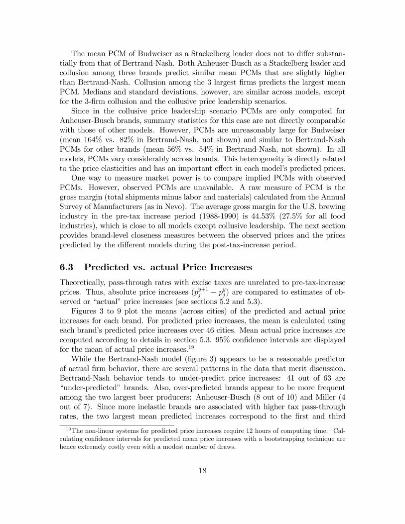
The mean PCM of Budweiser as a Stackelberg leader does not to di¤er substan-tially from that of Bertrand-Nash. Both Anheuser-Busch as a Stackelberg leader andcollusion among three brands predict similar mean PCMs that are slightly higherthan Bertrand-Nash. Collusion among the 3 largest �rms predicts the largest meanPCM. Medians and standard deviations, however, are similar across models, exceptfor the 3-�rm collusion and the collusive price leadership scenarios.Since in the collusive price leadership scenario PCMs are only computed for

Anheuser-Busch brands, summary statistics for this case are not directly comparablewith those of other models. However, PCMs are unreasonably large for Budweiser(mean 164% vs. 82% in Bertrand-Nash, not shown) and similar to Bertrand-NashPCMs for other brands (mean 56% vs. 54% in Bertrand-Nash, not shown). In allmodels, PCMs vary considerably across brands. This heterogeneity is directly relatedto the price elasticities and has an important e¤ect in each model�s predicted prices.One way to measure market power is to compare implied PCMs with observed

PCMs. However, observed PCMs are unavailable. A raw measure of PCM is thegross margin (total shipments minus labor and materials) calculated from the AnnualSurvey of Manufacturers (as in Nevo). The average gross margin for the U.S. brewingindustry in the pre-tax increase period (1988-1990) is 44.53% (27.5% for all foodindustries), which is close to all models except collusive leadership. The next sectionprovides brand-level closeness measures between the observed prices and the pricespredicted by the di¤erent models during the post-tax-increase period.

6.3 Predicted vs. actual Price Increases

Theoretically, pass-through rates with excise taxes are unrelated to pre-tax-increaseprices. Thus, absolute price increases (py+1j � pyj ) are compared to estimates of ob-served or �actual�price increases (see sections 5.2 and 5.3).Figures 3 to 9 plot the means (across cities) of the predicted and actual price

increases for each brand. For predicted price increases, the mean is calculated usingeach brand�s predicted price increases over 46 cities. Mean actual price increases arecomputed according to details in section 5.3. 95% con�dence intervals are displayedfor the mean of actual price increases.19

While the Bertrand-Nash model (�gure 3) appears to be a reasonable predictorof actual �rm behavior, there are several patterns in the data that merit discussion.Bertrand-Nash behavior tends to under-predict price increases: 41 out of 63 are�under-predicted�brands. Also, over-predicted brands appear to be more frequentamong the two largest beer producers: Anheuser-Busch (8 out of 10) and Miller (4out of 7). Since more inelastic brands are associated with higher tax pass-throughrates, the two largest mean predicted increases correspond to the �rst and third

19The non-linear systems for predicted price increases require 12 hours of computing time. Cal-culating con�dence intervals for predicted mean price increases with a bootstrapping technique arehence extremely costly even with a modest number of draws.

18

most inelastic brands in the sample: Budweiser (predicted: $4.94, actual $1.63) andBud Light (predicted: $3.24, actual $1.59). Many brands have tight 95% con�denceintervals around actual mean increases (around 15c/ and 20c/), indicating that priceincreases do not vary substantially across cities. This pattern can particularly beobserved for brewers that tend to produce nationally: Anheuser-Busch, Coors, Pabst,Miller and Stroh.The Stackelberg model in which Anheuser-Busch acts as the price leader with

all its brands (�gure 4) has a pattern that is similar to Bertrand-Nash. Althoughit can not be discerned from the �gure, in this model predicted increases are higherthan in Bertrand-Nash for all but one brand. For Anheuser-Busch�s brands, especiallyBudweiser, Bud Light and Natural Light, this di¤erence is larger and hence discerniblefrom the �gures.Aside from a larger over-prediction for Budweiser (60 c/), the Budweiser Stack-

elberg model (�gure 5), yields predicted mean price increases that are essentiallythe same to the Bertrand-Nash case. The reason for the small di¤erence betweenBertrand-Nash and Stackelberg models is that reaction functions of followers dependheavily on very small cross-price coe¢ cients. Thus the term dpm

dpjin (8) takes small

positive values making the �rst order conditions of the leader not substantially dif-ferent from those in Bertrand-Nash.Collusive price leadership by Budweiser (�gure 6) predicts unlikely price increases

that are, on average, almost 7 times larger than actual mean price increases, withsome of Anheuser-Busch�s brands in the vicinity of $15-$16. This extreme case cantherefore be rejected.The 3-�rm collusion scenario (�gure 7) over-predicts the price increases of the best

selling brands of the colluding �rms (e.g. Budweiser, Bud Light, Coors Light, MillerGenuine Draft and Miller Lite) by a large amount. The 3-brand collusion scenario(�gure 9) di¤ers less strikingly with Bertrand-Nash: there is a higher over-predictionfor Budweiser and, less noticeably, for the other two colluding brands: Coors andMiller Genuine Draft.<Figures 3 through 8 about here>The left part of table 4 presents summary statistics of price increases (i.e. the

absolute di¤erence in prices between the two quarters). The mean of predicted in-creases between Bertrand-Nash, the two Stackelberg models and collusion amongthree brands are similar and also close to the mean of actual increases, suggesting thatthese are superior models. Although the Anheuser-Busch Stackelberg model predictsthe mean of actual increases more accurately than Bertrand-Nash, closer inspectionof graph 4 indicates that this is due to larger over-predictions for Anheuser-Busch�sbrands, and not by smaller under-predictions of other brands. A similar argumentcan be made for the model of collusion among three brands.Medians and standard deviations indicate that price increases are more heteroge-

neous in the models than suggested by actual increases. While the median of actualincreases is similar to its mean, means of predicted increases are higher than their

19

respective medians (except in collusive price leadership) as a consequence of the out-liers of highly over-predicted brands (e.g. Budweiser, Bud Light). Larger standarddeviations of predicted increases with respect to standard deviations of actual priceincreases corroborates this heterogeneity.One metric of assessing the di¤erent models is the number of brands whose pre-

dicted mean price increases fall within the con�dence intervals of actual mean priceincreases shown in the graphs. The right part of table 4 presents this number (# Non-Rejections) for the models considered. According to this metric, collusion among 3�rms explains �rm behavior better than the other models.Two more rigorous metrics are considered. The �rst weighs price increases by each

brand�s market share. With this metric, accuracy in prediction is more importantfor more widely sold brands. Using this criterion, the Bertrand-Nash outperformsthe other models, though it is more than twice the value of weighted actual priceincreases (3.13 vs. 1.33). The second metric is the sum of squared deviations, wherea deviation is de�ned as the di¤erence between the predicted increase and the actualincrease.20 This criterion con�rms the superiority of Bertrand-Nash.<Table 4 about here>The large di¤erence between the weighted mean of predicted increases and actual

increases is due to the over-prediction of more popular brands: the combined shareof Budweiser (19%), Bud Light (6%), Coors Light (7%) and Miller Lite (9%) is 41%.In all models, there is an over-prediction for these brands, the largest of which isfor Budweiser. The similarity between the weighted actual increases and its non-weighted counterpart indicates that actual price increases tend to be homogeneousacross brands.

7 Conclusion

This paper analyzes market power and price competition in the U.S. brewing industrywhere there are some concerns about non-competitive behavior by the largest �rms.Bertrand-Nash, leadership and collusive models are considered as possible candidatesof pricing behavior. Leadership focuses on the largest �rm Anheuser-Busch and itsleading brand Budweiser. Collusive scenarios consider both the three largest �rms aswell as the three leading regular brands of beer. To choose the model that is bestsupported by the data, the 100% increase in the federal excise tax in January of 1991is used to compare observed price increases as a result of the tax hike with priceincreases predicted by the di¤erent models considered.Several metrics of closeness between predicted price increases and observed price

increases revealed that, overall, Bertrand-Nash appears to predict more closely theactual behavior of �rms, although Stackelberg predicts similar price increases toBertrand-Nash competition. The reason for the closeness between these two models

20The same conclusion is reached if each deviation is weighted.

20

is the small magnitude of cross-price coe¢ cients (common in markets with many dif-ferentiated products) which ultimately de�ne the closeness between Stackelberg andBertrand-Nash.One policy implication of the results in this paper is that antitrust concern towards

the leading beer producers should be low in terms of the non-competitive pricingforms considered in this paper. Although price-cost margins are relatively large inthis industry as indicated in section 6.2, results indicate that their source is not non-competitive pricing. This result is consistent with recent brand-level research in otherindustries. In a study of market power in the ready-to-eat breakfast cereals, Nevosuggests that the main source of market power is the result of product di¤erentiationand the portfolio e¤ect of �rms carrying more than one brand (the unilateral e¤ects)rather than actual collusive behavior (the coordinated e¤ects). Slade can not rejectthe null hypothesis of Bertrand-Nash competition in UK brewing and concurs withNevo�s conclusion.There are some systematic discrepancies at the brand level between Bertrand-Nash

prices and observed prices, however. Observed price increases do not conform wellwith the inverse relationship between own-price elasticity and excise tax pass-throughrates predicted by all models. As a consequence, Bertrand-Nash tends to over-predicttax pass-through rates of more price-inelastic brands, especially Budweiser, and tounder-predict price increases of more price-elastic brands. Overall, observed priceincreases tend to be more similar across brands than any of the models predict. Aninterpretation of this evidence is that, in a static oligopoly setting, Anheuser-Buschcould exert more market power even under Bertrand-Nash competition.The large heterogeneity in prices predicted by Bertrand-Nash is a special charac-

teristic of the present study. As opposed to the ready-to-eat breakfast cereal industrywhere the largest brand Corn Flakes captures less than 6% of the market21, the twolargest brands in this study (Budweiser with 19% and Miller Lite with 9%) capturemore than one quarter of all beer sales. Thus, price sensitivity in beer is heavilydriven by quantity sold and signi�cant brand loyalty. In breakfast cereals, in con-trast, brand concentration is more moderate and hence elasticities (and predictedprices) are more homogeneous across brands.The models considered here, as most models of pricing behavior, are built upon

the assumption of pro�t maximization. The unexplained homogeneity in price in-creases reported in this paper may be consistent with simpler, yet plausible pricingstrategies. For instance, the fact that actual price increases for large brewers�brands(Anheuser-Busch, Coors, Miller) as a result of the tax increase have minimal varia-tion across cities and are similar to actual price increases of smaller brewers�brandsmay be interpreted as leading brewers setting a common cost mark-up for all brands,regardless of where they are sold (and possibly of how elastic they are), and smallerbrewers matching these mark-ups. This conjecture is strengthened by the fact thatprice increases for elastic brands, which are produced mainly by smaller brewers and

21Based on IRI data used by Nevo (2001).

21

are generally more limited in their ability to increase prices, appear much higherthan what Bertrand-Nash and other models suggest, with values close to actual priceincreases of the more inelastic brands of larger brewers. While this conjecture isconsistent with the informal observations in the industry, the leadership models con-sidered do not conform with this pattern.22 Moreover, there is no clear way to testit within the pro�t maximization framework used in this paper. This issue henceremains as a potential extension.Scherer and Ross (p. 261-265) explain that a type of �rule-of-thumb�pricing of

the sort suggested above is common in many industries and is used as a way to copewith �uncertainties in the estimation of demand function shapes and elasticities�(p.262). Furthermore, this type of pricing behavior can be used as a coordinating device,especially when there are changes in costs and �rms in the industry share similarproduction technologies. To the extent that coordination existed in the brewingindustry as a consequence of the tax increase it appears that it bene�ted smallerbrewers rather than large �rms.Another explanation for the unexplained homogeneity of prices is �rms�poten-

tial unwillingness to match competitors�price increases (Sweezy, 1939). This pricestickiness in price increases has been documented in several industries (Bhaskar etal., 1991; Domberger and Fiebig, 1993). If Anheuser-Busch believes that followersare only going to match price increases up to a �reasonable� level, hiking pricesabove this threshold might not be pro�table for Anheuser-Busch. Prices above thethreshold might cause the demand for Anheuser-Busch�s brands to become too elas-tic as Anheuser-Busch�s consumers switch to competitors�cheaper brands. This isconsistent with demand estimates not being sensitive over the studied period (pre-tax-increase vs. post-tax-increase).The availability of more detailed data would allow to capture aspects not addressed

here. Dynamic models can be better assessed with less aggregated data on the timedimension. A dynamic setting is particularly important when future pro�ts are notindependent of the current state thereby making the static solution suboptimal. Also,detailed cost data at the manufacturer and retailer level can allow to extend theanalysis to vertical aspects and also more rigorous econometric tests of the competingpricing models considered here.

22The collusive leadership model considered yielded homogeneity in price increases that wouldmatch this observation. However, the magnitude of price increases is unlikely.

22

A Supply Details

A.1 Derivation of dpmdpjDe�ne a partition of the product set as = (f ;l), where f is the set of followerbrands and l is the set of leading brands, with JF and JL number of elementsrespectively. For each leader, a system of equations is constructed. Each lth systemof equations is used to compute the vector of all dpm

dplterms for leader l. An equation

in system l is obtained by totally di¤erentiating the price �rst order condition of allfollower brands (8)23 with respect to all followers�prices (pf , for all f 2 f) and theprice of the lth leader, pl (l 2 l):

Pf2f

"@qj@pf

+Pk2f

���kj(pk � ck)

@2qk@pj@pf

�+��

fj

@qf@pj

#| {z } dpf+

g(j;m)

+

"@qj@pl

+Pk2f

���kj(pk � ck)

@2qk@pj@pl

�#| {z } dpl = 0; j; k; f 2 f

h(j; l) (13)

where ��jk takes the value of one if brands j and k are produced by the same �rm

and zero otherwise. Therefore, for a given leader l there are JF equations like (13).Let G be the (JF � JF ) matrix that contains all g elements above and de�ne the(JF � 1) vectors Ds and Hl as:

Ds =

266664dp1:::

dpJF

377775 ; Hl =

266664�h(1; l)

:::

�h(JF ; l)

377775For a given pl, (13) is written in matrix notation as:

GDs �Hldpl = 0where dpl is treated as a scalar for matrix operations. The JF derivatives of thefollowers�prices with respect to a given pl are computed as:

23It is assumed that the �rst order condition with respect to advertising (9) does not play a rolein deriving dpm

dpj. Without this assumption, inversion of matrix G below is not possible since it is not

a square matrix. Results are unlikely to be sensitive to this assumption given the estimated smallimpact advertising has on demand.

23

Ds

dpl= G�1Hl (14)

Concatenating the (J�JF ) vectors of dimension (JF�1) given in (14) (one vectorfor each pl) gives D = G�1H. The JF � JL matrix D has a typical element dpf

dpl, for

f 2 f and l 2 l.

A.2 Marginal Costs in Leadership Models

Stackelberg ModelWhile marginal costs are obtained by applying (11), the derivative dpm

dpjneeds

to be computed �rst via equation (14). Several technical di¢ culties arise in thismodel. First, there is an immense number of possible Stackelberg scenarios. Giventhe motivation in this paper, only the case in which Anheuser-Busch acts as a leader,both with all its brands as well as with Budweiser, are considered.Second, since the term dpm

dpjin the leaders��rst order conditions is a function of

followers�marginal costs (see equation (14)), these marginal costs are computed �rst.When Anheuser-Busch acts as a leader with all its brands, followers�marginal costscan be obtained by inversion of a smaller system of dimension JF in (11). Thesemarginal costs are used to compute dpm

dpj, which is afterwards used to calculate the

marginal costs of the leading brands.When Budweiser is a sole brand leader, the term dpm

dpjis set to zero if m is pro-

duced by Anheuser-Busch, except for the brand Budweiser. Also, it is assumed thatBudweiser only leads brands produced by rival �rms (i.e. not by Anheuser-Busch).

Collusive Price Leadership ModelIn this case, only Anheuser-Busch�s marginal costs can be derived since �rst order

conditions of other �rms are not relevant (see section 3.2). These marginal costs arealso recovered by applying (11) to a system of dimension JL (where JL is the numberof brands sold by Anheuser-Busch) and by setting dpm

dpjto 1 in Budweiser�s �rst order

condition and zero in the remaining �rst order conditions.

24

B Data Details

IRI is a Chicago based marketing �rm that collects scanner data from a large sampleof supermarkets that is drawn from a universe of stores with annual sales of morethan 2 million dollars. This universe accounts for 82% of all grocery sales in theU.S. In most cities, the sample of supermarkets covers more than 20% of the relevantpopulation. In addition, IRI data correlates well with private sources in the BrewingIndustry (the correlation coe¢ cient of market shares for the top 10 brands betweendata from IRI and data from the Modern Brewery Age Blue Book is 0.95). Brandsthat had at least a 3% local market share in any given city were selected. Afterselecting brands according to this criterion, remaining observations are dropped ifthey had a local market share of less than 0.025%. Brands that appear in less than10 quarters are also dropped. Also, if a brand appears only in one city in a givenquarter, the observation for that quarter is not included either. This is done becausesome variables in other cities are used as instruments. On average there are 37 brandssold in each city market with a minimum of 24 brands and a maximum of 48 brands.Table 5 contains a list of the brands used with information on country of origin andthe corresponding brewers.The original data set contained observations in 63 cities; �ve cities were dropped

because of minimal number of brands or quantities. Overall, the number of citiesincreases over time; however, some cities appear only in a few quarters in the middleof the period. The average number of cities per quarter is 47. Brands are identi�edas regional or national as follows. First the percentage of cities in which each brandwas present was averaged over time. Brands with an average percentage close to100 are denoted national and brands with a percentage of (roughly) 50% or less aredenoted regional. The variable WAGES was constructed by averaging the hourlywages of interviewed individuals from the Bureau of Labor Statistics CPS monthlyearning �les at the NBER. For a given city-quarter combination, individuals workingin the retail sector were selected for that city over the corresponding three months.The average was then calculated over the number of individuals selected.

25

References

[1] Anderson, S., A. de Palma and B. Kreider, 2001, �Tax Incidence in Di¤erentiatedProduct Oligopoly�Journal of Public Economics, 81, 173-192.

[2] Anheuser-Busch 2003 Annual report, available at http://www.anheuser-busch.com/annual/2003/Domestic.pdf

[3] Annual Survey of Manufacturers, Census Bureau, various years

[4] Bhaskar, V. S. Machin and G. Reid (1991): �Testing a Model of the KinkedDemand Curve,�Journal of Industrial Economics, 39, 3, 241-254.

[5] Berry, S. (1994): �Estimating Discrete-Choice Models of Product Di¤erentia-tion,�RAND Journal of Economics, 25, 242-262.

[6] Brewers Almanac, various issues.

[7] Bureau of Labor Statistics, Current Population Survey Basic Monthly Files,Various issues, available at the National Bureau of Economic Research:http://www.nber.org/data/cps_index.html

[8] Case, G., A. Distefano and B. K. Logan (2000): �Tabulation of Alcohol Contenton Beer and Malt Beverages,�Journal of Analytical Toxicology, 24, 202-210.

[9] Deaton, A. and J. Muellbauer (1980): �An Almost Ideal Demand System,�American Economic Review, 70, 312-326.

[10] Demographia. www.demographia.com

[11] Domberger, S. and D. Fiebig (1993), �The Distribution of Price Changes inOligopoly,�Journal of Industrial Economics, 41, 3, 295-313.

[12] Gasmi, F., J. J. La¤ont and Q. Vuong (1992): �Econometric Analysis of Collu-sive Behavior in a Soft-Drink Market,�Journal of Economics and ManagementStrategy, 1, 277-311.

[13] Greer, D. (1998): �Beer: Causes of Structural Change,�in Industry Studies, ed.by L. Duetsch, NJ: Prentice Hall.

[14] Hausman, J., and G. Leonard (2002): �The Competitive E¤ects of a New Prod-uct Introduction: A Case Study,�Journal of Industrial Economics, 50, 237-263.

[15] Hausman, J., G. Leonard and D. Zona (1994): �Competitive Analysis with Dif-ferentiated Products,�Annales d�Économie et de Statistique, 34, 159-180.

26

[16] Kadiyali, V., N. Vilcassim and P. Chintagunta (1996): �Empirical Analysis ofCompetitive Product Line Pricing Decisions: Lead, Follow, or Move Together?,�Journal of Business, 69, 459-487.

[17] Moschini, G. (1995): �Units of Measurement and the Stone Index in DemandSystem Estimation,�American Journal of Agricultural Economics, 63-68.

[18] Modern Brewery Age, Blue Book, various issues.

[19] � � � (2001): �Measuring Market Power in the Ready-to-Eat Cereal Industry,�Econometrica, 69, 307-342.

[20] Pinkse, J., M. Slade and C. Brett (2002): �Spatial Price Competition: A Semi-parametric Approach,�Econometrica, 70, 1111-1155.

[21] Pinkse, J. and M. Slade (2004): �Mergers, Brand Competition, and the Price ofa Pint,�European Economic Review, 48.

[22] Rojas, C. and E. Peterson (2005): �Estimating Demand with Di¤erentiatedProducts: The Case of Beer in the U.S.,�Unpublished manuscript, available at:http://www.christianrojas.net

[23] Scherer, F. and D. Rosss (1990): Industrial Market Structure and EconomicPerformance, Houghton Mi­ in: Boston.

[24] Slade, M. (2004): �Market Power and Joint Dominance in UK Brewing,�Journalof Industrial Economics, 52, 133-163.

[25] Sweezy, P. (1939): �Demand Under Conditions of Oligopoly,�Journal of PoliticalEconomy, 47, 568-573.

[26] Tremblay, V. and C. Tremblay (1995): �Advertising, Price, and Welfare: Ev-idence from the U.S. Brewing Industry,� Southern Economic Journal, 62, 2,367-381.

[27] Tremblay, V. and C. Tremblay (2005): The U.S. Brewing Industry: Data andEconomic Analysis, MIT Press: Cambridge.

[28] U.S. Census Bureau, Concentration Ratios in Manufacturing, 1997 EconomicCensus. http://www.census.gov/prod/ec97/m31s-cr.pdf

27

Figure 1: Market Shares of Largest Brewers

0

10

20

30

40

50

60

1950

1955

1960

1965

1970

1975

1980

1985

1990

1996

2003

Mar

ket 

Shar

e (%

)

A­BMillerCoorsStroh/Schlitz

Source: Greer (1998), Beer Marketer's Insights, Anheuser­Busch's 2004 Annual ReportNote: Stroh exited the market in 1999. The 2003 number corresponds to Pabst's market share(the acquirer of some of Stroh's brands).

28

Figure 2: Quarterly Mean Prices, Various Segments (1988-1992)

21.2

19.0

10.1

8.9

15.5

14.1

0

5

10

15

20

25

88.I

88.II

88.III

88.IV

89.I

89.II

89.III

89.IV

90.I

90.II

90.III

90.IV

91.I

91.II

91.III

91.IV

92.I

92.II

92.III

92.IV

Mea

n P

rice

 ($/

288 

oz)

Import Budget Super­premium

Source: IRI Database, University of Connecticut

29

Figure3:PredictedPriceIncreasesbyBertrand-Nashbehaviorvs.ActualPriceIncreasesperbrandafter100%

Hikein

theFederalExciseTax(Meanover46cities)

­4­20246

1

3

5

7

10

12

14

16

18

20

22

24

26

28

30

32

34

36

38

40

42

44

46

48

50

52

54

56

58

60

62

64

Bra

nd I

D**

Price Increase ($/288 oz)

Pre

dic

ted I

ncr

ease

 ($)

Act

ual In

crea

se (

$)*

* V

erti

cal Lin

es a

re 9

5%

 Confiden

ce I

nte

rvals

** S

ee a

ppen

dix

 A for 

Bra

nd I

D's

Bud

wei

ser

Anh

euse

r­B

usch

Coo

rs

Bon

d C

orp

Pab

st

Mill

erSt

roh

Bud

 Lig

ht

30

Figure4:PredictedPriceIncreasesbyLeadershipofAnheuser-Buschvs.ActualPriceIncreasesperbrandafter100%

HikeintheFederalExciseTax(Meanover46cities)

­4­20246

1

3

5

7

10

12

14

16

18

20

22

24

26

28

30

32

34

36

38

40

42

44

46

48

50

52

54

56

58

60

62

64

Bra

nd I

D**

Price Increase ($)

Pre

dic

ted I

ncr

ease

 ($)

Act

ual In

crea

se (

$)*

* V

erti

cal Lin

es a

re 9

5%

 Confiden

ce I

nte

rvals

** S

ee a

ppen

dix

 A for 

Bra

nd I

D's

Mill

er L

ite

Bud

wei

ser

Anh

euse

r­B

usch

Coo

rs

Bon

d C

orp

Pab

st

Mill

erSt

roh

Bud

 Lig

ht

Nat

ural

Lig

ht

31

Figure5:PredictedPriceIncreasesbyLeadershipofBudweiservs.ActualPriceIncreasesperbrandafter100%

Hikein

theFederalExciseTax(Meanover46cities)

­4­20246

1

3

5

7

10

12

14

16

18

20

22

24

26

28

30

32

34

36

38

40

42

44

46

48

50

52

54

56

58

60

62

64

Bra

nd I

D**

Price Increase ($)

Pre

dic

ted I

ncr

ease

 ($)

Act

ual In

crea

se (

$)*

Mol

son

* V

erti

cal Lin

es a

re 9

5%

 Confiden

ce I

nte

rvals

** S

ee a

ppen

dix

 A for 

Bra

nd I

D's

Mill

er L

ite

Bud

wei

ser

Anh

euse

r­B

usch

Coo

rs

Bon

d C

orp

Pab

st

Mill

erSt

roh

Bud

 Lig

ht

32

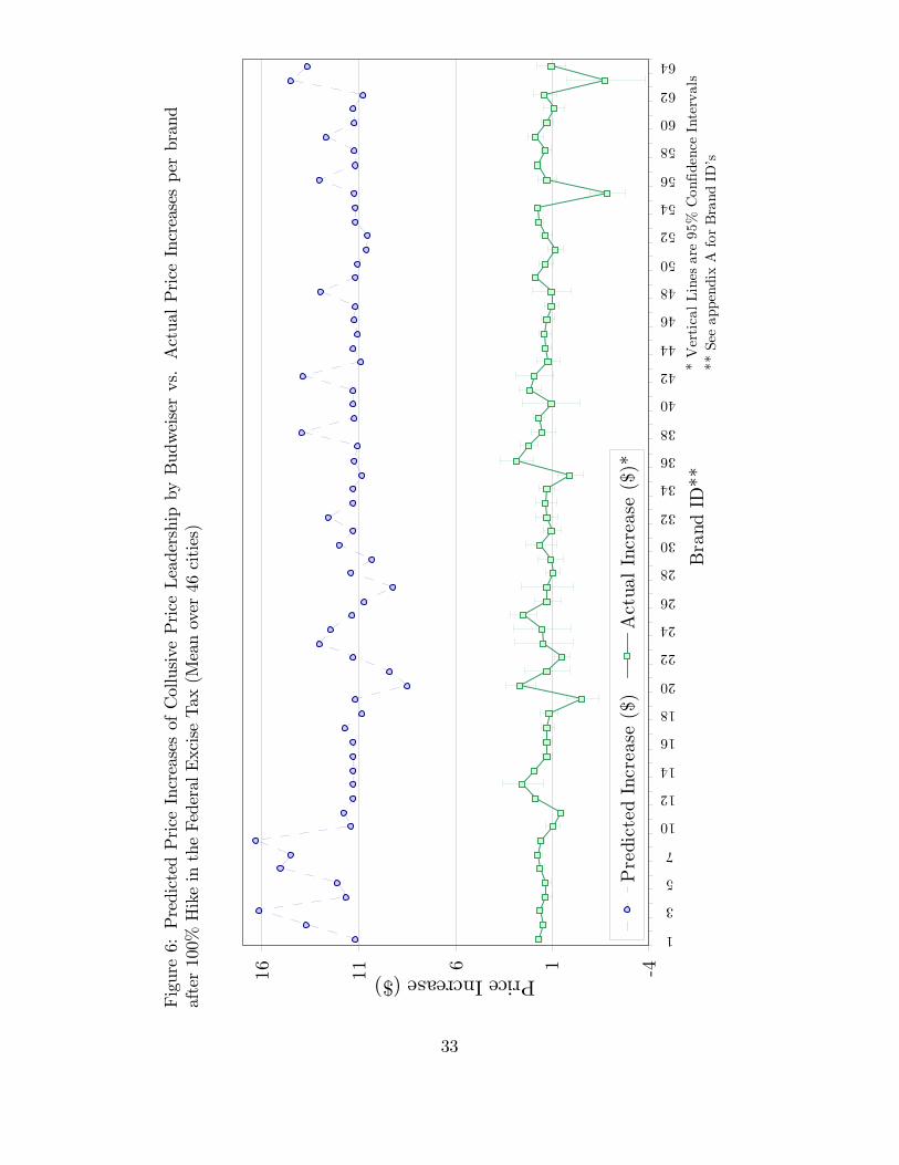
Figure6:PredictedPriceIncreasesofCollusivePriceLeadershipbyBudweiservs.ActualPriceIncreasesperbrand

after100%

HikeintheFederalExciseTax(Meanover46cities)

­416

11

16

1

3

5

7

10

12

14

16

18

20

22

24

26

28

30

32

34

36

38

40

42

44

46

48

50

52

54

56

58

60

62

64

Bra

nd I

D**

Price Increase ($)

Pre

dic

ted I

ncr

ease

 ($)

Act

ual In

crea

se (

$)*

* V

erti

cal Lin

es a

re 9

5%

 Confiden

ce I

nte

rvals

** S

ee a

ppen

dix

 A for 

Bra

nd I

D's

33

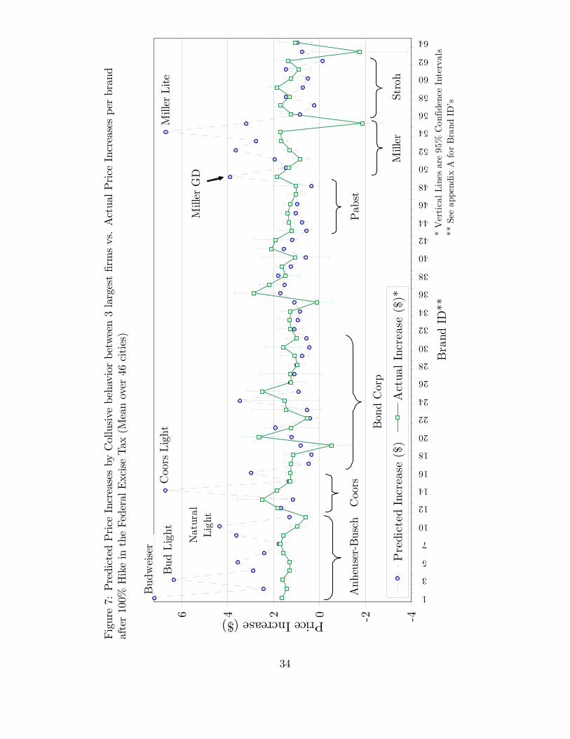
Figure7:PredictedPriceIncreasesbyCollusivebehaviorbetween3largest�rmsvs.ActualPriceIncreasesperbrand

after100%

HikeintheFederalExciseTax(Meanover46cities)

­4­20246

1

3

5

7

10

12

14

16

18

20

22

24

26

28

30

32

34

36

38

40

42

44

46

48

50

52

54

56

58

60

62

64

Bra

nd I

D**

Price Increase ($)

Pre

dic

ted I

ncr

ease

 ($)

Act

ual In

crea

se (

$)*

* V

erti

cal Lin

es a

re 9

5%

 Confiden

ce I

nte

rvals

** S

ee a

ppen

dix

 A for 

Bra

nd I

D's

Nat

ural

Lig

ht

Bud

wei

ser

Anh

euse

r­B

usch

Coo

rs

Bon

d C

orp

Pab

st

Mill

erSt

roh

Bud

 Lig

htC

oors

 Lig

htM

iller

 Lite

Mill

er G

D

34

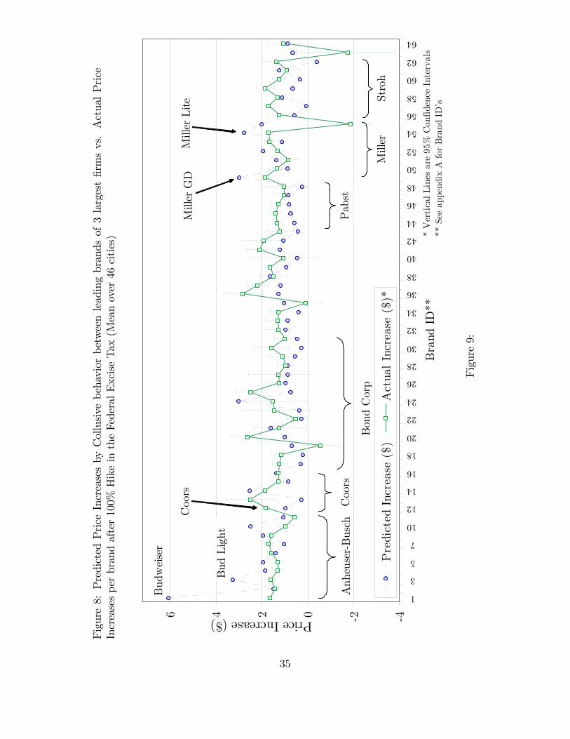
Figure8:PredictedPriceIncreasesbyCollusivebehaviorbetweenleadingbrandsof3largest�rmsvs.ActualPrice

Increasesperbrandafter100%

HikeintheFederalExciseTax(Meanover46cities)

­4­20246

1

3

5

7

10

12

14

16

18

20

22

24

26

28

30

32

34

36

38

40

42

44

46

48

50

52

54

56

58

60

62

64

Bra

nd I

D**

Price Increase ($)

Pre

dic

ted I

ncr

ease

 ($)

Act

ual In

crea

se (

$)*

* V

erti

cal Lin

es a

re 9

5%

 Confiden

ce I

nte

rvals

** S

ee a

ppen

dix

 A for 

Bra

nd I

D's

Bud

wei

ser

Anh

euse

r­B

usch

Coo

rs

Bon

d C

orp

Pab

st

Mill

erSt

roh

Bud

 Lig

ht

Mill

er L

ite

Mill

er G

DC

oors

Figure9:

35

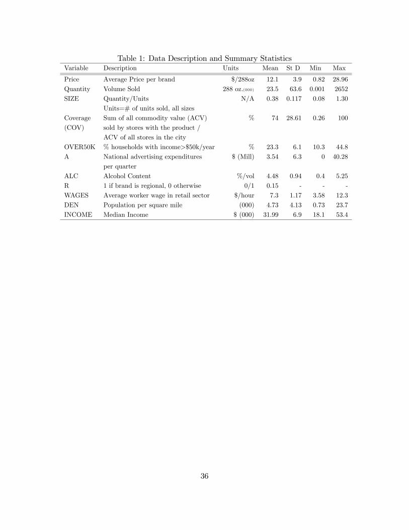
Table 1: Data Description and Summary StatisticsVariable Description Units Mean St D Min Max

Price Average Price per brand $/288oz 12.1 3.9 0.82 28.96

Quantity Volume Sold 288 oz.(000) 23.5 63.6 0.001 2652

SIZE Quantity/Units N/A 0.38 0.117 0.08 1.30

Units=# of units sold, all sizes

Coverage Sum of all commodity value (ACV) % 74 28.61 0.26 100

(COV) sold by stores with the product /

ACV of all stores in the city

OVER50K % households with income>$50k/year % 23.3 6.1 10.3 44.8

A National advertising expenditures $ (Mill) 3.54 6.3 0 40.28

per quarter

ALC Alcohol Content %/vol 4.48 0.94 0.4 5.25

R 1 if brand is regional, 0 otherwise 0/1 0.15 - - -

WAGES Average worker wage in retail sector $/hour 7.3 1.17 3.58 12.3

DEN Population per square mile (000) 4.73 4.13 0.73 23.7

INCOME Median Income $ (000) 31.99 6.9 18.1 53.4

36

Table 2: Results of GMM Estimation of Demand Model

Dependent Variable: Sales Share (wjt)a Model 1 Model 2Variable; Description Coe¤ (t-stat)b Coe¤ (t-stat)b

Constant, ajtBrand Dummies no no yes yes

Constantc - - -15.51 (-0.96)

ALCc - - 5.95 (3.24)

POPULARc - - 49.98 (14.84)

PREMIUMc - - 63.52 (13.95)

SUPER-PREMIUMc - - 131.81 (23.85)

IMPORTc - - 211.18 (22.55)

NCBAC; # common boundary neighbors, Alcohol content-Coverage space -1.15 (-0.85) -3.91 (-3.66)

OVER50K -94.84 (-0.57) -240.0 (-1.90)

Own Price (bjj) and Own-Advertising (cjj)logP -122.4 (-9.82) -252.9 (-5.71)

logP � (1=COV ) -0.56 (-2.38) -1.09 (-3.46)

logP �NCBCSP ; NCBCSP= # of CB neighbors in CS - price space -4.82 (-7.28) -7.14 (-11.35)

A 8.48 (31.15) 1.32 (4.39)

A �(1=COV ) -0.68 (-5.58) -0.19 (-3.47)

A �NCBCS; NCBCS=# common boundary neighbors, CS space -1.65 (-3.57) -0.16 (-4.53)

Weighted Cross-Price and Cross-Advertising Terms (�l and �m)Distance Measures for Price (Weighing Matrix Acronym)Alcohol content-product coverage, two-dimensional product space, (WAC) 2.10 (13.66) 5.32 (11.0)

Nearest Neighbors in Alcohol Content-Product Coverage space (WNNAC) -0.21 (-0.30) 8.87 (15.62)

Brewer Identity (WBREW) -12.18 (-5.38) 17.30 (5.31)

Product Classi�cation 2: Regular-Light (WPROD2) 52.39 (6.62) 93.56 (3.99)

National Identity (WREG) 40.83 (5.85) 49.61 (5.39)

Distance Measures for Advertising (Weighing Matrix Acronym)Container size, one-dimensional product space (WSIZE) 0.17 (7.83) 0.16 (8.64)

Common boundary in product coverage-cont. size-price space (WCBCSP) 0.85 (15.5) 0.71 (15.23)

Nearest neighbors in product coverage-container size space (WNNCS) 0.61 (14.7) 0.40 (12.24)

Product Classi�cation 3: Budget, light, premium (WPROD3) -2.78 (14.58) -3.22 (-9.10)

National Identity (WREG) -3.02 (-21.79) 5.30 (2.65)

Price Index (dj)log (xt=P

Lt ) 28.15 (1.08) 27.35 (1.38)

R2 (Centered, uncentered) 0.40, 0.58 0.66, 0.76

J-Statistic (p-value) 0.90 0.50aBased on 33,892 observations. Coe¢ cients have been multiplied by 10,000 for readability. All speci�cations

include time and city dummies (not reported) .bAsymptotic t-statistics in parenthesis.c Estimates from minimum distance (MD) procedure. The MD regression includes brewer dummies (not reported).

37

Table 3: Summary Statistics of Price Cost Margins for Di¤erent Models, (1988-1990)*Model Mean Median St. DevBertrand-Nash 39.50 36.68 25.96Anheuser-Busch Stackelberg Leadership 40.08 37.58 26.25Budweiser Stackelberg Leadership 39.52 36.68 26.00Collusive Leadership (Budweiser)�� 70.51 60.88 45.09Collusion 3 �rmsx 46.02 46.95 29.14Collusion 3 brands� 40.20 37.17 26.50�Margins are de�ned as 100� (p� c)=p.of the 18,369 (brand-city-quarter) observations in the pre-increase period (1988-1990).�� Price-cost margins obtained for Anheuser-Busch brands onlyx Anheuser-Busch, Adolph Coors and Miller� Budweiser, Coors, Miller Genuine Draft

Table 4: Summary Statistics of Actual and Predicted Price Increases and PerformanceMetrics of Models

Summary Statisticsa Performance MetricsMean Median St. Dev # No- Weighted SSDd

Rejectb Meanc

Actual Increases 1.38 1.37 0.65 N/A 1.33 N/A

Predicted Increases:Bertrand-Nash 1.24 0.97 1.41 20 3.13 3993

A-B Stackelberg Leadere 1.39 1.04 1.54 20 3.44 4663

Budweiser Stackelberg Leader 1.26 0.98 1.46 21 3.26 4232

Collusive Leadership (Bud) 11.83 11.03 2.93 0 11.44 20629

Collusion 3 �rmsf 2.21 1.50 2.40 22 5.20 11671

Collusion 3 brandsg 1.34 1.03 1.52 19 3.52 4545a Computed with absolute price increases for each brand: the absolute price di¤erence between

the �rst quarter of 1991 and the fourth quarter of 1990, over 46 cities (1748 observations)b Number of brands for which mean of predicted increases falls within the con�dence intervals

of mean of actual increases (see graphs 3 to 9)c Weighted average of absolute price increases (weight=volume of brand sold in city/ total volume

of all brands in all cities in the �rst quarter of 1991)d Sum of squared deviations over all brands and all cities; deviation=predicted-actual (1748 obs.)e A-B = Anheuser-Busch. f Anheuser-Busch, Adolph Coors, Miller (Philip Morris).g Budweiser, Coors, Miller Genuine Draft

38

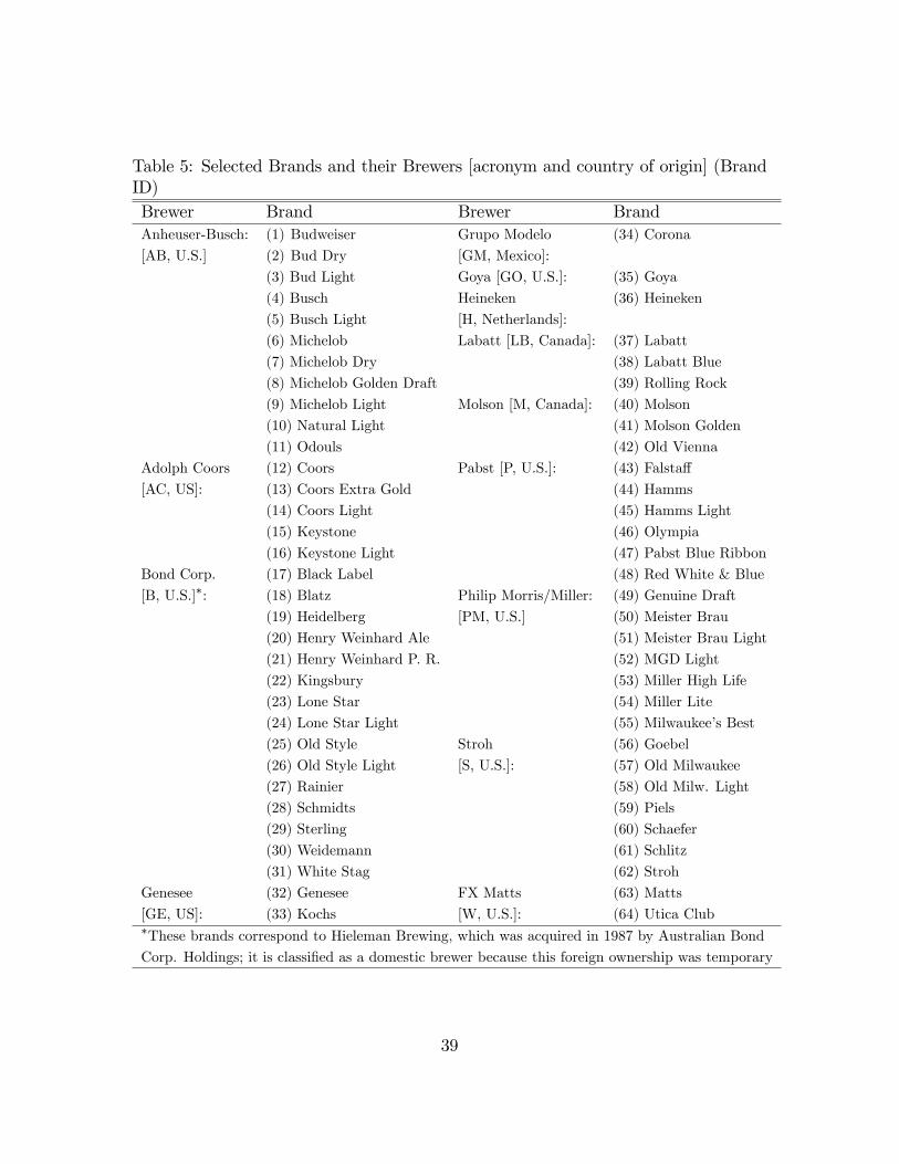
Table 5: Selected Brands and their Brewers [acronym and country of origin] (BrandID)Brewer Brand Brewer BrandAnheuser-Busch: (1) Budweiser Grupo Modelo (34) Corona

[AB, U.S.] (2) Bud Dry [GM, Mexico]:

(3) Bud Light Goya [GO, U.S.]: (35) Goya

(4) Busch Heineken (36) Heineken

(5) Busch Light [H, Netherlands]:

(6) Michelob Labatt [LB, Canada]: (37) Labatt

(7) Michelob Dry (38) Labatt Blue

(8) Michelob Golden Draft (39) Rolling Rock

(9) Michelob Light Molson [M, Canada]: (40) Molson

(10) Natural Light (41) Molson Golden

(11) Odouls (42) Old Vienna

Adolph Coors (12) Coors Pabst [P, U.S.]: (43) Falsta¤

[AC, US]: (13) Coors Extra Gold (44) Hamms

(14) Coors Light (45) Hamms Light

(15) Keystone (46) Olympia

(16) Keystone Light (47) Pabst Blue Ribbon

Bond Corp. (17) Black Label (48) Red White & Blue

[B, U.S.]�: (18) Blatz Philip Morris/Miller: (49) Genuine Draft

(19) Heidelberg [PM, U.S.] (50) Meister Brau

(20) Henry Weinhard Ale (51) Meister Brau Light

(21) Henry Weinhard P. R. (52) MGD Light

(22) Kingsbury (53) Miller High Life

(23) Lone Star (54) Miller Lite

(24) Lone Star Light (55) Milwaukee�s Best

(25) Old Style Stroh (56) Goebel

(26) Old Style Light [S, U.S.]: (57) Old Milwaukee

(27) Rainier (58) Old Milw. Light

(28) Schmidts (59) Piels

(29) Sterling (60) Schaefer

(30) Weidemann (61) Schlitz

(31) White Stag (62) Stroh

Genesee (32) Genesee FX Matts (63) Matts

[GE, US]: (33) Kochs [W, U.S.]: (64) Utica Club�These brands correspond to Hieleman Brewing, which was acquired in 1987 by Australian Bond

Corp. Holdings; it is classi�ed as a domestic brewer because this foreign ownership was temporary

39

FOOD MARKETING POLICY CENTER RESEARCH REPORT SERIES

This series includes final reports for contract research conducted by Policy Center Staff. The series also contains research direction and policy analysis papers. Some of these reports have been commissioned by the Center and are authored by especially qualified individuals from other institutions. (A list of previous reports in the series is available on our web site.) Other publications distributed by the Policy Center are the Working Paper Series, Journal Reprint Series for Regional Research Project NE-165: Private Strategies, Public Policies, and Food System Performance, and the Food Marketing Issue Paper Series. Food Marketing Policy Center staff contribute to these series. Individuals may receive a list of publications in these series and paper copies of older Research Reports are available for $20.00 each, $5.00 for students. Call or mail your request at the number or address below. Please make all checks payable to the University of Connecticut. Research Reports can be downloaded free of charge from our web site given below.

Food Marketing Policy Center 1376 Storrs Road, Unit 4021

University of Connecticut Storrs, CT 06269-4021

Tel: (860) 486-1927

FAX: (860) 486-2461 email: fmpc@uconn.edu

http://www.fmpc.uconn.edu