
Fusions of Description Logics and Abstract Description Systems
Upload
khangminh22Category
view
0download
0
1
DarkSUSY DarkSUSY_main
Manual and description of routines
Documentation harvested from documentation and source directories with harvestdoc.plSat Mar 19 12:21:07 2022
http://www.darksusy.org
Joakim Edsjöa∗, Torsten Bringmannb†, Paolo Gondoloc‡,Piero Ulliod§, Lars Bergströma¶, Mia Schelke‖,
Edward A. Baltz∗∗ and Gintaras Duda††
a The Oskar Klein Centre for Cosmoparticle Physics, Department of Physics, StockholmUniversity, AlbaNova, SE-106 91 Stockholm, Sweden.
b Department of Physics, University of Oslo, Box 1048, NO-0371 Oslo, Norwayc Department of Physics, University of Utah,115 South 1400 East, Suite 201, Salt Lake City, UT
84112-0830, USA.d SISSA and INFN, Sezione di Trieste, via Bonomea 265, 34136 Trieste, Italy.
∗E-mail address: [email protected]†E-mail address: [email protected]‡E-mail address: [email protected]§E-mail address: [email protected]¶E-mail address: [email protected]‖E-mail address: schelke@...
∗∗E-mail address: [email protected]††E-mail address: [email protected]

2
AbstractDarkSUSY is a package for numerical dark matter calculations including, but not limited to, super-symmetric dark matter. This manual describes the theoretical background as well as details aboutthe actual routines. Everything is not covered, but it should hopefully prove useful if you needmore information than in our published articles.
Disclaimer. This manual is work in progress.We try to keep it clear and up-to-date with the code, but there will be cases wherechanges/improvements in the code, for one reason or another, will not have propagatedinto the manual. Hence, check the actual code if you want to be certain about how agiven process/feature is implemented.
Contents
I Prelude 8
1 Introduction 9
2 Quick start guide 102.1 Installation . . . . . . . . . . . . . . . . . . . . . . . . . . . . . . . . . . . . . . . . . 10
2.1.1 Options for install . . . . . . . . . . . . . . . . . . . . . . . . . . . . . . . . . 112.1.2 System requirements . . . . . . . . . . . . . . . . . . . . . . . . . . . . . . . . 11
2.2 Example programs . . . . . . . . . . . . . . . . . . . . . . . . . . . . . . . . . . . . . 112.2.1 Auxiliary example programs . . . . . . . . . . . . . . . . . . . . . . . . . . . . 122.2.2 Making your own example programs . . . . . . . . . . . . . . . . . . . . . . . 13
2.3 Modifying individual subroutines or functions . . . . . . . . . . . . . . . . . . . . . . 13
3 Guiding principles of the code 143.1 The main DarkSUSY library ds_core . . . . . . . . . . . . . . . . . . . . . . . . . . . 143.2 Particle physics modules . . . . . . . . . . . . . . . . . . . . . . . . . . . . . . . . . . 15
3.2.1 Using a particle physics module . . . . . . . . . . . . . . . . . . . . . . . . . . 163.2.2 Adding a new particle physics module . . . . . . . . . . . . . . . . . . . . . . 17
3.3 Halo models . . . . . . . . . . . . . . . . . . . . . . . . . . . . . . . . . . . . . . . . . 183.4 Interface functions . . . . . . . . . . . . . . . . . . . . . . . . . . . . . . . . . . . . . 183.5 Commonly used functions . . . . . . . . . . . . . . . . . . . . . . . . . . . . . . . . . 203.6 Replaceable functions . . . . . . . . . . . . . . . . . . . . . . . . . . . . . . . . . . . 21
4 Comparison to previous DarkSUSY versions 22
5 Original articles 24
II Main DarkSUSY routines in src/ 25
6 an_yield: Annihilation yields in the halo – yields from simulations 266.1 Annihilation in the halo, yields – theory . . . . . . . . . . . . . . . . . . . . . . . . . 26
6.1.1 Monte Carlo simulations . . . . . . . . . . . . . . . . . . . . . . . . . . . . . . 26
7 aux: General routines 287.1 General routines . . . . . . . . . . . . . . . . . . . . . . . . . . . . . . . . . . . . . . 28
8 aux_xdiag: Diagonalization routines 298.1 XDIAG . . . . . . . . . . . . . . . . . . . . . . . . . . . . . . . . . . . . . . . . . . . 29
9 cr_aux: Cosmic rays – general 309.1 Cosmic Rays – auxiliary routines . . . . . . . . . . . . . . . . . . . . . . . . . . . . . 30
3

CONTENTS 4
10 cr_axi: Cosmic rays – diffusion routines for axisymmetric distributions 3110.1 Cosmic ray propagation in axially symmetric halos . . . . . . . . . . . . . . . . . . . 31
11 cr_gamma: Cosmic rays – Gamma fluxes 3411.1 Gamma rays from the halo – theory . . . . . . . . . . . . . . . . . . . . . . . . . . . 3411.2 Continuous gamma yields and line signals . . . . . . . . . . . . . . . . . . . . . . . . 3511.3 Fluxes . . . . . . . . . . . . . . . . . . . . . . . . . . . . . . . . . . . . . . . . . . . . 3511.4 Gamma rays from the halo – routines . . . . . . . . . . . . . . . . . . . . . . . . . . 36
12 cr_nu: Cosmic rays – Neutrino fluxes 3712.1 Neutrino fluxes from the halo – theory . . . . . . . . . . . . . . . . . . . . . . . . . . 37
13 cr_ps: Cosmic rays – point sources 3813.1 Cosmic Ray propagation for point sources . . . . . . . . . . . . . . . . . . . . . . . . 38
14 dd: Direct detection 3914.1 Direct detection – theory . . . . . . . . . . . . . . . . . . . . . . . . . . . . . . . . . 39
15 dmd_astro: Astrophysical source functions 40
16 dmd_mod: Dark matter distributions 4116.1 Dark matter distributions – theory . . . . . . . . . . . . . . . . . . . . . . . . . . . . 41
16.1.1 Rescaling of the WIMP density . . . . . . . . . . . . . . . . . . . . . . . . . . 4116.2 Implementation in DarkSUSY . . . . . . . . . . . . . . . . . . . . . . . . . . . . . . . 42
16.2.1 Dark matter distributions – routines . . . . . . . . . . . . . . . . . . . . . . . 43
17 dmd_vel: Dark matter velocity distributions 4417.1 Dark matter phase-space distributions – theory . . . . . . . . . . . . . . . . . . . . . 44
18 fi: Freeze-In 4518.1 Freeze-in – theory . . . . . . . . . . . . . . . . . . . . . . . . . . . . . . . . . . . . . 4518.2 Freeze-in – routines . . . . . . . . . . . . . . . . . . . . . . . . . . . . . . . . . . . . . 46
19 ini: Initialization routines 4819.1 Initialisation routines . . . . . . . . . . . . . . . . . . . . . . . . . . . . . . . . . . . . 48
20 kd: Kinetic decoupling 4920.1 Kinetic decoupling and microhalos (kd) – theory . . . . . . . . . . . . . . . . . . . . 49
20.1.1 Kinetic decoupling . . . . . . . . . . . . . . . . . . . . . . . . . . . . . . . . . 4920.1.2 The smallest protohalos . . . . . . . . . . . . . . . . . . . . . . . . . . . . . . 50
20.2 Kinetic decoupling – routines . . . . . . . . . . . . . . . . . . . . . . . . . . . . . . . 51
21 rd: Relic density 5221.1 Relic density – theoretical background . . . . . . . . . . . . . . . . . . . . . . . . . . 52
21.1.1 The Boltzmann equation and thermal averaging . . . . . . . . . . . . . . . . 5221.1.2 Review of the Boltzmann equation with coannihilations . . . . . . . . . . . . 5221.1.3 Thermal averaging . . . . . . . . . . . . . . . . . . . . . . . . . . . . . . . . . 5421.1.4 Reformulation of the Boltzmann equation . . . . . . . . . . . . . . . . . . . . 56
21.2 Relic density – numerical integration of the density equation . . . . . . . . . . . . . . 5921.3 Relic density – routines . . . . . . . . . . . . . . . . . . . . . . . . . . . . . . . . . . 60
21.3.1 Global parameters . . . . . . . . . . . . . . . . . . . . . . . . . . . . . . . . . 6021.3.2 Brief description of the internal routines . . . . . . . . . . . . . . . . . . . . . 61

CONTENTS 5
22 se_aux: Auxiliary routines for WIMP annihilation in the Sun/Earth 6322.1 Sun and Earth models – auxiliary routines . . . . . . . . . . . . . . . . . . . . . . . . 63
23 se_mod: Sun and Earth models 6423.1 Sun and Earth models – theory . . . . . . . . . . . . . . . . . . . . . . . . . . . . . . 6423.2 Sun and Earth models – routines . . . . . . . . . . . . . . . . . . . . . . . . . . . . . 64
24 se_nu: Capture and annihilation in the Sun/Earth 6524.1 Neutrinos from the Sun and Earth – theory . . . . . . . . . . . . . . . . . . . . . . . 65
24.1.1 Neutrino yield from annihilations . . . . . . . . . . . . . . . . . . . . . . . . . 6524.1.2 Evolution of the number density in the Earth/Sun . . . . . . . . . . . . . . . 6624.1.3 Approximate capture rate expressions . . . . . . . . . . . . . . . . . . . . . . 6724.1.4 Earth and Sun composition . . . . . . . . . . . . . . . . . . . . . . . . . . . . 6824.1.5 More accurate capture rate expressions . . . . . . . . . . . . . . . . . . . . . 6924.1.6 Accurate capture rates in the Earth for general velocity distributions . . . . . 6924.1.7 Accurate capture rates for the Earth for a Maxwell-Boltzmann velocity dis-
tribution . . . . . . . . . . . . . . . . . . . . . . . . . . . . . . . . . . . . . . 7124.1.8 Effects of WIMP diffusion in the solar system . . . . . . . . . . . . . . . . . . 72
24.2 Neutrinos from Sun and Earth – routines . . . . . . . . . . . . . . . . . . . . . . . . 73
25 se_yield: Yields from annihilation in the Sun/Earth 7425.1 Muon yields from annihilation in the Earth/Sun – theory . . . . . . . . . . . . . . . 74
25.1.1 Monte Carlo simulations with WimpSim . . . . . . . . . . . . . . . . . . . . . 74
26 si: Self-interactions 7926.1 Dark matter self-interactions (si) – theory . . . . . . . . . . . . . . . . . . . . . . . . 7926.2 Self-interactions – routines . . . . . . . . . . . . . . . . . . . . . . . . . . . . . . . . . 81
III Particle physics modules in src_models 82
27 Basic principles and common routines 8327.1 common/aux: auxiliary routines . . . . . . . . . . . . . . . . . . . . . . . . . . . . . . 8327.2 common/sm: standard model . . . . . . . . . . . . . . . . . . . . . . . . . . . . . . . 83
28 The empty model 85
29 Generic decaying dark matter 86
30 Generic FIMPs 8730.1 generic_fimp/fi: Freeze-in routines . . . . . . . . . . . . . . . . . . . . . . . . . . . . 88
31 Generic WIMPs 89
32 The Minimal Supersymmetric Standard Model 9032.1 mssm/ac: Accelerator constraints . . . . . . . . . . . . . . . . . . . . . . . . . . . . . 91
32.1.1 Accelerator bounds . . . . . . . . . . . . . . . . . . . . . . . . . . . . . . . . . 9132.2 mssm/an: (Co-)annihilation cross sections . . . . . . . . . . . . . . . . . . . . . . . . 92
32.2.1 Annihilation cross sections – theory . . . . . . . . . . . . . . . . . . . . . . . 9232.2.1.1 Annihilation cross sections . . . . . . . . . . . . . . . . . . . . . . . 9232.2.1.2 Coannihilation diagrams . . . . . . . . . . . . . . . . . . . . . . . . 9232.2.1.3 Neutralino and chargino annihilation . . . . . . . . . . . . . . . . . 9232.2.1.4 Squark-squark annihilation . . . . . . . . . . . . . . . . . . . . . . . 9332.2.1.5 Squark-neutralino annihilation . . . . . . . . . . . . . . . . . . . . . 97
CONTENTS 6
32.2.1.6 Squark-chargino annihilation . . . . . . . . . . . . . . . . . . . . . . 9732.2.1.7 Degrees of freedom . . . . . . . . . . . . . . . . . . . . . . . . . . . . 98
32.2.2 Annihilation routines - general remarks . . . . . . . . . . . . . . . . . . . . . 9832.2.2.1 General routines . . . . . . . . . . . . . . . . . . . . . . . . . . . . . 9932.2.2.2 Neutralino and chargino (co)annihilation cross sections . . . . . . . 99
32.3 mssm/an_1l: Annihilation cross sections (1-loop) . . . . . . . . . . . . . . . . . . . . 9932.3.1 Annihilation cross sections at 1-loop – general . . . . . . . . . . . . . . . . . 99
32.4 mssm/an_ib: Internal bremsstrahlung . . . . . . . . . . . . . . . . . . . . . . . . . . 9932.4.1 Internal Bremsstrahlung (IB) – theory . . . . . . . . . . . . . . . . . . . . . . 99
32.4.1.1 General considerations . . . . . . . . . . . . . . . . . . . . . . . . . 10032.4.1.2 IB from neutralino annihilations . . . . . . . . . . . . . . . . . . . . 10032.4.1.3 The implementation in DarkSUSY . . . . . . . . . . . . . . . . . . . 101
32.5 mssm/an_sf: Annihilation cross sections (with sfermions) . . . . . . . . . . . . . . . 10232.5.1 Annihilation cross sections with sfermions – general . . . . . . . . . . . . . . 102
32.6 mssm/an_stu: t, u and s diagrams for ff -annihilation . . . . . . . . . . . . . . . . . 10232.6.1 Annihilation amplitudes for fermion-fermion annihilation . . . . . . . . . . . 102
32.7 mssm/dd: Direct detection . . . . . . . . . . . . . . . . . . . . . . . . . . . . . . . . 10332.7.1 Direct detection – theory . . . . . . . . . . . . . . . . . . . . . . . . . . . . . 103
32.8 mssm/ge: General SUSY model setup: masses, vertices etc . . . . . . . . . . . . . . 10532.8.1 Supersymmetric model . . . . . . . . . . . . . . . . . . . . . . . . . . . . . . . 105
32.8.1.1 Parameters . . . . . . . . . . . . . . . . . . . . . . . . . . . . . . . . 10532.8.1.2 Mass spectrum . . . . . . . . . . . . . . . . . . . . . . . . . . . . . . 10532.8.1.3 Three-particle vertices . . . . . . . . . . . . . . . . . . . . . . . . . . 108
32.8.2 General supersymmetry – routines . . . . . . . . . . . . . . . . . . . . . . . . 11032.9 mssm/ge_cmssm: cMSSM interface (Isasugra) . . . . . . . . . . . . . . . . . . . . . 111
32.9.1 mSUGRA (ISASUGRA) interface to DarkSUSY . . . . . . . . . . . . . . . . 11132.10mssm/ge_slha: SUSY Les Houches Accord interface . . . . . . . . . . . . . . . . . . 111
32.10.1SUSY Les Houches Accord . . . . . . . . . . . . . . . . . . . . . . . . . . . . 11132.11mssm/ini: Initialization routines . . . . . . . . . . . . . . . . . . . . . . . . . . . . . 111
32.11.1 Initialization routines . . . . . . . . . . . . . . . . . . . . . . . . . . . . . . . 11132.12mssm/rd: Relic density . . . . . . . . . . . . . . . . . . . . . . . . . . . . . . . . . . 112
32.12.1Relic density of neutralinos . . . . . . . . . . . . . . . . . . . . . . . . . . . . 11232.12.2 Internal degrees of freedom . . . . . . . . . . . . . . . . . . . . . . . . . . . . 112
32.12.2.1 Neutralino-chargino annihilation . . . . . . . . . . . . . . . . . . . . 11232.12.2.2 Chargino-chargino annihilation . . . . . . . . . . . . . . . . . . . . . 11332.12.2.3 Neutralino-sfermion annihilation . . . . . . . . . . . . . . . . . . . . 11432.12.2.4 Chargino-sfermion annihilation . . . . . . . . . . . . . . . . . . . . . 11532.12.2.5 Sfermion-sfermion annihilation . . . . . . . . . . . . . . . . . . . . . 11532.12.2.6 Squark-squark annihilation . . . . . . . . . . . . . . . . . . . . . . . 11632.12.2.7 Sfermion-squark annihilation . . . . . . . . . . . . . . . . . . . . . . 11732.12.2.8 Summary of degrees of freedom . . . . . . . . . . . . . . . . . . . . . 117
32.13Relic density – more details on routines . . . . . . . . . . . . . . . . . . . . . . . . . 11732.13.1Global parameters . . . . . . . . . . . . . . . . . . . . . . . . . . . . . . . . . 117
33 Silveira-Zee (Scalar Singlet) 11933.1 silveira_zee/fi: Freeze-in routines . . . . . . . . . . . . . . . . . . . . . . . . . . . . . 119
34 Self-Interacting Dark Matter 12034.1 vdSIDM/an: Annihilation routines . . . . . . . . . . . . . . . . . . . . . . . . . . . . 12034.2 vdSIDM/cr: Cosmic rays . . . . . . . . . . . . . . . . . . . . . . . . . . . . . . . . . 12134.3 vdSIDM/ini: Model setup . . . . . . . . . . . . . . . . . . . . . . . . . . . . . . . . . 12134.4 vdSIDM/kd: Kinetic decoupling . . . . . . . . . . . . . . . . . . . . . . . . . . . . . 121

CONTENTS 7
34.5 vdSIDM/rd: Relic density . . . . . . . . . . . . . . . . . . . . . . . . . . . . . . . . . 12234.6 vdSIDM/si: Dark matter self-interactions . . . . . . . . . . . . . . . . . . . . . . . . 122
Bibliography 122

Part I
Prelude
8

Chapter 1
Introduction
DarkSUSY is a set of Fortran routines to allow advanced numerical calculations connected to darkmatter physics. In part I of this Manual we explain the basic structure of the code, and providean introduction on how to get quickly started and use it. Part II is devoted to a descriptionof the DarkSUSY core library, which contains all routines that are completely independent of theunderlying DM particle physics. In part III, we describe the additional libraries, or particle modules,for specific DM models that are currently implemented (including supersymmetric dark matter inthe Minimal Supersymmetric Standard Model, the MSSM). The modular structure of the codeallows to easily link the core library to any of those particle modules, as well as to add user-definednew modules in a straight-forward way.
In this manual we will mainly cover the more techincal aspects of DarkSUSY, i.e. how to calldifferent subroutines, both particle-physics dependent and not, and how to change various switchesand options in more advanced routines. We will only briefly review the necessary physics involvedwhen needed and refer the reader to [1, 2] and the original papers behind DarkSUSY (see Section5) for more details. If you use DarkSUSY please consider the original physics work behind and giveproper credit to [2] and the relevant references in Section 5. If you use non-standard options, e.g. adifferent propagation model for antiprotons, please remember to give proper credit to that model.
9

Chapter 2
Quick start guide
2.1 InstallationTo get started, first download DarkSUSY from www.darksusy.org and unpack the tar file. Tocompile, run the following in the folder where you unpacked it
./configuremake
You will then have compiled the main DarkSUSY library, as well as all supplied particle physicsmodules. To test whether the installation was successful, type
cd examples/test./dstest
The program will take up to a minute to run and reports if there are any problems.∗After about a minute’s runtime, you should get an output of the form
====================================
Summary of performed DarkSUSY tests
====================================
Number of errors reported by dstest_mssm: 0
Number of errors reported by dstest_silveira_zee: 0
Number of errors reported by dstest_genWIMP: 0
====================================
If you get something else then 0 errors, you should check the output more carefully. The waythe test program runs is that for each observable it compares the result with a pre-calculated value.
∗Strictly speaking, this is only a test of the default particle physics module, mssm. To see what happens behindthe scenes, you can run in verbose mode by replacing ‘testlevel/2/’ with ‘testlevel/1/’ at the beginning of dstest.f.Then type make and run dstest again. The program is also extensively commented, and can be used to learn aboutwhich DarkSUSY routines to call.
10
CHAPTER 2. QUICK START GUIDE 11
If the difference is larger than 0.3% an error is issued. You normally would not expect largerdifferences than this due to just numerical errors.
Even if you now have DarkSUSY running, it is more fun to start doing some calculations on yourown. Possible next steps are explained in the next Sections.
Happy running!
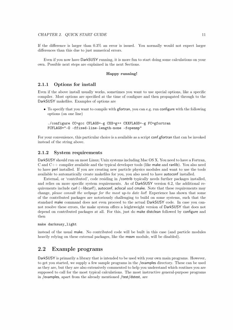
2.1.1 Options for installEven if the above install usually works, sometimes you want to use special options, like a specificcompiler. Most options are specified at the time of configure and then propagated through to theDarkSUSY makefiles. Examples of options are
• To specify that you want to compile with gfortran, you can e.g. run configure with the followingoptions (on one line)
./configure CC=gcc CFLAGS=-g CXX=g++ CXXFLAGS=-g FC=gfortranFCFLAGS="-O -ffixed-line-length-none -fopenmp"
For your convenience, this particular choice is a available as a script conf.gfortran that can be invokedinstead of the string above.
2.1.2 System requirementsDarkSUSY should run on most Linux/Unix systems including Mac OS X. You need to have a Fortran,C and C++ compiler available and the typical developer tools (like make and ranlib). You also needto have perl installed. If you are creating new particle physics modules and want to use the toolsavailable to automatically create makefiles for you, you also need to have autoconf installed.
External, or ‘contributed’, code residing in /contrib typically needs further packages installed,and relies on more specific system requirements. As of DarkSUSY version 6.2, the additional re-quirements include curl (+libcurl!), autoconf, aclocal and cmake. Note that these requirements maychange, please consult the webpage for the most up-to date list! Experience has shown that someof the contributed packages are notoriously challenging to build on some systems, such that thestandard make command does not even proceed to the actual DarkSUSY code. In case you can-not resolve these errors, the make system offers a leightweight version of DarkSUSY that does notdepend on contributed packages at all. For this, just do make distclean followed by configure andthen
make darksusy_light
instead of the usual make. No contributed code will be built in this case (and particle modulesheavily relying on these external packages, like the mssm module, will be disabled).
2.2 Example programsDarkSUSY is primarily a library that is intended to be used with your own main programs. However,to get you started, we supply a few sample programs in the /examples directory. These can be usedas they are, but they are also extensively commented to help you understand which routines you aresupposed to call for the most typical calculations. The most instructive general-purpose programsin /examples, apart from the already mentioned /test/dstest, are

CHAPTER 2. QUICK START GUIDE 12
dsmain_wimp.F An example main program to calculate various DM observables. It can be thestarting point if you want to write your own programs (see below). Note that you can run thesame code with different particle modules that provide a WIMP DM candidate (the defaultis the mssm module); simply do./> make -B dsmain_wimp DS_MODULE=〈MY_MODULE〉and then ./dsmain_wimp in the /examples directory. Choosing 〈MY_MODULE〉=generic_wimp,e.g., will produce results for a generic WIMP DM candidate (see Chapter 31 for details onthe implementation).
dsmain_decay.f A main program that calculates the same observables, where relevant, as ds-main_wimp.F – but for a generic decaying DM candidate (see Chapter 29 for details on theimplementation) rather than a WIMP.
2.2.1 Auxiliary example programsIn the folder examples/aux/ we list a set of instructive auxiliary example programs that illustratemore specific usage of DarkSUSY. These example programs are typically set up for specific particlephysics modules (e.g. generic_wimp) but, as explained below in more detail, it is straightforwardto use them for other particle physics modules as well. Below we describe some of the currentlyavailable auxiliary example programs – but note that the actual list of example programs in exam-ples/aux/ is growing with almost every, even minor, release. We thus strongly advise to check theactual list of these programs, and their headers for a quick summary.
flxconv.f This program can be used to convert between different fluxes from the Sun and the Earth.It can be use to convert a limit on a muon flux to a limit on the scattering cross section, orto a limit on the annihilation rate (or vice versa).
DMhalo_predef.f This program illustrates how to use the default version of dsdmsdriver (providedwith the DarkSUSY release) to load additional profiles into the currently active halo databaseby using its pre-defined halo parameterizations.
DMhalo_table.f This program demonstrates how to load a halo profile from a table in an accom-panying data file.
DMhalo_new.f This program demonstrates how to correctly extend dsdmsdriver when adding anew profile parameterization in order to consistently make it available to all DarkSUSY routinesthat rely on the DM density (in this concrete example, we add the spherical Zhao profile [3],aka αβγ profile).
DMhalo_bypass.f Here, we demonstrate a work-around of completely bypassing the default ds-dmsdriver setup when switching to a user-provided new DM density profile. While easier toimplement than DMhalo_new.f, such an approach has the significant drawback that the ad-vanced DarkSUSY system of automatic tabulation of quantities related to DM rates cannoteasily be exploited.
generic_wimp_oh2.f This program calculates the annihilation cross section needed to producethe correct relic density (as measured by Planck within errors). It does this for a range ofWIMP masses so that you can plot e.g. the required annihilation cross section versus mass.It also let’s you incorporate threshold effects (either as a hard cut, default), or with a moresophisticated sub-threshold treatment, that also illustrates the use of replaceable functions.
ScalarSinglet_RD.f This program calculates the couplings required to get the correct relic densityin the Silveira-Zee (scalar singlet) model.
ucmh_test.f This program is an example of how the ultra-compact mini halo routines can be used.

CHAPTER 2. QUICK START GUIDE 13
wimpyields.f This is a simple program that sets up a generic WIMP with a given mass that an-nihilates to a given channel and then calculates the yields of different particles from thehadronization/decay of the annihilation products.
caprates.f This is a simple program that scans a range of WIMP masses and calculates the capturerates in the Sun via spin-independent and spin-dependent scattering.
caprates_ff.f This program is similar to caprates.f, but a bit more advanced as it performs thecapture rate calculation with the most complete numerical setup and also calculates thecapture rate on individual elements in the Sun.
2.2.2 Making your own example programsThe simplest way to create your own example program is to copy one of the Fortran example filesin examples/aux/ to a directory of your choice, then change the name of that file and modify it.You also need to copy the makefile from examples/aux/ to the same directory, and make sure thatyou update the name of the file that you just changed.† Running ‘make’ then compiles your ownnew example program without touching the release version of the DarkSUSY code. Always keepingyour own code, or your modifications of DarkSUSY, separate like this is the recommended way toproceed because it facilitates debugging and minimizes the risk of introducing errors. Don’t modifyany of the DarkSUSY makefiles directly as they are overwritten every time you run configure.
If you want to compile with a different particle physics module, you will in general need to do gothrough three simple steps:
1. change the corresponding block in the makefile, i.e. simply set the variable DS_MODULE to adifferent value (you may also have to add additional libraries, e.g. lisajet for the mssm module)
2. update the model setup routines to the new particle module (see the various example pro-grams; for more details, have a look at the respective Section of this manual and the headerof setup routines starting with dsgivemodel).
3. make sure that your main program only calls routines that are supported for the new particlemodule. (If it doesn’t, it will not compile, stating the functions that are not supported)
An explicit demonstration of how all these three steps are taken care of in one single example isprovided in dsmain_wimp.F. Note that the pre-compiler directives in that example are only necessaryif you want to be able to compile the same code with two (or more) different particle modules.
2.3 Modifying individual subroutines or functionsIf you want to modify some existing DarkSUSY function or subroutine, don’t do it, instead add yourown routine as a replaceable function (see also Section 3.6), by running the script scr/make_replaceable.plon the routine you wish to have a user-replaceable version of. You will then find that version inthe corresponding user_replaceables folder, where you can edit it to your liking. Following thesesteps, it is guaranteed that the newly created user-replaceable function is properly included in thelibrary where the original DS function used to be, with all makefiles being automagically updated.
An alternative – and often even simpler – way of using user-replaceable functions is to leavethe DS libraries untouched, and to instead link to the user-supplied function only when making themain program (this option is indicated in the left-most part of Fig. 3.1). For an explicit example,see (the makefile for) generic_wimp_oh2.f.
†If you want, you can delete all the blocks for the other (not needed) example programs, in order to have themakefile look clearer and easier to understand.

Chapter 3
Guiding principles of the code
DarkSUSY (as of version 6) has a new structure compared to earlier versions of the code. The moststriking difference is that we have split the particle physics model dependent parts from the rest ofthe code. This means in practice that we have separated DarkSUSY into one set of routines, ds_core,which contains no reference to any specific particle model, as well as distinct sets of routines foreach implemented model of particle physics. For supersymmetry, for example, all routines thatrequire model-dependent information now reside in the mssm module. The advantage with thissetup is that ds_core and the particle physics modules may be put in separate FORTRAN libraries,which implies that DarkSUSY can now have several particle physics modules side by side. The userthen simply decides at the linking stage, i.e. when making the main program, which particle physicsmodule to include.
For this to work, the main library communicates with the particle physics modules via so-calledinterface functions (or subroutines), with pre-defined signatures and functionalities. Note that aparticle physics module does not have to provide all of these predefined functions: which of themare required is ultimately determined only when the user links the main program to the (ds_coreand particle module) libraries. Assume for example that the main program wants to calculate thegamma-ray flux from DM (a functionality provided by ds_core). This is only possible if the particlemodule provides an interface function for the local cosmic ray source function; if it does not, themain program will not compile and a warning is issued that points to the missing interface function.If, on the other hand, interface functions required by direct detection routines would be missing inthis example, this would not create any problems at either runtime or the compile stage.
In addition, we have added the concept of replaceable functions, which allows users to replaceessentially any function in DarkSUSY with a user-supplied version. DarkSUSY ships with dedicatedtools to assist you setting up both replaceable functions and new particle physics modules. Fig. 3.1illustrates these concepts by showing how a typical program would use DarkSUSY; below, we describeeach of them in more detail.
3.1 The main DarkSUSY library ds_coreAs introduced above, the main library is in some sense the heart of the new DarkSUSY , offeringall the functionality that a user typically would be interested in without having explicitly to referto specific characteristics of a given particle physics model (after initialization of such a model).The main library thus contains routines for, e.g., cosmic ray propagation, solar models, capturerates for the Sun/Earth, a Boltzmann solver for the relic density calculation, yield tables fromannihilation/decay etc. None of the routines in the main library contains any information aboutthe particle physics module. Instead any information needed is obtained by calling a requiredfunction that resides in the particle physics module which is linked to (see below).
14

CHAPTER 3. GUIDING PRINCIPLES OF THE CODE 15
Module ...
..
.
Module silveira_zeelibds_silveira_zee.a
Interface functionsInternal routines
Particle physics modulessrc_models/
Module mssmlibds_mssm.a
Interface functionsInternal routines
Linking to main library/user replaceableLinking to chosen module
Alternative calling sequence(if linked)
Calling sequence
Main programUser-supplied, e.g.
examples/dsmain_wimp.F
Userreplaceables
UserreplaceablesFunctions replacedand modifiedby user
UserreplaceablesFunctions replacedand modifiedby user
UserreplaceablesFunctions replacedand modifiedby user
DarkSUSY core librarysrc/libds_core.a
Observables (rates, relic density etc)
UserreplaceablesFunctions replacedand modifiedby user
Halo profilesdsdmsdriver with different halo profiles.
Figure 3.1: Conceptual illustration of how to use DarkSUSY. The main program links to boththe main library, ds_core, and to one of the available particle physics modules. User-replaceablefunctions are optional and may be linked to directly from the main program, or indirectly byincluding them in the various libraries. See examples/dsmain_wimp.F for an example of a mainprogram that demonstrates typical usage of DarkSUSY for different particle physics modules.
The source code for all functions and subroutines in the main library can be found in the src/directory of the DarkSUSY installation folder, with subdirectory names indicating subject areas assummarized in Table 3.1.
3.2 Particle physics modulesThe particle physics modules contain the parts of the code that depend on the respective particlephysics model. Examples are cross section calculations, yield calculations etc. The routines in theparticle physics module have access to all routines in ds_core, whereas the reverse is in generalnot true (with the exception of a very limited set of interface functions that each particle moduleprovides).
DarkSUSY 5 and earlier was primarily used for supersymmetric, and neutralino DM, and thoseparts of the code now reside in the MSSMmodulemssm. However, many people used DarkSUSY evenbefore for e.g. a generic WIMP setup, which was doable for parts of the code, but not all of it. Wenow provide a generic WIMP module generic_wimp that can be used for these kinds of calculationsin a much more general way. In a similar spirit, we also provide a module generic_decayingDM forphenomenological studies of decaying DM scenarios. As an example for an actual particle physicsmodel other than supersymmetry, DarkSUSY furthermore includes a module silveira_zee whichimplements the DM candidate originally proposed by Silveira and Zee [4] and which now is oftenreferred to as Scalar Singlet DM [5, 6, 7]. We also include an empty model, empty, which is ofcourse not doing any real calculations, but contains (empty versions of) all interface functions thatthe core library is aware of – which is very useful for debugging and testing purposes. Designingnew particle modules is a straight-forward exercise, see below, and it is generally a good idea tostart with the most similar module that is already available.

CHAPTER 3. GUIDING PRINCIPLES OF THE CODE 16
Subdirectoryname Descriptionan_yield Annihilation yields in the halo – yields from simulationsaux General routinesaux_xcernlib CERN routines needed by DarkSUSYaux_xdiag Diagonalization routinesaux_xnswclibaux_xquadpack CMLIB routines needed by DarkSUSYcr_aux Cosmic rays – generalcr_axi Cosmic rays – diffusion routines for axisymmetric distributionscr_gamma Cosmic rays – Gamma fluxescr_nu Cosmic rays – Neutrino fluxescr_ps Cosmic rays – point sourcesdd Direct detectiondmd_astro Astrophysical source functionsdmd_aux Auxiliary functions for dark matter distribution routinesdmd_mod Dark matter distributionsdmd_vel Dark matter velocity distributionsfi Freeze-Inini Initialization routineskd Kinetic decouplingrd Relic densityse_aux Auxiliary routines for WIMP annihilation in the Sun/Earthse_mod Sun and Earth modelsse_nu Capture and annihilation in the Sun/Earthse_yield Yields from annihilation in the Sun/Earthsi Self-interactionsucmh Ultra-compact mini-halos
Table 3.1: Organization of the main library ds_core: all functions and subroutines reside in thesrc/ folder of the DarkSUSY installation, with the names of the subdirectories indicating the subjectarea. (Note: this table is automatically generated from the actual directory structure in src/.)
A list of the currently available particle physics modules is given in table 3.2, and the source codefor the particle modules can be found in the src_models/ directory of the DarkSUSY installationfolder, each of the subdirectories (e.g. src_models/mssm/, src_models/generic_wimp/) typicallyreflecting a (sub)subdirectory structure analogous to what is shown in Table 3.1 for the core library.Many dark matter models, furthermore, constitute only relatively simple extensions to the standardmodel, inheriting most of its structure. For convenience, we therefore also provide various auxiliaryroutines, in src_models/common/sm, that each particle module automatically has access to, andwhich return basic standard model quantities like, e.g., the masses of standard model particles andtheir running (so additional BSM effects have to be implemented in the respective particle module).
3.2.1 Using a particle physics moduleHow to use a particle physics module obviously depends on how it is implemented, and in principlethere are no formal requirements on how this should be done – as long as the provided interface

CHAPTER 3. GUIDING PRINCIPLES OF THE CODE 17
Particle physics modulesModule ShortNo. name Description1 common Basic principles and common routines2 empty The empty model3 generic_decayingDM Generic decaying dark matter4 generic_fimp Generic FIMPs5 generic_wimp Generic WIMPs6 mssm The Minimal Supersymmetric Standard Model7 silveira_zee Silveira-Zee (Scalar Singlet)8 vdSIDM Self-Interacting Dark Matter
Table 3.2: List of particle physics modules currently available in src_models. (Note: this table isautomatically generated from the actual content of src_models.)
functions are correctly set up, see Section 3.4 further down. The one subroutine that is required toexist, however, is
dsinit_module
This is called directly from dsinit, and must be the first call to the particle module as it initializesall general settings and relevant common block variables.
While there is no required structure otherwise, there is a typical workflow associated to using aparticle physics module in a main program. First, one needs to initialize a given model by specifyingits model parameters. This is done by routines like
dsgivemodel...
A call to dsgivemodel_decayingDM, e.g., allows to enter the defining parameters for a DM model inthe generic_decayingDM module, while dsgivemodel_25 allows to enter the parameters for pMSSMmodel with 25 parameters in the mssm module. The next step is then typically a call to
dsmodelsetup
in order to transfer the model parameters to common blocks and calculate basic quantities likemasses and couplings. Once a model is set up like this, a main program can use the full functionalityof DarkSUSY supported by the respective module.
3.2.2 Adding a new particle physics moduleTo create a new particle physics module, the easiest way is to start from an existing one as atemplate and create a new one from that one. To help you in this process we provide a scriptscr/make_module.pl that takes two arguments, the module you want to start from and the newone you want to create (for further instructions, just call the script without arguments). It willthen copy the module to a new one, change its name throughout the module and make sure thatit is compiled by the makefiles and included properly when requested by the main programs. Ifyou specify the option -i only interface functions will be copied (which creates a cleaner startingpoint, but also will most likely not compile without modifications). When creating a new modulethis way, the best is to copy from a module that is as similar as possible to your new model. Ifyou want a clean setup, you can always copy from the empty module. If you want somethingmore phenomenological that has a basic framework for calculating observables, starting from thegeneric_wimp or generic_decayingDM might be a good idea. A general advice is to view the moduleswe provide as a starting point as inspiration for your new modules.

CHAPTER 3. GUIDING PRINCIPLES OF THE CODE 18
Even though a particle physics module does not need to include all interface functions (whichones are needed only depends on the observables you try to calculate in your main programs), itneeds to provide an initialization routine dsinit_module.f. This routine should set a global variablemoduletag to the name of the module so that routines that need to check if the correct module isloaded can do so. When using the script scr/make_module.pl this routine is always created andmoduletag set as it should.
Note that the script scr/make_module.pl only provides the framework in the configure script andmakefiles (or rather makefile.in’s) to make sure your module is compiled. It does not create a mainprogram that uses your module, that is up to you. A good starting point for that can either be e.g.dsmain_wimp.F in examples that already contain different blocks for different modules (controlledby pre-compiler directives, see the code for more details). Another option is to use any of theexample programs in examples/aux as a starting point.
To make upgrading to new DarkSUSY versions as smooth as possible, we advice to create yourown folder with your main programs, using e.g. the makefile in examples/aux as a starting point.Don’t modify any of the DarkSUSY makefiles directly as they are overwritten every time you runconfigure, see Section 2.2.2 for more details.
Note that for the scr/make_module.pl script to work you need to have autoconf installed as thescript adds your new module to configure.ac and runs autoconf to create a new configure script.
3.3 Halo modelsSeveral routines in the core library need to know which DM halo should be adopted for the calcula-tions. With this DarkSUSY version, we introduce a new and flexible scheme that avoids pre-definedhardcoded functions to describe the DM density profiles, and allows to consistently define differentDM targets at the same time. For convenience, we still provide several pre-defined options for suchhalo parameterizations, and the user can choose between, e.g., the Einasto [8] and the Navarrow-Frenk-White profile [9], or read in any tabulated axi-symmetric (or spherically symmetric) profile.On a technical level, the halo models are handled by the dsdmsdriver routine which contains adatabase of which halo profiles the user has set up, and consistently passes this information to allparts in the code where it is needed.∗
We provide detailed hands-on examples on how to use this system by a set of example programsDMhalo_*.f, see Section 2.2.1. For further details, we refer to Section 16.1 of this manual.
3.4 Interface functionsInterface functions are functions that routines in ds_core might need to call, and which thereforeevery particle physics module should contain if that particular observable is requested. Examplesof interface functions include dsddsigma that returns the equivalent DM nucleus cross section, dscr-source that returns the source term for DM-induced cosmic rays (relevant for indirect detection),dsanxw that returns the invariant annihilation rate (in the case of WIMPs), etc. All interface func-tions are found by looking in the empty module, and always contain the keyword ‘interface’ in thefunction or subroutine header.
If a particle physics module contains the full set of interface functions, all routines in the mainDarkSUSY code should work. However, this is not needed to set up a paticle physics module. E.g. ageneric WIMP model does not need to have decay rates set up. If a routine in the main DarkSUSY
∗From a technical point of view, it is actually not dsdmsdriver itself which acts as an interface to the rest ofthe code, but the set of wrapper routines collected in src/dmd_astro (which all call dsdmsdriver in a specific way).Only those routines are called by cosmic-ray flux routines and other functions in src, never dsdmsdriver directly. Theroutines in src/dmd_astro therefore provide examples of functions that cannot be replaced individually in a consistentway, but only as a whole set (along with dsdmsdriver, in case the user wants to change the structure of the driveritself).

CHAPTER 3. GUIDING PRINCIPLES OF THE CODE 19
routines is called that rely on this interface being present, an error will be thrown when trying tocompile your code. This of course applies to all interface functions, not just unphysical ones. E.g.if you are only interested in the relic density for a new particle physics module, you do not need toset up scattering rates, cosmic ray source functions, etc.
In Tab. 3.3, we provide the complete list of interface functions currently implemented in Dark-SUSY, along with a brief description. For more details, consult the headers of these files.
Appears inRoutine modules Used by Descriptiondsacbnd 2, 6 Check collider boundsdsanwx_finiteT 2, 4, 7 fi Self-annihilation invariant rate at finite
temperaturedsanwx 2, 4, 5, 6, 7, 8 fi, rd Self-annihilation invariant ratedscrsource_line 2, 3, 5, 6, 7, 8 cr_axi, cr_gamma,
cr_nuSource term for monochromatic contri-butions from dark matter
dscrsource 2, 3, 5, 6, 7, 8 cr_axi, cr_gamma,cr_nu, ucmh
Source term for dark matter inducedcosmic rays
dsddgpgn 2, 5, 6, 7, 8 se_nu Four fermion couplings.dsddsigma 1, 2 dd, se_nu UNpolarized *equivalent* WIMP nu-
cleus cross section including formfactors
dsdmspin 2, 3, 5, 6, 7, 8 se_nu dark matter spindsidnumberset 1dsidnumber 1 dddsinit_module 2, 3, 4, 5, 6, 7, 8 ini Intialzation of moduledskdm2simp 2, 5, 6, 7, 8 kd Scattering amplitude squared, ex-
panded in powers of energydskdm2 2, 5, 6, 7, 8 kd Full scattering amplitude squared, av-
eraged over momentum transferdskdparticles 2, 5, 6, 7, 8 kd, rd Initalization of kinetic decoupling for
moduledsmodelsetup 2, 3, 4, 5, 6, 7, 8 Sets up a new particle physics modeldsmwimp 2, 3, 4, 5, 6, 7, 8 cr_axi, dd, fi, kd,
rd, se_nuDark matter mass
dsrdparticles 2, 4, 5, 6, 7, 8 fi, rd Particles included in relic density calcu-lation (coannihilations, resonances andthresholds)
dsseyield 2, 5, 6, 7, 8 ini, se_nu Yields from annihilation in theSun/Earth
dssigmav0tot 2, 5, 6, 7, 8 cr_axi, se_nu Total annihilation cross section at v = 0
dssisigtm 2, 8 si Self-interaction momentum-transfercross section
Table 3.3: Table of interface functions, which modules that contain them (with numbering fromtable 3.2, where they are used and a short description of them. (Note: this table is automaticallygenerated from scanning through the particle physics modules in src_models. The description istaken from the empty module routine headers.)
CHAPTER 3. GUIDING PRINCIPLES OF THE CODE 20
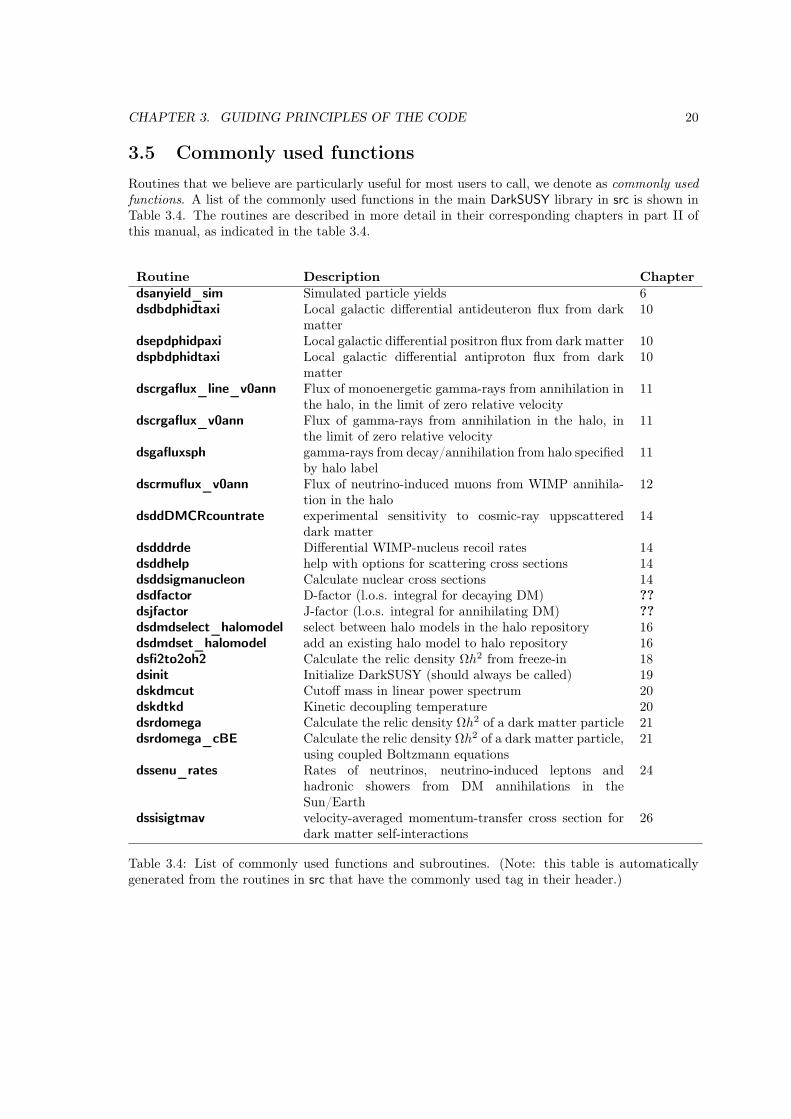
3.5 Commonly used functionsRoutines that we believe are particularly useful for most users to call, we denote as commonly usedfunctions. A list of the commonly used functions in the main DarkSUSY library in src is shown inTable 3.4. The routines are described in more detail in their corresponding chapters in part II ofthis manual, as indicated in the table 3.4.
Routine Description Chapterdsanyield_sim Simulated particle yields 6dsdbdphidtaxi Local galactic differential antideuteron flux from dark
matter10
dsepdphidpaxi Local galactic differential positron flux from dark matter 10dspbdphidtaxi Local galactic differential antiproton flux from dark
matter10
dscrgaflux_line_v0ann Flux of monoenergetic gamma-rays from annihilation inthe halo, in the limit of zero relative velocity
11
dscrgaflux_v0ann Flux of gamma-rays from annihilation in the halo, inthe limit of zero relative velocity
11
dsgafluxsph gamma-rays from decay/annihilation from halo specifiedby halo label
11
dscrmuflux_v0ann Flux of neutrino-induced muons from WIMP annihila-tion in the halo
12
dsddDMCRcountrate experimental sensitivity to cosmic-ray uppscattereddark matter
14
dsdddrde Differential WIMP-nucleus recoil rates 14dsddhelp help with options for scattering cross sections 14dsddsigmanucleon Calculate nuclear cross sections 14dsdfactor D-factor (l.o.s. integral for decaying DM) ??dsjfactor J-factor (l.o.s. integral for annihilating DM) ??dsdmdselect_halomodel select between halo models in the halo repository 16dsdmdset_halomodel add an existing halo model to halo repository 16dsfi2to2oh2 Calculate the relic density Ωh2 from freeze-in 18dsinit Initialize DarkSUSY (should always be called) 19dskdmcut Cutoff mass in linear power spectrum 20dskdtkd Kinetic decoupling temperature 20dsrdomega Calculate the relic density Ωh2 of a dark matter particle 21dsrdomega_cBE Calculate the relic density Ωh2 of a dark matter particle,
using coupled Boltzmann equations21
dssenu_rates Rates of neutrinos, neutrino-induced leptons andhadronic showers from DM annihilations in theSun/Earth
24
dssisigtmav velocity-averaged momentum-transfer cross section fordark matter self-interactions
26
Table 3.4: List of commonly used functions and subroutines. (Note: this table is automaticallygenerated from the routines in src that have the commonly used tag in their header.)
CHAPTER 3. GUIDING PRINCIPLES OF THE CODE 21
3.6 Replaceable functionsThe concept of replaceable functions introduces the possibility to replace a DarkSUSY routine withone of your own. The way it works is that the user-provided function will be linked when you makeyour main program instead of the DarkSUSY default one. If, for example, you want to replace theyields from a typical final state of DM annihilation or decay (like bb) with a new function of your own– e.g. because you are interested in comparing the tabulated Pythia [10] yields with those providedby PPPC [11] – you create your own version of the routine dsanyield_sim and let DarkSUSY use thisone instead. To help you with this setup, we provide tools that can create (or delete) a replaceablefunction from any DarkSUSY function and set up the makefiles to use this user-supplied functioninstead. We also provide a simply way of managing large ‘libraries’ of user-supplied functions, viaa list imported by the makefiles, where the user can determine on the fly which user-replaceablefunctions should be included and which ones should not. Note that both routines in ds_core andin any of the particle physics modules can be replaced in this way, including interface functions.There is also a possibility for the particle physics modules to replace a function in the core library.This is not used often, but is used e.g. for the function dsrdxi.f (which gives a possibility to havedifferent dark matter and background temperatures in the early Universe).
There is also a simple way to bypass this system – indicated in the left-most part of Fig. 3.1– by directly linking to the user-supplied function only when making the main program. For anexplicit example, see (the makefile for) generic_wimp_oh2.f.

Chapter 4
Comparison to previous DarkSUSYversions
For those DarkSUSY users who are familiar with previous version of the code, the main structuraldifference introduced with DarkSUSY 6.0 is a highly modular setup that allows to fully disentanglethe astrophysics-related parts from those that rely on a specific particle physics model (see Chapter3 for a detailed description). There are also many new or significantly improved physics capabilitiesintroduced after version 5 and 4 [1] – including electroweak and strong corrections to DM annihila-tion, improved routines to solve the Boltzmann equation for chemical and kinetic decoupling, and anew framework to handle the propagation of cosmic rays. For a detailed list of those new features,we refer to the publication describing this release of the code [2].
One technical aspect that has changed are the particle codes (k-variables), which are now treatedas (module-)internal codes. They can be used by the particle physics module if the module sowishes, but the interface functions and routines in ds_core instead use PDG codes when referringto particles.
In the course of re-organizing the code, it also became necessary to re-name some of the basicfunctions and subroutines that existed in earlier versions and which users may have become familiarwith. For convenience, we therefore list below, in Table 4.1, the most commonly used functionalitiesin version 4 and 5 that have changed in name or usage with the present version of the code.
routine name up to DarkSUSY 5 new routine name commentsdshmset dsdmdset_halomodel Setting up and refering to DM ha-
los has fundamentally changed. SeeSection 3.3 for an overview andall Chapters with names containingsrc_dmd in Part II of the manual formore details.
dshmj dsjfactor Line-of-sight integrals now take ahalo label as input, and can becomputed for various objects at thesame time.
dssusy [dsmodelsetup] Setting up a model (calculating themass spectrum, relevant 3-particlevertices etc.) now depends on theparticle module implementation.
22

CHAPTER 4. COMPARISON TO PREVIOUS DARKSUSY VERSIONS 23
dsmhtkddsmhmcut
dskdtkddskdmcut
The ’microhalo’ routines are nowmore properly referred to as ’kineticdecoupling’ routines.
dshmrescale_rho — A mismatch between local halo den-sity and DM abundance for a givenDarkSUSY module is no longer hid-den as a rescaling factor in a com-mon block. Instead, such factorstypically enter as explicit parame-ters in direct and indirect detectionroutines.
dshaloyield [dsanyield] total cosmic ray yield from neu-tralino annihilation
dshayield dsanyield_sim simulated cosmic ray yields fromindividual annihilation/decay chan-nels to SM particles. Note thatinternal channel codes are now re-placed with PDG codes of the finalstate particles as input.
dshrgacontdiff dsgafluxsph Gamma-ray flux routines now workseamlessly together with both thenew halo setup and the modular par-ticle physics structure.
dshrgaline dscrgaflux_line_v0anndscrgaflux_dec
Gamma-ray line routines now returnboth number, energies and widths ofall such signals that are present inthe current particle setup.
dshrpbardiffdshrdbardiffdsepdiff
dspbdphidtaxidsdbdphidtaxidsepdphidpaxi
Cosmic-ray propagation routineshave been re-written from scratch.They are now much more flexibleand can be used for any axisymmet-ric halo/diffusion model.
dsntrates dssenu_rates Neutrino rates from inside the sunor earth
dshrmuhalo dscrmuflux_v0anndscrmuflux_v0ann
Neutrino-induced muon flux fromthe halo (for annihilating and decay-ing DM, respectively).
Table 4.1: ‘Translation table’ for how the most commonly used functionalities in DarkSUSY version5 and earlier have changed with the present version of the code. Routines in parentheses, e.g.[dsanyield], are no longer part of the DarkSUSY main library and only provided by specific particlephysics modules. For more detailed descriptions of the new routines and functions, see the headersof the respective files.

Chapter 5
Original articles
A large part of the routines in the present DarkSUSY version have been implemented in the contextof original research work. Therefore, when using those routines, please give proper credit not onlyto the main DarkSUSY paper [1, 2] but also to the relevant articles in the following list:
Relic density – freeze-out P. Gondolo and G. Gelmini, Nucl. Phys. B360 (1991) 145 [12];J. Edsjö and P. Gondolo, Phys. Rev. D56 (1997) 1879 [13]; J. Edsjö, M. Schelke, P. Ullioand P. Gondolo, JCAP 04 (2003) 001 [14]. For coupled Boltzmann equations: T. Binder,T. Bringmann, M. Gustafsson and A. Hryczuk, Eur. Phys. J. C 81 (2021) 577 [15].
Relic density – freeze-in T. Bringmann, S. Heeba, F. Kahlhoefer and K. Vangsnes, arXiv: 2111.14871(2021) [16].
Kinetic decoupling and microhalos T. Bringmann, NJP 11 (2009) 10527 [17].
Continuous gamma-rays L. Bergström, J. Edsjö and P. Ullio, Phys. Rev. D58 (1998) 083507[18].
Neutrino telescopes L. Bergström, J. Edsjö and P. Gondolo, Phys. Rev.D58 (1998) 103519 [19].
Positrons E.A. Baltz and J. Edsjö, Phys. Rev. D59 (1999) 023511 [20].
Antiprotons L. Bergström, J. Edsjö and P. Ullio, ApJ 526 (1999) 215 [21].
QCD corrections to DM annihilation T. Bringmann, A. J. Galea, P. Walia, Phys.Rev. D93(2016) 043529 [22].
Cosmic-ray upscattered dark matter T. Bringmann and M. Pospelov, Phys. Rev. Lett. 122(2019) 17, 171801 [23]; K. Bondarenko et al., JHEP 03 (2020) 118 [24].
General MSSM, direct detection L. Bergström and P. Gondolo, Astrop. Phys. 5 (1996) 263[25].
Gamma lines from supersymmetric DM L. Bergström and P. Ullio, Nucl. Phys. B504(1997) 27 [26]; P. Ullio and L. Bergström, Phys. Rev. D57 (1998) 1962 [27].
Internal bremsstrahlung in the MSSM (γ and e+) T. Bringmann, L. Bergström and J. Ed-sjö, JHEP 0801 (2008) 049 [28]; L. Bergström, T. Bringmann and J. Edsjö, Phys.Rev. D78(2008) 103520 [29].
MSSM Electroweak corrections to indirect detection yields T. Bringmann and F. Calore,Phys.Rev.Lett. 112 (2014) 071301 [30]; T. Bringmann, F. Calore, A. J. Galea and M. Garny,JHEP 1709 (2016) 041 [31].
24

Part II
Main DarkSUSY routines in src/
25

Chapter 6
an_yield:Annihilation yields in the halo –yields from simulations
6.1 Annihilation in the halo, yields – theoryHere we calculate yields of different particles from annihilation of dark matter particles in the halo.
6.1.1 Monte Carlo simulationsWe need to evaluate the yield of different particles per WIMP annihilation. The hadronizationand/or decay of the annihilation products are simulated with Pythia [10] 6.426. The simulationsare done for a set of 18 WIMP masses, mχ = 10, 25, 50, 80.3, 91.2, 100, 150, 176, 200, 250, 350,500, 750, 1000, 1500, 2000, 3000 and 5000 GeV. We tabulate the yields and then interpolate thesetables in DarkSUSY.
The simulations are here simpler than those for annihilation in the Sun/Earth since we don’thave a surrounding medium that can stop the annihilation products. We here simulate for 8‘fundamental’ annihilation channels cc, bb, tt, τ+τ−, W+W−, Z0Z0, gg and µ+µ−. Comparedto the simulations in the Earth and the Sun, we now let pions and kaons decay and we alsolet antineutrons decay to antiprotons. For each mass we simulate 2.5 × 10⁶ annihilations andtabulate the yield of antiprotons, positrons, gamma rays (not the gamma lines), muon neutrinosand neutrino-to-muon conversion rates and the neutrino-induced muon yield, where in the last twocases the neutrino-nucleon interactions has been simulated with Pythia as outlined in section 25.1.1
With these simulations, we can calculate the yield for any of these particles for a given particlephysics model. In src, we only include the channels that are actually simulated. In the differentparticle physics modules in src_model, the summation over all possible final states and possiblymore complex channels, like scalars decaying to other particles is done.
Note that simulations are typically done without specifying a particular polarization state ofthe final state particles. This is however not entirely correct as the possible polarization states willdepend on the particle physics model we have.
Even if the simulations are not performed in this more general way yet, we have set up thestructure here to eventually provide the yields in this form. In particular the most general routineto calculate the yields from any of the simulated channels is dsanyield_sim_ls. Apart from themass, energy and yield type, this routine also takes are arguments the PDG codes of the final stateparticles and the polarization state of the final state. In particular, you are required to provide the
26

CHAPTER 6. AN_YIELD: ANNIHILATION YIELDS IN THE HALO – YIELDS FROM SIMULATIONS27
quantum numbers
j = the quantum number for the total angular momentumP = the parity of the final statel = the quantum number for the orbital angular momentum in the final states = the quantum number for the total spin in the final state
We want to move in a direction where this routine is the one that should be used. While gettingthere, we also provide a simpler routine which just gives the polarization state in terms of helcityand polarization, dsanyield_sim. This routine takes the PDG code of the final state and thepolarization as
• Left-handed or right-handed polarization for fermions.
• Longitudinal or transverse polarization for vector bosons.
This routine for simplicity assumes that the final state particles have the same polarization state.

Chapter 7
aux:General routines
7.1 General routinesIn aux/, we collect routines that are of general interest to many other routines in DarkSUSY. E.g.,we have routines to find elements in arrays (used for interpolation), Bessel functions, error functions,spline routines, etc.
28

Chapter 8
aux_xdiag:Diagonalization routines
8.1 XDIAGThis folder contains a set of routines to perform numerical diagonalization of complex matrices.Even though analytical routines can be used for up to 5 × 5 matrics, they tend to be numericallyunstable for matrices occuring in some particle physics models (for example supersymmetry). Hence,we use numerical routines to perform the diagonalization instead.
29
Chapter 9
cr_aux:Cosmic rays – general
9.1 Cosmic Rays – auxiliary routinesThis folder contains auxiliary functions needed by the cosmic ray routines. In particular, it containsdifferent versions of simple integration routines and a set of routines to handle the correct settingand interpreting of labels for the tabulation of confinement times and Green’s functions needed forthe calculation of cosmic ray fluxes.
30

Chapter 10
cr_axi:Cosmic rays – diffusion routines foraxisymmetric distributions
10.1 Cosmic ray propagation in axially symmetric halosThere is a clean asymmetry between particles and antiparticles in the standard cosmic ray picture:The bulk of cosmic rays – protons, nuclei and electrons – are mainly “primary" species, i.e. par-ticles accelerated in astrophysical sources and then copiously injected in the interstellar medium;“secondary" components, including antimatter, are instead produced in the interaction of primarieswith the interstellar medium during the propagation. It follows that there is a pronounced deficitof antimatter compared to matter in the locally measured cosmic ray flux (about 1 antiproton in104 protons). When considering instead a source term due to DM annihilations or decays, a sig-nificant particle-antiparticle asymmetry is in general not expected, and antiprotons, positrons andantideuterons turn out to be competitive indirect DM probes.
Charged particles propagate diffusively through the regular and turbulent components of Galac-tic magnetic fields. This makes it more involved for local measurements to track spectral andmorphological imprints of DM sources than, e.g., for the gamma-ray and neutrino channels (thoughsearches for spectral features in CR positron fluxes still lead to very competitive limits [?]). Infact the transport of cosmic rays in the Galaxy is still a debated subject: Most often one refersto the quasi-linear theory picture (with magnetic inhomogeneities as a perturbation compared toregular field lines) in which propagation can be described in terms of a (set of) equation(s) linearin the density of a given species, containing terms describing diffusion in real space, diffusion inmomentum space (the so-called reacceleration), convective effects due to Galactic winds, energy orfragmentation losses and primary and secondary sources (see, e.g., Ref. [?] for a review). Dedicatedcodes have been developed to solve numerically this transport equation, including GALPROP [?],DRAGON [?] and PICARD [?].
Here we follow instead a semi-analytical approach, analogous to that developed for the USINEcode [?]. In particular, we model the propagation of antiprotons and antideuterons by consideringthe steady state equation [21]
∂N
∂t= 0 = ∇ · (D∇N)−∇ · (~uN)− N
τN+Q . (10.1)
We solve it for situations where i) the diffusion coefficient D can have an arbitrary dependenceon the particle rigidity but can at most take two different values in the Galactic disc and in thediffusive halo, ii) the convective velocity ~u has a given fixed modulus and is oriented outwards
31

CHAPTER 10. CR_AXI: COSMIC RAYS – DIFFUSION ROUTINES FOR AXISYMMETRIC DISTRIBUTIONS32
and perpendicular to the disc, iii) the loss term due to inelastic collisions has an interaction timeτN which is energy dependent but spatially constant in the disc and going to infinity in the halo(corresponding to a constant target gas density in the disc and no gas in the halo), iv) the DMsource Q is spatially axisymmetric and has a generic energy dendence. Under these approximationsand assuming, as is usually done, that the propagation volume is a cylinder centred at the disc andthat particles can freely escape at the boundaries of the diffusion region, Eq. (10.1) can be solvedanalytically by expanding N in a Fourier-Bessel series; the computation of the flux involves, ateach energy, a sum over the series of zeros of a Bessel function of first kind and order zero, and avolume integral of the spatially dependent part in the axisymmetric source term Q (basically theDM density ρχ for decaying DM and its square for pair annihilating DM) times a weight functiondepending on the given zero in the series (see [21] for further details).
Since the path lengths for antiprotons and antideuterons are rather large, of the order of afew kpc, taking average values for parameters in the transport equation rather than the morerealistic modelling that can be implemented in full numerical solutions, has no large impact in caseof extended and rather smooth sources such as for DM. Eq. (10.1) neglects reacceleration effects,which may in general be relevant at low energies (rigidities below a few GV); however even thisdoes not have a large impact in case of the species at hand, see, e.g., [?] for a comparison of resultswith numerical and semi-analytical solutions for cosmic-ray antiprotons. The power of our semi-analytic approach is that one can store values of the solution of the transport equation obtainedby assuming a given mono-energetic source – provided by the functions dspbtdaxi and dsdbtdaxifor, respectively, antiprotons and antideuterons – and then apply these as weights to any particlesource term Sn(Ef ) as introduced above. For antiprotons and antideuterons, this latter step isdone in the functions that compute the local galactic differential fluxes from DM annihilation anddecay, dspbdphidtaxi and dsdbdphidtaxi, respectively. Note that while the outputs of dspbtdaxi anddsdbtdaxi are labelled “confinement time" in the code, since they do have a dimension of time andscale the dependence between source and flux, one cannot trade them for what is usually intendedas confinement time for standard cosmic ray components, given that the morphology of the DMsource is totally different from supernova remnant distributions usually implemented for describingordinary primary components.
The structure we implemented gives a particularly clear advantage when the code is used to scanover many particle physics DM models, but only over a limited number of propagation parametersand DM density profiles. For such an application, it is useful to tabulate the ’confinement times’(returned by dspbtdaxi and dsdbtdaxi) over a predefined range of energy; this is done in the functionsdspbtdaxitab and dsdbtdaxitab when calling the flux routines with an appropriate option (and only incase the DM halo profile currently active is within the halo profile database). Such tabulations canbe saved and re-loaded for later use; here the proper table association is ensured by a propagationparameter label setting system in analogy to the one implemented for the halo profile database.Computing such a table on the first call is rather CPU consuming, especially for DM profiles thatare singular towards the Galactic center, so in case only a few flux computations are needed itmay be better to switch off the tabulation option; this is true also in case the flux is needed at asmall number of energy values, since the latest 100 (non-equivalent) calls to dspbtdaxi and dsdbtdaxiare stored in memory (with the corresponding propagation parameters and halo model correctlyassociated).
The case for positrons is treated analogously, except that energy losses and spatial diffusion arethe most important effects for propagating cosmic ray leptons. The transport equation we solvesemi-analytically therefore has the form [20]
∂N
∂t= 0 = ∇ · (D∇N) +
∂
∂p
(dp
dtN
)+Q , (10.2)
where the functional form of D and Q can be chosen as for antiprotons and antideuterons, and theenergy loss rate dp/dt can have a generic momentum dependence but needs again to be spatiallyconstant. Assuming the same topology for the propagation volume and free escape conditions at

CHAPTER 10. CR_AXI: COSMIC RAYS – DIFFUSION ROUTINES FOR AXISYMMETRIC DISTRIBUTIONS33
the vertical boundaries (to compute the local positron flux the radial boundary turns out to beirrelevant) , the solution of the propagation equation is given in terms of a Green’s function inenergy (the function dsepgreenaxi in the code) to be convoluted over the source energy spectrum atemission for a given particle DM candidate. This last step is performed by the function dsepdndpaxireturning the local positron number density, while dsepdphidpaxi converts it to a flux and is thefunction which should be called from the main file. The method to implement this solution is a slightgeneralization of the one described [20] and generalizes the one introduced in [?] for a sphericallysymmetric configuration to an axisymmetric system.
The computation of the Green’s function involves a volume integral over the spatially dependentpart of the DM source function Q (again basically the DM density ρχ for decaying DM and its squarefor pair annihilating DM) and the implementation via the so-called method of image charges (againa sum over a series) of the free escape boundary condition. It can again be CPU expensive forsingular halo profiles, but its tabulation is always needed since the Green function appears in aconvolution. The main limiting factor with respect to full numerical solutions is that one is forcedto assume an (spatially) average value for dp/dt. However this has not a severe impact on ourresults for the local DM-induced positron flux since, especially for energies above 10 GeV, the bulkof the DM contribution to the local flux stems from a rather close-by emission volume; one thusjust has to make sure to normalize dp/dt to the mean value for local energy losses, as opposed to themean value in the Galaxy, which are mainly due to the synchrotron and inverse Compton processes.
While the transport equations (10.1) and (10.2) are essentially the same as considered in previousreleases of the code, their implementation in the present release is completely new and appears tobe numerically more stable. In particular cases with very singular DM profiles still give numericallyaccurate results and converge faster (in case of antiprotons and antideuterons implementing aprocedure which applies to point sources). Note however that the case of very singular DM profilesis also the one in which our models or any propagation model is subject to a significant uncertaintyrelated to the underlying physics, since propagation in the Galactic center region is difficult to modeland probably rather different from what can be tested in the local neighbourhood by measurementsof primary and secondary cosmic rays. Finally, the implementation starting from DarkSUSY 6 ismore flexible regarding parameter choices, such as for the rigidity scaling of the diffusion coefficientand energy scaling of energy losses, in a framework which is now fully consistent for antiprotons,antideuterons and positrons.
Chapter 11
cr_gamma:Cosmic rays – Gamma fluxes
11.1 Gamma rays from the halo – theoryAmong the yields of decay or pair annihilations of halo dark matter particles, the role played bygamma-rays could be a major one. Unlike the cases involving charged particles, for gamma-rays itis straightforward to relate the distribution of sources and the expected flux at the earth. Most fluxestimated can be obtained just by summing over the contributions along lines of sight (or better,geodesics): gamma-rays have a low enough cross section on gas and dust and therefore the Galaxyis essentially transparent to them (except perhaps in the innermost part, very close to the regionwhere a massive black hole is inferred); absorption by starlight and infrared background becomeseffecient only for very far away sources (redshift larger than about 1).
It follows that in case the gamma-ray signal is detectable, this might be the only chance for map-ping the fine structure of a dark halo, with a much better resolution for inhomogeneities (clumps)with respect to what is achievable through dynamical measurements or lensing effects. This is espe-cially true for annihilating dark matter. Turning the latter argument around, if the fine structure ofthe Galactic halo is clumpy, or if a large density enhancement is present towards the Galactic center,as seen in N-body simulations of dark matter halos, this dark matter detection technique may bemore promising than indicated by the estimates in which smooth non-singular halo scenarios areconsidered (recall that the fluxes per unit volume are proportional to the square of the dark matterdensity locally in space).
Several targets have been discussed as sources of gamma-rays from the annihilation of darkmatter particles. An obvious source is the dark halo of our own galaxy [32, 33, 34, 35] and inparticular the Galactic center, as the dark matter density profile is expected, in most models, tobe picked towards it, possibly with huge enhancements close to te central black hole. The Galacticcenter is an ideal target for both ground- and space-based gamma-ray telescopes. As satelliteexperiments have much wider field of views and will provide a full sky coverage, they can in principletest the hypothesis of gamma-rays emitted in clumps of dark matter which may be present in thehalo [36, 37, 38, 18, 39, 40]. Another possibility which has been considered is the case of gamma-ray fluxes from external nearby galaxies [41]. Furthermore, it has been proposed to search for anextragalactic flux originated by all cosmological annihilations of dark matter particles [42, 43, 44].DarkSUSY is suitable to compute the gamma-ray flux from all these (and possibly other) sources.
34
CHAPTER 11. CR_GAMMA: COSMIC RAYS – GAMMA FLUXES 35
11.2 Continuous gamma yields and line signalsThe bulk of the gamma-ray yield from DM annihilation or decay arises from quark jets that whenthey hadronize/decay give rise to neutral pions which decay to gamma rays. At loop level, it couldalso be possible to produce monochromatic gamma rays, which could be a smoking gun for darkmatter searches. The advantage with the gamma-ray lines is the distinctive spectral signature,which has no plausible astrophysical counterpart.
Compared to the monochromatic flux, the gamma-ray flux produced in π0 decays is much largerbut has less distinctive features. The photon spectrum in the process of a pion decaying into 2γis, independent of the pion energy, peaked at half of the π0 mass, about 70 MeV, and symmetricwith respect to this peak if plotted in logarithmic variables. Of course, this is true both for pionsproduced by DM and, e.g., for those generated by cosmic ray protons interacting with the interstellarmedium.
When considered together with to the cosmic-ray induced Galactic gamma-ray background, theDM induced signal looks like a component analogous to the secondary flux due to nucleon nucleoninteractions: it is drowned into the Bremsstrahlung component at low energy, while it may be thedominant contribution at energies above 1 GeV or so. In fact, if the exotic component is indeedsignificant an option to disentangle it would be to search for a break in the energy spectrum atabout the WIMP mass, where the line feature might be present as well: while the maximal energyfor a photon emitted in WIMP pair annihilations is equal to the WIMP mass, the component fromcosmic ray protons extends to much higher energies, essentially with the same spectral index as forthe proton spectrum (the role played by the third main background component, inverse Comptonemission, has still to settled at the time being and may worsen the problem of discrimination againstbackground).
Besides this (weak) spectral feature, another way to disentangle the dark matter signal may beto exploit a directional signature: data with a wide angular coverage should be analyzed to searchfor a gamma-ray flux component following the shape and density profile of the dark halo, includingeventual contributions from clumps.
11.3 FluxesGiven a density distribution of DM particles, we can define a source function that tells us howmany particles that are produced per volume element per time unit (and per energy interval fordifferential yields) from either annihilation or decay. The DM signal ultimately only depends onthe local injection rate of some stable (cosmic ray) particle f , per volume and energy,
dQ(Ef ,x)
dEf=∑n
ρnχ(x) 〈Sn(Ef )〉 . (11.1)
Here, ρχ is the DM density (of the respective component, in case of multi-component DM) andthe ensemble average 〈...〉 is taken over the DM velocities; in principle, it depends on the spatiallocation x, but in many applications of interest this can be neglected.
The particle source terms Sn(Ef ) encode the full information about the DM particle physicsmodel. For a typical WIMP DM candidate, e.g., only the annihilation part (n = 2) contributes,
S2(Ef ) =1
Nχm2χ
∑i
σivdNidEf
, (11.2)
where σi is the annihilation cross section of two DM particles into final state i and dNi/dEf isthe resulting number of stable particles of type f per such annihilation and unit energy. Nχ is asymmetry factor that depends on the nature of DM; if DM is (not) its own antiparticle we haveNχ = 2 (Nχ = 4). The right-hand side of the above expression must be further integrated over f(v),

CHAPTER 11. CR_GAMMA: COSMIC RAYS – GAMMA FLUXES 36
the velocity distribution of the relative velocity of the two dark matter particles, but in practice itis typically sufficient to evaluate it for v = 0.
For decaying DM, on the other hand, we have
S1(Ef ) =1
mχ
∑i
ΓidNidEf
, (11.3)
where Γi denotes the partial decay widths. Let us stress, however, that Eq. (11.1) is much moregeneral in that it encapsulates also DM that is both annihilating and decaying, multi-componentSM, as well as DM models with an internal Zn symmetry [45, 46, 47, 48].
For a telescope pointing in the direction ψ, the expected DM-induced differential flux in gammarays or neutrinos – i.e. the expected number of particles per unit area, time and energy – from asky-region ∆ψ is thus given by a line-of-sight integral
dΦ
dE=
1
4π
∫∆ψ
dΩ
∫l.o.s.
d`dQdE
. (11.4)
For an effectively point-like source at distance d, this line-of-sight integral simplifies to∫∆ψ
dΩ
∫l.o.s.
d`dQdE−→ 1
d2
∫dV
dQdE
, (11.5)
where the integral is over the extention of the source (much smaller than d).For decaying DM, the above line-of-sight integral always factorizes into the particle source term
S1 given in Eq. (11.3) and a term that only depends on the DM distribution,
dΦdec
dEdΩ=
1
4πJdecS1 , Jdec ≡
∫l.o.s.
d` ρ (11.6)
For annihilating DM, the corresponding factorization strictly speaking only holds if the annihilationrate is independent of velocity:
dΦann
dEdΩ=
1
4πJannS2 , Jann ≡
∫l.o.s.
d` ρ2 . (11.7)
While notable exceptions exist (in particular for resonances [49], p-wave annihilation [?] and Sommerfeld-enhanced annihilation [?]), this is a commonly encountered situation and hence of general interest.
11.4 Gamma rays from the halo – routinesDarkSUSY provides the functions dscrgaflux_dec and dscrgaflux_v0ann that take Jdec (or Jann) asinput and return the fluxes given in Eqs. (11.7) and (11.6). Here, the subscript _v0ann refers to thefact that, for the purpose of those routines, S2 is evaluated in the limit of vanishing relative velocityof the annihilating DM pair. While this is the only situation of practical interest in many DMmodels, future DarkSUSY versions will offer support for a full velocity dependence of this quantity.In analogy with dscrsource_line, the core library furthermore provides routines dscrgaflux_line_decand dscrgaflux_line_v0ann (and correspondingly for neutrinos) that return strength, width andlocation of monochromatic (‘line’) signals. The latter is a convenient change with respect to previousversions of the code, as one cannot generally know how many lines there are (this depends on theparticle physics module).
If a halo label is available, one can also more conveniently call dsgafluxsph instead. This functiondirectly returns the gamma-ray flux, for that halo, automatically calculating the required line-of-sight integrals and adding decaying and annihilating DM components depending on which particlemodel is initialized.

Chapter 12
cr_nu:Cosmic rays – Neutrino fluxes
12.1 Neutrino fluxes from the halo – theoryUsually, the flux of neutrinos from annihilation of WIMPs in the Milky Way halo is too small tobe detectable, but for some clumpy or cuspy models, it might be detectable. The calculation ofthe neutrino-flux follows closely the calculation of the continuous gamma ray flux, with the mainaddition that neutrino interactions close to the detector are also included. Hence, both the neutrinoflux and the neutrino-induced muon flux can be obtained. The neutrino to muon conversion ratein the Earth can also be obtained.
37

Chapter 13
cr_ps:Cosmic rays – point sources
13.1 Cosmic Ray propagation for point sourcesIn this directory, we collect the relevant cosmic ray routines for DM point sources like ordinary DMclumps or mini-spikes around intermediate-mass black holes.
38

Chapter 14
dd:Direct detection
14.1 Direct detection – theorySpecific choices of nuclear structure functions can be selected by calling dsdd_set(’sf’, label), wherethe character variable label indicates the set of structure functions. For the default option (’best’),e.g., the code automatically picks the best currently available structure function (depending on thenucleus). This mean, in order Fourier-Bessel, Sum-of-Gaussians, Fermi, Lewin-Smith. The functionreturning the value of σχT is to be provided by an interface function dsddsigma(v,Er,A,Z,sigij, ierr)residing in the particle physics module, where on input v=v, Er=ER, A=A, Z=Z and on outputthe 27×27 array sigij contains the (partial) equivalent cross sections σij in cm2 and the integerierr contains a possible error code. The order of the entries in sigij corresponds to that of theindependent nonrelativistic operators Oi; for the first 11 entries, we use the same operators andconvention as in Ref. [50], while for the last 16 entries we add the additional operators discussedin Ref. [51]. In particular, sigij(1,1) is the usual spin-independent cross section and sigij(4,4) isthe usual spin-dependent cross section. In addition, the direct detection module in DarkSUSYprovides utility functions that can be used in the computation of the cross section. For example,the subroutine dsddgg2sigma(v, er,A,Z,gg,sigij,ierr) computes the (partial) equivalent scattering crosssections σij for nucleus (A,Z) at relative velocity v and recoil energy ER starting from values ofthe GNi constants in gg, with nuclear structure functions set by the previous call to dsdd_set. Theactual nuclear recoil event rate as given in
dR
dER=∑T
cTρ0χ
mTmχ
∫v>vmin
dσχTdER
f(v, t)
vd3v , (14.1)
finally, is computed by the function dsdddrde. The latter two functions are independent of thespecific particle physics implementation and hence are contained in the core library. In the aboveexpression, the sum runs over nuclear species in the detector, cT being the detector mass fractionin nuclear species i. mT is the nuclear (target) mass, and µχT = mχmT /(mχ +mT ) is the reducedDM–nucleus mass. Furthermore, ρ0
χ is the local DM density, v the DM velocity relative to thedetector, v = |v|, and f(v, t) is the (3D) DM velocity distribution. In order to impart a recoilenergy ER to the nucleus, the DM particle needs a minimal speed of vmin =
√MTER/2µ2
χT .
39

Chapter 15
dmd_astro:Astrophysical source functions
In the folder src/dmd_astro we provide a set of wrapper routines that all call the halo driver functiondsdmsdriver in a specific way. The rest of the code communicates with dsdmsdriver, and hence thehalo model(s), only via these functions and never by calling dsdmsdriver directly. The routines insrc/dmd_astro therefore provide examples of functions that cannot be replaced individually in aconsistent way, but only as a whole set (along with dsdmsdriver, in case the user wants to changethe structure of the driver itself).
40

Chapter 16
dmd_mod:Dark matter distributions
16.1 Dark matter distributions – theoryAll the dark matter detection rates depend in one way or another on the properties of the Milky Waydark matter halo. We will here outline the halo model that by default is included with DarkSUSY.
Observationally, the distribution of DM on scales relevant for DM searches is only poorly con-strained. The situation is somewhat improved when instead referring to the results of large N -bodysimulations of gravitational clustering, which consistently find that DM halos on average are welldescribed by Einasto [8] or Navarro-Frenk-White profiles [9], with the halo mass being essentiallythe only free parameter (after taking into account that the halo concentration strongly correlateswith the halo mass [52]). On the other hand, there is a considerable halo-to-halo scatter associatedto these findings, so that it remains challenging to make concrete predictions for individual objects– in particular if they are located in cosmologically somewhat ‘special’ environments like in thecase of the Milky Way and its embedding in the Local Group. Even worse, baryonic physics canhave a large impact on the DM profiles, especially on their inner parts most relevant for indirectdetection, and even though hydrodynamic simulations taking into account such effect have madetremendous progress in recent years [53, 54, 55, 56], there is still a significant uncertainty related tothe modelling of the underlying processes. In light of this situation, there is a considerable degreeof freedom concerning halo models and the DM density profiles, and a code computing observablesrelated to DM should be able to fully explore this freedom.
16.1.1 Rescaling of the WIMP densityWhile it is natural to assume that the DM particles described by a given particle module imple-mented in DarkSUSY make up most of the DM in our galaxy, they may also just constitute asub-dominant part of a multi-component realization of DM. What is more, there might be both athermal contribution to the cosmological DM abundance – as computed by the relic density rou-tines in DarkSUSY– and a non-thermal contribution, e.g. via out-of-equilibrium production or viathe decay of heavier particles. In this context, it is important to remember that DM detectionrates only depend on the local DM density of that particular DM candidate. For the case of directdetection, e.g., the rate scales linearly with the local density at earth, while for indirect detection itscales linearly or quadratically with the local DM density at the point of of decay or or annihilation,respectively.
In previous versions of the code, the ratio of thermal relic abundance returned by dsrdomegaand observed cosmological DM abundance was used to internally rescale the results from rate
41

CHAPTER 16. DMD_MOD: DARK MATTER DISTRIBUTIONS 42
calculations. For the reasons given above, this is not fully satisfactory and in any case obscuresthe origin of this rescaling. Starting from DarkSUSY 6, this is therefore no longer the case. Allrate routines now assume that the local DM density equals the local density in the particular DMcandidate realized in the particle module – unless they explicitly take the local DM density asan input parameter (which in that case refers to the local density in the particles described bythe respective DarkSUSY module). An example for such an exception are the neutrino telescoperoutines, because the combined effect of DM capture and annihilation makes the dependence onthe local DM density more complicated. In all other cases, e.g. if DM rate routines just take a halolabel as input, the user has to make sure to rescale the rates, as described above, by hand to reflectpossible sub-dominant DM populations.
16.2 Implementation in DarkSUSYThe implementation of dark matter halo models and related quantities in the library ds_core followsa new and highly flexible scheme, compared to earlier versions of the code, avoiding pre-definedhardcoded functions. For convenience a few pre-defined options are provided, however these can beeither complemented by other profiles eventually needed, or the entire sample configuration can besimply replaced linking to a user-defined setup - in both cases without editing routines provided inthis release of the code. A further improvement compared to previous versions of DarkSUSY is thatdifferent dark matter density profiles, possibly referring to different dark matter detection targets,can be defined at the same time: E.g., one can easily switch back and forth from a computationof the local positron flux induced by dark matter annihilations or decays in the Milky Way halo tothe computation of the gamma-ray flux from an external halo or a Milky Way satellite within thesame particle physics scenario. Finally the present implementation simplifies the task of keepingtrack of consistent definitions for related quantities, such as, e.g., a proper connection between thedark matter profile and the source function for a given dark matter yield (see Chapter 6), or callingwithin an axisymmetric coordinate system a spherically symmetric function (and preventing theopposite).
At the basis of the implementation, there is the subroutine dsdmsdriver routine which acts asan interface to quantities related to the dark matter density profiles. This routine must contain acomplete set of instructions on how to retrieve the different observables: E.g. it checks the scaling ofthe various DM source functions (Chapter 6 with the DM density ρχ – namely ρ for decaying darkmatter and ρ2 for dark matter pair annihilations (in case the effect of substructures is neglected) –and passes this information to the routines for propagations of charged cosmic rays in the Galaxy(Chapter 10), assuming that such source function is axisymmetric; line of sight integration routines(needed, e.g. for the computation of gamma-ray fluxes, see Chapter 11) call this same subroutine,but may assume instead that the corresponding source function is spherically symmetric. Theroutine dsdmsdriver must contain the specification on whether the dark matter density profile isspherically symmetric or axisymmetric, and in the first case provide a consistent numerical outputto both calls, in the latter return an error to the second call (since a spherically symmetric profile wasexpected). It may also be useful to use the dsdmsdriver routine for initialization calls, for instance toset parameters for a given parametric density profile, and test calls, for instance to print which darkmatter profile is currently active within a set of available profiles. The input/output structure of theroutine is rather general, with the first entry being however fixed to an integer flag specifying theaction of the routine; currently available values and relative action are implicitly defined (throughinteger variables such as ‘idmddensph’ referring to the spherical dark matter density profile) in aninclude file and are global parameter. Such set of definitions should not be changed, but can beenlarged in case further profile-related quantities would be needed.
While a specific dsdmsdriver routine should match the user needs in the problem at hand, thepresent release provides a sample version, illustrating the flexibility of the setup. In particular theversion included in the library ds_core assumes that the dark matter density profile is spherically

CHAPTER 16. DMD_MOD: DARK MATTER DISTRIBUTIONS 43
symmetric and does not include dark matter substructure; it allows to choose as dark matter profileone among three parametric profiles, namely the Einasto [8], the Navarro-Frenk-White [9] and theBurkert [?] profiles, or a profile interpolated from a table of values of the dark matter density ata given radius. Besides providing parameters as needed in case of parametric profiles, to completethe initialization of a profile one should also specify: i) an inner truncation radius, namely someric fixing ρ(r) = ρ(ric) for any r < ric (the choice has an impact on predictions for dark matterrates only for very singular dark matter profiles; choosing a value which is not too small allows fora faster numerical convergence of some rate computations); ii) an outer truncation radius, namelysome roc beyond which the profile is assumed to be zero; iii) the distance from the observer of thecenter of the profile, corresponding to the Sun galactocentric distance only in case the profile refersto the Milky Way; iv) whether it is a profile that refers to the Milky Way and hence for which ratesthat are Milky Way specific, such as the local contribution to antimatter fluxes, can be computed;v) whether it is a profile to be saved in a halo profile database for later use.
Regarding this last point, the code implements a procedure of associating the set of entries fullyspecifying a halo profile (namely the choice of the parametric profile, the corresponding parametersand and the entries i)–v) above) to a given input label, and this can be reloaded at any timewhen needed; in particular all indirect detection flux routines have the label among their inputparameters, so that in case of several dark matter detection targets or several profiles for the sametargets it becomes unambiguous which profile is being considered. On the other hand it may bethe case that the user needs to loop over many different profiles without keeping track of all ofthem for later reuse (e.g., in a scan over parameter space in the estimate of line of sight integralstowards a dwarf satellite); in such case the profile can be defined as “temporary", with only thelatest set temporary profile available at any given time. For halos that are stored in the halo profiledatabase, one can save and/or read from disc tabulated quantities, such as, e.g., the Green functionneeded for the computation of the local positron flux, for temporary profiles tables can (or in somecases need) to be computed running the code but are overwritten any time the temporary profileis changed. While in the previous releases of DarkSUSY, halo parameters were typically set viacommon blocks to be included in the main file, the default dsdmsdriver.f implements a procedure inwhich, when initializing a given halo profile, parameters are given as an input in association witha corresponding parameter label, and profile settings are specified as character strings appearingwithin the profile label.
Along with the default dsdmsdriver.f routine, which is unfortunately rather involved since itallows for several different options, in the present release we provide example main files whichillustrate a few of the possible user needs. Those are described in the ‘quick start’ part of thismanual, see Section 2.2.1, and cover examples of how to use pre-defined halo profiles, read intabulated profiles as well as how to create completely new ones.
16.2.1 Dark matter distributions – routinesThe main routines in this directory are
dsdmsdriver Main driver function for setting the halo profile and retrieving observables. All callsto the halo models go through this routine.
dsdmssethm Wrapper routine for dsdmsdriver to set a halo model.
dsdmsselecthm Wrapper routine for dsdmsdriver to select an already defined halo model.

Chapter 17
dmd_vel:Dark matter velocity distributions
17.1 Dark matter phase-space distributions – theoryThe DM velocity and density profiles cannot be chosen independently, in principle, but have tosatisfy consistency relations. For a spherically symmetric and isotropic system, e.g., the two profilesare related by the Eddington equation [?, ?]. A fully self-consistent implementation of phase-spacedistributions will be available with a later DarkSUSY version, at which point the directory dmd_velwill become obsolete.
Until then, the user can freely choose a DM velocity distribution among those provided insrc/dmd_vel – but should keep in mind this consistency requirement when comparing direct de-tection rates (which require the local DM velocity profile) to, e.g., the gamma-ray flux from thegalactic center (which requires choosing a density profile). Concretely, it is the function dshmuDFthat returns the 3D distribution function f(v) needed by the direct detection routines. It allowsto switch between various pre-implemented functional forms, including tabulated velocity profiles,but can of course also be replaced by an arbitrary function supplied by the user (c.f. Section 3.6).
One of these options is the often adopted truncated gaussian, which in the detector frame movingat speed vO relative to the galactic halo reads
f(v) =1
Ncut
v2
uvOσ
exp
[− (u− vO)2
2σ2
]− exp
[−min(u+ vO, vcut)
2
2σ2
](17.1)
for vesc < v <√v2
esc + (vO + vcut)2 and zero otherwise, with u =√v2 + v2
esc and
Ncut =vcut
σexp
(−v
2cut
2σ2
)−√π
2erf
(vcut√
2σ
). (17.2)
As default, we have taken the halo line-of-sight (one-dimensional) velocity dispersion σ =120 km/s,∗the galactic escape speed vcut = 600 km/s, the relative Earth-halo speed vO = 264 km/s (a yearlyaverage) and the Earth escape speed vesc = 11.9 km/s. These parameters can be changed by theuser.
∗Other authors write exp(−3v2/2v2), in which case v =√3σ.
44

Chapter 18
fi:Freeze-In
18.1 Freeze-in – theoryThe freeze-in mechanism to produce DM in the early Universe describes scenarios where the interac-tion with the primordial heat bath is so weak that equilibrium was never obtained [57, 58, 59]. Thisis in contrast to the situation of typical WIMPs that acquire their relic density through the freeze-out mechanism, as described in Section 21.1. The implementation of freeze-in routines in DarkSUSYfollows a formulation [16] of the freeze-in process that maximizes the analogy with production byfreeze-out.
Concretely, the abundance of feably interacting particles (FIMPs) increases as
dYχdx
=
(nMBχ
)2xsH
〈σv〉 (18.1)
as long as it stays far below the equilibrium abundance (which we define here as the freeze-inregime). Here, the DM abundance is Yχ ≡ nχ/s, with nχ the DM density and s the total entropy(assumed to be conserved). Further, x ≡ mχ/T and H ≡ H/ [1 + (1/3)d(log gseff)/d(log T )], wheregseff denote the effective entropy degrees of freedom.
Following slightly different conventions, this is essentially Eq. (21.54) for the freeze-out case,with three important differences:
• By assumption, there is no ‘backreaction’ term that would describe the annihilation of FIMPsinto heat bath particles.
• The factor nMBχ denotes the number density corresponding to a would-be Maxwell-Boltzmann
distribution of DM particles. Unlike in the case of WIMPs – cf. the assumption fχ(E, T ) =A(T )f eq
χ (E/T ) entering in the derivation of Eq. (21.54) – the above formulation does notassume that the actual DM distribution is related to a thermal one.
• In analogy with the freeze-out case, Eq. (18.1) is formulated in terms the DM annihilationcross section σ. Different from WIMPs, however, DM is relativistic during a significant partof the production period, such that in particular effects due to quantum statistics can notbe neglected, viz. Bose enhancement/Fermi suppression due to large occupancies of the SMparticles in the final states.
The thermal average appearing in Eq. (18.1) is most conveniently expressed in terms of a model-
45

CHAPTER 18. FI: FREEZE-IN 46
independent thermal kernel and a model-dependent invariant rate Weff :
〈σv〉 =
∫ ∞1
dsx√s− 1K1
(2√sx)
2m2χK2
2(x)Weff(s, T ) . (18.2)
The main conceptual difference to the corresponding expression for WIMPs is that the invariant rateis itself T -dependent, as a direct consequence of the third point in the bullet list above. Concretely,the invariant rate is given by
Weff(s, T ) ≡ 16m2χ
xs√s− 1
K1
(2√sx) ∫ ∞
1
dγ√γ2 − 1e−2
√sxγ
∑ψ1ψ2
σχχ→ψ1ψ2(s, γ) , (18.3)
where the integration is over Lorentz boosts γ from the CMS to the cosmic rest frame, and thein-medium cross section can be written as
σχχ→ψ1ψ2(s, γ) =
N−1ψ
8πs
|kCM|√s− 4m2
χ
∫ 1
−1
d cos θ
2
∣∣M∣∣2χχ→ψ1ψ2
(s, cos θ)Gψ1ψ2(γ, s, cos θ) , (18.4)
where Nψ = 2 for identical SM particles (ψ1 = ψ2) and Nψ = 1 otherwise. The effect of quantumstatistics in the final state, leading to an enhancement or decrease of the corresponding cross sectionin vacuum, is encoded in the quantity
Gψ1ψ2(γ, s, cos θ) = 1 + ε2
ψe−2√sxγ (18.5)
−εψe− 1T
(Eψ1
γ+|kCM| cos θ√γ2−1
)+ e− 1T
(Eψ2
γ−|kCM| cos θ√γ2−1
),
with Eψi =√
k2CM +m2
ψiand εψ = +1 (εψ = −1) for fermions (bosons).
It is worth noting that for Gψ1ψ2 = 1 – which formally corresponds to setting ‘εψ = 0’ in the lastexpression – one recovers the standard expression for the cross section in the CMS frame which,in particular, is independent of γ. The integral in Eq. (18.4) can then be solved analytically [16]resulting as expected in the T -independent expression (21.18) for Weff in the non-relativistic case.
The other relevant observation is that Eq. (18.2) allows to include other T -dependent effectsin the model-dependent part as well. Notable examples include thermal masses as well as phasetransitions, which generally affect both interaction rates and the spectrum of relevant SM states.While this can in principle also affect relic density calculations for WIMPs – if freeze-out happens,e.g., very close to a phase transition – it is generically much more important for freeze-in becauseof the large range of temperatures during which freeze-in production is efficient.
18.2 Freeze-in – routinesThe routines provided in src/fi are accessible after an initial call to dsfi_init (as done directly fromdsinit), which sets some global performance flags related to the handling of SM phase-transitionsand finite-temperature effects (see documentation in the .f file for further details). Typically, thefunction of greatest interest will be dsfi2to2oh2, and there should be no need to call any of the otherroutines directly.
dsfi2to2oh2 numerically solves the Boltzmann equation (18.1) and returns the resulting DMrelic density in terms of Ωh2 as a function of the reheating temperature (defined as the startingpoint of the integration). As explained in more detail in the function header, and in analogyto the corresponding routine dsrdomega for freeze-out calculations, dsfi2to2oh2 further takes twoperformance flags as input – ‘option’ steering particle-module specific settings, and ‘fast’ allowing

CHAPTER 18. FI: FREEZE-IN 47
to adjust global settings (such as whether to take into account the effect of quantum statistics) tobe different from the default ones.
Technically, the integration of Eq. (18.1) – with the r.h.s. provided by dsfi2to2rhs – is performedin dsfi2to2ab, taking special care of not missing the QCD and EW phase transitions. Anotherfunction worth mentioning is dsfithav which returns the thermally averaged cross section as givenin Eq. (18.2). Internally, this function rescales the invariant rate to a normalization comparable toWIMPs, before using the same thermal average routine dsrdthav as in that case (which requires acall to the subroutine dsrd_set in order to notify the routines in /rd that the invariant rate dependson p and T rather than only on p).
There are two interface functions that a particle physics module must provide for the freeze-inroutines in src/ to work: i) subroutine dsrdparticles provides kinematic information about (poten-tially T -dependent) thresholds and resonances. The same interface function is also required by thefreeze-out routines in src/rd. ii) a function dsanwx_finiteT returning the temperature-dependentrate entering in Eq. (18.2).

Chapter 19
ini:Initialization routines
19.1 Initialisation routinesThis directory contains general initialisation routines that need to be called to prepare calculationswith DarkSUSY, but which are independent of the particle physics. Most importantly, it containsthe subroutine dsinit, which should be called at the beginning of any program using DarkSUSY. Inparticular, this routine calls various more specific initialisation routines that are relevant only forspecific applications (such as the relic density calculation) and therefore reside in the respectivedirectory in src/. It also calls dsinit_module, which initializes the specific particle module that theuser has chosen to link to when compiling the main program. Another subroutine called by dsinitis ini/dsreadnuclides. It reads in names and properties of nuclei and stores them in common blocks,to which both direct detection and solar/earth capture routines need access.
Lastly, the directory /ini also contains two files dsdirname.c.in and dsvername.c.in. These areneeded to provide a system-wide reference to the installation directory and version of DarkSUSY,respectively. These refer to include files that are set at configure time, dsdir.h and dsver.h. The usershould never have to modify these manually as they are determined at the configure stage.
48

Chapter 20
kd:Kinetic decoupling
20.1 Kinetic decoupling and microhalos (kd) – theoryEven after chemical decoupling, which sets the DM relic density (see Section 21.1.1), DM frequentlyscatters with the very abundant standard model particles and thereby stays in local thermal equi-librium with the heat bath until the temperature has dropped by another factor of between 10 anda few 1000 (for typical WIMPs like, e.g. neutralino DM in the MSSM); after kinetic decoupling,even these scattering events cease and DM no longer interacts with standard model particles. Inho-mogeneities in the DM density can only develop after this has happenened, and the DM particleshave sufficiently cooled down so that free streaming becomes negligible. The scale of kinetic de-coupling can therefore directly be translated into a cutoff in the power spectrum of (dark) matterfluctuations and thus the size of the smallest (at least when not taking into account primordialblack holes) gravitationally bound objects in the universe (for a review, see Ref. [17]).
20.1.1 Kinetic decouplingThe process of kinetic decoupling is governed by the full Boltzmann equation for the WIMP distri-bution function f(x,p), which in a flat Friedmann-Robertson Walker spacetime reads
E(∂t −H p · ∇p) f = C[f ] , (20.1)
where C[f ] is known as the collision term. The Boltzmann equation quoted in Eq. (21.1) forthe description of the (chemical) DM freeze-out process is actually just the first moment of thisexpression, i.e. obtained by integrating it over
∫d3p (after dividing it by E). As was realized in
[60, 17], kinetic decoupling can be described to a very high precision by considering, instead, thesecond moment of Eq. (20.1). For this purpose, one introduces the WIMP "temperature" Tχ,∫
d3p
(2π)3
p2
Ef(p) ≡ 3Tχnχ , (20.2)
as a parameter that characterizes the deviation from thermal equilibrium (for which Tχ = T holds).After kinetic decoupling, the DM ‘temperature’ will simply decrease due to the expansion of theuniverse and, for non-relativistic DM, scale like Tχ ∝ a−2. It is thus natural to define the momentof decoupling as the transition between these two regimes [17]. Allowing for the scattering partnersto have a different temperature (Tγ) than that of the photons (T ), this implies
Tχ(T ) =
Tγ(T ) for T & Tkd
Tγ(Tkd)(a(Tkd)a(T )
)2
for T . Tkd(20.3)
49

CHAPTER 20. KD: KINETIC DECOUPLING 50
For practical purposes, one may now further introduce
x ≡ mχ/T , (20.4)
y ≡ mχTχs−2/3 . (20.5)
Multiplying Eq.(20.1) by p2/E, integrating it over p and keeping only the leading order terms∗ inp2/m2
χ then results in [17, 62]
d log y
d log x=
(1− 1
3
d log g∗Sd log x
)γ(Tγ)
H(T )
(yeq
y− 1
). (20.6)
Here, g∗S is the number of effective entropy degrees of freedom, yeq is the value of y in thermalequilibrium and γ denotes the momentum transfer rate,
γ(Tγ) =1
48π3gχTγm3χ
∑i
∫dω k4
(1∓ g±i
)g±i (ω) |M|2t=0
s=m2χ+2mχω+m2
γ
, (20.7)
where the sum runs over all DM scattering partners (counting, e.g., electrons and positrons sepa-rately), k ≡ |k| is their momentum and ω their energy. The gi denote the SM distribution functions,which are assumed to be thermal (note, however, that no assumption has been made about theform of the WIMP distribution function f). The scattering amplitude squared in this expression,|M|2, is understood to be summed over all internal (spin or color) degrees of freedom, includinginitial ones. If it is not Taylor expandable around t = 0, one has to make the replacement [63, 64]
|M|2t=0s=m2
χ+2mχω+m2γ
−→⟨|M|2
⟩t≡ 1
8k4
∫ 0
−4k2CM
dt(−t) |M|2 (20.8)
in the above expression. We may easily check that the asymptotic behaviour for Tχ described byEq. (20.6) is consistent with the expectation outlined above: At large T , we have γ H, thusenforcing Tχ = T ; when T becomes small, the WIMPs completely decouple from the thermal bathand y stays constant, i.e. Tχ ∝ s2/3 ∝ a−2. A practical way to determine the kinetic decouplingtemperature Tkd as defined in Eq. (20.3) is by solving the above differential equation until y staysconstant (indicated by the ‘x→∞’):
xkd =mχ
Tkd≡ geff(Tkd) y|x→∞ . (20.9)
20.1.2 The smallest protohalosBefore kinetic decoupling, WIMPs are tightly coupled to the heat bath, so any small-scale pertur-bations in the DM fluid would immediately be washed out. For temperatures T . Tkd, however,this is no longer the case and perturbations in the DM density start to devolop under the influenceof gravity; however, the remaining viscous coupling between the two fluids and, subsequently, thefree-streaming of the WIMPs generate an exponential cutoff in the power spectrum [65], with a char-acteristic comoving damping scale kfs. The WIMP mass contained in a sphere of the correspondingsize is thus given by [17]
Mfs ≈4π
3ρχ
(π
kfs
)3
= 4.0× 10⁻⁶
1 + ln(g
1/4eff Tkd/30 MeV
)/18.6
(mχ/100 GeV)1/2
g1/4eff (Tkd/30 MeV)
1/2
3
M . (20.10)
∗For very early decoupling, next-order correction terms may become relevant [61].

CHAPTER 20. KD: KINETIC DECOUPLING 51
Acoustic oscillations also have to be taken into account as a damping mechanism and lead to asimilar exponential cutoff in the power spectrum [66, 67]. In this case, the characteristic dampingmass is given by the total amount of DM inside the horizon at the time of kinetic decoupling:
Mao ≈4π
3
ρχH3
∣∣∣T=Tkd
= 3.4× 10⁻⁶
(Tkdg
1/4eff
50 MeV
)−3
M . (20.11)
Note that Tkd in the above expressions only holds when using the definition given in Eq. (20.3);for an alternative definition, the expected magnitude of the cutoff mass has to be correspondinglyre-scaled.
In general, the actual cutoff in the power spectrum is given by Mcut = max [Mfs,Mao]; which ofthe two physically independent damping mechanisms is more efficient depends on the particle natureof the WIMP. The expected mass for the smallest gravitationally bound objects in the universe isthen also simply given by Mcut. Numerically, the formation of protohalos with masses down to thecutoff scale has been confirmed and their evolution could be followed until a redshift of z ∼ 26 [68];the further survival probabilities of these objects, however, as well as the resulting consequences forthe indirect detection of DM, are subject to a presently still ongoing discussion.
20.2 Kinetic decoupling – routinesBefore using any of the routines provided in src/kd for the first time, one has to call dskd_set inorder to make some necessary initializations; in particular, a call to this routine ensures that therelevant tables for the relativistic degrees of freedom in the early universe are correctly read in.Typically, the subroutines of greatest interest will be dskdtkd and dskdmcut, and there should beno need to call any of the other routines directly.
dskdtkd numerically solves the Boltzmann equation (20.6) and determines Tkd as given inEq. (20.9). Here, special care is taken to accurately handle potential resonances in the scatter-ing amplitude; to this end, dskdboltz_init identifies the location of all relevant resonances andpasses this information to dskdgammarate where the integral of Eq. (20.7) is performed.
Finally, dskdmcut returns the mass cutoff in the power spectrum, with an input parameterdetermining whether it is Mfs or Mao; the default call results in Mcut = max [Mfs,Mao], i.e. themass of the smallest protohalos.
There are three interface functions that a particle physics module must provide for the kineticdecoupling routines in src/ to work: dskdm2 returns the full scattering matrix element squared,evaluated at t = 0 or averaged over t, while dskdm2simp returns only the leading contribution forsmall ω (expressed as a simple power-law in ω, in which case there exists an analytic solution forTkd [60]). Lastly, the particle physics module must provide a routine dskdparticles which, in analogyto the routine dsrdparticles for the case of chemical decoupling discussed above, sets the location ofresonances in |M|2.

Chapter 21
rd:Relic density
21.1 Relic density – theoretical background
21.1.1 The Boltzmann equation and thermal averagingGriest and Seckel [69] have worked out the Boltzmann equation when coannihilations are included.We start by reviewing their expressions and then continue by rewriting them into a more convenientform that resembles the familiar case without coannihilations. This allows us to use similar expres-sions for calculating thermal averages and solving the Boltzmann equation whether coannihilationsare included or not. The implementation in DarkSUSY is based upon the work done in [13].
21.1.2 Review of the Boltzmann equation with coannihilationsConsider annihilation of N DM particles χi (i = 1, . . . , N) with masses mi and internal degreesof freedom (statistical weights) gi. Also assume that m1 ≤ m2 ≤ · · · ≤ mN−1 ≤ mN and thatR-parity is conserved. Note that for the mass of the lightest stable of the particles we will use thenotation mχ and m1 interchangeably.
The evolution of the number density ni of particle i is
dnidt
= −3Hni −N∑j=1
〈σijvij〉(ninj − neq
i neqj
)−∑j 6=i
[〈σ′Xijvij〉 (ninX − n
eqi n
eqX )− 〈σ′Xjivij〉
(njnX − neq
j neqX
) ]−∑j 6=i
[Γij (ni − neq
i )− Γji(nj − neq
j
) ]. (21.1)
The first term on the right-hand side is the dilution due to the expansion of the Universe. H is theHubble parameter. The second term describes χiχj annihilations, whose total annihilation crosssection is
σij =∑X
σ(χiχj → X). (21.2)
The third term describes χi → χj conversions by scattering off the cosmic thermal background,
σ′Xij =∑Y
σ(χiX → χjY ) (21.3)
52

CHAPTER 21. RD: RELIC DENSITY 53
being the inclusive scattering cross section. The last term accounts for χi decays, with inclusivedecay rates
Γij =∑X
Γ(χi → χjX). (21.4)
In the previous expressions, X and Y are (sets of) standard model particles involved in the inter-actions, vij is the ‘relative velocity’ defined by
vij =
√(pi · pj)2 −m2
im2j
EiEj(21.5)
with pi and Ei being the four-momentum and energy of particle i, and finally neqi is the equilibrium
number density of particle χi,
neqi =
gi(2π)3
∫d3pifi (21.6)
where pi is the three-momentum of particle i, and fi is its equilibrium distribution function. In theMaxwell-Boltzmann approximation it is given by
fi = e−Ei/T . (21.7)
The thermal average 〈σijvij〉 is defined with equilibrium distributions and is given by
〈σijvij〉 =
∫d3pid
3pjfifjσijvij∫d3pid3pjfifj
(21.8)
Normally, the decay rate of particles χi other than the lightest which is stable is much fasterthan the age of the universe. Since we have assumed R-parity conservation, all of these particlesdecay into the lightest one. So its final abundance is simply described by the sum
n =
N∑i=1
ni. (21.9)
For n we get the following evolution equation
dn
dt= −3Hn−
N∑i,j=1
〈σijvij〉(ninj − neq
i neqj
)(21.10)
where the terms on the second and third lines in Eq. (21.1) cancel in the sum.The scattering rate of DM particles off particles in the thermal background is much faster
than their annihilation rate, because the scattering cross sections σ′Xij are of the same order ofmagnitude as the annihilation cross sections σij but the background particle density nX is muchlarger than each of the DM particle densities ni when the former are relativistic and the latter arenon-relativistic, and so suppressed by a Boltzmann factor. In this case, the χi distributions remainin thermal equilibrium, and in particular their ratios are equal to the equilibrium values,
nin' neq
i
neq. (21.11)
We then getdn
dt= −3Hn− 〈σeffv〉
(n2 − n2
eq
)(21.12)
where
〈σeffv〉 =∑ij
〈σijvij〉neqi
neq
neqj
neq. (21.13)

CHAPTER 21. RD: RELIC DENSITY 54
21.1.3 Thermal averagingSo far the reviewing. Now let’s continue by reformulating the thermal averages into more convenientexpressions.
We rewrite Eq. (21.13) as
〈σeffv〉 =
∑ij〈σijvij〉n
eqi n
eqj
n2eq
=A
n2eq
. (21.14)
For the denominator we obtain, using Boltzmann statistics for fi,
neq =∑i
neqi =
∑i
gi(2π)3
∫d3pie
−Ei/T =T
2π2
∑i
gim2iK2
(mi
T
)(21.15)
where K2 is the modified Bessel function of the second kind of order 2.The numerator is the total annihilation rate per unit volume at temperature T ,
A =∑ij
〈σijvij〉neqi n
eqj =
∑ij
gigj(2π)6
∫d3pid
3pjfifjσijvij (21.16)
It is convenient to cast it in a covariant form,
A =∑ij
∫Wij
gifid3pi
(2π)32Ei
gjfjd3pj
(2π)32Ej. (21.17)
Wij is the (unpolarized) annihilation rate per unit volume corresponding to the covariant normal-ization of 2E colliding particles per unit volume. Wij is a dimensionless Lorentz invariant, relatedto the (unpolarized) cross section through∗
Wij = 4pij√sσij = 4σij
√(pi · pj)2 −m2
im2j = 4EiEjσijvij . (21.18)
Here
pij =
[s− (mi +mj)
2]1/2 [
s− (mi −mj)2]1/2
2√s
(21.19)
is the momentum of particle χi (or χj) in the center-of-mass frame of the pair χiχj .Averaging over initial and summing over final internal states, the contribution toWij of a general
n-body final state is
Wn−bodyij =
1
gigjSf
∑internal d.o.f.
∫|M|2 (2π)4δ4(pi + pj −
∑fpf )
∏f
d3pf(2π)32Ef
, (21.20)
where Sf is a symmetry factor accounting for identical final state particles (if there are K sets ofNk identical particles, k = 1, . . . ,K, then Sf =
∏Kk=1Nk!). In particular, the contribution of a
two-body final state can be written as
W 2−bodyij→kl =
pkl16π2gigjSkl
√s
∑internal d.o.f.
∫|M(ij → kl)|2 dΩ, (21.21)
where pkl is the final center-of-mass momentum, Skl is a symmetry factor equal to 2 for identicalfinal particles and to 1 otherwise, and the integration is over the outgoing directions of one of thefinal particles. As usual, an average over initial internal degrees of freedom is performed.
∗The quantity wij in Ref. [70] is Wij/4.

CHAPTER 21. RD: RELIC DENSITY 55
We now reduce the integral in the covariant expression for A, Eq. (21.17), from 6 dimensions to1. Using Boltzmann statistics for fi (a good approximation for T ∼< m)
A =∑ij
∫gigjWije
−Ei/T e−Ej/Td3pi
(2π)32Ei
d3pj(2π)32Ej
, (21.22)
where pi and pj are the three-momenta and Ei and Ej are the energies of the colliding particles.Following the procedure in Ref. [12] we then rewrite the momentum volume element as
d3pid3pj = 4π|pi|EidEi 4π|pj |EjdEj
1
2d cos θ (21.23)
where θ is the angle between pi and pj . Then we change integration variables from Ei, Ej , θ toE+, E− and s, given by
E+ = Ei + EjE− = Ei − Ejs = m2
i +m2j + 2EiEj − 2|pi||pj | cos θ,
(21.24)
whence the volume element becomes
d3pi(2π)32Ei
d3pj(2π)32Ej
=1
(2π)4
dE+dE−ds
8, (21.25)
and the integration region Ei ≥ mi, Ej ≥ mj , | cos θ| ≤ 1 transforms into
s ≥ (mi +mj)2, (21.26)
E+ ≥√s, (21.27)∣∣∣∣∣E− − E+
m2j −m2
i
s
∣∣∣∣∣ ≤ 2pij
√E2
+ − ss
. (21.28)
Notice now that the product of the equilibrium distribution functions depends only on E+ andnot E− due to the Maxwell-Boltzmann approximation, and that the invariant rate Wij dependsonly on s due to the neglect of final state statistical factors. Hence we can immediately integrateover E−, ∫
dE− = 4pij
√E2
+ − ss
. (21.29)
The volume element is now
d3pi(2π)32Ei
d3pj(2π)32Ej
=1
(2π)4
pij2
√E2
+ − ss
dE+ds (21.30)
We now perform the E+ integration. We obtain
A =T
32π4
∑ij
∫ ∞(mi+mj)2
dsgigjpijWijK1
(√s
T
)(21.31)
where K1 is the modified Bessel function of the second kind of order 1.We can take the sum inside the integral and define an effective annihilation rate Weff through∑
ij
gigjpijWij = g21peffWeff (21.32)
withpeff = p11 =
1
2
√s− 4m2
1. (21.33)

CHAPTER 21. RD: RELIC DENSITY 56
In other words
Weff =∑ij
pijp11
gigjg2
1
Wij =∑ij
√[s− (mi −mj)2][s− (mi +mj)2]
s(s− 4m21)
gigjg2
1
Wij . (21.34)
Because Wij(s) = 0 for s ≤ (mi +mj)2, the radicand is never negative.
In terms of cross sections, this is equivalent to the definition
σeff =∑ij
p2ij
p211
gigjg2
1
σij . (21.35)
Eq. (21.31) then reads
A =g2
1T
32π4
∫ ∞4m2
1
dspeffWeffK1
(√s
T
)(21.36)
This can be written in a form more suitable for numerical integration by using peff instead of s asintegration variable. From Eq. (21.33), we have ds = 8peffdpeff , and
A =g2
1T
4π4
∫ ∞0
dpeffp2effWeffK1
(√s
T
)(21.37)
withs = 4p2
eff + 4m21 (21.38)
So we have succeeded in rewriting A as a 1-dimensional integral.From Eqs. (21.37) and (21.15), the thermal average of the effective cross section results
〈σeffv〉 =
∫∞0dpeffp
2effWeffK1
(√sT
)m4
1T[∑
igig1
m2i
m21K2
(miT
)]2 . (21.39)
This expression is very similar to the case without coannihilations, the differences being the de-nominator and the replacement of the annihilation rate with the effective annihilation rate. Inthe absence of coannihilations, this expression correctly reduces to the formula in Gondolo andGelmini [12].
The definition of an effective annihilation rate independent of temperature is a remarkablecalculational advantage. As in the case without coannihilations, the effective annihilation rate canin fact be tabulated in advance, before taking the thermal average and solving the Boltzmannequation.
In the effective annihilation rate, coannihilations appear as thresholds at√s equal to the sum
of the masses of the coannihilating particles. We show an example for neutralino DM (in themssm module) in Fig. 21.1 where it is clearly seen that the coannihilation thresholds appear in theeffective invariant rate just as final state thresholds do. For the same example, Fig. 21.2 shows thedifferential annihilation rate per unit volume dA/dpeff , the integrand in Eq. (21.37), as a function ofpeff . We have chosen a temperature T = mχ/20, a typical freeze-out temperature. The Boltzmannsuppression contained in the exponential decay of K1 at high peff is clearly visible. At highertemperatures the peak shifts to the right and at lower temperatures to the left. For the particularmodel shown in Figs. 21.1–21.2, the relic density results Ωχh
2 = 0.030 when coannihilations areincluded and Ωχh
2 = 0.18 when they are not. Coannihilations have lowered Ωχh2 by a factor of 6.
21.1.4 Reformulation of the Boltzmann equationWe now follow Gondolo and Gelmini [12] to put Eq. (21.12) in a more convenient form by consideringthe ratio of the number density to the entropy density,
Y =n
s. (21.40)

CHAPTER 21. RD: RELIC DENSITY 57
10-8
10-7
10-6
10-5
10-4
10-3
10-2
10-1
100
0 10 20 30 40 50 60 70 80 90 100
Weff
peff [GeV]
W+ W
- final state
χ10 χ1
+
χ10 χ2
0χ1
+ χ1
- χ20 χ1
+χ2
0 χ2
0
mχ1
0 = 76.3 GeV
mχ2
0 = 96.3 GeV
mχ1
+ = 89.2 GeV
Figure 21.1: The effective invariant annihiliation rateWeff as a function of peff for an example mssmmodel. The final state threshold for annihilation into W+W− and the coannihilation thresholds,as given by Eq. (21.34), are indicated. The χ0
2χ02 coannihilation threshold is too small to be seen.
1037
1038
1039
1040
1041
1042
1043
1044
1045
1046
0 10 20 30 40 50 60 70 80 90 100
dA
/dp
eff [
cm
-3 s
-1 G
eV
-1]
peff [GeV]
W+ W
- final state
χ10 χ1
+
χ10 χ2
0
χ1+ χ1
-
χ20 χ1
+
χ20 χ2
0
mχ1
0 = 76.3 GeV
mχ2
0 = 96.3 GeV
mχ1
+ = 89.2 GeV
T = mχ/20
Figure 21.2: Total differential annihilation rate per unit volume dA/dpeff for the same model asin Fig. 21.1, evaluated at a temperature T = mχ/20, typical of freeze-out. Notice the Boltzmannsuppression at high peff .

CHAPTER 21. RD: RELIC DENSITY 58
ConsiderdY
dt=
d
dt
(ns
)=n
s− n
s2s (21.41)
where dot means time derivative. In absence of entropy production, S = R3s is constant (R is thescale factor). Differentiating with respect to time we see that
s = −3R
Rs = −3Hs (21.42)
which yields
Y =n
s+ 3H
n
s. (21.43)
Hence we can rewrite Eq. (21.12) as
Y = −s〈σeffv〉(Y 2 − Y 2
eq
). (21.44)
The right-hand side depends only on temperature, and it is therefore convenient to use temper-ature T instead of time t as independent variable. Defining x = m1/T we have
dY
dx= −m1
x2
1
3H
ds
dT〈σeffv〉
(Y 2 − Y 2
eq
). (21.45)
where we have used1
T=
1
s
ds
dT= − 1
3Hs
ds
dT(21.46)
which follows from Eq. (21.42). With the Friedmann equation in a radiation dominated universe
H2 =8πGρ
3, (21.47)
where G is the gravitational constant, and the usual parameterization of the energy and entropydensities in terms of the effective degrees of freedom geff and heff ,
ρ = geff(T )π2
30T 4, s = heff(T )
2π2
45T 3, (21.48)
we can cast Eq. (21.45) into the form [12]
dY
dx= −
√π
45G
g1/2∗ m1
x2〈σeffv〉
(Y 2 − Y 2
eq
)(21.49)
where Yeq can be written as
Yeq =neq
s=
45x2
4π4heff(T )
∑i
gi
(mi
m1
)2
K2
(xmi
m1
), (21.50)
using Eqs. (21.15), (21.40) and (21.48).The parameter g1/2
∗ is defined as
g1/2∗ =
heff√geff
(1 +
T
3heff
dheff
dT
)(21.51)
For geff , heff and g1/2∗ , the user can choose different implementations by a call to the routine
dsrd_set (see that routine for further details). The default for those effective relativistic degrees offreedom is to use the results from Drees et al [71].
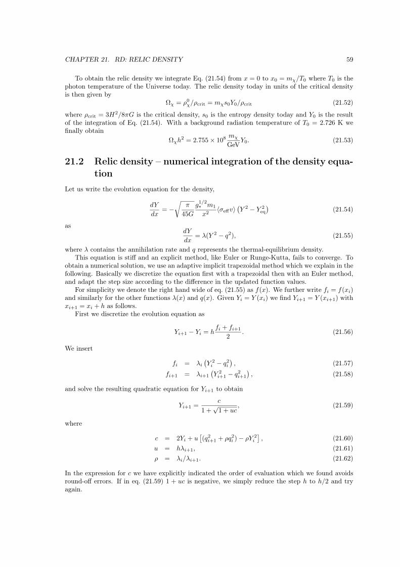
CHAPTER 21. RD: RELIC DENSITY 59
To obtain the relic density we integrate Eq. (21.54) from x = 0 to x0 = mχ/T0 where T0 is thephoton temperature of the Universe today. The relic density today in units of the critical densityis then given by
Ωχ = ρ0χ/ρcrit = mχs0Y0/ρcrit (21.52)
where ρcrit = 3H2/8πG is the critical density, s0 is the entropy density today and Y0 is the resultof the integration of Eq. (21.54). With a background radiation temperature of T0 = 2.726 K wefinally obtain
Ωχh2 = 2.755× 10⁸ mχ
GeVY0. (21.53)
21.2 Relic density – numerical integration of the density equa-tion
Let us write the evolution equation for the density,
dY
dx= −
√π
45G
g1/2∗ m1
x2〈σeffv〉
(Y 2 − Y 2
eq
)(21.54)
asdY
dx= λ(Y 2 − q2), (21.55)
where λ contains the annihilation rate and q represents the thermal-equilibrium density.This equation is stiff and an explicit method, like Euler or Runge-Kutta, fails to converge. To
obtain a numerical solution, we use an adaptive implicit trapezoidal method which we explain in thefollowing. Basically we discretize the equation first with a trapezoidal then with an Euler method,and adapt the step size according to the difference in the updated function values.
For simplicity we denote the right hand wide of eq. (21.55) as f(x). We further write fi = f(xi)and similarly for the other functions λ(x) and q(x). Given Yi = Y (xi) we find Yi+1 = Y (xi+1) withxi+1 = xi + h as follows.
First we discretize the evolution equation as
Yi+1 − Yi = hfi + fi+1
2. (21.56)
We insert
fi = λi(Y 2i − q2
i
), (21.57)
fi+1 = λi+1
(Y 2i+1 − q2
i+1
), (21.58)
and solve the resulting quadratic equation for Yi+1 to obtain
Yi+1 =c
1 +√
1 + uc, (21.59)
where
c = 2Yi + u[(q2i+1 + ρq2
i )− ρY 2i
], (21.60)
u = hλi+1, (21.61)ρ = λi/λi+1. (21.62)
In the expression for c we have explicitly indicated the order of evaluation which we found avoidsround-off errors. If in eq. (21.59) 1 + uc is negative, we simply reduce the step h to h/2 and tryagain.

CHAPTER 21. RD: RELIC DENSITY 60
Secondly we discretize the evolution equation as
Yi+1 − Yi = hfi+1. (21.63)
We insert the expression for fi+1 and solve the quadratic equation for Yi+1 to obtain
Y ′i+1 =1
2
c′
1 +√
1 + uc′, (21.64)
wherec′ = 4
(Yi + uq2
i+1
). (21.65)
Again if in eq. (21.64) 1 + uc′ < 0, we reduce the step h to h/2 and try again.We then adapt the step size according to the relative difference of Yi+1 and Y ′i+1,
d =
∣∣∣∣Yi+1 − Y ′i+1
Yi+1
∣∣∣∣ . (21.66)
If the difference is larger than a prefixed ε, set at 0.01, we reduce the step size h to hs/√ε but never
to less than h/10. s is a safety factor set to 0.9. If d < ε, we increase the step size by a factors/√ε but never by more than a factor of 5. We do not allow the step size to become smaller than
hmin = 10−9. Error code 5 is reported if this happens. Error code 4 occurs when xi+1 is numericallyequal to xi because of round-off. Error code 6 occurs when the number of steps exceeds a maximumof 100000. Finally the initial step size is taken to be 0.01.
21.3 Relic density – routinesIn src/rd, the general relic density routines are found. These routines can be used for any darkmatter candidate and e.g. the interface to neutralino dark matter is in src_models/mssm/rd.
The main routine for relic density calculations is dsrdomega. It calculates and returns the relicdensity as well as the approximate temperature of freeze-out. It taks a few arguments: i) one optionargument that typically (depending on the particle physics module) determines how co-annihilationsare included, ii) one fast argument that determines how careful the Boltzmann solver should be incalculating the relic density. See the header of dsrdomega for more details.
21.3.1 Global parametersAll internal settings of the relic density routines are set in common blocks in dsrdcom.h. The mostimportant parameters that can be changed by the user are
Important parameters in dsrdcom.hPurpose: Provide a set of parameters, with which the internal behaviour of the relic
density routines can be changed.Parameters
tharsi i Size of the coannihilation, resonance and threshold arrays (default=50). In-crease this size if you have more than 50 coannihilating particles, more than 50resonances or more than 50 thresholds.
rdluerr i Logical unit number where error messages are printed.rdtag c*12 Idtag that is printed in case of errors.cosmin r8 . . .waccd r8 . . .dpminr r8 . . .dpthr r8 . . .wdiffr r8 . . .

CHAPTER 21. RD: RELIC DENSITY 61
wdifft r8 . . .hstep r8 . . .rdt_max r8 Maximum number of seconds to spend on relic density calculation. If the time
limit is exceeded, dsrdomega returns with an error flag and the result 0. Thetime is the total CPU time (i.e. summed up over all cores/threads) and thelimit is approximate as it is only checked before a new point is added to theWeff tabulation.
21.3.2 Brief description of the internal routinesBelow, the remaining routines related to the relic density calculation are briefly mentioned. Formore details, we refer to the routines themselves.Routine Purposedsrdaddpt To add one point in the Weff -peff table.dsrdcom To initialize parameters in the common blocks in dsrdcom.h. If you want to
change these parameters yourself, include dsrdcom.h in your code and changethe parameters you want.
dsrddof Returns the degrees of freedom as a function of the temperature in the earlyUniverse.
dsrddpmin To return the allowed minimal distance in peff between two points in the Weff -peff plane. The returned value depends on if there is a resonance present or notat the given peff .
dsrdens Routine to solve the Boltzmann equation and return the relic density. Calledby dsrdomega.
dsrdeqn To solve the relic density equation by means of an implicit trapezoidal methodwith adaptive stepsize and termination.
dsrdfunc To return the invariant annihilation rate times the thermal distribution.dsrdfuncs To provide dsrdfunc in a form suitable for numerical integration.dsrdlny To return lnWeff for a given peff .dsrdnormlz To return a unit vector in a given direction.dsrdqad To calculate the relic density with a quick-and-dirty method. It uses the ap-
proximative expressions in Kolb & Turner with the cross section expaned inv.
dsrdqrkck To numerically integrate a function with a Runge-Kutta methoddsrdrhs To calculate terms on the right-hand side in the Boltzmann equation.dsrd_set To set the control parameters for the relic density calculation. Currently, only
the choice of effective degrees of freedom is implemented through dsrd_set; theother parameters are passed as arguments to dsrdomega.
dsrdspline To set up the table Weff -peff for spline interpolation.dsrdstart To sort and store information about coannihilations, resonances and thresholds
in common blocks.dsrdtab To set up the table Weff -peff .dsrdthav To calculate the thermally averaged annihilation cross section at a given tem-
perature.dsrdthclose ...dsrdthlim To determine the end-points for the thermal average integration.dsrdthtest To check if a given entry in the Weff -peff table is at a threshold.dsrdwfunc To write out dsrdfunc for a given x = mχ/T .

CHAPTER 21. RD: RELIC DENSITY 62
dsrdwintp To return the invariant rate Weff for any given peff by performing a splineinterpolation in the Weff -peff table.
dsrdwintpch To check the spline interpolation in theWeff -peff table and compare with a linearinterpolation.
dsrdwintrp To write out a table of the invariant rate Weff and some internal integrationvariables and expressions.
dsrdwres To write out the table Weff -peff .

Chapter 22
se_aux:Auxiliary routines for WIMPannihilation in the Sun/Earth
22.1 Sun and Earth models – auxiliary routinesThis directory contains parameterizations and semi-analytical calculations of auxiliary fluxes, likeEarth atmospheric fluxes. They are not up to date with the latest calculations and are provided asis for convenience.
63

Chapter 23
se_mod:Sun and Earth models
(JE: I am responsible for updating this part)
23.1 Sun and Earth models – theoryWe need to have accurate models for the Sun and the Earth, both in terms of mass distributions,but also in terms chemical compositions etc. We here include a set of Sun and Earth models.
The models here are used for the capture rate calculation for capture of WIMPs in the Sun andthe Earth, but they are also used for external packages like WimpSim which simulates neutrinointeractions and oscillations on the way out of the Sun/Earth. Those simulation results are includedas tables in se_yield.
23.2 Sun and Earth models – routinesThe main routines that could be of interest to most users are
64
Chapter 24
se_nu:Capture and annihilation in theSun/Earth
24.1 Neutrinos from the Sun and Earth – theory. Note. This chapter is not up to date with the latest additions to the code, butprovided as is as a reference right now.
There are several indirect methods for detection of WIMPs. One of the most promising [72, 73,74, 75, 76, 77, 78, 79, 80, 81, 82, 83, 84, 85, 86, 19] is to make use of the fact that scattering of haloneutralinos by the Sun and the planets, in particular the Earth, during the several billion years thatthe Solar system has existed, will have trapped these neutralinos within these astrophysical bodies.Being trapped within the Solar or terrestrial material, they will sink towards the center, where aconsiderable enrichment and corresponding increase of annihilation rate will occur.
Searches for neutralino annihilation into neutrinos will be subject to extensive experimentalinvestigations in view of the new neutrino telescopes (AMANDA, IceCube, Baikal, NESTOR,ANTARES) planned or under construction [87]. A high-energy neutrino signal in the directionof the centre of the Sun or Earth is an excellent experimental signature which may stand up againstthe background of neutrinos generated by cosmic-ray interactions in the Earth’s atmosphere.
There are several different approximations one could do, or processes to include when calculatingthe capture rates in the Earth/Sun and many of these are coded into DarkSUSY. The default inDarkSUSY is always to use the best calculations available, but more approximate (older) routines arealso available, as well as more speculative signals, like the Damour-Krauss signal (not included bydefault). If you want to use something else than the defaults, or want to call more internal rotuines(more internal than dsntrates or dsntdiffrates), you should read the following sections carefully.
24.1.1 Neutrino yield from annihilationsThe differential neutrino flux from neutralino annihilation is
dNνdEν
=ΓA
4πD2
∑f
BfχdNf
ν
dEν(24.1)
where ΓA is the annihilation rate, D is the distance of the detector from the source (the centralregion of the Earth or the Sun), f is the neutralino pair annihilation final states, and Bfχ are thebranching ratios into the final state f . dNf
ν /dEν are the energy distributions of neutrinos generated
65

CHAPTER 24. SE_NU: CAPTURE AND ANNIHILATION IN THE SUN/EARTH 66
by the final state f and are obtained from the Pythia simulations described in section ??. (JE:Update reference and description of WimpSim simulations.)
In comparison with calculations using the results of [88] (e.g. [89, 82, 90, 85, 84, 91, 92]), thisMonte Carlo treatment of the neutrino propagation through the Sun does not need the simplifyingassumptions previously made, namely neutral currents are no more assumed to be much weakerthan charged currents and energy loss is no more considered continuous.
The neutrino-induced muon flux may be detected in a neutrino telescope by measuring themuons that come from the direction of the centre of the Sun or Earth. For a shallow detector,this usually has to be done in the case of the Sun by looking (as always the case for the Earth)at upward-going muons, since there is a huge background of downward-going muons created bycosmic-ray interactions in the atmosphere. There is always in addition a more isotropic backgroundcoming from muon neutrinos created on the other side of the Earth in such cosmic-ray events (andalso from cosmic-ray interactions in the outer regions of the Sun). The flux of muons at the detectoris given by
dNµdEµ
= NA
∫ ∞Ethµ
dEν
∫ ∞0
dλ
∫ Eν
Eµ
dE′µ P (Eµ, E′µ;λ)
dσν(Eν , E′µ)
dE′µ
dNνdEν
, (24.2)
where λ is the muon range in the medium (ice or water for the large detectors in the ocean or atthe South Pole, or rock which surrounds the smaller underground detectors), dσν(Eν , E
′µ)/dE′µ is
the weak interaction cross section for production of a muon of energy E′µ from a parent neutrino ofenergy Eν , and P (Eµ, E
′µ;λ) is the probability for a muon of initial energy E′µ to have a final energy
Eµ after passing a path–length λ inside the detector medium. Ethµ is the detector threshold energy,
which for “small” neutrino telescopes like Baksan, MACRO and Super-Kamiokande is around 1GeV. Large area neutrino telescopes in the ocean or in Antarctic ice typically have thresholds ofthe order of tens of GeV, which makes them sensitive mainly to heavy neutralinos (above 100 GeV)[19].
The integrand in Eq. (24.2) is weighted towards high neutrino energies, both because the crosssection σν rises approximately linearly with energy and because the average muon energy, andtherefore the range λ, also grow approximately linearly with Eν . Therefore, final states which givea hard neutrino spectrum (such as heavy quarks, τ leptons and W or Z bosons) are usually moreimportant than the soft spectrum arising from light quarks and gluons.
24.1.2 Evolution of the number density in the Earth/SunNeutralinos are steadily being trapped in the Sun or Earth by scattering, whereas annihilationstake them away. Let N(t) be the total number of neutralinos trapped, at time t, in the core of, forexample, the Earth. The annihilation rate of neutralino pairs can be written as
Γa(t) =1
2CaN
2(t) . (24.3)
The evolution of N(t) is the result of the competition between capture and annihilation:
dN
dt= Cc(t)− CaN2 (24.4)
The constant Cc is the capture rate, and Ca entering equations (24.3) and (24.4) is linked to theannihilation cross-section σa, and to some effective volumes Vj , j = 1, 2, taking into account thequasi-thermal distribution of neutralinos in the Earth core:
Ca = 〈σa v〉V2
V 21
, (24.5)

CHAPTER 24. SE_NU: CAPTURE AND ANNIHILATION IN THE SUN/EARTH 67
Vj ' 2.3× 1025
(j mX
10 GeV
)−3/2
cm3 . (24.6)
This has the solution for the annihilation rate implemented in DarkSUSY
ΓA =Cc2
tanh2
(t
τ
), (24.7)
where the equilibration time scale τ = 1/√CcCa. In most cases for the Sun, and in the cases of
observable fluxes for the Earth, τ is much smaller than a few billion years, and therefore equilibriumis often a good approximation (N(t) = 0). This means that it is the capture rate which is theimportant quantity that determines the neutrino flux. However, in the program we keep the exactformula (24.7), with some modifications discussed in Sec. ??).
24.1.3 Approximate capture rate expressionsThe capture rate induced by scalar (spin-independent) interactions between the neutralinos andthe nuclei in the interior of the Earth or Sun is the most difficult one to compute, since it dependssensitively on the Higgs mass, form factors, and other poorly known quantities. However, thisspin-independent capture rate calculation is the same as for direct detection treated in Chapter 14.Therefore, there is a strong correlation between the neutrino flux expected from the Earth (whichis mainly composed of spin-less nuclei) and the signal predicted in direct detection experiments[19, 93]. It seems that even the large (kilometer-scale) neutrino telescopes planned, when searchingfor neutralino annihilation in the Earth, will not be competitive with the next generation of directdetection experiments when it comes to detecting neutralino dark matter. However, the situationconcerning the Sun is more favourable. Due to the low counting rates for the spin-dependentinteractions in terrestrial detectors, high-energy neutrinos from the Sun constitute a competitiveand complementary neutralino dark matter search. Of course, even if a neutralino is found throughdirect detection, it will be extremely important to confirm its identity and investigate its propertiesthrough indirect detection. In particular, the mass can be determined with reasonable accuracy bylooking at the angular distribution of the detected muons [94, 95].
For the Sun, dominated by hydrogen, the axial (spin-dependent) cross section is important andrelatively easy to compute. A reasonably good approximation is given by [96]
Csd
(1.3 · 1023 s−1) (270 km s−1/v)=( ρχ
0.3 GeV cm−3
)(100 GeV
mχ
)(σsdpχ
10−40 cm2
)(24.8)
where σsdpχ is the cross section for neutralino-proton elastic scattering via the axial-vector interac-
tion, v is the dark-matter velocity dispersion, and ρχ is the local dark matter mass. The capturerate in the Earth is dominated by scalar interactions, where there may be kinematic and otherenhancements, in particular if the mass of the neutralino almost matches one of the heavy elementsin the Earth. For this case, a more detailed analysis is called for, which is available in [97] withconvenient approximations in [96]. In fact, also for the Sun the spin-independent contribution canbe important, in particular iron may contribute non-negligibly. For the Sun, the approximation in[96] is also available,
Csi
(4.8 · 1022 s−1) (270 km s−1/v)=( ρχ
0.3 GeV cm−3
)(100 GeV
mχ
)×
∑A
(σsiA
10−40 cm2
)FA(mχ)fAφAS (mχ/mA) /mA, (24.9)
where fA is the mass fraction of element A and φA is the typical gravitational potential (relative tothe surface) for that element. I.e. an element that is concentrated in the core will have a higher φA

CHAPTER 24. SE_NU: CAPTURE AND ANNIHILATION IN THE SUN/EARTH 68
Average parametersElement Mass number (A) fi φiHydrogen, H 1 0.670 3.15Helium-4, 4He 4 0.311 3.40Carbon, C 12 0.00237 2.85Nitrogen, N 14 0.00188 3.83Oxygen, O 16 0.00878 3.25Neon, Ne 20 0.00193 3.22Magnesium, Mg 24 0.000733 3.22Silicon, Si 28 0.000798 3.22Sulphur, S 32 0.000550 3.22Iron, Fe 56 0.00142 3.22
Table 24.1: The composition of the Sun with average parameters to be used in the approximativerelations given in [96]. These values are updated with the solar model of [98] and differs slightlyfrom the values used in [96].
Mass Mass fraction Average parametersElement number (A) Core Mantle fi φiOxygen, O 16 0.0 0.440 0.298 1.20Silicon, Si 28 0.06 0.210 0.162 1.24Magnesium, Mg 24 0.0 0.228 0.154 1.20Iron, Fe 56 0.855 0.0626 0.319 1.546Calcium, Ca 40 0.0 0.0253 0.0171 1.20Phosphor, P 30 0.002 0.00009 0.00071 1.56Sodium, Na 23 0.0 0.0027 0.00183 1.20Sulphur, S 32 0.019 0.00025 0.0063 1.59Nickel, Ni 59 0.052 0.00196 0.0181 1.57Aluminum, Al 27 0.0 0.0235 0.0159 1.20Chromium, Cr 52 0.009 0.0026 0.0047 1.44
Table 24.2: The composition of the Earth’s core and mantle. The core mass fractions are from[99][Table 4] and the mantle mass fractions are from [99][Table 2]. The average mass fractions andpotentials in the last two columns are weighted averages assuming a core mass of 1.93 · 1024 kg anda mantle mass of 4.04 · 1024 kg with average potentials (relative to the surface) of 1.6 in the coreand 1.2 in the mantle [97].
than an element at the surface. A is the atomic number of the element and MA is its mass. Thefactor S is a kinematical suppression factor [96, 81]. In the next subsection we will go through thecompositions of the Earth/Sun that we use.
The approximate capture rate expressions above are coded into the routines dsntcapsun anddsntcapearth. More accurate expressions will follow in the coming subsections.
24.1.4 Earth and Sun compositionWhen the capture rates are calculated, we need to know the composition and density of theEarth/Sun as a function of depth.
In [96] they used average mass fractions and potentials for the location of the various elementsin the Sun. We have updated these to the BP2000 [98] values instead, as given in Table 24.1
For the Earth, we have also implemented more accurate density profiles and more up-to datechemical distributions within the Earth. We use the estimates for the Earth composition given in[99][Table 2 for the mantle and Table 4 for the core]. In Table 24.2 we list these values together with

CHAPTER 24. SE_NU: CAPTURE AND ANNIHILATION IN THE SUN/EARTH 69
0
2
4
6
8
10
12
14
Den
sity
(g/c
m3)
a)
1111.5
1212.5
1313.5
1414.5
15
0 1000 2000 3000 4000 5000 6000
Radius (km)
Esc
ap
e vel
oci
ty (
km
/s)
b)
Figure 24.1: In a) the density profile and in b) the escape velocity in the Earth is shown.
the average parameters fi and φi that should be used in the expressions for the approximate capturerates in the previous section. Note that using these average parameters instead of integrating overthe full radius is equivalent to putting all the elements of the give type at the gravitational potentialφi.
We also need the density profile of the Earth, and for this we use the values in [100]. Using thisdensity profile, we can calculate the gravitational potential, φ(r) inside the Earth and from this onethe escape velocity v inside the Earth,
v = 11.2
√φ(r)
φ(R⊕)km/s. (24.10)
In Fig. 24.1 we show the density profile and escape velocity inside the Earth.
24.1.5 More accurate capture rate expressionsAnother complicating factor when calculating the capture rates is the integration over the velocitydistribution. In [97], parts of the integrations are performed analytically for a Gaussian veolocitydistributions. These expressions are also coded in DarkSUSYfor the Earth and give a more accuratecalculation of the capture rate in the Earth than the approximations given above. The routinedsntcapearth2 performs these calculations for the Earth.
24.1.6 Accurate capture rates in the Earth for general velocity distribu-tions
If one wants even more accurate and general expressions for the capture rates in the Sun/Earth,we have also implemented the full expressions in [97], but without assuming that the velocity dis-tribution is a Gaussian (or Maxwell-Boltzmann). These routines are now the default in DarkSUSY.

CHAPTER 24. SE_NU: CAPTURE AND ANNIHILATION IN THE SUN/EARTH 70
We will here outline how these expressions look like for the Earth and how they can be usedboth for a Maxwell-Boltzmann distribution and for a general velocity distribution. The expressionswill of course look analogously for the Sun. We start with the general case and study the specialcase of a Maxwell-Boltzmann distribution in the next section.
We will divide the Earth into shells and calculate the capture from element i in each shellindividually. At the end we will integrate over all the shells and sum over all the elements in theEarth. The capture rate from element i per unit shell volume is given by [97][Eq. (2.8)]
dCidV
=
∫ umax
0
duf(u)
uwΩ−v,i(w) (24.11)
where f(u) is the velocity distribution (normalized such that∫∞
0f(u) = nχ where nχ is the number
density of WIMPs. The expression Ω−v,i(w) is related to the probability that we scatter to orbitsbelow the escape velocity. w is the velocity at the given shell and it is related to the velocity atinfinity u and the escape velocity v by
w =√u2 + v2. (24.12)
The upper limit of integration is a priori set to umax = ∞, but we will see below that due tokinematical reasons we can set it to a lower value (Eq. (24.17) below). If we allow for a form factorsuppression of the form [97][Eq. (A3)]
|F (q2)|2 = exp
(−∆E
E0
)(24.13)
with [97][Eq. (A4)]
E0 =3~2
2mχR2(24.14)
we can evaluate wΩ−v,i(w) and arrive at the expression [97][Eq. (A6)]
wΩ−v,i(w) = σiniµ2
+
µ2E0
[e−
mχu2
2E0 − e− µ
µ2+
mχu2+v2
2E0
]Θ
(µ
µ2+
− u2
u2 + v2
)(24.15)
where we have introducedµ =
mχ
mi; µ± =
µ± 1
2(24.16)
with mi the mass of element i. The Heaviside step function Θ plays the role of only includingWIMPs that can scatter to a velocity lower then the escape velocity v. To simplify our calculationswe can drop this step function in Eq. (24.15) and instead set the upper limit of integration inEq. (24.11) to
umax =
õ
µ2−v (24.17)
We also need the scattering cross section on element i, which can be written as [96][Eq. (9-25)]
σi = σpA2i
(mχmi)2
(mχ +mi)2
(mχ +mp)2
(mχmp)2(24.18)
where Ai is the atomic number of the element, mp is the proton mass and σp is the scattering crosssection on protons.
We now have what we need to calculate the capture rate. In Eq. (24.11) we integrate over thevelocity for our chosen velocity distribution. We then integrate this equation over the radius of theEarth and sum over all the different elements in the Earth,
C =
∫ R⊕
0
dr∑i
dCidV
4πr2 (24.19)

CHAPTER 24. SE_NU: CAPTURE AND ANNIHILATION IN THE SUN/EARTH 71
Note that we have not assumed anything special about our velocity distribution, it doesn’t evenhave to be isotropic since the distribution of elements evenly in the shells will make an anisotropicdistribution on average to behave as an isotropic one.
The routines that calculate the capture rates with these general (and accurate) expressions aredsntcapearthnum and dsntcapsunnum. As these calculations are somewhat time-consuming, we havealso added a possibility to tabulate the result and interpolate in these tables. To use (or create, ifthe table files are missing) instead call dsntcapearthtab and dsntcapsuntab. These last two routinesare the default in DarkSUSY. The velocity distribution used is determined by a switch when thehalo model is set (i.e. when dshm_set is called).
24.1.7 Accurate capture rates for the Earth for a Maxwell-Boltzmannvelocity distribution
We will here give some more information on how the approximations introduced in the beginningof this chapter are derived from the general expressions in the preceeding section.
If the velocity distribution is of Maxwell-Boltzmann type we can greatly simplify our expressionsabove as we can perform the integration over velocity analytically. The integration over radius canalso be further simplified by using the average mass fractions fi and potentials φi in Tables 24.1–24.2.
If the velocity distribution in the halo is Maxwell-Boltzmann, it looks like
fh(u)du = nχ4√π
(3
2
) 32 u2
v3e−
32u2
v2 du (24.20)
where v is the three-dimensional velocity dispersion and nχ is the number density of WIMPs in thehalo. However, the solar system moves through the halo with a velocity v∗ and the distribution onobserver with this velocity through the halo will see is
f∗(u) = fh(u)e−32
v2∗v2
sinh(
3uv∗v2
)3uv∗v2
= nχ
√3
2π
u
vv∗
[e−
32
(u−v∗)2
v2 − e−32
(u+v∗)2
v2
](24.21)
Now one would naively believe that this is not the distribution that an observer at the Earth willsee. First of all, the Earth is moving with respect to the Sun and secondly, the WIMPs havegained speed by the gravitational attraction of the Sun when they reach the Earth. Both of thesearguments are true and the distribution of WIMPs in the halo will not look like Eq. (24.21) to anobserver on the Earth. However, Gould [101] showed that WIMPs from the halo can diffuse intothe solar system due to gravitational interactions with the planets and this distribution of WIMPswill roughly look like as if the Earth was in free space moving through the halo with the velocityof the solar system, i.e. Eq. (24.21). We will later scrutinize this statement, as it turns out that itdoes not quite hold, but as a first guess it is a reasonable approximation. For the Sun, though, thevelocity distribution give above is the correct one for a Maxwell-Boltzmann distribution.
With the distribution Eq. (24.21) we can analytically perform the integration over velocity inEq. (24.11). After some algebra we arrive at [97][Eq. (A10)]
dCidV
=
(8
3π
) 12 σininχv
2bη[e−aη
2
√1 + a
[2erf(η)− erf(A+) + erf(A−)
]− e−bη
2
√1 + b
e−(a−b)A2[2erf(η)− erf(A+) + erf(A−)
] ](24.22)

CHAPTER 24. SE_NU: CAPTURE AND ANNIHILATION IN THE SUN/EARTH 72
where erf is the modified error function,
erf(x) =
√π
2erf(x) ; erf(x) =
2√π
∫ x
0
e−y2
dy. (24.23)
Following Gould [97], we have in Eq. (24.22) introduced the following shorthand notation:
η =√
32v2∗v2 ; a = mchiv
2
3E0; b = µ
µ2+a
η = η√1+a
; η = η√1+b
A2 = 32v2
v2µµ2−
; A = A√
1 + a ; A = A√
1 + b
A± = A± η ; A± = A± η
(24.24)
If we wish, we can now integrate Eq. (24.22) over radius just like in the previous section, but wecan without loosing too much accuracy, replace this integration with a sum over the elements inthe Earth with their respective typical location. I.e. we can write
C =∑i
dCidV
1
ni
fiM⊕mi
(24.25)
where we instead of the number density ni use the total number of atoms of the given type fiM⊕/mi.Note that for each element in the sum we should evaluate this expression at the given typicalgravitational potential φi of the element, i.e. with the escape velocity given by Eq. (24.10). Themass fractions fi and typical potentials φi are listed in Table 24.2 (and analogously in Table 24.1for the Sun). This approximation introduces an error of no more than about 1–2% for a Maxwell-Boltzmann distribution∗
The capture rate evaluated with the expressions shown here are encoded into the routine dsnt-capearth2. Note that we have not coded the corresponding approximate expressions for the Sun.Instead, as given in the preceeding section, we now have more accurate expressions for both theSun and the Earth.
24.1.8 Effects of WIMP diffusion in the solar systemAs the Earth has a rather low escape velocity, the Earth will only be able to capture WIMPs thathave a rather low velocity with respect to the Earth. However, WIMPs from the halo have gainedspeed in the gravitaional potential from the Sun and will essentially be impossible to capture by theEarth. Hence, the Earth will only capture WIMPs that have diffused around in the solar system (bygravitational interactions with the other planets). Gould showed [101] that effectively this diffusionwill lead to the same phase space distribution at the Earth as if the Earth was in free space (i.e.neglecting the solar potential). However, numerical simulations of asteroids showed that they arethrown into the Sun due to perturbations of the orbits by other planets, see e.g. [102]. Theseanalyses led to worried that maybe the population of WIMPs diffusing around in the solar systemis not as big as thought [103]. In [104], Lundberg and Edsjö investigated this issue with detailednumerical simulations of WIMP orbits in the solar system, showing that the annihilation rate inthe Earth is typically reduced by up to two orders of magnitude. In DarkSUSY, we include theseresults for the neutrino rates from the Earth by using the velocity distribution at the Earth (asobtained in [104]). This velocity distribution is then used as input for our numerical capture rateroutines instead of the usual approximation of using the halo velocity distribution directly. Usingthese new velocity distributions for the Earth is the default in DarkSUSY.
∗Note that it is not advisable to use this approximation for general velocity distributions. If one e.g. has a lowerlimit on possible velocities, umin, for heavy WIMPs capture will then only be possible very close to the central core.Replacing the actual distribution of potentials φ(r) with the typical value φi may then introduce larger errors. Wewill encounter these kind of distributions shortly.
CHAPTER 24. SE_NU: CAPTURE AND ANNIHILATION IN THE SUN/EARTH 73
24.2 Neutrinos from Sun and Earth – routinesThis folder contains routines to calculate the neutrino-induced muon flux from the Earth and theSun in various models.
There are several different methods of calculation available (determined by secalcmet in dssecom.h).Method 1 uses the approximate formulae for the capture rates in the Earth/Sun from the Jungman,Kamionkowski and Griest review [96]. Method 2, uses the same expression for the Sun, but the fullexpression from Gould [97] for capture in the Earth. Method 4 uses a full numerical integrationover the velocity distribution (instead of assuming that it is Gaussian) and method 5, finally, alsoperforms a full numerical integration over the momentum transfer in the form factors (instead ofassuming exponential form factors). The default is to use method 5, but instead of using the nu-merical routines directly, tables are used. One can always force using the numerical routines insteadof the tables if one so wishes. There are several options regarding how many elements to inclucein the Sun summation over elements (’lo’, ’med’ and ’hi’). The easiest way to select method is bycalling dssenu_set. For the Earth, method 5 is not expected to make a large difference due to thesmaller momentum transfers in the Earth and method 5 reverts back to method 4 for the Earth.
A call to dssenu_set(’default’) is made in dsinit, but can be changed by the user by callingdssenu_set after dsinit.
To calculate the neutrino-induced muon flux from the Earth, you call dssenu_rates.

Chapter 25
se_yield:Yields from annihilation in theSun/Earth
(JE: I am responsible for updating this part)
25.1 Muon yields from annihilation in the Earth/Sun – theoryWe need to take into account all processes that yield muon neutrinos from annihilation in theEarth/Sun. To do this, we use a Monte Carlo, WimpSim [105], to simulate annihilations in thecenter of the Sun/Earth, neutrino oscillations and neutrino interactions on the way out of theSun/Earth and to the detector.
25.1.1 Monte Carlo simulations with WimpSimWe need to evaluate the yield of different particles per neutralino annihilation. The hadronizationand/or decay of the annihilation products are simulated with Pythia [10] 6.426 and we here describehow the simulations are done. For annihilation in the Sun/Earth the simulations are done for a setof 22 neutralino masses, mχ = 3, 6, 10, 25, 50, 80.3, 91.2, 100, 150, 176, 200, 250, 350, 500, 750,1000, 1500, 2000, 3000, 5000, 7500 and 10000 GeV. We tabulate the yields and then interpolatethese tables in DarkSUSY.
We are mainly interested in the flux of high energy muon neutrinos and neutrino-induced muonsat a neutrino telescope. We simulate 13 ‘fundamental’ annihilation channels, for each mass (wherekinematically allowed) above. In Table 25.1 we list the ‘fundamental’ channels for which simulationsare run and the full set of more complex channels. Pions and kaons get stopped before they decayand are thus made stable in the Pythia simulations so that they don’t produce any neutrinos. Forannihilation channels containing Higgs bosons, we can calculate the yield from these fundamentalchannels by letting the Higgs bosons decaying in flight (see below). We also take into account theenergy losses of B-mesons in the Sun and the Earth by following the approximate treatment of[88] but with updated B-meson interaction cross sections as given in [106]. We also take neutrino-interactions on the way out of the Sun into account by considering the charged-current interactionas a neutrino-loss and the neutral current interactions are simulated with nusigma [107]. Theneutrino-nucleon charged current interactions close to the detector are also simulated with nusigmaand finally the multiple Coulomb scattering of the muon on its way to the detector is calculatedusing distributions from [108]. We have used the CTEQ6 structure functions in these simulations.We also take into account neutrino oscillations with a full three-neutrino Monte Carlo. All of these
74

CHAPTER 25. SE_YIELD: YIELDS FROM ANNIHILATION IN THE SUN/EARTH 75
processes are put into the simulation package WimpSim [105] that can be downloaded separately.Results from simulation runs with this package are included with DarkSUSY. For more details onthese simulations, see [109].
For each annihilation channel and mass we simulate 107 annihilations and tabulate the finalresults as a neutrino-yield, neutrino-to-lepton conversion rate, a muon yield and hadronic showeryields differential in energy and angle from the center of the Sun/Earth. We also tabulate theintegrated yield above a given threshold and below an opening angle θ. We assumed throughoutthat the surrounding medium is water with a density of 1.0 g/cm3. Hence, the neutrino-to-muonconversion rates have to be multiplied by the density of the medium. In the muon fluxes, thedensity cancels out (to within a few percent). All results are summarized as yield tables that canbe loaded and interpolated in with DarkSUSYThis is done with the function dswayieldf. There arethree kinds of yields (two-dimensional in opening angle θ and energy), kind=1 gives integratedyields, kind=2 gives differential yields and kind=3 gives yields integrated in angle, but differentialin θ. For each kind, there are 26 different types of yield available according to Table 25.4. As adefault, only type 3–4, 9–10 and 13–14 are included in the DarkSUSY download, as these are themost commonly used types. If you need any other types, download the auxiliary data files fromhttp://www.darksusy.org, unpack them in share/DarkSUSY in the DarkSUSY root directory, andthen do a usual configure and make to install them. Also note that the kind=3 yields are nottabulated directly, but are instead calculated and tabulated when the simulation tables are read induring DarkSUSY initialization.
With these simulations, we can calculate the yield for any of these particles for a given MSSMmodel. For the Higgs bosons, which decay in flight, an integration over the angle of the decayproducts with respect to the direction of the Higgs boson is performed. Given the branching ratiosfor different annihilation channels it is then straightforward to compute the yield above any givenenergy threshold and within any angular region around the Sun or the center of the Earth. Theroutine dswayieldone calculates the yield for one channel, i.e. even these complex channels containingHiggs bosons, whereas the main routine dswayield calculates the total yield for a given model. Notethat the WIMP annihilation yield routines do not know about SUSY at all, so before they arecalled, a routine dswasetup is called to set up the annihilation branching ratios for the WIMP anddecay channels for the Higgs bosons. In Tables 25.2 and 25.3, the Higgs decay width channelsare given. If these routines are used with other particle physics models, replace dswasetup with aroutine appropriate for your particle physics model and then call dswayield as usual.

CHAPTER 25. SE_YIELD: YIELDS FROM ANNIHILATION IN THE SUN/EARTH 76
Annihilation channel Internal channel Internal channel array indexch Particles chi chii1 S0
1S01 - -
2 S01S
02 - -
3 S02S
02 - -
4 S03S
03 - -
5 S01S
03 - -
6 S02S
03 - -
7 S−S+ - -8 Z0S0
1 - -9 Z0S0
2 - -10 Z0S0
3 - -11 W−S+/W+W− - -12 Z0Z0 9 913 W+W− 8 814 νeνe 12 1115 e+e− - -16 νµνµ 13 1217 µ+µ− 10 -18 ντ ντ 14 1319 τ+τ− 11 1020 uu 2 221 dd 1 122 cc 4 423 ss 3 324 tt 6 625 bb 5 526 gg 7 727 qqg - -28 γγ - -29 Z0γ - -
Table 25.1: The annihilation channels ch used in dswayieldone. Also shown are the internal channelnumbers chi used for the fundamental channels used in the simulations (used by routine dswayieldf).To save some additional space with the data files in memory, there are also array index channelnumbers chii that are only used internally to access the right elements of the yield arrays. S denotesscalars (Higgs bosons).
Decay width channeldch Particles1–29 Same as the annihilation channels in Table 25.1.30 Sfermions31 Neutralinos32 Charginos
Table 25.2: The neutral scalar (Higgs) decay width channels used. In DarkSUSY these are storedin the array hdwidth(i,j) where i is the decay channel index above and j is the Higgs number (1–3for H0
1 , H02 and H0
3 respectively). For the wa routines, these decay branching ratios (partial widthdivided by total width) are stored in dswas0br(i,j).

CHAPTER 25. SE_YIELD: YIELDS FROM ANNIHILATION IN THE SUN/EARTH 77
Decay width channeldch Particles1 ud2 us3 ub4 cd5 cs6 cb7 td8 ts9 tb10 νee
+
11 νµµ+
12 νττ+
13 W+S01
14 W+S02
15 W+S03
20 Sfermions21 Neutralinos and charginos
Table 25.3: The (positively) charged scalar (Higgs) decay width channels used. In DarkSUSY theseare stored in the array hdwidth(i,4) where i is the decay channel index above. For the wa routines,these decay branching ratios (partial width divided by total width) are stored in dswascbr(i).
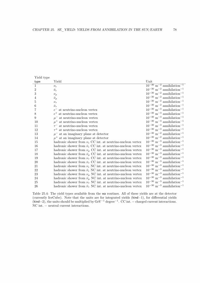
CHAPTER 25. SE_YIELD: YIELDS FROM ANNIHILATION IN THE SUN/EARTH 78
Yield typetype Yield Unit1 νe 10−30 m−2 annihilation−1
2 νe 10−30 m−2 annihilation−1
3 νµ 10−30 m−2 annihilation−1
4 νµ 10−30 m−2 annihilation−1
5 ντ 10−30 m−2 annihilation−1
6 ντ 10−30 m−2 annihilation−1
7 e− at neutrino-nucleon vertex 10−30 m−3 annihilation−1
8 e+ at neutrino-nucleon vertex 10−30 m−3 annihilation−1
9 µ− at neutrino-nucleon vertex 10−30 m−3 annihilation−1
10 µ+ at neutrino-nucleon vertex 10−30 m−3 annihilation−1
11 τ− at neutrino-nucleon vertex 10−30 m−3 annihilation−1
12 τ+ at neutrino-nucleon vertex 10−30 m−3 annihilation−1
13 µ− at an imaginary plane at detector 10−30 m−2 annihilation−1
14 µ+ at an imaginary plane at detector 10−30 m−2 annihilation−1
15 hadronic shower from νe CC int. at neutrino-nucleon vertex 10−30 m−3 annihilation−1
16 hadronic shower from νe CC int. at neutrino-nucleon vertex 10−30 m−3 annihilation−1
17 hadronic shower from νµ CC int. at neutrino-nucleon vertex 10−30 m−3 annihilation−1
18 hadronic shower from νµ CC int. at neutrino-nucleon vertex 10−30 m−3 annihilation−1
19 hadronic shower from ντ CC int. at neutrino-nucleon vertex 10−30 m−3 annihilation−1
20 hadronic shower from ντ CC int. at neutrino-nucleon vertex 10−30 m−3 annihilation−1
21 hadronic shower from νe NC int. at neutrino-nucleon vertex 10−30 m−3 annihilation−1
22 hadronic shower from νe NC int. at neutrino-nucleon vertex 10−30 m−3 annihilation−1
23 hadronic shower from νµ NC int. at neutrino-nucleon vertex 10−30 m−3 annihilation−1
24 hadronic shower from νµ NC int. at neutrino-nucleon vertex 10−30 m−3 annihilation−1
25 hadronic shower from ντ NC int. at neutrino-nucleon vertex 10−30 m−3 annihilation−1
26 hadronic shower from ντ NC int. at neutrino-nucleon vertex 10−30 m−3 annihilation−1
Table 25.4: The yield types available from the wa routines. All of these yields are at the detector(currently IceCube). Note that the units are for integrated yields (kind=1), for differential yields(kind=2), the units should be multiplied by GeV−1 degree−1. CC int. = charged current interactions.NC int. = neutral current interactions.
Chapter 26
si:Self-interactions
26.1 Dark matter self-interactions (si) – theoryThe CDM paradigm, resting on cold and collisionless dark matter, describes cosmological struc-ture formation with remarkable accuracy at scales larger than about one Mpc. At smaller cos-mological scales, on the other hand, this paradigm is less well tested, and currently still allowsfor DM self-interactions as strong as the interaction between nucleons – and thus much strongerthan current limits on DM interacting with SM particles. The possibility that DM could be rela-tively strongly interacting with itself [110] and thereby leave imprints on cosmological observablesrelated to structure formation has therefore seen significant interest in recent years, both froman astrophysical and a model-building perspective. Self-interacting DM (SIDM) could even ad-dress [111, 112, 113, 114, 115, 116, 117, 118] the most pressing potential small-scale problems ofΛCDM cosmology [119], referred to as ‘core-vs.-cusp” [120, 121], ‘too-big-to-fail’ [122, 123], ‘diver-sity’ [124, 125] and ‘missing satellites’ problems [126, 127] (the latter problem is addressed for SIDMwith late kinetic decoupling, which is a natural combination in many models [62]). Those specificdiscrepancies with the ΛCDM paradigm may of course well turn out to be either due to poorlymodelled baryonic effects or observational uncertainties – but these examples serve as evidence thatSIDM can leave observable imprints even in the absence of interactions with the SM. An unambigu-ous detection of such signatures, which are not expected in for example traditional WIMP modelsof DM, would significantly narrow down the range of possible particle explanations for the natureof DM.
The traditional reference quantity for the impact of DM self-interactions on the halo structureis the momentum transfer cross section,
σT ≡∫dΩ (1− cos θ)
dσ
dΩ, (26.1)
where σ is the standard cross section for DM-DM scattering. This has the advantage of regulatinglarge forward-scattering amplitudes, which should not affect the DM distribution (the same goes forbackward scattering which, however, is treated symmetrically in this prescription. See Ref. [128, 129]for a more detailed discussion). The size of this quantity that is of cosmological relevance is veryroughly given by
σT /mχ ∼ 1 cm2/g . (26.2)
Cross sections in this ballpark, in other words, may leave observable imprints and possibly addressthe various ΛCD; small-scale structure problems mentioned above, while much smaller cross sectionshave no impact on the structure of DM halos. Much larger values of σT /mχ are ruled out, on
79

CHAPTER 26. SI: SELF-INTERACTIONS 80
the other hand, in particular from observations of galaxy clusters. For a detailed review thatsummarizes both various constraints on DM self-interactions and models that have been discussedin the literature, we refer to Ref. [130].
The details of the DM self-interactions depend on the underlying particle theory. A simplecontact interaction term in the Lagrangian, for example, would lead to a constant (velocity-independent) σT . Another well-motivated option is that the interaction is mediated by a massiveparticle with mass mmed, which leads to a Yukawa potential between the two DM particles:
V (r) = ±αχre−mmedr . (26.3)
Here, αχ = g2χ/(4π) describes the coupling strength between mediator and DM particles, and the
different signs refer to attractive (-) and repulsive (+) potentials. Scalar mediators only gener-ate attractive potentials, while for vector mediators this depends on the particles involved in thescattering: for (e.g. Dirac) DM scattering with anti-DM, the force is attractive, otherwise it isrepulsive. An interesting phenomenological aspect for the scattering of nonrelativistic particles insuch a potential is the resulting strong velocity-dependence of σT ; this allows to achieve large scat-tering cross sections for the relatively small velocities of ∼30 km/s typically encountered in dwarfgalaxies (where one observes potential discrepancies with the ΛCDM expectations) while evadingthe strong bounds at cluster scales for velocities of ∼ 1000km/s. The transfer cross section resultingfrom scattering in a Yukawa potential has been extensively studied, and depends on the scatteringregime (vrel is the relative velocity between the DM particles):
• In the Born regime (αχmχ . mmed), σT can be calculated perturbatively, leading (for bothattractive and repulsive potentials) to [131]
σBornT =
8πα2χ
m2χv
4rel
(ln
[1 +
m2χv
2rel
m2med
]−
m2χv
2rel
m2med +m2
χv2rel
). (26.4)
• In the classical regime (mχvrel & mmed), a large numbers of partial waves contributes suchthat non-perturbative effects are important. In principle, this can be computed by numericallysolving the Schrödinger equation for each case and then summing all contributions [128]. Acomputationally much more efficient method is to use parameterizations [132] of numericalresults from the Plasma literature that have been obtained for screened Coulomb scattering[133, 134]. For an attractive potential, these are given by
σ−T =π
m2med
×
2β2 ln[1 + β−2] for β . 10−2
7β1.8+1960(β/10)10.3
1+1.4β+0.006β4+160(β/10)10 for 10−2 . β . 102
0.81 (1 + lnβ − (2 lnβ)−1)2 for β & 102
(26.5)
where β ≡ 2αχmmed/(mχv2rel) , while for a repulsive potential we have
σ+T =
π
m2med
×
2β2 ln[1 + β−2] for β . 10−2
8β1.8
1+5β0.9+0.85β1.6 for 10−2 . β . 104
(ln 2β − ln ln 2β)2 for β & 104
(26.6)
• Finally, there is the resonant regime (for mχvrel . mmed or αχmχ & mmed). Full numericalsolutions can be obtained by solving the Schrödinger equation explicitly in this regime. Theseare well described by the following analytic expressions that result from approximating theYukawa potential with a Hulthén potential [128]
σHulthnT =
16π
mχv2rel
sin2
(Arg
[iΓ[iΘvrel]
Γ[λ+] Γ[λ−]
]), (26.7)

CHAPTER 26. SI: SELF-INTERACTIONS 81
where Θ ≡ mχ√2ζ(3)mmed
and λ± ≡ 1 + iΘvrel/2±√αχΘ−Θ2v2
rel/4 for an attractive potential
and λ± ≡ 1 + iΘvrel/2± i√αχΘ + Θ2v2
rel/4 for a repulsive potential.
26.2 Self-interactions – routinesIn DarkSUSY, σT (vrel)/mχ is provided by an interface function dssigtm returned by the particlemodule which, from the perspective of the core library, can take any functional form. The functiondssigtmav then computes the velocity average 〈σT 〉/mχ, assuming a Maxwellian velocity distributionof the DM particles; this gives a better estimate of the effect of DM self-interactions than justevaluating dssigtm directly for a typical halo velocity. The core library furthermore provides severalauxiliary routines, to be used by any particle module, for the commonly encountered specific transfercross sections in the presence of a Yukawa potential as discussed above. In particular, dssisigmatbornreturns the expression given in Eq. (26.4), dssisigmatclassical those given in Eqs. (26.5, 26.6), anddssisigmatres those given in Eq. (26.7). For the latter, we adopt the complex gamma function asimplemented in the CERN library (based on Ref. [135]), and use analytic expansions where a naiveusage of these routines is problematic due to limited numerical precision (which is relevant for asignificant fraction of the physically interesting parameter range).

Part III
Particle physics modules insrc_models
82

Chapter 27
Basic principles and common routines
The general concept of a particle physics module, and how it communicates with the core libraryvia interface functions, was already introduced in Chapter 3 – see in particular Section 3.2, andTable 3.3 for an automatically updated list of all interface functions that the core library is awareof. Note that there is no principal restriction on which interface functions a particle module mustprovide: the main program will determine at compilation time whether it needs a functionality ofthe core library that requires certain interface functions to exist.
Every particle physics module must provide an independent representation of the full particlecontent of the respective particle theory. How this is done is fully flexible, and completely up to themodule. In practice, however, there are common frameworks, like the Standard Model, that appearrepeatedly. For convenience, we therefore store auxiliary routines and setups that may be usedby more than just one particle module in src_models/common. Common blocks and header filesincluded by more than one particle module are found in src_model/include. In order to keep up themodularity of the code, routines in src_models/common thus only include files in src_model/include.
27.1 common/aux: auxiliary routinesHere we collect various routines that belong to particle physics, and hence do not reside in ds_core,but are not only useful for one specific particle module. Currently, the most important are
• A set of functions to handle unique model IDs for each particle model, which is essential inorder not to repeat identical calculations when changing the model and thus to optimize nu-merical performance. A new such model ID should be assigned with dsnewidnumber whenevera new particle model is initalized (for the modules provided with the DarkSUSY release, this isautomatically done in dsmodelsetup). Any routine in src_models can test with dsidnumbersetwhether this ID number is indeed set, and retrieve its value with dsidnumber (which then canbe compared to the locally stored value of the ID number that was valid at the time whenthe respective routine was called the previous time).
• The function dsanthreshold returns the correction factor to a 2-body rate close to a kinematicalthreshold, resulting from the fact that one or both of the particles may be slightly off-shell.This implements the simplified treatment presented in Ref. [31], c.f. their Fig. 5, and henceassumes that the decay products of the virtual particle are (effectively) massless.
27.2 common/sm: standard modelThe routines collected in this folder provide a convenient shortcut to include the most basic proper-ties of the standard model in a BSM particle module. Currently, the most important functionalites
83

CHAPTER 27. BASIC PRINCIPLES AND COMMON ROUTINES 84
collected here are given by
• An initialization routine dsinit_sm, which can be called directly from the correspondingdsinit_module. After a call to this routine, the functions dsmass(kPDG) and dswidth(kPDG)correctly return masses and widths of the standard model particles – kPDG being the PDGcode [108] – as stored centrally in src_models/include/dssmparam.h.
• Running quark masses are provided up to the 4-loop level, with SM contributions only, bothfor pole and MS masses [136].
• The SM contributions to the strong coupling constant are also provided up to the 4-loop level.
• Another convenience function is dsgf2s2thw, which calculates sin2(θW ) at the mZ scale: inpraxis, its most important application is to ensure that a particle module can adopt a consis-tent relation between mZ and mW , which for example can be crucial in order to keep largenumerical cancellations under control.
Let us stress that standard model physics in DarkSUSY is by far not restricted to the routinescollected in common/sm. Much is presently still contained in the mssm module. It will be (further)disentangled from the SUSY-specific parts as new modules are added to the code that require thisfunctionality.

Chapter 28
The empty model
The empty module cannot be used to perform any real calculations. Its purpose is for debuggingand testing only, with the main advantage being that it contains (empty versions of) all interfacefunctions that the core library is aware of (for a full list, see Table 3.3). In some cases, this makesit a good starting point to create new particle physics modules.
85
Chapter 29
Generic decaying dark matter
This module provides a simple phenomenological template for a generic decaying dark matter model.It is fully specified by the DMmassmχ and the total decay rate Γ, along with a list of decay channels.The latter are specified by their branching ratios and the PDG codes of the final state standardmodel particles. Non-standard model final states can also be included, and are treated as invisibledecays.
The phenomenology of this module is restricted to indirect DM searches, with full access to thecorresponding routines in ds_core. DM scattering with nuclei is assumed to be negligible, as wellthermal production of DM in the early universe.
86
Chapter 30
Generic FIMPs
Similar to the case of generic_wimp, the module generic_fimp provides a simple phenomenologicaltemplate for a large class of DM candidates. Rather than being based on an actual particle physicsmodel, it mostly serves to provide an illustration of how the functionalities of DarkSUSY can beused in phenomenological freeze-in studies of ‘vanilla’ FIMP DM, when only providing the absoluteminimum of input parameters.
A generic FIMP model in DarkSUSY is set up by a call to dsgivemodel_generic_fimp, followedas usual by a call to dsmodelsetup. The model is thus fully defined by the input parameters ofdsgivemodel_generic_fimp: the mass mχ of the DM particle and a flag stating whether the DMparticle is its own anti-particle or not; a single SM species that the DM particle is assumed tocouple to (defined by its PDG code, PDGSM) and three parameters (c,Λ, n) that specify strengthand type of the interaction. Concretely, the squared amplitude for 2→ 2 production in this modelis assumed to take the form
|M|2 ≡ c( s
Λ2
)n, (30.1)
where s is the CMS energy squared.∗ Very roughly, this would, e.g., correspond to the amplitudeexpected for contact interactions in an effective field theory that results from integrating out heavyd.o.f. (where ‘heavy’ in this context means higher energies than the temperature where freeze-inproduction dominates.
Presently, the generic_fimp module only allows the user to calculate the relic density from freeze-in production (as well as, in principle, the would-be density from freeze-out), since rates are expectedto be too small to be relevant for indirect and direct detection signals. For phenomenological studiesof the latter, the generic_wimp module is thus better suited.
∗Technical note. Allowed values for PDGSM are all elementary SM particles in the EW broken phase. Strictlyspeaking, these choices are ill-defined above the EW phase transition and, for gluons and quarks, below the hadroniza-tion scale; results of freeze-in calculations must hence be interpreted with care if the dominant freeze-in productionhappens outside this range.
For reference, we treat situations outside this range as follows:• For quark and gluon final states, we use Eq. (30.1) only for T > Tqcd and for
√s > Ehadron (global parameters
set in dsinit and dsinit_sm, respectively); outside this range, we set |M|2 = 0.
• For T > TEW, fermions are chiral; we model their thermal masses as the average of the contributions fromleft- and right handed states – see dsmass_finiteT. Photons we continue to describe as a U(1) particle withelectromagnetic couplings, while we describe both Z and W± as unbroken SU(2) bosons (with temperature-dependent transverse masses).
We stress that this implementation is just a heuristic way of gauging the impact of phase transitions on the result offreeze-in calculations when insisting on the possibility of specifying the interacting SM species with a single (integer)parameter PDGSM (in analogy to the generic_wimp module). A more realistic implementation is necessarily model-dependent (see, e.g., the silveira_zee module described in Chapter 33).
87

CHAPTER 30. GENERIC FIMPS 88
30.1 generic_fimp/fi:Freeze-in routines
A call to dsfiset_generic_FIMP prior to dsfi2to2rhs allows to perform freeze-in calculations withmodified default settings. For example, call dsfiset_generic_FIMP(’quantum_statistics’,’off’) willlead to a freeze-in calculation without taking into account the effect of quantum statistics for the heatbath particles, and call dsfiset_generic_FIMP(’finiteT’,’off’) will switch off other finite-temperatureeffects (thermal masses and further temperature-dependence due to phase transitions). Defaultsettings are restored with corresponding calls to the same routine, replacing ’off’ with ’default’.

Chapter 31
Generic WIMPs
Similar to the case of generic_decayingDM, the module generic_wimp provides a simple phenomeno-logical template for a large class of DM candidates. Rather than being based on an actual particlephysics model, it mostly serves to provide an illustration of how the functionalities of DarkSUSYcan be used in phenomenological studies of ‘vanilla’ WIMP DM, when only providing the absoluteminimum of input parameters.
A generic WIMP model in DarkSUSY is set up by a call to dsgivemodel_generic_wimp, andhence fully defined by the input parameters of that routine: the mass mχ of the DM particle anda flag stating whether the DM particle is its own anti-particle or not; a constant annihilation rateσv in the CMS frame, along with the dominant annihilation channel into SM particles (as usualstated in terms of PDG codes); finally, the spin-independent scattering cross section σSI of DMwith nucleons.
This simple setup allows to use essentially the full functionality of the core library, from relicdensity calculation to direct detection rates and cosmic ray propagation and indirect detectionsignals in general.
89

Chapter 32
The Minimal SupersymmetricStandard Model
The implementation of the minimal supersymmetric standard model (MSSM) in the module mssmmainly follows that of DarkSUSYversions 4 [1] (see also Section 32.8 in this manual). In particular,the conventions for the superpotential and soft supersymmetry-breaking potential are the same asimplemented in [25], and thus similar to [137, 138]. The full set of input parameters to be providedat the weak scale thus consists of the pseudoscalar mass (mA), the ratio of Higgs vacuum expectationvalues (tanβ), the Higgsino (µ) and gaugino (M1, M2, M3) mass parameters, trilinear couplings(AEaa, AUaa, ADaa, with a = 1, 2, 3) as well as soft sfermion masses (M2
Qaa, M2Laa, M
2Uaa, M
2Daa,
M2Eaa, with a = 1, 2, 3).∗ Internally, those values are stored in mssm common blocks. The user may
either provide them directly or by setting up pre-defined phenomenological MSSM models with areduced number of parameters through a call to a routine like dsgive_model or dsgive_model25(followed by a call to dsmodelsetup). The former sets up the simplest of those models, definedby the input parameters µ, M2, mA, tanβ, a common scalar mass m0, and trilinear parametersAt and Ab; M1 and M3 are then calculated by assuming the GUT condition, and the remainingMSSM parameters are given by MQ = MU = MD = ME = ML = m01, AU = diag(0, 0, At),AD = diag(0, 0, Ab), AE = 0. Similarly, dsgive_model25 sets up a pMSSM model with 25 freeparameters (see the header of that file for details). Alternatively, all those values can be set byreading in an SLHA file, or providing GUT scale parameters in the case of cMSSM models (via aninterface to the ISASUGRA code, as included in ISAJET [139, 140]).
Compared to previous versions of the code, DarkSUSY 6 has a new interface to read and writeSUSY Les Houches Accord (SLHA) files [141, 142].
All particle and sparticle masses are stored in a common block array mass(). For neutralinomasses, we include the leading loop corrections [143, 144, 145] but neglect the relatively small cor-rections for charginos [143] (in both cases, masses cannot be negative in our convention).† Likewise,all mixing matrices and decay widths are available as common block arrays. The latter are currentlyonly computed for the Higgs particles (via an interface to the FeynHiggs [146, 147, 148, 149, 150]package), while the other sparticles have fictitious widths of 0.5% of the sparticle mass (for the solepurpose of regularizing annihilation amplitudes close to poles). Again, the conventions for massesand mixings follow exactly those of Ref. [1], to which we refer for further details.
∗Note that currently only diagonal matrices are allowed. While not being the most general ansatz possible, thisimplies the absence of flavour changing neutral currents at tree-level in all sectors of the model.
†Unless, of course, those values are provided by an SLHA file. This comment also applies to the followingsimplifications concerning both sparticle masses and widths.
90

CHAPTER 32. THE MINIMAL SUPERSYMMETRIC STANDARD MODEL 91
32.1 mssm/ac:Accelerator constraints
32.1.1 Accelerator boundsDarkSUSY contains a set of routines for a rough check whether a given model is excluded byaccelerator constraints. These routines are called dsacbnd[number]. The policy is that when weupdate DarkSUSY with new accelerator constraints, we keep the old routine, and add a new routinewith the last number incremented by one. Which routine that is called is determined by callingdsacset with a tag determining which routine to call. To check the accelerator constraints, thencall dsacbnd which calls the right routine for you. Upon return, dsacbnd returns an exclusion flag,warning. If zero, the model is OK, if non-zero, the model is likely excluded. The cause for theexclusion is coded in the bits of excl according to table 32.1.
We stress that these bounds are in most cases only approximate limits: DarkSUSY generallyfocusses on theoretical predictions for such observables, given a DM model realization, rather thanon the implementation of experimental likelihoods and the possibility to derive statistically well-defined limits from those. For the latter, we instead refer to packages like DarkBit [151] (or ColliderBit[152] for accelerator-based constraints)
exclBit set Octal value Decimal value Reason for exclusion
0 1 1 Chargino mass1 2 2 Gluino mass2 4 4 Squark mass3 10 8 Slepton mass4 20 16 Invisible Z width5 40 32 Higgs mass in excluded region6 100 64 Neutralino mass7 200 128 b→ sγ8 400 256 ρ parameter9 1000 512 (g − 2)µ10 2000 1024 Bs → µ+µ−
11 4000 2048 squark-gluino12 10000 4096 Higgs mass does not fit observed Higgs
Table 32.1: The bits of excl are set to indicate by which process this particular model is excluded.Check if a bit is set with btest(excl,bit).
Compared to previous DarkSUSY versions, we use in particular updated limits from HiggsBounds[153] on the mass of the MSSM Higgs bosons, as well as approximate bounds on squark and gluinomasses from LHC 8 TeV data [154]. For b→ sγ, we keep our genuine routines in mssm/ac_bsg forthis rare decay (see Ref. [1] for a more detailed description) but now use as a default the result fromSuperIso [155]; we compare this to the current limit of B(B → Xsγ) = (3.27±0.14)×10−4 as adoptedin FlavBit [156], based on data from BarBar and Belle [157, 158, 159]. SuperIso also computes the ratefor the rare leptonic decay B0
s → µ+µ−, which we compare to the LHCb measurement of B(B0s →
µ+µ−) = (3.0± 0.6+0.3−0.2)× 10−9 [160]. Finally, aµ ≡ (g − 2)µ/2 is calculated by dsgm2muon, based
on [161]; in dsacbnd, this is compared to the observed valued of aµ, obs = (11659208.9± 6.3)× 10−10
[162] after subtracting the SM expectation as specified in PrecisionBit [163].
CHAPTER 32. THE MINIMAL SUPERSYMMETRIC STANDARD MODEL 92
32.2 mssm/an:(Co-)annihilation cross sections
32.2.1 Annihilation cross sections – theoryFor the relic density calculations, we need all possible (co)annihilation cross sections between neu-tralinos, charginos and sfermions.
32.2.1.1 Annihilation cross sections
We have calculated all two-body final state cross sections at tree level involving neutralinos,charginos, sneutrinos, sleptons and squarks in the initial state. A complete list is given below.
Since we have so many different diagrams contributing, we have to use some method wherethe diagrams can be calculated efficiently. To achive this, we calculate the diagrams with generalexpressions for vertices, masses etc so that they can be reused for other processes. How we do thisin practice differs a bit between different sets of annihilation diagrams.
For neutralino-neutralino, neutralino-chargino and chargino-chargino annihilation, we classifythe diagrams according to their topology (s-, t- or u-channel) and to the spin of the particlesinvolved. We then compute the helicity amplitudes for each type of diagram analytically withReduce [164] using general expressions for the vertex couplings.
The strength of the helicity amplitude method is that the analytical calculation of a given typeof diagram has to be performed only once and the sum of the contributing diagrams for each set ofinitial and final states can be done numerically afterwards.
For the diagrams involving sfermions, Form is used to analytically calculate the amplitudes.This output is then converted into Fortran with a Perl script, form2f [165].
32.2.1.2 Coannihilation diagrams
All Feynman diagrams for which we calculate the annihilation cross section are listed in the comingsections. s(x), t(x) and u(x) denote a tree-level Feynman diagram in which particle x is exchangedin the s-, t- and u-channel respectively.
The convention used in this list of included coannihilation diagrams is that if a sfermion isdenoted f , then it’s antiparticle is denoted f∗.
32.2.1.3 Neutralino and chargino annihilation
Indices i, j, k run from 1 to 4, and indices c, d, e from 1 to 2. u, u, d, d, ν, ν, `, ˜, f and f are genericnotations for up-type quarks, up-type squarks, down-type quarks, down-type squarks, neutrinos,sneutrinos, leptons, sleptons, fermions and sfermions. A sum of diagrams over (s)fermion generationindices and over the neutralino and chargino indices k and e is understood (no sum over indicesi, j, c, d).
Neutralino-neutralino annihilation

CHAPTER 32. THE MINIMAL SUPERSYMMETRIC STANDARD MODEL 93
Initial state Final state Feynman diagramsH1H1, H1H2, H2H2, H3H3 t(χ0
k), u(χ0k), s(H1,2)
H1H3, H2H3 t(χ0k), u(χ0
k), s(H3), s(Z0)H−H+ t(χ+
e ), u(χ+e ), s(H1,2), s(Z0)
Z0H1, Z0H2 t(χ0k), u(χ0
k), s(H3), s(Z0)χ0iχ
0j Z0H3 t(χ0
k), u(χ0k), s(H1,2)
W−H+, W+H− t(χ+e ), u(χ+
e ), s(H1,2,3)Z0Z0 t(χ0
k), u(χ0k), s(H1,2)
W−W+ t(χ+e ), u(χ+
e ), s(H1,2), s(Z0)
ff t(fL,R), u(fL,R), s(H1,2,3), s(Z0)
Neutralino-chargino annihilation
Initial state Final state Feynman diagramsH+H1, H+H2 t(χ0
k), u(χ+e ), s(H+), s(W+)
H+H3 t(χ0k), u(χ+
e ), s(W+)W+H1, W+H2 t(χ0
k), u(χ+e ), s(H+), s(W+)
W+H3 t(χ0k), u(χ+
e ), s(H+)χ+c χ
0i H+Z0 t(χ0
k), u(χ+e ), s(H+)
γH+ t(χ+c ), s(H+)
W+Z0 t(χ0k), u(χ+
e ), s(W+)γW+ t(χ+
c ), s(W+)
ud t(dL,R), u(uL,R), s(H+), s(W+)
ν ¯ t(˜L,R), u(νL), s(H+), s(W+)
Chargino-chargino annihilation
Initial state Final state Feynman diagramsH1H1, H1H2, H2H2, H3H3 t(χ+
e ), u(χ+e ), s(H1,2)
H1H3, H2H3 t(χ+e ), u(χ+
e ), s(H3), s(Z0)H+H− t(χ0
k), s(H1,2), s(Z0, γ)Z0H1, Z0H2 t(χ+
e ), u(χ+e ), s(H3), s(Z0)
Z0H3 t(χ+e ), u(χ+
e ), s(H1,2)H+W−, W+H− t(χ0
k), s(H1,2,3)χ+c χ−d Z0Z0 t(χ+
e ), u(χ+e ), s(H1,2)
W+W− t(χ0k), s(H1,2), s(Z0, γ)
γγ (only for c = d) t(χ+c ), u(χ+
c )Z0γ t(χ+
d ), u(χ+c )
uu t(dL,R), s(H1,2,3), s(Z0, γ)
νν t(˜L,R), s(Z0)
dd t(uL,R), s(H1,2,3), s(Z0, γ)¯ t(νL), s(H1,2,3), s(Z0, γ)H+H+ t(χ0
k), u(χ0k)
χ+c χ
+d H+W+ t(χ0
k), u(χ0k)
W+W+ t(χ0k), u(χ0
k)
32.2.1.4 Squark-squark annihilation
Note: The tables below are not entirely up to date, more processes are included thanshown in the tables.
We will here denote squarks as qia and qjb where i and j are the family indices and a and b arethe mass eigenstate indices (running from 1 to 2). k and l will also be used as family indices for

CHAPTER 32. THE MINIMAL SUPERSYMMETRIC STANDARD MODEL 94
processes including more squarks. Colour indices are suppressed. ui is used as a generic notation forany up-type squark where i denotes the family index. Down-type squarks are denoted analogously.
Note that we will not (except in rare occations) show processes for ν and ˜ separately since theycan easily be obtained from the squark processes by replacing u with ν and d with ˜ (and notingthat we only have one mass eigenstate for the ν. Also note that the ν − ˜–sector is assumed not tobe flavour-changing.
diadi∗b annihilation
Initial state Final state Diagrams Notediad
i∗b γγ, Zγ t(di1,2), u(di1,2), p
diadi∗b ZZ t(di1,2), u(di1,2), p, s(H1, H2)
diadi∗b W−W+ p, s(H1, H2, Z, γ), t(uk
1,2) k = 1, 2, 3
diadi∗b ZH2, ZH1 t(di1,2), u(di1,2), s(Z,H3)
diadi∗b ZH3 t(di1,2), u(di1,2), s(H1, H2)
diadi∗b γH2, γH1, γH3 t(di1,2), u(di1,2)
diadi∗b H2H2, H1H1, H1H2 t(di1,2), u(di1,2), p, s(H1, H2)
diadi∗b H2H3, H1H3 s(Z,H3), t(di1,2), u(di1,2)
diadi∗b H3H3 s(H1, H2), p, t(di1,2), u(di1,2)
diadi∗b W−H+ s(H1, H2, H3), t(uk
1,2) k = 1, 2, 3
diadi∗b H−H+ s(H1, H2, Z, γ), p, t(uk
1,2) k = 1, 2, 3
diadi∗b ff (f 6= di) s(H?
1 , H?2 , H
?3 , Z, γ
?, g‡), t(χ+c )† †) f = uk (k = 1, 2, 3 ), ?)
Not for f = ν, ‡) Only forsquarks/quarks
diadi∗b didi s(H1, H2, H3, Z, γ, g
†), t(χ0k, g†) †) Only for squarks
diadi∗b Zg t(di1,2), u(di1,2), p Only for squarks
diadi∗b gg t(di1,2), u(di1,2), s(g), p Only for squarks
diadi∗b gγ t(di1,2), u(di1,2), p Only for squarks
diadi∗b gH1, gH2, gH3 t(di1,2), u(di1,2) Only for squarks
diadj∗b annihilation (i 6= j)
Initial state Final state Diagrams Notediad
j∗b W+W− t(uk1,2)† Not included at present
diadj∗b W+H− t(uk1,2)† Not included at present
diadj∗b H+H− t(uk1,2)† Not included at present
diad∗jb didj t(χ0
k, g†) †) Only for squarks
diad∗jb ukul t(χ+
c ) Only k = i, l = j at present
diadib annihilation
Initial state Final state Diagrams Notediad
ib didi t(χ0
k, g†), u(χ0
k, g†) †) Only for squarks
diadjb annihilation (i 6= j)
Initial state Final state Diagrams Notediad
jb didj t(χ0
k, g†) †) Only for squarks

CHAPTER 32. THE MINIMAL SUPERSYMMETRIC STANDARD MODEL 95
uiaui∗b annihilation
Initial state Final state Diagrams Noteuiau
i∗b γγ†, Zγ† t(ui
1,2), u(ui1,2), p †) Not for ν
uiau
i∗b ZZ t(ui
1,2), u(ui1,2), p, s(H1, H2)
uiau
i∗b W−W+ p, s(H1, H2, Z, γ
†), u(dk1,2) k = 1, 2, 3, †) Not for νuiau
i∗b ZH2, ZH1 t(ui
1,2), u(ui1,2), s(Z,H†3) †) Not for ν
uiau
i∗b ZH3 t(ui
1,2)†, u(ui1,2)†, s(H1, H2) †) Not for ν
uiau
i∗b γH†2 , γH†1 , γH†3 t(ui
1,2), u(ui1,2) †) Not for ν
uiau
i∗b H2H2, H1H1, H1H2 t(ui
1,2), u(ui1,2), p, s(H1, H2)
uiau
i∗b H2H3, H1H3 s(Z,H†3), t(ui
1,2)†, u(ui1,2)† †) Not for ν
uiau
i∗b H3H3 s(H1, H2), p, t(ui
1,2)†, u(ui1,2)† †) Not for ν
uiau
i∗b W−H+ s(H1, H2, H
†3), u(dk1,2) k = 1, 2, 3, †) Not for ν
uiau
i∗b H+H− s(H1, H2, Z, γ
†), p, t(dk1,2) k = 1, 2, 3, †) Not for νuiau
i∗b ff (f 6= ui) s(H×1 , H
×2 , H
†×3 , Z, γ†×, g‡), t(χ+
c )? †) Not for ν, ?) If f = dk
(k = 1, 2, 3), ‡) Only forsquarks/quarks, ×) Not forν
uiau
i∗b uiui s(H×1 , H
×2 , H
×3 , Z, γ
×, g‡), t(χ0k, g‡) ×) Not for ν, ‡) Only for
squarksuiau
i∗b Zg t(ui
1,2), u(ui1,2), p Only for squarks
uiau
i∗b gg t(ui
1,2), u(ui1,2), s(g), p Only for squarks
uiau
i∗b gγ t(ui
1,2), u(ui1,2), p Only for squarks
uiau
i∗b gH1, gH2, gH3 t(ui
1,2), u(ui1,2) Only for squarks
uiauj∗b annihilation (i 6= j)
Initial state Final state Diagrams Noteuiau
j∗b W+W− t(dk1,2)† Not included at present, †) Not for ˜
uiauj∗b W+H− t(dk1,2)† Not included at present, †) Not for ˜
uiauj∗b H+H− t(dk1,2)† Not included at present, †) Not for ˜
uiauj∗b uiuj t(χ0
k, g†) †) Only for squarks
uiauj∗b dkdl t(χ+
c ) Only k = i, l = j at present
uiauib annihilation
Initial state Final state Diagrams Noteuiau
ib uiui t(χ0
k, g†), u(χ0
k, g†) †) Only for squarks
uiaujb annihilation (i 6= j)
Initial state Final state Diagrams Noteuiau
jb uiuj t(χ0
k, g†) †) Only for squarks
uiadi∗b annihilation

CHAPTER 32. THE MINIMAL SUPERSYMMETRIC STANDARD MODEL 96
Initial state Final state Diagrams Noteuiad
i∗b H+H1, H+H2 t(di1,2), u(ui1,2), p, s(W+, H+)
uiadi∗b H+H3 t(di1,2), u(ui1,2)†, p, s(W+) †) Not for ˜
uiadi∗b γH+ t(ui1,2)†, u(di1,2), s(H+) †) Not for ˜
uiadi∗b ZH+ t(ui1,2), u(di1,2), s(H+)
uiadi∗b W+H1, W+H2 t(di1,2), u(ui1,2), s(W+, H+)
uiadi∗b W+H3 t(di1,2), u(ui1,2)†, s(H+) †) Not for ˜
uiadi∗b W+γ t(di1,2), u(ui1,2)†, s(W+), p †) Not for ˜
uiadi∗b W+Z t(di1,2), u(ui1,2), s(W+), p
uiadi∗b ukdl s(H+,W+)?, t(χ0
m, g†)δikδil †) Not for ˜, ?) Only k = l
at presentuiad
i∗b W+g t(di1,2), u(ui1,2), p Only for squarks
uiadi∗b gH+ t(ui1,2), u(di1,2) Only for squarks
uiadj∗b annihilation (i 6= j) For squarks we can have the following processes
Initial state Final state Diagrams Noteuiad
j∗b H+H1, H+H2 t(dj1,2), u(ui1,2), p, s(W+, H+) Not included at present
uiadj∗b H+H3 t(dj1,2), u(ui1,2), p, s(W+) Not included at present
uiadj∗b H+γ t(dj1,2), u(ui1,2), s(H+) Not included at present
uiadj∗b H+Z t(dj1,2), u(ui1,2), s(H+) Not included at present
uiadj∗b W+H1, W+H2 t(dj1,2), u(ui1,2), s(W+, H+) Not included at present
uiadj∗b W+H3 t(dj1,2), u(ui1,2), s(H+) Not included at present
uiadj∗b W+γ t(dj1,2), u(ui1,2), s(W+), p Not included at present
uiadj∗b W+Z t(dj1,2), u(ui1,2), s(W+), p Not included at present
uiadj∗b ukdl s(H+,W+)†, t(χ0
m, g)δikδjl †) Not included at present
whereas for sneutrinos and sleptons, we can only have the process
Initial state Final state Diagrams Noteνi ˜j∗b νi ¯j t(χ0
k)
uiadib annihilation
Initial state Final state Diagrams Noteuiad
ib ukdl t(χ0
m, g†)δikδil, u(χ+
c )? †) Only for squarks, ?)Only i = k = l at present
uiadjb annihilation (i 6= j)
Initial state Final state Diagrams Noteuiad
jb ukdl t(χ0
m, g†)δikδjl, u(χ+
c )×? †) Only for squarks, ×)For ν ˜ only when i =l, j = k, ?) Only includedwhen i = l, j = k atpresent

CHAPTER 32. THE MINIMAL SUPERSYMMETRIC STANDARD MODEL 97
32.2.1.5 Squark-neutralino annihilation
Note: The tables below are not entirely up to date, more processes are included thanshown in the tables.
We will here denote squarks as uia and dia where i is the family index and a is the mass eigenstateindex (running from 1 to 2).
uiaχ0j annihilation
Initial state Final state Diagrams Noteuiaχ
0j γui s(ui), t(ui1,2) Only for squarks
uiaχ0j Zui s(ui), t(ui1,2), u(χ0
k)uiaχ
0j H1u
i, H2ui s(ui)†, t(ui1,2), u(χ0
k) †) Only for squarksuiaχ
0j H3u
i s(ui)†, t(ui1,2)†, u(χ0k) †) Only for squarks
uiaχ0j W+dk s(ui), t(dk1,2), u(χ+
c ) k = 1, 2, 3, ui∗a χ0j →
W−dk in the codeuiaχ
0j H+dk s(ui), t(dk1,2), u(χ+
c ) k = 1, 2, 3, ui∗a χ0j → H−dk
in the codeuiaχ
0j gui s(ui), t(ui1,2)
diaχ0j annihilation
Initial state Final state Diagrams Notediaχ
0j γdi s(di), t(di1,2)
diaχ0j Zdi s(di), t(di1,2), u(χ0
k)
diaχ0j H1d
i, H2di s(di), t(di1,2), u(χ0
k)
diaχ0j H3d
i s(di), t(di1,2), u(χ0k)
diaχ0j W−uk s(di), t(uk1,2), u(χ+
c ) k = 1, 2, 3
diaχ0j H−uk s(di), t(uk1,2), u(χ+
c ) k = 1, 2, 3
diaχ0j gdi s(di), t(di1,2)
32.2.1.6 Squark-chargino annihilation
Note: The tables below are not entirely up to date, more processes are included thanshown in the tables.
We will here denote squarks as qia where i is the family index and a is the mass eigenstate index(running from 1 to 2).
uiaχ+c annihilation
Initial state Final state Diagrams Noteuiaχ
+c W+uk t(dl1,2), u(χ0
c)δik Only k = l = i at present
uiaχ+c H+uk t(dl1,2), u(χ0
c)δik Only k = l = i at present
ui∗a χ+c annihilation

CHAPTER 32. THE MINIMAL SUPERSYMMETRIC STANDARD MODEL 98
Initial state Final state Diagrams Noteui∗a χ
+c Zdk s(dk), t(ui1,2), u(χ+
c ) k = 1, 2, 3ui∗a χ
+c γdk s(dk), t(ui1,2)†, u(χ+
c ) k = 1, 2, 3, †) Only for squarksui∗a χ
+c H1d
k, H2dk s(dk), t(ui1,2), u(χ+
c ) k = 1, 2, 3ui∗a χ
+c H3d
k s(dk), t(ui1,2)†, u(χ+c ) k = 1, 2, 3, †) Only for squarks
ui∗a χ+c W+uk s(dl), u(χ0
c)δik Only k = l = i at present
ui∗a χ+c H+uk s(dl), u(χ0
c)δik Only k = l = i at present
ui∗a χ+c gdk s(dk), t(uia) k = 1, 2, 3, only for squarks
diaχ+c annihilation
Initial state Final state Diagrams Notediaχ
+c Zuk s(uk), t(di1,2), u(χ+
c ) Only k = i at presentdiaχ
+c γuk s(uk)†, t(di1,2), u(χ+
c ) Only k = i at present, †) Only for squarksdiaχ
+c H1u
k, H2uk s(uk)†, t(di1,2), u(χ+
c ) Only k = i at present, †) Only for squarksdiaχ
+c H3u
k s(uk)†, t(di1,2), u(χ+c ) Only k = i at present, †) Only for squarks
diaχ+c W+dk s(ul), u(χ0
c)δik Only k = l = i at present
diaχ+c H+dk s(ul), u(χ0
c)δik Only k = l = i at present
diaχ+c guk s(uk), t(dia) Only k = i at present, only for squarks
di∗a χ+c annihilation
Initial state Final state Diagrams Notedi∗a χ
+c W+dk t(ul1,2), u(χ0
c)δik Only k = l = i at present
di∗a χ+c H+dk t(ul1,2), u(χ0
c)δik Only k = l = i at present
32.2.1.7 Degrees of freedom
We have to be careful with the internal degrees of freedom, g, of the particles. We can either treate.g. a χ+
i and a χ−i as two separate particles with two degrees of freedom each, or we can treatthem as one particle χ±i with four degrees of freedom. The latter approach has an advantage thatwe simplify our expressions for the effective annihilation cross sections when coannihilations areneeded. Hence, we use that approach here. For a more detailed discussion about this, see Section32.12.2.
32.2.2 Annihilation routines - general remarksThe annihilation cross section routines is divided into several parts, mostly for historical reasons.The layout is roughly as follows:
src/an Here we keep the main routins for both neutralino- neutralino annihilation cross sectionsand the effective annihilation cross section in the relic density calculations. The steeringroutines for neutralino and chargino coannihilations are also kept here.
src/anstu Here keep the t−, u− and s− diagram expressions for fermion-fermion coannihilations(i.e. neutralino and chargino coannihilations).
src/as Here all the coannihilation cross sections including sfermions are kept.
We will here describe the src/an-routines.

CHAPTER 32. THE MINIMAL SUPERSYMMETRIC STANDARD MODEL 99
32.2.2.1 General routines
The general routine to call for an effective annihilation cross section (to be used for relic densitycalculations) is dsanwx, which returns the invariant annihilation rate (integrated over cos θ). Theactual cross section, differential in cos θ is calculated by dsandwdcos which includes all the coanni-hilations needed. This is set up in mssm/rd/dsrdparticles (typically called from dsrdomega in thecore library) which determines which coannihilating particles to include.
For other applications where the annihilation rate is needed, e.g. annihilation in the galactichalo, one can call the specific annihilation rate routine directly. The main one is dsandwdcosnnfor neutralino-neutralino annihilation. To simplify this task, we supply a routine dssigmav0 whichcalls dsandwdcosnn for neutralino-neutralino annihilation at zero relative velocity and returns theresult, either as the total annihilation cross section, or the cross section for a specific channel. Seethe header of dssigmav for details.
32.2.2.2 Neutralino and chargino (co)annihilation cross sections
The routines dsandwdcosnn, dsandwdcoscn and dsandwdcoscc calculate the annihilation crosssections (returning the invariant annihilation rate) for neutralino-neutralino, neutralino-charginoand chargino-chargino annihilations. Which particles the cross section is calculated for is given byparticle indices as defined in mssm/include/dsmssm.h.
All the annihilation routines return the invariant rate instead of the cross section. The invariantannihilation rate between particle i and j is defined as
Wij = 4pij√sσij = 4σij
√(pi · pj)2 −m2
im2j = 4EiEjσijvij . (32.1)
See Chapter 21 for more details.
32.3 mssm/an_1l:Annihilation cross sections (1-loop)
32.3.1 Annihilation cross sections at 1-loop – generalThe annihilation cross sections at 1-loop that we have implemented in DarkSUSY are those to γγ,Zγ and gg. The derivation of these is described in the works [26, 27]. Let us mention that theseone-loop expressions formally violate unitarity for diagrams with electroweak gauge-boson exchangebecause they do not take into account the nonperturbative effects related to multiple electroweakgauge boson exchange (‘Sommerfeld effect’) as described in [?, ?]. In practice, one can still trustthe result for sub-TeV neutralinos – but should keep in mind that the implemented cross sectionsbecome unphysical in the limit mW /mχ → 0.
To see how these routines are called, see the file src_models/mssm/an/dsandwdcosnn.f wherethe γγ, Zγ and gg contributions are added to the annihilation cross section at the end.
32.4 mssm/an_ib:Internal bremsstrahlung
32.4.1 Internal Bremsstrahlung (IB) – theoryWhenever WIMPs annihilate into pairs of charged particles XX, this process will inevitably beaccompanied by internal bremsstrahlung (IB), i.e. the emission of an additional photon in the finalstate (note that in contrast to ordinary, or external, bremsstrahlung no external electromagneticfield is required for the emission of the photon). In many cases, IB photons completely dominate

CHAPTER 32. THE MINIMAL SUPERSYMMETRIC STANDARD MODEL 100
the annihilation spectrum at the highest accessible energies. The resulting, characteristic sharp stepat an energy corresponding to the dark matter particle’s mass, often accompanied by a bump-likefeature at slightly smaller energies, is a spectral signature that is hard to mimic by astrophysicalsources and in that respect similar to monochromatic photons. In fact, being an O(αem) correctionto the tree-level annihilation rate, one would generically expect IB photons to be more copiouslyproduced than the loop-suppressed [i.e. O(α2
em)] monochromatic photons; this has been confirmedin [28] for a large part of the supersymmetric parameter space, not the least due to the appearanceof efficient enhancement mechanisms.
32.4.1.1 General considerations
For didactic purposes, one may follow [28] and distinguish between photons directly radiated offthe external legs (final state radiation, FSR) and photons radiated from virtual charged particles(virtual internal bremsstrahlung, VIB). The IB photons are thus the total contribution from bothFSR and VIB photons.
For relativistic charged final states, FSR diagrams are always dominated by photons emittedcollinearly with X or X. This is a purely kinematical effect and related to the fact that thepropagator of the corresponding outgoing particle,
D(p) ∝((k + p)2 −m2
X
)−1, (32.2)
diverges in this situation. Here, k and p denote the momenta of the photon and the outgoingparticle, respectively. The resulting photon spectrum turns out to be of a universal form, almostindependent of the underlying particle physics model (see, e.g., [166]):
dNXXγ,FSR
dx≈ αQ2
X
πFX(x) log
(s(1− x)
m2X
). (32.3)
Here, QX and mX are the electric charge and mass of X; the splitting function F(x) depends onlyon the spin of the final state particles and takes the form
Ffermion(x) =1 + (1− x)2
x(32.4)
for fermions andFboson(x) =
1− xx
(32.5)
for bosons. Due to the logarithmic enhancement that becomes apparent in Eq. (32.3), FSR photonsare often the main source for IB. A prominent example where FSR in this universal form not onlydominates IB but in fact the total gamma-ray spectrum from WIMP annihilations, is the case ofKaluza-Klein dark matter [167].
In general, one can single out two situations where photons emitted from virtual charged particlesmay give an even more important contribution to the total IB spectrum than FSR: i) the three-bodyfinal state XXγ satisfies a symmetry of the initial state that cannot be satisfied by the two-bodyfinal stateXX or ii)X is a boson and the annihilation into XX is dominated by t-channel diagrams,with the t-channel particle almost degenerate in mass with the annihilating WIMP. In contrast toFSR, the contribution from VIB photons can not be given in a model-independent way but is verysensitive to the underlying short-distance physics. For more details, see [28].
32.4.1.2 IB from neutralino annihilations
For supersymmetric dark matter annhilations, the relevant final states for IB are W+W−, W±H∓,H+H− and ff ; both of the situations just mentioned above can arise, and VIB contributionsbecome important in considerable regions of the parameter space.

CHAPTER 32. THE MINIMAL SUPERSYMMETRIC STANDARD MODEL 101
Let us first note that for neutralino annihilations, in contrast to the situation for, e.g., Kaluza-Klein dark matter, we cannot in general expect very large FSR contributions. This is becausethe lightest charged final states, for which the logarithmic enhancement shown in Eq. (32.3) wouldbe most effective, are fermionic and therefore strongly helicity suppressed. Fermion final statescontaining an additional photon, however, are not subject to such a suppression [168]. In the limitof vanishing fermion mass, and assuming that both corresponding sfermions have the same mass,the photon multiplicity is given by [28]
dNf+f−
dx= αemQ
2f
|gR|4 + |gL|4
64π2
(m2χ〈σv〉χχ→ff
)−1
(32.6)
×(1− x)
4x
(1 + µ)(1 + µ− 2x)− 2x
(1 + µ− x)2− (1 + µ)(1 + µ− 2x)
(1 + µ− x)3log
1 + µ
1 + µ− 2x
,
where µ ≡ m2fR/m2
χ = m2fL/m2
χ and gRPL (gLPR) denotes the coupling between neutralino, fermionand right-handed (left-handed) sfermion. In the above expression, a large factor m2
χ/m2f due to
the lifted helicity suppression (from 〈σv〉χχ→ff ∝ m2fmχ
−4) appears, and another enhancement athigh photon energies for sfermions degenerate with the neutralino.
For large neutralino masses mχ mW and charginos almost degenerate with the neutralino,W+W− andW±H∓ final states are affected by the second of the mechanisms for VIB enhancementthat were discussed in the previous subsection. Of these two channels, IB from W+W− nearlyalways dominates; for pure Higgsinos (or Winos), the resulting photon multiplicity in this limit iswell approximated by [28, 169]:
dNW+W−
dx≈ αem
π
4(1− x+ x2)2
(1− x+ ε/2)x
[log
(2
1− x+ ε/2
ε
)− 1/2 + x− x3
], (32.7)
where ε ≡ mW /mχ.Charged Higgs pairsH+H−, finally, provide yet another interesting example where the two-body
final state is not allowed due to symmetry restrictions; in this case, in the limit v → 0, enforced byCP conservation. The annihilation into H+H−γ, on the other hand, is possible. However, sincecharged Higgs bosons in most models have considerably larger masses than gauge bosons, they areexpected to give negligible IB contributions compared to the latter.
32.4.1.3 The implementation in DarkSUSY
Let us now briefly describe how IB is implemented in DarkSUSY. The total gamma-ray spectrumfrom WIMP annihilations is given by
dNγ,tot
dx=∑f
Bf
(dNf
γ,sec
dx+dNf
γ,IB
dx+dNf
γ,line
dx
), (32.8)
where Bf denotes the branching ratio into the annihilation channel f . The first term encodesthe contribution from secondary photons, mainly produced through the decay of neutral pions,as described in Chapter 11. We recall here that these contributions are included by using theMonte Carlo code Pythia [10] to simulate the decay of a hypothetical particle with mass 2mχ anduser-specified branching ratios Bf . In this way, also FSR associated to this decay is automaticallyincluded in dNf
γ,sec/dx (the main contribution here comes from photons directly radiated off theexternal legs, but also photons radiated from other particles in the decay cascade are taken intoaccount).
Of course, IB from the decay of such a hypothetical particle cannot in general be expectedto show the same characteristics as IB from the actual annihilation of two WIMPs and for thisreason an additional term dNf
γ,IB/dx is included that accounts for the difference between the full
CHAPTER 32. THE MINIMAL SUPERSYMMETRIC STANDARD MODEL 102
IB contribution and the FSR part already taken into account for by Pythia. For details regard-ing the implemented procedure of separating these two contributions in a consistent way, see [28].The contributions dNf
γ,IB/dx, in contrast to dNfγ,sec/dx, are generically highly model-dependent.
At the moment, they are fully implemented only for neutralino annihilations and included bydefault. However, one may easily switch to a user-defined contribution, choose to neglect IBcompletely or, for comparison, to only include the FSR part by replacing the call to dsibyieldin mssm/an_yield/dsanyield. For example, a version of dsibyield containing only the FSR part ofthe yield is provided in mssm/an_ib/dsanyield_fsr.
For the supersymmetric case, the full expressions for all relevant three-body final states areimplemented, i.e. not just the approximations given in the last subsection, which only apply tothe limits described there. For performance reasons, IB is only included when virtual t-channelparticles are sufficiently degenerate in mass that large IB contributions to the total spectrum canbe expected. With a call to dsIBset, this default behaviour can be customized. Finally, radiativecorrections to the annihilation into charged particles XX of course also change the number of XXpairs per annihilation and thus the corresponding yield of particles in the further decay of theannihilation products. At the moment, apart from the photon yield, only the IB positron yield isimplemented in DarkSUSY. By default, only the annihilation into the dominating channel e+e−γ istaken into account in this case; again, this behaviour can be modified by a call to dsIBset.
32.5 mssm/an_sf:Annihilation cross sections (with sfermions)
32.5.1 Annihilation cross sections with sfermions – generalIn this directory, all the (co)annihilation cross sections involving one or more sfermions in the initialstate are calculated. The code here is based upon the work described in [14]. All the cross sectionsare calculated with Form and converted to Fortran with a script form2f [165].
The main routines here areRoutine Purposedsasdwdcossfsf Calculates the invariant annihilation rate between two sfermions in the initial
state.dsasdwdcossfchi Calculates the invariant annihilation rate between one sfermion and one fermion
(neutralino or chargino) in the iniital state.
32.6 mssm/an_stu:t, u and s diagrams for ff-annihilation
32.6.1 Annihilation amplitudes for fermion-fermion annihilationIn this directory, all the helicity amplitudes needed for neutralino-neutralino, neutralino-charginoand chargino-chargino annihilation are calculated. The helicity amplitudes have been calculatedwith general expressions for vertices, masses etc. in Reduce and converted to Fortran files. Thecalculation of these are described in more detail in [13].
Each routine here adds the contribution to the helicity amplitudes from one particular diagramand the sum over contributed diagrams is done in the routines an/dsandwdcosnn, an/dsandwdcoscnand an/dsandwdcoscc. The naming convention for the routines here is the following: The first partof the routine name is dsan to indicate that they deal with annihilations in DarkSUSY. The nextcharacter tells which kind of process it is s-, t- or u-channel and the next two caracters tell whichinitial state particles we have (f for fermion), the next character is the kind of propagating particle(f for fermion, s for scalar and v for vector boson), and finally, the last two characters tell the

CHAPTER 32. THE MINIMAL SUPERSYMMETRIC STANDARD MODEL 103
kind of final state particles. So, to take an example, the routine dsansffsvv calculates the helicityamplitudes for annihilation of two fermions to two vector bosons via s-channel exchange of a scalar.There are also a few special cases (routines ending in ex or in) for diagrams with clashing arrows.
32.7 mssm/dd:Direct detection
32.7.1 Direct detection – theoryNOTE: The description below is outdated. DarkSUSY now includes much better formfactors.
If neutralinos are indeed the CDM needed on galaxy scales and larger, there should be a sub-stantial flux of these particles in the Milky Way halo. Since the interaction strength is essentiallygiven by the same weak couplings as, e.g., for neutrinos there is a non-negligible chance of detectingthem in low-background counting experiments [170]. Due to the large parameter space of MSSM,even with the simplifying assumptions above, there is a rather wide span of predictions for the eventrate in detectors of various types. It is interesting, however, that the models giving the largest ratesare already starting to be probed by present direct detection experiments [25, 171].
The rate for direct detection of galactic neutralinos, integrated over deposited energy assumingno energy threshold, is
R =∑i
Ninχ〈σiχv〉, (32.9)
where Ni is the number of nuclei of species i in the detector, nχ is the local galactic neutralinonumber density, σiχ is the neutralino-nucleus elastic cross section, and the angular brackets denotean average over v, the neutralino speed relative to the detector as described in Chapter 16.
In DarkSUSY, the basic quantities computed are the neutralino-nucleon cross sections, whichare free of complications related to nuclear structure, and various experimental details like energythreshold, efficiencies etc. However, as a crude estimate of the expected rates in realistic detectors,the total neutralino-nucleus scattering rates can be obtained for 76Ge, Al2O3 (sapphire) and NaI.Usually, it is the spin-independent interaction that gives the most important contribution in targetmaterials such as Na, Cs, Ge, I, or Xe, due to the enhancement caused by the coherence of allnucleons in the target nucleus.
The neutralino-nucleus elastic cross section can be written as
σiχ =1
4πv2
∫ 4m2iχv
2
0
dq2G2iχ(q2), (32.10)
where miχ is the neutralino-nucleus reduced mass, q is the momentum transfer and Giχ(q2) is theeffective neutralino-nucleus vertex. We write
G2iχ(q2) = A2
iF2S(q2)G2
S + 4Λ2iF
2A(q2)G2
A, (32.11)
which shows the coherent enhancement factor A2i for the spin-independent cross section (often Λ2
i
is written as λ2J(J + 1) ). We assume gaussian nuclear form factors [97]
FS(q2) = FA(q2) = exp(−q2R2i /6~2), (32.12)
Ri = (0.3 + 0.89A1/3i )fm, (32.13)
which should provide us with a good approximation of the integrated detection rate [172, 173],in which we are only interested. (To obtain the differential rate with reasonable accuracy, betterapproximations are needed [174].)

CHAPTER 32. THE MINIMAL SUPERSYMMETRIC STANDARD MODEL 104
Using heavy-squark effective lagrangians [175, 176, 177, 81, 178], we get
GS =∑
q=u,d,s,c,b,t
〈qq〉
∑h=H1,H2
ghχχghqqm2h
− 1
2
6∑k=1
gLqkχqgRqkχqm2qk
(32.14)
and
GA =∑
q=u,d,s
∆q
(gZχχgZqqm2Z
+1
8
6∑k=1
g2Lqkχq
+ g2Rqkχq
m2qk
). (32.15)
The g’s are elementary vertices involving the particles indicated by the indices, and they read
ghχχ =
(gZχ2 − gyZχ1) (−Zχ3 cosα+ Zχ4 sinα) , for H1,(gZχ2 − gyZχ1) (Zχ3 sinα+ Zχ4 cosα) , for H2,
(32.16)
ghqq =
−Yq cosα/
√2, for H1,
+Yq sinα/√
2, for H2,(32.17)
gZχχ =g
2 cos θW
(Z2χ3 − Z2
χ4
)(32.18)
gZqq = − g
2 cos θWT3q, (32.19)
gLqkχq = gLLΓkqQL + gRLΓkqQR, (32.20)
gRqkχq = gLRΓkqQL + gRRΓkqQR, (32.21)
with
gLL = − 1√2
(T3qgZχ2 +
1
3gyZχ1
), (32.22)
gRR =√
2eqgyZχ1, (32.23)
gLR = gRL =
−YqZχ3, for q = u, c, t,−YqZχ4, for q = d, s,b,
(32.24)
and
Yq =
mq/v2, for q = u, c, t,mq/v1, for q = d, s,b.
(32.25)
Defining (N = n, p)
fNTq ≡〈N |mq qq|N〉
mN, (32.26)
we take in DarkSUSY the numerical values [179]
fpTu = 0.023, fpTd = 0.034,
fpTc = 0.0595, fpTs = 0.14,
fpTt = 0.0595, fpTb = 0.0595 (32.27)
and
fnTu = 0.019, fnTd = 0.041,
fnTc = 0.0592 fnTs = 0.14,
fnTt = 0.0592, fnTb = 0.0592. (32.28)
For the quark contributions to the nucleon spin we take [180]
∆u = 0.77, ∆d = −0.40, ∆s = −0.12. (32.29)

CHAPTER 32. THE MINIMAL SUPERSYMMETRIC STANDARD MODEL 105
However, the older set of data [181]
∆u = 0.77, ∆d = −0.49, ∆s = −0.15 (32.30)
can optionally be used.Moreover, we take for the Λ factors
Λ2Al = 0.087, Λ2
Na = 0.041 and Λ2I = 0.007, (32.31)
according to the odd-group model [182].
32.8 mssm/ge:General SUSY model setup: masses, vertices etc
32.8.1 Supersymmetric modelWe will here review the definition of the MSSM as given in [1].
32.8.1.1 Parameters
In our notation, the superpotential and the soft supersymmetry-breaking scalar potential minimalsupersymmetric standard model (MSSM) with R-parity conservation [137, 138, 183] read respec-tively
W = εij
(−e∗RhE liLH
j1 − d∗RhDqiLH
j1 + u∗RhU qiLH
j2 − µHi
1Hj2
), (32.32)
Vsoft = εij
(−e∗RAEhE liLH
j1 − d∗RADhDqiLH
j1 + u∗RAUhU qiLH
j2 −BµHi
1Hj2
+h.c.)
+Hi∗1 m
21H
i1 +Hi∗
2 m22H
i2
+qi∗LM2QqiL + li∗LM2
L liL + u∗RM2U uR + d∗RM2
DdR + e∗RM2E eR. (32.33)
Here i and j are SU(2) indices (ε12 = +1), h’s, A’s and M’s are 3× 3 matrices in generation space,and the other boldface letters are vectors in generation space.
The current version of DarkSUSY uses only a restricted set of parameters. Namely the numberof free parameters (a grand total of 124 [184]) is reduced by setting the off-diagonal elements of theA’s and M’s to zero and imposing CP conservation (except in the CKM matrix).
32.8.1.2 Mass spectrum
For easy reference, we now give the particle mass matrices, together with our convention for themixing matrices.
Concerning the Higgs sector, we choose as independent parameters tanβ and the mass mA ofthe CP-odd Higgs boson. The code provides five options for the calculation of the Higgs masses:
higloop=0: tree level formulas; higloop=1: the effective potential approach in [185, 186, 187](correcting the sign of µ in eq. (4) of [187]); higloop=2: the effective potential approach in [188]with addition of D-terms and correction of some signs and numerical factors; higloop=3: the ana-lytical approximations to the RGE-improved effective potential in [189]; higloop=4: the pole masscalculation in [190]; higloop=5: FeynHiggs (requires FeynHiggs to be installed, default) [191]
The masses of the Higgs bosons are obtained from
M2H =
(m2Z cos2 β +m2
A sin2 β + ∆11 − sinβ cosβ(m2Z +m2
A) + ∆12
− sinβ cosβ(m2Z +m2
A) + ∆21 m2Z sin2 β +m2
A cos2 β + ∆22
)(32.34)
m2H± = m2
A +m2W + ∆±. (32.35)

CHAPTER 32. THE MINIMAL SUPERSYMMETRIC STANDARD MODEL 106
Higgs bosonChannel H0
1 H02 H0
3 H+
i= j=1 j=2 j=3 j=41 cc cc cc ud2 bb bb bb us3 tt tt tt ub4 τ+τ− τ+τ− τ+τ− cd5 W+W− W+W− – cs6 Z0Z0 Z0Z0 – cb7 – H0
1H01 – td
8 H02H
02 – – ts
9 H03H
03 H0
3H03 – tb
10 H+H− H+H− – νee+
11 – – ZH01 νµµ
+
12 – – ZH02 νττ
+
13 ZH03 ZH0
3 – W+H01
14 W+H−/W−H+ W+H−/W−H+ W+H−/W−H+ W+H02
15 µ+µ− µ+µ− µ+µ− W+H03
16 ss ss ss –17 gg gg gg –18 γγ γγ γγ –19 Z0γ Z0γ Z0γ –20 f f ′ f f ′ f f ′ f f ′
Table 32.2: Higgs partial widths hdwidth(i,j). Index i refers to the decay channel and index j to theHiggs boson. All widths are given in GeV. Note that typically we have that mH2 < mH3 < mH+ <mH1 so many of these decay channels are not kinematically allowed, but included for completeness.If the HDECAY interface is used, the channels where mH2
< mH3< mH+ < mH1
is not satisfiedare not included. Channels 16–19 are only included if HDECAY is used.
The quantities ∆ij and ∆± are the one-loop radiative corrections, calculated acording to the valueof higloop as described above. Diagonalization ofM2
H gives the two CP-even Higgs boson masses,mH1,2
, and their mixing angle α (−π/2 < α < 0). For higloop=4, the pole masses are then obtainedsolving m2pole
Hi= m2
Hi+ Πii(m
2poleHi
) − Πii(0), where Πii(p2) is HiHi the self-energy. In this case,
mH3is the pole mass and mA is the running mass.
The Higgs widths are calculated at tree level, but with QCD corrections. The decays to super-symmetric particles are also included in the total width, so the sum of the partial widths in Table32.2 does not necessarily sum up to the total width given in width(k). The loop corrections are alsoavailable via an interface to HDECAY.
The neutralinos χ0i are linear combinations of the neutral gauginos B, W3 and of the neutral
higgsinos H01 , H0
2 . In this basis, we write their mass matrix as
Mχ01,2,3,4
=
M1 0 −mZsW cβ +mZsW sβ0 M2 +mZcW cβ −mZcW sβ
−mZsW cβ +mZcW cβ δ33 −µ+mZsW sβ −mZcW sβ −µ δ44
, (32.36)
with cW = cos θW , sW = sin θW , cβ = cosβ, and sβ = sinβ. Here δ33 and δ44 are radiativecorrections important when two higgsinos are close in mass. Their explicit expressions are fromref. [143]. To neglect these radiative corrections set neuloop=0 instead of neuloop=1 (default). Theneutralino mass eigenstates are written as
χ0i = Ni1B +Ni2W
3 +Ni3H01 +Ni4H
02 . (32.37)

CHAPTER 32. THE MINIMAL SUPERSYMMETRIC STANDARD MODEL 107
The phases of Nij are chosen so that the neutralino masses mχ0i≥ 0.
The charginos are linear combinations of the charged gauge bosons W± and of the chargedhiggsinos H−1 , H+
2 . Their mass matrix,
Mχ± =
(M2
√2mW sinβ√
2mW cosβ µ
), (32.38)
is diagonalized by the following linear combinations
χ−i = Ui1W− + Ui2H
−1 , (32.39)
χ+i = Vi1W
+ + Vi2H+1 . (32.40)
We choose det(U) = 1 and U∗Mχ±V† = diag(mχ±1
,mχ±2) with non-negative chargino masses
mχ±i≥ 0.
When discussing the squark mass matrix including mixing, it is convenient to choose a basiswhere the squarks are rotated in the same way as the corresponding quarks in the standard model.We follow the conventions of the particle data group [192] and put the mixing in the left-handedd-quark fields, so that the definition of the Cabibbo-Kobayashi-Maskawa matrix is K = V1V
†2,
where V1 (V2) rotates the interaction left-handed u-quark (d-quark) fields to mass eigenstates. Forsleptons we choose an analogous basis, but due to the masslessness of neutrinos no analog of theCKM matrix appears.
We then obtain the general 6× 6 u- and d-squark mass matrices:
M2u =
(M2
Q + m†umu +DuLL1 m†u(A†U − µ∗ cotβ)
(AU − µ cotβ)mu M2U + mum†u +Du
RR1
), (32.41)
M2d
=
(K†M2
QK + mdm†d +Dd
LL1 m†d(A†D − µ∗ tanβ)
(AD − µ tanβ)md M2D + m†dmd +Dd
RR1
), (32.42)
and the general sneutrino and charged slepton mass matrices
M2ν = M2
L +DνLL1 (32.43)
M2e =
(M2
L + mem†e +DeLL1 m†e(A
†E − µ∗ tanβ)
(AE − µ tanβ)me M2E + m†eme +De
RR1
). (32.44)
HereDfLL = m2
Z cos 2β(T3f − ef sin2 θw), (32.45)
DfRR = m2
Z cos 2βef sin2 θw. (32.46)
In the chosen basis, mu = diag(mu,mc,mt), md = diag(md,ms,mb) and me = diag(me, mµ,mτ ).The slepton and squark mass eigenstates fk (νk with k = 1, 2, 3 and ek, uk and dk with k =
1, . . . , 6) diagonalize the previous mass matrices and are related to the current sfermion eigenstatesfL and fR via (a = 1, 2, 3)
fLa =
6∑k=1
fkΓ∗kaFL , (32.47)
fRa =
6∑k=1
fkΓ∗kaFR . (32.48)

CHAPTER 32. THE MINIMAL SUPERSYMMETRIC STANDARD MODEL 108
Table 32.3: Particle codes (synonyms are separated by commas).
νe knue,knu(1) γ kgamma χ0i kn(i) i = 1 . . . 4 u1 ksu(1),ksqu(1)
e ke,kl(1) W± kw χ±k kcha(k) k = 1, 2 u2 ksu(2),ksqu(4)νµ knumu,knu(2) Z0 kz g kgluin d1 ksd(1),ksqd(1)µ kmu,kl(2) g kgluon νe ksnue,ksnu(1) d2 ksd(2),ksqd(4)ντ knutau,knu(3) e1 kse(1),ksl(1) c1 ksc(1),ksqu(2)τ ktau,kl(3) e2 kse(2),ksl(4) c2 ksc(2),ksqu(5)u ku,kqu(1) H0 kh1 νµ ksnumu,ksnu(2) s1 kss(1),ksqd(2)d kd,kqd(1) h0 kh2 µ1 ksmu(1),ksl(2) s2 kss(2),ksqd(5)c kc,kqu(2) A0 kh3 µ2 ksmu(2),ksl(5) b1 ksb(1),ksqd(3)s ks,kqd(2) H± khc ντ ksnuta,ksnu(3) b2 ksb(2),ksqd(6)b kb,kqd(3) G0 kgold0 τ1 kstau(1),ksl(3) t1 kst(1),ksqu(3)t kt,kqu(3) G± kgoldc τ2 kstau(2),ksl(6) t2 kst(2),ksqu(6)
The squark and charged slepton mixing matrices ΓUL,R, ΓDL,R and ΓEL,R have dimension 6 × 3,while the sneutrino mixing matrix ΓνL has dimension 3× 3.
This version of DarkSUSY allows only for diagonal matrices AU , AD, AE , MQ, MU , MD, ME ,and ML. This ansatz, while not being the most general one, implies the absence of tree-level flavorchanging neutral currents in all sectors of the model. In this case, the squark mass matrices canbe diagonalized analytically. For example, for the top squark one has, in terms of the top squarkmixing angle θt,
Γt1 tUL = Γt2 tUR = cos θt, Γt2 tUL = −Γt1 tUR = sin θt. (32.49)
Special values of the sfermion masses can be set with the parameters msquarks, and msleptons.If msquarks=msleptons=0, the sfermion masses are obtained with the diagonalization describedabove. If msquarks>0 (or msleptons>0), all squark masses are set to msquarks (or all sleptonmasses to msleptons). Finally, if msquarks<0 (or msleptons<0), the squark (or slepton) masses areset equal to the neutralino mass but never less than |msquarks| (or |msleptons|). This is to providethe lightest possible sfermions compatible with a neutralino LSP. In all of these cases, there is nomixing between sfermions.
The particle masses are available in an array mass(p), where p is the particle code from table??. Similarly, particle decay width are available as width(p), but currently only the width of theHiggs bosons are calculated, the other particles having fictitious widths of 1 or 5 GeV (for the solepurpose of regularizing annihilation amplitudes close to poles).
32.8.1.3 Three-particle vertices
We define three-particle vertices gl(i,j,k)= gLijk and gr(i,j,k)= gRijk as follows. We adopt the con-vention that the order of the particles in the indices is the order in which they appear in thecorresponding lagrangian term, so the last particle is always entering. If there are charged particlesin the vertex, they are both assumed positively charged, and the particle that exits the vertex isindexed before the particle that enters.
• Three scalar bosons:Lint = gφiφjφkmWφiφjφk (32.50)
where φi is a Higgs or a Goldstone boson. In this case, gl=gr=g. Available vertices are φiφjφk= H0
iH0jH
0k , H
0iH−H+, H0
i A0A0, H0
i G0G0, H0
i G−G+, H0
i G−H+, H0
i G−G+, A0G−H+,
A0G0H0i , and permutations.

CHAPTER 32. THE MINIMAL SUPERSYMMETRIC STANDARD MODEL 109
• Two scalar and one vector bosons:
Lint = gV φ1φ2Vµφ1i
↔∂ µφ2. (32.51)
Available vertices are V φ1φ2 = Z0H0i A
0, Z0H−H+, γH−H+, W−H+A0, W−H+H0i , and
permutations.
• One scalar and two vector bosons:
Lint = gφV1V2mW gµνφVµ1 V
ν2 (32.52)
Available vertices are φV1V2 = H0iW
−W+, H0i Z
0Z0.
• Three vector bosons:
igV1V2V3 [(k1 − k3)νgµλ + (k3 − k2)µgλν + (k2 − k1)gµν ] (32.53)
with all momenta incoming and assigned as V µ1 (k1), V ν2 (k2) and V λ3 (k3). Available verticesare Z0W−W+ and γW−W+.
• One scalar boson and two Dirac fermions:
Lint = φψ1(gLφψ1ψ2PL + gRφψ1ψ2
PR)ψ2 (32.54)
Available vertices are φψ1ψ2 =
• One vector boson and two Dirac fermions:
Lint = Vµψ1γµ(gLV ψ1ψ2
PL + gRV ψ1ψ2PR)ψ2 (32.55)
Available vertices are V ψ1ψ2 =
• One scalar boson, one Dirac and one Majorana fermion:
Lint = φψ(gLφψχPL + gRφψχPR)χ (32.56)
Available vertices are φψχ =
• One vector boson, one Dirac and one Majorana fermion:
Lint = Vµψγµ(gLV ψχPL + gRV ψχPR)χ (32.57)
Available vertices are V ψχ =
• One scalar boson and two Majorana fermions:
Lint = (32.58)
Available vertices are. . .
• One vector boson and two Majorana fermions:
Lint = (32.59)
Explicit expressions for the coupling constants gijk can be obtained in [137, 138, 183], withradiative corrections to trilinear scalar couplings in [193]. We have rederived from the superpotentialall vertices we have implemented.
Implemented vertices: those listed above plus Z0W±W∓, Z0H0iH
0i , W±H∓A0, W±H∓H0
i ,H0iW
±W∓, H0i Z
0Z0, Z0A0H, H0i A
0A0, A0ff , H0i ff , Z0ff , Z0χ0χ0, H0
i χ0χ0, Z0χ0χ0,W∓χ0χ±,
H∓χ0χ±, qgq, f χ0f , H0i χ±χ∓, A0χ±χ∓ , W±ff ′, H±ff ′, γW±W∓, γH±H∓, Z0χ±χ∓, γχ±χ∓,
γff , GHH, GGH, G∓χ0χ±.
CHAPTER 32. THE MINIMAL SUPERSYMMETRIC STANDARD MODEL 110
32.8.2 General supersymmetry – routinesInput parameters, options, results, etc. are contained in common blocks in the file dsmssm.h, whichthe user has to include. The input parameters are (a = 1, 2, 3)ma= mA, tanbe= tanβ, mu= µ, m1= M1,m2= M2, m3= M3, asofte(a)= AEaa, asoftu(a)= AUaa,asoftd(a)= ADaa, mass2q(a)= M2
Qaa, mass2l(a)= M2Laa, mass2u(a)= M2
Uaa,mass2d(a)= M2
Daa, mass2e(a)= M2Eaa.
The options are (see previous subsections for a description)higloop choice of tree-level or radiatively corrected Higgs boson masses;neuloop choice of tree-level or radiatively corrected neutralino masses;msquarks,msleptons choice of squark and slepton masses.
To initialize DarkSUSY for a new model, you should callsubroutine dsmodelsetup(unphys,warning)
Purpose: To calculate the particle spectrum, widths and couplings.Output:
unphys i non-zero if the model is unphysicalwarning i non-zero if (typically the Higgs) code has issued a warning.
which calculates couplings, masses and some basic cross sections.The following subroutines specify the values of the model parameters, and read/write them to
a file. The user should create his own versions by editing a copy of them. Please call them with adifferent name.
subroutine dsgive_model(mu,m2,ma,tanbe,msq,atm,abm)Purpose: Set the MSSM parameters as specified by the arguments.Inputs:
mu r8 The µ parameter in GeV.m2 r8 The M2 parameter in GeV.ma r8 The mass of the CP-odd Higgs boson, mA in GeV.tanbe r8 tanβ.msq r8 Sets MQ, etc. to a common mass scale m0 in GeV.atm r8 Sets At in units of m0 (range: -3 — 3).abm r8 Sets Ab in units of m0 (range: -3 — 3).
There are also routines to setup more general MSSM models, the currently most general beingdsgive_model25.
The following subroutines are useful in the analysis.
subroutine wspctm(unit)Purpose: Write the particle mass spectrum and mixing matrices to unit unit.Inputs:
unit i Unit number to write to.
subroutine wvertx(unit)Purpose: Write all non-vanishing three-particle vertices to unit unit.Inputs:
unit i Unit number to write to.
subroutine wunph(unit)Purpose: Write the reason for which the model is not physically acceptable (tachyons,
etc.) to unit unit.Inputs:
unit i Unit number to write to.
CHAPTER 32. THE MINIMAL SUPERSYMMETRIC STANDARD MODEL 111
subroutine wexcl(unit)Purpose: Write the reason(s) for which the model is experimentally excluded to unit unit.Inputs:
unit i Unit number to write to.
subroutine dswhwar(unit)Purpose: Write the reason(s) for which the Higgs calculation issued warnings to unit unit.Inputs:
unit i Unit number to write to.
32.9 mssm/ge_cmssm:cMSSM interface (Isasugra)
32.9.1 mSUGRA (ISASUGRA) interface to DarkSUSYIf Isasugra is available, DarkSUSY can use Isasugra to generate mSUGRAmodels. In src_modles/mssm/ge_cmssm,routines are avaible to transfer the mSUGRA parameters from DarkSUSY to Isasugra, call Isasugraand then transfer back the results to DarkSUSY. The philosophy of this interface is that whenevera user uses Isasugra, we should use all the results of Isasugra also in DarkSUSY. That means thatinstead of calculating the mass spectrum from the low-energy parameters obtained from Isasugra,we extract the masses and mixings from Isasugra.
32.10 mssm/ge_slha:SUSY Les Houches Accord interface
32.10.1 SUSY Les Houches AccordDarkSUSY includes routines to read and write SUSY Les Houches Accord [141, 142] files (SLHAfiles). This is done with the help of SLHALIB by T. Hahn [194].
DarkSUSY will write SLHA2 files and expect to get SLHA2 as well. The implementation rightnow takes a middle path between dumping everything or just a minimal set of inputs to the SLHA2file. This choice was made to make most other SLHA2-aware programs able to exchange SLHA2files with DarkSUSY.
However, we have not made a careful testing with lots of other codes, so if you try this out,please let us know if there are some things that don’t work or could work better.
32.11 mssm/ini:Initialization routines
32.11.1 Initialization routinesBefore DarkSUSY is used for some calculations, it needs to be initialized. This is done with a callto dsinit, which in turn calls the particle-specific initialization routine dsinit_module that residesin each module. This means that the call to dsinit should be the first call in any program usingDarkSUSY. Any calls the user makes to other routines, either to calculte things or select a differentmodel (e.g. a different halo model) should come after the call to dsinit.
In the mssm module, the routine dsinit_module that all standard parameters are defined, such asstandard model parameters and particle codes. It also sets more particle-specific defaults for Dark-SUSY routines where this is available, via calls to routines such as dsddset_mssm and dsanset_mssm.

CHAPTER 32. THE MINIMAL SUPERSYMMETRIC STANDARD MODEL 112
32.12 mssm/rd:Relic density
32.12.1 Relic density of neutralinosIn the folder mssm/rd, we provide one of the two interface functions that are necessary for the corelibrary to solve the Boltzmann equation for any cold dark matter particle and hence calculate its relicdensity:‡ dsrdparticles determines which particles can coannihilate (based on their mass differences)and puts these particles into a common block for the annihilation rate routines (dsanwx); it alsochecks where we have resonances and thresholds and adds these to an array, which is passed tothe relic density routines. The relic density routines then use this knowledge to make sure thetabulation of the cross section and the integrations are performed correctly at these difficult points.
For convenience, we include one further routine in this folder: dsrdwrate writes the invariantrate to a specified unit. This is mostly useful for debugging purposes.
32.12.2 Internal degrees of freedomIn Section 21.1.2, we have reviewed the standard way of calculating the relic density. Here, we addsome comments which are specific to the implementation of the effective invariant rate in the mssmmodule
If we look at Eqs. (21.34) and (21.39) we see that we have a freedom on how to treat particlesdegenerate in mass, e.g. a chargino can be treated either
a) as two separate species χ+i and χ−i , each with internal degrees of freedom gχ+ = gχ− = 2, or,
b) as a single species χ±i with gχ±i = 4 internal degrees of freedom.
Of course the two views are equivalent, we just have to be careful including the gi’s consistentlywhichever view we take. In a), we have the advantage that all the Wij that enter into Eq. (21.34)enter as they are, i.e. without any correction factors for the degrees of freedom. On the other handwe get many terms in the sum that are identical and we need some book-keeping machinery toavoid calculating identical terms more than once. On the other hand, with option b), the sum overWij in Eq. (21.34) is much simpler only containing terms that are not identical (except for thetrivial identity Wij = Wji which is easily taken care of). However, the individual Wij will be somelinear combinations of the more basic Wij entering in option a), where the coefficients have to becalculated for each specific type of initial condition.
Below we will perform this calculation to show how the Wij look like in option b) for differentinitial states. We will use a prime on the Wij when they refer to these combined states to indicatethe difference.
32.12.2.1 Neutralino-chargino annihilation
The starting point is Eq. (21.34) which we will use to define the Wij in option b) such that Weff
is the same as in option a). Eq. (21.39) is then guaranteed to be the same in both cases since thesum in the denominator is linear in gi.
Now consider annihilation between χ0i and χ+
c or χ−c . The corresponding terms in Eq. (21.34)
‡The other, dsanwx, returns the effective invariant rate and resides in mssm/an/.
CHAPTER 32. THE MINIMAL SUPERSYMMETRIC STANDARD MODEL 113
does for option a) read
Weff =∑ij
pijp11
gigjg2
1
Wij =picp11
2 · 222
[Wχ0
iχ+c
+Wχ0iχ−c
+Wχ+c χ
0i︸ ︷︷ ︸
Wχ0iχ
+c
+Wχ−c χ0i︸ ︷︷ ︸
Wχ0iχ−c
]
= 2picp11
[Wχ0
iχ+c
+Wχ0iχ−c︸ ︷︷ ︸
Wχ0iχ
+c
]= 4
picp11
Wχ0iχ
+c
(32.60)
For option b), we instead get
Weff =∑ij
pijp11
gigjg2
1
Wij =picp11
2 · 422
[W ′χ0iχ±c
+W ′χ±c χ
0i︸ ︷︷ ︸
W ′χ0iχ±c
]= 4
picp11
W ′χ0iχ±c
(32.61)
Comparing Eq. (32.61) and Eq. (32.60) we see that they are indentical if we make the identification
W ′χ0iχ±c≡Wχ0
iχ+c
(32.62)
32.12.2.2 Chargino-chargino annihilation
First consider the case where we include the terms in the sum for which we have annihilationbetween χ+
c or χ−c and χ+d or χ−d with c 6= d.
In option a), the corresponding terms in Eq. (21.34) reads
Weff =∑ij
pijp11
gigjg2
1
Wij
=pcdp11
2 · 222
[Wχ+
c χ+d
+Wχ+c χ−d
+Wχ−c χ+d
+Wχ−c χ−d
+Wχ+d χ
+c︸ ︷︷ ︸
Wχ
+c χ
+d
+Wχ+d χ−c︸ ︷︷ ︸
Wχ−c χ
+d
+Wχ−d χ+c︸ ︷︷ ︸
Wχ
+c χ−d
+Wχ−d χ−c︸ ︷︷ ︸
Wχ−c χ−d
]
= 2pcdp11
[Wχ+
c χ+d
+Wχ+c χ−d
+Wχ−c χ+d︸ ︷︷ ︸
Wχ
+c χ−d
+Wχ−c χ−d︸ ︷︷ ︸
Wχ
+c χ
+d
]
= 4pcdp11
[Wχ+
c χ+d
+Wχ+c χ−d
](32.63)
In option b), the corresponding terms would instead read
Weff =∑ij
pijp11
gigjg2
1
W ′ij =pcdp11
4 · 422
[W ′χ±c χ
±d
+W ′χ±d χ
±c︸ ︷︷ ︸
W ′χ±c χ±d
]= 8
pcdp11
W ′χ±c χ
±d
(32.64)
Comparing Eq. (32.63) and Eq. (32.64) we see that they are identical if we make the followingidentifcation
W ′χ±c χ
±d
≡ 1
2
[Wχ+
c χ+d
+Wχ+c χ−d
](32.65)

CHAPTER 32. THE MINIMAL SUPERSYMMETRIC STANDARD MODEL 114
For clarity, let’s also consider the case where c = d. In option a), the terms in Weff are
Weff =∑ij
pijp11
gigjg2
1
Wij =pccp11
2 · 222
[Wχ+
c χ+c
+Wχ+c χ−c
+Wχ−c χ+c︸ ︷︷ ︸
Wχ
+c χ−c
+Wχ−c χ−c︸ ︷︷ ︸
Wχ
+c χ
+c
]
= 2pccp11
[Wχ+
c χ+c
+Wχ+c χ−c
](32.66)
In option b), the corresponding term would instead read
Weff =∑ij
pijp11
gigjg2
1
W ′ij =pccp11
4 · 422
W ′χ±c χ
±c
+ = 4pccp11
W ′χ±c χ
±c
(32.67)
Comparing Eq. (32.66) and Eq. (32.67) we see that they are identical if we make the followingidentifcation
W ′χ±c χ
±c≡ 1
2
[Wχ+
c χ+c
+Wχ+c χ−c
](32.68)
i.e. the same identification as in the case c 6= d.
32.12.2.3 Neutralino-sfermion annihilation
For each sfermion we have in total four different states, f1, f2, f∗1 and f∗2 . Of these, the f1
and f2 in general have different masses and have to be treated separately. Considering only onemass eigenstate fk, option a) then means that we treat fk and f∗k as two separate species withgi = 1 degree of freedom each, whereas option b) means that we treat them as one species f ′k withgi = 2 degrees of freedom. As before, the prime indicates that we mean both the particle and theantiparticle state.
Note, that for squarks we also have the number of colours Nc = 3 to take into account. Inoption a) we should choose to treat even colour state differently, i.e. gi = 1, whereas gi = 6 incase b). The expressions would be the same as above except that both the expression in a) and b)would be multiplied by the colour factor Nc = 3. The expression relating case a) and case b) isthus unaffected by this colour factor. Note however, that in option b) we take the average over thesquark colours (or in this case calculate it only for one colour. See sections 32.12.2.6 and 32.12.2.7below for more details.
For option a), Eq. (21.34) then reads
Weff =∑ij
pijp11
gigjg2
1
Wij =pikp11
2 · 122
[Wχ0
i fk+Wχ0
i f∗k
+Wfkχ0i︸ ︷︷ ︸
Wχ0ifk
+Wf∗kχ0i︸ ︷︷ ︸
Wχ0if∗k
]
=pikp11
[Wχ0
i fk+Wχ0
i f∗k︸ ︷︷ ︸
Wχ0ifk
]= 2
pikp11
Wχ0i fk
(32.69)
whereas for option b), Eq. (21.34) reads
Weff =∑ij
pijp11
gigjg2
1
W ′ij =pikp11
2 · 222
[W ′χ0i f′k
+W ′f ′kχ
0i︸ ︷︷ ︸
W ′χ0if′k
]= 2
pikp11
W ′χ0i f′k
(32.70)
Comparing Eq. (32.70) and Eq. (32.69) we see that they are indentical if we make the identification
W ′χ0i f′k≡Wχ0
i fk(32.71)

CHAPTER 32. THE MINIMAL SUPERSYMMETRIC STANDARD MODEL 115
For clarity, for squarks the corresponding expression would be
W ′χ0i q′k≡ 1
3
3∑a=1
Wχ0i qak
(32.72)
where a is a colour index.
32.12.2.4 Chargino-sfermion annihilation
In option a) the chargino has gi = 2 and the sfermion has gi = 1 degrees of freedom, whereas inoption b), the chargino has gi = 4 and the sfermion has gi = 2 degrees of freedom
For option a), Eq. (21.34) then reads
Weff =∑ij
pijp11
gigjg2
1
Wij
=pckp11
2 · 122
[Wχ+
c fk+Wχ+
c f∗k
+Wχ−c fk+Wχ−c f
∗k
+Wfkχ+c︸ ︷︷ ︸
Wχ
+c fk
+Wf∗kχ+c︸ ︷︷ ︸
Wχ
+c f∗k
+Wfkχ−c︸ ︷︷ ︸
Wχ−c fk
+Wf∗kχ−c︸ ︷︷ ︸
Wχ−c f∗k
]
=pckp11
[Wχ+
c fk+Wχ+
c f∗k
+Wχ−c fk︸ ︷︷ ︸Wχ
+c f∗k
+Wχ−c f∗k︸ ︷︷ ︸
Wχ
+c fk
]= 2
pckp11
[Wχ+
c fk+Wχ+
c f∗k
](32.73)
In option b), Eq. (21.34) reads
Weff =∑ij
pijp11
gigjg2
1
W ′ij =pckp11
4 · 222
[W ′χ±c f ′k
+W ′f ′kχ
±c︸ ︷︷ ︸
W ′χ±c f′k
]= 4
pckp11
W ′χ±c f ′k
(32.74)
Comparing Eq. (32.74) and Eq. (32.73) we see that they are indentical if we make the identifi-cation
W ′χ±c f ′k
≡ 1
2
[Wχ+
c fk+Wχ+
c f∗k
](32.75)
For clarity, for squarks the corresponding expression would be
W ′χ±c q′k
≡ 1
2
1
3
3∑a=1
[Wχ+
c qak
+Wχ+c q
a∗k
](32.76)
where a is a colour index.
32.12.2.5 Sfermion-sfermion annihilation
First consider the case where we have annihilation between sfmerions of different types, i.e. annihi-lation between fk or f∗k and fl or f∗l .

CHAPTER 32. THE MINIMAL SUPERSYMMETRIC STANDARD MODEL 116
For option a), Eq. (21.34) then reads
Weff =∑ij
pijp11
gigjg2
1
Wij
=pklp11
1 · 122
[Wfkfl
+Wfkf∗l+Wf∗k fl
+Wf∗k f∗l
+Wflfk︸ ︷︷ ︸Wfkfl
+Wflf∗k︸ ︷︷ ︸Wf∗
kfl
+Wf∗l fk︸ ︷︷ ︸Wfkf
∗l
+Wf∗l f∗k︸ ︷︷ ︸
Wf∗kf∗l
]
=1
2
pklp11
[Wfkfl
+Wfkf∗l+Wf∗k fl︸ ︷︷ ︸
Wfkf∗l
+Wf∗k f∗l︸ ︷︷ ︸
Wfkfl
]=pklp11
[Wfkfl
+Wfkf∗l
](32.77)
In option b) we would get
Weff =∑ij
pijp11
gigjg2
1
W ′ij
=pklp11
2 · 222
[W ′f ′kf
′l
+W ′f ′lf
′k︸ ︷︷ ︸
W ′f′kf′l
]= 2
pklp11
[W ′f ′kf
′l
](32.78)
Comparing Eq. (32.78) and Eq. (32.77) we see that they are indentical if we make the identification
W ′f ′kf
′l≡ 1
2
[Wfkfl
+Wfkf∗l
](32.79)
It is easy to show that this relation holds true even if k = l.
32.12.2.6 Squark-squark annihilation
Even though we treated sfermion-sfermion annihilation in the previous subsection, squarks havecolour which can complicate things, so let’s for clarity consider squarks separately.
Let’s denote the squarks qak where a is now a colour index. In option a) we will let each colourbe a seprate species, which means that gi = 1 in this case. In option b) we will instead have gi = 6.
In option a) we would have
Weff =∑ij
pijp11
gigjg2
1
Wij
=pklp11
1 · 122
3∑a,b=1
[Wqak q
bl
+Wqak qb∗l
+Wqa∗k qbl+Wqa∗k qb∗l
+Wqal qbk︸ ︷︷ ︸
Wqakqbl
+Wqal qb∗k︸ ︷︷ ︸
Wqa∗kqbl
+Wqa∗l qbk︸ ︷︷ ︸Wqakqb∗l
+Wqa∗l qb∗k︸ ︷︷ ︸Wqa∗kqb∗l
]
=1
2
pklp11
3∑a,b=1
[Wqak f
bl
+Wqak fb∗l
+Wqa∗k qbl︸ ︷︷ ︸Wqakqb∗l
+Wqa∗k qb∗l︸ ︷︷ ︸Wqakqbl
]=pklp11
3∑a,b=1
[Wqak q
bl
+Wqak qb∗l
](32.80)

CHAPTER 32. THE MINIMAL SUPERSYMMETRIC STANDARD MODEL 117
In option b) we would get
Weff =∑ij
pijp11
gigjg2
1
W ′ij
=pklp11
6 · 622
[W ′q′k q
′l
+W ′q′lq′k︸ ︷︷ ︸
W ′q′kq′l
]= 18
pklp11
[W ′q′k q
′l
](32.81)
Comparing Eq. (32.81) and Eq. (32.80) we see that they are indentical if we make the identification
W ′q′k q
′l≡ 1
2
1
9
3∑a,b=1
[Wqak q
bl
+Wqak qb∗l
](32.82)
i.e. we get the same relation as for other sfermions, the only difference being that we in option b)should also take the average over the colour states.
32.12.2.7 Sfermion-squark annihilation
For clarity, if we have annihilation between a non-coloured sfermion and a squark, we would in thesame way as in the previous subsection get
W ′f ′k q
′l≡ 1
2
1
3
3∑b=1
[Wfk qbl
+Wfk qb∗l
](32.83)
32.12.2.8 Summary of degrees of freedom
We have found above the following relations between option b) and option a),
W ′χ0iχ±j
≡ Wχ0iχ
+j
= Wχ0iχ−j
, ∀ i = 1, . . . , 4, j = 1, 2
W ′χ±i χ
±j
≡ 12
[Wχ+
i χ+j
+Wχ+i χ−j
]= 1
2
[Wχ−i χ
−j
+Wχ−i χ+j
], ∀ i = 1, 2, j = 1, 2
W ′χ0i f′k
≡ Wχ0i fk
, ∀i = 1, . . . 4, k = 1, 2
W ′χ±c f ′k
≡ 12
[Wχ+
c fk+Wχ+
c f∗k
], ∀c = 1, 2, k = 1, 2
W ′f ′kf
′l
≡ 12
[Wfkfl
+Wfkf∗l
], ∀k = 1, 2, l = 1, 2
W ′q′k q
′l
≡ 12
19
∑3a,b=1
[Wqak q
bl
+Wqak qb∗l
], ∀k = 1, 2, l = 1, 2
(32.84)
We don’t list all the possible cases with squarks explicitly, the principle being that we in optionb) should take the average over the squark colour states (see the squark-squark entry in the listabove).
We will choose option b) and the code (dsandwdcoscn, dsandwdcoscn, dsasdwdcossfsf and dsasd-wdcossfchi) should thus return W ′ as defined above. Note again that squarks are assumed to havegi = 6 degrees of freedom in this convention and the summing over colours should also be takeninto account in the code.
32.13 Relic density – more details on routines
32.13.1 Global parametersWhen the relic density has been calculated, the integer variable copart in dsandwcom.h is set toindicate which coannihilating particles that have been included in the calculation. In Table 32.4,the meaning of this variable is shown for the case of supersymmetric particles.

CHAPTER 32. THE MINIMAL SUPERSYMMETRIC STANDARD MODEL 118
copart PAW variablesBit set Octal value Decimal value cop1 bit cop2 bit Particle
0 1 1 0 – χ01
1 2 2 1 – χ02
2 4 4 2 – χ03
3 10 8 3 – χ04
4 20 16 4 – χ±15 40 32 5 – χ±26 100 64 6 – e1
7 200 128 7 – µ1
8 400 256 8 – τ19 1 000 512 9 – e2
10 2 000 1 024 10 – µ2
11 4 000 2 048 11 – τ212 10 000 4 096 12 – νe13 20 000 8 192 13 – νµ14 40 000 16 384 14 – ντ15 100 000 32 768 – 0 u1
16 200 000 65 536 – 1 c117 400 000 131 072 – 2 t118 1 000 000 262 144 – 3 u2
19 2 000 000 524 288 – 4 c220 4 000 000 1 048 576 – 5 t221 10 000 000 2 097 152 – 6 d1
22 20 000 000 4 197 304 – 7 s1
23 40 000 000 8 388 608 – 8 b124 100 000 000 16 777 216 – 9 d2
25 200 000 000 33 554 432 – 10 s2
26 400 000 000 67 108 864 – 11 b2
Table 32.4: The bits of copart are set to indicate which initial states that are included in thecoannihilation calculation. In the output file *.omegaco, the value of copart is written in octalformat. In PAW cop1 and cop2 are available. Check if a bit is set with btest(cop1,bit).
Chapter 33
Silveira-Zee (Scalar Singlet)
The module silveira_zee implements the scalar singlet DM model of Silveira and Zee [4], also referredto as ‘scalar phantoms’ (which is the original name in [4]) and ‘singlet Higgs DM’. This model addsa gauge-singlet real scalar field S to the standard model, with imposed Z2 symmetry S → −S. ItsLagrangian is
LSZ = LSM +1
2∂µS∂
µS − 1
2µ2S2 − 1
2λS2H†H, (33.1)
where H is the Standard Model Higgs doublet. After electroweak symmetry breaking, the S bosonacquires a tree-level mass
mS =
õ2 +
1
2λv2
0 , (33.2)
where v0 = (√
2GF )−1/2 = 246.2 GeV is the Higgs vacuum expectation value. The module uses theS mass mS and the S-Higgs coupling constant λ as model parameters. These parameters are setwith a call to dsgivemodel_silveira_zee, followed as usual by a call to dsmodelsetup to initialize themodel for use with DarkSUSY.
33.1 silveira_zee/fi:Freeze-in routines
A call to dsfiset_silveira_zee prior to dsfi2to2rhs allows to perform freeze-in calculations with mod-ified default settings. For example, call dsfiset_silveira_zee(’quantum_statistics’,’off’) will lead to afreeze-in calculation without taking into account the effect of quantum statistics for the heat bathparticles, and call dsfiset_silveira_zee(’finiteT’,’off’) will switch off other finite-temperature effects(thermal masses and further temperature-dependence due to phase transitions). Default settingsare restored with corresponding calls to the same routine, replacing ’off’ with ’default’.
119

Chapter 34
Self-Interacting Dark Matter
The vdSIDM module implements a simplified model setup where DM is confined to a dark sectorwithout (direct) interactions with the standard model. Besides the DM particle, which is assumedto be non-relativistic, there is also a dark radiation (DR) particle which in general will contributeto the relativistic degrees of freedom in the universe – a quantity which is conventionally stated interms of the contribution from a single neutrino species, ∆Neff , and which is tightly constrained byboth BBN and CMB. Finally, the module implements a mediator particle. In principle, the codestructure is set up such that arbitrary spin combinations of these three particles can be implemented,but presently only scalar and vector mediators (for Dirac DM and DR) are available. If the massof the mediator particle is much lighter than the DM mass, the resulting Yukawa potential betweenDM particles results in a self-scattering rate that is strongly velocity-dependent – as indicated inthe name of the module.
34.1 vdSIDM/an:Annihilation routines
For the spin combinations that are currently implemented in the vdSIDM module, DM annihilatesvia the t- and u-channel to a pair of mediators. In the limit of small CMS energies
√s→ 2mχ, this
gives the following contributions to the invariant rate:
Wχχ→V V −−−−−−→pCMmχ
4πα2χ
(1− m2
V
m2χ
)3/2(1− m2
V
2m2χ
)−2
(34.1)
Wχχ→φφ −−−−−−→pCMmχ
6πα2χp
2CM
(1−
m2φ
m2χ
)1/2(1−
m2φ
2m2χ
)−4(1− 8
9
m2φ
m2χ
+2
9
m4φ
m4χ
), (34.2)
where αχ ≡ gχ/(4π) and pCM is the initial CMS momentum of (each of) the DM particles. Fur-thermore, DM can annihilate to a pair of DR particles, by a mediator exchange in the s-channel.This gives
Wχχ→V ∗→γγ = 8παχs2
(1 +
2m2χ
s
)ΓV→γγmV
|DV |2 (34.3)
Wχχ→φ∗→γγ = 8παχs2
(1−
4m2χ
s
)Γφ→γγmφ
|Dφ|2 , (34.4)
120

CHAPTER 34. SELF-INTERACTING DARK MATTER 121
where DV,φ is defined as
|DH(s)|2 =1
(s−m2H)2 +m2
HΓ2H
, (34.5)
i.e. as the inverse of the denominator of the respective propagator.The interface function dsanwx adds the full tree-level expressions for these processes, and then
multiplies the leading-order expressions in the v → 0 limit by an enhancement factor S(v) due tothe Sommerfeld effect. The factor S(v) itself is provided by the auxiliary function dsansommerfeldresiding in src_models/common/aux, which implements the analytic expressions from Ref. [195, 128](resulting from approximating the Yukawa potential by a Hulthén potential). The Sommerfeldfactor depends on whether the process is s-wave dominated (as in the vector mediator case) orp-wave dominated (as in the scalar mediator case), which hence is one of the input parameters fordsansommerfeld.
34.2 vdSIDM/cr:Cosmic rays
The cosmic-ray source functions in vdSIDM simply return zero, as there are currently no couplingsto SM particles implemented. In a future version of the code, the user will be able to add partialwidths of the mediator particles to visible channels. The cosmic-ray source functions dscrsource anddscrsource_line will then be correspondingly updated.
34.3 vdSIDM/ini:Model setup
Currently, the module has two concrete example models fully implemented, where DM is a massiveDirac fermion ψχ, DR is a massless fermion ψγ , and the mediator is either a vector V or a scalarφ. The interaction parts of the respective Lagrangians are thus given by
∆Lvector = gχψχ /V ψχ + gγψγ /V ψγ (34.6)
and
∆Lscalar = gχψχψχφ+ gγψγψγφ . (34.7)
Calling dsgivemodel_vdSIDM_vector or dsgivemodel_vdSIDM_scalar sets the DM mass, mediatormass and couplings for these models after which, as usual, the model is set up by a call to dsmod-elsetup. This routine calculates for example the total decay width of the mediator, for which weadd the contributions from decay to DR and (for heavy mediators, if kinematically allowed) decayinto DM particles.
34.4 vdSIDM/kd:Kinetic decoupling
DM particles are kept in local thermal equilibrium via scattering with the DR particles. This isdominated by t-channel exchange of mediator particles, for which we implement the momentum-

CHAPTER 34. SELF-INTERACTING DARK MATTER 122
averaged scattering amplitude returned from Ref. [62]:
⟨|M|2
⟩vector
t=
256
3g2χg
2γ
(mχ
mV
)4(ω
mχ
)2
, (34.8)
⟨|M|2
⟩scalar
t=
512
3g2χg
2γ
(mχ
mφ
)4(ω
mχ
)2
, (34.9)
where ω is the energy of the DR particle. We also add the amplitudes for DM scattering directlyoff heat bath vector mediators,
⟨|M|2
⟩t
= 64g4χ/3, and scalar mediators,
⟨|M|2
⟩t
= 16g4χ/3 [62].
The interface function dskdm2 returns the sum of these two contributions.
34.5 vdSIDM/rd:Relic density
In src_models/vdSIDM/rd we collect a set of routines to handle the temperature of the dark sectorin this module. First of all, the interface function dsrdxi returns the temperature ratio ξ = Tγ/T ,where T is the photon temperature. This is calculated by assuming that the two sectors werein thermal equilubrium (ξ = 1) at very early times when the DM particles were still relativistic,e.g. due to some portal that is effective only at very high energies and hence not relevant for thelow-energy Lagrangian. After decoupling of the two sectors at a temperature Tdc mχ, entropywould be separately conserved, which implies that the temperature evolves as
ξ(T ) =
[gSM∗ (T )/gDS
∗ (T )] 1
3
[gSM∗ (Tdc)/gDS
∗ (Tdc)]13
, (34.10)
where gSM,DS∗ are the entropy degrees of freedom in the visible and dark sector, respectively. Of
course, dsrdxi could be replaced in the usual way by any user-supplied function in order to implementa different scenario for how the temperature of the dark sector evolves with time. Care must betaken, however, to ensure that such an implementation is consistent with the model assumptions.A constant value of ξ for example, as is often assumed for illustration, is not consistent with theassumption that there is no interaction between dark and visible sector.
Any additional relativistic energy density, as provided by the DR particles, is conventionallystated in terms of
∆Neff ≡ρDS
ρ1ν=
4
7gDS∗
(TγTν
)4
, (34.11)
where ρ1ν is the energy density contributed by one massless neutrino species, and Tν is the neutrinotemperature (which differs from the photon temperature after e± annihilation). For convenience,DarkSUSY provides a function dsrddeltaneff to compute ∆Neff as a function of (photon) temperature.
34.6 vdSIDM/si:Dark matter self-interactions
The interface function dssisigtm returns the transfer cross section σT for a Yukawa potential, byimplementing the explicit expressions for the various scattering regimes discussed in detail in Section26.1.

Bibliography
[1] P. Gondolo, J. Edsjö, P. Ullio, L. Bergström, M. Schelke and E. A. Baltz, DarkSUSY:Computing supersymmetric dark matter properties numerically, JCAP 0407 (2004) 008,[astro-ph/0406204].
[2] T. Bringmann, J. Edsjö, P. Gondolo, P. Ullio and L. Bergström, DarkSUSY 6: An AdvancedTool to Compute Dark Matter Properties Numerically, .
[3] H. Zhao, Analytical models for galactic nuclei, Mon. Not. Roy. Astron. Soc. 278 (1996)488–496, [astro-ph/9509122].
[4] V. Silveira and A. Zee, SCALAR PHANTOMS, Phys. Lett. B161 (1985) 136–140.
[5] J. McDonald, Gauge singlet scalars as cold dark matter, Phys. Rev. D50 (1994) 3637–3649,[hep-ph/0702143].
[6] C. P. Burgess, M. Pospelov and T. ter Veldhuis, The Minimal model of nonbaryonic darkmatter: A Singlet scalar, Nucl. Phys. B619 (2001) 709–728, [hep-ph/0011335].
[7] J. M. Cline, K. Kainulainen, P. Scott and C. Weniger, Update on scalar singlet dark matter,Phys. Rev. D88 (2013) 055025, [1306.4710].
[8] J. Einasto, On the Construction of a Composite Model for the Galaxy and on theDetermination of the System of Galactic Parameters, Trudy Astrofizicheskogo InstitutaAlma-Ata 5 (1965) 87–100.
[9] J. F. Navarro, C. S. Frenk and S. D. M. White, The Structure of cold dark matter halos,Astrophys. J. 462 (1996) 563–575, [astro-ph/9508025].
[10] T. Sjöstrand, S. Mrenna and P. Z. Skands, PYTHIA 6.4 Physics and Manual, JHEP 05(2006) 026, [hep-ph/0603175].
[11] M. Cirelli, G. Corcella, A. Hektor, G. Hutsi, M. Kadastik, P. Panci et al., PPPC 4 DM ID:A Poor Particle Physicist Cookbook for Dark Matter Indirect Detection, JCAP 1103 (2011)051, [1012.4515].
[12] P. Gondolo and G. Gelmini, Cosmic abundances of stable particles: Improved analysis, Nucl.Phys. B360 (1991) 145–179.
[13] J. Edsjö and P. Gondolo, Neutralino relic density including coannihilations, Phys. Rev. D56(1997) 1879–1894, [hep-ph/9704361].
[14] J. Edsjö, M. Schelke, P. Ullio and P. Gondolo, Accurate relic densities with neutralino,chargino and sfermion coannihilations in mSUGRA, JCAP 0304 (2003) 001,[hep-ph/0301106].
123

BIBLIOGRAPHY 124
[15] T. Binder, T. Bringmann, M. Gustafsson and A. Hryczuk, DRAKE: Dark matter RelicAbundance beyond Kinetic Equilibrium, Eur. Phys. J. C 81 (2021) 577, [2103.01944].
[16] T. Bringmann, S. Heeba, F. Kahlhoefer and K. Vangsnes, Freezing-in a hot bath:resonances, medium effects and phase transitions, 2111.14871.
[17] T. Bringmann, Particle Models and the Small-Scale Structure of Dark Matter, New J. Phys.11 (2009) 105027, [0903.0189].
[18] L. Bergström, J. Edsjö and P. Ullio, Possible indications of a clumpy dark matter halo,Phys. Rev. D58 (1998) 083507, [astro-ph/9804050].
[19] L. Bergström, J. Edsjö and P. Gondolo, Indirect detection of dark matter in km sizeneutrino telescopes, Phys. Rev. D58 (1998) 103519, [hep-ph/9806293].
[20] E. A. Baltz and J. Edsjo, Positron propagation and fluxes from neutralino annihilation inthe halo, Phys. Rev. D59 (1998) 023511, [astro-ph/9808243].
[21] L. Bergstrom, J. Edsjo and P. Ullio, Cosmic anti-protons as a probe for supersymmetricdark matter?, Astrophys. J. 526 (1999) 215–235, [astro-ph/9902012].
[22] T. Bringmann, A. J. Galea and P. Walia, Leading QCD Corrections for Indirect DarkMatter Searches: a Fresh Look, Phys. Rev. D93 (2016) 043529, [1510.02473].
[23] T. Bringmann and M. Pospelov, Novel direct detection constraints on light dark matter,Phys. Rev. Lett. 122 (2019) 171801, [1810.10543].
[24] K. Bondarenko, A. Boyarsky, T. Bringmann, M. Hufnagel, K. Schmidt-Hoberg andA. Sokolenko, Direct detection and complementary constraints for sub-GeV dark matter,JHEP 03 (2020) 118, [1909.08632].
[25] L. Bergström and P. Gondolo, Limits on direct detection of neutralino dark matter from b—> s gamma decays, Astropart. Phys. 5 (1996) 263–278, [hep-ph/9510252].
[26] L. Bergström and P. Ullio, Full one loop calculation of neutralino annihilation into twophotons, Nucl. Phys. B504 (1997) 27–44, [hep-ph/9706232].
[27] P. Ullio and L. Bergström, Neutralino annihilation into a photon and a Z boson, Phys. Rev.D57 (1998) 1962–1971, [hep-ph/9707333].
[28] T. Bringmann, L. Bergström and J. Edsjö, New Gamma-Ray Contributions toSupersymmetric Dark Matter Annihilation, JHEP 01 (2008) 049, [0710.3169].
[29] L. Bergström, T. Bringmann and J. Edsjö, New Positron Spectral Features fromSupersymmetric Dark Matter - a Way to Explain the PAMELA Data?, Phys. Rev. D78(2008) 103520, [0808.3725].
[30] T. Bringmann and F. Calore, Significant Enhancement of Neutralino Dark MatterAnnihilation from Electroweak Bremsstrahlung, Phys. Rev. Lett. 112 (2014) 071301,[1308.1089].
[31] T. Bringmann, F. Calore, A. Galea and M. Garny, Electroweak and Higgs Boson InternalBremsstrahlung: General considerations for Majorana dark matter annihilation andapplication to MSSM neutralinos, JHEP 09 (2017) 041, [1705.03466].
[32] M. S. Turner, Probing the Structure of the Galactic Halo with gamma Rays Produced byWIMP Annihilations, Phys. Rev. D34 (1986) 1921.

BIBLIOGRAPHY 125
[33] J. R. Ipser and P. Sikivie, Estimates of the Density of Dark Matter Near the Center of theGalaxy, Phys. Rev. D35 (1987) 3695.
[34] K. Freese and J. Silk, Halo gamma-rays from cold dark matter annihilation, Phys. Rev. D40(1989) 3828–3833.
[35] V. Berezinsky, A. Bottino and G. Mignola, High-energy gamma radiation from the galacticcenter due to neutralino annihilation, Phys. Lett. B325 (1994) 136–142, [hep-ph/9402215].
[36] G. Lake, Detectability of gamma-rays from clumps of dark matter, Nature 346 (1990) 39–40.
[37] J. Silk and A. Stebbins, Clumpy cold dark matter, Astrophys. J. 411 (1993) 439–449.
[38] C. Calcaneo-Roldan and B. Moore, The Surface brightness of dark matter: Uniquesignatures of neutralino annihilation in the galactic halo, Phys. Rev. D62 (2000) 123005,[astro-ph/0010056].
[39] L. Bergström, J. Edsjö, P. Gondolo and P. Ullio, Clumpy neutralino dark matter, Phys. Rev.D59 (1999) 043506, [astro-ph/9806072].
[40] L. Bergström, J. Edsjö and C. Gunnarsson, Neutralino gamma-ray signals from accretinghalo dark matter, Phys. Rev. D63 (2001) 083515, [astro-ph/0012346].
[41] E. A. Baltz, C. Briot, P. Salati, R. Taillet and J. Silk, Detection of neutralino annihilationphotons from external galaxies, Phys. Rev. D61 (2000) 023514, [astro-ph/9909112].
[42] D. B. Cline and Y.-T. Gao, Low-energy cosmic γ-rays from cosmological photinoannihilation, Astron. Astrophys. 231 (1990) L23–L26.
[43] Y.-T. Gao, F. W. Stecker and D. B. Cline, The Lightest supersymmetric particle and theextragalactic gamma-ray background, Astron. Astrophys. 249 (1991) 1–4.
[44] L. Bergström, J. Edsjö and P. Ullio, Spectral gamma-ray signatures of cosmological darkmatter annihilation, Phys. Rev. Lett. 87 (2001) 251301, [astro-ph/0105048].
[45] G. Belanger, K. Kannike, A. Pukhov and M. Raidal, Z3 Scalar Singlet Dark Matter, JCAP1301 (2013) 022, [1211.1014].
[46] G. Bélanger, K. Kannike, A. Pukhov and M. Raidal, Minimal semi-annihilating ZN scalardark matter, JCAP 1406 (2014) 021, [1403.4960].
[47] P. Ko and Y. Tang, Self-interacting scalar dark matter with local Z3 symmetry, JCAP 1405(2014) 047, [1402.6449].
[48] S.-M. Choi and H. M. Lee, SIMP dark matter with gauged Z3 symmetry, JHEP 09 (2015)063, [1505.00960].
[49] C. Arina, T. Bringmann, J. Silk and M. Vollmann, Enhanced Line Signals from AnnihilatingKaluza-Klein Dark Matter, Phys. Rev. D90 (2014) 083506, [1409.0007].
[50] A. L. Fitzpatrick, W. Haxton, E. Katz, N. Lubbers and Y. Xu, The Effective Field Theoryof Dark Matter Direct Detection, JCAP 1302 (2013) 004, [1203.3542].
[51] P. Gondolo and S. Scopel, , in prep. (2018) .
[52] A. V. Maccio’, A. A. Dutton and F. C. v. d. Bosch, Concentration, Spin and Shape of DarkMatter Haloes as a Function of the Cosmological Model: WMAP1, WMAP3 and WMAP5results, Mon. Not. Roy. Astron. Soc. 391 (2008) 1940–1954, [0805.1926].

BIBLIOGRAPHY 126
[53] J. Schaye et al., The EAGLE project: Simulating the evolution and assembly of galaxies andtheir environments, Mon. Not. Roy. Astron. Soc. 446 (2015) 521–554, [1407.7040].
[54] M. Schaller, C. S. Frenk, R. G. Bower, T. Theuns, A. Jenkins, J. Schaye et al., Baryoneffects on the internal structure of ΛCDM haloes in the EAGLE simulations, Mon. Not.Roy. Astron. Soc. 451 (2015) 1247–1267, [1409.8617].
[55] L. Wang, A. A. Dutton, G. S. Stinson, A. V. Macciò, C. Penzo, X. Kang et al., NIHAOproject – I. Reproducing the inefficiency of galaxy formation across cosmic time with a largesample of cosmological hydrodynamical simulations, Mon. Not. Roy. Astron. Soc. 454 (2015)83–94, [1503.04818].
[56] E. Tollet et al., NIHAO – IV: core creation and destruction in dark matter density profilesacross cosmic time, Mon. Not. Roy. Astron. Soc. 456 (2016) 3542–3552, [1507.03590].
[57] L. J. Hall, K. Jedamzik, J. March-Russell and S. M. West, Freeze-In Production of FIMPDark Matter, JHEP 03 (2010) 080, [0911.1120].
[58] X. Chu, T. Hambye and M. H. G. Tytgat, The Four Basic Ways of Creating Dark MatterThrough a Portal, JCAP 05 (2012) 034, [1112.0493].
[59] X. Chu, Y. Mambrini, J. Quevillon and B. Zaldivar, Thermal and non-thermal production ofdark matter via Z’-portal(s), JCAP 01 (2014) 034, [1306.4677].
[60] T. Bringmann and S. Hofmann, Thermal decoupling of WIMPs from first principles, JCAP0704 (2007) 016, [hep-ph/0612238].
[61] T. Binder, T. Bringmann, M. Gustafsson and A. Hryczuk, Early kinetic decoupling of darkmatter: when the standard way of calculating the thermal relic density fails, Phys. Rev. D96(2017) 115010, [1706.07433].
[62] T. Bringmann, H. T. Ihle, J. Kersten and P. Walia, Suppressing structure formation atdwarf galaxy scales and below: late kinetic decoupling as a compelling alternative to warmdark matter, Phys. Rev. D94 (2016) 103529, [1603.04884].
[63] J. Kasahara, Neutralino Dark Matter: The Mass of the smallest Halo and the golden Region,Ph.D. thesis, University of Utah, 2009.
[64] P. Gondolo, J. Hisano and K. Kadota, The Effect of quark interactions on dark matterkinetic decoupling and the mass of the smallest dark halos, Phys. Rev. D86 (2012) 083523,[1205.1914].
[65] A. M. Green, S. Hofmann and D. J. Schwarz, The First wimpy halos, JCAP 0508 (2005)003, [astro-ph/0503387].
[66] A. Loeb and M. Zaldarriaga, The Small-scale power spectrum of cold dark matter, Phys.Rev. D71 (2005) 103520, [astro-ph/0504112].
[67] E. Bertschinger, The Effects of Cold Dark Matter Decoupling and Pair Annihilation onCosmological Perturbations, Phys. Rev. D74 (2006) 063509, [astro-ph/0607319].
[68] J. Diemand, B. Moore and J. Stadel, Earth-mass dark-matter haloes as the first structuresin the early Universe, Nature 433 (2005) 389–391, [astro-ph/0501589].
[69] K. Griest and D. Seckel, Three exceptions in the calculation of relic abundances, Phys. Rev.D43 (1991) 3191–3203.

BIBLIOGRAPHY 127
[70] M. Srednicki, R. Watkins and K. A. Olive, Calculations of Relic Densities in the EarlyUniverse, Nucl. Phys. B310 (1988) 693.
[71] M. Drees, F. Hajkarim and E. R. Schmitz, The Effects of QCD Equation of State on theRelic Density of WIMP Dark Matter, JCAP 1506 (2015) 025, [1503.03513].
[72] L. M. Krauss.
[73] W. H. Press and D. N. Spergel, Capture by the sun of a galactic population of weaklyinteracting massive particles, Astrophys. J. 296 (1985) 679–684.
[74] J. Silk, K. A. Olive and M. Srednicki, The Photino, the Sun and High-Energy Neutrinos,Phys. Rev. Lett. 55 (1985) 257–259.
[75] L. M. Krauss, K. Freese, W. Press and D. Spergel, Cold dark matter candidates and thesolar neutrino problem, Astrophys. J. 299 (1985) 1001.
[76] L. M. Krauss, M. Srednicki and F. Wilczek, Solar System Constraints and Signatures forDark Matter Candidates, Phys. Rev. D33 (1986) 2079–2083.
[77] T. K. Gaisser, G. Steigman and S. Tilav, Limits on Cold Dark Matter Candidates from DeepUnderground Detectors, Phys. Rev. D34 (1986) 2206.
[78] K. Griest and D. Seckel, Cosmic Asymmetry, Neutrinos and the Sun, Nucl. Phys. B283(1987) 681–705.
[79] J. S. Hagelin, K. W. Ng and K. A. Olive, A High-energy Neutrino Signature FromSupersymmetric Relics, Phys. Lett. B180 (1986) 375–380.
[80] K. Freese, Can Scalar Neutrinos Or Massive Dirac Neutrinos Be the Missing Mass?, Phys.Lett. 167B (1986) 295–300.
[81] M. Kamionkowski, Energetic neutrinos from heavy neutralino annihilation in the sun, Phys.Rev. D44 (1991) 3021–3042.
[82] F. Halzen, T. Stelzer and M. Kamionkowski, Signatures of dark matter in undergrounddetectors, Phys. Rev. D45 (1992) 4439–4442.
[83] A. Bottino, V. de Alfaro, N. Fornengo, G. Mignola and M. Pignone, Indirect search forneutralinos at neutrino telescopes, Phys. Lett. B265 (1991) 57–63.
[84] A. Bottino, N. Fornengo, G. Mignola and L. Moscoso, Signals of neutralino dark matterfrom earth and sun, Astropart. Phys. 3 (1995) 65–76, [hep-ph/9408391].
[85] R. Gandhi, J. L. Lopez, D. V. Nanopoulos, K.-j. Yuan and A. Zichichi, Scrutinizingsupergravity models through neutrino telescopes, Phys. Rev. D49 (1994) 3691–3703,[astro-ph/9309048].
[86] L. Bergström, J. Edsjö and P. Gondolo, Indirect neutralino detection rates in neutrinotelescopes, Phys. Rev. D55 (1997) 1765–1770, [hep-ph/9607237].
[87] F. Halzen, Status of neutrino astronomy: The Quest for kilometer scale instruments,Comments Nucl. Part. Phys. 22 (1997) 155–170, [astro-ph/9701029].
[88] S. Ritz and D. Seckel, Detailed Neutrino Spectra From Cold Dark Matter Annihilations inthe Sun, Nucl. Phys. B304 (1988) 877–908.
[89] G. F. Giudice and E. Roulet, Energetic Neutrinos From Supersymmetric Dark Matter, Nucl.Phys. B316 (1989) 429–442.

BIBLIOGRAPHY 128
[90] M. Drees, G. Jungman, M. Kamionkowski and M. M. Nojiri, Neutralino annihilation intogluons, Phys. Rev. D49 (1994) 636–647, [hep-ph/9306325].
[91] G. Jungman and M. Kamionkowski, Neutrinos from particle decay in the sun and earth,Phys. Rev. D51 (1995) 328–340, [hep-ph/9407351].
[92] V. Berezinsky, A. Bottino, J. R. Ellis, N. Fornengo, G. Mignola and S. Scopel, Searching forrelic neutralinos using neutrino telescopes, Astropart. Phys. 5 (1996) 333–352,[hep-ph/9603342].
[93] M. Kamionkowski, K. Griest, G. Jungman and B. Sadoulet, Model independent comparisonof direct versus indirect detection of supersymmetric dark matter, Phys. Rev. Lett. 74 (1995)5174–5177, [hep-ph/9412213].
[94] J. Edsjö and P. Gondolo, WIMP mass determination with neutrino telescopes, Phys. Lett.B357 (1995) 595–601, [hep-ph/9504283].
[95] L. Bergström, J. Edsjö and M. Kamionkowski, Astrophysical neutrino detection with angularand energy resolution, Astropart. Phys. 7 (1997) 147–160, [astro-ph/9702037].
[96] G. Jungman, M. Kamionkowski and K. Griest, Supersymmetric dark matter, Phys. Rept.267 (1996) 195–373, [hep-ph/9506380].
[97] A. Gould, Resonant Enhancements in WIMP Capture by the Earth, Astrophys. J. 321(1987) 571.
[98] J. N. Bahcall, M. H. Pinsonneault and S. Basu, Solar models: Current epoch and timedependences, neutrinos, and helioseismological properties, Astrophys. J. 555 (2001)990–1012, [astro-ph/0010346].
[99] W. F. McDonough, Compositional Model for the Earth’s Core, Treatise on Geochemistry 2(Dec., 2003) 568.
[100] The Earth: its properties, composition, and structure. Encyclopædia Britannica, Inc., 1999.
[101] A. Gould, Gravitational diffusion of solar system WIMPs, Astrophys. J. 368 (Feb., 1991)610–615.
[102] P. Farinella, C. Froeschlé, C. Froeschlé, R. Gonczi, G. Hahn, A. Morbidelli et al., Asteroidsfalling into the Sun, Nature 371 (Sept., 1994) 314–317.
[103] A. Gould and S. M. Khairul Alam, Can heavy WIMPs be captured by the earth?, Astrophys.J. 549 (2001) 72–75, [astro-ph/9911288].
[104] J. Lundberg and J. Edsjö, WIMP diffusion in the solar system including solar depletion andits effect on earth capture rates, Phys. Rev. D69 (2004) 123505, [astro-ph/0401113].
[105] J. Edsjö, “WimpSim Neutrino Monte Carlo.” http://www.fysik.su.se/~edsjo/wimpsim/,2007.
[106] J. Edsjö, Aspects of neutrino detection of neutralino dark matter, Ph.D. thesis, Uppsala U.,1997. hep-ph/9704384.
[107] J. Edsjö, “NuSigma Neutrino Interaction Monte Carlo.”http://www.fysik.su.se/~edsjo/wimpsim/, 2007.
[108] Particle Data Group collaboration, D. E. Groom et al., Review of particle physics.Particle Data Group, Eur. Phys. J. C15 (2000) 1–878.

BIBLIOGRAPHY 129
[109] M. Blennow, J. Edsjö and T. Ohlsson, Neutrinos from WIMP annihilations using a fullthree-flavor Monte Carlo, JCAP 0801 (2008) 021, [0709.3898].
[110] D. N. Spergel and P. J. Steinhardt, Observational evidence for selfinteracting cold darkmatter, Phys. Rev. Lett. 84 (2000) 3760–3763, [astro-ph/9909386].
[111] A. Loeb and N. Weiner, Cores in Dwarf Galaxies from Dark Matter with a YukawaPotential, Phys. Rev. Lett. 106 (2011) 171302, [1011.6374].
[112] M. Vogelsberger, J. Zavala and A. Loeb, Subhaloes in Self-Interacting Galactic Dark MatterHaloes, Mon. Not. Roy. Astron. Soc. 423 (2012) 3740, [1201.5892].
[113] A. H. G. Peter, M. Rocha, J. S. Bullock and M. Kaplinghat, Cosmological Simulations withSelf-Interacting Dark Matter II: Halo Shapes vs. Observations, Mon. Not. Roy. Astron. Soc.430 (2013) 105, [1208.3026].
[114] J. Zavala, M. Vogelsberger and M. G. Walker, Constraining Self-Interacting Dark Matterwith the Milky Way’s dwarf spheroidals, Mon. Not. Roy. Astron. Soc. 431 (2013) L20–L24,[1211.6426].
[115] L. G. van den Aarssen, T. Bringmann and C. Pfrommer, Is dark matter with long-rangeinteractions a solution to all small-scale problems of ΛCDM cosmology?, Phys. Rev. Lett.109 (2012) 231301, [1205.5809].
[116] O. D. Elbert, J. S. Bullock, S. Garrison-Kimmel, M. Rocha, J. Onorbe and A. H. G. Peter,Core formation in dwarf haloes with self-interacting dark matter: no fine-tuning necessary,Mon. Not. Roy. Astron. Soc. 453 (2015) 29–37, [1412.1477].
[117] A. Kamada, M. Kaplinghat, A. B. Pace and H.-B. Yu, How the Self-Interacting Dark MatterModel Explains the Diverse Galactic Rotation Curves, Phys. Rev. Lett. 119 (2017) 111102,[1611.02716].
[118] A. Robertson et al., The diverse density profiles of galaxy clusters with self-interacting darkmatter plus baryons, Mon. Not. Roy. Astron. Soc. 476 (2018) L20–L24, [1711.09096].
[119] J. S. Bullock and M. Boylan-Kolchin, Small-Scale Challenges to the ΛCDM Paradigm, Ann.Rev. Astron. Astrophys. 55 (2017) 343–387, [1707.04256].
[120] R. A. Flores and J. R. Primack, Observational and theoretical constraints on singular darkmatter halos, Astrophys. J. 427 (1994) L1–4, [astro-ph/9402004].
[121] B. Moore, Evidence against dissipationless dark matter from observations of galaxy haloes,Nature 370 (1994) 629.
[122] M. Boylan-Kolchin, J. S. Bullock and M. Kaplinghat, Too big to fail? The puzzling darknessof massive Milky Way subhaloes, Mon. Not. Roy. Astron. Soc. 415 (2011) L40, [1103.0007].
[123] M. Boylan-Kolchin, J. S. Bullock and M. Kaplinghat, The Milky Way’s bright satellites as anapparent failure of LCDM, Mon. Not. Roy. Astron. Soc. 422 (2012) 1203–1218, [1111.2048].
[124] K. A. Oman et al., The unexpected diversity of dwarf galaxy rotation curves, Mon. Not. Roy.Astron. Soc. 452 (2015) 3650–3665, [1504.01437].
[125] K. A. Oman, J. F. Navarro, L. V. Sales, A. Fattahi, C. S. Frenk, T. Sawala et al., Missingdark matter in dwarf galaxies?, Mon. Not. Roy. Astron. Soc. 460 (2016) 3610–3623,[1601.01026].
BIBLIOGRAPHY 130
[126] B. Moore, S. Ghigna, F. Governato, G. Lake, T. R. Quinn, J. Stadel et al., Dark mattersubstructure within galactic halos, Astrophys. J. 524 (1999) L19–L22, [astro-ph/9907411].
[127] A. A. Klypin, A. V. Kravtsov, O. Valenzuela and F. Prada, Where are the missing Galacticsatellites?, Astrophys. J. 522 (1999) 82–92, [astro-ph/9901240].
[128] S. Tulin, H.-B. Yu and K. M. Zurek, Beyond Collisionless Dark Matter: Particle PhysicsDynamics for Dark Matter Halo Structure, Phys. Rev. D87 (2013) 115007, [1302.3898].
[129] F. Kahlhoefer, K. Schmidt-Hoberg and S. Wild, Dark matter self-interactions from a generalspin-0 mediator, JCAP 1708 (2017) 003, [1704.02149].
[130] S. Tulin and H.-B. Yu, Dark Matter Self-interactions and Small Scale Structure, Phys. Rept.730 (2018) 1–57, [1705.02358].
[131] J. L. Feng, M. Kaplinghat and H.-B. Yu, Halo Shape and Relic Density Exclusions ofSommerfeld-Enhanced Dark Matter Explanations of Cosmic Ray Excesses, Phys. Rev. Lett.104 (2010) 151301, [0911.0422].
[132] F.-Y. Cyr-Racine, K. Sigurdson, J. Zavala, T. Bringmann, M. Vogelsberger andC. Pfrommer, ETHOS—an effective theory of structure formation: From dark particlephysics to the matter distribution of the Universe, Phys. Rev. D93 (2016) 123527,[1512.05344].
[133] S. A. Khrapak, A. V. Ivlev, G. E. Morfill and S. K. Zhdanov, Scattering in the AttractiveYukawa Potential in the Limit of Strong Interaction, Phys. Rev. Lett. 90 (2003) 225002.
[134] S. A. Khrapak, A. V. Ivlev and G. E. Morfill, Momentum transfer in complex plasmas,Phys. Rev. E 70 (Nov, 2004) 056405.
[135] Y. L. Luke, The Special Functions and Their Approximations, vol. II of Mathematics inScience and Engineering, Volume 53-II, Editor: Richard Bellman. 1969.
[136] K. G. Chetyrkin, J. H. Kuhn and M. Steinhauser, RunDec: A Mathematica package forrunning and decoupling of the strong coupling and quark masses, Comput. Phys. Commun.133 (2000) 43–65, [hep-ph/0004189].
[137] H. E. Haber and G. L. Kane, The Search for Supersymmetry: Probing Physics Beyond theStandard Model, Phys. Rept. 117 (1985) 75–263.
[138] J. F. Gunion and H. E. Haber, Higgs Bosons in Supersymmetric Models. 1., Nucl. Phys.B272 (1986) 1.
[139] F. E. Paige, S. D. Protopopescu, H. Baer and X. Tata, ISAJET 7.69: A Monte Carlo eventgenerator for pp, anti-p p, and e+e- reactions, hep-ph/0312045.
[140] http://www.phy.bnl.gov/~isajet.
[141] P. Z. Skands et al., SUSY Les Houches accord: Interfacing SUSY spectrum calculators,decay packages, and event generators, JHEP 07 (2004) 036, [hep-ph/0311123].
[142] B. C. Allanach et al., SUSY Les Houches Accord 2, Comput. Phys. Commun. 180 (2009)8–25, [0801.0045].
[143] M. Drees, M. M. Nojiri, D. P. Roy and Y. Yamada, Light Higgsino dark matter, Phys. Rev.D56 (1997) 276–290, [hep-ph/9701219].
[144] D. Pierce and A. Papadopoulos, Radiative corrections to neutralino and chargino masses inthe minimal supersymmetric model, Phys. Rev. D50 (1994) 565–570, [hep-ph/9312248].

BIBLIOGRAPHY 131
[145] A. B. Lahanas, K. Tamvakis and N. D. Tracas, One loop corrections to the neutralino sectorand radiative electroweak breaking in the MSSM, Phys. Lett. B324 (1994) 387–396,[hep-ph/9312251].
[146] S. Heinemeyer, W. Hollik and G. Weiglein, FeynHiggs: A Program for the calculation of themasses of the neutral CP even Higgs bosons in the MSSM, Comput. Phys. Commun. 124(2000) 76–89, [hep-ph/9812320].
[147] http://www.feynhiggs.de.
[148] S. Heinemeyer, W. Hollik and G. Weiglein, QCD corrections to the masses of the neutral CP- even Higgs bosons in the MSSM, Phys. Rev. D58 (1998) 091701, [hep-ph/9803277].
[149] S. Heinemeyer, W. Hollik and G. Weiglein, The Masses of the neutral CP - even Higgsbosons in the MSSM: Accurate analysis at the two loop level, Eur. Phys. J. C9 (1999)343–366, [hep-ph/9812472].
[150] S. Heinemeyer, W. Hollik and G. Weiglein, The Mass of the lightest MSSM Higgs boson: ACompact analytical expression at the two loop level, Phys. Lett. B455 (1999) 179–191,[hep-ph/9903404].
[151] T. Bringmann et al., DarkBit: A GAMBIT module for computing dark matter observablesand likelihoods, Eur. Phys. J. C77 (2017) 831, [1705.07920].
[152] GAMBIT collaboration, C. Balázs et al., ColliderBit: a GAMBIT module for thecalculation of high-energy collider observables and likelihoods, Eur. Phys. J. C77 (2017) 795,[1705.07919].
[153] P. Bechtle, O. Brein, S. Heinemeyer, G. Weiglein and K. E. Williams, HiggsBounds:Confronting Arbitrary Higgs Sectors with Exclusion Bounds from LEP and the Tevatron,Comput. Phys. Commun. 181 (2010) 138–167, [0811.4169].
[154] ATLAS collaboration, G. Aad et al., Search for squarks and gluinos with the ATLASdetector in final states with jets and missing transverse momentum using
√s = 8 TeV
proton–proton collision data, JHEP 09 (2014) 176, [1405.7875].
[155] F. Mahmoudi, SuperIso: A Program for calculating the isospin asymmetry of B —> K*gamma in the MSSM, Comput. Phys. Commun. 178 (2008) 745–754, [0710.2067].
[156] The GAMBIT Flavour Workgroup collaboration, F. U. Bernlochner et al., FlavBit: AGAMBIT module for computing flavour observables and likelihoods, Eur. Phys. J. C77(2017) 786, [1705.07933].
[157] BaBar collaboration, J. P. Lees et al., Exclusive Measurements of b→ sγ Transition Rateand Photon Energy Spectrum, Phys. Rev. D86 (2012) 052012, [1207.2520].
[158] BaBar collaboration, J. P. Lees et al., Precision Measurement of the B → Xsγ PhotonEnergy Spectrum, Branching Fraction, and Direct CP Asymmetry ACP (B → Xs+dγ), Phys.Rev. Lett. 109 (2012) 191801, [1207.2690].
[159] Belle collaboration, A. Abdesselam et al., Measurement of the inclusive B → Xs+dγbranching fraction, photon energy spectrum and HQE parameters, in Proceedings, 38thInternational Conference on High Energy Physics (ICHEP 2016): Chicago, IL, USA,August 3-10, 2016, 2016, 1608.02344,https://inspirehep.net/record/1479946/files/arXiv:1608.02344.pdf.
BIBLIOGRAPHY 132
[160] LHCb collaboration, R. Aaij et al., Measurement of the B0s → µ+µ− branching fraction and
effective lifetime and search for B0 → µ+µ− decays, Phys. Rev. Lett. 118 (2017) 191801,[1703.05747].
[161] T. Moroi, The Muon anomalous magnetic dipole moment in the minimal supersymmetricstandard model, Phys. Rev. D53 (1996) 6565–6575, [hep-ph/9512396].
[162] Muon g-2 collaboration, G. W. Bennett et al., Final Report of the Muon E821 AnomalousMagnetic Moment Measurement at BNL, Phys. Rev. D73 (2006) 072003, [hep-ex/0602035].
[163] GAMBIT collaboration, P. Athron et al., SpecBit, DecayBit and PrecisionBit: GAMBITmodules for computing mass spectra, particle decay rates and precision observables,1705.07936.
[164] A. C. Hearn, Reduce 3.5, 1993.
[165] J. Edsjö, “form2f, perl script to convert form output to fortran.”
[166] A. Birkedal, K. T. Matchev, M. Perelstein and A. Spray, Robust gamma ray signature ofWIMP dark matter, hep-ph/0507194.
[167] L. Bergström, T. Bringmann, M. Eriksson and M. Gustafsson, Gamma rays fromKaluza-Klein dark matter, Phys. Rev. Lett. 94 (2005) 131301, [astro-ph/0410359].
[168] L. Bergström, Radiative Processes in Dark Matter Photino Annihilation, Phys. Lett. B225(1989) 372–380.
[169] L. Bergström, T. Bringmann, M. Eriksson and M. Gustafsson, Gamma rays from heavyneutralino dark matter, Phys. Rev. Lett. 95 (2005) 241301, [hep-ph/0507229].
[170] M. W. Goodman and E. Witten, Detectability of Certain Dark Matter Candidates, Phys.Rev. D31 (1985) 3059.
[171] A. Bottino, F. Donato, G. Mignola, S. Scopel, P. Belli and A. Incicchitti, Exploring thesupersymmetric parameter space by direct search for WIMPs, Phys. Lett. B402 (1997)113–121, [hep-ph/9612451].
[172] J. R. Ellis and R. A. Flores, Realistic Predictions for the Detection of Supersymmetric DarkMatter, Nucl. Phys. B307 (1988) 883–908.
[173] J. R. Ellis and R. A. Flores, Elastic supersymmetric relic - nucleus scattering revisited, Phys.Lett. B263 (1991) 259–266.
[174] J. Engel, Nuclear form-factors for the scattering of weakly interacting massive particles,Phys. Lett. B264 (1991) 114–119.
[175] K. Griest, Cross-Sections, Relic Abundance and Detection Rates for Neutralino DarkMatter, Phys. Rev. D38 (1988) 2357.
[176] R. Barbieri, M. Frigeni and G. F. Giudice, Dark Matter Neutralinos in SupergravityTheories, Nucl. Phys. B313 (1989) 725–735.
[177] G. B. Gelmini, P. Gondolo and E. Roulet, Neutralino dark matter searches, Nucl. Phys.B351 (1991) 623–644.
[178] A. Bottino, V. de Alfaro, N. Fornengo, S. Mignola and S. Scopel, On the neutralino as darkmatter candidate. 2. Direct detection., Astropart. Phys. 2 (1994) 77–90, [hep-ph/9309219].

BIBLIOGRAPHY 133
[179] J. Gasser, H. Leutwyler and M. E. Sainio, Sigma term update, Phys. Lett. B253 (1991)252–259.
[180] Spin Muon collaboration, D. Adams et al., A New measurement of the spin dependentstructure function g1(x) of the deuteron, Phys. Lett. B357 (1995) 248–254.
[181] R. L. Jaffe and A. Manohar, The G(1) Problem: Fact and Fantasy on the Spin of theProton, Nucl. Phys. B337 (1990) 509–546.
[182] J. Engel and P. Vogel, Spin dependent cross-sections of weakly interacting massive particleson nuclei, Phys. Rev. D40 (1989) 3132–3135.
[183] H. E. Haber and D. Wyler, RADIATIVE NEUTRALINO DECAY, Nucl. Phys. B323(1989) 267–310.
[184] S. Dimopoulos and S. D. Thomas, Dynamical relaxation of the supersymmetric CP violatingphases, Nucl. Phys. B465 (1996) 23–33, [hep-ph/9510220].
[185] J. R. Ellis, G. Ridolfi and F. Zwirner, Radiative corrections to the masses of supersymmetricHiggs bosons, Phys. Lett. B257 (1991) 83–91.
[186] J. R. Ellis, G. Ridolfi and F. Zwirner, On radiative corrections to supersymmetric Higgsboson masses and their implications for LEP searches, Phys. Lett. B262 (1991) 477–484.
[187] A. Brignole, J. R. Ellis, G. Ridolfi and F. Zwirner, The Supersymmetric charged Higgs bosonmass and LEP phenomenology, Phys. Lett. B271 (1991) 123–132.
[188] M. Drees and M. M. Nojiri, One loop corrections to the Higgs sector in minimal supergravitymodels, Phys. Rev. D45 (1992) 2482–2492.
[189] M. Carena, J. R. Espinosa, M. Quiros and C. E. M. Wagner, Analytical expressions forradiatively corrected Higgs masses and couplings in the MSSM, Phys. Lett. B355 (1995)209–221, [hep-ph/9504316].
[190] M. Carena, M. Quiros and C. E. M. Wagner, Effective potential methods and the Higgs massspectrum in the MSSM, Nucl. Phys. B461 (1996) 407–436, [hep-ph/9508343].
[191] T. Hahn, S. Heinemeyer, W. Hollik, H. Rzehak and G. Weiglein, FeynHiggs 2.7, Nucl. Phys.Proc. Suppl. 205-206 (2010) 152–157, [1007.0956].
[192] Particle Data Group collaboration, C. Patrignani et al., Review of Particle Physics,Chin. Phys. C40 (2016) 100001.
[193] H. E. Haber, Perspectives in Higgs Physics II. World Scientific, 1997.
[194] T. Hahn, SUSY Les Houches Accord 2 I/O made easy, Comput. Phys. Commun. 180 (2009)1681–1693, [hep-ph/0605049].
[195] S. Cassel, Sommerfeld factor for arbitrary partial wave processes, J. Phys. G37 (2010)105009, [0903.5307].
Copyright © 2022 FDOKUMEN