malone2014_1.pdf - Smart Digital Agriculture
17
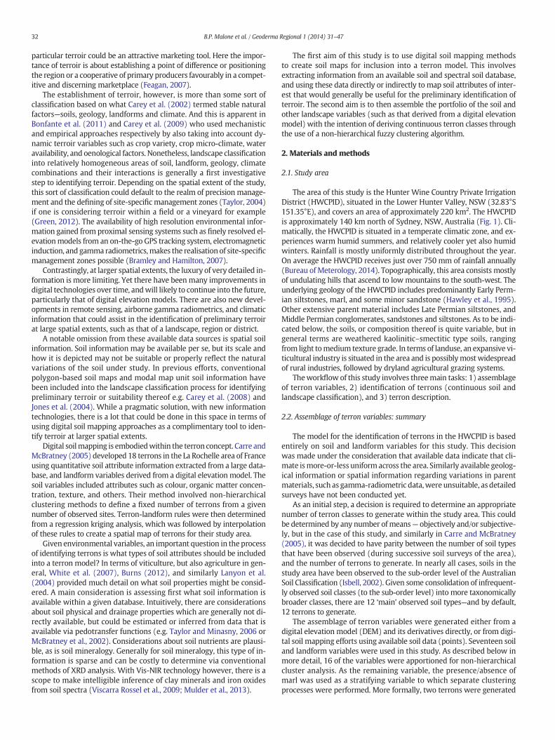
A model for the identification of terrons in the Lower Hunter Valley, Australia Brendan P. Malone ⁎, Philip Hughes, Alex B. McBratney, Budiman Minasny Faculty of Agriculture and Environment, The University of Sydney, Room 115, Biomedical Building, Australia Technology Park, Eveleigh, NSW 2015, Australia abstract article info Article history: Received 28 March 2014 Received in revised form 1 August 2014 Accepted 4 August 2014 Available online 8 August 2014 Keywords: Terroir Terron Digital soil mapping Wine region Soil-landscape characteristics WRB Luvisol Calcisol Gleysol Acrisol Cambisol Regosol Terroir in the Lower Hunter Valley – a prominent wine-producing region of Australia – is an appealing concept for landowners both in terms of enabling strategic land management and for positioning businesses favourably in a competitive consumer market. To those ends, preliminary steps are made in this study to establish common soil and landscape entities in the area using the terron concept that was proposed by Carré and McBratney (2005). Here soil and landscape variables were assembled and then used to generate 12 terrons or continuous soil- landscape units which are described quantitatively in terms of their distinguishing characteristics. Each terron is characterised by landscape variables (derived from a digital elevation model) and soil variables which include soil pH, clay percentage, soil mineralogy (clay types and presence of iron oxides), continuous soil classes, and presence or absence of marl. This study demonstrates a number of soil inferential techniques used for assembling the soil terron variables, based on common or easy to measure soil properties that populate most soil information databases. The approach is the first step in describing terroir; the next step will be to match the terrons with dif- ferent grape varietals. © 2014 Elsevier B.V. All rights reserved. 1. Introduction Terron, a soil and landscape concept, with an associated model, was described by Carre and McBratney (2005). The embodiment of terron is a continuous soil-landscape unit or class which combines soil knowl- edge, landscape information, and their interactions together. In some ways comparable to agroecozones (Liu and Samal, 2002), land systems (Chrisitan and Stewart, 1953), and terroir (Barham, 2003), terrons (plu- ral) can be described in terms of their soil and landscape attributes. A distinguishing characteristic of the terron concept, however, is that it has an underlying model, which is also based on the continuity of soil cover and landscape (Carre and McBratney, 2005). Thus terrons are ob- jectively realised, are observed as continuous entities across the land- scape, and their defining attributes can be described quantitatively. This objective and quantitative evaluation of soil and landscape is there- fore quite amenable for environmental assessment, such as determining land capability (or land evaluation) (Stewart, 1968), assessing enter- prise suitability (Kidd et al., 2012), and defining terroir-like zones of management (Taylor, 2004). Given an available soil information database, and information re- garding the landscape and digital modelling approaches, this study in- tends to explore the terron concept further as an initiating effort to indentifying terroir in the Lower Hunter Valley — a famous viticultural and wine producing region of Australia. A value-laden concept (Vaudour, 2002), terroir by definition refers to an area or terrain, usually small, whose soil and micro-climate impart distinctive qualities to food products (Wilson, 1998; Macqueen and Meinert, 2006; Dougherty, 2012). Terroir is usually associated with the production of wine, but is just as applicable to other agricultural domains and their related food products (Barham, 2003). Because the Lower Hunter Valley is situated in a predominantly viticultural zone, the con- cept is terroir has considerable appeal. From a land management per- spective, a terroir (or terron map in this case) map may be easier to interpret and more useful than just a soil map alone (Carre and McBratney, 2005). Additionally, terroir can be used for the determination of different agricultural areas or zones, and their suitability to produce or grow a given agricultural enterprise. In the case of wine production, identifying terroir could be reduced down to defining areas where viti- culture can be practiced, what varieties of grape can be grown and where, and what wine making styles are appropriate (Unwin, 2012). From a business perspective such as the advertising and labelling of food and wine products, the identification with and belongingness to a Geoderma Regional 1 (2014) 31–47 ⁎ Corresponding author. E-mail address: [email protected] (B.P. Malone). http://dx.doi.org/10.1016/j.geodrs.2014.08.001 2352-0094/© 2014 Elsevier B.V. All rights reserved. Contents lists available at ScienceDirect Geoderma Regional journal homepage: www.elsevier.com/locate/geodrs
-
Upload
khangminh22 -
Category
Documents
-
view
2 -
download
0
Transcript of malone2014_1.pdf - Smart Digital Agriculture
Geoderma Regional 1 (2014) 31–47
Contents lists available at ScienceDirect
Geoderma Regional
j ourna l homepage: www.e lsev ie r .com/ locate /geodrs
A model for the identification of terrons in the Lower HunterValley, Australia
Brendan P. Malone ⁎, Philip Hughes, Alex B. McBratney, Budiman MinasnyFaculty of Agriculture and Environment, The University of Sydney, Room 115, Biomedical Building, Australia Technology Park, Eveleigh, NSW 2015, Australia
⁎ Corresponding author.E-mail address: [email protected] (B.P.
http://dx.doi.org/10.1016/j.geodrs.2014.08.0012352-0094/© 2014 Elsevier B.V. All rights reserved.
a b s t r a c t
a r t i c l e i n f oArticle history:Received 28 March 2014Received in revised form 1 August 2014Accepted 4 August 2014Available online 8 August 2014
Keywords:TerroirTerronDigital soil mappingWine regionSoil-landscape characteristicsWRBLuvisolCalcisolGleysolAcrisolCambisolRegosol
Terroir in the LowerHunterValley– a prominentwine-producing region of Australia– is an appealing concept forlandowners both in terms of enabling strategic landmanagement and for positioning businesses favourably in acompetitive consumermarket. To those ends, preliminary steps are made in this study to establish common soiland landscape entities in the area using the terron concept that was proposed by Carré and McBratney (2005).Here soil and landscape variables were assembled and then used to generate 12 terrons or continuous soil-landscape units which are described quantitatively in terms of their distinguishing characteristics. Each terronis characterised by landscape variables (derived from a digital elevation model) and soil variables which includesoil pH, clay percentage, soil mineralogy (clay types and presence of iron oxides), continuous soil classes, andpresence or absence ofmarl. This study demonstrates a number of soil inferential techniques used for assemblingthe soil terron variables, based on common or easy tomeasure soil properties that populatemost soil informationdatabases. The approach is the first step in describing terroir; the next step will be to match the terrons with dif-ferent grape varietals.
© 2014 Elsevier B.V. All rights reserved.
1. Introduction
Terron, a soil and landscape concept, with an associated model, wasdescribed by Carre andMcBratney (2005). The embodiment of terron isa continuous soil-landscape unit or class which combines soil knowl-edge, landscape information, and their interactions together. In someways comparable to agroecozones (Liu and Samal, 2002), land systems(Chrisitan and Stewart, 1953), and terroir (Barham, 2003), terrons (plu-ral) can be described in terms of their soil and landscape attributes. Adistinguishing characteristic of the terron concept, however, is that ithas an underlying model, which is also based on the continuity of soilcover and landscape (Carre and McBratney, 2005). Thus terrons are ob-jectively realised, are observed as continuous entities across the land-scape, and their defining attributes can be described quantitatively.This objective and quantitative evaluation of soil and landscape is there-fore quite amenable for environmental assessment, such as determiningland capability (or land evaluation) (Stewart, 1968), assessing enter-prise suitability (Kidd et al., 2012), and defining terroir-like zones ofmanagement (Taylor, 2004).
Malone).
Given an available soil information database, and information re-garding the landscape and digital modelling approaches, this study in-tends to explore the terron concept further as an initiating effort toindentifying terroir in the Lower Hunter Valley — a famous viticulturaland wine producing region of Australia.
A value-laden concept (Vaudour, 2002), terroir by definition refers toan area or terrain, usually small, whose soil and micro-climate impartdistinctive qualities to food products (Wilson, 1998; Macqueen andMeinert, 2006; Dougherty, 2012). Terroir is usually associated with theproduction ofwine, but is just as applicable to other agricultural domainsand their related food products (Barham, 2003). Because the LowerHunter Valley is situated in a predominantly viticultural zone, the con-cept is terroir has considerable appeal. From a land management per-spective, a terroir (or terron map in this case) map may be easierto interpret and more useful than just a soil map alone (Carre andMcBratney, 2005). Additionally, terroir canbe used for the determinationof different agricultural areas or zones, and their suitability to produce orgrow a given agricultural enterprise. In the case of wine production,identifying terroir could be reduced down to defining areas where viti-culture can be practiced, what varieties of grape can be grown andwhere, and what wine making styles are appropriate (Unwin, 2012).From a business perspective such as the advertising and labelling offood and wine products, the identification with and belongingness to a
32 B.P. Malone et al. / Geoderma Regional 1 (2014) 31–47
particular terroir could be an attractive marketing tool. Here the impor-tance of terroir is about establishing a point of difference or positioningthe region or a cooperative of primary producers favourably in a compet-itive and discerning marketplace (Feagan, 2007).
The establishment of terroir, however, is more than some sort ofclassification based on what Carey et al. (2002) termed stable naturalfactors—soils, geology, landforms and climate. And this is apparent inBonfante et al. (2011) and Carey et al. (2009) who used mechanisticand empirical approaches respectively by also taking into account dy-namic terroir variables such as crop variety, crop micro-climate, wateravailability, and oenological factors. Nonetheless, landscape classificationinto relatively homogeneous areas of soil, landform, geology, climatecombinations and their interactions is generally a first investigativestep to identifying terroir. Depending on the spatial extent of the study,this sort of classification could default to the realm of precision manage-ment and the defining of site-specific management zones (Taylor, 2004)if one is considering terroir within a field or a vineyard for example(Green, 2012). The availability of high resolution environmental infor-mation gained from proximal sensing systems such as finely resolved el-evationmodels from an on-the-go GPS tracking system, electromagneticinduction, and gamma radiometrics,makes the realisation of site-specificmanagement zones possible (Bramley and Hamilton, 2007).
Contrastingly, at larger spatial extents, the luxury of very detailed in-formation is more limiting. Yet there have beenmany improvements indigital technologies over time, andwill likely to continue into the future,particularly that of digital elevation models. There are also new devel-opments in remote sensing, airborne gamma radiometrics, and climaticinformation that could assist in the identification of preliminary terroirat large spatial extents, such as that of a landscape, region or district.
A notable omission from these available data sources is spatial soilinformation. Soil information may be available per se, but its scale andhow it is depicted may not be suitable or properly reflect the naturalvariations of the soil under study. In previous efforts, conventionalpolygon-based soil maps and modal map unit soil information havebeen included into the landscape classification process for identifyingpreliminary terroir or suitability thereof e.g. Carey et al. (2008) andJones et al. (2004). While a pragmatic solution, with new informationtechnologies, there is a lot that could be done in this space in terms ofusing digital soil mapping approaches as a complimentary tool to iden-tify terroir at larger spatial extents.
Digital soilmapping is embodiedwithin the terron concept. Carre andMcBratney (2005) developed 18 terrons in the La Rochelle area of Franceusing quantitative soil attribute information extracted from a large data-base, and landform variables derived from a digital elevation model. Thesoil variables included attributes such as colour, organic matter concen-tration, texture, and others. Their method involved non-hierarchicalclustering methods to define a fixed number of terrons from a givennumber of observed sites. Terron-landform rules were then determinedfrom a regression kriging analysis, which was followed by interpolationof these rules to create a spatial map of terrons for their study area.
Given environmental variables, an important question in the processof identifying terrons is what types of soil attributes should be includedinto a terron model? In terms of viticulture, but also agriculture in gen-eral, White et al. (2007), Burns (2012), and similarly Lanyon et al.(2004) provided much detail on what soil properties might be consid-ered. A main consideration is assessing first what soil information isavailable within a given database. Intuitively, there are considerationsabout soil physical and drainage properties which are generally not di-rectly available, but could be estimated or inferred from data that isavailable via pedotransfer functions (e.g. Taylor and Minasny, 2006 orMcBratney et al., 2002). Considerations about soil nutrients are plausi-ble, as is soil mineralogy. Generally for soil mineralogy, this type of in-formation is sparse and can be costly to determine via conventionalmethods of XRD analysis. With Vis-NIR technology however, there is ascope to make intelligible inference of clay minerals and iron oxidesfrom soil spectra (Viscarra Rossel et al., 2009; Mulder et al., 2013).
The first aim of this study is to use digital soil mapping methodsto create soil maps for inclusion into a terron model. This involvesextracting information from an available soil and spectral soil database,and using these data directly or indirectly to map soil attributes of inter-est that would generally be useful for the preliminary identification ofterroir. The second aim is to then assemble the portfolio of the soil andother landscape variables (such as that derived from a digital elevationmodel) with the intention of deriving continuous terron classes throughthe use of a non-hierarchical fuzzy clustering algorithm.
2. Materials and methods
2.1. Study area
The area of this study is the Hunter Wine Country Private IrrigationDistrict (HWCPID), situated in the Lower Hunter Valley, NSW (32.83°S151.35°E), and covers an area of approximately 220 km2. The HWCPIDis approximately 140 km north of Sydney, NSW, Australia (Fig. 1). Cli-matically, the HWCPID is situated in a temperate climatic zone, and ex-periences warm humid summers, and relatively cooler yet also humidwinters. Rainfall is mostly uniformly distributed throughout the year.On average the HWCPID receives just over 750 mm of rainfall annually(Bureau of Meterology, 2014). Topographically, this area consists mostlyof undulating hills that ascend to low mountains to the south-west. Theunderlying geology of the HWCPID includes predominantly Early Perm-ian siltstones, marl, and some minor sandstone (Hawley et al., 1995).Other extensive parent material includes Late Permian siltstones, andMiddle Permian conglomerates, sandstones and siltstones. As to be indi-cated below, the soils, or composition thereof is quite variable, but ingeneral terms are weathered kaolinitic–smectitic type soils, rangingfrom light tomedium texture grade. In terms of landuse, an expansive vi-ticultural industry is situated in the area and is possiblymostwidespreadof rural industries, followed by dryland agricultural grazing systems.
Theworkflow of this study involves threemain tasks: 1) assemblageof terron variables, 2) identification of terrons (continuous soil andlandscape classification), and 3) terron description.
2.2. Assemblage of terron variables: summary
The model for the identification of terrons in the HWCPID is basedentirely on soil and landform variables for this study. This decisionwas made under the consideration that available data indicate that cli-mate ismore-or-less uniform across the area. Similarly available geolog-ical information or spatial information regarding variations in parentmaterials, such as gamma-radiometric data,were unsuitable, as detailedsurveys have not been conducted yet.
As an initial step, a decision is required to determine an appropriatenumber of terron classes to generate within the study area. This couldbe determined by any number ofmeans— objectively and/or subjective-ly, but in the case of this study, and similarly in Carre and McBratney(2005), it was decided to have parity between the number of soil typesthat have been observed (during successive soil surveys of the area),and the number of terrons to generate. In nearly all cases, soils in thestudy area have been observed to the sub-order level of the AustralianSoil Classification (Isbell, 2002). Given some consolidation of infrequent-ly observed soil classes (to the sub-order level) into more taxonomicallybroader classes, there are 12 ‘main’ observed soil types—and by default,12 terrons to generate.
The assemblage of terron variables were generated either from adigital elevation model (DEM) and its derivatives directly, or from digi-tal soil mapping efforts using available soil data (points). Seventeen soiland landform variables were used in this study. As described below inmore detail, 16 of the variables were apportioned for non-hierarchicalcluster analysis. As the remaining variable, the presence/absence ofmarl was used as a stratifying variable to which separate clusteringprocesses were performed. More formally, two terrons were generated
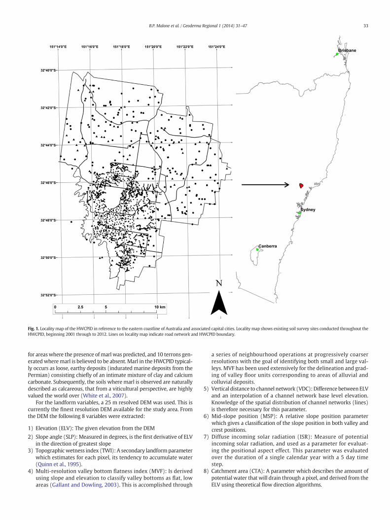
Fig. 1. Locality map of the HWCPID in reference to the eastern coastline of Australia and associated capital cities. Locality map shows existing soil survey sites conducted throughout theHWCPID, beginning 2001 through to 2012. Lines on locality map indicate road network and HWCPID boundary.
33B.P. Malone et al. / Geoderma Regional 1 (2014) 31–47
for areaswhere the presence ofmarl was predicted, and 10 terrons gen-eratedwheremarl is believed to be absent. Marl in the HWCPID typical-ly occurs as loose, earthy deposits (indurated marine deposits from thePermian) consisting chiefly of an intimate mixture of clay and calciumcarbonate. Subsequently, the soils where marl is observed are naturallydescribed as calcareous, that from a viticultural perspective, are highlyvalued the world over (White et al., 2007).
For the landform variables, a 25 m resolved DEM was used. This iscurrently the finest resolution DEM available for the study area. Fromthe DEM the following 8 variables were extracted:
1) Elevation (ELV): The given elevation from the DEM
2) Slope angle (SLP): Measured in degrees, is the first derivative of ELVin the direction of greatest slope
3) Topographicwetness index (TWI): A secondary landformparameterwhich estimates for each pixel, its tendency to accumulate water(Quinn et al., 1995).
4) Multi-resolution valley bottom flatness index (MVF): Is derivedusing slope and elevation to classify valley bottoms as flat, lowareas (Gallant and Dowling, 2003). This is accomplished through
a series of neighbourhood operations at progressively coarserresolutions with the goal of identifying both small and large val-leys. MVF has been used extensively for the delineation and grad-ing of valley floor units corresponding to areas of alluvial andcolluvial deposits.
5) Vertical distance to channel network (VDC): Difference betweenELVand an interpolation of a channel network base level elevation.Knowledge of the spatial distribution of channel networks (lines)is therefore necessary for this parameter.
6) Mid-slope position (MSP): A relative slope position parameterwhich gives a classification of the slope position in both valley andcrest positions.
7) Diffuse incoming solar radiation (ISR): Measure of potentialincoming solar radiation, and used as a parameter for evaluat-ing the positional aspect effect. This parameter was evaluatedover the duration of a single calendar year with a 5 day timestep.
8) Catchment area (CTA): A parameter which describes the amount ofpotential water that will drain through a pixel, and derived from theELV using theoretical flow direction algorithms.
34 B.P. Malone et al. / Geoderma Regional 1 (2014) 31–47
Algorithms for deriving these variables were implemented using theSAGA GIS software (http://www.saga-gis.org/en/index.html).
Eight soil variables (besides the presence of marl) used in this studyincluded:
1) The whole-soil averaged pH (to 1 m) (Bishop et al., 1999)2) The average sub-soil clay percentage (0.4–1 m)3) Soil drainage potential index (Malone et al., 2012)4) Soil mineralogy, specifically:
4.1. Likelihood of kaolinite presence4.2. Likelihood of the presence of a kaolinite and smectite mixture4.3. Likelihood of iron oxide presence
5) Classified soil classes, specifically:5.1. 1st principal component of continuous soil class predictions5.2. 2nd principal component of continuous soil class predictions.
These soil variables were selected for two main reasons: 1) toachieve a reasonable cross-section of attributes describing the physical,chemical andmineralogical properties of the soil, and 2) to use most ef-fectively the data that are stored within the available soil informationdatabase. Described in more detail below, the database used in thisstudy has many observations of soil classes, soil pH, clay percentageand colour, with limited observations of other usually commonly ob-served attributes such as soil organic carbon and exchangeable cations.Thus the intention overall was to make the most use out of what datawas ‘plentiful’. In terms of the soil mineralogical variables, Generallythis information is scarce in soil databases, but because a number ofthe soils examined have vis-NIR spectra, some estimate that their min-eral compositions could be approximated from these, for which is alsodescribed in more detail below.
In terms of available soil data for the calibration of spatial soil predic-tion functions, there is, in total, 1691 individual locationswhere soil hasbeen observed and described in one form or another (Fig. 1). These datahave been collected over successive years beginning in 2001 to thepresent time, and more detailed descriptions of them can be found inMalone et al. (2011) and Odgers et al. (2011). Essentially, all thesedata are compiled into a single database table which contains separatecolumns for different soil attributes (in addition to columns for labels,coordinates, soil depths and horizon nomenclature, etc.). Each row isan observation made for a particular location at a particular genetic ho-rizon, or sometimes a specified depth interval, and in many cases, theindividual observations have a measured Vis-NIR spectrum as well.Yet this database is by nomeans fully populatedwith a full complementofmeasured soil attributes or soil spectra at every sample. Therefore, foreach of the soil terron variables of interest in this study, filtering stepswere performed to remove missing data (instances where no datawas recorded for a whole profile), and other data anomalies such asmissing spatial coordinates.
The soil variables were mapped using the digital soil mappingscorpan approach (McBratney et al., 2003):
Sc x; y;� t½ � or Sp x; y;� t½ �¼ f s x; y;� t½ �; c x; y;� t½ �; o x; y;� t½ �; r x; y;� t½ �; p x; y;� t½ �; a x; y;� t½ �; nð Þ
ð1Þ
where:
Sc soil classSp soil propertys soils, other attributes of the soil at a pointc climate, climatic properties of the environment at a pointo organisms, vegetation, or fauna, or human activityr topography, landscape attributesp parent material, lithologya age, the time factorn space, spatial positiont time (where t is defined as an approximate time)
x,y the explicit spatial coordinatesf function or soil spatial prediction function (SSPF)
2.3. Assemblage of terron variables: specific description of soil variablemapping
The soil terron variables are mapped in Figs. 2 and 3. Following nowis the description of the pertinent information regarding how these var-iables were mapped across the HWCPID to 25 m resolution (the sameresolution and extent as for the landform variables). This informationis also summarised in Table 1.
2.3.1. Estimation of marl presence and whole-soil pH averageAfter data filtering, 1399 soil profiles remained that contained
measurements of soil pH (1:5 soil:water suspension) (Rayment andHigginson, 1992). These measurements, taken at various times, wereeither made directly in the field at the time of soil description or laterin a laboratory. In order to proceed with DSM, a continuous mass-preserving spline depth function (Bishop et al., 1999) was fitted toeach soil pH profile. This function was then integrated to return the av-erage for the 0–1 m depth interval. If a soil profile was not observed toreach beyond 1 m, the average for the whole profile was recorded.
Regression krigingwas used as the spatial predictionmodel formap-ping. Data were split into calibration and validation datasets (70% and30% respectively). Cubist regression tree models (Quinlan, 1992) wereused for regressing the averaged soil pH values against a suite of co-located environmental covariates. Some of the covariates have beendescribed above, in addition to further terrain variables plus other envi-ronmental covariates such as normalised difference vegetation index(NDVI) and other spectral combinations or ratios derived from LandsatETM+ imagery e.g. Band 3/Band 2, Band 3/Band 7, and Band 5/Band 7were used. Further information about soil enhancement ratios can befound in Boettinger et al. (2008). The Landsat ETM+ imagery used inthis work was collected during the southern hemisphere spring (Sep-tember) of 2009, which coincides with a time where rainfall is at itslong-term low, and when exposed soil cover is expected to be greatest.
Variography of the residuals (from the Cubist modelling) was usedto examine their spatial correlation structure. Given the number ofdata available, it was deemed suitable to use locally fitted variogramsbased on the nearest 200 points for spatial interpolation of the residualsacross the HWCPID. As a final step to regression kriging, the twomaps—the one derived from regression modelling and the other from residualkriging, were summed (Fig. 2). The validation dataset indicated that theroot mean square error of prediction for the soil pH was 0.76 pH units,which is similar to that observed in Malone et al. (2011).
Mapping the presence of marl involved application of expert knowl-edge, traditional GIS data analysis, and digital soil mapping. From theknowledge developed in the study area, a high soil pH in the sub-soilat a relatively high elevation and in areas that do not accumulatewater flow, is generally an indicative criterion for detecting marl pres-ence in a soil. Firstly using the spline fitted depth functions of soil pHat each profile, described previously, integration was performed to re-trieve the average soil pH between 0.4 and 1 m depth. Then using thisdata and their collocated values of ELV and TWI, each soil profile wasassessed for the presence or absence of marl. From some iteration, thecriteria ultimately used was averaged sub-soil pH N 6.85, ELV N 90 m,and TWI N 12. The threshold criteria were not optimised; instead, anumber of realistic combinations were tried before deciding that thefinal result – number of profiles detected as having marl present – didnot vary that much overall. From this process there were 122 and1277 soil profiles indicating either the presence or absence of marl re-spectively. Keeping the calibration and validation data configuration(70/30 random split) used for the spatial prediction of whole-profilesoil pH, a binary logistic model was used to regress the presence/
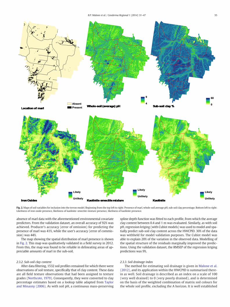
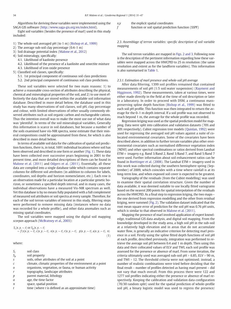
Fig. 2.Maps of soil variables for inclusion into the terronmodel. Beginning from the top left to right: Presence ofmarl, whole-soil average pH, sub-soil clay percentage. Bottom left to right:Likeliness of iron oxide presence, likeliness of kaolinite–smectite mixture presence, likeliness of kaolinite presence.
35B.P. Malone et al. / Geoderma Regional 1 (2014) 31–47
absence of marl data with the aforementioned environmental covariatepredictors. From the validation dataset, an overall accuracy of 92% wasachieved. Producer's accuracy (error of omission) for predicting thepresence of marl was 41%, while the user's accuracy (error of commis-sion) was 44%.
The map showing the spatial distribution of marl presence is shownin Fig. 2. This map was qualitatively validated in a field survey in 2012.From this, the map was found to be reliable in delineating areas of ap-preciable amounts of marl in the sub-soil.
2.3.2. Sub-soil clay contentAfter data filtering, 1532 soil profiles remained for which there were
observations of soil texture, specifically that of clay content. These dataare all field texture observations that had been assigned to texturegrades (Northcote, 1979). Consequently, they were converted to claypercentage estimates based on a lookup table adapted from Taylorand Minasny (2006). As with soil pH, a continuous mass-preserving
spline depth function was fitted to each profile, fromwhich the averageclay content between 0.4 and 1 m was evaluated. Similarly, as with soilpH, regression kriging (with Cubistmodels)was used tomodel and spa-tially predict sub-soil clay content across the HWCPID. 30% of the datawas withheld for model validation purposes. The Cubist model wasable to explain 20% of the variation in the observed data. Modelling ofthe spatial structure of the residuals marginally improved the predic-tions. Using the validation dataset, the RMSEP of the regression krigingpredictions was 9%.
2.3.3. Soil drainage indexThe method for estimating soil drainage is given in Malone et al.
(2012), and its application within the HWCPID is summarised there-in as well. Soil drainage is described as an index on a scale of 100(very well drained) to 0 (very poorly drained), and is determinedon the basis of the weighted combination of matrix soil colours forthe whole soil profile, excluding the A horizon. It is well established
Fig. 3. Soil class map of the HWCPID and associated first two principal component maps of the prediction confidences from See5 modelling.
36 B.P. Malone et al. / Geoderma Regional 1 (2014) 31–47
that soil colour can be used as a general purpose indicator of inter-nal soil drainage (Evans and Franzmeier, 1988). In the HWCPID, ared → brown → yellow → grey → black matrix soil colour sequenceis often indicative of soils ranging from well draining (red) to poorlydraining (black) (Kovac and Lawrie, 1990).
Because Munsell® HVC is not directly conducive for quantitativestudies; the drainage index calculation of Malone et al. (2012) is firstinitiated by converting soil colour descriptions to the CIELAB colourspace (Robertson, 1976; CIE, 1978). Next, archetypal colour/s to eachsoil of the drainage sequence is ascertained empirically from the avail-able soil colour dataset. A Euclidean distance is calculated to compareeach observation with each archetypal soil colour. The distances arethen used for a fuzzy classifier to assign each soil a fuzzy membershipto each soil colour class. An estimate of soil drainage is then calculatedthrough weighted averaging of the fuzzy memberships and the associ-ated value assigned to each archetypal colour. In this case, the archetyp-al red is assigned a value of 100, brown (75), yellow (50), grey (25), andblack (0).
From Malone et al. (2012), statistical relationships were found be-tween the soil drainage index and a number of terrain variables, nota-bly, the distance to a channel network and topographic wetness indexin the HWCPID. Independently validated, the spatial model (regressionkriging using Cubist models) of soil drainage index revealed a RMSEP of22 points. Themap in Fig. 2 shows the spatial variation of the soil drain-age index across the HWCPID.
2.3.4. Soil mineralogyVis-NIR spectroscopywas used for the detection of claymineral spe-
cies and iron oxides as an analytical step prior to mapping their spatialdistribution across the study area. Clay minerals and iron oxides absorbat specific wavelengths in the vis-NIR range of the electro-magneticspectrum (Clark et al., 1990). Subsequently, previous studies have dem-onstrated the use of soil vis-NIR spectra in soil compositional studieswith notable success (Viscarra Rossel et al., 2009; Brown et al., 2006).In the present work, 354 soil profiles (1571 soil horizons) have vis-NIRspectra for each of their recorded depths. Spectroscopic measurementwas made with an Agrispec portable spectrophotometer with a contactprobe attachment (Analytical Spectral Devices, Boulder, Colorado). This
particular instrument has a spectral range between 350 and 2500 nm.Soil samples were in air-dry condition and ground to b2 mm prior toscanning. To reduce signal-to-noise ratios of the spectra, five scansof each sample were performed, from which an averaged reflectancespectrum was derived. Calibration of the instrument was made with aSpectralon white tile and was re-calibrated after every 15 scans or 3samples.
Reference mineral spectra of the following end member clay min-erals and iron oxides were retrieved from U.S. Geological Survey digitalspectral library (Clark et al., 2007): kaolinite (KGa-2), illite (GDS4),smectite (SWy-1), kaolinite–smectite 50/50 mixture (H89-FR-2), goe-thite (GDS240), and hematite (GDS576). Clark et al. (2003) documentthe diagnostic wavelengths of these end member specimens whichare summarised in Table 2. The idea behind assessing the mineral com-position of soils with vis-NIR spectroscopy is to compare the reflectanceof the diagnostic wavelengths from the reference spectra with the re-flectance at the same wavelengths of the soil samples. To initiate this,for each of the reference and soil spectra, the wavelength ranges specif-ically diagnostic to each claymineral and iron oxide specimenwere iso-lated. Each range was then normalised separately by fitting a convexhull to it, followed by computation of the deviation from the fittedhull (Clark and Roush, 1984). Fig. 4 shows an example of the fitted con-vex hulls to the diagnostic reflectance ranges from the reference spectrafor smectite and kaolinite and the associated spectra once the continu-um is removed.
Once all the soil spectra have been normalised, the likely presence ofeach clay mineral and iron oxide in each soil is estimated when it iscompared to that of the normalised reference spectra. The methodused in this study is based on the approach developed by the U.S. Geo-logical Survey and implemented in their Tetracorder decision makingframework (Clark et al., 2003). Fundamentally, Tetracorder uses ashape-fitting algorithm, which essentially reduces down to a least-squares fit between the reference spectra and the observed soil spectra.The correlation coefficient of this fit (F) is a quantitative estimate of theshape similarity between the reference and soil spectra. The importanceof thismeasure can be exemplified in Fig. 4where both smectite and ka-olinite have similar diagnostic wavelength ranges yet quite different re-flectance behaviour—kaolinite with the distinctive doublet feature,
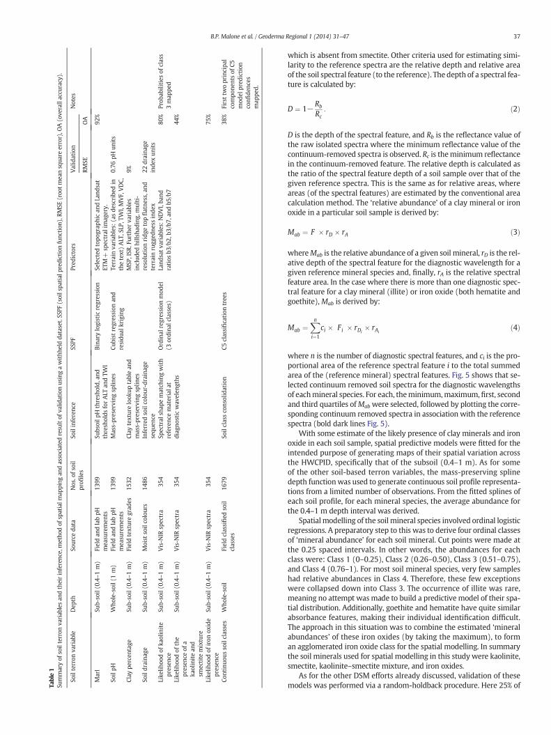
Table1
Summaryof
soilterron
variab
lesan
dtheirinferenc
e,metho
dof
spatialm
apping
andassociated
resu
ltof
valid
ationus
ingawithh
eldda
taset.SS
PF(soilspa
tial
pred
iction
func
tion
),RM
SE(roo
tmeansqua
reerror),O
A(ove
rallaccu
racy).
Soilterron
variab
leDep
thSo
urce
data
Nos.o
fsoil
profi
les
Soilinferenc
eSS
PFPred
ictors
Validation
Notes
RMSE
OA
Marl
Sub-soil(0
.4–1m)
Fieldan
dlabpH
mea
suremen
ts13
99Su
bsoilp
Hthresh
old,
and
thresh
olds
forALT
andTW
IBina
rylogistic
regression
Selected
topo
grap
hican
dLand
sat
ETM
+sp
ectral
imag
ery.
Terrainva
riab
les:
(asde
scribe
din
thetext)ALT
,SLP
,TW
I,MVF,VDC,
MSP
,ISR
.Further
variab
les
includ
edhills
hading
,multi-
resolution
ridg
etopflatne
ss,a
ndterrainrugg
edne
ssinde
xLand
satva
riab
les:
NDVI,ba
ndratios
b3/b2,
b3/b7,
andb5
/b7
92%
SoilpH
Who
le-soil(1m)
Fieldan
dlabpH
mea
suremen
ts13
99Mass-preserving
splin
esCu
bist
regression
and
residu
alkriging
0.76
pHun
its
Clay
percen
tage
Sub-soil(0
.4–1m)
Fieldtexturegrad
es15
32Clay
texturelook
uptablean
dmass-preserving
splin
es9%
Soildraina
geSu
b-soil(0
.4–1m)
Moist
soilco
lours
1486
Inferred
soilco
lour-drainag
esequ
ence
22draina
geinde
xun
its
Like
lihoo
dof
kaolinite
presen
ceSu
b-soil(0
.4–1m)
Vis-N
IRsp
ectra
354
Spectral
shap
ematch
ingwith
referenc
emateriala
tdiag
nostic
wav
elen
gths
Ordinal
regression
mod
el(3
ordina
lclasses)
80%
Prob
abilities
ofclass
3map
ped
Like
lihoo
dof
the
presen
ceof
aka
olinitean
dsm
ectite
mixture
Sub-soil(0
.4–1m)
Vis-N
IRsp
ectra
354
44%
Like
lihoo
dof
iron
oxide
presen
ceSu
b-soil(0
.4–1m)
Vis-N
IRsp
ectra
354
75%
Continuo
ussoilclasses
Who
le-soil
Fieldclassified
soil
classes
1679
Soilclassco
nsolidation
C5classification
tree
s38
%Firsttw
oprincipa
lco
mpo
nentsof
C5mod
elpred
iction
confi
denc
esmap
ped.
37B.P. Malone et al. / Geoderma Regional 1 (2014) 31–47
which is absent from smectite. Other criteria used for estimating simi-larity to the reference spectra are the relative depth and relative areaof the soil spectral feature (to the reference). The depth of a spectral fea-ture is calculated by:
D ¼ 1−Rb
Rc: ð2Þ
D is the depth of the spectral feature, and Rb is the reflectance value ofthe raw isolated spectra where the minimum reflectance value of thecontinuum-removed spectra is observed. Rc is theminimum reflectancein the continuum-removed feature. The relative depth is calculated asthe ratio of the spectral feature depth of a soil sample over that of thegiven reference spectra. This is the same as for relative areas, whereareas (of the spectral features) are estimated by the conventional areacalculation method. The ‘relative abundance’ of a clay mineral or ironoxide in a particular soil sample is derived by:
Mab ¼ F � rD � rA ð3Þ
whereMab is the relative abundance of a given soil mineral, rD is the rel-ative depth of the spectral feature for the diagnostic wavelength for agiven reference mineral species and, finally, rA is the relative spectralfeature area. In the case where there is more than one diagnostic spec-tral feature for a clay mineral (illite) or iron oxide (both hematite andgoethite),Mab is derived by:
Mab ¼Xn
i¼1
ci � Fi � rDi� rAi
ð4Þ
where n is the number of diagnostic spectral features, and ci is the pro-portional area of the reference spectral feature i to the total summedarea of the (reference mineral) spectral features. Fig. 5 shows that se-lected continuum removed soil spectra for the diagnostic wavelengthsof eachmineral species. For each, theminimum,maximum,first, secondand third quartiles ofMab were selected, followed by plotting the corre-sponding continuum removed spectra in association with the referencespectra (bold dark lines Fig. 5).
With some estimate of the likely presence of clay minerals and ironoxide in each soil sample, spatial predictive models were fitted for theintended purpose of generating maps of their spatial variation acrossthe HWCPID, specifically that of the subsoil (0.4–1 m). As for someof the other soil-based terron variables, the mass-preserving splinedepth functionwas used to generate continuous soil profile representa-tions from a limited number of observations. From the fitted splines ofeach soil profile, for each mineral species, the average abundance forthe 0.4–1 m depth interval was derived.
Spatialmodelling of the soil mineral species involved ordinal logisticregressions. A preparatory step to this was to derive four ordinal classesof ‘mineral abundance’ for each soil mineral. Cut points were made atthe 0.25 spaced intervals. In other words, the abundances for eachclass were: Class 1 (0–0.25), Class 2 (0.26–0.50), Class 3 (0.51–0.75),and Class 4 (0.76–1). For most soil mineral species, very few sampleshad relative abundances in Class 4. Therefore, these few exceptionswere collapsed down into Class 3. The occurrence of illite was rare,meaning no attempt wasmade to build a predictive model of their spa-tial distribution. Additionally, goethite and hematite have quite similarabsorbance features, making their individual identification difficult.The approach in this situation was to combine the estimated ‘mineralabundances’ of these iron oxides (by taking the maximum), to forman agglomerated iron oxide class for the spatial modelling. In summarythe soil minerals used for spatial modelling in this study were kaolinite,smectite, kaolinite–smectite mixture, and iron oxides.
As for the other DSM efforts already discussed, validation of thesemodels was performed via a random-holdback procedure. Here 25% of

Table 2Diagnostic wavelength ranges of clay minerals and iron oxides investigated in this study.
Mineral Diagnostic wavelength range/s
Kaolin 2079–2277 nmSmectite 2118–2287 nmKaolin-smectite 50–50 mixture 2128–2258 nmIllite 2155–2266 nm, 2306–2385 nmGoethite 457–563 nm, 776–1266 nmHematite 455–612 nm, 765–1050 nm
38 B.P. Malone et al. / Geoderma Regional 1 (2014) 31–47
the available data for each model was withheld from the model fittingprocess.
Specifically in terms of the spatial modelling, ordinal logistic regres-sion is an extension of logistic regression such that regression coeffi-cients are estimated (typically by maximum likelihood estimation) topredict the probability of a discrete outcome (such as a class) occurring(Hastie et al., 2001). This is performed using a logit link function, whichis the natural logarithm of the odds (log-odds) of a particular class orevent being observed. The proportional odds model (POM) is the most
Fig. 4.Diagnostic wavelength ranges for smectite and kaolinite. To prepare for analyses, spectracompared on the basis of the continuum removed spectra.
popular model for ordinal logistic regression (Agresti, 1984), and is anextension of logistic regression because it allows ordered data to bemodelled by analysing it as a number of dichotomies. For example, a bi-nary logistic regression model compares one dichotomy (e.g. the pres-ence or absence of marl model), whereas the proportional odds modelcompares a number of dichotomies by arranging the ordered categoriesinto a series of binary comparisons. A binary logistic regressionmodels asingle logit; the POM on the other hand models several cumulativelogits. Therefore, in the case of having 3 ordinal classes, 2 logits aremodelled, one for each of the following class cut points: Class 1 vs.Class 2, Class 3 vs. Class 1, and Class 2 vs. Class 3. From simple inferenceof these models, the probability of each ordinal class occurring can bemade. Agresti (1984) describes the theoretical framework of POMs ingreater detail. From validation (n= 89), the overall accuracy of the or-dinal models was: iron oxides — 75%, kaolinite — 80%, smectite — 40%,and kaolinite–smectite mixture — 44%. In consideration of the terronmodel, the 3 most accurately predicted variables for inclusion were se-lected. Mapping the three soil minerals (sub-soil iron oxides, kaolinite,and kaolinite–smectite mixture) involved mapping the probabilities of
need to be normalised by fitting a convex hull. Soil spectra and reference spectra are then
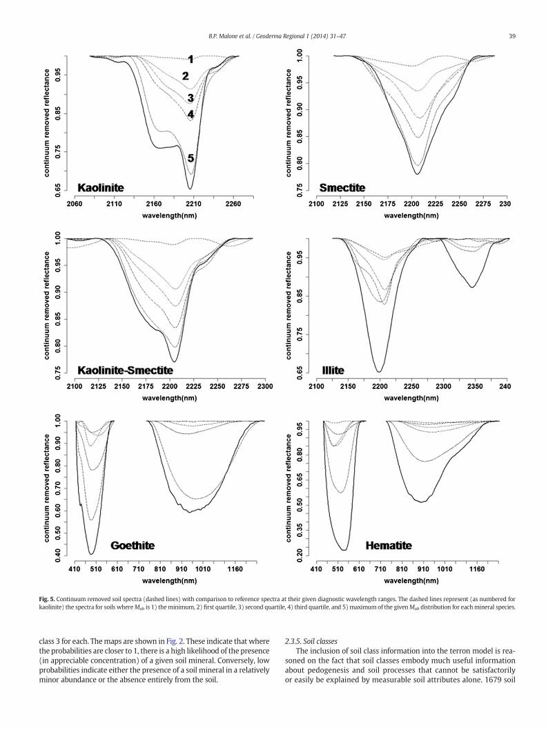
Fig. 5. Continuum removed soil spectra (dashed lines) with comparison to reference spectra at their given diagnostic wavelength ranges. The dashed lines represent (as numbered forkaolinite) the spectra for soils whereMab is 1) theminimum, 2) first quartile, 3) second quartile, 4) third quartile, and 5)maximum of the givenMab distribution for eachmineral species.
39B.P. Malone et al. / Geoderma Regional 1 (2014) 31–47
class 3 for each. Themaps are shown in Fig. 2. These indicate that wherethe probabilities are closer to 1, there is a high likelihood of the presence(in appreciable concentration) of a given soil mineral. Conversely, lowprobabilities indicate either the presence of a soil mineral in a relativelyminor abundance or the absence entirely from the soil.
2.3.5. Soil classesThe inclusion of soil class information into the terron model is rea-
soned on the fact that soil classes embody much useful informationabout pedogenesis and soil processes that cannot be satisfactorilyor easily be explained by measurable soil attributes alone. 1679 soil
40 B.P. Malone et al. / Geoderma Regional 1 (2014) 31–47
profiles in the available database have been classified to the sub-orderlevel of the Australian Soil Classification System (Isbell, 2002). A generalguide on theirWorld Reference Base (WRB) (IUSSWorkingGroupWRB,2007) and Soil Taxonomy (Soil Survey Staff, 2010) counterparts can befound inMorand (2013) or Isbell et al. (1997). At the Sub-Order level ofthe Australian Soil Classification, there have been 53 different soil typesobserved in the HWCPID. However 72% or 1201 are one of either foursoils: Brown Dermosol or Chromosol, or Red Dermosol or Chromosol(WRB Luvisols or Lixisols). As may be surmised, many of the soil typeshave been observed once or only a few times. Therefore to facilitatesoil class modelling, soil classes were consolidated into the followinggeneralised soil types (their proportion of the total observed populationin brackets): Calcarosols (Calcisols) (2%), Red Chromosols (8%), BrownChromosols (12%), other Chromosols (2%), Brown Dermosols (26%),Red Dermosols (26%), other Dermosols (7%), Hydrosols (Gleysols,Stagnosols, Fluvisols) (2%), Red Kurosols (Acrisols) (5%), other Kurosols(Acrisols) (4%), Tenosols (Regosols, Cambisols) (4%), and Kandosols(Cambisols) (2%).
After intersecting these observations with a suite of environmentalcovariates, followed by splitting the data into calibration–validationdatasets (75%–25%), Quinlan's C5.0 algorithm (Quinlan, 1993) wasused to fit a classification tree model to the calibration data. As de-scribed in Moran and Bui (2002), classification trees (or the algorithmthat builds them) partition a dataset into successionally more homoge-neous subsets. Nodes are where trees branch or split the dataset; termi-nal nodes are called leaves. At each node of the tree, C5.0 splits the datain such a way that most effectively results in subsets enriched in oneclass or another, and is more formally expressed as the normalised in-formation gain or difference in entropy (Quinlan, 1993). The attributewith the highest normalised information gain is chosen tomake the de-cision. Validation of the C5.0 model fitted to the soil class data resultedin an overall accuracy of 38%. The kappa (k) statistic for this model wasof fair agreement (k = 0.2).
The C5.0modelwas applied for thewhole study area, resulting in themap of Fig. 5 which displays the soil classes as Australian soil classes.Possibly due to the relative proportions of each soil class, four of thesoil classes were not predicted using this C5.0 model. As can be seen,it is quite clear of the dominance of Brown and Red Dermosols acrossthe HWCPID. This map however, because of its categorical nature isnot suitable to be included into the terronmodel, which can only permitcontinuous variables in its current form. To avert this issue, the predic-tion confidence values that are determined from the C5.0 model wereinvestigated. The confidence values of each class are given for everycase or prediction location, and range between 0 (no confidence) and1 (undoubtable confidence), and sum to unity across all classes. If acase is classified by a single leaf of a decision tree, the confidencevalue is the proportion of training cases at that leaf that belong to thepredicted class (pers. comm. R. Quinlan). If more than one leaf is in-volved (i.e., one or more of the attributes on the path has missingvalues), the value is a weighted sum of the individual leaves' confi-dences. Principal component analysis was used to reduce the vari-able dimension of the class confidences (12) to just a few (2) mainvariables. The first two principal components captured 82% of thevariation in the prediction confidences. These maps are displayedin Fig. 3, and by all accounts display the spatial variation patternsof the predicted soil classes.
2.4. Identification of terrons
Non-hierarchical fuzzy cluster analysis was performed on the fullyassembled suite of soil and landform variables. This was performedseparately for the areas where marl was predicted as being presentand where it was absent. For the area with marl present, the fuzzyk-means algorithm (Bezdek et al., 1984) was used to generate two clas-ses based on the 16 terron variables. Similarly, for the area with marl ab-sent, 10 classes were generated. The fuzzy-k algorithmwas implemented
through the stand-alone FuzMe software (Minasny and McBratney,2002). Besides setting the number of specified classes, Mahalanobisdistance was used for evaluating distance metrics in the fuzzy-kalgorithm – unlike Euclidean distance, the Mahalanobis distancetakes into account the correlation between input variables – and afuzzy exponent value of 1.2 was used. See McBratney and de Gruijter(1992) for a more detailed explanation of the algorithm. The outputsfrom both separate analyses, namely the membership classes, werere-assembled for mapping the spatial distribution of each terron.
3. Results
The two terrons for wheremarl was predicted to be presentwere la-belled as HVT_001 and HVT_002. The other 10 terronswere labelled se-quentially from HVT_003 to HVT_012. Maps of the terrons and theirmembership grades are shown in Fig. 6 with black colouring indicatinga high membership to a particular terron. By assigning each grid cell tothe terron of highest membership (i.e. hardening), a summary of eachterron's soil and landscape attributes is provided in Table 3. Thequantitative variables are summarised as a range of the 2.5% and97.5% quantiles. Regarding the soil classes, instead of summarisingthe principal components of the soil class probabilities, they aresummarised according to the most relevant consolidated AustralianSoil Classes that are mapped/occur in the given terron. Fig. 7 displaysthe associated spatial distribution of the hardened terrons across theHWCPID.
As a further aid to interpreting the different terron classes, Ward'smethod (Ward, 1963) of clustering or agglomerative hierarchical clus-tering was performed to examine their taxonomic similarities anddifferences. The dendrogram depicted in Fig. 8 shows the result ofthis agglomeration, whereby the terron centroids (resultant from thefuzzy clustering procedures) were used for the analysis. To accompanyFig. 8, Table 4 shows to Mahalanobis distance (taxonomic distance ma-trix) between terrons, and which was used for the hierarchical cluster-ing. Based on 1-way ANOVA tests between terron class and each inputterron soil and landscape variable, a significant difference (P b 0.001)was observed. But as can be observed from Table 4 and Fig. 8, someterron classes can be easily distinguished, while others share similari-ties. Fig. 9 shows the score plots of the first two principle componentsof the terron input variables. The scores of each terron class are colouredseparately. The first principle components explain 38% of the wholedata variation while the second component explained a further 18%. Inthe principle component space it is possible to visually distinguish be-tween the terrons, and also detect similarities. For example HVT_001and HVT_002 occupy similar regions of the principle componentspace, but together are quite distinct from the other terrons. Similar-ly, HVT_005 and HVT_008 are similar, which are both quite distinctfrom either HVT_006 or HVT_007 etc.
3.1. Terron descriptions
Using the information contained in Tables 3 and 4, and Figs. 7, 8 and9, a summary of the pertinent characteristics of each terron class isprovided.
3.1.1. HVT_001This terron is first of the marl terrons, and appears to be dominantly
situated to the south-west of the study area. Soils are dominantly Redand Brown Dermosols. Some Calcarosols are also present which is tobe expected given the calcareous nature of some of the parent materialhere. Subsequently the soils in this terron relative to other terrons havea higher pH. Soil clay content varies considerably in this terron whichcould be resultant from the nature of the parent material and the vari-ability of the terrain. In terms of landform, this terron is situated in a rel-atively high elevation position and is quite variable in terms of the slope.Soils are generallymoderate towell draining, based on the soil drainage
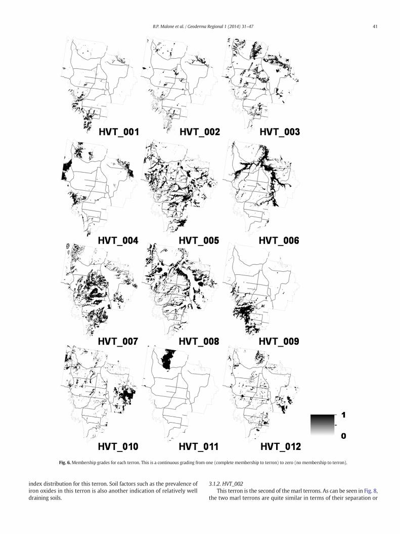
Fig. 6.Membership grades for each terron. This is a continuous grading from one (complete membership to terron) to zero (no membership to terron).
41B.P. Malone et al. / Geoderma Regional 1 (2014) 31–47
index distribution for this terron. Soil factors such as the prevalence ofiron oxides in this terron is also another indication of relatively welldraining soils.
3.1.2. HVT_002This terron is the second of themarl terrons. As can be seen in Fig. 8,
the two marl terrons are quite similar in terms of their separation or
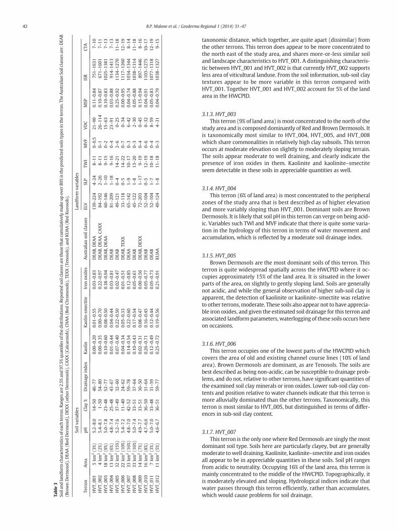
Table3
Soilan
dland
form
characteristicsof
each
terron
.Ran
gesare2.5%
and97
.5%qu
antileso
fthe
distribu
tion
s.Re
ported
soilclassesa
rethosethat
cumulativelymak
eup
over
80%isthepred
ictedsoils
type
sintheterron
.The
Aus
tralianSo
ilclassesare:
DEA
B(B
rownDermosol),DEA
A(R
edDermosol),DEX
X(other
Dermosols),C
AXX(C
alcarosols),CH
AA(R
edCh
romosols),T
EXX(Ten
osols),and
KUAA(R
edKurosols).
Soilva
riab
les
Land
form
variab
les
Terron
Area
pHClay
%Drainag
einde
xKao
linKao
lin-smectite
Iron
oxides
Aus
traliansoilclasses
ELV
SLP
TWI
MVF
VDC
MSP
ISR
CTA
HVT_
001
5km
2(3
%)5.2–
8.0
14–50
46–77
0.00
–0.20
0.01
–0.55
0.03
–0.83
DEA
B,DEA
A13
9–22
44–
248–
110–
0.5
21–90
0.11
–0.84
751–
1631
7–10
HVT_
002
4km
2(2
%)5.4–
8.1
1–50
54–80
0.00
–0.35
0.00
–0.70
0.22
–0.97
DEA
B,DEA
A,C
AXX
84–19
22–
268–
110–
126
–11
40.10
–0.87
671–
1601
7–11
HVT_
003
18km
2(9
%)5.0–
7.8
23–48
52–77
0.10
–0.60
0.08
–0.50
0.38
–0.94
DEA
B,DEA
A60
–14
61–
109–
150–
215
–63
0.10
–0.83
1025
–13
817–
13HVT_
004
13km
2(6
%)4.8–
7.4
25–48
43–67
0.01
–0.44
0.04
–0.44
0.03
–0.81
DEA
B81
–20
91–
189–
160–
423
–91
0.03
–0.88
914–
1413
7–13
HVT_
005
32km
2(1
5%)
5.2–
7.6
37–49
32–60
0.07
–0.40
0.22
–0.50
0.02
–0.47
DEA
B49
–12
10–
414
–21
2–6
0–25
0.25
–0.92
1134
–12
7011
–18
HVT_
006
22km
2(1
0%)
5.4–
7.2
11–40
24–62
0.04
–0.34
0.05
–0.33
0.01
–0.51
DEA
B,TE
XX
33–11
80–
514
–22
0–7
0–34
0.00
–0.95
1117
–12
6012
–19
HVT_
007
33km
2(1
6%)
4.8–
7.0
42–52
59–78
0.14
–0.54
0.22
–0.60
0.12
–0.85
DEA
A65
–14
21–
910
–17
0–3
6–42
0.04
–0.74
1034
–13
448–
14HVT_
008
33km
2(1
6%)
5.0–
7.4
33–51
37–64
0.10
–0.43
0.17
–0.54
0.05
–0.61
DEA
B45
–12
21–
813
–20
0–3
2–30
0.05
–0.88
1038
–13
1411
–18
HVT_
009
14km
2(7
%)4.9–
7.7
33–51
30–50
0.02
–0.31
0.08
–0.47
0.00
–0.56
DEA
B,DEX
X72
–20
31–
179–
190–
40–
450.15
–0.94
897–
1446
8–16
HVT_
010
16km
2(8
%)4.7–
6.6
36–50
31–64
0.26
–0.71
0.16
–0.45
0.05
–0.77
DEA
B52
–10
40–
512
–19
0–6
0–32
0.04
–0.91
1103
–12
7510
–17
HVT_
011
7km
2(3
%)5.0–
7.0
33–48
31–59
0.12
–0.49
0.12
–0.44
0.05
–0.73
DEA
B52
–10
41–
710
–18
0–4
8–59
0.05
–0.83
1077
–13
1812
–19
HVT_
012
11km
2(5
%)4.6–
6.7
36–51
59–77
0.25
–0.72
0.19
–0.56
0.21
–0.91
KUAA
49–12
41–
811
–18
0–3
4–31
0.04
–0.79
1038
–13
279–
15
42 B.P. Malone et al. / Geoderma Regional 1 (2014) 31–47
taxonomic distance, which together, are quite apart (dissimilar) fromthe other terrons. This terron does appear to be more concentrated tothe north east of the study area, and shares more-or-less similar soiland landscape characteristics to HVT_001. A distinguishing characteris-tic between HVT_001 and HVT_002 is that currently HVT_002 supportsless area of viticultural landuse. From the soil information, sub-soil claytextures appear to be more variable in this terron compared withHVT_001. Together HVT_001 and HVT_002 account for 5% of the landarea in the HWCPID.
3.1.3. HVT_003This terron (9% of land area) ismost concentrated to the north of the
study area and is composed dominantly of Red and BrownDermosols. Itis taxonomically most similar to HVT_004, HVT_005, and HVT_008which share commonalities in relatively high clay subsoils. This terronoccurs at moderate elevation on slightly to moderately sloping terrain.The soils appear moderate to well draining, and clearly indicate thepresence of iron oxides in them. Kaolinite and kaolinite–smectiteseem detectable in these soils in appreciable quantities as well.
3.1.4. HVT_004This terron (6% of land area) is most concentrated to the peripheral
zones of the study area that is best described as of higher elevationand more variably sloping than HVT_001. Dominant soils are BrownDermosols. It is likely that soil pH in this terron can verge on being acid-ic. Variables such TWI and MVF indicate that there is quite some varia-tion in the hydrology of this terron in terms of water movement andaccumulation, which is reflected by a moderate soil drainage index.
3.1.5. HVT_005Brown Dermosols are the most dominant soils of this terron. This
terron is quite widespread spatially across the HWCPID where it oc-cupies approximately 15% of the land area. It is situated in the lowerparts of the area, on slightly to gently sloping land. Soils are generallynot acidic, and while the general observation of higher sub-soil clay isapparent, the detection of kaolinite or kaolinite–smectite was relativeto other terrons,moderate. These soils also appear not to have apprecia-ble iron oxides, and given the estimated soil drainage for this terron andassociated landform parameters, waterlogging of these soils occurs hereon occasions.
3.1.6. HVT_006This terron occupies one of the lowest parts of the HWCPID which
covers the area of old and existing channel course lines (10% of landarea). Brown Dermosols are dominant, as are Tenosols. The soils arebest described as being non-acidic, can be susceptible to drainage prob-lems, and do not, relative to other terrons, have significant quantities ofthe examined soil clay minerals or iron oxides. Lower sub-soil clay con-tents and position relative to water channels indicate that this terron ismore alluvially dominated than the other terrons. Taxonomically, thisterron is most similar to HVT_005, but distinguished in terms of differ-ences in sub-soil clay content.
3.1.7. HVT_007This terron is the only onewhere Red Dermosols are singly themost
dominant soil type. Soils here are particularly clayey, but are generallymoderate towell draining. Kaolinite, kaolinite–smectite and iron oxidesall appear to be in appreciable quantities in these soils. Soil pH rangesfrom acidic to neutrality. Occupying 16% of the land area, this terron ismainly concentrated to the middle of the HWCPID. Topographically, itis moderately elevated and sloping. Hydrological indices indicate thatwater passes through this terron efficiently, rather than accumulates,which would cause problems for soil drainage.
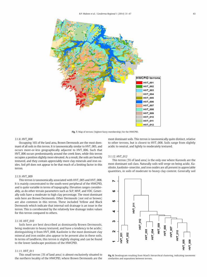
Fig. 7. Map of terrons (highest fuzzy membership) for the HWCPID.
Fig. 8. Dendrogram resulting from Ward's hierarchical clustering, indicating taxonomicsimilarities and separations between terrons.
43B.P. Malone et al. / Geoderma Regional 1 (2014) 31–47
3.1.8. HVT_008Occupying 16% of the land area, Brown Dermosols are the most dom-
inant of all soils in this terron. It is taxonomically similar to HVT_005, andoccurs more-or-less geographically adjacent to HVT_006. Such thatHVT_006 occurs predominantly around the creek lines, while this terronoccupies a position slightlymore elevated. As a result, the soils are heavilytextured, and they contain appreciably more clay minerals and iron ox-ides. Soil pH does not appear to be that much of a limiting factor in thisterron.
3.1.9. HVT_009This terron is taxonomically associated with HVT_005 and HVT_008.
It is mainly concentrated to the south-west peripheral of the HWCPID,and is quite variable in terms of topography. Elevation ranges consider-ably, as do other terrain parameters such as SLP, MVF, and VDC. Gener-ally soils have a moderate to high clay percentage. The most dominantsoils here are Brown Dermosols. Other Dermosols (not red or brown)are also common in this terron. These included Yellow and BlackDermosols which indicate that internal soil drainage is an issue in theterron. This is corroborated by the relatively low drainage index valuesfor this terron compared to others.
3.1.10. HVT_010Soils here are best described as dominantly Brown Dermosols,
being moderate to heavy textured, and have a tendency to be acidic;distinguishing it from HVT_008. Kaolinite is the most dominant claymineral and iron oxides also appear to be present also in these soils.In terms of landform, this terron is slightly sloping and can be foundto the lower landscape positions of the HWCPID.
3.1.11. HVT_011This small terron (3% of land area) is almost exclusively situated to
the northern locality of the HWCPID, where Brown Dermosols are the
most dominant soils. This terron is taxonomically quite distinct, relativeto other terrons, but is closest to HVT_008. Soils range from slightlyacidic to neutral, and lightly to moderately textured.
3.1.12. HVT_012This terron (5% of land area) is the only one where Kurosols are the
most dominant soil class. Naturally soils will verge on being acidic. Ka-olinite, kaolinite–smectite, and iron oxides are all present in appreciablequantities, in soils of moderate to heavy clay content. Generally soil
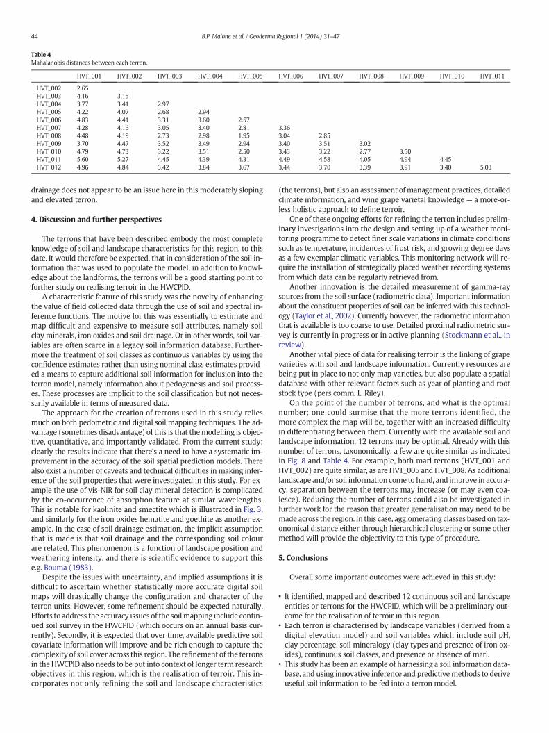
Table 4Mahalanobis distances between each terron.
HVT_001 HVT_002 HVT_003 HVT_004 HVT_005 HVT_006 HVT_007 HVT_008 HVT_009 HVT_010 HVT_011
HVT_002 2.65HVT_003 4.16 3.15HVT_004 3.77 3.41 2.97HVT_005 4.22 4.07 2.68 2.94HVT_006 4.83 4.41 3.31 3.60 2.57HVT_007 4.28 4.16 3.05 3.40 2.81 3.36HVT_008 4.48 4.19 2.73 2.98 1.95 3.04 2.85HVT_009 3.70 4.47 3.52 3.49 2.94 3.40 3.51 3.02HVT_010 4.79 4.73 3.22 3.51 2.50 3.43 3.22 2.77 3.50HVT_011 5.60 5.27 4.45 4.39 4.31 4.49 4.58 4.05 4.94 4.45HVT_012 4.96 4.84 3.42 3.84 3.67 3.44 3.70 3.39 3.91 3.40 5.03
44 B.P. Malone et al. / Geoderma Regional 1 (2014) 31–47
drainage does not appear to be an issue here in this moderately slopingand elevated terron.
4. Discussion and further perspectives
The terrons that have been described embody the most completeknowledge of soil and landscape characteristics for this region, to thisdate. It would therefore be expected, that in consideration of the soil in-formation that was used to populate the model, in addition to knowl-edge about the landforms, the terrons will be a good starting point tofurther study on realising terroir in the HWCPID.
A characteristic feature of this study was the novelty of enhancingthe value of field collected data through the use of soil and spectral in-ference functions. The motive for this was essentially to estimate andmap difficult and expensive to measure soil attributes, namely soilclay minerals, iron oxides and soil drainage. Or in other words, soil var-iables are often scarce in a legacy soil information database. Further-more the treatment of soil classes as continuous variables by using theconfidence estimates rather than using nominal class estimates provid-ed a means to capture additional soil information for inclusion into theterron model, namely information about pedogenesis and soil process-es. These processes are implicit to the soil classification but not neces-sarily available in terms of measured data.
The approach for the creation of terrons used in this study reliesmuch on both pedometric and digital soil mapping techniques. The ad-vantage (sometimes disadvantage) of this is that themodelling is objec-tive, quantitative, and importantly validated. From the current study;clearly the results indicate that there's a need to have a systematic im-provement in the accuracy of the soil spatial prediction models. Therealso exist a number of caveats and technical difficulties in making infer-ence of the soil properties that were investigated in this study. For ex-ample the use of vis-NIR for soil clay mineral detection is complicatedby the co-occurrence of absorption feature at similar wavelengths.This is notable for kaolinite and smectite which is illustrated in Fig. 3,and similarly for the iron oxides hematite and goethite as another ex-ample. In the case of soil drainage estimation, the implicit assumptionthat is made is that soil drainage and the corresponding soil colourare related. This phenomenon is a function of landscape position andweathering intensity, and there is scientific evidence to support thise.g. Bouma (1983).
Despite the issues with uncertainty, and implied assumptions it isdifficult to ascertain whether statistically more accurate digital soilmaps will drastically change the configuration and character of theterron units. However, some refinement should be expected naturally.Efforts to address the accuracy issues of the soilmapping include contin-ued soil survey in the HWCPID (which occurs on an annual basis cur-rently). Secondly, it is expected that over time, available predictive soilcovariate information will improve and be rich enough to capture thecomplexity of soil cover across this region. The refinement of the terronsin theHWCPID also needs to be put into context of longer term researchobjectives in this region, which is the realisation of terroir. This in-corporates not only refining the soil and landscape characteristics
(the terrons), but also an assessment ofmanagement practices, detailedclimate information, and wine grape varietal knowledge — a more-or-less holistic approach to define terroir.
One of these ongoing efforts for refining the terron includes prelim-inary investigations into the design and setting up of a weather moni-toring programme to detect finer scale variations in climate conditionssuch as temperature, incidences of frost risk, and growing degree daysas a few exemplar climatic variables. This monitoring network will re-quire the installation of strategically placed weather recording systemsfrom which data can be regularly retrieved from.
Another innovation is the detailed measurement of gamma-raysources from the soil surface (radiometric data). Important informationabout the constituent properties of soil can be inferred with this technol-ogy (Taylor et al., 2002). Currently however, the radiometric informationthat is available is too coarse to use. Detailed proximal radiometric sur-vey is currently in progress or in active planning (Stockmann et al., inreview).
Another vital piece of data for realising terroir is the linking of grapevarieties with soil and landscape information. Currently resources arebeing put in place to not only map varieties, but also populate a spatialdatabase with other relevant factors such as year of planting and rootstock type (pers comm. L. Riley).
On the point of the number of terrons, and what is the optimalnumber; one could surmise that the more terrons identified, themore complex the map will be, together with an increased difficultyin differentiating between them. Currently with the available soil andlandscape information, 12 terrons may be optimal. Already with thisnumber of terrons, taxonomically, a few are quite similar as indicatedin Fig. 8 and Table 4. For example, both marl terrons (HVT_001 andHVT_002) are quite similar, as are HVT_005 and HVT_008. As additionallandscape and/or soil information come to hand, and improve in accura-cy, separation between the terrons may increase (or may even coa-lesce). Reducing the number of terrons could also be investigated infurther work for the reason that greater generalisation may need to bemade across the region. In this case, agglomerating classes based on tax-onomical distance either through hierarchical clustering or some othermethod will provide the objectivity to this type of procedure.
5. Conclusions
Overall some important outcomes were achieved in this study:
• It identified, mapped and described 12 continuous soil and landscapeentities or terrons for the HWCPID, which will be a preliminary out-come for the realisation of terroir in this region.
• Each terron is characterised by landscape variables (derived from adigital elevation model) and soil variables which include soil pH,clay percentage, soil mineralogy (clay types and presence of iron ox-ides), continuous soil classes, and presence or absence of marl.
• This study has been an example of harnessing a soil information data-base, and using innovative inference and predictivemethods to deriveuseful soil information to be fed into a terron model.
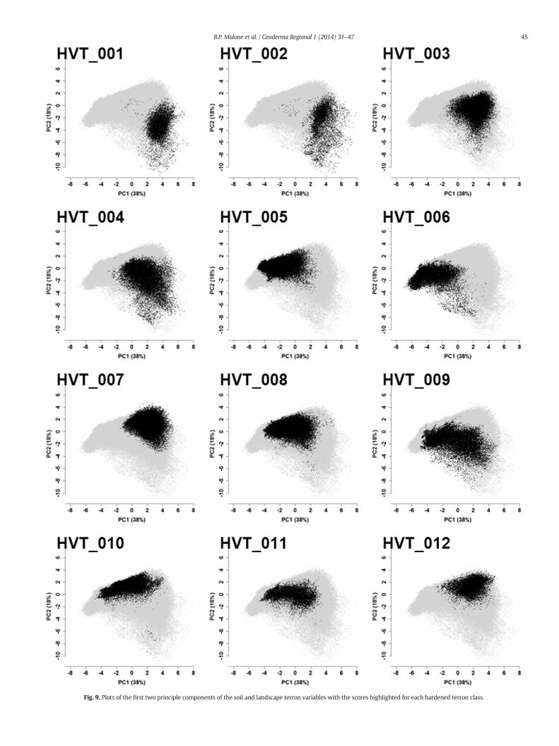
Fig. 9. Plots of the first two principle components of the soil and landscape terron variables with the scores highlighted for each hardened terron class.
45B.P. Malone et al. / Geoderma Regional 1 (2014) 31–47
46 B.P. Malone et al. / Geoderma Regional 1 (2014) 31–47
• The map of terrons is more useful than a soil class map alone (it actu-ally includes it), or a map of a given soil attribute. The embodiment ofsoil and landscapewill provide amore complete picture of the naturalenvironment. From a landowner's ormanager's perspective, this com-prehensive data will ideally lead to more informed decisions abouthow land management plans are implemented.
• The approach detailed in this paper is the first step in describingterroir for the HWCPID. Over time this work will be bolstered withthe acquisition of new and additional environmental variables in-cluding gamma radiometrics, and temperature and climate relatedindices. Furthermore, the matching of terrons with different grapevarietals will be a significant step to the full realisation of terroir inthis prominent Australian wine region.
Appendix A. Supplementary data
Supplementary data associated with this article can be found in theonline version, at http://dx.doi.org/10.1016/j.geodrs.2014.08.001. Thesedata include the Google map of the most important areas described inthis article.
References
Agresti, A., 1984. Analysis of Ordinal Categorical Data. Wiley, New York.Barham, E., 2003. Translating terroir: the global challenge of French AOC labelling. J. Rural.
Stud. 19 (1), 127–138.Bezdek, J.C., Ehrlich, R., Full, W., 1984. The fuzzy c-means clustering algorithm. Comput.
Geosci. 10, 191–203.Bishop, T.F.A.,McBratney, A.B.,Laslett, G.M., 1999. Modelling soil attribute depth functions
with equal-area quadratic smoothing splines. Geoderma 91 (1–2), 27–45.Boettinger, J.L., Ramsey, R.D.,Bodily, J.M.,Cole, N.J.,Kienast-Brown, S.,Nield, S.J., Saunders,
A.M., Stum, A.K., 2008. Landsat spectral data for digital soil mapping. In: Hartemink,A.E., McBratney, A.B., Mendonca-Santos, M.L. (Eds.), Digital Soil Mapping with Limit-ed Data. Springer Science, Australia, pp. 193–203.
Bonfante, A.,Basile, A., Langella, G.,Manna, P.,Terribile, F., 2011. A physically oriented ap-proach to analysis and mapping of terroirs. Geoderma 167–68, 103–117.
Bouma, J., 1983. Hydrology and soil genesis of soils with aquic moisture regimes. In:Wilding, L.P., Smeck, N.E., Hall, G.F. (Eds.), Pedogenesis and Soil Taxonomy. 1. Con-cepts and Interactions. Elsevier Science Publishers, The Netherlands, pp. 253–281.
Bramley, R.G.V.,Hamilton, R.P., 2007. Terroir and precision viticulture: are they compati-ble? Int. J. Vine Wine Sci. 41 (1), 1–8.
Brown, D.J.,Shepherd, K.D.,Walsh, M.G.,Mays, M.D.,Reinsch, T.G., 2006. Global soil charac-terizationwith VNIR diffuse reflectance spectroscopy. Geoderma 132 (3–4), 273–290.
Bureau ofMeterology, 2014. Climate data online: monthly rainfall. Retrieved from: http://www.bom.gov.au/jsp/ncc/cdio/weatherData/av?p_nccObsCode=139&p_display_type=dataFile&p_startYear=&p_c=&p_stn_num=061329.
Burns, S., 2012. The importance of soil and geology in tasting terroir with a case historyfrom the Willamette Valley, Oregon. In: Dougherty, P.H. (Ed.), The Geography ofWine. Springer, Netherlands, pp. 95–108.
Carey, V.A.,Archer, E.,Saayman, D., 2002. Natural Terroir Units: What Are They? How CanThey Help the Wine Farmer? WineLand.
Carey, V.A., Saayman, D.,Archer, E., Barbeau, G.,Wallace, M., 2008. Viticultural terroirs inStellenbosch, South Africa. I. The identification of natural terroir units. Int. J. VineWine Sci. 42 (4), 169–183.
Carey, V.A.,Archer, E.,Barbeau, G.,Saayman, D., 2009. Viticultural terroirs in Stellenbosch,South Africa. III. Spatialisation of viticultural and oenological potential for cabernet-sauvignon and sauvignon blanc by means of a preliminary model. Int. J. Vine WineSci. 43 (1), 1–12.
Carre, F.,McBratney, A.B., 2005. Digital terron mapping. Geoderma 128 (3–4), 340–353.Chrisitan, C.S.,Stewart, G.A., 1953. General report on survey of Katherine–Darwin region,
1946. Land Research Series No. 1Commonwealth Scientific and Industrial ResearchOrganisation, Melbourne.
Clark, R.N.,Roush, T.L., 1984. Reflectance spectroscopy: quantitative analysis techniquesfor remote sensing applications. J. Geophys. Res. 89 (NB7), 6329–6340.
Clark, R.N.,King, T.V.V.,Klejwa, M.,Swayze, G.A.,Vergo, N., 1990. High spectral resolutionreflectance spectroscopy of minerals. J. Geophys. Res. Solid Earth Planets 95 (B8),12653–12680.
Clark, R.N.,Swayze, G.A.,Livo, K.E.,Kokaly, R.F.,Sutley, S.J.,Dalton, J.B.,McDougal, R.R.,Gent,C.A., 2003. Imaging spectroscopy: earth and planetary remote sensing with the USGSTetracorder and expert systems. J. Geophys. Res. Planets 108 (E12), 1–44.
Clark, R.N.,Swayze, G.A.,Wise, R.,Livo, K.E.,Hoefen, T.M.,Kokaly, R.F.,Sutley, S.J., 2007. USGSDigital Spectral Library splib06a. U.S. Geological Survey, Data Series. 231.
Commission Interntionale de l'Eclairage, 1978. Recommendations on Uniform ColorSpaces, Color-Difference Equations, and Psychometric Color Terms, Supplement No.2 to Publication CIE No. 15(E-1.3.1)1971/(TC-1.3)1978. Bureau Central de la CIE,Paris.
Dougherty, P.H. (Ed.), 2012. The Geography of Wine: Regions, Terroir and Techniques.Springer, Netherlands (256 pp.).
Evans, C.V., Franzmeier, D.P., 1988. Color index values to represent wetness and aerationin some Indiana soils. Geoderma 41, 353–368.
Feagan, R., 2007. The place of food: mapping out the ‘local’ in local food systems. Prog.Hum. Geogr. 31 (1), 23–42.
Gallant, J.C.,Dowling, T.I., 2003. A multiresolution index of valley bottom flatness for map-ping depositional areas. Water Resour. Res. 39 (12).
Green, D.R., 2012. Geospatial tools and techniques for vineyard management in thetwenty-first century. In: Dougherty, P.H. (Ed.), The Geography of Wine. Springer,Netherlands, pp. 227–245.
Hastie, T.,Tibshirani, R., Friedman, J., 2001. The Elements of Statistical Learning. SpringerScience, New York.
Hawley, S.P., Glen, R.A., Baker, C.J., 1995. Newcastle Coalfield Regional Geology 1:100 000,1st Edition. Geological Survey of New South Wales, Sydney, Australia.
Isbell, R., 2002. The Australian Soil Classification. CSIRO Publishing, Melbourne.Isbell, R.,McDonald, W.S.,Ashton, L.J., 1997. Concepts and Rationale of the Australian Soil
Classification. ACLEP, CSIRO Land and Water, Canberra.IUSSWorking Group, W.R.B., 2007.World reference base for soil resources 2006. First up-
date 2007. World Soil Resources Report No. 103. FAO, Rome.Jones, G.V., Snead, N., Nelson, P., 2004. Geology and wine. 8. Modelling viticultural
landscapes: a GIS analysis of the terroir potential in the Umpqua Valley of Oregon.Geosci. Can. 31 (4).
Kidd, D.B., Webb, M.A., Grose, C.J., Moreton, R.M., Malone, B.P., McBratney, A.B.,Minasny, B., Viscarra Rossel, R.A., Cotching, L.A., Sparrow, L.A., Smith, R., 2012.Digital soil assessment: guiding irrigation expansion in Tasmania, Australia. In:Minasny, B., Malone, B.P., McBratney, A.B. (Eds.), Digital Soil Assessments andBeyond. CRC Press, The Netherlands, pp. 3–8.
Kovac, M., Lawrie, J.M., 1990. Soil Landscapes of the Singleton 1:250 000 Sheet. Soil Con-servation Service of NSW, Sydney, Australia.
Lanyon, D.M.,Cass, A.,Hansen, D., 2004. The effect of soil properties on vine performance.CSIRO Land and Water Technical Report No. 34/04. CSIRO Land and Water.
Liu, M.Q., Samal, A., 2002. A fuzzy clustering approach to delineate agroecozones. Ecol.Model. 149 (3), 215–228.
Macqueen, R.W., Meinert, L.D. (Eds.), 2006. Fine wine and terroir. The Geoscience per-spective. Geological Association of Canada, Geoscience Canada Reprint Series. 9(246 pp.).
Malone, B.P.,de Gruijter, J.J.,McBratney, A.B.,Minasny, B.,Brus, D.J., 2011. Using additionalcriteria formeasuring the quality of predictions and their uncertainties in a digital soilmapping framework. Soil Sci. Soc. Am. J. 75, 1032–1043.
Malone, B.P.,McBratney, A.B.,Minasny, B., 2012. Digital mapping of a soil drainage index inthe Lower Hunter Valley, NSW. Proceedings of the Joint SSA and NZSSS Soil ScienceConference: Soil Solutions for Diverse Landscapes, Hobart, Tasmania.
McBratney, A.B.,de Gruijter, J.J., 1992. A continuum approach to soil classification bymod-ified fuzzy k-means with extragrades. J. Soil Sci. 43, 159–175.
McBratney, A.B.,Minasny, B.,Cattle, S.R.,Vervoort, R.W., 2002. From pedotransfer functionsto soil inference systems. Geoderma 109 (1–2), 41–73.
McBratney, A.B., Mendonca-Santos, M.L., Minasny, B., 2003. On digital soil mapping.Geoderma 117 (1–2), 3–52.
Minasny, B.,McBratney, A.B., 2002. FuzME version 3.0. Australian Centre for Precision Ag-riculture, The University of Sydney, Australia.
Moran, C.J., Bui, E.N., 2002. Spatial data mining for enhanced soil map modelling. Int. J.Geogr. Inf. Sci. 16 (6), 533–549.
Morand, D.T., 2013. TheWorld Reference Base for Soils (WRB) and Soil Taxonomy: an ap-praisal of their application to the soils of the Northern Rivers of New South Wales.Soil Res. 51 (3), 167–181.
Mulder, V.L.,Plotze, M.,de Bruin, S.,Schaepman, M.E.,Mavris, C.,Kokaly, R.F.,Egli, M., 2013.Quantifying mineral abundances of complex mixtures by coupling spectraldeconvolution of SWIR spectra (2.1–2.4um) and regression tree analysis. Geoderma207–208, 279–290.
Northcote, K.H., 1979. A Factual Key for the Recognition of Australian Soils, 4th edition.Rellim Technical Publications, Glenside, South Australia.
Odgers, N.P.,McBratney, A.B.,Minasny, B., 2011. Bottom-up digital soil mapping. I. Soillayer classes. Geoderma 163, 38–44.
Quinlan, R., 1992. Learning with continuous classes. Proceedings of the 5th AustralianJoint Conference On Artificial Intelligence, Hobart, Tasmania, pp. 343–348.
Quinlan, R., 1993. C4.5: Programs for Machine Learning. Morgan Kaufmann Publishers,San Francisco.
Quinn, P.F.,Beven, K.J.,Lamb, R., 1995. The ln(a/tan b) index: how to calculate it and howto use it within the TOPMODEL framework. Hydrol. Process. 9 (2), 161–182.
Rayment, G.E.,Higginson, F.R., 1992. Australian Laboratory Handbook of Soil and WaterChemical Methods. Inkarta Press, Melbourne.
Robertson, A.R., 1976. The CIE 1976 colour-difference formulae. Color. Res. Appl. 2,7–11.
Soil Survey Staff, 2010. Keys to Soil Taxonomy, 11th edition. United States Department ofAgriculture, Natural Resources Conservation Service, Washington, DC.
Stewart, G.A., 1968. Land evaluation. In: Stewart, G.A. (Ed.), Land Evaluation. Papers of aCSIRO Symposium (CSIRO/UNESCO, Canberra). Macmillan, Melbourne.
Stockmann, U., Malone, B.P., McBratney, A.B., 2014. Landscape-scale exploratoryradiometric mapping using proximal soil sensing. Geoderma (in review).
Taylor, J.A., 2004. Digital Terroirs and Precision Agriculture: Investigations into the Appli-cation of Information Technology in Australian Vineyards. (PhD thesis) The Universi-ty of Sydney.
Taylor, J.A.,Minasny, B., 2006. A protocol for converting qualitative point soil pit surveydata into continuous soil property maps. Aust. J. Soil Res. 44 (5), 543–550.
Taylor, M.J.,Smettem, K.,Pracilio, G.,Verboom,W., 2002. Relationships between soil proper-ties and high-resolution radiometrics, central eastern Wheatbelt, Western Australia.Explor. Geophys. 33 (2), 95–102.

47B.P. Malone et al. / Geoderma Regional 1 (2014) 31–47
Unwin, T., 2012. Terroir: at the heart of geography. In: Dougherty, P.H. (Ed.), The Geogra-phy of Wine. Springer, Netherlands, pp. 37–48.
Vaudour, E., 2002. The quality of grapes and wine in relation to geography: notions ofTerroir at various scales. J. Wine Res. 13 (2), 117–141.
Viscarra Rossel, R.A.,Cattle, S.R.,Ortega, A., Fouad, Y., 2009. In situ measurements of soilcolour, mineral composition and clay content by vis-NIR spectroscopy. Geoderma150 (3–4), 253–266.
Ward, J.H., 1963. Hierarchical grouping to optimise an objective function. J. Am. Stat.Assoc. 58, 236–244.
White, R.,Balachandra, L.,Edis, R.,Chen, D., 2007. The soil component of terroir. Int. J. VineWine Sci. 41, 9–18.
Wilson, J.E., 1998. Terroir: The Role of Geology, Climate and Culture in the Making ofFrench Wines. Mitchell Beazley, London.