Making mortar visible in the archaeological record of Chatham ...
224
Between the Bricks: Making mortar visible in the archaeological record of Chatham and Effingham Counties, Georgia from 1830 to 1930. Volume 1 of 3: Thesis Dawn Danielle Chapman Submitted for the degree of PhD The University of York Department of Archaeology February 2012
-
Upload
khangminh22 -
Category
Documents
-
view
3 -
download
0
Transcript of Making mortar visible in the archaeological record of Chatham ...

Between the Bricks: Making mortar visible in the archaeological record of Chatham and Effingham Counties, Georgia from 1830 to 1930.
Volume 1 of 3: Thesis Dawn Danielle Chapman
Submitted for the degree of PhD The University of York Department of Archaeology
February 2012
2
Abstract
The research presented in this thesis originated in a general interest in lime mortar
and its use in the southeastern United States. Preliminary document-based
research on this topic revealed that a greater variety of mortar materials were used
in the United States during the 19th and early 20th centuries. As the use of these
materials was confirmed in the field, the potential limitations of existing building
conservation literature on historic mortars became apparent. This led to research
that investigated the full range of historic mortar materials and assessed their
potential cultural significance. Through a case study investigating the historic
mortars of Chatham and Effingham Counties in coastal Georgia between 1830
and 1930, this thesis assessed a wide variety of issues surrounding the
understanding of historic mortar materials, the contributions that they can make to
historical archaeology and building conservation in the United States.
The study area was selected, because it had relatively uniform geological and
geographical conditions, but a significant amount of cultural diversity. This
particular combination of characteristics emphasised the possible cultural factors
that influenced historic mortar methods and materials. This also facilitated a
discussion regarding the individuals that selected, used and maintained the
historic masonry buildings in the study area, which forced a philosophical and
practical reassessment of how archaeologists utilise the resource in the
southeastern United States and the effect that current building conservation
methods and materials will have on the integrity of mortar as an archaeological
resource. It argued that current historical archaeologists practicing in the region
fail to fully understand and incorporate mortar into their analysis of architectural
features. In addition, current building conservation literature and practice fail to
adequately conserve the diversity that defined the regional identity and have the
potential to obscure or destroy the cultural significance of mortar in the
archaeological record.

3
Contents
Abstract .................................................................................................................... 2
Contents ................................................................................................................... 3
List of Tables ........................................................................................................... 6
List of Figures .......................................................................................................... 8
List of Accompanying Data ................................................................................... 14
Acknowledgements ............................................................................................... 15
Author’s Declaration ............................................................................................. 16
Chapter 1: Introduction .......................................................................................... 17
1.1 Terminology ................................................................................................ 20
1.2 References ................................................................................................... 21
Chapter 2: Mortar and Previous Work .................................................................. 22
2.1 Mortar and Masonry Construction .............................................................. 23
2.2 Mortar Materials .......................................................................................... 29
2.2.1 Earth ..................................................................................................... 29
2.2.2 Gypsum ................................................................................................. 34
2.2.3 Lime ...................................................................................................... 35
2.2.4 Natural Cement ..................................................................................... 39
2.2.5 Portland Cement ................................................................................... 42
2.2.6 Gauging ................................................................................................ 43
2.2.7 Additives ............................................................................................... 45
2.3 Masonry Conservation and Archaeology .................................................... 46
2.4 Conclusion ................................................................................................... 55
Chapter 3: Theory and Methodology .................................................................... 56
3.1 Materiality ................................................................................................... 57
3.2 Case Study ................................................................................................... 59
3.3 Natural Resources ........................................................................................ 68
3.3.1 Geology ................................................................................................ 68
3.3.2 Geomorphology .................................................................................... 71
3.4 Human Population ....................................................................................... 75

4
3.5 Historic Building Population ....................................................................... 77
3.6 Sampling ...................................................................................................... 81
3.6.1 Building Sampling ................................................................................ 81
3.6.2 Mortar Sampling ................................................................................... 87
3.7 Analysis ....................................................................................................... 89
3.7.1 Geospatial Analysis .............................................................................. 90
3.7.2 Laboratory Analysis ............................................................................. 91
Visual Analysis .......................................................................................... 92
Mortar Disaggregation ............................................................................... 93
Petrographic Analysis ................................................................................ 95
3.7.3 Statistical Analysis ............................................................................... 96
3.8 Conclusion ................................................................................................... 99
Chapter 4: History and Context ........................................................................... 101
4.1 Precontact Period ....................................................................................... 101
4.1.1 North America .................................................................................... 102
4.1.2 Europe ................................................................................................. 106
4.1.3 Africa .................................................................................................. 109
4.2 Colonial Era ............................................................................................... 111
4.2.1 Early Contact Period ........................................................................... 112
4.2.2 Early Colonial Period ......................................................................... 113
4.2.3 Late Colonial and Federal Period ....................................................... 117
4.3 Study Area ................................................................................................. 121
4.3.1 1830 .................................................................................................... 122
4.3.2 1880 .................................................................................................... 126
4.3.3 1930 ................................................................................................... 128
4.3.4 Building population ............................................................................ 131
4.4 Conclusion ................................................................................................. 132
Chapter 5: Findings and Analysis ........................................................................ 133
5.1 Sample Populations ................................................................................... 134
5.1.1 Building Sample Population ............................................................... 135
5.1.2 Mortar Sample Population .................................................................. 136
5.2 Mortar Data ............................................................................................... 137
5
5.2.1 Mortar Use .......................................................................................... 139
Mortar Quantity ....................................................................................... 139
Building Category ................................................................................... 146
Type of Construction ............................................................................... 151
Conclusion ............................................................................................... 159
5.2.2 Binder Use .......................................................................................... 162
Binder Quantity ....................................................................................... 163
Binder Type ............................................................................................. 166
Additives .................................................................................................. 174
Compressive Strength .............................................................................. 183
Conclusion ............................................................................................... 195
5.2.3 Mortar Appearance ............................................................................. 201
Aggregate ................................................................................................ 202
Binder to Aggregate Ratio ....................................................................... 202
Preparation ............................................................................................... 204
Gradation ................................................................................................. 206
Colour ...................................................................................................... 208
Hue .......................................................................................................... 209
Value ........................................................................................................ 213
Chroma .................................................................................................... 213
Conclusion ............................................................................................... 214
5.3 Conclusion ................................................................................................. 217
Chapter 6: Conclusion ......................................................................................... 222
Appendix A – Human Population Statistical Data .............................................. 226
Appendix B – Building Population Statistical Data ............................................ 288
Appendix C – Mortar Sample Statistical Data .................................................... 314
Appendix D - Datasheets ..................................................................................... 422
List of Abbreviations ........................................................................................... 618
Bibliography ........................................................................................................ 619

6
List of Tables
Table 1: Classification of naturally occurring calcium carbonate based binder
materials used in the study area. Table adapted from a system proposed by
Holmes and Wingate (2002, 280-1). ............................................................. 38
Table 2: Estimated population of the southern colonies in 1770 (United States
Bureau of the Census 1975, 1168) ................................................................ 61
Table 3: Population of the former southern colonies in the 1820 federal census
(University of Virginia Library 2004) ........................................................... 61
Table 4: Comparison of the state and study area population data, 1800-1820
(University of Virginia Library 2004) ........................................................... 62
Table 5: Table of historic building population and relative percentage in each
category ......................................................................................................... 82
Table 6: Table of historic building population, human population and rate per
thousand ......................................................................................................... 83
Table 7: 1790 Federal Census data estimating the nationality of European settlers
in Georgia and South Carolina (United States Bureau of the Census 1975,
1168). ........................................................................................................... 107
Table 8: 1708 South Carolina Census (Gallay 2002, 200). ................................. 115
Table 9: Estimate of Native American slave population in South Carolina in 1715
(Gallay 2002, 15; Gallay 2002, 57; Gallay 2002, 103; Gallay 2002, 225-6;
Gallay 2002, 298-9). .................................................................................... 116
Table 10: Excerpt from the 1790 Federal Census of the State of Georgia
(University of Virginia Library 2004). ........................................................ 118
Table 11: Rate of change between 1790 and 1830 in Chatham County. ............ 124
Table 12: Rate of change between 1790 and 1830 in Effingham County. .......... 124
Table 13: 1830 Federal Census data for Chatham County (Ancestry). ............... 125
Table 14: 1830 Federal Census data for Effingham County (Ancestry). ............ 125
Table 15: 1880 Federal Census data for Chatham County (Ancestry). ............... 128
Table 16: 1880 Federal Census data for Effingham County (Ancestry). ............ 128
Table 17: 1930 Federal Census data for Chatham County (Ancestry). ............... 130
7
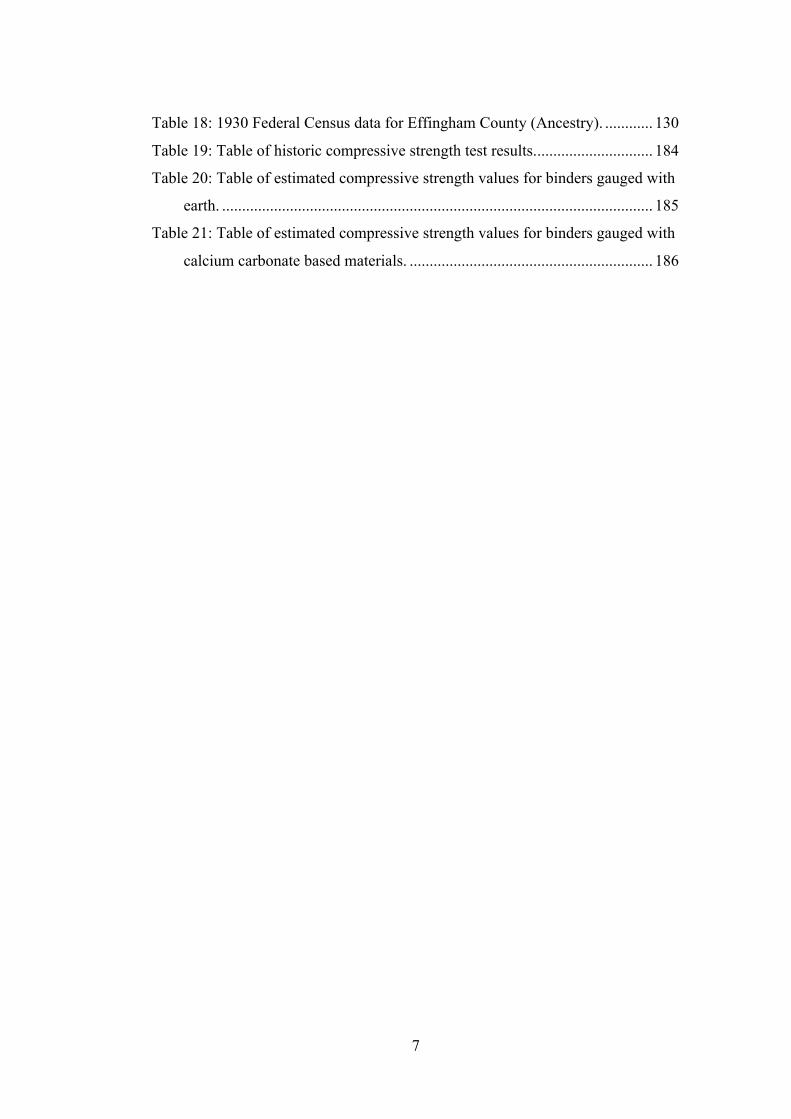
Table 18: 1930 Federal Census data for Effingham County (Ancestry). ............ 130
Table 19: Table of historic compressive strength test results. ............................. 184
Table 20: Table of estimated compressive strength values for binders gauged with
earth. ............................................................................................................ 185
Table 21: Table of estimated compressive strength values for binders gauged with
calcium carbonate based materials. ............................................................. 186

8
List of Figures
Figure 1: Map of the southeastern United States showing each of the states and the
terminology used to describe each subregion. ............................................... 20
Figure 2: Dry Bladen series soil in 140 mm, Data includes silt and clay fraction,
sand fraction, binder to aggregate ratio, average linear shrinkage and Munsell
soil colour ...................................................................................................... 32
Figure 3: Dry Blanton series soil in 140 mm, Data includes silt and clay fraction,
sand fraction, binder to aggregate ratio, average linear shrinkage and Munsell
soil colour ...................................................................................................... 32
Figure 4: Dry Cape Fear series soil in 140 mm, Data includes silt and clay
fraction, sand fraction, binder to aggregate ratio, average linear shrinkage and
Munsell soil colour ........................................................................................ 32
Figure 5: Dry Pooler series soil in 140 mm, Data includes silt and clay fraction,
sand fraction, binder to aggregate ratio, average linear shrinkage and Munsell
soil colour ...................................................................................................... 33
Figure 6: Dry Tawcaw series soil in 140 mm, Data includes silt and clay fraction,
sand fraction, binder to aggregate ratio, average linear shrinkage and Munsell
soil colour ...................................................................................................... 33
Figure 7: Map of Georgia (Minnesota Population Center 2010) .......................... 62
Figure 8: Graph of the total population of Chatham and Effingham Counties,
1790-1940 (University of Virginia Library 2004) ......................................... 63
Figure 9: Map of geographic provinces of present-day Georgia and South
Carolina (United States Geological Survey 2004b). ..................................... 69
Figure 10: Map depicting the arches and embayments of the Atlantic and eastern
Gulf Coastal Plains. The crosses indicate the orientation and relative size of
each arch (Ward et al. 1991, 275). ................................................................. 70
Figure 11: Map identifying calcium carbonate and gypsum deposits in the United
States. Solid green indicates areas with calcium carbonate rock outcrops,
green hatch pattern indicate areas with subsurface deposits, and orange
indicates the location of gypsum deposits, adapted from the revised USGS

9
Karst Map (Veni 2002). ................................................................................. 71
Figure 12: Excerpt from the USGS Tapestry geological and topographic map
identifying Paleogene and Neogene geological formations of the Atlantic
Deep South (United States Geological Survey 2004b) ................................. 72
Figure 13: Diagram depicting the existing barrier islands and the location and
elevation of six former barrier island systems in present-day Georgia (Hodler
and Schretter 1986, 27) .................................................................................. 74
Figure 14: Diagram of negatively skewed, symmetric and positively skewed
distributions (Triola 2008, 93). ...................................................................... 97
Figure 15: Southeast section of the Powell map of language families of 1915
(Goddard 2005, 2). ...................................................................................... 103
Figure 16: Southeast section of the Goddard map of language families of 2005
(Goddard 2005, 3). ...................................................................................... 104
Figure 17: Relative percentage of each European nationality in Georgia in 1790
(United States Bureau of the Census 1975, 1168). ...................................... 108
Figure 18: Map of Africa indicating the relative proportion of Africans embarking
from each of these regions during the 18th century and disembarking in the
Atlantic Deep South (Trans-Atlantic Slave Trade Database). The adjacent
shaded areas depict the proposed range of slaving activity into the interior
(Eltis 2000). ................................................................................................. 109
Figure 19: Map of Georgia and the Carolinas from 1663 to 1790. ..................... 114
Figure 20: Map indicating the origin of enslaved Native Americans, based on
Galley's estimates. The two toned symbol depicts the minimum and
maximum estimates for each people (Gallay 2002, 15; Gallay 2002, 57;
Gallay 2002, 103; Gallay 2002, 225-6; Gallay 2002, 298-9). ..................... 117
Figure 21: Chart of the relative percentage of one and two-mortar buildings in the
study area in 1830, 1880 and 1930. ............................................................. 140
Figure 22: Chart of the relative percentage of one and two-mortar buildings in an
urban environment in 1830, 1880 and 1930. ............................................... 140
Figure 23: Chart of the relative percentage of one and two-mortar buildings in a
rural environment in 1830, 1880 and 1930. ................................................ 140
Figure 24: Chart of the relative percentage of one and two-mortar buildings in the
10
African-American community in 1830, 1880 and 1930. ............................. 143
Figure 25: Chart of the relative percentage of one and two-mortar buildings in The
European-American community in 1830, 1880 and 1930. .......................... 143
Figure 26: Chart of the relative percentage of one and two-mortar buildings in the
integrated community in 1830, 1880 and 1930. .......................................... 143
Figure 27: Chart of the frequency of one and two-mortar single-family residences
and their mortars. ......................................................................................... 148
Figure 28: Chart of the relative percentage of each type of construction in the
study area, 1830, 1880 and 1930. ................................................................ 152
Figure 29: Chart of the relative percentage of mortar samples collected from each
type of construction in an urban environment in 1830, 1880 and 1930. ..... 156
Figure 30: Chart of the relative percentage of mortar samples collected from each
type of construction in a rural environment in 1830, 1880 and 1930. ......... 156
Figure 31: Chart of the relative percentage of mortar samples collected from each
type of construction in The African-American community in 1830, 1880 and
1930. ............................................................................................................ 157
Figure 32: Chart of the relative percentage of mortar samples collected from each
type of construction in The European-American community in 1830, 1880
and 1930. ..................................................................................................... 158
Figure 33: Chart of the relative percentage of mortar samples collected from each
type of construction in the integrated community in 1830, 1880 and 1930. 158
Figure 34: Chart of the relative percentage of mortars containing one and two
binders in urban environments in 1830, 1880 and 1930. ............................ 164
Figure 35: Chart of the relative percentage of mortars containing one and two
binders in rural environments in 1830, 1880 and 1930. .............................. 164
Figure 36: Chart of the relative percentage of one and two-binder mortars in The
African-American community in 1830, 1880 and 1930. ............................. 165
Figure 37: Chart of the relative percentage of one and two-binder mortars in the
integrated community in 1830, 1880 and 1930. .......................................... 165
Figure 38: Chart of the relative percentage of one and two-binder mortars in The
European-American community in 1830, 1880 and 1930. .......................... 165
Figure 39: Chart of the relative percentage of each type of binder in 1830, 1880
11
and 1930. ..................................................................................................... 167
Figure 40: Chart of the relative percentage of each type of binder used in urban
environments in 1830, 1880 and 1930. ....................................................... 169
Figure 41: Chart of the relative percentage of each type of binder used in rural
environments in 1830, 1880 and 1930. ....................................................... 169
Figure 42: Chart of the relative percentage of each type of binder used in The
African-American community in 1830, 1880 and 1930. ............................. 171
Figure 43: Chart of the relative percentage of each type of binder used in the
integrated community in 1830, 1880 and 1930. .......................................... 171
Figure 44: Chart of the relative percentage of each type of binder used in The
European-American community in 1830, 1880 and 1930. .......................... 172
Figure 45: Chart of the relative percentage of performance additives in relation to
all additives used in 1830, 1880 and 1930. ................................................. 175
Figure 46: Chart of the relative percentage of appearance additives in relation to
all additives used in 1830, 1880 and 1930. ................................................. 175
Figure 47: Chart of the relative percentage of performance additives in relation to
all additives used in urban environments in 1830, 1880 and 1930. ............ 177
Figure 48: Chart of the relative percentage of appearance additives in relation to
all additives used in urban environments in 1830, 1880 and 1930. ............ 177
Figure 49: Chart of the relative percentage of performance additives in relation to
all additives used in rural environments in 1830, 1880 and 1930. .............. 178
Figure 50: Chart of the relative percentage of appearance additives in relation to
all additives used in rural environments in 1830, 1880 and 1930. .............. 178
Figure 51: Chart of the relative percentage of performance additives in relation to
all additives used in The African-American community in 1830, 1880 and
1930. ............................................................................................................ 180
Figure 52: Chart of the relative percentage of performance additives in relation to
all additives used in the integrated community in 1830, 1880 and 1930. ... 180
Figure 53: Chart of the relative percentage of performance additives in relation to
all additives used in The European-American community in 1830, 1880 and
1930. ............................................................................................................ 180
Figure 54: Chart of the relative percentage of appearance additives in relation to
12
all additives used in The African-American community in 1830, 1880 and
1930. ............................................................................................................ 181
Figure 55: Chart of the relative percentage of appearance additives in relation to
all additives used in the integrated community in 1830, 1880 and 1930. ... 181
Figure 56: Chart of the relative percentage of appearance additives in relation to
all additives used in The European-American community in 1830, 1880 and
1930. ............................................................................................................ 181
Figure 57: Chart of the relative percentage of compressive strength values in
1830, 1880 and 1930. .................................................................................. 188
Figure 58: Chart of the relative percentage of compressive strength values in
urban environments in 1830, 1880 and 1930. ............................................. 189
Figure 59: Chart of the relative percentage of compressive strength values in rural
environments in 1830, 1880 and 1930. ....................................................... 189
Figure 60: Chart of the relative percentage of compressive strength values in The
African-American community in 1830, 1880 and 1930. ............................. 193
Figure 61: Chart of the relative percentage of compressive strength values in the
integrated community in 1830, 1880 and 1930. .......................................... 193
Figure 62: Chart of the relative percentage of compressive strength values in The
European-American community in 1830, 1880 and 1930. .......................... 193
Figure 63: Chart of the relative percentage of binder to aggregate ratios in 1830,
1880 and 1930. ............................................................................................ 203
Figure 64: Chart of the relative percentage of each level of aggregate preparation
in 1830, 1880 and 1930. .............................................................................. 205
Figure 65: Chart of the relative percentage of each level of aggregate gradation in
1830, 1880 and 1930. .................................................................................. 206
Figure 66: Chart of the relative percentage of each hue in 1830, 1880 and 1930.
..................................................................................................................... 210
Figure 67: Chart of the relative percentage of each hue in urban environments in
1830, 1880 and 1930. .................................................................................. 210
Figure 68: Chart of the relative percentage of each hue in rural environments in
1830, 1880 and 1930. .................................................................................. 210
Figure 69: Chart of the relative percentage of each hue in the African-American

13
community in 1830, 1880 and 1930. ........................................................... 212
Figure 70: Chart of the relative percentage of each hue in the integrated
community in 1830, 1880 and 1930. ........................................................... 212
Figure 71: Chart of the relative percentage of each hue in the European-American
community in 1830, 1880 and 1930. ........................................................... 212
Figure 72: Chart of the relative percentage of each value in 1830, 1880 and 1930.
..................................................................................................................... 213
Figure 73: Chart of the relative percentage of each chroma in 1830, 1880 and
1930. ............................................................................................................ 214

14
List of Accompanying Data
Volume 1 of 3: Between the Bricks: Making mortar visible in the archaeological record of Chatham and Effingham Counties, Georgia from 1830 to 1930. File Description ChapmanVolume1.pdf Thesis Volume 2 of 3: Appendices A, B and C File Description ChapmanVolume2-1.pdf Appendix A: Human Population Statistical Data Appendix B: Building Population Statistical Data Appendix C: Mortar Sample Statistical Data,
Figures C1 to C6 ChapmanVolume2-2.pdf Appendix C: Mortar Sample Statistical Data, Figures C7 to C150 Volume 3 of 3: Appendix D File Description ChapmanVolume3-1.pdf Appendix D: Datasheets ChapmanVolume3-2.pdf List of Abbreviations and Bibliography
15
Acknowledgements
The research presented in this thesis was the direct result of the remarkable
contributions of so many individuals, whose diverse experiences and broad array
of talents have graciously afforded me the opportunity to accomplish this work. I
am immeasurably grateful to all my friends, colleagues and family for their
enduring support, which enabled me to have the resources necessary to complete
this research. Their patience and love were the mortar that bound together each
aspect of this research and enabled me to complete a task that often seemed
insurmountable. The kindness and generosity of friends, family and often
strangers to share vast amounts of their time, talents and knowledge have not gone
unnoticed or unappreciated.

16
Author’s Declaration
I declare this thesis is entirely my own work, and the responsibility for any errors
is my own. All original research is presented here for the first time.
Dawn Danielle Chapman
Chapter 1: Introduction
The research presented in this thesis originated in a general interest in lime mortar
and its use in the southeastern United States. Initial expectations were based on
information contained primarily in current conservation literature pertaining to
historic mortars. It was expected to contribute to the general knowledge of historic
mortars in the United States through the survey and analysis of a specific building
material and its use in a particular region. It is likely that the research originally
planned would only have been of interest to academics and building
conservationists in this region, and of general interest to historic mortar specialists
throughout the rest of the country.
The preliminary research overturned all of these expectations, when an initial
comparison of building conservation literature and historic texts revealed
fundamentally different masonry construction methods and materials than
expressed in the current building conservation literature. Concerns that the
sources were simply marketing literature intended to exaggerate the importance
and utility of their products were quickly dispelled. The contents of these texts
were different from the conservation literature. The historic texts discussed a wide
range of mortar materials that were available in the United States and in the
southeastern region, including clay, gypsum, lime, natural cement and Portland
cement, while the building conservation literature addressed a more limited set of
materials, typically only lime and Portland cement. The building conservation
sources seemed to present a generalised assessment of the subject in an effort to
appeal to the needs of a broader audience. The preliminary research had certainly
raised more questions than it resolved. Was the full range of mortar materials
described in historic texts widely used or were they specialty products that
required the publication of more detailed practical advice and marketing
literature? To what extent have these materials survived to the current day? Why
were they overlooked in building conservation literature? These questions could
only be answered by developing an entirely different approach to the research.

18
At this point, the topic began its transformation from building conservation based
mortar analysis to an archaeological assessment of historic mortars and their
potential cultural significance. The questions raised by the preliminary research
were addressed by designing a case study that assessed a larger set of research
questions than those originally conceived for this research or were typically
addressed in building conservation. This also initiated a theoretical and practical
assessment of the effect that current building conservation methods and materials
have on the integrity of mortar as an archaeological resource. If the conservation
recommendations presented in building conservation literature had been widely
applied in the study area, would the conservation intervention have adversely
affected the historic masonry resources? The origin of current conservation
literature needed further attention to address the primary question. Who wrote
these texts? When were they written? What was their purpose? To answer these
questions, the research placed aspects of building conservation under the
microscope and reassessed the conventional wisdom in the field of mortar
conservation.
An informal survey was conducted in the state of Georgia, augmented with basic
enquiries in states throughout the region. This survey confirmed that there were
more materials in use historically in this region than lime and Portland cement.
The survey also seemed to contradict the notion that there was a linear evolution
of mortar materials from simple, inexpensive and less durable technologies to
increasingly complex, expensive and durable ones as soon as they became
available. In fact, this survey suggested that many of the less durable materials
were in use well into the 20th century alongside the more ‘advanced’ materials. In
order to assess the actual range of mortar materials and their rate of change, a
research design was established that reduced the intended size of the study area
and expanded the scope to include all types of mortar materials encountered in the
area.
A suitable study area was identified for this research, defined by the boundaries of
Chatham and Effingham Counties in coastal Georgia. The limited size of this
19
study area enabled the juxtaposition of relatively homogeneous environmental
conditions and a diverse set of cultural characteristics. The era between 1830 and
1930 was selected, because it provided a sufficient number of historic masonry
buildings and represented an era of significant technological and historical change.
During this time, technological developments transitioned the market from
traditional mortar materials, which had been in use for thousands of years, to one
that augmented the traditional materials with a variety of new products, such as
natural cement, Portland cement and a number of additives intended to alter the
performance or appearance characteristics of the mortar. It also witnessed the
transition from a slave-based economy in the early 19th century (Boney 1991, 129),
through the Civil War and the period of Reconstruction in the late 19th century
(Wynes 1991, 207) and the large-scale migration and urbanization of the south in
the early 20th century (Maloney 2010).
The study area provided a unique case study to assess the research questions
developed in the archaeological research design and presented in this thesis.
Specifically, how much diversity existed in historic mortars and mortar materials
in the 19th and early 20th centuries? How did the mortars and mortar materials
change over time? How does geography influence the selection and use of mortar
materials? How does ancestry influence the selection and use of mortar materials?
Together these questions defined the specific objectives of this research, which
were necessary achieve to overall aim of the research to determine whether or not
cultural factors influenced the use of historic mortar materials. The primary
objective of the fieldwork portion of this research was the documentation of the
diversity present in the mortar materials used in this area, while the approach to
data analysis focused on the patterns in the mortar data, which potentially
correlated with environmental and cultural factors, including geography and
demography. Using these methods, the research was able to provide a
significantly different understanding of the potential cultural factors influencing
the choice of mortar materials than would have been possible using a more
scientific and typical building conservation approach to the research. By bridging
the gap between historical archaeology and building conservation, the findings of

20
this research are relevant to both fields and provide the data necessary to argue for
a reassessment of mortar in each field. The application of the findings of this
research to the practice of historical archaeology in the southeast would provide
archaeologists the tools necessary to date many 19th and early 20th century mortars.
The findings of this research would also be useful to evaluate standard practices
and literature in the field of building conservation, as well as the actual effect of
these recommendations on the integrity of historic masonry buildings in the study
area.
1.1 Terminology
In this thesis, the region of the American South has been divided into various
subregions (Figure 1). In this thesis, the South is defined as those states that
seceded from the union in 1861, forming the Confederate States of America.
Those located along the Atlantic coastline are described as the Old South and are
Figure 1: Map of the southeastern United States showing each of the states and the terminology used to describe each subregion.

21
divided into the Upper South, including Virginia and North Carolina, and the
Deep South, including South Carolina and Georgia. Each of these states originally
extended west to the Mississippi and Ohio Rivers. New states were carved out of
this territory between 1792 and 1819. The state of Tennessee was formed from the
western portion of North Carolina, and Alabama and Mississippi were formed
from the western portion of Georgia. Together, these states are described in this
thesis as the Gulf South. Since Florida was not ceded by the Spanish until 1819
and did not become a state until 1845, it has not been included in the Deep South
or the Gulf South and is referred to by its state name in this thesis.
1.2 References
In order to clearly reference the variety of figures, tables, charts and datasheets
presented and discussed in this research, various formats have been employed to
refer the reader to the location of the specific data. References to figures and
tables located within the text of this thesis conformed to one of the following
formats: (Figure 1) or (Table 1). A simplified format was used to refer to the
individual datasheets for each of the buildings sampled in this research, which
were located in Appendix D. Instead of being numbered sequentially, the
datasheets are presented in order of the Resource ID, located in the upper right
corner of the datasheet. For example, references to the first and third datasheets in
Appendix D would conform to the following formats respectively; (000006) or
(000019B).

22
Chapter 2: Mortar and Previous Work
Historic buildings and their materials have occupied a hinterland between
architecture and archaeology, and were neither claimed nor adequately addressed
by either. From the perspective of architecture and building conservation, the
approach to historic buildings was often derived from the art and architectural
history perspective. Broadly speaking, the traditional focus has been on the
architectural style, detail and precedent or an evolutionary study of the site based
on the biography of the architect or owner. These approaches would have been
analogous to a pottery study based on attributes such as the size, shape and
decorative patterns of the pot or its place in the career of a single potter without
discussing the type of ware, the materials used to make it or the cultural
significance of the artefact. In the last few decades, architectural history and
building conservation have undoubtedly become more interested in the social and
cultural significance of historic buildings, most notably in the increasingly diverse
definition of significance and the resulting diversity in the types of buildings
worthy of study and preservation; however, these changes have fallen short of
assessing historic buildings as archaeological artefacts. This goal would probably
not be widely accepted by the building conservation community, which has seen
itself as distinct from archaeology and its practices. According to John Sprinkle,
Jr. in A Richer Heritage: Historic Preservation in the Twenty-First Century,
archaeology is “fundamentally different from other professions within historic
preservation”, because it “thrives on destruction of the past through excavation,
analysis, and interpretation” (2003, 253), even describing archaeology as “the
black sheep of the historic preservation movement” (2003, 270). The
uncomfortable relationship between building conservation and archaeology is also
well known in archaeology. Hicks and Horning address the depth and complexity
of the problem in The Cambridge Companion to Historical Archaeology, when
they explained that:
‘[t]he emphasis upon buildings in the present volume – which includes chapters on the archaeology of cities and households as well as this chapter on buildings archaeology – will surprise some historical archaeologists. For many, studying the historical built environment is the field of architectural and art historians, historical geographers or local historians, and the buried

23
remains of structures encountered by archaeologists are often seen as of less significance than the artefacts recovered from buried deposits associated with them.’ (2006, 273).
Although the divide between these professions is widely accepted, it is critical
that more research is conducted that attempts to navigate through this hinterland.
Architectural history and building conservation need to continue to expand
research into areas that address the cultural and social significance of historic
buildings and their components and materials. Archaeology needs to fully
integrate historic buildings into their current theoretical and methodological
frameworks in order to recognise that historic buildings are not just features, but
are also complex artefacts containing cultural information as relevant to the
interpretation of an entire site as the associated artefacts. By finding a common
ground between these professions, a more integrated and meaningful
understanding of the historical built environment will be developed, which will
inform future work in both building conservation and archaeology.
A notable exception to this general condition is the field of buildings archaeology,
which has gained prominence in British archaeology since the early 1990s
(Institute of Field Archaeologists Buildings Special Interest Group 1994), but has
had little influence on American archaeology. This research built on the progress
made in the United Kingdom by applying archaeological theory and methodology
to what would traditionally be considered American building conservation
research. As such, this chapter was structured to introduce the materials addressed
in this research, discuss the current status of American building conservation and
archaeology, and their current approaches to historic masonry buildings and
remains.
2.1 Mortar and Masonry Construction
Masonry is a type of construction that uses individual units and mortar in
assembly. The material and qualities of the units themselves vary and serve as a
24
system of classification. The materials are most commonly stone, a fired clay
material such as brick, tile and faience, or concrete. Additional descriptors can
also be provided, which indicate the method of preparation or execution, such as
“ashlar masonry” or “dry-stacked stone masonry” (Phillipps and Byrne 1908, 63).
Since stone suitable for construction is uncommon in the Atlantic coastal plain of
Georgia and South Carolina, brick is the most common historical masonry type in
the study area. Stone masonry is relatively rare, because masons in this area relied
on imported materials. Squared stone masonry was generally limited to civic and
commercial buildings or used as an accent in mixed masonry buildings (010661).
Uncoursed rubble masonry was used under unique conditions, particularly in
close proximity to a port, where ship ballast was a readily available building
material (006613).
Mortar serves several specific functions in masonry construction. The mortar
provides a plastic layer between each masonry course that can accommodate
variations in the individual masonry units. This enables masons to completely fill
the gaps between variable masonry units and construct a solid wall assembly to
keep out the elements. It also allows for the construction of even, level courses to
support and distribute the loads of other elements of the building (Plumridge and
Meulenkamp 1993, 173). It also serves a variety of aesthetic functions by
blending or contrasting with the adjacent masonry units. Mortars with a similar
colour to the adjacent masonry units can minimise the appearance of the joints
and create a more unified appearance to the masonry surface. By tooling the joint,
the surface of the joint can be recessed to create a shadow line from the masonry
course above (Plumridge and Meulenkamp 1993, 175) or prepare the joint for the
application of tuck-pointing. This detail involves the application of a thin line of
projecting mortar, usually white in colour and approximately 3 mm in width
(Phillipps and Byrne 1908, 70) , to give the visual impression of the narrow joints
associated with more finely worked, even masonry units (Plumridge and
Meulenkamp 1993, 176-7).

25
The terminology used to describe the position of mortar in an assembly is
important, as it is often misused. Bedding and jointing mortars comprise the bulk
of the wall, with bedding mortar filling the horizontal joints and jointing mortars
filling the vertical joints. Pointing is mortar that is applied at the time of original
construction to the face of the joint. Once the wall is constructed, but the mortar is
not fully set, the joints are raked out and a mortar mix is applied that achieves
different performance or aesthetic standards. Repointing describes the process of
raking out and replacing deteriorated mortar joints containing either bedding and
jointing or pointing mortar. After repointing, a wall that previously contained only
bedding and jointing mortar will also contain a pointing mortar. Tuck-pointing is
the finish detail previously described, not a term synonymous with the process of
repointing.
Mortar itself is generally composed of at least two basic components: binder and
aggregate. Binder is the component of a mortar that sets or hardens in place.
While it is possible to have a mortar composed solely of binder, these mortars
have a tendency to shrink while setting. In practice, the performance of nearly all
binders is improved with the addition of an aggregate, which is a non-reactive
component added to improve the dimensional stability of a mortar by creating a
structure or framework to which the binder adheres. This also generally makes the
mortar more economical by reducing the relative proportion of the binder, which
is typically the most expensive component.
Ideally, the aggregate is well-graded sand that ‘enables all voids between the
larger grains to be filled with the smaller ones’ (Holmes and Wingate 2002, 220).
‘Well-graded’ sand has a particle size distribution in the form of a bell curve,
meaning that the sizes of the majority of the particles are in the middle of the
curve with fewer large and small particles at each end of the curve. The
importance of well-graded sand becomes apparent if one were to imagine that the
sand contained in a mortar were instead pieces of stone being used in constructing
dry-stack stone masonry. A properly constructed dry-stack stonewall requires
each stone to be fitted as closely as possible to the adjacent stones, transferring the

26
load through the wall and down to the foundation. During construction, where
larger gaps occur in the stonework, smaller stones are fitted to increase the contact
between the stones and distribute the load to the foundation. The same principle
holds true for sands and other aggregates in mortar. An ideal mortar achieves this
on a smaller scale by allowing the sand particles to transfer a load, such as the
weight of the wall or thermal expansion and contraction, across the masonry joint
through adjacent particles, rather than crushing the binder. The binder serves to
fill the voids and bind together the sand particles. The ideal ratio of binder to
aggregate can be established by determining the void to aggregate ratio or the
amount of aggregate needed to entirely fill all voids without using an excess
amount of binder. One can easily determine this ratio by placing a dry sample of
the aggregate into a glass container and adding water until the sample is
completely saturated. The ratio of water to aggregate will define the optimum
amount of binder needed for that particular type of aggregate (Holmes and
Wingate 2002, 220).
The previous discussion of the function and composition of mortar is an
interesting concept and certainly quite useful as a general introduction to mortar
and its components, but it assumes that mortar is only a part of a unit masonry
assembly. A review of mortar literature identified definitions in prominent
publications, one from each of the time periods addressed in this research and the
present-day. The problem arose in the division between mortar and concrete. If
this research were located in another part of the country, the historical overlap
between mortar and concrete could be dismissed immediately. In this region, there
was an historical form of concrete construction called ‘tabby’, which was
composed of ‘equal proportions of lime, sand, oyster shell, and water’ (Sickels-
Taves and Sheehan 1999, 1). To construct a tabby wall, the material was poured
into forms similar to present-day concrete construction. Once the material set, the
forms were removed and reattached at the top of the wall to prepare for another
pour. The material was commonly used along the coast from the 16th to 19th
centuries. This form of concrete used the same materials as many of the historical
mortars in this region and may have influenced mortar materials in this area. For
27
these reasons, a closer look at the definition of mortar was essential for defining
an appropriate scope of work for this research.
The definition of mortar varied throughout the 19th and 20th centuries. By the end
of the 20th century, the term mortar referred to the construction material used to
bond individual masonry units as previously discussed. This definition
specifically excluded concrete, which was made of similar materials as mortar,
but was mixed with a larger aggregate and poured into forms, creating a solid
reinforced or unreinforced structure. The current separation of these two types of
materials could have been related to either the method of construction or the
relative percentage of the masonry units within the structure. The question of how
to group or separate mortar and concrete, either by identifying or characterising
the various components of the material or methods of construction, has been a
point of contention for nearly two centuries.
Although there was a general agreement in the definitions of these two materials
in the following examples from the 19th century and early 20th centuries, there
was little agreement on the reasoning for their decision. In 1838, Pasley criticised
a contemporary for describing ancient Roman ‘Cæmentum’ and French ‘Beton’ as
concrete (1838, 23). Although each of these materials were ‘composed of regular
mortar mixed with pebbles or small broken stones’, he argued that the material
was alternated with layers of wall tiles, flat stones or rubble stone and were
actually ‘masonry of small materials’ (Pasley 1838, 23-4). In this case, the
defining characteristic was the method of construction. The presence of masonry
units was the most important factor for Pasley. He felt that regardless of their
interval or their relative percentage in the structure, their mere presence in the
assembly defined the material as mortar, not concrete. Gillmore also
acknowledged that mortar and concrete were similar in 1879, but thought they
should have been considered to be different types of materials when he stated that:
‘…any mixture of fragmentary substances, like sand, gravel, pebbles, or pieces of brick or stone, formed into a state of aggregation by a calcareous cementing matter or matrix, might be termed mortar; but as this definition would evidently include concrete or beton, which is made by incorporating into mortar, fragments of brick or of stone, shells and pebbles, it is perhaps

28
well to retain the technical signification of the term mortar, by limiting its application to mixtures of sand and a paste of the cementing substances, reserving for a general classification of mortars and concrete under one head, the more comprehensive denomination of aggregates.’ (1879, 175).
While he seemed to have separated the materials for convenience rather than their
inherent differences, he clearly indicated that the defining characteristic of
concrete was the addition of a larger aggregate, not the absence of masonry units
in the structure. In 1927, Cowper seemed to more definitively separate the
materials when he described mortar as ‘…any material used in a plastic state
which can be trowelled, and becomes hard in place, and which is utilised for
bedding and jointing. The word ‘mortar’ was thus used without regard to the
composition of the material, but simply defining its use as a bonding material…’
(Cowper 1927, 51). While this definition clearly excluded concrete, he amended
the definition in the following paragraph, by stating that lime concrete was
‘…only a special case of lime mortar, wherein the cementing material unites the
particles of an aggregate consisting largely of gravel or crushed stone, &c., of a
size much larger than the particles of sand which form the whole aggregate in
ordinary mortar, in place of uniting bricks, ashlar stone blocks or rubble blocks.’
(Cowper 1927, 51). Even Cowper, who defined them as different materials,
acknowledged the similarity of mortar and concrete.
A closer look at these definitions was necessary when developing this research
topic. The review of the definition of mortar in key texts from the beginning of
the period of study to the present-day shed light on the inclusive or exclusive
nature of historical mortars. Pasley argued that the inclusion of masonry units
defined a mortar, even though the masonry units seem to have acted as lateral
reinforcement to tie the wall together. Gillmore concluded that a mortar with large
aggregate should be classified as a concrete, although he still found them to be
related enough that he included an entire chapter of his book to the material.
Cowper initially seemed to agree with Pasley, before making an exception for the
very material that instigated this discussion. Although each of these authorities
argued for a different terminology for materials similar to the tabby used in this
region, they also either made a specific exception for this type of material or
29
included it in their work anyway. A similar approach was taken in this research.
The differences in these materials have been clearly acknowledged, but both
materials have been included in this research.
2.2 Mortar Materials
The mortar materials addressed in this research included binders, aggregate and
various additives to modify the performance or appearance of a mortar. The
binders included earth, gypsum, lime, natural and artificial cements. This list
corresponded with the order in which these materials were developed historically
and generally progressed from the materials with least to greatest durability in the
climate of the study area. As understanding of the chemistry of these materials
increased between the 18th and 21st centuries, some of the historic definitions have
proven to be inadequate. This spurred debate within the building conservation
community between those that used the historic definitions and those that
incorporated the increased information available to current materials scientists.
When appropriate, information on historical and current definitions has been
provided.
2.2.1 Earth
The most basic and earliest binder used in historic mortars is earth. From the
earthen houses of Çatal Hüyük, which were constructed c. 7000 BC (Göktürk et
al. 2002, 407), to the present day, when at least 30% of the world’s population
live in an unfired earth dwelling (Houben and Guillaud 1994, 6), earth has
represented a significant part of the built environment. Paradoxically, the history
of this form of construction has not been well documented. Houben and Guillaud
suggested that this omission may be the result of the material being regarded as
‘inferior and archaic’ (1994, 8). This perception may have extended to the
documentation of earthen mortar as well. It is also possible that it was caused by
the ubiquitous nature of the material. This theory was supported by the omission

30
of the topic in a compendium of natural philosophy published in 1836, because
the ‘use of clay in forming mortar and in supplying the materials of bricks and the
various kinds of pottery, need hardly be pointed out, as every one is familiar with
it’ (Wesley and Mudie, 230). It could also have been the simplicity of the
technology itself that was perceived to require less explanation than other
masonry technologies. Regardless of the cause, the fact that earth is
underrepresented in the literature should not be perceived to be an indication of its
diminished use or importance in masonry construction.
From a technological perspective, earthen binders are used in an unfired state and
achieve a set by desiccation, or drying, rather than undergoing a chemical change
(Table 1). The soil is collected, moistened and allowed to rest for 1 or 2 days to
soften clay nodules within the soil. Afterward, the material is kneaded and mixed
with the other mortar ingredients (Chandigarh 1992). The primary weakness of
this type of mortar is that it is highly susceptible to weathering (Houben and
Guillaud 1994, 146-7), which effectively reverses the setting process and washes
away the binder, turning the mortar to sand. For this reason, earth mortars used in
wet climates, such as the study area, were often protected by frequently renewed
earth or lime render or by a coating of limewash or paint (Houben and Guillaud
1994, 335). In addition, earth structures were often designed and constructed with
large eaves to protect the exterior surface of the walls (Houben and Guillaud
1994, 283). A secondary problem associated with earth as a binder material is that
certain soils have a tendency to expand when wet and shrink when dry (Brady and
Weil 2002, 170-1). These are called expansive soils and are particularly
problematic when used as a mortar. Moisture added to the soil to improve the
workability of the material and facilitate the incorporation of the aggregate
materials causes the mortar to swell. Once in the wall, the mortar releases the
excess water and develops shrinkage cracks. Each of these issues requires the
careful selection of soils for use in masonry construction.
Due to the variability of soil types from region to region, it was not possible to use
standardised data to discuss the properties of the possible earthen binders in the

31
study area. For this reason, clays and sandy clays in Chatham and Effingham
Counties were identified in the county soil surveys (United States Department of
Agriculture Soil Conservation Service 1974) (United States Department of
Agriculture Soil Conservation Service 2009) and sampled in the preliminary
fieldwork in 2007 and 2008. Soil samples collected in Chatham County included
Cape Fear series (Figure 4) and Pooler series soils (Figure 5). Samples collected
in Effingham County included Bladen series (Figure 2), Blanton series (Figure 3)
and Tawcaw series soils (Figure 6). These particular soils were selected, because
each are clays or sandy clays with a clay content in excess of 25% (United States
Department of Agriculture Soil Conservation Service 1974, 44-7) (United States
Department of Agriculture Soil Conservation Service 2009, 180-3), which would
have a clay to sand ratio similar to the minimum binder to aggregate ratio of most
historic mortars.
Limited analysis was conducted to determine the suitability of each soil for use in
a mortar. The tests completed were designed to determine the naturally occurring
binder to aggregate ratio based on particle size and the expansiveness of the clays
in each soil sample. The methods used were specifically selected, because they
required a limited amount of specialised equipment and training. These methods
were preferred, because they were similar to ones that could have been employed
historically.
Firstly, the sand fraction was separated from the silt and clay fraction using the
particle size distribution analysis methods established in the Soil Survey
Laboratory Methods Manual of the United States Department of Agriculture
Natural Resources Conservation Service (Burt 2004, 17-27). In summary,
approximately 15 g of soil were dried and weighed. The sample was then washed
in an American Society for Testing and Materials No. 70 (British Standard Sieve
Series Mesh No. 72) test sieve to remove the particles less than 0.2 mm, which
constituted the silt and clay fraction of the soil. The sand fraction was dried and
weighed, and its relative percentage calculated. This determined the naturally
occurring binder to aggregate ratio of each of the samples. Since the soil types

32
Bladen Series
Silt and clay fraction: 91.09%
Sand fraction: 8.91%
Binder to aggregate ratio: 1:10
Average linear shrinkage: 9.17%
Munsell soil colour: 2.5YR 6/6
Blanton Series
Silt and clay fraction: 96.00%
Sand fraction: 4.00%
Binder to aggregate ratio: 1:24
Average linear shrinkage: 8.21%
Munsell soil colour: 5YR 5/8
Cape Fear Series
Silt and clay fraction: 98.97%
Sand fraction: 1.03%
Binder to aggregate ratio: 1:96
Average linear shrinkage: 16.55%
Munsell soil colour: 2.5Y 4/4
Figure 2: Dry Bladen series soil in 140 mm moulds. Data includes silt and clay fraction, sand fraction, binder to aggregate ratio, average linear shrinkage and Munsell soil colour.
Figure 3: Dry Blanton series soil in 140 mm moulds. Data includes silt and clay fraction, sand fraction, binder to aggregate ratio, average linear shrinkage and Munsell soil colour.
Figure 4: Dry Cape Fear series soil in 140 mm moulds. Data includes silt and clay fraction, sand fraction, binder to aggregate ratio, average linear shrinkage and Munsell soil colour.

33
Pooler Series
Silt and clay fraction: 99.01%
Sand fraction: 0.99%
Binder to aggregate ratio: 1:100
Average linear shrinkage: 14.29%
Munsell soil colour: 2.5Y 3/2
Tawcaw Series
Silt and clay fraction: 95.21%
Sand fraction: 4.79%
Binder to aggregate ratio: 1:20
Average linear shrinkage: 0.00%
Munsell soil colour: 2.5Y 6/4
selected for analysis were those with the highest clay contents, the amount of sand
in each sample was quite low. Each of these samples would have required the
addition of nearly full portions of aggregate in order to produce a binder to
aggregate ratio similar to most historic mortars.
Secondly, the expansiveness of each soil type was tested according to the Soil
Survey Standard Test Method for Linear Shrinkage established by the Australian
Department of Sustainable Natural Resources (nd). In summary, this method
began by wetting and testing the soil sample until it conformed to the standard
method described in BS 1377-2: 1990: Methods of test for soils for civil
engineering purposes (British Standards Institute 1990). The cone penetrometer
Figure 5: Dry Pooler series soil in 140 mm moulds. Data includes silt and clay fraction, sand fraction, binder to aggregate ratio, average linear shrinkage and Munsell soil colour.
Figure 6: Dry Tawcaw series soil in 140 mm moulds. Data includes silt and clay fraction, sand fraction, binder to aggregate ratio, average linear shrinkage and Munsell soil colour.

34
method allowed by the British standard was easier to replicate in a low-tech form,
since it relied simply on the timed release of a weighted cone into the soil sample.
The method allowed by the American standard, ASTM D4318-10 Standard Test
Methods for Liquid Limit, Plastic Limit, and Plasticity Index of Soils (American
Society for Testing and Materials International 2010), required the use of a
Casagrande cup, which was more complicated mechanically and returned the
same information as the cone penetrometer. Once the soil sample was at its liquid
limit, it was packed in half cylinder moulds and air dried for 24 hours. It was then
thoroughly dried in an oven until the sample maintained a constant mass for 1
hour. The amount of shrinkage was measured to determine the amount of
shrinkage one could expect from each soil when used as a binder material.
2.2.2 Gypsum
Gypsum mortars have been in use for at least 4500 years, as demonstrated at the
Pyramid of Khufu at Giza c. 2570 BC (Trachtenberg and Hyman 1986, 56).
Although this is the earliest known use, it is not clear how long the material was
in use prior to its incorporation in one of the largest masonry structures in the
ancient world. They were used in ancient Rome (Middendorf 2002, 165) and
Greece, medieval Germany (Sharpe and Cork 2006, 519), and through the mid
19th century in Germany and Italy. At this time, the material began to be displaced
by newly introduced cement products, such as Portland cement, only reemerging
Gypsum binders are derived by calcining, or burning, the gypsum mined from
natural deposits (dihydrous calcium sulfate). According to historic texts, calcining
the raw materials at 110 oC will convert the material to calcium sulfate (CaSO4).
During this process, a portion of the water is driven off to produce calcium sulfate
(CaSO4 · ½ H2O + 1 ½ H2O) (Cummings 1898, 50). When this material is
recombined with water, an exothermic chemical reaction occurs and the material
returns to its original hydrous state. The terminology used to describe this material
can be misleading since the term gypsum is used to describe both the raw and
processed or hydrous and anhydrous forms of the material. While this material is
referred to as Plaster of Paris in many other fields, it is relatively uncommon in
35
architecture with the exception of plaster mouldings. In this thesis, the term
gypsum was used to refer to the calcined building material.
It does not appear that the material ever had a significant market share as a mortar
material in the United States, since it was not addressed in Gillmore’s Practical
Treatise on Limes, Hydraulic Cement, and Mortars (1879) and Eckel’s Cements,
Limes and Plasters: Their Materials, Manufacture and Properties (1922). The use
of gypsum as a mortar material was briefly discussed in Cummings’ American
Cements (1898), when he stated that although the material ‘has not as yet received
the consideration due to its merits in this country’ (Cummings 1898, 52), the use
of gypsum would be confined to Southern states ‘until some means are discovered
for rendering it proof against the action of alternate freezing and thawing’
(Cummings 1898, 52). In fact, he only provided examples of gypsum mortar used
in the United States in the temporary structures of the World’s Fair Buildings in
Chicago in 1893. As of 1898, there were large gypsum deposits in the eastern
United States in New York, Virginia, Ohio, Michigan and Iowa, but only 58% of
the gypsum used in the United States was domestically produced, and nearly all of
it was used for interior work (Cummings, 53).
2.2.3 Lime
The origins of the use of lime are similar to gypsum. The earliest surviving
examples occur in ancient Greece and Rome (Cummings 1898, 41-2), but it is not
clear how long it had been in use prior to its use in Greek and Roman architecture.
The writings of Vitruvius, which date to the 1st century BC, provided the earliest
written accounts of the use of lime and offered insight into masonry construction
practices in the ancient world (Vitruvius Pollio 1960, 45-6). In Book II, Chapter V
of The Ten Books on Architecture, Vitruvius made observations on the selection
of appropriate limestone to manufacture lime (1960, 45) and how to determine
when the limestone is properly burned (1960, 46). Many of his recommendations
have stood the test of time and are consistent with the historic lime mortars

36
addressed in this research and current conservation practices. Lime has been in
constant use in the western world from antiquity through the present day.
Lime is derived by calcining calcium carbonate (CaCO3) at approximately 900 oC.
The most common raw material for the manufacture of lime is limestone, but any
calcium carbonate material can be used, including marble, chalk, marl, seashells
and coral. During the burning process, the carbon dioxide (CO2) is given off,
producing calcium oxide (CaO), commonly referred to as quicklime. When water
is added to the quicklime, it undergoes an exothermic chemical reaction and
becomes calcium hydroxide (Ca(OH)2). This process is commonly referred to
‘slaking’ and transforms the material into a powder called ‘hydrated lime.’ When
additional water is added, it achieves a plastic consistency and is referred to as
‘lime putty.’ Both of these materials are loosely referred to as ‘lime’ and are used
as the binder in a lime mortar. Water must be added to the hydrated lime when
mixing the mortar, while lime putty is used unaltered in the mortar mix. Another
method of mixing mortar is called a hot mix, which is created by combining the
sand and lime during the slaking process (Holmes and Wingate 2002, 8). In the
early 20th century, the most common method was ‘slaking the lime in the middle
of a ring of sand and almost immediately hoeing in the sand’ (Lazell 1915, 39-
40). Once used, the mortar sets by carbonation, which is the simultaneous
evaporation of water and absorption of atmospheric CO2, (re)forming calcium
carbonate. For this reason, the process is often described as the lime cycle
(Holmes and Wingate 2002, 8). The process of carbonation can be delayed
indefinitely by storing the hydrated lime, lime putty or the mixed mortar in an air-
tight container (Mack and Speweik 1998, 21), preventing the evaporation of water
and the absorption of CO2 from the air, which would complete the lime cycle.
The process described above, applies to a pure calcium carbonate. In practice, the
raw materials usually contain a variety of impurities that affect the way in which
the material sets or carbonates. The most common impurities are silicates and
aluminates from sand and clay particles present in the source material. When
calcined, these impurities combine with the calcium carbonate to produce

37
molecules that are able to achieve a set when combined with water. The greater
the amount of silicate and aluminate impurities in the source material, the greater
the number of molecules in the quicklime that are able to achieve a set during
hydration, rather than carbonation. This increases the hydraulic properties of the
material, which can be quite useful for a variety of construction projects including
those in wet environments or underwater. Source materials with lower amounts of
impurities will result in mortars that achieve an initial set by hydration, but only
achieve their full compressive strength by carbonation. Source materials with high
amounts of impurities will achieve nearly all of their compressive strength in the
initial hydration process and only moderately increase through carbonation.
The hydraulic properties of lime were the basis of the primary historical means of
classification established by Vicat in the early 19th century (Cowper 1927, 16) the
following classifications: fat, lean, feebly hydraulic, moderately hydraulic, and
eminently hydraulic limes (Table 1) (Holmes and Wingate 2002, 280); however,
the methods of manufacturing have also become an important part of the
classification and marketing of lime products. Prior to the early 20th century, pure
limes could be marketed as quicklime or lime putty. Quicklime is lightweight, but
it is highly exothermic when exposed to water and could start a fire in transit or
storage. Lime putty is more stable, but it has greater weight and volume. This was
not an option with hydraulic limes. They could only be sold in the form of
quicklime, because the addition of water could not be sufficiently controlled to
slake the material without activating the hydraulic components of the material,
which would cause it to set before being taken to market. Innovation in the
manufacture of lime products in the early 20th century provided another option
known as ‘dry slaking.’ This method involved ‘treating lime with water in a
suitable apparatus in which the lime combines with sufficient water to satisfy the
chemical requirements of calcium oxide forming a dry, finely divided flour, the so
call Hydrated Lime’ (Lazell 1915, 41). This term is somewhat problematic, as it is
often confused with hydraulic lime. For this reason, hydrated lime has been
referred to as dry hydrated lime in this thesis. This technology allowed limes with
various hydraulic properties to be marketed as a bagged powder, avoiding the

38
Table 1: Classification of naturally occurring calcium carbonate based binder materials used in the study area. Table adapted from a system proposed by Holmes and Wingate (2002, 280-1).
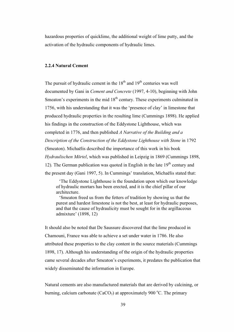
39
hazardous properties of quicklime, the additional weight of lime putty, and the
activation of the hydraulic components of hydraulic limes.
2.2.4 Natural Cement
The pursuit of hydraulic cement in the 18th and 19th centuries was well
documented by Gani in Cement and Concrete (1997, 4-10), beginning with John
Smeaton’s experiments in the mid 18th century. These experiments culminated in
1756, with his understanding that it was the ‘presence of clay’ in limestone that
produced hydraulic properties in the resulting lime (Cummings 1898). He applied
his findings in the construction of the Eddystone Lighthouse, which was
completed in 1776, and then published A Narrative of the Building and a
Description of the Construction of the Eddystone Lighthouse with Stone in 1792
(Smeaton). Michaëlis described the importance of this work in his book
Hydraulischen Mörtel, which was published in Leipzig in 1869 (Cummings 1898,
12). The German publication was quoted in English in the late 19th century and
the present day (Gani 1997, 5). In Cummings’ translation, Michaëlis stated that:
‘The Eddystone Lighthouse is the foundation upon which our knowledge of hydraulic mortars has been erected, and it is the chief pillar of our architecture.
‘Smeaton freed us from the fetters of tradition by showing us that the purest and hardest limestone is not the best, at least for hydraulic purposes, and that the cause of hydraulicity must be sought for in the argillaceous admixture’ (1898, 12)
It should also be noted that De Saussure discovered that the lime produced in
Chamouni, France was able to achieve a set under water in 1786. He also
attributed these properties to the clay content in the source materials (Cummings
1898, 17). Although his understanding of the origin of the hydraulic properties
came several decades after Smeaton’s experiments, it predates the publication that
widely disseminated the information in Europe.
Natural cements are also manufactured materials that are derived by calcining, or
burning, calcium carbonate (CaCO3) at approximately 900 oC. The primary

40
difference between hydraulic lime and natural cement is that cement has a
significantly higher percentage of impurities, greater than 45% and commonly
over 55%, than eminently hydraulic lime (Holmes and Wingate 2002, 281).
Although some historic sources indicate that this percentage could be as low as
38% (Cummings 1898, 27). These high levels of impurities cause the primary set
of this material to occur during hydration, rather than carbonation. Hydration is a
significantly more complicated chemical process than carbonation and involves
the combination of calcium carbonate (CaCO3) and magnesium carbonate
(MgCO3) with silicate of alumina or clay (Cummings 1898, 32). Cummings stated
that when ‘undergoing calcination the lime becomes caustic by reason of the
expulsion of the carbon dioxide, in which condition, and while at a high
temperature, it attacks and disassociates the silicate of alumina, rendering the
silica free as a silicic acid, the latter then combining in certain fixed ratios with the
bases present’ forming silicates (1898, 33). The resulting silicates vary depending
on the base material. Pure limestone will combine with silicate of alumina to form
bisilicates (silicate of lime and alumina) and dolomitic limestones will combine to
form trisilicates (silicate of lime, magnesia, and alumina) (Cummings 1898, 30).
Since both lime and natural cement are derived from argillaceous, or high clay
content, limestone and calcined at the same temperature, the historic definitions of
each material were based on performance. Both materials had hydraulic
properties, but some of the materials slaked and others did not. Those that did
were described as hydraulic lime; those that did not were described as natural
cement. As described above, the difference between lime and natural cement is a
sliding scale between pure lime and natural cement. The materials are similar
enough that Holmes and Wingate proposed a revision to the Vicat system of lime
classification that included natural cement (2002, 280-1) (Table 1). Each material
contains at least a minute portion of the other. The percentage of each material
that is capable of slaking is the portion that did not combine during calcination to
produce bisilicates and trisilicates. While greater levels of slaking may indicate a
lower percentage of these silicates in the calcined material, other impurities may
affect the ability of a feebly, moderately, or eminently hydraulic lime to slake,

41
giving a false indication that the product is natural cement rather than a naturally
hydraulic lime (Uracius pers. comm. 16 November 2005). In the manufacture of
natural cement, the calcined materials do not slake and must be reduced by
grinding to achieve a particle size suitable to achieve consistent hydration (Withey
1912, 78).
The greater understanding that developed out of the work of Smeaton and De
Saussure initiated more than a century of rapid development in mortar technology.
The earliest developments occurred in the natural cement industry as argillaceous
limestone deposits were identified and utilised in Europe and North America. In
1796, Parker patented a natural cement, which he called ‘Roman cement’ (Gani
1997, 5). In 1802, production began on a similar material in Boulogne, France
(Cummings 1898, 17). The production of natural cement did not commence in the
United States until 1818, when Canvass White discovered and patented the
production of the first American natural cement from suitable limestone deposits
near Syracuse, New York. The cement produced in this location was used in the
construction of the Erie Canal (Cummings 1898, 18). In 1828, production began
on the extensive deposits found in Rosendale, New York (Cummings 1898, 19).
The Rosendale cement works developed into the largest producer of natural
cement in the United States, manufacturing 42% of all American natural cement
by the mid 1890s (Cummings 1898, 290). Deposits were subsequently identified
in in the eastern United States in Louisville, Kentucky in 1829; Shepherdstown,
West Virginia in 1829; Cumberland, Maryland in 1836; Hancock, Maryland in
1837; Utica, Illinois in 1838; Akron, New York in 1839; Balcony Falls, Virginia
in 1848; Lehigh Valley, Pennsylvania in 1850; Cement, Georgia in 1850, and
Rossville, Georgia in 1901 (Cummings 1898, 19-21) (Maynard 1912, 59). There
is one other site located approximately 20 km south of the Rossville site in
northwest Georgia, which was listed in A Preliminary Report on the Mineral
Resources of Georgia in 1910 (McCallie, 52). Since no other information on this
site has been obtained, it is unclear if the company in this location was a
manufacturer or simply a cement and lime retailer.
42
The deposits in northwestern Georgia located in Cement and Rossville, Georgia
are of particular interest to this research due to their proximity to the study area.
Cement rock was identified in the area now known as Cement, Georgia in 1850
(Cummings 1898, 21). The company was organised the following year, and began
advertising their hydraulic cement in the Southern Cultivator periodical in 1853
(Howard Hydraulic Cement Company, 362). Production was interrupted by the
Civil War in the early 1860s and did not recommence until 1867 (Cummings
1898, 21). The company was in operation until at least 1912, when it was listed in
a Report on the Limestones and Cement Materials of North Georgia (Maynard
1912), producing a natural cement with the trade name ‘Red Keystone’ (Howard
Hydraulic Cement Company 1905). According to Cummings, this cement
‘probably has no superior in this or any other country’ (1898, 21). Far less
information is available regarding the Chickamauga Cement Company located in
Rossville, Georgia, which was founded in 1901 by the eminent natural cement
manufacturer and historian, Uriah Cummings (Maynard 1912, 220) and produced
natural cement under the trade name ‘Dixie Cement’ (Maynard 1912). Although it
is unclear when the company was dissolved, there are no records indicating that it
was in operation after 1910. Since this coincides with Cummings’ death, it seems
likely that it ceased operations around this time (Cement Age 1910, 362). This
site is worthy of further study due to it association with Cummings and its close
proximity to the Howard Hydraulic Cement Company cement works, which he
believed to be of the highest quality.
2.2.5 Portland Cement
The final material used within this period is artificial Portland cement. This
material is also produced from argillaceous limestone, but not those with
magnesium content greater than 3%. This is because artificial Portland cement is
calcined to the cintering point at approximately 1300 oC. Magnesium carbonate
(MgCO3) calcines at a lower temperature than calcium carbonate (CaCO3) and
‘overburns’ at such a high temperature, becoming inert and negatively affecting
the properties of the cement (Edison 2005). In order to produce optimum

43
compressive strength, the raw materials for artificial Portland cement are ground
(Cummings 1898, 184) and combined with clay and other impurities. This creates
the ideal ratio of calcium carbonate and impurities to produce the complex
silicates during calcination that give the material its exceptionally high
compressive strength and low vapour permeability. Once calcined to the cintering
point, the materials are reground to a powder and are ready for use (Withey 1912,
80).
Unfortunately, the exceptionally high compressive strength and low vapour
permeability characteristics can have a detrimental effect on many historic
building materials. The high compressive strength can damage stone and brick by
forcing the historic materials to bear the majority of the stress and strain exerted
on the wall during thermal expansion and contraction. The low vapour
permeability of Portland cement based mortars also exerts stress on the crystalline
structure of the adjacent masonry units by forcing the normal absorption and
evaporation of water on the surface of the wall to occur through the more
permeable historic materials. Water evaporates when it reaches the surface of the
historic material and leaves behind the minerals that were dissolved in it, which
reform as crystals and cause surface erosion. Historically, the mortar was intended
to be weaker than the adjacent masonry units and act as a relatively easily
replaced, sacrificial material in the assembly. The cyclical pointing of mortar
joints was an indication that the system was performing effectively and protecting
the adjacent materials. As Portland cement became more common in the late 19th
and early 20th centuries, it was increasingly used as a repointing material for
earlier buildings. For this reason, it is a particularly important material for
conservators to understand when addressing late 19th and early 20th century
historic masonry buildings, as well as repairs dating to all eras.
2.2.6 Gauging
Gauging is the practice of blending two or more binders in order to produce a
composite or ‘gauged mortar’ (Chandigarh 1992, 124). The most common gauged

44
mortar is Portland cement and lime (Chandigarh 1992, 124), but it is an equally
accurate description of earth and lime mortars or natural and Portland cement
mortars. By gauging the binder materials, the mason could alter the performance
and cost of the mortar. As expected, a gauged mortar has hydraulic properties,
compressive strength and workability between those of its components.
According to Spalding’s Hydraulic Cement: Its Properties, Testing, and Use, the
addition of 30% to 40% lime to a cement mortar does not significantly decrease
its strength or impair its hydraulic properties (1906, 246). In the absence of
specific data, it is assumed that the hydraulic properties of the mortar are
significantly decreased above this threshold. Experiments conducted by Greaves-
Walker and Lambertson on the suitability of clay as a mortar material tested the
compressive strength of mortars with equal parts of Portland cement and earth, as
well as Portland cement and lime. The compressive strength of the Portland
cement mortar gauged with earth was reduced by 77%, while the compressive
strength of the mortar gauged with lime was only reduced by 45% (Greaves-
Walker and Lambertson 1942, 17). Compressive strength is not the only possible
performance property affected by gauging mortars. A mortar is considered to be
workable when the ‘sand particles roll over each other with ease’ (Schuller et al.
1999, 156). Since lime mortars are particularly well known for their workability
(Schuller et al. 1999, 156), it is also possible that masons were intending to
improve the workability of the Portland cement mortar by gauging it with lime or
workable earthen materials. By varying these proportions, the mason could adjust
the performance or the cost of the mortar. For example, adding 30% to 40% lime
to a more expensive Portland cement mortar would not significantly alter its
performance, but would improve its workability and reduce the overall cost of the
mortar. By adding 50% lime to a Portland cement mortar, it is likely that the
mason was either intending to alter the compressive strength or workability of the
mortar or was simply willing to accept the alteration in exchange for a
significantly more economical mortar material.

45
2.2.7 Additives
Additives are another way that masons modified the performance properties of
mortar. The results are similar to those of a gauged mortar, including
improvements in performance and workability. Those intended to improve the
hydraulic properties and compressive strength are typically referred to as
pozzolans in reference to the ancient Roman material discovered near Mt.
Vesuvius in Pozzuoli, Italy. It is a volcanic ash containing silica and alumina
(Doebley and Spitzer 1996, 288), which are the same materials in the argillaceous
limestone that give hydraulic limes and natural cements their hydraulic properties.
The term pozzolan has come to describe mortar additives including volcanic ash,
brick dust and industrial by-products, such as slag and pulverised fuel ash. Each
of these materials has been fired and supplied the silica and alumina necessary to
combine with the carbonate materials to produce a hydraulic set. Other materials
were also employed historically to alter a mortar’s performance characteristics.
These materials varied so widely that Doebley and Spitzer noted that if a material
was ‘found around the farm or household, it seems that someone at sometime
added it to the mortar mix’ (1996, 289). Some of the more common of these
include egg whites, rosin, casein and animal glue, which were believed to improve
the bond or the adhesion of the mortar to the adjacent masonry units (Doebley and
Spitzer 1996, 289) (Stewart 2012, 66). Beeswax was used as a water repellent,
and fresh blood may have contributed to the early development of strength
(Stewart 2012, 66). These examples only provide a glimpse into the most
common additives used historically to modify the performance characteristics of
mortar.
Additives were also used to improve the workability of a mortar. Substances such
as malt and urine were used as ‘air entrainers’ (Doebley and Spitzer 1996, 289) to
improve workability by producing air bubbles in the mortar, which increased the
ease with which sand particles moved past each other when mixing and using the
mortar (Schuller et al. 1999). Around 1918, a bagged cement product was
introduced to the market called ‘masonry cement’ (Farny 2007, 1-2), which

46
contained a ‘finely ground limestone and hydrated or hydraulic lime’ (Farny
2007, 3). In this product, the ground limestone is a plasticiser, which makes the
material more plastic and workable (Farny 2007, 3).
2.3 Masonry Conservation and Archaeology
Although these disciplines are more closely related today, current professional
literature revealed that there may be tensions between conservation and
archaeology. To address this in further detail required a discussion of the
differences between American and international conservation terminology. In the
United States, the term historic preservation is used to describe the field that is
more commonly referred to as conservation in the international community.
American terminology has caused problems in practice in the United States, as
well as when engaging in conversations with the international community. One of
the most problematic aspects is the dual role of the term ‘historic preservation’
which can be synonymous with conservation in the rest of the world or as an
overarching title for all heritage related efforts in the United States, which may
include anthropology, archaeology, cultural resource management and building
conservation. For this reason, in the course of this thesis, the term conservation
was used to describe the narrow definition of historic preservation, which is
synonymous with conservation. Heritage management is used in place of the
wider definition of historic preservation, which describes all of the fields related
to the study and management of both tangible and intangible heritage. Of course,
this change will not occur in direct quotes. In these cases, the reader will need to
infer the intended meaning from its context in the passage.
Although both conservation and archaeology are included in the field of American
heritage management, the consideration and implementation of archaeological
theory in conservation projects may not be widely accepted. In a recent
publication on the future of American heritage management in the 21st century, it
was clear that archaeology’s relationships to other fields within this broad

47
classification was strained. In an article on ‘The Changing Role of Archaeology in
Historic Preservation’, John Sprinkle, who was an historian with the NPS, stated
that ‘Archaeology is perhaps best understood as modern-day alchemy: turning
base materials—soil and stone, bone and ceramic—into the gold of archaeological
observation and interpretation’ (2003, 253). This was hardly a glowing
endorsement of the potential positive influence that archaeology could have on
American heritage management. He supported his critical view of archaeology in
the opening paragraph by stating that:
‘Archaeology is fundamentally different from other professions within historic preservation. The difference is essentially one of orientation. Historic preservation is concerned with the future of old buildings, neighborhoods, and landscapes—managing change—whereas archaeology is primarily interested in recovering and interpreting human behavior of the past… Historic preservation exists on the rehabilitation and restoration of past places and landscapes, whereas American archaeology thrives on destruction of the past through excavation, analysis and interpretation’ (Sprinkle Jr 2003, 253)
Sprinkle was historically accurate in his assessment; however, recent trends in
these fields have softened the seemingly polar differences and have made them
more similar than at any time in the past.
In recent decades, conservation has been struggling with the current definition of
significance, which included sites that ‘possess’ historical, associative and artistic
significance, or were able to provide information on prehistory or history (Tainter
and Lucas 1983, 709). The syntax of this definition alone was problematic,
because it used the term significance to define the quality of significance. In
practice, the situation became even more problematic. If applied liberally, it could
have been used to argue that all old buildings were significant and should be
preserved, since almost all sites have some level of prehistoric or historic
significance. This forced the interpretation of this term into the realm of
professional practice. In reality, the available financial resources devoted to
conservation can only stretch so far. With such a broad definition, how will
conservation decide which buildings to save and which will be lost? The growing

48
necessity to cull less significant buildings placed conservation firmly in the
business of destruction.
During this time of historic uncertainty, archaeology has been under pressure
from within to conserve, rather than destroy both archaeological sites and
recovered artefacts. Archaeologists have conserved an increasing number of
known sites for future study (Bourque et al. 1980, 794). When possible, new
technologies such as ground penetrating radar have been used to assess a site or
gather basic information without disturbing the deposit. There has also been a
greater emphasis on the conservation of artefacts recovered from a site, including
the immediate care, stabilisation and long-term storage needs.
The similarities between archaeology and conservation begin in the most basic
terms. They are both dedicated to the study of the material remains of the past,
whether that is in the form of standing buildings or a variety of subsurface
archaeological remains. The ‘fundamental’ differences between these two
disciplines have decreased over the last century, and they are now in a position to
positively influence each other in theory and philosophy, as well as academic and
professional practice.
In assessing the current state of American building conservation and its ability to
incorporate a more culturally and philosophically based approach to the
architectural resources in its care, it became clear that the divide between the
cultural and scientific aspects of the field are more broadly speaking a divide
between philosophy and practice. The reasons for this probably lie in both the
cultural attitudes of the American people and the social and political environment
during the development of the discipline in the United States. In the 19th century,
conservation philosophy must be inferred from conservation practice. As a greater
number of documentary resources became available in the 20th century, our
understanding of the conservation philosophy of the time can be concluded by
reviewing legislation, policy documents, and academic and professional journals.
The process of inferring philosophy from either practice or related writing clearly

49
results in a strong relationship between the philosophical and practical aspects of
the field. By avoiding purely philosophical debate throughout most of its history,
American conservation developed according to the belief that philosophy was
both self-evident and static. It was only in the late 20th and early 21st centuries,
when overtly philosophical debate became more common that the differences
between the philosophical and practical aspects of the discipline became more
obvious. By analysing the influence of these factors on the development of the
current American conservation system, the unique problems that it faces today
become apparent.
Socially and politically, there are several factors that have had a lasting effect on
American conservation and created a different system than in other countries
around the world. The break from the British Empire prior to the rise of
historicism in the 19th century placed an emphasis on patriotism and the formation
of a national identity in early amateur conservation efforts, rather than artistic and
aesthetic issues that were so influential in other countries, particularly the United
Kingdom. As building conservation began to professionalise and develop into a
distinct discipline in the mid 20th century, it was heavily influenced by architects
and historians and has resulted in a lasting placement of building conservation
education within architecture departments. The relationship between state and
federal governments and the timing of the development of national conservation
legislation has also resulted in a uniquely American conservation system, which
required that each state establish a system to administer federal programmes. This
multilevel structure was more burdensome to amend and has been less able to
adapt to ongoing changes in social and cultural values.
The challenge in pursuing multi-disciplinary research was that it must address a
diverse set of issues from a potentially wide range of disciplines. A simple
solution to this problem was to pick and choose the elements that were the most
useful and quickly assimilated, and ignore the rest. This was certainly the trend
that American conservation has followed in recent decades. Its practitioners have
openly incorporated methodologies from related disciplines, particularly

50
archaeology, but have not fully incorporated the theoretical and cultural aspects of
the field. This presented a potential problem for the international conservation
community; however, the situation was more serious for American conservation,
which seemed to have avoided purely philosophical discourse throughout much of
its history. Instead, it has focused on the applied aspects of the discipline.
Increasingly scientific methods and terminology gave the overall impression of
objectivity. Unfortunately, they were often little more than disguises for intuition
or an individual’s implicit personal philosophy.
Since 1966, conservation has worked within the confines of the NHPA.
Theoretical concepts that have emerged in related fields since that time have
affected conservation philosophy, but they were generally restricted to aspects of
practice that are not specifically defined in the NHPA. Academic and professional
journals revealed a long-standing dissatisfaction with the existing definitions of
significance and the appropriate types of intervention as defined in the 1960s. The
use of new scientific methodologies and techniques in conservation research and
practice were also discussed in these journals, but they were normally presented
as purely scientific data that were unaffected by philosophical debate. Within the
public sector, the most flexible and responsive sources of information are policy
documents, which are published and updated to interpret legislative intent. These
ranged in content from general documents explaining the appropriate types of
intervention, such as The Secretary of the Interior’s Standards for the Treatment
of Historic Properties with Guidelines for Preserving, Rehabilitating, Restoring
and Reconstructing Historic Buildings (Weeks and Grimmer 1995) to specific
applied conservation documents including the Preservation Briefs and
Preservation Tech Notes published through the National Parks Service (NPS)
office of Technical Preservation Services. The publication of new policy
documents and updates to existing ones were the best means for the government
to respond to changes in conservation philosophy. The least frequent method of
response to these changes occured in the form of amendments to the NHPA. This
was a much more involved process than the revision of policy documents and was
normally reserved for the initiation or termination of federal conservation

51
programs. Through these public and private publications, the conservation
community has informally responded to wider trends in the humanities and social
sciences by pushing the legislative limits established in the 1960s and
incorporating aspects of these concepts in certain aspects of conservation practice.
The content of technical policy documents varied greatly depending on the subject
matter, author, and the date of original publication and subsequent updates. In
most cases, they contained generalised assessments of historic conditions in the
United States and material specifications that were based primarily on
performance issues. Reducing the variety of American building forms to a
‘manageable’ set of options was in direct opposition to wider theoretical trends,
which emphasised, value and promoted diversity. This was another example of
the assumption in the applied aspects of the discipline that the ‘scientific’ nature
of their work fell outside of the realm of philosophical debate.
In this environment, policy documents established a de facto standard for the
repair of historic mortars, which is still one of the oldest and most frequently cited
conservation standards in place in the United States after nearly two decades of
use. The content of both the original and revised documents reveal a normative
approach that focused solely on description and specification, and over-
generalised the many variables of this complex topic. The age, frequent use and
clearly traditional conservation approach of this standard made it an ideal example
of existing conservation policies and standards to frame this discussion.
The original version of the standard, entitled Preservation Briefs: 2, Repointing
Mortar Joints in Historic Brick Buildings, was issued in 1980 and addressed only
brick unit masonry. In addition, lime and Portland cement were the only materials
listed as potential binders for mortars used to repair historic buildings. While
Portland cement mortars were described as unsuitable for use in historic
buildings, the brief clearly indicated that Portland cement was a suitable
admixture to ‘improve workability or plasticity’ (Mack and Askins 1979). The
revised edition, entitled Preservation Briefs: 2, Repointing Mortar Joints in

52
Historic Masonry Buildings, was issued in 1998 and expanded to include
information on ‘all types of historic unit masonry’ (Mack and Speweik 1998). It
also acknowledged that architecture of the early 20th century, which was now
eligible for listing in the National Register of Historic Places, may have been
originally constructed using a Portland cement mortar (Mack and Askins 1979).
An examination of these two documents revealed the over-generalisation common
in many technical publications on historic mortars. Specifically, the idea that
mortars prior to the early 20th century used a lime binder, and mortars after the
early 20th century used a Portland cement binder. The revised brief only mentions
clay and natural cement as possible admixtures, along with other materials such as
crushed shells, brick dust, pigments and animal hair. This description overlooked
the fact that clay and natural cement were common binder materials in some
locations into the 20th century. Documentary and physical evidence suggested
that a broad palette of materials were commonly used in the United States and that
the development from one material to another was quite different from the
terminus ante quem/terminus post quem method of mortar analysis currently
accepted by many State Historic Preservation Offices (SHPO) and local historic
district review boards, based solely on the information contained in the NPS brief.
The emphasis on lime was based largely on a European understanding of historic
mortars, particularly those in the United Kingdom, which was highly influential in
the development of American preservation philosophy and conservation materials
science. It assumed that prior to the dominance of Portland cement that American
decisions about the methods and materials used to construct the built environment
were made according to the same set of environmental and cultural criteria
guiding decisions in Europe, specifically the United Kingdom. This discounted
both African and Native American traditions, including the strong earth
construction traditions in west and westcentral Africa and the Native American
population in the southeastern United States.
The role of mortars as a sacrificial element in a masonry wall creates and
interesting juxtaposition of he ephemeral and the permanent. These two materials
53
are interesting in that they represent opposite ends of the spectrum and illustrate
the fact that materials also abide by the same rules of value that govern buildings,
sites and larger cultural landscapes. When a material such as brick is defined as a
durable, eternal product, it is expected to last and the material itself becomes
valued. The opposite is true of lime, which is perceived to be an ephemeral
product and is defined, and therefore valued, more for its sacrificial and cyclical
nature. The difference in perception resulted in different approaches to everyday
conservation decisions.
The assembly of brick and lime combines the physical properties of each material,
as well as the values and expectations that society has in them. Brick is seen as a
durable product that needs little or no maintenance. In this sense, it is a
representation of the ‘static’ portion of our cultural heritage. This image causes
brick to be approached from a traditional perspective in which age, patina and
decay are seen as proof of its age value. This limits the amount of maintenance
that the material receives and discourages people from altering or replacing
elements. In some ways the association of permanence and brick is unexpected,
because it is a mass-produced material that does not reveal the ‘hand of the artist’
except for the most high-status buildings in which hand-carved detailing is used in
limited areas.
On the contrary, lime is a relatively weak and ephemeral material that is in need
of continued maintenance and repair. It is precisely this part of its nature that
makes it valuable to society. In nearly all of its applications, it is intended to be
the sacrificial or protective element in the assembly. This is seen in its use as a
mortar and as an exterior render. There is less of an emphasis on patina in this
material because of the relatively quick erosion and loss of the surface material.
There is more of a concern for patina when it is used as a render, but this is
minimal because in most cases lime renders would have been lime washed on a
regular basis in order to fill small cracks and imperfections that would
compromise its protective qualities.

54
In assembly, the physical properties of brick and lime are complimentary and
work is unison. As the brick expands and contracts, the lime absorbs the stress.
When the wall becomes wet, the lime mortar or render wicks the water out of the
more ‘permanent’ brick. However, our perceptions of the materials in assembly
have not been able to compromise as well. The difficulty could stem from issues
of workmanship. Philosophically, this could be the result of associations with the
craftsmanship of the original bricklayer. It may also be a functional issue
surrounding the difficulty in repointing without damaging the surrounding brick,
which we value in a much greater sense.
In theory, the development of conservation philosophy over time guides the
implementation and amendment of heritage legislation. Once in place, the general
framework and terminology established by the legislation is interpreted by
conservation policy and standard documents, which translate the intent of the
legislation into a practical and usable form. In practice, the process of
implementing and amending legislation is arduous and protracted. As such, it is
generally reserved for more significant shifts in philosophy, such as the
developments in American conservation during the early 20th century, when
historic buildings were recognised as significant in addition to the natural and
archaeological heritage addressed in earlier legislation. In contrast, policy
documents are ideally suited to respond to more subtle changes in the philosophy
and values of society, for example a reassessment of the types of buildings or
monuments that are recognised as significant.
The current paradigm used to establish and develop national conservation policies
and standards is a normative one that focuses on description and specification.
The initial emphasis is placed on the description of typical building forms,
materials and methods of construction, which is essential in order to establish a
limited number of “appropriate” specifications for the repair of the vast array of
historic resources in the United States. This approach is possibly a direct result of
the development of current legislation and policies from early 20th century
American heritage legislation, which would have been heavily influenced by the

55
culture historical philosophy prevalent in the social sciences at that time. It is also
possible that it was simply a way to limit the scope of policies and standards that
are, by their nature, intended to be practical and usable documents. While the
potential explanations are understandable, the continued use of this paradigm for
the establishment and development of all conservation policies and standards,
even the most complex, risks collapsing the entire breadth of historic resources in
the United States into no more than a handful of typical conditions.
2.4 Conclusion
The mortar samples collected in the current research should serve as an example
of the effective sampling and interpretation of mortar as an archaeological
artefact. If the methodology utilised in this research were applied to the
abundance of masonry remains located at historical sites in the southeast, mortar
could be utilised to its full potential as an accepted part of the analysis and
interpretive processes within the discipline of historical archaeology. This would
stand in stark contrast to the common practice in the southeastern United States of
simply weighing the brick and mortar fragments onsite and either rebury or
dispose of the materials without retaining a representative sample (Elliott 2013).
There is no reason that the process of mortar analysis should not be used to
provide the same types of dating and cultural information as any other type of
artefact. Given a large enough collection of mortar data, the value of mortar may
also be able to provide a dating resource similar to one of the current reference
tables, such as the Binford Pipe Scale. In building conservation, mortar is
generally perceived to be a sacrificial component of a masonry assembly. By its
very nature, it is seen as an ephemeral product valued more for its sacrificial and
cyclical nature than its inherent qualities. This research and its findings should
offer a reason for conservation to reassess this perception and the consider less
invasive conservation interventions, as well as more thorough documentation and
sampling of existing materials prior to conservation.
56
Chapter 3: Theory and Methodology
The theoretical approach of this research responded to the current divide between
the cultural and scientific aspects of conservation and archaeology by constructing
a materiality based research design. Referred to as materiality, material agency
(Jones 2004, 330) or social archaeometry, the central issue to the theoretical
approach is that there is a dynamic and inseparable connection between artefacts
and the societies that created, used and modified them (Bray and Pollard 2005,
179). It argues that the physical properties of a particular material affect the way
in which a society uses and assigns meaning to the material, which in turn affects
its subsequent use and meaning. The perpetual interaction between the artefact
and culture establishes a cycle that continually reinforces existing social structures
or modifies them in response to an agent of change (Needham 2005, 194). It
argues that neither the physical nor the cultural aspects of the past can be
adequately assessed individually. They can only be understood in the context of
an integrated scientific and theoretical analysis (Jones 2004, 331). By definition,
this theoretical approach encourages a more unified understanding of the cultural
and scientific aspects of the disciplines and the built environment.
Archaeologists engaged in the material agency dialogue openly acknowledge the
need for a more integrated approach in the assessment of material culture, but few
have addressed the need to reassess methodology as clearly as Dobres and Robb
(2005) or Hilditch (2010). Dobres and Robb criticised the ‘sparse methodological
developments’ (2005, 159) associated with material agency and argue that ‘it is
simply not possible to change fundamentally one’s theoretical orientation without
also reevaluating one’s methodology’ (2005, 160). They suggested that agency
operates in the present in a variety of contexts and scales, and it is likely that it did
so in the past as well. As a result, the physical evidence of agency in the
archaeological record is also likely to occur in a variety of contexts and scales
(Dobres and Robb 2005, 162). Hilditch also used a ‘multiscalar approach’ (2010,
2) to address interactions on the ‘micro-scale of individuals’, the ‘meso-scale of
group interaction’, and the ‘macro-scale of regional interactions’ (2010, 2). While

57
these approaches sought to characterise interactions within particular individuals,
groups and regions, this research has used a multi-scalar approach to assess
mortar and mortar materials on a variety of levels, including the use of binder and
additives in a particular mortar, the combined use of the binder and aggregate
components to establish the appearance characteristics of the mortar, and the use
of single or multiple mortars in a particular type of construction or building.
Both of these aspects of materiality have played a key role in the way that this
research was designed, implemented and analysed. Mortar was selected as the
focus of the research for several reasons. It is a material that is present in nearly
all historic buildings. It is a common issue addressed in conservation projects and
is routinely encountered on historical archaeology sites. Although masonry is a
common material to be addressed in each of these disciplines, neither have fully
acknowledged the cultural information that may be contained in the assembly by
investigating its materials and methods of construction. Within the masonry
assembly itself, one could focus on the unit masonry or the mortar. Since masonry
units are commonly salvaged and reused, the mortar as the key artefact in the
assembly. By its very nature, it is a material that can be used once and discarded.
This quality gives mortar an interesting position in the archaeological record. It is
not salvaged, moved, reused or even repurposed. Any information that can be
gathered from the material represents a single point in time. The question is what
details might be gleaned from mortar if it is looked at from an archaeological
perspective, specifically one that focused on the characteristics of the material
itself. That is why the concept of materiality was utilised in this research to guide
the development of the research design, as well as its implementation and the
analysis of its findings.
3.1 Materiality
The theoretical concept of materiality emerged in archaeology in the mid-1990s
with contributions from anthropology, material culture studies, and sociology

58
(Taylor 2008, 300) and emphasised the ‘direct connection to physical things, both
those created by human agency that are termed artifacts… and those natural things
recognized or resolved into categories so as to become objects to which value and
meaning can attach.’ (Taylor 2008, 299-300). In either case, the objects
themselves possess both material and formal characteristics. In most buildings
based research, emphasis has been placed on the formal characteristics of
architecture, rather than the materials. When materials are specifically addressed
in mortar conservation, an architectural and engineering approach is generally
taken with all efforts directed toward identifying and specifying an appropriate
repair material. In this context, the term appropriate generally means that the
repair will not harm the adjacent historical materials and that it can be
distinguished from the original materials. Neither addresses nor even
acknowledges mortar itself as a cultural resource. Historical archaeology in the
southeastern United States has limited the role of remaining architectural features
or standing buildings to defining the extent and function of a given site, which
establish the context of the other artefacts on site and place architectural features
in a secondary role. In general, conservation addresses the material characteristics
of masonry, but does not utilise the material itself as a valuable cultural resource.
While historical archaeology uses masonry remains to glean cultural information,
it generally uses these features for the purpose of providing context for the other,
presumably more important, artefacts in the collection.
The material characteristics are central to the role of historic masonry buildings as
an archaeological artefact. For the purposes of this research, the key issues of
materiality established by Jones in 2004 have guided the analysis and discussion
of the mortar samples collected in the study area. He defined these issues as
production, colour, use and durability (Jones 2004, 333-5) and identified them as
significant due to the way in which the physical characteristics of an artefact
affect the ‘social use and cultural perception’ (Jones 2004, 333). The issue of
production considers the way that the physical properties of a material affect the
way it is processed and the social organization of the means of production. The
issue was certainly relevant to this research, due to the varied methods of

59
production of each of the addressed binder types. As such, the relative price of
each binder material was used to estimate the specialised skills and equipment
necessary to produce each of the materials. Jones also addressed the aesthetic
properties of an object, focusing primarily its colour. This research has also
incorporated texture into the discussion, because mortar is a composite material,
which can be dramatically altered by the colour and texture of the aggregate
component. The concept of use was addressed in this research in terms of the
workability of each material. This issue is more difficult to quantify than the other
issues in the discussion of materiality, but is extremely important in terms of the
quality of the original construction and subsequent repairs and conservation. The
final issue proposed by Jones is durability, which has been considered in this
research in terms of the estimated compressive strength of each material.
Although changes in the mortar materials and technology have moved toward
stronger, more durable materials, it should be not be assumed that the most
durable material is always the preferred material when employed in historic
masonry buildings.
3.2 Case Study
The study area selected for this research is defined by the current political
boundaries of Chatham and Effingham Counties in coastal Georgia, which have
been in this location since the mid 1790s, with the exception of the annexation of
Ossabaw Island from Bryan County in 1847 (Sullivan 2000, 58). It is bounded on
the northeast by the Savannah River, the southeast by the Atlantic Ocean, the
southwest by the Ogeechee River, and to the northwest by the boundary between
Effingham and Screven Counties. The area is approximately 30 km wide, extends
northwest approximately 85 km inland from the Atlantic coast and contains 2,600
square km.
This area was selected to conduct the research, because Effingham County had
one of the lowest slave populations per capita in the coastal plain. These

60
conditions were even more striking, given its close proximity to Chatham County,
which had one of the highest slave populations per capita. In contrast, the
geography, soils and underlying geology of the area are relatively homogeneous.
The selection of a study area with these characteristics offered a unique
opportunity to minimise the potential environmental factors and isolate the
diverse cultural processes that may have influenced the methods and materials
used in masonry construction. This approach shifted the focus from the materials
themselves to the relationship between the materials and the individuals that
selected and used them during the period of study. This was a significant
departure from traditional materials science research in conservation and a clear
expansion of archaeological theory and methodology to historical resources
outside the purview of mainstream historical archaeology.
The eras selected for this research were initially based on 20-year spans centred
1830, 1880 and 1930. The methods used to select these dates balanced the
availability of human and historic building population data with key historical
eras. For the purposes of this research, the history of the original southern
colonies and states has been divided into the following eras: colonial (1607-1775),
federal (1776-1819), antebellum (1820-1864) (Boney 1991, 129), Reconstruction
and Redemption (1865-1914) (Wynes 1991, 207), and migration and urbanisation
(1915-1964) (Maloney 2010). Selection of the earliest time period was limited by
the historic building population in Effingham County, which has only one known
building constructed before 1819 that is located on its original site (Information
Technology Outreach Service 2006). This eliminated the colonial and federal eras
from this case study and identified the three historical eras adequately supported
by the historic building population of the study area. The research design
attempted to most accurately represent each of the historic eras by selecting the
census date nearest their centre point, specifically 1840, 1890 and 1940. There
were two problems with the human population data that prevented this selection.
Firstly, the enumeration forms from the 1890 census were almost entirely
destroyed by fire in 1921 (United States Bureau of the Census 1997, 1), and none
of the records for the study area survived. Secondly, the confidentiality of census

61
enumeration forms is protected by federal legislation for a period of 72 years,
meaning that the 1930 census provided the latest complete set of data available to
the public when the scope of this research was defined. By shifting each of these
dates one decade earlier, a complete set of human population data was available
and a 50-year interval was maintained.
The omission of the colonial and federal eras in this case study due to an
inadequate set of historic buildings should not draw into question the efficacy of
this particular study area. It is simply a reflection of the relatively late founding
and settlement of the Georgia Colony on the human and historic building
populations. When the Declaration of Independence was signed in 1776, the
Virginia and Carolina Colonies had been in existence for 169 and 106 years,
respectively. In contrast, the Georgia Colony was only 43 years old (Spalding
1991, 36). Later European settlement resulted in a significantly smaller population
than the other southern colonies at the end of the colonial era in 1770 (Table 2)
and the former southern colonies at the end of the federal era in 1820 (Table 3).
Table 2: Estimated population of the southern colonies in 1770 (United States Bureau of the Census 1975, 1168)
Table 3: Population of the former southern colonies in the 1820 federal census (University of Virginia Library 2004)
County DistrictFree
white SlaveFree
coloredAll
colored Indian Other TotalChatham All 2,456 8,201 112 8,313 0 0 10,769Effingham All 1,674 750 0 750 0 0 2,424
Total 4,130 8,951 112 9,063 0 0 13,193
ColonyVirginia 259,411 57.80% 187,605 54.69% 447,016 56.45%North Carolina 127,600 28.43% 69,600 20.29% 197,200 24.90%South Carolina 49,066 10.93% 75,178 21.92% 124,244 15.69%Georgia 12,750 2.84% 10,625 3.10% 23,375 2.95%Total 448,827 100.00% 343,008 100.00% 791,835 100.00%
Whites SlavesTotal southern
population

62
In 1770, the estimated population of Georgia was only 2.95% of the total southern
population. By the end of the federal era, the population had grown to 13.48% of
the former southern colonies. In terms of the actual population, the total increased
from 23,375 to 341,989. Although there was a 1363% increase in the population
of Georgia between 1770 and 1820, the decreasing percentage of the population
of the specific study area in relation to the state population during the first
decades of the 19th century (Table 4) indicates that the dramatic growth was
located in other areas of the state (University of Virginia Library 2004),
particularly in the southern and western portions of the state recently opened for
settlement (Figure 7) (Minnesota Population Center 2010). The 1800 census data
was used in this comparison because it was the earliest data available that
conforms to the approximate boundaries of the counties between 1800 and the
Area 1800 Census 1810 Census 1820 Census
Chatham 12,946 7.9% 13,540 5.4% 14,737 4.3%
Effingham 2,072 1.3% 2,586 1.0% 3,018 0.9%
Study area 15,018 9.2% 16,126 6.4% 17,755 5.2%
Georgia 163,879 100.0% 252,433 100.0% 341,989 100.0%
Table 4: Comparison of the state and study area population data, 1800-1820 (University of Virginia Library 2004)
Figure 7: Map of Georgia (Minnesota Population Center 2010)
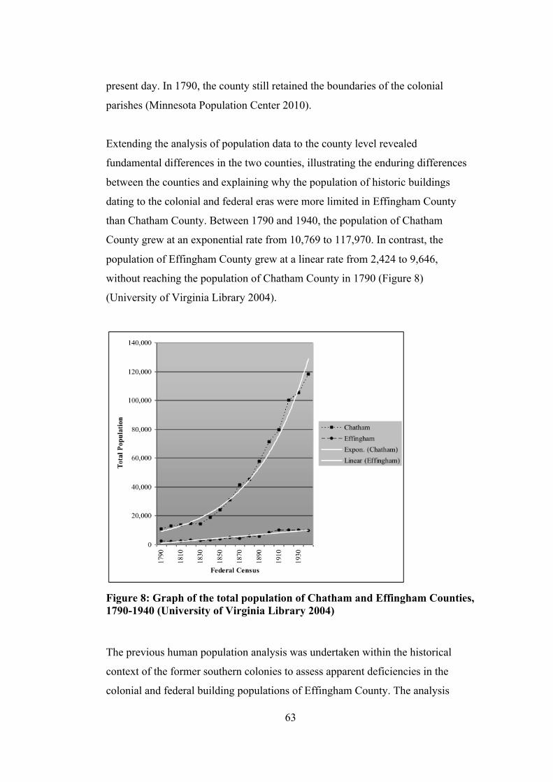
63
present day. In 1790, the county still retained the boundaries of the colonial
parishes (Minnesota Population Center 2010).
Extending the analysis of population data to the county level revealed
fundamental differences in the two counties, illustrating the enduring differences
between the counties and explaining why the population of historic buildings
dating to the colonial and federal eras were more limited in Effingham County
than Chatham County. Between 1790 and 1940, the population of Chatham
County grew at an exponential rate from 10,769 to 117,970. In contrast, the
population of Effingham County grew at a linear rate from 2,424 to 9,646,
without reaching the population of Chatham County in 1790 (Figure 8)
(University of Virginia Library 2004).
Figure 8: Graph of the total population of Chatham and Effingham Counties, 1790-1940 (University of Virginia Library 2004)
The previous human population analysis was undertaken within the historical
context of the former southern colonies to assess apparent deficiencies in the
colonial and federal building populations of Effingham County. The analysis

64
showed that the limited historic building resources were consistent with the
history of the study area, and provided evidence of the longstanding differences in
the demographics of the two counties. Not only did the analysis show that the
absence was not an unexplained anomaly, it showed that it was a condition
specific to this area that could be tied back to the human population and the wider
historical trends of the study area and region.
Once the study area was defined and vetted, it was necessary to further divide the
counties and perform analyses of the human and building populations similar to
those discussed in the previous section. The Georgia Militia Districts (GMDs)
were selected to subdivide the counties for several reasons. Firstly, they were
defined and modified based on population data, so the boundaries were
intentionally designed to reflect the characteristics of the population itself.
Secondly, they were the primary basis for many other types of administrative
districts in each county, including federal census enumeration districts. Thirdly,
they have been in continuous use in the state since the colonial era. The
continuation is a longer lasting version of the colonial parish boundaries, which
were adopted by the state in 1778 and modified in the mid 1790s (Hitz 1956, 1-2).
Even though there was a series of Militia Acts in the antebellum era, the role of
the militia did not chance significantly until after the Civil War, when the military
primacy of the GMDs was superseded by a variety of administrative functions,
including court, election and tax districts. The militia itself was replaced when the
National Guard was organised in 1916 (Hitz 1956, 1). Nevertheless, the districts
remained and continued to evolve based on changes in their populations. Their
longstanding use by federal, state and local governments, particularly as census
enumeration districts, was critical to the success of this research. Preliminary
research exposed a similar pattern in the availability of GMD boundary
information as was seen in the historic building population. The most significant
absence of data was in early Effingham County. In this case, it encompassed
Effingham County for the entire 19th century. As a result, the GMD boundaries
were reconstructed in reverse chronological order and utilised historic maps, land
plats and property deed records, state legislation, and federal census records. The

65
process became increasingly complex in the earlier time periods and meticulous,
and often unfruitful, archival research was conducted in order to locate any
evidence of the location of the boundaries. When available resources were
exhausted, the later configuration was retained. Although the boundaries defined
by this process are undoubtedly imperfect, the resulting estimates constitute the
most comprehensive interpretation to date. The additional attention given to this
topic was necessary because it significantly strengthened the link between the
human and historic building populations and facilitated an integrated analysis and
interpretation of the data.
Each county was divided into GMDs, which were established based on the
population required to raise a militia unit. There were eight districts in Chatham
County during the period of study. GMDs 1-4 are located in the city of Savannah,
and GMDs 5-8 divide the remainder of the county. In 1830, Effingham County
had between four and six militia districts. Six districts were in place in 1804
(Smith 2000, 129), but were consolidated into four GMDs, numbered 9-12 prior
to the 1860 Federal Census (Ancestry.com 2010a). In 1897, GMD 10 was
subdivided creating GMD 1559 (Effingham County Board of Commissioners
1897).
The GMD boundaries in 1930 were defined based on federal census records and
historic maps and were based on geographical features, roads, railroads and
canals. The boundaries of GMDs 1-4, located within the Savannah city limits,
were compiled from the enumeration district descriptions in the 1930 Federal
Census records (Ancestry.com 2009a). The boundaries of GMDs 5-8, located
outside Savannah, were not clearly described in the census records and were
defined for this research according to Act No. 210 passed by the General
Assembly of the State of Georgia in 1907, which revised the previous boundaries
defined in 1881 (General Assembly of the State of Georgia, Section I). The
locations of these boundaries were corroborated using a 1930 general map of
Chatham County (Scnreck et al. 1930), which confirmed that the boundaries did
not change between 1907 and 1930. The boundaries of the Effingham County

66
GMDs in 1930 were not described in the federal census records. They were
defined for this research based on a 1923 United States Department of Agriculture
(USDA) map of the county (Eason and Ryder).
The GMD boundaries in 1880 were based on a wide range of county and federal
records and were delineated by geographical features, roads and railroads. The
Chatham County GMDs were compiled from the enumeration district descriptions
in the 1880 federal census records, both within and outside the Savannah city
limits (Ancestry.com 2009b). The locations of the 1880 Effingham County
boundaries were estimated by plotting data points for residents of the county
identified in the 1870 and 1880 federal census records, as well as the land plats
recorded by the Effingham County Clerk of Court. The census records identified
the GMD containing the person’s primary residence, and the land plats located the
parcels of land surveyed for the person in Effingham County. When multiple
parcels were identified, preference was given to the earliest and largest parcels.
These points were compared to the 1930 configuration to identify boundaries that
were revised in the interim. In areas with insufficient data to assess the 1930
boundaries, additional points were plotted for specific parcels of land located in
the vicinity. In these cases, the chain of title was traced to search for late 19th
century legal descriptions, which sometimes record the GMD of the parcel at the
time ownership was transferred due to sale or inheritance.
The 1830 boundaries were based on government records similar to those used to
reconstruct the 1880 GMDs, and resulted in boundaries delineated by
geographical features and roads. The GMDs in the study area were estimated by
applying known changes to the 1880 configuration. In Chatham County, this
consisted of revising the Savannah city limits based on historical maps, which
reduced the extents of GMDs 1-4 and extended GMDs 5-8 to the 1830 city limits.
Boundaries dividing GMDs 1-4 within the Savannah city limits and GMDs 5-8 in
the county were maintained from the 1880 configuration. In Effingham County,
the most significant modification to the 1880 configuration was based on an 1809
land plat, which defined 17,703 m (11 mi.) of the boundary between GMD10 and
67
GMD12 (Moore, 225). The remaining boundaries were assessed by plotting data
points for residents identified in the 1860 federal census, which is the earliest
census that subdivided this county to the GMD level, and the 1864 partial state
census. The partial census was taken as a result of ‘An Act to re-organise the
Militia of the State of Georgia’ of 1863, which required the Aid-de-Camp of each
district to enrol ‘all free white males resident in his District, who are or shall be of
the age of sixteen years, and not over sixty years’, except those in the service of
the state or the Confederate States of America (CSA) (General Assembly of the
State of Georgia 1864, Section II). Although these sources are dated 21 years
earlier and up to 34 years later than 1830, they provide the best data available for
the reconstruction and analysis of the early time period in Effingham County. It is
also important to consider the two additional districts that were created prior to
1804 and eliminated by 1860. No attempt was made to identify the locations or
boundaries of either of these districts, because the lack of subdivision in the
corresponding census data, which is discussed in the following section, required
the complete reconstruction of the 1830 census data, effectively rendering this a
moot point.
The theoretical underpinnings of this research placed an emphasis on the
relationship between people and the objects that they created. In particular, it
addressed the historic masonry materials and methods used in an area in coastal
Georgia in the 19th and early 20th centuries. The people are gone, and only a
portion of the buildings that they constructed remain. Yet each needed to be
characterised in a detailed and thorough manner. The human population was
characterised by collecting available census data and, when necessary, modifying
it to create a set of data that is as consistent as possible over the entire span of
time addressed in this study. The characterisation of the building population was
developed from an historic resources survey compiled by the State of Georgia and
building data provided by the Chatham County Tax Commissioner’s Office and
the Effingham County Tax Assessor’s Office. These two sets of data provide the
foundation for the rest of the research.

68
3.3 Natural Resources
The mortar materials used in the study area were naturally constrained by the
geology and geomorphology of the region. There are five physiographic provinces
in the region, which generally define areas formed by similar geological
processes, often resulting in similar geological conditions. The mountainous area
in the northwest portion of the region consists of the Appalachian Plateau, Ridge
and Valley and Blue Ridge provinces (Figure 9) (United States Geological Survey
2004b). Most of the rivers of the region originate in this area and travel southeast
to the Atlantic Ocean through the Piedmont and the Atlantic Coastal Plain
provinces. The boundary between these two provinces is the fall line, which is a
‘low east-facing cliff paralleling the Atlantic coastline’ (United States Geological
Survey 2004a) that creates waterfalls and marks the end of the waterways
navigable from the Atlantic Ocean.
3.3.1 Geology
The underlying sedimentary bedrock of this region was formed prior to a series of
continental collisions in the Paleozic Era approximately 270 to 330 million years
ago, forming the Pangaea supercontinent (Horton and Zullo 1991, 9). The intense
pressure of these collisions may have compressed the earth’s crust by more than
200 km, uplifting the region and creating large metamorphic rock formations in
the Piedmont and Blue Ridge provinces and the thrust faults and dense folding of
sedimentary rock in the Ridge and Valley province (Horton and Zullo 1991, 9-
10). Erosion and sedimentation were then the primary geomorphological
processes (Soller and Mills 1991, 290) until the supercontinent began to separate
around 180 million years ago, forming the Atlantic Ocean (Horton and Zullo
1991, 10) (Hodler and Schretter 1986, 14). As the seafloor expanded, the bedrock
of the present coastal plain began to tilt toward the southeast (Horton and Zullo
1991, 10). Differences in sediment depth and stratigraphy on the continental shelf
indicate that for at least the last 34 million years ago, there have been areas of

69
Figure 9: Map of geographic provinces of present-day Georgia and South Carolina (United States Geological Survey 2004b).
consistent upward or downward movement within the bedrock in the area from
present-day Florida to New York (Weems and Lewis 2001, abstract), forming an
undulating pattern of arches and embayments (Figure 10), which most likely
occur along ‘older fault systems’ (Ward et al. 1991, 274). The Atlantic coastline
of the region is bracketed by the Ocala Arch in present-day south Georgia and the
Cape Fear Arch in the northern portion of present-day South Carolina. The region
has two embayments, the Southeast Georgia Embayment and the Charleston
Embayment, which are divided by the smaller Yamacraw Arch, located north of
the study area along the Savannah River.
The geological development of the region is quite relevant to this research, as it
identifies potential sources of mortar materials used in the study area. In the early
Paleozoic era, approximately 200 million years prior to the formation of the
Pangaea supercontinent and the Appalachian Mountains, the entire region was

70
Figure 10: Map depicting the arches and embayments of the Atlantic and eastern Gulf Coastal Plains. The crosses indicate the orientation and relative size of each arch (Ward et al. 1991, 275).
submerged under a ‘warm, shallow, equatorial sea’ (Hodler and Schretter 1986,
14). During this time, mostly carbonate materials were deposited on the ocean
floor (Horton and Zullo 1991, 10), providing the basis of the limestone of the
Appalachian Plateau, the limestone and marble of the Ridge and Valley, and Blue
Ridge provinces, and the tilted limestone bedrock underlying the coastal plain
(Figure 11). The carbonate materials above the fall line are generally more

71
accessible than those in the coastal plain due to uplift and erosion as well as
exposures in the folded layers of sedimentary rock in the Ridge and Valley
province. The majority of the carbonate materials in the coastal plain are located
below 60 to 200 m of sediment, with the exception of limestone outcrops more
prevalent near the Ocala, Yamacraw and Cape Fear Arch formations.
Figure 11: Map identifying calcium carbonate and gypsum deposits in the United States. Solid green indicates areas with calcium carbonate rock outcrops, green hatch pattern indicate areas with subsurface deposits, and orange indicates the location of gypsum deposits, adapted from the revised USGS Karst Map (Veni 2002).
3.3.2 Geomorphology
The geomorphological processes of erosion and sedimentation significantly
altered the geological formations described in the previous section. Estimates vary
regarding the elevation of the Appalachian Mountains during their initial
formation approximately 300 million years ago. The lowest estimate places the
Appalachian Mountains on par with the Rocky Mountains at 4,400 m and at its
highest estimate comparable to the Himalayas with a maximum height of 8,850
m. Although the elevation of the highest peak in the Appalachian Mountains is
currently 2,000 m, their elevation probably experienced much more significant

72
erosion due to the ‘isostatic response’ of the earth’s crust (Molnar and England
1990, 30). The isostatic response is the rise or subsidence of the earth’s mantle to
accommodate an increased or reduced load, such as the increase in mass during
mountain formation and the decrease in mountain mass from erosion, and
maintain a state of equilibrium between the downward force of the landform and
the upward force of the earth’s mantle. Molnar and England demonstrated that the
relatively even erosion of 1 km of material from a ‘gentle landscape’ would be
offset by approximately 0.83 km of uplift and reduce the mean elevation by
approximately 0.17 km. This is a significant point, because the mountains are not
the only locations affected by this erosion. The sediment found on the coastal
plain and continental shelf was significantly greater than what could be attributed
to the estimated 2,400 to 4,850 m reduction in the Appalachian Mountain’s
elevation. If this is true, then the combination of erosive materials and isostatic
response subsidence place the most common mortar materials at a greater depth in
the earth and greatly reducing access to the material.
Settlement of the limestone bedrock of the coastal plain, caused or accelerated by
the erosion of the Appalachian Mountains, and fluctuations in sea level, resulted
in the repeated inundation of the coastal plain during the Paleogene and Neogene
Figure 12: Excerpt from the USGS Tapestry geological and topographic map identifying Paleogene and Neogene geological formations of the Atlantic Deep South (United States Geological Survey 2004b)
73
(Figure 12) Periods from 65 million years to 1.8 million years ago (United States
Geological Survey 2004b) and the deposition of up to 60 and 200 m (Veni 2002)
of terrigeneous and marine sediments. At its highest point in the middle
Paleogene, the Atlantic Ocean covered most of the coastal plain. This increased
the relative percentage of marine sediments and formed carbonate deposits,
particularly in the outer portion of the coastal plain. The undulating surface of the
underlying bedrock concentrated the sediment in the embayments along the
Atlantic coastline. The formations in the Albemarle Embayment in present-day
North Carolina contain primarily sand and marine based carbonate deposits.
Terrigeneous sediment was deposited in greater quantities in the Charleston
Embayment and was ‘interbedded with sandy carbonates’ in the Southeast
Georgia Embayment (Horton and Zullo 1991, 10). The coastal plain was also
inundated to a lesser extent in the late Neogene Period; however, this only
resulted in a thin deposit of terrigeneous and marine sediments.
Global events occurring in the Quaternay Period, which extends from 1.8 million
years ago to the present-day, have had a significant effect on the surficial deposits
within this specific study area. During this period, a series of Sea Islands or
barrier islands formed along the coast of present-day South Carolina, Georgia and
northeast Florida. The island formations were deposited during ‘glacio-eustatic
events’ (Horton and Zullo 1991, 10), which are periods in which the expansion
and contraction of continental ice sheets and glaciers caused sea levels to rise and
fall globally. This type of event contrasts with the isostatic event discussed in the
previous section, in which erosion and sedimentation of the Appalachian
Mountains resulted in uplift of the mountains and subsidence of the coastal plain
and altered the relationship between sea level and local or regional landforms. The
global scale of the events also minimised the extent of inundation in this region,
affecting an approximately 60 km wide buffer along the coast of present-day
Georgia and tapering down to approximately 5 km wide buffer near the border of
present-day North and South Carolina (United States Geological Survey 2004b).

74
The barrier islands most likely began as sand dunes along an existing shoreline.
Minor increases in the sea level surrounded the dunes, forming islands separated
from the mainland by shallow lagoons. The tides deposited both terrigeneous and
marine sediments on the inland side of the former dunes, gradually converting
them into salt marshes (Hodler and Schretter 1986, 27). Further increases in sea
level would have eroded these low sandy islands and swept away the sediment in
the nascent salt marshes. Barrier islands can only be formed and preserved by the
ebb and flow of gradually decreasing sea levels, similar to the action of individual
waves in a receding tide. The study area contains portions of six earlier barrier
island systems (Figure 13). Two are located between the current barrier islands
and the city of Savannah, which was founded on the largest remaining island of
the third system at the Savannah River. The fourth system is adjacent to the
present boundary between Chatham and Effingham Counties, and the remaining
two systems are located in southeastern and central Effingham County. The
former barrier island systems create a series of sandy ridges aligned parallel to the
existing coastline and separated by the clay rich soils of the former lagoons and
marshes.
Figure 13: Diagram depicting the existing barrier islands and the location and elevation of six former barrier island systems in present-day Georgia (Hodler and Schretter 1986, 27)

75
A thorough understanding of the geology and geomorphology of this region was a
critical component of this research, because it determined the local and regional
availability of raw materials for use in historic mortars. The carbonate bedrock
uplifted and tightly folded in the Appalachian Plateau, Ridge and Valley, and
Blue Ridge provinces are commonly exposed at the surface; however, they would
likely have been difficult to access before the area was opened to European
American settlement and railroads constructed in the mid-19th century.
Metamorphic carbonate materials in the Piedmont were geographically closer, but
they were less accessible because they were not uplifted and folded to the extent
that Appalachian formations were. In addition, the overburden in this province is
deeper than in the mountains, making these deposits most accessible in the eroded
channels of creeks and rivers and at the fall line. Although there is a thick bed of
limestone bedrock under the coastal plain, the majority of these formations have
been buried by erosional sediment and subsidence. The notable exception to this
condition is the arch formation of carbonate rock located northwest of present-day
Charleston. As the only significant source of carbonate rock in this region, it is
likely that this material would have been in high demand in the Colonial and
Federal Eras.
3.4 Human Population
The collection and modification of census data characterising the human
population was a relatively simple process for 1880 and 1930. These primary data
sources were census records, which are public information and in most cases are
available online in a summarised (University of Virginia Library 2004) or detailed
form (Ancestry.com 2010b). In 1880, the census was taken according to the
GMDs, but the populations were only reported at the county level. As such, the
population of each GMD was enumerated by hand using the original forms
(United States Bureau of the Census 2007d) (United States Bureau of the Census
2007c). By 1930, the USBC publications were sufficiently detailed to report the
population of each county at the GMD level (United States Bureau of the Census

76
1932, 530). Due to increasingly detailed census data and a minor change in the
Chatham County boundary, it was necessary to modify some of the early data to
create more uniformity over the entire time span of this research.
The census data for Chatham County in 1830 (United States Bureau of the Census
2007a) was adjusted for several reasons. Firstly, only the total population of the
county was reported in USBC publications. Subdivisions within the county were
indicated on the enumeration forms, but not individually tallied. In order to
determine the distribution of the population in the county, the census was
enumerated by hand from the original forms. Secondly, the City of Savannah was
enumerated according to the fifteen wards that divided the city in 1830, rather
than the GMDs used to enumerate the remainder of the county. The plan of the
City of Savannah is based on a grid with relatively equally placed squares, each
marking the centre of a ward. In contrast, the GMDs divide the city into four long
districts along the streets orientated to the north and south, typically along streets
connecting the squares. In order to adjust the data to conform to the later two time
periods, the population of each of the bisected wards were subdivided,
transferring half of its population into each of the overlapping GMDs. Thirdly, the
enumeration forms for GMD 5, which is located along the Atlantic coast are
missing. The population of this district was calculated as the difference between
the published population of the county (University of Virginia Library 2004) and
the hand enumerated population of the remaining seven districts. Lastly, the
southern boundary of Chatham County was revised in 1847 to include Ossabaw
Island, which is located on the Atlantic coast had previously been a part of Bryan
County (Sullivan 2000, 58). The population of the Island was estimated and added
to the Chatham County population. There were four plantations located on the
island in 1830. One property was in foreclosure at the time and may have been
vacant or leased by the bank to an unknown person. The owners of the remaining
plantations were extended members of the Morel family (Sullivan 2000, 60-1).
Each household was located in the census records. Some had a primary residence
in Savannah and already appeared in the Chatham County census data. The
populations of the remaining households were located in the Bryan County census

77
records and were added GMD 5. At this time, 29.9% of the Chatham County
population was white, 67.1% was enslaved, and 3% were free blacks (University
of Virginia Library 2004).
The census data for Effingham County in 1830 (United States Bureau of the
Census 2007b) was enumerated as one census district. This was most likely due to
the relatively low population of the county at the time, which also made it feasible
with the scope of this research to search for each household individually in the
county land plat records. The location of nearly half of these households were
identified and plotted on the estimated 1830 GMD boundary map. When the head
of household owned more than one parcel, preference was given to the earliest
parcel, since these seemed to be the largest and often the best situated with respect
to waterways and roads. The remaining households were assigned to a particular
GMD based on their proximity to known households on the enumeration forms.
The population of each GMD was then enumerated by hand. Although both the
GMD boundaries and census data for this time period are estimates, they were
based on meticulous research in the county records and are the only
reconstructions available at this time.
3.5 Historic Building Population
The historic building population was identified and characterised based on the
Georgia Natural, Archaeological, and Historic Resources Geographic Information
System (GNAHRGIS), which was compiled by the Historic Preservation Division
of the Georgia Department of Natural Resources (HPD) from local and regional
surveys and the Georgia Archaeological Site File at the University of Georgia
(GASF). It was administered and made available on the internet by the
Information Technology Outreach Service of the Carl Vinson Institute of
Government at the University of Georgia (ITOS) (Information Technology
Outreach Service 2006). The GNAHRGIS data was imported into an historic
building database created using Filemaker Pro 9.0. This database was updated
78
throughout the fieldwork to maintain a current list of available buildings, which
included all sites constructed or altered within one or more of the time periods and
have not been moved, reconstructed or extensively repaired, typically as a result
of fire or storm damage. In its original form, the GNAHRGIS data was organised
by site, which combined all historic features located on a specific parcel of land
into a single record. 1,990 sites were reviewed, and 3,381 buildings were
identified and categorised as single-family residential, multi-family residential,
rental residential, private civic, public civic or commercial buildings as defined
below:
§ Single-family residential was limited to single-family residences,
including primary and secondary residences on an individual site, such as
servant, slave, tenant and guest houses.
§ Multi-family residential included attached and semi-detached residences
with an individual record for each unit. A separate category was defined
for single and multi-family residences, because it was more likely that
they were constructed as speculative housing than single-family
residences.
§ Rental residential included apartment buildings and other forms of rental
accommodation.
§ Civic private included privately funded community buildings, such as
churches, clubs, private libraries and charitable schools, children’s and
retirement homes.
§ Civic public included publicly funded community buildings, such as court
houses and jails; police and fire stations; schools and auditoriums; and
military sites, which include Army and Coast Guard facilities in this area.
§ Commercial included office, retail, and manufacturing buildings.
Outbuildings were initially intended to be included a variety of agricultural
buildings, carriage and buggy houses, garages and sheds. Since secondary
buildings were difficult to date based on architectural details and were rarely
listed in public records, this category was populated with outbuildings located on

79
the site of buildings in one of the other categories. The only outbuildings that
were omitted were those with functions or materials clearly outside of the era of
study, such as carports and prefabricated metal buildings.
These categories were developed based on the primary function of the building
and the most likely source of funding. For example, residential buildings were
categorised based on the probability that the building was intended for use by the
owner, sold or rented. This is due to the different design, specification and
construction process likely to be associated with each situation. When a site had
multiple buildings or a single building with an addition that was constructed in
more than one of the time periods, a duplicate record was created and the
buildings on the site were divided between the two records according to their
construction dates. Once categorised according to the number and type of
building, the data was exported and displayed using ArcMap 9.2, a common
geographic information system software package. Sites from each time period
were displayed separately, confirmed and assigned a GMD number based on the
boundaries during each era. The GMD data for each site was then transferred to
the database and updated as necessary throughout the fieldwork.
In the process of collecting historic mortar samples, discussed later in this chapter,
problems were identified in this data set, which required the correction or
modification of the GNAHRGIS data. The first was a variable error in the
geographical coordinates of each site, which may have resulted from the use of
less accurate global positioning system devices available when the surveys were
completed in the 1990s. In general, the data points for each site were displayed
south of their actual location. The error was most problematic in Savannah, where
this error typically resulted in an error of 3 to 8 city blocks. The data was
corrected using GIS. The sites were individually matched to a layer of address
data points in Chatham County, which were generated by the Savannah Area
Geographic Information System (SAGIS), and a layer of land parcels in
Effingham County, which was created by the Effingham County GIS department.
The geographical coordinates of the matching address points and centre points of
80
the land parcels were transferred to the historic site data points and redisplayed.
The correction resulted in a change of the GMD assignment in 11.1% of the sites
in Chatham County, most of which were located in Savannah. The lower density
of sites in Effingham County and the position of towns further away from the
GMD boundaries resulted in changes in only a few sites.
The second problem with the GNAHRGIS data emerged later in the fieldwork,
when an area of Savannah located in GMD 4 was identified that was developed in
the 1930 time period, but was not included in the GNAHRGIS data. The full set
of GNAHRGIS data for Chatham County data was reviewed, including the
buildings that were not constructed in any of the time periods. When the full set of
data was displayed, the voids were more apparent. Areas were ultimately
identified in each of the GMDs in Savannah, but their locations on the periphery
of Savannah effectively limited the issue to the 1930 time period. In order to
minimise the adverse effect of the omitted areas on the sampling, analysis and
interpretation of the data from this time period, property tax data from the
Chatham County Tax Commissioner’s Office for buildings and outbuildings
constructed between 1920 and 1940 were incorporated into the list of available
buildings. In its original form, the data was formatted with an individual record
for each building and outbuilding. To conform to the format of the existing
historic building data, the buildings and outbuildings were imported into a new
database and merged to create a single record for each site, which included a
count of each type of building. This data was then displayed in GIS and overlaid
with a layer delineating the areas of the county that appeared to have incomplete
survey data. It was assumed that areas with a high density of GNAHRGIS data
points had been adequately surveyed and were not included in this layer. The
property tax data points located in the affected areas were selected and exported.
They were then imported into the historic site database. Duplicate sites were
identified in the database by comparing addresses and in GIS by comparing
closely located data points. A revised set of building population statistics were
then created and compared to the sampling strategy discussed later in this chapter.
The final alteration to the GNAHRGIS data was the addition of individual historic

81
buildings and archaeological remains to address specific deficiencies in the
historic building population. Individual buildings were added when the date of a
surveyed building had been revised or a previously unsurveyed building was
identified. When available, archaeological sites with above ground masonry
remains were also added to fill voids in the historic building population, but
preference was always given to standing buildings. These resources were added
during the fieldwork portion of the research, because voids in the GNAHRGIS
data were higher than expected, due to the high rate of loss in the 19th century
historic building population, particularly in Effingham County. The loss was due
to the decay of the predominantly wood buildings in the study area and current
land uses, including residential or commercial development and the destructive
process of silviculture, or timber farming.
3.6 Sampling
This sampling methodology describes the statistical methods used to determine
the relative percentage of each building category, define a sample that adequately
reflects this composition, and select the specific historic buildings to be sampled,
as well as the field methods used collect the actual mortar samples. Together,
these methods generate a tangible collection of artefacts or mortar materials,
which represent the intangible historic building population data. This collection
provided the final set of data necessary to complete the analysis and interpretation
of the mortar materials and methods used in this area.
3.6.1 Building Sampling
According to this sampling methodology, the building population was defined as
the 3,381 buildings identified in Chatham and Effingham Counties, which were
constructed at a known date within fifteen years of 1830 and 1880 or an
approximate date within ten years of 1830, 1880 and 1930. The range was
extended an additional five years to include firmly dated sites in the 19th century,
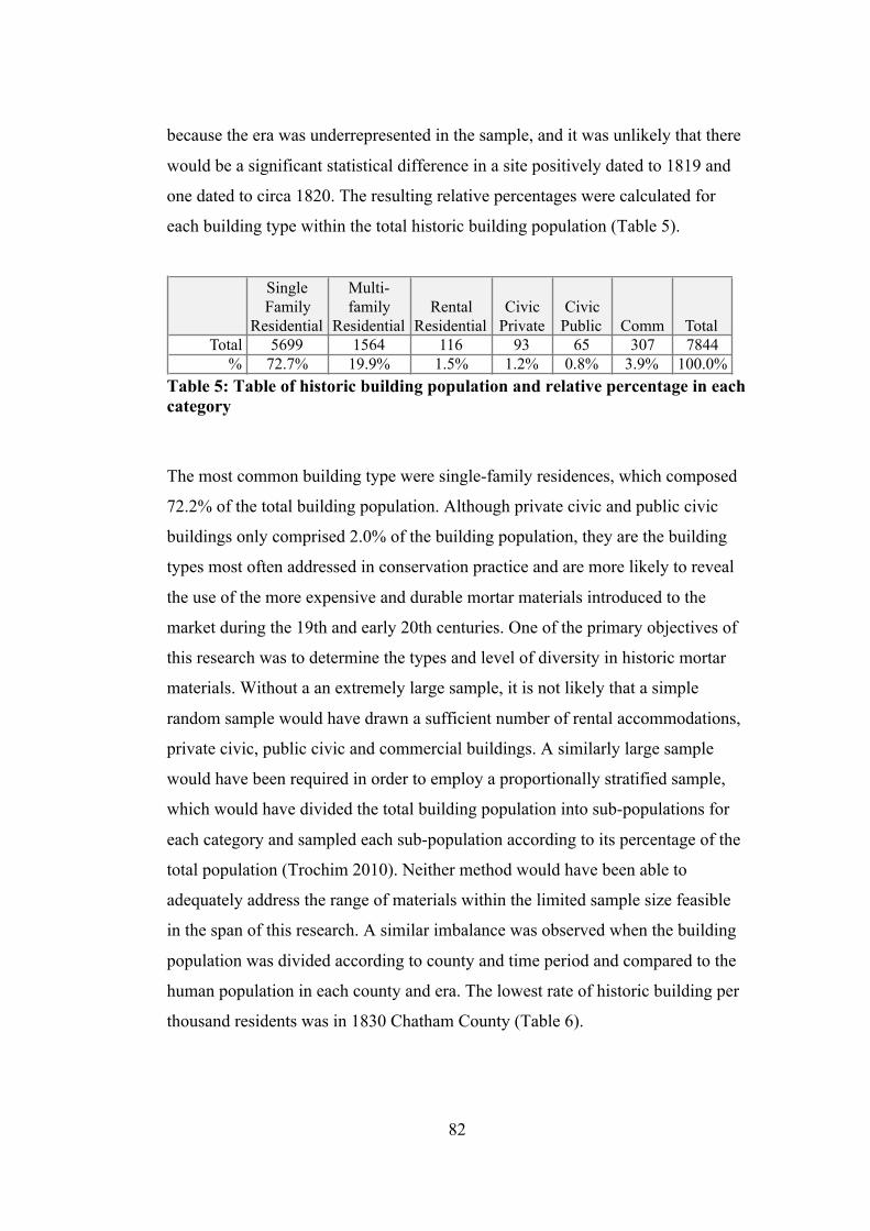
82
because the era was underrepresented in the sample, and it was unlikely that there
would be a significant statistical difference in a site positively dated to 1819 and
one dated to circa 1820. The resulting relative percentages were calculated for
each building type within the total historic building population (Table 5).
Table 5: Table of historic building population and relative percentage in each category
The most common building type were single-family residences, which composed
72.2% of the total building population. Although private civic and public civic
buildings only comprised 2.0% of the building population, they are the building
types most often addressed in conservation practice and are more likely to reveal
the use of the more expensive and durable mortar materials introduced to the
market during the 19th and early 20th centuries. One of the primary objectives of
this research was to determine the types and level of diversity in historic mortar
materials. Without a an extremely large sample, it is not likely that a simple
random sample would have drawn a sufficient number of rental accommodations,
private civic, public civic and commercial buildings. A similarly large sample
would have been required in order to employ a proportionally stratified sample,
which would have divided the total building population into sub-populations for
each category and sampled each sub-population according to its percentage of the
total population (Trochim 2010). Neither method would have been able to
adequately address the range of materials within the limited sample size feasible
in the span of this research. A similar imbalance was observed when the building
population was divided according to county and time period and compared to the
human population in each county and era. The lowest rate of historic building per
thousand residents was in 1830 Chatham County (Table 6).
Single Family
Residential
Multi-family
ResidentialRental
ResidentialCivic
PrivateCivic
Public Comm TotalTotal 5699 1564 116 93 65 307 7844
% 72.7% 19.9% 1.5% 1.2% 0.8% 3.9% 100.0%

83
Time period
Chatham County Effingham County
Buildings Population
Rate/
thousand Buildings Population
Rate/
thousand
1830 107 14,127 7.57 28 2,924 9.58
1880 769 45,023 17.08 223 5,979 37.30
1930 1712 105,431 16.24 542 10,164 53.33
Total 2,588 164,581 15.72 793 19,067 41.59
Table 6: Table of historic building population, human population and rate per thousand
The most striking aspect of the data presented in this figure was the wide range in
the number of buildings in each county and time period. The highest number of
buildings was in Chatham County in 1930, which was 61 times greater than the
number in Effingham County in 1830. As previously proposed, this condition was
most likely related to a similar condition in the human population in each county
and time period. The use of a proportionally stratified sample based on the
building or human population of each county and time period would have result in
a sample that is heavily weighted toward the types of materials used in 1930, and
obscure evidence of relationships that may be present in early eras.
The problems associated with the simple random and proportionally stratified
samples discussed above resulted in the selection of a disproportionately stratified
sample methodology for this research (Trochim 2010). The building population
was sampled using three levels of stratification, including time period, GMD and
building category. The time period strata ensured that the earliest time periods,
with the fewest buildings, were represented in the sample. The GMD strata
ensured that existing buildings in each district were represented in the sample, so
that there would be a minimum number of buildings directly related to the
subdivisions in the human population data. The building type strata ensured that
rental accommodations, private civic, public civic and commercial buildings were
represented in the sample, because these were the categories most likely to
contain mortar materials introduced in the span of this research. By using a

84
disproportional sampling method, the relative percentage of the single-family
residential, multi-family residential and outbuilding categories could be reduced
and the relative percentage of the remaining categories could be increased. This
created a sample, which established a minimum amount of data for each time
period, GMD and building category, while limiting the sample size to one that is
feasible within the span of this research.
This stratified sampling methodology proposed the random selection of four
single-family residential buildings, two small and two large, in each GMD from a
random list of available sites. The median area of single family residences were
calculated based on the original area of 30 randomly selected residential buildings
for each county at each time period. Small residential buildings were defined as
having an area less than the median, and large residential buildings were defined
as having an area greater than the median. Two multi-family residential buildings
and one building in each of the remaining categories in each GMD were selected
from a random list of available sites. When there was not an existing building in
the GMD, the site was omitted rather than replaced with a building from another
GMD, maintaining the relationship between the building sample and the
population data. The actual sample generated by this methodology resulted in
samples from 252 historic buildings. Using this methodology, the sample
addressed the requirements of the research objectives in the most efficient manner
possible, with a standard deviation of the relative proportions of the historic
building population and the actual sample between 0.44% and 10.53%. The
amount of data generated through this methodology provided mortar samples
from 52 sites in 1830, 84 sites in 1880 and 116 in 1930. It was common for
buildings to have more than one type of mortar dating to the original phase of
construction. Approximately half of the buildings surveyed had more than one
type of mortar, with some having as many as four. This resulted in a larger
number of samples analysed, than was originally projected according to this
sampling methodology, which was designed to meet or exceed the number of
samples necessary for the t-distribution to approach a normal, or z-distribution
curve (Rumsey 2003, 232). This provided a sufficient amount of data to assess the

85
level of diversity in the mortar materials of this case study without factoring in the
additional samples resulting from multiple mortar types.
The use of a stratified sample ensured a minimum amount of information for each
time period, GMD and building category (Kalton 1973, 24-8). It also provided the
information necessary to restructure the data for the analysis of potential
relationships between the historic mortar materials and methods and a wide
variety and combination of people who selected and used them. For example, the
data for each GMD was assessed individually and in combination with GMDs
with statistically similar demographic characteristics within or outside the county,
time period or building category. This allowed the data to be analysed in a
multitude of combinations. In this way, sub-populations with the fewest buildings
were assessed with statistically similar sub-populations when a larger set of data
was necessary to answer particular research questions. The sub-populations
created by the three strata did not need to provide enough data for individual
statistical analysis, they only needed to represent a series of known factors to
ensure that the data could be appropriately compiled and analysed in a variety of
data sets that were large enough to conduct tests of significance using a t-
distribution. As such, the disproportionately stratified sample was sufficient to
answer the specific research questions posed by this research.
Once the sampling methodology was in place, a list of the historic sites with one
or more buildings in the specific time period, GMD and building category was
exported to Microsoft Excel 2003. Sites with more than one building were
duplicated to reflect the total number of buildings, which met the specific criteria.
A random number was then assigned to each building record. The list was sorted
according to the random number to produce a randomly selected working list for
each time period, GMD, and building category. The random selection of sites was
necessary in order to minimise the effect of personal bias. Relying on the unique
GNAHRGIS Resource ID numbers would only have shifted the potential bias
from me to the survey team that completed the local historic resources surveys
during the last quarter of the 20th century. The earliest survey records dated from

86
the 1970s and were generally for buildings of long standing value to the
community, which were likely to have been more affluent or unique building
types. Since Resource ID numbers were assigned chronologically, sampling
according to these numbers would have limited the sample to the types of
buildings determined to be most significant in the earliest surveys. By applying a
random number to all known sites, this research circumvented my personal bias,
as well as those of the local surveyors.
The first step in the fieldwork was to perform a basic inspection of the exterior of
the selected building. If there was reason to believe that the masonry component
of the building had been compromised to the extent that the original mortar could
not be reliably identified or was no longer available, the site was omitted. Sites
were most commonly omitted for one of the following reasons. Firstly, the
masonry component of the building had been completely reconstructed using
either reused or new masonry units. Secondly, a building had been completely
repointed, leaving no traces of the original exterior pointing mortar. Thirdly, the
building was rendered after the original period of construction, obscuring the
possible presence of multiple mortar types and decorative joint treatments. If a
building was originally rendered, it was not omitted and was assumed to possess
only one mortar type.
If a preliminary exterior inspection indicated that a viable mortar sample could be
collected from the site, the property owner was identified through property tax
records. If telephone or email contact information was located in a search of basic
public records, an attempt was made to contact the owner by one of these means.
If this information was unavailable or there was no response to the initial contact,
an attempt was made to contact the owner in person. If the owner was not at
home, a hand-written note was left at the door. The personal nature of this
communication was often successful when other methods of contact had
previously failed. The preferred method of contact varied as much as the people
living and working in the area. Once contact had been made with the property
owner, they were provided with a brief introduction to the research and asked for

87
permission to sample and photograph their property. If permission was granted in
person, the sample and photographs were usually taken at that time. If contact had
been made by phone or email, or it was an inconvenient time for the owner, an
appointment was typically made for a date and time within one to two weeks. If
there was no contact with the owner after several weeks, or information from
neighbours or the property tax records indicated that the property has gone into
foreclosure, the site was omitted.
3.6.2 Mortar Sampling
To begin taking a mortar sample, the visible mortar conditions were inspected and
possible interior sampling locations were discussed with the building owner.
Sometimes the crawl space, basement, attic or penetrations through exterior walls
provided a larger, more intact sample than was available on the exterior of the
building. When samples were taken in these types of locations, only a small
sample was typically collected from the exterior for comparison in the lab. A
visual match of colour and texture within the same building was generally
considered to be the same mortar type. The samples were collected using a variety
of tools, including standard masonry chisels. Hand-held hacksaw blades that were
designed to cut metal and masonry also performed well. The small, even teeth on
the hacksaw blades used to cut metal resulted in narrower cuts and caused fewer
fractures in friable mortars. Hacksaw blades used to cut masonry materials that
consist of an 1/8” diameter, diamond encrusted rod were extremely effective in
almost all mortar types from the most friable 1830 lime mortar samples to the
most durable 1930 Portland cement mortars. A battery powered drill with bits
ranging in length from approximately 5 to 25 cm were also used, especially when
extracting a mortar sample from a location deeply recessed in an opening in the
wall or with extremely soft or friable mortars, which tended to turn to powder
when struck with a hammer. In these cases, the drill was moved laterally through
the mortar to cut loose a piece. Once loose, the samples were then placed in quart-
size polythene bags and labelled with a permanent marker.

88
Photographs were then taken of the sample location including a 1 cm by 5 cm
photographic scale. When possible, a photo was also taken to show the location of
the sample. General photos of each facade of the building were then taken
including a 2 m scale with 10 cm markings. All images were managed using
iPhoto, an application that allowed the assignment of keywords to individual
images, which were used to quickly sort and compare images. Each image was
assigned keywords in the following categories: county, era, GMD, building
category, the site’s unique GNAHRGIS identification number, and a description
of the image. The image descriptions included sample detail, sample location,
elevation (north, east, south and west), and miscellaneous sites or materials.
Although the size of the mortar samples was usually small enough that it would
not affect the load bearing capacity of the wall, the property owners usually
required the affected area to be repaired. This was particularly common when the
sample was taken from the exterior or another visible location. In these cases, the
repair mortar generally consisted of a high-calcium lime putty mortar, because it
has the lowest compressive strength and highest vapour permeability
characteristics of any commercially available conservation material and would be
compatible with the greatest number of sites. Mortars that were extremely durable
and were likely to have high cement contents were repaired using a moderately
hydraulic lime. Each of these mortars was selected in order to repair the affected
area with a mortar that had lower compressive strength and higher vapour
permeability than the existing mortar. When necessary, the mortars were coloured
using charcoal grey, buff, red or brown pigments. In order to provide a good
match, I referred to a collection of 30-40 cured mortar samples that were made
using various mixes of local materials. The repairs completed in the course of this
work differed dramatically from the masonry conservation practices discussed in
Chapter 6. This is because the primary objectives of the fieldwork repairs were to
minimise the risk of damage to adjacent materials in the future and satisfy the
property owner by providing the best possible visual match. This compromise was
acceptable, because of the limited size of the affected areas and the overarching

89
importance of maintaining a good relationship with the individual property
owners and the community.
Preliminary sample preparation was conducted in the field. At the end of each day
in the field, the polythene bags containing the mortar samples collected that day
were opened and placed in a rack. The rack prevented the samples from falling
out of the bag and becoming separated from the sample location information label
on the bag. They were left in this condition for 24-72 hours to dry, depending on
the moisture content of the particular samples. When there was no evidence of
moisture on the interior of the polythene bags, they were resealed and stored.
Once a week, the group of samples was dried in the oven at approximately 105° F
(40° C) until dry. The samples were then cooled to room temperature and placed
in new polythene bags labelled with the original information. The field bags were
stored for comparison at a later date if necessary, and the samples were stored for
further analysis.
3.7 Analysis
The analytical methods used in this research were actively employed from its
inception. The geospatial analysis was used to reconstruct and display historical
population data, as well as review and revise the geographical coordinates of the
historic building population data. Statistical analysis of the building population
helped establish the sampling methodology, which was designed and thoroughly
implemented to ensure the collection of a comprehensive cross-section of the
historic mortars used in the study area. Once the mortar samples were collected,
the laboratory phase of the research began. This analysis generated the detailed
numerical and categorical data used to accurately quantify and describe the
historic mortar materials and methods at the centre of this research. Statistical
analysis was also used to assess the demographic data in each era of the study and
identify statistically similar human populations in order to accurately group the
mortar samples and increase the sample size possible for population groups with

90
similar ancestry and enhance the validity of the findings of this research. The
statistical analysis of the mortar data was similar to those employed with the
historic building population data early in the research. Statistical analysis was the
common thread, winding through the research from the beginning to the end and
tying together the data generated by the geospatial and laboratory analyses.
3.7.1 Geospatial Analysis
In the initial phase of geospatial analysis, ArcGIS 8.3 was used to map the
boundaries of the study area, counties and define a 30 km buffer around the study
area. Additional layers displaying streets, railroads and wetland delineations were
then incorporated as frames of reference to define the 19th and early 20th century
configurations of the GMDs based on historical descriptions. As previously
discussed, GIS was then used to assign GMDs to the building population data, as
well as assessing and improving the accuracy of the geographical coordinates of
the GNAHRGIS data and adding additional resources to the 1930 building
population data. The analytical and statistical capabilities of ArcGIS 9.2 were
employed in the later phase of the research to generate area and current land use
data for the study area and its subdivisions in each era. This provided the
necessary contextual information to assess the human and building population
data, particularly the density of human, building and mortar characteristics in the
landscape (ESRI 2002, 133).
Following the fieldwork phase of the research, ArcGIS 9.2 was also used to
generate the maps presented in this thesis, which extend beyond the study area
and include maps of the southeastern and eastern United States, western Europe
and Africa. Due to the wide range in the scale and global position of these
features, different map projections were required for each dataset. These map
projections, or projected coordinate systems (PCS), are used to display three-
dimensional geographic coordinate system (GCS) data, such as latitude-longitude
coordinates, on a two-dimensional Cartesian coordinate plane (ESRI 2009). GCS
data is described by the angle between a line from the centre of the Earth to a

91
given point on the Earth’s surface and a line from the centre of the Earth to a point
on the equator or prime meridian, rather than the angle or distance between these
points on the Earth’s surface. The distance and angle between lines of latitude and
longitude, as well as the area and shape defined, vary depending on the distance
from the equator (ESRI 2009). Geographic transformations mathematically
convert geographic coordinate points to a Cartesian coordinate plane with a grid
of constant lengths and angles, but result in distortions in the shape or area of
features, or the distance or direction between points (ESRI 2009). Map projections
are designed to minimise one or more of these characteristics (ESRI 2009). The
map projections utilised in this research were selected based on the subject matter
to provided the most accurate representation of the area or shape as necessary.
3.7.2 Laboratory Analysis
The laboratory methodology included procedures for the preparation and analysis
of the mortar samples, ranging from descriptive methods to more complex
techniques, requiring specialised sample preparation, equipment and training.
Firstly, a basic visual analysis of each of the mortar samples was completed to
describe the colour and texture of each mortar. Then the binder to aggregate ratio
of each mortar was estimated by completing a digital point count. Petrographic
analysis was then used to identify the components of each binder. An analysis of
soil samples of clayey and sandy soil types from the study area was also
completed to facilitate the preparation of comparative mortar samples of a variety
of mixtures using locally available sands and a variety of pure and gauged
binders. The purpose of the soil analysis and mortar sample preparation was to
assess the performance of the local earth materials when used in a mortar, as well
as identify the range of colours and textures that could appear in mortar samples
made with these materials.

92
Visual Analysis
There were two phases of visual analysis in the laboratory. Firstly, the set of
samples collected from each building were placed on the work surface together.
The fragments were then removed and placed in front of their bags. The samples
were then compared at 10 times magnification under a 5000 K light source, which
approximates daylight conditions. The mortars were compared at this level of
magnification in order to compare the binder colour and the texture of the
aggregate. Once the number of unique mortar types was determined within the set
of mortars from one particular building, representative samples were selected for
thin section processing and for retention as a hand sample for future reference.
The sample to be thin section was trimmed to fit on a 1” by 1 7/8” (27 mm by 46
mm) glass slide, using the same mortar collection tools used in the field. The thin
section and hand samples were then bagged in 2” by 3” (5 cm by 7.6 cm)
polythene bags and labelled.
The colour of each mortar type was characterised at this time, in order to compare
the Munsell Soil Color Charts (Munsell Color 2000) with the bulk sample, thin
section sample and hand sample to ensure consistency. The largest four sides of
the sample prepared for thin section were then photographed in a light box under
5000 K light sources with an X-Rite Mini Color Checker Chart.
The sample was then prepared for shipping to National Petrographic Service, Inc.
in Houston, Texas for processing. The thin section specifications for this research
were standard for the petrographic analysis of historic masonry mortars. They
indicated that each of the mortar samples was impregnated with a blue epoxy
resin in a vacuum chamber to ensure that all of the voids were filled with the
epoxy resin. The resulting billet was trimmed to expose a portion of the mortar
sample. It was then ground in oil, rather than water to prevent damage to any
soluble materials present in the mortar sample. It was then mounted on a 1” by 1
7/8” (27 mm by 46 mm) glass slide and ground to a thickness able to transmit
light and covered with a slipsheet.
93
Mortar Disaggregation
A variety of methods have been used to separate and determine the ratio of binder
to aggregate, including wet chemical, manual and virtual methods. The use of the
acid digestion method of mortar disaggregation is the most well known and has
been in use for the last few decades, but it was not widely utilised in this research
due to the problems encountered when the aggregate is similar in chemical
composition to the binder. In concept, a dry mortar sample is weighed and
dissolved in an acid solution. It is assumed that the acid will dissolve the calcium
carbonate based binder and leave only the insoluble silica sand particles (Casadio
et al. 2005, 672). This fraction is dried and weighed to determine the ratio of
binder to aggregate by weight. In reality, this test can only accurately identify the
mass of the insoluble components of the mortar, which could include both
insoluble sand particles and insoluble components of a cement binder (Krotzer
and Walsh 2007) and would result in an overestimate of the amount of aggregate
in a mortar; however, it is more likely that a portion of the aggregate is soluble in
an acid solution and would result in an underestimate of the amount aggregate in
the mortar. Due to these inherent problems, the acid digestion method of analysis
was reserved for an example of each of the general types of mortar identified in
this research. The results were then compared to the results of the other type other
mortar disaggregation utilised in this research, in order to assess the effectiveness
of the method in the study area. A manual mortar disaggregation method was
assessed for use in this research, but was eliminated as an option. It involved
manually crushing the sample for 10 to 15 minutes, using a rubber soil pestle to
prevent crushing the aggregate particles. The ground sample is then ‘placed in a
beaker with deionised water and sonicated in an ultrasonic bath for 1 h.
Afterwards, the sample was sieved dry in order to determine its particle size
distribution.’ (Casadio et al. 2005, 676). Casadio, Chiari and Simon found that the
results of this method were satisfactory, particularly when cleaned in an ultrasonic
bath (2005, 687). It was not incorporated in this research because it was labour
intensive and did not account for the ratio of voids in the mortar sample. The
method attempted for this research was a virtual disaggregation method, which

94
had also been used in recent years to define the binder to aggregate ratio of
mortars without compromising their existing crystalline structures or
compromising the voids present in the sample (Casadio et al. 2005, 684), which is
destroyed in each of the previous methods. This method required the
consolidation of the mortar sample using a pigmented resin, which filled the voids
and gave the sample structural integrity. The sample was then ground and
polished and scanned using a standard flatbed scanner. Using an image processing
software package, the contrast between binder, aggregate and voids was enhanced
by selecting and modifying similar colour pixels. The software was then used to
calculate the relative proportions of each element. The specialised equipment
necessary for this method included only a flatbed scanner and image processing
software (Casadio et al. 2005, 687). Since this method required the least amount
of time to complete and offered additional information, this method was
attempted in this research. The methodology proved to be unsuccessful with this
particular set of mortar samples, because the colour of a significant portion of the
binders was so close to the colour of the aggregate that the image processing
software was unable to reliably identify the edge between the binder and
aggregate.
A modified version of this process was successfully adopted for this research.
Instead of using the impregnated mortar sample billet, the completed thin sections
were scanned at 1200 dpi, and a 1 cm2 portion of each scan was selected for point
count analysis. Using Adobe Photoshop CS5 Version 12, a grid was placed over
the point count image, which divided the image into 121 squares and created 100
vertices. The image was magnified 500% and the point count was completed,
quantifying the number of points located on binder, aggregate, fuel and blue
epoxy resin indicating a void in the mortar sample. The results recorded in
individual Microsoft Excel 2010 spreadsheets by row, and the totals were
incorporated into the Filemaker Pro 9 database.
95
Petrographic Analysis
The training necessary to conduct thin section petrographic analysis of mortar
samples was beyond the scope of this research and required the use of a
consultant. As such, the petrographic analysis was completed in conjunction with
John Walsh, a Senior Petrographer with Highbridge Materials Consulting, Inc.
Although these techniques can range from a simple visual analysis with no
magnification to the high-magnification imaging possible using specialised
equipment such as an electron microscope, the most common techniques used in
mortar analysis involve polarised light microscopy (PLM) (Krotzer and Walsh
2009, 40). The petrographic microscope has several specialised components
utilised in this type of analysis, including a graduated rotating stage and polarising
lens in the light path. These features ‘take advantage of the fact that crystals
refract light’ (Krotzer and Walsh 2009, 40) . Krotzer and Walsh argue that
only imaging methods are ‘capable of positively identifying binder materials’
(2009, 40), because they are the only ones able to identify the ‘presence of
preserved grains of partially or fully unreacted binder, or relicts, that are almost
invariably present microscopically’(2009, 40).
The petrographic analysis was performed in two phases in their laboratory. In the
first phase, I used a petrographic microscope to compare the mortar thin sections
in the research collection with representative samples in the Highbridge
collection. The types of binders and additives identified in the research collection
were recorded. The initial assessment of the slides was completed in
approximately two weeks in the laboratory. When complete, Walsh reviewed the
collection to confirm the identifications. Due to the value and demand on his time,
he was able to spend approximately 3-5 minutes reviewing each slide. With
regard to the primary binder materials, there was an approximate error rate of
10%. The error was almost exclusively restricted to the cement binders, which
were identified by their unique crystalline structures. His review was also critical
to the accurate identification of the mortar additives, particularly when the
pozzolans, plasticisers and pigments were only present in trace amounts. When a

96
sample contained an unburned fragment of the raw materials, Walsh was often
able to provide additional information on the source of the carbonate-based
materials. In these cases, petrographic analysis of the unburned fragments was
able to indicate whether the carbonate was from a sedimentary stone, such as a
limestone or marl, or a metamorphic stone such as marble.
3.7.3 Statistical Analysis
The type of statistical analysis employed in this research varied depending on the
phase of the work being completed. In the early stages of the project, relative
frequency distributions (Triola 2008, 51) were used to summarize the edited
GNAHRGIS building population data by GMD for each era, and a sampling
strategy was developed based on these distributions. At the same time, it was clear
that the only way to generate reliable data linking the built environment to the
human population was to quantify the demographic data in a similar manner. Due
to the complexity of this data, the statistical analysis necessary to define and
quantify the human population proved to be far more complex than the historic
building population. It required extensive two proportion tests (Triola 2008, 474-
6), which compared the relative proportions of the population of each ethnic
group in each GMD to the relative proportions of all of the other GMDs with
significance level of α = 0.05 (Triola 2008, 406). Tests resulting in a P-Value
greater than 0.05 were determined to be statistically similar and defined as
population groups. Once grouped, the human population data contained values for
multiple GMDs. For this reason, it was necessary to employ statistical analyses
that could analyse the variance between the datasets, rather than individual
proportions. One-way ANOVAs and t-tests were utilized for this purpose. Firstly,
the one-way ANOVA test was used to assess all of the population groups defined
for each era, which included 5 groups in 1830, 6 groups in 1880 and 7 groups in
1930. Resulting clusters were identified and tested using subsequent one-way
ANOVA tests. When only two groups remained, the t-test was substituted (Triola
2008, 487-8), as the one-way ANOVA is intended for use with ‘three or more
population means’ (Triola 2008, 659). In this way, the population groups were

97
combined with others having statistically similar ancestry. Once the mortar
samples were collected, processed and analysed, they were described using more
simple statistical methods. When assessing individual characteristics of the mortar
samples, the mean, median and mode were each used at times to characterize the
average for centre value of the dataset. A comparison of these values was also
employed to assess the distribution of the data being described (Figure 14). When
the mean and the median were less than the mode, the distribution was negatively
skewed. When they were similar, the distribution was symmetrical. When the
mean and median were greater than the mode, the distribution was positively
skewed (Triola 2008, 93). Although somewhat counterintuitive, negatively
skewed distributions indicated that the bulk of the data being described was
among the higher values, and positively skewed distributions indicated that the
bulk of the data being described was among the lower values of the data set.
Figure 14: Diagram of negatively skewed, symmetric and positively skewed distributions (Triola 2008, 93).
The frequency of unique values in the datasets was also assessed, particularly
when describing categorical rather than numerical data. Frequency and relative
frequency distributions were also used in a manner similar to those employed
when assessing and describing the historic building population.
Several software packages were utilised in the statistical analysis portion of this
research. All of the data generated in the fieldwork and laboratory analysis was
recorded and maintained in a FileMaker Pro 9 database. The data was then
exported to Microsoft Excel for Mac 2011 for statistical analysis and as a means

98
of transferring the data to Minitab Release 16, a statistical software package used
to simplify the execution of the two proportion tests, one-way ANOVA tests and
t-tests. The following is a summary of the calculations completed by the statistical
software package.
The two proportion test was used to estimate the ‘difference between
corresponding population proportions’ (Triola 2008, 474) of two independent
sample populations. This test is defined by Triola as (2008, 475):
where:
p = population proportion
n = size of the sample
x = number of successes in the sample
The one-way analysis of variance (ANOVA) test was used to estimate the
difference in the means of three or more independent sample populations by
analysing sample variances. This is defined by Triola as (2008, 659):
where:
n = number of values in the sample –x = variance of values in the sample =x = mean of all sample values combined
k = number of population means being compared –s = mean of values in the sample
ni
ni
ni
xi x
!!"
#
$$%
&' (
' (!!"
#
$$%
&(
('
)1()1(
1) (
2
2
samples within variance
samplesbetween variance k=F =
si
99
The hypothesis test statistic for two means, or t-test, was used to estimate the
difference in the means of two independent sample populations by analysing
sample variances. This is defined by Triola as (2008, 489):
where:
n = number of values in the sample
s = variance of values in the sample
x = mean of values in the sample
µ = mean of values in the population
3.8 Conclusion
As discussed in detail in the previous chapter, there is a divide between the
cultural and scientific aspects of conservation and historical archaeology. This
research attempted to address the issue by turning to recent theoretical debate on
materiality or material agency and the research projects it has influenced in the
closely related discipline of archaeology. It defined a case study intended to assess
the recursive relationship between people and the artefacts that they left behind
using historic buildings, an artefact that is traditionally within the purview of
conservation in the United States. It questioned whether or not people constructed
the masonry components of their buildings differently based on their cultural
background. To effectively answer these questions, this research needed a
carefully designed case study. The study area needed to have relatively
homogeneous geographical and environmental conditions and demographic
conditions that were as heterogeneous as possible. It also needed to have an
adequate number of historic buildings over an extended period of time, preferably
spanning a period of cultural change. The beginning of the chapter discussed the
t =( (x x1
1
1
12 2
222
2
µ µ) )
s s
n n

100
ways in which Chatham and Effingham Counties met each of these criteria. Then
it defined the statistical methods used to select a sample of historic buildings that
minimised bias and reflected the makeup of the total historic building population
as accurately as possible. It concluded with a description of the statistical and
analytical methods used to answer the research questions defined in this research.
101
Chapter 4: History and Context
This chapter sought to establish an understanding of the people who constructed
and maintained the built environment, specifically the historic masonry buildings,
of the study area. To build a solid foundation, the traditions of the people who
populated this area were discussed in the precontact period and Colonial era. The
chapter began with a discussion of the precontact period in order to establish the
identity and the construction traditions of the people from North America, Europe
and Africa, who lived in and settled in this area during the Colonial era. It then
discussed the period of contact and creolisation that occurred in the Colonial era.
It concluded by establishing the historical and cultural context of each of the study
eras of this research, including a demographic and statistical analysis of the
people living in the study area in 1830, 1880 and 1930.
4.1 Precontact Period
In the late pre-contact period, the people who converged in the Atlantic Deep
South came from three entirely different cultures. Understanding the Native
American history of the area presents greater obstacles than either European or
African history. Although the European explorers and settlers came from
locations across Western Europe, their history and architectural traditions are well
documented and studied. By Native American standards, African history and
architectural traditions are also relatively well known from centuries of contact
with Europe and the Middle East. In order to provide some balance to this
iniquity, the following discussion of Native America will be more detailed than
those for the other continents. In post-contact North America, the discussion
shifted to discuss demographic conditions and briefly introduce the history of the
region before providing more detailed information on the people who inhabited
the Atlantic Deep South from the late pre-contact period through the early 20th
century.
102
4.1.1 North America
The process of identifying the Native Americans who inhabited the region when
the English established the Carolina and Georgia Colonies was a daunting task. In
fact, a significant amount of research in the last several decades has systematically
deconstructed the assertions of early 20th century ethnographers, linguists and
historians such as Swanton, Powell and Ross. The complexity of the situation was
caused primarily by contact between European and Native Americans in this
region. Between 1540 and 1587, the Spanish and French made attempted to settle
the area, with the Spanish having the most lasting and widespread success and
contact with the native population. They dispatched expeditions into the interior
and maintained a series of missions along the coast. As a result, Spanish
narratives are the primary sources of information on the native population of this
region in the 16th century. The Spanish presence in this area certainly had a
detrimental effect on the native population. Spanish explorers documented
conflicts with the interior native population in which large numbers of native
people were killed and food stores pillaged. As Spanish settlement had not pushed
beyond the coastal barrier islands, it is most likely that their effect on the native
population through trade, which caused intertribal conflict by encouraging the
migration of inland tribes to the coast and the introduction of European diseases.
Attempts to tie their accounts to those of the English in the Carolina Colony in the
late 17th century are difficult, since the numerous tribes in the region coalesced
into a smaller number of groups in the intervening years. Further stress was
placed on the native population between the establishment of the Carolina Colony
in 1663 and the Georgia Colony in 1733 as European settlement pushed inland
and Carolina colonists engaged in the Native American slave trade. These
pressures had forced much of the coastal population to the south and west. The
remaining native people were gradually pushed west through the late Colonial era,
with the majority of the coastal tribes forming the Muskogee and Catawba nations
and virtually disappearing in the region following the Indian Removal Act of
1830.

103
Attempts by historians and ethnographers to reconstruct the configuration of the
southeastern tribes in what is now Georgia and South Carolina have had to
reconcile the information available about three distinct configurations of native
people from three periods of contact: 16th century Spanish, 17th century early
colonial English and 18th century late English colonial periods. The research of
early 20th century historians and ethnographers appear to have been based
primarily on Spanish accounts of the ability of native interpreters to communicate
with tribes in broad areas of the region. Hudson argues that this is problematic
(1990, 78), since multi-lingualism was common in the region (Goddard 2005, 5)
Figure 15: Southeast section of the Powell map of language families of 1915 (Goddard 2005, 2).
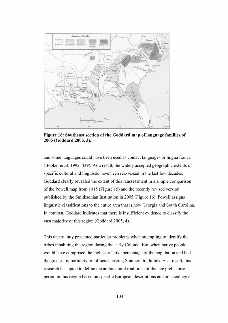
104
Figure 16: Southeast section of the Goddard map of language families of 2005 (Goddard 2005, 3).
and some languages could have been used as contact languages or lingua franca
(Booker et al. 1992, 439). As a result, the widely accepted geographic extents of
specific cultural and linguistic have been reassessed in the last few decades.
Goddard clearly revealed the extent of this reassessment in a simple comparison
of the Powell map from 1915 (Figure 15) and the recently revised version
published by the Smithsonian Institution in 2005 (Figure 16). Powell assigns
linguistic classifications to the entire area that is now Georgia and South Carolina.
In contrast, Goddard indicates that there is insufficient evidence to classify the
vast majority of this region (Goddard 2005, 4).
This uncertainty presented particular problems when attempting to identify the
tribes inhabiting the region during the early Colonial Era, when native people
would have comprised the highest relative percentage of the population and had
the greatest opportunity to influence lasting Southern traditions. As a result, this
research has opted to define the architectural traditions of the late prehistoric
period in this region based on specific European descriptions and archaeological

105
evidence, rather than attempting to define the individual tribes that may have been
present during this critical period and their particular architectural traditions.
Descriptions of inland architectural forms provided information more consistent
with archaeological evidence of pre-contact architectural in the Southeast, which
consist primarily of wattle and daub or timber buildings covered with local
vegetation. One account recorded by a member of the DeSoto expedition while
travelling inland from the Gulf of Mexico through present-day Georgia, South
Carolina and Tennessee in 1540, described the transition in native architecture and
materials at a settlement called Toa or Toallits in present-day west central
Georgia. He noted that:
‘Beyond that place, a difference was seen in the houses, for those behind were covered with hay and those of Toallits were covered with canes in the manner of tiles. Those houses are very clean and some have their walls plastered and appear to be made of mud. Throughout the cold lands each of the Indians has his house for the winter plastered inside and out. They shut the very small door at night and build a fire inside the house so that it gets as hot as an oven, and stays so all night long so that there is no need of clothing. Besides those houses they have others for summer with kitchens nearby where they build their fires and bake their bread.’ (Elvas 1540).
Although the image that Elvas provided is certainly in keeping with the bulk of
archaeological evidence of native architectural forms and materials in the Atlantic
Deep South, it should not discourage the reassessment of all available resources.
Not only has the entire body of knowledge about pre-contact southeastern Indians
been drawn into question in the last few decades, it has have been largely
overturned.
Nearly 250 years after the first European descriptions, William Bartram provided
greater detail in his descriptions of the construction methods of employed by
Native Americans in the southeast. Most significant to this research is his
description of the Yuchi and Creek use of clay plaster on the interior and exterior
of their buildings. He described Yuchi houses, which were ‘constructed of a
wooden frame, then lathed and plastered inside and out with a reddish well
tempered clay or mortar, which gives them the appearance of red brick walls, and

106
these houses are neatly covered or roofed with Cypress bark or shingles of that
tree…’ (Bartram 1791, 388). The discussed the use of clay mortar as a plaster or
render in Creek architecture in several different areas of the southeast (Bartram
1791, 453). He described another Creek house as having a ‘wooden frame with
plastered walls, and roofed with Cypress bark or shingles; every habitation
consists of four oblong square houses, of one story, of the same form and
dimensions, and so situated as to form an exact square, encompassing an area or
court yard of about a quarter of an acre of ground, leaving an entrance into it at
each corner…’ (Bartram 1791, 396). He even suggests that this form may have
been copied by French settlers in present-day Alabama who created structures
similar in plan and construction, with the exception of sometimes being
limewashed on the interior and exterior (Bartram 1791, 403). Specifically
comparing these buildings with those of French settlers, with the specific
exception of their use of lime, suggests that Bartram did not encounter Native
Americans using lime technology during his travels in the late 18th century. These
examples reveal the use of clay as a plaster and render as well as a solid wall
construction material; however, the texts only offer one reference to the process of
manufacturing this material when he stated that ‘every town cultivates a little
plantation of it having a large artificial pond, just without the town, planted and
almost overgrown with it, where they usually dig clay for pottery, and mortar and
plaster for their buildings …’ (Bartram 1791, 456).
4.1.2 Europe
The earliest available dataset defining the nationality of European settlers in this
region was the 1790 Federal Census. It defined the population of the region at the
end of the colonial period and suggested that England, Scotland and Ireland
dominated European settlement in the Carolina and Georgia Colonies. Alone, the
English composed 60.2% of the population of the region. Including the Scottish
and Irish populations, the British Isles claimed 90.0% of all European immigrants.
Immigrants of Germanic descent composed 5.8% of the population of the region
and 7.7% in the Georgia Colony, which was probably higher due to the
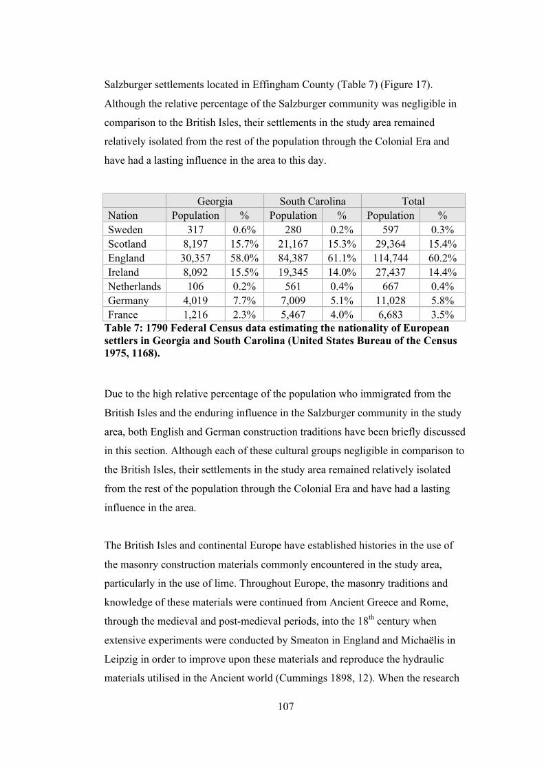
107
Salzburger settlements located in Effingham County (Table 7) (Figure 17).
Although the relative percentage of the Salzburger community was negligible in
comparison to the British Isles, their settlements in the study area remained
relatively isolated from the rest of the population through the Colonial Era and
have had a lasting influence in the area to this day.
Table 7: 1790 Federal Census data estimating the nationality of European settlers in Georgia and South Carolina (United States Bureau of the Census 1975, 1168).
Due to the high relative percentage of the population who immigrated from the
British Isles and the enduring influence in the Salzburger community in the study
area, both English and German construction traditions have been briefly discussed
in this section. Although each of these cultural groups negligible in comparison to
the British Isles, their settlements in the study area remained relatively isolated
from the rest of the population through the Colonial Era and have had a lasting
influence in the area.
The British Isles and continental Europe have established histories in the use of
the masonry construction materials commonly encountered in the study area,
particularly in the use of lime. Throughout Europe, the masonry traditions and
knowledge of these materials were continued from Ancient Greece and Rome,
through the medieval and post-medieval periods, into the 18th century when
extensive experiments were conducted by Smeaton in England and Michaëlis in
Leipzig in order to improve upon these materials and reproduce the hydraulic
materials utilised in the Ancient world (Cummings 1898, 12). When the research
Georgia South Carolina Total Nation Population % Population % Population % Sweden 317 0.6% 280 0.2% 597 0.3% Scotland 8,197 15.7% 21,167 15.3% 29,364 15.4% England 30,357 58.0% 84,387 61.1% 114,744 60.2% Ireland 8,092 15.5% 19,345 14.0% 27,437 14.4% Netherlands 106 0.2% 561 0.4% 667 0.4% Germany 4,019 7.7% 7,009 5.1% 11,028 5.8% France 1,216 2.3% 5,467 4.0% 6,683 3.5%
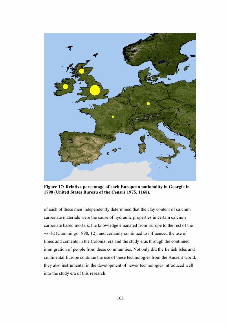
108
Figure 17: Relative percentage of each European nationality in Georgia in 1790 (United States Bureau of the Census 1975, 1168).
of each of these men independently determined that the clay content of calcium
carbonate materials were the cause of hydraulic properties in certain calcium
carbonate based mortars, the knowledge emanated from Europe to the rest of the
world (Cummings 1898, 12), and certainly continued to influenced the use of
limes and cements in the Colonial era and the study eras through the continued
immigration of people from these communities. Not only did the British Isles and
continental Europe continue the use of these technologies from the Ancient world,
they also instrumental in the development of newer technologies introduced well
into the study era of this research.

109
4.1.3 Africa
Africans first arrived in this area through the Atlantic slave trade. A substantial
amount of information has become available in the last several decades. One of
the most significant resources is the Trans-Atlantic Slave Trade Database
(www.slavevoyages.org), which documents over 35,000 individual voyages and
provides the best information available on the ports of embarkation of Africans
transported to the Carolina and Georgia colonies. When combined with estimates
on the range of inland slaving activities and cultural and architectural studies, it is
possible to develop an image of the people and the architectural traditions, which
were forcibly relocated to the Atlantic Deep South (Figure 18). The origins of
Africans disembarking in this area during the 18th century spanned the west and
Figure 18: Map of Africa indicating the relative proportion of Africans embarking from each of these regions during the 18th century and disembarking in the Atlantic Deep South (Trans-Atlantic Slave Trade Database). The adjacent shaded areas depict the proposed range of slaving activity into the interior (Eltis 2000).
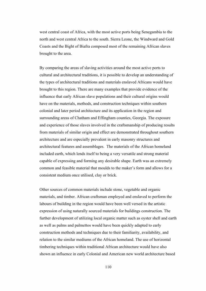
110
west central coast of Africa, with the most active ports being Senegambia to the
north and west central Africa to the south. Sierra Leone, the Windward and Gold
Coasts and the Bight of Biafra composed most of the remaining African slaves
brought to the area.
By comparing the areas of slaving activities around the most active ports to
cultural and architectural traditions, it is possible to develop an understanding of
the types of architectural traditions and materials enslaved Africans would have
brought to this region. There are many examples that provide evidence of the
influence that early African slave populations and their cultural origins would
have on the materials, methods, and construction techniques within southern
colonial and later period architecture and its application in the region and
surrounding areas of Chatham and Effingham counties, Georgia. The exposure
and experience of those slaves involved in the craftsmanship of producing results
from materials of similar origin and effect are demonstrated throughout southern
architecture and are especially prevalent in early masonry structures and
architectural features and assemblages. The materials of the African homeland
included earth, which lends itself to being a very versatile and strong material
capable of expressing and forming any desirable shape. Earth was an extremely
common and feasible material that moulds to the maker’s form and allows for a
consistent medium once utilised, clay or brick.
Other sources of common materials include stone, vegetable and organic
materials, and timber. African craftsman employed and enslaved to perform the
labours of building in the region would have been well versed in the artistic
expression of using naturally sourced materials for buildings construction. The
further development of utilizing local organic matter such as oyster shell and earth
as well as palms and palmettos would have been quickly adapted to early
construction methods and techniques due to their familiarity, availability, and
relation to the similar mediums of the African homeland. The use of horizontal
timbering techniques within traditional African architecture would have also
shown an influence in early Colonial and American new world architecture based

111
on those methods brought from Africa by early slaves and employed in the
building methodologies of colonial structures. There are many defined
relationships between these materials influencing traditional African Architecture
and its residual effects on Early American Architecture within this region and this
helps draw a correlation between the effective applied methodologies, origins,
varying sources, and productive usage throughout the building and construction
process in the early south.
4.2 Colonial Era
The Colonial Era in this area has been divided into the early contact period, the
Early Colonial Era and the Late Colonial Era, which roughly correspond to the
dates of the Spanish Colony of La Florida, the Province of Carolina, and the
Colony of Georgia. The first period of contact was with the Spanish in La Florida.
The most significant aspects of this period to this research are the observations
made by the Spanish on the native population and their architectural traditions and
the Spanish use of tabby along the coast of present-day Florida, Georgia and
southern South Carolina. The Early Colonial Era was characterised historically by
the close contact and tension between the Carolina Colony and the Native
American population, particularly in relation to the English involvement in the
Native American slave trade (Gallay 2002). These tensions came to the forefront
in 1715, with the start of the Yamassee War. After the war, the English were
forced to look elsewhere for slave labour. The minimal number of African slaves
that entered the region prior to 1715 increased sharply after this time. The Late
Colonial Era is often marked by the shift in enslaved people from native to
African populations. For the purposes of this research, the Late Colonial Era
began with the founding of the Georgia Colony in 1733.
112
4.2.1 Early Contact Period
Prior to the formation of the Georgia Colony, the Native American population of
the study area consisted primarily of the Creek and Yuchi (pronounced You-chee)
tribes. Although the Yuchi pre-date the Creeks in this area, they are often
overlooked in historic accounts of the region. They were among a large number of
small, independent tribes that existed throughout the southeast, particularly along
the Atlantic coast. They are both culturally and linguistically distinct from
adjacent tribes. Based on their origin stories and other cultural and linguistic
similarities, it is believed that the Yuchi tribe may have descended from the
mound builders of the Ohio River Valley and sparsely inhabited an area extending
from present day Illinois to Florida and the Carolinas to the Mississippi River.
Their language is most closely related to that of the Shawnee, who originally
inhabited an area encompassing present-day southern Ohio, West Virginia, and
western Pennsylvania (Pritzker 1998, 546). The Creeks were the dominant tribe in
the region and were actually a confederacy of related tribes inhabiting nearly the
entire area of present day Georgia and Alabama (Pritzker 1998, 545). According
to Creek tradition, they moved into the area from the west and are related to the
mound builders of northwest Georgia who were active after 950 AD. These sites
flourished for several centuries, but were abandoned prior to the mid 16th century,
when the expedition of Hernado de Soto travelled through the area. It is unclear
whether the mound builders of this area developed into the Creeks or were simply
absorbed by existing Creek tribes. The areas adjacent to the study area contained a
variety of tribes, representing Siouan, Algonquin, and Iroquois language and
cultural groups. The most significant of these tribes were the Cherokee, who
entered the region in the mid 17th century, possibly forced south by other Iroquois
people in the mid-Atlantic colonies. The southern and western migration pattern
was common throughout the colonial period due to increasing pressure with the
expansion of European settlement along the eastern seaboard. These sites
flourished for several centuries, but were abandoned prior to the mid 16th century,
when the expedition of Hernado de Soto travelled through the area.
113
4.2.2 Early Colonial Period
The earliest European settlement along the coast of present day Georgia and South
Carolina occurred in 1566 when the Spanish established missions on Jekyll and St.
Simon’s Islands in southern Georgia, neither of which are in the study area. By
the 1660s, Spanish settlement had expanded to eleven missions and three
garrisons extending from Florida to the south bank of the Ogeechee River in
present day Georgia, as well as a fort, mission and town near present day Beaufort,
South Carolina (Division of Historical Resources 2013). In order to halt Spanish
expansion toward English colonies to the north and to reward individuals for their
part in the restoration of the monarchy in England, the English established the
Carolina Colony in 1663 (Figure 19) (South Carolina State Library 2013). The
strategy was successful and the Spanish retreated to present day Florida in 1686.
For the next fifty years, the area of present day Georgia was claimed by Spain,
England and France.
The success of the Carolina Colony had a devastating effect on the native
population. First, European settlers introduced diseases that reduced the
population of many tribes by one half. Then, the continual expansion of European
settlements forced many tribes to migrate into the territory of neighboring tribes,
causing intertribal conflicts beginning in the mid 16th century. While these
certainly had a detrimental effect on Native American culture and population, they
pale in comparison to the intentional destruction that followed. In the 1680s,
settlers of the Carolina Colony began raiding Native American villages and
purchasing captives from intertribal conflicts for slave labor in the Carolina
Colony and as an export to northern colonies and the West Indies. As the coastal
population diminished, Europeans were forced to travel further inland in search of
slaves and began to encourage conflicts by “pitting one tribe against another with
offers of guns, powder and cheap English textiles and manufactured goods”
(Josephy 1994, 223). In conflicts directly between European and Native American
forces, the Europeans would often seek assistance from other tribes in exchange
for slaves or goods.

114
Figure 19: Map of Georgia and the Carolinas from 1663 to 1790.
In the early 18th century, the Creek and Yuchi tribes participated in a raid with
Carolina colonists into Spanish Florida in search of slaves. They returned with
6,000 Native American slaves, many of which were Christians taken from or
around the Spanish missions. By the early 18th century, the native population could
no longer sustain the needs of the colonists, and they turned to the African slave
trade to support the plantation system. Although African slaves were imported to
the colonies in the early 19th century, their numbers did not begin to climb at an
exponential rate until the mid 18th century. As late as 1730, approximately one
quarter of the slaves in South Carolina was Native American (Josephy 1994, 226),
and these people would have contributed significantly to the creolised slave
culture that developed in the early south.

115
When the English established their first permanent settlement within the bounds
of present-day South Carolina in 1670, the Native American population had
endured nearly 150 years of population decline, migration, and social and cultural
realignment. Between 1670 and 1700, the Spanish abandoned their remaining
missions in present-day Georgia and retreated into present-day Florida (Division
of Historical Resources 2013). Similar to the reassessment of early research on the
southeastern tribes, previously held beliefs regarding the origin of the early
European settlers in the Carolina Colony have also been reassessed in recent
years. It was previously believed that the majority of settlers arrived from
Barbados, but recent research has revealed that many of these individuals arrived
from England with only a brief stop in the West Indies. This is a relevant issue, it
will provide some insight into the origin of the 4,100 negro slaves listed in the
1708 Carolina Census (Table 8) (Gallay 2002, 200), who do not appear in the
Trans-Atlantic Slave Trade Database. The two most likely origins are the West
Indies and the Virginia Colony. Each of these areas has sufficient data to
characterise the initial African population in the Atlantic Deep South.
White White servant Negro slave Indian slave Total 3,960 120 4,100 1,400 9,580
Table 8: 1708 South Carolina Census (Gallay 2002, 200).
In addition to the 4,100 African slaves, this census lists 1,400 Native American
slaves. A map based on Gallay’s estimates of the number of native people
enslaved between 1670 and 1715 (Table 9) (Figure 20), reveals the reach of the
Native American slave trade during the early Colonial Era. The largest numbers
came from the Timuca, Apalachee and other Florida Tribes, as well as

116
Location Tribe Min Max Min% Max % Florida Timuca,
Apalachee and others
1,247 1,131 59.9% 52.0%
Georgia coast Guale and Mocama
43 29 2.1% 1.3%
Lower Mississippi River Valley
Arkansas, Taensa and Tunica
86 116 4.1% 5.3%
Southern Mississippi Choctaw 138 122 6.6% 5.6% North Carolina Tuscarora 95 110 4.6% 5.1% Central Savannah River Valley
Westo 43 87 2.1% 4.0%
Piedmont and Appalachian Mountains of Georgia, South Carolina, western North Carolina, northern Alabama and Mississippi
Creek, Savannah, Cherokee, Chickasaw, piedmont and others
430 580 20.7% 26.7%
Total 2,082 2,175 100.0% 100.0% Table 9: Estimate of Native American slave population in South Carolina in 1715 (Gallay 2002, 15; Gallay 2002, 57; Gallay 2002, 103; Gallay 2002, 225-6; Gallay 2002, 298-9).
the Creek, Savannah, the colonists shifted their efforts toward the enslavement of
African people. The Africans who arrived in the Carolina Colony prior to 1750
were predominantly from west central Africa, with significant numbers also
arriving from Senegambia, the Bight of Biafra and to a lesser extent, the Gold
Coast (Eltis and Halbert 2009). The composition of the Carolina slave population
leading up to the legalisation of slavery in the Georgia Colony in 1750 is quite
important, because these slaves moved back and forth across the Savannah River
as hired labour prior to 1750 and are the basis of the Georgia slave population,
which developed after that time.

117
Figure 20: Map indicating the origin of enslaved Native Americans, based on Galley's estimates. The two toned symbol depicts the minimum and maximum estimates for each people (Gallay 2002, 15; Gallay 2002, 57; Gallay 2002, 103; Gallay 2002, 225-6; Gallay 2002, 298-9).
4.2.3 Late Colonial and Federal Period
European colonization of the eastern seaboard continued when the English
established the Georgia Colony and the city of Savannah in 1733. Again, the
purpose of the new colony was to provide a buffer between the Spanish in Florida
and the English colonies to the north, but it was also intended to provide
economic opportunities for the English poor and a refuge for continental
European Protestants. The city of Savannah was founded on Yamacraw Bluff, the
location of the Creek town of Yamacraw on the south side of the Savannah River.
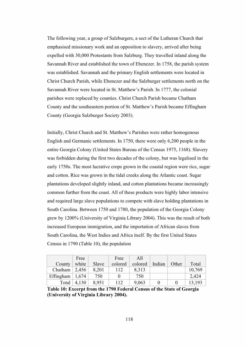
118
The following year, a group of Salzburgers, a sect of the Lutheran Church that
emphasised missionary work and an opposition to slavery, arrived after being
expelled with 30,000 Protestants from Salzburg. They travelled inland along the
Savannah River and established the town of Ebenezer. In 1758, the parish system
was established. Savannah and the primary English settlements were located in
Christ Church Parish, while Ebenezer and the Salzburger settlements north on the
Savannah River were located in St. Matthew’s Parish. In 1777, the colonial
parishes were replaced by counties. Christ Church Parish became Chatham
County and the southeastern portion of St. Matthew’s Parish became Effingham
County (Georgia Salzburger Society 2003).
Initially, Christ Church and St. Matthew’s Parishes were rather homogenous
English and Germanic settlements. In 1750, there were only 6,200 people in the
entire Georgia Colony (United States Bureau of the Census 1975, 1168). Slavery
was forbidden during the first two decades of the colony, but was legalised in the
early 1750s. The most lucrative crops grown in the coastal region were rice, sugar
and cotton. Rice was grown in the tidal creeks along the Atlantic coast. Sugar
plantations developed slightly inland, and cotton plantations became increasingly
common further from the coast. All of these products were highly labor intensive
and required large slave populations to compete with slave holding plantations in
South Carolina. Between 1750 and 1780, the population of the Georgia Colony
grew by 1200% (University of Virginia Library 2004). This was the result of both
increased European immigration, and the importation of African slaves from
South Carolina, the West Indies and Africa itself. By the first United States
Census in 1790 (Table 10), the population
County Free white Slave
Free colored
All colored Indian Other Total
Chatham 2,456 8,201 112 8,313 10,769 Effingham 1,674 750 0 750 2,424
Total 4,130 8,951 112 9,063 0 0 13,193 Table 10: Excerpt from the 1790 Federal Census of the State of Georgia (University of Virginia Library 2004).
119
of Chatham County had grown to 10,769, of which 8,201 or 76% were slaves. In
Effingham County, the population grew to 2,424, but only 750 or 31% of these
people were slaves (University of Virginia Library 2004). African slaves were
legally imported directly from Africa or from the established slave economies in
the West Indies and South America until 1808, when the Atlantic slave trade was
abolished. However, the illegal importation of African slaves continued in
reduced numbers until the Civil War in the early 1860s. Although these numbers
were drastically reduced, the established population continued to grow at nearly
the same rate through the turn of the 20th century.
The selection of these two counties with differing early European and slave
populations provides an interesting cultural context for this study. Initial concerns
about the rate at which the Salzburger community became the minority in St.
Matthew’s Parish, and therefore had less of an influence on the culture and its
built environment, diminished based on an 1860 map of slave populations in the
southern states. This reveals that at the end of the slave era, Effingham County
still had the lowest slave population in coastal Georgia and South Carolina. This
is possibly the result of the lasting influence of Salzburger beliefs, or simply a
result of the farming practices and crops established in this area, which would not
have depended as heavily on slave labor as the neighboring counties in Georgia
and South Carolina.
Early archaeologists and anthropologists often discounted the influence that the
slave population may have had on the built environment and the material culture
of the dominant culture. In recent decades, these attitudes have changed, and
archaeologists, anthropologists and historians have addressed a number of
examples of enduring African culture and traditions on American soil. Along the
southeastern seaboard, which Glassie defined as one of the “four major centers of
folk cultural dispersal on the East Coast” (1968, 35), examples include the Gullah
culture and language and African forms of basketry, pottery, and architecture
(Deetz 1996, 226).
120
While it is clear that the creolised slave culture that developed in this area
incorporated aspects of African cultures throughout west and west-central Africa,
the influence of the Native American population is not as easy to identify. This
may be due to the fact that most Native American slaves were captured in
conflicts between European settlers and local tribes in the early 18th century. The
Native American slaves would have been quickly outnumbered when the Atlantic
slave trade expanded exponentially in the mid to late 18th century, but aspects of
their culture may also have been retained by their descendants. One of the
problems presented by the creolization of both African and Native American
culture is illustrated in a structure documented by a HABS team in 1938 that was
lightly thatched with palmetto fronds (Ferguson 1992, 69). It is similar to both
African and Native American structures. Since it is unlikely that this ephemeral
building type would have endured more than a season or two, it was probably the
latest in a series of similar structures that reveals the enduring practices of the
slave population within the dominant culture, regardless of their origins.
More significant to the specific scope of this research is the strong tradition of
earthen construction in west and west central Africa, which may influence the use
of clay mortars in the study area. Structures similar to African building types have
been located at a number of slave and African American sites along the coast of
Georgia and South Carolina. Archaeologists located the remains of a mid 18th
century clay structure on Curribo Plantation along the Santee River in South
Carolina in 1983. The structure had upright posts used either as reinforcing
members or as a framework for wattle and daub construction (Ferguson 1992, 64).
The resulting structure would probably have had an appearance similar to an
earthen structure located in Nigeria, which was constructed with wood reinforcing
members (Ferguson 1992, 74), or a 19th century wattle and daub structure located
in Jamaica (Ferguson 1992, 66).
Aside from the materials, this structure is also notable for its proportions and
room arrangement, which are similar to typical West African dwellings (Ferguson
1992, 73). A variation on this type of construction was recently excavated on
121
Sapelo Island in coastal Georgia. The slave cabins are approximately 2.75 meters
by 1.5 meters with walls constructed of “small wooden posts spaced some six
inches apart, with paired posts set in the rounded corners of the structure. Next,
the wall posts were interlaced tightly with grapevines. The entire framework was
plastered inside and out with tabby mortar, then carefully finished to reveal a
smooth white surface (Crook 2001, 5). This structure is significant for several
reasons. First, it is a structure that is closely related to African proportions and
construction techniques. Second, the rounded corners created by double posts
suggest a familiarity with earth construction, which frequently has a rounded
corner detail. Finally, it is an interesting example of the creolization of African
wattle and daub construction with the lime technology more closely associated
with European construction.
Each of these broad cultural groups came together in the area that would become
the southeastern United States. They brought with them their unique knowledge
and traditions in all aspects of culture. The European based culture was certainly
dominant in the region, but it was heavily influenced by African and Native
American cultures. The most obvious examples of this influence occur in the
material culture, which may have been a result of the active role that the African
and Native American cultural groups had in the manufacture of these goods. For
the purposes of this research, the materials and methods used in masonry
construction in the study area will be compared with the geology, geography,
history and cultures of the region to better understand the influence that each of
these factors have on the built environment.
4.3 Study Area
As discussed in the Theory and Methodology Chapter, the eras selected for this
research were based on 30-year spans centred in 1830 and 1880, and a 20-year
span centred in 1930. These dates balanced the availability of human and historic
building population data with key historical eras characterised by the history of

122
the original southern colonies and states which for the purpose of this research has
been divided into the following eras: colonial (1607-1775), federal (1776-1819),
antebellum (1820-1864) (Boney 1991, 129), Reconstruction and Redemption
(1865-1914) (Wynes 1991, 207), and migration and urbanisation (1915-1964)
(Maloney 2010)
In order to establish the cultural context for each of the time periods of this study,
three main issues were addressed. Firstly, a basic history of each era was
presented. Secondly, demographic data were projected and analysed, highlighting
demographic changes from the previous era and placing trends within a larger
historical and geospatial context. It was imperative to adequately assess the
demographic data for the time periods of this study; therefore a more detailed
demographic analysis was conducted. Demographic data and human population
data for each time period began with a description of the total population of the
study area followed by a statistical analysis of the human population data for the
two counties addressed in the research. This analysis identified statistically similar
population groups based on the relative percentage by the African-American and
European-American populations of each GMD. These population groups were
then categorised into one of three ancestry groups: African-American, European-
American, or an integrated community. Thirdly building population data were
addressed and statistically analysed in order to provide a more accurate
description of the building population relating to the study area and reflecting
correlations between buildable verses unbuildable land areas in each respective
GMD while emphasising the corresponding demographics affected by this trend.
4.3.1 1830
History and Context
The decades following the American War of Independence were also known as
the federal era (1776-1819) (Boney 1991, 129), and they were full of economic
turmoil in Georgia, due to reverberations from the war. This was especially true in
123
the coastal regions, where rice and indigo plantations once flourished in the near
coastal freshwater swamps due to the loss of the British market and the rise in the
profitability of cotton after Eli Whitney invented the cotton gin at Mulberry Grove
Plantation west of Savannah in 1793 (Coleman 1991, 111). Coastal areas were
particularly slow to recover from the war and the changing agricultural practices,
because the new crops required a capital investment and investors were more
interested in the former Indian land in the upland areas of the state, which were
better suited for cotton agriculture (Coleman 1991, 110). The plantation economy
and slavery flourished in these areas, similar to the rice and indigo plantations in
along the coast in the 18th century (Coleman 1991, 112). The coastal economy
began to stabilise in the early 1800s, but the economic development was rooted in
the transportation of the inland crops to the marketplace. In order to meet these
demands, the coastal region made a number of river improvements and began
construction on the Savannah and Ogeechee Canal, which connected the
Savannah and Ogeechee Rivers through the western portion of Chatham County
(Coleman 1991, 110). Along with the decline of the Indian trade and the Georgia
Frontier, Savannah transitioned to an economy based on the trade of inland
agricultural products and the increasing sale of merchandise to inland
communities, making Savannah the trading centre of the state with the ‘largest
merchant houses’ (Coleman 1991, 113)
During the period of rapid economic growth in the early 19th century, Savannah
began to grow and invest in new commercial and civic buildings, including banks,
schools and churches (Coleman 1991, 119) and led to the growth of a ‘new
aristocracy’ among the yeoman farmer class (Coleman 1991, 116). The
integration of forced working-class African slaves into plantation life and culture,
had tremendous affect on the cultural aspects of life in the region during this
period. Many whites did not understand the effect of having such large numbers
of slaves on the large, coastal plantations. The high slave population was a
financial decision for their owners, who did not necessarily understand that areas
with higher concentrations of slaves and free blacks resulted in relatively
‘independent social and family life’. In this sort of community, the slave

124
population had more opportunities to live acquire new skills, even working as
drivers or overseers on large plantations (Coleman 1991, 117). Between 1790 and
1820, the slave population increased from 35.9% to 44.0%, with most of these
slaves transported to coastal Georgia from the states to the north (Coleman 1991,
119). In the years after 1830 leading to the culmination of the antebellum era
(1820-1864), Georgia filled with wealth and economic growth (Boney 1991, 129).
This era of growth was responsible for the construction of many of the masonry
buildings in the study area.
Demographic Data and Human Population
By 1830, the total population of the study area had grown 30.5% to 17,215 with
14,290 residing in Chatham County, and 2,925 residing in Effingham County.
Although the rate of growth of each county was 33% and 21% respectively, the
rate of growth within the subpopulations revealed that the growth was quite
different in each county (Table 11). The majority of the growth in Chatham
County was attributed to the free white population, which grew by 73%. The total
African American population grew by less than one third of the rate at only 21%.
In contrast, the free white population of Effingham County remained relatively
consistent, and the total African American population grew by 62% (Table 12).
The data revealed that both counties had changed dramatically from their Colonial
configurations.
County
Free
white Slave
Free
colored
All
colored Indian Other Total
Chatham 73% 17% 279% 21% - - 33%
Table 11: Rate of change between 1790 and 1830 in Chatham County.
County
Free
white Slave
Free
colored
All
colored Indian Other Total
Effingham 2% 61% - 62% - - 21%
Table 12: Rate of change between 1790 and 1830 in Effingham County.

125
In order to identify statistical correlations within the human population, data from
each of the GMDs were paired and analysed using the Minitab Correlation test.
Five distinct groups were identified in the study area in 1830 and were described
in this research as Urban, Sea Islands, Rural Plantation, Rural Farm Salzburger
and Rural Farm English. There were correlations between the GMDs for each of
the population groups (Tables 13-14), except the Sea Islands. This district is
located on the barrier islands along the coast. Since the area is geographically
distinct, it is the only district in the Sea Island population group.
County GMD
Free
white Slave
Free
colored
All
colored Indian Total
Chatham 1 755 703 91 794 0 1,549
Chatham 2 588 548 28 576 0 1,164
Chatham 3 1,343 1,276 85 1,361 0 2,704
Chatham 4 827 707 125 832 0 1,659
Chatham 5 151 597 73 670 0 821
Chatham 6 139 1,877 4 1,881 0 2,020
Chatham 7 158 1,618 16 1,634 0 1,792
Chatham 8 277 2,302 2 2,304 0 2,581
Total 4,238 9,628 424 10,052 0 14,290
Table 13: 1830 Federal Census data for Chatham County (Ancestry).
County GMD
Free
white Slave
Free
colored
All
colored Indian Total
Effingham 9 580 370 0 370 0 950
Effingham 10 360 300 0 300 0 660
Effingham 11 350 190 0 190 0 540
Effingham 12 420 350 5 355 0 775
Total 1,710 1,210 5 1,215 0 2,925
Table 14: 1830 Federal Census data for Effingham County (Ancestry).

126
4.3.2 1880
History and Context
The era following the Civil War in Georgia was known as the Reconstruction and
Redemption era (1865-1914) (Wynes 1991, 207) and brought with it many
struggles, including an attempt by many white southerners to regain their former
position in the landscape of an otherwise war torn state adjusting to life and
business without the use of slave labour. This loss of the slave labour force had
dealt a severe blow to cotton production, which was compounded by a
corresponding decline in the worldwide demand for cotton. Together, these
conditions left Georgia in dire financial circumstances (Bragg 2013). The
experience of Reconstruction in Georgia was similar to the hardships endured by
the residents of all of the southern states, including political tensions, struggles
over the federal occupation of the South and escalating racial tensions and
violence. More than 460,000 slaves were freed in Georgia during and after the
Civil War, which resulted in the movement of newly emancipated citizens. The
river and canal transportation, which had expanded during the early 19th century,
had been replaced by the railroad. This system now formed the backbone of the
state’s transportation infrastructure for the movement of merchandise and goods
and facilitated a shift in the population of many towns and cities within the state
(Bragg 2013).
In 1868, 27 duly elected black Republican legislators were expelled from the
Georgia General Assembly, despite the fact that there was a Republican governor
and Republican majority in the state senate. In light of the expulsion, the federal
government reinstated military rule in the state and banned newly elected
congressmen from taking their seats in the next elected House of Representatives
(Bragg 2013). This setback did caused Georgia to be the last of the former
confederate states to be readmitted to the Union. With its congressmen finally
seated on July 15, 1870, Reconstruction ended relatively early in the state (Bragg
2013). In late 1871, the state government returned to the full control of white
127
conservative Democrats, known as ‘Redeemers’ (Bragg 2013), thereby ushering
in what white southerners once termed the ‘Redemption era’ (Bragg 2013). At
that time, several other southern states were still under Republican rule and
military occupation, and would remain so for up to five more years. The
Redemption era in Georgia marked a return to power of a several antebellum and
wartime leaders. These politicians maintained power within Georgia as governors
and United States senators from 1872 until 1890, capitalizing on their positions to
industrialize the state, often for their own profit (Bragg 2013).
Georgia had remained a predominantly rural society during this era, with most of
the state's citizens making a living as farmers, most of whom had no choice but to
participate in the tenant and crop lien systems, which ‘imposed an exploitative
and stifling credit system’ (Bragg 2013). By 1880, 45% of all Georgia farmers,
had been forced into the tenant farming system. Due to the rise in property taxes,
even many Georgians, who had owned land prior to the Civil War, had lost their
land and become sharecroppers (Cobb and Inscoe 2013).
Demographic Data and Human Population
In 1880, fifteen years after the American Civil War, the disruption to the local
community was still clear in the analysis of the demographic data. Only one
correlation was identified, and it was between an urban district east of Savannah
and the rural district at the western end of the study area. Based on the geographic
separation between the districts, the correlation was determined to be a
coincidence for the purposes of this research. As a result, the 1880 population
groups were estimated, based on the configuration of the 1830 and 1930 censuses
(Tables 15-16). These were later described as Urban Periphery, Urban Centre, Sea
Islands, Rural Plantation, Rural Farm Salzburger and Rural Farm English.
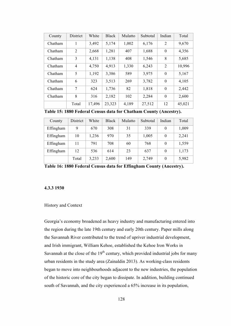
128
County District White Black Mulatto Subtotal Indian Total
Chatham 1 3,492 5,174 1,002 6,176 2 9,670
Chatham 2 2,668 1,281 407 1,688 0 4,356
Chatham 3 4,131 1,138 408 1,546 8 5,685
Chatham 4 4,750 4,913 1,330 6,243 2 10,996
Chatham 5 1,192 3,386 589 3,975 0 5,167
Chatham 6 323 3,513 269 3,782 0 4,105
Chatham 7 624 1,736 82 1,818 0 2,442
Chatham 8 316 2,182 102 2,284 0 2,600
Total 17,496 23,323 4,189 27,512 12 45,021
Table 15: 1880 Federal Census data for Chatham County (Ancestry).
County District White Black Mulatto Subtotal Indian Total
Effingham 9 670 308 31 339 0 1,009
Effingham 10 1,236 970 35 1,005 0 2,241
Effingham 11 791 708 60 768 0 1,559
Effingham 12 536 614 23 637 0 1,173
Total 3,233 2,600 149 2,749 0 5,982
Table 16: 1880 Federal Census data for Effingham County (Ancestry).
4.3.3 1930
History and Context
Georgia’s economy broadened as heavy industry and manufacturing entered into
the region during the late 19th century and early 20th century. Paper mills along
the Savannah River contributed to the trend of upriver industrial development,
and Irish immigrant, William Kehoe, established the Kehoe Iron Works in
Savannah at the close of the 19th century, which provided industrial jobs for many
urban residents in the study area (Zainaldin 2013). As working-class residents
began to move into neighbourhoods adjacent to the new industries, the population
of the historic core of the city began to dissipate. In addition, building continued
south of Savannah, and the city experienced a 65% increase in its population,

129
from 54,244 in 1900 to 83,252 in 1920 (Zainaldin 2013). Savannah's economy
also expanded in this era, due primarily to the export of naval stores, including
items like pitch and turpentine that were essential for the manufacture and upkeep
of wooden ships. Yellow pine was harvested in the uplands diversified
Savannah’s growing industrial economy into the lumber export industry.
Extensive yellow pine forests extending from the coast well into the coastal plain,
which established Savannah’s position as one of the largest exporters of naval
stores in the world (Zainaldin 2013).
During the 1920s more than 400,000 residents, the majority them being African-
American, migrated to other parts of the country due to the lack of work in
Georgia. Between 1910 and 1930 almost half of the state's agricultural workers
had abandoned farming altogether (Zainaldin 2013). In 1933, Roosevelt created
the Agricultural Adjustment Administration in an attempt to raise crop prices by
lowering agricultural production. One of the ‘unintended consequences’ of the
policy was the policy actually resulted in the loss of farming jobs, causing even
greater numbers to seek other means of employment (Zainaldin 2013). Due to the
loss of jobs in rural communities, these areas struggled to maintain their
populations.
The economic situation worsened when the boll weevil spread into southwest
Georgia in the early 20th century, destroying thousands of acres of cotton. This
insect, combined with the low price of cotton around 1920, made agricultural
diversification an imperative for farmers in the area. Cotton production in Georgia
declined from a high of more than 2,769,000 bales in 1911 to approximately
500,000 bales in 1923 (Zainaldin 2013). This drastic shift in economic conditions
and different commercial and industrial enterprises led to rapid expansion of
urbanization and a significant changes in the study area that required the
alterations to the built environment at a previously unprecedented level. In the
1930s and 1940s, many of the historic buildings in downtown Savannah were
demolished to make way for new development, including parking lots for the
rapidly expanding automobile sales. These circumstances and changes in industry

130
led to a transition in the patterns of urban and rural development that significantly
affected the built environment of the time (Zainaldin 2013) and demonstrated the
demographic shifts that were observed in the eras addressed in this study area.
Demographic Data and Human Population
Correlations in the population data for 1930 suggested that the population had re-
established itself (Tables 17-18). These groups are described in this research as
Urban African American, Urban European American, Sea Islands, Suburban
European American, Suburban African American, Rural Suburb and Rural. These
groups were then analysed using the Minitab Correlation Tool to define areas,
which are predominantly African American, European American and blended
African American-European American areas.
County District White Black Mulatto Subtotal Other Total
Chatham 1 5,088 22,585 0 22,585 26 27,699
Chatham 2 6,646 1,382 0 1,382 7 8,035
Chatham 3 9,962 1,047 0 1,047 13 11,022
Chatham 4 24,373 13,882 0 13,882 13 38,268
Chatham 5 4,188 2,286 0 2,286 1 6,475
Chatham 6 1,939 2,285 0 2,285 0 4,224
Chatham 7 644 2,252 0 2,252 5 2,901
Chatham 8 2,818 3,988 0 3,988 1 6,807
Total 55,658 49,707 0 49,707 66 105,431
Table 17: 1930 Federal Census data for Chatham County (Ancestry).
County District White Black Mulatto Subtotal Indian Total
Effingham 9 910 527 0 527 0 1,437
Effingham 10 1,709 1,033 0 1,033 0 2,742
Effingham 11 1,615 1,250 0 1,250 0 2,865
Effingham 12 1,064 906 0 906 0 1,970
Effingham 1559 712 438 0 438 0 1,150
Total 6,010 4,154 0 4,154 0 10,164
Table 18: 1930 Federal Census data for Effingham County (Ancestry).

131
4.3.4 Building population
Statistical analysis of the building population was combined with geospatial
analysis methods in order to provide a more accurate description of the building
population and surrounding areas. ArcGIS 9.2 was used to calculate the area of
each of the GMDs and helped in the identification of portions of the study area,
which were possibly over or under-represented in the historic resources survey.
The buildable land area for each era was calculated by deducting the area of
delineated wetlands, deepwater, marine wetlands, emergent wetlands, freshwater
wetlands, lakes, rivers and ponds from the total area of each GMD. The process of
identifying and excluding these areas allowed for more accurate assessments of
human population density to be conducted. To calculate buildable land area, the
wetland areas prevalent in this portion of the coastal plain were identified and
deducted from the total area of the study area, counties, and GMDs. The resulting
areas provided a more accurate projection of the portions of the study area
available for use in the 19th and early 20th centuries.
The human population data were compared to the buildable land area to determine
the historic human population densities for each district. When compared to
ancestry group data, it was clear that the African American communities were
located in the areas with the highest percentage of unbuildable land throughout the
19th century, but had become more evenly distributed across the landscape by
1930. Further calculations were completed that identified and deducted areas of
intensive development and farming from the buildable land area. The following
process then used geospatial analysis of the study area to identify portions of the
study area that were heavily modified in the 20th century. These changes were a
result of changing agricultural land use and residential, commercial, and industrial
land uses of the mid to late 20th century. Examples of this type of development
included modern residential subdivisions, big box stores and large-scale industrial
complexes such as the Georgia Port Authority. These approaches provided an
estimate of the portion of the GMD likely to contain historic resources.

132
4.4 Conclusion
This chapter established an understanding of the people who constructed and
maintained the historic masonry buildings in the study area. It built a solid
foundation, for the traditions of the people who populated the study area during
the precontact period and Colonial era. The chapter began with a discussion of the
precontact period in order to provide an understanding of the identity and the
construction traditions of the people from North America, Europe and Africa, who
converged in this area during the Colonial era. It then discussed the period of
contact and creolisation that occurred in the Colonial era. Then there was a brief
discussion of each of the study eras of this research by establishing an historical
and cultural context, which included a demographic and statistical analysis of the
people living in the study area in 1830, 1880 and 1930.

133
Chapter 5: Findings and Analysis
In order to address the primary research questions, three distinct datasets were
generated and analysed in the course of this research. The human population,
building population and mortar data were integral elements necessary to
effectively and accurately identify broad cultural patterns in the minute details of
the historic mortars of this area. Although the human population and building
population data were based on publicly available resources, each required a
significant amount of refinement and modification to meet the standards
necessary to generate the findings presented in this chapter. The research
necessary to reconstruct the historic GMD boundaries in each county and
subdivide the earliest Effingham County federal census data, which was presented
in the Theory and Methodology chapter, will benefit researchers in a variety of
fields. The building population data presented in the History and Context chapter
were developed from local historic resource surveys compiled by the State of
Georgia. The data were categorised and updated in conjunction with the fieldwork
and will be submitted to the local government and historical societies to be
incorporated into their records and made available to researchers in a variety of
fields. While these are both valuable contributions to future research in this area,
the notable strength of this research is the unique and comprehensive set of
historic mortar samples and data presented in this chapter. In the estimation of
John Walsh, a petrographer and mortar analysis specialist who has consulted on
both domestic and international projects, stated that:
‘This is without a doubt the most ambitious and comprehensive dataset amassed by a worker in the field of architectural conservation. This would have been a valuable dataset were it to have been collected from a region as large as the entire southeast. That it is sampled from only two counties in Georgia makes it even more so… This well-documented dataset should provide decades worth of research into historical masonry properties at a resolution previously unavailable.’ (Walsh 2012).
The full potential of the mortar data could not have been achieved without the
human and building population data. It was only through the extensive amount of
research and analysis in these areas that the mortar data could be accurately

134
collected and analysed. Together these three datasets provide a thorough and well-
supported assessment of the factors that potentially influenced the selection of
mortar materials in the study area in the 19th and early 20th centuries.
The quantity and detail of the mortar dataset generated in this research and
presented in this chapter are the first integral step in the process of making mortar
a visible and valued component in the archaeological record. Once the
relationship between culture and mortar has been established by this research and
other similar research of this kind, the recursive relationship between people and
objects addressed by materiality-based research can be more fully explored in
historic masonry as an archaeological artefact. By establishing a relationship
between culture and mortar, this research has also made a valuable contribution to
the on-going mortar discourse in the conservation community. Although well
established, conservation-based mortar research has typically focused on a
specific building, site or source of materials. In any case, the research was highly
scientific and failed to place the data generated into a wider, cultural context. This
generally limits the use of the research to conservators, architects and engineers
responsible for specifying repair mortars at similar sites. It was the primary aim of
this research to generate a baseline of historic mortar data with a firm theoretical
foundation in order to assess the relationship between culture and mortar. By
doing so, this research has made an initial step toward improving our
understanding of the cultural significance of a material often overlooked in the
discipline of archaeology and previously of interest only to scientists in the field
of buildings conservation. The findings of this research are important in
encouraging archaeologists and buildings conservationists to reassess their
perceptions of mortar and its potential contributions to both fields.
5.1 Sample Populations
There are two sample populations that should be considered when assessing the
mortars on the building level. These are the building sample population and the

135
mortar sample population. Both are relevant to this discussion because the number
of mortars identified in each building varied depending on the building category,
the type of construction, the urban and rural settlement pattern and the ancestry of
the human population.
5.1.1 Building Sample Population
The building sample population consisted of 164 buildings, which included 30
buildings from 1830, 57 buildings from 1880 and 77 buildings from 1930. As
discussed in the Theory and Methodology chapter, these buildings were selected
from randomly generated lists of historic masonry buildings in each building
category. The objective was to collect mortar samples from three single-family
residences, as well as samples from one of each of the following building types:
multi-family and rental residences, private and public civic buildings and
commercial buildings. Ideally, this would have resulted in mortar samples from
eight buildings in each GMD for each era, which would have included samples
from a total of 296 buildings. The number of buildings sampled was less than
originally projected due in part to the limited number of remaining buildings from
the earliest eras, particularly in rural areas. In the course of this research, a total of
176 buildings were sampled. While the mortars from these buildings were
sampled and processed, twelve of these buildings were excluded from the
statistical analysis. Three were known African American sites collected and
processed solely for comparison with documented African American sites
included in the building sample population. Following mortar analysis, additional
information indicated that the remaining nine buildings were ineligible for this
research based on the temporal and geographical criteria established in the
research design. As a result, the final building sample population included 164
buildings, which is only 55.4% of the originally projected sample. The reduction
was primarily due to the lack of remaining historic masonry buildings in some
GMDs, particularly in building categories other than single-family residential and
those in rural portions of the study area. In general, this building sample
population incorporates 25.9% of all the remaining historic masonry buildings
136
constructed in 1830, 5.4% of those constructed in 1880, and 1.2% of those
constructed in 1930.
5.1.2 Mortar Sample Population
There was a similar reduction in the mortar sample population during processing.
303 mortars were collected, prepared and analysed. Firstly, the seventeen mortars
associated with the twelve excluded buildings were omitted from the following
statistical analysis. Secondly, an additional 42 mortars from 33 buildings included
in the statistical analysis were omitted for various reasons described herein. 27 of
the mortars were omitted, because they duplicated one of the other mortar samples
from that particular site. Three were omitted, because it was determined that each
were collected from an addition constructed at an unknown date. One was
omitted, because it was determined to be a fragment of the Parker’s Roman
cement render instead of mortar. Another was omitted because it had been
damaged by water infiltration, which had leached the binder from portions of the
mortar sample. As such, it was not possible to conclusively determine if it was a
unique mortar type or a duplicate of the other mortar sample from the site. Nine
mortars were omitted, because each contained a material that was not available at
the date of original construction. The remaining mortar was omitted based solely
on its stratigraphic position. The materials in this sample were readily available at
the date of construction; however, it was a pointing mortar in a wall whose
bedding mortar contained materials that were not available for a minimum of 23
years after the date of construction. In this case, contextual analysis was crucial to
determining that the mortar sample was taken in a previously repaired area of the
wall and should be removed from the study. The remaining 244 mortar samples
constitute the mortar sample population, which was used to generate the statistics
presented in this chapter and represent a comprehensive cross section of historic
mortar data in the study area.
The loss of 59 mortars from 45 separate buildings reduced the total sample
population by 19.5%. Of these, 5.6% were excluded, because the site was
137
intended for comparison or the building was determined to be ineligible. The
remaining 13.9% were omitted on an individual basis. This preliminary evaluation
and elimination process actually highlighted the strength of the mortar analysis
methodology employed in this research by identifying mortars that failed to
conform to the research criteria. Characteristics of the mortar samples identified
during visual analysis in the laboratory under controlled conditions indicated that
the samples could have represented unique mortar types, warranting further
analysis. It was only the use of a range of microscopic methods, including
petrographic analysis of the binders, estimated particle size distribution analysis
of the aggregate, and point counts of the binder to aggregate ratios, which
identified mortar materials unavailable at the date of construction and duplicates
in the mortar sample population. In fact, only three of the omitted samples could
have been identified prior to processing, as they were collected from additions
whose date of construction could not be conclusively determined.
5.2 Mortar Data
The mortar data presented in the following sections have been organised into four
primary discussions. Firstly, the mortars were assessed on a building level, which
provided insight into the number of mortars used on each building, and the way in
which the usage varied by building category and the type of construction.
Secondly, microscopic analysis of this collection provided valuable insights into
the range and use of binder materials and mortar additives, including possible
sources of these materials and the regional and national trade patterns that brought
them to market. The binder and additive data also provided enough information to
estimate the compressive strength of the mortars and develop a discussion of their
performance characteristics. Thirdly, microscopic analysis also addressed the type
of aggregate materials used in the study area and their changes over time. Since
these materials were inert, bulk components of the mortar, they were less likely to
be imported to the study area from regional and national sources. As such,
changes in aggregate were more likely to be a result of different local sources of

138
materials and developments in preparation methods than changes in regional or
national trade patterns. Lastly, the binder, additive and aggregate components of
each of the mortars contributed to its overall appearance, which was characterised
using the Munsell Soil Color and Rock Color Systems. This provided data on the
hue, value and chroma of each of the mortars. By addressing these characteristics
last, it was also possible to discuss whether the colour characteristics were most
likely to be intentional or simply the result of the selection of binder or other
performance enhancing additives.
Within each of these sections, the data were discussed in relation to era, the urban
or rural settlement pattern of the area, and the ethnic origins of the specific human
population. This approach enabled multiple assessments of each of the mortar
data discussions. The era discussion addressed many of the basic factors
influencing the choice of mortar materials, notably the availability of new
materials over time and varying historical contexts, which may have limited the
ability of certain individuals to freely choose their own construction materials.
Mortar materials were also discussed in reference to the ethnic origins of the
population, including populations of predominantly African, African-European
and European ancestry. By assessing the data from multiple perspectives, this
research was able to establish multiple baselines of historic mortar data and
analysis that can be utilised in practical terms by the fields of archaeology and
buildings conservation. The data established a mortar material chronology, which
provided an unprecedented approach for archaeologists to utilise in dating
masonry remains and placing them within the wider context of historic masonry
construction. This chronology is also highly effective and valuable to conservators
when assessing the accuracy and relevance of current national guidelines for the
conservation of historic mortars on a regional, state or local level.
The discussion of the mortar data from multiple perspectives also offered great
insight into the more theoretical questions at the core of this research and
differentiated it from previous studies of historic mortars. It facilitated the
comparison of the relative strengths and weaknesses of the dataset, because it
139
presented it from each perspective, which allowed the research to directly address
the primary research questions of this study. How do historic mortars and mortar
materials change over time? How does geography influence the selection and use
of mortar materials? How does ethnicity influence the selection and use of mortar
materials? Together these three questions represent the aim of this research to
determine whether or not culture influences the use of historic mortar materials, as
well as the commonly accepted influence of availability and proximity.
5.2.1 Mortar Use
There are several discussions pertaining to the use of mortar on the building level,
which have been assessed in the following section in terms of era, urban and rural
settlement pattern, and ancestry. The primary discussion pertains to the number of
mortars used in each building, which provides a general overview of the
complexity of masonry construction methods and materials utilised in the study
area. Subsequent discussions of the number of mortars in each building category
and type of construction expand on this initial discussion and evaluate the
potential influence that geography and demography may have had on the overall
use of mortars in the study area.
Mortar Quantity
The number of mortars used in the historic masonry buildings in the study area
varied between one and four; however, the vast majority of buildings in each era
had no more than two mortars. This applied to 93.1% of the buildings in 1830,
96.5% of the buildings in 1880 and 97.5% of the buildings in 1930. While these
numbers do not vary significantly, a closer comparison of the frequency of
buildings containing one and two mortars reveals that the earliest era has

140
Figure 21: Chart of the relative percentage of one and two-mortar buildings in the study area in 1830, 1880 and 1930.
Figure 22: Chart of the relative percentage of one and two-mortar buildings in an urban environment in 1830, 1880 and 1930.
Figure 23: Chart of the relative percentage of one and two-mortar buildings in a rural environment in 1830, 1880 and 1930.
0 10 20 30 40 50 60 70 80 90
100
1830 1880 1930
1
2
0 10 20 30 40 50 60 70 80 90
100
1830 1880 1930
1
2
0 10 20 30 40 50 60 70 80 90
100
1830 1880 1930
1
2
141
significantly more one-mortar buildings than later eras (Figure 21). In fact, 75.9%
of buildings have only one mortar type in 1830, while later eras are more evenly
divided. In 1880, one and two-mortar buildings constitute 50.9% and 45.6% of the
buildings sampled respectively. By 1930, the percentages of one and two-mortar
buildings are even closer, with 49.4% and 48.1% respectively. The reason that the
1830 distribution differed from later eras was unclear based on these data alone.
This trend in the data may actually reflect broad cultural patterns and
socioeconomic factors that were influenced by significant historic events in the
study area, which had a tremendous effect on demographic conditions and further
influenced the selection of materials and architectural forms.
The two-mortar buildings are extremely diverse, including a rural homestead in
the northernmost portion of Effingham County (025307A), the locks of the
Savannah-Ogeechee Canal (081355) and one of the largest and most affluent
residences surviving from the era (081415). The diversity also extends to the two
buildings with more than two mortars. One of the buildings, which contained
three mortars, is a slave cabin located on Argyle Island in the Savannah River and
was once part of a rice plantation (022846A). The other building, which contains
four mortars, is a National Historic Landmark, Regency-style residence located in
downtown Savannah (081539A). The striking differences in these two residences
obscured any similarities, which may have influenced the decision to use multiple
mortars in their construction.
When considering the number of mortars used in each building, it was useful to
assess the issue from the perspective of urban or rural settlement patterns (Figures
22-23). Since buildings containing more than two mortars only constituted 6.9%,
3.5% and 2.5% of the building sample population, these buildings were
considered to be outliers for the purposes of establishing trends in urban and rural
environments. In an urban environment, there was a linear decline in the
frequency of one-mortar buildings and a corresponding increase in the frequency
of two-mortar buildings over the duration of the study. The relative percentage of
one-mortar buildings declined from 75.0% in 1830 to 48.0% in 1880 and 32.3%

142
in 1930. In contrast, the relative percentage of two-mortar buildings increased
from 18.8% in 1830 to 44.0% in 1880 and 61.3% in 1930. The overall increase in
the number of mortars per building was also clearly expressed in the mean
number of mortars in each era, which were 1.38, 1.60 and 1.74 respectively. The
data consistently indicated that there were a greater preference for multiple
mortars in an urban environment over the course of this study; however, this
pattern was not repeated in rural environments. While the pattern was similar
from 1830 to 1880, the trend had reversed by 1930. The relative percentage of
one-mortar buildings declined from76.9% in 1830 to 53.1% in 1880, before
increasing to 60.9% in 1930. In contrast, the relative percentage of two-mortar
buildings increased from 15.4% in 1830 to 46.9% in 1880, before decreasing to
39.1% in 1930. The reversal in the trend established in an urban environment and
begun in the 19th century rural environment was also clearly expressed in the
mean number of mortars in each era, which were 1.31, 1.47 and 1.39 respectively.
The data indicated that there was always a preference for one mortar type in rural
environments, as well as a distinct difference in the selection of masonry materials
in rural environments in the early 20th century that was not present in the previous
century or the early 20th century urban environment.
It was also useful to assess the number of mortars per building from the
perspective of the ancestry of the human population (Figures 24-26). Since
buildings containing more than two mortars represented the same relative
percentages of the building sample population, these buildings were also
considered to be outliers for the purposes of establishing trends in the discussion
of the role that ancestry may have played in the number of mortar types used in
each building over the duration of this study.
When considering the number of mortars used in each building from this
perspective, it was clear that the number of mortars used in each building in both
the African-American and European-American communities followed a similar
pattern to the one established when assessing the data according to era. The
relative percentage of the one-mortar buildings in areas with predominantly
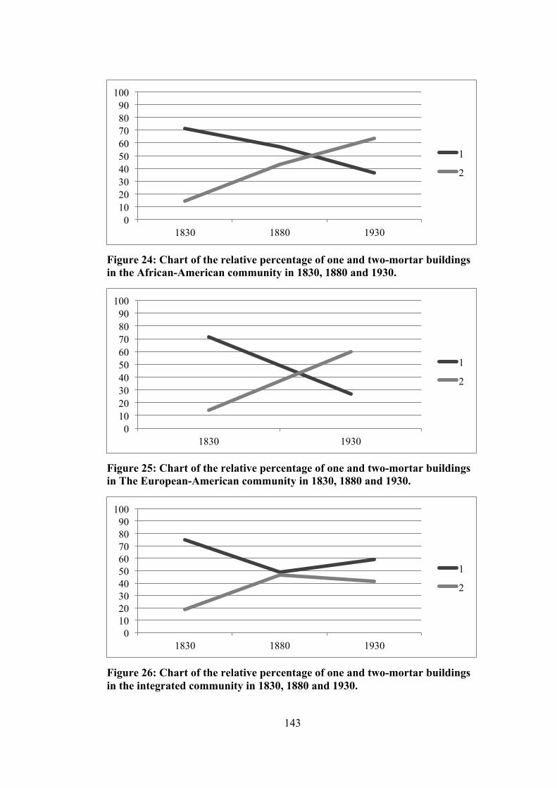
143
Figure 24: Chart of the relative percentage of one and two-mortar buildings in the African-American community in 1830, 1880 and 1930.
Figure 25: Chart of the relative percentage of one and two-mortar buildings in The European-American community in 1830, 1880 and 1930.
Figure 26: Chart of the relative percentage of one and two-mortar buildings in the integrated community in 1830, 1880 and 1930.
0 10 20 30 40 50 60 70 80 90
100
1830 1880 1930
1
2
0 10 20 30 40 50 60 70 80 90
100
1830 1930
1
2
0 10 20 30 40 50 60 70 80 90
100
1830 1880 1930
1
2

144
African-American ancestry declined from 71.4% in 1830 to 57.1% in 1880 and
36.4% in 1930. In contrast, the relative percentage of two-mortar buildings
increased from 14.3% in 1830 to 42.9% in 1880 and 63.7% in 1930. The data
indicated that there was a greater preference for multiple mortars in the African-
American community over the course of this study. A similar pattern appeared to
have been present in areas of European-American ancestry; however, this cannot
be determined conclusively, as no portion of the study area was statistically
determined to be of European-American ancestry in 1880. Therefore, the pattern
was based on data from only 1830 and 1930. This would have been of greater
concern in the current discussion, if the data from the earliest and latest eras had
not been almost identical to those in the African-American community. The
relative percentage of one-mortar buildings in The European-American
community declined from 71.4% in 1830 to 26.7% in 1930, which was relatively
similar to the distribution in the African-American community. The relative
percentage of two-mortar buildings increased from 14.3% in 1830 to 60.0% in
1930. In this case, the data for 1830 were the same, and the increase in the relative
percentage of two-mortar buildings in 1930 was only 3.7% less than in the
African-American community. Regardless of the null dataset in 1880, the data
still indicated that there was a greater preference for multiple mortars in areas
with European-American ancestry between the earliest and latest eras of this
study.
While the data regarding the number of mortars used in each building in African-
American and European-American communities were quite similar, there is a
significant difference in the integrated community, where the relative percentage
of people with African-American ancestry is comparable to the relative
percentage with people with European-American ancestry. In fact, this pattern
was closely related to the pattern established in rural environments over the
duration of this study. Again, the trend was similar from 1830 to 1880, but had
reversed by 1930. The relative percentage of one-mortar buildings declined from
75.0% in 1830 to 48.8% in 1880, before increasing to 58.8% in 1930. In contrast,
the relative percentage of two-mortar buildings increased from 18.8% in 1830 to
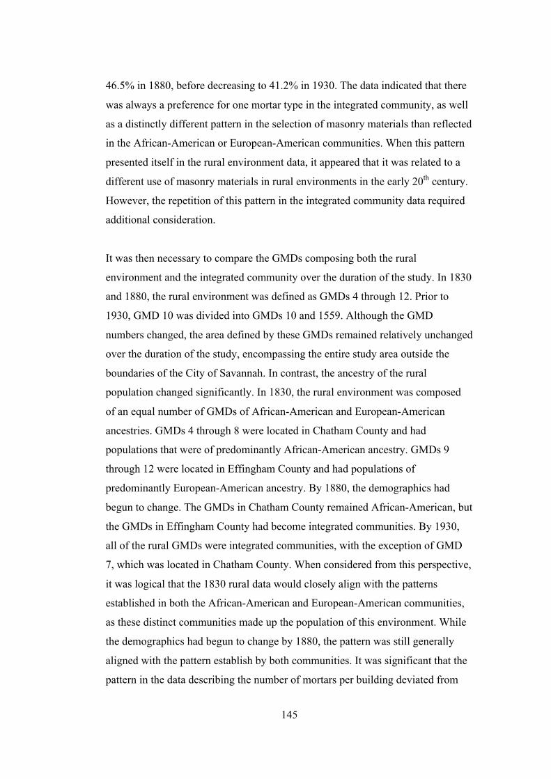
145
46.5% in 1880, before decreasing to 41.2% in 1930. The data indicated that there
was always a preference for one mortar type in the integrated community, as well
as a distinctly different pattern in the selection of masonry materials than reflected
in the African-American or European-American communities. When this pattern
presented itself in the rural environment data, it appeared that it was related to a
different use of masonry materials in rural environments in the early 20th century.
However, the repetition of this pattern in the integrated community data required
additional consideration.
It was then necessary to compare the GMDs composing both the rural
environment and the integrated community over the duration of the study. In 1830
and 1880, the rural environment was defined as GMDs 4 through 12. Prior to
1930, GMD 10 was divided into GMDs 10 and 1559. Although the GMD
numbers changed, the area defined by these GMDs remained relatively unchanged
over the duration of the study, encompassing the entire study area outside the
boundaries of the City of Savannah. In contrast, the ancestry of the rural
population changed significantly. In 1830, the rural environment was composed
of an equal number of GMDs of African-American and European-American
ancestries. GMDs 4 through 8 were located in Chatham County and had
populations that were of predominantly African-American ancestry. GMDs 9
through 12 were located in Effingham County and had populations of
predominantly European-American ancestry. By 1880, the demographics had
begun to change. The GMDs in Chatham County remained African-American, but
the GMDs in Effingham County had become integrated communities. By 1930,
all of the rural GMDs were integrated communities, with the exception of GMD
7, which was located in Chatham County. When considered from this perspective,
it was logical that the 1830 rural data would closely align with the patterns
established in both the African-American and European-American communities,
as these distinct communities made up the population of this environment. While
the demographics had begun to change by 1880, the pattern was still generally
aligned with the pattern establish by both communities. It was significant that the
pattern in the data describing the number of mortars per building deviated from
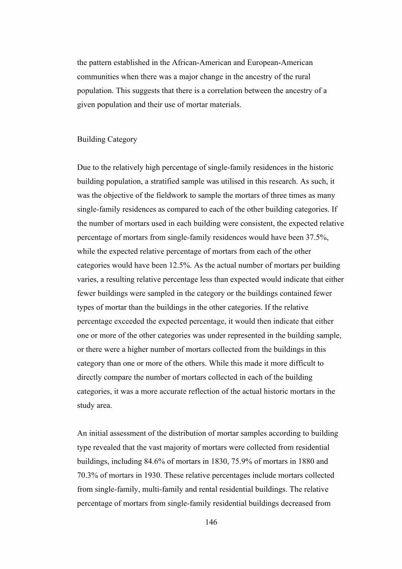
146
the pattern established in the African-American and European-American
communities when there was a major change in the ancestry of the rural
population. This suggests that there is a correlation between the ancestry of a
given population and their use of mortar materials.
Building Category
Due to the relatively high percentage of single-family residences in the historic
building population, a stratified sample was utilised in this research. As such, it
was the objective of the fieldwork to sample the mortars of three times as many
single-family residences as compared to each of the other building categories. If
the number of mortars used in each building were consistent, the expected relative
percentage of mortars from single-family residences would have been 37.5%,
while the expected relative percentage of mortars from each of the other
categories would have been 12.5%. As the actual number of mortars per building
varies, a resulting relative percentage less than expected would indicate that either
fewer buildings were sampled in the category or the buildings contained fewer
types of mortar than the buildings in the other categories. If the relative
percentage exceeded the expected percentage, it would then indicate that either
one or more of the other categories was under represented in the building sample,
or there were a higher number of mortars collected from the buildings in this
category than one or more of the others. While this made it more difficult to
directly compare the number of mortars collected in each of the building
categories, it was a more accurate reflection of the actual historic mortars in the
study area.
An initial assessment of the distribution of mortar samples according to building
type revealed that the vast majority of mortars were collected from residential
buildings, including 84.6% of mortars in 1830, 75.9% of mortars in 1880 and
70.3% of mortars in 1930. These relative percentages include mortars collected
from single-family, multi-family and rental residential buildings. The relative
percentage of mortars from single-family residential buildings decreased from

147
61.5% in 1830 to 57.5% in 1880 and 49.2% in 1930. The data were closely
aligned with a decrease in the relative percentage of single-family residences in
the building sample population, which were 63.3%, 56.1% and 50.6%
respectively. The mortars collected from multi-family residential buildings
experienced a similar decline from 17.9% in 1830 to 12.6% in 1880 and 11.9% in
1930. Again, the decrease closely aligned with a decrease in the relative
percentage of multi-family residences in the building sample population, which
were 16.7%, 12.3% and 1.0% respectively. In contrast to the other residential
categories, the relative percentage of mortars from rental residential buildings
increased from 5.1% in 1830 to 5.7% in 1880 and 9.3% in 1930. Although there
was a larger variation in the values than in the other residential categories, there
was also an increase in the relative percentage of rental residential buildings from
3.3% in 1830 to 5.3% in 1880 and 7.8% in 1930. Since these categories
represented such a large relative percentage of the mortar sample and building
sample populations, these findings strongly suggested that the number of mortars
collected from each building category was related to the number of available
buildings, rather than a significant preference for a different number of mortars
per building in each of the building categories represented.
In order to further test the initial findings, 132 mortars collected from 89 single-
family residential buildings were assessed in greater detail. This category was
selected, because it represents the largest single dataset in the building categories.
For clarity, the three and four-mortar buildings and their mortars were omitted
from the following analysis, because they were considered to be outliers. The
remaining 125 mortars from 87 buildings formed the basis of the following
analysis (Figure 27). When comparing the relative percentage of single-family
residences containing one or two mortars within the total building sample
population to the relative percentage of their mortars within the total mortar
sample population, the data were virtually identical. Each represented 58.6% of
the population in 1830. In 1880, the mortars composed 56.2% of the mortar
sample population, and the single-family residences composed 56.1% of the
building sample population. The relative percentages were equal again in 1930,
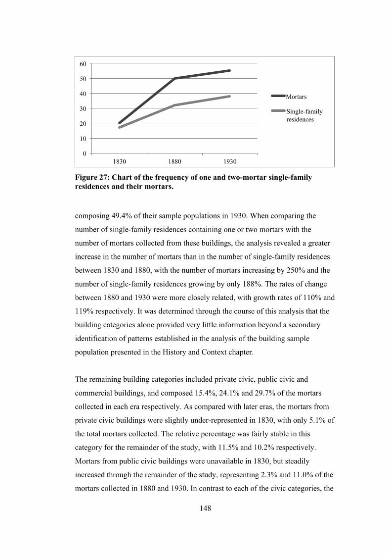
148
Figure 27: Chart of the frequency of one and two-mortar single-family residences and their mortars.
composing 49.4% of their sample populations in 1930. When comparing the
number of single-family residences containing one or two mortars with the
number of mortars collected from these buildings, the analysis revealed a greater
increase in the number of mortars than in the number of single-family residences
between 1830 and 1880, with the number of mortars increasing by 250% and the
number of single-family residences growing by only 188%. The rates of change
between 1880 and 1930 were more closely related, with growth rates of 110% and
119% respectively. It was determined through the course of this analysis that the
building categories alone provided very little information beyond a secondary
identification of patterns established in the analysis of the building sample
population presented in the History and Context chapter.
The remaining building categories included private civic, public civic and
commercial buildings, and composed 15.4%, 24.1% and 29.7% of the mortars
collected in each era respectively. As compared with later eras, the mortars from
private civic buildings were slightly under-represented in 1830, with only 5.1% of
the total mortars collected. The relative percentage was fairly stable in this
category for the remainder of the study, with 11.5% and 10.2% respectively.
Mortars from public civic buildings were unavailable in 1830, but steadily
increased through the remainder of the study, representing 2.3% and 11.0% of the
mortars collected in 1880 and 1930. In contrast to each of the civic categories, the
0
10
20
30
40
50
60
1830 1880 1930
Mortars
Single-family residences

149
relative percentage of mortars collected from commercial buildings were
relatively stable over the duration of the study, comprising 10.3% of the mortars
collected in 1830 and 1880, and 8.5% in 1930. While there was a general increase
in the relative percentage of the mortars collected from these building categories
over the duration of the study, the most significant finding in these categories was
that the changes also mirrored changes in the building sample population.
Similar issues presented themselves when assessing the frequency and relative
percentage of mortar samples collected from each building category in relation to
the urban and rural environment and the ancestry of the human population.
Although additional analysis was conducted, in a similar fashion to the analysis of
one and two-mortar buildings in the single-family residential category, the results
failed to reveal any additional information relevant to the research questions
established in this study. As such, only the initial analysis of the data in relation to
the urban and rural environment and the ancestry of the human population have
been presented here.
The only patterns that emerged from an initial analysis of mortar samples
collected from each building category in urban and rural environments related to
gaps in the mortar data, which were due to the lack of available buildings in
specific categories of the building sample population. For example, the frequency
distributions and relative percentages of mortar samples collected from each
building category in urban and rural environments were quite similar to the
frequency distribution and relative percentages of the mortar sample population.
The only exceptions were the absence of data in several building categories in
rural environments, including the rental residential and private civic categories in
1830 and the public civic category in 1880.
An initial analysis of the mortar samples collected from each building category
according to the ancestry of the human population also provided a minimal
amount of information beyond providing a secondary identification of the patterns
established in the analysis of the building sample population, which was presented
150
in the History and Context chapter. These included an absence of data in several
building categories in African-American and European-American communities. In
The African-American community, these included the rental residential categories
in 1830 and 1880, as well as the private civic and public civic categories in 1830.
In the European-American community, the gaps in data were so prevalent that
they obscured any pattern that may have existed historically. This was caused by a
lack of surviving historic buildings, which resulted in a less comprehensive
historic building population than in either the African-American or integrated
communities. It affected the multi-family and rental residential, private and public
civic and commercial categories in 1830; however, the demographic upheaval
following the Civil War was significantly worse and resulted in no statistically
European-American community in the study area in 1880. As a result, there were
no buildings, mortars or data to represent this community in 1880. There was only
a sufficient amount of data representing 1930, which prevented the analysis of any
trends in the European-American community over the duration of the study.
There is one notable variation in the multi-family residential category when
comparing the frequency distribution and relative percentages of mortar samples
collected from the African-American community to the mortar sample population.
In this case, there was a large decrease in the relative percentage of mortars
collected from The African-American community from 50.0% in 1830 to 15.0%
in 1880 and 5.6% in 1930, which was significantly different from the slight
reduction seen in the mortar sample population from 17.9% in 1830 to 12.6% in
1880 and 11.9% in 1930. The more exaggerated decrease was caused by a
combination of factors. One was the reduction in the number of multi-family
residences in each era. The other factor was the decrease in the number of mortars
per building over the duration of the study, as demonstrated by the means of the
number of mortars used per building, which were 1.67, 1.5 and 1 respectively.
The higher number of multi-family buildings in The African-American
community in 1830 as compared to European-American or integrated
communities was most likely related to the architectural form of slave quarters.
These residences were typically constructed as a row or parallel rows of identical

151
buildings, as duplexes sharing a back-to-back central chimney or a combination of
both in the study area. In any of these cases, these buildings would have been
categorised as multi-family residences in this study. The decline of the relative
percentage of multi-family residences in The African-American community in
1880 and 1930 may express the greater level of freedom to select the form of their
own residences following emancipation. The reason for the decline in the number
of mortars was less apparent, but may have been skewed by the Argyle Island
slave quarters in 1830 with three mortars (022846A) and a duplex in Savannah in
1880 with two mortars (007494A).
The analysis of the mortars from the perspective of the building categories proved
to be far less informative than the analysis presented in the previous section,
which assessed the number of mortars per building. These findings strongly
suggested that the number of mortars collected from each building category was
most closely related to the number of available buildings, rather than a significant
preference for a different number of mortars per building in each of the categories.
This was true, regardless of whether the analysis was conducted from the
perspective of the era, urban or rural settlement pattern or the ancestry of the
human population. The incorporation of building categories in the research design
was of greatest benefit to the study by ensuring that the building sample and
subsequent mortar samples provided a comprehensive cross-section of the historic
mortar materials used in the study area.
Type of Construction
The types of historic masonry construction utilised in the study area were well
documented in the course of this research. The most prevalent type of masonry
building sampled in each era was actually a wood building constructed with a
masonry foundation and chimney. Buildings constructed with a solid masonry
wall, with or without a render, were also quite common in the 19th century;
however, their usage tapered off by the early 20th century when solid wall
construction was replaced with masonry veneer construction methods. In addition,
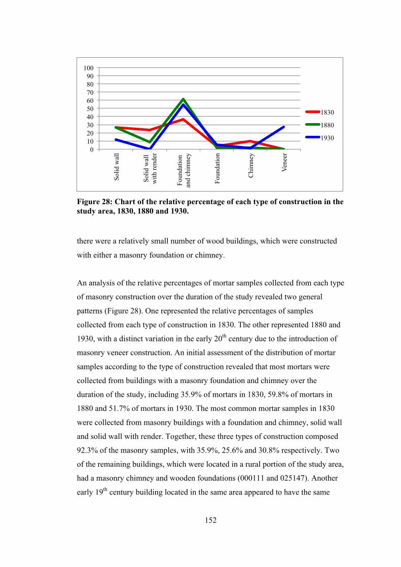
152
Figure 28: Chart of the relative percentage of each type of construction in the study area, 1830, 1880 and 1930.
there were a relatively small number of wood buildings, which were constructed
with either a masonry foundation or chimney.
An analysis of the relative percentages of mortar samples collected from each type
of masonry construction over the duration of the study revealed two general
patterns (Figure 28). One represented the relative percentages of samples
collected from each type of construction in 1830. The other represented 1880 and
1930, with a distinct variation in the early 20th century due to the introduction of
masonry veneer construction. An initial assessment of the distribution of mortar
samples according to the type of construction revealed that most mortars were
collected from buildings with a masonry foundation and chimney over the
duration of the study, including 35.9% of mortars in 1830, 59.8% of mortars in
1880 and 51.7% of mortars in 1930. The most common mortar samples in 1830
were collected from masonry buildings with a foundation and chimney, solid wall
and solid wall with render. Together, these three types of construction composed
92.3% of the masonry samples, with 35.9%, 25.6% and 30.8% respectively. Two
of the remaining buildings, which were located in a rural portion of the study area,
had a masonry chimney and wooden foundations (000111 and 025147). Another
early 19th century building located in the same area appeared to have the same
0 10 20 30 40 50 60 70 80 90
100
Solid
wal
l
Solid
wal
l w
ith re
nder
Foun
datio
n an
d ch
imne
y
Foun
datio
n
Chi
mne
y
Vene
er
1830
1880
1930

153
configuration; however, its mortar was determined to contain materials that were
unavailable until the early 20th century (025136A). The presence of an early 20th
century chimney on an 1830 residence could indicate the replacement of an earlier
chimney or suggest the use of a different type of chimney construction, such as
wattle and daub, in the study area in the early 19th century. Additional fieldwork
would be necessary to determine conclusively which of these options was the
most likely. There is no indication that the house has been moved, therefore
sufficient archaeological evidence should exist on the site to resolve this issue. If
a previous masonry chimney fell or was demolished on this site to allow for the
construction of the existing chimney, there should be a mortar scatter near the
approximate location of the previous chimney. It is unlikely that fragments from
an earlier chimney would be confused with construction debris from the existing
chimney. Mortar fragments that were once a part of an earlier chimney would
most likely have at least one flat face, where the mortar had once adhered to at
least one masonry unit. This supposition was verified through the collection of
mortar from three partially demolished 1830 sites in Effingham County
(025322A, 025479 and 025253A). The mortar samples from these sites were
collected from chimney falls and the remains of foundation piers. All of the
fragments had at least one flat face, but the majority of the samples had two
parallel faces. This condition would not be expected to occur in clumps of mortar
that had simply fallen off of the mason’s trowel or been scraped off of the wall
when the mason was finishing the joint.
There was also one building listed as having only a masonry foundation, which
was constructed of tabby and located in an area with relatively few buildings
meeting the criteria established in the research design. It had several internal
chimney structures, but they were inaccessible on each floor of the house,
including the attic. Based on their location, the chimneys were almost certainly
constructed of masonry, but it was unclear whether they were constructed of
tabby, brick or stone. Since the chimneys could not be sampled, the building was
defined as having only a masonry foundation. Although the decision to include
this building in the statistics was a difficult one, it was determined that it was

154
better to include the incomplete sample than to introduce an additional void in the
mortar data for that era. It should be noted that this building was one of three
buildings from this era that was constructed of tabby, rather than a unit masonry
system. Two of the buildings were high-end single-family residences (080292A
and 005695) and included masonry and wood frame components. The remaining
building was a multi-family residence constructed with a solid tabby wall.
In 1880 and 1930, the majority of mortar samples were collected from buildings
with a masonry foundation and chimney, with 59.8% and 51.7% respectively.
Although the distribution differed slightly from 1880 to 1930, the variations were
specifically related to the transition from solid wall construction, with and without
render common in the 19th century, to veneer construction methods introduced in
the early 20th century. Mortar samples from solid wall and rendered solid wall
construction had composed 56.4% of the samples in 1830, with 25.6% and 30.8%
respectively. In 1880, the relative percentage had dropped to 37.9%, but most of
the change was seen in the mortar samples from buildings with a rendered solid
wall, which had declined from 30.8% to 5.7% of the mortar sample population.
The decline continued, and by 1930, there were no mortar samples collected from
buildings with a rendered solid wall. It is also interesting to note that the building
categories employing rendered solid wall construction methods in 1830 were
typically high-end single-family residences (081415, 081539A, 081541 and
006671A), with the remainder being civic private and commercial buildings
(010662, 006635 and 006067). By 1880, this construction type was reserved for
civic and commercial buildings (006871, 080284, 006550, 006137 and 006409).
While mortar samples from solid wall buildings maintained their presence in the
late 19th century, they had dropped to only 12.7% of the mortar sample collected
in 1930. This relative percentage was also significantly lower than the 28.8% of
mortar samples representing masonry veneer buildings. By this time, veneer
buildings were second only to foundation and chimney buildings as the most
common sources of mortar samples in this study.

155
The remaining mortar samples were collected from buildings with either a
masonry foundation or chimney. While these types of construction were also the
least represented in the mortar sample population in 1830, the buildings
themselves were quite different. Instead of being exclusively single-family
residential buildings ((025147, 000111, 025136A and 005695), the buildings
expanded to include civic public and commercial buildings. In 1880, there was a
demolished, rural school building (000107) with a masonry chimney and a wood
foundation, as well as a demolished mill complex, which retained a massive brick
foundation and no remaining chimneys (000109). Due to its condition, it could
not be determined whether or not the mill once had one or more chimneys. By
1930, the buildings with only a masonry foundation or chimney represented a
greater range of building categories. Those with only a foundation were
predominantly single-family and multi-family residences (025133A, 025205A,
and 025416A), but did include a bridge in the civic public category (005872).
There was only one building with a chimney and no foundation constructed in
1930. This building is a remarkable structure requiring further study, as it differs
from all other buildings in the study area. Instead of being constructed on wood
foundation piers, this one-room residence was constructed with a wood sill placed
directly on the ground and had only an earth floor on the interior.
When considering the relative percentage of mortar samples collected from each
type of construction in urban and rural environments (Figures 29-30), it was clear
that there was a distinct difference in each relative distribution over the duration
of the study. The notable aspects of the urban distribution were the greater levels
of solid wall and solid wall with render types of construction and the complete
lack of buildings with only a masonry foundation or chimney in all eras.
In contrast, the rural distribution had a much lower relative percentage of mortars
collected from solid wall and veneer buildings than seen in the urban
environment, no mortars from rendered solid wall buildings and all of the mortars
collected from buildings with only a masonry foundation or chimney. In addition,
mortar samples collected from buildings with a masonry foundation and chimney

156
Figure 29: Chart of the relative percentage of mortar samples collected from each type of construction in an urban environment in 1830, 1880 and 1930.
Figure 30: Chart of the relative percentage of mortar samples collected from each type of construction in a rural environment in 1830, 1880 and 1930.
were clearly the dominant type of construction in the rural environment in all eras.
This was a stark contrast to the urban distribution, in which buildings with a
masonry foundation and chimney were more equally represented when compared
to the other types of construction. The urban and rural distributions depicting the
relative percentage of mortar samples collected from each type of construction in
urban and rural environments was significantly more informative than similar
distributions assessing the data according to building categories, which was
0 10 20 30 40 50 60 70 80 90
100
Solid
wal
l
Solid
wal
l w
ith re
nder
Foun
datio
n an
d ch
imne
y
Foun
datio
n
Chi
mne
y
Vene
er
1830
1880
1930
0 10 20 30 40 50 60 70 80 90
100
Solid
wal
l
Solid
wal
l w
ith re
nder
Foun
datio
n an
d ch
imne
y
Foun
datio
n
Chi
mne
y
Vene
er
1830
1880
1930

157
discussed in the previous section. This indicated that while buildings in a variety
of categories were necessary in both urban and rural environments, there were
distinct differences in the types of masonry construction selected for buildings in
each environment.
An assessment of the relative percentage distribution of mortar samples collected
from each type of construction according to the ancestry of the human population
was also more informative than similar distributions assessing the data according
to building categories (Figures 31-33). Although the data were also adversely
affected by the absence of data in several building categories in African-American
and European-American communities, the available data were sufficient to reveal
patterns in each distribution. In particular, the relative percentage distributions in
African-American and European-American communities were closely related to
the rural distribution pattern, while the relative percentage distribution of the
integrated community was closely related to the urban distribution pattern. This
certainly makes sense when considering that African-American and European-
American communities were distinctly rural and the integrated community was
distinctly urban in 1830. This pattern began to break down in 1880, when the
portion of the rural environment that had been European-American became an
Figure 31: Chart of the relative percentage of mortar samples collected from each type of construction in The African-American community in 1830, 1880 and 1930.
0 10 20 30 40 50 60 70 80 90
100
Solid
wal
l
Solid
wal
l w
ith re
nder
Foun
datio
n an
d ch
imne
y
Foun
datio
n
Chi
mne
y
Vene
er
1830
1880
1930

158
Figure 32: Chart of the relative percentage of mortar samples collected from each type of construction in The European-American community in 1830, 1880 and 1930.
Figure 33: Chart of the relative percentage of mortar samples collected from each type of construction in the integrated community in 1830, 1880 and 1930.
integrated community. By 1930, the relationship had completely broken down.
The urban environment was now predominantly segregated with African-
American and integrated communities on the periphery and the European-
American community in the urban centre.
0 10 20 30 40 50 60 70 80 90
100
Solid
wal
l
Solid
wal
l w
ith re
nder
Foun
datio
n an
d ch
imne
y
Foun
datio
n
Chi
mne
y
Vene
er
1830
1880
1930
0 10 20 30 40 50 60 70 80 90
100
Solid
wal
l
Solid
wal
l w
ith re
nder
Foun
datio
n an
d ch
imne
y
Foun
datio
n
Chi
mne
y
Vene
er
1830
1880
1930

159
Conclusion
This section discussed several issues pertaining to the use of mortar on the
building level, which were assessed according to era, urban and rural settlement
pattern and ancestry. The initial discussion pertained to the number of mortars
used in each building, which provided a general overview of the complexity of
masonry construction methods and materials utilised in the study area. Subsequent
discussions addressed the number of mortars in the mortar sample population
collected from each building category and type of construction. By addressing
each discussion from the perspective of era, urban and rural environment and
ancestry, the research was able to directly address and evaluate the potential
influence that geography and demography had on the use of mortars on the
building level in the study area. This section addressed each of the factors
influencing the selection of masonry construction methods on the macro level,
before delving into many of the same issues on the micro level of the mortars and
their constituents in the following sections. The three primary discussions
concerned the number of mortars used per building, the number of mortars
collected from each building category, and the number of mortars collected from
each type of construction, each revealed various patterns in the usage of mortars
on the building level.
The mortar quantity discussion showed that the vast majority of buildings
contained either one or two mortars, with only 3.7% of buildings containing more
than two mortars. When the entire body of historic mortars were assessed, the
analysis revealed a gradual decrease in the number of buildings containing one
more and a gradual increase in the number of buildings containing two mortars,
which converged at about 50% in the latest era of this study. When separated
according to urban and rural environments, it was clear that there were different
patterns in the data. In an urban environment there was a linear decline in the
number of buildings containing one mortar and a linear increase in the number of
buildings containing two mortars, which converged in the 1880s. Buildings
containing one mortar were more common in 1830, while one-mortar buildings
160
were more common in 1930. In contrast, the rural environment initiated a similar
pattern, with one-mortar buildings being more common in 1830, nearly
converging at around 50% each in 1880, before reversing the trend by the 1930s.
This analysis showed that there was an increasing preference for multiple mortars
in the urban environment over the duration of the study, while one-mortar
buildings remained more common in the rural environment over the same period.
When the data were analysed according to ancestry, African-American and
European-American communities mirrored the urban pattern in the number of
mortars, with both of these communities showing a greater preference for multiple
mortars in later eras. The data also showed that the integrated community
displayed a similar pattern to rural environments. Both of these distributions
deviated from the urban environment, and the African-American and European-
American communities in 1930. It was precisely this time that the demographic
conditions in the rural environment changed, not its geographic boundaries.
Unfortunately, the analysis of mortar use from the perspective of the building
categories proved to be far less informative than the analysis of the number of
mortars per building over the duration of the study. In fact, the findings in this
section strongly suggested that the relative percentage of mortars collected from
each building category was related almost entirely to the number of available
buildings, rather than a preference for a fewer or greater number of mortars per
building in each of the categories. This was generally true, regardless of whether
the analysis was conducted from the perspective of the era, urban or rural
settlement pattern or the ancestry of the human population. The only exception to
this pattern was a more significant decline in the number of mortars collected
from multi-family residences in The African-American community. While this
was undoubtedly related to the number of available buildings, it is possible that
the decline was exaggerated by a preference in the African-American community
for architectural forms that differed from those prevalent in the era of slavery. In
general, the analysis of the mortar usage data according to building category
revealed that the most important contribution of the building categories in the
research design was that it ensured that the building sample and their mortar

161
samples provided an accurate and comprehensive cross-section of the historic
mortar materials used in the study area.
The discussion of mortar usage according to the type of masonry construction
established that there were two distinct patterns in the data when assessed from
the perspective of era, urban and rural environments and ancestry. According to
era, the 1830 data revealed a different pattern of masonry construction methods in
1830 then in the later eras of this study. In 1830, the relative percentage of
mortars collected from solid wall, solid wall with render and foundation and
chimney buildings were relatively equally distributed. By 1880 and 1930
buildings with a masonry foundation and chimney were overwhelmingly
preferred. When assessed in terms of urban and rural environment, the data
showed two radically different distribution patterns. Mortar samples collected
from each type of construction in an urban environment showed that a greater
variety of construction methods were employed than in a rural environment,
where there was a clear preference for buildings with a masonry foundation and
chimney in all eras. When considered in terms of ancestry, the data revealed in
this analysis displayed a reversal of the pattern established in the mortar quantity
analysis. In terms of mortar quantity, there was a relationship between African-
American and European American communities and the pattern established in an
urban environment. The integrated community was more closely related to the
rural pattern. In the case of type of construction, these findings were reversed.
African-American and European American communities were closely related to
the rural pattern and the integrated community was closely related to the urban
pattern. Although the reason for this reversal is unclear, each of these discussions
demonstrated that there were different preferences for masonry construction
methods and mortar usage based on both geography and demography.
162
5.2.2 Binder Use
A total of 244 mortar samples were collected, analysed and included in the
statistical analysis presented in this chapter. As discussed in the Mortar chapter, a
mortar is composed of a binder and an aggregate. The binder provides properties
that allow the mortar to harden, and the aggregate provides dimensional stability.
In an ideal mortar, the binder should completely fill the voids present in clean dry
sand. Together, each of these components was critical to the proper use of mortar
materials in historic mortars. In order to alter the performance or appearance of a
mortar, a variety of alterations were made to the basic mortar mix described
above. In this study, these additives include materials intended to improve the
workability, durability or colour of a mortar.
Since the binder is the component of a mortar that provides a set, or causes the
mortar to harden, an understanding of the number and types of binders, as well as
any additives that may have been incorporated in the mix are critical to estimating
the performance characteristics of the mortar. In order to achieve this objective
and place the findings in a wider cultural context, the following section discussed
each of these aspects of the binder component from the perspective of era, urban
and rural settlement patterns and ancestry. The first discussion addressed the
number of binders used in each mortar, which assessed the overall complexity of
the historic mortars used in the study area. The discussion then turned to the types
of binders and additives in the mortars. The final discussion addressed the
combined properties of the binders and additives, by assessing the estimated
compressive strength of the historic mortars used in the study area. As
demonstrated in the previous section, a significant amount of understanding of the
use of binder materials was gained by discussing and evaluating the potential
influence that geography and demography may have had on the overall use of
binders in the study area.

163
Binder Quantity
The number of binders used in each of the historic mortars collected in the study
area varied from one to three. 52.5% of the mortars sampled contained one binder,
47.1% contained two binders, and only one mortar, which represented 0.4% of the
mortar sample population, contained three binder materials. Since all of the
mortars in 1830 and 1880, as well as 99.2% of the mortars in 1930 contained
either one or two binders, trends in the data were established using only the
mortars with one and two binders. The mortars containing one binder declined
from 94.9% in 1830 to 73.6% in 1880 and 22.9% in 1930, and there was a
corresponding increase in the mortars with two binders from 5.1% in 1830 to
26.4% in 1880 and 76.3% in 1930. While there was a continuous transition from
the use of one and two-binder mortars over the duration of the study, the rate of
change between 1880 and 1930 was three times the rate of change between 1830
and 1880.
When considering the use of mortars with one and two binders in urban and rural
environments (Figures 34-35), it was clear that changes in the use of binder
materials occurred differently in each area. In urban environments, none of the
mortars contained two binders in 1830. The transition from one to two-binder
mortars was nearly linear in this environment and concluding in 1930 with 69.8%
of all mortars containing two binders. The trend was quite different in rural
environments, where mortars with two binders constituted 11.8% of the mortars in
1830. This amount increased slowly to 21.3% in 1880, before accelerating rapidly
into the early 20th century to constitute 82.8% of all mortars in 1930. This
assessment of the use of mortars with multiple binders in urban and rural
environments revealed that multiple binders were not utilised as early in rural
environments, but they were ultimately a more common type of mortar in these
areas than in an urban environment.
An assessment of the use of mortars with one and two binders according to
ancestry (Figures 36-38) indicated that the urban and rural patterns were

164
Figure 34: Chart of the relative percentage of mortars containing one and two binders in urban environments in 1830, 1880 and 1930.
Figure 35: Chart of the relative percentage of mortars containing one and two binders in rural environments in 1830, 1880 and 1930.
associated with the ancestry of the human population in urban and rural
environments, rather than the settlement patterns themselves. An initial
assessment of the trends in the African-American, European-American, and
integrated communities revealed similarities between the African-American and
integrated communities. In each of these communities, the use of mortars with
two binders gradually increased through the 19th century, before sharply
increasing in the early 20th century. The pattern is somewhat more difficult to
discern in The European-American community over the duration of the study, due
to the lack of a statistically defined European-American community in 1880;
however, an extremely important detail was revealed in the comparison of
0 10 20 30 40 50 60 70 80 90
100
1830 1880 1930
1
2
0 10 20 30 40 50 60 70 80 90
100
1830 1880 1930
1
2

165
Figure 36: Chart of the relative percentage of one and two-binder mortars in The African-American community in 1830, 1880 and 1930.
Figure 37: Chart of the relative percentage of one and two-binder mortars in the integrated community in 1830, 1880 and 1930.
Figure 38: Chart of the relative percentage of one and two-binder mortars in The European-American community in 1830, 1880 and 1930.
0 10 20 30 40 50 60 70 80 90
100
1830 1880 1930
1
2
0 10 20 30 40 50 60 70 80 90
100
1830 1880 1930
1
2
0 10 20 30 40 50 60 70 80 90
100
1830 1880 1930
1
2
166
European-American and integrated communities. In 1830. There were no mortars
containing two binders in either of these communities in 1830. This means that
the mortars containing two binders that were present in the rural data were
probably the direct result of their use in the African-American community. Of
course, this raised the question as to why African-Americans living in the
integrated community did not utilise any mortar with two binders. This was
almost certainly due to restrictions placed on African-Americans by the European-
American population during the slave era. The area within the boundaries of the
city of Savannah was also the only integrated community in the study area in
1830. Although 50.4% of the human population of this area was African-
American, only 4.6% of the total population was composed of free blacks. The
remaining 45.8% of the African-American community were slaves, and
presumably unable to exert as much influence on masonry construction methods
and materials as either free blacks within the same community or slaves residing
in the African-American community, which may have had minimal European-
American oversight. This was possible given that the population of the African-
American community in 1830 was 88.6% slave, 1.3% free black and 10.0%
European-American.
Binder Type
As previously discussed, there was a significant shift from mortars containing one
binder in the 19th century to mortars containing two binders in the early 20th
century (Figure 39). This is clearly reflected in the relative percentage of each
type of binder over the duration of this study. In fact, the most prevalent binder in
both 1830 and 1880 was lime. By 1930, the most common binder was actually a
Portland cement and lime blend. This reflected both a preference for mortars with
two binders and the increase in the use of Portland cement in the early 20th
century. Although these particular binders represent the majority of binders used
in each of the eras, there were also a variety of mortars containing one and two
binders, which varied in each era depending on availability and innovation in the
market.

167
Figure 39: Chart of the relative percentage of each type of binder in 1830, 1880 and 1930.
In 1830, 87.2% of mortars sampled were lime based, and 7.7% were composed of
entirely of earth. The remaining 5.1% were mortars containing two binders,
specifically natural cement gauged with lime. The overwhelming percentage of
lime mortars dating to this era indicated that they were the most common type of
mortar across all building categories, environments and communities. The earth
mortars were only used in the three, rural single-family residences (000111-1,
025253A-1 and 025307A). The natural cement-lime mortars were collected from
one of the locks of the Savannah and Ogeechee Canal (081355), which were
highly-specialised masonry structures used to raise and lower barges travelling
laterally across the study area between the Savannah and Ogeechee Rivers.
By 1880, the number of mortar materials on the market had expanded
significantly, producing a much different baseline of historic mortars. The relative
percentage of lime mortars had declined to 70.1%, and natural cement-lime
mortars had increased to 11.5%. Portland cement entered the American market in
the early 1870s and made its first appearance in the historic mortars of the study
area in 1880, representing 10.3% of the mortar sample population in the form of
both one and two-binder mortars. The Portland cement mortar was used in the
0
20
40
60
80
100
1830
1880
1930

168
foundations of a rural sawmill (000109). The Portland cement-lime mortars were
used in a variety of buildings, including urban and were single-family residences
(010517 and 005759), a rural multi-family residence (007202A), a beach house
that served as a private club for veterans of the Civil War unit known as the
Chatham Artillery (010959A), and one railroad-related commercial warehouse
(010417). Earth mortars declined to 1.1% of the mortar sample population, while
earth-lime mortars represented 5.7%. The earth mortar was used in a rural single-
family residence (025253B). The earth-lime mortars included three rural single-
family residences (005879, 025536A and 025344B) and one rural commercial
building (000110). The only remaining mortar from this era was a gypsum mortar.
It was used on an urban single-family residence (006311A) and was the only
mortar of this kind in the study area. Although gypsum mortars have been in use
for thousands of years, they are almost exclusively employed in arid climates.
Therefore, the identification of the gypsum mortar on the exterior of a building in
the humid climate of the study area was entirely unexpected.
By 1930 Portland cement-lime was the most common binder, with 61.0% of the
mortar population. Lime was the next most common type of binder, representing
22.0% of the mortar sample population. Masonry cement, which contains Portland
cement, dry hydrated lime and a crushed calcium carbonate plasticiser to improve
workability, composed 15.2% of mortars. Each of these binders represented a
comprehensive cross-section of building categories in this era. There were two
additional mortars, each of which represented one mortar sample and 0.8% of
mortars from this era. One had a Portland cement and natural cement binder and
was used in a bridge foundation (005872). The other had a Portland cement,
natural cement and lime binder and was used in an urban, single-family residence
(008218). The reason that three binders were employed in this mortar was unclear,
but it is possible that the mason used leftover materials from other buildings or
that the material was accidentally contaminated with materials associated with
another job.

169
When considering the type of binders used in the study area according to urban
and rural environments (Figures 40-41), it was determined that the relative
percentage distributions of each environment was relatively similar to the overall
distribution for the era, with only a few exceptions. Firstly, there was a gradual
decline in the use of lime in urban environments, while the decline in rural
Figure 40: Chart of the relative percentage of each type of binder used in urban environments in 1830, 1880 and 1930.
Figure 41: Chart of the relative percentage of each type of binder used in rural environments in 1830, 1880 and 1930.
0
20
40
60
80
100
1830
1880
1930
0
20
40
60
80
100
1830
1880
1930

170
environments occurred more abruptly between 1880 and 1930. Secondly, there
were no earth or earth-lime binders used in mortars in an urban environment in
any era. These materials were confined to rural portions of the study area in 1830
and 1880. Thirdly, natural cement was only used in the study area in combination
with lime. It was primarily associated with urban environments in 1880 and was
used in civic private and public buildings (006942, 006340 and 006550), as well
as one rental residential building (006731) and one multi-family residence
(010515A). The only exception to this pattern was the early use of the material on
the Savannah and Ogeechee Canal (081355), which was constructed across a rural
portion of Chatham County in 1830. Finally, a comparison of the urban and rural
distributions revealed that masonry cement was strongly associated with rural
environments, representing 23.5% of all mortars in rural environments and only
5.6% of mortars in urban environments in 1930.
An assessment of the types of binders according to ancestry (Figures 42-44),
indicated that mortars with lime and Portland cement-lime binders were the most
common binders in each community over the duration of the study. Within the
African-American community, mortars with lime binders constituted 80.0% of the
mortars in 1830, 65.0% in 1880 and 33.3% in 1930. In the integrated community,
the relative percentage of mortars with this type of binder was 100.0% in 1830,
73.1% in 1880 and 15.3% in 1930. Again, the absence of a statistically European-
American community in 1880 resulted in data that established the beginning and
end of the trend, but no information to shed light on the shape of the trend.
Regardless, the 1830 and 1930 data provided enough information to compare the
findings of each era with the other communities. The data revealed that the use of
binders in the European-American community in 1930 was consistent with other
communities, with 64.3% of mortars using a Portland cement-lime binder and
32.1% of mortars using a lime binder. Where the European-American binder data
differed significantly was in the earliest era of the study, which revealed that this
community did not use mortars with a lime binder as frequently as the other
communities. In fact, only 57.1% of the mortars used a lime binder, as compared
to the African-American and integrated communities with 80.0% and 100.0%

171
Figure 42: Chart of the relative percentage of each type of binder used in The African-American community in 1830, 1880 and 1930.
Figure 43: Chart of the relative percentage of each type of binder used in the integrated community in 1830, 1880 and 1930.
respectively. The remaining findings revealed by an analysis of the binder
materials according to ancestry were identified among the less common binder
materials in each era. In particular, there was greater diversity in the binder
materials used in the integrated community than in the African-American
community. In 1880, The African-American community used mortars containing
0
20
40
60
80
100
1830
1880
1930
0
20
40
60
80
100
1830
1880
1930

172
Figure 44: Chart of the relative percentage of each type of binder used in The European-American community in 1830, 1880 and 1930.
lime, Portland cement-lime or earth-lime, which composed 10.0% of the mortars.
In contrast, the integrated community utilised earth, earth-lime, gypsum, natural
cement-lime, and Portland cement-lime mortars. The level of diversity contracted
on all fronts by 1930, when nearly all African-American and European-American
mortars utilised either Portland cement-lime or lime, while the integrated
community used Portland cement-lime, lime, and masonry cement.
The most unexpected aspect of this analysis was that the remaining 42.9% of the
mortars utilised by the European-American community in 1830 had only an earth
binder. These findings were in stark contrast to the other communities, which
used no mortars with an earth component of any kind. While there was not a
statistically European-American community in 1880, these people still existed.
They had simply begun to live in the integrated community. Given this, one might
have expected to find a significant number of mortars containing an earth
component in these communities; however, this was not the case. Only 4.5% of
the mortars in the integrated community used an earth component in their binder
in 1880. In fact, the highest relative percentage of mortars in 1880 with an earth
component in their binder actually occurred in the African-American community.
These findings raised two important questions. Why did the European-American
0
20
40
60
80
100
1830
1880
1930

173
community virtually abandon a binder material used as the sole binder material in
42.9% of their mortars in 1830? Why did the African-American community begin
using a material in 1880 that had not been utilised by their community in 1830?
When considering the 1830 buildings that used an earth binder, it was clear that
they were in fact from buildings constructed for European-American inhabitants.
These included the Biddenback House (000111) and the main house of Goshen
Plantation (025253A), which were located in Salzburger communities in the
portion of Effingham County with a strong connection to their Germanic ancestry.
The remaining building was the Foy Homestead (025307A), which was located in
a portion of Effingham County that was populated by people of predominantly
English ancestry. This would indicate that the European-American preference for
earth mortars in 1830 extended to both the Salzburger and English communities;
however, this may not be the case. An interesting connection emerged between
the Biddenback and Foy families in the mid 19th century census data, which
showed that there were several Biddenback family members living with the Foy
family in the Foy Homestead. The connection could be a coincidence, with the
Biddenback acting as servants or farm laborers, or there may have been a more
long-standing connection between these two families. Additional research would
need to be conducted to make an argument whether the use of earth binders was a
preference of the European-American in general or specific to the Salzburgers.
There may be a more straightforward answer to the question of why the African-
American community began using earth binders in 1880. As suggested in the
discussion regarding the rapid decline in multi-family residences in the African-
American community following emancipation, the incorporation of earth binders
in African-American mortars in 1880 may be an expression of a greater amount of
freedom in the selection of building materials, as well as architectural forms. Of
course, this assessment was based on the assumption that the African-American
community was immediately free to select every aspect of their built environment.
As discussed in the History and Context chapter, the transition from slavery to
freedom was often a slow an arduous process hampered by racism and a series of

174
Jim Crow laws, which restricted the many aspects of African-American life.
Unfortunately, a consideration of the buildings using earth binders in 1880
suggested that the later was the most likely conclusion. The five buildings were
all located in a rural environment, including three buildings that appear to have
been constructed for the European-American residents of the community and two
buildings constructed for African-American residents of the community. The
European-American buildings included a commercial building (000110) and two
single-family residences (025536 and 005879), which were constructed for
residents of English and Salzburger descent respectively. The remaining two
buildings were small, single-family residences located on the grounds of a larger
residence and were described as servant’s quarters (025344B and 025253B). In
this context, it is unlikely that the African-American residents were able to exert
much control over the selection of building materials or architectural form.
Additives
The additives used in the historic mortars in the study area included materials
intended to alter either the performance characteristics or appearance of the
binder. Performance additives included brick dust, slag, wood ash and crushed
calcium carbonate (Figure 45), and appearance additives included red, black and
yellow pigment (Figure 46). No additives of either type were identified in the
mortars collected from the sample population of buildings constructed in 1830. In
1880, 18.4% of the mortar samples from this era utilised additives. 43.8% of these
were intended to alter the performance of the binder, and 56.4% were pigments
intended to alter the appearance of the mortar. By 1930, the overall relative
percentage of buildings incorporating mortars with additives had risen to 39.8%
of the building sample population. The relative percentage of performance and
appearance additives had nearly reversed by 1930, when 52.9% of the additives
were performance altering, and only 47.1% were pigments. This shift indicated a
general preference for appearance additives in the late 19th century and
performance additives in the early 20th century.

175
Figure 45: Chart of the relative percentage of performance additives in relation to all additives used in 1830, 1880 and 1930.
Figure 46: Chart of the relative percentage of appearance additives in relation to all additives used in 1830, 1880 and 1930.
Performance additives used in the study area included brick dust, wood ash, slag
and crushed calcium carbonate. Brick dust and wood ash were only used in 1880,
while slag and crushed calcium carbonate were only used in 1930. Brick dust is a
pozzulan commonly used with lime binders, which reacts with the slaked lime or
calcium oxide to create hydraulic properties in the mortar. Since hydraulic
properties were not actually necessary in most buildings included in this study, the
additive was generally used to produce mortars with higher compressive strength
characteristics. The purpose of wood ash as an additive in lime mortars has not
been firmly established; however, research into the use of wood ash as an additive
in lime plaster suggested that the wood ash was used to increase the vapour
permeability characteristics of the material (Goodman 1998, 133). Higher vapour
permeability characteristics in lime mortars would have facilitated the process of
carbonation and decreased the curing time of the material. Based on these
0 10 20 30 40 50 60
Brick dust Slag Wood ash Crushed Calcium Carbonate
1830
1880
1930
0
10
20
30
40
50
60
Red pigment Black pigment Yellow pigment
1830
1880
1930

176
findings, the additives used in the late 19th century served two different functions.
One was intended to increase the compressive strength, and therefore the
durability of the mortar, and the other was intended to shorten the curing time of
the mortar materials. The additives used in 1930 were entirely different from
those used in 1880, including slag and crushed calcium carbonate. Slag, which is
a byproduct of the steel industry, was also a pozzulan used with lime and cement
binders in order to improve their hydraulic properties. Crushed calcium carbonate
is a finely crushed limestone aggregate, which was used as a plasticiser in
masonry cement. It reduced the cost and improved the workability of a typical
Portland cement and dry hydrated lime mortar. In this study, the additives used in
the early 20th century also served two different functions, with one improving the
hydraulic properties of the binder and one improving the workability of the
mortar. Since the performance additives used in each era were intended to alter
entirely different characteristics of the mortar, it was interesting and somewhat
surprising that they were never used together.
In contrast to the differences seen in the performance additives used in 1880 and
1930, the same colour pigments were used in the study area in both eras. Red
pigments were the most commonly selected appearance additive in 1880,
representing 43.8% of all of the additives used in this era. Black and yellow
pigments were used equally, but each only represented 6.3% of the additives used
in this era. Although the most commonly selected pigment in 1930 was still red,
its relative percentage had fallen to 26.4% of all additives used in this era. In
contrast, the use of black pigments increased to 11.3%, and the use of yellow
pigments increased to 9.4%.
Although none of the mortars included in this study contained more than one
appearance additive, there were six buildings that contained a mortar with a
performance and appearance additive. Three of these buildings contained slag and
a pigment, and three contained crushed calcium carbonate and pigment. The
buildings with mortars containing a slag additive were most commonly located in
an urban environment and included a commercial building (006173), a civic

177
private building (080164) and a single-family residence (103793A). The buildings
with mortars containing crushed calcium carbonate and pigment were located in
rural environments and included a civic private building (008849A), a rental
residential building (104284A) and a single-family residence (025534A).
When considering the use of additives in terms of urban and rural environments
(Figures 47-50), several patterns emerged. The most significant one revealed that
mortar additives used in urban environments were overwhelmingly appearance
based, unlike those used in rural environments, which were generally performance
based. For example, pigments accounted for 63.7% of the additives used in urban
areas in 1880 and 70.8% in 1930. In rural environments, pigments only accounted
for 40.0% of the additives used in 1880 and 27.5% in 1930. The data strongly
suggested that the appearance of a mortar was more valued in urban environments
Figure 47: Chart of the relative percentage of performance additives in relation to all additives used in urban environments in 1830, 1880 and 1930.
Figure 48: Chart of the relative percentage of appearance additives in relation to all additives used in urban environments in 1830, 1880 and 1930.
0 10 20 30 40 50 60
Brick dust Slag Wood ash Crushed Calcium Carbonate
1830
1880
1930
0
10
20
30
40
50
60
Red pigment Black pigment Yellow pigment
1830
1880
1930

178
Figure 49: Chart of the relative percentage of performance additives in relation to all additives used in rural environments in 1830, 1880 and 1930.
Figure 50: Chart of the relative percentage of appearance additives in relation to all additives used in rural environments in 1830, 1880 and 1930.
than rural environments. This supposition was confirmed with a comparison of
the relative percentage of buildings containing a pigment in urban and rural areas
over the duration of the study. In urban environments, 24.0% of buildings
contained a pigment in 1880, and 48.4% of buildings contained a pigment in
1930. The findings contrasted with those in rural environments, where only 6.3%
of buildings contained a pigment in 1880, and 17.4% of buildings contained a
pigment in 1930.
There were several other trends revealed by the assessment of additive data in
terms of urban and rural environment. Firstly, red pigments were clearly the
preferred pigment over the duration of the study. Although black and yellow
pigments were used in urban environments in 1880, they were completely absent
in rural environments at that time. By 1930, their use had dramatically increased
0 10 20 30 40 50 60
Brick dust Slag Wood ash Crushed Calcium Carbonate
1830
1880
1930
0
10
20
30
40
50
60
Red pigment Black pigment Yellow pigment
1830
1880
1930

179
in urban environments and been initiated in rural environments, although they had
still not reached the same level of use seen in 1880 urban environments. Secondly,
the use of performance additives in 1880 was quite different in urban and rural
environments. Wood ash comprised 40.0% of the additives used in a rural
environment, yet it was not present in any of the urban mortar samples from this
era. Brick dust was present in both environments, with 36.4% of the additives
used in an urban environment and 20% of those used in rural environments.
Thirdly, there was also a noticeable difference in the use of performance additives
in urban and rural environments in 1930. The relative percentage of the use of
slag in each environment was relatively similar, with 16.7% of the additives used
in urban areas and 20.7% of the additives used in rural environments. The
difference occurred in the use of masonry cement, which was identified by its
crushed calcium carbonate plasticiser and represented 20.7% of the additives used
in rural areas and only 12.5% of those used in urban areas. This is simply a
confirmation of the binder data, which also revealed a greater use of masonry
cement in rural areas than in urban areas.
When considering performance-enhancing additives in terms of ancestry (Figures
51-56), the overall number of communities and additives required additional
analysis in order to place the findings in context. This analysis assessed the actual
number of buildings that used performance or appearance additives with the
number of buildings in the building sample population in each community. This
enabled the analysis to differentiate between relative percentages that simply
appeared low from those that were actually lower than those in other
communities. Beginning in 1880, 21.3% of the buildings in the African-American
community used additives, compared with the integrated community that used
additives in 27.9% of the buildings in the European-American community. In the
African-American community, 66.7% of the additives were based on performance
and 33.3% were based on appearance. The conditions were nearly reversed in the
integrated community. In this community, 61.6% of their additives were
appearance, and only 38.5% of the additives were performance. By comparing the
actual number of buildings utilizing additives to the relative percentage of use of

180
Figure 51: Chart of the relative percentage of performance additives in relation to all additives used in The African-American community in 1830, 1880 and 1930.
Figure 52: Chart of the relative percentage of performance additives in relation to all additives used in the integrated community in 1830, 1880 and 1930.
Figure 53: Chart of the relative percentage of performance additives in relation to all additives used in The European-American community in 1830, 1880 and 1930.
performance and appearance additives, the additional analysis was able to reveal
that the findings in each assessment were consistent. Extending the additional
level of analysis to the 1930 revealed a more complex set of relationships between
0 10 20 30 40 50 60
Brick dust Slag Wood ash Crushed Calcium Carbonate
1830
1880
1930
0 10 20 30 40 50 60
Brick dust Slag Wood ash Crushed Calcium Carbonate
1830
1880
1930
0 10 20 30 40 50 60
Brick dust Slag Wood ash Crushed Calcium Carbonate
1830
1880
1930

181
Figure 54: Chart of the relative percentage of appearance additives in relation to all additives used in The African-American community in 1830, 1880 and 1930.
Figure 55: Chart of the relative percentage of appearance additives in relation to all additives used in the integrated community in 1830, 1880 and 1930.
Figure 56: Chart of the relative percentage of appearance additives in relation to all additives used in The European-American community in 1830, 1880 and 1930.
each community and their use of additives than seen in 1880. In this era, the
analysis evaluated data for the African-American, European-American and
integrated communities. The African-American and European-American
0
10
20
30
40
50
60
Red pigment Black pigment Yellow pigment
1830
1880
1930
0
10
20
30
40
50
60
Red pigment Black pigment Yellow pigment
1830
1880
1930
0
10
20
30
40
50
60
Red pigment Black pigment Yellow pigment
1830
1880
1930

182
communities used more appearance additives than performance additives. The
African-American community used appearance additives in 27.3% of their
buildings and performance additives in 18.2% of their buildings. The European-
American community used appearance additives in 73.3% of their buildings and
performance additives in only 20.0% of their buildings. There was a different
pattern in the integrated community, where 45.1% of buildings contained a
performance additive and only 21.6% of buildings contained an appearance
additive.
An assessment of the performance additives also revealed differences between
each of the communities. In 1880, there was a relatively similar use of brick dust
in the African-American and integrated communities with a relative percentage of
33.3% and 30.8% respectively, but not in the use of wood ash. This additive
composed a significantly higher relative percentage of the additives used in The
African-American community than in the integrated community, with 33.3% and
7.7% respectively. Differences also existed in the additive data in 1930, when slag
represented 40.0% of the additives used in The African-American community and
only 17.6% and 14.7% of the additives in the integrated and European-American
communities respectively. There was also a distinct preference for masonry
cement in the integrated and European-American communities, which accounted
for all use of this material and represented 50.0% and 7.1% of the additives used
in this era respectively.
Among the possible appearance additives, red was clearly the most commonly
used pigment in both 1880 and 1930. In 1880, it represented 46.2% of all
additives used in the integrated community. In fact, the African-American
community only used red pigments in this era. The integrated community also
used black and yellow pigments, but each of these pigments only constituted 7.7%
of all additives used by the community in this era. By 1930, the relative
percentages of red pigment used by the African-American and European-
American communities had increased to 40.0% and 42.9% respectively, yet it had
declined to 17.6% of the additives used by the integrated community. Black and
183
yellow pigments were also gaining in popularity. Black pigment was used in 9.1%
of buildings in the African-American community, while black and yellow
pigments were used in 33.3% of buildings in the European-American community.
Although the relative percentages of appearance additives seemed to have
declined in the integrated community in 1930, this was a statistical anomaly
resulting from their overwhelming use of masonry cement. While the relative
percentage of buildings containing red pigment in this community declined
slightly from 14.0% to 11.8%, the relative percentage of buildings containing of
black and yellow pigments rose from 2.3% each to 3.9% and 5.9% respectively.
Compressive Strength
As discussed in previous sections, a mortar is generally composed of a binder and
an aggregate. The binder is the active component of the mortar, which allows it to
cure or achieve a set. The aggregate is an inert, bulk material used to provide
dimensional stability. Since each binder has specific workability, strength and
durability characteristics, the selection of binder material or materials has the
greatest effect on the performance characteristics of the overall mortar. Based on
the types of binders and additives identified in the historic mortars of the study
area, there were also a wide variety of performance characteristics in these
mortars. Since masonry construction is most commonly used in compression, the
most common measure of mortar performance is compressive strength. In order to
assess the mortars in this study, a table was generated that compiled historic
compressive strength test results from key 19th and 20th century mortar texts
(Table 29). Unfortunately, a complete dataset was not available from historic texts
to account for each variable; however, there were several important test results
published in 1942 by Greaves-Walker and Lambertson concerning the
compressive strength of Portland cement, equal parts Portland cement-lime, and
equal parts Portland cement and earth mortars (Greaves-Walker and Lambertson
1942, 17). By assessing these values with published values for lime and earth
(Houben and Guillaud 1994, 120), the equation necessary to calculate the
relationship between the two binder materials was determined.

184
Table 19: Table of historic compressive strength test results.
Binder
Compressive
Strength (MPa) Source
Earth 0.31 (Houben and Guillaud 1994, 120)
Non-hydraulic lime 0.41 (Holmes and Wingate 2002, 296)
Eastern gypsum 0.92
(United States Bureau of Standards
1920, 356)
Slightly hydraulic lime 1.31 (Holmes and Wingate 2002, 296)
Western gypsum 1.36
(United States Bureau of Standards
1920, 356)
Lime and brick dust 2.90 (Moropoulou et al. 2002, 78)
Rosendale natural cement 3.96 (Cummings 1898, 150)
Masonry cement 4.14 (Farny 2007, 2)
Portland cement-earth 4.31
(Greaves-Walker and Lambertson
1942, 17)
Roman cement 10.14 (Holmes and Wingate 2002, 280-1)
E 20th C Portland cement-
lime 10.31
(Greaves-Walker and Lambertson
1942, 17)
Slag cement 10.54 (Eckel 1922, 614)
L 19th C Portland cement 15.69 (Cummings 1898, 117)
E 20th C Portland cement 18.62
(Greaves-Walker and Lambertson
1942, 17)
L 20th C Portland cement 28.41 (Holmes and Wingate 2002, 280-1)
( ( Portland cement – earth ) x ) + earth = 4.31 MPa ( ( 18.62 MPa – 0.31 MPa ) x ) + 0.31 MPa = 4.31 MPa
( 18.21 MPa ) x = 4.0 MPa x = 4.0 MPa / 18.21 MPa
x = 0.2185
( ( Portland cement – lime ) x ) + lime = 10.31 MPa ( ( 18.62 MPa – 0.41 MPa ) x ) + 0.41 MPa = 10.31 MPa
( 18.21 MPa ) x = 9.9 MPa x = 9.9 MPa / 18.21 MPa
x = 0.5435

185
Using the equations established to approximate the compressive strength test
results of the Portland cement-earth (Table 30) and Portland cement-lime mortars
(Table 31), the estimated compressive strength was calculated for each of the
possible combinations in the study area. Since historic test results could not be
located for natural cement blends, the value for lime blends was used for these
calculations, because they are both calcium carbonate based materials. The
following estimated compressive strength data were generated for each of the
mortars based on the binder and additive materials identified in each mortar
sample. It is important to note that the compressive strength estimates for the
gauged or blended mortars were based on mortars with equal parts of each binder
material, as it was beyond the scope of this work to conduct the chemical analysis
necessary to determine more specific estimates for each mortar.
Table 20: Table of estimated compressive strength values for binders gauged with earth.
Gauged with:
Compressive
Strength (MPa)
Estimated %
of
Difference
Estimated
Compressive
Strength (Mpa) Gauging Binder
Earth
Non-hydraulic lime 0.31 0.41 21.85% 0.33
Slightly hydraulic lime 0.31 1.31 21.85% 0.53
Lime and brick dust 0.31 2.90 21.85% 0.88
Rosendale natural cement 0.31 3.96 21.85% 1.11
Roman cement 0.31 10.14 21.85% 2.46
Slag cement 0.31 10.54 21.85% 2.55
L 19th C Portland cement 0.31 15.69 21.85% 3.67
E 20th C Portland cement 0.31 18.62 21.85% 4.31
L 20th C Portland cement 0.31 28.41 21.85% 6.45

186
Table 21: Table of estimated compressive strength values for binders gauged with calcium carbonate based materials.
Gauged with:
Compressive
Strength (MPa)
Estimated %
of
Difference
Estimated
Compressive
Strength (Mpa) Gauging Binder
Lime
Rosendale natural cement 0.41 3.96 54.35% 2.34
Roman cement 0.41 10.14 54.35% 5.70
L 19th C Portland cement 0.41 15.69 54.35% 8.71
E 20th C Portland cement 0.41 18.62 54.35% 10.31
L 20th C Portland cement 0.41 28.41 54.35% 15.63
Lime and brick dust
Rosendale natural cement 2.9 3.96 54.35% 3.48
Roman cement 2.9 10.14 54.35% 6.83
L 19th C Portland cement 2.9 15.69 54.35% 9.85
E 20th C Portland cement 2.9 18.62 54.35% 11.44
L 20th C Portland cement 2.9 28.41 54.35% 16.76
Rosendale natural cement
L 19th C Portland cement 3.96 15.69 54.35% 10.34
E 20th C Portland cement 3.96 18.62 54.35% 11.93
L 20th C Portland cement 3.96 28.41 54.35% 17.25
Roman cement
L 19th C Portland cement 10.14 10.48 54.35% 10.33
E 20th C Portland cement 10.14 12.11 54.35% 11.21
L 20th C Portland cement 10.14 17.55 54.35% 14.17
Gauged with slag lime
Rosendale natural cement 10.54 3.96 54.35% 6.96
Roman cement 10.54 10.14 54.35% 10.32
L 19th C Portland cement 10.54 15.69 54.35% 13.34
E 20th C Portland cement 10.54 18.62 54.35% 14.93
L 20th C Portland cement 10.54 28.41 54.35% 20.25

187
An assessment of the estimated compressive strength of each of the mortars
indicated that this performance characteristic of the historic mortars included in
this study generally increased over the 19th and early 20th centuries (Figure 57). In
1830, the mean estimated compressive strength was 0.50 MPa, and the median
was 0.41 MPa. In 1880, the mean had increased to 1.70 MPa, but the median
remained 0.41. Each of these values had increased substantially by 1930, when
the mean was 7.76 MPa, and the median was 10.31 MPa. The relatively close
relationship between the mean and median in 1830 indicated that the distribution
was fairly symmetrical, although slightly positively skewed. This was a reflection
of the fact that 87.2% of the mortars from this era were lime and had an estimated
compressive strength of 0.41 MPa. The remaining values were relatively evenly
divided. Earth mortars, with an estimated compressive strength of 0.31 MPa,
composed 7.7% of the mortars from this era. The remaining 5.1% of the mortars
were natural cement-lime mortars and had an estimated compressive strength of
2.34 MPa. The range in these values was only 2.03 MPa, which demonstrated that
the mortars in this era had relatively similar performance characteristics. The
widening gap between the mean and median values in 1880 indicated that the
distribution was less symmetrical than in 1830 and more positively skewed.
65.5% were still lime mortars with an estimated compressive strength of 0.41
MPa. Among the remaining mortars, 27.6% had a cement component that
provided higher estimated compressive strength values. These mortars
significantly outweighed the 6.9% of the mortars, which were earth or earth-lime
mortars and had an estimated compressive strength of 0.31 MPa and 33 MPa
respectively. The range in these values had grown to 15.38 MPa, which was 7.7
times greater than the range seen in 1830. This demonstrated a dramatic increase
in diversity in the estimated compressive strength of mortars in this era. The
positive skew to the data indicated that the growth in diversity was primarily in
the higher compressive strength values. Most of the samples were still lime
mortars with an estimated compressive strength of 0.41 MPa, but the growth in
the cement market had significantly changed the mean estimated compressive
strength and expanded the overall diversity in mortars used in this era. Although
the gap between the mean and median values in 1930 indicated that the
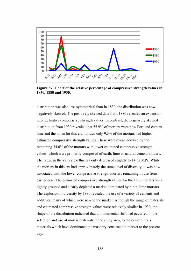
188
Figure 57: Chart of the relative percentage of compressive strength values in 1830, 1880 and 1930.
distribution was also less symmetrical than in 1830, the distribution was now
negatively skewed. The positively skewed data from 1880 revealed an expansion
into the higher compressive strength values. In contrast, the negatively skewed
distribution from 1930 revealed that 55.9% of mortars were now Portland cement-
lime and the norm for this era. In fact, only 9.3% of the mortars had higher
estimated compressive strength values. These were overshadowed by the
remaining 34.6% of the mortars with lower estimated compressive strength
values, which were primarily composed of earth, lime or natural cement binders.
The range in the values for this era only decreased slightly to 14.52 MPa. While
the mortars in this era had approximately the same level of diversity, it was now
associated with the lower compressive strength mortars remaining in use from
earlier eras. The estimated compressive strength values for the 1830 mortars were
tightly grouped and clearly depicted a market dominated by plain, lime mortars.
The explosion in diversity by 1880 revealed the use of a variety of cements and
additives, many of which were new to the market. Although the range of materials
and estimated compressive strength values were relatively similar in 1930, the
shape of the distribution indicated that a monumental shift had occurred in the
selection and use of mortar materials in the study area, to the cementitious
materials which have dominated the masonry construction market to the present
day.
0 10 20 30 40 50 60 70 80 90
100
1830
1880
1930

189
Figure 58: Chart of the relative percentage of compressive strength values in urban environments in 1830, 1880 and 1930.
Figure 59: Chart of the relative percentage of compressive strength values in rural environments in 1830, 1880 and 1930.
When considering the estimated compressive strength of mortars in urban and
rural environments (Figures 58-59), based primarily on the mean, median and
range of the data for each era, only one clear trend emerged. The mean data for
urban and rural environments were relatively similar with estimated compressive
strength values of 0.41 MPa and 0.62 MPa in 1830, 1.74 MPa and 1.66 MPa in
1880 and 7.61 MPa and 7.89 MPa in 1930 respectively. Similar conditions
occurred in the median data, where the median was 0.41 MPa in 1830 and 1880,
and 10.31 MPa in both urban and rural environments. There was such little
variation in each of these datasets that there appeared to be only minor differences
in the selection and use of mortar materials in urban and rural environments;
0 10 20 30 40 50 60 70 80 90
100
1830
1880
1930
0 10 20 30 40 50 60 70 80 90
100
1830
1880
1930
190
however, an assessment of the range of estimated compressive strength values in
each environment suggested that there was a difference. In 1830 urban
environments, the mortar materials were completely homogeneous. Each of the
urban mortars contained only a lime binder, which had an estimated compressive
strength of 0.41 MPa. This was different in rural environments, which contained
earth and natural cement-lime mortars and had a range of 2.03 MPa. The greater
level of diversity in rural environments was also present in 1880, when urban
environments had a range of 9.44 MPa, and rural environments had a range of
15.38 MPa. These differences had converged by 1930, when both environments
had a range of 14.52 MPa.
While the assessment of estimated compressive strength in urban and rural
environments over the duration of the study was less informative than the overall
trend in estimated compressive strength data for the entire study area, it did reveal
that there was greater diversity in the performance characteristics of mortars in
rural environments in the 19th century. Had the variation only occurred in the
minimum values, it could be argued that the variation was an indication of
subsistence level living conditions in rural environments, which necessitated the
selection of the most readily available or the least expensive option of an earth
mortar. While this situation may have occurred, it certainly does not account for
the increased range of estimated compressive strength values. Lime mortars were
the most common mortar in the 19th century in both environments and had an
estimated compressive strength of 0.41 MPa. The presence or absence of earth
mortars, which had an estimated compressive strength of 0.31 MPa, in one
community or another would have had very little effect on the range data.
The significant variation between urban and rural environments was on the higher
end of the distribution. In 1830, the maximum values in urban and rural
environments were 0.41 MPa and 2.34 MPa respectively. Although, it should be
noted that the maximum compressive strength value of 2.34 MPa in the rural
environment was associated with the specialised engineering employed in the
specification of methods and materials used to construct the locks of the Savannah

191
and Ogeechee Canal (081355). Although it was constructed through a rural
portion of the study area, the location was most likely due to geographic
conditions, which made this the most cost-effective route to connect the Savannah
and Ogeechee Rivers, rather than being specifically related to the residents of the
rural environment itself. In 1880, the highest estimated compressive strength
values in an urban environment were associated with a commercial warehouse
(010417), which contained a Portland cement-lime mortar, and single-family
residence (010517), which contained a Portland cement-lime mortar and a
Portland cement-lime mortar with a brick dust additive and had estimated
compressive strength values of 8.71 MPa and 9.85 MPa respectively. In the rural
environment, the range would have been quite similar to the range in the urban
environment if the 8.71 MPa estimated compressive strength value for the
Portland cement-lime mortars identified in a single-family residence (005759),
multi-family residence (007202A) and the civic private Chatham Artillery Club
beach house (010959A) had been the maximum estimated compressive strength
values in this environment. This was not the case. The foundation of a ruined
sawmill complex in the northern portion of the study area contained a Portland
cement mortar with an estimated compressive strength of 15.69 MPa. This
specialised form of construction was probably more closely associated with the
specialised requirements of the sawmill equipment than the mortar preferences of
the residents of the rural environment.
In each of these cases, an outlier created an anomaly in the data. When these
outliers are removed, the mean estimated compressive strength values for rural
environments in 1830 and 1880 were reduced to 0.37 MPa and 1.36 MPa
respectively. When compared to the median data, it was clear that the distribution
for 1830 was slightly negatively skewed in 1830 and positively skewed in 1880.
These findings were relatively consistent with the overall data for the study area,
which revealed extremely homogeneous data in 1830 and the incorporation of
new materials in 1880. Omitting the two outliers also changed the range values
for rural environments to 0.10 MPa in 1830 and 8.40 MPa in 1880. They were
now more closely related to the urban values for the same eras, which were 0.00

192
MPa and 9.44 MPa respectively. These similarities in these values after omitting
the outliers indicated that the overall performance characteristics of mortars in
these areas were not generally influenced by their use in urban and rural
environment.
When considering the estimated compressive strength characteristics of mortars in
the study area according to ancestry (Figures 60-62), it was clear that the two rural
commercial buildings that had significantly altered the mean and range data in the
previous discussion, would also affect the analysis of estimated compressive
strength data according to ancestry. As such, these two buildings were omitted
from the following analysis. The assessment of the remaining data was based
primarily on the mean, median and range data for each era.
The mean estimated compressive strength for each community was quite similar
in 1830 with values of 0.41 MPa in the African-American and integrated
communities, and 0.37 MPa in the European-American community. Each of the
communities retained a median estimated compressive strength value of 0.41
MPa. The similarity between the mean and median values indicated that the
distributions for each community were symmetrical. By extending the analysis to
an assessment of the range data for each community, the homogeneous character
of each community was confirmed. In fact, all of the mortars in the African-
American and integrated communities were lime and, therefore, had no range
value. Although there was range data for the European-American community, it
was only 0.10 MPa and accounted for the use of earth mortars by this community
in 1830.
Since there was no statistically European-American community in the study area
in 1880, the analysis of the data from this era was a simple comparison between
the African-American and integrated communities. The mean estimated
compressive strength values were 2.60 MPa in the African-American community
and 1.21 MPa in the integrated community. The median value for each
community was 0.41 MPa, which indicated that the distributions for each

193
Figure 60: Chart of the relative percentage of compressive strength values in The African-American community in 1830, 1880 and 1930.
Figure 61: Chart of the relative percentage of compressive strength values in the integrated community in 1830, 1880 and 1930.
Figure 62: Chart of the relative percentage of compressive strength values in The European-American community in 1830, 1880 and 1930.
0 10 20 30 40 50 60 70 80 90
100
1830
1880
1930
0 10 20 30 40 50 60 70 80 90
100
1830
1880
1930
0 10 20 30 40 50 60 70 80 90
100
1830
1880
1930

194
community were positively skewed. Since the positive skew indicated an
expansion in the use of mortars with higher compressive strength in the overall
data for the study area, it also indicated an expansion in both African-American
and integrated communities in 1880. The primary difference in their data was that
the distribution for the African-American community was over two times as
skewed as the distribution for the integrated community, which could indicate a
greater preference for higher compressive strength mortars in the African-
American community than the integrated community at this time.
In 1930, the mean estimated compressive strength values had increased to 7.93
MPa in the African-American community, 7.85 MPa in the integrated community
and 7.43 MPa in the European-American community. Since the median value for
each community was 10.31 MPa, the distributions for each of these communities
were negatively skewed. Since the negative skew indicated the continued use of
lower estimated compressive strength materials in the overall data for 1930, it also
indicated a similar pattern of use in the distributions of each of the individual
communities. Although the mean values were quite similar, the distributions for
African-American and integrated communities were more closely related to each
other than to the pattern seen in the European-American community. An
assessment of the range of estimated compressive strength values revealed a slight
difference in the diversity of the mortars used by each community. The range
value for the African-American community was 10.31 MPa. The values for the
integrated and European-American communities were both 14.52 MPa and were
the direct result of the use of Portland cement-lime mortars with a slag additive,
which increased the estimated compressive strength of this material from 10.31
MPa to 14.93 MPa. This material was used exclusively in single-family
residences (011217, 103740A, 103793A, 106019 and 106560) in the integrated
community, and in one civic public building in the European-American
community (006305).
The complete absence of Portland cement-lime mortars with a slag additive in the
African-American community could have indicated that there was a preference
195
against the use of slag additives in this community. In order to test this
supposition, all remaining buildings utilising a slag additive were identified in the
data. There were only three buildings in the study that were not included in the
discussion of Portland cement-lime mortars with a slag additive. These buildings
utilised a lime mortar with a slag additive, and they were evenly distributed
between the African-American, integrated and European-American communities.
The buildings in the integrated and European-American communities included a
single-family residence (025476A) and a commercial building (080164)
respectively. The building located in the African-American community was a
civic private building known as Charity Hospital. Two African-American
physicians founded the hospital in the late 19th century in order to better serve the
African-American community and provide a teaching hospital for African-
American nurses, and the current building was constructed using private
donations from the Ida Rosenwald Fund and Mrs. Henry W. Hodge, as well as
members of the community (Melton 2011, 6). The clear participation of
European-Americans in the funding and construction of the current building
raised a number of questions regarding the African-American classification of this
building for the purposes of this particular discussion. Given that Charity Hospital
was the only example of the use of a slag additive in an African-American
community and it was funded and constructed using a significant amount of
resources from outside the community, it seems most likely that the use of slag
was not preferred in the African-American community.
Conclusion
This section discussed several issues pertaining to the use of binders and
additives, and their effect on the historic mortars in the study area. The initial
discussion pertained to the number of binders used in each mortar, which
provided a general overview of the complexity of the mortar methods and
materials utilised in the study area. Later discussions addressed the types of
binders and additives identified in the mortar sample population. It concluded
with a discussion of the estimated compressive strength values for each of the
196
mortars included in the study, which quantified and assessed the combined effects
of each of the active mortar materials. In a manner similar to the previous section
on the patterns of use of mortars on the building level, each discussion was
presented and considered from the perspective of era, urban and rural environment
and ancestry. By doing so, the research was able to directly address and evaluate
the potential influence that geography and demography had on the use of binder
and additive materials in the study area. While the previous section addressed
each of the factors influencing the selection of masonry construction methods and
materials on the macro level, this section focused on many of the same issues on
the micro level of the binders and their constituent parts. These discussions
presented an assessment of the trends identified in the data, which were derived
from the micro-level analysis of the active components of the mortar, including
the binder and additives. The micro-level discussion was continued in the
following section by addressing the appearance of the mortars through an
assessment of the aggregate and the effect that it has on the texture and colour of
the mortar.
The binder quantity discussion showed that the vast majority of buildings
contained either one or two binders, with only 0.4% of buildings containing more
than two binders. When the entire body of historic mortars was considered, the
analysis revealed a gradual decrease in the number of mortars containing one
binder and a gradual increase in the number of mortars containing two binders,
which was similar to the transition seen in the number of mortars used per
building with one exception. The distributions of one-mortar and two-mortar
buildings converged around 1880, while the distributions of one and two-binder
mortars did not intersect until around 1900. In this case, the binder quantity data
corroborated the supposition presented in the mortar quantity discussion that the
methods and materials used in historic masonry construction in the study area
became significantly more complex over the duration of the study, particularly in
the late 19th and early 20th centuries. When assessed according to urban and rural
environments, it was clear that there were also different patterns in the data. In
urban environments, there was a linear decrease in the number of mortars

197
containing one binder and a corresponding increase in the number of mortars
containing two binders, which intersected around 1900 as expected based on the
findings of the binder quantity analysis for the entire study area. In contrast,
mortars containing only one binder were significantly more common in rural
environments during the entire 19th century, when they constituted approximately
90% and 80% of the mortar sample population for each era. Although the
decrease continued into the 20th century, it did so in a much more dramatic
manner. The relative percentage of mortars with one binder decreased by
approximately 10% between 1830 and 1880 and decreased by nearly 80%
between 1880 and 1930. The findings of this analysis suggested that the 19th
century urban environment accepted new methods and materials more readily than
rural environments, which continued to use the methods and materials most
common in the earliest era of this study. When the data were analysed according
to ancestry, the transition from one to two-binder mortars in the African-
American community was similar to the relatively linear transition seen in the
urban environment. In contrast, the distribution in the integrated community was
more closely related to the rural distribution, which continued to use one-binder
mortars through the end of the 19th century. Unfortunately, the pattern of change
in the European-American community could not be addressed in this section due
to the lack of a statistically European-American community in the study area in
1880. The beginning and end of the distribution were clearly defined, but the rate
of change could not be determined from the available data. As a result, it was
impossible to determine whether or not the transition proceeded according to the
pattern established in either the urban or rural environment.
The analysis of the types of binders used in the study area over the duration of the
study revealed several important trends. Firstly, there was a distinctly different
pattern in the types of binders used in the study area in the 19th and 20th centuries.
The most common binder utilised in 19th century mortars was lime, which
represented 87.2% and 65.5% of the binders used in 1830 and 1880 respectively.
By 1930, the most common binder was Portland cement-lime, which represented
55.9% of the binders used in this era. Secondly, there was a distinct relationship
198
between the type of binder and its use in specific environments or communities in
each era. For example, earth binders were primarily used in rural environments in
1830, which was consistent with the greater availability of earth binder materials
in rural environments. The unexpected aspect of the use of earth mortars was their
association with the European-American community in 1830. By 1880, the use
and associations of earth mortars had changed. The material served primarily as a
gauging material in lime-earth mortars used by the African-American and
integrated communities. In contrast to the pattern of use established by earth
binders, natural cement was primarily used in the urban environment in 1880,
with the exception of its early use in the locks of the Savannah and Ogeechee
canal in 1830. Although masonry cement was used throughout the study area in
1930, it was approximately five times more likely to be used in a rural
environment than an urban one. While this may have been related to the
environment, it was also possible that it was related to the ancestry of the area.
This was certainly possible, because the integrated community populated eight of
the nine GMDs composing the rural environment in this era. Thirdly, one mortar
was identified as having a gypsum binder in 1880. The use of this type of binder
was completely unexpected, because it was typically reserved for arid climates,
rather than the humid, subtropical climate of the study area. Its suitability for this
climate was proven by the overall condition of the mortar, which showed minimal
signs of deterioration from 130 years of exposure.
The assessment of the additives used in the study area was more complex than the
others in this section, because they were analysed and presented in two groups
based on their primary function in the mortar. Performance additives included
brick dust, wood ash, slag and crushed calcium carbonate. Appearance additives
included red, black and yellow pigments. When considering the additives
according to era, environment and ancestry, a variety of useful information was
identified in these data. Firstly, there were no additives present in the mortar
sample population in 1830. The relative percentage of the building sample
population containing one or more additives in its mortar was 26.3% in 1880 and
53.2% in 1930. Secondly, the majority of additives used in the study area in 1880

199
were intended to alter the appearance of the mortar, while the majority of those
used in 1930 were intended to alter its performance. Thirdly, each of the
performance additives identified in the historic mortars of the study area were
utilised in only one era. Brick dust and wood ash were used in in 1880, and slag
and crushed calcium carbonate were used in 1930. This contrasted with each of
the appearance additives, which were used in both 1880 and 1930. Although all of
the pigment colours were used in both eras, red was clearly the preferred pigment.
In fact, the relative percentage of red-pigmented mortar in the study area was
seven times greater than either black or yellow-pigmented mortar in 1880, and
two and a half times greater in 1930. When considered according to environment,
the data suggested that both performance and appearance additives were used
differently in urban and rural areas. In 1880, brick dust was used nearly twice as
often in urban environments, while wood ash was only used in rural
environments. By 1930, these materials had been replaced by slag and masonry
cement. In rural environments, slag was used slightly more often, and masonry
cement was used nearly twice as often. In contrast, the use of appearance
additives was significantly more common in urban environments over the
duration of the study, where they were used 60% more frequently in 1880 and
260% more frequently in 1930. This strongly suggested that a higher value and
emphasis was placed on the appearance of mortar in the urban environment in
both 1880 and 1930. When considered in terms of ancestry in 1880, the use of
brick dust appeared to be universal, while only the African-American community
used wood ash. By 1930, performance additives were preferred at one and a half
to two times the rate of appearance additives in both the African-American and
integrated communities. The use of additives in the European-American
community was strikingly different. Not only did 93.3% of their buildings contain
an additive, the community used appearance additives three and a half times more
than performance additives.
An analysis of the estimated compressive strength values of the mortars in the
study area seemed to reveal more about the technological development of the
mortar industry in the 19th and early 20th centuries than the potential influence of

200
either the geography or demography on the historic mortars of the study area. The
analysis revealed a narrow range of values in 1830, which indicated a general lack
of diversity in mortar performance characteristics and contrasted with the wide
range in each of the later eras. The mean estimated compressive strength values
for increased 340% between 1830 and 1880 and over 450% between 1880 and
1930. The mean values provided useful information reflecting the general trend
toward binder materials and, therefore, mortars with higher estimated compressive
strength characteristics; however, the ranges and distributions of the data provided
a more detailed understanding of the way in which these changes occurred. The
range of estimated compressive strength values for the mortars increased over
750% between 1830 and 1880 and remained relatively stable for the duration of
the study. These range values suggested that the early 19th century was
characterised by mortars with relatively homogeneous performance
characteristics, followed by a rapid expansion in diversity in the mid 19th century
that was maintained into the early 20th century. An assessment of the distributions
of the estimated compressive strength data from each era revealed that the data
was symmetrically distributed in 1830, positively skewed in 1880 and negatively
skewed in 1930. In terms of the mortar performance characteristics, the
distributions confirmed that the mortars were relatively homogeneous in 1830 and
differentiated between the diverse values for 1880 and 1930. In the late 19th
century, most mortars were a continuation of the technology utilised by the
homogeneous, early 19th century mortars. The positively skewed distribution was
an indication of the incorporation of mortar materials, including a variety of
cementitious binders and new performance additives introduced to the market in
the mid to late 19th century. The negatively skewed distribution in the early 20th
century indicated that the majority of mortars had adopted recent developments in
mortar technology, which had dramatically increased the estimated compressive
strength of these mortars. At this time, only a minority of mortars continued to
utilise the mortar technology that characterized early 19th century mortars.
The data presented in this section identified and quantified many of the
characteristics of historic mortars that are most relevant to the fields of
201
archaeology and conservation. It provided an overview of the complexity of the
historic mortar methods and materials utilised in the study area, by addressing the
number of binders used in each mortar, the types of binders and additives
identified in the mortar sample population, and the estimated compressive
strength of the active components of the mortar. By achieving these objectives,
this research generated the data necessary to assess many of widely-held beliefs in
the fields of archaeology and buildings conservation concerning the range of
historic mortar materials, their rate of change and the date that materials were
actually incorporated into the historic mortars of the study area. By assessing each
of these topics from the perspective of era, urban and rural environment and
ancestry, the research generated the data necessary to establish a relationship
between mortar methods and materials and the people who utilised them to build
their homes, churches, government buildings and businesses.
5.2.3 Mortar Appearance
This section addressed the appearance of each of the mortars included in this
research through an assessment of the aggregate materials and their effect on the
texture of each of the mortars. It was a logical extension of the previous micro-
level discussion of the binders and their constituent parts, which played active
roles in the performance of the mortar and combined with the aggregate to create
the colour of each mortar. In order to address these aesthetic issues, this section
quantified the physical characteristics of the aggregate component of each of the
mortars and established significant trends identified in the data when considered
from the perspective of the era, urban or rural environment and ancestry. By doing
so, the appearance of each mortar was assessed in a similar manner to the
previous sections on the use of mortars and binders in the study area. Although
the aesthetic aspects of each mortar also have the potential to improve our
knowledge and understanding of the people who utilised them to construct and
modify their built environment, these aspects of each mortar were more subjective
than the previous data regarding the use of mortars and binders in the study area.
As such, the full range of analysis completed for this section was not presented
202
here. Although the data and analysis necessary to make this determination has
been included in Appendix C, only the findings with the greatest potential to
increase the relevance and importance of mortars in the archaeological record and
buildings conservation practice were presented in this section.
Aggregate
As discussed in the Mortar Chapter, aggregate is an inert, bulk component of most
mortars, which is intended to improve the dimensional stability of the mortar by
providing structural support for the binder materials in the study area as they
achieve a set and respond to the ongoing loads exerted on the mortar and masonry
assembly, such as thermal expansion and contraction. In an ideal mortar, the
appropriate binder to aggregate ratio for a particular mortar should be calculated
to entirely fill the voids present in the clean, dry aggregate. In order to achieve
these objectives, the aggregate was typically prepared and graded to ensure that it
conformed to the performance requirements of each particular mortar. In addition
to the role that aggregate played in the dimensional stability of the historic
mortars included in this research, the aggregate gradation was the primary
component determining the overall texture of the mortar.
Binder to Aggregate Ratio
The binder to aggregate ratios for each of the mortar samples included in this
research varied from 1:0.25 to 1:3.5; however, 99.6% of the mortars had a ratio
between 1:0.25 and 1:2.5. Even though the mortar utilising a 1:3.5 ratio was
located well outside the normal distribution of the mortar sample population, it
was closer to the recommended 1:3 ratio for conservation mortars (Mack and
Speweik 1998) than 98.8% of the mortars documented in this study. For this
reason, the mortar utilising a 1:3.5 ratio was retained in the following analysis,
even though it appeared to be an outlier based on the frequency and relative
percentage distributions of the mortar sample population. When assessing the
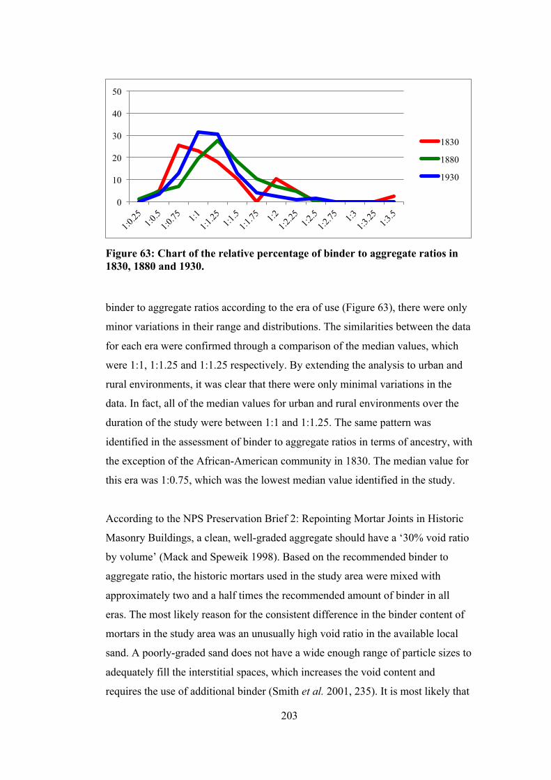
203
Figure 63: Chart of the relative percentage of binder to aggregate ratios in 1830, 1880 and 1930.
binder to aggregate ratios according to the era of use (Figure 63), there were only
minor variations in their range and distributions. The similarities between the data
for each era were confirmed through a comparison of the median values, which
were 1:1, 1:1.25 and 1:1.25 respectively. By extending the analysis to urban and
rural environments, it was clear that there were only minimal variations in the
data. In fact, all of the median values for urban and rural environments over the
duration of the study were between 1:1 and 1:1.25. The same pattern was
identified in the assessment of binder to aggregate ratios in terms of ancestry, with
the exception of the African-American community in 1830. The median value for
this era was 1:0.75, which was the lowest median value identified in the study.
According to the NPS Preservation Brief 2: Repointing Mortar Joints in Historic
Masonry Buildings, a clean, well-graded aggregate should have a ‘30% void ratio
by volume’ (Mack and Speweik 1998). Based on the recommended binder to
aggregate ratio, the historic mortars used in the study area were mixed with
approximately two and a half times the recommended amount of binder in all
eras. The most likely reason for the consistent difference in the binder content of
mortars in the study area was an unusually high void ratio in the available local
sand. A poorly-graded sand does not have a wide enough range of particle sizes to
adequately fill the interstitial spaces, which increases the void content and
requires the use of additional binder (Smith et al. 2001, 235). It is most likely that
0
10
20
30
40
50
1830
1880
1930

204
the consistently high binder to aggregate ratios identified throughout the study
area were the result of using poorly-graded local sand deposits.
Preparation
Four different conditions were identified in the aggregate component of the
mortar, which suggest various levels of sand preparation prior to its use in the
mortar. These conditions were identified in the thin sections of each of the mortar
samples collected in the study area, based primarily on a determination of the
presence or absence of clay coatings on the individual particles of sand and the
presence or absence of silt particles in the binder component of the mortar. For the
purposes of this analysis, the presence of clay coatings or silt particles were
determined to be an indication that the sand was not washed prior to its use in the
mortar. Although, it was possible that sands with clay coatings and no silt
particles may have actually been partially washed sand. These samples were
included in the following discussion as unwashed sand, because they did not meet
the criteria established for washed sand, which required the complete absence of
clay coatings and silt particles in the binder. Since the number of mortars that met
these criteria only composed 1.2% of the mortar sample population, it was
unlikely that the misidentification of this particular type of resource would have
significantly altered the findings presented in this section.
When considering the aggregate preparation data in terms of the era of
construction (Figure 64), it was clear that the use of washed sands was strongly
associated with early 20th century construction, since they composed 7.7% of the
mortar sample population in 1830, 4.6% in 1880 and 51.7% in 1930. When
assessing the data according to its location in an urban or rural environment, an
interesting pattern was identified in the distribution of the rural data over the
duration of the study. While none of the urban samples were identified as washed
sands in 1830, they constituted 17.6% of rural mortar samples in the same era. In
1880, the urban and rural values were similar, with 5.0% and 4.3% respectively.
By 1930, 64.8% of urban mortars and 40.6% of rural mortars used washed sand.

205
Figure 64: Chart of the relative percentage of each level of aggregate preparation in 1830, 1880 and 1930.
The most interesting aspect of this pattern was identified in the rural environment
in 1830, where washed sand was used to construct the locks of the Savannah and
Ogeechee Canal (081355) and the Argyle Island slave quarters (022846A). On the
surface, these two buildings appeared to be entirely different, but they were both
constructed in GMDs with large slave populations, which constituted 90.3% and
89.2% of the total populations of each GMD. In order to assess a potential
connection between the African-American community and the use of washed
sand, the sand preparation data was evaluated according to ancestry. An initial
assessment seemed to reveal a similar pattern of usage in the rural environment
and the African-American community; however, a more detailed review indicated
that both datasets referred to the canal and slave quarters. Since the canal was
designed and constructed by engineers and masons who had previously worked on
the Erie Canal in New York, it is unlikely that the local slave population was able
to influence the methods or materials used to construct the Savannah and
Ogeechee Canal. The other building that utilised washed sand in 1830 was the
Argyle Island slave quarters. Although this building was most likely constructed
by slaves, further historical documentation would be necessary to determine how
much control the slave population had on the design and construction of this
particular building. A comparison of the African-American and integrated
communities in 1880 identified the use of washed sand aggregate in 10.0% and
0 10 20 30 40 50 60 70 80
Clayey sand Clayey and silty sand
Silty sand Washed
1830
1880
1930

206
3.0% of their mortars respectively. By 1930, the relative percentage of washed
sand aggregate had grown to 50.0% and 44.4% respectively.
Gradation
Aggregate is the primary component establishing the texture of a mortar. In order
to quantify and evaluate the textures of each of the historic mortars collected in
this research, the aggregate component of each of the mortars was characterised as
a fine, medium or coarse grade. When assessed according to the era of
construction (Figure 65), the finely graded aggregate was clearly the most
common material, accounting for 89.7% of the aggregate used in 1830 and 74.7%
used in 1880. In fact, the distributions for each of these eras were quite similar,
indicating that there were probably similar sources and methods of preparing
aggregate materials throughout the 19th century. Between 1880 and 1930, there
was a significant change in the texture of the aggregate used in the study area. By
1930, the use of finely graded aggregate accounted for only 40.7% of the mortars
in the study area, and the use of the medium grade of aggregate remained
unchanged. In contrast, coarsely graded aggregate had become the most common
aggregate in the study area and was used in 48.3% of the mortars in the study
area. The significant shift away from finely graded aggregate to coarsely graded
Figure 65: Chart of the relative percentage of each level of aggregate gradation in 1830, 1880 and 1930.
0 10 20 30 40 50 60 70 80 90
100
Fine Medium Coarse
1830
1880
1930

207
aggregate most likely represented the addition of a new source of materials
between 1880 and 1930. The grade of aggregate selected and used in the historic
mortars in the study area was a critical component in determining the overall
texture and appearance of mortars in the study area.
When considering the grade of aggregate used in the mortar of the study area from
the perspective of the urban and rural environment and the ancestry of the human
population, only minor variations emerged. The consistency of each of these
datasets suggested that there may not have been any significant differences in the
sourcing of materials in different environments or communities. In fact, the minor
variations could have been the result of variations in the source materials of local
sand pits throughout the study area. In general, the aggregate used in the study
area was finely graded during the 19th century; however, it was particularly fine in
the urban environment. In this environment, it accounted for all of the aggregate
used in 1830 and 80.0% of the aggregate used in 1880. In the rural environment, it
only accounted for 76.5% and 70.2% of the aggregate used in each era
respectively. By 1930, coarsely graded aggregate was the most common aggregate
used in both environments; however, it was used in 59.3% of urban mortars and
39.1% of rural mortars. The other notable difference in usage between urban and
rural environments was that finely graded aggregate continued to be used in
48.4% of rural mortars, while it was only used in 31.5% of urban mortars. When
considered in terms of ancestry, the patterns expressed in urban and rural
environments were also revealed in the data for each community. For example,
the integrated community was entirely located in an urban environment in 1830.
As such, the data for the urban environment and integrated communities were
identical in this era. A similar situation occurred in the 1930 data for the rural
environment and the integrated community, because their boundaries nearly
coincided in this era. In general, the grade of aggregate used in African-American
and European-American communities in 1830 was typically a fine or medium
grade, while the integrated community used only finely graded aggregate.
Although, it was unclear whether the exclusive use of finely graded aggregate was
related to the urban environment or the integrated community. In 1880, the pattern

208
of aggregate use in the African-American and integrated communities was
relatively similar. By 1930, the data for the African-American and European-
American communities was very similar, with each community using
approximately 30% finely graded aggregate, 8% medium grade aggregate and
62% coarsely graded aggregate. In contrast, the integrated community, whose
location closely coincided with the rural environment, used more finely graded
aggregate and less coarsely graded aggregate than the other communities, with a
pattern of use consisting of 48.6% finely graded aggregate, 12.5% medium grade
aggregate and 38.9% coarsely graded aggregate. While there were variations in
the data when considered from the perspective of environment and ancestry, there
were significant overlaps in the data, which made it difficult to discern whether
slight variations were related to geographical or demographic influences.
Colour
As previously discussed, an ideal binder to aggregate ratio was defined by
calculating the amount of binder necessary to entirely fill the voids present in the
clean, dry aggregate. The binder should completely coat each aggregate particle.
In a newly placed mortar, the particles located on the surface of the mortar joint
should have a thin coating of binder material. This coating may have been
removed, and the aggregate particles exposed, when the mason finished the joint
or through a natural process of erosion caused by the exposure of the mortar to
wind and rain. In either case, the colour of the mortar was determined by the
combination of the binder materials filling each of the voids in the aggregate and
the aggregate particles themselves. In a controlled environment, free from
environmental factors such as pollution and vegetation, the original colour of the
mortar would have been best represented by the original surface of the mortar
joint. Since the conditions in the study area fostered a variety of environmental
contaminants, including automotive exhaust, mold, mildew and dirt, the surfaces
of the mortar joints were inconsistently weathered and stained. As such, an
interior surface was used for the description and analysis of colour, because it
provided a more consistent sample of the entire mortar sample population. By

209
using an interior surface, the colour data approximates the appearance of the
freshly placed mortar. Once the colour of each mortar sample was identified and
described, the hue, value and chroma values were analysed and incorporated in
this research and the following discussion.
Hue
The hue is the primary colour color designation in the Munsell Soil Color System.
There are six possible hues on the Munsell soil charts, including Gley 1, 10R,
2.5YR, 7.5YR, 10YR and 2.5YR. The most commonly occurring hues in the
mortar sample population were 10YR and 2.5Y, which indicates that the majority
of mortars in the study area were specific yellow-red or yellow hues (Figure 66).
In 1830, all of the mortars were one of these hues. Since there were no pigments
identified in the mortars of this era, these hues were probably closely related to
the hues of the locally available aggregate. In 1880 and 1930, 12.4% and 17.7%
of the mortars were classified as one of the other hues, including Gley 1, 10R,
2.5YR, 7.5YR. The additional hues were most likely a reflection of the
introduction of red, black and yellow pigments in the study area.
These findings were quite interesting when reassessed from the perspective of
environment and ancestry (Figures 67-68). For example, there was a clear
difference in mortar hues in urban and rural environments. Mortars with a hue of
2.5Y were more common in rural environments over the duration of the study,
constituting 35.3%, 42.6% and 28.1% of the mortars in each era respectively. This
contrasted with urban mortars, which did not have any mortars of this hue in
1830. In 1880 and 1930, mortars of this hue only composed 10.0% and 11.1% of
the mortars respectively. Since this hue was used in 1830, it was unlikely that the
majority of mortars with this hue were related to the use of pigment. If the hue
was derived from locally available aggregate, it is unclear why the hue was not
represented in the urban mortars as well. Since none of the urban mortars were
washed in 1830 and only 5.0% were washed in 1880, it is also unlikely that the
presence of this hue in rural environments can be attributed to clay or silt

210
Figure 66: Chart of the relative percentage of each hue in 1830, 1880 and 1930.
Figure 67: Chart of the relative percentage of each hue in urban environments in 1830, 1880 and 1930.
Figure 68: Chart of the relative percentage of each hue in rural environments in 1830, 1880 and 1930.
0 10 20 30 40 50 60 70 80 90
100
Gley 1 10R 2.5YR 7.5YR 10YR 2.5Y
1830
1880
1930
0 10 20 30 40 50 60 70 80 90
100
Gley 1 10R 2.5YR 7.5YR 10YR 2.5Y
1830
1880
1930
0 10 20 30 40 50 60 70 80 90
100
Gley 1 10R 2.5YR 7.5YR 10YR 2.5Y
1830
1880
1930

211
contaminants introduced through the use of unwashed sands. Instead, it seems
most likely that the 2.5Y mortars were related to a particular type of sand deposit,
which was less accessible to the urban environment.
Several interesting patterns were also observed in the hue data when it was
assessed in terms of ancestry (Figures 69-71). For example, most of the mortars in
the African-American community had a hue of 10YR, including 90.0% of the
mortars in 1830, 80.0% in 1880 and 77.8% in 1930. The most interesting aspect
of the African-American data was its consistency over the duration of the study,
even though the community migrated to different portions of the study area over
the duration of this study. Unfortunately, the lack of a statistically European-
American community in 1880 prohibited a complete analysis of the mortar hues
utilised by this community. Regardless, 71.4% of their mortars in 1830 had a hue
of 2.5Y. A review of the buildings containing this hue of mortar did not reveal
any specific pattern. In fact, the buildings extended from the barrier islands along
the coastline of Chatham County to the westernmost uplands of Effingham
County. Given the geographic diversity in the use of this mortar hue and its high
relative percentage in the European-American community, it may have been
specifically preferred by this community in 1830. In 1930, 2.5Y mortars only
composed 7.1% of European-American mortars. This could be an indication of
the waning preference for mortars of this hue or simply a reflection of the
migration of this community from rural Effingham County in 1830 to the GMDs
located in central Savannah in 1930. In the integrated community, there was a
gradual decline in the use of 10YR mortars in the 19th century from 100.0% in
1830 to 53.7% in 1880. At this time, the relative percentage of 10YR and 2.5Y
mortars stabilised for the duration of the study. In these eras, approximately 57%
of the mortars had a hue of 10YR and 30% of the mortars had a hue of 2.5Y.
These findings presented interesting patterns in the hue of the mortars in the study
area that can guide future research, additional information on the specific colour
of local sands will need to be conducted in order to establish whether or not there
is a relationship between ancestry and a preference for specific mortar hues.
While it is possible that the variations indicated a preference for particular mortar

212
Figure 69: Chart of the relative percentage of each hue in the African-American community in 1830, 1880 and 1930.
Figure 70: Chart of the relative percentage of each hue in the integrated community in 1830, 1880 and 1930.
Figure 71: Chart of the relative percentage of each hue in the European-American community in 1830, 1880 and 1930.
0 10 20 30 40 50 60 70 80 90
100
Gley 1 10R 2.5YR 7.5YR 10YR 2.5Y
1830
1880
1930
0 10 20 30 40 50 60 70 80 90
100
Gley 1 10R 2.5YR 7.5YR 10YR 2.5Y
1830
1880
1930
0 10 20 30 40 50 60 70 80 90
100
Gley 1 10R 2.5YR 7.5YR 10YR 2.5Y
1830
1880
1930

213
hues, it is also possible that the changes over time reflect the movement of this
community within the study area over the duration of this study.
Value
Value refers to the relative lightness or darkness of the colour. In the Munsell Soil
Color System, the minimum and maximum values are two and eight, with lower
values indicating darker colours and higher values indicating lighter colours.
Although the mortars included in this study have values between two and a half to
eight, 98.0% of them have a value between five and eight, and eight was the
median value in each era (Figure 72). The data derived from this aspect of the
Munsell Soil Color System was consistent in all eras, environments and
communities. It simply revealed a consistent preference for lighter mortars in this
area over the duration of the study.
Figure 72: Chart of the relative percentage of each value in 1830, 1880 and 1930.
Chroma
Chroma refers to the relative intensity of a colour. In the Munsell Soil Color
System, the minimum and maximum values are one and eight, with lower values
indicating more neutral colours and higher values indicating colours that are
0
10
20
30
40
50
60
70
80
2 2.5 3 4 5 6 7 8
1830
1880
1930

214
brighter or more intense. Although the mortars included in this study have chroma
values across the entire spectrum, 94.3% of them have a chroma value between
two and four. It had a positively skewed distribution, which expressed a general
preference for lighter mortars in this area over the duration of the study, and a
median chroma value of two. The overall consistency of the data derived from
this aspect of the Munsell Soil Color System was similar to the data regarding the
colour value.
Figure 73: Chart of the relative percentage of each chroma in 1830, 1880 and 1930.
Conclusion
This section addressed the appearance of the mortars included in this research by
assessing the aggregate materials and their effect on the appearance and texture of
each of the mortars. It was a continuation of the micro-level discussion of the
binders and their constituent parts presented in the previous section. This section
discussed the physical characteristics of the aggregate and identified significant
trends in the data when considered from the perspective of the era, urban or rural
environment and ancestry. This allowed the appearance of each mortar to be
analysed in a manner that was consistent with the previous sections on the use of
mortars and binders in the study area. As discussed at the beginning of this
section, the aesthetic aspects of mortar have the potential to expand our
0
10
20
30
40
50
60
70
80
1/N 2 3 4 6 8
1830
1880
1930

215
knowledge and understanding of the people who used them to construct and
modify their built environment; however, they are generally more subjective than
the previously discussed mortar data concerning the use of mortars and binders in
the study area. Although the data presented in this section was informative, the
findings and discussions were significantly different from those in the previous
sections due to the relative consistency of most of the appearance related datasets.
The section began with a discussion of the aggregate components of each of the
mortars in the study area, including their binder to aggregate ratios, sand
preparation and gradation. Perhaps the most important finding in this discussion
was the unusual binder to aggregate ratio of nearly all of the mortars included in
this study, which were significantly different from the recommended 1:3 ratios of
each of the conservation mortars recommended in the NPS Preservation Brief. In
fact, the median binder to aggregate ratios for each era were 1:1, 1:1.25 and 1:1.25
respectively. The larger binder components identified in the historic mortars of
the study area were probably necessary to accommodate higher than normal void
contents in the local sands. This was certainly an indication that local sand
deposits, which were the most likely source of aggregate in this area, probably
contain poorly graded sands. The assessment of the aggregate component also
considered the levels of sand preparation used in the study area and provided
some insight into the use of washed and unwashed sands over the duration of the
study. The findings of this research clearly indicated that the use of washed sand
was strongly associated with early 20th century mortars. In fact, washed sand only
composed 7.7% and 4.6% of the aggregate used in the study area in the 19th
century. In contrast, washed sand was used in 51.1% of the mortars in 1930. This
section also analysed the gradation of local sands used as aggregate in the mortars
in the study area. Each of the aggregates was classified as having a fine, medium
or coarse grade of sand. The data showed that 19th century mortars
overwhelmingly utilised finely graded sand, including 89.7% of mortars in 1830
and 74.7% of mortars in 1880. The consistency in the finely graded aggregate
used in these eras suggested that the materials were collected from similar local
sand deposits. The data also showed that the aggregate materials changed

216
significantly between 1880 and 1930. In the early 20th century, the used of finely
graded sand was only used in 40.7% of the mortars, and coarsely graded sand was
used in 48.3% of mortars. The data also indicated that the coarsely graded sand
was incorporated into urban mortars at a higher rate than rural mortars, composing
59.3% and 39.1% of mortars in each environment respectively.
Each of the aggregate characteristics discussed in this section identified
characteristics of the mortars in the study area, which differ dramatically from the
conservation mortars recommended by the NPS Preservation Brief. Firstly, the
mortars in the study area used a binder to aggregate ratio between 1:1 and 1:1.25,
as compared to the recommended 1:3 ratio. Secondly, the level of sand
preparation documented in the study area revealed that only 27.9% of the mortars
included in this study were washed. The aggregate used in the historic mortars of
the study area in the 19th century was typically fine, poorly graded sand. Although
coarse sands became more common in the early 20th century, they only accounted
for 48.3% of the mortars used in this era. As a result, the 73.0% of the mortars
included in this study utilised fine, poorly graded sand.
The typical sand preparation and gradation characteristics identified in the study
area are at odds with the NPS Preservation Brief recommendation to use clean,
well-graded sand in conservation mortars. When considering the actual number of
mortars in the study area that would be compatible with NPS recommended
conservation mortars, one would begin with the 66 mortars that utilise coarsely
graded aggregate and deduct the 19 mortars that utilised unwashed sand. Of the
remaining 47 mortars, none had a binder to aggregate ratio of 1:3. There was one
example each of mortar with a 1:2.5 and 1:2 ratio, and six mortars with a 1:1.5
ratio. This simply illustrates the fact that only eight of the mortars, which
compose approximately 3.3% of the mortars included in this study, would have a
similar mortar mix, sand preparation and gradation to the recommended
conservation mortar.

217
The discussion of colour in this section addressed the hue, value and chroma of
the mortars included in this study, as defined by the Munsell Soil Color System.
The findings of the colour analysis indicated the overall consistency of mortar
colours in the study area over the entire duration of the study. While this resulted
in a less detailed presentation, the finding was no less important than some of the
more complex relationships discussed in previous sections. The hue data revealed
that most of the mortars in the study area had a hue value of 10YR or 2.5Y. In
fact, these were the only two mortar hues present in 1830. There were more
mortar hues present in 1880 and 1930, which coincided with the increasing use of
pigments. In terms of ancestry, the data revealed that the African-American
community showed a distinct preference for 10YR mortars, composing 90.0%,
80.0% and 77.8% of the mortars in each era respectively. While the findings
identified in this data were interesting additions to the discussion, additional
research on the colour of local sands will need to be conducted in order to
determine if there was a relationship between certain communities and the use of
particular mortar hues.
5.3 Conclusion
The primary aim of this research was to determine whether or not there was a
relationship between the people living in the study area and the mortar methods
and materials that they used to construct their built environment. It achieved this
aim by establishing a number of relationships between the people who lived in the
study area and the mortar data on the level of the building, mortar and its
constituents. In doing so, this research argued that mortar should be a valued part
of the archaeological record and more widely incorporated in the practice of
historical archaeology. The importance of establishing the relevance of mortar as
an archaeological artefact extends beyond the discipline of archaeology to
buildings conservation practice. By evaluating the potential cultural significance
of a material that has been widely perceived to be a sacrificial component of
masonry construction would require building conservationists to reassess their

218
entire approach to masonry conservation, including more thorough documentation
and sampling prior to mortar conservation.
The most informative pattern identified in the mortar use discussion related to the
number of mortars used in each building. It demonstrated that nearly all of the
buildings in the building sample population contained either one or two mortars,
and there was a gradual transition in the number of buildings containing one
mortar to buildings containing two mortars, which converged at a relative
percentage of 50% each in the latest era of this study. The transition in urban
environments was relatively linear and converged in the 1880s. The rural
environment initiated a similar pattern, with a decline in one-mortar buildings and
an increase in two-mortar buildings that nearly converged around 1880; however,
the trend deviated from the urban pattern and reversed itself by 1930. As such, the
analysis showed that there was a general increase in buildings with multiple
mortars in the urban environment, while one-mortar buildings remained more
common in the rural environment over the duration of the study. When considered
in terms of ancestry, the African-American and European-American communities
mirrored the pattern established in the urban environment, while the integrated
community displayed a similar pattern to rural environments. The relationship
between the integrated community and the rural environment was most likely
related to changing demographic conditions. In this case, the integrated
community was located entirely within the boundaries of the City of Savannah in
1830. In 1880, this community had expanded to include all of the GMDs located
in Effingham County, which had previously been a European-American
community. By 1930, it was closely related to the rural portion of the study area.
Although the mortar quantity discussion identified and analysed potential
relationships between the use of mortars and the environmental and cultural data,
the most significant finding derived from this section was the consistent trend
toward greater complexity in the number of mortars used in each environment and
community.
219
The analysis and discussion of the use of binders and additives, and their effect on
the historic mortars in the study area, was the most complex dataset discussed in
this chapter. Similar to the discussion regarding the number of mortars used per
building, the analysis of the types of binders used in the study area provided a
general overview of the increasing complexity of the mortar methods and
materials utilised in the study area. It identified a variety patterns in the data,
which appear to be related to either the environment or ancestry and particularly
relevant to historical archaeology or building conservation. In this case, the
homogeneous character of the binders used in 1830 led to one of the most
unexpected findings of the research. As discussed in the Theory and Methodology
Chapter, it is often possible to characterize the type of raw materials used to
manufacture the components of a mortar. In 1830, 87.2% of the mortars in the
study area were composed of lime. The petrographic analysis of the samples from
this era identified fragments of the raw materials in the binder, which had not
completely burned and retained some of the physical characteristics of the raw
material. In fact, at least 68.2% of the mortars contained marble fragments, which
indicated that the calcium carbonate used to manufacture the lime had a marble
source. Since there were no known marble mines operating in the South in this
era, additional historical research was completed in order to identify the potential
source of the marble lime prevalent in the area in this era. A search of the
advertisements in the Daily Georgian newspaper from 1829 to 1831 identified
266 instances of the word ‘lime’, and 122 instances of Thomaston Lime
(Unknown 1829-1831), which accounted for 45.9% of all lime advertisements
over the three-year period. Further research identified a product originally known
as Thomaston Lime, which was quarried and manufactured in Rockland, Maine.
The area was famous for the production of lime, because it was the only known
marble deposit located on the eastern coast of the United States, which made the
transportation of the material to market an inexpensive endeavor (MacLachlan et
al. 2006). It is highly likely that Thomaston was the source of the marble limes
used in the study area in 1830, due to the presence of marble fragments in the
mortar, large number of advertisements and the fame of the Rockland deposit as
the only source on the east coast.

220
The assessment of the additives used in the mortars of the study area identified the
types of additives used over the duration of the study. The analysis of this data
revealed strikingly different patterns of use in the performance additives in each
era. For example, there were no additives present in the mortar sample population
in 1830. In 1880, the performance additives used in the study area were composed
of brick dust and wood ash. By 1930, the only performance additives identified in
the mortar sample population were slag and crushed calcium carbonate. The
relatively short duration in the use of each of these materials highlight the
potential for the use of binders and additives as tools for dating masonry
structures and remains.
The research also demonstrated that the aesthetic aspects of mortar have the
potential to expand our knowledge and understanding of the people who used
them to construct and modify their built environment; however, they are generally
more subjective than the previously discussed mortar data concerning the use of
mortars and binders in the study area. In addition to the performance
characteristics assessed through an analysis of the binders and additives, the
appearance of the mortars used in the study area This section addressed the
appearance of the mortars included in this research by assessing the aggregate
materials and their effect on the appearance and texture of each of the mortars.
This section discussed the physical characteristics of the aggregate and identified
significant trends in the data when considered from the perspective of the era,
urban or rural environment and ancestry. Although the data presented in this
section was informative, the findings and discussions were significantly different
from those in the previous sections due to the relative consistency of most of the
appearance related datasets.
Significant findings also emerged in the discussion of the mortar appearance data
presented in this chapter, which identified an unusual binder to aggregate ratio in
nearly all of the mortars included in this study. Each were significantly different
from the recommended 1:3 ratios of each of the conservation mortars
recommended in the NPS Preservation Brief. In fact, the median binder to

221
aggregate ratios for each era were 1:1, 1:1.25 and 1:1.25 respectively (Mack and
Speweik 1998). The larger binder components identified in the historic mortars of
the study area were probably necessary to accommodate higher than normal void
contents in the local sands. This was certainly an indication that local sand
deposits, which were the most likely source of aggregate in this area, probably
contain poorly graded sands.
In fact, each of the appearance characteristics discussed in this section identified
specific characteristics of the mortars in the study area, which differ dramatically
from the conservation mortars recommended by the NPS Preservation Brief. As
previously discussed, the mortars in the study area used a binder to aggregate ratio
between 1:1 and 1:1.25, as compared to the recommended 1:3 ratio (Mack and
Speweik 1998). In addition, 73.0% of the mortars included in this study utilised
fine, poorly graded sand. The typical sand preparation and gradation
characteristics identified in the study area would have produced mortar
appearance characteristics that were quite different from the NPS Preservation
Brief recommendations, which specify the use of clean, well-graded sand. When
considering the actual number of mortars in the study area that would be visually
compatible with NPS recommended conservation mortars, one would begin with
the 66 mortars that utilise coarsely graded aggregate and deduct the 19 mortars
that utilised unwashed sand. Of the remaining 47 mortars, none had a binder to
aggregate ratio of 1:3. There was one example each of mortar with a 1:2.5 and 1:2
ratio, and six mortars with a 1:1.5 ratio. This simply illustrates the fact that only
eight of the mortars, which composed approximately 3.3% of the mortars included
in this study, would have a similar mortar mix, sand preparation and gradation to
the recommended conservation mortar.

222
Chapter 6: Conclusion
Although this research began with a typical building conservation approach to the
use of lime mortars in the southeastern United States, it responded promptly to
historic masonry texts and archaeological evidence embodied in the remaining
historic masonry buildings of the southeastern United States, which indicated that
there was a more complex range of mortar materials in use in the historic period
than was reflected in the building conservation literature. By reassessing the
research design and incorporating research into building conservation and
archaeological practice, the research developed into a comprehensive
archaeological assessment of the masonry materials used in the study area in the
19th and 20th centuries and their potential cultural influences.
In order to adequately address the research questions presented in the Introduction
to this thesis, the research compiled three original sets of data pertaining to the
human population, the historic building population and ultimately the mortar
sample population. These three datasets were thoroughly analysed in order to
compile a unique and comprehensive set of mortar data that addressed each of the
research questions established in the Introduction to the thesis. Not only did the
research establish the level of diversity of mortar materials, it quantified both the
range and distribution of these materials and their changes over the duration of the
study. It then assessed the mortar data in terms of geographic factors, including
the urban and rural environment, and the ancestry of the human population in
order to identify patterns in the use of historic mortars and mortar materials when
assessed according to one of the cultural factors. By establishing numerous
examples of these types of patterns in the mortar use, binder use and mortar
appearance datasets, the research clearly established a strong foundation of
original data, suggesting that there were relationships between the human
population and the mortars they used to construct their built environment.
By compiling a comprehensive set of mortar data, which has been analysed in
relation to statistically defined ancestry groups within the human population, the
research has made a significant contribution to archaeological research. A study of

223
this scale has certainly made significant progress toward establishing the
relevance of mortar as an archaeological artefact. It demonstrated that mortar
should be valued as highly as other artefacts, even if it is located in a masonry
feature or a bulk assemblage large enough that it is impractical to retain or curate
with the other archaeological remains.
The findings most relevant to the building conservation community pertained to
the discrepancy between the building conservation standards and
recommendations and the actual mortars included in this study. Firstly, according
to the Preservation Briefs: 2, Repointing Mortar Joints in Historic Brick
Buildings, the recommended 1:3 binder to aggregate ratios of the conservation
mortars were significantly different than the median binder to aggregate ratios for
each era of the study, which were 1:1, 1:1.25 and 1:1.25 respectively. The use of
larger binder components in the historic mortar was probably intended to account
for the higher than normal void contents in the local sands, due to the use of
poorly graded sand aggregate. Secondly, the level of sand preparation documented
in the study area indicated that only 27.9% of the mortars included in this study
were washed. As a result, the aggregate used in the historic mortars of the study
area in the 19th century were typically fine, poorly graded sand. As a result, 73.0%
of the mortars included in this study contained fine, poorly graded sand. When
considering the actual number of mortars in the study area that would be
compatible with NPS recommended conservation mortars, the closest matches
would include one mortar with a 1:2.5 and 1:2 ratio, and six mortars with a 1:1.5
ratio, which illustrated the fact that only eight of the mortars, which composed
approximately 3.3% of the mortars included in this study, would have had a
similar mortar mix, sand preparation and gradation to the recommended
conservation mortar. The design and implementation of this research clearly
determined that the widely implemented use of mortars meeting the
recommendations of the NPS Preservation Brief would have had adversely
affected the appearance of the historic mortars in the study area and would
certainly have had a negative effect on the cultural integrity of historic masonry
resources in the study area.

224
When considering the findings of this research with the greatest potential to
support future work, there were almost too many valid options to consider. In fact,
the primary challenge will be finding an effective way of prioritising or grouping
the numerous options into a single research design. This assessment of the size
and range of possibilities presented by the mortar collection and dataset was
corroborated by John Walsh, a petrographer and mortar analysis specialist, when
he stated that this ‘well-documented dataset should provide decades worth of
research into historical masonry properties at a resolution previously unavailable.’
(Walsh 2012).
There are several areas of potential research, which seem particularly promising.
The first would expand on the extensive use of marble in the study area in 1830
and the trade networks, which brought the product from Maine to coastal Georgia.
This was a particularly interesting finding of the research, because the potential
source of materials was identified in the plain, lime mortars prevalent in this era.
This is significant, because it was identified in a type of mortar that has been in
use for thousands of years. Without the presence of a datable additive or gauging
material, it would have been easy to assume that no significant data could be
identified in the material. Instead, a few fragments of unburned marble revealed a
trade network that extended nearly the entire length of the eastern seaboard. One
future research project, relevant to both building conservation and archaeology,
would involve the compilation of a reference for dating mortars based on the era
of production for the available mortar materials. This type of reference material
would be a valuable resource for archaeologists, who are unlikely to invest in
expensive mortar analysis, but may consider a limited petrographic analysis,
which identifies the presence or absence of specific materials.