Title: Making and breaking power laws in evolutionary algorithm population dynamics

Authors: James M. Whitacrea,b,*, Ruhul A. Sarkerb, and Q. Tuan Phama

a: School of Chemical Sciences and Engineering, University of New South Wales, Sydney, 2052 Australia

b: School of Information Technology and Electrical Engineering, University of New South Wales (ADFA Campus), Canberra 2600

*Corresponding author. Tel: +61-2-9385-4319; fax: 61-2-9385-5966.

Email addresses: j.whitacre@adfa.edu.au (J. M. Whitacre), r.sarker@adfa.edu.au (R. A. Sarker), tuan.pham@unsw.edu.au (Q. T. Pham).

Abstract: Deepening our understanding of the characteristics and behaviors of population-based search algorithms remains an important ongoing challenge in Evolutionary Computation. To date however, most studies of Evolutionary Algorithms have only been able to take place within tightly restricted experimental conditions. For instance, many analytical methods can only be applied to canonical algorithmic forms or can only evaluate evolution over simple test functions. Analysis of EA behavior under more complex conditions is needed to broaden our understanding of this population-based search process. This paper presents an approach to analyzing EA behavior that can be applied to a diverse range of algorithm designs and environmental conditions. The approach is based on evaluating an individual’s impact on population dynamics using metrics derived from genealogical graphs.

From experiments conducted over a broad range of conditions, some important conclusions are drawn in this study. First, it is determined that very few individuals in an EA population have a significant influence on future population dynamics with the impact size fitting a power law distribution. The power law distribution indicates there is a non-negligible probability that single individuals will dominate the entire population, irrespective of population size. Two EA design features are however found to cause strong changes to this aspect of EA behavior: i) the population topology and ii) the introduction of completely new individuals. If the EA population topology has a long path length or if new (i.e. historically uncoupled) individuals are continually inserted into the population, then power law deviations are observed for large impact sizes. It is concluded that such EA designs can not be dominated by a small number of individuals and hence should theoretically be capable of exhibiting higher degrees of parallel search behavior.

Keywords: Evolutionary algorithms; Population dynamics; Genealogical graphs; Population topology; Historical coupling; Optimization; Algorithm analysis

1 Introduction

Over the last couple decades, there have been a number of studies aimed at understanding the behavior and dynamics of Evolutionary Algorithms. One common approach to characterizing EA behavior is to assess how genetic material spreads through a population. For example, the work presented in [1] measures the time required for the best individual to take over a population when crossover is not implemented. Another approach is to measure the loss of a population’s genetic diversity from one generation to the next [2] [3].

Other studies have assessed EA behavior based on the dynamics of the phenotype or fitness distribution in specific fitness landscapes as seen for instance in [4]. Still other studies have attempted to assess the evolvability of an EA in specific application domains [5] or have studied EA convergence behavior within specific fitness landscapes for specific EA design classes [6].

In almost all studies of EA behavior, experiments have been restricted to simple EA designs or to very specific fitness landscapes. Although some of these studies have played an important role in expanding our understanding of Evolutionary Algorithms, it is important to make inroads in understanding EA behavior under more complex conditions. For instance, it is important to determine what fundamental search behaviors are changed when we implement more sophisticated algorithm designs or when these algorithms are applied to specific application domains. Such issues are relevant because many of the EA designs in use today are vastly different from the canonical forms derived decades ago. Furthermore, it is well-known that performance on real-world problems can be quite different from what is observed from experiments on artificial fitness landscapes.

Similar to past studies of EA dynamical behavior, in this work we investigate how genetic material spreads through an EA population. However, the methods presented here are designed to characterize the spread of genetic material for all individuals in a population and are not restricted to studying the behavior of the best population member. Also, these methods have very few experimental requirements, meaning that a diverse range of EA designs can be explored with evolution taking place over any arbitrary fitness landscape.

The next section presents the Event Takeover Value (ETV) which is a metric for real-time analysis of an individual’s impact on EA population dynamics and is derived using genealogical graphs. Section 3 presents experimental results, which focus primarily on characterizing the ETV distribution and its sensitivity to experimental conditions. A discussion of our most interesting results is given in Section 4 with conclusions finishing the paper in Section 5.

2 Measuring an Individual’s Impact on Population Dynamics

For a population-based optimization algorithm like an Evolutionary Algorithm, an empirical measure of the importance of an individual can be obtained by measuring the individual’s impact on the

dynamics of the entire population. Looking at population dynamics on a small timescale such as a single generation, an individual will only impact the population through competition for survival and/or competition to reproduce. However, once longer timescales are considered, we find an individual’s impact is largely due to the survival and spread of its offspring.

This section describes the Event Takeover Value (ETV) which is used for measuring an individual’s impact on population dynamics using genealogical graphs. We start with a simple and straightforward explanation of ETV below and then proceed to address several of the practical challenges that arise with this measurement. Throughout the discussion, the term event is used to describe the creation of a new individual.

To help understand ETV, Figure 1 shows a directed graph which represents the family tree of an individual’s lineage. Here different generations are indicated by positioning on the horizontal axis, nodes represent individuals created in a particular generation and the parents and offspring of an individual are indicated by connections to the left and right (resp.). Starting at the root node on the far left of Figure 1, one can observe how this individual’s genetic material is able to spread through the population. At each generation, it is possible to count the number of individuals in the population that are historically linked to the root node. This can be thought of as an instantaneous measure of the individual’s impact on population dynamics and is referred to as ETVgen. A more detailed description of ETVgen is provided in the caption of Figure 1.

Observing Figure 1, it appears that a reasonable calculation of an individual’s impact on population dynamics would be to count the total number of descendants for a given individual. This is equivalent to summing up ETVgen for all generations where the individual’s lineage remains alive. One problem with this measurement is that an individual’s lineage occasionally is able to spread throughout the entire population so that the cumulative ETVgen value increases indefinitely. A useful alternative which is used in this work is to define ETV as the largest ETVgen value observed. This value naturally has an upper bound equal to the population size of the system. For the example given in Figure 1, the ETV value for the “Event Measured” would be ETV=7, which occurs in the sixth generation.

2.1 Multiple Parents and Genetic Dominance

Figure 1 shows how an individual can impact population dynamics through the spread of its genetic material, however it does not consider the fact that offspring are often created from multiple parents. Also, when using multi-parent search operations, offspring tend to be genetically biased to be more similar to one parent than the other(s). An accurate measure of ETV should account for the possibility of multiple parents as well as account for the possibility of dominance by one of the parents. On the other hand, when distributing credit, it is also important to account for the possibility of new innovations in an offspring that cannot be attributed to any of the parents. This credit assignment problem is a fundamental challenge in ETV calculations that places limits on any analysis of influence or causality in complex adaptive systems.

Due to these challenges in assigning a weighted importance to each of the parents, a dominant parent is chosen instead so that (for ETV calculation purposes) the offspring is seen as having only a single (dominant) parent. By using dominance, it is no longer necessary to address the issue of distributing credit among multiple parents meaning that Figure 1 is still a valid representation of the ETV measurement process. This also helps to greatly simplify implementation of the ETV calculation steps

as seen later. For the ETV calculation, genetic dominance is used where the dominant parent is selected to be the one most genetically similar to the offspring (by Normalized Euclidean Distance).

2.2 Genetic Hitchhiking

As described thus far, the ETV measurement implicitly assumes that an individual’s impact on future dynamics does not degrade with the passage of time. However the stochastic nature of an EA makes this time dependency true and unavoidable. Addressing time dependence in credit assignment has previously been done using exponential decay functions in [7], [8], [9], and [10]. Another possible approach is to set a time window beyond which an individual’s impact on population dynamics can no longer be measured.

Through careful study of the genealogical branching process, it has been found that certain branching structures can indicate exactly when confidence in the ETVgen measurement is lost. An example of these conditions is shown in Figure 2. Looking at the ancestors (i.e. nodes to the left) of the white node, it is noticed that all ancestors have the same ETVgen value and that this value is obtained solely due to their historical linkage to an important future event. Obtaining credit in this fashion is referred to here as Genetic Hitchhiking.

This phenomenon actually happens quite often. If an important event occurs, it will likely spread quickly throughout much of the population. However, all events prior to the important event also spread because they are historically linked. Care must be taken then to make sure an event has spread due to its own importance and not the importance of some later event. To account for this, ETVgen measurements of hitchhikers are disregarded.

2.3 ETV Calculation Procedure

To calculate ETV, a procedure is needed for recording genealogical information. The first step is to assign an ID to each event that uniquely identifies the offspring. Historical information in the form of these ID values is stored in each individual as an ordered list which represents the direct line of ancestry for that individual. An example of these ordered lists and their meaning within a genealogical tree is provided in Figure 3. When a new offspring is created, it inherits the historical records of the genetically dominant parent, and a new ID (representing the offspring) is added to the offspring’s historical record.

By going over the historical records that are stored in the individuals in the current population and counting the number of times that the ID of an event is observed, the ETVgen for that event (and that generation) can be calculated. Given a maximum size Tobs for the historical records list, an EA population size N, and individual population members M, the ETVgen measurement for event “ID” can be calculated using the equation below. Tobs is set to 250 in all experiments.

⎩⎨⎧ =

=

=∑∑= =

elseIDMIDif

IDETV

jiji

N

i

T

jjigen

Obs

0)(1

)(

,

1 1,

φ

φ

To check for genetic hitchhiking, the ETVgen value of an event must be compared with one of its offspring. If they are equal then the parent’s ETVgen value is set to zero. Given two events ID1 and ID2, genetic hitchhiking can be defined by the equation below.

( )( ) ( )( )( ) 0)()()( 121

121

==

== −

IDETVTHENIDETVIDETVAND

IDMIDANDIDMIDIF

gengengen

jiji

The final step in the ETV calculation is to compare each ETVgen value with the archived ETV value. If ETVgen is larger than the archived ETV, then the ETV value is updated, otherwise the old value is retained. The ETV calculation for an event is completed when an event’s ETVgen is found to be zero (i.e. a hitchhiker event).

The computational costs of the ETV calculations are reasonably small if properly implemented. Details of these costs are provided in [11].

3 Analysis of EA dynamics

This section studies EA population dynamics using the ETV measurement. Section 3.1 first describes the range of experimental conditions that are used in this paper. Section 3.2 then investigates the experimental conditions that affect the distribution of ETV sizes in EA population dynamics. Section 3.3 follows with an investigation of the conditions affecting the distribution of ETV ages where the age is the total amount of time that an individual is able to influence EA population dynamics. For additional studies that look at the relationship between ETV and an individual’s fitness, see [11].

3.1 Experimental Setup

Experiments were conducted using the test problems listed in Table 1. Definitions and test problem descriptions are provided in Appendix A in [11]. A number of Evolutionary Algorithm designs have also been used in these experiments as elaborated on below.

3.1.1 Panmictic EA designs

The Panmictic EA design refers to the standard EA design where spatial restrictions are not imposed on the population. A high level pseudocode is given below with the parent population of size μ at

generation t defined by P(t). For each new generation, an offspring population P`(t) of size λ is created through variation of the parent population. The parent population for the next generation is then selected from P`(t) and Q, where Q is subset of P(t). Q is derived from P(t) by selecting those in the parent population with an age less than or equal to κ.

Pseudocode for Panmictic EA designs t=0 Initialize P(t) Evaluate P(t) Do P`(t) = Variation(P(t)) Evaluate (P`(t)) P(t+1) = Select(P`(t) ∪ Q) t=t+1 Loop until termination criteria

Population updating: The generational (Gen) EA designs that were tested in these experiments used elitism for retaining the best parent and parameter settings μ=N/2, λ=N, κ=1 (κ=∞ for best individual). The steady state (SS) EA design that was used in these experiments actually involves a pseudo steady state population updating strategy with parameter settings μ=λ=N, κ=∞.

Selection: Selection occurs by either binary tournament selection without replacement (Tour), deterministic truncation selection (Trun), or random selection (Rand). Random selection is implemented in the same fashion as binary tournament selection except the winner of a tournament is chosen at random (without regard for fitness of the individuals).

Search Operators: For each EA design, an offspring is created by using a single search operator that is selected at random from the list in Table 2. Search operator descriptions are provided in Appendix B in [11].

Crowding: Crowding in Panmictic populations was implemented using Deterministic Crowding (DC) which is described in [12].

3.1.2 Spatially Distributed Populations

All distributed EA designs that are tested involve a cellular Genetic Algorithm (cGA) which is described in the pseudocode below. The algorithm starts by defining the initial population P on a ring topology with each node connected to exactly two others. For a given generation t, each node in the population is subject to standard genetic operators. Each node N1 is selected as a parent and a second parent N2 is selected among all neighbors within a radius R using linear ranking selection. An offspring is created using the two parents plus a single search operator selected at random from the list in Table 2. The better fit between the offspring and N1 is then stored in a temporary list Temp(N1) while genetic operators are used on each of the remaining nodes in the population. To begin the next generation, the population is updated with the temporary list. This process repeats until some stopping criteria is met.

Although not typically discussed in these terms, the neighborhood radius R actual changes the population topology for the cGA. When R=1, the topology is a ring structure as described above.

However, as R increases, the topology takes on more of a toroidal structure until finally reaching a Panmictic state at R=N/2. The path length is a term used to describe the distance between two individuals in the population. One will find that the average path length (also known as the characteristic path length) decreases with increasing R.

Pseudocode for cGA t=0 Initialize P(t) (at random) Initialize population topology (ring structure) Evaluate P(t) Do

For each N1 in P(t) Select N1 as first parent

Select N2 from Neighborhood(N1,R) Select Search Operator (at random)

Create and evaluate offspring Temp(N1) = Best_of(offspring, N1)

Next N1 t=t+1 P(t) = Temp() Loop until stopping criteria

Crowding: Distributed EA designs that include crowding procedures are modified so that the offspring competes with the parent (N1 or N2) that is most similar in phenotype.

3.2 ETV Size Results

This section discusses the experimental conditions that can influence the ETV distribution. There are many aspects of an EA design that have been modified or extended over the years meaning that any attempt at making broad statements about EA population dynamics requires a broad range of experimental conditions to be tested. Because a large number of experiments were necessary, only selected results are presented based on their capacity to illuminate system behavior. Section 3.2.1 looks at the impact that EA design features have on the ETV distribution while Section 3.2.2 investigates the impact of the fitness landscape. Section 3.2.3 follows up with an investigation of whether the ETV distribution is sensitive to the amount of time that evolution is observed.

3.2.1 Impact of EA design

The first EA design factors tested consisted of selection methods and population updating strategies for Panmictic EA designs, with results shown in Figure 4a and Figure 4b. Selection pressures varied from very weak (e.g. random selection) to very strong (e.g. truncation selection) and the population updating strategy varied from infinite maximum life spans (steady state) to single generation life spans (generational). The most remarkable conclusion from these results is that the ETV distribution has very little sensitivity to these design factors and consistently takes on a power law distribution. Particularly surprising was the results using random selection, which has no sensitivity to the fitness

landscape of the test problem being used. When random selection is used, the ETV distribution appears to take on a slightly smaller distribution tail although a power law is still clearly observed.

Experiments were also conducted to determine the impact of the population size. As seen in Figure 5a, EA designs which differ only in the value of N have nearly identical ETV distributions. The insensitivity to N was also observed for the other EA designs tested in Figure 4a and Figure 4b with N varying from 50 to 400 (results not shown).

The results in Figure 5 present what was found to be the most important factor impacting the ETV distribution. These experiments, which were run using the cellular Genetic Algorithm, found that spatial restrictions result in power law deviations for large ETV sizes. Furthermore, the extent of the deviation was clearly dependent upon the degree of spatial restrictions in the system. As seen in Figure 5b, the use of random selection changes the exponent of the power law (that best approximates the data) however power law deviations are still present.

Given that spatial restrictions are thus far the only EA design factor significantly influencing the ETV distribution, it was decided to consider other mechanisms for restricting interactions within an EA population. A common approach for restricting interactions are so called crowding methods where offspring are forced to compete with similar individuals in the population. The results in Figure 6 show that crowding does have a significant impact on the ETV distribution, but only for spatially distributed EA designs. For all but the smallest ETV value (ETV=1), the use of crowding decreases the ETV’s probability of occurrence by roughly an order of magnitude in the cGA. However, for Panmictic EA designs, the use of crowding did not appear to have a significant impact on the ETV distribution which is demonstrated using Deterministic Crowding (see inset of Figure 6).

All results presented thus far have been taken with evolution occurring on the 30-D Hyper-Ellipsoid test function. This test function was selected because each of the EA designs were able to evolve for long periods of time (achieving 1 million to 10 million events) which allowed for greater clarity in the distribution results. The next section addresses the impact of the fitness landscape.

3.2.2 Fitness Landscape Dependencies

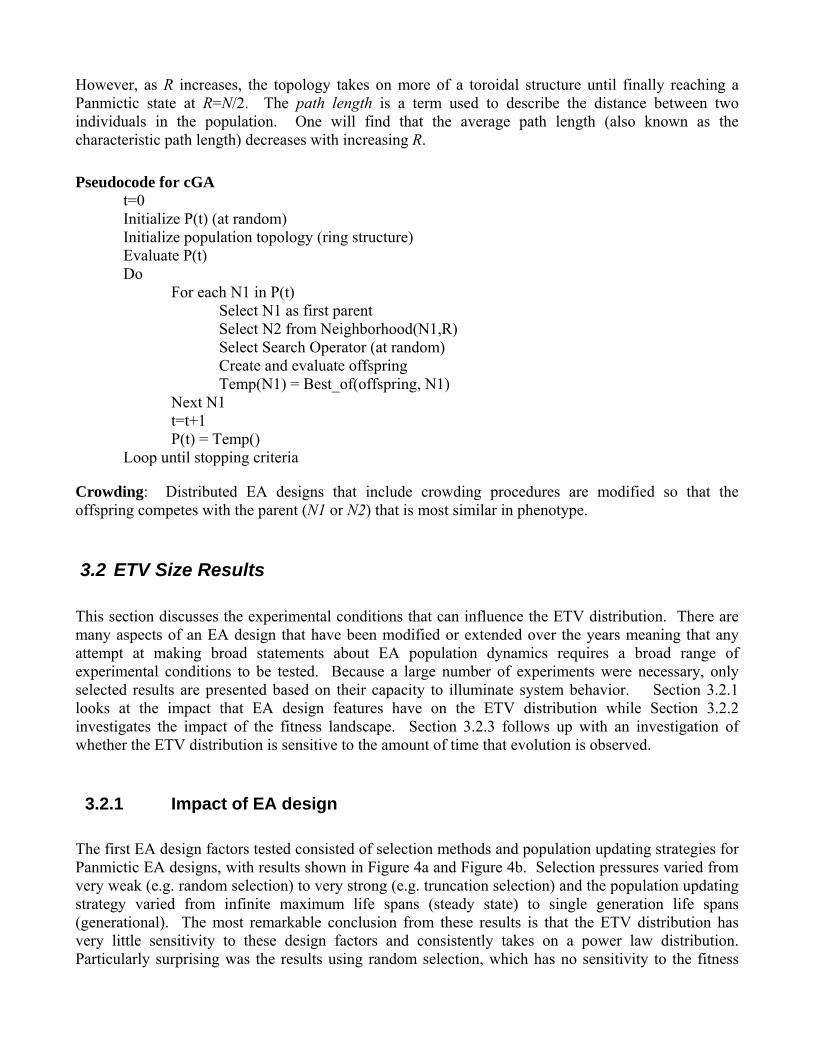
The fitness landscape that an EA population evolves on will obviously impact the trajectory that the population takes through parameter space. Hence, it was somewhat surprising to see how little the fitness landscape influenced the ETV distribution results. Test functions were selected from Table 1 and include unimodal and multimodal functions, linear and nonlinear functions, functions with strong and weak epistasis, as well as deceptive and non-deceptive functions. Results shown in Figure 7 and Figure 8 demonstrate little sensitivity to the fitness landscape on which evolution occurs. Other Panmictic EA designs were also tested with similar results (results not shown). For the distributed EA results, some sensitivity to the fitness landscape was observed when strong spatial restrictions were present in the EA population (e.g. see Figure 8a). However, the general conclusions from the previous section remain unchanged; only spatial restrictions in the EA population result in significant changes to the ETV distribution.

There are other experimental conditions that can influence the fitness landscape. One way to test the influence of the fitness landscape on ETV results is to use random selection, as was done in the previous section. The use of random selection in an EA design is similar to evolving on a completely flat fitness landscape. Implementing different search operators is also expected to have an impact that

is somewhat similar to changing the fitness landscape. Experiments conducted using different search operators (results not shown) were found to have a similar effect to varying the test function, although these results displayed even less sensitivity. This low sensitivity could be a consequence of the range of operators tested.

3.2.3 Impact of time length of evolution

In this section, tests were conducted with evolution taking place over different lengths of time. As seen in Figure 9, during the initial stages of evolution, the ETV distribution displays power law deviations for large ETV sizes however these deviations disappear as evolution is observed over longer periods of time.

The fact that ETV distribution results have only a brief transient where the distribution is sensitive to time, but is insensitive thereafter, possibly indicates that the distribution approaches a stationary state. The record statistics of ETV in Figure 10 also provide evidence that maximum ETV sizes have an initial time dependency. This could mean that the system does not initially start with population dynamics being defined by a power law distribution but instead that the system evolves to achieve that state over time.

It has been determined that the reason for this initial dynamical behavior is actually due to the lack of a genealogical or a historical coupling between individuals in the initial population. To confirm this, Figure 11 shows ETV distribution results where each new offspring has a probability Pnew of being historically uncoupled from the rest of the population. Historical uncoupling is simply done by preventing offspring from inheriting historical data from their parents. From a population dynamics perspective, this is equivalent to an EA design which includes a steady introduction of new individuals into the EA population (e.g. randomly generated individuals). As seen in Figure 11, a small amount of historical uncoupling can result in power law deviations for the largest ETV sizes. However, as Pnew is increased, the extent that the distribution deviates from a power law is found to increase only slightly.

3.2.4 Other Experimental Conditions

Additional tests were also conducted (results not shown) to help ensure that the ETV distribution results that have been presented in this work were not biased due to other experimental factors. This included experiments on selected EA designs at population sizes up to N=500, running evolution up to 100,000 generations, and experiments with the ETV calculation parameter Tobs set as high as 500. These experiments resulted in no observable changes to ETV distribution results.

3.3 ETV Age Results

In addition to measuring the size of an individual’s impact, one can also measure the amount of time that an individual is able to impact population dynamics. This is measured by recording the number of generations required for an individual’s ETV calculation to finish, which is referred to here as the ETV age. This section investigates this aspect of EA dynamics more closely, again with the aim of determining what experimental conditions impact the ETV age distribution.

Looking at Figure 12 and Figure 13, these results demonstrate that the ETV age repeatedly approximates a power law however different sensitivities to EA design conditions have emerged (compared with ETV size distribution results shown previously). Although there is still no sensitivity to the population size, these results reveal that the selection method and population updating strategy do have an impact on the ETV age distribution for Panmictic populations. This is seen for instance in the results presented in Figure 13b where EA designs with steady state population updating and tournament selection are found to have a clear power law deviation for large ages. On the other hand, the introduction of spatial restrictions to the EA population does not have any influence on this characteristic of population dynamics as seen in Figure 12. This is surprising considering the importance of spatial restrictions in the previous ETV size distribution results. Also shown in Figure 12, the addition of crowding to the cGA has a completely unexpected impact on the age distribution and appears to result in an almost log-periodic behavior that on average still tends toward a power law distribution. On the other hand, the addition of crowding in Panmictic Populations (e.g. Deterministic Crowding) was found to have little influence on the age distribution. In summary, these results indicate that most ETV age distributions are well approximated by power laws although changes to the distribution shape do occur under certain conditions.

As a final comment on these results, it is also worth mentioning that although the ETV has a maximum size equal to N, the ETV age measured here is only constrained by the amount of time that the system is observed. For these experiments, evolution was observed for up to 20,000 generations and ETV ages were found approaching 1000 without any evidence of power law deviations at large ages. Based on the observed distributions, it is concluded that the maximum age of events in EA dynamics is only limited by the amount of time that evolution is allowed to take place.1

4 Discussion

In previous work [11], it was suggested that the power law behavior observed in ETV results has some similarities to the evolutionary dynamics in natural evolution. Arguments were also presented that highlighted the possible compatibility of these results with the theory of Self-Organized Criticality (e.g. see [11]), as well as highlighting similarities to simple branching processes.

Regardless of the actual causes of the ETV power law, it is important to understand what this implies about the dynamical behavior of these systems. First and foremost, it provides us with a better sense of the upper bounds to parallel computation for population based search heuristics. As long as power law behavior is observed, we can expect that the entire system can (and will) be occasionally driven by low-probability individual events. In this paper, such power law behavior was found to be prevalent in many EA designs. However some EA designs displayed clear power law deviations so that there was almost no chance that single events could cause system-wide changes. Furthermore, the particular form of the power law deviation was found to be insensitive to population size suggesting that such

1 The maximum age can also be limited by the ETV calculation procedure, for instance by limits placed on the size of the historical records kept in the EA population. In these experiments, the maximum record size was set to Tobs=250 and under these conditions, it was found that roughly one in every 50,000 events failed to finish the ETV calculation before reaching a maximum record position.

deviations would play an increasingly important role (in modifying system behavior) as the system is scaled up to larger sizes.

The influence of the test function was also interesting. For most EA designs, the macroscopic features of population dynamics that were being measured here were not influenced by the landscape over which evolution takes place. However, when spatially distributed EA designed were implemented, we found that the ETV distribution shape was highly sensitive to the test function.

It is also worth noting the relevance of other features of the ETV distribution such as the power law exponent. This paper focused primarily on the existence of power laws, however one might have noticed that different EA designs were found to have different power law exponents. Only slight changes to this exponent are expected to have a significant influence on the probability of large scale events (e.g. ETV≈N) taking place, particularly in large populations.

Another observation worth noting is that the presence of crowding in distributed EA designs causes a large proportion of events to have a negligible impact (e.g. ETV=1), which is expected to result in a highly parallel search process. Evidence of this is given in Figure 6 where one can see that the probability of larger ETV sizes is reduced by roughly an order of magnitude

It should also be mentioned that, despite considerable efforts, the experiments were not exhaustive and so it is possible that other EA designs and certain landscape characteristics could result in ETV distributions which deviate from a power law or are otherwise different from what was presented here. As an example, EA designs which parameterize the amount of interaction between population subgroups (i.e. island model population structure) could be one unaccounted for situation where power laws would only be observed with the appropriate parameter settings. In addition, EA designs with a dynamic population size might also cause significant changes to the ETV distribution results.

4.1 Challenges and opportunities in ETV analysis

The ETV analysis is designed to characterize large scale features emerging within population-based adaptive systems that employ spatially and/or temporally localized operators. Requirements for this type of analysis include the ability to define a scope (unit) where operations are taking place and the ability to track influence among units that are created (and possibly change) over time. The generality of these conditions should permit an ETV analysis to be extended to other population-based search processes and potentially to other scales of observation within these systems. In the following discussion, we elaborate on some of the opportunities and challenges that arise with this direction of research.

4.1.1 Extensions

One scale of observation that is of considerable interest is that of individual genes. Because allelic frequencies change over time as a direct consequence of variation and selection operators, we suspect that an ETV analysis could be applied to the dynamics of genetic composition. While some of the conclusions drawn here may extend to this scale of observation, additional relevant factors are also likely to emerge. For example, search operators such as random mutation (i.e. unbiased sampling of

alleles) could have an effect similar to the introduction of historically uncoupled individuals as was tested in this study.

On the other hand, fitness landscape characteristics dramatically influence the speed and extent that genes become fixated and lost within a population. The transitory nature of simulated evolutionary processes also complicates such an analysis since many problems will only allow for brief periods of data collection. More generally, investigations at this scale of observation expose interactions between the algorithm and problem, raising new challenges but also potentially providing for new application opportunities. For instance, correlations in ETV growth could provide a means for discovering genetic building blocks and exploiting fitness landscape patterns.

At a larger scale of observation, one could apply a similar analysis to memetic algorithms to understand how the hybridization of local search and global meta-heuristics can influence emergent system properties such as the ETV distribution. For instance, each individual can be labelled to indicate the search operator used when creating that individual. By doing this, it is possible to establish ETV distributions for each search operator used, which then allows for a comparison of the relative influence of local search and recombinant search operations. Such information might be useful for the adaptive hybridization of memetic algorithms

Indeed, there is already some evidence to suggest that this application of ETV to memetic algorithms could prove useful. Previous studies have found ETV to be a useful metric for assigning value to different search operators in order to adapt their usage rates during a search process. For instance, in [11] it was concluded that the power law ETV distribution implies that most individuals have a negligible impact on population dynamics and do not provide useful information (i.e. act as noise) when determining the relative utility of different search operators. Statistical arguments were then used to filter out most ETV measurements, with the remaining ETV measurements used to adaptively modify search operator usage rates during algorithm runtime. Comparison to conventional “fitness-based” adaptive methods taken from the literature indicated that ETV provided more useful information than direct fitness measurements. Furthermore, these conclusions did not appear to be sensitive to fitness landscape characteristics including modality, epistasis, neutrality, or search space size.

4.1.2 Challenges

An overarching goal in the study of algorithm behavior is to derive methods that are flexible enough to accommodate a broad range of search algorithm designs. At the same time, analysis methods should aim to provide tools that probe algorithm behavior and allow for a better understanding, better comparisons, and intuitive classification of the ever expanding list of search algorithms described in the literature.

The ETV analysis improves upon past studies in terms of the breadth of experimental conditions that it can accommodate. Prior studies of EA behavior, as discussed in the introduction, have only been applicable to specific algorithm designs, specific fitness landscapes, or both. However serious attempts at general-purpose search algorithm analysis are still in their infancy. Moreover, there are limitations to the ETV analysis that need to be recognized and appreciated. For instance, it is straightforward to uncover limitations in the application of ETV to several meta-heuristics and hybrids, particularly those incorporating group based operations (e.g. Estimation of Distribution, Swarm, and Ant Colony Optimization).

Some of the difficulties with this type of analysis arise due to fundamental challenges related to the “credit assignment problem”. Credit assignment describes the tracking of influence or causality over time; an issue that is both highly relevant and highly challenging in the study of complex adaptive systems including population-based meta-heuristics. The difficulty comes from the assignment of credit for future system states to individual decisions in the past. In contrast to the assumptions made in this study, the value of an offspring is not derived by a single dominant parent. On the other hand, nor should we view this issue simply as one of distributing credit proportionately to the respective parents. In general, the effect of combining genes from individual parents is not additive or linear. It is not only the genes contributed by a parent that matters, but also how these effectively combine with contributions from the other parent(s). Stated another way, a full accounting of influence (or lack thereof) needs to account for the possibility of new innovations that cannot be attributed solely to historical bias. This is a fundamental issue in evolution (both natural and artificial) that places bounds on any analysis of causality.

Besides the issue of innovation, there are other additional challenges in the assignment of credit over long timescales. One challenge discussed in this paper is hitchhiking. A similar phenomenon occurs in natural evolution, where genetic hitchhiking refers to the fixation of both neutral and slightly maladaptive alleles when these are presented concurrently with a highly advantageous mutation [13] [14]. Although this study introduces a graph-based heuristic for reducing a similar type of hitchhiking within ETV calculations, it is important to note that there are implicit assumptions being made when using this heuristic.

In biological evolution, the phenotypic significance of genetic mutations can at times be cryptic, showing little immediate influence yet being highly relevant to the expression of future phenotypic novelty [15] [16]. This is a hotly researched topic in the study of biological evolution that is sometimes referred to as genetic buffering or cryptic genetic variation [17] [18] [19] [20] [21]. Similar phenomena can occur in an EA population and can limit the utility of information from an ETV measurement. In particular, an individual may be of modest reproductive value in a given generation yet prove important to longer term evolutionary dynamics. In other words, the hitch-hikers we eliminate from the ETV calculation could in some cases be of actual importance to the success or failure of future generations. This hitchhiking problem relates directly to the issue of search bias assumptions that are used in optimization research, which is discussed in some detail in Chapter 3.2 in [11] and also in [10].

There are other practical issues that also need to be addressed before the ETV measurement can effectively account for multi-parent operations. The current algorithm design (e.g. see Section 3.2.2 in [11] for relevant algorithm details) is not readily amendable to the expansive branching influence graphs that emerge when attempting to assign credit to more than a single parent. This, along with associated computational costs, is another reason why a single dominant parent is chosen in these experiments instead of distributing credit across multiple parents.

Finally, it is worth questioning whether credit should be distributed based on genotype or fitness? Although inheritance has a genetic basis, selection is based entirely on fitness. Ad hoc experiments have found that replacing genetic dominance with fitness dominance (i.e. similarity in parent and offspring fitness values) in the ETV calculation does not have a dramatic influence on the results or conclusions drawn in this study. On the other hand, it is worth investigating this issue in greater detail, as we suspect fitness dominance should allow for some sensitivity to fitness landscape properties.

5 Conclusions

A number of conclusions can be drawn from the results presented in this paper. First, it was found that the probability of an individual’s impact on EA dynamics fits a power law (exponent between 2.2 and 2.5). This is a robust property of the system which is largely insensitive to most experimental conditions including changes to population size, search operators, fitness landscape, selection scheme, population updating strategy, and the presence of crowding mechanisms. From these results, it is concluded that the large majority of individuals will have a negligible impact on future population dynamics.

Two experimental conditions were however found to result in power law deviations for large ETV sizes. The first was the steady introduction of new individuals that have no relation to others in the population (i.e. historically uncoupled). The second condition was the introduction of spatial restrictions into an EA population. Using either of these conditions effectively removes the possibility of single individuals dominating the dynamics of the entire population. The associated power law deviations can be understood as an indicator of increased parallel computation within the system.

The amount of time than an individual influences EA dynamics (i.e. ETV age) also was found to fit a power law with most individuals influencing the system for only brief periods of time. However, as suggested by the power law relation, there is a non-negligible probability that an individual will influence EA dynamics over very large time scales. This behavior was found to be robust and was almost completely insensitive to all experimental conditions tested.

6 References

[1] D. E. Goldberg and K. Deb, "A Comparative Analysis of Selection Schemes Used in Genetic Algorithms," Urbana, vol. 51, pp. 61801-2996.

[2] T. Blickle, "Theory of Evolutionary Algorithms and Application to System Synthesis," Swiss Federal Institute of Technology, 1996.

[3] W. Wieczorek and Z. J. Czech, "Selection Schemes in Evolutionary Algorithms," Proceedings of the Symposium on Intelligent Information Systems (IIS'2002 ), pp. 185-194, 2002.

[4] E. Van Nimwegen and J. P. Crutchfield, "Optimizing Epochal Evolutionary Search: Population-Size Dependent Theory," Machine Learning, vol. 45, pp. 77-114, 2001.

[5] T. Smith, P. Husbands, and M. O'Shea, "Local evolvability of statistically neutral GasNet robot controllers," Biosystems, vol. 69, pp. 223-243, 2003.

[6] S. Nijssen and T. Back, "An analysis of the behavior of simplified evolutionary algorithms on trap functions," IEEE Transactions on Evolutionary Computation, vol. 7, pp. 11-22, 2003.

[7] L. Davis, Handbook of Genetic Algorithms: Van Nostrand Reinhold New York, 1991.

[8] B. A. Julstrom, "What Have You Done for Me Lately? Adapting Operator Probabilities in a Steady-State Genetic Algorithm," Proceedings of the 6th International Conference on Genetic Algorithms, pp. 81-87, 1995.

[9] B. A. Julstrom, "Adaptive operator probabilities in a genetic algorithm that applies three operators," in ACM Symposium on Applied Computing (SAC '97) 1997, pp. 233-238.

[10] J. M. Whitacre, T. Q. Pham, and R. A. Sarker, "Credit assignment in adaptive evolutionary algorithms," in Proceedings of the 8th Annual Genetic and Evolutionary Computation Conference 2006, pp. 1353-1360.

[11] J. M. Whitacre, "Adaptation and Self-Organization in Evolutionary Algorithms," Thesis: University of New South Wales, 2007, p. 283.

[12] S. W. Mahfoud, "A Comparison of Parallel and Sequential Niching Methods," Conference on Genetic Algorithms, vol. 136, p. 143, 1995.

[13] P. Pfaffelhuber, A. Lehnert, and W. Stephan, "Linkage Disequilibrium Under Genetic Hitchhiking in Finite Populations," Genetics, vol. 179, p. 527, 2008.

[14] P. W. Hedrick, "Genetic Hitchhiking: A New Factor in Evolution?," Bioscience, vol. 32, 2007.

[15] M. A. Félix and A. Wagner, "Robustness and evolution: concepts, insights and challenges from a developmental model system," Heredity, vol. 100, pp. 132-140, 2008.

[16] A. Wagner, "Neutralism and selectionism: a network-based reconciliation," Nature Reviews Genetics, 2008.

[17] G. Gibson and I. Dworkin, "Uncovering cryptic genetic variation," Nature Reviews Genetics, vol. 5, pp. 681-690, 2004.

[18] C. D. Schlichting, "Hidden Reaction Norms, Cryptic Genetic Variation, and Evolvability," Annals of the New York Academy of Sciences, vol. 1133, pp. 187-203, 2008.

[19] J. Hermisson and G. P. Wagner, "The Population Genetic Theory of Hidden Variation and Genetic Robustness," Genetics, vol. 168, pp. 2271-2284, 2004.

[20] A. Bergman and M. L. Siegal, "Evolutionary capacitance as a general feature of complex gene networks," Nature, vol. 424, pp. 549-552, 2003.

[21] J. L. Hartman, B. Garvik, and L. Hartwell, "Principles for the Buffering of Genetic Variation," Science, vol. 291, pp. 1001-1004, 2001.

ETVgen = 1 2 3 5 6 6 7 3 3

1 2 3 4 5 6 7 80

Event Measured

Generation Figure 1: Visualizing an individual’s impact on population dynamics using genealogical graphs. An individual’s impact for a given generation (horizontal axis) is defined as the number of paths leading from the measured node to the current generation. This is referred to as ETVgen and is calculated for the “Event Measured” in the graph above by counting the number of nodes on the dotted vertical line for a given generation. As the population moves from one generation to the next, the number of individuals in the population that are descendants of the “Event Measured” will change. These changes are reflected in the ETVgen value as shown at the top of the graph. The maximum impact of an event is the maximum ETVgen value that is observed. To simplify the illustration, we assume a generational population updating strategy is used, meaning that each individual exists in a single generation only. Other updating strategies could also be used in which case some nodes would be stretched across multiple generations in the graph.

Current Generation

Figure 2: Genetic Hitchhiking in EA population dynamics. Considering ETVgen measurements based on the current generation, one can easily see that all nodes to the left of the white node will have the same ETVgen value (i.e. they all have the same number of paths leading to the current population). However, these nodes are assigned their ETVgen values only because of a single important descendant (the white node). These linear structures in the genealogical branching process are a sign of genetic hitchhiking and can be seen in several different places in the graph above (seven genetic hitchhiking occurrences in total).

P21P26

P33

P40

P23

P28P31P36

History

P40

P33

P26

P21

Parent 1History

P36

P31

P28

P23

Parent 2

P40

History

P40

P33

P26

P21

Offspring

New ID

Genetic Dominance

New ID

Figure 3: Transfer of Historical Data. Each individual holds historical information in addition to genetic information. The historical information represents the direct line of ancestry for an individual. Examples of historical data lists are shown above for Parent 1 (ID=P21) and Parent 2 (ID=P23) and their meaning is demonstrated by the genealogical graph on the right. A new offspring only takes historical information from the parent that is genetically most similar (i.e. genetically dominant). In this example, Parent 1 is assumed to be the genetically dominant parent. In addition, the offspring creates a new ID to indicate its placement in the genealogical tree.

Figure 4 ETV size distributions for a number of panmictic EA designs. Solid line represents a power law with exponent a) 2.5, b) 2.3. Results are taken over 20,000 generations of evolution on the 30-D Hyper Ellipsoid test function.

Figure 5 ETV size distributions for a number of spatially distributed EA designs. Solid line represents a power law with exponent a) 2.2, b) 2.5. Results are taken over 20,000 generations of evolution on the 30-D Hyper Ellipsoid test function.

Figure 6 ETV distributions for spatially distributed EA designs and EA designs using crowding. Results from using Deterministic Crowding (DC) are presented in the inset. Solid line represents a power law with exponent 2.2. Results from each EA design are taken over 20,000 generations of evolution on the 30-D Hyper Ellipsoid test function.

Figure 7 ETV distributions shown for selected EA designs on test functions taken from Table 1. Evolution occurred over 2000 generations and results shown are averages taken over 10 runs. To help in viewing results from a large number of test functions, data is grouped into bins. Solid line represents a power law with exponent a) 2.2, b) 2.2.

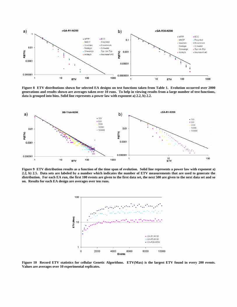
Figure 8 ETV distributions shown for selected EA designs on test functions taken from Table 1. Evolution occurred over 2000 generations and results shown are averages taken over 10 runs. To help in viewing results from a large number of test functions, data is grouped into bins. Solid line represents a power law with exponent a) 2.2, b) 2.2.

Figure 9 ETV distribution results as a function of the time span of evolution. Solid line represents a power law with exponent a) 2.2, b) 2.5. Data sets are labeled by a number which indicates the number of ETV measurements that are used to generate the distribution. For each EA run, the first 100 events are given to the first data set, the next 500 are given to the next data set and so on. Results for each EA design are averages over ten runs.

Figure 10 Record ETV statistics for cellular Genetic Algorithms. ETV(Max) is the largest ETV found in every 200 events. Values are averages over 10 experimental replicates.

Figure 11 ETV distributions with varying amounts of historical uncoupling in EA population dynamics. Experiments are conducted with a Steady State EA using truncation selection and population size N=100. Evolution took place over 20,000 generations on the 30-D Hyper Ellipsoid test function. When conducting the standard ETV calculation, historical event information is copied from the genetically dominant parent to its offspring. In these experiments, the step of historical transfer is skipped with probability Pnew. The solid line in the graph represents a power law with exponent = 2.1

Figure 12 ETV age distributions shown for spatially distributed EA designs and EA designs using crowding. Solid line represents a power law with exponent 3.2.

Figure 13 ETV age distributions for several EA designs. Solid line represents a power law with exponent a) 3, b) 2.5, c) 3.5.

Table 1 Names of test problems used in experiments. Detailed information on each of the test problems can be found in Appendix A in [11].

Table 2: List of search operators used in experiments. Details provided in this table include the search operator name, other common name, reference for description, and parameter settings if different from reference.