Thisisthepostpeer-reviewacceptedmanuscriptof:

M. Chiani, A. Giorgetti and E. Paolini, "Sensor Radar for Object Tracking," inProceedingsoftheIEEE,vol.106,no.6,pp.1022-1041,June2018.Thepublishedversionisavailableonlineat:https://doi.org/10.1109/JPROC.2018.2819697

©2018IEEE.Personaluseofthismaterialispermitted.PermissionfromIEEEmustbeobtainedforallotheruses, in any current or future media, including reprinting/republishing this material for advertising orpromotionalpurposes,creatingnewcollectiveworks,forresaleorredistributiontoserversorlists,orreuseofanycopyrightedcomponentofthisworkinotherworks.

PROCEEDINGS OF THE IEEE, VOL. 106, NO. 6, JUNE 2018 1

Sensor Radar for Object TrackingMarco Chiani, Fellow, IEEE, Andrea Giorgetti, Senior Member, IEEE, and Enrico Paolini, Member, IEEE

(Invited Paper)

Abstract—Precise localization and tracking of moving objectsis of great interest for a variety of emerging applications includingthe Internet-of-Things (IoT). The localization and tracking tasksare challenging in harsh wireless environments, such as indoorones, especially when objects are not equipped with dedicatedtags (non-collaborative). The problem of detecting, localizing,and tracking non-collaborative objects within a limited area hasoften been undertaken by exploiting a network of radio sensors,scanning the zone of interest through wideband radio signalsto create a radio image of the objects. This paper presents asensor network for radio imaging (sensor radar) along withall of the signal processing steps necessary to achieve high-accuracy objects tracking in harsh propagation environment.The described sensor radar is based on the impulse radio (IR)ultrawide-band (UWB) technology, entailing the transmission ofvery short duration pulses. Experimental results with actualUWB signals in indoor environments confirm the sensor radar’spotential in IoT applications.

Index Terms—Detection, indoor tracking, Internet-of-Things,localization, multistatic radar, sensor radar, ultrawide-band.

I. INTRODUCTION

LOCALIZATION and tracking of moving objects is acritical component for important new applications, in-

cluding medical services, military systems, search and rescueoperations, automotive safety, and logistics [1]–[7]. Indeed,wireless sensor networks and more generally the Internet-of-Things (IoT) consider localization as the enabling technologyto provide georeferenced information from sensors, machines,vehicles, and wearable devices, in the ever growing trend ofhyper-connected society [8]–[11].

Localization systems estimate object positions based onobservations (or measurements) gathered by a network ofsensors deployed in the environment [12]–[17]. The term “lo-calization” usually refers to the capability to infer the positionof collaborative objects, i.e., tagged objects interacting withthe system to facilitate the localization process [18]–[21].However, an increasing attention is recently being devoted tothe capability of detecting and tracking objects that do nottake actions to help the localization infrastructure or that donot wish to be detected and localized at all. This operationis referred to non-collaborative localization and is typical ofradar systems [22]. These systems are further classified basedon whether the network emits a signal designed for target de-tection and localization (active radar), or the network exploits

This work was supported in part by the European Project EuroCPS throughthe H2020 Framework under Grant 644090.

The authors are with the Department of Electrical, Electronic, and In-formation Engineering “Guglielmo Marconi” (DEI), University of Bologna,via Venezia 52, 47521 Cesena (FC), ITALY e-mail: ({marco.chiani, an-drea.giorgetti, e.paolini}@unibo.it). Author names are listed in alphabeticalorder.

signals emitted by other sources of opportunity (passive radar)[23]–[25].

The expressions “sensor radar” and “radar sensor network”are hereafter used interchangeably to refer to a network ofactive radars in a monostatic, bistatic, or multistatic configu-ration [26]–[30]. A multistatic radar is a network of multiple,independent radars, where each sensor performs a significantamount of processing. Pre-processed data are then collectedby central unit through a communication link [27]. Multistaticradar shall not be confused with multiple-input multiple-output(MIMO) radar, which refers to a radar system employingmultiple transmit waveforms (typically orthogonal to eachother) and having the ability to jointly process signals receivedat multiple antennas [31], [32]. Such a feature requires tightsynchronization among all sensors, to track phase changes,and limits the possibility to perform local processing [33].

Accurate localization via sensor radars becomes particularlychallenging in indoor environments characterized by densemultipath, clutter, signal obstructions (e.g., due to the pres-ence of walls), and interference. In a real-world scenariomeasurements are usually heavily affected by such impair-ments, severely affecting detection reliability and localizationaccuracy. These operating conditions may be mitigated by theadoption of waveforms characterized by large bandwidth, e.g.,ultrawide-band (UWB) ones, exploiting prior knowledge ofthe environment, selecting reliable measurements, and using awide range of signal processing tools [34]–[37].

The UWB technology, and in particular its impulse ra-dio (IR) version characterized by the transmission of a fewnanoseconds duration pulses [38]–[45], offers an extraordinaryresolution and localization precision in harsh environments,due to its ability to resolve multipath and penetrate obstacles[46]–[49]. Additional advantages include low power consump-tion, low probability of intercept, robustness to jamming, andcoexistence with a large number of systems in the ever increas-ing spectrum exploitation [50]–[52]. These features, togetherwith the property of IR-UWB devices to be light-weight,cost-effective, and characterized by low power emissions,have contributed to make UWB an ideal candidate for non-collaborative object detection in short-range radar sensor net-work (RSN) applications [53]–[65]. UWB has been employedin through wall imaging, which has the ability to locate indoormoving targets with a radar situated at a standoff range outsidebuildings [66]–[73]. It has also been successfully adopted in anumber of related applications including, e.g., radio-frequencyidentification [74]–[76], search and rescue of trapped victims[77]–[81], vital sign detection and estimation [82], [83], strokedetection [84], people counting [85], environmental imaging[86], [87], and non-destructive testing [88]. In the sensor radarfield a number of papers have addressed several aspects related

2 PROCEEDINGS OF THE IEEE, VOL. 106, NO. 6, JUNE 2018

TABLE ILIST OF ACRONYMS

AWGN additive white Gaussian noiseCA-CFAR cell averaging CFARc.d.f. cumulative distribution functionCFAR constant false alarm rateCPHD cardinalized PHDDP direct pathDTB-CFAR double threshold and buffer CFAREM expectation-maximizationER empty-roomG-CFAR global CFARIoT Internet-of-ThingsIR impulse radioLOS line-of-sightLS least squareMHT multiple hypothesis trackingMIMO multiple-input multiple-outputMTI moving target indicatorp.d.f. probability density functionPHD probability hypothesis densityPSD power spectral densityRCS radar cross sectionRE residual errorRFS random finite setRMSE root mean-square errorRSN radar sensor networkRx receiverSNR signal-to-noise ratioSUT sample under testToA time-of-arrivalTx transmitterUWB ultrawide-band

to the use of UWB, e.g., clutter removal and channel modeling[89], [90], detection [91]–[95], target recognition [96], tracking[97]–[111], sensors deployment [57], [112], [113], sensorspower allocation [114], and cognitive mechanisms [115]–[118].

The localization of non-collaborative objects poses severalproblems at different levels of the processing chain, rangingfrom clutter removal, ghost mitigation, detection and clus-tering, within each sensor, to measurement combining (datafusion), clustering, measurement selection and tracking, atthe network level. Finding a way to carry out all of theseprocessing steps and to exploit their mutual relationshipsis a hard task and requires an almost holistic view of thesystem. For this reason, this paper aims at presenting the mainaspects that involve detection, localization and tracking of non-collaborative objects in indoor environments using off-the-shelf IR-UWB technology. The most challenging problems atdifferent system levels are presented and possible solutions areproposed. The presentation is kept at introductory level, pro-viding in-depth references for the interested reader. A sensorradar demonstrator is used to address step-by-step processingof actual signals and data, which have been collected in areal indoor environment through an experimental campaign.The use of real equipments is important to gain insights fromreal-world waveforms and the associated challenging practicalaspects. The paper describes all steps from actual raw signalacquisition to object tracking through the complex processingchain of the network. The localization error performance willconfirm the effectiveness of the performed processing.

y1(t)

FilteringPulse integration

Sampling

Sensor 1

Sec. IV-A

Non-coherentdemodulation

Sec. IV-B

r1, rer

Direct pathToA estimation

Sec. IV-C

✏1, ✏er

Clutter removalGhost mitigation

Sec. IV-D

✏1, ✏er,�⌧0,1

CFAR detection

Sec. IV-E

d1

1D Clustering

Sec. IV-F

bb1

b1

y2(t)

FilteringPulse integration

Sampling

Sensor 2

Non-coherentdemodulation

r2, rer

Direct pathToA estimation

✏2, ✏er

Clutter removalGhost mitigation

✏2, ✏er,�⌧0,2

CFAR detection

d2

1D Clustering

bb2

b2

· · ·

yNr (t)

FilteringPulse integration

Sampling

Sensor Nr

Non-coherentdemodulation

rNr , rer

Direct pathToA estimation

✏Nr , ✏er

Clutter removalGhost mitigation

✏Nr , ✏er,�⌧0,Nr

CFAR detection

dNr

1D Clustering

bbNr

bNr

Detection

Network

Sec. V-A

False alarm rate reductionSec. V-B

Nd, {z1, z2, . . . , zNd }

Measurement clusteringSec. V-C

Nm, {z1, z2, . . . ,zNm }

Multiobject TrackingSec. V-D

Ncluster, Z1,Z2, . . . ,ZNcluster

Data AssociationSec. V-E

M, {x1, x2, . . . , xM}

M, {x1, x2, . . . , xM},T

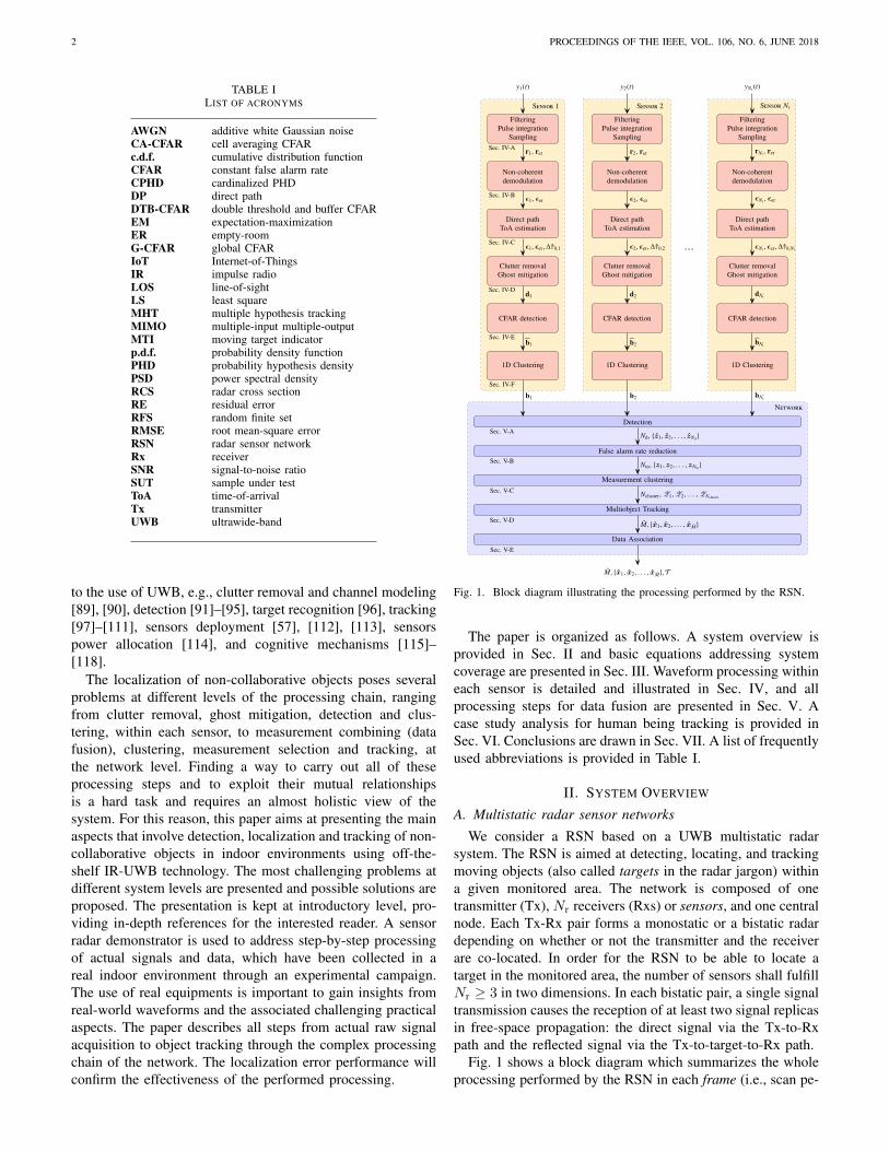
Fig. 1. Block diagram illustrating the processing performed by the RSN.

The paper is organized as follows. A system overview isprovided in Sec. II and basic equations addressing systemcoverage are presented in Sec. III. Waveform processing withineach sensor is detailed and illustrated in Sec. IV, and allprocessing steps for data fusion are presented in Sec. V. Acase study analysis for human being tracking is provided inSec. VI. Conclusions are drawn in Sec. VII. A list of frequentlyused abbreviations is provided in Table I.

II. SYSTEM OVERVIEW

A. Multistatic radar sensor networksWe consider a RSN based on a UWB multistatic radar

system. The RSN is aimed at detecting, locating, and trackingmoving objects (also called targets in the radar jargon) withina given monitored area. The network is composed of onetransmitter (Tx), N

r

receivers (Rxs) or sensors, and one centralnode. Each Tx-Rx pair forms a monostatic or a bistatic radardepending on whether or not the transmitter and the receiverare co-located. In order for the RSN to be able to locate atarget in the monitored area, the number of sensors shall fulfillN

r

� 3 in two dimensions. In each bistatic pair, a single signaltransmission causes the reception of at least two signal replicasin free-space propagation: the direct signal via the Tx-to-Rxpath and the reflected signal via the Tx-to-target-to-Rx path.

Fig. 1 shows a block diagram which summarizes the wholeprocessing performed by the RSN in each frame (i.e., scan pe-

CHIANI et al.: SENSOR RADAR FOR OBJECT TRACKING 3

y

x

Objects trajectory

�Detection & localization� 2D measurement selection� 2D clustering�Object tracking�Target association

Network processing

�Demodulation�ToA estimation�Clutter removal�Ghost mitigation�CFAR detection� 1D clustering�Measurement select.

In-sensor processing

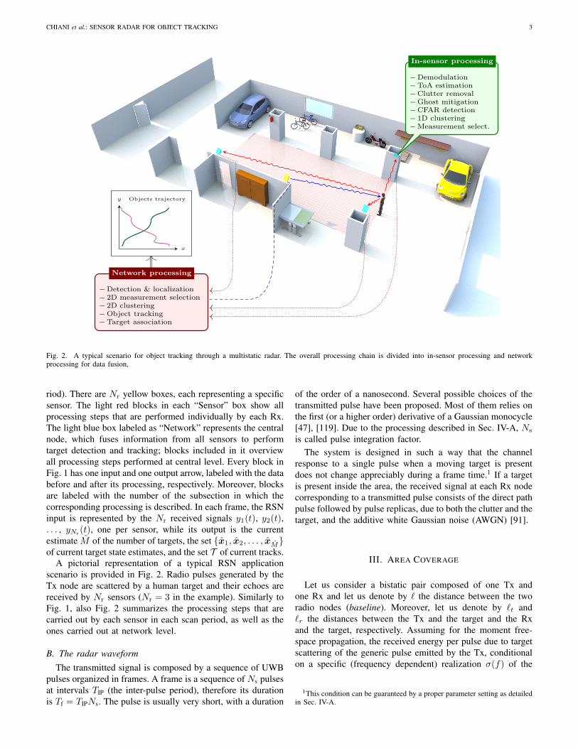
Fig. 2. A typical scenario for object tracking through a multistatic radar. The overall processing chain is divided into in-sensor processing and networkprocessing for data fusion,

riod). There are N

r

yellow boxes, each representing a specificsensor. The light red blocks in each “Sensor” box show allprocessing steps that are performed individually by each Rx.The light blue box labeled as “Network” represents the centralnode, which fuses information from all sensors to performtarget detection and tracking; blocks included in it overviewall processing steps performed at central level. Every block inFig. 1 has one input and one output arrow, labeled with the databefore and after its processing, respectively. Moreover, blocksare labeled with the number of the subsection in which thecorresponding processing is described. In each frame, the RSNinput is represented by the N

r

received signals y

1

(t), y2

(t),. . . , y

Nr(t), one per sensor, while its output is the currentestimate ˆ

M of the number of targets, the set {ˆx1

,

ˆ

x

2

, . . . ,

ˆ

x

ˆ

M

}of current target state estimates, and the set T of current tracks.

A pictorial representation of a typical RSN applicationscenario is provided in Fig. 2. Radio pulses generated by theTx node are scattered by a human target and their echoes arereceived by N

r

sensors (Nr

= 3 in the example). Similarly toFig. 1, also Fig. 2 summarizes the processing steps that arecarried out by each sensor in each scan period, as well as theones carried out at network level.

B. The radar waveformThe transmitted signal is composed by a sequence of UWB

pulses organized in frames. A frame is a sequence of Ns pulsesat intervals TIP (the inter-pulse period), therefore its durationis Tf = TIPNs. The pulse is usually very short, with a duration

of the order of a nanosecond. Several possible choices of thetransmitted pulse have been proposed. Most of them relies onthe first (or a higher order) derivative of a Gaussian monocycle[47], [119]. Due to the processing described in Sec. IV-A, N

s

is called pulse integration factor.The system is designed in such a way that the channel

response to a single pulse when a moving target is presentdoes not change appreciably during a frame time.1 If a targetis present inside the area, the received signal at each Rx nodecorresponding to a transmitted pulse consists of the direct pathpulse followed by pulse replicas, due to both the clutter and thetarget, and the additive white Gaussian noise (AWGN) [91].

III. AREA COVERAGE

Let us consider a bistatic pair composed of one Tx andone Rx and let us denote by ` the distance between the tworadio nodes (baseline). Moreover, let us denote by `

t

and`

r

the distances between the Tx and the target and the Rxand the target, respectively. Assuming for the moment free-space propagation, the received energy per pulse due to targetscattering of the generic pulse emitted by the Tx, conditionalon a specific (frequency dependent) realization �(f) of the

1This condition can be guaranteed by a proper parameter setting as detailedin Sec. IV-A.

4 PROCEEDINGS OF THE IEEE, VOL. 106, NO. 6, JUNE 2018

target radar cross section (RCS), may be expressed as

E =

fL+BZ

fL

E(f)Gt

(f)G

r

(f)�(f)

(4⇡)

3

(`

t

`

r

)

2

✓c

f

◆2

df . (1)

In (1), E(f) is the energy spectral density of the transmittedpulse, G

t

(f), G

r

(f) are the (frequency dependent) antennagains, (fL, fU) is the signal band, B = fU � fL is the signalbandwidth, and c is the speed of light.2

The signal-to-noise ratio (SNR) is defined as

SNR =

EN

s

N

0

=

�

(`

t

`

r

)

2

(2)

where N

0

is the one-sided noise PSD and

� = N

s

fL+BZ

fL

E(f)Gt

(f)G

r

(f)�(f)

(4⇡)

3

N

0

✓c

f

◆2

df (3)

is often referred to as the bistatic radar constant.3 Denotingby SNR

min

the minimum SNR necessary to achieve requiredmissed detection and false alarm probabilities, the largest valueof the product `

t

`

r

to meet the desired performance is given by

(`

t

`

r

)

max

=

r�

SNRmin

(4)

and is often referred to as the bistatic range of the Tx-Rx pair.From (2), over any plane containing both the Tx and the

Rx, the geometric curve corresponding to a constant product`

t

`

r

may be thought as associated with a constant value of theSNR.4 Geometrically, such a curve is named a Cassini ovaland is defined as the locus of the points in a plane such thatthe product of their distances from two fixed points, calledfoci, is a constant. The distance between the foci is usuallydenoted by 2a and the constant by b

2. For a bistatic pair, thepositions of the two foci coincide with the Tx and Rx ones,hence we have 2a = ` (baseline) and b

2

= `

t

`

r

. The shape ofa Cassini oval depends on the ratio

b

a

=

p`

t

`

r

`/2

. (5)

In particular, the curve consists of two loops around the fociwhen

p`

t

`

r

< `/2, it assumes a lemniscate shape whenp`

t

`

r

= `/2, and it is a single loop with a “dog bone” or anoval shape when

p`

t

`

r

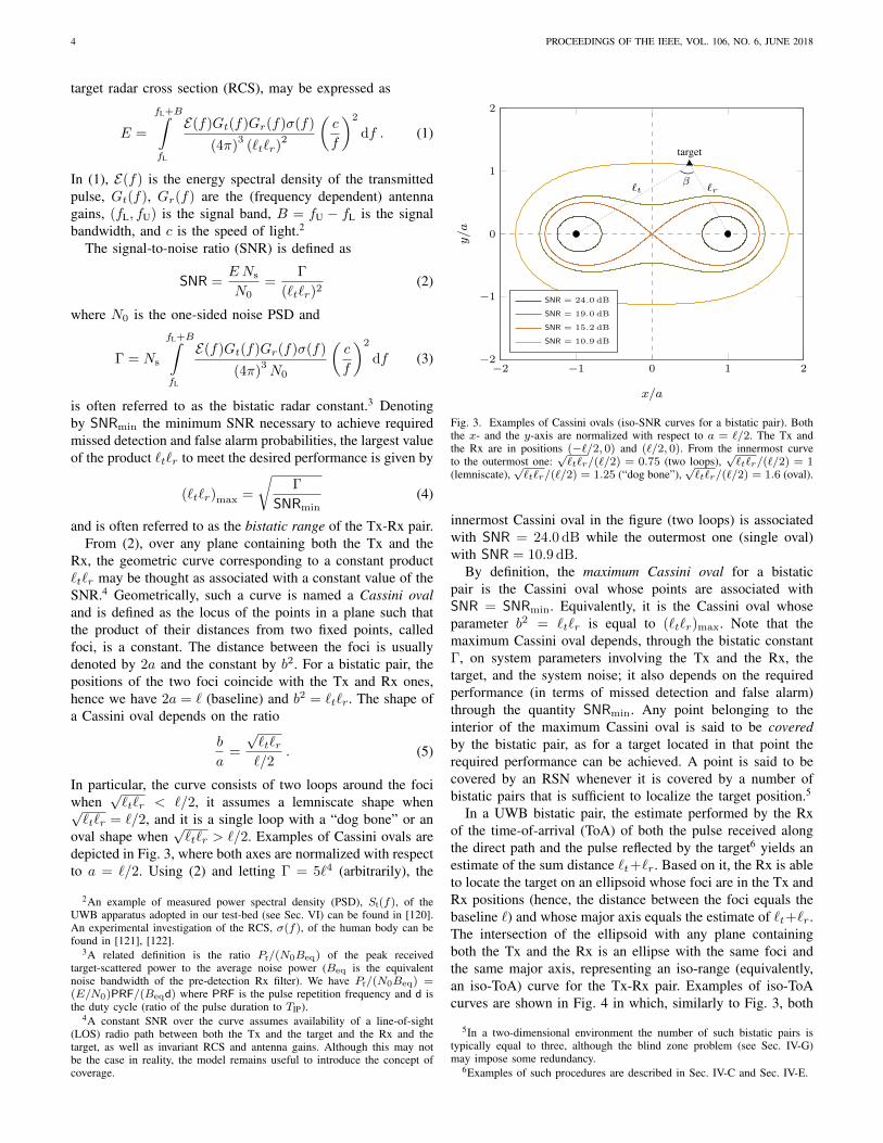
> `/2. Examples of Cassini ovals aredepicted in Fig. 3, where both axes are normalized with respectto a = `/2. Using (2) and letting � = 5`

4 (arbitrarily), the

2An example of measured power spectral density (PSD), St(f), of theUWB apparatus adopted in our test-bed (see Sec. VI) can be found in [120].An experimental investigation of the RCS, �(f), of the human body can befound in [121], [122].

3A related definition is the ratio Pr/(N0Beq) of the peak receivedtarget-scattered power to the average noise power (Beq is the equivalentnoise bandwidth of the pre-detection Rx filter). We have Pr/(N0Beq) =(E/N0)PRF/(Beqd) where PRF is the pulse repetition frequency and d isthe duty cycle (ratio of the pulse duration to TIP).

4A constant SNR over the curve assumes availability of a line-of-sight(LOS) radio path between both the Tx and the target and the Rx and thetarget, as well as invariant RCS and antenna gains. Although this may notbe the case in reality, the model remains useful to introduce the concept ofcoverage.

1

�2 �1 0 1 2

�2

�1

0

1

2

�

target

`

t

`

r

x/a

y/a

SNR = 24.0 dB

SNR = 19.0 dB

SNR = 15.2 dB

SNR = 10.9 dB

Fig. 3. Examples of Cassini ovals (iso-SNR curves for a bistatic pair). Boththe x- and the y-axis are normalized with respect to a = `/2. The Tx andthe Rx are in positions (�`/2, 0) and (`/2, 0). From the innermost curveto the outermost one:

p`t`r/(`/2) = 0.75 (two loops),

p`t`r/(`/2) = 1

(lemniscate),p`t`r/(`/2) = 1.25 (“dog bone”),

p`t`r/(`/2) = 1.6 (oval).

innermost Cassini oval in the figure (two loops) is associatedwith SNR = 24.0 dB while the outermost one (single oval)with SNR = 10.9 dB.

By definition, the maximum Cassini oval for a bistaticpair is the Cassini oval whose points are associated withSNR = SNR

min

. Equivalently, it is the Cassini oval whoseparameter b

2

= `

t

`

r

is equal to (`

t

`

r

)

max

. Note that themaximum Cassini oval depends, through the bistatic constant�, on system parameters involving the Tx and the Rx, thetarget, and the system noise; it also depends on the requiredperformance (in terms of missed detection and false alarm)through the quantity SNR

min

. Any point belonging to theinterior of the maximum Cassini oval is said to be coveredby the bistatic pair, as for a target located in that point therequired performance can be achieved. A point is said to becovered by an RSN whenever it is covered by a number ofbistatic pairs that is sufficient to localize the target position.5

In a UWB bistatic pair, the estimate performed by the Rxof the time-of-arrival (ToA) of both the pulse received alongthe direct path and the pulse reflected by the target6 yields anestimate of the sum distance `

t

+`

r

. Based on it, the Rx is ableto locate the target on an ellipsoid whose foci are in the Tx andRx positions (hence, the distance between the foci equals thebaseline `) and whose major axis equals the estimate of `

t

+`

r

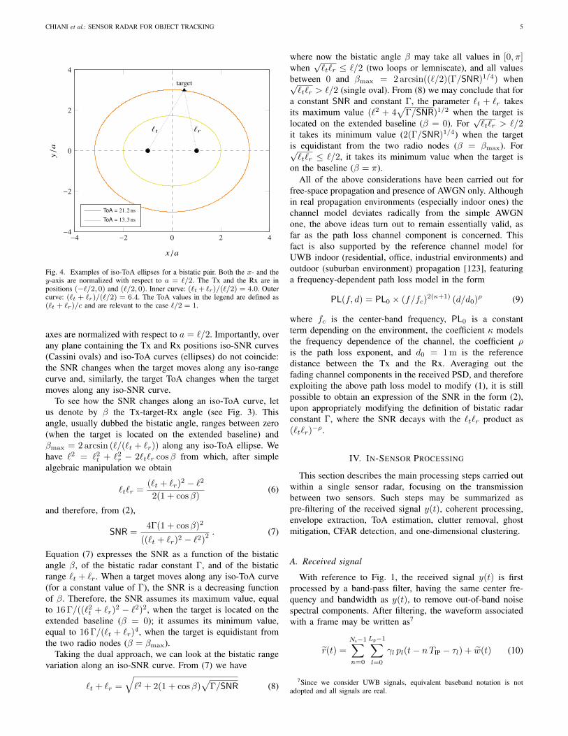
.The intersection of the ellipsoid with any plane containingboth the Tx and the Rx is an ellipse with the same foci andthe same major axis, representing an iso-range (equivalently,an iso-ToA) curve for the Tx-Rx pair. Examples of iso-ToAcurves are shown in Fig. 4 in which, similarly to Fig. 3, both

5In a two-dimensional environment the number of such bistatic pairs istypically equal to three, although the blind zone problem (see Sec. IV-G)may impose some redundancy.

6Examples of such procedures are described in Sec. IV-C and Sec. IV-E.

CHIANI et al.: SENSOR RADAR FOR OBJECT TRACKING 51

�4 �2 0 2 4�4

�2

0

2

4

target

`t `r

x/a

y/a

ToA = 21.2 ns

ToA = 13.3 ns

Fig. 4. Examples of iso-ToA ellipses for a bistatic pair. Both the x- and they-axis are normalized with respect to a = `/2. The Tx and the Rx are inpositions (�`/2, 0) and (`/2, 0). Inner curve: (`t + `r)/(`/2) = 4.0. Outercurve: (`t + `r)/(`/2) = 6.4. The ToA values in the legend are defined as(`t + `r)/c and are relevant to the case `/2 = 1.

axes are normalized with respect to a = `/2. Importantly, overany plane containing the Tx and Rx positions iso-SNR curves(Cassini ovals) and iso-ToA curves (ellipses) do not coincide:the SNR changes when the target moves along any iso-rangecurve and, similarly, the target ToA changes when the targetmoves along any iso-SNR curve.

To see how the SNR changes along an iso-ToA curve, letus denote by � the Tx-target-Rx angle (see Fig. 3). Thisangle, usually dubbed the bistatic angle, ranges between zero(when the target is located on the extended baseline) and�

max

= 2arcsin (`/(`

t

+ `

r

)) along any iso-ToA ellipse. Wehave `

2

= `

2

t

+ `

2

r

� 2`

t

`

r

cos� from which, after simplealgebraic manipulation we obtain

`

t

`

r

=

(`

t

+ `

r

)

2 � `

2

2(1 + cos�)

(6)

and therefore, from (2),

SNR =

4�(1 + cos�)

2

((`

t

+ `

r

)

2 � `

2

)

2

. (7)

Equation (7) expresses the SNR as a function of the bistaticangle �, of the bistatic radar constant �, and of the bistaticrange `

t

+ `

r

. When a target moves along any iso-ToA curve(for a constant value of �), the SNR is a decreasing functionof �. Therefore, the SNR assumes its maximum value, equalto 16�/((`

2

t

+ `

r

)

2 � `

2

)

2, when the target is located on theextended baseline (� = 0); it assumes its minimum value,equal to 16�/(`

t

+ `

r

)

4, when the target is equidistant fromthe two radio nodes (� = �

max

).Taking the dual approach, we can look at the bistatic range

variation along an iso-SNR curve. From (7) we have

`

t

+ `

r

=

q`

2

+ 2(1 + cos�)

p�/SNR (8)

where now the bistatic angle � may take all values in [0,⇡]

whenp`

t

`

r

`/2 (two loops or lemniscate), and all valuesbetween 0 and �

max

= 2arcsin((`/2)(�/SNR)1/4) whenp`

t

`

r

> `/2 (single oval). From (8) we may conclude that fora constant SNR and constant �, the parameter `

t

+ `

r

takesits maximum value (`

2

+ 4

p�/SNR)1/2 when the target is

located on the extended baseline (� = 0). Forp`

t

`

r

> `/2

it takes its minimum value (2(�/SNR)1/4) when the targetis equidistant from the two radio nodes (� = �

max

). Forp`

t

`

r

`/2, it takes its minimum value when the target ison the baseline (� = ⇡).

All of the above considerations have been carried out forfree-space propagation and presence of AWGN only. Althoughin real propagation environments (especially indoor ones) thechannel model deviates radically from the simple AWGNone, the above ideas turn out to remain essentially valid, asfar as the path loss channel component is concerned. Thisfact is also supported by the reference channel model forUWB indoor (residential, office, industrial environments) andoutdoor (suburban environment) propagation [123], featuringa frequency-dependent path loss model in the form

PL(f, d) = PL0

⇥ (f/f

c

)

2(+1)

(d/d

0

)

⇢ (9)

where f

c

is the center-band frequency, PL0

is a constantterm depending on the environment, the coefficient modelsthe frequency dependence of the channel, the coefficient ⇢

is the path loss exponent, and d

0

= 1m is the referencedistance between the Tx and the Rx. Averaging out thefading channel components in the received PSD, and thereforeexploiting the above path loss model to modify (1), it is stillpossible to obtain an expression of the SNR in the form (2),upon appropriately modifying the definition of bistatic radarconstant �, where the SNR decays with the `

t

`

r

product as(`

t

`

r

)

�⇢.

IV. IN-SENSOR PROCESSING

This section describes the main processing steps carried outwithin a single sensor radar, focusing on the transmissionbetween two sensors. Such steps may be summarized aspre-filtering of the received signal y(t), coherent processing,envelope extraction, ToA estimation, clutter removal, ghostmitigation, CFAR detection, and one-dimensional clustering.

A. Received signal

With reference to Fig. 1, the received signal y(t) is firstprocessed by a band-pass filter, having the same center fre-quency and bandwidth as y(t), to remove out-of-band noisespectral components. After filtering, the waveform associatedwith a frame may be written as7

er(t) =Ns�1X

n=0

Lp�1X

l=0

�

l

p

l

(t� nTIP � ⌧

l

) + ew(t) (10)

7Since we consider UWB signals, equivalent baseband notation is notadopted and all signals are real.

6 PROCEEDINGS OF THE IEEE, VOL. 106, NO. 6, JUNE 2018

where Lp is the number of received multipath components,each with gain �

l

and delay ⌧

l

, pl

(t) is the lth received pulse,8and ew(t) is the filtered AWGN. Note that the coefficients �

l

are assumed to be constant over a frame, a realistic assumptionin typical object tracking scenarios.

Next, let us denote by r(t) the coherent average of the N

s

pulses received within a frame. Such an averaging operation,also known as pulse integration, yields a significant improve-ment of the SNR at the receiver. This turns out to be verybeneficial for the whole detection and localization process asobject echoes may be very weak. After pulse integration thereceived signal relevant to a single frame, also referred to asa scan, may be written from (10) as

r(t) =

Lp�1X

l=0

�

l

p

l

(t� ⌧

l

) + w(t). (11)

Note that w(t) has a power reduced by a factor Ns

with respectto ew(t) in (10), resulting in an SNR increase by the samefactor. Note also that the scan waveform has a duration equal toTIP but the collection of the Ns pulses to form a scan requiresan entire frame of duration Tf.

The received scan waveform (11) is sampled at frequencyfs = 1/Ts, and its samples are collected into a vector r =

(r

1

, . . . , r

N

) of length N = Tf/Ts, where

r

k

= r(kTs) =

Lp�1X

l=0

�

l

p

l

(kTs � ⌧

l

)+w(kTs) k = 1, . . . , N.

(12)To better illustrate the in-sensor processing steps depicted

in Fig. 1, we show in Fig. 5 an example of the signal captured,after each processing block, in a real indoor scenario throughthe test-bed described in Sec. VI. The sampling frequencyis fs = 16.4GHz which corresponds to a sampling timeTs = 61 ps. The number of pulses per frame is N

s

= 20480

and the scan length is N = 1920 samples. Note that thetime required to collect samples for a scan is approximately9

Ns N Ts = 2.4ms. Such a duration is small enough to ensurethat the environment (including the target) is quasi-static and,therefore, that coherent integration is effective.

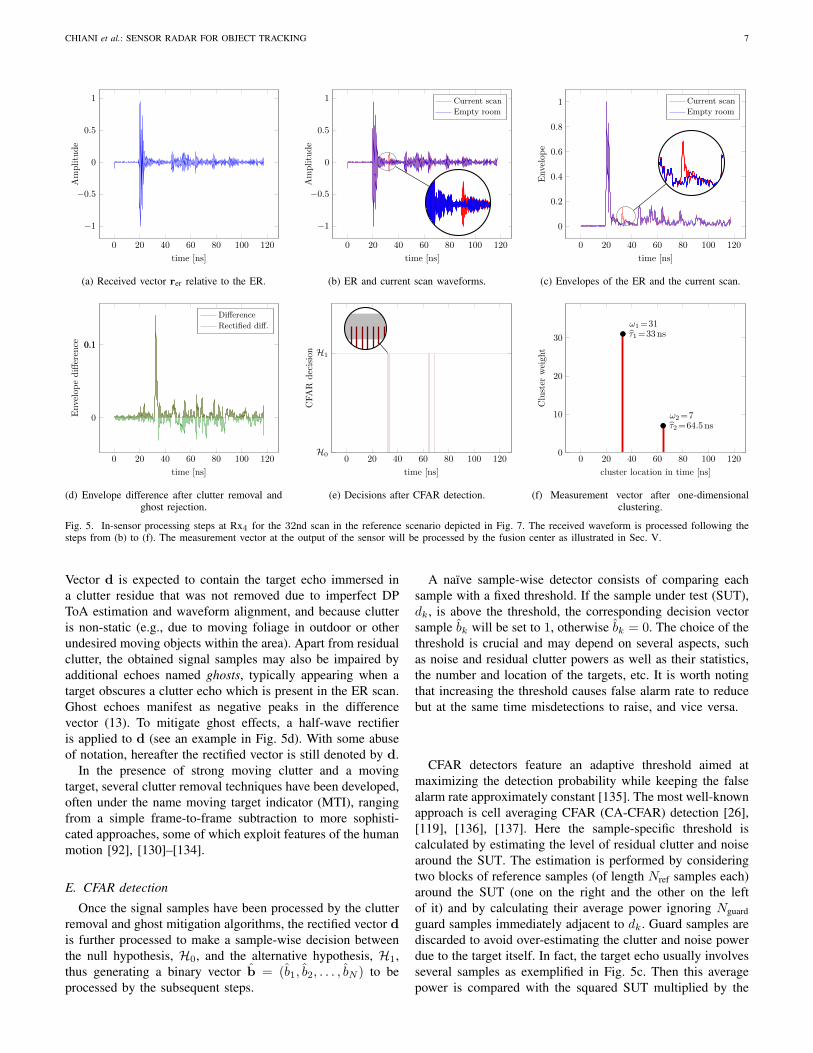
Fig. 5a shows the sampled scan waveform (12), rer

, whenthe target is not present, namely, in empty-room (ER) condi-tions. The scan presents a very high peak at ToA ⌧

0

= 20ns

due to the direct path (DP), as well as additional multipathcomponents induced by reflections in the propagation envi-ronment. In presence of a target in the monitored area, thesampled scan waveform r may look like the red one in Fig. 5b.As the figure emphasizes, the target produces an extra path,which is rather weak in the example waveform. This makesthe subsequent steps crucial for reliable detection and preciselocalization of the object. The target echo ToA is ⌧ = 32.6 ns.

B. Non-coherent demodulationBy processing vector r, whose kth element is given by

(12), it is possible to extract the ToA ⌧

0

of the DP. Since the8pl(t) may account for distortions due to antennas, reflections, frequency-

dependent RCS of the target, and filtering in the receiver front-end.9The actual scan duration is slightly higher as an inter-frame period is

present.

transmission is IR-based with a very large bandwidth, as theecho pulse is very short, ToA information may be extractedeven relying on non-coherent demodulation techniques, i.e.,the carrier phase needs neither to be estimated nor tracked[124]. This feature is very beneficial, as the pulse p

l

(t)

is usually unknown at the receiver because of unavoidabledistortions introduced by the channel and the antennas, dueto its very large bandwidth. A simple envelope detector maythus be applied both to the ER scan r

er

and to the current scanr to extract their envelopes ✏er and ✏.10 Envelope extractionmay be easily implemented by a squaring block followed bya low-pass filter. The result is exemplified in Fig. 5c, wherethe target echo is again detailed.

C. Direct path ToA estimationTo perform clutter removal (see next subsection), after

envelope extraction we need to provide an estimate ⌧

0

ofthe DP ToA, for both ✏er and ✏. In fact, once the twoDP ToA estimates are available, the two vectors can bealigned by shifting one of them by the appropriate amountb|⌧

0

� ⌧

0,er

|/Ts

c = b|�⌧

0

|/Ts

c.There are numerous techniques for ToA estimation in UWB-

IR systems; a detailed review may be found in [47]. A simpletechnique to detect the first arriving path is threshold crossing,where the signal envelope is compared with a threshold andthe first crossing gives the ToA [125], [126]. The thresh-old crossing detector performance is heavily influenced bythe threshold value, which needs to be carefully designedaccording to the operating conditions. A simple criterion todetermine a sub-optimal threshold, based on the evaluationof the probability of early detection and knowledge of noisepower, may be found in [125]. Several other sub-optimumapproaches have been proposed to reduce early detectionsthreshold-based estimation such as jump back and searchforward criterion (exploiting the detection of the strongestsample and a forward search procedure over a predefined timewindow), and serial backward search criterion (based on thedetection of the strongest sample and a search-back procedureover a predefined time window) [126], [127]. A comprehensiveframework for the analysis and design of threshold-based ToAestimators was developed in [128]. More robust techniques,which do not require knowledge of the signal statistics andnoise power, are investigated in [49], [129].

D. Clutter removal and ghost mitigationAfter alignment of the ER and the current scan, clutter

removal is performed as11

d = ✏� ✏er . (13)

10As opposed to ✏, which is computed in each frame, ER envelope ✏er isextracted only any time a new ER scan is acquired.

11In some cases, the alignment based on the DP ToA estimation of thetwo scans is not sufficiently accurate to perform an effective clutter removal.Since the two scans are very similar (see, e.g., Fig. 5c) cross-correlation peaksearching is an effective approach to estimate the relative temporal shift usedfor a finer alignment. Such approach can be further improved by performinginterpolation of the two scans at a higher sampling rate, before alignment,and then decimation after the scans subtraction, (13), to return to the initialsampling rate.

CHIANI et al.: SENSOR RADAR FOR OBJECT TRACKING 7

0 20 40 60 80 100 120

�1

�0.5

0

0.5

1

time [ns]

Amplitude

1

(a) Received vector rer relative to the ER.

0 20 40 60 80 100 120

�1

�0.5

0

0.5

1

time [ns]

Amplitude

Current scan

Empty room

0 20 40 60 80 100 120

�1

�0.5

0

0.5

1

time [ns]

Amplitude

Current scan

Empty room

1

(b) ER and current scan waveforms.

0 20 40 60 80 100 120

0

0.2

0.4

0.6

0.8

1

time [ns]

Envelope

Current scan

Empty room

0 20 40 60 80 100 120

0

0.2

0.4

0.6

0.8

1

time [ns]

Envelope

Current scan

Empty room

1

(c) Envelopes of the ER and the current scan.

0 20 40 60 80 100 120

0

0.10.1

time [ns]

Envelopedi↵erence

Di↵erence

Rectified di↵.

1

(d) Envelope difference after clutter removal andghost rejection.

0 20 40 60 80 100 120

H0

H1

time [ns]

CFAR

decision

0 20 40 60 80 100 120

H0

H1

time [ns]

CFAR

decision

1

(e) Decisions after CFAR detection.

0 20 40 60 80 100 120

0

10

20

30

!

1

=31

b⌧1

=33ns

!

2

=7

b⌧2

=64.5 ns

cluster location in time [ns]

Clusterweight

1

(f) Measurement vector after one-dimensionalclustering.

Fig. 5. In-sensor processing steps at Rx4 for the 32nd scan in the reference scenario depicted in Fig. 7. The received waveform is processed following thesteps from (b) to (f). The measurement vector at the output of the sensor will be processed by the fusion center as illustrated in Sec. V.

Vector d is expected to contain the target echo immersed ina clutter residue that was not removed due to imperfect DPToA estimation and waveform alignment, and because clutteris non-static (e.g., due to moving foliage in outdoor or otherundesired moving objects within the area). Apart from residualclutter, the obtained signal samples may also be impaired byadditional echoes named ghosts, typically appearing when atarget obscures a clutter echo which is present in the ER scan.Ghost echoes manifest as negative peaks in the differencevector (13). To mitigate ghost effects, a half-wave rectifieris applied to d (see an example in Fig. 5d). With some abuseof notation, hereafter the rectified vector is still denoted by d.

In the presence of strong moving clutter and a movingtarget, several clutter removal techniques have been developed,often under the name moving target indicator (MTI), rangingfrom a simple frame-to-frame subtraction to more sophisti-cated approaches, some of which exploit features of the humanmotion [92], [130]–[134].

E. CFAR detectionOnce the signal samples have been processed by the clutter

removal and ghost mitigation algorithms, the rectified vector dis further processed to make a sample-wise decision betweenthe null hypothesis, H

0

, and the alternative hypothesis, H1

,thus generating a binary vector ˆb = (

ˆ

b

1

,

ˆ

b

2

, . . . ,

ˆ

b

N

) to beprocessed by the subsequent steps.

A naïve sample-wise detector consists of comparing eachsample with a fixed threshold. If the sample under test (SUT),d

k

, is above the threshold, the corresponding decision vectorsample ˆb

k

will be set to 1, otherwise ˆbk

= 0. The choice of thethreshold is crucial and may depend on several aspects, suchas noise and residual clutter powers as well as their statistics,the number and location of the targets, etc. It is worth notingthat increasing the threshold causes false alarm rate to reducebut at the same time misdetections to raise, and vice versa.

CFAR detectors feature an adaptive threshold aimed atmaximizing the detection probability while keeping the falsealarm rate approximately constant [135]. The most well-knownapproach is cell averaging CFAR (CA-CFAR) detection [26],[119], [136], [137]. Here the sample-specific threshold iscalculated by estimating the level of residual clutter and noisearound the SUT. The estimation is performed by consideringtwo blocks of reference samples (of length Nref samples each)around the SUT (one on the right and the other on the leftof it) and by calculating their average power ignoring Nguardguard samples immediately adjacent to d

k

. Guard samples arediscarded to avoid over-estimating the clutter and noise powerdue to the target itself. In fact, the target echo usually involvesseveral samples as exemplified in Fig. 5c. Then this averagepower is compared with the squared SUT multiplied by the

8 PROCEEDINGS OF THE IEEE, VOL. 106, NO. 6, JUNE 2018

threshold ↵ as

d

2

k

H1

?H

0

↵

Pi2S

k

d

2

i

2Nrefk = 1, . . . , N (14)

where Sk

= {k�Nguard�Nref, . . . , k�Nguard�1, k+Nguard+

1, . . . , k+Nguard+Nref}\{1, 2, . . . , N} is the set of referencesamples.

A drawback of CA-CFAR is target masking, a problemarising when another target falls into the reference set S

k

,thus increasing considerably the reference power and leadingto a wrong decision for H

0

. To overcome such a limita-tion, several variants of the CA-CFAR detector have beenintroduced, depending on the specific type of waveform andon the scenario. A simple variation of CA-CFAR is globalCFAR (G-CFAR) where the reference samples are extendedto all scan samples except for the guard ones. Formally,the detector still has the structure (14) in which S

k

=

{1, . . . , k �Nguard � 1, k +Nguard + 1, . . . , N}. This way theSUT is compared with an estimated power which dependson the whole scan (and not on local reference samples), thusaveraging out the echoes from the other targets over a largerinterval. This approach turns out to be effective only whenthe number of targets inside the monitored area is small andthe scan period is long enough. As a drawback, moreover, theinformation associated with neighbor samples, which couldbe useful for a better decision based on local residual clutter,is now overlooked. This last aspect is quite important, as inan indoor scenario clutter is non-homogeneous [138]–[140].In these contexts, a more sophisticated variant of CA-CFAR,named ordered statistics (OS-CFAR), performs ordering of thereference samples S

k

according to their magnitude and byselecting a certain predefined value from the ordered sequence[135]. Thanks to ranking, OS-CFAR is proven to be morerobust than CA-CFAR and G-CFAR in the presence of outliers,has happens in non-homogeneous clutter.

In the context of UWB indoor radar tracking, a recent pro-posal called double threshold and buffer CFAR (DTB-CFAR)allows overcoming the above limitations by means of anadaptive threshold setting strategy [65]. For each sample d

k

of the rectified vector d, the detector takes a binary decision

d

2

k

H1

?H

0

↵lLp + ↵g Gp k = 1, . . . , N (15)

where Lp and Gp are defined as the local and the globalpower respectively, whereas ↵l and ↵g are weighting factors.The reference powers Lp and Gp, and thus the threshold⌘ = ↵lLp + ↵g Gp, are calculated through Algorithm 1. Inparticular, Gp = (1/N)

PN

i=1

d

2

i

is the average power of therectified vector d, whereas Lp is the average power of a firstin first out buffer, s = (s

1

, . . . , s

Nb), of length Nb, filled withthe already processed d samples that were found to be belowthreshold. This way we reduce the misdetection rate in caseof multiple-target scenarios as we keep track of the decisionspreviously taken during the scan. Keeping Nb short, it ispossible to get a local estimate of the noise and residual clutterpower level for the near-SUT samples. However, since target

echo has a length of several samples, the overall threshold(due to L

p

) increases very quickly, causing misdetections. Toavoid this phenomenon, if the increment of the SUT withrespect to the previous sample is larger than a predefinedvalue, �⌘, for at least qmax consecutive samples, then L

p

isnot updated. Thus, since residual clutter and target presenceare characterized by similar echoes with the only differencethat the latter ones are generally significantly larger than theformer ones, ⌘ is expected to increase quickly enough to avoidfalse alarms but also be frozen soon enough to properly detectthe target. Later, the value of L

p

is unfrozen when a waveformdecrease occurs.

To further decrease misdetections, because of the asymmet-ric target echo, DTB-CFAR is applied to the scan twice inopposite directions. Then, the two outputs are merged throughan element-wise OR operator to form the final vector. It hasbeen experimentally verified that DTB-CFAR provides betterperformance than conventional approaches (e.g., CA-CFAR) incase of multiple human targets in densely cluttered environ-ments. Hereafter, we denote by ˆb the binary vector generatedby DTB-CFAR from processing of d (see Fig. 1). An exampleis depicted in Fig. 5e when ↵l = 5, ↵g = 8, Nb = 25,and qmax = 4. In the example, ˆb exhibit three bursts of‘1’s corresponding to three possible targets. Such vector willbe further processed within the sensor by one-dimensionalclustering.12

F. One-dimensional clusteringThe generic vector ˆb returned by the detector is typically

characterized by bursts of ‘1’s, each due to a specific targetor (to a lesser extent) to residual clutter. To further filter outfalse alarms due to residual clutter and limit the computationalcomplexity of network processing, a clustering algorithm isapplied to the vector ˆb, resulting in a new binary vectordenoted by b. We call this clustering step one-dimensionalclustering (see Fig. 1). Since no a priori knowledge of thenumber of clusters is available, hierarchical clustering is aneffective approach [141], [142].

In the beginning, each ‘1’ forms a singleton cluster. Then,iteratively as long as the minimum distance between twoclusters is less than a preset distance threshold, dthr, the twoclusters at minimum distance are merged.13 At the end, eachsurvived cluster is replaced by a single ‘1’ in the medianposition. Furthermore, a weight ! equal to the number ofclusterized ‘1’s is associated with every final cluster. As theclusters associated with targets typically exhibit higher weightsthan those related to clutter or noise, it is useful to set alsoa weight-based threshold, !

min

, so that the lightest survivedclusters (having a weight less than !

min

), are discarded andthe corresponding elements of b are set to ‘0’.

12It is worthwhile remarking that the vector b computed by each sensornode contains detection information for all targets in the area. As the qualityof the channel between the Tx, a specific target, and a specific Rx depends onthe target position (e.g., this is true for the SNR given by (2)), different sensornodes are likely to deliver detection information with a different quality pereach target. This consideration applies to any in-sensor detector.

13We define the distance between two clusters as the distance between theircentroids (i.e., the median positions among the ‘1’s which compose thoseclusters at the current iteration).

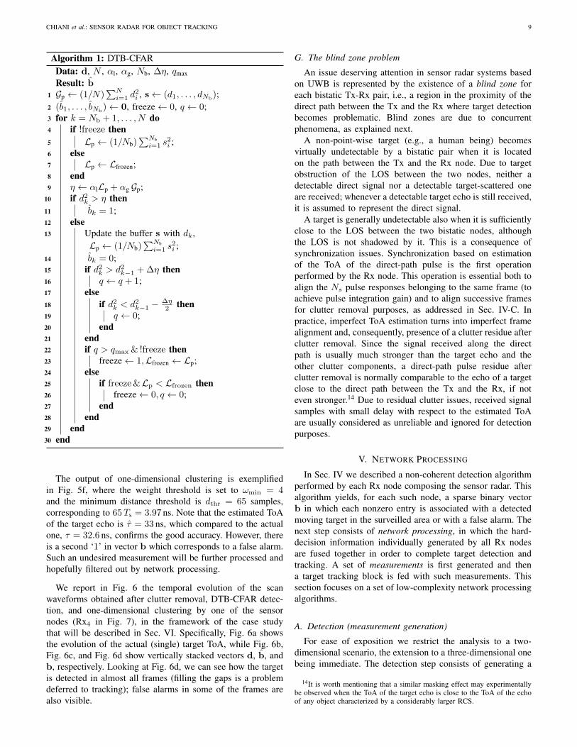
CHIANI et al.: SENSOR RADAR FOR OBJECT TRACKING 9

Algorithm 1: DTB-CFARData: d, N , ↵l, ↵g, Nb, �⌘, qmax

Result: ˆb1 Gp (1/N)

PN

i=1

d

2

i

, s (d

1

, . . . , d

Nb);2 (

ˆ

b

1

, . . . ,

ˆ

b

Nb) 0, freeze 0, q 0;3 for k = N

b

+ 1, . . . , N do4 if !freeze then5 Lp (1/Nb)

PNbi=1

s

2

i

;6 else7 Lp Lfrozen;8 end9 ⌘ ↵lLp + ↵g Gp;

10 if d2k

> ⌘ then11 ˆ

b

k

= 1;12 else13 Update the buffer s with d

k

,Lp (1/Nb)

PNbi=1

s

2

i

;14 ˆ

b

k

= 0;15 if d2

k

> d

2

k�1

+�⌘ then16 q q + 1;17 else18 if d2

k

< d

2

k�1

� �⌘

2

then19 q 0;20 end21 end22 if q > q

max

& !freeze then23 freeze 1,Lfrozen Lp;24 else25 if freeze&L

p

< Lfrozen

then26 freeze 0, q 0;27 end28 end29 end30 end

The output of one-dimensional clustering is exemplifiedin Fig. 5f, where the weight threshold is set to !

min

= 4

and the minimum distance threshold is d

thr

= 65 samples,corresponding to 65Ts = 3.97 ns. Note that the estimated ToAof the target echo is ⌧ = 33 ns, which compared to the actualone, ⌧ = 32.6 ns, confirms the good accuracy. However, thereis a second ‘1’ in vector b which corresponds to a false alarm.Such an undesired measurement will be further processed andhopefully filtered out by network processing.

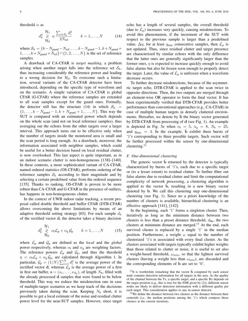
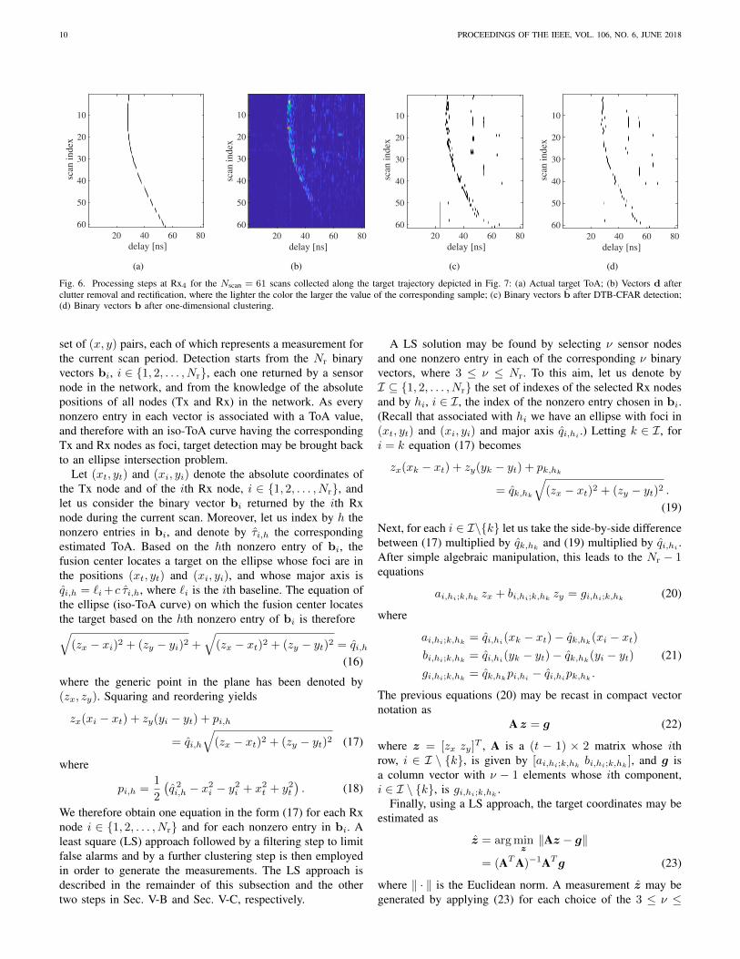
We report in Fig. 6 the temporal evolution of the scanwaveforms obtained after clutter removal, DTB-CFAR detec-tion, and one-dimensional clustering by one of the sensornodes (Rx

4

in Fig. 7), in the framework of the case studythat will be described in Sec. VI. Specifically, Fig. 6a showsthe evolution of the actual (single) target ToA, while Fig. 6b,Fig. 6c, and Fig. 6d show vertically stacked vectors d, ˆb, andb, respectively. Looking at Fig. 6d, we can see how the targetis detected in almost all frames (filling the gaps is a problemdeferred to tracking); false alarms in some of the frames arealso visible.

G. The blind zone problem

An issue deserving attention in sensor radar systems basedon UWB is represented by the existence of a blind zone foreach bistatic Tx-Rx pair, i.e., a region in the proximity of thedirect path between the Tx and the Rx where target detectionbecomes problematic. Blind zones are due to concurrentphenomena, as explained next.

A non-point-wise target (e.g., a human being) becomesvirtually undetectable by a bistatic pair when it is locatedon the path between the Tx and the Rx node. Due to targetobstruction of the LOS between the two nodes, neither adetectable direct signal nor a detectable target-scattered oneare received; whenever a detectable target echo is still received,it is assumed to represent the direct signal.

A target is generally undetectable also when it is sufficientlyclose to the LOS between the two bistatic nodes, althoughthe LOS is not shadowed by it. This is a consequence ofsynchronization issues. Synchronization based on estimationof the ToA of the direct-path pulse is the first operationperformed by the Rx node. This operation is essential both toalign the N

s

pulse responses belonging to the same frame (toachieve pulse integration gain) and to align successive framesfor clutter removal purposes, as addressed in Sec. IV-C. Inpractice, imperfect ToA estimation turns into imperfect framealignment and, consequently, presence of a clutter residue afterclutter removal. Since the signal received along the directpath is usually much stronger than the target echo and theother clutter components, a direct-path pulse residue afterclutter removal is normally comparable to the echo of a targetclose to the direct path between the Tx and the Rx, if noteven stronger.14 Due to residual clutter issues, received signalsamples with small delay with respect to the estimated ToAare usually considered as unreliable and ignored for detectionpurposes.

V. NETWORK PROCESSING

In Sec. IV we described a non-coherent detection algorithmperformed by each Rx node composing the sensor radar. Thisalgorithm yields, for each such node, a sparse binary vectorb in which each nonzero entry is associated with a detectedmoving target in the surveilled area or with a false alarm. Thenext step consists of network processing, in which the hard-decision information individually generated by all Rx nodesare fused together in order to complete target detection andtracking. A set of measurements is first generated and thena target tracking block is fed with such measurements. Thissection focuses on a set of low-complexity network processingalgorithms.

A. Detection (measurement generation)

For ease of exposition we restrict the analysis to a two-dimensional scenario, the extension to a three-dimensional onebeing immediate. The detection step consists of generating a

14It is worth mentioning that a similar masking effect may experimentallybe observed when the ToA of the target echo is close to the ToA of the echoof any object characterized by a considerably larger RCS.

10 PROCEEDINGS OF THE IEEE, VOL. 106, NO. 6, JUNE 2018

20 40 60 80delay [ns]

10

20

30

40

50

60

scan

index

1

(a)

20 40 60 80

delay [ns]

10

20

30

40

50

60sc

an i

ndex

1

(b)

20 40 60 80

delay [ns]

10

20

30

40

50

60

scan

index

1

(c)

20 40 60 80

10

20

30

40

50

60

scan

index

delay [ns]

1

(d)

Fig. 6. Processing steps at Rx4 for the Nscan = 61 scans collected along the target trajectory depicted in Fig. 7: (a) Actual target ToA; (b) Vectors d afterclutter removal and rectification, where the lighter the color the larger the value of the corresponding sample; (c) Binary vectors b after DTB-CFAR detection;(d) Binary vectors b after one-dimensional clustering.

set of (x, y) pairs, each of which represents a measurement forthe current scan period. Detection starts from the N

r

binaryvectors b

i

, i 2 {1, 2, . . . , Nr

}, each one returned by a sensornode in the network, and from the knowledge of the absolutepositions of all nodes (Tx and Rx) in the network. As everynonzero entry in each vector is associated with a ToA value,and therefore with an iso-ToA curve having the correspondingTx and Rx nodes as foci, target detection may be brought backto an ellipse intersection problem.

Let (xt

, y

t

) and (x

i

, y

i

) denote the absolute coordinates ofthe Tx node and of the ith Rx node, i 2 {1, 2, . . . , N

r

}, andlet us consider the binary vector b

i

returned by the ith Rxnode during the current scan. Moreover, let us index by h thenonzero entries in b

i

, and denote by ⌧

i,h

the correspondingestimated ToA. Based on the hth nonzero entry of b

i

, thefusion center locates a target on the ellipse whose foci are inthe positions (x

t

, y

t

) and (x

i

, y

i

), and whose major axis isq

i,h

= `

i

+ c ⌧

i,h

, where `

i

is the ith baseline. The equation ofthe ellipse (iso-ToA curve) on which the fusion center locatesthe target based on the hth nonzero entry of b

i

is thereforeq(z

x

� x

i

)

2

+ (z

y

� y

i

)

2

+

q(z

x

� x

t

)

2

+ (z

y

� y

t

)

2

= q

i,h

(16)

where the generic point in the plane has been denoted by(z

x

, z

y

). Squaring and reordering yields

z

x

(x

i

� x

t

) + z

y

(y

i

� y

t

) + p

i,h

= q

i,h

q(z

x

� x

t

)

2

+ (z

y

� y

t

)

2 (17)

where

p

i,h

=

1

2

�q

2

i,h

� x

2

i

� y

2

i

+ x

2

t

+ y

2

t

�. (18)

We therefore obtain one equation in the form (17) for each Rxnode i 2 {1, 2, . . . , N

r

} and for each nonzero entry in bi

. Aleast square (LS) approach followed by a filtering step to limitfalse alarms and by a further clustering step is then employedin order to generate the measurements. The LS approach isdescribed in the remainder of this subsection and the othertwo steps in Sec. V-B and Sec. V-C, respectively.

A LS solution may be found by selecting ⌫ sensor nodesand one nonzero entry in each of the corresponding ⌫ binaryvectors, where 3 ⌫ N

r

. To this aim, let us denote byI ✓ {1, 2, . . . , N

r

} the set of indexes of the selected Rx nodesand by h

i

, i 2 I, the index of the nonzero entry chosen in bi

.(Recall that associated with h

i

we have an ellipse with foci in(x

t

, y

t

) and (x

i

, y

i

) and major axis q

i,h

i

.) Letting k 2 I, fori = k equation (17) becomes

z

x

(x

k

� x

t

) + z

y

(y

k

� y

t

) + p

k,h

k

= q

k,h

k

q(z

x

� x

t

)

2

+ (z

y

� y

t

)

2

.

(19)

Next, for each i 2 I\{k} let us take the side-by-side differencebetween (17) multiplied by q

k,h

k

and (19) multiplied by q

i,h

i

.After simple algebraic manipulation, this leads to the N

r

� 1

equations

a

i,h

i

;k,h

k

z

x

+ b

i,h

i

;k,h

k

z

y

= g

i,h

i

;k,h

k

(20)

where

a

i,h

i

;k,h

k

= q

i,h

i

(x

k

� x

t

)� q

k,h

k

(x

i

� x

t

)

b

i,h

i

;k,h

k

= q

i,h

i

(y

k

� y

t

)� q

k,h

k

(y

i

� y

t

) (21)g

i,h

i

;k,h

k

= q

k,h

k

p

i,h

i

� q

i,h

i

p

k,h

k

.

The previous equations (20) may be recast in compact vectornotation as

A z = g (22)

where z = [z

x

z

y

]

T , A is a (t � 1) ⇥ 2 matrix whose ithrow, i 2 I \ {k}, is given by [a

i,h

i

;k,h

k

b

i,h

i

;k,h

k

], and g isa column vector with ⌫ � 1 elements whose ith component,i 2 I \ {k}, is g

i,h

i

;k,h

k

.Finally, using a LS approach, the target coordinates may be

estimated as

ˆ

z = argmin

zkAz � gk

= (AT A)

�1AT

g (23)

where k · k is the Euclidean norm. A measurement ˆ

z may begenerated by applying (23) for each choice of the 3 ⌫

CHIANI et al.: SENSOR RADAR FOR OBJECT TRACKING 11

N

r

nonzero elements, one per binary vector b created by aspecific sensor node as described in Sec. IV. The approachhere followed consists of choosing a value of ⌫, consideringall possible ⌫-tuples of nonzero vector elements, one per Rxnode, and generating one LS measurement per each ⌫-tuple.The number of measurements generated with this approach isdenoted by N

d

in Fig. 1.The described measurement generation method inherently

creates a relatively large number of false alarms. If no targetis present in the area, false alarms are due to LS solutionscombining nonzero vector elements caused by noise or clutterresidues (i.e., by local false alarms at the ⌫ Rx nodes). We willcall these false alarms as type-1 false alarms. When only onetarget is present, additional false alarms are due to LS solutionsthat combine nonzero vector elements associated with thetarget and nonzero vector elements being local false alarms.These false alarms will be referred to as type-2 false alarms.Finally, when multiple targets are present, additional falsealarms are generated by LS solutions that combine nonzerovector elements associated with different targets. False alarmsof this type will be referred to as type-3 false alarms.

The behavior of the detection algorithm (in terms of misseddetections and number of generated false alarms) is sensitive tochoice of the parameter ⌫. To see this, we can look for exampleat the number of generated type-3 false alarms. Under theassumption that all M � 2 targets are detected by each of the ⌫Rx nodes and that each target corresponds to a unique nonzeroelement in each vector (perfect one-dimensional clustering),the number of type-3 false alarms is readily given by

Nfa,3 =

N

r

!

⌫!(N

r

� ⌫)!

(M

⌫ �M) . (24)

For Nr

= 3, ⌫ is constrained to be equal to 3 yielding Nfa,3 =

M

3�M . For Nr

= 4, if M 2 {2, 3} then a smaller number oftype-3 false alarms is attained by ⌫ = 4, while it is attained by⌫ = 3 for any M � 4. For N

r

� 5, there exists ¯

M =

¯

M(N

r

)

such that: if M ¯

M then when ⌫ is increased from 3 to N

r

the value of Nfa,3 initially increases, then it reaches a peak andfinally decreases; if M >

¯

M then the value of Nfa,3 increasesmonotonically with ⌫ 2 {3, 4, . . . , N

r

}.

B. Decreasing the false alarm rate

Due to the relatively large number of false alarms generatedby the LS-based detector, a method to substantially reducethe false alarm rate at the input of the tracking filter becomesof fundamental importance. In this respect, a measurementselection is performed by introducing a notion of reliabilityfor LS solutions. This is possible by exploiting both theweight ! associated with each nonzero entry in each of theN

r

binary vectors bi

at the end of the in-sensor processing,and the residual error (RE), a measure of reliability inherentlyprovided by the LS approach.

The RE associated with a LS solution (23) is

RE(ˆz) = kAˆ

z � gk . (25)

The idea is to keep a measurement if and only if its associatedweight is above some threshold and its associated RE is below

some other threshold, where both thresholds are invariant forall measurements. The weight of a measurement is defined asthe sum of the weights of the ⌫ nonzero vector entries yieldingthat measurement through (23), i.e., ⌦ =

Pi2I !

i

. Settinga threshold ⌦th on the minimum acceptable measurementweight is effective in filtering out type-1 false alarms and thosetype-2 false alarms that are mostly contributed by local falsealarms at Rx nodes. Type-3 false alarms, however, are mostoften characterized by a weight above ⌦th since they arise ascombinations of local detections of different targets. Setting athreshold REth on the maximum tolerable RE is effective infiltering out also type-3 false alarms.

The number of surviving measurements after comparisonof their weight and RE on the corresponding thresholds isdenoted by N

m

N

d

. For the sake of notational sim-plicity, surviving measurements will be simply denoted byz

1

, z

2

, . . . , z

Nm (see Fig. 1). Residual false alarms are possibleeven after the described selection procedure. In particular,while type-1 false alarms are usually filtered out, the type-2 and type-3 ones being the result of combining some localdetections of the same target might survive. Since these falsealarms tend to generate measurements around the correspond-ing target position, a two-dimensional clustering operation iseffective in reducing their rate. Two-dimensional clustering isalso useful in presence of imperfect one-dimensional cluster-ing.

C. Measurement clustering

The N

m

measurements passing the false alarm reductionstep tend to form clouds of points; this is particularly true whenthe number of sensors in the radar network is larger than three.Since the complexity of the processing to be performed in thesubsequent tracking and data association steps is dependenton the number of measurements incoming from the detector,a further clustering operation (besides the one performed atnode level) is applied to measurements. The approach is againhierarchical, iterative, and without an a priori specified numberof clusters. It relies on the concept of distance between twoclusters, for which several definitions are in principle possible.

Letting Z1

= {z1,1

, z

1,2

, . . . , z

1,n

} and Z2

=

{z2,1

, z

2,2

, . . . , z

2,m

} be two clusters of measurements withcardinality n and m, respectively, a common notion of distancebetween Z

1

and Z2

, denoted by d

(c)

c

(Z1

,Z2

), is

d

(c)

c

(Z1

,Z2

) = kc(Z1

)� c(Z2

)k (26)

where c(Z ) is the centroid of cluster Z . It is defined as

c(Z ) =

1

|Z |X

z2Z

z (27)

and in general does not coincide with any element of thecluster.

As mentioned, (26) is not the only possible definition ofdistance between clusters, as at least two other definitionsare of practical interest. The first one measures the distancebetween two clusters Z

1

and Z2

as the minimum Euclidean

12 PROCEEDINGS OF THE IEEE, VOL. 106, NO. 6, JUNE 2018

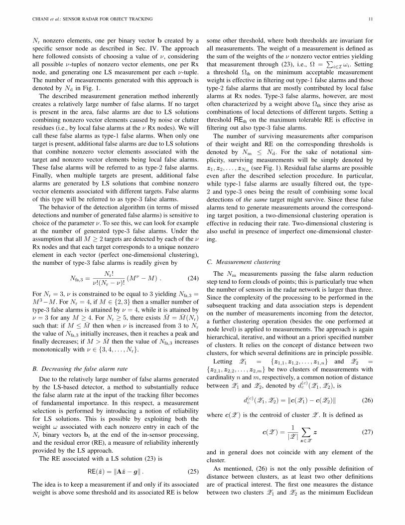
Algorithm 2: Measurement ClusteringData: N

m

, {z1

, z

2

, . . . , z

Nm}Result: N

cluster

, Z1

,Z2

, . . . ,ZNcluster

1 d

min

1; Ncluster

N

m

; stop 0;2 for i = 1, . . . , N

m

do3 Z

i

{zi

};4 end5 while (!stop) do6 for i = 1, . . . , N

cluster

� 1 do7 for j = i+ 1, . . . , N

cluster

do8 if d

c

(Zi

,Zj

) < d

min

then9 d

min

d

c

(Zi

,Zj

);10 i

min

= i;11 j

min

= j;12 end13 end14 end15 if d

min

< d

thr

then16 Z

imin Zimin [Z

jmin ;17 for j = j

min

, . . . , N

cluster

� 1 do18 Z

j

Zj+1

;19 end20 N

cluster

N

cluster

� 1;21 else22 stop 1;23 end24 end

distance between one element z

1

2 Z1

and one elementz

2

2 Z2

, namely,

d

(m)

c

(Z1

,Z2

) = min

(z1,z2)2Z1⇥Z2

kz1

� z

2

k . (28)

The second one is similar but relies on the maximum Eu-clidean distance between any two measurements of which onebelongs to the first cluster and the other to the second:

d

(M)

c

(Z1

,Z2

) = max

(z1,z2)2Z1⇥Z2

kz1

� z

2

k . (29)

The measurement clustering procedure is formalized inAlgorithm 2. As also shown in Fig. 1, its input is representedby the set of all measurements generated by the detectionblock and surviving the false alarm rate reduction step, alongwith its cardinality N

m

; its output is a partition of this setalong with the number of parts (i.e., clusters) N

cluster

. In thebeginning each measurements z

i

forms a singleton cluster{z

i

} and therefore N

cluster

= N

m

. At each iteration, theminimum distance d

min

between any two clusters is computedand compared with a threshold d

thr

; if d

min

< d

thr

then thetwo corresponding clusters are merged to form a new clusterof larger cardinality and the number of clusters N

cluster

isdecreased by one. The algorithm terminates when no pair ofclusters is found whose distance is smaller than the threshold.The N

cluster

centroids of the finals clusters are forwarded tothe multitarget tracking algorithm (Sec. V-D).

From a complexity viewpoint, during the first iteration ofthe algorithm, the one working on singleton clusters, we

need to compute�Nm

2

�Euclidean distance values. Moreover,

if the centroid-based definition of distance between clustersis adopted, during each subsequent iteration we need tocalculate one centroid (for the new cluster formed during theprevious iteration) through (27) and N

cluster

� 1 Euclideandistance values, where N

cluster

is the number of clusters at thebeginning of the iteration.15 The number of Euclidean distancevalues to be computed is then

✓N

m

2

◆+

NitX

i=2

(N

m

� i) (N

m

� 1)

2 (30)

where N

it

is the number of iterations (which depends on themeasurements and on the threshold d

thr

) and where the upperbound is obtained by observing that N

it

N

m

� 1. Thus, theright-hand side of (30) is the number of Euclidean distancecomputations in case all measurements are clustered together.

In Algorithm 2, the distance between two clusters Zi

andZ

j

has been generically denoted by d

c

(Zi

,Zj

). With respectto the definition (26) based on cluster centroids, the definition(28) based on the minimum distance between measurementstends to generate a smaller number N

cluster

of clusters ofrelatively larger size, while the definition (29) based on themaximum distance between measurements is more conser-vative and tends to give rise to a larger number N

cluster

ofclusters of relatively smaller size.

D. Object trackingThe output of the measurement clustering step at scan

period k is a finite set of (unordered) measurements Z

k

=

{z1

, z

2

, . . . , z

m

k

}k

, where m

k

= N

cluster

and where (withsome abuse of notation) z

i

is the centroid of the ith clusterout of the N

cluster

final ones. Individual measurements in theset Z

k

may be originated both by target detections and by falsealarms. An admissible value for Z

k

is ; (empty set, in case ofno false alarms and all targets missed) and its cardinality m

k

is subject to variations from frame to frame. In the following,the conventional notation Z

(k) will be used to indicate thesequence Z

1

, Z

2

, . . . , Z

k

of all observed measurement sets upto scan period k. In the specific case of the LS detector com-bining CFAR detections from individual sensors, if Z

k

6= ;then each measurement z 2 Z

k

comprises position coordinates(z = [z

x

z

y

]

T in a simple two-dimensional scenario).The state of a single target will be denoted by x and the

single target state space, to which x belongs, by X . The singletarget state x may in principle include target position, velocity,and acceleration components; in the RSN presented in thispaper, sticking to a simple two-dimensional scenario, we havedefined x = [x x y y]

T . Rigorously, the multitarget state isdefined as a random finite set (RFS) X = {x

1

,x

2

, . . . ,x

M

}whose cardinality M is the number of targets and whoseelements are the states of the M targets. Again, ; (no target)is an admissible value for X .

A multitarget Bayesian filter would allow optimally track-ing, in every scan period k, the a posteriori probability density

15The number of Euclidean distance values to be computed during alliteration but the first one is not

�Ncluster2

�since we only need to compute

the distance between the new cluster and the existing ones.

CHIANI et al.: SENSOR RADAR FOR OBJECT TRACKING 13

function (p.d.f.) fk|k(X|Z(k)

) of the multitarget state.16 Due tointractable complexity of the theoretically optimum solution,it is common to rely on approximations. A very popularapproximation of the multitarget Bayesian filter is representedby Mahler’s probability hypothesis density (PHD) filter [145],capable to recursively track the a posteriori multitarget statePHD. This latter quantity, a function D

k|k(x|Z(k)

) : X 7! R(hereafter also abbreviated to D

k|k(x)), represents the first-order moment of the a posteriori p.d.f. f

k|k(X|Z(k)

) and isoperatively given by

D

k|k(x) =

1X

n=0

1

n!

Z

Xf

k|k({x, ⇠1, . . . , ⇠n}) d⇠1 · · · d⇠n .(31)

It may be interpreted as the density of targets in the sin-gle target state space X . As such, its integral E[M ]

k|k :=RX D

k|k(x|Z(k)

) dx represents the expected number of targetsin the scene given the whole measurements history Z

(k).Multitarget state tracking based on the measurements gen-

erated by the LS-based detector followed by the clusteringstep has been performed by employing a basic single-sensorPHD filter (i.e., not in its cardinalized version also trackingthe probability mass function of the number of targets inthe scene). The single-sensor version of the filter may beemployed since, although the sensor radar is composed ofseveral sensors, measurements generation is performed at thefusion center. It should be remarked that the PHD filterderivation (see [145]) is based on a multitarget motion modelin which target motions are statistically independent, targetsmay disappear from the scene, new targets may appear in thescene (independently of existing targets), and new targets maybe spawned from existing ones. Furthermore, it assumes ameasurement model where each target generates at most onemeasurement, all measurements are independent conditionallyon the multitarget state X , missed detections are possible,and the false alarm process is a multi-object Poisson process.While the multitarget motion model seems not critical inUWB sensor radar applications, we underline that fulfillmentof the condition of having no more than one measurement pertarget heavily relies on the success of the described clusteringoperations.

The basic PHD filter prediction and (approximate) correc-tion equations are

D

k+1|k(x) = b

k+1|k(x) +

Z

XF

k+1|k(x|⇠)Dk|k(⇠) d⇠ (32)

and

D

k+1|k+1

(x) ⇡ D

k+1|k(x)h1� p

D

(x)

+

X

z2Z

k+1

p

D

(x)'

k+1

(z|x)� c

k+1

(z) +

RX p

D

(⇠)'

k+1

(z|⇠)d⇠i.

(33)

16For a rigorous probabilistic approach to RFSs and multitarget Bayesfiltering the reader is referred, for example, to [143] or to [144].

In (32), b

k+1|k(x) is the PHD of new targets appearing inthe scene17 while F

k+1|k(x|⇠) = p

s,k+1|k(⇠)µk+1|k(x|⇠) +�

k+1|k(x|⇠), being p

s,k+1|k(⇠) the probability that a targetexisting at time k with state ⇠ survives at time k + 1,µ

k+1|k(x|⇠) the single target motion model (transition den-sity), and �

k+1|k(x|⇠) the PHD of spawning targets.18 Fur-thermore, in (33), p

D

(x) := p

D,k+1

(x) is the probabilitythat a measurement is collected at scan time k + 1 from atarget having state x, � := �

k+1

is the average number offalse alarms, c

k+1

(z) is the false alarm distribution in themeasurement space, and '

k+1

(z|x) is the measurement model(or sensor likelihood function).

Equations (32) and (33) have been implemented using aparticle approach. The implemented particle filter comprisesthe usual steps, i.e., prediction (existing particles at scan timek are updated based on the motion model), correction (particleweights are updated based on new measurements), resampling.New particles are initialized in each iteration around eachmeasurement, in oder to track possible new targets appearingin the scene, the sum of the weights of these newly introducedparticles being equal to

RX b

k+1|k(x) dx as required. Thenumber of particles is maintained constant over time byresampling. At the end of the correction step of each iterationof the particle filter, the particles along with their weights forma discretized version of the PHD D

k|k(x). As such, the sumof all particle weights represents the particle approximationof the (a posteriori) expected number of targets in the scene,E[M ]

k|k. We then define the estimated number of targets atscan time k, ˆ

M

k|k, as the integer closest to E[M ]

k|k andthe (a posteriori) estimated target states as the ˆ

M

k|k largestpeaks of the PHD function. This latter step is performedthrough an expectation-maximization (EM) algorithm fittingthe discretized PHD with ˆ

M

k|k Gaussian functions.

E. Data association

In several RSN applications we may want to have one track(sequence of target states) associated with each detected target.When this is the case, a data association problem shall besolved, consisting of performing an association between exist-ing tracks and new filtered measurements. Popular solutionsfor data association in multi-target tracking problems dateback to the Seventies [146]–[149]; another popular techniqueis the multiple hypothesis tracking (MHT) algorithm [150].Since a plain PHD filter does not automatically perform dataassociation, this problem has been the subject of several morerecent studies in the framework of PHD filtering [151]–[153].

The data association method designed for the proposedsensor radar is a relatively-simple algorithm whose input atscan time k is represented by the set of existing tracks inheritedfrom scan time k � 1 and by the ˆ

M

k|k target state estimates(PHD peaks) returned by the PHD filter, and whose output is

17bk+1|k(x) =

P1n=0

1n!

RX bk+1|k({x, ⇠1, . . . , ⇠n}) d⇠1 · · · d⇠n,

where bk+1|k(X) is the p.d.f. of new targets with multitarget state X

appearing at scan time k + 1.18�k+1|k(x|⇠) =

P1n=0

1n!

RX �k+1|k({x, ⇠1, . . . , ⇠n|⇠}) d⇠1 · · · d⇠n,

where �k+1|k(X|⇠) is the p.d.f. of new targets with multitarget state X

spawned at scan time k + 1 from a target with state ⇠ at time k.

14 PROCEEDINGS OF THE IEEE, VOL. 106, NO. 6, JUNE 2018

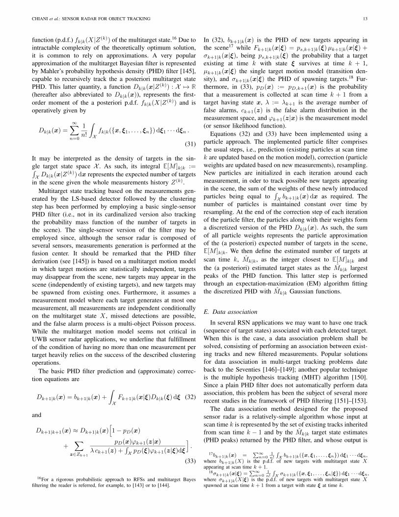
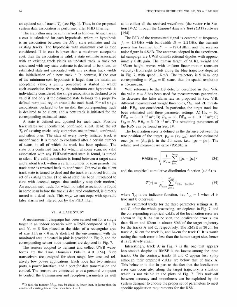
an updated set of tracks Tk

(see Fig. 1). Thus, in the proposedsystem data association is performed after PHD filtering.

The algorithm may be summarized as follows. At each scan,a cost is calculated for each hypothesis, where an hypothesisis an association between the ˆ

M

k|k state estimates and theexisting tracks. The hypothesis with minimum cost is thenconsidered. If its cost is lower than a maximum acceptablecost, then the association is valid: a state estimate associatedwith an existing track yields an updated track, a track notassociated with any state estimate is declared to be silent, anestimated state not associated with any existing track yieldsthe initialization of a new track.19 In contrast, if the costof the minimum-cost hypothesis is larger than the maximumacceptable value, a gating procedure is started in whicheach association foreseen by the minimum cost hypothesis isindividually considered: the single association is declared to bevalid if and only if the estimated state belongs to a properly-defined permitted region around the track head. For all singleassociations declared to be invalid, the corresponding trackis declared to be silent, and a new track is initiated for thecorresponding estimated state.

A state is defined and updated for each track. Possibletrack states are unconfirmed, confirmed, silent, dead; the setTk

of existing tracks only comprises unconfirmed, confirmed,and silent ones. The state of every newly initiated track isunconfirmed. It is turned to confirmed after a certain numberof scans, in all of which the track has been updated. Thestate of a confirmed track for which, at some scan, no validassociation with any PHD-estimated state is found, is turnedto silent. If a valid association is found between a target stateand a silent track within a certain number of scan periods, thetrack state is reverted back to confirmed. Otherwise the silenttrack state is turned to dead and the track is removed from theset of existing tracks. (The silent state has been introduced tocope with detected targets that suddenly stop their motion.)An unconfirmed track, for which no valid association is foundin some scan before the track is declared confirmed, is directlyturned to a dead track. This way, we can cope with sporadicfalse alarms not filtered out by the PHD filter.

VI. A CASE STUDY

A measurement campaign has been carried out for a singletarget in an indoor scenario with a RSN composed of a Txand N

r

= 6 Rxs placed at the sides of a rectangular areaof size 11.5m ⇥ 6m. A sketch of the environment with themonitored area indicated in pink is provided in Fig. 2, and thecorresponding sensor node locations are depicted in Fig. 7.

The sensors adopted to transmit and collect UWB wave-forms are the Time Domain’s PulsOn 410 [154]. Suchtransceivers are designed for short range, low cost and rel-atively low power applications. Each node has two antennaports, a power interface, and a port for data transmission andcontrol. The sensors are connected with a personal computerto control the transmission and reception parameters as well

19In fact, the number Mk|k may be equal to, lower than, or larger than thenumber of existing tracks from scan time k � 1.

as to collect all the received waveforms (the vector r in Sec-tion IV-A) through the Channel Analysis Tool (CAT) software[154].

The PSD of the transmitted signal is centered at frequencyfc = 4.3GHz with bandwidth B = 2.2GHz, the transmitpower has been set to Pt = �12.64 dBm, and the receivernoise figure is 4.8 dB. The antennas adopted in the experimen-tal campaign are UWB omnidirectional dipoles with approx-imately 0 dB gain. The human target, of 90Kg weight and185 cm height, moves with uniform linear motion (constantvelocity) from right to left along the blue trajectory depictedin Fig. 7, with speed 1.5m/s. The trajectory is 9.15m longcorresponding to Nscan = 61 scans, thus the spatial resolutionis 15 cm/scan.

With reference to the LS detector described in Sec. V-A,the value ⌫ = 3 has been used for measurements generation.To decrease the false alarm rate as proposed in Sec. V-B,different measurement weight thresholds, ⌦th, and RE thresh-olds, REth, are considered. In particular, the target track hasbeen estimated with three parameter settings: A) ⌦th = 40,REth = 6 ·10�13 m3; B) ⌦th = 56, REth = 4 ·10�13 m3; C)⌦th = 56, REth = 6 ·10�13 m3. The remaining parameters ofthe RSN can be found in Sec. IV.

The localization error is defined as the distance between thetrue position of the target, p

k

= (x

k

, y

k

), and the estimatedone, ˆp

k

= (x

k

, y

k

), in the kth scan, i.e., kpk

� ˆpk

k. Therelated root mean-square error (RMSE) is

RMSE =

vuut 1

Nscan

NscanX

k=1

kpk

� ˆpk

k2 (34)

and the empirical cumulative distribution function (c.d.f.) is

F(") =

1

Nscan

NscanX

k=1

kpk

�ˆpk

k6"

(35)

where A is the indicator function, i.e., A = 1 when A istrue and 0 otherwise.

The estimated tracks for the three parameter settings A, B,and C, after the whole processing, are depicted in Fig. 7, andthe corresponding empirical c.d.f.s of the localization error areshown in Fig. 8. As can be seen, the localization error is lessthan 40 cm and 60 cm in almost 80% of the target trajectoryfor the tracks A and C, respectively. The RMSE is 36 cm fortrack A, 61 cm for track B, and 54 cm for track C. It is worthnoting that such error is less than the human target size, henceit is relatively small.

Interestingly, track A in Fig. 7 is the one that appearsless smooth despite its RMSE is the lowest among the threetracks. On the contrary, tracks B and C appear less spikyalthough their empirical c.d.f.s are below that of track A.This behavior is due in part to the fact that the localizationerror can occur also along the target trajectory, a situationwhich is not visible in the plots of Fig. 7. This trade-offbetween accuracy and smoothness can be exploited by thesystem designer to choose the proper set of parameters to meetspecific application requirements for the RSN.

CHIANI et al.: SENSOR RADAR FOR OBJECT TRACKING 15

0 2 4 6 8 10 12

0

2

4

6

TxRx1 Rx2

Rx6

Rx5 Rx4

Rx3

x [m]

y[m

]

True trajectoryTrack ATrack BTrack C

1Fig. 7. The RSN configuration in the case study scenario depicted in Fig. 2,the trajectory of the target, and the estimated tracks for different parametersettings: A (green), B (red) and C (black). The monitored area is representedas in Fig. 2 with the pink rectangle.

VII. CONCLUSIONS AND FINAL REMARKS

This paper presented the fundamental aspects of non-collaborative object localization in indoor environments usingIR-UWB technology. To better understand the steps that leadto object tracking, a RSN demonstrator has been used to illus-trate the signals and data processed, when operating in a realindoor scenario. The case study assessed that the localizationaccuracy level that can be reached is very promising and inthe order of tens of centimeters.

Ubiquitous deployment of sensor radar systems is expectedto open new research directions and challenges. Examples arerepresented by reliably tracking a large number of objects indensely cluttered areas, the design of low-complexity archi-tectures, real-time capabilities, and energy efficient in-sensorprocessing design.

Concerning the specific steps described in this paper, ithas been highlighted how the first network processing step(measurement generation, Sec. V-A) has the disadvantage togive rise to a considerable number of false alarms, whichmust then be carefully filtered out by a false alarm mitiga-tion strategy (based on both measurement “weight” and RE)and subsequently by measurement clustering. Although theeffectiveness of these strategies has been verified with actualmeasurements, the overall network processing would benefitfrom a lower number of false alarms in the detection step.In this respect, it should be observed that different Rx nodesgenerally experience different channel qualities with respectto different targets and that performing a target-specific sensornode ranking becomes feasible if a feedback from the trackingfilter is available. This is expected to enable the generation ofmeasurements for targets being tracked using only few selectedsensor nodes, leading to a reduced number of false alarms anda lower computational burden on the false alarm mitigationsteps.

0 0.2 0.4 0.6 0.8 1 1.20

0.2

0.4

0.6

0.8

1

" [m]

F(")

Track ATrack BTrack C

1Fig. 8. The empirical c.d.f. of the localization error of the estimated tracksfor different parameter settings: A (green), B (red) and C (black).

Readers may have noted that Doppler effect is not ex-ploited by the described radar sensor network. This choicehas been dictated by the need to develop a low-complexityprocessing and by challenges in effectively exploiting Dopplereffect when using UWB waveforms to detect targets havingsimilar velocity (as it is often the case in indoor applications).Anyhow, a judicious processing allows extracting Dopplerinformation also in this challenging context (e.g., [155], [156]),which opens interesting directions of investigations, for exam-ple, concerning classification of detected targets that are beingtracked by the sensor radar.

Readers acquainted with multi-object tracking may alsowonder if a cardinalized PHD (CPHD) filter [157] or a multi-Bernoulli filter [158]–[160] may be able to improve the sensorradar performance. The use of a CPHD filter (propagatingthe random set cardinality distribution and its probabilitygenerating function along with the PHD) is expected toimprove performance, but at the cost of additional computa-tional complexity. Multi-Bernoulli filters, which propagate theparameters of a multi-Bernoulli distribution approximating thea posteriori p.d.f. of the multitarget state instead of its first-order moment, are characterized by a complexity similar tothat of the PHD filter. Their suitability with respect to themeasurement generated according to the proposed processingshould be carefully evaluated.

ACKNOWLEDGMENT

The authors would like to thank Matteo Mazzotti, Bita Sob-hani, and Mauro Montanari, for helpful discussions, as wellas the anonymous reviewers for their insightful comments.

REFERENCES

[1] M. Z. Win, A. Conti, S. Mazuelas, Y. Shen, W. M. Gifford, D. Dardari,and M. Chiani, “Network localization and navigation via cooperation,”IEEE Commun. Mag., vol. 49, no. 5, pp. 56–62, May 2011.

16 PROCEEDINGS OF THE IEEE, VOL. 106, NO. 6, JUNE 2018

[2] N. Patwari, J. Ash, S. Kyperountas, I. Hero, A.O., R. Moses, andN. Correal, “Locating the nodes: cooperative localization in wirelesssensor networks,” IEEE Signal Process. Mag., vol. 22, no. 4, pp. 54–69,Jul. 2005.

[3] E. A. de Reyna and P. M. Djuric, “Indoor localization with range-basedmeasurements and little prior information,” IEEE Sensors J., vol. 13,no. 5, pp. 1979–1987, May 2013.

[4] Y. Shen and M. Z. Win, “Fundamental limits of wideband localization –Part I: A general framework,” IEEE Trans. Inf. Theory, vol. 56, no. 10,pp. 4956–4980, Oct. 2010.

[5] Y. Shen, H. Wymeersch, and M. Z. Win, “Fundamental limits ofwideband localization – Part II: Cooperative networks,” IEEE Trans.Inf. Theory, vol. 56, no. 10, pp. 4981–5000, Oct. 2010.

[6] Y. Shen, S. Mazuelas, and M. Z. Win, “Network navigation: Theoryand interpretation,” IEEE J. Sel. Areas Commun., vol. 30, no. 9, pp.1823–1834, Oct. 2012.

[7] P. Withington, H. Fluhler, and S. Nag, “Enhancing homeland securitywith advanced UWB sensors,” IEEE Microw. Mag., vol. 4, no. 3, pp.51–58, Sep. 2003.

[8] E. Cianca, M. De Sanctis, and S. Di Domenico, “Radios as sensors,”IEEE Internet Things J., vol. 4, no. 2, pp. 363–373, Apr. 2017.

[9] B. Beck, R. Baxley, and J. Kim, “Real-time, anchor-free node trackingusing ultrawideband range and odometry data,” in IEEE Int. Conf. onUltra-WideBand (ICUWB), Paris, France, Sep. 2014, pp. 286–291.

[10] M. Bocca, O. Kaltiokallio, N. Patwari, and S. Venkatasubramanian,“Multiple target tracking with RF sensor networks,” IEEE Trans.Mobile Comput., vol. 13, no. 8, pp. 1787–1800, Jul. 2014.

[11] A. Giorgetti, M. Lucchi, E. Tavelli, M. Barla, G. Gigli, N. Casagli,M. Chiani, and D. Dardari, “A robust wireless sensor network forlandslide risk analysis: System design, deployment, and field testing,”IEEE Sensors J., vol. 16, no. 16, pp. 6374–6386, Aug. 2016.

[12] A. Conti, M. Guerra, D. Dardari, N. Decarli, and M. Z. Win, “Net-work experimentation for cooperative localization,” IEEE J. Sel. AreasCommun., vol. 30, no. 2, pp. 467–475, Feb. 2012.

[13] S. Mazuelas, Y. Shen, and M. Z. Win, “Belief condensation filtering,”IEEE Trans. Signal Process., vol. 61, no. 18, pp. 4403–4415, Sep.2013.

[14] A. Conti, D. Dardari, M. Guerra, L. Mucchi, and M. Z. Win, “Exper-imental characterization of diversity navigation,” IEEE Syst. J., vol. 8,no. 1, pp. 115–124, Mar. 2014.

[15] W. W.-L. Li, Y. Shen, Y. J. Zhang, and M. Z. Win, “Robust powerallocation for energy-efficient location-aware networks,” IEEE/ACMTrans. Netw., vol. 21, no. 6, pp. 1918–1930, Dec. 2013.

[16] Y. Shen, W. Dai, and M. Z. Win, “Power optimization for networklocalization,” IEEE/ACM Trans. Netw., vol. 22, no. 4, pp. 1337–1350,Aug. 2014.

[17] T. V. Nguyen, Y. Jeong, H. Shin, and M. Z. Win, “Least-squarecooperative localization,” IEEE Trans. Veh. Technol., vol. 64, no. 4,pp. 1318–1330, Apr. 2015.

[18] A. Conti, J. Wang, H. Shin, R. Annavajjala, and M. Z. Win, “Wirelesscooperative networks,” EURASIP J. Appl. Signal Process., vol. 2008,pp. 1–2, Article ID 810 149, 2008, special issue on Wireless Coopera-tive Networks.

[19] D. Dardari, A. Conti, J. Lien, and M. Z. Win, “The effect of cooperationon localization systems using UWB experimental data,” EURASIP J.Appl. Signal Process., vol. 2008, pp. 1–11, Article ID 513 873, 2008,special issue on Cooperative Localization in Wireless Ad Hoc andSensor Networks.

[20] Y. Shen and M. Z. Win, “On the accuracy of localization systems usingwideband antenna arrays,” IEEE Trans. Commun., vol. 58, no. 1, pp.270–280, Jan. 2010.

[21] S. Maranò, W. M. Gifford, H. Wymeersch, and M. Z. Win, “NLOSidentification and mitigation for localization based on UWB experimen-tal data,” IEEE J. Sel. Areas Commun., vol. 28, no. 7, pp. 1026–1035,Sep. 2010.

[22] W. C. Headley, C. R. C. M. da Silva, and R. M. Buehrer, “Indoorlocation positioning of non-active objects using ultra-wideband radios,”in IEEE Radio and Wireless Symp. (RWS), Long Beach, CA, USA, Jan.2007, pp. 105–108.

[23] F. Colone, P. Falcone, C. Bongioanni, and P. Lombardo, “WiFi-based passive bistatic radar: data processing schemes and experimentalresults,” IEEE Trans. Aerosp. Electron. Syst., vol. 48, no. 2, pp. 1061–1079, Apr. 2012.

[24] P. Falcone, F. Colone, and P. Lombardo, “Potentialities and challengesof WiFi-based passive radar,” IEEE Aerosp. Electron. Syst. Mag.,vol. 27, no. 11, pp. 15–26, Nov. 2012.

[25] F. Colone, D. Pastina, P. Falcone, and P. Lombardo, “WiFi-basedpassive ISAR for high-resolution cross-range profiling of movingtargets,” IEEE Trans. Geosci. Remote Sens., vol. 52, no. 6, pp. 3486–3501, Jun. 2014.

[26] M. I. Skolnik, Radar Handbook, 2nd ed. McGraw-Hill Professional,Jan. 1990.

[27] V. S. Chernyak, Fundamentals of Multisite Radar Systems. Gordonand Breach Science Publisher, 1998.

[28] “IEEE Standard Radar Definitions,” IEEE Std 686-2008 (Revision ofIEEE Std 686-1997), pp. c1–41, May 2008.

[29] “IEEE Standard for Ultrawideband Radar Definitions,” IEEE Std 1672-2006, pp. c1–9, May 2007.

[30] X. Gong, J. Zhang, D. Cochran, and K. Xing, “Optimal placement forbarrier coverage in bistatic radar sensor networks,” IEEE/ACM Trans.Netw., vol. 24, no. 1, pp. 259–271, Feb. 2016.

[31] F. C. Robey, S. Coutts, D. Weikle, J. C. McHarg, and K. Cuomo,“MIMO radar theory and experimental results,” in Asilomar Conf. onSignals, Systems and Comp., vol. 1, Pacific Grove, CA, USA, Nov.2004, pp. 300–304.

[32] A. M. Haimovich, R. S. Blum, and L. J. Cimini, “MIMO radar withwidely separated antennas,” IEEE Signal Process. Mag., vol. 25, no. 1,pp. 116–129, Jan. 2008.

[33] E. Brookner, “MIMO radar demystified and where it makes sense touse,” in Int. Radar Conf. (Radar), Lille, France, Oct. 2014, pp. 1–6.

[34] D. Hong, C. Chen, P. Shirui, L. Xin, and Z. Linhua, “Multistaticultra-wideband localization for NLOS environments,” in Int. Conf. onIntelligent Sys. Design and Eng. App. (ISDEA), Sanya, Hainan, China,Jan. 2012, pp. 380–384.

[35] S. Bartoletti, A. Giorgetti, and A. Conti, “Sensor radars with subsetdiversity,” in Proc. IEEE Int. Conf. on Commun. (ICC), Work. on Adv.in Net. Localization and Navigation (ANLN), Budapest, Hungary, Jun.2013, pp. 32–36.

[36] S. Bartoletti, A. Conti, A. Giorgetti, and M. Z. Win, “Sensor radarnetworks for indoor tracking,” IEEE Wireless Commun. Lett., vol. 3,no. 2, pp. 157–160, Apr. 2014.

[37] S. Bartoletti, A. Giorgetti, M. Z. Win, and A. Conti, “Blind selectionof representative observations for sensor radar networks,” IEEE Trans.Veh. Technol., vol. 64, no. 4, pp. 1388–1400, Apr. 2015.

[38] M. Z. Win and R. A. Scholtz, “Impulse radio: How it works,” IEEECommun. Lett., vol. 2, no. 2, pp. 36–38, Feb. 1998.

[39] ——, “Ultra-wide bandwidth time-hopping spread-spectrum impulseradio for wireless multiple-access communications,” IEEE Trans. Com-mun., vol. 48, no. 4, pp. 679–691, Apr. 2000.

[40] ——, “Characterization of ultra-wide bandwidth wireless indoor com-munications channel: A communication-theoretic view,” IEEE J. Sel.Areas Commun., vol. 20, no. 9, pp. 1613–1627, Dec. 2002.

[41] P. A. Catherwood and W. G. Scanlon, “Ultrawideband communications– an idea whose time has still yet to come?” IEEE Antennas Propag.Mag., vol. 57, no. 2, pp. 38–43, 2015.

[42] W. Suwansantisuk, M. Z. Win, and L. A. Shepp, “On the performanceof wide-bandwidth signal acquisition in dense multipath channels,”IEEE Trans. Veh. Technol., vol. 54, no. 5, pp. 1584–1594, Sep. 2005.

[43] M. Z. Win, G. Chrisikos, and A. F. Molisch, “Wideband diversity inmultipath channels with nonuniform power dispersion profiles,” IEEETrans. Wireless Commun., vol. 5, no. 5, pp. 1014–1022, May 2006.

[44] M. Z. Win, D. Dardari, A. F. Molisch, W. Wiesbeck, and J. Zhang,“History and applications of UWB,” Proc. IEEE, vol. 97, no. 2, pp.198–204, Feb. 2009.

[45] N. Decarli, A. Giorgetti, D. Dardari, M. Chiani, and M. Z. Win, “Stop-and-Go receivers for non-coherent impulse communications,” IEEETrans. Wireless Commun., vol. 13, no. 9, pp. 4821–4835, Sep. 2014.

[46] S. Gezici, T. Zhi, G. Giannakis, H. Kobayashi, A. Molisch, H. Poor,and Z. Sahinoglu, “Localization via ultra-wideband radios: a look atpositioning aspects for future sensor networks,” IEEE Signal Process.Mag., vol. 22, no. 4, pp. 70–84, Jul. 2005.

[47] D. Dardari, A. Conti, U. Ferner, A. Giorgetti, and M. Z. Win, “Rangingwith ultrawide bandwidth signals in multipath environments,” Proc.IEEE, vol. 97, no. 2, pp. 404–426, Feb. 2009, Invited Paper, (SpecialIssue on UWB Technology and Emerging Applications).

[48] R. Zekavat and R. Buehrer, Wireless Localization Using Ultra-Wideband Signals, 1st ed. Wiley-IEEE Press, 2012.

[49] A. Giorgetti and M. Chiani, “Time-of-arrival estimation based oninformation theoretic criteria,” IEEE Trans. Signal Process., vol. 61,no. 8, pp. 1869–1879, Apr. 2013.

[50] A. Giorgetti, M. Chiani, and M. Z. Win, “The effect of narrowbandinterference on wideband wireless communication systems,” IEEETrans. Commun., vol. 53, no. 12, pp. 2139–2149, Dec. 2005.

CHIANI et al.: SENSOR RADAR FOR OBJECT TRACKING 17

[51] M. Chiani and A. Giorgetti, “Coexistence between UWB and narrow-band wireless communication systems,” Proc. IEEE, vol. 97, no. 2, pp.231–254, Feb. 2009, Invited Paper, (Special Issue on UWB Technologyand Emerging Applications).

[52] P. Pinto, A. Giorgetti, M. Z. Win, and M. Chiani, “A stochasticgeometry approach to coexistence in heterogeneous wireless networks,”IEEE J. Sel. Areas Commun., vol. 27, no. 7, pp. 1268–1282, Sep.2009, (Special Issue on Stochastic Geometry and Random Graphs forWireless Networks).

[53] M. G. M. Hussain, “Ultra-wideband impulse radar - an overview ofthe principles,” IEEE Aerosp. Electron. Syst. Mag., vol. 13, no. 9, pp.9–14, Sep. 1998.

[54] V. Chernyak, “Multi-site ultra-wideband radar systems with informa-tion fusion: some principal features,” in Int. Conf. on InformationFusion (FUSION), Stockholm, Sweden, Jun. 2004, pp. 463–470.

[55] R. Thoma, O. Hirsch, J. Sachs, and R. Zetik, “UWB sensor networksfor position location and imaging of objects and environments,” inEurop. Conf. Ant. and Prop. (EuCAP), Edinburgh, UK, Nov. 2007, pp.1–9.

[56] W. Guohua, Z. Yuxiang, and W. Siliang, “Detection and localization ofhigh speed moving targets using a short-range UWB impulse radar,”in IEEE Radar Conf., Rome, Italy, May 2008, pp. 1–4.

[57] E. Paolini, A. Giorgetti, M. Chiani, R. Minutolo, and M. Montanari,“Localization capability of cooperative anti-intruder radar systems,”EURASIP J. Adv. in Signal Proc., vol. 2008, pp. 1–14, Apr. 2008.

[58] I. Y. Immoreev, “Ultrawideband radars: Features and capabilities,” J.Commun. Technol. Electron., vol. 54, no. 1, pp. 1–26, Feb. 2009.

[59] J. Liang and Q. Liang, “Design and analysis of distributed radar sensornetworks,” IEEE Trans. Parallel Distrib. Syst., vol. 22, no. 11, pp.1926–1933, Nov. 2011.

[60] D. Kocur, D. Novak, and J. Rovnáková, “Moving person tracking byUWB radar system in complex environment,” in IEEE Int. Symp. Intell.Signal Proc. (WISP), Funchal, Portugal, Sep. 2013, pp. 77–82.

[61] D. Kocur, P. Kažimír, J. Fortes, D. Novák, M. Drutarovsky, P. Galajda,and R. Zetik, “Short-range UWB radar: Surveillance robot equipmentof the future,” in IEEE Int. Conf. on Systems, Man and Cybernetics(SMC), San Diego, CA, USA, Oct. 2014, pp. 3767–3772.

[62] T. Sakamoto, T. Sato, P. Aubry, and A. Yarovoy, “Fast and accurateUWB radar imaging using hybrid of kirchhoff migration and Stolt’sFK migration with inverse boundary scattering transform,” in IEEEInt. Conf. on Ultra-WideBand (ICUWB), Paris, France, Sep. 2014, pp.191–196.

[63] W. Khawaja, K. Sasaoka, and I. Guvenc, “UWB radar for indoordetection and ranging of moving objects: An experimental study,” inInt. Work. on Antenna Tech. (iWAT), Cocoa Beach, FL, USA, Feb.2016, pp. 102–105.

[64] I. Maherin and Q. Liang, “Multistep information fusion for targetdetection using UWB radar sensor network,” IEEE Sensors J., vol. 15,no. 10, pp. 5927–5937, Oct. 2015.

[65] F. Valmori, A. Giorgetti, M. Mazzotti, E. Paolini, and M. Chiani,“Indoor detection and tracking of human targets with UWB radarsensor networks,” in IEEE Int. Conf. on Ubiquitous Wireless Broadband(ICUWB), Nanjing, China, Oct. 2016, pp. 1–4.

[66] A. Yarovoy, L. Ligthart, J. Matuzas, and B. Levitas, “UWB radar forhuman being detection,” IEEE Aerosp. Electron. Syst. Mag., vol. 21,no. 3, pp. 10–14, Apr. 2006.

[67] M. Aftanas, J. Rovnáková, M. Drutarovsky, and D. Kocur, “Efficientmethod of TOA estimation for through wall imaging by UWB radar,”in IEEE Int. Conf. on Ultra-Wideband (ICUWB), vol. 2, Hannover,Germany, Sep. 2008, pp. 101–104.

[68] D. Kocur, J. Rovnáková, and M. Švecová, “Through wall tracking ofmoving targets by M-sequence UWB radar,” in Towards IntelligentEngineering and Inf. Tech. Springer, 2009, pp. 349–364.

[69] D. Kocur, J. Gamec, M. Švecová, M. Gamcova, and J. Rovnáková,“Imaging method: A strong tool for moving target tracking by amultistatic UWB radar system,” in IEEE Int. Symp. Applied MachineIntelligence and Inf. (SAMI), Herlany, Slovakia, Jan. 2010, pp. 11–19.

[70] Z. Xiao-wei, A. Gaugue, C. Liebe, J. Khamlichi, and M. Ménard,“Through the wall detection and localization of a moving target with abistatic UWB radar system,” in European Radar Conf. (EuRAD), Paris,France, Sep. 2010, pp. 204–207.

[71] T. Kai, W. Shiyou, C. Jie, L. Xiaojun, and F. Guangyou, “An efficientand low-complexity through wall moving target tracking algorithm byUWB radar,” in Int. Conf. Ground Penetrating Radar (GPR), Shanghai,China, Jun. 2012, pp. 966–971.

[72] J. Li, Z. Zeng, J. Sun, and F. Liu, “Through-wall detection of humanbeing’s movement by UWB radar,” IEEE Geosci. Remote Sens. Lett.,vol. 9, no. 6, pp. 1079–1083, Nov. 2012.

[73] M. G. Amin, Through-the-wall radar imaging. CRC press, 2016.[74] D. Dardari, R. D’Errico, C. Roblin, A. Sibille, and M. Z. Win, “Ul-

trawide bandwidth RFID: The next generation?” Proc. IEEE, vol. 98,no. 9, pp. 1570–1582, Sep. 2010.

[75] N. Decarli, F. Guidi, and D. Dardari, “A novel joint RFID andradar sensor network for passive localization: Design and performancebounds,” IEEE J. Sel. Topics Signal Process., vol. 8, no. 1, pp. 80–95,Feb. 2014.

[76] ——, “Passive UWB RFID for tag localization: Architectures anddesign,” IEEE Sensors J., vol. 16, no. 5, pp. 1385–1397, Mar. 2016.

[77] V. Chernyak, “Signal processing in multisite UWB radar devices forsearching survivors in rubble,” in European Radar Conf. (EuRAD),Manchester, UK, Sep. 2006, pp. 190–193.

[78] A. Nezirovic, A. G. Yarovoy, and L. P. Ligthart, “Signal processing forimproved detection of trapped victims using UWB radar,” IEEE Trans.Geosci. Remote Sens., vol. 48, no. 4, pp. 2005–2014, 2010.

[79] J. Rovnáková and D. Kocur, “Short range tracking of moving personsby UWB sensor network,” in European Radar Conf. (EuRAD), Manch-ester, UK, Oct. 2011, pp. 321–324.

[80] Z. Zhang, X. Zhang, H. Lv, G. Lu, X. Jing, and J. Wang, “Human-target detection and surrounding structure estimation under a simulatedrubble via UWB radar,” IEEE Geosci. Remote Sens. Lett., vol. 10, no. 2,pp. 328–331, Mar. 2013.

[81] J. Li, L. Liu, Z. Zeng, and F. Liu, “Advanced signal processing for vitalsign extraction with applications in UWB radar detection of trappedvictims in complex environments,” IEEE J. Sel. Topics Appl. EarthObserv. Remote Sens., vol. 7, no. 3, pp. 783–791, Mar. 2014.

[82] E. Cianca and B. Gupta, “FM-UWB for communications and radar inmedical applications,” Wireless Personal Comm., vol. 51, no. 4, pp.793–809, Jul. 2009.

[83] D. Novák, D. Kocur, and J. Demcák, “Static person detection andlocalization with estimation of person’s breathing rate using single mul-tistatic UWB radar,” in IEEE Int. Symp. Applied Machine Intelligenceand Inf. (SAMI), Herlany, Slovakia, Jan. 2017, pp. 143–148.

[84] E. Ricci, E. Cianca, and T. Rossi, “Beamforming algorithms for UWBradar-based stroke detection: Trade-off performance-complexity,” J.Comm., Nav., Sens. Serv., vol. 2016, no. 1, pp. 11–28, Jan. 2016.

[85] J. W. Choi, S. H. Cho, Y. S. Kim, N. J. Kim, S. S. Kwon, and J. S. Shim,“A counting sensor for inbound and outbound people using IR-UWBradar sensors,” in IEEE Sensors Applications Symp. (SAS), Catania,Italy, Apr. 2016, pp. 1–5.

[86] R. Salman, I. Willms, T. Sakamoto, T. Sato, and A. Yarovoy, “En-vironmental imaging with a mobile UWB security robot for indoorlocalisation and positioning applications,” in European Radar Conf.(EuRAD), Nuremberg, Germany, Oct. 2013, pp. 331–334.

[87] T. Sakamoto, T. Sato, P. Aubry, and A. Yarovoy, “Fast imaging methodfor security systems using ultrawideband radar,” IEEE Trans. Aerosp.Electron. Syst., vol. 52, no. 2, pp. 658–670, Apr. 2016.

[88] S. Gubinelli, E. Paolini, A. Giorgetti, M. Mazzotti, A. Rizzo, E. Troiani,and M. Chiani, “An ultra-wideband radar approach to nondestructivetesting,” in IEEE Int. Conf. Ultra-Wideband (ICUWB), Paris, France,Sep. 2014, pp. 303–308.

[89] T. Sakamoto, T. Sato, P. J. Aubry, and A. G. Yarovoy, “Texture-basedautomatic separation of echoes from distributed moving targets in UWBradar signals,” IEEE Trans. Geosci. Remote Sens., vol. 53, no. 1, pp.352–361, 2015.

[90] Q. Liang, “Radar sensor wireless channel modeling in foliage environ-ment: UWB versus narrowband,” IEEE Sensors J., vol. 11, no. 6, pp.1448–1457, Jun. 2011.

[91] M. Chiani, A. Giorgetti, M. Mazzotti, R. Minutolo, and E. Paolini, “Tar-get detection metrics and tracking for UWB radar sensor networks,”in IEEE Int. Conf. Ultra-Wideband (ICUWB), Vancouver, CANADA,Sep. 2009, pp. 469–474.

[92] Y. He, T. Savelyev, and A. Yarovoy, “Two-stage algorithm for extendedtarget tracking by multistatic UWB radar,” in IEEE CIE Int. Conf. onRadar, vol. 1, Chengdu, China, Oct. 2011, pp. 795–799.

[93] K. Dae-Hyun, L. Dong-Woo, S. L. K. Hyung-Myung, W.Sung-Chul,and K. Hyun, “Localization methods of multi-targets for UWB radarsensor networks,” in Int. Asia-Pac. Conf. on Synth. Aperture Radar(APSAR), Seoul, Korea (South), Sep. 2011, pp. 1–4.

[94] M. McCracken and N. Patwari, “Hidden markov estimation of bistaticrange from cluttered ultra-wideband impulse responses,” IEEE Trans.Mobile Comput., vol. 13, no. 7, pp. 1509–1521, Jul. 2014.

18 PROCEEDINGS OF THE IEEE, VOL. 106, NO. 6, JUNE 2018

[95] S. A. T. Hosseini, H. Amindavar, and J. A. Ritcey, “Robust detec-tion in ultra-wideband impulse radar using DPSS-MMSE estimator,”EURASIP J. Adv. Signal Process., vol. 2016, no. 1, pp. 1–15, Dec.2016.

[96] Q. Liang, “Biologically inspired target recognition in radar sensornetworks,” EURASIP J. on Wireless Comm. and Netw., no. 1, pp. 523–435, Dec. 2009.

[97] T. Thiasiriphet and J. Lindner, “Particle filtering for uwb radar appli-cations,” in IEEE Int. Conf. Ultra-Wideband (ICUWB), Bologna, Italy,Sep. 2011, pp. 248–252.

[98] S. Bartoletti, A. Giorgetti, and A. Conti, “UWB sensor radar networksfor indoor passive navigation,” in Proc. Tyrrhenian Work. on Advancesin Radar and Remote Sensing, Napoli, Italy, Sep. 2012, pp. 1–6.

[99] B. Sobhani, E. Paolini, A. Giorgetti, M. Mazzotti, and M. Chiani,“Bayesian tracking in UWB radar sensor networks,” in Proc. IEEEInt. Conf. on Commun. (ICC), Work. on Adv. in Net. Localization andNavigation (ANLN), Budapest, Hungary, Jun. 2013, pp. 47–51.

[100] B. Sobhani, M. Mazzotti, E. Paolini, A. Giorgetti, and M. Chiani,“Effect of state space partitioning on bayesian tracking for UWBradar sensor networks,” in IEEE Int. Conf. Ultra-Wideband (ICUWB),Sydney, Australia, Sep. 2013, pp. 120–125.

[101] B. Gülmezoglu, “Indoor multi-person tracking via ultra-widebandradars,” Ph.D. dissertation, Bilkent University, 2014.

[102] B. Sobhani, M. Mazzotti, E. Paolini, A. Giorgetti, and M. Chiani,“Multiple target detection and localization in UWB multistatic radars,”in IEEE Int. Conf. Ultra-Wideband (ICUWB), Paris, France, Sep. 2014.

[103] B. Sobhani, E. Paolini, A. Giorgetti, M. Mazzotti, and M. Chiani,“Target tracking for UWB multistatic radar sensor networks,” IEEEJ. Sel. Topics Signal Process., vol. 8, no. 1, pp. 125–136, Feb. 2014.

[104] B.-H. Kim, S.-J. Han, G.-R. Kwon, and J.-Y. Pyun, “Signal processingfor tracking of moving object in multi-impulse radar network system,”Int. J. Distrib. Sen. Netw., vol. 2015, Jan. 2015.

[105] B. Gulmezoglu, M. B. Guldogan, and S. Gezici, “Multiperson trackingwith a network of ultrawideband radar sensors based on Gaussianmixture PHD filters,” IEEE Sensors J., vol. 15, no. 4, pp. 2227–2237,Apr. 2015.

[106] V.-H. Nguyen and J.-Y. Pyun, “Location detection and tracking ofmoving targets by a 2D IR-UWB radar system,” Sensors, vol. 15, no. 3,pp. 6740–6762, Mar. 2015.

[107] B. Sobhani, E. Paolini, M. Mazzotti, A. Giorgetti, and M. Chiani,“Multiple target tracking with particle filtering in UWB radar sensornetworks,” in Proc. Int. Conf. on Location and GNSS (ICL-GNSS),Gothenburg, Sweden, Jun. 2015, pp. 1–6.

[108] A. Eryildirim and M. B. Guldogan, “A Bernoulli filter for extendedtarget tracking using random matrices in a UWB sensor network,” IEEESensors J., vol. 16, no. 11, pp. 4362–4373, Jun. 2016.

[109] É. L. Souza, E. F. Nakamura, and R. W. Pazzi, “Target tracking forsensor networks: A survey,” ACM Comput. Surv., vol. 49, no. 2, pp.1–31, Jun. 2016.

[110] D. Kocur, J. Fortes, and M. Švecová, “Multiple moving person trackingby UWB sensors: the effect of mutual shielding persons and methodsreducing its impacts,” EURASIP J. on Wireless Comm. and Netw., vol.2017, no. 1, pp. 1–15, Apr. 2017.

[111] B. Sobhani, T. Zwick, and M. Chiani, “Target TOA association withthe Hough transform in UWB radars,” IEEE Trans. Aerosp. Electron.Syst., vol. 52, no. 2, pp. 743–754, Apr. 2016.

[112] S. Bartoletti, A. Conti, and A. Giorgetti, “Analysis of UWB radar sensornetworks,” in Proc. IEEE Int. Conf. on Commun. (ICC), Cape Town,SOUTH AFRICA, May 2010, pp. 1–6.

[113] Y. Yang, W. Yi, T. Zhang, G. Cui, L. Kong, and X. Yang, “Antennaplacement of multistatic radar system with detection and localizationperformance,” in Int. Conf. on Information Fusion (FUSION), Heidel-berg, Germany, Jul. 2016, pp. 620–625.

[114] G. Alirezaei, O. Taghizadeh, and R. Mathar, “Optimum power allo-cation in sensor networks for active radar applications,” IEEE Trans.Wireless Commun., vol. 14, no. 5, pp. 2854–2867, May 2015.

[115] S. Haykin, “Cognitive radar: a way of the future,” IEEE Signal Process.Mag., vol. 23, no. 1, pp. 30–40, Jan. 2006.

[116] Y. Nijsure, Y. Chen, S. Boussakta, C. Yuen, Y. H. Chew, and Z. Ding,“Novel system architecture and waveform design for cognitive radarradio networks,” IEEE Trans. Veh. Technol., vol. 61, no. 8, pp. 3630–3642, Oct. 2012.

[117] X. Li, Z. Hu, R. C. Qiu, Z. Wu, J. P. Browning, and M. C. Wicks,“Demonstration of cognitive radar for target localization under inter-ference,” IEEE Trans. Aerosp. Electron. Syst., vol. 50, no. 4, pp. 2440–2455, Oct. 2014.

[118] Y. Nijsure, G. Kaddoum, and H. Leung, “Cognitive chaotic UWB-MIMO radar based on nonparametric bayesian technique,” IEEE Trans.Aerosp. Electron. Syst., vol. 51, no. 3, pp. 2360–2378, Jul. 2015.

[119] J. D. Taylor, Ultra-wideband radar technology. CRC Press, 2000.[120] A. Lazaro, D. Girbau, and R. Villarino, “Techniques for clutter sup-

pression in the presence of body movements during the detection ofrespiratory activity through UWB radars,” Sensors, vol. 14, no. 2, pp.2595–2618, Feb. 2014.

[121] E. Piuzzi, S. Pisa, P. D’Atanasio, and A. Zambotti, “Radar cross sectionmeasurements of the human body for UWB radar applications,” inIEEE Int. Instr. Meas. Tech. Conf., Graz, Austria, May 2012, pp. 1290–1293.

[122] E. Piuzzi, P. D’Atanasio, S. Pisa, E. Pittella, and A. Zambotti, “Com-plex radar cross section measurements of the human body for breath-activity monitoring applications,” IEEE Trans. Instrum. Meas., vol. 64,no. 8, pp. 2247–2258, Aug. 2015.

[123] A. Molisch, “Ultra-wide-band propagation channels,” Proc. IEEE,vol. 97, no. 2, pp. 353–371, Feb. 2009.

[124] J. D. Taylor, Introduction to ultra wideband radar systems. CRCPress, 1995.

[125] D. Dardari, C. C. Chong, and M. Z. Win, “Threshold-based time-of-arrival estimators in UWB dense multipath channels,” IEEE Trans.Commun., vol. 56, no. 8, pp. 1366–1378, Aug. 2008.

[126] I. Guvenc and Z. Sahinoglu, “Threshold-based TOA estimation forimpulse radio UWB systems,” in IEEE Int. Conf. Ultra-Wideband(ICUWB), Zurich, Switzerland, Sep. 2005, pp. 420–425.

[127] I. Guvenc, Z. Sahinoglu, P. Orlik, and H. Arslan, “Searchback algo-rithms for TOA estimation in non-coherent low-rate IR-UWB systems,”Wirel. Pers. Commun., vol. 48, pp. 585–603, Mar. 2009.

[128] S. Bartoletti, W. Dai, A. Conti, and M. Z. Win, “A mathematical modelfor wideband ranging,” IEEE J. Sel. Topics Signal Process., vol. 9,no. 2, pp. 216–228, Mar. 2015.

[129] E. A. de Reyna, J. J. Murillo-Fuentes, and R. Boloix-Tortosa, “Blindlow complexity time-of-arrival estimation algorithm for UWB signals,”IEEE Signal Process. Lett., vol. 22, no. 11, pp. 2019–2023, Nov. 2015.

[130] J. Rovnáková and D. Kocur, “UWB radar signal processing for throughwall tracking of multiple moving targets,” in European Radar Conf.(EuRAD), Paris, France, Sep. 2010, pp. 372–375.

[131] D. Kocur, D. Novak, and J. Rovnáková, “Moving person tracking byUWB radar system in complex environment,” in IEEE Int. Symp. onIntelligent Signal Proc., Funchal, Portugal, Sep. 2013, pp. 77–82.

[132] Y. He, P. Aubry, and F. L. Chevalier, “Ultra-wideband multistatictracking of human targets,” in IET Int. Radar Conf., Xi’an, China,Apr. 2013, pp. 1–5.

[133] Y. He, P. Aubry, F. L. Chevalier, and A. Yarovoy, “Decentralisedtracking for human target in multistatic ultra-wideband radar,” IETRadar, Sonar & Navigation, vol. 8, no. 9, pp. 1215–1223, Dec. 2014.

[134] Y. He, “Human target tracking in multistatic ultra-wideband radar,”Ph.D. dissertation, Delft University of Technology, Delft, Netherlands,Apr. 2014.

[135] H. Rohling, “Radar CFAR thresholding in clutter and multiple targetsituations,” IEEE Trans. Aerosp. Electron. Syst., vol. AES-19, no. 4,pp. 608–621, Jul. 1983.

[136] N. J. Willis, Bistatic Radar, 2nd ed. SciTech Publishing, Jan. 2007.[137] M. Lops and M. Orsini, “Scan-by-scan averaging CFAR,” IEE Proc.

F - Radar and Signal Processing, vol. 136, no. 6, pp. 249–254, Dec.1989.

[138] D. Urdzik and D. Kocur, “CFAR detectors for through wall tracking ofmoving targets by M-sequence UWB radar,” in Int. Conf. Radioelek-tronika, Brno, Czech Republic, Apr. 2010, pp. 1–4.

[139] E. Conte, M. Lops, and G. Ricci, “Asymptotically optimum radar de-tection in compound-Gaussian clutter,” IEEE Trans. Aerosp. Electron.Syst., vol. 31, no. 2, pp. 617–625, Apr. 1995.

[140] E. Conte, M. Longo, and M. Lops, “Analysis of the excision CFARdetector in the presence of fluctuating targets,” IEE Proc. F - Radarand Signal Processing, vol. 136, no. 6, pp. 290–292, Dec. 1989.

[141] S. C. Johnson, “Hierarchical clustering schemes,” Psychometrika,vol. 32, no. 3, pp. 241–254, 1967.

[142] C. D. Manning, P. Raghavan, and H. Schütze, Introduction to Infor-mation Retrieval. New York, NY, USA: Cambridge University Press,2008.

[143] I. R. Goodman, R. P. S. Mahler, and H. T. Nguyen, Mathematics ofData Fusion. Kluwer Academic Publishers, 1997.

[144] R. P. S. Mahler, ““Statistics 102” for multisource-multitarget detectionand tracking,” IEEE J. Sel. Topics Signal Process., vol. 7, no. 4, pp.376–389, Oct. 2013.

CHIANI et al.: SENSOR RADAR FOR OBJECT TRACKING 19

[145] ——, “Multitarget Bayes filtering via first-order multitarget moments,”IEEE Trans. Aerosp. Electron. Syst., vol. 39, no. 4, pp. 1152–1178,Oct. 2003.

[146] R. A. Singer, R. G. Sea, and K. B. Housewright, “Derivation andevaluation of improved tracking filters for use in dense multi-targetenvironments,” IEEE Trans. Inf. Theory, vol. 20, no. 4, pp. 423–432,Jul. 1974.

[147] Y. Bar-Shalom and E. Tse, “Tracking in a cluttered environment withprobabilistic data association,” Automatica, vol. 11, pp. 451–460, 1975.

[148] J. J. Stein and S. S. Blackman, “Generalized correlation of multi-targettrack data,” IEEE Trans. Aerosp. Electron. Syst., vol. 11, no. 6, pp.1207–1217, 1975.

[149] D. B. Reid, “An algorithm for tracking multiple targets,” IEEE Trans.Autom. Control, vol. 24, no. 6, pp. 843–854, Dec. 1979.

[150] S. S. Blackman, “Multiple hypothesis tracking for multiple targettracking,” IEEE Aerosp. Electron. Syst. Mag., vol. 19, no. 1, pp. 5–854, Jan. 2004.

[151] L. Lin, Y. Bar-Shalom, and T. Kirubarajan, “Track labeling and PHDfilter for multi-target tracking,” IEEE Trans. Aerosp. Electron. Syst.,vol. 42, no. 3, Jul. 2006.

[152] K. Panta, B.-N. Vo, and S. Singh, “Novel data association schemes forthe probability hypothesis density filter,” IEEE Trans. Aerosp. Electron.Syst., vol. 43, no. 2, Apr. 2007.

[153] K. Panta, D. E. Clark, and B.-N. Vo, “Data association and trackmanagement for the Gaussian mixture probability hypothesis densityfilter,” IEEE Trans. Aerosp. Electron. Syst., vol. 45, no. 3, Jul. 2009.

[154] Time domain. [Online]. Available: http://www.timedomain.com[155] Y. Wang, Q. Liu, and A. E. Fathy, “CW and pulse-Doppler radar

processing based on FPGA for human sensing applications,” IEEETrans. Geosci. Remote Sens., vol. 51, no. 5, pp. 3097–3107, May 2013.

[156] M. Anabuki et al., “Ultrawideband radar imaging using adaptive arrayand Doppler separation,” IEEE Trans. Aerosp. Electron. Syst., vol. 53,no. 1, pp. 190–200, Feb. 2017.

[157] R. P. S. Mahler, “PHD filters of higher order in target number,” IEEETrans. Aerosp. Electron. Syst., vol. 43, no. 4, pp. 1523–1543, Oct. 2007.

[158] B.-T. Vo, B.-N. Vo, and A. Cantoni, “The cardinality balanced multi-target multi-Bernoulli filter and its implementations,” IEEE Trans.Signal Process., vol. 57, no. 2, pp. 409–423, Feb. 2009.

[159] B.-N. Vo, B.-T. Vo, N.-T. Pham, and D. Suter, “Joint detection andestimation of multiple objects from image observations,” IEEE Trans.Signal Process., vol. 58, no. 10, pp. 5129–5141, Oct. 2010.

[160] B.-T. Vo, B.-N. Vo, R. Hoseinnezhad, and R. P. S. Mahler, “Robustmulti-Bernoulli filtering,” IEEE J. Sel. Topics Signal Process., vol. 7,no. 3, pp. 399–409, Jun. 2013.

Marco Chiani (M’94–SM’02–F’11) received theDr. Ing. degree (summa cum laude) in electronicengineering and the Ph.D. degree in electronicand computer engineering from the University ofBologna, Italy, in 1989 and 1993, respectively.

He is a Full Professor in Telecommunications atthe University of Bologna. During summer 2001, hewas a Visiting Scientist at AT&T Research Labo-ratories, Middletown, NJ. Since 2003 he has beena frequent visitor at the Massachusetts Institute ofTechnology (MIT), Cambridge, where he presently

holds a Research Affiliate appointment. His research interests are in the areasof communications theory, wireless systems, and statistical signal processing,including MIMO statistical analysis, codes on graphs, wireless multimedia,cognitive radio techniques, and ultra-wideband radios.

In 2012 he has been appointed Distinguished Visiting Fellow of theRoyal Academy of Engineering, UK. He is the past chair (2002–2004) ofthe Radio Communications Committee of the IEEE Communication Societyand past Editor of Wireless Communication (2000–2007) for the journalIEEE TRANSACTIONS ON COMMUNICATIONS. He received the 2011 IEEECommunications Society Leonard G. Abraham Prize in the Field of Commu-nications Systems, the 2012 IEEE Communications Society Fred W. EllersickPrize, and the 2012 IEEE Communications Society Stephen O. Rice Prize inthe Field of Communications Theory.

Andrea Giorgetti (S’98–M’04–SM’13) received theDr. Ing. degree (summa cum laude) in electronicengineering and the Ph.D. degree in electronic engi-neering and computer science from the University ofBologna, Italy, in 1999 and 2003, respectively. From2003 to 2005, he was a Researcher with the NationalResearch Council, Italy. He joined the Department ofElectrical, Electronic, and Information Engineering“Guglielmo Marconi,” University of Bologna, as anAssistant Professor in 2006 and was promoted toAssociate Professor in 2014. In spring 2006, he

was with the Laboratory for Information and Decision Systems (LIDS),Massachusetts Institute of Technology (MIT), Cambridge, MA, USA. Sincethen, he has been a frequent visitor to the Wireless Information and NetworkSciences Laboratory at the MIT, where he presently holds the ResearchAffiliate appointment.

His research interests include ultrawide bandwidth communication systems,active and passive localization, wireless sensor networks, and cognitive radio.He has co-authored the book Cognitive Radio Techniques: Spectrum Sensing,Interference Mitigation, and Localization (Artech House, 2012). He was theTechnical Program Co-Chair of several symposia at the IEEE Int. Conf.on Commun. (ICC), and IEEE Global Commun. Conf. (Globecom). Hehas been an Editor for the IEEE COMMUNICATIONS LETTERS and forthe IEEE TRANSACTIONS ON WIRELESS COMMUNICATIONS. He has beenelected Chair of the IEEE Communications Society’s Radio CommunicationsTechnical Committee.

Enrico Paolini received the Dr. Ing. degree (summacum laude) in Telecommunications Engineering in2003 and the Ph.D. degree in Electrical Engineeringin 2007, both from the University of Bologna, Italy.While working toward the Ph.D. degree, he wasVisiting Research Scholar with the Department ofElectrical Engineering of the University of Hawai’iat Manoa, Honolulu, HI, USA.

From 2007 to 2010, he held a postdoctoral po-sition with the University of Bologna. He was aVisiting Scientist with the Institute of Communica-

tions and Navigation, German Aerospace Center, in 2012 and 2014, underDLR-DAAD fellowships. He joined the Department of Electrical, Electronic,and Information Engineering “Guglielmo Marconi”, University of Bologna,as an Assistant Professor in 2010 and was promoted to Associate Professorin 2015. His research interests include channel coding, detection and trackingin radar systems, medium access protocols for a massive number of devices.He has contributed to EU projects FP-7 EUWB, FP-7 OPTIMIX, and FP-7CONCERTO, and to several projects funded by the European Space Agency,including NEXCODE, HELIOS, SCAT.

Dr. Paolini is Editor of Coding and Information Theory for the IEEETRANSACTIONS ON COMMUNICATIONS and past Editor (2012-2015) for theIEEE COMMUNICATIONS LETTERS. He served as co-chair of the ICC’14,ICC’15, and ICC’16 Workshop on Massive Uncoordinated Access Protocols(MASSAP), as chair of the 2018 IEEE European School of InformationTheory (ESIT), and as treasurer of the 2011 IEEE International Conference onUltra-Wideband (ICUWB). He is also serving as Technical Program Commit-tee co-chair at IEEE GLOBECOM’19, Communication Theory Symposium.Dr. Paolini is member of the IEEE Communications Society and of the IEEEInformation Theory Society and vice-chair of the ITSoc Italy Section Chapter.