DISCUSSION PAPER SERIES

IZA DP No. 14611

Hiromi Hara

Núria Rodríguez-Planas

Long-Term Consequences of Teaching Gender Roles: Evidence from Desegregating Industrial Arts and Home Economics in Japan

JULY 2021

Any opinions expressed in this paper are those of the author(s) and not those of IZA. Research published in this series may include views on policy, but IZA takes no institutional policy positions. The IZA research network is committed to the IZA Guiding Principles of Research Integrity.

The IZA Institute of Labor Economics is an independent economic research institute that conducts research in labor economics and offers evidence-based policy advice on labor market issues. Supported by the Deutsche Post Foundation, IZA runs the world’s largest network of economists, whose research aims to provide answers to the global labor market challenges of our time. Our key objective is to build bridges between academic research, policymakers and society.

IZA Discussion Papers often represent preliminary work and are circulated to encourage discussion. Citation of such a paper should account for its provisional character. A revised version may be available directly from the author.

Schaumburg-Lippe-Straße 5–953113 Bonn, Germany

Phone: +49-228-3894-0Email: publications@iza.org www.iza.org

IZA – Institute of Labor Economics

DISCUSSION PAPER SERIES

IZA DP No. 14611

Long-Term Consequences of Teaching Gender Roles: Evidence from Desegregating Industrial Arts and Home Economics in Japan

JULY 2021

Hiromi HaraJapan Women’s University

Núria Rodríguez-PlanasCity University of New York and IZA

ABSTRACT

IZA DP No. 14611 JULY 2021

Long-Term Consequences of Teaching Gender Roles: Evidence from Desegregating Industrial Arts and Home Economics in Japan*

We explore whether a 1990 Japanese educational reform that eliminated gender-

segregated and gender-stereotyped industrial arts and home economics classes in junior

high schools led to behavioral changes among these students some two decades later

when they were married and in their early forties. Using a Regression Discontinuity (RD)

design and Japanese time-use data from 2016, we find that the reform had a direct impact

on Japanese women’s attachment to the labor force, which seems to have changed the

distribution of gender roles within the household, as we observe both a direct effect of the

reform on women spending more time in traditionally male tasks during the weekend and

an indirect effect on their husbands, who spend more time in traditionally female tasks.

We present suggestive evidence that women’s stronger attachment to the labor force may

have been driven by changes in beliefs regarding men’ and women’s gender roles. As for

men, the reform only had a direct impact on their weekend home production if they were

younger than their wives and had small children. In such relationships, the reform also had

the indirect effect of reducing their wives’ time spent in weekend home production without

increasing their labor-market attachment. Interestingly, the reform increased fertility only

when it decreased wives’ childcare. Otherwise, the reform delayed fertility.

JEL Classification: J22, J24, I2

Keywords: junior high school, coeducation of industrial arts and home

economics, gender gaps, time-use data, employment and labor

income, and fertility

Corresponding author:Hiromi HaraJapan Women’s UniversityDepartment of Social and Family Economy2-8-1 Mejirodai, Bunkyo-kuTokyo 112-8681Japan

E-mail: harahiromi@fc.jwu.ac.jp

* The authors would like to thank Editor Lawrence Katz and two anonymous referees for excellent feedback on

the paper. This paper has also benefitted from comments from Daniel Hamermesh, Elizabeth Ananat, Jessica Pan,

and Daiji Kawaguchi as well as participants of the Economics of Education Seminar at Teachers College, Columbia

University; University of Chicago, Harris Public School; Economics Research Seminar at Passau University; Victoria

University of Wellington; Motu Economic & Public Policy Research; Keio University; and SOLE, EALE, and ASSLE world

conference in Berlin, 2020 Econometric Society World Congress, Education Economics Workshop at University of

Tokyo/GRIPS; Tokyo Labor Economics Workshop; Kansai Labor Economics Workshop; The 4th Belgian-Japanese Public

Finance Workshop at CORE; Université Catholique de Louvain; and the 2018 Asian and Australasian Society of Labour

Economics Conference. Hiromi Hara was supported by the Japan Society for the Promotion of Science (Grants-

in-Aid for Scientific Research (C) #19K01725 and Challenging Research (Exploratory) #19K21687), and research

support from the Research Institute of Economy, Trade and Industry. Editorial support has been provided by Philip C.

MacLellan. All errors remain the responsibility of the authors.

1

1. Introduction

Despite the great convergence in the lives of men and women, especially in the labor market (Goldin 2014),

women continue to shoulder a disproportionate burden at home. On the one hand, gender disparities in the

division of domestic work hold back women’s professional careers. On the other hand, wives’ greater

involvement in household chores and childcare may also affect the hiring and promotion decisions of

employers regarding women, stalling gender convergence in the labor market. While more than 70% of

Japanese women aged 15 to 64 worked in 2018, only 44% did so on a full-time permanent basis.1 The

majority either worked part-time and/or on a fixed-term contract, reinforcing a large pay gap between men

and women.

At the same time, Japan has one of the highest disparities in the division of domestic work, with

Japanese husbands with children under six years old spending only 1 hour and 23 minutes per day on

housework and childcare, the shortest time among the developed countries.2 These disparities are likely

reinforced by well-defined Japanese social norms regarding traditional gender roles and society’s

demanding domestic expectations for wives. Despite a significant decrease in the share of Japanese who

agree with the statement “married women should stay at home”, still 37% of the population agreed with it

in 2018.3 Furthermore, over 83% of Japanese agreed with the statement “if a woman earns more money

than her husband, it is almost certain to cause problems,” the highest share among World Value Survey

participating countries (wave 6, 2010-2014).

In this paper, we analyze the causal effect of an early 1990s Japanese junior high school4 educational

reform on subsequent behavioral changes among adult married males and females within and outside the

household. More specifically, we study the long-term consequences of an educational reform that ended

over 30 years of gender segregation and stereotyping in industrial arts and home economics (IA-HE

hereafter) classes in Japanese junior high schools and instead began offering boys and girls the same IA-

HE curriculum, taught coeducationally. 1 Statistics Bureau of Japan, Labor Force Survey 2018.

2 Statistics Bureau of Japan, Survey on Time Use and Leisure Activities 2016. In contrast, American men

spend an average of 2 hours and 21 minutes per day on housework and childcare (American Time Use

Survey 2016), and European men over 2 and a half hours (Eurostat 2004).

3 NHK Broadcasting Culture Research Institute, The Japanese Value Orientations Survey 2018 (Nihonjin

no ishiki chosa in Japanese).

4 Japanese junior high schools cover grades 7 to 9.

2

Beyond teaching students to become independent in their daily lives by cooking, washing clothes

and cleaning rooms, the curriculum in home economics in Japanese schools is “carefully designed to get

children to value cooperation in the home and examine their own roles as contributing members of a family.

It encourages them to think about what kind of life, and what kind of household, they should have as adults”

(The Japan Times, November 16, 2001). As Kawamura (2016) explains, home economics “may provide a

good opportunity for all students to discover new things and widen their cultural perceptions. Some students

have already experienced something in their home, but experiences with their friends and teacher in katei-

ka (home economics) classes could widen their viewpoints even more. In other words, katei-ka can

encourage students in their daily lives and promote them to be more conscious in their lives.”

Since the reform was implemented at the beginning of the 1990 school year, the first cohort to

receive coeducational home economics and industrial arts during the three years of junior high school is the

cohort born between April in 1977 and March in 1978, referred hereafter as the 1977 cohort. Using a

Regression Discontinuity design and Japanese 2016 time-use data,5 we analyze whether the junior high

school education reform introduced on April 1st 1990 caused a behavioral change among these students

more than two decades later, when they were married men and women in their late thirties/early forties.

Among the behavioral changes we study are: time spent in home production by men and women during

weekdays and weekends, labor market preferences (measured by hours worked, type of employment, and

labor income), and preferences for children (measured by total number of children born by 2016 when the

youngest cohort was 37 years old). The analysis is done separately for men and women.

Our findings suggest that this educational reform, which mainly eliminated gender-segregated and

gender-stereotyped IA-HE courses in junior high school, was successful in modifying treated individuals’

long-term behavior. The reform closed the gender gaps in weekend home-production and weekend job-

related activities by increasing men’s engagement in traditionally female activities (home-production) and

decreasing their engagement in traditionally male activities (time spent in job-related activities), and the

opposite for women. More specifically, we find that men affected by the reform increased their weekend

home-production time by 20 minutes per day (18%) and their share of the couple’s weekend home-

production time by 2.3 percentage points, or 13%. At the same time, the reform reduced women’s home-

production weekend time by 16 minutes (5%) and their share of the couple’s weekend home-production

time by 1.3 percentage points, or 1.6%. Lastly, the reform also reduced the gender gap in weekend time

spent in job-related activities, as treated men reduced their weekend time in job-related activities by 30 5 The formal name of the Japanese time-use data is the Survey on Time Use and Leisure Activities (Syakai-

Seikatsu-Kihon-Chosa in Japanese) conducted by the Statistics Bureau of Japan.

3

minutes while women increased it by 13 minutes. We also find that the reform increased women’s regular

employment by 5 percentage points (or 20%) and wages by 5%, with no effect on male employment

outcomes, hence reducing the gender gap in both regular employment and annual labor income.

To disentangle the channels through which this reform may have operated, we analyze the direct

effect of the reform on men and women versus the indirect effect on their wives and husbands according to

whether the spouse was also treated or not. We find that the reform had a direct impact on Japanese women’s

attachment to the labor force, which seems to have changed the distribution of gender roles within the

household, as we observe both a direct effect of the reform on treated women and an indirect effect on their

husbands. Specifically, women spend more time in traditionally male tasks within the household during

the weekend and less time in traditionally female household tasks. Conversely, their husbands spend more

time in traditionally female household tasks and less time on traditionally male tasks. Interestingly, this

indirect effect of the reform on husbands’ higher home-production time holds and remains statistically

significant (albeit smaller in size) even if there are no small children in the household. As for the mechanism

causing women’s stronger attachment to the labor force, we present suggestive evidence that it may have

been driven by changes in their social norms. As for men, the reform only had a direct impact on their

weekend home production if they were younger than their wives and had small children. In such

relationships, the reform also had the indirect effect of reducing their wives’ time spent in weekend home

production without affecting their labor-market attachment. A final interesting result is that the reform

increased fertility only when it decreased wives’ childcare. Otherwise, the reform delayed fertility. The

above findings are robust to a battery of sensitivity checks and placebo tests.

While our work contributes to a recent but growing literature on how individuals allocate time between

market and non-market activities,6 this research is most directly related to the following two studies. First,

it speaks to recent work by Dahl, Kotsadam, and Rooth (2020) on whether working side-by-side with

women in a traditionally male-dominated setting has an impact on attitudes about productivity and gender

roles. In that study, the authors analyze a field experiment whereby females are recruited to some

Norwegian military squads but not others during an 8-week boot camp to see if men adopt more egalitarian

attitudes. They find an increase in the share of men who think mixed-gender teams perform as well or better

than same-gender teams and who think household work should be shared equally. Second, this paper relates 6 Several authors have analyzed how individuals modify their time between market and non-market activities as a response to temporary changes (Hamermesh 2002; Burda and Hamermesh 2010) or permanent changes (Lee, Hamermesh and Kawaguchi 2012; Stancanelli and van Soest 2012; Kawaguchi, Lee, Hamermesh 2013; Goux et al. 2014) in the time available for market work, or to shocks to market childcare prices (Cortés and Tessada 2010; Amuedo-Dorantes and Sevilla 2014).

4

to an evaluation of a randomized school-based program that engaged grade 7-10 students in India in

classroom discussions about gender equality (Dhar, Jain and Jayachandran 2018). That study finds that the

intervention caused gender attitudes to become more progressive and produced more gender-equal

behavior, especially among boys who reported doing more household chores. While these two related

studies focus on the short-run effects of these interventions on reshaping (mostly) gender attitudes, our

work focuses instead on whether the Japanese educational reform generated more gender-equal behavior

within and outside the household in the long run.

The structure of this paper is as follows. Section 2 explains the institutional background and the reform.

Section 3 explains the regression discontinuity design, while Section 4 presents the data and validates the

identification strategy. Section 5 presents the main findings and the robustness analysis, including placebo

tests. Section 6 disentangles the direct versus indirect effects of the reform, while Section 7 presents the

results on fertility and gender norms. Section 8 concludes the paper.

2. The Japanese Education System and the Reform

Japanese Education System Prior to the Reform

Compulsory schooling in Japan begins at age six and consists of six years of primary school and three years

of junior high school, after which most students proceed to high school. Compulsory schooling is mostly

public and coeducational,7 with students not separated into ability groups or gifted classes. Importantly for

our analysis, students remain in their age cohorts and are not advanced a grade if they are perceived to be

exceptionally able, nor are they held back if they are having difficulty (OECD 2010). Hence, individuals

enter first grade the year in which they are six years old on April 1, which is when the academic school year

begins in Japan, and they continue with the same cohort until they graduate.

The Japanese education system is regulated at the national level, including the setting of national

curriculum standards that define the content to be taught by grade and subject. To guarantee faithful

implementation of this curriculum across the country, the Japanese Ministry of Education, Culture, Sports,

Science and Technology (MEXT), with advice from the Central Council for Education and the assistance

of university professors and ministry staff, publishes detailed curriculum guidelines in the Government 7 Private school and same-sex education in junior high school is uncommon in Japan. The percentage of private junior high schools was 5.4% in 1990 and 7.6% in 2018 (The School Basic Survey by MEXT). Based on our calculations using data from The School Basic Survey, we estimate that the percentage of single-sex junior high schools was less than 3% during the 2017-18 academic year.

5

Guidelines for Education (GGE). In addition, MEXT funds each of the 47 prefectures (the government

jurisdiction between the county and national level roughly corresponding to a state or province which

implements national policy at the local level) and provides them with detailed explanatory booklets for each

subject and grade level so that instruction is based on the national curriculum standards throughout the

country.

Japan is recognized by the OECD (2010) as having very little flexibility to adapt or modify the

national curriculum, which requires students to take five core subjects (Japanese, social studies,

mathematics, science, and foreign language), music, arts, physical education, and industrial arts-home

economics (gijutsu-katei, IA-HE), which covers a wide range of skills from cooking, baby and child caring,

meal planning, grocery shopping and sewing to building electronic circuits and constructing wooden

furniture. Home economics was first introduced in 1947 as one of six areas8 covered in a new compulsory

course offered to all children from 5th grade to high school. According to Yokoyama (1996), soon thereafter,

this course was restructured into two courses, occupation and home economics, with boys specializing in

the former and girls in the latter. In 1958, Japan’s desire to promote science and technology education

prompted another revision of the GGE by which this course was renamed IA-HE, with industrial arts (wood

shop, machinery, and electronics) offered to boys and home economics (cooking, family, clothing, and

homemaking) to girls. Importantly, boys and girls were taught IA-HE during the same period but in

physically segregated rooms—the school shop and the home economics room— instilling and perpetuating

gender stereotypes during adolescence. This was in stark contrast with the core subjects, which were taught

coeducationally in the students’ homeroom.

In 1978, another GGE revision divided industrial arts into nine areas (wood-shop I and II, metal-

shop I and II, machinery I and II, electronics I and II, and horticulture), and home economics into eight

areas (clothing I, II, and III; food I, II, and III; housing; and nursing). It also required junior high school

boys to choose five areas from industrial arts and one from home economics, and junior high school girls

to choose one area from industrial arts and five areas from home economics. Hence, most of the content

(83%) of IA-HE education continued to be differentiated by gender and, crucially, gender segregation also

persisted, as boys and girls continued to be taught in physically segregated classrooms. It was not until the

1990 reform that gender-segregated and gender-stereotyped IA-HE junior high-school education was

completely abolished. 8 The six subject areas included agriculture, industry, business, fisheries, vocational guidance, and home

economics.

6

The Reform: Coeducation in 1990

In 1980, concerns about Japan’s international reputation prompted the Japanese government to sign the

United Nations Convention on the Elimination of all Forms of Discrimination against Women (CEDAW).

However, in order to ratify CEDAW, Japan needed to overcome several gender inequality hurdles in three

areas: nationality, employment, and education.9 With respect to education, concerns were raised that in

Japan, the IA-HE junior high-school course segregated boys and girls both physically and in content taught.

After pressure from the Ministry of Foreign Affairs, the Ministry of Education agreed to revise the IA-HE

education in March 1984 with the creation of the Panel on Home Economics Education whose objective

was to draft new regulations that would eliminate gender discrimination within junior high school IA-HE.

In March 1989, the Ministry of Education published new guidelines prohibiting any differential

treatment between boys and girls in IA-HE junior high-school education. The new regulations required IA-

HE to be taught coeducationally in the same physical room. In addition, it restructured its content into

eleven subject areas: wood-shop, electronics, family life, food, metal-shop, machinery, horticulture,

information technology, clothing, housing, and nursing, and made the first four subject areas compulsory

for both boys and girls. Moreover, it allowed schools to choose three additional subject areas among the

other seven (to be taught to both boys and girls) based on the characteristics of both the schools’ region and

student population. Among the eleven subject areas, two (family life and information technology) were

newly created to respond to the progress of computerization and changes in family functions. Family life

covered family care and relationships, as well as division of roles among family members. This GGE reform

implemented in the 1990 school year brought an end to over 30 years of gender segregation in IA-HE junior

high school education. As the normative changes (namely the two new subject areas) occurred at the same

time as the desegregation of home economics, and as we have no information on the specific home

economics courses individuals took in junior high school in the 1990s, we are unable to disentangle their

role in explaining our results.

Currently, students attend two classes of IA-HE per week and each class lasts 50 minutes. Before

the reform, students were required to take 245 classes of IA-HE over the three years of junior high school,

of which boys took between 20 and 35 classes in home economics and the rest in industrial arts, while girls 9 In terms of nationality, Japanese women married to foreign nationals could not give Japanese nationality

to their children (while Japanese men married to foreign nationals could). The ratification of CEDAW led

to the elimination of this gender asymmetry. In the labor market, men and women were also treated

differently, and the Equal Employment Opportunity Act for Men and Women enacted in 1986 addressed

the gender-differentiated treatment in this domain. To the extent that these changes affected all cohorts

equally, they are not a threat to our identification strategy.

7

took between 210 and 225 classes in home economics and the rest in industrial arts. After the reform, the

total number of classes of IA-HE required over the three years of junior high school ranged from 210 to

245 classes, with both boys and girls required to take a minimum of 70 classes in both subjects (industrial

arts and home economics). For the other 70 to 105 classes, schools had discretion on which combination of

industrial arts and home economics classes to offer as long as this combination was the same for both boys

and girls and taught coeducationally.

Since the reform was implemented at the beginning of the 1990 school year, the first cohort to

receive three full years of coeducational junior high school IA-HE is the cohort born after April 1977;

hereafter, the 1977 cohort (See Appendix Figure A1). While the majority of the entering 7th grade students

began coeducational IA-HE during the 1990 school year, most 8th and 9th grade students continued with

gender-segregated IA-HE education because of the limited availability of IA-HE teachers and facilities

(Yasuno 1991). Indeed, according to Yasuno (1991), during that year, 88% of junior high schools in Hyogo

prefecture introduced coeducational IA-HE courses in the 7th grade compared to only 41% in 8th grade and

16% in 9th grade.10 Even though some students from the 1975 and 1976 cohorts may have been taught IA-

HE coeducationally, this was for only one or two years as opposed to the full three years of junior high

school, and only after they had already experienced gender-segregated IA-HE for at least one year. It is

therefore likely that gender stereotypes would have already been formed, making it difficult for one or two

additional years of coeducation in IA-HE to reverse them. However, as both the 1975 and 1976 cohorts are

included in our pre-reform group, our estimates are thus the lower bounds of the effect of the reform to the

extent that these two cohorts may have been partially impacted by one or two years of coeducational home

economics in junior high school.

3. Econometric Framework

Our aim is to explore whether the introduction of coeducational IA-HE courses in junior high schools in

Japan in 1990 caused a behavioral change among those students several decades later when they were

married and in their late thirties or early forties. Among the behavioral changes we study are the total daily

minutes of home production, leisure, life-support activities, and market work during both weekdays and

weekends, 11 other labor market outcomes (regular versus non-regular job, self-employment, non- 10 Hyogo prefecture is a commercial center located in the western part of Japan.

11 The analysis distinguishes between weekdays and weekends because they each have distinct patterns of

time use.

8

employment, occupation and annual earnings) and fertility. The analysis is conducted separately for married

men and women.

We take advantage of a sharp discontinuity across cohorts in the coeducational nature of the IA-

HE curriculum and pedagogy during junior high school—from some (one to three full years of) gender-

segregated and gender-stereotyped education to three years of coeducation—that took place beginning

April 1, 1990, when the Japanese government implemented the reform. Our model implements a regression

discontinuity (RD) design in which treatment status (receiving three years of coeducational IA-HE during

junior high school) is a deterministic and discontinuous function of time. Academic year of birth 𝐷 is the

running variable 12 that determines whether individual i is exposed to full treatment or not and it is

normalized to 0 at the cut-off, which is April 1977. The empirical specification is:

= + 𝑜 977 + + ∑ 𝜇 (𝜋 )47= + ∑ 𝜂𝑚 𝑚7𝑚= + [ − 𝑜 977 ×𝑓 𝐷 ] + [ 𝑜 977 × 𝑓 𝐷 ] +

(1)

where is the outcome variable for individual i. 𝑜 977 is a dummy variable taking a value of one for

all individuals who were born after April 1977 and hence began junior high school after the implementation

of the reform, and zero otherwise. The vector contains variables that control for individual i’s socio-

demographic characteristics such as their highest educational attainment or whether they live in a three-

generation household. As these controls may be endogenous, they are not included in our preferred

specification, but instead are used as robustness checks. In some specifications, will also control for the

number of children and the presence of children under ten years old in the household. In addition to

prefecture j fixed effects, {𝜋 } =47 , which capture institutional and structural differences across prefectures,

we also include controls for the day of the week the time-use survey took place, { 𝑚}𝑚=7 .13 We allow for

a different trend 𝑓 𝐷 before (𝑗 = and after (𝑗 = the reform implementation date. In our baseline

specification, 𝑓 𝐷 is a linear function, but in the sensitivity analysis in Section 5, we present alternative

specifications with different windows around the threshold (from 3 to 10 years), as well as different orders

of the polynomial in the running variable. Standard errors are clustered at the level of the running variable, 12 Using the month and year of birth from the Japanese Time-Use Survey (JTUS), we assigned individuals

to their academic year.

13 Monday through Friday dummy variables represent weekdays, and Saturday and Sunday dummy

variables represent weekends.

9

which in our case is the year of birth.

The coefficient of interest, , captures the causal effect of the junior high school reform on the

outcomes of married individuals such as their daily time use in 2016. Note that at the cutoff point,

individuals were born in April 1977, so 𝑓 = for 𝑗 = , . Hence, any causal effect associated with the

implementation of the reform will be absorbed by our coefficient of interest, . For example, a positive and

statistically significant would provide evidence that the junior high school reform increased students’

daily time use within their marital household decades later.

Identification comes from assuming that the underlying potentially endogenous relationship

between and the year and month of birth is eliminated by the flexible functions 𝑓 𝐷 and 𝑓 𝐷 that

absorb any smooth relationship between the birth year and month and . To put it differently, the

polynomial cohort trend, 𝑓 𝐷 , controls for any variation in an individual’s outcome variable that would

have occurred in the absence of the reform, picking up smooth changes in that outcome variable caused by

other policies that take effect slowly over time. Crucially, these flexible linear cohort trends control for

potential variation arising from observations further and further away from the threshold. We also allow

these trends to differ on either side of the implementation date to increase flexibility in our specification.

Our identifying assumption is that having begun junior high school (attended 7th grade) during the

1990 school year is as good as random. If this assumption holds, we expect to observe no bunching in the

number of births around the cut-off date, and balanced socio-demographic characteristics around the

threshold, on average. We test for these implications in the next section.

4. Data

This study utilizes microdata from the nationally representative Japanese Time-Use Survey (JTUS). By

conducting this survey every five years since 1976, the Statistics Bureau of Japan collects the most

comprehensive and reliable data on daily time-allocation patterns, including total daily minutes of childcare,

housework, market work, and any other use of time. Because we are interested in analyzing how a junior

high school education reform in 1990 affected the long-run time-use distribution of home production within

households, it is important that we observe these individuals several years after they have formed their

families.14 Hence, we focus our analysis on the 2016 JTUS because, by that time, cohorts that had begun 14 The average age of first marriage was 31.1 years old for men and 29.4 years old for women in 2016

(MHLW, Vital Statistics).

10

junior high school three years before and after the 1990 academic year when the reform was implemented

were now between 37 and 42 years old.15

JTUS adopts a two-stage stratified sampling method in which enumeration districts (ED) from each

of the 47 prefectures are selected in the first stage and, within each selected ED, households are selected in

the second stage. Within the selected households, all individuals 10 years old or older are asked to respond

to the survey. In 2016, the JTUS collected time-use information on 176,285 individuals (83,670 of whom

were men) from 76,553 households. This information was collected during two consecutive days within the

nine-day period from October 15-23, 2016. For each of these two days, the individual was asked to provide

information on time use via a pre-coding questionnaire,16 which divides the 24 hours in a given day into 96

time segments of 15 minutes each17 and offers 20 possible activities.18 For each 15-minute time segment, the

respondent selects the most appropriate of the twenty pre-printed activities, with individuals engaged in more than

one activity at the same time instructed to report the primary activity. Our analysis focuses on home-production

time, defined as daily time spent (in minutes) by the husband (or the wife) in any of the following five activities:

housework,19 childcare, caregiving to sick children or the elderly, grocery shopping, and travel time for

home production (which excludes commuting time to and from school or work). In addition, we also

estimate the share of time the husband (or the wife) spends on the couple’s total daily time spent in home

production. Furthermore, we present a heterogeneity analysis by classifying home-production time into the 15 The cohort that began junior high school on April 1, 1987 was born between April 2, 1974 and April 1,

1975. Similarly, the cohort that began junior high school on April 1, 1993 was born between April 2, 1980

and April 1, 1981.

16 In contrast with the after-coding method whereby the respondent details his or her time use over a single day in

nominal terms (that is, not following categories or time ranges) that is commonly used in other countries such as

the US, the simplicity and efficiency of the pre-coding method allows for considerably larger samples. For example,

the 2016 JTUS interviews 76,553 households whereas the American Time Survey interviews 26,400 households.

17 Such as 0:00-0:15, 0:15-0:30, … 23:45-24:00. 18 The twenty activity categories are: 1) sleep, 2) personal up-keep, 3) meals, 4) commuting to and from

school or work, 5) work, 6) school, 7) housework, 8) caregiving to the elderly or sick children, 9) childcare,

10) shopping, 11) transportation (excluding commuting to and from school to work), 12) TV, radio,

newspaper, and magazine, 13) rest and relaxation, 14) job training, 15) hobby, 16) sports, 17) volunteering

and social services, 18) associations, 19) healthcare, and 20) other. 19 Housework includes many chores: cooking, washing dishes, cleaning, taking out the trash, doing laundry,

ironing, sewing, bed making, folding clothes, doing household accounts, managing the household’s assets,

weeding, doing banking or errands at city hall, car care, and furniture repair.

11

following three categories: housework, childcare, and “other” activities (with “other” an aggregation of the

remaining three categories of the original five because time devoted to these was relatively small).20

As of October 20, 2016, JTUS also collects socio-demographic individual characteristics for every

household member over 10 years old. These include information on age, sex, marital status, number of children,

relationship to household head, education, employment and self-employment status, usual weekly work hours, full-

time versus part-time status, regular versus non-regular work, and annual income. While regular jobs allow

workers to progress within the firm, have salary promotions, job benefits, and job security until retirement,

non-regular jobs are temporary or part-time jobs with low salaries and no benefits. The annual income is

taxable labor income from the previous year (from October 20, 2015 to October 19, 2016 for the 2016

JTUS).

Sample Restrictions

We restrict our analysis to married individuals who filled the time-use diary for at least one of the two

days.21 We focus on married individuals, as we are mostly interested in observing whether the 1990

implementation of the junior high school educational reform had an impact in the long run on those

students’ home production time within the household.22 Given our identification strategy, we further restrict

our sample to couples in which at least one of the spouses was born within the window of three years before

or after April 1977. In other words, we include all individuals born between academic years 1974 and 1979,

regardless of whether their spouse was born within those same cohorts.

The 2016 JTUS has information on 350,744 days, 166,429 of which were reported by men (62,895

weekdays and 103,534 weekends). Restricting the sample to men born between school years 1974 and 1979

leaves us with 5,981 weekdays and 10,001 weekends. Further restricting the sample to those who are

married and whose information on home production time is not missing leaves us with 3,564 weekdays and 20 The majority of time spent in “other activities” is grocery shopping—74.1% for men and 59.6% for

women. 21 All respondents are required to answer the time-use diary for two consecutive days. However, some

people only responded for one day, showing only a single-day diary. The number of individuals who

provided a one-day response is small: 306 men (4.8%) in the weekend sample (6,371), and 88 women

(1.1%) in the weekend sample (7,712). Overall, there are no large differences between one- and two-day

respondents.

22 In Japan, a household usually consists of a married man and woman because cohabitation outside of

marriage is uncommon, ranging from less than 1% of respondents in 1987 to close to 2% in 2005 based on

the Japanese National Fertility Survey conducted by the National Institute of Population and Social

Security Research.

12

6,371 weekends. A similar exercise leaves us with 4,589 weekdays and 7,712 weekends reported by

women.23 These are the samples used for the time-use analysis.

To analyze labor market outcomes and fertility, we use the 2016 JTUS information at the individual

level. Restricting the sample to individuals born between academic years 1974 and 1979 leaves us with

8,037 men and 8,399 women. Further restricting the sample to married individual with non-missing labor

market outcomes leaves us with 5,393 men and 6,251 women.

Descriptive Statistics

Table 1 presents the descriptive statistics of the time Japanese married men and women spent on home

production on weekdays and weekends in 2016. Estimates are shown separately for the 1974 to 1976 (pre-

reform) and the 1977 to 1979 (post-reform) cohorts. We observe a large gender disparity in home

production, as Japanese women in the pre-reform cohorts spent on average close to six hours per day in

home production during weekdays, close to ten times more than the amount spent by their male counterparts

(37 minutes per day). While this gender gap is reduced during weekends, women still spent 3.4 times more

on home production than men—5 hours and 54 minutes versus 1 hour and 46 minutes.

Comparing the change in home-production time across pre- and post-reform cohorts, the 25 percent

increase observed among men over the weekend is about four times larger than the 8 percent increase

observed among women, suggesting a differentiated change in growth rates across genders after the reform.

We also observe a 16 percent increase in men’s share of home production on weekends but only a slight 2

percent decrease in women’s.

Next, a similar gender disparity is observed in the amount of time spent on work-related activities

including working, commuting to and from work, and job training, with pre-reform men spending on

average about 10 hours (610 minutes) per day during weekdays, double the amount spent by women on

weekdays (301.7 minutes), as shown in Appendix Table A1. On weekends, men spent, on average, about 4

hours per day working, 2.5 times the amount spent by women. Similarly, Table 2 underscores significant

gender differences in labor market characteristics across Japanese married men and women. While most

pre-reform men (82%) work in regular jobs, pre-reform women are more likely to work in non-regular jobs

(45%) followed by regular jobs (25%) or not employed (23%). Not surprisingly, the gender gap in annual 23 Of the 184,315 days reported by women in the 2016 JTUS, 69,697 are weekdays and 114,618 weekends.

Restricting the sample to those born between school years 1974 and 1979 leaves us with 6,272 weekdays

and 10,454 weekends.

13

employment income is large, with women earning 62% lower annual labor earnings than men.24 Comparing

the change in women’s regular and non-regular jobs across pre- and post-reform cohorts, we observe a two

percentage point increase in regular jobs, and a seven percentage point decrease in non-regular jobs.

Finally, Table 2 also shows that 89% of pre-reform married men and 87% of pre-reform married

women have children, 2.5 and 2.6 children on average, with 57% of men and 51% of women having young

children under 10 years old. Children of post-reform cohorts are fewer and younger.

Manipulation of Running Variable Test

It is important for our identification assumption that the assignment to treatment around the threshold is

random and that the density of the running variable does not jump around the cutoff. A priori manipulation

of the running variable (time of birth) is very unlikely because these individuals were born between 1974

and 1979, more than a decade before the policy change was announced in 1989. Indeed, the distribution of

the running variable using the 2015 Japanese National Census reveals no discontinuity whatsoever at 1977

for either males or females born between 1972 and 1982 (shown in Appendix Figure A2).25 Moreover, since

advancing or holding back students a grade is extremely rare in Japan as explained in Section 2.1 above,

we do not need to worry about parents strategically placing their children in different grades.

Even though there is no manipulation of the running variable, a related concern would be a jump

in the density of the running variable in our sample of respondents. Figure 1 shows the distribution of the

running variable separately for the respondents in our samples of (1) weekday and (2) weekend time-use

and (3) labor market outcomes by gender. Among all three samples for women and the weekday sample

for men, there is little indication of a discontinuity near the cut-off point. Indeed, the density appears

generally quite smooth around the threshold, suggesting that individuals (or their parents) did not

manipulate their date of entry into junior high school. While this may be less clear for the weekend time-

use and labor market outcome samples for men, the 95% confidence interval of the Cattaneo, Jansson, and

Ma (2019) manipulation test of the running variable does not indicate a discontinuity at the cut-off point.

Moreover, as we could not reject the null hypothesis that the density of units is continuous near the cut-off

point in either of the data subsets, it is safe to assume that assignment to treatment near the threshold is

essentially randomized. 24 Based on annual male and female earnings in Table 2, we estimate the gender gap to be 63% = (509.8-191.3)/509.8*100.

25 The Japanese National Census only has information on the calendar year, not the school year. We observe

a declining fertility rate over time, but no jump at or around 1977.

14

Because we focus on married individuals, another potential concern is that there may be a

discontinuity in the marriage rate at the 1977 cut-off point. Appendix Figure A3 shows the marriage rate

by birth cohort separately for men and women in our sample using both the Census data and our JTUS

sample. Appendix Figure A3 shows a similar declining trend in the marriage rate across both datasets, with

younger cohorts less likely to be married than older ones. Importantly, we do not observe a discontinuity

in the marriage rate at the 1977 cut-off point among men or women. Moreover, we also do not observe any

statistically significant discontinuity at the 1977 cut-off point when estimating a 3-year bandwidth RD

model with prefecture and day of the week dummy variables and a marriage status indicator as the left-

hand-side variable for the sample of all men and women in the 2016 JTUS data set.26 The lack of

discontinuity in the marriage rate around the cut-off point indicates that the junior high school reform did

not have an impact on the marriage rate of men and women.

Endogenous Sorting Test

The validity of the RD design also depends on the non-existence of any endogenous sorting. To explore the

validity of this assumption, we examine whether individuals’ socio-demographic characteristics are

balanced (meaning they have equal conditional expectations) around the cut-off point. Evidence of no

discontinuity among observable covariates around the cutoff would suggest that discontinuity among

unobservable characteristics is less likely. These tests (shown in Table 3) reveal that, for men, two of our

six coefficients are statistically significantly different from zero at the 10% level, which is more than what

we would expect by chance, but none are statistically significantly different from zero at the 5% level,

which is the standard criterion for significance. For women, none of our coefficients are statistically

significantly different from zero.

Table 3 also shows the means for the different socio-demographic characteristics of pre-reform

men and women. On average, these individuals are close to 41 years old, have almost 14 years of education

(with men slightly more educated than women), and live in 4-person households. In addition, three fifths

of these individuals live in high minimum wage prefectures.27 Women in our sample are married to men

who are, on average, 2.5 years older than them, and men are married to women who are one year younger

than them.

26 The coefficient is 0.011 (standard error is 0.012).

27 Each Japanese prefecture sets its own minimum wage (MW). We classified prefectures with high MW as those 23 prefectures whose MW were above the median. These include Tokyo and Osaka.

15

5. Main Findings

Home-Production Time

Figure 2A plots the evolution of weekday and weekend home-production time spent by men (Panel a) and

women (Panel b) from cohorts 1974 to 1980 with its 95% confidential interval following the procedure of

Calonico, Cattaneo, and Titiunik (2015, 2014).28 The horizontal axis shows the running variable (time),

centered on April 1977 which is highlighted by a vertical line. After this date, which is normalized at zero,

cohorts were treated with three years of coeducational industrial arts and home economics (IA-HE)

instruction during junior high school. To gauge the importance of the discontinuity, the solid line is a linear

regression estimated to approximate the population conditional mean functions for the control and treated

units. This linear specification is the same as our baseline estimation in the RD regression model.

Figure 2A reveals a sharp upturn (of 20 minutes) in the time treated men spend in home production

on the weekend, but no effect on weekdays. The jump is less clear among women but, if anything, indicates

a decrease in weekend home production after the reform. This is preliminary evidence that the junior high

school reform may have had an effect on weekend home production among men at the cut-off point. Figure

2B plots the evolution of men’s share of the couples’ weekday and weekend home production. Consistent

with Figure 2A, it shows a jump in the treated men’s share of household home production during the

weekends relative to the pre-reform male cohort, suggesting that the reform affected the intra-household

distribution of home-production time.

To explore whether the educational reform has modified Japanese married couples’ distribution of

home-production time, Table 4 presents estimates of our RD model described in Section 3 using different

specifications. Panel A presents results for males and panel B presents results for females. In the first two

rows of each panel in Table 4, we use as left-hand-side (LHS) variables the weekday time spent in home

production in minutes and as a share of the couple’s total time spent in home production, respectively. The

next two rows present similar estimates using weekend home-production time and share as LHS variables.

Column 1 in Table 4 presents estimates from our baseline and preferred RD model that controls

only for prefecture and day-of-week fixed effects with a linear specification. Among men, we observe that

the coefficient of interest, ̂ , which captures the causal effect of the junior high school reform on the

outcome variable of married individuals is positive and statistically significant at the 5% level or higher

for: (1) the share of the couples’ weekday time spent in home production, (2) weekend home-production 28 The dots represent the local sample means over non-overlapping bins under evenly spaced partitions. The

number of bins is selected according to the mimicking variance method which is explicitly tailored to

approximate the underlying variability of the raw data and is thereby useful in depicting the data in a

disciplined and objective way.

16

time, and (3) the share of the couples’ weekend time spent in home production. In contrast, ̂ is negative

and statistically significant at the 5% level for women’s weekend time and the share of the couples’

weekend time spent in home production, suggesting that the educational reform reduced the weekend home

production gender gap.

The economic interpretation of the estimates is that the junior high school educational reform

increased the weekend home production of males by 20 minutes per day (the equivalent of an 18% increase

from the pre-reform average of 1 hour and 47 minutes) and the male share of the couple’s weekend home

production by 2.4 percentage points, or a 13% increase from the pre-reform average of 18.7%. At the same

time, the reform reduced the time women spent in home production by 16 minutes (a 5% decrease from the

pre-reform average) and their share of the couple’s weekend home production by 1.3 percentage points (or

1.6%).

Column 2 adds to the column 1 specification controls for an individual’s years of education and

whether he or she lives in a three-generation household, characteristics which are potentially endogenous.29

Importantly, adding them does not change the main finding for men. For women, only the reduction in the

share of the couples’ weekend home production remains statistically significant at the 1 percent level.

Potential concerns that our findings may be driven by a higher presence of young children in the household

are addressed in column 3, which adds to the specification in column 2 the number of young children in the

household and number of children under ten years old. While adding these controls changes slightly the

size of some of the ̂ coefficients, overall, the main results hold, suggesting that they are not driven by the

presence or number of young children in the household.

Weekend Home-Production Time Use by Type

To disentangle what type of activity is driving men’s increase in weekend home production, Figure 3 plots

the evolution of men’s weekend home-production time by type of activity. It reveals that the upturn is

driven by time spent on childcare and other housework, which includes grocery shopping, caregiving to

sick children and the elderly, and travel time for home production. For the sake of completeness, Appendix

Figure A4 shows the evolution of women’s weekend home-production time by type of activity. 29 Ichino and Sanz de Galdeano (2005) argue that the presence of grandparents in the household plays an

important role in determining how much time parents spend with their children in childcare. In our sample,

15% and 17% of our pre-reform men and women live in a three-generation household, respectively. These

averages are statistically significantly higher by 1.8 and 3.2 percentage points for post-reform men and

women.

17

Panel A of Table 5 presents estimates of our baseline specification using as LHS variables time

spent in different types of weekend home-production activities by treated males (row 1) and treated females

(row 3). Rows 2 and 4 show a similar analysis with the wives of treated males (row 2) and the husbands of

treated females (row 4). Note that in this case, we use as the running variable the husbands’ date of birth in

row 2 and the wives’ date of birth in row 4. These two rows capture the indirect effect of the reform on the

spouses of treated individuals. The different types of home production are housework (column 1), childcare

(column 2) and other (column 3).

Focusing on men first, we observe that those affected by the reform increased their weekend time

spent taking care of children by 14 minutes and doing other activities by 12 minutes and reduced their time

on housework by 6 minutes. Meanwhile, their wives decreased their weekend time spent on housework by

14 minutes and other home-production activities by 8 minutes (shown in row 2). All these estimates are

statistically significant at least at the 5% level. At the same time, row 3 shows that the reform reduced by 5

minutes the weekend time treated women spent doing other home-production activities at the expense of

their husbands, who increased such time by 15 minutes (shown in row 4). Hence, perhaps not surprisingly,

we observe that an externality of the reform was to also impact the weekend home-production time of the

spouses, independently of whether they themselves were directly affected by the reform or not.30 Section 6

below will analyze the direct and indirect effects of the reform distinguishing by whether the spouse was

treated or not.

Weekend Non-Home-Production Activities

Table 4 revealed that the junior high school reform had a long-term impact on the household distribution

of time during the weekends, as men increased their home-production time by 20 minutes and women

decreased it by 16 minutes. Similarly, Panel A of Table 5 revealed that the husbands of treated women

increased their weekend home-production time by 18 minutes while the wives of treated men decreased

their home-production time by 8 minutes. Consequently, one may wonder what weekend activities were

crowded out by the increase in men’s home-production time. Conversely, one may also ask what weekend

activities expanded as women reduced their home-production time.

To address these questions, Panel B of Table 5 shows the effect of the educational reform on

weekend time spent in activities other than home-production, namely leisure (column 4), life support 30 Rows 2 and 4 estimate the effect of the reform on the spouses, regardless of whether or not they were

directly affected by the reform.

18

(column 5) and (paid) work-related activities (column 6). Leisure activities include watching TV, listening

to the radio, reading the newspaper or magazines, resting and relaxing, doing hobbies or sports, volunteering

and participating in social services or associations. Life-support activities include activities involving

personal care, eating and sleeping, and work-related activities include working, commuting to and from

work, and job training. As in Panel A, the estimates are obtained using our baseline specification and are

shown for treated males and females (rows 1 and 3) and their spouses (rows 2 and 4).

We find that the reform reduced the gender gap in time spent in work-related activities on the

weekend. This is illustrated by Figure 4, which plots the evolution of weekend time in work-related

activities for men and women. For more detail, the plots for weekend time spent in the different types of

non-home-production activities are shown in Appendix Figures A5 and A6. As the junior high school

reform reduced treated men’s weekend time in work-related activities by 30 minutes and increased

women’s weekend time in work-related activities by 13 minutes, this gender gap was reduced by 43

minutes. Interestingly, treated women also reduced their weekend time spent in leisure activities by 7

minutes. Both treated men and women increased their time in life-support activities by 9 minutes.

Labor Market Outcomes

The evidence thus far indicates that the implementation of the junior high school reform reduced the gender

gaps in weekend home production and in (paid) work-related activities by increasing men’s engagement in

traditionally female activities (home production) and decreasing men’s engagement in traditionally male

activities (work-related activities), and the opposite for women. We also observe a small effect of the reform

on the gender gap in the weekday share of home production, as the reform increased the male share but had

no effect on female home-production time. We now proceed to analyze the impact of the reform on the

labor market outcomes of married women. To explore this, Figure 5 plots the evolution of different labor

market outcomes for Japanese married women such as the share of women who are working in regular and

non-regular jobs, self-employed or out of work, who are working in high-wage occupations31, and their

annual wage and salary income. At the cut-off point, we observe a discontinuity in the share of regular and

non-regular work and in annual wage and salary income. Appendix Figure A7 shows similar plots as in

Figure 5 for married men. To gauge the causal effect of the reform on these outcomes, Table 6 presents

estimates of our baseline specification using married women’s labor market outcomes as LHS variables; 31 A high-wage occupation dummy variable takes a value of 1 if the average occupation wage is higher than

the overall average and 0 otherwise. High-wage occupations include managers, professionals and engineers,

clerical workers, security workers, manufacturing workers, transportation and machine operation workers,

and workers in construction and mining. Low-wage occupations include sales, services, agriculture, forestry

and fishery, cleaning and packaging.

19

namely, time spent working on weekdays, the likelihood of working in a regular job or a non-regular job,

being self-employed and not working, and annual employment income. 32 The analysis is performed

separately for treated males and females (rows 1 and 2). Focusing first on treated women, we observe that

the reform increased women’s likelihood of working in a regular job by 5 percentage points (a 19%

increase) and decreased their likelihood of working in a non-regular job by 6 percentage points (or 12%).

The reform also increased women’s annual earnings by 12%, given average earnings of 1.91 million yen

($17,879, $1=107 yen) for the pre-reform cohorts. As no effect is found on the likelihood of working in

high-occupation jobs or at the intensive or extensive margin, this income effect is driven by the higher

access to well-paying jobs with benefits (i.e. regular jobs rather than non-regular jobs). It is interesting to

observe that the reform had a negligible impact on male labor market outcomes.33 It is noteworthy that the

reform only reduced men’s work time during the weekdays by a non-statistically significant 5 minutes,

despite pre-reform cohorts working, on average, 10 hours and 10 minutes daily. This lack of effect on the

long daily work hours would limit the capacity of the reform to increase men’s weekday home production,

especially if social norms in the labor market are such that men are expected to stay long hours in their job.

Sensitivity Analysis, Potential Confounders, and Placebo Tests

Table 7 presents robustness checks for our main outcome variables; namely, weekend home-production

time for men, and the likelihood of working in a regular job, a non-regular job, and annual employment

income for women. Column 1 presents our baseline estimates for comparison purposes. Columns 2 and 3

present estimates using one-year smaller and larger bandwidths, respectively. Columns 4 to 8 present

estimates using 5- or 10-year bandwidths and different functional polynomial forms. While we do observe

some changes in the size and precision of a few estimates, overall, the findings tell a consistent story; that

is, the reform reduced the gender gaps in weekend home production and in regular and non-regular

employment and annual income.

We follow the advice of Lee and Card (2008) to cluster standard errors at the level of the running

variable in an RD model with a discrete running variable, which in our case is the year of birth. Concerns

that our confidence intervals may be downward biased because of the small number of clusters (see

Cameron, Gelbach, and Miller, 2008) are addressed by following the advice of Kolesár and Rothe (2018)

and using White robust standard errors for inference instead. Appendix Table A2 presents estimates of our 32 A respondent is required to select an income range such as less than 500,000 yen, 500,000-999,999 yen,

and so on. We used the median of each category. If a respondent does not work, we set the income to 0.

33 The finding that family policies have a negligible impact on men’s labor market outcomes is not

uncommon (Farré and González 2019).

20

key outcomes without clustering the standard errors (column 1), clustering the standard errors at the year-

of-birth level, and using White robust standard errors. All the home production and labor market

coefficients remain statistically significant with White robust standard errors, albeit some may be less

precisely estimated.

Following an inflating asset price bubble in the late 1980s, Japan experienced a severe collapse in

asset prices in the early 1990s from which it has still not fully recovered, as measured by the Nikkei 225 or

TOPIX stock indices. During the collapse of the asset price bubble in 1991, our pre-reform cohorts were

between 15 and 17 years old, while our post-reform cohorts were between 11 and 14 years old. During the

Asian financial crisis (1997-98), our pre-reform cohorts were between 22 and 24 years old while our post-

reform cohorts were between 18 and 21 years old. To the extent that there are lasting scarring effects of

graduating during a recession (Genda, Kondo, and Ohta 2010; Hashimoto and Kondo 2012; Oreopoulos,

Von Wachter, and Heisz 2012; Raymo and Shibata 2017; Fernández-Kranz and Rodríguez-Planas 2018),

our pre- and post-reform cohorts may have been impacted differentially by the subsequent slack labor

market and high unemployment rates. In both cases, older cohorts may have been more directly impacted,

as their high-school or college graduation was closer in time to the peak of the crisis. To the extent that pre-

reform cohorts would have had a harder time finding (good) jobs than post-reform cohorts, one may be

concerned that our results might be confounded, with these crises differentially impacting the pre- and post-

reform cohorts in our analysis. However, because we find zero effects of the reform on men’s labor market

outcomes (shown in Table 6), it is very unlikely that our findings simply reflect worse labor markets at

graduation for the pre-reform than the post-reform cohorts unless the crises only affected women, which

would contradict our knowledge of the context and the findings in Genda, Kondo, and Ohta (2010).

Similarly, it is unclear how such crises would differentially impact men’s and women’s home-production

distribution. However, note that if these crises hit younger cohorts harder than older ones, our labor-market

estimates would be lower bound estimates.

Because we cannot test selection on unobserved variables around the discontinuity, Figure 6 shows

the effect of fictitious reforms 3, 2 and 1 year before 1990 and 1, 2 and 3 years after 1990. The estimate

shown at "0" is the coefficient of the actual reform in 1990. For each placebo estimate, we also display its

95% confidential interval. We find that the placebo estimates are either not statistically significantly

different from zero or have the wrong sign, so the placebo results from Figure 6 suggest that our results are

not due to uncaptured systematic differences between younger and older cohorts.

Subgroup Analysis

Table 8 presents subgroup analysis by education level (distinguishing between with a university degree or

higher and with only two years of college or less), whether the individual lives in a three- or two-generation

21

household, and whether they live in a high-wage prefecture (that is, Tokyo, Kanagawa, Aichi, Osaka) or a

low-wage prefecture (the rest of Japan).

Subgroup analysis by highest educational attainment allows us to address any potential concern

that our findings may be confounded with a Japanese labor market reform, the 1997 Revision of the 1986

Equal Employment Opportunity Law between Genders (EEOL), which introduced new prohibitions against

gender discrimination in job posting, hiring, and promotion, and was implemented in 1999. As the

implementation of the revised EEOL coincides with the year the 1977 cohort would have graduated from

university and, hence, entered the labor market, one may be concerned that we might be unable to

disentangle the effects from both reforms for university graduates. To address this, Columns 1 and 2 of

Table 8 show the effect of the reform separately according to whether or not individuals have a 4-year

university degree. If our results were driven by the EEOL reform, we would not find any effect on the non-

university educated subgroup (column 1). However, as the educational reform had a widespread impact in

both the home-production and labor-market outcomes of non-university female graduates, it is unlikely that

our findings are driven by this later reform. Furthermore, as less than one third of the 1977 female cohort

attended university (32.1%), it is the non-college group that is most salient in this cohort.

Further, we would expect the effect of the reform to be stronger among those living in more

traditional communities, and subgroup analysis according to whether the individual lives in a three- versus

two-generation household explores this. The effect of the reform on women’s labor market and men’s home

production activity is stronger among those living in three-generation households than those living in

nuclear families. The only exception is women’s home production time, which increases in traditional

households (albeit it is not statistically significantly different from zero). An alternative way to explore this

is to classify prefectures by whether they are high- or low-wage prefectures, as the ones in the high-wage

group (Tokyo, Kanagawa, Aichi, Osaka) are centers of economic activity in Japan and also have a higher

population density, as they are the largest metropolitan areas. While the effect of the reform on both male

and female home production is widespread across the two types of prefectures, we observe that the effect

on women’s employment is largely driven by women living in low-wage prefectures; that is, rural

prefectures (shown in columns 5 and 6).

6. Direct and Indirect Effects of the Reform by whether or not Spouse was also Treated

To disentangle the potential mechanisms at work, in Tables 9 and 10 we present the direct and indirect

effects of the reform by whether or not the spouse was also treated. The direct effect of the reform is the

effect on the individual who was actually treated, while the indirect effect is the effect of the reform on an

22

individual whose spouse was treated. The direct effects are estimated using equation (1) separately for

whether or not the spouse was treated, and these are shown highlighted in yellow in Tables 9 and 10.

Similarly, the indirect effects are also estimated separately by whether or not the spouse was treated, but,

in this case, the running variable for equation (1) is the spouse’s date of birth instead of the treated person’s

date of birth.

Focusing first on the impact of the reform on women’s labor market outcomes, Table 9 shows that

the labor market convergence is solely driven by the direct effect of the reform on women and that this

effect is stronger if the husband was also treated. When both spouses were treated (column 1), the reform

directly increased treated women’s likelihood of regular employment by 18 percentage points, or 72%, and

directly decreased their likelihood of non-regular employment by 18 percentage points (-43%) and of self-

employment by 6 percentage points (-100%). As a result, the reform also increased their annual earnings

by 384,610JPY (or $3,594, given $1=107 yen, an increase of 29%). Perhaps not surprisingly, the reform

had smaller (but far from negligible) labor market impacts for women whose husbands were not treated

(column 2): it increased their likelihood of regular employment by 6 percentage points (24%) and annual

earnings by 232,270JPY (approximately $2,127, an increase of 16%).34 The aforementioned coefficients

are statistically significant at the 5% level or better. In contrast, Panel B of Table 9 reveals that the reform

did not have any indirect effect on the labor market attachment or earnings of the wives of treated men, as

the coefficients on regular employment are close to zero and negative, and those on income are also small

and not statistically significant.

Moving to the impacts of the reform on the distribution of home production within the household,

Panel C in Table 10 presents the direct impact of the reform on women’s home-production time (highlighted

in yellow), and Panel A presents the indirect effect on their husbands’ outcomes; whereas Panel B presents

the direct impact of the reform on men’s home-production time (highlighted in yellow), and Panel D

presents the indirect effect on their wives.35 Focusing on the direct impact of the reform on women (Panel

C), the reform had a large impact on those with treated husbands (shown in column 1) as it decreased their

weekend childcare time by 48 minutes and increased their (paid) work-related time by 56 minutes (albeit

only marginally statistically significant at the 10% level). We also observe a reduction in other home

production activities, though smaller, for women whose husbands were not treated: a 14-minute decrease

in weekend time spent on other home-production activities and an 18-minute increase in job-related 34 The pre-reform means for these groups are available in Appendix Tables A.3 and A.4. 35 Panels A and C in Table 10 use as the running variable the wives’ date of birth, whereas Panels B and D

use as the running variable the husbands’ date of birth.

23

weekend activities. Subgroup analysis according to whether the couple has children younger than 10 years

old reveals that the direct effect of the reform on women whose husbands were also treated is larger if there

are small children in the household: a statistically significant reduction of 34 and 51 minutes in housework

and childcare, respectively, for mothers of small children versus a decrease of 13 and 14 minutes for those

without small children.36 The reduction for those with small children is statistically significant at the 5%

level or lower. The reduction for those without children lacks precision because the sample size is small.

Interestingly, the reform had a large indirect effect on the weekend home production time of the

husbands of treated women, and the effect is (not surprisingly) larger if the husband was himself also

treated, though the aggregated effect (shown in column 1, row 1 of Panel A) lacks precision. When both

spouses were treated, the indirect effect of the reform is to increase men’s housework by 12 minutes and

other home-production activities by 25 minutes (column 1 of Panel A). When only the wife was treated,

the indirect effect of the reform is to increase men’s childcare by 21 minutes and other home-production

activities by 14 minutes (column 2 of Panel A). Subgroup analysis according to whether the couple have

children younger than 10 years old reveals that the indirect effect on husbands’ home-production time is

the same regardless of the presence of young children if both the husband and wife are treated, and smaller

for couples without young children if the husband is untreated. At the same time, there are non-negligible

indirect effects of the reform on husbands’ time spent on job-related activities over the weekend, with a

reduction of 31 minutes (albeit not statistically significant) if the husbands were themselves treated (column

1 of Panel A) and 22 minutes if they were not (column 2 of Panel A). These findings suggest that males’

greater engagement in home production is, at least partially, channeled through the impact of the reform on

their wives.

In contrast, the direct effect of the reform on men’s weekend home-production time depends on

whether or not the wife was also treated. Column 4 of Panel B shows that if the wife was not treated (and

hence older than him), the reform increased men’s weekend time in childcare (28 minutes) and leisure (27

minutes) at the expense of time on job-related activities (a 45-minute decrease). Not surprisingly, subgroup

analysis according to whether the couple has children younger than 10 years old reveals that the fathers’

higher childcare involvement is driven solely by those with young children in the household, with an

increase of 46 minutes over the weekend. This estimate is statistically significant at the 1 percent level.

However, column 3 of Panel B shows that if both spouses were treated, the reform did not directly increase

men’s weekend home-production time.37 Instead, it increased men’s weekend time on life-support activities 36 Estimates for the presence of small children in the household are available from the authors upon request.

37 It actually decreased men’s time in housework by an average of 6 minutes.

24

(21 minutes) and work-related activities (24 minutes) at the expense of their leisure (a 42-minute

decrease)—shown in column 3 of Panel B. In summary, the impact of this reform on men’s’ higher

involvement in weekend home production seems to be driven indirectly through their wives. The reform

only had a direct impact on men’s’ home-production for those married with older wives and with young

children.

The indirect effect of the reform on the wives of treated men is a 14-minute reduction in other

home-production activities if the wife was untreated (and hence, older)—shown in column 4 of Panel D).

If both spouses were treated (column 3 of Panel D), the indirect effects of the reform on wives’ home

production cancel out, as the decrease in housework (29 minutes) by wives is neutralized by an increase in

childcare (27 minutes). This is solely driven by those with small children in the household.

In summary, the reform had a direct impact on the attachment of Japanese women to the labor

force, which seems to have changed the distribution of gender roles within the household, as we observe

both a direct effect of the reform on treated women and an indirect effect on their husbands. Specifically,

women spend more time in traditionally male tasks within the household during the weekend and less time

in traditionally female household tasks. Conversely, their husbands spend more time in traditionally female

household tasks and less time on traditionally male tasks. Interestingly, this indirect effect of the reform on

husbands’ increased home-production time holds and remains statistically significant (albeit smaller in size)

even if there are no small children in the household. As for men, the reform only had a positive direct impact

on their home production if they are younger than their wives and have small children. In such relationships,

the reform also indirectly impacted their wives by reducing their weekend time spent in home production.

However, the reform did not indirectly impact the labor-market attachment of treated men’s wives more

generally.

7. Fertility and Social Norms

Fertility

The evidence thus far indicates that the junior high school reform that abolished gender segregation and

gender-differentiated content in IA-HE instruction reduced the gender gaps both in weekend intra-

household home production and in the labor market. With the stronger labor market attachment of wives

and the change in the allocation of childcare duties between spouses, with fathers increasing their

involvement in childcare, it is conceivable that the reform might also have affected the desired number of

children and fertility outcomes. Indeed, Feyrer et al. (2008), Doepke and Kindermann (2016) and Farré and

González (2019) find that the distribution of the childcare burden between mothers and fathers is an

25

important determinant of fertility. Stronger female labor attachment may have increased the opportunity

costs of having children, and higher father involvement in childcare and housework more generally may

have increased their awareness of the full costs of having children, potentially shifting their preferences in

favor of quality of child upbringing rather than quantity of children.

Figure 7 and columns 1 and 4 of Table 11 analyze the effect of the junior high school reform on

fertility by using two different outcomes: the total number of children and of young children (under 10

years old) and the presence of them at the time of the survey. Interestingly, we observe that men treated by

the reform have fewer children overall by 2016 but more young children, suggesting that they delayed

fertility, which is consistent with Farré and González (2019). However, as we did not find that the reform

increased labor market attachment of their wives (indirectly through the husband’s treatment), the delay in

fertility among treated men must be the result of their increased awareness of the full costs of having

children or a change in their preferences in favor of quality of child upbringing. While columns 5 and 6

show that the delay in fertility seems to take place regardless of whether or not the wife was treated, this

effect is larger in those couples in which the wife was untreated, which is the group where we observe the

husband increasing childcare by 28 minutes during the weekends (shown in column 4 of Panel B of Table

10).38

In contrast, the lack of average effects of the reform on the fertility of treated women hides a

differential impact according to whether or not their husband was also treated. When both spouses were

treated, we observe an increase in fertility, with a 7% higher likelihood of having children relative to the

pre-reform mean and a 20% higher number of children on average. Note that among this group, women

decreased childcare time during the weekends by 48 minutes (shown in column 1, Panel C of Table 10). In

contrast, when only the wife was treated, the reform delayed fertility, and women did not decrease childcare

time during the weekends (shown in column 2, Panel C of Table 10), but their husbands increased it by 21

minutes (column 2, Panel A of Table 10). Only when the reform decreased wives’ childcare, do we observe

higher fertility outcomes

Robustness Checks

Table 12 presents a battery of robustness checks for our main outcome variables; namely, men’s and

women’s weekend home-production time and women’s likelihood of working in a regular job, annual

employment income, and fertility. Columns 1, 2, 4 and 5 present estimates using different year bandwidths 38 When both husband and wife were treated, we only observe the wife increasing childcare time by 29

minutes (column 3 of Panel D), while the husband reduces childcare by a non-statistically significant 9

minutes (column 3 of Panel B).

26

and functional polynomial forms. While we do observe some changes in the size and precision of a few

estimates, overall, the robustness checks tell a story consistent with the findings presented above.

Importantly, columns 3 and 6 re-estimate the baseline model using month of birth as the running variable

but, again, the results are very consistent with those of our main estimates using year of birth instead.

Social Norms

One potential mechanism of the reform is that it affected men’s and women’s views of traditional gender

roles. As the JTUS does not have information on social norms or beliefs, we conducted our own survey

through the survey company, Rakuten Insight, Inc. Between July 22 and July 27 in 2019 the survey was

fielded where we asked respondents about their socio-demographic characteristics and attitudes toward

traditional gender roles. The survey was targeted to married men and women born between April 1973 and

March 1982 (that is, from the same birth cohorts as in our main analysis) from among Rakuten Insight’s

registered respondents, who are a representative sample of the Japanese population. The target recovery

number was set at 1,750 individuals for each cohort and gender. The survey continued until the target

number was recovered; hence, we received responses from 31,500 people (=1,750 x 9 annual cohorts x 2

genders). However, to be consistent with our other regressions, for this analysis, we only used 7 years of

data, resulting in a total sample of 24,500. The final sample size was further reduced to 22,376 because of

missing values. We implemented this survey method to guarantee sufficiently large gender-cohort sample

sizes to maximize precision. We asked individuals whether they agreed or disagreed with statements on

gender roles, as described below.

Figure 8 and Table 13 explore whether the reform altered the share of married men and women

who disagree with either of these two statements: “the husband should work outside and the wife should

protect the family at home” or “if the husband has enough income, the wife should not have a job.”39 The

gender norm variable takes 1 if the respondent disagrees or somewhat disagrees with either statement above,

and 0 otherwise. While there is no evidence of an effect on married men’s beliefs on gender roles, Figure 8

and Table 12 reveal that the reform increased the likelihood that married women disagree with traditional

gender roles, suggesting that for women a potential mechanism of this educational reform is through

changes in their views of traditional gender norms. This is consistent with Rodríguez-Planas and Tanaka

(2021) who find a direct relationship between gender norms in Japan and women’s decision to work. The

fact that we find no effect of the reform on male gender norms, even though the reform increased their 39 Unfortunately, we did not ask about the spouse’s year of birth, preventing us from performing the

analysis according to whether or not the spouse was also treated.

27

weekend home-production time, provides further corroborating evidence that the mechanism for men may

well be through their wives’ stronger labor market attachment.

7. Conclusion

Using Regression Discontinuity design and Japanese time-use data from 2016, we analyze whether the

introduction of the junior high school education reform on April 1990 caused a behavioral change among

treated students more than two decades later, when they were married and in their late thirties/early forties.

Among the behavioral changes we study are: time spent by men and women in home production during

weekdays and weekends, their preferences for children (measured by number of children born by 2016),

and their labor market outcomes measured by time spent on work-related activity, type of employment and

labor income. The analysis is done separately for men and women, and evidence of behavioral change

among married men and women in their late thirties/early forties suggest that this educational reform, which

mainly eliminated segregated and gender-stereotyped industrial arts and home economics (IA-HE)

instruction in junior high school, was successful in modifying treated individuals’ long-term behavior.

We find robust evidence that the implementation of the junior high school reform reduced the

gender gaps in weekend home-production time and weekend time spent in work-related activities by

increasing men’s engagement in traditionally female activities (home-production) and decreasing men’s

engagement in traditionally male activities (time spent on work-related activities), and the opposite for

women. We also find that the reform reduced the gender gap in regular employment and annual labor

earnings, with effects on women driving these results.

By exploring the direct and indirect effects of the reform, we have also disentangled some of the

mechanisms underlying these findings. For instance, we find that the reform had a direct impact on women’s

labor-market attachment by increasing their odds of working in a regular job and their annual earnings. This

was channeled solely through the direct effect of the reform on treated women, not indirectly through the

effect of the reform on their husbands. At the same time, the reform reduced women’s home-production

time and also had an indirect positive effect on their husbands’ home-production time. Thus, women’s

stronger labor-market attachment seems to have been accompanied by a convergence of gender roles within

those households, suggesting that men married to women treated by the reform modified their attitudes

towards home production, regardless of whether they were treated themselves. We provide evidence that

the reform also changed women’s beliefs on their gender roles in society more generally.

28

While we find stronger direct effects of the reform on women’s home-production time and labor-

market outcomes when the husband is also treated (and hence younger) than when the husband is not

treated, we do not see similar direct effects of the reform on men’s outcomes. Instead, the reform has a

greater impact on men’s home-production time when the wife is untreated, and hence older than him, and

there are children younger than 10 years old in the household. Of course, the spouse’s age relative to one’s

own is unlikely to be random. So perhaps it is unsurprising that there is a greater direct impact of the reform

on men in marriages in which they are, atypically for Japan, younger than their wives. Interestingly, it is in

such marriages where we find the only evidence of an indirect effect of the reform on the wives of treated

men. This finding is consistent with Hwang et al. (2019), who find that among couples in South Korea,

women married to husbands with modern gender attitudes spend about 3 hours less in housework time per

week than those married to husband with traditional gender attitudes. However, we find no evidence of any

indirect impact of the reform on women’s attachment to the labor market through their husbands. We also

find no evidence that the reform impacted men’s gender norms.

Among men, the reform delayed fertility regardless of whether or not the wife was treated by the

junior high school reform. However, the lack of average effects of the reform on the fertility of treated

women hides a differential impact according to whether or not their husband was also treated, revealing an

increase in fertility when the husband was also treated. In such case, the reform also decreased women’s

childcare.

Finally, as home economics classes teach not only content that might raise students' awareness

about gender roles but also skills in home production, it is possible that the direct effect of the reform on

men's participation in home production might have changed due to skill accumulation rather than changes

in attitudes, which would be consistent with our lack of findings of the reform on men’s gender norms. A

related issue is the social expectation of long work hours for Japanese in regular jobs, which may well

constrain the impact of the educational reform on adult men’s behavioral changes (especially during the

weekday). This would suggest that educational reforms aiming to modify gender norms ought to go hand

in hand with labor-market reforms that make possible a better work-life balance for both genders.

29

References

Amuedo-Dorantes, Catalina, and Almudena Sevilla. 2014. “Low-Skilled Immigration and Parenting

Investments of College-Educated Mothers in the United States: Evidence from Time-Use Data,”

Journal of Human Resources, 49 (3): 509-539.

Burda, Michael, and Daniel Hamermesh. 2010. “Unemployment, Market Work and Household

Production,” Economics Letters, 107: 131-133.

Calonico, Sebastian, Matias D Cattaneo, and Rocio Titiunik. 2014. “Robust Data-driven Inference in the

Regression-Discontinuity Design,” Stata Journal, 14 (4): 909-946.

Calonico, Sebastian, Matias D Cattaneo, and Rocio Titiunik. 2015. “Optimal Data-Driven Regression

Discontinuity Plots,” Journal of the American Statistical Association, 110 (512): 1753-1769.

Cattaneo, Matias D., Michael Jansson, and Xinwei Ma. 2019. “Simple Local Polynomial Density

Estimators,” Journal of the American Statistical Association, forthcoming.

Cortés, Patricia, and José Tessada. 2011. “Low-Skilled Immigration and the Labor Supply of Highly Skilled

Women,” American Economic Journal: Applied Economics, 3 (3): 88–123.

Dahl, Gordon, Andreas Kotsadam, and Dan-Olof Rooth. 2018. “Does Integration Change Gender

Attitudes? The Effect of Randomly Assigning Women to Traditionally Male Teams,” The Quarterly

Journal of Economics, 136 (2): 987-1030.

Dhar, Diva, Tarun Jain and Seema Jayachandran. 2018. “Reshaping Adolescents’ Gender Attitudes:

Evidence from School-Based Experiment in India,” NBER Working Paper 25331, December 2018.

Doepke, Matthias, and Fabian Kindermann. 2019. "Bargaining over Babies: Theory, Evidence, and Policy

Implications," American Economic Review, 109 (9): 3264-3306.

Eurostat (2004) How Europeans Spend Their Time: Everyday Life of Women and Men,

https://ec.europa.eu/eurostat/web/products-pocketbooks/-/KS-58-04-998.

Farré, Lídia, and Libertad Gonzalez. 2019. “Does Paternity Leave Reduce Fertility?,” Journal of Public

Economics, 172: 52-66.

Fernández-Kranz, Daniel, and Nuria Rodríguez-Planas. (2018). "The Perfect Storm: Effects of Graduating

in a Recession in a Segmented Labor Market," Industrial and Labor Relations Review, 71(2): 492-

524.

30

Feyrer, James, Bruce Sacerdote, and Ariel Dora Stern. 2008. “Will the Stork Return to Europe and Japan?

Understanding Fertility within Developed Nations,” Journal of Economic Perspectives, 22 (3): 3-22.

Genda, Yuji, Ayako Kondo, and Souichi Ohta. 2010. “Long-Term Effects of a Recession at Labor Market

Entry in Japan and the United States,” Journal of Human Resources, 45 (1): 157-196.

Goldin, Claudia. 2014. “A Grand Gender Convergence: Its Last Chapter,” American Economic Review, 104

(4): 1091-1119.

Gordenker, Alice. 2001. “Sewing and Cookery Aren't Just for the Girls,” The Japan Times, November 16,

2001.

Goux, Dominique, Eric Maurin, and Barbara Petrongolo. 2014. "Worktime Regulations and Spousal Labor

Supply," American Economic Review, 104 (1): 252-76.

Hamermesh, Daniel. 2002. “Timing, Togetherness and Time Windfalls,” Journal of Population Economics,

15: 601-23.

Hashimoto, Yuki and Ayako Kondo. 2012. “Long-Term Effects of Labor Market Conditions on Family

Formation for Japanese Youth,” Journal of the Japanese and International Economies, 26 (1), 1–22.

Hwang, Jisoo, Chulhee Lee, and Esther Lee. 2019. “Gender Norms and Housework Time Allocation among

Dual-Earner Couples,” Labour Economics, 57: 102-116

Ichino, Andrea and Anna Sanz de Galdeano. 2005. “Reconciling Motherhood and Work: Evidence from

Time Use Data in Three Countries,” in D. Hamermesh and G. Pfann, eds., The Economics of Time

Use. Amsterdam: Elsevier, pp. 263-88.

Lee, David S., and David Card. (2008). “Regression Discontinuity Inference with Specification Error,”

Journal of Econometrics, 142 (2): 655-674.

Lee, Jungmin, Daiji Kawaguchi and Daniel Hamermesh. 2012. “Aggregate Impacts of a Gift of Time,”

American Economic Review, 102 (3): 612-616.

Kawaguchi, Daiji, Jungmin Lee, and Daniel Hamermesh. 2013. “A Gift of Time,” Labour Economics, 24:

205-216.

Kawamura, Miho. 2016. “Japanese Home Economics Education ‘Kateika’: All Children Love It,” Journal

of the Japan Association of Home Economics Education, 59 (1): 46-48.

Kolesár, Michal and Christoph Rothe. 2018. “Inference in Regression Discontinuity Designs with a

Discrete Running Variable,” American Economic Review, 108 (8): 2277-2304.

31

OECD. 2010. Education at a Glance 2010, OECD Publishing.

Oreopoulos, Philip, Till von Wachter, and Andrew Heisz. 2012. “The Short- and Long-Term Career Effects

of Graduating in a Recession,” American Economic Journal: Applied Economics, 4 (1): 1-29.

Raymo, James M. and Akihisa Shibata. 2017. “Unemployment, Nonstandard Employment, and Fertility:

Insights from Japan’s ‘Lost 20 Years’ Demography, 54 (6), 2301–2329.

Rodríguez-Planas, Núria and Ryuichi Tanaka. 2021. “Gender Social Norms and Women's Decision to

Work,” Review of Economics of the Household. Published online January 2021. https://rdcu.be/cevf1

Stancanelli, Elena, and Arthur Van Soest. 2012. "Retirement and Home Production: A Regression

Discontinuity Approach," American Economic Review, 102 (3): 600-605.

Yasuno, Rei. 1991. “Responsibility for Home Economics Education in Home Economics, Part V: From the

Perspective of Home Management on ``Family Life" (A New Home Economics Study Area in Junior

High School),” Kenmei Women's Junior College Bulletin, 26: 1-9 (in Japanese).

Yokoyama, Fumino. 1996. “Transition of Educational Policy for Home Economics: from the Gender

Perspective in the Education Curriculum,” Hongo Journal of Law and Politics, 5: 275-315 (in

Japanese).

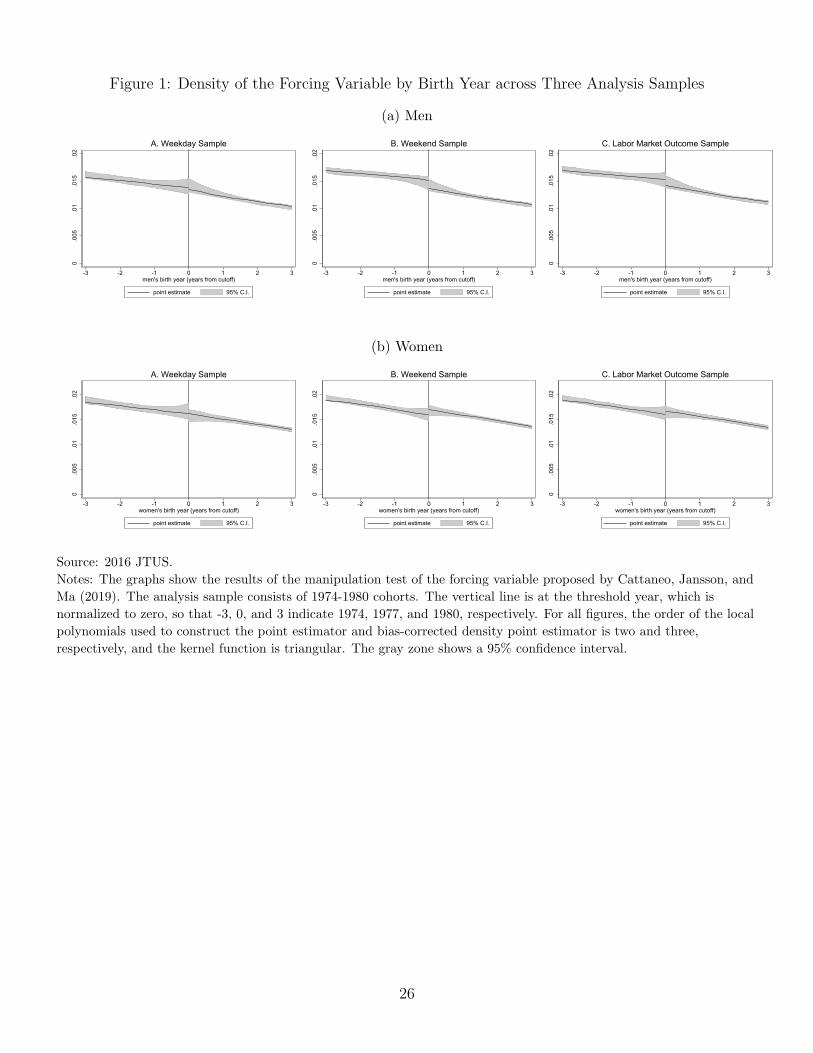
Figure 1: Density of the Forcing Variable by Birth Year across Three Analysis Samples

(a) Men

0.0

05.0

1.0

15.0

2

-3 -2 -1 0 1 2 3men's birth year (years from cutoff)

point estimate 95% C.I.

A. Weekday Sample

0.0

05.0

1.0

15.0

2

-3 -2 -1 0 1 2 3men's birth year (years from cutoff)

point estimate 95% C.I.

B. Weekend Sample

0.0

05.0

1.0

15.0

2

-3 -2 -1 0 1 2 3men's birth year (years from cutoff)

point estimate 95% C.I.

C. Labor Market Outcome Sample

(b) Women

0.0

05.0

1.0

15.0

2

-3 -2 -1 0 1 2 3women's birth year (years from cutoff)

point estimate 95% C.I.

A. Weekday Sample

0.0

05.0

1.0

15.0

2

-3 -2 -1 0 1 2 3women's birth year (years from cutoff)

point estimate 95% C.I.

B. Weekend Sample

0.0

05.0

1.0

15.0

2

-3 -2 -1 0 1 2 3women's birth year (years from cutoff)

point estimate 95% C.I.

C. Labor Market Outcome Sample

Source: 2016 JTUS.

Notes: The graphs show the results of the manipulation test of the forcing variable proposed by Cattaneo, Jansson, and

Ma (2019). The analysis sample consists of 1974-1980 cohorts. The vertical line is at the threshold year, which is

normalized to zero, so that -3, 0, and 3 indicate 1974, 1977, and 1980, respectively. For all figures, the order of the local

polynomials used to construct the point estimator and bias-corrected density point estimator is two and three,

respectively, and the kernel function is triangular. The gray zone shows a 95% confidence interval.

26

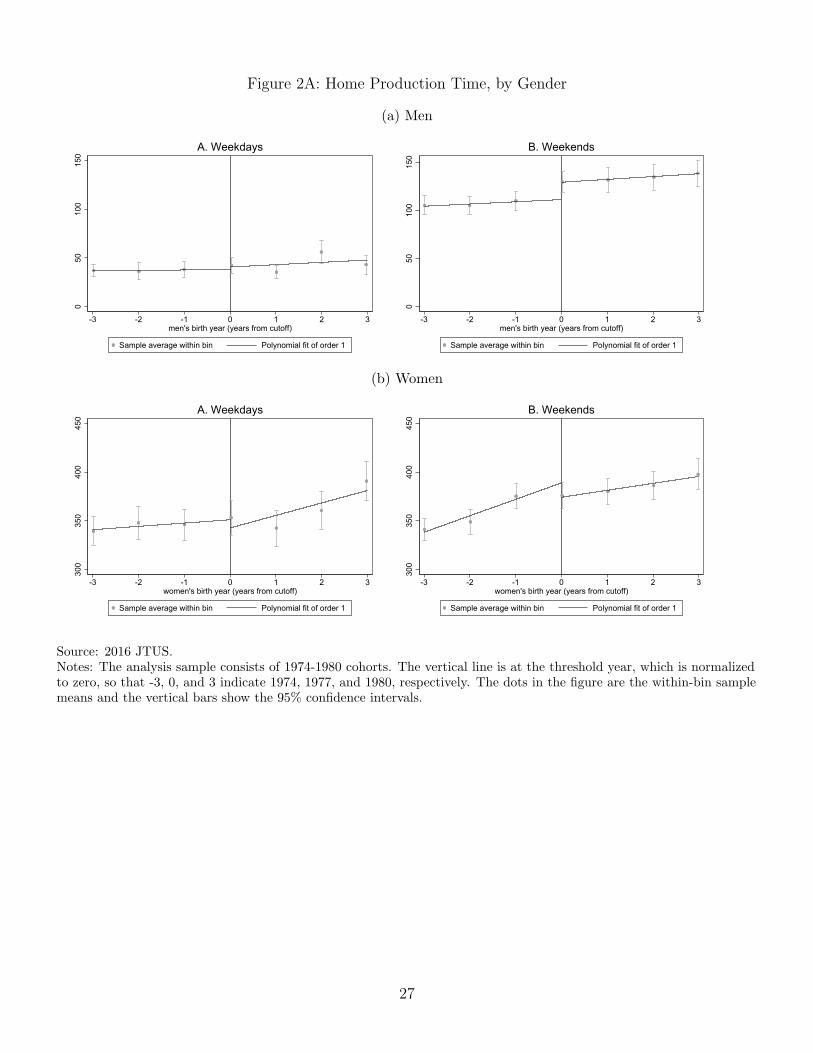
Figure 2A: Home Production Time, by Gender

(a) Men

050

100

150

-3 -2 -1 0 1 2 3men's birth year (years from cutoff)

Sample average within bin Polynomial fit of order 1

A. Weekdays

050

100

150

-3 -2 -1 0 1 2 3men's birth year (years from cutoff)

Sample average within bin Polynomial fit of order 1

B. Weekends

(b) Women

300

350

400

450

-3 -2 -1 0 1 2 3women's birth year (years from cutoff)

Sample average within bin Polynomial fit of order 1

A. Weekdays30

035

040

045

0

-3 -2 -1 0 1 2 3women's birth year (years from cutoff)

Sample average within bin Polynomial fit of order 1

B. Weekends

Source: 2016 JTUS.Notes: The analysis sample consists of 1974-1980 cohorts. The vertical line is at the threshold year, which is normalizedto zero, so that -3, 0, and 3 indicate 1974, 1977, and 1980, respectively. The dots in the figure are the within-bin samplemeans and the vertical bars show the 95% confidence intervals.

27

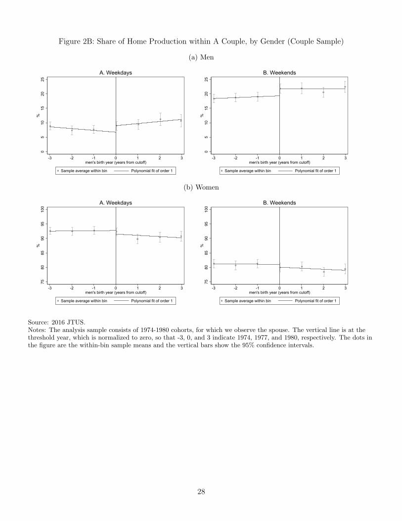
Figure 2B: Share of Home Production within A Couple, by Gender (Couple Sample)

(a) Men

05

1015

2025

%

-3 -2 -1 0 1 2 3men's birth year (years from cutoff)

Sample average within bin Polynomial fit of order 1

A. Weekdays

05

1015

2025

%

-3 -2 -1 0 1 2 3men's birth year (years from cutoff)

Sample average within bin Polynomial fit of order 1

B. Weekends

(b) Women

7580

8590

9510

0%

-3 -2 -1 0 1 2 3men's birth year (years from cutoff)

Sample average within bin Polynomial fit of order 1

A. Weekdays75

8085

9095

100

%

-3 -2 -1 0 1 2 3men's birth year (years from cutoff)

Sample average within bin Polynomial fit of order 1

B. Weekends

Source: 2016 JTUS.Notes: The analysis sample consists of 1974-1980 cohorts, for which we observe the spouse. The vertical line is at thethreshold year, which is normalized to zero, so that -3, 0, and 3 indicate 1974, 1977, and 1980, respectively. The dots inthe figure are the within-bin sample means and the vertical bars show the 95% confidence intervals.

28

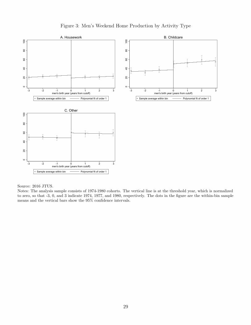
Figure 3: Men’s Weekend Home Production by Activity Type0

2040

6080

100

-3 -2 -1 0 1 2 3men's birth year (years from cutoff)

Sample average within bin Polynomial fit of order 1

A. Housework

020

4060

8010

0

-3 -2 -1 0 1 2 3men's birth year (years from cutoff)

Sample average within bin Polynomial fit of order 1

B. Childcare

020

4060

8010

0

-3 -2 -1 0 1 2 3men's birth year (years from cutoff)

Sample average within bin Polynomial fit of order 1

C. Other

Source: 2016 JTUS.Notes: The analysis sample consists of 1974-1980 cohorts. The vertical line is at the threshold year, which is normalizedto zero, so that -3, 0, and 3 indicate 1974, 1977, and 1980, respectively. The dots in the figure are the within-bin samplemeans and the vertical bars show the 95% confidence intervals.

29

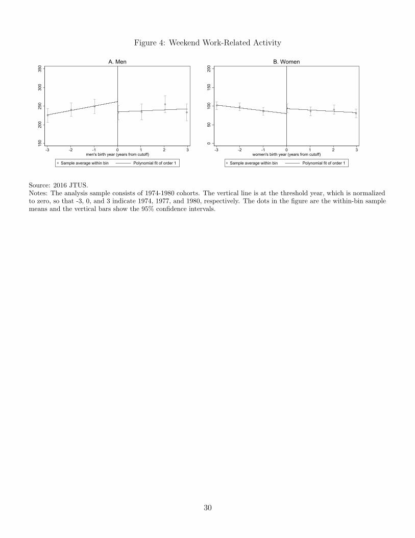
Figure 4: Weekend Work-Related Activity15

020

025

030

035

0

-3 -2 -1 0 1 2 3men's birth year (years from cutoff)

Sample average within bin Polynomial fit of order 1

A. Men

050

100

150

200

-3 -2 -1 0 1 2 3women's birth year (years from cutoff)

Sample average within bin Polynomial fit of order 1

B. Women

Source: 2016 JTUS.Notes: The analysis sample consists of 1974-1980 cohorts. The vertical line is at the threshold year, which is normalizedto zero, so that -3, 0, and 3 indicate 1974, 1977, and 1980, respectively. The dots in the figure are the within-bin samplemeans and the vertical bars show the 95% confidence intervals.

30

Figure 5: Labor Market Outcome, Women0

.1.2

.3.4

.5ra

tio

-3 -2 -1 0 1 2 3women's birth year (years from cutoff)

Sample average within bin Polynomial fit of order 1

A. Regular Worker

0.1

.2.3

.4.5

ratio

-3 -2 -1 0 1 2 3women's birth year (years from cutoff)

Sample average within bin Polynomial fit of order 1

B. Non-regular Worker

0.1

.2.3

.4.5

ratio

-3 -2 -1 0 1 2 3women's birth year (years from cutoff)

Sample average within bin Polynomial fit of order 1

C. Self-employed

0.1

.2.3

.4.5

ratio

-3 -2 -1 0 1 2 3women's birth year (years from cutoff)

Sample average within bin Polynomial fit of order 1

D. Not Working

100

150

200

250

mil.

JPY

-3 -2 -1 0 1 2 3women's birth year (years from cutoff)

Sample average within bin Polynomial fit of order 1

E. Income

0.1

.2.3

.4.5

ratio

-3 -2 -1 0 1 2 3women's birth year (years from cutoff)

Sample average within bin Polynomial fit of order 1

F. Occupation w/ High Wage

Source: 2016 JTUS.Notes: The analysis sample consists of 1974-1980 cohorts. The vertical line is at the threshold year, which is normalizedto zero, so that -3, 0, and 3 indicate 1974, 1977, and 1980, respectively. Information at the individual level is used. Thedots in the figure are the within-bin sample means and the vertical bars show the 95% confidence intervals.

31

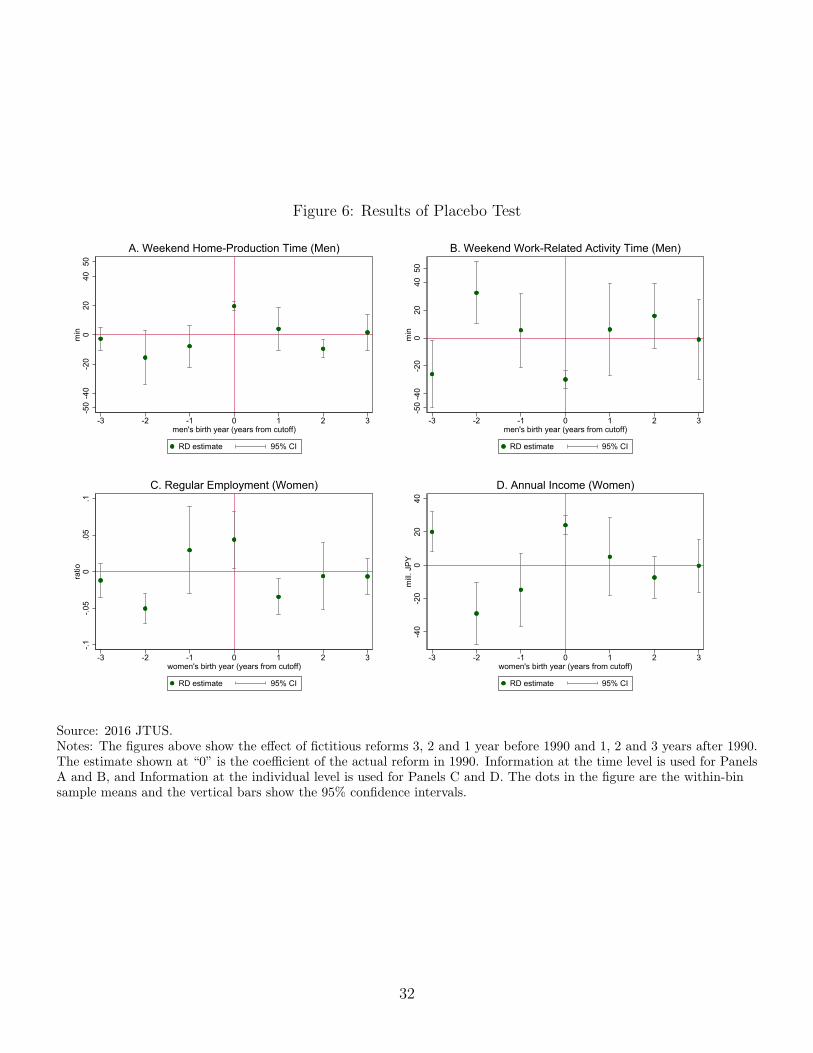
Figure 6: Results of Placebo Test

-50

-40

-20

020

4050

min

-3 -2 -1 0 1 2 3men's birth year (years from cutoff)

RD estimate 95% CI

A. Weekend Home-Production Time (Men)

-50

-40

-20

020

4050

min

-3 -2 -1 0 1 2 3men's birth year (years from cutoff)

RD estimate 95% CI

B. Weekend Work-Related Activity Time (Men)

-.1-.0

50

.05

.1ra

tio

-3 -2 -1 0 1 2 3women's birth year (years from cutoff)

RD estimate 95% CI

C. Regular Employment (Women)

-40

-20

020

40m

ill. J

PY

-3 -2 -1 0 1 2 3women's birth year (years from cutoff)

RD estimate 95% CI

D. Annual Income (Women)

Source: 2016 JTUS.Notes: The figures above show the effect of fictitious reforms 3, 2 and 1 year before 1990 and 1, 2 and 3 years after 1990.The estimate shown at “0” is the coefficient of the actual reform in 1990. Information at the time level is used for PanelsA and B, and Information at the individual level is used for Panels C and D. The dots in the figure are the within-binsample means and the vertical bars show the 95% confidence intervals.

32

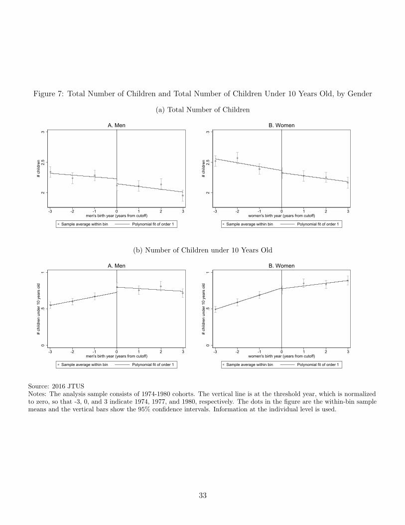
Figure 7: Total Number of Children and Total Number of Children Under 10 Years Old, by Gender

(a) Total Number of Children

22.

53

# ch

ildre

n

-3 -2 -1 0 1 2 3men's birth year (years from cutoff)

Sample average within bin Polynomial fit of order 1

A. Men

22.

53

# ch

ildre

n

-3 -2 -1 0 1 2 3women's birth year (years from cutoff)

Sample average within bin Polynomial fit of order 1

B. Women

(b) Number of Children under 10 Years Old

0.5

1#

child

ren

unde

r 10

year

s ol

d

-3 -2 -1 0 1 2 3men's birth year (years from cutoff)

Sample average within bin Polynomial fit of order 1

A. Men

0.5

1#

child

ren

unde

r 10

year

s ol

d

-3 -2 -1 0 1 2 3women's birth year (years from cutoff)

Sample average within bin Polynomial fit of order 1

B. Women

Source: 2016 JTUSNotes: The analysis sample consists of 1974-1980 cohorts. The vertical line is at the threshold year, which is normalizedto zero, so that -3, 0, and 3 indicate 1974, 1977, and 1980, respectively. The dots in the figure are the within-bin samplemeans and the vertical bars show the 95% confidence intervals. Information at the individual level is used.

33

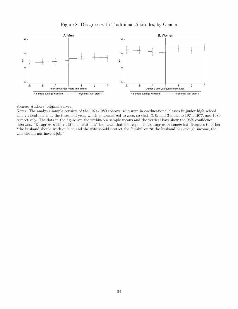
Figure 8: Disagrees with Traditional Attitudes, by Gender.2

.3.4

.5ra

tio

-3 -2 -1 0 1 2 3men's birth year (years from cutoff)

Sample average within bin Polynomial fit of order 1

A. Men

.2.3

.4.5

ratio

-3 -2 -1 0 1 2 3women's birth year (years from cutoff)

Sample average within bin Polynomial fit of order 1

B. Women

Source: Authors’ original survey.Notes: The analysis sample consists of the 1974-1980 cohorts, who were in coeducational classes in junior high school.The vertical line is at the threshold year, which is normalized to zero, so that -3, 0, and 3 indicate 1974, 1977, and 1980,respectively. The dots in the figure are the within-bin sample means and the vertical bars show the 95% confidenceintervals. “Disagrees with traditional attitudes” indicates that the respondent disagrees or somewhat disagrees to either“the husband should work outside and the wife should protect the family” or “if the husband has enough income, thewife should not have a job.”

34

Appendix A

Figure A1: Coeducation of IA-HE by Cohort

Notes: The gray cells indicate coeducation. “JHS” indicates junior high school, and 7th to 9th grade students areJapanese junior high school students. All years are school years (April 1 - March 31), not calendar years.

43

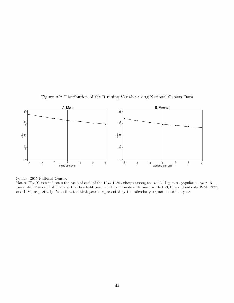
Figure A2: Distribution of the Running Variable using National Census Data

0.0

05.0

1.0

15.0

2ra

tio

-3 -2 -1 0 1 2 3men's birth year

A. Men

0.0

05.0

1.0

15.0

2ra

tio

-3 -2 -1 0 1 2 3women's birth year

B. Women

Source: 2015 National Census.Notes: The Y axis indicates the ratio of each of the 1974-1980 cohorts among the whole Japanese population over 15years old. The vertical line is at the threshold year, which is normalized to zero, so that -3, 0, and 3 indicate 1974, 1977,and 1980, respectively. Note that the birth year is represented by the calendar year, not the school year.

44

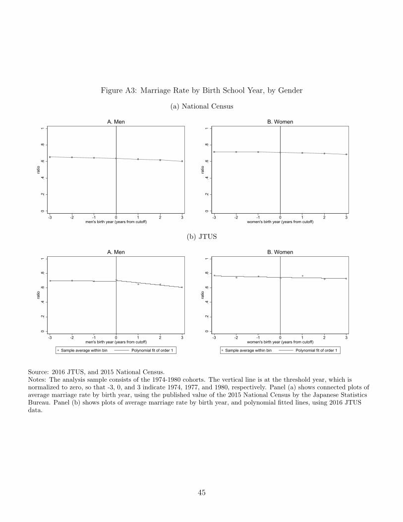
Figure A3: Marriage Rate by Birth School Year, by Gender

(a) National Census

0.2

.4.6

.81

ratio

-3 -2 -1 0 1 2 3men's birth year (years from cutoff)

A. Men

0.2

.4.6

.81

ratio

-3 -2 -1 0 1 2 3women's birth year (years from cutoff)

B. Women

(b) JTUS

0.2

.4.6

.81

ratio

-3 -2 -1 0 1 2 3men's birth year (years from cutoff)

Sample average within bin Polynomial fit of order 1

A. Men

0.2

.4.6

.81

ratio

-3 -2 -1 0 1 2 3women's birth year (years from cutoff)

Sample average within bin Polynomial fit of order 1

B. Women

Source: 2016 JTUS, and 2015 National Census.Notes: The analysis sample consists of the 1974-1980 cohorts. The vertical line is at the threshold year, which isnormalized to zero, so that -3, 0, and 3 indicate 1974, 1977, and 1980, respectively. Panel (a) shows connected plots ofaverage marriage rate by birth year, using the published value of the 2015 National Census by the Japanese StatisticsBureau. Panel (b) shows plots of average marriage rate by birth year, and polynomial fitted lines, using 2016 JTUSdata.

45

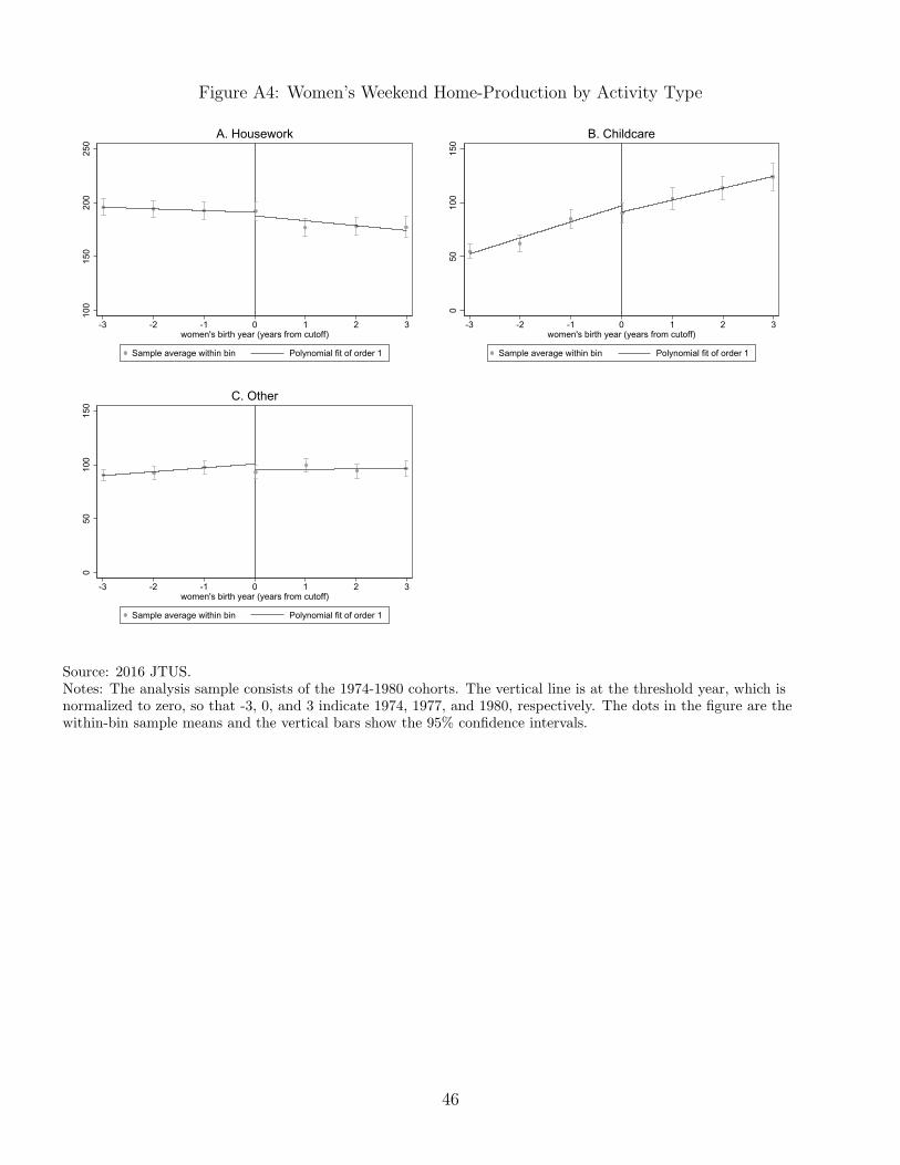
Figure A4: Women’s Weekend Home-Production by Activity Type10

015

020

025

0

-3 -2 -1 0 1 2 3women's birth year (years from cutoff)

Sample average within bin Polynomial fit of order 1

A. Housework

050

100

150

-3 -2 -1 0 1 2 3women's birth year (years from cutoff)

Sample average within bin Polynomial fit of order 1

B. Childcare

050

100

150

-3 -2 -1 0 1 2 3women's birth year (years from cutoff)

Sample average within bin Polynomial fit of order 1

C. Other

Source: 2016 JTUS.Notes: The analysis sample consists of the 1974-1980 cohorts. The vertical line is at the threshold year, which isnormalized to zero, so that -3, 0, and 3 indicate 1974, 1977, and 1980, respectively. The dots in the figure are thewithin-bin sample means and the vertical bars show the 95% confidence intervals.

46

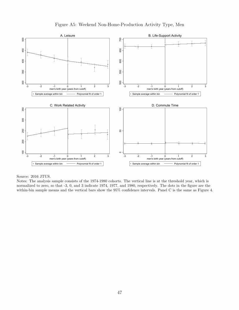
Figure A5: Weekend Non-Home-Production Activity Type, Men30

035

040

045

050

0

-3 -2 -1 0 1 2 3men's birth year (years from cutoff)

Sample average within bin Polynomial fit of order 1

A. Leisure

500

550

600

650

700

-3 -2 -1 0 1 2 3men's birth year (years from cutoff)

Sample average within bin Polynomial fit of order 1

B. Life-Support Activity

150

200

250

300

350

-3 -2 -1 0 1 2 3men's birth year (years from cutoff)

Sample average within bin Polynomial fit of order 1

C. Work Related Activity

050

100

-3 -2 -1 0 1 2 3men's birth year (years from cutoff)

Sample average within bin Polynomial fit of order 1

D. Commute Time

Source: 2016 JTUS.Notes: The analysis sample consists of the 1974-1980 cohorts. The vertical line is at the threshold year, which isnormalized to zero, so that -3, 0, and 3 indicate 1974, 1977, and 1980, respectively. The dots in the figure are thewithin-bin sample means and the vertical bars show the 95% confidence intervals. Panel C is the same as Figure 4.

47

Figure A6: Weekend Non-Home-Production Activity Type, Women20

025

030

035

040

0

-3 -2 -1 0 1 2 3women's birth year (years from cutoff)

Sample average within bin Polynomial fit of order 1

A. Leisure

500

550

600

650

700

-3 -2 -1 0 1 2 3women's birth year (years from cutoff)

Sample average within bin Polynomial fit of order 1

B. Life-Support Activity

050

100

150

200

-3 -2 -1 0 1 2 3women's birth year (years from cutoff)

Sample average within bin Polynomial fit of order 1

C. Work Related Activity

050

100

-3 -2 -1 0 1 2 3men's birth year (years from cutoff)

Sample average within bin Polynomial fit of order 1

D. Commute Time

Source: 2016 JTUS.Notes: The analysis sample consists of the 1974-1980 cohorts. The vertical line is at the threshold year, which isnormalized to zero, so that -3, 0, and 3 indicate 1974, 1977, and 1980, respectively. The dots in the figure are thewithin-bin sample means and the vertical bars show the 95% confidence intervals. Panel C is the same as Figure 4.

48

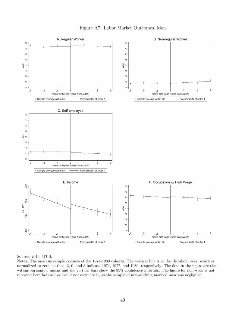
Figure A7: Labor Market Outcomes, Men0

.1.2

.3.4

.5.6

.7.8

ratio

-3 -2 -1 0 1 2 3men's birth year (years from cutoff)

Sample average within bin Polynomial fit of order 1

A. Regular Worker

0.1

.2.3

.4.5

.6.7

.8ra

tio

-3 -2 -1 0 1 2 3men's birth year (years from cutoff)

Sample average within bin Polynomial fit of order 1

B. Non-regular Worker

0.1

.2.3

.4.5

.6.7

.8ra

tio

-3 -2 -1 0 1 2 3men's birth year (years from cutoff)

Sample average within bin Polynomial fit of order 1

C. Self-employed

350

400

450

500

mil.

JPY

-3 -2 -1 0 1 2 3men's birth year (years from cutoff)

Sample average within bin Polynomial fit of order 1

E. Income

0.1

.2.3

.4.5

.6.7

.8ra

tio

-3 -2 -1 0 1 2 3men's birth year (years from cutoff)

Sample average within bin Polynomial fit of order 1

F. Occupation w/ High Wage

Source: 2016 JTUS.Notes: The analysis sample consists of the 1974-1980 cohorts. The vertical line is at the threshold year, which isnormalized to zero, so that -3, 0, and 3 indicate 1974, 1977, and 1980, respectively. The dots in the figure are thewithin-bin sample means and the vertical bars show the 95% confidence intervals. The figure for non-work is notreported here because we could not estimate it, as the sample of non-working married men was negligible.

49

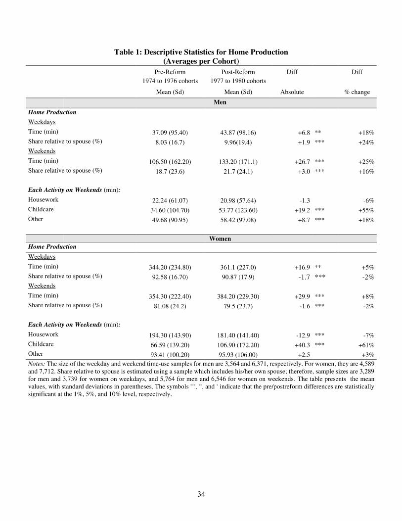
34

Table 1: Descriptive Statistics for Home Production

(Averages per Cohort) Pre-Reform Post-Reform Diff Diff

1974 to 1976 cohorts 1977 to 1980 cohorts

Mean (Sd) Mean (Sd) Absolute % change

Men

Home Production

Weekdays

Time (min) 37.09 (95.40) 43.87 (98.16) +6.8 ** +18%

Share relative to spouse (%) 8.03 (16.7) 9.96(19.4) +1.9 *** +24%

Weekends

Time (min) 106.50 (162.20) 133.20 (171.1) +26.7 *** +25%

Share relative to spouse (%) 18.7 (23.6) 21.7 (24.1) +3.0 *** +16%

Each Activity on Weekends (min):

Housework 22.24 (61.07) 20.98 (57.64) -1.3 -6%

Childcare 34.60 (104.70) 53.77 (123.60) +19.2 *** +55%

Other 49.68 (90.95) 58.42 (97.08) +8.7 *** +18%

Women

Home Production

Weekdays

Time (min) 344.20 (234.80) 361.1 (227.0) +16.9 ** +5%

Share relative to spouse (%) 92.58 (16.70) 90.87 (17.9) -1.7 *** -2%

Weekends Time (min) 354.30 (222.40) 384.20 (229.30) +29.9 *** +8%

Share relative to spouse (%) 81.08 (24.2) 79.5 (23.7) -1.6 *** -2%

Each Activity on Weekends (min):

Housework 194.30 (143.90) 181.40 (141.40) -12.9 *** -7%

Childcare 66.59 (139.20) 106.90 (172.20) +40.3 *** +61%

Other 93.41 (100.20) 95.93 (106.00) +2.5 +3%

Notes: The size of the weekday and weekend time-use samples for men are 3,564 and 6,371, respectively. For women, they are 4,589 and 7,712. Share relative to spouse is estimated using a sample which includes his/her own spouse; therefore, sample sizes are 3,289 for men and 3,739 for women on weekdays, and 5,764 for men and 6,546 for women on weekends. The table presents the mean values, with standard deviations in parentheses. The symbols ***, **, and * indicate that the pre/postreform differences are statistically significant at the 1%, 5%, and 10% level, respectively.

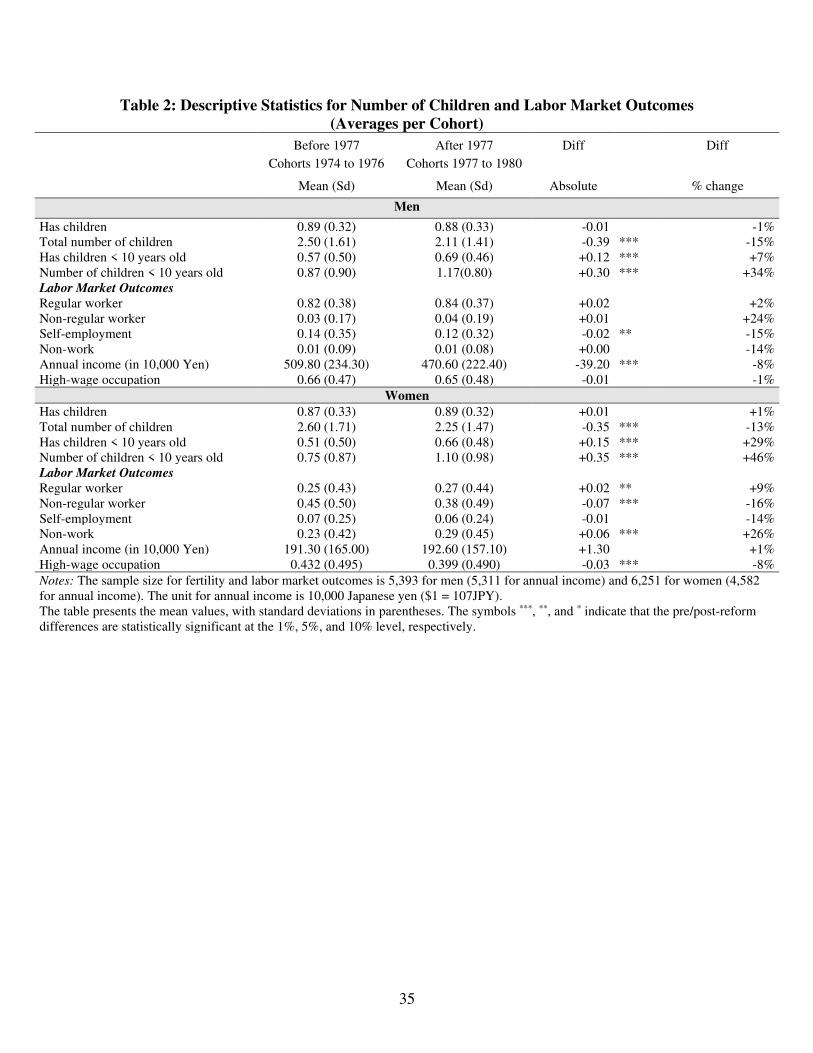
35

Table 2: Descriptive Statistics for Number of Children and Labor Market Outcomes

(Averages per Cohort) Before 1977 After 1977 Diff Diff

Cohorts 1974 to 1976 Cohorts 1977 to 1980

Mean (Sd) Mean (Sd) Absolute % change

Men

Has children 0.89 (0.32) 0.88 (0.33) -0.01 -1%

Total number of children 2.50 (1.61) 2.11 (1.41) -0.39 *** -15% Has children < 10 years old 0.57 (0.50) 0.69 (0.46) +0.12 *** +7% Number of children < 10 years old 0.87 (0.90) 1.17(0.80) +0.30 *** +34% Labor Market Outcomes Regular worker 0.82 (0.38) 0.84 (0.37) +0.02 +2% Non-regular worker 0.03 (0.17) 0.04 (0.19) +0.01 +24% Self-employment 0.14 (0.35) 0.12 (0.32) -0.02 ** -15% Non-work 0.01 (0.09) 0.01 (0.08) +0.00 -14% Annual income (in 10,000 Yen) 509.80 (234.30) 470.60 (222.40) -39.20 *** -8% High-wage occupation 0.66 (0.47) 0.65 (0.48) -0.01 -1%

Women

Has children 0.87 (0.33) 0.89 (0.32) +0.01 +1%

Total number of children 2.60 (1.71) 2.25 (1.47) -0.35 *** -13% Has children < 10 years old 0.51 (0.50) 0.66 (0.48) +0.15 *** +29% Number of children < 10 years old 0.75 (0.87) 1.10 (0.98) +0.35 *** +46% Labor Market Outcomes Regular worker 0.25 (0.43) 0.27 (0.44) +0.02 ** +9% Non-regular worker 0.45 (0.50) 0.38 (0.49) -0.07 *** -16% Self-employment 0.07 (0.25) 0.06 (0.24) -0.01 -14% Non-work 0.23 (0.42) 0.29 (0.45) +0.06 *** +26% Annual income (in 10,000 Yen) 191.30 (165.00) 192.60 (157.10) +1.30 +1% High-wage occupation 0.432 (0.495) 0.399 (0.490) -0.03 *** -8%

Notes: The sample size for fertility and labor market outcomes is 5,393 for men (5,311 for annual income) and 6,251 for women (4,582 for annual income). The unit for annual income is 10,000 Japanese yen ($1 = 107JPY). The table presents the mean values, with standard deviations in parentheses. The symbols ***, **, and * indicate that the pre/post-reform differences are statistically significant at the 1%, 5%, and 10% level, respectively.

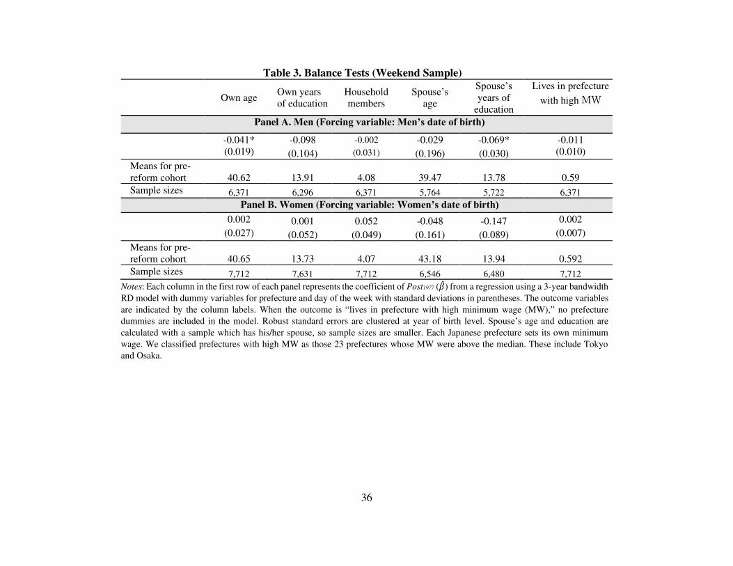
36 Table 3. Balance Tests (Weekend Sample)

Own age Own years of education

Household members

Spouse’s age

Spouse’s years of

education

Lives in prefecture

with high MW

Panel A. Men (Forcing variable: Men’s date of birth)

-0.041* -0.098 -0.002 -0.029 -0.069* -0.011 (0.019) (0.104) (0.031) (0.196) (0.030) (0.010)

Means for pre-reform cohort 40.62 13.91 4.08 39.47 13.78

0.59

Sample sizes 6,371 6,296 6,371 5,764 5,722 6,371

Panel B. Women (Forcing variable: Women’s date of birth) 0.002 0.001 0.052 -0.048 -0.147 0.002

(0.027) (0.052) (0.049) (0.161) (0.089) (0.007)

Means for pre-reform cohort 40.65 13.73 4.07 43.18 13.94

0.592

Sample sizes 7,712 7,631 7,712 6,546 6,480 7,712

Notes: Each column in the first row of each panel represents the coefficient of Post1977 (�̂�) from a regression using a 3-year bandwidth

RD model with dummy variables for prefecture and day of the week with standard deviations in parentheses. The outcome variables

are indicated by the column labels. When the outcome is “lives in prefecture with high minimum wage (MW),” no prefecture

dummies are included in the model. Robust standard errors are clustered at year of birth level. Spouse’s age and education are calculated with a sample which has his/her spouse, so sample sizes are smaller. Each Japanese prefecture sets its own minimum

wage. We classified prefectures with high MW as those 23 prefectures whose MW were above the median. These include Tokyo

and Osaka.

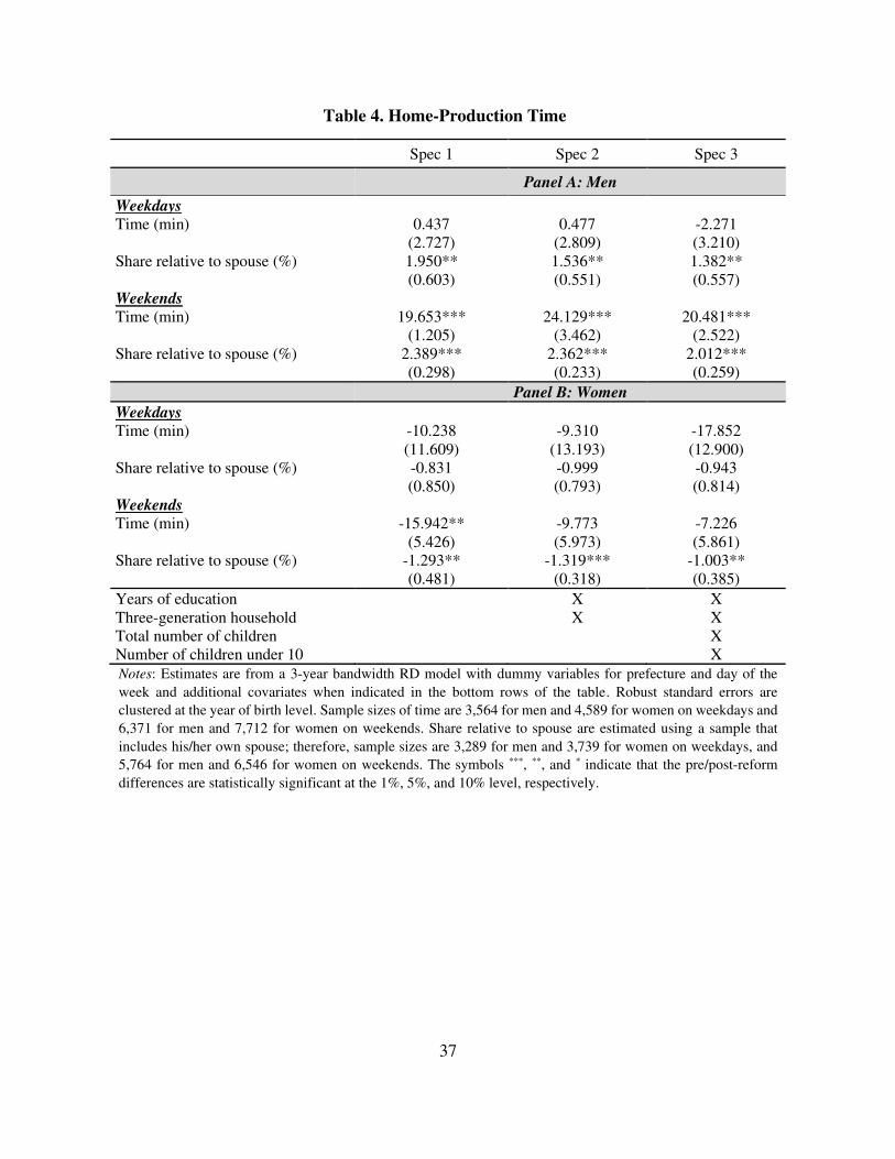
37 Table 4. Home-Production Time

Spec 1 Spec 2 Spec 3

Panel A: Men

Weekdays Time (min) 0.437 0.477 -2.271 (2.727) (2.809) (3.210) Share relative to spouse (%) 1.950** 1.536** 1.382** (0.603) (0.551) (0.557) Weekends Time (min) 19.653*** 24.129*** 20.481*** (1.205) (3.462) (2.522) Share relative to spouse (%) 2.389*** 2.362*** 2.012*** (0.298) (0.233) (0.259)

Panel B: Women

Weekdays Time (min) -10.238 -9.310 -17.852 (11.609) (13.193) (12.900) Share relative to spouse (%) -0.831 -0.999 -0.943 (0.850) (0.793) (0.814) Weekends Time (min) -15.942** -9.773 -7.226 (5.426) (5.973) (5.861) Share relative to spouse (%) -1.293** -1.319*** -1.003** (0.481) (0.318) (0.385)

Years of education X X Three-generation household X X Total number of children X Number of children under 10 X Notes: Estimates are from a 3-year bandwidth RD model with dummy variables for prefecture and day of the

week and additional covariates when indicated in the bottom rows of the table. Robust standard errors are

clustered at the year of birth level. Sample sizes of time are 3,564 for men and 4,589 for women on weekdays and

6,371 for men and 7,712 for women on weekends. Share relative to spouse are estimated using a sample that

includes his/her own spouse; therefore, sample sizes are 3,289 for men and 3,739 for women on weekdays, and

5,764 for men and 6,546 for women on weekends. The symbols ***, **, and * indicate that the pre/post-reform

differences are statistically significant at the 1%, 5%, and 10% level, respectively.

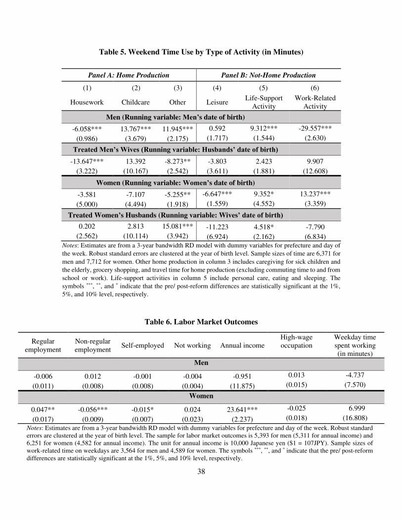
38 Table 5. Weekend Time Use by Type of Activity (in Minutes)

Panel A: Home Production Panel B: Not-Home Production

(1) (2) (3) (4) (5) (6)

Housework Childcare Other Leisure Life-Support

Activity Work-Related

Activity

Men (Running variable: Men’s date of birth)

-6.058*** 13.767*** 11.945*** 0.592 9.312*** -29.557***

(0.986) (3.679) (2.175) (1.717) (1.544) (2.630)

Treated Men’s Wives (Running variable: Husbands’ date of birth)

-13.647*** 13.392 -8.273** -3.803 2.423 9.907

(3.222) (10.167) (2.542) (3.611) (1.881) (12.608)

Women (Running variable: Women’s date of birth)

-3.581 -7.107 -5.255** -6.647*** 9.352* 13.237***

(5.000) (4.494) (1.918) (1.559) (4.552) (3.359)

Treated Women’s Husbands (Running variable: Wives’ date of birth)

0.202 2.813 15.081*** -11.223 4.518* -7.790

(2.562) (10.114) (3.942) (6.924) (2.162) (6.834) Notes: Estimates are from a 3-year bandwidth RD model with dummy variables for prefecture and day of

the week. Robust standard errors are clustered at the year of birth level. Sample sizes of time are 6,371 for

men and 7,712 for women. Other home production in column 3 includes caregiving for sick children and

the elderly, grocery shopping, and travel time for home production (excluding commuting time to and from

school or work). Life-support activities in column 5 include personal care, eating and sleeping. The

symbols ***, **, and * indicate that the pre/ post-reform differences are statistically significant at the 1%,

5%, and 10% level, respectively.

Table 6. Labor Market Outcomes

Regular employment

Non-regular employment

Self-employed Not working Annual income High-wage occupation

Weekday time spent working (in minutes)

Men

-0.006 0.012 -0.001 -0.004 -0.951 0.013 -4.737

(0.011) (0.008) (0.008) (0.004) (11.875) (0.015) (7.570)

Women

0.047** -0.056*** -0.015* 0.024 23.641*** -0.025 6.999

(0.017) (0.009) (0.007) (0.023) (2.237) (0.018) (16.808)

Notes: Estimates are from a 3-year bandwidth RD model with dummy variables for prefecture and day of the week. Robust standard errors are clustered at the year of birth level. The sample for labor market outcomes is 5,393 for men (5,311 for annual income) and 6,251 for women (4,582 for annual income). The unit for annual income is 10,000 Japanese yen ($1 = 107JPY). Sample sizes of work-related time on weekdays are 3,564 for men and 4,589 for women. The symbols ***, **, and * indicate that the pre/ post-reform differences are statistically significant at the 1%, 5%, and 10% level, respectively.

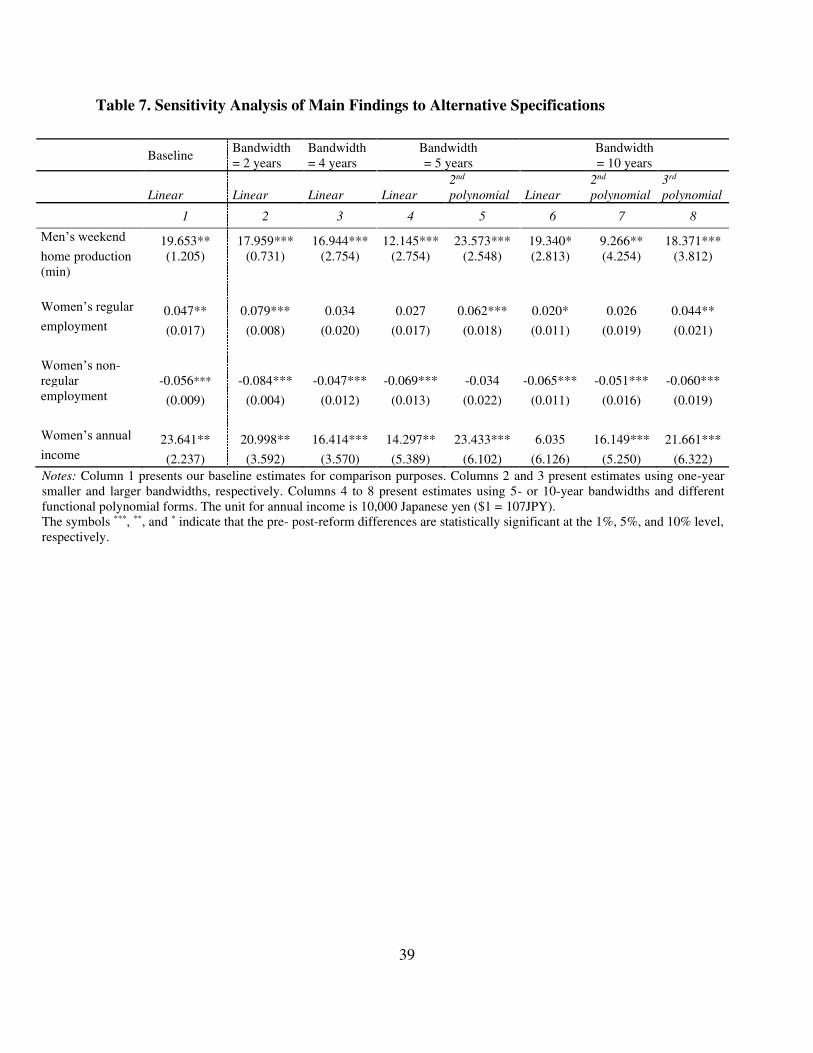
39 Table 7. Sensitivity Analysis of Main Findings to Alternative Specifications

Baseline

Bandwidth = 2 years

Bandwidth = 4 years

Bandwidth = 5 years

Bandwidth = 10 years

Linear Linear

Linear Linear

2nd

polynomial Linear 2nd

polynomial 3rd

polynomial

1 2 3 4 5 6 7 8

Men’s weekend 19.653** 17.959*** 16.944*** 12.145*** 23.573*** 19.340* 9.266** 18.371*** home production (min)

(1.205) (0.731) (2.754) (2.754) (2.548) (2.813) (4.254) (3.812)

Women’s regular 0.047** 0.079*** 0.034 0.027 0.062*** 0.020* 0.026 0.044** employment (0.017) (0.008) (0.020) (0.017) (0.018) (0.011) (0.019) (0.021) Women’s non-regular -0.056*** -0.084*** -0.047*** -0.069*** -0.034 -0.065*** -0.051*** -0.060*** employment (0.009) (0.004) (0.012) (0.013) (0.022) (0.011) (0.016) (0.019) Women’s annual 23.641** 20.998** 16.414*** 14.297** 23.433*** 6.035 16.149*** 21.661*** income (2.237) (3.592) (3.570) (5.389) (6.102) (6.126) (5.250) (6.322)

Notes: Column 1 presents our baseline estimates for comparison purposes. Columns 2 and 3 present estimates using one-year smaller and larger bandwidths, respectively. Columns 4 to 8 present estimates using 5- or 10-year bandwidths and different functional polynomial forms. The unit for annual income is 10,000 Japanese yen ($1 = 107JPY). The symbols ***, **, and * indicate that the pre- post-reform differences are statistically significant at the 1%, 5%, and 10% level, respectively.

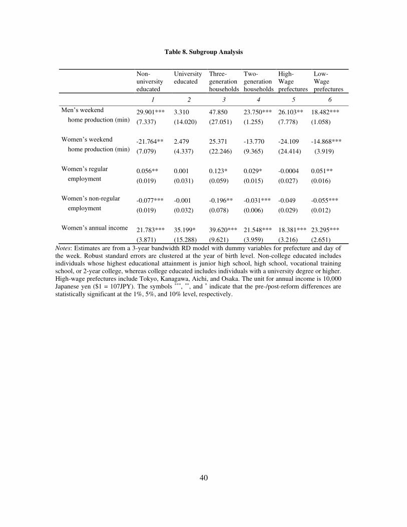
40 Table 8. Subgroup Analysis

Non-university educated

University educated

Three-generation households

Two-generation households

High-Wage prefectures

Low- Wage prefectures

1 2 3 4 5 6

Men’s weekend 29.901*** 3.310 47.850 23.750*** 26.103** 18.482*** home production (min) (7.337) (14.020) (27.051) (1.255) (7.778) (1.058)

Women’s weekend -21.764** 2.479 25.371 -13.770 -24.109 -14.868*** home production (min) (7.079) (4.337) (22.246) (9.365) (24.414) (3.919)

Women’s regular 0.056** 0.001 0.123* 0.029* -0.0004 0.051** employment (0.019) (0.031) (0.059) (0.015) (0.027) (0.016)

Women’s non-regular -0.077*** -0.001 -0.196** -0.031*** -0.049 -0.055*** employment (0.019) (0.032) (0.078) (0.006) (0.029) (0.012)

Women’s annual income 21.783*** 35.199* 39.620*** 21.548*** 18.381*** 23.295*** (3.871) (15.288) (9.621) (3.959) (3.216) (2.651)

Notes: Estimates are from a 3-year bandwidth RD model with dummy variables for prefecture and day of the week. Robust standard errors are clustered at the year of birth level. Non-college educated includes individuals whose highest educational attainment is junior high school, high school, vocational training school, or 2-year college, whereas college educated includes individuals with a university degree or higher. High-wage prefectures include Tokyo, Kanagawa, Aichi, and Osaka. The unit for annual income is 10,000 Japanese yen ($1 = 107JPY). The symbols ***, **, and * indicate that the pre-/post-reform differences are statistically significant at the 1%, 5%, and 10% level, respectively.

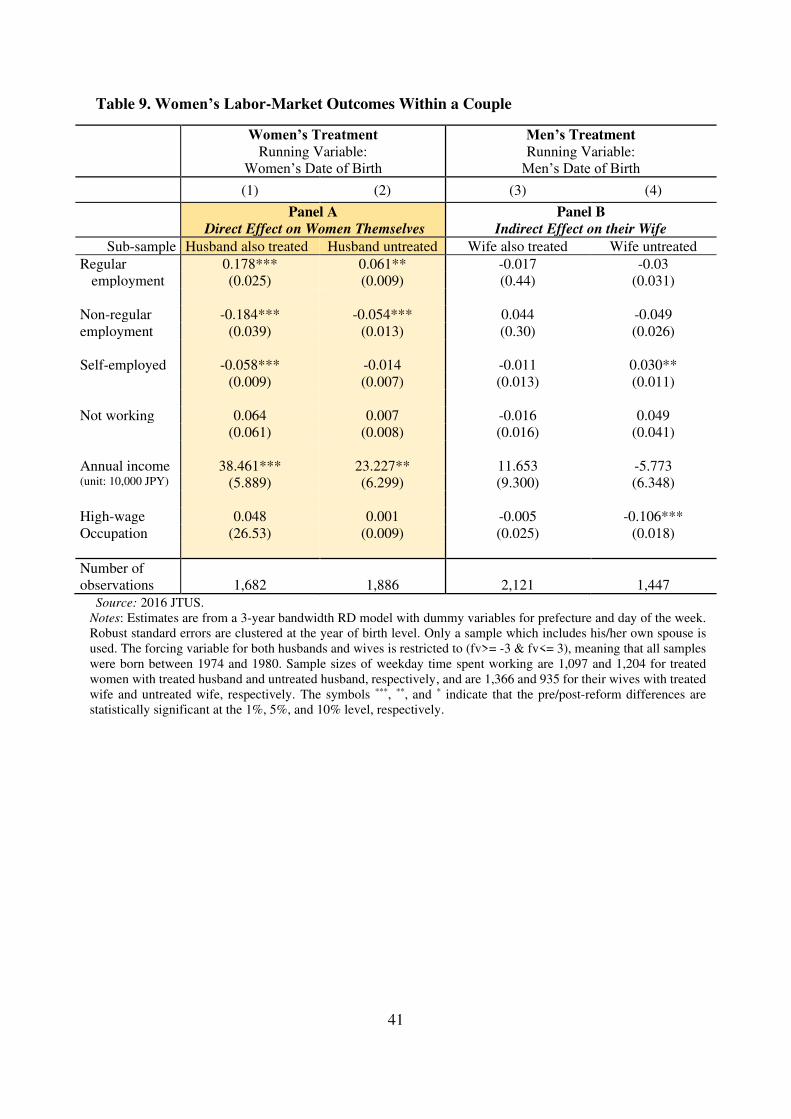
41

Table 9. Women’s Labor-Market Outcomes Within a Couple

Women’s Treatment

Running Variable: Women’s Date of Birth

Men’s Treatment

Running Variable: Men’s Date of Birth

(1) (2) (3) (4)

Panel A

Direct Effect on Women Themselves

Panel B

Indirect Effect on their Wife

Sub-sample Husband also treated Husband untreated Wife also treated Wife untreated

Regular 0.178*** 0.061** -0.017 -0.03 employment (0.025) (0.009) (0.44) (0.031)

Non-regular -0.184*** -0.054*** 0.044 -0.049 employment (0.039) (0.013) (0.30) (0.026) Self-employed -0.058*** -0.014 -0.011 0.030** (0.009) (0.007) (0.013) (0.011) Not working 0.064 0.007 -0.016 0.049 (0.061) (0.008) (0.016) (0.041) Annual income 38.461*** 23.227** 11.653 -5.773 (unit: 10,000 JPY) (5.889) (6.299) (9.300) (6.348) High-wage 0.048 0.001 -0.005 -0.106*** Occupation (26.53) (0.009) (0.025) (0.018)

Number of observations 1,682 1,886

2,121 1,447

Source: 2016 JTUS. Notes: Estimates are from a 3-year bandwidth RD model with dummy variables for prefecture and day of the week. Robust standard errors are clustered at the year of birth level. Only a sample which includes his/her own spouse is used. The forcing variable for both husbands and wives is restricted to (fv>= -3 & fv<= 3), meaning that all samples were born between 1974 and 1980. Sample sizes of weekday time spent working are 1,097 and 1,204 for treated women with treated husband and untreated husband, respectively, and are 1,366 and 935 for their wives with treated wife and untreated wife, respectively. The symbols ***, **, and * indicate that the pre/post-reform differences are statistically significant at the 1%, 5%, and 10% level, respectively.

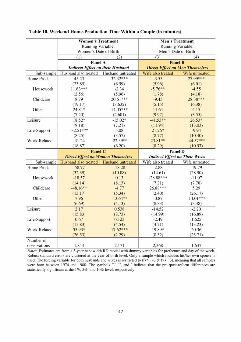
42

Table 10. Weekend Home-Production Time Within a Couple (in minutes)

Women’s Treatment

Running Variable: Women’s Date of Birth

Men’s Treatment

Running Variable: Men’s Date of Birth

(1) (2) (3) (4)

Panel A

Indirect Effect on their Husband

Panel B

Direct Effect on Men Themselves

Sub-sample Husband also treated Husband untreated Wife also treated Wife untreated

Home Prod. 45.23 32.32*** -3.55 27.99*** (23.85) (6.59) (5.96) (6.01) Housework 11.63*** -2.34 -5.76** -4.55 (2.56) (5.96) (1.78) (4.18) Childcare 8.79 20.61*** -9.43 28.38*** (19.17) (3.632) (5.15) (6.38) Other 24.81* 14.05*** 11.64 4.15 (7.20) (2.601) (9.97) (3.55)

Leisure 18.52* -15.02* -41.53** 26.53* (9.18) (7.21) (11.94) (13.03) Life-Support -32.51*** 5.08 21.26* -9.94 (8.25) (3.57) (8.77) (10.40) Work-Related -31.24 -22.39** 23.81** -44.57*** (18.87) (6.20) (8.29) (10.97)

Panel C

Direct Effect on Women Themselves

Panel D

Indirect Effect on Their Wives

Sub-sample Husband also treated Husband untreated Wife also treated Wife untreated

Home Prod. -58.77 -18.28 -2.88 -19.79 (32.39) (10.08) (14.61) (28.90) Housework -18.57 0.13 -28.88*** -11.07 (14.14) (8.13) (7.21) (7.78) Childcare -48.16** -4.77 26.88*** 5.29 (13.17) (5.34) (2.40) (26.17) Other 7.96 -13.64** -0.87 -14.01*** (6.69) (4.13) (8.33) (3.38)

Leisure 2.17 0.538 -14.52 -2.20 (15.83) (8.73) (14.99) (16.89) Life-Support 0.67 0.123 -2.49 1.625 (15.83) (4.54) (4.71) (13.23) Work-Related 55.93* 17.62*** 19.89* 20.36 (26.53) (2.29) (8.32) (25.71)

Number of observations 1,844 2,171

2,368 1,647

Notes: Estimates are from a 3-year bandwidth RD model with dummy variables for prefecture and day of the week. Robust standard errors are clustered at the year of birth level. Only a sample which includes his/her own spouse is used. The forcing variable for both husbands and wives is restricted to (fv>= -3 & fv<= 3), meaning that all samples were born between 1974 and 1980. The symbols ***, **, and * indicate that the pre-/post-reform differences are statistically significant at the 1%, 5%, and 10% level, respectively.

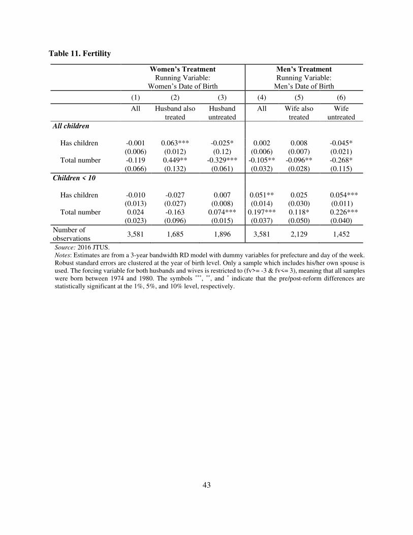
43 Table 11. Fertility

Women’s Treatment

Running Variable: Women’s Date of Birth

Men’s Treatment

Running Variable: Men’s Date of Birth

(1) (2) (3) (4) (5) (6)

All

Husband also treated

Husband untreated

All

Wife also treated

Wife untreated

All children Has children -0.001 0.063*** -0.025* 0.002 0.008 -0.045* (0.006) (0.012) (0.12) (0.006) (0.007) (0.021) Total number -0.119 0.449** -0.329*** -0.105** -0.096** -0.268* (0.066) (0.132) (0.061) (0.032) (0.028) (0.115)

Children < 10 Has children -0.010 -0.027 0.007 0.051** 0.025 0.054*** (0.013) (0.027) (0.008) (0.014) (0.030) (0.011) Total number 0.024 -0.163 0.074*** 0.197*** 0.118* 0.226*** (0.023) (0.096) (0.015) (0.037) (0.050) (0.040)

Number of observations

3,581 1,685 1,896 3,581 2,129 1,452

Source: 2016 JTUS. Notes: Estimates are from a 3-year bandwidth RD model with dummy variables for prefecture and day of the week. Robust standard errors are clustered at the year of birth level. Only a sample which includes his/her own spouse is used. The forcing variable for both husbands and wives is restricted to (fv>= -3 & fv<= 3), meaning that all samples were born between 1974 and 1980. The symbols ***, **, and * indicate that the pre/post-reform differences are statistically significant at the 1%, 5%, and 10% level, respectively.

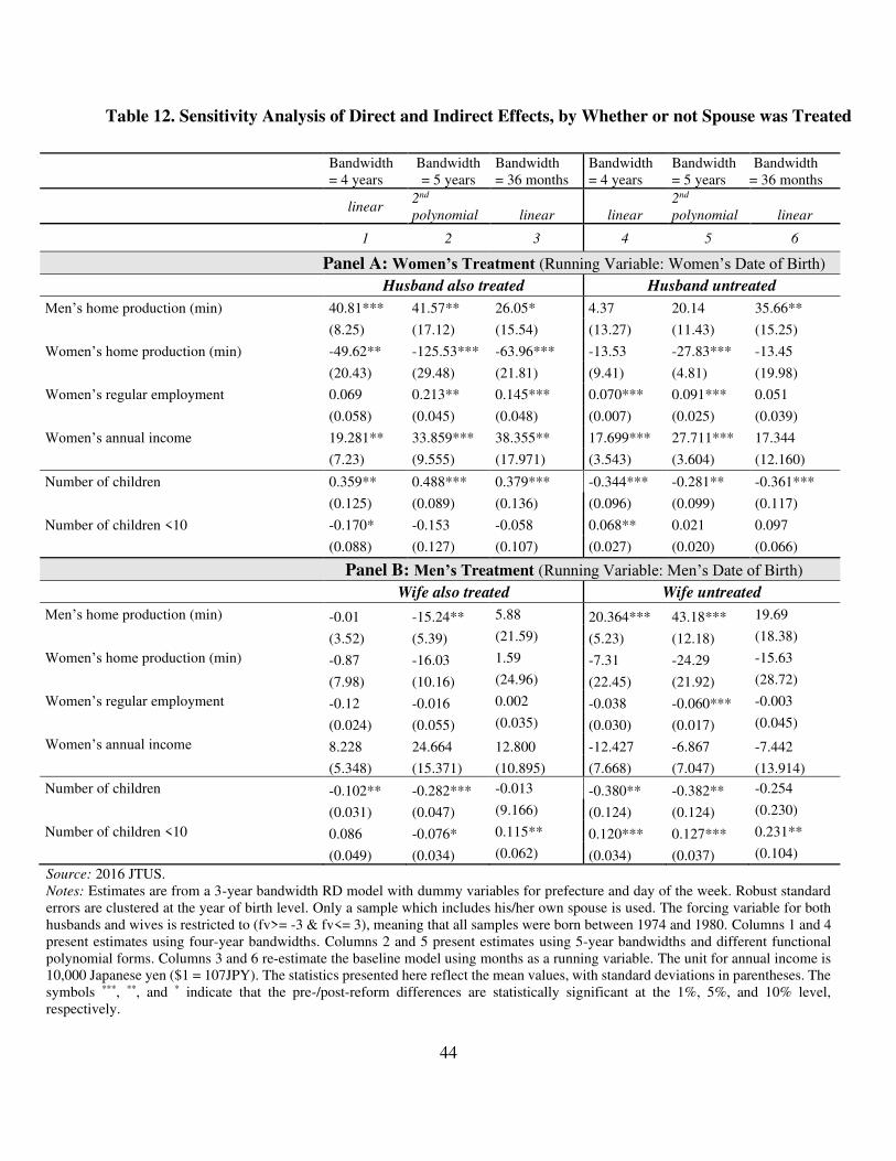
44 Table 12. Sensitivity Analysis of Direct and Indirect Effects, by Whether or not Spouse was Treated

Bandwidth = 4 years

Bandwidth = 5 years

Bandwidth = 36 months

Bandwidth = 4 years

Bandwidth = 5 years

Bandwidth = 36 months

linear 2nd

polynomial linear linear 2nd

polynomial linear

1 2 3 4 5 6

Panel A: Women’s Treatment (Running Variable: Women’s Date of Birth)

Husband also treated Husband untreated

Men’s home production (min) 40.81*** 41.57** 26.05* 4.37 20.14 35.66**

(8.25) (17.12) (15.54) (13.27) (11.43) (15.25)

Women’s home production (min) -49.62** -125.53*** -63.96*** -13.53 -27.83*** -13.45

(20.43) (29.48) (21.81) (9.41) (4.81) (19.98)

Women’s regular employment 0.069 0.213** 0.145*** 0.070*** 0.091*** 0.051

(0.058) (0.045) (0.048) (0.007) (0.025) (0.039)

Women’s annual income 19.281** 33.859*** 38.355** 17.699*** 27.711*** 17.344

(7.23) (9.555) (17.971) (3.543) (3.604) (12.160)

Number of children 0.359** 0.488*** 0.379*** -0.344*** -0.281** -0.361***

(0.125) (0.089) (0.136) (0.096) (0.099) (0.117)

Number of children <10 -0.170* -0.153 -0.058 0.068** 0.021 0.097

(0.088) (0.127) (0.107) (0.027) (0.020) (0.066)

Panel B: Men’s Treatment (Running Variable: Men’s Date of Birth)

Wife also treated Wife untreated

Men’s home production (min) -0.01 -15.24** 5.88 20.364*** 43.18*** 19.69

(3.52) (5.39) (21.59) (5.23) (12.18) (18.38)

Women’s home production (min) -0.87 -16.03 1.59 -7.31 -24.29 -15.63

(7.98) (10.16) (24.96) (22.45) (21.92) (28.72)

Women’s regular employment -0.12 -0.016 0.002 -0.038 -0.060*** -0.003

(0.024) (0.055) (0.035) (0.030) (0.017) (0.045)

Women’s annual income 8.228 24.664 12.800 -12.427 -6.867 -7.442

(5.348) (15.371) (10.895) (7.668) (7.047) (13.914)

Number of children -0.102** -0.282*** -0.013 -0.380** -0.382** -0.254

(0.031) (0.047) (9.166) (0.124) (0.124) (0.230)

Number of children <10 0.086 -0.076* 0.115** 0.120*** 0.127*** 0.231**

(0.049) (0.034) (0.062) (0.034) (0.037) (0.104)

Source: 2016 JTUS. Notes: Estimates are from a 3-year bandwidth RD model with dummy variables for prefecture and day of the week. Robust standard errors are clustered at the year of birth level. Only a sample which includes his/her own spouse is used. The forcing variable for both husbands and wives is restricted to (fv>= -3 & fv<= 3), meaning that all samples were born between 1974 and 1980. Columns 1 and 4 present estimates using four-year bandwidths. Columns 2 and 5 present estimates using 5-year bandwidths and different functional polynomial forms. Columns 3 and 6 re-estimate the baseline model using months as a running variable. The unit for annual income is 10,000 Japanese yen ($1 = 107JPY). The statistics presented here reflect the mean values, with standard deviations in parentheses. The symbols ***, **, and * indicate that the pre-/post-reform differences are statistically significant at the 1%, 5%, and 10% level, respectively.

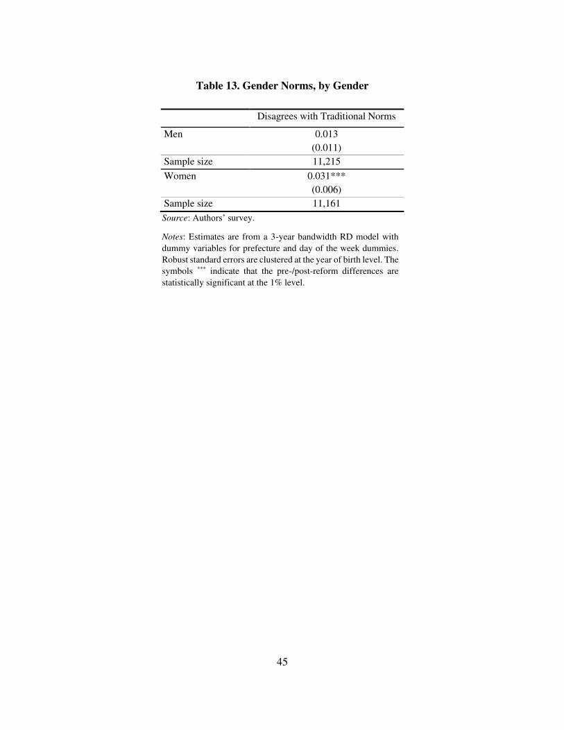
45

Table 13. Gender Norms, by Gender

Disagrees with Traditional Norms

Men 0.013

(0.011)

Sample size 11,215

Women 0.031***

(0.006)

Sample size 11,161

Source: Authors’ survey.

Notes: Estimates are from a 3-year bandwidth RD model with

dummy variables for prefecture and day of the week dummies.

Robust standard errors are clustered at the year of birth level. The

symbols *** indicate that the pre-/post-reform differences are

statistically significant at the 1% level.

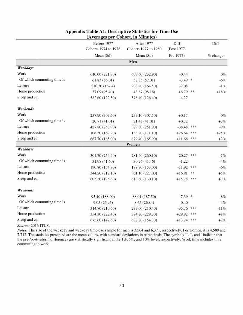
50 Appendix Table A1: Descriptive Statistics for Time Use

(Averages per Cohort, in Minutes) Before 1977 After 1977 Diff Diff

Cohorts 1974 to 1976 Cohorts 1977 to 1980 (Post 1977-

Mean (Sd) Mean (Sd) Pre 1977) % change

Men

Weekdays

Work 610.00 (221.90) 609.60 (232.90) -0.44 0%

Of which commuting time is 61.83 (56.01) 58.35 (52.01) -3.49 * -6%

Leisure 210.30 (167.4) 208.20 (164.50) -2.08 -1%

Home production 37.09 (95.40) 43.87 (98.16) +6.79 ** +18%

Sleep and eat 582.60 (122.50) 578.40 (126.40) -4.27

Weekends

Work 237.90 (307.50) 239.10 (307.50) +0.17 0%

Of which commuting time is 20.71 (41.01) 21.43 (41.01) +0.72 +3%

Leisure 427.80 (258.90) 389.30 (251.90) -38.48 *** -9%

Home production 106.50 (162.20) 133.20 (171.10) +26.64 *** +25%

Sleep and eat 667.70 (165.00) 679.40 (165.90) +11.66 *** +2%

Women

Weekdays

Work 301.70 (254.40) 281.40 (260.10) -20.27 *** -7%

Of which commuting time is 31.98 (41.60) 30.76 (41.46) -1.22 -4%

Leisure 190.80 (154.70) 178.90 (153.00) -11.92 *** -6%

Home production 344.20 (218.10) 361.10 (227.00) +16.91 ** +5%

Sleep and eat 603.30 (125.60) 618.60 (130.10) +15.28 *** +3%

Weekends

Work 95.40 (188.00) 88.01 (187.50) -7.39 * -8%

Of which commuting time is 9.05 (26.95) 8.65 (26.84) -0.40 -4%

Leisure 314.70 (210.60) 279.00 (210.40) -35.76 *** -11%

Home production 354.30 (222.40) 384.20 (229.30) +29.92 *** +8%

Sleep and eat 675.60 (147.60) 688.80 (154.30) +13.24 *** +2%

Source: 2016 JTUS. Notes: The size of the weekday and weekday time-use sample for men is 3,564 and 6,371, respectively. For women, it is 4,589 and 7,712. The statistics presented are the mean values, with standard deviations in parenthesis. The symbols ***, **, and * indicate that the pre-/post-reform differences are statistically significant at the 1%, 5%, and 10% level, respectively. Work time includes time commuting to work.

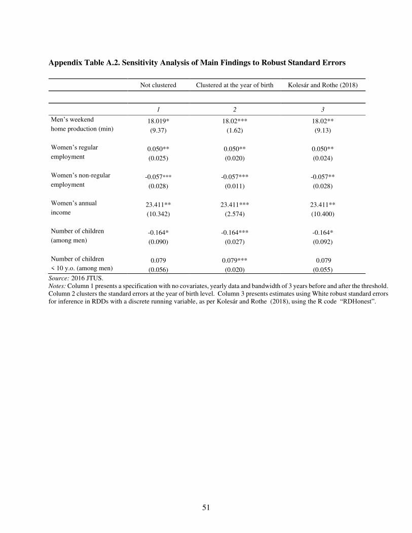
51

Appendix Table A.2. Sensitivity Analysis of Main Findings to Robust Standard Errors

Source: 2016 JTUS. Notes: Column 1 presents a specification with no covariates, yearly data and bandwidth of 3 years before and after the threshold. Column 2 clusters the standard errors at the year of birth level. Column 3 presents estimates using White robust standard errors for inference in RDDs with a discrete running variable, as per Kolesár and Rothe (2018), using the R code “RDHonest”.

Not clustered Clustered at the year of birth Kolesár and Rothe (2018)

1 2 3

Men’s weekend 18.019* 18.02*** 18.02** home production (min) (9.37) (1.62) (9.13) Women’s regular 0.050** 0.050** 0.050** employment (0.025) (0.020) (0.024) Women’s non-regular -0.057*** -0.057*** -0.057** employment (0.028) (0.011) (0.028) Women’s annual 23.411** 23.411*** 23.411** income (10.342) (2.574) (10.400) Number of children -0.164* -0.164*** -0.164* (among men) (0.090) (0.027) (0.092) Number of children 0.079 0.079*** 0.079 < 10 y.o. (among men) (0.056) (0.020) (0.055)

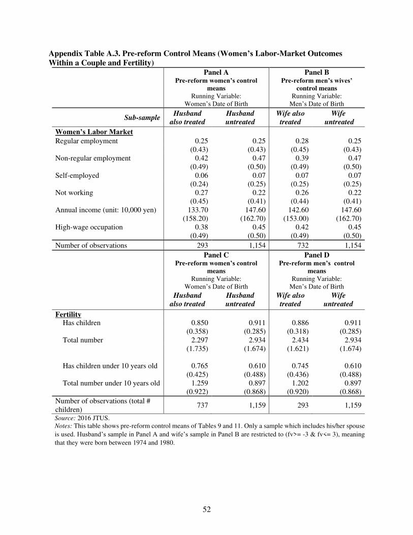
52

Appendix Table A.3. Pre-reform Control Means (Women’s Labor-Market Outcomes

Within a Couple and Fertility)

Panel A Pre-reform women’s control

means

Running Variable: Women’s Date of Birth

Panel B Pre-reform men’s wives’

control means

Running Variable: Men’s Date of Birth Sub-sample

Husband

also treated

Husband

untreated

Wife also

treated

Wife

untreated

Women’s Labor Market

Regular employment 0.25 0.25 0.28 0.25 (0.43) (0.43) (0.45) (0.43) Non-regular employment 0.42 0.47 0.39 0.47 (0.49) (0.50) (0.49) (0.50) Self-employed 0.06 0.07 0.07 0.07 (0.24) (0.25) (0.25) (0.25) Not working 0.27 0.22 0.26 0.22 (0.45) (0.41) (0.44) (0.41) Annual income (unit: 10,000 yen) 133.70 147.60 142.60 147.60 (158.20) (162.70) (153.00) (162.70) High-wage occupation 0.38 0.45 0.42 0.45 (0.49) (0.50) (0.49) (0.50)

Number of observations 293 1,154 732 1,154

Panel C Pre-reform women’s control

means

Running Variable: Women’s Date of Birth

Panel D Pre-reform men’s control

means

Running Variable: Men’s Date of Birth

Husband

also treated Husband

untreated Wife also

treated Wife

untreated

Fertility Has children 0.850 0.911 0.886 0.911 (0.358) (0.285) (0.318) (0.285) Total number 2.297 2.934 2.434 2.934 (1.735) (1.674) (1.621) (1.674)

Has children under 10 years old 0.765 0.610 0.745 0.610 (0.425) (0.488) (0.436) (0.488) Total number under 10 years old 1.259 0.897 1.202 0.897 (0.922) (0.868) (0.920) (0.868)

Number of observations (total # children)

737 1,159 293 1,159

Source: 2016 JTUS. Notes: This table shows pre-reform control means of Tables 9 and 11. Only a sample which includes his/her spouse

is used. Husband’s sample in Panel A and wife’s sample in Panel B are restricted to (fv>= -3 & fv<= 3), meaning

that they were born between 1974 and 1980.

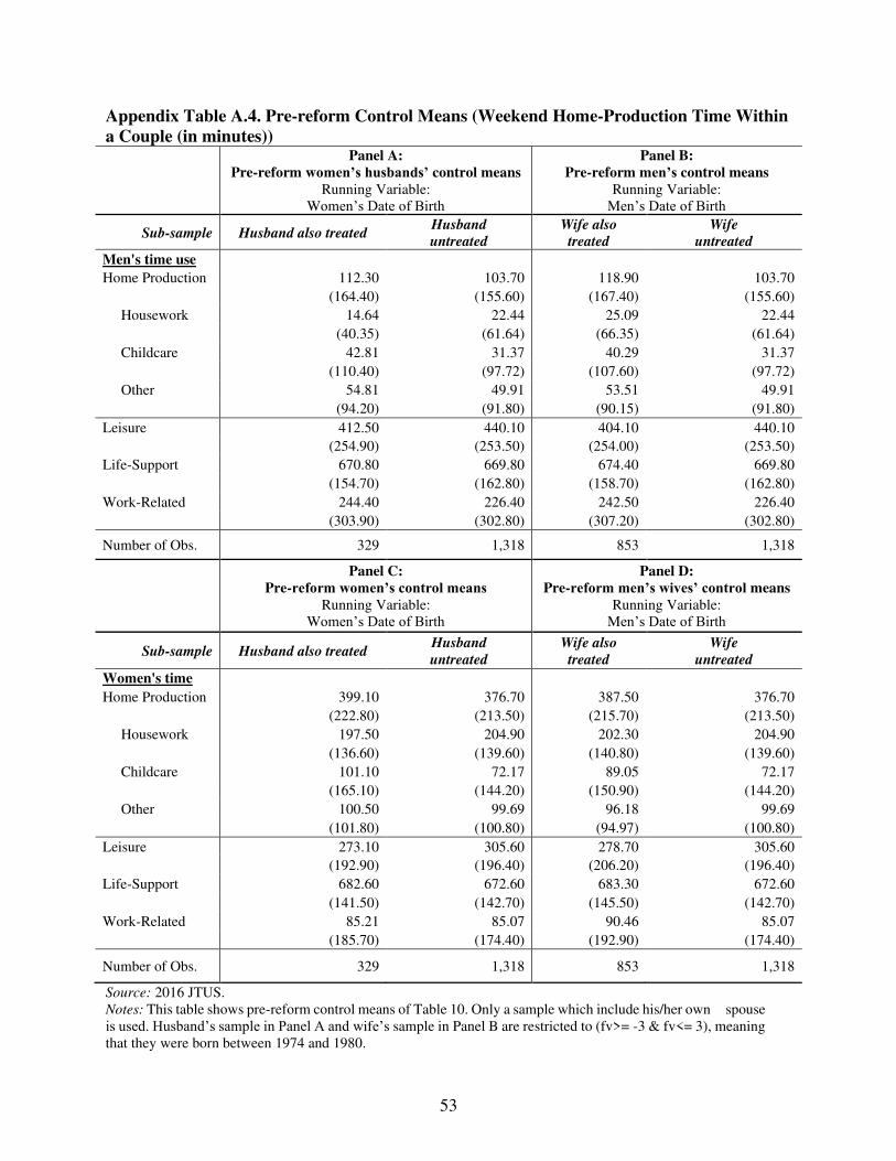
53

Appendix Table A.4. Pre-reform Control Means (Weekend Home-Production Time Within

a Couple (in minutes))

Panel A:

Pre-reform women’s husbands’ control means

Running Variable: Women’s Date of Birth

Panel B:

Pre-reform men’s control means

Running Variable: Men’s Date of Birth

Sub-sample Husband also treated Husband

untreated

Wife also

treated

Wife

untreated

Men's time use

Home Production 112.30 103.70 118.90 103.70 (164.40) (155.60) (167.40) (155.60)

Housework 14.64 22.44 25.09 22.44 (40.35) (61.64) (66.35) (61.64)

Childcare 42.81 31.37 40.29 31.37 (110.40) (97.72) (107.60) (97.72)

Other 54.81 49.91 53.51 49.91 (94.20) (91.80) (90.15) (91.80)

Leisure 412.50 440.10 404.10 440.10 (254.90) (253.50) (254.00) (253.50)

Life-Support 670.80 669.80 674.40 669.80 (154.70) (162.80) (158.70) (162.80)

Work-Related 244.40 226.40 242.50 226.40 (303.90) (302.80) (307.20) (302.80)

Number of Obs. 329 1,318 853 1,318

Panel C:

Pre-reform women’s control means

Running Variable: Women’s Date of Birth

Panel D:

Pre-reform men’s wives’ control means

Running Variable: Men’s Date of Birth

Sub-sample Husband also treated Husband

untreated

Wife also

treated

Wife

untreated

Women's time

Home Production 399.10 376.70 387.50 376.70 (222.80) (213.50) (215.70) (213.50)

Housework 197.50 204.90 202.30 204.90 (136.60) (139.60) (140.80) (139.60)

Childcare 101.10 72.17 89.05 72.17 (165.10) (144.20) (150.90) (144.20)

Other 100.50 99.69 96.18 99.69 (101.80) (100.80) (94.97) (100.80)

Leisure 273.10 305.60 278.70 305.60 (192.90) (196.40) (206.20) (196.40)

Life-Support 682.60 672.60 683.30 672.60 (141.50) (142.70) (145.50) (142.70)

Work-Related 85.21 85.07 90.46 85.07 (185.70) (174.40) (192.90) (174.40)

Number of Obs. 329 1,318 853 1,318

Source: 2016 JTUS. Notes: This table shows pre-reform control means of Table 10. Only a sample which include his/her own spouse is used. Husband’s sample in Panel A and wife’s sample in Panel B are restricted to (fv>= -3 & fv<= 3), meaning that they were born between 1974 and 1980.